IJCNLP 2017

The Eighth International Joint Conferenceon Natural Language Processing

Proceedings of the IJCNLP 2017, Shared Tasks

November 27 – December 1, 2017Taipei, Taiwan

c©2017 Asian Federation of Natural Language Processing

978-1-948087-03-2 (Proceedings of the IJCNLP 2017, Shared Tasks)

ii

Introduction

The 8th International Joint Conference on Natural Language Processing (IJCNLP 2017) took place inTaipei, Taiwan from November 27 to December 1, 2017. It was organized by the National Taiwan NormalUniversity and by the Association for Computational Linguistics and Chinese Language Processing(ACLCLP), and it was hosted by the Asian Federation of Natural Language Processing (AFNLP).

For a first time in the history of IJCNLP, the conference featured shared tasks. We received a total of tentask proposals, and after a rigurous review, we accepted the following five of them:

• Task 1: Chinese Grammatical Error Diagnosis. Participants were asked to build systemsto automatically detect the errors in Chinese sentences made by Chinese-as-Second-Languagelearners, i.e., redundant word, missing word, word selection and word ordering. (Organized by:Gaoqi Rao, Baolin Zhang, and Endong Xun)

• Task 2: Dimensional Sentiment Analysis for Chinese Phrases. Given a word or a phrase,participants were asked to generate a real-valued score between 1 and 9, indicating the degree ofvalence, from most negative to most positive, and for the degree of arousal, from most calm tomost excited. (Organized by Liang-Chih Yu, Lung-Hao Lee, Jin Wang, and Kam-Fai Wong)

• Task 3: Review Opinion Diversification. Participants were asked to build systems to rank productreviews based on a summary of opinions in two domains: books and electronics. (Organized byAnil Kumar Singh, Julian McAuley, Avijit Thawani, Mayank Panchal, Anubhav Gupta, and RajeshKumar Mundotiya)

• Task 4: Customer Feedback Analysis. Participants were asked to train classifiers for thedetection of meaning in customer feedback in English, French, Spanish, and Japanese: comment,request, bug, complaint, meaningless, and undetermined. (Organized by Chao-Hong Liu, YasufumiMoriya, Alberto Poncelas, and Declan Groves)

• Task 5: Multi-choice Question Answering in Examinations. Participants were asked to buildsystems to choose the correct option for a multi-choice question: for English and Chinese.(Organized by Jun Zhao, Kang Liu, Shizhu He, Zhuoyu Wei, and Shangmin Guo)

A total of 40 teams participated in the five tasks (and many more registered to participate, but endedup not submitting systems), submitting hundreds of runs for the different tasks and their subtasks: 5 fortask 1, 13 for task 2, 3 for task 3, 12 for task 4, and 7 for task 5. Moreover, most of the participatingteams contributed a system description paper: 3 for task 1, 10 for task 2, 3 for task 3, 9 for task 4, and 6for task 5. Finally, the organizers of each task prepared a task description paper. All these appear in thepresent proceedings.

We thank the shared task participants, as well as the task organizers, for all their great work. We furthertake the opportunity to thank the program committee and all reviewers for their thorough reviews.

The IJCNLP’2017 Shared Task Co-Chairs:

Chao-Hong Liu, ADAPT Centre, Dublin City University, IrelandPreslav Nakov, Qatar Computing Research Institute, HBKU, QatarNianwen Xue, Brandeis University, USA

iii

Organizing Committee

Shared Task Workshop Co-Chairs

Chao-Hong Liu, ADAPT Centre, Dublin City UniversityPreslav Nakov, Qatar Computing Research Institute, HBKUNianwen Xue, Brandeis University

Task 1: Chinese Grammatical Error Diagnosis (CGED) Organizers

Gaoqi Rao, Beijing Language and Culture UniversityBaolin Zhang, Beijing Language and Culture UniversityEndong Xun, Beijing Language and Culture University

Task 2: Dimensional Sentiment Analysis for Chinese Phrases (DSAP) Organizers

Liang-Chih Yu, Yuan Ze UniversityLung-Hao Lee, National Taiwan Normal UniversityJin Wang, Yunnan UniversityKam-Fai Wong, The Chinese University of Hong Kong

Task 3: Review Opinion Diversification Organizers

Anil Kumar Singh, Indian Institute of Technology (BHU) VaranasiJulian McAuley, University of California, San DiegoAvijit Thawani, Indian Institute of Technology (BHU) VaranasiMayank Panchal, Indian Institute of Technology (BHU) VaranasiAnubhav Gupta, Indian Institute of Technology (BHU) VaranasiRajesh Kumar Mundotiya, Indian Institute of Technology (BHU)

Task 4: Customer Feedback Analysis Organizers

Chao-Hong Liu, ADAPT Centre, Dublin City UniversityYasufumi Moriya, ADAPT Centre, Dublin City UniversityAlberto Poncelas, ADAPT Centre, Dublin City UniversityDeclan Groves, Microsoft Dublin

Task 5: Multi-choice Question Answering in Examinations Organizers

Jun Zhao, Institute of Automation, Chinese Academy of SciencesKang Liu, Institute of Automation, Chinese Academy of SciencesShizhu He, Institute of Automation, Chinese Academy of SciencesZhuoyu Wei, Institute of Automation, Chinese Academy of SciencesShangmin Guo, Institute of Automation, Chinese Academy of Sciences

v

Program Committee

Reviewers

Alberto Poncelas, ADAPT Centre, Dublin City UniversityAnil Kumar Singh, Indian Institute of Technology (BHU) VaranasiAnubhav Gupta, Indian Institute of Technology (BHU) VaranasiAvijit Thawani, Indian Institute of Technology (BHU) VaranasiBaolin Zhang, Beijing Language and Culture UniversityChao-Hong Liu, ADAPT Centre, Dublin City UniversityEndong Xun, Beijing Language and Culture UniversityGaoqi Rao, Beijing Language and Culture UniversityHaithem Afli, ADAPT Centre, Dublin City UniversityJin Wang, Yunnan UniversityJulian McAuley, University of California, San DiegoJun Zhao, Institute of Automation, Chinese Academy of SciencesKam-Fai Wong, The Chinese University of Hong KongKang Liu, Institute of Automation, Chinese Academy of SciencesLiang-Chih Yu, Yuan Ze UniversityLung-Hao Lee, National Taiwan Normal UniversityMayank Panchal, Indian Institute of Technology (BHU) VaranasiMonalisa Dey, Jadavpur UniversityNianwen Xue, Brandeis UniversityPreslav Nakov, Qatar Computing Research Institute, HBKUPruthwik Mishra, International Institute of Information Technology, HyderabadRajesh Kumar Mundotiya, Indian Institute of Technology (BHU) VaranasiShangmin Guo, Institute of Automation, Chinese Academy of SciencesShih-Hung Wu, Chaoyang University of TechnologyYasufumi Moriya, ADAPT Centre, Dublin City University

vi

Invited Talk

Public Health Surveillance Using Twitter: The Case for Biosurveillance andPharmacovigilance

Antonio Jimeno Yepes

IBM Research, Australia

Abstract

Public health surveillance using clinical data is challenging due to issues related to accessing healthcare data in a homogeneous way and in real-time, which is further affected by privacy concerns.Yet, it is still relevant to access this data in real-time to model potential disease outbreaks and todetect post-marketing adverse events of drugs. Social networks such as Twitter provide a largequantity of information that can be relevant as an alternative to clinical data. We have researchedthe usage of Twitter in several tasks related to public health surveillance. In this talk, I will presentthe work that we have done in IBM Research Australia using Twitter in public health relatedproblems and the challenges that we have faced using Twitter. Specifically, I will show resultsrelated to the prediction of the prevalence of flu in the USA and related to the identification ofpost-marketing adverse events of drugs.

Biography

Dr Antonio Jimeno Yepes is a senior researcher in text analytics in the Biomedical Data Scienceteam at IBM Research Australia. Before joining IBM, he worked as software engineer at CERNfrom 2000 to 2006, then as software engineer at the European Bioinformatics Institute (EBI) from2006 to 2010, as a post-doctoral researcher at the USA National Library of Medicine (NIH/NLM)from 2010 to 2012, as a researcher at National ICT Australia from 2012 to 2014 and as researcherat the CIS department at the University of Melbourne in 2014. He obtained his Masters degree inComputer Science in 2001, a master in Intelligent systems in 2008 and his PhD degree related tobiomedical natural languages and ontologies in 2009 from University Jaume I.

vii

Table of Contents

IJCNLP-2017 Task 1: Chinese Grammatical Error DiagnosisGaoqi RAO, Baolin Zhang, Endong XUN and Lung-Hao Lee . . . . . . . . . . . . . . . . . . . . . . . . . . . . . . . . 1

IJCNLP-2017 Task 2: Dimensional Sentiment Analysis for Chinese PhrasesLiang-Chih Yu, Lung-Hao Lee, Jin Wang and Kam-Fai Wong . . . . . . . . . . . . . . . . . . . . . . . . . . . . . . . . 9

IJCNLP-2017 Task 3: Review Opinion Diversification (RevOpiD-2017)Anil Kumar Singh, Avijit Thawani, Mayank Panchal, Anubhav Gupta and Julian McAuley . . . . . 17

IJCNLP-2017 Task 4: Customer Feedback AnalysisChao-Hong Liu, Yasufumi Moriya, Alberto Poncelas and Declan Groves . . . . . . . . . . . . . . . . . . . . . 26

IJCNLP-2017 Task 5: Multi-choice Question Answering in ExaminationsShangmin Guo, Kang Liu, Shizhu He, Cao Liu, Jun Zhao and Zhuoyu Wei . . . . . . . . . . . . . . . . . . . 34

Alibaba at IJCNLP-2017 Task 1: Embedding Grammatical Features into LSTMs for Chinese Grammat-ical Error Diagnosis Task

Yi yang, Pengjun Xie, Jun tao, Guangwei xu, Linlin li and Si luo . . . . . . . . . . . . . . . . . . . . . . . . . . . . 41

THU_NGN at IJCNLP-2017 Task 2: Dimensional Sentiment Analysis for Chinese Phrases with DeepLSTM

Chuhan Wu, Fangzhao Wu, Yongfeng Huang, Sixing Wu and Zhigang Yuan . . . . . . . . . . . . . . . . . . 47

IIIT-H at IJCNLP-2017 Task 3: A Bidirectional-LSTM Approach for Review Opinion DiversificationPruthwik Mishra, Prathyusha Danda, Silpa Kanneganti and Soujanya Lanka . . . . . . . . . . . . . . . . . . 53

Bingo at IJCNLP-2017 Task 4: Augmenting Data using Machine Translation for Cross-linguistic Cus-tomer Feedback Classification

Heba Elfardy, Manisha Srivastava, Wei Xiao, Jared Kramer and Tarun Agarwal . . . . . . . . . . . . . . . 59

ADAPT Centre Cone Team at IJCNLP-2017 Task 5: A Similarity-Based Logistic Regression Approachto Multi-choice Question Answering in an Examinations Shared Task

Daria Dzendzik, Alberto Poncelas, Carl Vogel and Qun Liu . . . . . . . . . . . . . . . . . . . . . . . . . . . . . . . . . 67

YNU-HPCC at IJCNLP-2017 Task 1: Chinese Grammatical Error Diagnosis Using a Bi-directionalLSTM-CRF Model

Quanlei Liao, Jin Wang, Jinnan Yang and Xuejie Zhang . . . . . . . . . . . . . . . . . . . . . . . . . . . . . . . . . . . . 73

CVTE at IJCNLP-2017 Task 1: Character Checking System for Chinese Grammatical Error DiagnosisTask

Xian Li, Peng Wang, Suixue Wang, Guanyu Jiang and Tianyuan You . . . . . . . . . . . . . . . . . . . . . . . . 78

LDCCNLP at IJCNLP-2017 Task 2: Dimensional Sentiment Analysis for Chinese Phrases Using Ma-chine Learning

Peng Zhong and Jingbin Wang . . . . . . . . . . . . . . . . . . . . . . . . . . . . . . . . . . . . . . . . . . . . . . . . . . . . . . . . . . . 84

CKIP at IJCNLP-2017 Task 2: Neural Valence-Arousal Prediction for PhrasesPeng-Hsuan Li, Wei-Yun Ma and Hsin-Yang Wang. . . . . . . . . . . . . . . . . . . . . . . . . . . . . . . . . . . . . . . . . 89

CIAL at IJCNLP-2017 Task 2: An Ensemble Valence-Arousal Analysis System for Chinese Words andPhrases

Zheng-Wen Lin, Yung-Chun Chang, Chen-Ann Wang, Yu-Lun Hsieh and Wen-Lian Hsu . . . . . . 95

ix

Alibaba at IJCNLP-2017 Task 2: A Boosted Deep System for Dimensional Sentiment Analysis of ChinesePhrases

Xin Zhou, Jian Wang, Xu Xie, Changlong Sun and Luo Si . . . . . . . . . . . . . . . . . . . . . . . . . . . . . . . . . 100

NLPSA at IJCNLP-2017 Task 2: Imagine Scenario: Leveraging Supportive Images for DimensionalSentiment Analysis

szu-min chen, Zi-Yuan Chen and Lun-Wei Ku . . . . . . . . . . . . . . . . . . . . . . . . . . . . . . . . . . . . . . . . . . . . 105

NCYU at IJCNLP-2017 Task 2: Dimensional Sentiment Analysis for Chinese Phrases using Vector Rep-resentations

Jui-Feng Yeh, Jian-Cheng Tsai, Bo-Wei Wu and Tai-You Kuang . . . . . . . . . . . . . . . . . . . . . . . . . . . . 112

MainiwayAI at IJCNLP-2017 Task 2: Ensembles of Deep Architectures for Valence-Arousal PredictionYassine Benajiba, Jin Sun, Yong Zhang, Zhiliang Weng and Or Biran . . . . . . . . . . . . . . . . . . . . . . . 118

NCTU-NTUT at IJCNLP-2017 Task 2: Deep Phrase Embedding using bi-LSTMs for Valence-ArousalRatings Prediction of Chinese Phrases

Yen-Hsuan Lee, Han-Yun Yeh, Yih-Ru Wang and Yuan-Fu Liao . . . . . . . . . . . . . . . . . . . . . . . . . . . . 124

NTOUA at IJCNLP-2017 Task 2: Predicting Sentiment Scores of Chinese Words and PhrasesChuan-Jie Lin and Hao-Tsung Chang . . . . . . . . . . . . . . . . . . . . . . . . . . . . . . . . . . . . . . . . . . . . . . . . . . . . 130

CYUT at IJCNLP-2017 Task 3: System Report for Review Opinion DiversificationShih-Hung Wu, Su-Yu Chang and Liang-Pu Chen . . . . . . . . . . . . . . . . . . . . . . . . . . . . . . . . . . . . . . . . . 134

JUNLP at IJCNLP-2017 Task 3: A Rank Prediction Model for Review Opinion DiversificationMonalisa Dey, Anupam Mondal and Dipankar Das . . . . . . . . . . . . . . . . . . . . . . . . . . . . . . . . . . . . . . . . 138

All-In-1 at IJCNLP-2017 Task 4: Short Text Classification with One Model for All LanguagesBarbara Plank . . . . . . . . . . . . . . . . . . . . . . . . . . . . . . . . . . . . . . . . . . . . . . . . . . . . . . . . . . . . . . . . . . . . . . . . . 143

SentiNLP at IJCNLP-2017 Task 4: Customer Feedback Analysis Using a Bi-LSTM-CNN ModelShuying Lin, Huosheng Xie, Liang-Chih Yu and K. Robert Lai . . . . . . . . . . . . . . . . . . . . . . . . . . . . . 149

IIIT-H at IJCNLP-2017 Task 4: Customer Feedback Analysis using Machine Learning and Neural Net-work Approaches

Prathyusha Danda, Pruthwik Mishra, Silpa Kanneganti and Soujanya Lanka . . . . . . . . . . . . . . . . . 155

ADAPT at IJCNLP-2017 Task 4: A Multinomial Naive Bayes Classification Approach for CustomerFeedback Analysis task

Pintu Lohar, Koel Dutta Chowdhury, Haithem Afli, Mohammed Hasanuzzaman and Andy Way161

OhioState at IJCNLP-2017 Task 4: Exploring Neural Architectures for Multilingual Customer FeedbackAnalysis

Dushyanta Dhyani . . . . . . . . . . . . . . . . . . . . . . . . . . . . . . . . . . . . . . . . . . . . . . . . . . . . . . . . . . . . . . . . . . . . . 170

YNU-HPCC at IJCNLP-2017 Task 4: Attention-based Bi-directional GRU Model for Customer FeedbackAnalysis Task of English

Nan Wang, Jin Wang and Xuejie Zhang . . . . . . . . . . . . . . . . . . . . . . . . . . . . . . . . . . . . . . . . . . . . . . . . . . 174

NITMZ-JU at IJCNLP-2017 Task 4: Customer Feedback AnalysisSomnath Banerjee, Partha Pakray, Riyanka Manna, Dipankar Das and Alexander Gelbukh . . . . 180

IITP at IJCNLP-2017 Task 4: Auto Analysis of Customer Feedback using CNN and GRU NetworkDeepak Gupta, Pabitra Lenka, Harsimran Bedi, Asif Ekbal and Pushpak Bhattacharyya . . . . . . . 184

x

YNUDLG at IJCNLP-2017 Task 5: A CNN-LSTM Model with Attention for Multi-choice Question An-swering in Examinations

Min Wang, Qingxun Liu, Peng Ding, Yongbin Li and Xiaobing Zhou . . . . . . . . . . . . . . . . . . . . . . . 194

ALS at IJCNLP-2017 Task 5: Answer Localization System for Multi-Choice Question Answering inExams

Changliang Li and Cunliang Kong. . . . . . . . . . . . . . . . . . . . . . . . . . . . . . . . . . . . . . . . . . . . . . . . . . . . . . .199

MappSent at IJCNLP-2017 Task 5: A Textual Similarity Approach Applied to Multi-choice QuestionAnswering in Examinations

Amir Hazem . . . . . . . . . . . . . . . . . . . . . . . . . . . . . . . . . . . . . . . . . . . . . . . . . . . . . . . . . . . . . . . . . . . . . . . . . . 203

YNU-HPCC at IJCNLP-2017 Task 5: Multi-choice Question Answering in Exams Using an Attention-based LSTM Model

Hang Yuan, You Zhang, Jin Wang and Xuejie Zhang . . . . . . . . . . . . . . . . . . . . . . . . . . . . . . . . . . . . . . 208

JU NITM at IJCNLP-2017 Task 5: A Classification Approach for Answer Selection in Multi-choiceQuestion Answering System

Sandip Sarkar, Dipankar Das and Partha Pakray . . . . . . . . . . . . . . . . . . . . . . . . . . . . . . . . . . . . . . . . . . 213

xi

Shared Tasks Program

Friday, December 1, 2017, Room 503

08:00–09:00 Registration

09:10–09:30 Opening Remarks

09:30–10:30 Keynote Talk by Antonio Jimeno Yepes on “Public Health Surveillance UsingTwitter: the Case for Biosurveillance and Pharmacovigilance”

10:30–11:00 Coffee Break

Session 1: Shared Tasks Overview

11:00–11:20 IJCNLP-2017 Task 1: Chinese Grammatical Error DiagnosisGaoqi RAO, Baolin Zhang, Endong XUN and Lung-Hao Lee

11:20–11:40 IJCNLP-2017 Task 2: Dimensional Sentiment Analysis for Chinese PhrasesLiang-Chih Yu, Lung-Hao Lee, Jin Wang and Kam-Fai Wong

11:40–12:00 IJCNLP-2017 Task 3: Review Opinion Diversification (RevOpiD-2017)Anil Kumar Singh, Avijit Thawani, Mayank Panchal, Anubhav Gupta and JulianMcAuley

12:00–12:20 IJCNLP-2017 Task 4: Customer Feedback AnalysisChao-Hong Liu, Yasufumi Moriya, Alberto Poncelas and Declan Groves

12:20–12:40 IJCNLP-2017 Task 5: Multi-choice Question Answering in ExaminationsShangmin Guo, Kang Liu, Shizhu He, Cao Liu, Jun Zhao and Zhuoyu Wei

12:40–13:20 Lunch

xiii

Friday, December 1, 2017, Room 503 (continued)

Session 2: IJCNLP-2017 Shared Tasks Oral Session

13:20–13:40 Alibaba at IJCNLP-2017 Task 1: Embedding Grammatical Features into LSTMs forChinese Grammatical Error Diagnosis TaskYi yang, Pengjun Xie, Jun tao, Guangwei xu, Linlin li and Si luo

13:40–14:00 THU_NGN at IJCNLP-2017 Task 2: Dimensional Sentiment Analysis for ChinesePhrases with Deep LSTMChuhan Wu, Fangzhao Wu, Yongfeng Huang, Sixing Wu and Zhigang Yuan

14:00–14:20 IIIT-H at IJCNLP-2017 Task 3: A Bidirectional-LSTM Approach for Review Opin-ion DiversificationPruthwik Mishra, Prathyusha Danda, Silpa Kanneganti and Soujanya Lanka

14:20–14:40 Bingo at IJCNLP-2017 Task 4: Augmenting Data using Machine Translation forCross-linguistic Customer Feedback ClassificationHeba Elfardy, Manisha Srivastava, Wei Xiao, Jared Kramer and Tarun Agarwal

14:40–15:00 ADAPT Centre Cone Team at IJCNLP-2017 Task 5: A Similarity-Based Logistic Re-gression Approach to Multi-choice Question Answering in an Examinations SharedTaskDaria Dzendzik, Alberto Poncelas, Carl Vogel and Qun Liu

15:00–15:30 Coffee Break

15:30–16:50 Session 3: IJCNLP-2017 Shared Tasks Poster Session

YNU-HPCC at IJCNLP-2017 Task 1: Chinese Grammatical Error Diagnosis Usinga Bi-directional LSTM-CRF ModelQuanlei Liao, Jin Wang, Jinnan Yang and Xuejie Zhang

CVTE at IJCNLP-2017 Task 1: Character Checking System for Chinese Grammat-ical Error Diagnosis TaskXian Li, Peng Wang, Suixue Wang, Guanyu Jiang and Tianyuan You

LDCCNLP at IJCNLP-2017 Task 2: Dimensional Sentiment Analysis for ChinesePhrases Using Machine LearningPeng Zhong and Jingbin Wang

CKIP at IJCNLP-2017 Task 2: Neural Valence-Arousal Prediction for PhrasesPeng-Hsuan Li, Wei-Yun Ma and Hsin-Yang Wang

xiv

Friday, December 1, 2017, Room 503 (continued)

CIAL at IJCNLP-2017 Task 2: An Ensemble Valence-Arousal Analysis System forChinese Words and PhrasesZheng-Wen Lin, Yung-Chun Chang, Chen-Ann Wang, Yu-Lun Hsieh and Wen-LianHsu

Alibaba at IJCNLP-2017 Task 2: A Boosted Deep System for Dimensional Senti-ment Analysis of Chinese PhrasesXin Zhou, Jian Wang, Xu Xie, Changlong Sun and Luo Si

NLPSA at IJCNLP-2017 Task 2: Imagine Scenario: Leveraging Supportive Imagesfor Dimensional Sentiment Analysisszu-min chen, Zi-Yuan Chen and Lun-Wei Ku

NCYU at IJCNLP-2017 Task 2: Dimensional Sentiment Analysis for ChinesePhrases using Vector RepresentationsJui-Feng Yeh, Jian-Cheng Tsai, Bo-Wei Wu and Tai-You Kuang

MainiwayAI at IJCNLP-2017 Task 2: Ensembles of Deep Architectures for Valence-Arousal PredictionYassine Benajiba, Jin Sun, Yong Zhang, Zhiliang Weng and Or Biran

NCTU-NTUT at IJCNLP-2017 Task 2: Deep Phrase Embedding using bi-LSTMsfor Valence-Arousal Ratings Prediction of Chinese PhrasesYen-Hsuan Lee, Han-Yun Yeh, Yih-Ru Wang and Yuan-Fu Liao

NTOUA at IJCNLP-2017 Task 2: Predicting Sentiment Scores of Chinese Wordsand PhrasesChuan-Jie Lin and Hao-Tsung Chang

CYUT at IJCNLP-2017 Task 3: System Report for Review Opinion DiversificationShih-Hung Wu, Su-Yu Chang and Liang-Pu Chen

JUNLP at IJCNLP-2017 Task 3: A Rank Prediction Model for Review OpinionDiversificationMonalisa Dey, Anupam Mondal and Dipankar Das

All-In-1 at IJCNLP-2017 Task 4: Short Text Classification with One Model for AllLanguagesBarbara Plank

SentiNLP at IJCNLP-2017 Task 4: Customer Feedback Analysis Using a Bi-LSTM-CNN ModelShuying Lin, Huosheng Xie, Liang-Chih Yu and K. Robert Lai

IIIT-H at IJCNLP-2017 Task 4: Customer Feedback Analysis using Machine Learn-ing and Neural Network ApproachesPrathyusha Danda, Pruthwik Mishra, Silpa Kanneganti and Soujanya Lanka

xv

Friday, December 1, 2017, Room 503 (continued)

ADAPT at IJCNLP-2017 Task 4: A Multinomial Naive Bayes Classification Ap-proach for Customer Feedback Analysis taskPintu Lohar, Koel Dutta Chowdhury, Haithem Afli, Mohammed Hasanuzzaman andAndy Way

OhioState at IJCNLP-2017 Task 4: Exploring Neural Architectures for MultilingualCustomer Feedback AnalysisDushyanta Dhyani

YNU-HPCC at IJCNLP-2017 Task 4: Attention-based Bi-directional GRU Modelfor Customer Feedback Analysis Task of EnglishNan Wang, Jin Wang and Xuejie Zhang

NITMZ-JU at IJCNLP-2017 Task 4: Customer Feedback AnalysisSomnath Banerjee, Partha Pakray, Riyanka Manna, Dipankar Das and AlexanderGelbukh

IITP at IJCNLP-2017 Task 4: Auto Analysis of Customer Feedback using CNN andGRU NetworkDeepak Gupta, Pabitra Lenka, Harsimran Bedi, Asif Ekbal and Pushpak Bhat-tacharyya

YNUDLG at IJCNLP-2017 Task 5: A CNN-LSTM Model with Attention for Multi-choice Question Answering in ExaminationsMin Wang, Qingxun Liu, Peng Ding, Yongbin Li and Xiaobing Zhou

ALS at IJCNLP-2017 Task 5: Answer Localization System for Multi-Choice Ques-tion Answering in ExamsChangliang Li and Cunliang Kong

MappSent at IJCNLP-2017 Task 5: A Textual Similarity Approach Applied to Multi-choice Question Answering in ExaminationsAmir Hazem

YNU-HPCC at IJCNLP-2017 Task 5: Multi-choice Question Answering in ExamsUsing an Attention-based LSTM ModelHang Yuan, You Zhang, Jin Wang and Xuejie Zhang

JU NITM at IJCNLP-2017 Task 5: A Classification Approach for Answer Selectionin Multi-choice Question Answering SystemSandip Sarkar, Dipankar Das and Partha Pakray

16:50–17:00 Closing Session

xvi

Proceedings of the 8th International Joint Conference on Natural Language Processing, Shared Tasks, pages 1–8,Taipei, Taiwan, November 27 – December 1, 2017. c©2017 AFNLP

IJCNLP-2017 Task 1: Chinese Grammatical Error Diagnosis

Gaoqi Rao1, Baolin Zhang2, Endong Xun3{1Center for Studies of Chinese as a Second Language, 2Faculty of Language Sciences,

3College of Information Science} Beijing Language and Culture Universityraogaoqi-fj@163.com, zhangbl@blcu.edu.cn, edxun@126.com

Abstract

This paper presents the IJCNLP 2017shared task for Chinese grammaticalerror diagnosis (CGED) which seeksto identify grammatical error types andtheir range of occurrence withinsentences written by learners ofChinese as foreign language. Wedescribe the task definition, datapreparation, performance metrics, andevaluation results. Of the 13 teamsregistered for this shared task, 5 teamsdeveloped the system and submitted atotal of 13 runs. We expected thisevaluation campaign could lead to thedevelopment of more advanced NLPtechniques for educational applications,especially for Chinese error detection.All data sets with gold standards andscoring scripts are made publiclyavailable to researchers.

1 Introduction

Recently, automated grammar checking forlearners of English as a foreign language hasattracted more attention. For example, HelpingOur Own (HOO) is a series of shared tasks incorrecting textual errors (Dale and Kilgarriff,2011; Dale et al., 2012). The shared tasks atCoNLL 2013 and CoNLL 2014 focused ongrammatical error correction, increasing thevisibility of educational application research inthe NLP community (Ng et al., 2013; 2014).Many of these learning technologies focus on

learners of English as a Foreign Language (EFL),while relatively few grammar checkingapplications have been developed to supportChinese as a Foreign Language(CFL) learners.

Those applications which do exist rely on a rangeof techniques, such as statistical learning (Changet al, 2012; Wu et al, 2010; Yu and Chen, 2012),rule-based analysis (Lee et al., 2013) and hybridmethods (Lee et al., 2014). In response to thelimited availability of CFL learner data formachine learning and linguistic analysis, theICCE-2014 workshop on Natural LanguageProcessing Techniques for EducationalApplications (NLP-TEA) organized a shared taskon diagnosing grammatical errors for CFL (Yu etal., 2014). A second version of this shared task inNLP-TEA was collocated with the ACL-IJCNLP-2015 (Lee et al., 2015) and COLING-2016 (Lee et al., 2016). In conjunction with theIJCNLP 2017, the shared task for Chinesegrammatical error diagnosis is organized again.The main purpose of these shared tasks is toprovide a common setting so that researcherswho approach the tasks using different linguisticfactors and computational techniques cancompare their results. Such technical evaluationsallow researchers to exchange their experiencesto advance the field and eventually developoptimal solutions to this shared task.The rest of this paper is organized as follows.

Section 2 describes the task in detail. Section 3introduces the constructed datasets. Section 4proposes evaluation metrics. Section 5 reportsthe results of the participants’ approaches.Conclusions are finally drawn in Section 6.

2 Task Description

The goal of this shared task is to develop NLPtechniques to automatically diagnose grammaticalerrors in Chinese sentences written by CFLlearners. Such errors are defined as redundantwords (denoted as a capital “R”), missing words(“M”), word selection errors (“S”), and word

1

ordering errors (“W”). The input sentence maycontain one or more such errors. The developedsystem should indicate which error types areembedded in the given unit (containing 1 to 5sentences) and the position at which they occur.Each input unit is given a unique number “sid”. Ifthe inputs contain no grammatical errors, thesystem should return: “sid, correct”. If an inputunit contains the grammatical errors, the outputformat should include four items “sid, start_off,

end_off, error_type”, where start_off and end_offrespectively denote the positions of starting andending character at which the grammatical erroroccurs, and error_type should be one of thedefined errors: “R”, “M”, “S”, and “W”. Eachcharacter or punctuation mark occupies 1 spacefor counting positions. Example sentences andcorresponding notes are shown as Table 1 shows.This year, we only have one track of HSK.

HSK (Simplified Chinese)

Example 1Input: (sid=00038800481) 我根本不能了解这妇女辞职回家的现象。在这个时代，为什么放弃自己

的工作，就回家当家庭主妇？Output: 00038800481, 6, 7, S

00038800481, 8, 8, R(Notes: “了解”should be “理解”. In addition, “这” is a redundant word.)

Example 2Input: (sid=00038800464)我真不明白。她们可能是追求一些前代的浪漫。Output: 00038800464, correct

Example 3Input: (sid=00038801261)人战胜了饥饿，才努力为了下一代作更好的、更健康的东西。Output: 00038801261, 9, 9, M

00038801261, 16, 16, S(Notes: “能” is missing. The word “作”should be “做”. The correct sentence is “才能努力为了下一代做

更好的”)

Example 4Input: (sid=00038801320)饥饿的问题也是应该解决的。世界上每天由于饥饿很多人死亡。Output: 00038801320, 19, 25, W(Notes: “由于饥饿很多人” should be “很多人由于饥饿”)

Table 1: Example sentences and corresponding notes.

3 Datasets

The learner corpora used in our shared task weretaken from the writing section of the HanyuShuiping Kaoshi(HSK, Test of ChineseLevel)(Cui et al, 2011; Zhang et al, 2013).Native Chinese speakers were trained to

manually annotate grammatical errors andprovide corrections corresponding to each error.The data were then split into two mutuallyexclusive sets as follows.(1) Training Set: All units in this set were used

to train the grammatical error diagnostic systems.Each unit contains 1 to 5 sentences with

annotated grammatical errors and theircorresponding corrections. All units arerepresented in SGML format, as shown in Table2. We provide 10,449 training units with a totalof 26,448 grammatical errors, categorized asredundant (5,852 instances), missing (7,010),word selection (11,591) and word ordering(1,995).In addition to the data sets provided,

participating research teams were allowed to useother public data for system development andimplementation. Use of other data should bespecified in the final system report.

2

<DOC><TEXT id="200307109523200140_2_2x3">因为养农作物时不用农药的话，生产率较低。那肯定价格要上升，那有钱的人想吃

多少，就吃多少。左边的文中已提出了世界上的有几亿人因缺少粮食而挨饿。</TEXT><CORRECTION>因为种植农作物时不用农药的话，生产率较低。那价格肯定要上升，那有钱的人想

吃多少，就吃多少。左边的文中已提出了世界上有几亿人因缺少粮食而挨饿。</CORRECTION><ERROR start_off="3" end_off="3" type="S"></ERROR><ERROR start_off="22" end_off="25" type="W"></ERROR><ERROR start_off="57" end_off="57" type="R"></ERROR></DOC>

<DOC><TEXT id="200210543634250003_2_1x3">对于“安乐死”的看法，向来都是一个极具争议性的题目，因为毕竟每个人对于死亡

的观念都不一样，怎样的情况下去判断，也自然产生出很多主观和客观的理论。每

个人都有着生存的权利，也代表着每个人都能去决定如何结束自己的生命的权利。

在我的个人观点中，如果一个长期受着病魔折磨的人，会是十分痛苦的事，不仅是

病人本身，以致病者的家人和朋友，都是一件难受的事。</TEXT><CORRECTION>对于“安乐死”的看法，向来都是一个极具争议性的题目，因为毕竟每个人对于死亡

的观念都不一样，无论在怎样的情况下去判断，都自然产生出很多主观和客观的理

论。每个人都有着生存的权利，也代表着每个人都能去决定如何结束自己的生命。

在我的个人观点中，如果一个长期受着病魔折磨的人活着，会是十分痛苦的事，不

仅是病人本身，对于病者的家人和朋友，都是一件难受的事。</CORRECTION><ERROR start_off="46" end_off="46" type="M"></ERROR><ERROR start_off="56" end_off="56" type="S"></ERROR><ERROR start_off="106" end_off="108" type="R"></ERROR><ERROR start_off="133" end_off="133" type="M"></ERROR><ERROR start_off="151" end_off="152" type="S"></ERROR></DOC>

Table 2: A training sentence denoted in SGML format.

(2) Test Set: This set consists of testingsentences used for evaluating systemperformance. Table 3 shows statistics for thetesting set for this year. About half of thesesentences are correct and do not containgrammatical errors, while the other half includeat least one error. The distributions of error types(shown in Table 4) are similar with that of thetraining set. The proportion of the correctsentences is sampled from data of the onlineDynamic Corpus of HSK1.

1 http://202.112.195.192:8060/hsk/login.asp

#Units #Correct #Erroneous3,154 (100%) 1,173 (48.38%) 1,628 (51.62%)

Table 3: The statistics of correct sentences intesting set.

Error Type

#R 1,062(21.78%)

#M 1,274(26.13%)

#S 2,155(44.20%)

#W 385

3

(7.90%)

#Error 4,876(100%)

Table 4: The distributions of error types intesting set.

4 Performance Metrics

Table 5 shows the confusion matrix used forevaluating system performance. In this matrix, TP(True Positive) is the number of sentences withgrammatical errors are correctly identified by thedeveloped system; FP (False Positive) is thenumber of sentences in which non-existentgrammatical errors are identified as errors; TN(True Negative) is the number of sentenceswithout grammatical errors that are correctlyidentified as such; FN (False Negative) is thenumber of sentences with grammatical errorswhich the system incorrectly identifies as beingcorrect.The criteria for judging correctness are

determined at three levels as follows.

(1) Detection-level: Binary classification of agiven sentence, that is, correct or incorrect, shouldbe completely identical with the gold standard. Allerror types will be regarded as incorrect.(2) Identification-level: This level could be

considered as a multi-class categorization problem.All error types should be clearly identified. Acorrect case should be completely identical withthe gold standard of the given error type.(3) Position-level: In addition to identifying the

error types, this level also judges the occurrencerange of the grammatical error. That is to say, thesystem results should be perfectly identical withthe quadruples of the gold standard.The following metrics are measured at all

levels with the help of the confusion matrix. False Positive Rate = FP / (FP+TN) Accuracy = (TP+TN) / (TP+FP+TN+FN) Precision = TP / (TP+FP) Recall = TP / (TP+FN) F1 = 2*Precision*Recall / (Precision +

Recall)

Confusion MatrixSystem Results

Positive (Erroneous) Negative(Correct)

Gold StandardPositive TP (True Positive) FN (False Negative)Negative FP (False Positive) TN (True Negative)

Table 5: Confusion matrix for evaluation.

For example, for 4 testing inputs with goldstandards shown as “00038800481, 6, 7, S”,“00038800481, 8, 8, R”, “00038800464, correct”,“00038801261, 9, 9, M”, “00038801261, 16, 16,S” and “00038801320, 19, 25, W”, the systemmay output the result as “00038800481, 2, 3, S”,“00038800481, 4, 5, S”, “00038800481, 8, 8, R”,“00038800464, correct”, “00038801261, 9, 9,M”, “00038801261, 16, 19, S” and“00038801320, 19, 25, M”. The scoring scriptwill yield the following performance.

False Positive Rate (FPR) = 0 (=0/1) Detection-level

Accuracy = 1 (=4/4) Precision = 1 (=3/3) Recall = 1 (=3/3) F1 = 1 (=(2*1*1)/(1+1))

Identification-level Accuracy = 0.8333 (=5/6) Precision = 0.8 (=4/5)

Recall = 0.8 (=4/5) F1 = 0.8 (=(2*0.8*0.8)/(0.8+08))

Position-level Accuracy = 0.4286 (=3/7) Precision = 0.3333 (=2/6) Recall = 0.4 (=2/5) F1 = 0.3636

(=(2*0.3333*0.4)/(0.3333+0.4))

5 Evaluation Results

Table 6 summarizes the submission statistics forthe 13 participating teams including 10 fromuniversities and research institutes in China(NTOUA, BLCU, SKY, PkU-Cherry,BNU_ICIP, CCNUNLP, CVTER, TONGTONG,AL_I_NLP), 1 from the U.S. (HarvardUniversity) and 1 private firm (Lingosail Inc.). Inthe official testing phase, each participating teamwas allowed to submit at most three runs. Of the

4

13 registered teams, 5 teams submitted theirtesting results, for a total of 13 runs.

Participant (Ordered by abbreviations of names) #RunsALI_NLP 3BLCU 0BNU_ICIP 3CCNUNLP 0Cherry 0CVTER 2Harvard University 0NTOUA 2PkU 0SKY 0TONGTONG 0YNU-HPCC 3Lingosail 0

Table 6: Submission statistics for all participants.

Table 7 shows the testing results ofCGED2017. The BNU team achieved the lowestfalse positive rate (denoted as “FPR”) of 0.098.Detection-level evaluations are designed todetect whether a sentence contains grammaticalerrors or not. A neutral baseline can be easilyachieved by always reporting all testingsentences as correct without errors. According tothe test data distribution, the baseline system canachieve an accuracy of 0.5162. However, not allsystems performed above the baseline. Thesystem result submitted by ALI_NLP achievedthe best detection accuracy of 0.6465. We use theF1 score to reflect the tradeoffs betweenprecision and recall. The ALI_NLP provided thebest error detection results, providing a high F1score of 0.8284. For identification-levelevaluations, the systems need to identify theerror types in a given sentences. The systemdeveloped by YNU-HPCC provided the highestF1 score of 0.7829 for grammatical erroridentification. For position-level evaluations,ALI_NLP achieved the best F1 score of 0.2693.Perfectly identifying the error types and theircorresponding positions is difficult in partbecause no word delimiters exist among Chinesewords in the given sentences.NTOUA, CVTE and ALI_NLP submit reports

on their develop systems. Though neuralnetworks achieved good performances in variousNLP tasks, traditional pipe-lines were stillwidely implemented in the CGED task.LSTM+CRF has been a standard implementation.Unlike CGED2016, though CRF model in pipe-

line were only equipped with simple designedfeature templates.In summary, none of the submitted systems

provided superior performance using differentmetrics, indicating the difficulty of developingsystems for effective grammatical error diagnosis,especially in CFL contexts. From organizers’perspectives, a good system should have a high F1score and a low false positive rate. Overall,ALI_NLP, YNU-HPCC and CVTE achievedrelatively better performances.

5

AL_I_NLP

BNU

CVTE

NTO

UA

YNU-

HPC

C

TEAM

run1

run2

run3

run1

run2

run3

run1

run2

run1

run2

run1

run2

run3

RUNs

0.6172(724/1173)

0.6607(775/1173)

0.3052(358/1173)

0.098(115/1173)

0.1355(159/1173)

0.1893(222/1173)

0.1441(169/1173)

0.3154(370/1173)

1(1173/1173)

1(1173/1173)

0.6513(764/1173)

0.7383(866/1173)

0.6104(716/1173)

FalsePositive

Rate

0.6439

0.6465

0.6173

0.4721

0.4794

0.5181

0.4756

0.539

0.6281

0.6281

0.5796

0.5891

0.5311

Detection

LevelAccuracy

0.686

0.6792

0.7597

0.7894

0.758

0.7547

0.7459

0.708

0.6281

0.6281

0.65

0.6417

0.6298

Precision

0.7986

0.8284

0.5714

0.2176

0.2514

0.3448

0.2504

0.4528

1 1

0.7163

0.7829

0.6148

Recall

0.738

0.7464

0.6523

0.3411

0.3776

0.4733

0.3749

0.5523

0.7716

0.7716

0.6816

0.7053

0.6222

F1

0.488

0.4654

0.5513

0.4337

0.4412

0.4696

0.4461

0.4711

0.3211

0.3889

0.4218

0.3879

0.3979

IdentificationLevel

Accuracy

0.4791

0.453

0.6007

0.5474

0.5527

0.5707

0.606

0.5391

0.3211

0.3889

0.4219

0.3825

0.4086

Precision

0.5657

0.6006

0.3756

0.106

0.131

0.1786

0.1214

0.2057

0.6099

0.506

0.4217

0.4575

0.3298

Recall

0.5188

0.5164

0.4622

0.1776

0.2118

0.2721

0.2023

0.2978

0.4207

0.4398

0.4218

0.4167

0.365

F1

0.2547

0.2264

0.4121

0.3775

0.3735

0.3798

0.3314

0.2602

0.0212

0.018

0.1778

0.1426

0.1702

PositionLevel

Accuracy

0.2169

0.1949

0.3663

0.2773

0.2818

0.2968

0.118

0.1093

0.0212

0.018

0.1262

0.1056

0.0981

Precision

0.2752

0.2941

0.213

0.0418

0.0515

0.0715

0.0204

0.0465

0.0958

0.082

0.1191

0.1191

0.0698

Recall

0.2426

0.2344

0.2693

0.0727

0.0871

0.1152

0.0348

0.0653

0.0348

0.0295

0.1225

0.112

0.0816

F1

6

Table 7: Testing results of CGED2017.

6 Conclusions

This study describes the NLP-TEA 2016 sharedtask for Chinese grammatical error diagnosis,including task design, data preparation,performance metrics, and evaluation results.Regardless of actual performance, allsubmissions contribute to the common effort todevelop Chinese grammatical error diagnosissystem, and the individual reports in theproceedings provide useful insights intocomputer-assisted language learning for CFLlearners.We hope the data sets collected and annotated

for this shared task can facilitate and expeditefuture development in this research area.Therefore, all data sets with gold standards andscoring scripts are publicly available online athttp://www.cged.science.

AcknowledgmentsWe thank all the participants for taking part inour shared task. We would like to thank Kuei-Ching Lee for implementing the evaluationprogram and the usage feedbacks from Bo Zheng(in proceeding of NLPTEA2016). Gong Qi, TangPeilan, Luo Ping and Chang Jie contributed inthe proofreading of data.This study was supported by the projects fromP.R.C: High-Tech Center of LanguageResource(KYD17004), BLCU InnovationPlatform(17PT05), Institute Project ofBLCU(16YBB16) Social Science Funding China(11BYY054, 12&ZD173, 16AYY007), SocialScience Funding Beijing (15WYA017), NationalLanguage Committee Project (YB125-42,ZDI135-3), MOE Project of Key ResearchInstitutes in Univ(16JJD740004).

ReferencesRu-Yng Chang, Chung-Hsien Wu, and Philips Kokoh

Prasetyo. 2012. Error diagnosis of Chinesesentences usign inductive learning algorithm anddecomposition-based testing mechanism. ACMTransactions on Asian Language InformationProcessing, 11(1), article 3.

Xiliang Cui, Bao-lin Zhang. 2011. The Principles forBuilding the “ International Corpus of Learner

Chinese”. Applied Linguistics, 2011(2), pages 100-108.

Robert Dale and Adam Kilgarriff. 2011. Helping ourown: The HOO 2011 pilot shared task. InProceedings of the 13th European Workshop onNatural Language Generation(ENLG ’11), pages 1-8, Nancy, France.

Reobert Dale, Ilya Anisimoff, and George Narroway.2012. HOO 2012: A report on the preposiiton anddeterminer error correction shared task. InProceedings of the 7th Workshop on the InnovativeUse of NLP for Building EducationalApplications(BEA ’ 12), pages 54-62, Montreal,Canada.

Hwee Tou Ng, Siew Mei Wu, Ted Briscoe, ChristianHadiwinoto, Raymond Hendy Susanto, andChristopher Bryant. 2014. The CoNLL-2014shared task on grammatical error correction. InProceedings of the 18th Conference onComputational Natural Language Learning(CoNLL ’14): Shared Task, pages 1-12, Baltimore,Maryland, USA.

Hwee Tou Ng, Siew Mei Wu, Yuanbin Wu, ChristianHadiwinoto, and Joel Tetreault. 2013. The CoNLL-2013 shared task on grammatical error correction.In Proceedings of the 17th Conference onComputational Natural LanguageLearning(CoNLL ’ 13): Shared Task, pages 1-14,Sofia, Bulgaria.

Lung-Hao Lee, Li-Ping Chang, and Yuen-Hsien Tseng.2016. Developing learner corpus annotation forChinese grammatical errors. In Proceedings of the20th International Conference on Asian LanguageProcessing (IALP’16), Tainan, Taiwan.

Lung-Hao Lee, Li-Ping Chang, Kuei-Ching Lee,Yuen-Hsien Tseng, and Hsin-Hsi Chen. 2013.Linguistic rules based Chinese error detection forsecond language learning. In Proceedings of the21st International Conference on Computers inEducation(ICCE ’13), pages 27-29, Denpasar Bali,Indonesia.

Lung-Hao Lee, Liang-Chih Yu, and Li-Ping Chang.2015. Overview of the NLP-TEA 2015 shared taskfor Chinese grammatical error diagnosis. InProceedings of the 2nd Workshop on NaturalLanguage Processing Techniques for EducationalApplications (NLP-TEA ’ 15), pages 1-6, Beijing,China.

Lung-Hao Lee, Liang-Chih Yu, Kuei-Ching Lee,Yuen-Hsien Tseng, Li-Ping Chang, and Hsin-HsiChen. 2014. A sentence judgment system forgrammatical error detection. In Proceedings of the

7

25th International Conference on ComputationalLinguistics (COLING ’ 14): Demos, pages 67-70,Dublin, Ireland.

Lung-Hao Lee, Rao Gaoqi, Liang-Chih Yu, Xun,Eendong, Zhang Baolin, and Chang Li-Ping. 2016.Overview of the NLP-TEA 2016 Shared Task forChinese Grammatical Error Diagnosis. TheWorkshop on Natural Language ProcessingTechniques for Educational Applications (NLP-TEA’ 16), pages 1-6, Osaka, Japan.

Chung-Hsien Wu, Chao-Hong Liu, Matthew Harris,and Liang-Chih Yu. 2010. Sentence correctionincorporating relative position and parse templatelanguage models. IEEE Transactions on Audio,Speech, and Language Processing, 18(6), pages1170-1181.

Chi-Hsin Yu and Hsin-Hsi Chen. 2012. Detectingword ordering errors in Chinese sentences forlearning Chinese as a foreign language. InProceedings of the 24th International Conferenceon Computational Linguistics (COLING’12), pages3003-3017, Bombay, India.

Liang-Chih Yu, Lung-Hao Lee, and Li-Ping Chang.2014. Overview of grammatical error diagnosis forlearning Chinese as foreign language. InProceedings of the 1stWorkshop on NaturalLanguage Processing Techniques for EducationalApplications (NLP-TEA ’ 14), pages 42-47, Nara,Japan.

Bao-lin Zhang, Xiliang Cui. 2013. Design Conceptsof “ the Construction and Research of the Inter-

language Corpus of Chinese from Global Learners”.Language Teaching and Linguistic Study, 2013(5),pages 27-34.

8

Proceedings of the 8th International Joint Conference on Natural Language Processing, Shared Tasks, pages 9–16,Taipei, Taiwan, November 27 – December 1, 2017. c©2017 AFNLP

IJCNLP-2017 Task 2: Dimensional Sentiment Analysis for Chinese Phrases

Liang-Chih Yu1,2, Lung-Hao Lee3, Jin Wang4, Kam-Fai Wong5 1Department of Information Management, Yuan Ze University, Taiwan

2Innovative Center for Big Data and Digital Convergence, Yuan Ze University, Taiwan 3Graduate Institute of Library and Information Studies, National Taiwan Normal University

4School of Information Science and Engineering, Yunnan University, Yunnan, China 5The Chinese University of Hong Kong, Hong Kong, China

Contact: lcyu@saturn.yzu.edu.tw, lhlee@ntnu.edu.tw, wangjin@ynu.edu.cn, kfwong@se.cuhk.edu.hk

Abstract

This paper presents the IJCNLP 2017 shared task on Dimensional Sentiment Analysis for Chinese Phrases (DSAP) which seeks to identify a real-value sentiment score of Chinese single words and multi-word phrases in the both valence and arousal dimensions. Valence represents the degree of pleasant and unpleasant (or positive and negative) feelings, and arousal represents the degree of excitement and calm. Of the 19 teams registered for this shared task for two-dimensional sentiment analysis, 13 submitted results. We expected that this evaluation campaign could pro-duce more advanced dimensional sen-timent analysis techniques, especially for Chinese affective computing. All data sets with gold standards and scor-ing script are made publicly available to researchers.

1 Introduction

Sentiment analysis has emerged as a leading tech-nique to automatically identify affective infor-mation within texts. In sentiment analysis, affec-tive states are generally represented using either categorical or dimensional approaches (Calvo and Kim, 2013). The categorical approach represents affective states as several discrete classes (e.g., positive, negative, neutral), while the dimensional approach represents affective states as continuous

numerical values on multiple dimensions, such as valence-arousal (VA) space (Russell, 1980), as shown in Fig. 1. The valence represents the degree of pleasant and unpleasant (or positive and nega-tive) feelings, and the arousal represents the de-gree of excitement and calm. Based on this two-dimensional representation, any affective state can be represented as a point in the VA coordinate plane by determining the degrees of valence and arousal of given words (Wei et al., 2011; Malandrakis et al., 2011; Wang et al., 2016a) or texts (Kim et al., 2010; Paltoglou et al, 2013; Wang et al., 2016b). Dimensional sentiment anal-ysis has emerged as a compelling topic for re-search with applications including antisocial be-havior detection (Munezero et al., 2011), mood analysis (De Choudhury et al., 2012) and product review ranking (Ren and Nickerson, 2014)

The IJCNLP 2017 features a shared task for dimensional sentiment analysis for Chinese words, providing an evaluation platform for the development and implementation of advanced techniques for affective computing. Sentiment lexicons with valence-arousal ratings are useful resources for the development of dimensional sen-timent applications. Due to the limited availability of such VA lexicons, especially for Chinese, the objective of the task is to automatically acquire the valence-arousal ratings of Chinese affective words and phrases.

The rest of this paper is organized as follows. Section II describes the task in detail. Section III introduces the constructed datasets. Section IV proposes evaluation metrics. Section V reports the results of the participants’ approaches. Conclu-sions are finally drawn in Section VI.

9

2 Task Description

This task seeks to evaluate the capability of sys-tems for predicting dimensional sentiments of Chinese words and phrases. For a given word or phrase, participants were asked to provide a real-valued score from 1 to 9 for both the valence and arousal dimensions, respectively indicating the degree from most negative to most positive for va-lence, and from most calm to most excited for arousal. The input format is “term_id, term”, and the output format is “term_id, valence_rating, arousal_rating”. Below are the input/output for-mats of the example words “好” (good), “非常好” (very good), “滿意” (satisfy) and “不滿意” (not satisfy). Example 1:

Input: 1, 好 Output: 1, 6.8, 5.2

Example 2: Input: 2, 非常好 Output: 2, 8.500, 6.625

Example 3: Input: 3, 滿意 Output: 3, 7.2, 5.6

Example 4: Input: 4, 不滿意 Output: 4, 2.813, 5.688

3 Datasets

Training set: For single words, the training set was taken from the Chinese Valence-Arousal Words (CVAW)1 (Yu et al., 2016a) version two, which contains 2,802 affective words annotated 1 http://nlp.innobic.yzu.edu.tw/resources/cvaw.html

with valence-arousal ratings. For multi-word phrases, we first selected a set of modifiers such as negators (e.g., not), degree adverbs (e.g., very) and modals (e.g., would). These modifiers were combined with the affective words in CVAW to form multi-word phrases. The frequency of each phrase was then retrieved from a large web-based corpus. Only phrases with a frequency greater than or equal to 3 were retained as candidates. To avoid several modifiers dominating the whole da-taset, each modifier (or modifier combination) can have at most 50 phrases. In addition, the phrases were selected to maximize the balance between positive and negative words. Finally, a total of 3,000 phrases were collected by excluding unusu-al and semantically incomplete candidate phrases, of which 2,250 phrases were randomly selected as the training set according to the proportions of each modifier (or modifier combination) in the original set, and the remaining 750 phrases were used as the test set.

Test set: For single words, we selected 750 words that were not included in the CVAW 2.0 from NTUSD (Ku and Chen, 2007) using the same method presented in our previous task on Dimen-sional Sentiment Analysis for Chinese Words (Yu et al, 2016b).

Each single word in both training and test sets was annotated with valence-arousal ratings by five annotators and the average ratings were taken as ground truth. Each multi-word phrase was rated by at least 10 different annotators. Once the rating process was finished, a corpus clean up procedure was performed to remove outlier ratings that did not fall within the mean plus/minus 1.5 standard deviations. They were then excluded from the cal-culation of the average ratings for each phrase.

The policy of this shared task was implemented as is an open test. That is, in addition to the above official datasets, participating teams were allowed to use other publicly available data for system de-velopment, but such sources should be specified in the final technical report.

4 Evaluation Metrics

Prediction performance is evaluated by examining the difference between machine-predicted ratings and human-annotated ratings, in which valence and arousal are treated independently. The evalua-tion metrics include Mean Absolute Error (MAE)

neutral positivenegative

Excited

Arousal

Valence

IHigh-Arousal,

Positive-Valence

IIHigh-Arousal,

Negative-Valence

IIILow-Arousal,

Negative-Valence

IVLow-Arousal,

Positive-Valencelow

high

Delighted

Happy

Content

Relaxed

CalmTired

Bored

Depressed

Tense

Angry

Frustrated

Figure 1: Two-dimensional valence-arousal space.

10

and Pearson Correction Coefficient (PCC), as shown in the following equations. Mean absolute error (MAE)

1

1 | |=

= −∑n

i ii

MAE A Pn

(1)

Pearson correlation coefficient (PCC)

1

1 ( )( )1 σ σ=

− −=

− ∑n

i i

i A P

A A P PPCCn

(2)

where Ai is the actual value, Pi is the predicted value, n is the number of test samples, A and P respectively denote the arithmetic mean of A and P, and σ is the standard deviation. The MAE measures the error rate and the PCC measures the linear correlation between the actual values and the predicted values. A lower MAE and a higher PCC indicate more accurate prediction perfor-mance.

5 Evaluation Results

5.1 Participants Table 1 summarizes the submission statistics for 19 participating teams including 7 from universi-ties and research institutes in China (CASIA, G-719, LDCCNLP, SAM, THU_NGN, TeeMo and XMUT), 6 from Taiwan (CIAL, CKIP, NCTU-NTUT, NCYU, NLPSA and NTOU), 2 private films (AL_I_NLP and Mainiway AI), 2 teams from India (DeepCybErNet and Dlg), one from Europe (DCU) and one team from USA (UIUC). Thirteen of the 19 registered teams submitted their testing results. In the testing phase, each team was allowed to submit at most two runs. Three teams submitted only one run, while the other 10 teams submitted two runs for a total of 23 runs.

Team Affiliation #Run

AL_I_NLP Alibaba 2

CASIA Institute of Automation, Chinese Academy of Sciences 1

CIAL Academia Sinica & Taipei Medical University 2

CKIP Institute of Information Science, Academia Sinica 2

DeepCybErNet Amrita University, India 0

Dlg IIT Hyderabad 0

DCU ADAPT Centre, Dublin City University, Ireland 0

G-719 Yunnan University 0

LDCCNLP Fuzhou University 2

Mainiway AI Shanghai Mainiway Corp. 2

NCTU-NTUT National Chiao Tung University & National Taipei University of Technology 2

NCYU National Chiayi University 2

NLPSA Institute of Information Science, Academia Sinica 2

NTOU National Taiwan Ocean University 2

SAM Soochow University 1

THU_NGN Department of Electronic Engineering, Tsinghua University 2

TeeMo Southeast University 0

UIUC University of Illinois at Urbana Champaign 0

XMUT Xiamen University of Technology 1

Table 1: Submission statistics for all participating teams.

11

5.2 Baseline We implemented a baseline by training a linear regression model using word vectors as the only features. For single words, the regression was im-plemented by directly training word vectors to de-termine VA scores.

Given a word wi, the baseline regression model is defined as

( )

( )i

i

val valw w i w

aro arow w i w

Val W vec w b

Aro W vec w b

= ⋅ +

= ⋅ + (3)

where Valwi and Arowi respectively denote the va-lence and arousal ratings of wi. W and b respec-

tively denote the weights and bias. For phrases, we first calculate the mean vector of the constitu-ent words in the phrase, considering each modifier word can also obtain its word vector. Give a phrase pj, its representation can be obtained by,

1 2( ) [ ( ), ( ),..., ( )]j nvec p mean vec w vec w vec w= (4)

where wi∈pj is the word in phrase pj. The regres-sion was then trained using vec(pj) as a feature, defined as

( )

( )j

j

val valp p i p

aro arop p i p

Val W vec p b

Aro W vec p b

= ⋅ +

= ⋅ + (5)

Word-Level Valence MAE Valence PCC Arousal MAE Arousal PCC

Baseline 0.984 0.643 1.031 0.456

AL_I_NLP-Run1 0.547 0.891 0.853 0.667

AL_I_NLP-Run2 0.545 0.892 0.857 0.678

CASIA-Run1 0.725 0.803 1.069 0.428

CIAL-Run1 0.644 0.853 1.039 0.423

CIAL-Run2 0.644 0.85 1.036 0.426

CKIP-Run1 0.602 0.858 0.949 0.576

CKIP-Run2 0.665 0.855 1.133 0.569

LDCCNLP-Run1 0.811 0.769 0.996 0.479

LDCCNLP-Run2 1.219 0.521 1.235 0.346

MainiwayAI-Run1 0.715 0.796 1.032 0.509

MainiwayAI-Run2 0.706 0.800 0.985 0.552

NCTU-NTUT-Run1 0.632 0.846 0.952 0.543

NCTU-NTUT-Run2 0.639 0.842 0.94 0.566

NCYU-Run1 0.922 0.645 1.155 0.428

NCYU-Run2 1.235 0.663 1.177 0.402

NLPSA-Run1 1.108 0.561 1.207 0.351

NLPSA-Run2 1.000 0.604 1.207 0.351

NTOU-Run1 0.913 0.700 1.133 0.163

NTOU-Run2 1.061 0.544 1.114 0.35

SAM-Run1 1.098 0.639 1.027 0.378

THU_NGN-Run1 0.610 0.857 0.940 0.623

THU_NGN-Run2 0.509 0.908 0.864 0.686

XMUT-Run1 0.946 0.701 1.036 0.451

Table 2: Comparative results of valence-arousal prediction for single words.

12

The word vectors were trained on the Chinese Wiki Corpus 2 using the CBOW model of word2vec 3 (Mikolov et al., 2013a; 2013b) (di-mensionality=300 and window size=5).

5.3 Results Tables 2 shows the results of valence-arousal pre-diction for single words. The three best perform-ing systems are summarized as follows. Valence MAE: THU_NGN, AL_I_NLP and

CKIP.

Valence PCC: THU_NGN, AL_I_NLP and CKIP.

2 https://dumps.wikimedia.org/

3 http://code.google.com/p/word2vec/

Arousal MAE: AL_I_NLP, THU_NGN and NCTU-NTUT.

Arousal PCC: THU_NGN, AL_I_NLP and CKIP.

Tables 3 shows the results of valence-arousal prediction for multi-word phrases. The three best performing systems are summarized as follows. Valence MAE: THU_NGN, CKIP and NCTU-

NTUT.

Valence PCC: THU_NGN, CKIP and NCTU-NTUT.

Arousal MAE: CKIP, THU_NGN and NTOU.

Arousal PCC: THU_NGN, CKIP and NTOU.

Phrase-Level Valence MAE Valence PCC Arousal MAE Arousal PCC

Baseline 1.051 0.610 0.607 0.730

AL_I_NLP-Run1 0.531 0.900 0.465 0.855

AL_I_NLP-Run2 0.526 0.901 0.465 0.854

CASIA-Run1 1.008 0.598 0.816 0.683

CIAL-Run1 0.723 0.835 0.914 0.756

CIAL-Run2 1.152 0.647 1.596 0.286

CKIP-Run1 0.492 0.921 0.382 0.908

CKIP-Run2 0.444 0.935 0.395 0.904

LDCCNLP-Run1 0.822 0.762 0.489 0.828

LDCCNLP-Run2 0.916 0.632 0.605 0.742

MainiwayAI-Run1 0.612 0.861 0.554 0.793

MainiwayAI-Run2 0.577 0.874 0.524 0.813

NCTU-NTUT-Run1 0.454 0.928 0.488 0.847

NCTU-NTUT-Run2 0.453 0.931 0.517 0.832

NCYU-Run1 1.035 0.725 0.735 0.670

NCYU-Run2 1.175 0.670 0.801 0.666

NLPSA-Run1 0.709 0.818 0.632 0.732

NLPSA-Run2 0.689 0.829 0.633 0.727

NTOU-Run1 0.472 0.910 0.420 0.882

NTOU-Run2 0.453 0.929 0.441 0.870

SAM-Run1 0.960 0.669 0.722 0.704

THU_NGN-Run1 0.349 0.960 0.389 0.909

THU_NGN-Run2 0.345 0.961 0.385 0.911

XMUT-Run1 1.723 0.064 1.163 0.084

Table 3: Comparative results of valence-arousal prediction for multi-word phrases.

13

Table 4 shows the overall results for both single words and multi-word phrases. We rank the MAE and PCC independently and calculate the mean rank (average of MAE rank and PCC rank) for or-dering system performance. The three best per-forming systems are THU_NGN, AL_I_NLP and CKIP.

Table 5 summarizes the approaches for each participating system. CASIA, SAM and XMUT did not submit reports on their developed meth-ods. Nearly all teams used word embeddings. The most commonly used word embeddings were word2vec (Mikolov et al., 2013a; 2013b) and GloVe (Pennington et al., 2014). Others included

FastText 4 (Bojanowski et al., 2017), character-enhanced word embedding (Chen et al., 2015) and Cw2vec (Cao et al., 2017). For machine learning algorithms, six teams used deep neural networks such as feed-forward neural network (CKIP), boosted neural network (BNN) (AL_I_NLP), convolutional neural network (CNN) (NLPSA), long short-term memory (LSTM) (NCTU-NTUT and THU_NGN) and ensembles (Mainiway AI and THU_NGN). Three teams used regression-based methods such as support vector regression (CIAL, CKIP, LDCCNLP) and linear regression (CIAL). Other methods included a lexicon-based

4 https://github.com/facebookresearch/fastText

All-Level V-MAE V-MAE Rank V- PCC V- PCC

Rank A-MAE A-MAE Rank A-PCC A-PCC

Rank Mean Rank

THU_NGN-Run2 0.427 1 0.9345 1 0.6245 1 0.7985 1 1

THU_NGN-Run1 0.4795 2 0.9085 2 0.6645 4 0.766 3 2.75

AL_I_NLP-Run2 0.5355 3 0.8965 3 0.661 3 0.766 2 2.75

AL_I_NLP-Run1 0.539 4 0.8955 4 0.659 2 0.761 4 3.5

CKIP-Run1 0.547 7 0.8895 6 0.6655 5 0.742 5 5.75

NCTU-NTUT-Run1 0.543 5 0.887 7 0.72 6 0.695 8 6.5

NCTU-NTUT-Run2 0.546 6 0.8865 8 0.7285 7 0.699 7 7

CKIP-Run2 0.5545 8 0.895 5 0.764 10 0.7365 6 7.25

MainiwayAI-Run2 0.6415 9 0.837 10 0.7545 9 0.6825 9 9.25

MainiwayAI-Run1 0.6635 10 0.8285 11 0.793 13 0.651 11 11.25

LDCCNLP-Run1 0.8165 14 0.7655 13 0.7425 8 0.6535 10 11.25

NTOU-Run2 0.757 13 0.7365 15 0.7775 12 0.61 12 13

CIAL-Run1 0.6835 11 0.844 9 0.9765 21 0.5895 14 13.75

NTOU-Run1 0.6925 12 0.805 12 0.7765 11 0.5225 22 14.25

CASIA-Run1 0.8665 16 0.7005 17 0.9425 19 0.5555 15 16.75

NLPSA-Run2 0.8445 15 0.7165 16 0.92 17 0.539 20 17

Baseline 1.0175 20 0.6265 22 0.819 14 0.593 13 17.25

NLPSA-Run1 0.9085 18 0.6895 18 0.9195 16 0.5415 18 17.5

NCYU-Run1 0.9785 19 0.685 19 0.945 20 0.549 16 18.5

SAM-Run1 1.029 21 0.654 21 0.8745 15 0.541 19 19

CIAL-Run2 0.898 17 0.7485 14 1.316 24 0.356 23 19.5

LDCCNLP-Run2 1.0675 22 0.5765 23 0.92 18 0.544 17 20

NCYU-Run2 1.205 23 0.6665 20 0.989 22 0.534 21 21.5

XMUT-Run1 1.3345 24 0.3825 24 1.0995 23 0.2675 24 23.75

Table 4: Comparative results of valence-arousal prediction for both words and phrases.

14

E-HowNet (Huang et al., 2008) predictor (CKIP) and heuristic-based ADV Weight List (CIAL).

6 Conclusions

This study describes an overview of the IJCNLP 2017 shared task on dimensional sentiment analy-sis for Chinese phrases, including task design, da-ta preparation, performance metrics, and evalua-tion results. Regardless of actual performance, all submissions contribute to the common effort to develop dimensional approaches for affective computing, and the individual report in the pro-ceedings provide useful insights into Chinese sen-timent analysis.

We hope the data sets collected and annotated for this shared task can facilitate and expedite fu-ture development in this research area. Therefore,

all data sets with gold standard and scoring script are publicly available5.

Acknowledgments This work was supported by the Ministry of Sci-ence and Technology, Taiwan, ROC, under Grant No. MOST 105-2221-E-155-059-MY2 and MOST 105-2218-E-006-028, and the Na-tional Natural Science Foundation of China (NSFC) under Grant No.61702443 and-No.61762091.

References Piotr Bojanowski, Edouard Grave, Armand Joulin,

and Tomas Mikolov. 2017. Enriching word vectors with subword information. Transactions of the As-sociation for Computational Linguistics 5:135–146.

5 http://nlp.innobic.yzu.edu.tw/tasks/dsa_p/

Team Approach Word/ Character

Embedding Word-Level Phrase-level

AL_I_NLP Boosted neural networks

Word2Vec GloVe Character-enhanced Cw2vec

CIAL

Valence 1. WVA+CVA 2. kNN Arousal 1. Linear regression 2. SVR

ADV Weight List Word2vec

CKIP 1. E-HowNet-based predictor 2. Word embedding with

kNN

1. SVR-RBF 2. Feed-forward neural

networks GloVe

LDCCNLP SVR GloVe

Mainiway AI Ensembles of deep neural networks FastText (character-level)

NCTU-NTUT Variable length/Bi-directional LSTM Word2vec (order-aware) Phrase2vec

NCYU Vector-based method sentiment phrase-like unit — NLPSA CNN (integration of words and images) GloVe

NTOU Co-occurrence, sentiment scores

Word, sentiment scores Random forest —

THU_NGN Densely connected deep LSTM with model ensemble Word2vec

Table 5: Summary of approaches used by the participating systems.

15

Rafael A. Calvo and Sunghwan Mac Kim. 2013. Emotions in text: dimensional and categorical models. Computational Intelligence, 29(3):527-543.

Shaosheng Cao, Wei Lu, Jun Zhou, and Xiaolong Li. 2017. Investigating chinese word embeddings based on stroke information.

Xinxiong Chen, Lei Xu, Zhiyuan Liu, Maosong Sun, and Huan-Bo Luan. 2015. Joint learning of charac-terand word embeddings. In Proc. of the 25th In-ternational Joint Conference on Artificial Intelli-gence (IJCAI-15), pages 1236–1242.

Munmun De Choudhury, Scott Counts, and Michael Gamon. 2012. Not all moods are created equal! Exploring human emotional states in social media. In Proc. of the 6th International AAAI Conference on Weblogs and Social Media (ICWSM-12), pages 66-73.

Shu-Ling Huang, Yueh-Yin Shih, and Keh-Jiann Chen. 2008. Knowledge representation for com-parative constructions in extended-HowNet. Lan-guage and Linguistics, 9(2):395-413, 2008.

Sunghwan Mac Kim, Alessandro Valitutti, and Rafael A. Calvo. 2010. Evaluation of unsupervised emo-tion models to textual affect recognition. In Proc. of the NAACL HLT 2010 Workshop on Computa-tional Approaches to Analysis and Generation of Emotion in Text, pages 62-70.

Lun-Wei Ku and Hsin-Hsi Chen. 2007. Mining Opin-ions from the Web: Beyond Relevance Retrieval. Journal of American Society for Information Sci-ence and Technology, Special Issue on Mining Web Resources for Enhancing Information Retrieval, 58(12):1838-1850.

Nikos Malandrakis, Alexandros Potamianos, Elias Iosif, and Shrikanth Narayanan, 2011. Kernel mod-els for affective lexicon creation. In Proc. of IN-TERSPEECH-11, pages 2977-2980.

Tomas Mikolov, Kai Chen, Greg Corrado, and Jeffrey Dean. 2013a. Distributed representations of words and phrases and their compositionality. In Proceedings of the Annual Conference on Advances in Neural Information Processing Systems (NIPS-13), pages 1-9.

Tomas Mikolov, Greg Corrado, Kai Chen, and Jeffrey Dean. 2013b. Efficient estimation of word representations in vector space. In Proceedings of the International Conference on Learning Representations (ICLR-2013), pages 1-12.

Myriam Munezero, Tuomo Kakkonen, and Calkin S. Montero. 2011. Towards automatic detection of an-tisocial behavior from texts. In Proc. of the Work-shop on Sentiment Analysis where AI meets Psy-chology (SAAIP) at IJCNLP-11, pages 20-27.

Georgios Paltoglou, Mathias Theunis, Arvid Kappas, and Mike Thelwall. 2013. Predicting emotional re-sponses to long informal text. IEEE Trans. Affec-tive Computing, 4(1):106-115.

Jeffrey Pennington, Richard Socher, and Christopher D. Manning. 2014. GloVe: Global vectors for word representation. In Proceedings of the Conference on Empirical Methods in Natural Language Processing (EMNLP-14), pages 1532-1543.

Jie Ren and Jeffrey V. Nickerson. 2014. Online review systems: How emotional language drives sales. In Proc. of the 20th Americas Conference on Infor-mation Systems (AMCIS-14).

James A. Russell. 1980. A circumplex model of affect. Journal of Personality and Social Psychology, 39(6):1161.

Wen-Li Wei, Chung-Hsien Wu, and Jen-Chun Lin. 2011. A regression approach to affective rating of Chinese words from ANEW. In Proc. of the 4th In-ternational Conference on Affective Computing and Intelligent Interaction (ACII-11), pages 121-131.

Liang-Chih Yu, Lung-Hao Lee, Shuai Hao, Jin Wang, Yunchao He, Jun Hu, K. Robert Lai, and Xuejie Zhang. 2016a. Building Chinese affective re-sources in valence-arousal dimensions. In Proc. of NAACL/HLT-16, pages 540-545.

Liang-Chih Yu, Lung-Hao Lee and Kam-Fai Wong. 2016b. Overview of the IALP 2016 shared task on dimensional sentiment analysis for Chinese words, in Proc. of the 20th International Conference on Asian Language Processing (IALP-16), pages 156-160.

Jin Wang, Liang-Chih Yu, K. Robert Lai and Xuejie Zhang. 2016a. Community-based weighted graph model for valence-arousal prediction of affective words, IEEE/ACM Trans. Audio, Speech and Lan-guage Processing, 24(11):1957-1968.

Jin Wang, Liang-Chih Yu, K. Robert Lai, and Xuejie Zhang. 2016b. Dimensional sentiment analysis us-ing a regional CNN-LSTM model. In Proc. of the 54th Annual Meeting of the Association for Com-putational Linguistics (ACL-16), pages 225-230.

16

Proceedings of the 8th International Joint Conference on Natural Language Processing, Shared Tasks, pages 17–25,Taipei, Taiwan, November 27 – December 1, 2017. c©2017 AFNLP

IJCNLP-2017 Task 3: Review Opinion Diversification (RevOpiD-2017)

Anil Kumar Singh, Avijit ThawaniMayank Panchal, Anubhav Gupta

IIT (BHU), Varanasi, India

Julian McAuleyUniversity of California, San Diego

Abstract

Unlike Entity Disambiguation in websearch results, Opinion Disambiguation isa relatively unexplored topic. RevOpiDshared task at IJCNLP-2107 aimed to at-tract attention towards this research prob-lem. In this paper, we summarize the firstrun of this task and introduce a new datasetthat we have annotated for the purpose ofevaluating Opinion Mining, Summariza-tion and Disambiguation methods.

1 Introduction

In the famous Asch Conformity experiment, indi-viduals were first shown a line segment on a card.Next, they were shown another card with 3 linesegments (with a significant difference in length)and were asked to decide which of the 3 matchedthe length of the previously shown line. The sametask was then to be performed in the presence ofa group of 8 people (where the remaining 7 wereconfederates/actors, all of whom were instructedbeforehand to give the wrong answer). The errorrate soared from a bare 1 percent in the case thesubject was alone, to 36.8 percent when the peoplearound expressed the wrong perception (Asch andGuetzkow, 1951). This goes to show how heav-ily can others’ opinions influence our own. Withthe ever growing influence of sources of opiniontoday, the need to regulate them is also at an alltime high. Documents in the form of social me-dia posts, web blogs, biased or fake news articles,tweets and product reviews can be listed as the pri-mary sources of opinionated information one en-counters on a daily basis. Vidulich et. al (Vidulichand Kaiman, 1961) also reported similar results inexperiments with the sources of conformity. Theyfound that dogmatists are influenced by the statusof the source of information.

The domains of Search Result Ranking andDocument Summarization then possess a great po-tential (and bear a great responsibility) in influenc-ing popular opinion about a target entity. For ex-ample, if on searching for ‘iPhone reviews’, wesee results (ranked by, say, PageRank) that coin-cidentally happen to be against the product, thenone might form a perception of the general opinionaround the world regarding the smartphone. Thisperception may or may not be in line with the orig-inal composition of the opinion worldwide. What,then, should be the basis of document ranking inInformation Retrieval methods?

To delve deeper into addressing this problem,we chose to limit ourselves to a single type of doc-uments: Product Reviews. The reason behind thischoice is manifold: Product Reviews are concise,targeted, opinionated (though sometimes descrip-tive and sometimes objective), diverse (in termsof the category of product), readily available asdatasets, and easily comprehended (which makesannotating such data relatively easier). Besides,finding a diverse subset of product review docu-ments (in terms of opinions) provides a good ap-plication, which might be of commercial interestto e-commerce websites.

For a product with several reviews, it can getcumbersome for a user to browse through themall. According to an internet source, 90 percentof consumers form an opinion by reading at most10 reviews, while 68 percent form their opinionafter reading just 1-6 reviews.1 It leads to a nat-ural curiosity into the manner in which reviewsare ordered. Order by date (most recent reviewsfirst), order by upvotes (reviews voted ‘helpful’the most are ranked first), group by words (showonly those reviews which contain specific words,eg. ‘battery’), group by stance (segregate reviews

1https://www.brightlocal.com/learn/local-consumer-review-survey/

17

into positive and negative), group by stars (filterreviews which gave a certain number of stars tothe product) are some of the techniques used insorting and ranking of online customer reviews.

However, only the last two of these take into ac-count the difference of opinions in reviews. Andnot even these take into account the overall opin-ion about the product. What we propose is aranked list that aims to represent a gist of opinionsof the whole set of reviews (for any given product).To this end, we will present a novel dataset thatcan be used as a benchmark for evaluating such aranked list in Section 3. We will also summarizethe details of RevOpiD 2017, the first run of Re-view Opinion Diversification shared task in Sec-tion 4.

2 Related Work

Many researchers have undertaken the study ofopinion diversity, but most exhibit limited scopeowing to the absence of a standard dataset amongthe community. The Blog Track Opinion Find-ing Task (TREC 6-8) has a favourable corpus, andwas initially meant to judge systems on their Re-ranking approach on web search results, based onopinion diversity.

The Aspect Based Sentiment Analysis task atSemEval 2014-2016 (Pontiki et al., 2014) was aninitiative towards the objective evaluation of sen-timent expressed in product reviews. In a wideenough corpora of 39 datasets, ranging across 7domains and 8 languages, the task was to iden-tify target entity and pick the attribute commentedupon (from a list of attributes already provided toannotators).

Our aim differs slightly in that we reward sys-tems which ultimately produce an opinion diversi-fied (and representative) ranking of a subset of thereview corpora. The motivation for this statementbases itself on two targeted benefits:

1. Due to absence of an inventory of aspects oropinions for the participants to ‘identify’, thesystems must mine new ‘aspects’ that varyenormously for different products. Thus,vague aspects in the form of topics modelledwill be rewarded equivalently to another ap-proach that, say, manages to match exact lex-icons to the subtopics retrieved.

2. We avoid evaluating the opinions on the opin-ions mined since the number of opinions ex-

pressed is a subjective choice made by anno-tators in the labelling process. For instance,if one annotator suggests having ‘affordable’and ‘worth the money’ as two different opin-ions whereas a system assumes both to ex-press the same opinion, it may still performwell on diversifying the ranked list. Henceour evaluation on the final ranked list pre-vents systems from over-fitting on the opin-ions mined.

Despite the limitations in previous opinion min-ing evaluations, a recurring and fundamental fea-ture in most of these methodologies is the iden-tification of nuggets (in summarization jargon) orsubtopics (in indexing terminology) or attributes(in product reviews); and their subsequent appli-cation in having a fine-grained view at the rele-vance contained in a document. In our pursuitof a tested and suitable data collection, we ob-served the small-scale attempts at similar data an-notation (Marcheggiani et al., 2014) (Tackstromand McDonald, 2011) (a few tens of reviews atmost, for evaluation of their own opinion min-ing and discourse analysis systems respectively).The most well known among these is the ‘Min-ing and Summarizing Customer Reviews’ paperby Bing et. al. (Hu and Liu, 2004). The experi-mentation in this publication is based on a compi-lation of the first 100 reviews of 5 products fromAmazon.com and cnet.com. Initially, there were9 and then 3 more products were added in subse-quent years (Ding et al., 2008) (Liu et al., 2015).These reviews were sentence-wise annotated withthe following:

1. feature on which opinion is expressed, if any

2. orientation of opinion (+ or -)

3. opinion strength (on a scale of 1 to 3)

An example of annotation by the human taggers(the authors of the paper themselves) for a Digi-tal Camera is: “affordability[+3]while , there areflaws with the machine , the xtra gets five stars be-cause of its affordability .”

3 Dataset

The dataset labelled by Bing et. al. is cre-ated through a fairly suitable and scalable anno-tation procedure, despite the inherent flaws asso-ciated with subjectivity of human annotation. A

18

Sterling Silver Cubic Zirconia Eternity Ring

Product Reviews Rating

1. Alex Date : 24/07/2016

This ring is pretty, it can go good with another ring. It narrow and the stone size is small byit self. It would be a good thumb ring. Again nice ring that does not have alot of bling.

3.0/5.0

2. Bran Date : 20/07/2016

The ring was a gift and my daughter loved it!!! It is very sparkly and fit just right! I wouldhighly recommend this product.

4.0/5.0

3. Chau Date : 14/07/2016

This ring is amazing for the price. It doesn’t turn my finger white, and the sizing is great.It’s just a little bling that isn’t too flashy. I wear it as a thumb ring. I think it’s really pretty,and very sparkly.

3.0/5.0

4. Dany Date : 29/06/2016

This sterling ring is not too wide, it has a nice touch with the CZ all the way around, makingit easier to wear for my wife, because she doesn’t worry about it spinning and cutting intothe fingers to the side. The CZ stones are recessed a bit making it pretty smooth.

1.0/5.0

Table 1: A Sample Ranking of Product Reviews

few drawbacks are yet to be addressed before wepresent our Opinion Labelling procedure:

1. Bing et. al. aimed to mine features andopinions from review texts, and hence it isjustifiable to practice sentence-wise labelling.On the other hand, for evaluation of opiniondiversity in reviews (or any document), la-belling of each statement is less of a benefitand very time consuming.

2. The referred dataset contained 96 unique fea-tures for a total of 95 reviews (product: Dig-ital Camera 2). Such an exhaustive labellingis again detrimental to the annotation efforts,and is of limited benefits. A reasoning behindthis can be observed from the way commer-cial websites continue to sort their reviews.TripAdvisor, for instance, uses a common setof just 6 attributes: ‘Location’, ‘Service’...

Note that identification of opinions on a per-product basis is a key point of the procedure de-scribed in this paper.

3.1 Labelling Procedure

Having established our primary objectives behindthe need for a opinion-labelled dataset, we nowpropose our opinion labelling procedure. La-belling process can be broken down into 2 steps.Note that this procedure is to be iterated for eachproduct individually.

1. Make an opinion list, i.e., a set of popularopinions recurrently occurring in the reviews.

2. Make an opinion matrix. The opinion-document matrix (or simply the opinion ma-trix) is a tabular output of the labelling pro-cess, with each row corresponding to a re-view and each column corresponding to anopinion from the opinion list of the product.

Due to the space constraints, we avoid fulltextual description and complete specification ofguidelines for the dataset. We proceed to showa sample Opinion List (Table 2) and a sampleOpinion-Document matrix (Table 3).

3.2 Proportion

Our opinion annotated dataset is derived froma subset of Amazon SNAP online reviewsdataset (McAuley and Leskovec, 2013). The orig-inal SNAP dataset contains more than 34 millionreviews spanning over 2 million products. 85products were chosen from among these, spanning12 categories, and were labelled with opinions.The number of reviews per product is shown inTable 4 and the number of opinions taken (as con-sidered by annotators) for each product are shownin Table 5. The products in both these tables havebeen grouped by their category. Eg. Office cat-egory has 6 products which are included in ourdataset.

19

Opinion List

Realistic lookGood deal

Thumb ring replacementPreference of sizes

Good for giftsMatches with jewelry collection

Dainty and sparkly ringComfortable fitQuality product

Long lasting and durableGreat substitute for wedding ring

Cleans easyNot upto the picLooks expensiveStones are small

‘Made in China’ on the interior looks badStones fallen outNot much sparkly

Table 2: Opinion List for “Sterling Silver CubicZirconia Eternity Ring”

Opinion MatrixRealisticLook

Gooddeal

Manysizes

Goodfor

gifts

Sparklyring

Review1 X X X

Review2 X

Review3 X X

Review4 X X

Review5 X X X

Review6 X X

Review7 X X

Review8 X X

Review9 X

Review10 X X X

Overall 5 4 5 4 4

Table 3: Opinion Matrix for “Sterling Silver CubicZirconia Eternity Ring”

3.3 Inter Annotator Confidence

Our proposed evaluation framework relies heavilyon the labelling procedure described above, whichin turn has the major factor of human subjectivity.What one annotator deems as an opinion (as ex-pressed in a certain number of reviews for a prod-uct) might not seem significant enough for anotherannotator. Thus inter annotator agreement stud-ies are crucial for judging our dataset’s reliability.We conducted an experiment asking 5 of our an-

notators to annotate a single product’s review files(only the first 25 reviews). Since opinion lists arenot marked 0s or 1s but contain natural language(opinions in the form of text), it is difficult tomeasure their agreement objectively. Instead, wechecked the inter-annotator confidence on whetherspecific opinions occur in a given review or not.For every pair of annotators A and B, whose interannotator agreement is to be calculated, we man-ually select certain opinions from O1 (opinion listof A) which have more or less equivalent opinionsin O2 (opinion list of B). Let this set be called O3.Thereafter, presence or absence of opinion oi in areview ri in opinion matrix M1 (matrix of A) iscompared with that in M2 (matrix of B).

Cohen’s Kappa inter-rater agreement (Fleissand Cohen, 1973) for different pairs of annotatorsis summarized in Table 6. For example annotatorsA1 and A2 show a Cohen’s Kappa coefficient of0.77 for the commonly occurring opinion “Real-istic look”. Some blank cells exist (for example,in A1-A3 and A2-A3 under ‘Moderate’) since notall opinions occur in the opinion lists of all anno-tators.

4 RevOpiD-2017

RevOpiD-2017 is a part of the 8th InternationalJoint Conference on Natural Language Process-ing (November 27 to December 1, 2017) at Taipei,Taiwan. The shared task consists of three indepen-dent subtasks. Participating systems are requiredto produce a top-k summarized ranking of reviews(one ranked list for each product for a given sub-task) from amongst the given set of reviews. Theredundancy of opinions expressed in the reviewcorpus must be minimised, along with maximisa-tion of a certain property. This property can be oneof the following (one property corresponds to onesubtask):

1. usefulness rating of the review (Subtask A)

2. representativeness of the overall corpus of re-views (Subtask B)

3. exhaustiveness of opinions expressed (Sub-task C)

Some Definitions:

1. Review: Review text and any other relevantmetadata as may be considered necessary tobe used by the participating system, from thegiven data.

20

Reviews per Product

Baby 133 113 111 103 132 124 100 107 125 111

Automotive 149 147 150 110 123 103 101 105 150

Health 112 114 104 101 127 120 103 126 107

Grocery 114 118 147 117 122 115 100 146

PetSupplies 105 132 100 128 120 146 105

Beauty 137 143 123 137 109 102 102

PatioLawn 143 115 109 104 105 119 150

Office 135 124 131 119 101 131

ToolsHome 123 99 146 138 135 131

DigitalMusic 130 129 102 125 142 102

VideoGames 117 108 108 101 116

ToysGames 114 126 138 149 111

Table 4: Reviews per Product

Opinions per Product

Baby 19 27 23 27 17 12 20 20 16 23

Automotive 22 23 23 14 23 13 17 18 23

Health 22 26 23 20 22 39 11 21 18

Grocery 21 26 14 21 27 11 17 22

PetSupplies 17 27 12 16 22 15 21

Beauty 22 26 13 16 23 18 20

PatioLawn 22 26 17 30 13 19 26

Office 19 27 18 15 11 18

ToolsHome 21 18 25 15 29 21

DigitalMusic 25 31 18 22 15 18

VideoGames 20 24 11 27 28

ToysGames 19 24 32 14 16

Table 5: Opinions per Product

2. Corpus: All the reviews for a given product.

3. Feature: A ratable aspect of the product.

4. Opinion: An ordered pair of an aspect andsentiment (for that aspect) in any review.

For the purpose of RevOpiD 2017, our deriveddataset was split into three parts:

1. Training Data: was the same as the SNAPdataset, except it being a subset of the latter.Statistics of the training data has been shownin Table 7.

2. Development Data: contained annotatedopinion matrices along with the text reviewfiles for 30 products. These matrices wereused by an evaluation script to measure theperformance of participating systems in Sub-tasks B and C (for representativeness and ex-huastiveness).

3. Test Data: The test data contained the re-view text files alone (also devoid of useful-ness scores) of 50 products. The opinion ma-trices were withheld by us to evaluate finalscores based on this test data.

4.1 Task Description

4.1.1 Subtask A (Usefulness Ranking)

Usefulness rating is a user-collected field in theprovided training dataset. Given a corpus of re-views for a particular product, the goal is to rankthe top-k of them, according to predicted useful-ness rating, while simultaneously penalizing re-dundancy among the ranked list of reviews. Anessential subsection of this task obviously includespredicting the usefulness rating for a particular re-view.

21

Kappa Inter Rater Agreement (on opinion matrix) scores for 3 of our annotators

A1-A2 A2-A3 A3-A1

Looks Real 0.77 0.77 0.61

Perfect Fit 0.43 0.38 0.29

Moderate 1.0

Pretty 0.30

Light Weight 1.0

Good Deal 0.34

Different from Image 0.64

Looks Cheap 0.0

Affordable 0.66

Alternate to wedding ring 0.78

Not bright 1.0

No Maintenance -0.05

Looks Expensive 1.0 1.0 1.0

Alternate to thumb ring 0.62

Good Gift 1.0

Matches with Jwellery 0.64

Cleans Easy 0.0

Overall 0.59 0.59 0.61

Table 6: Inter Rater Agreement (on opinion matrix) Kappa scores for 3 of our annotators.Product category: Automotive. Number of reviews: 25

.

Data Statistics

Products Reviews Avg Reviewsper Products

Automotive 569 172106 302

Baby 1000 352231 352

Beauty 1000 316536 316

Digital music 468 145075 309

Grocery 800 293629 367

Health 1000 357669 357

Office 1000 327556 327

Patio lawn 859 263489 306

Pet supplies 1000 398658 398

Tools home 1000 320162 320

Toys games 1000 314634 314

Video games 1000 358235 358

Table 7: Data Statistics

4.1.2 Subtask B (RepresentativenessRanking)

Given a corpus of reviews for a particular prod-uct, the goal is to rank the top-k of them, so asto maximize representativeness of the ranked list.The ranking should summarize the perspectivesexpressed in the reviews given as input, incorpo-rating a trade-off between diversity and novelty.

An ideal representation would be one that cov-ers the popular perspectives expressed in the cor-

pus, in proportion to their expression in the corpus(for that product), e.g. if 90 reviews claim thatthe iPhone cost is low, and 10 reviews claim thatit is high, the former perspective should have 90percent visibility in the final ranking and the lat-ter should have 10 percent (or may even be ig-nored owing to low popularity) in the final rank-ing. The ranking should be such that for every iin 1 <= i <= k, the top i reviews best representthe overall set of reviews for the product. That is,

22

the #1 review should be the best single review torepresent the overall opinion in the corpus; Thecombination of #1 and #2 reviews should be thebest pair of reviews to represent the corpus, and soon.

4.1.3 Subtask C (Exhaustive CoverageRanking)

Given a corpus of reviews for a particular prod-uct, the goal is to rank the top-k of them, so asto include the majority of popular perspectives inthe corpus regarding the product, while simulta-neously penalizing redundancy among the rankedlist of reviews. This is similar to Subtask B, exceptthat:

In Subtask B, the final ranking is judged onthe basis of how well the ranked list representsthe most popular opinions in the review corpus,in proportion. In Subtask C, the final ranking isjudged on the basis of the exhaustive coverage ofthe opinions in the final ranking. That means, mostof the significant (not necessarily all very popular)perspectives should be covered regardless of theirproportions of popularity in the review corpus, e.g.if 90 reviews claim that the iPhone cost is low, and10 reviews claim that it is high, both perspectivesshould be more or less equally reflected in the finalranked list.

4.2 EvaluationThis being the first run of RevOpiD, we experi-mented with several measures of evaluation (Singhet al.) and 8 of them were shortlisted to study theirvariations with the system submissions:

1. mth (More than half’s): The fraction of re-views included (in submitted ranked list) withmore than half votes in favour. In otherwords, if upvotes on a review be counted asthe number of users who found it helpful,and downvotes be counted as the number ofusers who didn’t find it helpful; then the mthcount will be incremented by one if upvotes> downvotes.

2. Cosine similarity: Cosine similarity betweenOverall Vector and Opinion Vector

3. Discounted Cosine similarity: Cosine simi-larity between Overall Vector and DiscountedOpinion Vector

4. Cumulative Proportionality: Based on SaintLague method, used in Electoral seat alloca-

tion. (Dang and Croft, 2012). A ranking Sis said to be proportional to the corpus D, ora proportional representation of D, with re-spect to opinions/aspects T, if and only if thenumber of documents in S that is relevant toeach of the aspects ti ∈ T is proportional toits overall popularity pi ∈ D.

5. α-DCG: A measure that rewards novel infor-mation (to be covered incrementally in eachreview) (Clarke et al., 2008).

6. Weighted Relevance: Discounted Cumula-tive Gain with the relevance of a review givenby sum of weights of the opinions covered inthe review (weight of an opinion = Numberof reviews in which it appears in the wholeopinion matrix / corpus size).

7. UnWeighted Relevance: A discounted sumof number of opinions present in the rankedlist.

8. Recall: The fraction of opinions/columnscovered by the ranking. An opinion is saidto be covered if atleast a single 1 appears inthat column in the ranked list submission.

4.3 SystemsThere were 3 participating systems at RevOpiD-2017, namely JUNLP, CYUT and FAAD. Also in-cluded in our analysis is the official baseline (Sub-tasks B and C) 2. The last row shows the scoresobtained for a random submission script averagedover 5 runs.

While CYUT and FAAD have attempted Sub-task A alone, JUNLP has submitted runs for eachof Subtasks A, B and C.

1. JUNLP (Dey et al.): Instead of posing thisas a regression problem, they have modeledit as a classification task where the aim isto identify whether a review is useful or not.They’ve employed a bi-directional LSTM torepresent each review which is used with asoftmax layer to predict the usefulness score.First they choose the review with highest use-fulness score, then they find its cosine simi-larity score with rest of the reviews. This isdone in order to ensure diversity in the selec-tion of top-k reviews.

2https://github.com/shreyansh26/RevOpiD/tree/master

23

RevOpiD final scores

mth cos d cos cpr a-dcg wt unwt recall

CYUT 1 0.71 0.83 0.84 0.7 4.28 504.18 14.31 0.71

CYUT 2 0.84 0.87 0.88 0.7 5.22 575.58 17.67 0.83

FAAD 1 0.78 0.86 0.87 0.49 4.27 494.03 14.04 0.76

FAAD 2 0.78 0.85 0.86 0.52 4.34 495.35 14.34 0.75

FAAD 3 0.78 0.84 0.85 0.51 4.11 486.51 13.35 0.72

JUNLP A 0.8 0.83 0.85 0.46 4.05 475.54 13.12 0.74

JUNLP B 0.7 0.86 0.87 0.71 4.98 556.94 16.9 0.81

JUNLP C 0.53 0.8 0.81 0.3 3.58 390.44 10.94 0.67

Baseline 0 0.64 0.84 0.84 0.74 4.53 533.41 15.33 0.73

Baseline 1 0.64 0.87 0.87 0.56 4.61 564.02 15.81 0.76

Baseline 2 0.65 0.86 0.86 0.54 4.6 566.68 15.85 0.75

Baseline 3 0.63 0.86 0.87 0.56 4.6 572.27 15.97 0.75

Expected 0.61 0.79 0.81 0.11 3.4 393.07 10.45 0.64

Table 8: System and Baseline Scores

2. CYUT (Wu et al.): This team (with priorwork in helpfulness rating prediction of Chi-nese online reviews) implemented two mod-els using linear regression with two differentloss functions: least squares (CYUT 1) andcross entropy (CYUT 2).

3. FAAD (Mishra et al.): Two supervised clas-sifiers (Naıve Bayes and Logistic Regres-sion) are fitted on top of several extractedfeatures such as the number of nouns, num-ber of verbs, and the number of sentimentwords etc. from the provided developmentand training datasets. Three runs (FAAD1,2,3) vary only in the weightage given to thetwo classifiers.

4. Baseline: A feature based opinion extractionbased on the work of Bing et al. This task isdone in three steps:

(i) Identify the features of the product thatcustomers have expressed opinions on (calledopinion features) and rank the features ac-cording to their frequencies that they appearin the reviews.

(ii) For each feature, identify how many cus-tomer reviews have positive, negative or neu-tral opinions. The specific reviews that ex-press these opinions are attached to the fea-ture.

(iii) Generate an opinion matrix based on

these predicted occurrences of opinions andgreedily select the best representative and ex-haustive rankings.

4.4 ResultsThe results of RevOpiD-2017 have been summa-rized in Table 8 for the chosen metrics already de-scribed above.

Based on the system performances, the featureselection mechanism in CYUT’s submission us-ing Cross Entropy loss function proves the leaderin Subtask A. JUNLP’s submission (representativeranking) outperforms others marginally in SubtaskB and Subtask C. Not a lot of improvement is re-ported over the baseline, therefore there exists alot of scope for improvement in Subtasks B and C.

Acknowledgments

This project was assisted upon by several enthusi-astic students as well as lab annotators: ShreyanshSingh (for developing the baseline), ShashwatTrivedi, Shivam Arora, Avijeet Diwaker, Divyan-shu Gupta, Avi Chawla, Ayush Sharma, TaraHemaliya, Vandana Singh, Neelam and RajeshKumar Mundotiya.

ReferencesSolomon E Asch and H Guetzkow. 1951. Effects of

group pressure upon the modification and distortionof judgments. Groups, leadership, and men, pages222–236.

24

Charles LA Clarke, Maheedhar Kolla, Gordon VCormack, Olga Vechtomova, Azin Ashkan, StefanButtcher, and Ian MacKinnon. 2008. Novelty anddiversity in information retrieval evaluation. In Pro-ceedings of the 31st annual international ACM SI-GIR conference on Research and development in in-formation retrieval, pages 659–666. ACM.

Van Dang and W Bruce Croft. 2012. Diversity by pro-portionality: an election-based approach to searchresult diversification. In Proceedings of the 35th in-ternational ACM SIGIR conference on Research anddevelopment in information retrieval, pages 65–74.ACM.

Monalisa Dey, Anupam Mondal, and Dipankar Das.Junlp: Ijcnlp-2017 revopid- a rank prediction modelfor review opinion diversification. In Proceedings ofthe IJCNLP-2017 Shared Tasks.

Xiaowen Ding, Bing Liu, and Philip S Yu. 2008. Aholistic lexicon-based approach to opinion mining.In Proceedings of the 2008 international conferenceon web search and data mining, pages 231–240.ACM.

Joseph L Fleiss and Jacob Cohen. 1973. The equiv-alence of weighted kappa and the intraclass corre-lation coefficient as measures of reliability. Educa-tional and psychological measurement, 33(3):613–619.

Minqing Hu and Bing Liu. 2004. Mining and summa-rizing customer reviews. In Proceedings of the tenthACM SIGKDD international conference on Knowl-edge discovery and data mining, pages 168–177.ACM.

Qian Liu, Zhiqiang Gao, Bing Liu, and Yuanlin Zhang.2015. Automated rule selection for aspect extrac-tion in opinion mining. In Proceeding of the IJCAI,pages 1291–1297.

Diego Marcheggiani, Oscar Tackstrom, Andrea Esuli,and Fabrizio Sebastiani. 2014. Hierarchical multi-label conditional random fields for aspect-orientedopinion mining. In Proceeding of the EuropeanConference on Information Retrieval, pages 273–285. Springer.

Julian McAuley and Jure Leskovec. 2013. Hidden fac-tors and hidden topics: understanding rating dimen-sions with review text. In Proceedings of the 7thACM conference on Recommender systems, pages165–172. ACM.

Pruthwik Mishra, Prathyusha Danda, Silpa Kan-neganti, and Soujanya Lanka. Ijcnlp-2017 revopidshared task: A bidirectional-lstm approach for re-view opinion diversification. In Proceedings of theIJCNLP-2017 Shared Tasks.

Maria Pontiki, Dimitris Galanis, John Pavlopoulos,Harris Papageorgiou, Ion Androutsopoulos, andSuresh Manandhar. 2014. Semeval-2014 task 4: As-pect based sentiment analysis. Proceedings of Se-mEval, pages 27–35.

Anil Kumar Singh, Avijit Thawani, Anubhav Gupta,and Rajesh Kumar Mundotiya. Evaluating opin-ion summarization in ranking. In Proceeding of the13th Asia Information Retrieval Societies Confer-ence (AIRS 2017).

Oscar Tackstrom and Ryan McDonald. 2011. Dis-covering fine-grained sentiment with latent variablestructured prediction models. In Proceeding ofthe European Conference on Information Retrieval,pages 368–374. Springer.

Robert N Vidulich and Ivan P Kaiman. 1961. The ef-fects of information source status and dogmatismupon conformity behavior. The Journal of Abnor-mal and Social Psychology, 63(3):639.

Shih-Hung Wu, Su-Yu Chang, and Liang-Pu Chen.System report of cyut team at revopid-2017 sharedtask in ijcnlp-2017. In Proceedings of the IJCNLP-2017 Shared Tasks.

25

Proceedings of the 8th International Joint Conference on Natural Language Processing, Shared Tasks, pages 26–33,Taipei, Taiwan, November 27 – December 1, 2017. c©2017 AFNLP

IJCNLP-2017 Task 4: Customer Feedback Analysis

Chao-Hong Liu, Yasufumi Moriya, Alberto Poncelas

ADAPT Centre, Ireland

Dublin City University

{chaohong.liu, yasufumi.moriya,

alberto.poncelas}@adaptcentre.ie

Declan Groves

Microsoft Ireland

Leopardstown, Dublin 18

degroves

@microsoft.com

Abstract

This document introduces the IJCNLP

2017 Shared Task on Customer Feedback

Analysis. In this shared task we have pre-

pared corpora of customer feedback in

four languages, i.e. English, French, Span-

ish and Japanese. They were annotated in

a common meanings categorization,

which was improved from an ADAPT-

Microsoft pivot study on customer feed-

back. Twenty teams participated in the

shared task and twelve of them have sub-

mitted prediction results. The results

show that performance of prediction

meanings of customer feedback is reason-

able well in four languages. Nine system

description papers are archived in the

shared tasks proceeding.

1 Introduction

In this paper we introduce the results of IJCNLP

2017 Shared Task on Customer Feedback Analy-

sis. The shared task is a follow-up of an ADAPT-

Microsoft joint pilot study on multilingual cus-

tomer feedback analysis. We have improved the

categorization and the classes (tags) used in the

corpora are the five-class “comment”, “request”,

“bug”, “complaint”, “meaningless”, and the “un-

determined” tag. By undetermined we mean that

the feedback could be annotated as one of the five

classes but due to lack of contexts it was annotated

as undetermined. Table 1 shows the numbers of

customer feedback sentences curated in the cor-

pora and how many they are grouped into training,

development and test sets. We also provided un-

annotated customer feedback sentences in the cor-

pora. Table 2 shows the statistics of each class in

the meaning categorization in the training set.

Noted we cannot find “meaningless” feedback

sentence in Japanese corpus. On the contrary,

there is no “undetermined” feedback sentence in

Spanish corpus. These might reflect some linguis-

tic and/or cultural differences in the curated cus-

tomer feedback corpora. Abbreviations EN, ES,

FR and JP are used interchangeably with English,

Spanish, French and Japanese where applicable.

Lang. Train. Dev. Test Unanno.

English 3,065 500 500 12,838

French 1,950 400 400 5,092

Spanish 1,631 301 299 6,035

Japanese 1,526 250 300 4,873

TOTAL 8,172 1,451 1,499 28,838

Table 1: Statistics of the curated Customer

Feedback Analysis Corpora for the shared task.

EN FR ES JP

Comment 276 259 224 142

Request 21 6 12 22

Bug 21 13 5 18

Complaint 148 112 39 73

Meaningless 48 36 1 0

Undetermined 3 1 0 9

Table 2: Numbers of customer feedback tags

that were annotated in the training set.

The purpose of the shared task is to try to an-

swer the question that if we need to 1) train native

systems for different languages (using the same

meanings categorization of customer feedback),

or it is good enough to 2) use Machine Translation

(MT) to translate customer feedback in other lan-

guages into English and use English based sys-

tems to do the detection of meanings of customer

feedback. If the answer is 1, we will have to pre-

pare corpora for different languages using the

same categorization. If the answer is 2, then it

would be more reasonable to put more efforts to

26

enhance the performance of English based sys-

tems and try to further improve the quality of MT

results.

There are several categorizations that could be

used for customer feedback analysis. First, differ-

ent kinds of sentiment categorizations that were

used in sentiment analysis in Microsoft Office and

many other institutions (Salameh et al., 2015)

Customer feedback analysis is now an industry in

its own right (Freshdesk, 2016; Burns, 2016).

One commonly used categorization is the Excel-

lent-Good-Average-Fair-Poor and its various

kinds of variants (Yin et al., 2016; Survey-

Monkey, 2016). (Freshdesk, 2016) and (Keatext,

2016) used a combined categorization of Positive-

Neutral-Negative-Answered-Unanswered. (Sift,

2016) has the Refund-Complaint-Pricing-Tech

Support-Store Locator-Feedback-Warranty Info

categorization in seven classes. We can also have

observed that there are many other categorizations

that are not publicly available (Equiniti, 2016;

UseResponse, 2016; Inmoment, 2016).

In this shared task, we followed (Liu et al.,

2017)’s five-class customer feedback meanings

categorization which is generalized from English,

Spanish and Japanese customer feedback, add an

“undetermined” class and prepared the corpora in

four languages (English, French, Spanish and Jap-

anese). The resulting categorization is as follows.

1. Comment

2. Request

3. Bug

4. Complaint

5. Meaningless

6. Undetermined

2 Measures

In this shared task, we concluded the results in

four different measures. The details of the results

can be download from the shared task website.

• Exact-match Accuracy: Feedback is con-

sidered correct only when "all its oracle

tags" are predicted correctly.

• Partial-match Accuracy: Feedback is con-

sidered correct if 'any' of its oracle tags is

predicted.

• Micro-Average of Precision, Recall and

F1

• Macro-Average of Precision, Recall and

F1: As the number of instances of each

tag varies a lot this measure might not be

suitable for comparisons in the shared

task.

In this paper we show mainly the results of 1) Ex-

act-match Accuracy and 2) Micro-Average of Pre-

cision, Recall and F1, which are more suitable

measures in our consideration.

3 Baseline and Submitted Systems

A baseline system was implemented using simi-

larity based method. It uses trigrams to calculate

the similarity of an input sentence and all the an-

notated customer feedback sentences in the cor-

pora and uses the annotation of the one (in the an-

notated training corpora) with highest similarity

score as the input sentence’s predicted annotation.

The baseline system is referred to as “Baseline-

Similarity” in this paper.

In this shared task, an initial team name was

given to each team in the release of results. For

example, TA was used to designate Team A. In

the report of these results, i.e. this paper, a team

name is revealed only when consent from its cor-

responding team is granted.

The mapping of each team name and its corre-

sponding system description paper is shown as

follows. Please refer to each paper for details of

the system/method they used for the problem of

customer feedback analysis

• ADAPT: (Lohar et al., 2017)

• Bingo: (Elfardy et al., 2017)

• IIIT-H: (Danda et al., 2017)

• OhioState: (Dhyani, 2017)

• Plank: (Plank, 2017)

• SentiNLP: (Lin et al., 2017)

• YNU-HPCC: (Wang et al., 2017)

4 Results in Exact-Match Accuracy

Tables 3-6 shows the results of each team-method

in exact-match accuracy in English, Spanish,

French and Japanese, respectively. The details of

each method implemented by each team are

described in their associated system description

papers. The method denoted as “entrans” is the

one that used machine translated sentences to do

the prediction of meanings of customer feedback.

For example, in the “Plank-entrans” system in

Table 4, the sentences in Spanish test set are

machine translated from Spanish to English using

Google Translate, and then use Plank’s English

based system to predict their tags.

It is observed that for exact-accuracy, the best

performers of submitted systems can achieve

71.00%, 88.63%, 73.75% and 75.00% in English,

Spanish, French and Japanese, respectively. First,

we can observe that the task seems to be easier in

27

Spanish which is the same phenomenon reported

in (Liu et al., 2017). Second, performances in

English, French and Japanese are also good and

around the same level. Third, using machine

translation the systems can achieve comparable

results for Spanish and French, which are only 4

and 2 points behind native systems, respectively.

For Japanese there is about 12 points behind the

best native system.

English Exact-Accuracy

YNU-HPCC-glove 71.00%

YNU-HPCC-EmbedCon-

catNoWeight

71.00%

SentiNLP-bilstmcnn 70.80%

SentiNLP-bilstm 70.40%

SentiNLP-bicnn 70.20%

IITP-CNN 70.00%

SentiNLP-cnnlstm 69.00%

Plank-monolingual 68.80%

Plank-multilingual 68.60%

YNU-HPCC-EmbedCon-

catWeight

68.60%

SentiNLP-cnn 68.20%

TJ-single-cnn 67.40%

IIIT-H-SVM 65.60%

TJ-ensemble-sentiment 65.40%

ADAPT-Run3 65.40%

IIIT-H-biLSTM 65.20%

TJ-ensemble-2 65.20%

YNU-HPCC-hotelWeight 65.00%

TJ-ensemble-epoch5 64.60%

TJ-ensemble-7 64.60%

TJ-ensemble-1 64.60%

TJ-ensemble-epoch10 64.40%

TJ-ensemble-5 64.20%

YNU-HPCC-hotel 64.00%

YNU-HPCC-gloveWeight 64.00%

TJ-ensemble-epoch5n10 64.00%

ADAPT-Run2 64.00%

TJ-ensemble-8 63.80%

TJ-ensemble-6 63.80%

TJ-ensemble-3 63.80%

TJ-ensemble-4 63.60%

OhioState-FastText 63.40%

ADAPT-Run1 63.40%

YNU-HPCC-SVM 63.00%

OhioState-biLSTM3 62.80%

YNU-HPCC-bayes 62.60%

TJ-single-cbow 62.00%

OhioState-biLSTM2 61.60%

IITP-RNN 61.40%

YNU-HPCC-hotelNoATT 61.20%

OhioState-biLSTM1 61.20%

Bingo-logistic-reg 55.80%

Bingo-lstm 54.40%

OhioState-CNN 54.20%

TD-M1 52.20%

TF-nn 51.20%

Baseline-Similarity 48.80%

Bingo-rf 47.40%

TF-ss-svm 41.00%

TF-ss-lr 41.00%

TF-ss-nb 40.40%

TF-ss 40.40%

TB-en-run2 38.80%

TB-en-run1 37.40%

TB-en-run3 37.00%

Table 3: Resulting scores of each team-method in

exact-match accuracy in English.

Spanish Exact-Accuracy

Plank-multilingual 88.63%

Plank-monolingual 88.29%

IIIT-H-biLSTM 86.29%

IITP-RNN 85.62%

OhioState-biLSTM2 85.28%

Plank-entrans 84.62%

IITP-CNN 84.62%

IIIT-H-SVM 84.62%

ADAPT-Run1 83.61%

OhioState-FastText 82.94%

IITP-CNN-entrans 82.61%

OhioState-biLSTM1 82.61%

IITP-RNN-entrans 81.94%

ADAPT-Run2 81.61%

OhioState-CNN 81.27%

OhioState-biLSTM3 79.93%

Baseline-Similarity 77.26%

TF-ss-lr-entrans 76.25%

Bingo-rf 75.92%

Bingo-logistic-reg 72.91%

Bingo-lstm 71.57%

TF-ss 62.21%

TF-cnn-entrans 60.54%

TF-nn 59.53%

TF-ss-svm 57.19%

TF-ss-nb 57.19%

28

TF-ss-lr 57.19%

Table 4: Resulting scores of each team-method in

exact-match accuracy in Spanish.

French Exact-Accuracy

Plank-monolingual 73.75%

IITP-CNN-entrans 71.75%

Plank-multilingual 71.50%

OhioState-biLSTM1 70.00%

IIIT-H-SVM 69.75%

ADAPT-Run1 69.50%

IITP-CNN 69.00%

OhioState-biLSTM2 68.50%

Plank-entrans 68.25%

IITP-RNN-entrans 68.25%

IITP-RNN 68.25%

OhioState-FastText 68.00%

TB-fr-run1 66.75%

ADAPT-Run2 66.75%

IIIT-H-biLSTM 65.25%

OhioState-biLSTM3 65.00%

OhioState-CNN 65.00%

TB-fr-run4 63.50%

TB-fr-run3 62.25%

Bingo-lstm 61.25%

TB-fr-run2 60.50%

Bingo-logistic-reg 59.00%

Baseline-Similarity 54.75%

Bingo-rf 48.75%

TF-ss-nb 48.25%

TF-ss-lr 48.25%

TF-nn2 47.75%

TF-nn 47.25%

TF-ss 44.50%

TF-nn3 39.00%

Table 5: Resulting scores of each team-method in

exact-match accuracy in French.

Japanese Exact-Accuracy

Plank-multilingual 75.00%

Plank-monolingual 73.33%

ADAPT-Run1 67.67%

Plank-entrans 63.67%

IITP-CNN-entrans 63.00%

Bingo-logistic-reg 60.67%

IITP-RNN-entrans 58.67%

ADAPT-Run2 57.67%

Baseline-Similarity 56.67%

IIIT-H-biLSTM 56.67%

OhioState-CNN 56.67%

IIIT-H-SVM 56.33%

OhioState-biLSTM1 56.33%

OhioState-biLSTM2 56.33%

IITP-RNN 56.00%

OhioState-biLSTM3 56.00%

OhioState-FastText 56.00%

TF-nn 55.67%

TF-ss-svm 55.00%

TF-ss-nb 55.00%

TF-ss 55.00%

IITP-CNN 54.00%

TF-cnn-entrans 53.33%

TF-ss-lr-entrans 53.00%

Bingo-lstm 53.00%

Bingo-rf 45.00%

TF-ss-lr 28.67%

Table 6: Resulting scores of each team-method in

exact-match accuracy in Japanese.

5 Results in Micro-Average Precision,

Recall and F1 measures

Likewise, Tables 7-10 show the results of each

team-method in micro-average precision, recall

and F1 measures in English, Spanish, French and

Japanese, respectively.

For micro-average F1, the best systems

achieved 75.57%, 88.63%, 76.59% and 77.05% in

English, Spanish, French and Japanese, respec-

tively. The results in Spanish exhibit the same

phenomenon as in exact-match accuracy results

and in (Liu et al., 2017). The performances in

English, French and Japanese are also good and

around the same level. Using machine translation,

the systems can also achieve comparable results

in this measure for Spanish and French, which are

4 and 2 points behind native systems, respec-

tively. There is 11 points behind in Japanese in

this regard.

English A.P A.R A.F1

SentiNLP-

bilstmcnn

74.86% 76.30% 75.57%

SentiNLP-

bicnn

73.83% 76.11% 74.95%

SentiNLP-

bilstm

73.77% 75.34% 74.55%

SentiNLP-

cnn

72.12% 74.76% 73.42%

29

SentiNLP-

cnnlstm

73.04% 73.60% 73.32%

YNU-

HPCC-Em-

bedConcat-

NoWeight

74.60% 71.87% 73.21%

YNU-

HPCC-glove

74.40% 71.68% 73.01%

IITP-CNN 73.80% 71.10% 72.42%

Plank-mono-

lingual

72.40% 69.75% 71.05%

Plank-multi-

lingual

72.20% 69.56% 70.85%

TJ-single-

cnn

70.85% 70.71% 70.78%

YNU-

HPCC-Em-

bedConcat-

Weight

72.00% 69.36% 70.66%

TJ-ensem-

ble-2

69.10% 69.36% 69.23%

TJ-ensem-

ble-senti-

ment

68.22% 67.82% 68.02%

TJ-ensem-

ble-epoch10

68.02% 68.02% 68.02%

TJ-ensem-

ble-8

67.82% 68.21% 68.01%

TJ-ensem-

ble-

epoch5n10

66.73% 69.17% 67.93%

ADAPT-

Run3

69.20% 66.67% 67.91%

IIIT-H-

biLSTM

67.82% 67.82% 67.82%

TJ-ensem-

ble-epoch5

67.62% 68.02% 67.82%

IIIT-H-SVM 69.22% 66.28% 67.72%

YNU-

HPCC-hotel-

Weight

68.60% 66.09% 67.32%

TJ-ensem-

ble-1

67.77% 66.86% 67.31%

TJ-ensem-

ble-4

67.18% 67.44% 67.31%

TJ-ensem-

ble-6

66.92% 67.44% 67.18%

TJ-ensem-

ble-7

67.18% 67.05% 67.12%

TJ-ensem-

ble-3

66.79% 67.44% 67.11%

TJ-ensem-

ble-5

66.99% 66.47% 66.73%

YNU-

HPCC-hotel

67.60% 65.13% 66.34%

YNU-

HPCC-

gloveWeight

67.40% 64.93% 66.14%

ADAPT-

Run2

67.40% 64.93% 66.14%

ADAPT-

Run1

66.87% 64.55% 65.69%

YNU-

HPCC-SVM

66.60% 64.16% 65.36%

OhioState-

FastText

66.60% 64.16% 65.36%

OhioState-

biLSTM3

66.20% 63.78% 64.97%

YNU-

HPCC-bayes

66.00% 63.58% 64.77%

TJ-single-

cbow

65.11% 64.35% 64.73%

Bingo-rf 54.35% 79.38% 64.53%

OhioState-

biLSTM2

65.20% 62.81% 63.98%

OhioState-

biLSTM1

65.00% 62.62% 63.79%

IITP-RNN 64.60% 62.24% 63.40%

YNU-

HPCC-ho-

telNoATT

63.40% 61.08% 62.22%

Bingo-lo-

gistic-reg

60.47% 63.97% 62.17%

TD-M1 55.78% 68.79% 61.60%

Bingo-lstm 56.97% 65.32% 60.86%

OhioState-

CNN

57.20% 55.11% 56.13%

Baseline-

Similarity

53.73% 54.14% 53.93%

TF-nn 54.40% 52.41% 53.39%

TB-en-run1 42.70% 44.51% 43.58%

TF-ss-svm 44.20% 42.58% 43.38%

TF-ss-lr 44.20% 42.58% 43.38%

TF-ss-nb 43.60% 42.00% 42.79%

TF-ss 43.60% 42.00% 42.79%

TB-en-run2 42.77% 42.77% 42.77%

TB-en-run3 41.32% 42.20% 41.75%

Table 7: Resulting scores of each team-method in

micro-average precision (A.P), recall (A.R) and

F1 (A.F1) measures in English.

Spanish A.P A.R A.F1

Plank-mul-

tilingual

88.63% 88.63% 88.63%

Plank-mono-

lingual

88.29% 88.29% 88.29%

30

IIIT-H-

biLSTM

86.29% 86.29% 86.29%

IITP-RNN 85.62% 85.62% 85.62%

OhioState-

biLSTM2

85.28% 85.28% 85.28%

Plank-en-

trans

84.62% 84.62% 84.62%

IITP-CNN 84.62% 84.62% 84.62%

IIIT-H-SVM 84.62% 84.62% 84.62%

ADAPT-

Run1

83.61% 83.61% 83.61%

OhioState-

FastText

82.94% 82.94% 82.94%

IITP-CNN-

entrans

82.61% 82.61% 82.61%

OhioState-

biLSTM1

82.61% 82.61% 82.61%

IITP-RNN-

entrans

81.94% 81.94% 81.94%

ADAPT-

Run2

81.61% 81.61% 81.61%

OhioState-

CNN

81.27% 81.27% 81.27%

Bingo-lo-

gistic-reg

82.29% 79.26% 80.75%

OhioState-

biLSTM3

79.93% 79.93% 79.93%

Bingo-lstm 71.35% 86.62% 78.25%

Bingo-rf 75.00% 81.27% 78.01%

Baseline-

Similarity

77.26% 77.26% 77.26%

TF-ss-lr-en-

trans

76.25% 76.25% 76.25%

TF-ss 62.21% 62.21% 62.21%

TF-cnn-en-

trans

60.54% 60.54% 60.54%

TF-nn 59.53% 59.53% 59.53%

TF-ss-svm 57.19% 57.19% 57.19%

TF-ss-nb 57.19% 57.19% 57.19%

TF-ss-lr 57.19% 57.19% 57.19%

Table 8: Resulting scores of each team-method in

micro-average precision (A.P), recall (A.R) and

F1 (A.F1) measures in Spanish.

French A.P A.R A.F1

Plank-mon-

olingual

78.50% 74.76% 76.59%

IITP-CNN-

entrans

76.50% 72.86% 74.63%

Plank-multi-

lingual

76.25% 72.62% 74.39%

OhioState-

biLSTM1

75.00% 71.43% 73.17%

ADAPT-

Run1

74.50% 70.95% 72.68%

IIIT-H-SVM 74.68% 70.24% 72.39%

IITP-CNN 73.50% 70.00% 71.71%

OhioState-

biLSTM2

73.50% 70.00% 71.71%

Plank-en-

trans

73.00% 69.52% 71.22%

IITP-RNN 72.75% 69.29% 70.98%

IITP-RNN-

entrans

72.25% 68.81% 70.49%

OhioState-

FastText

72.25% 68.81% 70.49%

TB-fr-run1 70.94% 69.76% 70.35%

Bingo-lstm 62.04% 79.76% 69.79%

ADAPT-

Run2

71.00% 67.62% 69.27%

IIIT-H-

biLSTM

72.63% 65.71% 69.00%

TB-fr-run4 68.10% 68.10% 68.10%

OhioState-

CNN

69.50% 66.19% 67.80%

OhioState-

biLSTM3

69.25% 65.95% 67.56%

Bingo-rf 58.03% 80.00% 67.27%

TB-fr-run3 66.75% 65.95% 66.35%

Bingo-lo-

gistic-reg

64.84% 67.62% 66.20%

TB-fr-run2 65.02% 62.86% 63.92%

Baseline-

Similarity

60.05% 60.48% 60.26%

TF-nn3 56.48% 53.80% 55.11%

TF-ss-nb 52.25% 49.76% 50.98%

TF-ss-lr 52.25% 49.76% 50.98%

TF-nn2 51.75% 49.29% 50.49%

TF-nn 51.50% 49.05% 50.24%

TF-ss 48.75% 46.43% 47.56%

Table 9: Resulting scores of each team-method in

micro-average precision (A.P), recall (A.R) and

F1 (A.F1) measures in French.

Japanese A.P A.R A.F1

Plank-multi-

lingual

79.12% 75.08% 77.05%

Plank-mono-

lingual

77.70% 73.48% 75.53%

ADAPT-

Run1

71.67% 68.69% 70.15%

IITP-CNN-

entrans

70.21% 63.26% 66.55%

Bingo-rf 56.36% 79.23% 65.87%

31

Plank-en-

trans

67.46% 63.58% 65.46%

Bingo-lo-

gistic-reg

63.86% 65.50% 64.67%

Bingo-lstm 58.38% 71.25% 64.17%

IITP-RNN-

entrans

65.60% 59.11% 62.18%

ADAPT-

Run2

62.24% 58.47% 60.30%

Baseline-

Similarity

59.24% 59.42% 59.33%

OhioState-

CNN

58.00% 55.59% 56.77%

IIIT-H-

biLSTM

57.33% 54.95% 56.12%

IIIT-H-SVM 57.33% 54.95% 56.12%

OhioState-

biLSTM1

57.00% 54.63% 55.79%

OhioState-

biLSTM2

57.00% 54.63% 55.79%

IITP-RNN 56.67% 54.31% 55.46%

OhioState-

biLSTM3

56.67% 54.31% 55.46%

OhioState-

FastText

56.67% 54.31% 55.46%

TF-nn 56.33% 53.99% 55.14%

TF-ss-svm 55.67% 53.35% 54.49%

TF-ss-nb 55.67% 53.35% 54.49%

TF-ss 55.67% 53.35% 54.49%

IITP-CNN 55.00% 52.72% 53.83%

TF-cnn-en-

trans

54.67% 52.40% 53.51%

TF-ss-lr-en-

trans

53.67% 51.44% 52.53%

TF-ss-lr 32.67% 31.31% 31.97%

Table 10: Resulting scores of each team-method

in micro-average precision (A.P), recall (A.R) and

F1 (A.F1) measures in Japanese.

6 Conclusions

In this shared task, we address the problem if we

should 1) train native systems for different lan-

guages, or 2) use MT to translate customer feed-

back into English and use English based systems

to predict meanings of customer feedback. By us-

ing the same categorization, we concluded that us-

ing native systems, the performances in the four

languages are all good. For Spanish and French,

using MT can achieve comparable results as using

native systems. Therefore, we would suggest im-

proving English based systems and probably pre-

paring the corpora in finer categorizations that

would help us understand customer feedbacks.

However, for Japanese or other languages where

MT still does not produce high quality transla-

tions, preparing native corpora and building na-

tive systems are still highly recommended.

Acknowledgements

This research is supported by the ADAPT Centre

for Digital Content Technology, funded under the

Science Foundation Ireland (SFI) Research Cen-

tres Programme (Grant 13/RC/2106). We are

grateful to ADAPT colleagues Anna Kostekidou,

Julie Connelly, Clare Conran, among others, for

their support to the project. We would like to

thank Ms Sara Garvey and Ms Rachel Costello of

Trinity College Dublin who prepared the English

and French parts of corpora and helped improve

the categorization. They also built an initial sys-

tem using a nascent version of the corpora to help

understand the performance that might be in both

English and French. Special thanks to Dr Barbara

Plank and Ms Shuying Lin for spotting the bug in

the calculation of exact-match accuracy. Barbara

also provided helpful comments on the use of

these measures, among others, which are much

appreciated. We are also grateful to Dr Heba

Elfardy and her team from Amazon who identi-

fied several issues of the corpora and helped im-

prove the corpora for the shared task. Finally, all

participants are much appreciated to take part of

this shared task and together help us better under-

stand the task questions.

References

Barbara Plank. All-In-1 at IJCNLP-2017 Task 4: Short

Text Classification with One Model for All Lan-

guages. In the Proceedings of IJCNLP, Shared

Tasks, pp. 143–148, 2017. AFNLP.

Bentley, Michael and Batra, Soumya. Giving Voice to

Office Customers: Best Practices in How Office

Handles Verbatim Text Feedback. In IEEE Interna-

tional Conference on Big Data. pp. 3826–3832,

2016.

Burns, Michelle. (2016, February). Kampyle Intro-

duces the NebulaCX Experience Optimizer. Re-

trieved from http://www.kampyle.com/kampyle-in-

troduces-the-nebulacx-experience-optimizer/

Chao-Hong Liu, Declan Groves, Akira Hayakawa, Al-

berto Poncelas and Qun Liu. Understanding Mean-

ings in Multilingual Customer Feedback. In the Pro-

ceedings of First Workshop on Social Media and

User Generated Content Machine Translation (So-

cial MT 2017), Prague, Czech Republic.

Dushyanta Dhyani. OhioState at IJCNLP-2017 Task 4:

Exploring Neural Architectures for Multilingual

32

Customer Feedback Analysis. In the Proceedings of

IJCNLP, Shared Tasks, pp. 170–173, 2017. AFNLP.

Equiniti. (2017, April). Complaints Management. Re-

trieved from https://www.equiniticharter.com/ser-

vices/complaints-management/#.WOH5X2_yt0w

Freshdesk Inc. (2017, February). Creating and sending

the Satisfaction Survey. Retrieved from https://sup-

port.freshdesk.com/support/solutions/arti-

cles/37886-creating-and-sending-the-satisfaction-

survey

Heba Elfardy, Manisha Srivastava, Wei Xiao, Jared

Kramer and Tarun Agarwal. Bingo at IJCNLP-2017

Task 4: Augmenting Data using Machine Transla-

tion for Cross-linguistic Customer Feedback Classi-

fication. In the Proceedings of IJCNLP, Shared

Tasks, pp. 59–66, 2017. AFNLP.

Inmoment. (2017, April). Software to Improve and Op-

timize the Customer Experience. Retrieved from

http://www.inmoment.com/products/

Keatext Inc. (2016, September). Text Analytics Made

Easy. Retrieved from http://www.keatext.ai/

Nan Wang, Jin Wang and Xuejie Zhang. YNU-HPCC

at IJCNLP-2017 Task 4: Attention-based Bi-direc-

tional GRU Model for Customer Feedback Analysis

Task of English. In the Proceedings of IJCNLP,

Shared Tasks, pp. 174–179, 2017. AFNLP.

Pintu Lohar, Koel Dutta Chowdhury, Haithem Afli,

Mohammed Hasanuzzaman and Andy Way.

ADAPT at IJCNLP-2017 Task 4: A Multinomial

Naive Bayes Classification Approach for Customer

Feedback Analysis task. In the Proceedings of

IJCNLP, Shared Tasks, pp. 161–169, 2017. AFNLP.

Potharaju, Rahul, Navendu Jain and Cristina Nita-

Rotaru. Juggling the Jigsaw: Towards Automated

Problem Inference from Network Trouble Tickets.

In 10th USENIX Symposium on Network Systems De-

sign and Implementation (NSDI 13). pp. 127–141,

2013.

Prathyusha Danda, Pruthwik Mishra, Silpa Kanneganti

and Soujanya Lanka. IIIT-H at IJCNLP-2017 Task

4: Customer Feedback Analysis using Machine

Learning and Neural Network Approaches. In the

Proceedings of IJCNLP, Shared Tasks, pp. 155–

160, 2017. AFNLP.

Salameh, Mohammad, Saif M Mohammad, and Svet-

lana Kiritchenko. Sentiment after translation: A

case-study on Arabic social media posts. In Pro-

ceedings of the 2015 Annual Conference of the

North American Chapter of the ACL, pp. 767–777,

2015.

Shuying Lin, Huosheng Xie, Liang-Chih Yu and K.

Robert Lai. SentiNLP at IJCNLP-2017 Task 4: Cus-

tomer Feedback Analysis Using a Bi-LSTM-CNN

Model. In the Proceedings of IJCNLP, Shared

Tasks, pp. 149–154, 2017. AFNLP.

SurveyMonkey Inc. (2017, April). Customer Service

and Satisfaction Survey. Retrieved from

https://www.surveymonkey.com/r/BHM_Survey

UseResponse. (2017, April). Customer Service & Cus-

tomer Support are best when automated. Retrieved

from https://www.useresponse.com/

Yin, Dawei, Yuening Hu, Jiliang Tang, Tim Daly, Mi-

anwei Zhou, Hua Ouyang, Jianhui Chen, Changsung

Kang, Hongbo Deng, Chikashi Nobata, Jean-Mark

Langlois, and Yi Chang. Ranking relevance in ya-

hoo search. In Proceedings of the 22nd ACM

SIGKDD International Conference on Knowledge

Discovery and Data Mining. pp. 323–332, 2016.

ACM.

33

Proceedings of the 8th International Joint Conference on Natural Language Processing, Shared Tasks, pages 34–40,Taipei, Taiwan, November 27 – December 1, 2017. c©2017 AFNLP

IJCNLP-2017 Task 5: Multi-choice Question Answering in Examinations

Shangmin Guo†, Kang Liu†‡, Shizhu He†, Zhuoyu Wei†, Cao Liu†‡ and Jun Zhao†‡† National Laboratory of Pattern Recognition, Institute of Automation,

Chinese Academy of Sciences, Beijing, 100190, China‡ University of Chinese Academy of Sciences, Beijing, 100049, China

Abstract

The IJCNLP-2017 Multi-choice QuestionAnswering(MCQA) task aims at explor-ing the performance of current QuestionAnswering(QA) techniques via the real-world complex questions collected fromChinese Senior High School Entrance Ex-amination papers and CK12 website1. Thequestions are all 4-way multi-choice ques-tions writing in Chinese and English re-spectively that cover a wide range of sub-jects, e.g. Biology, History, Life Scienceand etc. And, all questions are restrainedwithin the elementary and middle schoollevel. During the whole procedure of thistask, 7 teams submitted 323 runs in total.This paper describes the collected data, theformat and size of these questions, for-mal run statistics and results, overview andperformance statistics of different meth-ods.

1 Introduction

One critical but challenging problem in naturallanguage understanding (NLU) is to develop aquestion answering(QA) system which could con-sistently understand and correctly answer generalquestions about the world. ”Multi-choice Ques-tion Answering in Exams”(MCQA) is a typicalquestion answering task that aims to test how ac-curately the participant QA systems could answerthe questions in exams. All questions in this com-petition come from real examinations. We col-lected multiple choice questions from several cur-riculums, such as Biology, History, Life-Science,with a restrain that all questions are limited inthe elementary and middle school level. For ev-ery question, four answer candidates are provided,

1http://www.ck12.org/browse/

Peach trees have sweet-smelling blossoms and

produce rich fruit. What is the main purpose of the

flowers of a peach tree? (Answer is A.)

(A) to attract bees for pollination.

(B) to create flower arrangements.

(C) to protect the tree from disease.

(D) to feed migratory birds.

Figure 1: An example question from English Sub-set.

where each of them may be a word, a value, aphrase or even a sentence. The participant QAsystems are required to select the best one fromthese four candidates. Fig 1 is an example. To an-swer these questions, participants could utilize anypublic toolkits and any resources on the Web, butmanually annotation is not permitted.

As for the knowledge resources, we encourageparticipants to utilize any resource on Internet, in-cluding softwares, toolboxes, and all kinds of cor-pora. Meanwhile, we also provide a dump ofWikipedia2 and a collection of related Baidu BaikeCorpus3 under a specific license. These corporaand released questions are all provided in the XMLformat, which will be explained in section 2.2.

Main characteristics of our task are as follow:

• All the questions are from real word exami-nations.

• Most of questions require considerable infer-ence ability.

• Some questions require a deep understandingof context.

• Questions from different categories have dif-ferent characteristics, which makes it harder

2https://www.wikipedia.org/3https://baike.baidu.com/

34

for a model to have a good performance onall kinds of questions.

• It concentrates only on the textual content, asquestions with figures and tables are all fil-tered out.

2 Task and Data Description

All questions in MCQA consist of 2 parts, a ques-tion and 4 answer candidates, without any figureor table. The participant systems are required toselect the only right one from all candidates.

2.1 Languages and SubjectsIn order to explore the influence of diversity ofquestions, we collect questions from seven sub-jects in two languages, including an English sub-set and a Chinese subset. The subjects of Englishsubset contain biology, chemistry, physics, earthscience and life science. And the subjects of Chi-nese subset only contain biology and history. Thetotal number of questions is 14,447.

2.2 FormatAll questions in our dataset are consisted by thefollowing 7 parts:

1. ID, i.e. the identical number of a specificquestion;

2. Question, i.e. the question to be answered;

3. Option A, i.e. the content of first answer can-didate;

4. Option B, i.e. the content of second answercandidate;

5. Option C, i.e. the content of third answer can-didate;

6. Option D, i.e. the content of fourth answercandidate;

7. Correct Answer No., i.e. the number of thecorrect candidate(0, 1, 2 and 3, which corre-sponds to four options respectively).

Take a question in Figure 1 for example. Rolesof every part are as follow:

1. ID: wb415;

2. Question: ”Peach trees have sweet-smellingblossoms and produce rich fruit. What is themain purpose of the flowers of a peach tree?”;

3. Option A: ”to attract bees for pollination.”;

4. Option B: ”to create flower arrangements.”;

5. Option C: ”to protect the tree from disease.”;

6. Option D: ”to feed migratory birds.”;

7. Correct Answer No.: 0.

It needs to be specified that we exclude the Cor-rect Answer No. in the validation and test set.

2.3 Data SizeThe dataset totally contains 14,447 multiplechoice questions. In detail, English subset con-tains 5,367 questions and Chinese subset contains9,080 questions. We randomly split the datasetinto Train, Validation and Test sets. And more de-tail statistics is showed in Table 1.

Train Valid Test TotalEnglish Subset

Biology 281 70 210 561Chemistry 775 193 581 1549

Physics 299 74 224 597Earth Science 830 207 622 1659Life Science 501 125 375 1001English Total 2686 669 2012 5367

Chinese SubsetBiology 2266 566 1699 4531History 2275 568 1706 4549

Chinese Total 4541 1134 3405 9080Complete Dataset

Total 7227 1803 5417 14447

Table 1: The statistics of dataset.

2.4 English SubsetWe collected all the downloadable quiz fromCK12 and only reserved 5367 4-way multi-choicequestions with their tags which are also the basisof classifying the questions. For every subject, werandomly separate questions into 3 parts, train set,valid set and test set with 50%, 12.5% and 37.5%questions respectively.

2.5 Chinese SubsetAs questions in Senior High School Entrance Ex-amination(SHSEE) differs among different cities,we collected questions in SHSEE from as manycities as we can. After filtering out the questionscontaining more information than textual content,the answers of left questions were labeled by hu-man. Finally, we got 4,531 questions in Biologyand 4,549 questions in History. For every subject,we randomly separate questions into 3 parts, train

35

English SubsetBiology Chemistry Physics Earth Science Life Science All English

30% 21.24% 25.68% 31.88% 40% 29.45%Chinese Subset

Biology History All Chinese34.81% 54.42% 44.63%

All Datasets39%

Table 2: The detail performance of the baseline method.

set, valid set and test set with same ratio statedabove.

2.6 Evaluation

This challenge employs the accuracy of a methodon answering questions in test set as the metric,the accuracy is calculated as follow.

Accuracy =ncorrect

Ntotal× 100%

where ncorrect is the number of correctly answeredquestions and Ntotal is the total number of allquestions.

To automatically evaluate the performance ofQA systems, we built a web-site for participantsto submit solutions for valid and test data set andget accuracy immediately on the page.

2.7 Baseline

We employ a simple retrieval based method as abaseline, and it is implemented based on Lucene4

which is an open-source information retrieval soft-ware library. We employ the method to buildreverse-index on the whole Wikipedia dump5 forEnglish questions and on the Baidu Baike corpus6

for Chinese questions.This method scores pairs of the question and

each of its option, the detail steps are shown asfollows.

• concatenate a question with an option as thequery;

• use Lucene to search relevant documentswith the query;

• score relevant documents by the similaritybetween the query q and the document d,noted as Sim(q, d);

4http://lucene.apache.org/5https://dumps.wikimedia.org/6http://www.nlpr.ia.ac.cn/cip/ijcnlp/baidubaike corpus.html

• choose at most three highest scores to calcu-late the score of the pair of the question andthe option as

score(q, a) =1n

n∑1

Sim(q, d)

where n 6 3 and ifn = 0, score(q, a) = 0;

All questions and options are preprocessed byStanford CoreNLP7. The detail result of the base-line on the validation set is shown in Table 2.

3 Participation

7 teams as shown in Table 3 were participated inthe end.

Team Name AffliationYNU-HPCC Yunnan UniversityCASIA-NLP Institute of Automation,

Chinese Academy ofSciences

Cone Dublin City UniversityG623 Yunnan UniversityJU NITM Jadavpur UniversityTALN Universit de NantesQA challenge Free

Table 3: Active Participating Teams (as of Aug.31, 2017)

The details of participation of different lan-guage subsets are listed in the following Table 4.

4 Submission

In order to avoid the situation that participants sub-mit different permutation of answers to sniff thecorrect answer labels, we limited the times that ateam can submit their solutions. Before the releaseof test set, a team can submit no more than 5 solu-tions for valid set in 24 hours. After the release oftest set, a team can submit as many as 30 solutions

7https://stanfordnlp.github.io/CoreNLP/

36

Team Name LanguageYNU-HPCC BothCASIA-NLP ChineseCone EnglishG623 EnglishJU NITM EnglishTALN EnglishQA challenge English

Table 4: Language Selection of Teams (as of Aug.31, 2017)

for valid set per 24 hours, but no more than 5 so-lutions for test set in 24 hours. Finally, we got 323runs in total, in which there are 219 runs for validset and 104 runs for test set.

5 Results

In our evaluation system, only the best perfor-mance of participants were reserved. The detailresults of every subset is listed in the followingsubsections.

5.1 All QuestionsThere is only one team, “YNU-HPCC”, that tookthe challenge of both English subset and Chinesesubset. And, the performance of their system islisted in Table 5.

5.2 English SubsetTotally, there are 5 teams that only took the chal-lenge of English subset and details of their perfor-mance are listed in the Table 6.

5.3 Chinese SubsetThere are 1 team that only took the challenge ofChinese subset and their performance is listed inthe Table 7.

6 Overview of Participant Systems

6.1 YNU-HPCC, An Attetion-based LSTMYNU-HPCC (Yuan et al., 2017) proposed anattention-based LSTM(AT-LSTM) model forMCQA. According to them, this model can easilycapture long contextual information with thehelp of an attention mechanism. As illustrated inFigure 2, LSTM layer takes the vector represen-tions of question and answers as input and thencalculates out the hidden vectors which are theinput of attention layer to calculate the weightvector α and weighted hidden representation r.

Finally, an softmax layer takes r as input to selectthe right answer.

Figure 2: Architecture of AT-LSTM proposed byteam YNU-HPCC(Yuan et al., 2017).

6.2 CASIA-NLP, Internet Resources andLocalization Method

Based on the phenomenon that many web pagescontaining answers of the questions in MCQA,CASIA-NLP (Li and Kong, 2017) crawled on In-ternet and analyzed the content in these pages.When analyzing these pages, they use a localiza-tion method to locate the positions of sentencesthat have same meaning of questions in MCQA bymerging a score given by edit distance that eval-uates the structural similarity and a cosine scoregiven by a CNN network that evaluates the seman-tic similarity. Finally, the system can analyze an-swers to find out the right one. The overview ofthe system is illustrated in Figure 3 and the CNNnetwork they used is demonstrated in Figure 4.

Figure 3: Overview of CAISA-NLP’s system (Liand Kong, 2017). Communication between mod-ules is indicated by arrows.

37

Valid Set Test SetEnglish Chinese All English Chinese All34.5% 46.5% 42.1% 35.5% 46.5% 42.3%

Table 5: Performance of YNU-HPCC (as of Aug. 31, 2017)

Team Name Valid Set Test SetCone 48.7% 45.6%G623 42.8% 42.2%

JU NITM 40.7% 40.6%TALN 34.7% 30.3%

QA challenge 21.5% N/A

Table 6: Performance on English Subset (as ofAug. 31, 2017)

Team Name Valid Set Test SetCASIA-NLP 60.1% 58.1%

Table 7: Performance on English Subset (as ofAug. 31, 2017)

Figure 4: Convolutional architecture used inCASIA-NLP’s system (Li and Kong, 2017).

6.3 Cone, Wikipedia and Logistic RegressionThe system of Cone (Dzendzik et al., 2017), ateam from ADAPT Centre, based on a logistic re-gression over the string similarities between ques-tion, answer, and additional text. Their model isconstructed as a four-step pipeline as follow.

1. Preprocessing cleaning of the input data;

2. Data selection relative sentences are ex-tracted from Wikipedia based on key wordsfrom question;

3. Feature Vector Concatenation for everyquestion, a feature vector is built as a con-catenation of similarities between the answercandidates and sentences obtained in the pre-vious step;

4. Logistic Regression a logistic regressionover the feature vector.

The features they employed includes term fre-quencyinverse document frequency (Tf-IDf) met-ric, character n-grams (with n ranging from 1 to4), bag of words,and windows slide (a ratio be-tween answer and substrings of extracted data).While their model is trained in two ways, combin-ing training over all domains and separate modeltraining from each domain, the later one got thebest performance.

6.4 G623, A CNN-LSTM Model withAttention Mechanism

Figure 5: Architecture of the model proposed byG623(Min et al., 2017).

The system of G623 (Min et al., 2017) com-bined CNN with LSTM network and took into ac-count the attention mechanism. Fistly , question

38

and answer pairs are fed into a CNN network andproduce joint representations of these pairs whichare then fed into a LSTM network. The two sepa-rate vector representations of question and answerare then calculated to generate the weight vectorby dot multiplication. Finally, a softmax layer isapplied to classify the join representations with thehelp of attention weight. The diagram of their sys-tem is illustrated in Figure 5.

6.5 JU NITM, Complex Decision TreeTo handle the questions in MCQA, JU NITM(Sarkar et al., 2017) built a complex decision treeclassifier using word embedding features to pre-dict the right answer. The overview of the wholesystem is demonstrated in Figure 6. In distributedsemantic similarity module, they trained a wordembedding dictionary containing 3 million wordsin 300-dimensional space on GoogleNews. Then,a complex decision tree is used to select the rightanswer in step2, classification.

Figure 6: System Framework proposed byJU NITM(Sarkar et al., 2017).

6.6 TALN, MappSentMappsent is proposed in a previous work ofTALN, (Hazem et al., 2017). To adapt to the char-acteristics of MCQA, they retrofitted MappSentmodel in two different ways(Hazem, 2017). Thefirst approach illustrated in Figure 7 is to followthe same procedure as the question-to-question

similarity task, i.e. using anatated pairs of ques-tions and their corresponding answers to build themapping matrix. The second approach illustratedin Figure 8 tends to keep the strong hypothesis ofsentence pairs similarity. They built two mappingmatrices, one that represent similar question pairsand ther other one to represent similar answerspairs. For a give test question, the system canextracted the most similar quesiont in the trainingdata and select the candidate with highest similar-ity score as correct answer.

Figure 7: Fist adaptation of MappSent(Hazem,2017).

Figure 8: Second adaptation of MappSent(Hazem,2017).

39

7 Conclusions

We described the overview of the Multi-choiceQuestion Answering task. The goal is explor-ing the performance of current Question Answer-ing(QA) techniques via the real-world complexquestions collected from Chinese Senior HighSchool Entrance Examination(SHSEE) papers andCK12 website. We collected 14,447 questionscovering 2 language in 7 different subjects. 7teams submitted 323 runs in total. We describe thecollected data, the format and size of these ques-tions, formal run statistics and results, overviewand performance statistics of different methods inthis paper.

Acknowledgments

Our thanks to participants. This task organi-zation was supported by the Natural ScienceFoundation of China (No.61533018) and the Na-tional Basic Research Program of China (No.2014CB340503). And this research work was alsosupported by Google through focused researchawards program.

ReferencesDaria Dzendzik, Alberto Poncelas, Carl Vogel, and

Qun Liu. 2017. A similarity-based logistic regres-sion approach to multi-choice question answeringin an examinations shared task. In IJCNLP-2017,Shared Task 5.

Amir Hazem. 2017. A textual similarity approach ap-plied to multi-choice question answering in exami-nations shared task. In IJCNLP-2017, Shared Task5.

Amir Hazem, Basma el amel Boussaha, and NiclasHernandez. 2017. Mappsent: a textual mappingap-proach for question-toquestion similarity. InProceedings of the International Conference RecentAdvances in Natural Language Processing RANLP2017.

Changliang Li and Cunliang Kong. 2017. Answer lo-calization for multi-choice question answering in ex-ams. In IJCNLP-2017, Shared Task 5.

Wang Min, Qingxun Liu, Peng Ding, Yongbin Li, andXiaobing Zhou. 2017. A cnn-lstm model with atten-tion for multi-choice question answering in exami-nations. In IJCNLP-2017, Shared Task 5.

Sandip Sarkar, Dipankar Das, and Partha Pakray. 2017.Ju nitm: A classification approach for answer selec-tion in multi-choice question answering system. InIJCNLP-2017, Shared Task 5.

Hang Yuan, You Zhang, Jin Wang, and Xuejie Zhang.2017. Using an attention-based lstm for multi-choice question answering in exams. In IJCNLP-2017, Shared Task 5.

40

Proceedings of the 8th International Joint Conference on Natural Language Processing, Shared Tasks, pages 41–46,Taipei, Taiwan, November 27 – December 1, 2017. c©2017 AFNLP

Alibaba at IJCNLP-2017 Task 1: Embedding Grammatical Features intoLSTMs for Chinese Grammatical Error Diagnosis Task

Yi Yang and Pengjun Xie and Jun Tao and Guangwei Xu and Linlin Li and Si Luo{zongchen.yy, Jun.Tao, linyan.lll, luo.si}@alibaba-inc.com

chengchen.xpj, kunka.xgw@taobao.com@taobao.com

Abstract

This paper introduces Alibaba NLP teamsystem on IJCNLP 2017 shared task No.1 Chinese Grammatical Error Diagnosis(CGED). The task is to diagnose fourtypes of grammatical errors which are re-dundant words (R), missing words (M),bad word selection (S) and disorderedwords (W). We treat the task as a sequencetagging problem and design some hand-craft features to solve it. Our system ismainly based on the LSTM-CRF modeland 3 ensemble strategies are applied toimprove the performance. At the identifi-cation level and the position level our sys-tem gets the highest F1 scores. At the posi-tion level, which is the most difficult level,we perform best on all metrics.

1 Introduction

Chinese is one of the old and versatile languagesin the world. In its long use of history, it hasaccumulated a lot of difference from other lan-guages. For example, compared to English, Chi-nese has neither singular/plural change, nor thetense changes of the verb. It has more flexible ex-pression but loose structural grammar, uses moreshort sentences but less clauses. It also has morerepetitions, while English omits a lot. e.g. “Am-bition is the mother of destruction as well as ofevil. Œ√�≈/jvÑ9ê��ˆ_/¡mÑ9ê⇥” In English, “the mother of” evil iscompletely omitted. But in Chinese, it need beexpressed clearly in the sentence. All these differ-ences bring a lot of trouble to new learners. Withthe surging of Chinese Foreign Language(CFL)

Learners, an automatic Chinese Grammatical Er-ror Diagnosis will be very helpful. English Gram-mar Check has been studied for many years, with alot of progress being made, while Chinese Gram-mar Check, Error Detection and Correction studyis much less until very recently. Though the twolanguages have a lot of difference between them,they also share similarities, such as the fixed collo-cation of words. Experience can be obtained fromthe English NLP study. The CGED Task givesChinese NLP researchers an opportunity to buildand develop the Chinese Grammatical Error Diag-nosis System, compare their results and exchangetheir learning methods.

This paper is organized as follows: Section 2describes the Shared Task. Section 3 introducessome related work both in English and in Chinese.Section 4 describes our methodology, includingfeature generation, model architecture and ensem-ble. Section 5 shows the data analysis and finalresult on the evaluation data set. Section 6 con-cludes the paper and shows future work.

2 Chinese Grammatical Error Diagnosis

The NLPTea CGED has been held since 2014. Itprovides several sets of training data written byChinese Foreign Language(CFL) leaner. In thesetraining data sets, 4 kinds of error have been la-beled: R(redundant word error), S(word selectionerror), M(missing word error) and W(word order-ing error). With a test data set provided, an auto-matic Chinese Grammatical Error Diagnosis Sys-tem need to be developed to detect: (1) If the sen-tence is correct or not; (2) What kind of errorsthe sentence contains; (3) the exact error position.One thing need additional attention is that eachsentence may contain more than one error. Some

41

Table 1: Typical Error Examples.

Error Type Original Sentence Correct Sentence

M(missing word) ⌘≥πceш⇡⇥ ⌘(≥πceш⇡⇥R(redundant word) ALLÚJ…⌘Ï∞(Ñ⌘ÏÑ√⌃∂�⇥ ALLÚJ…⌘Ï∞(Ñ√⌃∂�⇥S(word selection) ÿ v÷Ñ∫_◊´≥⇥ ÿ v÷Ñ∫_◊$≥⇥W(word order) ,⇢ALL1⇢˘1£ñLÑLKÙ˜⇥ ⇢,ALL1⇢˘1£ñLÑLKÙ˜⇥

typical examples are shown in table 1:All these metrics are measured in the test re-

sults: False Positive Rate, Accuracy, Precision,Recall and F1.

3 Related Works

Grammatical Error Detection and Correction inCoNLL2013 and CoNLL2014 shared Task attractsa lot of English NLP researchers and different ap-proaches were adopted by the participants, e.g.hand-crafted rules, statistical model, translationmodel and language model(Ng et al., 2014). Thestudy on collocation also shows great improve-ment in Grammatical Error Detection(Chen et al.,2016; Ferraro et al., 2014). The long short termmemory (LSTM) has proved its efficiency in NLPgeneral sequence related modeling(Hochreiter andSchmidhuber, 1997) and Grammatical Error Diag-nosis(Zheng et al., 2016). Chinese GrammaticalError Detection research is much less comparedwith English, and lack of large publicly publisheddata also hinders its study. In 2012, a CRF basedClassifier is proposed to detect the word orderingerror(Yu and Chen, 2012). In 2014, Cheng etc pro-pose a rule based Diagnosis System(Chang et al.,2014). NLPTea 2014/2015/2016 CGED sharedtask also provides the Chinese NLP researchers achance to publish their progress on this topic(Yuet al., 2014; Lee et al., 2015, 2016). HIT pro-pose a CRF+BiLSTM model based on characterembedding on bigram embedding(Zheng et al.,2016). CYUT propose a CRF based model oncollocation, Part-Of-Speech (POS) linguistic fea-tures(Ferraro et al., 2014).

4 Methodology

4.1 Model DescriptionSame with the method of most teams in 2016,we treat the CGED problem as a sequence tag-ging problem. Specifically, given a sentence x,we generate a corresponding label sequence y us-ing the BIO encoding (Kim et al., 2004). The HIT

Figure 1: The LSTM-CRF model we applied.Note that we use bi-directional LSTM as the ba-sic neural unit.

team (Zheng et al., 2016) had used traditional CRFmodel and LSTM-based models to solve the se-quence tagging problem. However, it’s straightfor-ward to combine the two models, that results to arelatively new model named LSTM-CRF (Huanget al., 2015). With the help of the CRF, the LSTM-CRF model can predict the tagging sequence bet-ter. For instance, the LSTM-CRF model can avoidpredicting the ’I-X’ error compared with singleLSTM model. Same with the HIT team, we usethe bidirectional LSTM unit as the RNN unit tomodel the input sequence. The model architectureis illustrated in figure 1. As you can see from thefigure, the features are not specific in the architec-ture, we will explain them in the next section.

4.2 Feature Engineering

Since the lack of training data, the task heavily de-pends on the prior knowledge, such as POS fea-ture, provided by external data or domain expert.In another word, the feature engineering is veryimportant in this task. We designed several fea-tures. Figure 2 illustrates the features we used.Next we will introduce each feature one by one.

42

Figure 2: The features we used in this task. Use the feature at “®” in “;º®õ⇥” as an example.

• Char: We solved the sequence tagging prob-lem at the character level, it’s straightforwardto use the char embedding as an input feature.We randomly initialized the char embedding.

• Char Bigram: Bigram is an informative anddiscriminating feature in this task because itmakes the model easily to learn the degree ofcollocation between neighbor chars. We ob-tained the bigram embeddings the same wayas the HIT team.

• POS: Part-of-speech-tagging (POST) ofwords containing verb, adverb, adjective,noun. character’s POS tag is decided byits word POS tag, B-pos indicating thebeginning character’s POS tag while I-posindicating the middle and end characters’.

• POS Score: By analyzing the training data,we found that the POS tag of lots of errorwords are not the tag the word showing mostof times. For example, the POS tag for theword “_$” in the sentence “Ωfl�>_$´Se∑” is VV, which is not its usualtag. This is a S error and the word shouldbe changed to “_≥”. We used the discreteprobability of the word’s tag as a feature. Theprobabilities are calculated by the Gigawordsdataset (Graff and Chen, 2005). Note that wealso attached position indicators to this fea-ture in the same way as the POS feature.

• Adjacent Word Collocation: In the trainingdata, we found that wrong collocation hap-pens between the neighbor words. Basedon this observation, we calculated a point-wise mutual information (PMI) (Church andHanks, 1990) score using the Gigawordsdataset for each adjacent words pair. The for-mula for calculating the PMI score is:

PMI(w1, w2) = log(p(w1, w2)

p(w1) ⇤ p(w2)) (1)

Figure 3: The dependency feature sub-network.

For example, the score of the words pair<“;º”, “®õ”> in the sentence ”));º®õ⇥” is very low, while the scoreof < “;º”, “˝õ”> is much higher. Simi-larly, the score of <“�Ë”, “5q”> is muchhigher than <“�”, “5q”>. We embed-ded the discrete PMI score into a low dimen-sion vector as one of input features for ourLSTM-CRF model. Since we solved the taskat the character level, we also added the posi-tion indicators to the discrete PMI score.

• Dependent Word Collocation: The adjacentword PMI score represents the collocationbetween adjacent words. However the col-location relationship is not limited to the ad-jacent words. For example, the word “�*” in sentence “÷⇢⇢˙HÜ�*∞Ñ✏Ù.” is used to modify the word “✏Ù”. By using dependency parser, we can getthe dependent word for each word. At eachposition, we model the collocation relation-ship feature through a sub-network. The in-put of the sub-network is a concatenation ofthe word’s embedding, the dependent word’sembedding and the dependent type. Figure 3illustrates the sub-network.

4.3 Model EnsembleBecause of random initialization, random dropout(Srivastava et al., 2014) and random training or-der, the model result may be different at the endof each training. After the experiments, we foundthat each model gave very different predicted re-

43

sult even they share the same set of pre-trained pa-rameters. According to this situation, we designed3 different ensemble methods to improve the re-sult.

The first ensemble method was just simplemerging all results. We found that the precisionof a single model was much higher than the re-call. It’s straightforward to merge different modelresults to increase the recall. After applying themerging-all strategy, the recall was increased asexpected, but the precision decreased greatly. Sowe designed a second ensemble method to bal-ance the precision and the recall. We used thescore generated by the LSTM-CRF to rank the er-rors generated by each model. We deleted the fi-nal ranking 20% errors for each single model andthen merged the rest results. The second ensemblemethod can increase the precision to some extent,but it is hard to exceed the single model. In orderto increase the precision further, the third ensem-ble method we applied was voting. Voting is re-ally a powerful method in this task because it cangreatly increase the precision while keep the recallsame as long as the model quantity is big enough.

In all of our experiments, we used 4 differ-ent groups of parameters and trained 2 modelsfor each parameter groups, so totally we used 8models. Surprisingly, we found that the 3 differ-ent ensemble methods achieved the best F1-scorerespectively in the detection level, identificationlevel and position level.

5 Experiments

5.1 Data Split and Experiment Settings

We collected data sets of year 2015, 2016, and2017, of which 20% data of year 2017 are used forvalidation and the rest for training. In our experi-ments, we found that adding the correct sentencecould improve the result, so all correct sentencewere added into the training set.

We pretrained bigram-char embeddings andword embeddings using the Gigawords dateset andfixed them when training models. For other pa-rameters, we randomly initialized them.

The performance metrics were calculated atthree levels, detection-level, identification-leveland position-level. For each level, false positiverate, accuracy, precision, recall and F1-score wereincluded.

5.2 Experiment Results

5.2.1 Results on Validation DatasetWe used the validation dataset to select the besthyper-parameters for single LSTM-CRF model.Among the parameters, we chose 4 groups of pa-rameters and trained 2 models for each parame-ters group to ensemble. There exists a certain de-gree of difference among the 4 groups, while themodel performance is also good for each singleparameters group. Table 2 shows the result. Aswe can see, the ensemble method 1 (simple merg-ing all) has the highest recall at all 3 levels as in-tended. It gets the best F1-score at detection levelat the same time. The ensemble method 2 (merg-ing after removing low-score errors) has relativelygood performance at all 3 levels, especially getsthe highest F1-score at detection level. The en-semble method 3 (voting) gets the best precisionat all 3 levels. It gets the best F1-score at posi-tion level. As intended, we can figure out that theprecision is increasing from ensemble method 1 tomethod 3, and the recall is decreasing. Further-more, all 3 ensemble methods are very effectivecompared with single model and achieve great im-provement on F1-score at all 3 levels.

5.2.2 Results on Evaluation DatasetWhen testing on the final evaluation dataset, wemerged our training dataset and validation dataset,and retrained our models. Table 3 shows the re-sults of our 3 submissions, each submission corre-sponds to an ensemble method.

Our system achieves the best F1 scores at iden-tification level and position level, and achieve thebest recall rates in all 3 levels. At detection level,if not taking all sentences to be error into consider-ation, our F1 score is also the highest. At the posi-tion level, our system perform best on all the met-rics. It is a little pity that the best F1-score we havegotten at position level is just 0.2693. To some ex-tent, it is because that the problem is very hard andthe training data is not enough. However, we areoptimistic about the solving the CGED problemcompletely.

6 Conclusion and Future Work

This article describes our system approach in IJC-NLP TASK1, CGED. We combined some hand-craft features, like the POS, dependency featuresand PMI Score, etc, and trained LSTM-CRF mod-els based on these features. Later, we designed

44

Table 2: Results on Validation Dataset. Single Model refers to the LSTM-CRF model. Ensemble Method1 refers to merging results of 8 models. Ensemble Method 2 refers to merging results after removing the20% low-score errors. Ensemble Method 3 refers to voting. We keep errors occurred at least 2 timesamong 8 results when voting.

MethodDetection Level Identification Level Position Level

Precision Recall F1 Precision Recall F1 Precision Recall F1

Single Model 0.66 0.46 0.54 0.52 0.26 0.36 0.31 0.13 0.19Ensemble Method 1 0.55 0.84 0.6745 0.25 0.62 0.36 0.15 0.29 0.202Ensemble Method 2 0.56 0.81 0.66 0.39 0.58 0.47 0.17 0.27 0.21Ensemble Method 3 0.67 0.56 0.61 0.54 0.36 0.43 0.30 0.20 0.24

Table 3: Results on Evaluation Dataset

MethodDetection Level Identification Level Position Level

Precision Recall F1 Precision Recall F1 Precision Recall F1

Ensemble Method 1 0.6792 00.8284 0.7464 0.453 0.6006 0.5164 0.1949 0.2941 0.2344Ensemble Method 2 0.686 0.7986 0.738 0.4791 0.5657 0.5188 0.2169 0.2752 0.2426Ensemble Method 3 0.7597 0.5714 0.6523 0.6007 0.3756 0.4622 0.3663 0.213 0.2693

different ensemble strategies for the 3 levels. Theresults show that our strategies are valid. At theidentification level and the position level we getthe highest F1 scores. At detection level, withouttaking all sentences to be error into consideration,our F1 score is also the highest. At the positionlevel, which is the most difficult level, our accu-racy, precision, recall, and F1 score are the high-est.

In the future, with more training data, we hopenot only to identify the error, but also directlycorrect the error based on models like seq2seq(Sutskever et al., 2014). Chinese Grammatic ErrorCorrection will be more helpful for the non-nativelanguage learners to learn Chinese. Currently, Weused many handcraft features in this task. In thefuture, we will design a more automatic neural ar-chitecture to get an end-to-end grammatical errorrecognition system by combining the pre-trainedlanguage model and other related multi-task mod-els, which will help the recognition and correctionof grammatical errors.

7 References

References

Tao Hsing Chang, Yao Ting Sung, Jia Fei Hong, andJen I Chang. 2014. Knged: A tool for grammaticalerror diagnosis of chinese sentences. In 22nd In-ternational Conference on Computers in Education,

ICCE 2014. Asia-Pacific Society for Computers inEducation.

Po-Lin Chen, Shih-Hung Wu, Liang-Pu Chen, andPing-Che Yang. 2016. Improving the selection er-ror recognition in a chinese grammar error detectionsystem. In Information Reuse and Integration (IRI),2016 IEEE 17th International Conference on, pages525–530. IEEE.

Kenneth Ward Church and Patrick Hanks. 1990. Wordassociation norms, mutual information, and lexicog-raphy. Computational linguistics, 16(1):22–29.

Gabriela Ferraro, Rogelio Nazar, Margarita AlonsoRamos, and Leo Wanner. 2014. Towards ad-vanced collocation error correction in spanishlearner corpora. Language resources and evalua-tion, 48(1):45–64.

David Graff and Ke Chen. 2005. Chinese gigaword.LDC Catalog No.: LDC2003T09, ISBN, 1:58563–58230.

Sepp Hochreiter and Jurgen Schmidhuber. 1997.Long short-term memory. Neural computation,9(8):1735–1780.

Zhiheng Huang, Wei Xu, and Kai Yu. 2015. Bidirec-tional lstm-crf models for sequence tagging. arXivpreprint arXiv:1508.01991.

Jin-Dong Kim, Tomoko Ohta, Yoshimasa Tsuruoka,Yuka Tateisi, and Nigel Collier. 2004. Introductionto the bio-entity recognition task at jnlpba. In Pro-ceedings of the international joint workshop on nat-ural language processing in biomedicine and its ap-plications, pages 70–75. Association for Computa-tional Linguistics.

45

Lung-Hao Lee, RAO Gaoqi, Liang-Chih Yu, XUNEndong, Baolin Zhang, and Li-Ping Chang. 2016.Overview of nlp-tea 2016 shared task for chi-nese grammatical error diagnosis. In Proceed-ings of the 3rd Workshop on Natural LanguageProcessing Techniques for Educational Applications(NLPTEA2016), pages 40–48.

Lung Hao Lee, Liang Chih Yu, and Li Ping Chang.2015. Overview of the nlp-tea 2015 shared task forchinese grammatical error diagnosis. In Overview ofthe NLP-TEA 2015 Shared Task for Chinese Gram-matical Error Diagnosis.

HT Ng, SM Wu, and Y Wu. Ch. hadiwinoto, and j.tetreault. 2013. the conll-2013 shared task on gram-matical error correction. Proceedings of CoNLL:Shared Task.

Hwee Tou Ng, Siew Mei Wu, Ted Briscoe, ChristianHadiwinoto, Raymond Hendy Susanto, and Christo-pher Bryant. 2014. The conll-2014 shared task ongrammatical error correction. In CoNLL SharedTask, pages 1–14.

Nitish Srivastava, Geoffrey E Hinton, Alex Krizhevsky,Ilya Sutskever, and Ruslan Salakhutdinov. 2014.Dropout: a simple way to prevent neural networksfrom overfitting. Journal of machine learning re-search, 15(1):1929–1958.

Ilya Sutskever, Oriol Vinyals, and Quoc V Le. 2014.Sequence to sequence learning with neural net-works. In Advances in neural information process-ing systems, pages 3104–3112.

Chi-Hsin Yu and Hsin-Hsi Chen. 2012. Detecting wordordering errors in chinese sentences for learning chi-nese as a foreign language. In COLING, pages3003–3018.

Liang-Chih Yu, Lung-Hao Lee, and Li-Ping Chang.2014. Overview of grammatical error diagnosis forlearning chinese as a foreign language. In Proceed-ings of the 1st Workshop on Natural Language Pro-cessing Techniques for Educational Applications,pages 42–47.

Bo Zheng, Wanxiang Che, Jiang Guo, and Ting Liu.2016. Chinese grammatical error diagnosis withlong short-term memory networks. NLPTEA 2016,page 49.

46

Proceedings of the 8th International Joint Conference on Natural Language Processing, Shared Tasks, pages 47–52,Taipei, Taiwan, November 27 – December 1, 2017. c©2017 AFNLP

THU NGN at IJCNLP-2017 Task 2: Dimensional Sentiment Analysis forChinese Phrases with Deep LSTM

Chuhan Wu1, Fangzhao Wu2, Yongfeng Huang1, Sixing Wu1 and Zhigang Yuan1

1Tsinghua National Laboratory for Information Science and Technology,Department of Electronic Engineering, Tsinghua University, Beijing 100084, China{wuch15,wu-sx15,yuanzg14}@mails.tsinghua.edu.cn, yfhuang@mail.tsinghua.edu.cn

2Microsoft Research Asia, wufangzhao@gmail.com

Abstract

Predicting valence-arousal ratings forwords and phrases is very useful for con-structing affective resources for dimen-sional sentiment analysis. Since the exist-ing valence-arousal resources of Chineseare mainly in word-level and there is alack of phrase-level ones, the Dimension-al Sentiment Analysis for Chinese Phrases(DSAP) task aims to predict the valence-arousal ratings for Chinese affective word-s and phrases automatically. In this task,we propose an approach using a denselyconnected LSTM network and word fea-tures to identify dimensional sentiment onvalence and arousal for words and phrasesjointly. We use word embedding as majorfeature and choose part of speech (POS)and word clusters as additional features totrain the dense LSTM network. The eval-uation results of our submissions (1st and2nd in average performance) validate theeffectiveness of our system to predict va-lence and arousal dimensions for Chinesewords and phrases.

1 Introduction

Sentiment analysis is an important task in opinionmining for both academic and business use. Tra-ditional sentiment analysis approaches mainly in-tend to identify the positive or negative sentimentpolarities of text. This field has been widely re-searched and has many effective approaches basedon rules or statistical methods. However, analyz-ing only the polarities of sentiments is rough andcan’t differ sentiment distinctions in fine-grained.In order to go further in fine-grained sentimentanalysis, some approaches were proposed to ad-dress this problem in more categories or in real-

value, such as dimensional sentiment analysis. E-valuating sentiment in valence-arousal (VA) spacewas first proposed by Ressel (1980). As shown inFigure 1, the valence dimension represents the de-gree of positive or negative sentiment, while thearousal dimension indicates the intensity of sen-timent. Based on this two-dimensional represen-tation, any affective state can be represented as apoint in the VA coordinate plane by determiningthe degrees of valence and arousal of given word-s (Wei et al., 2011; Malandrakis et al., 2011; Yuet al., 2015; Wang et al., 2016) or texts(Kim et al.,2010; Paltoglou et al., 2013).

Arousal

Valence

I

High-Arousal,

Positive-Valence

II

High-Arousal,

Negative-Valence

III

Low-Arousal,

Negative-Valence

IV

Low-Arousal,

Positive-Valence

high

low

neutral positivenegative

Tense

Angry

Frustrated

Depressed

Bored

Tired Calm

Relaxed

Content

Happy

Delighted

Excited

Figure 1: Two-dimensional valence-arousal space.

External VA resources like lexicons are neces-sary to VA sentiment evaluation. However, thereis a lack of these resources especially for Chinese,and it’s usually difficult to construct them man-ually. Thus in order to get large scale lexiconsin a reasonable cost, the objective of the sharedtask DSAP is to automatically acquire the valence-arousal ratings of Chinese affective words andphrases. Some typical approaches to word-levelVA rating task are based on statistical observation-s like linear regression (Wei et al., 2011) and ker-nel function (Malandrakis et al., 2011). Howev-er, these methods deeply rely on the affective lex-

47

icons and may ignore some high level sentimen-t features. After an effective word representationproposed by Mikolov et al. (2013), some meth-ods based on word embedding were introduced tothis task such as weighted graph (Yu et al., 2015;Wang et al., 2016). And in recent years, NN-basedmethods (Chou et al., 2016; Du and Zhang, 2016)were employed for this task and show better per-formance.

However, deep learning methods haven’t beenapplied to such word-level and phrase-level taskyet. Motivated by the successful applicationsof deep learning such as DenseNet proposed byHuang et al. (2016), we propose a densely con-nected deep LSTM network to predict VA ratingsfor words and phrases jointly. We segment al-l words and phrases and pad them to the samelength for joint training. In network training, weuse word embedding as the representation of wordand add POS embedding and word clusters as ad-ditional features. The evaluation results of our sys-tem (1st and 2nd of two runs) in this task show theeffectiveness of our method.

2 Densely Connected LSTM with WordFeatures

2.1 Network Architecture

Due to the feature self-extraction ability of deepnetwork, features in different level can be learnedby different layers. If we concatenate these fea-tures, layers can learn linguistic features of differ-ent levels at the same time. Since the input is se-quential data, the layers of network can be imple-mented with LSTM. The architecture of our denseLSTM network is shown in Figure 2. Output fromevery top LSTM layer will be concatenated togeth-er as the input for bottom layers. Thus for a N -layer dense LSTM, there will be N(N−1)

2 connec-tions.

The input of our network is word embeddingconcatenated with additional features. The detailsof features will presents in the following subsec-tions. In this dense network, we pad all N LSTMlayers to the same length L. We mark the outputhidden state of i-th LSTM layer as hi. Thus, thefitting function of hi can be represented as follows:

hi = Fi(h1;h2; ...;h(i−1)) (1)

whereFi denotes the fitting function of i-th LSTMlayer. Finally, a linear decoder is used to dense

the output from the bottom LSTM layer into VAratings. So the final output y is:

y = W · hNL + b (2)

Where hNL denotes the last hidden state of theN -th layer. From Eq. 1 we can see that each layer canlearn all levels of features from previous layers atthe same time. Thus it may be easier for the net-work to learn a better representation by combininglow-level semantic and high-level sentiment infor-mation.

2.2 Word Features

In our method, word embedding is the major fea-ture for network’s training, while POS embeddingand the one-hot representation of word cluster arechosen as additional linguistic features. We con-catenate these features of each word to feed thenetwork. These features are described as follows.

2.2.1 Word EmbeddingIn our model, we embed each word into a v1-dimvector. The word embedding model is trained ona mixed corpus including SogouCA News dump1

and wiki dump2. Since the linguistic features forout-vocabulary word are missing, and the misssegments can also cause similar problem. So weuse 500 collected sentences from the Internet tofix this problem in run2 submission. The embed-ding we use is Google Embedding (Mikolov et al.,2013) proposed by Mikolov et al. We use the opensource word2vec tool3 to train word embeddingand get word clusters.

2.2.2 POS EmbeddingWe get the POS tags of words and phrases afterparsing. Since the POS tags of words also car-ry rich linguistic information, we embed POS tagsinto a v2-dim vector when training on the datasetinstead of using one-hot representation.

2.2.3 Word ClusterAfter getting the embedding of words, we clusterall words in the dictionary into k classes by K-means method. The selection of k is based on the10-fold cross validation results in our experiment.The class of a word will be one-hot encoded andthen merged directly with other features.

1https://www.sogou.com/labs/resource/ca.php2http://download.wikipedia.com/zhwiki/latest/zhwiki-

latest-pages-articles.xml.bz23https://code.google.com/archive/p/word2vec/

48

Word

embedding

POS

embedding

Word

cluster

LinearV

A

LSTM layers

Output

ℎ1 ℎ2 ℎ3 ℎ4

可能(v)

有(v)

点(q)

累(a)

Padding

(null)

Figure 2: Dense LSTM network architecture. This figure shows a 5 layers dense LSTM as an example.The dashed lines represent the highway connection of different layers.

3 Experiment

3.1 Experiment Settings

3.1.1 Dataset and Metrics

In this task we use the dataset provided by theorganizer which contains 2,802 words and 2,250phrases for training, 750 words and 750 phras-es for test. This dataset is based on the Chinesevalence-arousal words (CVAW) dataset with 1,654words and its later extensions. The annotations ofvalence and arousal are real-value from 1 to 9.

Prediction performance is evaluated by examin-ing the difference between machine-predicted rat-ings and human annotated ratings. The evaluationmetrics include Mean Absolute Error (MAE) andPearson Correlation Coefficient (PCC), as shownin the following equations.

• Mean absolute error(MAE)

MAE =1n

n∑i=1

|Ai − Pi|

• Pearson correlation coefficient(PCC)

PCC =1

n− 1

n∑i=1

(Ai − AσA

)(Pi − PσP

)

where Ai is the actual value, Pi is the predictedvalue, n is the number of test samples, A and Prespectively denote the arithmetic mean of A andP , and σ is the standard deviation.

3.1.2 PreprocessingSince we don’t have enough corpus of traditionalChinese, we first translate the data into simplifiedChinese. We use the ANSJ tool4 to segment allwords and phrases, because some words can alsobe splited into smaller subwords. Finally we padall of them to the length of 5 for network training.

3.1.3 Network TrainingIn our experiment, the word embedding dimensionv1 is set to 300 and the POS embedding dimensionv2 is set to 50. The hidden states of every LSTMlayer are 100-dim. The word cluster classes k isset to 250 for word-level prediction and 350 forphrase-level prediction. The objective function inour experiment is MAE and we use RMSProp op-timizer to train the network. In order to preventoverfitting, we apply dropout after embedding andall LSTM layers. And specially in our run2 sub-mission, we use a randomly selected dropout ratein every model, and the training samples are ran-domly selected from the whole training set. In or-der to suppress data noise and the randomicity in-troduced by dropout, we train our model for 100times and ensemble all the model outputs by meanas the final predictions.

3.2 Performance Evaluation

The evaluation results of our system are shownin Table 1. Our approach shows effectiveness inboth word and phrase level and significantly out-performs these baselines. Besides, in the averag-ing performance, we reach 0.427 and 0.6245 of

4https://github.com/NLPchina/ansj seg.git

49

MAE, 0.9345 and 0.7985 of PCC in the valenceand arousal dimension respectively. And especial-ly in phrase-level, our approach reach very lowMAE (0.345 and 0.385) and very high PCC (0.961and 0.911). We can see that our approach work-s better in phrase-level, which may indicate thatour recurrent-NN based method makes better useof sequential information. And the word-level re-sults in run1 are much lower than our cross val-idation results. It may due to the out-dictionarywords or network overfitting. To solve these prob-lems in run2, we use our collected sentences fromthe Internet to re-train the embedding, and ensem-ble models that trained by randomly selected dataand dropout rate to reduce the risk of overfitting.The final evaluation results show the significantimprovement made by these processes.

Model Valence ArousalMAE PCC MAE PCC

WordBaseline 0.984 0.643 1.031 0.456MLP 0.728 0.802 0.955 0.577CNN 0.765 0.772 0.992 0.537LSTM 0.707 0.804 1.055 0.588Our Run1 0.610 0.857 0.940 0.623Our Run2 0.509 0.908 0.864 0.686

PhraseBaseline 1.051 0.610 0.607 0.730MLP 0.831 0.763 0.449 0.872CNN 0.512 0.911 0.471 0.861LSTM 0.429 0.939 0.450 0.869Our Run1 0.349 0.960 0.389 0.909Our Run2 0.345 0.961 0.385 0.911

Table 1: Evaluation results of our two submissionsand some baselines for comparison.

3.3 Influence of Network Depth

We compare the validation MAE performance ofnetwork with different depth, as shown in Figure3. Note that we don’t use word cluster here. WhenN = 1 this network is equal to a single LSTM lay-er, and when N = 2 it’s equal to a 2-layer deep L-STM. From two figures, we can see that the denseLSTM network has better performance than a sin-gle LSTM or a standard deep LSTM, and a 5-layerdense LSTM network is the most suitable for thistask. This result indicates that our dense LSTMnetwork can learn a better representation of senti-ment by combining different levels of features.

Model Valence ArousalMAE PCC MAE PCC

Word+POS 0.516 0.898 0.719 0.748w/o POS 0.540 0.874 0.732 0.721

Phrase+POS 0.335 0.968 0.387 0.918w/o POS 0.364 0.960 0.402 0.911

Table 2: Performance with POS embedding or not.

1 2 3 4 5 6

Network Depth

0.3

0.4

0.5

0.6

0.7

0.8

0.9

1.0

MA

E

Word ValenceWord ArousalPhrase ValencePhrase Arousal

Figure 3: Validation MAE with different networkdepth.

0 50 100 150 200 250 300 350

Cluster

0.3

0.4

0.5

0.6

0.7

0.8

0.9

MA

E

Word ValenceWord ArousalPhrase ValencePhrase Arousal

Figure 4: Validation MAE with cluster size k.

3.4 Influence of Word Features

3.4.1 POS embeddingWe compare the validation performance of net-work with POS embedding and without. From Ta-ble 2, We can see that the significant improvementmade by POS feature. This result indicates thatPOS tags of words contain very useful linguisticinformation and can improve the performance ofdeep model in DSA task.

3.4.2 Word clusterWe choose the cluster size k according to the val-idation performance and we use the network set-

50

tings in run1. See Figure 4. The validation MAEresults show that word cluster can improve the per-formance of network. We found the cluster sizek = 250 is slightly better for word-level predic-tion while k = 350 is slightly better for phrase-level prediction.

3.5 Model Ensemble

We ensemble the output predictions of modelstrained by different hyper-parameters and trainingdata. The results is shown in Table 3. We can seethat the model ensembling can improve the per-formance very siginicicantly. This may becausethe ensembled model have a better generalizationablility and is more stable with the data noise.

Model Valence ArousalMAE PCC MAE PCC

Word+ensemble 0.469 0.927 0.688 0.767w/o ensemble 0.516 0.898 0.719 0.748

Phrase+ensemble 0.286 0.975 0.348 0.930w/o ensemble 0.335 0.968 0.387 0.918

Table 3: The influence of model ensembling.

4 Conclusion

In this paper, we introduce a novel approach us-ing a densely connected LSTM network with wordfeatures to DSAP shared task for Chinese word-s and phrases. We combine deep network andword features including POS and word cluster toaddress this task. In addition, we also use a ran-dom model ensemble strategy to improve the per-formance of our approach. The evaluation results(1st and 2nd averaging performance in two runs)show the effectiveness of our approach.

Acknowledgments

This research is supported by the Key Program ofNational Natural Science Foundation of China un-der Grant No. U1405254 and U1536201.

ReferencesStefano Baccianella, Andrea Esuli, and Fabrizio Sebas-

tiani. 2010. Sentiwordnet 3.0: An enhanced lexicalresource for sentiment analysis and opinion mining.In LREC, volume 10, pages 2200–2204.

Margaret M Bradley and Peter J Lang. 1999. Affectivenorms for english words (anew): Instruction manu-al and affective ratings. Technical report, Technicalreport C-1, the center for research in psychophysiol-ogy, University of Florida.

Wei-Chieh Chou, Chin-Kui Lin, Yih-Ru Wang, andYuan-Fu Liao. 2016. Evaluation of weightedgraph and neural network models on predicting thevalence-arousal ratings of chinese words. In AsianLanguage Processing (IALP), 2016 InternationalConference on, pages 168–171. IEEE.

Junyoung Chung, Caglar Gulcehre, KyungHyun Cho,and Yoshua Bengio. 2014. Empirical evaluation ofgated recurrent neural networks on sequence model-ing. arXiv preprint arXiv:1412.3555.

Steven Du and Xi Zhang. 2016. Aicyber’s systemfor ialp 2016 shared task: Character-enhanced wordvectors and boosted neural networks. In Asian Lan-guage Processing (IALP), 2016 International Con-ference on, pages 161–163. IEEE.

Andrea Esuli and Fabrizio Sebastiani. 2006. Senti-wordnet: A publicly available lexical resource foropinion mining. In In Proceedings of the 5th Con-ference on Language Resources and Evaluation (L-REC06, pages 417–422.

Gao Huang, Zhuang Liu, Kilian Q Weinberger, andLaurens van der Maaten. 2016. Densely connect-ed convolutional networks. arXiv preprint arX-iv:1608.06993.

Sunghwan Mac Kim, Alessandro Valitutti, andRafael A Calvo. 2010. Evaluation of unsupervisedemotion models to textual affect recognition. InProceedings of the NAACL HLT 2010 Workshop onComputational Approaches to Analysis and Gener-ation of Emotion in Text, pages 62–70. Associationfor Computational Linguistics.

Baoli Li. 2016. Learning dimensional sentiment oftraditional chinese words with word embedding andsupport vector regression. In Asian Language Pro-cessing (IALP), 2016 International Conference on,pages 324–327. IEEE.

Nikos Malandrakis, Alexandros Potamianos, EliasIosif, and Shrikanth Narayanan. 2011. Kernel mod-els for affective lexicon creation. In Twelfth AnnualConference of the International Speech Communi-cation Association.

Tomas Mikolov, Kai Chen, Greg Corrado, and Jef-frey Dean. 2013. Efficient estimation of word rep-resentations in vector space. arXiv preprint arX-iv:1301.3781.

Georgios Paltoglou, Mathias Theunis, Arvid Kappas,and Mike Thelwall. 2013. Predicting emotional re-sponses to long informal text. IEEE transactions onaffective computing, 4(1):106–115.

51

JA Ressel. 1980. A circumplex model of affect. J.Personality and Social Psychology, 39:1161–78.

Jin Wang, Liang-Chih Yu, K Robert Lai, and XuejieZhang. 2016. Community-based weighted graphmodel for valence-arousal prediction of affectivewords. IEEE/ACM Transactions on Audio, Speech,and Language Processing, 24(11):1957–1968.

Wen-Li Wei, Chung-Hsien Wu, and Jen-Chun Lin.2011. A regression approach to affective rating ofchinese words from anew. Affective Computing andIntelligent Interaction, pages 121–131.

Liang-Chih Yu, Lung-Hao Lee, Shuai Hao, Jin Wang,Yunchao He, Jun Hu, K Robert Lai, and Xue-jieZhang. 2016. Building chinese affective resourcesin valence-arousal dimensions. In HLT-NAACL,pages 540–545.

Liang-Chih Yu, Jin Wang, K Robert Lai, and Xue-jieZhang. 2015. Predicting valence-arousal ratings ofwords using a weighted graph method. In ACL (2),pages 788–793.

52

Proceedings of the 8th International Joint Conference on Natural Language Processing, Shared Tasks, pages 53–58,Taipei, Taiwan, November 27 – December 1, 2017. c©2017 AFNLP

IIIT-H at IJCNLP-2017 Task 3: A Bidirectional-LSTM Approach forReview Opinion Diversification

Pruthwik Mishra1

IIIT-HyderabadHyderabad, India

500032

Prathyusha Danda1

IIIT-HyderabadHyderabad, India

500032

Silpa Kanneganti2

i.am+ LLC.Bangalore, India

560071

Soujanya Lanka3

i.am+ LLC.37 Mapex buildingSingapore - 577177

Abstract

The Review Opinion Diversification(Revopid-2017) shared task (Singh et al.,2017b) focuses on selecting top-k reviewsfrom a set of reviews for a particularproduct based on a specific criteria. Inthis paper, we describe our approachesand results for modeling the ranking ofreviews based on their usefulness score,this being the first of the three subtasksunder this shared task. Instead of posingthis as a regression problem, we modeledthis as a classification task where we wantto identify whether a review is useful ornot. We employed a bi-directional LSTMto represent each review and is used witha softmax layer to predict the usefulnessscore. We chose the review with highestusefulness score, then find its cosinesimilarity score with rest of the reviews.This is done in order to ensure diversityin the selection of top-k reviews. On thetop-5 list prediction, we finished 3rd whilein top-10 list one, we are placed 2nd in theshared task. We have discussed the modeland the results in detail in the paper.

1 Introduction

With the increase in usage of e-commerce web-sites like Amazon, the views of the consumerson products that they purchase, have become bothmassive and vital to the on-line purchasing com-munity. The facility to express one’s views on apurchased product, helps the community membersgain perspective on the features as well as qual-ity of the product. This helps them in their deci-sion making of buying the product. Hence, prod-uct reviews have tremendous effect on the salesof a product. Due to all these factors, it is very

important for the sellers to know which reviewsare immediately visible to the buyers. A reviewshould not be given importance just based on itsrecency. For someone, it might not be very infor-mative compared to not so recent or old reviews.It is vital that the top k reviews that are displayedto the customer are as descriptive as possible.

In view of the above, the IJCNLP shared task:Review Opinion Diversification focuses on rank-ing the product reviews based on certain criteria.The criteria is unique for each of the three subtasksunder this shared task. Ranking must be donebased on usefulness score in the case of SubtaskA, where as in Subtask B, the goal is to rank thetop-k, so as to maximize representativeness of theranked list. In both Subtask A and B there shouldalso be less redundancy among the top ranked re-views. The goal of Subtask C is to get the top-kreviews which will cover majority of the popularperspectives that are in the data. Similar to Sub-task A and B, Subtask C should also have less re-dundancy among the ranked reviews. In this pa-per we have aimed for the Subtask A- UsefulnessRanking. Usefulness score of a review is the ratioof number of people who have found the reviewuseful to the total number of people who have as-sessed the review as useful or not.

We built a model for the Usefulness Rankingsubtask using neural networks. We have posed theranking task as a regression problem in the earlystage and then used cosine similarity to achievethe goal. We used bi-directional Long Short-TermMemory units (bi-LSTM) to get a representationof the reviews. Using these vector representationswe obtained the top-k most useful, less redundantreviews for each product.

The paper is organized as per the following -section 2 explains the related work and detailsabout the corpus. Different approaches employedare explained in the subsequent sections. Results

53

and Error Analysis constitute sections 5 and 6 re-spectively. The evaluation metrics are detailed insection 7. We conclude our paper with the Con-clusion & Future Work section.

2 Related Work

(Zhou and Xu) dealt with classification of Ama-zon Fine Food reviews, based on usefulness scoreof the review. The classification of a review is bi-nary, it will be classified as either useful or notuseful. In their training data they have tagged areview as useful if it has been voted by at leaston user as well as more than 50% percent of theusers find it helpful. They have employed bothfeed-forward neural networks (Bishop, 2006) andLSTMs (Hochreiter and Schmidhuber, 1997) forclassifying the products. In feed-forward neu-ral networks, they used GloVe (Pennington et al.,2014) as embedding for word vectors and inLSTM model, self-trained word vectors were usedto represent the reviews. The best feed-forwardmodel had F1 score of 0.78 where as the LSTMmodel had 0.86.

In (Hu et al., 2017) a multi-text summariza-tion technique is proposed. The idea is to iden-tify the top-k most informative sentences to usethem to summarize the reviews. The training dataused are hotel reviews obtained from online siteslike TripAdvisor. The novelty of the approach isto consider critical factors like author reliability,review time, review usefulness along with con-flicting opinions. Their research method starts bycollecting hotel reviews and then proceeds to re-view preprocessing. Next, sentence importanceand sentence similarity are calculated by takingauthor credibility and usefulness scores into con-sideration. The last task is the selection of thetop-k sentences, which involves grouping the sen-tences into k clusters, which is done by using k-medoids (Ester et al., 1996) algorithm. Humanevaluation was done and the results showed thatthe proposed approach provided more comprehen-sive hotel information.

3 Corpus Details

The corpus provided for the task was extracted andannotated from Amazon SNAP Review Dataset1

(McAuley and Leskovec, 2013). Examples ofsome reviews in the training data are given below-

1https://snap.stanford.edu/data/web-Amazon.html

• ’reviewerID’: ’A30O9Z1A927GZK’, ’asin’:’B00004TFT1’, ’helpful’: [0, 0], ’review-Text’: ’Good price. Nice to have one charg-ing when the other one is being used. Theywere more expensive in the stores, if you canfind it.’, ’overall’: 5.0, ’summary’: ’Powerwheels 12 volt battery’, ’unixReviewTime’:1405209600, ’reviewTime’: ’07 13, 2014’

– ’reviewerID’ gives the ID of the re-viewer

– ’asin’ is ID of the product reviewed– ’name’ field gives the name of the re-

viewer– ’helpful’ is the usefulness rating of the

review which is a list of two numbers 1st

being the number of people who foundthe product helpful and 2nd denotes thetotal number of people who accessed thereview

– ’reviewText’ is the text of the review– ’overall’ is the overall rating of the prod-

uct– ’summary’ is summary of the review– ’unixReviewTime’ is the time of the re-

view– ’reviewTime’ is time of the review (raw)

• ’reviewerID’: ’A1D9U33OHQTO18’, ’asin’:’B00000016W’, ’reviewerName’: ’Julie L.Friedman’, ’helpful’: [0, 6], ’reviewText’:’This album is the Beach Boys at their best.The genius of Brian Wilson, the beautifulvoice of Carl Wilson, Denis Wilson on theDrums, Al Jardine with rhythm guitar andMike Love with the Lyrics. A true clas-sic. By Gregg L. Friedman MD, Psychiatrist,Hallandale Beach, FL’, ’overall’: 5.0, ’sum-mary’: ’Gregg L. Friedman MD, Psychia-trist, Hallandale Beach, FL’, ’unixReview-Time’: 1343865600, ’reviewTime’: ’08 2,2012’ This review got a usefulness score of0 because 6 persons who accessed the reviewdid not find the review useful.

The training corpus details are shown in table3

• Product Type→ Type of the product

• MaxLen→Maximum Length of a review

54

Product Type MaxLen Non-Useful TotalReviews

TotalProducts

Automotive 2974 112035 172016 569Beauty 4399 185061 316536 1000Toys Games 5853 217766 314634 1000Grocery 5532 183146 293629 800Video Games 7785 169455 358235 1000Baby Products 5217 236950 352231 1000Office 5043 195627 327556 1000Patio Lawn 3963 152329 263489 859Health 5566 200859 357669 1000Tools Home 5939 205331 320162 1000Digital Music 6397 56502 145075 468Pet Supplies 5263 271616 398658 1000

Table 1: Training Corpus Details

• Non-Useful → the total number of reviewswith a usefulness score = [0, 0]

• Total Reviews→ total number of reviews ofa product-type

• Total Products → Total number of productsunder a product-type

We did not include the Non-useful reviews de-fined above in training our network.

4 Approach

The main task here is to predict the usefulness of areview. The usefulness score describes the fractionof people who found the review useful. e.g. if 5users have seen a review and 3 of them have foundit useful, then the usefulness score = 3/5 = 0.6.The usefulness score is a continuous value.

We implemented a bi-directional LSTM (bi-LSTM) (Graves and Schmidhuber, 2005) for thistask. The architecture and model details are ex-plained in the following sections.

4.1 ArchitectureEach review is modeled as a sequence of Glovevectors (Pennington et al., 2014). Bi-LSTMspresent better semantic representations for a se-quence where future and past information are en-coded. Figure 4.1 shows the architecture of thebi-LSTM. We used glove embeddings trained onamazon reviews data for each word.

4.2 ModelWe implemented a bi-LSTM using keras deeplearning library (Chollet et al., 2015). We la-bel any review as useful if its usefulness score is

1http://www.wildml.com/2015/09/recurrent-neural-networks-tutorial-part-1-introduction-to-rnns/

Figure 1: Bidirectional-LSTM 2

Figure 2: System Architecture

greater than 0.5, non-useful otherwise. The lossfunction used is binary cross entropy which is themost common loss function for binary classifica-tion tasks. Each glove vector is of 300 dimensions.The maximum sequence length is found from thethe training set. The output layer uses softmax(Bishop, 2006) activation function. The dropout(Srivastava et al., 2014) rate in the network is 20%or 0.2. Adam (Kingma and Ba, 2014) optimizerwas used to model the network.

55

System mth cos d cos cpr a-dcg wt unwt recallS1-Top-5 0.71 0.81 0.82 0.63 6.77 670.16 21.27 0.70S2-Top-5 0.69 0.81 0.83 0.73 6.88 681.75 21.54 0.73S3-Top-5 0.79 0.82 0.84 0.74 6.65 678.66 21.16 0.68S1-Top-10 0.80 0.89 0.91 0.73 8.25 1768.09 54.77 0.88S2-Top-10 0.77 0.88 0.90 0.78 8.28 1759.26 55.14 0.88S3-Top-10 0.84 0.88 0.89 0.77 8.24 1772.34 54.99 0.86

Table 2: Results on Development Data

4.3 Scoring Measures

The main task here is to pick top-k reviews max-imizing the usefulness score and minimizing theoverall redundancy among the selected reviews.So we used 3 different weighting schemes wherethe hyper-parameters are tuned using Grid-Searchtechnique. We used a linear interpolated weightsfor the overall usefulness estimate.

4.3.1 Basic Scoring MeasureIn this scoring scheme, we sorted the reviewsof any product based on it predicted usefulnessscore. The proposed model assigned a classifi-cation probability to any incoming review basedon its usefulness. The probability score of decid-ing whether a review is useful or not is directlyproportional to the usefulness of the review. Theassignment of higher usefulness score to a reviewwith high classification probability of being usefulseemed a fair assumption. We chose top-N usefulreviews (N=20 for this experiment). We pick thebi-LSTM representation of the review which hasthe maximum score. Then the cosine similaritybetween each of the rest of the vectors of reviewswith the most useful review was evaluated. Wepicked the k-reviews which had least cosine sim-ilarity with the highest one. This ensured diver-sity as well as usefulness in the selected reviews.The cosine similarity between two sequences withBag-Of-Words (BOW) representation many timesfails to capture the semantic similarity betweenthem. So the bidirectional-LSTM representationof a sequence which captures long range depen-dencies in the both the directions proved to be abetter alternative.

4.3.2 Weighted Scoring MeasureTo have a better weighted score with useful-ness and diversity, we used two scoring measureswhich are explained below.

ui = α ∗ pi − β ∗ cosim(vmax, vi) (1)

• ui → usefulness score of the ith review

• pi → predicted usefulness score of the ith re-view• cosim(a, b) → Cosine-Similarity between

vectors a and b, vmax →bi-LSTM outputvector of the review with maximum useful-ness score• vi →bi-LSTM output vector of ith review• α, β → tunable hyper-parameters

ui = α ∗ (pi)− β ∗ (cosim(vmax, vi)− 1.0) (2)

The variables in equation 2 are the same asthose defined in equation 1. We introduced an ad-ditional discounting factor while considering thecosine similarity between the vectors. The bestvalues of the hyper-parameters were empiricallyfound at α = 0.8 and β = 0.2 through grid searchcross-validation. Equation 2 refers to the relativedifference between the cosine similarity betweenthe most useful reviews and ith review and themaximum possible cosine similarity score i.e. 1.0.The cosine similarity has nothing to do with thecosine similarity between overall vector represen-tation of the review and opinion vector accordingto opinion matrix terminology defined by the eval-uation system provided by the organizers.

5 Results

The results on the test and development data is tab-ulated in Table 2.

The systems described in tables 2 and 3 are de-fined as per the following.

• S1 → Predictions using basic scoring mea-sure• S2 → Predictions using scoring scheme de-

fined in equation 1• S3 → Predictions using scoring scheme de-

fined in equation 2• Top-5→ List of Top 5 predictions• Top-10→ List of Top 10 predictions

We observed that the weighted scoring measureshave a positive impact on most of the metrics used

56

System mth cos d cos cpr a-dcg wt unwt recallS1-Top-5 0.78 0.86 0.87 0.49 4.27 494.03 14.04 0.76S2-Top-5 0.78 0.85 0.86 0.52 4.34 495.35 14.34 0.75S3-Top-5 0.78 0.84 0.85 0.51 4.11 486.51 13.35 0.72S1-Top-10 0.81 0.92 0.93 0.61 5.18 1325.2 37.54 0.89S2-Top-10 0.84 0.91 0.92 0.65 5.2 1318.8 37.8 0.9S3-Top-10 0.83 0.92 0.94 0.65 5.16 1317.5 36.8 0.92

Table 3: Results on Test Data

for evaluation. The evaluation of the mentionedmetrics are done against an opinion matrix foreach product. This opinion matrix has been cre-ated by evaluators. The evaluation code was pro-vided by the shared task organizers.

6 Error Analysis

There are some reviews where the ’reviewText’field is blank. The input sequence in this case werea series of zero vectors. The usefulness score forthese reviews were wrongly predicted. There werecases where the system incorrectly assigned high-est probability score to non-useful review.

• ’reviewerID’: ’A3S3HYY3BDTYA7’,’asin’: ’B00003XAKR’, ’reviewerName’:’Shellzbell’, ’helpful’: [0, 0], ’reviewText’:’Love this thing.. what a bed saver... I wasfinishing potty training my 2 year old andbed time was my biggest concern. But withthis I do not have to worry about the foammattress I have on my daughters bed. It iseasy to wash and put back on the bed.. lovethis thing.’, ’overall’: 5.0, ’summary’: ’Whata find’, ’unixReviewTime’: 1365292800,’reviewTime’: ’04 7, 2013’.

• This review is given highest usefulness dur-ing the prediction. Then an incorrect list ofreviews were returned which was not be rep-resentative of any product.

The usefulness score for a review is very subjec-tive. e.g if 6 out of 7 people have found a reviewuseful, then the usefulness score = 6/7 = 0.86.If 1 out of 1 person found one review helpful, it isassigned higher score 1/1 = 1.0 compared to theprevious review. So the usefulness score shouldnot be concerned only with the usefulness score,but it should also take into account the total num-ber of people who access a review.

7 Evaluation

The organizers provided an evaluation system(Singh et al., 2017a) for evaluating the perfor-

mance of the submitted systems 3. There weredifferent evaluation metrics for different subtasks.Those evaluation metrics are briefly describedhere

• SubTaskA

– mth (More Than Half’s) - The fractionof reviews where more than half of thereviewers voted in favour of them.

• SubTaskB

– Cosine Similarity - The cosine similaritybetween the overall vector and the opin-ion vector. The opinion vectors were de-signed by human evaluators. This vec-tors are different from the vector rep-resentation used after training our bi-LSTM network

– Discounted Cosine Similarity - The co-sine similarity between the overall vec-tor and the discounted opinion vector.

– Cumulative Proportionality - This met-ric is based on Saint Lague method andwidely used in Electoral Seat Allocation(Dang and Croft, 2012)

– Alpha-DCG - This measures the diver-sity and novelty in ranking (Clarke et al.,2008)

– Weighted Relevance - This is a dis-counted cumulative gain where the rele-vance of a review is evaluated by sum-ming the weights of the opinions ex-pressed in the review

• SubTaskC

– Unweighted Relevance - This metriccaptures a discounted sum of number ofopinion covered in a ranked reviews list

– Recall - This is a measure of how manyopinions are actually covered out of allpossible opinions in the ranking

3https://sites.google.com/itbhu.ac.in/revopid-2017/evaluation

57

8 Conclusion & Future Work

In this paper, we showed that bi-directionalLSTMs perform decently for a task of rankingthe top-k reviews based on their usefulness score.This showed that a sequence of word vectorspresented a good alternative for training systemswithout any hand-crafted features.

We can remove the blank reviews and train oursystem for further analysis. We intend to use char-acter embedding along with the word embeddingsto get better representation of a sequence, in thiscase a review. This will also help in getting abetter representation for out-of-vocabulary(OOV)words. We can also include some linguistic reg-ularization (Qian et al., 2016) while learning thebi-LSTM to take advantage of intensifiers, nega-tive words, positive words, sentiment words andother cue words.

Acknowledgements

We thank Vandan Mujadia and Pranav Dhakras fortheir valuable inputs and feedback for us on thepaper.

ReferencesChristopher M Bishop. 2006. Pattern recognition and

machine learning. springer.

Francois Chollet et al. 2015. Keras. https://github.com/fchollet/keras.

Charles LA Clarke, Maheedhar Kolla, Gordon VCormack, Olga Vechtomova, Azin Ashkan, StefanButtcher, and Ian MacKinnon. 2008. Novelty anddiversity in information retrieval evaluation. In Pro-ceedings of the 31st annual international ACM SI-GIR conference on Research and development in in-formation retrieval, pages 659–666. ACM.

Van Dang and W Bruce Croft. 2012. Diversity by pro-portionality: an election-based approach to searchresult diversification. In Proceedings of the 35th in-ternational ACM SIGIR conference on Research anddevelopment in information retrieval, pages 65–74.ACM.

Martin Ester, Hans-Peter Kriegel, Jorg Sander, XiaoweiXu, et al. 1996. A density-based algorithm fordiscovering clusters in large spatial databases withnoise. In Kdd, volume 96, pages 226–231.

Alex Graves and Jurgen Schmidhuber. 2005. Frame-wise phoneme classification with bidirectional lstmand other neural network architectures. Neural Net-works, 18(5):602–610.

Sepp Hochreiter and Jurgen Schmidhuber. 1997.Long short-term memory. Neural computation,9(8):1735–1780.

Ya-Han Hu, Yen-Liang Chen, and Hui-Ling Chou.2017. Opinion mining from online hotel reviews–atext summarization approach. Information Process-ing & Management, 53(2):436–449.

Diederik Kingma and Jimmy Ba. 2014. Adam amethod for stochastic optimization. arXiv preprintarXiv:1412.6980.

Julian McAuley and Jure Leskovec. 2013. Hidden fac-tors and hidden topics: understanding rating dimen-sions with review text. In Proceedings of the 7thACM conference on Recommender systems, pages165–172. ACM.

Jeffrey Pennington, Richard Socher, and ChristopherManning. 2014. Glove: Global vectors for wordrepresentation. In Proceedings of the 2014 confer-ence on empirical methods in natural language pro-cessing (EMNLP), pages 1532–1543.

Qiao Qian, Minlie Huang, and Xiaoyan Zhu. 2016.Linguistically regularized lstms for sentiment clas-sification. arXiv preprint arXiv:1611.03949.

Anil Kumar Singh, Avijit Thawani, Anubhav Gupta,and Rajesh Kumar Mundotiya. 2017a. EvaluatingOpinion Summarization in Ranking. In Proceed-ing of the 13th Asia Information Retrieval SocietiesConference (AIRS 2017), Jeju island, Korea.

Anil Kumar Singh, Avijit Thawani, Mayank Pan-chal, Anubhav Gupta, and Julian McAuley. 2017b.Overview of the IJCNLP-2017 Shared Task onReview Opinion Diversification (RevOpiD-2017).In Proceedings of the IJCNLP-2017 Shared Tasks,Taipei, Taiwan. AFNLP.

Nitish Srivastava, Geoffrey E Hinton, Alex Krizhevsky,Ilya Sutskever, and Ruslan Salakhutdinov. 2014.Dropout: a simple way to prevent neural networksfrom overfitting. Journal of machine learning re-search, 15(1):1929–1958.

Zhenxiang Zhou and Lan Xu. Amazon food reviewclassification using deep learning and recommendersystem.

58

Proceedings of the 8th International Joint Conference on Natural Language Processing, Shared Tasks, pages 59–66,Taipei, Taiwan, November 27 – December 1, 2017. c©2017 AFNLP

Bingo at IJCNLP-2017 Task 4: Augmenting Data using MachineTranslation for Cross-linguistic Customer Feedback Classification

Heba Elfardy, Manisha Srivastava, Wei Xiao, Jared Kramer, Tarun Agarwal{helfardy,mansri,weixiaow,jaredkra,tagar}@amazon.com

AmazonSeattle, WA, USA

Abstract

The ability to automatically and accuratelyprocess customer feedback is a necessityin the private sector. Unfortunately, cus-tomer feedback can be one of the mostdifficult types of data to work with dueto the sheer volume and variety of ser-vices, products, languages, and culturesthat comprise the customer experience. Inorder to address this issue, our team builta suite of classifiers trained on a four-language, multi-label corpus released aspart of the shared task on “Customer Feed-back Analysis” at IJCNLP 2017. In ad-dition to standard text preprocessing, wetranslated each dataset into each other lan-guage to increase the size of the trainingdatasets. Additionally, we also used wordembeddings in our feature engineeringstep. Ultimately, we trained classifiers us-ing Logistic Regression, Random Forest,and Long Short-Term Memory (LSTM)Recurrent Neural Networks. Overall, weachieved a Macro-Average Fβ=1 score be-tween 48.7% and 56.0% for the four lan-guages and ranked 3/12 for English, 3/7for Spanish, 1/8 for French, and 2/7 forJapanese.

1 Introduction

Customer feedback constitutes the primary back-channel for improving most business offerings.Due to the sheer volume that is typical for cus-tomer feedback, there is a strong industry needfor systems that can automatically classify thisdata. Unfortunately, this classification task isnot straightforward; every product has a uniquecustomer experience and every company hasparticular goals when extracting constructive

information from feedback. These targets varyacross not only products and services, but acrossthe languages and cultures of their customersas well. To complicate the matter further, theprivate nature of businesses in need of thisclassification–as well as businesses offering thisclassification as a service–has resulted in a lack ofany agreed-upon classification standards.

To address this gap, IJCNLP 2017 hosted ashared task and released a corpus of multi-lingual,multi-label customer feedback. This data is orga-nized according to a five-plus-one label schemaconsisting of the following labels: “bug”, “com-ment”, “complaint”, “meaningless”, “request” or“undetermined” across four languages; English(en), Spanish (es), French (fr) and Japanese (jp).As part of this shared task, our team has traineda suite of classifiers over this corpus and herereports the performance of our system. In theremainder of this paper, we will first describerelated work in Section 2 before briefly describ-ing the dataset in Section 3. In Section 4, wedescribe our classification approach, including thetranslation of the data, our approach to featureengineering, and the learning methods used totrain our classifiers, before offering results anddiscussion in Section 5.

2 Related Work

While text classification is a well-establishedfield, its application on customer feedback issomewhat less mature. One area that has receiveda fair amount of attention is the task of sentimentclassification of customer feedback (Gupta et al.,2010; Gamon, 2004; Kiritchenko et al., 2014).However, sentiment classification enjoys the useof established labeling schemas, typically two,three, or five-way labeling to indicate the presence

59

lang bug comment complaint meaningless request undeter. # Posts Avg Post Len.train 73 1,624 877 283 97 20 2,851 13.1

en dev 19 410 219 71 25 5 714 13.3test 10 285 145 62 13 4 500 13.0train 15 997 460 8 64 0 1,544 11.1

es dev 4 250 115 2 17 0 388 11.3test 2 229 53 1 14 0 299 11.5train 48 1,192 512 171 36 8 1,877 10.0

fr dev 13 300 129 43 8 3 473 10.3test 8 255 104 40 11 2 400 12.1train 85 775 484 0 94 43 1,419 13.3

jp dev 22 193 120 0 25 11 357 12.7test 14 170 94 0 26 9 300 12.6

Table 1: Number of posts per class and average post length in the training (folds 1-4), development (fold5) and held-out test sets of the dataset

or intensity of positivity, negativity, or neutralityof customer text (Balahur et al., 2014).

More recently, several customer feedback la-beling schemas have been published, includingBentley and Batra (2016) who make the dis-tinction between Customer Service data andCustomer Feedback such as product reviewsand in-app comments. The authors classify textaccording to product-specific labels defined bydomain experts. Potharaju et al. (2013) built asystem to identify three distinct labels in networktrouble tickets including problem symptoms,troubleshooting activities and resolution actions.Arora et al. (2009) classify product reviews asqualified claims or bald claims depending on howquantifiable a customer claim is. Other labelingschema do of course exist, though they are keptprivate as part of private products that help usersanalyze and synthesize customer complaints andcomments.

3 Data

In an effort to close the gap in a unified labelingschema for customer feedback, this shared taskon Customer Feedback Analysis aims to organizecustomer feedback according to a more univer-sally applicable label set. This label set includes:“bug”, “comment”, “complaint”, “meaningless”,“request” or “undetermined”. This label set ismulti-label where each customer utterance canbelong to one or more of these classes. Forexample, “We didn’t eat there again and thankful

it was only 1 night.” is both a “comment” and a“complaint” while “Transactions made on week-end are updated on Tuesday Please improve.” isa “request” and a “complaint”. The corpus thatwas created for this shared task consists of datafor four languages: English (en), Spanish (es),French (fr), and Japanese (jp).

For each language, we first combine the trainingand development sets together. We then performstratified sampling based on the label to splitthe combined dataset into five folds. Each foldcontains roughly 20% of the utterances and allfolds have similar label distribution. We thenpick one fold as a development set and use allthe other four folds for training. Table 1 showsthe complete statistics of the dataset. For alllanguages, the utterances are quite short–˜10 to13 words–which makes the task more challenging.Another challenge is the skewed distribution ofthe class labels: some labels are much morecommon than others, with “comment” and “com-plaint” being the most common classes and onlya few utterances per language–if any–belongingto the “meaningless” and “undetermined” classes.Indeed, the “undetermined” label does not exist inthe Spanish data and the “meaningless” class isnot found in the Japanese data. The shared tasksystems’ performance were evaluated accordingto Accuracy, Micro and Macro-Average Fβ=1

score. In this paper, we do not report on theaccuracy because the dataset is highly unbalancedand Fβ=1 score is thus a better indicator of

60

Language Without Translations With Translations Percentage Increase

en 3,565 9,623 170%es 1,932 9,623 390%fr 2,350 9,623 309%jp 1,776 9,623 442%

Table 2: Number of utterances in the training data before and after including the translations from allother three languages

performance. For the development set, we tuneour systems using the unweighted average Fβ=1

score of all six class labels. However, on the testset we also report Micro and Macro averages.

4 Approach

We train classifiers using three different learningmethods: Random Forest, Logistic Regression,and Long Short-Term Memory Recurrent NeuralNetwork (LSTM). In this section, we describe ourdata preprocessing (including machine translationof the sub-corpora), our use of word embedddings,and each of the learning methods used to train ourclassifiers.

4.1 Preprocessing

We tokenize and stem the English and Spanishdata using Stanford Core NLP toolkit (Manninget al., 2014) . For French, we use an in-housetool for both tokenization and stemming while forJapanese, we use MeCab (Kudo, 2005) to tokenizethe data.

4.2 Translation

We translate the data in each language pairwiseto the other three languages to increase the sizeof the training data. Our assumption here wasthat the increased amount of data would morethan make up for the introduction of noise thatcomes from using machine translation. We usethe Neural Machine Translation (NMT) model inGoogle Cloud Translation API 1 to perform thetranslations.

Table 2 shows the number of labeled sen-tences that were provided in each language, andthe number of labeled sentences after translation.

1https://cloud.google.com/translate/docs

4.3 Word Embeddings

Word-embeddings convert the high-dimensionaln-grams space to a low-dimensional continuousvector space by calculating the distributional sim-ilarity of words. Accordingly, words that tendto occur in similar contexts will be close toeach other in the resulting vector space. Word-embeddings have been shown to help with a vari-ety of NLP tasks (Socher et al., 2011; Turian et al.,2010; Collobert et al., 2011; Baroni et al., 2014).For each language, we use Facebook’s FastTextembeddings (Bojanowski et al., 2016) that weretrained on that language’s Wikipedia articles togenerate a vector of 300 dimensions for each wordin a given tokenized utterance. As opposed toWord2Vec (Mikolov et al., 2013) which assignsa vector to each word, FastText represents eachword as a bag of character n-grams and maps eachcharacter n-gram to a vector. Accordingly, it isable to model the morphology of words.

4.4 Learning Methods

We train classifiers using three learning methods:Random Forest, Logistic Regression, and LSTM.In this section, we provide a brief overview of eachlearning method.

4.4.1 Random ForestRandom Forest (Breiman, 2001) is an ensemblelearning method. It averages over a large collec-tion of de-correlated decision trees. Thus, it canmodel interaction effects among features whileavoiding over-fitting the data. Random forestsbuild decision trees on bootstrapped samples. Ineach split of the tree, the Random Forest randomlyselects a proportion of predictors as the candi-dates. This approach makes the decision trees gen-erated by Random Forest de-correlated. When av-eraging over these de-correlated trees, we get astable predictor with low variance. Compared withboosting, Random Forest is easier to train and tune

61

(Friedman et al., 2001).

4.4.2 Logistic RegressionFor our Logistic Regression classifier we usethe implementation included in the Scikit-Learntoolkit (Pedregosa et al., 2011) 2. Logistic Regres-sion is a regression model for classification prob-lems where a logistic function is used to model theprobabilities of all possible class labels of a datainstance. We use L2 regularization and set the in-verse of regularization strength (C) to 100.

4.4.3 LSTMWe also experiment with an LSTM classifier. Asentence is a sequence of words, and LSTM is anow common approach for sequence classifica-tion. It encodes an entire sentence into a featurevector which is used to classify the sentenceinstead of using bigrams/trigrams occurring inthe sentence. LSTMs use the embeddings of thewords, hence encode the semantic similarity be-tween words that occur in similar contexts. Usingembeddings also helps in reducing the sparsityproblem that we encounter with bigrams/trigramsmodels.

For this classifier, we map each input sen-tence to a sequence of maximum length 30,and pad the sequence with zeros if the length isless than 30. We initialize the embedding usingthe pre-trained embeddings presented earlier inSection 4.3. Our final LSTM architecture has80 nodes–except for French, where each LSTMhas 100 nodes–and 0.1 dropout on both the inputand hidden layer weights. Using the same hyperparameters for the French model resulted in apoor performance, so the number of nodes inthe LSTM was increased to 100. The last layeris a fully-connected layer with six output nodescorresponding to the six output classes. Weused RMSProp optimizer to train the model. Forprediction, we create a one-hot-encoding for theoutput labels. For each multi-label utterance, wecreate two samples, one for each label. We usea sigmoid function at the final layer instead ofsoftmax, in order to be able to threshold eachoutput node individually to decide whether theinput sentence belongs to that class or not.

2http://scikit-learn.org/stable/modules/linear_model.html#logistic-regression

class en es fr jp

bug 31.2 14.3 31.9 56.0

comment 77.8 87.6 81.7 76.9

complaint 62.4 72.3 62.3 60.7

meaningless 36.5 4.5 45.5 0.0

request 20.2 33.9 22.4 38.4

undetermined 2.6 0.0 0.0 20.9

Avg 38.5 35.4 40.6 42.2

Table 3: Development Set Performance of Ran-dom Forest measured in Fβ=1 score

class en es fr jpbug 31.2 40.0 21.1 45.0

comment 79.7 88.6 81.8 81.4

complaint 60.4 61.4 58.2 57.7

meaningless 41.9 0.0 37.3 0.0

request 30.3 53.3 32.0 50.9

undetermined 0.0 0.0 0.0 20.0

Avg 40.6 40.6 38.4 42.5

Micro Avg 64.5 78.0 67.2 65.9

Macro Avg 42.5 50.0 39.7 52.3

Table 4: Held-Out Test Set Performance of Ran-dom Forest measured in Fβ=1 score

Since the labels’ distribution in the trainingdata is skewed, we weight the classes inverselyby the number of utterances of the class in thetraining data. The weights assigned to the classesare as follows: “bug”: 20.0, “complaint”: 2.0,“comment”: 1.0, “meaningless”: 10.0, “request”:20.0, “undetermined”: 50.0

We train a separate LSTM for each language. Thevocabulary size for all four LSTMs is 7,000. Allmodels are trained for 10 epochs with a learningrate of 0.001 and optimized using a categoricalcross-entropy loss function.

5 Results & Discussion

For each classifier, we vary the experimental se-tups and feature sets.

62

en es fr jp

Ngram 37.5 34.8 33.8 43.4Ngram-Stem 39.2 33.6 31.8 -

Ngram+Stem 36.2 36.6 36.0 -

EMB 32.0 29.1 36.3 30.5

Ngram+EMB 40.7 38.6 39.2 40.1

Ngram-Stem+EMB 40.2 41.9 34.3 -

Ngram+Stem+EMB 41.6 39.2 36.2 -

Table 5: Development Set Performance of different setups of Logistic Regression measured in Fβ=1

score

en es fr jp

bug 40.0 22.3 21.1 57.9

comment 78.7 90.6 82.3 83.6

complaint 59.1 71.6 68.7 68.0

meaningless 38.5 16.7 43.8 0.0

request 33.3 50.0 15.4 41.9

undetermined 0.0 0.0 4.3 8.9

Avg 41.6 41.9 39.2 43.8

Table 6: Per-class Development Set Performanceof Logistic Regression measured in Fβ=1 score

5.1 Random Forest

We use standard n-gram features (1 to 3) andpre-trained FastText word-embeddings to traina binary Random Forest classifier for each ofthe different classes. For word embeddings,we calculate the average of embeddings of allwords in a given training/test instance and use theresulting scores as features. In this experiment,we do not augment each language’s trainingdata with the translations and only rely on eachlanguage’s training data. Here we choose separatecutoff point for each class. The cutoff point for aclass is defined in such a way that if the predictedprobability is larger than the cutoff point, then thecorresponding label is added to the prediction forthe sentence. The cutoff point for a class is chosenby maximizing the average Fβ=1 score of thecorresponding class over the five pairs of trainingand development datasets. The performance ofRandom Forest on the development and test setsis given in Tables 3 and 4.

en es fr jp

bug 55.6 57.1 46.2 62.1

comment 76.8 91.7 82.1 78.3

complaint 59.1 57.7 59.8 63.2

meaningless 32.6 0.0 32.8 0.0

request 50.0 35.3 23.5 46.2

undetermined 2.8 0.0 0.0 6.8

Avg 46.1 40.3 40.8 42.7

Micro Avg 62.1 80.8 32.6 64.7

Macro Avg 48.8 56.0 41.3 53.7

Table 7: Held-Out Test Set Performance of Lo-gistic Regression measured in Fβ=1 score

5.2 Logistic RegressionFor this model, we experiment with the followingfeature sets for each language:

• N-grams: For this feature-set, we use theTFIDF score of n-grams (1 to 3) that ap-pear in more than five training instances. ForJapanese data, we use the MeCab-tokenizedtext while for the other three languages weuse the white-space tokenzied text.

• Stemmed N-grams: In addition to tradi-tional n-grams, we use the stemmed English,French and Spanish data to extract stemmedn-grams.

• Word Embeddings: Similar to the RandomForest experiment, we use the average of em-beddings of all words in a given training/testinstance as features in our classifier.

For all languages we combine the original data

63

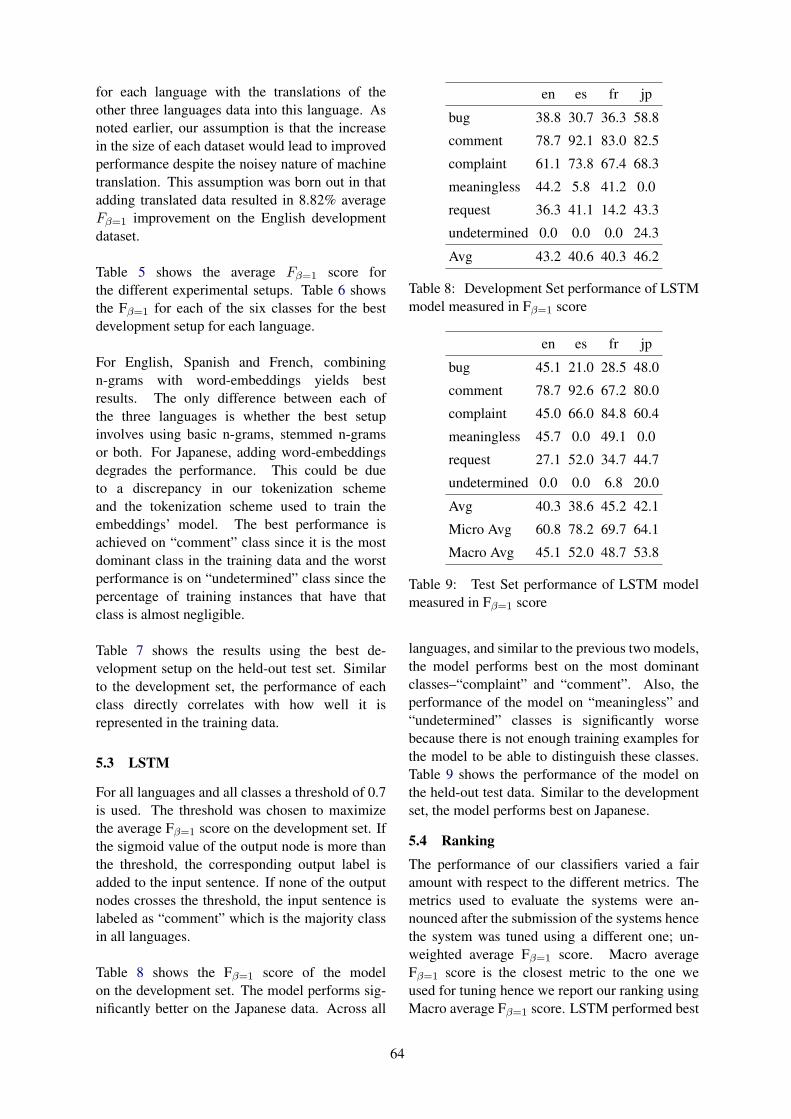
for each language with the translations of theother three languages data into this language. Asnoted earlier, our assumption is that the increasein the size of each dataset would lead to improvedperformance despite the noisey nature of machinetranslation. This assumption was born out in thatadding translated data resulted in 8.82% averageFβ=1 improvement on the English developmentdataset.

Table 5 shows the average Fβ=1 score forthe different experimental setups. Table 6 showsthe Fβ=1 for each of the six classes for the bestdevelopment setup for each language.

For English, Spanish and French, combiningn-grams with word-embeddings yields bestresults. The only difference between each ofthe three languages is whether the best setupinvolves using basic n-grams, stemmed n-gramsor both. For Japanese, adding word-embeddingsdegrades the performance. This could be dueto a discrepancy in our tokenization schemeand the tokenization scheme used to train theembeddings’ model. The best performance isachieved on “comment” class since it is the mostdominant class in the training data and the worstperformance is on “undetermined” class since thepercentage of training instances that have thatclass is almost negligible.

Table 7 shows the results using the best de-velopment setup on the held-out test set. Similarto the development set, the performance of eachclass directly correlates with how well it isrepresented in the training data.

5.3 LSTM

For all languages and all classes a threshold of 0.7is used. The threshold was chosen to maximizethe average Fβ=1 score on the development set. Ifthe sigmoid value of the output node is more thanthe threshold, the corresponding output label isadded to the input sentence. If none of the outputnodes crosses the threshold, the input sentence islabeled as “comment” which is the majority classin all languages.

Table 8 shows the Fβ=1 score of the modelon the development set. The model performs sig-nificantly better on the Japanese data. Across all

en es fr jp

bug 38.8 30.7 36.3 58.8

comment 78.7 92.1 83.0 82.5

complaint 61.1 73.8 67.4 68.3

meaningless 44.2 5.8 41.2 0.0

request 36.3 41.1 14.2 43.3

undetermined 0.0 0.0 0.0 24.3

Avg 43.2 40.6 40.3 46.2

Table 8: Development Set performance of LSTMmodel measured in Fβ=1 score

en es fr jp

bug 45.1 21.0 28.5 48.0

comment 78.7 92.6 67.2 80.0

complaint 45.0 66.0 84.8 60.4

meaningless 45.7 0.0 49.1 0.0

request 27.1 52.0 34.7 44.7

undetermined 0.0 0.0 6.8 20.0

Avg 40.3 38.6 45.2 42.1

Micro Avg 60.8 78.2 69.7 64.1

Macro Avg 45.1 52.0 48.7 53.8

Table 9: Test Set performance of LSTM modelmeasured in Fβ=1 score

languages, and similar to the previous two models,the model performs best on the most dominantclasses–“complaint” and “comment”. Also, theperformance of the model on “meaningless” and“undetermined” classes is significantly worsebecause there is not enough training examples forthe model to be able to distinguish these classes.Table 9 shows the performance of the model onthe held-out test data. Similar to the developmentset, the model performs best on Japanese.

5.4 RankingThe performance of our classifiers varied a fairamount with respect to the different metrics. Themetrics used to evaluate the systems were an-nounced after the submission of the systems hencethe system was tuned using a different one; un-weighted average Fβ=1 score. Macro averageFβ=1 score is the closest metric to the one weused for tuning hence we report our ranking usingMacro average Fβ=1 score. LSTM performed best

64

on French and Japanese and ranked 1/8 and 2/7 oneach of them while Logistic Regression performedbest on English where it ranked 3/12 and Spanishranking 3/7.

6 Conclusion

This shared task was created with the intent of es-tablishing a labeling schema that is both widelyapplicable and publicly available. Ultimately, theperformance of our classifiers varied a fair amountwith respect to the different metrics. Overall, us-ing Macro-Average Fβ=1, we ranked 3/12, 3/7,1/8 and 2/7 on English, Spanish, French andJapanese datasets respectively. The inclusion ofword embeddings and machine translation offeredthe largest boosts to system performance. Futuredirections for work in this area could include ex-panding the amount of data, which in turn mightimprove the performance of deep learning meth-ods. Included in this shared task was an unan-notated dataset for each language. Though ourteam did not explore a semi-supervised approach,our experiments with translated data indicate thiswould be low-hanging fruit.

ReferencesShilpa Arora, Mahesh Joshi, and Carolyn P Rose. 2009.

Identifying types of claims in online customer re-views. In Proceedings of the Annual Conference ofthe North American Chapter of the Association forComputational Linguistics.

Alexandra Balahur, Rada Mihalcea, and Andres Mon-toyo. 2014. Computational approaches to subjec-tivity and sentiment analysis: Present and envisagedmethods and applications. Computer Speech & Lan-guage, 1(28):1–6.

Marco Baroni, Georgiana Dinu, and GermanKruszewski. 2014. Don’t count, predict! asystematic comparison of context-counting vs.context-predicting semantic vectors. In Proceedingsof the 52nd Annual Meeting of the Association forComputational Linguistics.

Michael Bentley and Soumya Batra. 2016. Givingvoice to office customers: Best practices in how of-fice handles verbatim text feedback. In 2016 IEEEInternational Conference on Big Data, pages 3826–3832. IEEE.

Piotr Bojanowski, Edouard Grave, Armand Joulin,and Tomas Mikolov. 2016. Enriching word vec-tors with subword information. arXiv preprintarXiv:1607.04606.

Leo Breiman. 2001. Random forests. Machine Learn-ing, 45(1):5–32.

Ronan Collobert, Jason Weston, Leon Bottou, MichaelKarlen, Koray Kavukcuoglu, and Pavel Kuksa.2011. Natural language processing (almost) fromscratch. Journal of Machine Learning Research,12(Aug):2493–2537.

Jerome Friedman, Trevor Hastie, and Robert Tibshi-rani. 2001. The Elements of Statistical Learning,volume 1. Springer series in statistics New York.

Michael Gamon. 2004. Sentiment classification oncustomer feedback data: noisy data, large featurevectors, and the role of linguistic analysis. In Pro-ceedings of the 20th International Conference onComputational Linguistics.

Narendra Gupta, Mazin Gilbert, and Giuseppe Di Fab-brizio. 2010. Emotion detection in email customercare. In Proceedings of the NAACL HLT 2010 Work-shop on Computational Approaches to Analysis andGeneration of Emotion in Text.

Svetlana Kiritchenko, Xiaodan Zhu, Colin Cherry, andSaif Mohammad. 2014. Nrc-canada-2014: Detect-ing aspects and sentiment in customer reviews. InProceedings of the 8th International Workshop onSemantic Evaluation (SemEval).

Taku Kudo. 2005. Mecab: Yet another part-of-speechand morphological analyzer.

Christopher D Manning, Mihai Surdeanu, John Bauer,Jenny Rose Finkel, Steven Bethard, and David Mc-Closky. 2014. The stanford corenlp natural lan-guage processing toolkit. In ACL (System Demon-strations).

Tomas Mikolov, Ilya Sutskever, Kai Chen, Greg S Cor-rado, and Jeff Dean. 2013. Distributed representa-tions of words and phrases and their compositional-ity. In Advances in neural information processingsystems.

Fabian Pedregosa, Gael Varoquaux, Alexandre Gram-fort, Vincent Michel, Bertrand Thirion, OlivierGrisel, Mathieu Blondel, Peter Prettenhofer, RonWeiss, Vincent Dubourg, et al. 2011. Scikit-learn:Machine learning in python. Journal of MachineLearning Research, 12(Oct):2825–2830.

Rahul Potharaju, Navendu Jain, and Cristina Nita-Rotaru. 2013. Juggling the jigsaw: Towards auto-mated problem inference from network trouble tick-ets. In Proceedings of the 10th USENIX Sympo-sium on Network Systems Design and Implementa-tion (NSDI’13), pages 127–141.

Richard Socher, Jeffrey Pennington, Eric H Huang,Andrew Y Ng, and Christopher D Manning. 2011.Semi-supervised recursive autoencoders for predict-ing sentiment distributions. In Proceedings of the2011 Conference on Empirical Methods in NaturalLanguage Processing.

65

Joseph Turian, Lev Ratinov, and Yoshua Bengio. 2010.Word representations: A simple and general methodfor semi-supervised learning. In Proceedings of the48th Annual Meeting of the Association for Compu-tational Linguistics.

66

Proceedings of the 8th International Joint Conference on Natural Language Processing, Shared Tasks, pages 67–72,Taipei, Taiwan, November 27 – December 1, 2017. c©2017 AFNLP

ADAPT Centre Cone Team at IJCNLP-2017 Task 5:A Similarity-Based Logistic Regression Approach to Multi-choice

Question Answering in an Examinations Shared TaskDaria DzendzikADAPT Centre

School of ComputingDublin City University

Dublin, Irelanddaria.dzendzik@adaptcentre.ie

Alberto PoncelasADAPT Centre

School of ComputingDublin City University

Dublin, Irelandalberto.poncelas@adaptcentre.ie

Carl VogelSchool of Computer Science and Statistics

Trinity College Dublin the University of DublinDublin, Irelandvogel@tcd.ie

Qun LiuADAPT Centre

School of ComputingDublin City University

Dublin, Irelandqun.liu@adaptcentre.ie

Abstract

We describe the work of a team from theADAPT Centre in Ireland in addressingautomatic answer selection for the Multi-choice Question Answering in Examina-tions shared task. The system is based ona logistic regression over the string simi-larities between question, answer, and ad-ditional text. We obtain the highest gradeout of six systems: 48.7% accuracy on avalidation set (vs. a baseline of 29.45%)and 45.6% on a test set.

1 Introduction

This paper describes the participation of theADAPT Centre team in the Multi-choice QuestionAnswering in Examinations Shared Task 2017.1

This is a typical question answering task that aimsto test how accurately the answers of the ques-tions in exams could be selected. Any additionalsources, such as knowledge base, textbooks or ar-ticles, can be used to exploit support information.The English subset contains 5,367 questions fromfive domains: Biology, Chemistry, Earth Science,Life Science and Physical Science. The questionscome from real exams. Every question has fouranswer candidates which may be a word, a value,a phrase or a sentence. This challenge is an im-portant step towards a rational, quantitative assess-ment of natural language understanding capabili-ties.

1See http://www.nlpr.ia.ac.cn/cip/ijcnlp/Multi-choice_Question_Answering_in_Exams.html – October 2017.

Our approach is to extract relevant informationfrom Wikipedia2 and to apply logistic regressionover string similarities. We used an adaptation ofmethods developed for a comparable task in rela-tion to question answering about films (Dzendziket al., 2017). The features we employ are simi-larities of a term frequency–inverse document fre-quency (TF-IDF) metric, character n-grams (withn ranging from 2 to 5), bag of words, and windowsslide (a ratio between answer and substrings of ex-tracted data) – the window slide ratio is describedin further detail below (section 2.3). We train ourmodel in two ways: combining training over alldomains and separate model training for each do-main. The second way yields a better result on thevalidation set: 48.7% of accuracy vs. 43.6%. Fi-nally, we obtained 45.6% accuracy on the test set,and this is the best result for the English dataset ofthe six competing systems.

The paper is organized as follows: We detail ourapproach in Section 2. In Section 3, we describeexperiments and results on the training, validationand test data. In Section 4, we compare our ap-proach to previous research in answering exami-nation questions. Finally, Section 5 contains con-clusions and directions of future work.

2 Approach

We constructed our model as a four-step pipeline:

1. Preprocessing – cleaning of the input data.

2. Data selection – based on key words from thequestion we extract relative sentences from

2wikipedia.org– September 2017

67

Wikipedia.

3. Feature Vector Concatenation – for everyquestion, a feature vector is built as a con-catenation of vectors of similarities betweenthe answer candidates and sentences obtainedin the previous step.

4. Logistic Regression – a logistic regressionover the feature vector.

Later in this section, we describe our approachto multi-choice question answering in detail.

2.1 Preprocessing

The first step is to clean the question and answersstatements. Using regular expressions, the exist-ing serial numbers and letters of the question andanswer candidates are deleted. See the examples(1)-(3).

(1) “3. What ...”→ “What ... ”

(2) “8) Who ...”→ “Who ... ”

(3) “a) Paper: Paper degrades ... ”→“Paper: Paper degrades ...”

2.2 Data Selection

A list of keywords are extracted from the questionstatement using Natural Language Toolkit (nltk)3

implementation of the Rapid Automatic KeywordExtraction (RAKE) algorithm (Rose et al., 2010).These words are used to retrieve a list of sentencesfrom an information source. For each question, weselect the top-50 sentences as ranked by contain-ing (unweighted) keywords related to the item

The information source used in this system is aset of sentences from articles of Wikipedia. Eachsentence is stored as a document in an inverted in-dex data structure using Lucene.4

2.3 Feature Vector Creation

The data is organized in triplets (q, a, S) where ais a candidate answer, q is the question that a be-longs to, and S is the set of sentences retrievedfrom Wikipedia by querying the keywords of thequestion q.

Then, for every triplet a feature vector is cre-ated by concatenating different features. Each fea-ture is a function of two arguments and encodes

3https://github.com/csurfer/rake-nltk –September 2017

4https://lucene.apache.org/core/ –September 2017

the similarity between two strings. The first ar-gument is either the answer a or a concatenationof the question and the answer q + a and the sec-ond argument is S. The value of every feature isbetween 0 and 1: the higher the value, the moresimilar the strings are.

The five similarities are based on the work of(Dzendzik et al., 2017), and are described below.

• TF-IDF cosine similarity - the cosine simi-larity between TF-IDF representations as de-fined in Equation (4).

cos tfidf(a, S) =wa · wS

|wa||wS | (4)

where wa and wS are TF-IDF vector repre-sentations of the answer (or question + an-swer) and the sentences correspondingly.

• Bag of words ratio similarity - a bag ofwords measure shows the ratio of sentenceswords which exist in the answer (or question+ answer) as shown in Equation (5).

bow(a, S) =|Wa ∩WS ||Wa| (5)

where Wa - bag of words from the answer(or the question + the answer) and WS bag ofwords from sentences.

• Window slide ratio similarity - returns thehighest ratio of sequence match between an-swer (or question + answer) and all sentencessubstrings. The window of the substrings hasa size equal to a length of the answer. See theEquation (6).

wSlide(a, S) = maxi(2 ∗Mi

Ti) (6)

where Ti = |a| + |si| is the total numberof character elements in both sequences: theanswer a and si. si is i–substring of S,∀isi ∈ S, |si| = |a| and Mi is the numberof matches between all substrings of a andsi.

• Character N-gram - similar toWindow Slide but on character level.The size of the window is limited by parame-ter n (We consider n = 2,3,4,5 characters). Asa result, we get the ratio of n-grams overlapincluding white spaces in the answer (or thequestion + the answer) and the sentences.

68

• Word2vec cosine similarity The cosine dis-tance similarity (as in Equation (7)) betweenskip-gram representations (Mikolov et al.,2013).

w2v cos(a, S) =va · vS

|va||vS | (7)

where va and vS are Word2vec representa-tions of the answer (or the question + the an-swer) and the sentences correspondingly.

We use a pre-trained word2vec model basedon small subset of Wikipedia (Tapaswi et al.,2016).

Using this metrics 17 different features are built:

1. f1 = w2v cos(q, S) + w2v cos(a, S)

2. f2 = w2v cos(a, S)

3. f3 = cos tfidf(a, S)

4. f4 = bow overlap(a, S)

5. f5 = windowSlide(a, S)

6. f6 = charNgramm2(a, S)

7. f7 = charNgramm3(a, S)

8. f8 = charNgramm4(a, S)

9. f9 = charNgramm5(a, S)

10. f10 = w2v cos(q + a, S)

11. f11 = cos tfidf(q + a, S)

12. f12 = bow overlap(q + a, S)

13. f13 = windowSlide(q + a, S)

14. f14 = charNgramm2(q + a, S)

15. f15 = charNgramm3(q + a, S)

16. f16 = charNgramm4(q + a, S)

17. f17 = charNgramm5(q + a, S)

Here q+a is the concatenation of q and a. Somequestions from the dataset are presented as sen-tences with one or many gaps. If the question qincludes gaps, instead of concatenating, the candi-date answer a will be used to fill the gaps in thequestion. See the example (8).

(8) Question: “ obtain energy by using thechemical energy stored in inorganic com-pounds”

Answer candidates:

1. Photoautotrophs

2. Chemoautotrophs

3. Heterotrophs

4. None of the above

Concatenation strings:

1. Photoautotrophs obtain energy by usingthe chemical energy stored in inorganiccompounds

2. Chemoautotrophs obtain energy by us-ing the chemical energy stored in inor-ganic compounds

3. Heterotrophs obtain energy by usingthe chemical energy stored in inorganiccompounds

4. None of the above obtain energy by us-ing the chemical energy stored in inor-ganic compounds

For a question q the similarity features of itsanswer candidates a1, a2, a3, a4 are concatenatedinto one single vector as shown in Figure 1.

Following this method, for each question, thereis one feature vector which contains informationfor all answer candidates inside.

2.4 Logistic Regression

The final step of our system is logistic regressionover the vector. It returns the eventual answer. Weuse a scikit-learn5 implementation with liblinearcore and one-versus-rest schemes.

3 Experiments

In this section, we describe the data and results ofour experiments.

3.1 Data

The dataset provides examination questions in twolanguages: English and Chinese. We focus ourresearch on English subset of data which con-tains 5,367 questions from five domains: Biology,Chemistry, Earth Science, Life Science and Phys-ical Science. Table 1 presents the division of thedataset into training, validation and test sets.

As mentioned before, we use Wikipedia dumpas source of additional data.

5http://scikit-learn.org/stable/modules/generated/sklearn.linear_model.LogisticRegression.html – September 2017

69

Figure 1: Feature vector concatenation.

Domain Train Val Test TotalBiology 281 70 210 561Chemistry 775 193 581 1549Physical 299 74 224 597Earth Science 830 207 622 1659Life Science 501 125 375 1001Total 2686 669 2012 5367

Table 1: The number of questions for each domainand a division for training, validation and test sets.

3.2 Results

The systems built are the following:

• Combined training: Data from all domainsis combined together to train one singlemodel.

• Domain training: Use separate modelstrained in each domain. The parameters ofthe logistic regressions are the same for ev-ery domain.

The results obtained by these systems and thebaseline6 are presented in tables 2 and 3.

Using the Combined training approach we ob-tained 44.82% accuracy on the training data and43.6% on the validation set (table 2 line 2). Thisresult significantly outperforms the baseline (table2 line 1). Using the Domain training approach weobserve that the average score is better (51.71%)than Combined training. In addition, this approachenables evaluation of the method in each domain.The best performance is obtained in the Chemi-cal subset – 69.55% accuracy. However, for EarthScience and for Life Science we obtained 41.08%and 42.91%, respectively. Unfortunately, we canobtain the results of separate domains only for thetrainin set; we cannot compare it with the pub-lished baseline on the validation set. Finally, byconcatenating the results from separate domains

6The baseline is provided by the shared task organizers–see footnote 1.

we obtain 48.7% accuracy on the validation setand 45.6% on the test set.

System Train Valid TestBaseline – 29.45 –Combined training 44.82 43.6 –Domain training 51.71 48.7 45.6

Table 2: Results of all English subset of the base-line system on the validation set and our systemfor combined and domain training on the training,validation and test sets.

Bio Chem Phys Earth LifeBaseline

Valid 30 21.24 25.68 31.88 40Domain training

Train 49.47 69.55 51.84 41.08 42.91

Table 3: Results of the baseline system on thevalidation set and results of domain training on thetrain set for each domain.

4 Related Work

As mentioned before, this system is based on thework of (Dzendzik et al., 2017). The main dif-ference is the data selection module: in the ear-lier work we select sentences from movie plot us-ing similarities; here we extract relevant sentencesfrom Wikipedia. Another difference is that we donot build semantic features in this shared task.

The core of our method is text similarity. Weconsider only five types of similarities. Gomaaand Fahmy (2013) consider more than 25 textsimilarity metrics in five categories: character-based similarity, term-based similarity, corpus-based similarity, knowledge-based similarity, andhybrid similarity measures. They also mention co-sine similarity (for the mathematical function thatdetermines the metric), Tf-IDf (which we deemto be a hybrid of term-based and corpus-based)

70

and N-grams similarities (which may be character-based or term based), all of which we use, too.

There is interest in answering examinationquestions automatically. Wang et al. (2014) de-scribe CMUs UIMA-based7 modular automaticquestion answering system to automatically an-swer multiple-choice questions for the entranceexam in world history in English. The ap-proach relies on two different test collection: theoriginal test collection provided by NTCIR (NIITestbeds and Community for Information accessResearch)8 organizers and the collection createdby the authors.

Li et al. (2013) described the system that wasused in the Entrance Exams task of Question An-swering for Machine Reading Evaluation on Con-ference and Labs of the Evaluation Forum 2013(QA4MRE CLEF) (Sutcliffe et al., 2013). It con-sists of three components, Character Resolver,Sentence Extractor and Recognizing Textual En-tailment. In the system, the documents are pro-cessed by the Character Resolver in order to tageach story with a character as ID. The SentenceExtractor then extracts related sentences for eachquestion and creates a Hypothesis (H) and Text(T). Finally it inputs this T/H pair into the Rec-ognizing Textual Entailment system to select ananswer.

5 Conclusions and Future Work

In this paper, we described the work of ADAPTCentre for the multi-choice question answering inexamination shared task. In this work we haveused a sentence retrieval approach with combi-nation of logistic regression over string similari-ties. Our submission shows an improvement overthe baseline system. According to the shared taskleader board, six teams submitted their results forEnglish subset. Our submission shows the best re-sult on validation and test dataset and significantlyoutperform the baseline system.

At the same time, we believe that our systemcan be improved in the future: a) Using more in-domain data, for this system a set of Wikipediaarticles has been used as the information source,the accuracy may be improved by using techni-cal books or manuals; b) exploring different meth-ods for selecting sentences from the information

7https://uima.apache.org/ – September 20178http://research.nii.ac.jp/ntcir/

index-en.html – September 2017

source (such as considering the keywords from thecandidate answers); or c) Extracting a different setof keywords (for example, maximizing semanticdistance among keywords selected).

Acknowledgments

This research is supported by the Science Foun-dation Ireland (Grant 12/CE/I2267) as part ofADAPT centre (www.adaptcentre.ie) at DublinCity University. The ADAPT Centre for Digi-tal Content Technology is funded under the SFIResearch Centres Programme (Grant 13/RC/2106)and is cofunded under the European Regional De-velopment Fund.

ReferencesDaria Dzendzik, Carl Vogel, and Qun Liu. 2017. Who

framed roger rabbit? answering questions aboutmovie plot. The Joint Video and Language Under-standing Workshop: MovieQA and The Large ScaleMovie Description Challenge (LSMDC), at ICCV2017, 23th of October, Venice, Italy.

Wael H. Gomaa and Aly A. Fahmy. 2013. Article: Asurvey of text similarity approaches. InternationalJournal of Computer Applications, 68(13):13–18.Full text available.

Xinjian Li, Ran Tian, Ngan L. T. Nguyen, YusukeMiyao, and Akiko Aizawa. 2013. Question answer-ing system for entrance exams in QA4MRE. InWorking Notes for CLEF 2013 Conference , Valen-cia, Spain, September 23-26, 2013.

Tomas Mikolov, Kai Chen, Greg Corrado, and JeffreyDean. 2013. Efficient estimation of word represen-tations in vector space. CoRR, abs/1301.3781.

Stuart Rose, Dave Engel, Nick Cramer, and WendyCowley. 2010. Automatic keyword extraction fromindividual documents.

Richard FE Sutcliffe, Anselmo Penas, Eduard HHovy, Pamela Forner, Alvaro Rodrigo, CorinaForascu, Yassine Benajiba, and Petya Osenova.2013. Overview of qa4mre main task at clef 2013.In CLEF (Working Notes).

Makarand Tapaswi, Yukun Zhu, Rainer Stiefelhagen,Antonio Torralba, Raquel Urtasun, and Sanja Fi-dler. 2016. Movieqa: Understanding stories inmovies through question-answering. In IEEE Con-ference on Computer Vision and Pattern Recognition(CVPR).

Di Wang, Leonid Boytsov, Jun Araki, Alkesh Patel, JeffGee, Zhengzhong Liu, Eric Nyberg, and Teruko Mi-tamura. 2014. CMU multiple-choice question an-swering system at NTCIR-11 qa-lab. In Proceed-ings of the 11th NTCIR Conference on Evaluation

71

of Information Access Technologies, NTCIR-11, Na-tional Center of Sciences, Tokyo, Japan, December9-12, 2014.

72

Proceedings of the 8th International Joint Conference on Natural Language Processing, Shared Tasks, pages 73–77,Taipei, Taiwan, November 27 – December 1, 2017. c©2017 AFNLP

YNU-HPCC at IJCNLP-2017 Task 1: Chinese Grammatical ErrorDiagnosis Using a Bi-directional LSTM-CRF Model

Quanlei Liao, Jin Wang, Jinnan Yang and Xuejie ZhangSchool of Information Science and Engineering

Yunnan UniversityKunming, P.R. China

Contact:xjzhang@ynu.edu.cn

Abstract

Building a system to detect Chinese gram-matical errors is a challenge for natural-language processing researchers. As Chi-nese learners are increasing, developingsuch a system can help them study Chinesemore easily. This paper introduces a bi-directional long short-term memory (BiL-STM) - conditional random field (CRF)model to produce the sequences that in-dicate an error type for every positionof a sentence, since we regard Chinesegrammatical error diagnosis (CGED) as asequence-labeling problem. Among theparticipants this year of CGED shard task,our model ranked third in the detection-level and identification-level results. In theposition-level, our results ranked second a-mong the participants.

1 Introduction

With China’s rapid development, more and moreforeign people have begun to learn Chinese. Writ-ing is an important part of language learning, andgrammar is the basis of writing. Traditional learn-ing methods rely on artificial work to point outgrammatical errors in an article. This requiresmore time and labor costs. Thus, it is quite practi-cal to develop a system that can automatically cor-rect the grammatical errors in an article. This isthe aim of the CGED shared task.

In the shared task, Chinese-grammar errors aredivided into four types: redundant words, word-selection errors, missing words, and incorrec-t word order (Lee et al., 2016). They are represent-ed as uppercase letters “R”, “S”, “M”, and “W”,respectively. For each sentence, the task shouldfirst determine whether the sentence is correct. If

the sentence is incorrect, it should indicate the spe-cific error types and their locations.

In this paper, the CGED task is treated as a se-quence labeling problem, which is a classic naturallanguage processing problem. The traditional so-lutions are a series of statistical learning methods,including the hidden Markov model (HMM), themaximum-entropy Markov model (MEMM), andthe conditional random field.

The HMM model makes two assumptions.First, that the current implicit state is only relatedto the last implied state; second, that the currentoutput state is only related to the current impliedstate (Dugad and Desai, 1996). However, the real-ity is not so simple. A CRF uses the entire outputsequence and two adjacent implicit states to finda conditional probability (Lafferty et al., 2001).It can fit more complex situations. Practice hasproven that the CRF works better than other mod-els.

Recently, artificial neural networks have beenused to do natural language processing tasks. Forthe sequence labeling problem, because of its e-qual length output, a recurrent neural network(RNN) is an appropriate model. It is more capableof understanding the information context; howev-er, this is not a good method for learning statetransfer laws. To improve the problems of explod-ing and vanishing gradients, new RNN units, e.g.,long short-term memory (LSTM) and gated recur-rent units (GRUs) (Chung et al., 2014), have beenproposed.

In this study, we propose a BiLSTM-CRF mod-el. Our model combines statistical learning withneural networks. The BiLSTM is used to obtaininformation about long or short distances in twodirections (Huang et al., 2015). It then feeds theinformation to the CRF. Thus, the CRF can betteruse conditional probabilities to fit the data withouthandmade features. The CRF and LSTM models

73

are also used as part of the experiment to comparethe models’ performance.

The rest of this paper is organized as follows.Section 2 describes our model in detail. Section3 presents our experiment, including the data pre-processing and results. Conclusions are drawn inSection 4.

2 Proposed Model

The proposed model consists of three major parts:the word-embedding layer, the bi-directional LST-M layer, and the CRF layer. CRF is a traditional s-tatistical learning method for sequence labeling. Ithas two limits. First, it heavily depends on hand-crafted features. Second, it cannot capture longdistance context information. The context infor-mation for a CGED task is very important. Forexample, here are two correct sentences.

• “只有努力，才能过的更好。” (Only youwork hard, you can be better.)

• “只要努力，就能过的更好。” (As long asyou work hard, you will be able to be better.)

It is impossible to determine whether the sentence,“才能过的更好。” is correct without the previouscontext information. On the other hand, handcraft-ed features greatly increase the workload. Thus,our model combines an RNN with a CRF to im-prove the above problems. To capture informa-tion from two directions (Ma and Hovy, 2016), weuse a bi-directional RNN instead of a unidirection-al RNN. In addition, an LSTM cell is selected toavoid vanishing and exploding gradients (Sunder-meyer et al., 2012).

We trained four models for four error types be-cause there may be two or more errors in one posi-tion. Each model is given the original text index asinput, its label sequence outputs 0 for correct and1 for error.

The model includes three layers: a word-embedding layer to transfer the word index intoword embedding, a BiLSTM layer to extract theinformation and features for each position, and aCRF layer to decode and produce labels. The threelayers are introduced in the following sections.

2.1 Embedding Layer

A diagram of the embedding layer’s structure isshown in Figure 1. It shows a pre-trained word-embedding lookup table. Every line of this table

W1 W2 W3 W4 Wn

V1 V2 V3 V4 Vn

...

...

...

...

... ...

Original text index

Word embedding

look-up table

Word vector

Figure 1: Embedding Layer

stands for one Chinese word. Therefore, the orig-inal text of the training data should be turned intoa sequence of indexes for every word. This lay-er takes a sequence that contains the word indices,e.g., w1, w2,. . . , wi,. . . , wn where wi, is an in-dex number indicating the position of the originalword in the table. Then, the layer finds the wordvector for every index and outputs them in a newsequence, e.g., v1, v2,. . . , vi,. . . , vn where vi is aword vector.

If the dimensionality of the original text index isN and the dimensionality of the word vector isM ,the dimensionality of the output sequence shouldbe M ∗N .

2.2 Bi-directional LSTM Layer

An RNN can effectively extract features from theentire sentence because of its ability to capturecontext information. For the reasons mentionedabove, a bi-directional LSTM network was cho-sen.

An LSTM is a special type of RNN unit thatcan learn long-term dependency information. It isdesigned to avoid the long-term dependence prob-lem. An LSTM can remove or increase the infor-mation to a cell state using a well-designed struc-ture called a “gate”. The gate determines whetherinformation should pass. The LSTM uses thefollowing formulas (Hochreiter and Schmidhuber,1997):

it = σ(Wvivt +Whiht−1 + bi) (1)

ft = σ(Wvfvt +Whfht−1 + bf ) (2)

ct = ftct−1+it tanh(Wvcvt+Whcht−1+bc) (3)

ot = σ(Wvovt +Whoht−1 + bo) (4)

74

V3V1 V2 V4

Forward LSTM

Backward LSTM

Output

X1

LSTMLSTM LSTM LSTM

X2 X3 X4

LSTMLSTMLSTM LSTM

Figure 2: Bi-directional LSTM Layer

ht = ot tanh(ct) (5)

where v is the input vector from the embeddinglayer. σ is the sigmoid activation function. i is theinput gate, f is the forget gate, and o is the out-put gate. Parameters {Wvi, Whi, Wvf , Whf , Wvc,Whc, Wvo, Who, bi, bf , bc, bo} are the weightsand biases of an LSTM cell. c is the cell vectorand h is the hidden cell. K represents the outputdimensionality of the LSTM unit. N is the dimen-sionality of the word vector. The size of the lastfour bias vectors are K and the others are N ∗K.Figure 2 shows a bi-directional LSTM network.The embedding output is fed into two LSTM lay-ers with forward and backward directions. Twooutputs from two layers at one position are linkedinto a new vector as the layer’s output.

The dimensionality of the input is M ∗ N . Mis the length of the original text. Each word vec-tor of input is also called an RNN time step. Forinstance, v1, v2,. . . , vi,. . . , vn is input, each vi

is a time step. For each time step, vi is fed intotwo LSTMs; the forward LSTM layer producesan output vector oi−forward with dimensionali-ty K, and the backward LSTM layer producesoi−backward. Therefore, the result of a time stepis xi(oi−forward, oi−backward) and the dimension-ality is 2 ∗K, which is the result of combining thetwo layers’ output. Thus, the dimensionality of thefinal output is M ∗ (2 ∗K).

2.3 CRF Layer

Because of the importance of the relationships be-tween neighboring tags in CGED, a CRF is select-ed to capture the relationship. The CRF is a type ofundirected discriminative graph model. In general,a CRF is a Markov random field with an observa-tion set. A general CRF is defined as a Markovrandom field with random variable Y under thecondition of random variable X . Y constitutes aMarkov random field represented by an undirectedgraph, as in the formula below (Sutton and Mccal-

X1 X2 X3 Xn

Input

Y1 Y2 Y3 YnCRF Layer

Figure 3: CRF Layer

lum, 2010):

P (Yv|X,Yw, w 6= v)=P (Yv|X,Yw, w ∼ v) (6)

where operator∼means that w and v have a pub-lic edge. X is the input variable or state sequence,and Y is the output variable or tag sequence. Inour problem, we assume that X and Y have thesame linear structure, as shown in Figure 3.

The conditional probability of random variabley with value x is given as follows:

P (y|x) =

n∏i=1

Mi(yi−1, yi, x)

Z(x)(7)

The denominator is a normalization item:

Z(x) =∑y

n∏i=1

Mi(yi−1, yi, x) (8)

whereMi(y′, y′′, x) is a potential function, x is theinput vector produced by the BiLSTM layer and yis the labeling of the input sentence.

3 Experiment

This section describes the contents of the ex-periment, including the training data processing,choice of parameters, experimental results, etc.

3.1 DatasetThe word embedding was trained using theword2vec toolkit with the Chinese Wikipedia cor-pus. According to the experimental results, theword-embedding results from word2vec are bet-ter than GloVe (Yang et al., 2016). In addition tothe CGED17 training data, the HSK (i.e., ChineseProficiency Test) training data from CGED16 wasused. The number of training sets is 20,048, with10,447 from CGED17 and 9,601 from CGED16.

For the reasons mentioned above, four modelsfor every error type were selected. Thus, we pre-processed training sets for four error type models.For each error type, the position’s label is 0 if cor-rect, or 1 if erroneous. The training-data text wastransferred into the word-index sequence, accord-ing to the pre-trained word-embedding table.

75

Model Acc Pre Rec F1CRF 0.1805 0.1136 0.1483 0.1287

LSTM 0.1696 0.1824 0.0816 0.1128BiLSTM-CRF 0.3325 0.2769 0.3502 0.3093

Table 1: Comparative results of three models.

3.2 Implementation Details

The experiment contains three models for compar-ison: CRF, LSTM, and BiLSTM-CRF. CRF rep-resents the statistical learning method, which isthe best simple statistical learning model in a vari-ety of sequence labeling tasks. LSTM is a typicalneural network model for sequence labeling. Theabove two models were used as the baseline for theexperiment. The last model, proposed in this pa-per, combines both neural network and statisticallearning models.

The CRF model was implemented using theCRF++ toolkit. CRF++ is an open-source, easy-to-use implementation of CRF, written in C++.The LSTM model and the BiLSTM-CRF mod-el were implemented using the Keras frameworkwith a Tensorflow backend. The CRF layer im-plementation in the BiLSTM-CRF model used K-eras contrib.

The training data for the three models comesfrom CGED16 or CGED17. Hence, the trainingdata is regarded as a hyper-parameter. It will beCGED16 or CGED17 or a combination of both. Inaddition, there is a public hyper-parameter for thethree models. The hyper-parameter for the CR-F model is c, which controls the over-fitting ofthe training data. The hyper-parameters for LSTMand BiLSTM-CRF include the LSTM cell numberand the training epoch.

Some empirical parameters are given as candi-date values for the model. A grid search algorithmwas used to find the best hyper-parameter combi-nations.

To evaluate the model’s performance, we usedfour metrics such as accuracy (Acc), precision(Pre), recall (Rec) and F1-score (F1) for all threemodels on CGED16 HSK test data. Table 1 showsthe best results for each model on position-level.The results show that the BiLSTM-CRF model hasthe best results in Table 1.

3.3 Experimental Results

Five teams submitted 13 results. We submit-ted three running results. The three results wereproduced by the three BiLSTM-CRF models that

Parameter Dataset LSTM cell EpochRun1 CGED16,17 120 22Run2 CGED16,17 100 18Run3 CGED16 100 18

Table 2: Parameter selection for BiLSTM-CRFmodels.

Results Detection-LevelAcc Pre Rec F1

Run1 0.5796 0.65 0.7163 0.6816Run2 0.5891 0.6417 0.7829 0.7053Run3 0.5311 0.6298 0.6148 0.6222

Table 3: Comparative results on detection-level.

had the best three results on the CGED16 HSKtest data. The three results have different hyper-parameters, as shown in Table 2.

The next three tables show the final test result-s for the three BiLSTM-CRF models. Table 3shows the detection-level results. Table 4 showsthe identification-level results. Table 5 shows theposition-level results.

The false positive (FP) rates of the three resultsof BiLSTM-CRF models are 0.5796, 0.7383, and0.614 shown in Table 6. The highest one is over70%. This is because the model uses four sub-models to generate the sentence label. If only onemodel misjudges the label of one position, from0 to 1, it will produce a false negative (FN) sam-ple. Thus, the model produces a high false positiverate. In addition, the experimental results showthat the recall of the first two results is better thanthe previous in the detection level. This model ismore likely to produce positive examples.

4 Conclusion

Compared with most previous models (Lee et al.,2016), the F1-score of the position level greatlyincreased with the CGED16 HSK test data. Itwas observed that neural network and statistical-learning methods could be combined to obtainbetter results. Among the participants this year,our model ranked third in the detection-level andidentification-level results. In the position-level,

Results Identification-LevelAcc Pre Rec F1

Run1 0.4218 0.4219 0.4217 0.4218Run2 0.3819 0.3825 0.4575 0.4167Run3 0.3979 0.4086 0.3298 0.365

Table 4: Comparative results on identification-level.

76

Results Position-LevelAcc Pre Rec F1

Run1 0.1778 0.1262 0.1191 0.1225Run2 0.1426 0.1056 0.1191 0.112Run3 0.1702 0.0981 0.0698 0.0816

Table 5: Comparative results on position-Level.

Result False Positive RateRun1 0.5796Run2 0.7383Run3 0.614

Table 6: False positive rates of three results.

our results ranked second among the participants.Our model is a combination of BiLSTM and

CRF. It combines the extraction capabilities ofthe LSTM context information and the condition-al probability of CRF’s local features. More com-plex models contain more parameters that need tobe trained. Thus, more training data can improvethe model; too little training data may cause over-fitting.

The shared task provided us with more in-depthunderstanding about CGED. Our next step is toobtain more training data to enhance the model.

Acknowledgments

This work was supported by the National NaturalScience Foundation of China (NSFC) under GrantNo.61702443 and No.61762091, and in part byEducational Commission of Yunnan Province ofChina under Grant No.2017ZZX030.The authorswould like to thank the anonymous reviewers andthe area chairs for their constructive comments.

ReferencesJunyoung Chung, Caglar Gulcehre, KyungHyun Cho,

and Yoshua Bengio. 2014. Empirical evaluation ofgated recurrent neural networks on sequence model-ing. In arXiv preprint arXiv:1412.3555.

Rakesh Dugad and U B Desai. 1996. A tutorial on hid-den markov models. In Proceedings of the IEEE,pages 257–286.

Sepp Hochreiter and Jurgen Schmidhuber. 1997.Long short-term memory. Neural Computation,9(8):1735–1780.

Zhiheng Huang, Wei Xu, and Kai Yu. 2015. Bidirec-tional lstm-crf models for sequence tagging. In arX-iv preprint arXiv:1508.01991.

John Lafferty, Andrew Mccallum, and FernandoPereira. 2001. Conditional random fields: Prob-

abilistic models for segmenting and labeling se-quence data. In Proceedings of the InternationalConference on Machine Learning (ICML-01), pages282–289.

Lung-Hao Lee, Liang-Chih Yu, and Li-Ping Chang.2016. Overview of nlp-tea 2016 shared task for Chi-nese grammatical error diagnosis. In Proceedingsof the 3rd Workshop on Natural Language Process-ing Techniques for Educational Applications (NLP-TEA-16), pages 40–48.

Xuezhe Ma and Eduard Hovy. 2016. End-to-end se-quence labeling via bi-directional lstm-cnns-crf. InProceedings of the 54th Annual Meeting of the As-sociation for Computational Linguistics (ACL-16),pages 1064–1074.

Martin Sundermeyer, Ralf Schluter, and Hermann Ney.2012. Lstm neural networks for language modeling.In Proceedings of INTERSPEECH 2013, pages 601–608.

Charles Sutton and Andrew Mccallum. 2010. An Intro-duction to Conditional Random Fields. Now Pub-lishers Inc.

Jinnan Yang, Bo Peng, Jin Wang, Jixian Zhang, and X-uejie Zhang. 2016. Chinese grammatical error diag-nosis using single word embedding. In Proceedingsof the 3rd Workshop on Natural Language Process-ing Techniques for Educational Applications (NLP-TEA-16), pages 155–161.

77

Proceedings of the 8th International Joint Conference on Natural Language Processing, Shared Tasks, pages 78–83,Taipei, Taiwan, November 27 – December 1, 2017. c©2017 AFNLP

     

CVTE at IJCNLP-2017 Task 1: Character Checking System for Chinese Grammatical Error Diagnosis Task 

 Xian Li, Peng Wang, Suixue Wang, Guanyu Jiang, Tianyuan You

CVTE Central R&D Institute lixian@cvte.com  

  

Abstract

Grammatical error diagnosis is an important task in natural language processing. This paper intro-duces CVTE Character  Checking  System  in  the NLP-TEA-4 shared task for CGED 2017, we use Bi-LSTM  to  generate  the  probability  of  every character, then take two kinds of strategies to de-cide  whether  a  character  is  correct  or  not.  This system is probably more suitable to deal with the error type of bad word selection, which is one of four  types  of  errors,  and  the  rest  are  words  re-dundancy,  words  missing  and  words  disorder. Finally  the  second  strategy  achieves  better  F1 score  than  the  first one  at  all  of  detection  level, identification level, position level. 

1 Introduction

Nowadays,  Chinese  language  gains  more  popu-larity  in  the  world,  many  foreigners  begin  to learn  Chinese.  Unlike  English,  Chinese  has  no verb tenses and pluralities, and a sentence can be expressed in many ways, a native Chinese speak-er can handle well all of these different grammat-ical phenomena, but for the foreigners, these are difficult  parts  to  learn  the  Chinese  well.  In  the HSK  (Hanyu  Shuiping  Kaoshi),  which  is  an  in-ternational  standard  test  for  Chinese  language proficiency of non-native speakers, after analyz-ing a considerable number of examination papers, it shows that foreigners who study Chinese often make grammatical mistakes by having redundant 

words,  missing  words,  bad  word  selection  and disorder words due to their language false analo-gy, over-generalization, teaching methods, learn-ing strategies and other reasons. For all grammat-ical  errors,  it  is  proposed  that  a  task  named CGED  (Chinese  Grammatical  Error  Diagnosis) as one of share task of NLPTEA in three consec-utive  years  2014-2016,  CGED  2014  (Yu  etal., 2014) defined  four kinds of  grammatical  errors: words redundancy, words missing, bad word se-lection  and    words  disorder.  At  most  one  error occurred  in  one  sentence.  The  evaluation  was based  on  error  detection  and  error  classification in sentence level. CGED 2015 (Lee et al., 2015) further  required  the  positions  of  the  errors. CGED 2016 tested on the ability to detect multi-ple errors in one sentence.  

2 Task Definition

The  shared  task  of  CGED  is  defined  as  below: There  are  four  types  of  grammatical  errors  in  a sentence, which are redundancy (R), words miss-ing (M), bad selection (S) and disorder (D). The systems participating this shared task should de-tect whether the sentence contains errors (Detec-tion-level), find out which type the error belongs to (Identification-level), and where the errors are (Position-level). 

Table1 and Table2 show two examples in test data:

 

1 2 3 4 5 6 7 8 9 10 11 12 13 14 15 16 17 18 19 20我真 不明白。她 们 可 能 是 追 求 一 些 前 代 的 浪 漫  

Correction 1 2 3 4 5 6 7 8 9 10 11 12 13 14 15 16 17 18 19 20我真 不明白。她 们可能 是 追 求 一 些 前 代 的 浪 漫  

Detection-level  correct Identification-level  -  - 

Position-level  -  - 

Table 1: The sentence is correct. 

   

78

     

 

1 2 3 4 5 6 7 8 9 10 11 12 13 14 15 16 17我根 本 不 能了解 这 妇女 辞 职 回 家 的 现 象  

Correction 1 2 3 4 5 6 7 8 9 10 11 12 13 14 15 16我根 本 不 能 理 解 妇女 辞 职 回 家 的 现 象  

Detection-level  - Identification-level  S  R 

Position-level  6,7  8,8 

Table 2: Two errors are found in the sentence above, one is bad word selection (S) error from position 6 to 7, the other one is redundant words (R) error at position 8. 

 

3 The Unified Framework of CVTE Character Checking System

For  this  shared  task,  we  propose  a  unified framework  called  CVTE  Character  Checking System in Figure 1, just as its name implies, the system can handle with Chinese character errors which are almost S errors in CGED-2017, hence our  system  mainly  focuses  on  S  errors  for  the moment. 

 

Figure 1: A unified framework of CVTE Charac-ter Checking System 

Data  preprocessing  step  is  to  split  a  sentence into  sub-sentences  by  punctuation.  Probability Generating by Bi-LSTM step generates the prob-ability  of  each  character  of  the  input  sub-sentence. In Tactics Selection step,  the sole pur-pose  is  to  choose  which  error  deciding  strategy 

we are going to use. The First Run Strategies and The  Second  Run  Strategies  are  error  deciding steps. Format output step is to format the output into CGED-2017 style. 

3.1 Data preparation

Data provided by organizer is in the form of long sentences  and  contains  some  non-Chinese  char-acters.  In  our  system,  only  short  sentences  are supported,  and  they  can’t  contain  non-Chinese characters and punctuations. In order to meet the input  requirement of our  system,  long sentences were  splitted  into  some  short  sub-sentences  by punctuation,  and  non-Chinese  characters  were removed determined by its unicode. 

This task is an open test and some training da-ta is provided, but considering that a larger train-ing  set  can  improve  the  performance  of  our framework,  we  crawl  corpus  in  addition  from composition  website  and  novel  website  as  our training data. 

3.2 Probability Generating by Bi-LSTM Model

In  order  to  achieve  good  performance  of  neural network language model (Bengio Y.,2003), we 

implement  RNN  neural  network  (Mikolov T.,2012)  to  train  our  language  model.  A  Bi-LSTM  multi-layer  network  is  applied  into  the structure of training model, so that both previous and  posterior  sub-sentences  could  be  taken  into consideration. 

In  the  Chinese  information  processing,  the performance  of  word  segmentation  determines the upper bound of tasks. In addition, the number of words is much larger than the number of char-acters.  Words  based  features  will  bring  sparse-ness to the training data, and will also reduce the training speed of  the neural network. In order to get rid of these problems, the Chinese characters are taken as the input of the neural network lan-guage  model.  1 2 ... nS C C C  stands  for  the  sen-

tence  to  be  detected,  as  shown  in  figure  1,  and 

79

     

iC  is  a  single Chinese character. After  sentence 

S  is  put  into  the neural network,  the probability of every character at its position will be exported, which  we  name  "position  probability  distribu-tion".  The  forward  input  sequence  is 

1 1... ns C C ,  and  the  backward  input  sequence 

is  2 1... /nC C s ,  and  the  label  sequence  is 

1 2 ... nC C C .  In  all  of  forward and backward  input 

sequences,  s  and  /s    represent  the  start and  the  end  of  a  sequence  respectively.  Taking the  probability  distribution  of  position  of  2C  as 

an example, Bi-LSTM utilizes the context infor-mation of both  1 s C  and  3... /C s  .  

 

Figure 2: The Bi-LSTM language model based on characters 

3.3 Error Detection Strategies

Based  on  the  neural  network  language  model mentioned  in  the  previous  section,  we  propose two Strategies for the final detection of the error position. 

3.3.1 The First Run Strategy After a sequence is input, we can get the position probability  distribution  and  the  probability  of each character. The main process of this strategy has two parts. Firstly, whether a character is cor-rect  may  be  judged  directly  by  the  character probability. Secondly, if it is hard to make such a decision,  generating  the  scores  of  all  candidate sentences  which  are  built  by  replacing  certain characters  with  confusion  characters  which  own 

the  top  3  probability  values  in  confusion  set,  and choosing the one with top score in candidate sen-tences  and  original  sentence.  Confusion  charac-ters  share  the  same Pinyin  with  each other. The score  of  a  sentence  is  computed  by  multiplying every character probability which is the output of Bi-LSTM model in the sentence. The same posi-tion where the character is different between top score sentence and original sentence  is  the error position  the  system  finds  out.  The  details  are shown as pseudo code in Table 3. 

3.3.2 The Second Run Strategy We also put forward another strategy which can 

improve  the  recall  rate.  The  specific  process  is shown in the pseudo code of Table 4 and Table 5. 

 The pseudo code of the first strategy 

1: FOR each character  originiC  with probability 

originiP  in sentence  originS : 

    IF    0.1originiP  THEN: 

      originiC  correct and continue 

    IF  0.001 0.1originiP  THEN: 

      Get the maximum probability valueiCQ of character in confusion set 

iCF  

      IF  ==i

origini CP Q  THEN： 

        originiC  correct and continue 

       

    Select the characters  1

originiCT  ,  2

originiCT  ,  3

originiCT  with top 3 probability values in 

iCF  

3: Generate the candidate sentences by replace  originiC  with  1

originiCT ,  2

originiCT ,  3

originiCT  in  originS  

4: Input these candidate sentences  originCijT

S  back into model，and get  originCijT

Score , 

   where 1

logorigin

Cij

originCi

j

NT

kT

Score P   

5: FOR position  i  in  originS : 

    IF  origin originCiij

C TScore Score  THEN: 

80

     

      iC  correct    

    IF  origin originCiij

C TScore Score  THEN: 

      iC  error 

Table 3: The pseudo code of the firs strategy 

Table 4: The pseudo code of Rule_Top_3 

The process of strategy two 

1: FOR each character  originiC  with probability 

originiP  in sentence  originS : 

    IF  0.1originiP  

THEN: 

      originiC  correct and continue 

    IF  0.0001originiP  THEN:  

      originiC  error and continue 

    Select two sets based on Rule_Top_3 shown in Table 4 

    IF  originiC  in  1U  THEN: 

      originiC  correct and continue 

    IF  originiC  not in  2U  THEN: 

      originiC  error and continue 

     

2: Generate the candidate sentences  originCijT

S  by replace  originiC  with all character  jT  in confusion set 

iCF  

3: Input these candidate sentences  originCijT

S  back into model，and get  originCijT

Score , 

Rule_Top_3 

FOR position  i , Bi-LSTM output set of  softmax probabilities is  iD ,  1p ,  2p ,  3p are top three proba-

bilities in  iD  THEN: 

  1 2 3_ _ 3=sum top p p p   

  IF  _ _ 3 0.99sum top  THEN: 

    1 10N  and  1 30M   

    select top  2N  characters that make the sum of probabilities is greater than 0.998 

    select top  2M  characters that make the sum of probabilities is just greater than 0.97 

  IF  _ _ 3 0.99sum top  AND  _ _ 3 0.95sum top  THEN: 

    1 20N  and  1 40M  

    select top  2N  characters that make the sum of probabilities is greater than 0.995 

    select top  2M  characters that make the sum of probabilities is greater than 0.965 

  IF  _ _ 3 0.95sum top  AND  _ _ 3 0.65sum top  THEN: 

    1 30N  and  1 70M  

    select top  2N  characters that make the sum of probabilities is greater than 0.992 

    select top  2M  characters that make the sum of probabilities is greater than 0.96 

  IF  _ _ 3 0.65sum top  THEN: 

    1 50N  and  1 100M  

    select top  2N  characters that make the sum of probabilities is greater than 0.99 

    select top  2M  characters that make the sum of probabilities is greater than 0.95 

  1 2( , ) m NiN Nn   

  1 2( , ) M mi Mn M   

The  N number of characters make up set one  1U  

The  M number of characters make up set two  2U  

81

     

   where 1

logorigin

Cij

originCi

j

NT

kT

Score P   

    IF  originiC

Score  is in top 20 percent of set  ,origin originCii

jC T

Score Score

 THEN: 

      originiC  correct and continue 

    ELSE: 

      originiC  error and continue 

Table 5: The pseudo code of the second strategy 

4 Experiments

In  the  formal  run  of  CGED2017  shared  task, there are 5 participants in HSK, 13 runs in total. Two  runs  (CVTE-Run1,  Run2)  of  HSK  were submitted  to CGED 2017 shared  task  for offi-cial  evaluation.  The  submission  of  Run1  is generated  by  The  First  Run  Strategies  system and the Run2 is generated by The Second Run Strategies system. Table 6 shows the false pos-itive  rate,  our  system  has  relatively  low  false positive rate comparing with other participants. 

Table 7, Table 8, and Table 9 show the formal run  result  of  our  system  in  Detection  level, Identification  level  and Position  level,  respec-tively. Our  system  mainly  focuses on  the De-tection level, as for this task, Run2 plays better than  Run1,  and  it  has  relatively  better  perfor-mance  on  Accuracy,  Precision  and  F1-score indicators.  As  for  Identification  level  task, Run1 achieves the highest precision rate com-paring  with  other  teams,  but  the  recall  rate  of our system is fare. 

Submission  False Positive Rate 

CVTE-Run1  0.1441 (169/1173) 

CVTE-Run2  0.3154 (370/1173) 

Table 6: False Positive Rate 

Submission  Acc  Pre  Rec  F1 CVTE-Run1  0.475  0.745  0.250  0.374 CVTE-Run2  0.539  0.708  0.452  0.552 

Table 7: Detection Level 

Submission  Acc  Pre  Rec  F1 CVTE-Run1  0.446  0.606  0.121  0.202 CVTE-Run2  0.471  0.539  0.205  0.297 

Table 8: Identification Level 

Submission  Acc   Pre  Rec  F1 CVTE-Run1  0.331  0.118  0.020  0.034 CVTE-Run2  0.260  0.109  0.046  0.065 

Table 9: Position Level 

5 Conclusion

This  paper  proposes  a  unified  framework called  CVTE  Character  Checking  System which only  aims  to handle  with bad  word  se-lection error. Bi-LSTM and two kinds of strat-egies  are  applied  into  our  system.  However, the other  types of errors such as words redun-dancy, words missing, and words disorder are not  considered  in  the  system,  which  may  not give  fine  results.  Chinese  character  error  and Chinese grammatical  error  are different  levels of error in a sentence, so the solutions are quite different. 

In  future  studies,  works  on  both  Chinese character check and Chinese grammatical error diagnosis could be done to improve our system, which  include:  (1)  Taking  the  word  level  Bi-LSTM model for Chinese character check. (2) Containing  a  sequence  to  sequence  model  for Chinese  grammatical  error  diagnosis.  (3)  Im-plementing  an  online  toolkit  and  service  for Chinese  character  check  and  Chinese  gram-matical error diagnosis as a stimulator for this empirical research topic. 

Acknowledgments

This research was funded by the Guangzhou Huangpu Postdoctoral Science Foundation. 

References

Liang-Chih  Yu,  Lung-Hao  Lee,  and  Li-Ping Chang  (2014).  Overview  of  Grammatical Error Diagnosis for Learning Chinese as a Foreign  Language.  Proceedings of the 1st Workshop on Natural Language Pro-cessing Techniques for Educational Appli-cations (NLPTEA'14), Nara, Japan, 30 November, 2014, pp. 42-47. 

Lung-Hao  Lee,  Liang-Chih  Yu,  and  Li-Ping Chang.  2015.  Overview  of  the  NLP-TEA 2015  shared  task  for Chinese grammatical error diagnosis.  In Proceedings of the 2nd

82

     

Workshop on Natural Language Pro-cessing Techniques for Educational Appli-cations (NLP-TEA’15), pages 1-6, Beijing, China. 

Bengio  Y,  Ducharme  R,  Vincent  P,  et  al.  A neural  probabilistic  language  model[J]. 

Journal of machine learning research, 2003, 3(Feb): 1137-1155. 

Mikolov  T.  Statistical  language  models  based on  neural  networks[J].  Presentation at Google, Mountain View,  2nd  April,  2012.

83

Proceedings of the 8th International Joint Conference on Natural Language Processing, Shared Tasks, pages 84–88,Taipei, Taiwan, November 27 – December 1, 2017. c©2017 AFNLP

LDCCNLP at IJCNLP-2017 Task 2: Dimensional Sentiment Analysis

for Chinese Phrases Using Machine Learning

Peng Zhong1, Jingbin Wang1

1 College of Mathematics and Computer Science, Fuzhou University, Fuzhou, P.R. China

Abstract

Sentiment analysis on Chinese text has in-

tensively studied. The basic task for related

research is to construct an affective lexicon and

thereby predict emotional scores of different

levels. However, finite lexicon resources make

it difficult to effectively and automatically dis-

tinguish between various types of sentiment in-

formation in Chinese texts. This IJCNLP2017-

Task2 competition seeks to automatically cal-

culate Valence and Arousal ratings within the

hierarchies of vocabulary and phrases in Chi-

nese. We introduce a regression methodology

to automatically recognize continuous emo-

tional values, and incorporate a word embed-

ding technique. In our system, the MAE pre-

dictive values of Valence and Arousal were

0.811 and 0.996, respectively, for the sentiment

dimension prediction of words in Chinese. In

phrase prediction, the corresponding results

were 0.822 and 0.489, ranking sixth among all

teams.

1 Introduction

Emotional analysis is a technique of mining and

identifying potential emotional information in texts.

Such techniques can allow for the automatic analy-

sis of public opinion to help guide government pol-

icy making, can help firms improve products and

services in response to customer feedback, and can

help improve medical treatment through automati-

cally identifying emotional labels in patients' medi-

cal records.

In general, affective states can be described in

two ways: categorical representation and dimen-

sional representation. (Calvo and D’Mello, 2010).

Many studies have examined sentiment classifica-

tion (Jiang et al., 2011; Boni et al., 2015). The cate-

gorical analysis represents affective states as several

discrete class, such as positive and negative (Ekman,

1992). However, the categorical representation

can’t express the fine-grained intensity of emotion.

Therefore, dimensional representation has emerged

as an important topic in sentiment analysis emerge

for application in different fields (Li and Hovy,

2014; Preotiuc-Pietro, 2015; Choudhury, 2012;

Wang et al., 2016a; 2016b; Yu et al., 2016a). The

dimensional representation can represent any affec-

tive state as a point in a continuous multi-dimen-

sional space. In linguistic theory, sentiment can be

represented as a point in a bi-dimensional space de-

fined in terms of Valence (the degree of pleasant

and unpleasant) and Arousal (the degree of exciting

and calm) (Russell, 1980). The resulting space is

called VA space.

Dimensional sentiment analysis has attracted

widespread attention for tasks involving natural lan-

guage processing. The dimensional affective lexi-

con has been widely used in dimensional sentiment

analysis, such as in CVAW (Yu et al., 2016b),

ANEW (Bradley and Lang, 1999) and so on. Given

the limited availability of affective lexicons, espe-

cially for Chinese, the aim of the IJCNLP 2017 task

2 is to automatic identify VA ratings of word-level

and phrase-level in Chinese. This paper presents a

system that uses word embeddings (Mikolov et al.,

2013a; 2013b; Pennington et al., 2014; Yu et al.,

2017) to represent the Chinese word and phase as

84

input, and uses the regression method to fit the va-

lence and arousal ratings (Brereton and Lloyd,

2010).

The rest of this paper is organized as follows.

Section 2 presents the method used to train the word

vectors of the traditional Chinese corpus. Section 3

describes the evaluation methods and results. Sec-

tion 4 presents conclusions.

2 PROPOSED METHOD

2.1 Data Collection

The task of this competition is based on the predic-

tion of traditional Chinese texts. The domain and di-

mension of the corpus will affect the quality of the

word vector (Lai et al., 2016). Therefore，for this

task, we collected two kinds of corpus for the con-

struction of a traditional Chinese corpus:

1. Chinese Wikipedia Dumps

The Wikipedia Extractor tool is used to extract arti-

cles from Wikipedia text. After removing punctua-

tion, OpenCC is used to convert all remaining text

into Traditional Chinese.

2. Taiwan Commercial Times

To obtain a richer traditional Chinese text, we

used crawler programs to obtain news content on the

webpages of the Taiwan Commercial Times. text is

obtained with the scale of 0.65G in total after clean-

ing up punctuations and non-Chinese content.

After obtaining the traditional Chinese corpus,

the two pieces of corpora are merged, scaling 1.6G.

We then used the CKIP word segmentation system

to segment the text to produce a traditional Chinese

corpus containing 767,103 words.

2.2 Word Vector Training

After constructing the Chinese corpus, we needed to

transform the words into numerical vectors usable

by the machine learning regression algorithm. Word

embedding techniques can represent words as con-

tinuous low-dimensional vectors which contain the

semantic and syntactic information of words. The

semantic similarity between words can be obtained

by calculating the distance between vectors. We use

two methods to train two types of word vectors.

Word embeddings can be obtained by using a

neural network to train the language model (Xu and

Rudnicky, 2000). Using the relationship between

word contexts, we can obtain the feature output of

the hidden layer in the process of word prediction.

Google’s Word2Vec tool is based on this principle,

and we can use it to train different dimensions of the

word vector.

Words that always appear together are semanti-

cally similar, and their meaning may be reflected by

co-occurrence context (Chen and You, 2002).

Through matrix co-occurrence, we can also train

low-dimensional word vectors with semantic simi-

larity. We use the Glove tool (Pennington et al.,

2014) to train this kind of co-occurrence based word

vector. For each type of word vector, we will train

five dimension vectors, with dimensions of 100, 150,

200, 250 and 300.

2.3 Model

For each subtask, we use five regression models in

machine learning to carry out experiment: Ridge

Regression, K Nearest Neighbors (KNN), Decision

Trees(DT), Support Vector Regression (SVR), and

AdaBoost. These models are implemented by scikit-

learn.

3 Experiments and Evaluation

3.1 Dataset

The Shared Task2 contains two subtasks: namely

VA rating prediction of words and phrases in Chi-

nese.

The training set of the word VA ratings prediction

task 2,802 emotion words with valence-arousal rat-

ings in the CVAW2.0 affective lexicons (Yu et al.,

2016) provided by the organizer. In the prediction

task of the VA rating of the phrases, the training set

contains 2250 phrases, VA ratings also annotated.

The contest test set consists of 750 words and 750

phrases that are not annotated with VA ratings.

3.2 Evaluation metrics.

Performance was evaluated by comparing the dif-

ference between the predicted values and the corre-

sponding actual values in the test set. The IJCNLP

2017 Task 4 published results for all participants us-

ing both mean absolute error (MAE) and Pearson

correlation coefficient (PCC).

85

1

1 n

i i

i

MAE A Pn

1

1

1

ni i

i A P

A A P PPCC

n

where Ai is the actual value, P

i is the predicted

value, n is the number of test samples, A and P

respectively denote the arithmetic mean of A and P,

and is the standard deviation. The MAE measures

the error rate and the Pearson correlation coefficient

shows the correlation between the actual value and

predicted result.

3.3 Implementation details

For the two sub-tasks, we divided the experiment

into two parts.

In the word prediction task, we use word vectors

of different dimensions and different types obtained

from training mentioned above to convert the words

in the training set into corresponding word vectors.

An n-dimensional random vector is generated as

corresponding token with the value for each dimen-

sion within the range of -0.25 and +0.25, given that

the word doesn’t belong to the realm of our corpus,

where n represents current word embedding dimen-

sion.

For the phrase predicting task, such steps are ex-

ecuted, follow these steps: First, with CKIP system

phrases are divided into words, with a maximum of

three words per phrase. Then we translate each word

in phrases into corresponding word vector, the con-

version method used here identical to the transfor-

mation process of the word task; finally, each phrase

is embodied by phrase vectors of 3*n with feature

vectors of all words preserved; for a phrase com-

prised of less than 3 words, 0 is used to fill the va-

cant values of phrase vectors.

Before each experiment, we disrupted the train-

ing set and performed 5-fold validation to adjust and

record the parameters of each model based on the

cross-validation results.

Different model parameters affect the perfor-

mance of the regression algorithm. In each subtask,

we adjust the model parameters based on the perfor-

mance of forecast results with evaluation matrice.

The following is an example of parameter adjust-

ment process for the SRV algorithm with phrase VA

prediction task based on the 300-dimensional word

vector produced by the Glove, in which we use the

MAE and Pearson correlation coefficients to recog-

nize the prediction performance．First, the kernel

function of appropriate SRV algorithm is selected

by predicting the result of crossing validation sets.

After the comparison, we use rbf kernel function.

Then, the value of the gamma parameter of the rbf

kernel is adjusted again by the result of 5-fold cross

validation.

In Fig. 1(a), the point x on the abscissa is an inte-

ger ranging from 1 to 10, representing the change in

the value of gamma, and the value of gamma is

equal to the x power of 0.1．The ordinate is the

MAE evaluation result from different gamma values

(a) (b)

Figure 1: Parameter gamma selection for support vector regression methods, evaluated on the development set of Chinese phase

using MAE and PCC.

86

with the SVR algorithm. It can be seen from Fig. 1

that when x = 2, that is, gamma 0.01, the model has

the best MAE value for Valence and Arousal pre-

diction of the phrase.

Figure 1(b) shows the influence of different

gamma values over the Pearson correlation coeffi-

cients of the predicted results. When gamma is 0.01,

the coefficient value for Valence and Arousal pre-

diction results reaches highest. Results.

For the two sub-tasks, we use the Word2Vec and

GloVe word vector with 100, 150, 200, 250, and

300 dimensions to compare the effect of the regres-

sion model. The following figure shows the results

of the phrase prediction task.

Figure 2 evaluates the prediction results of the

phrase test set using the SVR regression model. The

abscissa represents the number of word vector di-

mensions from 100 to 300. For each dimension, we

perform experiments on the word vector trained by

Word2Vec (Mikolov et al., 2013a; Mikolov et al.,

2013b) and GloVe (Pennington et al., 2014). The or-

dinate is the MAE evaluation value of the test set

prediction results for specific model.

1) As the number of word vector dimensions in-

creases, the predictive result is getting better, both

for the Word2Vec word vector and the GloVe word

vector, the same outcome seen for richer features of

word vectors. Experiments show that the same con-

clusion can be drawn from comparing the predic-

tions of words and phrases in the other proposed re-

gression models.

2) The word vectors based on word concurrence

matrix trained by GloVe is better than that of

Word2Vec related to word contexts in VA rating

prediction task for phrases. However, in word pre-

diction tasks, using Word2Vec to train the word

vector performs better than GloVe.

Table 1 summarizes the best predictive results for

each model in the two subtasks. The best results for

predictions of words and phrases are obtained using

the SVR regression models.

4 Conclusions

To automatically identify the valence-arousal rat-

ings for lexicon augmentation, this paper presents a

machine learning regression model to predict va-

lence-arousal ratings of Chinese words and phrases.

We use the word embeddings to produce the word

vector for the lexicon vocabulary. Experiments on

both Chinese words and phrases show that the pro-

posed method provides good predictive results. The

SVR method outperformed other regression meth-

ods. Future work will focus on further improving

predicative performance. The modifier can be con-

sidered as the characteristic of Chinese phase for the

predictive result.

References

Mohammad Al Boni, Keira Zhou, Hongning Wang, and

Matthew S. Gerber. 2015. Model adaptation for per-

sonalized opinion analysis. In Proceedings of the 53rd

Word Valence Arousal

MAE PCC MAE PCC

KNN 1.219 0.521 1.235 0.346

DT 1.372 0.407 1.385 0.181

SVR 0.811 0.769 0.996 0.479

AdaBoot 0.934 0.696 1.091 0.364

Ridge 0.857 0.754 1.056 0.451

Phase Valence Arousal

MAE PCC MAE PCC

KNN 0.916 0.632 0.605 0.743

DT 1.092 0.495 0.821 0.543

SVR 0.822 0.762 0.489 0.828

AdaBoot 1.035 0.723 0.622 0.744

Ridge 1.779 0.322 1.019 0.481

Table 1: The best predictions for each model in

word and phrase prediction tasks

Figure 2: Selection of the dimension and type of word

vector.

87

Annual Meeting of the Association for Computational Linguistics and the 7th International Joint Confer-

ence on Natural Language Processing (ACL/IJCNLP-

15), pages 769–774.

Margaret M. Bradley and Peter J. Lang. 1999. Affective

norms for English words (ANEW): Instruction manual

and affective ratings. Technical Report C-1, Univerity

of Florida, Gainesville, FL.

R. G. Brereton and G. R. Lloyd. 2010. Support vector machines for classification and regression. Analyst,

135(2):230–267. R. A. Calvo and Sidney. D'Mello. 2010. Affect detection:

An interdisciplinary review of models, methods, and

their applications. IEEE Trans. Affective Computing,

1(1): 18-37.

Keh Jiann Chen and Jia Ming You. 2002. A study on word similarity using context vector models. Compu-

tational Linguistics and Chinese Language Pro-

cessing, 7(2):37–58.

Munmun De Choudhury, Scott Counts, and Michael

Gamon. 2012. Not all moods are created equal! Ex-

ploring human emotional states in social media. In Sixth international AAAI conference on weblogs and social media, pages 66–73.

Paul Ekman. 1992. An argument for basic emotions.

Cognition and Emotion, 6(3-4), 169-200.

Long Jiang, Mo Yu, Ming Zhou, Xiaohua Liu, and Tiejun

Zhao. 2011. Target-dependent twitter sentiment clas-

sification. In Proceedings of the 49th Annual Meeting

of the Association for Computational Linguistics: Hu-

man Language Technologies (ACL-11), pages 151–

160.

Siwei Lai, Kang Liu, Shizhu He, and Jun Zhao. 2016. How to generate a good word embedding. IEEE Intel-

ligent Systems, 31(6):5–14.

Jiwei Li and Eduard Hovy. 2014. Sentiment Analysis on

the People's Daily. In Proc. of the 2014 Conference

on Empirical Methods in Natural Language Pro-

cessing (EMNLP-14), pages 467–476.

Tomas Mikolov, Kai Chen, Greg Corrado, and Jeffrey Dean. 2013a. Efficient estimation of word representa-

tions in vector space. Computer Science.

Tomas Mikolov, Ilya Sutskever, Kai Chen, Greg Corrado, and Jeffrey Dean. 2013b. Distributed representations of words and phrases and their compositionality. Ad-

vances in Neural Information Processing Systems,

26:3111–3119.

Jeffrey Pennington, Richard Socher, and Christopher Manning. 2014. Glove: Global vectors for word rep-

resentation. In Proc. of the 2014 Conference on Em-

pirical Methods in Natural Language Processing

(EMNLP-14), pages 1532–1543.

Daniel Preotiuc-Pietro, Johannes Eichstaedt, Gregory Park, Maarten Sap, Laura Smith, Victoria Tobolsky, H.

Andrew Schwartz, and Lyle Ungar. 2015. The role of

personality, age, and gender in tweeting about mental

illness. In Proc. of the Workshop on Computational Linguistics and Clinical Psychology: From Linguistic Signal To Clinical Reality, pages 21–30.

James A Russell. 1980. A circumplex model of affect. Journal of Personality and Social Psychology, 39(6):1161–1178.

Jin Wang, Liang-Chih Yu, K. Robert Lai, and Xuejie

Zhang. 2016a. Community-based weighted graph model for valence-arousal prediction of affective

words. IEEE/ACM Transactions on Audio Speech and Language Processing, 24(11):1957–1968.

Jin Wang, Liang-Chih Yu, K. Robert Lai, and Xuejie

Zhang. 2016b. Dimensional sentiment analysis using

a regional CNN-LSTM model. In Proc. of the 54th An-

nual Meeting of the Association for Computational

Linguistics (ACL-16), pages 225-230, 2016.

Wei Xu, Alexander I Rudnicky. 2000. Can artificial neu-

ral networks learn language models? In The Proceed-

ings of the Sixth International Conference on Spoken

Language Processing, pages 202–205.

Liang-Chih Yu, Lung-Hao Lee, and Kam-Fai Wong.

2016a. Overview of the IALP 2016 shared task on di-

mensional sentiment analysis for Chinese words, in

Proc. of the 20th International Conference on Asian

Language Processing (IALP-16), pages 156-160.

Liang-Chih Yu, Lung-Hao Lee, Shuai Hao, Jin Wang,

Yunchao He, Jun Hu, K. Robert Lai, and Xuejie Zhang.

2016b. Building Chinese affective resources in va-

lence-arousal dimensions. In Proceedings of the 15th

Annual Conference of the North American Chapter of

the Association for Computational Linguistics: Hu-

man Language Technologies (NAACL/HLT-16), pages

540-545.

Liang-Chih Yu, Jin Wang, K. Robert Lai, Xue-jie Zhang.

2017. Refining word embeddings for sentiment analy-

sis. In Proc. of the 2017 Conference on Empirical

Methods in Natural Language Processing (EMNLP-

17), pages 545–550.

88

Proceedings of the 8th International Joint Conference on Natural Language Processing, Shared Tasks, pages 89–94,Taipei, Taiwan, November 27 – December 1, 2017. c©2017 AFNLP

CKIP at IJCNLP-2017 Task 2: Neural Valence-Arousal Prediction forPhrases

Peng-Hsuan LiCSIE, National Taiwan University

No. 1, Sec. 4, Roosevelt Rd.Taipei 10617, Taiwan

jacobvsdanniel@gmail.com

Wei-Yun MaIIS, Academia Sinica

No. 128, Sec. 2, Academia Rd.Taipei 11529, Taiwan

ma@iis.sinica.edu.tw

Hsin-Yang WangIIS, Academia Sinica

No. 128, Sec. 2, Academia Rd.Taipei 11529, Taiwan

whyntut@gmail.com

Abstract

CKIP takes part in solving the Dimen-sional Sentiment Analysis for ChinesePhrases (DSAP) share task of IJCNLP2017. This task calls for systems thatcan predict the valence and the arousalof Chinese phrases, which are real val-ues between 1 and 9. To achieve this,functions mapping Chinese character se-quences to real numbers are built by re-gression techniques. In addition, theCKIP phrase Valence-Arousal (VA) pre-dictor depends on knowledge of modifierwords and head words. This includes thetypes of known modifier words, VA ofhead words, and distributional semanticsof both these words. The predictor tookthe second place out of 13 teams on phraseVA prediction, with 0.444 MAE and 0.935PCC on valence, and 0.395 MAE and0.904 PCC on arousal.

1 Introduction

Sentiment analysis can be a useful tool in under-standing public opinions for items of various sub-jects, such as movies, hotels, and political figures,from unstructured texts. The problem is often de-fined in two different ways: one that assigns textsto discrete categories, and the other that seeks toget every sample a real value for each dimension(Calvo and Mac Kim, 2013).

For the Dimensional Sentiment Analysis forChinese Phrases (DSAP) share task of IJCNLP2017, two dimensions are used to capture the emo-tions people put in phrases: valence, which cap-tures the positive-negative polarity of phrases, and

Type Count VA LabelNegation Word 4 No

Modal Word 6 NoDegree Word 42 No

Head Word 2802 YesPhrase 2250 Yes

Table 1: Training data statistics for DSAP.

arousal, which represents the degree of excite-ment. The values of both dimensions are limitedto a closed interval between 1 and 9, where 1 rep-resents most negative for valence and calmest forarousal.

The DSAP shared task calls for systems thatautomatically predict VA for Chinese phrases toovercome the scarcity of labeled Chinese phrasesand words. Lists of words for different types ofmodifiers are provided. This includes negationwords like 不 and 沒有, modal words like 本來and 應該, and degree words like 有點 and 更加.In addition, some head words with VA annotationsare also provided (Yu et al., 2016). Finally, a train-ing data of VA-annotated phrases with their mod-ifier types, e.g. (deg neg, 稍微不小心), are pro-vided. Table 1 shows the statistics of the trainingdata.

However, besides predicting VA for phrases ofwhich the VA of the head words are known, aseemingly separate task of predicting the VA ofunseen words is also required for the competition.Hence, effectively, multiple predictors were builtto solve the 4 different problems: phrase valence,phrase arousal, word valence, and word arousal.

89

Hyper-parameter Trial Range Final SettingValence Arousal

C 10−3, 10−2, 10−1, 100, 101, 102, 103 101 101

ε 10−4, 10−3, 10−2, 10−1, 100, 101, 102, 103 10−2 10−1

γ 10−5, 10−4, 10−3, 10−2, 10−1, 100, 101, 102, 103, 954−1 10−2 954−1

Table 2: Grid search hyper-parameters for SVR-RBF.

2 Phrase VA Predictors

Two predictors are constructed and trained simi-larly for the phrase valence problem and phrasearousal problem. The predictors can be separatedinto two stages: one that acquires an embeddingfor a given phrase, and the other that performs themapping to VA values based on regression analy-ses.

2.1 Word Segmentation

The first step is to segment a phrase into words.One general way of doing this is to use a pop-ular existing Chinese word segmentation system(Ma and Chen, 2004). However, to best utilize thegiven knowledge about modifiers and head wordswith known VA, we developed a simple longest-match segmentation system which uses given datafiles to make its decision.

For each phrase that are given as a sequence ofcharacters, we first try to match trailing charactersto a head word with known VA. Then iterativelyleading characters are matched with known modi-fier words, resulting in a segmented phrase with asequence of types of its modifiers. For the trainingdata, this matching scheme successfully segmentsmost phrases with correct modifier sequences. Thetwo exceptions are documented below.

First, for the phrase 不是, no head word withknown VA can be found. One general solution tothis situation is to use word VA predictors to gen-erate the VA of its head word (either不是 or是).However, since this phrase is actually not a goodsentiment-expressing phrase, we think it is betterto simply exclude it from the training data.

The other exception is a set of phrases that endsin不爽, e.g. 十分不爽. Although both爽 and不爽 are words with known VA,不爽 should be pre-ferred in resolving the segmentation ambiguity ac-cording to our longest match principle. However,the resulting modifier type sequence (degree) of(十分,不爽) would be different from the provided(degree,negation) of (十分,不,爽). Recognizing

both segmentation can be correct, we choose tosplit不 and爽 as this reduces data sparsity.

2.2 Phrase Features

Having acquired the correct segmentation ofphrases, the next question is then how a phraseembedding should be generated for this specificproblem. This includes how word embeddings aregenerated, and how they are combined into phraseembeddings. In addition, some other phrase fea-tures that are useful for the problem should be con-catenated to these embeddings.

Due to the sparsity of labeled Chinese phrasesand words for sentiment analysis, we use unsu-pervised word embeddings without further tun-ing. The corpus on which we compute the distri-butional semantics of Chinese words comes fromboth the Chinese Gigaword corpus (Graff andChen, 2003) and the Sinica Corpus (Chen et al.,1996). The former contains over 735 million Chi-nese characters from the Central News Agency ofTaiwan, and the latter contains over 17 millionChinese characters from documents of balancedtopics. We use the GloVe algorithm (Penningtonet al., 2014) to obtain 300-dimensional word em-beddings from a union of these corpora. The re-sulting 517,015 embeddings cover all words in thetraining phrases.

To combine word embeddings of phrases tophrase embeddings, we notice the sparsity ofavailable phrase and hence take a simple approach.Observing all given phrases are a compound ofone to two modifier words and one head word,we append the word embeddings of the modifierwords of a phrase to the word embedding of itshead word. With zero paddings to the phrases withonly one modifier word, 900-dimensional phraseembeddings are acquired for all phrases.

Finally, two additional features are concate-nated to these embeddings. The first is a 2-dimensional VA vector of the head word of eachphrase. The second is a 52-dimensional vector in-dicating which of the 52 modifiers exist in each

90

phrase. As a result, a 954-dimensional feature vec-tor is composed for every phrase.

2.3 Regression Models

We deploy a series of regression models to gradu-ally approach the problem from the most general-izable models to the most powerful ones, includ-ing ridge regression, Support Vector Regressionwith RBF kernels (SVR-RBF), and multi-layeredfeed-forward Neural Networks (NN).

The ridge regression is an L2-regularized linearmodel which is the simplest and fastest becausethe optimization has an analytical solution. TheSVR-RBF adds a non-linear feature transforma-tion before a linear tube regression, leaving manyhyper-parameters to be decided but still guaran-teeing global optimum for each set of hyper-parameter values. Finally, NN-flavored modelsare so powerful that every real-valued functionswith close-interval domains can be approximatedas good as required. However, there is not a guar-anteed selection of training schedules of parame-ters to reach the global optimum.

We acknowledge the sparsity of the labeled dataof this task as well as the difficulties in analyzingthe non-linear relationships between features andtargets of many natural language tasks. Hence, allthese models are explored and searched for goodhyper-parameters to give an empirical comparisonand a suggestion of the best model.

3 Word VA Predictors

As described by Wang and Ma (2016), three pre-dictors are constructed to solve the dimensionalsentiment analysis problem for Chinese words.

3.1 E-HowNet-Based Predictor

The first word VA predictor is based on E-HowNet, an expert-built ontology containing thedefinitions of and relations between about 90 thou-sand Chinese words. With the knowledge of thesets of synonyms (synsets), the VA of unlabeledwords can be predicted by its synonyms of whichVA are known.

If multiple labeled synonyms exist for an unla-beled word, the known VA are averaged to givea single prediction. However, if no labeled syn-onyms of a word can be found, the predictor wouldfail to predict its VA.

3.2 Word Embedding-Based PredictorThe second predictor relies on distributional se-mantics of words to determine their similarity. Forevery unlabeled word, top 10 similar words withknown VA are selected, and their VA are averagedas the prediction.

The predictor gains from the fact that mostwords have pre-trained word embeddings, andhence seldom fails. However, the root causeof failure, the sparsity of labeled words, is notresolved. While the E-HowNet-based predictorgives better results by enforcing synonymity, theembedding-based predictor traded performancefor coverage by considering all labeled words inselecting the most similar ones. As a result, theVA of 惡夢 (nightmare) might be used for 美夢(good dream) because its word embedding is theclosest among all labeled words. Averaging theVA of the 10 most similar words other than select-ing the most similar one as the prediction some-how alleviates this problem.

3.3 Character-Based PredictorTo enhance the performance of word arousal pre-dictions, a third predictor based on individualcharacters to propagate labeled arousal is built.The heuristics is that, for many words or evenphrases in Chinese, the semantics of their char-acters contributes strongly to the semantics of thewhole. This holds especially when the compos-ing characters are synonyms or near synonyms,e.g. 踴 (leap) and躍 (jump) for踴躍 (enthusias-tic). Although the contribution is poetic, we couldleverage that the words containing similar charac-ters might have similar arousal levels, e.g. 活躍(active) and踴躍.

Specifically, the arousal of a character is com-puted as the average arousal of the labeled wordsthat contains it. Then the arousal of a testing wordis predicted as the average arousal of its compos-ing characters which have arousal computed.

4 Experiments

4.1 Phrase Validation DataThe hyper-parameter values of phrase VA predic-tor models are selected by their performance onthe validation set, and the two top-performing pre-dictors are submitted to be evaluated on the test-ing set. However, as there are only 2250 labeledphrases, 5-fold cross validation is used to gainmore reliable evaluations.

91

Model Valence MAE Valence PCC Arousal MAE Arousal PCCHead Word 1.535 0.432 0.794 0.667Modifier Multiplication 0.522 0.924 0.572 0.836Ridge 0.967 0.718 0.419 0.898SVR-RBF 0.408 0.949 0.371 0.919NN-(750,600,600,450) 0.334 0.966 0.361 0.922

Table 3: Cross validation results on training phrases.

Model Valence MAE Valence PCC Arousal MAE Arousal PCCOfficial Linear Baseline 1.051 0.610 0.607 0.730CKIP-Run1 0.492 0.921 0.382 0.908CKIP-Run2 0.444 0.935 0.395 0.904THU NGN-Run1 0.349 0.960 0.389 0.909THU NGN-Run2 0.345 0.961 0.385 0.911

Table 4: Testing results of DSAP best submissions.

Specifically, the 2249 segmented phrases, ex-cluding不是, are randomly shuffled and the first 5sets of 449 phrases are used as validation samplesin turn. All models then share the same 5-fold splitof training data.

In addition, we do not group phrases with thesame head words, so for example, 也許喜歡,本來喜歡, and 可能喜歡 might be in differentsplits. This simulates the fact that unseen phrasesmight have the same head words as some labeledphrases. However, this could also suffer fromoverfitting due to data sparsity.

4.2 Baseline ModelsTwo explainable models are tested to serve as thebaseline for the Chinese phrase VA task. The firstone, head word model, predicts the VA of a phraseby that of its head word. The second, modifier-multiplication model, multiplies trainable scalarweights of known modifiers to the head word VA(Equation 1 and Equation 2).

vp = 5 + (vh − 5)∏

m∈M

wvm (1)

ap = 1 + (ah − 1)∏

m∈M

wam (2)

p is the testing phrase, h is the head word of p,and M is the set of modifiers of p. v stands forvalence, a stands for arousal, and w stands for thetrainable weights of each modifier.

The modifier-multiplication model centers headword valence around the median 5, which is pre-sumably the neutrality of opinion polarity. On the

other hand, head word arousal are centered around1, assuming it stands for no excitement. Note thatthe models degenerate to the head word baselinewhen all modifier weights default to 1.

Table 3 shows the validation results of the base-line models as well as other models. It can be seenthat the multiplication model serves as a strongand explainable baseline.

4.3 Phrase VA ModelsRidgeThe ridge regression model has one hyper-parameter: the regularization weight. However,we leave it to be decided by a leave-one-out crossvalidation of the training split. This gives a non-parametric ridge regression model. As shown inTable 3, it performs worse than the strong baselineon valence but better on arousal.

SVR-RBFThe SVR-RBF model has three hyper-parameters:the error parameter C, the tube parameter ε, andthe RBF kernel parameter γ. Table 2 shows thetrial range of our grid search and the selected bestset of values. This non-linear model brings a sig-nificant improvement.

NNOur feed-forward neural networks have a fix L2-regularzation weight of 1. However, we set thepossible number of hidden layers to include 1 to4, and possible dimensions for each layer to in-clude 150, 300, 450, 600, and 750. With a con-straint that a layer cannot have a higher dimension

92

SVR-RBF Valence MAE Valence PCC Arousal MAE Arousal PCCh, m, va, mod 0.41 0.95 0.37 0.92

m, va, mod 0.36 0.96 0.36 0.92va, mod 0.45 0.93 0.40 0.90

va 1.34 0.44 0.73 0.67mod 1.31 0.35 0.71 0.66

NN-(300,300,300) Valence MAE Valence PCC Arousal MAE Arousal PCCh, m, va, mod 0.34 0.97 0.36 0.92

m, va, mod 0.37 0.96 0.38 0.91

Table 5: Feature analysis results by cross validation. h stands for the 300d head word embedding, mstands for the 600d modifier embeddings, va stands for the 2d head word VA, and mod stands for the52d modifier existence vector.

than its previous layer, this yields a total of 125permutations of network shapes, which will eas-ily explode were a few more dimensions and lay-ers added. Table 3 shows the best configuration,which surpasses other simpler models.

4.4 Phrase VA Test Results

The DSAP shared task releases 750 phrases asthe testing set. These phrases have neither VAlabels nor modifier information. We use the ap-proaches described in Section 2.1 and Section 2.2to segment the testing phrases and obtain their954-dimensional feature vectors.

We submitted the predictions of SVR-RBF andNN, the second and the best performing model incross validation, as CKIP-Run1 and CKIP-Run2.Our NN model turns out to be one of the bestphrase VA predictors, second only to the submis-sions of team THU NGN. Table 4 shows these re-sults as well as the official baseline performanceof a linear model on word embeddings.

4.5 Phrase VA Feature Analysis

We perform an ablation analysis to shed lighton the contributions of each features that lead tohighly correlated outputs to the ground truth la-bels. Table 5 shows the results on cross valida-tion using decreasingly less features. It turns outthat just the head word VA plus the information ofmodifier existence is enough to make highly cor-related deductions of phrase VA (above 0.9 PCC),but no single one of them would do. In addition,the contribution of head word embeddings seemsto be weak.

4.6 Word VA Test Results

As in the Dimensional Sentiment Analysis ofChinese Words (DSAW) shared task of IALP2016, An ensemble of the three predictors, theE-HowNet-based, the embedding-based, and thecharacter-based, is used to generate the final sub-mission of testing results. A simple 5:5 ensem-ble between the E-HowNet-based predictor andthe embedding-based predictor (before adding thecharacter-based predictor for arousal) turns outto be one of the best predictors, second only tothe submissions of team THU NGN and teamAL I NLP. Specifically, 0.602 MAE and 0.858PCC are achieved for word valence, and 0.949MAE and 0.576 PCC are achieved for wordarousal.

5 Conclusion

We have demonstrated the approaches behind thesubmissions of team CKIP on the DSAP sharedtask, and the results on the testing set shows thatthey are suitable for the task. For the predictionof the valence and the arousal of Chinese phrases,our feature analysis indicates that the non-linearrelations between the VA of the head word and theinformation of modifier appearances are enoughto produce highly correlated results to the groundtruth. For the prediction of the valence and thearousal of Chinese words, the E-HowNet ontologyshows its usefulness again.

The approaches as a whole achieve compellingresults for future takes on Chinese sentiment anal-ysis problems, which are expected to be more so-phisticated and toward real-world applications.

93

ReferencesRafael A Calvo and Sunghwan Mac Kim. 2013. Emo-

tions in Text: Dimensional and Categorical Models.Computational Intelligence, 29(3):527–543.

Keh-Jiann Chen, Chu-Ren Huang, Li-Ping Chang, andHui-Li Hsu. 1996. Sinica Corpus: Design Method-ology for Balanced Corpora. Language, 167:176.

David Graff and Ke Chen. 2003. Chinese GigawordLDC2003T09. Philadelphia: Linguistic Data Con-sortium.

Wei-Yun Ma and Keh-Jiann Chen. 2004. Design ofCKIP Chinese Word Segmentation System. In-ternational Journal of Asian Language Processing,14(3):235–249.

Jeffrey Pennington, Richard Socher, and Christo-pher D. Manning. 2014. Glove: Global Vectors forWord Representation. In EMNLP, volume 14, pages1532–1543.

Hsin-Yang Wang and Wei-Yun Ma. 2016. CKIPValence-Arousal Predictor for IALP 2016 SharedTask. In International Conference on Asian Lan-guage Processing, pages 164–167.

Liang-Chih Yu, Lung-Hao Lee, Shuai Hao, Jin Wang,Yunchao He, Jun Hu, K. Robert Lai, and XuejieZhang. 2016. Building Chinese Affective Resourcesin Valence-Arousal Dimensions. In Proceedings ofthe 2016 Conference of the North American Chap-ter of the Association for Computational Linguis-tics: Human Language Technologies, pages 540–545, San Diego, California. Association for Com-putational Linguistics.

94

Proceedings of the 8th International Joint Conference on Natural Language Processing, Shared Tasks, pages 95–99,Taipei, Taiwan, November 27 – December 1, 2017. c©2017 AFNLP

CIAL at IJCNLP-2017 Task 2: An Ensemble Valence-Arousal AnalysisSystem for Chinese Words and Phrases

Zheng-Wen LinISA, National Tsing

Hua University, Taiwanvictorlin12345@gmail.com

Yung-Chun ChangGraduate Institute of Data Science,Taipei Medical University, Taiwan

changyc@tmu.edu.tw

Chen-Ann WangISA, National Tsing

Hua University, Taiwanopenan7@gmail.com

Yu-Lun HsiehIIS, Academia Sinica, Taiwanmorphe@iis.sinica.edu.tw

Wen-Lian HsuIIS, Academia Sinica, Taiwan

hsu@iis.sinica.edu.tw

Abstract

Sentiment lexicon is very helpful in di-mensional sentiment applications. Be-cause of countless Chinese words, devel-oping a method to predict unseen Chinesewords is required. The proposed methodcan handle both words and phrases by us-ing an ADVWeight List for word predic-tion, which in turn improves our perfor-mance at phrase level. The evaluation re-sults demonstrate that our system is effec-tive in dimensional sentiment analysis forChinese phrases. The Mean Absolute Er-ror (MAE) and Pearson’s Correlation Co-efficient (PCC) for Valence are 0.723 and0.835, respectively, and those for Arousalare 0.914 and 0.756, respectively.

1 Introduction

Due to the vigorous development of social me-dia in recent years, more and more user-generatedsentiment data have been shared on the Web. Itis a useful means to understand the opinion ofthe masses, which is a major issue for businesses.However, they exist in the forms of comments ina live webcast, opinion sites, or social media, andoften contain considerable amount of noise. Suchcharacteristics pose obstacles to those who intendto collect this type of information efficiently. Itis the reason why opinion mining has recently be-come a topic of interest in both academia and busi-ness institutions. Sentiment analysis is a type ofopinion mining where affective states are repre-sented categorically or by multi-dimensional con-tinuous values (Yu et al., 2015). The categoricalapproach aims at classifying the sentiment into po-larity classes (such as positive, neutral, and neg-ative,) or Ekman’s six basic emotions, i.e., anger,happiness, fear, sadness, disgust, and surprise (Ek-

man, 1992). This approach is extensively stud-ied because it can provide a desirable outcome,which is an overall evaluation of the sentiment inthe material that is being analyzed. For instance, apopular form of media in recent years is live we-bcasting. This kind of applications usually pro-vide viewers with the ability to comment imme-diately while the stream is live. Categorical sen-timent analysis can immediately classify each re-sponse as either positive or negative, thus helpingthe host to quickly summarize every period of theirbroadcast.

On the other hand, the dimensional approachrepresents affective states as continuous numericalvalues in multiple dimensions, such as valence-arousal space (Markus and Kitayama, 1991), asshown in Fig. 1. The valence represents the de-

Valence

Arousal

low

high

negative positive

Happy

Delighted

Excited

Calm

Relaxed

Content

Bored

Tired

Depressed

Tense

Angry

Frustrated

neutral

IHigh-ArousalPositive-Valence

IIHigh-ArousalNegative-Valence

IVLow-ArousalPositive-Valence

IILow-Arousal

Negative-Valence

Figure 1: Two-dimensional valence-arousal space.

gree of pleasant and unpleasant (i.e., positive andnegative) feelings, while the arousal representsthe degree of excitement. According to the two-dimensional representation, any affective state canbe represented as a point in the valence-arousalspace by determining the degrees of valence andarousal of given words (Wei et al., 2011; Yuet al., 2015) or texts (Kim et al., 2010). Dimen-

95

sional sentiment analysis is an increasingly activeresearch field with potential applications includ-ing antisocial behavior detection (Munezero et al.,2011) and mood analysis (De Choudhury et al.,2012).

In light of this, the objective of the DimensionalSentiment Analysis for Chinese Words (DSAW)shared task at the 21th International Conferenceon Asian Language Processing is to automaticallyacquire the valence-arousal ratings of Chinese af-fective words and phrases for compiling Chinesevalence-arousal lexicons. The expected output ofthis task is to predict a real-valued score from 1to 9 for both valence and arousal dimensions ofthe given 750 test words and phrases. The scoreindicates the degree from most negative to mostpositive for valence, and from most calm to mostexcited for arousal. The performance is evalu-ated by calculating mean absolute error and Pear-son correlation coefficient between predicted andhuman-annotated reference scores for two dimen-sions separately. Participants are required to pre-dict a valence-arousal score for each word, andeach phrase.

In order to tackle this problem at the word level,we propose a hybrid approach that integrates va-lence extension and word embedding-based modelwith cos similarity to predict valence dimensions.Word embedding-based model with SVM and re-gression to predict arousal dimensions. At phraselevel, we use our ADVWeight List extracted fromtraining sets and our word level method to predictboth valence and arousal.

The remainder of this paper is organized as fol-lows. The proposed method is in Section 2. InSection 3, we evaluate performance and compareit with other methods. Finally, some conclusionsare listed in Section 4.

2 Method

This study takes 2,802 single words in CVAW2.0 (Yu et al., 2016) and 2,250 multi-word phrases,both annotated with valence-arousal ratings, astraining material. At word level, we use E-HowNet (Chen et al., 2005), a system that is de-signed for the purpose of automatic semantic com-position and decomposition, to extract synonymsof the words from CVAW 2.0, and expand it to19,611 words with valence-arousal ratings, calledWVA. Fig. 2 illustrates the proposed framework.In order to cope with the problem of unknown

Yahoo NewsCorpus

Word2vec

WordEmbeddings

Training DataCVAW 2.0

E-HowNet

WordValence Arousal

(WVA)

Valence Model

Arousal Model

Testing Data

Valence Value

Arousal Value

Figure 2: Process of Word Emotional dimensionmodel construction.

words, we separate words in WVA into 4,184 char-acters with valence-arousal ratings, called CVA.The valence-arousal score of the unknown wordcan be obtained by averaging the matched CVA.Moreover, previous research suggested that it ispossible to improve the performance by aggre-gating the results of a number of valence-arousalmethods (Yu et al., 2015). Thus, we use two sets ofmethods for the prediction of valence: (1) predic-tion based on WVA and CVA, and (2) a kNN va-lence prediction method. The results of these twomethods are averaged as the final valence score.

Valence PredictionUsing WVA

Valence PredictionUsing CVA

通知

完成 完成V:7.0

通知V:unknown

通 V:5.8

知 V:5.4

通知V:5.6

average

Figure 3: Word Valence prediction method basedon WVA and CVA.

First, we describe the prediction of valence val-ues. As shown in Fig. 3, the “完成” of the testdata exists in the WVA, so we can directly obtainits valence value of 7.0. However, another word“通知” does not exist in the WVA, so we searchin CVA and calculate a valence value of 5.6. Ad-ditionally, we propose another prediction methodof the valence value, as shown in Fig. 4, basedon kNN. We begin by computing the similaritybetween words using word embeddings(Mikolov

96

et al., 2013). Then, 10 most similar words are se-lected and their scores calculated by Eq. 1.

ValenceKNN =∑x

i=1 Nx

X(1)

通知

K-NN in WVA

打電話登記資遣教唆出院接到搭車送回隔天聯絡Word Embeddings corpus

(2163851 words, 300 dimensions)

Word Embeddings

開心難過

:通知

:媽媽拜拜

:

0.124567 -0.54678…..

0.457231 0.874631…..

0.451442 -0.685412…..

0.789665 -0.35545…..

0.456456 0.99987…..

CosineSimilarity

V:5.0V:6.5V:4.8 V:4.2V:1.9V:5.5V:5.2V:3.9V:4.6V:4.9

通知V:6.4

Valence ofnearest

Neighborhood(VNN)

Average

Figure 4: Word valence prediction method basedon kNN.

As for the arousal prediction, we propose twomethods: (1) linear regression, and (2) supportvector regression (SVR) which averages linear re-gression and SVM predictions as the final arousalscore. As shown in Fig. 6, this study considers thelinear regression equation in each range accord-ing to the valence-arousal value of words in WVA.According to our observation of the data, valencevalues are generally distributed in the value of 3-7. In order to boost learning of different ranges ofdata, we distribute them in to two categories. Forexample, the work “殺害” has a valence value of1.6. By our design, it will be distributed to cate-gories with valance value of 1 and 2. When the lin-ear regression training is finished, we can predictthe corresponding arousal score according to thevalence value of the word. As for the SVR-basedapproach, we first train 300-dimensional word em-beddings for all words in WVA using online Chi-nese news corpus1. As shown in Fig. 6, L is thelabel of the sample, and Dim represents the di-mension of the features. We then predict the valueof arousal through SVR. Finally, we aggregate thearousal scores predicted by these two methods bytaking an average. We observe that the values ob-tained by linear regression are convergent, whilethe SVR values are more divergent. So, averagingof the two values can overcome the shortcomingsof these methods.

At phrase level, we first experiment with usingthe proposed word-level model to predict the va-

1Collected from Yahoo News between years 2007–2017.

舉行

Valence Extraction

發展

參加

增加

合作

接受

進行

PredictedArousal

舉行A:4.5

發展A:4.3

參加A:4.3

增加A:4.3

合作A:4.4

接受A:4.5

進行A:4.7

舉行 V:4.4

發展 V:5.1

參加 V:4.2

增加 V:4.2

合作 V:5.3

接受 V:5.5

進行 V:4.6

Linear Regression

Modely=a5x+b5

y=0.97x+0.22

y=a6x+b6

y=0.80x+0.13

Figure 5: Arousal prediction method based on lin-ear regression.

lence and arousal values. Unfortunately, the re-sults are not satisfactory. We then explore the pos-sibility to incorporate linguistic knowledge intothe model. Structurally, phrases can be split intothe adverb (ADV) and the adjective (ADJ). Anadverb is a word that modifies an adjective ina phrase. For instance, “開心” (happy) with apreceding “非常 (very)” becomes “非常開心 (veryhappy),” which we consider has an increased de-gree of happiness. Following this line of thought,we explore ADVs as weighting factors for ADJs.The ADVList and ADVWeight List are extractedfrom 2,250 multi-word phrases. We employ themto split phrases into ADV and ADJ parts. Subse-quently, the valence and arousal values of an ADJis determined by the word-level prediction model,while those of the ADV is used as an offset. Anillustration of our phrase-level prediction processis in Fig. 7.

Training DataWVA

悲傷L:4.4

Dim:300

質問L:4.5

Dim:300

虛空L:5.0

Dim:300

………

x

SVR-based Arousal

Prediction

Figure 6: Arousal prediction method based onsupport vector regression (SVR).

As shown in Fig. 7, in order to obtain the weightof the ADV word “最,” we need to use ADVListto split phrases that contain “最” into the formatof “[ADV] [ADJ].” Then, our word prediction

97

Compute valence-arousal for

ADJ

[最] [可怕][最] [喜歡][最] [嚴重][最] [好笑][最] [差][最] [帥][最] [弱][最] [強][最] [怕]

:

[ADV] [ADJ] Positive

Negative

Positive VA( +1.77, +2.6 )

Negative VA( -2.04, +1.9 )

Phrase VA ADJ VA DevVA

最喜歡 (8.0, 7.3) 喜歡 (7.0, 5.8) (1.0, 1.5)

最好笑 (7.0, 5.8) 好笑 (6.2, 6.0) (0.8, -0.2)

最帥 (7.0, 5.3) 帥 (6.0, 6.4) (1.0, -1.1)

: : : : :

Phrase VA ADJ VA DevVA

最可怕 (2.0, 7.0) 可怕 (3.4, 6.0) (-1.4, 1.0)

最嚴重 (1.2, 8.0) 嚴重 (3.2, 7.0) (-2.0, 1.0)

最差 (7.0, 5.0) 差 (3.4, 4.0) (3.6, 1.0)

: : : : :

[ valence ≧ 5.0 ]

[ valence < 5.0 ]

ADVWeight List

Average

Average

Figure 7: ADV Weight List construction.

model is used to obtain valence (VA) value of theADJ part. It will be deducted from the VA ofthe corresponding phrases, and then the remain-ders are averaged to become the final ADV weightof the word “最”. That is, ADVWeight(最) =mean(VAPhrase−VAADJ). Most importantly, wehypothesize that ADVs have different effects onphrases with different ADJs, namely, those withvalence values ≥ 5.0 and < 5.0. Thus, we haveto consider them separately. In the end, there willbe four weights for the ADV “最”: Positive va-lence offset, Positive arousal offset, Negative va-lence offset, and Negative arousal offset.

3 Experiments

We utilize the test data in DSAP TestW Input,which contains 750 samples, for performanceevaluation. The metrics used are mean absoluteerror (Mean Absolute Error) and Pearson Corre-lation Coefficient (P < 0.01). In this sharedtask, valence and arousal values are evaluated sep-arately.

Table 1 shows the results of valence’s perfor-mance evaluation, VWVA is the result of WVAalone, and VCVA is the result of CVA. VWCVA isthe combination of WVA and CVA of the fore-cast results. VkNN is a valence prediction methodbased on kNN. VWVAE is in WVA through wordembeddings to find 10 neighbors, and take the av-erage. Through the comparison of performance,we found that VWCVA and VWVAE obtained goodresults with MAEs being 0.527 and 0.508, respec-tively, and the PCCs are 0.816 and 0.824. Theseresults suggest that they are highly relevant, so wetry to combine the two methods (namely, Vmixed.)The final MAE and PCC were 0.496 and 0.845,which is the best-performing method.

Table 2 shows the performance of arousal fordifferent regression methods. RPolyfit and RLinearuse Polyfit Regression and Linear Regression to

Table 1: Valence method performance.VWVA VCVA VWCVA VkNN VWVAE Vmixed

MAEV 0.701 0.616 0.527 0.778 0.508 0.496PCCV 0.831 0.795 0.816 0.728 0.824 0.845

Table 2: Arousal method performance.RPolyfit RLinear RWVA SCVAW SWVA RS

MAEA 1.043 0.953 0.939 1.281 1.003 0.858PCCA 0.294 0.296 -0.003 0.367 0.471 0.474

predict arousal, while RWVA is based on linearregression. In addition, SCVAW and SWVA usenon-corpusated SVR models. RWVA achieved anoutstanding performance of an MAE of 0.939,but was the worst performer in PCC; SWVA wasslightly inferior to RWVA in MAE, but was superiorin PCC with a value of 0.427. Notably, the valuespredicted by SWVA are evenly distributed and aremore similar to the actual answers, so we try tocombine the two methods (RS) to achieve a per-formance of 0.858 and 0.474 on MAE and PCC,achieving the most outstanding results.

Table 3: Average word-level score and rank ofruns 1 and 2 from the participating teams.

Team VMAE VPCC AMAE APCC Rank

AL I NLP 0.546 0.8915 0.855 0.6725 1THU NGN 0.5595 0.8825 0.9022 0.6545 2

NCTU-NTUT 0.6355 0.844 0.946 0.5545 4CKIP 0.6335 0.8565 1.041 0.5725 4.5

MainiwayAI 0.7105 0.798 1.0085 0.5305 5.5CIAL 0.644 0.8515 1.0375 0.4245 6.5

XMUT 0.946 0.701 1.036 0.451 7.5CASIA 0.725 0.803 1.036 0.451 7.5Baseline 0.984 0.643 1.031 0.456 8.6

FZU-NLP 1.015 0.645 1.1155 0.4125 10.75SAM 1.098 0.639 1.027 0.378 10.75

NCYU 1.0785 0.654 1.166 0.415 11.25NTOU 0.987 0.622 1.1235 0.2565 12.25NLPSA 1.054 0.5825 1.207 0.351 13.25

Table 3 lists the averaged word-level score andrank of runs 1 and 2 from the participating teams.The Rank column in Table 3 represents the av-eraged rank of each team. The best-performingteam, AL I NLP, obtained 0.546 in VMAE, 0.8915in VPCC, 0.855 in AMAE, and 0.6725 in APCC. Ourmethod (CIAL) only rank in the middle.

Table 4 lists the averaged phrase-level scoreand rank of runs 1 and 2 from the participat-ing teams. The Rank column in Table 4 repre-sents the averaged rank of each team. The best-performing team, THU NGN, obtained 0.347 in

98

Table 4: Average phrase-level score and rank ofruns 1 and 2 from the participating teams.

Team VMAE VPCC AMAE APCC Rank

THU NGN 0.347 0.9605 0.387 0.91 1CKIP 0.468 0.928 0.3885 0.906 2.75NTOU 0.4625 0.9195 0.4305 0.876 3.25

NCTU-NTUT 0.4535 0.9295 0.5025 0.8395 3.5AL I NLP 0.5285 0.9005 0.465 0.8545 4.5

MainiwayAI 0.5945 0.8675 0.539 0.803 6NLPSA 0.699 0.8235 0.6325 0.7295 7.75

FZU-NLP 0.869 0.697 0.5477 0.785 8SAM 0.96 0.669 0.722 0.704 10CIAL 0.9375 0.741 1.255 0.521 11

NCYU 1.105 0.6975 0.768 0.668 11Baseline 1.051 0.61 0.61 0.61 11CASIA 1.008 0.598 0.816 0.683 11.5XMUT 1.723 0.064 1.163 0.084 13.75

VMAE, 0.9695 in VPCC, 0.387 in AMAE, and 0.91in APCC. Our method (CIAL) surpasses baseline.

4 Conclusion

The system we developed for DSAW integratesE-HowNet and word embeddings with K-NearestNeighbors in valence dimension. Support vectorregression and linear regression in arousal dimen-sions. The evaluation results show that the systemperformance outperforms previous work, but onlyachieves mediocre performance in this competi-tion. Since the method we used for arousal pre-diction is still very straightforward, addressing theimprovement of its performance should be our tar-get for future research of dimensional sentimentanalysis.

Acknowledgments

We are grateful for the constructive commentsfrom three anonymous reviewers. This workwas supported by grant MOST106-3114-E-001-002 and MOST105-2221-E-001-008-MY3 fromthe Ministry of Science and Technology, Taiwan.

ReferencesKeh-Jiann Chen, Shu-Ling Huang, Yueh-Yin Shih, and

Yi-Jun Chen. 2005. Extended-HowNet – a represen-tational framework for concepts. In Proceedings ofOntoLex 2005 - Ontologies and Lexical ResourcesIJCNLP-05 Workshop.

Munmun De Choudhury, Scott Counts, and MichaelGamon. 2012. Not all moods are created equal! ex-ploring human emotional states in social media. InSixth international AAAI conference on weblogs andsocial media.

Paul Ekman. 1992. An argument for basic emotions.Cognition & emotion 6(3-4):169–200.

Sunghwan Mac Kim, Alessandro Valitutti, andRafael A Calvo. 2010. Evaluation of unsupervisedemotion models to textual affect recognition. InProceedings of the NAACL HLT 2010 Workshop onComputational Approaches to Analysis and Gener-ation of Emotion in Text. Association for Computa-tional Linguistics, pages 62–70.

Hazel R Markus and Shinobu Kitayama. 1991. Cultureand the self: Implications for cognition, emotion,and motivation. Psychological review 98(2):224.

Tomas Mikolov, Ilya Sutskever, Kai Chen, Greg S Cor-rado, and Jeff Dean. 2013. Distributed representa-tions of words and phrases and their compositional-ity. In Advances in neural information processingsystems. pages 3111–3119.

Myriam Munezero, Tuomo Kakkonen, and Calkin SMontero. 2011. Towards automatic detection ofantisocial behavior from texts. Sentiment Analysiswhere AI meets Psychology (SAAIP) page 20.

Wen-Li Wei, Chung-Hsien Wu, and Jen-Chun Lin.2011. A regression approach to affective rating ofchinese words from anew. Affective Computing andIntelligent Interaction pages 121–131.

Liang-Chih Yu, Lung-Hao Lee, Shuai Hao, Jin Wang,Yunchao He, Jun Hu, K Robert Lai, and Xue-jieZhang. 2016. Building chinese affective resourcesin valence-arousal dimensions. In NAACL/HLT-16.pages 540–545.

Liang-Chih Yu, Jin Wang, K Robert Lai, and Xue-jieZhang. 2015. Predicting valence-arousal ratings ofwords using a weighted graph method. In ACL (2).pages 788–793.

99

Proceedings of the 8th International Joint Conference on Natural Language Processing, Shared Tasks, pages 100–104,Taipei, Taiwan, November 27 – December 1, 2017. c©2017 AFNLP

Alibaba at IJCNLP-2017 Task 2: A Boosted Deep System for DimensionalSentiment Analysis of Chinese Phrases

Xin Zhou and Jian Wang and Xu Xie and Changlong Sun and Luo Si{eric.zx,eric.wj,Xu.Xie,luo.si}@alibaba-inc.com

changlong.scl@taobao.com

Abstract

This paper introduces Team Alibabas sys-tems participating IJCNLP 2017 sharedtask No. 2 Dimensional Sentiment Anal-ysis for Chinese Phrases (DSAP). Thesystems mainly utilize a multi-layer neu-ral networks, with multiple features inputsuch as word embedding, part-of-speech-tagging (POST), word clustering, prefixtype, character embedding, cross senti-ment input, and AdaBoost method formodel training. For word level task ourbest run achieved MAE 0.545 (ranked2nd), PCC 0.892 (ranked 2nd) in va-lence prediction and MAE 0.857 (ranked1st), PCC 0.678 (ranked 2nd) in arousalprediction. For average performance ofword and phrase task we achieved MAE0.5355 (ranked 3rd), PCC 0.8965 (ranked3rd) in valence prediction and MAE 0.661(ranked 3rd), PCC 0.766 (ranked 2nd) inarousal prediction. In the final our submit-ted system achieved 2nd in mean rank.

1 Introduction

The task is to predict the affective states of agiven (traditional) Chinese word in a continu-ous numerical value (score from 1 to 9) in thetwo-dimensional valence-arousal (V-A) space (Yuet al., 2016), indicating the degree from most neg-ative to most positive for valence, and from mostcalm to most excited for arousal, which is the sameas 2016s task. And in addition, predict the affec-tive states of a given (traditional) Chinese phrasein the same V-A space. A human-tagged trainingdata set containing 2802 words and 2250 phrases

is used as the training set, another set of 750 wordsand 750 phrases is used as testing set. The re-sult is measured by Mean Absolute Error (MAE)and Pearson Correlation Coefficient (PCC) respec-tively.

This paper aims to present an introduction toTeam Alibabas systems: data resources, featureengineering, model construction, and evaluation.

2 Chinese Corpus for Model Training

We have used the following text corpus with grate-fulness for the openness of knowledge sharing.

1. Chinese Wikipedia dump with timestamp of 2017-07-20. There are over1.3 million articles. Download link is athttps://dumps.wikimedia.org/zhwiki/20170720/

2. Several forums dump (hot, boy-girl, movie,etc) from Taiwan online discussion boardhttps://www.ptt.cc/bbs. There arearound 70,000 articles. In addition to themain body, there are also 10 to 20 user com-ments in each article.

3. Liberty News Times articles from 2016-01-01 to 2017-08-15. We have used several sub-boards include Focus, Politics, Society, Lo-cal, Movie and Sports. There are around100,000 articles.

All corpus is normalized to simplified Chi-nese characters before input into word embeddingtraining. And after some evaluation only the firsttwo sets of corpus are used to train the final modelfor V-A prediction.

100

3 Word Embedding

Although in the final model there are multiple fea-tures input, it is worthwhile describing word em-bedding in more details, because first, it has beena widely used representation of Chinese sentimentand semantic aspects recently, and second, it isalso the input for other feature engineering. Inour work, we have tried the following methods forword embedding in word V-A modeling.

• word2vec

We have used open source python toolkitGensim (Khosrovian et al., 2008) package.Skip-gram (Mikolov et al., 2013) methods areexplored.

These CWE models are trained with win-dow size of 5, 15 iterations, 5 negative exam-ples, minimum word count of 10, Skip-Gram(Mikolov et al., 2013) with starting learningrate of 0.025 , the output word vectors are of300 dimensions.

• GloVe

GloVe (Pennington et al., 2014) is an un-supervised learning algorithm for obtainingvector representations for words.

The GloVe model is trained with window sizeof 8, minimum word count of 5 and maxi-mum iteration of 20, the output word vectorsare of 300 dimensions.

• Character-enhanced word embedding (CWE)

Character-enhanced word embedding (Chenet al., 2015) (CWE) leverage composingcharacters to model the semantic meaning ofword which shows effectiveness.

The model setting is same as that ofword2vec.

• cw2vec

Cw2vec (Cao et al., 2017) proposes a stroken-gram method for better handling of Chi-nese characters than Roman alphabets. Ananalogy to FastText (Bojanowski et al., 2016)that use sub-word information to enrich wordembedding can help understand the method:in Chinese characters stroke n-gram is usedas sub-word.

The model setting is same as that ofword2vec.

Different word embedding schemes are evalu-ated for both word and phrase level.

For phrase V-A modeling, word segmentationand average pooling are performed, and thenword2vec is used to output word embedding.

4 Feature Engineering

In this section other more complex features are inaddition to word embedding will be introduced.

For word level modeling

• CE: Average pooling of character embeddingwith 300 dimensions. The character embed-ding is trained with cw2vec as in section 3.

• CLU: Cluster feature of word. We use K-means to obtain 300 clusters with the wordembedding trained with cw2vec as in section3 and then represent the word cluster by onehot vector of 300 dimensions.

• POS: Part-of-speech-tagging (POST) ofwords containing verb, adverb, adjective,noun.

• VA: Words valence value used in arousalmodel training, and vice versa. The feature isrepresented by a one-dimension vector nor-malized to 1.

• POL: The polarity of word in NTUSD sen-timent lexicon dictionary. The polarity ofword is either positive of negative. TheNTUSD sentiment dictionary is availableat http://academiasinicanlplab.github.io/

For phrase level modeling

• TYPE: The prefix word of each phrase con-tains degree word (DEG),negative (NEG)word and modal word (MOD). As a resultthe prefix type is categorized into DEG /DEG-NEG /NEG-DEG / MOD-DEG / NEG/ MOD-NEG / MOD. For example the typeof ”DEG-NEG” means the phase has a prefixwith a degree word followed by a negativeword. There are 7 prefix types, so this featureis represented by one hot vector of 7 dimen-sions.

• TAG: Word type feature. There are 4 typesof words in the phrase - degree word (DEG),negative word (NEG), modal word (MOD),

101

sentiment word (SEN), so each word type canbe represented by a one hot vector of 4 di-mensions. Finally the TAG feature is repre-sented by a concatenation of word type vec-tor.

• CE: Same as word level

5 Model Construction

Inspired by (Du and Zhang, 2016) in submittedsystem, boosted neural network is used. Adaptive-Boosting (AdaBoosting) (Freund et al., 1996;Drucker, 1997) is used as boosting algorithm andthere are 30 base regression models as most.

Neural network is used as base regressionmodel with relu (Glorot et al., 2011) as activa-tion function and Adam (Kingma and Ba, 2014)as its training algorithm and a constant learningrate of 0.001. For word V-A modeling the neu-ral network is with 5 hidden layers and each layeris with 100/100/50/50/20 neurons. For phrase V-A modeling a one-layer neutral of 100 neurons insize network is used.

6 Evaluation

Evaluation is conducted locally by mean value of5 rounds of 10 folds cross validation on trainingdata, each round has constant and unique randomseed.

6.1 Word level task

For word level we evaluate the performance of dif-ferent word embedding methods and then we fixthe word embedding type and evaluate differentfeatures.All manual features are converted to onehot vector or dense vector as a part of the inputlayer of neural network in addition to embeddingfeatures.

Word embedding comparisonDifferent embedding methods in section 3 are

evaluated with boosted neural network, and weonly report skip-gram schema in word2vec, CWEand cw2vec.

In Table 1, cw2vec outperforms all and CWEis slightly better than word2vec. Maybe we don’tobtain the best hyper parameter so that GloVe getsworst performance.

Feature comparisonDifferent features in section 4 are evaluated in

this part. WE denotes word embedding feature andother symbol are as listed in section 4.

Embeddings Valence ArousalMAE PCC MAE PCC

GloVe 0.605 0.809 1.241 0.618word2vec 0.531 0.896 0.739 0.718CWE 0.527 0.899 0.731 0.728cw2vec 0.493 0.911 0.722 0.733

Table 1: Embedding comparison for word level

Features Valence ArousalMAE PCC MAE PCC

WE 0.493 0.911 0.722 0.733WE+POS 0.491 0.913 0.723 0.734WE+CE 0.460 0.924 0.683 0.768WE+VA 0.495 0.908 0.723 0.726WE+CE+POS 0.460 0.924 0.682 0.770WE+CE+POL 0.437 0.932 0.677 0.773WE+CE+POS+POL 0.435 0.933 0.675 0.773WE+CE+POS+POL+CLU 0.413 0.938 0.567 0.840

Table 2: Feature comparison for word level

In Table 2, we can see CE (character embeddingfeature) and CLU(cluster feature) improve perfor-mance significantly. SEN (polarity feature) ben-efits valence prediction over arousal prediction,while POS feature and VA feature improve modelperformance slightly.

6.2 Phrase level task

For phrase level we also evaluate different poolingapproaches besides the comparisons in word leveltask.

Embedding comparisonFor phrase level experiment, phrase are seg-

mented into words and use average pooling ofword embedding to denote the phrase.

In Table 3 different from word level experi-ment word2vec achieves the best performance andGloVe under-performs other methods. Cw2vec isslightly better than CWE.

Embedding pooling comparisonAs word2vec is fixed we evaluate the maximum

pooling and average pooling. Table 4 shows av-erage pooling is obviously better than maximumpooling as expected.

Features comparisonNow we have fixed the the embedding method

Embeddings Valence ArousalMAE PCC MAE PCC

GloVe 0.551 0.866 0.879 0.612word2vec 0.462 0.937 0.434 0.883CWE 0.479 0.929 0.439 0.88cw2vec 0.475 0.934 0.438 0.881

Table 3: Embedding comparison for phrase level

102

Pooling Valence ArousalMAE PCC MAE PCC

average pooling 0.462 0.937 0.434 0.883max pooling 0.590 0.897 0.610 0.851

Table 4: Pooling comparison for phrase level

Embeddings Valence ArousalMAE PCC MAE PCC

AWE 0.462 0.938 0.434 0.883AWE+CE 0.463 0.937 0.434 0.884AWE+POL 0.434 0.945 0.436 0.884AWE+TAG 0.427 0.945 0.398 0.901AWE+TYPE 0.416 0.948 0.396 0.903AWE+TAG+POL 0.393 0.953 0.398 0.901AWE+TYPE+POL 0.192 0.988 0.224 0.967

Table 5: Feature comparison for phrase level

to word2vec and average pooling is used. In thispart AWE denotes average pooling of word em-beddings, CE denotes average pooling of charac-ter embeddings. POL is a concatenation of onehot vector in words of phrase segmentation andpadding 0 upto the longest length, so is TAG.Other features are described in section 4.

Table 5 presents the result that CE (characterembedding feature) doesn’t achieves positive re-sult while TAG and TYPE and POL achieve ex-tremely good performance. From the experimentwe figure out the prefix type and polarity featurecontains rich information for this task.

In the final submission for word level task, weuse all features above. Run2 is an average boostedneural network applied with word embedding fea-tures on cw2vec and CWE while Run1 is gener-ated on cw2vec alone. For phrase level task AWE,TYPE and POL are the best features used in Run1and Run2. Run1 and Run2 use the same featuresand method with different random initial parame-ters for boosted neural network.

7 Conclusion

This system paper demonstrates Alibabas systemfor Dimensional Sentiment Analysis of ChineseWords and Phrases. We use boosted neural net-work as model for both word and phrase task. Forword task cw2vec word embedding, average char-acter embedding, cluster feature and polarity areidentified as the best features. For phrase taskword2vec word embedding, prefix type and polar-ity are identified as the best features. In the fi-nal test set we achieved MAE 0.545, PCC 0.892in word valence estimation and MAE 0.857, PCC0.678 in word arousal estimation and achieved

MAE 0.526, PCC 0.901 in phrase valence estima-tion and MAE 0.465, PCC 0.854 in phrase arousalestimation. For average performance of wordand phrase task we achieved MAE 0.5355(3rd),PCC 0.8965(3rd) in valence prediction and MAE0.661(3rd), PCC 0.766(2nd) in arousal prediction.Our final submitted system achieved 2nd place inmean rank.

References

Piotr Bojanowski, Edouard Grave, Armand Joulin,and Tomas Mikolov. 2016. Enriching word vec-tors with subword information. arXiv preprintarXiv:1607.04606.

Shaosheng Cao, Wei Lu, Jun Zhou, and Xiaolong Li.2017. Investigating chinese word embeddings basedon stroke information.

Xinxiong Chen, Lei Xu, Zhiyuan Liu, Maosong Sun,and Huan-Bo Luan. 2015. Joint learning of charac-ter and word embeddings. In IJCAI, pages 1236–1242.

Harris Drucker. 1997. Improving regressors usingboosting techniques. In ICML, volume 97, pages107–115.

Steven Du and Xi Zhang. 2016. Aicyber’s systemfor ialp 2016 shared task: Character-enhanced wordvectors and boosted neural networks. In Asian Lan-guage Processing (IALP), 2016 International Con-ference on, pages 161–163. IEEE.

Yoav Freund, Robert E Schapire, et al. 1996. Experi-ments with a new boosting algorithm. In Icml, vol-ume 96, pages 148–156.

Xavier Glorot, Antoine Bordes, and Yoshua Bengio.2011. Deep sparse rectifier neural networks. In Pro-ceedings of the Fourteenth International Conferenceon Artificial Intelligence and Statistics, pages 315–323.

Keyvan Khosrovian, Dietmar Pfahl, and VahidGarousi. 2008. Gensim 2.0: a customizable processsimulation model for software process evaluation.Making Globally Distributed Software Developmenta Success Story, pages 294–306.

Diederik Kingma and Jimmy Ba. 2014. Adam: Amethod for stochastic optimization. arXiv preprintarXiv:1412.6980.

Tomas Mikolov, Ilya Sutskever, Kai Chen, Greg S Cor-rado, and Jeff Dean. 2013. Distributed representa-tions of words and phrases and their compositional-ity. In Advances in neural information processingsystems, pages 3111–3119.

103

Jeffrey Pennington, Richard Socher, and ChristopherManning. 2014. Glove: Global vectors for wordrepresentation. In Proceedings of the 2014 confer-ence on empirical methods in natural language pro-cessing (EMNLP), pages 1532–1543.

Liang-Chih Yu, Lung-Hao Lee, Shuai Hao, Jin Wang,Yunchao He, Jun Hu, K Robert Lai, and Xue-jieZhang. 2016. Building chinese affective resourcesin valence-arousal dimensions. In HLT-NAACL,pages 540–545.

104

Proceedings of the 8th International Joint Conference on Natural Language Processing, Shared Tasks, pages 105–111,Taipei, Taiwan, November 27 – December 1, 2017. c©2017 AFNLP

NLPSA at IJCNLP-2017 Task 2:Imagine Scenario: Leveraging Supportive Images

for Dimensional Sentiment Analysis

Szu-Min Chen, Zi-Yuan Chen, Lun-Wei KuAcademia Sinica

128 Academia Road, Section2Nankang, Taipei 11529, Taiwan

{b02902026, b02902017}@ntu.edu.twlwku@iis.sinica.edu.tw

Abstract

Categorical sentiment classification hasdrawn much attention in the field of NLP,while less work has been conducted for di-mensional sentiment analysis (DSA). Re-cent works for DSA utilize either wordembedding, knowledge base features, orbilingual language resources. In this pa-per, we propose our model for IJCNLP2017 Dimensional Sentiment Analysis forChinese Phrases shared task. Our modelincorporates word embedding as well asimage features, attempting to simulate hu-man’s imaging behavior toward sentimentanalysis. Though the performance is notcomparable to others in the end, we con-duct several experiments with possiblereasons discussed, and analyze the draw-backs of our model.

1 Introduction

Dimensional Sentiment prediction is a subcate-gory of sentiment analysis. Traditionally, the goalof the sentiment classification task is either binary,mostly positive and negative, or categorical, suchas happy, angry, and sad(Pang et al., 2002; Rosen-thal et al., 2017). Instead of categorizing differentemotions to a fixed number of classes, the dimen-sional approach projects each emotion to valence-arousal (VA) space. Valence indicates the levelof pleasant and unpleasant, while arousal showsthe level of excitement and calm. This method-ology has drawn more attention recently since thevalence-arousal space is continuous comparing tothe discrete classes used previously, so it impliesthe better capability to describe the emotion, whilebetter benefiting downstream model for further ap-plication.

In this paper we propose our model partici-pating in the IJCNLP 2017 dimensional senti-ment analysis shared task in which participants areasked to predict the numerical valence-arousal onwords and phrases. For details of the shared task,2,802 words are given for training and 750 wordsare for testing; 2,250 and 750 phrases are providedin the phrase track, for training and testing respec-tively. Phrases are composed by at least one of thedegree, negation or modal with a word. Degreestands the level for the feeling, negation means thenegative of the feeling, and modal represents thefrequency of the feeling. Examples can be foundin Table 2. And the type of modifier of each phraseis given, as shown in Table 3. The predict resultis evaluated by the organizer with the mean abso-lute error (MAE) and the Pearson correlation co-efficient (PCC) (Pearson, 1895) as metrics.

Recent approaches tackling the VA predic-tion problem on word and phrase includesneural-network based method and graphical-basedmethod, with detail described in Section 3. How-ever, the former suffers from the insufficient data,especially data in Chinese, while the latter heavilyutilizes pretrained word-embedding which mostlycapture syntactic features of words but not seman-tic features.

We therefore consider the way how human willdetermine sentiment of given words or phrases.In our experience, humans imagine the scenewhen they are given such word or phrase. Forexample, when humans heard the word ”欣喜若狂”(ecstatic), they will think of acclamation,laughter on faces, and other positive scenes, asshown in Figure 1. These imaginations canbe regarded as contexts of the word ”欣喜若狂”(ecstatic), which helps humans decide the de-gree of positive/negative and exciting/calm of theword.

Considering the data inadequacy of annotated

105

Figure 1: The example of scene that people mayimagine with the word ”欣喜若狂”(ecstatic).These images are directly downloaded from theInternet.

WordWord Valence Arousal

成功(success) 8.2 6.6暗殺(assassinate) 1.8 6狂喜(ecstatic) 8.6 8.8

PhrasePhrase Valence Arousal

最為出色most excellent) 8.056 6.288極度失望(very disappoint) 1.63 7.244略為放鬆(little relaxing) 6.2 1.2

Table 1: Examples of word and phrase training in-stances.

VA corpus and the behavior of human, we pro-posed a model that takes the word as well as theimages related to that word, which are directlydownloaded from internet, as input. The key ideais to leverage the huge amount of information onthe Internet and the feature extraction ability ofconvolution neural network to overcome the smallsize of annotated datas, and also balance the im-portance of word embedding with respect to theview from model.

The rest of this paper is organized as follow-ing: Section 2 overviews the shared task,relatedworks are reviews in Section 3, Section 4 illus-trates our valence-arousal prediction with imagemodel, Section 5 is for the experiment and the re-sult,the experimental results are discussed and an-alyzed in Section 6, and Section 7 concludes thepaper with future works.

2 Related Work

There are several different methods toward the VAprediction task, some researches about the valencearousal prediction on paragraphs are conducted(Wang et al., 2016b; Nicolaou et al., 2011), while

degree negation modal十分(really) 不能(cannot) 也許(maybe)稍微(little) 沒(no) 本來(originally)超級(very) 沒有(no) 應該(perhaps)

Table 2: Examples of degree, negation, modifierin phrase

modifier’s type phrasedeg 異常驚人

neg deg 沒有太驚訝mod neg 本來不支持

Table 3: Examples of types of modifiers and corre-sponding phrases. ”deg”, ”neg”, ”mod” stand for”degree”, ”negation”, ”modal” respectively. Be-sides, the ” ” symbol denotes combinations ofmodifiers in order. The three phrases in sec-ond column represent ”extraordinarily surprising”,”not too surprised”, and ”was not supported origi-nally” in English, respectively.

in this work, our goal is to directly predict the val-ues of valence and arousal on words and phrasesonly. Thus, we will discuss those works which uti-lize the words and some kinds of auxiliary infor-mation, like the translation from English to Chi-nese or word tag from Wordnet, but do not in-corporate the context information, like a sentenceannotated with VA score. Also, we will brieflycover some works corresponding to image senti-ment classification.

2.1 Graph-Based Approach

In the work of (Yu et al., 2015), the objective isto predict the V and A score for each single word.The method proposed is a weighted graph model,each vertex is a vector representation of a word,and the edge is weighted by the cosine similar-ity between two words. The unseen words usethe neighboring seed words’ labeled scores, whichweighted by the similarity, to update themselves’score. This can be considered an iterative processand will loop until converge, and since the simi-larity is calculated based on word embedding, itis critical that the word embedding used in train-ing can indeed represent the relationship betweenword with respect to sentiment. In the work of(Wang et al., 2016a), they try to deal with the taskby purposing a community-based method. Theydefine a Modularity term which can be viewed asthe difference between the sum of all similaritiesbetween words within a community C, and the

106

sum of all similarities between words in C and allthe other words that not belongs to C. The trainingstep is to maximize the modularity term with re-spect to all communities. After convergence theytreat each community as a new graph and predictunseen words’ rating from their neighbors. A maindrawback of graph-based method is that they al-most depend solely on the information providedby word embedding which contain inadequate se-mantic features, thus make the model cannot beinterpreted intuitively.

2.2 Linear-Regression ApproachBesides graphical model, some of the other worksuse linear regression to deal with the problem as in(Wei et al., 2011) and (Wang et al., 2015). Both ofthe works use English corpus (ANEW) as sourcedomain and transform the rating to the Chinesewords. The former work first cluster both Englishand Chinese work into several groups based onthe SUMO concept in WordNet, then for each dif-ferent cluster they use a linear regression modelto predict Chinese words’ VA score based on thecorresponding English words. The latter workuse a variation of linear regression, where a dat-apoint will be locally weighted by its neighbors’VA score. Also we found that the interrelationshipbetween valence and arousal ratings is consideredin this work, and they use quadratic polynominalfunction to model the relationship and use it as theregression features.

2.3 Image Sentiment ClassificationThough object or facial detection of image hasmade lots of progress in recent years, we noticethat, as far as we know, only few works try todeal with sentiment classification in image do-main. Reasons might be the lack of annotated dataand the difficulty of this task, which need to de-termine the emotion by taking all the informationin the picture into consideration, such as the facialexpressions or color tone of the picture that relatedto some higher-level abstract concept, rather thanmerely find some specific objects. The work in(You et al., 2015) train a convolution neural net-work model on a weakly-labeled (where labels aremachine generated) Flicker dataset. It uses a pro-gressive training method which first makes pre-diction then selects a subset with higher predic-tion confidence in term of probability in the train-ing data, then use them to further fine-tuned themodel. The experiment was also be conducted that

Figure 2: Model for dimensional sentiment analy-sis

transfer the model from Flicker dataset to Twitterand yield promising performance, thus we thinkconvolution neural net indeed can extract somesentiment features.

3 Dimensional Sentiment Analysis byImage

This section introduces the model architecture.Section 4.1 propose our model for word track, andSection 4.2 illustrates our model for phrase track.Settings of hyperparameters are defined in Section6.1.

3.1 Word-Level

The model we proposed is in figure 2. For eachword in training set, we will choose five imagesgathered from the internet as input as well as thatword. The model has two separate parts for pro-cessing two different kinds of input.

3.1.1 Image ProcessingThe right part of the model is for processing im-ages. There are six convolution layers totally,while each two layers can be viewed as a blocksince they have same filter sizes and filter num-bers. At the end of each block there is a max-pooling layer. After the CNN there is a fully-connected layer used to extract the features fromimages. Then we use another dense layer to gen-erate a scalar, which indicates the polarity of theword, from each of five vectors. The scalars are

107

denoted as Pj ∈ Rk, where k is the dimension ofword embedding, j ∈ {0, 1, 2, 3, 4} means the jth

image

3.1.2 Word ProcessingThe left part of the model is used to process wordinformation. We use Glove as pretrained wordembedding and freeze the weight during trainingphase. Then we use two fully connected layers,by which we hope to extract sentiment featuresfrom original word embedding, the output can beviewed as sentiment word vector, denoted as hi.

3.1.3 Integration of word and imagesAfter processing two kinds of inputs, we apply theattention mechanism on five polarity scalars withrespect to the sentiment word vectors. The calcu-lation of attention weights can be written as

ei,j = tanh(Wahi + WbPij + b

)(1)

ai,j =exp(ei,j

)∑4j′=0 exp

(ei,j′

) (2)

where Wa ∈ R1×k, Wb ∈ R1×k, b ∈ R arelearned by the model during training. After thecalculation of the attention weight, we performelement-wise multiplication on the polarity vec-tors obtained from images.

ci =4∑

j′=0

ai,j′Pi (3)

Obtaining the weighted polarity vector ci, wethen perform element-wise multiplication on sen-timent word vector and the output vector of atten-tion mechanism to calculate

h′i = ci ⊗ hi (4)

Since the images are collected from the Inter-net, we have no guarantee about the qualities of theimages. Some images, in consequence, might beuseless or even have negative effect for the modelto predict valence or arousal score. The attentionmechanism above gives our model the capacity todetermine how importance each image is with re-spect to reflecting the sentiment. For example,it can give lower attention weight to images re-garded as irrelevant to the proceeding words, then

using less feature from the images in final predic-tion stage.

The last part of the model is a fully-connectedlayer with sigmoid activation function, of whichoutput is a real-value prediction.

3.2 PhraseWe model a phrase as a word with modifiers, thuswe add several layers to deal with modifiers ex-plicitly and leave other parts of model unchanged.

Since the modifiers’ types are given, an intuitivemethod to process phrase is to multiply the repre-sentation of those modifiers and word. The rea-son is that the modifiers will change the meaningand/or intensity of a word, which can be explainedas the alteration of a vector in word embeddingspace.

A concrete example is to represent a negation,we could multiply −1 on it. Multiplying −1makes opposite direction of any vectors, so it givesthe opposite meaning of word vectors. Note thatsince we are using same embedding for modifiersand words, they are in the same embedding space.So the direct multiplication of the modifier embed-ding and the word embedding is achievable andreasonable.

Given a phrase, we first split it into degree,negation, modal and word, while a matrix fulledwith one is used if such modifier does not exist. Asame pretrained word embedding is used to pro-cess them to the same embedding space. With theembedding, a dense regression is performed on thedegree embedding, negation embedding, and themodal embedding, while a different dense regres-sion is used for the word embedding. In the end,we multiply the vectors to get the representationof phrase.

With the same process attention mechanismperformed on images, we then multiply the rep-resentation of phrase we obtain above with the po-larity from images. Then a fully-connected neuralnetwork and a sigmoid function is used to com-pute the final output.

4 Experiment

In this section, we describe the setting of modelwe use on shared task. Furthermore, we conducttwo additional experiment as below, to analyze thebehavior of our model.

1. Using different numbers of images for eachword and comparing the performance.

108

Submit Valence MAE Valence PCC Arousal MAE Arousal PCCWord Level

Run1 1.108 (22) 0.561 (22) 1.207 (23) 0.351 (22)Run2 1 (19) 0.604 (22) 1.207 (23) 0.351 (22)

Phrase LevelRun1 0.709 (14) 0.818 (15) 0.632 (16) 0.732 (16)Run2 0.689 (13) 0.829 (14) 0.633 (17) 0.727 (17)

Table 4: Result of IJCNLP 2017 dimensional sentiment analysis shared task. Rank among all submissionis shown in the bracket.

2. Comparing the model with the other neural-network based model which does not incor-porate the image information

4.1 Model SettingsIn the word-level experiment, we use 50-dimension GloVe which trained on Chinese Gi-gaword Corpus as pretrained word embedding, 3CNN blocks use 16, 32, 64 as filter numbers re-spectively and 3x3 as kernel size. Following theCNN we use a fully-connected layer with 200 hid-den units. On the other side of the model, a twolayers dense with hidden size 50 is used for re-gression. In the end, there is a dense layer withhidden size 16 for final computation.

About training, we use mean squared error asour loss function, mini-batch with size 16, and useNadam(Dozat, 2016) for optimization, learningrate is initialized to 0.005 and 0.004 scheduled de-cay. Dropout layers (Srivastava et al., 2014) withdropout rate 0.3 and batch normalization mecha-nism (Ioffe and Szegedy, 2015) are inserted af-ter each CNN block, while early-stopping beingused with monitoring the behavior of validationmean absolute error since it is the metric used inshared task. We shuffle and partition the data totrain on 2661 instances and validation on 141 in-stances. Hoping to lower the variance in the train-ing data, we manually divide the VA rating with10 and multiply it back to original scale after pre-diction. At each epoch we save the best modelwith respect to validation mean absolute error anduse it to evaluate the current Pearson CorrelationCoefficient.

Only slightly different settings are applied tophrase-level experiment. There are two regres-sions for modifiers and words, each with hiddensize 50, and there is no batch normalization mech-anism after each CNN block. After shuffle and thesame partition strategy, we have 2025 training in-stances and 225 validation instances. In the end,

Figure 3: Most of images show no relevance to thecorresponding word and phrase.

a same methodology to prevent high variance isadapted.

We submit two runs to the system. In the sec-ond run we fine-tuned the hyper-parameter of thephrase model and we use over-sampling to trainthe word model since we find there are few in-stances with extreme ratings. So for those data-points whose ratings are very large (> 7) or small(< 3), we replicate them two times in training set.

4.2 Additional Experiment

The details of two additional experiments are in-troduced as following.

Using different numbers of images Motivationof our first experiment is that the images we usedin our models are automatically downloaded fromthe Internet, and we have no guarantee about rel-evance between images and corresponding wordsor phrases. Therefore we try different numbers ofimages for training, trying to implicitly control thedegree our model relies on image information.

Comparing to an FFNN model To evaluate theusefulness of images, we also implement a feed-forward neural network (FFNN) containing twohidden layers that directly takes word embeddingas input and output the valence or arousal rating ofeach word.

109

number of images Valence MAE Valence PCC Arousal MAE Arousal PCC5 images 0.618(1.15) 0.838(0.55) 0.845(1.15) 0.54(0.37)4 images 0.718(1.07) 0.74(0.59) 0.811(1.054) 0.60(0.39)3 images 0.792(1.01) 0.75(0.60) 0.868(1.072) 0.57(0.37)2 images 0.679(1.06) 0.82(0.53) 0.826(1.063) 0.53(0.35)

Table 5: The relationship between number of images and performance in validation set, while the valuein the bracket denotes the performance on testing set.

Model Valence MAE Valence PCC Arousal MAE Arousal PCCFFNN 0.746(1.108) 0.79(0.57) 0.780(1.13) 0.58(0.35)

Our model 0.618(1.15) 0.838(0.55) 0.845(1.15) 0.54(0.37)

Table 6: Two model’s behavior on the validation and testing set, our model using 5 images as input.

5 Results & Discussion

Results of shared task The shared task resultsof word- and phrase-track are showed in Table 4.The rank of each team is decided by the averageof rank considering each metric, which is shownbetween brackets. In word-level, our models showrelatively unsatisfactory performance among otherteams, with rank 17.5/24 in first run and 17/24 insecond run. We discover that the testing resultis significantly worse than training and validation,and since the distribution of VA ratings in train-ing and testing are similar after analysis, the pos-sible reason is that the training set is too small formodel that it’s ability of generalize to unseen datais weak.

Result of phrase-level is better than that ofword-level. We think the reason is that when ourmodel encounter different phrase with some or allthe same modifiers, the same modifiers can standas a reference. This reference helps our model pre-ciously update its representation of the differentpart of the phrase, which results in better perfor-mance.

Using different numbers of images The exper-iment result is shown in Table 6. We find that thereis no obvious difference of the performance nomatter how many images we utilize. By lookingto Figure 4, the fourth row shows that the model isable to attend relevant images, but in second row,all the images are irrelevant so the model doesn’tknow what to do and give all the image and wordembedding same attention weights. This indicatesthat the attention mechanism is not mature enoughto ignore the useless images. The lack of trainingdata is one reason and the quality of images alsolargely affects the model.

Comparing to an FFNN model The result isshown in Table 7. According to this experiment,we notice that though FFNN model is quite unsta-ble and the mean absolute error varies over multi-ple training phases, the model with image performonly slightly better than FFNN, sometimes evenworse.After some investigation we conclude thatthis result is due to the poor relevance between im-ages and words. So we further analyze the imagedata.

Quality of images We manually check lots ofimages and find that a considerable portion of theimages crawled from internet are very irrelevant tothe corresponding word and thus have negative ef-fect, as shown in Figure 3. We use Google searchdue to the lack of image dataset with Chinese la-bel. However, since the Google image search willconsider the relation between a query and the para-graph that co-occur with each image, so we mightdownload lots of images have little or no relevanceto the word, and since many words in the datasethave abstract meaning, e.g. happy or sad, ratherthan just represent an object, e.g. table or cat, soit is much harder to get the images which repre-sent the words accurately. For example, the firsttwo images of the word ”生育”(fertility) is ap-peared in article discusses the fertility policy ofNazi Germany, while the images of the word ”誠實”(honesty) are some images and posters of themovie ”Gone Girl”. ”誠實”(honesty) is indeedrelevant to the plot of the movie ”Gone Girl”, butthe images of that movie are useless to our model.These pictures can serve as a distraction to themodel rather than provide useful information.

Possible solutions Since the result of the sharedtask is unsatisfactory to us, we’re going to point

110

Figure 4: The attention heat map of words and im-ages shows that it cannot attend on words only,while often attend on irrelevant images.

out some problems and propose some possible so-lution. For the severe problem of image mentionedabove, maybe we can use some image dataset withEnglish label such as ImageNet since it is muchbigger, then translate the Chinese word to Englishto obtain corresponding pictures and using Googlesearch for auxiliary. Another reason should ac-count for the bad performance is the lack of train-ing data, it is hard to train a large network by usingless than three thousand instances. To tackle thisproblem we can also incorporate English corpuswith VA ratings to pretrain our model, or train anetwork for sentiment classifier first and transferthe weight to initialize our model.

6 Conclusion

In this paper, we propose a novel approach totackle the dimensional sentiment analysis by in-corporating information from images, a resourcethat, as far as we know, hasn’t been used in this do-main. Although the result isn’t promising enough,we conduct several experiments and some feasiblesolutions are proposed, hoping to better utilize ourmodel.

ReferencesTimothy Dozat. 2016. Incorporating nesterov momen-

tum into adam.

Sergey Ioffe and Christian Szegedy. 2015. Batch nor-malization: Accelerating deep network training byreducing internal covariate shift. In InternationalConference on Machine Learning, pages 448–456.

Mihalis A Nicolaou, Hatice Gunes, and Maja Pantic.2011. Continuous prediction of spontaneous af-fect from multiple cues and modalities in valence-

arousal space. IEEE Transactions on Affective Com-puting, 2(2):92–105.

Bo Pang, Lillian Lee, and Shivakumar Vaithyanathan.2002. Thumbs up?: sentiment classification usingmachine learning techniques. In Proceedings of theACL-02 conference on Empirical methods in naturallanguage processing-Volume 10, pages 79–86. As-sociation for Computational Linguistics.

Karl Pearson. 1895. Note on regression and inheritancein the case of two parents. Proceedings of the RoyalSociety of London, 58:240–242.

Sara Rosenthal, Noura Farra, and Preslav Nakov.2017. Semeval-2017 task 4: Sentiment analysis intwitter. In Proceedings of the 11th InternationalWorkshop on Semantic Evaluation (SemEval-2017),pages 502–518.

Nitish Srivastava, Geoffrey E Hinton, Alex Krizhevsky,Ilya Sutskever, and Ruslan Salakhutdinov. 2014.Dropout: a simple way to prevent neural networksfrom overfitting. Journal of machine learning re-search, 15(1):1929–1958.

Jin Wang, Liang-Chih Yu, K Robert Lai, and Xue-jieZhang. 2015. A locally weighted method to improvelinear regression for lexical-based valence-arousalprediction. In Affective Computing and IntelligentInteraction (ACII), 2015 International Conferenceon, pages 415–420. IEEE.

Jin Wang, Liang-Chih Yu, K Robert Lai, and XuejieZhang. 2016a. Community-based weighted graphmodel for valence-arousal prediction of affectivewords. IEEE/ACM Transactions on Audio, Speech,and Language Processing, 24(11):1957–1968.

Jin Wang, Liang-Chih Yu, K Robert Lai, and XuejieZhang. 2016b. Dimensional sentiment analysis us-ing a regional cnn-lstm model.

Wen-Li Wei, Chung-Hsien Wu, and Jen-Chun Lin.2011. A regression approach to affective rating ofchinese words from anew. Affective Computing andIntelligent Interaction, pages 121–131.

Quanzeng You, Jiebo Luo, Hailin Jin, and JianchaoYang. 2015. Robust image sentiment analysis usingprogressively trained and domain transferred deepnetworks. In AAAI, pages 381–388.

Liang-Chih Yu, Jin Wang, K Robert Lai, and Xue-jieZhang. 2015. Predicting valence-arousal ratings ofwords using a weighted graph method. In ACL (2),pages 788–793.

111

Proceedings of the 8th International Joint Conference on Natural Language Processing, Shared Tasks, pages 112–117,Taipei, Taiwan, November 27 – December 1, 2017. c©2017 AFNLP

1

NCYU at IJCNLP-2017 Task 2: Dimensional Sentiment Analysis for

Chinese Phrases using Vector Representations

Jui-Feng Yeh*, Jian-Cheng Tsai, Bo-Wei Wu, Tai-You Kuang

Department of Computer Science & Information Engineering,

National Chia-Yi University,

Chiayi city, Taiwan (R.O.C.)

{ralph, s1033027, s1032881, s1050470}@mail.ncyu.edu.tw

Abstract

This paper presents two vector repre-

sentations proposed by National

Chiayi University (NCYU) about

phrased-based sentiment detection

which was used to compete in dimen-

sional sentiment analysis for Chinese

phrases (DSACP) at IJCNLP 2017.

The vector-based sentiment phrase-

like unit analysis models are proposed

in this article. E-HowNet-based clus-

tering is used to obtain the values of

valence and arousal for sentiment

words first. An out-of-vocabulary

function is also defined in this article

to measure the dimensional emotion

values for unknown words. For pre-

dicting the corresponding values of

sentiment phrase-like unit, a vector-

based approach is proposed here. Ac-

cording to the experimental results, we

can find the proposed approach is effi-

cacious.

1 Introduction

As we known, humanity is composed of rationali-

ty and sensibility. In the latest decays, the compu-

tational thinking based-on logical inference has

been mature than that based on perceptual ones.

However, the computation technologies cannot be

practical perfectly in real life without perceptual

sensibility indeed. Consequently, affective com-

puting is one of the most essential trends in artifi-

cial intelligence in the near future. Nowadays,

logic inference has been developed and practiced

in the real-life in latest decays. Actually, no emo-

tional expression makes the intelligent systems

and robots to act like machine, but not human.

The goal of affective computing is to compute the

issues related to, arises from, or deliberately in-

fluences emotions. Only rational interpretation

without human-like emotion cannot express the

full meaning and intension in human-machine in-

teractions.

As increasing of the number of the network us-

ers, the on-line social computing has more and

more popular. Therefore, the detection of the user

in cyber space is more and more desired (Pang

and Lee, 2008). Considering of the data styles, the

two major ones are image and text in social media

such as Facebook, Twitter, LinkedIn, Pinterest,

Instagram and Snapchat. Actually, the emotion

sates of the users are detected from their post in-

formation (Rosenthal et al., 2015). Hao et al.

(2015) proposed that the sentiment is analyzed by

the complex network. They also used sentiment

modes network which built by the sentiment dic-

tionary for sentiment analysis. The method of

building sentiment modes network is converted

the abstract posts into sentiment fragments by sen-

timent dictionary and coarse graining to build the

sentiment modes. However, to detect the affective

information from the image-based data such as

picture is still one of the open questions. We plan

to classify the emotion from the text data at this

time. Due to the symbolic representation of text,

the new computing technologies usually applied

in treating the problems in natural language first.

From the psychological constructionist views,

emotions are experienced when affective stated

are made meaningful as specific instances of the

emotion categories (Lindquis et al., 2016).

Lindquis et al. also proposed a think: putting

words into feelings and putting feelings into

words. From this view point, we can sure that lan-

112

guage is corrected with emotion. Therefore, the

emotional element embedded in natural language

is one of important works about affective compu-

ting in the near future.

This paper is organized as follows. Section 2

describes the related works; affective computing

and the description about the emotion categories

and dimensional valence-arousal space are illus-

trated. Section 3 the proposed method of vector-

based approach is presented with derivation of

mathematical formulas. In Section 4, we analyze

the performance in experimental results of the

proposed approach. Finally, Section 5 will draw

the conclusion of this paper.

2 Related Works

Since affective computing is a new trend in com-

puter science, considerable quantity researches are

invested within the latest twenty years. As we

known, the aim of the affective computing is to

obtain and provide the functionality of human-like

sensibility, the real-life data is important for sys-

tem building.

Affective computing means the technologies

computes that related to, arises from and deliber-

ately influences emotions. The goal of affective

computing is to recognize, express, and generate

emotions from environment. Instead on rational

computing only, the systems are desired to act like

human. Since Turing test, computer scientists

have much effort on artificial intelligence espe-

cially in detecting, percept and express emotion.

Therefore, social rules extended to machine in

several media type. For example, computer vision

technology can be applied to detect the emotional

facial expression. Combined with audio and

speech, a multimodal agent with emotional inter-

action functions can be developed and practically

applied in real environment. Enabling communi-

cation of emotion is an attracting in human-

machine interactions. “The question is not wheth-

er intelligent machines can have any emotions,

but whether machines can be intelligent without

any emotions.” said by Marvin Minsky. It is trying

to make computer with the capability to deal with

the emotional issues in human machine interac-

tions.

About recognition of emotion/sentiment, the goal

is to classify the type and degree of emotion that is

displayed by users. First, we can divide the emo-

tion classification into two kinds: discrete catego-

ries and dimensional models. The former means

the emotion classes are discrete and with different

constructs. The latter denotes that emotions should

be described as continuous value regression in

dimensional basis in groups.

Due to the alteration of word usage, Li et al.

(2017) pointed out the importance of partition sen-

tence correctly which influence the meaning of the

sentiment. The article proposed a method is ac-

cording the enhanced mutual information (EMI)

score of new word user-invented to get the new

words. EMI score of the words represent the pos-

sibility it is a new words, it the higher the more

possible. Similarly, new sentiment word detection

is still one of essential issues for affective compu-

ting. Herein, Huang et al. (2014) found the senti-

ment word and polarity prediction of new senti-

ment word is one of the main contributions of this

paper. They used the likelihood ratio test (LRT)

method which can quantify the degree of associa-

tion to find the new words and the method pro-

duce the framework is fully unsupervised. Moreo-

ver, the polarity prediction of sentiment word is

benefit for classification of sentiment Words and

sentiment analysis.

Word embedding for sentiment classification is

one of main steams (Tang et al., 2014; Yao and Li,

2016). Wang et al. (2016b) adopted the deep

learning method, CNN-LSTM, to deal with the

sentiment analysis problems. Wang et al. (2016)

adopted the deep learning method, CNN-LSTM,

to deal with the sentiment analysis problems. Yao

and Li (2016) presented the method which finding

the feature vector of special word in context is by

word2vec. In addition, the paper proposes a new

idea which is using the feature vector represent the

words’ sentiment polarity. Yet, this idea remains

more and more research to prove because their

corpus in a particular context is limited. Yeh et al.

(2016) adopted the linear regression for the values

about valence and arousal of Chinese words.

Mellem et al. (2016) invested a sentence pro-

cessing in anterior superior temporal cortex shows

a social-emotional bias.

3 Vector Representations and Estima-

tion

The term “sentiment phrase-like unit” is de-

fined as a constitution that is composed of a head

word and modifier words. Herein, the head word

must be a sentiment word. The modifier can be

empty, or degree and negation words. An exam-

ple is illustrated in the Figure 1. After word seg-

113

mentation and parsing, a parse tree is obtained.

We can find that sentiment word is “喜歡(like)”

and two modifiers “不(dis)” and “很(very)” in this

sentence. According to the previous definition,

three “Sentiment phrase-like unit”, “喜歡(like),”

不喜歡(dis-like), “很不喜歡(dis-like very much)”

are extracted here.

Since the sentiment phrase-like unit is essential

for affective computing, the question which has

been touched from time to time but not explored is

how to provide the values of the sentiment phrase-

like unit automatically in valence and arousal.

Thus, we will describe the process of building a

Chinese emotional dictionary with valence-

arousal values and the way of how to predict the

valence-arousal values of the phrases based on the

values of emotional words. In the part of building

our dictionary, we used up to four ontologies, E-

HowNet, ANTUSD, SentiWordNet 3.0 and

CVAW as knowledge bases. In the part of predict-

ing the valence-arousal values of the phrases, we

used the CVAP ontology as our training data to

train the influence degree value of degree and

negative adverb.

The knowledge bases used in the proposed

method are illustrated as follows. E-HowNet is a

frame-based and extended from HowNet. The

purpose of E-HowNet is that makes the concept of

the real world can be written in a way that the

computer can read. It includes the element, basic

concept element, related function and additional

symbol. We used these relations of E-HowNet to

classify the training words, as shown in Figure 2.

The ANTUSD contains 27,370 words and collects

handbook noted of word for a long time. It in-

cludes NTUSD, NTCIR MOAT task dataset, Chi-

nese Opinion Treebank, AciBiMA, CopeOpi and

E-HowNet.SentiWordNet 3.0 is a lexical resource

publicly available for research purposes and ex-

plicitly devised for supporting sentiment analysis

and opinion mining applications. It is also the re-

sult of automatically annotating all WordNet

synsets according to their degrees of positivity,

negativity, and neutrality. The sentiment scores of

SentiWordNet 3.0 are ranging from 0 to 1 includ-

ing 0 and 1.The CVAW which contains 1,653

words noted with valence-arousal ratings built by

Chinese valence-arousal resources. It contains

seven attributes which is the number, Va-

lence_Mean, Valence_SD, Arousal_Mean, Arous-

al_SD and Frequency in sequence. The valence-

arousal ratings of CVAW are scored a value be-

tween 0 and 9.The CVAP contains 2,251 pharses

which classified as six types including degree, de-

gree_negative, mod, mod_degree, negative and

negative_degree that annotated with valence-

arousal ratings. The valence-arousal ratings of

CVAP are scored a value between 0 and 9.

For building a lexical-based sentiment word set,

an E-HowNet-based clustering is used here. The

word of included relation was defined in the E-

HowNet ontology. We cluster the words by using

level definition of E-HowNet and let the words of

synsets are clustered a group. Every group of

synsets are corresponded to a hypernym. At the

end, the group of hypernym is formed by gathered

the words of CVAW gathered, as shown in Figure

2. By using the hypernym, we can get more the

emotional words of classified in the same synset.

And then, we can expand the words of the dic-

tionary when we used the more hypernym to get

more synsets. Based the all above ontology, we

convert the valence-arousal values of our diction-

ary from the valence-arousal values of words. The

function of calculate the words is used our dic-

tionary to find the valence-arousal values of words

and if the word is build in our dictionary by

ANTUSD ontology, we used OOV function to

predict the arousal values because the all values of

the words are neutral. If the words do not exist in

our dictionary, we still can predict the values by

the OOV function which is in the next section.

The Sentiment phrase-like unit is composed of

the degree adverb, negative adverb and the emo-

我們(We)

都(all)

不(dis-)

喜歡(like)

蟑螂(cockroach)

Experiencer

Head: NP

quantity

Dab

negation

Dc

Head

VK1

Goal

Hed: Nab

Sentence

➊

很(very)

degree

Dfa

➋

Figure 1: An example for sentiment phrase-like unit

in a parse tree of the Chinese sentence “我們很不喜

歡蟑螂(We all dis-like cockroach very much).”

Figure 2: An example of the words in same synset

and the same hypernym.

114

tional words. If we want to predict the value, we

can start from the value of the words. The valence

and arousal value of words can be obtained by the

above function and the degree and negative ad-

verb can be acquired from training data, so we

used as follow formula to achieve goals:

(1)

and

(2)

where and denote the original value of va-

lence and arousal and

and represent the

value after calculating. C is center value of the va-

lence and arousal and 、 is a real-number

show the degree and negative adverb influence

how much the degree of the word value. As the

Formula, we believe the modified mood is not the

addition result of the composed of words so we

used the multiplication to show that. The reason

why we need to subtract the C from the 、

is the subtracted value represent the degree of

original emotion and we used that to predict can

get the closer emotion value. Additionally, a func-

tion for out of vocabulary is defined here. OOV is

the abbreviation of the Out of vocabulary and the

timing of use is a word cannot be calculated by

above function that word does not be found in our

dictionary. By OOV function, we can solve the

problem which the word does not exist in our dic-

tionary and the formula is as follows.

(3)

and

(4)

The OOV function is used to predict valence-

arousal value of the undefined words by defined

word in our dictionary. We get the average va-

lence-arousal value of each character separately

and add the all values to gain the average as the

valence-arousal value of the undefined words.

Although the OOV function is mainly to solve the

above problem, we have also designed a function

in it which is support the calculation of phrases. In

order to solve the tough which the calculation of

phrase may go wrong because the phrase is not

consist by only a degree adverb, a negative adverb

and a word, we decided adding the function of

again searching the adverb and again calculating

assume the adverb was found in OOV to let the

result of phrase calculation better.

4 Experimental Results

For evaluating for the proposed approach, a sys-

tem was developed. The data preparation, metric

and results are illustrated as following sections.

Based on Chinese valence-arousal words 2.0

(CVAW 2.0) developed by (Yu et al. 2016), we

have the adjustment set defined in (Yeh et al.

2016). According to the definitions, we proposed

two vector-based approaches for predicting for the

values of the valence and arousal. Since the test

corpus consists 750 word-level and 750 phrases-

like level sentiment units. We need the data struc-

ture to simultaneously represent the valence-

arousal value and the degree of the emotion, the

float scores are used here. For a given input test

pattern either in word level or phrase-like level,

we can get the float scores from 1 to 9 for both va-

lence and arousal which is the mainly dimensional

representation about the extent of the emotion

from most negative to most positive for valence

and from most calm to most excited for arousal.

The input and output formats are “word/ phrase_id,

word/phrase”, and “word/ phrase_id,

vallence_value, arousal_value” separately. The

following is an example of the input and output,

the part of word is :認真(earnest), 寬恕(forgive),

and 說服(convince) and the part of phrase is:十分

不滿(very dissatisfied), 很可怕(very scary), and

十分壯觀(very spectacular). The word input are

“1001, 認真,” “1002, 寬恕,” and “1003, 說服”

and the phrase input are “2001, 十分不滿,”

“2002, 很可怕,” and “2003, 十分壯觀.” The

word output are “1001, 7.0, 5.0,” “1002, 6.2,

4.6,” and “1003, 5.2, 3.6.” The correspond-

ing phrase output are “2001, 2.256, 7.444,”

“2002, 2.500, 7.000,”and “2003, 7.722, 7.138.”

There are totally 750 testing instances of test data

including word and phrase level units as described

previously. The performance is assessed by cen-

soring the difference between machine-predicted

ratings and human-annotated which valence and

arousal are treated independently. The metrics are

the same as those were used in IALP 2016 includ-

ing Mean Absolute Error (MAE) and Pearson cor-

relation coefficient (PCC). The corresponding

formulates are illustrated as the eq. (3) and (4).

(5)

and

115

(6)

where denotes the human-annotated ratings and

denotes the machine-predicted ratings. is the

number of test samples, and respectively de-

note the arithmetic mean of and , and is the

standard deviation.

According to the above function, we predict the

valence-arousal values with the test data and the

results are displayed on the dimension graph as

Figure 3, Figure 4, Figure 5, and Figure 6. X-axis

and Y-axis represents valence and arousal individ-

ually. We performed the experiment 2 times by

two different proposed approaches to predict the

valence-arousal values for the input test patterns.

First way is just using OOV function and second

way is using above all functions. From the obser-

vations, we can get total 1,500 results of valence-

arousal values which there are 750 respectively

belong to word and phrase and scale to the emo-

tional space.

: The result of NCYU-Run1’s phrase

Figure 5: The result of NCYU-Run2’s phrase

Figure 6: The result of NCYU-Run2’s word

Considering of the baseline system, the experi-

mental results about the proposed approaches are

shown in following Table 1, Table 2, and Table 3.

Table 1 and Table 2 shows the results of analyzed

the valence and arousal in MAE and PCC. We can

find the performance of the proposed approaches

is near to that of baseline system. These results

shows that the proposed method is able to provide

a correct automatically labeling. From Table 3, we

can find that the similar condition appears in mean

rank.

Figure 3: The result of NCYU-Run1’s phrase

Figure 4: The result of NCYU-Run1’s word

116

Submission Valence MAE

(rank)

Valence PCC

(rank)

NCYU-Run1 0.9785 (19) 0.685 (19)

Baseline 1.0175 (20) 0.6265 (22)

NCYU-Run2 1.2050 (23) 0.6665 (20)

Table 1: The results of analyzed the valence in

averaging performance.

Submission Arousal MAE

(rank)

Arousal PCC

(rank)

Baseline 0.819 (14) 0.593 (13)

NCYU-Run1 0.945 (20) 0.549 (16)

NCYU-Run2 0.989 (22) 0.534 (21)

Table 2: The result of analyzed the arousal in av-

eraging performance

Submission Mean Rank

Baseline 17.25

NCYU-Run1 18.5

NCYU-Run2 21.5

5 Conclusions

A vector-based approach containing the E-

HowNet-based clustering and OOV function for

sentiment phrase-like unit is proposed in this pa-

per. Since the dimensional affective representation

is increasing, a valence-arousal space is reasona-

ble. According the structure of sentiment phrase-

like unit that contains the emotion word as head-

word and negation and degree words as modifiers

is defined. Applied the proposed method, we can

observe that the proposed approach is workable

and efficient.

References

Hao, X., An, H., Zhang, L., Li, H., and Wei, G. 2015.

Sentiment Diffusion of Public Opinions about Hot

Events: Based on Complex Network. PloS one,

10(10), e0140027.

Huang, M., Ye, B., Wang, Y., Chen, H., Cheng, J., and

Zhu, X. 2014. New Word Detection for Sentiment

Analysis. In ACL (1) : 531-541.

Li, W., Guo, K., Shi, Y., Zhu, L., & Zheng, Y. 2017.

Improved New Word Detection Method Used in

Tourism Field. Procedia Computer Science, 108:

1251-1260.

Lindquist, K., Gendron, M., Satpute, A. B., & Lind-

quist, K. 2016. Language and emotion. In Hand-

book of emotions. The Guilford Press New York,

NY.

Mellem, M. S., Jasmin, K. M., Peng, C., & Martin, A.

2016. Sentence processing in anterior superior

temporal cortex shows a social-emotional bias.

Neuropsychologia, 89: 217-224.

Pang, B. and Lee L. 2008. Opinion Mining and Sen-

timent Analysis. Foundations and Trends in Infor-

mation Retrieval, 2(1-2):1–135.

Rosenthal S., Nakov P., Kiritchenko S., Mohammad

Saif M, Alan Ritter, and Veselin Stoyanov. 2015.

Semeval-2015 Task 10: Sentiment Analysis in Twit-

ter. In Proceedings of the 9th International Workshop

on Semantic Evaluation, SemEval: 451–463.

Tang, D., Wei, F., Yang, N., Zhou, M., Liu, T., & Qin,

B. 2014. Learning Sentiment-Specific Word Em-

bedding for Twitter Sentiment Classification. In

ACL (1) : 1555-1565.

Wang, J., Yu, L. C., Lai, K. R., & Zhang, X. 2016.

August). Dimensional sentiment analysis using a

regional CNN-LSTM model. In ACL 2016—

Proceedings of the 54th Annual Meeting of the As-

sociation for Computational Linguistics. Berlin,

Germany 2: 225-230.

Yao, Y., & Li, G. 2016. Context-aware Sentiment

Word Identification: sentiword2vec. arXiv preprint

arXiv:1612.03769.

Yeh, J. F., Kuang, T. Y., Huang, Y. J., & Wu, M. R.

2016. Dimensional sentiment analysis in valence-

arousal for Chinese words by linear regression. In

Proceedings of International Conference on Asian

Language Processing (IALP), 2016:328-331

Yu L. C., Lee L.-H., Hao S., Wang J., He Y., Hu J.,

Lai K. Robert, and Zhang X.. 2016. Building Chi-

nese affective resources in valence-arousal dimen-

sions. In Proceedings of NAACL/HLT-16: 540-545.

Submission Valence MAE

(rank)

Valence PCC

(rank)

NCYU-Run1 0.9785 (19) 0.685 (19)

Baseline 1.0175 (20) 0.6265 (22)

NCYU-Run2 1.2050 (23) 0.6665 (20)

Table 1: The results of analyzed the valence in averag-

ing performance.

Submission Arousal MAE

(rank)

Arousal PCC

(rank)

Baseline 0.819 (14) 0.593 (13)

NCYU-Run1 0.945 (20) 0.549 (16)

NCYU-Run2 0.989 (22) 0.534 (21)

Table 2: The result of analyzed the arousal in averag-

ing performance

Submission Mean Rank

Baseline 17.25

NCYU-Run1 18.5

NCYU-Run2 21.5

Table 3: The mean rank of averaging performance

117

Proceedings of the 8th International Joint Conference on Natural Language Processing, Shared Tasks, pages 118–123,Taipei, Taiwan, November 27 – December 1, 2017. c©2017 AFNLP

MainiwayAI at IJCNLP-2017 Task 2: Ensembles of Deep Architecturesfor Valence-Arousal Prediction

Yassine Benajiba Jin Sun Yong Zhang Zhiliang Weng Or Biran

Mainiway AI Lab{yassine,jin.sun,yong.zhang,zhiliang.weng,or.biran}@mainiway.com

Abstract

This paper introduces Mainiway AI Labssubmitted system for the IJCNLP 2017shared task on Dimensional SentimentAnalysis of Chinese Phrases (DSAP), andrelated experiments. Our approach con-sists of deep neural networks with vari-ous architectures, and our best system isa voted ensemble of networks. We achievea Mean Absolute Error of 0.64 in valenceprediction and 0.68 in arousal predictionon the test set, both placing us as the 5thranked team in the competition.

1 Introduction

While traditional sentiment analysis is concernedwith discrete polarity classes, the dimensional ap-proach has recently drawn considerable attentionas a way of modeling sentiment more accurately.In this framework, affective states are representedas points in a multi-dimensional continuous space,such as the Valence-Arousal (VA) space describedby Russell (1980), and shown in Figure 1.

Figure 1: The two-dimensional Valence-Arousalspace.

The DSAP shared task at IJCNLP 2017 is thesecond task related to Chinese sentiment analy-

sis in the VA space, the first being the Dimen-sional Sentiment Analysis of Chinese Words atIALP 2016 (Yu et al., 2016a)(Yu et al., 2016b).The evaluation metrics in DSAP, as in the previouscompetition, are the Mean Absolute Error (MAE)and the Pearson Correlation Coefficient (PCC).

In contrast to the IALP task, where the testset consisted of single words only, the DSAP testset contains both single words and multi-wordphrases. The variable length of the input addsa technical complexity to the typical modern ap-proach to this task, which relies on an artificialneural network applied to the input in an embed-ding space, as phrase-level representations presentmany difficulties and are an ongoing area of re-search.

This paper presents our method of acquiringembedded representations, the various networkarchitectures we utilize in the final system andour ensemble method, along with pre-competitionexperiments. In addition, we discuss the re-sults of experiments with a nearest neighbor-basedsmoothing approach that was not included in thefinal system but provided interesting and valuableinsight.

2 Models and Embeddings

This section describes several deep neural networkarchitectures used in our experiments as well asthe embedded word representation we use as inputto the networks.

2.1 EmbeddingsWord embeddings - continuous vector represen-tations of textual units such as words or charac-ters - are a standard approach for representing se-mantics. One popular option is word2vec, whichgenerates embeddings for single words using ei-ther the CBOW or the skip-gram model (Mikolovet al., 2013). A more powerful approach is that

118

of fastText,1 a tool for generating embeddings atthe word or character level (Bojanowski et al.,2017). Like word2vec, fastText uses either theCBOW or the skip-gram model to learn embed-dings from a text corpus. The difference betweenthe two is illustrated in Figure 2; in this paper, weuse character-level embeddings of 300 dimensionstrained on Chinese Wikipedia with fastText usingthe skip-gram model.

Figure 2: CBOW and skip-gram training architec-tures

The input to the neural network (described inthe next section) is the embedding space repre-sentation of the text input. In the case of unseenwords or phrases, the representation is constructedby fastText from its constituent character n-grams.

2.2 Network architecture

We treat the prediction of valence and arousal val-ues as two regression tasks, and use a deep neu-ral network to represent them. As the competi-tion rules allow two separate runs, we chose two ofthese architectures as our final systems; in this sec-tion, we describe several architectures and ideasfrom which we made our choices. Section 3 de-scribes the experimental results for these options,as well as the two systems that participated in thecompetition.

In all variations described below, the input layeris a 300-dimensional embedding space and theoutput layer is a single output. The hidden lay-ers are all dense, with ReLU for the activationfunction and Adam for the optimization algorithm,with a batch size of 135 and no dropout. The lossfunction is the Mean Squared Error (MSE).

Using these base parameters, we first experi-ment with varying the number of hidden layers.Using a rectangle architecture, where all hiddenlayers consist of 300 fully connected neurons, we

1https://github.com/facebookresearch/fastText

experimented with zero, three, and six hidden lay-ers.

In addition to the rectangle architecture, we alsotried an hourglass architecture with six hidden lay-ers where the dimensionalities of the hidden layers(after the 300-dimensional input layer) are 225,175, 100, 175, 225 and 300. The idea here is tocompact the semantic information of the embed-dings into a lower-dimensional sentiment informa-tion as it passes through the network, alleviatingoverfitting. This is conceptually similar to the in-tuition behind Auto Encoders.

Finally, we leverage both architectures using anensemble method which averages the predictionsof both models. To generalize from a two-modelensemble, we define a 2n-model ensemble whichaverages between the predictions of 2n models, nrectangular (R) and n hourglass (H):

y =λ

n∑i=1

Ri(x) + (1− λ)n∑

i=1Hi(x)

n

Where λ is a tunable weight hyperparameterwhich in this work we keep at 0.5. This adds afinal layer to the model, illustrated for 20 modelsin Figure 3. The ensemble approach reduces thevariance of the results and increase the accuracyof individual predictions.

Figure 3: A final layer averaging 20 model predic-tions

3 Experimental Results and Task Results

This section describes the experiments we con-ducted with the variants described in the previoussection as well as the final selected systems andtheir performance in the competition.

In addition to our architecture variants, we in-clude two baselines to put these results in con-text: a linear classifier baseline, and a single-layerBoosted Neural Network (BNN), an architecture

119

Model Layers (dense)Rectangle, no hidden layers [ 300; 1 ]Rectangle, 3 hidden layers [ 300; 300, 300, 300; 1 ]Rectangle, 6 hidden layers [ 300; 300, 300, 300, 300, 300, 300; 1 ]Hourglass, 6 hidden layers [ 300; 225, 175, 100, 175, 225, 300; 1 ]Ensemble, n = 1 Ensemble of Rectangle(6) and Hourglass(6)Ensemble, n = 10 Ensemble of Rectangle(6) ×10 and Hourglass(6) ×10

Table 1: Model architectures

ModelCVAW CVAP

Valence Arousal Valence ArousalMAE PCC MAE PCC MAE PCC MAE PCC

Linear 0.740 0.805 0.877 0.593 1.044 0.657 0.579 0.785BNN 0.633 0.856 0.762 0.690 0.706 0.848 0.505 0.844Rectangle, no hidden layers 0.697 0.829 0.838 0.638 0.659 0.864 0.521 0.840Rectangle, 3 hidden layers 0.577 0.869 0.787 0.670 0.491 0.913 0.465 0.867Rectangle, 6 hidden layers 0.585 0.854 0.816 0.634 0.452 0.909 0.488 0.850Hourglass, 6 hidden layers 0.580 0.863 0.793 0.663 0.502 0.907 0.471 0.861Ensemble, n = 1 0.557 0.878 0.771 0.679 0.487 0.912 0.459 0.870Ensemble, n = 10 0.531 0.887 0.740 0.707 0.461 0.922 0.448 0.876

Table 2: Experimental results

that was popular at the IALP 2016 task (Du andZhang, 2016). The architectures of the differentvariants are listed in detail in Table 1.

The results are shown in Table 2, highlighted bybest MAE. The first thing to notice is that all deeparchitectures (three and six hidden layers) performsignificantly better than the baseline and the BNN;that result validated our intuition that predicting asentiment output from a semantic-space input re-quires multiple transformative layers.

Clearly, the n = 10 ensemble model has thebest performance overall. The 6-hidden-layer rect-angle model achieves better performance in Va-lence on CVAP, however. We therefore chosethese two models as our two systems for the com-petition: the rectangular model with 6 hidden lay-ers for Run 1, and the n = 10 ensemble model forRun 2. The architectures of these models are illus-trated further in Figure 4 and Figure 5 for Run 1and Run 2, respectively.

Note that while the same architecture was usedin each run for both valence and arousal, the modelwas trained separately for each of the two tasks,using the training data provided for the competi-tion.

Figure 4: Run 1 architecture diagram

Figure 5: Run 2 architecture diagram

120

Submission Valence Arousal MeanMAE Rank PCC Rank MAE Rank PCC Rank Rank

THU NGN-Run2 0.427 1 0.9345 1 0.6245 1 0.7985 1 1THU NGN-Run1 0.4795 2 0.9085 2 0.6645 4 0.766 3 2.75AL I NLP-Run2 0.5355 3 0.8965 3 0.661 3 0.766 2 2.75AL I NLP-Run1 0.539 4 0.8955 4 0.659 2 0.761 4 3.5CKIP-Run1 0.547 7 0.8895 6 0.6655 5 0.742 5 5.75NCTU-NTUT-Run1 0.543 5 0.887 7 0.72 6 0.695 8 6.5NCTU-NTUT-Run2 0.546 6 0.8865 8 0.7285 7 0.699 7 7CKIP-Run2 0.5545 8 0.895 5 0.764 10 0.7365 6 7.25MainiwayAI-Run2 0.6415 9 0.837 10 0.7545 9 0.6825 9 9.25MainiwayAI-Run1 0.6635 10 0.8285 11 0.793 13 0.651 11 11.25FZU-NLP-Run1 0.8165 14 0.7655 13 0.7425 8 0.6535 10 11.25NTOU-Run2 0.757 13 0.7365 15 0.7775 12 0.61 12 13CIAL-Run1 0.6835 11 0.844 9 0.9765 21 0.5895 14 13.75NTOU-Run1 0.6925 12 0.805 12 0.7765 11 0.5225 22 14.25CASIA-Run1 0.8665 16 0.7005 17 0.9425 19 0.5555 15 16.75NLPSA-Run2 0.8445 15 0.7165 16 0.92 17 0.539 20 17Baseline 1.0175 20 0.6265 22 0.819 14 0.593 13 17.25NLPSA-Run1 0.9085 18 0.6895 18 0.9195 16 0.5415 18 17.5NCYU-Run1 0.9785 19 0.685 19 0.945 20 0.549 16 18.5SAM-Run1 1.029 21 0.654 21 0.8745 15 0.541 19 19CIAL-Run2 0.898 17 0.7485 14 1.316 24 0.356 23 19.5FZU-NLP-Run2 1.0675 22 0.5765 23 0.92 18 0.544 17 20NCYU-Run2 1.205 23 0.6665 20 0.989 22 0.534 21 21.5XMUT-Run1 1.3345 24 0.3825 24 1.0995 23 0.2675 24 23.75

Table 3: task results.

3.1 Task ResultsThe final competition results are shown in Table 3,with our system highlighted. The ensemble ap-proach of Run 2 achieved higher results than therectangular network of Run 1, which is consistentwith our experimental results. Compared to otherparticipants, we ranked fifth out of the 13 par-ticipating teams, with the Tsinghua and Alibabateams coming first and second, respectively. TheRun 2 system retained a very consistent rank of9-10 across all task / dataset combinations.

4 Nearest Neighbor Experiments

The major drawback of embeddings when weare modeling a sentiment-related problem is thatwords of opposite polarities obtain very similarembeddings since they occur in similar contexts.The experiments we report in the previous sectionsshow our research work to build a robust statisticalmodel for valence and arousal despite this limita-tion of the embeddings. As we have shown, sig-nificantly good results can be obtained by using adeep network of dense layers.

We have experimented with a different idea thatwe would like to discuss separately in this sectionsince we did not include it in the runs we submit-ted to the shared task. This idea consists of en-riching the fastText embeddings with additional di-mensions that indicate the valence/arousal values

of the immediate semantic neighborhood in whichthe word we want to score is encountered. Thesteps that we take to infer these new dimensionscan be described as follows:

1. w ← word we want to score

2. v ← fastText embedding of w

3. nnList← list ofN nearest neighbors of v inthe training set

4. sortedNnList ← sort nnList from lowestto highest value of valence/arousal score

As specified in the algorithm, the sorting is per-formed according to the score. Consequently,we obtain a different embedding for valence andarousal since both the order and the values of thenew dimensions are different. Also, it is impor-tant to note that, the main reason behind sortingthe scores of the nearest neighbors is to give a se-mantic consistency to the newly added features.By doing so, we make sure that the neural net-work that is going to perform the regression findsin these new dimensions an indication of the dis-tribution of valence/arousal values in the immedi-ate semantic neighborhood of the word we wantto score. Sorting the nearest neighbors accordingto distance does not allow to achieve this semanticconsistency of the dimensions.

121

Figure 6: Impact on Valence MAE for neural networks ofdifferent depths after adding N nearest neighbor features

Figure 7: Impact on Arousal MAE for neural networks ofdifferent depths after adding N nearest neighbor features

Figures 6 and 7 show the obtained results.The figures show the impact of adding the new

features discussed in this section with differencevalues of N for neural networks with different lay-ers. The general trend for both valence and arousalis that there an inflection point before and afterwhich the new features either hurt or don’t signif-icantly help the results. We can also see howeverthat for arousal the impact of the new features issignificant even when N has a value between 3 and7. Whereas for valence, we can only see a signifi-cant impact when the value of N is above 20.

This means that there is no clear correlationbetween the semantic neighborhood and the va-lence/arousal score, yet the situation is seeminglydifferent between valence and arousal at the de-tailed level. For this reason, we wanted to go onestep further in our analysis to shed more light onthe relationship between the Euclidean distance(which we use to find the nearest neighbors) andthe valence/arousal score. This is important spe-cially because the learning machine needed infor-

mation from less neighbors and ended up benefit-ing more from them for arousal scoring than va-lence.

In order to be able to visualize and try to in-terpret this relationship the difference between thescore of a word from the mean score of its seman-tic neighborhood, i.e. we compute the histogramof the z-score of the words score with respect tothe distribution of their semantic neighborhood.Figures 8 and 9 show these histograms for valenceand arousal, respectively.

The two histograms clearly show that whereasthe arousal distribution is similar to a Gaussiandistribution centered around 0, the valence distri-bution looks more like a mixture of two Gaussiansone centered around 5 and the other around−5. Inother words, the arousal score of a word is moreoften than not the average arousal score of its im-mediate neighbors. This explains why in our ex-periments the nearest neighbor features were veryhelpful. For valence, however, the score of a wordis very often at a standard deviation distance of−5 or 5 from the mean. We believe, this could bethe main reason why it was harder for the neuralnetwork to use the semantic neighborhood infor-mation more efficiently in the case of valence.

Figure 8: Histogram of Valence Z-score in the immediateSemantic Neighborhood

Finally, we would like to mention that the mainreason we didn’t include these new features in ourfinal run is because the final MAE is better whenwe use deep networks with fastText features only.

5 Conclusion and Future Work

In this paper we describe our participation inDSAP 2017 shared task. We describe the vari-ous neural networks we explored. We also de-scribe how we use ensemble methods to improve

122

Figure 9: Histogram of Arousal Z-score in the immediateSemantic Neighborhood

the performance. In the latter, each classifier istrained independently with fine tuned layer param-eters and we combine them by voting (averagingthe scores).

In this work, we use character n-gram basedword embedding with the help of fastText, hencethe performance is limited by the embedding it-self. We report our analysis of the relationshipbetween the semantic neighborhood of a wordand its valence/arousal score. In the future, wewould extend our work to use sub-character com-ponents (radicals/strokes/components) learning intogether with word embeddings to improve theperformance further.

References

Piotr Bojanowski, Edouard Grave, Armand Joulin, andTomas Mikolov. 2017. Enriching word vectors withsubword information. Transactions of the Associa-tion for Computational Linguistics 5:135–146.

Steven Du and Xi Zhang. 2016. Aicyber’s system forIALP 2016 shared task: Character-enhanced wordvectors and boosted neural networks. In 2016 Inter-national Conference on Asian Language Processing,IALP 2016, Tainan, Taiwan, November 21-23, 2016.pages 161–163.

Tomas Mikolov, Ilya Sutskever, Kai Chen, Greg S Cor-rado, and Jeff Dean. 2013. Distributed representa-tions of words and phrases and their composition-ality. In C. J. C. Burges, L. Bottou, M. Welling,Z. Ghahramani, and K. Q. Weinberger, editors, Ad-vances in Neural Information Processing Systems26, pages 3111–3119.

J.A. Russell. 1980. A circumplex model of af-fect. Journal of personality and social psychology39(6):1161–1178.

Liang-Chih Yu, Lung-Hao Lee, Shuai Hao, Jin Wang,Yunchao He, Jun Hu, K. Robert Lai, and XuejieZhang. 2016a. Building chinese affective resourcesin valence-arousal dimensions. In Proceedings ofthe 2016 Conference of the North American Chap-ter of the Association for Computational Linguistics:Human Language Technologies. San Diego, Califor-nia, pages 540–545.

Liang-Chih Yu, Lung-Hao Lee, and Kam-Fai Wong.2016b. Overview of the IALP 2016 shared task ondimensional sentiment analysis for chinese words.In 2016 International Conference on Asian Lan-guage Processing, IALP. Tainan, Taiwan, pages156–160.

123

Proceedings of the 8th International Joint Conference on Natural Language Processing, Shared Tasks, pages 124–129,Taipei, Taiwan, November 27 – December 1, 2017. c©2017 AFNLP

NCTU-NTUT at IJCNLP-2017 Task 2: Deep Phrase Embedding using Bi-LSTMs for Valence-Arousal Rat-

ings Prediction of Chinese Phrases

Yen-Hsuan Lee, Han-Yun Yeh and Yih-Ru Wang

Department of Electrical Engineering, National Chiao Tung University

Hsinchu, Taiwan, ROC yhl0305.cm05g@g2.nctu.edu.tw

henry034.cm05g@g2.nctu.edu.tw yrwang@mail.nctu.edu.tw

Yuan-Fu Liao

Department of Electronic Engineering, National Taipei University of Technology

Taipei, Taiwan, ROC yfliao@ntut.edu.tw

Abstract

In this paper, a deep phrase embedding approach using bi-directional long short-term memory (Bi-LSTM) neural net-works is proposed to predict the va-lence-arousal ratings of Chinese phrases. It adopts a Chinese word seg-mentation frontend, a local order-aware word-, a global phrase-embedding rep-resentations and a deep regression neu-ral network (DRNN) model. The per-formance of the proposed method was benchmarked on the IJCNLP 2017 shared task 2. According the official evaluation results, our system achieved mean rank 6.5 among all 24 submis-sions.

1 Introduction

Recently, sentiment analysis has been ap-proached from many different views. Among them, the two-dimensional valence-arousal space (Yu, et al., 2016) (as in Fig. 1) is promising. In this framework, the valence dimension describes the degree to which an emotion is pleasant or un-pleasant, and the arousal dimension describes the degree to which an emotion is associated with high or low energy.

To promote this framework to Chinese lan-guage, a series of dimensional sentiment analysis shared tasks (Yu, et al., 2016) had been estab-lished since 2016. This paper reports our entry to the second one, i.e., the IJCNLP 2017 Shared

1 http://nlp.innobic.yzu.edu.tw/tasks/dsa_p/

Task: Dimensional Sentiment Analysis for Chi-nese Phrases1.

Different from previous round, this year’s task takes the ratings of phrases into considered. Unlike words, phrases usually have adverbs that could modify or even turn over the sentiment words in different degrees. For example, the word “爽” by itself describes a person in a pleasure mood. And the phrase “好 爽” means the man is feeling so good. But the phrase “不 爽” in fact indicates that person is unhappy. Moreover, the order of words is critical. Comparing the two phrases “完全 不 同意” and “不 完全 同意”, the first one means “totally disagree”, but the latter one to some extent represents “agree”.

Figure 1: The two-dimensional valence-arousal (VA) space (from [1]).

In order to handle both the modifiers and word order issues, we refresh our previous model (Chou, et al., 2016) and proposed a new deep phrase embedding approach in this paper. The main idea is to build both a local order-aware word- and a recurrent neural network (RNN)-based phrase-embedding representations. To this end, a VA prediction system as shown in Fig. 2 is

124

proposed. It adopts a Chinese word segmentation frontend, a local order-aware Word2Vec, a Bi-LSTM Phrase2Vec and a DRNN module.

Figure 2: The Block Diagram of the proposed VA ratings prediction of Chinese Phrases approach.

It is worth mentioning that, the purpose of this study is not only to build an effective VA rat-ings prediction of Chinese phrases system but also to test the performance of our condition random field (CRF)-based Chinese parser (Wang and Liao, 2012). Because a good Chinese word segmenta-tion frontend plays an important role in the suc-cess of this task.

2 The Proposed VA Prediction System

The procedures to build the proposed VA rat-ings system are shown in Fig. 3. First of all, a CRF-based Chinese parser is applied for word segmentation. Then an order-aware Word2Vec and a Phrase2Vec model are trained. Finally, a re-gression model is adopted to predict the VA rat-ings of Chinese phrases using the extracted phrase embeddings.

2 http://www.aclclp.org.tw/use_asbc.php

Figure 3: The procedure flowchart to build the pro-posed system for VA ratings prediction of Chinese phrases.

In the following subsections, four major sys-tem modules will be described in more detail in-cluding the (1) CRF-based Chinese parser, (2) or-der-aware Word2Vec, (3) Bi-LSTM Phrase2Vec and (4) DRNN models.

2.1 Chinese Word Segmentation Our Chinese word segmentation frontend is a

CRF-based parser as shown in Fig. 4. There are three main modules in this system, including (1) text normalization, (2) word segmentation and (3) part of speech (POS) tagging. The whole system was trained using error-corrected version of Sinica Balanced Corpus ver. 4.02.

Figure 4: The schematic diagram of the CRF-based Chinese parser.

2.2 Order-Aware Word2Vec Word to vector (Word2Vec) algorithms

(Mikolov, et al., 2013), such as Skip-gram and continuous bag of words (CBOW), are widely used in natural language processing tasks. How-ever, Skip-gram and CBOW only consider the context words but ignore their positions in a phrase. The Consequence is that they cannot deal well with the word order issue.

Word Segmentation

LSTM Phrase2Vec

Order-Aware Word2Vec

Deep Regression Neural Network

POS Tag-

Correction of Frequently Er-

Words

Word Construction

Sys- Lexi-

User Lexi-

Base-Phrase Chunke

Charac-ters se-

Symbols

Normaliza-

Charac-ters se-

Top-N Candi-dates of Words

Words/POS

Words/POSs sequence

Words/POSs Se-quence with

Base-phrase tag-ging

Word construc-

Rule

Word Segmentation

Correction of Frequently Er-

Words

125

To solve this problem, we adopted a modi-fied version of the Continuous Window (CWin-dow) and Structured Skip-gram approaches pro-posed by Wang (2015) to preserve the order cues, i.e., the 2-Bag-of-Words (2-BOW) and 2-Skip-gram methods as shown in Fig. 5.

Unlike conventional CBOW and Skip-gram models, 2-BOW and 2-Skip-gram take two con-textual bags of words (before and after the target word) into consideration and use two separate projection matrices to preserve the word order in-formation. By this way, order-aware word embed-ding representations could be generated.

Figure 5: The architectures of the 2-BOW (left) and 2-Skip-gram (right) models.

2.3 Bi-LSTM-based Phrase2Vec The other difficulty is that the length of

phrases is variable. To deal with this problem, the many-to-one LSTM-based (Sepp and Schmidhu-ber) Phrase2Vec model as shown in Fig. 6 is pro-posed here.

Figure 6: The architecture of the many-to-one LSTM-based Phrase2Vec model.

This is a sequence-to-sequence approach.

Each word in a phrase is fed into the LSTM one-by-one at different time step and the last LSTM state vector is treated as the embedding represen-tation of the whole phrase. Using this model, phrases with different numbers of words could all be successfully processed in the same way.

Moreover, a Bi-LSTM-based (Schuster and Paliwal) Phrase2Vec model (as shown in Fig. 7) is also introduced in this paper. The purpose is to explore the word order cues in both the forward and backward directions.

Figure 7: The architecture of the bi-directional LSTM-based Phrase2Vec model.

2.4 Deep Regression Neural Network Finally, a fully connected feedforward net-

work as shown in Fig. 8 is applied as a non-linear regression model to predict the VA ratings of Chi-nese phrases.

Figure 8: The deep regression neural network for VA ratings prediction of Chinese phrases.

3 Sentiment Analysis Experiments

To benchmark the proposed methods, sev-eral preliminary experiments were first conducted to find the optimal model configurations. Then two sets of VA ratings prediction results gener-ated by the best models were submitted for offi-cial evaluation.

In the following subsections, the perfor-mance of different model combinations will be described in detail.

126

3.1 Experimental Settings

3.1.1 Text Corpora for Word Embeddings In this paper, the Skip-gram, CBOW, 2-Skip-

gram and 2-BOW models were all trained using the same set of text corpora including (1) LDC Chinese Gigaword Second Edition 3, (2) Sinica Balanced Corpus ver. 4.0, (3) CIRB03034, (Chi-nese Information Retrieval Benchmark, version 3.03), (4) Taiwan Panorama Magazine 5 , (5) TCC3006 and (6) Wikipedia (ZH_TW version).

They were then utilized to project every Chi-nese word into a high dimensional vector space for further VA analysis.

3.1.2 VA Corpora The Chinese Valence-Arousal Words 2.0

(CVAW 2.0) and Chinese Valence-Arousal Phrase (CVAP) databases provided by IJCNLP-2017 shared task were divided into a training and a test subsets and used in all the following exper-iments. Among them, CVAW 2.0 consists of 2,802 affective words and CVAP has 2,250 multi-words phrases. They are all annotated with va-lence-arousal ratings by hand. In all the following experiments, 10% of CVAW 2.0 and CVAP data are used for validation.

3.1.3 Official Evaluation Metrics Two evaluation metrics were adopted by the

IJCNLP-2017 shared task. The first one is the mean absolute error (MAE, as defined in Eq. (1), lower is better).

1

1 | |n

i ii

MAE A Pn =

= −∑ …… (1)

Here iA denotes the VA ratings ground-

truths annotated by human, iP is automatically predicted VA rating values, n is the number of test samples.

Another one is the Pearson correlation coeffi-cient (PCC, as shown in Eq. (2), higher is better)

1

1 ( )( )1

ni i

i A P

A A P PPCCn σ σ=

− −=

− ∑ …… (2)

Here { , AA σ } and { , PP σ } represent the means and the standard deviations of the human-annotated and machine predicted VA ratings, re-spectively.

3 https://catalog.ldc.upenn.edu/LDC2005T14 4 http://www.aclclp.org.tw/use_cir.php

3.2 Preliminary Experimental Results

3.2.1 Different Word Embedding Models Since the performance of sentiment analysis

highly depends on the quality of word embed-dings, five different word embedding models in-cluding: Skip-gram, CBOW, 2-Skip-gram, 2-CBOW and 2-Skip-gram+2-CBOW were first tested using the same variable input length LSTM (vLSTM) Phrase2Vec backend. In all the experi-ments, cross validation approach was used to train and test the models. And the window size was all fixed at 15.

Table 1 shows the performances of different Word2Vec models. It was found that 2-Skip-gram+2-BOW and 2-BOW approaches with 300-dimensional embedding vectors achieved the best prediction results for words and phrases, respec-tively.

Table 1: Performance (MAE) comparison of VA ratings prediction of Chinese words and phrases on different Word2Vec models.

Word Dimension 200 250 300

Skip-gram 0.8275 0.845 0.836 CBOW 0.819 0.8165 0.8205

2-Skip-gram 0.839 0.843 0.8185 2-BOW 0.8085 0.8035 0.8615

2-Skip-gram+2-BOW 0.8035 0.812 0.783

Phrase Dimension 200 250 300

Skip-gram 0.541 0.5105 0.491 CBOW 0.4075 0.4055 0.4025

2-Skip-gram 0.4965 0.46 0.458 2-BOW 0.4335 0.4105 0.3965

2-Skip-gram+2-BOW 0.397 0.4005 0.407

3.2.2 Different LSTM Structures Four types of LSTM models were then trained

using the same cross validation approaches, in-cluding: Fixed length LSTM (LSTM): the input se-

quence was word-padded to the same length. Variable length LSTM (vLSTM): The length

input sequence is dynamic without word-pad-ding.

Bi-directional LSTM (Bi-LSTM): Fixed input length but with bi-directional LSTM model.

5 https://www.taiwan-panorama.com/en 6 http://www.aclclp.org.tw/use_mat.php#tcc300edu

127

Variable length bi-directional LSTM (vBi-LSTM): Dynamic sequence length plus the bi-directional LSTM model. Table 2 reports the performance of different

LSTM models (all with the 2-Skip-gram+2BOW with 300-dimension word embeddings frontend). The results indicate that, in general, the variable input length LSTM models work better than the fixed ones.

Table 2: Performance (MAE) comparison of VA ratings prediction of Chinese words and phrases on different LSTM models.

Word Valence Arousal Average LSTM 0.64 0.954 0.797

vLSTM 0.625 0.982 0.8035 Bi-LSTM 0.622 0.961 0.7915 vBi-LSTM 0.638 0.928 0.783

Phrase Valence Arousal Average LSTM 0.377 0.415 0.396

vLSTM 0.364 0.418 0.391 Bi-LSTM 0.387 0.402 0.3945 vBi-LSTM 0.388 0.426 0.407

3.3 Official Evaluation Results Based on the results of the preliminary exper-

iments, two runs (NCTU+NTUT run1 and run2) were submitted to ICJNLP2017 shared task for of-ficial benchmark. Both run1 and run2 adopted the 2-Skip-gram+2-BOW model with 300-dimension word embeddings plus the variable input length LSTM models. The only difference is that run1 used the vLSTM and run2 adopted the vBi-LSTM model, respectively.

Table 3 and 4 shows the official evaluation re-sults of our two submissions. The performance of the run1 and run2 are all promising (with only a marginal difference between these two models). Table 3: Official MAE evaluation results of the NCTU+NTUT’s submissions (Run1 and Run2).

Word Valence Arousal Average Run1 0.632 0.952 0.792 Run2 0.639 0.94 0.7895

Phrase Valence Arousal Average Run1 0.454 0.488 0.471 Run2 0.453 0.517 0.485

Table 4: Official PCC evaluation results of the NCTU+NTUT’s submissions (Run1 and Run2).

Word Valence Arousal Average Run1 0.846 0.543 0.6945 Run2 0.842 0.566 0.704

Phrase Valence Arousal Average Run1 0.928 0.847 0.8875 Run2 0.931 0.832 0.8815

4 Conclusions

In this paper, we had proposed and evaluated various order-aware embedding representations in both word- and phrase-levels. It is found that the order-aware Word2Vec and LSTM-based Phrase2Vec all could improve the performance of VA ratings prediction of Chinese phrases. In brief, our system achieved mean rank 6.5 among in total 24 submissions in the official ICJNLP2017 shared task evaluation. Finally, the latest version of our Chinese parser is available on-line at http://par-ser.speech.cm.nctu.edu.tw/.

Acknowledgments This work was supported by the Ministry of

Science and Technology, Taiwan with contract 105-2221-E-027-119, 105-2221-E-009-142-MY2 and 106-2221-E-027-128.

References Liang-Chih Yu, Lung-Hao Lee, Shuai Hao, Jin Wang,

Yunchao He, Jun Hu, K. Robert Lai, and Xuejie Zhang. 2016a. Building Chinese affective resources in valence-arousal dimensions. In NAACL/HLT, pages 540-545.

Liang-Chih Yu, Lung-Hao Lee and Kam-Fai Wong. 2016b. Overview of the IALP 2016 shared task on dimensional sentiment analysis for Chinese words. In IALP, pages 156-160.

Wei-Chieh Chou, Chin-Kui Lin, Yih-Ru Wang, Yuan-Fu Liao. 2016. Evaluation of weighted graph and neural network models on predicting the valence-arousal ratings of Chinese words. In IALP pages 168-171.

Yih-Ru Wang and Yuan-Fu Liao. 2012. A Conditional Random Field-based Traditional Chinese Base-Phrase Parser for SIGHAN Bake-off 2012 Evalua-tion. In CLP 2012. pages 231.

Tomas Mikolov, Ilya Sutskever, Kai Chen, Greg S Cor-rado, and Jeff Dean. 2013. Distributed representa-tions of words and phrases and their compositional-ity. In Advances in Neural Information Processing Systems, pages 3111–3119.

128

Ling Wang, Chris Dyer, Alan Black and Isabel Trancoso. 2015. Two/Too Simple Adaptations of Word2Vec for Syntax Problems. In HLT-NAACL.

Hochreiter Sepp and Jürgen Schmidhuber. 1997. Long short-term memory. In Neural computation 9.8, pages 1735-1780.

Mike Schuster and Kuldip K. Paliwal. 1997. Bidirec-tional recurrent neural networks. In IEEE Transac-tions on Signal Processing 45.11. pages 2673-2681

129

Proceedings of the 8th International Joint Conference on Natural Language Processing, Shared Tasks, pages 130–133,Taipei, Taiwan, November 27 – December 1, 2017. c©2017 AFNLP

NTOUA at IJCNLP-2017 Task 2: Predicting Sentiment Scores of Chinese Words and Phrases

Chuan-Jie Lin and Hao-Tsung Chang Department of Computer Science and Engineering

National Taiwan Ocean University Keelung, Taiwan ROC.

{cjlin, htchang.cse}@ntou.edu.tw

Abstract

This paper describes the approaches of sen-timental score prediction in the NTOU DSA system participating in DSAP this year. The modules to predict scores for words are adapted from our system last year. The approach to predict scores for phrases is keyword-based machine learning method. The performance of our system is good in predicting scores of phrases.

1 Introduction

The task of Dimensional Sentiment Analysis for Chinese Phrases (DSAP), a shared task held in IJCNLP 2017, fo-cuses on predicting valence and arousal scores of Chi-nese words and phrases. It is the second evaluation pro-ject of sentiment score prediction in word level (Yu et al., 2016b), but the first task in phrase level.

The valence of a word or phrase represents the degree of pleasant and unpleasant (or positive and negative) feelings. For example, “happy” is a positive word and “sad” is negative.

The arousal of a word or phrase represents the degree of excitement and calm. For example, “surprise” is more excited and “tired” is calmer.

Valence and arousal can be used to define a space where the features denote dimensions (Russell 1980; Kim et al., 2010; Malandrakis et al., 2011; Wei et al., 2011; Calvo and Kim, 2013; Paltoglou et al., 2013; Yu et al., 2015; Wang et al., 2016). These two dimensions are independent. There are positive-excited words like “delighted”, positive-calm words like “relaxed”, nega-tive-excited words like “angry”, and negative-calm words like “bored”.

The applications of sentiment analysis include antiso-cial behavior detection (Munezero et al., 2011), mood analysis (Choudhury et al., 2012) and product review ranking (Ren and Nickerson, 2014).

It was our second attempt of sentiment rating predic-tion in word level. We simply chose the best two sys-tems developed during DSAW in 2016 (Yu et al., 2016a), 1 https://catalog.ldc.upenn.edu/LDC2006T13

which are described in Section 2. For phrases, we pro-posed a simple keyword-based machine learning method as described in Section 3.

2 Predicting by Co-Occurrence

This year, we experimented two simple methods to pre-dict sentiment scores of words. One method focuses on predicting valence scores and the other on arousal scores. Both systems use co-occurrence information from Google Web 1T 5-grams1 (Google N-grams for short hereafter).

To illustrate our method, we first define two functions of co-occurrence scores between a target word t and a context word w. The right co-occurrence frequency coFreqR(t, w, n) is the frequency of the n-gram a1a2…an where a1 = t and an = w. The left co-occurrence fre-quency coFreqL(t, w, n) is the frequency of the n-gram a1a2…an where a1 = w and an = t. Note that we only used bigram to 5-gram data, therefore 2 n 5.

2.1 Co-Occurrence with Sentiment Words

The first system predicts sentiment scores of a target word by its co-occurrence with other sentiment words. All sentiment words provided in the DSAW training data are considered as the “context words” in the coFreq() functions. Two kinds of features are defined as follows.

The right co-occurrence sentiment features sfnR of a target word t is the average of

sentiScore(w) log(coFreqR(t, w, n))

for all the sentiment words w whose coFreqR(t, w, n) values are positive, where sentiScore(w) is either the va-lence or arousal score of w.

Similarly, the left co-occurrence sentiment features sfnL of a target word t is the average of sentiScore(w) log(coFreqL(t, w, n)) for all the sentiment words w whose coFreqL(t, w, n) values are positive. Given that 2 n 5, totally four right co-occurrence sentiment fea-tures and four left co-occurrence sentiment features are defined.

130

2.2 Co-Occurrence with Degree Adverbs

The second system predicts sentiment scores of a target word by its co-occurrence with degree adverbs such as “非常” (very) and “有點” (a little). We collected a set of degree adverbs from Tongyici Cilin, a dictionary about Chinese synonyms. These degree adverbs are considered as the “context words” in the coFreq() func-tions. Two kinds of features are defined as follows.

The right co-occurrence degree features dfnR of a target word t is the average of log(coFreqR(t, d, n)) for all the degree adverbs d whose coFreqR(t, d, n) values are positive. Similarly, the left co-occurrence degree features dfnL of a target word t is the average of log(coFreqL(t, d, n)) for all the degree adverbs d whose coFreqL(t, d, n) values are positive. Given that 2 n 5, totally four right co-occurrence degree features and four left co-occurrence degree features are defined.

3 Sentiment Changing by Adverbs

This is the first evaluation project of sentiment score pre-diction in phrase level. The “phrases” used this year have the same pattern: [RB | MD]+ JJ, where JJ is an ad-jective, preceded by one or more adverbs (RB) or modals (MD). It is interesting to see how an adverb or modal word can change the sentiment score of an adjective.

There are two types of adverbs seen in the test data this year: negation words (NEG) and adverbs of degree (DEG). A negation word such as “不” (not) often alters a sentiment score into its opposite direction in some de-gree, while an adverb of degree such as “非常” (very) often enhance a sentiment score along its original direc-tion.

However, the effect of modal words (MOD) such as “應該” (should) or “可能” (might) is less predictable. Maybe they would change the sentiment degrees toward the neutral point.

These adverbs and modal words can be compound as well. There are 4 combinations seen in the training data:

DEG_NEG: such as “完全 不 怕” (totally not afraid)

MOD_DEG: such as “可能 很 怕” (might-be very afraid)

MOD_NEG: such as “可能 不 怕” (might not be-afraid)

NEG_DEG: such as “不 太 怕” (not very afraid)

Based on the adverbs or modal words detected before an adjective, we proposed two different methods to pre-dict sentiment scores of phrases, as described in Sections 3.2 and 3.3. Before that, we will explain how we decide the preceding adverb combinations.

3.1 Adverb-Combination Detection

As we know that the phrases are written in the pattern of [RB | MD]+ JJ, we use the following recursive grammars to detect the preceding adverbs and modal words.

sentiPhrase := [RB | MD] sentiPhrase sentiPhrase := [RB | MD] JJ

When parsing a phrase P, if it can be divided into an adverb (or modal) with an adjective (which appears in the dictionary), the division is accepted and the parsing is finished. Otherwise, if P can be divided into A+B where A is an adverb (or modal), B will be further parsed with the same grammars.

For example, the phrase “很難過” (very sad) is di-vided into “很” (very) and “難過” (sad), because “很” (very) is known as an adverb and “難過” (sad) is an ad-jective collected in the sentiment dictionary.

For another example, the phrase “沒有太難過” (not too sad) is divided into “沒有” (not) and “太難過” (too sad). Because “太難過” (too sad) is not a word, it is further divided into “太” (too) and “難過” (sad).

Note that the process can be repeated as many times as necessary with no limitation, so are our proposed methods. The longest combination found in the test data has only two words.

3.2 Phrase-Level Features

3.2.1 Deciding Core-Adjective Feature Values

The first two features we used are the valence and arousal scores of the core adjective. In the training pro-cess, only those training examples whose core adjectives can be also be found in the DSAW training set (which means their sentiment scores are correct) are used. In the testing process, if we do not know the sentiment scores of the core adjective, we will use our DSAW sys-tem to predict their scores in advance.

Note that both valence and arousal scores of the core adjective are used together, no matter when it is predict-ing the valence score or arousal score of a phrase.

3.2.2 Adverb-Combination Feature

The third feature we used is the adverb combination de-tected in front of the core adjective. We inserted under-scores between adverbs, such as “應該_沒有_太”, “沒有_太”, or “沒有” if only one adverb is found.

In another experiment, we only take the leftmost ad-verb as the feature value, which method is described in Section 3.3.2.

3.3 Phrase-Level Sentiment Prediction

We proposed two different systems to predict sentiment scores of phrases. The two systems worked on similar features but different procedures.

131

3.3.1 Predicting by Adverb-Combinations

The first system took the whole phrase of preceding ad-verbs and modal words as the third feature. Some ex-amples of feature values are given here, where the first column depicts the phrases and the second the feature values:

更加小心 更加, 4.6, 6

稍微不小心 稍微_不, 4.6, 6

稍微不痛 稍微_不, 3, 6.2

In the first two examples, the core adjective is “小心” (careful) whose valence score is 4.6 and arousal score is 6, and the core adjective in the third example is “痛” (hurtful) whose valence score is 3 and arousal score is 6.2.

As mentioned in Section 3.2.1, if the sentiment scores of a core adjective is unknown (i.e. not found in the training data), its score will be predicted by DSAW sys-tem first in the testing process, or this example will be discarded during the training process.

3.3.2 Predicting by Single Adverbs

The second system only took the leading adverb or modal word as the third feature.

In the training process, these two sets of phrases were chosen as training data:

Phrases in the pattern of [RB | MD] JJ whose core adjectives appear in the DSAW training set.

Phrases in the pattern of [RB | MD] AA where AA is a phrase that appears in the DSAP training set.

In these two sets, the sentiment scores of the core adjec-tives or phrases are accurate thus can be used as feature values. There are two examples:

超級可愛 超級, 7, 6.2

超級不安全 超級, 3.444, 5

In the first example, the core adjective is “可愛” (cute), and the DSAW training data provides its valence score as 7 and arousal score as 6.2. In the second example, the core phrase is “不安全” (not safe), and the DSAP train-ing data provides its valence score as 3.444 and arousal score as 5.

In the testing process, a given phrase is first divided into an adverb (or modal word) and a core phrase. If the sentiment scores of this core phrase can be found in the training data, the given phrase can be predicted directly.

If the sentiment scores of the core phrase are un-known, these scores should be predicted in advance, ei-ther by DSAP system or DSAW system. For example, to predict the phrase “超級不可恨”, it is divided into “超級” + “不” + “可恨” first. The sentiment scores of

the adjective “可恨” (hateful) is predicted by our DSAW system. And then the phrase “不” + “可恨” (not hateful) is predicted by our DSAP system with the just-predicted sentiment scores of “可恨” as feature values. Finally, the phrase “超級” + “不” + “可恨” (extremely not hate-ful) is predicted by our DSAP system by the sentiment scores of “不可恨” as feature values.

4 Run Submission and Evaluation Re-sults

Two runs were submitted to the IJCLCLP 2017 Shared Task: Dimensional Sentiment Analysis for Chinese Phrases as requested by the organizers. Their strategies to train DSAW (for predicting words) and DSAP (for predicting phrases) modules are described as follows.

NTOUA1: the DSAW module was trained by us-ing co-occurrence sentiment features, and the DSAP was using trained by adverb-combination features.

NTOUA2: the DSAW module was trained by us-ing co-occurrence degree features; the DSAP was trained by using single-adverb features, and its prediction process was recursive as described in Section 3.3.2.

Both systems were trained by the random forest algo-rithm, a machine learning method. This method per-formed the best during our training process.

Table 1 lists the evaluation results of our submitted runs. Results were evaluated on (1) words (2) phrases (3) all about valence and arousal scores, respectively, in the metrics of mean absolute error (MAE) and Pearson correlation coefficient (PCC). The ranks of our systems among all the submitted systems are also depicted.

Table 1. Performance of NTOU Runs in DSAP 2017

Task & Metric (rank) NTOUA1 NTOUA2 Word, Valence, MAE 0.913(15) 1.061(19) Word, Valence, PCC 0.700(16) 0.544(22) Word, Arousal, MAE 1.133(17) 1.114(16) Word, Arousal, PCC 0.163(23) 0.350(21)

Phrase, Valence, MAE 0.472(7) 0.453(4) Phrase, Valence, PCC 0.910(8) 0.929(5) Phrase, Arousal, MAE 0.420(5) 0.441(6) Phrase, Arousal, PCC 0.882(5) 0.870(6)

All, Valence, MAE 0.692(12) 0.757(13) All, Valence, PCC 0.805(12) 0.737(15) All, Arousal, MAE 0.777(11) 0.778(12) All, Arousal, PCC 0.523(22) 0.610(12) All, Rank 14.25 13

Both our DSAP modules perform very well in predicting sentiment scores of phrases (best ranked at Top 4).

132

There may not be significant difference between the two DSAP methods.

Simple adverb features are very effective. It also means that the sentiment score of the core adjective is the most critical information in sentiment prediction. This year, all the accurate sentiment scores of core ad-jectives can be found in the training data.

Unfortunately, neither of our DSAW modules achieved good performance in the formal test. We should greatly improve our DSAW module in the future.

5 Conclusion

This paper proposed two approaches to predict valence and arousal scores of Chinese words and two approaches for scores of Chinese phrases.

Before predicting a Chinese phrase, its leading ad-verbs or modal words are detected in advance. Its senti-ment score can be predicted either by considering the whole set of leading adverbs, or recursively decided by single leading adverbs. The results show that this strat-egy achieves rather good performance.

Since the key to successfully predict sentiment scores of phrases is still a good DSAW system, we will study more about DSAW in the future.

References

Rafael Calvo, and Sunghwan Mac Kim. 2013. “Emo-tions in text: dimensional and categorical models,” Computational Intelligence, 29(3): 527-543.

Munmun De Choudhury, Scott Counts, and Michael Gamon. 2012. “Not all moods are created equal! Ex-ploring human emotional states in social media,” Proceedings of ICWSM-12, 66-73.

Sunghwan Mac Kim, Alessandro Valitutti, and Rafael Calvo. 2010. “Evaluation of unsupervised emotion models to textual affect recognition,” Proceedings of the NAACL HLT 2010 Workshop on Computa-tional Approaches to Analysis and Generation of Emotion in Text, 62-70.

Su-Chu Lin, Shu-Ling Huang, You-Shan Chung, and Keh-Jiann Chen. 2013. “The lexical knowledge and semantic representation of E-HowNet,” Contempo-rary Linguistics, 15(2): 177-194.

Nikos Malandrakis, Alexandros Potamianos, Elias Iosif, and Shrikanth Narayanan. 2011. “Kernel mod-els for affective lexicon creation,” Proceedings of INTERSPEECH-11, 2977-2980.

Myriam Munezero, Tuomo Kakkonen, and Calkin Montero. 2011. “Towards automatic detection of an-tisocial behavior from texts,” Proceedings of the Workshop on Sentiment Analysis where AI meets Psychology (SAAIP) at IJCNLP-11, 20-27.

Georgios Paltoglou, Mathias Theunis, Arvid Kappas, and Mike Thelwall. 2013. “Predicting emotional re-sponses to long informal text,” IEEE Transaction Affective Computing, 4(1): 106-115.

Jie Ren and Jeffrey Nickerson. 2014. “Online review systems: How emotional language drives sales,” Proceedings of AMCIS-14.

James Russell. 1980. “A circumplex model of affect,” Journal of Personality and Social Psychology, 39(6): 1161-1178.

Jin Wang, Liang-Chih Yu, K. Robert Lai and Xuejie Zhang. 2016. “Community-based weighted graph model for valence-arousal prediction of affective words,” IEEE/ACM Transaction Audio, Speech and Language Processing, 24(11): 1957-1968.

Wen-Li Wei, Chung-Hsien Wu, and Jen-Chun Lin. 2011. “A regression approach to affective rating of Chinese words from ANEW,” Proceedings of ACII-11, 121-131.

Liang-Chih Yu, Jin Wang, Robert Lai and Xuejie Zhang. 2015. “Predicting valence-arousal ratings of words using a weighted graph method,” Proceed-ings of ACL/IJCNLP-15, 788-793.

Liang-Chih Yu, Lung-Hao Lee, Shuai Hao, Jin Wang, Yunchao He, Jun Hu, K. Robert Lai, and Xuejie Zhang. 2016a. “Building Chinese affective re-sources in valence-arousal dimensions,” Proceed-ings of NAACL/HLT-16, 540-545.

Liang-Chih Yu, Lung-Hao Lee and Kam-Fai Wong. 2016b. “Overview of the IALP 2016 shared task on dimensional sentiment analysis for Chinese words”, Proceedings of IALP-16, 156-160.

133

Proceedings of the 8th International Joint Conference on Natural Language Processing, Shared Tasks, pages 134–137,Taipei, Taiwan, November 27 – December 1, 2017. c©2017 AFNLP

CYUT at IJCNLP-2017 Task 3: System Report for Review Opinion

Diversification

Shih-Hung Wu 1, Su-Yu Chang 2, and Liang-Pu Chen3 1, 2 Dept. of CSIE, Chaoyang University of Technology, Taichung, Taiwan (R.O.C)

3DSI, Institute for Information Industry, Taipei, Taiwan (R.O.C)

Abstract

Review Opinion Diversification

(RevOpiD) 2017 is a shared task which

is held in International Joint Confer-

ence on Natural Language Processing

(IJCNLP). The shared task aims at se-

lecting top-k reviews, as a summary,

from a set of re-views. There are three

subtasks in RevOpiD: helpfulness

ranking, representativeness ranking,

and exhaustive coverage ranking. This

year, our team submitted runs by three

models. We focus on ranking reviews

based on the helpfulness of the reviews.

In the first two models, we use linear

regression with two different loss func-

tions. First one is least squares, and sec-

ond one is cross entropy. The third run

is a random baseline. For both k=5 and

k=10, our second model gets the best

scores in the official evaluation metrics.

1 Introduction

This paper reports how our team participated the

Review Opinion Diversification (RevOpiD) 20171

shared task held in International Joint Conference

on Natural Language Processing (IJCNLP). The

shared task aims at selecting top-k reviews from a

set of Amazon online product reviews on three dif-

ferent aspects, which are corresponding to three

subtasks in RevOpiD: helpfulness ranking, repre-

sentativeness ranking, and exhaustive coverage

ranking (Singh et al., 2017).

This year, for k=5 and k=10, our team submitted

three runs each by three models. We focus on rank-

ing reviews based on the helpfulness of the reviews.

In the first two models, we use linear regression

with two different loss functions. The third run is a

random baseline.

The paper is organized as follows: Section 2

gives the basic thought of how we construct our 1 https://sites.google.com/itbhu.ac.in/revopid-2017

system. Section 3 shows our system architecture.

The result is discussed in section 4. The conclusion

and future works is in section 5.

2 Methodology

Our system follows the general machine learning

approach. 1. Prepare the training data, 2. Find the

proper features, 3. Train a model, and 4. Evaluate

the result.

After observing the training data a little bit, we

found that there are many reviews with zero vote

(e.g. helpful[0/0]), which means there is no one

voting this review at all. We cannot tell whether the

review is not helpful, so that nobody voted, or the

review is too new so people had no opportunity to

vote it before the data was gathered. Therefore, we

decide to filter out all the reviews with zero vote in

the training set. The data preprocessing helps to get

a better training result on training set. The zero vote

data cause a lot of training error, since the zero vote

data will make a regression system to give very low

weights on all features.

Our system used two kinds of features: the

length of a review, and the numbers of words with

certain part-of-speech (POS) in the review; based

on our experience on Chinese online review help-

fulness prediction. In our previous works, we found

that the distribution of certain part-of-speech (POS)

will affect the ranking of opinion (Hsieh et al.,

2014). Traditionally speaking, verbs, nouns, and

adjectives are grouped as content words. The more

content words are involved, the more informative,

so the more helpful, the review is.

We chose the linear regression model this year.

Many previous works have shown that linear re-

gression model can be used to predict the helpful-

ness (Wu et al., 2017).

Our optimization goal is to rank the helpfulness

according to the helpful votes. The problem has

been studied by several previous works and shows

promising result that text analysis results can help

134

helpfulness prediction (Zeng and Wu. 2013)(Zeng

et al., 2014).

3 System Architecture

3.1 Data Preprocessing

During the pre-processing, our system filtered out

the reviews with zero vote. There are 3,619,981 re-

views in the Training data. After filtering out the

zero vote reviews, there are only 1,215,671 reviews

remaining in our training set. There are 2,404,310

zero-vote-reviews, which occupies about 66% of

the original training set.

3.2 Features

Our system used four features: the first one is the

length of a review. The second to fourth ones are

the numbers of verbs (VB), nouns (NN), and adjec-

tives (JJ) in the review. The POS of words in review

is tagged by the tagging function of a python toolkit

NLTK (Loper and Bird, 2002). The tag set is de-

fined as Penn treebank (Santorini, 1990), shown in

Table 1. Actually there are other tags that also verbs

(VBD, VBG, VBN, VBP, VBZ), nouns (NNS,

NNP, NNPS), and adjectives (JJR, JJS). Due to the

time limitation, we do not count them in in our sys-

tem. We believed that the proportion of each POS

tag in the reviews should be similar.

3.3 The Linear Regression Model A

To implement the linear regression in model A, we

use the Python Scikit-learn (Pedregosa et al., 2011)

In this linear regression module, the training data is

standardized by the fit_transform() function, and

the loss function is Least squares. The test data is

then ranked according to the helpfulness prediction

of the regression model.

3.4 The Linear Regression Model B

The second model is implemented with the Google

TensorFlow toolkit (Allaire et al., 2016). The train-

ing data is not standardized. The linear regression

formula is as follows:

Hypothesis = (W*X) + b (1)

where X is the input data matrix. The weights W

and the bias b are randomly initialized. The learn-

ing rate is 0.01. The optimizer is GradientDescen-

tOptimizer. The training_epochs is 10,000. The

loss function is the reduce_mean function, which is

the average cross entropy of each training batch.

The model is then used as our second model. The

test data is then ranked according to the helpfulness

prediction of the regression model.

4 Experiments

4.1 The Data Set

Data set is provide by the task organizer. The train-

ing, development and test data have been extracted

and annotated from Amazon SNAP Review Da-

taset. (He and McAuley, 2016)

Tag Description

1 CC Coordinating conjunction

2 CD Cardinal number

3 DT Determiner

4 EX Existential there

5 FW Foreign word

6 IN Preposition or subordinating con-

junction

7 JJ Adjective

8 JJR Adjective, comparative

9 JJS Adjective, superlative

10 LS List item marker

11 MD Modal

12 NN Noun, singular or mass

13 NNS Noun, plural

14 NNP Proper noun, singular

15 NNPS Proper noun, plural

16 PDT Predeterminer

17 POS Possessive ending

18 PRP Personal pronoun

19 PRP$ Possessive pronoun

20 RB Adverb

21 RBR Adverb, comparative

22 RBS Adverb, superlative

23 RP Particle

24 SYM Symbol

25 TO to

26 UH Interjection

27 VB Verb, base form

28 VBD Verb, past tense

29 VBG Verb, gerund or present participle

30 VBN Verb, past participle

31 VBP Verb, non-3rd person singular pre-

sent

32 VBZ Verb, 3rd person singular present

33 WDT Wh-determiner

34 WP Wh-pronoun

35 WP$ Possessive wh-pronoun

36 WRB Wh-adverb

Table 1: part-of-speech tags used in the

Penn Treebank

135

4.2 The Official Evaluation Results

The official evaluation results is shown in Table 2

and 3. Our three runs are denoted as CYUT#_A_k

for k=5 and k=10, # for 1, 2, and 3. The metric ab-

breviations are as follows (Singh et al., 2017):

For subtask A:

mth: The fraction of reviews included with

more than half votes in favor.

For subtask B:

cos_d: discounted cosine similarity

cos: Cosine Similarity

cpr: cumulative proportionality (Dang and

Croft, 2012)

a-dcg: Alpha-DCG (Clarke et al., 2008)

wt: weighted relevance

For subtask C:

unwt: unweighted relevance

recall: The fraction of opinions/columns cov-

ered by the top k ranked list.

4.3 Discussion

For k=5, the second run (CYUT2_A_5) gets the

highest scores in seven of the eight official evalua-

tion metrics. For k=10, the second run

(CYUT2_A_10) gets the highest scores in six of the

eight official evaluation metrics. This study shows

that optimization the helpfulness (Subtask A) with

cross entropy can also help exhaustive coverage

(Subtask C), and help representativeness (Subtask

B).

For sub-

task A For subtask B For subtask C

METRICS LIST: mth cos_d cos cpr a-dcg wt unwt recall

CYUT1_A_5 0.71 0.83 0.84 0.7 4.28 504.18 14.31 0.71

CYUT2_A_5 0.84 0.87 0.88 0.7 5.22 575.58 17.67 0.83

CYUT3_A_5

(random baseline) 0.7 0.79 0.81 0.07 3.53 408.58 11.04 0.66

FAAD1_A_5 0.78 0.86 0.87 0.49 4.27 494.03 14.04 0.76

FAAD2_A_5 0.78 0.85 0.86 0.52 4.34 495.35 14.34 0.75

FAAD3_A_5 0.78 0.84 0.85 0.51 4.11 486.51 13.35 0.72

JUNLP_A_5 0.8 0.83 0.85 0.46 4.05 475.54 13.12 0.74

JUNLP_B_5 0.7 0.86 0.87 0.71 4.98 556.94 16.9 0.81

BASE_R_B_5 0.64 0.84 0.84 0.74 4.53 533.41 15.33 0.73

JUNLP_C_5 0.53 0.8 0.81 0.3 3.58 390.44 10.94 0.67

Table 2: Official Run Results of RevOpiD 2017 for k=5

For sub-

task A For subtask B For subtask C

METRICS LIST: mth cos_d cos cpr a-dcg wt unwt recall

CYUT1_A_10 0.76 0.9 0.92 0.7 5.22 1280.6 36.53 0.89

CYUT2_A_10 0.86 0.91 0.92 0.76 6.06 1517.1 45.79 0.95

CYUT3_A_10

(random baseline) 0.75 0.89 0.9 0.14 4.48 1135.9 30.29 0.88

FAAD1_A_10 0.81 0.92 0.93 0.61 5.18 1325.2 37.54 0.89

FAAD2_A_10 0.84 0.91 0.92 0.65 5.2 1318.8 37.8 0.9

FAAD3_A_10 0.83 0.92 0.94 0.65 5.16 1317.5 36.8 0.92

JUNLP_A_10 0.84 0.91 0.92 0.59 5.04 1301.4 36.21 0.92

JUNLP_B_10 0.75 0.9 0.91 0.68 5.71 1384.6 41.03 0.91

JUNLP_C_10 0.73 0.88 0.9 0.39 4.46 1045.6 28.93 0.85

Table 3: Official Run Results of RevOpiD 2017 for k=10

136

5 Conclusions and Future Works

Our team participated the RevOpiD 2017, focused

on ranking reviews based on the helpfulness of the

reviews. However, the result shows that it can also

help on the exhaustive coverage, and representa-

tiveness. Our second linear regression model gets

the highest scores in the official evaluation metrics

for both k=5 and k=10.

We chose the linear regression model this year.

There are still other machine learning models could

be used in the future, such as deep neural networks.

In deep learning paradigm, it is possible to bypass

the feature engineering efforts. That is, we do not

need to worry about which features are more useful.

Acknowledgments

This study is conducted under the "Online and Of-

fline integrated Smart Commerce Platform (4/4)"

of the Institute for Information Industry which is

subsidized by the Ministry of Economic Affairs of

the Republic of China. This study is also supported

by the Ministry of Science under the grant numbers

MOST106-2221-E-324-021-MY2.

References

JJ Allaire, Dirk Eddelbuettel, Nick Golding, and Yuan

Tang. 2016. tensorflow: R Interface to TensorFlow.

https://github.com/rstudio/tensorflow

Charles L.A. Clarke, Maheedhar Kolla, Gordon V. Cor-

mack, Olga Vechtomova, Azin Ashkan, Stefan Büt-

tcher, and Ian MacKinnon. 2008. Novelty and diver-

sity in information retrieval evaluation. In Proceed-

ings of the 31st annual international ACM SIGIR

conference on Research and development in infor-

mation retrieval (SIGIR '08). ACM, New York, NY,

USA, 659-666. DOI:

http://dx.doi.org/10.1145/1390334.1390446

Van Dang and W. Bruce Croft. 2012. Diversity by pro-

portionality: an election-based approach to search

result diversification. In Proceedings of the 35th in-

ternational ACM SIGIR conference on Research

and development in information retrieval (SIGIR

'12). ACM, New York, NY, USA, 65-74. DOI:

https://doi.org/10.1145/2348283.2348296

Ruining He and Julian McAuley. 2016. Ups and

Downs: Modeling the Visual Evolution of Fashion

Trends with One-Class Collaborative Filtering. In

Proceedings of the 25th International Conference on

World Wide Web (WWW '16). International World

Wide Web Conferences Steering Committee, Re-

public and Canton of Geneva, Switzerland, 507-517.

DOI: https://doi.org/10.1145/2872427.2883037

Hsien-You Hsieh, Vitaly Klyuev, Qiangfu Zhao, Shih-

Hung Wu. 2014. SVR-based outlier detection and its

application to hotel ranking. In proceedings of

IEEE 6th International Conference on Awareness

Science and Technology (iCAST-2014), Paris,

France.

Edward Loper and Steven Bird. 2002. NLTK: the Nat-

ural Language Toolkit. In Proceedings of the ACL-

02 Workshop on Effective tools and methodologies

for teaching natural language processing and com-

putational linguistics - Volume 1 (ETMTNLP '02),

Vol. 1. Association for Computational Linguistics,

Stroudsburg, PA, USA, 63-70. DOI:

https://doi.org/10.3115/1118108.1118117

Fabian Pedregosa, Gaël Varoquaux, Alexandre Gram-

fort, Vincent Michel, Bertrand Thirion, Olivier

Grisel, Mathieu Blondel, Peter Prettenhofer, Ron

Weiss, Vincent Dubourg, Jake Vanderplas, Alexan-

dre Passos, David Cournapeau, Matthieu Brucher,

Matthieu Perrot, Édouard Duchesnay. 2011. Scikit-

learn: Machine Learning in Python. Journal of Ma-

chine Learning Research, 12(Oct): 2825−2830.

Beatrice Santorini. 1990. "Part-of-Speech Tagging

Guidelines for the Penn Treebank Project (3rd Revi-

sion)", July.

Anil Kumar Singh, Avijit Thawani, Anubhav Gupta

and Rajesh Kumar Mundotiya. Evaluating Opinion

Summarization in Ranking. Proceedings of the 13th

Asia Information Retrieval Societies Conference

(AIRS 2017). Jeju island, Korea. November, 2017.

Anil Kumar Singh, Avijit Thawani, Mayank Panchal,

Anubhav Gupta and Julian McAuley. Overview of

the IJCNLP-2017 Shared Task on Review Opinion

Diversification (RevOpiD-2017). In Proceedings of

the IJCNLP-2017 Shared Tasks. Taipei, Taiwan. De-

cember, 2017.

Shih-Hung Wu, Yi-Hsiang Hsieh, Liang-Pu Chen,

Ping-Che Yang, Liu Fanghuizhu. 2017. Temporal

Model of the Online Customer Review Helpfulness

Prediction. in Proceedings of the 2017 IEEE/ACM

International Conference on Advances in Social

Networks Analysis and Mining (ASONAM), Syd-

ney, Australia, 31 July - 03 August.

Yi-Ching Zeng and Shih-Hung Wu. 2013. Modeling

the Helpful Opinion Mining of Online Consumer

Reviews as a Three-class Classification Problem. in

Proceedings of the SocialNLP workshop, Nagoya,

Japan, Oct. 14, 2013.

Yi-Ching Zeng, Tsun Ku, Shih-Hung Wu, Liang-Pu

Chen, and Gwo-Dong Chen. 2014. Modeling the

Helpful Opinion Mining of Online Consumer Re-

views as a Classification Problem, International

Journal of Computational Linguistics & Chinese

Language Processing ,Vol. 19, No. 2, June.

137

Proceedings of the 8th International Joint Conference on Natural Language Processing, Shared Tasks, pages 138–142,Taipei, Taiwan, November 27 – December 1, 2017. c©2017 AFNLP

JUNLP at IJCNLP-2017 Task 3: A Rank Prediction Model for ReviewOpinion Diversification

Monalisa Dey, Anupam Mondal, Dipankar DasJadavpur University, Kolkata, Indiamonalisa.dey.21@gmail.com,

anupam@sentic.net, ddas@cse.jdvu.ac.in

Abstract

IJCNLP-17 Review Opinion Diversifica-tion (RevOpiD-2017) task has been de-signed for ranking the top-k reviews of aproduct from a set of reviews, which as-sists in identifying a summarized outputto express the opinion of the entire reviewset. The task is divided into three inde-pendent subtasks as subtask-A, subtask-B,and subtask-C. Each of these three sub-tasks selects the top-k reviews based onhelpfulness, representativeness, and ex-haustiveness of the opinions expressed inthe review set individually. In order to de-velop the modules and predict the rank ofreviews for all three subtasks, we have em-ployed two well-known supervised clas-sifiers namely, Naıve Bayes and LogisticRegression on the top of several extractedfeatures such as the number of nouns,number of verbs, and number of sentimentwords etc from the provided datasets. Fi-nally, the organizers have helped to val-idate the predicted outputs for all threesubtasks by using their evaluation met-rics. The metrics provide the scores oflist size 5 as (0.80 (mth)) for subtask-A,(0.86 (cos), 0.87 (cos d), 0.71 (cpr), 4.98(a-dcg), and 556.94 (wt)) for subtask B,and (10.94 (unwt) and 0.67 (recall)) forsubtask C individually.

1 Introduction

Review opinion diversification shared task aims toproduce top-k reviews for each product from a setof reviews, so that the selected top-k reviews actas a summary of all the opinions expressed in thereviews set. The three independent subtasks incor-porate three different ways of selecting the top-k

reviews, based on helpfulness, representativeness,and exhaustiveness of the opinions expressed inthe review set. The helpfulness refers to the use-fulness rating of reviews. Representativeness in-dicates the popular perspectives expressed in thecorpus, whereas exhaustiveness shows the opinionbased coverage of reviews of the products (Singhet al., b).

In order to rank and identify the top-k re-views for all the subtasks, we have designed threeisolated modules using two well-known machinelearning classifiers as Naıve Bayes and LogisticRegression on the top of our extracted featuressuch as number of nouns, verbs, and sentiment etc.

These modules help to resolve the followingchallenges to identify the top-k reviews of prod-ucts for the corpus, which is presented as a contri-bution of the paper.

A. Dataset collection for each subtasks: To theprocess, the organizers have provided two datasetsas training and development 1.

B. Module building for all three subtasks: Inorder to build the prediction modules, we have ex-tracted various features such as number of nouns,number of verbs, number of negation words, andsentiment etc. from the provided datasets. There-after, these features are applied on Naıve Bayesand Logistic Regression classifiers to learn andpredict the score of reviews based on helpfulness,representativeness, and exhaustiveness. The pre-dicted scores assist in identifying the top-k reviewsof the products from the corpus.

C. Evaluation of the proposed module for allthree subtasks: To evaluate, we have processed thetest dataset provided by the organizers on the pro-posed modules and obtained the results for all thethree subtasks individually. Thereafter, these re-sults are applied on the evaluation metrics offered

1https://sites.google.com/itbhu.ac.in/revopid-2017/data

138

by the organizers to validate all the modules.The proposed modules help to design various

opinion-based diversification applications alongwith summarization (Krestel and Dokoohaki,2011; Kacimi and Gamper, 2011; Krestel andDokoohaki, 2015; Dey, ). In the following sec-tions, we have discussed the contribution of thepaper as proposed modules and evaluation tech-niques in details.

2 Proposed Modules

In the present work, we have designed three mod-ules to attempt subtasks A, B, and C accord-ing to the properties as usefulness, representative-ness, and exhaustiveness. These modules help toidentify the top-k reviews against their predictedrank. So, we have used two well-known classi-fiers namely Naıve Bayes and Logistic Regres-sion in the presence of extracted features fromthe datasets. The features have been diversifiedbased on the above-mentioned nature and type ofthe subtasks. The following subsections discussthe data collection, feature extraction, and modulebuilding steps in details.

2.1 Data Collection

A well defined dataset is very important to de-velop any information extraction system. To theprocess, the organizers provided three datasetsnamely development, training, and test, whichthey have collected from Amazon SNAP Reviewdataset. Thereafter, the organizers have annotatedthe development and test datasets. The annotateddataset sample of a review contains various fea-tures namely, ID of the reviewer, ID of the product,name of the reviewer, helpfulness rating of the re-view, review text, rating of the product, summaryof the review, and time of the review. The devel-opment dataset is used for learning the three mod-ules, whereas test dataset is applied for predictingand evaluating the top-k reviews of each product.

2.2 Subtasks Description and FeatureExtraction

Subtask-A: Subtask-A aims to produce aranked list of k reviews based on its predictedusefulness while simultaneously trying to reducethe redundancy among the ranked list.

In the given data, the usefulness rating featureis a user-collected field. We have observed fromthe development and training datasets that certain

linguistic features play a major role in determiningthe usefulness of a review. Keeping this in mind,we have extracted various features namely, num-ber of words, number of stop words, number ofbi-grams, number of trigrams, and tf-idf from thedatasets. In order to extract these features, we havewritten few python (python 2.7) scripts using var-ious packages such as nltk 2.

Subtask-B: The subtask focuses on producing aranked list of k reviews so as to maximize repre-sentativeness of the ranked list. The ranked list ofreviews should summarize the opinions expressedin the reviews, both diverse and novel.

To achieve this, we have studied the datasetcarefully and observed that the lexical features ofthe review are presented as an important part inidentifying an ideal representation covering pop-ular perspectives. Hence, we have used the fea-tures extracted for subtask-A along with three ad-ditional features namely, number of verbs, num-ber of nouns, and number of adjectives from thedatasets to prepare the final feature set for subtask-B. Number of nouns and verbs help to identify theimportant linguistic keywords from the reviews,whereas, number of adjectives assist in recogniz-ing useful sentiment keywords.

Subtask-C: Subtask-C emphasizes on produc-ing a ranked list so as to include the majority ofopinions regarding the product. The correctness ofthe list is judged on the basis of how exhaustivelythe list covers all the opinions. It is to be noted thatthe ranked list should be the best in expressing allforms of opinions.

In order to achieve this objective, we have cho-sen to observe the sentiments expressed in eachopinion. We have also perceived that both posi-tive and negative opinions have to be included inorder to increase the opinion coverage. Besides,linguistic features also take part in determining allforms of viewpoints. Keeping all these observa-tions in mind, we have prepared the feature setby adding few sentiment features namely, numberof sentiment words, number of negations, numberof positive words, and number of negative wordsalong with the mentioned linguistic features ofsubtask-B. The sentiment features have been ex-tracted using SentiWordNet 3 and SenticNet 4 re-

2www.nltk.org/3http://sentiwordnet.isti.cnr.it/s4http://sentic.net/

139

sources (Esuli and Sebastiani, 2006; Cambria etal., 2016).

For example, the following review has been la-beled with the sentiment features such as numberof sentiment words (6), number of negations (2),number of positive words (5), and number of neg-ative words (1).

”It arrived quickly, looks sturdy and doesn’ttake too much room in the trunk, but I haven’tneeded it yet, so only 4 stars.”

2.3 Modules Building

In order to predict the rank for all the three sub-tasks, we have applied two conventional super-vised machine learning classifiers viz. NaıveBayes and Logistic Regression. These classifiershave been learned using the extracted features asmentioned in the previous subsections. Thereafter,to predict the final rank for the reviews of the prod-ucts, we have used the test dataset provided by theorganizers. To obtain a single predicted output asrank for each review, we have calculated the aver-age of both of the models predicted scores. Thefollowing steps illustrate the overview of the mod-eling building parts.

Step-1: The development dataset suppliedby the organizers has been processed with ourwritten python scripts (python version 2.7) andfew sentiment resources to extract various featuressuch as number of nouns, number verbs, numberof negation words, and sentiment words etc for allthe subtasks.

Step-2: The extracted features are distributedinto three segments based on the nature of thesubtasks namely helpfulness, representativeness,and exhaustiveness.

Step-3: Thereafter, the segments are processedwith the Naıve Bayes and Logistic Regressionclassifiers to develop all the three modules conse-quently.

Step-4: The test dataset provided by theorganizers is applied on the proposed modulesindividually to predict the rank of reviews.

Step-5: The predicted ranks help to identifytop-k (the value of k decided by the organizers as5 and 10) reviews of each product from the dataset.

The following section describes the overallevaluation process for all the subtasks.

3 Evaluation

In order to evaluate the output of the proposedmodules as top-k reviews from the given reviewsset for all three subtasks, we have taken help ofthe organizers provided evaluation metrics (Singhet al., a). The metrics are presented for all the threesubtasks. Subtask-A has been evaluated usingmore than half’s (mth), whereas Subtask-B is val-idated through cosine similarity (cos), discountedcosine similarity (cos d), cumulative proportion-ality (cpr), alpha-DCG (a-dcg), and weighted rele-vance (wt) metrics. On the other hand, unweightedrelevance (unwt) and recall metrics are applied toevaluate Subtask-C. The following subsections arediscussed about the output of the designed mod-ules for each subtasks in details.

3.1 Validation of Subtask-A

The applied mth metric refers the fraction of re-views included with more than half votes in favour.Hence, they have calculated Upvotes, users whofound the review helpful and Downvotes, userswho didn’t find the review helpful to find thefavour as yes, no, and not counted. The total num-ber of yes favours and combination of yes andno favours help to calculate the mth as shown inEquation 1.

mth =yes

yes + no, (1)

where yes and no represent the total number of yesand no favours respectively.

The equation assists in measuring the mth scoreof our proposed module for two different files withlist size 5 and list size 10 (Singh et al., b). Table 1shows a comparative study between our module(JUNLP) and other modules of participants of thisshared task.

3.2 Validation of Subtask-B

Subtask-B has been evaluated using five differentmetrics viz. cosine similarity (cos), discountedcosine similarity (cos d), cumulative proportion-ality (cpr), alpha-DCG (a-dcg), and weighted rel-evance (wt) 5. Table 2 and Table 3 indicate thementioned metrics scores for our proposed module

5https://sites.google.com/itbhu.ac.in/revopid-201fsu7/evaluation

140

Participating Groups List size 5 List size 10CYUT1 0.71 0.76CYUT2 0.84 0.86CYUT3 0.70 0.75JUNLP 0.80 0.84FAAD1 0.78 0.81FAAD2 0.78 0.84FAAD3 0.78 0.83

Table 1: A comparative study between all partici-pants of subtask-A of this shared task for two dif-ferent files with list size 5 and 10.

and a comparative study between all the submittedmodule of this subtask.

Metrics List size 5 List size 10cos 0.86 0.90cos d 0.87 0.91cpr 0.71 0.68a-dcg 4.98 5.71wt 556.94 1384.6

Table 2: The evaluation output of our proposedmodule (JUNLP) for subtask-B.

JUNLP BASE RMetrics List size 5 List size 10 List size 5 List size 10cos 0.86 0.90 0.84 -cos d 0.87 0.91 0.84 -cpr 0.71 0.68 0.74 -a-dcg 4.98 5.71 4.53 -wt 556.94 1384.6 533.41 -

Table 3: A comparative study between all the sub-mitted modules for subtask-B of this shared task.

3.3 Validation of Subtask-C

Another two metrics as unweighted relevance(unwt) and recall are used to validate the output ofsubtask-C. Unweighted relevance indicates a dis-counted sum of number of opinions present in theranked list, whereas recall is the fraction of the rel-evant opinions that are successfully retrieved bythe ranking. The output of the proposed modulefor subtask-C is presented in Table 4.

Finally, we can conclude that our proposedmodules provide noticeable scores for all threesubtasks as compared to other participants.

Metrics List size 5 List size 10unwt 10.94 28.93recall 0.67 0.85

Table 4: Evaluation output of our proposed mod-ule (JUNLP) for subtask-C.

4 Conclusion and Future Scopes

This paper presents a rank prediction model forreview opinion diversification to IJCNLP-2017RevOpiD shared task. The task is distributedinto three subtasks viz. helpfulness, representa-tiveness, and exhaustiveness based ranking of theproduct reviews. We have developed three iso-lated modules for the subtasks individually. Twowell-known machine learning classifiers namelyNaıve Bayes and Logistic Regression have beenapplied on the extracted features to design thesemodules. We are able to obtain noticeable outputsusing evaluation metrics provided by the organiz-ers for all the proposed modules. Finally, the paperpresents comparative studies between all the sub-mitted systems and our system for all the subtasks.In future, we will attempt to improve the accuracyof our proposed modules by incorporating morefine grained features.

References

Erik Cambria, Soujanya Poria, Rajiv Bajpai, andBjorn W Schuller. 2016. Senticnet 4: A semanticresource for sentiment analysis based on conceptualprimitives. In COLING, pages 2666–2677.

Monalisa Dey. Ntcir-12 mobileclick: Sense-basedranking and summarization of english queries.

Andrea Esuli and Fabrizio Sebastiani. 2006. Senti-wordnet: A publicly available lexical resource foropinion mining. In Proceedings of LREC, volume 6,pages 417–422. Citeseer.

Mouna Kacimi and Johann Gamper. 2011. Diversify-ing search results of controversial queries. In Pro-ceedings of the 20th ACM international conferenceon Information and knowledge management, pages93–98. ACM.

Ralf Krestel and Nima Dokoohaki. 2011. Diversifyingproduct review rankings: Getting the full picture. InProceedings of the 2011 IEEE/WIC/ACM Interna-tional Conferences on Web Intelligence and Intelli-gent Agent Technology-Volume 01, pages 138–145.IEEE Computer Society.

141

Ralf Krestel and Nima Dokoohaki. 2015. Diversifyingcustomer review rankings. Neural Networks, 66:36–45.

Anil Kumar Singh, Avijit Thawani, Anubhav Gupta,and Rajesh Kumar Mundotiya. Evaluating opin-ion summarization in ranking. In Proceeding of the13th Asia Information Retrieval Societies Confer-ence (AIRS 2017), November.

Anil Kumar Singh, Avijit Thawani, Mayank Panchal,Anubhav Gupta, and Julian McAuley. Overview ofthe ijcnlp-2017 shared task on review opinion di-versification (revopid-2017). In Proceedings of theIJCNLP-2017 Shared Tasks, December.

142

Proceedings of the 8th International Joint Conference on Natural Language Processing, Shared Tasks, pages 143–148,Taipei, Taiwan, November 27 – December 1, 2017. c©2017 AFNLP

ALL-IN-1 at IJCNLP-2017 Task 4:Short Text Classification with One Model for All Languages

Barbara PlankCenter for Language and Cognition

University of Groningenb.plank@rug.nl

Abstract

We present ALL-IN-1, a simple model formultilingual text classification that doesnot require any parallel data. It is based ona traditional Support Vector Machine clas-sifier exploiting multilingual word embed-dings and character n-grams. Our modelis simple, easily extendable yet very effec-tive, overall ranking 1st (out of 12 teams)in the IJCNLP 2017 shared task on cus-tomer feedback analysis in four languages:English, French, Japanese and Spanish.

1 Introduction

Customer feedback analysis is the task of classi-fying short text messages into a set of predefinedlabels (e.g., bug, request). It is an important steptowards effective customer support.

However, a real bottleneck for successful clas-sification of customer feedback in a multilingualenvironment is the limited transferability of suchmodels, i.e., typically each time a new languageis encountered a new model is built from scratch.This is clearly impractical, as maintaining sepa-rate models is cumbersome, besides the fact thatexisting annotations are simply not leveraged.

In this paper we present our submission to theIJCNLP 2017 shared task on customer feedbackanalysis, in which data from four languages wasavailable (English, French, Japanese and Spanish).Our goal was to build a single system for all fourlanguages, and compare it to the traditional ap-proach of creating separate systems for each lan-guage. We hypothesize that a single system is ben-eficial, as it can provide positive transfer, particu-larly for the languages for which less data is avail-able. The contributions of this paper are:

• We propose a very simple multilingual modelfor four languages that overall ranks first (out

of 12 teams) in the IJCNLP 2017 shared taskon Customer Feedback Analysis.

• We show that a traditional model outperformsneural approaches in this low-data scenario.

• We show the effectiveness of a very simpleapproach to induce multilingual embeddingsthat does not require any parallel data.

• Our ALL-IN-1 model is particularly effectiveon languages for which little data is available.

• Finally, we compare our approach to auto-matic translation, showing that translationnegatively impacts classification accuracy.

• To support reproducibility and follow-up work all code is available at:https://github.com/bplank/ijcnlp2017-customer-feedback

2 ALL-IN-1: One Model for All

Motivated by the goal to evaluate how good a sin-gle model for multiple languages fares, we de-cided to build a very simple model that can handleany of the four languages. We aimed at an ap-proach that does not require any language-specificprocessing (beyond tokenization) nor requires anyparallel data. We set out to build a simple baseline,which turned out to be surprisingly effective. Ourmodel is depicted in Figure 1.

EmbedsEN

EmbedsFR

EmbedsES

EmbedsJA

booklivrelivre

multilingual word embeddings

“pseudo-dictionary”

EN

FR

JA

All-in-1: char n-grams (train data)

+ ES

Figure 1: Overview of our ALL-IN-1 model.

143

Our key motivation is to provide a simple, gen-eral system as opposed to the usual ad-hoc setupsone can expect in a multilingual shared task. Sowe rely on character n-grams, word embeddings,and a traditional classifier, motivated as follows.

First, character n-grams and traditional machinelearning algorithms have proven successful fora variety of classification tasks, e.g., native lan-guage identification and language detection. Inrecent shared tasks simple traditional models out-performed deep neural approaches like CNNs orRNNs, e.g., (Medvedeva et al., 2017; Zampieriet al., 2017; Malmasi et al., 2017; Kulmizev et al.,2017). This motivated our choice of using a tradi-tional model with character n-gram features.

Second, we build upon the recent success ofmultilingual embeddings. These are embeddingspaces in which word types of different languagesare embedded into the same high-dimensionalspace. Early approaches focus mainly on bilingualapproaches, while recent research aims at mappingseveral languages into a single space. The body ofliterature is huge, but an excellent recent overviewis given in Ruder (2017). We chose a very simpleand recently proposed method that does not relyon any parallel data (Smith et al., 2017) and ex-tend it to the multilingual case. In particular, themethod falls under the broad umbrella of mono-lingual mappings. These approaches first trainmonolingual embeddings on large unlabeled cor-pora for the single languages. They then learnlinear mappings between the monolingual embed-dings to map them to the same space. The ap-proach we apply here is particularly interestingas it does not require parallel data (parallel sen-tences/documents or dictionaries) and is readilyapplicable to off-the-shelf embeddings. In brief,the approach aims at learning a transformation inwhich word vector spaces are orthogonal (by ap-plying SVD) and it leverages so-called “pseudo-dictionaries”. That is, the method first finds thecommon word types in two embedding spaces,and uses those as pivots to learn to align the twospaces (cf. further details in Smith et al. (2017)).

3 Experimental Setup

In this section we first describe the IJCNLP 2017shared task 41 including the data, the features,model and evaluation metrics.

1https://sites.google.com/view/customer-feedback-analysis/

EN ES FR JP

TRAIN 3066 1632 1951 1527DEV 501 302 401 251TEST 501 300 401 301

Table 1: Overview of the dataset (instances).

3.1 Task DescriptionThe customer feedback analysis task (Liu et al.,2017) is a short text classification task. Given acustomer feedback message, the goal is to detectthe type of customer feedback. For each message,the organizers provided one or more labels. Togive a more concrete idea of the data, the follow-ing are examples of the English dataset:

• “Still calls keep dropping with the new up-date” (bug)

• “Room was grubby, mold on windowsframes.” (complaint)

• “The new update is amazing.” (comment)

• “Needs more control s and tricks..” (request)

• “Enjoy the sunshine!!” (meaningless)

3.2 DataThe data stems from a joint ADAPT-Microsoftproject. An overview of the provided dataset isgiven in Table 1. Notice that the available amountof data differs per language.

0

600

1,200

1,800

EN ES FR JP

comment complaint meaningless request bug

Figure 2: Distribution of the labels per language.

We treat the customer feedback analysis prob-lem as a single-class classification task and ac-tually ignore multi-label instances, as motivatednext. The final label distribution for the data isgiven in Figure 2.

In initial investigations of the data we noticedthat very few instances had multiple labels, e.g.,“comment,complaint”. In the English training datathis amounted to ∼4% of the data. We decided toignore those additional labels (just picked the first

144

in case of multiple labels) and treat the problemas a single-class classification problem. This wasmotivated by the fact that some labels were ex-pected to be easily confused. Finally, there weresome labels in the data that did not map to anyof the labels in the task description (i.e., ‘unde-termined’, ‘undefined’, ‘nonsense’ and ‘noneless’,they were presumably typos) so we mapped themall to the ‘meaningless’ label. This frames the taskas a 5-class classification problem with the follow-ing classes:

• bug,

• comment,

• complaint,

• meaningless and

• request.

At test time the organizers additionally providedus with translations of the three language-specifictest datasets back to English. These translationswere obtained by Google translate. This allowedus to evaluate our English model on the transla-tions, to gauge whether translation is a viable al-ternative to training a multilingual model.

3.3 Pre-processing

We perform two simple preprocessing steps. Firstof all, we tokenize all data using off-the-shelf tok-enizers. We use tinysegmenter2 for Japaneseand the NLTK TweetTokenizer for all otherlanguages. The Japanese segmenter was crucial toget sufficient coverage from the word embeddingslater. No additional preprocessing is performed.

3.4 Multilingual Embeddings

Word embeddings for single languages are readilyavailable, for example the Polyglot3 or Facebookembeddings (Bojanowski et al., 2016), which wererecently released.

In this work we start from the monolingual em-beddings provided by the Polyglot project (Al-Rfou et al., 2013). We use the recently proposedapproach based on SVD decomposition and a“pseudo-dictionary” (Smith et al., 2017) obtainedfrom the monolingual embeddings to project em-bedding spaces. To extend their method from the

2https://pypi.python.org/pypi/tinysegmenter

3Despite their name the Polyglot embeddings are actuallymonolingual embeddings, but available for many languages.

bilingual to the multilingual case, we apply pair-wise projections by using English as pivot, simi-lar in spirit to Ammar et al. (2016). We took En-glish as our development language. We also exper-imented with using larger embeddings (Facebookembeddings; larger in the sense of both trainedon more data and having higher dimensionality),however, results were comparable while trainingtime increased, therefore we decided to stick to thesmaller 64-dimensional Polyglot embeddings.

3.5 Model and Features

As classifier we use a traditional model, a Sup-port Vector Machine (SVM) with linear kernel im-plemented in scikit-learn (Pedregosa et al.,2011). We tune the regularization parameter C onthe English development set and keep the param-eter fixed for the remaining experiments and alllanguages (C = 10).

We compared the SVM to fastText (Joulinet al., 2016). As we had expected fastTextgave consistently lower performance, presumablybecause of the small amounts of training data.Therefore we did not further explore neural ap-proaches.

Our features are character n-grams (3-10 grams,with binary tf-idf) and word embeddings. For thelatter we use a simple continuous bag-of-word rep-resentation (Collobert et al., 2011) based on aver-aging and min-max scaling.

Additionally, we experimented with addingPart-Of-Speech (POS) tags to our model. How-ever, to keep in line with our goal to build a sin-gle system for all languages we trained a singlemultilingual POS tagger by exploiting the pro-jected multilingual embeddings. In particular, wetrained a state-of-the-art bidirectional LSTM tag-ger (Plank et al., 2016)4 that uses both word andcharacter representations on the concatenation oflanguage-specific data provided from the Univer-sal Dependencies data (version 1.2 for En, Fr andEs and version 2.0 data for Japanese, as the latterwas not available in free-form in the earlier ver-sion). The word embeddings module of the taggeris initialized with the multilingual embeddings.We investigated POS n-grams (1 to 3 grams) asadditional features.

4https://github.com/bplank/bilstm-aux

145

EN ES FR JP AVG

MONOLINGUAL MODELS

Embeds 50.6 82.0 66.5 65.1 66.05Words (W) 66.1 86.9 73.2 73.6 74.95Chars (C) 68.2 87.1 76.1 74.0 76.35W+Chars (C) 65.9 87.7 75.7 74.0 75.82C+Embeds‡ 66.1 86.6 76.5 77.1 76.58W+C+Embeds 65.9 87.8 75.6 76.8 76.52

BILINGUAL MODEL

En+Es 67.6 86.6 – – –En+Fr 66.6 – 77.8 – –En+Jp 66.7 – – 77.9 –

MULTILINGUAL MODEL

En+Es+Fr 68.3 87.0 77.9 – –ALL-IN-1‡ 68.8 87.7 76.4 77.2 77.5

ALL-IN-1+POS 68.4 86.0 74.4 74.5 75.8

Table 2: Results on the development data,weighted F1. MONOLINGUAL: per-languagemodel; MULTILINGUAL: ALL-IN-1 (withC+Embeds features trained on En+Es+Fr+Jp). ‡indicates submitted systems.

3.6 Evaluation

We decided to evaluate our model using weightedF1-score, i.e., the per-class F1 score is calculatedand averaged by weighting each label by its sup-port. Notice, since our setup deviates from theshared task setup (single-label versus multi-labelclassification), the final evaluation metric is dif-ferent. We will report on weighted F1-score forthe development and test set (with simple macroaveraging), but use Exact-Accuracy and Micro F1over all labels when presenting official results onthe test sets. The latter two metrics were part ofthe official evaluation metrics. For details we referthe reader to the shared task overview paper (Liuet al., 2017).

4 Results

We first present results on the provided develop-ment set, then on the official evaluation test set.

4.1 Results on Development

First of all, we evaluated different feature rep-resentations. As shown in Table 2 character n-grams alone prove very effective, outperformingword n-grams and word embeddings alone. Over-all simple character n-grams (C) in isolation areoften more beneficial than word and character n-grams together, albeit for some languages results

EN ES FR JP AVG

MONOLING 68.6 88.2 76.1 74.3 76.8MULTILING 68.1 88.7 73.9 76.7 76.9TRANSLATE – 83.4 69.5 61.6 –

Table 3: Results on the test data, weighted F1.MONOLING: monolingual models. MULTILING:the multilingual ALL-IN-1 model. TRANS: trans-lated targets to English and classified with EN

model.

are close. The best representation are charactern-grams with word embeddings. This representa-tion provides the basis for our multilingual modelwhich relies on multilingual embeddings. Thetwo officially submitted models both use charactern-grams (3-10) and word embeddings. Our firstofficial submission, MONOLINGUAL is the per-language trained model using this representation.

Next we investigated adding more languagesto the model, by relying on the multilingual em-beddings as bridge. For instance in Table 2, themodel indicated as En+Es is a character and wordembedding-based SVM trained using bilingualembeddings created by mapping the two mono-lingual embeddings onto the same space and us-ing both the English and Spanish training material.As the results show, using multiple languages canimprove over the in-language development perfor-mance of the character+embedding model. How-ever, the bilingual models are still only able to han-dle pairs of languages. We therefore mapped allembeddings to a common space and train a singlemultilingual ALL-IN-1 model on the union of alltraining data. This is the second model that wesubmitted to the shared task. As we can see fromthe development data, on average the multilingualmodel shows promising, overall (macro average)outperforming the single language-specific mod-els. However, the multilingual model does notconsistently fare better than single models, for ex-ample on French a monolingual model would bemore beneficial.

Adding POS tags did not help (cf. Table 2), ac-tually dropped performance. We disregard thisfeature for the final official runs.

4.2 Test Performance

We trained the final models on the concatenationof TRAIN and DEV data. The results on the testset (using our internally used weighted F1 metric)

146

are given in Table 3.There are two take-away points from the main

results: First, we see a positive transfer for lan-guages with little data, i.e., the single multilingualmodel outperforms the language-specific mod-els on the two languages (Spanish and Japanese)which have the least amount of training data.Overall results between the monolingual and mul-tilingual model are close, but the advantage of ourmultilingual ALL-IN-1 approach is that it is a sin-gle model that can be applied to all four languages.Second, automatic translation harms, the perfor-mance of the EN model on the translated data issubstantially lower than the respective in-languagemodel. We could investigate this as the organizersprovided us with translations of French, Spanishand Japanese back to English.

EN ES FR JP AVG

Ours (MULTILING ) 68.60 88.63 71.50 75.00 76.04Ours (MONOLING) 68.80 88.29 73.75 73.33 75.93YNU-HPP-glove† 71.00 – – – –FYZU-bilstmcnn 70.80 – – – –IITP-CNN/RNN 70.00 85.62 69.00 63.00 71.90TJ-single-CNN† 67.40 – – –Baseline 48.80 77.26 54.75 56.67 59.37

Table 4: Final test set results (Exact accuracy) fortop 5 teams (ranked by macro average accuracy).Rankings for micro F1 are similar, we refer to theshared task paper for details. Winning system perlanguage in bold. †: no system description avail-able at the time of writing this description paper.

Averaged over all languages our system rankedfirst, cf. Table 4 for the results of the top 5 submis-sions. The multilingual model reaches the overallbest exact accuracy, for two languages training ain-language model would be slightly more bene-ficial at the cost of maintaining a separate model.The similarity-based baseline provided by the or-ganizers5 is considerably lower.

Our system was outperformed on English bythree teams, most of which focused only on En-glish. Unfortunately at the time of writing thereis no system description available for most othertop systems, so that we cannot say whether theyused more English-specific features. From thesystem names of other teams we may infer thatmost teams used neural approaches, and they score

5“Using n-grams (n=1,2,3) to compute sentence similar-ity (which is normalized by the length of sentence). Use thetag(s) of the most similar sentence in training set as predictedtag(s) of a sentence in the test set.”

comm compl req ml bug

EN (MONOLING) 82.3 64.4 60.0 27.5 0EN (MULTILING) 82.0 65.0 42.1 28.6 0

ES (MONOLING) 93.3 75.2 72.7 0 0ES (MULTILING) 93.5 76.2 66.6 0 66.6ES (TRANSLATE) 92.6 67.2 11.8 0 0

FR (MONOLING) 86.4 65.6 14.3 47.6 54.5FR (MULTILING) 85.5 61.5 16.6 41.2 50.0FR (TRANSLATE) 82.9 58.9 16.6 34.5 0

JP (MONOLING) 85.7 67.8 55.8 0 50.0JP (MULTILING ) 87.0 67.8 65.2 0 50.0JP (TRANSLATE ) 76.5 61.3 7.2 0 0

Table 5: Test set results (F1) per category (com-ment (comm), complaint (compl), request (req),meaningless (ml) and bug), official evaluation.

worse than our SVM-based system.The per-label breakdown of our systems on the

official test data (using micro F1 as calculated bythe organizers) is given in Table 5. Unsurprisinglyless frequent labels are more difficult to predict.

5 Conclusions

We presented a simple model that can effectivelyhandle multiple languages in a single system. Themodel is based on a traditional SVM, character n-grams and multilingual embeddings. The modelranked first in the shared task of customer feed-back analysis, outperforming other approachesthat mostly relied on deep neural networks.

There are two take-away messages of this work:1) multilingual embeddings are very promising6 tobuild single multilingual models; and 2) it is im-portant to compare deep learning methods to sim-ple traditional baselines; while deep approachesare undoubtedly very attractive (and fun!), we al-ways deem it important to compare deep neural totraditional approaches, as the latter often turn outto be surprisingly effective. Doing so will add tothe literature and help to shed more light on under-standing why and when this is the case.

Acknowledgments

I would like to thank the organizers, in particularChao-Hong Liu, for his quick replies. I also thankRob van der Goot, Hector Martınez Alonso andMalvina Nissim for valuable comments on earlierdrafts of this paper.

6Our study is limited to using a single multilingual em-bedding method and craves for evaluating alternatives!

147

ReferencesRami Al-Rfou, Bryan Perozzi, and Steven Skiena.

2013. Polyglot: Distributed Word Representationsfor Multilingual NLP. In CoNLL.

Waleed Ammar, George Mulcaire, Yulia Tsvetkov,Guillaume Lample, Chris Dyer, and Noah A Smith.2016. Massively Multilingual Word Embeddings.arXiv preprint arXiv:1602.01925.

Piotr Bojanowski, Edouard Grave, Armand Joulin,and Tomas Mikolov. 2016. Enriching word vec-tors with subword information. arXiv preprintarXiv:1607.04606.

Ronan Collobert, Jason Weston, Leon Bottou, MichaelKarlen, Koray Kavukcuoglu, and Pavel Kuksa.2011. Natural language processing (almost) fromscratch. Journal of Machine Learning Research,12(Aug):2493–2537.

Armand Joulin, Edouard Grave, Piotr Bojanowski, andTomas Mikolov. 2016. Bag of tricks for efficient textclassification. arXiv preprint arXiv:1607.01759.

Artur Kulmizev, Bo Blankers, Johannes Bjerva, Malv-ina Nissim, Gertjan van Noord, Barbara Plank, andMartijn Wieling. 2017. The power of character n-grams in native language identification. In Pro-ceedings of the 12th Workshop on Innovative Use ofNLP for Building Educational Applications, Copen-hagen, Denmark. Association for ComputationalLinguistics.

Chao-Hong Liu, Yasufumi Moriya, Alberto Ponce-las, Declan Groves, Akira Hayakawa, and Qun Liu.2017. Introduction to ijcnlp 2017 shared task oncustomer feedback analysis. In Proceedings of the8th International Joint Conference on Natural Lan-guage Processing, pages 1–7, Taipei, Taiwan. Asso-ciation for Computational Linguistics.

Shervin Malmasi, Keelan Evanini, Aoife Cahill, JoelTetreault, Robert Pugh, Christopher Hamill, DianeNapolitano, and Yao Qian. 2017. A report on the2017 native language identification shared task. InProceedings of the 12th Workshop on InnovativeUse of NLP for Building Educational Applications,Copenhagen, Denmark. Association for Computa-tional Linguistics.

Maria Medvedeva, Martin Kroon, and Barbara Plank.2017. When sparse traditional models outperformdense neural networks: the curious case of discrimi-nating between similar languages. In Proceedingsof the Fourth Workshop on NLP for Similar Lan-guages, Varieties and Dialects (VarDial), Valencia,Spain. Association for Computational Linguistics.

F. Pedregosa, G. Varoquaux, A. Gramfort, V. Michel,B. Thirion, O. Grisel, M. Blondel, P. Pretten-hofer, R. Weiss, V. Dubourg, J. Vanderplas, A. Pas-sos, D. Cournapeau, M. Brucher, M. Perrot, andE. Duchesnay. 2011. Scikit-learn: Machine learningin Python. Journal of Machine Learning Research,12:2825–2830.

Barbara Plank, Anders Søgaard, and Yoav Goldberg.2016. Multilingual part-of-speech tagging withbidirectional long short-term memory models andauxiliary loss. In Proceedings of the 54th An-nual Meeting of the Association for ComputationalLinguistics (Volume 2: Short Papers), pages 412–418, Berlin, Germany. Association for Computa-tional Linguistics.

Sebastian Ruder. 2017. A survey of cross-lingual em-bedding models. CoRR, abs/1706.04902.

Samuel L Smith, David HP Turban, Steven Hamblin,and Nils Y Hammerla. 2017. Offline bilingual wordvectors, orthogonal transformations and the invertedsoftmax. arXiv preprint arXiv:1702.03859.

Marcos Zampieri, Shervin Malmasi, Nikola Ljubesic,Preslav Nakov, Ahmed Ali, Jorg Tiedemann, YvesScherrer, and Noemi Aepli. 2017. Findings of thevardial evaluation campaign 2017. In Proceedingsof the Fourth Workshop on NLP for Similar Lan-guages, Varieties and Dialects (VarDial), Valencia,Spain. Association for Computational Linguistics.

148

Proceedings of the 8th International Joint Conference on Natural Language Processing, Shared Tasks, pages 149–154,Taipei, Taiwan, November 27 – December 1, 2017. c©2017 AFNLP

SentiNLP at IJCNLP-2017 Task 4: Customer Feedback Analysis Using a Bi-LSTM-CNN Model

Shuying Lin1,3,4, Huosheng Xie1 Liang-Chih Yu2,3 and K. Robert Lai3,4

1College of Mathematics and Computer Science, Fuzhou University, Fuzhou, P.R. China 2Department of Information Management, Yuan Ze University, Taiwan

3Innovation Center for Big Data and Digital Convergence, Yuan Ze University, Taiwan 4Department of Computer Science & Engineering, Yuan Ze University, Taiwan

Contact: lcyu@saturn.yzu.edu.tw

Abstract

Analysis of customer feedback helps improve customer service. Much online customer feedback takes the form of online reviews, but the tremendous volume of such data makes manual classification impractical, raising the need for automatic classification to allow analysis systems to identify meanings or in-tentions expressed by customers. The aim of shared Task 4 of IJCNLP 2017 is to classify customer feedback into six tags. We present a system that uses word embeddings to express features of the sentence in the corpus, using the neural network as the classifier to com-plete the shared task. The ensemble method is then used to obtain a final predictive result. The proposed method ranked first among twelve submissions in terms of micro-averaged F1 and second for accuracy.

1 Introduction

Software companies receive tremendous amounts of online customer feedback every day, including product comments, bug reports, new feature re-quests, response complaints, capacity concerns and so on. The effective classification of this customer feedback can provide a foundation for improved customer service, but the huge amounts of data make manual classification impractical, raising the need for automatic classification to accurately identify customer meanings or intentions.

Sentence classification is a fundamental task for natural language processing (Collobert et al., 2011).

The goal of this shared task is to classify the cross language customer feedback into six categories (comment, request, bug, complaint, meaningless, and undetermined). Each sentence will be assigned at least one tag. It can be treated as a multi-label classification problem.

In recent years, deep neural network models such as convolutional neural networks (CNN) (Cun et al., 1990), recurrent neural networks (RNN) (Goller and Kuchler, 1996), long short-term memory (LSTM) (Hochreiter and Schmidhuber, 1997), and their combinations (Wang et al., 2016) have achieved remarkable results in many NLP tasks, including sentence classification (Kim, 2014; Kalchbrenner et al., 2014), sentiment analysis (Ir-soy and Cardie, 2014; Liu et al., 2015), sarcasm detection (Ghosh and Veale, 2016; Amir et al., 2016). The neural network models can automati-cally infer the features and can be used as a sen-tence classifier. The word embeddings (Mikolov et al., 2013a; 2013b; Pennington et al, 214; Yu et al., 2017) can provide word vector representation that captures semantic and syntactic information of words. The word vector is used to build the sen-tence matrix and then inject information into sen-tence classifier. The LSTM can provide the sen-tence sequence information in one direction. For-ward and backward networks respectively capture past and future information. Therefore, we used the bi-directional LSTM for our model.

This paper presents a system to classify English customer feedback into six labels (comment, re-quest, bug, complaint, meaningless, and undeter-mined). The system uses the word vector of the

149

sentence as input, and the neural network as the

classifier. The neural network uses the sentence matrix as input to classify the sentence into six la-bels. For multi-label classification, we construct a binary classifier for each label. The proposed mod-el for sentence classification consists of two parts: a bi-directional LSTM and CNN. The bi-directional LSTM is used to capture the context of a sentence through sequential modeling. The se-quence feature is used as the input for the CNN layer, which is then used to extract the most im-portant feature to form the sentence representation. The logistic regression layer on the top is used to output the sentence labels.

The rest of this paper is organized as follows. Section 2 describes the model for sentence classifi-cation. Section 3 briefly introduces the ensemble method used in this paper. Section 4 reports exper-imental results and analysis. Section 5 presents conclusions and suggests directions for future work.

2 Model for Sentence Classification

The model aims to classify a sentence into six la-bels according to its sentence texts. Figure 1 shows the framework of the bi-directional LSTM-CNN model for sentence classification. In the input layer, the sentence is transformed into a sentence matrix based on the word vector. The word vectors of vo-cabulary words are trained from a large corpus us-ing the Glove (Pennington et al., 2014) toolkit. The sentence matrix is fed into a forward LSTM network and a backward LSTM network. The rep-resentation sequence is then averaged over all timesteps and then concatenated to produce the fi-nal sequence representation. The sequence is the input of the CNN layer. The CNN extract the se-quence feature information followed by logistic re-gression layer whose target is the class label for given sentence.

For a given corpus, we store the word vector in a look up matrix | |M R d V×∈ , where |V| is the vocabulary size of the given texts and d is the dimensionality of the word vector. For the sen-tence 1 2{ , , , }nS s s s= … , n is the length of the sentence. Let |V| denote the vocabulary of words, while d is the dimensionality of word vectors. The sentence matrix representation 1 2 nX={ , , ..., }x x x ,

ix is the word vector of word is in accordance with the look up matrix M .

2.1 Recurrent Neural Network

To capture the relationship between the input se-quences, we can use the RNN layer to transform word vector into the sentence feature representa-tion.

Due to the vanishing gradients and exploding gradients problem (Pascanu et al., 2012), the LSTM (a certain type of RNN) is introduced for sequence modeling (Tang et al., 2015; Tai et al., 2015). The LSTM consists of three gates: input gate i, forget gate f and output gate o. The gate mechanisms work collaboratively to learn the long-term dependencies. At each time step t, the LSTM is calculated as follows:

Sentence Matrix

Bi-LSTM Layer

Convolutional Layer

Max Pooling Layer

Output

Figure 1: System architecture of the proposed

bi-LSTM -CNN model.

150

1

1

1

1

1

( )

( )

tanh( )

( )

tanh( )

i i i

f f f

g g g

o o o

t t t

t t t

t t t

t t t

t t t t t

t t t

i W x U h b

f W x U h b

g W x U h b

o W x U h b

c f c i gh o c

σ

σ

σ

−

−

−

−

−

= + +

= + +

= + +

= + +

= ∗ + ∗= ∗

(1)

where tx is the input from lower layer. ht-1 is the hidden state at time step t-1. The ti , tf , to are re-spectively called the input, forget and output gates.

dW Rω×∈ and dU Rω×∈ are the weight matrices for different gates for input tx and hidden state ht-1. b denotes bias vectors. Here * is the element-wise multiplication, and the ( )σ ⋅ and tanh( )⋅ are the el-ement-wise activation function. The d can be the dimension of the word vector or the size of the hidden state in the lower layer.

A forward network and a backward network can respectively capture the past and future infor-mation. For sentence classification, it is beneficial to combine the past and future information in se-quence modeling. Therefore, we use bi-directional LSTM to obtain the contextual information in sen-tence sequence modeling.

2.2 Convolutional Neural Network

The convolutional is used to extract n-gram fea-tures. We use a convolution filter F dRω×∈ to ob-tain the feature map 1Y R n ω− +∈ , The j-th element

jy is given by:

( ): + -1j j jy f W x bω= + (2)

where f is the Relu activation function, W is the weight matrix of convolution filter, b is a bias, ω is the length of the filter, and d is the dimension of the word vector. The convolutional layer uses mul-tiple filters in parallel to obtain feature maps. It al-so can use convolutional filters of various length to extract different feature information.

The feature maps are fed into the max-pooling layer to obtain the most salient information to form the feature vector. The feature vector is useful for determining the output result.

3 Ensemble method

In statistics, ensemble methods use multiple learn-ing algorithms to obtain better predictive perfor-mance (Maclin and Opitz, 1999; Rokach, 2010). In this paper, the ensemble methods use multiple re-sults produced by the same NN-based method in different training times to obtain better predictive

performance. For multi-label classification, we make a variation of the voting rules in the ensem-ble method. The predictive outputs can be calculat-ed in two steps: For each label, we assign the sen-tence to label i if the proportion of positive results in more than half of the total predictive result. Af-ter that, we assign it to label j with the most com-ponent predictions if the sentence was unannotated.

4 Experiments and Evaluation

Dataset. For the shared task on customer feedback analysis, several sentences of annotated and unan-notated customer feedback in English were pre-pared, with a total of 3065 training texts, 500 de-velopment texts and 500 test texts. The training and development texts were annotated with six la-bels (comment, request, bug, complaint, meaning-less, and undetermined). We evaluated the pro-posed bidirectional LSTM-CNN model by submit-ting the results of the test set to the IJCNLP 2017 Task 4 Customer Feedback Analysis. The distribu-tion of the six labels shown in Table 1 indicates a data imbalance. Most of the data were assigned one of five class labels, and only a few were anno-

Class Training set Development set

Comment 1758 276

Complaint 950 146

Meaningless 306 48

Request 103 19

Bug 72 20

Undetermined 22 3

Table 1: Data distributions of sentence labels in customer feedback: comment, complaint, meaningless, request, bug, and undetermined

151

tated as being undetermined. There are many pre-trained word vectors for English provided by word embeddings tool. We use the pre-trained word vec-tors trained on 840B tokens from common crawls and its dimensionality is 300 provided by Glove (Pennington et al., 2014 ) because of the high vol-ume of the vocabulary. Word vectors are randomly initialized with uniform distribution sample if the word is not in the vocabulary of the pre-trained

word vectors. Let Y be the vector representation of the label

of the sentence. The labels ls={ l1, l2, l3, l4, l5, l6 }and the sentence has multiple labels {l1, l2}. For each label, we use a binary classifier. Therefore, we can express the labels as: Y=(1, 1, 0, 0, 0, 0) to calculate the loss function through binary cross-entropy. Experimental settings. The dataset containing the development set and training set is randomly shuf-fled and then re-divided for the 5-fold cross valida-tion. The hyper-parameters of the neural network are chosen based on the performance on the devel-opment data. We obtain the final hyper-parameters by averaging the ten evaluation results of the de-velopment set in the 5-fold cross validation.

The epoch time is 10 to minimize the loss func-tion. To avoid overfitting, we use the early stop mechanism and random dropout (rate of 0.25 or 0.5) (Srivastava et al., 2014). The nadam (Dozat, 2016) update rule is used to automatically tune the learning rate. The activation function in the top layer is a sigmoid function, which scales each label within a range 0 to 1. If the continuous result iy is greater than 0.5, it is rounded up to 1, or set to 0 otherwise. The predicted result Y=(0, 0, 0, 0, 0, 0) for six labels is assigned to label i with the max-imum value iy of Y.

We first run experiments on CNN, LSTM and their combinations, including LSTM-CNN, CNN-LSTM, bi-LSTM and bi-LSTM-CNN. CNN1 and CNN2 have different hyper-parameters, a filter window of 3 with 256 feature maps in CNN1, and a filter window of 3 and 5 with 128 feature maps in CNN2.

We compare the results generated by the NN-based methods and select the best five results on

the development set data in micro-averaged F1 to produce the ensemble result. Evaluation metrics. IJCNLP 2017 Task 4 pub-lished the results for all participants assessed based on both accuracy and micro-averaged F1 measure. Given a binary classification, there are four basic outcomes: true positive (tp), true negative (tn), false positives (fp) and false negative (fn). The ac-curacy and F1 score (Powers, 2011) are evaluation measures B(tp, tn, fp, fn) used to evaluate the per-formance of a binary classification problem. Accu-racy is the proportion of true results (both tp and tn) among the total test set. The micro-averaged F1 has a binary evaluation for its overall counts among all labels. Results. A total of twelve teams participated in task 4. Table 2 shows the result of the ensemble

Micro- F1 Acc

Scores 0.7557 0.708

Rank 1 2

Table 2: Results of ensemble method for the best of the five results produced by the neural network model for IJCNLP-2017 Task 4.

NN-based Ensemble

Micro- F1 Acc Micro-

F1 Acc

CNN1 0.7223 0.668 0.7342 0.682

CNN2 0.7383 0.694 0.7495 0.702

LSTM 0.5947 0.57 0.6425 0.618

LSTM-CNN 0.6931 0.658 0.7181 0.68

CNN-LSTM 0.7155 0.68 0.7332 0.69

Bi-LSTM 0.7417 0.7 0.7455 0.704

Bi-LSTM-CNN 0.7309 0.69 0.7557 0.708

Table 3: Comparative results of ensemble method with all NN-based methods for sentence classification.

152

method with the best of the five results produced by the bi-directional LSTM-CNN model. We ob-tain the best result by sorting the micro-averaged F1 for all labels. The ensemble result ranked first for micro-averaged F1 and second for accuracy.

Table 3 shows the best experimental results of ten runs for the neural network model for both ac-curacy and micro-averaged F1, along with rive runs for the ensemble method. We found that the ensemble method shows better performance, indi-cating that it can improve on all NN-based meth-ods. The ensemble result in bi-LSTM-CNN achieves the best performance in all NN-based methods. The bi-LSTM yielded better performance without ensemble.

5 Conclusions

This study presents a neural network model to classify text-based customer feedback into six la-bels. We use the ensemble method to obtain the best of five results sorted by the micro-averaged F1. The use of the ensemble method can further im-prove performance in all NN-based methods. The bi-directional LSTM produces the sentence se-quence feature, and the convolutional layer ex-tracts the salient information from the sequence representation to classify the sentence into the mul-ti-labels. Experimental results show that the bi-directional LSTM-CNN achieves best performance.

Future work will focus on exploring customer feedback in multiple languages and high-order cor-relations between labels should be taken into ac-count to improve classification performance for both micro- and macro-averaged F1.

Acknowledgments This work was supported by the Ministry of Sci-ence and Technology, Taiwan, ROC, under Grant No. MOST 105-2221-E-155-059-MY2 and MOST 105-2218-E-006-028.

References Silvio Amir, Byron C. Wallace, Hao Lyu, Paula Car-

valho, and Mario J. Silva. 2016. Modelling context with user embeddings for sarcasm detection in social media. In Proc. of The 20th SIGNLL Conference on Computational Natural Language Learning, pages 167–177.

Ronan Collobert, Jason Weston, Michael Karlen, Koray Kavukcuoglu, and Pavel Kuksa. 2011. Natural lan-guage processing (almost) from scratch. Journal of Machine Learning Research, 12(1):2493–2537.

Y. Le Cun, B. Boser, J. S. Denker, R. E. Howard, W. Habbard, L. D. Jackel, and D. Henderson. 1990. Handwritten digit recognition with a backpropagation network. In Advances in Neural Information Pro-cessing Systems, pages 396–404.

Timothy Dozat. 2016. Incorporating nesterov momen-tum into adam. In ICLR 2016 workshop, page 107.

Aniruddha Ghosh and Tony Veale. 2016. Fracking sar-casm using neural network. In Proc. of the 7th Work-shop on Computational Approaches to Subjectivity, Sentiment and Social Media Analysis (WASSA-16), pages 161-169.

C. Goller and A. Kuchler. 1996. Learning task-dependent distributed representations by backpropa-gation through structure. In Proc. of the IEEE Inter-national Conference on Neural Networks (ICNN-96), pages 347–352.

Sepp Hochreiter and J¨urgen Schmidhuber. 1997. Long short-term memory. Neural computation, 9(8):1735–1780.

Ozan Irsoy and Claire Cardie. 2014. Opinion mining with deep recurrent neural networks. In Proc. of the 2014 Conference on Empirical Methods in Natural Language Processing (EMNLP-14), pages 720–728.

Nal Kalchbrenner, Edward Grefenstette, and Phil Blun-som. 2014. A convolutional neural network for mod-elling sentences. Eprint Arxiv, 1.

Yoon Kim. 2014. Convolutional neural networks for sentence classification. Eprint Arxiv.

Pengfei Liu, Shafiq Joty, and Helen Meng. 2015. Fine-grained opinion mining with recurrent neural net-works and word embeddings. In Proc. of the 2015 Conference on Empirical Methods in Natural Lan-guage Processing (EMNLP-15), pages 1433–1443.

R. Maclin and D. Opitz. 1999. Popular ensemble meth-ods: An empirical study. Journal of Artificial Intelli-gence Research, 11:169–198.

Tomas Mikolov, Kai Chen, Greg Corrado, and Jeffrey Dean. 2013a. Efficient estimation of word representa-tions in vector space. Computer Science.

Tomas Mikolov, Ilya Sutskever, Kai Chen, Greg Cor-rado, and Jeffrey Dean. 2013b. Distributed represen-tations of words and phrases and their compositional-ity. Advances in Neural Information Processing Sys-tems, 26:3111–3119.

153

Razvan Pascanu, Tomas Mikolov, and Yoshua Bengio. 2012. On the difficulty of training recurrent neural networks. Computer Science, 52(3):III–1310.

Jeffrey Pennington, Richard Socher, and Christopher Manning. 2014. Glove: Global vectors for word rep-resentation. In Proc. of the 2014 Conference on Em-pirical Methods in Natural Language Processing (EMNLP-14), pages 1532– 1543.

David M W Powers. 2011. Evaluation: From precision, recall and f-factor to roc, informedness, markedness & correlation. Journal of Machine Learning Tech-nologies, 2:2229–3981.

Lior Rokach. 2010. Ensemble-based classifiers. Kluwer cademic Publishers.

Nitish Srivastava, Geoffrey Hinton, Alex Krizhevsky, Ilya Sutskever, and Ruslan Salakhutdinov. 2014. Dropout: a simple way to prevent neural networks from overfitting. Journal of Machine Learning Re-search, 15(1):1929–1958.

Kai Sheng Tai, Richard Socher, and Christopher D. Manning. 2015. Improved semantic representations from tree-structured long short-term memory net-works. In Proceedings of the 53rd Annual Meeting of the Association for Computational Linguistics and the 7th International Joint Conference on Natural Language Processing (ACL/IJCNLP-15), pages 1556–1566.

Duyu Tang, Bing Qin, and Ting Liu. 2015. Document modeling with gated recurrent neural network for sentiment classification. In Proc. of the 2015 Confer-ence on Empirical Methods in Natural Language Processing (EMNLP-15), pages 1422–1432.

Jin Wang, Liang-Chih Yu, K. Robert Lai, and Xuejie Zhang. 2016. Dimensional sentiment analysis using a regional CNN-LSTM model. In Proc. of the 54th Annual Meeting of the Association for Computational Linguistics (ACL-16), pages 225-230.

Liang-Chih Yu, Jin Wang, K. Robert Lai, and Xue-jie Zhang. 2017. Refining word embeddings for senti-ment analysis. In Proc. of the 2017 Conference on Empirical Methods in Natural Language Processing (EMNLP-17), pages 545–550.

154

Proceedings of the 8th International Joint Conference on Natural Language Processing, Shared Tasks, pages 155–160,Taipei, Taiwan, November 27 – December 1, 2017. c©2017 AFNLP

IIIT-H at IJCNLP-2017 Task 4: Customer Feedback Analysis usingMachine Learning and Neural Network Approaches

Prathyusha Danda1

IIIT-HyderabadHyderabad, India

500032

Pruthwik Mishra1

IIIT-HyderabadHyderabad, India

500032

Silpa Kanneganti2

i.am+ LLC.Bangalore, India

560071

Soujanya Lanka3

i.am+ LLC.37 Mapex buildingSingapore - 577177

Abstract

The IJCNLP 2017 shared task on Cus-tomer Feedback Analysis focuses on clas-sifying customer feedback into one of apredefined set of categories or classes.In this paper, we describe our ap-proach to this problem and the resultson four languages, i.e. English, French,Japanese and Spanish. Our system im-plemented a bidirectional LSTM(Gravesand Schmidhuber, 2005) using pre-trainedglove(Pennington et al., 2014) and fast-Text(Joulin et al., 2016) embeddings, andSVM (Cortes and Vapnik, 1995) with TF-IDF vectors for classifying the feedbackdata which is described in the later sec-tions. We also tried different machinelearning techniques and compared the re-sults in this paper. Out of the 12 partic-ipating teams, our systems obtained 0.65,0.86, 0.70 and 0.56 exact accuracy scorein English, Spanish, French and Japaneserespectively. We observed that our sys-tems perform better than the baseline sys-tems in three languages while we matchthe baseline accuracy for Japanese on oursubmitted systems. We noticed significantimprovements in Japanese in later exper-iments, matching the highest performingsystem that was submitted in the sharedtask, which we will discuss in this paper.

1 Introduction

Customer feedback analysis is a dominant prob-lem, to the extent that there are companies whoseprincipal purpose is to categorize feedback data.Classification of customer feedback would helpcompanies gain a better perspective on the viewsof the customer. Comprehending customer feed-

back not only helps to understand the customerpulse better, but also to reply with an appropri-ate response. Hence, many companies understand-ably want an automated customer feedback anal-ysis system. A major hurdle while doing this isdealing with the multilingual environment that isexistent in most of the countries.

Considering the above points, the aim of theIJCNLP shared task on Customer Feedback Anal-ysis is to classify real world customer feedbackreviews into pre-defined set of classes. The goalis to achieve this by using data driven techniquesin machine learning, which will help automatethe classification process. The customer feedbackare extracted, from Microsoft Office customers, infour languages, i.e. English, French, Spanish andJapanese. Since, there is no universal categoriza-tion for customer feedback, a set of six classeswhich would be applicable to all the entire set ir-respective of the language they belong to, are cre-ated. These six classes are comment, request, bug,complaint, meaningless and undetermined. Eachfeedback was tagged with one or more classes.The task was to use this annotated data and builda model using supervised techniques. The modelshould be able to categorize a given review in oneof the four aforementioned languages, into one ormore of the classes.

We used bi-directional LSTMs (Graves andSchmidhuber, 2005) for the classification task athand. We also used simple Naive Bayes clas-sifier and SVM models as separate alternate ap-proaches to achieve the intended goal. We foundthat the accuracy of the SVM model was almoston par with the bi-directional LSTM for English.We used glove pre-trained embeddings1 (Penning-ton et al., 2014) for English while for the rest

1we used Common Crawl corpus with 840B tokens, 2.2Mvocab, case-sensitive, 300-dimensional vectors available onhttps://nlp.stanford.edu/projects/glove/

155

of the languages we used fastText2 (Joulin et al.,2016) embeddings. The SVM model with TF-IDF as features performed better for French datacompared to the bi-directional LSTM with fast-Text word embeddings. For Japanese and Span-ish language data, bi-directional LSTM with fast-Text models have performed better compared tothe SVM with TF-df models respectively. Boththese models made use of fastText word embed-dings of those particular languages. The NaiveBayes with TF-IDF (McCallum et al., 1998) mod-els on all four languages gave lesser accuraciescompared to the SVM (Cortes and Vapnik, 1995)and bi-LSTM models.

This paper is organized as the following - sec-tion 2 explains the related work and section 3 de-tails about the corpus. Different approaches em-ployed are explained in the subsequent sections.Results constitutes sections 5 and Error Analysis& Observation are presented in section 6. Weconclude our paper with the Conclusion & FutureWork section.

2 Related Work

(Bentley and Batra, 2016) dealt with Microsoft Of-fice users feedback, on which they applied var-ious machine learning techniques. They imple-mented classification techniques on labeled dataand applied clustering approaches for unlabeleddata. They had reported 0.5667 recall and 0.7656precision on English data using logistic regressionin a one-versus-rest setting. The text was lemma-tized, stop words were removed and POS tags andnamed entities were tagged in the pre-processingstage. They used n-grams up to 3 in a bag-of-words approach along with non-text features suchas star rating, sentiment and the categorizationthat an agent gave to the feedback, from the pre-defined Agent Taxonomy. Another key point ofthis particular model is that the users have scopeto label the already predicted data, thus making re-building and re-predicting feasible with newer andlarger data, which can increase the precision of themodel.

The 2017 GermEval task (Wojatzki et al., 2017)has been designed to extract opinions from thecustomer feedback on the services offered by aGerman public train operator Deutsche Bahn. Theshared task included 4 subtasks - relevance predic-

2https://github.com/facebookresearch/fastText/blob/master/pretrained-vectors.md

tion, document polarity identification, aspect andcategory identification, target opinion extraction.SVM (Cortes and Vapnik, 1995) and CRF (Laf-ferty et al., 2001) have been used to create baselinemodels3.

Sentiment analysis on customer feedback databy (Gamon, 2004) using linear SVM for classifi-cation had yielded satisfying results. They usedfeedback items from a Global Support Servicessurvey and a Knowledge Base survey. Satisfac-tion scores were on a scale from 1(not satisfied) to4 (very satisfied). Each feedback was given oneof these 4 scores. They used surface level fea-tures like n-grams as well as linguistic features likePOS tagging. All the features were representedin a binary form (present or not present) exceptfor the length of sentence. Feature reduction wasdone based on log likelihood ratio. F1 measureof 74.62 was reported for 1 versus 4 classificationand 58.14 for 1 and 2 grouped together versus 3and 4 grouped together, both using top 2k features.

3 Corpus Details

The statistics of the corpus used for this task is de-tailed in Table 1. A few examples extracted fromthe training set are given below:-

• The sentence “Some are fairly easy, but I def-initely get stuck.” is tagged as a “comment”.

• The sentence “The only thing that wasn’t thatperfect was the internet connection.” is la-beled as “comment, complaint”.

• “All offered drinks and food at the restaurantsand bars are too expensive.” is a sentencewith tag “complaint”.

4 Approach

Many machine learning algorithms rely heavily onfeatures designed by domain experts which makesthe labeling task cost inefficient. So we have notused any language specific features like part-of-speech tag, morph features, dependency labels etc.for the task. We describe our approaches in thefollowing subsections.

4.1 Machine Learning ApproachesWe used Support Vector Machines (SVM), logis-tic regression(Log-Reg), k-Nearest Neighbor(k=3,5 for our experiments) and Gaussian Naive

3https://github.com/uhh-lt/GermEval2017-Baseline

156

Lang Type #Tokens-Case-Sensitive

#Tokens-Lowercase

EnglishTrain 5449 4674Dev 1848 1663Test 1788 1589

SpanishTrain 3524 3119Dev 1043 933Test 1109 1015

FrenchTrain 3930 3515Dev 1454 1332Test 1407 1306

JapaneseTrain 1651 1648Dev 282 281Test 320 320

Table 1: Corpus Statistics for the Shared Task

Lang Tag Model MicroAvg

English

bug bi-LSTM 0.19SVM -1.0

comment bi-LSTM 0.81SVM 0.80

complaint bi-LSTM 0.63SVM 0.62

meaningless bi-LSTM 0.40SVM 0.25

request bi-LSTM 0.13SVM 0.29

undetermined bi-LSTM -1.0SVM -1.0

Spanish

bug bi-LSTM -1.0SVM -1.0

comment bi-LSTM 0.92SVM 0.92

complaint bi-LSTM 0.75SVM 0.68

meaningless bi-LSTM -1.0SVM -1.0

request bi-LSTM 0.50SVM 0.53

French

bug bi-LSTM 0.17SVM 0.22

comment bi-LSTM 0.80SVM 0.84

complaint bi-LSTM 0.61SVM 0.61

meaningless bi-LSTM 0.44SVM 0.36

request bi-LSTM 0.15SVM -1.0

undetermined bi-LSTM -1.0SVM -1.0

Table 2: Results on Test Data for English, Spanishand French using SVM with fastText features

Tag MicroAvgbug 0.4comment 0.86complaint 0.74request 0.44undetermined -1.0

Table 3: Updated Test Results for Japanese. SVMmodel here used unigram-bigram tf-idf vectors asfeatures

Bayes(NB) using sklearn library (Pedregosa et al.,2011). In the ML approaches, we used TF-IDF(Sparck Jones, 1972) vectors for the words(uni)4

present in the training corpus. We also experi-mented with TF-IDF vectors for bigrams(bi) andtrigrams(tri). Sklearn uses count vectorizers toconvert text input into a collection of tokens. Itgives the flexibility of including higher n-gramsin the vocabulary. This can prove to be helpfulin the classification task. We used sklearn linearSVM library with the settings mentioned in Ta-ble 9. We employed the one-versus-one strategyfor the classification task. We implemented NaiveBayes where all the features are assumed to followGaussian distribution. We also created a logisticregression model with maximum iteration of 100and tolerance level of 0.0001.

4.2 Neural Networks

We implemented mainly two neural networkmodels - bi-directional LSTM(bi-LSTM) (Gravesand Schmidhuber, 2005), multi-layer perceptron(MLP) (Sparck Jones, 1972) using (Chollet et al.,2015). The accuracies of these models are re-ported in the subsequent sections. These neuralnetwork models used word embeddings as fea-tures. Glove embeddings were used for Englishand fastText embedding for other three languages.For encoding a sequence, bidirectional LSTM usescontextual information in both the directions - pastand future word vectors. This enables them tohave a better semantic representation of any se-quential data. The maximum length of the samplewas set to 100. We used word embeddings of size300 for all the languages. For MLP, we used asingle hidden layer of 300 nodes. The sentenceswhich have more than 100 tokens would be trun-cated and only the first 100 tokens take part in thelearning. Adam optimizer (Kingma and Ba, 2014)was used for learning with default learning rate of0.001 and categorical cross-entropy loss function.

5 Results

The experimental results on the development andtest data for different languages are shown in Ta-bles 2-9. The highest performing system measuresare marked in bold. From the tables 4, 6 and 7, itcan be seen that SVM with a linear kernel and TF-IDF features outperforms all other machine learn-

4All the keywords written in parenthesis are later used inthe tables.

157

Lang Model Features Exact-Accuracy

Partial-Accuracy

Macro-Average

Micro-Average

English

SVMuni 0.67 0.67 0.35 0.68uni-bi 0.67 0.67 0.34 0.68uni-bi-tri 0.68 0.68 0.35 0.69glove-vectors

0.57 0.57 0.35 0.59

NB uni 0.67 0.67 0.35 0.683-NN uni 0.55 0.55 0.25 0.555-NN uni 0.55 0.55 0.23 0.56Log-Reg uni 0.66 0.66 0.24 0.67

Spanish

SVMuni 0.90 0.90 0.46 0.89uni-bi 0.82 0.82 0.27 0.82uni-bi-tri 0.82 0.82 0.27 0.82

NB uni 0.77 0.77 0.32 0.773-NN uni 0.84 0.84 0.57 0.845-NN uni 0.85 0.85 0.55 0.85Log-Reg uni 0.88 0.88 0.32 0.88

French

SVMuni 0.74 0.74 0.36 0.76uni-bi 0.60 0.60 0.16 0.62uni-bi-tri 0.60 0.60 0.16 0.62

NB uni 0.52 0.52 0.30 0.633-NN uni 0.64 0.64 0.30 0.665-NN uni 0.61 0.61 0.26 0.64Log-Reg uni 0.88 0.88 0.32 0.88

Japanese

SVMuni 0.70 0.70 0.59 0.72uni-bi 0.73 0.73 0.62 0.75uni-bi-tri 0.74 0.74 0.65 0.77

NB uni 0.38 0.39 0.31 0.44Log-Reg uni 0.68 0.68 0.45 0.70

Table 4: Results on Development Data for English, Spanish, French and Japanese using ML Approaches.Updated models used for Japanese

Language Model Features Exact Ac-curacy

Micro-Average

Partial Ac-curacy

Macro-Average

EnglishMLP glove 0.63 0.63 0.36 0.65SVM fastText 0.57 0.57 0.35 0.59bi-LSTM glove 0.65 0.66 0.45 0.68

SpanishMLP fastText 0.81 0.81 0.32 0.81SVM fastText 0.76 0.76 0.36 0.76bi-LSTM fastText 0.86 0.86 0.42 0.86

FrenchMLP fastText 0.66 0.66 0.33 0.69SVM fastText 0.60 0.60 0.27 0.64bi-LSTM fastText 0.71 0.71 0.38 0.74

Japanese MLP fastText 0.57 0.57 0.30 0.57SVM uni 0.60 0.60 0.47 0.60

Table 5: Results on Development Data Using Neural Networks. SVM model here uses fastText vectorsas features for English, Spanish and French, where as character unigrams for Japanese. Updated modelsused for Japanese

Language Model Exact Ac-curacy

Partial Ac-curacy

Micro-Average

Macro-Average

English bi-LSTM

0.65 0.65 0.68 0.36

SVM 0.65 0.66 0.68 0.34

Spanish bi-LSTM

0.86 0.86 0.86 0.44

SVM 0.85 0.85 0.85 0.45

French bi-LSTM

0.65 0.65 0.69 0.38

SVM 0.70 0.70 0.72 0.38

Japanese bi-LSTM

0.56 0.57 0.56 0.28

SVM 0.56 0.56 0.56 0.26

Table 6: Test Results; using older Japanese models. SVM model here uses TF-IDF vectors as features

158

Lang Model Features Exact-Accuracy

Partial-Accuracy

Macro-Average

Micro-Average

JapaneseSVM

uni 0.74 0.74 0.52 0.75uni-bi 0.76 0.76 0.52 0.77uni-bi-tri 0.75 0.75 0.51 0.76

Log-Reg uni 0.67 0.70 0.45 0.70

Table 7: Updated Test Results for Japanese

Parameter ValueLoss Squared Hinge LossPenalty L2Iterations 1000Tolerance 0.0001

Table 8: SVM Parameters

ing techniques. Naive Bayes’ classifier relyingon the maximum likelihood estimates performedpoor across languages. K-nearest neighbor algo-rithm which depends on the vector representationof feedback and the euclidean distance from othervectors also did not perform reliably which is ev-ident from the tables. From Table-5, we observedthat bidirectional-LSTMs outperformed MLP andSVM when word vectors were considered as fea-tures. Bi-LSTMs represent a sequence better thanthe other two which in-turn increases the classifi-cation accuracy.

6 Error Analysis & Observation

A major observation in the data is that many wordsoverlapped between different classes. The maxi-mum overlap is observed between comment andcomplaints and this contributes to many false pos-itives. The meaningless tag adds to the confu-sion, as these sentences have a huge overlap withcomment and complaint classes. As the “undeter-mined” tag was not present in the training data,the system was unable to predict it. The labelswhich are combinations of two atomic labels arealso contentious ones. For example: the label“comment, complaint” gets confused with “com-ment” as well as “complaint”. The partial ac-curacy metric captures this whether one label ismatched when the true label consists of two la-bels. The top four overlapping classes for Englishare shown in the Table 9. The statistics were goton English data as it had the maximum trainingsamples. Examples of test errors-

• For the sentences “Lunch, they forgot onemeal.”, the system wrongly predicts the tagas “comment” while the correct label corre-sponds to “complaint”.

Class Pairs #CommonWords

Complaint Comment 1155Meaningless Comment 657Complaint Meaningless 584Comment,Complaint Comment 514

Table 9: Class Distribution of Overlapping En-glish Training Data

• The sentence “This editor is good, but couldstill use some Hot needed improvements!” istagged as “comment, complaint”. Our systemcould only predict it as “comment”.

The bi-LSTMs outperform MLPs as MLPs d nottake any positional information into account. Wealso experimented with POS tags as features butwe found that they do not offer any advantagein neural networks, instead they introduce addi-tional noise to the data. The frequent classes ex-hibit better classification accuracy, as the modelcan classify them with high confidence. The ac-curacy was high for Spanish because it had rel-atively few labels compared to other languages.But the rare classes with low occurrence in thetraining data are ambiguous and difficult to clas-sify correctly. Japanese was different compared tothe rest of the three languages because of its ag-glutinative nature. Segmentation is a major chal-lenge for Japanese language. So instead of tok-enizing words with white spaces, we consideredcharacters as tokens and obtained significant im-provements in development and test data. For theimprovements in the Japanese system, we usedunigram TF-IDF vectors for SVM. No externaltools were used for Japanese text segmentation.Our submitted Japanese system used whitespace-separated word vectors for SVM and bi-LSTM.

7 Conclusion & Future Work

In this paper, we showed that machine learning ap-proaches and neural networks could achieve com-parable accuracy to the systems relying on hand-crafted features. The bi-directional LSTMs alsoperformed reasonably well with limited amount of

159

data.In the future, we intend to use character em-

beddings along with the word embeddings to getbetter representation of a sentence. This willalso help in getting a representation for out-of-vocabulary(OOV) words. We can explore multi-lingual embeddings where words in one languagecan be mapped to its equivalent in another lan-guage. This can also help improve the classifica-tion accuracy. We intend to include some linguis-tic regularization (Qian et al., 2016) while learn-ing the bi-LSTM to take advantage of intensi-fiers, negative words, positive words and other cuewords.

Acknowledgements

We thank Vandan Mujadia and Pranav Dhakras fortheir valuable inputs and feedback for us on thepaper.

ReferencesMichael Bentley and Soumya Batra. 2016. Giving

voice to office customers: Best practices in how of-fice handles verbatim text feedback. In Big Data(Big Data), 2016 IEEE International Conference on,pages 3826–3832. IEEE.

Francois Chollet et al. 2015. Keras. https://github.com/fchollet/keras.

Corinna Cortes and Vladimir Vapnik. 1995. Supportvector machine. Machine learning, 20(3):273–297.

Michael Gamon. 2004. Sentiment classification oncustomer feedback data: noisy data, large featurevectors, and the role of linguistic analysis. In Pro-ceedings of the 20th international conference onComputational Linguistics, page 841. Associationfor Computational Linguistics.

Alex Graves and Jurgen Schmidhuber. 2005. Frame-wise phoneme classification with bidirectional lstmand other neural network architectures. Neural Net-works, 18(5):602–610.

Armand Joulin, Edouard Grave, Piotr Bojanowski, andTomas Mikolov. 2016. Bag of tricks for efficient textclassification. arXiv preprint arXiv:1607.01759.

Diederik Kingma and Jimmy Ba. 2014. Adam: Amethod for stochastic optimization. arXiv preprintarXiv:1412.6980.

John Lafferty, Andrew McCallum, and Fernando CNPereira. 2001. Conditional random fields: Prob-abilistic models for segmenting and labeling se-quence data. Proceedings of the 18th Interna-tional Conference on Machine Learning, ICML-2001, pages 282–289.

Andrew McCallum, Kamal Nigam, et al. 1998. A com-parison of event models for naive bayes text classi-fication. In AAAI-98 workshop on learning for textcategorization, volume 752, pages 41–48. Madison,WI.

Fabian Pedregosa, Gael Varoquaux, Alexandre Gram-fort, Vincent Michel, Bertrand Thirion, OlivierGrisel, Mathieu Blondel, Peter Prettenhofer, RonWeiss, Vincent Dubourg, Jake Vanderplas, Alexan-dre Passos, David Cournapeau, Matthieu Brucher,Matthieu Perrot, and Edouard Duchesnay. 2011.Scikit-learn: Machine learning in python. J. Mach.Learn. Res., 12:2825–2830.

Jeffrey Pennington, Richard Socher, and ChristopherManning. 2014. Glove: Global vectors for wordrepresentation. In Proceedings of the 2014 confer-ence on empirical methods in natural language pro-cessing (EMNLP), pages 1532–1543.

Qiao Qian, Minlie Huang, and Xiaoyan Zhu. 2016.Linguistically regularized lstms for sentiment clas-sification. arXiv preprint arXiv:1611.03949.

Karen Sparck Jones. 1972. A statistical interpretationof term specificity and its application in retrieval.Journal of documentation, 28(1):11–21.

Michael Wojatzki, Eugen Ruppert, Sarah Holschnei-der, Torsten Zesch, and Chris Biemann. 2017. Ger-meval 2017: Shared task on aspect-based sentimentin social media customer feedback. In Proceedingsof the GSCL GermEval Shared Task on Aspect-basedSentiment in Social Media Customer Feedback.

160

Proceedings of the 8th International Joint Conference on Natural Language Processing, Shared Tasks, pages 161–169,Taipei, Taiwan, November 27 – December 1, 2017. c©2017 AFNLP

ADAPT at IJCNLP-2017 Task 4: A Multinomial Naive BayesClassification Approach for Customer Feedback Analysis task

Pintu Lohar, Koel Dutta Chowdhury, Haithem Afli, Mohammed Hasanuzzaman and Andy WayADAPT Centre

School of ComputingDublin City University

Dublin, Ireland{FirstName.LastName}@adaptcentre.ie

Abstract

In this age of the digital economy, promot-ing organisations attempt their best to en-gage the customers in the feedback pro-visioning process. With the assistance ofcustomer insights, an organisation can de-velop a better product and provide a bet-ter service to its customer. In this pa-per, we analyse the real world samplesof customer feedback from Microsoft Of-fice customers in four languages, i.e., En-glish, French, Spanish and Japanese andconclude a five-plus-one-classes categori-sation (comment, request, bug, complaint,meaningless and undetermined) for mean-ing classification. The task is to determinewhat class(es) the customer feedback sen-tences should be annotated as in four lan-guages. We propose following approachesto accomplish this task: (i) a multinomialnaive bayes (MNB) approach for multi-label classification, (ii) MNB with one-vs-rest classifier approach, and (iii) the com-bination of the multilabel classification-based and the sentiment classification-based approach. Our best system producesF-scores of 0.67, 0.83, 0.72 and 0.7 forEnglish, Spanish, French and Japanese, re-spectively. The results are competitive tothe best ones for all languages and se-cure 3rd and 5th position for Japanese andFrench, respectively, among all submittedsystems.

1 Introduction

With the rapid development of the Internet, thegeneration of online content has been near expo-nential during the last few years. A snapshot ofthe amount of online content generated per minute

is shown in Figure 1. One of the items (shown by

Figure 1: Statistics of UGC generated per minute2

an arrow) in this figure shows that a huge amountof money ($750k) is spent online per minute. Suchan activity of the Internet users reflects how theyare very much involved in online shopping. Dueto this reason, industry sectors nowadays are moreinclined to make use of online business develop-ment. For example, the big multinational compa-nies (e.g., Microsoft3, Ebay4, Amazon5 etc.) ad-vertise and sell products via Internet. In responseto this, customers frequently post product reviewson various websites in different languages. It isvery important to understand the customers’ be-haviour because it provides marketers and busi-ness owners with insight that they can use to im-prove their business, products and overall cus-

2Created by Lori Lewis, Vice President, Social Media -Cumulus Media/Westwood One

3https://www.microsoft.com/4https://www.ebay.com/5https://www.amazon.com/

161

tomer experience. The present work is basedon a joint ADAPT6-Microsoft research project,where the representative real world samples ofcustomer feedback are extracted from MicrosoftOffice customers in four languages, i.e. English,French, Spanish and Japanese and concluded afive-plus-one-classes categorisation (comment, re-quest, bug, complaint, meaningless and undeter-mined) for meaning classification. They preparedthis corpus in order to provide an open resourcefor international customer feedback analysis. Thetask is to develop a system in order to find outwhich one among the provided six classes a cus-tomer feedback sentence belongs to. Accordingto the criteria of classification, each feedback sen-tence must have at least one tag assigned to it. Thesentence can also be annotated with multiple tags.We propose following three approaches to accom-plish the task of feedback categorisation:

(i) the multinomial naive bayes (MNB) ap-proach for multi-label classification,

(ii) the MNB with one-vs-rest classifier ap-proach, and

(iii) the combination of the multilabel classifica-tion and the sentiment classification-basedapproach.

For sentiment classification, we use an automaticsentiment analysis tool (see Section 4.3). The ex-perimental results show that the MNB with one-vs-rest classifier alone is sufficient enough to pro-duce competitive results and hence becomes ourbest system among all the three approaches. Oursystem secures 3rd and 5th positions for Japaneseand French, respectively.

The remainder of this paper is organised as fol-lows. In Section 2, we provide a brief history ofworks in this field. Section 3 describe the processof customer feedback analysis along with someexamples provided in this shared task. We pro-vide a detailed description of the experiments inSection 4. The results are discussed in Section 5.Finally, we conclude and point out some possiblefuture works in Section 6.

2 Related work

There is a number of research works done in thearea of feedback analysis. For example, Bent-

6https://www.adaptcentre.ie/

ley and Batra (2016) implement the Office Cus-tomer Voice system that combines classification,on-demand clustering and other machine learningtechniques with a rich web user interface. Theyuse this approach to solve the problem of findingthe signal in the feedback posted by the Microsoftoffice users. The work in Potharaju et al. (2013)presents NetSieve, a problem inference systemthat aims to automatically analyse ticket text writ-ten in natural language to infer the problem symp-toms, troubleshooting activities, and resolution ac-tions. In Nasr et al. (2014), they contribute tothe literature on Transformative Service Researchand customer feedback management by studyingthe overlooked area of positive customer feed-back impact on the well-being of service entities.Wu et al. (2015) perform following three stepsfor understanding the customer reviews: (i) col-lectively using multiple machine learning algo-rithms to pre-process review classification, (ii) se-lecting the reviews on which all machine learningalgorithms cannot agree and assign them to hu-mans to process, and (iii) the results from machinelearning and crowd-sourcing are aggregated to bethe final analysis results. The work in Morales-Ramirez et al. (2015) presents a user feedback on-tology specified in ontoUML (Guizzardi (2005)).They focus on online feedback given by the usersupon their experience in using a software serviceor application. Dalal and Zaveri (2014) proposean opinion mining system that can be used forboth binary and fine-grained sentiment classifica-tions of user reviews. Their technique extends thefeature-based classification approach to incorpo-rate the effect of various linguistic hedges by us-ing fuzzy functions to emulate the effect of mod-ifiers, concentrators, and dilators. The work pre-sented in Hu and Liu (2004) aims at mining andsummarising all the customer reviews of a prod-uct. They only mine the features of the product onwhich the customers have expressed their opinionsand whether the opinions are positive or negative.Their task is performed in three steps: (i) min-ing product features that have been commented onby customers, (ii) identifying opinion sentences ineach review and deciding whether each opinionsentence is positive or negative, and (iii) finallysummarizing the results.

Customer feedback analysis has a strong inter-connection with sentiment analysis as the feed-back is essentially the customers’ reactions to-

162

Figure 2: Some examples of Feedback sentences in Spanish and Japanese

wards the product they are using and hence con-veys a specific sentiment (e.g., negative, neu-tral, positive etc.). The work in Fang and Zhan(2015) categorises sentiment polarity of the on-line product reviews collected from Amazon.comby performing the experiments for both sentence-level categorisation and review-level categorisa-tion. Broß (2013) detect the individual productaspects reviewers have commented on and to de-cide whether the comments are rather positive ornegative. They focus on the two main subtasksof aspect-oriented review mining: (i) identify-ing relevant product aspects, and (ii) determiningand classifying expressions of sentiment. Grabneret al. (2012) propose a system that performs theclassification of customer reviews of hotels bymeans of a sentiment analysis. They elaborate on aprocess to extract a domain-specific lexicon of se-mantically relevant words based on a given corpus(Scharl et al. (2003); Pak and Paroubek (2010)).The resulting lexicon backs the sentiment analysisfor generating a classification of the reviews.

3 Customer feedback analysis

Most app companies treat the contents of thesereports as confidential materials and also regardthings such as categorisation of customer feed-back as business secrets. To the best of ourknowledge, there are only few openly availablecategorisations from these app companies. Oneof them is the commonly used categorisationwhich could be found in many websites, i.e.,the five-class Excellent-Good-Average-Fair-Poor

(SurveyMonkey7). The other one is a combinedcategorisation of sentiment and responsiveness,i.e. another five-class Positive-Neutral-Negative-Answered-Unanswered, used by an app companyFreshdesk8. There are many other categorisationsfor customer feedback analysis, however, most ofthem are not publicly available (e.g., Clarabridge9,Inmoment10)

To provide an open resource for internationalcustomer feedback analysis, the organisers ofthe shared task of customer feedback analysis inIJCNLP-2017 prepared a corpus using their pro-posed five-class categorisation of meanings as an-notation scheme. As mentioned earlier in Section1, a feedback sentence must have at least one tagand can also be annotated with multiple tags. Fig-ure 2 shows some feedback examples in Spanishand Japanese provided by the organisers of theshared task. These examples are taken directlyfrom the shared task webpage11. We can see fromthese examples that each sentence is most likely tobe assigned one tag but it is also possible to assignmore than one tag in case of multiple possibilities.For example, one of the sentences in Japanese inFigure 2 is assigned two tags (bug and comment).

4 Experiments

Statistics of the whole data sets in all fourlanguages (i.e., English, Spanish, French and

7https://www.surveymonkey.com/r/BHM_Survey

8https://freshdesk.com/9http://www.clarabridge.com/

10https://www.inmoment.com/11https://sites.google.com/view/

customer-feedback-analysis/

163

Japanese) is shown in Table 1. In this paper, we

Language Train Dev TestEnglish 3,065 500 500Spanish 1,631 301 299French 1,950 400 400English 1,526 250 300

Table 1: Data statistics per language

propose three different approaches (see Section4.1, 4.2 and 4.3) to analyse the customer feedbackin English. For the other languages, we apply themethod that produces the best output for Englishfeedback. In addition to this, we also apply thismethod to the available translations of the Span-ish, French and Japanese feedback into English(see Section 4.4).

4.1 MNB classification

MNB is a specific instance of a Naive Bayes clas-sifier which uses a multinomial distribution12 foreach of the features instead of referring to con-ditional independence of each of the features inthe model. In this classification method, the dis-tribution is estimated by considering the genera-tive Naive Bayes principle, which assumes that thefeatures are multinomially distributed in order tocompute the probability of the document for eachlabel and keep the label maximizing probability.Assuming the feature probabilities P (xi|cj) areindependent given the class c and for a document drepresented as features x1, x2, ..., xn; the equationfor MNB can be written as follows:

CNB = arg maxc∈C

P (cj)∏x∈X

P (x|c) (1)

Applying MNB classifiers to text classification,the equation can be represented as:

CNB = arg maxcj∈C

P (cj)∏

i∈positions

P (xi|cj) (2)

where, positions← all word positions in test doc-ument

For this task, we initially applied MNB classi-fication method to label the whole training datasetin a single step. Subsequently, we also performediterative process which is discussed in detail in thefollowing section.

12https://web.stanford.edu/class/cs124/lec/naivebayes.pdf

4.2 MNB with one-vs-rest approach

This approach is a variation of MNB classificationthat works as follows:

(i) We apply an iterative process of one-vs-restclassification method. As there are total ofsix different categories available (comment,complaint, meaningless, request, bug andundetermined), we select one of these cate-gories as one-class and consider the remain-ing as the rest-class. For example, we mayselect comment as one-class and treat theremaining as rest-class. These two groupsof feedback can be considered as commentand non-comment classes, respectively. Wethen perform the classification process be-tween the comment and the non-commentcategories.

(ii) Once the feedback sentences are labeled ascomment and non-comment classes, we optout the sentences tagged as comment classand consider the rest with two new groupof classes (for example, complaint and non-complaint). This iterative process continuesuntil all the feedback sentences are assignedtags.

Figure 3 shows the iterative MNB classificationusing one-vs-rest approach. In each step, we clas-sify the sentences into two categories exactly inthe same way as discussed in step (i) and step (ii)above. We group the feedback into two classes;namely comment and non-comment. The non-comment class consists of other five remaining cat-egories; (i) complaint, (ii) meaningless, (iii) re-quest, (iv) bug, and (v) undetermined. Those sen-tences which are assigned comment tag are optedout and the remaining are considered for the nextiteration. The process continued until only twocategories are left (bug and undetermined) forclassification. However, we can also begin withany other feedback categories instead of comment.The reason behind selecting comment is that in theinitial experiments, our system performed betterin tagging the comment class as compared to theother ones. It is easier to tag the feedback sen-tences that belong to this class because the totalnumber of comment feedback is much more thanthat of any other classes and hence the systemlearns a better model for this class. The same istrue for the other classes (i.e., complaint, meaning-

164

Figure 3: Iterative MNB classification with one-vs-rest approach

less, request, bug and undetermined) in the subse-quent steps.

4.3 Multilabel classifier with sentimentclassification

In addition to the approaches discussed in Section4.1 and Section 4.2, we also apply sentiment clas-sification approach and incorporate with the mul-tilabel classification approach. We extract the sen-timent scores (between 0 and 1, both inclusive) ofall the feedback sentences using an automatic sen-timent analysis tool (Afli et al., 2017), with 0 be-ing extremely negative and 1 being extremely pos-itive whereas any score close to 0.5 is consideredto be neutral. Table 2 shows the observed senti-ment range for different categories.

category sentiment rangebug, complaint 0.2 to 0.6

meaningless, request 0.4 to 0.7comment 0.4 to 0.9

undetermined not fixed

Table 2: Sentiment range of Feedback categories

It is observed that some of the categories belongto overlapping ranges of sentiment scores. Thisobservation implies that it is very difficult to iden-tify a specific feedback category solely based onthe sentiment scores due to the overlapping range

of sentiment scores. However, it is visible in Table2 that the bug and the complaint classes fall underthe lower sentiment-score category. In contrast,meaningless, request and comment categories usu-ally have higher sentiment scores, whereas thesentiment score for the undetermined categorydoes not have any fixed range. Figure 4 shows thecombination of multilabel classification and sen-timent classification-based approach. Initially wefilter out the undetermined and meaningless cate-gories using the multilabel classification approach.The reasons behind performing this filtering are asfollows: (i) the undetermined class has no fixedsentiment range, and (ii) the meaningless class hasa specific sentiment range, but they are not relatedto customer feedback. This method works in fol-lowing steps:

(i) Out of the six categories, meaningless andundetermined are filtered out using multil-abel classification approach.

(ii) Sentiment scores are extracted for all the re-maining feedback sentences.

(iii) Depending upon the sentiment scores, thesefeedback sentences are grouped into two dif-ferent classes. For instance, if score ≥ 0.5,the sentence is considered to be either com-ment or request class, and grouped togetheras Comment Request category. In contrast,

165

Figure 4: Machine learning combined with sentiment classification

if score < 0.5, it is treated as either bugor complaint class, and grouped together asBug Complaint category.

(iv) Finally, we apply multilabel classification tothe Comment Request category and identifyeach of Comment and Request classes. In asimilar manner, each of Bug and Complaintclasses are identified from the Bug Commentgroup.

4.4 MNB for translated feedbackThe translations of non-English (i.e., Spanish,French and Japanese) test data into English arealso provided by the organisers. Since the trans-lations of training data in these languages are notavailable, we train our classifier on English train-ing data and then test it on the translations of Span-ish, French and Japanese test data, respectively.Although our objective was to utilise the providedtranslations, this approach produces lower scoresthan other two approaches. The probable reason isthat the trained model and the test data were orig-inally in different languages.

5 Results

As the training and development data in Englishare larger than that of the other languages, weperform a series of different approaches (dis-cussed in Section 4.1, Section 4.2 and Sec-tion 4.3) on English training data and appliedthe best approach to identify the feedback cat-egories in other languages. These three ap-proaches are termed as (i) MNB all (for the MNB

classification), (ii) ML SentClass (for the multi-label classifier with sentiment classification ap-proach), and (iii) MNB one-vs-rest (for the MNBwith one-vs-rest approach). It can be seen from

Systems Precision Recall F1 scoreMNB all 0.674 0.6493 0.6614

ML SentClass 0.6687 0.6455 0.6569MNB one vs rest 0.692 0.6667 0.6791

Table 3: Three different methods for English data

the table that the best results are obtained bythe “MNB one vs rest” approach. For the othertwo approaches the scores obtained are relativelylower due to the fact that (i) in MNB all approach(see Section 4.1 for details), we identify the tagsfor all categories in a single step which is relativelymore difficult task as compared to the iterativeapproach, and (ii) in ML SentClass system (seeSection 4.3), it is difficult to distinguish betweenthe feedback categories based on their sentimentscores as some of them have overlapping range ofscores as shown in Table 2. Based on the above ob-servations, we apply the “MNB one vs rest” ap-proach to the other languages. However, each ofthe above three systems performs more or lesssimilar in predicting the feedback sentences percategory. For more detailed analysis, we provideTable 4 that highlights the performance of one ofour systems per feedback category.

It can be observed for Table 4 that our sys-tem produce the best results for the commentclass. Two probable reasons for this can be asfollows: (i) all the feedback sentences belonging

166

Tag Oracle count Predicted Correct Precision Recall F1 scorecomment 285 261 214 0.8199 0.7508 0.7838complaint 145 178 103 0.5786 0.7103 0.6377

bug 10 11 2 0.1818 0.2 0.1904meaningless 62 27 11 0.4074 0.1774 0.2471

request 13 23 7 0.3043 0.5384 0.3888undetermined 4 0 0 0 0 0

Table 4: System performance per feedback category using MNB one vs rest approach

to the comment category contain positive words,and (ii) it is seen that the majority of the train-ing data belongs to the comment class. It thereforebecomes easier for the system to learn the modelthat can better identify a feedback under this cate-gory as compared to the other ones. In contrast,the other categories share much smaller portionof the whole training data and hence it becomesmore difficult to correctly identify these tags bythe models learned from these categories. How-ever, our system fails to identify any tag under un-determined category as the training data for thiscategory is too small to train a classifier model.

Table 5 provides the summary of the results forEnglish feedback. A total of 53 systems was sub-mitted and this table shows some of them. Theranking was performed in the decreasing order ofF1 scores. A total of 12 teams participated in thisshared task in 4 languages mentioned above. Theteam names are published as coded names start-ing from “TA” to “TJ” and end with languagecode name (e.g., “EN” for English). The fullname of a submission is represented as “<TX>-<method name>-<land ID>” where X can beany letter from “A” to “J”. All of our submittedsystems start with “TK”. For example, our bestperforming system (highlighted in bold letters inTable 5) is named as “TK-MNB one vs rest-EN”where “‘MNB one vs rest” is the method nameand “EN” is the language ID (English in this case).Most of the teams submitted multiple runs for allthe 4 languages. As mentioned earlier, we con-duct 3 different experiments and applied the bestone to the other language data sets. In additionto this, we also test our system on the transla-tions of Spanish, French and Japanese feedbacksentences into English. Therefore, we submitted 3systems for English and 2 systems for each of theother languages but as mentioned earlier in Sec-tion 4.4, the models learned from the English dataproduce lower score when tested on the translated

non-English test data into English. We thereforeapply “MNB one vs rest” method to the other lan-guages. The performance of all the systems areevaluated using the precision, recall and F1 scores.

We can observe in Table 5 that out of the53 submissions in English, our system (TK-MNB-one vs rest-EN) secures 18th position with0.6791 of F1 score whereas the highest F1 scoreachieved is 0.7557 and the lowest is 0.4175. Ta-ble 6, 7 and 8 show the results for Spanish, Frenchand Japanese, respectively. For French and Span-ish test data, our system achieves 5th and 7th rankwith the F1 scores of 0.8361 and 0.7268, respec-tively. The system performs best for the Japanesedata in terms of ranking and secures the 3rd po-sition. In overall, we can observe from the Ta-ble 5,6,7 and 8 that all the scores produced by ourapproach are relatively much closer to the highestscores than the lowest scores for all languages.

Rank Systems Precision Recall F1 score1 TL-biLSTMCNN-EN 0.7485 0.7630 0.75572 TL-biCNN-EN 0.7383 0.7611 0.7495... ... ... ... ...18 TK-MNB one vs rest-EN 0.692 0.6667 0.679119 TG-biLSTM-EN 0.6782 0.6782 0.6782... ... ... ... ...52 TB-M2-EN 0.4277 0.4277 0.427753 TB-M3-EN 0.4132 0.422 0.4175

Table 5: Results for English feedback sentences

Rank Systems Precision Recall F1 score1 TA-M2-ES 0.8862 0.8862 0.88622 TA-M1-ES 0.8829 0.8829 0.8829... ... ... ... ...7 TK-MNB one vs rest-ES 0.8361 0.8361 0.83618 TH-fastText-ES 0.8294 0.8294 0.8294... ... ... ... ...23 TF-NB-ES 0.5719 0.5719 0.571924 TF-SVM-ES 0.5719 0.5719 0.5719

Table 6: Results for Spanish feedback sentences

Finally, Table 9 highlights the summary of theoverall results in all languages. It provides the

167

Rank Systems Precision Recall F1 score1 TA-M1-FR 0.785 0.7476 0.76582 TC-CNN-FR-entrans 0.765 0.7286 0.7463... ... ... ...5 TK-MNB one vs rest-FR 0.745 0.7095 0.72686 TC-CNN-FR 0.735 0.7 0.7171... ... ... ... ...26 TF-NN-FR 0.515 0.4905 0.502427 TF-ss predtest-FR 0.4875 0.4643 0.4756

Table 7: Results for French feedback sentences

Rank Systems Precision Recall F1 score1 TA-M2-JP 0.7912 0.7507 0.77042 TA-M1-JP 0.777 0.7348 0.75533 TK-MNB one vs rest-JP 0.7167 0.6869 0.7015... ... ... ... ...10 TK-ML Trans-JP 0.6224 0.5847 0.60311 TH-CNN-JP 0.58 0.5559 0.5677... ... ... ... ...23 TF-LR-JP-entrans 0.5367 0.5144 0.525324 TF-LR-JP 0.3267 0.3131 0.3197

Table 8: Results for Japanese feedback sentences

Lang No. of Our Highest Baseline Lowest Oursubmission rank score score score score

JP 24 3 0.7704 0.5933 0.3197 0.7015FR 27 5 0.7658 0.6026 0.4756 0.7268ES 24 7 0.8862 0.7726 0.5719 0.8361EN 53 18 0.7557 0.5393 0.4175 0.6791

Table 9: Summary of results for all languages

comparison among the highest score, the base-line scores (provided by the organisers), the lowestscores and the scores produced by our system. Forall languages, our system performs better than thebaseline and produces comparable results to thetop ones. Our system secures 3rd and 5th rank forJapanese and French, respectively. In overall, thescores produced by our approach are competitiveand relatively much closer to the highest scoresthan the lowest scores for all languages.

6 Conclusions and Future work

In this work, we presented different approachesbased on (i) multinomial naive bayes algorithm,and (ii) a combination of multilabel classificationand sentiment analysis technique to identify thetags of a collection of customer feedback in fourlanguages. Initially we applied three differentapproaches for customer feedback-classificationin English. We then selected one of these ap-proaches that produced the highest scores and ap-plied it to the other languages. In addition to this,we also tested our system on the translations ofthe feedback sentences (non-English feedback intoEnglish). Our system produced competitive re-

sults for all of the languages and secured 3rd and5th rank for Japanese and French, respectively interms of F1 score. However, all of the method-ologies were not tested on non-English datasets.In future, we plan to apply them to the other lan-guages in order to see the effects in the results. Wewill also extend our study on the frameworks us-ing other efficient machine learning techniques todevelop a new algorithm utilising the benefits ofthe sentiment analyser so that it can be effectivelyused in prediction.

Acknowledgments

This research is supported by Science FoundationIreland in the ADAPT Centre (Grant 13/RC/2106)(www.adaptcentre.ie) at Dublin City Uni-versity.

ReferencesHaithem Afli, Sorcha McGuire, and Andy Way. 2017.

Sentiment translation for low resourced languages:Experiments on irish general election tweets. InProceedings of the 18th International Conference onComputational Linguistics and Intelligent Text Pro-cessing, Budapest, Hungary.

Michael Bentley and Soumya Batra. 2016. Givingvoice to office customers: Best practices in how of-fice handles verbatim text feedback. In The fourthIEEE International Conference on Big Data, pages3826–3832, Washington DC, USA.

Jurgen Broß. 2013. Aspect-Oriented Sentiment Analy-sis of Customer Reviews Using Distant SupervisionTechniques. Ph.D. thesis, Freie Universitat Berlin,Berlin, Germany.

Mita K. Dalal and Mukesh A. Zaveri. 2014. Opinionmining from online user reviews using fuzzy linguis-tic hedges. Applied Computational Intelligence andSoft Computing, 2014:735942:1–735942:9.

Xing Fang and Justin Zhan. 2015. Sentiment analy-sis using product review data. Journal of Big Data,2(1):5.

Dietmar Grabner, Markus Zanker, Gunther Fliedl, andMatthias Fuchs. 2012. Classification of customerreviews based on sentiment analysis. In Proceed-ings of the International Conference on Informationand Communication Technologies, pages 460–470,Helsingborg, Sweden. Springer Vienna.

Giancarlo Guizzardi. 2005. Ontological foundationsfor structural conceptual models. Ph.D. thesis.

Minqing Hu and Bing Liu. 2004. Mining and summa-rizing customer reviews. In Proceedings of the Tenth

168

ACM SIGKDD International Conference on Knowl-edge Discovery and Data Mining, pages 168–177,Seattle, Washington, USA. ACM.

Itzel Morales-Ramirez, Anna Perini, and Renata S. S.Guizzardi. 2015. An ontology of online user feed-back in software engineering. Applied Ontology,10:297–330.

Linda Nasr, Jamie Burton, Thorsten Gruber, and JanKitshoff. 2014. Exploring the impact of customerfeedback on the well-being of service entities: Atsr perspective. Journal of Service Management,25(4):531–555.

Alexander Pak and Patrick Paroubek. 2010. Twitter asa corpus for sentiment analysis and opinion mining.In Proceedings of the Seventh conference on Inter-national Language Resources and Evaluation, pages1320–1326, Valletta, Malta.

Rahul Potharaju, Navendu Jain, and Cristina Nita-Rotaru. 2013. Juggling the jigsaw: Towards auto-mated problem inference from network trouble tick-ets. In The 10th USENIX Symposium on NetworkedSystems Design and Implementation (NSDI), pages127–141, Lombard, Illinois, USA.

Arno Scharl, Irene Pollach, and Christian Bauer. 2003.Determining the semantic orientation of web-basedcorpora. In 4th International Conference on Intel-ligent Data Engineering and Automated Learning,Hong Kong, China.

Heting Wu, Hailong Sun, Yili Fang, Kefan Hu,Yongqing Xie, Yangqiu Song, and Xudong Liu.2015. Combining machine learning and crowd-sourcing for better understanding commodity re-views. In Proceedings of the Twenty-Ninth AAAIConference on Artificial Intelligence, pages 4220–4221.

169

Proceedings of the 8th International Joint Conference on Natural Language Processing, Shared Tasks, pages 170–173,Taipei, Taiwan, November 27 – December 1, 2017. c©2017 AFNLP

OhioState at IJCNLP-2017 Task 4: Exploring Neural Architectures forMultilingual Customer Feedback Analysis

Dushyanta DhyaniThe Ohio State University OH, USA

dhyani.2@osu.edu

Abstract

This paper describes our systems for IJC-NLP 2017 Shared Task on Customer Feed-back Analysis. We experimented withsimple neural architectures that gave com-petitive performance on certain tasks. Thisincludes shallow CNN and Bi-DirectionalLSTM architectures with Facebook’s Fast-text as a baseline model. Our bestperforming model was in the Top 5systems using the Exact-Accuracy andMicro-Average-F1 metrics for the Span-ish (85.28% for both) and French (70%and 73.17% respectively) task, and outper-formed all the other models on comment(87.28%) and meaningless (51.85%) tagsusing Micro Average F1 by Tags metric forthe French task.

1 Introduction

Customer Feedback Analysis (CFA) aims to ana-lyze the feedback given by customers to variousproducts/organizations. A primary component ofCFA is to identify what the feedback is discussingso that further processing can be carried out ap-propriately. This requirement serves as a moti-vation for this shared task, which aims to clas-sify user feedback in multiple languages into pre-defined categories and automate the process usingmachine learning methods for document classifi-cation.

2 Related Work

Document Classification is a well-studied prob-lem in the NLP community with applicationslike sentiment analysis (Chen et al., 2016), lan-guage identification (Lui and Baldwin, 2012),email/document routing and even adverse drug re-action classification (Huynh et al., 2016). How-

ever, the problem and various proposed solutionsare highly domain and use-case specific. Stateof the art sentiment analysis models/architecturesthat perform well for news articles fail to performwell for Twitter sentiment analysis. Moreover, theTwitter sentiment analysis models have to be re-designed for tasks like target dependent sentimentanalysis (Vo and Zhang, 2015). This shows thatthe type of models used for a particular domaindepends a lot on the data and the granularity ofthe categories. Recent efforts (Kim, 2014; Zhanget al., 2015; Conneau et al., 2016; Yang et al.,2016; Joulin et al., 2016) show the applicabilityof a single (generally neural) model over a vari-ety of datasets, showing their capability to modeltext classification tasks in a domain and languageagnostic way.

3 Task Description

The goal of the shared task is: Given customerfeedback in four languages (English, French,Spanish and Japanese) the participants should de-sign systems that can classify customer feedbackinto pre-defined categories (comment, request,bug, complaint, meaningless and undetermined).Evaluation is done on per-language basis using avariety of metrics.

3.1 DatasetThe contest organizers provided customer feed-back data in four languages. The size oftrain/dev/test samples for each of the sub task isshown in Table 1. About 5% of the samples acrossthe data splits for English, French and Japanesetask have multiple labels, while each sample inthe Spanish task has only one label. For thedata samples with a single label, the distributionwas highly biased towards certain classes, withthe comment and complaint categories covering80%-95% across all data splits for each sub-task.

170

The contest organizers also provided a relativelylarger corpus of unlabeled data. While this couldbe used in different ways like learning domain-specific word embeddings, we exclude it in ourexperiments.

Language Train Dev TestEnglish(en) 3066 501 501Spanish(es) 1632 302 300French(fr) 1951 401 401

Japanese(jp) 1527 251 301Total 8176 1455 1503

Table 1: Number of Training Samples for eachsub-task

3.2 Evaluation

The contest organizers use 3 metrics to evaluatethe submitted systems

• Exact Accuracy: All tags should be pre-dicted correctly.

• Micro-Average F1: As discussed in (Man-ning et al., 2008), micro-average F1 gathersdocument level decisions across classes, thusgiving more weight to large classes, which isthe case across all the sub-tasks

• Micro-Average by Tags: Label specificmicro-average F1.

4 Proposed Approach

Motivated by the success of a variety of architec-tures for document classification task, we use mul-tiple methods for the given challenge. We used arecently released open source tool called Fasttextas our baseline. In addition to that, we used a com-monly used CNN architecture and multiple LSTMbased architectures. In this section we discuss var-ious components of our systems.

4.1 Pre-processing

We used minimal text pre-processing by using in-built tokenizer’s from TensorFlow (Abadi et al.,2015) and Keras (Chollet et al., 2015) across allour architectures. In addition to that, we appliedsome elementary text cleaning to the English dataonly, given our lack of understanding of other lan-guages.

4.2 Models4.2.1 fastText (OhioState-FastText)Given its ease of use, we used the fastText (Joulinet al., 2016) tool1 as our baseline model. At itscore, fastText is a linear model with a few neattricks to make the training fast and efficient. Ittakes individual word representations and aver-ages them to get the representation of the giventext. This representation is then passed througha softmax to get class distribution. Training isperformed using Stochastic Gradient Descent tominimize the negative log-likelihood over all theclasses. We used most of the default parameters asin the original tool. We, however, found that themodel performs best on the dev set when the em-bedding dimension is set to 200 and the model istrained for 100 epochs. Since the size of trainingdata and number of training labels were small, weused the softmax loss function (and not the hierar-chical softmax and negative sampling methods) astraining time was not a constraint.

4.3 Convolution Neural Networks(OhioState-CNN)

We also performed some basic experiments withCNN’s given their applicability to text classifi-cation (Kim, 2014; Zhang et al., 2015; Conneauet al., 2016; Kalchbrenner et al., 2014) problems.We used a simplified version of the architecturefrom (Kim, 2014) as discussed here2. We set theword embedding size to 100 and trained the archi-tecture for 10 epochs (after which it starts overfit-ting) . We used 128 filters of filter width 3,4 and5 and added a dropout layer with retention prob-ability of 0.5. We trained the model using Adam(Kingma and Ba, 2014) and the sigmoid cross en-tropy loss.

4.4 Bi-Directional LSTMLSTM’s have been shown to be extremely effec-tive for learning representations for text, not onlyfor sequence to sequence labeling tasks, but forgeneral classification tasks (Yang et al., 2016) aswell as language modeling (Li et al., 2015). Weuse Keras’ ability to plug and play layers to exper-iment with a couple of architectures.

• OhioState-biLSTM1 : A single layer Bi-directional LSTM with an embedding layer

1We used the Python wrapper from pypi2http://www.wildml.com/2015/12/implementing-a-cnn-

for-text-classification-in-tensorflow/

171

Sub-TasksEN ES FR

Models EA MAF Both EA & MAF EA MAFOhioState-FastText 63.4 65.36 82.94 68 70.49

OhioState-CNN 54.20 56.13 81.27 65 67.8OhioState-biLSTM1 61.2 63.79 82.61 70 73.17OhioState-biLSTM2 61.6 63.98 85.28 68.5 71.71OhioState-biLSTM3 62.8 64.97 79.93 65 67.56

Table 2: Performance of Various Models for Exact Accuracy (EA) and Micro-Average F1 (MAF) score

ES FRBoth EA & MAF EA MAF

Plank-multilingual 88.63 Plank-monolingual 73.75 Plank-monolingual 76.59Plank-monolingual 88.29 IITP-CNN-entrans 71.75 IITP-CNN-entrans 74.63

IIIT-H-biLSTM 86.29 Plank-multilingual 71.50 Plank-multilingual 74.39IITP-RNN 85.62 OhioState-biLSTM1 70.00 OhioState-biLSTM1 73.17

OhioState-biLSTM2 85.28 IIIT-H-SVM 69.75 ADAPT-Run1 72.68

Table 3: Top-5 Performing systems for the Spanish and French Sub-Tasks

for the vocabulary and a dense layer with asigmoid activation for the class labels. Wealso added a Dropout layer (with retentionprobability of 0.3) after the LSTM layer.

• OhioState-biLSTM2 : We added a 1D Con-volutional (with ReLU activation) and Max-Pooling layer after the word embedding layerwhich has shown to better represent n-gramlike characteristics in text.

• OhioState-biLSTM3 : We also added aBatch Normalization layer after the Convo-lution layer in the above architecture(thoughit decreased the performance)

Note that we did not make use of any pre-trained embeddings. We used the same trainingparameters for the 3 Bi-LSTM variants discussedabove: Word embedding dimension, LSTM unitsize and Batch Size were set to 64. We used theAdam (Kingma and Ba, 2014) optimizer with bi-nary cross entropy loss.

A few points worth mentioning: While theCNN and Bi-LSTM architectures were trained ina multi-label setting, at prediction time, we onlypredict the label with the maximum score. Also,Japanese text in the corpus either has no or a sin-gle space and thus tokenization is not effective.So even though we achieve some (unconvincing)results for the Japanese task, we do not considerthem as relevant to this sub-task which requires

more sub-word level treatment.

5 Results

We report the performance on 3 sub-tasks (leavingout Japanese for reasons previously discussed) forour models in Table 2 and comparison with sys-tems designed by other teams in Table 3 using theexact accuracy and micro-average F1 metric.

While there is a considerable difference be-tween our best performing system and the top sys-tems for the English sub-task, we obtain competi-tive performance for the Spanish and French sub-tasks. Moreover, our LSTM based models outper-form other systems for comment and meaning-less category when evaluated using Micro Aver-age by Tags metric for the French sub-task with anF-1 accuracy of 87.28% and 51.85% respectively.However, as shown in Table 4, our neural mod-els failed to generalize to the infrequent labels ascompared to a shallow model like fastText whichis an expected behavior.

6 Conclusion

We propose some simple but effective neural ar-chitectures for customer feedback analysis. Weshow the effectiveness of LSTM based modelsfor Text Classification in French and Spanish sub-tasks without any prior information like heavy pre-trained embeddings, thus making it easy to per-form fast and effective hyper-parameter tuning and

172

Task Comments Complaint Meaningless Bug RequestEN BiLSTM2 (77.8) BiLSTM1 (63.4) fastText (48.3) fastText (16.7) fastText (53.9)FR BiLSTM2 (87.3) BiLSTM1 (57.4) BiLSTM1 (51.9) fastText (20) fastText (15.4)ES BiLSTM2 (92.6) BiLSTM2 (68.9) 0 0 fastText (31.6)

Table 4: Our best performing models (F1) for each label of the English, French and Spanish sub-task(Scores in bold perform best amongst all submitted systems)

architecture exploration.

ReferencesMartın Abadi, Ashish Agarwal, Paul Barham, Eugene

Brevdo, Zhifeng Chen, Craig Citro, Greg S. Cor-rado, Andy Davis, Jeffrey Dean, Matthieu Devin,Sanjay Ghemawat, Ian Goodfellow, Andrew Harp,Geoffrey Irving, Michael Isard, Yangqing Jia, RafalJozefowicz, Lukasz Kaiser, Manjunath Kudlur, JoshLevenberg, Dan Mane, Rajat Monga, Sherry Moore,Derek Murray, Chris Olah, Mike Schuster, JonathonShlens, Benoit Steiner, Ilya Sutskever, Kunal Tal-war, Paul Tucker, Vincent Vanhoucke, Vijay Vasude-van, Fernanda Viegas, Oriol Vinyals, Pete Warden,Martin Wattenberg, Martin Wicke, Yuan Yu, and Xi-aoqiang Zheng. 2015. TensorFlow: Large-scale ma-chine learning on heterogeneous systems. Softwareavailable from tensorflow.org.

Huimin Chen, Maosong Sun, Cunchao Tu, Yankai Lin,and Zhiyuan Liu. 2016. Neural sentiment classifi-cation with user and product attention. In EMNLP,pages 1650–1659.

Francois Chollet et al. 2015. Keras. https://github.com/fchollet/keras.

Alexis Conneau, Holger Schwenk, Loıc Barrault, andYann Lecun. 2016. Very deep convolutional net-works for natural language processing. arXivpreprint arXiv:1606.01781.

Trung Huynh, Yulan He, Alistair Willis, and StefanRuger. 2016. Adverse drug reaction classificationwith deep neural networks. In Proceedings of COL-ING 2016, the 26th International Conference onComputational Linguistics: Technical Papers, pages877–887.

Armand Joulin, Edouard Grave, Piotr Bojanowski, andTomas Mikolov. 2016. Bag of tricks for efficient textclassification. arXiv preprint arXiv:1607.01759.

Nal Kalchbrenner, Edward Grefenstette, and PhilBlunsom. 2014. A convolutional neural net-work for modelling sentences. arXiv preprintarXiv:1404.2188.

Yoon Kim. 2014. Convolutional neural net-works for sentence classification. arXiv preprintarXiv:1408.5882.

Diederik Kingma and Jimmy Ba. 2014. Adam: Amethod for stochastic optimization. arXiv preprintarXiv:1412.6980.

Jiwei Li, Minh-Thang Luong, and Dan Jurafsky. 2015.A hierarchical neural autoencoder for paragraphsand documents. arXiv preprint arXiv:1506.01057.

Marco Lui and Timothy Baldwin. 2012. langid. py: Anoff-the-shelf language identification tool. In Pro-ceedings of the ACL 2012 system demonstrations,pages 25–30. Association for Computational Lin-guistics.

Christopher D. Manning, Prabhakar Raghavan, andHinrich Schutze. 2008. Introduction to InformationRetrieval. Cambridge University Press, New York,NY, USA.

Nitish Srivastava, Geoffrey E Hinton, Alex Krizhevsky,Ilya Sutskever, and Ruslan Salakhutdinov. 2014.Dropout: a simple way to prevent neural networksfrom overfitting. Journal of machine learning re-search, 15(1):1929–1958.

Duy-Tin Vo and Yue Zhang. 2015. Target-dependenttwitter sentiment classification with rich automaticfeatures. In IJCAI, pages 1347–1353.

Zichao Yang, Diyi Yang, Chris Dyer, Xiaodong He,Alexander J Smola, and Eduard H Hovy. 2016. Hi-erarchical attention networks for document classifi-cation. In HLT-NAACL, pages 1480–1489.

Xiang Zhang, Junbo Zhao, and Yann LeCun. 2015.Character-level convolutional networks for text clas-sification. In Advances in neural information pro-cessing systems, pages 649–657.

173

Proceedings of the 8th International Joint Conference on Natural Language Processing, Shared Tasks, pages 174–179,Taipei, Taiwan, November 27 – December 1, 2017. c©2017 AFNLP

YNU-HPCC at IJCNLP-2017 Task 4: Attention-based Bi-directional GRUModel for Customer Feedback Analysis Task of English

Nan Wang, Jin Wang and Xuejie ZhangSchool of Information Science and Engineering

Yunnan UniversityKunming, P.R. China

Contact:xjzhang@ynu.edu.cn

Abstract

This paper describes our submission to I-JCNLP 2017 shared task 4, for predict-ing the tags of unseen customer feedbacksentences, such as comments, complaints,bugs, requests, and meaningless and un-determined statements. With the use ofa neural network, a large number of deeplearning methods have been developed,which perform very well on text classifi-cation. Our ensemble classification modelis based on a bi-directional gated recurren-t unit and an attention mechanism whichshows a 3.8% improvement in classifica-tion accuracy. To enhance the model per-formance, we also compared it with sev-eral word-embedding models. The com-parative results show that a combinationof both word2vec and GloVe achieves thebest performance.

1 Introduction

Understanding and being able to react to customerfeedback is the most fundamental task in provid-ing good customer service. The goal of task 4 ofthe custom feedback analysis of IJCNLP-2017 isto train classifiers for the detection of meaning incustomer feedback provided in English, French, S-panish, and Japanese. This task can be considereda short-text classification task, which has recentlybecome popular in many areas of natural languageprocessing, including sentiment analysis, questionanswering, and dialog management. The featurerepresentation of a short text is a key to classifica-tion, which is usually extracted as features basedon uni-gram, bi-gram, n-gram, or other combina-tion patterns of the bag-of-words (BoW) model.

Deep neural networks (Hinton and Salakhutdi-nov, 2006) and representation learning (Bengio

et al., 2003) have recently brought new ideas toresolving the data sparsity problem, and variousneural models for learning word representation-s have been proposed (Bengio et al., 2003; Col-lobert et al., 2011; Huang et al., 2012; Mikolovet al., 2013b). Mikolov et al. (2013b) showed thatmeaningful syntactic and semantic regularities canbe captured in pre-trained word embedding. Theembedding model measures the word relevance bysimply using the cosine distance between two em-bedded vectors.

Using pre-trained word embedding, neural net-works have achieved remarkable results, includinga convolutional neural network (CNN) (Collobertet al., 2011) and recurrent neural network (RNN)(Mikolov et al., 2010). Furthermore, several ad-vanced architectures such as long short-term mem-ory (LSTM) (Hochreiter and Urgen Schmidhu-ber, 1997) and a gated recurrent unit (GRU) (Choet al., 2014) have been proposed owing to theirbetter ability to capture long-term dependencies.They are equipped with gates to balance the in-formation flow from the previous and current timesteps dynamically. In addition, neural processesinvolving attention have been extensively studiedin the field of computational neuroscience (Ittiet al., 1998; Desimone and Duncan, 1995). Re-cent studies have shown that attention mechanismsare flexible techniques, and that new changes canbe used to create elegant and powerful solutions.Yang et al. (2016) introduced an attention mech-anism using a single matrix and outputting a s-ingle vector. Instead of deriving a context vectorin terms of the input, a summary is calculated byreferring to the context vector learning as a mod-el parameter. Raffel and Ellis (2015) proposeda feed-forward network model with an attentionmechanism, which selects the most important ele-ment from each time step using learnable weightsdepending on the target. In addition, Parikh et al.

174

(2016) introduced an attention mechanism for twosentence matrices, which outputs a single vector,and built an alignment (similarity) matrix by mul-tiplying learned vectors from each matrix, com-puting the context vectors from the alignment ma-trix, and mixing with the original signal.

In the present study, we used a uni-gram andbi-gram as features for a support vector machine(SVM) and naıve bayes as baseline methods. Adeep learning method was also implemented forbetter text classification results. We created ourmodel using a bi-directional gate recurrent unit(Bi-GRU) with an attention mechanism, and com-pared the results with different word-embeddingmodels (word2vec, GloVe, and their concatenatemodes). We found that our model using word2vecor GloVe slightly outperformed the baseline meth-ods, whereas the ensemble model using bothword2vec and GloVe achieved better performancein comparison to the other models.

2 Bi-GRUATT

Our model is based on a bidirectional GRU (Bah-danau et al., 2014) with an attention mechanism(Raffel and Ellis, 2015). GRU was designed tohave more persistent memory, thereby making iteasier to capture long-term dependencies than anRNN. Irsoy and Cardie (2014) showed that sucha bi-directional deep neural network maintains t-wo hidden layers, one for the left-to-right propaga-tion, and the other for the right-to-left propagation.We chose the Bi-GRU model because it could ob-tain full information through two propagations. Inaddition, attention mechanisms allow for a moredirect dependence between the states of the mod-el at different points in time. In this section, ourmodel is described using the following four steps:embedding, encoding, attending, and prediction.The model architecture is shown in Fig. 1.

Embedding. We took size L tokens of text asinput, where L was the maximum length of al-l training texts. In this English training dataset,L is 117. In addition, every word in the text wasembedded into a 300-dimensional vector throughthe pre-trained embedding model. For those wordsthat cannot be recognized in the pre-trained mod-el, the same dimensional vector of zeros was re-placed. This was also used for padding out thesentence when it was shorter than L.

Mikolov et al. (2013a) proposed word2vec,which allows training on larger corpora, and

Input(L,300)

Bi-GRU(L,234)

Attention(1,234)

Drop out(1,234)

Dense(1,100)

Drop out(1,100)

Dense(1,6)

Output

...

...

...

...

...

Nothing

at

all

...

...

...

...

...

Encode

Embed

Attend

Predict

Figure 1: Architecture of Bi-GRUATT model.(the left-hand side ignores dropout layers whichmarked up on the right hand side, and L is themaximum length of all training texts.)

showed how semantic relationships emerge fromsuch training. Pennington et al. (2014) proposedthe GloVe approach, which maintains the seman-tic capacity of word2vec while introducing statis-tical information from a latent semantic analysis(LSA), which shows improvement in semantic andsyntactic tasks. We tested word2vec and GloVeon pre-trained embedding models, and combinedthese two vectors, converted from each model, toa new 600-dimensional vector to obtain the advan-tages of both word2vec and GloVe.

Encoding. Through the given sequence of wordvectors, the encoding step computes a represen-tation of a sentence matrix, where each row rep-resents the meaning of each token in the con-text of the rest of the sentence. We used a bi-directional GRU to summarize the contextual in-formation from both directions of a sentence text,and obtained a full sentence matrix vector by con-catenating the sentence matrix vector forward andbackward at each time step. Similarly to the L-

175

IN

OUT

h hr

z

~

Figure 2: Illustration of gated recurrent units.(r and z are the reset and update gates, and h andh are the activation and the candidate activation.)

STM unit, the GRU has gating units that modulatethe flow of information inside the unit, however,without having a separate memory cells (Chunget al., 2014). As is shown in Fig. 2. A GRUhas two gates(a reset gate r, and an update gatez) rather than three gates in LSTM. Intuitively, thereset gate determines how to combine the new in-put with the previous memory, and the update gatedefines how much of the previous memory to keeparound. We ultized Bi-GRU instead of Bi-LSTMfor its better performance on this task. For the ac-tivation function, softsign was used.

Attending. The attending step reduces the matrixrepresentation generated by the encoding step intoa single vector. The formula used by the attentionmechanism to produce a single vector can be de-scribed as follows:

et = tanh(Wht) (1)

αt = softmax(et) (2)

c =T∑t

αtht (3)

where ht denotes the hidden state at each timestep, and T is the total number of time steps in theinput sequence. Vectors in hidden state sequenceht are fed into the learnable function αt to producea probability vector α. Based on the weightinggiven by α, vector c is computed as the weightedaverage of ht.

The characteristic advantage of an attentionmechanism over other reduction operations is thatthe attention mechanism takes an auxiliary con-text vector as input. The context vector is crucialbecause it indicates which information to discard,and thus a summary vector is tailored to the net-

Train Dev TestComment 1758 276 285Complaint 950 146 145

Request 103 19 13Bug 72 20 10

Meaningless 306 48 62Undefined 22 3 4

Total 3065 500 500

Table 1: Customer feedback classification of En-glish dataset distribution of the shared task.

work using it. The activation function of a denselayer during the attending step is tanh.

Prediction. After the text has been reduced to a s-ingle vector, we can learn the target representationas a class label, real value, or vector. The activa-tion function of a dense layer during the predictionstep is softmax.

3 Experiment

For comparison, we used SVM and Naıve Bayesmodels as the baseline methods to evaluateour system performance. The following sub-sections describe the baseline methods and the bi-directional GRU approach with an attention mech-anism. We then tested the system results using d-ifferent word embedding models individually andin combination.

3.1 Datasets

For this shared task, we got four languages (En-glish, French, Spanish and Japanese) of customerfeedback datasets. In this paper, only Englishdatasets were used. The training data published bythe organizers included sets of sentences annotat-ed with six tags, comments, requests, bugs, com-plaints, and meaningless or undetermined state-ments. Each sentence has at least one tag assignedto it, and might be annotated with multiple tags.The distribution of all datasets is shown in Table1. The total number is not equal to the sum ofeach category because several samples have mul-tiple labels. We took these multi-labeled samplesas separate samples with the same text and differ-ent labels.

For a better performance with deep learning,we additionally crawled user comments from the

176

Booking1 and Amazon APP2 websites, and trainedthe word2vec (Mikolov et al., 2013b) word-embedding model on about 26,148,855 tokens.GloVe (Pennington et al., 2014) was also used todevelop the system using pre-trained word vectorglove.840B.300d, which was trained on 840B to-kens and is publicly available3.

3.2 Implementation Details

The two baseline methods were implemented us-ing scikit-learn (Pedregosa et al., 2011) in Python.Instead of a simple whitespace tokenizer, we usedUnitok4 as a full tokenizer because of its betterperformance. Baseline methods were used one-vs-all SVM method with linear kernel and multi-nomial Naıve Bayes method. All parameters wereadjusted using a grid search function. We experi-mented with uni-gram and bi-gram separately, andin combination, using the word level as features.

We implemented our model using the PythonKeras library with a TensorFlow backend. The re-current dropout rate of the GRU was set to 0.2, andtwo other layers with dropout rates of 0.3 and 0.5were added before the dense layer during the at-tending and prediction steps, respectively, to avoidoverfitting of the system. The model was trainedusing rmsprop with a mini-batch size of 32 to min-imize the loss of function of a categorical crossentropy.

We found that the provided training data wereimbalanced. The smallest number of class sampleswas only 22, which accounts for 0.7% of the entiretraining dataset. The largest number of class sam-ples was 1,758, which accounts for 54.7% of thetraining data. For this reason, an additional param-eter sample weight was set for balancing the data.The loss was multiplied by the sample weight toimprove the accuracy of a small number of class-es.

Finally, the epoch was set to depend on an earlystop, which relied on a validation set to determinewhen to stop the training. The epoch was fixed ataround 20.

1https://www.booking.com/2https://www.amazon.com/Best-

SellersAppstoreAndroid/zgbs/mobile-apps/ref=zg bs nav 0

3https://nlp.stanford.edu/projects/glove/4http://corpus.tools/wiki/Unitok

Methods Acc F1-ScoreMicro Macro

word2vecSVM 63.0 65.4 40.3Naive Bayes 62.6 64.8 36.1Bi-GRU (with weight) 61.2 62.2 41.2Bi-GRUATT (no weight) 64.0 66.3 35.1Bi-GRUATT (with weight) 65.0 67.3 44.1

GloVeBi-GRUATT (no weight) 71.0 73.0 47.0Bi-GRUATT (with weight) 64.0 66.1 47.7

word2vec+GloVeBi-GRUATT (no weight) 71.0 73.2 48.8Bi-GRUATT (with weight) 68.6 70.7 49.9

Table 2: Comparative results of methods with dif-ferent word embedding.

3.3 Results

We validated the performance based on the devel-opment dataset, and used the same model weighton the test dataset to output the test results. Forthis shared task, the micro-average (Micro) andmacro-average (Macro) were used in the evalua-tion along with the accuracy (Acc). The results ofthe baseline and our proposed models based on theword2vec embedding are shown in Table 2.

We found that using the combination of a uni-gam and bi-gram performed better than only a uni-gram or bi-gram individually for both the SVMand Naıve Bayes models. The attention mecha-nism enhanced 3-5% for the three evaluation indi-cators, and showed remarkable improvement withthe parameter sample weight for the macro F1-score.

Different word-embedding models were em-ployed in our experiment, the comparative re-sults of which are also presented in Table 2.GloVe showed a clearly better performance overword2vec embedding, with a 7% improvement inaccuracy owing to the training on larger corpora.Moreover, using the parameter sample weight tobalance the training data, the model was trained tobe biased toward small sample classes. As a result,the macro F1-score of Bi-GRUATT with the sam-ple weight increased, whereas the micro F1-scoredecreased. And the combination of word2vec andglove achieved the best performance.

The model using word2vec and GloVe showeddifferent performance on different tags. For ex-ample, as shown in Table 3, compared to Bi-GRUATT with weight of word2vec, F1-score oftags complaint, bug, meaningless increased 3-8%in the model with GloVe, however, decreased

177

Tags Bi-GRUATT(with weight)word2vec GloVe word2vec+GloVe

comment 79.0 76.0 80.5complaint 61.5 64.8 63.0

bug 30.8 38.5 38.5meaningless 48.5 54.4 54.5

request 42.9 37.5 57.1undetermined -1 -1 -1

Table 3: Comparative F1-score of each tag withdifferent word embedding.

0.05-3% in tags comment and request. By com-bining word2vec and GloVe together, we not onlygot the higher score of their each tag, but also ad-vanced the score of each tag.

The task attracted a total of 139 submissions offour languages from 12 teams. Our Bi-GRUATTmodel with a combination of word2vec and GloVeachieved the best result in terms of accuracy, andranked sixth in micro F1-score, third in macro F1-score out of 56 submissions for the English lan-guage.

4 Conclusion and Future Work

In this paper, we presented our implemented so-lutions to IJCNLP task 4, with the goal of classi-fying six classes for customer feedback sentencesof English. We promoted a bi-directional GRUwith an attention mechanism, and presented twoother baseline methods (SVM and Naıve Bayes)for comparison. The experiment results showedan improvement of around 8% when using the Bi-GRUATT model with GloVe and word2vec rela-tive to the baseline methods; in addition, a sampleweight parameter for imbalanced data achieved agood macro-average score, but with a decline inaccuracy and micro-average score.

As future work, we will attempt a multi-labelclassification of this task, and test the performanceof our model in other languages, such as Spanish,French, and Japanese.

Acknowledgments

This work was supported by the National NaturalScience Foundation of China (NSFC) under GrantNo.61702443 and No.61762091, and in part byEducational Commission of Yunnan Province ofChina under Grant No.2017ZZX030. The authorswould like to thank the anonymous reviewers andthe area chairs for their constructive comments.

ReferencesDzmitry Bahdanau, Kyunghyun Cho, and Yoshua Ben-

gio. 2014. Neural Machine Translation by Joint-ly Learning to Align and Translate. CoRR, ab-s/1409.0473.

Yoshua Bengio, Rejean Ducharme, Pascal Vincent, andChristian Janvin. 2003. A Neural Probabilistic Lan-guage Model. The Journal of Machine Learning Re-search, 3:1137–1155.

Kyunghyun Cho, Bart van Merrienboer, Dzmitry Bah-danau, and Yoshua Bengio. 2014. On the propertiesof neural machine translation: Encoder-decoder ap-proaches. In SSST@EMNLP, pages 103–111. Asso-ciation for Computational Linguistics.

Junyoung Chung, Caglar Gulcehre, KyungHyun Cho,and Yoshua Bengio. 2014. Empirical Evaluationof Gated Recurrent Neural Networks on SequenceModeling. CoRR, abs/1412.3555.

Ronan Collobert, Jason Weston, Leon Bottou, MichaelKarlen, Koray Kavukcuoglu, and Pavel Kuksa.2011. Natural Language Processing (Almost) fromScratch. Journal of Machine Learning Research,12:2493–2537.

Robert Desimone and John Duncan. 1995. NeuralMechanisms of Selective Visual Attention. AnnualReview of Neuroscience, 18(1):193–222.

G. E. Hinton and R. R. Salakhutdinov. 2006. Reducingthe Dimensionality of Data with Neural Networks.Science, 313(5786):504–507.

Sepp Hochreiter and J Urgen Schmidhuber. 1997.Long Short-Term Memory. Neural Computation,9(8):1735–1780.

Eric H. Huang, Richard Socher, Christopher D. Man-ning, and Andrew Y. Ng. 2012. Improving wordrepresentations via global context and multiple wordprototypes. In ACL (1), pages 873–882. The Asso-ciation for Computer Linguistics.

Ozan Irsoy and Claire Cardie. 2014. Opinion miningwith deep recurrent neural networks. In EMNLP,pages 720–728. Association for Computational Lin-guistics.

Laurent Itti, Christof Koch, and Ernst Niebur. 1998.A model of saliency-based visual attention for rapidscene analysis. IEEE Transactions on Pattern Anal-ysis and Machine Intelligence, 20(11):1254–1259.

Tomas Mikolov, Kai Chen, Greg Corrado, and JeffreyDean. 2013a. Efficient estimation of word represen-tations in vector space. CoRR, abs/1301.3781.

Tomas Mikolov, Martin Karafiat, Lukas Burget, JanCernocky, and Sanjeev Khudanpur. 2010. RecurrentNeural Network Based Language Model. In Inter-speech, pages 1045–1048.

178

Tomas Mikolov, Wen-tau Yih, and Geoffrey Zweig.2013b. Linguistic regularities in continuous spaceword representations. In HLT-NAACL, pages 746–751.

Ankur P. Parikh, Oscar Tackstrom, Dipanjan Das, andJakob Uszkoreit. 2016. A Decomposable AttentionModel for Natural Language Inference. In EMNLP,pages 2249–2255. The Association for Computa-tional Linguistics.

Fabian Pedregosa, Gael Varoquaux, Alexandre Gram-fort, Vincent Michel, Bertrand Thirion, OlivierGrisel, Mathieu Blondel, Gilles Louppe, PeterPrettenhofer, Ron Weiss, Vincent Dubourg, JakeVanderplas, Alexandre Passos, David Cournapeau,Matthieu Brucher, Matthieu Perrot, and EdouardDuchesnay. 2011. Scikit-learn: Machine Learningin Python. Journal of Machine Learning Research,12:2825–2830.

Jeffrey Pennington, Richard Socher, and Christopher DManning. 2014. Glove: Global vectors for wordrepresentation. In EMNLP, volume 14, pages 1532–1543.

Colin Raffel and Daniel P. W. Ellis. 2015. Feed-forward networks with attention can solvesome long-term memory problems. CoRR, ab-s/1512.08756.

Zichao Yang, Diyi Yang, Chris Dyer, Xiaodong He,Alexander J. Smola, and Eduard H. Hovy. 2016. Hi-erarchical attention networks for document classifi-cation. In HLT-NAACL, pages 1480–1489. The As-sociation for Computational Linguistics.

179

Proceedings of the 8th International Joint Conference on Natural Language Processing, Shared Tasks, pages 180–183,Taipei, Taiwan, November 27 – December 1, 2017. c©2017 AFNLP

NITMZ-JU at IJCNLP-2017 Task 4: Customer Feedback Analysis

Somnath BanerjeeJadavpur University, India

Partha PakrayNIT Mizoram, India

Riyanka Manna and Dipankar DasJadavpur University, India

Alexander GelbukhInstituto Politecnico Nacional, Mexico

Abstract

In this paper, we describe a deep learn-ing framework for analyzing the customerfeedback as part of our participation in theshared task on Customer Feedback Anal-ysis at the 8th International Joint Con-ference on Natural Language Processing(IJCNLP 2017). A Convolutional Neu-ral Network (CNN) based deep neural net-work model was employed for the cus-tomer feedback task. The proposed systemwas evaluated on two languages, namely,English and French.

1 Introduction

Most of the companies provide their clients orcustomers provision to feedback in terms of reg-ister comments, complaints or suggestions in or-der to enhance service quality and the reputationof the company. Companies even provide tollfree numbers for interactive communication wherecustomers can speak with a service representative.Drastic change has been observed in customerfeedback scenario after the advent of the computer.The use of computer has simplified the acquisitionof information that is provided by customers. Theuse of Internet now allows companies to receivecustomer comments via electronic mail (email)and web page feedback techniques. Recently, apopular system is online dialogue interface wherethe service representatives interact with the cus-tomers live. Additionally, companies nowadayscollect the customers feedback from various socialmedia sites.

Understanding customer feedback is the mostfundamental task to provide good customer ser-vices. The customer feedback is so valuable to-day that customer feedback analysis nowadays hasbecome an industry on its own. A number of in-

ternet companies (also referred to as app compa-nies) provide support to process and analyse thecustomer feedback for other companies. The busi-ness model for these app companies is to acquirecustomer feedback data from their clients and afteranalyzing the data using their internal tools thesecompanies provide the reports to their clients peri-odically (Freshdesk, Nebula).

It is quite understandable that the reports whichare generated by the app companies for their clientare confidential materials. Also, the app com-panies keep the categorization of customer feed-back as business secrets. However, three catego-rizations of customer feedback are openly avail-able. The most commonly used categorizationadopted by many website (SurveyMonkey1) isthe five-class categorization, namely, Excellent,Good, Average, Fair, Poor (Yin et al., 2016).Another categorization, adopted by an app com-pany Freshdesk, is also a five class classificationwhich is a combined categorization of sentimentand responsiveness. The categorization includesthe classes- Positive, Neutral, Negative, Answered,Unanswered. However, another app companycalled Sift adopted a seven-class classificationwhich includes the classes- Refund, Complaint,Pricing, Tech Support, Store Locator, Feedback,Warranty Info. Although other categorizations forcustomer feedback analysis are present, most ofthem are not available publicly (Clarabridge, In-moment2, Equiniti3).

A common approach to text classification is touse Bag of Words (Harris, 1954) , N-gram (Cavnaret al., 1994), and their term frequency-inverse doc-ument frequency (TF-IDF) (Sparck Jones, 1972)as features, and traditional models such as SVM

1https://www.surveymonkey.com2http://www.inmoment.com/products/3https://www.equiniticharter.com/services/complaints-

management

180

(Joachims, 1998), Naive Bayes (McCallum et al.,1998) as classifiers. However, recently, many re-searchers (Collobert et al., 2011; Conneau et al.,2016; Kim, 2014; Zhang et al., 2015), usingdeep learning model, particularly the Convolu-tional Neural Networks. Our model is highly mo-tivated by the CNN architecture described in (Col-lobert et al., 2011).

2 Task Description

In general perspective, this task is a classificationproblem. In a global multilingual environment,the two main challenges for international com-panies (such as Microsoft) to automatically de-tect the meanings of customer feedback are: i) nowidely acknowledged classes for understandingthe meanings for customer feedback, ii) the clas-sification may not be applicable in multiple lan-guages. The participants were provided real worldsamples of customer feedback from Microsoft Of-fice customers in four languages (namely English,French, Spanish and Japanese) and a five-plus-one-classes categorization (namely comment, re-quest, bug, complaint, meaningless and undeter-mined) for customer feedback meaning classifica-tion. A participant has to develop a system that canpredict the class(es) for customer feedback sen-tences across four defined languages.

3 Dataset and Resources

The organizer of the customer feedback analy-sis provided the participants customer feedbacksentences which were collected from MicrosoftOffice customers as part of the joint ADAPT-Microsoft research project. The sentences wereannotated with six classes: comment, request, bug,complaint, meaningless, and undetermined. Thedataset was provided in four languages, namelyEnglish, French, Spanish and Japanese. Each sen-tence has at least one tag assigned to it and may beannotated with multiple tags. We did not use anyexternal resources as additional data, i.e., we usedonly the dataset which was provided for this task.

4 Proposed Architecture

The proposed model is inspired by the CNN archi-tecture described in (Collobert et al., 2011). Theproposed model for the customer feedback catego-rization is shown in Figure 1.

Pre-processing: We pre-processed the datasetprovided for building the system. Initially, we re-moved the index from the data samples. In theprovided dataset, a number of data samples weretagged with multiple classes. If a data sample wastagged with multiple tags, the data sample wasmodified. The following example shows the pro-cessing of a data sample tagged with two tags fortraining as a single tagged.Original:

Renovations underway...dated. ⇒ comment, complaint

After pre-processing:Renovations underway...is dated. ⇒ comment

Renovations underway...is dated. ⇒ complaint

Embedding layer: Instead of using any pre-trained word embedding scheme, we have builta vocabulary table which is learnt from trainingdata. The embedding layer works as a lookup ta-ble which maps vocabulary word indices into low-dimensional vector representations. The proposedarchitecture works for all the languages exceptJapanese because the Japanese sentences were notsegmented.

Convolutional layer: This layer is the heart ofthe architecture. This layer made up of three 1D-Convolution layers. Each 1D-Convolution layerhas kernel size equal to 3 and feature map equal to128. During convolution operation filters are ap-plied to extract the features. Then, max-poolingoperation is applied to the feature map s to obtainthe maximum value s′ = max{s} for a particu-lar filter. The objective of the max pooling is tocapture the most important feature with the high-est value for each feature map. Thus, one featureis extracted from one filter. However, the proposedarchitecture uses multiple filters with varying win-dow sizes to obtain multiple features. We used theReLU (Nair and Hinton, 2010) as our nonlinearactivation function. .

Fully Connected layer: The max-pooling oper-ation selects the best features from each convo-lutional kernel. Thus, all the resulting featureswhich are selected from the max-pooling are com-bining in the fully-connected layer. The output offully connected layer is passed to the output layer.

Output layer: The final layer (i.e., the outputlayer) made of 6 neurons as the customer feedbackhas 6 target classes. The output layer uses softmaxas the nonlinear activation function.

181

Figure 1: Model architecture

5 Results and Discussion

We have submitted the runs for English andFrench customer feedback. For English feed-back, three runs were submitted. However, fourruns were submitted for the customer feedbackin French. In this shared task, for overall per-formance accuracy, macro-averaging and micro-averaging was used. The class specific perfor-mance was measured using precision, recall andF1-measure. For English, the best run achieved0.388 in terms of accuracy. The evaluation isshown in Table 5. It is observed from Table 5 thatthe proposed model identified the ‘comment’ classmore effectively than other classes. For English,the model did not identified the ‘bug’ and ‘request’classes.

Overall performanceAccuracy 0.388Macro-Avg 0.245895 0.204983 0.223583Micro-Avg 0.427746 0.427746 0.427746

Class specific performanceTag Precision Recall F1-score

comment 0.5549 0.6211 0.5861complaint 0.2901 0.2621 0.2754bug 0.0000 0.0000 NAmeaningless 0.1304 0.0968 0.1111request 0.0000 0.0000 NAundetermined 0.5000 0.2500 0.3333

Table 1: English Customer Feedback Evaluation

For French, we submitted 4 runs and the bestrun achieved 0.6675 in terms of accuracy. Themacro-average and micro-average values werealso satisfactory. The evaluation is shown in Ta-ble 2. It is observed from Table 2 that the proposedmodel performed the best for the ‘complaint’ class(F1-score: 0.8526). However, the model per-

formed well on ‘comment’ (F1-score: 0.5455) and‘bug’ (F1-score: 0.4717) classes. The model didnot identified the ‘meaningless’, ‘request’ and ‘un-determined’ classes.

Overall performanceAccuracy 0.6675Macro-Avg 0.303275 0.330574 0.316337Micro-Avg 0.709443 0.697619 0.703481

Class specific performanceTag Precision Recall F1-score

comment 0.5745 0.5192 0.5455complaint 0.8664 0.8392 0.8526bug 0.3788 0.6250 0.4717meaningless NA NA NArequest 0.0000 0.0000 NAundetermined 0.0000 0.0000 NA

Table 2: French Customer Feedback Evaluation

During data pre-processing, we made the multi-ple tag data samples into single tagged. Therefore,for the same feedback text the system trained withtwo different tags. This created the ambiguity forthe system. We believed that this ambiguity is themain reason for the decrease in performance of theproposed system.

6 Conclusions

We present this paper as part of our participationin the Customer Feedback Analysis shared task atIJCNLP. We proposed a CNN based deep learningframework for English and French. However, theproposed model performed well on French datathan English data. Our embedding scheme did notwork on Japanese as the sentences were not seg-mented. In future, we will employ Recurrent Neu-ral Network to tackle the customer feedback anal-ysis.

182

Acknowledgments

We would like to thank the organizers for orga-nizing a wonderful research problem and givingopportunities for researchers to participate in it.

ReferencesWilliam B Cavnar, John M Trenkle, et al. 1994. N-

gram-based text categorization. Ann Arbor MI,48113(2):161–175.

Ronan Collobert, Jason Weston, Leon Bottou, MichaelKarlen, Koray Kavukcuoglu, and Pavel Kuksa.2011. Natural language processing (almost) fromscratch. Journal of Machine Learning Research,12(Aug):2493–2537.

Alexis Conneau, Holger Schwenk, Loıc Barrault, andYann Lecun. 2016. Very deep convolutional net-works for natural language processing. arXivpreprint arXiv:1606.01781.

Zellig S Harris. 1954. Distributional structure. Word,10(2-3):146–162.

Thorsten Joachims. 1998. Text categorization withsupport vector machines: Learning with many rel-evant features. Machine learning: ECML-98, pages137–142.

Yoon Kim. 2014. Convolutional neural net-works for sentence classification. arXiv preprintarXiv:1408.5882.

Andrew McCallum, Kamal Nigam, et al. 1998. A com-parison of event models for naive bayes text classi-fication. In AAAI-98 workshop on learning for textcategorization, volume 752, pages 41–48. Madison,WI.

Vinod Nair and Geoffrey E Hinton. 2010. Rectifiedlinear units improve restricted boltzmann machines.In Proceedings of the 27th international conferenceon machine learning (ICML-10), pages 807–814.

Karen Sparck Jones. 1972. A statistical interpretationof term specificity and its application in retrieval.Journal of documentation, 28(1):11–21.

Dawei Yin, Yuening Hu, Jiliang Tang, Tim Daly, Mi-anwei Zhou, Hua Ouyang, Jianhui Chen, ChangsungKang, Hongbo Deng, Chikashi Nobata, et al. 2016.Ranking relevance in yahoo search. In Proceedingsof the 22nd ACM SIGKDD International Conferenceon Knowledge Discovery and Data Mining, pages323–332. ACM.

Xiang Zhang, Junbo Zhao, and Yann LeCun. 2015.Character-level convolutional networks for text clas-sification. In Advances in neural information pro-cessing systems, pages 649–657.

183

Proceedings of the 8th International Joint Conference on Natural Language Processing, Shared Tasks, pages 184–193,Taipei, Taiwan, November 27 – December 1, 2017. c©2017 AFNLP

IITP at IJCNLP-2017 Task 4: Auto Analysis of Customer Feedback usingCNN and GRU Network

Deepak Gupta∗, Pabitra Lenka†, Harsimran Bedi∗, Asif Ekbal∗, Pushpak Bhattacharyya∗∗Indian Institute of Technology Patna, India

†International Institute of Information Technology Bhubaneswar, India∗{deepak.pcs16, harsimran.mtcs16, asif, pb}@iitp.ac.in

†pabitra.lenka18@gmail.com

Abstract

Analyzing customer feedback is the bestway to channelize the data into new mar-keting strategies that benefit entrepreneursas well as customers. Therefore an au-tomated system which can analyze thecustomer behavior is in great demand.Users may write feedbacks in any lan-guage, and hence mining appropriate in-formation often becomes intractable. Es-pecially in a traditional feature-based su-pervised model, it is difficult to builda generic system as one has to under-stand the concerned language for find-ing the relevant features. In order toovercome this, we propose deep Convo-lutional Neural Network (CNN) and Re-current Neural Network (RNN) based ap-proaches that do not require handcraft-ing of features. We evaluate these tech-niques for analyzing customer feedbacksentences on four languages, namely En-glish, French, Japanese and Spanish. Ourempirical analysis shows that our mod-els perform well in all the four languageson the setups of IJCNLP Shared Task onCustomer Feedback Analysis. Our modelachieved the second rank in French, withan accuracy of 71.75% and third ranks forall the other languages.

1 Introduction

Exploration and exploitation of customer feed-backs have become highly relevant and crucial forall the customer-centric business firms in today’sworld. Product manufacturers would like to knowwhat their customers are liking or complainingabout in order to improve their services or launchimproved versions of products. Service providers

would like to know how happy or unhappy a cus-tomer is with their service. According to a survey1

96% of unhappy customers do not complain butthey advise 15% of their friends to not have anybusiness dealings with the particular firm. Withthe huge amount of feedback data available, it isimpossible to manually analyze each and every re-view. So there arises a need to automate this entireprocess to aid the business firms in customer feed-back management.

A customer review analysis can be associatedwith its sentiment polarity (‘positive’, ‘negative’,‘neutral’ and ‘conflict’) or with its interpretation(‘request’, ‘comment’, ‘complaint’). There ex-ists a significant number of works for sentimentclassification (Pang et al., 2002; Glorot et al.,2011; Socher et al., 2013; Gupta et al., 2015;Deepak Gupta and Bhattacharyya, 2016), emo-tion classification (Yang et al., 2007; Li and Lu,2009; Padgett and Cottrell, 1997) and customerreview analysis (Yang and Fang, 2004; Mudambiand Schuff, 2010; Hu and Liu, 2004). However,the meaning of customer reviews (request, com-plaint, comment etc.) remains a relatively notmuch explored area of research.

Our present work deals with classifiyng a cus-tomer review into one of the six predefined cate-gories. This can be trated as a document classifi-cation problem.

The classes are comment, request, bug, com-plaint, meaningless and undetermined. The feed-back classification is performed across four differ-ent languages, namely English (EN), French (FR),Japanese (JP) and Spanish (ES). In Table 1 wedepict few instances of customer feedbacks withtheir label(s) in different languages. One of criticalissues in traditional supervised model is to comeup with a good set of features that could be ef-

1https://goo.gl/8KVwBh

184

fective in solving the problem. Hence it is chal-lenging to build a generic model that could per-form reasonably well acoross different domainsand languages. In recent times, the emergence ofdeep learning methods have inspired researchersto develop solutions that do not require carefulfeature engineering. Deep Convolutional NeuralNetwork (CNN) and Recurrent Neural Network(RNN) are two very popular deep learning tech-niques that have been successfully used in solvingmany sentence and document classification (Kim,2014; Xiao and Cho, 2016) problems. We aimat developing a generic model that can be usedacross different languages and platforms for cus-tomer feedback analysis.

The remainder of our paper is structured as fol-lows: Section 2 offers the related literature surveyfor customer feedback analysis, where we discussabout the existing approaches. Section 3 describesour two proposed approaches, one based on CNNand the other based on amalgamation of RNN withCNN. Section 4 provides the detailed informationabout the data set used in the experiment and theexperimental setup. Results, analysis and discus-sion are elucidated in Section 5. We put forwardthe future work and conclude the paper with Sec-tion 6. The source code of our system can be foundhere.2

2 Related Work

Analysis of customer feedback has been of signif-icant interest to many companies over the years.Given the large amount of feedbacks available, in-teresting trends and opinions among the customerscan be investigated for many purposes. In this sec-tion, we discuss the related literature in the analy-sis of customer feedbacks.

Bentley and Batra (2016) developed a Officecustomer voice (OCV) system that classifies cus-tomer feedback on Microsoft Office products intoknown issues. The classification algorithm is builton logistic regression classifiers of the Python sci-kit framework. They have also employed a customclustering algorithm along with topic modeling toidentify new issues from the feedback data. A do-main specific approach described in (Potharajuet al., 2013) infers problems, activities and actionsfrom network trouble tickets. The authors devel-oped a domain specific knowledge base and an on-

2https://github.com/pabitralenka/Customer-Feedback-Analysis

tology model using pattern mining and statisticalNatural Language Processing (NLP) and used itfor the inference. Brun and Hagege (2013) of-fers a pattern to extract suggestions for improve-ments from user reviews. They combine linguis-tic knowledge with an opinion mining system toextract the suggestive expressions from a review.The presence of a suggestion indicates that theuser is not completely satisfied with the product.

Over the years, many companies have devel-oped feedback management systems to help othercompanies gain useful insight from the customerfeedback data. Customer satisfaction survey doneby Freshdesk 3 defines metrics for measuring cus-tomer satisfaction. They use a five class cate-gorization (‘positive’, ‘neutral’, ‘negative’, ‘an-swered’ and ‘unanswered’), thereby combiningsentiment and responsiveness. Survey Monkey4

also facilitates us to create survey forms and ana-lyze them for customer satisfaction. It also uses afive-class categorization (‘excellent’, ‘good’, ‘av-erage’, ‘fair’ and ‘poor’), a commonly used ratingmechanism. Customer Complaints Management5

provides services and softwares to help businessfirms to manage and retain their customers.Identifying a category for customer feedback re-quires deep semantic analysis of the lexiconsto identify the emotions expressed. Authors in(Asher et al., 2009) have provided detailed annota-tion guidelines for opinion expressions where eachopinion lies in the four top level categories of ‘Re-porting’, ‘Judgement’, ‘Advise’ and ‘Sentiment’.With the advent of deep learning, in recent yearsthere has been a phenomenal growth in the use ofneural network models for text analysis.Yin et al.(2016) have provided practical and effective com-prehensive relevance solutions in Yahoo searchengine. They have designed ranking functions,semantic matching features and query rewritingtechniques for base relevance. Their networkmodel incorporates a deep neural network and it istested with the commercial Yahoo search engine.

In this shared task the organizers have intro-duced a customer feedback analysis model wherethe task is to classify a feedback into one of the sixcategories. In following section we describe ourproposed deep learning based classification model

3https://freshdesk.com/4https://www.surveymonkey.com/5http://www.newgensoft.com/

solutions/cross-industry-solutions/customer-complaints-management/

185

Feedback Class(es)nouveau bug : le rayon led anti yeux rouges se declanche intempestivement apres avoir envoye la photo ! bugあと、タイムラインで他の人がお気に入りの記事を表示しないように設定できるようにしたい request

Saw advertisements through an Internet travel booking site for hotel and zoo tickets in a package deal. commentLa decoracion en el hotel es excelente y las habitaciones tienen un toque chic. comment

it is fast, but the controls are lousy, plus it keeps installing on my desktop shortcuts to place I don’t want. complaintMi pareja y yo hicimos una escapada romantica a Barcelona de cuatro dıas. meaningless

Pour moi et avec modesties d’eloges, nero multimedia me rassure en ce sens que je peux: undetermined編集で付けようとしても、どうしてもその人のだけ消えてしまう bug, comment

Table 1: Some instances of customer feedback in different languages annotated with their class(es)

for customer feedback analysis.

3 Network Architecture for FeedbackClassification

In this section we describe our proposed neuralnetwork architecture for feedback classification.We propose two variants, the first one is convo-lution operation inspired CNN and the second oneis the amalgamation of CNN with RNN.

3.1 Feedback classification using CNNIn this model a feedback sentence is subjected toCNN and the model predicts the most probablefeedback class along with the confidence (proba-bility) score. The model architecture is depictedin Fig 1. The input and output of the model are asfollows:INPUT: A feedback F , labeled with any of thesix classes: (comment, request, bug, complaint,meaningless, and undetermined)OUTPUT: Class(es) of the corresponding FOur model uses similar network architecturesused by Kim (2014) for performing the feedbackclassification task. We depict our model archi-tecture in Figure 1. The architecture of a typicalCNN is composed of a stack of distinct layerswhere each layer performs a specific function oftransforming its input into a useful representation.A CNN comprises of sentence representation, oneor more convolutional layers often interweavedwith pooling layer (max-pooling being extremelypopular), followed by fully-connected layer lead-ing into a softmax classifier. The components ofCNN are described as follows:

3.1.1 Feedback Sentence RepresentationAs CNNs deal with fixed length inputs, we en-sure that every input feedback sentence has thesame length. To achieve this, input feedback sen-tences are padded according to the need. Each

feedback sentence is padded to the maximum sen-tence length6. Padding of feedback sentences tothe same length is useful because it allows us toefficiently batch our data while training. Let afeedback sentence F consisting of ‘n’ words be theinput to our model such that x = [x1, x2, . . . xn]where xi is the ith word in the feedback sentence.Each token xi ∈ F is represented by its dis-tributed representation pi ∈ Rk which is the k-dimensional word vector. The distributed repre-sentation p is looked up into the word embeddingmatrix W which is initialized either by a randomprocess or by some pre-trained word embeddingslike Word2Vec (Mikolov et al., 2013) or GloVe(Pennington et al., 2014). We then concatenate(row wise) the distributed representation pi for ev-ery ith token in the feedback F and build the feed-back sentence representation matrix. The feed-back sentence representation matrix p1:n can berepresented as:

p1:n = p1 ⊕ p2 ⊕ · · · ⊕ pn (1)

where ⊕ is the concatenation operator. Each rowof the sentence representation matrix correspondsto the word vector representation of each token.The result of the embedding operation yields a 3-dimensional tensor.

3.1.2 Convolutional LayerThe convolutional layer is the core building blockof a CNN. The common patterns (n-grams) in thetraining data are extracted by applying the convo-lution operation. These patterns are then passed tothe next hidden layer to extract more complex pat-terns, or directly fed to a standard classifier (usu-ally a softmax layer) to output the final predic-tion. The convolution operation is performed onthe feedback representation matrix via linear fil-

6maximum feedback sentence length: EN=116, FR=73,JP=7 and ES=92

186

Figure 1: Convolution neural network based feedback classification model

ters (feature detectors). Owing to the inherent se-quential structure of the text data, we use filterswith fixed width. Then we simply vary the heightof the filter, i.e. the number of adjacent rows (to-kens) considered together. Here the height of thefilter is the region size of the filter.

We consider a filter parameterized by the weightmatrix w with a region size h. Thereafter we de-note the feedback representation matrix by S ∈Rn× k, where k is the dimension of the word vec-tor. The generated output outi ∈ Rn− h + 1 of theconvolutional operator is obtained by repeatedlyapplying the filter on sub-matrices of S:

outi = w · S[i : i+ h− 1], (2)

The sub-matrix of S from ith row to i + h − 1th

row is represented by S[i : i + h − 1], where i =1 . . . n − h + 1 and h is the height of the filter.A bias term b ∈ R and an activation function fto each outi is added which generates the featuremap c ∈ Rn− h + 1 for this filter where:

ci = f(outi + b) (3)

But the dimensions of the feature map producedby each filter will differ as a function of the num-ber of words in the feedback sentence and the filterregion size. Thus we apply a pooling function overeach feature map to generate a vector of the fixedlength.

3.1.3 Pooling Layer

The output of the convolutional layer is the in-put to the pooling layer. The primary utility ofthe pooling layer lies in progressively reducing thespatial dimensions of the intermediate representa-tions. The operation performed by this layer isalso called down-sampling, as there is a loss ofinformation due to the reduction of dimensions.However, such a loss is beneficial for the networkfor two reasons:

1. Decreases the computational overhead of thenetwork; and

2. Controls over-fitting.

The pooling layer takes a sliding window or a cer-tain region that is moved in stride across the in-put which transforms the values into representa-tive values. There are several pooling operationsin practice such as max pooling, min pooling, av-erage pooling and dynamic pooling. We have ap-plied the max pooling operation (Collobert et al.,2011) on the feature map which transforms therepresentation by taking the maximum value fromthe values observable in the window. Max poolinghas been favored over others due to its better per-formance. It also provides a form of translationinvariance and robustness to position. However,Springenberg et al. (2014) have proposed to dis-card the pooling layer in the CNN architecture.

187

3.1.4 Fully-connected LayerFully-connected layers are typically used in the fi-nal stages of the CNN to connect to the outputlayer. It looks at what high level features moststrongly correlate to a particular class. The fea-tures generated from the pooling layer p form thepenultimate layer and are fed to a fully connectedsoftmax layer to generate the classification. Thesoftmax classifier gives an intuitive output (nor-malized class probabilities) and also has a proba-bilistic interpretation. The output of the softmaxfunction is the probability distribution over tags(comment, request, bug, complaint, meaningless,and undetermined).

P (c = i|F, p, z) = softmaxi(pTwi + zi)

=epT wi+zi∑K

k=1 epT wk+zk

(4)

where zk and wk are the bias and weight vector ofthe kth labels.

3.2 Feedback Classification using CNNcoupled with RNN

We propose a second method for feedback classi-fication that combines both CNN and RNN. Thetypical architecture of these combinations is com-posed of a convolutional feature extractor appliedon the input, then a recurrent network on top ofthe CNN’s output, then an optional fully connectedlayer is added to RNN’s output and finally fed intothe softmax layer. We use convolutional layer asit learns to extract higher-level features that are in-variant to local translation. By stacking up mul-tiple convolutional layers, the network can extracthigher-level, abstract, (locally) translation invari-ant features from the input sequence.

Apart from this advantage, it is noticed that sev-eral layers of convolution are required to capturelong-term dependencies, due to the locality of theconvolution and pooling. In order to capture long-term dependencies even when there is only a sin-gle layer present in the network, the recurrent layercomes handy. However, the recurrent layer in-creases the computational overhead due to its lin-early growing computational complexity with re-spect to the length of the input sequence. So wehave used a combination of convolutional and re-current layers in a single model to ensure that itcan capture long-term dependencies from the in-put more efficiently for the feedback classificationtask. Our model is similar to the one proposed

in Xiao and Cho (2016). They have used LSTMunit, however we have employed GRU (Cho et al.,2014).

zi = σ(Wzci + Vzhi−1 + bz)ri = σ(Wrci + Vrhi−1 + br)ci = tanh(Wci + V(ri � hi−1) + b)hi = zi � hi−1 + (1− zi)� ci

where zi, ri and ci are update gate, reset get andnew memory content, respectively. ci is the con-volution output at time t. We take the last hiddenstates of both directions and concatenate them toform a fixed-dimensional vector, which are laterfed into the next layer.

4 Datasets and Experimental Setup

4.1 DatasetsThe data sets used in our experiments are pro-vided by the organizers of the shared task on Cus-tomer Feedback Analysis of IJCNLP-2017. Datasets consist of representative real world samplesof customer feedback from Microsoft Office cus-tomers in four languages, namely English, French,Japanese and Spanish. We obtain the Englishtranslations of test data of other three languages(French, Japanese and Spanish) which were trans-lated using Google translate7. Each feedback inthe data is annotated with one or multiple tagsfrom the set of six tags (comment, request, bug,complaint, meaningless and undetermined). Weshow the dataset statistics for each language in Ta-ble 2.

4.2 Data PreprocessingSome of the feedback sentences are annotated withmultiple classes. Before feeding them to the net-work, we preprocessed the data by replicating theparticular instance with all the possible classes.

4.3 RegularizationIn order to prevent the model from over-fitting,we employed a dropout regularization (set to 50%)proposed by Srivastava et al. (2014) on the penulti-mate layer of the network. It “drops out” a randomset of activations in the network. Dropout preventsfeature co-adaptation by randomly setting someportion of hidden units to zero during the forwardpropagation when passing it to the softmax outputlayer in the end to perform classification. It also

7https://translate.google.com/

188

Training Development TestLanguage CO CP RQ BG ME UD Total CO CP RQ BG ME UD Total CO CP RQ BG ME UD Total

EN 1758 950 103 72 306 22 3211 276 146 19 20 48 3 512 285 145 13 10 62 4 519ES 1003 536 69 14 9 0 1631 244 39 12 5 1 0 301 229 53 14 2 1 0 299FR 1236 529 38 53 178 10 2044 256 112 6 8 36 1 419 255 104 11 8 40 2 420JP 826 531 97 89 0 45 1588 142 73 22 18 0 9 264 170 94 26 14 0 9 313

Total 4823 2546 307 228 493 77 8474 918 370 59 51 85 13 1496 939 396 64 34 103 15 1551

Table 2: Data set statistics of all the languages. Notations used are defined as follows, CO: comment,CP: complaint, RQ: request, BG: bug, ME: meaningless and UD: undetermined,

forces the network to be redundant i.e. it should beable to provide the correct classification or outputfor a specific input even if some of the activationsare dropped out.

4.4 Network Training and Hyper-parametersWe have applied the rectified linear units (ReLu)(Nair and Hinton, 2010) as the activation functionin our experiment. We use the development datato fine-tune the hyper-parameters. In order to trainthe network, the stochastic gradient descent (SGD)over mini-batch is used and Backpropagation al-gorithm (Hecht-Nielsen, 1992) is used to computethe gradients in each learning iteration. We havenot enforced L2 norm constraints on the weightvectors as Zhang and Wallace (2015) found thatthe constraints had a minimal effect on the end re-sult. We have used cross-entropy loss as the lossfunction. The hyper-parameters of the best systemin each language are listed in Table 6.

4.5 ExperimentsWe conduct experiments in two different ways:CNN based and CNN+RNN based. Further weperform the experiments with original test dataand English translated test data. In each set-ting we experiment with all the four languages8.Through the experimental results we wanted toestablish the fact that whether a simple machinetranslation would work or there is a need of nativetools for the other languages. The following arethe descriptions of our submission in the sharedtask.

1. CNN: The results obtained from the CNNmodel described in Section 3.1.

(a) With original test data: We train theCNN model using the dataset providedfor training and used the respective testdata to obtain the results. This setting

8In the “English translated test data” setting, the experi-ments were performed with three languages (FR: French, JP:Japanese and ES: Spanish )

of experiments are employed on all fourlanguages (EN, FR, JP and ES).

(b) English translated test data: We trainthe CNN model using the English train-ing dataset and use the English trans-lated test data of other languages (FR,JP and ES) to obtain the results.

2. CNN+RNN: The results obtained from theCNN+RNN model described in Section 3.2.

(a) With original test data: Similar toCNN we train the CNN+RNN model us-ing the dataset provided for training anduse the respective test data to obtain theresults. This setting of experiments areemployed on all the four languages (EN,FR, JP and ES).

(b) English translated test data:Again similar to CNN, we train theCNN+RNN model using the Englishtraining dataset and use the Englishtranslated test data of other languages(FR, JP and ES) for the evaluation.

We use the pre-trained Google word embedding9

to initialize the word embedding matrix for En-glish. The word embedding matrix for other threelanguages are initialized randomly10.

5 Results and Discussions

We have submitted our results using both the mod-els as discussed in Section 4.5. Table 3 sum-marizes the performance of both the models withoriginal test data. Table 4 summarizes the perfor-mance of both the models on English translatedtest data. Table 7 shows the exact accuracy com-parison with the models which achieve the best ac-curacy as compared to our model and also with the

9https://code.google.com/archive/p/word2vec/

10due to some computational issues, we were unable to usepre-trained embeddings of other languages.

189

CNN CNN + RNNLanguage Tags Precision Recall F1-Score Precision Recall F1-ScoreJapanese comment 0.564 0.965 0.711 0.569 0.994 0.724Japanese complaint 0.167 0.011 0.020 0.333 0.011 0.021French comment 0.789 0.867 0.826 0.785 0.886 0.832French complaint 0.630 0.558 0.592 0.603 0.452 0.516French request −1 0 −1 1 0.091 0.167French meaningless 0.577 0.375 0.455 0.531 0.425 0.472Spanish comment 0.917 0.913 0.915 0.906 0.930 0.918Spanish complaint 0.597 0.755 0.667 0.656 0.755 0.702Spanish request 1 0.286 0.444 1 0.214 0.353English comment 0.826 0.818 0.822 0.713 0.775 0.743English complaint 0.611 0.738 0.669 0.538 0.593 0.564English request 1 0.077 0.143 0.625 0.385 0.476English meaningless 0.667 0.452 0.538 0.500 0.177 0.262

Table 3: Performance results of the model with original test data at the tags level. We did not providethe results of those tags which were not detected by our model.

CNN CNN + RNNLanguage Tags Precision Recall F1-Score Precision Recall F1-ScoreJapanese comment 0.808 0.741 0.773 0.706 0.776 0.739Japanese complaint 0.571 0.766 0.655 0.552 0.511 0.530Japanese request -1 0 -1 0.667 0.154 0.250Japanese bug -1 0 -1 0.500 0.071 0.125French comment 0.837 0.863 0.849 0.766 0.875 0.817French complaint 0.679 0.692 0.686 0.651 0.538 0.589French request 1.000 0.091 0.167 -1 0 -1French meaningless 0.433 0.325 0.371 0.435 0.250 0.317Spanish comment 0.915 0.895 0.905 0.901 0.913 0.907Spanish complaint 0.636 0.792 0.706 0.603 0.660 0.631Spanish request -1 0 -1 0.500 0.071 0.125

Table 4: Performance results of the model with English translated test data at the tags level. We did notprovide the results of those tags which were not detected by our model.

baseline scores. Our systems easily predicted thetrue labels of sentences which had either positiveconnotation words like “great”, “pleasant”, “nice”,“good”, etc or negative connotation words like“not”, “slow”, “unable”, “horrible”, etc and classi-fied them into comment and complaint classes re-spectively. The negative connotation words alsoappeared in the feedback sentences of bug class.But owing to the larger amount of training data inthe complaint class as compared to the bug class,the negative connotation words appeared signifi-cantly in the complaint class. As a result, oursystems had difficulty in predicting the true labelsfor the feedback sentences associated with the bugclass. Our systems were unable to detect some

tags due to the class imbalance problem in thetraining as well as test data. The scores of our sys-tems could have been much better, provided thatwe should have more labeled training data. Thesystem performance can be improved by the lan-guage specific pre-trained word embeddings.

5.1 Error Analysis

We perform error analysis on the outputs of ourbest performing model. Our system failed to de-tect some of the true positive classes due to someinadequacy in the training data. Table 5 providessome examples (from different languages) whereour system fails to detect the correct tags. Wedivide those inadequacy into three different cate-

190

Error Type Language Feedback Reference PredictedAmbiguous EN Make a paid version so we don’t have to deal with the ads request complaintAmbiguous ES La verdad, ir, ir, no va mal. comment complaint

Ambiguous FRUne bouilloire et du the et du cafe dans la chAmbiguousre(ainsi que sucre et lait). La salle de bain etait grande.

comment complaint

Ambiguous JP その後大浴場でサンセットを見てゆっくり入浴 comment complaintMissing Target Entity EN Work with any type of PDF comment meaninglessMissing Target Entity ES El agua salpicaba el suelo del bano. complaint commentMissing Target Entity FR de la grosse arnaque ! complaint meaninglessMissing Target Entity JP 英語の勉強にもなりそう comment meaningless

Too short EN I gave up. comment complaintToo short ES Decepcionante complaint meaninglessToo short FR Brunch en famille meaningless commentToo short JP 使えん complaint meaningless

Table 5: Some of the feedback instances from different languages where our model failed to predict thecorrect tags.

Parameter Name EN ES FR JPEmbeddings Pre-trained Random Pre-trained Pre-trained

Maximum epochs 100 200 100 100Mini batch size 64 64 64 64

Number of filters 128 128 128 128Filter window sizes 3,4,5 3,4,5 3,4,5 3,4,5

Dimensionality of word embedding 300 300 300 300Dropout keep probability 0.5 0.5 0.5 0.5

Hidden unit size (CNN+RNN) - 300 - -

Table 6: Network hyper-parameters for the best system (ref: Table 7) in each language

AccuracyLanguage Best System Our Best System Best Baseline

EN 71.00% 70.00% (CNN) 48.80%ES 88.63% 85.62% (CNN+RNN) 77.26%FR 73.75% 71.75% (CNN-Trans) 54.75%JP 75.00% 63.00% (CNN-Trans) 56.67%

Table 7: Performance comparison with the bestsystem in the shared task and the best baselines(3-gram features based SVM classifier). CNN-Trans: CNN model with English translated testdata

gories:

• Ambiguous Feedback: Ambiguous feed-back sentences have several possible mean-ings or interpretations. Our system fails tocomprehend such doubtful or uncertain na-ture of customer feedback.

• Missing Target Entity in Feedback: Wefound some feedback which were prettystraight without having a particular subjectentitled to it. These type of feedback sen-tences fail to address about what is being re-ferred to in the sentences. These sentencesdo not sound complete. Let’s take an exam-

ple : “Work with any type of PDF”. It doesnot specify any comprehensive meaning. Sothe questions like “What will work?”, “Whatis being talked about?” are bound to comeup when the feedback sentences have an un-stated subject. This, in turn, generates mis-classification.

• Too Short Feedback: There are severalshorter-length feedback sentences, which aregeneric and do not provide any good evi-dence. Sometimes, these type of feedbacksentences fail to convey any proper meaningto the end user who deals with it. The sys-tems also experience difficulty to correctlytag those feedback sentences.

6 Future Work and Conclusion

Convolutional neural networks (CNN) and recur-rent neural networks (RNN) are architecturallytwo different ways of processing dimensioned andordered data. These model the way the human vi-sual cortex works, and has been shown to work in-credibly well for natural language modeling anda number of other tasks. In our work, we ex-tensively made use of CNN and RNN (GRU) to

191

perform classification of customer feedback sen-tences into six different categories. Our proposedmodel performed well for all the languages. Wehave performed thorough error analysis to under-stand where our system fails. We believe that theperformance can be improved by employing pre-trained word embeddings of the individual lan-guages. Future work would focus on investigatingappropriate deep learning method for classifyingthe short feedback sentences.

ReferencesNicholas Asher, Farah Benamara, and Yvette Yannick

Mathieu. 2009. Appraisal of opinion expressions indiscourse. Lingvisticæ Investigationes, 32(2):279–292.

Michael Bentley and Soumya Batra. 2016. Givingvoice to office customers: Best practices in howoffice handles verbatim text feedback. 2016 IEEEInternational Conference on Big Data (Big Data),pages 3826–3832.

Caroline Brun and Caroline Hagege. 2013. Suggestionmining: Detecting suggestions for improvement inusers’ comments. Research in Computing Science,70:199–209.

Kyunghyun Cho, Bart van Merrienboer, Caglar Gul-cehre, Dzmitry Bahdanau, Fethi Bougares, HolgerSchwenk, and Yoshua Bengio. 2014. Learningphrase representations using rnn encoder–decoderfor statistical machine translation. In Proceedings ofthe 2014 Conference on Empirical Methods in Nat-ural Language Processing (EMNLP), pages 1724–1734, Doha, Qatar. Association for ComputationalLinguistics.

Ronan Collobert, Jason Weston, Leon Bottou, MichaelKarlen, Koray Kavukcuoglu, and Pavel Kuksa.2011. Natural language processing (almost) fromscratch. J. Mach. Learn. Res., 12:2493–2537.

Asif Ekbal Deepak Gupta, Ankit Lamba and PushpakBhattacharyya. 2016. Opinion mining in a code-mixed environment: A case study with governmentportals. In International Conference on NaturalLanguage Processing, pages 249–258. NLP Asso-ciation of India.

Xavier Glorot, Antoine Bordes, and Yoshua Bengio.2011. Domain adaptation for large-scale sentimentclassification: A deep learning approach. In Pro-ceedings of the 28th international conference on ma-chine learning (ICML-11), pages 513–520.

Deepak Kumar Gupta, Kandula Srikanth Reddy, AsifEkbal, et al. 2015. Pso-asent: Feature selectionusing particle swarm optimization for aspect basedsentiment analysis. In International Conference onApplications of Natural Language to InformationSystems, pages 220–233. Springer, Cham.

Robert Hecht-Nielsen. 1992. Neural networks forperception (vol. 2). chapter Theory of the Back-propagation Neural Network, pages 65–93. HarcourtBrace & Co., Orlando, FL, USA.

Minqing Hu and Bing Liu. 2004. Mining and summa-rizing customer reviews. In Proceedings of the tenthACM SIGKDD international conference on Knowl-edge discovery and data mining, pages 168–177.ACM.

Yoon Kim. 2014. Convolutional neural networksfor sentence classification. In Proceedings of the2014 Conference on Empirical Methods in NaturalLanguage Processing (EMNLP), pages 1746–1751,Doha, Qatar. Association for Computational Lin-guistics.

Mu Li and Bao-Liang Lu. 2009. Emotion classifica-tion based on gamma-band eeg. In Engineering inMedicine and Biology Society, 2009. EMBC 2009.Annual International Conference of the IEEE, pages1223–1226. IEEE.

Tomas Mikolov, Ilya Sutskever, Kai Chen, Greg S Cor-rado, and Jeff Dean. 2013. Distributed representa-tions of words and phrases and their composition-ality. In C. J. C. Burges, L. Bottou, M. Welling,Z. Ghahramani, and K. Q. Weinberger, editors, Ad-vances in Neural Information Processing Systems26, pages 3111–3119. Curran Associates, Inc.

Susan M Mudambi and David Schuff. 2010. Whatmakes a helpful review? a study of customer reviewson amazon. com.

Vinod Nair and Geoffrey E. Hinton. 2010. Rectifiedlinear units improve restricted boltzmann machines.In Proceedings of the 27th International Conferenceon International Conference on Machine Learning,ICML’10, pages 807–814, USA. Omnipress.

Curtis Padgett and Garrison W Cottrell. 1997. Repre-senting face images for emotion classification. InAdvances in neural information processing systems,pages 894–900.

Bo Pang, Lillian Lee, and Shivakumar Vaithyanathan.2002. Thumbs up?: sentiment classification usingmachine learning techniques. In Proceedings of theACL-02 conference on Empirical methods in naturallanguage processing-Volume 10, pages 79–86. As-sociation for Computational Linguistics.

Jeffrey Pennington, Richard Socher, and Christo-pher D. Manning. 2014. Glove: Global vectors forword representation. In Empirical Methods in Nat-ural Language Processing (EMNLP), pages 1532–1543.

Rahul Potharaju, Navendu Jain, and Cristina Nita-Rotaru. 2013. Juggling the jigsaw: Towards auto-mated problem inference from network trouble tick-ets. In Proceedings of the 10th USENIX Confer-ence on Networked Systems Design and Implemen-tation, nsdi’13, pages 127–142, Berkeley, CA, USA.USENIX Association.

192

Richard Socher, Alex Perelygin, Jean Wu, JasonChuang, Christopher D Manning, Andrew Ng, andChristopher Potts. 2013. Recursive deep modelsfor semantic compositionality over a sentiment tree-bank. In Proceedings of the 2013 conference onempirical methods in natural language processing,pages 1631–1642.

Jost Tobias Springenberg, Alexey Dosovitskiy, ThomasBrox, and Martin A. Riedmiller. 2014. Strivingfor simplicity: The all convolutional net. CoRR,abs/1412.6806.

Nitish Srivastava, Geoffrey E Hinton, Alex Krizhevsky,Ilya Sutskever, and Ruslan Salakhutdinov. 2014.Dropout: a simple way to prevent neural networksfrom overfitting. Journal of machine learning re-search, 15(1):1929–1958.

Yijun Xiao and Kyunghyun Cho. 2016. Efficientcharacter-level document classification by com-bining convolution and recurrent layers. CoRR,abs/1602.00367.

Changhua Yang, Kevin Hsin-Yih Lin, and Hsin-HsiChen. 2007. Emotion classification using web blogcorpora. In Web Intelligence, IEEE/WIC/ACM In-ternational Conference on, pages 275–278. IEEE.

Zhilin Yang and Xiang Fang. 2004. Online servicequality dimensions and their relationships with sat-isfaction: A content analysis of customer reviews ofsecurities brokerage services. International Journalof Service Industry Management, 15(3):302–326.

Dawei Yin, Yuening Hu, Jiliang Tang, Tim Daly, Mi-anwei Zhou, Hua Ouyang, Jianhui Chen, Chang-sung Kang, Hongbo Deng, Chikashi Nobata, Jean-Marc Langlois, and Yi Chang. 2016. Ranking rele-vance in yahoo search. In Proceedings of the 22NdACM SIGKDD International Conference on Knowl-edge Discovery and Data Mining, KDD ’16, pages323–332, New York, NY, USA. ACM.

Ye Zhang and Byron C. Wallace. 2015. A sensitiv-ity analysis of (and practitioners’ guide to) convo-lutional neural networks for sentence classification.CoRR, abs/1510.03820.

193

Proceedings of the 8th International Joint Conference on Natural Language Processing, Shared Tasks, pages 194–198,Taipei, Taiwan, November 27 – December 1, 2017. c©2017 AFNLP

YNUDLG at IJCNLP-2017 Task 5: A CNN-LSTM Model with

Attention for Multi-choice Question Answering in Examinations

Min Wang, Qingxun Liu, Peng Ding, Yongbin Li, Xiaobing Zhou*

School of Information Science and Engineering,

Yunnan University, Yunnan, P.R. China

*Corresponding author, zhouxb.cn@gmail.com

Abstract

“Multi-choice Question Answering in

Exams” is a typical question answering

task, which aims to test how accurately the

participants could answer the questions in

exams. Most of the existing QA systems

typically rely on handcrafted features and

rules to conduct question understanding

and/or answer ranking. In this paper, we

perform convolutional neural networks

(CNN) to learn the joint representations of

question-answer pairs first, then use the

joint representations as the inputs of the

long short-term memory (LSTM) with

attention to learn the answer sequence of a

question for labeling the matching quality

of each answer. All questions are

restrained within the elementary and

middle school level. We also incor-

porating external knowledge by training

Word2Vec on Flashcards data, thus we

get more compact embedding. Experi-

mental results show that our method

achieves better or comparable perform-

ance compared with the baseline system.

The proposed approach achieves the

accuracy of 0.39, 0.42 in English valid

set, test set, respectively.

1 Introduction

Multi-choice question answering systems

return the correct answer from four

candidates to natural language questions.

In recent years, a typical method is to

model Question-Answer pairs and classify

them (Severyn et al., 2016).

The nature of this way is to transform QA

problem to classification problem. Some people

tackle this directly by computing the cosine

distance between question and answer (Feng et al.,

2015; Santos et al., 2016). Besides, the

development of largescale knowledge bases, such

as FREEBASE (Bollacker et al., 2008), provides a

rich resource to answer open domain questions.

With the generative adversarial nets (Goodfellow,

et al., 2014) emerging, it achieves higher

performance in NLP or NLU. Neural generative

question answering (Yin et al., 2015) is built on

the encoder-decoder framework for sequence-to-

sequence learning, and the architecture of this

system holds the ability to enquire the knowledge-

base, and is trained on a corpus of question-

answer pairs.

Up to now, there are three mainstream methods

for question answering tasks. The first one is

based on sentiment contained in question-answer

pairs (Zhou et al., 2015). The sentiment method

learns to understand natural language questions by

converting them into classification problem, 0/1

respectively represents negative or positive

sentiment of the Q-A pairs, i.e., wrong answer or

correct answer. The second approach uses

information extraction techniques for open

question answering (Yin et al., 2015; Yao and Van

Durme, 2014; Bordes et al., 2014a; Bordes et al.,

2014b; Yang et al,. 2015). This method retrieves a

set of candidate answers from the knowledge-base,

and then extract features from the question and

their candidates to rank them. Yin (2015) enquires

candidate answers from knowledge-base

organized in the form of (subject, predicate,

object) and then ranks the similarity between

question and candidate answers, finally put out

the answer sentence by a generator with

194

attention. And, the method proposed by Yao and

Van Durme (2014) relies on rules and

dependency parse results to extract handcrafted

features for questions. Moreover, some methods

(Bordes et al., 2014a; Bordes et al., 2014b) use

the summation of question word embeddings to

represent questions, which ignores word order

information and cannot process complicated

questions. The third way is correspondingly easy

and directly computes the cosine distance

between question and answer. Question and

answer vectors are put into a hidden layer and

then go through a CNN layer and maxpooling

layer, finally computes the cosine distance

between question and answer. This way doesn’t

use pre-trained word embeddings and can’t

accurately represent the relationship among

words. Based on the above analyses, in this paper,

we combine the first and second ways to model

and train on large question answer datasets.

Specifically, we transform this issue to classify

question answer pairs negative or positive to

judge the answer wrong or correct. Similar to the

second way, we train word embeddings from

external knowledge-base (KB), which creates a

small, more compact embedding. Unlike some

work or the baseline described retrieving related

text from KB according to question or answer

query, our system trains word embeddings on

external KB and use CNN and LSTM model with

attention mechanism to classify Q-A pairs. The

model shares the same word embeddings trained

by word2vec.

2 Data

We consider the question answer problem in

Multi-choice as a sequence labeling task. All

questions are restrained within the elementary and

middle school level. The subjects of English subset

contain biology, chemistry, physics, earth science

and life science. We collect many question answer

data based on the subjects including these five

categories from Allen Institute for Artificial

Intelligence (http://allenai.org/data.ht). Summary

statistics of the datasets are listed in table 1.

Table 1: Summary statistics for the datasets: Aristo and SS

are used to train word embedding and the other used to

train model. Number of questions stands for how many

questions the dataset contains, each question has four

candidate answers.

AI2 Science Questions v2: 5,059 real

science exam questions derived from a

variety of regional and state science exams.

The AI2 Science Questions dataset consists

of questions used in student assessments in

the United States across elementary and

middle school grade levels. Each question is

4-way multiple choice format and may or

may not include a diagram element.

Textbook Question Answering: 1,076

textbook lessons, 26,260 questions, 6,229

images. Each lesson has a set of multiple

choice questions that address concepts

taught in that lesson. TQA has a total of

26,260 questions, in which 12,567 have

accompanying diagrams. We just use the

questions without diagrams from this dataset.

SciQ dataset: 13,679 science questions with

supporting sentences. The SciQ dataset

contains 13,679 crowdsourced science exam

questions about Physics, Chemistry, Biology,

and other subjects. The questions are in

multiple-choice format with 4 answer

options each. For the majority of the

questions, an additional paragraph with

supporting evidence for the correct answer

is provided.

Aristo MINI Corpus: The Aristo Mini

corpus contains 1,197,377 (very loosely

science-relevant sentences drawn from

public data). It provides simple science-

relevant text that may be useful to help

answer elementary science questions.

StudyStack Flashcards: This content

source is from StudyStack and manually

organized in the form of question answer

pairs. This gives us 400k flashcard records,

questions followed by the correct answer.

We use this and Aristo corpus to train the

word embeddings.

3 System

This section explains the architecture of our deep

learning model for modeling question-answer

pairs and then to classify them. The system

Data Num of Questions

SciQ AI2 TQA

Aristo

SS

13,679 1,459

13,693

20k

46k

TrainSet

ValidSet

2,686

669

195

combines CNN with LSTM network, and the

attention mechanism is also taken into account.

First we put question and answer pairs into

CNN network, and get question answer joint

representations, then we input them into LSTM

network, next we merge question and answer

vectors by dot mode. Finally the softmax layer is

applied to classify the joint representations.

Figure 1: Our deep learning architecture for classifying question-answer pairs. The attention is developed by merging two LSTM output layers with the ‘dot’ mode.

3.1 CNN for QA Joint learning

The architecture of our CNN network for mapping

sentences to feature vectors is shown in Fig.1. It is

mainly inspired by the convolutional architectures

used in (Blunsom et al., 2014; Kim, 2014;

Aliaksei et al., 2016) for performing different

sentence classification tasks. Different from the

previous work, the goal of our distributional

sentence model is to learn intermediate

representations of questions and answers used to

classify them into negative or positive. We use the

following parameters: word embedding dimension

is 300, sentence length is 64, kernel size is 5,

number of filters is 32. In our model the input

shape of the sentence (question or answer) is

(None, 64), input this into embedding layer the

shape changes to (None, 64, 300), next through

convolution computing, we get sentences shape

(None, 60, 32). After pooling, we get (None, 30,

30) sentences vectors.

Figure 2: Our sentence model for mapping input sentences to

their intermediate representations.

3.2 Combining LSTM and CNN for Ordi-nary Classification

Based on the joint representation of QA pairs, the

LSTM layer of our model performs answer

sequence learning to model semantic links

between continuous answers. In Fig.1, unlike a

conventional LSTM model which directly uses

word embeddings as input, the proposed model

takes outputs from a single layer CNN with

maxpooling.

Due to the gradient vanishing problem,

conventional RNNs are found difficult to be

trained to exploit long-range dependencies. In

order to mitigate this weak point in conventional

RNNs, specially designed activation functions

have been introduced. LSTM is one of the earliest

attempts and still a popular option to tackle this

problem. In the LSTM architecture, there are three

gates (input i, forget f and output o), and a cell

memory activation vector c. The vector formulas

for recurrent hidden layer function H in this version

of LSTM network are implemented as follows:

1

1

1 1

1

     

           

                               

       

  

=

  

t xi t hi t i

t xi t hi t

t t t t xc t hc t c

t xo t ho t o

t t t

f

i W x W h b

f W x W h b

c f c i W x W h b

o W x W h b

h o c

where τ and θ are the cell input and cell output non-

linear activation functions which are stated as tanh

in this paper.

196

3.3 Attention mechanism

Problem with RNNs in general is the vanishing

gradient problem. While LSTMs address the

problem, in QA contexts they can’t characterize

interaction between question and answer. The

solution to this is attention mechanism, where the

network is forced to look at certain parts of the

context and ignore (in a relative sense) everything

else. We just adopt a relatively easy way to

accomplish this task.

The Keras merge layer provides a series of layer

objects and methods for fusing two or more tensors.

The Merge layer supports some predefined merge

patterns, including sum, concat, mul, dot et al.

Mode mul is to deal with the combined layer

output to do a simple multiplication operation.

Unlike mul, mode dot is used to tensor

multiplication. One can use the dot_axis keyword

parameter to specify the axis to be eliminated. For

example, if the shapes of two tensors a and b are

(batch_size,n), the output of dot is a tensor such as

(batch_size, 1). We consider this as the attention

vector in question and answer.

4 Experiment and Result analysis

We only participate in the English task, and this

challenge employs the accuracy of a method on

answering questions in test set as the metric, the

accuracy is calculated as:

number of correct questions

total number of questionsAccuracy

As indicated in Table 2, the CNN-LSTM with

attention model shows better experiment result

than single CNN or LSTM. LSTM performs better

than CNN, one reason may be when implementing

convolution operation, there are much zeroes in

sentences matrix after padding. Obviously, when

adding attention mechanism, CNN and LSTM can

obtain much improvements. In our experiment, we

test two layer LSTMs with attention and CNN-

LSTM with attention, this two models perform

almost the same on valid set and test set,

respectively. Finally, we choose the CNN-LSTM

with attention model.

Model Valid Acc Test Acc

CNN LSTM

CNN+Attention LSTM+Attention

CNN-LSTM+Attention

0.277 0.286 0.301 0.343 0.396

0.260 0.292 0.283 0.305 0.422

Table 2: Overview of our result on the English Multi-

choice question answering subset in examinations.

5 Conclusion and Future Work

In this paper, we present a question answer

learning model, CNN-LSTM with attention for

Multi-choice in examinations. This transfor-

mation from QA into classification problem is

easy and clear. True question answer is complex,

there is a need to take into account other features

such similarity overlap words between questions

and answers. The experiments provide strong

evidence that distributed and joint representations

are feasible in tackling QA problem. Experiment

results demonstrate that our approach can learn

the useful context from answering to improve the

performance of Multi-choice question answer in

exams, compared to baseline model. One of the

reasons why our model performs well may be our

training data is large and highly correlate to the

valid set and test set.

In the future, we plan to explore the method

using KB or other neural networks like generative

adversarial networks (GAN), variational

autoencoder (VAE) to model sentences and

perform other NLP tasks.

Acknowledgments

This work was supported by the Natural Science

Foundations of China under Grants No.61463050,

No.61702443, No.61762091, the NSF of Yunnan

Province under Grant No. 2015FB113, the Project

of Innovative Research Team of Yunnan Province.

References

Severyn A, Moschitti A. 2016. Modeling Relational Information in Question-Answer Pairs with Convolutional Neural Networks. arXiv preprint arXiv:1604.01178.

Feng M, Xiang B, Glass M R, et al. 2015. Applying deep learning to answer selection: A study and an open task. In IEEE Workshop on Automatic Speech Recognition and Understanding, Pages 813-820.

Santos C D, Tan M, Xiang B, et al. 2016. Attentive Pooling Networks. arXiv preprint arXiv: 1602.03609.

Bollacker, K, Evans, C, Paritosh, P, et al. 2008. Freebase: a collaboratively created graph database for structuring human knowledge. In International Conference on Management of Data, pages 1247-1250.

197

Goodfellow I, Pouget-Abadie J, Mirza M, et al.

2014.Generative Adversarial Nets. In Advances in Neural Information Processing Systems, pages 2672-2680.

Yin J, Jiang X, Lu Z, et al. 2016. Neural Generative Question Answering. In Proceedings of the Twenty-Fifth International Joint Conference on Artificial Intelligence, pages 2972-2978.

Zhou X, Hu B, Chen Q, et al. 2015. Answer Sequence Learning with Neural Networks for AnswerSelection in Community Question Answering. arXiv preprint arXiv:1506.06490.

Yao X, Van Durme B. 2014. Information extraction over structured data: Question answering with freebase. In Proceedings of the 52nd Annual Meeting of the Association for Computational Linguistics (Volume 1: Long Papers), pages 956-966. Association for Computational Linguistics.

Yao X, Berant J, Van Durme B. 2014. QA: Information Extraction or Semantic Parsing? In Proceedings of the ACL 2014 Workshop on Semantic Parsing, pages 82-86. Association for Computational Linguistics.

Bordes A, Chopra S, Weston J. 2014a. Question answering with subgraph embeddings. In Proceedings of the 2014 Conference on Empirical Methods in Natural Language Processing (EMNLP), pages 615-620. Association for Computational Linguistics.

Bordes A, Weston J, Usunier N. 2014b. Open question answering with weakly supervised embedding models. In Machine Learning and Knowledge Discovery in Databases—European Conference, ECML PKDD 2014, Nancy, France, September 15-19, 2014. Proceedings, Part I, pages 165–180.

Yang Y, Yih W, Meek C. WikiQA: A Challenge Dataset for Open-Domain Question Answering. In Proceedings of the 2015 Conference on Empirical Methods in Natural Language Processing, pages 2013–2018.

Huang J, Zhou M, Yang D. 2007. Extracting chatbot knowledge from online discussion forums. In Proceedings of the 20th international joint conference on artificial intelligence, pages 423-428.

Ding S, Cong G, Lin C Y, et al. 2008. Using Conditional Random Fields to Extract Contexts and Answers of Questions from Online Forums. In Proceedings of the Meeting of the Association for Computational Linguistics, pages 710-718.

Wang B, Wang X, Sun C, et al. 2010. Modeling semantic relevance for question-answer pairs in web social communities. In Proceedings of the 48th Annual Meeting of the Association for Computational Linguistics, pages 1230-1238.

Yu L, Hermann K M, Blunsom P, et al. 2014. Deep Learning for Answer Sentence Selection. arXiv preprint arXiv:1412.1632.

Echihabi A, Marcu D. 2003. A noisy-channel

approach to question answering. In Proceedings of the 41st Annual Meeting on Association for Computational Linguistics-Volume 1, pages 16-23. Association for Computational Linguistics.

Yang M C, Duan N, Zhou M, et al. 2014. Joint Relational Embeddings for Knowledge-based Question Answering. In Conference on Empirical Methods in Natural Language Processing, page 645-650. Association for Computational Linguistics.

Blunsom P, Grefenstette E, Kalchbrenner N. 2014. A convolutional neural network for modelling senten- ces. In Proceedings of the 52nd Annual Meeting of the Association for Computational Linguistics, pages 655-665.

Kim Y. 2014. Convolutional Neural Networks for Sentence Classification. In Proceedings of the 2014 Conference on Empirical Methods in Natural Language Processing (EMNLP), pages 1746–1751.

198

Proceedings of the 8th International Joint Conference on Natural Language Processing, Shared Tasks, pages 199–202,Taipei, Taiwan, November 27 – December 1, 2017. c©2017 AFNLP

ALS at IJCNLP-2017 Task 5: Answer Localization System for Multi-

Choice Question Answering in Exams

Changliang Li1, Cunliang Kong1,2 1Institute of Automation, Chinese Academy of Sciences

2Beijing Language and Culture University

changliang.li@ia.ac.cn, 201621198311@stu.blcu.edu.cn

Abstract

Multi-choice question answering in

exams is a typical QA task. To accom-

plish this task, we present an answer

localization method to locate answers

shown in web pages, considering

structural information and semantic in-

formation both. Using this method as

basis, we analyze sentences and para-

graphs appeared on web pages to get

predictions. With this answer localiza-

tion system, we get effective results on

both validation dataset and test dataset.

1 Introduction

Multi-Choice Question Answering in Exami-

nations is the 5th shared task in IJCNLP-2017,

which aims to test how accurately system built by

participants could answer the questions in exams.

The dataset contains multiple choice questions

from science and history curriculum, and is com-

prised of English part and Chinese part. In this

work, we focus on the Chinese part.

We found that there are many web pages con-

taining answers of the questions in dataset. To ac-

complish the task, we crawled these web pages

and analyze answers appeared on them. When

analyzing these pages, we need to compare sen-

tences in the original dataset and sentences on

web pages. There are many sentence pairs have

the same meaning but with different forms. To

process these sentences pairs, we use a localiza-

tion method to locate the positions of sentences in

web pages. We use edit distance of sentence pairs

to represent structural similarities, and use cosine

score of two vectors represented by a convolu-

tional neural network (CNN) to represent seman-

tic similarities. With merging these two scores to-

gether, we locate choices appeared on web pages.

Finally, we use the analyzed answer to find out

the right choice.

This system can solve multi-choice question

answering in exams as long as there are relevant

web pages. The answer localization method used

in the system can provide high robustness. The

system is applicable to a variety of situations,

even when choices on the web pages show differ-

ent orders and different forms with choices in the

original dataset.

The final accuracy score of our system on the

test dataset is 58%, and on the validation dataset

is 60%, while the baseline given by the organizer

is 44.63%.

2 System Description

The system is comprised of three modules: spi-

der module, positioning module and analysis

module. Full system is as shown in figure 1. The

following will describe these three parts separate-

ly.

Figure 1: Overview of our system. Communi-

cation between modules is indicated by arrows.

199

2.1 Spider Module

To search related resources on the Internet, for

each line in the dataset, we concatenate the ques-

tion and choices as a query. After that, we use

Baidu Search Engine to search relevant web pages

with the query. We analyze and save web pages

that relevant to each line as a single file with Ja-

vaScript Object Notation (JSON) format.

For line l in dataset, we have a question sen-

tence q, choices ci (0 ≤ 𝑖 ≤ 3), and an answer a.

And there are several web pages related to l, each

of them is saved into two fields: QUE and ANS.

Filed QUE contains the question and choices, and

field ANS contains the answer shown on the web

page.

2.2 Positioning Module

The positioning module is to select the fittest

web page related to l, and position each choice

shown on the web page.

Our target is to analyze predictions from field

ANS of web pages. But the order of choices shown

on web pages might be different from the order of

choices shown in original dataset (as is shown in

figure 1). Moreover, choices shown on web pages

might have different forms, while they have the

same meaning. There are various cases, we can

cite some cases here as examples.

(1) Increasing or reducing words. The phrase

生物克隆 and the phrase 生物克隆技术

have the same meaning of cloning technol-

ogy, but the latter has two more words than

the former.

(2) Changing of word order. The phrase 种子

的有无 means have or not have seeds,

while the phrase 有无种子 has the same

meaning.

(3) Synonyms. The phrase 产生二氧化碳 and

the phrase 产生 CO2 have the same mean-

ing of producing carbon dioxide while 二

氧化碳 and CO2 are synonyms.

As we can see, it is necessary to solve the prob-

lem of orders and multiple forms. We use follow-

ing steps to solve these problems.

Step 1, select the fittest web page. We use two

strategies to choose the best one from several web

pages.

(1) Field ANS should contains at least one

character in ‘A, B, C, D’.

(2) Field QUE should have the minimum edit

distance ratio with the original question.

The edit distance ratio of two strings a and

b is defined as below.

𝑟𝑒(𝑎, 𝑏) = 1 −𝐸𝐷(𝑎,𝑏)

maxlen (𝑎,𝑏) (1)

where 𝑟𝑒 is edit distance ratio, ED stands

for edit distance.

Step 2, positioning each choice in field QUE.

(1) Computing structural similarities.

For ci as the 𝑖𝑡ℎchoice, we have a window size

𝑜𝑖 defined as following:

𝑜𝑖 = 𝑙𝑒𝑛(𝑐𝑖) + 𝑠𝑖𝑧𝑒 (2)

where size is an hyperparameter tuned using train-

ing dataset.

Getting 𝑜𝑖 words from field QUE as a string 𝑠𝑡,

where the first word of 𝑠𝑡 is the 𝑡𝑡ℎ word of field

QUE, we use edit distance ratio to compute the

structural similarity of ci and 𝑠𝑡. i.e.:

𝑠𝑖𝑚𝑖,𝑡𝑓

= 𝑟𝑒(𝑐𝑖 , 𝑠𝑡) (3)

(2) Computing semantic similarities.

We use CNNs to represent the semantic infor-

mation of ci and 𝑠𝑡 as two vectors 𝑣𝑖𝑐 and 𝑣𝑡

𝑠 re-

spectively. And we compute cosine score 𝑠𝑖𝑚𝑖,𝑡𝑠 of

𝑣𝑖𝑐 and 𝑣𝑡

𝑠 as the semantic similarity of ci and 𝑠𝑡.

In our implementation, we pad sentences to

have the same length z, which is the max length of

these sentences. As is shown in figure 2, there are

four layers in the CNN model: input layer, convo-

lution layer, average pooling layer and output lay-

er. We now describe each in turn.

Input Layer. In each sentence, each word is

represented as a d0-dimensional precomputed

word2vec (Mikolov et al. 2013) embedding. In

this work, we set d0 = 30. In this way, each sen-

Figure 2: Convolutional architecture we used

for computing semantic similarities.

200

tence is represented as a matrix of dimension

𝑑0 × 𝑧.

Convolution layer. Let 𝜔 be the filter width,

and (𝑣0, 𝑣1, … , 𝑣𝑠) be the words of a sentence. We

concatenate embeddings of (𝑣𝑘−𝜔+1, … , 𝑣𝑘) to be

𝑐𝑘 ∈ ℝ𝜔∙𝑑0 (𝜔 < 𝑘 < 𝑧). Then, we generate the

representation 𝑝𝑘 ∈ ℝ𝑑1 for 𝑐𝑘 using convolution

weights W ∈ ℝ𝑑1×𝜔𝑑0 as follows:

𝑝𝑘 = 𝑓(W ∙ 𝑐𝑘 + b) (4)

where f is the activation function, b ∈ ℝ𝑑1 is the

bias.

Average pooling layer. There are several kinds

of pooling commonly used to extract robust fea-

tures from convolution, such as min pooling, max

pooling and average pooling. In this work, we

found average pooling showing the best result.

This layer generates a pair of representation vec-

tors for each of the two sentences. These two rep-

resentations are then the basis for similarity com-

putation.

Output layer. The last layer returns the output.

In our work, we use cosine similarity of two rep-

resentation vectors mentioned above as the output.

i.e.:

𝑠𝑖𝑚𝑖,𝑡𝑠 =

𝑣𝑖𝑐∙𝑣𝑡

𝑠

‖𝑣𝑖𝑐‖ ‖𝑣𝑡

𝑠‖ (5)

(3) Merging.

Merging structural similarity 𝑠𝑖𝑚𝑖,𝑡𝑓

and seman-

tic similarity 𝑠𝑖𝑚𝑖,𝑡𝑠 together, we get the final simi-

larity 𝑠𝑖𝑚𝑖,𝑡 of ci and 𝑠𝑡.

𝑠𝑖𝑚𝑖,𝑡 = α𝑠𝑖𝑚𝑖,𝑡𝑓

+ (1 − α)𝑠𝑖𝑚𝑖,𝑡𝑠 (6)

where α is an hyperparameter tuned using train

dataset.

To get the position of ci in field QUE, we select

the 𝑠𝑡 that has biggest similarity with ci. i.e.:

𝑡∗ = argmax(𝑠𝑖𝑚𝑖,𝑡) (7)

Finally, we get a tuple (𝑖, 𝑡∗) that contains the

order of a choice and its index in field QUE. Since

there are four choices, we get a list L of four tu-

ples.

Step 3, sorting the list and get the right order.

We sort the list L by the second element of tu-

ples, and we assume the order after sorting is the

order of choices appeared on the web page. i.e.,

the first tuple is the choice A, the second tuple is

the choice B, and so on.

2.3 Analysis Module

In this module, we analyze the field ANS in

saved web pages. In this way, we get the answer

given by the web page such as A, B, C or D.

For ease of calculation, we use 0, 1, 2, 3 instead

of A, B, C, D, so we get the result n (0 ≤ 𝑛 ≤ 3).

To get the final result, we select the first ele-

ment of the 𝑛𝑡ℎ tuple in sorted list L as 𝑎∗. And 𝑎∗

is the predicted answer of q.

3 Related Work

We got a lot of inspiration from others’ work,

they’ve given many shoulders on which this paper

is standing.

Question answering has attracted lots of atten-

tion in recent years. Sukhbaatar et al. (2015) in-

troduced a neural network with a recurrent atten-

tion model over a possibly large external memory,

which is called end-to-end memory networks. Af-

ter that, Kumar et al. (2015) introduced the dy-

namic memory network (DMN) which processes

input sequences and questions, forms episodic

memories, and generates relevant answers. Based

on DMN, Xiong et al. (2016) proposed several

improvements for memory and input modules,

and introduced a novel input module for images in

order to be able to answer visual questions. With

rapid growth of knowledge bases (KBs) on the

web and the development of neural network based

(NN-based) methods, NN-based KB-QA has al-

ready achieved impressive results. Zhang et al.

(2016) presented a neural attention-based model

to represent the question with dynamic attention.

Wang et al. (2016) have done a lot of valuable ex-

ploration of different attention methods in recur-

rent neural network (RNN) models.

Convolutional neural networks (CNNs) has

been widely used in NLP fields in recent years,

and yield effective results. Kalchbrenner et al.

(2014) introduced a convolutional architecture

dubbed the Dynamic Convolutional Neural Net-

work (DCNN) for the semantic modeling of sen-

tences. Kim (2014) used CNN for sentence classi-

fication, and achieved excellent results on multi-

ple benchmarks. Yin et al. (2015) presented a gen-

eral Attention Based Convolutional Neural Net-

work (ABCNN) for modeling a pair of sentences,

which can be applied to a wide variety of tasks.

Hu et al. (2015) used CNN architectures for

matching natural language sentences.

201

4 Experiment

The dataset we used is given by the organizer

of IJCNLP-2017, shared task 5. The dataset totally

contains 9080 lines in Chinese and is randomly

divided into train, validation and test datasets,

each line has the form like:

id, “q”, “c0”, “c1”, “c2”, “c3”, a

where id is the unique integer id for each question,

q is the question text, c0, c1, c2, c3 is four choices

respectively, and a is the correct answer which is

only available for train dataset.

The dataset contains two subjects: biology and

history. And detail statistics is showed as table 1.

We only use edit distance at first to collect

choices on web pages with their similar choices in

dataset as sentence pairs marked label ‘1’. Then

we collect the same amount of sentence pairs

which are not similar marked label ‘0’. With these

sentence pairs, we set filter width 𝜔 in the convo-

lutional architecture to be 3, and uses mean

squared error loss function to train the CNN mod-

el.

After trained the convolutional architecture, we

set hyperparameter size in Eq. 2 as 5, α in Eq. 6 as

0.95. And the result of our system on test dataset

is as shown in figure 3. As we can see, the answer

localization system performed well on both test

dataset and validation dataset, while the accuracy

on test dataset is 58%, on validation dataset is

60.01%.

5 Conclusion

This system uses an answer localization method

of merging structural information and semantic in-

formation together, and uses this information to

locate the correct answer appeared on web pages.

The final results proved the effectiveness of the

proposed method.

References

Yin, W., Schütze, H., Xiang, B., & Zhou, B. (2015).

Abcnn: attention-based convolutional neural network

for modeling sentence pairs. Computer Science.

Kalchbrenner, N., Grefenstette, E., & Blunsom, P.

(2014). A convolutional neural network for modelling

sentences. Eprint Arxiv, 1.

Hu, B., Lu, Z., Li, H., & Chen, Q. (2015). Convolu-

tional neural network architectures for matching natu-

ral language sentences. , 3, 2042-2050.

Kim, Y. (2014). Convolutional neural networks for

sentence classification. Eprint Arxiv.

Sukhbaatar, S., Szlam, A., Weston, J., & Fergus, R.

(2015). End-to-end memory networks. Computer Sci-

ence.

Kumar, A., Irsoy, O., Ondruska, P., Iyyer, M., Brad-

bury, J., & Gulrajani, I., et al. (2015). Ask me any-

thing: dynamic memory networks for natural language

processing. 1378-1387.

Xiong, C., Merity, S., & Socher, R. (2016). Dynamic

memory networks for visual and textual question an-

swering.

Mikolov, T., Sutskever, I., Chen, K., Corrado, G., &

Dean, J. (2013). Distributed representations of words

and phrases and their compositionality. Advances in

Neural Information Processing Systems,26, 3111-

3119.

Wang, B., Liu, K., & Zhao, J. (2016). Inner Attention

based Recurrent Neural Networks for Answer Selec-

tion. Meeting of the Association for Computational

Linguistics (pp.1288-1297).

Zhang, Y., Liu, K., He, S., Ji, G., Liu, Z., & Wu, H.,

et al. (2016). Question answering over knowledge

base with neural attention combining global

knowledge information.

Figure 3: Comparing of system results. (a): The

retrieval based method baseline. (b): The answer

localization system on test dataset. (c): The an-

swer localization system on validation dataset.

Train Validation Test Total

Biology 2266 566 1699 4531

History 2275 568 1706 4549

Total 4541 1134 3405 9080

Table 1: Detail statistics of dataset.

202

Proceedings of the 8th International Joint Conference on Natural Language Processing, Shared Tasks, pages 203–207,Taipei, Taiwan, November 27 – December 1, 2017. c©2017 AFNLP

MappSent at IJCNLP-2017 Task 5: A Textual Similarity ApproachApplied to Multi-choice Question Answering in Examinations

Amir Hazem1 Basma El Amal Boussaha1 Nicolas Hernandez1

1 LS2N - UMR CNRS 6004, Universite de Nantes, France{Amir.Hazem,Basma.Boussaha,Nicolas.Hernandez}@univ-nantes.fr

Abstract

In this paper we present MappSent, atextual similarity approach that we ap-plied to the multi-choice question answer-ing in exams shared task. MappSent hasinitially been proposed for question-to-question similarity (Hazem et al., 2017).In this work, we present the results of twoadaptations of MappSent for the questionanswering task on the English dataset.

1 Introduction

Question-Answering is certainly one of the mostchallenging area of research of information re-trieval (IR) and natural language processing (NLP)domains. If many investigations and countless ap-proaches have been proposed so far, the devel-oped systems still have difficulties to deal with textunderstanding. Mainly because of the complex-ity of the language in terms of lexical, semanticand pragmatic representations. However, with theboom of neural networks, various deep learningapproaches ranging from a word level embeddingrepresentation (Bengio et al., 2003; Collobert andWeston, 2008; Mikolov et al., 2013; Penningtonet al., 2014) to a longer textual level embeddingrepresentation such as phrases, sentences, para-graphs or documents (Socher et al., 2011; Mikolovet al., 2013; Le and Mikolov, 2014; Kalchbren-ner et al., 2014; Kiros et al., 2015; Wieting et al.,2016; Arora et al., 2017) have been proposed andhave shown promising results in many applica-tions. Not to mention other more sophisticatedapproaches like recurrent neural networks (RNN)(Socher et al., 2011, 2014; Kiros et al., 2015),long short-term memory (LSTM) to capture longdistance dependency (Tai et al., 2015) or convo-lutional neural networks (CNNs) (Kalchbrenneret al., 2014) to represent sentences.

Inspired by the new textual embedding rep-resentations (Wieting et al., 2016; Arora et al.,2017), we propose in this paper to adapt MappSent(Hazem et al., 2017) an approach that have ini-tially been developed for question pairs similar-ity, to the task of multi-choice question answeringin examinations. Two adaptations are proposed.The first one is a direct application of MappSentto question-answer pairs, while the second onecan be seen as a pivot-based approach in whichquestions and answers are treated separately intwo different sub-spaces. Then, the correct candi-date is extracted by transitivity thanks to the sim-ilarity of test question-answering pairs regardingquestion-answering pairs of the training corpus. Ifthe shared task provides datasets in two languages:Chinese and English, we only deal with English.

The remainder of this paper is organized as fol-lows. Section 2 presents the multi-choice questionanswering in examination task and the providedtraining datasets. Section 3 describes MappSent,the textual similarity approach and its two adapta-tions to multi-choice question answering. Section4 is devoted to the evaluation of the different ap-proaches. Section 5 discusses the results and fi-nally, Section 6 presents our conclusion.

2 Task and Resource Description

The task consists of a multi-choice question chal-lenge. Given a question, four answers are providedand the purpose is to find the correct one among allof them. Answers can be words, values, phrases orsentences. The questions and their correspondinganswers are of the elementary and middle schoollevel extracted from science and history corpora.Two datasets are proposed: Chinese and Englishof five domains which are: Biology, Chemistry,Physics, Earth Science and Life Science. The sizeof the English dataset is 2686 questions for the

203

training set, 669 questions for the development setand 2012 for the test set. Hereafter an exampleextracted from the Earth Science domain:

• Most tsunami are caused by:

1. (A) Earthquakes2. (B) Meteorites3. (C) Volcanic eruptions4. (D) Collisions of ships at sea

3 System Description

In order to understand the principle behindMappSent approach, it is important to introducethe task for which it has been designed. Wefirst introduce the Question-to-Question similaritytask of SemEval shared task 1, then we presentMappSent, the approach that has been designedfor this task and finally, we present its adaptationto the multi-choice question answering in exami-nations task.

3.1 Question-to-Question Similarity Task

In community question answering, the question-to-question similarity task (Task3, SubtaskB inSemEval) consists of reranking 10 related ques-tions according to their similarity with respect to agiven original question. Candidates are labeled asPerfectMatch, Relevant or Irrelevant. The train-ing and development datasets consist of 317 orig-inal questions and 3,170 related questions2. Thetest sets of 2016 and 2017 respectively consistof 70 original/700 related questions and 88 orig-inal/880 related questions. The official evaluationmeasure towards which all systems were evalu-ated is the mean average precision (MAP) usingthe 10 ranked related questions. The experimen-tal results of MappSent (Hazem et al., 2017) haveshown the best results on SemEval (2016/2017)question-to-question similarity task over state-of-art approaches.

3.2 MappSent Approach

MappSent approach aims at providing a betterrepresentation of pairs of similar sentences, para-graphs and more generally, pieces of texts of anylength. A prior condition is to have a training dataset of annotated pairs of sentences. The main idea

1http://alt.qcri.org/semeval2017/task3/

2http://alt.qcri.org/semeval2016/task3/index.php?id=data-and-tools

is: given a set of similar sentences, the goal is tobuild a more discriminant and representative sen-tence embedding space. We first compute wordembeddings of the entire corpus, then, each sen-tence is represented by an element-wise additionof its word embedding vectors. Finally, a map-ping matrix is built using the SVD decompositionto project sentences in a new subspace. Similarsentences are moved closer thanks to a mappingmatrix (Artetxe et al., 2016) learned from a train-ing dataset containing annotated similar sentences.Basically, a set of similar sentence pairs is usedas seed information to build the mapping matrix.The optimal mapping is computed by minimizingthe Euclidean distance between the seed sentencepairs.

MappSent approach consists of the followingsteps:

1. We train a Skip-Gram 3 model using Gensim(Rehurek and Sojka, 2010)4 on a lemmatizedtraining dataset.

2. Each training and test sentence is pre-processed. We remove stopwords and onlykeep nouns, verbs and adjectives while com-puting sentence embedding vectors and themapping matrix. This step is not appliedwhen learning word embeddings (cf.Step 1).

3. For each given pre-processed sentence, webuild its embedding vector which is theelement-wise addition of its words embed-ding vectors (Mikolov et al., 2013; Wietinget al., 2016; Arora et al., 2017). Unlike Aroraet al. (2017) we do not use any weighting pro-cedure while computing vectors embeddingsum5.

4. We build a mapping matrix where test sen-tences can be projected. We adapted Artetxeet al. (2016) approach in a monolingual sce-nario as follows:

• To build the mapping matrix we need amapping dictionary which contains sim-ilar sentence pairs.

3CBOW model had also been experienced but it turnedout to give lower results while compared to the SkipGrammodel.

4To ensure the comparability of our experiments, we fixedthe python hash function that is used to generate random ini-tialization. By doing so, we are sure to obtain the same em-beddings for a given configuration.

5We explored this direction without success.

204

• The mapping matrix is built by learninga linear transformation which minimizesthe sum of squared Euclidean distancesfor the dictionary entries and using anorthogonality constraint to preserve thelength normalization.• While in the bilingual scenario, source

words are projected in the target spaceby using the bilingual mapping matrix,in our case, original and related ques-tions are both projected in a similar sub-space using the monolingual sentencemapping matrix. This consists of ouradaptation of the bilingual mapping.

5. Test sentences are projected in the new sub-space thanks to the mapping matrix.

6. The cosine similarity is then used to measurethe similarity between the projected test sen-tences.

3.3 MappSent AdaptationTwo ways of adapting MappSent to the question-answering task can be considered. The first ap-proach illustrated in Figure 1 is to follow thesame procedure as the question-to-question sim-ilarity task. This would consist on using anno-tated pairs of questions and there correspondinganswers to build the mapping matrix. However,this approach may be counter-intuitive since an-swers are not similar to questions as opposed tothe question-to-question similarity task where thestrong hypothesis is the similarity between ques-tion pairs. Since the mapping matrix aims at rep-resenting sentences in a subspace based on a givencriteria. One can assume that mapping pairs ofquestions and their correct answers in a new sub-space as a plausible alternative. We denote thisfirst adaptation by MappSentQA.

The second approach illustrated in Figure 2 anddenoted MappSentQQAA tends to keep the stronghypothesis of sentence pairs similarity. Hence, in-stead of building one mapping matrix to representquestions and answers, we built two mapping ma-trices, one that represent similar question pairs andthe other one to represent similar answers pairs.Finally, for a given test question, we extract themost similar question in the training data. Then,we compute a Cosine similarity between its corre-sponding answer, and the four test candidates. Weselect as correct answer the test candidate with thehighest similarity score.

test question

test answer

Train

TestDict

Q/A test embedding vectors

Mapping matrixQ/A embedding vectors

Cosine

SVD

Figure 1: First adaptation: MappSentQA

test question test answer

TrainTestDict

Q/A test embedding vectors

Answers MappingQ/A

embedding vectors

Cosine

SVD

Q1Cosine

Question Mapping

A1

Figure 2: Second adaptation: MappSentQQAA

3.4 Baseline

The baseline is a simple retrieval based approachwhich scores pairs of the question and each of itsoption as follows:

• concatenate a question with one of the candi-date answers as a query

• use Lucene to search and extract relevantdocuments with the query

205

• score relevant documents by the similaritybetween the query and a given extracted doc-ument

• choose at most three highest scores to calcu-late the score of the pair of the question andthe option

• output the pair with the highest score as thecorrect answer

4 Results

Method Dev Test

Baseline 29.45 -

MappSentQA 33.3 29.5

MappSentQQAA 34.1 30.3

Table 1: Results (Accuracy%) on IJCNLP 2017 shared task

Table 1 presents the results on the multi-choicequestion answering in examination task. We com-pare the two adaptations of MappSent approachthat is: MappSentQA and MappSentQQAA tothe baseline. We see that the two adaptationsMappSentQA and MappSentQQAA outperformthe baseline6 on the development set. We seealso that MappSentQQAA is slightly better thanMappSentQA on both the development and thetest sets. The best scores are 34.1% of accuracyon the development set and 30.1% of accuracy onthe test set using MappSentQQAA approach.

5 Discussion

Several points have to be discussed regardingthe obtained results of the two adaptations ofMappSent. First, MappSent has been designed forquestion-to-question similarity. A direct applica-tion to question-answering pairs might be inap-propriate. If the relations between similar ques-tion pairs are mainly lexical, semantics, reformu-lations, duplicates or near duplicates. Question-answering pairs are of a more complex relationnature, which can be pragmatic, rhetorical, elab-oration, explanation, etc. This might explain thedifficulties to capture these information and themitigated results. Second, the task of multi-choicequestion answering exhibit specific particularitiesof the candidates. Answers can be words, values,

6We do not have yet the results of the baseline on the testset

phrases or sentences. In the case of words or val-ues for instance, it is hard, if not impossible to rep-resent the answer by an efficient embedding vec-tor because of the lack of information conveyedby the candidates. Typically, our approach willalways fail when answers are very short or con-tain only values. The third point that should bementioned here is that MappSent didn’t use anyexternal data. This is of course an important draw-back. The training data doesn’t contain all thedocuments that might provide answers to the testquestions. This is one of the clues that we letfor future work. Another specificity of the multi-choice question is the fourth answer which can beof the form: ”All of these”, ”all of the above” or”None of the above”, etc. Lets see the followingexample:

• In the process of cell division, the parent celldivides to form the:

1. Continuation cells2. Next generation cells3. Daughter cells4. None of the above

We do not take into account this particular casein which the fourth answer: ”none of the above”,should be addressed in a special way. This is alsoa drawback that we need to deal with to improveour models.

6 Conclusion

In this paper, we have presented MappSent a noveland simple approach for textual similarity and pro-posed two adaptations for the task of multi-choicequestion answering. Our approaches allow to mapsentences in a joint more representative sub-space.The experimental results have shown interestingresults and lend support the idea that a mappingmatrix is an appropriate method for textual rep-resentation and a promising approach for multi-choice question answering task. Furthermore, noattention has been given to external data and tothe particularities of the multi-choice question an-swering data, drawbacks that we let for futurework.

ReferencesSanjeev Arora, Liang Yingyu, and Ma Tengyu. 2017.

A simple but tough to beat baseline for sentence

206

embeddings. In Proceedings of the 17th Inter-national Conference on Learning Representations(ICLR’17), pages 1–11.

Mikel Artetxe, Gorka Labaka, and Eneko Agirre. 2016.Learning principled bilingual mappings of word em-beddings while preserving monolingual invariance.In Proceedings of the 2016 Conference on Em-pirical Methods in Natural Language Processing(EMNLP’16), pages 2289–2294, Austin, TX, USA.

Yoshua Bengio, Rjean Ducharme, Pascal Vincent, andChristian Jauvin. 2003. A neural probabilistic lan-guage model. JOURNAL OF MACHINE LEARN-ING RESEARCH, 3:1137–1155.

R. Collobert and J. Weston. 2008. A unified architec-ture for natural language processing: Deep neuralnetworks with multitask learning. In InternationalConference on Machine Learning, ICML.

Amir Hazem, Basma el amel Boussaha, and NicolasHernandez. 2017. Mappsent: a textual mapping ap-proach for question-toquestion similarity. RecentAdvances in Natural Language Processing, RANLP2017, 2-8 September, 2017, Varna, Bulgaria.

Nal Kalchbrenner, Edward Grefenstette, and Phil Blun-som. 2014. A convolutional neural network formodelling sentences. CoRR, abs/1404.2188.

Ryan Kiros, Yukun Zhu, Ruslan R Salakhutdinov,Richard Zemel, Raquel Urtasun, Antonio Torralba,and Sanja Fidler. 2015. Skip-thought vectors. InC. Cortes, N. D. Lawrence, D. D. Lee, M. Sugiyama,and R. Garnett, editors, Advances in Neural Infor-mation Processing Systems 28, pages 3294–3302.Curran Associates, Inc.

Quoc V. Le and Tomas Mikolov. 2014. Distributedrepresentations of sentences and documents. CoRR,abs/1405.4053.

Tomas Mikolov, Ilya Sutskever, Kai Chen, Greg S Cor-rado, and Jeff Dean. 2013. Distributed representa-tions of words and phrases and their composition-ality. In C. J. C. Burges, L. Bottou, M. Welling,Z. Ghahramani, and K. Q. Weinberger, editors, Ad-vances in Neural Information Processing Systems26, pages 3111–3119. Curran Associates, Inc.

Jeffrey Pennington, Richard Socher, and Christopher DManning. 2014. Glove: Global vectors for wordrepresentation. In Empirical Methods in NaturalLanguage Processing (EMNLP), pages 1532–1543.

Radim Rehurek and Petr Sojka. 2010. Software Frame-work for Topic Modelling with Large Corpora. InProceedings of the LREC 2010 Workshop on NewChallenges for NLP Frameworks, pages 45–50, Val-letta, Malta. ELRA. http://is.muni.cz/publication/884893/en.

Richard Socher, Eric H. Huang, Jeffrey Pennington,Andrew Y. Ng, and Christopher D. Manning. 2011.

Dynamic Pooling and Unfolding Recursive Autoen-coders for Paraphrase Detection. In Advances inNeural Information Processing Systems 24.

Richard Socher, Andrej Karpathy, Quoc V. Le, Christo-pher D. Manning, and Andrew Y. Ng. 2014.Grounded compositional semantics for finding anddescribing images with sentences. TACL, 2:207–218.

Kai Sheng Tai, Richard Socher, and Christopher D.Manning. 2015. Improved semantic representationsfrom tree-structured long short-term memory net-works. CoRR, abs/1503.00075.

John Wieting, Mohit Bansal, Kevin Gimpel, and KarenLivescu. 2016. Towards universal paraphrastic sen-tence embeddings. Internationa Conference onLearning Representations, CoRR, abs/1511.08198.

207

Proceedings of the 8th International Joint Conference on Natural Language Processing, Shared Tasks, pages 208–212,Taipei, Taiwan, November 27 – December 1, 2017. c©2017 AFNLP

YNU-HPCC at IJCNLP-2017 Task 5: Multi-choice Question Answering inExams Using an Attention-based LSTM Model

Hang Yuan, You Zhang, Jin Wang and Xuejie ZhangSchool of Information Science and Engineering

Yunnan UniversityKunming, P.R. China

Contact:xjzhang@ynu.edu.cn

Abstract

A shared task is a typical question answer-ing task that aims to test how accuratelythe participants can answer the question-s in exams. Typically, for each question,there are four candidate answers, and onlyone of the answers is correct. The exist-ing methods for such a task usually imple-ment a recurrent neural network (RNN) orlong short-term memory (LSTM). Howev-er, both RNN and LSTM are biased mod-els in which the words in the tail of a sen-tence are more dominant than the wordsin the header. In this paper, we proposethe use of an attention-based LSTM (AT-LSTM) model for these tasks. By addingan attention mechanism to the standard L-STM, this model can more easily capturelong contextual information. Our submis-sion ranked first among 35 teams in termsof the accuracy at the IJCNLP-2017 multi-choice question answering in Exams forall datasets.

1 Introduction

Designing an intelligent question answering sys-tem that can answer general scientific questionshas always been an important research directionin natural language processing. In this field, var-ious scholars have made very important contribu-tions before, for example, IBM insuranceQA andThe Allen AI Science Challenge on the Kaggle(Schoenick et al., 2017). Multi-choice questionanswering in exams is a typical natural languageprocessing task. For this task, it is required to de-sign a question and answer system that can solvethe examination of a general subject, such as bi-ology and chemistry. The task can be consideredas a binary classification that requires a system for

determining whether the answer of the candidateis correct or not.

In the recent research field of question answer-ing, various methods have proved to be highly use-ful. The difference between the existing method-s is mainly reflected in the access to the knowl-edge and reasoning framework. Clark et al. (2013)proposed a method based on text statistical rules.Clark (2015) described how to obtain more infor-mation from the background knowledge base, i.e.,they introduced the use of background knowledgeto build the best scene. Sachan et al. (2016) pre-sented a unified max-margin framework that learn-s to detect the hidden structures that explain thecorrectness of an answer when provided with thequestion and instructional materials. A system thatextracts information from the corpus for automat-ic generation of test questions was designed byKhot et al. (2015), whereas a structured inferencesystem based on integer linear programming wasproposed by Khashabi et al. (2016). A more com-plex method is presented in (Clark et al., 2016).This model operates at three levels of represen-tation and reasoning: information retrieval, cor-pus statistics, and simple inference over a semi-automatically constructed knowledge base.

In this paper, we mainly focus on an attention-based long short-term memory (AT-LSTM) mod-el. Two different word embeddings are used tolearn the word vectors in both the Chinese andEnglish corpora. Subsequently, the word vectorsare fed into the long short-term memory (LSTM)layer, and the attention mechanism is combined.The prediction results are output via softmax acti-vation. There are two probabilities for each candi-date: positive probability (probability of a correctanswer) and negative probability (probability of awrong answer). The sum of the positive and neg-ative probabilities is one. The candidate answerwith the highest probability of positive probabili-

208

tanh

σ σ tanh σ

wi

hi

Figure 1: Architecture of a standard LSTM cell.

ty will be considered as our predictive answer. Toobtain better experimental results, several modelssuch as convolution neural network (CNN), LST-M, and AT-LSTM are employed for comparison.We also attempt to use different types of word em-bedding in the process. The experimental result-s show that the AT-LSTM model yields the bestresults when using GoogleNews for word embed-ding. The results of this model are presented inthis paper.

The rest of our paper is structured as follows:Section 2 introduces the LSTM and AT-LSTMmodels. Section 3 provides a detailed descriptionof our experiments and evaluation. The conclu-sions are drawn in Section 4.

2 Model

Three models are implemented in this competi-tion for comparison: CNN, LSTM, and AT-LSTMmodels. For the two different subsets of Englishand Chinese, two different word embeddings areused to process the input data. The experimen-tal results also reflect the theoretical analysis, andthe AT-LSTM model achieves better results. Com-pared with a standard LSTM model, this modeladds an attention mechanism after the LSTM lay-er. The input questions and answers are convertedinto word vectors after the embedding layer. Thefunction of the LSTM layer is to train the inputword vectors into hidden vectors. The key to thismodel is that the attention mechanism generates aweight for each hidden vector. The hidden vectorsand attention weights are combined and passed tothe following layer for calculation.

LSTM. Recurrent neural networks (RNNs) are as-sociated with the gradient vanishing or exploding

problems. To overcome these possible problems,the LSTM method was developed and it exhibiteda better performance. The most significant differ-ence between LSTM and RNN is that the formercombined a processor to determine whether the in-formation is useful or not (Sainath et al., 2015).Such processor is a memory cell. Each cell hasthree gates to control the transmission of informa-tion. They are called the input gate, forget gate,and output gate.

After the input data is fed into an LSTM system,the system will determine the usefulness of the in-formation according to established rules. Only theinformation that is identified as useful will be re-tained, and the rest will be abandoned. Figure 1 il-lustrates the architecture of a standard LSTM cell.In the figure, wi and hi represent the cell unit in-put and hidden layer vector, respectively, and σdenotes a sigmoid function. The output of the hid-den layer can be considered as the representationof a sentence. The hidden vectors will eventuallybe passed to the softmax layer for the classificationprediction. For each candidate answer, the predict-ed result will consist of two parts: probability of acorrect answer and probability of a wrong answer.The sum of these two probabilities is one. Theanswer with the highest correct probability amongthe four answers will be accepted.

AT-LSTM. Although LSTM addresses the prob-lem of gradient vanishing and explosion, it is notvery suitable for solving QA problems becausethere are very long distances involved in the QAcontext (Wang et al., 2016). One of the solutionsis to add a mechanism of attention.

The original questions and answers are convert-ed into vector representations by the embeddinglayer, and these word vectors are fed into the L-STM layer. Subsequently, the word vectors areexpressed as hidden vectors. Then, the attentionmechanism assigns a weight to each hidden vec-tor. The attention mechanism produces attentionweight vector α and weighted hidden representa-tion r. Both the attention weight vector and hid-den vectors are fed into the softmax layer. Figure2 illustrates the architecture of the proposed AT-LSTM.

The attention mechanism allows the model toretain some important hidden information whenthe sentences are quite long. In our task, the ques-tions and answers are relatively long sentences.The use of a standard LSTM will result in the loss

209

LSTM LSTM

Dense

Dense

Question

Word

representation

Hidden vectors

Attention

α

r

AnswerOutput

Input

Softmax

Figure 2: Architecture of the proposed AT-LSTM.

of hidden information. To solve this possible prob-lem, AT-LSTM is used to design the question andanswer system.

3 Experiments and Evaluation

Data pre-processing. The competition is divid-ed into two contests: English subset and Chinesesubset. Our team participates in both the contest-s. The datasets of the organizer include trainingdatasets, validation datasets, and test datasets. TheEnglish training data mainly contains five subjec-t corpora: biology, chemistry, earth-science, life-science, and physical-science. The Chinese train-ing data mainly contains biology and history. Al-l these corpora contain the question ID, questioncontent, four candidate answers, and correct an-swers. The validation data is used to initially as-sess the quality of the trained model and assist inthe selection of the model parameters. As with thetest data, the validation data is not provided thecorrect answer. For the English subset, we useda tokenizer to process the questions and answersinto an array of tokens. The English word embed-ding is GoogleNews. Here, all the punctuationsare ignored and all non-English letters are treat-ed as unknown words. In the word vectors, un-known word vectors are randomly generated froma uniform distribution U(−0.25, 0.25). For theChinese subset, first, we use the Jieba toolkit toimplement word segmentation on the original cor-pus. Then the sentences are changed into the wordvectors through our own training word embedding.To obtain better training results, we increase thetraining data. We crwaled numerous junior highschool and high school corresponding subject ex-amination questions from the Internet. These areprocessed into the original training data format to

English Subset AccCNN (GoogleNews) 0.275LSTM (GoogleNews) 0.289AT-LSTM (GoogleNews) 0.353CNN (GloVe) 0.261LSTM (GloVe) 0.271AT-LSTM (GloVe) 0.307Chinese Subset AccCNN (character vector) 0.297LSTM (character vector) 0.313AT-LSTM (character vector) 0.332CNN (word vector) 0.308LSTM (word vector) 0.347AT-LSTM (word vector) 0.465

Table 1: Comparative experiment results

train the model (Yi et al., 2015).In this experiment, for the English subset, the

original corpus is transformed into a word vectorby two different word embeddings: GoogleNewsand GloVe (Pennington et al., 2014). The resultsshow that GoogleNews can be used to obtain bet-ter results. It is used to initialize the weight ofthe embedding layer in build 300-dimension wordvectors for all the questions and answers. For theChinese subset, we also use a character vector andword vector with two different word embeddings.The character word embedding is trained from theChinese version of Wikipedia, whereas the wordvector embedding is trained from the news (12G),Baidu Encyclopedia (20G), and a novel (90G).The dimensions of the character vector and wordvector are 200 and 64, respectively. In the exper-iment, we notice that after the Jieba toolkit wordsegmentation, the accuracy of the Chinese subsetis significantly improved. We combine the bestresults of English subsets and Chinese subsets toform our final submissions.

Implementation. The source code for this exper-iment is written in Python, and the main frame-work of the program is Keras. The backend usedin this experiment is TensorFlow. We use the sameAT-LSTM to obtain the results for both the En-glish and Chinese corpora. Both results outper-form the baseline. We first use the CNN mod-el to implement this system, but the result is notgood. The reason is that some texts are extremelylong, whereas a few are extremely short, makingthe CNN model inefficient. Next, we use the L-STM model to complete this task. The results ofthe LSTM model are better than the CNN model,but are still unable to reach the base-line. To bet-ter solve the problem of the longer distance depen-dent relationship, we added an attention mechanis-

210

Parameters English ChineseFilter number 64 64Filter length 3 3Dropout rate 0.3 0.1

Epoch 20 20Batch size 32 64

Word embedding dim 300 64Score 0.353 0.465

Table 2: Optimal parameters

Corpura English Chinese AllOur score 0.353 0.465 0.423

Rank 1 team 0.456 0.581 0.423Baseline score 0.2945 0.4463 0.39

Our rank 4 2 1

Table 3: Final testing results and ranking

m to the LSTM model. The results show that, un-der the same experimental equipment conditions,the AT-LSTM model can yield better results. Table1 presents the results of a comparative experimentfor an English Subset and a Chinese Subset.

The Sklearn grid search function (Liu et al.,2015) is used to determine the best combinationof the parameters. Although the same model isused for both the datasets, as the two datasets inthe Chinese and English pretreatment are not thesame, the parameters that achieve the best resultsmay be different. Table 2 lists the parameters ofthe model when the best results are obtained.

For the English subset, the best-tuned parame-ters are as follows: number of the filters in CNNis 64, length of a filter is 3, dropout rate is 0.3,dimensionality of the hidden layer in AT-LSTMand LSTM is 300, batch size is 32, and numberof epochs is 20. Simultaneously, the optimizeris Adam, loss function is the categorical cross-entropy, and activation function is softmax.

For the Chinese subset, the best-tuned parame-ters are as follows: The number of filters in CNNis 64, length of the filter is 3, dropout rate is 0.1,dimensionality of the hidden layer in AT-LSTMand LSTM is 64, batch size is 64, and number ofepochs is 20. The rest of the model parameters arethe same as for the English Subset.

Evaluation Metrics. For this experiment, the goalis to choose the correct answer from the four can-didate answers. The results of the experiment areonly the two categories of right and wrong. Thebaseline score of the organizer is also evaluatedby the accuracy. Therefore, the system is evaluat-ed by calculating the accuracy.

Results. According to the results provided by theorganizers, a total of 35 teams enrolled in the com-petition. As can be seen from the comparison ex-periment in Table 2, the accuracy of using the AT-LSTM model is the highest for both the Chineseand English subsets. The difference between thelength of the input sentence varies significantly;therefore, the AT-LSTM model is used to completethe task. Furthermore, the use of GoogleNews em-bedding for the English subset is better than theGloVe embedding. The main difference betweenthe two embeddings is in the training sets. Thetraining sets of GoogleNews are practically fromthe news, while the training sets of GloVe are fromTwitter. Obviously, the GoogleNews data sourceis closer to this task. For the Chinese data sets, theuse of word vectors is significantly better than thecharacter vector. The meaning of Chinese words isnot equivalent to the combination of the meaningof single characters. Compared with the charactervector, the word vector can more accurately rep-resent the original input information. Therefore,the results of the AT-LSTM model with Google-News embedding is chosen as the final uploadedEnglish subset result. The Chinese subset selectsthe result of the AT-LSTM with our own trainingembedding as the final submission. Table 3 showsour final scores and ranking.

4 Conclusion

In this paper, we introduce the task of multi-choicequestion answering in exams. The AT-LSTMmodel is used to solve this problem. This modelallows the extraction of the long distance depen-dencies. For more complex scientific questions,this model is proven to be superior to the standardLSTM. In our experiments also, the model exhibit-s a good performance (better than the standard C-NN and standard LSTM models). In the future, wewill attempt to improve the model or increase theknowledge of other corpus to enhance the accura-cy of the system. Better preprocessing and moredetailed word embedding are also helpful for im-proving the results.

Acknowledgments

This work was supported by the National Nat-ural Science Foundation of China (NSFC) un-der Grants No.61702443 and No.61762091, andin part by Educational Commission of YunnanProvince of China under Grant No.2017ZZX030.

211

The authors would like to thank the anonymousreviewers and the area chairs for their constructivecomments.

ReferencesPeter Clark. 2015. Elementary school science and math

tests as a driver for ai: Take the aristo challenge! InProceedings of the TwentyNinth AAAI Conferenceon Artificial Intelligence (AAAI-15), pages 4019–4021.

Peter Clark, Oren Etzioni, Tushar Khot, Ashish Sab-harwal, Oyvind Tafjord, Peter Turney, and DanielKhashabi. 2016. Combining retrieval, statistics, andinference to answer elementary science questions.In Proceedings of Thirtieth AAAI Conference on Ar-tificial Intelligence, pages 2580–2586.

Peter Clark, Philip Harrison, and Niranjan Balasubra-manian. 2013. A study of the knowledge base re-quirements for passing an elementary science test.In Proceedings of the 2013 Workshop on Automat-ed Knowledge Base Construction.(AKBC-13), pages37–42.

Daniel Khashabi, Tushar Khot, Ashish Sabharwal, Pe-ter Clark, Oren Etzioni, and Dan Roth. 2016. Ques-tion answering via integer programming over semi-structured knowledge. In Proceedings of the 25thInternational Joint Conference on Artificial Intelli-gence (IJCAI-16), pages 1145–1152.

Tushar Khot, Niranjan Balasubramanian, Eric Gribkof-f, Ashish Sabharwal, Peter Clark, and Oren Etzioni.2015. Exploring markov logic networks for ques-tion answering. In Proceedings of Conference onEmpirical Methods in Natural Language Process-ing, pages 685–694.

Pengfei Liu, Shafiq Joty, and Helen Meng. 2015. Fine-grained opinion mining with recurrent neural net-works and word embeddings. In Proceedings ofConference on Empirical Methods in Natural Lan-guage Processing, pages 1433–1443.

Jeffrey Pennington, Richard Socher, and ChristopherManning. 2014. Glove: Global vectors for wordrepresentation. In Proceedings of Conference onEmpirical Methods in Natural Language Process-ing, pages 1532–1543.

Mrinmaya Sachan, Avinava Dubey, and Eric P. Xing.2016. Science question answering using instruction-al materials. CoRR abs/1602.04375.

T. N Sainath, O Vinyals, A Senior, and H Sak.2015. Convolutional, long short-term memory, ful-ly connected deep neural networks. In Proceed-ings of IEEE International Conference on Acoustics,Speech and Signal Processing, pages 4580–4584.

Carissa Schoenick, Peter Clark, Oyvind Tafjord, PeterTurney, and Oren Etzioni. 2017. Moving beyond the

turing test with the allen ai science challenge. arXivpreprint arXiv:1604.04315.

Jin Wang, Liang Chih Yu, K. Robert Lai, and XuejieZhang. 2016. Dimensional sentiment analysis usinga regional cnn-lstm model. In Proceedings of the As-sociation for Computational Linguistics, pages 225–230.

Yang Yi, Wen Tau Yih, and Christopher Meek. 2015.Wikiqa: A challenge dataset for open-domain ques-tion answering. In Proceedings of Conference onEmpirical Methods in Natural Language Process-ing, pages 2013–2018.

212

Proceedings of the 8th International Joint Conference on Natural Language Processing, Shared Tasks, pages 213–216,Taipei, Taiwan, November 27 – December 1, 2017. c©2017 AFNLP

JU NITM at IJCNLP-2017 Task 5: A Classification Approach for AnswerSelection in Multi-choice Question Answering System

Sandip SarkarComputer Science and Application

Hijli College, Kharagpursandipsarkar.ju@gmail.com

Dipankar DasComputer Science and Engineering

Jadavpur University, Kolkatadipankar.dipnil2005@gmail.com

Partha PakrayComputer Science and Engineering

NIT Mizoram, Mizoramparthapakray@gmail.com

Abstract

The present task describes the participa-tion of the JU NITM team in IJCNLP-2017 Shared Task 5: ”Multi-choice Ques-tion Answering in Examinations”. Oneof the main aims of this shared task isto choose the correct option for each ofthe multi-choice questions. We representeach of the questions and its correspond-ing answer in vector space and find the co-sine similarity between two vectors. Ourproposed model also includes supervisedclassification techniques to find the correctanswer. Our system was only developedfor the English language, and it also ob-tains an accuracy of 40.07% for the testdataset and 40.06% for validation dataset,respectively.

1 Introduction

In the era of computer and internet, we are gettingany information at our fingertips. Besides, Natu-ral Language Processing (NLP) is used to improvecomputer intelligence and to understand the natu-ral languages given by us. If we consider infor-mation retrieval, semantic level of matching alsoholds a major role to retrieve similar documents(Onal et al., 2016). Question Answering (QA) asa sub field of Natural Language Processing (NLP)and Information Retrieval (IR) aims to give an-swer of a given question in natural language. Inthe present task, we proposed a method to choosecorrect answer in multi-choice question answeringdomain. First, we find the relation between thequestion and answers in the same vector space us-ing cosine similarity. After that, we used a super-vised classification approach to predict the correctanswer from multiple options that are consideredas our classes.

The rest of the paper is organized as follows.Section 2 describes the detail information of thisshared whereas related work is discussed in Sec-tion 3. Similarly, Section 4 describes our proposedmodel in detail. Dataset information of this sharedtask is given in Section 5. We present results of oursystem in Section 6. Finally, Section 7 presents theconclusions and future work.

2 Task Overview

IJCNLP-2017 Task 5: ”Multi-choice QuestionAnswering in Examinations” challenged the par-ticipants to automatically predict the correct an-swer in multi choice Question Answering in ex-ams. This shared task contains complex questionslike in real exam. All questions are from the el-ementary and middle school level. Each ques-tion contains four possible answers. Questionsare collected from different domains like biology,physics, chemistry etc. The format of the dataset isgiven in Table 1. In Table 1 in Correct answer col-umn 0,1,2,3, denote answer A, answer B, answerC, answer D respectively.

3 Related Work

In recent time community question answering(cQA) plays an important role to find desired in-formation. Many researchers proposed differenttype of approaches to deal with community ques-tion answering. To solve this problem most of theresearcher used traditional information retrievalsystem.

Besides the use of neural network in informa-tion retrieval is gradually increasing because oftheir advantages. In the same time, distributed se-mantic model plays an important role to find thesimilarity between two sentences or documents(Sarkar et al., 2016a). Neural language modelfor learning distributed vector representations of

213

Quesion Answer A Answer B Answer C Answer D Correctanswer

What component ofblood carries oxygen?

red bloodcells

white bloodcells

plasma platelets 0

The primary componentof steel is .

copper iron cobalt nickel 3

The deepest canyonin the ocean floor.

HellenicTrench

PhilippineTrench

MarianasTrench

Japan Trench 2

Which are examplesof altricial birds?

the domesticchicken

ducks the magapodesthe GreatFrigatebird

3

The nucleus contains protons neutrons electronstwo ofthe above

3

Table 1: Multiple Choice Question With Correct Answer

words is known as word embedding. The nameof those methods are the continuous bag-of-wordsmodel and the skip-gram model. These methodscapture higher order relationships between wordsand sentences. SemEval- 2015 Task 3 on AnswerSelection in cQA is similar type of shared task(Agirre et al., 2015). The main aim of SemEval-2015 Task 3 shared task was to develop a sys-tem that automatically detects the most relevantanswers from the irrelevant ones.

4 System Framework

To deal with this shared task we use word em-beddings to find the relation between questionsand answer options. Word embeddings is wellknown approach for semantic textual similarity,question answering and information retrieval sys-tem(Rehurek and Sojka, 2010; Elman, 1990). Forclassification, we used Matlab toolkit. 1 classifi-cation module have been used with respect to eachof the corresponding runs submitted by our teamto the shared task.

In this shared task, we build a complex decisiontree classifier using word2vec 2 feature to predictthe correct answer. Figure 1 describes our systemarchitecture.

4.1 Distributed Semantic Similarity

Distributional semantic is very useful to capturethe textual similarity between sentences. Themodel is mainly based on one hypothesis that themeaning of a word depends on the surroundingwords. (Pennington et al., 2014) The underlying

1http://in.mathworks.com/help/stats/classification-trees-and-regression-trees.html

2https://radimrehurek.com/gensim/models/word2vec.html

Figure 1: System Framework

214

idea of this concept is that ”a word is character-ized by the company it keeps”. (Firth, 1957) Re-searchers are trying to improve this model that canbe achieved from integrating distributional vectorssemantics which is also known as word embed-dings. Two such methods are the continuous bag-of-words model and the skip-gram model. Thesemethods have been shown to produce embeddingsthat capture higher order relationships betweenwords that are highly effective in natural languageprocessing tasks involving the use of word simi-larity and word analogy. (Zuccon et al., 2015)

To find the relation between question and op-tions we used the GoogleNews vectors datasetwhich is available on Google word2vec website.3 The vocabulary size of this trained model is3,000,000 word and the size of word vector is 300-dimensional. The model is trained on 100 billionwords.

4.2 Classification Approach

Classification technique is used in different sci-entific fields to build a classification models fromfeatures of input data set. Different types of classi-fication approach have been proposed like proba-bilistic neural network, rule based classifier, de-cision tree classifier, support vector machine tosolve different types of problem (Sarkar et al.,2016b). In decision tree classification approacha series of question are asked and each time ananswer is given to make a decision. Finally, wederived a conclusion of the problem. The series ofquestion and answer are organized in the form ofhierarchical structure.

For our experiment, we used complex decisiontree approach to predict the correct answer. Thetraining dataset set is used to build a classificationmodel, which is used to predict the class labels oftest dataset. The accuracy of a classification modelis calculated using the count of correct and incor-rect prediction by the model. .

5 Dataset

The 2017 IJCNLP Task 5 shared task collect ques-tions from different subjects i.e. biology, chem-istry, physics, earth science and life science. Thevariety of the questions is very challenging for theparticipants. The questions are given in two lan-guages English and Chinese. We are participat-ing only English dataset. The statistics of IJC-

3https://code.google.com/archive/p/word2vec/

NLP English dataset is described in the Table 2.In this shared task questions are provided in csvfile where each row defines each question.

English SubsetTrain Valid Test Total

Biology 281 70 210 561Chemistry 775 193 581 1549Physics 299 74 224 597Earth Science 830 207 622 1659Life Science 501 125 375 1001English Total 2686 669 2012 5367

Table 2: Statistics of IJCNLP Dataset

6 Results

In this section, we discuss about our experimentresults on valid and test dataset. In the same time,we also shown the comparison between winnerscore and our system score on those datasets. Ta-ble 3 shows that our model gives better result withcompare to winner score. Our model is not basedon traditional information retrieval system. Be-sides our model is simple and easily implementedon different types of dataset. However, our systemface problem to capture the semantic meaning ofchemical equations as well as integer values.

The accuracy is calculated using the followingequation

Accuracy =numberofcorrectquestions

totalnumberofquestions(1)

Organizer implemented simple retrieval basedmethod as a baseline, and they used ApacheLucene which is a well-known software for infor-mation retrieval. For baseline system organizer,concatenate question with option and generate thequery. Next use this query to find the relevant doc-uments. In equation 2 the query and document aredenoted by q and d respectively similarity betweenquery and document is calculated using Sim(q,d).Finally, they are taking top three similarity to cal-culate the score using following equation

Score(q, a) =1n

n∑1

Sim(q, d) (2)

7 Conclusion and Future Work

In this paper we present distributed semanticmodel on IJCNLP-2017 Task 5 dataset in ”Multi-choice Question Answering in Exams” shared

215

DatasetValid Test

Winner Score 0.487 0.456JU NITM Score 0.407 0.406

Table 3: Comparison between Winner Score andOur System Score

task. Our proposed method achieved good resultcompare with winner score. The advantage of dis-tributed semantic model is that this model is sim-ple and robust. This model not only find exactterms from the questions and answers from re-sources but also find semantic information fromresources. Dealing with IJCNLP dataset we ob-serve that our proposed method can be easily im-plemented into complex applied systems. In thesame time, we face some problem to deal withchemistry dataset because our model does not rep-resent the chemical equations in vector space.

Our future aim is to overcome from this prob-lem. We are trying to improve our dataset fromwhich we build our distributed semantic model sothat we can represent chemical equation in vectorspace. In the same this we are also trying to imple-ment doc2vec model to deal with complex system.

Acknowledgments

This work presented here is under the ResearchProject Grant No. YSS/2015/000988 and sup-ported is by the Department of Science & Tech-nology (DST) and Science and Engineering Re-search Board (SERB), Govt. of India. Authorsare also acknowledges the Department of Com-puter Science & Engineering of National Instituteof Technology Mizoram, India for providing in-frastructural facilities and support.

ReferencesEneko Agirre, Carmen Banea, Claire Cardie, Daniel

Cer, Mona Diab, Aitor Gonzalez-Agirre, WeiweiGuo, Inigo Lopez-Gazpio, Montse Maritxalar, RadaMihalcea, German Rigau, Larraitz Uria, and JanyceWiebe. 2015. SemEval-2015 Task 2: Semantic Tex-tual Similarity, English, Spanish and Pilot on Inter-pretability. In Proceedings of the 9th InternationalWorkshop on Semantic Evaluation (SemEval 2015),pages 252–263, Denver, Colorado. Association forComputational Linguistics.

Jeffrey L. Elman. 1990. Finding Structure in Time.Cognitive Science, 14(2):179–211.

J. R. Firth. 1957. A synopsis of linguistic theory 1930-55. 1952-59:1–32.

Kezban Dilek Onal, Ismail Sengor Altingovde, PinarKaragoz, and Maarten de Rijke. 2016. GettingStarted with Neural Models for Semantic Matchingin Web Search. CoRR, abs/1611.03305.

Jeffrey Pennington, Richard Socher, and Christo-pher D. Manning. 2014. Glove: Global vectors forword representation. In In EMNLP.

Radim Rehurek and Petr Sojka. 2010. Software Frame-work for Topic Modelling with Large Corpora. InProceedings of the LREC 2010 Workshop on NewChallenges for NLP Frameworks, pages 45–50, Val-letta, Malta. ELRA.

Sandip Sarkar, Partha Pakray, Dipankar Das, andAlexander Gelbukh. 2016a. Regression Based Ap-proaches for Detecting and Measuring Textual Simi-larity. In Mining Intelligence and Knowledge Explo-ration: 4th International Conference, MIKE 2016,pages pp. 144–152, Mexico City. Springer Interna-tional Publishing.

Sandip Sarkar, Saurav Saha, Jereemi Bentham, ParthaPakray, Dipankar Das, and Alexander Gelbukh.2016b. NLP-NITMZ@DPIL-FIRE2016: LanguageIndependent Paraphrases Detection. In Sharedtask on detecting paraphrases in Indian languages(DPIL), Forum for Information Retrieval Evaluation(FIRE), pages pp. 256–259, Kolkata, India.

Guido Zuccon, Bevan Koopman, Peter Bruza, and LeifAzzopardi. 2015. Integrating and Evaluating NeuralWord Embeddings in Information Retrieval. In Pro-ceedings of the 20th Australasian Document Com-puting Symposium, ADCS ’15, pages 12:1–12:8,New York, NY, USA. ACM.

216

Author Index

Afli, Haithem, 161Agarwal, Tarun, 59

Banerjee, Somnath, 180Bedi, Harsimran, 184Benajiba, Yassine, 118Bhattacharyya, Pushpak, 184Biran, Or, 118

Chang, Hao-Tsung, 130Chang, Su-Yu, 134Chang, Yung-Chun, 95Chen, Liang-Pu, 134chen, szu-min, 105Chen, Zi-Yuan, 105

Danda, Prathyusha, 53, 155Das, Dipankar, 138, 180, 213Dey, Monalisa, 138Dhyani, Dushyanta, 170Ding, Peng, 194Dutta Chowdhury, Koel, 161Dzendzik, Daria, 67

Ekbal, Asif, 184Elfardy, Heba, 59

Gelbukh, Alexander, 180Groves, Declan, 26Guo, Shangmin, 34Gupta, Anubhav, 17Gupta, Deepak, 184

Hasanuzzaman, Mohammed, 161Hazem, Amir, 203He, Shizhu, 34Hsieh, Yu-Lun, 95Hsu, Wen-Lian, 95Huang, Yongfeng, 47

Jiang, Guanyu, 78

Kanneganti, Silpa, 53, 155Kong, Cunliang, 199Kramer, Jared, 59Ku, Lun-Wei, 105

Kuang, Tai-You, 112Kumar Singh, Anil, 17

Lai, K. Robert, 149Lanka, Soujanya, 53, 155Lee, Lung-Hao, 1, 9Lee, Yen-Hsuan, 124Lenka, Pabitra, 184Li, Changliang, 199li, Linlin, 41Li, Peng-Hsuan, 89Li, Xian, 78Li, Yongbin, 194Liao, Quanlei, 73Liao, Yuan-Fu, 124Lin, Chuan-Jie, 130Lin, Shuying, 149Lin, Zheng-Wen, 95Liu, Cao, 34Liu, Chao-Hong, 26Liu, Kang, 34Liu, Qingxun, 194Liu, Qun, 67Lohar, Pintu, 161luo, Si, 41

Ma, Wei-Yun, 89Manna, Riyanka, 180McAuley, Julian, 17Mishra, Pruthwik, 53, 155Mondal, Anupam, 138Moriya, Yasufumi, 26

Pakray, Partha, 180, 213Panchal, Mayank, 17Plank, Barbara, 143Poncelas, Alberto, 26, 67

RAO, Gaoqi, 1

Sarkar, Sandip, 213Si, Luo, 100Srivastava, Manisha, 59Sun, Changlong, 100Sun, Jin, 118

217

tao, Jun, 41Thawani, Avijit, 17Tsai, Jian-Cheng, 112

Vogel, Carl, 67

Wang, Chen-Ann, 95Wang, Hsin-Yang, 89Wang, Jian, 100Wang, Jin, 9, 73, 174, 208Wang, Jingbin, 84Wang, Min, 194Wang, Nan, 174Wang, Peng, 78Wang, Suixue, 78Wang, Yih-Ru, 124Way, Andy, 161Wei, Zhuoyu, 34Weng, Zhiliang, 118Wong, Kam-Fai, 9Wu, Bo-Wei, 112Wu, Chuhan, 47Wu, Fangzhao, 47Wu, Shih-Hung, 134Wu, Sixing, 47

Xiao, Wei, 59Xie, Huosheng, 149Xie, Pengjun, 41Xie, Xu, 100xu, Guangwei, 41XUN, Endong, 1

Yang, Jinnan, 73yang, Yi, 41Yeh, Han-Yun, 124Yeh, Jui-Feng, 112You, Tianyuan, 78Yu, Liang-Chih, 9, 149Yuan, Hang, 208Yuan, Zhigang, 47

Zhang, Baolin, 1Zhang, Xuejie, 73, 174, 208Zhang, Yong, 118Zhang, You, 208Zhao, Jun, 34Zhong, Peng, 84Zhou, Xiaobing, 194Zhou, Xin, 100