Understanding the Yarowsky Algorithm - ACL Anthology

c© 2004 Association for Computational Linguistics

Understanding the Yarowsky Algorithm

Steven Abney∗

University of Michigan

Many problems in computational linguistics are well suited for bootstrapping (semisupervisedlearning) techniques. The Yarowsky algorithm is a well-known bootstrapping algorithm, butit is not mathematically well understood. This article analyzes it as optimizing an objectivefunction. More specifically, a number of variants of the Yarowsky algorithm (though not theoriginal algorithm itself) are shown to optimize either likelihood or a closely related objectivefunction K.

1. Introduction

Bootstrapping, or semisupervised learning, has become an important topic in com-putational linguistics. For many language-processing tasks, there are an abundanceof unlabeled data, but labeled data are lacking and too expensive to create in largequantities, making bootstrapping techniques desirable.

The Yarowsky (1995) algorithm was one of the first bootstrapping algorithms to be-come widely known in computational linguistics. In brief, it consists of two loops. The“inner loop” or base learner is a supervised learning algorithm. Specifically, Yarowskyuses a simple decision list learner that considers rules of the form “If instance x con-tains feature f , then predict label j” and selects those rules whose precision on thetraining data is highest.

The “outer loop” is given a seed set of rules to start with. In each iteration, it usesthe current set of rules to assign labels to unlabeled data. It selects those instancesregarding which the base learner’s predictions are most confident and constructs alabeled training set from them. It then calls the inner loop to construct a new classifier(that is, a new set of rules), and the cycle repeats.

An alternative algorithm, co-training (Blum and Mitchell 1998), has subsequentlybecome more popular, perhaps in part because it has proven amenable to theoreticalanalysis (Dasgupta, Littman, and McAllester 2001), in contrast to the Yarowsky al-gorithm, which is as yet mathematically poorly understood. The current article aimsto rectify this lack of understanding, increasing the attractiveness of the Yarowskyalgorithm as an alternative to co-training. The Yarowsky algorithm does have the ad-vantage of placing less of a restriction on the data sets it can be applied to. Co-trainingrequires data attributes to be separable into two views that are conditionally indepen-dent given the target label; the Yarowsky algorithm makes no such assumption aboutits data.

In previous work, I did propose an assumption about the data called precisionindependence, under which the Yarowsky algorithm could be shown effective (Ab-ney 2002). That assumption is ultimately unsatisfactory, however, not only because it

∗ 4080 Frieze Bldg., 105 S. State Street, Ann Arbor, MI 48109-1285. E-mail: abney.umich.edu.

Submission received: 26 August 2003; Revised submission received: 21 December 2003; Accepted forpublication: 10 February 2004

366

Computational Linguistics Volume 30, Number 3

Table 1The Yarowsky algorithm variants. Y-1/DL-EM reduces H; the othersreduce K.

Y-1/DL-EM-Λ EM inner loop that uses labeled examples onlyY-1/DL-EM-X EM inner loop that uses all examplesY-1/DL-1-R Near-original Yarowsky inner loop, no smoothingY-1/DL-1-VS Near-original Yarowsky inner loop, “variable smoothing”YS-P Sequential update, “antismoothing”YS-R Sequential update, no smoothingYS-FS Sequential update, original Yarowsky smoothing

restricts the data sets on which the algorithm can be shown effective, but also for ad-ditional internal reasons. A detailed discussion would take us too far afield here, butsuffice it to say that precision independence is a property that it would be preferablenot to assume, but rather to derive from more basic properties of a data set, and thatcloser empirical study shows that precision independence fails to be satisfied in somedata sets on which the Yarowsky algorithm is effective.

This article proposes a different approach. Instead of making assumptions aboutthe data, it views the Yarowsky algorithm as optimizing an objective function. We willshow that several variants of the algorithm (though not the algorithm in precisely itsoriginal form) optimize either negative log likelihood H or an alternative objectivefunction, K, that imposes an upper bound on H.

Ideally, we would like to show that the Yarowsky algorithm minimizes H. Un-fortunately, we are not able to do so. But we are able to show that a variant of theYarowsky algorithm, which we call Y-1/DL-EM, decreases H in each iteration. It com-bines the outer loop of the Yarowsky algorithm with a different inner loop based onthe expectation-maximization (EM) algorithm.

A second proposed variant of the Yarowsky algorithm, Y-1/DL-1, has the advan-tage that its inner loop is very similar to the original Yarowsky inner loop, unlikeY-1/DL-EM, whose inner loop bears little resemblance to the original. Y-1/DL-1 hasthe disadvantage that it does not directly reduce H, but we show that it does reducethe alternative objective function K.

We also consider a third variant, YS. It differs from Y-1/DL-EM and Y-1/DL-1in that it updates sequentially (adding a single rule in each iteration), rather than inparallel (updating all rules in each iteration). Besides having the intrinsic interest ofsequential update, YS can be proven effective when using exactly the same smoothingmethod as used in the original Yarowsky algorithm, in contrast to Y-1/DL-1, whichuses either no smoothing or a nonstandard “variable smoothing.” YS is proven todecrease K.

The Yarowsky algorithm variants that we consider are summarized in Table 1. Tothe extent that these variants capture the essence of the original algorithm, we havea better formal understanding of its effectiveness. Even if the variants are deemed todepart substantially from the original algorithm, we have at least obtained a familyof new bootstrapping algorithms that are mathematically understood.

2. The Generic Yarowsky Algorithm

2.1 The Original Algorithm Y-0The original Yarowsky algorithm, which we refer to as Y-0, is given in table 2. It isan iterative algorithm. One begins with a seed set Λ(0) of labeled examples and a

367

Abney Understanding the Yarowsky Algorithm

Table 2The generic Yarowsky algorithm (Y-0)

(1) Given: examples X, and initial labeling Y(0)

(2) For t ∈ {0, 1, . . .}(2.1) Train classifier on labeled examples (Λ(t), Y(t)), where Λ(t) = {x ∈ X|Y(t) �= ⊥}

The resulting classifier predicts label j for example x with probability π(t+1)x (j)

(2.2) For each example x ∈ X:(2.2.1) Set y = arg maxj π

(t+1)x (j)

(2.2.2) Set Y(t+1)x =

Y(0)x if x ∈ Λ(0)

y if π(t+1)x (y) > ζ

⊥ otherwise(2.3) If Y(t+1) = Y(t), stop

set V(0) of unlabeled examples. At each iteration, a classifier is constructed from thelabeled examples; then the classifier is applied to the unlabeled examples to create anew labeled set.

To discuss the algorithm formally, we require some notation. We assume first a setof examples X and a feature set Fx for each x ∈ X. The set of examples with feature fis Xf . Note that x ∈ Xf if and only if f ∈ Fx.

We also require a series of labelings Y(t), where t represents the iteration number.We write Y(t)

x for the label of example x under labeling Y(t). An unlabeled example isone for which Y(t)

x is undefined, in which case we write Y(t)x = ⊥. We write V(t) for

the set of unlabeled examples and Λ(t) for the set of labeled examples. It will also beuseful to have a notation for the set of examples with label j:

Λ(t)j ≡ {x ∈ X|Y(t)

x = j �= ⊥}

Note that Λ(t) is the disjoint union of the sets Λ(t)j . When t is clear from context, we

drop the superscript (t) and write simply Λj, V, Yx, etc.At the risk of ambiguity, we will also sometimes write Λf for the set of labeled

examples with feature f , trusting to the index to discriminate between Λf (labeledexamples with feature f ) and Λj (labeled examples with label j). We always use f andg to represent features and j and k to represent labels. The reader may wish to referto Table 3, which summarizes notation used throughout the article.

In each iteration, the Yarowsky algorithm uses a supervised learner to train a clas-sifier on the labeled examples. Let us call this supervised learner the base learningalgorithm; it is a function from (X, Y(t)) to a classifier π drawn from a space of classi-fiers Π. It is assumed that the classifier makes confidence-weighted predictions. Thatis, the classifier defines a scoring function π(x, j), and the predicted label for examplex is

y ≡ arg maxjπ(x, j) (1)

Ties are broken arbitrarily. Technically, we assume a fixed order over labels and definethe maximization as returning the first label in the ordering, in case of a tie.

It will be convenient to assume that the scoring function is nonnegative andbounded, in which case we can normalize it to make π(x, j) a conditional distributionover labels j for a given example x. Henceforward, we write πx(j) instead of π(x, j),

368


Table 3Summary of notation.

X set of examples, both labeled and unlabeledY the current labeling; Y(t) is the labeling at iteration tΛ the (current) set of labeled examplesV the (current) set of unlabeled examplesx an example indexf , g feature indicesj, k label indicesFx the features of example xYx the label of example x; value is undefined (⊥) if x is unlabeledXf , Λf , Vf examples, labeled examples, unlabeled examples that have feature fΛj, Λfj examples with label j, examples with feature f and label jm the number of features of a given example: |Fx| (cf. equation (12))L the number of labelsφx(j) labeling distribution (equation (5))πx(j) prediction distribution (equation (12); except for DL-0, which uses equation (11))θfj score for rule f → j; we view θf as the prediction distribution of fy label that maximizes πx(j) for given x (equation (1)[[Φ]] truth value of Φ: value is 0 or 1H objective function, negative log-likelihood (equation (6))H(p) entropy of distribution pH(p||q) cross entropy: −

∑x p(x) log q(x) (cf. equations (2) and (3))

K objective function, upper bound on H (equation (20))qf (j) precision of rule f → j (equation (9))qf (j) smoothed precision (equation (10))qf (j) “peaked” precision (equation (25))j† the label that maximizes precision qf (j) for a given feature f (equation (26))j∗ the label that maximizes rule score θfj for a given feature f (equation (28))u(·) uniform distribution

understanding πx to be a probability distribution over labels j. We call this distributionthe prediction distribution of the classifier on example x.

To complete an iteration of the Yarowsky algorithm, one recomputes labels forexamples. Specifically, the label y is assigned to example x if the score πx(y) exceeds athreshold ζ, called the labeling threshold. The new labeled set Λ(t+1) contains all ex-amples for which πx(y) > ζ. Relabeling applies only to examples in V(0). The labels forexamples in Λ(0) are indelible, because Λ(0) constitutes the original manually labeleddata, as opposed to data that have been labeled by the learning algorithm itself.

The algorithm continues until convergence. The particular base learning algorithmthat Yarowsky uses is deterministic, in the sense that the classifier induced is a deter-ministic function of the labeled data. Hence, the algorithm is known to have convergedat whatever point the labeling remains unchanged.

Note that the algorithm as stated leaves the base learning algorithm unspecified.We can distinguish between the generic Yarowsky algorithm Y-0, for which the baselearning algorithm is an open parameter, and the specific Yarowsky algorithm, whichincludes a specification of the base learner. Informally, we call the generic algorithmthe outer loop and the base learner the inner loop of the specific Yarowsky algorithm.The base learner that Yarowsky assumes is a decision list induction algorithm. Wepostpone discussion of it until Section 3.

369


2.2 An Objective FunctionMachine learning algorithms are typically designed to optimize some objective func-tion that represents a formal measure of performance. The maximum-likelihood crite-rion is the most commonly used objective function. Suppose we have a set of examplesΛ, with labels Yx for x ∈ Λ, and a parametric family of models πθ such that π(j|x; θ)represents the probability of assigning label j to example x, according to the model.The likelihood of θ is the probability of the full data set according to the model, viewedas a function of θ, and the maximum-likelihood criterion instructs us to choose theparameter settings θ that maximize likelihood, or equivalently, log-likelihood:

l(θ) = log∏x∈Λ

π(Yx|x; θ)

=∑x∈Λ

logπ(Yx|x; θ)

=∑x∈Λ

∑j

[[j = Yx]] logπ(j|x; θ)

(The notation [[Φ]] represents the truth value of the proposition Φ; it is one if Φ is trueand zero otherwise.)

Let us defineφx(j) = [[j = Yx]] for x ∈ Λ

Note that φx satisfies the formal requirements of a probability distribution over labelsj: Specifically, it is a point distribution with all its mass concentrated on Yx. We call itthe labeling distribution. Now we can write

l(θ) =∑x∈Λ

∑j

φx(j) logπ(j|x; θ)

= −∑x∈Λ

H(φx||πx) (2)

In (2) we have written πx for the distribution π(·|x; θ), leaving the dependence on θimplicit. We have also used the nonstandard notation H(p||q) for what is sometimescalled cross entropy. It is easy to verify that

H(p||q) = H(p) + D(p||q) (3)

where H(p) is the entropy of p and D is Kullback-Leibler divergence. Note that whenp is a point distribution, H(p) = 0 and hence H(p||q) = D(p||q). In particular:

l(θ) = −∑x∈Λ

D(φx||πx) (4)

Thus when, as here, φx is a point distribution, we can restate the maximum-likelihoodcriterion as instructing us to choose the model that minimizes the total divergencebetween the empirical labeling distributions φx and the model’s prediction distribu-tions πx.

To extend l(θ) to unlabeled examples, we need only observe that unlabeled exam-ples are ones about whose labels the data provide no information. Accordingly, we

370


revise the definition of φx to treat unlabeled examples as ones whose labeling distribu-tion is the maximally uncertain distribution, which is to say, the uniform distribution:

φx(j) =

{[[j = Yx]] for x ∈ Λ1L for x ∈ V

(5)

where L is the number of labels. Equivalently:

φx(j) = [[x ∈ Λj]] + [[x ∈ V]]1L

When we replace Λ with X, expressions (2) and (4) are no longer equivalent; wemust use (2). Since H(φx||πx) = H(φx) + D(φx||πx), and H(φx) is minimized when x islabeled, minimizing H(φx||πx) forces one to label unlabeled examples. On labeled ex-amples, H(φx||πx) = D(φx||πx), and D(φx||πx) is minimized when the labels of examplesagree with the predictions of the model.

In short, we adopt as objective function

H ≡∑x∈X

H(φx||πx) = −l(φ, θ) (6)

We seek to minimize H.

2.3 The Modified Algorithm Y-1We can show that a modified version of the Yarowsky algorithm finds a local minimumof H. Two modifications are necessary:

• The labeling function Y is recomputed in each iteration as before, butwith the constraint that an example once labeled stays labeled. The labelmay change, but a labeled example cannot become unlabeled again.

• We eliminate the threshold ζ or (equivalently) fix it at 1/L. As a result,the only examples that remain unlabeled after the labeling step are thosefor which πx is the uniform distribution. The problem with an arbitrarythreshold is that it prevents the algorithm from converging to aminimum of H. A threshold that gradually decreases to 1/L would alsoaddress the problem but would complicate the analysis.

The modified algorithm, Y-1, is given in Table 4.To obtain a proof, it will be necessary to make an assumption about the supervised

classifier π(t+1) induced by the base learner in step 2.1 of the algorithm. A natural as-sumption is that the base learner chooses π(t+1) so as to minimize

∑x∈Λ(t) D(φ

(t)x ||π(t+1)

x ).A weaker assumption will suffice, however. We assume that the base learner reducesdivergence, if possible. That is, we assume

∆DΛ ≡∑

x∈Λ(t)

D(φ(t)x ||π(t+1)

x ) −∑

x∈Λ(t)

D(φ(t)x ||π(t)

x ) ≤ 0 (7)

with equality only if there is no classifier π(t+1) ∈ Π that makes ∆DΛ < 0. Notethat any learning algorithm that minimizes

∑x∈Λ(t) D(φ

(t)x ||π(t+1)

x ) satisfies the weakerassumption (7), inasmuch as the option of setting π

(t+1)x = π

(t)x is always available.

371


Table 4The modified generic Yarowsky algorithm (Y-1).

(1) Given: X, Y(0)

(2) For t ∈ {0, 1, . . .}(2.1) Train classifier on (Λ(t), Y(t)); result is π(t+1)

(2.2) For each example x ∈ X:(2.2.1) Set y = arg maxj π

(t+1)x (j)

(2.2.2) Set Y(t+1)x =

Y(0)x if x ∈ Λ(0)

y if x ∈ Λ(t) ∨ π(t+1)x (y) > 1/L

⊥ otherwise(2.3) If Y(t+1) = Y(t), stop

We also consider a somewhat stronger assumption, namely, that the base learnerreduces divergence over all examples, not just over labeled examples:

∆DX ≡∑x∈X

D(φ(t)x ||π(t+1)

x ) −∑x∈X

D(φ(t)x ||π(t)

x ) ≤ 0 (8)

If a base learning algorithm satisfies (8), the proof of theorem 1 is shorter; but (7) isthe more natural condition for a base learner to satisfy.

We can now state the main theorem of this section.

Theorem 1If the base learning algorithm satisfies (7) or (8), algorithm Y-1 decreases H at eachiteration until it reaches a critical point of H.

We require the following lemma in order to prove the theorem:

Lemma 1For all distributions p

H(p) ≥ log1

maxj p(j)

with equality iff p is the uniform distribution.

ProofBy definition, for all k:

p(k) ≤ maxj

p(j)

log1

p(k)≥ log

1maxj p(j)

Since this is true for all k, it is true if we take the expectation with respect to p:

∑k

p(k) log1

p(k)≥

∑k

p(k) log1

maxj p(j)

H(p) ≥ log1

maxj p(j)

372


We have equality only if p(k) = maxj p(j) for all k, that is, only if p is the uniformdistribution.

We now prove the theorem.

Proof of Theorem 1The algorithm produces a sequence of labelings φ(0),φ(1), . . . and a sequence of clas-sifiers π(1),π(2), . . . . The classifier π(t+1) is trained on φ(t), and the labeling φ(t+1) iscreated using π(t+1).

Recall thatH =

∑x∈X

[H(φx) + D(φx||πx)

]In the training step (2.1) of the algorithm, we hold φ fixed and change π, and in thelabeling step (2.2), we hold π fixed and change φ. We will show that the training stepminimizes H as a function of π, and the labeling step minimizes H as a function of φexcept in examples in which it is at a critical point of H. Hence, H is nonincreasing ineach iteration of the algorithm and is strictly decreasing unless (φ(t),π(t)) is a criticalpoint of H.

Let us consider the labeling step first. In this step, π is held constant, but φ (pos-sibly) changes, and we have

∆H =∑x∈X

∆H(x)

where∆H(x) ≡ H(φ

(t+1)x ||π(t+1)

x ) − H(φ(t)x ||π(t+1)

x )

We can show that ∆H is nonpositive if we can show that ∆H(x) is nonpositive for allx.

We can guarantee that ∆H(x) ≤ 0 if φ(t+1) minimizes H(p||π(t+1)x ) viewed as a

function of p. By definition:

H(p||π(t+1)x ) =

∑j

pj log1

π(t+1)x (j)

We wish to find the distribution p that minimizes H(p||π(t+1)x ). Clearly, we accomplish

that by placing all the mass of p in pj∗, where j∗ minimizes − logπ(t+1)x (j). If there

is more than one minimizer, H(p||π(t+1)x ) is minimized by any distribution p that dis-

tributes all its mass among the minimizers of − logπ(t+1)x (j). Observe further that

arg minj

log1

π(t+1)x (j)

= arg maxjπ

(t+1)x (j)

= y

That is, we minimize H(p||π(t+1)x ) by setting pj = [[j = y]], which is to say, by labeling

x as predicted by π(t+1). That is how algorithm Y-1 defines φ(t+1)x for all examples

x ∈ Λ(t+1) whose labels are modifiable (that is, excluding x ∈ Λ(0)).Note that φ(t+1)

x does not minimize H(p||π(t+1)x ) for examples x ∈ V(t+1), that is, for

examples x that remain unlabeled at t + 1. However, in algorithm Y-1, any examplethat is unlabeled at t + 1 is necessarily also unlabeled at t, so for any such example,

373


∆H(x) = 0. Hence, if any label changes in the labeling step, H decreases, and if nolabel changes, H remains unchanged; in either case, H does not increase.

We can show further that even for examples x ∈ V(t+1), the labeling distributionφ

(t+1)x assigned by Y-1 represents a critical point of H. For any example x ∈ V(t+1),

the prediction distribution π(t+1)x is the uniform distribution (otherwise Y-1 would

have labeled x). Hence the divergence between φ(t+1) and π(t+1) is zero, and thus ata minimum. It would be possible to decrease H(φ

(t+1)x ||π(t+1)

x ) by decreasing H(φ(t+1)x )

at the cost of an increase in D(φ(t+1)x ||π(t+1)

x ), but all directions of motion (all ways ofselecting labels to receive increased probability mass) are equally good. That is to say,the gradient of H is zero; we are at a critical point.

Essentially, we have reached a saddle point. We have minimized H with respectto φx(j) along those dimensions with a nonzero gradient. Along the remaining dimen-sions, we are actually at a local maximum, but without a gradient to choose a directionof descent.

Now let us consider the algorithm’s training step (2.1). In this step, φ is heldconstant, so the change in H is equal to the change in D—recall that H(φ||π) = H(φ) +D(φ||π). By the hypothesis of the theorem, there are two cases: The base learner satisfieseither (7) or (8). If it satisfies (8), the base learner minimizes D as a function of π, henceit follows immediately that it minimizes H as a function of π.

Suppose instead that the base learner satisfies (7). We can express H as

H =∑x∈X

H(φx) +∑

x∈Λ(t)

D(φx||πx) +∑

x∈V(t)

D(φx||πx)

In the training step, the first term remains constant. The second term decreases, byhypothesis. But the third term may increase. However, we can show that any increasein the third term is more than offset in the labeling step.

Consider an arbitrary example x in V(t). Since it is unlabeled at time t, we knowthat φ(t)

x is the uniform distribution u:

u(j) =1L

Moreover, π(t)x must also be the uniform distribution; otherwise example x would

have been labeled in a previous iteration. Therefore the value of H(x) = H(φx||πx) atthe beginning of iteration t is H0:

H0 =∑

j

φ(t)x (j) log

1

π(t)x (j)

=∑

j

u(j) log1

u(j)= H(u)

After the training step, the value is H1:

H1 =∑

j

φ(t)x (j) log

1

π(t+1)x (j)

If πx remains unchanged in the training step, then the new distribution π(t+1)x , like the

old one, is the uniform distribution, and the example remains unlabeled. Hence thereis no change in H, and in particular, H is nonincreasing, as desired. On the other hand,if πx does change, then the new distribution π

(t+1)x is nonuniform, and the example is

374


labeled in the labeling step. Hence the value of H(x) at the end of the iteration, afterthe labeling step, is H2:

H2 =∑

j

φ(t+1)x (j) log

1

π(t+1)x (j)

= log1

π(t+1)x (y)

By Lemma 1, H2 < H(u); hence H2 < H0.As we observed above, H1 > H0, but if we consider the change overall, we find

that the increase in the training step is more than offset in the labeling step:

∆H(x) = H2 − H1 + H1 − H0 < 0

3. The Specific Yarowsky Algorithm

3.1 The Original Decision List Induction Algorithm DL-0When one speaks of the Yarowsky algorithm, one often has in mind not just the genericalgorithm Y-0 (or Y-1), but an algorithm whose specification includes the particularchoice of base learning algorithm made by Yarowsky. Specifically, Yarowsky’s baselearner constructs a decision list, that is, a list of rules of form f → j, where f is afeature and j is a label, with score θfj. A rule f → j matches example x if x possessesthe feature f . The label predicted for a given example x is the label of the highestscoring rule that matches x.

Yarowsky uses smoothed precision for rule scoring. As the name suggests,smoothed precision qf (j) is a smoothed version of (raw) precision qf (j), which is theprobability that rule f → j is correct given that it matches

qf (j) ≡{

|Λfj|/|Λf | if |Λf | > 01/L otherwise (9)

where Λf is the set of labeled examples that possess feature f , and Λfj is the set oflabeled examples with feature f and label j.

Smoothed precision q(j|f ; ε) is defined as follows:

q(j|f ; ε) ≡|Λfj| + ε

|Λf | + Lε(10)

We also write qf (j) when ε is clear from context.Yarowsky defines a rule’s score to be its smoothed precision:

θfj = qf (j)

Anticipating later needs, we will also consider raw precision as an alternative: θfj =qf (j). Both raw and smoothed precision have the properties of a conditional probabilitydistribution. Generally, we view θfj as a conditional distribution over labels j for a fixedfeature f .

Yarowsky defines the confidence of the decision list to be the score of the highest-scoring rule that matches the instance being classified. This is equivalent to defining

πx(j) ∝ maxf∈Fx

θfj (11)

(Recall that Fx is the set of features of x.) Since the classifier’s prediction for x isdefined, in equation (1), to be the label that maximizes πx(j), definition (11) implies

375


Table 5The decision list induction algorithm DL-0. The value accumulated in N[f , j] is |Λfj|, and thevalue accumulated in Z[f ] is |Λf |.

(0) Given: a fixed value for ε > 0Initialize arrays N[f , j] = 0, Z[f ] = 0 for all f , j

(1) For each example x ∈ Λ(1.1) Let j be the label of x(1.2) Increment N[f , j], Z[f ], for each feature f of x

(2) For each feature f and label j(2.1) Set θfj =

N[f ,j]+ε

Z[f ]+Lε(*) Define πx(j) ∝ maxf∈Fx θfj

that the classifier’s prediction is the label of the highest-scoring rule matching x, asdesired.

We have written ∝ in (11) rather than = because maximizing θfj across f ∈ Fx foreach label j will not in general yield a probability distribution over labels—though thescores will be positive and bounded, and hence normalizable. Considering only thefinal predicted label y for a given example x, the normalization will have no effect,inasmuch as all scores θfj being compared will be scaled in the same way.

As characterized by Yarowsky, a decision list contains only those rules f → j whosescore qf (j) exceeds the labeling threshold ζ. This can be seen purely as an efficiencymeasure. Including rules whose score falls below the labeling threshold will have noeffect on the classifier’s predictions, as the threshold will be applied when the classifieris applied to examples. For this reason, we do not prune the list. That is, we representa decision list as a set of parameters {θfj}, one for every possible rule f → j in the crossproduct of the set of features and the set of labels.

The decision list induction algorithm used by Yarowsky is summarized in Table 5;we refer to it as DL-0. Note that the step labeled (*) is not actually a step of theinduction algorithm but rather specifies how the decision list is used to compute aprediction distribution πx for a given example x.

Unfortunately, we cannot prove anything about DL-0 as it stands. In particular,we are unable to show that DL-0 reduces divergence between prediction and labelingdistributions (7). In the next section, we describe an alternative decision list induc-tion algorithm, DL-EM, that does satisfy (7); hence we can apply Theorem 1 to thecombination Y-1/DL-EM to show that it reduces H. However, a disadvantage of DL-EM is that it does not resemble the algorithm DL-0 used by Yarowsky. We return insection 3.4 to a close variant of DL-0 called DL-1 and show that though it does notdirectly reduce H, it does reduce the upper bound K.

3.2 The Decision List Induction Algorithm DL-EMThe algorithm DL-EM is a special case of the EM algorithm. We consider two versionsof the algorithm: DL-EM-Λ and DL-EM-X. They differ in that DL-EM-Λ is trained onlabeled examples only, whereas DL-EM-X is trained on both labeled and unlabeledexamples. However, the basic outline of the algorithm is the same for both.

First, the DL-EM algorithms do not assume Yarowsky’s definition of π, given in(11). As discussed above, the parameters θfj can be thought of as defining a predictiondistribution θf (j) over labels j for each feature f . Hence equation (11) specifies how theprediction distributions θf for the features of example x are to be combined to yield a

376


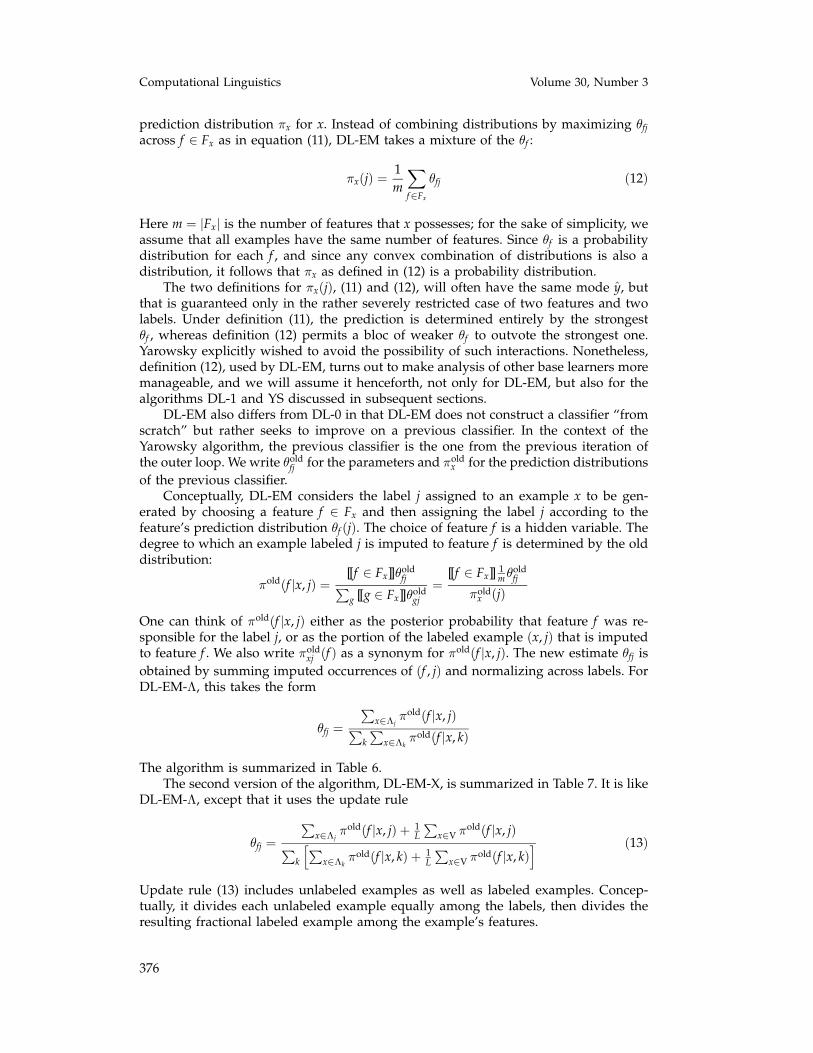
prediction distribution πx for x. Instead of combining distributions by maximizing θfjacross f ∈ Fx as in equation (11), DL-EM takes a mixture of the θf :

πx(j) =1m

∑f∈Fx

θfj (12)

Here m = |Fx| is the number of features that x possesses; for the sake of simplicity, weassume that all examples have the same number of features. Since θf is a probabilitydistribution for each f , and since any convex combination of distributions is also adistribution, it follows that πx as defined in (12) is a probability distribution.

The two definitions for πx(j), (11) and (12), will often have the same mode y, butthat is guaranteed only in the rather severely restricted case of two features and twolabels. Under definition (11), the prediction is determined entirely by the strongestθf , whereas definition (12) permits a bloc of weaker θf to outvote the strongest one.Yarowsky explicitly wished to avoid the possibility of such interactions. Nonetheless,definition (12), used by DL-EM, turns out to make analysis of other base learners moremanageable, and we will assume it henceforth, not only for DL-EM, but also for thealgorithms DL-1 and YS discussed in subsequent sections.

DL-EM also differs from DL-0 in that DL-EM does not construct a classifier “fromscratch” but rather seeks to improve on a previous classifier. In the context of theYarowsky algorithm, the previous classifier is the one from the previous iteration ofthe outer loop. We write θold

fj for the parameters and πoldx for the prediction distributions

of the previous classifier.Conceptually, DL-EM considers the label j assigned to an example x to be gen-

erated by choosing a feature f ∈ Fx and then assigning the label j according to thefeature’s prediction distribution θf (j). The choice of feature f is a hidden variable. Thedegree to which an example labeled j is imputed to feature f is determined by the olddistribution:

πold(f |x, j) =[[f ∈ Fx]]θold

fj∑g [[g ∈ Fx]]θold

gj

=[[f ∈ Fx]] 1

mθoldfj

πoldx (j)

One can think of πold(f |x, j) either as the posterior probability that feature f was re-sponsible for the label j, or as the portion of the labeled example (x, j) that is imputedto feature f . We also write πold

xj (f ) as a synonym for πold(f |x, j). The new estimate θfj isobtained by summing imputed occurrences of (f , j) and normalizing across labels. ForDL-EM-Λ, this takes the form

θfj =

∑x∈Λj

πold(f |x, j)∑k

∑x∈Λk

πold(f |x, k)

The algorithm is summarized in Table 6.The second version of the algorithm, DL-EM-X, is summarized in Table 7. It is like

DL-EM-Λ, except that it uses the update rule

θfj =

∑x∈Λj

πold(f |x, j) + 1L

∑x∈V π

old(f |x, j)∑k

[∑x∈Λk

πold(f |x, k) + 1L

∑x∈V π

old(f |x, k)] (13)

Update rule (13) includes unlabeled examples as well as labeled examples. Concep-tually, it divides each unlabeled example equally among the labels, then divides theresulting fractional labeled example among the example’s features.

377


Table 6DL-EM-Λ decision list induction algorithm.

(0) Initialize N[f , j] = 0 for all f , j(1) For each example x labeled j

(1.1) Let Z =∑

g∈Fxθold

gj

(1.2) For each f ∈ Fx, increment N[f , j] by 1Zθ

oldfj

(2) For each feature f(2.1) Let Z =

∑j N[f , j]

(2.2) For each label j, set θfj = 1Z N[f , j]

Table 7DL-EM-X decision list induction algorithm.

(0) Initialize N[f , j] = 0 and U[f , j] = 0, for all f , j(1) For each example x labeled j

(1.1) Let Z =∑

g∈Fxθold

gj

(1.2) For each f ∈ Fx, increment N[f , j] by 1Zθ

oldfj

(2) For each unlabeled example x(2.1) Let Z =

∑g∈Fx

θoldgj

(2.2) For each f ∈ Fx, increment U[f , j] by 1Zθ

oldfj

(3) For each feature f(3.1) Let Z =

∑j(N[f , j] + 1

L U[f , j])(3.2) For each label j, set θfj = 1

Z

(N[f , j] + 1

L U[f , j])

We note that both variants of the DL-EM algorithm constitute a single iterationof an EM-like algorithm. A single iteration suffices to prove the following theorem,though multiple iterations would also be effective:

Theorem 2The classifier produced by the DL-EM-Λ algorithm satisfies equation (7), and the clas-sifier produced by the DL-EM-X algorithm satisfies equation (8).

Combining Theorems 1 and 2 yields the following corollary:

CorollaryThe Yarowsky algorithm Y-1, using DL-EM-Λ or DL-EM-X as its base learning algo-rithm, decreases H at each iteration until it reaches a critical point of H.

Proof of Theorem 2Let θold represent the parameter values at the beginning of the call to DL-EM, let θrepresent a family of free variables that we will optimize, and let πold and π be thecorresponding prediction distributions. The labeling distribution φ is fixed. For anyset of examples α, let ∆Dα be the change in

∑x∈α D(φx||πx) resulting from the change

in θ. We are obviously particularly interested in two cases: that in which α is the setof all examples X (for DL-EM-X) and that in which α is the set of labeled examples

378


Λ (for DL-EM-Λ). In either case, we will show that ∆Dα ≤ 0, with equality only if nochoice of θ decreases D.

We first derive an expression for −∆Dα that we will put to use shortly:

−∆Dα =∑x∈α

[D(φx||πold

x ) − D(φx||πx)]

=∑x∈α

[H(φx||πold

x ) − H(φx) − H(φx||πx) + H(φx)]

=∑x∈α

∑j

φx(j)[logπx(j) − logπold

x (j)]

(14)

The EM algorithm is based on the fact that divergence is non-negative, and strictlypositive if the distributions compared are not identical:

0 ≤∑

j

∑x∈α

φx(j)D(πoldxj ||πxj)

=∑

j

∑x∈α

φx(j)∑f∈Fx

πoldxj (f ) log

πoldxj (f )

πxj(f )

=∑

j

∑x∈α

φx(j)∑f∈Fx

πoldxj (f ) log

(θold

fj

πoldx (j)

· πx(j)θfj

)

which yields the inequality

∑j

∑x∈α

φx(j)[logπx(j) − logπold

x (j)]≥∑

j

∑x∈α

φx(j)∑f∈Fx

πoldxj (f )

[log θfj − log θold

fj

]

By (14), this can be written as

− ∆Dα ≥∑

j

∑x∈α

φx(j)∑f∈Fx

πoldxj (f )

[log θfj − log θold

fj

](15)

Since θoldfj is constant, by maximizing

∑j

∑x∈α

φx(j)∑f∈Fx

πoldxj (f ) log θfj (16)

we maximize a lower bound on −∆Dα. It is easy to see that −∆Dα is bounded aboveby zero: we simply set θfj = θold

fj . Since divergence is zero only if the two distributionsare identical, we have strict inequality in (15) unless the best choice for θ is θold, inwhich case no choice of θ makes ∆Dα < 0.

It remains to show that DL-EM computes the parameter set θ that maximizes (16).We wish to maximize (16) under the constraints that the values {θfj} for fixed f sum tounity across choices of j, so we apply Lagrange’s method. We express the constraintsin the form

Cf = 0

whereCf ≡

∑j

θfj − 1

379


We seek a solution to the family of equations that results from expressing the gradientof (16) as a linear combination of the gradients of the constraints:

∂

∂θfj

∑k

∑x∈α

φx(k)∑g∈Fx

πoldxk (g) log θgk = λf

∂Cf

∂θfj(17)

We derive an expression for the derivative on the left-hand side:

∂

∂θfj

∑k

∑x∈α

φx(k)∑g∈Fx

πoldxk (g) log θgk =

∑x∈Xf∩α

φx(j)πoldxj (f )

1θfj

Similarly for the right-hand side:∂Cf

∂θfj= 1

Substituting these into equation (17):

∑x∈Xf∩α

φx(j)πoldxj (f )

1θfj

= λf

θfj =∑

x∈Xf∩α

φx(j)πoldxj (f )

1λf

(18)

Using the constraint Cf = 0 and solving for λf :

∑j

∑x∈Xf∩α

φx(j)πoldxj (f )

1λf

− 1 = 0

λf =∑

j

∑x∈Xf∩α

φx(j)πoldxj (f )

Substituting back into (18):

θfj =

∑x∈Xf∩α φx(j)πold

xj (f )∑k

∑x∈Xf∩α φx(k)πold

xk (f )(19)

If we consider the case where α is the set of all examples and expand φx in (19),we obtain

θfj =1Z

∑

x∈Λfj

πoldxj (f ) +

1L

∑x∈Vf

πoldxj (f )

where Z normalizes θf . It is not hard to see that this is the update rule that DL-EM-Xcomputes, using the intermediate values:

N[f , j] =∑x∈Λfj

πoldxj (f )

U[f , j] =∑x∈Vf

πoldxj (f )

380


If we consider the case where α is the set of labeled examples and expand φx in (19),we obtain

θfj =1Z

∑x∈Λfj

πoldxj (f )

This is the update rule that DL-EM-Λ computes. Thus we see that DL-EM-X reducesDX, and DL-EM-Λ reduces DΛ.

We note in closing that DL-EM-X can be simplified when used with algorithm Y-1,inasmuch as it is known that θfj = 1/L for all (f , j), where f ∈ Fx for some x ∈ V. Thenthe expression for U[f , j] simplifies as follows:

∑x∈Vf

πoldxj (f )

=∑x∈Vf

[1/L∑

g∈Fx1/L

]

=|Vf |m

The dependence on j disappears, so we can replace U[f , j] with U[f ] in algorithmDL-EM-X, delete step 2.1, and replace step 2.2 with the statement “For each f ∈ Fx,increment U[f ] by 1/m.”

3.3 The Objective Function KY-1/DL-EM is the only variation on the Yarowsky algorithm that we can show toreduce negative log-likelihood, H. The variants that we discuss in the remainder ofthe article, Y-1/DL-1 and YS, reduce an alternative objective function, K, which wenow define.

The value K (or, more precisely, the value K/m) is an upper bound on H, whichwe derive using Jensen’s inequality, as follows:

H = −∑x∈X

∑j

φxj log∑g∈Fx

1mθgj

≤ −∑x∈X

∑j

φxj

∑g∈Fx

1m

log θgj

=1m

∑x∈X

∑g∈Fx

H(φx||θg)

We defineK ≡

∑x∈X

∑g∈Fx

H(φx||θg) (20)

By minimizing K, we minimize an upper bound on H. Moreover, it is in principlepossible to reduce K to zero. Since H(φx||θg) = H(φx) + D(φx||θg), K is reduced to zeroif all examples are labeled, each feature concentrates its prediction distribution in asingle label, and the label of every example agrees with the prediction of every featureit possesses. In this limiting case, any minimizer of K is also a minimizer of H.

381


Table 8The decision list induction algorithm DL-1-R.

(0) Initialize N[f , j] = 0, Z[f ] = 0 for all f , j(1) For each example-label pair (x, j)

(1.1) For each feature f ∈ Fx, increment N[f , j], Z[f ](2) For each feature f and label j

(2.1) Set θfj =N[f ,j]Z[f ]

(*) Define πx(j) = 1m

∑f∈Fx

θfj

Table 9The decision list induction algorithm DL-1-VS.

(0) Initialize N[f , j] = 0, Z[f ] = 0, U[f ] = 0 for all f , j(1) For each example-label pair (x, j)

(1.1) For each feature f ∈ Fx, increment N[f , j], Z[f ](2) For each unlabeled example x

(2.1) For each feature f ∈ Fx, increment U[f ](3) For each feature f and label j

(3.1) Set ε = U[f ]/L(3.2) Set θfj =

N[f ,j]+ε

Z[f ]+U[f ]

(*) Define πx(j) = 1m

∑f∈Fx

θfj

We hasten to add a proviso: It is not possible to reduce K to zero for all data sets.The following provides a necessary and sufficient condition for being able to do so.Consider an undirected bipartite graph G whose nodes are examples and features.There is an edge between example x and feature f just in case f is a feature of x.Define examples x1 and x2 to be neighbors if they both belong to the same connectedcomponent of G. K is reducible to zero if and only if x1 and x2 have the same labelaccording to Y(0), for all pairs of neighbors x1 and x2 in Λ(0).

3.4 Algorithm DL-1We consider two variants of DL-0, called DL-1-R and DL-1-VS. They differ from DL-0in two ways. First, the DL-1 algorithms assume the “mean” definition of πx given inequation (12) rather than the “max” definition of equation (11). This is not actually adifference in the induction algorithm itself, but in the way the decision list is used toconstruct a prediction distribution πx.

Second, the DL-1 algorithms use update rules that differ from the smoothed pre-cision of DL-0. DL-1-R (Table 8) uses raw precision instead of smoothed precision.DL-1-VS (Table 9) uses smoothed precision, but unlike DL-0, DL-1-VS does not usea fixed smoothing constant ε; rather ε varies from feature to feature. Specifically, incomputing the score θfj, DL-1-VS uses |Vf |/L as its value for ε.

The value of ε used by DL-1-VS can be expressed in another way that will proveuseful. Let us define

p(Λ|f ) ≡|Λf ||Xf |

p(V|f ) ≡|Vf ||Xf |

382


Lemma 2The parameter values {θfj} computed by DL-1-VS can be expressed as

θfj = p(Λ|f )qf (j) + p(V|f )u(j) (21)

where u(j) is the uniform distribution over labels.

ProofIf |Λf | = 0, then p(Λ|f ) = 0 and θfj = u(j). Further, N[f , j] = Z[f ] = 0, so DL-1-VScomputes θfj = u(j), and the lemma is proved. Hence we need only consider the case|Λf | > 0.

First we show that smoothed precision can be expressed as a convex combinationof raw precision (9) and the uniform distribution. Define δ = ε/|Λf |. Then:

qf (j) =|Λfj| + ε

|Λf | + Lε

=|Λfj|/|Λf | + δ

1 + Lδ

=1

1 + Lδqf (j) +

Lδ1 + Lδ

· δLδ

=1

1 + Lδqf (j) +

Lδ1 + Lδ

u(j) (22)

Now we show that the mixing coefficient 1/(1 + Lδ) of (22) is the same as the mixingcoefficient p(Λ|f ) of the lemma, when ε = |Vf |/L as in step 3.1 of DL-1-VS:

ε =|Vf |

L

=|Λf |

L· p(V|f )

p(Λ|f )

Lδ =1

p(Λ|f ) − 1

11 + Lδ

= p(Λ|f )

The main theorem of this section (Theorem 5) is that the specific Yarowsky al-gorithm Y-1/DL-1 decreases K in each iteration until it reaches a critical point. It isproved as a corollary of two theorems. The first (Theorem 3) shows that DL-1 min-imizes K as a function of θ, holding φ constant, and the second (Theorem 4) showsthat Y-1 decreases K as a function of φ, holding θ constant. More precisely, DL-1-Rminimizes K over labeled examples Λ, and DL-1-VS minimizes K over all examplesX. Either is sufficient for Y-1 to be effective.

Theorem 3DL-1 minimizes K as a function of θ, holding φ constant. Specifically, DL-1-R minimizesK over labeled examples Λ, and DL-1-VS minimizes K over all examples X.

ProofWe wish to minimize K as a function of θ under the constraints

Cf ≡∑

j

θfj − 1 = 0

383


for each f . As before, to minimize K under the constraints Cf = 0, we express thegradient of K as a linear combination of the gradients of the constraints and solve theresulting system of equations:

∂K∂θfj

= λf∂Cf

∂θfj(23)

First we derive expressions for the derivatives of Cf and K. The variable α representsthe set of examples over which we are minimizing K:

∂Cf

∂θfj= 1

∂K∂θfj

= − ∂

∂θfj

∑x∈α

∑g∈Fx

∑k

φxk log θgk

= −∑

x∈Xf∩α

φxj1θfj

We substitute these expressions into (23) and solve for θfj:

−∑

x∈Xf∩α

φxj1θfj

= λf

θfj = −∑

x∈Xf∩α

φxj/λf

Substituting the latter expression into the equation for Cf = 0 and solving for f yields

∑j

−

∑x∈Xf∩α

φxj/λf

= 1

−|Xf ∩ α| = λf

Substituting this back into the expression for θfj gives us

θfj =1

|Xf ∩ α|∑

x∈Xf∩α

φxj (24)

If α = Λ, we have

θfj =1

|Λf |∑x∈Λf

[[x ∈ Λj]]

= qf (j)

This is the update computed by DL-1-R, showing that DL-1-R computes the parametervalues {θfj} that minimize K over the labeled examples Λ.

384


If α = X, we have

θfj =1

|Xf |∑x∈Λf

[[x ∈ Λj]] +1

|Xf |∑x∈Vf

1L

=|Λf ||Xf |

·|Λfj||Λf |

+|Vf ||Xf |

· 1L

= p(Λ|f ) · qf (j) + p(V|f ) · u(j)

By Lemma 2, this is the update computed by DL-1-VS, hence DL-1-VS minimizes Kover the complete set of examples X.

Theorem 4If the base learner decreases K over X or over Λ, where the prediction distribution iscomputed as

πx(j) =1m

∑f∈Fx

θfj

then algorithm Y-1 decreases K at each iteration until it reaches a critical point, con-sidering K as a function of φ with θ held constant.

ProofThe proof has the same structure as the proof of Theorem 1, so we give only a sketchhere. We minimize K as a function of φ by minimizing it for each example separately:

K(x) =∑g∈Fx

H(φx||θg)

=∑

j

φxj

∑g∈Fx

log1θgj

To minimize K(x), we choose φxj so as to concentrate all mass in

arg minj

∑g∈Fx

log1θgj

= arg maxjπx(j)

This is the labeling rule used by Y-1.If the base learner minimizes over Λ only, rather than X, it can be shown that any

increase in K on unlabeled examples is compensated for in the labeling step, as in theproof of Theorem 1.

Theorem 5The specific Yarowsky algorithms Y-1/DL-1-R and Y-1/DL-1-VS decrease K at eachiteration until they reach a critical point.

ProofImmediate from Theorems 3 and 4.

4. Sequential Algorithms

4.1 The Family YSThe Yarowsky algorithm variants we have considered up to now do “parallel” updatesin the sense that the parameters {θfj} are completely recomputed at each iteration. In

385


this section, we consider a family YS of “sequential” variants of the Yarowsky al-gorithm, in which a single feature is selected for update at each iteration. The YSalgorithms resemble the “Yarowsky-Cautious” algorithm of Collins & Singer (1999),though they differ from that algorithm in that they update a single feature in each iter-ation, rather than a small set of features, as in Yarowsky-Cautious. The YS algorithmsare intended to be as close to the Y-1/DL-1 algorithm as is consonant with single-feature updates. The YS algorithms differ from one another, and from Y-1/DL-1, inthe choice of update rule. An interesting range of update rules work in the sequentialsetting. In particular, smoothed precision with fixed ε, as in the original algorithmY-0/DL-0, works in the sequential setting, though with a proviso that will be spelledout later.

Instead of an initial labeled set, there is an initial classifier consisting of a set ofselected features S0 and initial parameter set θ(0) with θ

(0)fj = 1/L for all f �∈ S0. At

each iteration, one feature is selected to be added to the selected set. A feature, onceselected, remains in the selected set. It is permissible for a feature to be selected morethan once; this permits us to continue reducing K even after all features have beenselected. In short, there is a sequence of selected features f0, f1, . . . , and

St+1 = St ∪ {ft}

The parameters for the selected feature are also updated. At iteration t, the pa-rameters θgj, with g = ft, may be modified, but all other parameters remain constant.That is:

θ(t+1)gj = θ

(t)gj for g �= ft

It follows that, for all t:

θ(t)gj =

1L

for g �∈ St

However, parameters for features in S0 may not be modified, inasmuch as they playthe role of manually labeled data.

In each iteration, one selects a feature ft and computes (or recomputes) the predic-tion distribution θft for the selected feature ft. Then labels are recomputed as follows.Recall that y ≡ arg maxj πx(j), where we continue to assume πx(j) to have the “mix-ture” definition (equation (12)). The label of example x is set to y if any feature of xbelongs to St+1. In particular, all previously labeled examples continue to be labeled(though their labels may change), and any unlabeled examples possessing feature ftbecome labeled.

The algorithm is summarized in Table 10. It is actually an algorithm schema;the definition for “update” needs to be supplied. We consider three different updatefunctions: one that uses raw precision as its prediction distribution, one that usessmoothed precision, and one that goes in the opposite direction, using what we mightcall “peaked precision.” As we have seen, smoothed precision can be expressed as amixture of raw precision and the uniform (i.e., maximum-entropy) distribution (22).Peaked precision q(f ) mixes in a certain amount of the point (i.e., minimum-entropy)distribution that has all its mass on the label that maximizes raw precision:

qf (j) ≡ p(Λ(t)|f )qf (j) + p(V(t)|f )[[j = j†]] (25)

wherej† ≡ arg max

jqf (j) (26)

386


Table 10The sequential algorithm YS.

(0) Given: S(0), θ(0), with θ(0)gj = 1/L for g �∈ S(0)

(1) Initialization(1.1) Set S = S(0), θ = θ(0)

(1.2) For each example x ∈ XIf x possesses a feature in S(0), set Yx = y, else set Yx = ⊥

(2) Loop:(2.1) Choose a feature f �∈ S(0) such that Λf �= ∅ and θf �= qf

If there is none, stop(2.2) Add f to S(2.3) For each label j, set θfj = update(f , j)(2.4) For each example x possessing a feature in S, set Yx = y

Note that peaked precision involves a variable amount of “peaking”; the mixing pa-rameters depend on the relative proportions of labeled and unlabeled examples. Notealso that j† is a function of f , though we do not explicitly represent that dependence.

The three instantiations of algorithm YS that we consider are

YS-P (“peaked”) θfj = qf (j)YS-R (“raw”) θfj = qf (j)YS-FS (“fixed smoothing”) θfj = qf (j)

We will show that the first two algorithms reduce K in each iteration. We will showthat the third algorithm, YS-FS, reduces K in iterations in which ft is a new feature,not previously selected. Unfortunately, we are unable to show that YS-FS reduces Kwhen ft is a previously selected feature. This suggests employing a mixed algorithmin which smoothed precision is used for new features but raw or peaked precision isused for previously selected features.

A final issue with the algorithm schema YS concerns the selection of featuresin step 2.1. The schema as stated does not specify which feature is to be selected.In essence, the manner in which rules are selected does not matter, as long as oneselects rules that have room for improvement, in the sense that the current predictiondistribution θf differs from raw precision qf . (The justification for this choice is givenin Theorem 9.) The theorems in the following sections show that K decreases in eachiteration, so long as any such rule can be found.

One could choose greedily by choosing the feature that maximizes gain G (equa-tion (27)), though in the next section we give lower bounds for G that are rather moreeasily computed (Theorems 6 and 7).

4.2 GainFrom this point on, we consider a single iteration of the YS algorithm and discard thevariable t. We write θold and φold for the parameter set and labeling at the beginning ofthe iteration, and we write simply θ and φ for the new parameter set and new label-ing. The set Λ (respectively, V) represents the examples that are labeled (respectively,unlabeled) at the beginning of the iteration. The selected feature is f .

We wish to choose a prediction distribution for f so as to guarantee that K decreasesin each iteration. The gain in the current iteration is

G =∑x∈X

∑g∈Fx

[H(φold

x ||θoldg ) − H(φx||θg)

](27)

387


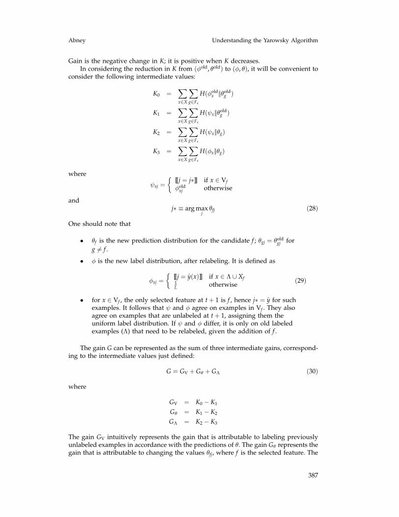
Gain is the negative change in K; it is positive when K decreases.In considering the reduction in K from (φold, θold) to (φ, θ), it will be convenient to

consider the following intermediate values:

K0 =∑x∈X

∑g∈Fx

H(φoldx ||θold

g )

K1 =∑x∈X

∑g∈Fx

H(ψx||θoldg )

K2 =∑x∈X

∑g∈Fx

H(ψx||θg)

K3 =∑x∈X

∑g∈Fx

H(φx||θg)

where

ψxj =

{[[j = j∗]] if x ∈ Vf

φoldxj otherwise

andj∗ ≡ arg max

jθfj (28)

One should note that

• θf is the new prediction distribution for the candidate f ; θgj = θoldgj for

g �= f .

• φ is the new label distribution, after relabeling. It is defined as

φxj =

{[[j = y(x)]] if x ∈ Λ ∪ Xf1L otherwise

(29)

• for x ∈ Vf , the only selected feature at t + 1 is f , hence j∗ = y for suchexamples. It follows that ψ and φ agree on examples in Vf . They alsoagree on examples that are unlabeled at t + 1, assigning them theuniform label distribution. If ψ and φ differ, it is only on old labeledexamples (Λ) that need to be relabeled, given the addition of f .

The gain G can be represented as the sum of three intermediate gains, correspond-ing to the intermediate values just defined:

G = GV + Gθ + GΛ (30)

where

GV = K0 − K1

Gθ = K1 − K2

GΛ = K2 − K3

The gain GV intuitively represents the gain that is attributable to labeling previouslyunlabeled examples in accordance with the predictions of θ. The gain Gθ represents thegain that is attributable to changing the values θfj, where f is the selected feature. The

388


gain GΛ represents the gain that is attributable to changing the labels of previouslylabeled examples to make labels agree with the predictions of the new model θ. Thegain Gθ corresponds to step 2.3 of algorithm YS, in which θ is changed but φ is heldconstant; and the combined GV and GΛ gains correspond to step 2.4 of algorithm YS,in which φ is changed while holding θ constant.

In the remainder of this section, we derive two lower bounds for G. In followingsections, we show that the updates YS-P, YS-R, and YS-FS guarantee that the lowerbounds given below are non-negative, and hence that G is non-negative.

Lemma 3GV = 0

ProofWe show that K remains unchanged if we substitute ψ for φold in K0. The only propertyof ψ that we need is that it agrees with φold on previously labeled examples.

Since ψx = φoldx for x ∈ Λ, we need only consider examples in V. Since these

examples are unlabeled at the beginning of the iteration, none of their features havebeen selected, hence θold

gj = 1/L for all their features g. Hence

K1 = −∑x∈V

∑g∈Fx

∑j

ψxj log θoldgj

= −∑x∈V

∑g∈Fx

∑

j

ψxj

log

1L

= −∑x∈V

∑g∈Fx

∑

j

φoldxj

log

1L

= −∑x∈V

∑g∈Fx

∑j

φoldxj log θold

gj = K0

(Note that ψxj is not in general equal to φoldxj , but

∑j ψxj and

∑j φ

oldxj both equal 1.) This

shows that K0 = K1, and hence that GV = 0.

Lemma 4GΛ ≥ 0.

We must show that relabeling old labeled examples—that is, setting φx(j) = [[j = y]]for x ∈ Λ—does not increase K. The proof has the same structure as the proof ofTheorem 1 and is omitted.

Lemma 5Gθ is equal to

|Λf |[H(qf ||θold

f ) − H(qf ||θf )]

+ |Vf |[

log L − log1θf j∗

](31)

ProofBy definition, Gθ = K1−K2, and K1 and K2 are identical everywhere except on examples

389


in Xf . Hence

Gθ =∑x∈Xf

∑g∈Fx

[H(ψx||θold

g ) − H(ψx||θg)]

We divide this sum into three partial sums:

Gθ = A + B + C (32)

A =∑x∈Λf

[H(ψx||θold

f ) − H(ψx||θf )]

B =∑x∈Vf

[H(ψx||θold

f ) − H(ψx||θf )]

C =∑x∈Xf

∑g�=f∈Fx

[H(ψx||θold

g ) − H(ψx||θg)]

We consider each partial sum separately:

A =∑x∈Λf

[H(ψx||θold

f ) − H(ψx||θf )]

= −∑x∈Λf

∑k

ψxk

[log θold

fk − log θfk

]

= −∑x∈Λf

∑k

[[x ∈ Λk]][log θold

fk − log θfk

]

= −∑

k

|Λfk|[log θold

fk − log θfk

]

= −|Λf |∑

k

qf (k)[log θold

fk − log θfk

]

= |Λf |[H(qf ||θold

f ) − H(qf ||θf )]

(33)

B =∑x∈Vf

[H(ψx||θold

f ) − H(ψx||θf )]

= −∑x∈Vf

∑k

ψxk

[log θold

fk − log θfk

]

= −∑x∈Vf

∑k

[[k = j∗]][log θold

fk − log θfk

]

= |Vf |[

log1θold

f j∗− log

1θf j∗

]

= |Vf |[


](34)

The justification for the last step is a bit subtle. If f is a new feature, not previouslyselected, then θold

fk = 1/L for all k, and the substitution is valid. On the other hand, iff is a previously selected feature, then |Vf | = 0, and even though the substitution of

390


1/L for θoldf j∗ may not be valid, it is innocuous.

C =∑x∈Xf

∑g�=f∈Fx

[H(ψx||θold

g ) − H(ψx||θg)]

=∑x∈Xf

∑g�=f∈Fx

[H(ψx||θold

g ) − H(ψx||θoldg )]

= 0 (35)

Combining (32), (33), (34), and (35) yields the lemma.

Theorem 6G is bounded below by (31).

ProofCombining (30) with Lemmas 3, 4, and 5.

Theorem 7G is bounded below by

|Λf |[H(qf ||θold

f ) − H(qf ||θf )]

ProofThe theorem follows immediately from Theorem 6 if we can show that


≥ 0

Observe first that log L = H(u). (Recall that u(j) = 1/L is the uniform distribution overlabels.) By Lemma 1, we know that

H(u) − log1θf j∗

≥ H(u) − H(θf )

≥ 0

The latter follows because the uniform distribution maximizes entropy.

Theorem 8G is bounded below by

|Λf |[D(qf ||θold

f ) − D(qf ||θf )]

ProofImmediate from Theorem 7 and the fact that

H(qf ||θoldf ) − H(qf ||θf ) = H(qf ) + D(qf ||θold

f ) − H(qf ) − D(qf ||θf )

= D(qf ||θoldf ) − D(qf ||θf )

Theorem 9If θold

f �= qf , then there is a choice of θf that yields strictly positive gain.

391


ProofIf θold

f �= qf , then

D(qf ||θoldf ) > 0

Setting θf = qf has the result that

|Λf |[D(qf ||θold

f ) − D(qf ||θf )]

= |Λf |D(qf ||θoldf ) > 0

Hence G > 0 by Theorem 8.

4.3 Algorithm YS-PWe now use the results of the previous section to show that the algorithm YS-P iscorrect in the sense that it reduces K in every iteration.

Theorem 10In each iteration of algorithm YS-P, K decreases.

ProofWe wish to show that G > 0. By Theorem 6, that is true if expression (31) is positive.By Theorem 9, there exist choices for θf that make (31) positive, hence in particular,we guarantee G > 0 by maximizing (31). We maximize (31) by minimizing

|Λf |H(qf ||θf ) + |Vf | log1θf j∗

(36)

SinceH(qf ||θf ) = H(qf ) + D(qf ||θf )

we minimize (36) by minimizing

|Λf |D(qf ||θf ) + |Vf | log1θf j∗

(37)

Both terms are nonnegative. The first term is zero if θf = qf . The second term is zerofor any distribution that concentrates all its mass in a single label j∗; it is symmetricin all choices of j∗ and decreases monotonically as θf j∗ approaches one. Hence, theminimum of (37) will have j∗ equal to the mode of qf , though it may be more peakedthan qf , at the cost of an increase in the first term, but offset by a decrease in thesecond term.

Recall that j† = arg maxj qf (j). By the reasoning of the previous paragraph, weknow that j† = j∗ at the minimum of (37). Hence we can minimize (37) by minimizing

|Λf |D(qf ||θf ) − |Vf |∑

k

[[k = j†]] log θfk (38)

We compute the gradient:

∂

∂θfj

[|Λf |D(qf ||θf ) − |Vf |

∑k

[[k = j†]] log θfk

]

=∂

∂θfj

[|Λf |H(qf ||θf ) − |Λf |H(qf ) − |Vf |

∑k


]

392


=∂

∂θfj|Λf |H(qf ||θf ) −

∂

∂θfj|Vf |

∑k


= −|Λf |∂

∂θfj

∑k

qf (k) log θfk − |Vf |∂

∂θfj

∑k


= −|Λf |∂

∂θfjqf (j) log θfj − |Vf |

∂

∂θfj[[j = j†]] log θfj

= −|Λf |qf (j)1θfj

− |Vf |[[j = j†]]1θfj

(39)

As before, the derivative of the constraint Cf = 0 is one, and we minimize (38) underthe constraint by solving

−|Λf |qf (j)1θfj

− |Vf |[[j = j†]]1θfj

= λ

θfj =(−|Λf |qf (j) − |Vf |[[j = j†]]

)/λ (40)

Substituting into the constraint gives us

∑j

(−|Λf |qf (j) − |Vf |[[j = j†]]

)/λ = 1

−|Λf | − |Vf | = λ

−|Xf | = λ

Substituting this back into (40) yields:

θfj = p(Λ|f )qf (j) + p(V|f )[[j = j†]] (41)

That is, the maximizing solution is peaked precision, which is the update rule for YS-P.

4.4 Algorithm YS-RWe now show that YS-R also decreases K in each iteration. In fact, it has essentiallyalready been proven.

Theorem 11Algorithm YS-R decreases K in each iteration.

ProofIn the proof of Theorem 9, we showed that the choice

θf = qf

yields strictly positive gain. This is the update rule used by YS-R.

4.5 Algorithm YS-FSThe original Yarowsky algorithm YS-0/DL-0 used smoothed precision with fixed εas update rule. We have been unsuccessful at justifying this choice of update rulein general. However, we are able at least to show that it does decrease K when theselected feature is a new feature, not previously selected.

393


Theorem 12Algorithm YS-FS has positive gain in each iteration in which the selected feature hasnot been previously selected.

ProofBy Theorem 7, gain is positive if

H(qf ||θoldf ) > H(qf ||θf ) (42)

By the assumption that the selected feature f has not been previously selected, θoldf is

the uniform distribution u, and the left-hand side of (42) is equal to H(qf ||u). It is easyto verify that H(p||u) = H(u) for any distribution p; hence the left-hand side of (42) isequal to H(u). Further, YS-FS uses smoothed precision as update rule, θf = qf , so (42)can be rewritten as

H(u) > H(qf ||qf )

This condition does not hold trivially, inasmuch as cross entropy, like divergence, isunbounded. But we can show that it holds in this particular case.

We derive an upper bound for H(qf ||qf ):

H(qf ||qf ) = −∑

j

qf (j) log qf (j)

= −∑

j

qf (j) log[

11 + Lε

qf (j) +Lε

1 + Lεu(j)

]

≤ −∑

j

qf (j)[

11 + Lε

log qf (j) +Lε

1 + Lεlog u(j)

]

=1

1 + LεH(qf ) +

Lε1 + Lε

H(qf ||u)

=1

1 + LεH(qf ) +

Lε1 + Lε

H(u) (43)

Observe that

H(u) >1

1 + LεH(qf ) +

Lε1 + Lε

H(u) (44)

iff [1 − Lε

1 + Lε

]H(u) >

11 + Lε

H(qf )

iffH(u) > H(qf )

We know that H(u) ≥ H(qf ) because the uniform distribution maximizes entropy. Weknow that the inequality is strict by the following reasoning. Since f is a new feature,θold

f = u. Because of the restriction on step 2.1 in algorithm YS, θoldf �= qf , hence qf �= u,

and H(u) is strictly greater than H(qf ).Hence (44) is true, and combining (44) with (43), we have shown (42) to be true,

proving the theorem.

394


5. Minimization of Feature Entropy

At the beginning of the article, the co-training algorithm was mentioned as an alterna-tive to the Yarowsky algorithm. There is in fact a connection between co-training andthe Yarowsky algorithm. In the original co-training paper (Blum and Mitchell 1998), itwas suggested that the algorithm be understood as seeking to maximize agreement onunlabeled data between classifiers trained on two different “views” of the data. Subse-quent work (Dasgupta, Littman, and McAllester 2001) has proven a direct connectionbetween classifier error and such cross-view agreement on unlabeled data.

In the current context, there is also justification for pursuing agreement on unla-beled data. However, the Yarowsky algorithm does not assume the existence of twoconditionally independent views of the data. Rather, there is a motivation for seekingagreement on unlabeled data between arbitrary pairs of features.

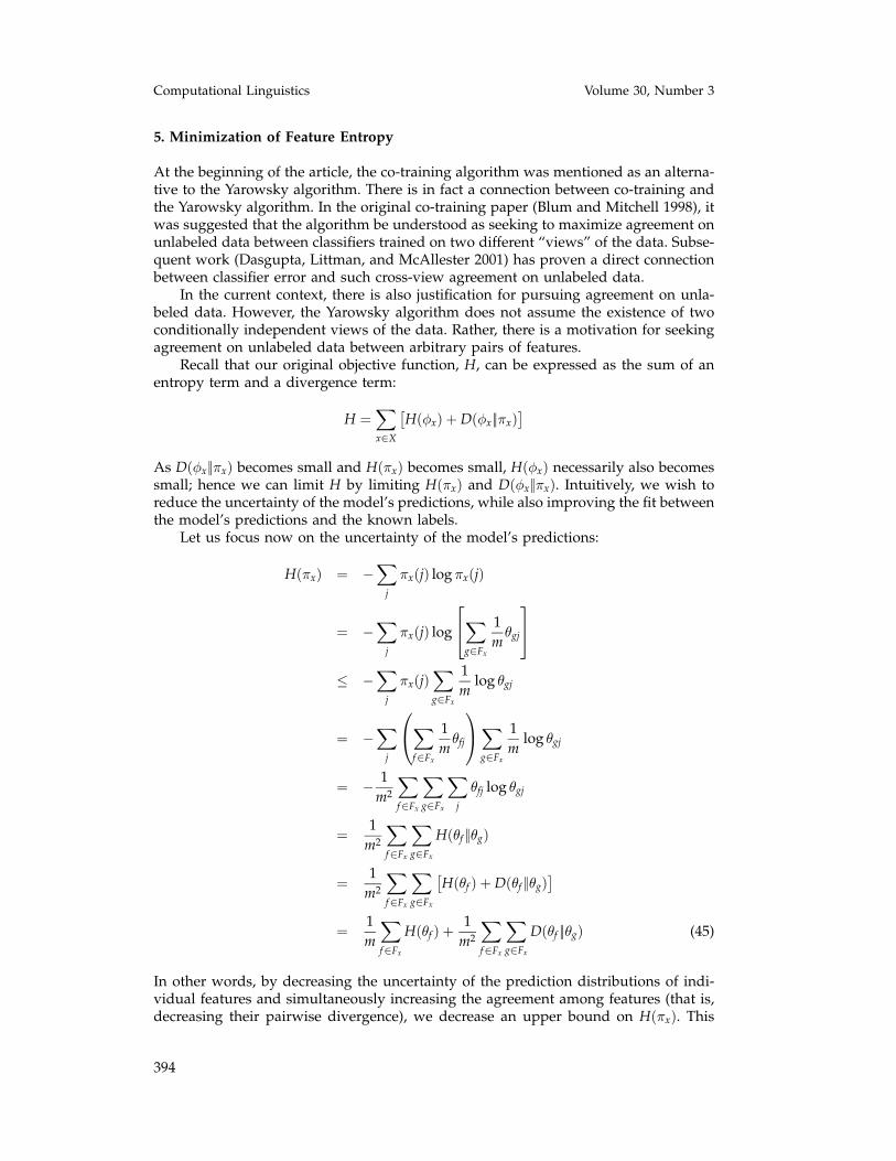
Recall that our original objective function, H, can be expressed as the sum of anentropy term and a divergence term:

H =∑x∈X

[H(φx) + D(φx||πx)

]

As D(φx||πx) becomes small and H(πx) becomes small, H(φx) necessarily also becomessmall; hence we can limit H by limiting H(πx) and D(φx||πx). Intuitively, we wish toreduce the uncertainty of the model’s predictions, while also improving the fit betweenthe model’s predictions and the known labels.

Let us focus now on the uncertainty of the model’s predictions:

H(πx) = −∑

j

πx(j) logπx(j)

= −∑

j

πx(j) log

∑

g∈Fx

1mθgj

≤ −∑

j

πx(j)∑g∈Fx

1m

log θgj

= −∑

j

∑

f∈Fx

1mθfj

∑

g∈Fx

1m

log θgj

= − 1m2

∑f∈Fx

∑g∈Fx

∑j

θfj log θgj

=1

m2

∑f∈Fx

∑g∈Fx

H(θf ||θg)

=1

m2

∑f∈Fx

∑g∈Fx

[H(θf ) + D(θf ||θg)

]

=1m

∑f∈Fx

H(θf ) +1

m2

∑f∈Fx

∑g∈Fx

D(θf ||θg) (45)

In other words, by decreasing the uncertainty of the prediction distributions of indi-vidual features and simultaneously increasing the agreement among features (that is,decreasing their pairwise divergence), we decrease an upper bound on H(πx). This

395


motivates interfeature agreement without recourse to an assumption of independentviews.

6. Conclusion

In this article, we have presented a number of variants of the Yarowsky algorithm,and we have shown that they optimize natural objective functions. We consideredfirst the modified generic Yarowsky algorithm Y-1 and showed that it minimizes theobjective function H (which is equivalent to maximizing likelihood), provided that itsbase learner reduces H.

We then considered three families of specific Yarowsky-like algorithms. TheY-1/DL-EM algorithms (Y-1/DL-EM-Λ and Y-1/DL-EM-X) minimize H but have thedisadvantage that the DL-EM base learner has no similarity to Yarowsky’s original baselearner. A much better approximation to Yarowsky’s original base learner is providedby DL-1, and the Y-1/DL-1 algorithms (Y-1/DL-1-R and Y-1/DL-1-VS) were shown tominimize the objective function K, an upper bound for H. Finally, the YS algorithms(YS-P, YS-R, and YS-FS) are sequential variants, reminiscent of the Yarowsky-Cautiousalgorithm of Collins and Singer; we showed that they minimize K.

To the extent that these algorithms capture the essence of the original Yarowskyalgorithm, they provide a formal understanding of Yarowsky’s approach. Even if theyare deemed to diverge too much from the original to cast light on its workings, theyat least represent a new family of bootstrapping algorithms with solid mathematicalfoundations.

ReferencesAbney, Steven. 2002. Bootstrapping. In

Proceedings of 40th Annual Meeting of theAssociation for Computational Linguistics(ACL), Philadelphia, pages 360–367.

Blum, Avrim and Tom Mitchell. 1998.Combining labeled and unlabeled datawith co-training. In Proceedings of the 11thAnnual Conference on ComputationalLearning Theory (COLT), pages 92–100.Morgan Kaufmann, San Francisco.

Collins, Michael and Yoram Singer. 1999.Unsupervised models for named entityclassification. In Proceedings of EmpiricalMethods in Natural Language Processing

(EMNLP), College Park, MD,pages 100–110.

Dasgupta, Sanjoy, Michael Littman, andDavid McAllester. 2001. PACgeneralization bounds for co-training. InProceedings of Advances in NeuralInformation Processing Systems 14 (NIPS),Vancouver, British Columbia, Canada.

Yarowsky, David. 1995. Unsupervised wordsense disambiguation rivaling supervisedmethods. In Proceedings of the 33rd AnnualMeeting of the Association for ComputationalLinguistics, Cambridge, MA, pages189–196.

Understanding the Yarowsky Algorithm - ACL Anthology

Documents

Transcript of Understanding the Yarowsky Algorithm - ACL Anthology