Squib

How to Distinguish Languages and Dialects

Søren WichmannLeiden University Centre forLinguistics, Kazan Federal University,and Beijing Advanced Innovation Centerfor Language Resourceswichmannsoeren@gmail.com

The terms “language” and “dialect” are ingrained, but linguists nevertheless tend to agreethat it is impossible to apply a non-arbitrary distinction such that two speech varieties can beidentified as either distinct languages or two dialects of one and the same language. A databaseof lexical information for more than 7,500 speech varieties, however, unveils a strong tendencyfor linguistic distances to be bimodally distributed. For a given language group the linguisticdistances pertaining to either cluster can be teased apart, identifying a mixture of normaldistributions within the data and then separating them fitting curves and finding the point wherethey cross. The thresholds identified are remarkably consistent across data sets, qualifying theirmean as a universal criterion for distinguishing between language and dialect pairs. The meanof the thresholds identified translates into a temporal distance of around one to one-and-a-halfmillennia (1,075–1,635 years).

1. Two Approaches

Most linguists would agree that it is difficult and often controversial to distinguish lan-guages from dialects. Many, however, would also agree that the notions of language anddialect are still useful, even for the linguist who is aware of the problems of definitionthat they entail (Agard 1984). The distinction is useful for many different purposes, suchas cataloguing languages, assigning ISO 639-3 codes, preparing maps of languages,planning revitalization efforts, or for doing statistics on language distributions (e.g.,calculating diversity or density indices) (Korjakov 2017). More importantly, perhaps: Ifsuch a distinction is a feature of the way that language varieties are distributed ratherthan just a distinction we impose in some arbitrary way, then this would be importantfor the understanding of the sociology of language at large.

There are two main directions to go in order to establish a quantitative distinction.One direction is to measure mutual intelligibility; another is to apply some consistentand objective measure of differences between two variants with regard to phonology,morphology, syntax, lexicon, or some combination.

Early applications of mutual intelligibility testing are detailed in Casad (1974), andmore recent work in this area includes Whaley, Grenoble, and Li (1999), Szeto (2000),Gooskens and Schneider (2016), and Gooskens et al. (2018).

Submission received: 18 February 2019; revised version received: 11 July 2019; accepted for publication:15 September 2019.

https://doi.org/10.1162/COLI a 00366

© 2019 Association for Computational LinguisticsPublished under a Creative Commons Attribution-NonCommercial-NoDerivatives 4.0 International(CC BY-NC-ND 4.0) license

Computational Linguistics Volume 45, Number 4

Glottolog (Hammarstrom, Forkel, and Haspelmath 2017) adopts the criterion ofmutual intelligibility, positing that a language variant that is not mutually intelligiblewith any other language variant should be counted as a separate language.1 By thiscriterion, Glottolog 4.0 contains 7,592 spoken L1 (mother-tongue) languages, excludingsign languages. There are, however, two problems with this criterion. The more seriousproblem is that intelligibility is often not symmetrical. Thus language variant A canbe more intelligible to speakers of language variant B than language variant B is tospeakers of language variant A. Such a situation may arise when A is the larger,more influential language, causing speakers of B to have more exposure to A thanthe other way around. However, the amount of exposure that speakers have to otherlanguage variants is entirely determined by historical and sociological factors, and thisor other extraneous factors2 should not affect a linguistically based classification. Insome situations the factor of exposure can be circumvented, narrowing in on “inherentintelligibility” (Gooskens and van Heuven 2019), but this is not an easy task. The morepractical problem with the criterion of mutual intelligibility is that measurements areusually simply not available.

The second approach was referred to by Voegelin and Harris (1951) as “countsameness.” While recognizing that “sameness” can be measured for different areas oflinguistic structure, they place emphasis on the then recent approach of Swadesh (1950),who had presented counts of cognates for different varieties of Salishan languages—anapproach that represented the birth of glottochronology and lexicostatistics.

In this paper I will use a phonologial distance coming from lexical data, and I willnot discuss measures from other types of linguistic data; the fact is that we presentlyonly have sufficient coverage for the lexical domain. I will also leave the issue of mutualintelligibility measures, but it is worth mentioning that such measures actually havebeen shown to correlate well with counts of cognates on standardized word lists (Biggs1957; Ladefoged, Glick, and Criper 1972; Bender and Cooper 1971).

2. Using the Normalized Levenshtein Distance (LDN)

The ASJP database (Wichmann, Holman, and Brown 2018) contains word lists for a40-item subset of the Swadesh 100-item list from 7,655 doculects (language varietiesas defined by the source in which they are documented). Stating how many languagesthis corresponds to would beg the question that interests us here, but if a unique ISO639-3 code represents a unique language then the database can be said to representaround two-thirds of the world’s languages. Only word lists are used that are 70%complete (i.e., having at least 28 words out of the 40) and represent languages recordedwithin the last few centuries. Creoles and pidgins are excluded. This leaves a sample of5,800 doculects. Although the word lists are short, it has been shown by Jager (2015),who also used the 70% completeness criterion for his selection of word lists from theASJP database, that reliability as measured by Cronbach’s alpha, following Heeringaet al. (2006), is sufficient for phylogenetic purposes. The word lists are transcribed in asimplified system called ASJPcode. The pros and cons of this system are discussed inBrown, Wichmann, and Holman (2013).

A linguistic distance measure that can be applied to the ASJP data is a version ofthe Levenshtein (or edit) distance, averaged over word pairs. The Levenshtein distance

1 See http://glottolog.org/glottolog/glottologinformation (accessed 2019-07-01).2 Even a factor such as differences in ethnic background may affect perceived intelligibility, despite two

people speaking the same language (Rubin 1992).

824

Wichmann How to Distinguish Languages and Dialects

is the number of substitutions, insertions, or deletions required to transform one wordinto another. Given two word lists, one can measure the Levenshtein distance for eachword pair divided by the length of the longer of the two words. The mean of theseindividual word distances may be called the LDN (Levenshtein distance normalized).A further modification is to divide the LDN by the average LDNs for words in the twolists that do not refer to the same concepts. This has been called LDND (Levenshteindistance normalized divided) (Wichmann et al. 2010). The second modification is in-tended primarily for comparisons of languages that are regarded as being unrelated,since it controls for accidental similarities due to similar sound inventories. For thepresent purposes of using ASJP for distinguishing languages and dialects, we are onlyinterested in comparing genealogically related language varieties. Thus, we can resortto the simpler and faster LDN measure. Nevertheless, LDND measures will also be citedbecause they translate into years of separation of two related speech varieties (Holmanet al. 2011). Both the LDN and the LDND are implemented in Wichmann (2019), whichis used here for the following experiments.

3. Distinguishing Languages and Dialects by LDN

Before trying to find a value of LDN that might serve as a criterion for distinguishinglanguages and dialects, it is of interest to look at the distribution of LDNs for puta-tive language vs. dialect pairs using the ISO 639-3 codes of Ethnologue (Simons andFennig 2017). Figure 1 is a comparison of two boxplots, the one to the left showingthe distribution of LDNs for doculects in ASJP belonging to the same ISO 639-3 codelanguage and the one to the right showing the distribution of LDNs for doculects inASJP not belonging to the same ISO 639-3 code language but belonging to the samegenus (group of relatively closely related languages using the scheme of WALS [Dryerand Haspelmath 2013]).

0.0

0.2

0.4

0.6

0.8

1.0

same ISO−code different ISO−code

LDN

Figure 1Boxplots of LDNs for ASJP doculects belonging to same vs. different ISO 639-3 codes (but samegenera).

825

Computational Linguistics Volume 45, Number 4

As expected, Figure 1 shows that same-ISO-code LDNs tend to be smaller thandifferent-ISO-code LDNs. But we also see that there are many outliers where same-ISO-code LDNs are extremely large and different-ISO-code LDNs extremely small. Nodoubt, some of these outliers are due to ISO 639-3 codes that were misassigned either inthe original sources used by ASJP transcribers or by these transcribers themselves. Evenwhen the outliers are ignored, however, there is an overlap.

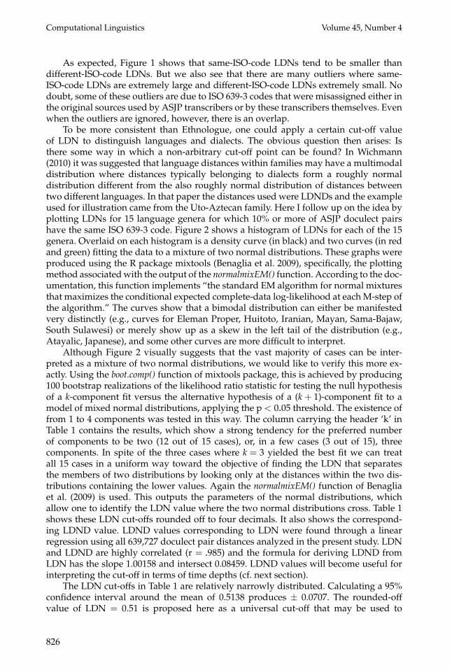
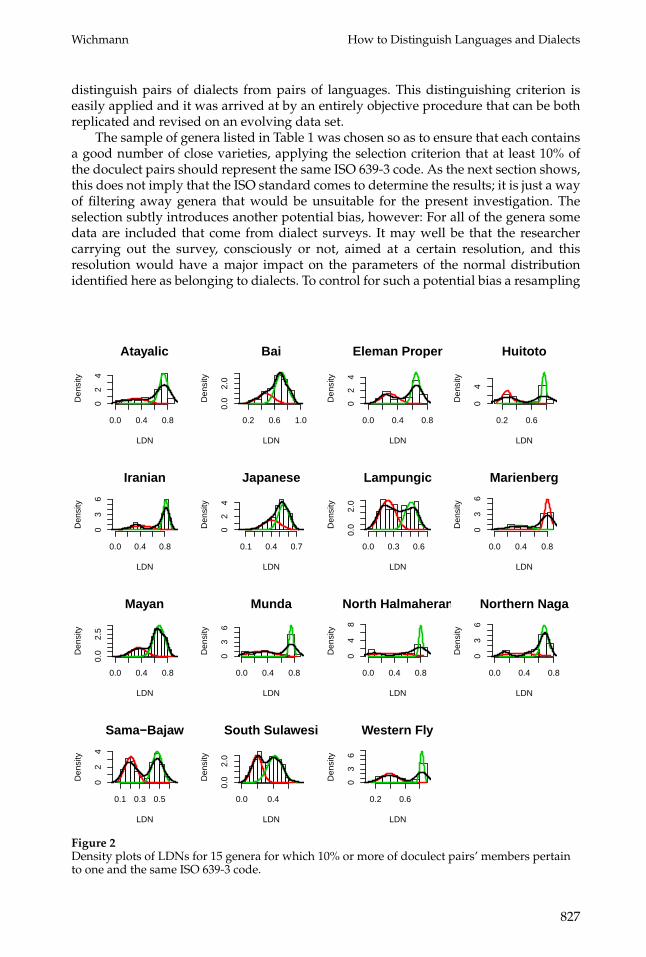
To be more consistent than Ethnologue, one could apply a certain cut-off valueof LDN to distinguish languages and dialects. The obvious question then arises: Isthere some way in which a non-arbitrary cut-off point can be found? In Wichmann(2010) it was suggested that language distances within families may have a multimodaldistribution where distances typically belonging to dialects form a roughly normaldistribution different from the also roughly normal distribution of distances betweentwo different languages. In that paper the distances used were LDNDs and the exampleused for illustration came from the Uto-Aztecan family. Here I follow up on the idea byplotting LDNs for 15 language genera for which 10% or more of ASJP doculect pairshave the same ISO 639-3 code. Figure 2 shows a histogram of LDNs for each of the 15genera. Overlaid on each histogram is a density curve (in black) and two curves (in redand green) fitting the data to a mixture of two normal distributions. These graphs wereproduced using the R package mixtools (Benaglia et al. 2009), specifically, the plottingmethod associated with the output of the normalmixEM() function. According to the doc-umentation, this function implements “the standard EM algorithm for normal mixturesthat maximizes the conditional expected complete-data log-likelihood at each M-step ofthe algorithm.” The curves show that a bimodal distribution can either be manifestedvery distinctly (e.g., curves for Eleman Proper, Huitoto, Iranian, Mayan, Sama-Bajaw,South Sulawesi) or merely show up as a skew in the left tail of the distribution (e.g.,Atayalic, Japanese), and some other curves are more difficult to interpret.

Although Figure 2 visually suggests that the vast majority of cases can be inter-preted as a mixture of two normal distributions, we would like to verify this more ex-actly. Using the boot.comp() function of mixtools package, this is achieved by producing100 bootstrap realizations of the likelihood ratio statistic for testing the null hypothesisof a k-component fit versus the alternative hypothesis of a (k + 1)-component fit to amodel of mixed normal distributions, applying the p < 0.05 threshold. The existence offrom 1 to 4 components was tested in this way. The column carrying the header ‘k’ inTable 1 contains the results, which show a strong tendency for the preferred numberof components to be two (12 out of 15 cases), or, in a few cases (3 out of 15), threecomponents. In spite of the three cases where k = 3 yielded the best fit we can treatall 15 cases in a uniform way toward the objective of finding the LDN that separatesthe members of two distributions by looking only at the distances within the two dis-tributions containing the lower values. Again the normalmixEM() function of Benagliaet al. (2009) is used. This outputs the parameters of the normal distributions, whichallow one to identify the LDN value where the two normal distributions cross. Table 1shows these LDN cut-offs rounded off to four decimals. It also shows the correspond-ing LDND value. LDND values corresponding to LDN were found through a linearregression using all 639,727 doculect pair distances analyzed in the present study. LDNand LDND are highly correlated (r = .985) and the formula for deriving LDND fromLDN has the slope 1.00158 and intersect 0.08459. LDND values will become useful forinterpreting the cut-off in terms of time depths (cf. next section).

The LDN cut-offs in Table 1 are relatively narrowly distributed. Calculating a 95%confidence interval around the mean of 0.5138 produces ± 0.0707. The rounded-offvalue of LDN = 0.51 is proposed here as a universal cut-off that may be used to

826

Wichmann How to Distinguish Languages and Dialects

distinguish pairs of dialects from pairs of languages. This distinguishing criterion iseasily applied and it was arrived at by an entirely objective procedure that can be bothreplicated and revised on an evolving data set.

The sample of genera listed in Table 1 was chosen so as to ensure that each containsa good number of close varieties, applying the selection criterion that at least 10% ofthe doculect pairs should represent the same ISO 639-3 code. As the next section shows,this does not imply that the ISO standard comes to determine the results; it is just a wayof filtering away genera that would be unsuitable for the present investigation. Theselection subtly introduces another potential bias, however: For all of the genera somedata are included that come from dialect surveys. It may well be that the researchercarrying out the survey, consciously or not, aimed at a certain resolution, and thisresolution would have a major impact on the parameters of the normal distributionidentified here as belonging to dialects. To control for such a potential bias a resampling

Atayalic

LDN

Den

sity

0.0 0.4 0.8

02

4

Bai

LDN

Den

sity

0.2 0.6 1.0

0.0

2.0

Eleman Proper

LDN

Den

sity

0.0 0.4 0.8

02

4Huitoto

LDN

Den

sity

0.2 0.6

04

Iranian

LDN

Den

sity

0.0 0.4 0.8

03

6

Japanese

LDN

Den

sity

0.1 0.4 0.7

02

4

Lampungic

LDN

Den

sity

0.0 0.3 0.6

0.0

2.0

Marienberg

LDN

Den

sity

0.0 0.4 0.8

03

6

Mayan

LDN

Den

sity

0.0 0.4 0.8

0.0

2.5

Munda

LDN

Den

sity

0.0 0.4 0.8

03

6

North Halmaheran

LDN

Den

sity

0.0 0.4 0.8

04

8

Northern Naga

LDN

Den

sity

0.0 0.4 0.8

03

6

Sama−Bajaw

LDN

Den

sity

0.1 0.3 0.5

02

4

South Sulawesi

LDN

Den

sity

0.0 0.4

0.0

2.0

Western Fly

LDN

Den

sity

0.2 0.6

03

6

Figure 2Density plots of LDNs for 15 genera for which 10% or more of doculect pairs’ members pertainto one and the same ISO 639-3 code.

827

Computational Linguistics Volume 45, Number 4

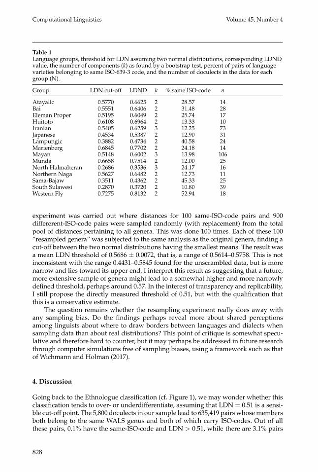
Table 1Language groups, threshold for LDN assuming two normal distributions, corresponding LDNDvalue, the number of components (k) as found by a bootstrap test, percent of pairs of languagevarieties belonging to same ISO-639-3 code, and the number of doculects in the data for eachgroup (N).

Group LDN cut-off LDND k % same ISO-code n

Atayalic 0.5770 0.6625 2 28.57 14Bai 0.5551 0.6406 2 31.48 28Eleman Proper 0.5195 0.6049 2 25.74 17Huitoto 0.6108 0.6964 2 13.33 10Iranian 0.5405 0.6259 3 12.25 73Japanese 0.4534 0.5387 2 12.90 31Lampungic 0.3882 0.4734 2 40.58 24Marienberg 0.6845 0.7702 2 24.18 14Mayan 0.5148 0.6002 3 13.98 106Munda 0.6658 0.7514 2 12.00 25North Halmaheran 0.2686 0.3536 3 24.17 16Northern Naga 0.5627 0.6482 2 12.73 11Sama-Bajaw 0.3511 0.4362 2 45.33 25South Sulawesi 0.2870 0.3720 2 10.80 39Western Fly 0.7275 0.8132 2 52.94 18

experiment was carried out where distances for 100 same-ISO-code pairs and 900differerent-ISO-code pairs were sampled randomly (with replacement) from the totalpool of distances pertaining to all genera. This was done 100 times. Each of these 100“resampled genera” was subjected to the same analysis as the original genera, finding acut-off between the two normal distributions having the smallest means. The result wasa mean LDN threshold of 0.5686 ± 0.0072, that is, a range of 0.5614–0.5758. This is notinconsistent with the range 0.4431–0.5845 found for the unscrambled data, but is morenarrow and lies toward its upper end. I interpret this result as suggesting that a future,more extensive sample of genera might lead to a somewhat higher and more narrowlydefined threshold, perhaps around 0.57. In the interest of transparency and replicability,I still propose the directly measured threshold of 0.51, but with the qualification thatthis is a conservative estimate.

The question remains whether the resampling experiment really does away withany sampling bias. Do the findings perhaps reveal more about shared perceptionsamong linguists about where to draw borders between languages and dialects whensampling data than about real distributions? This point of critique is somewhat specu-lative and therefore hard to counter, but it may perhaps be addressed in future researchthrough computer simulations free of sampling biases, using a framework such as thatof Wichmann and Holman (2017).

4. Discussion

Going back to the Ethnologue classification (cf. Figure 1), we may wonder whether thisclassification tends to over- or underdifferentiate, assuming that LDN = 0.51 is a sensi-ble cut-off point. The 5,800 doculects in our sample lead to 635,419 pairs whose membersboth belong to the same WALS genus and both of which carry ISO-codes. Out of allthese pairs, 0.1% have the same-ISO-code and LDN > 0.51, while there are 3.1% pairs

828

Wichmann How to Distinguish Languages and Dialects

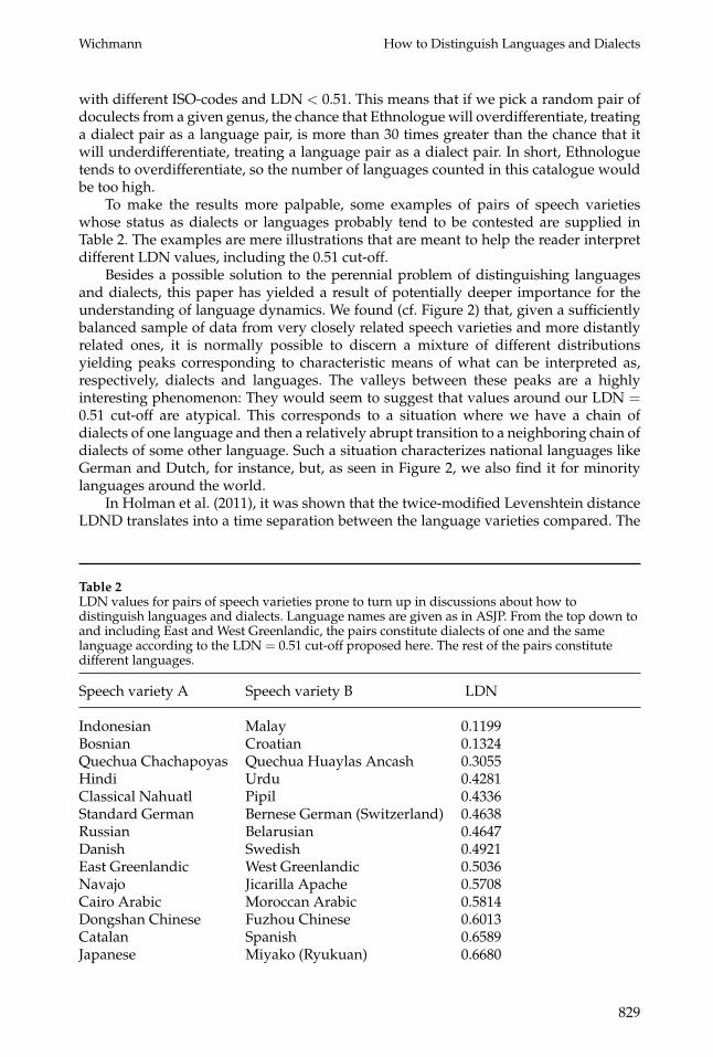
with different ISO-codes and LDN < 0.51. This means that if we pick a random pair ofdoculects from a given genus, the chance that Ethnologue will overdifferentiate, treatinga dialect pair as a language pair, is more than 30 times greater than the chance that itwill underdifferentiate, treating a language pair as a dialect pair. In short, Ethnologuetends to overdifferentiate, so the number of languages counted in this catalogue wouldbe too high.

To make the results more palpable, some examples of pairs of speech varietieswhose status as dialects or languages probably tend to be contested are supplied inTable 2. The examples are mere illustrations that are meant to help the reader interpretdifferent LDN values, including the 0.51 cut-off.

Besides a possible solution to the perennial problem of distinguishing languagesand dialects, this paper has yielded a result of potentially deeper importance for theunderstanding of language dynamics. We found (cf. Figure 2) that, given a sufficientlybalanced sample of data from very closely related speech varieties and more distantlyrelated ones, it is normally possible to discern a mixture of different distributionsyielding peaks corresponding to characteristic means of what can be interpreted as,respectively, dialects and languages. The valleys between these peaks are a highlyinteresting phenomenon: They would seem to suggest that values around our LDN =0.51 cut-off are atypical. This corresponds to a situation where we have a chain ofdialects of one language and then a relatively abrupt transition to a neighboring chain ofdialects of some other language. Such a situation characterizes national languages likeGerman and Dutch, for instance, but, as seen in Figure 2, we also find it for minoritylanguages around the world.

In Holman et al. (2011), it was shown that the twice-modified Levenshtein distanceLDND translates into a time separation between the language varieties compared. The

Table 2LDN values for pairs of speech varieties prone to turn up in discussions about how todistinguish languages and dialects. Language names are given as in ASJP. From the top down toand including East and West Greenlandic, the pairs constitute dialects of one and the samelanguage according to the LDN = 0.51 cut-off proposed here. The rest of the pairs constitutedifferent languages.

Speech variety A Speech variety B LDN

Indonesian Malay 0.1199Bosnian Croatian 0.1324Quechua Chachapoyas Quechua Huaylas Ancash 0.3055Hindi Urdu 0.4281Classical Nahuatl Pipil 0.4336Standard German Bernese German (Switzerland) 0.4638Russian Belarusian 0.4647Danish Swedish 0.4921East Greenlandic West Greenlandic 0.5036Navajo Jicarilla Apache 0.5708Cairo Arabic Moroccan Arabic 0.5814Dongshan Chinese Fuzhou Chinese 0.6013Catalan Spanish 0.6589Japanese Miyako (Ryukuan) 0.6680

829

Computational Linguistics Volume 45, Number 4

LDND values in Table 1 have a mean of 0.5992 ± 0.0709. Using the formula of Holmanet al. (2011) this is equivalent to a range of 1,075–1,635 years. Thus, it takes around oneto one-and-a-half millennia for a speech community to diverge into different languagegroups.

Why can we find those valleys in the distributions in Figure 2? Or, put differently,what is it about the way that speakers interact that allows us to distinguish languagesand dialects? A possible explanation is that there is a threshold of mutual intelligibilitywhere language varieties will influence one another if they are below the threshold butwill cease to influence one another if they are above it. If mutual intelligibility betweenvariety A and B is impeded completely, speakers may take recourse to just the moreprestigious of the two, if not some third language, leaving A and B to drift apart morerapidly than would the case if both A and B were used for communication betweenthe two groups. It awaits future studies to corroborate this idea through modeling and,ideally, through systematic sampling of both lexical data and data on intelligibility fromthe cells of a large but also fine geographically defined grid or, less ideally, through ananalysis of the literature on mutual intelligibility.

5. Conclusion

In this paper the question of how to distinguish languages and dialects was addressedby studying the distribution of lexical distances within groups of uncontroversiallyrelated languages (the genera of Dryer and Haspelmath [2013]). Following up on anidea tentatively suggested in Wichmann (2010), it was verified that distances amongspeech varieties represent mixed distributions, including a cluster that may be said tocorrespond to dialects and another cluster corresponding to languages. Applying anexpectation-maximization algorithm to tease apart the mixture of normal distributionsacross a sample of 15 language groups, the average cut-off point between the twodistributions was found to be LDN = 0.51, where LDN is the normalized Levenshteindistance across word pairs in the ASJP 40-item word lists of Wichmann, Holman, andBrown (2018). The corresponding temporal distance lies around 1,355 years, withinthe interval 1,075–1,635 years. Thus, we now have a principled way of distinguishinglanguages and dialects. A tantalizing question for future research is why there seems tobe a real distinction, not just a theoretical or arbitrary one. Some suggestions for waysto approach this question were suggested.

AcknowledgmentsThanks go to Eric Holman, HaraldHammarstrom, Qibin Ran, and fouranonymousreviewers forstimulatingdiscussion.The research was carried out under the auspicesof the project “The Dictionary/GrammarReading Machine: Computational Tools forAccessing the World’s Linguistic Heritage”(NWO proj. no. 335-54-102) within theEuropean JPI Cultural Heritage and GlobalChange programme. It was additionallyfunded by a subsidy from the Russiangovernment to support the Programme ofCompetitive Development of Kazan FederalUniversity and a grant (KYR17018) fromBeijing Language Innovation Center insupport of a sub-topic directed by Qibin Ran.

ReferencesAgard, Frederick. 1984. A Course in Romance

Linguistics. Georgetown University Press.Benaglia, Tatiana, Didier Chauveau,

David R. Hunter, and Derek S. Young.2009. mixtools: An R package foranalyzing finite mixture models. Journal ofStatistical Software, 32(6):1–29.

Bender, Marvin L. and Robert L. Cooper.1971. Mutual intelligibility within Sidamo.Lingua, 27:32–52.

Biggs, Bruce. 1957. Testing mutualintelligibility among Yuman languages.International Journal of American Linguistics,23(2):57–62.

Brown, Cecil H., Søren Wichmann, andEric W. Holman. 2013. Sound

830

Wichmann How to Distinguish Languages and Dialects

correspondences in the world’s languages.Language, 89(1):4–29.

Casad, Eugene H. 1974. Dialect IntelligibilityTesting. Summer Institute of Linguistics ofthe University of Oklahoma, Norman.

Dryer, Matthew S. and Martin Haspelmath,editors. 2013. The World Atlas of LanguageStructures Online. http://wals.info. MaxPlanck Institute for EvolutionaryAnthropology, Leipzig.

Gooskens, Charlotte and Vincent J. vanHeuven. 2019. How well can intelligibilityof closely related languages in Europe bepredicted by linguistic and non-linguisticvariables? Linguistic Approaches toBilingualism, Early online publication,https://doi.org/10.1075/lab.17084.goo.

Gooskens, Charlotte, Vincent J. van Heuven,Jelena Golubovic, Anja Schuppert, FemkeSwarte, and Stefanie Voigt. 2018. Mutualintelligibility between closely relatedlanguages in Europe. International Journalof Multilingualism, 15(2):169–193.

Gooskens, Charlotte and Cindy Schneider.2016. Testing mutual intelligibilitybetween closely related languages in anoral society. Language Documentation andConservation, 10:278–305.

Hammarstrom, Harald, Robert Forkel, andMartin Haspelmath. 2017. Glottolog 3.0.http://glottolog.org. Max PlanckInstitute for the Science of Human History,Jena.

Heeringa, Wilbert, Peter Kleiweg, CharlotteGooskens, and John Nerbonne. 2006.Evaluation of string distance algorithmsfor dialectology. In Proceedings of theWorkshop on Linguistic Distances,pages 51–62, Sydney.

Holman, Eric W., Cecil H. Brown, SørenWichmann, Andre Muller, VivekaVelupillai, Harald Hammarstrom,Sebastian Sauppe, Hagen Jung, DikBakker, Pamela Brown, Oleg Belyaev,Matthias Urban, Robert Mailhammer,Johann-Mattis List, and Dmitry Egorov.2011. Automated dating of the world’slanguage families based on lexicalsimilarity. Current Anthropology,52(6):841–875.

Jager, Gerhard. 2015. Support for linguisticmacrofamilies from weighted sequencealignment. Proceedings of the National

Academy of Sciences of the U.S.A.,112(41):12752–12757.

Korjakov, Yurij Borisovich. 2017. Problema“jazyk ili dialekt” i popytkaleksikostatisticheskogo podxoda. VoprosyJazykoznanija, 6:79–101.

Ladefoged, Peter, Ruth Glick, and CliveCriper. 1972. Language in Uganda. OxfordUniversity Press.

Rubin, Donald L. 1992. Nonlanguage factorsaffecting undergraduates’ judgments ofnonnative English-speaking teachingassistants. Research in Higher Education,33(4):511–531.

Simons, Gary F. and Charles D. Fennig. 2017.Ethnologue: Languages of the World, TwentiethEdition. SIL International, Dallas, TX.

Swadesh, Morris. 1950. Salish internalrelationships. International Journal ofAmerican Linguistics, 16(4):157–164.

Szeto, Cecilia. 2000. Testing intelligibilityamong Sinitic dialects. In Proceedings ofALS2K, the 2000 Conference of the AustralianLinguistic Society, Melbourne.

Voegelin, Charles F. and Zellig S. Harris.1951. Methods for determiningintelligibility among dialects of naturallanguages. Proceedings of the AmericanPhilosophical Society, 95(3):322–329.

Whaley, Lindsay J., Lenore A. Grenoble, andFengxiang Li. 1999. Revisiting Tungusic.Language, 75(2):286–321.

Wichmann, Søren. 2010. Internal languageclassification. In Luraghi, Silvia and VitBubenik, editors, The ContinuumCompanion to Historical Linguistics.Continuum Books, London/New York,pages 70–86.

Wichmann, Søren. 2019. Interactive Rprogram for ASJP version 1. https://github.com/Sokiwi/InteractiveASJP01.

Wichmann, Søren and Eric W. Holman. 2017.New evidence from linguistic phylogeneticssupports phyletic gradualism. SystematicBiology, 66(4):604–610.

Wichmann, Søren, Eric W. Holman, DikBakker, and Cecil H. Brown. 2010.Evaluating linguistic distance measures.Physica A, 389:3632–3639.

Wichmann, Søren, Eric W. Holman, andCecil H. Brown, editors. 2018. The ASJPDatabase (version 18). http://asjp.clld.org/.

831