BioNLP 2017 - ACL Anthology
400
BioNLP 2017 SIGBioMed Workshop on Biomedical Natural Language Processing Proceedings of the 16th BioNLP Workshop August 4, 2017 Vancouver, Canada
-
Upload
khangminh22 -
Category
Documents
-
view
2 -
download
0
Transcript of BioNLP 2017 - ACL Anthology

BioNLP 2017
SIGBioMed Workshop on Biomedical Natural LanguageProcessing
Proceedings of the 16th BioNLP Workshop
August 4, 2017Vancouver, Canada

c©2017 The Association for Computational Linguistics
ISBN 978-1-945626-59-3
ii

Biomedical natural language processing in 2017:The view from computational linguistics
Kevin Bretonnel Cohen, Dina Demner-Fushman,Sophia Ananiadou, and Jun-ichi Tsujii
According to the Association for Computational Linguistics guidelines on special interest groups (SIGs),The function of a SIG is to encourage interest and activity in specific areas within the ACL’s field[1]. Isthe SIGBioMed special interest group “within the ACL’s field”? The titles of this year’s papers suggestthat it is, in that the current interest in deep learning in its many and varied manifestations is mirrored inthose titles. Do those papers cover a specific area? They do, and in doing so, they demonstrate one ofthe great satisfactions of working in biomedical natural language processing.
One of the joys of involvement in the biomedical natural language processing community is seeingthe development of research with clinical applications. As examples of such work being presented atBioNLP 2017, we would like to point out the two papers that discuss the application of natural languageprocessing to the diagnosis of neurological disorders. Bhatia et al.[2] describe an approach to usingspeech processing in the assessment of patients with amyotrophic lateral sclerosis (also known as LouGehrig’s disease), one of the more horrific motor neuron diseases. Good assessment of amyotrophiclateral sclerosis patients is important for a number of reasons, including the fact that accurate trackingof the inevitable deterioration that is a hallmark of this disease gives patients and their families thepossibility of purposeful planning for the attendant disability and death. However, current methodologiesfor evaluating the status of amyotrophic lateral sclerosis patients necessarily involve expensive equipmentand highly trained personnel; when further developed, this methodology could make such evaluationmuch more, and more frequently, available to ALS patients. The fact that the work reported here involvesa speech modality is especially exciting, as speech-related indicators of future ALS can be present longbefore diagnosis. The paper uses measurements of phonological features of speech and their divergencefrom a baseline, and demonstrates correlation with physiological measures.
Adams et al.[3] describe work on detecting and categorizing word production errors associated withanomia, a particular kind of inability to find words. Screening for anomia is important because anomiais a symptom of stroke, but it is difficult and time-consuming to do, and therefore is not done as oftenas it should be. Automatic detection of anomia could be a nice enabler of improved care for strokevictims, but it is made difficult due to the subtlety of the phonological and semantic judgments that haveto be made when assessing the phenomenon. The paper uses a combination of language modeling andphonologically-based edit distance calculation to approach the task, applying these techniques to datafrom the AphasiaBank collection of transcribed aphasic and healthy speech.
Although we have summarized only these two examples that address neurological disorders, there areseveral other papers on the use of natural language processing in clinical applications: patient-producedcontent in dementia [4], and health records ([5] on sepsis, [6] on e-cig use, [7] on pain and confusion);in the aggregate, these papers illustrate very nicely the potential for natural language processing tocontribute to human well-being. Additionally, the current interest in the potential of natural languageprocessing for social media is reflected in papers on studying medication intake via Twitter [8] and onmonitoring dementia via blog posts [9]. Linguistics and language resources are represented in this year’spapers, as well, including work on comparative structures [10] and a corpus construction effort [11].
The work in biomedical NLP was dominated by applications of deep learning to: punctuation restoration[12], text classification [13], relation extraction [14], [15], [16], information retrieval [17], and similarityjudgments [18], among other exciting progress in biomedical language processing.
These are just a few examples of the high-quality research presented in BioNLP 2017.
iii

In addition to the excellent submissions to the BioNLP workshop, this year features equally strongsubmissions to BioASQ challenge on large-scale biomedical semantic indexing and question answering,a shared task affiliated with BioNLP 2017. This year, the BioASQ challenge, which started in 2013, hadthree tasks:
• Large-Scale Online Biomedical Semantic Indexing• Biomedical Semantic Question Answering• Funding Information Extraction From Biomedical Literature
An overview of the tasks and the results of the challenge [19] are presented in an invited talk. Theinvited speaker, George Paliouras, is a senior researcher and head of the Intelligent Information Systemsdivision of the Institute of Informatics and Telecommunications at NCSR “Demokritos”, Greece. Heholds a PhD in Machine Learning and has performed basic and applied research in Artificial Intelligencefor the last 20 years. He is interested in the development of novel methods for addressing challengingbig and small data analysis problems, such as learning complex models from structured relational data,learning from noisy and sparse data, learning from multiple heterogeneous data streams, and discoveringpatterns in hypergraphs. His research is motivated by the real-world problems. George has contributed tosolving a variety of such problems, ranging from spam filtering and Web personalization to biomedicalinformation retrieval. He has co-founded the spin-off company em i-sieve Technologies, which providesonline reputation monitoring services.
Among various contributions to the research community, George Paliouras has served as board memberin national and international scientific societies; he is serving on the editorial boards of internationaljournals, and has chaired international conferences. He is involved in several research projects, in therole of scientific coordinator/principal investigator in some of them. In particular, he has coordinated andprovided the infrastructure for the BioASQ project that was funded by the European Commission. He iscurrently coordinating iASiS, another project funded by the European Commission to develop big dataintegration and analysis methods that will provide insight to public health policy-making for personalizedmedicine.
Acknowledging the community
As always, the organizers thank the authors who submitted their work to BioNLP 2017 —without them,there would be no meeting, no opportunity to share the progress and the pain of the past year with thecommunity. We have listed above only a few of the exceptional submissions that were accepted for oral(20) and poster (28) presentations.
The distribution of scores this year suggests that a large amount of excellent work was submittedfor review and resulted in 77% acceptance ratio. At the same time, the distribution suggests thatthe reviewers were careful and thorough, and the organizers thank them for that, and for thoroughlyreviewing up to five papers on a very tight schedule.
We greatly appreciate the BioNLP core authors and program committee members who have been buildingup the community and the workshop for the past sixteen years. We are also happy to see the excellentnew submissions and the new reviewers, and hope they will continue contributing to BioNLP.
References
[1] SIG Creation Guidelines https://goo.gl/yIQCHo 2017.
iv

[2] Archna Bhatia, Bonnie Dorr, Kristy Hollingshead, Samuel L. Phillips and Barbara McKenzieCharacterization of Divergence in Impaired Speech of ALS Patients 2017.
[3] Joel Adams, Steven Bedrick, Gerasimos Fergadiotis, Kyle Gorman and Jan van Santen Target wordprediction and paraphasia classification in spoken discourse 2017.
[4] Vaden Masrani, Gabriel Murray, Thalia Field and Giuseppe Carenini Detecting Dementia throughRetrospective Analysis of Routine Blog Posts by Bloggers with Dementia 2017.
[5] Emilia Apostolova and Tom Velez Toward Automated Early Sepsis Alerting: Identifying InfectionPatients from Nursing Notes 2017.
[6] Danielle Mowery, Brett South, Olga Patterson, Shu-Hong Zhu and Mike Conway Investigating theDocumentation of Electronic Cigarette Use in the Veteran Affairs Electronic Health Record: A PilotStudy 2017.
[7] Hans Moen, Kai Hakala, Farrokh Mehryary, Laura-Maria Peltonen, Tapio Salakoski, Filip Ginterand Sanna Salanterä Detecting mentions of pain and acute confusion in Finnish clinical text 2017.
[8] Ari Klein, Abeed Sarker, Masoud Rouhizadeh, Karen O’Connor and Graciela Gonzalez DetectingPersonal Medication Intake in Twitter: An Annotated Corpus and Baseline Classification System2017.
[9] Vaden Masrani, Gabriel Murray, Thalia Field and Giuseppe Carenini Detecting Dementia throughRetrospective Analysis of Routine Blog Posts by Bloggers with Dementia 2017.
[10] Samir Gupta, A.S.M. Ashique Mahmood, Karen Ross, Cathy Wu and K. Vijay-Shanker IdentifyingComparative Structures in Biomedical Text 2017.
[11] Rezarta Islamaj Dogan, Andrew Chatr-aryamontri, Sun Kim, Chih-Hsuan Wei, Yifan Peng, DonaldComeau and Zhiyong Lu BioCreative VI Precision Medicine Track: creating a training corpus formining protein-protein interactions affected by mutations 2017.
[12] Wael Salloum, Greg Finley, Erik Edwards, Mark Miller and David Suendermann-Oeft DeepLearning for Punctuation Restoration in Medical Reports 2017.
[13] Simon Baker and Anna Korhonen Initializing neural networks for hierarchical multi-label textclassification 2017.
[14] Chen Lin, Timothy Miller, Dmitriy Dligach, Steven Bethard and Guergana Savova Representationsof Time Expressions for Temporal Relation Extraction with Convolutional Neural Networks 2017.
[15] Masaki Asada, Makoto Miwa and Yutaka Sasaki Extracting Drug-Drug Interactions with AttentionCNNs 2017.
[16] Yifan Peng and Zhiyong Lu Deep learning for extracting protein-protein interactions frombiomedical literature 2017.
[17] Sunil Mohan, Nicolas Fiorini, Sun Kim and Zhiyong Lu Deep Learning for Biomedical InformationRetrieval: Learning Textual Relevance from Click Logs 2017.
[18] Bridget McInnes and Ted Pedersen Improving Correlation with Human Judgments by IntegratingSemantic Similarity with Second–Order Vectors 2017.
[19] Anastasios Nentidis, Konstantinos Bougiatiotis, Anastasia Krithara, Georgios Paliouras and IoannisKakadiaris Results of the fifth edition of the BioASQ Challenge 2017.
v


Organizers:
Kevin Bretonnel Cohen, University of Colorado School of Medicine, USADina Demner-Fushman, US National Library of MedicineSophia Ananiadou, National Centre for Text Mining and University of Manchester, UKJun-ichi Tsujii, National Institute of Advanced Industrial Science and Technology, Japan
Program Committee:
Sophia Ananiadou, National Centre for Text Mining and University of Manchester, UKIon Androutsopoulos, Athens University of Economics and Business, GreeceEmilia Apostolova, Language.ai, USAEiji Aramaki, University of Tokyo, JapanAlan Aronson, US National Library of MedicineAsma Ben Abacha, US National Library of MedicineOlivier Bodenreider, US National Library of MedicineKevin Bretonnel Cohen, University of Colorado School of Medicine, USALeonardo Campillos Llanos, LIMSI - CNRS, FranceKevin Bretonnel Cohen, University of Colorado School of Medicine, USANigel Collier, University of Cambridge, UKDina Demner-Fushman, US National Library of MedicineFilip Ginter, University of Turku, FinlandGraciela Gonzalez, University of Pennsylvania, USACyril Grouin, LIMSI - CNRS, FranceAntonio Jimeno Yepes, IBM, Melbourne Area, AustraliaHalil Kilicoglu, US National Library of MedicineAris Kosmopoulos, NCSR Demokritos, GreeceRobert Leaman, US National Library of MedicineChris Lu, US National Library of MedicineZhiyong Lu, US National Library of MedicineJuan Miguel Cejuela, Technische Universität München, GermanyTimothy Miller, Children’s Hospital Boston, USAMakoto Miwa, Toyota Technological Institute, JapanDanielle L Mowery, VA Salt Lake City Health Care System, USADiego Molla, Macquarie University, AustraliaJim Mork, National Library of Medicine, USAYassine Mrabet, US National Library of MedicineHenning Müller, University of Applied Sciences, SwitzerlandClaire Nédellec, INRA, FranceAnastasios Nentidis, NCSR Demokritos, Athens, GreeceAurélie Névéol, LIMSI - CNRS, FranceMariana Neves, Hasso Plattner Institute and University of Potsdam, GermanyNhung Nguyen, The University of Manchester, ManchesterNaoaki Okazaki, Tohoku University, JapanGeorgios Paliouras, NCSR Demokritos, Athens, GreeceIoannis Partalas, Viseo group, FranceJohn Prager, Thomas J. Watson Research Center, IBM, USASampo Pyysalo, University of Cambridge, UK
vii

Francisco J. Ribadas-Pena, University of Vigo, SpainFabio Rinaldi, University of Zurich, SwitzerlandAngus Roberts, The University of Sheffield, UKKirk Roberts, The University of Texas Health Science Center at Houston, USAHagit Shatkay, University of Delaware, USAPontus Stenetorp, University College London, UKKarin Verspoor, The University of Melbourne, AustraliaEllen Voorhees, National Institute of Standards and Technology, USAByron C. Wallace, University of Texas at Austin, USAW John Wilbur, US National Library of MedicineHai Zhao, Shanghai Jiao Tong University, ShanghaiPierre Zweigenbaum, LIMSI - CNRS, France
Additional Reviewers:
Moumita Bhattacharya, University of Delaware, USALouise Deléger, INRA - MaIAGE, FranceLenz Furrer, Institute of Computational Linguistics, UZH, Zurich, SwitzerlandGenevieve Gorrell, Sheffield University, UKAri Klein, University of Pennsylvania School of MedicineYifan Peng, US National Library of MedicineVassiliki Rentoumi, National Centre for Scientific Research Demokritos, Athens, GreeceMasoud Rouhizadeh, University of Pennsylvania, USAAbeed Sarker, University of Pennsylvania, USAXingyi Song, University of Sheffield, UKTasnia Tahsin, Arizona State University, USAHegler Tissot, Federal University of Parana, BrazilKen Yano, Nara Institute of Science and Technology, Japan
Invited Speaker:
George Paliouras, National Centre for Scientific Research Demokritos, Athens, Greece
viii

Table of Contents
Target word prediction and paraphasia classification in spoken discourseJoel Adams, Steven Bedrick, Gerasimos Fergadiotis, Kyle Gorman and Jan van Santen . . . . . . . . . 1
Extracting Drug-Drug Interactions with Attention CNNsMasaki Asada, Makoto Miwa and Yutaka Sasaki . . . . . . . . . . . . . . . . . . . . . . . . . . . . . . . . . . . . . . . . . . . . 9
Insights into Analogy Completion from the Biomedical DomainDenis Newman-Griffis, Albert Lai and Eric Fosler-Lussier . . . . . . . . . . . . . . . . . . . . . . . . . . . . . . . . . . 19
Deep learning for extracting protein-protein interactions from biomedical literatureYifan Peng and Zhiyong Lu . . . . . . . . . . . . . . . . . . . . . . . . . . . . . . . . . . . . . . . . . . . . . . . . . . . . . . . . . . . . . . 29
Stacking With Auxiliary Features for Entity Linking in the Medical DomainNazneen Fatema Rajani, Mihaela Bornea and Ken Barker . . . . . . . . . . . . . . . . . . . . . . . . . . . . . . . . . . . 39
Results of the fifth edition of the BioASQ ChallengeAnastasios Nentidis, Konstantinos Bougiatiotis, Anastasia Krithara, Georgios Paliouras and Ioannis
Kakadiaris . . . . . . . . . . . . . . . . . . . . . . . . . . . . . . . . . . . . . . . . . . . . . . . . . . . . . . . . . . . . . . . . . . . . . . . . . . . . . . . . . . 48
Tackling Biomedical Text Summarization: OAQA at BioASQ 5BKhyathi Chandu, Aakanksha Naik, Aditya Chandrasekar, Zi Yang, Niloy Gupta and Eric Nyberg58
Macquarie University at BioASQ 5b – Query-based Summarisation Techniques for Selecting the IdealAnswers
Diego Molla . . . . . . . . . . . . . . . . . . . . . . . . . . . . . . . . . . . . . . . . . . . . . . . . . . . . . . . . . . . . . . . . . . . . . . . . . . . 67
Neural Question Answering at BioASQ 5BGeorg Wiese, Dirk Weissenborn and Mariana Neves. . . . . . . . . . . . . . . . . . . . . . . . . . . . . . . . . . . . . . . .76
End-to-End System for Bacteria Habitat ExtractionFarrokh Mehryary, Kai Hakala, Suwisa Kaewphan, Jari Björne, Tapio Salakoski and Filip Ginter80
Creation and evaluation of a dictionary-based tagger for virus species and proteinsHelen Cook, Rudolfs Berzins, Cristina Leal Rodrıguez, Juan Miguel Cejuela and Lars Juhl Jensen
91
Representation of complex terms in a vector space structured by an ontology for a normalization taskArnaud Ferré, Pierre Zweigenbaum and Claire Nédellec . . . . . . . . . . . . . . . . . . . . . . . . . . . . . . . . . . . . 99
Improving Correlation with Human Judgments by Integrating Semantic Similarity with Second–OrderVectors
Bridget McInnes and Ted Pedersen . . . . . . . . . . . . . . . . . . . . . . . . . . . . . . . . . . . . . . . . . . . . . . . . . . . . . . 107
Proactive Learning for Named Entity RecognitionMaolin Li, Nhung Nguyen and Sophia Ananiadou . . . . . . . . . . . . . . . . . . . . . . . . . . . . . . . . . . . . . . . . 117
Biomedical Event Extraction using Abstract Meaning RepresentationSudha Rao, Daniel Marcu, Kevin Knight and Hal Daumé III . . . . . . . . . . . . . . . . . . . . . . . . . . . . . . . 126
Detecting Personal Medication Intake in Twitter: An Annotated Corpus and Baseline ClassificationSystem
Ari Klein, Abeed Sarker, Masoud Rouhizadeh, Karen O’Connor and Graciela Gonzalez . . . . . . 136
ix

Unsupervised Context-Sensitive Spelling Correction of Clinical Free-Text with Word and Character N-Gram Embeddings
Pieter Fivez, Simon Suster and Walter Daelemans . . . . . . . . . . . . . . . . . . . . . . . . . . . . . . . . . . . . . . . . . 143
Characterization of Divergence in Impaired Speech of ALS PatientsArchna Bhatia, Bonnie Dorr, Kristy Hollingshead, Samuel L. Phillips and Barbara McKenzie . 149
Deep Learning for Punctuation Restoration in Medical ReportsWael Salloum, Greg Finley, Erik Edwards, Mark Miller and David Suendermann-Oeft . . . . . . . . 159
Unsupervised Domain Adaptation for Clinical Negation DetectionTimothy Miller, Steven Bethard, Hadi Amiri and Guergana Savova . . . . . . . . . . . . . . . . . . . . . . . . . 165
BioCreative VI Precision Medicine Track: creating a training corpus for mining protein-protein interac-tions affected by mutations
Rezarta Islamaj Dogan, Andrew Chatr-aryamontri, Sun Kim, Chih-Hsuan Wei, Yifan Peng, DonaldComeau and Zhiyong Lu . . . . . . . . . . . . . . . . . . . . . . . . . . . . . . . . . . . . . . . . . . . . . . . . . . . . . . . . . . . . . . . . . . . . 171
Painless Relation Extraction with KindredJake Lever and Steven Jones . . . . . . . . . . . . . . . . . . . . . . . . . . . . . . . . . . . . . . . . . . . . . . . . . . . . . . . . . . . . 176
Noise Reduction Methods for Distantly Supervised Biomedical Relation ExtractionGang Li, Cathy Wu and K. Vijay-Shanker . . . . . . . . . . . . . . . . . . . . . . . . . . . . . . . . . . . . . . . . . . . . . . . . 184
Role-Preserving Redaction of Medical Records to Enable Ontology-Driven ProcessingSeth Polsley, Atif Tahir, Muppala Raju, Akintayo Akinleye and Duane Steward . . . . . . . . . . . . . . 194
Annotation of pain and anesthesia events for surgery-related processes and outcomes extractionWen-wai Yim, Dario Tedesco, Catherine Curtin and Tina Hernandez-Boussard . . . . . . . . . . . . . . 200
Identifying Comparative Structures in Biomedical TextSamir Gupta, A.S.M. Ashique Mahmood, Karen Ross, Cathy Wu and K. Vijay-Shanker . . . . . . 206
Tagging Funding Agencies and Grants in Scientific Articles using Sequential Learning ModelsSubhradeep Kayal, Zubair Afzal, George Tsatsaronis, Sophia Katrenko, Pascal Coupet, Marius
Doornenbal and Michelle Gregory . . . . . . . . . . . . . . . . . . . . . . . . . . . . . . . . . . . . . . . . . . . . . . . . . . . . . . . . . . . 216
Deep Learning for Biomedical Information Retrieval: Learning Textual Relevance from Click LogsSunil Mohan, Nicolas Fiorini, Sun Kim and Zhiyong Lu . . . . . . . . . . . . . . . . . . . . . . . . . . . . . . . . . . . 222
Detecting Dementia through Retrospective Analysis of Routine Blog Posts by Bloggers with DementiaVaden Masrani, Gabriel Murray, Thalia Field and Giuseppe Carenini . . . . . . . . . . . . . . . . . . . . . . . 232
Protein Word Detection using Text Segmentation TechniquesDevi Ganesan, Ashish V. Tendulkar and Sutanu Chakraborti . . . . . . . . . . . . . . . . . . . . . . . . . . . . . . . 238
External Evaluation of Event Extraction Classifiers for Automatic Pathway Curation: An extended studyof the mTOR pathway
Wojciech Kusa and Michael Spranger. . . . . . . . . . . . . . . . . . . . . . . . . . . . . . . . . . . . . . . . . . . . . . . . . . . .247
Toward Automated Early Sepsis Alerting: Identifying Infection Patients from Nursing NotesEmilia Apostolova and Tom Velez . . . . . . . . . . . . . . . . . . . . . . . . . . . . . . . . . . . . . . . . . . . . . . . . . . . . . . . 257
Enhancing Automatic ICD-9-CM Code Assignment forMedical Texts with PubMed
Danchen Zhang, Daqing He, Sanqiang Zhao and Lei Li . . . . . . . . . . . . . . . . . . . . . . . . . . . . . . . . . . . .263
x

Evaluating Feature Extraction Methods for Knowledge-based Biomedical Word Sense DisambiguationSam Henry, Clint Cuffy and Bridget McInnes . . . . . . . . . . . . . . . . . . . . . . . . . . . . . . . . . . . . . . . . . . . . 272
Investigating the Documentation of Electronic Cigarette Use in the Veteran Affairs Electronic HealthRecord: A Pilot Study
Danielle Mowery, Brett South, Olga Patterson, Shu-Hong Zhu and Mike Conway . . . . . . . . . . . . 282
Automated Preamble Detection in Dictated Medical ReportsWael Salloum, Greg Finley, Erik Edwards, Mark Miller and David Suendermann-Oeft . . . . . . . . 287
A Biomedical Question Answering System in BioASQ 2017Mourad Sarrouti and Said Ouatik El Alaoui . . . . . . . . . . . . . . . . . . . . . . . . . . . . . . . . . . . . . . . . . . . . . . 296
Adapting Pre-trained Word Embeddings For Use In Medical CodingKevin Patel, Divya Patel, Mansi Golakiya, Pushpak Bhattacharyya and Nilesh Birari . . . . . . . . . 302
Initializing neural networks for hierarchical multi-label text classificationSimon Baker and Anna Korhonen . . . . . . . . . . . . . . . . . . . . . . . . . . . . . . . . . . . . . . . . . . . . . . . . . . . . . . . 307
Biomedical Event Trigger Identification Using Bidirectional Recurrent Neural Network Based ModelsRahul V S S Patchigolla, Sunil Sahu and Ashish Anand . . . . . . . . . . . . . . . . . . . . . . . . . . . . . . . . . . . 316
Representations of Time Expressions for Temporal Relation Extraction with Convolutional Neural Net-works
Chen Lin, Timothy Miller, Dmitriy Dligach, Steven Bethard and Guergana Savova . . . . . . . . . . . 322
Automatic Diagnosis Coding of Radiology Reports: A Comparison of Deep Learning and ConventionalClassification Methods
Sarvnaz Karimi, Xiang Dai, Hamedh Hassanzadeh and Anthony Nguyen . . . . . . . . . . . . . . . . . . . . 328
Automatic classification of doctor-patient questions for a virtual patient record query taskLeonardo Campillos Llanos, Sophie Rosset and Pierre Zweigenbaum . . . . . . . . . . . . . . . . . . . . . . . 333
Assessing the performance of Olelo, a real-time biomedical question answering applicationMariana Neves, Fabian Eckert, Hendrik Folkerts and Matthias Uflacker . . . . . . . . . . . . . . . . . . . . . 342
Clinical Event Detection with Hybrid Neural ArchitectureAdyasha Maharana and Meliha Yetisgen . . . . . . . . . . . . . . . . . . . . . . . . . . . . . . . . . . . . . . . . . . . . . . . . . 351
Extracting Personal Medical Events for User Timeline Construction using Minimal SupervisionAakanksha Naik, Chris Bogart and Carolyn Rose . . . . . . . . . . . . . . . . . . . . . . . . . . . . . . . . . . . . . . . . . 356
Detecting mentions of pain and acute confusion in Finnish clinical textHans Moen, Kai Hakala, Farrokh Mehryary, Laura-Maria Peltonen, Tapio Salakoski, Filip Ginter
and Sanna Salanterä . . . . . . . . . . . . . . . . . . . . . . . . . . . . . . . . . . . . . . . . . . . . . . . . . . . . . . . . . . . . . . . . . . . . . . . . 365
A Multi-strategy Query Processing Approach for Biomedical Question Answering: USTB_PRIR at BioASQ2017 Task 5B
Zan-Xia Jin, Bo-Wen Zhang, Fan Fang, Le-Le Zhang and Xu-Cheng Yin . . . . . . . . . . . . . . . . . . . . 373
xi


Conference Program
Friday August 4, 2017
8:30–8:45 Opening remarks
8:45–10:30 Session 1: Prediction and relation extraction
8:45–9:00 Target word prediction and paraphasia classification in spoken discourseJoel Adams, Steven Bedrick, Gerasimos Fergadiotis, Kyle Gorman and Jan vanSanten
9:00–9:15 Extracting Drug-Drug Interactions with Attention CNNsMasaki Asada, Makoto Miwa and Yutaka Sasaki
9:15–9:30 Insights into Analogy Completion from the Biomedical DomainDenis Newman-Griffis, Albert Lai and Eric Fosler-Lussier
9:30–9:45 Deep learning for extracting protein-protein interactions from biomedical literatureYifan Peng and Zhiyong Lu
9:45–10:00 Stacking With Auxiliary Features for Entity Linking in the Medical DomainNazneen Fatema Rajani, Mihaela Bornea and Ken Barker
10:00–10:30 Invited Talk: "Results of the 5th edition of BioASQ Challenge" – GeorgiosPaliouras
Results of the fifth edition of the BioASQ ChallengeAnastasios Nentidis, Konstantinos Bougiatiotis, Anastasia Krithara, GeorgiosPaliouras and Ioannis Kakadiaris
10:30–11:00 Coffee Break
xiii

Friday August 4, 2017 (continued)
11:00–12:30 Session 2: BioASQ 2017 and more
11:00–11:15 Tackling Biomedical Text Summarization: OAQA at BioASQ 5BKhyathi Chandu, Aakanksha Naik, Aditya Chandrasekar, Zi Yang, Niloy Gupta andEric Nyberg
11:15–11:30 Macquarie University at BioASQ 5b – Query-based Summarisation Techniques forSelecting the Ideal AnswersDiego Molla
11:30–11:45 Neural Question Answering at BioASQ 5BGeorg Wiese, Dirk Weissenborn and Mariana Neves
11:45–12:00 End-to-End System for Bacteria Habitat ExtractionFarrokh Mehryary, Kai Hakala, Suwisa Kaewphan, Jari Björne, Tapio Salakoski andFilip Ginter
12:00–12:15 Creation and evaluation of a dictionary-based tagger for virus species and proteinsHelen Cook, Rudolfs Berzins, Cristina Leal Rodrıguez, Juan Miguel Cejuela andLars Juhl Jensen
12:15–12:30 Representation of complex terms in a vector space structured by an ontology for anormalization taskArnaud Ferré, Pierre Zweigenbaum and Claire Nédellec
12:30–14:00 Lunch break
xiv

Friday August 4, 2017 (continued)
14:00–15:30 Session 3: From bio to clinical NLP
14:00–14:15 Improving Correlation with Human Judgments by Integrating Semantic Similaritywith Second–Order VectorsBridget McInnes and Ted Pedersen
14:15–14:30 Proactive Learning for Named Entity RecognitionMaolin Li, Nhung Nguyen and Sophia Ananiadou
14:30–14:45 Biomedical Event Extraction using Abstract Meaning RepresentationSudha Rao, Daniel Marcu, Kevin Knight and Hal Daumé III
14:45–15:00 Detecting Personal Medication Intake in Twitter: An Annotated Corpus and Base-line Classification SystemAri Klein, Abeed Sarker, Masoud Rouhizadeh, Karen O’Connor and Graciela Gon-zalez
15:00–15:15 Unsupervised Context-Sensitive Spelling Correction of Clinical Free-Text with Wordand Character N-Gram EmbeddingsPieter Fivez, Simon Suster and Walter Daelemans
15:15–15:30 Characterization of Divergence in Impaired Speech of ALS PatientsArchna Bhatia, Bonnie Dorr, Kristy Hollingshead, Samuel L. Phillips and BarbaraMcKenzie
15:30–16:00 Coffee Break
xv

Friday August 4, 2017 (continued)
16:00–16:30 Session 4 More clinical NLP
16:00–16:15 Deep Learning for Punctuation Restoration in Medical ReportsWael Salloum, Greg Finley, Erik Edwards, Mark Miller and David Suendermann-Oeft
16:15–16:30 Unsupervised Domain Adaptation for Clinical Negation DetectionTimothy Miller, Steven Bethard, Hadi Amiri and Guergana Savova
16:30–18:00 Poster Session
BioCreative VI Precision Medicine Track: creating a training corpus for miningprotein-protein interactions affected by mutationsRezarta Islamaj Dogan, Andrew Chatr-aryamontri, Sun Kim, Chih-Hsuan Wei, Yi-fan Peng, Donald Comeau and Zhiyong Lu
Painless Relation Extraction with KindredJake Lever and Steven Jones
Noise Reduction Methods for Distantly Supervised Biomedical Relation ExtractionGang Li, Cathy Wu and K. Vijay-Shanker
Role-Preserving Redaction of Medical Records to Enable Ontology-Driven Pro-cessingSeth Polsley, Atif Tahir, Muppala Raju, Akintayo Akinleye and Duane Steward
Annotation of pain and anesthesia events for surgery-related processes and out-comes extractionWen-wai Yim, Dario Tedesco, Catherine Curtin and Tina Hernandez-Boussard
Identifying Comparative Structures in Biomedical TextSamir Gupta, A.S.M. Ashique Mahmood, Karen Ross, Cathy Wu and K. Vijay-Shanker
Tagging Funding Agencies and Grants in Scientific Articles using Sequential Learn-ing ModelsSubhradeep Kayal, Zubair Afzal, George Tsatsaronis, Sophia Katrenko, PascalCoupet, Marius Doornenbal and Michelle Gregory
Deep Learning for Biomedical Information Retrieval: Learning Textual Relevancefrom Click LogsSunil Mohan, Nicolas Fiorini, Sun Kim and Zhiyong Lu
xvi

Friday August 4, 2017 (continued)
Detecting Dementia through Retrospective Analysis of Routine Blog Posts by Blog-gers with DementiaVaden Masrani, Gabriel Murray, Thalia Field and Giuseppe Carenini
Protein Word Detection using Text Segmentation TechniquesDevi Ganesan, Ashish V. Tendulkar and Sutanu Chakraborti
External Evaluation of Event Extraction Classifiers for Automatic Pathway Cura-tion: An extended study of the mTOR pathwayWojciech Kusa and Michael Spranger
Toward Automated Early Sepsis Alerting: Identifying Infection Patients from Nurs-ing NotesEmilia Apostolova and Tom Velez
Enhancing Automatic ICD-9-CM Code Assignment forMedical Texts with PubMedDanchen Zhang, Daqing He, Sanqiang Zhao and Lei Li
Evaluating Feature Extraction Methods for Knowledge-based Biomedical WordSense DisambiguationSam Henry, Clint Cuffy and Bridget McInnes
Investigating the Documentation of Electronic Cigarette Use in the Veteran AffairsElectronic Health Record: A Pilot StudyDanielle Mowery, Brett South, Olga Patterson, Shu-Hong Zhu and Mike Conway
Automated Preamble Detection in Dictated Medical ReportsWael Salloum, Greg Finley, Erik Edwards, Mark Miller and David Suendermann-Oeft
A Biomedical Question Answering System in BioASQ 2017Mourad Sarrouti and Said Ouatik El Alaoui
Adapting Pre-trained Word Embeddings For Use In Medical CodingKevin Patel, Divya Patel, Mansi Golakiya, Pushpak Bhattacharyya and Nilesh Birari
Initializing neural networks for hierarchical multi-label text classificationSimon Baker and Anna Korhonen
Biomedical Event Trigger Identification Using Bidirectional Recurrent Neural Net-work Based ModelsRahul V S S Patchigolla, Sunil Sahu and Ashish Anand
xvii

Friday August 4, 2017 (continued)
Representations of Time Expressions for Temporal Relation Extraction with Convo-lutional Neural NetworksChen Lin, Timothy Miller, Dmitriy Dligach, Steven Bethard and Guergana Savova
Automatic Diagnosis Coding of Radiology Reports: A Comparison of Deep Learn-ing and Conventional Classification MethodsSarvnaz Karimi, Xiang Dai, Hamedh Hassanzadeh and Anthony Nguyen
Automatic classification of doctor-patient questions for a virtual patient recordquery taskLeonardo Campillos Llanos, Sophie Rosset and Pierre Zweigenbaum
Assessing the performance of Olelo, a real-time biomedical question answering ap-plicationMariana Neves, Fabian Eckert, Hendrik Folkerts and Matthias Uflacker
Clinical Event Detection with Hybrid Neural ArchitectureAdyasha Maharana and Meliha Yetisgen
Extracting Personal Medical Events for User Timeline Construction using MinimalSupervisionAakanksha Naik, Chris Bogart and Carolyn Rose
Detecting mentions of pain and acute confusion in Finnish clinical textHans Moen, Kai Hakala, Farrokh Mehryary, Laura-Maria Peltonen, TapioSalakoski, Filip Ginter and Sanna Salanterä
A Multi-strategy Query Processing Approach for Biomedical Question Answering:USTB_PRIR at BioASQ 2017 Task 5BZan-Xia Jin, Bo-Wen Zhang, Fan Fang, Le-Le Zhang and Xu-Cheng Yin
xviii

Proceedings of the BioNLP 2017 workshop, pages 1–8,Vancouver, Canada, August 4, 2017. c©2017 Association for Computational Linguistics
Target word prediction and paraphasia classification in spoken discourse
Joel Adams1, Steven Bedrick1, Gerasimos Fergadiotis2, Kyle Gorman3 and Jan van Santen1
1Center for Spoken Language Understanding, Oregon Health & Science University, Portland, OR2Speech & Hearing Sciences Department, Portland State University, Portland, OR
3Google, Inc., New York, NY
Abstract
We present a system for automaticallydetecting and classifying phonologicallyanomalous productions in the speech ofindividuals with aphasia. Working fromtranscribed discourse samples, our systemidentifies neologisms, and uses a combina-tion of string alignment and language mod-els to produce a lattice of plausible wordsthat the speaker may have intended to pro-duce. We then score this lattice accord-ing to various features, and attempt to de-termine whether the anomalous productionrepresented a phonemic error or a genuineneologism. This approach has the potentialto be expanded to consider other types ofparaphasic errors, and could be applied toa wide variety of screening and therapeuticapplications.
1 Introduction
Aphasia is an acquired neurogenic language dis-order in which an individual’s ability to produceor comprehend language is compromised. It canbe caused by a number of different underlyingpathologies, but can generally be traced back tophysical damage to the individual’s brain: tissuedamage following ischemic or hemorrhagic stroke,lesions caused by a traumatic brain injury or infec-tion, etc. It can also be associated with various neu-rodegenerative diseases, as in the case of PrimaryProgressive Aphasia. According to the NationalInstitute of Neurological Disorders and Stroke, ap-proximately 1,000,000 people in the United Statessuffer from aphasia, and aphasia is a common con-sequence of strokes (prevalence estimates for apha-sia among stroke patients vary, but are typically inthe neighborhood of 30% (Engelter et al., 2006)).
Anomia is a the inability to access and re-trieve words during language production, and is acommon manifestation of aphasia (Goodglass andWingfield, 1997). An anomic individual will ex-perience difficulty producing words and namingitems, which can cause substantial difficulties inday-to-day communication.The process of screening for, diagnosing, and
assessing anomia is typically manual in nature,and requires substantial time, labor, and exper-tise. Compared to other neuropsychological as-sessment instruments, aphasia-related assessmentsare particularly difficult to computerize, as theytypically depend on subtle and complex linguis-tic judgments about the phonological and semanticsimilarity of words, and also require the examinerto interpret phonologically disordered speech. Fur-thermore, themost commonly used assessments fo-cus for practical reasons on relatively constrainedtasks such as picture naming, which may lack eco-logical validity (Mayer and Murray, 2003).In this work, we describe an approach to au-
tomatically detecting and analyzing certain cate-gories of word production errors characteristic ofanomia in connected speech. Our approach is afirst step towards an automated anomia assessmenttool that could be used cost effectively in bothclinical and research settings,1 and could also beapplied to other disorders of speech production.The method we propose uses statistical languagemodels to identify possible errors, and employs aphonologically-informed edit distancemodel to de-termine phonological similarity between the sub-ject’s utterance and a set of plausible “intendedwords.” We then apply machine learning tech-niques to determine which of several categoriesa given erroneous production may fall into. We
1As in the computer-administered (but manually-scored)assessments developed by Fergadiotis and colleagues (Ferga-diotis et al., 2015; Hula et al., 2015).
1

show results on intrinsic evaluations comparableto state-of-the-art sentence completion, as well asan extrinsic measure of classification well above a“most-frequent” baseline strategy.
1.1 Anomia and Paraphasias
Anomia can take several different forms, but in thiswork we are concerned with paraphasias, whichare unintended errors in word production.2There are several categories of paraphasic error.
Semantic errors arise when an individual uninten-tionally produces a semantically-related word totheir original, intended word (their “target word”).A classic semantic error would be saying “cat”when one intended to say “dog.”
Phonemic (sometimes called “formal”) errorsoccur when the speaker produces an unrelatedword that is phonemically related to their target:“mat” for “cat”, for example. It is also possible foran erroneous production to be mixed, that is bothsemantically and phonemically related to the tar-get word: “rat” for “cat.” Individuals with anomiaalso produce unrelated errors, which are wordsthat are neither semantically or phonemically re-lated to their intended target word: for example,producing “skis” instead of “zipper.”Each of these categories shares the commonal-
ity that the word produced by the individual is a“real” word. There is another family of anomic er-rors, neologisms, in which the individual producesnon-word productions. A neologistic productionmay be phonemically related to the target, but con-taining phonological errors: “[dɑɪnoʊsɔɹ]” for “di-nosaur.” These are often referred to as phonologi-cal paraphasias. Alternatively, the individual mayproduce abstruse neologisms, in which the pro-duced phonemes bear no discernable similarity toany “real” lexical item (“[æpməl]” for “comb”3).The present work focuses exclusively on neol-
ogisms, both of the phonological variety as wellas the abstruse variety. However, our fundamentalapproach can be extended to include other forms,
2Note that individuals without any sort of language dis-order do occasionally produce errors in their speech; thisfact has led to a truly shocking amount of study by linguists.Frisch &Wright (2002) provide a reasonable overview of thebackground and phonology of the phenomenon.
3This example was taken from a corpus of responses to aconfrontation naming test (Mirman et al., 2010), in which thesubject is shown a picture and required to name its contents.As such, in the case of this specific error, we have a prioriknowledge of what the target word “should” have been. Ob-viously, in a more naturalistic task or setting, we would nothave this advantage.
as described in section 6.Typical methods of diagnosing, staging, and oth-
erwise characterizing anomia involve determiningthe number and kinds of paraphasias produced byan individual while undergoing some structuredlanguage elicitation process, for example a con-frontation naming test (see (Kendall et al., 2013)and (Brookshire et al., 2014) for examples of sucha study). As alluded to previously, producing thesecounts and classifications is a complex and labori-ous process. Furthermore, it is also often an in-herently subjective process: are “carrot” and “ba-nana” semantically related? What about “hose”and “rope”?Reliability estimates of expert human perfor-
mance at paraphasia classification in confronta-tion naming scenarios reflect the difficulty in thistask. One recent study reported a kappa-equivalentscore of 0.76 — a score that that is certainly ac-ceptable, but that leaves much room for disagree-ment on the status of specific erroneous produc-tions (Minkina et al., 2015). Other reported scoresfall in a similar range (Kristensson et al., 2015), in-cluding when the productions are from neurotyp-ical individuals (Nicholas et al., 1989). Automat-ing this aspect of the task would not only improveefficiency, but would also decrease scoring vari-ability. Having a reliable, automated method toanalyze paraphasic errors would also expand thescope of what is currently possible in terms of as-sessment methodologies.Notably, the approach we outline in this paper is
explicitly designed to work on samples of natural,connected speech. It builds upon previous work byFergadiotis et al. (2016) on automated analysis oferrors produced in confrontation naming tests, andextends it into the realm of naturalistic discourse.It is our hope that, by enabling automated calcu-lation of error frequencies and types on narrativespeech, we might make using such material far eas-ier in practice than it is today.
2 Data
For this work, we use the data set provided by theAphasiaBank project (MacWhinney et al., 2011),which has assembled a large database of tran-scribed interactions between examiners and peoplewith aphasia, nearly all of whom have suffered astroke. Notably, AphasiaBank also includes tran-scribed sessions with neurotypical controls. Eachinteraction follows a common protocol and script,
2

and is transcribed in great detail using a standard-ized set of annotation guidelines. The transcriptsinclude word-level error codes, according to a de-tailed taxonomy of errors and associated annota-tions. In the case of semantic, formal, and phone-mic errors, the word-level annotations include a“best guess” on the part of the transcriber as to whatthe speaker’s intended production may have been.Each transcribed session consists of a prescribed
sequence of language elicitation activities, includ-ing a set of personal narratives (e.g.,“Do you re-member when you had your stroke? Please tell meabout it.”), standardized picture description tasks,a story retelling task (involving the story of Cin-derella), and a procedural discourse task.We noted that the distribution of errors within
sentences seems to obey the power law , with themajority of error-containing sentences containg-ing a single error, followed somewhat distantly bysentences containing two errors, with a relativelysteep dropoff thereafter. For the present study, werestricted our analysis to sentences that containeda single error. Our reasoning for this restrictionwas that we do not presently have a theoretically-informed model of what, if any, relationship theremay be between multiple errors within a sentence.However, it seems quite likely that the errors oc-curring in a sentence containing (for instance) fiveparaphasic errors might be somehow related to oneanother. We anticipate exploring this phenomenonin the future (see section 6).We chose to restrict our data to the story retelling
task due to the constrained and focused vocabularyof the Cinderella story. This resulted in ≈ 1000sentences from 385 individuals. We then identi-fied sentences containing instances of our errors ofinterest: phonological paraphasia (AphasiaBankcodes “p:n”, “p:m”) or abstruse neologism (“n:uk”and “n:k”).
3 Methods
We first tokenized the AphasiaBank data using amodified version of the Penn Treebank tokenizerwhich left contractions as a single word and simplyremoved the connecting apostrophe, as these occa-sionally appear as target words and thus we neededto treat them as a single token. We left stopwordsintact, and case-folded all sentences to upper-case.Cardinal numbers were collapsed into a categorytoken, as were ordinal numbers and dates (eachcategory was given its own token). The Aphasia-
Bank transcripts include detailed IPA-encoded rep-resentations of neologistic productions, but any“real-world” usage scenario for our algorithm isunlikely to benefit from such high-quality tran-scription. We therefore translated the non-lexicalproductions into a simulated “best-guess” ortho-graphic representation of the subject’s non-lexicalproductions.We next turned to the question of identifying ne-
ologisms in our sentences. Simply using a stan-dard dictionary to determine lexicality could re-sult in numerous “false positives,” driven largelyby proper names of people, brands, etc. Toavoid this, we used the SUBTLEX-US corpus(Brysbaert and New, 2009) to identify neologisms.SUBTLEX-US was build using subtitles fromEnglish-language television shows and movies,and Brysbaert and New have demonstrated that itcorrelates with a number of psycholinguistic be-havior measures (most notably, naming latencies)better than better-known frequency norms such asthose derived from the Brown corpus or CELEX-2.Upon identifying a possible non-word produc-
tion, recall that our next goal is to determinewhether it represents a phonemic error (substi-tuting “[dɑɪnoʊsɔɹ]” for “dinosaur”) or an ab-struse neologism (a completely novel sequence ofphonemes that does not correspond to an actualword). To help accomplish this, we train a lan-guage model to identify plausible words that couldfit in the slot occupied by the erroneous produc-tion, and produce a lattice of these candidate targetwords (i.e., words that the subject may have beenintending to produce, given what we know aboutthe context in which they were speaking).Our languagemodels for this studywere built us-
ing the New York Times section of the Gigawordnewswire corpus (Parker et al., 2011). After suc-cess in preliminary experiments, we filtered thiscorpus by first training a Latent Dirichlet Alloca-tion (LDA) topic model on the corpus using Gen-sim (Řehůřek and Sojka, 2010) over 20 topics. Wethen projected the text of each of the Cinderella nar-rative samples into the resulting topic space, andcalculated the centroids for the narrative task. Thisyielded a subset of the larger corpus of New YorkTimes articles that was “most similar” to the Cin-derella retellings, and we used these to build ourlanguage models.We investigated two different language model-
3

ing approaches: a traditional FST-encoded ngramlanguage model, and a neural-net based log-bilinear (LBL) language model. For the FST rep-resentation, we used the the OpenGrm-NGramlanguage modeling toolkit (Roark et al., 2012)and used an n-gram order of 4, with Kneser-Neysmoothing (Kneser and Ney, 1995). For the LBLapproach, we used a Python implementation4 ofthe language model described by Mnih and Teh(Mnih and Teh, 2012). We used word embeddingsof dimension 100, and a 5-gram context window.In both cases we trained two language models: onetrained on the “task-specific” subset of Gigaword,and another trained on the AphasiaBank controldata. We combined these with a simple mixing co-efficient, λ as shown in Equation 1 where PGW(w)is the language model probability of word w com-puted against the Gigaword corpus and the PAB(w)is the language model probability trained on theAphasiaBank controls.
P(w) = λ · PAB(w) + (1− λ) · PGW(w) (1)
We evaluate non-lexical productions as fol-lows. First, we use the Phonetisaurus grapheme-to-phoneme toolkit (Novak et al., 2012) to trans-late our orthographic representation into an esti-mated phoneme sequence. We then calculate aphonologically-aware edit distance between eachnon-word production and every word in our lexi-con up to somemaximum edit distance (in our case4.0). Phonemes from a related class (e.g. vowels)are considered lower cost replacements than thosefrom another class (e.g. unvoiced fricatives). Thisgives us a set of candidates which are phonologi-cally similar to the production.We next used our language models to produce
lattices representing a set of possible sentences thatthe subject could plausibly have been intending toproduce. At the point in the produced sentencewhere our error detection system indicated that anon-word production occurred, we represent theanomaly by the union of all possible words in ouredit-distance constrained lexicon (see figure 3 foran example sentence lattice). Finally, we use thelanguagemodels to score the resulting sentence lat-tice so as to be able to rank the candidate words,and use the estimated sentence-level probabilityfor each candidate word (i.e., the hypothesized in-tended utterance featuring that word). Put simply,
4https://github.com/ddahlmeier/neural_lm
� ��
������
�����
���
�
�����
���
�����
����
�����
�����
���
�����
Figure 1: An example candidate word lattice forthe production “I can’t move my [vɑɪ] hand.”
for each candidate intended word, we produce aversion of the subject’s utterance with that hypoth-esized word in place of the anomalous utterance,and score this hypothesized utterance with the lan-guage model.At this point in the process, we have the follow-
ing information about each erroneous production:a best-guess orthographic transcription of what theindividual actually produced, and a ranked list ofplausible words that they could potentially havebeen attempting to produce, together with proba-bility estimates for each hypothesized production.To determine the category of our error
productions— again, between productions repre-senting phonological errors such as “[dɑɪnoʊsɔɹ]”for “dinosaur”, and productions representing ab-struse neologisms— we trained a binary classifierusing features representing the characteristicsof the candidate word space surrounding theerroneous production. Our intuition is that phone-mic errors were much more likely than abstruseneologisms to have highly-ranked candidate targetwords that were also phonologically similar to thesubject’s actual production.To capture this, we performed the following pro-
cedure for each error-containing utterance. Wefirst divide our list of candidate intended wordsinto buckets by edit distance (0.5, 1.0, 1.5, etc.5).Each bucket can now be thought of as a rankedlist of probabilities, each representing a possiblehypothesized intended utterance featuring a wordwithin that bucket’s edit distance of the actual(anomalous) utterance.We next represent each bucket with a feature
vector consisting of the count of words in that
5Recall that our phonological edit distance metric allowsfor partial costs for related phonological substitutions.
4

bucket, as well as descriptive statistics regard-ing the distribution of language model probabil-ities in that bucket (min, max, etc.). We thenconcatenate each bucket’s features together into amaster feature vector for the utterance. Our ex-pectation is that these features will be relativelyevenly distributed across buckets in the case of ut-terances containing abstruse neologisms, whereasutterances featuring phonological paraphasias willvary according to phonological edit distance.Oncewe have computed feature vectors for each
utterance, we used the Scikit-learn Python ma-chine learning library (Pedregosa et al., 2011) totrain a Support Vector Machine classifier to dis-tinguish between utterances phonological and ab-struse neologisms. We evaluate its performanceusing leave-one-out cross-validation.
4 Results
We perform two evaluations of our model: an in-trinsic evaluation of how often our system includesthe target word in the top-n ranked candidates, andan extrinsic evaluation where we attempt to clas-sify a paraphasia between phonological errors andabstruse neologisms.Our motivation for evaluating our system’s per-
formance on target word prediction is tied to ourclassification assumptions. In an ideal case fora phonological error, the target word should fallwithin one of the buckets representing a low editdistance. If our language model successfully ratesthe target as likely, we would see an high maxi-mum probability within that bucket, which is a fea-ture in our classifier.The performance of our language models on
the top-n ranked evaluation can be seen in Table1. The log-bilinear model outperformed the FSTin all cases. This finding is similar to state ofthe art results for automatic sentence completionsystems–particularly for phonemic errors–as we’lldiscuss in greater detail in Section 5. Both systemsdid a better job of predicting the target word forphonemic errors than they did for abstruse neolo-gisms. It’s not immediately clear what the reasonfor this is. However, anecdotally, sentences includ-ing abstruse neologisms are also often agrammati-cal.For the evaluation of our classification, we cre-
ated a simple majority class baseline classifier thatalways chooses the largest class of errors (phone-mic errors in this case). This baseline classifier has
Error n FST LBLPhonemic 1 .43 .52Phonemic 5 .54 .66Phonemic 10 .59 .69Phonemic 20 .67 .77Phonemic 50 .72 .81Abstruse Neo. 1 .29 .35Abstruse Neo. 5 .41 .49Abstruse Neo. 10 .44 .51Abstruse Neo. 20 .51 .59Abstruse Neo. 50 .54 .60
Table 1: Accuracy of language model predictingthe correct target word within the first n results.
Features FST LBLcount, mean .612 .661count, mean, max .621 .680count, mean, max, min .610 .659count, mean, max, dist. .610 .659
Table 2: Classification accuracy by model. Base-line accuracy of choosing the most common errortype is .510.
a classification accuracy of .51. The results of clas-sification can be seen in Table 2. Both of our sys-tems handily outperformed baseline: the FST bya relative 20% improvement, and the LBL nearly33%. Aswe expected from the top-n results, classi-fication based on the LBL outperformed that basedon the FST.The “dist” feature listed in table 2 is the edit
distance of a given bucket normalized by the num-ber of phonemes in the actual error production. Itwas not found to be productive as a feature, norwas the minimum language model probability ofwords in a given bucket (“min” in the table). Thebest results for both systems were a combination ofcount of candidate terms per bucket (“count”) con-catenated with the maximum and mean languagemodel probabilities within a bucket (“max” and“min”, respectively).
We varied the mixing-coefficient (λ) from Equa-tion 1 in both the FST and LBL approaches. Aslong as the resulting model includes a non-trivialweighting of the Cinderella corpus (typically any-thing better than λ = 3), the actual value of themixing coefficient was irrelevant to either of ourevaluations. In this, it appears to work as designed,with the Gigaword corpus providing backgroundprobabilities, and the AphasiaBank Cinderella con-
5

trol retellings increasing the weight of topically im-portant words that are otherwise rare (like “Cin-derella” and “carriage”).
5 Related Work & Discussion
As far back as Shannon’s word-guessing game(Shannon, 1951), researchers have sought to lever-age the statistical regularities in natural language topredict missing or subsequent words. In practice,however, this proves to be a surprisingly challeng-ing problem. Language occurs at levels beyondsimply choosing lexical items, and local statisti-cal characteristics of language often fail to capturesyntactic and semantic patterns. Zweig & Burges(2012) provide an enlightening discussion on thelimitations of relying on n-gram guessing for syn-tactically complex tasks such as “identify the miss-ing word in the sentence,” and also describe a verychallenging language model evaluation task builtaround this problem. They tested a variety of lan-guage modeling approaches using their task, andreport that well-trained generative n-gram modelsachieve correct predictions ≈ 30% of the time.State-of-the-art performance on the their word pre-diction task using recurrent neural network lan-gage models,6 report highest scores are in the mid-50% range (Mirowski and Vlachos, 2015; Mnihand Kavukcuoglu, 2013).In our case, the nature of our data renders this
task even more challenging. Our sentences are of-ten short and agrammatical (often missing or mis-using determiners, for example), and are producedby individuals with impaired language ability.As such, our results are actually quite similar to
those reported in recent literature. Our average ac-curacy of our FST n-gram (over both classes oferrors) selecting the appropriate word is ≈ 35%while our LBL model’s performance of ≈ 43%is comparable to the 5-gram LBL performanceof 49.3 reported by Mnih and Teh on the MSRSentence Completion Challenge dataset (Mnih andTeh, 2012).
6 Conclusion & Future Work
While the system’s performance is quite good onboth intrinsic and extrinsic evaluation, there re-mains much interesting work left to do on the prob-lem.
6See De Mulder et al. (2015) for a recent review on thissubject.
We currently only evaluate sentences with a sin-gle error, and more generally have not investigatedwhether sentences with multiple errors are differ-ent from mono-error sentences in terms of errordistribution or structure. However, our approachshould be able to generalize to sentences with ad-ditional errors, and we will be investigating this infuture work.
Additionally, the AphasiaBank transcripts in-clude phrasal dependency and part-of-speech tagswhich we are currently not using. In future workwe will investigate including these as features inlanguage modelling, as there is some evidence thatthis improves the conceptually related task of con-textual spellcheck(Fossati and Di Eugenio, 2008).
There is quite a bit of work that can be doneon the language models as well. A more nuancedapproach to topic adaptation is worth investigat-ing, and we plan to experiment with using non-newswire corpora. Despite our attempts to focusthe corpus via LDA, there is a major difference be-tween the written language of the NewYork Times,and the spoken dialogue between the aphasic sub-jects and their clinicians.
The most exciting area for further research is theinclusion of semantic information in our classifica-tion. While our topic-specific language model pro-vides our model with some implicit semantic infor-mation, amore principled approach to semantic rel-evance could potentially improve the classificationof phonemic errors versus abstruse neologisms bydetermining whether a given candidate word is se-mantically relevant in context. More intriguingly,it would give us a way to start investigating se-mantic errors, and those errors that include “real”words (for example, the previously discussed errorof replacing “dog” with “cat”).
One major limitation of our current system isits reliance on human-produced transcriptions ofspeech samples. In practice, transcription is rarelyfeasible in clinical settings, and even in researchsettings is often challenging, which may seemto limit the applicability of our approach. No-tably, however, our system does not require de-tailed phonetic transcription, and merely requires“best-guess” orthographic transcription of neolo-gisms. As such, one could in principle use au-tomatic speech recognition (ASR) to analyze arecording of a patient or research subject, and pro-duce a transcript on which our methods could be
6

run.7 Fraser et al. (2015) have had some successat applying ASR to samples of aphasic speech andperforming downstream analysis on the resultingtranscripts, and we anticipate experimenting withsimilar techniques in the future.
Acknowledgments
We thank the BioNLP reviewers for their helpfulcomments and advice. This material is based uponwork supported in part by the National Instituteon Deafness and Other Communication Disordersof the National Institutes of Health under awardsR01DC012033 and R03DC014556. The contentis solely the responsibility of the authors and doesnot necessarily represent the official views of thegranting agencies or any other individual.
ReferencesC. E. Brookshire, T. Conway, R. H. Pompon, M. Oelke,
and D. L. Kendall. 2014. Effects of intensivephonomotor treatment on reading in eight individu-als with aphasia and phonological alexia. AmericanJournal of Speech-Language Pathology 23(2):S300–S311.
M. Brysbaert and B. New. 2009. Moving beyondKučera and Francis: A critical evaluation of currentword frequency norms and the introduction of a newand improvedword frequencymeasure for AmericanEnglish. Behavior Research Methods 41(4):977–990.
Wim De Mulder, Steven Bethard, and Marie-FrancineMoens. 2015. A survey on the application of recur-rent neural networks to statistical languagemodeling.Computer Speech & Language 30(1):61–98.
S. T. Engelter, M. Gostynski, S. Papa, M. Frei, C. Born,V. Ajdacic-Gross, F. Gutzwiller, and P. A. Lyrer.2006. Epidemiology of aphasia attributable to firstischemic stroke: Incidence, severity, fluency, etiol-ogy, and thrombolysis. Stroke 37(6):1379–1384.
G. Fergadiotis, S. Kellough, and W. D. Hula. 2015.Item Response Theory modeling of the PhiladelphiaNaming Test. Journal of Speech, Language, andHearing Research 58(3):865–877.
Gerasimos Fergadiotis, Kyle Gorman, and StevenBedrick. 2016. Algorithmic Classification of FiveCharacteristic Types of Paraphasias. American Jour-nal of Speech-Language Pathology 25(4S):S776–12.
Davide Fossati and Barbara Di Eugenio. 2008. I sawtree trees in the park: How to correct real-wordspelling mistakes. In LREC.7Depending on the specifics of the ASR system, it may
in fact be possible to retain phonological information, which,while not necessary, certainly could be helpful to our system.
K. C. Fraser, N. Ben-David, G. Hirst, N. Graham, andE. Rochon. 2015. Sentence segmentation of aphasicspeech. In ACL. pages 862–871.
S. A. Frisch and R. Wright. 2002. The phonetics ofphonological speech errors: An acoustic analysis ofslips of the tongue. Journal of Phonetics 30(2):139–162.
H. Goodglass and A. Wingfield. 1997. Anomia: Neu-roanatomical and cognitive correlates. AcademicPress, New York.
W. D. Hula, S. Kellough, and G. Fergadiotis. 2015. De-velopment and simulation testing of a computerizedadaptive version of the Philadelphia Naming Test.Journal of Speech, Language, andHearing Research58(3):878–890.
D. L. Kendall, R. H. Pompon, C. E. Brookshire, I.Mink-ina, and L. Bislick. 2013. An analysis of apha-sic naming errors as an indicator of improved lin-guistic processing following phonomotor treatment.American Journal of Speech-Language Pathology22(2):S240–S249.
R Kneser and H Ney. 1995. Improved backing-off forM-gram language modeling. In 1995 InternationalConference on Acoustics, Speech, and Signal Pro-cessing. IEEE, pages 181–184.
J. Kristensson, I. Behrns, and C. Saldert. 2015. Effectson communication from intensive treatment with se-mantic feature analysis in aphasia. Aphasiology29(4):466–487.
B. MacWhinney, D. Fromm, M. Forbes, and A. Hol-land. 2011. AphasiaBank: Methods for studying dis-course. Aphasiology 25(11):1286–1307.
J. Mayer and L. Murray. 2003. Functional measuresof naming in aphasia: Word retrieval in confronta-tion naming versus connected speech. Aphasiology17(5):481–497.
I. Minkina, M. Oelke, L. P. Bislick, C. E. Brookshire,R. Hunting Pompon, J. P. Silkes, and D. L. Kendall.2015. An investigation of aphasic naming error evo-lution following phonomotor treatment. Aphasiol-ogy epub ahead of print.
D. Mirman, T. J. Strauss, A. Brecher, G. M. Walker,P. Sobel, G. S. Dell, and M. F. Schwartz. 2010.A large, searchable, web-based database of apha-sic performance on picture naming and other testsof cognitive function. Cognitive Neuropsychology27(6):495–504.
Piotr Mirowski and Andreas Vlachos. 2015. Depen-dency Recurrent Neural Language Models for Sen-tence Completion. In Proceedings of the 53rd An-nual Meeting of the Association for ComputationalLinguistics and the 7th International Joint Confer-ence on Natural Language Processing (Volume 2:Short Papers). Association for Computational Lin-guistics, Beijing, China, pages 511–517.
7

Andriy Mnih and Koray Kavukcuoglu. 2013. Learningword embeddings efficiently with noise-contrastiveestimation. In C J C Burges, L Bottou, M Welling,Z Ghahramani, and K Q Weinberger, editors, Ad-vances in Neural Information Processing Systems 26,Curran Associates, Inc., pages 2265–2273.
Andriy Mnih and Yee Whye Teh. 2012. A fast andsimple algorithm for training neural probabilistic lan-guage models. arXiv preprint arXiv:1206.6426 .
L. E. Nicholas, R. H.and Maclennan D. L. Brook-shire, J. G. Schumacher, and S. A. Porrazzo. 1989.Revised administration and scoring procedures forthe Boston Naming Test and norms for non-brain-damaged adults. Aphasiology 3(6):569–580.
J. R. Novak, N. Minematsu, and K. Hirose. 2012.WFST-based grapheme-to-phoneme conversion:Open source tools for alignment, model-buildingand decoding. In International Workshop on FiniteState Methods and Natural Language Processing.pages 45–49.
R. Parker, D. Graff, J. Kong, K. Chen, and K. Maeda.2011. English Gigaword 5th Edition. LinguisticData Consortium: LDC2011T07.
F. Pedregosa, G. Varoquaux, A. Gramfort, V. Michel,B. Thirion, O. Grisel, M. Blondel, P. Prettenhofer,R. Weiss, V. Dubourg, J. Vanderplas, A. Passos,D. Cournapeau, M. Brucher, M. Perrot, and E. Duch-esnay. 2011. Scikit-learn: Machine learning inPython. Journal of Machine Learning Research12:2825–2830.
B. Roark, R. Sproat, C. Allauzen, M. Riley, J. Sorensen,and T. Tai. 2012. The OpenGrm open-source finite-state grammar software libraries. In ACL. pages 61–66.
C. Shannon. 1951. Prediction and entropy of printedEnglish. Bell System Technical Journal 50:50–64.
Geoffrey Zweig and Chris J C Burges. 2012. A Chal-lenge Set for Advancing Language Modeling. InProceedings of the NAACL-HLT 2012 Workshop:Will We Ever Really Replace the N-gram Model?On the Future of Language Modeling for HLT . As-sociation for Computational Linguistics, Montréal,Canada, pages 29–36.
R. Řehůřek and P. Sojka. 2010. Software framework fortopic modelling with large corpora. In LREC. pages45–50.
8

Proceedings of the BioNLP 2017 workshop, pages 9–18,Vancouver, Canada, August 4, 2017. c©2017 Association for Computational Linguistics
Extracting Drug-Drug Interactions with Attention CNNs
Masaki Asada, Makoto Miwa and Yutaka SasakiComputational Intelligence Laboratory
Toyota Technological Institute2-12-1 Hisakata, Tempaku-ku, Nagoya, Aichi, 468-8511, Japan
{sd17402, makoto-miwa, yutaka.sasaki}@toyota-ti.ac.jp
Abstract
We propose a novel attention mecha-nism for a Convolutional Neural Net-work (CNN)-based Drug-Drug Interaction(DDI) extraction model. CNNs have beenshown to have a great potential on DDI ex-traction tasks; however, attention mecha-nisms, which emphasize important wordsin the sentence of a target-entity pair, havenot been investigated with the CNNs de-spite the fact that attention mechanismsare shown to be effective for a general do-main relation classification task. We eval-uated our model on the Task 9.2 of theDDIExtraction-2013 shared task. As a re-sult, our attention mechanism improvedthe performance of our base CNN-basedDDI model, and the model achieved anF-score of 69.12%, which is competitivewith the state-of-the-art models.
1 Introduction
When drugs are concomitantly administered topatients, the effects of the drugs may be en-hanced or weakened, which may cause side ef-fects. These kinds of interactions are called Drug-Drug Interactions (DDIs). Several drug databases,such as DrugBank (Law et al., 2014), Therapeu-tic Target Database (Yang et al., 2016), and Phar-mGKB (Thorn et al., 2013), have been providedto summarize drug and DDI information for re-searchers and professionals; however, many newlydiscovered or rarely reported interactions are notcovered in the databases, and they are still buriedin biomedical texts. Therefore, studies on auto-matic DDI extraction that extract DDIs from textsare expected to support maintenance of databaseswith high coverage and quick update to help med-ical experts deepen their understanding of DDIs.
For the DDI extraction, deep neural network-based methods have recently drawn a considerable
attention (Liu et al., 2016; Zhao et al., 2016; Sahuand Anand, 2017). Deep neural networks havebeen widely used in the NLP field. They showhigh performance on several NLP tasks withoutrequiring manual feature engineering. Convolu-tional Neural Networks (CNNs) and RecurrentNeural Networks (RNNs) are often employed forthe network architectures. Among these, CNNshave an advantage that they can be easily paral-lelized and the calculation is thus fast with recentGraphical Processing Units (GPUs).
Liu et al. (2016) showed that CNN-based modelcan achieve a high accuracy on the task of DDIextraction. Sahu and Anand (2017) proposed anRNN-based model with attention mechanism totackle the DDI extraction task and show the state-of-the-art performance. The integration of an at-tention mechanism into a CNN-based relation ex-traction is proposed by Wang et al. (2016). Thisis applied to a general domain relation extrac-tion task SemEval 2010 Task 8 (Hendrickx et al.,2009). Their model showed the state-of-the-artperformance on the task. CNNs with attentionmechanisms, however, are not evaluated on thetask of DDI extraction.
In this study, we propose a novel attentionmechanism that is integrated into a CNN-basedDDI extraction model. The attention mecha-nism extends attention mechanism by Wang et al.(2016) in that it deals with anonymized entitiesseparately from other words and incorporates asmoothing parameter. We implement a CNN-based relation extraction model and integrate thenovel mechanism into the model. We evaluate ourmodel on the Task 9.2 of the DDIExtraction-2013shared task (Segura Bedmar et al., 2013).
The contribution of this paper is as follows.First, this paper proposes a novel attention mech-anism that can boost the performance on CNN-based DDI extraction. Second, the DDI extrac-tion model with the attention mechanism achieves
9
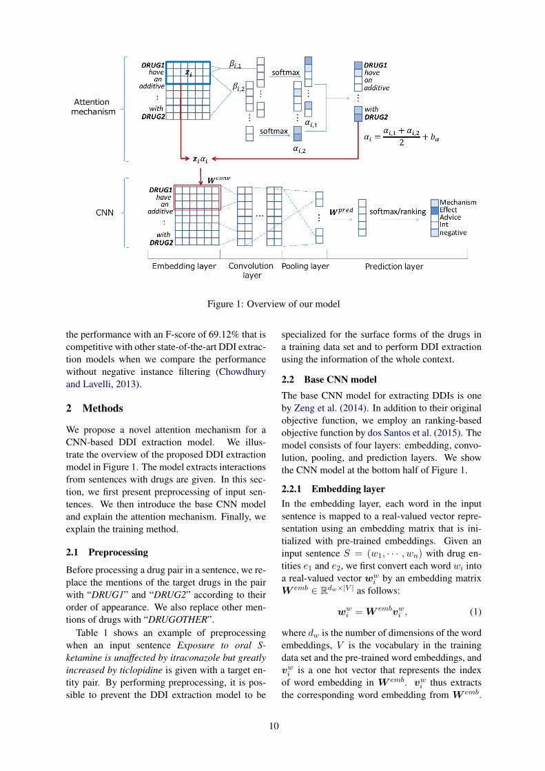
Figure 1: Overview of our model
the performance with an F-score of 69.12% that iscompetitive with other state-of-the-art DDI extrac-tion models when we compare the performancewithout negative instance filtering (Chowdhuryand Lavelli, 2013).
2 Methods
We propose a novel attention mechanism for aCNN-based DDI extraction model. We illus-trate the overview of the proposed DDI extractionmodel in Figure 1. The model extracts interactionsfrom sentences with drugs are given. In this sec-tion, we first present preprocessing of input sen-tences. We then introduce the base CNN modeland explain the attention mechanism. Finally, weexplain the training method.
2.1 Preprocessing
Before processing a drug pair in a sentence, we re-place the mentions of the target drugs in the pairwith “DRUG1” and “DRUG2” according to theirorder of appearance. We also replace other men-tions of drugs with “DRUGOTHER”.
Table 1 shows an example of preprocessingwhen an input sentence Exposure to oral S-ketamine is unaffected by itraconazole but greatlyincreased by ticlopidine is given with a target en-tity pair. By performing preprocessing, it is pos-sible to prevent the DDI extraction model to be
specialized for the surface forms of the drugs ina training data set and to perform DDI extractionusing the information of the whole context.
2.2 Base CNN modelThe base CNN model for extracting DDIs is oneby Zeng et al. (2014). In addition to their originalobjective function, we employ an ranking-basedobjective function by dos Santos et al. (2015). Themodel consists of four layers: embedding, convo-lution, pooling, and prediction layers. We showthe CNN model at the bottom half of Figure 1.
2.2.1 Embedding layerIn the embedding layer, each word in the inputsentence is mapped to a real-valued vector repre-sentation using an embedding matrix that is ini-tialized with pre-trained embeddings. Given aninput sentence S = (w1, · · · , wn) with drug en-tities e1 and e2, we first convert each word wi intoa real-valued vector ww
i by an embedding matrixW emb ∈ Rdw×|V | as follows:
wwi = W embvwi , (1)
where dw is the number of dimensions of the wordembeddings, V is the vocabulary in the trainingdata set and the pre-trained word embeddings, andvwi is a one hot vector that represents the indexof word embedding in W emb. vwi thus extractsthe corresponding word embedding from W emb.
10

Entity1 Entity2 Preprocessed input sentenceS-ketamine itraconazole Exposure to oral DRUG1 is unaffected by DRUG2 but greatly
increased by DRUGOTHER.S-ketamine ticlopidine Exposure to oral DRUG1 is unaffected by DRUGOTHER but
greatly increased by DRUG2.itraconazole ticlopidine Exposure to oral DRUGOTHER is unaffected by DRUG1 but
greatly increased by DRUG2.
Table 1: An example of preprocessing on the sentence “Exposure to oral S-ketamine is unaffected byitraconazole but greatly increased by ticlopidine” for each target pair.
The word embedding matrix W emb is fine-tunedduring training.
We also prepare dwp-dimensional word positionembeddings wp
i,1 and wpi,2 that correspond to the
relative positions from first and second target en-tities, respectively. We concatenate the word em-bedding ww
i and these word position embeddingswpi,1 and wp
i,2 as in the following Equation (2), andwe use the resulting vector as the input to the sub-sequent convolution layer:
wi = [wwi ; wp
i,1; wpi,2]. (2)
2.2.2 Convolution layerWe define a weight tensor for convolution asW conv
k ∈Rdc×(dw+2dwp)×k and we represent the j-th column of W conv
k as W convk,j ∈R(dw+2dwp)×k.
Here, dc denotes the number of filters for eachwindow size, k is a window size, and K is a setof the window sizes of the filters. We also intro-duce zi,k that is concatenated k word embeddings:
zi,k = [wTbi−(k−1)/2c; . . . ; w
Tbi−(k+1)/2c]
T. (3)
We apply the convolution to the embedding matrixas follows:
mi,j,k = f(W convk,j � zi,k + b), (4)
where � is an element-wise product, b is the biasterm, and f is the ReLU function defined as:
f(x) =
{x, if x > 00, otherwise.
(5)
2.2.3 Pooling layerWe employ the max pooling (Boureau et al., 2010)to convert the output of each filter in the convolu-tion layer into a fixed-size vector as follows:
ck = [c1,k, · · · , cdc,k], cj,k = maximi,j,k. (6)
We then obtain the dp-dimensional output of thispooling layer, where dp equals to dc×|K|, by con-catenating the obtained outputs ck for all the win-dow sizes k1, · · · , kK(∈ K):
c = [ck1 ; . . . ; cki; . . . ; ckK
]. (7)
2.2.4 Prediction layerWe predict the relation types using the output ofthe pooling layer. We first convert c into scoresusing a weight matrix W pred ∈ Ro×dp :
s = W predc, (8)
where o is the total number of relationships to beclassified and s = [s1, · · · , so]. We then employthe following two different objective functions forprediction.
Softmax We convert s into the probability ofpossible relations p by a softmax function:
p = [p1, · · · , po], pj =exp (sj)∑ol=1 exp (sl)
. (9)
The loss function Lsoftmax is defined as in theEquation (10) when the gold type distribution yis given. y is a one-hot vector where the proba-bility of the gold label is 1 and the others are 0.
Lsoftmax = −∑
y log p (10)
Ranking We employ the ranking-based objec-tive function following dos Santos et al. (2015).Using the scores s in the Equation (8), the loss iscalculated as follows:
Lranking = log(1 + exp(γ(m+ − sy))+ log(1 + exp(γ(m− + sc)), (11)
where m+ and m− are margins, γ is a scaling fac-tor, y is a gold label, and c ( 6= y) is a negative la-bel with the highest score in s. We set γ to 2, m+
to 2.5 and m− to 0.5 following dos Santos et al.(2015).
11

Figure 2: Workflow of DDI extraction
2.3 Attention mechanismOur attention mechanism is based on the input at-tention by Wang et al. (2016)1. The proposed at-tention mechanism is different from the base onein that we prepare separate attentions for enti-ties and we incorporate a bias term to adjust thesmoothness of attentions. We illustrate the atten-tion mechanism at the upper half of Figure 1.
We define the word index of the first and secondtarget drug entities in the sentence as e1 and e2,respectively. We also denote by E = {e1, e2} theset of indices and by j ∈ {1, 2} the index of theentities. We calculate our attentions using these:
βi,j = wej ·wi (12)
αi,j =
{exp (βi,j)∑
1≤l≤n,l/∈E exp (βl,j), if i /∈ E
adrug, otherwise(13)
αi =αi,1 + αi,2
2+ bα. (14)
Here, adrug is an attention parameter for entitiesand bα is the bias term. adrug and bα are tunedduring training. If we set E to empty and bα tozero, the attention will be the same as one by Wanget al. (2016). We incorporate the attentions αi intothe CNN model by replacing the Equation (4) withthe following equation:
mi,j,k = f(W convj � zi,kαi + b). (15)
2.4 Training methodWe use L2 regularization to avoid over-fitting.We use the following objective functions L′∗(L′softmax or L′ranking) by incorporating the L2regularization on weights to the Equation (10).
L′∗ = L∗ + λ(||W emb||2F + ||W conv||2F (16)
+||W pred||2F )1We do not incorporate the attention-based pooling in
Wang et al. (2016). We leave this for future work.
Here, λ is a regularization parameter and || · ||Fdenotes the Frobenius norm. We update all theparameters including the weights W emb, W conv,and W pred, biases b and bα, and the attention pa-rameter adrug to minimize L′∗. We use the adap-tive moment estimation (Adam) (Kingma and Ba,2015) for the optimizer. We randomly shuffletraining data set and divide them into mini-batchsamples in each epoch.
3 Experimental settings
We illustrate the workflow of the DDI extractionin Figure 2. As preprocessing, we performed wordsegmentation of the input sentences using the GE-NIA tagger (Tsuruoka et al., 2005). In this section,we explain the settings for the data sets, tasks, ini-tial embeddings, and hyper-parameter tuning.
3.1 Data set
We used the data set from the DDIExtraction-2013shared task (SemEval-2013 Task 9) (Segura Bed-mar et al., 2013; Herrero-Zazo et al., 2013) for theevaluation. This data set is composed of docu-ments annotated with drug mentions and their re-lationships. The data set consists of two parts:MEDLINE and DrugBank. MEDLINE consists ofabstracts in PubMed articles, and DrugBank con-sists of the descriptions of drug interactions in theDrugBank database. This data set annotates thefollowing four types of interactions.
• Mechanism: A sentence describes phar-macokinetic mechanisms of a DDI, e.g.,“Grepafloxacine may inhibit the metabolismof theobromine.”
• Effect: A sentence represents the effect of aDDI, e.g., “Methionine may protect againstthe ototoxic effects of gentamicin.”
12

Train TestDrugBank MEDLINE DrugBank MEDLINE
No. of documents 572 142 158 33No. of sentences 5,675 1,301 973 326No. of pairs 26,005 1,787 5,265 451No. of positive DDIs 3,789 232 884 95No. of negative DDIs 22,216 1,555 4,381 356No. of Mechanism pairs 1,257 62 278 24No. of Effect pairs 1,535 152 298 62No. of Advice pairs 818 8 214 7No. of Int pairs 179 10 94 2
Table 2: Statistics for the DDIExtraction-2013 shared task data set
Parameter ValueWord embedding size 200Word position embeddings size 20Convolutional window size [3, 4, 5]Convolutional filter size 100Initial learning rate 0.001Mini-batch size 100L2 regularization parameter 0.0001
Table 3: Hyperparamters
CountsSentences 1,404Pairs 4,998Mechanism pairs 232Effect pairs 339Advice pairs 132Int pairs 48
Table 4: Statistics of the development data set
• Advice: A sentence represents a recommen-dation or advice on the concomitant use oftwo drugs, e.g., “Alpha-blockers should notbe combined with uroxatral.”
• Int: A sentence simply represents the occur-rence of a DDI without any information aboutthe DDI, e.g., “The interaction of omeprazoleand ketoconazole has established.”
The statistics of the data set is shown in Table 2.As shown in this table, the number of pairs thathave no interaction (negative pairs) is larger thanthat of pairs that have interactions (positive pairs).
3.2 Task settingsWe followed the task setting of Task 9.2 in theDDIExtraction-2013 shared task (SemEval task
9). The task is to classify a given pair of drugsinto the four interaction types or no interaction.We evaluated the performance with precision (P),recall (R), and F-score (F) on each interaction typeas well as micro-averaged precision, recall, and F-score on all the interaction types. We used the of-ficial evaluation script provided by the task orga-nizers and report the averages of 10 runs. Pleasenote that we took averages of precision, recall andF-scores individually, so F-scores cannot be calcu-lated from precision and recall.
3.3 Initializing embeddingsSkip-gram (Mikolov et al., 2013) was employedfor the pre-training of word embeddings. We used2014 MEDLINE/PubMed baseline distribution,and the size of vocabulary was 1,630,978. The em-bedding of the drugs, i.e., “DRUG1”, “DRUG2”and “DRUGOTHER” are initialized with the pre-trained embedding of the word “drug”. The em-beddings of training words that did not appear inthe pre-trained embeddings, as well as the wordposition embeddings, are initialized with the ran-dom values drawn from a uniform distribution andnormalized to unit vectors. Words whose frequen-cies are one in the training data were replaced withan “UNK” word during training, and the embed-ding of words in the test data set that did not ap-pear in both training and pre-trained embeddingswere set to the embedding of the “UNK” word.
3.4 Hyperparameter tuningWe split the official training data set into two parts:training and development data sets. We tuned thehyper-parameters on the development data set onthe softmax model without attentions. Table 3shows the best hyperparameters on the softmaxmodel without attentions. We applied the same
13

Type P (%) R (%) F (%)Softmax without attention
Mechanism 76.24 (±4.48) 57.58 (±4.41) 65.31 (±1.76)Effect 67.84 (±3.56) 63.61 (±4.95) 65.39 (±1.38)Advice 82.26 (±7.04) 66.65 (±9.07) 72.75 (±2.72)Int 78.99 (±6.87) 33.55 (±2.62) 47.05 (±1.71)All (micro) 73.69 (±3.00) 59.92 (±3.73) 65.93 (±1.21)
Softmax with attentionMechanism 76.34 (±4.20) 64.43 (±5.72) 67.86 (±4.10)Effect 66.84 (±3.12) 65.98 (±2.63) 65.58 (±2.09)Advice 80.98 (±6.14) 70.83 (±2.72) 76.28 (±1.40)Int 73.21 (±6.30) 38.44 (±9.82) 46.11 (±3.96)All (micro) 73.74 (±1.88) 63.05 (±1.39) 67.94 (±0.70)
Ranking without attentionMechanism 78.41 (±3.99) 58.17 (±5.10) 66.51 (±2.61)Effect 68.16 (±3.30) 65.75 (±3.22) 66.80 (±1.46)Advice 84.49 (±3.55) 67.14 (±4.68) 74.61 (±1.82)Int 73.95 (±7.09) 33.43 (±1.18) 45.91 (±1.23)All (micro) 74.79 (±2.41) 60.99 (±2.65) 67.10 (±1.09)
Ranking with attentionMechanism 80.75 (±2.76) 61.09 (±3.03) 69.45 (±1.45)Effect 69.73 (±2.64) 66.63 (±2.93) 68.05 (±1.29)Advice 83.86 (±2.29) 71.81 (±2.61) 77.30 (±1.13)Int 74.20 (±8.95) 33.02 (±1.40) 45.50 (±1.51)All (micro) 76.30 (±2.18) 63.25 (±1.71) 69.12 (±0.71)
Table 5: Performance of softmax/ranking CNN models with and without our attention mechanism. Thehighest scores are shown in bold.
hyperparameters to the other models. The statis-tics of our development data set is shown in Ta-ble 4. We set the sizes of the convolution windowsto [3, 4, 5] that are the same as in Kim (2014). Wechose the word position embedding size from {10,20, 30, 40, 50}, the convolutional filter size from{10, 50, 100, 200}, the learning rate of Adam from{0.01, 0.001, 0.0001}, the mini-batch size from{10, 20, 50, 100, 200}, and the L2 regularizationparameter λ from {0.01, 0.001, 0.0001, 0.00001}.
4 Results
In this section, we first summarize the perfor-mance of the proposed models and compare theperformance with existing models. We then com-pare attention mechanisms and finally illustratesome results for the analysis of the attentions.
4.1 Performance analysis
The performance of the base CNN models withtwo objective functions, as well as with or with-out the proposed attention mechanism, is summa-
rized in Table 5. The incorporation of the atten-tion mechanism improved the F-scores by about2 percent points (pp) on models with both ob-jective functions. Both improvements were sta-tistically significant (p < 0.01) with t-test. Thisshows that the attention mechanism is effectivefor both models. The improvement of F-scoresfrom the least performing model (softmax objec-tive function without our attention mechanism)to the best performing model (ranking objectivefunction with our attention mechanism) is 3.19 pp(69.12% versus 65.93%), and this shows both ob-jective function and attention mechanism are keyto improve the performance. When looking intothe individual types, ranking function with our at-tention mechanism archived the best F-scores onMechanism, Effect, Advice, while the base CNNmodel achieved the best F-score on Int.
4.2 Comparison with existing models
We show comparison with the existing state-of-the-art models in Table 6. We mainly compare
14

Methods P (%) R (%) F (%)No negative instance filtering
CNN (Liu et al., 2016) 75.29 60.37 67.01MCCNN (Quan et al., 2016) - - 67.80SCNN (Zhao et al., 2016) 68.5 61.0 64.5Joint AB-LSTM (Sahu and Anand, 2017) 71.82 66.90 69.27Proposed model 76.30 63.25 69.12
With negative instance filteringFBK-irst (Chowdhury and Lavelli, 2013) 64.6 65.6 65.1Kim et al. (2015) - - 67.0CNN (Liu et al., 2016) 75.72 64.66 69.75MCCNN (Quan et al., 2016) 75.99 65.25 70.21SCNN (Zhao et al., 2016) 72.5 65.1 68.6Joint AB-LSTM (Sahu and Anand, 2017) 73.41 69.66 71.48
Table 6: Comparison with existing models
P (%) R (%) F (%)No attention 74.79 (±2.41) 60.99 (±2.65) 67.10 (±1.09)Input attention by Wang et al. (2016) 73.48 (±1.96) 59.58 (±1.51) 65.77 (±0.80)Our attention 76.30 (±2.66) 63.25 (±2.59) 69.12 (±0.71)Our attention without separate attentions adrug 74.03 (±2.11) 63.30 (±2.41) 68.17 (±0.71)Our attention without the bias term bα 71.56 (±2.18) 64.19 (±2.21) 67.62 (±0.96)
Table 7: Comparison of attention mechanisms on CNN models with ranking objective function
the performance without negative instance filter-ing, which omits some apparent negative instancepairs with rules (Chowdhury and Lavelli, 2013),since we did not incorporate it. We also show theperformance of the existing models with negativeinstance filtering for reference.
In the comparison without negative instance fil-tering, our model outperformed the existing CNNmodels (Liu et al., 2016; Quan et al., 2016; Zhaoet al., 2016). The model was competitive withJoint AB-LSTM model (Sahu and Anand, 2017)that was composed of multiple RNN models.
When considering negative instance filtering,our model showed lower performance than thestate-of-the-art. However we believe we can getsimilar performance with theirs if we incorporatenegative instance filtering. Still, the model outper-formed several models such as Kim et al. (2015),Chowdhury and Lavelli (2013) and SCNN modeleven if we consider negative instance filtering.
4.3 Comparison of attention mechanisms
We compare the proposed attention mechanismwith the input attention of Wang et al. (2016) toshow the effectiveness of our attention mecha-nism. Table 7 shows the comparison of the atten-
tion mechanisms. We also show the base CNN-based model with ranking loss for reference, andthe results of ablation tests. As is shown in the ta-ble, the attention mechanism by Wang et al. (2016)did not work in DDI extraction. However, ourattention improved the performance. This resultshows that the proposed extensions are crucial formodeling attentions in DDI extraction. The abla-tion test results show that both extensions to ourattention mechanism, i.e., separate attentions forentities and incorporation of the bias term, are ef-fective for the task.
4.4 Visual analysis
Figure 3 shows visualization of attentions onsome sentences with DDI pairs using our atten-tion mechanism. In the first sentence, “DRUG1”and “DRUG2” have a Mechanism interaction. Theattention mechanism successfully highlights thekeyword “concentration”. In the second sentence,which have an Effect interaction, the attentionmechanism put high weights on “increase” and“effects”. The word “necessary” has a high weighton the third sentence with an Advice interaction.For an Int interaction in the last sentence, the word“interaction” is most highlighted.
15

Figure 3: Visualization of attention
5 Related work
Various feature-based methods have been pro-posed during and after the DDIExtraction-2013shared task (Segura Bedmar et al., 2013). Bjorneet al. (2013) tackled with DDI extraction usingTurku Event Extraction System (TEES), which isan event extraction system based on the SupportVector Machines (SVMs). Thomas et al. (2013)and Chowdhury and Lavelli (2013) proposed two-phase processing models that first detected DDIsand then classified the extracted DDIs into one ofthe four proposed types. Thomas et al. (2013) usedthe ensembles of several kernel methods, whileChowdhury and Lavelli (2013) proposed hybridkernel-based approach with negative instance fil-tering. The negative instance filtering is employedby all the subsequent models except for ours. Kimet al. (2015) proposed a two-phase SVM-basedapproach that employed a linear SVM with richfeatures including word features, word pairs, de-pendency relations, parse tree structures, and nounphrase-based constraint features. Our model doesnot use features and instead employs CNNs.
Deep learning-based models recently domi-nated the DDI extraction task. Among these,CNN-based models have been often employed andRNNs has received less attention. Liu et al. (2016)built a CNN-based model on word embedding andword position embeddings. Zhao et al. (2016) pro-posed Syntax CNN (SCNN) that employs syntaxword embeddings with the syntactic informationof a sentence as well as features of POS tags anddependency trees. Liu et al. (2016) tackled DDIextraction using Multi-Channel CNN (MCCNN)that enables the fusion of multiple word embed-dings. Our work is different from theirs in that weemployed an attention mechanism.
As for RNN-based approach, Sahu and Anand(2017) proposed an RNN-based model namedJoint AB-LSTM (Long Short-Term Memory).
Joint AB-LSTM is composed of the concatenationof two RNN-based models: bidirectional LSTM(Bi-LSTM) and attentive pooling Bi-LSTM. Themodel showed the state-of-the-art performance onthe DDIExtraction-2013 shared task data set. Ourmodel is a single model with a CNN and attentionmechanism, and it performed comparable to theirsas shown in Table 6.
Wang et al. (2016) proposed muli-level atten-tion CNNs and applied it to a general domain rela-tion classification task SemEval 2010 Task 8 (Hen-drickx et al., 2009). Their attention mechanismimproved the macro F1 score by 1.9pp (from86.1% to 88.0%), and their model achieved thestate-of-the-art performance on the task.
6 Conclusions
In this paper, we proposed a novel attention mech-anism for the extraction of DDIs. We built baseCNN-based DDI extraction models with two dif-ferent objective functions, softmax and ranking,and we incorporated the attention mechanism intothe models. We evaluated the performance on theTask 9.2 of the DDIExtraction-2013 shared task,and we showed that both attention mechanism andranking-based objective function are effective forthe extraction of DDIs. Our final model achievedan F-score of 69.12% that is competitive with thestate-of-the-art model when we compared the per-formance without negative instance filtering.
As future work, we would like to incorporate anattention mechanism in the pooling layer (Wanget al., 2016) and adopt negative instance filter-ing (Chowdhury and Lavelli, 2013) for the fur-ther performance improvement and fair compari-son with the state-of-the-art methods.
Acknowledgments
This work was supported by JSPS KAKENHIGrant Number 17K12741.
16

ReferencesJari Bjorne, Suwisa Kaewphan, and Tapio Salakoski.
2013. UTurku: drug named entity recognition anddrug-drug interaction extraction using SVM classifi-cation and domain knowledge. In Second Joint Con-ference on Lexical and Computational Semantics (*SEM). volume 2, pages 651–659.
Y-Lan Boureau, Jean Ponce, and Yann LeCun. 2010.A theoretical analysis of feature pooling in visualrecognition. In Proceedings of the 27th interna-tional conference on machine learning (ICML-10).pages 111–118.
Md Faisal Mahbub Chowdhury and Alberto Lavelli.2013. FBK-irst: A multi-phase kernel based ap-proach for drug-drug interaction detection and clas-sification that exploits linguistic information. At-lanta, Georgia, USA 351:53.
Cicero Nogueira dos Santos, Bing Xiang, and BowenZhou. 2015. Classifying relations by ranking withconvolutional neural networks. In Proceedings ofthe 53rd Annual Meeting of the Association forComputational Linguistics. Association for Compu-tational Linguistics. volume 1, pages 626–634.
Iris Hendrickx, Su Nam Kim, Zornitsa Kozareva,Preslav Nakov, Diarmuid O Seaghdha, SebastianPado, Marco Pennacchiotti, Lorenza Romano, andStan Szpakowicz. 2009. SemEval-2010 Task 8:Multi-way classification of semantic relations be-tween pairs of nominals. In Proceedings ofthe Workshop on Semantic Evaluations: RecentAchievements and Future Directions. Associationfor Computational Linguistics, pages 94–99.
Marıa Herrero-Zazo, Isabel Segura-Bedmar, PalomaMartınez, and Thierry Declerck. 2013. The DDIcorpus: An annotated corpus with pharmacologicalsubstances and drug–drug interactions. Journal ofbiomedical informatics 46(5):914–920.
Sun Kim, Haibin Liu, Lana Yeganova, and W JohnWilbur. 2015. Extracting drug–drug interactionsfrom literature using a rich feature-based linear ker-nel approach. Journal of biomedical informatics55:23–30.
Yoon Kim. 2014. Convolutional neural networks forsentence classification. In Proceedings of the 2014Conference on Empirical Methods in Natural Lan-guage Processing, EMNLP 2014, October 25-29,2014, Doha, Qatar, A meeting of SIGDAT, a SpecialInterest Group of the ACL. pages 1746–1751.
Diederik Kingma and Jimmy Ba. 2015. Adam: Amethod for stochastic optimization. In The Inter-national Conference on Learning Representations(ICLR), San Diego, 2015.
Vivian Law, Craig Knox, Yannick Djoumbou, TimJewison, An Chi Guo, Yifeng Liu, Adam Ma-ciejewski, David Arndt, Michael Wilson, VanessaNeveu, et al. 2014. DrugBank 4.0: shedding new
light on drug metabolism. Nucleic acids research42(D1):D1091–D1097.
Shengyu Liu, Buzhou Tang, Qingcai Chen, and Xiao-long Wang. 2016. Drug-drug interaction extractionvia convolutional neural networks. Computationaland mathematical methods in medicine 2016.
Tomas Mikolov, Ilya Sutskever, Kai Chen, Greg S Cor-rado, and Jeff Dean. 2013. Distributed representa-tions of words and phrases and their compositional-ity. In Advances in neural information processingsystems. pages 3111–3119.
Chanqin Quan, Lei Hua, Xiao Sun, and Wenjun Bai.2016. Multichannel convolutional neural networkfor biological relation extraction. BioMed ResearchInternational 2016.
Sunil Kumar Sahu and Ashish Anand. 2017. Drug-drug interaction extraction from biomedical text us-ing long short term memory network. arXiv preprintarXiv:1701.08303 .
Isabel Segura Bedmar, Paloma Martınez, and MarıaHerrero Zazo. 2013. SemEval-2013 Task 9: Extrac-tion of drug-drug interactions from biomedical texts(DDIExtraction 2013). In Proceedings of the 7th In-ternational Workshop on Semantic Evaluations. As-sociation for Computational Linguistics, pages 341–350.
Philippe Thomas, Mariana Neves, Tim Rocktaschel,and Ulf Leser. 2013. WBI-DDI: drug-drug inter-action extraction using majority voting. In SecondJoint Conference on Lexical and Computational Se-mantics (* SEM). volume 2, pages 628–635.
Caroline F Thorn, Teri E Klein, and Russ B Altman.2013. PharmGKB: the pharmacogenomics knowl-edge base. Pharmacogenomics: Methods and Pro-tocols pages 311–320.
Yoshimasa Tsuruoka, Yuka Tateishi, Jin-Dong Kim,Tomoko Ohta, John McNaught, Sophia Ananiadou,and Junichi Tsujii. 2005. Developing a robust part-of-speech tagger for biomedical text. In PanhellenicConference on Informatics. Springer, pages 382–392.
Linlin Wang, Zhu Cao, Gerard de Melo, and ZhiyuanLiu. 2016. Relation classification via multi-level at-tention CNNs. In Proceedings of the 54th AnnualMeeting of the Association for Computational Lin-guistics. Association for Computational Linguistics.pages 1298–1307.
Hong Yang, Chu Qin, Ying Hong Li, Lin Tao, Jin Zhou,Chun Yan Yu, Feng Xu, Zhe Chen, Feng Zhu, andYu Zong Chen. 2016. Therapeutic target databaseupdate 2016: enriched resource for bench to clinicaldrug target and targeted pathway information. Nu-cleic acids research 44(D1):D1069–D1074.
17

Daojian Zeng, Kang Liu, Siwei Lai, Guangyou Zhou,Jun Zhao, et al. 2014. Relation classification viaconvolutional deep neural network. In COLING.pages 2335–2344.
Zhehuan Zhao, Zhihao Yang, Ling Luo, HongfeiLin, and Jian Wang. 2016. Drug drug interac-tion extraction from biomedical literature using syn-tax convolutional neural network. Bioinformatics32(22):3444–3453.
18
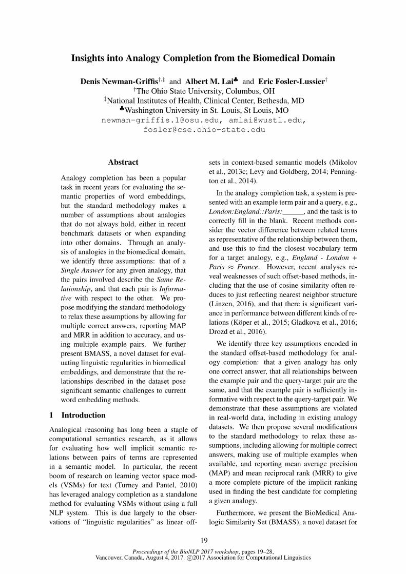
Proceedings of the BioNLP 2017 workshop, pages 19–28,Vancouver, Canada, August 4, 2017. c©2017 Association for Computational Linguistics
Insights into Analogy Completion from the Biomedical Domain
Denis Newman-Griffis†,‡ and Albert M. Lai♣ and Eric Fosler-Lussier††The Ohio State University, Columbus, OH
‡National Institutes of Health, Clinical Center, Bethesda, MD♣Washington University in St. Louis, St Louis, MO
[email protected], [email protected],[email protected]
Abstract
Analogy completion has been a populartask in recent years for evaluating the se-mantic properties of word embeddings,but the standard methodology makes anumber of assumptions about analogiesthat do not always hold, either in recentbenchmark datasets or when expandinginto other domains. Through an analy-sis of analogies in the biomedical domain,we identify three assumptions: that of aSingle Answer for any given analogy, thatthe pairs involved describe the Same Re-lationship, and that each pair is Informa-tive with respect to the other. We pro-pose modifying the standard methodologyto relax these assumptions by allowing formultiple correct answers, reporting MAPand MRR in addition to accuracy, and us-ing multiple example pairs. We furtherpresent BMASS, a novel dataset for eval-uating linguistic regularities in biomedicalembeddings, and demonstrate that the re-lationships described in the dataset posesignificant semantic challenges to currentword embedding methods.
1 Introduction
Analogical reasoning has long been a staple ofcomputational semantics research, as it allowsfor evaluating how well implicit semantic re-lations between pairs of terms are representedin a semantic model. In particular, the recentboom of research on learning vector space mod-els (VSMs) for text (Turney and Pantel, 2010)has leveraged analogy completion as a standalonemethod for evaluating VSMs without using a fullNLP system. This is due largely to the obser-vations of “linguistic regularities” as linear off-
sets in context-based semantic models (Mikolovet al., 2013c; Levy and Goldberg, 2014; Penning-ton et al., 2014).
In the analogy completion task, a system is pre-sented with an example term pair and a query, e.g.,London:England::Paris: , and the task is tocorrectly fill in the blank. Recent methods con-sider the vector difference between related termsas representative of the relationship between them,and use this to find the closest vocabulary termfor a target analogy, e.g., England - London +Paris ≈ France. However, recent analyses re-veal weaknesses of such offset-based methods, in-cluding that the use of cosine similarity often re-duces to just reflecting nearest neighbor structure(Linzen, 2016), and that there is significant vari-ance in performance between different kinds of re-lations (Koper et al., 2015; Gladkova et al., 2016;Drozd et al., 2016).
We identify three key assumptions encoded inthe standard offset-based methodology for anal-ogy completion: that a given analogy has onlyone correct answer, that all relationships betweenthe example pair and the query-target pair are thesame, and that the example pair is sufficiently in-formative with respect to the query-target pair. Wedemonstrate that these assumptions are violatedin real-world data, including in existing analogydatasets. We then propose several modificationsto the standard methodology to relax these as-sumptions, including allowing for multiple correctanswers, making use of multiple examples whenavailable, and reporting mean average precision(MAP) and mean reciprocal rank (MRR) to givea more complete picture of the implicit rankingused in finding the best candidate for completinga given analogy.
Furthermore, we present the BioMedical Ana-logic Similarity Set (BMASS), a novel dataset for
19

analogical reasoning in the biomedical domain.This new resource presents real-world examplesof semantic relations of interest for biomedi-cal natural language processing research, and wehope it will support further research into biomed-ical VSMs (Chiu et al., 2016; Choi et al., 2016).1
2 Related work
Analogical reasoning has been studied both on itsown and as a component of downstream tasks,using a range of systems. Early work usedrule-based systems for world knowledge (Reit-man, 1965) and syntactic (Federici and Pirelli,1997) relationships. Supervised models wereused for SAT (Scholastic Aptitude Test) analo-gies (Veale, 2004), and later for synonymy,antonymy, and some world knowledge (Turney,2008; Herdagdelen and Baroni, 2009). Analog-ical reasoning has also been used in support ofdownstream tasks, including word sense disam-biguation (Federici et al., 1997) and morphologi-cal analysis (Lepage and Goh, 2009; Lavallee andLanglais, 2010; Soricut and Och, 2015).
Recent work on analogies has largely focusedon their use as an intrinsic evaluation of the prop-erties of a VSM. The analogy dataset of Mikolovet al. (2013a), often referred to as the Googledataset, has become a standard evaluation forgeneral-domain word embedding models (Pen-nington et al., 2014; Levy and Goldberg, 2014;Schnabel et al., 2015; Faruqui et al., 2015), andincludes both world knowledge and morphosyn-tactic relations. Other datasets include the MSRanalogies (Mikolov et al., 2013c), which describemorphological relations only; and BATS (Glad-kova et al., 2016), which includes both morpho-logical and semantic relations. The semantic rela-tions from SemEval-2012 Task 2 (Jurgens et al.,2012) have also been used to derive analogies;however, as with the lexical Sem-Para datasetof Koper et al. (2015), the semantic relation-ships tend to be significantly more challenging forembedding-based methods (Drozd et al., 2016).Additionally, Levy et al. (2015b) demonstrate thateven for some lexical relations where embeddingsappear to perform well, they are actually learningprototypicality as opposed to relatedness.
1The dataset, and all code used forour experiments, is available online athttps://github.com/OSU-slatelab/BMASS.
3 Analogy completion task
3.1 Standard methodology
Given an analogy a:b::c:d, the evaluation task isto guess d out of the vocabulary, given a, b, c asevidence. Recent methods for this involve usingthe vector difference between embedded represen-tations of the related pairs to rank all terms in thevocabulary by how well they complete the anal-ogy, and choosing the best fit. The vector differ-ence is most commonly used in one of three ways,where cos is cosine similarity:
argmaxd∈V(cos(d, b− a+ c)
)(1)
argmaxd∈V(cos(d− c, b− a)) (2)
argmaxd∈Vcos(d, b)cos(d, c)cos(d, a) + ε
(3)
Following the terminology of Levy and Goldberg(2014), we refer to Equation 1 as 3COSADD,Equation 2 as PAIRWISEDISTANCE, and Equa-tion 3 (which is equivalent to 3COSADD with logcosine similarities) as 3COSMUL.
In order to generate analogy data for this task,recent datasets have followed a similar process(Mikolov et al., 2013a,c; Koper et al., 2015; Glad-kova et al., 2016). First, relations of interest weremanually selected for the target domains: syntac-tic/morphological, lexical (e.g., hypernymy, syn-onymy), or semantic (e.g., CapitalOf). Then, foreach relation, example word pairs were manuallyselected or automatically generated from existingresources (e.g., WordNet). The final analogieswere then generated by exhaustively combiningthe sets of word pairs within each relation.
3.2 Assumptions
Several key assumptions are inherent in this stan-dard methodology that are not reflected in recentbenchmark analogy datasets. The first we referto as the Single-Target assumption: namely, thatthere is a single correct answer for any given anal-ogy. Since the target d is chosen via argmax, if weconsider the following two analogies:
flu:nausea::fever:?coughflu:nausea::fever:?light-headedness
we must necessarily get at least one answerwrong. Gladkova et al. (2016) convert theseanalogies into a single case:
flu:nausea::fever:?[cough, light-headedness]
20

Pair Relations
brother:sisterFemaleCounterpart
SiblingOf
husband:wifeFemaleCounterpart
MarriedTo
Table 1: Binary semantic relations in “brother is tosister as husband is to wife.” The target commonrelation is shown in bold.
where either cough or lightheadedness is a cor-rect guess. However, this still misses our desireto get both correct answers, if possible. Relationswith multiple correct targets are present in all ofGoogle, BATS, and Sem-Para.
The second key assumption is that all the infor-mation relating a to b also relates c to d. While thepairs are chosen based on a single common rela-tionship, each pair may actually pertain to multi-ple relationships. An example from the Googledataset is brother:sister::husband:wife; Table 1shows the semantic relations involved in this anal-ogy. While the target relation FemaleCounterpartis present in both pairs, by comparing the offsetssister − brother and wife − husband, we as-sume that either all ways in which each pair isrelated are present in both, or that FemaleCoun-terpart dominates the offset. We refer to this asthe Same-Relationship assumption.
Finally, it is not sufficient for two pairs toshare a common relationship label; that relation-ship must be both representative and informa-tive for analogies to make sense (the Informa-tivity assumption). Relation labels may be suf-ficiently broad as to be meaningless, as we en-countered when drawing unfiltered binary rela-tions from the Unified Medical Language Sys-tem (UMLS) Metathesaurus. One sample analogyfrom the RO:Null relation (indicating “related insome way”) was socks:stockings::Finns:Finnishlanguage. While both pairs are of related terms,they are in no way related to one another.
Furthermore, even when two pairs are exam-ples of the same kind of clearly-defined relation,they may still be relatively uninformative. For ex-ample, in the Sem-Para Meronym analogy apri-cot:stone::trumpet:mouthpiece the meronymic re-lationship between apricot and stone could plau-sibly identify a number of parts of a trumpet:mouthpiece, valves, slide, etc.2 The extremely
2While this is similar to the Single-Target assumption, it
high-level nature of several of the Sem-Para re-lations (hypernymy, antonymy, and synonymy)suggests that some of the difficulty observed byKoper et al. (2015) is due to violations of Infor-mativity.
4 BMASS
We present BMASS (the BioMedical AnalogicSimilarity Set), a dataset of biomedical analogies,generated using the expert-curated knowledge inthe Unified Medical Language System (UMLS)3
(Bodenreider, 2004) in order to identify medicalterm pairs sharing the same relationships. We fol-lowed the standard process for dataset generationoutlined in Section 3.1, with some adjustments forthe assumptions in Section 3.2.
The UMLS Metathesaurus is centered aroundnormalized concepts, represented by ConceptUnique Identifiers (CUIs). Each concept can berepresented in textual form by one or more terms(e.g., C0009443→ “Common cold”, “acute rhini-tis”). These terms may be multi-word expressions(MWEs); in fact, many concepts in the UMLShave no unigram terms.
The Metathesaurus also contains 〈subject, re-lation, object〉 triples describing binary relation-ships between concepts. These relationships arespecified at two levels: relationship types (RELs),such as broader-than and qualified-by, and spe-cific relationships (RELAs) within each type, e.g.,tradename-of and has-finding-site. For this work,we used the 721 unique REL/RELA pairings asour source relationships, and treated the 〈subject,object〉 pairs linked within each of these relation-ships as candidates for generating analogies.
To enable a word embedding–based evaluation,we first identified terms that appeared at least 25times in the 2016 PubMed baseline collection ofbiomedical abstracts,4 and removed all 〈subject,object〉 pairs involving concepts that did not corre-spond to these frequent terms. Most relationshipsin the Metathesaurus are many-to-many (i.e., eachsubject can be paired with multiple objects and
bears separate consideration in that Single-Target refers tomultiple valid objects of a specific relationship, while this isan issue of multiple valid relationships being described.
3We use the 2016AA release of the UMLS.4We chose 25 as our minimum frequency to ensure that
each term appeared often enough to learn reasonable embed-dings for its component words. To determine term frequency,we first lowercased and stripped punctuation from both thePubMed corpus and the term list extracted from UMLS, thensearched the corpus for exact term matches.
21

vice versa), and thus may challenge Single-Targetand Informativity assumptions; we therefore nextidentified relations that had at least 50 1:1 in-stances, i.e., a subject and object that are onlypaired with one another within a specific relation-ship. Since 1:1 instances are not sufficient to guar-antee Informativity, we then manually reviewedthe remaining relations to identify those those thatwe deemed to satisfy Informativity constraints.For example, the is-a relationship between tonguemuscles and head muscle is not specific enough tosuggest that carbon monoxide should elicit gaso-transmitters as its corresponding answer. How-ever, for associated-with, sampled pairs such asleg injuries : leg and histamine release : histaminewere sufficiently consistent that we deemed it In-formative. This gave us a final set of 25 binaryrelations, listed in Table 2.5
We follow Gladkova et al. (2016) in generatinga balanced dataset, to enable a more robust com-parative analysis between relations. We randomlysampled 50 〈subject, object〉 pairs from each re-lation, again restricting to concepts with stringsappearing frequently in PubMed. For each sub-ject concept that we sampled, we collected allvalid object concepts and bundled them as a sin-gle 〈subject, objects〉 pair. We then exhaustivelycombined each concept pair with the others in itsrelation to create 2,450 analogies, giving us a to-tal dataset size of 61,250 analogies. Finally, foreach concept, we chose a single frequent term torepresent it, giving us both CUI and string repre-sentations of each analogy.
5 Evaluation
We assess how well biomedical word embeddingscan perform on our dataset, and explore modi-fications to the standard evaluation methodologyto relax the assumptions described in Section 3.2.We use the skip-gram embeddings trained by Chiuet al. (2016) on the PubMed citation database,one set using a window size of 2 (PM-2) and an-other set with window size 30 (PM-30). All otherword2vec hyperparameters were tuned by Chiu etal. on a combination of similarity and relatednessand named entity recognition tasks.
Additionally, we use the hyperparameters theyidentified (minimum frequency=5, vector dimen-sion=200, negative samples=10, sample=1e-4,
5Examples of each relation, along with their mappings toUMLS REL/RELA values, are available online.
ID Name AmbLab/RxL1 form-of 1.0L2 has-lab-number 1.1L3 has-tradename 1.5L4 tradename-of 1.3L5 associated-substance 1.6L6 has-free-acid-or-base-form 1.0L7 has-salt-form 1.1L8 measured-component-of 1.3HierarchicalH1 refers-to 1.0H2 same-type 10.4MorphologicalM1 adjectival-form-of 1.1M2 noun-form-of 1.0ClinicalC1 associated-with-malfunction-of-
gene-product2.6
C2 gene-product-malfunction-associated-with-disease
1.5
C3 causative-agent-of 4.6C4 has-causative-agent 2.0C5 has-finding-site 1.9C6 associated-with 1.2AnatomyA1 anatomic-structure-is-part-of 1.6A2 anatomic-structure-has-part 5.4A3 is-located-in 1.4BiologyB1 regulated-by 1.0B2 regulates 1.0B3 gene-encodes-product 1.1B4 gene-product-encoded-by 2.4
Table 2: List of the relations kept after manualfiltering; Amb is the average ambiguity, i.e., theaverage number of correct answers per analogy.
α=0.05, window size=2) to train our own embed-dings on a subset of the 2016 PubMed Baseline(14.7 million documents, 2.7 billion tokens). Wetrain word2vec (Mikolov et al., 2013a) sampleswith the continuous bag-of-words (CBOW) andskip-gram (SGNS) models, trained for 10 itera-tions, and GloVe (Pennington et al., 2014) sam-ples, trained for 50 iterations.
We performed our evaluation with each of3COSADD, PAIRWISEDISTANCE, and 3COS-MUL as the scoring function over the vocabulary.In contrast to the prior findings of Levy and Gold-
22

berg (2014) on the Google dataset, performanceon BMASS is roughly equivalent among the threemethods, often differing by only one or two cor-rect answers. We therefore only report results with3COSADD, since it is the most familiar method.
5.1 Modifications to the standard method
We consider 3COSADD under three settings ofthe analogies in our dataset. For a given analogya:b::c:?d, we refer to 〈a, b〉 as the exemplar pairand 〈c, d〉 as the query pair; ?d signifies the targetanswer.
Single-Answer puts analogies in a:b::c:d for-mat, with a single example object b and a singlecorrect object d, by taking the first object listed foreach term pair. This enforces the Single-Answerassumption.
Multi-Answer takes the first object listed forthe exemplar term pair, but keeps all valid an-swers, i.e. a:b::c:[d1,d2,. . . ]; this is similar tothe approach of Gladkova et al. (2016). There areapproximately 16k analogies in our dataset withmultiple valid answers.
All-Info keeps all valid objects for both the ex-emplar and query pairs. The exemplar offset isthen calculated over B = [b1, b2, . . . ] as
a−B =1|B|
∑i
a− bi
Though this is superficially similar to 3COSAVG
(Drozd et al., 2016), we average over objects for aspecific subject, as opposed to averaging over allsubject-object pairs.
We report a relaxed accuracy (denoted AccR),in which the guess is correct if it is in the set ofcorrect answers. (In the Single-Answer case, thisreduces to standard accuracy.) AccR, as with stan-dard accuracy, necessitates ignoring a, b, or c ifthey are the top results (Linzen, 2016).
In order to capture information about all cor-rect answers, we also report Mean Average Pre-cision (MAP) and Mean Reciprocal Rank (MRR)over the set of correct answers in the vocabulary,as ranked by Equation 1. Since MAP and MRR donot have a cutoff in terms of searching for the cor-rect answer in the ranked vocabulary, they can beused without the adjustment of ignoring a, b, andc; thus, they can give a more accurate picture ofhow close the correct terms are to the calculatedguesses.
5.2 MWEs and candidate answersAs noted in Section 4, the terms in our analogydataset may be multi-word expressions (MWEs).We follow the common baseline approach of rep-resenting an MWE as the average of its compo-nent words (Mikolov et al., 2013b; Chen et al.,2013; Wieting et al., 2016). For phrasal termscontaining one or more words that are out of ourembedding vocabulary, we only consider the in-vocabulary words: thus, if “parathyroid” is not inthe vocabulary, then the embedding of parathyroidhypertensive factor will be
hypertensive+ factor
2For any individual analogy a:b::c:?d, the vo-
cabulary of candidate phrases to complete theanalogy is derived by calculating averaged wordembeddings for each UMLS term appearing inPubMed abstracts at least 25 times. Terms forwhich none of the component words are in vocab-ulary are discarded. This yields a candidate setof 229,898 phrases for the PM-2 and PM-30, and263,316 for our CBOW, SGNS, and GloVe sam-ples.
Since prior work on analogies has primarilybeen concerned with unigram data, we also iden-tified a subset of our data for which we couldfind single-word string realizations for all con-cepts in an analogy, using the full vocabulary ofour trained embeddings. Even in the All-Info set-ting, we could only identify 606 such analogies;Table 3 shows MAP results for PM-2 and CBOWembeddings on the three relations with at least100 unigram analogies. The unigram analogiesare slightly better captured than the full MWEdata for has-lab-number (L2) and has-tradename(L3); however, lower performance on the unigramsubset in tradename-of (L4) shows that unigramanalogies are not always easier. We see a smalleffect from the much larger set of candidate an-swers in the unigram case (>1m unigrams), asshown by the slightly higher MAP numbers in theUniM case. In general, it is clear that the difficultyof some of the relations in our dataset is not duesolely to using MWEs in the analogies.
5.3 Metric comparisonFigure 1 shows AccR, MAP, and MRR resultsfor each relation in BMASS, using PM-2 embed-dings in the Multi-Answer setting. Overall, per-formance varies widely between relations, with all
23

Figure 1: AccR, MAP, and MRR for each relation, using PM-2 embeddings under the Multi-Answersetting. Note that MAP is calculated using the position of all correct answers in the ranked list, whileMRR reflects only the position of the first correct answer found in the ranked list for each individualquery.
Figure 2: AccR per relation for PM-2 on BMASS, under Single-Answer, Multi-Answer, and All-Infosettings.
Figure 3: Per-relation MAP for all embeddings under the Multi-Answer setting.
three metrics staying under 0.1 in the majority ofcases; this mirrors previous findings on other anal-ogy datasets (Levy and Goldberg, 2014; Gladkovaet al., 2016; Drozd et al., 2016).
MAP further fleshes out these differences by re-porting performance over all correct answers for agiven analogy. This lets us distinguish between re-lations like has-salt-form (L7), where noticeablylower MAP numbers reflect a wider distributionof the multiple correct answers, and relations likeregulates (B2) or associated-with (C6), where alow AccR reflects many incorrect answers, but ahigher MAP indicates that the correct answers arerelatively near the guess.
MRR, on the other hand, more optimisticallyreports how close we got to finding any correctanswer. Thus, for the has-causative-agent (C4) re-lation, low AccR is belied by a noticeably higherMRR, suggesting that even when we guess wrong,the correct answer is close. This contrasts withrelations like refers-to (H1) or causative-agent-of (C3), where MRR is more consistent withAccR, indicating that wrong guesses tend to befarther from the truth. Since most of our analo-gies (45,178 samples, or about 74%) have only asingle correct answer, MAP and MRR tend to behighly similar. However, in high-ambiguity rela-tions like same-type (H2), higher MRR numbers
24

give a better sense of our best case performance.
5.4 Analogy settings
To compare across the Single-Answer, Multi-Answer, and All-Info settings, we first look atAccR for each relation in BMASS, shown for PM-2 embeddings in Figure 2 (the observed patternsare similar with the other embeddings). Unsur-prisingly, allowing for multiple answers in Multi-Answer and All-Info slightly raises AccR in mostcases. What is surprising, however, is that includ-ing more sample exemplar objects in the All-Infosetting had widely varying results. In some cases,such as same-type (H2), associated-substance(L5), and gene-product-encoded-by (B4), the ad-ditional exemplars gave a noticeable improvementin accuracy. In others, accuracy actually wentdown: form-of (L1) and has-free-acid-or-base-form (L6) are the most striking examples, withabsolute decreases of 4% and 8% respectivelyfrom the Multi-Answer case for PM-2 (the de-creases are similar with other embeddings). Thus,it seems that multiple examples may help with In-formativity in some cases, but confuse it in oth-ers. Taken together with the improvements seenin Drozd et al. (2016) from using 3COSAVG, thisis another indication that any single subject-objectpair may not be sufficiently representative of thetarget relationship.
5.5 Embedding methods
Averaging over all relations, the five embeddingsettings we tested behaved roughly the same, withour trained embeddings slightly outperforming thepretrained embeddings of Chiu et al. (2016); sum-mary AccR, MAP, and MRR performances aregiven in Table 4. At the level of individual re-lations, Figure 3 shows MAP performance in theMulti-Answer setting. The four word2vec sam-
Rel PM-2 CBOWUni UniM MWE Uni UniM MWE
L2 0.05 0.04 0.03 0.11 0.13 0.06L3 0.10 0.12 0.04 0.12 0.17 0.06L4 0.00 0.00 0.01 0.04 0.05 0.07
Table 3: MAP performance on the three BMASSrelations with≥100 unigram analogies. Uni is us-ing unigram embeddings on unigram data, UniMis using MWE embeddings on unigram data, andMWE is performance with MWE embeddingsover the full MWE data.
ples tend to behave similarly, with some incon-sistent variations. Interestingly, CBOW outper-forms the other embeddings by a large margin inseveral relations, including regulated-by (B1) andhas-tradename (L3).
GloVe varies much more widely across the re-lations, as reflected in the higher standard devia-tions in Table 4. While GloVe consistently outper-forms word2vec embeddings on has-free-acid-or-base-form (L6) and has-salt-form (L7), it signif-icantly underperforms on the morphological andhierarchical relations, among others. Most no-tably, while the word2vec embeddings show mi-nor differences in performance between the Multi-Answer and All-Info settings, GloVe AccR perfor-mance falls drastically on form-of (L1) and has-free-acid-or-base-form (L6), as shown in Table 5.However, its MAP and MRR numbers stay simi-lar, suggesting that there is only a reshuffling ofresults closest to the guess.
5.6 Error analysis
Several interesting patterns emerge in review-ing individual a:b::c:?d predictions. A num-ber of errors follow directly from our word av-eraging approach to MWEs: words that ap-pear in b or c often appear in the predictions,as in gosorelin:ici 118630::letrozole:*ici 164384.Prefix substitutions also occurred, as withmianserin hydrochloride:mianserin::scopolaminehydrobromide:*scopolamine methylbromide.
Often, the b term(s) would outweigh c,leading to many of the top guesses be-ing variants on b. In one analogy, sodiumacetylsalicyclate:aspirin::intravenous im-munoglobulins:?immunoglobulin g, the topguesses were: *aspirin prophylaxis, *aspirin,*aspirin antiplatelet, and *low-dose aspirin.
In other cases, related to the nearest neighbor-hood over-reporting observed by Linzen (2016),we saw guesses very similar to c, regardlessof a or b, as with acute inflammations:acutelyinflamed::endoderm:*embryonic endoderm; othernear guesses included *endoderm cell and epi-blast.
Finally, we found several analogies wherethe incorrect guesses made were highly relatedto the correct answer, despite not matching.One such analogy was oropharyngeal suction-ing:substances::thallium scan:?radioisotopes;the top guess was *radioactive substances, and
25

Setting Single-Answer Multi-Answer All-InfoAccR MAP MRR AccR MAP MRR AccR MAP MRR
PM-2 .08 (.16) .07 (.13) .07 (.13) .08 (.15) .07 (.12) .08 (.11) .07 (.13) .07 (.11) .07 (.11)PM-30 .08 (.16) .08 (.13) .08 (.13) .09 (.16) .08 (.13) .09 (.13) .08 (.13) .08 (.12) .09 (.12)GloVe .11 (.22) .09 (.16) .09 (.16) .11 (.22) .09 (.16) .10 (.15) .10 (.18) .09 (.16) .10 (.15)
CBOW .11 (.18) .11 (.14) .11 (.14) .12 (.18) .12 (.14) .12 (.14) .11 (.17) .12 (.14) .13 (.14)SGNS .11 (.18) .11 (.14) .11 (.14) .11 (.18) .11 (.14) .12 (.13) .11 (.17) .12 (.14) .12 (.14)
Table 4: Average performance over all relations in the dataset, for each set of embeddings. Results arereported as “Mean (Standard deviation)” for each metric.
Metric L1 L6SA MA AI SA MA AI
AccR 0.49 0.49 0.24 0.62 0.62 0.39MAP 0.28 0.28 0.28 0.39 0.39 0.39MRR 0.28 0.28 0.28 0.39 0.39 0.39
Table 5: AccR, MAP, and MRR performancevariation between Single-Answer (SA), Multi-Answer (MA), and All-Info (AI) settings forGloVe embeddings on form-of (L1) and has-free-acid-or-base-form (L6)
*gallium compounds was two guesses fartherdown. Showing some mixed effect from theneighborhood of b, *performance-enhancingsubstances was the next-ranked candidate.
6 Discussion
Relaxing the Single-Answer, Same-Relationship,and Informativity assumptions by including mul-tiple correct answers and multiple exemplar pairsand by reporting MAP and MRR in addition toaccuracy paints a more complete picture of howwell word embeddings are performing on anal-ogy completion, but leaves a number of ques-tions unanswered. While we can more clearly seethe relations where we correctly complete analo-gies (or come close), and contrast with relationswhere a vector arithmetic approach completelymisses the mark, what distinguishes these casesremains unclear. Some more straightforward rela-tionships, such as gene-encodes-product (B3) andits inverse gene-product-encoded-by (B4), showsurprisingly poor results, while the very broadsynonymy of refers-to (H1) is captured compar-atively well. Additionally, in contrast to priorwork with morphological relations, adjectival-form-of (M1) and noun-form-of (M2) are muchmore challenging in the biomedical domain, aswe see non-morphological related pairs such aspredisposed:disease susceptibility and venous lu-men:endovenous, in addition to more normal pairslike sweating:sweaty and muscular:muscle. Fur-
ther analysis may provide some insight into spe-cific challenges posed by the relations in ourdataset, as well as why performance with PAIR-WISEDISTANCE and 3COSMUL did not notice-ably differ from 3COSADD.
In terms of specific model errors, we did notevaluate the effects of any embedding hyperpa-rameters on performance in BMASS, opting touse hyperparameter settings tuned for general-purpose use in the biomedical domain. Levy et al.(2015a) and Chiu et al. (2016), among others,show significant impact of embedding hyperpa-rameters on downstream performance. Exploringdifferent settings may be one way to get a bet-ter sense of exactly what incorrect answers arebeing highly-ranked, and why those are emerg-ing from the affine organization of the embeddingspace. Additionally, the higher variance in per-relation performance we observed with GloVe em-beddings suggests that there is more to unpack asto what the GloVe model is capturing or failing tocapture compared to word2vec approaches.
Finally, while we considered Informativity dur-ing the generation of BMASS, and relaxed theSingle-Answer assumption in our evaluation, wehave not really addressed the Same-Relationshipassumption. Using multiple exemplar pairs is oneattempt to reduce the impact of confusing extrane-ous relationships, but in practice this helps somerelations and harms others. Drozd et al. (2016)tackle this problem with the LRCos method; how-ever, their findings of mis-applied features anderrors due to very slight mis-rankings show thatthere is still room for improvement. One questionis whether this problem can be addressed at allwith non-parametric models like the vector offsetapproaches, to retain the advantages of evaluatingdirectly from the word embedding space, or if alearned model (like LRCos) is necessary to sepa-rate out the different aspects of a related term pair.
26

7 Conclusions
We identified three key assumptions in the stan-dard methodology for analogy-based evaluationsof word embeddings: Single-Answer (that thereis a single correct answer for an analogy), Same-Relationship (that the exemplar and query pairsare related in the same way), and Informativity(that the exemplar pair is informative with respectto the query pair). We showed that these assump-tions do not hold in recent benchmark datasets orin biomedical data. Therefore, to relax these as-sumptions, we modified analogy evaluation to al-low for multiple correct answers and multiple ex-emplar pairs, and reported Mean Average Preci-sion and Mean Reciprocal Recall over the rankedvocabulary, in addition to accuracy of the highest-ranked choice.
We also presented the BioMedical AnalogicSimilarity Set (BMASS), a novel analogy comple-tion dataset for the biomedical domain. In contrastto existing datasets, BMASS was automaticallygenerated from a large-scale database of 〈subject,relation, object〉 triples in the UMLS Metathe-saurus, and represents a number of challengingreal-world relationships. Similar to prior results,we find wide variation in word embedding perfor-mance on this dataset, with accuracies above 50%on some relationships such as has-salt-form andregulated-by, and numbers below 5% on others,e.g., anatomic-structure-is-part-of and measured-component-of.
Finally, we are able to address the Single-Answer assumption by modifying the analogyevaluation to accommodate multiple correct an-swers, and we consider Informativity in generat-ing our dataset and using multiple example pairs.However, the Same-Relationship assumption re-mains a challenge, as does a more automated ap-proach to either evaluating or relaxing Informa-tivity. These offer promising directions for futurework in analogy-based evaluations.
Acknowledgments
We would like to thank the CLLT group at OhioState and the anonymous reviewers for their help-ful comments. Denis is a pre-doctoral fellow atthe National Institutes of Health Clinical Center,Bethesda, MD.
ReferencesOlivier Bodenreider. 2004. The Unified Med-
ical Language System (UMLS): integratingbiomedical terminology. Nucleic Acids Research32(90001):D267–D270.
Danqi Chen, Richard Socher, Christopher D. Manning,and Andrew Y. Ng. 2013. Learning New FactsFrom Knowledge Bases With Neural Tensor Net-works and Semantic Word Vectors. arXiv preprintarXiv:1301.3618 pages 1–4.
Billy Chiu, Gamal Crichton, Anna Korhonen, andSampo Pyysalo. 2016. How to Train Good WordEmbeddings for Biomedical NLP. Proceedingsof the 15th Workshop on Biomedical Natural Lan-guage Processing pages 166–174.
Edward Choi, Mohammad Taha Bahadori, Eliza-beth Searles, Catherine Coffey, Michael Thomp-son, James Bost, Javier Tejedor-Sojo, and JimengSun. 2016. Multi-layer Representation Learning forMedical Concepts. In Proceedings of the 22nd ACMSIGKDD International Conference on KnowledgeDiscovery and Data Mining. ACM, San Francisco,California, USA, KDD ’16, pages 1495–1504.
Aleksandr Drozd, Anna Gladkova, and Satoshi Mat-suoka. 2016. Word Embeddings, Analogies, andMachine Learning: Beyond king - man + woman= queen. In Proceedings of COLING 2016, the26th International Conference on ComputationalLinguistics: Technical Papers. The COLING 2016Organizing Committee, Osaka, Japan, pages 3519–3530.
Manaal Faruqui, Jesse Dodge, Sujay Kumar Jauhar,Chris Dyer, Eduard Hovy, and Noah A Smith. 2015.Retrofitting Word Vectors to Semantic Lexicons. InProceedings of the 2015 Conference of the NorthAmerican Chapter of the Association for Computa-tional Linguistics: Human Language Technologies.Association for Computational Linguistics, Denver,Colorado, pages 1606–1615.
Stefano Federici, Simonetta Montemagni, and VitoPirelli. 1997. Inferring Semantic Similarity fromDistributional Evidence: An Analogy-Based Ap-proach to Word Sense Disambiguation. AutomaticInformation Extraction and Building of Lexical Se-mantic Resources for NLP Applications pages 90–97.
Stefano Federici and Vito Pirelli. 1997. Analogy, com-putation, and linguistic theory. In New Methods inLanguage Processing, UCL Press, pages 16–34.
Anna Gladkova, Aleksandr Drozd, and Satoshi Mat-suoka. 2016. Analogy-based Detection of Morpho-logical and Semantic Relations With Word Embed-dings: What Works and What Doesn’t. Proceedingsof the NAACL Student Research Workshop pages 8–15.
27

Amac Herdagdelen and Marco Baroni. 2009. Bag-Pack: A General Framework to Represent SemanticRelations. In Proceedings of the Workshop on Ge-ometrical Models of Natural Language Semantics.Association for Computational Linguistics, Athens,Greece, pages 33–40.
David Jurgens, Saif Mohammad, Peter Turney, andKeith Holyoak. 2012. SemEval-2012 Task 2: Mea-suring Degrees of Relational Similarity. In *SEM2012, Volume 2: Proceedings of the Sixth Interna-tional Workshop on Semantic Evaluation (SemEval2012). Association for Computational Linguistics,Montreal, Canada, pages 356–364.
Maximilian Koper, Christian Scheible, and Sabineim Walde. 2015. Multilingual Reliability and ”Se-mantic” Structure of Continuous Word Spaces. InProceedings of the 11th International Conferenceon Computational Semantics. Association for Com-putational Linguistics, London, UK, pages 40–45.
Jean-Francois Lavallee and Philippe Langlais. 2010.Unsupervised Morphological Analysis by FormalAnalogy, Springer Berlin Heidelberg, Berlin, Hei-delberg, pages 617–624.
Yves Lepage and Chooi Ling Goh. 2009. Towards au-tomatic acquisition of linguistic features. In Pro-ceedings of the 17th Nordic Conference of Com-putational Linguistics (NODALIDA 2009). North-ern European Association for Language Technology(NEALT), Odense, Denmark, pages 118–125.
Omer Levy and Yoav Goldberg. 2014. Linguistic Reg-ularities in Sparse and Explicit Word Representa-tions. In Proceedings of the Eighteenth Conferenceon Computational Natural Language Learning. As-sociation for Computational Linguistics, Ann Arbor,Michigan, pages 171–180.
Omer Levy, Yoav Goldberg, and Ido Dagan. 2015a.Improving Distributional Similarity with LessonsLearned from Word Embeddings. Transactionsof the Association for Computational Linguistics3:211–225.
Omer Levy, Steffen Remus, Chris Biemann, and IdoDagan. 2015b. Do Supervised Distributional Meth-ods Really Learn Lexical Inference Relations? InProceedings of the 2015 Conference of the NorthAmerican Chapter of the Association for Computa-tional Linguistics: Human Language Technologies.Association for Computational Linguistics, Denver,Colorado, pages 970–976.
Tal Linzen. 2016. Issues in evaluating semantic spacesusing word analogies. In Proceedings of the 1stWorkshop on Evaluating Vector-Space Representa-tions for NLP. pages 13–18.
Tomas Mikolov, Kai Chen, Greg Corrado, and Jef-frey Dean. 2013a. Efficient Estimation of WordRepresentations in Vector Space. arXiv preprintarXiv:1301.3781 pages 1–12.
Tomas Mikolov, Ilya Sutskever, Kai Chen, Greg S Cor-rado, and Jeff Dean. 2013b. Distributed Representa-tions of Words and Phrases and Their Composition-ality. In Advances in Neural Information Process-ing Systems 26. Curran Associates, Inc., NIPS ’13,pages 3111–3119.
Tomas Mikolov, Wen-tau Yih, and Geoffrey Zweig.2013c. Linguistic Regularities in Continuous SpaceWord Representations. In Proceedings of the 2013Conference of the North American Chapter of theAssociation for Computational Linguistics: HumanLanguage Technologies. Association for Computa-tional Linguistics, Atlanta, Georgia, pages 746–751.
Jeffrey Pennington, Richard Socher, and Christo-pher D. Manning. 2014. Glove: Global Vectors forWord Representation. In Proceedings of the 2014Conference on Empirical Methods in Natural Lan-guage Processing. Association for ComputationalLinguistics, Doha, Qatar, pages 1532–1543.
Walter R Reitman. 1965. Cognition and Thought: AnInformation Processing Approach. John Wiley andSons, New York, NY.
Tobias Schnabel, Igor Labutov, David Mimno, andThorsten Joachims. 2015. Evaluation methods forunsupervised word embeddings. In Proceedings ofthe 2015 Conference on Empirical Methods in Natu-ral Language Processing. Association for Computa-tional Linguistics, Lisbon, Portugal, pages 298–307.
Radu Soricut and Franz Och. 2015. UnsupervisedMorphology Induction Using Word Embeddings. InProceedings of the 2015 Conference of the NorthAmerican Chapter of the Association for Computa-tional Linguistics: Human Language Technologies.Association for Computational Linguistics, Denver,Colorado, pages 1627–1637.
Peter D Turney. 2008. A Uniform Approach to Analo-gies, Synonyms, Antonyms, and Associations. InProceedings of the 22nd International Conferenceon Computational Linguistics - Volume 1. Associ-ation for Computational Linguistics, Stroudsburg,PA, USA, COLING ’08, pages 905–912.
Peter D Turney and Patrick Pantel. 2010. From Fre-quency to Meaning: Vector Space Models of Se-mantics. Journal of Artificial Intelligence Research37:141–188.
Tony Veale. 2004. WordNet Sits the S.A.T. AKnowledge-based Approach to Lexical Analogy.In Proceedings of the 16th European Conferenceon Artificial Intelligence. IOS Press, Amsterdam,The Netherlands, The Netherlands, ECAI’04, pages606–610.
John Wieting, Mohit Bansal, Kevin Gimpel, and KarenLivescu. 2016. Towards Universal ParaphrasticSentence Embeddings. In Proceedings of the 4thInternational Conference on Learning Representa-tions.
28

Proceedings of the BioNLP 2017 workshop, pages 29–38,Vancouver, Canada, August 4, 2017. c©2017 Association for Computational Linguistics
Deep learning for extracting protein-protein interactions from biomedicalliterature
Yifan Peng Zhiyong LuNational Center for Biotechnology Information
National Library of MedicineNational Institutes of Health
Bethesda, MD 20894{yifan.peng, zhiyong.lu}@nih.gov
Abstract
State-of-the-art methods for protein-protein interaction (PPI) extraction areprimarily feature-based or kernel-basedby leveraging lexical and syntactic in-formation. But how to incorporate suchknowledge in the recent deep learningmethods remains an open question. Inthis paper, we propose a multichanneldependency-based convolutional neu-ral network model (McDepCNN). Itapplies one channel to the embeddingvector of each word in the sentence,and another channel to the embeddingvector of the head of the correspondingword. Therefore, the model can usericher information obtained from differentchannels. Experiments on two publicbenchmarking datasets, AIMed andBioInfer, demonstrate that McDepCNNcompares favorably to the state-of-the-artrich-feature and single-kernel based meth-ods. In addition, McDepCNN achieves24.4% relative improvement in F1-scoreover the state-of-the-art methods on cross-corpus evaluation and 12% improvementin F1-score over kernel-based methods on“difficult” instances. These results suggestthat McDepCNN generalizes more easilyover different corpora, and is capable ofcapturing long distance features in thesentences.
1 Introduction
With the growing amount of biomedical infor-mation available in the textual form, there hasbeen considerable interest in applying natural lan-guage processing (NLP) techniques and machinelearning (ML) methods to the biomedical litera-
ture (Huang and Lu, 2015; Leaman and Lu, 2016;Singhal et al., 2016; Peng et al., 2016). One of themost important tasks is to extract protein-proteininteraction relations (Krallinger et al., 2008).
Protein-protein interaction (PPI) extraction is atask to identify interaction relations between pro-tein entities mentioned within a document. WhilePPI relations can span over sentences and evencross documents, current works mostly focus onPPI in individual sentences (Pyysalo et al., 2008;Tikk et al., 2010). For example, “ARFTS” and“XIAP-BIR3” are in a PPI relation in the sentence“ARFTSPROT1 specifically binds to a distinct do-main in XIAP-BIR3PROT2”.
Recently, deep learning methods have achievednotable results in various NLP tasks (Manning,2015). For PPI extraction, convolutional neuralnetworks (CNN) have been adopted and appliedeffectively (Zeng et al., 2014; Quan et al., 2016;Hua and Quan, 2016). Compared with traditionalsupervised ML methods, the CNN model is moregeneralizable and does not require tedious featureengineering efforts. However, how to incorporatelinguistic and semantic information into the CNNmodel remains an open question. Thus previousCNN-based methods have not achieved state-of-the-art performance in the PPI task (Zhao et al.,2016a).
In this paper, we propose a multichanneldependency-based convolutional neural network,McDepCNN, to provide a new way to modelthe syntactic sentence structure in CNN mod-els. Compared with the widely-used one-hot CNNmodel (e.g., the shortest-path information is firstlytransformed into a binary vector which is zero inall positions except at this shortest-path’s index,and then applied to CNN), McDepCNN utilizesa separate channel to capture the dependencies ofthe sentence syntactic structure.
To assess McDepCNN, we evaluated our
29

model on two benchmarking PPI corpora,AIMed (Bunescu et al., 2005) and BioIn-fer (Pyysalo et al., 2007). Our results show thatMcDepCNN performs better than the state-of-the-art feature- and kernel-based methods.
We further examined McDepCNN in two exper-imental settings: a cross-corpus evaluation and anevaluation on a subset of “difficult” PPI instancespreviously reported (Tikk et al., 2013). Our re-sults suggest that McDepCNN is more generaliz-able and capable of capturing long distance infor-mation than kernel methods.
The rest of the manuscript is organized as fol-lows. We first present related work. Then, wedescribe our model in Section 3, followed by anextensive evaluation and discussion in Section 4.We conclude in the last section.
2 Related work
From the ML perspective, we formulate the PPItask as a binary classification problem where dis-criminative classifiers are trained with a set of pos-itive and negative relation instances. In the lastdecade, ML-based methods for the PPI tasks havebeen dominated by two main types: the feature-based vs. kernel based method. The commoncharacteristic of these methods is to transform re-lation instances into a set of features or rich struc-tural representations like trees or graphs, by lever-aging linguistic analysis and knowledge resources.Then a discriminative classifier is used, such assupport vector machines (Vapnik, 1995) or condi-tional random fields (Lafferty et al., 2001).
While these methods allow the relation extrac-tion systems to inherit the knowledge discoveredby the NLP community for the pre-processingtasks, they are highly dependent on feature en-gineering (Fundel et al., 2007; Van Landeghemet al., 2008; Miwa et al., 2009b; Bui et al., 2011).The difficulty with feature-based methods is thatdata cannot always be easily represented by ex-plicit feature vectors.
Since natural language processing applica-tions involve structured representations of theinput data, deriving good features is difficult,time-consuming, and requires expert knowledge.Kernel-based methods attempt to solve this prob-lem by implicitly calculating dot products for ev-ery pair of examples (Erkan et al., 2007; Airolaet al., 2008; Miwa et al., 2009a; Kim et al., 2010;Chowdhury et al., 2011). Instead of extracting fea-
ture vectors from examples, they apply a similar-ity function between examples and use a discrim-inative method to label new examples (Tikk et al.,2010). However, this method also requires manualeffort to design a similarity function which can notonly encode linguistic and semantic information inthe complex structures but also successfully dis-criminate between examples. Kernel-based meth-ods are also criticized for having higher computa-tional complexity (Collins and Duffy, 2002).
Convolutional neural networks (CNN) haverecently achieved promising results in the PPItask (Zeng et al., 2014; Hua and Quan, 2016).CNNs are a type of feed-forward artificial neu-ral network whose layers are formed by a con-volution operation followed by a pooling opera-tion (LeCun et al., 1998). Unlike feature- andkernel-based methods which have been well stud-ied for decades, few studies investigated how to in-corporate syntactic and semantic information intothe CNN model. To this end, we propose a neu-ral network model that makes use of automati-cally learned features (by different CNN layers)together with manually crafted ones (via domainknowledge), such as words, part-of-speech tags,chunks, named entities, and dependency graph ofsentences. Such a combination in feature engi-neering has been shown to be effective in otherNLP tasks also (e.g. (Shimaoka et al., 2017)).
Furthermore, we propose a multichannel CNN,a model that was suggested to capture different“views” of input data. In the image processing,(Krizhevsky et al., 2012) applied different RGB(red, green, blue) channels to color images. InNLP research, such models often use separatechannels for different word embeddings (Yin andSchutze, 2015; Shi et al., 2016). For example, onecould have separate channels for different wordembeddings (Quan et al., 2016), or have one chan-nel that is kept static throughout training and theother that is fine-tuned via backpropagation (Kim,2014). Unlike these studies, we utilize the head ofthe word in a sentence as a separate channel.
3 CNN Model
3.1 Model Architecture Overview
Figure 1 illustrates the overview of our model,which takes a complete sentence with mentionedentities as input and outputs a probability vector(two elements) corresponding to whether there isa relation between the two entities. Our model
30

mainly consists of three layers: a multichannelembedding layer, a convolution layer, and a fully-connected layer.
3.2 Embedding Layer
In our model, as shown in Figure 1, each word in asentence is represented by concatenating its wordembedding, part-of-speech, chunk, named entity,dependency, and position features.
3.2.1 Word embeddingWord embedding is a language modeling tech-niques where words from the vocabulary aremapped to vectors of real numbers. It has beenshown to boost the performance in NLP tasks. Inthis paper, we used pre-trained word embeddingvectors (Pyysalo et al., 2013) learned on PubMedarticles using the word2vec tool (Mikolov et al.,2013). The dimensionality of word vectors is 200.
3.2.2 Part-of-speechWe used the part-of-speech (POS) feature to ex-tend the word embedding. Similar to (Zhao et al.,2016b), we divided POS into eight groups. Theneach group is mapped to an eight-bit binary vector.In this way, the dimensionality of the POS featureis 8.
3.2.3 ChunkWe used the chunk tags obtained from Genia Tag-ger for each word (Tsuruoka and Tsujii, 2005).We encoded the chunk features using a one-hotscheme. The dimensionality of chunk tags is 18.
3.2.4 Named entityTo generalize the model, we used four types ofnamed entity encodings for each word. The namedentities were provided as input by the task data. Inone PPI instance, the types of two proteins of inter-est are PROT1 and PROT2 respectively. The typeof other proteins is PROT, and the type of otherwords is O. If a protein mention spans multiplewords, we marked each word with the same type(we did not use a scheme such as IOB). The di-mensionality of named entity is thus 4.
3.2.5 DependencyTo add the dependency information of each word,we used the label of “incoming” edge of thatword in the dependency graph. Take the sen-tence from Figure 2 as an example, the depen-dency of “ARFTS” is “nsubj” and the dependency
of “binds” is “ROOT”. We encoded the depen-dency features using a one-hot scheme, and theirdimensionality is 101.
3.2.6 Position featureIn this work, we consider the relationship of twoprotein mentions in a sentence. Thus, we used theposition feature proposed in (Sahu et al., 2016),which consists of two relative distances, d1 andd2, for representing the distances of the currentword to PROT1 and PROT2 respectively. For ex-ample in Figure 2, the relative distances of theword “binds” to PROT1 (“ARFTs”) and PROT2(“XIAP-BIR3”) are 2 and -6, respectively. Sameas in Table S4 of (Zhao et al., 2016b), both d1 andd2 are non-linearly mapped to a ten-bit binary vec-tor, where the first bit stands for the sign and theremaining bits for the distance.
3.3 Multichannel Embedding Layer
A novel aspect of McDepCNN is to add the “head”word representation of each word as the secondchannel of the embedding layer. For example,the second channel of the sentence in Figure 2 is“binds binds ROOT binds domain domain bindsdomain” as shown in Figure 1. There are severaladvantages of using the “head” of a word as a sep-arate channel.
First, it intuitively incorporates the dependencygraph structure into the CNN model. Comparedwith (Hua and Quan, 2016) which used the short-est path between two entities as the sole inputfor CNN, our model does not discard informa-tion outside the scope of two entities. Such in-formation was reported to be useful (Zhou et al.,2007). Compared with (Zhao et al., 2016b) whichused the shortest path as a bag-of-word sparse 0-1vector, our model intuitively reflects the syntac-tic structure of the dependencies of the input sen-tence.
Second, together with convolution, our modelcan better capture longer distance dependenciesthan the sliding window size. As shown in Fig-ure 2, the second channel of McDepCNN breaksthe dependency graph structure into structural<head word, child word> pairs where each wordis a modifier of its previous word. In this way,it reflects the skeleton of a constituent where thesecond channel shadows the detailed informationof all sub-constituents in the first channel. Fromthe perspective of the sentence string, the secondchannel is similar to a gapped n-gram or a skipped
31

Multichannel embedding layer Max poolingConvolution layer with multiple window sizes
Fully-connected layer with softmax
Word POS Chunk NE Dpendency d1 d2
ARTS
specifically
binds
to
a
distinct
domain
in
XIAP-BIR3
domain
binds
domain
domain
ROOT
binds
binds
domain
binds
Head word channel
Word channel
...
DependencyGraph
...
Figure 1: Overview of the CNN model.
NN RB VBZ TO DT JJ NN IN NNARFTS specifically binds to a distinct domain in XIAP-BIR3
nsubj
advmod amod
detcase
nmod:to
nmod:in
case
ROOT
Figure 2: Dependency graph.
n-gram where the skipped words are based on thestructure of the sentence.
3.4 ConvolutionWe applied convolution to input sentences to com-bine two channels and get local features (Col-lobert et al., 2011). Consider x1, . . . , xn to bethe sequence of word representations in a sentencewhere
xi = Eword ⊕ · · · ⊕ Epoistion, i = 1, . . . , n (1)
Here ⊕ is concatenation operation so xi ∈ Rd isthe embedding vector for the ith word with the di-mensionality d. Let xci:i+k−1 represent a windowof size k in the sentence for channel c. Then theoutput sequence of the convolution layer is
coni = f(∑c
wckxci:i+k−1 + bk) (2)
where f is a rectify linear unit (ReLU) functionand bk is the biased term. Both wck and bk are thelearning parameters.
1-max pooling was then performed over eachmap, i.e., the largest number from each featuremap was recorded. In this way, we obtained fixedlength global features for the whole sentence. Theunderlying intuition is to consider only the mostuseful feature from the entire sentence.
mk = max1≤i≤n−k+1
(coni) (3)
3.5 Fully Connected Layer with SoftmaxTo make a classifier over extracted global features,we first applied a fully connected layer to the fea-ture vectors of multichannel obtained above.
O = wo(m3 ⊕m5 ⊕m7) + bo (4)
The final softmax then receives this vector Oas input and uses it to classify the PPI; here weassume binary classification for the PPI task andhence depict two possible output states.
p(ppi|x, θ) =eOppi
eOppi + eOother(5)
Here, θ is a vector of the hyper-parameters of themodel, such as wck, bk, wo, and bo. Further, weused dropout technique in the output of the maxpooling layer for regularization (Srivastava et al.,2014). This prevented our method from overfittingby randomly “dropping” with probability (1 − p)neurons during each forward/backward pass whiletraining.
32

3.6 Training
To train the parameters, we used the log-likelihoodof parameters on a mini-batch training with abatch size of m. We use the Adam algorithm tooptimize the loss function (Kingma and Ba, 2015).
J(θ) =∑m
p(ppi(m)|x(m), θ) (6)
3.7 Experimental setup
For our experiments, we used the Genia Tagger toobtain the part-of-speech, chunk tags, and namedentities of each word (Tsuruoka and Tsujii, 2005).We parsed each sentence using the Bllip parserwith the biomedical model (Charniak, 2000; Mc-Closky, 2009). The universal dependencies werethen obtained by applying the Stanford dependen-cies converter on the parse tree with the CCPro-cessed and Universal options (De Marneffe et al.,2014).
We implemented the model using Tensor-Flow (Abadi et al., 2016). All trainable variableswere initialized using the Xavier algorithm (Glo-rot and Bengio, 2010). We set the maximum sen-tence length to 160. That is, longer sentences werepruned, and shorter sentences were padded withzeros. We set the learning rate to be 0.0007 and thedropping probability 0.5. During the training, weran 250 epochs of all the training examples. Foreach epoch, we randomized the training examplesand conducted a mini-batch training with a batchsize of 128 (m = 128).
In this paper, we experimented with three win-dow sizes: 3, 5 and 7, each of which has 400 fil-ters. Every filter performs convolution on the sen-tence matrix and generates variable-length featuremaps. We got the best results using the single win-dow of size 3 (see Section 4.2)
4 Results and Discussion
4.1 Data
We evaluated McDepCNN on two benchmarkingPPI corpora, AIMed (Bunescu et al., 2005) andBioInfer (Pyysalo et al., 2007). These two corporahave different sizes (Table 1) and vary slightly intheir definition of PPI (Pyysalo et al., 2008).
Tikk et al. (2010) conducted a comparison ofa variety of PPI extraction systems on these twocorpora1. In order to compare, we followed their
1http://mars.cs.utu.fi/PPICorpora
Table 1: Statistics of the corpora.Corpus Sentences # Positives # NegativesAIMed 1,955 1,000 4,834BioInfer 1,100 2,534 7,132
experimental setup to evaluate our methods: self-interactions were excluded from the corpora and10-fold cross-validation (CV) was performed.
4.2 Results and discussion
Our system performance, as measured by Preci-sion, Recall, and F1-score, is shown in Table 2.To compare, we also include the results publishedin (Tikk et al., 2010; Peng et al., 2015; Van Lan-deghem et al., 2008; Fundel et al., 2007). Row2 reports the results of the previous best deeplearning system on these two corpora. Rows 3and 4 report the results of two previous best sin-gle kernel-based methods, an APG kernel (Airolaet al., 2008; Tikk et al., 2010) and an edit ker-nel (Peng et al., 2015). Rows 5-6 report the re-sults of two rule-based systems. As can be seen,McDepCNN achieved the highest results in bothprecision and overall F1-score on both datasets.
Note that we did not compare our results withtwo recent deep-learning approaches (Hua andQuan, 2016; Quan et al., 2016). This is becauseunlike other previous studies, they artificially re-moved sentences that cannot be parsed and dis-carded pairs which are in a coordinate struc-ture. Thus, our results are not directly comparablewith theirs. Neither did we compare our methodwith (Miwa et al., 2009b) because they combined,in a rich vector, analysis from different parsers andthe output of multiple kernels.
To further test the generalizability of ourmethod, we conducted the cross-corpus experi-ments where we trained the model on one corpusand tested it on the other (Table 3). Here we com-pared our results with the shallow linguistic modelwhich is reported as the best kernel-based methodin (Tikk et al., 2013).
The cross-corpus results show that McDepCNNachieved 24.4% improvement in F-score whentrained on BioInfer and tested on AIMed, and18.2% vice versa.
To better understand the advantages of McDe-pCNN over kernel-based methods, we followedthe lead of (Tikk et al., 2013) to compare themethod performance on some known “difficult”
33

Table 2: Evaluation results. Performance is reported in terms of Precision, Recall, and F1-score.AIMed BioInfer
Method P R F P R F1 McDepCNN 67.3 60.1 63.5 62.7 68.2 65.32 Deep neutral network (Zhao et al., 2016a) 51.5 63.4 56.1 53.9 72.9 61.63 All-path graph kernel (Tikk et al., 2010) 49.2 64.6 55.3 53.3 70.1 60.04 Edit kernel (Peng et al., 2015) 65.3 57.3 61.1 59.9 57.6 58.75 Rich-feature (Van Landeghem et al., 2008) 49.0 44.0 46.0 – – –6 RelEx (Fundel et al., 2007) 40.0 50.0 44.0 39.0 45.0 41.0
Table 3: Cross-corpus results. Performance is reported in terms of Precision, Recall, and F1-score.AIMed BioInfer
Method Training corpus P R F P R FMcDepCNN AIMed – – – 39.5 61.4 48.0
BioInfer 40.1 65.9 49.9 – – –Shallow linguistic (Tikk et al., 2010) AIMed – – – 29.2 66.8 40.6
BioInfer 76.8 27.2 41.5 – – –
Table 4: Instances that are the most difficult toclassify correctly by the collection of kernels us-ing cross-validation (Tikk et al., 2013).
Corpus Positive difficult Negative difficultAIMed 61 184BioInfer 111 295
instances in AIMed and BioInfer. This subset ofdifficult instances is defined as 10% of all pairswith the least number of 14 kernels being able toclassify correctly (Table 4).
Table 5 shows the comparisons between McDe-pCNN and kernel-based methods on difficult in-stances. The results of McDepCNN were ob-tained from the difficult instances combined fromAIMed and BioInfer (172 positives and 479 nega-tives). And the results of APG, Edit, and SL wereobtained from AIMed, BioInfer, HPRD50, IEPA,and LLL (190 positives and 521 negatives) (Tikket al., 2013). While the input datasets are dif-ferent, our outcomes are remarkably higher thanthe prior studies. The results show that McDe-pCNN achieves 17.3% in F1-score on difficult in-stances which is more than three times better thanother kernels. Since there are no examples of diffi-cult instances that could not be classified correctlyby at least one of the 14 kernel methods, below,we only list some examples that McDepCNN canclassify correctly.
1. Immunoprecipitation experiments further re-
veal that the fully assembled receptor com-plex is composed of two IL-6PROT1, two IL-6R alphaPROT2, and two gp130 molecules.
2. The phagocyte NADPH oxidase is a complexof membrane cytochrome b558 (comprisedof subunits p22-phox and gp91-phox) andthree cytosol proteins (p47-phoxPROT1, p67-phox, and p21rac) that translocate to mem-brane and bind to cytochrome b558PROT2.
Together with the conclusions in (Tikk et al.,2013), “positive pairs are more difficult to classifyin longer sentences” and “most of the analyzedclassifiers fail to capture the characteristics of rarepositive pairs in longer sentences”, this compari-son suggests that McDepCNN is probably capableof better capturing long distance features from thesentence and are more generalizable than kernelmethods.
Finally, Table 6 compares the effects of differ-ent parts in McDepCNN. Here we tested McDe-pCNN using 10-fold of AIMed. Row 1 used a sin-gle window with the length of 3, row 2 used twowindows, and row 3 used three windows. The re-duced performance indicate that adding more win-dows did not improve the model. This is par-tially because the multichannel in McDepCNNhas captured good context features for PPI. Sec-ond, we used the single channel and retrained themodel with window size 3. The performance thendropped 1.1%. The results underscore the effec-tiveness of using the head word as a separate chan-
34

Table 5: Comparisons on the difficult instanceswith CV evaluation. Performance is reported interms of Precision, Recall, and F1-score∗.
Method P R FMcDepCNN 14.0 22.7 17.3All-path graph kernel 4.3 7.9 5.5Edit kernel 4.8 5.8 5.3Shallow linguistic 3.6 7.9 4.9
∗ The results of McDepCNN were obtained on the difficultinstances combined from AIMed and BioInfer (172 positivesand 479 negatives). The results of others (Tikk et al., 2013)were obtained from AIMed, BioInfer, HPRD50, IEPA, andLLL (190 positives and 521 negatives).
Table 6: Contributions of different parts in McDe-pCNN. Performance is reported in terms of Preci-sion, Recall, and F1-score.
Method P R F ∆window = 3 67.3 60.1 63.5window = [3,5] 60.9 62.4 61.6 (1.9)window = [3,5,7] 61.7 61.9 61.8 (1.7)Single channel 62.8 62.3 62.6 (1.1)
nel in CNN.
5 Conclusion
In this paper, we describe a multichanneldependency-based convolutional neural networkfor the sentence-based PPI task. Experiments ontwo benchmarking corpora demonstrate that theproposed model outperformed the current deeplearning model and single feature-based or kernel-based models. Further analysis suggests that ourmodel is substantially more generalizable acrossdifferent datasets. Utilizing the dependency struc-ture of sentences as a separated channel also en-ables the model to capture global informationmore effectively.
In the future, we would like to investigate howto assemble different resources into our model,similar to what has been done to rich-feature-based methods (Miwa et al., 2009b) where thecurrent best performance was reported (F-score of64.0% (AIMed) and 66.7% (BioInfer)). We arealso interested in extending the method to PPIs be-yond the sentence boundary. Finally, we wouldlike to test and generalize this approach to otherbiomedical relations such as chemical-disease re-lations (Wei et al., 2016).
Acknowledgments
This work was supported by the Intramural Re-search Programs of the National Institutes ofHealth, National Library of Medicine. We are alsograteful to Robert Leaman for the helpful discus-sion.
ReferencesMartın Abadi, Ashish Agarwal, Paul Barham, Eugene
Brevdo, Zhifeng Chen, Craig Citro, Greg S Corrado,Andy Davis, Jeffrey Dean, Matthieu Devin, et al.2016. Tensorflow: Large-scale machine learning onheterogeneous distributed systems. arXiv preprintarXiv:1603.04467 https://arxiv.org/abs/1603.04467.
Antti Airola, Sampo Pyysalo, Jari Bjorne, TapioPahikkala, Filip Ginter, and Tapio Salakoski. 2008.All-paths graph kernel for protein-protein inter-action extraction with evaluation of cross-corpuslearning. BMC Bioinformatics 9(Suppl 11):1–12.https://doi.org/10.1186/1471-2105-9-s11-s2.
Quoc-Chinh Bui, Sophia Katrenko, and Peter M. A.Sloot. 2011. A hybrid approach to extract protein-protein interactions. Bioinformatics 27(2):259–265.https://doi.org/10.1186/1471-2105-9-s11-s2.
Razvan C. Bunescu, Ruifang Ge, Rohit J. Kate, Ed-ward M. Marcotte, Raymond J. Mooney, Arun K.Ramani, and Yuk Wah Wong. 2005. Com-parative experiments on learning information ex-tractors for proteins and their interactions. Ar-tificial Intelligence in Medicine 33(2):139–155.https://doi.org/10.1016/j.artmed.2004.07.016.
Eugene Charniak. 2000. A maximum-entropy-inspiredparser. In Annual Conference of the NorthAmerican Chapter of the Association for Com-putational Linguistics (NAACL). pages 132–139.http://dl.acm.org/citation.cfm?id=974323.
Faisal Md. Chowdhury, Alberto Lavelli, andAlessandro Moschitti. 2011. A study on de-pendency tree kernels for automatic extractionof protein-protein interaction. In Proceedingsof BioNLP 2011 Workshop. pages 124–133.http://aclweb.org/anthology/W11-0216.
Michael Collins and Nigel Duffy. 2002. New rank-ing algorithms for parsing and tagging: Kernels overdiscrete structures, and the voted perceptron. InProceedings of the 40th annual meeting on associ-ation for computational linguistics (ACL). Associa-tion for Computational Linguistics, pages 263–270.http://aclweb.org/anthology/P02-1034.
Ronan Collobert, Jason Weston, Leon Bottou, MichaelKarlen, Koray Kavukcuoglu, and Pavel Kuksa.2011. Natural language processing (almost) fromscratch. Journal of Machine Learning Research12(Aug):2493–2537.
35

Marie-Catherine De Marneffe, Timothy Dozat, Na-talia Silveira, Katri Haverinen, Filip Ginter, JoakimNivre, and Christopher D Manning. 2014. UniversalStanford dependencies: A cross-linguistic typology.In Proceedings of 9th International Conference onLanguage Resources and Evaluation (LREC). vol-ume 14, pages 4585–4592.
Gunes Erkan, Arzucan Ozgur, and Dragomir R Radev.2007. Semi-supervised classification for extract-ing protein interaction sentences using dependencyparsing. In Proceedings of the 2007 Joint Confer-ence on Empirical Methods in Natural LanguageProcessing and Computational Natural LanguageLearning (EMNLP-CoNLL). volume 7, pages 228–237. http://aclweb.org/anthology/D07-1024.
Katrin Fundel, Robert Kuffner, and Ralf Zimmer.2007. RelEx-relation extraction using depen-dency parse trees. Bioinformatics 23(3):365–371.https://doi.org/10.1093/bioinformatics/btl616.
Xavier Glorot and Yoshua Bengio. 2010. Understand-ing the difficulty of training deep feedforward neuralnetworks. In Proceedings of the 13th InternationalConference on Artificial Intelligence and Statistics(AISTATS). volume 9, pages 249–256.
Lei Hua and Chanqin Quan. 2016. A short-est dependency path based convolutional neu-ral network for protein-protein relation extrac-tion. BioMed Research International 2016.https://doi.org/10.1155/2016/8479587.
Chung-Chi Huang and Zhiyong Lu. 2015. Com-munity challenges in biomedical text miningover 10 years: success, failure and the fu-ture. Briefings in Bioinformatics 17(1):132–144.https://doi.org/10.1093/bib/bbv024.
Seonho Kim, Juntae Yoon, Jihoon Yang, andSeog Park. 2010. Walk-weighted subsequencekernels for protein-protein interaction ex-traction. BMC Bioinformatics 11(107):1–21.https://doi.org/10.1186/1471-2105-11-107.
Yoon Kim. 2014. Convolutional neural networksfor sentence classification. In the 2014 Con-ference on Empirical Methods in Natural Lan-guage Processing (EMNLP). pages 1746–1751.http://aclweb.org/anthology/D14-1181.
Diederik Kingma and Jimmy Ba. 2015. Adam: Amethod for stochastic optimization. In InternationalConference on Learning Representations (ICLR).pages 1–15. https://arxiv.org/abs/1412.6980.
Martin Krallinger, Florian Leitner, Carlos Rodriguez-Penagos, Alfonso Valencia, et al. 2008. Overview ofthe protein-protein interaction annotation extractiontask of BioCreative II. Genome Biology 9(Suppl2):S4. https://doi.org/10.1186/gb-2008-9-s2-s4.
Alex Krizhevsky, Ilya Sutskever, and Geoffrey E Hin-ton. 2012. ImageNet classification with deep con-volutional neural networks. In Advances in neural
information processing systems. pages 1097–1105.http://dl.acm.org/citation.cfm?id=2999257.
John Lafferty, Andrew McCallum, and Fer-nando Pereira. 2001. Conditional randomfields: probabilistic models for segmentingand labeling sequence data. In Proceed-ings of the International Conference on Ma-chine Learning (ICML 01). pages 282–289.http://dl.acm.org/citation.cfm?id=655813.
Robert Leaman and Zhiyong Lu. 2016. Tag-gerOne: joint named entity recognitionand normalization with semi-markov mod-els. Bioinformatics 32(18):2839–2846.https://doi.org/10.1093/bioinformatics/btw343.
Yann LeCun, Leon Bottou, Yoshua Bengio, andPatrick Haffner. 1998. Gradient-based learn-ing applied to document recognition. Pro-ceedings of the IEEE 86(11):2278–2324.https://doi.org/10.1109/5.726791.
Christopher D Manning. 2015. Computa-tional linguistics and deep learning. Com-putational Linguistics 41(4):701–707.https://doi.org/10.1162/coli a 00239.
David McClosky. 2009. Any domain parsing: auto-matic domain adaptation for natural language pars-ing. Thesis, Department of Computer Science,Brown University.
Tomas Mikolov, Ilya Sutskever, Kai Chen, Greg SCorrado, and Jeff Dean. 2013. Distributedrepresentations of words and phrases and theircompositionality. In Advances in neural in-formation processing systems. pages 3111–3119.http://dl.acm.org/citation.cfm?id=2999959.
Makoto Miwa, Rune Sætre, Yusuke Miyao, and JunıchiTsujii. 2009a. Protein-protein interaction extractionby leveraging multiple kernels and parsers. Interna-tional Journal of Medical Informatics 78(12):e39–46. https://doi.org/10.1016/j.ijmedinf.2009.04.010.
Makoto Miwa, Rune Sætre, Yusuke Miyao, andJun’ichi Tsujii. 2009b. A rich feature vector forprotein-protein interaction extraction from multi-ple corpora. In Proceedings of the 2009 Con-ference on Empirical Methods in Natural Lan-guage Processing. volume 1, pages 121–130.http://aclweb.org/anthology/D09-1013.
Yifan Peng, Samir Gupta, Cathy H Wu, and K Vijay-Shanker. 2015. An extended dependency graphfor relation extraction in biomedical texts. In Pro-ceedings of BioNLP 2015 Workshop. pages 21–30.http://aclweb.org/anthology/W15-3803.
Yifan Peng, Chih-Hsuan Wei, and Zhiyong Lu.2016. Improving chemical disease relation ex-traction with rich features and weakly labeleddata. Journal of Cheminformatics 8(53):1–12.https://doi.org/10.1186/s13321-016-0165-z.
36

Sampo Pyysalo, Antti Airola, Juho Heimonen, JariBjorne, Filip Ginter, and Tapio Salakoski. 2008.Comparative analysis of five protein-protein interac-tion corpora. BMC Bioinformatics 9(Suppl 3):1–11.https://doi.org/10.1186/1471-2105-9-S3-S6.
Sampo Pyysalo, Filip Ginter, Juho Heimonen, JariBjorne, Jorma Boberg, Jouni Jarvinen, and TapioSalakoski. 2007. BioInfer: a corpus for informationextraction in the biomedical domain. BMC Bioin-formatics 8(50):1–24. https://doi.org/10.1186/1471-2105-8-50.
Sampo Pyysalo, Filip Ginter, Hans Moen, TapioSalakoski, and Sophia Ananiadou. 2013. Distribu-tional semantics resources for biomedical text pro-cessing. In International Symposium on Languagesin Biology and Medicine (LBM). pages 39–44.
Chanqin Quan, Lei Hua, Xiao Sun, and Wen-jun Bai. 2016. Multichannel convolutionalneural network for biological relation extrac-tion. BioMed Research International 2016:1–10.https://doi.org/10.1155/2016/1850404.
Sunil Kumar Sahu, Ashish Anand, Krishnadev Oru-ganty, and Mahanandeeshwar Gattu. 2016. Re-lation extraction from clinical texts using do-main invariant convolutional neural network. InProceedings of the 15th Workshop on Biomedi-cal Natural Language Processing. pages 206–215.https://aclweb.org/anthology/W16-2928.
Hongjie Shi, Takashi Ushio, Mitsuru Endo, Kat-suyoshi Yamagami, and Noriaki Horii. 2016.A multichannel convolutional neural network forcross-language dialog state tracking. In 2016IEEE Workshop on Spoken Language Technol-ogy Workshop (SLT). IEEE, pages 559–564.https://arxiv.org/abs/1701.06247.
Sonse Shimaoka, Pontus Stenetorp, Kentaro Inui,and Sebastian Riedel. 2017. Neural architec-tures for fine-grained entity type classification.In Proceedings of the 15th Conference of theEuropean Chapter of the Association for Com-putational Linguistics (EACL). pages 1271–1280.http://aclweb.org/anthology/E17-1119.
Ayush Singhal, Michael Simmons, and ZhiyongLu. 2016. Text mining genotype-phenotyperelationships from biomedical literature fordatabase curation and precision medicine.PLOS Computational Biology 12(11):e1005017.https://doi.org/10.1371/journal.pcbi.1005017.
Nitish Srivastava, Geoffrey E Hinton, Alex Krizhevsky,Ilya Sutskever, and Ruslan Salakhutdinov. 2014.Dropout: a simple way to prevent neural networksfrom overfitting. Journal of Machine Learning Re-search 15(1):1929–1958.
Domonkos Tikk, Illes Solt, Philippe Thomas, andUlf Leser. 2013. A detailed error analysis of
13 kernel methods for protein-protein interac-tion extraction. BMC Bioinformatics 14(1):12.https://doi.org/10.1186/1471-2105-14-12.
Domonkos Tikk, Philippe Thomas, Peter Palaga,Jorg Hakenberg, and Ulf Leser. 2010. Acomprehensive benchmark of kernel methods toextract protein-protein interactions from litera-ture. PLoS Computational Biology 6(7):1–19.https://doi.org/10.1371/journal.pcbi.1000837.
Yoshimasa Tsuruoka and Jun’ichi Tsujii. 2005. Bidi-rectional inference with the easiest-first strategyfor tagging sequence data. In Proceedings ofthe Conference on Human Language Technologyand Empirical Methods in Natural Language Pro-cessing (HLT-EMNLP). HLT ’05, pages 467–474.https://doi.org/10.3115/1220575.1220634.
Sofie Van Landeghem, Yvan Saeys, Bernard De Baets,and Yves Van de Peer. 2008. Extracting protein-protein interactions from text using rich feature vec-tors and feature selection. In Proceedings of the3rd International Symposium on Semantic Mining inBiomedicine (SMBM). pages 77–84.
Vladimir N. Vapnik. 1995. The nature of statisticallearning theory. Springer-Verlag New York, Inc.
Chih-Hsuan Wei, Yifan Peng, Robert Leaman, Al-lan Peter Davis, Carolyn J. Mattingly, Jiao Li,Thomas C. Wiegers, and Zhiyong Lu. 2016. As-sessing the state of the art in biomedical relation ex-traction: overview of the BioCreative V chemical-disease relation (CDR) task. Database pages 1–8.https://doi.org/10.1093/database/baw032.
Wenpeng Yin and Hinrich Schutze. 2015. Multichan-nel variable-size convolution for sentence classifi-cation. In Proceedings of the 19th Conference onComputational Language Learning (CoNLL). Asso-ciation for Computational Linguistics, pages 204–214. http://aclweb.org/anthology/K15-1021.
Daojian Zeng, Kang Liu, Siwei Lai, Guangyou Zhou,Jun Zhao, et al. 2014. Relation classificationvia Convolutional Deep Neural Network. In Pro-ceedings of the 25th International Conference onComputational Linguistics (COLING). pages 2335–2344. http://aclweb.org/anthology/C14-1220.
Zhehuan Zhao, Zhihao Yang, Hongfei Lin, JianWang, and Song Gao. 2016a. A protein-protein interaction extraction approach based ondeep neural network. International Journal ofData Mining and Bioinformatics 15(2):145–164.https://doi.org/10.1504/ijdmb.2016.076534.
Zhehuan Zhao, Zhihao Yang, Ling Luo, HongfeiLin, and Jian Wang. 2016b. Drug drug in-teraction extraction from biomedical litera-ture using syntax convolutional neural net-work. Bioinformatics 32(22):3444–3453.https://doi.org/10.1093/bioinformatics/btw486.
37

Guodong Zhou, Min Zhang, Dong Hong, andJi Qiaoming Zhu. 2007. Tree kernel-based relationextraction with context-sensitive structured parsetree information. In Proceedings of the 2007 JointConference on Empirical Methods in Natural Lan-guage Processing and Computational Natural Lan-guage Learning (EMNLP-CoNLL). pages 728–736.http://aclweb.org/anthology/D07-1076.
38

Proceedings of the BioNLP 2017 workshop, pages 39–47,Vancouver, Canada, August 4, 2017. c©2017 Association for Computational Linguistics
Stacking with Auxiliary Features for Entity Linking in the MedicalDomain
Nazneen Fatema RajaniDepartment of Computer Science
University of Texas at [email protected]
Mihaela Bornea Ken BarkerT.J. Watson Research Center
IBM Research{mabornea, kjbarker}@us.ibm.com
Abstract
Linking spans of natural language text toconcepts in a structured source is an im-portant task for many problems. It allowsintelligent systems to leverage rich knowl-edge available in those sources (such asconcept properties and relations) to en-hance the semantics of the mentions ofthese concepts in text. In the medi-cal domain, it is common to link textspans to medical concepts in large, cu-rated knowledge repositories such as theUnified Medical Language System. Dif-ferent approaches have different strengths:some are precision-oriented, some recall-oriented; some better at considering con-text but more prone to hallucination. Thevariety of techniques suggests that ensem-bling could outperform component tech-nologies at this task. In this paper, we de-scribe our process for building a Stackingensemble using additional, auxiliary fea-tures for Entity Linking in the medical do-main. Our best model beats several base-lines and produces state-of-the-art resultson several medical datasets.
1 Introduction
Entity Linking is the task of mapping phrases intext (mention spans) to concepts in a structuredsource, such as a knowledge base. The mentionspan is usually a word or short phrase describinga single, coherent concept. For example, “backpain” may be a mention span for a Dorsalgia con-cept in a knowledge base. The span context is awindow of text surrounding the mention span thatmay be useful for disambiguating it. For example,the sentence “The patient reports suffering fromback pain for several years prior to treatment” may
be useful for determining that “back pain” refersto the concept Chronic Dorsalgia in this context.In the medical domain, it is common to map men-tion spans to concepts in the Unified Medical Lan-guage System (UMLS)1. Concepts in UMLS haveunique identifiers called CUIs (Concept UniqueIdentifiers). For example, the CUI for the conceptDorsalgia is C0004604.
The concepts in UMLS come from mergingconcepts from many disparate contributing vo-cabularies. Since automatic merging is imper-fect, UMLS often contains multiple distinct CUIsfor what amounts to the same semantic concept.For example, the three distinct CUIs C0425687,C1167958 and C3263244 are all Jugular Ve-nous Distension. An Entity Linking system at-tempting to link a span such as “engorgement ofthe jugular vein” should be required to return allthree CUIs. A ground truth dataset should includeall the three mappings as well. UMLS also con-tains multiple textual labels for each CUI (called“variants”) and semantic relations between CUIs,such as Acetaminophen may treat: Pain.
Ensembling multiple systems is a well knownstandard approach to improving accuracy in ma-chine learning (Dietterich, 2000). Ensembles havebeen applied to a wide variety of problems in alldomains of artificial intelligence including natu-ral language processing (NLP). However, thesetechniques do not learn to discriminate adequatelyacross the component systems and thus are unableto integrate them optimally. Combining systemsintelligently is crucial for improving the overallperformance. In this paper, we use an approachcalled Stacking with Auxiliary Features (SWAF)(Rajani and Mooney, 2017) for combining multi-ple diverse models. Stacking (Wolpert, 1992) usessupervised learning to train a meta-classifier to
1UMLS: http://www.nlm.nih.gov/research/umls/
39

combine multiple system outputs. SWAF enablesthe stacker to fuse additional relevant knowledgefrom multiple systems and thus leverage them toimprove prediction. The idea behind using auxil-iary features is that an output is more reliable ifnot just multiple systems produce it but also agreeon its provenance and there is sufficient support-ing evidence. We are the first to use ensemblingfor entity linking in the medical domain that lackslabeled data. All the publicly available datasets arevery small and thus learning is a problem. Our ap-proach is designed to overcome these challengesin the medical domain by using auxiliary featuresthat are precision-focused and can be used to forma classification boundary from small amounts ofdata.
2 Component Entity Linking Systems
The entity linking ensemble we have built includeseight component systems. Given a span of text,each component links the entities in text to zeroor more matching concepts in UMLS. The ensem-ble examines all concepts produced by each com-ponent system for the given span and determinesthe final entity linking outcome. All the compo-nent systems use traditional rule-based methodsand thus only perform well on certain types of con-cepts. The errors produced by these base systemsare de-correlated and our goal is to leverage thesystems to the fullest by using carefully designedauxiliary features. We used the following compo-nent systems in our ensemble.
Medical Concept Resolution: Three of thecomponents systems are variations of the MedicalConcept Resolution (MCR) approach introducedin (Aggarwal et al., 2015). The MCR systems findUMLS concepts that best capture the meaning ofthe input span as expressed in the textual contextwhere the span appears. The algorithms consistof two main steps: candidate overgeneration andcandidate ranking. Candidate overgeneration findsall concepts having any variant containing any ofthe tokens in the mention text. This step resultsin a large number of candidate concepts, manyof them irrelevant. In the second step, the can-didate concepts are ranked by measuring the simi-larity between mention context and candidate con-text. The mention context is a window of text sur-rounding the span. The candidate context is gen-erated differently by each of the three MCR sys-tems. Both the span context and the candidate con-
text are treated as IDF-weighted bags-of-words forcomputing their cosine similarity. The higher thecosine similarity, the higher the rank of the candi-date concept for the given span. The three varia-tions of the MCR systems used are:
• Gloss-Based MCR (GBMCR): generates thecandidate context from the concept defini-tions in UMLS. In GBMCR, candidates areranked according to the similarity betweenthe words in the span mention (and its con-text) and the words in the UMLS definitionsof the candidate.
• Neighbor-Based MCR (NBMCR): generatesthe candidate context from the set of vari-ants of the candidate’s neighbors in UMLS.Neighbors are CUIs related to the candiateCUI by any of a select set of UMLS semanticrelations. In NBMCR, candidates are rankedaccording to the similarity between the wordsin the span+context and the words in the vari-ants of the candidate’s neighbors.
• Variants-Based MCR (VBMCR): generatesthe candidate context from the candidate’svariants in UMLS. In VBMCR, candidatesare ranked according to the similarity be-tween the words in the span+context and thewords in the candidate’s variants.
Concept Mapper: Apache Concept Mappermatches text to dictionary entries. The dictionarycontains surface forms and the concept identifiersthose surface forms map to. The system includedin the ensemble is based on a dictionary derivedfrom the complete set of UMLS variants. Prepro-cessing of UMLS variants removes some supreflu-ous acronyms (e.g. “nos” = “not otherwise spec-ified”; “nec” = “not elsewhere classified”). Thedictionary is also expanded beyond the UMLSvariants by including adjective-to-noun and plural-to-singular transformations, as well as additionalspelling variants and synonymous phrases derivedfrom wikipedia redirect pages.
CUI Finder Verbatim (CFV): CFV (Aggar-wal et al., 2015) is a dictionary-based system sim-ilar to ConceptMapper with advanced matchingalgorithms and synonym expansion. If no con-cept is found when matching the dictionary us-ing the entire span, CFV attempts to find conceptsfor smaller windows by removing words from thespan iteratively. The algorithm considers both left-to-right and right-to-left shrinking of the span. If
40
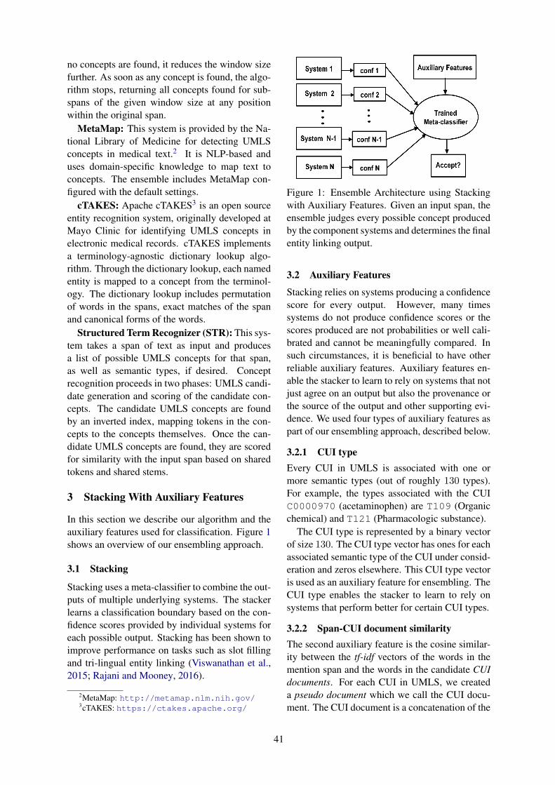
no concepts are found, it reduces the window sizefurther. As soon as any concept is found, the algo-rithm stops, returning all concepts found for sub-spans of the given window size at any positionwithin the original span.
MetaMap: This system is provided by the Na-tional Library of Medicine for detecting UMLSconcepts in medical text.2 It is NLP-based anduses domain-specific knowledge to map text toconcepts. The ensemble includes MetaMap con-figured with the default settings.
cTAKES: Apache cTAKES3 is an open sourceentity recognition system, originally developed atMayo Clinic for identifying UMLS concepts inelectronic medical records. cTAKES implementsa terminology-agnostic dictionary lookup algo-rithm. Through the dictionary lookup, each namedentity is mapped to a concept from the terminol-ogy. The dictionary lookup includes permutationof words in the spans, exact matches of the spanand canonical forms of the words.
Structured Term Recognizer (STR): This sys-tem takes a span of text as input and producesa list of possible UMLS concepts for that span,as well as semantic types, if desired. Conceptrecognition proceeds in two phases: UMLS candi-date generation and scoring of the candidate con-cepts. The candidate UMLS concepts are foundby an inverted index, mapping tokens in the con-cepts to the concepts themselves. Once the can-didate UMLS concepts are found, they are scoredfor similarity with the input span based on sharedtokens and shared stems.
3 Stacking With Auxiliary Features
In this section we describe our algorithm and theauxiliary features used for classification. Figure 1shows an overview of our ensembling approach.
3.1 Stacking
Stacking uses a meta-classifier to combine the out-puts of multiple underlying systems. The stackerlearns a classification boundary based on the con-fidence scores provided by individual systems foreach possible output. Stacking has been shown toimprove performance on tasks such as slot fillingand tri-lingual entity linking (Viswanathan et al.,2015; Rajani and Mooney, 2016).
2MetaMap: http://metamap.nlm.nih.gov/3cTAKES: https://ctakes.apache.org/
Figure 1: Ensemble Architecture using Stackingwith Auxiliary Features. Given an input span, theensemble judges every possible concept producedby the component systems and determines the finalentity linking output.
3.2 Auxiliary Features
Stacking relies on systems producing a confidencescore for every output. However, many timessystems do not produce confidence scores or thescores produced are not probabilities or well cali-brated and cannot be meaningfully compared. Insuch circumstances, it is beneficial to have otherreliable auxiliary features. Auxiliary features en-able the stacker to learn to rely on systems that notjust agree on an output but also the provenance orthe source of the output and other supporting evi-dence. We used four types of auxiliary features aspart of our ensembling approach, described below.
3.2.1 CUI typeEvery CUI in UMLS is associated with one ormore semantic types (out of roughly 130 types).For example, the types associated with the CUIC0000970 (acetaminophen) are T109 (Organicchemical) and T121 (Pharmacologic substance).
The CUI type is represented by a binary vectorof size 130. The CUI type vector has ones for eachassociated semantic type of the CUI under consid-eration and zeros elsewhere. This CUI type vectoris used as an auxiliary feature for ensembling. TheCUI type enables the stacker to learn to rely onsystems that perform better for certain CUI types.
3.2.2 Span-CUI document similarityThe second auxiliary feature is the cosine similar-ity between the tf-idf vectors of the words in themention span and the words in the candidate CUIdocuments. For each CUI in UMLS, we createda pseudo document which we call the CUI docu-ment. The CUI document is a concatenation of the
41

following information from UMLS:
1. CUI ID and label; for example, C0000970(acetaminophen)
2. Names of the types of the CUI; e.g., OrganicChemical; Pharmacologic Substance
3. Definition text for the CUI; e.g., analgesicantipyretic derivative of acetanilide; weakantiinflammatory properties and is used asa common analgesic, but may cause liver,blood cell, and kidney damage.
4. All variants for the CUI; e.g., Ac-etaminophen, Paracetamol
5. Select semantic relations between the CUIunder consideration and other CUIs; for ex-ample, (may treat: fever), (may treat: pain).
The intuition behind using this feature is that thespan would have a greater lexical overlap witha CUI document that it links to and thus have ahigher similarity score.
3.2.3 Context-CUI document similarityThis auxiliary feature is very much like the span-CUI document similarity feature. For this featureas well, we use the pseudo CUI documents cre-ated using UMLS. However, instead of using thespan for calculating the similarity we use the entirecontext surrounding the span. In the earlier exam-ple, the entire sentence “The patient reports suffer-ing from back pain for several years prior to treat-ment” is the context. We note that for short docu-ments, the context may be the entire document thatcontains the span to be linked. This means thatsome unique spans could have the same context.The context-CUI document similarity is the cosinesimilarity between the tf-idf vectors of words in thecontext and words in the CUI document.
3.2.4 Word embeddingsThe auxiliary features discussed so far only cap-ture the superficial lexical aspects of the dataused for ensembling. The word embeddings fea-tures capture the semantic dimension of the data.We trained the continuous bag of words model(Mikolov et al., 2013) on the entire UMLS knowl-edge base with word vector dimension of 200 andwindow-size of 10. Ling et al. (2015) show thatthese parameters enable capturing long range de-pendencies. In this way we obtain a vector repre-sentation for every word in UMLS. We note that
we chose the UMLS corpus as opposed to medicaldocuments so as to have better CUI coverage.
We used these word vectors to create the CUIdocument vector representation in the followingway. Recall that the CUI document is a pseudodocument made up of information about the CUIin UMLS. In order to obtain the embedding for acontext, span or document, we use the techniquedescribed in (Le and Mikolov, 2014). We add upall the embedding vectors representing the wordsin the CUI document and normalize the sum bythe number of words. The resultant vector repre-sents the CUI document embedding. Similarly, wealso obtain the span and the context embeddingsby adding and normalizing the vectors represent-ing the words in the span and context respectively.Note that if a word in the span or context doesnot have a vector representation then we just ig-nore it. Finally, we measure the cosine similaritybetween the span-CUI document and context-CUIdocument embedding vectors and use it as a fea-ture for our classifier. Representing the conceptsin vector space enables the stacker to learn deepsemantic patterns for cases where just lexical in-formation is not sufficient.
4 Experimental Results
4.1 Baselines
We compare our approach to several supervisedand unsupervised baselines. The first is Unionwhich accepts all predictions for all systems tomaximize recall. It classifies all span-CUI linksas correct and always includes them.
The second baseline is Voting. For this ap-proach, we vary the threshold on the number ofsystems that must agree on a span-CUI link fromone to all. This gradually changes the system be-havior from union to intersection of the links. Weidentify the threshold that results in the highest F1score on the training dataset. We use this thresholdfor the voting baseline on the test dataset.
The third baseline is an oracle threshold versionof Voting. Since the best threshold on the trainingdata may not necessarily be the best threshold forthe test data, we identify the best threshold for thetest data by plotting a precision-recall curve andfinding the best F1 score for the voting baseline.Note that this gives an upper bound on the bestresults that can be achieved with voting, assumingan optimal threshold is chosen. Since the upperbound can not be predicted without using the test
42

dataset, this baseline has an unfair advantage.In addition to the above common baselines, we
also compare our approach to a state-of-the-art en-sembling system, Bipartite Graph based Consen-sus Maximization (BGCM) (Gao et al. (2009)). Inaddition to the output of supervised models, thisensembling technique uses unsupervised modelsto provide additional constraints and evidence tothe classification algorithm. The rationale behindthis approach is that objects that are in the samecluster should be more likely to receive the sameclass label compared to the objects in differentclusters. The objective is to predict the class la-bel of an instance in a way that favors agreementbetween supervised components and at the sametime satisfies the constraints enforced by the clus-tering models. BGCM ensembles multiple mod-els by performing an optimization over a bipartitegraph of systems and outputs.
4.2 Dataset Description
All systems and baselines were evaluated on threedatasets. Scores reflect the quality of concepts as-signed to text spans, as decided by human judges.Detecting span boundaries is not part of this eval-uation – all systems are given the same span asinput. Annotations were performed by several hu-man judges. For scoring, each text span was pairedwith a list of concepts produced by all componentsystems. Annotators marked each span-conceptpair correct or incorrect.
The MCR dataset (Aggarwal et al., 2015) re-sulted from running a CRF-based entity recog-nition system that extracted 1,570 clinical fac-tors from 100 short descriptions (averaging 8 sen-tences, 100 words) of patient scenarios. The an-notated dataset contains a subset of 400 spans re-sulting in 6,139 annotated span-CUI pairs. Theaverage of the pairwise kappa scores for annotatoragreement on the MCR dataset was 0.56.
The i2b2 dataset (Uzuner et al., 2011) is basedon the annotated patient discharge summaries re-leased with the 2010 i2b2/VA challenge. The con-cept extraction task was to identify and extract thetext span corresponding to patient medical prob-lems, treatments and tests in unannotated patientrecord text. We created an entity linking datasetfrom a random subset of 100 annotated text spans.We ran all available entity linking systems andproduced 2,224 annotated span-CUI pairs. Theaverage pairwise kappa score for annotator agree-
ment on the i2b2 dataset was 0.52.The Electronic Medical Record dataset (EMR)
is a private dataset containing spans of medicalterms identified in doctors’ notes within patientmedical records. This dataset has 350 text spanswith 3,991 annotated span-CUI pairs. Annotatorsfor the EMR dataset reconciled their annotationsto build the ground truth.
4.3 Evaluation Metrics
As noted in section 1, UMLS often has multipledistinct CUIs for the same semantic concept. Sofor a given span from a dataset, there may be manytrue positive concepts in the ground truth. Thisleads to two possible scoring schemes: CUI leveland Span level. For CUI level scoring, every CUIin the ground truth is a ground truth positive in-stance. A CUI produced by the Entity Linkingsystem for a given span is a true positive if it is inthe ground truth for that span and a false positiveif it is not. CUIs in the ground truth for the spanthat are not produced by the system are countedas false negatives. Spans that have many CUIs inthe ground truth, therefore, will have more weightin the precision and recall than spans with fewerCUIs. But since the number of appropriate CUIsfor a span is often a side effect of the imperfectautomatic merging of concepts in building UMLS,the bias is unnatural.
An alternative scoring scheme awards only onetrue positive, false positive or false negative foreach span, not each CUI. For this span level scor-ing, we report two versions of the metrics. Thefirst version, which we call “Factor Level” inthe reported results, aggregates CUI scores usingMAX. The system scores a true positive if any ofthe CUIs it produces are in the ground truth for thespan. It scores a false positive if none of its CUIsare in the ground truth. It scores a false negative ifit produces no CUIs and there is at least one CUIin the ground truth.
The second version of span level scoring ac-counts for the fact that the system may producea mixture of correct and incorrect CUIs for thesame span. Each span still has a weight of one inthe overall precision and recall, but the system’sscore for “true positiveness” and “false positive-ness” can be a real number between 0 and 1. Wecall this scoring scheme “Quantum”. The quan-tum true positive score for a span is the numberof CUIs produced by the system that are in the
43

Approach CUI Level Factor Level Quantum
P R F1 P R F1 P R F1
GBMCR 0.349 0.242 0.286 0.395 0.437 0.415 0.357 0.268 0.306NBMCR 0.414 0.179 0.250 0.463 0.511 0.486 0.423 0.163 0.236VBMCR 0.496 0.215 0.300 0.548 0.605 0.575 0.513 0.198 0.285
CFV 0.587 0.405 0.479 0.903 0.461 0.611 0.716 0.188 0.298CTakes 0.384 0.245 0.299 0.711 0.577 0.637 0.498 0.202 0.287
MetaMap 0.447 0.219 0.293 0.623 0.652 0.637 0.535 0.215 0.306CMap 0.179 0.549 0.270 0.802 0.870 0.834 0.305 0.461 0.367STR 0.623 0.217 0.322 0.623 0.688 0.654 0.623 0.217 0.322
Union 0.207 0.797 0.329 0.888 0.981 0.932 0.278 0.765 0.408Majority Voting 0.746 0.182 0.293 0.768 0.522 0.622 0.745 0.169 0.275Oracle Voting 0.626 0.290 0.396 0.723 0.707 0.715 0.629 0.251 0.359
BGCM 0.481 0.430 0.454 0.753 0.822 0.786 0.525 0.368 0.433
Stacking 0.481 0.508 0.494 0.785 0.848 0.815 0.501 0.412 0.452+ CUI Type 0.474 0.573 0.519 0.816 0.889 0.851 0.484 0.502 0.493
+ Span & Context Similarity 0.472 0.575 0.519 0.811 0.886 0.847 0.485 0.508 0.496+ CBOW embedding 0.567 0.500 0.532 0.824 0.892 0.857 0.491 0.507 0.499
Table 1: Results on the MCR dataset.
ground truth for the span divided by the total num-ber of CUIs produced by the system (i.e., the span-level Precision). Quantum false positive score isthe number of incorrect CUIs produced by the sys-tem divided by the total number of CUIs produced.
4.4 Results
We present results for entity linking in the medicaldomain on the three datasets described in section4.2 using the evaluation metrics defined in section4.3. The results include the performance of theindividual models, several baselines and variousablations of the auxiliary features using stacking.Tables 1, 2 and 3 show performance on the MCR,i2b2 and EMR datasets respectively.
Although we observe similar trends across allthe datasets, no single individual model performsbetter than others across all the evaluation met-rics. This led us to conclude that each individualmodel is optimized for a particular type of entityor data. For example, a model that is good at link-ing medical drugs might not perform as well onlinking medical diseases. In order to leverage thestrengths of each individual model, we ensemblethem into one powerful model that works acrossall datasets as well as different evaluation metrics.
As expected, the Union baseline obtains the bestrecall and Majority Voting has the highest preci-sion across all datasets. Oracle Voting is optimizedfor F1 and thus obtains an F1 higher than MajorityVoting. Vanilla stacking beats the best componentand baseline systems’ F1 scores for CUI level andquantum metrics on all datasets. Adding each aux-
Figure 2: Ablation on the component systems inthe ensemble for the MCR dataset using the CUIlevel metric. The systems are arranged in decreas-ing order of F1 score.
iliary feature further boosts the performance andwe obtain the highest F1 for all datasets using allthe features combined. Stacking outperforms theBGCM ensembling baseline on all datasets.
For a deeper understanding of the results, weperformed ablation tests on the systems used in thefinal ensemble. Figure 2 shows the performanceof the ensemble with each component ablated inturn. This experiment shows that every componentsystem contributes to the ensemble in either preci-sion, recall or both. While each component con-tributes to the overall performance, the strength ofthe ensemble is determined by the combination of
44

Approach CUI Level Factor Level Quantum
P R F1 P R F1 P R F1
GBMCR 0.507 0.375 0.431 0.790 0.807 0.798 0.515 0.427 0.467NBMCR 0.478 0.356 0.408 0.779 0.796 0.787 0.486 0.403 0.441VBMCR 0.554 0.404 0.467 0.800 0.817 0.809 0.564 0.468 0.511
CFV 0.173 0.457 0.251 0.884 0.903 0.894 0.577 0.327 0.417CTakes 0.564 0.213 0.309 0.861 0.731 0.791 0.677 0.195 0.303
MetaMap 0.565 0.154 0.242 0.750 0.742 0.746 0.647 0.153 0.248CMap 0.216 0.360 0.270 0.894 0.903 0.898 0.410 0.260 0.318STR 0.825 0.176 0.290 0.833 0.860 0.847 0.566 0.236 0.333
Union 0.191 0.855 0.312 0.969 1.000 0.984 0.352 0.849 0.498Majority Voting 0.705 0.189 0.298 0.846 0.828 0.837 0.766 0.176 0.286Oracle Voting 0.624 0.270 0.373 0.874 0.893 0.883 0.709 0.227 0.344
BGCM 0.469 0.406 0.435 0.938 0.968 0.952 0.509 0.386 0.439
Stacking 0.434 0.697 0.535 0.958 0.989 0.974 0.481 0.655 0.555+ CUI Type 0.525 0.730 0.611 0.927 0.957 0.942 0.547 0.563 0.555
+ Span & Context Similarity 0.528 0.756 0.622 0.927 0.957 0.942 0.544 0.639 0.588+ CBOW embedding 0.528 0.756 0.622 0.938 0.968 0.952 0.546 0.700 0.607
Table 2: Results on the i2b2 dataset.
Approach CUI Level Factor Level Quantum
P R F1 P R F1 P R F1
GBMCR 0.338 0.134 0.192 0.369 0.351 0.36 0.360 0.315 0.196NBMCR 0.381 0.151 0.217 0.410 0.390 0.400 0.396 0.148 0.216VBMCR 0.564 0.224 0.321 0.618 0.589 0.603 0.600 0.225 0.327
CFV 0.510 0.353 0.417 0.914 0.607 0.729 0.692 0.249 0.366CTakes 0.403 0.321 0.357 0.706 0.628 0.665 0.527 0.268 0.355
MetaMap 0.460 0.220 0.298 0.575 0.568 0.571 0.527 0.223 0.313CMap 0.205 0.597 0.305 0.761 0.766 0.763 0.334 0.597 0.428STR 0.714 0.284 0.406 0.714 0.748 0.730 0.714 0.284 0.406
Union 0.187 0.739 0.299 0.857 0.852 0.854 0.272 0.676 0.388Majority Voting 0.879 0.225 0.359 0.912 0.561 0.695 0.894 0.220 0.353Oracle Voting 0.668 0.297 0.412 0.820 0.661 0.732 0.719 0.276 0.399
BGCM 0.453 0.419 0.435 0.801 0.809 0.805 0.482 0.409 0.442
Stacking 0.443 0.517 0.477 0.794 0.832 0.812 0.488 0.463 0.475+ CUI Type 0.559 0.548 0.554 0.807 0.778 0.792 0.571 0.436 0.495
+ Span & Context Similarity 0.593 0.554 0.573 0.820 0.781 0.800 0.616 0.443 0.515+ CBOW embedding 0.667 0.549 0.602 0.830 0.775 0.801 0.669 0.439 0.530
Table 3: Results on the EMR dataset.
the component systems. The ablation of the CMapsystem has the highest impact on the ensemble, re-ducing the F1 score by 5.2%. We obtained similarplots for the factor level and quantum metrics andwe expect to see similar trends for the i2b2 and theEMR datasets as well.
5 Discussion
The experimental results presented in section 4.4confirm that the different component systemsshow significantly different behavior on differentmetrics for different datasets. No individual sys-tem was universally the best. CMap had consis-tently good Recall but low Precision. CFV scoredwell in certain circumstances on precision, re-call and F1 score, but this varied from dataset to
dataset and metric to metric. STR usually had rel-atively high precision, but low recall, and VBMCRhad very good F1 scores on i2b2, but was less im-pressive on the other datasets.
These observations imply good conditions forensembling to make a difference. Even so, thebest baseline ensemble only outperforms the bestcomponent system on F1 in four of the nine ex-periments (metric-dataset combinations). Stack-ing outperforms the best component system in allnine, and outperforms the best ensembling base-line for six of the nine – all of the CUI level met-rics and quantum, but never at the factor level. Thefactor level scoring is much more generous, but itis not immediately clear why this would benefitnaıve ensembling over stacking.
45

Auxiliary features almost always improvestacking. Again the exception is with factor levelscoring. Interestingly, auxiliary features almostuniversally improve precision significantly with-out too damaging an effect on recall. This resultsuggests that it would be worthwhile experiment-ing with the precision-vs-recall bias of componentsystems to see if Stacking with auxiliary featurescould be used, for example, to recover precisionwith recall-biased components.
6 Related Work
The problem of entity linking has received con-siderable attention in the research community.Several community tasks are focused specificallyon the medical domain and are addressing theproblem of linking disease/disorder entities toSNOMED CT.4 SNOMED CT concepts are alsoincluded in UMLS.
The ShARe/CLEF eHealth Evaluation Lab2013 (Suominen et al., 2013) consists of a collec-tion of tasks focused on facilitating patients’ un-derstanding of their medical discharge summaries.The assumption is that an improved understand-ing of medical concepts in such documents can beachieved by normalizing all health conditions tostandardized SNOMED CT concepts. Using theseconcepts, the medical documents can further beconnected to other patient friendly sources.
The Open Biomedical Annotator (OBA) (Jon-quet et al., 2009) is an ontology-based Web servicethat annotates public datasets with biomedical on-tology concepts, including concepts from UMLS.The OBA is based on dictionary matching. Thedictionary is a list of strings that identify ontologyconcepts. The dictionary is constructed by access-ing biomedical ontologies and extracting all con-cept names, their synonyms or labels. The webservice takes as input the user’s free text. The toolrecognizes concepts using string matching on thedictionary and outputs the concept annotations.
There are several notable approaches to performentity linking in the open domain. These opendomain approaches often deal with named enti-ties. The linking targets in this case are often sin-gle, unambiguous, specific concepts. The problemof finding domain-specific concepts, on the otherhand, can be more challenging as there may beappropriate concepts at different levels of speci-ficity, and concepts are more compositional and
4SNOMED CT: http://www.snomed.org/
contextual. Approaches such as DBPedia Spot-light (Mendes et al., 2011) and AIDA (Hoffartet al., 2011) use Wikipedia to find the links of rec-ognized entity mentions.
To overcome challenges of obtaining labeledmedical datasets, Zheng et al. (2015) proposed anunsupervised approach for entity linking. Moretraditional sieve-based techniques have been usedfor this task recently (D’Souza and Ng, 2015).
Using ensembling techniques for open domainentity linking has shown good performance inthe past (Rajani and Mooney, 2017) on the Tri-lingual Entity Discovery and Linking (TEDL)task. TEDL is an entity linking task conducted byNIST. The goal of this task is to discover entitiesin the three included languages (English, Span-ish and Chinese) from a supplied text corpus andlink these entities to an existing English knowl-edge base (a reduced version of FreeBase).
Rajani and Mooney (2016) proposed an ap-proach for combining multiple supervised and un-supervised models for entity linking. Their tech-nique improves the previous result on the TEDLtask. Another ensembling approach is Mixturesof Experts (Jacobs et al., 1991) which employsdivide-and-conquer principle to soft switch be-tween learners covering different sub-spaces of theinput using Expectation-Maximization (EM). Ourwork is the first we know of to use ensembling forentity linking in the medical domain.
7 Conclusion
We have identified an entity linking task in themedical domain for which existing technologiesperform differently on different metrics for differ-ent datasets. Such an environment presents an ob-vious opportunity for ensembling techniques.
We have built a stacking ensembler using mul-tiple diverse entity linking systems. The auxiliaryfeatures further boost the stacker’s performance.Experiments confirm that naıve ensembling doesnot always outperform component entity linkingsystems, but that vanilla stacking does. Addingauxiliary features to the stacker almost universallyimproves its precision without harming recall, giv-ing it generally the best F1 scores overall.
Our model is able to fuse additional relevantknowledge from multiple systems and leveragethem to improve prediction.
46

ReferencesNitish Aggarwal, Ken Barker, and Chris Welty. 2015.
Medical concept resolution. In Proceedings of theISWC 2015 Posters & Demonstrations Track co-located with the 14th International Semantic WebConference (ISWC-2015), Bethlehem, PA, USA, Oc-tober 11, 2015..
T. Dietterich. 2000. Ensemble methods in machinelearning. In J. Kittler and F. Roli, editors, FirstInternational Workshop on Multiple Classifier Sys-tems, Lecture Notes in Computer Science. Springer-Verlag, pages 1–15.
Jennifer D’Souza and Vincent Ng. 2015. Sieve-basedentity linking for the biomedical domain. In ACL(2). pages 297–302.
Jing Gao, Feng Liang, Wei Fan, Yizhou Sun, and Ji-awei Han. 2009. Graph-based consensus maximiza-tion among multiple supervised and unsupervisedmodels. In NIPS2009. pages 585–593.
Johannes Hoffart, Mohamed Amir Yosef, Ilaria Bor-dino, Hagen Furstenau, Manfred Pinkal, Marc Span-iol, Bilyana Taneva, Stefan Thater, and GerhardWeikum. 2011. Robust disambiguation of namedentities in text. In Proceedings of the Seventh In-ternational Conference on Semantic Systems. pages1–8.
Robert A Jacobs, Michael I Jordan, Steven J Nowlan,and Geoffrey E Hinton. 1991. Adaptive mixtures oflocal experts. Neural computation 3(1):79–87.
Clement Jonquet, Nigam Shah, and Mark Musen. 2009.The open biomedical annotator. pages 56–60.
Quoc V Le and Tomas Mikolov. 2014. Distributed rep-resentations of sentences and documents. In Pro-ceedings of the International Conference on Ma-chine Learning. volume 14, pages 1188–1196.
Wang Ling, Lin Chu-Cheng, Yulia Tsvetkov, and Sil-vio Amir. 2015. Not all contexts are created equal:Better word representations with variable attention.In Proceedings of the 2015 Conference on EmpiricalMethods in Natural Language Processing (EMNLP-15). Citeseer.
Pablo N. Mendes, Max Jakob, Andres Garcia-Silva,and Christian Bizer. 2011. DBpedia spotlight: shed-ding light on the web of documents. In Proceedingsof the Seventh International Conference on SemanticSystems. pages 1–8.
Tomas Mikolov, Ilya Sutskever, Kai Chen, Greg S Cor-rado, and Jeff Dean. 2013. Distributed representa-tions of words and phrases and their compositional-ity. In Advances in neural information processingsystems. pages 3111–3119.
Nazneen Fatema Rajani and Raymond J. Mooney.2016. Combining Supervised and Unsupervised En-sembles for Knowledge Base Population. In Pro-ceedings of the 2016 Conference on Empirical Meth-ods in Natural Language Processing (EMNLP-16).
Nazneen Fatema Rajani and Raymond J. Mooney.2017. Stacking With Auxiliary Features. In Pro-ceedings of the Twenty-Sixth International JointConference on Artificial Intelligence (IJCAI2017).Melbourne, Australia.
Hanna Suominen, Sanna Salantera, Sumithra Velupil-lai, Wendy W. Chapman, Guergana Savova,Noemie Elhadad, Sameer Pradhan, Brett R. South,Danielle L. Mowery, Gareth J. F. Jones, JohannesLeveling, Liadh Kelly, Lorraine Goeuriot, DavidMartinez, and Guido Zuccon. 2013. Overview of theShARe/CLEF eHealth Evaluation Lab 2013, pages212–231.
Ozlem Uzuner, Brett R. South, Shuying Shen, andScott L. DuVall. 2011. 2010 i2b2/va challenge onconcepts, assertions, and relations in clinical text.JAMIA 18(5):552–556.
Vidhoon Viswanathan, Nazneen Fatema Rajani, YinonBentor, and Raymond J. Mooney. 2015. Stacked En-sembles of Information Extractors for Knowledge-Base Population. In Association for ComputationalLinguistics (ACL2015). Beijing, China, pages 177–187.
David H. Wolpert. 1992. Stacked Generalization. Neu-ral Networks 5:241–259.
Jin G Zheng, Daniel Howsmon, Boliang Zhang, Juer-gen Hahn, Deborah McGuinness, James Hendler,and Heng Ji. 2015. Entity linking for biomedicalliterature. BMC medical informatics and decisionmaking 15(1):S4.
47

Proceedings of the BioNLP 2017 workshop, pages 48–57,Vancouver, Canada, August 4, 2017. c©2017 Association for Computational Linguistics
Results of the fifth edition of the BioASQ Challenge
Anastasios Nentidis1, Konstantinos Bougiatiotis1, Anastasia Krithara1,Georgios Paliouras1 and Ioannis Kakadiaris2
1National Center for Scientific Research “Demokritos”, Athens, Greece2University of Houston, Texas, USA
AbstractThe goal of the BioASQ challenge is toengage researchers into creating cutting-edge biomedical information systems.Specifically, it aims at the promotionof systems and methodologies that areable to deal with a plethora of differenttasks in the biomedical domain. This isachieved through the organization of chal-lenges. The fifth challenge consisted ofthree tasks: semantic indexing, questionanswering and a new task on informationextraction. In total, 29 teams with morethan 95 systems participated in the chal-lenge. Overall, as in previous years, thebest systems were able to outperform thestrong baselines. This suggests that state-of-the art systems are continuously im-proving, pushing the frontier of research.
1 Introduction
The aim of this paper is twofold. First, we aimto give an overview of the data issued during theBioASQ challenge in 2017. In addition, we aim topresent the systems that participated in the chal-lenge and evaluate their performance. To achievethese goals, we begin by giving a brief overview ofthe tasks, which took place from February to May2017, and the challenge’s data. Thereafter, we pro-vide an overview of the systems that participatedin the challenge. Detailed descriptions of someof the systems are given in workshop proceedings.The evaluation of the systems, which was carriedout using state-of-the-art measures or manual as-sessment, is the last focal point of this paper, withremarks regarding the results of each task. Theconclusions sum up this year’s challenge.
2 Overview of the Tasks
The challenge comprised three tasks: (1) a large-scale semantic indexing task (Task 5a), (2) a ques-
tion answering task (Task 5b) and (3) a fundinginformation extraction task (Task 5c), described inmore detail in the following sections.
2.1 Large-scale semantic indexing - 5a
In Task 5a the goal is to classify documents fromthe PubMed digital library into concepts of theMeSH hierarchy. Here, new PubMed articles thatare not yet annotated by MEDLINE indexers arecollected and used as test sets for the evaluation ofthe participating systems. In contrast to previousyears, articles from all journals were included inthe test data sets of task 5a. As soon as the an-notations are available from the MEDLINE index-ers, the performance of each system is calculatedusing standard flat information retrieval measures,as well as, hierarchical ones. As in previous years,an on-line and large-scale scenario was provided,dividing the task into three independent batches of5 weekly test sets each. Participants had 21 hoursto provide their answers for each test set. Table1 shows the number of articles in each test set ofeach batch of the challenge. 12,834,585 articleswith 27,773 labels were provided as training datato the participants.
2.2 Biomedical semantic QA - 5b
The goal of Task 5b was to provide a large-scale question answering challenge where the sys-tems had to cope with all the stages of a ques-tion answering task for four types of biomedi-cal questions: yes/no, factoid, list and summaryquestions (Balikas et al., 2013). As in previousyears, the task comprised two phases: In phase A,BioASQ released 100 questions and participantswere asked to respond with relevant elements fromspecific resources, including relevant MEDLINEarticles, relevant snippets extracted from the arti-cles, relevant concepts and relevant RDF triples.In phase B, the released questions were enhancedwith relevant articles and snippets selected manu-
48

Batch Articles AnnotatedArticles
Labelsper
Article
1
6,880 6,661 12.497,457 6,599 12.4910,319 9,656 12.497,523 4,697 11.787,940 6,659 12.50
Total 40,119 34,272 12.39
2
7,431 7,080 12.406,746 6,357 12.625,944 5,479 12.876,986 6,526 12.656,055 5,492 12.41
Total 33,162 30,934 12.58
3
9,233 5,341 12.787,816 2,911 12.587,206 4,110 12.707,955 3,569 12.1710,225 984 13.72
Total 42,435 21,323 12.68
Table 1: Statistics on test datasets for Task 5a.
ally and the participants had to respond with ex-act answers, as well as with summaries in nat-ural language (dubbed ideal answers). The taskwas split into five independent batches and the twophases for each batch were run with a time gap of24 hours. In each phase, the participants received100 questions and had 24 hours to submit their an-swers. Table 2 presents the statistics of the train-ing and test data provided to the participants. Theevaluation included five test batches.
Batch Size Documents SnippetsTrain 1,799 11.86 20.38Test 1 100 4.87 6.03Test 2 100 3.93 5.13Test 3 100 4.03 5.47Test 4 100 3.23 4.52Test 5 100 3.61 5.01Total 2,299 10.14 17.09
Table 2: Statistics on the training and test datasetsof Task 5b. All the numbers for the documents andsnippets refer to averages.
2.3 Funding information extraction - 5c
Task 5c was introduced for the first time this yearand the challenge at hand was to extract grant in-
formation from Biomedical articles. Funding in-formation can be very useful; in order to estimate,for example, the impact of an agency’s funding inthe biomedical scientific literature or to identifyagencies actively supporting specific directions inresearch. MEDLINE citations are annotated withinformation about funding from specified agen-cies1. This funding information is either providedby the author manuscript submission systems orextracted manually from the full text of articlesduring the indexing process. In particular, NLMhuman indexers identify the grant ID and the fund-ing agencies can be extracted from the string of thegrant ID2. In some cases, only the funding agencyis mentioned in the article, without the grant ID.
In this task funding information from MED-LINE was used, as golden data, in order to trainand evaluate systems. The systems were askedto extract grant information mentioned in the fulltext, but author-provided information is not nec-essarily mentioned in the article. Therefore, grantIDs not mentioned in the article were filtered out.This filtering also excluded grant IDs deviatingfrom NLM’s general policy of storing grant IDsas published, without any normalization. Whenan agency was mentioned in the text without agrant ID, it was kept only if it appeared in the listof agencies and abbreviations provided by NLM.Cases of misspellings or alternative naming ofagencies were removed. In addition, informationfor funding agencies that are no longer indexed byNLM was omitted. Consequently, the golden dataused in the task consisted of a subset of all fundinginformation mentioned in the articles.
During the challenge, a training and a testdataset were prepared. The test set of MED-LINE documents with their full-text available inPubMed Central was released and the participantswere asked to extract grant IDs and grant agen-cies mentioned in each test article. The participat-ing systems were evaluated on (a) the extractionof grant IDs, (b) the extraction of grant agenciesand (c) full-grant extraction, i.e. the combinationof grant ID and the corresponding funding agency.Table 3 contains details regarding the datasets fortraining and test.
1https://www.nlm.nih.gov/bsd/grant_acronym.html
2https://www.nlm.nih.gov/bsd/mms/medlineelements.html#gr
49

Dataset Articles GrantIDs Agencies Time
PeriodTraining 62,952 111,528 128,329 2005-13
Test 22,610 42,711 47,266 2015-17
Table 3: Dataset overview for Task 5c.
3 Overview of Participants
3.1 Task 5a
For this task, 10 teams participated and resultsfrom 31 different systems were submitted. In thefollowing paragraphs we describe those systemsfor which a description was obtained, stressingtheir key characteristics. An overview of the sys-tems and their approaches can be seen in Table 4.
System Approach
Search systemsearch engine, UIMA
ConceptMapper
MZtf-idf, LDA, BR
classification
Sequencerrecurrent neural
networksDeepMesh d2v, tf-idf, MESHlabeler
AUTHd2v, tf-idf, LLDA,SVM, ensembles
Iriabigrams, Luchene Index,
k-NN, ensembles,UIMA ConceptMapper
Table 4: Systems and approaches for Task 5a. Sys-tems for which no description was available at thetime of writing are omitted.
The “Search system” and its variants were de-veloped as a UIMA-based text and data miningworkflow, where different search strategies wereadopted to automatically annotate documents withMeSH terms. On the other hand, the “MZ” sys-tems applied Binary Relevance (BR) classifica-tion, using TF-IDF features, and Latent Dirich-let allocation (LDA) models with label frequen-cies per journal as prior frequencies, using regres-sion for threshold prediction. A different approachis adopted by the “Sequencer” systems, devel-oped by the team from the Technical University ofDarmstadt, that considers the task as a sequence-to-sequence prediction problem and use recurrentneural networks based algorithm to cope with it.
The “DeepMeSH” systems implement docu-ment to vector (d2v) and tf-idf feature embeddings
(Peng et al., 2016), alongside the MESHLabelersystem (Liu et al., 2015) that achieved the bestscores overall, integrating multiple evidence us-ing learning to rank (LTR). A similar approach,with regards to the d2v and tf-idf representationsof the text, is followed by the “AUTH” team. Re-garding the learning algorithms they’ve extendedtheir previous system (Papagiannopoulou et al.,2016), improving the Labeled LDA and SVMbase models, as well as introducing a new ensem-ble methodology based on label frequencies andmulti-label stacking. Last but not least, the teamfrom the University of Vigo developed the “Iria”systems. Building upon their previous approach(Ribadas et al., 2014) that uses an Apache LuceneIndex to provide most similar citations, they de-veloped two systems that follow a multilabel k-NN approach. They also incorporated token bi-grams and PMI scores to capture relevant mul-tiword terms through a voting ensemble schemeand the ConceptMapper annotator tool, from theApache UIMA project (Tanenblatt et al., 2010), tomatch subject headings with the citation’s abstracttext.
Baselines: During the challenge, two systemsserved as baselines. The first baseline is a state-of-the-art method called Medical Text Indexer(MTI) (Mork et al., 2014) with recent improve-ments incorporated as described in (Zavorin et al.,2016). MTI is developed by the National Libraryof Medicine (NLM) and serves as a classificationsystem for articles of MEDLINE, assisting the in-dexers in the annotation process. The second base-line is an extension of the system MTI, incorpo-rating features of the winning system of the firstBioASQ challenge (Tsoumakas et al., 2013).
3.2 Task 5b
The question answering task was tackled by 51different systems, developed by 17 teams. In thefirst phase, which concerns the retrieval of infor-mation required to answer a question, 9 teamswith 25 systems participated. In the second phase,where teams are requested to submit exact andideal answers, 10 teams with 29 different sys-tems participated. Two of the teams participatedin both phases. An overview of the technologiesemployed by each team can be seen in Table 5.
The “Basic QA pipeline” approach is one ofthe two that participated in both Phases. It usesMetaMap for query expansion, taking into account
50

Systems Phase ApproachBasic QApipeline
A, B MetaMap, BM25
Olelo A, BNER, UMLS, SAP
HANA, SRL
USTB Asequential dependence
models, ensembles
fdu AMESHLabeler,
Language model, wordsimilarity
UNCC AStanford Parser,
Semantic Indexing
MQU Bdeep learning, neural
nets, regression
Oaqa B
agglomerativeclustering, tf-idf, wordembeddings, maximum
margin relevance
LabZhu BPubTator, StandfordPOS tool, ranking
DeepQA B FastQA, SQuAD
sarrouti BUMLS, BM25,
dictionaries
Table 5: Systems and approaches for Task 5b. Sys-tems for which no information was available at thetime of writing are omitted.
the text and the title of each article, and the BM25probabilistic model (Robertson et al., 1995) in or-der to match questions with documents, snippetsetc. The same goes for phase B, except for theexact answers, where stop words were removedand the top-k most frequent words were selected.“Olelo” is the second approach that tackles bothphases of task B. It is built on top of the SAPHANA database and uses various NLP compo-nents, such as question processing, document andpassage retrieval, answer processing and multi-document summarization based on previous ap-proaches (Schulze et al., 2016) to develop a com-prehensive system that retrieves relevant informa-tion and provides both exact and ideal answersfor biomedical questions. Semantic role labeling(SRL) based extensions were also investigated.
One of the teams that participated only in phaseA, is “USTB” who combined different strategies toenrich query terms. Specifically, sequential depen-dence models (Metzler and Croft, 2005), pseudo-relevance feedback models, fielded sequential de-pendence models and divergence from random-
ness models are used on the training data to cre-ate better search queries. The “fdu” systems, as inprevious years (Peng et al., 2015), use a languagemodel in order to retrieve relevant documents andkeyword scoring with word similarity for snippetextraction. The “UNCC” team on the other hand,focused mainly on the retrieval of relevant con-cepts and articles using the Stanford Parser (Chenand Manning, 2014) and semantic indexing.
In Phase B, the Macquarie University (MQU)team focused on ideal answers (Molla, 2017), sub-mitting different models ranging from a “triv-ial baseline” of relevant snippets to deep learn-ing under regression settings (Malakasiotis et al.,2015) and neural networks with word embeddings.The Carnegie Mellon University team (“OAQA”),focused also on ideal answer generation, build-ing upon previous versions of the “OAQA” sys-tem. They used extractive summarization tech-niques and experimented with different biomedi-cal ontologies and algorithms including agglom-erative clustering, Maximum Marginal Relevanceand sentence compression. They also introduceda novel similarity metric that incorporates both se-mantic information (using word embeddings) andtf-idf statistics for each sentence/question.
Many systems used a modular approach break-ing the problem down to question analysis, candi-date answer generation and answer ranking. The“LabZhu” systems, followed this approach, basedon previous years’ methodologies (Peng et al.,2015). In particular, they applied rule-based ques-tion type analysis and used Standford POS tooland PubTator for candidate answer generation.They also used word frequencies for candidate an-swer ranking. The “DeepQA” systems focused onfactoid and list questions, using an extractive QAmodel, restricting the system to output substringsof the provided text snippets. At the core of theirsystem stands a state-of-the-art neural QA system,namely FastQA (Weissenborn et al., 2017), ex-tended with biomedical word embeddings. Themodel was pre-trained on a large-scale open-domain QA dataset, SQuAD (Rajpurkar et al.,2016), and then the parameters were fine-tuned onthe BioASQ training set. Finally, the “sarrouti”system, from Morocco’s USMBA, uses amongothers a dictionary approach, term frequencies ofUMLS metathesaurus’ concepts and the BM25model.
Baselines: For this challenge the open source
51

OAQA system proposed by (Yang et al., 2016) forBioASQ4 was used as a strong baseline. This sys-tem, as well as its previous version (Yang et al.,2015) for BioASQ3, had achieved top perfor-mance in producing exact answers. The systemuses an UIMA based framework to combine dif-ferent components. Question and snippet pars-ing is based on ClearNLP. MetaMap, TmTool, C-Value and LingPipe are used for concept identi-fication and UMLS Terminology Services (UTS)for concept retrieval. In addition, identification ofconcept, document and snippet relevance is basedon classifier components and scoring, ranking andreranking techniques are also applied in the finalsteps.
3.3 Task 5c
In this inaugural year for task c, 3 teams partici-pated with a total of 11 systems. A brief outline ofthe techniques used by the participating systems isprovided in table 6.
Systems Approach
Simpleregions of interest, SVM, regular
expressions, hand-made rules,char-distances, ensemble
DZGregions of interest, SVM, tf-idf ofbigrams, HMMs, MaxEnt, CRFs,
ensembleAUTH regions of interest, regular expressions
Table 6: Overview of the methodologies used bythe participating systems in Task 5c.
The Fudan University team, participated witha series of similar systems (“Simple” systems) aswell as their ensemble. The general approachincluded the following steps: First, the articleswere parsed and some sections, such as affilia-tion or references, were removed. Then, usingNLP techniques, alongside pre-defined rules, eachparagraph was split into sentences. These sen-tences were classified as positive (i.e. contain-ing grant information) or not, using a linear SVM.The positive sentences were scanned for grant IDsand agencies through the use of regular expres-sions and hand-made rules. Finally, multiple clas-sifiers were trained in order to merge grant IDs andagencies into suitable pairs, based on a wide rangeof features, such as character-level features of thegrant ID, the agency in the sentence and the dis-tance between the grant ID and the agency in the
sentence.The “DZG” systems followed a similar method-
ology, in order to classify snippets of text as pos-sible grant information sources, implementing alinear SVM with tf-idf vectors of bigrams as in-put features. However, their methodology dif-fered from that of Fudan in two ways. Firstly,they used an in-house-created dataset consistingof more than 1,600 articles with grant informationin order to train their systems. Secondly, the sys-tems deployed were based on a variety of sequen-tial learning models namely conditional randomfields (Finkel et al., 2005), hidden markov mod-els (Collins, 2002) and maximum entropy models(Ratnaparkhi, 1998). The final system deployedwas a pooling ensemble of these three approaches,in order to maximize recall and exploit comple-mentarity between predictions of different mod-els. Likewise, the AUTH team, with systems “As-clepius”, “Gallen” and “Hippocrates” emphasizedon specific sections of the text that could containgrant support information and extracted grant IDsand agencies using regular expressions.
Baselines: For this challenge a baseline wasprovided by NLM (“BioASQ Filtering”) which isbased on a two-step procedure. First, the systemclassifies snippets from the full-text, as possiblegrant support “zones” based on the average prob-ability ratio, generated separately by Naive Bayes(Zhang et al., 2009) and SVM (Kim et al., 2009).Then, the system identified grant IDs and agen-cies in these selected grant support “zones”, usingmainly heuristic rules, such as regular expressions,especially for detecting uncommon and irregularlyformatted grant IDs.
4 Results
4.1 Task 5a
Each of the three batches of task 5a was evaluatedindependently. The classification performance ofthe systems was measured using flat and hierar-chical evaluation measures (Balikas et al., 2013).The micro F-measure (MiF) and the Lowest Com-mon Ancestor F-measure (LCA-F) were used tochoose the winners for each batch (Kosmopouloset al., 2013).
According to (Demsar, 2006) the appropriateway to compare multiple classification systemsover multiple datasets is based on their averagerank across all the datasets. On each dataset thesystem with the best performance gets rank 1.0,
52

System Batch 1 Batch 2 Batch 3MiF LCA-F MiF LCA-F MiF LCA-F
auth1 8.88 8.25 10.50 9.75 10.25 9.75auth2 7.25 6.50 7.63 7.50 8.88 9.75auth3 6.75 8.25 7.50 10.25 6.50 7.00auth4 - - 7.38 8.25 9.63 9.75auth5 - - 7.50 7.00 8.50 7.50
DeepMeSH1 1.88 1.88 1.00 2.00 1.00 1.50DeepMeSH2 1.00 1.00 3.00 3.00 2.50 2.75DeepMeSH3 4.00 4.63 4.00 4.00 4.00 4.13DeepMeSH4 5.00 4.38 5.00 5.50 4.88 5.63DeepMeSH5 2.63 2.63 1.75 1.00 2.25 1.25
iria-1 - - 13.75 13.75 12.75 12.75iria-2 - - - - 11.75 11.75MZ1 10.75 10.75 - - - -
Optimize MacroAUC
- - - - 19.25 19.25
Optimize MicroAUC
- - - - 15.75 18.25
Search system-1 12.25 12.25 - - 13.75 13.25Search system-2 13.25 13.25 - - 14.75 14.25Search system-3 16.25 16.25 - - 18.50 17.50Search system-4 15.25 15.25 - - 16.75 16.25Search system-5 14.25 14.25 - - 15.75 15.25
Default MTI 7.50 6.25 8.75 6.00 7.50 6.75MTI First Line
Index9.13 9.25 11.50 11.50 9.50 8.75
Table 7: Average system ranks across the batches of the Task 5a. A hyphenation symbol (-) is used when-ever the system participated in fewer than 4 tests in the batch. Systems with fewer than 4 participationsin all batches are omitted.
the second best rank 2.0 and so on. In case twoor more systems tie, they all receive the averagerank. Table 7 presents the average rank (accordingto MiF and LCA-F) of each system over all the testsets for the corresponding batches. Note, that theaverage ranks are calculated for the 4 best resultsof each system in the batch according to the rulesof the challenge.
On both test batches and for both flat and hier-archical measures, the DeepMeSH systems (Penget al., 2016) and the AUTH systems outperformthe strong baselines, indicating the importance ofthe methodologies proposed, including d2v andtf-idf transformations to generate feature embed-dings, for semantic indexing. More detailed re-sults can be found in the online results page 3.
3http://participants-area.bioasq.org/results/5a/
4.2 Task 5b
Phase A: For phase A and for each of the fourtypes of annotations: documents, concepts, snip-pets and RDF triples, we rank the systems accord-ing to the Mean Average Precision (MAP) mea-sure. The final ranking for each batch is calcu-lated as the average of the individual rankings inthe different categories. In tables 8 and 9 some in-dicative results from batch 3 are presented. Fullresults are available in the online results page oftask 5b, phase A4.
It is worth noting that document and snippet re-trieval for the given questions were the most pop-ular part of the task. Moreover, for different evalu-ation metrics, there are different systems perform-ing best, indicating that different approaches to thetask may be preferable depending on the target
4http://participants-area.bioasq.org/results/5b/phaseA/
53

System MeanPrecision Mean Recall Mean
F-measure MAP GMAP
testtext 0.1255 0.1789 0.1331 0.0931 0.0017ustb-prir1 0.1306 0.1838 0.1372 0.0935 0.0016ustb-prir4 0.1323 0.2003 0.1412 0.1027 0.0016ustb-prir3 0.1307 0.1846 0.1376 0.0982 0.0015ustb-prir2 0.1270 0.1832 0.1340 0.0975 0.0013
fdu 0.1551 0.1401 0.1286 0.0650 0.0005fdu2 0.1611 0.1296 0.1185 0.0653 0.0005Olelo 0.0702 0.1135 0.0764 0.0386 0.0003
HPI-S1 0.0475 0.1032 0.0593 0.0367 0.0003KNU-SG 0.0678 0.0980 0.0702 0.0465 0.0003
c-e-50 0.0493 0.0662 0.0488 0.0345 0.0001c-50 0.0520 0.0772 0.0530 0.0360 0.0001
c-idf-qe-1 0.0414 0.0574 0.0427 0.0326 0.0001c-f-200 0.0485 0.0685 0.0484 0.0299 0.0001
Table 8: Results for snippet retrieval in batch 3 of phase A of Task 5b.
System MeanPrecision Mean Recall Mean
F-measure MAP GMAP
ustb-prir4 0.1707 0.4787 0.2200 0.1143 0.0066ustb-prir1 0.1680 0.4750 0.2155 0.1108 0.0060
fdu2 0.1645 0.4628 0.2135 0.0976 0.0059ustb-prir2 0.1737 0.4754 0.2220 0.1134 0.0059ustb-prir3 0.1620 0.4803 0.2111 0.1157 0.0050
fdu 0.1615 0.4475 0.2120 0.1021 0.0049testtext 0.1610 0.4690 0.2087 0.1138 0.0048
fdu4 0.1420 0.4310 0.1856 0.0926 0.0044fdu3 0.1390 0.4098 0.1809 0.0976 0.0031
UNCC System1
0.2317 0.3340 0.2322 0.0825 0.0009
fdu5 0.1060 0.2461 0.1298 0.0737 0.0007Olelo 0.1327 0.2444 0.1481 0.0658 0.0005
HPI-S1 0.0823 0.2152 0.0997 0.0464 0.0005KNU-SG 0.0730 0.2149 0.0967 0.0521 0.0005
c-e-50 0.0720 0.1921 0.0861 0.0547 0.0003c-50 0.0720 0.1921 0.0861 0.0547 0.0003
c-idf-qe-1 0.0720 0.1921 0.0861 0.0547 0.0003c-f-200 0.0720 0.1921 0.0861 0.0547 0.0003
Table 9: Results for document retrieval in batch 3 of phase A of Task 5b.
outcome. For example, one can see that the UNCCSystem 1 performed the best on some unorderedmeasures, namely mean precision and f-measure,however using MAP or GMAP to consider the or-der of retrieved elements, it is out preformed byother systems, such as the ustb-prir. Additionally,the combination of some of these approaches seemlike a promising direction for future research.
Phase B: In phase B of Task 5b the systems
were asked to produce exact and ideal answers.For ideal answers, the systems will eventuallybe ranked according to manual evaluation by theBioASQ experts (Balikas et al., 2013). Regard-ing exact answers5, the systems were ranked ac-cording to accuracy for the yes/no questions, meanreciprocal rank (MRR) for the factoids and mean
5For summary questions, no exact answers are required
54

System Yes/No Factoid List
AccuracyStrictAcc.
LenientAcc.
MRR Precision RecallF-
measureLab Zhu,Fudan
Univer0.5517 0.1818 0.3030 0.2298 0.3608 0.4231 0.3752
LabZhu,FDU 0.5517 0.2424 0.3636 0.2904 0.3608 0.4231 0.3752LabZhu-FDU 0.5517 0.2727 0.3939 0.3207 0.3608 0.4231 0.3752
Deep QA(ensemble)
0.5517 0.3030 0.4545 0.3606 0.2833 0.3436 0.2927
Deep QA (single) 0.5517 0.2424 0.3939 0.2965 0.2254 0.3564 0.2419Oaqa-5b 0.6552 0.1515 0.1818 0.1667 0.1252 0.5353 0.1909Oaqa 5b 0.6207 0.0909 0.1212 0.1061 0.1165 0.4615 0.1792
Oaqa5b-tfidf 0.6207 0.0909 0.1212 0.1061 0.1165 0.4615 0.1792LabZhu-FDU 0.5517 0.0909 0.1818 0.1313 0.1239 0.3077 0.1692Lab Zhu ,Fdan
Univer0.5517 0.1212 0.2121 0.1591 0.1143 0.3077 0.1599
sarrouti 0.6207 0.0909 0.1212 0.0970 0.1077 0.2013 0.1369Basic QA pipline 0.5517 0.0606 0.1818 0.1035 0.0769 0.1462 0.0967
SemanticRoleLabeling
0.5517 0.0303 0.0606 0.0379 0.0846 0.1122 0.0943
fa1 0.5517 0.0909 0.1818 0.1187 0.0564 0.1333 0.0718Olelo 0.5517 0.0000 0.0606 0.0253 0.0513 0.0513 0.0513
Olelo-GS 0.5172 - - - 0.0513 0.0513 0.0513L2PS - Relations 0.5172 0.0303 0.0303 0.0303 0.0371 0.1667 0.0504L2PS - DeepQA 0.5172 0.0000 0.0303 0.0061 0.0207 0.2423 0.0338
L2PS 0.5172 - - - 0.0192 0.0513 0.0280Simple system 0.5517 - - - - - -
fa2 0.5517 0.0303 0.0606 0.0404 - - -fa3 0.5517 0.0303 0.0909 0.0465 - - -
Using NNR 0.5517 - - - - - -Using regression 0.5517 - - - - - -Trivial baseline 0.5517 - - - - - -
BioASQ-Baseline 0.4828 0.0303 0.1212 0.0682 0.1624 0.4276 0.2180
Table 10: Results for batch 4 for exact answers in phase B of Task 5b.
F-measure for the list questions. Table 10 showsthe results for exact answers for the fourth batchof task 5b. The symbol (-) is used when systemsdon’t provide exact answers for a particular typeof question. The full results of phase B of task 5bare available online6.
From the results presented in Table 10, it can beseen that systems achieve high scores in the yes/noquestions. This was especially in the first batches,where a high imbalance in yes-no classes leaded totrivial baseline solutions being very strong. Thiswas amended in the later batches, as shown in thetable for batch 4, where the best systems outper-
6http://participants-area.bioasq.org/results/5b/phaseB/
form baseline approaches.On the other hand, the performance in factoid
and list questions indicates that there is more roomfor improvement in these types of answer.
4.3 Task 5c
Regarding the evaluation of Task 5c and takinginto account the fact that only a subset of grant IDsand agencies mentioned in the full text were in-cluded in the ground truth data sets, both for train-ing and testing, micro-recall was the evaluationmeasure used for all three sub-tasks. This meansthat each system was assigned a micro-recall scorefor grant IDs, agencies and full-grants indepen-dently and the top-two contenders for each sub-
55

System Grant ID MR Grant Agency MR Full-Grant MRSimple-ML2 0.9750 0.9900 0.9526Simple-ML 0.9702 0.9907 0.9523
simpleSystem 0.9684 0.9890 0.9505Simple-Regex2 0.9550 0.9847 0.9416
Gallen 0.9498 0.9862 0.9412Hippocrates 0.9491 0.9859 0.9409
Simple-Regex 0.9530 0.9844 0.9397Asclepius 0.9472 0.9859 0.9390
DZG1 0.9232 0.9122 0.8443DZG-agency 0.0000 0.8829 0.0000DZG-grants 0.9235 0.0000 0.0000
BIOASQ Filtering 0.8167 0.8312 0.7174
Table 11: Micro Recall (MR) results on the test set of Task 5c.
task were selected as winners.The results of the participating systems can be
seen in Table 11. Firstly, it can be seen that thegrant ID extraction task is harder compared to theagency extraction. Moreover, the overall perfor-mance of the participants was very good, and cer-tainly better than the baseline system. This indi-cates that the currently deployed techniques canbe improved and as discussed in section 3.3, thiscan be done through the use of multiple method-ologies. Finally, these results, despite being ob-tained on a filtered subset of the data available,could serve as a springboard to enhance and re-deploy the currently implemented systems.
5 Conclusion
In this paper, an overview of the fifth BioASQchallenge is presented. The challenge consisted ofthree tasks: semantic indexing, question answer-ing and funding information extraction. Overall,as in previous years, the best systems were ableto outperform the strong baselines provided by theorganizers. This suggests that advances over thestate of the art were achieved through the BioASQchallenge but also that the benchmark in itself ischallenging. Consequently, we believe that thechallenge is successfully towards pushing the re-search frontier in on biomedical information sys-tems.
In future editions of the challenge, we aim toprovide even more benchmark data derived froma community-driven acquisition process and de-sign a multi-batch scenario for Task 5c similarto the other tasks. Finally, as a concluding re-mark, it is worth mentioning that the increase
in challenge participation this year7 highlightsthe healthy growth of the BioASQ community,gathering attention from different teams aroundthe globe and constituting a reference point forbiomedical semantic indexing and question an-swering.
Acknowledgments
The fifth edition of BioASQ is supported by aconference grant from the NIH/NLM (number1R13LM012214-01) and sponsored by the AtyponSystems inc. BioASQ is grateful to NLM for pro-viding baselines for tasks 5a and 5c and the CMUteam for providing the baselines for task 5b. Fi-nally, we would also like to thank all teams fortheir participation.
ReferencesGeorgios Balikas, Ioannis Partalas, Aris Kosmopoulos,
Sergios Petridis, Prodromos Malakasiotis, IoannisPavlopoulos, Ion Androutsopoulos, Nicolas Baskio-tis, Eric Gaussier, Thierry Artieres, and Patrick Gal-linari. 2013. Evaluation framework specifications.Project deliverable D4.1, UPMC.
Danqi Chen and Christopher D Manning. 2014. A fastand accurate dependency parser using neural net-works. In EMNLP. pages 740–750.
Michael Collins. 2002. Discriminative training meth-ods for hidden markov models: Theory and exper-iments with perceptron algorithms. In Proceedingsof the ACL-02 conference on Empirical methods innatural language processing-Volume 10. Associa-tion for Computational Linguistics, pages 1–8.
7In BioASQ4, 6 teams participated in task 4a with 16 Sys-tems and 11 teams in task 4b with 25 systems.
56

Janez Demsar. 2006. Statistical comparisons of clas-sifiers over multiple data sets. Journal of MachineLearning Research 7:1–30.
Jenny Rose Finkel, Trond Grenager, and ChristopherManning. 2005. Incorporating non-local informa-tion into information extraction systems by gibbssampling. In Proceedings of the 43rd annual meet-ing on association for computational linguistics. As-sociation for Computational Linguistics, pages 363–370.
Jongwoo Kim, Daniel X Le, and George R Thoma.2009. Inferring grant support types from onlinebiomedical articles. In Computer-Based MedicalSystems, 2009. CBMS 2009. 22nd IEEE Interna-tional Symposium on. IEEE, pages 1–6.
Aris Kosmopoulos, Ioannis Partalas, Eric Gaussier,Georgios Paliouras, and Ion Androutsopoulos. 2013.Evaluation Measures for Hierarchical Classifica-tion: a unified view and novel approaches. CoRRabs/1306.6802. http://arxiv.org/pdf/1306.6802v2.
Ke Liu, Shengwen Peng, Junqiu Wu, ChengxiangZhai, Hiroshi Mamitsuka, and Shanfeng Zhu. 2015.Meshlabeler: improving the accuracy of large-scale mesh indexing by integrating diverse evidence.Bioinformatics 31(12):i339–i347.
Prodromos Malakasiotis, Emmanouil Archontakis, IonAndroutsopoulos, Dimitrios Galanis, and Harris Pa-pageorgiou. 2015. Biomedical question-focusedmulti-document summarization: Ilsp and aueb atbioasq3. In CLEF (Working Notes).
Donald Metzler and W Bruce Croft. 2005. A markovrandom field model for term dependencies. In Pro-ceedings of the 28th annual international ACM SI-GIR conference on Research and development in in-formation retrieval. ACM, pages 472–479.
Diego Molla. 2017. Macquarie university at bioasq 5bquery-based summarisation techniques for selectingthe ideal answers. In Proceedings BioNLP 2017.
James G. Mork, Dina Demner-Fushman, Susan C.Schmidt, and Alan R. Aronson. 2014. Recent en-hancements to the nlm medical text indexer. In Pro-ceedings of Question Answering Lab at CLEF.
E Papagiannopoulou, Y Papanikolaou, D Dimitriadis,S Lagopoulos, G Tsoumakas, M Laliotis, N Markan-tonatos, and I Vlahavas. 2016. Large-scale seman-tic indexing and question answering in biomedicine.ACL 2016 page 50.
Shengwen Peng, Ronghui You, Hongning Wang,Chengxiang Zhai, Hiroshi Mamitsuka, and Shan-feng Zhu. 2016. Deepmesh: deep semantic repre-sentation for improving large-scale mesh indexing.Bioinformatics 32(12):i70–i79.
Shengwen Peng, Ronghui You, Zhikai Xie, YanchunZhang, and Shanfeng Zhu. 2015. The fudan par-ticipation in the 2015 bioasq challenge: Large-scale
biomedical semantic indexing and question answer-ing. In CEUR Workshop Proceedings. CEUR Work-shop Proceedings, volume 1391.
Pranav Rajpurkar, Jian Zhang, Konstantin Lopyrev,and Percy Liang. 2016. Squad: 100, 000+ ques-tions for machine comprehension of text. CoRRabs/1606.05250. http://arxiv.org/abs/1606.05250.
Adwait Ratnaparkhi. 1998. Maximum entropy modelsfor natural language ambiguity resolution. Ph.D.thesis, University of Pennsylvania.
Francisco J Ribadas, Luis M De Campos, Vıctor MDarriba, and Alfonso E Romero. 2014. Cole andutai participation at the 2014 bioasq semantic index-ing challenge. In Proceedings of the CLEF BioASQWorkshop. Citeseer, pages 1361–1374.
Stephen E Robertson, Steve Walker, Susan Jones,Micheline M Hancock-Beaulieu, Mike Gatford,et al. 1995. Okapi at trec-3. Nist Special Publica-tion Sp 109:109.
Frederik Schulze, Ricarda Schuler, Tim Draeger,Daniel Dummer, Alexander Ernst, Pedro Flemming,Cindy Perscheid, and Mariana Neves. 2016. Hpiquestion answering system in bioasq 2016. In Pro-ceedings of the Fourth BioASQ workshop at the Con-ference of the Association for Computational Lin-guistics. pages 38–44.
Michael A Tanenblatt, Anni Coden, and Igor L Somin-sky. 2010. The conceptmapper approach to namedentity recognition. In LREC.
Grigorios Tsoumakas, Manos Laliotis, Nikos Markon-tanatos, and Ioannis Vlahavas. 2013. Large-ScaleSemantic Indexing of Biomedical Publications. In1st BioASQ Workshop: A challenge on large-scalebiomedical semantic indexing and question answer-ing.
Dirk Weissenborn, Georg Wiese, and Laura Seiffe.2017. Fastqa: A simple and efficient neural ar-chitecture for question answering. arXiv preprintarXiv:1703.04816 .
Zi Yang, Niloy Gupta, Xiangyu Sun, Di Xu, Chi Zhang,and Eric Nyberg. 2015. Learning to answer biomed-ical factoid & list questions: Oaqa at bioasq 3b. InCLEF (Working Notes).
Zi Yang, Yue Zhou, and Nyberg Eric. 2016. Learningto answer biomedical questions: Oaqa at bioasq 4b.ACL 2016 page 23.
Ilya Zavorin, James G Mork, and Dina Demner-Fushman. 2016. Using learning-to-rank to enhancenlm medical text indexer results. ACL 2016 page 8.
Xiaoli Zhang, Jie Zou, Daniel X Le, and GeorgeThoma. 2009. A semi-supervised learning methodto classify grant support zone in web-based medi-cal articles. In IS&T/SPIE Electronic Imaging. In-ternational Society for Optics and Photonics, pages72470W–72470W.
57
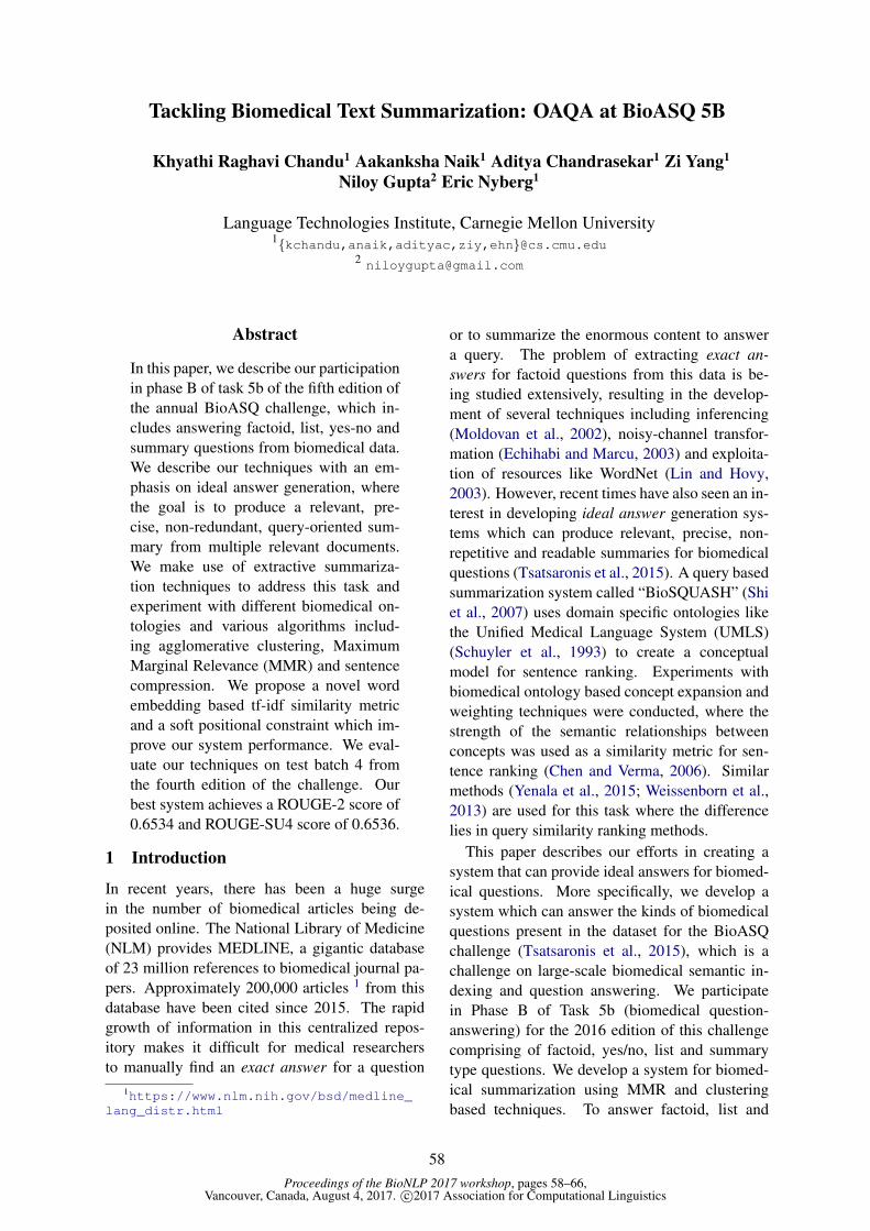
Proceedings of the BioNLP 2017 workshop, pages 58–66,Vancouver, Canada, August 4, 2017. c©2017 Association for Computational Linguistics
Tackling Biomedical Text Summarization: OAQA at BioASQ 5B
Khyathi Raghavi Chandu1 Aakanksha Naik1 Aditya Chandrasekar1 Zi Yang1
Niloy Gupta2 Eric Nyberg1
Language Technologies Institute, Carnegie Mellon University1{kchandu,anaik,adityac,ziy,ehn}@cs.cmu.edu
Abstract
In this paper, we describe our participationin phase B of task 5b of the fifth edition ofthe annual BioASQ challenge, which in-cludes answering factoid, list, yes-no andsummary questions from biomedical data.We describe our techniques with an em-phasis on ideal answer generation, wherethe goal is to produce a relevant, pre-cise, non-redundant, query-oriented sum-mary from multiple relevant documents.We make use of extractive summariza-tion techniques to address this task andexperiment with different biomedical on-tologies and various algorithms includ-ing agglomerative clustering, MaximumMarginal Relevance (MMR) and sentencecompression. We propose a novel wordembedding based tf-idf similarity metricand a soft positional constraint which im-prove our system performance. We eval-uate our techniques on test batch 4 fromthe fourth edition of the challenge. Ourbest system achieves a ROUGE-2 score of0.6534 and ROUGE-SU4 score of 0.6536.
1 Introduction
In recent years, there has been a huge surgein the number of biomedical articles being de-posited online. The National Library of Medicine(NLM) provides MEDLINE, a gigantic databaseof 23 million references to biomedical journal pa-pers. Approximately 200,000 articles 1 from thisdatabase have been cited since 2015. The rapidgrowth of information in this centralized repos-itory makes it difficult for medical researchersto manually find an exact answer for a question
1https://www.nlm.nih.gov/bsd/medline_lang_distr.html
or to summarize the enormous content to answera query. The problem of extracting exact an-swers for factoid questions from this data is be-ing studied extensively, resulting in the develop-ment of several techniques including inferencing(Moldovan et al., 2002), noisy-channel transfor-mation (Echihabi and Marcu, 2003) and exploita-tion of resources like WordNet (Lin and Hovy,2003). However, recent times have also seen an in-terest in developing ideal answer generation sys-tems which can produce relevant, precise, non-repetitive and readable summaries for biomedicalquestions (Tsatsaronis et al., 2015). A query basedsummarization system called “BioSQUASH” (Shiet al., 2007) uses domain specific ontologies likethe Unified Medical Language System (UMLS)(Schuyler et al., 1993) to create a conceptualmodel for sentence ranking. Experiments withbiomedical ontology based concept expansion andweighting techniques were conducted, where thestrength of the semantic relationships betweenconcepts was used as a similarity metric for sen-tence ranking (Chen and Verma, 2006). Similarmethods (Yenala et al., 2015; Weissenborn et al.,2013) are used for this task where the differencelies in query similarity ranking methods.
This paper describes our efforts in creating asystem that can provide ideal answers for biomed-ical questions. More specifically, we develop asystem which can answer the kinds of biomedicalquestions present in the dataset for the BioASQchallenge (Tsatsaronis et al., 2015), which is achallenge on large-scale biomedical semantic in-dexing and question answering. We participatein Phase B of Task 5b (biomedical question-answering) for the 2016 edition of this challengecomprising of factoid, yes/no, list and summarytype questions. We develop a system for biomed-ical summarization using MMR and clusteringbased techniques. To answer factoid, list and
58
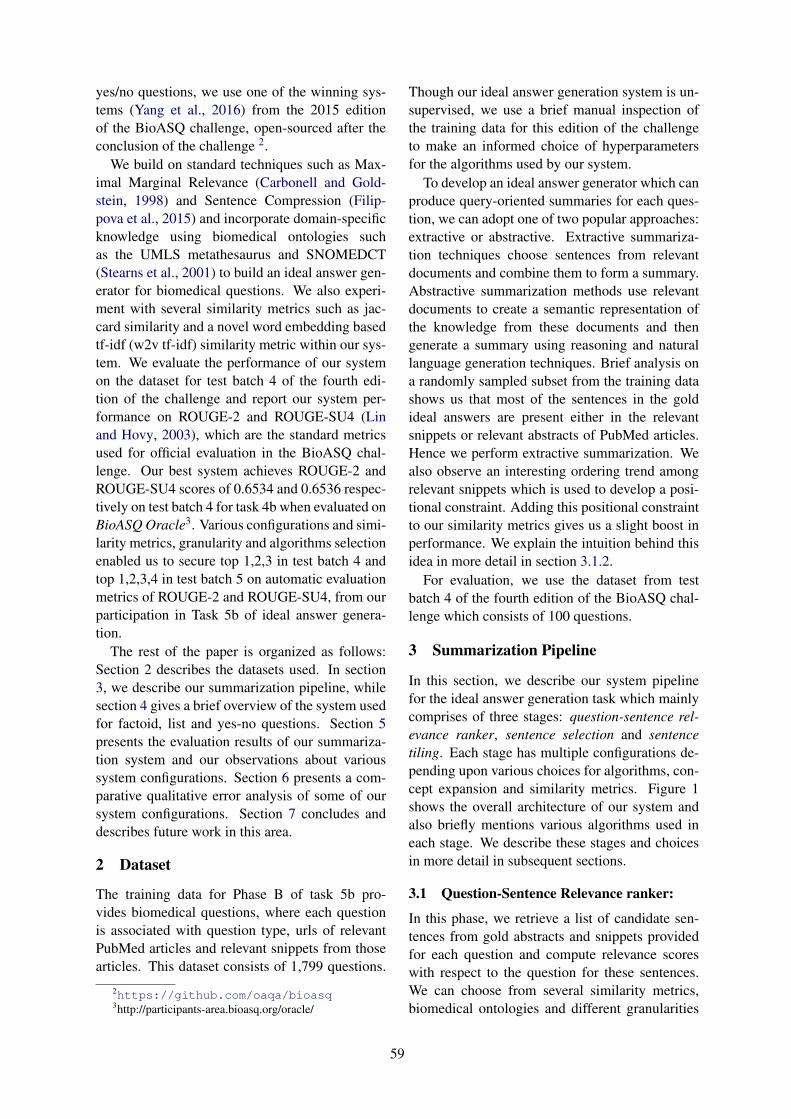
yes/no questions, we use one of the winning sys-tems (Yang et al., 2016) from the 2015 editionof the BioASQ challenge, open-sourced after theconclusion of the challenge 2.
We build on standard techniques such as Max-imal Marginal Relevance (Carbonell and Gold-stein, 1998) and Sentence Compression (Filip-pova et al., 2015) and incorporate domain-specificknowledge using biomedical ontologies suchas the UMLS metathesaurus and SNOMEDCT(Stearns et al., 2001) to build an ideal answer gen-erator for biomedical questions. We also experi-ment with several similarity metrics such as jac-card similarity and a novel word embedding basedtf-idf (w2v tf-idf) similarity metric within our sys-tem. We evaluate the performance of our systemon the dataset for test batch 4 of the fourth edi-tion of the challenge and report our system per-formance on ROUGE-2 and ROUGE-SU4 (Linand Hovy, 2003), which are the standard metricsused for official evaluation in the BioASQ chal-lenge. Our best system achieves ROUGE-2 andROUGE-SU4 scores of 0.6534 and 0.6536 respec-tively on test batch 4 for task 4b when evaluated onBioASQ Oracle3. Various configurations and simi-larity metrics, granularity and algorithms selectionenabled us to secure top 1,2,3 in test batch 4 andtop 1,2,3,4 in test batch 5 on automatic evaluationmetrics of ROUGE-2 and ROUGE-SU4, from ourparticipation in Task 5b of ideal answer genera-tion.
The rest of the paper is organized as follows:Section 2 describes the datasets used. In section3, we describe our summarization pipeline, whilesection 4 gives a brief overview of the system usedfor factoid, list and yes-no questions. Section 5presents the evaluation results of our summariza-tion system and our observations about varioussystem configurations. Section 6 presents a com-parative qualitative error analysis of some of oursystem configurations. Section 7 concludes anddescribes future work in this area.
2 Dataset
The training data for Phase B of task 5b pro-vides biomedical questions, where each questionis associated with question type, urls of relevantPubMed articles and relevant snippets from thosearticles. This dataset consists of 1,799 questions.
2https://github.com/oaqa/bioasq3http://participants-area.bioasq.org/oracle/
Though our ideal answer generation system is un-supervised, we use a brief manual inspection ofthe training data for this edition of the challengeto make an informed choice of hyperparametersfor the algorithms used by our system.
To develop an ideal answer generator which canproduce query-oriented summaries for each ques-tion, we can adopt one of two popular approaches:extractive or abstractive. Extractive summariza-tion techniques choose sentences from relevantdocuments and combine them to form a summary.Abstractive summarization methods use relevantdocuments to create a semantic representation ofthe knowledge from these documents and thengenerate a summary using reasoning and naturallanguage generation techniques. Brief analysis ona randomly sampled subset from the training datashows us that most of the sentences in the goldideal answers are present either in the relevantsnippets or relevant abstracts of PubMed articles.Hence we perform extractive summarization. Wealso observe an interesting ordering trend amongrelevant snippets which is used to develop a posi-tional constraint. Adding this positional constraintto our similarity metrics gives us a slight boost inperformance. We explain the intuition behind thisidea in more detail in section 3.1.2.
For evaluation, we use the dataset from testbatch 4 of the fourth edition of the BioASQ chal-lenge which consists of 100 questions.
3 Summarization Pipeline
In this section, we describe our system pipelinefor the ideal answer generation task which mainlycomprises of three stages: question-sentence rel-evance ranker, sentence selection and sentencetiling. Each stage has multiple configurations de-pending upon various choices for algorithms, con-cept expansion and similarity metrics. Figure 1shows the overall architecture of our system andalso briefly mentions various algorithms used ineach stage. We describe these stages and choicesin more detail in subsequent sections.
3.1 Question-Sentence Relevance ranker:
In this phase, we retrieve a list of candidate sen-tences from gold abstracts and snippets providedfor each question and compute relevance scoreswith respect to the question for these sentences.We can choose from several similarity metrics,biomedical ontologies and different granularities
59

MedlineDocuments
Question+
Snippets
Document list Lucene Indexer
Ranked Sentences + Relevance Scores
Relevance RankerGranularity
Abstracts/SnippetsSimilarity metrics
Jaccard/Tf-idf + Word Embeddings/ Positional Constraints
ExpansionUMLS/SNOMEDCT
Pair-wise Sentence Similarity
Sentence Selection
Agglomerative Clustering
Maximal Marginal Relevance
Sentence Tiling
Concatenation Compression
Ideal Answer
Figure 1: System pipeline for Ideal Answer Generation (with configuration choices)
for sentence scoring in this stage.
3.1.1 Granularity for Candidate SentenceExtraction
The training data provided for the BioASQ taskcontains a list of PubMed IDs of gold relevantdocuments from NLM, along with gold relevantsnippets from these documents, for each question.Since, the training data only contains PubMed IDsof relevant documents, we extract complete ab-stract text for these documents by first indexing allMedline abstracts 4 via Lucene and then retrievingrelevant documents based on PubMed IDs.
We now have two choices of granularity for can-didate sentence extraction: using entire abstracttexts from relevant documents or using only rel-evant snippets. We experiment with both possi-bilities. However, since relevant snippets for eachquestion are a subset of abstract texts, which arehighly relevant to the question, leveraging this in-sight and using only snippets for candidate sen-tence extraction gives us better performance, as wesee from the results in Section 5.
3.1.2 Similarity metricsThe performance of both, the relevance ranker andthe sentence selection phase (which is the follow-ing phase in the pipeline), depends on the sim-ilarity metrics used to capture question-sentencerelevance and sentence-sentence similarity. In
4https://www.nlm.nih.gov/databases/download/pubmed_medline.html
this section, we describe various similarity metricswhich we experiment with.Jaccard similarity: For each sentence, its rele-vance with respect to the question is computed asthe Jaccard index between the sets containing allwords occurring in the question and the sentence.This is the simplest metric which captures surface(word-level) similarity between the question andthe sentence. Including related concepts obtainedby concept expansion in these word sets providessome measure of semantic overlap, but this tech-nique is not very effective as we show in section5.Tf-idf based similarity with word embeddings:Using ontologies such as WordNet (for generalEnglish) and UMLS/ SNOMEDCT (for biomed-ical domain) for concept expansion to incorporatesome semantics while computing sentence simi-larity, is not sufficient due to the unbounded natureof such ontologies. Hence, to assimilate semanticinformation in a more controlled manner, we usea novel similarity metric inspired by the widely-used tf-idf cosine similarity metric which incorpo-rates semantic information by making use of wordembeddings (Mikolov et al., 2013).
Let W represent the symmetric word-to-wordsimilarity matrix and ~a, ~b represent tf-idf vectorsfor the sentences. The similarity metric is definedas:
sim(~a,~b) =~aTW~b√
~aTW~a√~bTW~b
(1)
60

The word-to-word similarity matrix W is com-puted using cosine similarity between word em-beddings for each word. We use word embed-dings which have been pre-trained on PubMed,PMC and Wikipedia articles to incorporate do-main knowledge 5.Similarity function with positional constraints:As described in section 2, the data provided foreach question contains a list of relevant abstractsof PubMed articles, as well as a list of relevantsnippets extracted from these abstracts. The ab-stracts are ordered by relevance. Snippets on theother hand, are not ordered by relevance, but areordered according to the abstracts that they are ex-tracted from. Since the abstracts themselves areordered by relevance, this gives an inherent dis-course structure to the snippets. This observa-tion motivates us to incorporate information abouta snippet’s position in the list into the similarityfunction to improve the summaries generated byour system. We first test this hypothesis usinga simple baseline which gives the first snippet inthe list as the summary for every question. Thissimple baseline is able to achieve good ROUGEscores as shown in Table 1. We experiment withtwo different ways of incorporating this constraint:·Hard positional constraint: In this method, weenforce snippet position as a hard constraint. Weachieve this by restricting the algorithm to selectthe first sentence of the summary from the firstsnippet (most relevant snippet) in the list. Remain-ing sentences can be selected from any snippet.This method does not have much improvement onour ROUGE scores as explained in section 5.· Soft positional constraint: This method in-corporates snippet position as a soft constraintby adding it to the similarity function. Theaugmented similarity function after incorporatingsnippet position is presented below:
positionalSim(q, s) = α ∗ sim(q, s)+(1− α) ∗ rank(s) (2)
Here, q and s denote the question and sentencerespectively; sim(q, s) denotes a function whichcomputes similarity between question and sen-tence (we experiment with Jaccard and tf-idfbased similarities); rank(s) denotes the boost
5 These pre-trained word vectors are pro-vided by http://evexdb.org/pmresources/vec-space-models/
given to the sentence based on the position of thesnippet to which it belongs and α is a weightingparameter. The value of rank(s) for a sentence iscomputed as follows:
rank(s) = 1− pos(s)pos(s) = snippetPos(s)/#snippets
Here, snippetPos(s) denotes the position (index)of the snippet, to which the sentence belongs, inthe list of relevant snippets. If a sentence belongsto multiple snippets, we consider the lowest index.#snippets denotes the number of relevant snip-pets for the current question. This positional boostgives higher weight to sentences with lower posi-tion values (since they occur earlier in the list) andreturns a normalized value in the range 0-1, to en-sure that it is comparable to the range of valuesproduced by the similarity function. Adding thisconstraint boosts our ROUGE scores.
3.1.3 Biomedical Tools and OntologiesWe experiment with various biomedical tools andontologies for concept expansion, in order to in-corporate relations between concepts while com-puting similarity. To perform concept expansion,the first step is to identify biomedical conceptsfrom a sentence. We choose the MetaMap con-cept identification tool and use a python wrapper,pymetamap6 for this purpose. This API identifiesbiomedical concepts from a sentence and returns aConcept Unique Identification (CUI) for each con-cept. This CUI acts as a unique identifier for theconcept which is shared across ontologies, i.e itcan be used as an ID to retrieve the same conceptfrom the UMLS ontology. After biomedical con-cepts are identified, we experiment with two on-tologies for concept expansion: UMLS Metathe-saurus and SNOMEDCT.
• UMLS Metathesaurus: The UMLSMetathesarus contains many types of rela-tions for each biomedical concept. For ourtask, three relation types are of interest to us:‘RB’ (broader relationship), ‘RL’ (similaror alike relationship) and ‘RQ’ (relatedand possibly synonymous relationship).However, none of the biomedical conceptsidentified from questions and sentences in
6https://github.com/AnthonyMRios/pymetamap
61

our training dataset contained relations ofthe type ‘RL’ or ‘RQ’. Hence we performexpansion for each biomedical concept bycollecting all concepts linked to it by the‘RB’ relation.
• SNOMEDCT: The SNOMEDCT ontologydoes not contain CUIs for biomedical con-cepts. Hence, we need to use a differenttechnique to locate concepts in this ontol-ogy. In addition to CUI, pymetamap alsoprovides a “preferred name” for each con-cept. We use this preferred name to perform afull-text search in the SNOMEDCT ontology.All concepts returned by this search are thenconsidered to be related concepts and usedfor expansion. Using this ontology for con-cept expansion returns a much larger numberof related concepts, due to the nature of oursearch (using fuzzy text search instead of pre-cise identifiers).
We use these techniques to perform concept ex-pansion on both questions and sentences from rel-evant snippets. In Section 6, we present the resultsof various system configurations with and withoutdomain specific concept expansion.
3.2 Sentence Selection
In this stage, we want to select sentences for thefinal summary from candidate sentences extractedby the previous stage. Since the BioASQ taskhas a word limit of 200, we limit the number ofsentences selected for the final summary to five.This sentence limit gives us good ROUGE scoresacross multiple system configurations.
The simplest way of performing sentence selec-tion is to continue selecting the sentence with thehighest relevance score with respect to the ques-tion, till the sentence limit is reached. However,sentences having high relevance with respect tothe question may be semantically similar, thus in-troducing redundancy in the generated summary.We use two algorithms to combat this issue: ag-glomerative clustering based on sentence similar-ity and Maximum Marginal Relevance (MMR)(Carbonell and Goldstein, 1998). Both algorithmsrequire effective similarity metrics to compute se-mantic similarity between sentences. We experi-ment with various similarity metrics described insection 3.1.2. We also experiment with conceptexpansion using multiple biomedical ontologies.
3.2.1 Agglomerative ClusteringRedundancy reduction via clustering is one ofthe techniques that was proposed for biomedicalquery-oriented summarization (Chen and Verma,2006). In this technique, we create all possiblesentence pairs from our set of candidate sentencesand compute pair-wise similarities. We then per-form agglomerative clustering on the sentences us-ing these pair-wise similarity scores. Finally, weselect one sentence from each cluster to generatethe final summary, in such a way that the sentencehaving maximum question relevance score is se-lected from every cluster. The number of clus-ters is set to the maximum number of sentenceswe need in the final summary (five in this case).The intuition behind this technique is that agglom-erative clustering forces semantically similar sen-tences to fall into the same cluster. Since we onlyselect one sentence from each cluster in the end,we discard sentences which are highly similar tothe selected ones.
3.2.2 Maximal Marginal RelevanceMaximal Marginal Relevance (Carbonell andGoldstein, 1998) is a widely-used summarizationalgorithm which was proposed to tackle the issueof redundancy while maintaining query relevancein summarization. This algorithm selects new sen-tences based on a combination of relevance scorewith respect to the question as well as similarityscore with respect to the sentences which have al-ready been selected for the final summary. Thus,this algorithm incorporates sentence similarity asa constraint, instead of explicitly clustering sen-tences.
3.3 Sentence TilingIn the final stage, we combine all selected sen-tences to produce the final summary. The simplestway is to append all selected sentences while con-straining summary length (because of the word-limit constraint for this task). We also experi-ment with an LSTM-based sentence compressionmethod. We train a neural network based on awork done previously (Filippova et al., 2015) forsentence compression. We generate training datafor this network by pairing sentences from abstracttexts with their full text versions. Given that thisdataset is too small to train the neural network,we add in training instances from existing sen-tence compression data-sets. Input to this modelincludes the word vector representation for a word
62

Experiment ROUGE-2 ROUGE-SU41 Clustering + Abstract texts (with average constraint) 0.2906 0.31382 Clustering + Snippets (with average constraint) 0.4314 0.43473 Clustering + Snippets (without average constraint) 0.5609 0.56324 Clustering + UMLS expansion 0.5488 0.55215 Clustering + SNOMEDCT expansion 0.5514 0.55866 Clustering + UMLS expansion + weighting 0.5402 0.54317 Clustering + SNOMEDCT expansion + weighting 0.5530 0.55888 Clustering + UMLS expansion + weighted normalization 0.5592 0.56329 Clustering + SNOMEDCT expansion + weighted normalization 0.5585 0.565010 MMR 0.6338 0.629611 MMR + w2v tf-idf similarity 0.6168 0.612612 First snippet baseline 0.3363 0.330813 MMR + Hard positional constraint + Jaccard similarity 0.6338 0.629614 MMR + Soft positional constraint + Jaccard similarity 0.6419 0.641015 Hard positional constraint + Jaccard similarity 0.6328 0.625416 Soft positional constraint + Jaccard similarity 0.6433 0.642917 Soft positional constraint + w2v tf-idf similarity 0.6534 0.653618 MMR + tf-idf similarity + LSTM compression 0.5689 0.5723
Table 1: ROUGE scores with different algorithms, ontologies and similarity metrics
and a binary value to indicate whether the previousword was included in the output sentence. Basedon these inputs, the output of the model predictswhether the word should be deleted or not. Sen-tences generated after word deletion are concate-nated together to generate the final summary. It isto be noted that this model does not require anylinguistic features.
4 Overview of system for exact answergeneration
To answer factoid, list and yes/no questions, weuse the publicly available system (Yang et al.,2016), which builds on participation in 2015(Yang et al., 2015). This system uses TmToolin place of UTS (unlike (Yang et al., 2015)) forconcept identification as some of the constituentparsers of TmTool identify concepts based on mor-phological features instead of previously codedontologies. Also, the c-value method is used tomine frequent multi-word concepts that might nothave been identified by tools such as TmTool,MetaMap and LingPipe. The idea of reranking acandidate answer based on its similarity to othercandidate answers is introduced in this system forlist type questions. The intuition behind this ap-proach is that all answers to a list type questionshould have the same semantic type and therefore,it is useful to increase the score of a low-ranked
candidate answer that has the same semantic type,and vice-versa.
Yes/No questions are answered using the tech-nique of question inversion. The last biomedicalconcept present in the question is considered to bethe expected answer. The concept mentions andtokens of the expected answer are removed fromthe question, which is then converted to a factoidtype question. Candidate answers are generatedfor this factoid question using the snippets for theoriginal question. The expected answer is thencompared to the ranked list of candidate answersretrieved. The answer to the yes/no type questionwill be yes if the expected answer is among the topranked candidate answers and no otherwise.
5 Evaluation and Discussion
We experiment with ideal answer generation usingvarious system configurations which differ in sim-ilarity metrics, biomedical ontologies, sentenceselection algorithms(clustering/MMR) and tilingalgorithms used. The official evaluation for idealanswers includes manual evaluation by biomedi-cal experts in the BioASQ team as well as auto-matic evaluation via ROUGE scores. To presentcomparable and standardized results, we run oursystem on the batch 4 dataset for Phase B of task4b and get our results evaluated via the BioASQOracle. These results are shown in Table 1. We
63

Category Question/Summary
Question What is the effect that EZH2 has on chromatin?
Gold Ideal Answer
Ez that catalyzes di- and trimethylation of histone H3 lysine 27 (H3K37me2/3), marks repressive to transcription.[1] The mammalian homologs Ezh1 and Ezh2 form similar PRC2 complexes but exhibit contrasting repressive roles.[2] PRC2-Ezh2 catalyzes H3K27me2/3 and its knockdown affects global H3K27me2/3 levels.[3] EZH2 thus maintains chromatin in a repressive state.
Clustering + Snippets
During progenitor cell differentiation and ageing, PcG silencer EZH2 attenuates, causing loss of PRC binding and transcriptional activation of INK4b and INK4a Treg-specific ablation of Ezh2 resulted in spontaneous autoimmunity with reduced Foxp3(+) cells in non-lymphoid tissues and impaired resolution of experimental autoimmune encephalomyelitis We report that the mammalian homologs Ezh1 and Ezh2 form similar PRC2 complexes but exhibit contrasting repressive roles.[2] In this study, we found the inverse correlation between FOXP3 and Ezh2, an enzyme for histone H3K27 trimethylation (H3K27me3) and a central epigenetic regulator in cancer the PRC2-Ezh2 complex, which is bound to the myogenin (MyoG) promoter and muscle creatine kinase (mCK) enhancer in proliferating myoblasts, and the PRC2-Ezh1 complex, which replaces PRC2-Ezh2 on MyoG promoter in post-mitotic myotubes.
Clustering + UMLS expansion + weighted normalization
During progenitor cell differentiation and ageing, PcG silencer EZH2 attenuates, causing loss of PRC binding and transcriptional activation of INK4b and INK4a. We report that the mammalian homologs Ezh1 and Ezh2 form similar PRC2 complexes but exhibit contrasting repressive roles. [2] Treg-specific ablation of Ezh2 resulted in spontaneous autoimmunity with reduced Foxp3(+) cells in non-lymphoid tissues and impaired resolution of experimental autoimmune encephalomyelitis Ez that catalyzes di- and trimethylation of histone H3 lysine 27 (H3K37me2/3) [3], marks repressive to transcription.[1] the PRC2-Ezh2 complex, which is bound to the myogenin (MyoG) promoter and muscle creatine kinase (mCK) enhancer in proliferating myoblasts, and the PRC2-Ezh1 complex, which replaces PRC2-Ezh2 on MyoG promoter in post-mitotic myotubes.
Clustering + SNOMEDCT expansion + weighted normalization
During progenitor cell differentiation and ageing, PcG silencer EZH2 attenuates, causing loss of PRC binding and transcriptional activation of INK4b and INK4a Treg-specific ablation of Ezh2 resulted in spontaneous autoimmunity with reduced Foxp3(+) cells in non-lymphoid tissues and impaired resolution of experimental autoimmune encephalomyelitis We report that the mammalian homologs Ezh1 and Ezh2 form similar PRC2 complexes but exhibit contrasting repressive roles.[2] Ez that catalyzes di- and trimethylation of histone H3 lysine 27 (H3K37me2/3), marks repressive to transcription.[1] the PRC2-Ezh2 complex, which is bound to the myogenin (MyoG) promoter and muscle creatine kinase (mCK) enhancer in proliferating myoblasts, and the PRC2-Ezh1 complex, which replaces PRC2-Ezh2 on MyoG promoter in post-mitotic myotubes.
MMR Ezh1 and Ezh2 maintain repressive chromatin through different mechanisms.[1] The chromatin-modifying enzyme Ezh2 is critical for the maintenance of regulatory T cell identity after activation. Treg-specific ablation of Ezh2 resulted in spontaneous autoimmunity with reduced Foxp3(+) cells in non-lymphoid tissues and impaired resolution of experimental autoimmune encephalomyelitis. the PRC2-Ezh2 complex, which is bound to the myogenin (MyoG) promoter and muscle creatine kinase (mCK) enhancer in proliferating myoblasts, and the PRC2-Ezh1 complex, which replaces PRC2-Ezh2 on MyoG promoter in post-mitotic myotubes. In this study, we found the inverse correlation between FOXP3 and Ezh2, an enzyme for histone H3K27 trimethylation (H3K27me3) and a central epigenetic regulator in cancer.
MMR + w2v tf-idf
Ezh1 and Ezh2 maintain repressive chromatin through different mechanisms.[1] In this study, we found the inverse correlation between FOXP3 and Ezh2, an enzyme for histone H3K27 trimethylation (H3K27me3) and a central epigenetic regulator in cancer. These studies reveal a critical role for Ezh2 in the maintenance of Treg cell identity during cellular activation. We report that the mammalian homologs Ezh1 and Ezh2 form similar PRC2 complexes but exhibit contrasting repressive roles.[2] The chromatin-modifying enzyme Ezh2 is critical for the maintenance of regulatory T cell identity after activation.
Soft constraint + w2v tf-idf
Ezh1 and Ezh2 maintain repressive chromatin through different mechanisms.[1] We report that the mammalian homologs Ezh1 and Ezh2 form similar PRC2 complexes but exhibit contrasting repressive roles.[2] Ez that catalyzes di- and trimethylation of histone H3 lysine 27 (H3K37me2/3), marks repressive to transcription. During progenitor cell differentiation and ageing, PcG silencer EZH2 attenuates, causing loss of PRC binding and transcriptional activation of INK4b and INK4a. the PRC2-Ezh2 complex, which is bound to the myogenin (MyoG) promoter and muscle creatine kinase (mCK) enhancer in proliferating myoblasts, and the PRC2-Ezh1 complex, which replaces PRC2-Ezh2 on MyoG promoter in post-mitotic myotubes.
MMR + w2v tf-idf + LSTM sentence compression
and ezh2 maintain repressive chromatin through different mechanisms.[1] this study , found the inverse correlation between foxp3 and ezh2 , an enzyme for histone h3k27 trimethylation (h3k27me3) and a central epigenetic regulator in cancer . prc2-ezh2 complex , which is bound to the myogenin (myog) promoter and muscle creatine kinase (mck) enhancer in proliferating myoblasts , and the prc2-ezh1 complex , which replaces prc2-ezh2 on myog promoter in post-mitotic myotubes .
Figure 2: Summaries generated with different techniques
obtain the best results among these configurationsby using soft positional constraint with tf-idf basedsimilarity on snippets.
The first three rows in Table 1 show our experi-ments with different granularities for sentence ex-traction. While using abstract texts for sentenceselection, we observe that our clustering techniquefrequently puts sentences with low query rele-vance into the same clusters. Since our selec-tion method picks one sentence from each clus-ter, some sentences with low query relevance fromthese “bad” clusters are also selected for the finalsummary. To solve this issue, we imposed a con-straint which filtered out sentences having a lower-than-average relevance score with respect to thequestion before clustering. We also tried addingthis constraint while using relevant snippets, butthis reduced our scores, because sentences fromsnippets are already relevant to the question andwe end up discarding important information by fil-
tering. We also observed that switching granular-ity from abstract texts to relevant snippets signifi-cantly boosted the ROUGE scores. Hence all sub-sequent experiments (rows 4-18) use snippets forsentence extraction.
Rows 4-9 show our experiments with conceptexpansion using various biomedical ontologiesand weighting techniques. We use the followingweighting technique: while calculating similarity,words from the original question and sentencescarry a weight of 1, while words obtained addedafter concept expansion carry a weight of 0.5. Wedo not observe significant gains using concept ex-pansion. The unbounded nature of concept expan-sion hurts our performance and so we refrain fromusing this technique in further experiments. Row10 shows our experiment using MMR for sentenceselection instead of clustering. MMR provides asignificant boost in ROUGE score. Row 11 showsour experiment with the w2v tf-idf based similar-
64

ity metric instead of Jaccard similarity, which de-creases our ROUGE scores slightly, but is stillbetter than previous system configurations. Row12 shows the scores of a baseline system whichreturns the first snippet from the list, which isquite high, validating our assumption that snip-pet position is an important factor. Rows 13-17 shows our experiments with different waysof adding positional constraints described in sec-tion 3.1.2. While using a hard constraint doesnot show much improvement, soft positional con-straint gives a slight boost. Results with and with-out MMR for this metric are nearly comparable.Soft constraint gives a huge boost when used withw2v tf-idf based similarity. Row 18 shows our ex-periment adding LSTM-based compression on topof MMR with w2v tf-idf based similarity, whichreduces our scores. Row 17 is the system con-figuration with the highest ROUGE score on ourdataset, which uses soft positional constraint withw2v tf-idf similarity.
6 Comparative Qualitative ErrorAnalysis
Figure 2 presents ideal answers generated by someof our system configurations for a randomly se-lected summary question from Task 4b Phase Bdata to provide a comparative qualitative erroranalysis. Each sentence in the ideal gold answeris indexed with a number as shown in the figure.We perform a relative analysis of the extent of in-formation captured by a selected subset of systemconfigurations from Table 1.
The sentence indexed [1] in the gold idealanswer is present word-for-word in summariescreated by two configurations: Clustering +SNOMEDCT expansion + weighted normaliza-tion and Soft constraint + w2v tf-idf. Clustering +UMLS expansion + weighted normalization con-tains a longer version of this sentence. We alsoobserve that this sentence does not contain any ofthe terms from the original question. Hence, sum-maries generated by all configurations using onlyJaccard similarity (Clustering + Snippets, MMR)do not contain this sentence since there is nosurface-level similarity. However, methods whichincorporate some semantic information via wordembeddings (w2v tf-idf similarity) or concept ex-pansion (UMLS/ SNOMEDCT) include this sen-tence in the final summary, which shows that in-corporating semantic information is important to
bridge the vocabulary gap in some situations.The sentence indexed [2] in the gold answer is
present in summaries generated by most of theconfigurations as shown but with extra phrasessuch as ‘We report that’ at the beginning of thesentence. Though the presence of such wordsdoes not have a major impact on automatic scoreslike ROUGE, it influences the manual evaluationwhich also judges summary readability. How-ever, the LSTM-based compression method re-moves these words via deletion. We observe thatthis sentence contains the concept “Ezh2” which isalso present in the question. Hence, some configu-rations which use surface-level similarity (Cluster-ing+Snippets) also pick this sentence for the finalsummary. But this sentence is not present in thesummary generated by the MMR + snippets con-figuration. This happens because many sentencesselected by the algorithm already contain the con-cept “Ezh2” and so this sentence is excluded dueto its similarity to already selected sentences.
7 Conclusion and Future Work
In this paper, we present a system for query-oriented summary generation. Our comparisonof MMR and agglomerative clustering-based tech-niques shows that while clustering selects distinctsentences, it is unable to select sentences withhigh query relevance. This can be improved bylearning hyperparameters like number of clustersand number of sentences to be selected from eachcluster based on the type of question. We planto investigate this in the future. We find thatunbounded concept expansion hurts our systemscores. LSTM-based compression also hurts oursystem scores and we need to investigate uponthis in the future to select the optimal parame-ters for compression ratio in order to maximizerecall and precision. We also find that incorporat-ing word embedding based tf-idf similarity alongwith soft positional constraints outperforms sur-face level word similarity with soft positional con-straints. This is because the former captures bothsemantic information of the content as well as rel-evance to query based on sentence position.
Acknowledgments
This research was supported in parts by grantsfrom Accenture PLC (PI: Anatole Gershman),NSF IIS 1546393 and NHLBI R01 HL122639.
65

ReferencesJaime Carbonell and Jade Goldstein. 1998. The use of
mmr, diversity-based reranking for reordering doc-uments and producing summaries. In Proceedingsof the 21st annual international ACM SIGIR confer-ence on Research and development in informationretrieval. ACM, pages 335–336.
Ping Chen and Rakesh Verma. 2006. A query-basedmedical information summarization system usingontology knowledge. In Computer-Based MedicalSystems, 2006. CBMS 2006. 19th IEEE Interna-tional Symposium on. IEEE, pages 37–42.
Abdessamad Echihabi and Daniel Marcu. 2003. Anoisy-channel approach to question answering. InProceedings of the 41st Annual Meeting on Associa-tion for Computational Linguistics-Volume 1. Asso-ciation for Computational Linguistics, pages 16–23.
Katja Filippova, Enrique Alfonseca, Carlos A Col-menares, Lukasz Kaiser, and Oriol Vinyals. 2015.Sentence compression by deletion with lstms. InEMNLP. pages 360–368.
Chin-Yew Lin and Eduard Hovy. 2003. Auto-matic evaluation of summaries using n-gram co-occurrence statistics. In Proceedings of the 2003Conference of the North American Chapter of theAssociation for Computational Linguistics on Hu-man Language Technology-Volume 1. Associationfor Computational Linguistics, pages 71–78.
Tomas Mikolov, Ilya Sutskever, Kai Chen, Greg S Cor-rado, and Jeff Dean. 2013. Distributed representa-tions of words and phrases and their compositional-ity. In Advances in neural information processingsystems. pages 3111–3119.
Dan I Moldovan, Sanda M Harabagiu, Roxana Girju,Paul Morarescu, V Finley Lacatusu, Adrian Novis-chi, Adriana Badulescu, and Orest Bolohan. 2002.Lcc tools for question answering. In TREC.
Peri L Schuyler, William T Hole, Mark S Tuttle,and David D Sherertz. 1993. The umls metathe-saurus: representing different views of biomedicalconcepts. Bulletin of the Medical Library Associa-tion 81(2):217.
Zhongmin Shi, Gabor Melli, Yang Wang, Yudong Liu,Baohua Gu, Mehdi M Kashani, Anoop Sarkar, andFred Popowich. 2007. Question answering sum-marization of multiple biomedical documents. InAdvances in Artificial Intelligence, Springer, pages284–295.
Michael Q Stearns, Colin Price, Kent A Spackman,and Amy Y Wang. 2001. Snomed clinical terms:overview of the development process and projectstatus. In Proceedings of the AMIA Symposium.American Medical Informatics Association, page662.
George Tsatsaronis, Georgios Balikas, ProdromosMalakasiotis, Ioannis Partalas, Matthias Zschunke,Michael R Alvers, Dirk Weissenborn, AnastasiaKrithara, Sergios Petridis, Dimitris Polychronopou-los, et al. 2015. An overview of the bioasqlarge-scale biomedical semantic indexing and ques-tion answering competition. BMC bioinformatics16(1):138.
Dirk Weissenborn, George Tsatsaronis, and MichaelSchroeder. 2013. Answering factoid questions in thebiomedical domain. BioASQ@ CLEF 1094.
Zi Yang, Niloy Gupta, Xiangyu Sun, Di Xu, Chi Zhang,and Eric Nyberg. 2015. Learning to answer biomed-ical factoid & list questions: Oaqa at bioasq 3b. InCLEF (Working Notes).
Zi Yang, Yue Zhou, and Eric Nyberg. 2016. Learningto answer biomedical questions: Oaqa at bioasq 4b.ACL 2016 page 23.
Harish Yenala, Avinash Kamineni, Manish Shrivastava,and Manoj Kumar Chinnakotla. 2015. Iiith at bioasqchallange 2015 task 3b: Bio-medical question an-swering system. In CLEF (Working Notes).
66

Proceedings of the BioNLP 2017 workshop, pages 67–75,Vancouver, Canada, August 4, 2017. c©2017 Association for Computational Linguistics
Macquarie University at BioASQ 5b – Query-based SummarisationTechniques for Selecting the Ideal Answers
Diego MollaDepartment of Computing
Macquarie UniversitySydney, Australia
Abstract
Macquarie University’s contribution to theBioASQ challenge (Task 5b Phase B) fo-cused on the use of query-based extractivesummarisation techniques for the genera-tion of the ideal answers. Four runs weresubmitted, with approaches ranging froma trivial system that selected the first nsnippets, to the use of deep learning ap-proaches under a regression framework.Our experiments and the ROUGE resultsof the five test batches of BioASQ indi-cate surprisingly good results for the triv-ial approach. Overall, most of our runs onthe first three test batches achieved the bestROUGE-SU4 results in the challenge.
1 Introduction
The main goal of query-focused multi-documentsummarisation is to summarise a collection ofdocuments from the point of view of a particu-lar query. In this paper we compare the use ofvarious techniques for query-focused summarisa-tion within the context of the BioASQ challenge.The BioASQ challenge (Tsatsaronis et al., 2015)started in 2013 and it comprises various tasks cen-tred on biomedical semantic indexing and ques-tion answering. The fifth run of the BioASQ chal-lenge (Nentidis et al., 2017), in particular, hadthree tasks:
• BioASQ 5a: Large-scale online biomedicalsemantic indexing.
• BioASQ 5b: Biomedical semantic questionanswering. This task had two phases:
– Phase A: Identification of relevant infor-mation.
– Phase B: Question answering.
• BioASQ 5c: Funding information extractionfrom biomedical literature.
The questions used in BioASQ 5b were of threetypes: yes/no, factoid, list, and summary. Submis-sions to the challenge needed to provide an exactanswer and an ideal answer. Figure 1 shows ex-amples of exact and ideal answers for each typeof question. We can see that the ideal answersare full sentences that expand the information pro-vided by the exact answers. These ideal answerscould be seen as the result of query-focused multi-document summarisation. We therefore focusedon Task 5b Phase B, and in that phase we didnot attempt to provide exact answers. Instead, ourruns provided the ideal answers only.
In this paper we will describe the techniquesand experiment results that were most relevant toour final system runs. Some of our runs werevery simple, yet our preliminary experiments re-vealed that they were very effective and, as ex-pected, the simpler approaches were much fasterthan the more complex approaches.
Each of the questions in the BioASQ test setscontained the text of the question, the questiontype, a list of source documents, and a list of rele-vant snippets from the source documents. We usedthis information, plus the source documents whichare PubMed abstracts accessible using the URLprovided in the test sets.
Overall, the summarisation process of our runsconsisted of the following two steps:
1. Split the input text (source documents orsnippets) into candidate sentences and scoreeach candidate sentence.
2. Return the n sentences with highest score.
The value of n was determined empirically andit depended on the question type, as shown in Ta-ble 1.
67

yes/no Does Apolipoprotein E (ApoE) have anti-inflammatory activity?
• Exact answer: yes• Ideal answer: Yes. ApoE has anti-inflammatory activity
factoid Which type of lung cancer is afatinib used for?
• Exact answer: EGFR-mutant non small cell lung carcinoma• Ideal answer: Afatinib is a small molecule covalently binding and inhibiting the EGFR, HER2
and HER4 receptor tyrosine kinases. Trials showed promising efficacy in patients with EGFR-mutant NSCLC or enriched for clinical benefit from EGFR tyrosine kinase inhibitors gefitinibor erlotinib.
list Which are the Yamanaka factors?
• Exact answer: [OCT4, SOX2, MYC, KLF4]• Ideal answer: The Yamanaka factors are the OCT4, SOX2, MYC, and KLF4 transcription
factors
summary What is the role of brain natriuretic peptide in traumatic brain injury patients ?
• Exact answer: N/A• Ideal answer: Brain natriuretic peptide concentrations are elevated in patients with traumatic
brain during the acute phase and correlate with poor outcomes. In traumatic brain injury pa-tients higher brain natriuretic peptide concentrations are associated with more extensive SAH,elevated ICP and hyponatremia. Brain natriuretic peptide may play an adaptive role in recoverythrough augmentation of cerebral blood flow.
Figure 1: Examples of questions with their exact and ideal answers in BioASQ 5b.
68

Summary Factoid Yesno List
n 6 2 2 3
Table 1: Value of n (the number of sentences re-turned as the ideal answer) for each question type.
2 Simple Runs
As a first baseline, we submitted a run labelledtrivial that simply returned the first n snippets ofeach question. The reason for this choice was that,in some of our initial experiments, we incorpo-rated the position of the snippet as a feature fora machine learning system. In those experiments,the resulting system did not learn anything andsimply returned the input snippets verbatim. Sub-sequent experiments revealed that a trivial base-line that returned the first snippets of the questionwas very hard to beat. In fact, for the task ofsummarisation of other domains such as news, ithas been observed that a baseline that returns thefirst sentences often outperformed other methods(Brandow et al., 1995).
As a second baseline, we submitted a run la-belled simple that selected the n snippets whatwere most similar to the question. We used co-sine similarity, and we tried two alternatives forcomputing the question and snippet vectors:
tfidf-svd: First, generate the tf.idf vector of thequestion and the snippets. We followedthe usual procedure, and the tf.idf vectorsof these sentences are bag-of-word vectorswhere each dimension represents the tf.idfof a word. Then, reduce the dimensionality ofthe vectors by selecting the first 200 compo-nents after applying Singular Value Decom-position. In contrast with a traditional ap-proach to generate the tf.idf (and SVD) vec-tors where the statistics are based on the in-put text solely (question and snippets in ourcase), we used the text of the question andthe text of the ideal answers of the trainingdata.1 The reason for using this variant wasbased on empirical results during our prelim-inary experiments.
word2vec: Train Word2Vec (Mikolov et al.,1In particular, we used the “TfidfVectorizer” module of
the sklearn toolkit (http://scikit-learn.org) andfitted it with the list of questions and ideal answers. We thenused the “TruncatedSVD” module and fitted it with the tf.idfvectors of the list of questions and ideal answers.
trivial simpletfidf-svd word2vec
Mean F1 0.2157 0.1643 0.1715Stdev F1 0.0209 0.0097 0.0128
Table 2: ROUGE-SU4 of the simple runs.
2013) using a set of over 10 million PubMedabstracts provided by the organisers ofBioASQ. Using these pre-trained word em-beddings, look up the word embeddings ofeach word in the question and the snippet.The vector representing a question (or snip-pet) is the sum of embeddings of each wordin the question (or snippet). The dimensionof the word embeddings was set to 200.
Table 2 shows the F1 values of ROUGE-SU4of the resulting summaries. The table shows themean and the standard deviation of the evalua-tion results after splitting the training data set forBioASQ 5b into 10 folds (for comparison with theapproaches presented in the following sections).
We observe that the trivial run has the best re-sults, and that the run that uses word2vec is secondbest. Our run labelled “simple” therefore used co-sine similarity of the sum of word embeddings re-turned by word2vec.
3 Regression Approaches
For our run labelled regression, we experimentedwith the use of Support Vector Regression (SVR).The regression setup and features are based on thework by Malakasiotis et al. (2015), who reportedthe best results in BioASQ 3b (2015).
The target scores used to train the SVR systemwere the F1 ROUGE-SU4 score of each individualcandidate sentence.
In contrast with the simple approaches de-scribed in Section 2, which used the snippets asthe input data, this time we used all the sentencesof the source abstracts. We also incorporated in-formation about whether the sentence was in facta snippet as described below.
As features, we used:
• tf.idf vector of the candidate sentence. Incontrast with the approach described in Sec-tion 2, The statistics used to determine thetf.idf vectors were based on the text of thequestion, the text of the ideal answers, andthe text of the snippets.
69

• Cosine similarity between the tf.idf vectorof the question and the tf.idf vector of thecandidate sentence.
• The smallest cosine similarity between thetf.idf vector of candidate sentence and thetf.idf vector of each of the snippets relatedto the question. Note that this feature was notused by Malakasiotis et al. (2015).
• Cosine similarity between the sum ofword2vec embeddings of the words in thequestion and the word2vec embeddings of thewords in the candidate sentence. As in ourrun labelled “simple”, we used vectors of di-mension 200.
• Pairwise cosine similarities between thewords of the question and the words of thecandidate sentence. As in the work byMalakasiotis et al. (2015), we used word2vecto compute the word vectors. These wordvectors were the same as used in Section 2.We then computed the pairwise cosine simi-larities and selected the following features:
– The mean, median, maximum, and min-imum of all pairwise cosine similarities.
– The mean of the 2 highest, mean of the 3highest, mean of the 2 lowest, and meanof the 3 lowest.
• Weighted pairwise cosine similarities, alsobased in the work by Malakasiotis et al.(2015). In particular, now each word vec-tor was multiplied by the tf.idf of the word,we computed the pairwise cosine similarities,and we used the mean, median, maximum,minimum, mean of 2 highest, mean of 3 high-est, mean of 2 lowest, and mean of 3 lowest.
Figure 2 shows the result of grid search by vary-ing the gamma parameter of SVR, fixing C to1.0, and using the RBF kernel.2 The figure showsthe result of an extrinsic evaluation that reports theF1 ROUGE-SU4 of the final summary, and the re-sult of an intrinsic evaluation that reports the MeanSquare Error (MSE) between the target and thepredicted SU4 of each individual candidate sen-tence.
We can observe discrepancy between the resultsof the intrinsic and the extrinsic evaluations. This
2We used the Scikit-learn Python package.
Figure 2: Grid search of the Gamma parameterfor the experiments using Support Vector Regres-sion. The continuous lines indicate the mean of10-fold cross-validation over the training data setof BioASQ 5b. The dashed lines indicate 2 × thestandard deviation.
discrepancy could be due to the fact that the dataare highly imbalanced in the sense that most anno-tated SU4 scores in the training data have low val-ues. Consequently, the regressor would attempt tominimise the errors in the low values of the train-ing data at the expense of errors in the high values.But the few sentences with high SU4 scores aremost important for the final summary, and thesehave higher prediction error. This can be observedin the scatter plot of Figure 3, which plots the tar-get against the predicted SU4 in the SVR experi-ments for each value of gamma. The SVR systemhas learnt to predict the low SU4 scores to somedegree, but it does not appear to have learnt to dis-criminate among SU4 scores over a value of 0.4.
Our run labelled “regression” used gamma =0.1 since it gave the best MSE in our intrinsic eval-uation, and Figure 3 appeared to indicate that thesystem learnt best.
4 Deep Learning Approaches
For our run labelled nnr we experimented with theuse of deep learning approaches to predict the can-didate sentence scores under a regression setup.The regression setup is the same as in Section 3.
Figure 4 shows the general architecture of thedeep learning systems explored in our experi-ments. In a pre-processing stage, and not shown inthe figure, the main text of the source PubMed ab-stracts is split into sentences by using the defaultNLTK3 sentence segmenter. The candidate sen-
3http://www.nltk.org
70

Figure 3: Target vs. predicted SU4 in the SVR experiments for various values of gamma.
sent
ence
ques
tion
embeddingmatrix
word embeddings
sentencereduction
questionreduction
sentence embeddings
×similarity
relu linear
Figure 4: Architecture of the regression system.
71

tences and questions undergo a simple preprocess-ing stage that removes punctuation characters, andlowercases the string and splits on blank spaces.Then, these are fed to the system as a sequence oftoken identifiers. Figure 4 shows that the input tothe system is a candidate sentence and the question(as sequences of token IDs). The input is first con-verted to sequences of word embeddings by apply-ing an embedding matrix. The word embeddingstage is followed by a sentence and question re-duction stage that combines the word embeddingsof each sentence into a sentence embedding. Then,the sentence embedding and the question embed-ding are compared by applying a similarity opera-tion, and the vector resulting from the comparisonis concatenated to the sentence embedding for a fi-nal regression comprising of a hidden layer of rec-tilinear units (relu) and a final linear combination.
The weights of all stages are optimised by back-propagation in order to minimise the MSE of thepredicted score at training time. Our experimentsvaried on the approach for sentence and ques-tion reduction, and the approach to incorporate thesimilarity between sentence and question, as de-scribed below.
To produce word embeddings we use word2vec,trained on a collection of over 10 million PubMedabstracts as described in previous sections. Theresulting word embeddings are encoded in the em-bedding matrix of Figure 4. We experimented withthe possibility of adjusting the weights of the em-bedding matrix by backpropagation, but the resultsdid not improve. The results reported in this paper,therefore, used a constant embedding matrix. Weexperimented with various sizes of word embed-dings and chose 100 for the experiments in thispaper.
After obtaining the word embeddings, we ex-perimented with the following approaches to pro-duce the sentence vectors:
Mean: The word embeddings provided byword2vec map words into a dimensionalspace that roughly represents the wordmeanings, such that words that are similarin meaning are also near in the embeddedspace. This embedding space has the prop-erty that some semantic relations betweenwords are also mapped in the embeddedspace (Mikolov et al., 2013). It is thereforenatural to apply vector arithmetics such asthe sum or the mean of word embeddings
of a sentence in order to obtain the sentenceembedding. In fact, this approach has beenused in a range of applications, on its own,or as a baseline against which to compareother more sophisticated approaches toobtain word embeddings, e.g. work by Yuet al. (2014) and Kageback et al. (2014). Toaccommodate for different sentence lengths,in our experiments we use the mean of wordembeddings instead of the sum.
CNN: Convolutional Neural Nets (CNN) wereoriginally developed for image processing,for tasks where the important informationmay appear on arbitrary fragments of the im-age (Fukushima, 1980). By applying a con-volutional layer, the image is scanned forsalient information. When the convolutionallayer is followed by a maxpool layer, themost salient information is kept for furtherprocessing.
We follow the usual approach for the applica-tion of CNN for word sequences, e.g. as de-scribed by Kim (2014). In particular, the em-beddings of the words in a sentence (or ques-tion) are arranged in a matrix where each rowrepresents a word embedding. Then, a set ofconvolutional filters are applied. Each con-volutional filter uses a window of width thetotal number of columns (that is, the entireword embedding). Each convolutional filterhas a fixed height, ranging from 2 to 4 rowsin our experiments. These filters aim to cap-ture salient ngrams. The convolutional filtersare then followed by a maxpool layer.
Our final sentence embedding concatenatesthe output of 32 different convolutional fil-ters, each at filter heights 2, 3, and 4. Thesentence embedding, therefore, has a size of32× 3 = 96.
LSTM: The third approach that we have usedto obtain the sentence embeddings is recur-rent networks, and in particular Long ShortTerm Memory (LSTM). LSTM has been ap-plied successfully to applications that pro-cess sequences of samples (Hochreiter et al.,1997). Our experiments use TensorFlow’simplementation of LSTM cells as describedby Pham et al. (2013).
In order to incorporate the context on the left
72

and right of each word we have used the bidi-rectional variant that concatenates the outputof a forward and a backward LSTM chain.As is usual practice, all the LSTM cells in theforward chain share a set of weights, and allthe LSTM cells in the backward chain sharea different set of weights. This way the net-work can generalise to an arbitrary positionof a word in the sentence. However, we ex-pect that the words of the question behavedifferently from the words of the candidatesentence. He have therefore used four dis-tinct sets of weights, two for the forward andbackward chains of the candidate sentences,and two for the question sentences.
In our experiments, the size of the output of achain of LSTM cells is the same as the num-ber of features in the input data, that is, thesize of the word embeddings. Accountingfor forward and backward chains, and givenword embeddings of size 100, the size of thefinal sentence embedding is 200.
Figure 4 shows how we incorporated the simi-larity between the question and the candidate sen-tence. In particular, we calculated a weighted dotproduct, where the weights wi can be learnt bybackpropagation:
sim(q, s) =∑i
wiqisi
Since the sum will be performed by the subse-quent relu layer, our comparison between the sen-tence and the question is implemented as a simpleelement-wise product between the weights, sen-tence embeddings, and question embeddings.
An alternative similarity metric that we havealso tried is as proposed by Yu et al. (2014). Theirsimilarity metric allows for interactions betweendifferent components of the sentence vectors, byapplying a d× d weight matrix W , where d is thesentence embedding size, and adding a bias term:
simY u(q, s) = qTWs + b
In both cases, the optimal weights and bias arelearnt by backpropagation as part of the completeneural network model of the system.
Table 3 shows the average MSE of 10-fold cross-validation over the training data ofBioASQ 5b. “Tf.idf” is a neural network witha hidden layer of 50 relu cells, followed by a
Method Plain Sim SimYu
Tf.idf 0.00354
SVD 0.00345 0.00334 0.00342
Mean 0.00341 0.00330 0.00331CNN 0.00350 0.00348 0.00349LSTM 0.00344 0.00335 0.00336
Table 3: Average MSE of 10-fold cross-validation.
linear cell, where the inputs are the tf.idf of thewords. “SVD” computes the sentence vectors asdescribed in Section 2, with the only differencebeing that now we chose 100 SVD components(instead of 200) for comparison with the other ap-proaches shown in Table 3.
We observe that all experiments perform betterthan the Tf.idf baseline, but there are no major dif-ferences between the use of SVD and the three ap-proaches based on word embeddings. The systemswhich integrated a sentence similarity performedbetter than those not using it, though the differ-ences when using CNN are negligible. Each cellin Table 3 shows the best results after grid searchesvarying the dropout rate and the number of epochsduring training.
For the “nnr” run, we chose the combination“Mean” and “Sim” of Table 3, since they pro-duced the best results in our experiments (althoughonly marginally better than some of the other ap-proaches shown in the table).
5 Submission Results
At the time of writing, the human evaluations hadnot been released, and only the ROUGE results ofall 5 batches were available. Table 4 shows the F1score of ROUGE-SU4.
Figure 5 shows the same information as a plotthat includes our runs and all runs of other partic-ipating systems with higher ROUGE scores. Thefigure shows that, in the first three batches, onlyone run by another participant was among ourresults (shown as a dashed line in the figure).Batches 4 and 5 show consistent results by ourruns, and improved results of runs of other en-trants.
The results are consistent with our experiments,though the absolute values are higher than thosein our experiments. This is probably because weused the entire training set of BioASQ 5b for ourcross-validation results, and this data is the aggre-
73

System Batch 1 Batch 2 Batch 3 Batch 4 Batch 5
trivial 0.5498 0.4901 0.5832 0.5431 0.4950simple 0.5068 0.5182 0.6186 0.5769 0.5840regression 0.5186 0.4795 0.5785 0.5436 0.4784nnr 0.4192 0.3920 0.5196 0.4445 0.4000
Table 4: ROUGE-SU4 of the 5 batches of BioASQ 2017.
Figure 5: Top ROUGE-SU4 scores of the 5batches of BioASQ 2017.
gation of the training sets of the BioASQ tasks ofprevious years. It is possible that the data of latteryears are of higher quality, and it might be usefulto devise learning approaches that would accountfor this possibility.
6 Conclusions
At the time of writing, only the ROUGE scoresof BioASQ 5b were available. The conclusionspresented here, therefore, do not incorporate anyinsights of the human judgements that are also partof the final evaluation of BioASQ.
Our experiments show that a trivial baselinesystem that returned the first n snippets appearsto be hard to beat. This implies that the order ofthe snippets matters. Even though the judges werenot given specific instructions about the order ofthe snippets, it would be interesting to study whatcriteria they used to present the snippets.
Our runs using regression were not significantlybetter than simpler approaches, and the runs usingdeep learning reported the lowest results. Note,however, that the input features used in the runsusing deep learning did not incorporate informa-tion about the snippets. Table 3 shows that the re-sults using deep learning are comparable to resultsusing tf.idf and using SVD, so it is possible that
an extension of the system that incorporates infor-mation from the snippets would equal or better theother systems.
Note that none of the experiments described inthis paper used information specific to the biomed-ical domain and therefore the methods describedhere could be applied to any other domain.
Acknowledgments
Some of the experiments in this research werecarried out in cloud machines under a MicrosoftAzure for Research Award.
ReferencesRonald Brandow, Karl Mitze, and Lisa F. Rau. 1995.
Automatic condensation of electronic publicationsby sentence selection. Information Processing andManagement 31(5):675–685.
Kunihiko Fukushima. 1980. Neocognitron: A self-organizing neural network model for a mechanismof pattern recognition unaffected by shift in position.Biological Cybernetics 36(4):193–202.
Sepp Hochreiter, Jurgen Schmidhuber, Sepp Hochre-iter, Jurgen Schmidhuber, and Jurgen Schmidhuber.1997. Long short-term memory. Neural Computa-tion 9(8):1735–80.
Mikael Kageback, Olof Mogren, Nina Tahmasebi, andDevdatt Dubhashi. 2014. Extractive summariza-tion using continuous vector space models. In Pro-ceedings of the 2nd Workshop on Continuous VectorSpace Models and their Compositionality (CVSC).pages 31–39.
Yoon Kim. 2014. Convolutional neural networks forsentence classification. Proceedings of the 2014Conference on Empirical Methods in Natural Lan-guage Processing (EMNLP 2014) pages 1746–1751.
Prodromos Malakasiotis, Emmanouil Archontakis, andIon Androutsopoulos. 2015. Biomedical question-focused multi-document summarization: ILSP andAUEB at BioASQ3. In CLEF 2015 Working Notes.
Tomas Mikolov, Kai Chen, Greg Corrado, and JeffreyDean. 2013. Efficient estimation of word represen-tations in vector space. In Proceedings of Workshopat ICLR. pages 1–12.
74

Anastasios Nentidis, Konstantinos Bougiatiotis, Anas-tasia Krithara, Georgios Paliouras, and IoannisKakadiaris. 2017. Results of the fifth edition of theBioASQ Challenge. In Proceedings BioNLP 2017.
Vu Pham, Theodore Bluche, Christopher Kermorvant,and Jerome Louradour. 2013. Dropout improves re-current neural networks for handwriting recognition.Technical report.
George Tsatsaronis, Georgios Balikas, ProdromosMalakasiotis, Ioannis Partalas, Matthias Zschunke,Michael R Alvers, Dirk Weissenborn, AnastasiaKrithara, Sergios Petridis, Dimitris Polychronopou-los, Yannis Almirantis, John Pavlopoulos, Nico-las Baskiotis, Patrick Gallinari, Thierry Artieres,Axel-Cyrille Ngonga Ngomo, Norman Heino, EricGaussier, Liliana Barrio-Alvers, Michael Schroeder,Ion Androutsopoulos, and Georgios Paliouras. 2015.An overview of the BIOASQ large-scale biomedicalsemantic indexing and question answering competi-tion. BMC Bioinformatics 16(1):138.
Lei Yu, Karl Moritz Hermann, Phil Blunsom, andStephen Pulman. 2014. Deep learning for answersentence selection. In NIPS Deep Learning Work-shop. page 9.
75

Proceedings of the BioNLP 2017 workshop, pages 76–79,Vancouver, Canada, August 4, 2017. c©2017 Association for Computational Linguistics
Neural Question Answering at BioASQ 5B
Georg Wiese1,2, Dirk Weissenborn2 and Mariana Neves1
1 Hasso Plattner Institute, August Bebel Strasse 88, Potsdam 14482 Germany2 Language Technology Lab, DFKI, Alt-Moabit 91c, Berlin, Germany
[email protected],[email protected], [email protected]
Abstract
This paper describes our submission to the2017 BioASQ challenge. We participatedin Task B, Phase B which is concernedwith biomedical question answering (QA).We focus on factoid and list question, us-ing an extractive QA model, that is, werestrict our system to output substrings ofthe provided text snippets. At the coreof our system, we use FastQA, a state-of-the-art neural QA system. We extendedit with biomedical word embeddings andchanged its answer layer to be able toanswer list questions in addition to fac-toid questions. We pre-trained the modelon a large-scale open-domain QA dataset,SQuAD, and then fine-tuned the parame-ters on the BioASQ training set. With ourapproach, we achieve state-of-the-art re-sults on factoid questions and competitiveresults on list questions.
1 Introduction
BioASQ is a semantic indexing, question answer-ing (QA) and information extraction challenge(Tsatsaronis et al., 2015). We participated inTask B of the challenge which is concerned withbiomedical QA. More specifically, our system par-ticipated in Task B, Phase B: Given a questionand gold-standard snippets (i.e., pieces of text thatcontain the answer(s) to the question), the systemis asked to return a list of answer candidates.
The fifth BioASQ challenge is taking place atthe time of writing. Five batches of 100 questionseach were released every two weeks. Participatingsystems have 24 hours to submit their results. Atthe time of writing, all batches had been released.
The questions are categorized into differentquestion types: factoid, list, summary and yes/no.
Our work concentrates on answering factoid andlist questions. For factoid questions, the system’sresponses are interpreted as a ranked list of an-swer candidates. They are evaluated using mean-reciprocal rank (MRR). For list questions, the sys-tem’s responses are interpreted as a set of answersto the list question. Precision and recall are com-puted by comparing the given answers to the gold-standard answers. F1 score, i.e., the harmonicmean of precision and recall, is used as the offi-cial evaluation measure 1.
Most existing biomedical QA systems employa traditional QA pipeline, similar in structure tothe baseline system by Weissenborn et al. (2013).They consist of several discrete steps, e.g., named-entity recognition, question classification, andcandidate answer scoring. These systems require alarge amount of resources and feature engineeringthat is specific to the biomedical domain. For ex-ample, OAQA (Zi et al., 2016), which has beenvery successful in last year’s challenge, uses abiomedical parser, entity tagger and a thesaurus toretrieve synonyms.
Our system, on the other hand, is based on aneural network QA architecture that is trained end-to-end on the target task. We build upon FastQA(Weissenborn et al., 2017), an extractive factoidQA system which achieves state-of-the-art resultson QA benchmarks that provide large amounts oftraining data. For example, SQuAD (Rajpurkaret al., 2016) provides a dataset of ≈ 100, 000questions on Wikipedia articles. Our approachis to train FastQA (with some extensions) on theSQuAD dataset and then fine-tune the model pa-rameters on the BioASQ training set.
Note that by using an extractive QA network asour central component, we restrict our system’s
1The details of the evaluation can be found athttp://participants-area.bioasq.org/Tasks/b/eval_meas/
76

End Probabilities p(e|s)End Probabilities p(e|s)
End Scores e(s)End Scores e(s)
... ...Biomedical Embeddings
GloVe Embeddings
Character Embeddings
Context Embeddings Question Embeddings
Start Scores ystart
Start Probabilities pstart
End Scores yend
End Probabilities pendsigmoid softmax
Extractive QA System
Question Type Features
Figure 1: Neural architecture of our system. Ques-tion and context (i.e., the snippets) are mapped di-rectly to start and end probabilities for each con-text token. We use FastQA (Weissenborn et al.,2017) with modified input vectors and an outputlayer that supports list answers in addition to fac-toid answers.
responses to substrings in the provided snippets.This also implies that the network will not be ableto answer yes/no questions. We do, however, gen-eralize the FastQA output layer in order to be ableto answer list questions in addition to factoid ques-tions.
2 Model
Our system is a neural network which takes as in-put a question and a context (i.e., the snippets) andoutputs start and end pointers to tokens in the con-text. At its core, we use FastQA (Weissenbornet al., 2017), a state-of-the-art neural QA system.In the following, we describe our changes to thearchitecture and how the network is trained.
2.1 Network architectureIn the input layer, the context and question to-kens are mapped to high-dimensional word vec-tors. Our word vectors consists of three compo-nents, which are concatenated to form a singlevector:
• GloVe embedding: We use 300-dimensionalGloVe embeddings 2 (Pennington et al.,
2We use the 840B embeddings available here: https://nlp.stanford.edu/projects/glove/
2014) which have been trained on a large col-lection of web documents.
• Character embedding: This embedding iscomputed by a 1-dimensional convolutionalneural network from the characters of thewords, as introduced by Seo et al. (2016).
• Biomedical Word2Vec embeddings: Weuse the biomedical word embeddings pro-vided by Pavlopoulos et al. (2014). Theseare 200-dimensional Word2Vec embeddings(Mikolov et al., 2013) which were trained on≈ 10 million PubMed abstracts.
To the embedding vectors, we concatenate aone-hot encoding of the question type (list or fac-toid). Note that these features are identical for alltokens.
Following our embedding layer, we invokeFastQA in order to compute start and end scoresfor all context tokens. Because end scores are con-ditioned on the chosen start, there are O(n2) endscores where n is the number of context tokens.We denote the start index by i ∈ [1, n], the endindex by j ∈ [i, n], the start scores by yistart, andend scores by yi,jend.
In our output layer, the start, end, and span prob-abilities are computed as:
pistart = σ(yistart) (1)
pi,·end = softmax(yi,·end) (2)
pi,jspan = pistart · pi,jend (3)
where σ denotes the sigmoid function. By com-puting the start probability via the sigmoid ratherthan softmax function (as used in FastQA), we en-able the model to output multiple spans as likelyanswer spans. This generalizes the factoid QA net-work to list questions.
2.2 Training & decoding
Loss We define our loss as the cross-entropy ofthe correct start and end indices. In the case ofmultiple occurrences of the same answer, we onlyminimize the span of the lowest loss.
77

Factoid MRR List F1Batch Single Ensemble Single Ensemble
1 52.0% (2/10) 57.1% (1/10) 33.6% (1/11) 33.5%(2/11)2 38.3% (3/15) 42.6% (2/15) 29.0% (8/15) 26.2%(9/15)3 43.1% (1/16) 42.1% (2/16) 41.5% (2/17) 49.5%(1/17)4 30.0% (3/20) 36.1% (1/20) 24.2% (5/20) 29.3%(4/20)5 39.2% (3/17) 35.1% (4/17) 36.1% (4/20) 39.1%(2/20)Average 40.5% 42.6% 32.9% 35.1%
Table 1: Preliminary results for factoid and list questions for all five batches and for our single andensemble systems. We report MRR and F1 scores for factoid and list questions, respectively. In paren-theses, we report the rank of the respective systems relative to all other systems in the challenge. Thelast row averages the performance numbers of the respective system and question type across the fivebatches.
Optimization We train the network in two steps:First, the network is trained on SQuAD, followingthe procedure by Weissenborn et al. (2017) (pre-training phase). Second, we fine-tune the networkparameters on BioASQ (fine-tuning phase). Forboth phases, we use the Adam optimizer (Kingmaand Ba, 2014) with an exponentially decayinglearning rate. We start with learning rates of10−3 and 10−4 for the pre-training and fine-tuningphases, respectively.
BioASQ dataset preparation During fine-tuning, we extract answer spans from the BioASQtraining data by looking for occurrences of thegold standard answer in the provided snippets.Note that this approach is not perfect as it can pro-duce false positives (e.g., the answer is mentionedin a sentence which does not answer the question)and false negatives (e.g., a sentence answers thequestion, but the exact string used is not in the syn-onym list).
Because BioASQ usually contains multiplesnippets for a given question, we process all snip-pets independently and then aggregate the answerspans, sorting globally according to their probabil-ity pi,jspan.
Decoding During the inference phase, we re-trieve the top 20 answers span via beam searchwith beam size 20. From this sorted list of an-swer strings, we remove all duplicate strings. Forfactoid questions, we output the top five answerstrings as our ranked list of answer candidates. Forlist questions, we use a probability cutoff thresholdt, such that {(i, j)|pi,jspan ≥ t} is the set of answers.We set t to be the threshold for which the list F1score on the development set is optimized.
Ensemble In order to further tweak the perfor-mance of our systems, we built a model ensemble.For this, we trained five single models using 5-foldcross-validation on the entire training set. Thesemodels are combined by averaging their start andend scores before computing the span probabili-ties (Equations 1-3). As a result, we submit twosystems to the challenge: The best single model(according to its development set) and the modelensemble.
Implementation We implemented our systemusing TensorFlow (Abadi et al., 2016). It wastrained on an NVidia GForce Titan X GPU.
3 Results & discussion
We report the results for all five test batches ofBioASQ 5 (Task 5b, Phase B) in Table 1. Notethat the performance numbers are not final, as theprovided synonyms in the gold-standard answerswill be updated as a manual step, in order to reflectvalid responses by the participating systems. Thishas not been done by the time of writing3. Notealso that – in contrast to previous BioASQ chal-lenges – systems are no longer allowed to providean own list of synonyms in this year’s challenge.
In general, the single and ensemble system areperforming very similar relative to the rest of field:Their ranks are almost always right next to eachother. Between the two, the ensemble model per-formed slightly better on average.
On factoid questions, our system has been verysuccessful, winning three out of five batches. On
3The final results will be published at http://participants-area.bioasq.org/results/5b/phaseB/
78

list questions, however, the relative performancevaries significantly. We expect our system to per-form better on factoid questions than list ques-tions, because our pre-training dataset (SQuAD)does not contain any list questions.
Starting with batch 3, we also submitted re-sponses to yes/no questions by always answeringyes. Because of a very skewed class distributionin the BioASQ dataset, this is a strong baseline.Because this is done merely to have baseline per-formance for this question type and because of thenaivety of the method, we do not list or discuss theresults here.
4 Conclusion
In this paper, we summarized the system designof our BioASQ 5B submission for factoid and listquestions. We use a neural architecture which istrained end-to-end on the QA task. This approachhas not been applied to BioASQ questions in pre-vious challenges. Our results show that our ap-proach achieves state-of-the art results on factoidquestions and competitive results on list questions.
ReferencesMartın Abadi, Ashish Agarwal, Paul Barham, Eugene
Brevdo, Zhifeng Chen, Craig Citro, Greg S Corrado,Andy Davis, Jeffrey Dean, Matthieu Devin, et al.2016. Tensorflow: Large-scale machine learning onheterogeneous distributed systems. arXiv preprintarXiv:1603.04467 .
Diederik Kingma and Jimmy Ba. 2014. Adam: Amethod for stochastic optimization. arXiv preprintarXiv:1412.6980 .
Tomas Mikolov, Ilya Sutskever, Kai Chen, Greg S Cor-rado, and Jeff Dean. 2013. Distributed representa-tions of words and phrases and their compositional-ity. In Advances in neural information processingsystems. pages 3111–3119.
Ioannis Pavlopoulos, Aris Kosmopoulos, andIon Androutsopoulos. 2014. Continuousspace word vectors obtained by applyingword2vec to abstracts of biomedical articleshttp://bioasq.lip6.fr/info/BioASQword2vec/.
Jeffrey Pennington, Richard Socher, and Christo-pher D. Manning. 2014. Glove: Global vectors forword representation. In Empirical Methods in Nat-ural Language Processing (EMNLP). pages 1532–1543. http://www.aclweb.org/anthology/D14-1162.
Pranav Rajpurkar, Jian Zhang, Konstantin Lopyrev, andPercy Liang. 2016. Squad: 100,000+ questionsfor machine comprehension of text. arXiv preprintarXiv:1606.05250 .
Minjoon Seo, Aniruddha Kembhavi, Ali Farhadi, andHannaneh Hajishirzi. 2016. Bidirectional attentionflow for machine comprehension. arXiv preprintarXiv:1611.01603 .
George Tsatsaronis, Georgios Balikas, ProdromosMalakasiotis, Ioannis Partalas, Matthias Zschunke,Michael R Alvers, Dirk Weissenborn, AnastasiaKrithara, Sergios Petridis, Dimitris Polychronopou-los, et al. 2015. An overview of the bioasq large-scale biomedical semantic indexing and question an-swering competition. BMC bioinformatics 16(1):1.
Dirk Weissenborn, George Tsatsaronis, and MichaelSchroeder. 2013. Answering factoid questions in thebiomedical domain. BioASQ@ CLEF 1094.
Dirk Weissenborn, Georg Wiese, and Laura Seiffe.2017. Making neural qa as simple as possible butnot simpler. arXiv preprint arXiv:1703.04816 .
Yang Zi, Zhou Yue, and Eric Nyberg. 2016. Learningto answer biomedical questions: Oaqa at bioasq 4b.ACL 2016 page 23.
79

Proceedings of the BioNLP 2017 workshop, pages 80–90,Vancouver, Canada, August 4, 2017. c©2017 Association for Computational Linguistics
End-to-End System for Bacteria Habitat Extraction
Farrokh Mehryary1,2∗, Kai Hakala1,2∗, Suwisa Kaewphan1,2,3∗,Jari Bjorne1, Tapio Salakoski1,3 and Filip Ginter1
1. Turku NLP Group, Department of FT, University of Turku, Finland2. The University of Turku Graduate School (UTUGS), University of Turku, Finland
3. Turku Centre for Computer Science (TUCS), [email protected]
Abstract
We introduce an end-to-end system capa-ble of named-entity detection, normaliza-tion and relation extraction for extractinginformation about bacteria and their habi-tats from biomedical literature. Our sys-tem is based on deep learning, CRF clas-sifiers and vector space models. We trainand evaluate the system on the BioNLP2016 Shared Task Bacteria Biotope data.The official evaluation shows that the jointperformance of our entity detection and re-lation extraction models outperforms thewinning team of the Shared Task by 19ppon F-score, establishing a new top scorefor the task. We also achieve state-of-the-art results in the normalization task.Our system is open source and freelyavailable at https://github.com/TurkuNLP/BHE.
1 Introduction
Knowledge about habitats of bacteria is crucial forthe study of microbial communities, e.g. metage-nomics, as well as for various applications suchas food processing and health sciences. Althoughthis type of information is available in the biomed-ical literature, comprehensive resources accumu-lating the knowledge do not exist (Deleger et al.,2016).
The BioNLP Bacteria Biotope (BB) SharedTasks are organized to provide a common evalua-tion platform for language technology researchersinterested in developing information extractionmethods adapted for the detection of bacteria andtheir physical locations mentioned in the literature.So far three BB shared tasks have been organized,the latest in 2016 (BB3) consisting of three main
∗These authors contributed equally.
subtasks: named entity recognition and catego-rization (BB3-cat and BB3-cat+ner), event extrac-tion (BB3-event and BB3-event+ner) and knowl-edge base extraction. The NER task includes threerelevant entity types: HABITAT, BACTERIA andGEOGRAPHICAL, the categorization task focuseson normalizing the mentions to established ontol-ogy concepts, although GEOGRAPHICAL entitiesare excluded from this task, whereas the event ex-traction aims at finding the relations between theseentities, i.e. extracting in which locations certainbacteria live in. The knowledge base extractiontask is centered upon aggregating this type of in-formation from a large text corpus.
In this paper we revisit the BB3 subtasks ofNER, categorization and event extraction, all ofwhich are essential for building a real-world infor-mation extraction pipeline. As a result, we presenta text mining pipeline which achieves state-of-the-art results for the joint evaluation of NER andevent extraction as well as for the categorizationtask using the official BB3 shared task datasets andevaluation tools. Building such end-to-end sys-tem is important for bringing the results from theshared tasks to the actual intended users. To ourbest knowledge, no such system is openly avail-able for bacteria habitat extraction.
The pipeline utilizes deep neural networks, con-ditional random field classifiers and vector spacemodels to solve the various subtasks and the codeis freely available at https://github.com/TurkuNLP/BHE. In the following sections wediscuss our system, divided into three modules:entity recognition, categorization and event ex-traction. We then analyze the results and finallydiscuss the potential future research directions.
80

2 Method
2.1 Named entity detection
Detecting the BB3 HABITAT, BACTERIA and GE-OGRAPHICAL mentions is a standard named entityrecognition task, evaluated based on the correct-ness of the type and character offsets of the dis-covered text spans. In our NER pipeline, all doc-uments are preprocessed following the approachof Hakala et al. (2016). In brief, we first con-vert all documents and annotation files from UTF-8 to ASCII encoding using a modified versionof publicly available tool designed for parsingPubMed documents (Pyysalo et al., 2013) 1. Nextwe split documents into sentences using the Ge-nia Sentence Splitter (Sætre et al., 2007) and thesentences are subsequently tokenized and part-of-speech tagged using the tokenization and POS-tagging modules in NERsuite 2, respectively.
To detect the entity mentions we use NERsuite,a named entity recognition toolkit, as it is rela-tively easy to train on new corpora, yet supportsadding novel user-defined features. In biomedicalNER, NERsuite has been a versatile tool achiev-ing excellent performance for various entity types(Ohta et al., 2012; Kaewphan et al., 2014, 2016),however, it is not capable of dealing with overlap-ping entities. Therefore, we only use the longestspans of overlapping annotated entities as ourtraining data, ignoring embedded entities whichare substrings of the longest spans.
In biomedical NER, domain knowledge suchas controlled vocabularies has been crucial forachieving high performance. In this work we pre-pare 3 dictionaries, specific for each entity type.For BACTERIA, we compile a dictionary of namesexclusively from the NCBI Taxonomy database3
by including all names under bacteria superking-dom (NCBI taxonomy identifier 2). The scien-tific names are expanded to include abbreviationswhose genus names are conventionally abbrevi-ated with the first and/or second alphabet, whereasthe rest of the names, such as species epithet andstrains, remains unchanged. For HABITAT, wecombine all symbols from the OntoBiotope on-tology 4 and use them without any further mod-ifications. Similar to HABITAT, we also pre-pare dictionary for GEOGRAPHICAL by taking all
1https://github.com/spyysalo/nxml2txt2http://nersuite.nlplab.org/3https://www.ncbi.nlm.nih.gov/taxonomy4http://agroportal.lirmm.fr/ontologies/ONTOBIOTOPE
strings under the semantic type geographical areafrom UMLS database (version 2016AA) (Boden-reider, 2004). All dictionaries prepared in thisstep are directly provided to NERsuite through thedictionary-tagging module without any normaliza-tion. The tagging provides additional features de-scribing whether the tokens are present in somesemantic categories, such as bacteria names or ge-ographical places. For GEOGRAPHICAL model,we also add token-level tagging results for loca-tion from Stanford NER (SNER) (Finkel et al.,2005) as binary values to NERsuite; 1 and 0 forlocation and non-location, respectively.
Although utilizing dictionary features is benefi-cial for NER, strict string matching tends to leadto low coverage, an issue which is also common inthe categorization task. To remedy this problem,we also generate fuzzy matching features basedon our categorization system (see Section 2.2) bymeasuring the maximum similarity of each tokenagainst the NCBI Taxonomy and OntoBiotope on-tologies for BACTERIA and HABITAT respectively.Thus, instead of a binary feature denoting whethera token is present in the ontology or not, a sim-ilarity score ranging from 0 to 1 is assigned foreach token. This approach is similar to (Kaewphanet al., 2014), but instead of using word embeddingsimilarities, our fuzzy matching relies on characterngrams. We do not use these features for the GEO-GRAPHICALentities, which are not categorized byour system.
In the official BB3 evaluation, NER is jointlyevaluated with either categorization or event ex-traction system. In BB3-cat+ner task, SER (SlotError Rate) is used as the main scoring metric,whereas in BB3-event+ner, participating teamsare ranked based on F-score of extracted rela-tions. Due to the lack of an official evaluationon NER for all entities in BB3-event+ner andfor GEOGRAPHICAL in BB3-cat+ner, we use ourown implementation by calculating the F-scoreusing exact string matching criteria as our mainscoring metric. In this study, we consider BB3-event+ner as our primary subtask and thus allhyper-parameters in model selection are optimizedagainst F-score instead of SER.
2.2 Named entity categorization
In the BB3 categorization subtask each BACTE-RIA and HABITAT mention has to be assigned tothe corresponding ontology concepts, specifically
81

to NCBI Taxonomy and OntoBiotope identifiersrespectively. This task is commonly known asnamed entity normalization or entity linking andvarious approaches ranging from Levenshtein editdistances to recurrent neural networks have beensuggested as the plausible solutions (Tiftikci et al.,2016; Limsopatham and Collier, 2016).
Our categorization method is based on the com-mon approach of TFIDF weighted sparse vectorspace representations (Salton and Buckley, 1988;Leaman et al., 2013; Hakala, 2015), i.e. the prob-lem is seen as an information retrieval task whereeach concept name in the ontology is considereda document and the IDF weights are based onthese names. Consequently, each concept nameand each entity mention is represented with aTFIDF weighted vector and the concept with thehighest cosine similarity is assigned for a givenentity. Whereas these representations are com-monly formed in a bag-of-words fashion, in ourexperiments using character-level ngrams resultedin better outcome. In the final system we usengrams of length 1, 2 and 3 characters. Thesengram lengths produced the highest accuracy onthe official development set for both BACTERIA
and HABITAT entities, each entity type evaluatedseparately. The TFIDF vectorization was imple-mented using the scikit-learn library (Pedregosaet al., 2011) and default parameter values exceptfor using the character level ngrams instead ofwords.
For both included ontologies we use the pre-ferred names as well as the listed synonyms torepresent the concepts. Since the task is restrictedto bacteria mentions instead of all organisms, wealso narrow down the NCBI Taxonomy ontologyto cover only the Bacteria superkingdom, i.e. thecategorization system is not allowed to assign tax-onomy identifiers which do not belong to this su-perkingdom. Otherwise all concepts from the usedontologies are included.
As preprocessing steps we use three main ap-proaches: abbreviation expansion, acronym ex-pansion and stemming. For stemming we use thePorter stemmer (Porter, 1980) and stem each to-ken in the entities and concept names. Accord-ing to our evaluation this is not beneficial for theBACTERIA entities and is thus included only forthe HABITAT entities.
In biomedical literature the genus names inBACTERIA mentions are commonly shortened af-
ter the first mention, e.g. Staphylococcus aureusis abbreviated as S. aureus, but the NCBI Taxon-omy ontology does not include these abbreviatedforms as synonyms for the corresponding con-cepts. Thus, if an entity mention includes a tokenwith a period in it, we expand the given token byfinding the most common token with the same ini-tial from all previously mentioned entities of thesame type within the same document.
Another commonly used naming convention forBACTERIA mentions is forming acronyms, e.g.lactic acid bacteria is often referred to as LAB.Consequently, when we detect a BACTERIA men-tion with less than five characters or written inuppercase, we try to find the corresponding fullform by generating acronyms for all previouslymentioned BACTERIA entities by simply concate-nating their initials. However, many BACTERIA
acronyms do not follow this format strictly, e.gLactobacillus casei strain Shirota should be short-ened to LcS instead of LCSS and Francisella tu-larensis Live Vaccine Strain as LVS instead ofFTLVS. Thus, instead of using strict matchingto find the corresponding full form, we utilizethe same character-level TFIDF representationsas used for the actual categorization for theseacronyms to find the most similar full form. In ourevaluation, using the same approach for HABITAT
entities dramatically decreased the performancehence was thus not used for this entity type (seeSection 3.2).
Both of these expansion methods have similarintentions as the preprocessing steps utilized bythe winning system in BB3 (BOUN) by Tiftikciet al. (2016), but our system uses more relaxedcriteria for finding the full forms and should thusresult in better recall at the expense of precision.
2.3 Event extraction
The BB3-event and BB3-event+ner tasks demandextraction of undirected binary associations of twonamed entities: a BACTERIA entity and either aHABITAT or a GEOGRAPHICAL entity; and theserelations represent the locations in which bacterialive. We thus formulate this task as a binary clas-sification task and assign the label positive if suchrelation holds for a given entity pair and negativeotherwise.
To address this task, we present a deep learning-based relation extraction system that generatesfeatures along the shortest dependency path (SDP)
82

Train Devel TestTotal sentences 527 319 508Sentences w/examples 158 117 158Sentences w/o examples 369 202 350Total examples 524 506 534Positive examples 251 177 -Negative examples 273 329 -
Table 1: BB3-event data statistics.
which connects the two candidate entities in thesyntactic parse graph. Many successful relationextraction systems have been built utilizing SDP(Cai et al., 2016; Mehryary et al., 2016; Xu et al.,2015; Bjorne and Salakoski, 2013; Bjorne et al.,2012; Bunescu and Mooney, 2005) since it isknown to contain most of the relevant words forexpressing the relation between the two entitieswhile excluding less relevant and uninformativewords. Since this approach focuses on a singlesentence parse graph at a time, it is unable to detectplausible cross-sentence relations, i.e, the cases inwhich the two candidate entities belong to differ-ent sentences. As discussed by Kim et al. (2011),detecting such relations is a major challenge forrelation extraction systems. We simply excludeany cross-sentence relations from training, devel-opment and test sets.5 Table 1 summarizes thestatistics of the data that is used for building ourrelation extraction system after removing cross-sentence relations.
2.3.1 PreprocessingFor preprocessing, we use the preprocessingpipeline of the TEES system (Bjorne andSalakoski, 2013) which automates tokenization,part-of-speech tagging and sentence parsing.TEES runs the BLLIP parser (Charniak and John-son, 2005) with the biomedical domain model cre-ated by McClosky (2010). The resulting phrasestructure trees are then converted to dependencygraphs (nonCollapsed variant of Stanford Depen-dency) using the Stanford conversion tool (version2.0.1) (de Marneffe et al., 2006).
2.3.2 Relation extraction system architectureThe architecture of our deep learning-based rela-tion extraction system is centered around utiliz-ing three separate convolutional neural networks(CNN): for the sequence of words, the sequence of
5Official evaluation results on the development and testdata are of course comparable to those of other systems: anycross-sentence relations in the development/test data countagainst our submissions as false negatives.
POS tags, and the sequence of dependency types(the edges of the parse graph), along the SDP con-necting the two candidate entities (see Figure 1).Even though the parse graph is directed, we re-gard it as an undirected graph and always traversethe SDP by starting the path from the BACTERIA
entity mention to the HABITAT/GEOGRAPHICAL,regardless of the order of their occurrence in thesentence. Evaluation against the development setshowed that this approach leads to better general-ization in comparison with simply traversing thepath from the first occurring entity mention to thesecond (with/without considering the direction ofthe edges).
The structure of each CNN is similar: the words(or POS tags or dependency types) in the sequenceare mapped into their corresponding vector repre-sentations using an embedding lookup layer. Theresulting sequence of vectors is then forwardedinto a convolutional layer which creates a convo-lution kernel that is applied on the layer input overa single spatial dimension to produce a tensor ofoutputs. These outputs are then forwarded to amax-pooling layer that gathers information fromlocal features of the SDP. Hence, the three CNNsproduce three vector representations.
Subsequently, the output vectors of the CNNsand two 1-hot-encoded entity-type vectors areconcatenated. The first entity-type vector repre-sents the type of the first occurring entity in thesentence (BACTERIA, HABITAT or GEOGRAPH-ICAL), and the other is used for the second one.The resulting vector is then forwarded into a fullyconnected hidden layer and finally, the hiddenlayer connects to a single-node binary classifica-tion layer.
For the word features, we use a vector spacemodel with 200-dimensional word embeddingspre-trained by Pyysalo et al. (2013). These arefine-tuned during the training while the POS-tagand dependency type embeddings are learned fromscratch after being randomly initialized.
Based on experiments on the development set,we have set the dimensionality of the POS tag em-beddings to 200, and for dependency types to 300.For all convolutional layers, the number of filtershas been set to 100 and the window size (filterlength) to 4. Finally, dimensionality of the hid-den layer has been set to 100.The ReLU activationfunction is applied on the output of the convolu-tional layers while we apply sigmoid activation to
83

detection NN products NNSSalmonellae NNP nn prep
detection products NNP NN NNS nn prep
Concatenate
Fully connected
Fully connected
CNNs/max-pooling
Embedding
Input sentence + candidate entities
Shortest path+ target type
Habitat
Salmonellae
words parts of speech dependencies
in
convolution/max-pooling
IN pobj
convolution/max-pooling convolution/max-pooling
in IN pobj
Figure 1: Proposed network architecture.
the output of the hidden layer.
2.3.3 Training and optimization
We use binary cross-entropy as the objectivefunction and the Adam optimization algorithm(Kingma and Ba, 2014) for training the network.Applying the dropout (Srivastava et al., 2014) withrate of 50% on the output of the hidden layer is theonly network regularization method used to avoidoverfitting.
When the number of weights in a neural net-work is high and the training set is very small (e.g.,there are only 524 examples in the BB3-eventtraining set), the initial random state of the modelcan have a significant impact on the final modeland its generalization performance. Mehryaryet al. (2016) have reported that the F-score on thedevelopment set of BB3-event task can vary up to9 percentage points based on the different initialrandom state of the network.
To overcome this problem, we implement thesimple but effective strategy proposed by them,which consists of training the neural networkmodel 15 times with different initial randomstates, predicting the development/test set exam-ples and aggregating the 15 classifiers’ predictionsusing a simple voting algorithm.
For each development/test example, the votingalgorithm combines the predictions based on agiven threshold parameter t: the relation is voted
to be positive if at least t classifiers have predictedit to be positive, otherwise, it will be considered asa negative. Obviously, the lowest threshold value(t = 1) produces the highest recall and lowest pre-cision and the highest threshold (t = 15) producesthe highest precision and lowest recall and the aimis to find be best threshold value which maximizesthe F-score.
Our experiments on the development set (us-ing the proposed network architecture) showedthat for the BB3-event task the optimal resultsare achieved when we train the networks for 2epochs and set the threshold value to 4, and for theBB3-event+ner task, when we train the networksfor 2 epochs and set the threshold value to 3.
3 Results and discussion
3.1 Named entity detectionFor the named entity detection task, we obtainthe baseline performance by training NERsuite foreach entity-type independently. As shown in Ta-ble 2, the F-scores for BACTERIA, GEOGRAPH-ICAL and HABITAT are 0.713, 0.516 and 0.482respectively. The baseline performance of HABI-TAT and GEOGRAPHICAL models is significantlylower than BACTERIA.
For all entities, adding dictionary features im-proves the performance of the model. A substan-tial improvement in F-score is found for GEO-GRAPHICAL where the performance is increased
84

Entity/Experiment Precision Recall F-scoreBacteriaBB3 0.787 0.652 0.713BB3 + dict 0.833 0.697 0.759BB3 + tfidf 0.793 0.660 0.720BB3 + tfidf + dict 0.822 0.717 0.766BB3 + BB2 + dict 0.902 0.713 0.796BB3 + BB1 + dict 0.893 0.721 0.798HabitatBB3 0.589 0.407 0.482BB3 + dict 0.649 0.465 0.541BB3 + tfidf 0.697 0.482 0.570BB3 + tfidf + dict 0.715 0.520 0.602BB3 + BB2 + dict 0.560 0.500 0.529GeographicalBB3 0.667 0.421 0.516BB3 + dict 0.719 0.605 0.657BB3 + SNER 0.694 0.658 0.676BB3 + dict + SNER 0.788 0.684 0.732BB3 + BB2 + dict 0.903 0.737 0.812
Table 2: The performance of our named entity de-tection system on BACTERIA, HABITAT and GE-OGRAPHICAL mentions using internal evaluationsystem. The models are evaluated on the BB3 de-velopment data.
by more than 14pp compared to 6pp and 5pp forHABITAT and BACTERIA, respectively. Addingfuzzy matching features further improves the F-score for HABITAT by more than 12pp comparedto 8pp for BACTERIA. This result shows that hav-ing both domain knowledge and relaxed matchingcriteria can significantly enhance the model per-formance.
We improve equally the baseline performancefor GEOGRAPHICAL by adding features fromSNER tagging. The increase in F-score, 0.657versus 0.676, is about the same as independentlyadding UMLS-geographical area dictionary fea-tures. Further increase in F-score is achieved bycombining both features, likely due to the ex-panded coverage of geographical names.
The BB3 corpus is relatively small in terms ofentity frequency and the number of unique entities.We explore the possibility of increasing modelperformance through adding additional trainingdata from previously organized BB Shared Tasks(i.e, BB1 (Bossy et al., 2011) and BB2 (Bossyet al., 2013)). Annotations for BACTERIA men-tions are available in both BB1 and BB2 SharedTasks and we thus train NERsuite models byadding these annotations to the training data. Theresults show that the models, trained with addi-tional datasets, achieve higher performance. BB1provides a slightly better F-score than BB2, 0.798vs 0.796.
For GEOGRAPHICAL and HABITAT entities,compatible annotations are only available fromBB2 (Bossy et al., 2013), subtask 2. We thus trainNERsuite for both HABITAT and GEOGRAPHI-CAL by using combined BB3 and BB2 data. Theresult for GEOGRAPHICAL is similar to the oneobserved with BACTERIA and additional data canincrease the model F-score by more than 15pp.However, the result for HABITAT is different asF-score slightly drops from 0541 to 0.529. Thebest NER model for HABITAT thus remains un-changed.
Finally, we train our final model by combiningtraining and development datasets and use hyper-parameters obtained from the best performing sys-tem on development dataset. The official evalua-tion of the NER task jointly with either catego-rization or event extraction system is discussed inSection 3.2 and Section 3.3, respectively.
3.2 Categorization
To analyze our categorization approaches, weevaluate their performance on the official develop-ment set. During the development we used accu-racy for evaluating the effects of different hyper-parameters and preprocessing steps. To get com-parable results to previous systems we, however,report the results in this paper using the precisionscores from the official evaluation service. As theused ontologies form hierarchical structures, theofficial evaluation penalizes the incorrect predic-tions based on the distance from the gold standardannotations, whereas our internal accuracy evalua-tion measures exact matches. Our accuracy scoresand the official evaluation seem to correlate to thelevel that all improvements validated using the ac-curacy score also improved the performance ac-cording to the official evaluation.
The performance of our system and various pre-processing steps are shown incrementally in Ta-ble 3. As a baseline system we use TFIDF bag-of-words representations without any of our pre-processing steps. By simply switching to charac-ter level representations the precision is increasedby 1.3pp for HABITAT and 14.1pp for BACTERIA
mentions.Adding the abbreviation expansion step further
improves precision for BACTERIA by 14.1pp, butdoes not influence HABITAT entities as most likelythere are no abbreviated mentions in this category.The acronym expansion has a lesser, but still no-
85
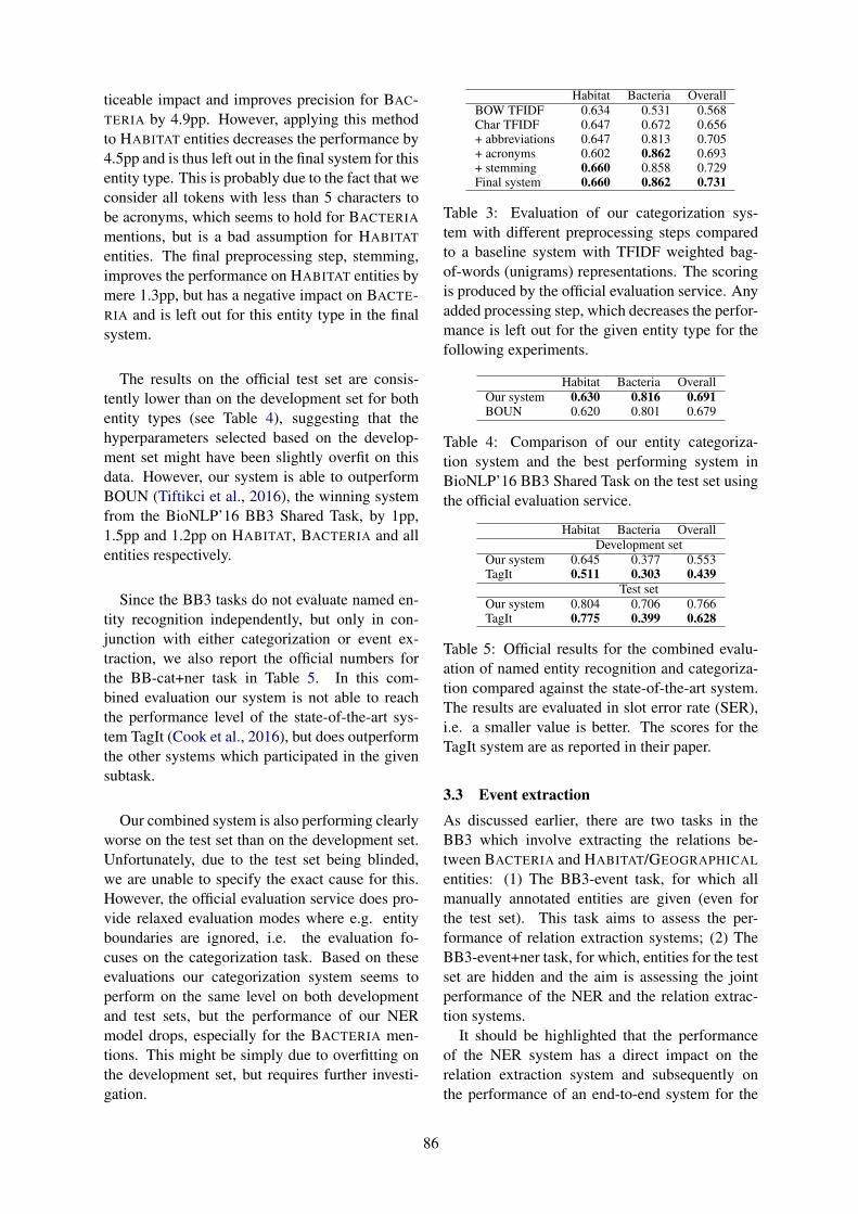
ticeable impact and improves precision for BAC-TERIA by 4.9pp. However, applying this methodto HABITAT entities decreases the performance by4.5pp and is thus left out in the final system for thisentity type. This is probably due to the fact that weconsider all tokens with less than 5 characters tobe acronyms, which seems to hold for BACTERIA
mentions, but is a bad assumption for HABITAT
entities. The final preprocessing step, stemming,improves the performance on HABITAT entities bymere 1.3pp, but has a negative impact on BACTE-RIA and is left out for this entity type in the finalsystem.
The results on the official test set are consis-tently lower than on the development set for bothentity types (see Table 4), suggesting that thehyperparameters selected based on the develop-ment set might have been slightly overfit on thisdata. However, our system is able to outperformBOUN (Tiftikci et al., 2016), the winning systemfrom the BioNLP’16 BB3 Shared Task, by 1pp,1.5pp and 1.2pp on HABITAT, BACTERIA and allentities respectively.
Since the BB3 tasks do not evaluate named en-tity recognition independently, but only in con-junction with either categorization or event ex-traction, we also report the official numbers forthe BB-cat+ner task in Table 5. In this com-bined evaluation our system is not able to reachthe performance level of the state-of-the-art sys-tem TagIt (Cook et al., 2016), but does outperformthe other systems which participated in the givensubtask.
Our combined system is also performing clearlyworse on the test set than on the development set.Unfortunately, due to the test set being blinded,we are unable to specify the exact cause for this.However, the official evaluation service does pro-vide relaxed evaluation modes where e.g. entityboundaries are ignored, i.e. the evaluation fo-cuses on the categorization task. Based on theseevaluations our categorization system seems toperform on the same level on both developmentand test sets, but the performance of our NERmodel drops, especially for the BACTERIA men-tions. This might be simply due to overfitting onthe development set, but requires further investi-gation.
Habitat Bacteria OverallBOW TFIDF 0.634 0.531 0.568Char TFIDF 0.647 0.672 0.656+ abbreviations 0.647 0.813 0.705+ acronyms 0.602 0.862 0.693+ stemming 0.660 0.858 0.729Final system 0.660 0.862 0.731
Table 3: Evaluation of our categorization sys-tem with different preprocessing steps comparedto a baseline system with TFIDF weighted bag-of-words (unigrams) representations. The scoringis produced by the official evaluation service. Anyadded processing step, which decreases the perfor-mance is left out for the given entity type for thefollowing experiments.
Habitat Bacteria OverallOur system 0.630 0.816 0.691BOUN 0.620 0.801 0.679
Table 4: Comparison of our entity categoriza-tion system and the best performing system inBioNLP’16 BB3 Shared Task on the test set usingthe official evaluation service.
Habitat Bacteria OverallDevelopment set
Our system 0.645 0.377 0.553TagIt 0.511 0.303 0.439
Test setOur system 0.804 0.706 0.766TagIt 0.775 0.399 0.628
Table 5: Official results for the combined evalu-ation of named entity recognition and categoriza-tion compared against the state-of-the-art system.The results are evaluated in slot error rate (SER),i.e. a smaller value is better. The scores for theTagIt system are as reported in their paper.
3.3 Event extractionAs discussed earlier, there are two tasks in theBB3 which involve extracting the relations be-tween BACTERIA and HABITAT/GEOGRAPHICAL
entities: (1) The BB3-event task, for which allmanually annotated entities are given (even forthe test set). This task aims to assess the per-formance of relation extraction systems; (2) TheBB3-event+ner task, for which, entities for the testset are hidden and the aim is assessing the jointperformance of the NER and the relation extrac-tion systems.
It should be highlighted that the performanceof the NER system has a direct impact on therelation extraction system and subsequently onthe performance of an end-to-end system for the
86

BB3-event+ner task. On one hand, if the NERsystem produces extremely low recall outputs, therelation extraction system will fail to extract someof the valid relations, simply because it only inves-tigates the existence of possible relations amongthe given entities. On the other hand, if the NERsystem provides high recall but very low precisionpredictions, this means that words mistakenly de-tected as valid entities are given to the relationextraction system. For each given entity, the re-lation extraction system pairs it with other pro-vided entities in the sentence and tries to classifyall candidate pairs. Hence, invalid entities willlead to generation of candidate pairs in which oneor even both of the entities are actually invalid.Since the relation extraction system is trained onvalid entity pairs, i.e., (BACTERIA,HABITAT) or(BACTERIA,GEOGRAPHICAL), it can easily pro-duce a plethora of false-positives and hence, itsprecision will dramatically drop.
To summarize, if the NER system performanceis low (low precision and/or low recall), even avery high-performance relation extraction systemwill not be able to compensate. Thus, when build-ing an end-to-end system, the joint performanceof NER and relation extraction should be assessedsince individual performances do not reflect howefficiently the system will work in real-world ap-plications.
The official performance of our relation extrac-tion system alone when evaluated against the testset of the BB3-event task is 0.512 measured in F-score (0.444 recall and 0.605 precision), achievingthe third place among Shared Task participants forthis task.
Dataset Overall Habitat GeographyDevelopment setWith sub-optimalentities 0.423 0.390 0.576
With optimalentities 0.429 0.395 0.604
Test setWith sub-optimalentities 0.372 0.388 0.207
With optimalentities 0.381 0.386 0.319
Table 6: Combined performance of our named en-tity recognition and event extraction systems onthe event+ner task reported in F-score as measuredby the official evaluation service.
For the BB3-event+ner task, the official resultson the development and the test set are given in Ta-
ble 6. As discussed earlier, to increase the perfor-mance of the NER system, we combine the BB3with older BB datasets. This leads to the best pre-diction performance (denoted as optimal). Thus,we report and compare the overall performanceof the end-to-end system when we use these en-tities. To establish a fair comparison with previ-ously published systems we also report results formodels trained only on the BB3 (denoted as sub-optimal). As Table 6 shows, using previous BB-ST data for training the NER leads to 3pp increasein F-score of (BACTERIA,GEOGRAPHICAL) rela-tions on the development set and about 11pp forthe test set, probably due to the drastically in-creased performance for GEOGRAPHICAL entitydetection. Unfortunately, since there are muchless (BACTERIA,GEOGRAPHICAL) relations than(BACTERIA,HABITAT) relations in the data, ourapproach increases the overall F-score only by 1ppfor the test set.
Table 7 compares the performance of our end-to-end system with the winning team in theBB3-event+ner task (LIMSI, developed by Grouin(2016)). As it can be seen in the table, our sys-tem outperforms the winning team by 19pp in F-score, achieving the new state-of-the-art score forthe task. Even if we solely rely on BB3 data for theNER system, the improvement is 18pp in F-score.We emphasize that no other data than BB3 is usedfor training/optimization of our relation extractionsystem in any way.
Teams F-score Recall Precision SERLIMSI 0.192 0.191 0.193 1.558Our system 0.381 0.292 0.548 0.891
Table 7: Official evaluation results for BB3-event+ner test data of our system compared toLIMSI, the winning team in the Shared Task.
4 Conclusions and future work
In this work, we introduced an open-source end-to-end system, capable of named-entity detec-tion/normalization and relation extraction to ex-tract information about bacteria and their habitatsfrom text. Our system is trained and evaluated onthe BioNLP Shared Task 2016 Bacteria Biotopedata.
According to the official evaluation, our entitydetection and categorization system would haveachieved the second place in BB3. Compared tothe best performing system on cat+ner, TagIt, we
87

consider that our approach on NER can still beimproved, especially for HABITAT entities. First,we consider employing a post-processing step inorder to recover embedded entities which are notcurrently handled by NERsuite. An effective post-processing step should have a substantial impacton our NER system as the embedded entities ac-counted for over 10% of all HABITAT mentions.
Our categorization system outperforms the bestperforming system of BB3 by 1.2pp in the offi-cial evaluation, constituting the new state-of-the-art for this task. Our system also relies less onrule-based or heuristic preprocessing steps anduses the same general approach for both BACTE-RIA and HABITAT mentions suggesting that it willbe more adaptable for new entity types.
As 9.6% of the HABITAT entities in the officialtraining set have more than one gold standard on-tology annotation whereas our current system isonly assigning a single concept for each entity, onefuture work direction is to assess different ways ofassociating entities with multiple concepts. In thesimplest form this could be implemented by defin-ing a similarity threshold instead of selecting onlythe best matching concept.
Since the character level ngrams resulted in sig-nificantly better performance than our word levelbaseline, the exploration of character level neuralapproaches is also warranted for the categorizationtask and will be tested in the future.
Official evaluation shows that the joint perfor-mance of entity detection and relation extractionof our end-to-end system outperforms the winningteam by 19pp on F-score, establishing a new topscore for the event+ner task. In this work we didnot use previous BB Shared Task data for trainingthe relation extraction system. However, as a fu-ture work we would like to investigate the effectof utilizing previous BB Shared Task data.
As a future work, we would like to run our sys-tem on large-scale, on all PubMed abstracts andPubMed Central Open Access full articles to forma publicly available knowledge base.
We highlight that the methods discussed andused in this work are not only applicable for BB3tasks and can be beneficial for other entity detec-tion/normalization and relation extraction projectsas well.
5 Acknowledgements
This work was supported by ATT Tieto kayttoongrant. Computational resources were provided byCSC - IT Center For Science Ltd., Espoo, Finland.
ReferencesJari Bjorne, Filip Ginter, and Tapio Salakoski. 2012.
University of Turku in the BioNLP’11 Shared Task.BMC bioinformatics 13(11):S4.
Jari Bjorne and Tapio Salakoski. 2013. TEES 2.1: Au-tomated annotation scheme learning in the BioNLP2013 Shared Task. In Proceedings of the BioNLPShared Task 2013 Workshop. pages 16–25.
Olivier Bodenreider. 2004. The unified medicallanguage system (UMLS): integrating biomedicalterminology. Nucleic acids research 32(suppl1):D267–D270.
Robert Bossy, Wiktoria Golik, Zorana Ratkovic,Philippe Bessieres, and Claire Nedellec. 2013.BioNLP Shared Task 2013–an overview of the Bac-teria Biotope task. In Proceedings of the BioNLPShared Task 2013 Workshop. pages 161–169.
Robert Bossy, Julien Jourde, Philippe Bessieres,Maarten Van De Guchte, and Claire Nedellec. 2011.BioNLP Shared Task 2011: Bacteria Biotope. InProceedings of the BioNLP Shared Task 2011 Work-shop. Association for Computational Linguistics,pages 56–64.
Razvan C. Bunescu and Raymond J. Mooney. 2005.A shortest path dependency kernel for relation ex-traction. In Proceedings of Human LanguageTechnology Conference and Conference on Em-pirical Methods in Natural Language Processing(HLT/EMNLP). pages 724–731.
Rui Cai, Xiaodong Zhang, and Houfeng Wang. 2016.Bidirectional recurrent convolutional neural networkfor relation classification. In Proceedings of the54th Annual Meeting of the Association for Compu-tational Linguistics, ACL 2016, August 7-12, 2016,Berlin, Germany, Volume 1: Long Papers.
Eugene Charniak and Mark Johnson. 2005. Coarse-to-fine n-best parsing and maxent discriminativereranking. In Proceedings of the 43rd annual meet-ing on association for computational linguistics. As-sociation for Computational Linguistics, pages 173–180.
Helen V Cook, Evangelos Pafilis, and Lars Juhl Jensen.2016. A dictionary-and rule-based system for iden-tification of bacteria and habitats in text. In Proceed-ings of the 4th BioNLP Shared Task 2016 Workshop.Association for Computational Linguistics, Berlin,Germany.
88

Marie-Catherine de Marneffe, Bill MacCartney, andChristopher D. Manning. 2006. Generating typeddependency parses from phrase structure parses. InProceedings of the 5th International Conference onLanguage Resources and Evaluation (LREC 2006).pages 449–454.
Louise Deleger, Robert Bossy, Estelle Chaix,Mouhamadou Ba, Arnaud Ferre, Philippe Bessieres,and Claire Nedellec. 2016. Overview of the BacteriaBiotope task at BioNLP Shared Task 2016. In Pro-ceedings of the 4th BioNLP Shared Task Workshop.Berlin: Association for Computational Linguistics.Association for Computational Linguistics, Berlin,Germany.
Jenny Rose Finkel, Trond Grenager, and ChristopherManning. 2005. Incorporating non-local informa-tion into information extraction systems by Gibbssampling. In Proceedings of the 43rd annual meet-ing on association for computational linguistics. As-sociation for Computational Linguistics, pages 363–370.
Cyril Grouin. 2016. Identification of mentions and re-lations between bacteria and biotope from PubMedabstracts. In Proceedings of the 4th BioNLP SharedTask Workshop. Association for Computational Lin-guistics, Berlin, Germany, pages 64–72.
Kai Hakala. 2015. UTU: Adapting biomedical eventextraction system to disorder attribute detection. InProceedings of the 9th International Workshop onSemantic Evaluation (SemEval 2015). Associationfor Computational Linguistics, pages 375–379.
Kai Hakala, Suwisa Kaewphan, Tapio Salakoski, andFilip Ginter. 2016. Syntactic analyses and namedentity recognition for PubMed and PubMed Central–up-to-the-minute. In Proceedings of the 4th BioNLPShared Task Workshop. Association for Computa-tional Linguistics, Berlin, Germany, pages 102–107.
Suwisa Kaewphan, Kai Hakaka, and Filip Ginter. 2014.UTU: Disease mention recognition and normaliza-tion with CRFs and vector space representations.Proceedings of the 8th International Workshop onSemantic Evaluation (SemEval 2014) pages 807–11.
Suwisa Kaewphan, Sofie Van Landeghem, TomokoOhta, Yves Van de Peer, Filip Ginter, and SampoPyysalo. 2016. Cell line name recognition in sup-port of the identification of synthetic lethality in can-cer from text. Bioinformatics 32(2):276–282.
Jin-Dong Kim, Tomoko Ohta, Sampo Pyysalo, Yoshi-nobu Kano, and Jun’ichi Tsujii. 2011. Extract-ing bio-molecular events from literature – theBioNLP’09 shared task. Computational Intelligence27(4):513–540.
Diederik P. Kingma and Jimmy Ba. 2014. Adam:A method for stochastic optimization. CoRRabs/1412.6980. http://arxiv.org/abs/1412.6980.
Robert Leaman, Rezarta Islamaj Dogan, and ZhiyongLu. 2013. DNorm: disease name normalizationwith pairwise learning to rank. Bioinformatics pagebtt474.
Nut Limsopatham and Nigel Collier. 2016. Normalis-ing medical concepts in social media texts by learn-ing semantic representation. In Proceedings of the54th Annual Meeting of the Association for Compu-tational Linguistics (Volume 1: Long Papers). Asso-ciation for Computational Linguistics, Berlin, Ger-many, pages 1014–1023.
David McClosky. 2010. Any Domain Parsing: Au-tomatic Domain Adaptation for Natural LanguageParsing. Ph.D. thesis.
Farrokh Mehryary, Jari Bjrne, Sampo Pyysalo, TapioSalakoski, and Filip Ginter. 2016. Deep learningwith minimal training data: TurkuNLP Entry in theBioNLP Shared Task 2016. In Proceedings of the4th BioNLP Shared Task Workshop. Association forComputational Linguistics, Berlin, Germany, pages73–81.
Tomoko Ohta, Sampo Pyysalo, Jun’ichi Tsujii, andSophia Ananiadou. 2012. Open-domain anatomi-cal entity mention detection. In Proceedings of theWorkshop on Detecting Structure in Scholarly Dis-course. Association for Computational Linguistics,pages 27–36.
Fabian Pedregosa, Gael Varoquaux, Alexandre Gram-fort, Vincent Michel, Bertrand Thirion, OlivierGrisel, Mathieu Blondel, Peter Prettenhofer, RonWeiss, Vincent Dubourg, Jake Vanderplas, Alexan-dre Passos, David Cournapeau, Matthieu Brucher,Matthieu Perrot, and Edouard Duchesnay. 2011.Scikit-learn: Machine learning in Python. Journalof Machine Learning Research 12:2825–2830.
Martin F Porter. 1980. An algorithm for suffix strip-ping. Program 14(3):130–137.
Sampo Pyysalo, Filip Ginter, Hans Moen, TapioSalakoski, and Sophia Ananiadou. 2013. Distribu-tional semantics resources for biomedical text pro-cessing. In Proceedings of the 5th InternationalSymposium on Languages in Biology and Medicine(LBM 2013). pages 39–44.
Rune Sætre, Kazuhiro Yoshida, Akane Yakushiji,Yusuke Miyao, Yuichiro Matsubayashi, and TomokoOhta. 2007. AKANE system: protein-protein in-teraction pairs in BioCreAtIvE2 challenge, PPI-IPSsubtask. In Proceedings of the Second BioCreativeChallenge Workshop. pages 209–212.
Gerard Salton and Christopher Buckley. 1988. Term-weighting approaches in automatic text retrieval.Information processing & management 24(5):513–523.
Nitish Srivastava, Geoffrey Hinton, Alex Krizhevsky,Ilya Sutskever, and Ruslan Salakhutdinov. 2014.
89

Dropout: A simple way to prevent neural networksfrom overfitting. Journal of Machine Learning Re-search 15:1929–1958.
Mert Tiftikci, Hakan Sahin, Berfu Buyukoz, AlperYayıkcı, and Arzucan Ozgur. 2016. Ontology-basedcategorization of bacteria and habitat entities usinginformation retrieval techniques. In Proceedings ofthe 4th BioNLP Shared Task 2016 Workshop. Asso-ciation for Computational Linguistics, Berlin, Ger-many.
Yan Xu, Lili Mou, Ge Li, Yunchuan Chen, Hao Peng,and Zhi Jin. 2015. Classifying relations via longshort term memory networks along shortest depen-dency paths. In In Proceedings of the 2015 Con-ference on Empirical Methods in Natural LanguageProcessing. pages 1785–1794.
90

Proceedings of the BioNLP 2017 workshop, pages 91–98,Vancouver, Canada, August 4, 2017. c©2017 Association for Computational Linguistics
Creation and evaluation of a dictionary-based taggerfor virus species and proteins
Helen Victoria CookRudolfs Berzins
Cristina Leal RodrıguezNovo Nordisk Foundation
Center for Protein Research,
Faculty of Health and Medical Sciences,
University of Copenhagen, Denmark
Juan Miguel CejuelaTUM, Department of Informatics,
Bioinformatics & Computational Biology,
i12, Boltzmannstr. 3, 85748
Garching/Munich, Germany
Lars Juhl JensenNovo Nordisk Foundation
Center for Protein Research,
Faculty of Health and Medical Sciences,
University of Copenhagen, Denmark
Abstract
Text mining automatically extracts infor-mation from the literature with the goalof making it available for further analy-sis, for example by incorporating it intobiomedical databases. A key first steptowards this goal is to identify and nor-malize the named entities, such as pro-teins and species, which are mentioned intext. Despite the large detrimental im-pact that viruses have on human and agri-cultural health, very little previous text-mining work has focused on identifyingvirus species and proteins in the literature.Here, we present an improved dictionary-based system for viral species and thefirst dictionary for viral proteins, whichwe benchmark on a new corpus of 300manually annotated abstracts. We achieve81.0% precision and 72.7% recall at thetask of recognizing and normalizing viralspecies and 76.2% precision and 34.9% re-call on viral proteins. These results areachieved despite the many challenges in-volved with the names of viral species and,especially, proteins. This work provides afoundation that can be used to extract morecomplicated relations about viruses fromthe literature.
1 Introduction
Viruses are major human and agriculturalpathogens. Influenza A in the US alone costsbillions of dollars each year in lost wages andmedical expenses (Molinari et al., 2007). World-wide, Influenza, Human papilloma virus andHepatitis C virus are each responsible for at leasta quarter of a million deaths each year (WHO,2014). At the same time, viruses such as Zika
virus are emerging as global health threats asthe habitats of their vectors are expanding dueto climate change (Mills et al., 2010; Fauci andMorens, 2016). Such arboviruses are previouslyneglected diseases, and as such vaccines andantiviral drugs are not available for them, posinga large health risk.
The impact of outbreaks in livestock can also beimmense. The 2001 Foot and mouth disease virusoutbreak in the UK cost an estimated 8 billion(Knight-Jones and Rushton, 2013) and still todaymuch remains unknown about the virus, includ-ing the mechanisms for persistent infection (Paulet al., 2010), and the virus’ interactions with theimmune system that may aid cross serotype vac-cine production (Paton and Taylor, 2011).
The study of viruses is aided by bioinformat-ics resources such as protein–protein interactiondatabases. Having a comprehensive picture of avirus protein’s interaction partners is crucial to theunderstanding of the viral lifecycle and aids in thesearch for vaccines and antiviral drugs (Shah et al.,2015). However, manually creating and maintain-ing such resources is a cost, time and labour in-tensive endeavour (Attwood et al., 2015). Textmining provides a means to automatically iden-tify relevant publications and the entities of inter-est that are mentioned in them quickly and at lowcost. A first step towards building these resourcesfor viruses is the identification of viral species andtheir proteins in text.
1.1 Background
Text mining for viruses presents several chal-lenges over text mining for species of cellular or-ganisms. Viruses are often known by many differ-ent names, either because a virus was identifiedin different countries and given different names(e.g. Bovine pestivirus and Bovine viral diarrhoeavirus), or because the taxonomy has changed (e.g.
91

polyomaviruses). Another source of synonyms isthe use of the disease that the virus causes in placeof the virus name.
Viral proteins are even more challenging to textmine, as they are often referred to by one-letternames such as E or M. Further, even if their namesare longer, they can be written in many differentorthographic variants e.g. U(S)11, Us11, or US11.Viral proteins may also have many synonyms re-lated to the gene name, position on a segment,or may be referred to by their function e.g. “thepolymerase”. Some RNA viruses have polypro-teins which complicates their analysis. Their vi-ral mRNA codes for a single open reading framethat is translated to a polypeptide product, whichis then post translationally cleaved into functionalprotein products. Bioinformatics databases suchas UniProt (The UniProt Consortium, 2014) of-ten give first class identifiers to the polyprotein butnot to the cleavage products, thus complicating theprocess of referring to the functional protein prod-uct.
These challenges can be mitigated by using adictionary approach to text mining. In such an ap-proach, comprehensive dictionaries are created tocontain all the alternative names that are likely tobe referred to in a corpus. In this work, we havechosen to use a dictionary based method based onthe success of this approach to identify bacteriaspecies and biotopes (Cook et al., 2016). We havechosen to use curated databases (NCBI taxonomyand UniProt) to populate the dictionary instead ofother approaches such as unsupervised methods tolearn which items are named entities (Neelakan-tan and Collins, 2014), as the data available inthese databases is high quality and openly avail-able. Furthermore, starting with a resource dra-matically reduces the difficulty of normalizationof recognized entities.
Previous work in this field includes LINNAEUS(Gerner et al., 2010), a dictionary-based systemthat is also designed to recognize species in ab-stracts. The SPECIES tagger (Pafilis et al., 2013)is a newer and faster dictionary system that aimsto identify names of any species in biomedical ab-stracts. SPECIES has achieved good performancewhen tagging names of viruses species in abstractsfrom virology journals. A more recent and spe-cialized effort used the dictionary and template-based ANDSystem to text mine the HCV interac-tome (Saik et al., 2015).
Here, we improve on the SPECIES dictionaryfor all virus species, and additionally tag namesof virus proteins for those proteins that have ref-erence proteomes in UniProt. We have createdviral species and protein dictionaries, and a gold-standard corpus that has been annotated by 4 hu-man annotators.
2 Availability
The version of the dictionaries usedin this publication are available athttp://figshare.com/articles/virus_entities_tsv/4721287 andthe most recent version will be available athttp://download.jensenlab.org/.The V300 corpus and annotator guide-lines is publicly available at http://www.tagtog.net/-corpora. The eval-uation code is available at http://github.com/bitmask/textmining-stats.The tagger software used for this work isavailable at http://bitbucket.org/larsjuhljensen/tagger.
3 Methods
3.1 Dictionary creation and taggingVirus names were taken from NCBI Taxonomy(Sayers et al., 2009) and included all synonyms atall taxonomic levels under the viruses superking-dom. Disease names were taken from the DiseaseOntology (Kibbe et al., 2015) and were manuallymapped onto the correct virus taxid, giving an ad-ditional 387 names for 102 species that are hu-man pathogens. This resulted in a total of 173,367names for 150,885 virus tax levels.
Virus species name acronyms were taken fromthe ninth ICTV report on virus taxonomy (Kinget al., 2012) by text mining the document and ex-tracting any text in parentheses that appears to bean acronym and that follows a match for a virusname. This way we found 778 acronyms, morethan 500 of which were not found in the previoussources, for 662 virus species.
Virus protein names were taken from UniProtreference proteomes (The UniProt Consortium,2014) as of Aug 31, 2015. Viruses that did nothave complete proteomes were not included in theprotein dictionary, although they are included inthe species dictionary. Protein names and syn-onyms were taken from all fields in the UniProtrecord, including the protein name, short name,
92

gene, and chain entries if the protein is a polypro-tein. Additionally, many variants of the proteinnames were generated following a set of rules tocover orthographic variation, such as “X protein”is expanded to “protein X” and “X”. For a com-plete list of rules, refer to the code. This resultedin 16,580 proteins with 112,013 names from 397virus species.
Stopwords were adapted from the text miningdone for the text-mining channel of the STRINGdatabase (Szklarczyk et al., 2015). Additionalstopwords were found by running the dictionaryover all documents in PubMed and inspecting the100 most frequent matches to determine if theyshould be stopworded. Although normally consid-ered to be stopwords by the tagging system, spe-cific one and two letter names from the dictionarywere permitted to be matches to enable findingvery short protein names.
Automated tagging used the dictionaries de-scribed above and the tagger text-mining systemdeveloped for the SPECIES resource (Pafilis et al.,2013).
3.2 Corpus creation and gold standardcreation
300 abstracts were selected randomly by filteringabstracts mentioned in reviewed UniProt entriesfor viral proteins for top virology journals as deter-mined by impact factor. Documents were dividedamong four annotators such that each pair of an-notators shared 10 documents, implying that 20%of the documents were annotated by two annota-tors. These overlapping documents were used tocalculate inter-annotator agreement (IAA), and theannotators were blind to which documents were inthis set throughout the project.
Annotation guidelines were agreed upon fol-lowing the annotation of 10 documents in a pilotset, which were not used in the evaluation of IAAor to assess the performance of the tagger. All ab-stracts were manually annotated using tagtog (Ce-juela et al., 2014), an online system for text min-ing. Species names were normalized to NCBI tax-onomic identifiers. Protein names were normal-ized to UniProt entry names, unless they were thecleavage product of a polyprotein, in which casethey were normalized to their chain name.
3.3 EvaluationThe IAA among the human annotators was deter-mined separately for viral species and proteins by
determining the number of annotations that over-lap and contain the same normalization. Bound-aries of annotations were considered to match ifthe annotations overlapped.
Species normalizations were considered tomatch if one was a parent of the other and if bothwere at or below species level, or if both were be-low species level and had a common parent. Forexample, both of the following pairs were con-sidered matches: “Influenza A” and “Influenza AH1N1”, and “Influenza A H1N1” and “InfluenzaA H7N9”. This allowed for an annotation to notbe penalized if the strain was annotated instead ofthe species, or if two different strains of the samespecies were annotated. Protein normalizationswere considered to match if they were within 90%identity according to BLAST (Zhang et al., 2000).
IAA was measured by F-score, however sincewe allow boundaries to overlap, this measure maynot be symmetric. If one annotator has annotated“long form (short form)” as one annotation, andanother annotator has annotated it as two annota-tions, then this will count as one true positive whencomparing the first annotator to the second, but astwo true positives when comparing the second an-notator to the first. To avoid this asymmetry, wecounted all the true positives, false negatives andfalse positives across both annotators.
The guidelines specify that if a span refers tomultiple entities, then it should be normalized toeach of them. Each normalization was treated ascontributing separately to the number of true orfalse positives. A special case was establishedfor Adenovirus, which is a large genus containingvery many species of viruses that have a highlyconserved set of proteins. Adenovirus proteins areoften referred to in general in the literature, with-out specifying a specific species. Manual anno-tation of Adenovirus proteins required that onlyone representative protein from one species betagged, thus effectively treating this genus as a sin-gle species.
The recall and precision of the tagger was cal-culated against the consensus of the human an-notations. The consensus was determined as fol-lows. If only one annotator annotated the doc-ument, their annotations were taken as the goldstandard. The annotations were similarly acceptedas the gold standard if two annotators agreed onposition and normalization. However, if there wasa disagreement, then a third annotator was asked to
93

resolve it. For positions that overlapped, the unionof the spans was used as the consensus.
The precision and recall were calculated in threedifferent ways. The first method required thatthe boundaries and normalizations of the con-sensus and tagger annotations match. The sec-ond method, “boundaries only”, required only theboundaries of the annotations to match. The lastmethod, “document level normalization”, com-pared the lists of unique normalizations found inthe document, regardless of position and numberof occurrences.
4 Results and Discussion
4.1 Corpus and Inter-annotator agreement
The corpus consisted of 300 documents with 1,826species and 2,540 protein annotations. There wasoverall good agreement between annotators forboth species and proteins. The mean IAA F-scorefor species was 87.3%, and considering bound-aries only was 90.0%. For proteins, the mean IAAF-score was 76.5%, which rose to 86.9% whenconsidering boundaries only. Detailed results areshown in figure 1.
There was substantial agreement between anno-tators regarding the location of species and proteinannotations, and there was also good agreement onthe normalization of species. However, there wasless agreement among protein normalizations thanthose for species. 26% of these disagreements in-volve one annotator normalizing a protein name toa UniProt entry, and the second annotator report-ing the normalization as unknown. An additional20% of the disagreement is due to an annotatornormalizing a span to multiple entities and anotherannotator normalizing it to fewer entities. Suchcases, in which an abstract discusses a proteinin one virus and compares it to a closely relatedprotein, can be ambiguous and refer to the pro-tein without being completely clear about whichspecies is being referred to.
However, the largest part this disagreementcomes from instances in which annotators havenormalized to different proteins that are differentenough to not pass the 90% identity BLAST cri-terion. Manual inspection of these proteins indi-cate that the majority are correct, but that fast vi-ral evolution has caused the protein sequences ofsimilar isolates to diverge. The set of documentsrandomly chosen to calculate IAA was unlucky tocontain a few documents containing proteins that
0.82
0.86
0.86
0.93
0.85
0.9
0.820.77
0.73
0.8
0.62
0.85
0.95
0.92
0.94
0.9
0.83
0.85
0.920.9
0.94
0.85
0.84
0.78
proteinsspecies
Cristina Helen Juanmi Rudolfs Cristina Helen Juanmi Rudolfs
Cristina
Helen
Juanmi
Rudolfs
0.7
0.8
0.9
fscore
Figure 1: Inter-annotator agreement for viralproteins and species. Above the diagonal bothnormalization and boundaries are required to becorrect, below the diagonal only identification ofboundaries are required to be correct.
are quite divergent, but this is not representative ofthe whole corpus. This can be seen by droppingthe BLAST identity criterion to 50%, which thenaccounts for 29% of the difference between anno-tators, but increases the tagger precision and recallby only 1%.
4.2 Tagger performance for speciesThe automatic tagger achieved 81.5% precisionand 73.3% recall for the combined task of rec-ognizing and normalizing viral species. Whenrequiring only the boundaries to be correct, i.e.recognition but not normalization, the precisionand recall were 93.1% and 79.8% respectively. Atthe document level, the normalization precisionwas 74.9% and the recall was 85.4%. Results aresummarized in table 1. Combined, this shows thatif the tagger identifies a viral species, it is verylikely that a viral species is mentioned at the re-ported position, and it is also likely that the taggerhas normalized it correctly. Also, the tagger cor-rectly identifies most of the species that are men-tioned in a document.
In 43% of the cases of incorrect species nor-malization, the tagger has identified both the cor-rect species normalization and additional normal-izations with the same abbreviation. For example,the tagger normalized SV40 to “Simian virus 40”,which is correct, but also to “Polyomavirus sp.”under unclassified Polyomaviridae because bothtaxa have SV40 as an abbreviation in the NCBItaxonomy. The abbreviation SV40 will thus countas both a true positive and a false positive with re-spect to normalization. If instead such partiallycorrect normalizations were counted only as truepositives, the precision would rise from 81.5% to85.8%.
94

The tagger does not attempt to correctly identifyall referenced entities in sentence constructs suchas “HSV types 1 and 2” although such normal-izations are obvious to human annotators. Moreambiguously, papers that discuss Influenza pro-teins or Adenovirus proteins, without specifyingthe species (such as Influenza A, or Adenovirustype 1) are not clear about what exactly is beingreferred to.
In an additional 32% of the cases of incorrectspecies normalization, an annotator identified thevirus as unclassified in which case it and the taxaidentified by the tagger joined the taxonomic treeabove the species level, and so was not consideredto be a match by the matching code. If the match isrelaxed to genus level, then the precision will risefrom 81.5% to 85.0% and to 86.3% if acceptingalso partially correct normalizations as describedabove.
Despite efforts to be comprehensive, some ab-breviations are missing from the virus dictionary,for example the abbreviations Ad2 and Ad5 forAdenovirus type 2 and 5 respectively were notincluded in the dictionary. The tagger does con-tain logic to identify and expand acronyms on thefly, but has very strict matching criteria to preventfalse positives (Pafilis et al., 2013). Further, syn-onyms that are not present in NCBI taxonomy willnot be identified. For example “Blackberry yel-low vein disease” was not identified as as synonymfor “Blackberry yellow vein virus” and so was notfound by the tagger. This could be improved withmore comprehensive synonym generation.
The tagger will tag all instances of entries in itsdictionary, even in contexts that are not appropri-ate. The annotation guidelines state that virusesthat are used as vectors should not be tagged, sincethe scientific work they are mentioned in is not pri-marily about the virus. However, this is a matterof opinion and the opposite case could also be ar-gued. Regardless, the tagger cannot distinguishthe context in which viruses are mentioned, andwill blindly tag all occurrences of the virus name.
4.3 Tagger performance for proteins
For combined recognition and normalization of vi-ral proteins, the precision and recall of the taggerwere 76.2% and 34.9% respectively. Observingboundaries only, the precision and recall rose to87.4% and 40.0% respectively. At the documentlevel, the normalization precision was 76.2% and
Precision RecallNormalisation 81.5% 73.3%
Boundaries only 93.1% 79.8%Doc level normalisation 74.9% 85.4%Partially correct norm 85.8% 73.3%Match at genus level 85.0% 73.5%Previous two criteria 86.3% 73.5%
Table 1: Summary of species precision and re-call for different evaluation criteria: Normaliza-tion and recognition, recognition of boundariesonly, normalization at the document level, treatingentities that have been normalized to multiple en-tities as correct if one of the normalizations is cor-rect, relaxing the matching criterion to the genuslevel, and finally allowing both of the previous twocriteria.
the recall was 38.1%. Results are summarized intable 2.
Since viral protein names are so short and notunique to one species, the tagger will only tag pro-tein names for species that have already been iden-tified. This means that the theoretical upper boundfor tagging proteins is equivalent to the speciesdocument level normalization recall (85.4%) as-suming that all the proteins are present in the dic-tionary. However, the dictionary only containsprotein names for species that are contained in re-viewed UniProt proteomes, a total of 348 speciesand 88.1% of the proteins mentioned in the corpus.This gives a maximum possible recall of 75.2% forproteins. Conversely, since the tagger detects pro-teins only after the species has been detected, thenormalization of the viral proteins that are foundis quite accurate.
Considering only annotation of the proteins inthe dictionary, the precision was 86.0% and therecall 35.5%. Recall does not change significantlyfrom considering all proteins because there are 10times more false negatives due to not locating theprotein compared to false negatives due to incor-rectly normalizing the protein. At the documentlevel, the normalization precision of proteins thatwere present in the dictionary is 77.1% and the re-call is 50.7%.
Viral proteins are very hard for the tagger toidentify due to the diversity of names that are usedto refer to them. For example, the tagger hasmissed 97% of names in which the protein is re-ferred to by its molecular weight (e.g. “the 33K
95

protein”). Including these synonyms would in-crease the recall by 4 percentage points. Similarly,the tagger has tagged only 10% of the cases inwhich the viral protein is referred to by its func-tion (e.g. “the helicase”). Including these syn-onyms would increase the recall by 6 percentagepoints. As observed for species, the tagger doesnot recognize novel abbreviations, such as “sGP”for the Ebola virus nonstructural small glycopro-tein, and such constructs are used quite frequentlyin the literature. Better on-the-fly acronym identi-fication in the tagger may help increase this recallrate.
Another source of error is the ambiguity ofterms used in the text to refer to parts of the virusthat are also names of proteins such as “capsid”.Although the frequently-named capsid protein isthe main constituent of the viral capsid, referencesin the text to “capsid” are often ambiguous as towhether they refer to the protein or to the assem-bled virus part. The annotation guidelines statethat such terms should only be tagged if they re-fer to the protein and should not be tagged if theyrefer to part of the virus, but these cases are oftendifficult to distinguish in practice.
The tagger identifies false positives at a muchlower rate than false negatives. Since very shortprotein names are present in the dictionary, it ismuch more likely for these names to appear inplaces that are not in the context of a protein. Forexample, Coronavirus infectious bronchitis virushas a spike protein abbreviated S, however discus-sion of the polyprotein cleavage site before a ser-ine residue will be false positively tagged as serineis also abbreviated S.
Normalization of protein names to multiple en-tities can also be incorrect in instances where anabstract discusses both a specific protein in onespecies, and the same protein in many species. Thetagger will tag all instances of the protein namewith all species and will not be able to distinguishthe instances that refer only to the protein in a spe-cific species, whereas human annotators are moreeasily able to distinguish these cases.
4.4 Results in other corpora
Compared to the S800 virus corpus (Pafilis et al.,2013), the improved dictionary finds over 100more mentions, including new abbreviations, butdoes not tag more general terms such as “infec-tious virus” and “avian viruses” which refer to
Precision RecallNormalisation 77.5% 35.5%
Boundaries only 87.4% 40.0%Doc level normalisation 77.1% 50.7%Theoretical max recall - 75.2%
Table 2: Summary of results for protein detec-tion for different evaluation criteria: normalizationand recognition, recognition of boundaries onlyand document level normalization. The theoreticalmaximum recall based on requiring the species tobe recognized and present in the dictionary is alsolisted.
more than one species. Measured against the S800gold standard for only virus annotations in thevirus subset of the corpus, the improved taggerhas a precision and recall of 63.3% and 57.0%respectively, compared to the initial results fromSPECIES of 63.2% and 53.0% respectively.
Running the tagger over all of Medline findsover 53 million mentions of 8063 viral speciesin more than 1.5M articles. Of these, we haveprotein level detail for 348 species, and find over10M mentions of 4668 unique proteins. The mostcommonly mentioned species is HIV-1, making upover 3% of species mentions.
5 Conclusions and Perspectives
As the biomedical literature continues to grow atan exponential rate (Lu, 2011), automated tools,such as text mining, are necessary to enable ex-tracting information from the literature in a timelyand efficient manner. Text mining is a means toautomatically extract information from the litera-ture without requiring manual curation of a largenumber of documents. It can be used success-fully to extract virus species and proteins from ab-stracts that pertain to viruses with good precisionand also, in the case of species, good recall. Thereis still much room to improve the recall of pro-teins due to the abundance of alternative namesthat are used to refer to them. Further, the tag-ger does not recognize disjoint entities, and sincethere has recently been progress in this field (Tanget al., 2013), this could also be an area for futureimprovement of the tagger.
These results can be used in future work to ex-tract co-occurrences of virus and host proteins,which could imply an interaction between theseproteins. Integrating virus-host protein-protein in-
96

teractions into the larger host interaction networkmay provide insight into viral mechanisms of dis-ease. Work done specifically on EBV, HPV, andHepatitis C virus (Gulbahce et al., 2012; Moscaet al., 2014) revealed that host proteins local to vi-ral targets form network modules that are relatedto the diseases caused by these viruses. With thevirus-agnostic tools presented here, such work canbe scaled up to easily enable investigation of allviruses for which there is sufficient data.
The work presented here could also be used asa foundation to identify viruses that are understud-ied compared to their impact, and may reveal fu-ture directions that are promising to study. Theinterrelationship of proteins and diseases has beenexplored recently using text mining to assess boththe strength of an interaction between a proteinand a disease, and also the scarceness of publica-tions about a given protein target (Cannon et al.,2017). This gives researchers an overview of un-derstudied proteins that could be relevant for dis-ease etiology. A similar approach could be takento reveal new directions in virus research.
Acknowledgements
The authors would like to thank Jorge Campos forhis work on the interface of tagtog to support thisproject.
ReferencesTeresa Attwood, Bora Agit, and Lynda Ellis. 2015.
Longevity of Biological Databases. EMBnet.journal21(0).
Daniel C Cannon, Jeremy J Yang, Stephen L Math-ias, Oleg Ursu, Subramani Mani, Anna Waller,Stephan C Schurer, Lars Juhl Jensen, Larry A Sklar,Cristian G Bologa, and Tudor I Oprea. 2017. TIN-X: Target Importance and Novelty Explorer. Bioin-formatics pages 1–3.
Juan Miguel Cejuela, Peter McQuilton, Laura Ponting,S. J. Marygold, Raymund Stefancsik, Gillian H.Millburn, and Burkhard Rost. 2014. Tagtog: Inter-active and text-mining-assisted annotation of genementions in PLOS full-text articles. Database2014:1–8. https://doi.org/10.1093/database/bau033.
Helen Cook, Evangelos Pafilis, and Lars Jensen.2016. A dictionary- and rule-based sys-tem for identification of bacteria and habi-tats in text. In Proceedings of the 4thBioNLP Shared Task Workshop. pages 50–55.http://www.aclweb.org/anthology/W/W16/W16-30.pdf#page=60.
Anthony S Fauci and David M Morens.2016. Zika Virus in the Americas YetAnother Arbovirus Threat. The New Eng-land journal of medicine 374:601–604.https://doi.org/10.1056/NEJMp1600297.
Martin Gerner, Goran Nenadic, and Casey M Bergman.2010. LINNAEUS: a species name identificationsystem for biomedical literature. BMC bioinformat-ics 11(1):85. https://doi.org/10.1186/1471-2105-11-85.
Natali Gulbahce, Han Yan, Amelie Dricot, MeghaPadi, Danielle Byrdsong, Rachel Franchi, Deok-Sun Lee, Orit Rozenblatt-Rosen, Jessica C. Mar,Michael A. Calderwood, Amy Baldwin, Bo Zhao,Balaji Santhanam, Pascal Braun, Nicolas Simo-nis, Kyung-Won Huh, Karin Hellner, MirandaGrace, Alyce Chen, Renee Rubio, Jarrod A. Marto,Nicholas A. Christakis, Elliott Kieff, Frederick P.Roth, Jennifer Roecklein-Canfield, James A. De-Caprio, Michael E. Cusick, John Quackenbush,David E. Hill, Karl Munger, Marc Vidal, andAlbert-Laszlo Barabasi. 2012. Viral Perturba-tions of Host Networks Reflect Disease Etiol-ogy. PLoS Computational Biology 8(6):e1002531.https://doi.org/10.1371/journal.pcbi.1002531.
Warren A. Kibbe, Cesar Arze, Victor Felix, ElviraMitraka, Evan Bolton, Gang Fu, Christopher J.Mungall, Janos X. Binder, James Malone, DrashttiVasant, Helen Parkinson, and Lynn M. Schriml.2015. Disease Ontology 2015 update: An ex-panded and updated database of Human diseasesfor linking biomedical knowledge through diseasedata. Nucleic Acids Research 43(D1):D1071–D1078. https://doi.org/10.1093/nar/gku1011.
Andrew M.Q. King, Michael J. Adams, Eric B.Carstens, and Elliot J. Lefkowitz, editors. 2012.Virus Taxonomy: Classification and Nomenclatureof Viruses: Ninth Report of the International Com-mittee on Taxonomy of Viruses. Elsevier AcademicPress. https://doi.org/10.1016/B978-0-12-384684-6.X0001-8.
T. J D Knight-Jones and J. Rushton. 2013. The eco-nomic impacts of foot and mouth disease - What arethey, how big are they and where do they occur?Preventive Veterinary Medicine 112(3-4):162–173.https://doi.org/10.1016/j.prevetmed.2013.07.013.
Zhiyong Lu. 2011. PubMed and beyond: Asurvey of web tools for searching biomed-ical literature. Database 2011:1–13.https://doi.org/10.1093/database/baq036.
James N. Mills, Kenneth L. Gage, and Ali S.Khan. 2010. Potential influence of climatechange on vector-borne and zoonotic diseases:A review and proposed research plan. Envi-ronmental Health Perspectives 118(11):1507–1514.https://doi.org/10.1289/ehp.0901389.
97

Noelle Angelique M. Molinari, Ismael R. Ortega-Sanchez, Mark L. Messonnier, William W. Thomp-son, Pascale M. Wortley, Eric Weintraub, and Car-olyn B. Bridges. 2007. The annual impact ofseasonal influenza in the US: Measuring diseaseburden and costs. Vaccine 25(27):5086–5096.https://doi.org/10.1016/j.vaccine.2007.03.046.
Ettore Mosca, Roberta Alfieri, and Luciano Milanesi.2014. Diffusion of Information throughout theHost Interactome Reveals Gene Expression Varia-tions in Network Proximity to Target Proteins ofHepatitis C Virus. PLoS ONE 9(12):e113660.https://doi.org/10.1371/journal.pone.0113660.
Arvind Neelakantan and Michael Collins. 2014.Learning Dictionaries for Named Entity Recogni-tion using Minimal Supervision. Proceedings of the14th Conference of the European Chapter of the As-sociation for Computational Linguistics pages 452–461. http://www.aclweb.org/anthology/E14-1048.
Evangelos Pafilis, Sune P. Frankild, Lucia Fanini,Sarah Faulwetter, Christina Pavloudi, AikateriniVasileiadou, Christos Arvanitidis, and Lars JuhlJensen. 2013. The SPECIES and ORGANISMSResources for Fast and Accurate Identification ofTaxonomic Names in Text. PLoS ONE 8(6):2–7.https://doi.org/10.1371/journal.pone.0065390.
David J Paton and Geraldine Taylor. 2011. Devel-oping vaccines against foot-and-mouth disease andsome other exotic viral diseases of livestock. Philo-sophical transactions of the Royal Society of Lon-don. Series B, Biological sciences 366(1579):2774–81. https://doi.org/10.1098/rstb.2011.0107.
William E Paul, Michael Mcheyzer-williams,and David Barthold, Stephen. Bowen, R.Hedrick, Ronald. Knowles, Donald. Lair-more, Michael. Parrish, Colin. Saif, Linda.Swayne. 2010. Fenner’S Veterinary Vi-rology. Elsevier 5th editio(August):43–51.https://doi.org/10.1016/B978-0-12-375158-4.X0001-6.
Olga V. Saik, Timofey V. Ivanisenko, Pavel S. De-menkov, and Vladimir A. Ivanisenko. 2015. In-teractome of the hepatitis C virus: Literature min-ing with ANDSystem. Virus Research 218:40–48.https://doi.org/10.1016/j.virusres.2015.12.003.
Eric W Sayers, Tanya Barrett, Dennis A Benson,Stephen H Bryant, Kathi Canese, VyacheslavChetvernin, Deanna M Church, Michael DiCuc-cio, Ron Edgar, Scott Federhen, Michael Feolo,Lewis Y Geer, Wolfgang Helmberg, Yuri Kapustin,David Landsman, David J Lipman, Thomas LMadden, Donna R Maglott, Vadim Miller, IleneMizrachi, James Ostell, Kim D Pruitt, Gregory DSchuler, Edwin Sequeira, Stephen T Sherry, MartinShumway, Karl Sirotkin, Alexandre Souvorov, Grig-ory Starchenko, Tatiana A Tatusova, Lukas Wagner,Eugene Yaschenko, and Jian Ye. 2009. Databaseresources of the National Center for Biotechnology
Information. Nucleic Acids Research 37:D5–15.https://doi.org/10.1093/nar/gkn741.
Priya S. Shah, Jason A. Wojcechowskyj, Manon Eck-hardt, and Nevan J. Krogan. 2015. Comparativemapping of host-pathogen protein-protein interac-tions. Current Opinion in Microbiology 27:62–68.https://doi.org/10.1016/j.mib.2015.07.008.
Damian Szklarczyk, Andrea Franceschini, StefanWyder, Kristoffer Forslund, Davide Heller, JaimeHuerta-Cepas, Milan Simonovic, Alexander Roth,Alberto Santos, Kalliopi P. Tsafou, Michael Kuhn,Peer Bork, Lars J. Jensen, and Christian VonMering. 2015. STRING v10: Protein-proteininteraction networks, integrated over the tree oflife. Nucleic Acids Research 43(D1):D447–D452.https://doi.org/10.1093/nar/gku1003.
Buzhou Tang, Yonghui Wu, Min Jiang, Joshua C.Denny, and Hua Xu. 2013. Recognizing and Encod-ing Discorder Concepts in Clinical Text using Ma-chine Learning and Vector Space. Proceedings ofthe ShARe/CLEF Evaluation Lab http://www.clef-initiative.eu/documents/71612/d596ae25-c4b3-4a9a-be4a-648a77712aaf.
The UniProt Consortium. 2014. UniProt:a hub for protein information. Nu-cleic Acids Research 43(D1):D204–212.https://doi.org/10.1093/nar/gku989.
WHO. 2014. WHO Fact Sheets: Influenza, HCV,HPV. http://www.who.int/mediacentre/factsheets/.
Zheng Zhang, Scott Schwartz, Lukas Wagner,and Webb Miller. 2000. A Greedy Algo-rithm for Aligning DNA Sequences. Jour-nal of Computational Biology 7(12):203–214.https://doi.org/10.1089/10665270050081478.
98

Proceedings of the BioNLP 2017 workshop, pages 99–106,Vancouver, Canada, August 4, 2017. c©2017 Association for Computational Linguistics
Representation of complex terms in a vector space structured by an
ontology for a normalization task
Arnaud Ferré 1,2, Pierre Zweigenbaum2, Claire Nédellec1
1MaIAGE, INRA, Université Paris-Saclay, 78350 Jouy-en-Josas, France 2LIMSI, CNRS, Université Paris-Saclay, 91405 Orsay, France [email protected]
Abstract
We propose in this paper a semi-
supervised method for labeling terms of
texts with concepts of a domain ontology.
The method generates continuous vector
representations of complex terms in a se-
mantic space structured by the ontology.
The proposed method relies on a distribu-
tional semantics approach, which gener-
ates initial vectors for each of the extracted
terms. Then these vectors are embedded in
the vector space constructed from the
structure of the ontology. This embedding
is carried out by training a linear model.
Finally, we apply a cosine similarity to de-
termine the proximity between vectors of
terms and vectors of concepts and thus to
assign ontology labels to terms. We have
evaluated the quality of these representa-
tions for a normalization task by using the
concepts of an ontology as semantic la-
bels. Normalization of terms is an im-
portant step to extract a part of the infor-
mation contained in texts, but the vector
space generated might find other applica-
tions. The performance of this method is
comparable to that of the state of the art
for this task of standardization, opening up
encouraging prospects.
1 Introduction
A lot of biomedical or biological knowledge is
in a non-structured form, such as that expressed
in scientific articles (Kang et al., 2013). For ex-
perts from these fields, the substantial increase in
the specialized literature has created a significant
need for automatic methods of information ex-
traction (Ananiadou and McNaught, 2006). The
task of normalization is one of the main tasks to
respond to this need.
Normalization consists in standardizing terms
(single- or multi-word) extracted from texts by
linking them to non-ambiguous references, such
as entries from existing knowledge bases. Con-
cepts from an ontology can be used to represent
these references in a formal and structured way.
Term and their relationships carry a lot of the
knowledge contained in texts, thus successful
term identification is a key to getting access to
the information (Krauthammer and Nenadic,
2004).
Standardization encounters several difficulties,
such as the significant variability of the form of
the terms, whether they are represented by one
word (e.g. “child” / “kid” or “accommodation” /
”home”, etc.) or by several (e.g. “child” / ”little
boy” or “accommodation” / ”dwelling place”,
etc.) (Nazarenko et al., 2006). Multiword terms,
which have varied morphosyntactic structures
and complex imbrications (mainly complex noun
phrases), are particularly difficult to normalize
(e.g. only with a different syntactic organization:
“breast cancer” / “cancer of the breast”). In the
literature, such as scientific articles in life sci-
ences, complex noun groups are abundant (Ma-
niez, 2007). An approach based on the similarity
of form between term and semantic label appears
limited to perform this task (Golik et al., 2011),
because the form of the labels of the concepts is
not necessarily close to the form of the terms to
be annotated. Another difficulty arises from the
large number of ontology concepts, making a su-
pervised classification approach costly in manual
annotation (e.g. over 2,000 categories for exam-
ple in the ontology of bacterial habitats OntoBi-
otope (Bossy et al., 2015)).
An alternative approach is to calculate the se-
mantic proximity between terms by distributional
semantics. It is an approach based on the correla-
tion between the similarity of meaning and the
distribution similarity of semantic units (word,
combination of words, sentence, documents, ...)
(Firth, 1957; Harris, 1954). A semantic unit can
then be represented by a vector: it is constructed
from the context information in which the se-
mantic unit is found. The proximity of vectors in
99

this space can be transposed to a semantic prox-
imity (Fabre and Lenci, 2015). Today, there are
many methods for generating such vector spaces,
such as Word2Vec (Mikolov et al., 2013), but
they usually focus on massive data sets (Fabre et
al., 2014) in which information is often repeated.
The question is: how to use distributional se-
mantics to normalize terms by an ontology? In
other words how to relate distributional infor-
mation to the categories of ontology? In the con-
text of specialized literature, we often deal with
relatively small corpora and a large number of
semantic categories.
We propose an original method in which we
represent complex terms based on word embed-
ding, embed the ontology in a vector space, and
learn a transformation from term vectors to con-
cept vectors. Then, this transformation is used to
determine the most suitable concept for an input
term.
2 Material
The data used are those of the Bacteria Biotope
categorization task (Task 3) of the 2016 BioNLP
Shared Task (Deléger et al., 2016). The documents
are references from MEDLINE, composed of ti-
tles and abstracts of scientific articles in the field
of biology. The task consists in assigning a cate-
gory from the OntoBiotope ontology to given cor-
pus terms related to bacterial habitats. The corpus
is divided into three subparts: the training corpus,
the development corpus and the test corpus. In the
training and development corpus, the categories of
terms are given: they have been used to train our
method. The terms from the test corpus are those
which categories have to be predicted: it is the
corpus used to evaluate our method for the task of
normalization. The entities of each of these corpo-
ra have been manually annotated. Table 1 pro-
vides a summary of their characteristics:
Train Dev. Test Total
Documents 71 36 54 161
Words 16,295 8,890 13,797 38,982
Entities 747 454 720 1,921
Distinct
entities
476 267 478 1,125
Semantic cat. 825 535 861 2,221
Distinct cat. 210 122 177 329
Table 1: Descriptive statistics for the Bacteria Bi-
otope corpus (“cat.” = categories, “Dev.” = devel-
opment corpus)
In addition to this corpus, an extended corpus
of the same domain is used to generate vector
representations of each word. It is composed of
approximately 100,000 sentences (4,800,000
words) from titles and abstracts of scientific arti-
cles in the field of biology available on PubMed.
This represents a relatively small size corpus,
which contains a majority of words with a low
frequency of occurrence (cf. Table 2). Other cor-
pus, larger and/or more general could be used,
also direct words embedding as the one released
by BioASQ (Pavlopoulos et al., 2014). Neverthe-
less, the very accurate domain of the used ex-
tended corpus and its desired small size seemed
to be more adapted.
Repeated >2 72,412 35%
Repeated 2 times 31,569 15%
Not repeated 105,364 50%
Words (without stopwords) 209,345 100%
Table 2: Descriptive statistics of extended corpus
3 Method
Figure 1: A. Process to create word vectors.
B. Process to create term vectors.
3.1 Word vectors
The vector space of the terms (VST) is ob-
tained by generating a vector for each word of
the extended corpus and the Bacteria Biotope
corpus. For this, we used the Word2Vec tool
100

(Mikolov et al., 2013), taking as context of a
word, a list containing all the words of their sen-
tence. To have enough training data for the gen-
eration of meaningful word vectors, and also to
avoid taking into account typos or errors, it is
usually advisable to use Word2Vec without the
infrequent words appearing only once or twice
throughout the corpus. But our corpus contains
many words of interest with a low frequency, so
we choose not to apply this frequency threshold.
After some performance tests, the dimension 200
was selected for the output vectors (cf. Figure
1A), which is of the same order of magnitude as
what is usually advised (Mikolov et al., 2013).
3.2 Term vectors
To compute the vector representations of the
multiword terms (cf. Figure 1B), segmenting
them into words is the first step. For each word,
which is not a stopword, the vector calculated by
Word2Vec is used. Then the vector of the multi-
word term is obtained by averaging the vectors of
the words which compose it:
𝑣𝑡𝑘= ∑ 𝑣
𝑚𝑖𝑘
𝑛𝑘𝑖=1 𝑛𝑘⁄ (1)
where 𝑣𝑡𝑘 is the associated vector of the term 𝑡𝑘,
𝑛𝑘 is the number of words (without stopwords) of
the term 𝑡𝑘, 𝑣𝑚𝑖
𝑘 is the vector of the word 𝑚𝑖𝑘
from our Word2Vec computation, and the term 𝑡𝑘
is such that :
∀𝑖 ∈ [1, 𝑛𝑘], 𝑚𝑖𝑘 ∈ 𝑡𝑘 (2)
Even if it is not the aim of this paper, future
works could test other methods.
3.3 Concept vectors
Figure 2: Process to create concept vector
To construct the concept vectors and thus a vec-
tor space of an ontology (VSO), null vectors with
as many dimensions as the number of concepts in
the ontology are initialized. Each value of the vec-
tor is thus related to one of the concepts of the on-
tology, which is set to 1 for the considered con-
cept. The value is also 1 if the current axis is relat-
ed to a concept which is an ancestor of the consid-
ered concept, and 0 otherwise:
𝑣𝑐𝑘= ( 𝑤𝑐k
0 , … , 𝑤𝑐𝑘𝑖 , … , 𝑤𝑐𝑘
𝑛 ) (3)
where 𝑣𝑐𝑘 is the vector related to the concept 𝑐𝑘, n
is the number of concepts in the ontology and 𝑤𝑐𝑘𝑖
is the value of vector 𝑣𝑐𝑘 for the axis i, such as:
𝑤𝑐𝑘𝑖 = {
1, 𝑖𝑓 𝑖 = 𝑘1, 𝑖𝑓 𝑐𝑖 𝑝𝑎𝑟𝑒𝑛𝑡 𝑜𝑓 𝑐𝑘
0, otherwise (4)
This representation has the advantage of pre-
serving the similarity arrangement (with cosine
distance) expected between the concepts (cf. Fig-
ure 3 and Table 3): a concept is more similar to
his children and his parents.
Figure 3: Abstract ontology representation (dis-
played by Protégé)
Concept 02 Similarity
Concept 02 1,0000
Concept 021 0,8165
Concept 022 0,8165
Concept 0 0,7071
Concept 01 0,5000
Concept 011 0,4082
Table 3: Cosine distances between concepts of
an abstract ontology (cf. Figure 3)
We can notice that the dimension of the gener-
ated VSO is the number of concepts of the ontol-
ogy (e.g. more than 2,000 for the OntoBiotope on-
tology). It is a high dimension in comparison to
the VST but concept vectors are very sparse (with
a maximum of 13 non-zero values in a vector) and
they only contain binary values. Therefore, to
make them more comparable to term vectors, we
experimented with reducing the VSO to denser
101

representations in a lower-dimension space (cf.
Figure 2). Two methods have been tested: Princi-
pal Component Analysis (PCA) and Multi-
Dimensional Scaling (MDS).
3.4 Training with general linear model
Figure 4: Training process to determine a trans-
formation VST to VSO
The objective of the training step is to deter-
mine a transformation from VST to VSO, which
minimizes all the distances between the vectors of
terms resulting from this transformation and the
vectors of the associated concepts. In this paper, a
linear transformation is studied with the aim of
keeping a strong similarity between the distribu-
tion of term vectors in the VST and the distribu-
tion of the projections in the VSO. Indeed, a non-
linear transformation could strongly distort the re-
sulting distribution to fit better to training data.
This training aims to obtain the best parameters
to approximate this matrix equation:
𝑌 = 𝑋. 𝐵 + 𝑈 (5)
where Y is a matrix resulting in a series of concept
vectors, X is a matrix resulting in a series of term
vectors (where the ith line of X is the vector of a
term which has for category a concept which has
for vector the ith line of Y), B is a matrix contain-
ing parameters that are usually to be estimated and
U is a matrix containing noise following a multi-
variate Gaussian distribution. This training is per-
formed on the training and development corpora
(cf. Figure 4).
The obtained matrix enables us to design a lin-
ear transformation function then make it possible
to predict new vectors associated with the terms of
the test corpus expressed in the VSO:
𝑓: (𝑉𝑆𝑇 → 𝑉𝑆𝑂
𝑣term → 𝑣term′ = 𝑓(𝑣term)) (6)
where 𝑣term is a vector of term in the VST and
𝑣term′ is the resulting vector of the same term pro-
jected in the VSO. To satisfy the requirements of
the evaluation task, the concept vector nearest to
𝑣term′ (as determined by cosine distance) is cho-
sen as category for the annotated term (cf. Figure
5).
Figure 5: Process of predicting semantic catego-
ries associated with extracted terms
3.5 Evaluation
We evaluate the performance of our normal-
ization method on the Bacteria Biotope normal-
ization task of the BioNLP Shared Task 2016. The
dataset was presented in Section 2. The predicted
concepts identifiers are compared to the gold
standard concepts according to the similarity
measure of (Wang et al., 2007), with the weight
parameter set to 0.65. The evaluation was per-
formed by submitting our results to the evaluation
server run at the BioNLP-ST 2016 challenge site.
4 Results
4.1 Normalization
Team Similarity score
BOUN 0.6200
CONTES 0.5968
LIMSI 0.4380
Baseline 0.3217
Table 4: Results on the normalization task of
BioNLP-ST 2016
We applied our concept normalization method
to the test dataset of the Bacteria Biotope 2017
Task 3. We computed baseline results by assigning
all terms to the concept "bacteria habitat", which
is the root of the OntoBiotope ontology hierarchy.
We also compared these results to those of the two
teams who participated in this task of BioNLP-ST
2016. We report all results in Table 4. The base-
line obtains a score of 0.3217. Our method
102

(CONTES - CONcept-TErm System) obtained a
score of 59.68%, much higher than the baseline,
and close to that of the top team (Tiftikci et al.,
2016). This score is also significantly above the
method of LIMSI (Grouin, 2016), which is based
on a morphological approach.
4.2 Term vectors
In spite of the low frequency of occurrence of
the words of the extended corpus (cf. Table 2), the
resulting word vectors seem to have relatively sat-
isfactory proximities, from the point of view of
the semantic similarity of the associated terms.
Moreover, the method used to compute vectors for
complex terms also seems satisfactory, as illus-
trated Table 5.
cell Similarity
HCE cell 0.9999
13C-labeled cell 0.9998
parietal cell 0.9989
Schwann cell 0.9965
CD8+ T cell 0.9770
PMN cell 0.9669
macrophage cell 0.9473
Table 5: Terms nearest to the term “cell”
It also appears that lexical variation can be
overcome (cf. Table 6 and Table 7), which was
one of the desired properties. Although more gen-
erally, it seems that terms with similar lexical
forms are closer (Table 5).
Nevertheless, the co-occurrence of some words
seems to cluster certain terms from different cate-
gories: two words appearing frequently in com-
mon contexts are then found close. This similarity
persists when calculating multiword term vectors.
This applies, for example, to the terms relating to
fish and those relating to fish farms (cf. Table 8).
These cases are less satisfactory because they do
not differentiate between terms which should be
annotated with different semantic categories (e.g.
“fish” and “healthy fish” should be annotated by
<OBT:001902: fish>, “fish farm” and “disease-free
fish farm” by <OBT:000295: fish farm> and “fish
farm sediments” by <OBT:000704: sediment>).
younger ones Similarity
children less than five years of age 0.8087
children less than 2 years of age 0.8060
children less than two years of age 0.7995
Table 6: Terms nearest to the term
‘younger ones’
seawater Similarity
sediments 0.7696
sediment sample from a disease-free
fish farm 0.7499
fish farm sediments 0.7342
subterranean brine 0.7320
lagoon on the outskirts of the city
of Cagliari 0.7128
petroleum reservoir 0.7095
marine environments 0.7077
marine bivalves 0.6896
sediment samples from diseased
farms 0.6870
urine sediments 0.6819
petroleum 0.6576
subterranean environment 0.6497
fresh water 0.6494
fresh water supply 0.6395
Seafood 0.6390
marine 0.6366
Table 7: Terms nearest to the term ‘seawater’
fish Similarity
fish farming 0.9875
fish farm 0.9170
disease-free fish farm 0.9124
fish farm sediments 0.8683
healthy fish 0.8145
Table 8: Terms nearest to the term ‘fish’
4.3 Concept vectors
<OBT:001922: algae> sans ACP Similarity
<OBT:001777: aquatic plant> 0.9258
<OBT:001895: submersed aquatic
plant> 0.8571
<OBT:001967: seaweed> 0.8018
Table 9: Concepts nearest to the concept
<OBT:001922: algae>
We can estimate the quality of the created con-
cept vectors by observing the consistency between
the proximity of two vectors and the similarity of
their meanings. Table 9 and Figure 6 show the
example of the 'algae' concept: the nearest neigh-
bors of its vector are its father in the ontology, its
sibling and the immediate descendant of its sib-
ling.
103

Figure 6: Taxonomy of concepts around concept
"algae" (displayed by Protégé)
By comparing several examples, it seems that
PCA does not modify the order of proximity of
the concepts, but an increase in vector density can
be observed (cf. comparison between Table 9 and
Table 10).
<OBT:001922: algae> avec ACP Similarity
<OBT:001777: aquatic plant> 0.9990
<OBT:001895: submersed aquatic
plant> 0.9982
<OBT:001967: seaweed> 0.9943
<OBT:000372: sponge> 0.9303
<OBT:000269: marine eukaryotic spe-
cies> 0.9303
Table 10: Concepts nearest to the concept
<OBT:001922: algae> after a PCA with a final
dimension of 100
4.4 Impact of the size of the VST
Figure 7: Comparison between CBOW and
Skip-Gram architectures for the VST
Word2Vec allows the use of 2 different archi-
tectures to generate word vectors from a corpus:
Continuous Bag Of Words (CBOW) and Skip-
Gram. We tested the 2 architectures on different
output vector sizes (cf. Figure 7). For vector spac-
es generated with a dimension between 100 and
250, the final scores appear to be relatively stable,
especially with CBOW. Similarly, the score dif-
ference between the two architectures remains be-
low 3%. Above a dimension of 250, there is a de-
crease in the score for the 2 architectures, with a
greater slope for CBOW.
4.5 Impact of a dimension reduction on the
VSO
Figure 8: Evolution of performance depending
on the final size of the VSO after reduction
(here with a VST with 100 dimensions)
The VSO has a large dimension compared to
the specific information that it contains (i.e. the
ontology structure). This may present combinato-
rial but also theoretical difficulties: a linear projec-
tion of the VST on the VSO (with a higher dimen-
sion than the VST) should then only be performed
on a subspace of the VSO. Thus, it theoretically
limits the results. It was therefore interesting to
study the impact of a reduction of the VSO size on
the final score. We can then observe that a reduc-
tion PCA (with similar results with MDS) system-
atically decreases the score obtained when using a
non-reduced VSO (cf. Figure 8).
Nevertheless, there is a level with relatively
high performance (less than 3% below the score
without reduction) which collapses below a cer-
tain dimension. This threshold might have a link
with the number of concepts that have at least 2
distinct parents.
5 Discussion
To extend the interpretations derived from ex-
amples, it would be interesting to evaluate the
overall quality of the generated vector spaces:
vector spaces of words, terms, concepts as well as
the final space containing the transformations of
the vectors of the terms. We plan to perform this
in further work.
104

One of the difficulties of the task is that in this
normalization task, a term can be annotated by
several distinct concepts of the ontology (e.g.
"school age children with wheezing illness"
should be annotated by the concept <OBT:
002307: pediatric patient> as well as the concept
<OBT: 002187: patient with disease>). This diffi-
culty is linked to the ontology of interest. In 2016,
all participating systems of the task skip this diffi-
culty, which is not anecdotal among the extracted
terms.
6 Future work
For future work, it would be relevant to apply
methods of global evaluation of the quality of the
generated vector spaces. In particular, this would
make it possible to evaluate the intermediate pro-
cesses more thoroughly and to observe the impact
of the modifications on their internal parameters
more precisely. New methods could then be con-
sidered to improve outcomes. For example, it
would certainly be positive to use a method of
vector representation of an ontology that would
generate a space with a smaller dimension while
retaining the possibility of discerning the initial
structure of the ontology. Similarly, the method
used here to generate the VST vectors could be
improved to take into account the syntactic con-
text of the terms. This could solve the semantic
similarity problems between "fish" and "fish
farm" (cf. Table 8).
In the Bacteria Biotope normalization task,
terms often have to be annotated with several con-
cepts of the target ontology (for example, "chil-
dren greater than 9 years of age who had lower
respiratory illness" should be annotated by the
concept <OBT: 002307: pediatric patient> and by
the concept <OBT: 002187: patient with dis-
ease>). Having a completely defined ontology
(i.e. containing all the concepts sufficient to anno-
tate uniquely each possible extracted term - for
example, a concept 'pediatric patient with disease'
which is a subset of <OBT: 002307: pediatric pa-
tient> and of <OBT: 002187: patient with dis-
ease>) should improve the results. If such ontolo-
gies seem to be relatively rare in the biological
domain, it might be interesting to start by auto-
matically generating all the concepts equivalent to
the intersection of the non-disjoint concepts to an-
swer this problem. Nevertheless, if the concepts
share many intersections between them or the dis-
joint property has not been formalized, the size of
the generated ontology may pose combinatorial
difficulties.
We addressed a task in which entities have al-
ready been detected in text. Since entity detection
and terminology extraction methods have relative-
ly acceptable performance, it would be useful to
use them to extend the current task to an end-to-
end concept detection and normalization system.
Finally, despite the inherent limitation of nor-
malization methods based on word form similari-
ty, these could nevertheless be used to carry out a
pre-normalization of the corpus. As a result, one
might consider using these annotations to drive
the training part of the method (cf. 3.4 Training
with general linear model) instead of using a manu-
al annotation (i.e. a test corpora). Thus, this would
transform this method into a fully unsupervised
method.
7 Conclusion
The aim of this article was to propose an ap-
proach for the creation of vector representations
for (complex or non-complex) terms in a semantic
space. In addition, it aimed to propose a method
capable of adapting to a small specialized corpus
where the interest terms appear with a relatively
low frequency. The most widely used methods
currently generate vector spaces which meaning is
difficult to interpret other than in terms of spatial
proximity / semantic similarity. Our method
seems to show that by combining relatively clas-
sical approaches, it is possible to use an ontology
to generate vectors in a more interpretable vector
space. The results are comparable to those of the
state of the art, which seems to open up encourag-
ing prospects. Beyond the standardization task,
new efficient methods of generating interpretable
vector spaces could apply to a number of further
tasks.
Acknowledgments
This work is supported by the "IDI 2015" pro-
ject funded by the IDEX Paris-Saclay, ANR-11-
IDEX-0003-02.
References
Sophia Ananiadou and John McNaught, editors. 2006.
Text mining for biology and biomedicine. Artech
House, Boston.
Robert Bossy, Wiktoria Golik, Zorana Ratkovic, Di-
alekti Valsamou, Philippe Bessières, and Claire
Nédellec. 2015. Overview of the gene regulation
network and the bacteria biotope tasks in Bi-
oNLP’13 shared task. BMC bioinformatics,
16(10):S1.
105

Louise Deléger, Estelle Chaix, Mouhamadou Ba, Ar-
naud Ferré, Philippe Bessières, and Claire Nédel-
lec. 2016. Overview of the Bacteria Biotope Task
at BioNLP Shared Task 2016.
Cécile Fabre, Nabil Hathout, Franck Sajous, and Lu-
dovic Tanguy. 2014. Ajuster l’analyse distribution-
nelle à un corpus spécialisé de petite taille. In 21e
Conférence sur le Traitement Automatique des
Langues Naturelles (TALN 2014), pages 266–279.
Cécile Fabre and Alessandro Lenci. 2015. Distribu-
tional Semantics Today Introduction to the special
issue. Traitement Automatique des Langues,
56(2):7–20.
J. R. Firth. 1957. The technique of semantics.
Wiktoria Golik, Pierre Warnier, and Claire Nédellec.
2011. Corpus-based extension of termino-ontology
by linguistic analysis: a use case in biomedical
event extraction. In WS 2 Workshop Extended Ab-
stracts, 9th International Conference on Terminol-
ogy and Artificial Intelligence, pages 37–39.
Cyril Grouin. 2016. Identification of Mentions and
Relations between Bacteria and Biotope from
PubMed Abstracts. ACL 2016:64.
Zellig S. Harris. 1954. Distributional Structure.
WORD, 10(2–3):146–162, August.
Ning Kang, Bharat Singh, Zubair Afzal, Erik M van
Mulligen, and Jan A Kors. 2013. Using rule-based
natural language processing to improve disease
normalization in biomedical text. Journal of the
American Medical Informatics Association,
20(5):876–881, September.
Michael Krauthammer and Goran Nenadic. 2004.
Term identification in the biomedical literature.
Journal of Biomedical Informatics, 37(6):512–526,
December.
François Maniez. 2007. Prémodification et coordina-
tion : quelques problèmes de traduction des
groupes nominaux complexes en anglais médical.
ASp(51–52):71–94, December.
Tomas Mikolov, Kai Chen, Greg Corrado, and Jeffrey
Dean. 2013. Efficient estimation of word represen-
tations in vector space. arXiv preprint
arXiv:1301.3781.
Adeline Nazarenko, Claire Nédellec, Erick Alphonse,
Sophie Aubin, Thierry Hamon, and Alain-Pierre
Manine. 2006. Semantic annotation in the alvis
project. In International Workshop on Intelligent
Information Access (IIIA), page 5–pages.
Ioannis Pavlopoulos, Aris Kosmopoulos, and Ion An-
droutsopoulos. 2014. Continuous Space Word Vec-
tors Obtained by Applying Word2Vec to Abstracts
of Biomedical Articles. March.
Mert Tiftikci, Hakan Sahin, Berfu Büyüköz, Alper
Yayıkçı, and Arzucan Ozgür. 2016. Ontology-
based Categorization of Bacteria and Habitat Enti-
ties using Information Retrieval Techniques. ACL
2016:56.
J. Z. Wang, Z. Du, R. Payattakool, P. S. Yu, and C.-F.
Chen. 2007. A new method to measure the seman-
tic similarity of GO terms. Bioinformatics,
23(10):1274–1281, May.
106

Proceedings of the BioNLP 2017 workshop, pages 107–116,Vancouver, Canada, August 4, 2017. c©2017 Association for Computational Linguistics
Improving Correlation with Human Judgmentsby Integrating Semantic Similarity with Second–Order Vectors
Bridget T. McInnesDepartment of Computer Science
Virginia Commonwealth UniversityRichmond, VA 23284 [email protected]
Ted PedersenDepartment of Computer Science
University of MinnesotaDuluth, MN 55812 [email protected]
Abstract
Vector space methods that measure se-mantic similarity and relatedness oftenrely on distributional information such asco–occurrence frequencies or statisticalmeasures of association to weight the im-portance of particular co–occurrences. Inthis paper, we extend these methods byincorporating a measure of semantic sim-ilarity based on a human curated taxon-omy into a second–order vector represen-tation. This results in a measure of seman-tic relatedness that combines both the con-textual information available in a corpus–based vector space representation with thesemantic knowledge found in a biomedicalontology. Our results show that incorpo-rating semantic similarity into a second or-der co–occurrence matrices improves cor-relation with human judgments for bothsimilarity and relatedness, and that ourmethod compares favorably to various dif-ferent word embedding methods that haverecently been evaluated on the same refer-ence standards we have used.
1 Introduction
Measures of semantic similarity and relatednessquantify the degree to which two concepts aresimilar (e.g., lung–heart) or related (e.g., lung–bronchitis). Semantic similarity can be viewedas a special case of semantic relatedness – to besimilar is one of many ways that a pair of con-cepts may be related. The automated discoveryof groups of semantically similar or related termsis critical to improving the retrieval (Rada et al.,1989) and clustering (Lin et al., 2007) of biomed-ical and clinical documents, and the development
of biomedical terminologies and ontologies (Bo-denreider and Burgun, 2004).
There is a long history in using distributionalmethods to discover semantic similarity and re-latedness (e.g., (Lin and Pantel, 2002; Reisingerand Mooney, 2010; Radinsky et al., 2011; Yih andQazvinian, 2012)). These methods are all based onthe distributional hypothesis, which holds that twoterms that are distributionally similar (i.e., used inthe same context) will also be semantically similar(Harris, 1954; Weeds et al., 2004). Recently wordembedding techniques such as word2vec (Mikolovet al., 2013) have become very popular. Despitethe prominent role that neural networks play inmany of these approaches, at their core they re-main distributional techniques that typically startwith a word by word co–occurrence matrix, muchlike many of the more traditional approaches.
However, despite these successes distributionalmethods do not perform well when data is verysparse (which is common). One possible solu-tion is to use second–order co–occurrence vec-tors (Schutze, 1992; Schutze, 1998). In this ap-proach the similarity between two words is notstrictly based on their co–occurrence frequencies,but rather on the frequencies of the other wordswhich occur with both of them (i.e., second orderco–occurrences). This approach has been shownto be successful in quantifying semantic related-ness (Islam and Inkpen, 2006; Pedersen et al.,2007). However, while more robust in the face ofsparsity, second–order methods can result in sig-nificant amounts of noise, where contextual infor-mation that is overly general is included and doesnot contribute to quantifying the semantic related-ness between the two concepts.
Our goal then is to discover methods that auto-matically reduce the amount of noise in a second–order co–occurrence vector. We achieve this byincorporating pairwise semantic similarity scores
107

derived from a taxonomy into our second–ordervectors, and then using these scores to selectonly the most semantically similar co–occurrences(thereby reducing noise).
We evaluate our method on two datasets thathave been annotated in multiple ways. One hasbeen annotated for both similarity and relatedness,and the other has been annotated for relatednessby two different types of experts (medical doctorsand medical coders). Our results show that in-tegrating second order co–occurrences with mea-sures of semantic similarity increases correlationwith our human reference standards. We also com-pare our result to a number of other studies whichhave applied various word embedding methods tothe same reference standards we have used. Wefind that our method often performs at a compara-ble or higher level than these approaches. Theseresults suggest that our methods of integrating se-mantic similarity and relatedness values have thepotential to improve performance of purely distri-butional methods.
2 Similarity and Relatedness Measures
This section describes the similarity and related-ness measures we integrate in our second–orderco–occurrence vectors. We use two taxonomies inthis study, SNOMED–CT and MeSH. SNOMED–CT (Systematized Nomenclature of Medicine Clin-ical Terms) is a comprehensive clinical terminol-ogy created for the electronic representation ofclinical health information. MeSH (Medical Sub-ject Headings) is a taxonomy of biomedical termsdeveloped for indexing biomedical journal arti-cles.
We obtain SNOMED–CT and MeSH viathe Unified Medical Language System (UMLS)Metathesaurus (version 2016AA). The Metathe-saurus contains approximately 2 million biomed-ical and clinical concepts from over 150 differentterminologies that have been semi–automaticallyintegrated into a single source. Concepts inthe Metathesaurus are connected largely by twotypes of hierarchical relations: parent/child(PAR/CHD) and broader/narrower (RB/RN).
2.1 Similarity Measures
Measures of semantic similarity can be classifiedinto three broad categories : path–based, feature–based and information content (IC). Path–basedsimilarity measures use the structure of a taxon-
omy to measure similarity – concepts positionedclose to each other are more similar than thosefurther apart. Feature–based methods rely on settheoretic measures of overlap between features(union and intersection). The information contentmeasures quantify the amount of information thata concept provides – more specific concepts havea higher amount of information content.
2.1.1 Path–based MeasuresRada et al. (1989) introduce the Conceptual Dis-tance measure. This measure is simply the lengthof the shortest path between two concepts (c1 andc2) in the MeSH hierarchy. Paths are based onbroader than (RB) and narrower than (RN) rela-tions. Caviedes and Cimino (2004) extends thismeasure to use parent (PAR) and child (CHD) re-lations. Our path measure is simply the recipro-cal of this shortest path value (Equation 1), so thatlarger values (approaching 1) indicate a high de-gree of similarity.
path =1
spath(c1, c2)(1)
While the simplicity of path is appealing, it canbe misleading when concepts are at different lev-els of specificity. Two very general concepts mayhave the same path length as two very specific con-cepts. Wu and Palmer (1994) introduce a correc-tion to path that incorporates the depth of the con-cepts, and the depth of their Least Common Sub-sumer (LCS). This is the most specific ancestortwo concepts share. In this measure, similarity istwice the depth of the two concept’s LCS dividedby the product of the depths of the individual con-cepts (Equation 2). Note that if there are multipleLCSs for a pair of concepts, the deepest of them isused in this measure.
wup =2 ∗ depth(lcs(c1, c2))depth(c1) + depth(c2)
(2)
Zhong et al. (2002) take a very similar approachand again scale the depth of the LCS by the sum ofthe depths of the two concepts (Equation 3), wherem(c) = k−depth(c). The value of k was set to 2based on their recommendations.
zhong =2 ∗m(lcs(c1, c2))m(c1) +m(c2)
(3)
Pekar and Staab (2002) offer another variationon path, where the shortest path of the two con-cepts to the LCS is used, in addition to the shortest
108

bath between the LCS and the root of the taxon-omy (Equation 4).
pks = − logspath(lcs(c1, c2), root)∑
x=c1,c2,rootspath(lcs(c1, c2), x)
(4)
2.1.2 Feature–based MeasuresFeature–based methods represent each concept asa set of features and then measure the overlap orsharing of features to measure similarity. In par-ticular, each concept is represented as the set oftheir ancestors, and similarity is a ratio of the in-tersection and union of these features.
Maedche and Staab (2001) quantify the similar-ity between two concepts as the ratio of the inter-section over their union as shown in Equation 5.
cmatch =|A(c1)
⋂A(c2)|
|A(c1)⋃A(c2)| (5)
Batet et al. (2011) extend this by excluding anyshared features (in the numerator) as shown inEquation 6.
batet = −log2( |A(c1)⋃A(c2)| − |A(c1)
⋂A(c2)|
|A(c1)⋃A(c2)| )
(6)
2.1.3 Information Content MeasuresInformation content is formally defined as the neg-ative log of the probability of a concept. The effectof this is to assign rare (low probability) conceptsa high measure of information content, since theunderlying assumption is that more specific con-cepts are less frequently used than more commonones.
Resnik (1995) modified this notion of informa-tion content in order to use it as a similarity mea-sure. He defines the similarity of two conceptsto be the information content of their LCS (Equa-tion 7).
res = IC(lcs(c1, c2) = − log(P (lcs(c1, c2)))(7)
Jiang and Conrath (1997), Lin (1998), and Pirroand Euzenat (2010) extend res by incorporatingthe information content of the individual conceptsin various different ways. Lin (1998) defines thesimilarity between two concepts as the ratio of in-formation content of the LCS with the sum of the
individual concept’s information content (Equa-tion 8). Note that lin has the same form as wupand zhong, and is in effect using information con-tent as a measure of specificity (rather than depth).If there is more than one possible LCS, the LCSwith the greatest IC is chosen.
lin =2 ∗ IC(lcs(c1, c2))IC(c1) + IC(c2)
(8)
Jiang and Conrath (1997) define the distance be-tween two concepts to be the sum of the infor-mation content of the two concepts minus twicethe information content of the concepts’ LCS. Wemodify this from a distance to a similarity mea-sure by taking the reciprocal of the distance (Equa-tion 9). Note that the denominator of jcn is verysimilar to the numerator of batet.
jcn =1
IC(c1) + IC(c2)− 2 ∗ IC(lcs(c1, c2))(9)
Pirro and Euzenat (2010) define the similar-ity between two concepts as the information con-tent of the two concept’s LCS divided by the sumof their individual information content values mi-nus the information content of their LCS (Equa-tion 10). Note that batet can be viewed as a set–theoretic version of faith.
faith =IC(lcs(c1, c2))
IC(c1) + IC(c2)− IC(lcs(c1, c2))(10)
2.2 Information ContentThe information content of a concept may be de-rived from a corpus (corpus–based) or directlyfrom a taxonomy (intrinsic–based). In this workwe focus on corpus–based techniques.
For corpus–based information content, we esti-mate the probability of a concept c by taking thesum of the probability of the concept P (c) and theprobability its descendants P (d) (Equation 11).
P (c∗) = P (c) +∑
d∈descendant(c)P (d) (11)
The initial probabilities of a concept (P (c)) andits descendants (P (d)) are obtained by dividingthe number of times each concept and descendantoccurs in the corpus, and dividing that by the totalnumbers of concepts (N ).
109

Ideally the corpus from which we are estimatingthe probabilities of concepts will be sense–tagged.However, sense–tagging is a challenging problemin its own right, and it is not always possible tocarry out reliably on larger amounts of text. In factin this paper we did not use any sense–tagging ofthe corpus we derived information content from.
Instead, we estimated the probability of a con-cept by using the UMLSonMedline dataset. Thiswas created by the National Library of Medicineand consists of concepts from the 2009AB UMLSand the counts of the number of times they oc-curred in a snapshot of Medline taken on 12 Jan-uary, 2009. These counts were obtained by usingthe Essie Search Engine (Ide et al., 2007) whichqueried Medline with normalized strings from the2009AB MRCONSO table in the UMLS. The fre-quency of a CUI was obtained by aggregating thefrequency counts of the terms associated with theCUI to provide a rough estimate of its frequency.The information content measures then use this in-formation to calculate the probability of a concept.
Another alternative is the use of Intrinsic In-formation Content. It assess the informativenessof concept based on its placement within a tax-onomy by considering the number of incoming(ancestors) relative to outgoing (descendant) links(Sanchez et al., 2011) (Equation 12).
IC(c) = −log(|leaves(c)|
|subsumers(c)| + 1
max leaves+ 1) (12)
where leaves are the number of descendants ofconcept c that are leaf nodes, subsumers are thenumber of concept c’s ancestors and max leavesare the total number of leaf nodes in the taxonomy.
2.3 Relatedness MeasuresLesk (1986) observed that concepts that are relatedshould share more words in their respective defi-nitions than concepts that are less connected. Hewas able to perform word sense disambiguation byidentifying the senses of words in a sentence withthe largest number of overlaps between their defi-nitions. An overlap is the longest sequence of oneor more consecutive words that occur in both def-initions. Banerjee and Pedersen (2003) extendedthis idea to WordNet, but observed that WordNetglosses are often very short, and did not containenough information to distinguish between mul-tiple concepts. Therefore, they created a super–gloss for each concept by adding the glosses of
related concepts to the gloss of the concept itself(and then finding overlaps).
Patwardhan and Pedersen (2006) adapted thismeasure to second–order co–occurrence vectors.In this approach, a vector is created for each wordin a concept’s definition that shows which wordsco–occur with it in a corpus. These word vec-tors are averaged to create a single co-occurrencevector for the concept. The similarity betweenthe concepts is calculated by taking the cosinebetween the concepts second–order vectors. Liuet al. (2012) modified and extended this measureto be used to quantify the relatedness betweenbiomedical and clinical terms in the UMLS. Thework in this paper can be seen as a further exten-sion of Patwardhan and Pedersen (2006) and Liuet al. (2012).
3 Method
In this section, we describe our second–order simi-larity vector measure. This incorporates both con-textual information using the term pair’s defini-tion and their pairwise semantic similarity scoresderived from a taxonomy. There are two stagesto our approach. First, a co–occurrence matrixmust be constructed. Second, this matrix is usedto construct a second–order co–occurrence vectorfor each concept in a pair of concepts to be mea-sured for relatedness.
3.1 Co–occurrence Matrix Construction
We build anm×n similarity matrix using an exter-nal corpus where the rows and columns representwords within the corpus and the element containsthe similarity score between the row word and col-umn word using the similarity measures discussedabove. If a word maps to more than one possi-ble sense, we use the sense that returns the highestsimilarity score.
For this paper our external corpus was the NLM2015 Medline baseline. Medline is a biblio-graphic database containing over 23 million ci-tations to journal articles in the biomedical do-main and is maintained by National Library ofMedicine. The 2015 Medline Baseline encom-passes approximately 5,600 journals starting from1948 and contains 23,343,329 citations, of which2,579,239 contain abstracts. In this work, we useMedline titles and abstracts from 1975 to presentday. Prior to 1975, only 2% of the citations con-tained an abstract. We then calculate the similarity
110

for each bigram in this dataset and include thosethat have a similarity score greater than a specifiedthreshold on these experiments.
3.2 Measure Term Pairs for RelatednessWe obtain definitions for each of the two terms wewish to measure. Due to the sparsity and incon-sistencies of the definitions in the UMLS, we notonly use the definition of the term (CUI) but alsoinclude the definition of its related concepts. Thisfollows the method proposed by Patwardhan andPedersen (2006) for general English and Word-Net, and which was adapted for the UMLS and themedical domain by Liu et al. (2012). In particularwe add the definitions of any concepts connectedvia a parent (PAR), child (CHD), RB (broaderthan), RN (narrower than) or TERM (terms asso-ciated with CUI) relation. All of the definitions fora term are combined into a single super–gloss. Atthe end of this process we should have two super–glosses, one for each term to be measured for re-latedness.
Next, we process each super–gloss as follows:
1. We extract a first–order co–occurrence vectorfor each term in the super–gloss from the co–occurrence matrix created previously.
2. We take the average of the first order co–occurrence vectors associated with the termsin a super–gloss and use that to represent themeaning of the term. This is a second–orderco–occurrence vector.
3. After a second–order co–occurrence vectorhas been constructed for each term, then wecalculate the cosine between these two vec-tors to measure the relatedness of the terms.
4 Data
We use two reference standards to evaluate thesemantic similarity and relatedness measures 1.UMNSRS was annotated for both similarity andrelatedness by medical residents. MiniMayoSRSwas annotated for relatedness by medical doctors(MD) and medical coders (coder). In this section,we describe these data sets and describe a few oftheir differences.
MiniMayoSRS: The MayoSRS, developed byPakhomov et al. (2011), consists of 101 clinicalterm pairs whose relatedness was determined by
1http://www.people.vcu.edu/ btmcinnes/downloads.html
nine medical coders and three physicians fromthe Mayo Clinic. The relatedness of each termpair was assessed based on a four point scale:(4.0) practically synonymous, (3.0) related, (2.0)marginally related and (1.0) unrelated. Mini-MayoSRS is a subset of the MayoSRS and con-sists of 30 term pairs on which a higher inter–annotator agreement was achieved. The averagecorrelation between physicians is 0.68. The av-erage correlation between medical coders is 0.78.We evaluate our method on the mean of the physi-cian scores, and the mean of the coders scores inthis subset in the same manner as reported by Ped-ersen et al. (2007).
UMNSRS: The University of Minnesota Se-mantic Relatedness Set (UMNSRS) was devel-oped by Pakhomov et al. (2010), and consists of725 clinical term pairs whose semantic similarityand relatedness was determined independently byfour medical residents from the University of Min-nesota Medical School. The similarity and relat-edness of each term pair was annotated based on acontinuous scale by having the resident touch a baron a touch sensitive computer screen to indicatethe degree of similarity or relatedness. The Intr-aclass Correlation Coefficient (ICC) for the refer-ence standard tagged for similarity was 0.47, and0.50 for relatedness. Therefore, as suggested byPakhomov and colleagues,we use a subset of theratings consisting of 401 pairs for the similarityset and 430 pairs for the relatedness set which eachhave an ICC of 0.73.
5 Experimental Framework
We conducted our experiments using thefreely available open source software packageUMLS::Similarity (McInnes et al., 2009) version1.472. This package takes as input two terms(or UMLS concepts) and returns their similarityor relatedness using the measures discussed inSection 2.
Correlation between the similarity measuresand human judgments were estimated using Spear-man’s Rank Correlation (ρ). Spearman’s measuresthe statistical dependence between two variablesto assess how well the relationship between therankings of the variables can be described using amonotonic function. We used Fisher’s r-to-z trans-formation (Fisher, 1915) to calculate the signifi-cance between the correlation results.
2http://search.cpan.org/edist/UMLS-Similarity/
111

6 Results and Discussion
Table 1 shows the Spearman’s Rank Correlationbetween the human scores from the four referencestandards and the scores from the various mea-sures of similarity introduced in Section 2. Eachclass of measure is followed by the scores obtainedwhen integrating our second order vector approachwith these measures of semantic similarity.
6.1 Results Comparison
The results for UMNSRS tagged for similarity(sim) and MiniMayoSRS tagged by coders showthat all of the second-order similarity vector mea-sures (Integrated) except for vector-jcn obtain ahigher correlation than the original measures. Wefound that vector-res and vector-faith obtainthe highest correlations of all these results with hu-man judgments.
For the UMNSRS dataset tagged for relatednessand MiniMayoSRS tagged by physicians (MD),the original vector measure obtains a higher cor-relation than our measure (Integrated) althoughthe difference is not statistically significant (p ≤0.2).
In order to analyze and better understand theseresults, we filtered the bigram pairs used to createthe initial similarity matrix based on the strengthof their similarity using the faith and the resmeasures. Note that the faith measure holds toa 0 to 1 scale, while res ranges from 0 to an un-specified upper bound that is dependent on the sizeof the corpus from which information content isestimated. As such we use a different range ofthreshold values for each measure. We discuss theresults of this filtering below.
6.2 Thresholding Experiments
Table 2 shows the results of applying the thresholdparameter on each of the reference standards usingthe res measure. For example, a threshold of 0indicates that all of the bigrams were included inthe similarity matrix; and a threshold of 1 indicatesthat only the bigram pairs with a similarity scoregreater than one were included.
These results show that using a threshold cutoffof 2 obtains the highest correlation for the UMN-SRS dataset, and that a threshold cutoff of 4 ob-tains the highest correlation for the MiniMayoSRSdataset. All of the results show an increase incorrelation with human judgments when incorpo-rating a threshold cutoff over all of the original
Table 1: Spearman’s Correlation ResultsUMNSRS MiniMayoSRSResident MD Coder
sim rel relatednessPath
path 0.52 0.28 0.35 0.45wup 0.50 0.24 0.39 0.51pks 0.49 0.25 0.38 0.50zhong 0.50 0.25 0.42 0.50
Integratedvector-path 0.60 0.43 0.54 0.54vector-wup 0.60 0.42 0.55 0.55vector-pks 0.60 0.42 0.53 0.53vector-zhong 0.58 0.41 0.54 0.53
Featurebatet 0.16 0.33 0.16 0.15cmatch 0.33 0.17 0.35 0.35
Integratedvector-batet 0.59 0.43 0.53 0.51vector-cmatch 0.60 0.43 0.54 0.55
ICres 0.49 0.26 0.36 0.47lin 0.51 0.29 0.44 0.54jcn 0.52 0.33 0.42 0.52faith 0.51 0.29 0.43 0.54
Integratedvector-res 0.57 0.41 0.58 0.65vector-lin 0.57 0.41 0.59 0.64vector-jcn 0.42 0.15 0.26 0.41vector-faith 0.59 0.42 0.58 0.63
Intrinsic ICires 0.49 0.26 0.40 0.50ilin 0.50 0.28 0.41 0.50ijcn 0.51 0.29 0.39 0.50ifaith 0.50 0.28 0.41 0.50
Integratedvector-ires 0.57 0.41 0.50 0.52vector-ilin 0.57 0.41 0.55 0.59vector-ijcn 0.50 0.41 0.54 0.54vector-ifaith 0.58 0.42 0.58 0.64Relatedness
lesk 0.49 0.33 0.52 0.56o1vector 0.47 0.36 0.43 0.54o2vector 0.54 0.45 0.63 0.59
112

Table 2: Threshold Correlation with vector-resUMNSRS MiniMayoSRS
T # bigrams sim rel MD coder0 850,959 0.58 0.41 0.58 0.651 166,003 0.56 0.39 0.60 0.672 65,502 0.64 0.47 0.56 0.623 27,744 0.60 0.46 0.62 0.714 10,991 0.56 0.43 0.75 0.765 3,305 0.26 0.16 0.36 0.36
Table 3: Threshold Correlation with vector-faith# UMNSRS MiniMayoSRS
T bigrams sim rel MD coder0 838,353 0.59 0.42 0.58 0.63
0.1 197,189 0.58 0.41 0.57 0.630.2 121,839 0.58 0.41 0.58 0.630.3 71,353 0.63 0.46 0.54 0.550.4 45,335 0.64 0.48 0.50 0.510.5 29,734 0.66 0.49 0.49 0.530.6 19,347 0.65 0.49 0.52 0.560.7 11,946 0.64 0.48 0.53 0.550.8 7,349 0.64 0.49 0.53 0.560.9 4,731 0.62 0.49 0.53 0.57
measures. The increase in the correlation for theUMNSRS tagged for similarity is statistically sig-nificant (p ≤ 0.05), however this is not the casefor the UMNSRS tagged for relatedness nor forthe MiniMayoSRS data.
Similarly, Table 3 shows the results of apply-ing the threshold parameter (T) on each of the ref-erence standards using the faith measure. Al-though, unlike res whose scores are greater thanor equal to 0 without an upper limit, the faithmeasure returns scores between 0 and 1 (inclu-sive). Therefore, here a threshold of 0 indicatesthat all of the bigrams were included in the sim-ilarity matrix; and a threshold of 0.1 indicatesthat only the bigram pairs with a similarity scoregreater than 0.1 were included. The results showan increase in accuracy for all of the datasetsexcept for the MiniMayoSRS tagged for physi-cians. The increase in the results for the UMNSRStagged for similarity and the MayoSRS is statisti-cally significant (p ≤ 0.05). This is not the casefor the UMNSRS tagged for relatedness nor theMiniMayoSRS.
Overall, these results indicate that includingonly those bigrams that have a sufficiently high
similarity score increases the correlation resultswith human judgments, but what quantifies as suf-ficiently high varies depending on the dataset andmeasure.
6.3 Comparison with Previous Work
Recently, word embeddings (Mikolov et al., 2013)have become a popular method for measuring se-mantic relatedness in the biomedical domain. Thisis a neural network based approach that learns arepresentation of a word by word co–occurrencematrix. The basic idea is that the neural net-work learns a series of weights (the hidden layerwithin the neural network) that either maximizesthe probability of a word given its context, referredto as the continuous bag of words (CBOW) ap-proach, or that maximizes the probability of thecontext given a word, referred to as the Skip–gramapproach. These approaches have been used in nu-merous recent papers.
Muneeb et al. (2015) trained both the Skip–gram and CBOW models over the PubMed Cen-tral Open Access (PMC) corpus of approximately1.25 million articles. They evaluated the modelson a subset of the UMNSRS data, removing wordpairs that did not occur in their training corpusmore than ten times. Chiu et al. (2016) evaluatedboth the the Skip–gram and CBOW models overthe PMC corpus and PubMed. They also evaluatedthe models on a subset of the UMNSRS ignoringthose words that did not appear in their trainingcorpus. Pakhomov et al. (2016) trained CBOWmodel over three different types of corpora: clin-ical (clinical notes from the Fairview Health Sys-tem), biomedical (PMC corpus), and general En-glish (Wikipedia). They evaluated their methodusing a subset of the UMNSRS restricting to sin-gle word term pairs and removing those not foundwithin their training corpus. Sajadi et al. (2015)trained the Skip–gram model over CUIs identifiedby MetaMap on the OHSUMED corpus, a collec-tion of 348,566 biomedical research articles. Theyevaluated the method on the complete UMNSRS,MiniMayoSRS and the MayoSRS datasets; anysubset information about the dataset was not ex-plicitly stated therefore we believe a direct com-parison may be possible.
In addition, a previous work very closely relatedto ours is a retrofitting vector method proposed byYu et al. (2016) that incorporates ontological in-formation into a vector representation by includ-
113

Table 4: Comparison with Previous WorkMethod UMNSRS MayoSRS MiniMayoSRS
Subsets Full (N=101) (N=29)sim rel sim (N=566) rel (N=587) rel MD coder avg
vector–res (ours) 0.64 (N=401) 0.49 (N=430) 0.59 0.48 0.51 0.75 0.76 0.76vector–faith (ours) 0.66 (N=401) 0.49 (N=430) 0.61 0.49 0.46 0.58 0.63 0.63(Yu et al., 2016) 0.70 0.67(Sajadi et al., 2015) 0.39 0.39 0.63 0.8(Pakhomov et al., 2016) 0.62 (N=449) 0.58 (N=458)(Muneeb et al., 2015) 0.52 (N=462) 0.45 (N=465)(Chiu et al., 2016) 0.65 (N=UK) 0.60 (N=UK)
ing semantically related words. In their measure,they first map a biomedical term to MeSH terms,and second build a word vector based on the doc-uments assigned to the respective MeSH term.They then retrofit the vector by including seman-tically related words found in the Unified MedicalLanguage System. They evaluate their method onthe MiniMayoSRS dataset.
Table 4 shows a comparison to the top corre-lation scores reported by each of these works onthe respective datasets (or subsets) they evaluatedtheir methods on. N refers to the number of termpairs in the dataset the authors report they eval-uated their method. The table also includes ourtop scoring results: the integrated vector-res andvector-faith. The results show that integrating se-mantic similarity measures into second–order co–occurrence vectors obtains a higher or on–par cor-relation with human judgments as the previousworks reported results with the exception of theUMNSRS rel dataset. The results reported byPakhomov et al. (2016) and Chiu et al. (2016) ob-tain a higher correlation although the results cannot be directly compared because both works useddifferent subsets of the term pairs from the UMN-SRS dataset.
7 Conclusion and Future Work
We have presented a method for quantifying thesimilarity and relatedness between two terms thatintegrates pair–wise similarity scores into second–order vectors. The goal of this approach is two–fold. First, we restrict the context used by thevector measure to words that exist in the biomed-ical domain, and second, we apply larger weightsto those word pairs that are more similar to eachother. Our hypothesis was that this combinationwould reduce the amount of noise in the vectorsand therefore increase their correlation with hu-man judgments. We evaluated our method on
datasets that have been manually annotated forrelatedness and similarity and found evidence tosupport this hypothesis. In particular we dis-covered that guiding the creation of a second–order context vector by selecting term pairs frombiomedical text based on their semantic similarityled to improved levels of correlation with humanjudgment.
We also explored using a threshold cutoff to in-clude only those term pairs that obtained a suf-ficiently large level of similarity. We found thateliminating less similar pairs improved the over-all results (to a point). In the future, we planto explore metrics to automatically determine thethreshold cutoff appropriate for a given dataset andmeasure. We also plan to explore additional fea-tures that can be integrated with a second–ordervector measure that will reduce the noise but stillprovide sufficient information to quantify related-ness. We are particularly interested in approachesthat learn word, phrase, and sentence embeddingsfrom structured corpora such as literature (Hillet al., 2016a) and dictionary entries (Hill et al.,2016b). Such embeddings could be integrated intoa second–order vector or be used on their own.
Finally, we compared our proposed methodto other distributional approaches, focusing onthose that used word embeddings. Our resultsshowed that integrating semantic similarity mea-sures into second–order co–occurrence vectors ob-tains the same or higher correlation with humanjudgments as do various different word embed-ding approaches. However, a direct comparisonwas not possible due to variations in the subsetsof the UMNSRS evaluation dataset used. In thefuture, we would not only like to conduct a directcomparison but also explore integrating semanticsimilarity into various kinds of word embeddingsby training on pair–wise values of semantic simi-larity as well as co–occurrence statistics.
114

ReferencesS. Banerjee and T. Pedersen. 2003. Extended gloss
overlaps as a measure of semantic relatedness. InProceedings of the Eighteenth International JointConference on Artificial Intelligence. Acapulco,Mexico, pages 805–810.
M. Batet, D. Sanchez, and A. Valls. 2011. Anontology-based measure to compute semantic sim-ilarity in biomedicine. Journal of biomedical infor-matics 44(1):118–125.
O. Bodenreider and A. Burgun. 2004. Aligning knowl-edge sources in the UMLS: methods, quantitativeresults, and applications. In Proceedings of the11th World Congress on Medical Informatics (MED-INFO). San Fransico, CA, pages 327–331.
J.E. Caviedes and J.J. Cimino. 2004. Towards thedevelopment of a conceptual distance metric forthe UMLS. Journal of Biomedical Informatics37(2):77–85.
B. Chiu, G. Crichton, A. Korhonen, and S. Pyysalo.2016. How to Train Good Word Embeddings forBiomedical NLP. In Proceedings of the 15th Work-shop on Biomedical Natural Language Processing.pages 166–174.
R.A. Fisher. 1915. Frequency distribution of the valuesof the correlation coefficient in samples from an in-definitely large population. Biometrika pages 507–521.
Z. Harris. 1954. Distributional structure. Word10(23):146–162.
F. Hill, K. Cho, and A. Korhonen. 2016a. Learningdistributed representations of sentences from unla-belled data. In Proceedings of the 2016 Conferenceof the North American Chapter of the Associationfor Computational Linguistics: Human LanguageTechnologies. Association for Computational Lin-guistics, San Diego, California, pages 1367–1377.
F. Hill, K. Cho, A. Korhonen, and Y. Bengio. 2016b.Learning to understand phrases by embedding thedictionary. Transactions of the Association for Com-putational Linguistics 4:17–30.
N.C. Ide, R.F. Loane, and D. Demner-Fushman. 2007.Essie: a concept-based search engine for structuredbiomedical text. Journal of the American MedicalInformatics Association 14(3):253–263.
A. Islam and D. Inkpen. 2006. Second order co-occurrence pmi for determining the semantic simi-larity of words. In Proceedings of the InternationalConference on Language Resources and Evaluation,Genoa, Italy. pages 1033–1038.
J. Jiang and D. Conrath. 1997. Semantic similar-ity based on corpus statistics and lexical taxonomy.In Proceedings on International Conference on Re-search in Computational Linguistics. Tapei, Taiwan,pages 19–33.
M. Lesk. 1986. Automatic sense disambiguation us-ing machine readable dictionaries: how to tell a pinecone from an ice cream cone. In Proceedings ofthe 5th Annual International Conference on SystemsDocumentation. Toronto, Canada, pages 24–26.
D. Lin. 1998. An information-theoretic definition ofsimilarity. In Intl Conf ML Proc.. San Francisco,CA, pages 296–304.
D. Lin and P. Pantel. 2002. Concept discovery fromtext. In Proceedings of the 19th International Con-ference on Computational Linguistics (COLING-02). Taipei, Taiwan, pages 577–583.
Y. Lin, W. Li, K. Chen, and Y. Liu. 2007. A documentclustering and ranking system for exploring MED-LINE citations. Journal of the American MedicalInformatics Association 14(5):651–661.
Y. Liu, B.T. McInnes, T. Pedersen, G. Melton-Meaux,and S. Pakhomov. 2012. Semantic relatedness studyusing second order co-occurrence vectors computedfrom biomedical corpora, UMLS and WordNet. InProceedings of the 2nd ACM SIGHIT symposium onInternational health informatics. ACM, pages 363–372.
A. Maedche and S. Staab. 2001. Comparingontologies-similarity measures and a comparisonstudy. AIFB.
B.T. McInnes, T. Pedersen, and S.V. Pakhomov.2009. UMLS-Interface and UMLS-Similarity:Open source software for measuring paths and se-mantic similarity. In Proceedings of the Ameri-can Medical Informatics Association (AMIA) Sym-posium. San Fransico, CA, pages 431–435.
T. Mikolov, I. Sutskever, K. Chen, G.S. Corrado, andJ. Dean. 2013. Distributed representations of wordsand phrases and their compositionality. In Ad-vances in neural information processing systems.pages 3111–3119.
T.H. Muneeb, Sunil Sahu, and Ashish Anand. 2015.Evaluating distributed word representations for cap-turing semantics of biomedical concepts. In Pro-ceedings of BioNLP 15. Association for Computa-tional Linguistics, Beijing, China, pages 158–163.
S. Pakhomov, B.T. McInnes, T. Adam, Y. Liu, T. Ped-ersen, and G.B. Melton. 2010. Semantic similar-ity and relatedness between clinical terms: An ex-perimental study. In Proceedings of the Ameri-can Medical Informatics Association (AMIA) Sym-posium. Washington, DC, pages 572–576.
S.V. Pakhomov, G. Finley, R. McEwan, Y. Wang, andG.B. Melton. 2016. Corpus domain effects on dis-tributional semantic modeling of medical terms —Bioinformatics — Oxford Academic. Bioinformat-ics 32:3635–3644.
115

S.V.S. Pakhomov, T. Pedersen, B. McInnes, G.B.Melton, A. Ruggieri, and C.G. Chute. 2011. To-wards a framework for developing semantic relat-edness reference standards. Journal of BiomedicalInformatics 44(2):251–265.
S. Patwardhan and T. Pedersen. 2006. Using WordNet-based context vectors to estimate the semantic re-latedness of concepts. In Proceedings of the EACL2006 Workshop Making Sense of Sense - Bring-ing Computational Linguistics and Psycholinguis-tics Together. Trento, Italy, pages 1–8.
T. Pedersen, S.V.S. Pakhomov, S. Patwardhan, andC.G. Chute. 2007. Measures of semantic similarityand relatedness in the biomedical domain. Journalof Biomedical Informatics 40(3):288–299.
V. Pekar and S. Staab. 2002. Taxonomy learning:Factoring the structure of a taxonomy into a se-mantic classification decision. In Proceedings ofthe 19th International Conference on ComputationalLinguistics - Volume 1. Association for Computa-tional Linguistics, Stroudsburg, PA, USA, COLING’02, pages 1–7.
G. Pirro and J. Euzenat. 2010. A feature and infor-mation theoretic framework for semantic similarityand relatedness. In The Semantic Web–ISWC 2010,Springer, pages 615–630.
R. Rada, H. Mili, E. Bicknell, and M. Blettner. 1989.Development and application of a metric on seman-tic nets. IEEE Transactions on Systems, Man, andCybernetics 19(1):17–30.
K. Radinsky, E. Agichtein, E. Gabrilovich, andS. Markovitch. 2011. A word at a time: computingword relatedness using temporal semantic analysis.In Proceedings of the 20th international conferenceon World wide web. ACM, pages 337–346.
J. Reisinger and R.J. Mooney. 2010. Multi-prototypevector-space models of word meaning. In HumanLanguage Technologies: The 2010 Annual Confer-ence of the North American Chapter of the Associa-tion for Computational Linguistics. Association forComputational Linguistics, pages 109–117.
P. Resnik. 1995. Using information content to evaluatesemantic similarity in a taxonomy. In Proceedingsof the 14th International Joint Conference on Artifi-cial Intelligence. Montreal, Canada, pages 448–453.
A. Sajadi, E.E. Milios, V. Keselj, and J.C.M. Janssen.2015. Domain-specific semantic relatedness fromWikipedia structure: A case study in biomedicaltext. In Proceedings of the 16th International Con-ference on Computational Linguistics and Intelli-gent Text Processing (CICLing 2015)). Cairo, Egypt,pages 347–360.
D. Sanchez, M. Batet, and D. Isern. 2011.Ontology-based information content computa-tion. Knowledge-Based Systems 24(2):297–303.
H. Schutze. 1992. Dimensions of meaning. In Pro-ceedings of the ACM/IEEE Conference on Super-computing. Minneapolis, MN, pages 787–796.
H. Schutze. 1998. Automatic word sense discrimina-tion. Computational Linguistics 24(1):97–123.
J. Weeds, D. Weir, and D. McCarthy. 2004. Character-ising measures of lexical distributional similarity. InProceedings of the 20th international conference onComputational Linguistics. Association for Compu-tational Linguistics, page 1015.
Z. Wu and M. Palmer. 1994. Verbs semantics and lex-ical selection. In Proceedings of the 32nd Meet-ing of Association of Computational Linguistics. LasCruces, NM, pages 133–138.
W. Yih and V. Qazvinian. 2012. Measuring word re-latedness using heterogeneous vector space models.In Proceedings of the 2012 Conference of the NorthAmerican Chapter of the Association for Computa-tional Linguistics: Human Language Technologies.Association for Computational Linguistics, pages616–620.
Z. Yu, T. Cohen, B. Wallace, E. Bernstam, and T. John-son. 2016. Retrofitting word vectors of mesh termsto improve semantic similarity measures. In Pro-ceedings of the Seventh International Workshop onHealth Text Mining and Information Analysis. Asso-ciation for Computational Linguistics, Auxtin, TX,pages 43–51.
J. Zhong, H. Zhu, J. Li, and Y. Yu. 2002. Conceptualgraph matching for semantic search. In Proceedingsof the 10th International Conference on ConceptualStructures. pages 92–106.
116

Proceedings of the BioNLP 2017 workshop, pages 117–125,Vancouver, Canada, August 4, 2017. c©2017 Association for Computational Linguistics
Proactive Learning for Named Entity Recognition
Maolin Li, Nhung T. H. Nguyen, Sophia AnaniadouNational Centre for Text Mining
School of Computer Science, The University of Manchester, United Kingdom{maolin.li, nhung.nguyen, sophia.ananiadou}@manchester.ac.uk
Abstract
The goal of active learning is to minimisethe cost of producing an annotated dataset,in which annotators are assumed to be per-fect, i.e., they always choose the correct la-bels. However, in practice, annotators arenot infallible, and they are likely to assignincorrect labels to some instances. Proac-tive learning is a generalisation of activelearning that can model different kinds ofannotators. Although proactive learninghas been applied to certain labelling tasks,such as text classification, there is littlework on its application to named entity(NE) tagging. In this paper, we proposea proactive learning method for produc-ing NE annotated corpora, using two an-notators with different levels of expertise,and who charge different amounts basedon their levels of experience. To opti-mise both cost and annotation quality, wealso propose a mechanism to present mul-tiple sentences to annotators at each itera-tion. Experimental results for several cor-pora show that our method facilitates theconstruction of high-quality NE labelleddatasets at minimal cost.
1 Introduction
Manually annotating a dataset with NEs is bothtime-consuming and costly. Active learning, asemi-supervised machine learning algorithm, aimsto address such issues (Lewis, 1995; Settles,2010). Instead of asking annotators to label thewhole dataset, active learning methods presentonly representative and informative instances toannotators. Through iterative application of thisprocess, a high-quality annotated corpus can be
produced in less time and at lower cost than tra-ditional annotation methods.
There are two strong assumptions in activelearning: (1) instances are labelled by experts,who always produce correct annotations and arenot affected by the tedious and repetitive natureof the task; (2) all annotators are paid equally, re-gardless of their annotation quality or level of ex-pertise. However, in practice, it is highly unlikelythat all annotators will assign accurate labels allof the time. For example, especially for complexannotation tasks, some labels are likely to be as-signed incorrectly (Donmez and Carbonell, 2008,2010; Settles, 2010). Furthermore, if annotation iscarried out for long periods of time, tiredness andreduced concentration may ensue (Settles, 2010),which can lead to annotation errors. An additionalissue is that different annotators may have varyinglevels of expertise, which could make them reluc-tant to annotate certain cases, and they may assignincorrect labels in other cases. It is also possiblethat an inexperienced annotator may assign ran-dom labels.
To address the above-mentioned assumptions,proactive learning has been proposed to model dif-ferent types of experts (Donmez and Carbonell,2008, 2010). Proactive learning assumes that (1)not all annotators are perfect, but that there isat least one “perfect” expert and one less expe-rienced or “fallible” annotator; (2) as the perfectexpert always provides correct answers, their timeis more expensive than that of the fallible annota-tor. The annotation process in proactive learningis similar to traditional active learning. At eachiteration, annotators will be asked to tag an unla-belled instance, the result of which will be addedto the labelled dataset. However, the differencewith proactive learning is that, in order to reduceannotation cost, an appropriate annotator is cho-sen to label each selected instance. For example, if
117

there is a high probability that the fallible annota-tor will provide the correct label for an unlabelledinstance, then proactive learning will send this in-stance to be annotated by fallible annotator. Thisaims to ensure a simultaneous saving of costs andmaintenance of the quality of the data.
Proactive learning has been used for severalannotation tasks, such as binary and multi-classtext classification, and parsing (Donmez and Car-bonell, 2008, 2010; Olsson, 2009). In contrast,this paper proposes a proactive learning methodfor NE tagging, i.e., a sequence labelling task.
Similarly to other efforts that have used proac-tive learning, our method models two annotators:a reliable one and a fallible one, who have differ-ent probabilities of providing correct labels. Thereliable annotator is much more likely to producecorrect annotations, but their time is expensive.In contrast, the fallible annotator is likely to as-sign incorrect annotations more often, but chargesless for their services. It should be noted that thecharacteristics of our reliable expert are differentfrom those proposed in previous work (Donmezand Carbonell, 2008, 2010). Specifically, in theconventional proactive learning, the reliable ex-pert is assumed to be perfect, i.e., he/she alwaysprovides correct annotations. However, in prac-tice, such an assumption is too strong, especiallyfor NE annotation. Therefore, we assume that thereliable expert is not perfect, but that he/she hasa higher expertise level in the target domain, andhas a very low error rate. In order to determine anappropriate annotator for each sentence, we cal-culate the probability that an annotator will assignthe correct sequence of labels in a selected unla-belled sentence. Furthermore, at each iteration, weuse a batch sampling mechanism to select severalsentences for annotators to label (instead of select-ing only a single sentence), which optimises bothcost and performance.
For evaluation purposes, we simulate the twoannotators by using two machine-learning basedNER methods, namely LSTM-CRF (Lample et al.,2016) as the reliable expert, and CRF (Laffertyet al., 2001) as the fallible expert. We then ap-ply our method to three corpora from different do-mains: ACE2005 (Walker et al., 2006) for generallanguage entities, COPIOUS—an in-house corpusof biodiversity entities1, and GENIA (Kim et al.,2003)—a corpus of biomedical entities. Our ex-
1The corpus is available upon request.
perimental results demonstrate that by using theproposed method, we can obtain a high-quality la-belled corpus at a lower cost than current baselinemethods.
The contributions of our work are as follows.Firstly, we have modified the conventional proac-tive learning method to ensure its suitability fora sequence labelling task. Secondly, in con-trast to previous work, which selects a single in-stance for each annotator at each iteration (Don-mez and Carbonell, 2008, 2010; Moon and Car-bonell, 2014), our method selects multiple sen-tences for presentation to annotators. Thirdly, byapplying our method to a number of different cor-pora, we demonstrate that our method is general-isable to different domains.
2 Methodology
The proposed proactive learning for NE taggingis outlined in Algorithm 1. As an initial step,the performance of each expert is estimated basedon a benchmark dataset (see Section 2.1). Sub-sequently, at each iteration, all sentences in theunlabelled dataset are sorted according to an ac-tive learning criterion. The top-N most informa-tive sentences are then used as input to the batchsampling step. In this step, a batch of sentencesis divided into two sets to be distributed to the re-liable and fallible experts, respectively. Sentencesdistributed to the fallible experts are not only infor-mative, but there is also a high probability that theexpert will provide correct labels for them. Mean-while, only those sentences that are estimated tobe too difficult for the fallible expert to annotatewill be sent to the reliable expert. By applyingthis process, annotation cost can be reduced. Fur-ther details about the batch sampling algorithm arepresented in Section 2.2.
In Algorithm 1, ULr is the set of selected un-labelled sentences assigned to the reliable expertand ULf is the set assigned to the fallible expert.Lr, Lf are the annotated results of ULr, ULf .
2.1 Expert performance estimation
As mentioned above, our method assumes thatthere are two types of experts. One is reliable,who has a higher probability of assigning the cor-rect sequence of labels for a sentence, and hasa high cost for their time. The other expert isfallible, meaning that they may assign a higherproportion of incorrect labels for a sequence, but
118

Algorithm 1: Proactive Learning for NERInput: a labelled dataset L, an unlabelled dataset UL, a
test dataset T , a budget B, a reliable expert er
with cost Cr for each sentence, a fallible expertef with cost Cf , the current cost C
Output: a labelled dataset L1 Estimate the performance of each expert as described in
Section 2.1;2 while C < B do3 Train a named entity recognition model M on L;4 Sort all sentences in the unlabelled dataset
according to an active learning criterion;5 Select the top N sentences;6 ULr, ULf =
BatchSampling(M, top N sentences);7 Lr, Lf ← er and ef annotate ULr and ULf
respectively;8 L = L ∪ Lr ∪ Lf ;9 UL = UL− ULr − ULf ;
10 C = C + Cr ∗ |Lr|+ Cf ∗ |Lf |;11 end
charges less for their time. The likely anno-tation quality of each expert is estimated basedon two different probabilities: the class probabil-ity, p(label|expert, c) and the sentence probabil-ity p(CorrectLabels|expert,x).
2.1.1 Class probabilityThe class probability, p(label|expert, c), is theprobability that an expert provides a correct la-bel when annotating a named entity of class c.This probability is obtained by asking both the re-liable and fallible experts to annotate a benchmarkdataset and calculating F1 scores for each of themagainst the gold standard annotations.
2.1.2 Sentence probabilityThe sentence probability is the probability that anexpert provides a sequence of correct labels for asentence x.
We firstly compute the probability for each to-ken in the sentence by combining the class proba-bility and the likelihood that an expert provides acorrect label for the token xi, as shown in Equa-tion 1. The equation is inspired by Moon and Car-bonell (2014), who used it for a classification task.
p(CorrectLabel|expert,xi) =|C|∑c
p(c|xi) ∗ p(label|expert, c) (1)
C is the set of all entity labels and the label O.p(c|xi) is the probability that a token xi is anentity of class c, which is predicted by an NERmodel.
Algorithm 2: Batch SamplingInput: a named entity recognition model M , top-N
sentences selected according to an activelearning criterion
Output: ULr , ULf
1 ULr = ∅;2 ULf = ∅;3 while Batch Size do
// Stage 14 foreach sentence x do5 if p(CorrectLabels|fallible,x) > α then6 ULf = ULf ∪ {x};7 BatchSize = BatchSize - 18 end9 end
// Stage 210 if Batch Size 6= 0 then11 Sort the remaining sentences according to a
re-ranking criterion;12 Calculate threshold β;13 foreach sentence x do14 if Batch Size 6= 0 then15 if diff(reliable, fallible,x) < β
then16 ULf = ULf ∪ {x};17 else18 ULr = ULr ∪ {x};19 end20 BatchSize = BatchSize - 1;21 end22 end23 end24 end
Given the probabilities that an expert will pro-vide correct labels for each tokens in a sentence,the sentence probability is calculated by averag-ing all of these probabilities, as presented in Equa-tion 2.
p(CorrectLabels|expert,x) =∑|x|i p(CorrectLabel|expert,xi)
|x| (2)
|x| is the length of the sentence x.
2.2 Batch sampling
Instead of asking annotators to label only one sen-tence at each iteration, it is more efficient to askthem to annotate several sentences. To facilitatethis, we propose a batch sampling algorithm thatcan select a set of sentences and assign them toappropriate annotators (see Algorithm 2).
The input of the algorithm is a set of sentencesin the unlabelled dataset that are considered tobe the most informative ones, based on an activelearning criterion (as described in line 5 of Algo-rithm 1).
119

This batch sampling process is divided into twostages. In the first stage, unlabelled sentences forwhich the sentence probability for the fallible ex-pert is higher than a threshold α, will be assignedto the fallible expert. Otherwise, the sentencewill be passed to the second stage. In the secondstage, we firstly reorder sentences according to are-ranking criterion, as shown in Equation 3. Theintuition behind this re-ranking step is that in orderto save on annotation costs, we set a high priorityfor sentences to be assigned to the fallible expertin certain cases. Specifically, for sentences that areinformative and for which there is a small differ-ence between the sentence probabilities for the re-liable and fallible experts, we favour the selectionof the fallible one.
ReRankingCriterion =ActiveLearningCriterion(x)diff(reliable, fallible,x)
(3)
For an unlabelled sentence x, the difference be-tween the sentence probabilities for the two ex-perts is calculated as shown in Equation 4.
diff(reliable, fallible,x)= |p(CorrectLabels|reliable,x)− p(CorrectLabels|fallible,x)| (4)
If the above difference is not significant, i.e., it isless than a threshold β, x will be distributed to thefallible expert. Otherwise, x will be assigned tothe reliable expert.
Equations (5) - (7) describe the estimation ofthe threshold β, in which xi is the ith sentence inthe top-N sentences selected by an active learn-ing criterion. γ is a parameter that controls thevalue of the threshold β. γ ranges from 0 to 1. Ifγ = 0, no sentences will be given to the fallible ex-pert to annotate. If γ = 1, the fallible expert willlabel all the BatchSize sentences. It should benoted that β is a dynamic threshold, which is recal-culated based on the difference between diffmaxand diffmin at each iteration.
diffmin = minNi (diff(reliable, fallible,xi))(5)
diffmax = maxNi (diff(reliable, fallible,xi))(6)
β = diffmin + γ(diffmax − diffmin) (7)
3 Experiments
3.1 Dataset
We have applied our method to three different cor-pora: (1) ACE2005 (Walker et al., 2006) which in-cludes named entities for the general domain, e.g.,person, location, and organisation; (2) COPIOUSthat includes five categories of biodiversity enti-ties, such as taxon, habitat, and geographical loca-tion; (3) GENIA (Kim et al., 2003), a biomedicalnamed entity corpus.
Table 1 shows the entity classes and the numberof entities of each class that are annotated in thethree corpora. As shown in the table, for the GE-NIA corpus, we combined the DNA and RNA en-tities into a single named entity class. Meanwhile,for ACE2005, although top-level entity classes aredivided into a number of different subtypes, weonly considered the top-level classes, as shown inthe table.
For active and proactive learning experiments,1% and 20% of sentences of each corpus wereused as the initial labelled set and the test set, re-spectively. The remaining 79% of sentences wereregarded as unlabelled data.
3.2 Expert simulation
We simulated the reliable and fallible expertsby using two machine learning models: LSTM-CRF (Lample et al., 2016)—a neural networkNER and CRF (Lafferty et al., 2001). To evaluatethe performance of the two models, we conductedpreliminary experiments, by firstly trained the twomodels on 80% of the labelled corpora and subse-quently testing them on the remaining 20% of thedata.
Word embeddings As the three corpora belongto three different domains, we used three corre-sponding pre-trained word embeddings as input tothe LSTM-CRF model.
• ACE2005: GoogleNews vectors2, which in-clude approximately 100 billion words.
• COPIOUS: we applied word2vec to the En-glish subset of the Biodiversity Heritage Li-brary3 to learn vectors for biodiversity enti-ties. The set has approximately 26 millionpages with more than 8 billion words.
2http://code.google.com/archive/p/word2vec/3http://www.biodiversitylibrary.org/
120

Corpus Entity Labelled Unlabelled Test Total
ACE2005
Person (PER) 291 22853 5179 28323Organization (ORG) 36 4554 690 5280Geo-Political Entity (GPE) 21 5813 1360 7194Location (LOC) 7 760 168 935Facility (FAC) 5 1136 227 1368Weapon (WEA) 8 609 178 795Vehicle (VEH) 7 640 123 770
COPIOUS
Habitat 23 619 366 1008Taxon 116 4485 1728 6329Person 24 768 258 1050Geographical Location (GeoLoc) 42 4373 1942 6357Temporal Expression (TempExp) 20 904 358 1282
GENIADNA&RNA 88 6592 1757 8437Cell 133 9623 2437 12193Protein 316 24940 6402 31658
Table 1: Statistic information of the three corpora
• GENIA: word vectors trained on a combina-tion of PubMed, PMC and English Wikipediatexts (Pyysalo et al., 2013).
CRF features To train the CRF model, we usedCRF++4 and employed following features: wordbase, lemma, part-of-speech tag and chunk tag of atoken. We also used unigram and bigram featuresthat combine the features of the previous, currentand following token.
As illustrated in Table 2, the LSTM-CRF modelis mostly more precise and achieves wider cover-age than CRF. We therefore selected LSTM-CRFto simulate the reliable expert and CRF to simulatethe fallible expert.
Corpus CRF LSTM-CRFPre. Re. F1 Pre. Re. F1
ACE2005 73.89 65.07 69.20 75.69 74.11 74.89COPIOUS 81.01 48.58 60.74 77.18 74.77 75.96GENIA 73.90 64.52 68.89 75.41 73.91 74.66
Table 2: Performance of CRF and LSTM-CRF onthe three corpora
The reliable expert (the LSTM-CRF model) wastrained on 80% of the labelled data, while the falli-ble one (the CRF model) was trained on 60%. TheF1 scores of the reliable and fallible experts whenapplied to the test dataset are presented in Table 3.
Corpus Fallible ReliableACE2005 61.19 74.89COPIOUS 50.92 75.96GENIA 57.67 74.66
Table 3: F1 scores of each expert on the three cor-pora
4https://taku910.github.io/crfpp/
The class probability of each expert is pre-calculated based on the the F1 score of each classthat an expert can achieve on the 1% initial la-belled set. Meanwhile, the sentence probability ofeach expert is estimated at each iteration.
3.3 Active learning criteria
Various active learning criteria were investigatedusing the three corpora. We firstly estimatedthe performance (F1 score) of a supervised NERmodel by using CRF++ and the above-mentionedfeatures. We then compared the performance ofeach active learning criterion with that of the su-pervised model. If the performance of one crite-rion approximates that of the supervised with theleast number of iterations, we consider the crite-rion as the best one for proactive learning experi-ments.
We experimented with the following criteria:least confidence (Culotta and McCallum, 2005),normalized entropy (Kim et al., 2006), MMR(Maximal Marginal Relevance) (Kim et al., 2006),density (Settles and Craven, 2008) when using fea-ture vectors and word embeddings, and the com-bination of least confidence and density criterion.Equation 8 describes the combination criterionused in our experiments. In this equation, UL isthe current unlabelled dataset, xu is the uth un-labelled sentence in UL, the parameter λ = 0.8,and the similarity score (Settles and Craven, 2008)were calculated by using feature vectors.
x∗ = arg maxx
(λ ∗ Least Confidence(x)
+ (1− λ)1|UL|
|UL|∑u=1
similarity(x,xu)) (8)
121

Corpus Entity Class Best Criterion
ACE2005
PER Density (w2v)ORG Density (f2v)GPE EntropyLOC Least ConfidenceFAC LongestWEA MMRVEH Longest
(Overall) Entropy
COPIOUS
Habitat Density (f2v)Taxon EntropyPerson Density (f2v)GeoLoc Entropy
TempExp Least Confidence(Overall) Entropy
GENIA
Protein EntropyCell LC+Density (f2v)
DNA&RNA Entropy(Overall) Entropy
Table 4: The best active learning criteria on thethree corpora
We also implemented two baseline criteria. Thefirst one is random selection, in which a batch ofsentences is selected randomly at each iteration.The second one, namely longest, is a criterion thatselects the longest sentences to be labelled.
Among these criteria, we selected the best crite-rion for further experiments. The best criterion isthe one that produced competitive or better perfor-mance (F-score) than that of a supervised learn-ing method with the least number of training in-stances. We report these criteria for each entityclass as well as for the overall corpus in Table 4.In this table, Density (f2v) and Density (w2v) rep-resent the density criteria when using feature andword vectors, respectively. Entropy is the normal-ized entropy. LC+Density is the combined crite-rion, described in Equation 8. As shown in thetable, the best criteria at the level of individualclasses are diverse. However, overall, normalizedentropy is the best criterion for all three corpora.We therefore selected this criterion in our proac-tive learning experiments.
3.4 Proactive learning results
Our method was evaluated on the test datasets ofthe three corpora mentioned in Section 3.1. Forall experiments with proactive learning, we usedthe following settings: α = 0.975, γ = 0.05,N = 200, and the annotation costs are 3 and 1per sentence for the reliable and fallible experts,respectively.
3.4.1 BatchSize
We investigated different values of BatchSizeincluding 20, 10, 5, and 1. The results whenBatchSize is 1 was not shown in Figure 1 as ourmethod always selects the fallible expert at ev-ery iteration, which results in a performance thatis inferior to the baselines. For the GENIA cor-pus, the F-scores are comparable, regardless of theBatchSize used. Meanwhile, for the ACE2005corpus, the F-scores are the highest when the batchsize is 20. In contrast, for the COPIOUS corpus,the best scores are obtained with a batch size of10.
3.4.2 Comparison with baselinesFigure 2 compares the experimental results of thetwo baseline methods (Reliable andFallible) andthe best performance of the proposed proactivelearning method (PA) with batch sizes of 20, 10,and 5, respectively, on the three corpora. Reliablerefers to a baseline in which we only select the re-liable expert at each iteration. Similarly, only thefallible expert was selected in the Fallible exper-iments.
It can be seen that the performance of the threemodels is comparable between ACE2005 and theCOPIOUS corpus. For these two corpora, PAoutperformed the two baselines. In most cases,by using PA, better F-scores are obtained at thesame cost as the two baselines. Both PA andReliable performance is increased when the to-tal cost is increased. Meanwhile, for the Falliblemodel, the performance stabilises at a lower levelthan the other methods when cost rises above acertain level.
Regarding the GENIA corpus, PA acheived ahigher performance than Reliable, but a lowerperformance than Fallible in the range of costsfrom 0 to approximately 3,500. This can be partlyexplained by the fact that there are only three NEclasses in this corpus. Hence, the annotation taskis simpler than for the the other corpora, even forthe fallible expert. However, when the cost isgreater than 3,500, the performance of Falliblebecomes stable, while the performance of PAcontinues to increase.
We also investigated the number of times thateach expert was selected during the iterative pro-cess of PA. The results are shown in Figure 3.PA (Reliable) and PA (Fallible) correspond tonumber of times that the reliable and fallible ex-pert respectively, were selected in PA, while
122

Figure 1: Pro-active learning results on the three corpora when using different BatchSize
Figure 2: The best pro-active learning results on the three corpora in comparison to the baselines
Reliable corresponds to the number of times thatthe reliable expert was selected in Reliable base-line experiment. The figure illustrates that thenumber of times that the fallible expert is selectedgrows continually as the number of iterations in-creases. This shows that our method can effec-tively distribute appropriate unlabelled sentencesto the fallible expert, in order to save on annota-tion costs.
4 Related work
4.1 Active learning for NER
Active learning aims to decrease annotation cost,whilst maintaining acceptable quality of annotateddata. To achieve this, the method iteratively se-lects the most informative sentences to be anno-tated from an unlabelled data set.
One of the most common selection criteria usedin applying active learning to the task of NE la-belling is the uncertainty-based criterion. This cri-terion assumes that the most uncertain sentence
is the most useful instance for learning an NERmodel. There are several ways to implement this,such as least confidence (Culotta and McCallum,2005)–the lower the probability of a sequence oflabels, the less confidence the model, and en-tropy (Kim et al., 2006) that can measure the un-certainty of a probability distribution. Some othercriteria are a diversity measurement (Kim et al.,2006) and a density criterion (Settles and Craven,2008).
4.2 Cost-sensitive active learning
Cost-sensitive active learning is a type of activelearning method that considers the annotation cost,e.g., budget, time or effort required to complete theannotation process (Olsson, 2009). Since proac-tive learning also models the reliability or exper-tise of each annotator in addition to the annotationcost, it can be considered as another case of cost-sensitive active learning.
Donmez and Carbonell (2008, 2010) investi-gated proactive learning for binary classification.
123

Figure 3: Number of times that each expert is selected in PA and Reliable models
They predicted the probability that a reluctant or-acle refuses to annotate an instance and the prob-ability that a fallible oracle assigns a random la-bel to an instance. Each oracle charges a dif-ferent amount for their efforts. They also pro-posed a model that assigns different costs to unla-belled instances according to their annotation diffi-culty. For the multi-class classification task, Moonand Carbonell (2014) used the same approach butthey had multiple experts, each of whom is spe-cialised for each class. Kapoor et al. (2007) pro-posed a decision-theoretic method for the task ofvoice mail classification. They defined a criterionnamed “expected value-of-information” that com-bines the misclassification risk with the labellingcost.
Cost-sensitive active learning was also appliedto part-of-speech (POS) tagging (Haertel et al.,2008). In this work, an hourly cost measurementwas determined and a linear regression modelwas trained to predict the annotation cost. Hwa(2000) aimed to reduce the manual effort for aparsing task by using tree entropy cost. Mean-while, Baldridge and Osborne (2004) measuredthe total annotation cost to create a treebank byusing unit cost and discriminant cost.
5 Conclusion and future work
Our work constitutes the first attempt to use proac-tive learning method for named entity labelling.We simulated the behaviour of reliable and fal-lible experts having different levels of expertiseand different costs. To save annotation costs andto ensure acceptable quality of the resulting an-notated data, the method favours the selection ofthe fallible expert. In order to increase efficiency,we also proposed a batch sampling algorithm toselect more than one sentence in each iteration.
Experimental results for three corpora belongingto different domains demonstrate that the employ-ment of non-perfect experts can help to build goldstandard dataset at reasonable cost. Moreover, ourmethod performed well across the three differentcorpora, demonstrating the generality of our ap-proach.
A potential limitation of our approach is thatthe initial step is reliant on the availability of agold standard corpus to estimate the experts’ per-formance. However, for some domains, it may bedifficult to obtain such a dataset. Therefore, asfuture work, we will explore how we can assessexperts’ performance without the need for gold-standard labelled data.
As a further extension to our work, we willexplore the deployment of our method on crowdsourcing platforms, such as CrowdFlower5 andAmazon Mechanical Turk6. These platforms al-low annotations to be obtained from non-expertannotators in a rapid and cost-effective man-ner (Snow et al., 2008). These non-experts can betreated as non-perfect annotators in our proposedproactive learning method.
Acknowledgement
We would like to thank Paul Thompson for hisvaluable comments. This work is partially fundedby the British Council (COPIOUS 172722806)and the Biotechnology and Biological SciencesResearch Council, UK (EMPATHY, Grant No.BB/M006891/1).
5https://www.crowdflower.com/6https://www.mturk.com/mturk/welcome
124

ReferencesJason Baldridge and Miles Osborne. 2004. Active
Learning and the Total Cost of Annotation. InEMNLP. pages 9–16.
Aron Culotta and Andrew McCallum. 2005. Reduc-ing labeling effort for structured prediction tasks. InAAAI. volume 5, pages 746–51.
Pinar Donmez and Jaime G Carbonell. 2008. Proactivelearning: cost-sensitive active learning with multipleimperfect oracles. In Proceedings of the 17th ACMconference on Information and knowledge manage-ment. ACM, pages 619–628.
Pinar Donmez and Jaime G Carbonell. 2010. From ac-tive to proactive learning methods. In Advances inMachine Learning I, Springer, pages 97–120.
Robbie Haertel, Eric Ringger, Kevin Seppi, James Car-roll, and Peter McClanahan. 2008. Assessing thecosts of sampling methods in active learning for an-notation. In Proceedings of the 46th Annual Meetingof the Association for Computational Linguistics onHuman Language Technologies: Short Papers. As-sociation for Computational Linguistics, pages 65–68.
Rebecca Hwa. 2000. Sample selection for statis-tical grammar induction. In Proceedings of the2000 Joint SIGDAT conference on Empirical meth-ods in natural language processing and very largecorpora: held in conjunction with the 38th An-nual Meeting of the Association for ComputationalLinguistics-Volume 13. Association for Computa-tional Linguistics, pages 45–52.
Ashish Kapoor, Eric Horvitz, and Sumit Basu. 2007.Selective Supervision: Guiding Supervised Learn-ing with Decision-Theoretic Active Learning. In IJ-CAI. volume 7, pages 877–882.
J-D Kim, Tomoko Ohta, Yuka Tateisi, and Junichi Tsu-jii. 2003. GENIA corpus–a semantically annotatedcorpus for bio-textmining. Bioinformatics 19(suppl1):i180–i182.
Seokhwan Kim, Yu Song, Kyungduk Kim, Jeong-WonCha, and Gary Geunbae Lee. 2006. Mmr-based ac-tive machine learning for bio named entity recogni-tion. In Proceedings of the Human Language Tech-nology Conference of the NAACL, Companion Vol-ume: Short Papers. Association for ComputationalLinguistics, pages 69–72.
John Lafferty, Andrew McCallum, Fernando Pereira,et al. 2001. Conditional random fields: Probabilis-tic models for segmenting and labeling sequencedata. In Proceedings of the eighteenth internationalconference on machine learning, ICML. volume 1,pages 282–289.
Guillaume Lample, Miguel Ballesteros, Sandeep Sub-ramanian, Kazuya Kawakami, and Chris Dyer. 2016.Neural Architectures for Named Entity Recognition.
In Kevin Knight, Ani Nenkova, and Owen Rambow,editors, HLT-NAACL. The Association for Compu-tational Linguistics, pages 260–270.
David D Lewis. 1995. Evaluating and optimizing au-tonomous text classification systems. In Proceed-ings of the 18th annual international ACM SIGIRconference on Research and development in infor-mation retrieval. ACM, pages 246–254.
Seungwhan Moon and Jaime G Carbonell. 2014.Proactive learning with multiple class-sensitive la-belers. In Data Science and Advanced Analytics(DSAA), 2014 International Conference on. IEEE,pages 32–38.
Fredrik Olsson. 2009. A literature survey of active ma-chine learning in the context of natural language pro-cessing. Swedish Institute of Computer Science.
Sampo Pyysalo, Filip Ginter, Hans Moen, TapioSalakoski, and Sophia Ananiadou. 2013. Distribu-tional semantics resources for biomedical text pro-cessing. In Proceedings of LBM 2013. LBM, pages39–44.
Burr Settles. 2010. Active learning literature survey.University of Wisconsin, Madison 52(55-66):11.
Burr Settles and Mark Craven. 2008. An analysis of ac-tive learning strategies for sequence labeling tasks.In Proceedings of the conference on empirical meth-ods in natural language processing. Association forComputational Linguistics, pages 1070–1079.
Rion Snow, Brendan O’Connor, Daniel Jurafsky, andAndrew Y Ng. 2008. Cheap and fast—but is itgood?: evaluating non-expert annotations for natu-ral language tasks. In Proceedings of the confer-ence on empirical methods in natural language pro-cessing. Association for Computational Linguistics,pages 254–263.
Christopher Walker, Stephanie Strassel, Julie Medero,and Kazuaki Maeda. 2006. ACE 2005 multilin-gual training corpus. Linguistic Data Consortium,Philadelphia 57.
125

Proceedings of the BioNLP 2017 workshop, pages 126–135,Vancouver, Canada, August 4, 2017. c©2017 Association for Computational Linguistics
Biomedical Event Extraction using Abstract Meaning Representation
Sudha Rao1, Daniel Marcu2, Kevin Knight2, Hal Daume III1
1Computer Science, University of Maryland, College Park,2Information Sciences Institute, University of Southern California
[email protected], [email protected], [email protected], [email protected]
Abstract
We propose a novel, Abstract MeaningRepresentation (AMR) based approach toidentifying molecular events/interactionsin biomedical text. Our key contributionsare: (1) an empirical validation of our hy-pothesis that an event is a subgraph of theAMR graph, (2) a neural network-basedmodel that identifies such an event sub-graph given an AMR, and (3) a distant su-pervision based approach to gather addi-tional training data. We evaluate our ap-proach on the 2013 Genia Event Extrac-tion dataset1 (Kim et al., 2013) and showpromising results.
1 Introduction
For several years now, the biomedical communityhas been working towards the goal of creating acurated knowledge base of biomolecule entity in-teractions. The scientific literature in the biomed-ical domain runs to millions of articles and is anexcellent source of such information. However,automatically extracting information from text isa challenge because natural language allows usto express the same information in several differ-ent ways. The series of Genia Event Extractionshared tasks (Kim et al., 2009, 2011, 2013, 2016)has resulted in various significant approaches tobiomolecule event extraction spanning methodsthat use learnt patterns from annotated text (Buiet al., 2013) to machine learning methods (Bjorneand Salakoski, 2013) that use syntactic parses asfeatures. In this work, we find that a semanticanalysis of text that relies on Abstract MeaningRepresentations (Banarescu et al., 2013) is highlyuseful because it normalizes many lexical and syn-tactic variations in text.
1This dataset is different from BioNLP 2016 GE dataset
Figure 1: AMR with sample event annotations forsentence “This LPA-induced rapid phosphoryla-tion of radixin was significantly suppressed in thepresence of C3 toxin, a potent inhibitor of Rho”
AMR is a rooted, directed acyclic graph (DAG)that captures the notion of who did what to whomin text, in a way that sentences that have the samebasic meaning often have the same AMR. Thenodes in the graph (also called concepts) map towords in the sentence and the edges map to re-lations between the words. In the recent past,there have been several efforts towards parsinga sentence into its AMR (Flanigan et al., 2014;Wang et al., 2015; Pust et al., 2015; May, 2016).AMR naturally captures hierarchical relations be-tween entities in text making it favorable for com-plex event detection. For example, consider thefollowing sentence from the biomedical litera-ture: “This LPA-induced rapid phosphorylation ofradixin was significantly suppressed in the pres-ence of C3 toxin, a potent inhibitor of Rho”. Fig-ure 1 shows its Abstract Meaning Representation(AMR). The subgraph rooted at phosphorylate-01identifies the event E1 and the subgraph rooted atinduce-01 identifies the event E2 where
E1 = phosphorylation of radixin;E2 = LPA induces E1.
We hypothesize that an event structure is a sub-
126
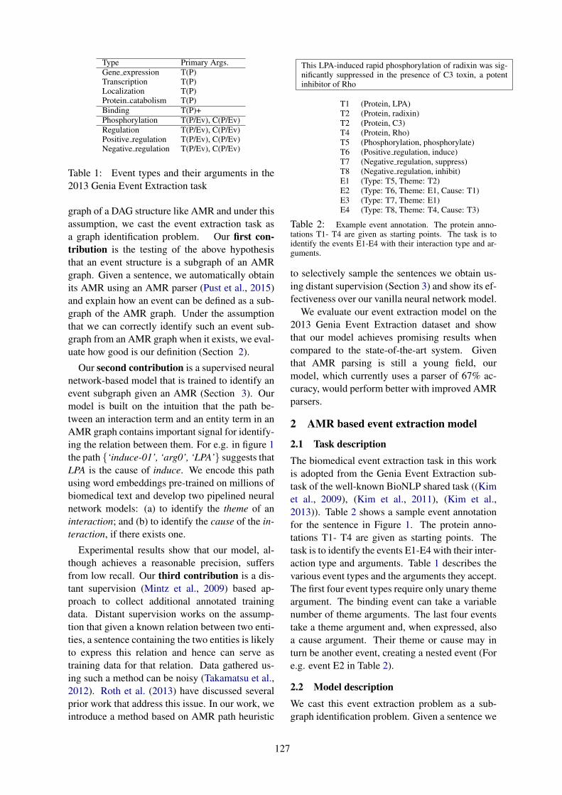
Type Primary Args.Gene expression T(P)Transcription T(P)Localization T(P)Protein catabolism T(P)Binding T(P)+Phosphorylation T(P/Ev), C(P/Ev)Regulation T(P/Ev), C(P/Ev)Positive regulation T(P/Ev), C(P/Ev)Negative regulation T(P/Ev), C(P/Ev)
Table 1: Event types and their arguments in the2013 Genia Event Extraction task
graph of a DAG structure like AMR and under thisassumption, we cast the event extraction task asa graph identification problem. Our first con-tribution is the testing of the above hypothesisthat an event structure is a subgraph of an AMRgraph. Given a sentence, we automatically obtainits AMR using an AMR parser (Pust et al., 2015)and explain how an event can be defined as a sub-graph of the AMR graph. Under the assumptionthat we can correctly identify such an event sub-graph from an AMR graph when it exists, we eval-uate how good is our definition (Section 2).
Our second contribution is a supervised neuralnetwork-based model that is trained to identify anevent subgraph given an AMR (Section 3). Ourmodel is built on the intuition that the path be-tween an interaction term and an entity term in anAMR graph contains important signal for identify-ing the relation between them. For e.g. in figure 1the path {‘induce-01’, ‘arg0’, ‘LPA’} suggests thatLPA is the cause of induce. We encode this pathusing word embeddings pre-trained on millions ofbiomedical text and develop two pipelined neuralnetwork models: (a) to identify the theme of aninteraction; and (b) to identify the cause of the in-teraction, if there exists one.
Experimental results show that our model, al-though achieves a reasonable precision, suffersfrom low recall. Our third contribution is a dis-tant supervision (Mintz et al., 2009) based ap-proach to collect additional annotated trainingdata. Distant supervision works on the assump-tion that given a known relation between two enti-ties, a sentence containing the two entities is likelyto express this relation and hence can serve astraining data for that relation. Data gathered us-ing such a method can be noisy (Takamatsu et al.,2012). Roth et al. (2013) have discussed severalprior work that address this issue. In our work, weintroduce a method based on AMR path heuristic
This LPA-induced rapid phosphorylation of radixin was sig-nificantly suppressed in the presence of C3 toxin, a potentinhibitor of Rho
T1 (Protein, LPA)T2 (Protein, radixin)T2 (Protein, C3)T4 (Protein, Rho)T5 (Phosphorylation, phosphorylate)T6 (Positive regulation, induce)T7 (Negative regulation, suppress)T8 (Negative regulation, inhibit)E1 (Type: T5, Theme: T2)E2 (Type: T6, Theme: E1, Cause: T1)E3 (Type: T7, Theme: E1)E4 (Type: T8, Theme: T4, Cause: T3)
Table 2: Example event annotation. The protein anno-tations T1- T4 are given as starting points. The task is toidentify the events E1-E4 with their interaction type and ar-guments.
to selectively sample the sentences we obtain us-ing distant supervision (Section 3) and show its ef-fectiveness over our vanilla neural network model.
We evaluate our event extraction model on the2013 Genia Event Extraction dataset and showthat our model achieves promising results whencompared to the state-of-the-art system. Giventhat AMR parsing is still a young field, ourmodel, which currently uses a parser of 67% ac-curacy, would perform better with improved AMRparsers.
2 AMR based event extraction model
2.1 Task descriptionThe biomedical event extraction task in this workis adopted from the Genia Event Extraction sub-task of the well-known BioNLP shared task ((Kimet al., 2009), (Kim et al., 2011), (Kim et al.,2013)). Table 2 shows a sample event annotationfor the sentence in Figure 1. The protein anno-tations T1- T4 are given as starting points. Thetask is to identify the events E1-E4 with their inter-action type and arguments. Table 1 describes thevarious event types and the arguments they accept.The first four event types require only unary themeargument. The binding event can take a variablenumber of theme arguments. The last four eventstake a theme argument and, when expressed, alsoa cause argument. Their theme or cause may inturn be another event, creating a nested event (Fore.g. event E2 in Table 2).
2.2 Model descriptionWe cast this event extraction problem as a sub-graph identification problem. Given a sentence we
127

first obtain its AMR graph automatically using anAMR parser (Pust et al., 2015). Next, we identifyprotein nodes and interaction nodes in the graph.Protein Node Identification: In both the trainingand the test set, protein terms are pre-annotated(e.g. T1 to T4 in Table 2). We then use the AMRgraph alignment information to identify nodes inthe AMR graph aligned to these protein terms toget our protein nodes P .Interaction Node Identification: In the trainingdata, interaction terms are pre-annotated (e.g. T5to T8 in Table 2). To identify the interactionterms in the test set we use the following heuristic:any term that was annotated as an interaction termmore than once in the training data is consideredas an interaction term in the test data as well. Wethen use the AMR graph alignment information toidentify nodes in the AMR graph aligned to the in-teraction terms to get our interaction nodes T .Given P and T , we identify an event sub-graphusing the following two-step process:a. Theme Identification: Every pair (pi, tj)where pi ∈ P and tj ∈ T , is a candidate for anevent em defined as em: (Type: tj , Theme: pi)where Type is one of the nine event types in Ta-ble 1. If em can take other events as arguments(last four event types in Table 1) and if the short-est path between tj and pi includes an interactionterm tk, such that the pair (pi, tk) is an event enin itself, then we define the event em instead asem: (Type: tj , Theme: en). For e.g. in Figure 1,the path between induce-01 and radixin includesphosphorylate-01 which is an event in itself (E1).Hence event E2 is defined with E1 as its theme (inTable 2).b. Cause Identification: For events em: (Type:tj: Theme: pi) that can take a cause argument,we identify possible candidates for their cause byagain looking for all pairs (pl, tj) where pl ∈ Pand l 6= i and add cause to the event em as em:(Type: tj , Theme: pi, Cause: pl). Since theseevents can even take other events as their causeargument, we identify additional candidates fortheir cause by looking for all pairs (en, tj) whereen ∈ E and n 6= m and add cause to the event emas em: (Type: tj , Theme: pi, Cause: en).
2.3 Upper bound using “event is a subgraphof AMR” hypothesis
Before we learn to identify event sub-graphs froman AMR graph, we first calculate the upper bound
Event Type R P F1 F1 ()Gene expression 87.82 100.00 93.51
Transcription 65.31 100.00 79.01Localization 86.80 100.00 92.93
Protein catabolism 90.00 100.00 94.74==[SVT-TOTAL]== 82.48 100.00 90.04 76.59
Binding 67.83 95.83 79.43 42.88Phosphorylation 60.62 80.14 69.03 65.37
Regulation 42.61 61.73 50.42Positive regulation 41.93 65.43 51.11Negative regulation 50.94 65.85 57.45==[REG-TOTAL]== 45.16 64.33 53.00 38.41==[ALL-TOTAL]== 65.98 85.44 74.18 50.97
Table 3: Upper bound on the dev set using our“event is a subgraph of AMR” hypothesis
that we are setting for our model because we areusing an AMR parser instead of obtaining goldAMRs. For calculating this upper bound, we firstobtain the AMR graph of a sentence using theAMR parser and then assume that if an event isa sub-graph of this AMR graph then we can iden-tify it correctly. Table 3 shows the upper boundwe get on the dev set of the 2013 Genia Event Ex-traction dataset (described in Section 5.1). Thelast column in the table is the state-of-the-art F1score obtained by the system EVEX (Hakala et al.,2013) on the test set of the dataset2.
In case of simple events i.e. events that takeonly proteins as theme arguments, an event is al-ways a subgraph of the AMR unless there is analignment error causing the protein node or theinteraction node to be missing. Hence the upperbound on our precision is 100% whereas the up-per bound on our recall is 82.48% for these simpleevents. In case of the other event types where anevent can take other events as arguments, an eventis correctly identified only if the path between thepair (pi, tj) in the AMR graph includes all its sub-events. Therefore we lose more on the precisionand recall in these cases due to AMR parsing er-rors bringing our overall upper bound on precisiondown to 85.44% and our overall upper bound onrecall down to 65.98%. These results give us fol-lowing two important insights:
1. By using this hypothesis we have set an upperbound of 74.18% F1-score for our learningmodel.
2. As the accuracy of automatic AMR parsersimprove, our model will perform better at theevent extraction task.
2We compare our numbers on the dev set to the EVEXnumbers on test set since gold annotations for the test set arenot available for download
128

3 LSTM based learning model
In this section we will describe our model thatlearns to identify an event sub-graph from anAMR graph. The key idea is that the path betweenthe interaction node and the entity node (where theterm entity is used to denote both a protein anda sub-event) contains information about how theevent is structured. We build on this idea to de-velop a supervised model using Long Short TermMemory (LSTM) (Hochreiter and Schmidhuber,1997) architecture that can learn to identify eventsusing the nodes and the edges in the AMR pathbetween the interaction term and the entity term.
3.1 Motivation
The input to our problem is a sequence of words(wi) interwound with edge labels (ej) of the form:w1, e1, w2, e2, ..., en−1, wn that exists in the pathbetween an interaction node and an entity nodein an AMR graph. Due to large semantic varia-tions that exist in naturally occurring texts, tradi-tional feature based methods suffer from sparsityissues while learning from such a sequence. Neu-ral network based models provide a framework forlearning from non-sparse representations. Specifi-cally, LSTM is known to handle sequences of vari-able length and capture long range dependencieswell. Since the input sequence in our case fallsinto this category, we build our model using theLSTM framework.
3.2 Event identification
We model the event identification task as a two-step process: Theme Identification and CauseIdentification. For simple events, this process in-cludes only theme identification (since they don’thave cause). We describe the two LSTM modelscorresponding to the two steps as follows:
3.2.1 Theme IdentificationGiven a pair of interaction node (tj) and proteinnode (pi), the task is to identify if there existsan event with tj as the interaction and pi as thetheme; and if yes, what is the type of the event.We cast this problem as a multi-class classificationtask with label set as L : {NULL ∪ Event types}where Event types correspond to the nine eventtypes described in Table 1 and NULL correspondsto no event. We train an LSTM model for thistask with the input layer as the embeddings cor-responding to the sequence of words interwound
Figure 2: Theme identification and Cause identi-fication stages
with edge labels in the shortest path between piand tj in the AMR graph. We use a hidden layerof size 100 and an output layer of the size of ourlabel set L. For e.g. in Figure 2, the sequence{‘phosphorylate-01’, ‘arg1’, ‘radixin’} is the in-put sequence and the event type Phosphorylationis its label.
3.2.2 Cause IdentificationThe last four event types in Table 1 can take pro-teins or other events as cause argument. We castthis problem as a binary classification task wherefor an event we ask the question if a protein/eventis its cause argument or not for every protein andevery other event in that sentence. Let em be theevent identified as em : (Type : tj , Theme : pi)that can take a cause argument. Let C = P ∪ Ewhere P is the set of all other proteins in the AMRgraph (except pi) and E is the set of all identifiedevents (except em). For every ck ∈ C, we getthe shortest path between ck and tj and combineit with the shortest path between pi and tj and usethe words and edges in this combined path as theinput layer of our second LSTM model. We usea hidden layer of size 100 and an output layer ofsize one corresponding to the binary prediction ofwhether ck is the cause of the event em or not.
3.3 Initialization of Embeddings
When initializing our model, we have two choices:we can initialize the embeddings in the input layerrandomly or we can initialize them with valuesthat reflect the meanings of the word types. Ithas been seen that using pre-defined word embed-dings improves the performance of RNN modelsover random initializations (Collobert and Weston,
129

2008; Socher et al., 2011). We initialize the vec-tors corresponding to words in our input layer with100-dimensional vectors generated by a word2vec(Mikolov et al., 2013) model trained on over onemillion words from the PubMed central articlerepository. Words not included in the pre-trainedmodel and the edges are initialized randomly usinguniform sampling from [-0.25, +0.25] to match theembedding standard deviation.
3.4 Event Construction
During test time, we first make predictions us-ing our LSTM model for Theme identification.For every pair (pi, tj) with a non-zero label l,we construct events as follows: For label l cor-responding to interaction types that take only pro-teins as theme arguments, we construct event asem : (Type : tj , Theme : pi). For label l corre-sponding to interaction types that can take anotherevent as its theme, we look at the path betweentj and pi in the AMR. If this path includes a pair(tk, pi) that has a non-zero label, then we constructan event en : (Type : tj , Theme : ep) where ep isthe event constructed from the pair (tk, pi). Oth-erwise, we construct the event as en : (Type :tj , Theme : pi).
For each of the predicted event em : (Type :tj : Theme : pi) that can take a cause argument,we run the second LSTM model for its Cause iden-tification. If there is a pair (pi, ck) which has apositive label, then we assign ck as the cause ofthe event em.
4 Distant Supervision
An empirical evaluation of our LSTM-basedlearning model (Section 5.4) shows that it can suf-fer from low recall. Obtaining additional humanannotated data for our complex event extractiontask can be very costly. This motivates us to de-velop an approach that can gather more trainingdata with minimal supervision.
4.1 Motivation
Distant supervision as a learning paradigm was in-troduced by Mintz et al. (2009) for relation extrac-tion in general domain. They use Freebase to geta set of relation instances and entity pairs partici-pating in those relations, extract all sentences con-taining those two entity pairs from Wikipedia textand use these sentences as their training data. Thiswork and many others show that distant supervi-
Figure 3: Distant Supervision: Sentences extracted fromPubMed Central articles using BioPax database relations
sion technique yields significant improvements inrelation extraction. Neural network models likeLSTM need to be trained on substantial amountsof training data for them to be able to general-ize well. However due to lack of labeled data inbiomedical domain, most work in relation extrac-tion in this domain has been restricted to purelysupervised techniques. In this work we cope withthis problem by gathering additional training datausing distant supervision from a knowledge base.
4.2 MethodologyRelation extraction using distant supervision re-quires two things: 1) A knowledge base contain-ing relations between proteins, and 2) A large cor-pus of unannotated text that contain protein men-tions. We use the BioPax (Biological PathwayExchange) database (Demir et al., 2010) as ourknowledge base of protein relations and we use thePubMed central articles as our unannotated textcorpus. Given a database entry of the form (‘Pro-tein1’, ‘Protein2’, ‘relation’), we extract all sen-tences from the PubMed central articles in whichthe two proteins co-occur. For example, Figure3 shows some sample sentences extracted for thedatabase entry (’DAG’, ’PKC’, increases). Thefirst two sentences in the figure indeed expressthe relation in the database but the third sentencejust mentions the two proteins in a comma sepa-rated list. We observe that a lot of the extractedsentences fall into the category of the third sen-tence. Hence as a first step, we filter such instancesby tagging the sentence with their parts-of-speechand removing those in which the two proteins areseparated only by nouns (or punctuations).
4.3 AMR Path Based SelectionThe traditional distant supervision approach saysthat all the sentences extracted using the methodabove can be used as additional training data un-
130

Event Type Biopax relationGene expression adds modification
Transcription adds modificationLocalization adds modification
Protein catabolism adds modificationBinding binds
Phosphorylation adds modificationRegulation increases, increases activity
Positive regulation increases, increases activityNegative regulation -
Table 4: Mapping between event types andBiopax model relations
der the assumption that all sentences in which theproteins co-occur express the relation mentionedin the database. However Takamatsu et al. (2012)note that this approach can often lead to a lot offalse positives. Roth et al. (2013) have discussedseveral prior work that try to reduce such noise inthe data. In our work, we develop a novel selec-tion technique for reducing such noise using AMRpath heuristic. We make the observation that giventwo protein nodes in an AMR, if there is a relationr between the two then the shortest path betweenthe two protein nodes in the AMR contains the in-teraction term expressing the relation r.
For e.g. Figure 4 shows the AMR for the sen-tence “DAG is important for the activation ofPKC, which phosphorylates tyrosinase, and canalso be released...” that was extracted using thedatabase entry {‘DAG’, ‘PKC’, ‘increases’}. Theinteraction term ‘activate’ suggesting the relation‘increases’ exists in the shortest path between theproteins DAG and PKC. Figure 5 shows AMRfor the sentence “The sun-network links TCF3with ZYX and HOXA9 via NEDD9 and CREBBP,respectively.” extracted for the pair (‘TCF3’,‘HOXA9’, increases). There is no interaction termsuggesting the relation ‘increases’ in the shortestpath between the proteins TCF3 and HOXA9.
Table 4 shows the mapping we define betweenthe event types and the relations found in the en-tries (‘Protein1’, ‘Protein2’, ‘relation’) that weextracted from the Biopax model. In each sentenceextracted for the database entry (‘P1’, ‘P2’, ‘r’) ,we check if the shortest path between the two pro-tein nodes P1 and P2 in the AMR of the sentencecontains one of the interaction terms correspond-ing to the event type mapped to the relation r. Wediscard all those sentences that do not satisfy thisconstraint.
Figure 4: Interaction term ‘activate’ corresponding to therelation ’increases’ exists in the shortest path between DAGand PKC
Figure 5: No interaction term corresponding to the rela-tion ‘increases’ exists in the shortest path between TCF3 andHOXA9
4.4 Using Data for LSTM Model
We use these selected sentences as additionaltraining data for our two LSTM models as follows:a. Theme identification: Let S be the sentenceextracted for the database entry (‘DAG’, ‘PKC’,‘increases’) and let ‘activates′ be the interactionterm that exists in the shortest path between theprotein nodes. Since the database entry refers to‘DAG’ as the cause and ‘PKC’ as the theme, weassume these roles for the two proteins in the ex-tracted sentence S as well. Therefore, we can nowuse the path between the interaction term ‘acti-vates’ and the theme ‘PKC’ as an input sequencefor our model with the label corresponding to theevent type of the interaction term ’activates’.b. Cause identification: In case of cause identifi-cation instead of using the path between the inter-action term and the theme entity, we use the short-est path between the cause entity and the themeentity via the interaction term and use this as aninput sequence to our model with a positive label.
131

5 Experiments
5.1 Dataset and task settingThe event extraction task described in this workcorresponds to the Task 1 of the Genia EventExtraction task described by the BioNLP SharedTask series (2009, 2011 and 2013). We traina model on a combination of abstract collection(from 2009 edition) and full text collection (from2011 and 2013). We test our model on the dev setof the 2013 edition (since the gold annotation ispublicly available only for the dev set and not thetest set).
5.2 Data preprarationThe dataset made available for the Shared Task isin the form of sentences and event annotations asshown in Table 2. We convert these event annota-tions into input sequences and labels for our multi-class classification task (theme identification) andfor our binary classification task (cause identifica-tion) as followsa. Theme identification: Given a sentence, wedefine the set T as the set of interaction terms cor-responding to all its event annotations. We de-fine the set P as the set of all its protein men-tions. For every pair (tj , pi) where pi ∈ P andtj ∈ T , we create a training data of the form{w1, e1, w2, e2, ..., en−1, wn, label} where the in-put sequence corresponds to the words interwoundwith edge labels in shortest path between tj and pi;and the label is the event type of the event em ifthere exists an event em : (Type : tj , Theme :pi), NULL otherwise. We create the test data sim-ilarly; except we do not use event annotations forcreating the set T but instead identify terms in thesentence that was annotated as an interaction termin the training data more than once.b. Cause identification: For every pair (tj , pk)where tj is part of some event annotation em :(Type : tj , Theme : pi) of event type that cantake cause argument and pk ∈ P , we create a train-ing data of the form {w1, e1, w2, e2, ..., en−1, wn,label} where the input sequence corresponds tothe shortest path between pk and pi via tj ; andthe label is 1 if pk is the cause of the event em,0 otherwise.
5.3 LSTM model setupWe implement our LSTM model using the lasagnelibrary. For the first LSTM model, we use softmaxas our non-linear function and optimize the cat-
egorical cross entropy loss using adam (Kingmaand Ba, 2014). For the second LSTM model, weuse a sigmoid non-linear function and optimize thebinary loss using adam. We use a dropout of 0.5,batch size of 100 and a learning rate of 0.001.
5.4 Results and Discussion
Table 5 shows the results of our LSTM and dis-tant supervision based event extraction model. Wecompare our results with the state-of-the-art eventextraction system EVEX (Hakala et al., 2013). Wereport the Approximate Span/Approximate Re-cursive metric in all our tables (described in theShared Task (Kim et al., 2013)). The columnsto the left (with column heading LSTM) showthe performance of our model trained only onthe official training data. The columns to theright (with column heading LSTM+Distant Super-vision) show the performance of our model trainedon official training data plus the additional trainingdata of 11792 sentences we gather using our dis-tant supervision strategy.
The table highlights some of our results. Firstly,we note that, in cases where we obtain a largenumber of extra sentences using distant supervi-sion (highlighted in the column “DS Sents”), wesee a considerable gain in the recall values be-tween “LSTM” and “LSTM+Distant Supervision”models. On the contrary, in cases where we ex-tract only a small number, we see a small gain(or sometimes even a decrease in performance).This suggests we explore further ways of selectingour extra sentences. Secondly, although the over-all performance of our model using the automaticAMR parser is lower than the current state-of-the-art system, the gap of 5% in the F1 score can hope-fully be reduced with the ongoing improvementsin AMR parsing.
6 Related work
The biomedical event extraction task describedin this work was first introduced in the BioNLPShared Task in 2009 (Kim et al., 2009). Thistask helped shift the focus of relation extrac-tion efforts from identifying simple binary inter-actions to identifying complex nested events thatbetter represent the biological interactions statedfrequently in text. Existing approaches to thistask include SVM (Bjorne and Salakoski, 2013)other ML based approaches (Riedel and McCal-lum, 2011; Miwa et al., 2010, 2012). Methods like
132

LSTM LSTM + Distant Supervision EVEXEvent Type Recall Precision F1 Recall Precision F1 DS Sents Recall Precision F1
Gene expression 66.33 66.55 66.44 76.98 61.48 68.36 868Transcription 55.10 28.57 37.63 57.14 26.92 36.60 807Localization 36.55 63.72 46.45 38.07 85.06 52.60 96
Protein catabolism 73.33 84.62 78.57 60.00 94.74 73.47 7==[SVT-TOTAL]== 57.82 60.86 57.27 56.35 68.05 57.60 73.83 79.56 76.59
Binding 27.61 25.94 26.75 28.57 26.12 27.29 139 41.14 44.77 42.88Phosphorylation 49.21 53.75 51.38 73.45 45.55 56.23 3183
Regulation 16.30 29.18 20.92 26.07 21.00 23.26 2131Positive regulation 25.98 35.16 29.88 37.41 29.17 32.78 4561Negative regulation 23.17 30.50 26.33 22.97 29.44 25.81 0==[REG-TOTAL]== 21.81 31.61 25.71 28.81 26.53 27.28 32.41 47.16 38.41==[ALL-TOTAL]== 44.42 51.01 46.37 46.73 46.60 46.66 11792 45.44 58.03 50.97
Table 5: Evaluation results (Recall/Precision/F1) on the 2013 Genia Event Extraction dev set. LSTMand LSTM + Distant Supervision are our models. The last column corresponds to the results of EVEX(Hakala et al., 2013) model on the 2013 test set. Certain notable numbers are emphasized and discussedunder results 5.4.
(Liu et al., 2013; MacKinlay et al., 2013) learnsubgraph patterns from the event annotations inthe training data and cast the event detection assubgraph matching problem. Non-feature basedapproaches like graph kernels compare syntacticstructures directly (Airola et al., 2008; Bunescuet al., 2005). Rule based methods that eitheruse manually crafted rules or generate rules fromtraining data (Cohen et al., 2009; Kaljurand et al.,2009; Kilicoglu and Bergler, 2011; Bui et al.,2013) have obtained high precision on these tasks.
In our work, we take inspiration from theTurk Event Extraction System (TEES) (Bjorneand Salakoski, 2013) (the event extraction systemfor EVEX) that has consistently been the top per-former in these series of tasks. They representevents using a graph format and break the eventextraction task into separate multi-class classifica-tion tasks using SVM as their classifier. In ourwork we take a step further by making use of adeeper semantic representation as a starting pointand identifying subgraphs in the AMR graph.
AMR has been successfully used for deeper se-mantic tasks like entity linking (Pan et al., 2015)and abstractive summarization (Mihalcea et al.,2015). Work by Garg et al. (2015) is the first oneto make use of AMR representation for extractinginteractions from biomedical text. They use graphkernel methods to answer the binary question ofwhether a given AMR subgraph expresses an in-teraction or not. Our work departs from theirs inthat they concentrate only on binary interactionswhereas we use AMR to identify complex nestedevents. Also, our approach additionally makes useof distant supervision to cope with the problem of
limited annotated data.Distant supervision techniques have been suc-
cessfully used before for relation extraction(Mintz et al., 2009) in general domain. Recentwork by (Liu et al., 2014) uses minimal supervi-sion strategy for extracting relations particularly inbiomedical texts. Our work departs from theirs inthat we introduce a novel AMR path based heuris-tic to selectively sample the sentences obtainedfrom distant supervision.
7 Conclusion
In this work, we show the effectiveness of usinga deep semantic representation based on AbstractMeaning Representations for extracting complexnested events expressed in biomedical text. Wehypothesize that an event structure is an AMRsubgraph and empirically validate our hypothesis.For learning to extract such event subgraphs fromAMR automatically, we develop two RecurrentNeural Network based models: one for identifyingthe theme, and the other for identifying the causeof the event. To overcome the dearth of manuallyannotated data in biomedical domain, which ex-plains the low recall of event extraction systems,we train our model on additional training datagathered automatically using a selective distant su-pervision strategy. Our experiments strongly sug-gest that AMR parsing improvements, which areexpected given the youth of this scientific field ofinquiry, and the exploitation of larger, manuallycurated Biopax-like models and collections of bio-molecular texts will be easy to capitalize on cata-lysts for driving future improvements in this task.
133

ReferencesAntti Airola, Sampo Pyysalo, Jari Bjorne, Tapio
Pahikkala, Filip Ginter, and Tapio Salakoski. 2008.All-paths graph kernel for protein-protein interac-tion extraction with evaluation of cross-corpus learn-ing. BMC bioinformatics 9(11):1.
Laura Banarescu, Claire Bonial, Shu Cai, MadalinaGeorgescu, Kira Griffitt, Ulf Hermjakob, KevinKnight, Philipp Koehn, Martha Palmer, and NathanSchneider. 2013. Abstract meaning representationfor sembanking. In Association for ComputationalLinguistics.
Jari Bjorne and Tapio Salakoski. 2013. Tees 2.1: Au-tomated annotation scheme learning in the bionlp2013 shared task. In Proceedings of the BioNLPShared Task 2013 Workshop. pages 16–25.
Quoc-Chinh Bui, David Campos, Erik van Mulligen,and Jan Kors. 2013. A fast rule-based approach forbiomedical event extraction. In Proceedings of theBioNLP Shared Task 2013 Workshop. Associationfor Computational Linguistics, pages 104–108.
Razvan Bunescu, Ruifang Ge, Rohit J Kate, Edward MMarcotte, Raymond J Mooney, Arun K Ramani, andYuk Wah Wong. 2005. Comparative experimentson learning information extractors for proteins andtheir interactions. Artificial intelligence in medicine33(2):139–155.
K Bretonnel Cohen, Karin Verspoor, Helen L Johnson,Chris Roeder, Philip V Ogren, William A Baum-gartner Jr, Elizabeth White, Hannah Tipney, andLawrence Hunter. 2009. High-precision biologi-cal event extraction with a concept recognizer. InProceedings of the Workshop on Current Trends inBiomedical Natural Language Processing: SharedTask. Association for Computational Linguistics,pages 50–58.
Ronan Collobert and Jason Weston. 2008. A unifiedarchitecture for natural language processing: Deepneural networks with multitask learning. In Pro-ceedings of the 25th international conference onMachine learning. ACM, pages 160–167.
Emek Demir, Michael P Cary, Suzanne Paley, KenFukuda, Christian Lemer, Imre Vastrik, GuanmingWu, Peter D’Eustachio, Carl Schaefer, Joanne Lu-ciano, et al. 2010. The biopax community stan-dard for pathway data sharing. Nature biotechnol-ogy 28(9):935–942.
Jeffrey Flanigan, Sam Thomson, Jaime Carbonell,Chris Dyer, and Noah A Smith. 2014. A discrim-inative graph-based parser for the abstract meaningrepresentation. In In ACL. Citeseer.
Sahil Garg, Aram Galstyan, Ulf Hermjakob, andDaniel Marcu. 2015. Extracting biomolecular inter-actions using semantic parsing of biomedical text.arXiv preprint arXiv:1512.01587 .
Kai Hakala, Sofie Van Landeghem, Tapio Salakoski,Yves Van de Peer, and Filip Ginter. 2013. Evexin st?13: Application of a large-scale text miningresource to event extraction and network construc-tion. In Proceedings of the BioNLP Shared Task2013 Workshop. Association for Computational Lin-guistics, pages 26–34.
Sepp Hochreiter and Jurgen Schmidhuber. 1997.Long short-term memory. Neural computation9(8):1735–1780.
Kaarel Kaljurand, Gerold Schneider, and Fabio Ri-naldi. 2009. Uzurich in the bionlp 2009 sharedtask. In Proceedings of the Workshop on CurrentTrends in Biomedical Natural Language Process-ing: Shared Task. Association for ComputationalLinguistics, pages 28–36.
Halil Kilicoglu and Sabine Bergler. 2011. Adapting ageneral semantic interpretation approach to biologi-cal event extraction. In Proceedings of the BioNLPShared Task 2011 Workshop. Association for Com-putational Linguistics, pages 173–182.
Jin-Dong Kim, Tomoko Ohta, Sampo Pyysalo, Yoshi-nobu Kano, and Jun’ichi Tsujii. 2009. Overviewof bionlp’09 shared task on event extraction. InProceedings of the Workshop on Current Trends inBiomedical Natural Language Processing: SharedTask. Association for Computational Linguistics,pages 1–9.
Jin-Dong Kim, Yue Wang, Nicola Colic, Seung HanBaek, Yong Hwan Kim, and Min Song. 2016.Refactoring the genia event extraction shared tasktoward a general framework for ie-driven kb devel-opment. ACL 2016 page 23.
Jin-Dong Kim, Yue Wang, Toshihisa Takagi, and Aki-nori Yonezawa. 2011. Overview of genia event taskin bionlp shared task 2011. In Proceedings of theBioNLP Shared Task 2011 Workshop. Associationfor Computational Linguistics, pages 7–15.
Jin-Dong Kim, Yue Wang, and Yamamoto Yasunori.2013. The genia event extraction shared task, 2013edition-overview. In Proceedings of the BioNLPShared Task 2013 Workshop. Association for Com-putational Linguistics, pages 8–15.
Diederik Kingma and Jimmy Ba. 2014. Adam: Amethod for stochastic optimization. arXiv preprintarXiv:1412.6980 .
Haibin Liu, Karin Verspoor, Donald C Comeau, An-drew MacKinlay, and W John Wilbur. 2013. Gen-eralizing an approximate subgraph matching-basedsystem to extract events in molecular biology andcancer genetics. In Proceedings of the BioNLPShared Task 2013 Workshop. pages 76–85.
Mengwen Liu, Yuan Ling, Yuan An, and Xiaohua Hu.2014. Relation extraction from biomedical litera-ture with minimal supervision and grouping strategy.In Bioinformatics and Biomedicine (BIBM), 2014
134

IEEE International Conference on. IEEE, pages444–449.
Andrew MacKinlay, David Martinez, Antonio JimenoYepes, Haibin Liu, W John Wilbur, and Karin Ver-spoor. 2013. Extracting biomedical events and mod-ifications using subgraph matching with noisy train-ing data. In Proceedings of the BioNLP Shared Task2013 Workshop. Association for Computational Lin-guistics, Sofia, Bulgaria. pages 35–44.
Jonathan May. 2016. Semeval-2016 task 8: Mean-ing representation parsing. Proceedings of SemEvalpages 1063–1073.
Rada Mihalcea, Joyce Yue Chai, and Anoop Sarkar,editors. 2015. NAACL HLT 2015, The 2015 Con-ference of the North American Chapter of the Asso-ciation for Computational Linguistics: Human Lan-guage Technologies, Denver, Colorado, USA, May31 - June 5, 2015. The Association for Computa-tional Linguistics.
Tomas Mikolov, Ilya Sutskever, Kai Chen, Greg S Cor-rado, and Jeff Dean. 2013. Distributed representa-tions of words and phrases and their compositional-ity. In Advances in neural information processingsystems. pages 3111–3119.
Mike Mintz, Steven Bills, Rion Snow, and Dan Ju-rafsky. 2009. Distant supervision for relation ex-traction without labeled data. In Proceedings ofthe Joint Conference of the 47th Annual Meeting ofthe ACL and the 4th International Joint Conferenceon Natural Language Processing of the AFNLP:Volume 2-Volume 2. Association for ComputationalLinguistics, pages 1003–1011.
Makoto Miwa, Rune Sætre, Jin-Dong Kim, andJun’ichi Tsujii. 2010. Event extraction with com-plex event classification using rich features. Jour-nal of bioinformatics and computational biology8(01):131–146.
Makoto Miwa, Paul Thompson, and Sophia Ana-niadou. 2012. Boosting automatic event ex-traction from the literature using domain adapta-tion and coreference resolution. Bioinformatics28(13):1759–1765.
Xiaoman Pan, Taylor Cassidy, Ulf Hermjakob, HengJi, and Kevin Knight. 2015. Unsupervised en-tity linking with abstract meaning representation.In (Mihalcea et al., 2015), pages 1130–1139.http://aclweb.org/anthology/N/N15/N15-1119.pdf.
Michael Pust, Ulf Hermjakob, Kevin Knight, DanielMarcu, and Jonathan May. 2015. Using syntax-based machine translation to parse english into ab-stract meaning representation. In EMNLP.
Sebastian Riedel and Andrew McCallum. 2011. Ro-bust biomedical event extraction with dual decom-position and minimal domain adaptation. In Pro-ceedings of the BioNLP Shared Task 2011 Work-shop. Association for Computational Linguistics,pages 46–50.
Benjamin Roth, Tassilo Barth, Michael Wiegand, andDietrich Klakow. 2013. A survey of noise reductionmethods for distant supervision. In Proceedings ofthe 2013 workshop on Automated knowledge baseconstruction. ACM, pages 73–78.
Richard Socher, Eric H Huang, Jeffrey Pennin, Christo-pher D Manning, and Andrew Y Ng. 2011. Dy-namic pooling and unfolding recursive autoencodersfor paraphrase detection. In Advances in Neural In-formation Processing Systems. pages 801–809.
Shingo Takamatsu, Issei Sato, and Hiroshi Nakagawa.2012. Reducing wrong labels in distant supervi-sion for relation extraction. In Proceedings of the50th Annual Meeting of the Association for Compu-tational Linguistics: Long Papers-Volume 1. Associ-ation for Computational Linguistics, pages 721–729.
Chuan Wang, Nianwen Xue, Sameer Pradhan, andSameer Pradhan. 2015. A transition-based algo-rithm for amr parsing. In HLT-NAACL. pages 366–375.
135

Proceedings of the BioNLP 2017 workshop, pages 136–142,Vancouver, Canada, August 4, 2017. c©2017 Association for Computational Linguistics
1
Detecting Personal Medication Intake in Twitter: An Annotated Corpus and Baseline Classification System
Ari Z. Klein, Abeed Sarker, Masoud Rouhizadeh, Karen O’Connor, Graciela Gonzalez Department of Biostatistics, Epidemiology, and Informatics
Perelman School of Medicine University of Pennsylvania
{ariklein,abeed,mrou,karoc,gragon}@upenn.edu
Abstract
Social media sites (e.g., Twitter) have been used for surveillance of drug safety at the pop-ulation level, but studies that focus on the ef-fects of medications on specific sets of indi-viduals have had to rely on other sources of data. Mining social media data for this infor-mation would require the ability to distinguish indications of personal medication intake in this media. Towards that end, this paper pre-sents an annotated corpus that can be used to train machine learning systems to determine whether a tweet that mentions a medication in-dicates that the individual posting has taken that medication (at a specific time). To demon-strate the utility of the corpus as a training set, we present baseline results of supervised clas-sification.
1 Introduction
Social media allows researchers and public health professionals to obtain relevant infor-mation in large amounts directly from populations and/or specific cohorts of interest, and it has evolved into a useful resource for performing pub-lic health monitoring and surveillance. According to a Pew report (Greenwood et al., 2016), nearly half of adults worldwide and two-thirds of all American adults (65%) use social media, includ-ing over 90% of 18-29 year olds. Recent studies have attempted to utilize social media data for tasks such as pharmacovigilance (Leaman et al., 2010), identifying user behavioral patterns (Struik and Baskerville, 2014), analyzing social circles with common behaviors (Hanson et al., 2013b), and tracking infectious disease spread (Broniatowski et al., 2015).
A large subset of the public health-related re-search using social media data, including our prior
work in the domain, focuses on mining infor-mation (e.g., adverse drug reactions, medication abuse, and user sentiment) from posts mentioning medications (Korkontzelos et al., 2016; Hanson et al., 2013b; Nikfarjam et al., 2015). Typically, these and similar studies focus on information at the population level, but processing and deriving information from individual user posts poses sig-nificant challenges from the natural language pro-cessing (NLP) perspective. Researchers attempt to overcome the noise and inaccuracies in the data by relying on large amounts of data. For example, Hanson et al. (2013b; 2013a) attempted to esti-mate the abuse of Adderall® using Twitter by de-tecting the total number of mentions of the medi-cation. The authors did not attempt to assess if a mention represented personal intake or not.
While such a strategy may suffice for deriving estimates “by proxy” at the population level (e.g., higher volume of chatter means higher rates of use), it has at least two limitations: (i) the actual number of tweets representing personal intake within a given sample of tweets is unknown, and (ii) it is not possible to assess the effects of medi-cation intake on subsets of users of interest who take the medication. Studies focusing on specific subsets of individuals rely on other sources of data, such as electronic health records and pub-lished literature from clinical trials, where infor-mation about the individuals’ medication intake is explicit (e.g., Akbarov et al., 2015; Zhou et al., 2016; Romagnoli et al., 2017). Harnessing social media for studying the effects of medications on specific cohorts would require developing sys-tems that can automatically distinguish posts that express personal intake from those that do not.
Due to the very recent incorporation of social media data in healthcare systems, published re-search on our target task of creating a corpus for automatic detection of personal medication intake
136

2
information is scarce. The study by Alvaro et al. (2015) is perhaps the most closely related work to ours. The authors annotated 1,548 tweets for whether they contain “first-hand experiences” of adverse drug reactions (ADRs) to prescription medications, and they used this annotated data in a supervised classification framework aimed at automatically identifying tweets that report per-sonal usage. As far as we are aware, however, they have not made their annotated data public; none-theless, we do not believe that it would have been exactly the right training set for our classification task. Because our focus is to help set the ground-work for using social media data in medication-related cohort studies, we included a subtle but key factor in our criteria for identifying personal intake: when the medication was taken. We will discuss this factor in more detail in the next sec-tion. In this paper, we present (i) an analysis of medication-mentioning chatter on Twitter, (ii) a publicly available, annotated corpus of tweets that can be used to advance automatic systems, and (iii) baseline supervised classification results to validate the utility of the annotated data.
2 Method
We chose Twitter as the data source for this study because of its growing popularity in public health research, and its easy-to-use public APIs. We dis-cuss the three primary tasks—data collection, an-notation, and classification—in the following sub-sections.
2.1 Data Collection
To build the corpus, we queried 73,800 Twitter user timelines (that we collected for related work) for 55 medication names, including both prescrip-tion and over-the-counter medications, brand and generic names, and types of medications (e.g., steroid). Using a tool that was developed by Pimpalkhute et al. (2014), we generated frequent misspellings of the medications in order to expand the query. We then tokenized all of the tweets, us-ing the ARK Twokenizer (O’Connor et al., 2010; Owoputi et al., 2013), and identified 35,075 tweets containing a target medication. To account for the linguistic idiosyncrasies of how Twitter us-ers might express their medication intake, we ran-domly selected one medication tweet from the 18,033 timelines that included such a tweet, and we prepared them for annotation. For this paper, 1 The annotation guidelines and a sample of the annotated data are available at: https://healthlanguageprocessing.org/twitter-med-intake/
10,260 tweets were annotated, with overlapping annotations for 1,026 (10%).
2.2 Annotation
In order to control for studying the effects of med-ication intake on subsets of individuals in a social media setting, we decided that tweets of interest should not only represent the author’s personal us-age of the target medication in the tweet; they should also indicate the specific instance in which the user took the mentioned medication, since re-searchers using social media data cannot physically observe and record when medications were taken. Only if the tweets provide this additional infor-mation about the time of intake can we potentially use Twitter data to assess causal associations be-tween users’ health information (also mined from social media data) and the usage of particular med-ications. As we mentioned earlier, the way that time factors into our definition of “intake” marks an im-portant distinction between our annotated data and Alvaro et al.’s (2015).
We found that, under minimal guidance, intui-tively agreeing on what constituted a personal in-take of medication, given the above criteria, was very difficult. We attribute this difficulty to the wide range of linguistic patterns in which we found medication mentions occurring. In an effort to ob-tain high inter-annotator agreement and address the human disagreement that Alvaro et al. seek to over-come, we analyzed linguistic patterns in samples of the data and used this analysis to inform the devel-opment of annotation guidelines;1 in addition, we limited the number of annotation classes to the three high-level classes that we thought were most directly relevant to the classification task at hand: intake, possible intake, and no intake.
We will summarize our analysis of the three classes of tweets here. Intake tweets indicate that (i) the medication was actually taken, (ii) the author of the tweet personally took the medication, and (iii) the medication was taken at a specific time. To illustrate (i), consider the following tweets:
(a) Migraine from hell… Took 6 Motrin and
nothing’s touching it (b) I've been off adderall about a month now
and I'm so much happier, but COM-PLETELY useless. I'm like a child again.
.
137

3
(c) A lot of people hate on prednisone but I feel better already. #stuffworksforme
(d) this ibuprofen still ain't kicked in my head poundin
While only (a) uses a verb phrase that explicitly indicates intake (took…), we can infer from fea-tures of the other tweets that the medication was taken: (b) being off the medication, (c) experienc-ing the effects of the medication, and (d) waiting for the medication to kick in all entail that the medication was taken.
Moreover, intake tweets should indicate that the author of the tweet took the medication:
(e) Sorry for this rant thingy, I took my
Vyvanse today lol (f) Sick and only had a Tylenol PM at work so
now i feel better but i am fighting sleep😂 (g) Just threw back these Xanax (h) In soooo much pain tonight and Tylenol just
isn't cutting it. Literally hurting all over
Through the use of the first-person reference I, (e) explicitly states that the author took the medica-tion, and (f) explicitly attributes the experiential effects of the medication (feel better, but fighting sleep) to the author. While (g) and (h) do not ex-plicitly reveal that the author took the medication (threw back) or is (not) experiencing the effect of the medication (isn’t cutting it), respectively, the high degree of self-presentation in social media (e.g., Kaplan and Haenlein, 2010; Papacharissi, 2012; Seidman, 2013) allows us to infer that the authors are writing about their own intake and ex-periences.
Finally, intake tweets also specify when the med-ication was taken:
(i) I've been sick for the last 3 days taking Ibu-
profen just feel better and to fight Infection "swelling"
(j) Tylenol is my bestfriend at the moment (k) maybe i'm tired as had 2 tramadol my bk is
sore sore sore... #scoliosis (l) Prednisone headache! Ahhhh
Tweet (i) uses a temporal marker that explicitly specifies an instance of intake, and, similarly, (j) explicitly indicates when the effect of the intake occurred. Although (k) and (l) do not explicitly specify instances of intake, Twitter’s real-time na-
ture (Sakaki et al., 2010) gives us reason to be-lieve that the author of (k) recently had the medi-cation and that the effect in (l) is being currently experienced, which represents an intake in the re-cent past (i.e., a specific instance).
Unlike intake tweets, some tweets do not specify that the author actually took the medication or when the medication was taken, but, unlike no in-take tweets, are generally about the author’s intake. Consider the following tweets:
(m) I want to cry it's that painful 😭gonna take
codeine this morning for sure (n) 800 mg of Advil cause this headache is
real (o) I need a Xanax like right now (p) Codeine is one hell of a drug. 😴😴😴 (q) 😭😭😭 I never understood why I get so an-
gryyyy omg I was so mellow on Xanax 🌚 (r) I pretty much eat Advil like it's
candy.💊🙆 We consider a tweet to be a possible intake if it expresses the intake as a future event (m); it con-tains merely a purpose for intake (n); it expresses a present-tense need for the medication (o); it ab-stractly praises (or criticizes) the medication with-out describing a concrete effect (p); it indicates that the author has used the medication in the past, but does not specify when (q); or, similarly, it in-dicates that the author uses the medication fre-quently, but does not specify an instance of intake (r). We decided to distinguish possible intake tweets because they can direct us to a user’s time-line for manual probing, where we may find, for example, that a series of tweets aggregate to form a sort of composite intake tweet.
In contrast to intake and possible intake tweets, no intake tweets are not about the author’s intake of the medication. While some no intake tweets are not about intake at all, some may be about the in-take by others, not the author:
(s) @[Username redacted] Mine hurt for days
last year!! Take some paracetamol hun 😊 (t) Gave James 2 ibuprofen pm and I'm being
repaid by the sound of him snoring penetrat-ing through my earplugs
The act of suggesting a medication (s) or giving someone a medication (t) might be interpreted as implying that the author has taken the medication in the past (i.e., a possible intake), but, because the
138

4
tweets are not primarily about the author’s intake, we consider this inferential leap to be too large to warrant the same classification as other possible intake tweets.
While (s) and (t) are explicitly not about the au-thor’s intake, other tweets may not be as obvious, such as tweets that contain merely the name of a medication:
(u) @[Username redacted] @[Username re-dacted] @[Username redacted] @[Username redacted] methadone !
Although (u) also might be interpreted as indicat-ing the author’s use of the medication, the textual evidence does not seem to favor this interpretation over other possible ones, such as mere question-answering. We classify tweets that contain merely the name of a medication as no intake because, unlike intake and possible intake tweets, they do not contain enough information for us to conclude that they are about the author’s intake.
The “addressivity” (Bakhtin, 1986) markers “@” in (u) reflect the “dialogic” (Bakhtin, 1981) space of social media, wherein the linguistic data that we are mining is not only textual, but “inter-textual” (Kristeva, 1980)—that is, oriented to what has already been said by others. Tweets also mark this social orientation to others through features of “reported speech” (Voloshinov, 1973). Consider the following tweets:
(v) @[Username redacted] "I don't either cause
these Tylenol aren't doing crap!" Lol (w) I just wanna give a shoutout to adderall for
helping me get through the semester - Flor-ida State
While (v) and (w) would otherwise be classified as intake tweets, the quotation marks in (v) and the hyphen in (w) mark that the authors are di-rectly reporting the words of others—in (w), a stu-dent at Florida State—not their own medication intake.
Other cases of reported speech involve tweets that make cultural references about taking medica-tions—for example, song lyrics or lines from mov-ies. As our analysis of the three classes suggests, identifying indications of personal medication in-take in social media required grappling with a num-ber of annotation issues, which forecast the chal-lenges of using this data to train classifiers. 2 Available at: http://www.cs.waikato.ac.nz/ml/weka/. Ac-cessed: 5/25/2017.
2.3 Classification
We performed supervised classification experi-ments using several algorithms. The goal for these experiments was not to identify the best perform-ing classification strategy, but to (i) verify that au-tomatic classifiers could be trained using this data, and (ii) generate baseline performance estimates.
We used stratified 80-20 (training/test) split of the annotated set for the experiments. As features, we used only word n-grams (n = 1, 2, and 3) fol-lowing standard preprocessing (e.g., stemming us-ing the Porter stemmer (Porter, 1980) and lower-casing). We experimented with four classifiers—naïve bayes (NB), support vector machines (SVM), random forest (RF), logistic regression (LR), and a majority-voting based ensemble of the last three. Pairwise classification (i.e., 1-vs-1) is used to adapt the SVMs to the multiclass problem. Parameter op-timization for the individual classifiers was per-formed via 10-fold cross validation over the train-ing set, with an objective function that maximizes the F-score for the intake class.
Following the classification experiments, we performed brief error and feature analyses to iden-tify common misclassification patterns and possi-ble future approaches for improving classification performance. To identify informative n-grams for the intake class, we applied the Information Gain feature evaluation technique, which computes the importance of an attribute with respect to a class according to the following equation:
, |
represents the information entropy for a given
state (Yang and Pedersen, 1997). We used the Weka 3 tool2 for all machine learning and feature analysis experiments. We present the results for these exper-iments in the next section.
3 Results and Discussion
In this section, we present and discuss the results of annotation and the baseline classification experi-ments, including a brief error analysis of misclassi-fied intake tweets and a feature analysis to identify informative n-grams.
3.1 Annotation
For the corpus that we present in this paper, two expert annotators have annotated 10,260 tweets,
139

5
with overlapping annotations for 1,026 (10%). Their inter-annotator agreement was κ = 0.88 (Co-hen’s Kappa). They disagreed on 81 tweets, which the first author of this paper resolved through in-dependent annotation. In total, 1,952 tweets (19%) were annotated as intake; 3,219 (31%) were annotated as possible intake; and 5,089 (50%) were annotated as no intake. These fre-quencies suggest that a minority of tweets that mention medications represent personal intake, which substantiates the need for this classification when mining large amounts of social media data for drug safety surveillance.
3.2 Classification
Table 1 presents the performances of the different classifiers. The overall accuracy (Acc) over the three classes and the F-scores (F) for each of the three classes are shown. The no intake (NI) class has the best F-score due to the larger number of training instances. SVMs, RF and LR classifiers have comparable accuracies, and they outperform the NB baseline. SVMs have the highest F-score for the intake (I) class, suggesting that it might be the most suitable classifier for this task.
The voting-based ensemble of the three classifi-ers does not improve performance over the SVMs. Post-classification analyses revealed that this is be-cause the individual classifiers in the ensemble, particularly the LR and SVMs classifiers, make al-most identical predictions given the feature set of n-grams. The confusion matrices for the classifiers’ predictions are also alike, with strong inter-classi-fier agreements in terms of false and true positives and negatives. The results and the analyses suggest that incorporating/generating features that are more informative is more likely to improve performance on this task, rather than combining multiple classi-fiers on the same feature vectors.
Table 1: Class-specific F-scores and accuracies for four classifiers and ensemble
The promising results obtained from automatic classification verify that our annotated dataset may indeed be used for training automated classi-
fication systems. Including more informative fea-tures is likely to further improve performance, particularly for the smallest (intake) class.
3.3 Error and Feature Analyses
An analysis of the false negative results of the in-take class from the SVM classifier suggests that the majority of the errors (62%) could be attributed to the implicit indication that (i) the medication was taken, (ii) the author of the tweet personally took the medication, or (iii) the medication was taken at a specific time. In 69% of these cases, the intake tweet did not explicitly state (i), that the medication was taken. The next largest set of misclassified in-take tweets comprised instances where the intake tweets contain lexical features that seem to fre-quently occur in the other classes (e.g., negation). Incorporating semantic features into the SVM clas-sifier is likely to improve classification of the in-take tweets.
Table 2 presents the 15 most informative n-grams for distinguishing the intake class from the others, as identified by the information gain meas-ure. The table suggests that certain personal pro-nouns and explicit markers of personal consump-tion (e.g., I took), information about effectiveness (e.g., not working), and expressions indicating the need for a medication (e.g., need a) are useful n-grams for the classification task.
i not helping i ve taken took i need not working
i took ve been taking still in took some took two need a to kick in i ve taken just took Table 2: Most informative n-grams that distin-
guish the intake class from the others
4 Conclusion
In this paper, we presented a brief analysis of what we consider to be linguistic representations of per-sonal medication intake on Twitter. This linguistic analysis informed our manual annotation of 10,260 tweets. We presented baseline supervised classification results that suggest that this anno-tated corpus can be used for training automated classification systems to detect personal medica-tion intake in large amounts of social media data, and we will seek to improve the performance of our classifiers in future work. We believe that this classification is an important step towards broad-ening the use of social media for surveillance of drug safety.
I (F)
PI (F)
NI (F)
Acc (%)
95% CI
NB 0.59 0.58 0.73 64.4 62.4-66.3
SVM 0.67 0.69 0.80 73.4 71.5-75.1
RF 0.60 0.68 0.80 72.2 70.4-74.0
LR 0.65 0.68 0.79 72.5 70.7-74.3
Ensemble 0.67 0.69 0.80 73.3 71.4-75.1
140

6
References
Artur Akbarov, Evangelos Kontopantelis, Matthew Sperrin, Susan J. Stocks, Richard Williams, Sarah Rodgers, Anthony Avery, Iain Buchan, and Darren M Ashcroft. 2015. Primary care medication safety surveillance with integrated primary and secondary care electronic health records: A cross-sectional study. Drug Safety, 38(7):671–682, July.
Nestor Alvaro, Mike Conway, Son Doan, Christoph Lofi, John Overington, and Nigel Collier. 2015. Crowdsourcing Twitter annotations to identify first-hand experiences of prescription drug use. Journal of Biomedical Informatics, 58: 280-287, December.
Mikhail M. Bakhtin. 1981. The Dialogic Imagination. University of Texas Press, Austin, TX.
Mikhail M. Bakhtin. 1986. Speech Genres & Other Essays. University of Texas Press, Austin, TX.
David Andre Broniatowski, Mark Dredze, Michael J. Paul, and Andrea Dugas. 2015. Using social media to perform local influenza surveillance in an inner-city hospital: A retrospective observational study. JMIR Public Health Surveill 2015; 1(1):e5 https://publichealth.jmir.org/2015/1/e5/, 1(1):e5.
Shannon Greenwood, Andrew Perrin, and Maeve Duggan. 2016. PEW Research Center Social Media Update 2016.
Carl L. Hanson, Scott H. Burton, Christophe Giraud-Carrier, Josh H. West, Michael D. Barnes, and Bret Hansen. 2013a. Tweaking and tweeting: exploring Twitter for nonmedical use of a psychostimulant drug (Adderall) among college students. Journal of Medical Internet Research, 15(4):e62, April.
Carl Lee Hanson, Ben Cannon, Scott Burton, and Christophe Giraud-Carrier. 2013b. An exploration of social circles and prescription drug abuse through Twitter. Journal of Medical Internet Research, 15(9):e189, January.
Andreas M. Kaplan and Michael Haenlein. 2010. Users of the world, unite! The challenges and opportunities of social media. Business Horizons, 53(1):59-68, January-February.
Ioannis Korkontzelos, Azadeh Nikfarjam, Matthew Shardlow, Abeed Sarker, Sophia Ananiadou, and Graciela H. Gonzalez. 2016. Analysis of the effect of sentiment analysis on extracting adverse drug reactions from tweets and forum posts. Journal of Biomedical Informatics, 62:148–158, August.
Julia Kristeva. 1980. Desire in Language: A Semiotic Approach to Literature and Art. Columbia University Press, New York.
Robert Leaman, Laura Wojtulewicz, Ryan Sullivan, Annie Skariah, Jian Yang, and Graciela Gonzalez. 2010. Towards Internet-Age Pharmacovigilance:
Extracting Adverse Drug Reactions from User Posts to Health-Related Social Networks. In Workshop on Biomedical Natural Language Processing, pages 117–125, Uppsala, Sweden.
Azadeh Nikfarjam, Abeed Sarker, Karen O’Connor, Rachel Ginn, and Graciela Gonzalez. 2015. Pharmacovigilance from social media: Mining adverse drug reaction mentions using sequence labeling with word embedding cluster features. Journal of the American Medical Informatics Association, 22(3):671–81, March.
Brendan O'Connor, Michael Krieger, and David Ahn. 2010. TweetMotif: Exploratory search and topic summarization for Twitter. In Proceedings of the Fourth International AAAI Conference on Weblogs and Social Media, pages 384-385, Washington, DC.
Olutobi Owoputi, Brendan O'Connor, Chris Dyer, Kevin Gimpel, Nathan Schneider, and Noah A. Smith. 2013. Improved part-of-speech tagging for online conversational text with word clusters. In Proceedings of the Conference of the North American Chapter of the Association for Computational Linguistics: Human Language Technologies, pages 380-391, Atlanta, GA.
Zizi Papacharissi. 2012. Without you, I'm nothing: Performances of the self on Twitter. International Journal of Communication, 6:1989-2006,
Pranoti Pimpalkhute, Apurv Patki, Azadeh Nikfarjam, and Graciela Gonzalez. 2014. Phonetic spelling filter for keyword selection in drug mention mining from social media. In AMIA Joint Summits on Translational Science proceedings AMIA Summit on Translational Science, pages 90–5.
M. F. Porter. 1980. An algorithm for suffix stripping. Program, 14(3):130–137.
Katrina M. Romagnoli, Scott D. Nelson, Lisa Hines, Philip Empey, Richard D Boyce, and Harry Hochheiser. 2017. Information needs for making clinical recommendations about potential drug-drug interactions: a synthesis of literature review and interviews. BMC Medical Informatics and Decision Making, 17(21).
Takeshi Sakaki, Makoto Okazaki, and Yutaka Matsuo. 2010. Earthquake shakes Twitter users: Real-time event detection by social sensors. In Proceedings of the 19th International World Wide Web Conference, pages 851-860, Raleigh, NC.
Gwendolyn Seidman. 2013. Self-presentation and belonging on Facebook: How personality influences social media use and motivations. Personality and Differences, 54(3):402-407, February.
Laura Louise Struik and Neill Bruce Baskerville. 2014. The role of Facebook in Crush the Crave, a mobile- and social media-based smoking cessation intervention: Qualitative Framework Analysis of
141

7
posts. Journal of Medical Internet Research, 16(7):e170, July.
Valentin N. Voloshinov. 1973. Marxism and the Philosophy of Language. Seminar Press, New York.
Yiming Yang, and Jan O. Pedersen. A Comparative Study on Feature Selection in Text Categorization. In Proceedings of the Fourteenth International Conference on Machine Learning, pages 412–420.
Li Zhou, Neil Dhopeshwarkar, Kimberly G Blumenthal, Foster R. Goss, Maxim Topaz, Sarah P. Slight, and David W. Bates. 2016. Drug allergies documented in electronic health records of a large healthcare system. Allergy, 71(9):1305–1313, September.
142

Proceedings of the BioNLP 2017 workshop, pages 143–148,Vancouver, Canada, August 4, 2017. c©2017 Association for Computational Linguistics
Unsupervised Context-Sensitive Spelling Correction of Clinical Free-Textwith Word and Character N-Gram Embeddings
Pieter Fivez∗ Simon Suster∗†
∗CLiPS, University of Antwerp, Antwerp, Belgium†Antwerp University Hospital, Edegem, [email protected]
Walter Daelemans∗
Abstract
We present an unsupervised context-sensitive spelling correction method forclinical free-text that uses word and char-acter n-gram embeddings. Our methodgenerates misspelling replacement candi-dates and ranks them according to their se-mantic fit, by calculating a weighted co-sine similarity between the vectorized rep-resentation of a candidate and the mis-spelling context. We greatly outperformtwo baseline off-the-shelf spelling cor-rection tools on a manually annotatedMIMIC-III test set, and counter the fre-quency bias of an optimized noisy channelmodel, showing that neural embeddingscan be successfully exploited to includecontext-awareness in a spelling correctionmodel. Our source code, including ascript to extract the annotated test data, canbe found at https://github.com/pieterfivez/bionlp2017.
1 Introduction
The genre of clinical free-text is notoriously noisy.Corpora contain observed spelling error rateswhich range from 0.1% (Liu et al., 2012) and 0.4%(Lai et al., 2015) to 4% and 7% (Tolentino et al.,2007), and even 10% (Ruch et al., 2003). Thishigh spelling error rate, combined with the vari-able lexical characteristics of clinical text, can ren-der traditional spell checkers ineffective (Patricket al., 2010).
Recently, Lai et al. (2015) have achieved nearly80% correction accuracy on a test set of clinicalnotes with their noisy channel model. However,their model does not leverage any contextual in-formation, while the context of a misspelling canprovide important clues for the spelling correction
process, for instance to counter the frequency biasof a context-insensitive corpus frequency-basedsystem. Flor (2012) also pointed out that ignor-ing contextual clues harms performance where aspecific misspelling maps to different correctionsin different contexts, e.g. iron deficiency due toenemia → anemia vs. fluid injected with enemia→ enema. A noisy channel model like the one byLai et al. will choose the same item for both cor-rections.
Our proposed method exploits contextual cluesby using neural embeddings to rank misspellingreplacement candidates according to their seman-tic fit in the misspelling context. Neural embed-dings have recently proven useful for a variety ofrelated tasks, such as unsupervised normalization(Sridhar, 2015) and reducing the candidate searchspace for spelling correction (Pande, 2017).
We hypothesize that, by using neural embed-dings, our method can counter the frequency biasof a noisy channel model. We test our sys-tem on manually annotated misspellings from theMIMIC-III (Johnson et al., 2016) clinical notes. Inthis paper, we focus on already detected non-wordmisspellings, i.e. where the misspellings are notreal words, following Lai et al.
2 Approach
2.1 Candidate GenerationWe generate replacement candidates in 2 phases.First, we extract all items within a Damerau-Levenshtein edit distance of 2 from a referencelexicon. Secondly, to allow for candidates be-yond that edit distance, we also apply the Dou-ble Metaphone matching popularized by the opensource spell checker Aspell.1 This algorithmconverts lexical forms to an approximate pho-netic consonant skeleton, and matches all Dou-
1http://aspell.net/metaphone/
143

ble Metaphone representations within a Damerau-Levenshtein edit distance of 1. As reference lexi-con, we use a union of the UMLS R© SPECIALISTlexicon2 and the general dictionary from Jazzy3, aJava open source spell checker.
2.2 Candidate Ranking
Our setup computes the cosine similarity be-tween the vector representation of a candidate andthe composed vector representations of the mis-spelling context, weights this score with other pa-rameters, and uses it as the ranking criterium. Thissetup is similar to the contextual similarity scoreby Kilicoglu et al. (2015), which proved unsuc-cessful in their experiments. However, their ex-periments were preliminary. They used a limitedcontext window of 2 tokens, could not account forcandidates which are not observed in the train-ing data, and did not investigate whether a big-ger training corpus leads to vector representationswhich scale better to the complexity of the task.
We attempt a more thorough examination of theapplicability of neural embeddings to the spellingcorrection task. To tune the parameters of ourunsupervised context-sensitive spelling correctionmodel, we generate tuning corpora with self-induced spelling errors for three different scenar-ios following the procedures described in section3.2. These three corpora present increasingly dif-ficult scenarios for the spelling correction task.Setup 1 is generated from the same corpus whichis used to train the neural embeddings, and exclu-sively contains corrections which are present in thevocabulary of these neural embeddings. Setup 2 isgenerated from a corpus in a different clinical sub-domain, and also exclusively contains in-vector-vocabulary corrections. Setup 3 presents the mostdifficult scenario, where we use the same corpus asfor Setup 2, but only include corrections which arenot present in the embedding vocabulary (OOV).In other words, here our model has to deal withboth domain change and data sparsity.
Correcting OOV tokens in Setup 3 is made pos-sible by using a combination of word and char-acter n-gram embeddings. We train these embed-dings with the fastText model (Bojanowski et al.,2016), an extension of the popular Word2Vecmodel (Mikolov et al., 2013), which creates vec-
2https://lexsrv3.nlm.nih.gov/LexSysGroup/Projects/lexicon/current/web/index.html
3http://jazzy.sourceforge.net
Divide by OOV penalty
Is candidate OOV?Divide by edit distance
For each candidate
Cosine similarity
Vectorize misspelling context words
Rank by score
Vectorize candidate
No
Yes
Addition with reciprocal weighting
Figure 1: The final architecture of our model. Itvectorizes every context word on each side withina specified scope if it is present in the vector vo-cabulary, applies reciprocal weighting, and sumsthe representations. It then calculates the cosinesimilarity with each candidate vector, and dividesthis score by the Damerau-Levenshtein edit dis-tance between the candidate and misspelling. Ifthe candidate is OOV, the score is divided by anOOV penalty.
tor representations for character n-grams and sumsthese with word unigram vectors to create the finalword vectors. FastText allows for creating vectorrepresentations for misspelling replacement can-didates absent from the trained embedding space,by only summing the vectors of the character n-grams.
We report our tuning experiments with the dif-ferent setups in 4.1. The final architecture of ourmodel is described in Figure 1. We evaluate thismodel on our test data in section 4.2.
3 Materials
We tokenize all data with the Pattern tokenizer (DeSmedt and Daelemans, 2012). All text is lower-cased, and we remove all tokens that include any-thing different from alphabetic characters or hy-phens.
144

3.1 Neural embeddings
We train a fastText skipgram model on 425Mwords from the MIMIC-III corpus, which containsmedical records from critical care units. We usethe default parameters, except for the dimension-ality, which we raise to 300.
3.2 Tuning corpora
In order to tune our model parameters in anunsupervised way, we automatically create self-induced error corpora. We generate these tuningcorpora by randomly sampling lines from a refer-ence corpus, randomly sampling a single word perline if the word is present in our reference lexi-con, transforming these words with either 1 (80%)or 2 (20%) random Damerau-Levenshtein opera-tions to a non-word, and then extracting these mis-spelling instances with a context window of up to10 tokens on each side, crossing sentence bound-aries. For Setup 1, we perform this procedurefor MIMIC-III, the same corpus which we use totrain our neural embeddings, and exclusively sam-ple words present in our vector vocabulary, re-sulting in 5,000 instances. For Setup 2, we per-form our procedure for the THYME (Styler IVet al., 2014) corpus, which contains 1,254 clin-ical notes on the topics of brain and colon can-cer. We once again exclusively sample in-vector-vocabulary words, resulting in 5,000 instances.For Setup 3, we again perform our procedure forthe THYME corpus, but this time we exclusivelysample OOV words, resulting in 1,500 instances.
3.3 Test corpus
No benchmark test sets are publicly available forclinical spelling correction. A straightforward an-notation task is costly and can lead to small cor-pora, such as the one by Lai et al., which con-tains just 78 misspelling instances. Therefore, weadopt a more cost-effective approach. We spotmisspellings in MIMIC-III by looking at itemswith a frequency of 5 or lower which are ab-sent from our lexicon. We then extract and an-notate instances of these misspellings along withtheir context, resulting in 873 contextually dif-ferent instances of 357 unique error types. Wedo not control for the different genres covered inthe MIMIC-III database (e.g. physician-generatedprogress notes vs. nursing notes). However,in all cases we make sure to annotate actualspelling mistakes and typos as opposed to abbre-
viations and shorthand, resulting in instances suchas phebilitis → phlebitis and sympots → symp-toms. We provide a script to extract this test setfrom MIMIC-III at https://github.com/pieterfivez/bionlp2017.
4 Results
For all experiments, we use accuracy as the metricto evaluate the performance of models. Accuracyis simply defined as the percentage of correct mis-spelling replacements found by a model.
4.1 Parameter tuningTo tune our model, we investigate a variety of pa-rameters:
Vector composition functions
(a) addition(b) multiplication(c) max embedding by Wu et al. (2015)
Context metrics
(a) Window size (1 to 10)(b) Reciprocal weighting(c) Removing stop words using the English stop
word list from scikit-learn (Pedregosa et al.,2011)
(d) Including a vectorized representation of themisspelling
Edit distance penalty
(a) Damerau-Levenshtein(b) Double Metaphone(c) Damerau-Levenshtein + Double Metaphone(d) Spell score by Lai et al.
We perform a grid search for Setup 1 and Setup 2to discover which parameter combination leads tothe highest accuracy averaged over both corpora.In this setting, we only allow for candidates whichare present in the vector vocabulary. We then in-troduce OOV candidates for Setup 1, 2 and 3, andexperiment with penalizing them, since their rep-resentations are less reliable. As these representa-tions are only composed out of character n-gramvectors, with no word unigram vector, they aresusceptible to noise caused by the particular na-ture of the n-grams. As a result, sometimes thesemantic similarity of OOV vectors to other vec-tors can be inflated in cases of strong orthographicoverlap.
145

Table 1: Correction accuracies for our 3 tuningsetups.
Setup 1 Setup 2 Setup 3
Context 90.24 88.20 57.00Noisy Channel 85.02 85.86 39.73
Since OOV replacement candidates are moreoften redundant than necessary, as the majority ofcorrect misspelling replacements will be present inthe trained vector space, we try to penalize OOVrepresentations to the extent that they do not causenoise in cases where they are redundant, but stillrank first in cases where they are the correct re-placement. We tune this OOV penalty by maxi-mizing the accuracy for Setup 3 while minimizingthe performance drop for Setup 1 and 2, using aweighted average of their correction accuracies.
All parameters used in our final model architec-ture are described in Figure 1. The optimal con-text window size is 9, whereas the optimal OOVpenalty is 1.5.
To compare our method against a referencenoisy channel model in the most direct and fairway, we implement the ranking component of Laiet al.’s model in our pipeline (Noisy Channel),and optimize it with the same MIMIC-III materialsthat we use to train our embeddings. We performthe optimization by extracting corpus frequencies,which are used to estimate the prior probabilitiesin the ranking model, from this large data con-taining 425M words. In comparison, Lai et al.’sown implementation uses corpus frequencies ex-tracted from data containing only 107K words,which is a rather small amount to estimate reliableprior probabilities for a noisy channel model. Inthe optimized setting, our context-sensitive model(Context) outperforms the noisy channel for eachcorpus in our tuning phase, as shown in Table 1.
4.2 Test
Table 2 shows the correction accuracies for Con-text and Noisy Channel, as compared to two base-line off-the-shelf tools. The first tool is Hun-Spell, a popular open source spell checker used byGoogle Chrome and Firefox. The second tool isthe original implementation of Lai et al.’s model,which they shared with us. The salient differencein performance with our own implementation oftheir noisy channel model highlights the influence
Figure 2: 2-dimensional t-SNE projection of thecontext of the test misspelling “goint” and 4 re-placement candidates in the trained vector space.Dot size denotes corpus frequency, numbers de-note cosine similarity. The misspelling context is“new central line lower extremity bypass with sobnow [goint] to [be] intubated”. While the noisychannel chooses the most frequent “point”, ourmodel correctly chooses the most semantically fit-ting “going”.
of training resources and tuning decisions on thegeneral applicability of spelling correction mod-els.
The performance of our model on the test setis slightly held back by the incomplete coverageof our reference lexicon. Missing corrections aremostly highly specialized medical terms, or in-flections of more common terminology. Table 2shows the scenario where these corrections areadded to the reference lexicon, leading to a scorewhich is actually higher than those for the tuningcorpora.
To analyze whether our context-sensitive modelsuccessfully counters the frequency bias of our op-timized noisy channel model, we divide the in-stances of the test set into three scenarios accord-ing to the relative frequency of the correct replace-ment compared to the other replacement candi-dates. In cases where the correct replacement isthe most or second most frequent candidate, thenoisy channel scores slightly better. In all othercases, however, our method is more stable. Figure2 visualizes an example.
Nevertheless, some issues have to be raised.First of all, for the cases with low relative fre-quency of the correct replacement, the small sam-ple size should be kept in mind: the difference be-tween both models concerns 6 correct instances on
146

Table 2: The correction accuracies for our test set, evaluated for two different scenarios. Off-the-shelf :gives the accuracies of all off-the-shelf tools. With completed lexicon: gives the accuracies of ourimplemented models for the scenario where correct replacements missing from the lexicon are includedin the lexicon before the experiment.
Evaluation HunSpell Lai et al. Context Noisy Channel
OFF-THE-SHELF 52.69 61.97 88.21 87.85WITH COMPLETED LEXICON 93.02 92.66
a total of 243. While the difference is very pro-nounced in the much larger tuning corpora, theartificial nature of those corpora does not lead tostrong evidence. Moreover, considering the simi-larity of the general performance of both modelson the test set, more test data is needed to makea strong empirical claim about this specific aspectof our model.
While we have optimized the prior probabilitiesof Lai et al.’s ranking model, the posterior prob-abilities are still estimated with Lai et al.’s rudi-mentary spell score, which is a weighted combi-nation of Damerau-Levenshtein and Double Meta-phone edit distance. While this error model leadsto a noisy channel model which is robust in per-formance, as shown by our test results, an empir-ical error model derived from a large confusionmatrix can for example help correct the instancedescribed in Figure 2, by capturing that the word-final transformation t → g is more probable thanthe word-initial transformation g→ p. As of now,however, such a resource is not available for theclinical domain.
The errors that our model makes concern, pre-dictably, misspellings for which the contextualclues are too unspecific or misguiding. Thesecases remain challenging for the concept of ourmethod. While our tuning experiments have ex-plicitly tried to maximize the scope and efficiencyof our model, there is still room for improvement,especially for OOV corrections, even as we han-dle them more effectively than context-insensitivefrequency-based methods.
5 Conclusion and future research
In this article, we have proposed an unsupervisedcontext-sensitive model for clinical spelling cor-rection which uses word and character n-gram em-beddings. This simple ranking model, which canbe tuned to a specific domain by generating self-induced error corpora, counters the frequency bias
of a noisy channel model by exploiting contextualclues. As an implemented spelling correction tool,our method greatly outperforms two baseline off-the-shelf spelling correction tools, both a broadlyused and a domain-specific one, for empiricallyobserved misspellings in MIMIC-III.
Future research can investigate whether ourmethod transfers well to other genres and do-mains. Secondly, handling corrections which arenot observed in any training data still proves to bea tough task, which might benefit from new con-ceptual insights. Lastly, it is worthwhile to investi-gate how our model interacts with the misspellingdetection task compared to existing models.
6 Acknowledgements
This research was carried out in the frameworkof the Accumulate VLAIO SBO project, fundedby the government agency Flanders Innovation &Entrepreneurship (VLAIO). We would also like tothank Stephan Tulkens for his logistic support withcoding.
ReferencesPiotr Bojanowski, Edouard Grave, Armand Joulin,
and Tomas Mikolov. 2016. Enriching word vec-tors with subword information. arXiv preprintarXiv:1607.04606 .
Tom De Smedt and Walter Daelemans. 2012. Patternfor Python. Journal of Machine Learning Research13:2031–2035.
Michael Flor. 2012. Four types of context for auto-matic spelling correction. TAL 53(3):61–99.
Alistair E.W. Johnson, Tom J. Pollard, Lu Shen, Li weiH. Lehman, Mengling Feng, Mohammad Ghassemi,Benjamin Moody, Peter Szolovits, Leo AnthonyCeli, and Roger G. Mark. 2016. MIMIC-III, a freelyaccessible critical care database. Scientific Data 3.
Halil Kilicoglu, Marcelo Fiszman, Kirk Roberts, andDina Demner-Fushman. 2015. An ensemble methodfor spelling correction in consumer health questions.
147

AMIA Annual Symposium Proceedings pages 727–73.
Kenneth H. Lai, Maxim Topaz, Foster R. Goss, andLi Zhou. 2015. Automated misspelling detectionand correction in clinical free-text records. Journalof Biomedical Informatics 55:188–195.
Hongfang Liu, Stephen T. Wu, Dingcheng Li, Sid-dharta Jonnalagadda, Sunghwan Sohn, KavishwarWagholikar, Peter J. Haug, Stanley M. Huff, andChristopher G Chute. 2012. Towards a semantic lex-icon for clinical natural language processing. AMIAAnnual Symposium Proceedings .
Tomas Mikolov, Kai Chen, Greg Corrado, and JeffreyDean. 2013. Efficient estimation of word represen-tations in vector space. Proceedings of Workshop atInternational Conference on Learning Representa-tions .
Harshit Pande. 2017. Effective search space reductionfor spell correction using character neural embed-dings. Proceedings of the 15th Conference of theEuropean Chapter of the Association for Compu-tational Linguistics: Volume 2, Short Papers pages170–174.
J. Patrick, M. Sabbagh, S. Jain, and H. Zheng. 2010.Spelling correction in clinical notes with empha-sis on first suggestion accuracy. 2nd Workshop onBuilding and Evaluating Resources for BiomedicalText Mining pages 2–8.
Fabrian Pedregosa, Gael Varoquaux, Alexandre Gram-fort, Vincent Michel, Bertrand Thirion, OlivierGrisel, Mathieu Blondel, Peter Prettenhofer, RonWeiss, Vincent Dubourg, and et al. 2011. Scikit-learn: Machine learning in Python. The Journal ofMachine Learning Research 12:2825–2830.
Patrick Ruch, Robert Baud, and Antoine Geissbuhler.2003. Using lexical disambiguation and named-entity recognition to improve spelling correction inthe electronic patient record. Artificial Intelligencein Medicine 29:169–184.
Vivek Kumar Rangarajan Sridhar. 2015. Unsupervisedtext normalization using distributed representationsof words and phrases. Proceedings of NAACL-HLT2015 pages 8–16.
William F. Styler IV, Steven Bethard, Sean Finan,Martha Palmer, Sameer Pradhan, Piet C de Groen,Brad Erickson, Timothy Miller, Chen Lin, GuerganaSavova, and James Pustejovsky. 2014. Temporal an-notation in the clinical domain. Transactions of theAssociation for Computational Linguistics 2:143–154.
Herman D. Tolentino, Michael D. Matters, WikkeWalop, Barbara Law, Wesley Tong, Fang Liu, PaulFontelo, Katrin Kohl, and Daniel C. Payne. 2007. AUMLS-based spell checker for natural language pro-cessing in vaccine safety. BMC Medical Informaticsand Decision Making 7(3).
Yonghui Wu, Jun Xu, Yaoyun Zhang, and Hua Xu.2015. Clinical abbreviation disambiguation usingneural word embeddings. Proceedings of the 2015Workshop on Biomedical Natural Language Pro-cessing (BioNLP) pages 171–176.
148

Proceedings of the BioNLP 2017 workshop, pages 149–158,Vancouver, Canada, August 4, 2017. c©2017 Association for Computational Linguistics
Characterization of Divergence in Impaired Speech of ALS Patients
Archna Bhatia1, Bonnie J. Dorr1, Kristy Hollingshead1, Samuel L. Phillips2, and Barbara McKenzie2
1Florida Institute for Human and Machine Cognition, 15 SE Osceola Ave, Ocala, FL 344712James A. Haley VA Hospital, 13000 Bruce B. Downs, Tampa, FL 33612
1{abhatia,bdorr,kseitz}@ihmc.us2{samuel.phillips,barbara.mckenzie}@va.gov
Abstract
Approximately 80% to 95% of patientswith Amyotrophic Lateral Sclerosis (ALS)eventually develop speech impairments(Beukelman et al., 2011), such as defectivearticulation, slow laborious speech and hy-pernasality (Duffy, 2013). The relation-ship between impaired speech and asymp-tomatic speech may be seen as a diver-gence from a baseline. This relationshipcan be characterized in terms of measur-able combinations of phonological charac-teristics that are indicative of the degreeto which the two diverge. We demon-strate that divergence measurements basedon phonological characteristics of speechcorrelate with physiological assessmentsof ALS. Speech-based assessments offerbenefits over commonly-used physiologi-cal assessments in that they are inexpen-sive, non-intrusive, and do not requiretrained clinical personnel for administer-ing and interpreting the results.
1 IntroductionAmyotrophic lateral sclerosis (ALS) or LouGehrig’s Disease, the most common form of mo-tor neuron disease, is a rapidly progressive, neu-rodegenerative condition. It is characterized bymuscle atrophy, muscle weakness, muscle spastic-ity, hyperreflexia, difficulty speaking (dysarthria),difficulty swallowing (dysphagia), and difficultybreathing (dyspnea). Mean survival time for ALSpatients is three to five years from the time itis diagnosed; however, death may occur withinmonths, or survival may last decades.
Most physiological assessments used to deter-mine the functional status of patients with ALS areinvasive, involving the use of expensive equipment
and requiring trained clinical personnel to admin-ister the tests and interpret the results. This is thecase for a number of standardized objective assess-ments of bulbar function in ALS patients (Greenet al., 2013), for example: breathing patterns, ar-ticulatory patterns, and voice loudness. These aregenerally measured by technologies that recordchest wall movements, oral pressures and flows,oral movement and strength, and speech acoustics.
This paper lays the foundation for the devel-opment of less invasive phonologically-inspiredmeasures that correlate strongly with (more inva-sive) physiological measures of ALS. Speech im-pairments eventually affect 80% to 95% of pa-tients with ALS (Beukelman et al., 2011). Infact, Yorkston et al. (1993) noted that speech im-pairments may be present up to 33 months priorto diagnosis of ALS. Several previous studies(Yunusova et al., 2016) have shown that speechimpairments correlate with physiological changesassociated with ALS. Thus, we focus on corre-lating measures based on phonological featureswith standard physiological measures, thus en-abling new, non-invasive measures for assessingthe functionality of an ALS patient without signif-icant overhead for personnel training and adminis-tration.
To bring this about, we determine the degree ofdivergence of symptomatic speech from asymp-tomatic speech taken as a baseline.1 This determi-nation is based on phonological features in speech,most of which have been previously identified inthe literature as being associated with ALS, e.g.,monoloudness, hypernasality and distorted vow-els, see (Duffy, 2013). These are annotated, forthe current study, by specialists, i.e., a phonolo-
1As part of a longitudinal study, we are exploring indi-vidual baselines for each ALS speaker: speech from eachspeaker’s first visit is taken as an individual baseline for thespeaker.
149

gist and a speech therapist experienced in workingwith ALS patients. The degree of divergence iscorrelated with physiological assessments of ALS,namely %FVC (Forced Vital Capacity) in sitting(%FVC-SIT) as well as supine (%FVC-SUP) po-sitions.2
The rest of the paper is organized as follows: InSection 2 we discuss related work that motivatesand informs our research. Section 3 describes dataused for our experiments. A discussion of speechdivergence is presented in Section 4. Section 5presents an assessment of the degree to whichdivergent characteristics in the speech match thelevel of progress of the ALS condition. This isfollowed by a discussion of future work and con-clusions in Section 6.
2 Related WorkA number of past studies have investigated theutility of measuring the “voice signal” in orderto answer questions about a speaker’s state fromtheir speech (Schuller et al., 2015, 2011). Onesuch study attempts to distinguish classes of in-dividuals with various speech impairments, suchas stuttering (Noth et al., 2000), aphasia (Fraseret al., 2014), and developmental language dis-orders (Gorman et al., 2016). The recognitionof impaired speech has been employed to de-tect Alzheimer’s (Rudzicz et al., 2014). Variousspeech-related features have been employed to de-tect whether the speech is affected by Parkinson’sDisease (Bocklet et al., 2011). Relatedly, varia-tions in speech properties under intoxicated andsober conditions have also been conducted (Bi-adsy et al., 2011).
Our work differs from prior approaches in thatwe explore perceivable phonological characteris-tics through the analysis of language divergences.One of the motivations for using phonological fea-tures exclusively rather than also using other fea-tures employed in prior studies was that phono-logical features did not require expensive equip-ment to collect data from speakers as e.g., a fea-ture like maximum subglottal pressure would re-quire. Since the goal of this work is to developa measure that is completely based on speech fea-tures that can be identified with a simple click on a
2%FVC-SUP refers to the percent value of the ForcedVital Capacity while the person is in supine position, and%FVC-SIT refers to the percent value of the Forced Vital Ca-pacity while the person is in sitting position. See (Brinkmannet al., 1997; Czaplinski et al., 2006) for additional informa-tion about use of FVC in ALS assessments.
device such as a phone, we focused on phonologi-cal features on which a machine can be trained toanalyze automatically. Our focus on correlationswith phonological features—tied to the notion ofdivergence from a baseline—is a significant con-tribution beyond what has been investigated previ-ously.
The notion of divergence itself is not a new onein natural language processing. The characteriza-tion of divergence classes (Dorr, 1994) has been atthe heart of solutions to many different problemsranging from word alignment (Dorr et al., 2002)to machine translation (Habash and Dorr, 2002)to acquisition of semantic lexicons (Olsen et al.,1998). Finding the minimal primitive units—anddetermining their possible combinations—was thefoundation for this earlier work. However, in theseearlier studies, primitives consisted of propertiesthat were syntactic, lexical, or semantic in nature,whereas the primitives for the current work consistof properties that are phonological in nature.
Beukelman et al. (2011), Duffy (2013), Greenet al. (2013), and Orimaye et al. (2014) have es-tablished that pronunciation varies systematicallywithin categories of speech impairment. (Silber-gleit et al., 1997; Carrow et al., 1974) have shownthat ALS speech shows deviant characteristics.For example, (Ball et al., 2001) observe that ALSspeakers manifest altered voice quality. A num-ber of speaker-level characteristics associated withimpaired speech studied in prior work have beenleveraged for our speech-related divergence detec-tion. For example, Duffy (2013) specifically hasenumerated speaker-level characteristics, such asmonopitch and monoloudness.
Rong et al. (2015; 2016), and Yunusova etal. (2016) have previously attempted to iden-tify measures of speech motor function for ALSspeech. While certain components of speech suchas speaking rate, breathing patterns, and voiceloudness have proven too variable to provide a re-liable marker (Green et al., 2013), we demonstratethat divergence measurements based on phonolog-ical characteristics of speech correlate with physi-ological assessments of ALS.
In addition to speaker-level characteristics andassociated properties, our work defines divergencein terms of speech/span-level characteristics, asdescribed in Section 3. Smaller vowel space ar-eas have been found in ALS speech (Turner et al.,1995; Weismer et al., 2001) which suggests that
150

vowels may be distorted in ALS speech. Simi-larly, Kent et al (Kent et al., 1990) found placeand manner of articulation for some consonants,and regulation of tongue height for vowels to di-verge from asymptomatic speech; these were ex-pected to result in imprecise consonants and dis-torted vowels. Caruso and Burton (1987) observedthat ALS speakers and asymptomatic speakers ex-hibited significant differences in stop-gap dura-tions as well as in vowel durations.
Yunusova et al. (2016) have also previouslyshown a correlation between speaking rate andphysiological measures of ALS, specifically ALSFunctional Rating Scale (ALSFRS).3 Our ownwork differs from this prior work in that we de-fine divergence in terms of a wider range of speechcharacteristics—beyond speaking rate—and thendemonstrate that divergence measures correlatewith physiological measures of ALS.
3 Data: Transcriptions and PhonologicalAnnotations
The data for our experiments consist of recordedspeech of 16 recruited subjects with ALS in a clin-ical setting, collected quarterly for each subject.The subjects range between 35-74 years of age.Their age distribution is as follows: one subjectin the 30s, two subjects in their 40s, one subjectin their 50s, five subjects in their 60s, and sevensubjects in their 70s. Out of the 16 subjects, onlyone of them is female, the other 15 subjects aremale. In terms of race of the subjects, we havethe following distribution: White (12), Asian (1),African-American (1), Not reported (2).
The criteria for the recruitment of a particularsubject are that the subject: (1) has been diagnosedwith ALS; (2) is a native monolingual speakerof American English; (3) has bulbar involvementidentified during initial ALS inpatient evaluation;(4) has a forced vital capacity (FVC) of greaterthan 50% of the expected value for age; and (5) hasan ALSFRS-R score4 of 40 or greater. Excludedfrom the study are those who have received a diag-nosis of dementia, FVC of less than 50%, inabilityto speak, or inability to follow directions.
As part of their standard clinical care, eachALS-diagnosed subject reports for a quarterly
3ALSFRS is a standard questionnaire-based scale to mea-sure functionality of a person in carrying out daily activities,see (Cedarbaum and Stambler, 1997; Brooks, 1997).
4ALSFRS-R is a revised ALSFRS that incorporates as-sessments of respiratory function (Cedarbaum et al., 1999).
evaluation during which the following measuresare collected: Forced Vital Capacity (FVC;(Brinkmann et al., 1997; Czaplinski et al.,2006)), Penetration-Aspiration Scale (a paper-pencil screen; (Rosenbek et al., 1996)), ALSFRS-R (Cedarbaum and Stambler, 1997; Cedarbaumet al., 1999), and Speech Intelligibility Test (SIT(Beukelman et al., 2011; Yorkston et al., 2007)).
1. She held your dark suit in greasy wash water all year.2. Don’t ask me to hold an oily rag like that.3. The big dog loved to chew on the old rag doll.4. Chocolate and roses never fail as a romantic gift.
Table 1: Four TIMIT Sentences
Speech recordings of the same four sentences,that have been preselected, are made during each(quarterly) visit of each of the patients.5 The foursentences, presented in Table 1, are selected fromthe Texas-Instrument/MIT (TIMIT) corpus (Garo-folo et al., 1993) and were designed to be pho-netically rich, thus providing solid coverage of thephonetic space from each subject.6
The data also include recordings of four control(asymptomatic) subjects, two of whom are femaleand two are male, reading the same four TIMITsentences in the same setting as the symptomaticsubjects. These are used as the baseline speechagainst which divergence scores (defined in thenext section) are calculated for the ALS symp-tomatic speech.
Our hypothesis is that a higher divergence is in-dicative of the progression of the ALS condition.This study focuses on divergence with respectto asymptomatic speech—taken as a baseline—to determine whether the divergence is speakerdependent or whether it is more generally in-dicative of ALS progression. If the latter, thiswould help diagnose patients for which no previ-ous/longitudinal data is available.7
ALS speech data for the 16 subjects was tran-scribed and annotated via speech-analysis soft-ware called Praat (Boersma and van Heuven,2001) for the 14 phonological characteristicsenumerated in Table 2. These characteristics
5All uses of these data as reported in this paper have beenapproved by the relevant Institutional Review Board (IRB).
6Note the TIMIT sentences 1 and 2 are slightly differentfrom the original TIMIT sentences; the original TIMIT sen-tences are as follows: (1) She had your dark suit in greasywash water all year; (2) Don’t ask me to carry an oily raglike that.
7However, as longitudinal data becomes available to usin our future work, we will also look at divergence based onspeaker dependent baselines.
151

Speaker level characteristicsmonopitch Voice lacks inflectional changes; pitch does not change much.monoloudness Voice for which the volume/loudness does not change, hence lacking normal variations in loudness.
Speech/span related characteristicsharshness Voice seems harsh, rough and raspy—sometimes referred to as pressed voice—similar to what hap-
pens when a person talks while lifting a heavy load.impreciseconsonants
Consonant sounds lack precision. There may be slurring, inadequate sharpness, distortions, lack ofcrispness, and clumsiness in transitioning from one consonant to another. For example, a “w” maybe produced instead of a “b”.
distortedvowels
Vowel sounds distorted throughout their total duration. For example, a “a” may be produced insteadof “i”.
prolongedphonemes
A phoneme (i.e., a consonant or a vowel) is prolonged, i.e., its sound (when it is produced) continuesover an unusual period of time.
inappropriatesilences
Pauses that are produced not at syntactic or prosodic boundaries.
hypernasality Vowels that are supposed to be non-nasalized are instead nasalized in speech.strained orstrangledquality
Tenseness in voice (as with overall muscular tension). Perceived as increased effort, may seem tenseor harsh as if talking and lifting at the same time or as if talking with breath held.
breathiness Voice seems breathy, weak and thin. May seem like a sighing sound. There may be non-modulatedturbulence noise in the produced sound, i.e., audible air escape in voice or bursts of breathiness.
audible inspi-ration/stridor
Noisy breathing and wheezing may accompany inhaling. There may be a harsh, crowing, or vibra-tory sound of variable pitch resulting from turbulent air flow caused by partial obstruction of therespiratory passages.
unusual stress Speech sounds where most important parts of a sentence may be de-stressed or all parts of a sentenceare stressed as if all are important or speech sounds may be perceived as robotic, with the samestress—where there is no variation in stress throughout sentence/phrase/word/syllable.
hoarseness Abnormal voice changes, where voice may sound breathy, raspy, strained, or there may be changesin volume (loudness) or pitch (how high or low the voice is).
vocal fry Popping or rattling sound of a very low frequency—also known as a creaky voice.
Table 2: Phonological characteristics annotated in symptomatic speech
were pre-identified mostly based on the clini-cal research literature on ALS speech, e.g., seeDuffy (2013): p248. The phonological annota-tions were made by two specialists: one of whomwas a phonologist and the other was a speech ther-apist with experience working with ALS speakers.
Two classes of phonological characteristicsserved as the basis of annotations, each with a setof primitive phonological features: speaker levelcharacteristics and speech/span related character-istics. Speaker level characteristics refer to fea-tures in speech that are more characteristic of aspecific speaker’s voice—independent of individ-ual sounds/spans, e.g., monopitch which indicatesthe lack of inflectional changes in voice. Thesewere annotated only once for each speaker.
Speech/span related characteristics, on theother hand, refer to features in speech that arecharacteristic of a specific sound or are observedfor a portion of speech—as opposed to featuresthat are characteristic of the voice itself. For ex-ample, the feature imprecise consonants refers tothe portion of speech where a specific consonantis produced imprecisely, it may involve slurringor inadequate sharpness, e.g., producing a “w”instead of a “b”. For these annotations, spansin speech were marked over which these features
were observed.
For each of these characteristics, the annotatorsalso assigned a 1-10 Likert scale (Likert, 1932)rating to indicate the severity of the characteris-tic when it is observed, where 10 indicates “verysevere” and 1 indicates “negligible.”
4 Divergence in SpeechUnderstanding the relationship between impairedspeech and asymptomatic speech is facilitatedby measuring the degree to which symptomaticspeech diverges from a baseline. For the cur-rent study, asymptomatic speech—which servesas a baseline—was created from a combinationof recordings from asymptomatic speakers as de-scribed in Section 3. Simplistically, the degree ofdivergence is defined as the sum of the changes ina speech utterance from its asymptomatic equiv-alent. For a correlation to be supported, a largenumber of changes in speech (i.e., a strong diver-gence from asymptomatic speech) would corre-spond to advanced progression of the disease. Therelationship between impaired speech and asymp-tomatic speech is characterized in terms of mea-surable combinations of phonological characteris-tics that are indicative of the degree to which thetwo diverge. The degree of divergence can be used
152

as a diagnostic tool at regular intervals for check-ing the severity of physiological changes.
Multiple methods have been applied in order tocalculate divergence scores:1. Feature count based divergence score: Fea-
ture count refers to the number of character-istics observed in the speech samples.8 TheFeature count based divergence score for eachALS speaker is the difference between the fea-ture count for the ALS speech and the featurecount for the control asymptomatic speech.Four variations of this score are used based onhow the feature count for the control asymp-tomatic speech is obtained:(a) Average feature count for controls: It is
assumed that asymptomatic speakers maydisplay characteristics identified in Table 2but to a much smaller extent. Thus, takinga simple average of the feature count forcontrol speakers is taken to be most rep-resentative of all asymptomatic speakers.The feature count for the control asymp-tomatic speech is the average of the featurecount for all the control speakers.
(b) Minimum feature count for controls:The control speaker with the minimumnumber of characteristics in his/her speechis assumed to be the most asymptomatic.Hence, the feature count for the controlasymptomatic speech is the minimum ofthe feature counts for all control speakers.
(c) Gender dependent average featurecount for controls: The presence (orabsence) of characteristics may be de-pendent on the gender of the speaker. Tocalculate divergence scores, it is best ifspeakers of the same gender are compared.Hence, the feature count for the controlasymptomatic speech is the average of thefeature count for all the control speakersof the same gender as the ALS speaker.
(d) Gender dependent minimum featurecount for controls: It is assumed the con-trol speaker with the minimum numberof characteristics in his/her speech is themost asymptomatic, but the presence (orabsence) of characteristics may be genderdependent. To calculate divergence scores,it is best if speakers of the same gender
8The counts from the two annotators were combined to-gether in five different ways described in Section 5.1.
are compared. Hence, the feature countfor the control asymptomatic speech is theminimum of the feature count for all thecontrol speakers of the same gender as theALS speaker.
2. Total frequency based divergence score: Foreach speaker, an observed frequency score iscomputed as an aggregate of the frequenciesof all observed characteristics in the speech ofthe speaker.9 The average of the observed fre-quency score of both the annotators for a givenspeaker is taken as the frequency score for thespeaker. The divergence score for an ALSspeaker is the difference between the frequencyscore for the ALS speech and the frequencyscore for the control asymptomatic speech.The same four variations of this score are ex-amined as described in the case of Featurecount based divergence score, depending onhow the frequency score for the control asymp-tomatic speech is obtained.
3. Likert Scale rating based divergence score:It is assumed that each of the characteristicsmay be as indicative of the condition as othercharacteristics in various ALS speakers. It isalso assumed that the severity of the charac-teristics indicates progression of ALS. An ob-served Likert score of the speech samples froma speaker is taken to be an aggregate of the mul-tiples of Likert Scale rating assigned by an an-notator for each occurrence of a characteristicwith the weight of the characteristic (which isuniformly taken to be 1 for all the character-istics in the current analysis). A Likert scorefor a speaker is calculated as an average ofthe two annotators’ observed Likert scores ofthe speech samples from the speaker. A LikertScale rating based divergence score for eachALS speaker is then taken to be the differencebetween the Likert score for the ALS speechand the Likert score for the control asymp-tomatic speech. The same four variations ofthis score are examined as described in the caseof Feature count based divergence score, de-pending on how the Likert score for the controlasymptomatic speech is obtained.For each of the three divergence measures de-
fined above, a higher score indicates that thepatients speech diverges from an asymptomatic
9For example, if a characteristic, say distorted vowels, isobserved 6 times, the frequency for distorted vowels is 6.
153

Spkr %FVC-SUP
%FVC-SIT
Featurecount
Total fre-quency
Likertscale
18 79 88 -0.75 -5 52.59 77 78 4.25 7 53.251 77 77 0.25 -2.5 37.756 75 79 0.5 0.5 29.514 66 41 4.5 10.25 83.510 53 64 7 13.75 98.755 52 56 7.5 22 127.254 51 44 8.75 29.5 189.758 50 56 5.75 13.75 53.2517 50 52 4.25 16 150.252 38 78 9.25 87 59311 32 26 6.25 7 82.7513 29 46 9.25 36 263.4619 29 40 3.5 1.25 52.57 29 29 6.75 36.5 297.2512 25 26 4.75 12 123.25
Table 3: Physiological Scores (%FVC) and Di-vergence Scores (D.S.) variant (d) for average ofall four utterances for ALS speakers. The featurecount was based on a union of features across thetwo annotators. Total frequency and Likert scalevalues were computed as a maximum across thetwo annotators.
speech baseline more than would be indicated bya lower score. Divergence scores are expected tocorrelate with physiological measures of changesassociated with ALS. Increasing divergence scoreswould thus serve as an indicator of the diseaseprogression, analogous to decreasing physiologi-cal outputs (lower scores) associated with ALS—thus, the two measures are expected to be nega-tively correlated.
5 Results and DiscussionTable 3 presents two physiological assessmentscores (%FVC-SUP and %FVC-SIT) and three di-vergence scores (defined above) for the 16 ALSspeakers.10 The scores are sorted by %FVC-SUP.The table indicates that the %FVC scores tend todrop as the divergence scores go up. As expected,a decrease in %FVC scores indicates disease pro-gression, and similarly, a higher divergence scoreindicates disease progression.
5.1 Dealing with differences in Annotationsto Calculate Divergence Scores
Since the nature of the annotated phonologicalcharacteristics was such that multiple characteris-tics might share various aspects of speech, anno-tators were asked to mark all characteristics that
10Only the variant (d) for each of the divergence scorescomputed using the three methods is presented in the tableto maintain clarity. Note variant (d) refers to the divergencescores calculated with Gender dependent minimum featurecount for controls setting, as described in Section 4 above.
Divergence Score Type Correlation p-valueFeature ct D.S.(d)-Union 0.65 0.007Feature ct D.S.(d)-Avg 0.58 0.017Feature ct D.S.(d)-Max 0.58 0.018Feature ct D.S.(d)-Min 0.58 0.019Feature ct D.S.(d)-Intersection
0.51 0.045
Likert D.S.(a)-Max 0.49 0.055
Table 4: Correlations between the PhysiologicalScores (%FVC) and Divergence Scores (D.S.) forall four variants
seemed relevant to them. The general descriptionsprovided in Table 2 were used as heuristics by theannotators, providing additional help in identify-ing the characteristics.11 In order to resolve dif-ferences across annotations, we used five differentmethods to combine the two sets of annotations.Table 3 shows a representative combination of thefirst case below for the feature count measure andthe third case below for both total frequency mea-sure and Likert scale measure:1. Union: The characteristics identified by both
the annotators were considered only once.2. Intersection: Only the features annotated by
both the annotators were considered.3. Max: The maximum of the two annotators’ fea-
ture counts was used.4. Min: Minimum of the two annotators’ feature
counts was used.5. Avg: An average of the two annotators’ feature
counts was used.
5.2 Association between Divergence Scoresand Physiological Scores
To determine whether there was an association be-tween any or all of the divergence scores and thephysiological measures of ALS, we correlated thedivergence scores with the physiological assess-ment scores, %FVC-SUP and %FVC-SIT, usingPearson’s correlation coefficient. The results arepresented in Table 4. For simplicity, we reportthe correlations in the table as−1∗〈correlation〉.Refer Section A for correlations with all the diver-gence scores.
We observe that while divergence scores do notseem to correlate with the %FVC-SIT score, theydo show a moderate correlation with the %FVC-
11Although these descriptions were somewhat coarse-grained, the idea was to start at this level and to learn moreprecise features associated with acoustic inputs correspond-ing to these characteristics. These precise features are ex-pected to be critical for automatic classification of speechsamples with respect to ALS progression and, correspond-ingly, predictive of the physiological scores for patients.
154

SUP score (0.49 < r < 0.66) with moderate p-values (p < 0.05). The stronger correlation effectwe observe with %FVC-SUP than with %FVC-SIT may be due to higher difficulty in breathingthat a patient may experience when (s)he is insupine position than in sitting position.
Consistent with the point above, patients withother pulmonary conditions have also been re-ported to experience higher difficulty in breathingwhen in supine position than in sitting or standingpositions. Since the patients need to exert highereffort to achieve the same result in supine positionthan in sitting position, they may not be physio-logically able to perform the same in the two po-sitions, i.e., %FVC-SUP may be more sensitivethan %FVC-SIT to the condition’s progression.Since speech symptoms have also been found tobe more readily apparent than other physiologi-cal symptoms (Yorkston et al., 1993), this resultsin a stronger correlation of the speech divergencescores with %FVC-SUP than with %FVC-SIT.
The table also indicates that divergence scoresbased on a simple measure—counts of features ob-served in ALS speech—correlate even better with%FVC-SUP scores than divergence scores that arebased on slightly more complicated measures suchas features’ frequency or the Likert Scale ratings.
6 Conclusion and Future WorkThis paper has presented a case for viewing therelationship between impaired speech and asymp-tomatic speech as a divergence from a base-line. Novel divergence measures have been devel-oped for distinguishing asymptomatic speech fromsymptomatic speech, and these have been testedfor correlations with physiological measures ofALS progression.
These speech divergence measures are a firststep toward developing automated speech-basedassessments of progression of the ALS conditionthat are both less expensive and less intrusive thantheir physiological counterparts. The current ap-proach has enabled the identification speech-basedmeasures that correlate well with other physiolog-ical measures currently used to monitor the pro-gression of the ALS condition. The next step isto test if these measures can be used to predict thevalues for the currently used physiological mea-sures including %FVC.
Also, the current study is based on manual an-notations provided by human specialist annota-tors. Future research will involve exploration of
approaches that can be trained to produce such an-notations automatically. These could, in turn, beused to calculate divergence scores and eventuallyto predict values for other physiological measures.
The theoretical groundwork for developingspeech-based measures defines speech diver-gence in terms of clinically-informed phonolog-ical speech characteristics associated with ALSsymptomatic speech. We presented three methods,with four variants apiece, to compute speech di-vergence scores for symptomatic speech. We alsoshowed that speech divergence scores are indeedcorrelated with physiological assessment scoresfor the progression of the disease.
Future research will investigate other methodsto compute divergence between the symptomaticand asymptomatic speech that yield even strongercorrelations with the physiological assessmentsmeasures. For example, it would be useful to ex-plore whether the proportion of speech that is af-fected by the characteristics listed in Table 2 hasany relation to the progression of the disease. Di-vergence scores that incorporate characteristics re-lated to a proportion of the span are expected to bestrongly correlated with the progression of ALS.
Two possible variants of how one may com-pute divergence scores based on such proportion-related information are as follows:
(1) Take proportion to be the proportion ofspeech that is affected by any of the characteris-tics.12 One may calculate a divergence score foreach ALS speaker as the difference between theproportion of speech of the ALS speaker affectedby these characteristics and the proportion of con-trols’ speech affected by these characteristics. Anaverage of the proportion in the annotators’ anno-tations may be used for the calculation of the di-vergence score.
(2) As a simple analytic, one may also con-sider proportion-based divergence scores corre-sponding to each of the characteristics for eachALS speaker. This analytic may be useful for pro-viding a direct relation between a specific charac-teristic and the progression of the condition. How-ever, it may also be useful to explore divergenceclasses based on groupings of characteristics thatare similarly affected due to the progression of thecondition, if any.13
12Note there may be overlapping spans for more than onecharacteristics.
13For the calculation of this variant, an average across theportions of speech for which a characteristic is annotated may
155

Some characteristics may be grouped to furtherexplore divergences. Green et al. (2013) groupedfeatures according to the speech subsystem in-volved (e.g., respiratory, phonatory, resonatoryand articulatory). A reviewer also mentioned thatgender-specific degree of severity of certain fea-tures would be interesting to explore. For ex-ample, there seems to be evidence that voicingcontrol is more vulnerable in male patients (Kentet al., 1994). Such findings suggest that character-istics such as gender and possibly age may alsoneed to be considered while developing speechdivergence-based measures.
In addition, for the current study, each of thecharacteristics was treated uniformly with respectto ALS. Future work will explore the hypothesisthat certain characteristics are more indicative thanothers with respect to the progression of ALS.
Finally, while prior studies indicate thatprosodic recognition is not affected in ALS speak-ers (Zimmerman et al., 2007), articulatory orphonatory deficits might alter the correct produc-tion of interrogative, imperative, or declariativesentences (Congia et al., 1987). These may befound to be useful in the development of speech-based measures of ALS. Thus, future work will in-vestigate the extent to which these variables wouldbe more or less difficult to analyze automatically.
AcknowledgmentsThis work is supported in part by the VA Office ofRural Health Program “Increasing access to pul-monary function testing for rural veterans withALS through at home testing” (N08-FY15Q1-S1-P01346) and Award Number 1I21RX001902 titled“DESIPHER: Speech Degradation as an Indicatorof Physiological Degeneration in ALS.” Addition-ally, the work is supported by resources and theuse of facilities at the James A. Haley Veterans’Hospital. The contents of this paper representssolely the views of the authors and not the views ofthe Department of Veterans Affairs or the UnitedStates Government. The authors are also grate-ful for constructive feedback from anonymous re-viewers. An additional thank you is extended tothe two specialists for their time and expertise inproviding us with annotations of the phonologicalfeatures in ALS speech that enabled us to conductthe analyses reported herein.
be used to determine the proportion of speech for a specificspeaker that is affected by the characteristics.
References
L.J. Ball, A. Willis, D.R. Beukelman, and G.L. Pattee.2001. A protocol for identification of early bulbarsigns in als. Journal of the Neurological Sciences191:43–53.
D. Beukelman, S. Fager, and A. Nordness. 2011. Com-munication support for people with ALS. NeurologyResearch International .
F. Biadsy, W.Y. Wang, and A. Rosenberg. 2011. In-toxication detection using phonetic, phonotactic andprosodic cues. In Proceedings of INTERSPEECH.
T. Bocklet, E. Noth, G. Stemmer, H. Ruzickova, andJ. Rusz. 2011. Detection of persons with Parkin-son’s disease by acoustic, vocal, and prosodic anal-ysis. In Proceedings of ASRU.
P. Boersma and V. van Heuven. 2001. Praat, a systemfor doing phonetics by computer. Glot International5(9/10):341–345.
J.R. Brinkmann, P. Andres, M. Mendoza, and M. San-jak. 1997. Guidelines for the use and performance ofquantitative outcome measures in als clinical trials.Journal of the Neurological Sciences 147(1):97–111.
B.R. Brooks. 1997. Amyotrophic lateral sclerosisclinimetric scales guidelines for administration andscoring. In Herndon R., editor, Handbook of clinicalneurologic scales, Demos Vermande, pages 27–80.
E. Carrow, V. Rivera, M. Mauldin, and Shamblin L.1974. Deviant speech characteristic in motor neu-ron disease. Archives of Otolaryngology - Head andNeck Surgery Journal 100:212–218.
A.J. Caruso and E.K. Burton. 1987. Temporal acousticmeasures of dysarthria associated with amyotrophiclateral sclerosis. Journal of Speech, Language, andHearing Research 30(1):80–87.
J.M. Cedarbaum and N. Stambler. 1997. Performanceof the amyotrophic lateral sclerosis functional ratingscale (ALSFRS) in multicenter clinical trials. Jour-nal of Neurological Sciences 152(Suppl 1):S1–S9.
J.M. Cedarbaum, N. Stambler, E. Malta, C. Fuller,D. Hilt, B. Thurmond, and A. Nakanishi. 1999. TheALSFRS-R: a revised ALS functional rating scalethat incorporates assessments of respiratory func-tion. Journal of the Neurological Sciences 169(1-2):13–21.
S. Congia, S. Di Ninni, F. Zonza, and M. Melis. 1987.Prosody alterations in amyotrophic lateral sclero-sis. In Amyotrophic Lateral Sclerosis, Springer US,pages 121–123.
A. Czaplinski, A.A. Yen, and S.H. Appel. 2006.Forced vital capacity (fvc) as an indicator of survivaland disease progression in an als clinic population.Journal of Neurology, Neurosurgery, and Psychiatry77(3):390–392.
B.J. Dorr. 1994. Machine translation divergences: Aformal description and proposed solution. Compu-tational Linguistics 20(4):597–633.
B.J. Dorr, L. Pearl, R. Hwa, and N. Habash. 2002.DUSTer: A method for unraveling cross-language
156

divergences for statistical word-level alignment. InProceedings of the Fifth Conference of the Asso-ciation for Machine Translation in the Americas(AMTA). pages 31–43.
J. Duffy. 2013. Motor Speech Disorders: Substrates,Differential Diagnosis, and Management. ElsevierHealth Sciences, 3rd edition.
K.C. Fraser, G. Hirst, N.L. Graham, J.A. Meltzer, S.E.Black, and E. Rochon. 2014. Comparison of dif-ferent feature sets for identification of variants inprogressive aphasia. In Proceedings of the ACLCLPsych Workshop. pages 17–26.
J. Garofolo, L. Lamel, W. Fisher, J. Fiscus, D. Pallett,N. Dahlgren, and V. Zue. 1993. TIMIT acoustic-phonetic continuous speech corpus. http://web.mit.edu/course/6/6.863/share/nltk_lite/timit/allsenlist.txt.
K. Gorman, L. Olson, A.P. Hill, R. Lunsford, P.A. Hee-man, and J.P.H. van Santen. 2016. Uh and um inchildren with autism spectrum disorders or languageimpairment. Autism Research 9(8):854–865.
J.R. Green, Y. Yunusova, M.S. Kuruvilla, J. Wang,G.L. Pattee, L. Synhorst, L. Zinman, and J.D.Berry. 2013. Bulbar and speech motor assessmentin ALS: Challenges and future directions. Amy-otrophic Lateral Sclerosis and Frontotemporal De-generation 14:494–500.
N. Habash and B.J. Dorr. 2002. Handling transla-tion divergences: Combining statistical and sym-bolic techniques in generation-heavy machine trans-lation. In Proceedings of the Fifth Conference of theAssociation for Machine Translation in the Ameri-cas, AMTA-2002. pages 84–93.
R.D. Kent, J.F. Kent, G. Weismer, R.L. Sufit, J.C.Rosenbek, R.E. Martin, and B.R. Brooks. 1990. Im-pairment of speech intelligibility in men with amy-otrophic lateral sclerosis. Journal of Speech andHearing Disorders 55:721–728.
R.D. Kent, H. Kim, G. Weismer, J.F. Kent, J.C. Rosen-bek, B.R. Brooks, and M. Workinger. 1994. La-ryngeal dysfunction in neurological disease: Amy-otrophic lateral sclerosis, parkinson disease, andstroke. Journal of Medical Speech-LanguagePathology 2(3).
R. Likert. 1932. A technique for the measurement ofattitudes. Archives of Psychology 140:1–55.
E. Noth, H. Niemann, T. Haderlein, M. Decher,U. Eysholgt, F. Rosanowski, and T. Wittenberg.2000. Automatic stuttering recognition using hid-den Markov models. In Proceedings of ICSLP.
M.B. Olsen, B.J. Dorr, and S. Thomas. 1998. Enhanc-ing automatic acquisition of thematic structure in alarge-scale lexicon for mandarin chinese. In Pro-ceedings of the Fifth Conference of the Associationfor Machine Translation in the Americas, AMTA-2002. Langhorne, PA, pages 41–50.
S.O. Orimaye, J. Wong, and K.J. Golden. 2014. Learn-ing predictive linguistic features for Alzheimer’sdisease and related dementias using verbal utter-ances. In Proceedings of the ACL Workshop on
Computational Linguistics and Clinical Psychology:From Linguistic Signal to Clinical Reality. pages78–87.
P. Rong, Y. Yunusova, J. Wang, and J.R. Green. 2015.Predicting early bulbar decline in amyotrophic lat-eral sclerosis: A speech subsystem approach. Be-havioral Neurology .
P. Rong, Y. Yunusova, J. Wang, L. Zinman, G.L. Pattee,J.D. Berry, B. Perry, and J.R. Green. 2016. Predict-ing speech intelligibility decline in amyotrophic lat-eral sclerosis based on the deterioration of individualspeech subsystems. PLoS ONE 11(5).
J.C. Rosenbek, J.A. Robbins, E.B. Roecker, J.L. Coyle,and J.L. Wood. 1996. A penetration-aspirationscale. Dysphagia 11(2):93–98.
F. Rudzicz, L. Chan Currie, A. Danks, T. Mehta, andS. Zhao. 2014. Automatically identifying trouble-indicating speech behaviors in Alzheimer’s disease.In Proceedings of ASSETS. ACM, pages 241–242.
B. Schuller, S. Steidl, A. Batliner, S. Hankte, F. Honig,J.R. Orozco-Arroyave, E. Noth, Y. Zhang, andF. Weninger. 2015. The interspeech 2015 computa-tional paralinguistics challenge: nativeness, parkin-son’s & eating condition.
B. Schuller, S. Steidl, A. Batliner, F. Schiel, and J. Kra-jewski. 2011. The INTERSPEECH 2011 speakerstate challenge. In Proceedings of INTERSPEECH.pages 3201–3204.
A.K. Silbergleit, A.F. Johnson, and B.H. Jacobson.1997. Acousticanalysis of voice in individuals withamyotrophic lateral sclerosis and perceptually nor-mal vocal quality. Journal of Voice 11:222–231.
G.S. Turner, K. Tjaden, and G. Weismer. 1995. The in-fluence of speaking rate on vowel space and speechintelligibility for individuals with amyotrophic lat-eral sclerosis. Journal of Speech, Language, andHearing Research 38:1001–1013.
G. Weismer, J.-Y. Jeng, J.S. Laures, R.D. Kent, and J.F.Kent. 2001. Acoustic and intelligibility character-istics of sentence production in neurogenic speechdisorders. Folia Phoniatr Logop 53:1–18.
K. Yorkston, D. Beukelman, M. Hakel, and M. Dorsey.2007. Sentence intelligibility test, speech intelligi-bility test.
K.M. Yorkston, E. Strand, R. Miller, A. Hillel, andK. Smith. 1993. Speech deterioration in amy-otrophic lateral sclerosis: implications for the timingof intervention. Journal of medical speech-languagepathology 1:35–46.
Y. Yunusova, N.L. Graham, S. Shellikeri, K. Phuong,M. Kulkarni, E. Rochon, D.F. Tang-Wai, T.W. Chow,S.E. Black, L.H. Zinman, and J.R. Green. 2016.Profiling speech and pausing in amyotrophic lat-eral sclerosis (ALS) and frontotemporal dementia(FTD). PLoS ONE 11(1).
E.K. Zimmerman, P.J. Eslinger, Z. Simmons, and A.M.Barrett. 2007. Emotional perception deficits in amy-otrophic lateral sclerosis. Cognitive and BehavioralNeurology 20(2):70–82.
157

A Supplemental MaterialThe correlation results between each of the threetypes of speech divergence scores with all of theirvariants and the %FVC-SUP are presented in Ta-bles 5, 6, and 7. As mentioned before, for sim-plicity, we report the correlations in the tables as−1 ∗ 〈correlation〉.Divergence Score Type Correlation p-valueFeature ct D.S.(a)-Max 0.58 0.018Feature ct D.S.(a)-Min 0.58 0.019Feature ct D.S.(a)-Ave 0.58 0.017Feature ct D.S.(a)-Union 0.65 0.007Feature ct D.S.(a)-Intersection 0.51 0.045Feature ct D.S.(b)-Max 0.58 0.018Feature ct D.S.(b)-Min 0.58 0.019Feature ct D.S.(b)-Ave 0.58 0.017Feature ct D.S.(b)-Union 0.65 0.007Feature ct D.S.(b)-Intersection 0.51 0.045Feature ct D.S.(c)-Max 0.58 0.018Feature ct D.S.(c)-Min 0.58 0.019Feature ct D.S.(c)-Ave 0.58 0.017Feature ct D.S.(c)-Union 0.64 0.007Feature ct D.S.(c)-Intersection 0.50 0.045Feature ct D.S.(d)-Max 0.58 0.018Feature ct D.S.(d)-Min 0.58 0.019Feature ct D.S.(d)-Avg 0.58 0.017Feature ct D.S.(d)-Union 0.65 0.007Feature ct D.S.(d)-Intersection 0.51 0.045
Table 5: Correlations between the PhysiologicalScores (%FVC) and Feature Count Based Diver-gence Scores (D.S.) for all four variants
Divergence Score Type Correlation p-valueFeature freq D.S.(a)-Max 0.45 0.077Feature freq D.S.(a)-Min 0.42 0.103Feature freq D.S.(a)-Ave 0.44 0.085Feature freq D.S.(b)-Max 0.45 0.077Feature freq D.S.(b)-Min 0.42 0.103Feature freq D.S.(b)-Ave 0.44 0.085Feature freq D.S.(c)-Max 0.45 0.083Feature freq D.S.(c)-Min 0.42 0.106Feature freq D.S.(c)-Ave 0.44 0.09Feature freq D.S.(d)-Max 0.46 0.075Feature freq D.S.(d)-Min 0.42 0.103Feature freq D.S.(d)-Avg 0.45 0.083
Table 6: Correlations between the PhysiologicalScores (%FVC) and Feature Frequency Based Di-vergence Scores (D.S.) for all four variants
Divergence Score Type Correlation p-valueLikert Scale D.S.(a)-Max 0.49 0.055Likert Scale D.S.(a)-Min 0.44 0.089Likert Scale D.S.(a)-Ave 0.47 0.068Likert Scale D.S.(b)-Max 0.48 0.061Likert Scale D.S.(b)-Min 0.43 0.095Likert Scale D.S.(b)-Ave 0.46 0.074Likert Scale D.S.(c)-Max 0.48 0.059Likert Scale D.S.(c)-Min 0.43 0.094Likert Scale D.S.(c)-Ave 0.46 0.071Likert Scale D.S.(d)-Max 0.47 0.067Likert Scale D.S.(d)-Min 0.43 0.094Likert Scale D.S.(d)-Avg 0.46 0.076
Table 7: Correlations between the PhysiologicalScores (%FVC) and Likert Scale Based Diver-gence Scores (D.S.) for all four variants
158

Proceedings of the BioNLP 2017 workshop, pages 159–164,Vancouver, Canada, August 4, 2017. c©2017 Association for Computational Linguistics
Deep Learning for Punctuation Restoration in Medical Reports
Wael Salloum, Greg Finley, Erik Edwards, Mark Miller, and David Suendermann-OeftEMR.AI Inc
90 New Montgomery St #400San Francisco, CA 94105, USA
Abstract
In clinical dictation, speakers try to be asconcise as possible to save time, often re-sulting in utterances without explicit punc-tuation commands. Since the end productof a dictated report, e.g. an out-patient let-ter, does require correct orthography, in-cluding exact punctuation, the latter needto be restored, preferably by automatedmeans. This paper describes a method forpunctuation restoration based on a state-of-the-art stack of NLP and machine learn-ing techniques including B-RNNs with anattention mechanism and late fusion, aswell as a feature extraction technique tai-lored to the processing of medical termi-nology using a novel vocabulary reductionmodel. To the best of our knowledge, theresulting performance is superior to thatreported in prior art on similar tasks.
1 Introduction
Medical dictation has been a major instrumentin clinical settings to minimize the administrativeburden on physicians (Johnson et al., 2014; Ham-mana et al., 2015; Hodgson and Coiera, 2016).Rather than having to fill forms in electronic med-ical record systems (EMRs) or typing out-patientletters, such labor is often outsourced to medicaltranscription providers, many of which make useof automated speech recognition (ASR), coupledwith a manual correction step, to increase effec-tiveness and speed of transcription (Salloum et al.,2017). Despite the fact that medical dictation re-duces time physicians spend on clinical documen-tation substantially, an average dictation still takesabout three minutes (Edwards et al., 2017). In anattempt to dictate as efficiently as possible, oftenphysicians (a) speak extremely fast, (b) use pre-
dictated paragraphs (so-called physician normals),(c) make massive use of abbreviations, and (d) in-clude very limited (if any) instructions regardingformatting and punctuation.
While the ASR system is in charge of turningspoken words into their textual representation, asophisticated NLP unit, the post-processor, takescare of formatting and structuring the output toproduce a draft resembling the out-patient letteras well as possible. Among other responsibilities(such as formatting numerical expressions, dates,section headers, etc.), the post-processor is alsocharged with restoring punctuation in the letter’snarrative. This paper focuses on the automatedpunctuation restoration in clinical reports, draw-ing on the latest advances in the NLP sector.
To achieve best possible results in this study, wepaid particular attention to the specific challengesfaced in medical texts. Foremost among these is alarge domain-specific vocabulary, which makes itdifficult if not impossible to apply tools developedfor general-domain text. When building a systemfrom scratch, however, several factors conspire tomake it hard to obtain enough training data: thelarge medical vocabulary increases problems re-lated to data sparsity and the handling of out-of-vocabulary (OOV) terms; the data often containsensitive information and have restricted access oravailability; and modern methods, such as neu-ral networks as used here, typically require largeamounts of data.
We overcame these issues by developing a textpre-processing strategy to reduce vocabulary size,collapsing particular roots and exploiting the factthat many medical terms are built from relativelyfew morphemes. Our method, which we call thevocabulary reduction model, effectively allows thepunctuation restoration neural network to focuson morphosyntactic features of words rather thantheir full semantic representation, as usually cap-
159

Normalized Text Reduced TextSet types OOVs tokens types tokens PERIOD COLON COMMA
Training 57,046 n/a 15,886,158 11,766 15,933,901 1,803,626 631,452 760,444Dev 28,509 1,561 2,243,187 10,321 2,248,305 268,374 89,647 111,571Blind Test 31,806 3,108 2,944,787 10,767 2,952,873 325,549 103,693 127,895
Table 1: Corpus statistics after normalization and vocabulary reduction. No OOVs are reported on thereduced text since the vocabulary reduction algorithm will map OOVs to classes. The last three columnsshow the counts of each punctuation tag per set.
tured by word embeddings, being less importantto the placement of punctuation.
After reviewing the prior art in the field of punc-tuation restoration in Section 2, we describe thecorpus used in this study in Section 3. The sys-tem’s general architecture based on bidirectionalrecurrent neural networks with attention mecha-nism and late fusion is discussed in Section 4, fol-lowed by Section 5 providing details on the vo-cabulary reduction model. Evaluation results arecovered in Section 6, and conclusion and futureoutlook in Section 7.
2 Related Work
Early efforts in this field used hidden-event n-gram language modeling to predict where punc-tuation should be inserted (Stolcke et al., 1998;Beeferman et al., 1998). Numerous other strate-gies have also been devised: combining n-gramswith constituency parse information (Shieber andTao, 2003); maximum entropy using n-gram andpart-of-speech features (Huang and Zweig, 2002);conditional random fields (CRFs) (Ueffing et al.,2013); feed-forward neural networks and CRFson n-gram and lexical features (Cho et al., 2015);even reframing the problem as monolingual ma-chine translation (Peitz et al., 2011).
Most recently, it has been demonstrated that re-current neural networks can restore punctuationvery effectively (Tilk and Alumae, 2015, 2016).Such methods are promising because they shouldbe able to handle long-distance dependencies thatare missed by other methods.
There has been little work on punctuationrestoration in the medical domain specifically.While using pauses showed to help in punctua-tion restoration for rehearsed speech such as TEDTalks (Tilk and Alumae, 2016), Deoras and Fritsch(2008) note that medical dictations pose a particu-lar challenge because the speech is often deliveredrapidly and without typical prosodic cues, such as
pauses where one would write commas or otherpunctuation. Thus, although acoustic informationhas been successfully incorporated for other do-mains (Huang and Zweig, 2002; Christensen et al.,2001), the same may not be feasible for medicaltext, so it is especially desirable to have a reliabletext-only method.
3 Corpus
The corpus we are using in this study is composedof 32,275 medical reports (i.e., out-patient letters),which we converted into a sequence of tokens withpunctuation as tags (since they are the most rel-evant to medical dictations, we focused on threepunctuation marks: colon, comma, and period,represented in the tag set {COLON, COMMA, PE-RIOD}). We randomly split our corpus into train-ing set, development set, and blind test set. De-tailed corpus statistics are given in Table 1.
To reduce the size of the vocabulary, we per-formed two layers of text preprocessing. First,we performed several text normalization stepssuch as converting all digits to “D”, normalizingnumbers, dates, and times into familiar formats(e.g., “D.D”, “DD/DDDD”, “DD/DD”, “DD/D-D/DDDD”, “DD:DD”), as well as other tokens ofthe medical domain into normalized formats (e.g.,“DDD/DD” for blood pressure, “lD-lD” for lum-bar spinal discs, and “q.D+h” meaning “every D+hours”). Normalization also included lowercasing,unifying abbreviations (e.g., “p.r.n” and “p.r.n.”),and performing simple segmentation (e.g., split-ting “’s” from a word). Second, we ran a vo-cabulary reduction algorithm, as detailed in Sec-tion 5, that maps infrequent and OOV words toword classes. The combination of these two lay-ers dramatically reduced the vocabulary size, asshown in Table 1.
160

Figure 1: Neural network design for punctuationrestoration. The diagram shows an input contextfor the word xt and the stack of layers that resultin the tag yt representing the punctuation decisionfor xt.
4 The Neural Network Model
We define punctuation restoration as a taggingproblem. We try to tag every word in the inputsequence with one of four tags: {NONE, COLON,COMMA, PERIOD}. Tagging a word by a punctua-tion means that the punctuation should be insertedafter this word, while tagging with NONE meansthat the word does not have a punctuation after it.Our neural network approach is based on the workof Tilk and Alumae (2016). Inspired by Bahdanauet al. (2016), our deep neural network model usesa bidirectional recurrent neural network (B-RNN)(Schuster and Paliwal, 1997) with gated recurrentunits (Cho et al., 2014). B-RNNs help in learn-ing long range dependencies on the left and rightof the current input word. The B-RNN is com-posed of a forward RNN and a backward RNN thatare preceded by the same word embedding layer.A sliding window of 256 words are passed to theshared embedding layer as one-hot vectors.
On top of the B-RNN, we stack a unidirec-
tional RNN with an attention mechanism (Bah-danau et al., 2016) to assist in capturing relevantcontexts that support punctuation restoration de-cisions. Finally, we use late fusion (Wang andCho, 2015) to combine the output of the atten-tion mechanism with the current position in theB-RNN without interfering with its memory.
5 The Vocabulary Reduction Model
To improve the modeling of rare words and to dealwith OOV words in the test and development sets,we implemented a step that maps rare words tocommon word classes, reducing the overall sizeof the vocabulary. This vocabulary reduction al-lows us to reduce the number of model parame-ters, which is crucial for fast decoding in a liverecognizer.
Table 2 shows examples of prefixes and suffixesthat capture the semantic and morpho-syntactic in-formation of infrequent words in our training datasuch as medical terminology and proper names.For every input word consisting of alphabeticalcharacters only, our vocabulary reduction algo-rithm goes through the prefix and suffix lists start-ing from the longer affixes to the shorter ones andtries to match them to the beginning or end ofthe word, while ensuring that the stem is at leastfour letters long. If the word starts with a prefixp+ of the prefix list we replace it with “pAAAA”(where “AAAA” represents an alphabetical stem).If it starts with a suffix +q, we replace it with“AAAAq”. Finally, if the word matches a pre-fix p+ and a suffix +q, we split it into two to-kens “pAA+” and “+AAq”, respectively, to ensurethat the information in them gets modeled sepa-rately. Every rare word consisting of alphabeti-cal characters only that does not match any suffixor prefix is replaced with a token that representsits length range. The length range is computedwith a step of five characters resulting in tokenslike AAAA 5 for words shorter than five charac-ters, AAAA 10 for words shorter than ten char-acters, etc. For example, “angiotensinconvertin-genzyme” is replaced with AAAA 30. All otherrare words (e.g., “t1cn0m0”) are replaced with thetoken “RARE”. These handcrafted rare classes al-low us to increase the threshold for considering aword rare. This technique not only significantlyreduces the size of the vocabulary, but also allowsus to better model rare classes with a higher num-ber of tokens.
161

Size Prefix Suffix4 inte+, anti+, post+, tran+, over+, intr+, peri+,
hype+, para+, neur+, hypo+, micr+, rein+,mult+, card+, comp+, retr+, reco+, self+,gran+, extr+, medi+, hemi+, well+, semi+,endo+, radi+, hemo+, fibr+, oste+, elec+
+tion, +ions, +type, +ness, +ized, +date,+able, +gery, +tive, +sult, +tomy, +ated,+tory, +sion, +ates, +ular, +ical, +osis,+ment, +nary, +rate, +ings, +arge, +onal,+itis, +ents, +like, +lity, +ance, +berg
3 non+, pre+, per+, pro+, mar+, sub+, sch+,str+, tri+, ben+
+ing, +ion, +ted, +ate, +lly, +ive, +tic, +ers,+ble, +ies, +ity, +cal, +man, +sis, +son, +ial,+ous, +ell, +ary, +lar, +tes, +ton, +dez
2 re+, de+, mc+, un+, le+, la+, vi+ +ed, +er, +es, +al, +ry, +te, +ic, +ly, +le
Table 2: Examples of affixes of medical terminology and proper names that capture the semantic and/ormorpho-syntactic information of infrequent words in our training data.
Punctuation Precision Recall F-ScoreCOLON 98.6% 98.6% 98.6%COMMA 84.0% 82.2% 83.1%PERIOD 96.1% 96.4% 96.3%Overall 94.2% 94.0% 94.1%
Table 3: Evaluation of punctuation restoration per-formance on the blind test set.
We replace a word with its rare class wheneverwe find it 20 or fewer times in the training data,and we perform the affix-based replacement de-scribed above whenever the word occurred lessthan 100 times. These thresholds were tuned on aheld-out development set. Running this algorithmon top of the normalized text results in loweringthe vocabulary size in our training data to 11,766types, meaning that four out of five types are re-placed with a class.
6 Evaluation
For the present study, we used Keras with Tensor-Flow backend (Chollet, 2015; Abadi et al., 2016;Chollet, 2017). We evaluated on the blind test setby passing the whole set to our system as a se-quence of about three million tokens without anyindication of beginning or end of sentence, para-graph, or report. All words were lowercased, asdescribed earlier, to avoid giving out any hint ofsentence or section header start or end. We reportthe results in Table 3.
We achieve 96.3% F-Score on periods, whichwe consider the most important as they define sen-tence boundaries. The latter are crucial for vir-tually any subsequent NLP process, such as au-tomatic coding of medical reports (Suendermann-Oeft et al., 2016).
The second most important punctuation type inmedical reports is colons, as they define sectionheaders and, thus, help format the report structure.We achieve 98.6% F-Score on colons.
Finally, we get 83.1% F-Score on commas, thehardest tag to predict due to human inconsistencyin using them. This inconsistency affects the ac-curacy of the training data as well as the fairnessin the evaluation against the test set. The overallperformance of the system on all tags is 94.1% interms of F-Score. Refer to Table 4 for examples ofour system’s output.
7 Conclusion and Future Work
Although prior work on punctuation restorationhas used different corpora from the work pre-sented in this paper, our result (F-Score 94.1%)compares very favorably with previous publica-tions. For example, Cho et al. (2015) achieve anF-Score of 61.8% on a meeting and lecture corpus,Tilk and Alumae (2016) produce 64.4% on TEDtalk transcripts, and Ueffing et al. (2013) reportan F-Score of 66.8% on one of Nuance’s in-housedictation corpora.
While we have tested the performance of thepresented punctuation restoration algorithm onnaturalistic medical dictations, we have not yetmeasured the impact the speech recognizer’s worderror rate has on the F-Score, a task we plan toaddress in the near future. We are also inter-ested to learn whether analyzing the speech wave-form and characteristic pauses and prosodic pat-terns in medical dictations can be exploited in ahybrid speech/text punctuation restoration systemto enhance accuracy even further. We also planto replace the vocabulary reduction model by fus-ing a morphology-aware neural network such as a
162

Input ... review of systems general positive for fatigue excessive perspiration feeling sick ...Gold ... review of systems: general: positive for fatigue, excessive perspiration, feeling sick. ...Punctuated ... review of systems COLON general COLON positive for fatigue COMMA excessive perAA+ +AAtion COMMA
feeling sick PERIOD ...Input ... chronic pruritus dermatology felt that this was neurodermatosis and neurotic excoriations ...Gold ... chronic pruritus. dermatology felt that this was neurodermatosis and neurotic excoriations. ...Punctuated ... chronic pruritus PERIOD deAAAA felt that this was neurAA+ +AAosis and neurAA+ +AAtic AAAAions
PERIOD ...Input ... it is available review of systems positive for still some ongoing lower extremity weakness tremulousness and
unsteadiness otherwise review of ...Gold ... it is available. review of systems: positive for still some ongoing lower extremity weakness, tremulousness
and unsteadiness. otherwise, review of ...Punctuated ... it is available PERIOD review of systems COLON positive for still some ongoing lower extremity weakness
COMMA AAAAness and unAA+ +AAness PERIOD otherwise COMMA review of ...Input ... severe clinical depression including hopelessness helplessness worthlessness difficulty focusing concentra-
tion and a lot of thoughts of death and dying ...Gold ... severe clinical depression including hopelessness, helplessness, worthlessness, difficulty focusing, concen-
tration, and a lot of thoughts of death and dying. ...Punctuated ... severe clinical depression including AAAAness COMMA AAAAness COMMA AAAAness COMMA diffi-
culty AAAAing COMMA concentration COMMA and a lot of thoughts of death and dying PERIOD ...Input ... is reasonable we will optimize his medications by adding low dose angiotensinconvertingenzyme inhibitors
which he currently is not on if the ...Gold ... is reasonable. we will optimize his medications by adding low dose angiotensinconvertingenzyme inhibitors,
which he currently is not on. if the ...Punctuated ... is reasonable PERIOD we will optimize his medications by adding low dose AAAA 30 inhibitors COMMA
which he currently is not on PERIOD if the ...
Table 4: Examples of the output of our system on word sequences of the input. The first exampleshows the correct handling of consecutive colons indicating a section header and a subsection header.The second example shows the preprocessing of infrequent medical terminology like “neurodermato-sis”, “neurotic”, and “excoriations” by capturing their semantic and part-of-speech information. Thethird and fourth examples emphasize the case of parallelism captured by mapping “tremulousness andunsteadiness” to “AAAAness and unAA+ +AAness” and “hopelessness helplessness worthlessness” to“AAAAness AAAAness AAAAness”, thus predicting commas when needed since the meaning is ir-relevant to the punctuation task. The fourth example also shows the correct prediction of coordinatedlists, separating them with commas. The final example presents the mapping of a very long word, “an-giotensinconvertingenzyme”, into “AAAA 30”, which reduces the confusion of the network and resultsin the correct prediction.
character-based convolutional network.
ReferencesM Abadi, A Agarwal, P Barham, E Brevdo, Z Chen,
C Citro, GS Corrado, A Davis, J Dean, M Devin,S Ghemawat, I Goodfellow, A Harp, G Irving, M Is-ard, Y Jia, R Jozefowicz, L Kaiser, M Kudlur, J Lev-enberg, D Mane, R Monga, S Moore, D Murray,C Olah, M Schuster, J Shlens, B Steiner, I Sutskever,K Talwar, P Tucker, V Vanhoucke, V Vasudevan,F Viegas, O Vinyals, P Warden, M Wattenberg,M Wicke, Y Yu, and X Zheng. 2016. Tensorflow:large-scale machine learning on heterogeneous dis-tributed systems. arXiv 1603(04467):1–19.
D Bahdanau, K Cho, and Y Bengio. 2016. Neu-ral machine translation by jointly learning to alignand translate [conference paper at iclr 2015]. arXiv1409(0473):1–15.
D Beeferman, A Berger, and JD Lafferty. 1998. Cyber-
punc: a lightweight punctuation annotation systemfor speech. In Proc ICASSP. IEEE, volume 2, pages689–692.
E Cho, K Kilgour, J Niehues, and A Waibel. 2015.Combination of nn and crf models for joint detec-tion of punctuation and disfluencies. In Proc Inter-speech. ISCA, pages 3650–3654.
K Cho, B van Merrienboer, D Bahdanau, and Y Ben-gio. 2014. On the properties of neural machinetranslation: encoder-decoder approaches. arXiv1409(1259):1–9.
F Chollet. 2015. Keras: deep learning library fortheano and tensorflow. https://keras.io/.
F Chollet. 2017. Deep learning with Python. Manning,Shelter Island, NY.
H Christensen, Y Gotoh, and S Renals. 2001. Punctua-tion annotation using statistical prosody models. InProc ITRW on Prosody in Speech Recognition andUnderstanding. ISCA, paper 6, pages 1–6.
163

A Deoras and J Fritsch. 2008. Decoding-time predic-tion of non-verbalized punctuation. In Proc Inter-speech. ISCA, pages 1449–1452.
E Edwards, W Salloum, GP Finley, J Fone, G Cardiff,M Miller, and D Suendermann-Oeft. 2017. Medicalspeech recognition: reaching parity with humans. InProc SPECOM. Springer, pages 1–10.
I Hammana, L Lepanto, T Poder, C Bellemare, and M-S Ly. 2015. Speech recognition in the radiology de-partment: a systematic review. HIM J 44(2):4–10.
T Hodgson and EW Coiera. 2016. Risks and ben-efits of speech recognition for clinical documenta-tion: a systematic review. J Am Med Inform Assoc23(e1):169–179.
J Huang and G Zweig. 2002. Maximum entropy modelfor punctuation annotation from speech. In Proc IC-SLP. ISCA, pages 917–920.
M Johnson, S Lapkin, V Long, P Sanchez, H Suomi-nen, J Basilakis, and L Dawson. 2014. A systematicreview of speech recognition technology in healthcare. BMC Med Inform Decis Mak 14(94):1–14.
S Peitz, M Freitag, A Mauser, and H Ney. 2011. Mod-eling punctuation prediction as machine translation.In Proc IWSLT . pages 238–245.
W Salloum, E Edwards, S Ghaffarzadegan,D Suendermann-Oeft, and M Miller. 2017. Crowd-sourced continuous improvement of medical speechrecognition. In Proc AAAI Wrkshp Crowdsourcing.AAAI, San Francisco, CA.
M Schuster and KK Paliwal. 1997. Bidirectional re-current neural networks. IEEE Trans Signal Process45(11):2673–2681.
SM Shieber and X Tao. 2003. Comma restoration us-ing constituency information. In Proc HLT-NAACL.ACL, volume 1, pages 142–148.
A Stolcke, E Shriberg, R Bates, M Ostendorf,D Hakkani, M Plauche, G Tur, and Y Lu. 1998. Au-tomatic detection of sentence boundaries and disflu-encies based on recognized words. In Proc ICSLP.ISCA, paper 0059, pages 1–4.
D Suendermann-Oeft, S Ghaffarzadegan, E Edwards,W Salloum, and M Miller. 2016. A system for au-tomated extraction of clinical standard codes in spo-ken medical reports. In Proc Wrkshp SLT . IEEE,San Diego, CA.
O Tilk and T Alumae. 2015. Lstm for punctuationrestoration in speech transcripts. In Proc Inter-speech. ISCA, pages 683–687.
O Tilk and T Alumae. 2016. Bidirectional recur-rent neural network with attention mechanism forpunctuation restoration. In Proc Interspeech. ISCA,pages 3047–3051.
N Ueffing, M Bisani, and P Vozila. 2013. Improvedmodels for automatic punctuation prediction for spo-ken and written text. In Proc Interspeech. ISCA,pages 3097–3101.
T Wang and K Cho. 2015. Larger-context languagemodelling. arXiv 1511(03729):1–14.
164

Proceedings of the BioNLP 2017 workshop, pages 165–170,Vancouver, Canada, August 4, 2017. c©2017 Association for Computational Linguistics
Unsupervised Domain Adaptation for Clinical Negation Detection
Timothy A. Miller1, Steven Bethard2, Hadi Amiri1, Guergana Savova1
1 Boston Children’s Hospital Informatics Program, Harvard Medical School{firstname.lastname}@childrens.harvard.edu
2 School of Information, University of [email protected]
Abstract
Detecting negated concepts in clinical textsis an important part of NLP informationextraction systems. However, generaliz-ability of negation systems is lacking, ascross-domain experiments suffer dramaticperformance losses. We examine the per-formance of multiple unsupervised domainadaptation algorithms on clinical negationdetection, finding only modest gains thatfall well short of in-domain performance.
1 Introduction
Natural language processing applied to health-related texts, including clinical reports, can be valu-able for extracting information that does not existin any other form. One important NLP task for clin-ical texts is concept extraction and normalization,where text spans representing medical conceptsare found (e.g., colon cancer) and mapped to con-trolled vocabularies such as the Unified MedicalLanguage System (UMLS) (Bodenreider and Mc-Cray, 2003). However, clinical texts often referto concepts that are explicitly not present in thepatient, for example, to document the process ofruling out a diagnosis. These negated concepts, ifnot correctly recognized and extracted, can causeproblems in downstream use cases. For example, inphenotyping, a concept for a disease (e.g., asthma)is a strong feature for a classifier finding patientswith asthma. But if the text ruled out asthma occursand the negation is not detected, this text will givethe exact opposite signal that its inclusion intended.
There exist many systems for negation detectionin the clinical domain (Chapman et al., 2001, 2007;Harkema et al., 2009; Sohn et al., 2012; Wu et al.,2014; Mehrabi et al., 2015), and there are also avariety of datasets available (Uzuner et al., 2011;Albright et al., 2013). However generalizability of
negation systems is still lacking, as cross-domainexperiments suffer dramatic performance losses,even while obtaining F1 scores over 90% in thedomain of the training data (Wu et al., 2014).
Prior work has shown that there is a problemof generalizability in negation detection, but hasdone little to address it. In this work, we describepreliminary experiments to assess the difficulty ofthe problem, and evaluate the efficacy of existingdomain adaptation algorithms on the problem. Weimplement three unsupervised domain adaptationmethods from the machine learning literature, andfind that multiple methods obtain similarly modestperformance gains, falling well short of in-domainperformance. Our research has broader implica-tions, as the general problem of generalizabiliyapplies to all clinical NLP problems. Research inunsupervised domain adaptation can have a hugeimpact on the adoption of machine learning-basedNLP methods for clinical applications.
2 Background
Domain adaptation is the task of using labeled datafrom one domain (the source domain) to train aclassifier that will be applied to a new domain (thetarget domain). When there is some labeled dataavailable in the target domain, this is referred toas supervised domain adaptation, and when thereis no labeled data in the target domain, the taskis called unsupervised domain adaptation (UDA).As the unsupervised version of the problem moreclosely aligns to real-world clinical use cases, wefocus on that setting.
One common UDA method in natural languageprocessing is structural correspondence learning(SCL; Blitzer et al. (2006)). SCL hypothesizes thatsome features act consistently across domains (so-called pivot features) while others are still informa-tive but are domain-dependent. The SCL method
165

combines source and target extracted feature sets,and trains classifiers to predict the value of pivotfeatures, uses singular value decomposition to re-duce the dimensionality of the pivot feature space,and uses this reduced dimensionality space as anadditional set of features. This method has beensuccessful for part of speech tagging (Blitzer et al.,2006), sentiment analysis (Blitzer et al., 2007), andauthorship attribution (Sapkota et al., 2015), amongothers, but to our knowledge has not been appliedto negation detection (or any other biomedical NLPtasks). One difficulty of SCL is in selecting thepivot features, for which most existing approachesuse heuristics about what features are likely to bedomain independent.
Another approach to UDA, known as bootstrap-ping or self-training, uses a classifier trained in thesource domain to label target instances, and addsconfidently predicted target instances to the train-ing data with the predicted label. This method hasbeen successfully applied to POS tagging, spamemail classification, named entity classification,and syntactic parsing (Jiang and Zhai, 2007; Mc-Closky et al., 2006).
Clinical negation detection has a long historybecause of its importance to clinical informa-tion extraction. Rule-based systems such asNegex (Chapman et al., 2001) and its successor,ConText (Harkema et al., 2009) contain manuallycurated lists of negation cue words and apply rulesabout their scopes based on word distance and in-tervening cues. While these methods do not learn,the word distance parameter can be tuned by ex-perts to apply to their own datasets. The DepNegsystem (Sohn et al., 2012) used manually curateddependency path features in a rule-based system toabstract away from surface features. The Deepenalgorithm (Mehrabi et al., 2015) algorithm alsouses dependency parses in a rule-based system, butapplies the rules as a post-process to Negex, andonly to the concepts marked as negated.
Machine learning approaches typically use su-pervised classifiers such as logistic regression orsupport vector machines to label individual con-cepts based on features extracted from surround-ing context. These features may include manuallycurated lists, such as those from Negex and Con-Text, as well as features intended to emulate therules of those systems, as well as more exhaustivecontextual features common to NLP classificationproblems. The 2010 i2b2/VA Challenge (Uzuner
et al., 2011) had an “assertion classification” task,where concepts had mutually exclusive present,absent (negated), possible, conditional, hypotheti-cal, and non-patient attributes, and this task had avariety of approaches submitted that used somekind of machine learning. The top-performingsystem (de Bruijn et al., 2011) used a multi-levelensemble classifier, classifying assertion status ofeach word with three different machine learningsystems, then feeding those outputs into a concept-level multi-class support vector machine classifierfor the final prediction. In addition to standardbag of words features for representing context, thissystem used Brown clusters to abstract away fromsurface feature representations. The MITRE sys-tem (Clark et al., 2011) used conditional randomfields to tag cues and their scopes, then incorpo-rated cue information, section features, semanticand syntactic class features, and lexical surfacefeatures into a maximum entropy classifier. Fi-nally, Wu et al. (2014) incorporated many of thedependency features from rule-based DepNeg sys-tem (Sohn et al., 2012) and the best features fromthe i2b2 Challenge into a machine learning system.
3 Methods
In this work, we apply unsupervised domain adap-tation algorithms to machine learning systems forclinical negation detection, evaluating the extent towhich performance can be improved when systemsare trained on one domain and applied to a newdomain. We make use of the (Wu et al., 2014) sys-tem in these experiments, as it is freely available aspart of the Apache cTAKES (Savova et al., 2010)1
clinical NLP software, and can be easily retrained.Unsupervised domain adaptation (UDA) takes
place in the setting where there is a source datasetDs = {X, ~y}, and a target dataset Dt = {X},where feature representations X ∈ RN×D for Ninstances and D feature dimensions and labels~y ∈ RN . Our goal is to build classifiers that willperform well on instances from Ds as well as Dt,despite having no gold labels from Dt to use attraining time. Here we describe a variety of ap-proaches that we have implemented.
The baseline cTAKES system that we use is asupport vector machine-based system with L1 andL2 regularization. Regularization is a penalty termadded to the classifier’s cost function during train-ing that penalizes “more complex” hypotheses, and
1http://ctakes.apache.org
166

is intended to reduce overfitting to the training data.L2 regularization adds the L2 norm to the classi-fier cost function as a penalty and tends to favorsmaller feature weights. L1 regularization addsthe L1 norm as a penalty and favors sparse featureweights (i.e., setting many weights to zero).
Before attempting any explicit UDA methods,we evaluate the simple method of increasing regu-larization. While regularization is already intendedto reduce overfitting, it may still overfit on a tar-get domain since its hyper-parameter is tuned onthe source domain. In a real unsupervised domainadaptation scenario it is not possible to tune thisparameter on the target domain, so for this workwe use heuristic methods to set the adapted regu-larization parameter. We first find the optimal regu-larization hyperparameter C using cross-validationon the source data, then increase it by an orderof magnitude and retrain before testing on targetdata. For example, if we find that the best F1 scoreoccurs when C = 1 for a 5-fold cross-validationexperiment on the source data, we retrain the classi-fier at C = 0.1 before applying to target test data.2
Changing this parameter by one order of magni-tude is purely a heuristic approach, chosen becausethat is how we (the authors) typically would varythis parameter during tuning. Future work may ex-plore whether this parameter on target data withoutsupervision, perhaps by using some informationabout the data distribution in the target domain.
The first UDA algorithm we implement is struc-tural correspondence learning (SCL) (Blitzer et al.,2006). Following Blitzer et al. we select as pivotfeatures those features that occur more than 50times in both the source and target data. Then, foreach data instance i in Xc = {Xs ∪ Xt}, and eachpivot feature p, we extract the non-pivot features ofi (non-pivot features are simply all features not se-lected as pivot features), ~xi = Xc[i, non-pivots],and a classification target, yi[p] = JXc[i, p] >0.5K.3 For each pivot feature p, we train a linearclassifier on the (~xi, yi[p]) classification instances,take the resulting feature weights, wp, and concate-nate them into a matrix W . We decompose Wusing singular value decomposition: W = UΣV T ,and construct θ as the first d dimensions of U . Thismatrix θ represents a projection from non-pivotfeatures to a reduced dimensionality version of the
2Note that since C is the cost of misclassifying traininginstances, increasing regularization means lowering C.
3We use JexprK to denote the indicator function, whichreturns 1 if expr is true and 0 otherwise.
Test corpusTrain corpus Seed Stratified Mipacq i2b2Seed 0.88 0.76 0.65 0.79Stratified 0.66 0.83 0.67 0.79Mipacq 0.73 0.78 0.75 0.85i2b2 0.65 0.59 0.64 0.93
Table 1: Results (F1 scores) of baseline cross-domain experiments. Bold diagonals indicatein-domain results, which were obtained with 5-fold cross-validation. Off-diagonal elements weretrained on source data and tested on target data.
pivot-feature space. At training and test time, fea-tures are extracted normally, and non-pivot featurevalues are multiplied by θ to create correspondencefeatures in the reduced-dimensionality pivot space.Following Sapkota et al. (2016), we experimentwith two methods of combining correspondencefeatures with the original features: All+New, whichcombines all the original features with the corre-spondence features, and Pivot+New which com-bines only the pivot features from the original spacewith the correspondence features.
The next UDA algorithm we implement is boot-strapping. Jiang and Zhai (2007) introduced a va-riety of methods for UDA, under the broad head-ing of instance weighting, but the method they callbootstrapping was the only one which does not relyon any target domain labeled data. This methodcreates pseudo-labels for a portion of the target databy running a classifier trained only on source dataon the target data, and adding confidently classifiedtarget instances to the training data, labeled withwhatever the classifier decided. Jiang and Zhaiexperiment with the weights of these instances, ei-ther giving higher weights to target instances orweighting them the same as source instances. Weimplemented a simpler version of bootstrappingthat does not modify instance weights, and addsinstances based on the initial classifier score (ratherthan iteratively re-training and adding additional in-stances). We allow up to 1% of the target instancesto be added.
In addition to adding the highest-scoring in-stances, we also experiment with adding only high-scoring instances from the minority class. In manyNLP tasks, including negation detection, the labelof interest has low prevalence, and there is a dangerthat the classifier will be most confident on the ma-jority class and only add target instances with that
167

Source Target None 10xReg SCL A+N SCL P+N BS-All BS-Minority ISFSeed (L1) Strat 0.76 0.8 0.8 0.69 0.79 0.79 0.8
Mipacq 0.65 0.66 0.69 0.6 0.69 0.7 0.69i2b2 0.79 0.83 0.83 0.71 0.83 0.83 0.83
Strat (L1) Seed 0.66 0.66 0.66 0.58 0.66 0.67 0.66Mipacq 0.67 0.68 0.68 0.65 0.68 0.66 0.68i2b2 0.79 0.79 0.79 0.71 0.79 0.8 0.79
Mipacq (L2) Seed 0.73 0.59 0.73 0.71 0.73 0.71 0.73Strat 0.78 0.76 0.78 0.71 0.78 0.79 0.78i2b2 0.85 0.77 0.85 0.84 0.84 0.85 0.85
i2b2 (L1) Seed 0.65 0.72 0.72 0.67 0.72 0.72 0.72Strat 0.59 0.68 0.69 0.62 0.68 0.68 0.68Mipacq 0.64 0.69 0.69 0.68 0.69 0.69 0.69
Average 0.71 0.72 0.74 0.68 0.74 0.74 0.74
Table 2: Results of unsupervised domain adaptation algorithms (F1 scores). None=No adaptation,10xReg=Regularization with 10x penalty, SCL A+N is structural correspondence learning with all featuresin addition to projected (new) features, SCL P+N is SCL with pivot features and projected features,BS-All=Bootstrapping with instances of all classes added to source, BS-Minority=Bootstrapping withonly instances of minority class added to source, ISF=Instance similarity features.
label. We therefore experiment with only addingminority class instances, enriching the training datato have a more even class distribution.
The final UDA algorithm we experiment withuses instance similarity features (ISF) (Yu andJiang, 2015). This method extends the featurespace in the source domain with a set of similarityfeatures computed by comparison to features ex-tracted from target domain instances. Formally, themethod selects a random subset of K exemplar in-stances from Dt and normalizes them as ~e = ~e
||~e|| .Similarity feature k for instance i in the sourcedata set is computed as the dot product Xt[i] · ~e[k].Following Yu and Jiang, we set K = 50 and con-catenate the similarity features to the full set ofextracted features for each source instance at train-ing. These exemplar instances must be kept aroundpast training time, so that at test time similarityfeatures can be similarly created for test instances.
4 Evaluation
Our evaluation makes use of four corpora of clini-cal notes with negation annotations – i2b2 (Uzuneret al., 2011), Mipacq (Albright et al., 2013),SHARP (Seed), and SHARP (Stratified). We firstperform cross-domain experiments in the no adap-tation setting to replicate Wu et al.’s experiments.4
One difference to Wu et al. is that we evaluate on
4See that paper for an discussion of corpus differences.
the training split of the target domain – we madethis choice because the development and test setsfor some of the corpora are quite small and thetraining data gives us a more stable estimate of per-formance. We tune two hyperparameters, L1 vs.L2 regularization and the values of regularizationparameter C, with five-fold cross validation on thesource corpus. We record results for training on allfour corpora, testing on all three target domains, aswell as a cross-validation experiment to measurein-domain performance. Table 1 shows these re-sults, which replicate Wu et al. in finding dramaticperformance declines across corpora.
In our domain adaptation experiments, we alsouse all four corpora as source domains, and for eachsource domain we perform experiments where theother three corpora are target domains. This resultis reported in Table 2.
5 Discussion and Conclusion
These results show that unsupervised domain adap-tation can provide, at best, a small improvement toclinical negation detection systems.
Strong regularization, while not obtaining thehighest average performance, provides nominal im-provements over no adaptation in all settings ex-cept when the source corpus is Mipacq, in whichcase performance suffers severely. Mipacq has twounique aspects that might be relevant; first, it isthe largest training set, and second, it pulls docu-
168

ments from a very diverse set of sources (clinicalnotes, clinical questions, and medical encyclope-dias), while the other corpora only contain clinicalnotes. Perhaps because the within-corpus variationis already quite high, the regularization parameterthat performs best during tuning is already suffi-cient to prevent overfitting on any target corpuswith less variation, and increasing it leads to un-derfitting and thus poor target domain performance.Future work may explore this hypothesis, whichmust include some attempt to relate the within- andbetween-corpus variation.
Four different systems all obtain the highest aver-age performance, with BS-All (standard bootstrap-ping), BS-Minority (bootstrapping with minorityclass enrichment), structural correspondence learn-ing (SCL A+N), and instance similarity features(ISF) all showing 3% gain in performance (71%to 74%). While the presence of some improve-ment is encouraging, the improvements within anygiven technique are not consistent, so that withoutlabeled data from the target domain it would not bepossible to know which UDA technique to use. Weset aside the question of “statistical significance,”as that is probably too low of a bar – whether ornot these results reach that threshold, they are stilldisappointingly low and likely to cause issues ifapplied to new data.
In summary, selecting a method is difficult, andmany of these methods have hyper-parameters (e.g.,pivot selection for SCL, number of bootstrappinginstances, number of similarity features) that couldpotentially be tuned, yet in the unsupervised set-ting there are no clear metrics to use for tuningperformance. Future work will explore the use ofunsupervised performance metrics that can serveas proxies to test set performance for optimizinghyperparameters and selecting UDA techniques fora given problem.
Acknowledgments
This work was supported by National Institutes ofHealth grants R01GM114355 from the National In-stitute of General Medical Sciences (NIGMS) andU24CA184407 from the National Cancer Institute(NCI). The content is solely the responsibility ofthe authors and does not necessarily represent theofficial views of the National Institutes of Health.
ReferencesDaniel Albright, Arrick Lanfranchi, Anwen Fredrik-
sen, Will F Styler, Colin Warner, Jena D Hwang,Jinho D Choi, Dmitriy Dligach, Rodney D Nielsen,James H Martin, Wayne Ward, Martha Palmer, andGuergana K Savova. 2013. Towards comprehen-sive syntactic and semantic annotations of the clin-ical narrative. Journal of the American Medi-cal Informatics Association: JAMIA 20(5):922–930.https://doi.org/10.1136/amiajnl-2012-001317.
J Blitzer, M Dredze, and F Pereira. 2007. Bi-ographies, Bollywood, Boom-boxes andBlenders: Domain Adaptation for Senti-ment Classification. In ACL 2007. page 440.http://www.cs.brandeis.edu/ marc/misc/proceedings/acl-2007/ACLMain/pdf/ACLMain56.pdf.
J Blitzer, R McDonald, and F Pereira. 2006. Domainadaptation with structural correspondence learning.Proceedings of the 2006 Conference on EmpiricalMethods in Natural Language Processing (EMNLP2006) http://dl.acm.org/citation.cfm?id=1610094.
Olivier Bodenreider and Alexa T. McCray. 2003. Ex-ploring semantic groups through visual approaches.Journal of Biomedical Informatics 36(6):414–432.https://doi.org/10.1016/j.jbi.2003.11.002.
W W Chapman, W Bridewell, P Hanbury, G FCooper, and B G Buchanan. 2001. A sim-ple algorithm for identifying negated findingsand diseases in discharge summaries. Jour-nal of biomedical informatics 34(5):301–310.https://doi.org/10.1006/jbin.2001.1029.
Wendy W. Chapman, David Chu, and John N. Dowling.2007. ConText : An Algorithm for Identifying Con-textual Features from Clinical Text. Proceedings ofthe Workshop on BioNLP 2007: Biological, Transla-tional, and Clinical Language Processing (June):81–88.
Cheryl Clark, John Aberdeen, Matt Coarr, DavidTresner-Kirsch, Ben Wellner, Alexander Yeh, andLynette Hirschman. 2011. MITRE system for clin-ical assertion status classification. Journal of theAmerican Medical Informatics Association : JAMIA18(5):563–567. https://doi.org/10.1136/amiajnl-2011-000164.
Berry de Bruijn, Colin Cherry, Svetlana Kiritchenko,Joel Martin, and Xiaodan Zhu. 2011. Machine-learned solutions for three stages of clinicalinformation extraction: the state of the art ati2b2 2010. Journal of the American Med-ical Informatics Association 18(5):557–562.https://doi.org/10.1136/amiajnl-2011-000150.
Henk Harkema, John N. Dowling, Tyler Thornblade,and Wendy W. Chapman. 2009. ConText: an al-gorithm for determining negation, experiencer, andtemporal status from clinical reports. Journal ofbiomedical 42(5):839–851.
169

J Jiang and CX Zhai. 2007. Instance weighting for do-main adaptation in NLP. ACL .
David McClosky, Eugene Charniak, and Mark Johnson.2006. Effective Self-Training for Parsing. In Pro-ceedings of {NAACL HLT} 2006. New York City,USA, pages 152–159.
Saeed Mehrabi, Anand Krishnan, Sunghwan Sohn,Alexandra M. Roch, Heidi Schmidt, Joe Kesterson,Chris Beesley, Paul Dexter, C. Max Schmidt, Hong-fang Liu, and Mathew Palakal. 2015. DEEPEN:A negation detection system for clinical textincorporating dependency relation into NegEx.Journal of Biomedical Informatics 54:213–219.https://doi.org/10.1016/j.jbi.2015.02.010.
U Sapkota, T Solorio, M Montes-y Gomez, andS Bethard. 2016. Domain Adaptation forAuthorship Attribution: Improved StructuralCorrespondence Learning. In Proceedings ofthe 54th Annual Meeting of the Association forComputational Linguistics. pages 2226–2235.https://www.aclweb.org/anthology/P/P16/P16-1210.pdf.
Upendra Sapkota, Steven Bethard, and Manuel Montes-y g. 2015. Not All Character N -grams Are CreatedEqual : A Study in Authorship Attribution. In Pro-ceedings of NAACL 2015. pages 93–102.
GK Savova, JJ Masanz, and PV Ogren. 2010. Mayoclinical Text Analysis and Knowledge ExtractionSystem (cTAKES): architecture, component evalua-tion and applications. Journal of the American Med-ical Informatics Association .
Sunghwan Sohn, Stephen Wu, and Christopher GChute. 2012. Dependency Parser-based NegationDetection in Clinical Narratives. AMIA Joint Sum-mits on Translational Science proceedings AMIASummit on Translational Science 2012:1–8.
Ozlem Uzuner, Brett R South, Shuying Shen,and Scott L DuVall. 2011. 2010 i2b2/VAchallenge on concepts, assertions, and rela-tions in clinical text. Journal of the Americanhttp://jamia.oxfordjournals.org/content/18/5/552.short.
S Wu, T Miller, J Masanz, M Coarr, and S Halgrim.2014. Negation’s not solved: generalizability versusoptimizability in clinical natural language process-ing. PloS one .
J Yu and J Jiang. 2015. A Hassle-Free UnsupervisedDomain Adaptation Method Using Instance Similar-ity Features. ACL (2) .
170

Proceedings of the BioNLP 2017 workshop, pages 171–175,Vancouver, Canada, August 4, 2017. c©2017 Association for Computational Linguistics
BioCreative VI Precision Medicine Track: creating a training corpus
for mining protein-protein interactions affected by mutations
Rezarta Islamaj Doğan1, Andrew Chatr-aryamontri2, Sun Kim1, Chih-Hsuan Wei1,
Yifan Peng1, Donald C. Comeau1 and Zhiyong Lu1 1National Center for Biotechnology Information, National Library of Medicine, National
Institutes of Health, Bethesda, MD 20894, USA 2Institute for Research in Immunology and Cancer, Université de Montréal, Montréal, QC
H3C 3J7, Canada
Abstract
The Precision Medicine Track in BioCrea-
tive VI aims to bring together the BioNLP
community for a novel challenge focused
on mining the biomedical literature in
search of mutations and protein-protein in-
teractions (PPI). In order to support this
track with an effective training dataset with
limited curator time, the track organizers
carefully reviewed PubMed articles from
two different sources: curated public PPI
databases, and the results of state-of-the-art
public text mining tools. We detail here the
data collection, manual review and annota-
tion process and describe this training cor-
pus characteristics. We also describe a cor-
pus performance baseline. This analysis
will provide useful information to develop-
ers and researchers for comparing and de-
veloping innovative text mining ap-
proaches for the BioCreative VI challenge
and other Precision Medicine related appli-
cations.
1 Introduction
Genomic technologies now make possible the
routine sequencing of individual genomes and such
data makes possible to understand how genetic var-
iations are distributed in healthy and sick popula-
tions. On the other hand, proteomics and metabo-
lomics approaches are charting the metabolic and
interactions maps of the cell. Such data deluge has
generated great expectations in the cure of human
diseases. Nonetheless, it is still difficult to predict
the phenotypic outcome of a specific genome and
designing the most appropriate treatment or estab-
lishing preventive programs. Linking allelic varia-
tion and genomic mutations to protein-protein in-
teractions (PPI) is crucial to understand how cellu-
lar networks rewire and to support personalized
medicine approaches.
To date, no tool is available to facilitate the spe-
cific retrieval of such information that remains bur-
ied in the unstructured text within the biomedical
literature. Our goal is to foster the development of
text mining algorithms that specialize in scanning
the published biomedical literature and to extract
the reported discoveries of protein interactions
changing in nature due to the presence of a ge-
nomic variations or artificial mutations.
The Precision Medicine Track in BioCreative VI
is a community challenge that addresses this prob-
lem in the form of two tasks:
Document Triage: Identification of relevant
PubMed citations describing mutations af-
fecting protein-protein interactions
Relation Extraction: Extraction of experi-
mentally verified PPI pairs affected by the
presence of a genetic mutation
Traditionally biological database curators have
contributed to the various BioCreative challenges
(Hirschman, Yeh et al. 2005, Chatr-aryamontri,
Kerrien et al. 2008, Krallinger, Morgan et al. 2008,
Lu and Hirschman 2012) supporting the identifica-
tion of stages in the curation workflow suitable for
text mining applications and manually annotating
the training and test corpora. Because the manual
curation of the current exponentially growing body
of biomedical literature is an impossible task, the
insertion of robust text mining tools in the curation
pipeline represent a feasible and sustainable solu-
tion to this problem (Hirschman, Burns et al. 2012).
171

As we prepared to create our corpus we faced
the common situation of limited reviewer time. We
took two steps to maximize this limited, valuable
resource: First, we reviewed annotations readily
available from manually curated PPI databases
(Orchard, Ammari et al. 2014) and marked the rel-
evant publications that could be used for the pur-
poses of this challenge; next, we expanded the
training set using a set of publically available text
mining tools (Kim, Kwon et al. 2012, Wei, Harris
et al. 2013) specifically for the retrieval of literature
reporting protein interaction and mutation data.
Both of these sets were manually reviewed and
categorized as: 1) Articles describing PPI and mu-
tations affecting those molecular interactions, 2)
Articles describing mutations and molecular inter-
actions, with no affect or no relation between the
two events, 3) Articles describing PPI, 4) Articles
describing mutations or genetic variation, and 5)
Articles not relevant for either molecular interac-
tion or mutation information. In addition, the data-
base extracted interactions were carefully reviewed
and validated in two important aspects: 1) the an-
notated PPI were described in the PubMed abstract
of the corresponding article, as opposed to the full
text, and 2) the extracted interactions were affected
by a mutation, and this was stated in the abstract.
All manually selected, categorized and carefully
reviewed articles make up a set of 4,082 PubMed
abstracts. All of these articles can be used for build-
ing machine learning methods and other innovative
applications for the Precision Medicine Track in
BioCreative VI. Of these, 598 PubMed articles are
annotated with specific interactions. This smaller
set can be used to develop algorithms for the Rela-
tion Extraction task and other similar biomedical
text mining problems.
We provide here a detailed description of the as-
sembly of this dataset and report the on-going ef-
forts of building the test corpus.
2 Training Corpus
The Precision Medicine track training corpus
was generated as a result of two data selection and
validation methods:
Data repurposing
Text mining triage and manual validation
These approaches are different and as noticed in
the article composition resulting from each of
them, they are both important contributors to this
dataset. Here we describe the procedure followed
in each of these approaches, starting with our anno-
tation guidelines and a detailed view of the corpus
characteristics. Figure 1 shows an example article
in our dataset.
2.1 Annotation guidelines
All selected articles were manually annotated to
answer these questions:
Does this article describe experimentally
verified protein-protein interactions?
Does this article describe a disease known
mutation or a mutational analysis experi-
ment?
Are the database curated PPI pairs for this ar-
ticle mentioned in the abstract?
Figure 1 A PubMed article describing a protein-protein interaction affected by mutation
172

Is the PPI affected by the mutation?
Then, based on the above annotations, articles
are carefully categorized as 1) True Positives, for
articles specifically describing PPI influenced by
genetic mutations, 2) True Negatives, for articles
describing both PPIs and genetic variation analysis
with no inference of relation between them, 3) arti-
cles containing PPI but no mutations, 4) articles
containing mutations but no PPI, and 5) articles
mentioning neither.
2.2 Curated Database article selection
The IntAct Molecular Interaction Database
(Orchard, Ammari et al. 2014) is a freely available,
open source database system and analysis tool for
molecular interaction data. It currently lists 14,584
manually annotated PubMed full-text articles with
720,711 molecular interactions for 98,289 different
interactors. The curation of these molecular inter-
actions is captured at a required level of detail and
frequent updates include mapping to binding re-
gions, point mutations and post-translational mod-
ifications to a specified sequence with a reference
protein sequence database.
A set of 2,852 articles, containing in-the-abstract
information about binding interfaces and mutations
influencing the interactions, was retrieved from In-
tAct and these articles went through a careful re-
view and validation round by an experienced cura-
tor. Each one of these articles was carefully consid-
ered for their suitability for the precision medicine
task.
A second manual validation round was then per-
formed on all positively annotated articles of the
first round. As a result, 598 articles were identified
as relevant for the Relation Extraction task, with 1 https://www.ncbi.nlm.nih.gov/CBBresearch/Wil-
bur/IRET/PIE/
experimentally verified interactions influenced by
mutations and with explicit interactors in the ab-
stract. All of these interactors were expressed with
both their UniProt ID and Gene Entrez ID. The
non-relevant articles were further categorized into
the more specific categories as described above.
2.3 Text Mining based article selection
The Text Mining approach used two well-known
publically available text mining tools: PIE the
search (Kim, Kwon et al. 2012) and tmVar (Wei,
Harris et al. 2013). PIE1 the search is a web service
that provides an alternate way of querying PubMed
for biologists and database curators. The returned
articles are ranked based on their probability of de-
scribing protein-protein interactions, using a very
competitive algorithm and the winner of BioCrea-
tive III ACT competition (Krallinger, Vazquez et al.
2011). tmVar2 is another text mining tool that is the
current gold-standard for recognizing sequence
variants in PubMed literature. An article marked by
tmVar signals the presence of a sequence variant of
a mutation in the title and abstract.
These tools were used as follows:
Step 1: PIE the search was used to select the
top scoring (for PPI) PubMed articles pub-
lished in the last 10 years. This method se-
lected over 13,000 articles.
Step 2. tmVar was used on the resulting set
of Step 1 to select all articles which had a se-
quence variant in the title or abstract. This
method selected around 1,200 articles.
2 https://www.ncbi.nlm.nih.gov/CBBre-
search/Lu/Demo/tmTools/#tmVar
Table 1 Training Set annotation and distribution amongst different categories
Annotation Category Curated data-base selected
articles (PPI set)
Text mining tools selected articles
(TM set)
Complete Training Set
True positives 1079 651 1,730 42% True Negatives 55 322 377 9% Negative, Yes PPI, No Mutation 1538 82 1,620 40% Negative, No PPI, Yes Mutation 136 87 99 2.4% Negative, No PPI, No Mutation 12 120 256 6.3%
Total 2820 1262 4082 100%
173

Step 3. All articles in Step 2 were manually
annotated as described in the annotation
guidelines.
3 Results and Discussion
3.1 Precision Medicine Task Training Cor-
pus Characteristics
The Precision Medicine Task training corpus
contains 4,082 selected PubMed abstracts that
come from two different sources: curated databases
and text mining tool selection. It is important to see
the dataset as a whole and to notice the different
composition of classified articles coming from
both sources as detailed in Table 1.
In addition, we looked at the PIE score distribu-
tion of all articles in the dataset. We noticed that the
PubMed articles selected via text mining tools had
a higher PIE score average than the articles re-
trieved from curated databases. In particular, while
the PIE scores of the articles selected from the cu-
rated databases form a normal distribution, the
scores of the text mining selected articles are
skewed towards high scores.
On a different experiment, we ran the tmVar tool
on all curated database selected articles. Interest-
ingly, only 311 out of 1079 positives articles were
marked by tmVar.
Thus, if novel algorithm developers only gave
more importance to articles selected via text min-
ing tools, or only the text mining tools used in our
experiment, they risk biasing curators to only a par-
ticular set of articles. Innovative text mining tools
should make use of both sets of articles in order to
ensure a better coverage of curatable articles.
3.2 Benchmark results and corpus use
A baseline SVM method was designed using
unigram and bigram features from titles and ab-
stracts of the training corpus, as shown in the re-
sults in Table 2. A first experiment used articles
from the curated database for training in a 10-fold
cross validation (CV) setting, and tested on the text
mining selected articles. And a second experiment
mixed all articles in a 10-fold cross validation set-
ting. Results are detailed in Table 2.
The test dataset for BioCreative VI Precision
Medicine Track will be a set selected by database
curators. First articles will be retrieved via text
mining tools and then each article will be manually
evaluated by four experienced curators.
4 Conclusions and Public Availability
A vast amount of precision medicine related in-
formation can be found in published literature and
extracted by skilled domain expert curators. The
BioCreative VI Precision Medicine Track corpus
characteristics provide important insights on 1) un-
derstanding the structure of biological information
and why it is relevant for precision medicine pur-
poses, and 2) the best practices for designing com-
putational automatic methods capable of extracting
such information from unstructured text.
By releasing this data we aim to facilitate the cu-
ration of precision medicine related information
available in published literature. This corpus fos-
ters development of innovative text mining algo-
rithms that may help database curators in identify-
ing molecular interactions that differ based on the
presence of a specific genetic variant, information
which could be translated to clinical practice.
This data comes from two realistic, important
data sources: 1) articles retrieved from expert cu-
rated PPI databases, re-evaluated and found useful
for precision medicine purposes, and 2) articles re-
trieved via state-of-the-art text mining tools trained
to identify articles describing PPI and containing
identifiable sequence variants. Both sets of data
have slightly different, but useful characteristics
and as such, novel text mining tools need to use
both sources of information for best application in
this new domain.
The BioCreative VI Precision Medicine training
corpus will be available to task participants from
the BioCreative website and later to the whole sci-
entific community.
Table 2 Document Triage Task results
Methods Avg. Prec. Precision Recall F1 Positive Negative Ratio
10-fold CV (PPI set) 0.7577 0.7184 0.6321 0.6725 1079 1741 38%
Validation (TM set) 0.6551 0.6210 0.6897 0.6536 651 611 52%
10-fold CV (all data) 0.7225 0.6891 0.6260 0.6561 1730 2352 42%
174

5 References
Chatr-aryamontri, A., S. Kerrien, J. Khadake, S.
Orchard, A. Ceol, L. Licata, L. Castagnoli, S. Costa,
C. Derow, R. Huntley, B. Aranda, C. Leroy, D.
Thorneycroft, R. Apweiler, G. Cesareni and H.
Hermjakob (2008). "MINT and IntAct contribute to
the Second BioCreative challenge: serving the text-
mining community with high quality molecular
interaction data." Genome Biol 9 Suppl 2: S5.
Hirschman, L., G. A. Burns, M. Krallinger, C. Arighi,
K. B. Cohen, A. Valencia, C. H. Wu, A. Chatr-
Aryamontri, K. G. Dowell, E. Huala, A. Lourenco,
R. Nash, A. L. Veuthey, T. Wiegers and A. G. Winter
(2012). "Text mining for the biocuration workflow."
Database (Oxford) 2012: bas020.
Hirschman, L., A. Yeh, C. Blaschke and A. Valencia
(2005). "Overview of BioCreAtIvE: critical
assessment of information extraction for biology."
BMC bioinformatics 6 Suppl 1: S1.
Kim, S., D. Kwon, S. Y. Shin and W. J. Wilbur (2012).
"PIE the search: searching PubMed literature for
protein interaction information." Bioinformatics
28(4): 597-598.
Krallinger, M., A. Morgan, L. Smith, F. Leitner, L.
Tanabe, J. Wilbur, L. Hirschman and A. Valencia
(2008). "Evaluation of text-mining systems for
biology: overview of the Second BioCreative
community challenge." Genome Biol 9 Suppl 2: S1.
Krallinger, M., M. Vazquez, F. Leitner, D. Salgado, A.
Chatr-aryamontri, A. Winter, L. Perfetto, L.
Briganti, L. Licata, M. Iannuccelli, L. Castagnoli, G.
Cesareni, M. Tyers, G. Schneider, F. Rinaldi, R.
Leaman, G. Gonzalez, S. Matos, S. Kim, W. Wilbur,
L. Rocha, H. Shatkay, A. Tendulkar, S. Agarwal, F.
Liu, X. Wang, R. Rak, K. Noto, C. Elkan and Z. Lu
(2011). "The Protein-Protein Interaction tasks of
BioCreative III: classification/ranking of articles
and linking bio-ontology concepts to full text."
BMC bioinformatics 12(Suppl 8): S3.
Lu, Z. and L. Hirschman (2012). "Biocuration
workflows and text mining: overview of the
BioCreative 2012 Workshop Track II." Database :
the journal of biological databases and curation:
bas043.
Orchard, S., M. Ammari, B. Aranda, L. Breuza, L.
Briganti, F. Broackes-Carter, N. H. Campbell, G.
Chavali, C. Chen, N. del-Toro, M. Duesbury, M.
Dumousseau, E. Galeota, U. Hinz, M. Iannuccelli,
S. Jagannathan, R. Jimenez, J. Khadake, A. Lagreid,
L. Licata, R. C. Lovering, B. Meldal, A. N.
Melidoni, M. Milagros, D. Peluso, L. Perfetto, P.
Porras, A. Raghunath, S. Ricard-Blum, B. Roechert,
A. Stutz, M. Tognolli, K. van Roey, G. Cesareni and
H. Hermjakob (2014). "The MIntAct project--
IntAct as a common curation platform for 11
molecular interaction databases." Nucleic Acids Res
42(Database issue): D358-363.
Wei, C. H., B. R. Harris, H. Y. Kao and Z. Lu (2013).
"tmVar: a text mining approach for extracting
sequence variants in biomedical literature."
Bioinformatics 29(11): 1433-1439.
175

Proceedings of the BioNLP 2017 workshop, pages 176–183,Vancouver, Canada, August 4, 2017. c©2017 Association for Computational Linguistics
Painless Relation Extraction with Kindred
Jake Lever and Steven JM JonesCanada’s Michael Smith Genome Sciences Centre
570 W 7th Ave, VancouverBC, V5Z 4S6, Canada
{jlever,sjones}@bcgsc.ca
Abstract
Relation extraction methods are essentialfor creating robust text mining tools tohelp researchers find useful knowledge inthe vast published literature. Easy-to-use and generalizable methods are neededto encourage an ecosystem in which re-searchers can easily use shared resourcesand build upon each others’ methods. Wepresent the Kindred Python package1 forrelation extraction. It builds upon meth-ods from the most successful tools in therecent BioNLP Shared Task to predicthigh-quality predictions with low com-putational cost. It also integrates withPubAnnotation, PubTator, and BioNLPShared Task data in order to allow easy de-velopment and application of relation ex-traction models.
1 Introduction
Modern biomedical research is beginning to relyon text mining tools to help search and curatethe ever-growing published literature and to inter-pret large numbers of electronic health records.Many text mining tools employ information ex-traction (IE) methods to translate knowledge dis-cussed in free text into a form that can be eas-ily searched, analyzed and used to build valuablebiomedical databases. Examples of applicationsof IE methods include building protein-protein in-teraction networks (Donaldson et al., 2003) andautomatically retrieving information about pro-teins (Rebholz-Schuhmann et al., 2007).
Information extraction relies on several keytechnologies including relation extraction. Rela-tion extraction focuses on understanding the rela-tion between two of more biomedical terms in a
1http://www.github.com/jakelever/kindred
stretch of text. This may be understanding howone protein interacts with another protein, whethera drug treats or causes a particular symptom andmany other uses. Most methods assume that en-tities (e.g. gene and drug names) in the sen-tence have already been identified, either througha named entity recognition tools (e.g. BANNER(Leaman et al., 2008)) or basic dictionary match-ing against a word list. The method must thenuse linguistic cues within the sentence to predictwhether or not a relation exists between each pairor group of entities and exactly which type of re-lation it is.
The BioNLP Shared Task has catalyzed re-search in relation extraction tools by providing anenvironment for friendly competition between dif-ferent relation extraction approaches. The orga-nizers of the relation extraction subtasks providetext from published literature with entities and re-lations annotated. The participating researchersbuild relation extraction models and predicted re-lations on a test set. The participants’ predictionsare then analyzed by the organizers and the re-sults presented to all. The BioNLP Shared Taskhas been held in 2009, 2011, 2013 and recentlyin 2016. The recent 2016 relation extraction prob-lems focused on two areas: bacteria biotopes (BB3subtask) and seed development (SeeDev subtask).The BB3 subtask required participants to predictrelations between bacteria and their habitats. TheSeeDev subtask involved prediction of over twentydifferent relation types related to seed develop-ment.
Two main approaches to relation extractionhave been taken, a rule-based method and a vector-based method. A rule-based approach identifiescommon patterns that capture a relation. For in-stance, two gene names with the word ”regulates”between them generally implies a regulation rela-tion between the two entities. The BioSem method
176

(Bui et al., 2013) identifies common patterns ofwords and parts-of-speech between biomedicalterms and performed well in the BioNLP SharedTask in 2013.
The vector-based approach transforms a span oftext and candidate relation into a numerical vectorthat can be used in a traditional machine learningclassification approach. Support vector machines(SVM) have commonly been used. The TEES(Bjorne and Salakoski, 2013) and VERSE (Leverand Jones, 2016) methods, which were success-ful in many of the shared tasks, use this approachwith different approaches for creating the vectorsand selecting the parameters for classification.
Deep learning, already very popular in naturallanguage processing (LeCun et al., 2015), has be-gun to be used in the biomedical text mining fieldwith one entry in the BioNLP Shared Task usinga recurrent neural network approach (Mehryaryet al., 2016). The paper examined the use of longshort-term memory (LSTM) networks for rela-tion extraction, especially in situations with smalltraining dataset sizes. Given such a complicatedmodel, the problem of overfitting becomes verylarge. They proposed approaches to reduce over-fitting and the entry performed very well, comingsecond in the competition.
The VERSE method came first in the BB3 eventsubtask and third in the SeeDev binary subtaskin the BioNLP Shared Task 2016. An analysisof the two systems that outperformed VERSE inthe SeeDev subtask points to interesting direc-tions for further development. The SeeDev sub-task differs greatly from the BB3 subtask as thereare 24 relation types compared to only 1 in BB3and the training set size for each relation is drasti-cally smaller. The LitWay approach, which camefirst, uses a hybrid approach of rule-based andvector-based (Li et al., 2016). For ”simpler” rela-tions, defined using a custom list, a rule-based ap-proach is used using a predefined set of patterns.The UniMelb approach created individual classi-fiers for each relation type and was able to predictmultiple relations for a candidate relation (Panyamet al., 2016). This approach of treating relationtypes differently suggests that there may be largedifferences in how a relation should be treated interms of the linguistic cues used to identify it andthe best algorithm approach to identify it.
There are several shortcomings in the ap-proaches to the BioNLP Shared Tasks, the great-
est of all is the poor number of participants thatprovide code. It is also clear that the advantagesof some of the most successful tools are tailoredspecifically to these datasets and may not be ableto generalize easily to other relation extractiontasks. Some tools that do share code such as TEESand VERSE have a large number of dependen-cies, though TEES ameliorates this problem withan excellent installing tool that manages depen-dencies. These tools can also be computationallycostly, with both TEES and VERSE taking a pa-rameter optimization strategy that requires a clus-ter for reasonable performance.
The biomedical text mining community is en-deavoring to improve consistency and ease-of-usefor text mining tools. In 2012, the BiocreativeBioC Interoperability Initiative (Comeau et al.,2014) encouraged researchers to develop biomed-ical text mining tools around the BioC file for-mat (Comeau et al., 2013). More recently, oneof the Biocreative BeCalm tasks focuses on ”tech-nical interoperability and performance of annota-tion servers” for a named entity recognition sys-tems. This initiative encourages an ecosystem oftools and datasets that will make text mining amore common tool in biology research. PubAn-notation (Kim and Wang, 2012), which is partof this approach, is a public resource for shar-ing annotated biomedical texts. The hope of thisresource is to provide data to improve biomed-ical text mining tools and as a launching pointfor future shared tasks. The PubTator tool (Weiet al., 2013b) provides PubMed abstracts with var-ious biomedical entities annotated using severalnamed entity recognition tools including tmVar(Wei et al., 2013a) and DNorm (Leaman et al.,2013).
In order to overcome some of the challengesin the relation extraction community in termsof ease-of-use and integration, we present Kin-dred. Kindred is an easy-to-install Python pack-age for relation extraction using a vector-based ap-proach. It abstracts away much of the underly-ing algorithms in order to allow a user to easilystart extracting biomedical knowledge from sen-tences. However, the user can easily use individualcomponents of Kindred in conjunction with otherparsers or machine learning algorithms. It inte-grates seamlessly with PubAnnotation and PubTa-tor to allow easy access to training data and text tobe applied to. Furthermore, we show that it per-
177

Figure 1: An example of a relation between two entities in the same sentence and the representations ofthe relation in four input/output formats that Kindred supports.
forms very well on the BioNLP Shared Task 2016relation subtasks.
2 Methods
Kindred is a Python package that builds upon theStanford CoreNLP framework (Manning et al.,2014) and the scikit-learn machine learning library(Pedregosa et al., 2011). The decision to build apackage was based on the understanding that eachtext mining problem is different. It seemed morevaluable to make the individual features of the re-lation extraction system available to the commu-nity than a bespoke tool that was designed to solvea fixed type of biomedical text mining problem.Python was selected due to the excellent supportfor machine learning and the easy distribution ofPython packages.
The ethos of the design is based on the scikit-learn API that allows complex operations to oc-cur in very few lines of code, but also gives de-tailed control of the individual components. In-dividual computational units are encapsulated inseparate classes to improve modularity and alloweasier testing. Nevertheless, the main goal was
to allow the user to download annotated data andbuild a relation extraction classifier in as few linesof code as possible.
2.1 Package development
The package has been developed for ease-of-useand reliability. The code for the package is hostedon Github. It was also developed using the contin-uous integration system Travis CI in order to im-prove the robustness of the tool. This allows reg-ular tests to be run whenever code is committedto the repository. This will enable further devel-opment of Kindred and ensure that it continues towork with both Python 2 and Python 3. Coverallsand the Python coverage tool are used to evaluatecode coverage and assist in test evaluation.
These approaches were in line with the recentrecommendations on improving research software(Taschuk and Wilson, 2017). We hope these tech-niques will allow for and encourage others to makeuse of and contribute to the Kindred package.
178

2.2 Data Formats
As illustrated in Figure 1, Kindred accepts data infour different formats: the standoff format used byBioNLP Shared Tasks, the JSON format used byPubAnnotation, the BioC format (Comeau et al.,2013) and a simple tag format. The standoff for-mat uses three files, a TXT file that contains theraw text, an A1 file that contains information onthe tagged entities and an A2 file that containsinformation on the relations between the entities.The JSON, BioC and simple tag formats integratethis information into single files. The input textin each of these formats must have already beenannotated for entities.
The simple tag format was implemented primar-ily for simple illustrations of Kindred and for eas-ier testing purposes. It is parsed using an XMLparser to identify all tags. A relation tag shouldcontain a ”type” attribute that denotes the relationtype (e.g. causes). All other attributes are assumedto be arguments for the relation and their valuesshould be IDs for entities in the same text. A non-relation tag is assumed to be describing an entityand should have an ID attribute that is used for as-sociating relations.
2.3 Parsing and Candidate Building
The text data is loaded, and where possible, theannotations are checked for validity. In order toprepare the data for classification, the first step issentence splitting and tokenization. We use theStanford CoreNLP toolkit for this which is alsoused for dependency parsing for each sentence.
Once parsing has completed, the associated en-tity information must then be matched with thecorresponding sentences. An entity can containnon-contiguous tokens as was the case for the BB3event dataset in the BioNLP 2016 Shared Task.Therefore each token that overlaps with an anno-tation for an entity is linked to that entity.
Any relations that occur entirely within a sen-tence are associated with that sentence. The de-cision to focus on relations contained within sen-tence boundaries is based on the poor perfor-mance of relation extraction systems in the past.The VERSE tool explored predicting relationsthat spanned sentence boundaries in the BioNLPShared Task and found that the false positive ratewas too high. The sentence is also parsed togenerate a dependency graph which is stored asa set of triples (tokeni, tokenj , dependencyij)
where dependencyij is the type of edge in thedependency graph between tokens i and j. Theedge types use the Universal Dependencies format(Nivre et al., 2016).
Relation candidates are then created by find-ing every possible pair of entities within each sen-tence. The candidates that are annotated relationsare stored with a class number for use in the mul-ticlass classifier. The class zero denotes no rela-tion. All other classes denote relations of specifictypes. The types of relations and therefore howmany classes are required for the multiclass clas-sifier are based on the training data provided toKindred.
2.4 VectorizationEach candidate is then vectorized in order to trans-form the tokenized sentence and set of entity in-formation into a numerical vector that can be pro-cessed using the scikit-learn classifiers. In order tokeep Kindred simple and improve performance, itonly generates a small set of features as outlinedbelow.
• Entity types in the candidate relation
• Unigrams between entities
• Bigrams for the full sentence
• Edges in dependency path
• Edges in dependency path that are next toeach entity.
For the entity type and edge relations, they arestored in a one-hot format. For the entity specificrelations, features are created for each entity. Forinstance, if there are three relation types for rela-tions between two arguments, then six binary fea-tures would be required to capture the entity types.
The unigrams and bigrams use a bag-of-wordsapproach. Term-frequency inverse-document fre-quency (TF-IDF) is used for all bag-of-wordsbased features. The dependency path, using thesame method as VERSE, is calculated as the min-imum spanning tree between the nodes in the de-pendency graph that are associated with the enti-ties in the candidate relation.
2.5 ClassificationKindred has in-built support for the support vec-tor machine (SVM) and logistic regression classi-fiers implemented in scikit-learn. By default, the
179

SVM classifier is used with the vectorized can-didate relations. The linear kernel has shown togive good performance and is substantially fasterto train than alternative SVM kernels such as ra-dial basis function or exponential.
The success of the LitWay and UniMelb entriesto the SeeDev shared task suggested that individ-ual classifiers for unique relation types may giveimproved performance. This may be due to thesignificant differences in complexity between dif-ferent relation types. For instance, one relationtype may require information from across the sen-tence for good classification, whereas another rela-tion type may require only the neighboring word.
Using one classifier per relation type, insteadof a single multiclass classifier, means that a re-lation candidate may be predicted to be multiplerelation types. Depending on the dataset, this maybe the appropriate decision as relations may over-lap. Kindred offers this functionality of one clas-sifier per relation type. However, for the SeeDevdataset, we found that the best performance wasactually through a single multiclass classifier.
2.6 FilteringThe predicted set of relations is then filtered us-ing the associated relation type and types of theentities in the relation. Kindred uses the set ofrelations in the training data to infer the possibleargument types for each relation.
2.7 Precision-recall tradeoffThe importance of precision and recall depends onthe specific text mining problem. The BioNLPShared Task has favored the F1-score, giving anequal weighting to precision and recall. Other textmining projects may prefer higher precision in or-der to avoid biocurators having to manually filterout spurious results. Alternatively, projects mayrequire higher recall in order to not miss any pos-sibly important results. Kindred gives the user thecontrol of a threshold for making predictions. Inthis case, the logistic regression classifier is usedas it allows for easier thresholding. This is be-cause the underlying predicted values can be in-terpreted as probabilities. We found that logisticregression achieved performance very close to theSVM classifier. By selecting a higher threshold,the classifier will become more conservative, de-crease the number of false positives and thereforeimprove precision at the cost of recall. By us-ing cross-validation, the user can get an idea of
Figure 2: The precision-recall tradeoff whentrained on the training set for the BB3 and SeeDevresults and evaluating on the development set us-ing different thresholds. The numbers shown onthe plot are the thresholds.
the precision-recall tradeoff. The tradeoffs for theBB3 and SeeDev tasks are shown in 2. This allowsthe user to select the appropriate threshold for theirtask.
2.8 Parameter optimization
TEES took a grid-search approach to parameteroptimization and focused on the parameters of theSVM classifier. VERSE had a significantly largerselection of parameters and grid search was notcomputationally feasible so a stochastic approachwas used. Both approaches are computationallyexpensive and generally need a computer cluster.
Kindred takes a much simpler approach to pa-rameter optimization and can work out of the boxwith default values. To improve performance, theuser can choose to do minor parameter optimiza-tion. The only parameter optimized by Kindredis the exact set of features used for classifica-tion. This decision was made with the hypothesisthat some relations potentially require words fromacross the sentence and other need only the infor-mation from the dependency parse.
The feature choice optimization uses a greedyalgorithm. It calculates the F1-score using crossvalidation for each feature type. It then selectsthe best one and tries adding the remaining fea-ture types to it. It continues growing the feature
180

Figure 3: An illustration of the greedy approach toselecting feature types for the BB3 dataset.
set until the cross-validated F1 score does not im-prove.
Figure 3 illustrates the process for the BB3 sub-task using the training set and evaluating on the de-velopment set. At the first stage, the entity typesfeature is selected. This is understandable as thetypes of entity are highly predictive of whethera candidate relation is reasonable for a particularcandidate type, e.g. two gene entities are unlikelyto be associated in a ’IS TREATMENT FOR’ re-lation. At the next stage, the unigrams betweenentities feature is selected. And on the third stage,no improvement is made. Hence for this dataset,two features are selected. We use this approach forthe BB3 dataset but found that the default featureset performed best for the SeeDev dataset.
2.9 DependenciesThe main dependencies of Kindred are the scikit-learn machine learning library and the StanfordCoreNLP toolkit. Kindred will check for a locallyrunning CoreNLP server and connect if possible.If none is found, then the CoreNLP archive filewill be downloaded. After checking the SHA256checksum to confirm the file integrity, it is ex-
tracted. It will then launch CoreNLP as a back-ground process and wait until the toolkit is readybefore proceeding to send parse requests to it. Italso makes sure to kill the CoreNLP process whenthe Kindred package exits. Kindred also dependson the wget package for easy downloading of files,the IntervalTree python package for identifyingentity spans in text and NetworkX for generatingthe dependency path (Schult and Swart, 2008).
2.10 PubAnnotation integrationIn order to make use of existing resources in thebiomedical text mining community, Kindred in-tegrates with PubAnnotation. This allows anno-tated text to be downloaded from PubAnnotationand used to train classifiers.
The PubAnnotation platform provides a REST-ful API that allows easy download of annotationsfrom a given project. Kindred will initially down-load the listing of all available text sources withannotation for a given project. The listing is pro-vided as a JSON data file. It will then downloadthe complete set of texts with annotations.
2.11 PubTator integrationKindred can also download a set of annotatedPubMed abstracts that have already been anno-tated with named entities through the PubTatorframework using the RESTful API. This requiresthe user to provide a set of PubMed IDs which arethen requested from the PubTator server using theJSON data format. The same loader used for Pub-Annotation data is then used for the PubTator data.
2.12 BioNLP Shared Task integrationKindred gives easy access to the data from themost recent BioNLP Shared Task. By providingthe name of the test and specific data set (e.g.training, development or testing), Kindred man-ages the download of the appropriate archive, un-zipping and loading of the data. As with theCoreNLP dependency, the SHA256 checksum ofthe downloaded archive is checked before unzip-ping occurs.
2.13 APIOne of the main goals of Kindred is to open up theinternal functionality of a relation extraction sys-tem to other developers. The authors are keenlyaware that their specific interest in relation extrac-tion, in order to build knowledge bases related tocancer, differs from other researchers. With this
181

Precision Recall F1 ScoreFold 1 0.319 0.715 0.441Fold 2 0.460 0.684 0.550
Test Set 0.579 0.443 0.502VERSE 0.510 0.615 0.558
Table 1: Cross-validated results (Fold1/Fold2) andfinal test set results for Kindred predictions in Bac-teria Biotope (BB3) event subtask with test set re-sults for the top performing tool VERSE.
in mind, the API is designed to give easy accessto the different modules of Kindred that may beused independently. For instance, the candidatebuilder or vectorizer could easily be integratedwith functionality from other Python packages,which would allow for other machine learning al-gorithms or deep learning techniques to be tested.Other parsers could easily be integrated and testedwith the other parts of the Kindred in order to un-derstand how the parser performance affects theoverall performance of the system. We hope thatthis ease-of-use will encourage others to use Kin-dred as a baseline method for comparison in futureresearch.
3 Results and Discussion
In order to show the efficacy of Kindred, we eval-uate the performance on the BioNLP 2016 SharedTask data for the BB3 event extraction subtask andthe SeeDev binary relation subtask. Parameter op-timization was used for BB3 subtask but not forthe SeeDev subtask which used the default set offeature types. Both tasks used a single multiclassclassifier. Tables 1 and 2 shows both the cross-validated results using the provided training/devel-opment split as well as the final results for the testset.
The results are in line with the best perform-ing tools in the shared task. It is to be expectedthat it does not achieve the best score in eithertask. VERSE, which achieved the best score in theBB3 subtask, utilized a computational cluster totest out different parameter settings for vectoriza-tion as well as classification. LitWay, the winnerof the SeeDev subtask, used hand-crafted rules fora number of the relation types. Given the computa-tional speed and simplicity of the system, Kindredis a valuable contribution to the community.
These results suggest several possible exten-sions of Kindred. Firstly, a hybrid system that
Precision Recall F1 ScoreFold 1 0.333 0.411 0.368Fold 2 0.255 0.393 0.309
Test Set 0.344 0.479 0.400LitWay 0.417 0.448 0.432
Table 2: Cross-validated results (Fold1/Fold2) andfinal test set results for Kindred predictions inSeed Development (SeeDev) binary subtask withtest set results for the top performing tool LitWay.
mixes a vector-based classifier with some hand-crafted rules may improve system performance.This would need to be implemented to allow cus-tomization in order to support different biomedi-cal tasks. Kindred is also geared towards PubMedabstract text, especially given the integration withPubTator. Using PubTator’s API to annotate othertext would allow Kindred to easily integrate othertext sources, including full-text articles where pos-sible. Given the open nature of the API, we hopethat these improvements, if desired by the commu-nity, could be easily developed and tested.
Kindred has several weaknesses that we hope toimprove. It does not properly handle entities thatlie within tokens. For example, a token ”HER2+”,with ”HER” annotated as a gene name, denotes abreast cancer subtype that is positive for the HER2receptor. Kindred will currently associate the fulltoken as a gene entity and will not properly dealthe ”+”. This is not a concern for the BioNLPShared Task problem but may become importantin other text mining tasks.
4 Conclusion
We have presented the Kindred relation extractionpackage. It is designed for ease-of-use to encour-age more researchers to test out relation extrac-tion in their research. By integrating a selectionof file formats and connecting to a set of exist-ing resources including PubAnnotation and Pub-Tator, Kindred will make the first steps for a re-searcher must less cumbersome. We also hope thatthe codebase will allow researchers to build uponthe methods to make further improvements in re-lation extraction research.
182

Acknowledgments
This research was supported by a Vanier CanadaGraduate Scholarship. The authors would liketo thank Compute Canada for computational re-sources used in this project.
ReferencesJari Bjorne and Tapio Salakoski. 2013. TEES 2.1: Au-
tomated annotation scheme learning in the BioNLP2013 Shared Task. In Proceedings of the BioNLPShared Task 2013 Workshop. pages 16–25.
Quoc-Chinh Bui, David Campos, Erik van Mulligen,and Jan Kors. 2013. A fast rule-based approach forbiomedical event extraction. In Proceedings of theBioNLP Shared Task 2013 Workshop. Associationfor Computational Linguistics, pages 104–108.
Donald C Comeau, Riza Theresa Batista-Navarro,Hong-Jie Dai, Rezarta Islamaj Dogan, Antonio Ji-meno Yepes, Ritu Khare, Zhiyong Lu, HernaniMarques, Carolyn J Mattingly, Mariana Neves,et al. 2014. Bioc interoperability track overview.Database 2014.
Donald C Comeau, Rezarta Islamaj Dogan, Paolo Ci-ccarese, Kevin Bretonnel Cohen, Martin Krallinger,Florian Leitner, Zhiyong Lu, Yifan Peng, Fabio Ri-naldi, Manabu Torii, et al. 2013. Bioc: a minimalistapproach to interoperability for biomedical text pro-cessing. Database 2013.
Ian Donaldson, Joel Martin, Berry De Bruijn, CherylWolting, Vicki Lay, Brigitte Tuekam, ShudongZhang, Berivan Baskin, Gary D Bader, KaterinaMichalickova, et al. 2003. PreBIND and Textomy–mining the biomedical literature for protein-proteininteractions using a support vector machine. BMCBioinformatics 4(1):11.
Jin-Dong Kim and Yue Wang. 2012. PubAnnotation: apersistent and sharable corpus and annotation repos-itory. In Proceedings of the 2012 Workshop onBiomedical Natural Language Processing. Associa-tion for Computational Linguistics, pages 202–205.
Robert Leaman, Rezarta Islamaj Dogan, and ZhiyongLu. 2013. DNorm: disease name normalization withpairwise learning to rank. Bioinformatics .
Robert Leaman, Graciela Gonzalez, et al. 2008. BAN-NER: an executable survey of advances in biomedi-cal named entity recognition. In Pacific Symposiumon Biocomputing. volume 13, pages 652–663.
Yann LeCun, Yoshua Bengio, and Geoffrey Hinton.2015. Deep learning. Nature 521(7553):436–444.
Jake Lever and Steven JM Jones. 2016. VERSE: Eventand Relation Extraction in the BioNLP 2016 SharedTask. Proceedings of the 4th BioNLP Shared TaskWorkshop page 42.
Chen Li, Zhiqiang Rao, and Xiangrong Zhang. 2016.LitWay, Discriminative Extraction for Different Bio-Events. Proceedings of the 4th BioNLP Shared TaskWorkshop page 32.
Christopher D Manning, Mihai Surdeanu, John Bauer,Jenny Rose Finkel, Steven Bethard, and David Mc-Closky. 2014. The Stanford CoreNLP Natural Lan-guage Processing Toolkit. In ACL (System Demon-strations). pages 55–60.
Farrokh Mehryary, Jari Bjorne, Sampo Pyysalo, TapioSalakoski, and Filip Ginter. 2016. Deep Learningwith Minimal Training Data: TurkuNLP Entry in theBioNLP Shared Task 2016. Proceedings of the 4thBioNLP Shared Task Workshop page 73.
Joakim Nivre, Marie-Catherine de Marneffe, Filip Gin-ter, Yoav Goldberg, Jan Hajic, Christopher D Man-ning, Ryan McDonald, Slav Petrov, Sampo Pyysalo,Natalia Silveira, et al. 2016. Universal Dependen-cies v1: A multilingual treebank collection. In Pro-ceedings of the 10th International Conference onLanguage Resources and Evaluation (LREC 2016).pages 1659–1666.
Nagesh C Panyam, Gitansh Khirbat, Karin Verspoor,Trevor Cohn, and Kotagiri Ramamohanarao. 2016.SeeDev Binary Event Extraction using SVMs and aRich Feature Set. Proceedings of the 4th BioNLPShared Task Workshop page 82.
Fabian Pedregosa, Gael Varoquaux, Alexandre Gram-fort, Vincent Michel, Bertrand Thirion, OlivierGrisel, Mathieu Blondel, Peter Prettenhofer, RonWeiss, Vincent Dubourg, et al. 2011. Scikit-learn:Machine learning in Python. Journal of MachineLearning Research 12(Oct):2825–2830.
Dietrich Rebholz-Schuhmann, Harald Kirsch, MiguelArregui, Sylvain Gaudan, Mark Riethoven, and Pe-ter Stoehr. 2007. EBIMedtext crunching to gatherfacts for proteins from Medline. Bioinformatics23(2):e237–e244.
Daniel A Schult and P Swart. 2008. Exploring networkstructure, dynamics, and function using NetworkX.In Proceedings of the 7th Python in Science Confer-ences (SciPy 2008). volume 2008, pages 11–16.
Morgan Taschuk and Greg Wilson. 2017. Ten SimpleRules for Making Research Software More Robust.PLOS Computational Biology 13(4).
Chih-Hsuan Wei, Bethany R Harris, Hung-Yu Kao, andZhiyong Lu. 2013a. tmVar: a text mining approachfor extracting sequence variants in biomedical liter-ature. Bioinformatics .
Chih-Hsuan Wei, Hung-Yu Kao, and Zhiyong Lu.2013b. PubTator: a web-based text mining tool forassisting biocuration. Nucleic acids research .
183

Proceedings of the BioNLP 2017 workshop, pages 184–193,Vancouver, Canada, August 4, 2017. c©2017 Association for Computational Linguistics
Noise Reduction Methods forDistantly Supervised Biomedical Relation Extraction
Gang Li1 Cathy H. Wu1,2 K. Vijay-Shanker1
1Department of Computer Information & Sciences2Center for Bioinformatics and Computational Biology
University of DelawareNewark, DE 19716, USA
{ligang,wuc,vijay}@udel.edu
Abstract
Distant supervision has been applied toautomatically generate labeled data forbiomedical relation extraction. Noise ex-ists in both positively and negatively-labeled data and affects the performance ofsupervised machine learning methods. Inthis paper, we propose three novel heuris-tics based on the notion of proximity, trig-ger word and confidence of patterns toleverage lexical and syntactic informationto reduce the level of noise in the distantlylabeled data. Experiments on three dif-ferent tasks, extraction of protein-protein-interaction, miRNA-gene regulation rela-tion and protein-localization event, showthat the proposed methods can improvethe F-score over the baseline by 6, 10 and14 points for the three tasks, respectively.We also show that when the models areconfigured to output high-confidence re-sults, high precisions can be obtained us-ing the proposed methods, making thempromising for facilitating manual curationfor databases.
1 Introduction
Biomedical relation extraction is a widely studiedfield that is concerned with the detection of dif-ferent kinds of relations between bio-entities men-tioned in text. With the rapid growth of biomed-ical literature, it has attracted much research in-terest as it makes possible to automatically ex-tract structured information from large amounts oftext. Biomedical relation extraction has helpedfacilitate manual curation of many biomedicaldatabases as well as biological hypothesis gener-ation.
Various tasks have been studied for biomedi-cal relation extraction, e.g., extraction of protein-protein interaction (Airola et al., 2008), drug-drug interaction (Segura-Bedmar et al., 2013)and mutation-disease association (Singhal et al.,2016). In recent years, community-organizedevents, such as BioNLP (Kim et al., 2012, 2013)and BioCreative (Arighi et al., 2014; Wei et al.,2015b), provide comprehensive evaluation for ex-traction systems of a wide range of biomedicalrelations and events. In these tasks, supervisedlearning methods are commonly used and achievestate-of-the-art results.
When applying supervised learning methods, atraining corpus is required to train the extractionmodel. The creation of a training corpus usu-ally requires curators with domain knowledge, andis a time-consuming and labor-intensive process.Thus, it is one of the main obstacles in the use ofsupervised learning methods for relation extrac-tion. To address this issue, recently researchershave been using distant supervision to constructtraining data automatically.
In distant supervision, a heuristic labeling pro-cess is used to label a text corpus using known re-lated entity pairs from a database. Text containingthese entity mentions or their different name varia-tions are labeled as positive instances. To illustratethe labeling process, we show two example sen-tences labeled using interacting protein pairs fromthe database IntAct (Orchard et al., 2014).
• 〈NgR, p75〉: NgR interacted with p75 in lipidrafts
• 〈Mdm2, p53〉: As a consequence, N-terminally truncated Mdm2 binds p53 andpromotes its stability.
The above sentences are labeled as positive in-stances and express protein-protein interaction re-
184

lation between the protein mention pair. Whena protein pair mentioned in a sentence is notrecorded by IntAct, the sentence is then labeled asa negative instance. The positively and negatively-labeled data generated by this process can poten-tially be used by supervised learning algorithmsto train a model. Various existing biologicaldatabases and the large amount of Medline ab-stracts and PMC full-length articles can supportapplying distant supervision for many biomedicalrelation extraction tasks. However, the main draw-back of distant supervision is that the created datacan be very noisy, due to the guideless heuristiclabeling process. Wrongly labeled instances ex-ist in both positively and negatively-labeled data.For example, consider the two labeled sentencesbelow for protein-protein interaction.
• 〈Mdm2, p53〉: Ribosomal protein S3: Amulti-functional protein that interacts withboth p53 and MDM2 through its KH domain.
• 〈LRAP35a, MYO18A〉: LRAP35a binds in-dependently to MYO18A and MRCK.
In the first sentence, although the protein pair〈Mdm2, p53〉 are interacting with each other ac-cording to IntAct, no explicit description in thesentence expresses such an interaction relation. Itis labeled as a positive instance by the heuristic la-beling process, which is a wrong annotation. Onthe other hand, if a related entity pair has not beenrecorded in the database, all the sentences con-taining their mentions will be labeled as negativeinstances, which may also contain wrong annota-tions. As an example, the protein pair 〈LRAP35a,MYO18A〉 in the second sentence is not recordedby IntAct. The sentence is labeled as negative,while it expresses an interaction relation betweenthe two proteins. Thus, it is a wrong annotation inthe negatively-labeled data.
In this paper, we propose three novel heuristicsthat attempt to reduce the noise in the positively-labeled data set P as well as the negatively-labeleddata set N . First, noise can be removed from P us-ing lexical and syntactic information of the entitymention pairs. Next, high-confidence patterns canbe discovered using the purified P , which can thenbe used to remove noise from N . Experiments onthree tasks, extraction of protein-protein interac-tion, miRNA-gene regulation relation and protein-localization event, show that our methods can im-prove the F-score by 6, 10 and 14 points over the
baseline for the three tasks, respectively. Further-more, we show that our methods obtain 0.71, 0.95and 0.77 precision at recall level 0.30 for the threetasks, respectively, making them promising for fa-cilitating database curation.
In the rest of the paper, we first discuss therelated work in Section 2. Section 3 describesthe three tasks for experiments, as well as thedatabases and text corpora used in our experimentsfor applying distant supervision. In Section 4, wedescribe the details of the proposed methods. Ex-periments results will be reported in Section 5. Weconclude with future work in Section 6.
2 Related Work
Distant supervision for relation extraction was firstproposed by Craven and Kumlien (1999) to ex-tract protein-localization relation. Mintz et al.(2009) used Freebase relations to annotate arti-cles in Wikipedia and trained a logistic regressionmodel to extract 102 different types of relations.Riedel et al. (2010) proposed to use multi-instancelearning to tolerate noise in the positively-labeleddata. They relaxed the original assumption in dis-tant supervision that all the positively-labeled sen-tences of an entity pair express the relation of in-terest and instead, they assume that at least oneof the sentences does. Hoffmann et al. (2011)and Surdeanu et al. (2012) continued to augmentthe multi-instance model with a multi-label clas-sifier for each entity pair, to exploit correlationsand conflicts among different relations to improveperformance. In these approaches, researchers fo-cus on developing models that can tolerate noiseand improve extraction performance on entity pairlevel. However, it is important to note that thenoise is not explicitly removed from the labeleddata, and extraction on sentence level is not opti-mized directly.
Focusing on explicitly reducing noise fromthe distantly-labeled training data, Intxaurrondoet al. (2013) proposed three simple heuristics toremove noise from the positively-labeled data.They tried to filter out positively-labeled instancesthat appear too frequently or have a large dis-tance from their cluster centroid, or positive en-tity pairs that have a low partial mutual informa-tion. Takamatsu et al. (2012) proposed a statisti-cal model to estimate P (relation|pattern), andremoved positively-labeled instances that matcha low-probability pattern. Xu et al. (2013)
185

used pseudo-relevance feedback to discover high-confidence related entity pairs which do not existin the database, and removed negatively-labeledinstances of these entity pairs. Roller et al. (2015)tried to reduce noise in the negatively-labeled databy inferring new relations of a knowledge graphusing a random-walk algorithm. Roth et al. (2013)gave a nice review of some of the above methods.
Distant supervision has also been applied to ex-tract biomedical relation. Zheng and Blake (2015)used a heuristic based on dependency path fre-quency to reduce noise in the positively-labeleddata for extraction of protein-localization rela-tions. Thomas et al. (2011) used a list of wordswhich are frequently employed to indicate proteininteraction to filter out noise for protein-protein in-teraction extraction. Roller and Stevenson (2015)tried to combine existing hand-labeled data withdistantly labeled data to improve the performancefor drug-condition relations. Multi-instance learn-ing was used by Roller et al. (2015) to extract twosubsets of relations in UMLS database with re-duced noise by a path ranking algorithm, and byLamurias et al. (2017) to extract miRNA-gene re-lations.
3 Resources
3.1 Task Definition
In this paper, we use three tasks, extractionof protein-protein interaction (PPI), miRNA-gene regulation relation (MIRGENE) and protein-localization event (PLOC), to evaluate our meth-ods. Extraction of PPIs is a well-studied task(Miwa et al., 2009; Peng et al., 2016). We aimto extract interacting protein pairs from text us-ing distant supervision, and evaluate it on one ofthe public corpora used by previous work. Ex-traction of miRNA-gene regulation relations haveattracted much interest recently because of therapid growth of miRNA-related literature (Bage-wadi et al., 2014; Li et al., 2015). In a MIRGENErelation, a miRNA regulates gene expression viadirect binding to the gene’s 3’ UTR or indirectpathway effect. Extraction of protein-localizationevent has been a subtask in BioNLP shared taskfrom 2009 to 2013 in the Genia track (Kim et al.,2013). It describes the event that a protein is lo-calized to a subcellular location. We only con-sider extraction of such events when the sentencementions the protein and the location, same withZheng and Blake (2015). We list an example sen-
tence for each task below.
• PPI: Interaction of Shc with Grb2 regulatesassociation of Grb2 with mSOS.
• MIRGENE: MicroRNA-223 regulatesFOXO1 expression and cell proliferation.
• PLOC: The cyclin G1 protein was localizedin nucleus.
3.2 Training Data Construction
To construct the training set, we need a databasecontaining related entity pairs and a large amountof text for the heuristic labeling. Table 1lists the databases, text corpora and numbers ofpositively/negatively-labeled instances producedby the heuristic labeling process for the threetasks.
Task Database Abstracts Positive / NegativePPI IntAct 14,769 67,099 / 108,016MIRGENE Tarbase, miRTarBase 30,000 75,632 / 97,118PLOC UniProt 30,000 28,985 / 82,132
Table 1: Databases, text corpora and distantly la-beled data for the three tasks.
From all the Medline abstracts, we randomlysampled 30,000 abstracts with sentences men-tioning a pair of miRNA and gene for miRNA-gene regulation relation, and 30,000 abstractswith sentences mentioning a pair of protein andsubcellular location for protein-localization event.We tried sampling more abstracts but the ex-periment results were not significantly different.For protein-protein interaction, using Medline ab-stracts leads to a skewed labeled data set (1:7.4positive/negative ratio), we turned to use all theabstracts that are curated by IntAct database as thetext corpus. Although this may result in less noise,we will show that our proposed methods are stillable to improve performance over the baseline inthe experiments.
In the heuristic labeling process, we need torecognize entity mentions in text and map themto their database entry. For gene/protein, we usethe output from GenNorm++ (Wei et al., 2015a).We use simple regular expressions to recognizemiRNA mentions, and map them to a miRNA en-try in TarBase (Vlachos et al., 2014) or miRTar-Base (Hsu et al., 2014) using the number in themiRNA name. For subcellular location, similar toZheng and Blake (2015), we use a dictionary from
186

UniProt (UniProt Consortium, 2014) and performstring matching to find subcellular location men-tions. The entry "secreted" is removed as it isnot a specific subcellular location. The dictionarycontains name variants for each location, and wenormalize a matched variant in text to its standardname.
3.3 Test DataWe evaluate the baselines and proposed methodson a test set directly for the three tasks. Note thatin the context of distant supervision, we should ex-pect little or no hand-labeled data. Hence, we cannot assume the availability of a development setfor the purpose of parameter tuning. Thus, whena method has multiple possible choices for a pa-rameter, we will report the results using differentparameter values.
For the test set, we use the AIMed corpus(Bunescu et al., 2005) for PPI extraction, samewith Bobic et al. (2012). We extend the corpus inour work (Li et al., 2015) to include relation men-tion annotations, and use the development set toevaluate MIRGENE extraction. For PLOC extrac-tion we use BioNLP 2011 Genia training and de-velopment set, same with Zheng and Blake (2015).Gold entity annotations in these corpora are usedexcept for subcellular location, we use the dictio-nary from UniProt to recognize them, as BioNLPGenia corpus only annotates subcellular locationsthat participate in an event. The characteristics ofthe three test corpora are listed in Table 2. Weensure that the test sets do not overlap with thetraining sets. Specifically, all the abstracts used bythe test sets are removed from the document poolsfrom where the training sets are sampled.
Task Documents Annotations (P/N)PPI 225 1,000 / 4,611MIRGENE 200 464 / 775PLOC 1,167 125 / 1,783
Table 2: Test sets for the three tasks.
4 Methods
4.1 Model and Feature SetLogistic regression (LR) model is used for all ourproposed methods in the experiments. An exam-ple sentence with relevant dependency relationsand its extracted features are shown in Fig. 1 andTable 3. E-walk and v-walk features are 〈edge,
stem, edge〉 and 〈stem, edge, stem〉 triples includ-ing the direction extracted from the shortest de-pendency path. They preserve partial structure in-formation and are more generalizable than the fulldependency path.
Figure 1: Example sentence for feature extraction.
No. Feature1 P1←nmod:of←→nmod:with→P22 nmod:of←interact→nmod:with3 P1←nmod:of→interact
interact→nmod:with→P24 P1_with_P2
of_P2_with_P2_beinteract_of_P1_with_P2_be_confirm
5 26 1
Table 3: Features extracted from the example sen-tence. P1 and P2 represent the two protein men-tions. 1: unlexicalized shortest dependency path;2: e-walk features; 3: v-walks features; 4: threestem sequences, 5: number of edges on the short-est dependency path; 6: number of stems on thefirst stem sequence.
For all the lexical terms, we use their stems pro-duced by Porter’s stemmer (Porter, 1980). Char-niak parser (Charniak, 2000; Charniak and John-son, 2005) with the biomedical model (Mcclosky,2010) is used to produce constituency parse foreach sentence, which is converted to collapseddependency parse using Stanford CoreNLP con-verter (Manning et al., 2014) with CCprocessedsetting. We remove features that only appear oncein the whole training set.
4.2 Baselines
The baseline is a LR model trained on the distantlylabeled set without any filtering of noise. Wealso implement two previous methods for compar-ison. First, we train a LR model on the distantlylabeled set filtered by a heuristic (DPFreq) pro-posed by Zheng and Blake (2015), which removespositively-labeled instances with a shortest depen-dency path that appear less than k times in the pos-itive set. They hypothesize that rare dependencypath is unlikely to express a relation. As we trieddifferent values of k and obtained similar F-scores
187

for the three tasks, we only report the results fork = 5 to save space. Note that since differentfeatures, text corpus and named entity recognitiontool are used, we are not trying to reproduce theexact results reported in Zheng and Blake (2015).In addition, we implement a widely-used multi-instance model described in Surdeanu et al. (2012)and train it on unfiltered distantly labeled data.
4.3 Proposed Heuristics
We propose three novel filtering methods to re-move noise from both positively and negatively-labeled data. These methods are applied in a se-quential manner so that each step removes morenoise based on the filtered data from the previousstep.
The first heuristic is concerned with multiplementions of an entity in a sentence. If the entityis related to another entity mentioned in the sen-tence, all the binary combinations of their men-tions will be labeled as positive by the defaultlabeling process. This usually introduces noise,since not all combinations are likely to be in therelation. For example, consider the sentence be-low.
Overexpression of miR-193b inhibited the ex-pression of CCND1, and knock-down of CCND1inhibited the proliferation of GC cells, suggestingthat miR-193b exerted its anti-tumorigenic role inGC cells through targeting CCND1 gene.
miR-193b regulates CCND1 according to thedatabase TarBase. The six binary combinationsbetween miR-193b and CCND1 in the sentencewill be labeled as positive instances. However, thesentence only expresses miRNA-gene regulationrelation for the first and the last combination. Theother four are wrongly labeled and hence consti-tute noise in the positively-labeled data.
To remove such noise, we hypothesize that onlythe closest pair of the entity mentions express therelation. The closest pair is defined as follow-ing: for a positively-labeled entity mention pair〈e1, e2〉, if their shortest dependency path has thesmallest length among all the positively-labeledinstances that involve either e1 or e2, the pair〈e1, e2〉 is considered as a closest pair. When com-puting the dependency path length, we skip the ap-pos relation. The heuristic is described as below.
Heuristic of closest pairs (CP): removepositively-labeled instances that are not closestpair, when multiple mentions of one or both en-
tities are present in the sentence.For the three tasks and many other biomedical
text-mining tasks, the relation or event is often in-dicated by a small set of trigger words (e.g., inter-act/bind for PPI, regulate/target for MIRGENE,and localize/translocate for PLOC). Following theusage in the BioNLP Genia corpus, we can termthese words as trigger words. With knowledge ofa comprehensive set of trigger words, we can hy-pothesize that sentences without a trigger word areless likely to express the target relation or event.We propose to automatically mine such triggerwords from the large distantly-labeled corpus, anduse them to remove noise from the positively-labeled data.
Trigger words are usually verbs, or in their nom-inal or adjectival form. Our target is then to iden-tify stems of verb triggers, which can also be usedto match nominal or adjectival form of the verb.A simple procedure is used: first, count all theverb stems on the shortest dependency paths ofthe positively-labeled instances generated by theheuristic labeling process. As we want to choosetriggers that are strongly associated with the re-lation, we only use dependency paths that con-tain one token, excluding the two entity mentions.These verb stems are then sorted by frequency andthe high-frequency stems are chosen for the trig-ger list. We list the top 10 verb stems for the threetasks in Table 4.
For each positively-labeled instance, we searchfor trigger stems in the tokens on its shortestdependency path or in the maximum dominat-ing noun phrase. A maximum dominating nounphrase is defined as the maximally-spanning nounphrase that encloses the two entity mentions, withonly noun or prepositional phrases as descendants.For example, in the text fragment "interaction be-tween FAK and PP1 regulates a process", themaximum dominating noun phrase is "interactionbetween FAK with PP1" for this protein mentionpair. As sentences without a trigger word are lesslikely to express the target relation or event, weuse the heuristic described below to remove noise.
Heuristic of trigger word (TW): removepositively-labeled instances if a trigger stem is notfound on the shortest dependency path or in themaximum dominating noun phrase of the entitymention pair.
By using heuristic CP and TW, we can alreadyfilter out a substantial part of the positively-labeled
188

Task Verb stems Pattern and example sentence
PPIinteract, bind, associ, phosphoryl, re-cruit, activ, coloc, coimmunoprecipit, co-immunoprecipit, regul
PROTEIN1←nsubj←interact→nmod:with→PROTEIN2mGrb10 interacts with Nedd4.
MIRGENE target, regul, inhibit, downregul, suppress,repress, down-regul, correl, induc, promot
GENE←dobj←target←advcl←root→nsubj→MIRNAMiR-429 play its role in PDAC by targeting TBK1.
PLOC local, transloc, express, associ, interact, de-tect, coloc, find, co-loc, target
PROTEIN←nmod:of←transloc→amod→LOCATIONImportin beta mediates nuclear translocation of Smad 3.
Table 4: The top 10 verb stems and top pattern and example sentence for the three tasks.
data. Using heuristic CP+TW with 50 triggerstems, 65% of the positively-labeled data can beremoved for PPI. For MIRGENE and PLOC, theremoval ratio is 38% and 59%, respectively. Wehypothesize that the remaining set will still con-tain a large amount of data for training and moreimportantly, it will be of high quality, and thus itwould be possible to discover high-confidence pat-terns from it using pattern occurrence frequency.
Finally, we turn to the last heuristic that weintroduce. Recall noisy instances in negatively-labeled data should be labeled as positive but arenegatively labeled because of incompleteness ofthe database used for distant supervision. We tryto mine some high-confidence patterns from thepurified positively-labeled set after the applicationof heuristic CP and TW. We define a pattern as ashortest dependency path lexicalized by a triggerstem between the entity mention pair. The patternfrequencies in the positively-labeled data filteredby heuristic CP and TW are counted. The mostfrequent pattern and an example sentence for eachtask are shown in Table 4.
Our hypothesis is that any entity mention pairconnected by a high-confidence pattern is likelyto be related and hence probably constitute noisein the negatively-labeled data. Therefore, we con-sider the next heuristic described below.
Heuristic of high-confidence patterns (HP):remove negatively-labeled instances which matcha high-confidence pattern mined from positively-labeled data.
Note that heuristic DPFreq, CP and TW re-move instances from the positively-labeled data,whereas HP is the only heuristic that removes in-stances from the negatively-labeled data. Heuris-tic TW depends on the number of trigger stems,while heuristic HP depends on both the numberof trigger stems and high-confidence patterns, asit needs the trigger stems to lexicalize the shortestdependency path to form a pattern.
5 Results and Discussions
We use precision, recall and F-score to evaluatethe baselines and proposed methods. The top 50trigger stems were used in heuristic TW, while thetop 50 trigger stems and the top 100 patterns wereused in heuristic HP. The results are presented inTable 5. Specificity is also presented. We will dis-cuss how different numbers of trigger stems andpatterns may affect the results later.
Table 5 shows that the multi-instance modeland the use of heuristic DPFreq or CP increasedprecision compared to the baseline for all thethree tasks, indicating that they can effectively re-move noise from the positively-labeled data. Us-ing heuristic CP+TW further improved precisionsover heuristic CP for the three tasks. However, us-ing heuristic DPFreq, CP or CP+TW did not im-prove the F-score over the baseline for PPI andMIRGENE, due the decreased recall. By remov-ing noise from the negatively-labeled data usingheuristic HP in addition to CP and TW, the re-calls can be improved with minor or no decreasein precision, resulting in higher F-scores than thebaseline, the MI model and other heuristics forall the three tasks. This suggests that the pro-posed heuristics can effectively remove noise fromboth positively and negatively-labeled data, andto obtain better F-scores, it is important to filterboth positive and negative set to improve preci-sion and recall simultaneously. Although PLOCextraction did not obtain a good precision in all theexperiments, we will show that high precision canbe achieved for high-confidence PLOC extractionlater in this section.
By applying heuristic CP+TW+HP, the F-scorecan be improved by 10 points for PPI extractioncompared to Bobic et al. (2012), and 11 points forPLOC extraction compared to Zheng and Blake(2015).
Different numbers of trigger stems: as differ-ent numbers of trigger stems can be used in heuris-tic TW and HP, we investigated how they affect
189

PPI MIRGENE PLOCMethod P R F S P R F S P R F SBobic et al. (2012) 0.26 0.78 0.39 - - - - - - - - -Zheng and Blake (2015) - - - - - - - - 0.43 0.25 0.31 -Baseline 0.37 0.52 0.43 0.86 0.56 0.58 0.57 0.74 0.18 0.57 0.28 0.94Multi-instance (MI) 0.57 0.35 0.43 0.91 0.64 0.56 0.59 0.78 0.22 0.38 0.29 0.94DPFreq 0.42 0.41 0.41 0.87 0.63 0.50 0.56 0.78 0.21 0.39 0.29 0.94CP 0.55 0.34 0.42 0.95 0.68 0.50 0.57 0.81 0.26 0.51 0.35 0.95CP+TW 0.69 0.28 0.40 0.93 0.72 0.44 0.55 0.83 0.34 0.42 0.37 0.95CP+TW+HP 0.65 0.39 0.49 0.93 0.73 0.61 0.67 0.84 0.35 0.53 0.42 0.95
Table 5: Precision, recall, F-score and specificity of all the methods for three extraction tasks.
the performance for the three tasks. In Fig. 2(a)-(c), precisions, recalls and F-scores are shownfor applying heuristic CP+TW and CP+TW+HP(using top 100 patterns) with different numbersof trigger stems. PPI and MIRGENE extractionmaintained a stable precision with increasing re-call when the number of trigger stem increased.For PLOC extraction precision decreased with in-creased recall when more trigger stems were used,indicating that the quality of the trigger stems canbe improved. Using 100 patterns to remove noiseresulted in much better recalls and F-scores for allthe three tasks across different numbers of trig-ger stems, further confirming that heuristic HPis an effective method to remove noise from thenegatively-labeled data.
Different numbers of patterns: we investi-gated how different numbers of patterns used byheuristic HP affect the results. In Fig. 2 (d)-(f),precisions, recalls and F-scores are shown for ap-plying CP+TW+HP (using top 50 trigger stems)with different number of patterns. The perfor-mances using heuristic CP+TW with 50 triggerstems are included for comparison. We can seethat recalls can be consistently improved whenmore patterns were used, with minor or no de-crease in precision. Compared to the results onlyusing heuristic CP+TW, even using small numberof patterns can achieve better performance.
A major use case of biomedical relation ex-traction is to help identify high-confidence entitypairs to facilitate manual curation for databases.Thus, a desired property of a relation extractor isto achieve high precision for such high-confidenceextractions. Logistic regression model outputs aprobability for each test instance, and high proba-bility indicates high confidence to be positive.
To investigate the performance of the proposedmethods for the high-confidence extractions, we
draw precision-recall curves using the probabilityproduced by the logistic regression model. By def-inition, logistic regression model predicts an in-stance as positive if the probability is greater than0.5. By varying the threshold, we can calculateprecisions at different recall levels. For example,when the threshold is set to 0.9, the model onlypredicts an instance with probability greater than0.9 as positive. Ideally the model should achievebetter precision when the threshold is high.
For each task, six curves are drawn in Fig. 3.We can see that using heuristic CP+TW+HP ob-tained higher precisions than the baselines andother heuristics on the left side of the figures,which correspond to the performance for high-confidence extractions. The multi-instance modelalso obtained better precisions compared to thebaseline at lower recall levels. Specifically, byusing heuristic CP+TW+HP, PPI, MIRGENE andPLOC extraction can achieve the highest preci-sions among the six curves, which are 0.71, 0.95and 0.77, respectively, at recall level 0.30.
6 Conclusion
In this paper, we proposed three novel heuristicsthat use lexical and syntactic information to re-move noise from labeled data generated by dis-tant supervision. Experiments showed that theproposed methods achieved significantly higher F-scores than the baseline and previous works forthe three tasks, and high precision can be obtainedfor high-confidence results. For future work, weplan to improve the trigger stem list by asking cu-rators to remove non-informative stems. Aggre-gating evidences from all the sentences for entitypair level extraction or incorporating direct super-vision (Wallace et al., 2016) are two interesting di-rections.
The code and data used in the experiments
190

(a) PPI (b) MIRGENE (c) PLOC
(d) PPI (e) MIRGENE (f) PLOC
Figure 2: Results of using different numbers of trigger stems (a)-(c) and patterns (d)-(f). Markers:precision (circle), recall (square), F-score (triangle). (a)-(c): CP+TW (solid) and CP+TW+HP (dashed).(d)-(f): CP+TW (dashed) and CP+TW+HP (solid).
(a) PPI (b) MIRGENE (c) PLOC
Figure 3: Precision-recall curves for the three tasks. Y-axis represents precision and X-axis representsrecall. Markers: baseline (+), multi-instance (diamond), DPFreq (x), CP (square), CP+TW using 50trigger stems (triangle), CP+TW+HP using 50 trigger stems and 100 patterns (circle).
of this paper are available at http://biotm.cis.udel.edu/biotm/projects/ds.
Acknowledgments
Research reported in this manuscript was sup-ported by the National Institutes of Health un-der the Grant No. U01GM120953. The fundershad no role in study design, data collection andanalysis, decision to publish, or preparation of themanuscript.
ReferencesAntti Airola, Sampo Pyysalo, Jari Björne, Tapio
Pahikkala, Filip Ginter, and Tapio Salakoski. 2008.All-paths graph kernel for protein-protein inter-
action extraction with evaluation of cross-corpuslearning. BMC Bioinformatics 9 Suppl 11:S2.https://doi.org/10.1186/1471-2105-9-S11-S2.
Cecilia N Arighi, Cathy H Wu, Kevin B Co-hen, Lynette Hirschman, Martin Krallinger,Alfonso Valencia, Zhiyong Lu, John WWilbur, and Thomas C Wiegers. 2014.BioCreative-IV virtual issue. Database 2014.https://doi.org/10.1093/database/bau039.
Shweta Bagewadi, Tamara Bobic, Martin Hofmann-Apitius, Juliane Fluck, and Roman Klinger.2014. Detecting miRNA mentions and rela-tions in biomedical literature. F1000Res. 3.https://doi.org/10.12688/f1000research.4591.3.
Tamara Bobic, Roman Klinger, Philippe Thomas,and Martin Hofmann-Apitius. 2012. Proceed-ings of the Joint Workshop on Unsupervised
191

and Semi-Supervised Learning in NLP, Associa-tion for Computational Linguistics, chapter Im-proving Distantly Supervised Extraction of Drug-Drug and Protein-Protein Interactions, pages 35–43.http://aclweb.org/anthology/W12-0705.
Razvan Bunescu, Ruifang Ge, Rohit J Kate, Edward MMarcotte, Raymond J Mooney, Arun K Ramani, andYuk Wah Wong. 2005. Comparative experimentson learning information extractors for proteins andtheir interactions. Artif. Intell. Med. 33(2):139–155.https://doi.org/10.1016/j.artmed.2004.07.016.
Eugene Charniak. 2000. A maximum-entropy-inspiredparser. In 1st Meeting of the North American Chap-ter of the Association for Computational Linguistics.http://aclweb.org/anthology/A00-2018.
Eugene Charniak and Mark Johnson. 2005. Coarse-to-fine n-best parsing and MaxEnt discriminativereranking. In Proceedings of the 43rd Annual Meet-ing on Association for Computational Linguistics.Association for Computational Linguistics, Strouds-burg, PA, USA, volume 1 of ACL ’05, pages 173–180. http://aclweb.org/anthology/P05-1022.
M Craven and J Kumlien. 1999. Constructing biologi-cal knowledge bases by extracting information fromtext sources. Proc. Int. Conf. Intell. Syst. Mol. Biol.pages 77–86.
Raphael Hoffmann, Congle Zhang, Xiao Ling,Luke Zettlemoyer, and S. Daniel Weld. 2011.Knowledge-based weak supervision for infor-mation extraction of overlapping relations. InProceedings of the 49th Annual Meeting ofthe Association for Computational Linguistics:Human Language Technologies. Associationfor Computational Linguistics, pages 541–550.http://aclweb.org/anthology/P11-1055.
Sheng-Da Hsu, Yu-Ting Tseng, Sirjana Shrestha, Yu-Ling Lin, Anas Khaleel, Chih-Hung Chou, Chao-Fang Chu, Hsi-Yuan Huang, Ching-Min Lin, Shu-Yi Ho, Ting-Yan Jian, Feng-Mao Lin, Tzu-HaoChang, Shun-Long Weng, Kuang-Wen Liao, I-EnLiao, Chun-Chi Liu, and Hsien-Da Huang. 2014.miRTarBase update 2014: an information resourcefor experimentally validated miRNA-target interac-tions. Nucleic Acids Res. 42(Database issue):D78–85. https://doi.org/10.1093/nar/gkt1266.
Ander Intxaurrondo, Mihai Surdeanu, Oier Lopezde Lacalle, and Eneko Agirre. 2013. Removingnoisy mentions for distant supervision. Proce-samiento del Lenguaje Natural 51(0):41–48.
Jin-Dong Kim, Ngan Nguyen, Yue Wang, Jun’ichiTsujii, Toshihisa Takagi, and Akinori Yonezawa.2012. The genia event and protein corefer-ence tasks of the BioNLP shared task 2011.BMC Bioinformatics 13 Suppl 1(Suppl 11):S1.https://doi.org/10.1186/1471-2105-13-S11-S1.
Jin-Dong Kim, Yue Wang, and Yamamoto Yasunori.2013. Proceedings of the BioNLP Shared Task2013 Workshop, Association for ComputationalLinguistics, chapter The Genia Event ExtractionShared Task, 2013 Edition - Overview, pages 8–15.http://aclweb.org/anthology/W13-2002.
Andre Lamurias, Luka A Clarke, and Francisco MCouto. 2017. Extracting microRNA-gene re-lations from biomedical literature using dis-tant supervision. PLoS One 12(3):e0171929.https://doi.org/10.1371/journal.pone.0171929.
Gang Li, Karen E Ross, Cecilia N Arighi, Yifan Peng,Cathy H Wu, and K Vijay-Shanker. 2015. miR-Tex: A text mining system for miRNA-Gene relationextraction. PLoS Comput. Biol. 11(9):e1004391.https://doi.org/10.1371/journal.pcbi.1004391.
Christopher Manning, Mihai Surdeanu, John Bauer,Jenny Finkel, Steven Bethard, and David Mc-Closky. 2014. The stanford corenlp natural lan-guage processing toolkit. In Proceedings of 52ndAnnual Meeting of the Association for Computa-tional Linguistics: System Demonstrations. Associ-ation for Computational Linguistics, pages 55–60.https://doi.org/10.3115/v1/P14-5010.
David Mcclosky. 2010. Any Domain Parsing: Au-tomatic Domain Adaptation for Natural LanguageParsing. Ph.D. thesis, Brown University, Provi-dence, RI, USA.
Mike Mintz, Steven Bills, Rion Snow, and Daniel Ju-rafsky. 2009. Distant supervision for relation ex-traction without labeled data. In Proceedings of theJoint Conference of the 47th Annual Meeting of theACL and the 4th International Joint Conference onNatural Language Processing of the AFNLP. Asso-ciation for Computational Linguistics, pages 1003–1011. http://aclweb.org/anthology/P09-1113.
Makoto Miwa, Rune Saetre, Yusuke Miyao, andJun’ichi Tsujii. 2009. Protein-protein interac-tion extraction by leveraging multiple kernels andparsers. Int. J. Med. Inform. 78(12):e39–46.https://doi.org/10.1016/j.ijmedinf.2009.04.010.
Sandra Orchard, Mais Ammari, Bruno Aranda, Li-onel Breuza, Leonardo Briganti, Fiona Broackes-Carter, Nancy H Campbell, Gayatri Chavali,Carol Chen, Noemi del Toro, Margaret Dues-bury, Marine Dumousseau, Eugenia Galeota, Ur-sula Hinz, Marta Iannuccelli, Sruthi Jagannathan,Rafael Jimenez, Jyoti Khadake, Astrid Lagreid,Luana Licata, Ruth C Lovering, Birgit Mel-dal, Anna N Melidoni, Mila Milagros, DanielePeluso, Livia Perfetto, Pablo Porras, Arathi Raghu-nath, Sylvie Ricard-Blum, Bernd Roechert, An-dre Stutz, Michael Tognolli, Kim van Roey, Gi-anni Cesareni, and Henning Hermjakob. 2014.The MIntAct project–IntAct as a common cura-tion platform for 11 molecular interaction databases.Nucleic Acids Res. 42(Database issue):D358–63.https://doi.org/10.1093/nar/gkt1115.
192

Yifan Peng, Cecilia Arighi, Cathy H Wu, and K Vijay-Shanker. 2016. BioC-compatible full-text pas-sage detection for protein-protein interactions us-ing extended dependency graph. Database 2016.https://doi.org/10.1093/database/baw072.
M F Porter. 1980. An algorithm for suffix stripping.Programmirovanie 14(3):130–137.
Sebastian Riedel, Limin Yao, and Andrew McCallum.2010. Modeling Relations and Their Mentions with-out Labeled Text, Springer Berlin Heidelberg, vol-ume 6323 of Lecture Notes in Computer Science,page 148–163. https://doi.org/10.1007/978-3-642-15939-8_10.
Roland Roller, Eneko Agirre, Aitor Soroa, andMark Stevenson. 2015. Improving distant su-pervision using inference learning. In Proceed-ings of the 53rd Annual Meeting of the Associa-tion for Computational Linguistics and the 7th In-ternational Joint Conference on Natural LanguageProcessing (Volume 2: Short Papers). Associa-tion for Computational Linguistics, pages 273–278.https://doi.org/10.3115/v1/P15-2045.
Roland Roller and Mark Stevenson. 2015. Proceedingsof BioNLP 15, Association for Computational Lin-guistics, chapter Making the most of limited train-ing data using distant supervision, pages 12–20.https://doi.org/10.18653/v1/W15-3802.
Benjamin Roth, Tassilo Barth, Michael Wiegand, andDietrich Klakow. 2013. A survey of noise re-duction methods for distant supervision. In Pro-ceedings of the 2013 workshop on Automatedknowledge base construction. ACM, pages 73–78.https://doi.org/10.1145/2509558.2509571.
Isabel Segura-Bedmar, Paloma Martınez, and MarıaHerrero-Zazo. 2013. Semeval-2013 task 9: Extrac-tion of drug-drug interactions from biomedical texts(ddiextraction 2013). Proceedings of Semeval pages341–350.
Ayush Singhal, Michael Simmons, and Zhiy-ong Lu. 2016. Text mining Genotype-Phenotype relationships from biomedical lit-erature for database curation and precisionmedicine. PLoS Comput. Biol. 12(11):e1005017.https://doi.org/10.1371/journal.pcbi.1005017.
Mihai Surdeanu, Julie Tibshirani, Ramesh Nallapati,and D. Christopher Manning. 2012. Multi-instancemulti-label learning for relation extraction. In Pro-ceedings of the 2012 Joint Conference on Empiri-cal Methods in Natural Language Processing andComputational Natural Language Learning. Associ-ation for Computational Linguistics, pages 455–465.http://aclweb.org/anthology/D12-1042.
Shingo Takamatsu, Issei Sato, and Hiroshi Nakagawa.2012. Reducing wrong labels in distant supervi-sion for relation extraction. In Proceedings of the
50th Annual Meeting of the Association for Compu-tational Linguistics (Volume 1: Long Papers). As-sociation for Computational Linguistics, pages 721–729. http://aclweb.org/anthology/P12-1076.
Philippe Thomas, Illès Solt, Roman Klinger, and UlfLeser. 2011. Proceedings of Workshop on RobustUnsupervised and Semisupervised Methods in Natu-ral Language Processing, Association for Computa-tional Linguistics, chapter Learning Protein ProteinInteraction Extraction using Distant Supervision,pages 25–32. http://aclweb.org/anthology/W11-3904.
UniProt Consortium. 2014. Activities at theuniversal protein resource (UniProt). Nu-cleic Acids Res. 42(Database issue):D191–8.https://doi.org/10.1093/nar/gkt1140.
Ioannis S Vlachos, Maria D Paraskevopoulou,Dimitra Karagkouni, Georgios Georgakilas, Thana-sis Vergoulis, Ilias Kanellos, Ioannis-LaertisAnastasopoulos, Sofia Maniou, KonstantinaKarathanou, Despina Kalfakakou, AthanasiosFevgas, Theodore Dalamagas, and Artemis G Hatzi-georgiou. 2014. DIANA-TarBase v7.0: indexingmore than half a million experimentally supportedmiRNA:mRNA interactions. Nucleic Acids Res.https://doi.org/10.1093/nar/gku1215.
Byron C Wallace, Joël Kuiper, Aakash Sharma,Mingxi Brian Zhu, and Iain J Marshall. 2016. Ex-tracting PICO sentences from clinical trial reportsusing supervised distant supervision. J. Mach.Learn. Res. 17.
Chih-Hsuan Wei, Hung-Yu Kao, and Zhiyong Lu.2015a. GNormPlus: An integrative approachfor tagging genes, gene families, and pro-tein domains. Biomed Res. Int. 2015:918710.https://doi.org/10.1155/2015/918710.
Chih-Hsuan Wei, Yifan Peng, Robert Leaman, Al-lan Peter Davis, Carolyn J Mattingly, Jiao Li,Thomas C Wiegers, and Zhiyong Lu. 2015b.Overview of the BioCreative V chemical diseaserelation (CDR) task. In Proceedings of the fifthBioCreative challenge evaluation workshop. pages154–166.
Wei Xu, Raphael Hoffmann, Le Zhao, and Ralph Gr-ishman. 2013. Filling knowledge base gaps for dis-tant supervision of relation extraction. In Proceed-ings of the 51st Annual Meeting of the Associa-tion for Computational Linguistics (Volume 2: ShortPapers). Association for Computational Linguistics,pages 665–670. http://aclweb.org/anthology/P13-2117.
Wu Zheng and Catherine Blake. 2015. Us-ing distant supervised learning to identifyprotein subcellular localizations from full-text scientific articles. J. Biomed. Inform.https://doi.org/10.1016/j.jbi.2015.07.013.
193

Proceedings of the BioNLP 2017 workshop, pages 194–199,Vancouver, Canada, August 4, 2017. c©2017 Association for Computational Linguistics
Role-Preserving Redaction of Medical Records toEnable Ontology-Driven Processing
Seth Polsley, Atif Tahir, Muppala Raju, Akintayo Akinleye, Duane StewardTexas A&M Health Science Center
College of Medicine Biomedical Informatics Research groupCollege Station, Texas
spolsley,atif.tahir,mnpr84,akinleyeakintayo,[email protected]
Abstract
Electronic medical records (EMR) havelargely replaced hand-written patient filesin healthcare. The growing pool ofEMR data presents a significant resourcein medical research, but the U.S. HealthInsurance Portability and AccountabilityAct (HIPAA) mandates redacting medicalrecords before performing any analysis onthe same. This process complicates ob-taining medical data and can remove muchuseful information from the record. Aspart of a larger project involving ontology-driven medical processing, we employ amethod of recognizing protected health in-formation (PHI) that maps to ontologi-cal terms. We then use the relationshipsdefined in the ontology to redact medi-cal texts so that roles and semantics ofterms are retained without compromisinganonymity. The method is evaluated byclinical experts on several hundred med-ical documents, achieving up to a 98.8%f-score, and has already shown promisefor retaining semantic information in laterprocessing.
1 Introduction
Medical health records data has immense poten-tial for research in furthering the field of auto-mated healthcare. Unfortunately, one of the chal-lenges facing medical informatics is the dissemi-nation and sharing of digital records for researchand analysis due to strict regulations regarding pa-tient confidentiality. Protecting protected healthinformation (PHI) is a critical responsibility ofhealth care providers, with the U.S. Health Insur-ance Portability and Accountability Act (HIPAA)outlining a number of principles. Removing PHI
can also mean removing critical parts of a record,so building redaction techniques that preserve asmuch information about the original data as possi-ble while still retaining anonymity is an importantpre-processing step.
In this work, we discuss a redaction frameworkfor removing PHI from medical records throughde-identification. One of the primary goals ofthis framework is to preserve valuable informa-tion like roles, semantics, and time intervals asmuch as possible. Because this forms the pre-processing stage of future text processing, weelected to model roles according to a formal on-tology; this maintains relationships and enablesstraightforward detection of ontological terms inlater phases.
2 Background
Knowledge buried in medical text is valuable, butdue to federal law protecting sensitive data, it mustbe de-identified for distribution. Most existingmethods rely on rule-based systems that matchpatterns and dictionaries of expressions that fre-quently contain PHI. Sweeny’s Scrub tool usestemplates and a context window to replace PHI(Sweeney, 1996). Datafly, also by Sweeny, offersuser-specific profiles, including a list of preferredfields to be scrubbed (Sweeney, 1997). Thomasdeveloped a method that uses a lexicon of 1.8 mil-lion names to identify people along with “Clin-ical and Common Usage” words from the Uni-fied Medical Language System (UMLS) (Thomaset al., 2002). Miller developed a de-identificationsystem for cleaning proper names from recordsof indexed surgical pathology reports at the JohnsHopkins Hospital (Miller et al., 2001). Propernames were identified from available lists of per-sons, places and institutions, or by their proximityto keywords, such as “Dr.” or “hospital.” The Perl
194

tool Deid is a recent development which combinesseveral of these rule-based and lexical approacheswith some additional capabilities like better han-dling of time (Neamatullah et al., 2008).
While identifying PHI for removal oranonymization remains an open challenge,simply redacting texts overlooks one of themore fundamental aspects of recent biomedicalinformatics, which has incorporated a focus onontology-driven development (Mortensen et al.,2012; Ye et al., 2009; Tao et al., 2013; Sariet al., 2013; Omran et al., 2009; Lumsden et al.,2011; Pathak et al., 2009). In a domain likehealthcare – where information is dense, diverse,and specialized – an ontology allows representingknowledge in a usable manner, because it de-scribes a framework for clearly defining knownterms and their relationships (Hakimpour andGeppert, 2005; Lee et al., 2006; Pieterse andKourie, 2014; Strohmaier et al., 2013; Kapoor andSharma, 2010). Once the data has been formallydescribed via an ontology, new applicationsbecome apparent. To provide several examples,simply by formalizing electronic records as anontology, researchers have shared better ways torepresent patient care profiles (Riano et al., 2012),perform risk assessment (Draghici and Draghici,2000), evaluate elderly care (Hsieh et al., 2015),and more (Rector et al., 2009; Rajamani et al.,2014). Perhaps the greatest promise lies inontology-driven computational models, where thestructure of an ontology makes the data accessibleto programmatic operations, and there have beenseveral applications to the problem of automateddiagnosis (Bertaud-Gounot et al., 2012; Hauget al., 2013; Hoogendoorn et al., 2016).
Some of these ontology-driven techniques doconsider redaction as it relates to the ontology. Ofparticular note is the extensive work by South etal. in identifying the exact types of PHI presentthroughout the medical record according to risk(South et al., 2014). Dernoncourt applied recur-rent neural networks to the task of identifying PHIby type to remove the need for large dictionarieson the i2b2 dataset (Dernoncourt et al., 2016). Inthe future, we hope to share a more direct con-trast between our role-labeling and South et al.’s,but our goals remain distinct from either South etal. or Dernoncourt. Because our ontology cen-ters around the medical encounter, we must lever-age the EMR’s dynamic list of patients, caregivers,
and providers to ensure roles are preserved accord-ing to their specific encounter. In this way, ourwork is more similar to Douglass’ MIMIC dataset,which uses a patient list to assure role (Douglasset al., 2004).
3 Methods
The core reasoning for our methodology is thatknowing the role of a redacted name can be vital,and since we will be processing patient records atthe encounter-level, tying specific roles to singleencounters is necessary. For instance, was a con-dition reported by the caregiver or by the clinicianand at what time? That is just a single question il-lustrating the potential for confusion when namesare redacted without roles or ordering, yet, thereis no need to blindly attempt to extract roles fromfree text. Nearly every EMR maintains structureddata like a patient’s name, family contact, and at-tending physician. By leveraging this knowledge,pseudonyms can be constructed that remove con-fusion regarding roles in the final text.
To formally support role-preservation, we be-gin by defining a very simple ontology to relatekey roles and terms. Patients are treated by clini-cians and observed by caregivers. Treatments (orinterventions) are given on the basis of a medicalencounter, and, depending on the outcome, maylead to more medical encounters or the end of therecord of care. This is a very basic means of mod-eling roles in medical texts, but it supports cross-domain redaction that preserves much of the se-mantics and relationships after the anonymizationstage.
The redaction pipeline operates on data in twostages to support better identification of roles inthe text. First, the structured data is used to extractwhatever knowledge is available, typically roleslike doctors and patients, to perform knowledge-based redaction. Second, the unstructured text un-dergoes entity recognition to clean missed terms.While this approach requires some insight aboutthe data beforehand, it is a logical means of ensur-ing we can remove all PHI without damaging rolesand relationships.
3.1 Structured
3.1.1 Patient-Centric Role PreservationOur system initially builds a dictionary of knownindividuals in each role. A person can have anynumber of names of any length but all of them are
195

Table 1: Sample dictionary of namesPatients Caregivers Providers
OriginalIra Jones Michael Jones Daniel Moore
Barbara Davis Mary JohnsonRedacted
ClarkClarkCAREGIV ER1 ClarkPROV IDER1
ClarkCAREGIV ER2 ClarkPROV IDER2
drawn directly from the fields in the EMR. In ac-cordance with the ontology, patients will be iden-tified first as the subject of care, a unique field inmost systems. Depending on the domain, therewill be a personal doctor, an attending physician,or some other clinician name given in a separatefield. Caregivers may be drawn from locations likebilling or family contacts. For this part, knowl-edge of the data structure is necessary, but oncethe source fields are identified, they will be con-sistent across the other records.
Once the dictionary of names and roles is built,patients are assigned a pseudonym randomly froma list of non-matching family names to provideanonymity and linked to the pseudonym in thedictionary. Subsequently, all individuals associ-ated with that patient are assigned a derivativepseudonym denoting their role. Consider the ex-ample shown in Table 1. For this small dictionaryof a single patient, we see more than one caregiverand provider listed. The system first replaces thepatient’s name, Patricia Jones, with a false name,Clark. This identifier then becomes the basis forall subsequent individuals with a connection to thepatient.
After the dictionary has been constructed, thesystem knows all the original names and their newpseudonyms. The medical texts are scanned forany occurrence of any known name, ignoring caseor modifiers like possessive forms. Full nameswill be on file, but given names and family namesmay appear separately in the record. Regular ex-pressions are used to match variants of nameswhile enforcing order.
3.1.2 Date Offsets
It is worth emphasizing the importance of datesin medical record data. One can simply removeor replace dates to redact PHI, as with names, butjust like names, we wished to preserve more infor-mation in support of the ontology. In particular,intervals between encounters or patient ages un-der 89 are compliant with HIPAA and useful for
tasks like association mining. A common solutionis to use offsets for dates because the original datewill be erased from the document without losingintervals. However, an unconstrained random off-set still loses information. For instance, intervalsgiven in the free text will be broken if a day of theweek is mentioned and then a date given. Our sys-tem ensures intervals are undamaged by constrain-ing date offsets in week-long intervals. Thus, evenif the dates are moved by years, there’s no loss inday-granular intervals.
The date offset is applied across all records of asingle patient uniformly to maintain interval andcontinuity of encounters. Furthermore, the sys-tem is very flexible about handling dates in freetext, using as much knowledge as possible to piecetogether correct, redacted dates. For example, asnippet of a medical note may read: ”A surgerywas performed in 2005 to correct the issue; onMarch 4, the patient...” Because the redaction sys-tem makes use of the structured fields, it wouldextract the date of entry for this medical note. As-suming that date is March 7, 2006, the system willmove forward labeling unspecified years as 2006,giving a means of differentiating the vague dates2005 and March 7.
3.2 Unstructured
The second pass of de-identification also operatesover free text, but it does not make use of knowninformation such as the dictionary of names or thedates of an entry. Instead, general attributes of po-tential PHI are used to locate and remove sensitivedata. Email addresses, phone numbers, mailingaddresses, and medical case numbers are locatedthrough common regular expressions. ZIP codesare retained because they are not considered PHIand can be useful for location-based operations.
Unknown entities appear frequently in the textdue to other names of people or places being writ-ten that are not listed in the dictionary of names.To account for these entities, Stanford’s CoreNLPis used to detect any remaining entities in the textwhich do not belong to a linked pseudonym (Man-ning et al., 2014). All entities are redacted accord-ing to their determined type, e.g. NAME1 for aperson or LOCATION1 for a place. Even in theunstructured phase, sequential naming schemesensure unknown people and places do not becomeconfounded with any other entities.
196

3.3 Complete Pipeline
By the time the pipeline has finished, the text hasbeen run through two rounds of de-identification.First, any useful knowledge is pulled from the datain the EMR to build a dictionary for rule-basedredaction that preserves roles. Second, operat-ing without any knowledge, a set of regular ex-pressions and more sophisticated entity recogni-tion methods are employed to clear other sensi-tive data without adding ambiguity or destroyingvaluable non-PHI information. The inclusion ofCoreNLP in the final part supports more advancedlanguage models than simply using rules and regu-lar expressions. This allows the complete pipelineto capture almost any potential PHI while still rec-ognizing known entities, particularly those rele-vant to the ontology, or types of entities, such ascontact numbers of locations.
4 Evaluation
We worked with data sets from two different do-mains – veterinary and hospice care. Fortunately,due to the cross-domain design of our ontology,there was little difficulty in identifying fields thatmapped to elements of the ontology. Upon defin-ing this mapping, huge portions of text from bothdomains were pushed through the full pipeline.The resulting text included ontological terms andother marked regions, e.g. ZIP codes, while re-moving as little other information as possible.
Ideally, the final medical texts appear identicalto the original files with only the PHI removed. Toevaluate this, a team of clinical experts reviewedhundreds of documents, marking missed PHI ortext that was unnecessarily redacted in each. Fromthe veterinarian domain, where we studied com-plete discharge summaries (DS), two medical doc-tors reviewed 122 cases. From the hospice do-main, which operated on shorter clinical notes(CN), the same experts reviewed 500 notes. Toprovide a simple baseline for comparison, we alsotested a single rule-based approach for matchingpatient names against a data set of 15 documents.
As we see in Table 2, the system performedvery well at correctly identifying PHI and non-PHI, especially in contrast with the patient-namesbaseline. In the discharge summaries, the ma-jority of false negatives were due to previously-unnamed doctors who were neither in the dictio-nary nor detected during entity recognition. Onlyone misspelling of a patient name was detected.
Table 2: Word-level metrics for baseline (BL), dis-charge summaries (DS), and clinical notes (CN)
Count BL DS CNFalse Negatives 498 76 4False Positives 0 5 250True Positives 63 3391 1655True Negatives 17191 75694 50460
Table 3: Performance of baseline (BL), dischargesummaries (DS), and clinical notes (CN).
Metric BL DS CNSpecificity 100% 99.9% 99.5%Sensitivity 11.2% 97.8% 99.8%Precision 100% 99.9% 86.9%F-Score 20.2% 98.8% 92.9%
In the clinical notes, there were a great deal morefalse positives. Because the final step incorporatesCoreNLP, certain texts will include many entitiesthat are not PHI. Table 3 shows that specificity,sensitivity/recall, and precision are high for both,although the precision for clinical notes suffersdue to the many false positives. While the baselineachieves high precision by matching only patientnames, the lower sensitivity and f-score demon-strate the high number of PHI belonging to othercategories that the full system captures.
5 Conclusion and Ongoing Work
Medical records can provide a wealth of informa-tion for data scientists but due to their sensitivenature, are often limited in availability. Effective,reliable redaction is the best known solution to theproblem, but most techniques will lose exact de-tails like encounter-level roles. In this work, weintegrate knowledge and model-based approachesto augment redaction. In future works, we seek toshare some of the benefits we have seen using rolesto create better semantic clusters and word modelsthan achieved through only pseudonyms. We hopethat such de-identification pipelines, highly cog-nizant of the original data structure, will encour-age a future of richer and more capable ontology-driven analysis.
Acknowledgments
We wish to thank Girish Kasiviswanathan, PratikMrinal, Amber Schulze, Preston Baker, RuihongHuang, and Tracy Hammond for their support.
197

ReferencesValerie Bertaud-Gounot, Regis Duvauferrier, and Anita
Burgun. 2012. Ontology and medical diagnosis. In-formatics for Health and Social Care 37(2):51–61.
Franck Dernoncourt, Ji Young Lee, Ozlem Uzuner, andPeter Szolovits. 2016. De-identification of patientnotes with recurrent neural networks. Journal ofthe American Medical Informatics Association pageocw156.
M Douglass, GD Clifford, Andrew Reisner,GB Moody, and RG Mark. 2004. Computer-assisted de-identification of free text in the mimic iidatabase. In Computers in Cardiology, 2004. IEEE,pages 341–344.
Anca Draghici and George Draghici. 2000. Cross-disciplinary approach for the risk assessment on-tology design. Information Resources ManagementJournal (IRMJ) 26(1):37–53.
Farshad Hakimpour and Andreas Geppert. 2005. Reso-lution of semantic heterogeneity in database schemaintegration using formal ontologies. InformationTechnology and Management 6(1):97–122.
Peter J Haug, Jeffrey P Ferraro, John Holmen, XinziWu, Kumar Mynam, Matthew Ebert, Nathan Dean,and Jason Jones. 2013. An ontology-driven, diag-nostic modeling system. Journal of the AmericanMedical Informatics Association 20(e1):e102–e110.
Mark Hoogendoorn, Peter Szolovits, Leon MG Moons,and Mattijs E Numans. 2016. Utilizing uncodedconsultation notes from electronic medical recordsfor predictive modeling of colorectal cancer. Artifi-cial intelligence in medicine 69:53–61.
Nan-Chen Hsieh, Rui-Dong Chiang, and Wen-PinHung. 2015. Ontology based integration of residen-tial care of the elderly system in long-term care in-stitutions. Journal of Advances in Information Tech-nology 6(3).
Bhaskar Kapoor and Savita Sharma. 2010. A compar-ative study ontology building tools for semantic webapplications. International Journal of Web & Se-mantic Technology (IJWesT) 1(3):1–13.
Yugyung Lee, Kaustubh Supekar, and James Geller.2006. Ontology integration: Experience with med-ical terminologies. Computers in Biology andMedicine 36(7):893–919.
Jim Lumsden, Hazel Hall, and Peter Cruickshank.2011. Ontology definition and construction, andepistemological adequacy for systems interoperabil-ity: A practitioner analysis. Journal of InformationScience 37(3):246–253.
Christopher D Manning, Mihai Surdeanu, John Bauer,Jenny Rose Finkel, Steven Bethard, and David Mc-Closky. 2014. The stanford corenlp natural lan-guage processing toolkit. In ACL (System Demon-strations). pages 55–60.
R Miller, JK Boitnott, and GW Moore. 2001. Web-based free-text query system for surgical pathologyreports with automatic case deidentification. ArchPathol Lab Med 125:1011.
Jonathan Mortensen, Matthew Horridge, Mark AMusen, and Natalya Fridman Noy. 2012. Applica-tions of ontology design patterns in biomedical on-tologies. In AMIA.
Ishna Neamatullah, Margaret M Douglass, H LehmanLi-wei, Andrew Reisner, Mauricio Villarroel,William J Long, Peter Szolovits, George B Moody,Roger G Mark, and Gari D Clifford. 2008. Auto-mated de-identification of free-text medical records.BMC medical informatics and decision making8(1):32.
Esraa Omran, Albert Bokma, Shereef Abu Al-Maati,and David Nelson. 2009. Implementation of a chainontology based approach in the health care sector.Journal of Digital Information Management 7(5).
Jyotishman Pathak, Harold R Solbrig, James D Bun-trock, Thomas M Johnson, and Christopher GChute. 2009. Lexgrid: a framework for represent-ing, storing, and querying biomedical terminologiesfrom simple to sublime. Journal of the AmericanMedical Informatics Association 16(3):305–315.
Vreda Pieterse and Derrick G Kourie. 2014. Lists, tax-onomies, lattices, thesauri and ontologies: Paving apathway through a terminological jungle. Knowl-edge Organization 41(3).
Sripriya Rajamani, Elizabeth S Chen, Mari E Akre,Yan Wang, and Genevieve B Melton. 2014. Assess-ing the adequacy of the hl7/loinc document ontologyrole axis. Journal of the American Medical Infor-matics Association pages amiajnl–2014.
Alan L Rector, Rahil Qamar, and Tom Marley. 2009.Binding ontologies and coding systems to electronichealth records and messages. Applied Ontology4(1):51–69.
David Riano, Francis Real, Joan Albert Lopez-Vallverdu, Fabio Campana, Sara Ercolani, PatriziaMecocci, Roberta Annicchiarico, and Carlo Calta-girone. 2012. An ontology-based personalization ofhealth-care knowledge to support clinical decisionsfor chronically ill patients. Journal of biomedicalinformatics 45(3):429–446.
Anny Kartika Sari, Wenny Rahayu, and Mehul Bhatt.2013. An approach for sub-ontology evolution in adistributed health care enterprise. Information Sys-tems 38(5):727–744.
Brett R South, Danielle Mowery, Ying Suo, JianweiLeng, Oscar Ferrandez, Stephane M Meystre, andWendy W Chapman. 2014. Evaluating the effectsof machine pre-annotation and an interactive annota-tion interface on manual de-identification of clinicaltext. Journal of biomedical informatics 50:162–172.
198
Markus Strohmaier, Simon Walk, Jan Poschko, DanielLamprecht, Tania Tudorache, Csongor Nyulas,Mark A Musen, and Natalya F Noy. 2013. Howontologies are made: Studying the hidden socialdynamics behind collaborative ontology engineer-ing projects. Web Semantics: Science, Services andAgents on the World Wide Web 20:18–34.
Latanya Sweeney. 1996. Replacing personally-identifying information in medical records, the scrubsystem. In Proceedings of the AMIA annual fallsymposium. American Medical Informatics Associ-ation, page 333.
Latanya Sweeney. 1997. Guaranteeing anonymitywhen sharing medical data, the datafly system.In Proceedings of the AMIA Annual Fall Sympo-sium. American Medical Informatics Association,page 51.
Cui Tao, Guoqian Jiang, Thomas A Oniki, Robert RFreimuth, Qian Zhu, Deepak Sharma, JyotishmanPathak, Stanley M Huff, and Christopher G Chute.2013. A semantic-web oriented representation ofthe clinical element model for secondary use of elec-tronic health records data. Journal of the AmericanMedical Informatics Association 20(3):554–562.
Sean M Thomas, Burke Mamlin, Gunther Schadow,and Clement McDonald. 2002. A successful tech-nique for removing names in pathology reports usingan augmented search and replace method. In Pro-ceedings of the AMIA Symposium. American Medi-cal Informatics Association, page 777.
Yan Ye, Zhibin Jiang, Xiaodi Diao, Dong Yang, andGang Du. 2009. An ontology-based hierarchicalsemantic modeling approach to clinical pathwayworkflows. Computers in biology and medicine39(8):722–732.
199

Proceedings of the BioNLP 2017 workshop, pages 200–205,Vancouver, Canada, August 4, 2017. c©2017 Association for Computational Linguistics
Annotation of pain and anesthesia events for surgery-related processesand outcomes extraction
Wen-wai YimPalo Alto Veterans Affairs
Stanford UniversityPalo Alto, CA 94305, [email protected]
Dario TedescoUniversity of BolognaBologna, 40126, ItalyStanford University
Palo Alto, CA 94305, [email protected]
Catherine CurtinPalo Alto Veterans Affairs
Stanford UniversityPalo Alto, CA 94305, [email protected]
Tina Hernandez-BoussardStanford University
Palo Alto, CA 94305, [email protected]
Abstract
Pain and anesthesia information are cru-cial elements to identifying surgery-related processes and outcomes. How-ever pain is not consistently recorded inthe electronic medical record. Even whenrecorded, the rich complex granularity ofthe pain experience may be lost. Simi-larly, anesthesia information is recordedusing local electronic collection systems;though the accuracy and completeness ofthe information is unknown. We proposean annotation schema to capture pain, painmanagement, and anesthesia event infor-mation.
1 Introduction
Post surgical pain continues to be a challengingproblem for the health system. Firstly, continuedpain after surgery, or chronic persistent postsurgi-cal pain, is common with about 20% of patientshaving pain long after the wounds have healed(Neil and Macrae, 2009; Kehlet et al., 2006). Sec-ondly, inadequate acute post operative pain con-trol contributes to adverse events such as impairedpulmonary function and impaired immune func-tion (White and Kehlet, 2010). Finally, post surgi-cal pain can be a gateway to addiction, which hastaken on increased urgency with the current opioidcrisis (Waljee et al., 2017). To improve these prob-lems, it is crucial to have a clear understanding ofthe patients’ pain and its treatments.
There is some evidence that different inter-ventions such as the use of multi-modal painmanagement and different anesthesia types, e.g.
use of regional anesthesia and nonsteroidal anti-inflammatory drugs, can improve pain manage-ment (Baratta et al., 2014). However, differentanalgesic treatments have different side-effect pro-files; moreover, some treatment combinations arenot appropriate for certain populations. Further-more, genetics, age, prior exposure to surgery, andsocial norms influences the experience of pain.Therefore, there is a clear need to capture anes-thesia and pain information and relate them to in-dividual history, social, and genetic factors to im-prove surgical outcomes.
Even with mandated collection, pain is not al-ways recorded (Lorenz et al., 2009). Even whenrecorded as structured data, there are a varietyof scales that are institution-dependent, e.g. asite-specific 0-10 numeric rating scale or a multi-dimensional questionnaire such as the Brief PainInventory. Additionally, it is difficult to cap-ture the rich complex characteristics of pain instructured ways. Anesthesia type, on the otherhand, may be recorded or inferred from proce-dures, medications, or structured input as part ofsurgery documentation. However, such recordingpractices differ by institution and local software.
In this work, we present annotation schemasfor pain, pain treatment, and anesthesia events fortext extraction, as well as report on inter-annotatoragreement and corpus statistics. The ultimate goalis to build a new system or adapt an existing sys-tem, using this annotated corpus, to automaticallyextract such information from clinical free text.The extracted data could then be used to comple-ment missing structured information, facilitatinggreater opportunities for longitudinal study of pa-tients’ pain experience long after initial surgery.
200

2 Related work
To our knowledge, there is no systematic creationof a pain annotation schema for text extraction,however we reference two extraction systems thatidentify pain information based on their own tar-geted needs. (Heintzelman et al., 2013) createda system that extracted pain mentions, severity,start date, end date. Their annotation was basedon a created 4-value severity of pain created bythe development team. Items were identified usingthe Unified Medical Language System (UMLS)vocabularies for dictionary look-up (Bodenreider,2004). Dates and locations were extracted by de-veloped contextual rules. In another work, (Reddet al., 2016) used a series of regular expressionsto extract pain score in intensive care unit notes.In contrast to previous works, our work providesa more detailed set of annotations that include dif-ferent clinical aspects of pain, as well as two otherevent types (treatment and anesthesia) importantfor studying outcomes. Similarly, there has notbeen any work on anesthesia-specific annotationand extraction.
Relating this work to a larger context, ourpain, treatment, and anesthesia event annotationscan be thought of as more specific reincarna-tions of the CLEF corpus and i2b2 event annota-tions (Roberts et al., 2008; Uzuner et al., 2011).For example, under the CLEF annotation schema,pain would fall under the condition entity, withthe pain’s location aligning to CLEF’s locus/sub-location/locality schema. Drug, intervention, andnegation for conditions are also elements we cap-ture in our annotation schema. Under the i2b2/VA2010 concepts, assertions, and relations challengeschema, pain would be considered a medical prob-lem and pain treatments or anesthesia could beidentified treatments. Our annotation of status’ arerelated to assertion and relations between pain andtreatment function similarly to their medical prob-lem treatment relations. Pain and treatment an-notation can also be compared to medication andadverse drug events, where instead the focus ofevents are on pain symptoms and treatment con-cepts (Uzuner et al., 2010; Karimi et al., 2015).
3 Corpus creation
We drew data from two sources (1) Stanford Uni-versity’s (SU) Clarity electronic medical recorddatabase, a component of the Epic Systems soft-ware, and (2) MTSamples.com, a online source of
anonymized dictated notes. With approval of aninstitutional review board, we identified a cohortof surgical patients that underwent 5 proceduresassociated with high pain: distal radius fracture,hernia replacement, knee replacement, mastec-tomy, and thoracotomy. We focused on threenote types: anesthesia, operative, and outpatientclinic visit notes. Anesthesia and operative noteswere sampled from the day of surgery, whereasclinic notes were randomly sampled within 3months prior and 1 year after the surgery. Becauseof the variation in clinic notes, we performedstratified random sampling per sub-note type andper surgery category.
From MTsamples, we isolated operative(surgery) and clinic visit notes. Clinic notes wereconsidered those not grouped into specializedcategories, e.g. surgery, autopsy, discharge.Frequencies by type are shown in Table 1.
Corpus Anesthesia Clinic OperativeMTsamples - 90 75
SU 90 90 75TOTAL 90 180 150
Table 1: Breakdown of note types
4 Guideline Creation
Annotation guidelines were created iterativelywith a medical general practitioner as well as abiomedical informatics scientist. The initial painevent schema was derived from existing literature(Fink, 2000) and cues from Stanford Health Care’spain collection practices. Schemas were designedand altered according to feedback from a surgicalattendee and an anesthesiologist.
Our annotation focuses on three event types:pain, treatment, and anesthesia events. Below isa description of the entities (in some cases phrasalhighlights) for each type of event. Those conceptsmarked with a * are event heads for which otherentities may attach to.
Pain information:Pain* - indication of pain including signs andsymptoms that denote pain or diseases definition-ally characterized as pain, e.g. “myalgia”, withattributes Goal:{binary} and Status:{Current,Past, None, Unknown, Not Patient}Description - descriptive characteristics of theindicated pain, e.g. “burning”Frequency - information regarding periodic oc-
201

Figure 1: Example pain and treatment events
Figure 2: General and nerve block anesthesia text
Figure 3: MAC and local anesthesia text
curence of the indicated pain, e.g. “occasional”Location - location of pain, with attributes Lat-erality:{Bilateral, Left, Right, Unspecified} andType:{Abdomen, Ankle, Arm, Back, Back-lower,Back-upper, Breast, Buttocks, ChestArea, Ear,Elbow, Eye, Foot, Generalized, Groin, Hand,Head, Hip, Incisional, Jaw, Knee, Leg, Mouth,Neck, Nose, Pelvis, Shoulder, Throat, Wrist,Other} (This attribute is useful for matching withstructured data that pre-specify locations)Severity - severity of pain, with attribute Sever-ityattribute: {0,1,..10, mild, moderate, severe }Temporal - demarkations of time points at whichpain occurs, including time relative to eventsTreatment - interventions used on patient (seenext section for more information)Trend - trend of pain with attribute TrendAt-tribute: {Increasing, Decreasing, No change}Trigger - events that cause somechange in pain, with attribute TriggerAt-tribute:{Increase,Decrease}Treatment information:Effectiveness - Effectiveness of treatment withattributes EffectivenessAttribute: {Alleviates,Worsens, No change}
Treatment* - possible treatments for painwith attributes Type:{Acupuncture, Electrother-apy, Heat/cold therapy, Medication, No furtheraction, Other, Physical Therapy, Steroid injection,Surgical procedure} and Status:{Current, Past,None, Planned, Requested, Recommended, Con-ditionalRecommended, NotPatient}Temporal - demarkations of time points at whichtreatment occurs, including time relative to events
Anesthesia information:Pre-incisional intervention* - anesthetic in-tervention that occurs prior to incision, withattributes Status:{Current, Past, None, Planned,Requested, Recommended, NotPatient} andType:{General, Regional-unspecified, Nerveblock, Spinal block, Epidural, MAC (monitoredanesthesia care), Local infiltration}Event heads, e.g. treatment, were always anno-tated whereas event arguments, e.g. effective-ness, were only annotated when an event head waspresent. Only pain medications defined in a cu-rated list (or its synonyms) were annotated as treat-ment entities to avoid medical knowledge reliance.To avoid annotation fatigue, Status attributes wereunmarked if Current.
5 Annotation
After development of an initial schema, a randomsample of documents from each SU and MTSam-ples of anesthesia, operative, and clinical noteswere drawn to measure inter-annotator agreementbetween a general practitioner and a biomedicalinformatics scientist. Pain and treatment eventswere annotated for clinical notes, whereas onlypre-incisional intervention events were annotated
202

Field Set1 Set2 Set1+2 FullDescription 1.00 0.250 0.625 36Effectiveness – 0.833 0.769 22Frequency 0.889 0.909 0.900 36Location 0.800 0.870 0.832 512Pain 0.912 0.947 0.929 613Severity 0.966 0.914 0.921 88Temporal 0.500 0.698 0.628 200Treatment 0.686 0.832 0.791 671Trend 0.770 0.00 0.625 21Trigger 0.884 0.851 0.839 128ALL 0.797 0.858 0.831 2327
Table 2: IAA and counts for clinic note entities
Field Set1 Set2 Set1+2 FullEffectivenessAttribute – 0.333 0.308 21LateralityAttribute 0.758 0.804 0.774 101LocationAttribute 0.737 0.716 0.700 457Goal – 0.920 0.911 16Pain:StatusAttribute 0.756 0.885 0.822 201SeverityAttribute 0.966 0.778 0.843 87Treatment:Type 0.647 0.773 0.744 654Treatment:StatusAttribute 0.595 0.569 0.597 499TrendAttribute 0.769 0.00 0.625 21TriggerAttribute 0.465 0.766 0.602 126ALL 0.697 0.766 0.749 2183
Table 3: IAA and counts for clinic note attributes
for anesthesia and surgery notes.An initial set (Set1) included 15 clinic and 15
operative notes from MTSamples; and 30 anes-thesia, 15 clinic, and 15 operative notes from SU.Two rounds of revision and agreement were per-formed on this set. Changes or adjustments to an-notation guidelines were made as necessary duringannotator agreement cycles. Because clinic notespresented more complexity, we drew another 15documents from MTSamples and 15 from SU re-sulting in a new subset (Set2). EffectivenessAt-tribute and Goal attributes were added from thesecond set onwards. Two rounds of revisions wereperformed on this set. Finally, the combined setwas revised. The remaining corpus (60 anesthe-sia, 120 clinic, 120 operative notes) was evenlysplit and single-annotated by the two annotators.We used brat, a web-based software, for our anno-tation (Stenetorp et al., 2012).
Inter-annotator agreement (IAA) was evaluatedusing F1 measure, the harmonic mean of positivepredictive value and sensitivity, for entities, re-lations, and attributes (Hripcsak and Rothschild,2005). All reported measures are based on par-tial matches (text spans need only to overlap). Forthis, relations require that corresponding entity ar-guments overlap with accurate relation labels.
Field Set1 Set2 Set1+2 FullDescription-Arg 0.667 0.250 0.533 38Effectiveness-Arg – 0.909 0.909 23Frequency-Arg 0.923 0.769 0.846 37Location-Arg 0.738 0.864 0.795 520Severity-Arg 0.968 0.889 0.909 91Temporal-Arg 0.449 0.738 0.620 221Treatment-Arg 0.800 0.500 0.522 41Trend-Arg 0.769 0.00 0.625 21Trigger-Arg 0.883 0.773 0.800 131ALL 0.744 0.797 0.760 1123
Table 4: IAA and counts for clinic note relations
Field Set1 Set2 Set1+2 FullType 0.906 – 0.906 257StatusAttribute 0.898 – 0.898 40ALL 0.902 – 0.902 297
Table 5: IAA and counts for anesthesia note at-tributes
Field Set1 Set2 Set1+2 FullType 0.935 – 0.935 237StatusAttribute 0.860 – 0.860 5ALL 0.897 – 0.897 242
Table 6: IAA counts for operative note attributes
6 Results
Tables 2-6 show final agreement levels for the sep-arate sets of inter-annotator documents and thenfor the full inter-annotator corpus for the entities,attributes, and relation levels. We also report thefrequencies of each field for the full corpus.
For clinic notes, 125 documents had at least oneentity, with 19 ± 19 entities, 10 ± 11 relationsper non-empty report. Table 7 shows the top 90%of unique co-occurring relation combinations at-tached to the same pain entity. Most pain enti-ties appeared either without attached relations orwith a Location-Arg. For treatment entities not at-tached to pain entities as an argument (632 enti-ties), 74% had no attachments, 24% were attachedto a Temporal-Arg alone, the rest had either anEffectiveness-Arg relation alone or both. Most re-lations existed within a close context, however asmall number did appear at 2 or more sentencesaway. This included 10% of Trigger-Arg, 7% ofTreatment-Arg, 2% of Severity-Arg, and 2% ofTemporal-Arg relations. The remaining relationsappeared on the same or one sentence away.
Identification of pain and treatment events forclinical notes was relatively challenging. Ten enti-ties with their related attributes, as well as 8 re-lation types were involved. Moreover, clinical
203

Top co-occurring relations for same pain Count Fraction Cum. Fract.{Location-Arg} 285 0.465 0.465{} 45 0.073 0.538{Trigger-Arg} 35 0.057 0.595{Location-Arg, Trigger-Arg} 28 0.046 0.641{Location-Arg, Temporal-Argv} 26 0.042 0.684{Severity-Arg} 22 0.036 0.719{Location-Arg, Severity-Arg} 18 0.029 0.749{Description-Arg, Location-Arg} 16 0.026 0.775{Frequency-Arg, Location-Arg} 16 0.026 0.801{Severity-Arg, Trigger-Arg} 12 0.020 0.821{Location-Arg, Treatment-Arg} 9 0.015 0.835{Temporal-Arg} 9 0.015 0.850{Treatment-Arg} 8 0.013 0.863{Trend-Arg} 8 0.013 0.876{Location-Arg, Severity-Arg, Trigger-Arg} 7 0.011 0.887{Effectiveness-Arg, Treatment-Arg} 5 0.008 0.896{Location-Arg, Trend-Arg} 5 0.008 0.904
Table 7: Frequency of relation-combinations con-necting to same pain entity
notes tend to contain unpredictable expressions,e.g. “pain [...] waxing and waning” or “worsewith hiking”, and narrative information that spansover several sentences, the conclusion of whichcould communicate a resolved status. Thirteen outof 613 mentions of pain were attributed as past.Out of 126 marked TriggerAttributes, 114 wereaggravating factors (Increase), with only 12 men-tions of alleviating factors (Decrease). Interest-ingly, many severity attributes were qualitative de-scriptions with 22 for mild, 13 for moderate, and23 for severe out of 87 total marked. For treatmenttypes, of 654 identified treatment types, 428 weresurgical procedures, 116 medication, 82 physicaltherapy, 12 steroid injection. The remaining hadfrequencies of 3-5 each.
Ideologically, there were nuances to annotatingpain information. While the easiest references topain were trivial, e.g. pain, some required ref-erencing dictionaries, e.g. myalgia, or readingcontext, e.g. discomfort. Distinguishing betweencause of and timing for pain was not always clear.For example, in “pain is worse in the morning”and “pain [...] when running”, both underlinescould be considered as either Trigger or Tempo-ral. Our final decision was to mark as a Trig-ger when believed to be causal of the pain ratherthan delineating chronology. Some pain attributeshad multiple connotations. For example, “chronicpain”, defined as presence of pain for longer than3 months, has both a duration and frequency con-text. We decided to assign chronic as a descriptionattribute. Extent of decisions were specified in an-notation guidelines. Finally, there are unavoidablelimitations in text interpretation. For example, in“patient is very tender to palpation”, very may benormalized to moderate or severe based on anno-
tator subjectivity. Furthermore, pain may be sug-gested but not explicitly stated, e.g. “woman [...]with [...] debilitating abdominal wall hernias”(most likely painful), and therefore not captured.
Anesthesia and operative note entity agreementwas at 0.923 F1 and 0.934 F1. There was a to-tal of 235 and 254 entities for anesthesia and op-erative notes. For anesthesia reports, 72 had atleast one entity, with 4 ± 5 entities each; oper-ative reports, 130 had at least one entity, with 2± 1 entities each. 15% of Pre-incisional inter-vention entities were marked as Planned for anes-thesia reports; 1% for operative reports. Agree-ments for operative and anesthesia entities and at-tributes were high (Table 5 and 6). This is dueto the focused nature of these domains. How-ever, our annotation schema did not include im-plicit references, e.g. “skin was anesthetized with1% lidocaine solution” where lidocaine is oftenused for local anesthesia.
To improve IAA, further annotation would ben-efit from pre-annotation of entities trained on thisstarting set. This would increase consistency andthroughput. Additional annotation of a larger cor-pus would provide larger samples sizes to estimatetask challenge for less populated classes.
7 Conclusions and Future Work
In this work, we present a rich annotation schemafor pain and pain interventions, as well as an an-notation categorization for anesthesia types. Al-though this work was developed in the surgicalsetting, the pain annotation schema presented herecan be adapted for other settings. Future work in-cludes building our extraction system and apply-ing these data to assess important patient outcomesand health services research.
Annotation guidelines and the MTSamples por-tion of our corpus is available through our group’swebsite (med.stanford.edu/boussard-lab.html).
Acknowledgments
This project was partially funded from the Veter-ans Affairs Big Data Scientist Training Enhance-ment Program. This project was supported bygrant number R01HS024096 from the Agency forHealthcare Research and Quality. The content issolely the responsibility of the authors and doesnot necessarily represent the official views of theAgency for Healthcare Research and Quality orthe Department of Veterans Affairs.
204

ReferencesJaime L Baratta, Eric S Schwenk, and Eugene R Vis-
cusi. 2014. Clinical consequences of inadequatepain relief: barriers to optimal pain management.Plastic and reconstructive surgery 134(4S-2):15S–21S.
Olivier Bodenreider. 2004. The unified medical lan-guage system (umls): integrating biomedical termi-nology. Nucleic acids research 32(suppl 1):D267–D270.
Regina Fink. 2000. Pain assessment: the cornerstoneto optimal pain management. In Baylor Univer-sity Medical Center. Proceedings. Baylor UniversityMedical Center, volume 13, page 236.
Norris H Heintzelman, Robert J Taylor, Lone Si-monsen, Roger Lustig, Doug Anderko, Jennifer AHaythornthwaite, Lois C Childs, and George StevenBova. 2013. Longitudinal analysis of pain in pa-tients with metastatic prostate cancer using naturallanguage processing of medical record text. Jour-nal of the American Medical Informatics Associa-tion 20(5):898–905.
George Hripcsak and Adam S Rothschild. 2005.Agreement, the f-measure, and reliability in infor-mation retrieval. Journal of the American MedicalInformatics Association 12(3):296–298.
Sarvnaz Karimi, Alejandro Metke-Jimenez, MadonnaKemp, and Chen Wang. 2015. Cadec: A corpus ofadverse drug event annotations. Journal of biomed-ical informatics 55:73–81.
Henrik Kehlet, Troels S Jensen, and Clifford J Woolf.2006. Persistent postsurgical pain: risk factors andprevention. The Lancet 367(9522):1618–1625.
Karl A Lorenz, Cathy D Sherbourne, Lisa R Shugar-man, Lisa V Rubenstein, Li Wen, Angela Cohen,Joy R Goebel, Emily Hagenmeier, Barbara Simon,Andy Lanto, et al. 2009. How reliable is pain as thefifth vital sign? The Journal of the American Boardof Family Medicine 22(3):291–298.
Michael JE Neil and William A Macrae. 2009. Postsurgical pain-the transition from acute to chronicpain. Reviews in pain 3(2):6–9.
Douglas Redd, Cynthia Brandt, Kathleen Akgun, Jin-qiu Kuang, and Qing Zheng-Treitler. 2016. Improv-ing pain assessment in medical intensive care unitthrough natural language processing. In AmericanMedical Informatics Association Annual Conference2016.
Angus Roberts, Robert Gaizauskas, Mark Hepple,George Demetriou, Yikun Guo, Andrea Setzer, andIan Roberts. 2008. Semantic annotation of clini-cal text: The clef corpus. In Proceedings of theLREC 2008 workshop on building and evaluatingresources for biomedical text mining. pages 19–26.
Pontus Stenetorp, Sampo Pyysalo, Goran Topic,Tomoko Ohta, Sophia Ananiadou, and Jun’ichi Tsu-jii. 2012. Brat: a web-based tool for nlp-assisted textannotation. In Proceedings of the Demonstrations atthe 13th Conference of the European Chapter of theAssociation for Computational Linguistics. Associa-tion for Computational Linguistics, pages 102–107.
Ozlem Uzuner, Imre Solti, and Eithon Cadag. 2010.Extracting medication information from clinicaltext. Journal of the American Medical InformaticsAssociation 17(5):514–518.
Ozlem Uzuner, Brett R South, Shuying Shen, andScott L DuVall. 2011. 2010 i2b2/va challenge onconcepts, assertions, and relations in clinical text.Journal of the American Medical Informatics Asso-ciation 18(5):552–556.
Jennifer F Waljee, Linda Li, Chad M Brummett, andMichael J Englesbe. 2017. Iatrogenic opioid depen-dence in the united states: Are surgeons the gate-keepers? Annals of surgery 265(4):728–730.
Paul F White and Henrik Kehlet. 2010. Improvingpostoperative pain managementwhat are the unre-solved issues? The Journal of the American Societyof Anesthesiologists 112(1):220–225.
205

Proceedings of the BioNLP 2017 workshop, pages 206–215,Vancouver, Canada, August 4, 2017. c©2017 Association for Computational Linguistics
Identifying Comparative Structures in Biomedical Text
Samir Gupta1, A. S. M. Ashique Mahmood1, Karen E. Ross2, Cathy H. Wu1,3, K. Vijay-Shanker1
1Department of Computer & Information Sciences3Center for Bioinformatics and Computational Biology
University of Delaware, Newark, DE{sgupta, ashique, wuc, vijay}@udel.edu
2Department of Biochemistry and Molecular & Cellular BiologyGeorgetown University Medical Center, Washington, DC
Abstract
Comparison sentences are very commonlyused by authors in biomedical literatureto report results of experiments. In suchcomparisons, authors typically make ob-servations under two different scenarios.In this paper, we present a system to au-tomatically identify such comparative sen-tences and their components i.e. the com-pared entities, the scale of the comparisonand the aspect on which the entities are be-ing compared. Our methodology is basedon dependencies obtained by applying aparser to extract a wide range of compar-ison structures. We evaluated our systemfor its effectiveness in identifying compar-isons and their components. The systemachieved a F-score of 0.87 for compari-son sentence identification and 0.77-0.81for identifying its components.
1 Introduction
Biomedical researchers conduct experiments tovalidate their hypotheses and infer associations be-tween biological concepts and entities, such asmutation and disease or therapy and outcome. Itis often not enough to simply report the effects ofan intervention; instead, the most common way tovalidate such observations is to perform compar-isons. In such studies, researchers make observa-tions under two different scenarios (e.g., diseasesample vs. control sample). When the differencesbetween the groups are statistically significant, as-sociation can be inferred.
Comparative studies are prevalent in nearly ev-ery field of biomedical/clinical research. For ex-ample, in the experimental approach known as“reverse genetics”, researchers draw inferencesabout gene function by comparing the pheno-
type of a gene knockdown sample to that of asample expressing the gene at the normal level.In clinical trial studies, researchers study the ef-fectiveness or side-effects of a drug comparedto a placebo. A simple PubMed query “com-pared[TIAB] OR than[TIAB] OR versus[TIAB]”returned 3,149,702 citations, which provides arough estimate of the pervasive nature of compar-isons in the biomedical literature. Thus, devel-opment of automated techniques to identify suchstatements would be highly useful.
Comparative sentences typically contain two (ormore) entities, which are being compared with re-spect to some common aspect. Consider sentence(1), which compares gene expression level in can-cerous vs. non-cancerous tissues:
(1) The expression of GPC5 gene was lower inlung cancer tissues compared with adjacentnoncancerous tissues.
Typically, the entities, which we will refer ascompared entities, are of the same type. In the ex-ample, the entities being compared are two tissues:“lung cancer tissues” and “adjacent noncancerousissues”, which are separated by the phrase “com-pared with”. “Expression of GPC5 gene”, whichwe call the compared aspect, is the aspect onwhich comparison between the two entities is be-ing made. The word “lower” indicates the scaleof the comparison, thereby providing an orderingof the compared entities with respect to the com-pared aspect. These definitions are similar to thosedescribed in (Park and Blake, 2012).
In this paper, we describe a system to au-tomatically identify comparative structures fromtext. We have developed patterns based on sen-tence syntactic dependency information to identifycomparison sentences and also extract the variouscomponents (compared aspect, compared entities
206

and scale). The developed system identifies ex-plicit comparative structures at the sentence level,where all the components of the comparison arepresent in the sentence. The main challenge is tocapture patterns at a sufficiently high level giventhe sheer variety of comparative structures. In therest of the paper we will define the task, describeour approach and comparison patterns and presentthe results of our evaluation. We achieved a F-score of 0.87 for identifying comparison sentencesand 0.78, 0.81, 0.77 for extracting the comparedaspect, scale indicator and compared entities, re-spectively. Thus the major contributions of thiswork are:• Development of a general approach for iden-
tifying comparison sentences using syntacticdependencies.• Development of methods to extract all of the
components of the comparative structure.
2 Related Works
The sentence constructions used to make compar-isons in English are complex and variable. Bres-nan (1973) discussed the syntax of comparativeclause construction in English and noted its syn-tactic complexity, ‘exhibiting a variety of gram-matical processes’. Friedman (1989) reported ageneral treatment of comparative structures basedon basic linguistic principles and noted that auto-matically identifying them is computationally dif-ficult. They also noted that comparative struc-tures resemble and can be transformed into othersyntactic forms such as general coordinate con-junctions, relative clauses, and certain subordinateand adverbial clauses and thus ‘syntactically thecomparative is extraordinarily diverse’. In (Staaband Hahn, 1997), the authors proposed a model ofcomparative interpretation that abstracts from tex-tual variations using descriptive logic representa-tion.
The above studies provide an analysis of com-parative sentences from a linguistic point of view.Computational systems for identifying compar-isons have also been developed. Jindal and Liu(2006a) proposed a machine learning approach toidentify comparative sentences from text. The sys-tem first categorizes comparative sentences intodifferent types, and then presents a pattern dis-covery and supervised learning approach to clas-sify each sentence into two classes: compara-tive and non-comparative. Class sequential rules
based on words and part-of-speech tags automat-ically generated while learning the model wereused as features in this work. The authors eval-uated their classifier on product review sentencescontaining comparison between products and re-ported a precision of 79% and a recall of 81%.The authors extended their work (Jindal and Liu,2006b) to extract comparative relations i.e. thecompared entities and their features, and com-parison keywords from the identified comparisonsentences. In (Xu et al., 2011), the authors de-scribed a machine learning approach to extractand visualize comparative relations between prod-ucts from Amazon customer reviews. They de-scribe a comparative relation as a 4-tuple, con-taining the two compared products, the comparedaspect and a comparison direction (better, worse,same). They reported a F-score of 38.81% usingmulti-class SVM and 56.68% using ConditionalRandom Fields (CRF). (Jindal and Liu, 2006b; Xuet al., 2011) are the only works that extract the dif-ferent components of the comparison. In (Ganap-athibhotla and Liu, 2008), the authors focused onmining opinions from comparative sentences fromproduct review sentences and extracting the pre-ferred product. Yang and Ko (2009) proposed amachine learning approach to identify compara-tive sentences from Korean web-based text but didnot address the extraction of the comparison ar-guments. They first constructed a set of compar-ative keywords manually and extracted candidatecomparative sentences and then used MaximumEntropy Model (MEM) and Naive Bayes (NB)to eliminate non-comparative sentences from thecandidates.
Relatively few works on identifying com-parative sentences and/or its components frombiomedical text have been developed. Park andBlake (2012) reported a machine learning ap-proach to identify comparative claims automati-cally from full-text scientific articles. They in-troduced a set of semantic and syntactic featuresfor classifications using three different classifiers:Naive Bayes (NB), a Support Vector Machine(SVM) and a Bayesian network (BN). They evalu-ated their approach on full-text toxicology articlesand achieved F1 score of 0.76, 0.65, and 0.74 ona validation set for the NB, SVM and BN, respec-tively. The focus of this work was on identify-ing comparison sentences and the extraction of itscomponents was not addressed.
207

Fiszman et al. (2007) described a technique toidentify comparative constructions in MEDLINEcitations using under-specified semantic interpre-tation. The authors used textual patterns com-bined with semantic predications extracted fromthe semantic processor SemRep (Rindflesch andFiszman, 2003; Rindflesch et al., 2005). Thepredications extracted by SemRep are based onthe Unified Medical Language System (UMLS)(Humphreys et al., 1998). Their system extractsthe compared entities (limited to drugs) and thescale of the comparison. They reported an aver-age F-score of 0.78 for identifying the compareddrug names, scale and scale position. To the bestof our knowledge, (Fiszman et al., 2007) is theonly reported work that goes beyond identificationof comparison sentences to identify the differentcomponents of the comparison in biomedical text.But unlike our work, theirs is limited to compari-son between drugs, does not extract the compari-son aspect and appears to be limited in their cov-erage of comparison structures.
3 Method
3.1 Task DefinitionBasic comparison sentences contain two or morecompared entities (CE) and a comparison as-pect (CA) on which compared entities are beingcompared. Additionally, there are two parts insuch sentences indicating the comparison. Thefirst is the presence of a word that indicates thescale of the comparison and the other separates thetwo compared entities. The former is often com-parative adjectives or adverbs (such as “higher”,“lower”, “better”, etc.), while the latter can be ex-pressed with phrases or words (such as “than”,“compared with”, “versus” etc.). We will refer tothe former comparative word indicating the scaleas the Scale Indicator (SI) and the latter, separat-ing the entities, as the Entity Separator (ES). Inexample (2) below the key parts of such a compar-ison structure are highlighted.
(2) [Arteriolar sclerosis]CA was significantlyhigherSI in addictsCE thanES controlsCE.
Jindal and Liu (2006b) categorized comparativestructures into four classes: (1) Non-Equal Grad-able, (2) Equative, (3) Superlative and (4) Non-Gradable. Non-Equal Gradable comparison indi-cate relations of the type greater or less than, pro-viding an ordering of the compared entities. Equa-
tive structures indicate equal relation between thetwo entities with respect to the aspect. Com-parisons where one entity is “ better” than allother entities are termed as Superlative. Sentencesin which the compared entities are not explicitlygraded are called Non-Gradable.
Based on our previous discussion, we will beaddressing only the first two types: Non-EqualGradable and Equative comparison. First, weconsider processing at the sentence-level only.While there are cases of comparisons, where thecontext provided by a larger body of text mightprovide the information about all the components,they are not considered in this work. Thus mostof the superlative cases will not be considered be-cause all the compared entities are rarely men-tioned within a single sentence. It also rules outcases such as in Example (3a), where the secondcompared entity must be inferred from previoussentences. Second, we consider only those sen-tences where the authors mention the result or con-clusion of an experiment/study. Thus, we will notconsider sentences such as in Example (3b), sinceit only mentions the intention to perform a com-parison but does not indicate the result of the ex-periment. While such sentences can still be cap-tured with minor changes to our existing patterns,our goal here is to only consider sentences that in-dicate the results of experiment by means of com-parison. The patterns developed in this work iden-tify explicit comparative structures at the sentencelevel and extract all components of the comparisonrelations, i.e., the compared aspect, entities and thescale indicator.
(3) a. Mean procedure time was significantlyshorter for the percutaneous procedure.
b. We compared lesion growth betweenplacebo and tissue plasminogen activator-treated patients.
3.2 ApproachThe different steps of our system are depictedin Figure 1. Given an input text, typically aMedline abstract, we first tokenize and split thetext into sentences using the Stanford CoreNLPtoolkit (Manning et al., 2014). We then use theCharniak-Johnson parser (Charniak, 2000; Char-niak and Johnson, 2005) with David McClosky’sadaptation to the biomedical domain (Mcclosky,2010) to obtain constituency parse trees for eachsentence. Next we use the Stanford conversion
208

tool (Manning et al., 2014; De Marneffe et al.,2014) to convert the parse tree to into the syntac-tic dependency graph (SDG). We use the “CCPro-cessed” representation, which collapses and prop-agates dependencies allowing for an appropriatetreatment of sentences that involve conjunctions.Note that “CCProccessed” is helpful as dependen-cies involving preposition, conjuncts, as well asreferent of relative clauses are “collapsed” to getdirect dependencies between context words. Thus,as seen in Figure 2, which shows the “CCPro-cessed” SDG, there is a direct edge from “lower”to the cells in the Noun Phrase (NP) “Hep3B cells”rather than a path with two edges where the firstreaches the preposition “in” and the second from“in” word to the word “cells”. This simplifies thepattern development in relation extraction.
Based on this syntactic dependencies represen-tation, we have developed patterns to identify thedifferent arguments of the comparison relation.Next we use Semgrex, which is a part of the Stan-ford NLP Toolkit, to specify the translated patternsas regular expressions based on lemmas, part-of-speech tags, and dependency labels, which will au-tomatically match with the sentence dependencyparse structure. We have developed a total of35 and 8 patterns to identify Non-Equal Gradableand Equative comparisons respectively. The de-veloped Semgrex rules as well as the evaluationtest set can be found at the link below1. Each Sem-grex rule/pattern identifies all components of thecomparison, specifically the head of the compar-ison aspect, entities and scale. Since the compo-nents are typically Noun Phrases (NPs), we look atthe outgoing edges from the head nouns to obtainthe NPs corresponding to the comparison compo-nents. In the next subsection, we will discuss thedevelopment of different comparison patterns.
3.3 Comparative Patterns
As discussed earlier in subsection 3.1, the two keyparts in a basic comparison sentence are a ScaleIndicator (SI), indicating the scale of the compar-ison and a Entity Separator (ES), separating thecompared entities. We will use dependencies fromthese SI and ES words to extract the comparedaspect and the compared entities. We have de-veloped rules based on syntactic dependencies forvarious combinations of the two keys parts. Webroadly categorize our comparison patterns based
1http://biotm.cis.udel.edu/biotm/projects/comparison/
Abstract(Text Preprocessing
Charniak5Johnson(Parser
SDG(Construction
Pattern(Matching
Comparison(Patterns
Comparison(Output
Sentences
Parse(Trees
Dependencies
Figure 1: Comparison Pipeline.
miR-181a expression was lower in HepG2 cells than in Hep3B cells
nsubjcop
nmod:in
nmod:in
case
Figure 2: Example SDG
on the Scale Indicator word indicating either Non-Equal Gradable or Equative Comparison.
3.3.1 Non-Equal GradableNon-Equal Gradable comparison indicates a dif-ference between the compared entities. Based onthree part-of-speech tags (POS) of the Scale In-dicator, different syntactic structures are possible,as described below. Note that in all the figures de-picting the dependency graph the compared aspectis highlighted in blue and the compared entities inyellow.
Comparative Adjective: Starting with the mostfrequent case for Scale Indicator, which is a com-parative adjective(JJR) such as “better”, “higher”,“lower” etc., there are two broad categories of syn-tactic structures which we consider. The first cat-egory involves copular structures, where the JJRserves as the predicate of the comparison relation.The compared aspect is typically the subject of theJJR as shown in Figure 3a. Thus we follow thensubj edge from the JJR to get the head of com-pared aspect. We use the nmod:than from JJR toextract one of the compared entities. The secondentity will also have an edge from the JJR, whichcan be prepositional edge (nmod:in as in Figure3a). Thus we use nmod edges from the predicateJJR to determine the second compared entity. Noteall prepositional edges such as “with”, “for”, “dur-ing” etc. are considered. Additionally, the sec-ond compared entity will be separated by an EntitySeparator (“than” in this case) from the first com-
209

Arteriolar sclerosis was significantly higher in addicts than controls
amod
nsubjcop
advmodnmod:in
nmod:than
case
(a)
Etanercept is better than acitretin in the treatment of psoriasis
nsubjcop
nmod:than
nmod:in
case
(b)
Figure 3: Comparative Adjective copular forms.
pared entity. Thus we further verify that the ex-tracted compared entities are separated by an ES.
The position of the entity separator “than” iscritical for determining the second compared en-tity as well as the first compared entity. As shownin Figure 3b, despite the similar copular structureto the sentence in Figure 3a, the subject of the JJR(“better” in this case) is the compared entity ratherthan the aspect. This is due to the fact that the JJRis followed by the ES “than”. Thus ordering ofthe words is an important clue when differentiat-ing between these cases.
The second category involves sentences, wherethe comparative adjective modifies a head nounand this modified noun provides the compared as-pect, as shown in Figures 4 and 5. Since the com-pared aspect is modified by the JJR, we used theamod edge to detect the aspect. In these cases,the noun phrase containing the Scale Indicator willbe connected to a verb and typically serves as thepredicate of the comparison relation. The entityseparator in the sentence in Figure 4 is “comparedto” and we can extract one of the compared en-tities (“intravenous morphine”) by following theadvcl:compared to edge from the predicate verb(“offers”).
Note that in the first example (Figure 4), theVerb Group (“offer”) is in the active form and inthe second example (Figure 5), it is in the pas-sive form (“was observed in”). Due to the ac-tive/passive form difference, the aspect is in theobject position and one of the compared entitiesin the subject position in the first example, whilethe reverse is true for the second example. In thedependency representation, the nsubj edge and thenmod:in edge provide the subjects in active andpassive cases and dobj and nsubjpass provide thepossible objects. Note that in certain cases, the au-thor might use an adjective (JJ) instead of the com-parative form (“high” instead of “higher”). We
treat such cases in the same way we treat the com-parative adjective (JJR) form.
Note that the Semgrex patterns only identifiesthe head words of the various components, whichare typically NPs. We follow outgoing depen-dency edges from these head words to extractphrases corresponding to each comparison compo-nent. For example, in Figure 3a “sclerosis” is iden-tified as the aspect head and we follow the edgeamod to extract the aspect phrase “Arteriolar scle-rosis”. In Figure 5, we extract “TP expression” asthe aspect phrase and not “Higher TP expression”as “higher” is the trigger of the comparison andidentified as the scale.
Comparative Adverb: In these sentences, thecomparison scale is indicated through comparativeadverbs (RBR) such as “more”, “less” etc.. Typi-cally, the RBR modifies an adjective (JJ) as shownin Figure 6, where the adjective is “effective”.This adjective serves as the predicate of the com-parison and dependency edges from it are used todetermine the aspect and entities. The syntacticstructure and our rules are very similar to the firstcategory of the Comparative Adjective case. Thuswe use the nsubj and advcl:compared to edgesfrom “effective” to determine the compared enti-ties. Note that the compared aspect in this exam-ple is a clause headed by a VBG (“reducing MCP-1 levels”) and thus in addition to nmod edges, weneed to consider the adverbial clause modifier (ad-vcl) edge to determine the aspect.
Verbs: Certain verbs such as “increased”, “de-creased” as well as “improved” indicate differ-ences and can be used as a SI. This verb servesas the predicate of the comparison relation andoutgoing dependencies can be used to determinethe arguments of the comparison. We have ob-served two categories based on the voice (passivevs. active) of the Verb Group containing this verb.The passive case is depicted in Figure 7a (“was in-creased in”). In this case, we follow the nsubjpassedge to determine the compared aspect. In Fig-ure 7b, since the scale indicator “improved” is inactive voice, the direct object of the verb will in-stead provide the aspect. Extraction and verifica-tion of the compared entities is similar to the casesdescribed previously (e.g. nmod:in in Figure 7a;dobj and advcl:compared with in Figure 7b).
Note that a verb in past participle tense (VBN)can be used as an adjective and modify a noun(e.g., Increased TP expression was found in . . . ).
210

Epidural morphine offers better pain control compared to intravenous morphine
nsubj
dobj
advcl:compared to
amodcase
Figure 4: Comparative Adjective modifier form 1.
Higher TP expression was observed in ovarian cancers than in normal ovaries
amodcompound
nsubjpassauxpass
nmod:in
nmod:in
case
Figure 5: Comparative Adjective modifier form 2.
We treat cases when the scale indicator verb isused as a modifier of a NP like the second cate-gory of Comparative Adjectives.
3.3.2 Equative
A sentence with Equative comparison correspondsto cases, where the result of comparison indicatesno difference between the compared entities (as inFigure 8). In these cases, it is very rare to findthe usual Entity Separator (ES) and instead wordssuch as conjuctions (“and”, “or”), “ between” and“among” play the role of the ES. We have ob-served three frequently occurring types of suchEquative comparative structures.
The first category involves the structure “X asJJ as Y”, where JJ is an adjective. In these cases,the adjective serves as the predicate of the com-parison. Figure 8 depicts such a case, where theadjective is “effective”. Here one of the comparedentity “botox” is the subject of the JJ “effective”.The second compared entity “oral medication” ispreceded by the ES “as” and a nmod:as edge fromthe JJ to the entity is present. The compared aspectis typically attached to the second compared entitythrough a nmod edge (nmod:for in this case). Notethat the ES “as” need not appear immediately af-ter the JJ (e.g. “Botox is as effective for overactivebladder as oral medication”). Due to the “CCPro-cessed” representation of collapsing edges we canstill consider the nmod:as from “effective” to de-termine the second compared entity. The only dif-ference in this case is that the nmod:for edge usedto determine the aspect is from the predicate “ef-fective”.
The second case involves the Scale Indicatorphrase “similar to” as shown in Figure 9. Here thesubject of the adjective “similar” is the compared
aspect. The nmod edges (nmod:in in this example)from “similar” are used to determine the comparedentities. The entities in these cases are separatedthrough conjunctions. Note that the SI “similar”can also modify the compared aspect (e.g. “Simi-lar CA was observed in CE1 and CE2”). This caseclosely resembles the second category of compar-ative adjectives and similar rules are used.
The third category involves Scale Indicatorphrases such ‘‘no differences”, “no changes” etc.Similar to the case of the second category com-parative adjectives, here the SI “difference” is partof a NP and hence is connected to a verb, whichserves as the predicate. Typically these verbs canbe “linking” verbs (‘is”, “was” etc.) in active formor certain verbs indicating presence (“found in”,“noted in”, “observed in”) in the passive form.In active voice case, as shown in Figure 10, theSI typically follows an existential such as “there”.In these cases, the nmod:between from the pred-icate verb ( “was” in this case) is used to deter-mine the compared entities. Other nmod edges weconsider are nmod:among and nmod:in. The com-pared aspect is attached to the second comparedentity though nmod edges (nmod:for in this exam-ple). A large proportion of Equative structures donot mention the compared entities explicitly, andas per the definition of our task, we do not extractthe comparison components in these cases.
4 Evaluation
We evaluated our system for its effectiveness inidentifying comparative sentences and its compo-nents on a test set of 189 comparisons from 125abstracts annotated by a co-author, who was notinvolved in the design and development of the sys-
211

Compared to metformin , exenatide was more effective in reducing MCP-1 levels
case
advcl:compared tonsubj
copadvmod
advclmark
Figure 6: Comparative Adverb copular form.
PNPLA3 expression was increased in NAFLD than in NL
nsubjpassauxpass
nmod:in
nmod:in
case
(a) Passive
Tiotropium significantly increased spirometry compared with placebo
nsubjadvmod dobj
advcl:compared withcase
(b) Active
Figure 7: Comparative Verb forms.
Botox is as effective as oral medication for overactive bladder
nsubjcop
nmod:ascase
nmod:for
Figure 8: Equative Form 1.
tem. Note that the annotator also annotated an ad-ditional 50 abstracts, which was used in the de-velopment of the comparison patterns. Althoughthe work by Fiszman et al. (2007) attempts totackle the similar task of identifying comparisonsentences and its components, we do not directlycompare with their results. This is due to the factthat their implementation is limited to “direct com-parisons of the pharmacological actions of twodrugs”. We ran their system on our annotated testdata and only 8 out of the 189 comparisons wereidentified by their system as their implementationonly detects comparison if the two compared en-tities (CEs) are drugs. We also ran their systemon some artificially created sentences obtained byreplacing CEs with drugs and observed that theirsystem seemed limited in the coverage of compari-son structures. In the subsequent sections, we willdescribe the evaluation methodology, present theresults and provide an analysis of errors.
4.1 Experimental Setup
To evaluate our system’s performance, we havecreated a test set of 125 abstracts. We selectedabstracts that usually draw conclusions by meansof comparing between two contrasting situations.Randomized controlled trials (RCT), which com-pare the outcome between two randomly selected
groups, fit this definition very well. For this rea-son, we searched for RCTs in PubMed with thequery “(Randomized Controlled Trial[PublicationType]). This query yielded 431,226 abstracts.However, we noticed that this set lacked abstractsconcerning gene expression studies. Thus, we ap-pended to our initial dataset with abstracts relatedto the effect of differential expression of genes ondiseases. As we target to identify comparison sen-tences, we chose abstracts tagged as “compara-tive study” in PubMed because they tend to con-tain comparisons. We used the PubMed query:“(Comparative Study [Publication Type]) ANDexpression[TIAB] AND (cancer[TI] OR carci-noma[TI])”, restricting the comparative studies togene expressions and cancer related studies. Thisquery yielded 8,479 abstracts.
From this initial set of abstracts, we randomlyselected 125 abstracts for annotation by a biomed-ical researcher expert who did not take part in thedevelopment of the system. 150 sentences fromthe 125 abstracts were annotated as comparisonsentences and included 189 comparisons. Ourguidelines required the annotation of the four com-ponents for each comparison: the compared as-pect (CA), the two compared entities (CE1 andCE2) and a word or phrase that indicates the scaleof comparison (SI). Additionally, they (the guide-lines) required annotation at a sentence level forsentences which had a explicit conclusion i.e. in-dicated the scale of comparison and is not a men-tion of a planned investigation.
4.2 Results and Discussion
Annotations of the test set of 125 abstracts yielded189 comparisons, each containing a compared as-pect, a scale indicator and two compared entities.We ran our system on the test set and evaluated itsperformance on correctly identifying the (1) com-parison sentences, (2) compared aspect, (3) scaleindicator and (4) compared entities. When com-puting true positives, we compared the head wordof the annotated components with the head wordsextracted by our system. A mismatch resulted
212

Attrition at 24 weeks was similar in the MTX monotherapy and combination groups
nsubj
cop
nmod:in
nmod:in
cc
conj:and
Figure 9: Equative Form 2.
There was no difference between the control and sleep-deprived groups for learning of surgical tasks
nsubjneg
nmod:between
ccconj:and
case
nmod:fornmod:of
Figure 10: Equative Form 3.
Table 1: Evaluation Results.
Type Precison Recall F-Score
Sentence 0.91 0.83 0.87Comparison Aspect 0.85 0.72 0.78Scale Indicator 0.87 0.75 0.81Compared Entities 0.84 0.72 0.77
in both a false negative and false positive. Wecomputed Precision (P), Recall (R), and F-score(F) measures for each evaluation type, results ofwhich are shown in Table 1.
We analyzed the errors made by our systemand majority of the errors (more than 80%) en-countered were due to incorrect parsing of com-plicated sentences. For example, in sentence (4),the clause modifier edge acl to “compared” wasfrom “feed” instead of the aspect “palatable”. Ifthe clause “with significantly less consumption oftreated feed” is removed, thereby simplifying thesentence, the parse is correct and we correctly ex-tract the comparison.
(4) Pro-Dynam was significantly less palatable,with significantly less consumption of treatedfeed compared with either EquipalazonePowder or Danilon Equidos
A second but rarer category of error involvescases, where we did not consider certain Scale In-dicators (SI) such as “superior”, “non-inferior”,“extra” as in sentence (5). In such examples,the parser tagged the SI as adjective (JJ) and nota comparative adjective (JJR) even though thesewords indicate a comparison. Since our treatmentof such patterns was limited to JJR scale indica-tors, we missed these cases. It is important to notethat our system will identify such structures if wereplace such JJ scale indicators by a JJR.
(5) Moxifloxacin was non-inferior to ceftriax-one/metronidazole in terms of clinical re-sponse at test-of-cure in the PP population
The third category involved cases missed dueto missing patterns such as seen in sentences (6).In sentence (6a), two set of patients are beingcompared with respect to improvement extent,while sentence (6b) compares the concentrationof “plasma F2-isoprostane” before and after drugadministration. These cases where a comparisonsentence was not detected due to missing patternswere very few.
(6) a. Both paroxetine and placebo-treated pa-tients improved to a similar extent on sel-frated pain measures
b. Maximal plasma F2-isoprostane concen-trations after IS + C (iron sucrose + vi-tamin C) were significantly elevated frombaseline
More than 90% of the false positive cases,where we detected a component of a comparisonincorrectly was due to parsing error. For example,in sentence (7), the compared aspect is incorrectlyidentified as “Sixty minutes” as the parser detectsit as the subject of “higher” rather than “FEV(1)%increase”. If the phrase “Sixty minutes after” is re-moved, the parse is correct and we correctly iden-tify the aspect. We would like to emphasis thatmost of the errors, either FN or FP, were due toincorrect parsing of complicated sentences ratherthan the incompleteness of our developed patterns.
(7) Sixty minutes after the bronchodilator inhala-tion, the FEV(1)% increase was higher inOXI groups than in the IB group.
213

5 Conclusion
We have presented a system to identify compari-son sentences and extract their components fromliterature using syntactic dependencies. The sig-nificance of developing a system to identify com-parisons arises from the prevalent nature of com-parative structures in the biomedical literature.We have observed that in a sample of abstractsdescribing randomized controlled trials or com-parative studies, almost every abstract containedat least one comparison. Moreover, other text-mining applications might rely on extracting thearguments of a comparison. For example, thisapproach could be applied to mining reports ofdifferential expression experiments, which are in-herently comparisons. In (Yang et al., 2010), theauthors defined seven comparative classes of dif-ferential expression analyses relevant to the pro-cesses of neoplastic transformation and progres-sion, including cancer vs. normal tissue, highgrade vs. low grade samples, and metastasis vs.primary cancer. Because comparative statementsare often used to summarize the results of a study,these sentences are often of high interest to thereader. To the best of our knowledge, ours is theonly work that attempts to cover a wide range ofcomparisons, capture all comparison components,and does not impose any restrictions on the type ofcompared entities. Our system achieved F-scoresof 0.87, 0.78, 0.81 and 0.77 for identifying com-parison sentences, aspects, scale and entities re-spectively. We plan to extend this work to considersituations, where one of the entities is implied andneeds to be extracted from context.
Acknowledgments
Research reported in this manuscript is supportedby the National Institutes of Health under GrantsNo. U01GM120953 and No. 1 U01 HG008390-01. The funders had no role in study design,data collection and analysis, decision to publish,or preparation of the manuscript.
References
Joan W Bresnan. 1973. Syntax of the compara-tive clause construction in english. Linguist. Inq.4(3):275–343.
Eugene Charniak. 2000. A maximum-entropy-inspiredparser. In Proceedings of the 1st North American
Chapter of the Association for Computational Lin-guistics Conference. Association for ComputationalLinguistics, Stroudsburg, PA, USA, NAACL 2000,pages 132–139.
Eugene Charniak and Mark Johnson. 2005. Coarse-to-fine n-best parsing and MaxEnt discriminativereranking. In Proceedings of the 43rd Annual Meet-ing on Association for Computational Linguistics.Association for Computational Linguistics, Strouds-burg, PA, USA, ACL ’05, pages 173–180.
Marie-Catherine De Marneffe, Timothy Dozat, Na-talia Silveira, Katri Haverinen, Filip Ginter, JoakimNivre, and Christopher D Manning. 2014. Universalstanford dependencies: A cross-linguistic typology.In LREC. volume 14, pages 4585–4592.
Marcelo Fiszman, Dina Demner-Fushman, Francois MLang, Philip Goetz, and Thomas C Rindflesch. 2007.Interpreting comparative constructions in biomedi-cal text. In Proceedings of the Workshop on BioNLP2007: Biological, Translational, and Clinical Lan-guage Processing. Association for ComputationalLinguistics, Stroudsburg, PA, USA, BioNLP ’07,pages 137–144.
Carol Friedman. 1989. A general computational treat-ment of the comparative. In Proceedings of the 27thAnnual Meeting on Association for ComputationalLinguistics. Association for Computational Linguis-tics, Stroudsburg, PA, USA, ACL ’89, pages 161–168.
Murthy Ganapathibhotla and Bing Liu. 2008. Miningopinions in comparative sentences. In Proceedingsof the 22Nd International Conference on Computa-tional Linguistics - Volume 1. Association for Com-putational Linguistics, Stroudsburg, PA, USA, COL-ING ’08, pages 241–248.
Betsy L Humphreys, Donald A B Lindberg, Harold MSchoolman, and G Octo Barnett. 1998. The unifiedmedical language system. J. Am. Med. Inform. As-soc. 5(1):1–11.
Nitin Jindal and Bing Liu. 2006a. Identifying compara-tive sentences in text documents. In Proceedings ofthe 29th Annual International ACM SIGIR Confer-ence on Research and Development in InformationRetrieval. ACM, New York, NY, USA, SIGIR ’06,pages 244–251.
Nitin Jindal and Bing Liu. 2006b. Mining comparativesentences and relations. AAAI .
Christopher D Manning, Mihai Surdeanu, John Bauer,Jenny Rose Finkel, Steven Bethard, and David Mc-Closky. 2014. The stanford corenlp natural lan-guage processing toolkit. In ACL (System Demon-strations). pages 55–60.
David Mcclosky. 2010. Any Domain Parsing: Au-tomatic Domain Adaptation for Natural LanguageParsing. Ph.D. thesis, Providence, RI, USA.
214

Dae Hoon Park and Catherine Blake. 2012. Identify-ing comparative claim sentences in full-text scien-tific articles. In Proceedings of the Workshop onDetecting Structure in Scholarly Discourse. Asso-ciation for Computational Linguistics, Stroudsburg,PA, USA, ACL ’12, pages 1–9.
Thomas C Rindflesch and Marcelo Fiszman. 2003.The interaction of domain knowledge and linguisticstructure in natural language processing: interpret-ing hypernymic propositions in biomedical text. J.Biomed. Inform. 36(6):462–477.
Thomas C Rindflesch, Marcelo Fiszman, and BisharahLibbus. 2005. Semantic interpretation for thebiomedical research literature. In Hsinchun Chen,Sherrilynne S Fuller, Carol Friedman, and WilliamHersh, editors, Medical Informatics, Springer US,Integrated Series in Information Systems, pages399–422.
Steffen Staab and Udo Hahn. 1997. Comparatives incontext. In Proceedings of the Fourteenth NationalConference on Artificial Intelligence and Ninth Con-ference on Innovative Applications of Artificial In-telligence. AAAI Press, Providence, Rhode Island,AAAI’97/IAAI’97, pages 616–621.
Kaiquan Xu, Stephen Shaoyi Liao, Jiexun Li, andYuxia Song. 2011. Mining comparative opinionsfrom customer reviews for competitive intelligence.Decis. Support Syst. 50(4):743–754.
Seon Yang and Youngjoong Ko. 2009. Extract-ing comparative sentences from korean text docu-ments using comparative lexical patterns and ma-chine learning techniques. In Proceedings of theACL-IJCNLP 2009 Conference Short Papers. Asso-ciation for Computational Linguistics, Stroudsburg,PA, USA, ACLShort ’09, pages 153–156.
Zhen Yang, Fei Ren, Changning Liu, Shunmin He,Gang Sun, Qian Gao, Lei Yao, Yangde Zhang,Ruoyu Miao, Ying Cao, Yi Zhao, Yang Zhong, andHaitao Zhao. 2010. dbDEMC: a database of differ-entially expressed miRNAs in human cancers. BMCGenomics 11 Suppl 4:S5.
215

Proceedings of the BioNLP 2017 workshop, pages 216–221,Vancouver, Canada, August 4, 2017. c©2017 Association for Computational Linguistics
Tagging Funding Agencies and Grants in Scientific Articles usingSequential Learning Models
Subhradeep Kayal Zubair Afzal George Tsatsaronis Sophia KatrenkoPascal Coupet Marius Doornenbal Michelle Gregory
Content and Innovation GroupOperations Division
Elsevier B.V.The Netherlands
{d.kayal, m.afzal.1, g.tsatsaronis, s.katrenko, p.coupet, m.doornenbal, m.gregory}@elsevier.com
Abstract
In this paper we present a solution for tag-ging funding bodies and grants in scien-tific articles using a combination of trainedsequential learning models, namely con-ditional random fields (CRF), hiddenmarkov models (HMM) and maximum en-tropy models (MaxEnt), on a benchmarkset created in-house. We apply the trainedmodels to address the BioASQ challenge5c, which is a newly introduced task thataims to solve the problem of funding infor-mation extraction from scientific articles.Results in the dry-run data set of BioASQtask 5c show that the suggested approachcan achieve a micro-recall of more than85% in tagging both funding bodies andgrants.
1 Introduction and Description of theBioASQ Task 5c
The scientific research and development market isa $136bn industry in the US alone, with a 5-yeargrowth of 2.3%, as recorded in 20171. Withinthis economy, organizations which fund researchneed to ensure that they are awarding funds to theright research teams and topics so that they canmaximize the impact of the associated availablefunds. As a result, institutions and researchers arerequired to report on funded research outcomes,and acknowledge the funding source and grants.In parallel, funding bodies should be in a posi-tion to trace back these acknowledgements andjustify the impact and results of their research al-located funds to their stakeholders and the tax-payers alike. Researchers should also be able tohave access to such information, which can help
1https://www.ibisworld.com/industry/default.aspx?indid=1430
them make better educated decisions during theircareers, and help them discover appropriate fund-ing opportunities for their scientific interests, ex-perience and profile. This situation creates uniqueopportunities for the affiliated industry, to coordi-nate and develop low-cost, or cost-free, solutionsthat can serve funding agencies and researchers. Afundamental problem that needs to be addressedis, however, the ability to automatically extract thefunding information from scientific articles, whichcan in turn become searchable in bibliographicdatabases.
In this work we address this problem of au-tomating the extraction of funding informationfrom text, using machine learning techniques. Weevaluate and combine several state-of-the-art se-quential learning approaches, to accept a scientificarticle as a raw text input and provide the detectedfunding agencies and associated grant IDs as out-put.
In order to test our approach, we have partici-pated in the BioASQ challenge 5c2, which is a partof the larger BioASQ challenge. BioASQ organizeschallenges which include tasks relevant to hier-archical text classification, machine learning, in-formation retrieval, QA from texts and structureddata, multi-document summarization and manyother areas (Tsatsaronis et al., 2015). In this par-ticular task (challenge 5c), the participants areasked to extract grant and funding agency informa-tion from full text documents available in PubMedCentral3. Annotations from PubMed are used toevaluate the information extraction performanceof participating systems, with the evaluation cri-terion being micro-recall. Furthermore, the agen-cies to be reported must be in a predetermined listas provided by the National Library of Medicine
2http://participants-area.bioasq.org/general_information/Task5c/
3https://www.ncbi.nlm.nih.gov/pmc/
216

(NLM)4.
2 Background Literature
2.1 Named Entity Recognition
Named entity recognition (NER) locates units ofinformation, such as names of organizations, per-sons and locations and numeric expressions, fromunstructured text. Each such unit of informationis then known as a named entity. In the context ofthis paper, the named entities that are identified areeither Funding Agencies (FA) or Grant IDs (GR).As an example, given a text of the form: “Thiswork was supported by the Funding Organizationwith grant No. 1234”, the NER task is to label“Funding Organization” in text as FA and “1234”as GR. In principle, effective NER systems usu-ally employ rule-based (Farmakiotou et al., 2000;Cucerzan and Yarowsky, 1999; Chiticariu et al.,2010), gazetteer (Ritter et al., 2011; Torisawa,2007) and machine learning approaches (Chieu,2002; McCallum and Li, 2003; Florian et al.,2003; Zhou and Su, 2002). In this work we utilizeseveral sequential learning (Dietterich, 2002) ma-chine learning approaches for NER, which are dis-cussed next. A detailed survey of NER techniquesfor further reading may be found in the work ofNadeau et al. (2007).
2.1.1 Sequential Learning ApproachesSequential learning approaches model the rela-tionships between nearby data points and theirclass labels, and can be classified into genera-tive or discriminative. In the context of NER,Hidden Markov Models (HMMs) are generativemodels that learn the joint distribution betweenwords and their labels (Bikel et al., 1999; Zhouand Su, 2002). A HMM is a Markov chain withhidden states, and in NER the observed statesare words while the hidden states are their la-bels. Given labelled sentences as training exam-ples, NER HMMs find the maximum likelihoodestimate of the parameters of the joint distribu-tion, a problem for which many algorithmic so-lutions are known (Rabiner, 1990). ConditionalRandom Fields (CRFs) are discriminative, in con-trast to HMMs, and find the most likely sequenceof labels or entities given a sequence of words.The relationship between the labels is modelled bya Markov Random Field. Linear chain CRFs are
4https://www.nlm.nih.gov/bsd/grant_acronym.html
well suited to sequence analysis and have been ap-plied succssfully in the past in parts-of-speech tag-ging (Lafferty et al., 2001), shallow parsing (Shaand Pereira, 2003) and NER (McCallum and Li,2003). Finally, another way of modelling datafor NER is Maximum Entropy (MaxEnt) models,which select the probability distribution that max-imizes entropy, thereby making as little assump-tions about the data as possible. Following theseminal work of Berger et al. (1996), maximumentropy estimation has been successfully appliedto NER in many works (Chieu, 2002; Bender et al.,2003). Essentially, CRFs are also maximum en-tropy models working over the entire sequence,whereas MaxEnt models make decisions for eachstate independently of the other states.
2.1.2 State-of-the-art Open-source Toolkits
Several open-source toolkits implement one ormore of the learning approaches mentioned in theprevious section. This section discusses three ofthem in particular, which have been found to be ef-ficient, scalable and robust in practice, and whichare used as base approaches in the current work.
The Stanford CoreNLP toolkit5 is a JVM-basedtext annotation framework whose NER implemen-tation is based on enhanced CRFs with long-distance features to capture more of the structurein text (Finkel et al., 2005). An important featureof the toolkit is the ability to use distributionalsimilarity measures, which assume that similarwords appear in similar contexts (Curran, 2003).The toolkit is released with a well-engineered fea-ture extractor, as well as pre-trained models forrecognizing persons, locations and organizations.
LingPipe6 is another Java-based NLP toolkit,whose efficient HMM implementation includes n-gram features. The toolkit has been successfullyapplied in the past in gene recognition in text (Car-penter, 2007).
Finally, in this work we also use the ApacheOpenNLP7 toolkit, which implements NER eitherby using discriminative trained HMMs (Collins,2002), or by training MaxEnt models (Ratna-parkhi, 1998).
5http://stanfordnlp.github.io/CoreNLP/6http://alias-i.com/lingpipe/demos/
tutorial/read-me.html7https://opennlp.apache.org/
217

2.2 Related WorkTo the best of our knowledge, this is the first pieceof research work that systematically explores theconcept of extracting funding information fromthe full text of scientific articles. The next clos-est category of related published research worksmostly aims at extracting names of organizationsfrom affiliation strings, e.g., the works of Jonnala-gadda et al. (2010), and Yu et al. (2007), bothof which aim at extracting names of organizationsfrom the metadata of published scientific articles.There are, however, several initiatives that startedrecently and are aiming at a similar direction to thecurrent work, such as the ERC project “Extractingfunding statements from full text research articlesin the life sciences”8.
3 Methodology
3.1 OverviewThe suggested approach receives as input a textchunk, e.g., the raw full text of a scientific arti-cle, and annotates the input text with entities cor-responding to Funding Agencies (FAs) and GrantIDs (GRs), where present. A two-step search strat-egy for finding FA and GR entities in text has beenimplemented. The process starts by splitting theinput text into paragraphs, which are in turn givensequentially as input to a binary text classifier thatidentifies only those paragraphs which may con-tain any funding information. NER is performednext, only on the said filtered text paragraphs, toannotate them with FA and GR labels. This designenjoys several benefits; primarily it minimizes theexecution time of the approach, as the most costlycomponent, which is the NER part, is only exe-cuted in a small selection of paragraphs in whichthe binary text classifier has detected evidence offunding information. In parallel, it reduces signif-icantly the false positives of the approach, as thereare many text segments in a scientific full text ar-ticle that contain strings which a NER componentcould potentially annotate falsely as FA, e.g., theorganisation names in the affiliation informationof the authors.
3.2 Training Data GatheringFor this task, we have created a “Gold” set fortraining, i.e., a manually curated and annotated setof scientific articles with FA and GR labels. Such
8http://cordis.europa.eu/result/rcn/186297_en.html
a gold set was created, even though BioASQ task5c provides a training set, as several discrepancieswere observed in the said training set, the mostimportant being the absence of entity offsets. The“gold” set was created with journal articles froma large number of scientific publishers, and com-prises 1, 950 articles annotated by three profes-sional annotators, who were provided with com-prehensive guidelines explaining the process andthe entities. A harmonization process then mergedthe annotations of the three experts; when all threeagreed, annotations were automatically harmo-nized, whilst the disagreements between the an-notators were resolved manually by a subject mat-ter expert (SME). From the 1, 950 articles, 1, 682contained at least one funding-related annotation.As for the individual entities, a total of 3, 428 FAand 2, 592 GR annotations exist in the set. Pair-wise averaged Cohen’s kappa (Cohen, 1960) wasused to calculate the inter-annotators agreement,which for this set was measured at 0.89, suggest-ing a high-quality dataset. The “gold” set was usedfor two purposes: (i) to train the binary text classi-fier that detects the paragraphs of text which con-tain funding information; the number of positivesamples were found to be 1, 682, while the num-ber of negative samples had a much higher valueat 47, 565, constituting a highly imbalanced set forthe task, and, (ii) to train the NER components thatdetect FA and GR entities.
3.3 Detecting Text with Funding Information
The first step is to separate the parts of the textwhich contain funding information from the partswhich do not. To address this problem, we haveused Support Vector Machines (SVMs), which areknown to perform favourably on text classificationproblems (Joachims, 1998). More precisely, anL2 regularized linear SVM has been used, oper-ating on TF-IDF vectors extracted from the seg-ments of each input text, based on a bigram bag-of-words representation. The SVM was trained onthe examples of positive and negative segments,i.e., paragraphs with and without funding infor-mation, which could be found in the “gold” setdescribed in the previous section. The regular-ization parameter for the SVM was found to beC = 2 based on cross-validation experiments tomaximize the final recall.
218

3.4 Training and Using Sequential LearningModels
As described in section 2.1.1 and 2.1.2, we haveemployed a variety of complementary techniquesto best extract the described entities from text. Allof the individual models, namely, a CRF imple-mentation from the Stanford CoreNLP, a LingPipebased enhanced HMM, and an OpenNLP imple-mentation of the MaxEnt tagger, were trained onthe said “gold” set using the default hyperparame-ter settings, as provided by their respective imple-mentations.
Additionally, word clusters were provided to theStanford CoreNLP toolkit, which has the abilityto utilize distributional similarity features. Theclustering was performed by first extracting word-embedding vectors from the “gold” set, using theunsupervised Word2Vec algorithm by Mikolov etal. (2013), followed by performing k-means clus-tering to create the clusters, based on the cosine-similarity of the word vectors.
For the specific purpose of BioASQ challenge5c, keeping in mind that it is evaluated on micro-recall, the unique outputs of the various modelswere pooled in, to create the final list of namedentities to be provided as output.
3.5 Task Specific Post-processing DetectedEntities
In order to perform well on BioASQ 5c, some ad-ditional post-processing steps were performed.
Extraction of Funding Agency from Grant IDUsually grant IDs contain an acronym from whichthe corresponding funding agencies can be in-ferred. As an example, a fictitious grant of theform “MRC123A” would contain the acronym“MRC”, signifying that it has been sanctioned bythe “Medical Research Council”. For task 5c ofBioASQ, NLM provides a dictionary of acronymsmapped to the respective agency9, which has beenused to retrieve funding agencies from the detectedgrant IDs.
Corrections to Grants In some cases the prefixof grant numbers was incorrectly published with aletter ’O’ rather than the numeric ’0’. For exam-ple, RO1/AI45338-04 instead of R01/AI45338-04.As NLM has corrected these in their annotations,so did we in a post-processing step.
9https://www.nlm.nih.gov/bsd/grant_acronym.html
Method FA µR GR µR
HMM 80.4 82.3MaxEnt 81.1 83.9
CRF-distsim 83.3 86.1Pooled 85.2 86.2
Table 1: Percentage Micro-recall results for theidentification of Funding Agencies (FA) and GrantIDs (GR) from the dry-run dataset of BioASQ task5c.
4 Results
As the aforementioned models are trained on a en-tirely different manually curated “gold” set, evalu-ations could be made in one pass on the entire dry-run data set of BioASQ task 5c, which consisted of15, 205 documents from PubMed.
Table 1 presents the micro-recall results of thetrained models being evaluated on the dry-rundataset. The models listed as HMM and Max-Ent are self-explanatory, while CRF-distsim isthe Stanford CoreNLP toolkit based CRF modelwhich also utilizes distributional similarities, asdescribed in section 3.4. Pooling represents themeta-model created by pooling in all the outputsfrom the individual models. In each case, the out-puts undergo the same post-processing step, as de-scribed in the previous section.
The table shows that the CRF model performsextremely well and is complemented by the othermodels, all of which better the micro-recall of thepooled meta-model, which performs 1.9 percent-age points better than the CRF in detecting FA en-tities, while performing comparably for GR anno-tations.
5 Conclusions
In this paper we have tackled the problem of fund-ing information extraction from scientific articles,in the context of the BioASQ challenge 5c. Wehave tested and combined state-of-the-art sequen-tial learning models, along with creating a bench-mark dataset for training. The results on the dry-run dataset of the challenge indicate the good per-formance of Conditional Random Fields as well asthe complementary performance of the other mod-els, whose combination is evaluated at an overallbest micro-recall of 85.2% for Funding Agenciesand 86.2% for Grant IDs.
219
ReferencesOliver Bender, Franz Josef Och, and Hermann Ney.
2003. Maximum entropy models for named entityrecognition. In Proceedings of the Seventh Confer-ence on Natural Language Learning at HLT-NAACL2003. pages 148–151.
Adam L. Berger, Vincent J. Della Pietra, and StephenA. Della Pietra. 1996. A maximum entropy ap-proach to natural language processing. Computa-tional Linguistics 22(1):39–71.
Daniel M. Bikel, Richard Schwartz, and Ralph M.Weischedel. 1999. An algorithm that learns what’sin a name. Machine Learning 34(1-3):211–231.
Bob Carpenter. 2007. Lingpipe for 99.99% recall ofgene mentions. In Proceedings of the 2nd BioCre-ative Workshop.
Hai Leong Chieu. 2002. Named entity recognition: amaximum entropy approach using global informa-tion. In Proceedings of the 2002 International Con-ference on Computational Linguistics. pages 190–196.
Laura Chiticariu, Rajasekar Krishnamurthy, YunyaoLi, Frederick Reiss, and Shivakumar Vaithyanathan.2010. Domain adaptation of rule-based annotatorsfor named-entity recognition tasks. In Proceedingsof the 2010 Conference on Empirical Methods inNatural Language Processing. pages 1002–1012.
Jacob Cohen. 1960. A Coefficient of Agreement forNominal Scales. Educational and psychologicalmeasurement 20(1):37–46.
Michael Collins. 2002. Discriminative training meth-ods for hidden markov models: Theory and exper-iments with perceptron algorithms. In Proceedingsof the ACL-02 Conference on Empirical Methods inNatural Language Processing. pages 1–8.
Silviu Cucerzan and David Yarowsky. 1999. Lan-guage independent named entity recognition com-bining morphological and contextual evidence. InProceedings of the Joint SIGDAT Conference onEMNLP and VLC. pages 90–99.
James R. Curran. 2003. From distributional to seman-tic similarity. Ph.D. thesis, University of Edinburgh.
Thomas G. Dietterich. 2002. Machine learning for se-quential data: A review. In Proceedings of the JointIAPR International Workshop on Structural, Syntac-tic, and Statistical Pattern Recognition. pages 15–30.
Dimitra Farmakiotou, Vangelis Karkaletsis, John Kout-sias, George Sigletos, Constantine D. Spyropoulos,and Panagiotis Stamatopoulos. 2000. Rule-basednamed entity recognition for greek financial texts.In Proceedings of the Workshop on ComputationalLexicography and Multimedia Dictionaries (COM-LEX 2000. pages 75–78.
Jenny Rose Finkel, Trond Grenager, and ChristopherManning. 2005. Incorporating non-local informa-tion into information extraction systems by gibbssampling. In Proceedings of the 43rd Annual Meet-ing on Association for Computational Linguistics.pages 363–370.
Radu Florian, Abe Ittycheriah, Hongyan Jing, andTong Zhang. 2003. Named entity recognitionthrough classifier combination. In Proceedingsof the Seventh Conference on Natural LanguageLearning at HLT-NAACL 2003 - Volume 4. pages168–171.
Thorsten Joachims. 1998. Text categorization with su-port vector machines: Learning with many relevantfeatures. In Proceedings of the 10th European Con-ference on Machine Learning. pages 137–142.
Siddhartha Jonnalagadda and Philip Topham. 2010.Nemo: Extraction and normalization of organizationnames from pubmed affiliation strings. Journal ofBiomedical Discovery and Collaboration 5:50–75.
John D. Lafferty, Andrew McCallum, and FernandoC. N. Pereira. 2001. Conditional random fields:Probabilistic models for segmenting and labeling se-quence data. In Proceedings of the Eighteenth In-ternational Conference on Machine Learning. pages282–289.
Andrew McCallum and Wei Li. 2003. Early results fornamed entity recognition with conditional randomfields, feature induction and web-enhanced lexicons.In Proceedings of the Seventh Conference on Natu-ral Language Learning at HLT-NAACL 2003 - Vol-ume 4. pages 188–191.
Tomas Mikolov, Ilya Sutskever, Kai Chen, Greg Cor-rado, and Jeffrey Dean. 2013. Distributed represen-tations of words and phrases and their composition-ality. In Proceedings of the 26th International Con-ference on Neural Information Processing Systems.pages 3111–3119.
David Nadeau and Satoshi Sekine. 2007. A surveyof named entity recognition and classification. Lin-guisticae Investigationes 30(1):3–26.
Lawrence R. Rabiner. 1990. In Readings in SpeechRecognition, chapter A Tutorial on Hidden MarkovModels and Selected Applications in Speech Recog-nition, pages 267–296.
Adwait Ratnaparkhi. 1998. Maximum Entropy Modelsfor Natural Language Ambiguity Resolution. Ph.D.thesis, University of Pennsylvania.
Alan Ritter, Sam Clark, Mausam, and Oren Etzioni.2011. Named entity recognition in tweets: An ex-perimental study. In Proceedings of the Conferenceon Empirical Methods in Natural Language Pro-cessing. pages 1524–1534.
220

Fei Sha and Fernando Pereira. 2003. Shallow parsingwith conditional random fields. In Proceedings ofthe 2003 Conference of the North American Chap-ter of the Association for Computational Linguisticson Human Language Technology - Volume 1. pages134–141.
Kentaro Torisawa. 2007. Exploiting wikipedia as ex-ternal knowledge for named entity recognition. InProceedings of the Joint Conference on EmpiricalMethods in Natural Language Processing and Com-putational Natural Language Learning. pages 698–707.
George Tsatsaronis, Georgios Balikas, ProdromosMalakasiotis, Ioannis Partalas, Matthias Zschunke,Michael R. Alvers, Dirk Weissenborn, AnastasiaKrithara, Sergios Petridis, Dimitris Polychronopou-los, Yannis Almirantis, John Pavlopoulos, Nico-las Baskiotis, Patrick Gallinari, Thierry Artieres,Axel-Cyrille Ngonga Ngomo, Norman Heino, EricGaussier, Liliana Barrio-Alvers, Michael Schroeder,Ion Androutsopoulos, and Georgios Paliouras. 2015.An overview of the bioasq large-scale biomedicalsemantic indexing and question answering compe-tition. BMC Bioinformatics 16(1).
Wei Yu, Ajay Yesupriya, Anja Wulf, Junfeng Qu,Marta Gwinn, and Muin J. Khoury. 2007. An auto-matic method to generate domain-specific investiga-tor networks using pubmed abstracts. BMC MedicalInformatics and Decision Making 7(1).
GuoDong Zhou and Jian Su. 2002. Named entityrecognition using an HMM-based chunk tagger. InProceedings of the 40th Annual Meeting on Associa-tion for Computational Linguistics. pages 473–480.
221

Proceedings of the BioNLP 2017 workshop, pages 222–231,Vancouver, Canada, August 4, 2017. c©2017 Association for Computational Linguistics
Deep Learning for Biomedical Information Retrieval: Learning TextualRelevance from Click Logs
Sunil Mohan, Nicolas Fiorini, Sun Kim, Zhiyong LuNational Center for Biotechnology Information
Bethesda, MD 20894, USA{sunil.mohan, nicolas.fiorini, sun.kim, zhiyong.lu}@nih.gov
Abstract
We describe a Deep Learning approach tomodeling the relevance of a document’stext to a query, applied to biomedical lit-erature. Instead of mapping each docu-ment and query to a common semanticspace, we compute a variable-length dif-ference vector between the query and doc-ument which is then passed through a deepconvolution stage followed by a deep re-gression network to produce the estimatedprobability of the document’s relevanceto the query. Despite the small amountof training data, this approach produces amore robust predictor than computing sim-ilarities between semantic vector represen-tations of the query and document, andalso results in significant improvementsover traditional IR text factors. In the fu-ture, we plan to explore its application inimproving PubMed search.
1 Introduction
The goal of this research was to explore DeepLearning models for learning textual relevance ofdocuments to simple keyword-style queries, as ap-plied to biomedical literature. We wanted to ad-dress two main research questions: (1) Withoutusing a curated thesaurus of synonyms and relatedterms, or an industry ontology like Medical Sub-ject Headings (MeSH R©) (Lu et al., 2009), can aneural network relevance model go beyond mea-suring the presence of query words in a document,and capture some of the semantics in the rest ofthe document text? (2) Can a deep learning modeldemonstrate robust performance despite trainingon a relatively small amount of labelled data?
We had access to a month of click logs from
PubMed R©1, a biomedical literature search engineserving about 3 million queries a day, 20 re-sults per page (Dogan et al., 2009). Most cur-rent users of the system are domain experts look-ing for the most recent papers by an author orsearch with complex topical boolean query expres-sions on document aspects. For a small proportion(∼ 5%) of the searches in PubMed, the retrievedarticles are sorte by relevance, instead of the de-fault sort order by date. Usage analysis has shown(ibid.) that topic-based queries are a significantpart of the search traffic. Such queries often com-bine two or more entities (e.g. gene and disease),and while users still use short queries, the usersare persistent and will frequently reformulate theirqueries to narrow the search results. So improv-ing the ranking is important to satisfy the needs ofPubMed’s expanding user base.
Traditional lexical Information Retrieval (IR)factors measure the prominence of query termsin documents treated as bags of words. Whilesuch factors like Okapi BM25 (Robertson et al.,1994) and Query Likelihood (Miller et al., 1999)are quite effective, there are several cases wherethey fail. Two that we wanted to target were: (i)under-specified query problem, where even irrel-evant documents have prominent presence of thequery terms, and relevance requires analysis of thetopics and semantics not directly specified in thequery, and (ii) the term mismatch problem (Furnaset al., 1987), which requires detection of relatedalternative terms or phrases in the document whenthe actual query terms are not in the document.
2 Background
Deep Learning models have been applied to vari-ous types of text matching problems. Their com-mon goal is to go beyond the lexical bag-of-words
1http://ncbi.nlm.nih.gov/pubmed
222

treatment and model text matching as a complexfunction in a continuous space. An overview ofneural retrieval models can be found in (Zhanget al., 2016; Mitra and Craswell, 2017). We reviewsome of this work that motivated our research.
Most text Deep Learning models start with a nu-meric vector representation of text’s lexical units,most commonly terms or words. Ideally these vec-tors are trained as part of the model, however whentraining data is limited, many researchers pre-train these word-vectors in an unsupervised man-ner on a large text corpus, often using one of theword2vec models (Mikolov et al., 2013a,b). Weused the SkipGram Hierarchical Softmax methodto pre-train our word-vectors on Titles and Ab-stracts from all documents in PubMed.
Word Mover’s Distance (WMD) (Kusner et al.,2015) is an (untrained) model for determining thesemantic similarity between two texts by comput-ing the pairwise distances between the words’ vec-tors. It leverages the similarity of vectors of se-mantically related words. When applied to ad hocIR, it often successfully tackles the term mismatchproblem. We compare our model’s performanceagainst WMD, and show that the added complex-ity produces further improvements in ranking.
Many deep learning text similarity and IR mod-els first project the query and each document tovectors to a common latent semantic space. Asecond stage then determines the ‘match’ betweenthe query and document vectors. In the rele-vance model described in (Huang et al., 2013) thelast stage is the cosine similarity function, andin follow-up work (Shen et al., 2014) the authorsuse a convolutional layer as part of the semanticmapping network, and a feed-forward classifica-tion network is trained to compute the similarity.Instead of training word embeddings, their docu-ment presentation is based on representing eachword as a bag of letter tri-grams. Their modelis trained on about 30 million labelled query-document pairs extracted from the click logs of aweb search engine. The convolution layer is usedto capture a word’s context and word n-grams. Asimilar approach is taken in (Gao et al., 2014). TheARC-I semantic similarity model of (Hu et al.,2014) uses a stack of interleaving convolution andmax-pooling layers to map a sentence to a se-mantic vector. They argue that stacking convolu-tions of width 3 or more allows them to capturericher compositional semantics than the recurrent
(Mikolov et al., 2010) or recursive (Socher et al.,2011a,b) approaches. However convolutional ar-chitectures do have fixed depths that bound thelevel of composition. Our use of a vertical stackof convolutional layers without interleaving pool-ing layers is similar to the successful image recog-nition models AlexNet (Krizhevsky et al., 2012)and VGGNet (Simonyan and Zisserman, 2015).
Severyn & Moschitti’s (2015) model to rankshort text pairs is trained on small data (∼ 50k −100k samples). Word embeddings are pretrainedusing word2vec, a convolutional network mapsdocuments to a semantic vector, followed by a dif-ference matrix and a 3-layer classification networkto compute the similarity between the input texts.This is much closer to our final approach, and wecompare the performance of our relevance modelagainst this model, but using word-embeddings ofsize 300 rather than 50 to try to capture richer se-mantics in biomedical literature.
Another approach to text matching first devel-ops ‘local interactions’ by comparing all possiblecombinations of words and word sequences be-tween the two texts. Examples are described in(Hu et al., 2014; Lu and Li, 2013). A recent IRmodel based on this approach is described in (Guoet al., 2016). Authors argue that the local inter-action based approach is better at capturing de-tail, especially exact query term matches. Our ap-proach simplifies the local-interactions by pairingeach document word with a single query word, fol-lowed by deep convolutions to attempt to capturesome related compositional semantics.
3 The Data
3.1 The Input
We extracted query-document pairs from onemonth of PubMed click logs where users selected‘Best Match’ (relevance) as the retrieval sort order.For each search resulting in a click, the first pageof up to 20 documents was recorded. If the clickeddocument was not on the first page, it was added tothis list. The first click on a PubMed search resulttakes you to a document summary page. Furtherclicks to the full text of the document were alsorecorded. Documents that received clicks were la-belled as relevant. This binary notion of relevancewas used to train our models, and for model eval-uation using precision-based ranking metrics. Wealso experimented with relevance levels, based ona formula hand-tuned to match human-perceived
223
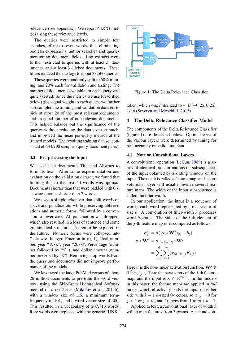
relevance (see appendix). We report NDCG met-rics using these relevance levels.
The queries were restricted to simple textsearches, of up to seven words, thus eliminatingboolean expressions, author searches and queriesmentioning document fields. Log extracts werefurther restricted to queries with at least 21 doc-uments, and at least 3 clicked documents. Thesefilters reduced the the logs to about 33,500 queries.
These queries were randomly split to 60% train-ing, and 20% each for validation and testing. Thenumber of documents available for each query wasquite skewed. Since the metrics we use (describedbelow) give equal weight to each query, we furthersub-sampled the training and validation datasets topick at most 20 of the most relevant documentsand an equal number of non-relevant documents.This helped balance out the significance of thequeries without reducing the data size too much,and improved the mean per-query metrics of thetrained models. The resulting training dataset con-sisted of 634,790 samples (query-document pairs).
3.2 Pre-processing the Input
We used each document’s Title and Abstract toform its text. After some experimentation andevaluation on the validation dataset, we found thatlimiting this to the first 50 words was optimal.Documents shorter than that were padded with 0’s,as were queries shorter than 7 words.
We used a simple tokenizer that split words onspace and punctuation, while preserving abbrevi-ations and numeric forms, followed by a conver-sion to lower-case. All punctuation was dropped,which also resulted in a loss of sentence and somegrammatical structure, an area to be explored inthe future. Numeric forms were collapsed into7 classes: Integer, Fraction in (0, 1), Real num-ber, year “19xx”, year “20xx”, Percentage (num-ber followed by “%”), and dollar amount (num-ber preceded by “$”). Removing stop-words fromthe query and documents did not improve perfor-mance of the models.
We leveraged the large PubMed corpus of about26 million documents to pre-train the word vec-tors, using the SkipGram Hierarchical Softmaxmethod of word2vec (Mikolov et al., 2013b),with a window size of ±5, a minimum term-frequency of 101, and a word-vector size of 300.This resulted in a vocabulary of 207,716 words.Rare words were replaced with the generic “UNK”
word2vec
OverlapFeatures
Query
DeltaScanner
DifferenceFeatures
Doc: Title + Abstract, truncated
Figure 1: The Delta Relevance Classifier.
token, which was initialized to ∼ U [−0.25, 0.25],as in (Severyn and Moschitti, 2015).
4 The Delta Relevance Classifier Model
The components of the Delta Relevance Classifier(figure 1) are described below. Optimal sizes ofthe various layers were determined by tuning forbest accuracy on validation data.
4.1 Note on Convolutional LayersA convolutional operation (LeCun, 1989) is a se-ries of identical transformations on subsequencesof the input obtained by a sliding window on theinput. The result is called a feature map, and a con-volutional layer will usually involve several fea-ture maps. The width of the input subsequence iscalled the filter width.
In our application, the input is a sequence ofwords, each word represented by a real vector ofsize d. A convolution of filter-width k processesword k-grams. The value of the t-th element ofthe j-th feature map cj is computed as follows:
cj[t] = σ((x ∗Wj)[t] + bj)
x ∗Wj = x[t−k+1:t] ·Wj
=d∑i=1
m∑j=1
(xi,t−k+jKi,j)
Here σ is the non-linear activation function, Wj ∈Rd×k, bj ∈ R are the parameters of the j-th featuremap, and the input is x ∈ Rd×m. In the modelsin this paper, the feature maps are applied in fullmode, which effectively pads the input on eitherside with k − 1 d-sized 0-vectors, so xi,j = 0 forj < 1 or j > m, and t ranges from 1 to m+k−1.
Applied to text, a convolutional layer of width 3will extract features from 3-grams. A second con-
224

Full Test Data Neg20+ OneNewWord AllNewWords
Nbr. of Queries 6,797 2,600 1,823 1,002Nbr. of Samples 416,509 208,734 90,353 50,827Prop. of Samples +ive 45.2% 39.5% 48.9% 48.8%Prop. of Samples -ive 54.8% 60.5% 51.1% 51.2%+ives without all Query terms in Title 38.9% 13.9% 34.0% 25.2%-ives with all Query terms in Title 59.1% 83.6% 65.4% 73.4%
Table 1: Test Data and its subsets
volutional layer of the same width stacked abovethen extracts features from 5-grams, and so on.
4.2 Query-Document Overlap Features
Following (Severyn and Moschitti, 2015), wecompute some overlap features to aid relevancedetection when dealing with exact matches, andrare words collpased to the ‘UNK’ token. Weuse the following overlap features, the first two ofwhich are taken directly from that paper: (i) pro-portion of query and document words in common,(ii) IDF-weighted version of (i), (iii) proportion ofquery words in the document, and (iv) proportionof query bigrams in the document.
4.3 Difference Features Stage
Instead of developing all pairwise local interac-tions between query and document terms, we cap-ture interactions between pairs of closest terms.This simplifies the model, and since queries areshort, we are unlikely to loose any useful inter-actions. The difference features are computed intwo steps (algorithm 1). First, for each word inthe document of a query-document pair, the clos-est query word in absolute vector distance is iden-tified (skipping all “UNK” words in the query anddocument). We then output the difference vector,along with its length and the cosine angle betweenthe two vectors. With word-vectors of size d and adocument of T words, the output of this stage is areal matrix of size d× (T + 2). We found T = 50produced the best results for the Delta models.
Algorithm 1 Query-Doc Difference FeaturesInput: Query text Q and Document text D.for each word vector w in D s.t. w 6= UNK do:
Find wq = arg min(u ∈ Q, u 6= UNK) ‖w − u‖Output: (w − wq), ‖w − wq‖, cos(w, wq)
end for
4.4 Delta Scanner Stage
The Delta Scanner stage is a vertical stack ofthree Convolutional layers of 256 filters each, fol-
lowed by a Dropout layer, and then a Global Max-Pooling layer outputting a fixed-width vector. Allfeature maps use the ReLU (Rectified Linear Unit)activation function.
The input to the Delta Scanner stage is thed × (T + 2) matrix produced by the DifferenceFeatures stage. Documents whose text is fewerthan T words are right-padded with 0’s, and theDelta Scanner supports a mask input that it uses toignore the padding. The output of this stage is avector of size 256, representing the semantic dif-ference between the the query and the documentin a query-document pair. The remaining hyper-parameters are: Dropout probability, and the L2-regularization coefficient.
4.5 Relevance Classifier StageThis is a deep fully connected feed-forward lo-gistic regression stage. The input to the Rele-vance Classifier stage is the combined vectors out-put from the Overlap Features and Delta Scannerstages, with a total width of 260 = (4+256). Thisdata is fed through the following layers:
i. a Dropout layer,ii. two feed-forward layers, each of width 260,
using the ReLU activation function,iii. another Dropout layer, andiv. a sigmoid-based Classification layer.
The Relevance Classifier’s output is an estimate ofthe probability of the input document’s relevanceto the query. Documents are ranked in reverse or-der on this estimated probability.
This stage’s hyper-parameters are: Dropoutprobability (same value used for both Dropout lay-ers), and the L2-regularization coefficient.
4.6 Loss Function and Sample WeightingThe data labels capture a binary sense of rele-vance, and our models are binary classifiers, so weused the standard binary cross-entropy loss.
In the default mode, the neural network modelswere trained without any weighting of the training
225

samples. We trained a second set of models withsample weights derived from the non-binary rele-vance levels (described above). For each relevancelevel r, a weight of max[1, log(1 + r)] was used.This damped the relevance levels, while ensuringthat each relevant document received at least thesame weight as a non-relevant document.
4.7 Optimization and Implementation NotesAll the neural network models were optimized us-ing Adadelta (Zeiler, 2012), with mini-batches of256 samples. Mini-batch gradient descent was runfor 10 epochs, and the trained values at the endof the epoch producing the best classification ac-curacy on the Validation dataset were chosen. Agreedy search was done in the grid space of thehyper-parameters for the Delta Scanner and Rel-evance Classifier stages, and the values that pro-duced the best validation accuracy were selected.
5 Experimental Setup
We compare the performance of the relevancemodels on the following ranking metrics: NDCGat rank 20, Precision at ranks 5, 10 and 20, andMean Average Precision (MAP). Scoring ties wereresolved by sorting on decreasing document-id.
5.1 Methods ComparedWe compared the performance of our deeplearning model against: BM25; the UnigramQuery Likelihood Model (UQLM) with Dirich-let Smoothing (Zhai and Lafferty, 2004); WordMover’s Distance (WMD) that leverages pre-trained word-vectors; and a couple of neural net-work models based on the architecture describedin (Severyn and Moschitti, 2015).
We tested BM25 on the document Title, Ab-stract and Title + Abstract, and found BM25 onTitle to give the best ranking performance, withparameters k1 = 2.0, b = 0.75. Similarly, UQLMapplied to the document Title and WMD appliedto the document Title after removal of stop-wordsperformed better than the other alternatives.
5.1.1 Severyn-Moschitti ModelWe tested four variants of the relevance classi-fier described in (Severyn and Moschitti, 2015).All versions used the same input data and word-vectors as used for the Delta model. In the ba-sic version, which we will refer to as “SevMos-C1”, the query and document were fed into asingle-layer Convolutional stage as described in
section 4.1, with 256 feature maps and a filterwidth of 5. This was followed by a Dropout layerand then Global Max-Pooling. The outputs of thequery and document convolutions, along with theoverlap features described in section 4.2, were fedinto a Classifier stage. This stage computed a dif-ference between the query and document featuresusing a difference matrix, and this value alongwith the other inputs were fed into a deep clas-sification stage identical to that used in the Deltamodel (section 4.5), sized to match these inputs.
In the “SevMos-C3” variant of this model, wereplaced the single-layer convolution stage with adeeper 3-layer stack of convolutions of filter width3, followed by global max-pooling, just like theDelta model’s ‘Delta Scanner’ stage.
In addition to training the models on un-weighted samples, we also trained separate mod-els on relevance-based weighted samples (see sec-tion 4.6), which we refer to below as “SevMos-C1 w” and “SevMos-C3 w”.
Optimal values for the L2-regularization andDropout probability hyper-parameters were deter-mined by doing a greedy grid search, as describedfor the Delta model.
5.2 The Test Data
The test data used to compare performance of thedifferent textual relevance approaches is the held-out 20% split of the data extracted from searchlogs, as described in section 3.1, without any fur-ther sub-sampling. Of the relevant documents(“+ives”), 38.9% did not contain all query termsin the title. Similarly among the non-relevant doc-uments (“-ives”), 59.1% contained all the queryterms in the title (see table 1).
In addition to comparing ranking metrics ofthe different approaches on the test data, wealso wanted to explore the main research ques-tions motivating this work: (i) the problems ofunder-specified queries and term mismatch, and(ii) model robustness. To help answer these ques-tions, we also compare ranking metrics on the fol-lowing subsets of the test data:
Neg20+: This consists of all queries for whichthere were at least 20 non-relevant documentsthat contained all the query words in the title.This helps evaluate performance on under-specified queries.
OneNewWord: The 1,823 test queries which
226

NDCG.20 MAP Prec.5 Prec.10 Prec.20
rev DocID 0.164 0.456 0.344 0.376 0.406BM25-Title 0.353 0.568 0.592 0.550 0.502UQLM-Title 0.341 0.561 0.575 0.541 0.500WMD-Title 0.356 0.579 0.602 0.565 0.516SevMos-C1 0.345 0.581 0.599 0.569 0.528SevMos-C3 0.339 0.577 0.597 0.564 0.524Delta 0.375 0.597 0.627 0.586 0.539Delta – WMD +5.3% +3.1% +4.2% +3.7% +4.5%Delta – SevMos-C1 +8.7% +2.8% +4.7% +3.0% +2.1%
Table 2: Ranking metrics on the Full Test Data
contain at least one new word that did not oc-cur in any training or validation queries.
AllNewWords: A smaller subset of queries all ofwhose words are new: none of the training orvalidation queries included these words.
The last two subsets will help us evaluate modelrobustness. The statistics of the test data and itssubsets are summarized in table 1.
6 Main Results and Discussion
6.1 Models trained on Un-weighted SamplesTable 2 compares the performance of all the aboveranking factors and models on the full test data.The first row shows the metrics obtained by rank-ing all the documents on reverse order of Docu-ment ID. We use this as a score tie-breaker for allthe other rankers, so it provides a useful baselineperformance of an uninformed ranker.
As also seen in (Shen et al., 2014), BM25 on Ti-tle slightly outperforms the Unigram Query Like-lihood Model. We have seen other cases whereUQLM outperforms BM25. We believe the betterperformance of BM25 here is partly due to it be-ing a strong factor in the relevance ranking fromwhich these click logs were extracted, thus bias-ing the click data to some extent.
Word Mover’s Distance (WMD-Title) is the firstfactor in the table that takes non-query words intoaccount, and it does show an improvement overBM25. However WMD relies on the word-vectorsobtained by unsupervised training, using a simpleEuclidean distance on these vectors as the seman-tic distance between words. This, and its relativelysimple computation, limit how well it performs.
The SevMos-C1 model applies a complex non-linear transformation on the word-vector basedtext space, in an attempt to better capture compara-ble semantics of documents. However its NDCG
numbers are worse than both WMD and BM25,although its precision numbers, while better thanBM25, are about the same as those for WMD.Given that the neural network models in this ta-ble were trained on a boolean version of relevance,we expect the main gains to be in the precision-based metrics, which also use a boolean notion ofrelevance. The lack of improvement in precisionmetrics over WMD shows that SevMos-C1’s non-linear transformations are not doing a better job ofcapturing query and document semantics.
The SevMos-C3 model learns a more complexnon-linear transformation than SevMos-C1, by us-ing a stack of three non-linear convolution layersinstead of one in the first part of the model. How-ever its metrics are no better (actually somewhatworse) than SevMos-C1 across the board. So in-creasing the expressive power of the model did nothelp. Lack of sufficient training data might be lim-iting the performance of these models.
The main difference between the Delta modeland SevMos-C3 is that the Delta Model starts bycomputing a difference vector between the Doc-ument and Query’s word-vector representations.This local interaction vector is inspired by WordMover’s Distance, and in the Delta model we hopeto combine the benefits of the WMD and Sev-Mos approaches, while at the same time reduc-ing the complexity of the input space, and thus al-lowing us to extract more benefit from the smallamount of training data. The performance metricsfor the Delta model do indeed show sizeable im-provements over both WMD and SevMos-C1 (andthus also over BM25 and UQLM). The relative im-provements in the metrics are shown in the last tworows of the table2.
The ‘Neg20+’ section of the table 3 compares
2All cited improvements have been verified to be statis-tically significant to at least a 99% confidence level using apaired t-test.
227
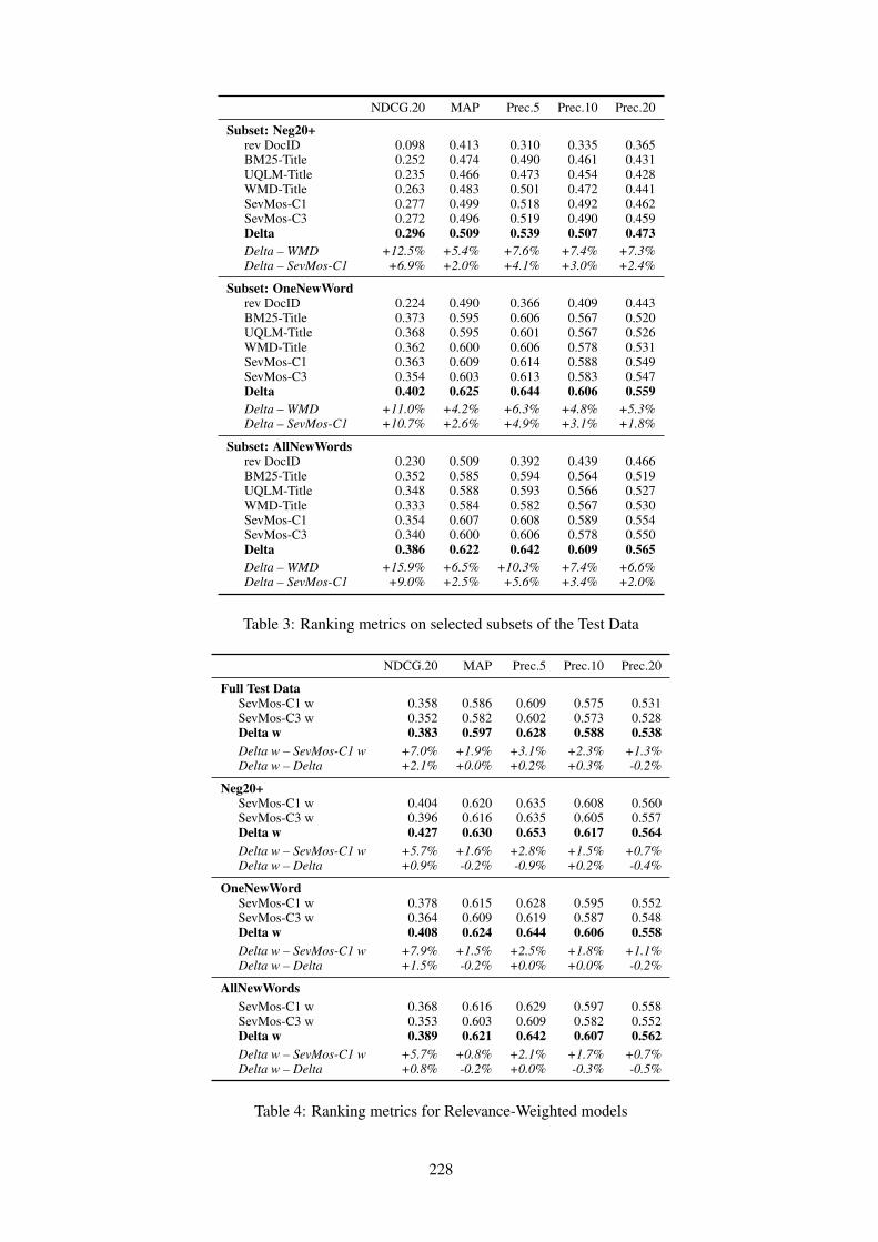
NDCG.20 MAP Prec.5 Prec.10 Prec.20
Subset: Neg20+rev DocID 0.098 0.413 0.310 0.335 0.365BM25-Title 0.252 0.474 0.490 0.461 0.431UQLM-Title 0.235 0.466 0.473 0.454 0.428WMD-Title 0.263 0.483 0.501 0.472 0.441SevMos-C1 0.277 0.499 0.518 0.492 0.462SevMos-C3 0.272 0.496 0.519 0.490 0.459Delta 0.296 0.509 0.539 0.507 0.473Delta – WMD +12.5% +5.4% +7.6% +7.4% +7.3%Delta – SevMos-C1 +6.9% +2.0% +4.1% +3.0% +2.4%
Subset: OneNewWordrev DocID 0.224 0.490 0.366 0.409 0.443BM25-Title 0.373 0.595 0.606 0.567 0.520UQLM-Title 0.368 0.595 0.601 0.567 0.526WMD-Title 0.362 0.600 0.606 0.578 0.531SevMos-C1 0.363 0.609 0.614 0.588 0.549SevMos-C3 0.354 0.603 0.613 0.583 0.547Delta 0.402 0.625 0.644 0.606 0.559Delta – WMD +11.0% +4.2% +6.3% +4.8% +5.3%Delta – SevMos-C1 +10.7% +2.6% +4.9% +3.1% +1.8%
Subset: AllNewWordsrev DocID 0.230 0.509 0.392 0.439 0.466BM25-Title 0.352 0.585 0.594 0.564 0.519UQLM-Title 0.348 0.588 0.593 0.566 0.527WMD-Title 0.333 0.584 0.582 0.567 0.530SevMos-C1 0.354 0.607 0.608 0.589 0.554SevMos-C3 0.340 0.600 0.606 0.578 0.550Delta 0.386 0.622 0.642 0.609 0.565Delta – WMD +15.9% +6.5% +10.3% +7.4% +6.6%Delta – SevMos-C1 +9.0% +2.5% +5.6% +3.4% +2.0%
Table 3: Ranking metrics on selected subsets of the Test Data
NDCG.20 MAP Prec.5 Prec.10 Prec.20
Full Test DataSevMos-C1 w 0.358 0.586 0.609 0.575 0.531SevMos-C3 w 0.352 0.582 0.602 0.573 0.528Delta w 0.383 0.597 0.628 0.588 0.538Delta w – SevMos-C1 w +7.0% +1.9% +3.1% +2.3% +1.3%Delta w – Delta +2.1% +0.0% +0.2% +0.3% -0.2%
Neg20+SevMos-C1 w 0.404 0.620 0.635 0.608 0.560SevMos-C3 w 0.396 0.616 0.635 0.605 0.557Delta w 0.427 0.630 0.653 0.617 0.564Delta w – SevMos-C1 w +5.7% +1.6% +2.8% +1.5% +0.7%Delta w – Delta +0.9% -0.2% -0.9% +0.2% -0.4%
OneNewWordSevMos-C1 w 0.378 0.615 0.628 0.595 0.552SevMos-C3 w 0.364 0.609 0.619 0.587 0.548Delta w 0.408 0.624 0.644 0.606 0.558Delta w – SevMos-C1 w +7.9% +1.5% +2.5% +1.8% +1.1%Delta w – Delta +1.5% -0.2% +0.0% +0.0% -0.2%
AllNewWordsSevMos-C1 w 0.368 0.616 0.629 0.597 0.558SevMos-C3 w 0.353 0.603 0.609 0.582 0.552Delta w 0.389 0.621 0.642 0.607 0.562Delta w – SevMos-C1 w +5.7% +0.8% +2.1% +1.7% +0.7%Delta w – Delta +0.8% -0.2% +0.0% -0.3% -0.5%
Table 4: Ranking metrics for Relevance-Weighted models
228

ranking performance on a subset of the test datathat should be harder to rank for factors and mod-els that do not give some consideration to the non-query words in the document. In this data a signif-icant number of non-relevant documents containall the query words in the title. Comparing thesenumbers with the previous table shows that thereis indeed a significant drop in performance for allthe factors and models considered here. Howeverwhile BM25’s NDCG metrics drop by 28.6%, theDelta model’s NDCG drops by only 21.1%, withthe corresponding drops in MAP being 16.5% and14.7%, respectively. The Delta model still showsthe best metrics on this test set, and its degree ofimprovement over WMD is bigger, as expectedfrom a more complex model.
Model robustness is tested when queries withwords not seen during training (i.e. trainingand validation datasets) are encountered. Thisis explored in sections ‘OneNewWord’ and ‘All-NewWords’ of table 3. Both these sub-tablesshow a consistently better performance by theDelta model over the other approaches comparedhere. Interestingly, the improvements in the Deltamodel’s NDCG at 20 metrics over the other ap-proaches are quite sizeable, even though for a sim-ple un-weighted relevance classifier, the primarytarget was precision and not NDCG.
6.2 Relevance Weighted Models
In this section we explore the performance of theDelta model trained on relevance-weighted sam-ples against the corresponding weighted versionsof the neural network models SevMos-C1 andSevMos-C3. These metrics are shown in table 4.A quick comparison with previous tables showsthat all the models turn in better NDCG num-bers than their un-weighted versions. In particu-lar, the “Delta w” model continues to depict sta-tistically significant better metrics than the otherweighted neural network models “SevMos-C1 w”and “SevMos-C3 w”.
Comparing the Delta weighted model againstthe unweighted Delta model, we see that there is astatistically significant improvment in the NDCGmetrics for all the Test subsets (at the 99% con-fidence level). However the precision metrics donot show a significant change. So by weighting thesamples we have been able to improve the NDCGwithout hurting the precision.
7 Concluding Remarks
We have demonstrated a Deep Learning approachfor learning textual relevance from a fairly smalllabelled training dataset. We show that this modelis robust and it outperforms both traditional IR fac-tors as well as related shallow (WMD) and deep(SevMos) models based on continuous represen-tations of text, with better results on the under-specified query and term mismatch problems.
While the Delta model is comparable to otherlocal-interaction ranking models, we computefewer and richer interactions. We believe the fewerinteractions captured in the difference vector aresufficient for the shorter queries in our data. As acomparison, the model in (Guo et al., 2016) com-putes a match histogram based on cosine similaritybetween all document-query word pairs, and alsoquery-term IDF based weighting. We plan to testthis model on our data.
The main advantage to the separate semanticvector approach is that document semantic vectorscan be pre-computed. Prediction run-time thenprimarily depends on the complexity of the sim-ilarity computation between these semantic vec-tors. Local-interaction models, including ours, donot allow this pre-computation, significantly in-creasing the ranker’s run-time cost.
We believe the most promising directions for fu-ture research include: modeling deeper semantics(see example in appendix), unsupervised trainingon data auto-generated from the corpus and fine-tuning with supervised training, improving extrac-tion of non-binary relevance levels and using apair-wise ranking target. Further investigation isalso warranted for incorporating these models intoPubMed.
Acknowledgments
This research was supported by the Intramural Re-search Program of the NIH, National Library ofMedicine.
ReferencesRezarta Islamaj Dogan, G Craig Murray, Aurelie
Neveol, and Zhiyong Lu. 2009. UnderstandingPubMed R© user search behavior through log analy-sis. Database 2009:bap018.
G. W. Furnas, T. K. Landauer, L. M. Gomez, and S. T.Dumais. 1987. The vocabulary problem in humansystem communication. CACM 30(11):964–971.
229

Jianfeng Gao, Patrick Pantel, Michael Gamon, Xi-aodong He, and Li Deng. 2014. Modeling interest-ingness with deep neural networks. In Proceedingsof EMNLP 2014. ACL, Doha, Qatar, pages 2–13.
Jiafeng Guo, Yixing Fan, Qingyao Ai, and W. BruceCroft. 2016. A deep relevance matching model forad-hoc retrieval. In Proceedings of CIKM 2016.ACM, New York, NY, USA, pages 55–64.
Baotian Hu, Zhengdong Lu, Hang Li, and QingcaiChen. 2014. Convolutional neural network archi-tectures for matching natural language sentences.In Z. Ghahramani, M. Welling, C. Cortes, N. D.Lawrence, and K. Q. Weinberger, editors, Advancesin NIPS 27, pages 2042–2050.
Po-Sen Huang, Xiaodong He, Jianfeng Gao, Li Deng,Alex Acero, and Larry Heck. 2013. Learning deepstructured semantic models for web search usingclickthrough data. In Proceedings of CIKM 2013.ACM, New York, NY, USA, pages 2333–2338.
Alex Krizhevsky, Ilya Sutskever, and Geoffrey E Hin-ton. 2012. Imagenet classification with deep con-volutional neural networks. In F. Pereira, C. J. C.Burges, L. Bottou, and K. Q. Weinberger, editors,Advances in NIPS 25, pages 1097–1105.
Matt Kusner, Yu Sun, Nicholas Kolkin, and KilianWeinberger. 2015. From word embeddings to doc-ument distances. In Proceedings of The 32nd Inter-national Conference on Machine Learning. JMLR,ICML 2015, pages 957–966.
Yann LeCun. 1989. Generalization and network designstrategies. In R. Pfeifer, Z. Schreter, F. Fogelman,and L. Steels, editors, Connectionism in Perspective,Elsevier, Zurich, Switzerland.
Zhengdong Lu and Hang Li. 2013. A deep architecturefor matching short texts. In C. Burges, L. Bottou,M. Welling, Z. Ghahramani, and K. Q. Weinberger,editors, Advances in NIPS 26, pages 1367–1375.
Zhiyong Lu, Won Kim, and W John Wilbur. 2009.Evaluation of query expansion using MeSH inPubMed. Information retrieval 12(1):69–80.
Tomas Mikolov, Kai Chen, Greg Corrado, and JeffreyDean. 2013a. Efficient estimation of word represen-tations in vector space. In Proceedings of the Work-shop at ICLR 2013.
Tomas Mikolov, Martin Karafiat, Lukas Burget, JanCernocky, and Sanjeev Khudanpur. 2010. Recurrentneural network based language model. In Proceed-ings of INTERSPEECH 2010.
Tomas Mikolov, Ilya Sutskever, Kai Chen, Greg S Cor-rado, and Jeff Dean. 2013b. Distributed represen-tations of words and phrases and their composition-ality. In C. J. C. Burges, L. Bottou, M. Welling,Z. Ghahramani, and K. Q. Weinberger, editors, Ad-vances in NIPS 26, pages 3111–3119.
David R. H. Miller, Tim Leek, and Richard M.Schwartz. 1999. A hidden markov model informa-tion retrieval system. In Proceedings of SIGIR 1999.ACM, New York, NY, USA, pages 214–221.
Bhaskar Mitra and Nick Craswell. 2017. Neural mod-els for information retrieval. CoRR abs/1705.01509.https://arxiv.org/abs/1705.01509.
Stephen E. Robertson, Steve Walker, Susan Jones,Micheline Hancock-Beaulieu, and Mike Gatford.1994. Okapi at TREC-3. In Proceedings of TREC1994. NIST, Dept. of Commerce, pages 109–126.
Aliaksei Severyn and Alessandro Moschitti. 2015.Learning to rank short text pairs with convolutionaldeep neural networks. In Proceedings of SIGIR2015. ACM, New York, NY, USA, pages 373–382.
Yelong Shen, Xiaodong He, Jianfeng Gao, Li Deng,and Gregoire Mesnil. 2014. A latent semantic modelwith convolutional-pooling structure for informationretrieval. In Proceedings of CIKM 2014. ACM, NewYork, NY, USA, pages 101–110.
Karen Simonyan and Andrew Zisserman. 2015. Verydeep convolutional networks for large-scale imagerecognition. In Proceedings of ICLR 2015.
Richard Socher, Cliff Chiung-Yu Lin, Andrew Ng, andChris Manning. 2011a. Parsing natural scenes andnatural language with recursive neural networks. InLise Getoor and Tobias Scheffer, editors, Proceed-ings of ICML 2011. ACM, New York, NY, USA,pages 129–136.
Richard Socher, Jeffrey Pennington, Eric H. Huang,Andrew Y. Ng, and Christopher D. Manning. 2011b.Semi-supervised recursive autoencoders for predict-ing sentiment distributions. In Proceedings ofEMNLP 2011. ACL, pages 151–161.
Matthew D. Zeiler. 2012. ADADELTA: an adaptivelearning rate method. CoRR abs/1212.5701.
Chengxiang Zhai and John Lafferty. 2004. A studyof smoothing methods for language models appliedto information retrieval. ACM Trans. Inf. Syst.22(2):179–214.
Y. Zhang, M. M. Rahman, A. Braylan, B. Dang,H. Chang, H. Kim, Q. McNamara, A. Angert,E. Banner, V. Khetan, T. McDonnell, A. T. Nguyen,D. Xu, B. C. Wallace, and M. Lease. 2016. Neu-ral information retrieval: A literature review. CoRRabs/1611.06792. http://arxiv.org/abs/1611.06792.
A Document Relevance Levels
Deriving relevance level of a document to a queryfrom observed clicks is still experimental. We usethe following formula:
µ×AbClicks + (1− µ)× FTClicks
+1λ×IsDocWithoutFullText×AbClicks
230

with the parameters µ = 0.33, λ = 15, whereAbClicks is the number of observed clicks to thedocument summary page in PubMed, FTClicks isthe number of observed clicks to the document’sfull text, if available, and the value of IsDocWith-outFullText is 1 if the full text for that documentis not available, and 0 otherwise. The formula at-tempts to capture the increased notion of relevanceif the user accesses the document’s full text, with-out penalizing documents whose full-text is notavailable. The parameters were hand-tuned to re-flect domain experts’ relevance judgments.
B Rankings on Some Example Queries
Here are some example queries from the test setshowing the titles of the top 3 ranked documentsfor the Delta weighted model, BM25 and WMD.Relevance levels of the documents are indicatedinside parentheses before the titles.
B.1 Query: cryoglobulinemia
This word did not occur in training or validationqueries. Delta w ranks the most relevant docu-ment at the top despite its use of an alternativespelling. BM25 and WMD seem to prefer shortertitles with exact matches. Number of documentsin the test dataset: relevant = 27, non-relevant =26. Top three relevance levels: 39.0, 11.0, 4.0.
As ranked by Delta w:i. (39.0) Diagnostics and treatment of cryoglobulinaemia:
it takes two to tango.ii. (0.0) Clinical features of 30 patients with cryoglobu-
linemia.iii. (4.0) The diagnosis and classification of the cryoglob-
ulinemic syndrome.
As ranked by BM25:i. (11.0) Cryoglobulinemia Vasculitis.
ii. (3.0) Cryoglobulinemia (review).iii. (1.0) Role of CXCL10 in cryoglobulinemia.
As ranked by WMD:i. (11.0) Cryoglobulinemia Vasculitis.
ii. (3.0) Cryoglobulinemia (review).iii. (3.0) Primary cryoglobulinemia with cutaneous fea-
tures.
B.2 Query: oesophageal cancerreview
The word oesophageal did not occur in trainingor validation queries. The word review does notoccur in the title of all relevant documents. BothDelta w and WMD successfully locate alternativespellings of the word. Number of documents inthe test dataset: relevant = 22, non-relevant = 28.Top three relevance levels: 7.0, 4.0, 4.0.
As ranked by Delta w:i. (7.0) Esophageal cancer: Recent advances in screen-
ing, targeted therapy, and management.ii. (3.0) Esophageal cancer: A Review of epidemiology,
pathogenesis, staging workup and treatment modali-ties.
iii. (3.0) Esophageal Cancer Staging.
As ranked by BM25:i. (3.0) Imaging of oesophageal cancer with FDG-
PET/CT and MRI.ii. (0.0) Systematic review and network meta-analysis:
neoadjuvant chemoradiotherapy for locoregional eso-phageal cancer.
iii. (0.0) Serum autoantibodies in the early detection ofesophageal cancer: a systematic review.
As ranked by WMD:i. (3.0) Esophageal Cancer Staging.
ii. (0.0) Outcomes in the management of esophageal can-cer.
iii. (4.0) Endoscopic Management of Early EsophagealCancer.
B.3 Query: chronic headache anddepression review
In this example, both WMD and Delta w are ableto leverage word vectors to relate headache to mi-graine. However both miss the most relevant doc-ument, whose title is “Psychological Risk Factors in
Headache” (relevance level = 6.0). This exampledemonstrates the need for deeper semantic model-ing. Number of documents in the test dataset: rel-evant = 23, non-relevant = 18. Top three relevancelevels: 6.0, 3.0, 3.0.
As ranked by Delta w:i. (3.0) Migraine and depression: common pathogenetic
and therapeutic ground?ii. (3.0) Migraine and depression comorbidity: antide-
pressant options.iii. (3.0) Migraine and depression: bidirectional co-
morbidities?
As ranked by BM25:i. (3.0) Comprehensive management of headache and de-
pression.ii. (0.0) Chronic daily headache in children and adoles-
cents.iii. (0.0) Screening for depression and anxiety disorder in
children with headache.
As ranked by WMD:i. (3.0) Comprehensive management of headache and de-
pression.ii. (3.0) Chronic headaches and the neurobiology of som-
atization.iii. (3.0) Migraine and depression: biological aspects.
231

Proceedings of the BioNLP 2017 workshop, pages 232–237,Vancouver, Canada, August 4, 2017. c©2017 Association for Computational Linguistics
Detecting Dementia through Retrospective Analysis of Routine Blog Postsby Bloggers with Dementia
Vaden MasraniDept. of Computer Science
University of British [email protected]
Gabriel MurrayDept. of Computer Information Systems
University of the Fraser [email protected]
Thalia FieldDept. of Neurology
University of British [email protected]
Giuseppe CareniniDept. of Computer Science
University of British [email protected]
AbstractWe investigate if writers with demen-tia can be automatically distinguishedfrom those without by analyzing linguis-tic markers in written text, in the form ofblog posts. We have built a corpus of sev-eral thousand blog posts, some by peoplewith dementia and others by people withloved ones with dementia. We use thisdataset to train and test several machinelearning methods, and achieve predictionperformance at a level far above the base-line.
1 Introduction
Dementia is estimated to become a trillion dollardisease worldwide by 2018, and prevalence is ex-pected to double to 74.7 million by 2030 (Prince,2015). Dementia is a clinical syndrome caused byneurodegenerative illnesses (e.g. Alzheimer’s Dis-ease, vascular dementia, Lewy Body dementia).Symptoms can include memory loss, decreasedreasoning ability, behavioral changes, and – rel-evant to our work – speech and language impair-ment, including fluency, word choice and sentencestructure (Klimova and Kuca, 2016).
Recently, there have been attempts to combineclinical information with language analysis usingmachine learning and NLP techniques to aid in di-agnosis of dementia, and to distinguish betweentypes of pathologies (Jarrold et al., 2014; Ren-toumi et al., 2014; Orimaye et al., 2014; Fraseret al., 2015; Masrani et al., 2017). This wouldprovide an inexpensive, non-invasive and efficientscreening tool to assist in early detection, treat-ment and institution of supports. Yet, much of thework to date has focused on analyzing spoken lan-guage collected during formal assessment, usuallywith standardized exam tools.
There has been comparatively little work doneon analyzing written language spontaneously gen-erated by people with dementia. In coming years,there will be an increased number of tech-savvyseniors using the internet, and popular online com-mentators will continue to age. There will there-fore be a growing dataset available in the form oftweets, blog posts, and comments on social media,on which to train a classifier. Provided our writershave a verified clinical diagnosis of dementia, sucha dataset would be large, inexpensive to acquire,easy to process, and require no manual transcrip-tions.
There are downsides to using written languagesamples as well. Unlike spoken language, writ-ten text can be edited or revised by oneself orothers. People with dementia may have “gooddays” and “bad days,” and may write only on dayswhen they are feeling lucid, and therefore writtensamples may be biased towards more intact lan-guage. Furthermore, we do not have an accompa-nying audio file and patients are not constrainedto a single topic; people with dementia may havegreater facility discussing familiar topics. A non-standardized dataset will also prevent the collec-tion of common test-specific linguistic or acous-tic features. However, working with a very largedataset may be able to mitigate the effects of theselimitations.
In this work we gather a corpus of blog postspublicly available online, some by people with de-mentia and others by the loved ones of people withdementia. We extract a variety of linguistic fea-tures from the texts, and compare multiple ma-chine learning methods for detecting posts writtenby people with dementia. All models perform wellabove the baseline, demonstrating the feasibilityof this detection task.
232

2 Related Work
Early signs of dementia can be detected throughanalysis of writing samples (Le et al., 2011; Ri-ley et al., 2005; Kemper et al., 2001). In the “NunStudy” researchers analyzed autobiographies writ-ten in the US by members of the School Sistersof Notre Dame between 1931-1996. Those nunswho met criteria for dementia had lower grammat-ical complexity scores and lower “idea density” intheir autobiographies.Le et al. (2011) performed a longitudinal analysisof the writing styles of three novelists: Iris Mur-doch who died with Alzheimer’s disease (AD),Agatha Christie (suspected AD), and P.D. James(normal brain aging). Measurements of syntacticand lexical complexity were made from 51 nov-els spanning each of the author careers. Murdochand Christie exhibited evidence of linguistic de-cline in later works, such as vocabulary loss, in-creased repetition, and a deficit of noun tokens (Leet al., 2011).Despite evidence that linguistic markers predic-tive of dementia can be found in writing samples,there have been no attempts to train models toclassify dementia based on writing alone. Previ-ous work has been successful in training modelsusing transcribed utterances from patients under-going formal examinations, but this data is diffi-cult to acquire and many models use audio and/ortest-specific features which would not be availablefrom online text (Rentoumi et al., 2014; Orimayeet al., 2014; Fraser et al., 2014; Roark et al., 2011).State-of-the-art classification accuracy of 81.92%was achieved by Fraser et al. (2015) with logis-tic regression using acoustic, textual, and test-specific features on 473 samples from Demen-tiaBank dataset, an American cohort of 204 per-sons with dementia and 102 controls describingthe “Cookie Theft Picture”, a component of theBoston Diagnostic Aphasia Examination (Beckeret al., 1994; Giles et al., 1996). More recently,these results have been extended via domain adap-tation by Masrani et al. (Masrani et al., 2017).
Our methods are similar to Fraser et al. (2015),with the main difference being the dataset usedand their inclusion of audio and test-specific fea-tures, which are not available in our case. To thebest of our knowledge, ours is the first compari-son of models trained exclusively on unstructuredwritten samples from persons with dementia.
3 Experimental Design
In this section, we describe the novel blog corpusand experimental setup.
3.1 CorpusWe scraped the text of 2805 posts from 6 publicblogs as described in Table 1. Three blogs werewritten by persons with dementia (First blogger:male, AD, age unknown. Second blogger: female,AD, age 61. Third blogger: Male, Dementia withLewy Bodies, age 66) and three written by fam-ily members of persons with dementia to be usedas control (all female, ages unknown). Other de-mographic information, such as education level,was unavailable. From each of the three demen-tia blogs, we manually filtered all texts not writ-ten by the owner of the blog (e.g. fan letters) orposts containing more images than text. We wereleft with 1654 samples written by persons with de-mentia and 1151 from healthy controls. The scriptto download the corpus is available at https://github.com/vadmas/blog_corpus/.
3.2 Classification FeaturesFollowing Fraser et al. (2015), we extracted 101features across six categories from each blog post.These features are described below.
Parts Of Speech (14) We use the Stanford Tag-ger (Toutanova et al., 2003) to capture the fre-quency of various parts of speech tags (nouns,verbs, adjectives, adverbs, pronouns, determin-ers, etc). Frequency counts are normalized by thenumber of words in the sentence, and we reportthe sentence average for a given post. We alsocount not-in-dictionary words and word-type ra-tios (noun to verb, pronoun to noun, etc).
Context Free Grammar (45) Features whichcount how often a phrase structure rule occurs in asentence, including NP→VP PP, NP→DT NP, etc.Parse trees come from the Stanford parser (Kleinand Manning, 2003).
Syntactic Complexity (28) Features whichmeasure the complexity of an utterance throughmetrics such as the depth of the parse tree, meanlength of word, sentences, T-Units and clauses andclauses per sentence. We used the L2 SyntacticComplexity Analyzer (Lu, 2010).
Psycholingustic (5) Psycholinguistic featuresare linguistic properties of words that effect word
233

URL Posts Mean words Start Date Diagnosishttps://creatingmemories.blogspot.ca/ 618 242.22 (s=169.42) Dec 2003 ADhttp://living-with-alzhiemers.blogspot.ca/ 344 263.03 (s=140.28) Sept 2006 ADhttp://parkblog-silverfox.blogspot.ca/ 692 393.21 (s=181.54) May 2009 Lewy Bodyhttp://journeywithdementia.blogspot.ca/ 201 803.91 (s=548.34) Mar 2012 Controlhttp://earlyonset.blogspot.ca/ 452 615.11 (s=206.72) Jan 2008 Controlhttp://helpparentsagewell.blogspot.ca/ 498 227.12 (s=209.17) Sept 2009 Control
Table 1: Blog Information.
processing and learnability (Salsbury et al., 2011).We used five psycholinguisic features: Familiar-ity, Concreteness, Imageability, Age of acquisi-tion, and the SUBTL , which is a measure of thefrequency with which a word is used in dailylife (Kuperman et al., 2012; Brysbaert and New,2009a; Salsbury et al., 2011). Psycholinguis-tic word scores are derived from human ratings1
while the SUBTL frequency norm2 is based on50 million words from television and film subti-tles (Brysbaert and New, 2009b).
Vocabulary Richness (4) We calculated fourmetrics which capture the range of vocabulary ina text: type-token ratio, Brunet’s index, a lengthinsensitive version of the type-token ratio, Hon-ore’s statistic, and the moving-average type-tokenratio (MATTR) (Asp and De Villiers, 2010; Cov-ington and McFall, 2010). These metrics havebeen shown to be effective in previous AD re-search (Bucks et al., 2000; Fraser et al., 2015)
Repetitiveness (5) We represent sentences asTF-IDF vectors and compute the cosine similaritybetween sentences. We then report the proportionof sentence pairs below three similarity thresholds(0, 0.3, 0.5) as well as the min and average cosinedistance across all pairs of sentences.
3.3 Training and Testing
We perform a 9-fold cross validation by trainingeach model on all the posts of four blogs and test-ing on the remaining two, where we assure thateach test set contains the posts of one control blogand one dementia blog. Within each fold we per-form a feature selection step before training wherewe select for inclusion into the model the first kfeatures which have the highest absolute correla-tion with the labels in the training fold.
1http://websites.psychology.uwa.edu.au/school/MRCDatabase/uwa_mrc.htm
2http://subtlexus.lexique.org/
4 Results
For each machine learning model, we calculate theROC curve and the area under the curve (AUC),comparing with a random performance baselineAUC of 0.5. The AUC results are shown in Fig-ure 1, with all models well above the baseline of0.5. The best performing models are logistic re-gression and neural networks, with average AUCscores of 0.815 and 0.848, respectively.
The SUBTL measure of vocabulary richnesswas the feature most correlated with the outcomevariable in eight out of nine folds. Figure 2 showsthe SUBTL scores for each blog post in the cor-pus, arranged by blog and with the bloggers withdementia shown in the top row. A lower score in-dicates a richer vocabulary. We can see that thebloggers with dementia have a less rich vocabu-lary. Interestingly, however, the longitudinal trenddoes not show their vocabularies worsening duringthe time-period captured in this corpus. The analy-sis of other features highly informative for the tar-get prediction is ongoing, and additional findingswill be discussed at the workshop.
5 Conclusion
We have shown that it is possible to distinguishbloggers with dementia from those without, on anovel corpus of blog data. We extracted linguis-tic features from the texts and compared a largenumber of machine learning methods, all of whichperformed well above the baseline. While featureanalysis is ongoing, we have made some interest-ing observations about the effect of the SUBTLmeasure of vocabulary richness. Future work willinclude liaising with patient and caregiver supportgroups to expand this new dementia corpus, in-clusion of a topic clustering preprocessing step tocontrol for variation across content, and furtherlongitudinal analysis.
234

Figure 1: Comparison of models. We show the mean AUC and 90% confidence intervals across a 9-foldCV. All the posts of a blog appear in either the training or test set, but not both.
Figure 2: SUBTL word scores for each post in a given blog. Bloggers with dementia (AD or Dementiaw/ Lewy Bodies) appear in the top row.
235

ReferencesElissa D Asp and Jessica De Villiers. 2010. When lan-
guage breaks down: Analysing discourse in clinicalcontexts. Cambridge University Press.
James T Becker, Francois Boiler, Oscar L Lopez, Ju-dith Saxton, and Karen L McGonigle. 1994. Thenatural history of alzheimer’s disease: description ofstudy cohort and accuracy of diagnosis. Archives ofNeurology 51(6):585–594.
Marc Brysbaert and Boris New. 2009a. Moving be-yond Kucera and Francis: A critical evaluation ofcurrent word frequency norms and the introductionof a new and improved word frequency measurefor american english. Behavior Research Methods41:977–990.
Marc Brysbaert and Boris New. 2009b. Moving be-yond kucera and francis: A critical evaluation ofcurrent word frequency norms and the introductionof a new and improved word frequency measurefor american english. Behavior research methods41(4):977–990.
Romola S Bucks, Sameer Singh, Joanne M Cuer-den, and Gordon K Wilcock. 2000. Analysis ofspontaneous, conversational speech in dementia ofalzheimer type: Evaluation of an objective tech-nique for analysing lexical performance. Aphasiol-ogy 14(1):71–91.
Michael A Covington and Joe D McFall. 2010. Cut-ting the gordian knot: The moving-average type–token ratio (mattr). Journal of Quantitative Linguis-tics 17(2):94–100.
Kathleen C Fraser, Graeme Hirst, Naida L Graham,Jed A Meltzer, Sandra E Black, and Elizabeth Ro-chon. 2014. Comparison of different feature setsfor identification of variants in progressive aphasia.ACL 2014 page 17.
Kathleen C Fraser, Jed A Meltzer, and Frank Rudz-icz. 2015. Linguistic features identify alzheimersdisease in narrative speech. Journal of Alzheimer’sDisease 49(2):407–422.
Elaine Giles, Karalyn Patterson, and John R Hodges.1996. Performance on the boston cookie theft pic-ture description task in patients with early dementiaof the alzheimer’s type: missing information. Apha-siology 10(4):395–408.
William Jarrold, Bart Peintner, David Wilkins, Dim-itra Vergryi, Colleen Richey, Maria Luisa Gorno-Tempini, and Jennifer Ogar. 2014. Aided diagnosisof dementia type through computer-based analysisof spontaneous speech. In Proceedings of the ACLWorkshop on Computational Linguistics and Clini-cal Psychology. pages 27–36.
Susan Kemper, Lydia H Greiner, Janet G Marquis,Katherine Prenovost, and Tracy L Mitzner. 2001.Language decline across the life span: findings fromthe nun study. Psychology and aging 16(2):227.
Dan Klein and Christopher D Manning. 2003. Accu-rate unlexicalized parsing. In Proc. of ACL, Sap-poro, Japan. Association for Computational Lin-guistics, pages 423–430.
Blanka Klimova and Kamil Kuca. 2016. Speech andlanguage impairments in dementia. Journal of Ap-plied Biomedicine 14(2):97–103.
Victor Kuperman, Hans Stadthagen-Gonzalez, andMarc Brysbaert. 2012. Age-of-acquisition ratingsfor 30,000 english words. Behavior Research Meth-ods 44(4):978–990.
Xuan Le, Ian Lancashire, Graeme Hirst, and ReginaJokel. 2011. Longitudinal detection of dementiathrough lexical and syntactic changes in writing: acase study of three british novelists. Literary andLinguistic Computing 26(4):435–461.
Xiaofei Lu. 2010. Automatic analysis of syntacticcomplexity in second language writing. Interna-tional Journal of Corpus Linguistics 15(4):474–496.
Vaden Masrani, Gabriel Murray, Thalia Field, andGiuseppe Carenini. 2017. Domain adaptation fordetecting mild cognitive impairment. In Proc. ofCanadian AI, Edmonton, Canada.
Sylvester Olubolu Orimaye, Jojo Sze-Meng Wong, andKaren Jennifer Golden. 2014. Learning predictivelinguistic features for alzheimer’s disease and re-lated dementias using verbal utterances. In Proc. 1stWorkshop. Computational Linguistics and ClinicalPsychology (CLPsych).
Martin James Prince. 2015. World Alzheimer Report2015: the global impact of dementia: an analysis ofprevalence, incidence, cost and trends. London.
Vassiliki Rentoumi, Ladan Raoufian, Samrah Ahmed,Celeste A de Jager, and Peter Garrard. 2014. Fea-tures and machine learning classification of con-nected speech samples from patients with autopsyproven alzheimer’s disease with and without addi-tional vascular pathology. Journal of Alzheimer’sDisease 42(s3).
Kathryn P Riley, David A Snowdon, Mark FDesrosiers, and William R Markesbery. 2005. Earlylife linguistic ability, late life cognitive function, andneuropathology: findings from the nun study. Neu-robiology of aging 26(3):341–347.
Brian Roark, Margaret Mitchell, John-Paul Hosom,Kristy Hollingshead, and Jeffrey Kaye. 2011. Spo-ken language derived measures for detecting mildcognitive impairment. IEEE Transactions on Au-dio, Speech, and Language Processing 19(7):2081–2090.
Tom Salsbury, Scott A Crossley, and Danielle S McNa-mara. 2011. Psycholinguistic word information insecond language oral discourse. Second LanguageResearch 27(3):343–360.
236

Kristina Toutanova, Dan Klein, Christopher D Man-ning, and Yoram Singer. 2003. Feature-rich part-of-speech tagging with a cyclic dependency network.In Proc. of NAACL, Edmonton, Canada. Associationfor Computational Linguistics, pages 173–180.
237

Proceedings of the BioNLP 2017 workshop, pages 238–246,Vancouver, Canada, August 4, 2017. c©2017 Association for Computational Linguistics
Protein Word Detection using Text Segmentation Techniques
G.DeviDepartment of CSE
IIT MadrasChennai-600036, India
Ashish V. TendulkarGoogle Inc.,
Hyderabad-500084, [email protected]
Sutanu ChakrabortiDepartment of CSE
IIT MadrasChennai-600036, India
Abstract
Literature in Molecular Biology is abun-dant with linguistic metaphors. There havebeen works in the past that attempt todraw parallels between linguistics and bi-ology, driven by the fundamental premisethat proteins have a language of their own.Since word detection is crucial to the de-cipherment of any unknown language, weattempt to establish a problem mappingfrom natural language text to protein se-quences at the level of words. Towards thisend, we explore the use of an unsupervisedtext segmentation algorithm to the task ofextracting ”biological words” from pro-tein sequences. In particular, we demon-strate the effectiveness of using domainknowledge to complement data driven ap-proaches in the text segmentation task, aswell as in its biological counterpart. Wealso propose a novel extrinsic evaluationmeasure for protein words through proteinfamily classification.
1 Introduction
Research works in the field of Protein Linguistics(Searls, 2002) are largely based on the underlyinghypothesis that proteins have a language of theirown. However, modeling of protein molecules us-ing linguistic approaches is yet to be explored indepth. This might be due to the structural com-plexities inherent to protein molecules. Instead ofresorting to purely wet lab experiments, we pro-pose to make use of the abundant data availablein the form of protein sequences together withknowledge from domain experts to model the pro-tein language. From a linguistic point of view,the first step in deciphering an unknown language
will be to identify the independent lexical units orwords of the language. This motivates our currentattempt to establish a problem mapping from nat-ural language text to protein sequences at the levelof words. Towards this end, we explore the useof an unsupervised word segmentation algorithmto the task of extracting ”biological words” fromprotein sequences.
Many unsupervised word segmentation algo-rithms use compression based techniques ((Chen,2013), (Hewlett and Cohen, 2011), (Zhikov et al.,2010), (Argamon et al., 2004), (Kityz and Wilksz,1999)) and are largely centred around the princi-ple of Minimum Description Length (MDL). Weuse the MDL based segmentation algorithm de-scribed in (Kityz and Wilksz, 1999) which makesuse of the repeating subsequences present withintext corpus to compress it. It is found that the seg-ments generated by this algorithm exhibit close re-semblances to words of English language. Thereare also other non-compression based unsuper-vised word segmentation and morphology induc-tion algorithms in literature ((Mochihashi et al.,2009), (Hammarstrom and Borin, 2011), (Sori-cut and Och, 2015)). However, in this context ofprotein sequence analysis, we have chosen to useMDL based unsupervised segmentation because itresembles closely the first natural attempt of a lin-guist in identifying words of an unknown languagei.e. looking for repeating subsequences as candi-dates for words.
As we do not have access to ground-truthknowledge about protein words, we propose touse a novel extrinsic evaluation measure based onprotein family classification. SCOPe is an ex-tended database of SCOP hierarchy (Murzin et al.,1995) which classifies protein domains based onthe structural and sequence similarities. We haveproposed a MDL based classifier for the task of
238

automatic SCOPe prediction. The performance ofthis classifier is used as an extrinsic measure of thequality of protein segments.
Finally, the MDL based word segmentationused in (Kityz and Wilksz, 1999) is purely datadriven and does not have access to any domain-specific knowledge source. We propose that con-straints based on domain knowledge can be prof-itably used to improve the performance of segmen-tation algorithms. In English, we use constraintsbased on pronounceability rules to improve wordsegmentation. In protein segmentation, we useknowledge of SCOPe Class labels (Fox et al.,2014) to impose constraints. In both cases, con-straints based on domain knowledge are seen toimprove the segmentation quality.
To summarize, the main contributions of ourwork are the following :
1. We attempt to establish a mapping from pro-tein sequences to language at the level ofwords which is a vital step in the linguisticapproach to protein language decoding. To-wards this end, we explore the use of an un-supervised text segmentation algorithm to thetask of extracting ”biological words” fromprotein sequences.
2. We propose a novel extrinsic evaluation mea-sure for protein words via protein family clas-sification.
3. We demonstrate the effectiveness of us-ing domain knowledge to complement datadriven approaches in the text segmentationtask, as well as in its biological counterpart.
2 Related Work
Protein Linguistics (Searls, 2002) is the study ofapplying linguistic approaches to understand thestructure and function of protein molecules. Re-search in the field of Protein Linguistics is largelybased on the underlying assumption that proteinshave a language of their own. David Searls drawsmany analogies between Linguistics and Molecu-lar Biology to show how a linguistic metaphor canbe seen interwoven into many problems of Molec-ular Biology. The fundamental analogy is that the20 amino acids of proteins and 4 nucleotides ofgenes are analogous to the 26 letters in English al-phabet.
Literature is abundant with parallels betweenlanguage and biology (Bralley, 1996; Searls,
2002; Atkinson and Gray, 2005; Gimona, 2006;Tendulkar and Chakraborti, 2013). There are strik-ing similarities between the structure of a proteinmolecule and a sentence in a Natural Languagetext some of which have been highlighted in Fig-ure 1.
Gimona (2006) presents an excellent discus-sion on linguistics-based protein annotation andraises the interesting question of whether compo-sitional semantics could improve our understand-ing of protein organization and functional plastic-ity. Tendulkar and Chakraborti (2013) also havedrawn many parallels between biology and lin-guistics.
The wide gap between available primary se-quences and their three dimensional structuresleads to the thought that the current protein struc-ture prediction methods might struggle due to lackof understanding of the folding code from proteinsequence. If biological sequences are analogousto strings generated from a specific but unknownlanguage, then it will be useful to find the rules ofthe unknown language. And, word identificationis fundamental to the task of learning rules of anunknown language.
Motomura et. al ((2012),(2013)) use a fre-quency based linguistic approach to protein de-coding and design. They call the short consequentsequences (SCS) present in protein sequences aswords and use availability scores to assess the bi-ological usage bias of SCS. Our approach of usingMDL for segmentation is interesting in that it doesnot require prior fixing of word length as in (Mo-tomura et al., 2012), (Motomura et al., 2013).
3 Word Segmentation
Word is defined as a single distinct conceptualunit of language, comprising inflected and vari-ant forms1. In English, though space acts as agood approximation for word delimiter, propernouns like New York or phrases like once in a bluemoon make sense only when taken as a single unit.Therefore, space is not a good choice for delimit-ing atomic units of meaning.
Imagine a corpus of English text with spacesand other delimiters removed. Now, word seg-mentation is the problem of dividing a continu-ous piece of text into meaningful units. For exam-ple, imagine a piece of text in English with delim-iters removed such as ’BIRDONTHETREE’. The contin-
1https://en.oxforddictionaries.com/definition/word
239

Figure 1: Structural levels in a Protein Molecule [Image source : (Wikipedia, 2017)] vs. Natural Lan-guage Sentence
uous text can be segmented into four meaningfulunits as ’BIRD’,’ON’,’THE’,’TREE’. Analogously, we de-fine protein segmentation as the problem of divid-ing the amino acid sequence of a protein moleculeinto biologically meaningful segments. For exam-ple, the toy protein sequence ’MATGQKLMRAIRVFEFGG-
PEVLKLQSDVVVPVPQSHQ’ can consist of three segments’MATGQKLMRAIR’, ’VFEFGGPEV’, ’LKLQSDVVVPVPQSHQ’. Forour work, we assume that the word segmentationalgorithm does not have knowledge about Englishlexicon. The significance of this assumption canbe understood in the context of protein segmenta-tion. Since the ground truth about words in proteinlanguage is not known, we consider the problem ofprotein segmentation to be analogous to unsuper-vised word segmentation in English.
We begin this section by explaining why MDLcan be a good model selection principle for learn-ing words followed by description of the algorithmused and results obtained on Brown corpus.
3.1 MDL for SegmentationAccording to the principle of Minimum Descrip-tion Length (MDL),
Data compression→ Learning
Any regularity present in data can be used tocompress the data which can also be seen as learn-ing of a model underlying the data (Grunwald,2005). In an unsegmented text corpus, the rep-etition of words creates statistical regularities.Therefore, the key idea behind using MDL forword segmentation is that we can learn word-likesegments by compressing the text corpus.
Description Length (DL) of a corpus X is de-fined as the number of bits needed to encode it us-ing Shannon Fano coding [ (Shannon, 2001),(Ki-tyz and Wilksz, 1999)] and is expressed as givenbelow.
DL(X) = −∑xεV
c(x) logc(x)|X| (1)
where, V is the language vocabulary, c(x) is thefrequency of word x in the given corpus and |X|is total number of words in X .
As an unsupervised learning algorithm does nothave access to language lexicon, the initial DLof the corpus is calculated by using the languagealphabet as its vocabulary. When the algorithmlearns word-like segments, we can expect the DLof corpus to get reduced. According to MDL, thesegmentation model that best minimizes the com-bined description length of data + model (i.e. cor-pus+ vocabulary) is the best approximation of theunderlying word segmentation.
An exponential number of candidate segmenta-tions is possible for a piece of unsegmented text.For example, some candidate segmentations forthe text ’BIRDONTHETREE’ are given below.
’B’,’IRDONTHETREE’
’BI’,’RD’,’ONTHET’,’R’,’E’,’E’
’B’,’I’,’R’,’D’,’ONTHET’,’REE’
’BIR’,’D’,’ONT’,’HE’,’TREE’
’BIRDON’,’THE’,’TREE’
’BIRD’,’ON’,’THETREE’
240

(Kityz and Wilksz, 1999) define a goodnessmeasure called Description Length Gain (DLG)to quantify the compression effect produced by acandidate segmentation. DLG of a candidate seg-mentation is equal to the sum of DLGs of indi-vidual segments within it. DLG of a segment sis defined as the reduction in description lengthachieved by retaining this segment as a single lex-ical unit while aDLG stands for the average de-scription length gain as given below.
DLG(s) = DL(X)−DL(X[r → s]⊕ s)
aDLG(s) =DLG(s)
c(s)
where, X[r → s] represents the new corpus ob-tained by replacing all occurrences of the segments by a single token r, c(s) is the frequency of thesegment s in corpus and ⊕ represents the con-catenation of two strings with a delimiter in be-tween. This is necessary because MDL minimizesthe combined DL of corpus and vocabulary. (Ki-tyz and Wilksz, 1999) uses Viterbi algorithm tofind the optimal segmentation of a corpus. Timecomplexity of the algorithm is O(mn) where nis the length of the corpus and m is the maximalword length.
3.2 Imposing Language ConstraintsMDL based algorithm as described in (Kityzand Wilksz, 1999) performs uninformed searchthrough the space of word segmentations. Wepropose to improve the performance of unsuper-vised algorithm by introducing constraints basedon domain knowledge. These constraints help toimprove the word-like quality of the MDL seg-ments. For example, in English domain, we haveused the following language constraints, mainlyinspired by the fact that legal English words arepronounceable.
1. Every legal English word has at least onevowel in it
2. There cannot be three consecutive conso-nants in the word beginning except when thefirst consonant is ’s’
3. Some word beginnings are impossible. Forexample, ’db’, ’km’, ’lp’, ’mp’, ’ns’, ’ms’,’td’, ’kd’, ’md’, ’ld’, ’bd’, ’cd’, ’fd’, ’gd’,’hd’, ’jd’, ’nd’, ’pd’, ’qd’, ’rd’, ’sd’, ’vd’,’wd’, ’xd’, ’yd’, ’zd’
4. Bigrams having high probability of occur-rence at word boundaries are obtained apriorifrom a knowledge base to facilitate splittingof long segments
3.3 MDL Segmentation of Brown CorpusThe goal of our experiments is twofold. First, weapply an MDL based algorithm to identify wordboundaries. Second, we use constraints based ondomain knowledge to further constrain the searchspace and thereby improving the quality of seg-ments.
The following is a sample input text fromBrown corpus (Francis and Kucera, 1979) used inour experiment.
implementationofgeorgiasautomobiletitlelawwasalsorecommendedbytheoutgoingjuryiturgedthatthenextlegislatureprovideenablingfundsandresettheeffectivedatesothatanorderlyimplementationofthelawmaybeeffect
The output segmentation obtained after apply-ing MDL algorithm is given below. It can be seenthat the segments identified by the MDL algorithmare close to the actual words of English language.
implementationof georgias automo-bile title l a w wasalso recom-mend edbythe outgoing jury i turg edthat thenext legislature pro-vide enabling funds andre s ettheeffective d ate sothat anorderlyimplementationof thelaw maybe ef-fect ed
The segments generated by MDL are improvedby applying the language constraints listed in pre-vious section. Sample output is shown below.We can observe the effect of constraints on seg-ments, for example, [l][a][w] is merged into [law]; [d][ate] is merged into [date].
implementationof georgias automo-bile title law wasalso recommendedbythe outgoing jury i tur gedthat thenext legislature provide en-abling funds andre set theeffectivedate sothat anorderly implementa-tionof thelaw maybe effect ed
Segmentation results are evaluated by averagingthe precision and recall over multiple random sam-ples of Brown Corpus. A segment is declared as
241

Algorithm Precision RecallMDL (Kityz andWilksz, 1999)
79.24 34.36
MDL + Constraints 82.57 41.06
Table 1: Boundary Detection by MDL Segmenta-tion
Algorithm Precision RecallMDL(Kityz andWilksz, 1999)
39.81 17.26
MDL + Constraints 52.94 26.36
Table 2: Word Detection by MDL Segmentation
a correct word only if both the starting and endingboundaries are identified correctly by the segmen-tation algorithm. Word precision and word recallare defined as follows.
Word Precision =No. of correct segments
Total no. of segments
Word Recall =No. of correct segments
Total no. of words in corpus
Boundary precision and boundary recall are de-fined as follows.
Boundary Precision =# correct segment boundaries
# segment boundaries
Boundary Recall =# correct segment boundaries
# word boundaries
The performance of our learning algorithm av-eraged over 10 samples of size 10,000 characters(from random indices in Brown corpus) is shownin Tables 1 and 2. The reported results are in linewith our proposed hypothesis that domain con-straints help in improving the performance of un-supervised MDL segmentation.
4 Protein Segmentation
In this section, we discuss our experiments in pro-tein domain. Choice of protein corpus is verycritical to the success of MDL based segmenta-tion. If we look at the problem of corpus selectionfrom a language perspective, we know that simi-lar documents will share more words in commonthan dissimilar documents. Hence, we have cho-sen our corpus from databases of protein familieslike SCOPe and PROSITE. We believe that proteinsequences performing similar functions will havesimilar words.
4.1 Qualitative Analysis
The objective of our experiments on PROSITEdatabase (Sigrist et al., 2012) is to qualitativelyanalyse the protein segments. It can be observedthat within a protein family, some regions of theprotein sequences have been better conserved thanothers during evolution. These conserved regionsare found to be important for realizing the proteinfunction and/or for the maintenance of its three di-mensional structure. As part of our study, we ex-amined if the MDL segments are able to capturethe conserved residues represented by PROSITEpatterns.
MDL segmentation algorithm was applied to 15randomly chosen PROSITE families containingvarying number of protein sequences. 2 Within aPROSITE family, some sequences get compressedmore than others. An interesting observation isthat the less compressed sequences are those thathave evolved over time and hence have low se-quence similarity with other members of the pro-tein family. But, they have the conserved residuesintact and MDL segmentation algorithm is able tocapture those conserved residues.
For example, consider the PROSITE pattern 3
for Amidase enzyme (PS00571) G-[GAV]-S-[GS](2)-G-
x-[GSAE]-[GSAVYCT]-x-[LIVMT]- [GSA]-x(6)-[GSAT]-x- [GA]-x-[DE]-x-
[GA]-x-S- [LIVM]-R-x-P-[GSACTL] . The symbol ’x’ in aPROSITE pattern is used for a position where anyamino acid is accepted. ’x(6)’ stands for a chainof five amino acids of any type. For patterns withlong chains of x, MDL algorithm captures the con-served regions as a series of adjacent segments.For example, in the protein sequence with UniPro-tKB id O00519, the conserved residues and MDLsegments are shown in Figure 2.
As another example, consider the familyPS00319 with pattern G-[VT]-[EK]-[FY]-V-C-C-P . ThisPROSITE pattern is short and does not contain any’x’. In such cases, the conserved residues can getcaptured accurately by MDL segments. The pro-tein sequence with UniProtKB id P14599 has lesssequence similarity but its conserved residues GVE-
FVCCP are captured exactly in a single MDL seg-ment. We also studied the distribution of segmentlengths among the PROSITE families. A singlecorpus was created combining the sequences from
2The output segments are available athttps://1drv.ms/f/s!AnQHeUjduCq0ae9rWhuoybZoA-U
3A PROSITE pattern like [AC]-x-V-x(4)-AV is to betranslated as: [Ala or Cys]-any-Val-any-any-any-any-Ala-Val
242

Figure 2: Conserved residues and MDL segmentsof a protein sequence (UniProtKB id O00519) inPROSITE family PS00571
Figure 3: Distribution of MDL segment lengthsamong PROSITE families PS00319, PS00460,PS00488, PS00806 and PS00818
5 randomly chosen PROSITE families and the dis-tribution of segment lengths is shown in Figure 3.Protein segments that were common among thefamilies were typically four or five amino acidsin length. However, within each individual familythere were longer segments unique to that family.Very long segments (length >15) are formed whenthe corpus contains many sequences with high se-quence similarities.
4.2 Quantitative Analysis
Unlike in English language, we do not have accessto ground truth about words in proteins. Hence, wepropose to use a novel extrinsic evaluation mea-sure based on protein family classification. Wedescribe a compression based classifier that usesthe MDL segments (envisaged as words in pro-teins) for SCOPe predictions.The performance ofthe MDL based classifier on SCOPe predictions isused as an extrinsic evaluation measure of proteinsegments.
4.2.1 MDL based ClassifierSuppose we want to classify a protein sequencep into one of k protein families, the MDL basedclassifier is given by,
family (p) = argmaxfamily
DLG(p, family1...k) (2)
where DLG(p,familyi) is the measure of the com-pression effect produced by protein sequence p inthe protein corpus of familyi. We hypothesize thata protein sequence will be compressed more bythe protein family it belongs to, because of thepresence of similar words among the same familymembers.
Experimental Setup The dataset used for pro-tein classification is ASTRAL Compendium(Chandonia et al., 2004). It contains proteindomain sequences for domains classified by theSCOPe hierarchy. ASTRAL 95 subset based onSCOPe v2.05 is used as training corpus and thetest set is created by accumulating the protein do-main sequences that were newly added in SCOPev2.06. Performance of the MDL classifier is dis-cussed in four SCOPe levels - Class, Fold, Su-perfamily and Family. At all levels, we consideronly the protein domains belonging to four SCOPeclasses A,B,C and D representing All Alpha, AllBeta, Alpha+Beta, Alpha/Beta respectively. Theblind test set contains a total of 4821 protein do-main sequences.
SCOPe classification poses the problem of classimbalance due to the non-uniform distribution ofdomains among different classes at all SCOPe lev-els. Due to this problem, we use macro precisionand macro recall (Yang, 1999) as performancemeasures and are given by the below equations.
Precisionmacro =1q
q∑i=1
TPiTPi + FPi
(3)
Recallmacro =1q
q∑i=1
TPiTPi + FNi
(4)
4.2.2 Performance of MDL ClassifierClass Prediction Out of 4821 domain se-quences in the test data, the MDL classifier ab-stains from prediction for 71 sequences due tomultiple classes giving the same measure of com-pression. The MDL Classifier achieves a macroprecision of 75.64% and macro recall of 69.63%in Class prediction.
243

SCOPe level MacroAveragePrecision
MacroAverageRecall
Class 75.64 69.63Fold 60.59 45.08
Super family 56.65 43.73Family 43.25 37.7
Table 3: Performance of MDL Classifier inSCOPe Prediction
SCOPe level WeightedAveragePrecision
WeightedAverageRecall
Class 76.38 69.77Fold 81.49 49.25
Super family 72.80 48.23Family 45.02 35.85
Table 4: Performance of MDL Classifier inSCOPe Prediction - Weighted Measures
Fold Prediction SCOPe v2.05 contains a totalof 1208 folds out of which 991 folds belong toclasses A,B,C and D. The distribution of proteinsequences among the folds is non-uniform rangingfrom 1 to 2254 sequences with 250 folds contain-ing only one sequence. MDL Classifier achievesa macro precision of 60.59% and macro recall of45.08% in fold classification.
Impact of Corpus Size The number of pro-tein domains per class decreases greatly down theSCOPe hierarchy. The folds (or families, super-families) that have very few sequences should haveless contribution in the overall prediction accu-racy. We weighted the macro measures basedon the number of instances which resulted in theweighted averages reported in Table 4. The MDLclassifier achieves a weighted macro precision of81.49% in SCOPe fold prediction which is higherthan the precision at any other level. This obser-vation highlights the quality of protein segmentsgenerated by MDL algorithm. It is also importantto note that fold prediction is an important sub taskof protein structure prediction just as how worddetection is crucial to understanding the meaningof a sentence.
4.3 MDL Classifier as a FilterThe folds which are closer to each other in theSCOPe hierarchy tend to compress protein se-quences almost equally. Instead of returning a
Figure 4: Variation of Filter Utility with Filter Sizek
single fold giving maximum compression, if theMDL classifier returns the top-k candidates, thenwe can reduce the search space for manual or highcost inspections. We define utility of the MDLclassifier when used as a filter as given below.
Utility = No. of predictions where correct fold is in top-k listTotal no. of predictions
Figure 4 shows the k versus utility on test data. Itcan be seen from the graph that at k=400 (which isapproximately 33% of the total number of folds),top-k predictions are able to give 93% utility. Inother words, in 93% of the test sequences, MDLfilter can be used to achieve nearly 67% reductionin the search space of 1208 folds.
4.4 Impact of Constraints based on DomainKnowledge
Similar to experiments in English domain, theMDL algorithm on protein dataset can also beenhanced by including constraints from proteindomain knowledge. For example, in a proteinmolecule, hydrophobic amino acids are likelyto be found in the interior, whereas hydrophilicamino acids are more likely to be in contact withthe aqueous environment. This information can beused to introduce checks on allowable amino acidsat the beginning and end of protein segments.Unlike in English, identifying constraints basedon protein domain knowledge is difficult becausethere are no lexicon or protein language rules read-ily available. Domain expertise is needed for get-ting explicit constraints.
As proof of concept, we use the SCOPe classlabels of protein sequences as domain knowledgeand study its impact on the utility of the MDL fil-ter. After introducing class knowledge, MDL filterachieves an utility of 93% at k=100, i.e., in 93%
244

Figure 5: Variation of Filter Utility with Filter Sizek after adding constraints based on SCOPe Classlabels
of the test sequences, MDL filter can be used toachieve nearly 90% reduction in the search spaceof 1208 folds. In the absence of class knowledge,the same filter utility was obtained at k=400 whichis only 67% reduction of search space (Figure 5).Through this experiment, we emphasize that ap-propriate domain knowledge can help in improv-ing the quality of word segmentation in protein se-quences. Such domain knowledge could be im-posed in the form of constraints during unsuper-vised learning of protein words. We would like toemphasize the fact that introducing domain knowl-edge in the form of class labels as in supervised orsemi-supervised learning frameworks may not beappropriate in protein sequences due to our currentignorance of the true protein words.
5 Discussion
In the words of Jones and Pevzner (Jones andPevzner, 2004), ”It stands to reason that if aword occurs considerably more frequently thanexpected, then it is more likely to be some sort of’signal’ and it is crucially important to figure outthe biological meaning of the signal”. In this pa-per, we have proposed protein segments obtainedfrom MDL segmentation as the signals to be de-coded.
As part of our future work, we would like tostudy the performance of SCS words (Motomuraet al., 2012), (Motomura et al., 2013) in proteinfamily classification and compare it against MDLwords; We would also like to measure the avail-ability scores of MDL segments. It may also be in-sightful to study the co-occurrence matrix of MDLsegments.
6 Conclusion
Given the abundance of unlabelled data, datadriven approaches have witnessed significant suc-cess over the last decade in several tasks in vi-sion, language and speech. Inspired by the corre-spondence between biological and linguistic tasksat various levels of abstraction as revealed by thestudy of Protein Linguistics, it is only natural thatthere would be a propensity to extend such ap-proaches to several tasks in Computational Biol-ogy. A linguist already knows a lot about languagehowever, and a biologist knows lot about biology;so, it does make sense to incorporate what they al-ready know to constrain the hypothesis space of amachine learner, rather than make the learner re-discover what the experts already know. The latteroption is not only demanding in terms of data andcomputational resources, it may need us to solveriddles we just do not have answers to. Classifyinga piece of text as humorous or otherwise is hard atthe state of the art; there are far too many inter-actions between variables than we can model, notonly do the words interact between them, they alsointeract with the mental model of the person read-ing the joke. It stretches our wildest imaginationsto think of a purely bottom up Deep Learner thatis deprived of common-sense and world knowl-edge to learn such end-to-end mappings reliablyby looking at data alone. The same is true inbiological domains where non-linear interactionsbetween a large number of functional units makemacro-properties ”emerge” out of interactions be-tween individual functional units. We feel that arealistic route is one where top down (knowledgedriven) approaches complement bottom up (datadriven) approaches effectively. This paper wouldhave served a modest goal if it has aligned itself to-wards demonstrating such a possibility within thescope of discovering biological words, which isjust one small step in the fascinating quest towardsdeciphering the language in which biological se-quences express themselves.
ReferencesShlomo Argamon, Navot Akiva, Amihood Amir, and
Oren Kapah. 2004. Efficient unsupervised recur-sive word segmentation using minimum descriptionlength. In Proceedings of the 20th internationalconference on Computational Linguistics. Associa-tion for Computational Linguistics, page 1058.
Quentin D Atkinson and Russell D Gray. 2005. Cu-
245

rious parallels and curious connectionsphylogeneticthinking in biology and historical linguistics. Sys-tematic biology 54(4):513–526.
Patricia Bralley. 1996. An introduction to molecularlinguistics. BioScience 46(2):146–153.
John-Marc Chandonia, Gary Hon, Nigel S Walker,Loredana Lo Conte, Patrice Koehl, Michael Levitt,and Steven E Brenner. 2004. The ASTRAL com-pendium in 2004. Nucleic acids research 32(suppl1):D189—-D192.
Ruey-Cheng Chen. 2013. An improved mdl-basedcompression algorithm for unsupervised word seg-mentation. In ACL (2). pages 166–170.
Naomi K Fox, Steven E Brenner, and John-Marc Chan-donia. 2014. Scope: Structural classification of pro-teinsextended, integrating scop and astral data andclassification of new structures. Nucleic acids re-search 42(D1):D304–D309.
W Nelson Francis and Henry Kucera. 1979. The browncorpus: A standard corpus of present-day editedamerican english. Providence, RI: Department ofLinguistics, Brown University [producer and dis-tributor] .
Mario Gimona. 2006. Protein linguisticsa grammar formodular protein assembly? Nature Reviews Molec-ular Cell Biology 7(1):68–73.
Peter Grunwald. 2005. A tutorial introduction to theminimum description length principle. Advances inminimum description length: Theory and applica-tions pages 23–81.
Harald Hammarstrom and Lars Borin. 2011. Unsuper-vised learning of morphology. Computational Lin-guistics 37(2):309–350.
Daniel Hewlett and Paul Cohen. 2011. Fully unsuper-vised word segmentation with bve and mdl. In Pro-ceedings of the 49th Annual Meeting of the Associ-ation for Computational Linguistics: Human Lan-guage Technologies: short papers-Volume 2. Asso-ciation for Computational Linguistics, pages 540–545.
Neil C Jones and Pavel Pevzner. 2004. An introductionto bioinformatics algorithms. MIT press.
Chunyu Kityz and Yorick Wilksz. 1999. Unsupervisedlearning of word boundary with description lengthgain. In Proceedings of the CoNLL99 ACL Work-shop. Bergen, Norway: Association f or Computa-tional Linguistics. Citeseer, pages 1–6.
Daichi Mochihashi, Takeshi Yamada, and NaonoriUeda. 2009. Bayesian unsupervised word segmen-tation with nested pitman-yor language modeling.In Proceedings of the Joint Conference of the 47thAnnual Meeting of the ACL and the 4th InternationalJoint Conference on Natural Language Processingof the AFNLP: Volume 1-Volume 1. Association forComputational Linguistics, pages 100–108.
Kenta Motomura, Tomohiro Fujita, Motosuke Tsut-sumi, Satsuki Kikuzato, Morikazu Nakamura, andJoji M Otaki. 2012. Word decoding of protein aminoacid sequences with availability analysis: a linguis-tic approach. PloS one 7(11):e50039.
Kenta Motomura, Morikazu Nakamura, and Joji MOtaki. 2013. A frequency-based linguistic approachto protein decoding and design: Simple concepts, di-verse applications, and the scs package. Computa-tional and structural biotechnology journal 5(6):1–9.
Alexey G Murzin, Steven E Brenner, Tim Hubbard, andCyrus Chothia. 1995. Scop: a structural classifica-tion of proteins database for the investigation of se-quences and structures. Journal of molecular biol-ogy 247(4):536–540.
David B Searls. 2002. The language of genes. Nature420(6912):211–217.
Claude Elwood Shannon. 2001. A mathematical the-ory of communication. ACM SIGMOBILE MobileComputing and Communications Review 5(1):3–55.
Christian JA Sigrist, Edouard De Castro, LorenzoCerutti, Beatrice A Cuche, Nicolas Hulo, AlanBridge, Lydie Bougueleret, and Ioannis Xenarios.2012. New and continuing developments at prosite.Nucleic acids research page gks1067.
Radu Soricut and Franz Josef Och. 2015. Unsu-pervised morphology induction using word embed-dings. In HLT-NAACL. pages 1627–1637.
Ashish Vijay Tendulkar and Sutanu Chakraborti. 2013.Parallels between linguistics and biology. In Pro-ceedings of the 2013 Workshop on Biomedical Nat-ural Language Processing, Sofia, Bulgaria: Associ-ation for Computational Linguistics. Citeseer, pages120–123.
Wikipedia. 2017. Protein structure — Wikipedia, thefree encyclopedia. http://en.wikipedia.org/w/index.php?title=Protein%20structure&oldid=774730776. [Online;accessed 22-April-2017].
Yiming Yang. 1999. An evaluation of statistical ap-proaches to text categorization. Information re-trieval 1(1-2):69–90.
Valentin Zhikov, Hiroya Takamura, and Manabu Oku-mura. 2010. An efficient algorithm for unsupervisedword segmentation with branching entropy and mdl.In Proceedings of the 2010 Conference on EmpiricalMethods in Natural Language Processing. Associa-tion for Computational Linguistics, pages 832–842.
246

Proceedings of the BioNLP 2017 workshop, pages 247–256,Vancouver, Canada, August 4, 2017. c©2017 Association for Computational Linguistics
External Evaluation of Event Extraction Classifiers for AutomaticPathway Curation: An extended study of the mTOR pathway
Wojciech KusaAGH University of
Science and TechnologyCracow, Poland
Michael SprangerSony Computer Science
Laboratories Inc.Tokyo, Japan
Abstract
This paper evaluates the impact of vari-ous event extraction systems on automaticpathway curation using the popular mTORpathway. We quantify the impact of train-ing data sets as well as different machinelearning classifiers and show that someimprove the quality of automatically ex-tracted pathways.
1 Introduction
Biological pathways encode sequences of biolog-ical reactions, such as phosphorylation, activa-tion etc, involving various biological species, suchas genes, proteins (Aldridge et al., 2006; Kitano,2002). Studying and analyzing pathways is cru-cial to understanding biological systems and forthe development of effective disease treatmentsand drugs (Creixell et al., 2015; Khatri et al.,2012). There have been numerous efforts to re-construct detailed process-based and disease levelpathway maps such as Parkinson disease map (Fu-jita et al., 2014), Alzheimers disease Map (Mizunoet al., 2012), mTOR pathway Map (Caron et al.,2010), and the TLR pathway map (Oda and Ki-tano, 2006). Traditionally, these maps are con-structed and curated by expert pathway curatorswho manually read numerous biomedical docu-ments, comprehend and assimilate the knowledgein them and construct the pathway.
With increasing number of scientific publica-tions manual pathway curation is becoming moreand more impossible. Therefore, Automated Path-way Curation (APC) and semi-automated biolog-ical knowledge extraction has been an active re-search area (Ananiadou et al., 2010; Ohta et al.,2013; Szostak et al., 2015) trying to overcomethe limitations of manual curation using vari-ous techniques from hand-crafted NLP systems
(Allen et al., 2015) to machine learning techniques(Bjorne et al., 2011). Machine-learning NLP sys-tems, in particular, show good performance inBioNLP tasks, but they are still performing lessgood in automated pathway curation, partly be-cause there have been few attempts to measure theperformance of NLP systems for APC directly.
Recently, there has been some attempt at rem-edying the situation and new datasets and eval-uation measures have been proposed. For in-stance, Spranger et al. (2016) use the popu-lar human-generated mTOR pathway map (Caronet al., 2010; Efeyan and Sabatini, 2010; Katiyaret al., 2009) and quantify the performance of a par-ticular APC system and its ability to recreate thecomplete pathway automatically. Results reportedwere mixed.
One of the key components in such APC sys-tems is identification of triggers, events and theirrelationships. These machine learning-based sys-tems are essentially just supervised classificationcomponents.
This paper explores whether we can improveresults of automated pathway curation for mTORpathway by using different training datasets andlearning algorithms. We show that the choice ofevent extraction classifiers increases F-score by upto 20% compared to state-of-the-art system. Ourresults also show that within limits the choice oftraining data has significantly less impact on re-sults than the choice of classifier. Our resultsalso suggest that additional research is necessaryto solve the problem of APC.
2 Automatic Pathway Curation
We constructed an automatic pathway curationsystem that take as input scientific articles in PDFformat and transforms them into SBML encoded,annotated pathway maps. The pipeline has multi-
247
ple steps.
1. PDFs are translated into pure text files usingthe cermine1 tool.
2. Preprocessing provides tokenization, POStagging, dependency and syntax parsing.
3. An event extraction system extracts the men-tions of entities (genes, proteins etc), reac-tions (e.g. phosphorylation) and their argu-ments (theme, cause, product).
4. A converter constructs pathways from the in-formation provided by the event extractionsystem.
5. An annotation system maps extracted entitiesand events to Entrez gene identifiers and SBOterms.
The following sections detail steps 3 to 5.
2.1 Event Extraction
We used the TURKU Event Extraction System(TEES) for event extraction (Bjorne et al., 2010).This system is one of the most successful BioNLPsystems. It has not only won 1st place in BioNLPcompetitions but was also the only one NLP sys-tem that participated in all BioNLP-ST 2013 tasks(Bjorne et al., 2012). The system combines var-ious NLP techniques to extract information fromtext. TEES workflow consists of four steps:
1. Trigger Detection - detection of named enti-ties and event triggers in a given sentence toconstruct nodes of the event graph.
2. Edge detection - construction of complexevents linking few triggers to create eventgraph. Output produced during this step isoften a directed, typed edge connecting twoentity nodes.
3. Unmerging - event nodes from merged eventgraph are duplicated in order to separate ar-guments into valid combinations. This stepis needed for evaluation of final results inBioNLP Shared Task standard.
4. Modifiers detection - final component thatdefines additional attributes for events suchas speculation and negation modifiers.
By default TEES trains a different instance ofmulticlass Support Vector Machines (SVM) foreach step. Recent versions of TEES (Bjorne and
1http://cermine.ceon.pl/index.html
Salakoski, 2015) allow to easily exchange theSVM classifiers with other supervised classifica-tion algorithms. For example, all scikit-learn mul-ticlass, supervised learning algorithms that sup-port sparse feature matrices can be applied (Pe-dregosa et al., 2011). Thanks to this it is possi-ble to test different algorithms for event extractiontask and automatic pathway extraction. For thispaper, we exchanges classifiers in all steps 1-4sas described in Section 3. The output of TEES isa standoff formatted representation of entities andevents.
2.2 Conversion Standoff to SBML pathways
In principle events and entities extracted by TEEScorrespond to biological species and reactions.We translate the NLP representation into SBML– the standard, XML-based markup languagefor representing biological models (Hucka et al.,2003). SBML essentially encodes models us-ing biological players called sbml:species2.sbml:species can participate in interac-tions, called sbml:reaction. Species par-ticipate in interaction as sbml:reactant,sbml:product and sbml:modifier. Thebasic idea being that some quantity of reactant isconsumed to produce a product. Reactions areinfluenced by modifiers. The mapping algorithmis adopted from and described in more detail inSpranger et al. (2015).
2.3 SBO/GO, Entrez Gene Annotations
The SBML encoded, automatically extracted path-way is further annotated using Systems BiologyOntology (SBO) (Le Novere, 2006) and Gene On-tology (GO) terms. SBO also provides a class hi-erarchy for reaction types. For instance, the NLPsystem identify phosphorylation reactions, whichare a subclass of conversion reactions. All reac-tions in the data are automatically annotated withSBO/GO term (coverage 100%) using an annota-tion scheme detailed in (Spranger et al., 2015).
Species (e.g. proteins, genes) were annotatedusing the gene/protein named entity recognitionand normalization software GNAT (Hakenberget al., 2011) - a publicly available gene/proteinnormalization tool. GNAT returns a set of En-trez Gene identifiers (Maglott et al., 2005) for eachinput string. Species were annotated using allreturned Entrez Gene identifiers for a particular
2We refer to SBML vocabulary using the prefix “sbml”.
248

species (organism human). We call the set of En-trez Gene identifiers returned by GNAT for eachspecies Entrez Gene signature.
3 Classifiers for Event Extraction
In this paper we evaluate classifiers for event ex-traction (Section 2.1) and their impact on the over-all performance of the automatic pathway extrac-tion system. We compare the following classifiers:
• Support Vector Machines (SVM) is the de-fault TEES classifier (Joachims, 1999). Itwas optimized for linear classification and itsperformance scales linearly with the numberof training examples.
• Decision Tree (DT) creates a model that canpredict the target value by learning simple de-cision rules inferred from the training data.Compared to the other techniques they arerelatively fast, cost of using tree is logarith-mic in the number of examples. We use Giniimpurity criterion to evaluate quality of thesplit.
• Random Forest (RF) classifiers fit a numberof ensembled decision tree classifiers, eachbuilt from a bootstrap sample of a trainingset. The best split of node is chosen only froma random subset of the features, not all fea-tures. Final classifiers are combined by av-eraging their probabilistic prediction. Singletree have a higher bias but, due to averagingvariance of the random forest as a whole de-creases.
• Multinomial Naive Bayes (MNNB) This isan implementation of the naive Bayes algo-rithm for multinomial data which is one ofthe classic variants used in classification ofdiscrete features (e.g. text classification).Additive smoothing parameter was set to 1.
• Multi-layer Perceptron (MLP) MLP is afeedforward neural network model. We usehidden layer with 100 neurons and rectifiedlinear unit activation function. We optimizefor logarithmic loss using stochastic gradientdescent. Learning rate is constant and equalto 0.001.
For DT, RF, MNNB and MLP we use imple-mentations from scikit-learn Python library (Pe-dregosa et al., 2011).
Item ANN GE11 PC13Documents 60 908 260Words 11960 205729 53811Entities 1921 11625 7855Events 1284 10310 5992Modifiers 71 1382 317Renaming 101 571 455
Table 1: Corpora statisticsReaction type ANN GE11 PC13Acetylation 0 0 38Activation 0 0 359Binding 211 988 606Catalysis 87 0 0Conversion 0 0 124Deacetylation 0 0 1Degradation 0 0 49Demethylation 0 0 4Dephosphorylation 14 0 22Deubiquitination 0 0 3Dissociation 55 0 54Gene expression 46 2265 384Hydroxylation 0 0 1Inactivation 0 0 76Localization 27 281 96Methylation 0 0 7Negative regulation 194 1309 801Pathway 0 0 443Phosphorylation 252 192 406Positive regulation 235 3385 1506Protein catabolism 18 110 0Regulation 132 1113 707Transcription 8 667 74Translation 1 0 11Transport 0 0 189Ubiquitination 4 0 31
Table 2: Reaction types annotated for training datasets.
4 Datasets
4.1 Training Datasets
In order to quantify the impact of training data, wetest the following three training sets.
• ANN - consists of 60 abstracts of scien-tific papers from Pubmed database related tothe mTORpathway map. This dataset washuman-annotated for NLP system training(Ohta et al., 2011, Corpus annotations (c)GENIA Project) .
249

• GE11 consists of 908 abstracts and full textsof scientific papers used in BioNLP ST 2011GENIA Event Extraction task as training data(Kim et al., 2012).
• PC13 consists of 260 abstracts of scientificpapers used in BioNLP ST 2013 PathwayCuration task as training data (Ohta et al.,2013). The task goal was to evaluate the ap-plicability of event extraction systems to sup-port the automatic curation and evaluation ofbiomolecular pathway models.
The overall corpora statistics are summarized inTable 1. GE11 and PC13 have the largest numberof annotated events. ANN is much smaller in com-parison. Also, the distribution of event types dif-fers between data sets (Table 2). GE11 uses moregeneral terms (Binding, Regulation) compared toPC13 where some specific events appear only afew times (Deacetylation, Hydroxylation, Methy-lation).
We train classifiers on four combinations ofthe three training datasets: 1) standalone GE11;2) GE11+ANN - combined GE11 and ANN; 3)combined GE11+PC13+ANN - GE11, PC13 andANN; 4) PC13+ANN - combined PC13 and ANN.For instance, DT+GE11 refers to a decision treeclassifier trained on GE11.
We use GE11-Devel BioNLP ST2011 datasetfor hyperparameter optimization of all classifiers.
4.2 Test DataPerformance of classifiers is tested on the mTORpathway map (Caron et al., 2010). The map wasconstructed by expert human curators using 522full text papers from the PubMed database. Theexperts curated a single large map using CellDe-signer (Funahashi et al., 2008) - a software formodeling and executing mechanistic models ofpathways. CellDesigner represents informationusing a heavily customized XML-based SBMLformat (Hucka et al., 2003).
Target Human expert data We translate thecurator map into standard SBML and further en-rich the information using SBO/GO and EntrezGene annotations. For SBO/GO, we use existingannotations provided by curators and extend themby automatic annotations deduced from reactantsand products of reactions. For example, if a phos-phoryl group is added in a reaction, it is annotatedusing the SBO term for phosphorylation. Each re-action may be annotated with multiple SBO/GO
terms. Also we annotate the curated map with En-trez gene identifiers (similar to the automatic ex-traction data). We call this pathway TARGET.
Testing classifiers The 522 full text papers –used by human curators for the construction of themTOR pathway – are used for evaluating the dif-ferent text mining classifiers. For this, we plugin (trained) classifiers into the automatic pathwayextraction pipeline which performs preprocessing,event extraction, conversion to SBML and anno-tation (see also Section 2). The output of this isan annotated SBML file that is subsequently com-pared to human-curated SBML-encoded pathwaydata.
5 Evaluation
Evaluation of the classifiers (and the system asa whole) is performed by comparing the auto-matically extracted pathway with the hand-curatedpathway. Spranger et al. (2016) propose a num-ber of graph overlap algorithms for quantifying thedifference and similarity of two pathways. Herewe employ the same measures. The followingsummarizes the strategies.
Species In order to decide whether species intwo pathways are the same, we use the name ofthe identifiers and their Entrez gene signatures.
nmeq: Two species are equal if their names areexactly equal. We remove certain prefixesfrom the names (e.g. phosphorylated).
appeq: Two species are equal if their namesare approximately equal. Two names areapproximately equal iff their Levenshtein-based string distance is above 90 (Leven-shtein, 1966)
enteq: Two species are equal if their entrez geneidentifiers are exactly equal. This basicallytranslates to the two species bqbiol:is identi-fier sets being exactly the same (order doesnot matter).
entov: Two species are equal if their entrez geneidentifiers sets overlap. This basically trans-lates to the two species bqbiol:is identifiersets overlapping.
wc: Human curated data contains complexspecies that contain other species as con-stituents (species that consist of various pro-teins etc). wc allows species to match withconstituents of complexes.
Reaction match based on their SBO/GO anno-tations
250

sboeq: Two reactions are equal iff their signa-tures are exactly the same. That is, the wholeset of SBO/GO terms of one reaction is thesame as of the other reaction.
sboov: Two reactions are equal, iff their signa-tures overlap. That is, the intersection of theset of SBO/GO terms of one reaction is withthe set of SBO/GO terms of the other reactionis not empty.
sobisa: Two reactions are equal, iff there is atleast one SBO/GO term in each signature thatrelate in a is a relationship in the SBO re-action type hierarchy. For instance, if thereis a phosphorylation reaction and a conver-sion reaction, then sboisa will match becausephosphorylation is a subclass of conversionaccording to the SBO type hierarchy.
Edges only match if their labels are strictlyequal. So if an edge is a reactant, then it has tobe a reactant in the other pathway. Same holds forproducts and modifiers.
Subgraph matching strategies are combina-tions of matching strategies for species, reactions(and for edges which is always the same). For in-stance, the matching strategy nmeq, sboeq is themost strict and requires that species names are ex-actly equal and that SBO/GO signatures of reac-tions are exactly equal. The matching strategyappeq/enteq/wc, sboisa is the most loose strategy.In this strategy, two species match if their namesare approximately equal or if their Entrez geneidentifiers overlap or if any of this applies to one ofthe constituents of the two species. Two reactionsmatch if any of their SBO/GO terms are in a is arelationship. We compare a total of 24 matchingstrategies.
Subgraph overlap is computed as follows.For each subgraph in the extracted pathway wesearch for subgraphs in the human curated datathat match according to some subgraph matchingstrategy. We use micro-averaged F-score, preci-sion and recall (Sokolova and Lapalme, 2009) forquantifying the retrieval results. F-score is usedto quantify the overlap of species, reactions andedges. We then macro-average these results to geta total F-score quantifying performance of the ex-traction system as a whole.
6 Results
Some classifiers take long to train, so we only havepartial results for MLP. However, all other classi-
fiers (DT, MNNB, RF, SVM) finished training onall selected combinations of training data sets.
Since we tested 24 subgraph overlap measureswith 18 classifiers, we receive a lot of data thatcannot be discussed in detail in this paper. Here,we concentrate on general trends in the data. Codeand datasets are published as appropriate3.
6.1 Extraction Results: Species, Reactions,Subgraphs
Generally speaking the extracted pathways con-tain two order of magnitudes more species reac-tions, and edges than the TARGET pathway (seeTable 3 for all results). This is normal since theextracted pathways consist of all combinations ofentity and event mentions in text. The same enti-ties may occur more often in the text then they arereferenced in the actual pathway.
Our results show that extraction classifiers per-form inconsistent with respect to the identificationof compartments. While some classifiers retrievea lot of compartment information (via localizationevents), others (especially MNNB trained on ANNand PC13 datasets) do not extract any compart-ments. MNNB with our parameter choice mightnot be able to learn many different event types soit skips least frequent reaction types (one of whichis localization event).
Measuring how many subgraphs there are perpathway, we can see that more than half of allspecies extracted by classifiers are isolated and notconnected to any reactions. Similarly we see many(small) subgraphs being extracted by the classi-fiers, whereas TARGET consists of essentially onelarge connected graph (with a few modeling mis-takes).
6.2 General Trends Subgraphs overlapLet us first concentrate on overall performanceespecially with respect to previous results. Forthis we compute the best classifiers and theirscore for different matching strategies. For eachmatching strategy, we evaluate all classifiers andthen choose the best performing one and com-pare it with the results reported in Spranger et al.(2016)/Spr16. Table 4 shows that the best classi-fiers outperform Spr16 in all cases and for somesubgraph overlap measures by 10 points.
If we analyze the classifiers from this paper inmore detail, results (Figure 1, Table 5) show that
3https://github.com/sbnlp/2017BioNLPEvaluation/
251

name # species
# reacti
ons
# compart
ments
# edges
# reacta
nt edges
# edges
product
# modifiers
# isolat
edspeci
es
# isolat
edsubgrap
hs
DT+GE11 282361 92899 201 195531 89001 91895 14635 118162 187871DT+GE11+ANN 284187 95096 188 212490 100529 93886 18075 115427 184542DT+GE11+PC13+ANN 289504 94496 208 207447 94044 93559 19844 118281 188013DT+PC13+ANN 279647 82977 20 188325 86802 82469 19054 123309 184698MLP+GE11+ANN 278510 88502 230 193150 88655 87636 16859 114541 182456MNNB+GE11 264413 69744 202 137828 61448 69250 7130 139402 198972MNNB+GE11+ANN 245680 45690 0 86771 40102 45676 993 166712 206606MNNB+GE11+PC13+ANN 269008 68926 0 142712 70292 68894 3526 151495 203903MNNB+PC13+ANN 287314 76932 0 183029 94693 76925 11411 154210 199844RF+GE11 227613 29573 9 50444 20786 29133 525 178233 206874RF+GE11+ANN 261414 67974 347 130556 57195 67271 6090 136180 199157RF+GE11+PC13+ANN 203314 32075 1 58083 25312 31704 1067 146342 177371RF+PC13+ANN 236220 37018 0 68559 30493 36909 1157 168927 204771SVM+GE11 288421 98938 451 200595 89769 97791 13035 109060 191175SVM+GE11+ANN 262327 81207 388 169841 73033 80203 16605 109862 177023SVM+GE11+PC13+ANN 275303 85435 312 179661 77587 84549 17525 114941 184481SVM+PC13+ANN 275256 82119 59 177651 79239 81512 16900 120729 186122TARGET 2242 777 7 2457 1044 892 521 15 4
Table 3: General statistics of all datasets. Number of extracted species, reactions and compartments.Total number of edges and of product, reactant and modifier edges. The table also shows the number ofisolated species and the number of unconnected subgraphs for each pathway. The human curated mTORpathway TARGET numbers are shown in the last row.
this Spr16f-score f-score
nmeq, sboeq 11.7 7.6nmeq, sboov 15.3 11.4nmeq, sboisa 18.1 13.6appeq, sboeq 12.5 8.1appeq, sboov 16.3 12.0appeq, sboisa 19.4 14.5appeq/enteq, sboeq 16.9 11.9appeq/enteq, sboov 21.7 17.1appeq/enteq, sboisa 26.0 20.4appeq/entov, sboeq 36.2 26.9appeq/entov, sboov 41.9 34.7appeq/entov, sboisa 48.6 39.5nmeq/wc, sboeq 23.3 15.0nmeq/wc, sboov 26.0 19.6nmeq/wc, sboisa 29.1 22.0appeq/wc, sboeq 24.6 15.7appeq/wc, sboov 27.4 20.4appeq/wc, sboisa 30.9 23.1appeq/enteq/wc, sboeq 39.7 29.1appeq/enteq/wc, sboov 45.3 37.2appeq/enteq/wc, sboisa 52.0 42.2appeq/entov/wc, sboeq 39.7 29.1appeq/entov/wc, sboov 45.3 37.2appeq/entov/wc, sboisa 52.0 42.2
Table 4: This table compares macro F-score per-formance of the classifiers discussed in this paperwith results reported in Spranger et al. (2016)
for the strictest matching strategy (nmeq, sboeq)the best classifiers reach a macro F-score of 12
Figure 1: Best performing classifier f-score, pre-cision and recall for each subgraph overlap func-tions. The x-axis are the different subgraph over-lap function. The y-axis shows precision, recall,f-score of the highest classifier for each subgraphoverlap function. Notice that these can be differ-ent classifiers for each subgraph overlap function(see Table 5 for all results).
(with 14 precision, 13 recall scores). For the loos-est strategy (appeq/entov/wc, sboisa) this goes upto F-score 52 (47 precision, 66 recall). These re-sults show that when it comes to exact extractionthe classifiers fail badly, whereas with more looseroverlap strategies, performance becomes reason-able and there is some overlap between the ex-
252

tracted and the human-curated data. Of course,this also entails that the automatically extractedpathway does not completely capture what hu-mans are constructing from the text.
Generally speaking overlap strategies that areloose with respect to constituents of complexspecies (wc) outperform their non wc counterparts.For instance, nmeq/wc, sboeq performs much bet-ter than nmeq, sboeq. This shows that complexspecies are important for the mTOR pathway buttheir extraction is not very detailed - which is whythe overlap matching strategy has to be lenientwith respect to complex species constituents. Theincrease in F-score for wc matching strategies isprimarily driven by an increase in recall score. Forinstance, the difference between nmeq, sboeq andnmeq/wc, sboeq is more than 20 points, whereasprecision does not improve that much. The rea-sons for that is that the same subgraphs in the ex-tracted pathway overlap with more subgraphs inTARGET. So it is not the case that other subgraphsin the extracted pathway overlap with TARGET.
Results also show that recall is in general muchhigher than precision for looser strategies. Forinstance, wc strategies (right hand side of Figure1) double the recall score w.r.t to their precisionscores. This also shows that in principle loosen-ing matching strategies impacts mostly recall asthe same subgraphs in the extracted data overlapwith the human curated data.
6.3 Classifier Performance in Detail
The bottom figure in Figure 2 shows the best clas-sifiers in terms of precision, recall and F-score. Wemeasured how often a classifier is the best classi-fier (for each of the 24 subgraph overlap strate-gies). It is clear that overall Random Forest classi-fier (RF) performance is the best. For all 24 match-ing strategies it is a Random Forest classifier thatis better than any other competitor with RF trainedon PC13 and ANN being the most frequent bestclassifier overall. Second place is Random For-est trained simply on GE11 (the largest dataset interms of entities and events). No other classifiers(SVM, MLP, MNNB, DT) outperform RF. Train-ing on all datasets (RF+GE11+PC13+ANN) doesnot seem to increase success significantly. Perfor-mance across different RF classifiers is on par andgood (see Table 5)
Results in the top figure of Figure 2 showthat RF has the best precision performance.
Figure 2: Histogram of best classifiers. This his-togram is generated by counting how often a clas-sifier is the best for a particular subgraph matchingstrategy.
RF+PC13+ANN is the most frequent bestclassifier w.r.t precision. RF+GE11 andRF+GE11+PC13+ANN also performing compa-rably. Compared to recall this means that RF winsF-score because they are best in precision.
No RF classifier performs best in recall. Resultsshow that MLP, DT and SVM all perform well forcertain subgraph overlap strategies with SVM be-
253

Figure 3: Statistics of classifier performanceacross all matching strategies. X-axis - classifiers.Y-axis - macro precision top, macro recall middleand macro f-score bottom (with 100 being perfectscore).
ing most often the best classifier, followed by var-ious DT-based classifiers and MLP.
Figure 3 gives results for all classifiers acrossall matching strategies. Looser strategies give themax and strict matching strategies the min datapoints. We can see that performance is primar-ily driven by the choice of classifier as the F-scoremostly varies with the type of classifier used (eventhough there are a few outliers). Situation is a bitmore varied for precision and recall. Interestinglychoice of dataset seems to have less impact. Gen-erally speaking MNNB are the least successful.RF clearly dominate precision on average but areclose enough to DT and SVM on recall.
7 Conclusion
This paper continues the current trend of extend-ing NLP systems for APC and building more com-plete systems that allow evaluation with respectto some external standard - here the hand curatedmTOR pathway.
We measured the impact of different classifierson retrieval performance and showed that certainclassifiers have the potential to increase retrievalperformance. Especially Random Forest classi-fiers perform much better on mTOR than previ-ously tried Support Vector Machines. On the otherhand, the training data choice seems to have lit-tle impact (at least for the tested ANN, GE11 andPC13 training datasets).
Spranger et al. (2016) argue that not all of theproblems of APC can be overcome by using moretraining data on event extraction systems. They ar-gue that additions such as complex species recog-nition, co-reference resolution and pathway con-struction are needed to ultimately solve the prob-lem posed by APC. This certainly remains true andis not directly questioned by results in this paper.The system described here does not automaticallycompose single pathway maps from the extracteddata. Nevertheless, our results suggest that a lot ofprogress can be made by improving on the eventextraction part of the pipeline.
This paper focuses on evaluating current ma-chine learning techniques for event extraction. Weare currently in the process of evaluating other sys-tems including rule-based ones.
Acknowledgments
We would like to thank the authors of the TurkuEvent Extraction System for providing such an ex-cellent system to the community. We also thankSBI for making the mTOR dataset available andtheir collaboration on evaluation and measure-ments.
ReferencesB. B Aldridge, J. M Burke, D. A Lauffenburger, and
P. K Sorger. 2006. Physicochemical modellingof cell signalling pathways. Nature cell biology8(11):1195–1203.
J. Allen, W. de Beaumont, L. Galescu, and C. M.Teng. 2015. Complex event extraction using drum.BioNLP 2015 Workshop on Biomedical NaturalLanguage Processing pages 1–11.
254

S. Ananiadou, S. Pyysalo, J. Tsujii, and D. Kell. 2010.Event extraction for systems biology by text miningthe literature. Trends in biotechnology 28(7):381–90.
J. Bjorne, F. Ginter, S. Pyysalo, J. Tsujii, andT. Salakoski. 2010. Complex event extraction atpubmed scale. Bioinformatics 26(12):i382–i390.
J. Bjorne, F. Ginter, and T. Salakoski. 2012. Universityof turku in the bionlp’11 shared task. BMC bioin-formatics 13(11):1.
J. Bjorne, J. Heimonen, F. Ginter, A. Airola,T. Pahikkala, and T. Salakoski. 2011. Extractingcontextualized complex biological events with richgraph-based feature sets. Computational Intelli-gence 27(4):541–557.
J. Bjorne and T. Salakoski. 2015. Tees 2.2: Biomedicalevent extraction for diverse corpora. BMC Bioinfor-matics 16(16):S4.
E. Caron, S. Ghosh, Y. Matsuoka, et al. 2010. Acomprehensive map of the mtor signaling network.Molecular systems biology 6(1).
P. Creixell, J. Reimand, S. Haider, et al. 2015. Path-way and network analysis of cancer genomes. Na-ture methods 12(7):615.
A. Efeyan and D. Sabatini. 2010. mtor and cancer:many loops in one pathway. Current opinion in cellbiology 22(2):169–176.
A. Funahashi, Y. Matsuoka, A. Jouraku, et al. 2008.Celldesigner 3.5: a versatile modeling tool forbiochemical networks. Proceedings of the IEEE96(8):1254–1265.
J. Hakenberg, M. Gerner, M. Haeussler, I. Solt,C. Plake, M. Schroeder, G. Gonzalez, G. Nenadic,and C. M Bergman. 2011. The gnat library for localand remote gene mention normalization. Bioinfor-matics 27(19):2769–2771.
M. Hucka, A. Finney, H. Sauro, et al. 2003. The sys-tems biology markup language (sbml): a mediumfor representation and exchange of biochemical net-work models. Bioinformatics 19(4):524–531.
T. Joachims. 1999. Making large-scale SVM learningpractical. In B. Scholkopf, C. Burges, and A. Smola,editors, Advances in Kernel Methods - Support Vec-tor Learning, MIT Press, Cambridge, MA, chap-ter 11, pages 169–184.
S. Katiyar, E. Liu, C. Knutzen, et al. 2009. Redd1,an inhibitor of mtor signalling, is regulated bythe cul4a–ddb1 ubiquitin ligase. EMBO reports10(8):866–872.
P. Khatri, M. Sirota, and A. Butte. 2012. Ten years ofpathway analysis: current approaches and outstand-ing challenges. PLoS Comput Biol 8(2).
J.-D. Kim, N. Nguyen, Y. Wang, J. Tsujii, T. Takagi,and A. Yonezawa. 2012. The genia event and pro-tein coreference tasks of the bionlp shared task 2011.BMC Bioinformatics 13(11):S1.
H. Kitano. 2002. Systems biology: a brief overview.Science 295(5560):1662–1664.
N. Le Novere. 2006. Model storage, exchange and in-tegration. BMC neuroscience .
V. I Levenshtein. 1966. Binary codes capable of cor-recting deletions, insertions, and reversals. In Sovietphysics doklady. volume 10, pages 707–710.
D. Maglott, J. Ostell, K. D Pruitt, and T. Tatusova.2005. Entrez gene: gene-centered information atncbi. Nucleic acids research 33(suppl 1):D54–D58.
S. Mizuno, R. Iijima, S. Ogishima, et al. 2012. Alz-pathway: a comprehensive map of signaling path-ways of alzheimer’s disease. BMC systems biology6(1):52.
K. Oda and H. Kitano. 2006. A comprehensive map ofthe toll-like receptor signaling network. Molecularsystems biology 2(1).
T. Ohta, S. Pyysalo, R. Rak, et al. 2013. Overview ofthe pathway curation (pc) task of bionlp shared task2013. In Proceedings of the BioNLP Shared Task2013 Workshop. ACL, pages 67–75.
T. Ohta, S. Pyysalo, and J. Tsujii. 2011. From path-ways to biomolecular events: opportunities andchallenges. In Proceedings of BioNLP 2011 Work-shop. ACL, pages 105–113.
F. Pedregosa, G. Varoquaux, A. Gramfort, V. Michel,B. Thirion, O. Grisel, M. Blondel, P. Pretten-hofer, R. Weiss, V. Dubourg, J. Vanderplas, A. Pas-sos, D. Cournapeau, M. Brucher, M. Perrot, andE. Duchesnay. 2011. Scikit-learn: Machine learningin Python. Journal of Machine Learning Research12:2825–2830.
M. Sokolova and G. Lapalme. 2009. A systematicanalysis of performance measures for classifica-tion tasks. Information Processing & Management45(4):427–437.
M. Spranger, S. Palaniappan, and S. Ghosh. 2015. Ex-tracting biological pathway models from nlp eventrepresentations. In Proceedings of the 2015 Work-shop on Biomedical Natural Language Processing(BioNLP 2015). ACL, pages 42—51.
M. Spranger, S. K. Palaniappan, and S. Ghosh. 2016.Measuring the State of the Art of Automated Path-way Curation Using Graph Algorithms - A CaseStudy of the mTOR Pathway. ArXiv e-prints .
J. Szostak, S. Ansari, S. Madan, J. Fluck, M. Talikka,A. Iskandar, H. De Leon, M. Hofmann-Apitius,M. C Peitsch, and J. Hoeng. 2015. Constructionof biological networks from unstructured informa-tion based on a semi-automated curation workflow.Database 2015:bav057.
255

DT+GE11
DT+GE11+ANN
DT+GE11+PC13+ANN
DT+PC13+ANN
MLP+GE11+ANN
MNNB+GE11
MNNB+GE11+ANN
MNNB+GE11+PC13+ANN
MNNB+PC13+ANN
RF+GE11
RF+GE11+ANN
RF+GE11+PC13+ANN
RF+PC13+ANN
SVM+GE11
SVM+GE11+ANN
SVM+GE11+PC13+ANN
SVM+PC13+ANN
nmeq
,sbo
eq6.
56.
16.
36.
46.
67.
24.
34.
55.
711
.79.
311
.511
.57.
67.
57.
57.
5nm
eq,s
boov
10.1
9.5
9.8
9.6
9.7
12.0
10.1
11.0
9.5
15.3
13.8
15.1
14.6
11.4
11.4
11.1
10.2
nmeq
,sbo
isa
11.9
11.4
11.7
11.7
11.6
14.2
12.2
12.3
10.2
18.1
16.1
17.6
17.7
13.5
13.5
13.2
12.3
appe
q,sb
oeq
7.0
6.6
6.8
7.0
7.1
7.5
4.5
4.6
6.0
12.5
10.0
12.4
12.4
8.0
7.9
8.0
8.0
appe
q,sb
oov
10.8
10.1
10.4
10.4
10.3
12.5
10.8
11.5
10.0
16.3
14.5
16.1
15.7
12.0
12.0
11.7
10.8
appe
q,sb
oisa
12.8
12.2
12.5
12.6
12.5
14.9
13.1
13.0
10.7
19.4
17.1
18.9
19.1
14.4
14.4
14.1
13.1
appe
q/en
teq,
sboe
q10
.29.
910
.210
.410
.510
.66.
06.
08.
316
.814
.116
.916
.711
.711
.511
.711
.8ap
peq/
ente
q,sb
oov
15.2
14.7
15.0
14.9
15.0
17.2
14.1
14.9
13.6
21.6
20.0
21.7
21.2
17.0
16.9
16.6
15.7
appe
q/en
teq,
sboi
sa18
.117
.618
.018
.017
.920
.617
.417
.114
.725
.923
.525
.426
.020
.220
.119
.818
.9ap
peq/
ento
v,sb
oeq
23.6
23.0
22.9
23.3
24.2
24.1
17.2
16.3
17.2
33.8
31.6
35.2
36.2
26.4
26.2
25.7
25.3
appe
q/en
tov,
sboo
v31
.030
.130
.230
.231
.034
.229
.629
.225
.939
.940
.641
.641
.934
.134
.233
.231
.3ap
peq/
ento
v,sb
oisa
35.5
34.6
34.9
35.0
35.6
39.0
33.9
32.3
27.4
46.4
45.9
47.2
48.6
38.9
39.2
38.2
36.4
nmeq
/wc,
sboe
q13
.412
.412
.212
.512
.913
.66.
96.
48.
422
.017
.922
.323
.314
.914
.413
.914
.0nm
eq/w
c,sb
oov
17.9
16.9
16.6
16.5
16.9
20.1
16.8
16.4
14.1
25.4
23.5
25.8
26.0
19.5
19.3
18.3
17.2
nmeq
/wc,
sboi
sa20
.119
.118
.819
.019
.122
.518
.517
.614
.728
.526
.228
.529
.122
.021
.820
.819
.7ap
peq/
wc,
sboe
q14
.113
.112
.913
.213
.714
.27.
16.
68.
823
.218
.923
.424
.615
.615
.014
.714
.8ap
peq/
wc,
sboo
v18
.717
.617
.317
.317
.720
.817
.316
.914
.626
.724
.527
.027
.420
.320
.019
.218
.1ap
peq/
wc,
sboi
sa21
.120
.119
.820
.120
.223
.519
.318
.315
.230
.327
.530
.130
.923
.122
.822
.020
.8ap
peq/
ente
q/w
c,sb
oeq
25.7
25.1
24.8
25.3
26.3
26.4
18.3
16.9
18.0
36.7
34.1
38.3
39.7
28.7
28.6
28.0
27.5
appe
q/en
teq/
wc,
sboo
v33
.532
.732
.532
.433
.537
.132
.331
.227
.642
.743
.444
.745
.336
.737
.035
.833
.6ap
peq/
ente
q/w
c,sb
oisa
38.2
37.4
37.4
37.6
38.2
42.0
36.6
34.3
29.1
49.4
48.9
50.4
52.0
41.7
42.1
41.0
39.0
appe
q/en
tov/
wc,
sboe
q25
.725
.124
.825
.326
.326
.418
.316
.918
.036
.734
.138
.339
.728
.728
.628
.027
.5ap
peq/
ento
v/w
c,sb
oov
33.5
32.7
32.5
32.4
33.5
37.1
32.3
31.2
27.6
42.7
43.4
44.7
45.3
36.7
37.0
35.8
33.6
appe
q/en
tov/
wc,
sboi
sa38
.237
.437
.437
.638
.242
.036
.634
.329
.149
.448
.950
.452
.041
.742
.141
.039
.0
Tabl
e5:
Supp
lem
enta
rym
ater
ials
:Mac
roF-
scor
eal
lres
ults
256

Proceedings of the BioNLP 2017 workshop, pages 257–262,Vancouver, Canada, August 4, 2017. c©2017 Association for Computational Linguistics
Toward Automated Early Sepsis Alerting: Identifying Infection Patientsfrom Nursing Notes
Emilia ApostolovaLanguage.ai
Chicago, IL, [email protected]
Tom VelezVivace Health Solutions
Cardiff, CA, [email protected]
Abstract
Severe sepsis and septic shock are condi-tions that affect millions of patients andhave close to 50% mortality rate. Earlyidentification of at-risk patients signifi-cantly improves outcomes. Electronicsurveillance tools have been developedto monitor structured Electronic MedicalRecords and automatically recognize earlysigns of sepsis. However, many sepsisrisk factors (e.g. symptoms and signs ofinfection) are often captured only in freetext clinical notes. In this study, we de-veloped a method for automatic monitor-ing of nursing notes for signs and symp-toms of infection. We utilized a creativeapproach to automatically generate an an-notated dataset. The dataset was usedto create a Machine Learning model thatachieved an F1-score ranging from 79 to96%.
1 Introduction
Severe sepsis and septic shock are rapidly progres-sive, life-threatening conditions caused by compli-cations from an infection. They are major health-care problems that affect millions of patients glob-ally each year (Kim and Hong, 2016). The mortal-ity rate for severe sepsis and septic shock is ap-proaching 50% (Nguyen et al., 2006).
A key goal in critical care medicine is the earlyidentification and treatment of infected patientswith early stage sepsis. The most recent guide-lines for the management of severe sepsis and sep-tic shock include early recognition and manage-ment of these conditions as medical emergencies,immediate administration of resuscitative fluids,frequent reassessment, and empiric antibiotics assoon as possible following recognition (Dellinger
et al., 2008).Early recognition of infections that can lead to
sepsis, severe sepsis and/or septic shock can bechallenging for several reasons: 1) these condi-tions can quickly develop from any form of com-mon infections (bacterial, viral or fungal) and canbe localized or generalized; 2) culture-dependentdiagnosis of infection is commonly slow and prioruse of antibiotics may make cultures falsely neg-ative (Vincent, 2016); 3) systemic inflammatoryresponse syndrome, traditionally associated withsepsis, may be the result of other noninfectiousdisease processes (Bone et al., 1992). Conse-quently, clinicians frequently rely on a myriad ofnon-specific symptoms of infections and physio-logical signs of systemic inflammatory responsefor rapid diagnosis. Each hour of delay in theadministration of recommended therapy is associ-ated with a linear increase in the risk of mortalityrate (Kumar et al., 2006; Han et al., 2003), drivingthe need for automation of early sepsis recogni-tion.
In response to this need, electronic surveil-lance tools have been developed to monitor for thearrival of new patient electronic medical record(EMR) data, automatically recognize early signsof sepsis risk in specific patients, and trigger alertsto clinicians to help guide timely, effective inter-ventions (Herasevich et al., 2011; Azzam et al.,2009; Koenig et al., 2011). The automated deci-sion logic used in many existing sepsis screeningtools, for example (Nguyen et al., 2014; Hooperet al., 2012; Nelson et al., 2011), relies on consen-sus criteria-based rules.
Structured EMR data, such as diagnostic codes,vital signs and orders for tests, imaging and med-ications, can be a reliable source of sepsis crite-ria. However, many sepsis risk factors (e.g. symp-toms and signs of infection) are routinely capturedsolely in free text clinical notes. The aim of this
257
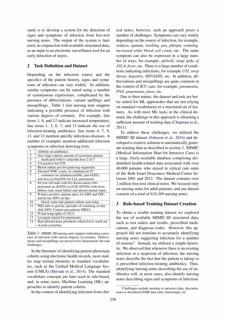
study is to develop a system for the detection ofsigns and symptoms of infection from free-textnursing notes. The output of the system is laterused, in conjunction with available structured data,as an input to an electronic surveillance tool for anearly detection of sepsis.
2 Task Definition and Dataset
Depending on the infection source and thespecifics of the patient history, signs and symp-toms of infection can vary widely. In addition,similar symptoms can be stated using a numberof synonymous expressions, complicated by thepresence of abbreviations, variant spellings andmisspellings. Table 1 lists nursing note snippetsindicating a possible presence of infection withvarious degrees of certainty. For example, lineitems 1, 8, and 12 indicate increased temperature;line items 1, 3, 6, 7, and 13 indicate the use ofinfection-treating antibiotics; line items 4, 7, 9,11, and 13 mention specific infectious diseases. Anumber of examples mention additional infectionsymptoms or infection detecting tests.
1 Afebrile on antibiotics.2 Very large copious amount of secretions,sputum3 ... medicated with iv cefazolin dose 2 of 34 UA positive for UTI.5 Blood culture pos for gram neg organisms.6 Elevated WBC count, on clindamycin IV.7 ... continues on clindamycin(D6), pen-G(D5)
and doxycycline(D4) for LLL pneumonia8 84 year old male with h/o throat cancer who
presented on [DATE] to [LOCATION] with fever,diffuse rash, renal failure and altered mental status.
9 Pt had a positive sputum specs for GBS and GPC,and he has HSV on lips.
10 ... blood, urine and sputum culture sent today ...11 PEG tube to gravity, episodes of vomitting on day
shift,NPO. Contact precautions MRSA.12 Pt had temp spike of 102.413 Levaquin started for pnuemonia.14 Had infected knee prosthesis which led to wash out
of joint yesterday.
Table 1: MIMIC-III nursing note snippets indicating a pres-ence of infection with various degrees of certainty. Abbrevi-ations and misspellings are preserved to demonstrate the taskchallenges.
In the literature of identifying patient phenotypecohorts using electronic health records, most stud-ies map textual elements to standard vocabular-ies, such as the Unified Medical Language Sys-tem (UMLS) (Shivade et al., 2014). The standardvocabulary concepts are later used in rule-based,and, in some cases, Machine Learning (ML) ap-proaches to identify patient cohorts.
In the context of identifying infection from clin-
ical notes, however, such an approach poses anumber of challenges. Symptoms can vary widelydepending on the source of infection, for example,redness, sputum, swelling, pus, phlegm, vomiting,increased white blood cell count, etc. The samesymptom can also be expressed in a large num-ber of ways, for example, afebrile, temp spike of102.4, fever, etc. There is a large number of condi-tions indicating infections, for example UTI, strepthroat, hepatitis, HIV/AIDS, etc. In addition, ab-breviations and misspellings are quite common inthe context of ICU care, for example, pneumonia,PNA, pnuemonia, pneu, etc.
Due to their nature, the dataset and task are bet-ter suited for ML approaches that are not relyingon standard vocabularies or a structured set of fea-tures. As with most ML tasks in the clinical do-main, the challenge in this approach is obtaining asufficient amount of training data (Chapman et al.,2011).
To address these challenges, we utilized theMIMIC-III dataset (Johnson et al., 2016) and de-veloped a creative solution to automatically gener-ate training data as described in section 3. MIMIC(Medical Information Mart for Intensive Care) isa large, freely-available database comprising dei-dentified health-related data associated with over40,000 patients who stayed in critical care unitsof the Beth Israel Deaconess Medical Center be-tween 2001 and 2012. The dataset contains over2 million free-text clinical notes. We focused onlyon nursing notes for adult patients, and our datasetconsists of a total of 634,369 nursing notes.
3 Rule-based Training Dataset Creation
To obtain a sizable training dataset we exploredthe use of available MIMIC-III structured data,such as test orders and results, prescribed medi-cations, and diagnosis codes. However, this ap-proach did not translate to accurately identifyingnursing notes suggesting infection for a numberof reasons1. Instead, we utilized a simple heuris-tic. We observed that whenever there is an existinginfection or a suspicion of infection, the nursingnotes describe the fact that the patient is taking oris prescribed infection-treating antibiotics. Thus,identifying nursing notes describing the use of an-tibiotics will, in most cases, also identify nursingnotes describing signs and symptoms of infection.
1Challenges include missing or incorrect data, discontin-uous or disordered EMR data entry timestamps, etc.
258

To identify positive mentions of administeredantibiotics, we used a list of the 60 most com-monly administered infection-treating antibioticsin the MIMIC dataset (Misquitta, 2013). This ini-tial list was then extended to include additionalantibiotic names, brands, abbreviations, spellingvariations, and common misspellings. We semi-automated this laborious task by utilizing wordembeddings (Mikolov et al., 2013). Word em-beddings were generated utilizing all availableMIMIC-III nursing notes2. The initial set of an-tibiotics was then extended using the closest wordembeddings in terms of cosine distance. For ex-ample, the closest words to the antibiotic amox-icillin are amox, amoxacillin, amoxycillin, ce-fixime, suprax, amoxcillin, amoxicilin. As shown,this includes misspellings, abbreviations, similardrugs and brand names. The extended list was thenmanually reviewed. The final infection-treatingantibiotic list consists of 402 unambiguous expres-sions indicating antibiotics.
Antibiotics, however, are sometimes negatedand are often mentioned in the context of aller-gies (e.g. allergic to penicillin). To distinguishbetween affirmed, negated, and speculated men-tions of administered antibiotics, we also devel-oped a set of rules in the form of keyword trig-gers. Similarly to the NegEx algorithm (Chapmanet al., 2001), we identified phrases that indicateuncertain or negated mentions of antibiotics thatprecede or follow a list of hand-crafted expressionat the sentence and clause levels. Word embed-dings were again used to extend the list of triggerswith synonyms, spelling variations, abbreviations,and misspellings. For example, the words allergic,anaphylaxis, anaphalaxis, allerg, and anaphylax-sis are all used as triggers indicating the negationof an antibiotic use. The full list of keywords in-dicating antibiotics, negation/speculation triggersand conjunctions is available online3.
The described approach identified 186,158nursing notes suggesting the unambiguous pres-ence of infection (29%) and 3,262 notes suggest-ing possible infection. The remaining 448,211notes (70%) were considered to comprise our neg-ative dataset, i.e. not suggesting infection.
2We used vector size 200, window size 7, and continuousbag-of-words model.
3https://github.com/ema-/antibiotic-dictionary
4 Machine Learning Results
We modeled the task as a binary classificationof free-form clinical notes. It has been shownthat Support Vector Machines (Cortes and Vapnik,1995) achieve superior results in most text clas-sifications tasks and were selected as a sensiblefirst choice. The individual nursing notes wererepresented as a bag-of-words (1-grams). The to-kens were all converted to lower case and non-alphanumeric characters were discarded. Tokensthat are present in more than 60% of all samples orless than 6 times were also discarded. The tokenswere weighted using the tf-idf scheme (Salton andMcGill, 1986). We trained the model using lin-ear kernel SVMs4 (Chang and Lin, 2011). We setthe positive class weight to 2 to address the un-balanced dataset. 70% of the automatically gener-ated dataset was used for training and the remain-ing 30% for testing. This resulted in a precision of93.12 and a recall of 99.04 as shown in Table 2.
Precision Recall F1-scoreSVMauto 93.12 99.04 95.99SVMgold 92.10 68.46 78.53
Table 2: Classification Results. SVMauto=Results from ap-plying the SVM model on an automatically generated testset of 190,000 nursing notes; SVMgold=Results from apply-ing the SVM model on a manually reviewed dataset of 200nursing notes.
As the training dataset was automatically cre-ated, the above results do not truly reflect themodel performance. To evaluate the model onthe ground truth, a qualified professional manuallyreviewed 200 randomly selected nursing notes.These results are also shown in Table 2. While themodel precision remained high (92.10), the recalldropped significantly to 68.46.
The drop in recall can be partially attributedto the manner in which the testing data was cre-ated. Nursing notes describing signs of infectionbut failing to mention the use of antibiotics wereconsidered (incorrectly) negative examples. How-ever, an error analysis revealed that the majority ofthe false negatives (contributing to the low recall)were actually all indicating low level of suspicionof infection. For example, the human annotatorconsidered the following snippets sufficient to in-dicate a possible infection afebrile, bld cx’s sent;monitor temp, wbc’s, await stool cx results; lungscoarse, thick yellow secretions suctioned from ett;
4We used the LibSVM library with both the cost andgamma parameters set to 2 (obtained via grid-search param-eter estimation).
259

awaiting results of CT, malignancy vs pneumonia.In all cases, the note expresses only a suspicion forinfection, pending further tests.
We further attempted to improve the system per-formance by utilizing Paragraph Vectors (Le andMikolov, 2014). Unsupervised algorithms havebeen used to represent variable pieces of texts suchas paragraphs and documents as fixed-length fea-ture representations (Paragraph Vectors). Stud-ies have shown that Paragraph Vectors outperformbag-of-words models on some text classificationtasks. We used the text from all nursing notesto create Paragraph Vectors. We generated doc-ument embeddings using a distributed memorymodel and distributed bag-of-words model, eachof size 300 with a window size of 7. Combin-ing the vectors of the distributed memory modeland the distributed bag-of-words model, we rep-resented each document as a vector of size 600.The paragraph vectors of the training instanceswere then fed to a logistic regression, K-nearestneighbors, and an SVM classifier. Results signif-icantly under-performed the SVM bag-of-wordsmodel and we were able to achieve a maximumprecision and recall of 63% and 77% respectively.
5 Related Work
A review of approaches to identifying patient phe-notype cohorts using EMR data (Shivade et al.,2014) describes a number of studies using clinicalnotes, most often in combination with additionalstructured information, such as diagnosis codes.The study asserts that clinical notes are often theonly source of information from which to infer im-portant phenotypic characteristics.
Demner-Fushman et al. (2009) note that clinicalevents monitoring is one of the most common andessential tasks of Clinical Decision Support sys-tems. The task is in many respects similar to thetask of identifying patient phenotype cohorts andit has been observed that free text clinical notes areagain the best source of information. For example,Murff et al. (2003) found the electronic dischargesummaries to be an excellent source for detectingadverse events. They also note that simple key-words and triggers are not sufficient to detect suchevents.
In the context of identifying infection from clin-ical text, most studies map textual elements tostandard vocabularies, such as UMLS. For exam-ple, Matheny et al. (2012) develop a system for de-tecting infectious symptoms from emergency de-
partment and primary care clinical documentation,utilizing keywords and SNOMED-CT concepts.Bejan et al. (2012) describe a system for pneu-monia identification from narrative reports usingn-grams and UMLS concepts. Similarly, Elkinet al. (2008) encoded radiology reports usingSNOMED-CT concepts and developed a set ofrules to identify pneumonia cases.
Horng et al. (2017) develop an automated trig-ger for sepsis clinical decision support at emer-gency department triage. They utilize machinelearning and establish that free text drastically im-proves the discriminatory ability of identifyinginfection (increase in AUC from 0.67 to 0.86).Arnold et al. (2014) develop an EHR screen-ing tool to identify sepsis patients. They utilizeNLP applied to clinical documentation, providinggreater clinical context than laboratory and vitalsign screening alone. DeLisle et al. (2010) useda combination of structured EMR parameters andtext analysis to detect acute respiratory infections.Murff et al. (2011) develop a natural languageprocessing search approach to identify postoper-ative surgical complications within a comprehen-sive electronic medical record.
Halpern et al. (2014) describe a system forlearning to estimate and predict clinical state vari-ables without labeled data. Similar to our ap-proach, they use a combination of domain exper-tise and vast amounts of unlabeled data, withoutrequiring labor-intensive manual labeling. In theirsystem, an expert encodes a certain amount ofdomain knowledge (identifying anchor variables)which is later used to train classifiers. Elkan andNoto (2008) show that a classifier trained on posi-tive and unlabeled examples predicts probabilitiesthat differ by only a constant factor from the trueconditional probabilities of being positive.
6 Discussion
We presented an approach to identifying nursingnotes describing the suspicion or presence of aninfection. We utilized the MIMIC-III dataset anda creative approach to obtain an ample amount ofannotated data. We then applied ML methods tothe task and achieved performance sufficient forpractical applications. The ultimate goal of thisstudy is to utilize free-text notes, in combinationwith structured EMR data, to build an automatedsurveillance system for early detection of patientsat risk of sepsis.
260

ReferencesR Arnold, J Isserman, S Smola, and E Jackson. 2014.
Comprehensive assessment of the true sepsis bur-den using electronic health record screening aug-mented by natural language processing. CriticalCare 18(1):P244.
Helen C Azzam, Satjeet S Khalsa, Richard Urbani,Chirag V Shah, Jason D Christie, Paul N Lanken,and Barry D Fuchs. 2009. Validation study of an au-tomated electronic acute lung injury screening tool.Journal of the American Medical Informatics Asso-ciation 16(4):503–508.
Cosmin Adrian Bejan, Fei Xia, Lucy Vanderwende,Mark M Wurfel, and Meliha Yetisgen-Yildiz. 2012.Pneumonia identification using statistical feature se-lection. Journal of the American Medical Informat-ics Association 19(5):817–823.
Roger C Bone, William J Sibbald, and Charles LSprung. 1992. The accp-sccm consensus confer-ence on sepsis and organ failure. CHEST journal101(6):1481–1483.
Chih-Chung Chang and Chih-Jen Lin. 2011. LIB-SVM: A library for support vector machines. ACMTransactions on Intelligent Systems and Technol-ogy 2:27:1–27:27. Software available at http://www.csie.ntu.edu.tw/˜cjlin/libsvm.
Wendy W Chapman, Will Bridewell, Paul Hanbury,Gregory F Cooper, and Bruce G Buchanan. 2001.A simple algorithm for identifying negated findingsand diseases in discharge summaries. Journal ofbiomedical informatics 34(5):301–310.
Wendy W Chapman, Prakash M Nadkarni, LynetteHirschman, Leonard W D’avolio, Guergana KSavova, and Ozlem Uzuner. 2011. Overcoming bar-riers to nlp for clinical text: the role of shared tasksand the need for additional creative solutions.
Corinna Cortes and Vladimir Vapnik. 1995. Support-vector networks. Machine learning 20(3):273–297.
Sylvain DeLisle, Brett South, Jill A Anthony, ErickaKalp, Adi Gundlapallli, Frank C Curriero, Greg EGlass, Matthew Samore, and Trish M Perl. 2010.Combining free text and structured electronic med-ical record entries to detect acute respiratory infec-tions. PloS one 5(10):e13377.
R Phillip Dellinger, Mitchell M Levy, Jean M Carlet,Julian Bion, Margaret M Parker, Roman Jaeschke,Konrad Reinhart, Derek C Angus, Christian Brun-Buisson, Richard Beale, et al. 2008. Surviving sep-sis campaign: international guidelines for manage-ment of severe sepsis and septic shock: 2008. Inten-sive care medicine 34(1):17–60.
Dina Demner-Fushman, Wendy W Chapman, andClement J McDonald. 2009. What can natural lan-guage processing do for clinical decision support?Journal of biomedical informatics 42(5):760–772.
Charles Elkan and Keith Noto. 2008. Learning classi-fiers from only positive and unlabeled data. In Pro-ceedings of the 14th ACM SIGKDD internationalconference on Knowledge discovery and data min-ing. ACM, pages 213–220.
Peter L Elkin, David Froehling, Dietlind Wahner-Roedler, Brett E Trusko, Gail Welsh, Haobo Ma,Armen X Asatryan, Jerome I Tokars, S Trent Rosen-bloom, and Steven H Brown. 2008. Nlp-based iden-tification of pneumonia cases from free-text radio-logical reports. In AMIA.
Yoni Halpern, Youngduck Choi, Steven Horng, andDavid Sontag. 2014. Using anchors to estimate clin-ical state without labeled data. In AMIA AnnualSymposium Proceedings. American Medical Infor-matics Association, volume 2014, page 606.
Yong Y Han, Joseph A Carcillo, Michelle A Dragotta,Debra M Bills, R Scott Watson, Mark E Wester-man, and Richard A Orr. 2003. Early reversalof pediatric-neonatal septic shock by communityphysicians is associated with improved outcome.Pediatrics 112(4):793–799.
Vitaly Herasevich, Mykola Tsapenko, Marija Kojicic,Adil Ahmed, Rachul Kashyap, Chakradhar Venkata,Khurram Shahjehan, Sweta J Thakur, Brian W Pick-ering, Jiajie Zhang, et al. 2011. Limiting ventilator-induced lung injury through individual electronicmedical record surveillance. Critical care medicine39(1):34–39.
Michael H Hooper, Lisa Weavind, Arthur P Wheeler,Jason B Martin, Supriya Srinivasa Gowda,Matthew W Semler, Rachel M Hayes, Daniel WAlbert, Norment B Deane, Hui Nian, et al. 2012.Randomized trial of automated, electronic mon-itoring to facilitate early detection of sepsis inthe intensive care unit. Critical care medicine40(7):2096.
Steven Horng, David A Sontag, Yoni Halpern, YacineJernite, Nathan I Shapiro, and Larry A Nathanson.2017. Creating an automated trigger for sepsis clin-ical decision support at emergency department triageusing machine learning. PloS one 12(4):e0174708.
Alistair EW Johnson, Tom J Pollard, Lu Shen, Li-wei H Lehman, Mengling Feng, Mohammad Ghas-semi, Benjamin Moody, Peter Szolovits, Leo An-thony Celi, and Roger G Mark. 2016. Mimic-iii,a freely accessible critical care database. Scientificdata 3.
Won-Young Kim and Sang-Bum Hong. 2016. Sep-sis and acute respiratory distress syndrome: re-cent update. Tuberculosis and respiratory diseases79(2):53–57.
Helen C Koenig, Barbara B Finkel, Satjeet S Khalsa,Paul N Lanken, Meeta Prasad, Richard Urbani, andBarry D Fuchs. 2011. Performance of an automatedelectronic acute lung injury screening system in in-tensive care unit patients. Critical care medicine39(1):98–104.
261

Anand Kumar, Daniel Roberts, Kenneth E Wood,Bruce Light, Joseph E Parrillo, Satendra Sharma,Robert Suppes, Daniel Feinstein, Sergio Zanotti,Leo Taiberg, et al. 2006. Duration of hypotensionbefore initiation of effective antimicrobial therapy isthe critical determinant of survival in human septicshock. Critical care medicine 34(6):1589–1596.
Quoc V Le and Tomas Mikolov. 2014. Distributed rep-resentations of sentences and documents. In ICML.volume 14, pages 1188–1196.
Michael E Matheny, Fern FitzHenry, Theodore Sper-off, Jennifer K Green, Michelle L Griffith, Eduard EVasilevskis, Elliot M Fielstein, Peter L Elkin, andSteven H Brown. 2012. Detection of infectioussymptoms from va emergency department and pri-mary care clinical documentation. Internationaljournal of medical informatics 81(3):143–156.
Tomas Mikolov, Ilya Sutskever, Kai Chen, Greg S Cor-rado, and Jeff Dean. 2013. Distributed representa-tions of words and phrases and their compositional-ity. In Advances in neural information processingsystems. pages 3111–3119.
Donald Misquitta. 2013. Early Prediction of Antibi-otics in Intensive Care Unit Patients. Ph.D. thesis,The Center for Biomedical Informatics at the Har-vard Medical School.
Harvey J Murff, Fern FitzHenry, Michael E Matheny,Nancy Gentry, Kristen L Kotter, Kimberly Crimin,Robert S Dittus, Amy K Rosen, Peter L Elkin,Steven H Brown, et al. 2011. Automated identifica-tion of postoperative complications within an elec-tronic medical record using natural language pro-cessing. Jama 306(8):848–855.
Harvey J Murff, Vimla L Patel, George Hripcsak, andDavid W Bates. 2003. Detecting adverse eventsfor patient safety research: a review of currentmethodologies. Journal of biomedical informatics36(1):131–143.
Jessica L Nelson, Barbara L Smith, Jeremy D Jared,and John G Younger. 2011. Prospective trial of real-time electronic surveillance to expedite early careof severe sepsis. Annals of emergency medicine57(5):500–504.
H Bryant Nguyen, Emanuel P Rivers, Fredrick MAbrahamian, Gregory J Moran, Edward Abraham,Stephen Trzeciak, David T Huang, Tiffany Osborn,Dennis Stevens, David A Talan, et al. 2006. Severesepsis and septic shock: review of the literature andemergency department management guidelines. An-nals of emergency medicine 48(1):54–e1.
Su Q Nguyen, Edwin Mwakalindile, James S Booth,Vicki Hogan, Jordan Morgan, Charles T Prickett,John P Donnelly, and Henry E Wang. 2014. Auto-mated electronic medical record sepsis detection inthe emergency department. PeerJ 2:e343.
Gerard Salton and Michael J McGill. 1986. Introduc-tion to modern information retrieval .
Chaitanya Shivade, Preethi Raghavan, Eric Fosler-Lussier, Peter J Embi, Noemie Elhadad, Stephen BJohnson, and Albert M Lai. 2014. A review ofapproaches to identifying patient phenotype co-horts using electronic health records. Journalof the American Medical Informatics Association21(2):221–230.
Jean-Louis Vincent. 2016. The clinical challenge ofsepsis identification and monitoring. PLoS Med13(5):e1002022.
262

Proceedings of the BioNLP 2017 workshop, pages 263–271,Vancouver, Canada, August 4, 2017. c©2017 Association for Computational Linguistics
Enhancing Automatic ICD-9-CM Code Assignment forMedical Texts with PubMed
Danchen Zhang1, Daqing He1, Sanqiang Zhao1, Lei Li21School of Information Sciences, University of Pittsburgh
2School of Economics and Management, Nanjing University of Science and Technology{daz45, dah44, saz31}@pitt.edu, [email protected]
Abstract
Assigning a standard ICD-9-CM code todisease symptoms in medical texts is animportant task in the medical domain. Au-tomating this process could greatly reducethe costs. However, the effectiveness of anautomatic ICD-9-CM code classifier facesa serious problem, which can be triggeredby unbalanced training data. Frequent dis-eases often have more training data, whichhelps its classification to perform betterthan that of an infrequent disease. How-ever, a diseases frequency does not nec-essarily reflect its importance. To resolvethis training data shortage problem, wepropose to strategically draw data fromPubMed to enrich the training data whenthere is such need. We validate our methodon the CMC dataset, and the evaluation re-sults indicate that our method can signifi-cantly improve the code assignment classi-fiers’ performance at the macro-averaginglevel.
1 Introduction and Background
The rapid computerization of medical contentsuch as electronic medical records (EMRs), doc-tors notes and death certificates, drives a crucialneed to apply automatic techniques to better as-sist medical professionals in creating and manag-ing medical information. A standard procedure inhospital is to assign the International Classifica-tion of Diseases (ICD) codes to diseases appear-ing in medical texts by professional coders. As aresult, several recent studies have been devoted toautomatically extracting ICD code from medicaltexts to help manual coders (Crammer et al., 2007;Farkas and Szarvas, 2008; Aronson et al., 2007;Kavuluru et al., 2015, 2013; Zuccon and Nguyen,
Figure 1: An example radiology report with man-ually labeled ICD-9-CM code from CMC dataset.
2013; Koopman et al., 2015).In this paper, we focus on ICD-9-CM (the 9th
version ICD, Clinical Modification), although ourwork is portable to ICD-10-CM (the 10th versionICD). The reason to conduct our study on ICD-9-CM is to compare with the state-of-art methods,whose evaluations have mostly conducted on ICD-9-CM code (Aronson et al., 2007; Kavuluru et al.,2015, 2013; Patrick et al., 2007; Ira et al., 2007;Zhang, 2008). ICD-9-CM codes are organized hi-erarchically, and each code corresponds to a tex-tual description, such as ”786.2, cough”. Multi-ple codes can be assigned to a medical text, and aspecific ICD-9-CM code is preferred than a moregeneric one when both are suitable (Pestian et al.,2007). Figure 1 shows a code assignment examplewhere a radiology report is labeled with ”786.2,cough”.
Existing methods for automatic ICD-9-CM as-signment have been mostly supervised methodsbecause of the effectiveness the training; how-ever, classification performance heavily relies onthe sufficiency of training data (He and Garcia,2009). To certain degree, micro-average mea-sures, commonly used to evaluate the classifica-tion performance of existing algorithms, pays at-
263

Figure 2: The distribution of radiology reports for45 ICD-9-CM codes in the CMC dataset.
tention to the correctness of the code assignmentto each EHR (individual case), which helps tohide the impact of unbalanced training data. How-ever, a useful classification system should performconsistently across all ICD-9-CM codes regard-less of the popularity of the codes (Jackson andMoulinier, 2007). This motivated us to examinethe imbalanced training data and its impacts to theclassifier. Specifically, we pay more attention tomacro-average measures, which helps to examinethe consistency across all codes.
Unfortunately, in a real dataset for studyingICD-9-CM code classification, the data availablefor each code is highly imbalanced. For example,Figure 2 shows the count of available radiologyreports for each of the 45 ICD-9-CM codes in theCMC dataset (Pestian et al., 2007). Common dis-eases like ”786.2, cough”, can have 266 reportsas the training data, whereas unpopular disease”758.6, Gonadal dysgenesis” only has one. Sim-ilarly, Kavuluru et al. (2015) found that 874 of1,231 ICD-9-CM code in their UKLarge datasethave less than 350 supporting data, and only 92codes have more than 1,430 supporting data. Inanother example, Koopman et al. (2015) foundthat 85% of the whole death certificate dataset arerelated to top 20 common cancers, and only rest15% is associated with 65 rarer cancers. Theselong tail supporting data problems are very com-mon, which makes data imbalance an noticeableproblem.
Our approach for resolving this problem is tointroduce additional information resources. Fur-thermore, due to the privacy concern of medical-related content, this study is particularly interestedin obtaining extra relevant training data from pub-
licly available medical datasets. PubMed1, as avast and broad medical literature dataset, coversa great number of disease related information andimposes few restrictions on data access. There-fore, it is a perfect starting point to explore ourapproach. The hypothesis is that training data canbe obtained from PubMed articles that talk about adisease corresponding to a ICD-9-CM code. Withthe abundant PubMed articles, we would be ableto alleviate the training data imbalance problem.
There are several contributions in our study.Firstly, we examine the data imbalance problemin ICD-9-CM code assignment. Secondly, we pro-pose and compare several methods to resolve thedata imbalance problem. Thirdly, we give a com-prehensive discussion on the current classificationchallenges. Finally, our method can be adaptedto ICD-10-CM code assignment task with minormodifications.
The rest of this paper is organized as follows.In Section 2, we will discuss related research. Ourmethods and experiments will appear in Section 3and 4. Limitations are discussed in Section 5 andthe conclusion is provided in Section 6.
2 Related Work
The existing studies of automating ICD-9 codeassignment can be classified into two groups.Through examining how professional coders as-signing ICD codes, the first one used rule-basedapproaches. Ira et al. (2007) developed a rule-based system considering factors such as uncer-tainty, negation, synonymy, and lexical elements.Farkas and Szarvas (2008) used Decision Tree(DT) and Maximum Entropy (ME) to automati-cally generate a rule-based coding system. Cram-mer et al. (2007) composed a hybrid system con-sisting of a machine learning system with naturallanguage features, a rule-based system based onthe overlap between the reports and code descrip-tions, and an automatic policy system. Their re-sults showed better performance than each singlesystem.
The second group employed supervised ma-chine learning methods for the assignment task,and their performance has been being equivalentor even better than those rule-based systems thatneed experts manually crafting knowledge. Aron-son et al. (2007) used a stacked model to combinethe results of four modules: Support Vector Ma-
1https://www.ncbi.nlm.nih.gov/pubmed/
264

chine (SVM), K-Nearest Neighbors (KNN), Pat-tern Matching (PM) and a hybrid Medical TextIndexer (MTI) system. Patrick et al. (2007) usedME and SVM classifiers, enhanced by a feature-engineering module that explores the best combi-nation of several types of features. Zhang (2008)proposed a hierarchical text categorization methodutilizing the ICD-9-CM codes structure. Zuc-con and Nguyen (2013) conducted a comparisonstudy on four classifiers (SVM, Adaboost, DT, andNaive Bayes) and different features on a 5,000free-text death certificate dataset, and found thatSVM with a stemmed unigram feature performedthe best.
Along with the introduction of supervised meth-ods, many past studies indicated that data imbal-ance problem can severely affect the classifier’sperformance. For example, Kavuluru et al. (2015)found that 874 of 1,231 ICD-9-CM codes in UK-Large dataset have less than 350 supporting data,whereas only 92 codes have more than 1,430 sup-porting data. The former group has macro F1value of 51.3%, but the latter group only has16.1%. To resolve data imbalance problem, theyused optimal training set (OTS) selection approachto sample negative instance subset that providesbest performance on validation set. However, OTSdid not work on UKLarge dataset because sev-eral codes have so few training examples that evencarefully selecting negative instances could nothelp. When Koopman et al. (2015) found that85% of the whole death certificate dataset is asso-ciated with only top 20 common cancers, whereasthe other 65 rarer cancers only have the rest 15%of the dataset, they tried to construct the balancedtraining set by randomly sampling a static num-ber of negative examples for each class. Their re-sults reflected the benefits of having more train-ing data in improving the classifiers’ performance.Since result of original model learned with imbal-anced data is not provided, we cannot know the ac-tual improvement. In addition, to deal with codesthat only appear once in the dataset, Patrick et al.(2007) used a rule-based module to supplementME and SVM classifiers.
Consistent to the existing works, our approachutilizes supervised methods for automatic ICD-9-CM code assignment, and our focus is on address-ing the training data imbalance problem. But ourwork tries to solve the data imbalance problem byadding extra positive instances, which is not lim-
ited to the existing training data distribution or ex-pert’s knowledge. Adding positive instances havebeen proven to be effective in supervised machinelearning in other domains(Caruana, 2000; He andGarcia, 2009), and we are first to find open sourcedataset as supplementary data for improving ICD-9-CM assignment performance.
3 Methods
In this section, we will first introduce the dataseton which our methods will be evaluated, then wepropose two methods of collecting supplementarytraining data from PubMed dataset.
3.1 Dataset
We validate our methods on the official datasetof the 2007 Computational Medicine Challenge(CMC dataset), collected by Cincinnati Children’sHospital Medical Center (Pestian et al., 2007),which is frequently used by researchers workingon the ICD-9-CM code assignment task. TheCMC dataset consists of training and testingdataset, but only training dataset is accessible forus. Fortunately, most studies publish their systemperformance on both training and testing dataset,and then we can compare our methods with state-of-art methods. This corpus consists of 978 radi-ological reports taken from real medical records,and each report has been manually labeled withICD-9-CM codes by professional companies. Theexample in Figure 1 comes from this dataset. Intotal, there are 45 ICD-9-CM codes appearing inthe CMC dataset, and each report is labeled withone or more ICD-9-CM codes. This is a very im-balanced collection, with around half codes havingless than 10 training data (see Figure 2).
3.2 Method I: Retrieving PubMed articlesusing ICD-9-CM code official description
Through examining the reports available to us, andalso based on the discussions in previous work(Farkas and Szarvas, 2008; Ira et al., 2007; Cram-mer et al., 2007; Farkas and Szarvas, 2008), wehypothesize that the text description part of ICD-9-CM code can play important role for code as-signers to build up the connection between a med-ical text and a ICD-9 code. Therefore, this mo-tivated us to view the identifying extra trainingdata in PubMed for an ICD-9-CM code as a re-trieval problem where the text description part ofan ICD-9-CM code can act as the query, and the
265

whole PubMed dataset as a document collection.For example, based on ICD-9-CM code ”786.2,cough”, we can retrieve PubMed articles with aquery ”cough”. Our initial informal testing con-firmed our hypothesis.
To avoid bring back too much noise, we re-stricted the PubMed retrieval to only search onthe article title field. Our motivation is that thetitle generally introduces the main topic of thewhole paper. For the same reason, we also onlyutilized the title and abstract of top returned arti-cles as the supplementary training data. In case ofempty retrieval result, certain ICD-9-CM descrip-tion terms that would not appear in PubMed ar-ticle titles, such as ”other”, ”unspecified”, ”spec-ified”, ”NOS”, and ”nonspecific”, are removedfrom the query. For example, ICD-9-CM code”599.0”, whose description is ”urinary tract infec-tion, site not specified”, will generate a cleanedquery ”urinary tract infection”, and ICD-9-CMcode ”596.54”, whose description is ”neurogenicbladder NOS”, will generate a cleaned query ”neu-rogenic bladder”.
3.3 Method II: Retrieving PubMed articleswith both official and synonymsICD-9-CM code description
Despite great overlap among them, ICD-9-CMcode descriptions and the radiology reports in theCMC collection are written by different groups ofpeople with different purposes. Therefore, therecould be term mis-match problems between them.When this happens, it is actually better to not usethe terms in the ICD-9-CM official description asthe query for finding relevant PubMed articles,but actually to use the related terms in the CMCdataset as the query terms instead. This would en-able the model trained on these returned PubMedarticles can be more effectively classifying CMCreports. For example, the description ”Anorexia”of code ”783.0” does not appear in CMC dataset.Instead, ”loss of appetite” exists in the radiologyreports labeled with ”783.0”, while according todata in ICD9Data.com, ”loss of appetite” is thesynonym of ”Anorexia”. Therefore, in this case,it is better to use ”loss of appetite” rather than”Anorexia” to be the query when search for train-ing data in PubMed.
ICD9Data.com is an online website, providingrich and free ICD-9-CM coding information. Itcontains code definition, hierarchy structure, ap-
proximate synonyms, etc. We crawled the 45codes’ synonyms from the website. In method II,besides the queries from the official description,we also conducted PubMed searches with queriesbased on the synonyms of the descriptions. Eachsynonym is an individual PubMed query, and onlywhen all its terms appear in CMC dataset, thequery is considered. If one ICDcode has n queriesand totally needs m supplementary documents fortraining, only top m/n retrieved PubMed articlesfrom each query are considered.
4 EXPERIMENTS
4.1 Evaluation metrics
Following the past studies (Pestian et al., 2007;Kavuluru et al., 2015), we evaluate the classifica-tion performance through a micro F1 score (i.e.,sum of the individual classification performanceand divided by the individual amount) and a macroF1 score (i.e., sum of the classifiers performanceand divided by the classifiers amount). We ex-pect that by alleviating the data imbalance prob-lem, macro F1 scores can increase significantly.All experiments in this study have gone through10-fold cross validation, because it can provide areliable result when data is limited (Witten et al.,2016).
4.2 Pre-process and Features
Following the past studies (Crammer et al., 2007;Aronson et al., 2007; Kavuluru et al., 2015, 2013;Koopman et al., 2015; Patrick et al., 2007; Iraet al., 2007), the CMC dataset is preprocessed withfollowing steps:
• Full name restoration. Medical abbreviationrestoration is a hard topic, which is not ex-plored in this study. We manually generate alist of full names for abbreviations appearingin CMC dataset 2.
• Word lemmatization. Lemmatization ofwords are restored with WordNet 3.0 (Miller,1995).
• Negation detection and removal. Negex(Chapman et al., 2001) is used to detectthe negation expression, and negation targetterms are removed after detection.
2https://github.com/daz45/CMC-data-set-abbreviations/tree/master
266

Figure 3: Feature selection on LR and SVM.
• Phrase recognition. MetaMap (Aronson andLang, 2010) is utilized to extract the medicalconcept phrase appearing in the text, which isappended to the text.
After preprocessing, the example radiology re-port in Figure 1 will be ”ten year old with chestpain x two week. the lung be well expand andclear. there be. the cardiac and mediastinal silhou-ette be normal. there be. chest pain”. Supplemen-tary data collected from PubMed will be prepro-cessed in the same way.
4.3 BaselinesAccording to the past studies(Farkas and Szarvas,2008; Aronson et al., 2007; Kavuluru et al., 2015),Support Vector Machine (SVM) and Logistic Re-gression (LR) are the most effective and com-monly used classification models in this task.Therefore, we selected them as the two baselines.Each ICD-9-CM code has one binary classifierimplemented using Scikit-Learn(Pedregosa et al.,2011). We name these two sets of baselines asBaseline LR and Baseline SVM.
Features consist of unigrams and bigrams ap-pearing in preprocessed radiology reports, and thefeature vector values are binary, indicating the ap-pearance or absence of the word in text.
We performed feature selection on two base-lines to avoid over-fit and extra computation cost.χ2 based feature selection was employed for fea-ture selection (Liu and Setiono, 1995). As shownin Figure 3, We find that 500 features can providestable micro F1 performance and best macro F1performance for Baseline LR and Baseline SVM.In all the following experiments, all classifiers are
trained on these 500 selected features.Our baseline performance were compared with
the state-of-art methods in Table 1. Stackingis a stacked model combining four classificationmodels (Aronson et al., 2007). Hybrid rule-based+MaxEnt is a hybrid system combining rule-based method with MaxEnt (Aronson et al., 2007).Although Table 1 shows that their performance issignificantly better than our baselines, for the pur-pose of studying the methods for addressing im-balanced training data, we have to use the twocurrent baselines since these advanced and com-plicated systems would hide the effects that wewant to observe. In addition, any improvement weachieve in single classifier can be later integratedinto these systems, which could be an interestingfuture work. These methods concentrated on mi-cro averaging performance, while in this study wewill explore the macro averaging performance.
Method Micro F1Baseline LR 86.51%Baseline SVM 87.26%Stacking 89.00%Hybrid rule-based+MaxEnt 90.26%
Table 1: Baseline performance and existing bestperformed methods from related work.
Figure 4 shows the individual classification per-formance of 45 classifiers, and we can find an un-stable performance across 45 classifiers. We useMacro F1 score as the split line, and we can findthat, for both baseline system, there are 21 classi-fiers having a below-average performance, and allof them have relatively less training data than theclassifiers with above-average performance. Thisindicates that the data imbalance leads to the per-formance instability across all classes.
With the Macro F1 score, we separate 45 classi-fiers into two groups: Group 1 consists of 24 clas-sifiers, union set of classifiers with below-averageperformance in two baselines, and Group 2 con-sists of rest 21 classifiers with above-average clas-sification performance. Though Group 1 has 24classifier, radiological reports labeled with themonly takes 11.56% of 978 reports. To deal withthis data imbalance problem, we will introducesupplementary training data from PubMed dataset.Through adding additional data, we expect thatclassification performance of the whole system,especially Group 1, will be improved.
267

Figure 4: Individual classification performance of 45 classifiers trained with LR and SVM model inBaseline.
4.4 Experiment I: retrieving PubMed articleswith ICD code official description
In the first experiment, supplementary data is col-lected based on ICD-9-CM code official descrip-tion, as described in method I. The supplement-ing document size is set to be 10, 20, 40 and60. Supplementary training data is added to 24classifiers in Group 1. We name these two newruns as Group 1 Description LR (G1 desc LR)and Group 1 Description SVM (G1 desc SVM),appended with supplementary data size. The re-sults in Table 2 also show that supplementing 10documents can generate best performance, andwith more documents added, both macro and mi-cro F1 will decrease.
Method Micro F1 Macro F1Baseline LR 86.51% 51.52%G1 desc LR 10 86.68% 55.78%G1 desc LR 20 86.07% 55.23%G1 desc LR 40 85.18% 52.01%G1 desc LR 60 84.97% 51.40%Baseline SVM 87.26% 48.03%G1 desc SVM 10 86.96% 57.09%G1 desc SVM 20 86.67% 55.43%G1 desc SVM 40 85.87% 57.61%G1 desc SVM 60 86.25% 54.77%
Table 2: Enhance classifiers in Group 1 with sup-plementary data collected with method I, while theevaluation is performed on all classes.
Through Wilcoxon Signed Ranks test, there isno significant difference between G1 desc LR 10
and Baseline LR. Nor does G1 desc SVM 10.Further, we compare both methods against base-line on Group 1 and Group 2 separately. How-ever, there is still no significant difference existing.Take G1 desc SVM 10 for example, from Figure5, we can see that 11 classes still have F1=0%,while 5 classes’ performance decrease, and only 8got F1 improved. It indicates that the method I isineffective.
After exploring the results, we find sometimesthe supplementary data does not help training. Forexample, for ICD-9-CM code ”783.0 Anorexia”,the classification performance stays 0%. Thecorresponding radiology report doesn’t have term”Anorexia”, making the supplementary data use-less. It implies we need to collect PubMed arti-cles containing same features with the radiologyreports in CMC dataset.
4.5 Experiment II: Retrieving PubMedarticles with ICD code official andsynonyms descriptions
In this second experiment, we collect PubMeddata through the ICD-9-CM code’s both of-ficial and synonyms description that appearsin CMC dataset. We name these two runsas Group 1 Synonym LR (G1 syn LR) andGroup 1 Synonym SVM (G1 syn SVM). Due tothe paper size limitation, here we only show thebest results with supplementary document sizebeing 10 in Table 3.
Through Wilcoxon Signed Ranks test,G1 syn SVM 10 significantly outperformsbaseline (p − value < 0.01), but has no signifi-
268

cant difference compared with G1 desc SVM 10.However, if only classifiers in Group 1 are consid-ered, G1 syn SVM 10 significantly outperformsG1 desc SVM 10 (p − value < 0.01). Thisindicates that our propose method II can generateeffective supplementary training data. On theother hand, G1 syn LR 10 is found to outperformBaseline LR significantly only on Group 1 classes(p− value < 0.01).
Method Micro F1 Macro F1Baseline LR 86.51% 51.52%G1 desc LR 10 86.68% 55.78%G1 syn LR 10 86.30% 62.85%‡All syn LR 10 86.60% 62.19%‡Baseline SVM 87.26% 48.03%G1 desc SVM 10 86.96% 57.09%G1 syn SVM 10 87.22% 67.43%†‡All syn SVM 10 87.88% 64.54%†‡
Table 3: Experiment results. †means significantlyoutperform baseline. ‡means significant outper-form baseline on Group 1.
It shows that on SVM model, PubMed datacollected with ICD-9-CM code descriptions syn-onyms works better in solving the data imbalanceproblem than with the official descriptions. Afterdata supplementation, there are still 6 classifierswith F1 score being 0%, which will be further dis-cussed in Section 5.
4.6 Experiment III: adding supplementarytraining data to all classifiers
In the third experiment, we add supplemen-tary data to all 45 classifiers to explore whetheradding supplementary data to the classifiers thatoriginally have sufficient training data still cangain performance improvement. We name thesetwo runs as All Synonym LR (All syn LR) andAll Synonym SVM (All syn SVM). Also, onlythe best results with supplementary document sizebeing 10 is shown in Table 3. Through WilcoxonSigned Ranks test, All syn SVM 10 significantlyoutperforms the baseline, and All syn LR 10 sig-nificantly outperforms the baseline only on Group1 (p − value < 0.01), but both have no signifi-cant difference with G1 syn and G1 desc. Thesemeans that adding supplementary training data iseffective on solving data imbalance problem, butfor the classifiers that originally have sufficienttraining data, extra training data seems have no
significant effect.
5 Discussion
Experiment results indicates that our proposedsupplementing training data method can help theclassifiers to reach to a relatively balanced perfor-mance. Such improvement mainly comes fromchanging the word weight ranking so that im-portant words rank higher. For example, forcode ”758.6 turner syndrome”, in the baseline LR(F1=0%), top 3 features with highest weights are”duplicate left, partially, turner syndrome”. Butin G1 syn LR 10 (F1=67%), top 3 features are”turner, turner syndrome, syndrome”. Supplemen-tary data trains term in ”turner syndrome” a higherweight in LR model, explaining this code’s classi-fication performance increase.
In addition, supplementary data will improveclassification through boosting the weight of thefeatures. For example, the top features for code”786.59, Other chest pain” are basically similarin both baseline LR (F1=0%) and G1 syn LR 10(F1=40%), including ”tightness, chest tightness,chest pain”. However, the weight differs a lot. Forbaseline LR, weights are all under 1.5, while inG1 syn LR 10, top 5 features are all above 1.5, in-dicating the classification model have much higherconfidence on these features.
Finally, supplementary data mainly supportcode assignment effectively in Group 1, and wefind that classification performance in Group 2 ba-sically has no significant difference across all ex-periments. Meanwhile, 978 reports, dominatedby Group 2 classes, also show no significant dif-ference across all experiments. Therefore, extratraining data does not improve Group 2’s perfor-mance, and hence supplementary data is not sug-gested for classes having sufficient training data.
Besides, our proposed methods can be directlyused in ICD-10-CM classification with little mod-ification. Just update the PubMed query with theICD-10-CM textual descriptions and synonyms.
Though data imbalance problem has beenlargely alleviated, there are still a few classifiersin Group 1 have poor performance. After explor-ing, we think there are mainly four reasons:
• Word level feature matching limitation. Forexample, description of code ”V72.5 Radio-logical examination” does not appear in thecollection, and it has no synonyms. Radio-logical examination actually means a variety
269

Figure 5: Individual classification performance of 45 classifiers on Baseline and three experiments.
of imaging techniques, and such word levelfeature matching cannot help classification.
• ”History of” ICD-9-CM codes. For codes”V13.02, Personal history, urinary tract in-fection” and ”V13.09 Personal history ofother specified urinary system disorders”,adding supplementary data doesn’t help theirperformance. We find their radiology re-ports are basically classified to ”599.0 urinarytract infection” and ”593.70 vesicoureteralreflux”. ”history of” feature is ignored. Extratraining data has no effect on this problem.
• Speculative expression. In prepossessingprocedure, negation terms are removed, butspeculative expressions are kept. It results inthat when doctor is not sure whether a patientmay get a disease, but write it down to re-ports, classification results will rely on thesespeculative terms, and cause false positive.For example, code ”518.0” has a low F1 scorebecause in many reports labeled with othercodes, doctors write that the patient may havedisease ”atelectasis”, while ”atelectasis” is avery important word to recognize ”518.0”.
• Data missing due to expert disagreement. InCMC dataset, three experts manually assigncodes to 978 radiology reports. Only whentwo or more experts agree, code is approved.However, sometimes the conflict opinions re-
sults in code assignment failure. For exam-ple, reports 99619963 and 99803917 shouldbe labeled with ”741.90 Spina bifida”. How-ever, one expert assigned ”741.90”, anotherassigned ”741.9”, and the third expert missthis code at all. This led to ”741.90 Spina bi-fida” was not assigned to these two reports.However, with the supplementary data addedinto the training, our method correctly as-signs ”741.90 Spina bifida” to these two re-ports, but this assignment was counted aswrong since the ground truth does not havethis code due to expert disagreements.
6 Conclusion and Future Work
In this study, we studied to address the data im-balance problem in ICD-9-CM code automatic as-signment task. Using ICD-9-CM codes synonymscan accurately search medical texts relevant docu-ments from PubMed. Collected data, used as sup-plementary training data, can significantly boostsystems macro averaging performance as the dataimbalance problem is largely alleviated. However,for the classifiers that originally have sufficienttraining data, additional data basically has no sig-nificant effect. As future work, we will modifythe Context algorithm (Harkema et al., 2009) todetect the historical mentions and speculative ex-pressions in the radiology reports. Also, we wouldexplore the difference of same features extractedfrom different field of radiology reports.
270
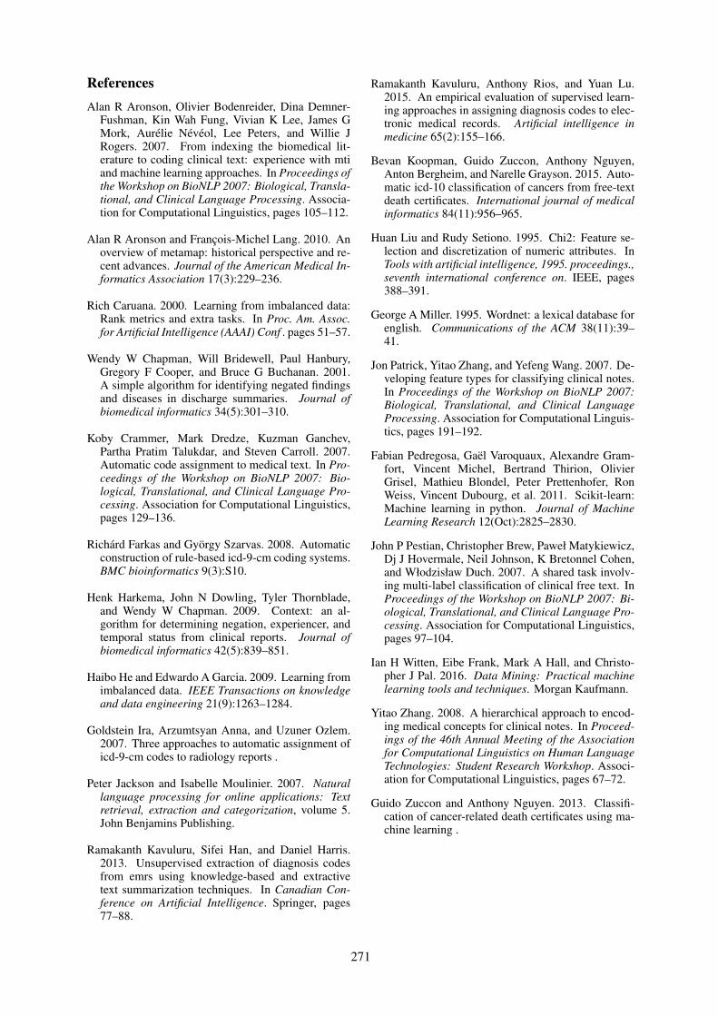
ReferencesAlan R Aronson, Olivier Bodenreider, Dina Demner-
Fushman, Kin Wah Fung, Vivian K Lee, James GMork, Aurelie Neveol, Lee Peters, and Willie JRogers. 2007. From indexing the biomedical lit-erature to coding clinical text: experience with mtiand machine learning approaches. In Proceedings ofthe Workshop on BioNLP 2007: Biological, Transla-tional, and Clinical Language Processing. Associa-tion for Computational Linguistics, pages 105–112.
Alan R Aronson and Francois-Michel Lang. 2010. Anoverview of metamap: historical perspective and re-cent advances. Journal of the American Medical In-formatics Association 17(3):229–236.
Rich Caruana. 2000. Learning from imbalanced data:Rank metrics and extra tasks. In Proc. Am. Assoc.for Artificial Intelligence (AAAI) Conf . pages 51–57.
Wendy W Chapman, Will Bridewell, Paul Hanbury,Gregory F Cooper, and Bruce G Buchanan. 2001.A simple algorithm for identifying negated findingsand diseases in discharge summaries. Journal ofbiomedical informatics 34(5):301–310.
Koby Crammer, Mark Dredze, Kuzman Ganchev,Partha Pratim Talukdar, and Steven Carroll. 2007.Automatic code assignment to medical text. In Pro-ceedings of the Workshop on BioNLP 2007: Bio-logical, Translational, and Clinical Language Pro-cessing. Association for Computational Linguistics,pages 129–136.
Richard Farkas and Gyorgy Szarvas. 2008. Automaticconstruction of rule-based icd-9-cm coding systems.BMC bioinformatics 9(3):S10.
Henk Harkema, John N Dowling, Tyler Thornblade,and Wendy W Chapman. 2009. Context: an al-gorithm for determining negation, experiencer, andtemporal status from clinical reports. Journal ofbiomedical informatics 42(5):839–851.
Haibo He and Edwardo A Garcia. 2009. Learning fromimbalanced data. IEEE Transactions on knowledgeand data engineering 21(9):1263–1284.
Goldstein Ira, Arzumtsyan Anna, and Uzuner Ozlem.2007. Three approaches to automatic assignment oficd-9-cm codes to radiology reports .
Peter Jackson and Isabelle Moulinier. 2007. Naturallanguage processing for online applications: Textretrieval, extraction and categorization, volume 5.John Benjamins Publishing.
Ramakanth Kavuluru, Sifei Han, and Daniel Harris.2013. Unsupervised extraction of diagnosis codesfrom emrs using knowledge-based and extractivetext summarization techniques. In Canadian Con-ference on Artificial Intelligence. Springer, pages77–88.
Ramakanth Kavuluru, Anthony Rios, and Yuan Lu.2015. An empirical evaluation of supervised learn-ing approaches in assigning diagnosis codes to elec-tronic medical records. Artificial intelligence inmedicine 65(2):155–166.
Bevan Koopman, Guido Zuccon, Anthony Nguyen,Anton Bergheim, and Narelle Grayson. 2015. Auto-matic icd-10 classification of cancers from free-textdeath certificates. International journal of medicalinformatics 84(11):956–965.
Huan Liu and Rudy Setiono. 1995. Chi2: Feature se-lection and discretization of numeric attributes. InTools with artificial intelligence, 1995. proceedings.,seventh international conference on. IEEE, pages388–391.
George A Miller. 1995. Wordnet: a lexical database forenglish. Communications of the ACM 38(11):39–41.
Jon Patrick, Yitao Zhang, and Yefeng Wang. 2007. De-veloping feature types for classifying clinical notes.In Proceedings of the Workshop on BioNLP 2007:Biological, Translational, and Clinical LanguageProcessing. Association for Computational Linguis-tics, pages 191–192.
Fabian Pedregosa, Gael Varoquaux, Alexandre Gram-fort, Vincent Michel, Bertrand Thirion, OlivierGrisel, Mathieu Blondel, Peter Prettenhofer, RonWeiss, Vincent Dubourg, et al. 2011. Scikit-learn:Machine learning in python. Journal of MachineLearning Research 12(Oct):2825–2830.
John P Pestian, Christopher Brew, Paweł Matykiewicz,Dj J Hovermale, Neil Johnson, K Bretonnel Cohen,and Włodzisław Duch. 2007. A shared task involv-ing multi-label classification of clinical free text. InProceedings of the Workshop on BioNLP 2007: Bi-ological, Translational, and Clinical Language Pro-cessing. Association for Computational Linguistics,pages 97–104.
Ian H Witten, Eibe Frank, Mark A Hall, and Christo-pher J Pal. 2016. Data Mining: Practical machinelearning tools and techniques. Morgan Kaufmann.
Yitao Zhang. 2008. A hierarchical approach to encod-ing medical concepts for clinical notes. In Proceed-ings of the 46th Annual Meeting of the Associationfor Computational Linguistics on Human LanguageTechnologies: Student Research Workshop. Associ-ation for Computational Linguistics, pages 67–72.
Guido Zuccon and Anthony Nguyen. 2013. Classifi-cation of cancer-related death certificates using ma-chine learning .
271

Proceedings of the BioNLP 2017 workshop, pages 272–281,Vancouver, Canada, August 4, 2017. c©2017 Association for Computational Linguistics
Evaluating Feature Extraction Methods for Knowledge-based BiomedicalWord Sense Disambiguation
Sam Henry Clint Cuffy
Department of Computer ScienceVirginia Commonwealth University
Richmond, VA 23284 USA
[email protected] [email protected] [email protected]
Bridget T. McInnes
Abstract
In this paper, we present an analysis offeature extraction methods via dimension-ality reduction for the task of biomedi-cal Word Sense Disambiguation (WSD).We modify the vector representations inthe 2-MRD WSD algorithm, and evalu-ate four dimensionality reduction meth-ods: Word Embeddings using Continu-ous Bag of Words and Skip Gram, Sin-gular Value Decomposition (SVD), andPrincipal Component Analysis (PCA). Wealso evaluate the effects of vector size onthe performance of each of these meth-ods. Results are evaluated on five stan-dard evaluation datasets (Abbrev.100, Ab-brev.200, Abbrev.300, NLM-WSD, andMSH-WSD). We find that vector sizes of100 are sufficient for all techniques exceptSVD, for which a vector size of 1500 ispreferred. We also show that SVD per-forms on par with Word Embeddings forall but one dataset.
1 Introduction
Word Sense Disambiguation (WSD) is thetask of automatically identifying the intendedsense (or concept) of an ambiguous word based onthe context in which the word is used. Automati-cally identifying the intended sense of ambiguouswords improves the performance of clinical andbiomedical applications such as medical codingand indexing for quality assessment, cohort dis-covery (Plaza et al., 2011; Preiss and Stevenson,2015), and other secondary uses of data such asinformation retrieval and extraction (Stokoe et al.,2003), and question answering systems (Ferrandezet al., 2006). These capabilities are becoming es-sential tasks due to the growing amount of in-
formation available to researchers, the transitionof health care documentation towards electronichealth records, and the push for quality and effi-ciency in health care.
Previous methods using distributional contextvectors have been shown to perform well for thetask of WSD. One problem with distributionalvectors is the sparseness of the vectors and noise(defined here as information that does not aid inthe discrimination between word senses). Wordembeddings have become an increasingly popularmethod to reduce the dimensionality of vector rep-resentations, and have been shown to be a valu-able resource for NLP tasks including WSD (Sab-bir et al., 2016).
Prior to word embeddings, (Deerwester et al.,1990) proposed Latent Semantic Indexing (LSI)which reduces dimensionality using the factoranalysis technique, singular value decomposition(SVD). When performing SVD, some informa-tion is lost. Intuitively the lost information isnoise, and its removal causes the similarity andnon-similarity between words to be more dis-cernible (Pedersen, 2006).
Similar to SVD is principal component analy-sis (PCA). PCA transforms the vectors into a newbasis of principal components, which are createdby orthogonal linear combinations of the originalfeatures. Each principal component captures asmuch variance in the data as possible while main-taining orthogonality. Dimensionality reduction isperformed by removing principal components thatcapture little variance.
In this paper, we evaluate the performance ofword embeddings, SVD, and PCA for dimension-ality reduction for the task of knowledge-basedWSD. Explicit vectors are trained on Medline ab-stracts and performance is evaluated on five refer-ence standards. Specifically, the contributions ofthis paper are an analysis of:
272

• Vector Representation: SVD, PCA, and wordembeddings using continuous bag of words(CBOW) and skip-gram are evaluated as di-mensionality reduction techniques applied tothe task of knowledge-based WSD. Evalua-tion is performed on several standard evalu-ation datasets, and compared against explicitco-occurrence vectors as a baseline.
• Dimensionality: the dimensionality of the re-duced vectors is a parameter, and the valuecan effect performance. We evaluate eachvector representation’s performance at di-mensionalities of 100, 200, 500, 1000, and1500.
2 Related Work
Existing biomedical WSD methods can be clas-sified into three groups: unsupervised (Brody andLapata, 2009; Pedersen, 2010), supervised (Zhongand Ng, 2010; Stevenson et al., 2008), andknowledge-based methods (Navigli et al., 2011).Unsupervised methods use the distributional char-acteristics of an outside corpus and do not rely onsense information or a knowledge source (Peder-sen, 2006).
Supervised methods use machine learning al-gorithms to assign senses to instances contain-ing the ambiguous word. Although supervisedmethods have the best performance, they requiretraining data for each target word to be disam-biguated. Whether this is done manually or au-tomatically, it is infeasible to create such data on alarge scale. Recently, (Sugawara et al., 2015) cre-ated a supervised system that uses word2vec wordembeddings as input to a support vector machineclassifier. They compare the word vectors gener-ated by word2vec with the word vectors generatedby SVD, and show that word2vec slightly outper-forms SVD with vector dimensionality of 300.
Knowledge-based methods do not use manu-ally or automatically generated training data, butinstead use information from an external knowl-edge source (e.g. taxonomy). These knowledge-based methods can be classified into two cate-gories, graph-based and vector-based approaches.Here, we focus on vector-based approaches as itrelates to this research.
(Humphrey et al., 2006) introduce a vector-based method that assigns a sense to a target wordby first identifying its semantic type with the as-sumption that each possible sense has a distinct
semantic type. In this method, semantic type (st-) vectors are created for each possible semantictype. The st-vectors consist of binary values foreach one word term in the United Medical Lan-guage System (UMLS); a one if that word has asense of the semantic type, else a zero. A tar-get word (tw-) vector is created using the wordssurrounding the target word. The cosine of theangle between the tw-vector and each of the st-vectors is calculated and the sense whose st-vectoris closest to the tw-vector is assigned to the targetword. The limitation of this method is that twopossible senses may have the same semantic type.For example, the term cortices can refer to eitherthe cerebral cortex (C0007776) or the kidney cor-tex (C0022655), both of which have the same se-mantic type, “Body Part, Organ, or Organ Compo-nent”. Analysis of the 2009 Medline data 1 showsthat there are 1,072,902 terms in Medline that ex-ist in the UMLS of which 35,013 are ambiguousand 2,979 have two or more senses with the samesemantic type. This indicates that approximately12% of the ambiguous words cannot be disam-biguated using the knowledge-based methods dis-cussed above, and another method is required.
(Jimeno-Yepes et al., 2011) attempt to addressthis limitation by introducing two methods, MRDand 2-MRD. In these methods a sense vector (s-vector) is created for each possible sense of a tar-get word using the definition information from theUMLS. A target word (tw-) vector is created usingthe words surrounding the target word. The co-sine of the angle between the tw-vector and eachof the s-vectors is calculated and the sense whoses-vector is closest to the tw-vector is assigned tothe target word. The MRD method uses the wordswithin the definition weighted based on their oc-currence statistics across definitions in the UMLS.The 2-MRD method (discussed more fully in Sec-tion 3) uses second-order context vectors to repre-sent the concept’s definition.
(Pakhomov et al., 2016) and (Tulkens et al.,2016) explore using the 2-MRD method in con-junction with word embeddings, and evaluate theirperformance with varying training corpora. Theirresults are promising, however evaluation is lim-ited to a single dataset (MSH-WSD), vector size isnot varied, and they do not compare performancewith different word2vec models.
1http://mbr.nlm.nih.gov/index.shtml
273

3 Method
We modify the vector representations of the 2-MRD WSD algorithm using four different vec-tor representations: SVD, PCA, and word embed-dings using continuous bag of words (CBOW) andskip-gram. Explicit vectors are word-by-word co-occurrence vectors, and are used as a baseline. Thedisadvantage of explicit vectors is that the word-by-word co-occurrence matrix is sparse and sub-ject to noise introduced by features that do not dis-tinguish between the different senses of a word.The goal of the dimensionality reduction tech-niques is to generate vector representations that re-duce this type of noise. Each method is describedin detail here.
3.1 2-MRD Algorithm
In this section we describe the 2-MRD WSD algo-rithm at a high level: a vector is created for eachpossible sense of an ambiguous word, and the am-biguous word itself. The appropriate sense is thendetermined by computing the cosine similarity be-tween the vector representing the ambiguous wordand each of the vectors representing the possiblesenses. The sense whose vector has the smallestangle between it and the vector of the ambiguousword is chosen as the most likely sense.
To create a vector for a possible sense, wefirst obtain a textual description of sense fromthe UMLS, which we refer to as the extendeddefinition. Each sense, from our evaluation set,was mapped to a concept in the UMLS, there-fore, we use the sense’s definition plus the def-inition of its parent/children and narrow/broaderrelations and associated synonymous terms. Af-ter the extended definition is obtained, we createthe second-order vector by first creating a wordby word co-occurrence matrix in which the rowsrepresent the content words in the extended defi-nition, and the columns represent words that co-occur in Medline abstracts with the words in thedefinition. Each word in the extended definitionis replaced by its corresponding vector, as givenin the co-occurrence matrix. The centroid of thesevectors constitutes the second order co-occurrencevector that is used to represent the sense.
The second-order co-occurrence vector for theambiguous word is created in a similar fashion,only rather than using words in the extended defi-nition, we use the words surrounding the word inthe instance. Second-order co-occurrence vectors
were first described by (Schutze, 1998) and ex-tended by (Purandare and Pedersen, 2004) and(Patwardhan and Pedersen, 2006) for the task ofword sense discrimination. Later, (McInnes et al.,2011; Jimeno-Yepes et al., 2011) adapted thesevectors for the task of disambiguation rather thandiscrimination.
3.2 Singular Value DecompositionSingular Value Decomposition (SVD), used in La-tent Semantic Indexing, is a factor analysis tech-nique to decompose a matrix, M into a product ofthree simpler matrices, such that M = U ·Σ · V T .The matrices U and V are orthonormal and Σ is adiagonal matrix of eigenvalues in decreasing or-der. Limiting the eigenvalues to d, we can re-duce the dimensionality of our matrix to Md =Ud · Σd · V T
d . The columns of Ud correspond tothe eigenvectors of Md. Typically this decomposi-tion is achieved without any loss of information.Here though, SVD reduces a word-by-word co-occurrence matrix from thousands of dimensionsto hundreds, and therefore the original matrix can-not be perfectly reconstructed from the three de-composed matrices. The intuition is that any infor-mation lost is noise, the removal of which causesthe similarity and non-similarity between words tobe more discernible (Pedersen, 2006).
3.3 Principal Component AnalysisPrincipal Component Analysis (PCA) is similar toSVD, and is commonly used for dimensionalityreduction. The goal of PCA is to map data to a newbasis of orthogonal principal components. Theseprincipal components are linear combinations ofthe original features, and are ordered by their vari-ance. Therefore, the first principal componentscapture the most variance in the data. Under theassumption that the dimensions with the most vari-ance are the most discriminative, dimensions withlow variance (the last principal components) cansafely be removed with little information loss.
PCA may be performed in a variety of ways,however the implementation we chose makes theparallels between PCA and SVD clear. First theco-occurrence matrix, M is centered to producethe matrix C. Centering consists of subtractingthe mean of each column from values in that col-umn. PCA is sensitive to scale, and this pre-vents the variance of features with higher absolutecounts from dominating. Mathematically, this al-lows us to compute the principal components us-
274

ing SVD on C. This is because CTC is propor-tional to the covariance matrix of M , and is usedin the calculation of SVD. Applying SVD to C,such that C = U · Σ · V T , the principal compo-nents are obtained by the product of U and Σ (e.g.MPCA = U · Σ). For dimensionality reductionall but the first d columns of MPCA are removed.This captures as much variation in the data withthe fewest possible dimensions.
3.4 Word embeddings
The word embeddings method, proposed by(Mikolov et al., 2013), is a neural network basedapproach that learns a representation of a word-word co-occurrence matrix. The basic idea isthat a neural network is used to learn a series ofweights (hidden layer with in the neural network)that either maximizes the probability of a wordgiven the surrounding context, referred to as thecontinuous bag of words (CBOW) approach, orto maximize the probability of the context givena word, referred to as the Skip-gram approach;
For either approach, the resulting hidden layerconsists of a matrix where each row represents aword in the vocabulary and columns a word em-bedding. The basic intuition behind this methodis that words closer in meaning will have vectorscloser to each other in this reduced space.
4 Data
4.1 Training Data
We develop our vectors using co-occurrence in-formation from Medline 2. Medline is a biblio-graphic database containing around 23 million ci-tations to journal articles in the biomedical do-main and is maintained by National Library ofMedicine. The 2015 Medline Baseline encom-passes approximately 5,600 journals starting from1948, and contains 22,775,609 citations, of which13,835,206 contain abstracts. In this work, we useMedline titles and abstracts from 1975 to presentday to generate word embeddings, and to generatethe co-occurrence matrix of explicit vectors that isthe input into SVD and PCA. Prior to 1975, only2% of the citations contained an abstract.
4.2 Evaluation Data
We evaluate using several standard WSD evalua-tion datasets which include the following.
2http://mbr.nlm.nih.gov/Download/index.shtml
Abbrev. The Abbrev dataset 3 developed byStevenson, et al. (Stevenson et al., 2009) containsexamples of 300 ambiguous abbreviations foundin MEDLINE that were initially presented by (Liuet al., 2001). The data set was automatically re-created by identifying the abbreviations and long-forms (unabbreviated terms) in MEDLINE ab-stracts, and replacing the long-form in the abstractwith its abbreviation. The abbreviations’ long-forms were manually mapped to concepts in theUMLS by Stevenson, et al. Each abstract containsapproximately 216 words. The datasets consist ofa set of 21 different ambiguous abbreviations forwhich the number of labeled instances of thoseabbreviations varies. Abbrev.100 contains 100 in-stances, Abbrev.200 contains 200, and Abbrev.300contains 300 labeled instances. Two abbreviationscontain less than 200 instances, and three abbre-viations contain less than 300 instances, and areomitted from Abbrev.200 and Abbrev.300 respec-tively. The average number of long-forms per ab-breviation is 2.6 and the average majority senseacross all subsets is 70%.
NLM-WSD. The National Library ofMedicine’s Word Sense Disambiguation (NLM-WSD) dataset 4 developed by (Weeber et al.,2001) contains 50 frequently occurring ambiguouswords from the 1998 MEDLINE baseline. Eachambiguous word in the NLM-WSD dataset con-tains 100 ambiguous instances randomly selectedfrom the abstracts totaling to 5,000 instances.The instances were manually disambiguated by11 evaluators who assigned the ambiguous wordto a concept (CUI) in the UMLS, or assignedthe concept as “None” if none of the possibleconcepts described the term. The average numberof senses per term is 2.3, and the average majoritysense is 78%.
MSH-WSD. The National Library ofMedicine’s MSH Word Sense Disambiguation(MSH-WSD) dataset 5 developed by (Jimeno-Yepes et al., 2011) contains 203 ambiguous termsand abbreviations from the 2010 MEDLINE base-line. Each target word contains approximately187 instances, has 2.08 possible senses, and has a54.5% majority sense. Out of 203 target words,106 are terms, 88 are abbreviations, and 9 havepossible senses that are both abbreviations and
3http://nlp.shef.ac.uk/BioWSD/downloads/corpora4http://wsd.nlm.nih.gov5http://wsd.nlm.nih.gov
275

Figure 1: Comparison between accuracy of vector representations on WSD datasets
terms. For example, the target word cold has theabbreviation Chronic Obstructive Lung Diseaseas a possible sense, as well as the term ColdTemperature. The total number of instances is37,888.
5 Experimental Framework
We used the following packages to obtain our vec-tor representations:
[1] Explicit Representation: We used theText::NSP packaged developed by (Pedersenet al., 2011). We used a windows size of 8,a frequency cutoff of 5, and removed stop-words.
[2] Singular Value Decomposition: We ran theMATLAB R2016b implementation of sparsematrix SVD (svds) on the explicit representa-tion matrix, and used each row of the result-ing U matrix as a reduced vector.
[3] Principal Component Analysis: We centeredthe explicit representation matrix, and usedthe MATLAB R2016b implementation ofsparse matrix SVD (svds) on the centeredmatrix to obtain the U and Σ matrices. Thereduced vectors are obtained from the prod-uct of U and Σ.
[4] Word Embeddings: We used the word2vecpackage developed by (Mikolov et al., 2013)
for the continuous-bag-of-words (CBOW)and skip-gram word embedding models witha window size of 8, a frequency cutoff of 5,and default settings for all other parameters.
We use the Word2vec::Interface package 6 ver-sion 0.03 to obtain the disambiguation accuracyfor each of the WSD datasets. The differences be-tween the means of disambiguation accuracy weretested for statistical significance using pair-wiseStudents t-test.
6 Results and Analysis
6.1 Results
Figure 1 compares the performance of each vec-tor representation technique, and shows the bestresults (best among all dimensionalities tested) ofeach of the vector representations on the WSDdatasets. Explicit refers to the co-occurrence vec-tor without dimensionality reduction, PCA refersto the principal component analysis representa-tion, SVD refers to singular value decompositionrepresentation, CBOW refers to the word embed-dings continuous bag of words representation andSG refers to the word embeddings skip gram rep-resentation. The colored bars show results for in-dividual datasets, and the total length shows thesum of accuracies for all datasets.
6http://search.cpan.org/dist/Word2vec-Interface/
276

Figure 2: Effect of dimensionality on accuracy
Abbrev.100PCA SVD CBOW SG
explicit 0.65 0.0008 0.0015 0.0006PCA 0.0007 0.0013 0.0005SVD 0.94 0.97
CBOW 0.93Abbrev.200
PCA SVD CBOW SGexplicit 0.29 0.006 0.0047 0.0045
PCA 0.005 0.0042 0.0037SVD 0.56 0.93
CBOW 0.60Abbrev.300
PCA SVD CBOW SGexplicit 1.0 1.0 0.41 0.63
PCA 1.0 0.41 0.63SVD 0.29 0.21
CBOW 0.08NLM-WSD
PCA SVD CBOW SG)explicit 0.35 0.10 0.0062 0.0127
PCA 0.087 0.0042 0.009SVD 0.2489 0.2993
CBOW 0.66MSH-WSD
PCA SVD CBOW SGexplicit 0.37 0.0001 0.0001 0.0001
PCA 0.0356 0.0005 0.0001SVD 0.0005 0.0346
CBOW 0.056
Table 1: The p-values using Student’s pairwise t-test. Each table corresponds to a different dataset,each row and column a different dimensionalityreduction technique.
The Abbrev.100, Abbrev.200, and Abbrev.300results show that SVD (0.87/0.84/0.62), CBOW(0.87/0.86/0.62), and SG (0.87/0.84/0.59) ob-tained a statistically higher overall disambiguationaccuracy (p ≤ 0.05) than explicit (0.69/0.70/0.59)and PCA (0.59/0.70/0.59), while the differencebetween their respective results was not statis-tically significant. The NLM-WSD results alsoshow that SVD (0.61), CBOW (0.65), and SG(0.65) obtained a statistically higher disambigua-tion accuracy than explicit (0.54) and PCA (0.54),while the difference between their respective re-sults was not statistically significant. The MSH-WSD results show a statistically significant dif-ference (p ≤ 0.05) between explicit (0.64), PCA(0.64), SVD (0.77), CBOW (0.81), and SG (0.79)except for Explicit and PCA. Table 1 shows thep-values between the vector representations foreach of the datasets.
Figure 2 shows the effects of dimensionality on
277

Figure 3: Effect of dimensionality on the accuracy of SVD
disambiguation accuracy of PCA, SVD, CBOW 7,and SG for each of the datasets for dimensionalityreduction of d = 100, 200, 500, 1000 and 1500.The PCA, CBOW, and SG all show little changein accuracy as the dimensions vary. This indicateslower dimensional vector representations are suffi-cient for these techniques. SVD on the other handshows for all of the datasets except NLM-WSD, anincrease in accuracy as dimensionality increases.To discover an upper bound on dimensionality andperformance, we continued to increase the dimen-sions of SVD up to 3000. Results are shown inFigure 3, and indicate that after d = 1500 there arenot significant gains in accuracy, indicating that adimensionality of 1500 is sufficient for SVD.
6.2 Analysis
This study indicates that SVD performs on parwith word embeddings for most datasets. This isexciting because the co-occurrence matrix that isthe input for SVD can be easily modified to hope-fully increase performance. The word embeddingsalgorithms use a neural network approach whichcan approximate any function, but does not pro-vide any insights about the features being approx-imated; instead accuracy gains are often achievedby increasing the amount of training data.
One disadvantage of SVD is that it, unlike wordembeddings, may not be scalable to massive cor-
7CBOW crashed due to memory constraints for d = 1500
pora. Since we are using the majority of MED-LINE, we feel that SVD is sufficient, and previousstudies (Pakhomov et al., 2016; Pedersen et al.,2007) have shown that beyond 100 million tokenslittle performance gains can be achieved.
Surprisingly the results showed that PCA didnot obtain a higher accuracy than the explicit co-occurrence vector. We believe this is a resultof centering the matrix, and believe that in lan-guage absolute counts are important. When thematrix is centered, only relative counts are con-sidered. This could create a situation where infre-quently used words have distributions similar tocommonly used words, adversely effecting results.
With respect to dimensionality, we found thatlow vector dimensionality (d = 100) is sufficientfor CBOW and SG, but that a higher dimensional-ity (d = 1500) obtained better results with SVD.In addition, we found that although PCA is com-monly used for dimensionality reduction in manyfields, it does not improve results for WSD.
We found that CBOW and SG achieve approx-imately the same accuracy which is importantbecause SG takes much longer to compute (ourrough estimates indicate that SG takes between 5and 9 times as long to train).
6.3 Comparison with previous work
Recently, word embeddings have been used forword sense disambiguation in the biomedical do-
278

Table 2: Comparison with Previous Work on MSH-WSDMethod Medline MIMIC-III BioASQ Fairview PMC(Pakhomov et al., 2016) (CBOW) 0.72 0.78(Tulkens et al., 2016) (SG) 0.80 0.69 0.84SG 0.81CBOW 0.79SVD 0.77PCA 0.64Explicit 0.64
main. (Tulkens et al., 2016) evaluated the skipgram model on the MSH-WSD dataset with threedifferent sets of training data: a subset of Medlineabstracts, the MIMIC-III corpus of clinical notes,and BioASQ Medline abstracts. (Pakhomov et al.,2016) evaluated CBOW on the MSH-WSD datasetusing two different types of training data: clinical(clinical notes from the Fairview Health System)and biomedical (PMC corpus).
Table 2 shows the comparison between the pre-vious works’ reported results and our current re-sults. The table shows that our skip gram andCBOW results are similar to those reported byboth (Tulkens et al., 2016) (0.80 versus 0.81) and(Pakhomov et al., 2016) (0.78 versus 0.79) respec-tively. We believe that the small variations in accu-racy are due to the difference in training data. Thetable also shows that SVD performs on par withprevious word embeddings results.
6.4 LimitationsThis study focused on comparing vector represen-tations and the effects of dimensionality for WSD.We did not experiment with other parameters, suchas window size, cut-off level, and sampling pa-rameters. We also limited our technique to the 2-MRD WSD algorithm. This is a well known algo-rithm that has been shown to perform well in thepast, and allows comparison between similar pa-pers. These vector representations can be used forother WSD algorithms as well, including super-vised or “distantly supervised” approaches (Sab-bir et al., 2016) which may achieve higher accura-cies, but are limited to pre-labeled or preprocesseddatasets.
7 Conclusions and Future Work
In this study we analyzed the performance of vec-tor representations using the dimensionality re-duction techniques of word embeddings (continu-ous bag of words and skip-gram), singular value
decomposition (SVD), and principal componentanalysis (PCA) on five evaluation standards (Ab-brev.100, Abbrev.200, Abbrev.300, NLM-WSD,MSH-WSD). We used explicit co-occurrence vec-tors as the baseline. The results show that wordembeddings and SVD outperform PCA and ex-plicit representations for all datasets. PCA doesnot increase performance over explicit, and wordembeddings are significantly different from SVDon just a single dataset (MSH-WSD). The method(CBOW versus SG) in which word embeddingsare generated makes no statistically significant dif-ference in WSD results. We also varied the dimen-sionality of the vectors to 100, 300, 500, 1000, and1500. We found that the smallest dimensionalityof 100 is sufficient for all vector representationsexcept SVD. For SVD we found that increasingdimensionality does increase performance, andcontinued to increase the dimensionality to 2000,2500, and 3000. Accuracy stopped increasing at1500, indicating that a dimensionality of 1500 issufficient for SVD.
An interesting result of this research is thatSVD performs essentially on par with word em-beddings. In the future we hope to increase theaccuracy of SVD by modifying the co-occurrencematrix that is input into SVD to include incorpo-rating knowledge sources (such as the UMLS) forterm expansion by capturing co-occurrences withsynonymous terms, and creating a UMLS con-cept (CUI) co-occurrence matrix. Additionally,this concept co-occurrence matrix can then be aug-mented to exploit the hierarchical structure of theUMLS. Using a matrix of similarities or associ-ation scores may also be interesting. Independentfrom how vectors are generated, we could use sim-ilarity metrics other than cosine, similar to thosefrom (Sabbir et al., 2016) that incorporate bothmagnitude and orientation.
279

ReferencesS. Brody and M. Lapata. 2009. Bayesian word sense
induction. In Proceedings of the 12th Conference ofthe European Chapter of the Association for Compu-tational Linguistics. Association for ComputationalLinguistics, pages 103–111.
S. Deerwester, S.T. Dumais, G.W. Furnas, T.K. Lan-dauer, and R. Harshman. 1990. Indexing by latentsemantic analysis. Journal of the American societyfor information science 41(6):391.
S. Ferrandez, S. Roger, A. Ferrandez, A. Aguilar, andP. Lopez-Moreno. 2006. A new proposal of wordsense disambiguation for nouns on a question an-swering system. Advances in Natural LanguageProcessing. Research in Computing Science 18:83–92.
S.M. Humphrey, W.J. Rogers, H. Kilicoglu,D. Demner-Fushman, and T.C. Rindflesch. 2006.Word sense disambiguation by selecting the bestsemantic type based on journal descriptor indexing:Preliminary experiment. Journal of the AmericanSociety for Information Science and Technolology57(1):96–113.
A. Jimeno-Yepes, B.T. McInnes, and A. Aronson.2011. Exploiting mesh indexing in medline to gen-erate a data set for word sense disambiguation. BMCBioinformatics .
H. Liu, Y.A. Lussier, and C. Friedman. 2001. Disam-biguating ambiguous biomedical terms in biomedi-cal narrative text: an unsupervised method. Journalof Biomedical Informatics 34(4):249–261.
B.T. McInnes, T. Pedersen, Y. Liu, S.V. Pakhomov, andG.B Melton. 2011. Using second-order vectors in aknowledge-based method for acronym disambigua-tion. In Proceedings of the Fifteenth Conference onComputational Natural Language Learning. Associ-ation for Computational Linguistics, pages 145–153.
T. Mikolov, I. Sutskever, Kai Chen, G.S. Corrado,and J. Dean. 2013. Distributed representations ofwords and phrases and their compositionality. InAdvances in neural information processing systems.pages 3111–3119.
R. Navigli, S. Faralli, A. Soroa, O. de Lacalle, andE. Agirre. 2011. Two birds with one stone: learningsemantic models for text categorization and wordsense disambiguation. In Proceedings of the 20thACM international conference on Information andknowledge management. ACM, pages 2317–2320.
S.V. Pakhomov, G. Finley, R. McEwan, Y. Wang,and G.B. Melton. 2016. Corpus domain effects ondistributional semantic modeling of medical terms.Bioinformatics 32(23):3635–3644.
S. Patwardhan and T. Pedersen. 2006. Using WordNet-based Context Vectors to Estimate the Semantic Re-latedness of Concepts. In Proceedings of the EACL
2006 Workshop Making Sense of Sense - Bring-ing Computational Linguistics and Psycholinguis-tics Together. Trento, Italy, pages 1–8.
T. Pedersen. 2006. Unsupervised corpus-based meth-ods for wsd. Word sense disambiguation: algo-rithms and applications pages 133–166.
T. Pedersen. 2010. The Effect of Different ContextRepresentations on Word Sense Discrimination inBiomedical Texts. In Proceedings of the 1st ACMInternational Health Informatics Symposium. pages56–65.
T. Pedersen, S. Banerjee, B.T. McInnes, S. Kohli,M. Joshi, and Y. Liu. 2011. The Ngram statis-tics package (Text::NSP): A flexible tool for iden-tifying ngrams, collocations, and word associations.In Proceedings of the Workshop on Multiword Ex-pressions: from Parsing and Generation to the RealWorld. Association for Computational Linguistics,pages 131–133.
T. Pedersen, S.V. Pakhomov, S. Patwardhan, and C.G.Chute. 2007. Measures of semantic similarity andrelatedness in the biomedical domain. Journal ofBiomedical Informatics 40(3):288–299.
L. Plaza, A.and Dıaz A. Jimeno-Yepes, and A.R. Aron-son. 2011. Studying the correlation between differ-ent word sense disambiguation methods and sum-marization effectiveness in biomedical texts. BMCbioinformatics 12(1):355.
J. Preiss and M. Stevenson. 2015. The effect of wordsense disambiguation accuracy on literature baseddiscovery. In Proceedings of the ACM Ninth In-ternational Workshop on Data and Text Mining inBiomedical Informatics. ACM, pages 1–1.
A. Purandare and T. Pedersen. 2004. Word sense dis-crimination by clustering contexts in vector and sim-ilarity spaces. In Proceedings of the Conferenceon Natural Language Learning. Boston, MA, pages41–48.
AKM Sabbir, A.J. Yepes, and R. Kavuluru. 2016.Knowledge-based biomedical word sense disam-biguation with neural concept embeddings and dis-tant supervision. arXiv preprint arXiv:1610.08557.
H. Schutze. 1998. Automatic word sense discrimina-tion. Computational Linguistics 24(1):97–123.
M. Stevenson, Y. Guo, A. Al Amri, and R. Gaizauskas.2009. Disambiguation of biomedical abbreviations.In Proceedings of the ACL BioNLP Workshop. pages71–79.
M. Stevenson, Y. Guo, R. Gaizauskas, and D. Martinez.2008. Disambiguation of biomedical text using di-verse sources of information. BMC Bioinformatics9(Suppl 11):11.
280

C. Stokoe, M.P. Oakes, and J. Tait. 2003. Word sensedisambiguation in information retrieval revisited. InProceedings of the 26th annual international ACMSIGIR conference on Research and development ininformaion retrieval. ACM, pages 159–166.
H. Sugawara, H. Takamura, R. Sasano, and M. Oku-mura. 2015. Context representation with word em-beddings for wsd. In International Conference ofthe Pacific Association for Computational Linguis-tics. Springer, pages 108–119.
S. Tulkens, S. Suster, and W. Daelemans. 2016.Using distributed representations to disambiguatebiomedical and clinical concepts. arXiv preprintarXiv:1608.05605 .
M. Weeber, J.G. Mork, and A.R. Aronson. 2001. De-veloping a test collection for biomedical word sensedisambiguation. In Proceedings of the AmericanMedical Informatics Association Symposium. Wash-ington, DC, pages 746–750.
Z. Zhong and H.T. Ng. 2010. It makes sense: Awide-coverage word sense disambiguation systemfor free text. In Proceedings of the ACL 2010 Sys-tem Demonstrations. Association for ComputationalLinguistics, pages 78–83.
281

Proceedings of the BioNLP 2017 workshop, pages 282–286,Vancouver, Canada, August 4, 2017. c©2017 Association for Computational Linguistics
Investigating the Documentation of Electronic Cigarette Use in theVeteran Affairs Electronic Health Record: A Pilot Study
Danielle L. MoweryDept. of Biomedical Informatics
University of UtahSalt Lake City, UT 84108, USA
Brett R. SouthDept. of Biomedical Informatics
University of UtahSalt Lake City, UT 84108, USA
Shu-Hong ZhuDept. of Family Medicine & Public Health
University of California San DiegoLa Jolla, CA 92093, USA
Olga V. PattersonDivision of Epidemiology
University of UtahSalt Lake City, UT 84132, [email protected]
Mike ConwayDept. of Biomedical Informatics
University of UtahSalt Lake City, UT 84108, [email protected]
Abstract
In this paper, we present pilot workon characterising the documentation ofelectronic cigarettes (e-cigarettes) in theUnited States Veterans AdministrationElectronic Health Record. The VeteransHealth Administration is the largest healthcare system in the United States with1,233 health care facilities nationwide,serving 8.9 million veterans per year. Weidentified a random sample of 2000 Veter-ans Administration patients, coded as cur-rent tobacco users, from 2008 to 2014. Us-ing simple keyword matching techniquescombined with qualitative analysis, weinvestigated the prevalence and distribu-tion of e-cigarette terms in these clinicalnotes, discovering that for current smok-ers, 11.9% of patient records contain an e-cigarette related term.
1 Introduction
Electronic cigarettes — e-cigarettes — were de-veloped in China in the early 2000s and first in-troduced to the US market in 2007. Once es-tablished in the US, the product experienced ex-plosive growth, with the number of e-cigaretteusers doubling every year between 2008 and 2012(Grana et al., 2014). In 2012 it was estimated that75% of US adults had heard of e-cigarettes, and
8.1% had tried them (Zhu et al., 2013). By 2014,the proportion of adult Americans who had triede-cigarettes increased to 12.6% (Schoenborn andGindi, 2015).
Public health practitioners, government regula-tory authorities, professional associations, the me-dia, as well as individual clinicians and healthworkers are divided as to whether e-cigarettes rep-resent an exciting new smoking cessation oppor-tunity (Green et al., 2016; McNeill et al., 2015;Caponnetto et al., 2013) or are an untested, poten-tially dangerous technology that risks undermin-ing recent successes in “denormalising” smoking(Choi et al., 2012; Etter et al., 2011; Gornall, 2015;U.S. Department of Health and Human Services,2016; Department of Health and Human Services,2014).
Currently, little is known about how clinicians“on-the-ground” advise patients who use, or areconsidering using, e-cigarettes. While Windenet al. (2015) has gone some way to describinge-cigarette Electronic Health Record (EHR) doc-umentation behaviour in the context of a med-ical system in Vermont, national patterns in e-cigarette documentation have not been explored.In this paper, we present pilot work on charac-terising the documentation of e-cigarettes in theUnited States Veterans Administration ElectronicHealth Record. The Veterans Health Administra-tion (VA) is the largest health care system in the
282

United States with 1,233 health care facilities na-tionwide, serving 8.9 million veterans per year.VA EHR data provides the opportunity for nation-wide population-health surveillance of e-cigaretteuse.
The remainder of this document consists of fivesections. Following a discussion of related workin Section 2, Section 3 describes both our cohortselection procedure, and our method of identifyinge-cigarette documentation in clinical notes, whileSections 4 and 5 present the results of out analysis,and some discussion of those results. The finalsection outlines some broad conclusions.
2 Background
The VA collects data about patient smoking his-tory and status using several approaches at thetime of a patient encounter. Most patient clin-ical encounters have an associated health factor(i.e. semi-structured data that describes patientsmoking status or smoking history (Barnett et al.,2014)). In addition, if the veteran has receiveddental care, the VA dental data contains descrip-tions of patient smoking status as a coded databasefield. However, neither of these data sources canbe used to define what type of tobacco the patientuses and more specifically, if the patient uses e-cigarettes. This information is only found embed-ded in clinical text.
Given the rapid rise in popularity of e-cigarettes, and the lack of adequate public healthsurveillance systems currently focussing on thesenovel tobacco products, various methods and datasources have been used to understand changesin e-cigarette prevalence and usage patterns, in-cluding analysing search engine queries relevantto e-cigarettes (Ayers et al., 2011), mining so-cial media data (Myslın et al., 2013; Chen et al.,2015), and — the focus of this paper — analysingEHR data for e-cigarette related documentation(Winden et al., 2015).
Previous work on smoking status identificationin the EHR context has focussed on structureddata (e.g. Wiley et al. (2013) used ICD-9 codessuccessfully to identify current smokers in theVanderbilt Medical Center EHR), semi-structureddata (e.g. McGinnis et al. (2011) used VA EHRhealth factors to reliably identify current smok-ers), and unstructured data (e.g. Clark et al.(2008); Savova et al. (2008); Da Silva et al. (2011)applied natural language processing methods to
EHR clinical notes to identify smoking status).EHR corpus analysis has been the focus of sev-
eral research efforts in the tobacco domain. Forexample, Chen et al. (2014) investigated the docu-mentation of general tobacco use in clinical notesfrom Vermont’s Fletcher Allen Health Center, dis-covering that free-text clinical notes are frequentlyused to document amount of tobacco used, to-bacco use frequency, and start and end dates oftobacco use (i.e. important clinical informationthat is difficult to represent with structured data).In follow-up work focussing specifically on e-cigarettes rather than general tobacco use, Windenet al. (2015), again using EHR data from FletcherAllen Health Center, developed a sophisticated an-notation scheme to code e-cigarette documenta-tion, with categories including dose, device type,frequency, and use for smoking cessation. One re-sult of particular note garnered from this researchis the observation that less than 1% of patients hade-cigarette mentions in their note.
In this pilot study, our aim is to complete an ini-tial corpus analysis of VA patient record data withthe goal of quantifying the frequency with whiche-cigarette usage is documented within the VA pa-tient record.
3 Materials and Methods
We queried the VA dental record data found inthe VA Corporate Data Warehouse to identify anational cohort of all Veterans Affairs patientswith a coded history of current (or current andpast) smoking between the years 2008-2014. Den-tal records were chosen as a data source as theyare believed to be the most reliable indicators ofsmoking status in the VA context. From these datawe identified 87,392 unique patients (77,491 cur-rent smokers, 9,901 current and past smokers). Wethen selected a random sample of 2,000 patientsand extracted their associated clinical notes yield-ing 154,991 clinical notes. Note types includeprogress notes, consultation notes, consent docu-ments, instructions, triage notes, history and phys-ical notes, amongst others.
Based on an iterative process of corpus explo-ration, along with insights gleaned from previ-ous work on e-cigarette related natural languageprocessing (Myslın et al., 2013; Winden et al.,2015), we identified twenty e-cigarette relatedterms (listed in Table 1), and — using these terms— performed a keyword search within the pa-
283

tient clinical notes. We reviewed each e-cigaretteterm instance in its context to ascertain whetherthe e-cigarette term instance actually referred to e-cigarette usage.
We report the precision of each e-cigarette termdefined as the proportion of term match instancesactually referencing e-cigarette usage of all termmatches.
4 Results
Term Total TP FP Precisionecig 14 14 0 100.0electronic cig 10 10 0 100.0liquid nicotine 5 5 0 100.0Ecig 4 4 0 100.0E CIG 4 4 0 100.0electric cig 1 1 0 100.0ecigarette 1 1 0 100.0Ecigarette 1 1 0 100.0E Cig 1 1 0 100.0vape 19 18 1 0.947e cig 7 6 1 0.857Vape 6 5 1 0.833VAPOR 9 7 2 0.778VAPE 2 1 1 0.500vapor 241 81 160 0.336vaporizer 192 36 156 0.188Vapor 73 4 69 0.055Vaporizer 3 0 3 0.000VAPORIZER 3 0 3 0.000ECIG 5 0 5 0.000Total 601 199 402 –
Table 1: Proposed e-cigarette related termsranked by precision
We analysed notes from 2,000 VA patients.From these notes, we observed 238 patients(11.9%) with one or more e-cigarette mentionswithin their notes (see Figure 1). In total, therewere 601 mentions, with 436 notes containingmore than one mention. Of these 601 mentions,199 (33.1%) mentions described true e-cigaretteusage (Table 1) as ascertained by manual inspec-tion. The most frequent e-cigarette term matchesincluded variants of the term vapor (vapor: 241,vaporizer: 192, Vapor: 73). These terms were alsothe most frequent sources of false positives (va-por: 160, vaporizer: 156, and Vapor: 69). Thir-teen of the twenty terms yielded precision scoresgreater than 0.500. Of these high-precision terms,
the most prevalent terms included vape: 19, ecig:14, and electronic cig: 10.
5 Discussion
We observed a variety of linguistic contexts de-scribing e-cigarette usage. Patients report useof e-cigarettes with other tobacco products (e.g.,“smokes 10 tobacco cigs per day and uses vape”).Similar to tobacco cessation, clinicians report pro-viding encouragement and counselling for patientsto stop e-cigarette use. Patients often contem-plate e-cigarettes as an alternative to tobacco us-age (e.g., “thinking about switching to ecig”) oras an approach to tobacco cessation (e.g., “usesnicotine vaporizer and hasn’t smoked tobacco in6 mos”). This was not a surprising finding giventhat, according to the Centers for Disease Control,“among current cigarette smokers who had triedto quit smoking in the past year, more than one-half had ever tried an e-cigarette and 20.3% werecurrent e-cigarette users” (Schoenborn and Gindi,2015). Patients reported differing experiences ofusing e-cigarettes as a smoking cessation aid, withone patient stating directly that e-cigarettes werean ineffective tool in his struggle to quit smoking.Consistent with current uncertainty regarding thesafety of e-cigarettes and their utility as a smokingcessation aid, not all clinicians support the use ofe-cigarettes as a safe alternative to tobacco usage(e.g., “I do not recommend ecig/vapor”).
Analogous to the “packs-per-day” metric usedby clinicians to document volume of com-bustable tobacco use, patients report their fre-quency of e-cigarette use in volume over time(e.g., “6mg/day”). E-cigarette usage goals are of-ten set by both clinicians (“reducing consumptionfrom 9 grams to 3 with goal of quitting”) andpatients (“using e cig and cutting back by half”)alike. One clinician reported a patient’s use of e-cigarettes with “no side effects with current meds”suggesting that clinicians are aware that knownside effects with medication use is a possibility.
Although most of the twenty e-cigarette termsused in this study yielded precision scores greaterthan 0.500, we also observed a substantial propor-tion of term matches that did not indicate actuale-cigarette usage. Many false positives occurreddue to the ambiguous nature of the word vapor-izer and its variants. For example, the domesticuse of a vaporizer to increase room humidity, thetreatment of patients with over-the-counter sinus
284

0 25 50 75
100 125 150 175 200 225 250 275
vapor
vaporizer
Vapor
vape
ecig
electonic cig
VAPOR
e cig
Vape
liquid nico<ne
ECIG
E CIG Ec
ig
VAPORIZER
Vaporizer
VAPE
EcigareB
e
ecigareB
e E Cig
electronic cig
Figure 1: Frequency of e-cigarette terms in the clinical notes of a cohort of 2,000 VA smokers
relief (“Vicks vapor rub”), or the use of vaporis-ers to ingest medical marijuana (“MJ via vapor-izer”). These non-relevant mentions of e-cigaretterelated terms are most frequently found in anaes-thesia consent notes (n=185 mentions).
From notes containing matched e-cigarette vari-ants, we discovered several co-occurring termswhich could improve the term’s precision, withexamples including nicotine vaporizer, vapor-nicotine, vapor cig, vapor cigarettes, vapor pens,vapor cigarets, methonol vapor, and vapor nico-tine.
The pilot work described in this short paper hasseveral limitations. First, our list of e-cigaretterelated keywords was limited to twenty. As in-dicated above, there may well be additional highprecision e-cigarette related terms that we did notuse in this work. Second, unlike Winden et al.(2015) we have not conducted a large scale anno-tation effort or mapped to an annotation scheme.Finally, while the VA is the largest integrated med-ical system in the United States, and the only na-tionwide system, VA patients are not necessarilyrepresentative of the general population. It is par-ticularly important to note that approximately 92%of veterans are male (National Center for VeteransAnalysis and Statistics, 2013).
6 Conclusion
In conclusion, we have demonstrated that forcurrent smokers, e-cigarette terms are present in11.9% (238) of VA patient records. Of this 11.9%
of patients, it is estimated that around two thirds ofe-cigarette mentions are false positives, suggest-ing that around 4% of smokers have e-cigarette usedocumented in their clinical notes.
Acknowledgments
This research was supported by the National Li-brary of Medicine of the National Institutes ofHealth under award numbers R00LM011393 &K99LM011393, and University of Utah funds.
Ethics Statement
This study was approved by the University of UtahInstitutional Review Board (IRB 00088382).
ReferencesJohn W. Ayers, Kurt M. Ribisl, and John S. Brownstein.
2011. Tracking the rise in popularity of electronicnicotine delivery systems (electronic cigarettes) us-ing search query surveillance. American Journal ofPreventive Medicine 40(4):448–453.
Paul Barnett, Adam Chow, and Nicole Flo-res. 2014. Using health factors data forVA health service research. Technical Re-port 28, Health Economic Resource Center.https://www.herc.research.va.gov/files/RPRT 768.pdf.
Pasquale Caponnetto, Cristina Russo, Cosimo Bruno,Angela Alamo, Maria Amaradio, and RicardoPolosa. 2013. Electronic cigarette: a possible substi-tute for cigarette dependence. Monaldi Arch ChestDis 79(1):12–9.
285

Annie T Chen, Shu-Hong Zhu, and Mike Conway.2015. What online communities can tell us aboutelectronic cigarettes and hookah use: A study usingtext mining and visualization techniques. J Med In-ternet Res 17(9):e220.
Elizabeth S Chen, Elizabeth W Carter, Indra NeilSarkar, Tamara J Winden, and Genevieve B Melton.2014. Examining the use, contents, and qual-ity of free-text tobacco use documentation in theelectronic health record. AMIA Annu Symp Proc2014:366–74.
Kelvin Choi, Lindsey Fabian, Neli Mottey, AmandaCorbett, and Jean Forster. 2012. Young adults’favorable perceptions of snus, dissolvable tobaccoproducts, and electronic cigarettes: findings froma focus group study. Am J Public Health102(11):2088–93.
Cheryl Clark, Kathleen Good, Lesley Jezierny, MelissaMacpherson, Brian Wilson, and Urszula Chajewska.2008. Identifying smokers with a medical extractionsystem. J Am Med Inform Assoc 15(1):36–9.
Lalindra Da Silva, Thomas Ginter, Tyler Forbus, NeilNokes, Brian Fay, Ted Mikuls, Grant Cannon, andScott DuVall. 2011. Extraction and quantificationof pack-years and classification of smoker informa-tion in semi-structured medical records. In Proceed-ings of the 28th International Conference on Ma-chine Learning, Bellevue, WA.
Department of Health and Human Services. 2014.The health consequences of smoking – 50 years ofprogress. Technical report, Surgeon General.
Jean-Francois Etter, Chris Bullen, Andreas D Flouris,Murray Laugesen, and Thomas Eissenberg. 2011.Electronic nicotine delivery systems: a researchagenda. Tob Control 20(3):243–8.
Jonathan Gornall. 2015. Public Health England’s trou-bled trail. BMJ 351:h5826.
Rachel Grana, Neal Benowitz, and Stanton A Glantz.2014. E-cigarettes: a scientific review. Circulation129(19):1972–86.
Sharon H Green, Ronald Bayer, and Amy L Fairchild.2016. Evidence, policy, and e-cigarettes–willEngland reframe the debate? N Engl J Med374(14):1301–3.
Kathleen A McGinnis, Cynthia A Brandt, MelissaSkanderson, Amy C Justice, Shahida Shahrir,Adeel A Butt, Sheldon T Brown, Matthew SFreiberg, Cynthia L Gibert, Matthew Bidwell Goetz,Joon Woo Kim, Margaret A Pisani, David Rim-land, Maria C Rodriguez-Barradas, Jason J Sico, Hi-lary A Tindle, and Kristina Crothers. 2011. Validat-ing smoking data from the Veteran’s Affairs healthfactors dataset, an electronic data source. NicotineTob Res 13(12):1233–9.
Ann McNeill, Leonie Brose, Robert Calder, and SaraHitchman. 2015. E-cigarettes: an evidence update- report commissioned by Public Health England.Technical report, Public Health England.
Mark Myslın, Shu-Hong Zhu, Wendy Chapman, andMike Conway. 2013. Using Twitter to examinesmoking behavior and perceptions of emerging to-bacco products. J Med Internet Res 15(8):e174.
National Center for Veterans Analysis and Statistics.2013. Women veteran profile. Technical re-port, United States Department of Veterans Affairs.https://www.va.gov/vetdata/docs/SpecialReports/Women Veteran Profile5.pdf.
Guergana K Savova, Philip V Ogren, Patrick H Duffy,James D Buntrock, and Christopher G Chute. 2008.Mayo clinic NLP system for patient smoking statusidentification. J Am Med Inform Assoc 15(1):25–8.
Charlotte Schoenborn and Renee Gindi. 2015.Electronic cigarette use among adults: UnitedStates, 2014. Technical Report 217, NCHS.https://www.cdc.gov/nchs/data/databriefs/db217.pdf.
U.S. Department of Health and Human Services. 2016.E-cigarette use among youth and young adults: a re-port of the Surgeon General. Technical report.
Laura K Wiley, Anushi Shah, Hua Xu, and William SBush. 2013. ICD-9 tobacco use codes are effectiveidentifiers of smoking status. J Am Med Inform As-soc 20(4):652–8.
Tamara J Winden, Elizabeth S Chen, Yan Wang,Indra Neil Sarkar, Elizabeth W Carter, andGenevieve B Melton. 2015. Towards the standard-ized documentation of e-cigarette use in the elec-tronic health record for population health surveil-lance and research. AMIA Jt Summits Transl SciProc 2015:199–203.
Shu-Hong Zhu, Anthony Gamst, Madeleine Lee,Sharon Cummins, Lu Yin, and Leslie Zoref. 2013.The use and perception of electronic cigarettesand snus among the US population. PloS One8(10):e79332
286

Proceedings of the BioNLP 2017 workshop, pages 287–295,Vancouver, Canada, August 4, 2017. c©2017 Association for Computational Linguistics
Automated Preamble Detection in Dictated Medical Reports
Wael Salloum, Greg Finley, Erik Edwards, Mark Miller, and David Suendermann-OeftEMR.AI Inc
90 New Montgomery St #400San Francisco, CA 94105, USA
Abstract
Dictated medical reports very often fea-ture a preamble containing metainforma-tion about the report such as patient andphysician names, location and name of theclinic, date of procedure, and so on. In themedical transcription process, the pream-ble is usually omitted from the final report,as it contains information already avail-able in the electronic medical record. Wepresent a method which is able to automat-ically identify preambles in medical dic-tations. The method makes use of state-of-the-art NLP techniques including wordembeddings and Bi-LSTMs and achievespreamble detection performance superiorto humans.
1 Introduction
For decades, medical dictation and transcriptionhas been used as a convenient and cost-effectiveway to document patient-physician encounters andprocedures and bring reports into a form whichcan be stored in an electronic medical record(EMR) system, formatted as an out-patient let-ter, etc (Hayrinen et al., 2008; Johnson et al.,2008; Meystre et al., 2008; Holroyd-Leduc et al.,2011; Kalra et al., 2012; Logan, 2012; Hypponenet al., 2014; Campanella et al., 2015; Moreno-Conde et al., 2015; Alkureishi et al., 2016; Fordet al., 2016). While dictated speech has tradition-ally been transcribed by humans (such as clinicalassistants or professional transcription personnel),sometimes in multiple stages, it is common nowa-days for speech recognition technology to be de-ployed in the first stage to increase transcriptionspeed and cope with the enormous amount of dic-tated episodes in the clinical context (Hammanaet al., 2015; Hodgson and Coiera, 2016; Edwards
et al., 2017).In its purest form, a speech recognizer trans-
forms spoken into written words, as exemplifiedin Figure 1. Obviously, this raw output will haveto undergo multiple transformation steps to for-mat it in a way it can be stored in an EMR orsent out as a letter to the patient, including: for-matting numbers, dates, units, etc.; punctuationrestoration (Salloum et al., 2017b); and process-ing physician normals.
Furthermore, dictated reports often containmetadata in a preamble containing information notintended to be copied into the letter, such as pa-tient and physician names, location and name ofthe clinic, date of procedure, and so on. Rather,the metadata serves the sole purpose of enablingrealigning dictations with a particular record orfile, in case this alignment is not otherwise pos-sible (usually, metadata in medical transcriptionsystems is automatically retrieved from the EMRsystem and inserted into the outpatient letter). SeeFigure 2 for the same text sample as Figure 1with the preamble highlighted and the above post-processing rules applied.
In a second stage, medical transcriptionists takethe speech recognizer output and perform a post-editing exercise and quality check before enteringthe final report into the EMR or sending it off asan outpatient letter. This stage usually involves theremoval of metadata, i.e. the preamble, from thedictation’s main text body. To facilitate this pro-cedure, this paper explores techniques to automat-ically mark preambles.
It is worth noting that the accurate detection ofpreambles in dictated reports is a non-trivial task,even for humans. Clinical dictations may (a) con-tain metadata at multiple places throughout the re-port (see Figure 3 for an example), (b) or no suchdata at all, (c) feature sentences convolving meta-data and general narrative, or (d) have grammati-
287

this is doctor mike miller dictating
a maximum medical improvement slash
impairment rating evaluation for
john j o h n doe d o e social one
two three four five six seven eight
nine service i d one two three four
five six seven eight nine service
date august eight two thousand and
sixteen subjective and treatment to
date the examinee is a thirty-nine
year-old golf course maintenance
worker with the apache harding park
who was injured on eight seven two
thousand sixteen
Figure 1: Raw output of a medical speech recog-nizer.
This is Dr Mike Miller dictating a Maximum
Medical Improvement/Impairment Rating
Evaluation for John Doe.SSN: 123-45-6789Service ID: 123 456 789Service Date: 08/08/16
Subjective and Treatment:To date, the examinee is a 39 year-old golfcourse maintenance worker with the ApacheHarding Park who was injured on 08/07/16.
Figure 2: Output of post-processor with preamblehighlighted.
cal inaccuracies and lack overall structure causedby the spontaneous nature of dictated speech, in-cluding the total absence of punctuations. To sys-tematically quantify the task’s complexity, we alsodetermined the human baseline performance ofdetecting the preamble in clinical dictation.
This paper is structured as follows: After dis-cussing related work in Section 2, we describe thecorpus and determine the human baseline in Sec-tion 3.3. Section 4 provides details on the tech-niques we used for the automated detection ofpreambles, followed by evaluation results and dis-cussion in Section 5. We conclude the paper andprovide an outlook on future work in Section 6.
This is Dr Mike Miller.The patient is a baking associate over at Back-werk.Today’s date is 03/10/2016.
The patient noted he strained his back whilehe was helping his mother move some house-hold items.
Figure 3: Example of a report intertwining pream-ble and main body. Physician name and dateof the visit are commonly considered preamble,whereas the patient’s profession and employer arenot. When spontaneously dictating, physicianssometimes remember to mention preamble state-ments only after they have already started the mainbody narrative, such as the date of visit in this ex-ample.
2 Related Work
To our knowledge, the problem of automatedpreamble detection in medical transcriptions hasnot been addressed before. That said, we dobuild upon classic methods in NLP: specifically,our system is a generalization of sequence tag-ging, which has seen use in other tasks such aspart-of-speech tagging, shallow parsing or chunk-ing, named entity recognition, and semantic rolelabeling. Traditionally, sequential tagging hasbeen handled using either generative methods,such as hidden Markov models (Kupiec, 1992),or sequence-based discriminative methods, suchas conditional random fields (Lafferty et al., 2001;Sha and Pereira, 2003).
More modern approaches have shown perfor-mance gains and increased generalizability withneural networks (NNs). Collobert and colleagues(Collobert and Weston, 2008; Collobert et al.,2011) successfully apply NNs to several sequen-tial NLP tasks without the need for separate fea-ture engineering for each task. Their networks fea-ture concatenated windowed word vectors as in-puts or, in the case of sentence-level tasks, a con-volutional architecture to allow interaction overthe entire sentence.
However, this approach still does not cleanlycapture nonlocal information. In recent years, re-current NN architectures, often using gated recur-rent (Cho et al., 2014; Tang et al., 2016; Dey andSalem, 2017) or long short-term memory (LSTM)units (Hochreiter and Schmidhuber, 1997; Ham-
288

merton, 2003), have been applied with excel-lent results to various sequence labeling problems.Many linguistic problems feature dependencies atlonger distances, which LSTMs are better ableto capture than convolutional or plain recurrentapproaches. Bidirection LSTM (Bi-LSTM) net-works (Graves and Schmidhuber, 2005; Graveset al., 2005; Wollmer et al., 2010) also use fu-ture context, and recent work has shown advan-tages of Bi-LSTM networks for sequence labelingand named entity recognition (Huang et al., 2015;Chiu and Nichols, 2015; Wang et al., 2015; Lam-ple et al., 2016; Ma and Hovy, 2016; Plank et al.,2016).
In some approaches, tag labels from NN out-puts are combined in a final step, such as condi-tional random fields, especially when the goal isto apply a single label to a continuous sequence oftags. Our architecture, as described in Section 4,also utilizes a post-tagging step to define a clearpreamble endpoint.
3 Corpus and Inter-AnnotatorAgreement
In this section we report on the corpus used forthis study, the methodology for computing inter-annotator agreement, and we analyze the preamblesplit positions in more detail.
3.1 The Data
A total of 10,517 dictated medical reports weretranscribed by a team of professional medical tran-scriptionists (MTs) organized in a private crowdas described in (Salloum et al., 2017a). The pro-duced transcriptions were raw, i.e., only lower-case alphabetic characters, dash, and underscorewere permitted, resulting in output as shown inFigure 1.
In a separate round, we sent these transcribedreports to a private crowd of MTs to acquire a to-tal of five annotation jobs per file. Since we cannotspecify all types of information that are expectedto be found in preambles ahead of time, we letthe MTs, who are well experienced in transcrib-ing medical dictations, determine the exact splitposition that, in their opinion, separated preambletext from main report. This approach allows us toharvest the wisdom of the crowd and define whatthey agree on as the ground truth, which we canthen learn automatically.
Figure 4: Histogram of the maximum number ofexact agreements obtained for the annotated re-ports
3.2 Inter-Annotator Agreement
In order to establish a corpus with reliable labelswhich subsequently can be used to measure humanaccuracy and train and test the automatic preambledetector, we defined a gold-standard annotation tobe one where at least three annotators agreed onthe exact split between preamble and main body.Figure 4 shows a histogram of the frequency ofnumber of agreements. For example, out of the10,517 reports, 5,092 have all annotators agreeon the split position while only 5 reports have 5different annotations. By reducing the corpus toonly those reports with at least three annotators inagreement about the split position, we ended upwith a total of 9,754 reports, or 92.75% of theoriginal body of data. 4.4% of the reports werenot annotated by all five annotators, constitutingthe majority of omitted files. The lack of anno-tations is presumably due to annotators not beingsure how to split, or due to oversight. Missing an-notations makes it harder for such files to matchthe three-agreement threshold.
Overall, it became clear that the lack of guide-lines on specific types of phenomena featured inthe preamble, such as including or excluding apatient’s employer, led to disagreements that ulti-mately caused the exclusion of reports—althoughnote that nearly half of included reports do haveat least one dissenting opinion. This analysis isspecifically helpful for designing new guidelinesfor the next round of annotations, which will leadto cleaner data fed to our system.
We split the 9,754 reports randomly into train-ing and test sets. Table 1 shows some statisticsabout the data split. The test set out-of-vocabulary
289

Set # reports # tokens # typesTraining Set 8,711 3,335,588 30,707Test Set 1,043 415,491 13,507
Table 1: Corpus statistics.
(OOV) rate against the training set is 10.76%(1,454 types).
In order to quantify the inter-annotator agree-ment, we compared each annotator against the ma-jority vote, resulting in the following annotatorsplit accuracy scores: 83.22%, 86.09%, 86.09%,86.58%, 88.20%. The average inter-annotatoragreement score, 86.04%, will serve as standardof comparison in this paper.
3.3 Analysis of Preamble Split Positions
As motivated in the introduction, the use of pream-bles in medical dictations is not very consistent.E.g., a good amount of dictations do not contain apreamble at all, whereas others contain multiple,even others convolve preamble and main text somuch that it is very hard to determine the exactsplit position. In this work, annotators were re-quired to provide a single split tag at the locationwere they found the boundary to be most appro-priate. If annotators did not find any preamble inthe dictation, the tag was placed in front of the firsttoken of the dictation.
Figure 5 displays a histogram of the split posi-tion in reports. The vast majority of split positionsare below 100 tokens into the dictation (comparedto the average total token count for the dictationsin our corpus of 385; see Table 1 for exact statis-tics). There are 319 reports (3.3%) with no pream-ble and, hence, split position 0.
If we define the problem as a sequence taggingproblem where every token in a preamble is taggedwith I-P (Inside Preamble) and every token in themain report is tagged with I-M (Inside Main), weget the histogram in Figure 6.
4 Approach
Although the training data contains 3.3 M to-kens, the evaluation is at the level of reports, ofwhich we have only 8.7 K examples. We deter-mined from preliminary experiments that this lim-ited amount of examples is not enough to train anend-to-end neural network to predict the split po-sition. Therefore, we use a two-step approach topreamble detection:
1. A sequence tagger that labels every word inthe input sequence with one of two tags: I-P (Inside Preamble) and I-M (Inside Main).This tagger leverages the large number of to-kens in our data, as opposed to the smallnumber of example reports, which leads tonear perfect tagging accuracy.
2. A report splitter that determines heuristicallyat what position to split the tagged report intopreamble and main. This splitter attempts tocorrect the tagger’s mistakes.
4.1 The Tagging Model
Like other recent work, our model is based onLSTM NNs. We experimented with both unidirec-tional and bidirectional networks. The stack con-sists of an embedding layer (see Section 4.3 fordetails), a (Bi-)LSTM layer, and a time-distributeddense layer with softmax activation (illustrated inFigure 7). For the present study, we used Keraswith TensorFlow backend (Chollet, 2015; Abadiet al., 2016; Chollet, 2017). We applied a cate-gorical cross-entropy cost function and Adam op-timization (Kingma and Ba, 2014).
In addition to word meaning and context, theanalysis we did in Section 3.3 motivates that thecorrect prediction of tags depends on the locationof words in the report as well (Figure 5 and Fig-ure 6). Therefore, instead of tagging the input se-quence using a sliding window like many taggersdo, we have a fixed size input to the network com-prising the first 512 tokens of the report. Wordsafter this limit are truncated. We add padding forreports with less than 512 tokens. Informal exper-iments showed that varying the window length to256 or 1024 tokens deteriorated preamble detec-tion performance.
Since the data we have is limited in size, we useword vectors pretrained on large amounts of unla-beled text collected from medical reports and med-ical dictation transcriptions. This transfer learn-ing technique is often used in deep learning ap-proaches to NLP since the vectors learned frommassive amounts of unlabeled text can be trans-fered to another NLP task where labeled data islimited and might not be enough to train the em-bedding layer.
4.2 The Heuristic Splitter
The training examples of the tagging model al-ways have preamble tags (I-P) preceding main re-
290
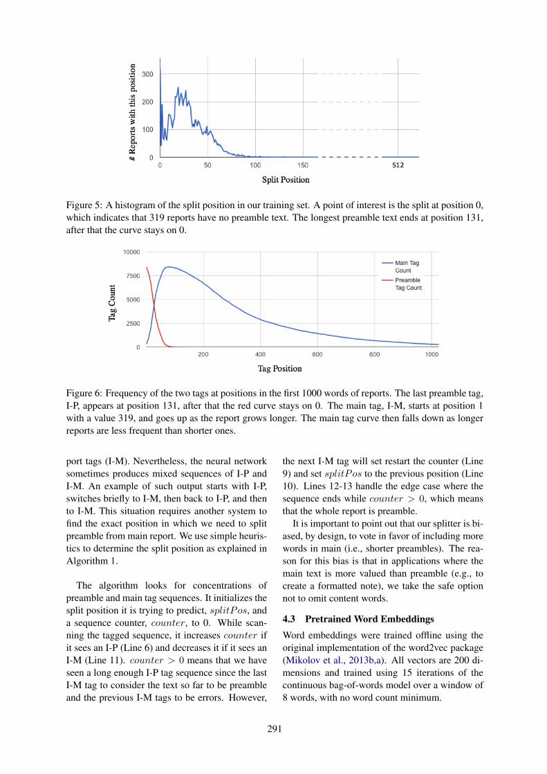
Figure 5: A histogram of the split position in our training set. A point of interest is the split at position 0,which indicates that 319 reports have no preamble text. The longest preamble text ends at position 131,after that the curve stays on 0.
Figure 6: Frequency of the two tags at positions in the first 1000 words of reports. The last preamble tag,I-P, appears at position 131, after that the red curve stays on 0. The main tag, I-M, starts at position 1with a value 319, and goes up as the report grows longer. The main tag curve then falls down as longerreports are less frequent than shorter ones.
port tags (I-M). Nevertheless, the neural networksometimes produces mixed sequences of I-P andI-M. An example of such output starts with I-P,switches briefly to I-M, then back to I-P, and thento I-M. This situation requires another system tofind the exact position in which we need to splitpreamble from main report. We use simple heuris-tics to determine the split position as explained inAlgorithm 1.
The algorithm looks for concentrations ofpreamble and main tag sequences. It initializes thesplit position it is trying to predict, splitPos, anda sequence counter, counter, to 0. While scan-ning the tagged sequence, it increases counter ifit sees an I-P (Line 6) and decreases it if it sees anI-M (Line 11). counter > 0 means that we haveseen a long enough I-P tag sequence since the lastI-M tag to consider the text so far to be preambleand the previous I-M tags to be errors. However,
the next I-M tag will set restart the counter (Line9) and set splitPos to the previous position (Line10). Lines 12-13 handle the edge case where thesequence ends while counter > 0, which meansthat the whole report is preamble.
It is important to point out that our splitter is bi-ased, by design, to vote in favor of including morewords in main (i.e., shorter preambles). The rea-son for this bias is that in applications where themain text is more valued than preamble (e.g., tocreate a formatted note), we take the safe optionnot to omit content words.
4.3 Pretrained Word EmbeddingsWord embeddings were trained offline using theoriginal implementation of the word2vec package(Mikolov et al., 2013b,a). All vectors are 200 di-mensions and trained using 15 iterations of thecontinuous bag-of-words model over a window of8 words, with no word count minimum.
291

Figure 7: The NN stack using Bi-LSTM. An em-bedding at each word step is fed into forward andbackward LSTM layers, which are fully connectedto a softmax-activated output layer. (For the uni-directional LSTM, the backward layer is omitted.)
We experimented with three sets of embed-dings, each trained on cumulatively more text:
• “SplitEmb” was trained on the same tran-scriptions as the tagging model (plus thoseon which only two annotators agreed on thesplit), with the insertion of a line break atthe split between the preamble and main text.This break causes word2vec not to train onco-occurrences of tokens on either side ofthe split, hypothetically leading to decreasedsimilarity between words typically found in-side and outside of preambles. (3.7 M tokenstotal.)
• “SplitTransEmb” added more transcribedmedical dictations which were not part of thepreamble-annotated set. (8.3 M tokens.)
• “SplitTransRepEmb” added formattedmedical reports processed to look liketranscriptions—numerals spelled out, punc-tuation removed, etc. (60 M tokens.)
5 Evaluation
As a first sanity check, we measured the pream-ble tagging accuracy on the token level. In otherwords, we determined how many of the tokens inthe test set were correctly tagged as being eitherpart of the preamble or the main body. In this task,
Algorithm 1 The Heuristic Splitter.1: splitPos← 0 // predicted split position.2: counter ← 0 // sequence counter.
3: for pos := 1→ length(tags) do4: switch tags[pos] do
// ... padding is ignored.
5: case I-P6: counter++7: case I-M8: if counter > 0 then9: counter ← 0 // reset
10: splitPos← pos− 111: counter--12: if counter > 0 then13: return length(predictedTags)14: else15: return splitPos
our system achieved an accuracy of 99.80%, withonly 816 mismatches among the total of 415,491tokens in the test set.
As motivated in Section 3.2, the ultimate per-formance measure we are using counts how manyperfect splits the preamble detector found, i.e. thesplit accuracy. Table 2 shows detailed results ofthe systems introduced in Section 4, comparingall pre-trained word embedding models across twoembedding schemes (trainable vs. frozen) and forboth Uni- and Bi-LSTM. The best overall systemuses Bi-LSTMs and frozen embeddings, perform-ing at 89.84% split accuracy. In comparison, ascalculated earlier, the human split accuracy on ourcorpus was determined to be 86.04% which con-stitutes a statistically significant difference. Thefact that our automated preamble detection systemoutperforms humans demonstrates the strength ofthe presented methods in exploiting synergistic ef-fects across a crowd of annotators.
We were also interested in the effectiveness ofthe heuristic splitter introduced in Section 4.2.We therefore determined results for both Uni-LSTM (75.74%) and Bi-LSTM (87.44%) whenleaving out the splitter. Compared to the indi-vidual best results for Uni- and Bi-LSTMs in Ta-ble 2, this constitutes a difference of 8.25% and2.4%, demonstrating a clear positive impact of theheuristic splitter.
292

Test OOVs(first 512)
LSTM Bi-LSTMTrainable Emb. Frozen Emb. Trainable Emb. Frozen Emb.
# types rate # PS % # PS % # PS % # PS %Fully-trained Emb. n/a n/a 754 72.29% n/a n/a 863 82.74% n/a n/aSplitEmb 1133 8.59% 809 77.56% 839 80.44% 911 87.34% 916 87.82%SplitTransEmb 905 6.86% 809 77.56% 846 81.11% 899 86.19% 937 89.84%SplitTransRepEmb 230 1.74% 798 76.51% 876 83.99% 907 86.96% 925 88.69%
Table 2: Evaluation of our LSTM and Bi-LSTM models across all pretrained word embedding models.The first column shows the different pretrained word embedding models we used. The “Test OOVs”column shows the OOV count and rate against each pretrained embedding model. This only includestypes in the first 512 words of the report (that are passed to the NN) which contain 13,186 types outof the 13,507. Columns with title “Trainable Emb.” report results where backpropagation is allowed toupdate the pretrained embedding layer after it is loaded, while columns with title “Frozen Emb.” doesnot allow such updates. # PS is the number of Perfect Splits.
6 Conclusion and Future Work
The work presented in this paper shows yet againthat careful design and execution of state-of-the-art NLP techniques when applied to traditionallymanual tasks (in this case, the detection of pream-bles in medical dictations) can approach or evensurpass human performance. We assume that thepresented NLP stack with Bi-LSTMs makes use ofthe wisdom of the crowd: it exploits the fact that,even though the annotators working on this taskwere professional MTs, the provided guidelines onhow to tell preambles from main body were notvery detailed.
In future investigations, we would like to seehow more elaborate annotation guidelines can im-prove human performance and what impact theimproved annotations have on the performance ofan automated preamble detector. It is specificallyinteresting to investigate how situations of inter-twined preamble and main body, as exemplifiedin Figure 3, can be resolved by clearer guidelinesor, alternatively, by an annotation scheme allow-ing for more than a single hard split.
We are also interested to further enhance theautomatic preamble detector by combining thetagger and splitter into a joint neural networkmodel, or by implementing a transfer learning stepwhich reuses the learned tagger weight in a neural-network-based splitter.
ReferencesM Abadi, A Agarwal, P Barham, E Brevdo, Z Chen,
C Citro, GS Corrado, A Davis, J Dean, M Devin,S Ghemawat, I Goodfellow, A Harp, G Irving, M Is-ard, Y Jia, R Jozefowicz, L Kaiser, M Kudlur, J Lev-enberg, D Mane, R Monga, S Moore, D Murray,
C Olah, M Schuster, J Shlens, B Steiner, I Sutskever,K Talwar, P Tucker, V Vanhoucke, V Vasudevan,F Viegas, O Vinyals, P Warden, M Wattenberg,M Wicke, Y Yu, and X Zheng. 2016. Tensorflow:large-scale machine learning on heterogeneous dis-tributed systems. arXiv 1603(04467):1–19.
MA Alkureishi, WW Lee, M Lyons, VG Press,S Imam, A Nkansah-Amankra, D Werner, andVM Arora. 2016. Impact of electronic medicalrecord use on the patient-doctor relationship andcommunication: a systematic review. J Gen InternMed 31(5):548–560.
P Campanella, E Lovato, C Marone, L Fallacara,A Mancuso, W Ricciardi, and ML Specchia. 2015.The impact of electronic health records on health-care quality: a systematic review and meta-analysis.Eur J Public Health 26(1):60–64.
JPC Chiu and E Nichols. 2015. Named entityrecognition with bidirectional lstm-cnns. arXiv1511(08308):1–14.
K Cho, B van Merrienboer, D Bahdanau, and Y Ben-gio. 2014. On the properties of neural machinetranslation: encoder-decoder approaches. arXiv1409(1259):1–9.
F Chollet. 2015. Keras: deep learning library fortheano and tensorflow. https://keras.io/.
F Chollet. 2017. Deep learning with Python. Manning,Shelter Island, NY.
R Collobert and J Weston. 2008. A unified architec-ture for natural language processing: deep neuralnetworks with multitask learning. In Proc ICML.ACM, pages 160–167.
R Collobert, J Weston, L Bottou, M Karlen,K Kavukcuoglu, and P Kuksa. 2011. Natural lan-guage processing (almost) from scratch. J MachLearn Res 12(8):2493–2537.
R Dey and FM Salem. 2017. Gate-variants ofgated recurrent unit (gru) neural networks. arXiv1701(05923):1–5.
293

E Edwards, W Salloum, GP Finley, J Fone, G Cardiff,M Miller, and D Suendermann-Oeft. 2017. Medicalspeech recognition: reaching parity with humans. InSPECOM. page 10 p.
E Ford, JA Carroll, HE Smith, D Scott, and JA Cas-sell. 2016. Extracting information from the text ofelectronic medical records to improve case detec-tion: a systematic review. J Am Med Inform Assoc23(5):1007–1015.
A Graves, S Fernandez, and J Schmidhuber. 2005.Bidirectional lstm networks for improved phonemeclassification and recognition. In Proc ICANN.Springer, pages 799–804.
A Graves and J Schmidhuber. 2005. Framewisephoneme classification with bidirectional lstm net-works. In Proc IJCNN. IEEE, volume 4, pages2047–2052.
I Hammana, L Lepanto, T Poder, C Bellemare, and M-S Ly. 2015. Speech recognition in the radiology de-partment: a systematic review. HIM J 44(2):4–10.
J Hammerton. 2003. Named entity recognition withlong short-term memory. In Proc HLT-NAACL.ACL, volume 4, pages 172–175.
K Hayrinen, K Saranto, and P Nykanen. 2008. Defini-tion, structure, content, use and impacts of electronichealth records: a review of the research literature.Int J Med Inform 77(5):291–304.
S Hochreiter and J Schmidhuber. 1997. Long short-term memory. Neural Comput 9(8):1735–1780.
T Hodgson and EW Coiera. 2016. Risks and ben-efits of speech recognition for clinical documenta-tion: a systematic review. J Am Med Inform Assoc23(e1):e169–e179.
JM Holroyd-Leduc, D Lorenzetti, SE Straus, L Sykes,and H Quan. 2011. The impact of the electronicmedical record on structure, process, and outcomeswithin primary care: a systematic review of the evi-dence. J Am Med Inform Assoc 18(6):732–737.
Z Huang, W Xu, and K Yu. 2015. Bidirectionallstm-crf models for sequence tagging. arXiv1508(01991):1–10.
H Hypponen, K Saranto, R Vuokko, P Makela-Bengs,P Doupi, M Lindqvist, and M Makela. 2014. Im-pacts of structuring the electronic health record: asystematic review protocol and results of previousreviews. Int J Med Inform 83(3):159–169.
SB Johnson, S Bakken, D Dine, S Hyun, E Mendonca,F Morrison, T Bright, T Van Vleck, J Wrenn, andP Stetson. 2008. An electronic health record basedon structured narrative. J Am Med Inform Assoc15(1):54–64.
D Kalra, B Fernando, Z Morrison, and A Sheikh. 2012.A review of the empirical evidence of the value ofstructuring and coding of clinical information withinelectronic health records for direct patient care. In-form Prim Care 20(3):171–180.
DP Kingma and J Ba. 2014. Adam: a method forstochastic optimization. arXiv 1412(6980):1–9.
J Kupiec. 1992. Robust part-of-speech tagging us-ing a hidden markov model. Comput Speech Lang6(3):225–242.
JD Lafferty, A McCallum, and FCN Pereira. 2001.Conditional random fields: probabilistic models forsegmenting and labeling sequence data. In ProcICML. ACM, pages 282–289.
G Lample, M Ballesteros, S Subramanian,K Kawakami, and C Dyer. 2016. Neural ar-chitectures for named entity recognition. arXiv1603(01360):1–11.
J Logan. 2012. Electronic health information systemimplementation models a review. Stud Health Tech-nol Inform 178:117–123.
X Ma and EH Hovy. 2016. End-to-end sequencelabeling via bi-directional lstm-cnns-crf. arXiv1603(01354):1–12.
SM Meystre, GK Savova, KC Kipper-Schuler, andJF Hurdle. 2008. Extracting information fromtextual documents in the electronic health record:a review of recent research. Yearb Med Inform2008:128–144.
T Mikolov, K Chen, GS Corrado, and J Dean. 2013a.Efficient estimation of word representations in vec-tor space. arXiv 1301(3781):1–13.
T Mikolov, W-t Yih, and G Zweig. 2013b. Linguis-tic regularities in continuous space word representa-tions. In Proc HLT-NAACL. ACL, volume 13, pages746–751.
A Moreno-Conde, D Moner, WD da Cruz, MR San-tos, JA Maldonado, M Robles, and D Kalra. 2015.Clinical information modeling processes for seman-tic interoperability of electronic health records: sys-tematic review and inductive analysis. J Am MedInform Assoc 22(4):925–934.
B Plank, A Søgaard, and Y Goldberg. 2016. Multilin-gual part-of-speech tagging with bidirectional longshort-term memory models and auxiliary loss. arXiv1604(05529):1–7.
W Salloum, E Edwards, S Ghaffarzadegan,D Suendermann-Oeft, and M Miller. 2017a.Crowdsourced continuous improvement of med-ical speech recognition. In Proc AAAI WrkshpCrowdsourcing. AAAI, San Francisco, CA.
294

Wael Salloum, Greg Finley, Erik Edwards, MarkMiller, and David Suendermann-Oeft. 2017b. Deeplearning for punctuation restoration in medical re-ports. In Proceedings of the ACL BioNLP Workshop.Association for Computational Linguistics.
F Sha and F Pereira. 2003. Shallow parsing with con-ditional random fields. In Proc HLT-NAACL. ACL,volume 1, pages 134–141.
Y Tang, Z Wu, H Meng, M Xu, and L Cai. 2016. Anal-ysis on gated recurrent unit based question detectionapproach. In Proc Interspeech. ISCA, San Fran-cisco, CA, pages 735–739.
P Wang, Y Qian, FK Soong, L He, and H Zhao. 2015.A unified tagging solution: bidirectional lstm recur-rent neural network with word embedding. arXiv1511(00215):1–10.
M Wollmer, F Eyben, A Graves, B Schuller, andG Rigoll. 2010. Bidirectional lstm networks forcontext-sensitive keyword detection in a cognitivevirtual agent framework. Cognit Comput 2(3):180–190.
295

Proceedings of the BioNLP 2017 workshop, pages 296–301,Vancouver, Canada, August 4, 2017. c©2017 Association for Computational Linguistics
A Biomedical Question Answering System in BioASQ 2017
Mourad Sarrouti, Said Ouatik El AlaouiLaboratory of Computer Science and Modeling
Faculty of Sciences Dhar El MahrazSidi Mohammed Ben Abdellah University
Fez, [email protected]
Abstract
Question answering, the identification ofshort accurate answers to users questions,is a longstanding challenge widely stud-ied over the last decades in the open-domain. However, it still requires fur-ther efforts in the biomedical domain. Inthis paper, we describe our participation inphase B of task 5b in the 2017 BioASQchallenge using our biomedical questionanswering system. Our system, dealingwith four types of questions (i.e., yes/no,factoid, list, and summary), is based on(1) a dictionary-based approach for gen-erating the exact answers of yes/no ques-tions, (2) UMLS metathesaurus and termfrequency metric for extracting the ex-act answers of factoid and list questions,and (3) the BM25 model and UMLS con-cepts for retrieving the ideal answers (i.e.,paragraph-sized summaries). Preliminaryresults show that our system achieves goodand competitive results in both exact andideal answers extraction tasks as comparedwith the participating systems.
1 Introduction
Finding accurate answers to biomedical questionswritten in natural language from the biomedi-cal literature is the key to creating high-qualitysystematic reviews that support the practice ofevidence-based medicine (Kropf et al., 2017;Wang et al., 2017; Sarrouti and Lachkar, 2017)and improve the quality of patient care (Sarroutiand Alaoui, 2017b). However, with the large andincreasing volume of textual data in the biomedi-cal domain makes it difficult to absorb all relevantinformation (Sarrouti and Alaoui, 2017a). Sincetime and quality are of the essence in finding an-
swers to biomedical questions, developing and im-proving question answering systems are desirable.Question answering (QA) systems aim at directlyproducing and providing short precise answers tousers questions by automatically analyzing thou-sands of articles using information extraction andnatural language processing methods.
Although different types of QA systems havedifferent architectures, most of them, especiallyin the biomedical domain, follow a framework inwhich (1) question classification and query for-mulation, (2) document retrieval, (3) passage re-trieval, and (4) answer extraction components playa vital role (Athenikos and Han, 2010; Neves andLeser, 2015; Abacha and Zweigenbaum, 2015).
Question answering in the open-domain is alongstanding challenge widely studied over thelast decades (Green et al., 1961; Katz et al.,2002). However, it still remains a real challengein the biomedical domain. As has been exten-sively documented in the recent research litera-ture (Athenikos and Han, 2010), open-domain QAis concerned with questions which were not re-stricted to any domain, while in restricted-domainQA such as the biomedical one, the domain of ap-plication provides a context for the QA process.Additionally, Athenikos and Han (2010) report thefollowing characteristics for QA in the biomedicaldomain: (1) large-sized textual corpora, (2) highlycomplex domain-specific terminology, and (3) do-main specific format and typology of questions.
Since the launch of the biomedical QA track atthe BioASQ1 challenge (Tsatsaronis et al., 2015),various approaches in biomedical QA have beenpresented. The BioASQ challenge, within 2017edition, comprised three tasks: (1) task 5a onlarge-scale online biomedical semantic indexing,(2) task 5b on biomedical semantic QA, and (3)
1http://bioasq.org/
296

Document Processing
Query
IR system
Document Retrieval
Candidate Answers
Question Processing
Query Formulation
Question Analysis
And
Classification
Documents
Answer Processing
1. Yes/No answer extraction 2. Factoid answer extraction
3. List answer extraction
4. Summary answer extraction
Question Type
1. yes/no
2. factoid
3. list 4. summary
Expected Answer Format
NL Questions: e.g., Is CHEK2 involved in cell
cycle control?
E.g., Yes
Ask your question
Passage Retrieval
Phase 1
Phase 2
Phase 3
Figure 1: Overall architecture of the proposed biomedical question-answering system
task 5c on funding information extraction frombiomedical literature. Task 5b consists of twophases: In phase A, BioASQ released questionsin English from benchmark datasets. There werefour types of questions: yes/no, factoid, list andsummary questions (Balikas et al., 2013). Partic-ipants had to respond with relevant concepts, rel-evant documents, relevant snippets retrieved fromthe relevant documents, and relevant RDF triples.In phase B, the released questions contained thegolden answers for the required elements (docu-ments and snippets) of the first phase. The par-ticipants had to answer with exact answers (e.g.,biomedical entity, number, list of biomedical en-tities, yes, no, etc.) as well as with ideal an-swers (i.e., paragraph-sized summaries) (Kritharaet al., 2016). In this paper, we describe our par-ticipation in the phase B (i.e., exact and ideal an-swers) of task5b in the 2017 BioASQ challenge.In our biomedical QA system, we have used (1)a dictionary-based approach to generate the exactanswers to yes/no questions, (2) the unified med-ical language system (UMLS) metathesaurus andterm frequency metrics for extracting the exact an-swers of factoid and list questions, and (3) theBM25 model and UMLS concepts for retrieving
the ideal answers. Figure 1 illustrates the genericarchitecture of our biomedical QA system.
The remainder of the paper is organized as fol-lows. Section 2 introduces related work and dis-cussion about the main biomedical QA approacheswith a particular focus on BioASQ participants.Section 3 describes the answer extraction meth-ods used in our biomedical QA system. Section 4presents the preliminary results we obtained in the2017 BioASQ challenge. Finally, the conclusionand future work are made in Section 5.
2 Related work
Since the launch of the BioASQ challenge (Tsat-saronis et al., 2015), QA in the biomedical do-main has received much attention from the re-search community. The BioASQ challenge, whichtakes place regularly every year since 2013, is anEU-funded support action to set up a challengeon biomedical semantic indexing and QA. Yenalaet al. (2015) have presented IIITH biomedical QAsystem in BioASQ 2015 based on PubMed searchengine, leverage web search results, and domainwords. The authors have relied on the PubMedsearch engine to retrieve relevant documents andthen applied their own snippet extraction meth-
297

ods, which is based on number of common do-main words of the top 10 sentences of the retrieveddocuments and the question. Zhang et al. (2015)have described USTB biomedical QA system inthe 2015 BioASQ challenge. They have built ageneric retrieval model based on the sequentialdependence model, word embedding and rankingmodel for document retrieval. After splitting thetop-ranked documents into sentences, the authorsthen have applied the same approach for snippetsretrieval. Yang et al. (2016) have described theOAQA system in BioASQ 4b based on NLP an-notators, machine learning algorithms for searchresult scoring, collective answer re-ranking, andyes/no answer prediction. Schulze et al. (2016)have presented HPI biomedical QA system basedon NLP functionality from a in-memory database(IMDB). The authors have participated in phaseA and B of BioASQ 4b. They have used theLexRank algorithm and biomedical entity namesfor generating ideal answers. Lee et al. (2016)have described KSAnswer biomedical QA systemthat returns relevant documents and snippets inBioASQ 4b. KSAnswer, which is participated inphase A of task 4b in the 2016 BioASQ challenge,retrieves candidate snippets using a cluster-basedlanguage model. Then, it reranks the retrieved top-N snippets using five independent similarity mod-els based on shallow semantic analysis.
3 Methods
In this section, we describe the answer extractionmodule of our biomedical QA system. Althoughour biomedical QA system is composed of manycomponents (cf. Figure 1) which are included inthree main phases, i.e., question processing, docu-ment processing, and answer processing, we haveonly used its answer extraction module since wehave participated only in phase B (i.e., exact andideal answers) of task 5b in BioASQ 2017.
During phase B, BioASQ organizers releasedthe test set of biomedical questions along withtheir relevant documents, relevant snippets, andquestions types, i.e., whether yes/no, factoid, listor summary. For each question, each participat-ing system may return an ideal answer, i.e., aparagraph-sized summary of relevant information.In the case of yes/no, factoid, and list questions,the systems may also return exact answers; forsummary questions, no exact answers will be re-turned. In the following sections (cf. Sections 3.1
and 3.2), we will provide a detailed descriptionof the proposed methods used to extract exact andideal answers for yes/no, factoid, list and summaryquestions.
3.1 Exact answers
As it has already been described by the BioASQchallenge, the participating systems in phase B oftask 5b may return exact answers for yes/no, fac-toid, and list questions, while no exact answerswill be returned for summary questions.Yes/No questions: For each yes/no question, theexact answer of each participating system willhave be either “yes” or “no”. The decision forthe answers “yes” or “no” in our system is ob-tained by a sentiment analysis-based approach. In-deed, we first have used the Stanford CoreNLP(Manning et al., 2014) for tokenization and part-of-speech tagging one by one the N retrieved snip-pets (s1, s2, ..., sn) from benchmark datatsets. Wethen have assigned a sentiment score using theSentiWordNet (Baccianella et al., 2010) lexical re-source to each word in the set of retrieved snippets.Finally, the decision for the answers “yes” or “no”is based on the number of positive and negativesnippets.Factoid questions:
For each factoid question, each participatingsystem will have to return a list of up to 5 entitynames (e.g., up to 5 names of drugs), numbers,or similar short expressions, ordered by decreas-ing confidence. To answer a factoid question inour biomedical QA system, we have first mappedboth the given question and its N relevant snippetsretrieved from benchmark datasets to the UMLSmetathesaurus in order to extract a set of biomedi-cal entity names. To do so, the MetaMap2 programwas used (Aronson, 2001). We then re-ranked theobtained set of biomedical entity names based onterm frequency metrics, i.e., the number of timesan entity name appeared in the set of biomedicalentity names. Indeed, the biomedical entity namesappeared in the question are ignored. We finallykept the 5 top-ranked biomedical entity names asanswers. A factoid question has one correct an-swer, but up to five candidate answers are allowedin BioASQ 2017.List questions: For each list question, each par-ticipating system will have to return a single listof entity names, numbers, or similar short expres-
2https://metamap.nlm.nih.gov/
298

sions. The proposed method used to answer listquestions in our system is similar to the one de-scribed for factoid questions. Indeed, the exactanswer is the same of factoid questions, only theinterpretation is different for list questions: All Ntop-ranked biomedical entities are considered partof the same answer for the list question, not ascandidates. In this work, we have used the fivetop-ranked (N = 5) entities as answers for listquestions.
3.2 Ideal answers
To formulate and generate the ideal answers fora given yes/no, factoid, list or summary ques-tion, we have used the proposed retrieval modelpresented in (Sarrouti and Alaoui, 2017b). Morespecifically, after retrieving the N relevant snip-pets from benchmark datasets to a given biomed-ical question, we have re-ranked them based onthe BM25 model as retrieval model, stemmedwords and UMLS concepts as features. First, wehave preprocessed the retrieved set of snippets, in-cluding tokenization using the Stanford CoreNLP(Manning et al., 2014), removing stop words3, andapplying Porter’ stemmer (Porter, 1980) to ex-tract stemmed words. Additionally, we have usedMetaMap to map both questions and snippets toUMLS metathesaurus concepts so as to extractUMLS concepts. Then, we have re-ranked the setof snippets using stemmed words and UMLS con-cepts as features for the BM25 model. Finally, theideal answer is obtained by concatenating the twotop-ranked snippets.
4 Experimental results and discussion
In this section, we present the preliminary resultswe obtained in BioASQ 2017. We first introducethe evaluation metrics, then give the experimentalresults, and finally discuss the results.
4.1 Evaluation metrics
The evaluation metrics used for the exact answersin phase B of task 5b are accuracy, strict accu-racy and lenient accuracy, mean reciprocal rank(MRR), mean precision, mean recall, and meanF-measure. Accuracy, MRR and F-measure arethe official measures used for evaluating the ex-act answers of yes/no, factoid and list questions,respectively. ROUGE-2 and ROUGE-SU4, on the
3http://www.textfixer.com/resources/common-english-words.txt
other hand, are the main measures for an automaticevaluation of ideal answers. Details of these eval-uations metrics appear in (Balikas et al., 2013).
4.2 Results and discussion
Table 1 highlights the preliminary results of oursystem in phase B (i.e., exact and ideal answers)of BioASQ task 5b. More details on the resultscan be found in the BioASQ web site4.
Our system performed well in the challengeranking as compared with the participating sys-tems. In batch 1, it achieved the third and the fifthposition within the 15 participating systems for ex-tracting the exact answers of list and factoid ques-tions respectively. More specifically, our systemobtained the second and the third position whenconsidering results by teams, instead of each in-dividual run. In batch 2, considering results byteams, our system obtained the second and thefourth position for extracting the exact answers oflist and factoid questions respectively. For yes/noquestions, our system achieved the first and thesecond position respectively in batch 3 and batch4, while it obtained the fifteenth position in batch5.
On the other hand, for the ideal answers, oursystem in terms of ROUGE-2 achieved the fourthposition as compared to the 15 and 21 participat-ing systems in batch 1, batch 2 and batch 3 respec-tively. While in terms of ROUGE-SU4, our sys-tem obtained the third position in batch 1 and thefourth position in batch 2. In batch 4 and batch 5,our systems achieved respectively the second andthird position within the 27 participating systemsin terms of ROUGE-2 and ROUGE-SU4 whenconsidering results by teams, instead of each indi-vidual run. This proves that the proposed methodcould effectively identify the ideal answers to agiven biomedical question.
Overall, from the results and analysis on fivesbatches of testing data of BioASQ task 5b, we candraw a conclusion that our system is very compet-itive as compared with the participating systems inboth exact and ideal answers tasks.
5 Conclusion and future work
In this paper, we presented the obtained resultsfor the answer extraction module of our biomed-ical QA system that participated in task 5b of
4http://participants-area.bioasq.org/results/5b/phaseB/
299

DatasetsExact answers Idial answersYes/No Factoid List
Accuracy MRR P R F ROUGE-2 ROUGE-SU4Batch 1 0.7647 0.2033
(5/15)0.1909 0.2658 0.2129
(3/15)0.4943(4/15)
0.5108 (3/15)
Batch 2 0.7778 0.0887(10/21)
0.2400 0.3922 0.2920(6/21)
0.4579(4/21)
0.4583 (4/21)
Batch 3 0.8387(1/21)
0.2212(9/21)
0.2000 0.4151 0.2640(6/21)
0.5566(4/21)
0.5656 (4/21)
Batch 4 0.6207(2/27)
0.0970(13/27)
0.1077 0.2013 0.1369(12/27)
0.5895(4/27)
0.5832 (4/27)
Batch 5 0.4615(15/25)
0.2071(9/25)
0.2091 0.3087 0.2438(11/25)
0.5772(7/25)
0.5756 (7/25)
Table 1: The primarily results of our system in phase B of BioASQ task 5b. P, R, and F indicateprecision, recall, and F-measure, respectively. The values inside parameters indicate our current rankand the total number of submissions for the batch.
the 2017 BioASQ challenge. The proposed ap-proach is based on (1) the SentiWordNet lexi-cal resource to generate the exact answers foryes/questions, (2) UMLS metathesaurus and termfrequency metrics for answering factoid and listquestions, (3) our retrieval model based on UMLSconcepts and the BM25 model for generating theideal answers. The preliminary results show thatour system achieved good performances and isvery competitive as compared with the participat-ing systems.
In future research, we intend to present the end-to-end evaluations of our biomedical QA systemwhich includes question classification, documentretrieval, passage retrieval, and answer extractioncomponents.
References
Asma Ben Abacha and Pierre Zweigenbaum.2015. MEANS: A medical question-answeringsystem combining NLP techniques and se-mantic Web technologies. InformationProcessing & Management 51(5):570–594.https://doi.org/10.1016/j.ipm.2015.04.006.
Alan R Aronson. 2001. Effective mapping of biomed-ical text to the UMLS metathesaurus: the MetaMapprogram. In Proceedings of the AMIA Sympo-sium. American Medical Informatics Association,page 17.
Sofia J Athenikos and Hyoil Han. 2010. Biomed-ical question answering: A survey. Computermethods and programs in biomedicine 99(1):1–24.https://doi.org/10.1016/j.cmpb.2009.10.003.
Stefano Baccianella, Andrea Esuli, and Fabrizio Sebas-tiani. 2010. SentiWordNet 3.0: An enhanced lexicalresource for sentiment analysis and opinion mining.In LREC. volume 10, pages 2200–2204.
Georgios Balikas, Ioannis Partalas, Aris Kosmopoulos,Sergios Petridis, Prodromos Malakasiotis, IoannisPavlopoulos, Ion Androutsopoulos, Nicolas Baski-otis, Eric Gaussier, Thierry Artiere, and Patrick Gal-linari. 2013. Evaluation framework specifications.project deliverable d4.1, 05/2013.
Bert F. Green, Alice K. Wolf, Carol Chom-sky, and Kenneth Laughery. 1961. Base-ball. In western joint IRE-AIEE-ACM com-puter conference on - IRE-AIEE-ACM 61 (West-ern). Association for Computing Machinery (ACM).https://doi.org/10.1145/1460690.1460714.
Boris Katz, Sue Felshin, Deniz Yuret, Ali Ibrahim,Jimmy Lin, Gregory Marton, Alton Jerome McFar-land, and Baris Temelkuran. 2002. Omnibase: Uni-form access to heterogeneous data for question an-swering. In Natural Language Processing and In-formation Systems, Springer Nature, pages 230–234.https://doi.org/10.1007/3-540-36271-1 23.
Anastasia Krithara, Anastasios Nentidis, GeorgePaliouras, and Ioannis Kakadiaris. 2016. Results ofthe 4th edition of BioASQ challenge. In Proceed-ings of the Fourth BioASQ workshop at the Confer-ence of the Association for Computational Linguis-tics. pages 1–7.
S. Kropf, P. Krcken, W. Mueller, and K. Denecke.2017. Structuring legacy pathology reports byopenEHR archetypes to enable semantic query-ing. Methods of Information in Medicine 56(2).https://doi.org/10.3414/me16-01-0073.
Hyeon-gu Lee, Minkyoung Kim, Harksoo Kim, JuaeKim, Sunjae Kwon, Jungyun Seo, Jungkyu Choi,
300

and Yi-reun Kim. 2016. KSAnswer: Question-answering system of kangwon national universityand sogang university in the 2016 BioASQ chal-lenge. ACL 2016 page 45.
Christopher Manning, Mihai Surdeanu, John Bauer,Jenny Finkel, Steven Bethard, and David Mc-Closky. 2014. The stanford CoreNLP naturallanguage processing toolkit. In Proceedings of52nd Annual Meeting of the Association for Com-putational Linguistics: System Demonstrations.https://doi.org/10.3115/v1/p14-5010.
Mariana Neves and Ulf Leser. 2015. Ques-tion answering for biology. Methods 74:36–46.https://doi.org/10.1016/j.ymeth.2014.10.023.
M.F. Porter. 1980. An algorithm for suf-fix stripping. Program: electronic libraryand information systems 14(3):130–137.https://doi.org/10.1108/eb046814.
Mourad Sarrouti and Said Ouatik El Alaoui. 2017a.A machine learning-based method for questiontype classification in biomedical question answer-ing. Methods of Information in Medicine 56(3).https://doi.org/10.3414/me16-01-0116.
Mourad Sarrouti and Said Ouatik El Alaoui.2017b. A passage retrieval method based onprobabilistic information retrieval and UMLSconcepts in biomedical question answering.Journal of Biomedical Informatics 68:96–103.https://doi.org/10.1016/j.jbi.2017.03.001.
Mourad Sarrouti and Abdelmonaime Lachkar. 2017. Anew and efficient method based on syntactic depen-dency relations features for ad hoc clinical questionclassification. International Journal of Bioinfor-matics Research and Applications 13(2):161–177.https://doi.org/10.1504/ijbra.2017.10003490.
Frederik Schulze, Ricarda Schuler, Tim Draeger,Daniel Dummer, Alexander Ernst, Pedro Flemming,Cindy Perscheid, and Mariana Neves. 2016. HPIquestion answering system in bioasq 2016. In Pro-ceedings of the Fourth BioASQ workshop at the Con-ference of the Association for Computational Lin-guistics. pages 38–44.
George Tsatsaronis, Georgios Balikas, ProdromosMalakasiotis, Ioannis Partalas, Matthias Zschunke,Michael R. Alvers, Dirk Weissenborn, AnastasiaKrithara, Sergios Petridis, Dimitris Polychronopou-los, Yannis Almirantis, John Pavlopoulos, Nico-las Baskiotis, Patrick Gallinari, Thierry Artieres,Axel-Cyrille Ngonga Ngomo, Norman Heino, EricGaussier, Liliana Barrio-Alvers, Michael Schroeder,Ion Androutsopoulos, and Georgios Paliouras. 2015.An overview of the BIOASQ large-scale biomed-ical semantic indexing and question answeringcompetition. BMC Bioinformatics 16(1):1–28.https://doi.org/10.1186/s12859-015-0564-6.
Liqin Wang, Guilherme Del Fiol, Bruce E. Bray,and Peter J. Haug. 2017. Generating disease-pertinent treatment vocabularies from MEDLINE ci-tations. Journal of Biomedical Informatics 65:46–57. https://doi.org/10.1016/j.jbi.2016.11.004.
Zi Yang, Yue Zhou, and Eric Nyberg. 2016. Learningto answer biomedical questions: OAQA at BioASQ4b. ACL 2016 page 23.
Harish Yenala, Avinash Kamineni, Manish Shrivas-tava, and Manoj Kumar Chinnakotla. 2015. IIITH atBioASQ challange 2015 task 3b: Bio-medical ques-tion answering system. In CLEF 2015.
Zhijuan Zhang, Tiantian Liu, Bo-Wen Zhang, Yan Li,Chun Hua Zhao, Shao-Hui Feng, Xu-Cheng Yin,and Fang Zhou. 2015. A generic retrieval systemfor biomedical literatures: USTB at BioASQ 2015question answering task. In CLEF 2015.
301

Proceedings of the BioNLP 2017 workshop, pages 302–306,Vancouver, Canada, August 4, 2017. c©2017 Association for Computational Linguistics
Adapting Pre-trained Word Embeddings For Use In Medical Coding
Kevin Patel1, Divya Patel2, Mansi Golakiya2, Pushpak Bhattacharyya1, Nilesh Birari3
1Indian Institute of Technology Bombay, India2Dharmsinh Desai University, India, 3ezDI Inc, India
1{kevin.patel,pb}@cse.iitb.ac.in, [email protected]{divya.patel.8796,golkiya.mansi}@gmail.com
Abstract
Word embeddings are a crucial compo-nent in modern NLP. Pre-trained embed-dings released by different groups havebeen a major reason for their popularity.However, they are trained on generic cor-pora, which limits their direct use for do-main specific tasks. In this paper, we pro-pose a method to add task specific infor-mation to pre-trained word embeddings.Such information can improve their util-ity. We add information from medical cod-ing data, as well as the first level fromthe hierarchy of ICD-10 medical codeset to different pre-trained word embed-dings. We adapt CBOW algorithm fromthe word2vec package for our purpose. Weevaluated our approach on five differentpre-trained word embeddings. Both theoriginal word embeddings, and their mod-ified versions (the ones with added infor-mation) were used for automated review ofmedical coding. The modified word em-beddings give an improvement in f-scoreby 1% on the 5-fold evaluation on a pri-vate medical claims dataset. Our resultsshow that adding extra information is pos-sible and beneficial for the task at hand.
1 Introduction
Word embeddings are a recent addition to an NLPresearcher’s toolkit. They are dense, real-valuedvector representations of words that capture inter-esting properties among them. Word embeddingsare learned from raw corpora. Usually, the largerthe corpora, the better is the quality of the em-beddings learned. However, the larger the cor-pora, the larger is the amount of resources and timeneeded for their training. Thus, different groupsrelease their learned embeddings publicly. Such
pre-trained embeddings is a primary reason for theinclusion of word embeddings in mainstream NLP.However, such pre-trained embeddings are usuallylearned on generic corpora. Using such embed-dings in a particular domain such as medical do-main leads to following problems:
• No embeddings for domain-specific words.For example, phenacetin is not present in pre-trained vectors released by Google.
• Even those words that do have embeddings,may have a poor quality of the embedding,due to different senses of the words, some ofwhich belonging to different domains.
It is difficult to obtain large amounts of domain-specific data. However, many NLP applicationshave benefited from the addition of informationfrom small domain-specific corpus to that ob-tained from a large generic corpus (Ito et al.,1997). This raises the following questions:
• Can we use additional domain-specific datato learn the missing embeddings?
• Can we use additional domain-specific datato improve the quality of already availableembeddings?
In this paper, we address the second question:Given pre-trained word embeddings, and domainspecific data, we tune the pre-trained word em-beddings such that they can achieve better perfor-mance. We tune the embeddings for and evaluatethem on an automated review of medical coding.
The rest of the paper is organized as follows:Section 2 provides some background on differentnotions used later in the paper. Section 3 moti-vates our approach through examples. Section 4explains our approach in detail. Section 5 enliststhe experimental setup. Section 6 details the re-sults and analysis, followed by conclusion and fu-ture work.
302

2 Background
2.1 Word Embeddings
Word embeddings are a crucial component ofmodern NLP. They are learned in an unsupervisedmanner from large amounts of raw corpora. Ben-gio et al. (2003) were the first to propose neuralword embeddings. Many word embedding mod-els have been proposed since then (Collobert andWeston, 2008; Huang et al., 2012; Mikolov et al.,2013; Levy and Goldberg, 2014). The central ideabehind word embeddings is the distributional hy-pothesis, which states that words which are simi-lar in meaning occur in similar contexts (Ruben-stein and Goodenough, 1965). Consider the Con-tinuous Bag of Words model by (Mikolov et al.,2013), where the following problem is poised toa neural network: given the context, predict theword that comes in between. The weights ofthe network are the word embeddings. Trainingthe model over running text brings embeddings ofwords with similar meaning closer.
2.2 Medical Coding
Medical coding is the process of assigning prede-fined alphanumeric medical codes to informationcontained in patient medical records.
Babre et al. (2010) shows a typical medical cod-ing pipeline. Note that the coding (both automaticand/or manual) is followed by a manual review.This is due to the critical nature of the coding pro-cess, and the high cost incurred due to any errors.However, any human involvement increases costboth in terms of time and money. Thus, in order toreduce human involvement in the review process,an automatic review component can be insertedjust before the human review. Automated review-ing is a binary classification problem. Those in-stances that are rejected by the automated reviewcomponent can be directly sent back for recoding,whereas those instances that are accepted by theautomated review component should be sent to hu-man reviewers for further checking. Such a modi-fication decreases the load on the human reviewer,thereby reducing the cost of overall pipeline.
Given the textual nature of medical data, manynatural language processing challenges manifestthemselves while performing either automatedmedical coding or automated review of medicalcoding. Common challenges include, but are notlimited to:
• Synonymy: Multiple words can have samemeaning (Synonym). For instance, HighBlood Sugar and Diabetes have the samemeaning.
• Abbreviation: Medical staff, in their hurry,often abbreviate words and sentences. For in-stance, hypertension can be written as HTN.The automated system needs to understandthat both these strings ultimately mean thesame thing.
One can note that both in case of synonym andabbreviations, the context will be almost same.Thus, word embeddings are well suited to handleboth these challenges.
3 Motivation
Consider the following medical terms (the abbre-viations in parentheses will be used to refer to theterms later):- High Blood Pressure (HBP)- Low Blood Pressure (LBP)- High Blood Sugar (HBS)- Liver Failure (LF)- Diabetes (D)- Hypertension- HTN
We would ideally like the embeddings of theterms to be learned such that the following con-straints hold:
• Similarity (HBP, HBS) should be higher thanSimilarity (HBP, LBP), which in turn, shouldbe higher than Similarity (HBP, LF) (as permedical knowledge).
• Similarity (HBS, D) should be high (as theyare synonyms).
• Similarity (Hypertension, HTN) should behigh (as HTN is abbreviation of hyperten-sion).
Information about such relations might not beavailable in generic corpus on which most pre-trained embeddings are trained. However, it mightbe available in domain specific corpora, or evenlabeled data, such as those used in medical claims.Approaches that can add that information to pre-trained embeddings will definitely improve theirutility.
303
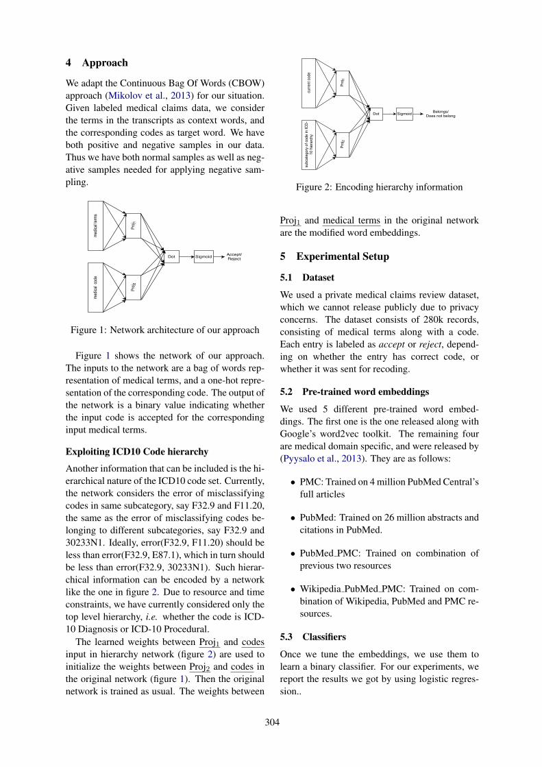
4 Approach
We adapt the Continuous Bag Of Words (CBOW)approach (Mikolov et al., 2013) for our situation.Given labeled medical claims data, we considerthe terms in the transcripts as context words, andthe corresponding codes as target word. We haveboth positive and negative samples in our data.Thus we have both normal samples as well as neg-ative samples needed for applying negative sam-pling.
Figure 1: Network architecture of our approach
Figure 1 shows the network of our approach.The inputs to the network are a bag of words rep-resentation of medical terms, and a one-hot repre-sentation of the corresponding code. The output ofthe network is a binary value indicating whetherthe input code is accepted for the correspondinginput medical terms.
Exploiting ICD10 Code hierarchy
Another information that can be included is the hi-erarchical nature of the ICD10 code set. Currently,the network considers the error of misclassifyingcodes in same subcategory, say F32.9 and F11.20,the same as the error of misclassifying codes be-longing to different subcategories, say F32.9 and30233N1. Ideally, error(F32.9, F11.20) should beless than error(F32.9, E87.1), which in turn shouldbe less than error(F32.9, 30233N1). Such hierar-chical information can be encoded by a networklike the one in figure 2. Due to resource and timeconstraints, we have currently considered only thetop level hierarchy, i.e. whether the code is ICD-10 Diagnosis or ICD-10 Procedural.
The learned weights between Proj1 and codesinput in hierarchy network (figure 2) are used toinitialize the weights between Proj2 and codes inthe original network (figure 1). Then the originalnetwork is trained as usual. The weights between
Figure 2: Encoding hierarchy information
Proj1 and medical terms in the original networkare the modified word embeddings.
5 Experimental Setup
5.1 Dataset
We used a private medical claims review dataset,which we cannot release publicly due to privacyconcerns. The dataset consists of 280k records,consisting of medical terms along with a code.Each entry is labeled as accept or reject, depend-ing on whether the entry has correct code, orwhether it was sent for recoding.
5.2 Pre-trained word embeddings
We used 5 different pre-trained word embed-dings. The first one is the one released along withGoogle’s word2vec toolkit. The remaining fourare medical domain specific, and were released by(Pyysalo et al., 2013). They are as follows:
• PMC: Trained on 4 million PubMed Central’sfull articles
• PubMed: Trained on 26 million abstracts andcitations in PubMed.
• PubMed PMC: Trained on combination ofprevious two resources
• Wikipedia PubMed PMC: Trained on com-bination of Wikipedia, PubMed and PMC re-sources.
5.3 Classifiers
Once we tune the embeddings, we use them tolearn a binary classifier. For our experiments, wereport the results we got by using logistic regres-sion..
304

Medical Knowledge Synonym AbbreviationHBP,HBS HBP,LBP HBP,LF HBS,Diabetes Hypertension,HTN
GoogleOrig 0.534 0.895 0.181 0.293 0Mod 0.549 0.640 0.089 0.350 -0.004
PMCOrig 0.599 0.980 0.173 0.141 0.608Mod 0.638 0.477 -0.054 0.221 0.947
PubMedOrig 0.529 0.970 0.006 0.091 0.465Mod 0.636 0.474 -0.090 0.188 0.952
PubMed PMCOrig 0.592 0.976 0.116 0.141 0.575Mod 0.641 0.450 -0.039 0.241 0.952
WikipediaPubMed PMC
Orig 0.595 0.976 0.158 0.156 0.617Mod 0.653 0.474 -0.061 0.190 0.950
Table 1: Cosine similarities of pairs of examples from Section 3
Pre-trainedEmbeddings
OriginalEmbeddings
ModifiedEmbeddings
Google 82.78 83.37PMC 82.93 83.96PubMed 83.18 84.00PubMed PMC 82.88 83.92WikipediaPubMed PMC
83.12 83.91
Table 2: Average 5-fold cross validation F-scoreon automated review of medical coding
6 Results and Analysis
Table 2 shows the results of 5-fold evaluation onautomated review of medical coding. Note thatthe modified embeddings consistently outperformthe original ones for all pre-trained embeddingsthat we used. The reason behind this improve-ment is evident from the analysis table 1 wherewe show how the constraints are better modeledby the modified embeddings (Mod) as comparedto the original embeddings (Orig).
7 Related Work
Word embeddings have proved to be useful forvarious tasks, such as Part of Speech Tagging(Collobert and Weston, 2008), Named EntityRecognition Sentence Classification (Kim, 2014),Sentiment Analysis (Liu et al., 2015), SarcasmDetection (Joshi et al., 2016). Medical domainspecific pre-trained word embeddings were re-leased by different groups, such as Pyysalo et al.(2013), Brokos et al. (2016), etc. Wu et al. (2015)apply word embeddings for clinical abbreviationdisambiguation.
8 Conclusion and Future Work
In this paper, we proposed a modification of theCBOW algorithm to add task and domain specificinformation to pre-trained word embeddings. Weadded information from a medical claims datasetand the ICD-10 code hierarchy to improve the util-ity of the pre-trained word embeddings. We ob-tained an improvement of approximately 1% us-ing the modified word embeddings as comparedto using the original word embeddings. Such im-provement was achieved by including only the toplevel hierarchy. We hypothesize that using the fullhierarchy will lead to better improvements, whichwe shall investigate in the future.
ReferencesDeven Babre et al. 2010. Medical coding in clinical
trials. Perspectives in clinical research 1(1):29.
Yoshua Bengio, Rejean Ducharme, Pascal Vincent, andChristian Janvin. 2003. A neural probabilistic lan-guage model. J. Mach. Learn. Res. 3:1137–1155.
Georgios-Ioannis Brokos, Prodromos Malakasiotis,and Ion Androutsopoulos. 2016. Using centroidsof word embeddings and word mover’s distancefor biomedical document retrieval in question an-swering. In Proceedings of 15th Workshop onBiomedical Natural Language Processing (BioNLP2016), at the 54th Annual Meeting of theAssociation for Computational Linguistics (ACL2016).
Ronan Collobert and Jason Weston. 2008. A uni-fied architecture for natural language processing:deep neural networks with multitask learning. InWilliam W. Cohen, Andrew McCallum, and Sam T.Roweis, editors, ICML. ACM, volume 307 of ACMInternational Conference Proceeding Series, pages160–167.
305

Eric H. Huang, Richard Socher, Christopher D. Man-ning, and Andrew Y. Ng. 2012. Improving WordRepresentations via Global Context and MultipleWord Prototypes. In Annual Meeting of theAssociation for Computational Linguistics (ACL).
Akinori Ito, Hideyuki Saitoh, Masaharu Katoh, andMasaki Kohda. 1997. N-gram language modeladaptation using small corpus for spoken dialogrecognition. In ASJ. volume 3000, page 96779.
Aditya Joshi, Vaibhav Tripathi, Kevin Patel, PushpakBhattacharyya, and Mark Carman. 2016. Are wordembedding-based features useful for sarcasm detec-tion? In Proceedings of the 2016 Conference onEmpirical Methods in Natural Language Processing.Association for Computational Linguistics, Austin,Texas, pages 1006–1011.
Yoon Kim. 2014. Convolutional neural networksfor sentence classification. In Proceedings ofthe 2014 Conference on Empirical Methods inNatural Language Processing (EMNLP). Associa-tion for Computational Linguistics, Doha, Qatar,pages 1746–1751.
Omer Levy and Yoav Goldberg. 2014. Dependency-based word embeddings. In Proceedings ofthe 52nd Annual Meeting of the Association forComputational Linguistics, ACL 2014, June 22-27,2014, Baltimore, MD, USA, Volume 2: ShortPapers. pages 302–308.
Pengfei Liu, Shafiq R Joty, and Helen M Meng. 2015.Fine-grained opinion mining with recurrent neuralnetworks and word embeddings. In EMNLP. pages1433–1443.
Tomas Mikolov, Ilya Sutskever, Kai Chen, Greg S Cor-rado, and Jeff Dean. 2013. Distributed representa-tions of words and phrases and their compositional-ity. In Advances in neural information processingsystems. pages 3111–3119.
S Pyysalo, F Ginter, H Moen, T Salakoski, and S Ana-niadou. 2013. Distributional semantics resources forbiomedical text processing. In Proceedings of LBM2013. pages 39–44.
Herbert Rubenstein and John B. Goode-nough. 1965. Contextual correlates of syn-onymy. Commun. ACM 8(10):627–633.https://doi.org/10.1145/365628.365657.
Yonghui Wu, Jun Xu, Yaoyun Zhang, and Hua Xu.2015. Clinical abbreviation disambiguation us-ing neural word embeddings. In Proceedings of14th Workshop on Biomedical Natural LanguageProcessing (BioNLP 2016), at the 53th AnnualMeeting of the Association for ComputationalLinguistics (ACL 2015). page 171.
306

Proceedings of the BioNLP 2017 workshop, pages 307–315,Vancouver, Canada, August 4, 2017. c©2017 Association for Computational Linguistics
Initializing neural networks for hierarchical multi-label text classification
Simon Baker 1,2 Anna Korhonen 2
1Computer Laboratory, 15 JJ Thomson Avenue2 Language Technology Lab, DTAL
University of Cambridge, [email protected], [email protected]
Abstract
Many tasks in the biomedical domain re-quire the assignment of one or more pre-defined labels to input text, where the la-bels are a part of a hierarchical structure(such as a taxonomy). The conventionalapproach is to use a one-vs.-rest (OVR)classification setup, where a binary clas-sifier is trained for each label in the tax-onomy or ontology where all instances notbelonging to the class are considered nega-tive examples. The main drawbacks to thisapproach are that dependencies betweenclasses are not leveraged in the trainingand classification process, and the addi-tional computational cost of training par-allel classifiers. In this paper, we applya new method for hierarchical multi-labeltext classification that initializes a neuralnetwork model final hidden layer such thatit leverages label co-occurrence relationssuch as hypernymy. This approach ele-gantly lends itself to hierarchical classifi-cation. We evaluated this approach usingtwo hierarchical multi-label text classifica-tion tasks in the biomedical domain usingboth sentence- and document-level classi-fication. Our evaluation shows promisingresults for this approach.
1 Introduction
Many tasks in biomedical natural language pro-cessing require the assignment of one or more la-bels to input text, where there exists some struc-ture (such as a taxonomy or ontology) between thelabels: for example, the assignment of MedicalSubject Headings (MeSH) to PubMed abstracts(Lipscomb, 2000).
A typical approach to classifying multi-label
documents is to construct a binary classifier foreach label in the taxonomy or ontology where alldocuments not belonging to the class are consid-ered negative examples, i.e. one-vs.-rest (OVR)classification (Hong and Cho, 2008). This ap-proach has two major drawbacks: first, it makesthe hard assumption that the classes are indepen-dent which often does not reflect reality; second,it is more computationally expensive (albeit by aconstant factor): if there are a very large numberof classes, the approach becomes computationallyunrealistic.
In this paper, we investigate a simple and com-putationally fast approach for multi-label classifi-cation with a focus on labels that share a structure,such as a hierarchy (taxonomy). This approachcan work with established neural network archi-tectures such as a convolutional neural network(CNN) by simply initializing the final output layerto leverage the co-occurrences between the labelsin the training data.
Figure 1: Hierarchical multi-label classification.Nodes represent possible labels that can be as-signed to text: a dark grey node denotes an explicitlabel assignment and light grey denotes implicitassignment due to a hypernymy relationship withthe explicitly assigned label.
307

First, we need to define hierarchical multi-labelclassification. In multi-label text classification, in-put text can be associated with multiple labels (la-bel co-occurrence). When the labels form a hi-erarchy, they share a hypernym–hyponym relation(Figure 1). When multiple labels are assigned tothe text, if it is explicitly labeled by a subclass itmust also implicitly include all of the its super-classes.
The co-occurrence between subclasses and su-perclasses as labels for the input text contains in-formation we would like to leverage to improvemulti-label classification using a neural network.
In this paper we experiment with this approachusing two hierarchical multi-label text classifica-tion tasks in the biomedical domain, using bothdocument- and sentence-level classification.
We first briefly summarize related literature onthe topic of multi-label classification using neuralnetworks, we then describe our methodology andevaluation procedure, and then we present and dis-cuss our results.
2 Related work
There have been numerous works that focus onsolving hierarchical text classification. Sun andLim (2001) proposed top-down level-based SVM
classification. More recently, Sokolov and Ben-Hur (2010); Sokolov et al. (2013) predict ontol-ogy terms by explicitly modeling the structure hi-erarchy using kernel methods for structured outputspace. Clark and Radivojac (2013) use a Bayesiannetwork, structured according to the underlyingontology to model the prior probability.
Within the context of neural networks, Kurataet al. (2016) propose a scheme for initializing neu-ral networks hidden output layers by taking intoaccount multi-label co-occurrence. Their methodtreats some of the neurons in the final hidden layeras dedicated neurons for each pattern of label co-occurrence. These dedicated neurons are initial-ized to connect to the corresponding co-occurringlabels with stronger weights than to others. Theyevaluated their approach on the RCV1-v2 dataset(Lewis et al., 2004) from the general domain, con-taining only flat labels. Their evaluation showspromising results. However, their applicability tothe biomedical domain with more a complex setof labels that share a hierarchy remains an openquestion.
Chen et al. (2017) propose a convolutional
neural network (CNN) and recurrent neural net-work (RNN) ensemble method that is capable ofefficiently representing text features and mod-eling high-order label correlation (including co-occurrence). However, they show that theirmethod is susceptible to overfitting with smalldatasets.
Cerri et al. (2014) propose a method for hierar-chical multi-label text classification that incremen-tally trains a multi-layer perceptron for each levelof the classification hierarchy. Predictions madeby a neural network in a given level are used as in-puts to the neural network responsible for the pre-diction in the next level. Their method was eval-uated against several datasets with convincing re-sults.
There are also several relevant works that pro-pose the inclusion of multi-label co-occurrenceinto loss functions such as pairwise ranking loss(Zhang and Zhou, 2006) and more recent work byNam et al. (2014), who report that binary cross-entropy can outperform the pairwise ranking lossby leveraging rectified linear units (ReLUs) fornonlinearity.
3 Method
In this section, we describe the approach of initial-izing a neural network for multi-label classifica-tion. We base our CNN architecture on the modelof Kim (2014), which has been used widely in textclassification tasks, but this approach can be ap-plied to any other architecture.
Briefly, this model consists of an initial embed-ding layer that maps input texts into matrices, fol-lowed by convolutions of different filter sizes and1-max pooling, and finally a fully connected layer.The architecture is illustrated in Figure 2.
To perform multi-label classification using thisarchitecture, the final output layer uses logistic(sigmoid) activation function σ:
σ(x) =1
1 + e−x(1)
where x is the input signal. The output range of thefunction is between zero and one; if it is above acut-off threshold Tσ (which is tuned by grid searchon the development dataset) then the prediction y′kfor label yk is positive. We use a binary cross-entropy loss function L:
308

L(θ, (x, y)) = −K∑k=1
yk log(y′k)+(1−yk) log(1−y′k)(2)
where θ is the model parameters and K is thenumber of classes.
As shown in Figure 2, the multi-label initial-ization happens in output layer of the network.Figure 3 illustrates the initialization process. Therows represent the units in the final hidden layer,while the columns represent the output classes.
The idea is to initialize the final hidden layerwith rows that map to co-occurrence of labelsin the training data. This can be implicit hy-pernymy relations between the labels, or explicitco-occurrence in the annotation. For each co-occurrence, the value ω is assigned to the associ-ated classes and a value of zero is assigned to therest. The value ω is the upper bound of the normal-ized initialization proposed by Glorot and Bengio(2010), which is calculated as follows:
ω =√
6√nh + nk
(3)
where nh is the number of units in the final hiddenlayer and nk is the number of units in the outputlayer (i.e. classes). This value was also success-fully used by Kurata et al. (2016) in their initial-ization procedure.
The motivation for this initialization is to inclineunits in the hidden layer to be dedicated to repre-senting co-occurrence of labels by triggering onlythe corresponding label nodes in the output layerwhen they are active.
The number of units in the final hidden layer canexceed the number of label co-occurrences in thetraining data. We must therefore decide what todo with the remaining hidden units. Kurata et al.(2016) assign random values to these units (shownin Figure 3 (B)). We will also use this scheme, butin addition we propose another variant: we assignthe value zero for these neurons, so that the hid-den layer will only be initialized with nodes thatrepresent label co-occurrence.
We implement the neural network and the ini-tialization using Keras (Chollet, 2015). the hyper-parameters for our model and baselines are thoseof Kim (2014), summarized in Table 1.
We use word2vec embeddings trained onPubMed by Chiu et al. (2016).
Hyperparameter Value
Word vector size 300Filter sizes 3, 4, and 5Number of filters 300 (100 of each size)Dropout probability 0.5Minibatch size 50Input size (in tokens) 500 (documents), 100 (sentences)
Table 1: Our baseline model, based on Kim (2014)model hyperparameters.
4 Data
We investigate our approach using two multi-labelclassification tasks. In this section, we describethe nature of these tasks and the annotated goldstandard data.
Task 1: The Hallmarks of Cancer The Hall-marks of Cancer describe a set of interrelated bi-ological properties and behaviors that enable can-cer to thrive in the body. Introduced in the sem-inal paper by Hanahan and Weinberg (2000)—the most cited paper in the journal Cell—the hall-marks of cancer have seen widespread use inBioNLP for many systems and works, includingthe BioNLP Shared Task 2013, ‘Cancer Geneticstask’ (Pyysalo et al., 2013), which involved the ex-traction of events (i.e. biological processes) fromcancer-domain texts. Baker et al. (2016) have re-leased an expert-annotated dataset for cancer hall-mark classification for both sentences and docu-ments from PubMed. The data consists of multi-labelled documents and sentences using a taxon-omy of 37 classes.
Task 2: The exposure taxonomy Larsson et al.(2017) introduce a new task and an associated an-notated dataset for the classification of text (doc-uments or sentences) for chemical risk assess-ment: more specifically, the assessment of ex-posure routes (such as ingestion, inhalation, ordermal absorption) and human biomonitoring (themeasurement of exposure biomarkers). The tax-onomy of 32 classes is divided into two branches:Biomonitoring and Exposure routes.
We split both datasets (by documents) into train,development (dev), and test splits in order to eval-uate our methodology. Table 4 summarizes keystatistics for these splits.
309

ApplyFilters
ApplyFilters
P53
binds
the
DNA
max pool
max pool flatten
flatten
dense
y1
y2
y3
y4
Initialization
to
Figure 2: Convolutional Neural Network (CNN) architecture with the initialization layer outlined. TheCNN architecture is based on the model of Kim (2014).
y1
y2
y3
y4
y1y3,
y2y4,
00
y2y4,y
1,
ω ω
0ω0 ω
0ω ωω
00 00
{
}
{}
{
{
}
}
y1
y2
y3
y4
y1y3,
y2y4,
00
y2y4,y
1,
ω ω
0ω0 ω
0ω ωω
{
}
{}
{
{
}
}
# # # #
A B
Figure 3: The two initialization schemes: (A) ini-tializing non label co-occurrence nodes with zero,(B) initializing non label co-occurrence with a ran-dom value (#) drawn from a uniform distribution.
Task 1 Task 2
Document Sentence Document Sentence
Train 1,303 12,279 2,555 25,307Dev 183 1,775 384 3,770Test 366 3,410 722 7,100Total 1,852 17,464 3,661 36,177
Table 2: Summary statistics for Tasks 1 and 2.
We also measure the overlap in the data betweenpairs of labels. We use Jaccard similarity J tomeasure this overlap using the following equation:
J(A,B) =A ∩BA ∪B (4)
Where A and B are sets of instances labelledwith these classes. Table 4 summarizes the aver-age and maximum pairwise Jaccard similarity be-tween the labels in both tasks.
Table 4 shows that Task 1 labels have slightlymore overlap than those of Task 2.
Task 1 Task 2
Document Sentence Document Sentence
Avg 4.1 2.3 5.7 3.0Max 49.3 49.4 45.7 42.5
Table 3: Jaccard similarity scores (expressed aspercentages) between label pairs.
The large difference in values between docu-ment and sentence label overlap is due to the factthat documents have more labels per instance thansentences. The average score is much lower asmost pair combinations would not have overlaps;where there is overlap it is typically significant (asshown by the Max row in Table 4).
5 Evaluation
In this section, we describe our experimental setupand our baselines.
5.1 Experimental setupWe ascertain the performance of our approach un-der a controlled experimental setup. We comparetwo baseline models (described in the next sec-tion), and two variants of the initialization mod-els corresponding to the two initialization schemesdescribed in Figure 3. We will refer to the firstscheme (allocating all units in the final hiddenlayer to representing label co-occurrences and ze-roing all other units) as INIT-A, and the secondscheme (allocating a random value drawn from auniform distribution for non co-occurrence hiddenunits) as INIT-B. We use the hyperparameters inTable 1 and data splits in Table 4 for all models.
We check the model’s performance (F1-score)on development data at the end of every epoch. We
310

select the model from the best-performing epochand train it until its performance does not improvefor ten epochs.
5.2 Baselines
We compare two baselines in our setup: one-vs.-rest (OVR) and multi-label baseline (MULTI-BASIC)
One-vs.-rest (OVR) We train and evaluate K in-dependent binary CNN classifiers (i.e. a singleclassifier per class with the instances of that classas positive samples and all other instances as neg-atives).
Multi-label baseline (MULTI-BASIC) We trainand evaluate a multi-label baseline based on Fig-ure 2 without initialization of the final hiddenlayer. This enables us to directly compare theeffect of the initialization step. As with the ini-tialization models (INIT-A and INIT-B), we gridsearch the sigmoid cut-off parameter Tσ on the de-velopment data at the end of each epoch to be usedwith the selected best model on the test split.
5.3 Post-processing label correction
The predicted output labels from all of our mod-els can be inconsistent with respect to the label hi-erarchy: a subclass label might be positive whileits superclass is negative, thereby contradicting thehypernmy relation (illustrated in Figure 4 (A)).
We can apply two kinds of post-processing cor-rections to the predicted labels in order for themto be well-formed. We call the first transitive cor-rection (Figure 4 (B)), wherein we correct all su-perclass labels (transitively) to be positive. Thealternative is retractive correction (Figure 4 (C)),where we ignore the positive classification of thesubclass label, and accept only the chain of su-perclass labels (from the root), as long as they arewell-formed.
We apply both of these post-processing correc-tion policies to all of the models, and observe theeffect on their performance.
6 Results
In this section, we describe the results for the eval-uation setup described in the last section. We as-sess the performance of the models by measuringthe precision (P), recall (R), and F1-scores of thelabels in the model using the one-vs.-rest setup.
Document Sentence
P R F1 P R F1
Task 1OVR 77.8 51.7 62.1 56.8 30.7 39.9MULTI-BASIC 71.0 71.6 71.3 42.0 71.9 53.0INIT-A 73.4 76.9 75.1 42.7 70.6 53.2INIT-B 68.3 83.4 75.1 40.1 72.2 51.6
Task 2OVR 89.5 87.1 88.3 66.2 62.8 64.5MULTI-BASIC 86.0 90.0 88.0 51.7 75.6 61.4INIT-A 86.7 91.1 88.9 49.5 80.7 61.4INIT-B 75.7 91.3 82.8 47.0 83.2 60.1
Table 4: Performance results for Tasks 1 and 2.All figures are micro-averages expressed as per-centages.
Table 6 shows the micro-averaged scores acrossall labels for both tasks.
The results show that for Task 1, all multi-labeled models significantly outperform the OVR
model in F1-score, which is explained by a verysubstantial improvement in recall. INIT-A outper-forms all models in this task, particularly at thedocument level where there is 5 point improve-ment over MULTI-BASIC.
The results for Task 2 on are more mixed. Over-all, all models achieve a similar F1-score at thedocument level. However, there is a clear im-provement in recall at the cost of lower preci-sion when compared to OVR. The best perform-ing model at the document level is INIT-A. On thesentence level, OVR seems to outperform all multi-label models by a good margin. This indicates thatthe multi-label approach did not aid sentence-levelclassification in this particular task.
The figures in Table 6 do not show a completepicture as the interactions between the labels arenot taken into account.
We can observe the proportion of the numberof labels assigned to each instance by the classi-fiers, and compare these proportions to the anno-tated gold standard test data. Figure 5 shows thisdistribution for each classifier. We can see in Fig-ure 5 that the overall distributions for all sentence-level classifiers (for both tasks) are closer to thegold standard distribution (compared to documentlevel). This is due to the fact that most sentenceshave no assigned labels. For Task 2, the classifierstend to assign more labels than the gold standard.
Document-level classification shows two out-
311

A B C
Figure 4: Illustrating post-processing label correction, with (A) showing the output prediction from theneural network model, (B) applying transitive correction, (C) applying retractive correction.
liers. For Task 1, we observe that OVR dispropor-tionately assigns exactly one label per documentcompared to gold standard (where documents havetwo to three labels on average). In Task 2, INIT-B
assigns more labels per document than the goldstandard (and every other model).
In addition to looking at the number of labelsper class, we also measure the proportion of exactlabel matches that each model predicts as shownin Table 6.
Task 1 Task 2
Doc. Sent. Doc. Sent.
OVR 18.0 67.9 43.4 61.7MULTI-BASIC 26.2 59.3 40.9 54.2INIT-A 33.9 65.9 45.6 53.1INIT-B 31.3 62.6 12.7 49.7
Table 5: The proportion (%) of exact matches.
For document classification in Task 1, INIT-A
outperforms all models, while OVR significantlyunderperforms. However, OVR performs signif-icantly better than all other models when classi-fying sentences when considering exact matchesonly.
Finally, we look at how consistent (well-formed) the predictions output by each model are.We do this by running the post-processing labelcorrection policies described in Section 5.3. Ta-ble 6 summarizes these results.
For Task 1, OVR shows the largest variance af-ter the application of any method of correction,whereas no multi-labeled model shows this vari-ation. This indicates that the post-processing cor-rections had little effect on the predicted results asthey were already well-formed. For Task 2, thereis very little variance for all multi-labeled models,with only a slight change for OVR.
Document Sentence
O T R O T R
Task 1OVR 62.1 63.9 60.6 39.9 42.2 37.5MULTI-BASIC 71.3 71.3 71.2 53.0 53.0 53.0INIT-A 75.1 75.0 75.2 53.2 53.2 53.3INIT-B 75.1 74.9 75.3 51.6 51.5 51.6
Task 2OVR 88.3 88.4 88.2 64.5 65.3 63.3MULTI-BASIC 88.0 87.7 88.1 61.4 61.3 61.7INIT-A 88.9 88.7 89.0 61.4 61.3 61.5INIT-B 82.8 82.8 82.8 60.1 59.8 60.4
Table 6: Post-processing label correction. O isthe predicted output, T is transitive correction, andR is retractive correction. All figures are micro-averaged F1-scores expressed as percentages.
7 Discussion
The strength of using the hidden-layer initializa-tion for multi-label classification lies in leverag-ing the co-occurrence between labels. Naturally,if such co-occurrences are relatively rare in thedataset, then this approach becomes less effective.This implies that this approach is especially at-tractive for hierarchical multi-label classification,because of the implicit hypernym–hyponym rela-tions between the labels, which by definition guar-antees co-occurrence of labels in the datasets. Thesuperclass labels must be included when labelinga given example in order to model the hierarchicalnature of the labels.
Another key strength of this approach is its lowcomputational cost, which is only proportional tothe size of the input text, and the number of labelco-occurrences.
However, when there is a large amount of train-ing data, the number of label co-occurrences canbe larger than the number of the hidden units. Insuch a case, one possible option is to select an ap-
312

02468
Gold Standard OVR MULTI-BASIC INIT-A INIT-B
0.0%
5.0%
10.0%
15.0%
20.0%
25.0%
30.0%
35.0%
0 1 2 3 4 5 6 7 8
TASK 1 - DOCUMENTS
0%
10%
20%
30%
40%
50%
60%
70%
80%
90%
1 2 3 4 5 6 7 8
TASK 1 - SENTENCES
0%
5%
10%
15%
20%
25%
30%
35%
1 2 3 4 5 6 7 8
TASK 2 - DOCUMENTS
0%
10%
20%
30%
40%
50%
60%
70%
1 2 3 4 5 6 7 8
TASK 2 - SENTENCES
Figure 5: The distribution of instances according to the number labels per instance. The number of labelsper instance (x-axis), and y-axis is the proportion of instances in the test dataset that have that numberof labels. The black line indicates the distribution of the gold standard annotation (i.e. ground truth).
propriate subset of label co-occurrences using acertain criteria such as the frequency in the train-ing data. For the datasets used in this paper, thiswas not necessary.
Overall, the results of the evaluation showthat initializing the model using only label co-occurrences (INIT-A) generally produced a higherperformance compared to the other models, in-cluding the random initialization of remaining hid-den units in the final hidden layer (the INIT-B
model) as proposed by Kurata et al. (2016). How-ever, there was one key exception in Task 2 sen-tence level classification, where the one-vs.-restOVR model achieved the best results.
Both variants of the initialization models in-vestigated here achieved generally positive resultswhen the scope of text is larger (i.e. documents),where there are more labels assigned per text in-stance. However, due to time and computationalconstraints, this initialization method was not fullyutilized as we could only investigate its perfor-mance under a closed set of hyperparamaters forthe CNN model.
It may be possible for this approach to yieldeven better results if further parameters are in-
cluded in the CNN models (e.g. more filters andfilter sizes). It is also important to note that col-lectively the one-vs.-rest models have much moreparameters than any of the the multi-label modelsin our experiment setup, and therefore they havea higher capacity to capture correlations. In spiteof this, the multi-label models have largely outper-formed the OVR model.
8 Conclusions
There are many tasks in the biomedical domainthat require the assignment of one or more labelsto input text. These labels often exists within somehierarchical structure (such as a taxonomy).
The conventional approach is to use a one-vs.-rest classification setup: a binary classifier istrained for each label in the taxonomy or ontol-ogy where all instances not belonging to the classare considered negative examples. The main draw-backs to this approach are that dependencies be-tween classes are not leveraged in the training andclassification process, and the additional computa-tional cost of training a classifier for each class.
We applied a new method for multi-label clas-sification that initializes a neural network model
313

final hidden layer to leverage label co-occurrence.This approach elegantly lends itself to hierarchicalclassification.
We evaluated this approach using two hierarchi-cal multi-label classification tasks using both sen-tence and document level classification. We usea baseline CNN model with a sigmoid output foreach class, and a binary cross-entropy loss func-tion. We investigated two variants of the initial-ization procedure. One used only co-occurrence(and hierarchical information), while the otherrandomly assigned random values to the remain-ing hidden units in the final hidden layer as pro-posed by Kurata et al. (2016). The experimentalresults for both tasks show that overall, our pro-posed initialization procedure (INIT-A) achievedbetter results than all of the the other models, withthe exception of sentence-level classification inTask 2, where one-vs.-rest classification attainedthe best result. We believe that this approachshows promising potential for improving the per-formance for hierarchical multi-label text classifi-cation tasks.
For future work, we plan to try different ini-tialization schemes in addition to the upper boundparameter by Glorot and Bengio (2010) that wasused in the paper, and the application of this ap-proach to other tasks and datasets such as MedicalSubject headings (MeSH) text classification.
Acknowledgements
The first author is funded by the Common-wealth Scholarship Commission and the Cam-bridge Trust. This work is supported by MedicalResearch Council grant MR/M013049/1 and theGoogle Faculty Award. We thank Tyler Griffithsfor his help in proofreading and editing this paper.
ReferencesSimon Baker, Ilona Silins, Yufan Guo, Imran Ali, Jo-
han Hogberg, Ulla Stenius, and Anna Korhonen.2016. Automatic semantic classification of scien-tific literature according to the hallmarks of cancer.Bioinformatics 32(3):432–440.
Ricardo Cerri, Rodrigo C Barros, and Andre CPLFDe Carvalho. 2014. Hierarchical multi-label clas-sification using local neural networks. Journal ofComputer and System Sciences 80(1):39–56.
Guibin Chen, Deheng Ye, Erik Cambria, Jieshan Chen,and Zhenchang Xing. 2017. Ensemble applicationof convolutional and recurrent neural networks formulti-label text categorization. IJCNN.
Billy Chiu, Gamal Crichton, Anna Korhonen, andSampo Pyysalo. 2016. How to train good word em-beddings for biomedical NLP. In Proceedings ofBioNLP.
Francois Chollet. 2015. Keras. https://github.com/fchollet/keras.
Wyatt T Clark and Predrag Radivojac. 2013.Information-theoretic evaluation of predicted onto-logical annotations. Bioinformatics 29(13):i53–i61.
Xavier Glorot and Yoshua Bengio. 2010. Understand-ing the difficulty of training deep feedforward neuralnetworks. In Aistats. volume 9, pages 249–256.
Douglas Hanahan and Robert A Weinberg. 2000. Thehallmarks of cancer. Cell 100(1):57–70.
Jin-Hyuk Hong and Sung-Bae Cho. 2008. A proba-bilistic multi-class strategy of one-vs.-rest supportvector machines for cancer classification. Neuro-computing 71(16):3275–3281.
Yoon Kim. 2014. Convolutional neural net-works for sentence classification. arXiv preprintarXiv:1408.5882 .
Gakuto Kurata, Bing Xiang, and Bowen Zhou. 2016.Improved neural network-based multi-label classifi-cation with better initialization leveraging label co-occurrence. In Proceedings of NAACL-HLT . pages521–526.
Kristin Larsson, Simon Baker, Ilona Silins, Yufan Guo,Ulla Stenius, Anna Korhonen, and Marika Berglund.2017. Text mining for improved exposure assess-ment. PloS one 12(3):e0173132.
David D Lewis, Yiming Yang, Tony G Rose, and FanLi. 2004. Rcv1: A new benchmark collection fortext categorization research. Journal of machinelearning research 5(Apr):361–397.
Carolyn E Lipscomb. 2000. Medical subject headings(mesh). Bulletin of the Medical Library Association88(3):265.
Jinseok Nam, Jungi Kim, Eneldo Loza Mencıa, IrynaGurevych, and Johannes Furnkranz. 2014. Large-scale multi-label text classificationrevisiting neu-ral networks. In Joint European Conference onMachine Learning and Knowledge Discovery inDatabases. Springer, pages 437–452.
Sampo Pyysalo, Tomoko Ohta, and Sophia Ananiadou.2013. Overview of the cancer genetics (CG) task ofBioNLP Shared Task 2013. In BioNLP Shared Task2013 Workshop.
Artem Sokolov and Asa Ben-Hur. 2010. Hierarchi-cal classification of gene ontology terms using thegostruct method. Journal of bioinformatics andcomputational biology 8(02):357–376.
314

Artem Sokolov, Christopher Funk, Kiley Graim, KarinVerspoor, and Asa Ben-Hur. 2013. Combin-ing heterogeneous data sources for accurate func-tional annotation of proteins. BMC bioinformatics14(3):S10.
Aixin Sun and Ee-Peng Lim. 2001. Hierarchical textclassification and evaluation. In Data Mining, 2001.ICDM 2001, Proceedings IEEE International Con-ference on. IEEE, pages 521–528.
Min-Ling Zhang and Zhi-Hua Zhou. 2006. Multilabelneural networks with applications to functional ge-nomics and text categorization. IEEE transactionson Knowledge and Data Engineering 18(10):1338–1351.
315

Proceedings of the BioNLP 2017 workshop, pages 316–321,Vancouver, Canada, August 4, 2017. c©2017 Association for Computational Linguistics
Biomedical Event Trigger Identification Using Bidirectional RecurrentNeural Network Based Models
Patchigolla V S S Rahul, Sunil Kumar Sahu, Ashish AnandDepartment of Computer Science and Engineering
Indian Institute of Technology Guwahati, Assam, [email protected]
{sunil.sahu, anand.ashish}@iitg.ernet.in
Abstract
Biomedical events describe complex inter-actions between various biomedical enti-ties. Event trigger is a word or a phrasewhich typically signifies the occurrence ofan event. Event trigger identification is animportant first step in all event extractionmethods. However many of the currentapproaches either rely on complex hand-crafted features or consider features onlywithin a window. In this paper we pro-pose a method that takes the advantageof recurrent neural network (RNN) to ex-tract higher level features present acrossthe sentence. Thus hidden state represen-tation of RNN along with word and entitytype embedding as features avoid relyingon the complex hand-crafted features gen-erated using various NLP toolkits. Our ex-periments have shown to achieve state-of-art F1-score on Multi Level Event Extrac-tion (MLEE) corpus. We have also per-formed category-wise analysis of the re-sult and discussed the importance of var-ious features in trigger identification task.
1 Introduction
Biomedical events play an important role in im-proving biomedical research in many ways. Someof its applications include pathway curation (Ohtaet al., 2013) and development of domain spe-cific semantic search engine (Ananiadou et al.,2015). So as to gain attraction among researchersmany challenges such as BioNLP’09 (Kim et al.,2009), BioNLP’11 (Kim et al., 2011), BioNLP’13(Nedellec et al., 2013) have been organized andmany novel methods have also been proposed ad-dressing these tasks.
Figure 1: Example of a complex biomedical event
An event can be defined as a combination ofa trigger word and arbitrary number of argu-ments. Figure 1 shows two events with triggerwords as “Inhibition” and “Angiogenesis” of trig-ger types “Negative Regulation” and “Blood VesselDevelopment” respectively. Pipelined based ap-proaches for biomedical event extraction includeevent trigger identification followed by event ar-gument identification. Analysis in multiple stud-ies (Wang et al., 2016b; Zhou et al., 2014) revealthat more than 60% of event extraction errors arecaused due to incorrect trigger identification.
Existing event trigger identification modelscan be broadly categorized in two ways: rulebased approaches and machine learning basedapproaches. Rule based approaches use variousstrategies including pattern matching and regularexpression to define rules (Vlachos et al., 2009).However, defining these rules are very difficult,time consuming and requires domain knowledge.The overall performance of the task depends onthe quality of rules defined. These approaches of-ten fail to generalize for new datasets when com-pared with machine learning based approaches.Machine learning based approaches treat the trig-ger identification problem as a word level classi-fication problem, where many features from thedata are extracted using various NLP toolkits(Pyysalo et al., 2012; Zhou et al., 2014) or learnedautomatically (Wang et al., 2016a,b).
In this paper, we propose an approach usingRNN to learn higher level features without the re-quirement of complex feature engineering. Wethoroughly evaluate our proposed approach on
316

MLEE corpus. We also have performed category-wise analysis and investigate the importance ofdifferent features in trigger identification task.
2 Related Work
Many approaches have been proposed to ad-dress the problem of event trigger identification.Pyysalo et al. (2012) proposed a model where var-ious hand-crafted features are extracted from theprocessed data and fed into a Support Vector Ma-chine (SVM) to perform final classification. Zhouet al. (2014) proposed a novel framework for trig-ger identification where embedding features of theword combined with hand-crafted features are fedto SVM for final classification using multiple ker-nel learning. Wei et al. (2015) proposed a pipelinemethod on BioNLP’13 corpus based on Condi-tional Random Field (CRF) and Support vectormachine (SVM) where the CRF is used to tagvalid triggers and SVM is finally used to identifythe trigger type. The above methods rely on var-ious NLP toolkits to extract the hand-crafted fea-tures which leads to error propagation thus affect-ing the classifier’s performance. These methodsoften need to tailor different features for differenttasks, thus not making them generalizable. Mostof the hand-crafted features are also traditionallysparse one-hot features vector which fail to cap-ture the semantic information.
Wang et al. (2016b) proposed a neural net-work model where dependency based word em-beddings (Levy and Goldberg, 2014) within a win-dow around the word are fed into a feed for-ward neural network (FFNN) (Collobert et al.,2011) to perform final classification. Wang et al.(2016a) proposed another model based on convo-lutional neural network (CNN) where word andentity mention features of words within a windowaround the word are fed to a CNN to perform fi-nal classification. Although both of the methodshave achieved good performance they fail to cap-ture features outside the window.
3 Model Architecture
We present our model based on bidirectional RNNas shown in Figure 2 for the trigger identificationtask. The proposed model detects trigger word aswell as their type. Our model uses embedding fea-tures of words in the input layer and learns higherlevel representations in the subsequent layers and
Figure 2: Model Architecture
makes use of both the input layer and higher levelfeatures to perform the final classification. Wenow briefly explain about each component of ourmodel.
3.1 Input Feature Layer
For every word in the sentence we extract twofeatures, exact word w ∈ W and entity type e ∈E. Here W refers the dictionary of words and Erefers to dictionary of entities. Apart from all theentities, E also contains a None entity type whichindicates absence of an entity. In some cases theentity might span through multiple words, in thatcase we assign every word spanned by that entitythe same entity type.
3.2 Embedding or Lookup Layer
In this layer every input feature is mapped to adense feature vector. Let us say that Ew and Ee
be the embedding matrices of W and E respec-tively. The features obtained from these embed-ding matrices are concatenated and treated as thefinal word-level feature (l) of the model.
The Ew ∈ Rnw×dw embedding matrix is ini-tialized with pre-trained word embeddings and Ee
∈ Rne×de embedding matrix is initialized withrandom values. Here nw, ne refer to length of theword dictionary and entity type dictionary respec-tively and dw, de refer to dimension of word andentity type embedding respectively.
3.3 Bidirectional RNN Layer
RNN is a powerful model for learning fea-tures from sequential data. We use both LSTM(Hochreiter and Schmidhuber, 1997) and GRU(Chung et al., 2014) variants of RNN in our ex-
317

periments as they handle the vanishing and ex-ploding gradient problem (Pascanu et al., 2012)in a better way. We use bidirectional version ofRNN (Graves, 2013) where for every word for-ward RNN captures features from the past and thebackward RNN captures features from future, in-herently each word has information about wholesentence.
3.4 Feed Forward Neural Network
The hidden state of the bidirectional RNN layeracts as sentence-level feature (g), the word andentity type embeddings (l) act as a word-levelfeatures, are both concatenated (1) and passedthrough a series of hidden layers (2), (3) withdropout (Srivastava et al., 2014) and an outputlayer. In the output layer, the number of neuronsare equal to the number of trigger labels. Finallywe use Softmax function (4) to obtain probabil-ity score for each class.
f = gk ⊕ lk (1)
h0 = tanh(W0f + b0) (2)
hi = tanh(Wihi−1 + bi) (3)
p(y|x) = Softmax(Wohi + bo) (4)
Here k refers to the kth word of the sentence, irefers to the ith hidden layer in the network and⊕ refers to concatenation operation. Wi,Wo andbi,bo are parameters of the hidden and output lay-ers of the network respectively.
3.5 Training and Hyperparameters
We use cross entropy loss function and the modelis trained using stochastic gradient descent. Theimplementation1 of the model is done in pythonlanguage using Theano (Bergstra et al., 2010) li-brary. We use pre-trained word embeddings ob-tained by Moen et al. (2013) using word2vec tool(Mikolov et al., 2013).
We use training and development set for hyper-parameter selection. We use word embeddings of200 dimension, entity type embeddings of 50 di-mension, RNN hidden state dimension of 250 and2 hidden layers with dimension 150 and 100. Inboth the hidden layers we use dropout of 0.2.
1Implementation is available at https://github.com/rahulpatchigolla/EventTriggerDetection
4 Experiments and discussion
4.1 Dataset Description
We use MLEE (Pyysalo et al., 2012) corpus forperforming our trigger identification experiments.Unlike other corpora on event extraction it coversevents across various levels from molecular to or-ganism level. The events in this corpus are broadlydivided into 4 categories namely “Anatomical”,“Molecular”, “General”, “Planned” which arefurther divided into 19 sub-categories as shown inTable 1. Here our task is to identify correct sub-category of an event. The entity types associatedwith the dataset are summarized in Table 2.
Category Trigger label Train count Test count
Anatomical
Cell Proliferation (CELLP) 82 43Development (DEV) 202 98Blood Vessel Development (BVD) 540 305Death (DTH) 57 36Breakdown (BRK) 44 23Remodeling (REMDL) 22 10Growth (GRO) 107 56
Molecular
Synthesis (SYN) 13 4Gene Expression (GENEXP) 210 132Transcription (TRANS) 16 7Catabolism (CATA) 20 4Phosphorylation (PHO) 26 3Dephosphorylation (DEPHO) 2 1
General
Localization (LOC) 282 133Binding (BIND) 102 56Regulation (REG) 362 178Positive Regulation (PREG) 654 312Negative Regulation (NREG) 450 233
Planned Planned Process (PLP) 407 175
Table 1: Statistics of event triggers in MLEE corpus
Category Entity label Train count Test count
MoleculeDrug or Compound 637 307Gene or Gene Product 1961 1001
Anatomy
Organism Subdivision 27 22Anatomical System 10 8Organ 123 53Multi-tissue Structure 348 166Tissue 304 122Cell 866 332Cellular Component 105 40Developing Anatomical Structure 4 2Organism Substance 82 60Immaterial Anatomical Entity 11 4Pathological Formation 553 357
Organism Organism 485 237
Table 2: Statistics of entities in MLEE corpus
4.2 Experimental Design
The data is provided in three parts as training,development and test sets. Hyperparameters aretuned using development set and then final modelis trained on the combined set of training and de-velopment sets using the selected hyperparame-ters. The final results reported here are the bestresults over 5 runs.
318

Figure 3: Confusion matrix of trigger classes with abbreviations mentioned in Table 1
We have used micro averaged F1-score as theevaluation metric and evaluated the performanceof the model by ignoring the trigger classes withcounts ≤ 10 in test set while training and consid-ered them directly as false-negative while testing.
4.3 Performance comparison with BaselineModels
We compare our results with baseline modelsshown in Table 3. Pyysalo et al. (2012) defined aSVM based classifier with hand-crafted features.Zhou et al. (2014) also defined a SVM based clas-sifier with word embeddings and hand-crafted fea-tures. Wang et al. (2016a) defined window basedCNN classifier. Apart from the proposed modelswe also compare our results with two more base-line methods FFNN and CNNψ which are our im-plementations. Here FFNN is a window basedfeed forward neural network where embeddingfeatures of words within the window are used topredict the trigger label (Collobert et al., 2011).We chose window size as 3 (one word from left
and one word from right) after tuning it in vali-dation set. CNNψ is our implementation of win-dow based CNN classifier proposed by Wang et al.(2016a) due to unavailability of their code in pub-lic domain. Our proposed model have shownslight improvement in F1-score when comparedwith baseline models. The proposed model’s abil-ity to capture the context of the whole sentence islikely to be one of the reasons of improvement inperformance.
We perform one-side t-test over 5 runs of F1-Scores to verify our proposed model’s perfor-mance when compared with FFNN and CNNΨ.The p value of the proposed model (GRU) whencompared with FFNN and CNNψ are 8.57×10−07
and 1.178 × 10⁻¹⁰ respectively. This indicatesstatistically superior performance of the proposedmodel.
4.4 Category Wise Performance Analysis
The category wise performance of the proposedmodel is shown in Table 4. It can be observed that
319

Method Precision Recall F1-ScoreSVM (Pyysalo et al., 2012) 81.44 69.48 75.67
SVM+We (Zhou et al., 2014) 80.60 74.23 77.82CNN (Wang et al., 2016a) 80.67 76.76 78.67
FFNN 77.53 75.55 76.53CNNψ 80.75 69.36 74.62
Proposed (LSTM) 78.58 78.84 78.71Proposed (GRU) 79.78 78.45 79.11
Table 3: Comparison of performance of our model with base-line models
model’s performance in anatomical and molecu-lar categories are better than general and plannedcategories. We can also infer from the confusionmatrix shown in Figure 3 that positive regulation,negative regulation and regulation among generalcategory and planned category triggers are caus-ing many false positives and false negatives thusdegrading the model’s performance.
Trigger Category Precision Recall F1-ScoreAnatomical 88.86 83.06 85.87Molecular 88.80 73.51 80.43General 75.69 78.53 77.09Planned 67.63 67.24 67.43Overall 79.78 78.45 79.11
Table 4: Category wise performance of the model
4.5 Further Analysis
In this section we investigate the importance ofvarious features and model variants as shown inTable 5. Here Ew and Ee refer to using word andentity type embedding as a feature in the model, land g refer to using word-level and sentence-levelfeature respectively for the final prediction. Forexample, Ew + Ee and g means using both wordand entity type embedding as the input feature forthe model and g means only using the global fea-ture (hidden state of RNN) for final prediction.
Index Method F1-Score1 Ew and g 76.522 Ew and l + g 77.593 Ew + Ee and g 78.704 Ew + Ee and l + g 79.11
Table 5: Affect on F1-Score based on feature analysis andmodel variants
Examples in Table 6 illustrate importance offeatures used in best performing models. In phrase1 the word “knockdown”, is a part of an en-tity namely “round about knockdown endothelial
cells” of type “Cell” and in phrase 2 it is triggerword of type “Planned Process”, methods 1 and 2failed to differentiate both of them because of noknowledge about the entity type. In phrase 3 “im-paired” is a trigger word of type “Negative Regu-lation” methods 1 and 3 failed to correctly iden-tify but when reinforced with word-level featurethe model succeeded in identification. So, we cansay that Ee feature and l + g model variant help inimproving the model’s performance.
Index Phrase
1silencing of directional migrationin round about knockdownendothelial cells
2we show that PSMA inhibitionknockdown or deficiency decrease
3display altered maternal hormoneconcentrations indicative of animpaired trophoblast capacity
Table 6: Example phrases for Further Analysis
5 Conclusion and Future Work
In this paper we have proposed a novel approachfor trigger identification by learning higher levelfeatures using RNN. Our experiments have shownto achieve state-of-art results on MLEE corpus. Infuture we would like to perform complete eventextraction using deep learning techniques.
ReferencesSophia Ananiadou, Paul Thompson, Raheel Nawaz,
John McNaught, and Douglas B Kell. 2015.Event-based text mining for biology and func-tional genomics. Briefings in functional genomics14(3):213–230.
James Bergstra, Olivier Breuleux, Frederic Bastien,Pascal Lamblin, Razvan Pascanu, Guillaume Des-jardins, Joseph Turian, David Warde-Farley, andYoshua Bengio. 2010. Theano: A cpu and gpu mathcompiler in python. In Proc. 9th Python in ScienceConf . pages 1–7.
Junyoung Chung, Caglar Gulcehre, KyungHyun Cho,and Yoshua Bengio. 2014. Empirical evaluation ofgated recurrent neural networks on sequence model-ing. CoRR abs/1412.3555.
Ronan Collobert, Jason Weston, Leon Bottou, MichaelKarlen, Koray Kavukcuoglu, and Pavel Kuksa.2011. Natural language processing (almost) fromscratch. J. Mach. Learn. Res. 12:2493–2537.
320

Alex Graves. 2013. Generating sequences with recur-rent neural networks. CoRR abs/1308.0850.
Sepp Hochreiter and Jurgen Schmidhuber. 1997. Longshort-term memory. Neural Comput. pages 1735–1780.
Jin-Dong Kim, Tomoko Ohta, Sampo Pyysalo, Yoshi-nobu Kano, and Jun’ichi Tsujii. 2009. Overviewof bionlp’09 shared task on event extraction. InProceedings of the Workshop on Current Trends inBiomedical Natural Language Processing: SharedTask. Association for Computational Linguistics,pages 1–9.
Jin-Dong Kim, Sampo Pyysalo, Tomoko Ohta, RobertBossy, Ngan Nguyen, and Jun’ichi Tsujii. 2011.Overview of bionlp shared task 2011. In Proceed-ings of the BioNLP Shared Task 2011 Workshop. As-sociation for Computational Linguistics, pages 1–6.
Omer Levy and Yoav Goldberg. 2014. Dependency-based word embeddings. In ACL 2014. pages 302–308.
Tomas Mikolov, Ilya Sutskever, Kai Chen, Greg S Cor-rado, and Jeff Dean. 2013. Distributed representa-tions of words and phrases and their compositional-ity. In Advances in neural information processingsystems. pages 3111–3119.
Hans Moen, Sampo Pyysalo, Filip Ginter, TapioSalakoski, and Sophia Ananiadou. 2013. Distribu-tional semantics resources for biomedical text pro-cessing.
Claire Nedellec, Robert Bossy, Jin-Dong Kim, Jung-Jae Kim, Tomoko Ohta, Sampo Pyysalo, and PierreZweigenbaum. 2013. Overview of bionlp sharedtask 2013. In Proceedings of the BioNLP SharedTask 2013 Workshop. Association for ComputationalLinguistics, pages 1–7.
Tomoko Ohta, Sampo Pyysalo, Rafal Rak, AndrewRowley, Hong-Woo Chun, Sung-Jae Jung, Chang-hoo Jeong, Sung-pil Choi, and Sophia Ananiadou.2013. Overview of the pathway curation (pc) taskof bionlp shared task 2013 .
Razvan Pascanu, Tomas Mikolov, and Yoshua Bengio.2012. Understanding the exploding gradient prob-lem. CoRR, abs/1211.5063 .
Sampo Pyysalo, Tomoko Ohta, Makoto Miwa, Han-Cheol Cho, Jun’ichi Tsujii, and Sophia Ananiadou.2012. Event extraction across multiple levels of bi-ological organization. Bioinformatics 28(18):575–581.
Nitish Srivastava, Geoffrey E Hinton, Alex Krizhevsky,Ilya Sutskever, and Ruslan Salakhutdinov. 2014.Dropout: a simple way to prevent neural networksfrom overfitting. Journal of Machine Learning Re-search 15(1):1929–1958.
Andreas Vlachos, Paula Buttery, Diarmuid OSeaghdha, and Ted Briscoe. 2009. Biomedicalevent extraction without training data. In Pro-ceedings of the Workshop on Current Trends inBiomedical Natural Language Processing: SharedTask. Association for Computational Linguistics,pages 37–40.
Jian Wang, Honglei Li, Yuan An, Hongfei Lin, and Zhi-hao Yang. 2016a. Biomedical event trigger detec-tion based on convolutional neural network. Inter-national Journal of Data Mining and Bioinformatics15(3):195–213.
Jian Wang, Jianhai Zhang, Yuan An, Hongfei Lin, Zhi-hao Yang, Yijia Zhang, and Yuanyuan Sun. 2016b.Biomedical event trigger detection by dependency-based word embedding. BMC Medical Genomics9(2):45.
Xiaomei Wei, Qin Zhu, Chen Lyu, Kai Ren, andBo Chen. 2015. A hybrid method to extract triggersin biomedical events. Journal of Digital InformationManagement 13(4):299.
Deyu Zhou, Dayou Zhong, and Yulan He. 2014.Event trigger identification for biomedical events ex-traction using domain knowledge. Bioinformatics30(11):1587–1594.
321

Proceedings of the BioNLP 2017 workshop, pages 322–327,Vancouver, Canada, August 4, 2017. c©2017 Association for Computational Linguistics
Representations of Time Expressions for Temporal Relation Extractionwith Convolutional Neural Networks
Chen Lin1, Timothy Miller1, Dmitriy Dligach2, Steven Bethard3 and Guergana Savova1
1Boston Children’s Hospital and Harvard Medical School2Loyola University Chicago
3University of Arizona1{first.last}@childrens.harvard.edu
[email protected]@email.arizona.edu
Abstract
Token sequences are often used as the in-put for Convolutional Neural Networks(CNNs) in natural language processing.However, they might not be an ideal repre-sentation for time expressions, which arelong, highly varied, and semantically com-plex. We describe a method for represent-ing time expressions with single pseudo-tokens for CNNs. With this method, weestablish a new state-of-the-art result for aclinical temporal relation extraction task.
1 Introduction
Convolutional Neural Networks (CNNs) utilizeconvolving filters and pooling layers for explor-ing and subsampling a feature space, and showexcellent results in tasks such as semantic pars-ing (Yih et al., 2014), search query retrieval (Shenet al., 2014), sentence modeling (Kalchbrenneret al., 2014), and many other natural language pro-cessing (NLP) tasks (Collobert et al., 2011).
Token sequences are often used as the input fora CNN model in NLP. Each token is represented asa vector. Such vectors could be either word embed-dings trained on the fly (Kalchbrenner et al., 2014),pre-trained on a corpus (Pennington et al., 2014;Mikolov et al., 2013), or one-hot vectors that indexthe token into a vocabulary (Johnson and Zhang,2014). CNN filters then act as n-grams over contin-uous representations. Subsequent network layerslearn to combine these n-gram filters to detect pat-terns in the input sequence.
This token vector sequence representation hasworked for many NLP tasks, but has not been well-studied for temporal relation extraction. Time ex-pressions are complex linguistic expressions thatare challenging to represent because of their lengthand variety. For example, for the time expressionsin the THYME (Styler IV et al., 2014) colon can-cer training corpus, there are 3,833 occurrences of
Figure 1: CNN with encoded timex
2,014 unique expressions of which 1,624 (80.6%)are multi-token, 1,104 span three or more tokens,and some span as many as 10 tokens. CNNs, whichrepresent meaning through fragments of word se-quences, might struggle to compose these frag-ments to represent the meaning of time expressions.For example, can a CNN properly generalize thatMay 7 as a date is closer to April 30 than May20? Can it embed years like 2012 and 2040 to rec-ognize that the former was in the past, while thelatter is in the future? Time normalization systemscan handle such phenomena, but they are complexand language-specific, and often require signifi-cant manual effort to re-engineer for a new domain(Strotgen and Gertz, 2013; Bethard, 2013).
Fortunately, not all tasks require full time nor-malization, so if the CNN can at least embed ameaningful subset of the time expression seman-tics, it may still be helpful in such tasks. An openquestion then, is how to best feed time expressionsto the CNN so that it can usefully generalize overthem as part of its solution to a larger task.
We propose representing time expressions as sin-gle pseudo-tokens, with single vector representa-tions (as in Figure 1), that encode easily extractableinformation about the time expression that is valu-able for the task of temporal relation extraction.The benefits are two-fold: 1) Only minimal linguis-tic preprocessing is required: off-the-shelf timeexpression identifiers are available with low over-
322

AEVENT
surgery is scheduled onTIME
Mar 11 .⇓
1: a 〈e〉 surgery 〈/e〉 is scheduled on 〈t〉 mar 11 〈/t〉 .2: a 〈e〉 surgery 〈/e〉 is scheduled on 〈t〉 〈timex〉 〈/t〉 .3: a 〈e〉 surgery 〈/e〉 is scheduled on 〈t〉 〈date〉 〈/t〉 .4: a 〈e〉 surgery 〈/e〉 is scheduled on 〈t〉 〈nn cd〉 〈/t〉 .5: a 〈e〉 surgery 〈/e〉 is scheduled on 〈t〉 〈date nn cd〉 〈/t〉 .6: a 〈e〉 surgery 〈/e〉 is scheduled on 〈t〉 〈index 721〉 〈/t〉 .7: a 〈e〉 surgery 〈/e〉 is scheduled on 〈t〉 mar 11 〈date〉 〈/t〉 .8: 〈o〉 〈o〉 〈o〉 〈o〉 〈o〉 〈b〉 〈i〉 〈o〉 〈o〉9: 〈o〉 〈o〉 〈o〉 〈o〉 〈o〉 〈b date〉 〈i date〉 〈o〉 〈o〉10: a 〈e1〉 surgery 〈/e1〉 is 〈e2〉 scheduled 〈/e2〉 on .
Figure 2: Representations of an input sequence
head and high accuracy (Miller et al., 2015). 2)CNN filters are more effective because they oper-ate over the time expression as one unit. The filterprocess can thus focus on the informative surround-ing context to catch generalizable patterns insteadof being trapped within lengthy time expressions.
We explored a variety of one-tag representationsfor time expressions, from very specific to verygeneral. We also experimented with other ways toinject temporal information into the CNN modelsand compared them with our one-tag representa-tions. We picked a challenging learning task wheretime expressions are critical cues for evaluating ourproposed representation: clinical temporal relationextraction. The identification of temporal relationsin medical text has been drawing growing attentionbecause of its potential to dramatically increase theunderstanding of many medical phenomena suchas disease progression, longitudinal effects of med-ications, a patient’s clinical course, and its manyclinical applications such as question answering(Das and Musen, 1995; Kahn et al., 1990), clinicaloutcomes prediction (Schmidt et al., 2005), andthe recognition of temporal patterns and timelines(Zhou and Hripcsak, 2007; Lin et al., 2014).
Through experiments, we not only demonstratethe usefulness of one-tag representations for timeexpressions, but also establish a new state-of-the-art result for clinical temporal relation extraction.
2 Methods
We trained two CNN-based classifiers for recog-nizing two types of within-sentence temporal re-lations, event-event and event-time relations, asthey usually call for different temporal cues (Linet al., 2016a). The input to our classifiers wasmanually annotated (gold) events and time expres-sions during both training and testing stages. That
way we isolated the task of time expression rep-resentation for temporal relation extraction fromthe tasks of event and time expression recognition.We adopted the same xml-tag marked-up token se-quence representation and model setup as (Dligachet al., 2017). Figure 2(1) illustrates the marked-uptoken sequence for an event-time instance, in whichthe event is marked by 〈e〉 and 〈/e〉 and the timeexpression is marked by 〈t〉 and 〈/t〉. Event-eventinstances are handled similarly, e.g. a 〈e1〉 surgery〈/e1〉 is 〈e2〉 scheduled 〈/e2〉 on march 11.
We tried different ways of representing a time ex-pression as a one-token tag. The most coarse optionwould be to represent all time expressions with oneuniversal tag, 〈timex〉, as in Figure 2(2). For moregranular options, we experimented with these addi-tional representations: 1) The time class1 of a timeexpression, as in Figure 2(3), where the time ex-pression, Mar 11, is represented by its class, 〈date〉.2) The Penn Treebank POS tags of the tokens in atime expression, as in Figure 2(4), where the timeexpression, Mar 11, is represented by concatenat-ing two POS tags, 〈nn cd〉. 3) The combination oftime class and POS tags, as in Figure 2(5), wherethe time expression is represented by 〈date nn cd〉.4) A fine-grained representation that assigns anindex to each unique time expression, as in Fig-ure 2(6), where the time expression is representedby 〈index 721〉, the index used every time the timeexpression Mar 11 appears. For event-event rela-tions, where time expressions are not part of therelational arguments, we tried removing the timeexpressions altogether, as in Figure 2(10), whereMar 11 has been removed.
To show the contribution of one-tag represen-tations versus adding new information to the sys-tem, we explored incorporating temporal informa-tion by adding time-class tags to the original to-ken sequences (Figure 2(7)) and adding BIO tagswith/without time classes for time expression (Fig-ure 2(8,9)) alongside the original token sequences.
We used the same CNN architecture as theCNN used in (Dligach et al., 2017), and fo-cused on extracting the contains relation. Theword embeddings were randomly initialized2 and
1We used the standard clinical domain classification(Styler IV et al., 2014), where the classes are date (e.g., nextFriday, this month), time (e.g. 3:00 pm), duration (e.g., fiveyears), quantifier (e.g. twice, four times), prepostexp (e.g.,preoperative, post-surgery), and set (e.g., twice monthly).
2Our preliminary experiments showed better results forrandomly-initialized embeddings than several pre-trained em-beddings. One-hot vectors were too slow for processing.
323

Model Event-time relations Event-event relationsP R F1 P R F1
THYME system 0.583 0.810 0.678 0.569 0.574 0.5721. CNN tokens 0.660 0.775 0.713 0.566 0.522 0.5432. CNN <timex> 0.697 0.710 0.703 0.681 0.397 0.5013. CNN time class tags 0.705 0.759 0.731 0.582 0.495 0.5354. CNN POS tags 0.727 0.710 0.719 0.619 0.462 0.5295. CNN time class+ POS tags 0.709 0.747 0.727 0.553 0.521 0.5376. CNN indexed time expressions 0.692 0.727 0.709 0.645 0.429 0.5167. CNN token + time class tags 0.749 0.626 0.682 0.437 0.589 0.5028. CNN token + BIO tags 0.691 0.708 0.700 0.570 0.423 0.4869. CNN token + BIO-time class tags 0.713 0.726 0.719 0.428 0.542 0.47810. CNN remove all time expressions n/a n/a n/a 0.635 0.446 0.524
Table 1: Event-time and event-event contains relation on the dev set (all notes included)
learned through training. For the combined to-ken and BIO sequence input, we used two em-bedding/convolutional branches: one for the tokensequence, and one for the BIO sequence; the result-ing vectors were concatenated into the same dense,dropout and final softmax layers. All models wereimplemented in Keras 1.0.4 (Chollet, 2015) withTheano (Theano Development Team, 2016) back-end. Models were trained with a batch size of 50,a dropout rate of 0.25, RMSprop optimizer, and alearning rate of 0.0001, on a GTX Titan X GPU.Our code will be made publicly available.
3 Evaluation Methodology and Results
We tested our new representations of time expres-sions on the THYME corpus (Styler IV et al., 2014).We followed the evaluation setup of Clinical Temp-Eval 2016 (Bethard et al., 2016). The THYMEcorpus contains a colon cancer set and a brain can-cer set. The colon cancer set was our main focus.Models were trained on the colon cancer trainingset, hyper-parameters were tuned on the colon can-cer development set. Finally, the best models werere-trained using the best hyper-parameters on thecombined training and development sets, tested andcompared on the colon cancer test set.
As a secondary validation set, we also consid-ered the brain cancer portion of the THYME corpus.The models were re-trained on the brain cancertraining and development sets (using the best hyper-parameters found for colon cancer) and tested onthe brain cancer test set.
For results on the test sets, we used the officialClinical TempEval evaluation scripts (with closure-enhanced precision, recall, and F1-score).
Table 1 shows performance on the colon devel-opment set for the THYME system and the variousmethods of representing time expressions to CNNmodels. The order of representation settings is iden-tical to that in Figure 2. For event-time relations,all our neural models outperformed the state-of-the-art THYME system’s F1. Three one-tag tempo-ral representations with moderate granularity, timeclass (Table 1(3)), POS tags (Table 1(4)), and timeclass plus POS tags (Table 1(5)), performed betterthan the token sequence CNN baseline (Table 1(1)),with the time class tag representation achievingthe highest score (Table 1(3)). CNNs were betterable to leverage time class information in our tag-based representation (Table 1(3)), than adding timeclass information to the original token sequence(Table 1(7)) or adding a separate time-class neuralembedding (Table 1(9)).
For event-event relations, none of the neuralmodels performed as well as the state-of-the-artTHYME system. The CNN token-based model hadsimilar performance as some of the one-tag tem-poral representations (Table 1(3,4,5)). Removingthe time expression entirely (Table 1(10)) did nothurt performance much, confirming that time ex-pressions were not critical cues for within-sentenceevent-event relation reasoning (Xu et al., 2013).Thus, on the colon test set, we evaluated the contri-bution of encoding time expressions on the event-time CNN model only. For the event-event part, weused the THYME event-event system, so that ourresults were directly comparable with the outcomesof Clinical TempEval 2016 (Bethard et al., 2016)and the performance of the THYME system (Linet al., 2016a,b). As for the Brain cancer data, we
324

Corpus Model contains relationsP R F1 p-value
Colon cancer Top Clinical TempEval 2016 system 0.588 0.559 0.573THYME system 0.669 0.534 0.594CNN (tokens) event-time + THYME event-event 0.654 0.576 0.612CNN (encode) event-time + THYME event-event 0.662 0.585 0.621 0.03
Brain cancer CNN (tokens) event-time 0.765 0.371 0.500CNN (encode) event-time 0.726 0.429 0.539 0.0002
Table 2: Performance on both Colon and Brain test sets with the Clinical TempEval evaluation.
only evaluated on the event-time CNN models, sothat we could directly assess the contribution ofencoding time expressions as time class tags.
The top 4 rows of Table 2 show performance onthe colon cancer test set for the best model fromClinical TempEval 2016, the THYME system, ourCNN model with tokens only, and our CNN modelwhere time expressions are encoded with time classtags. (To allow comparison with prior work, theevent-time relation predictions made by our CNNmodels were coupled with the event-event relationpredictions from the THYME system.) The bottomtwo rows of Table 2 show performance on the braincancer test set. On both colon and brain corpora,the encoded CNN model outperformed the regu-lar CNN model significantly, based on a Wilcoxonsigned-rank test over document-by-document com-parisons, as in (Cherry et al., 2013).
4 Discussion
The CNN filters in the first layers are designed todetect the presence of highly discriminative pat-terns. For the event-time relation extraction task,one such pattern signaling a contains relation is“on Mar 11, 2014” as in Figure 1. However, a moregeneralizable pattern should be – “on DATE”. Ourtime-class tag representation provided such infor-mation and contributed towards generalizability.A size-two filter can easily capture such a usefulpattern, instead of picking up less generalizable pat-terns like “on March” or “11 ,” (shown in Figure 1).For a time-sensitive learning task, especially theevent-time relation extraction, our time encodingtechnique has been proved effective on two corpora.We hypothesize the contribution is from generaliz-ability and efficient filter computation.
Our method did not work for event-event rela-tions because time expressions are not critical cuesfor such relations. CNN models as a whole didnot outperform the conventional THYME event-
event system, as confirmed by Dligach et al. (2017).Event-event relations have lower inter-annotatoragreement and usually leverage more of the syn-tactic information and event properties (Xu et al.,2013), which are not perfectly captured by tokensequences. The class imbalance issues are moresevere for event-event relations than for event-timerelations as well (Dligach et al., 2017). These likelylead to a lower performance for event-event CNNs.In the future, we will investigate methods to im-prove the event-event model including incorporat-ing syntactic information and event properties intoa deep neural framework, and positive instanceaugmentation Yu and Jiang (2016).
Word embeddings trained by conventional meth-ods such as word2vec and GloVe did not prove tobe useful in our preliminary experiments. This islikely due to (1) lack of sufficiently large publiclyavailable domain-specific corpora, and (2) inabilityof the conventional methods to capture the seman-tic properties of events that are key for the relationextraction task (such as event durations).
Currently, when we combined our encodedCNN-based event-time model with the THYMEevent-event model, we achieved the state-of-the-art performance (0.621F) on the colon cancer data.The best 2016 Clinical TempEval system achieved0.573F (Bethard et al. (2016); row 1 of Table 2), theresult of the THYME system was 0.594F (Lin et al.(2016b); row 2 of Table 2), while our best com-bined model reached 0.621F, significantly higher(p=0.03) than the 0.612F of the combination of aregular CNN event-time model and the THYMEevent-event model. Note that the number of goldevent-time contains relation instances is similarto the number of gold event-event contains rela-tions (Lin et al., 2016a). Having a better event-timemodel indeed made the difference.
The conventional machine learning world hasfocused on heavy feature engineering, while the
325

new deep learning world has called for minimal-istic pre-processing as input to powerful learners.We propose a new direction to combine the best ofboth worlds – infusing some knowledge into thelearner input. For CNN models, multi-word timeexpressions are imperfectly represented in the to-ken sequence representation. With a little engineer-ing, we can encapsulate the time expressions in onetag with different granularities. Our experimentsshow that this small change still takes minimumlinguistic preprocessing but delivers a significantperformance boost for a temporal relation extrac-tion task. There are other multi-token named enti-ties (locations, organizations, etc.) where it may behard to generalize over their multiple tokens. Webelieve our encoding strategy is likely to benefittasks where critical linguistic information residesin phrases or multi-word units.
Acknowledgments
The study was funded by R01LM10090 (THYME),R01GM103859 (iPGx), and U24CA184407 (Deep-Phe). The content is solely the responsibility of theauthors and does not necessarily represent the offi-cial views of the National Institutes of Health. TheTitan X GPU used for this research was donated bythe NVIDIA Corporation.
ReferencesSteven Bethard. 2013. A synchronous context free
grammar for time normalization. In Proceedings ofthe 2013 Conference on Empirical Methods in Natu-ral Language Processing. Association for Computa-tional Linguistics, Seattle, Washington, USA, pages821–826. http://www.aclweb.org/anthology/D13-1078.
Steven Bethard, Guergana Savova, Wei-Te Chen, LeonDerczynski, James Pustejovsky, and Marc Verhagen.2016. Semeval-2016 task 12: Clinical tempeval.Proceedings of SemEval pages 1052–1062.
Colin Cherry, Xiaodan Zhu, Joel Martin, and Berryde Bruijn. 2013. la recherche du temps perdu:extracting temporal relations from medical text inthe 2012 i2b2 nlp challenge. Journal of the Ameri-can Medical Informatics Association 20(5):843–848.https://doi.org/10.1136/amiajnl-2013-001624.
Francois Chollet. 2015. Keras. https://github.com/fchollet/keras.
Ronan Collobert, Jason Weston, Leon Bottou, MichaelKarlen, Koray Kavukcuoglu, and Pavel Kuksa.2011. Natural language processing (almost) fromscratch. Journal of Machine Learning Research12(Aug):2493–2537.
Amar K Das and Mark A Musen. 1995. A compari-son of the temporal expressiveness of three databasequery methods. In Proceedings of the Annual Sym-posium on Computer Application in Medical Care.American Medical Informatics Association, page331.
Dmitriy Dligach, Timothy Miller, Chen Lin, StevenBethard, and Guergana Savova. 2017. Neural tem-poral relation extraction. EACL 2017 page 746.
Rie Johnson and Tong Zhang. 2014. Effective use ofword order for text categorization with convolutionalneural networks. arXiv preprint arXiv:1412.1058 .
Michael G Kahn, Larry M Fagan, and Samson Tu.1990. Extensions to the time-oriented databasemodel to support temporal reasoning in medical ex-pert systems. Methods of information in medicine30(1):4–14.
Nal Kalchbrenner, Edward Grefenstette, and Phil Blun-som. 2014. A convolutional neural network for mod-elling sentences. arXiv preprint arXiv:1404.2188 .
Chen Lin, Dmitriy Dligach, Timothy A Miller, StevenBethard, and Guergana K Savova. 2016a. Multi-layered temporal modeling for the clinical domain.Journal of the American Medical Informatics Asso-ciation 23(2):387–395.
Chen Lin, Elizabeth W Karlson, Dmitriy Dligach,Monica P Ramirez, Timothy A Miller, Huan Mo,Natalie S Braggs, Andrew Cagan, Vivian Gainer,Joshua C Denny, and Guergana K Savova. 2014.Automatic identification of methotrexate-inducedliver toxicity in patients with rheumatoid arthri-tis from the electronic medical record. Journalof the American Medical Informatics Associationhttps://doi.org/10.1136/amiajnl-2014-002642.
Chen Lin, Timothy Miller, Dmitriy Dligach, StevenBethard, and Guergana Savova. 2016b. Improvingtemporal relation extraction with training instanceaugmentation. In Proceedings of the 15th Workshopon Biomedical Natural Language Processing. Asso-ciation for Computational Linguistics, pages 108–113.
Tomas Mikolov, Ilya Sutskever, Kai Chen, Greg S Cor-rado, and Jeff Dean. 2013. Distributed representa-tions of words and phrases and their compositional-ity. In Advances in neural information processingsystems. pages 3111–3119.
Timothy A Miller, Steven Bethard, Dmitriy Dligach,Chen Lin, and Guergana K Savova. 2015. Extract-ing time expressions from clinical text. In Proceed-ings of the 2015 Workshop on Biomedical NaturalLanguage Processing (BioNLP 2015). Associationfor Computational Linguistics, pages 81–91.
Jeffrey Pennington, Richard Socher, and Christopher DManning. 2014. Glove: Global vectors for word rep-resentation. In EMNLP. volume 14, pages 1532–43.
326

Reinhold Schmidt, Stefan Ropele, Christian Enzinger,Katja Petrovic, Stephen Smith, Helena Schmidt,Paul M Matthews, and Franz Fazekas. 2005. Whitematter lesion progression, brain atrophy, and cog-nitive decline: the austrian stroke prevention study.Annals of neurology 58(4):610–616.
Yelong Shen, Xiaodong He, Jianfeng Gao, Li Deng,and Gregoire Mesnil. 2014. Learning semantic rep-resentations using convolutional neural networks forweb search. In Proceedings of the 23rd Interna-tional Conference on World Wide Web. ACM, pages373–374.
Jannik Strotgen and Michael Gertz. 2013. Multi-lingual and cross-domain temporal tagging. Lan-guage Resources and Evaluation 47(2):269–298.https://doi.org/10.1007/s10579-012-9179-y.
William F Styler IV, Steven Bethard, Sean Finan,Martha Palmer, Sameer Pradhan, Piet C de Groen,Brad Erickson, Timothy Miller, Chen Lin, GuerganaSavova, et al. 2014. Temporal annotation in the clin-ical domain. Transactions of the Association forComputational Linguistics 2:143–154.
Theano Development Team. 2016. Theano: APython framework for fast computation of mathe-matical expressions. arXiv e-prints abs/1605.02688.http://arxiv.org/abs/1605.02688.
Yan Xu, Yining Wang, Tianren Liu, Junichi Tsujii,I Eric, and Chao Chang. 2013. An end-to-end sys-tem to identify temporal relation in discharge sum-maries: 2012 i2b2 challenge. Journal of the Amer-ican Medical Informatics Association 20(5):849–858.
Wen-tau Yih, Xiaodong He, and Christopher Meek.2014. Semantic parsing for single-relation questionanswering. In ACL (2). Citeseer, pages 643–648.
Jianfei Yu and Jing Jiang. 2016. Pairwise relation clas-sification with mirror instances and a combined con-volutional neural network. Proceedings of COLING2016 .
Li Zhou and George Hripcsak. 2007. Temporal rea-soning with medical dataa review with emphasis onmedical natural language processing. Journal ofbiomedical informatics 40(2):183–202.
327

Proceedings of the BioNLP 2017 workshop, pages 328–332,Vancouver, Canada, August 4, 2017. c©2017 Association for Computational Linguistics
Automatic Diagnosis Coding of Radiology Reports: A Comparisonof Deep Learning and Conventional Classification Methods
Sarvnaz Karimi1, Xiang Dai1,2, Hamed Hassanzadeh3, and Anthony Nguyen3
1Data61, CSIRO, Sydney, Australia2School of Information Technologies, University of Sydney, Sydney, Australia
3The Australian e-Health Research Centre, CSIRO, Brisbane, Australia
Abstract
Diagnosis autocoding is intended toboth improve the productivity of clini-cal coders and the accuracy of the cod-ing. We investigate the applicability ofdeep learning at autocoding of radiol-ogy reports using International Classi-fication of Diseases (ICD). Deep learn-ing methods are known to requirelarge training data. Our goal is to ex-plore how to use these methods whenthe training data is sparse, skewedand relatively small, and how their ef-fectiveness compares to conventionalmethods. We identify optimal param-eters for setting up a convolutionalneural network for autocoding withcomparable results to that of conven-tional methods.
1 Introduction
Hospitals and other medical clinics invest inclinical coders to abstract relevant informa-tion from patients’ medical records and de-cide which diagnoses and procedures meetthe criteria for coding, as per coding stan-dards such as International Statistical Classi-fication of Diseases referred to as ICD Code.For example, Multiple fractures of foot is rep-resented by the ICD-10 code ‘S92.7’. Thesecodes are used to find statistics on diseasesand treatments as well as for billing pur-poses. Clinical coding is a specialized skillrequiring excellent knowledge of medicalterminology, disease processes, and codingrules, as well as attention to detail, and an-alytical skills. Apart from high costs of labor,human errors could lead to over and under-coding resulting in misleading statistics.
To alleviate the costs and increase the accu-racy of coding, autocoding has been studiedby the Natural Language Processing (NLP)community. It has been studied for a va-riety of clinical texts such as radiology re-ports (Crammer et al., 2007; Perotte et al.,2014; Kavuluru et al., 2015; Scheurwegs et al.,2016), surveillance of diseases or type of can-cer from death certificates (Koopman et al.,2015a,b), and coding of cancer sites and mor-phologies (Nguyen et al., 2015).
Text classification using deep learning isrelatively recent with promises to reduce theload of domain or application specific fea-ture engineering. Conventional classifierssuch as SVMs with well-engineered featureshave long shown high performance in differ-ent domains. We investigate if deep learn-ing methods can further improve clinicaltext classification. Specifically, we investigatehow and in what setting some of the mostpopular neural architectures such as Convo-lutional Neural Networks (CNNs) can be ap-plied to the autocoding of radiology reports.The outcomes of our work can inform simi-lar tasks with decision making on type andsettings of text classifiers.
2 Related Work
In 2007 Pestian et al. (2007) organised ashared task which introduced a dataset of ra-diology reports to be autocoded with ICD9codes. This multi-label classification taskattracted a large body of research overthe years—e.g., (Farkas and Szarvas, 2008;Suominen et al., 2008)—which tackled theproblem with methods such as rule-based,decision trees, entropy and SVM classifiers.Text classification using SVM has long beenknown to be state-of-the-art.
328

Best ValuesParameter Definition Range Default ICD9 rICD9 IMDB
Batch size Number of samples that will be prop-agated through the network at eachpoint of time
8–256 8 16 16 32
Number of epochs Epoch is one forward pass and onebackward pass of all training data
1–40 30 30 30 3
Activation functionon convolution layer
Non-linearity function applied on theoutput of convolution layer neurons
linear, tanh, sigmoid, soft-plus, softsign, relu, relu6,leaky_relu, prelu, elu
relu leaky_relu relu6 relu
Activation functionon fully connectedlayer
Non-linearity function applied onthe output of neurons in the fully-connected layer
linear, tanh, sigmoid, soft-max, softplus, softsign, relu,relu6, leaky_relu, prelu, elu
softmax softmax softplus softmax
Dropout rate At each training stage, node can bedropped out of the network with prob-ability 1 − p. The reduced network isthen trained on the data in that stage
0.1 - 1.0 0.5 0.7 0.5 0.3
Filter size Receptive field of each neuron alsoknown as local connectivity
1–7 and all combinations (3, 4, 5) (2, 3, 4) (2;3;4;5;6) (3;4;5)
Depth Number of filters per filter size 40 - 5000 100 800 100 200Learning rate Controls the size of weight and bias
changes during training0.0001 - 0.03 0.001 0.001 0.001 0.001
Word representation How words in text are represented asinput to the network
See Table 3 random Medline (300) Medline (100) Medline (40)
Vector size Size of input vectors. When word em-beddings are used, this represents theembedding size
32–512 128 128 128 128
Stride Size of sliding window for moving filterover input
1 1 1 1 1
Table 1: Hyperpameters, range of grid search for finding optimal values, initial and bestvalues for three datasets.
Recently, neural network based learningmethods have been investigated in genericNLP as well as domain-specific applications.For text classification, two dominant meth-ods are: (1) Convolutional Neural Networks(CNNs) from the category of feed-forwardneural networks; and (2) Long Short-TermMemory (LSTM) with a recurrent neural net-work (RNN) architecture. Also the use ofword embeddings (Le and Mikolov, 2014)—which are to capture semantic representa-tions of words in text—has been investigatedin a variety of applications to replace one-hot(vector space) models which is the traditionalmethod of text representation.
Text classification using CNNs has beenincreasingly studied in recent years (Kalch-brenner et al., 2014; Kim, 2014; Rios andKavuluru, 2015). For example, Rios andKavuluru (2015) applied CNN to classifybiomedical articles for indexing, and Kavu-luru et al. (2016) on suicide watch forums.
3 Method
We build a CNN network with the architec-ture proposed by (Kim, 2014). It consists ofone convolutional layer using multiple filtersand filter sizes followed by a max poolingand fully-connected layer to assign a label.
This model is chosen based on its success inother tasks. This will set a base for what isachievable using this set of algorithms with-out using a very deep network or more com-plicated architecture.
Input text to the network is represented us-ing two different settings: (1) a matrix of ran-dom vectors representing all the words in adocument; or (2) word embeddings. We re-fer to word embeddings created from a cor-pus of medical text such as Medline cita-tions as in-domain, and out-of-domain other-wise (i.e., using Wikipedia). We also experi-mented with static and dynamic embeddings.In static setting, the embedding vector valueswere pre-fixed based on the collection theywere created on, whereas dynamic embed-dings changed values during the training.
One goal of this work is to quantify the im-pact of CNN hyperparameters. Tuning hy-perparameters can be considered equivalentof feature engineering in conventional ma-chine learning tasks. We list some of themain hyperparameters to be set in a CNN inTable 1 (first two columns). Our experimentsare focused on tuning these and investigatehow they differ for different datasets.
329

Classifier Accuracy Precision Recall F1-score
SVM 80.52 66.02 67.69 65.63Random Forests 68.22 50.85 49.38 48.66Logistic Regression 79.43 66.08 66.15 64.63
CNN (default) 81.55 78.93 81.55 79.05CNN (optimal) 83.84 81.44 83.84 81.55
Table 2: Comparison of conventional classi-fiers with CNN on ICD9.4 Datasets
We experiment on two different datasets, in-domain and out-of-domain, in order to findcommon characteristics and domain specificproperties of these datasets for text classifica-tion. These datasets are: (a) ICD9, a datasetof radiology reports, and (b) IMDB, a sen-timent analysis dataset. These corpora arepublicly available and are explained below.
ICD9 dataset is an open challenge datasetpublished by the Computational MedicineCenter in 2007 (Pestian et al., 2007). Thedataset consists of clinical free text which isa set of 978 anonymized radiology reportsand their corresponding ICD-9-CM codes.1
There are 38 unique ICD-9 codes present inthe dataset. Given the imbalance of differentdisease categories in the dataset with somecategories only having one or two instances,we created a revised subset rICD9. In rICD9those codes with less than 15 instances areremoved. This subset contains 894 docu-ments with 16 unique codes. To measurehow our grid search for hyper-parametersare robust and how much they are task anddataset dependent, we use an out-of-domaindataset. IMDB movie review dataset is asentiment analysis dataset provided by Maaset al. (2011). It contains 100, 000 movie re-views from IMDB.
5 Experimental Setup
We treat this task as a multi-label classifica-tion problem. Our implementations use Ten-sorflow and Scikit-learn. For word embed-dings we use Word2Vec (Mikolov et al., 2013).For SVM and other conventional methods,we used normalized tf-idf features similarto (Wang and Manning, 2012).
Evaluation For evaluations on ICD9 and itsvariant rICD9, we use stratified 10-fold cross-validation. We measure classification accu-
1Testing data for this dataset is no longer available.
Word embedding Vector Size Dynamic ICD9 rICD9 IMDB
Random embedding 81.93 86.69 87.75
Word2Vec 40 Yes 81.03 86.24 88.79Wikipedia No 69.75 74.90 85.02
100 Yes 82.04 86.86 88.55No 75.93 81.40 86.98
300 Yes 82.41 87.22 88.21No 79.34 84.94 88.14
400 Yes 82.60 87.24 88.10No 80.03 85.53 88.19
Word2Vec 40 Yes 81.59 87.06 89.00Medline No 72.31 78.05 82.11
100 Yes 82.55 87.76 89.00No 78.66 84.06 85.70
300 Yes 83.84 87.45 88.58No 80.88 86.30 87.10
400 Yes 82.55 87.56 88.62No 81.39 86.66 87.21
Table 3: Impact of methods of generatingword embeddings on classification accuracy.
racy, precision, recall, and F-score by macro-averaging. Stratified cross-validation is usedto make label distribution in each trainingand validation fold as consistent as possible.IMDB dataset has been divided into trainingdata and testing data by its providers. Wetherefore train the model on the training dataand evaluate the results on the test data. Forall datasets, all experiments are run for 50times, and reported results are averaged overrepeated experiments.
Hyperparameter Tuning Effect of varyingdifferent hyperparameters on classificationaccuracy is examined by a grid searchmethod that incrementally changes the val-ues of hyperparameters. We start from a de-fault setting as shown in Table 1 as a base-line. We also change one parameter at a time,according to a wide range given in columnthree, and analyze the results to find the opti-mal hyperparameter values. Based on the op-timal parameter values, all experiments arerepeated to measure the effects.
6 Experiments and Results
CNN versus Conventional ClassifiersClassification accuracy was calculated vary-ing values of different hyperparameters.Based on the best results we chose the opti-mal values for each hyper parameter as listedin columns 5 to 7 of Table 1. Table 2 com-pares three conventional classifiers, includ-ing SVM, Random Forests and logistics re-gression to CNNs. The results for CNN withdefault values as well as accuracy- optimizedvalues on ICD9 dataset shows comparable re-
330

sults to all the three conventional classifiers.That means the two sets of algorithms canachieve similar baselines with minimal fea-ture engineering or parameter tuning.
Effect of Pre-trained Word VectorsPre-trained word vectors can be consideredas prior knowledge on meaning of words ina dataset. That is, instead of random val-ues, the embedding layer can be initializedto values obtained from word embeddings.We investigated whether using word embed-dings would improve classification accuracyin our coding task. Therefore, we createddifferent word vectors trained using bothWikipedia and Medline with various vectorsizes. We then compared the accuracy ofrandom embeddings with these pre-trainedembeddings. Our results, shown in Table 3,can be summarized as below: (1) Pre-trainedword vectors improve the classification ac-curacy: The best accuracy achieved on allthree datasets come from using pre-trainedword vectors. It shows that pre-trained wordvectors did improve the effectiveness of ourmodel (t-test, p-value < 0.05); (2) Dynamicword vectors are better than static ones: Al-most all dynamic word vectors achieve bet-ter accuracy than their corresponding staticword vectors; (3) In-domain word vectorsare better than generic ones: On ICD9 andits variant dataset, word vectors trained us-ing Medline which is a collection of med-ical articles outperformed the word vectorstrained using Wikipedia. It shows in-domainword vectors can better capture the meaningof medical terminology. On the other hand,for IMDB dataset, word vectors trained us-ing Wikipedia were more effective than wordvectors trained using Medline, but that wasonly if the word vectors were static. Webelieve that a dynamic word vector, regard-less of what source it is built on, eventuallyleads to more accurate classification; and (4)Larger embedding size does not always leadto higher accuracy: For all three datasets,once the vector size was set to 100, the ac-curacy leveled with higher vector sizes. Itmeans that the computation load associatedwith bigger vectors may not be necessary.
Error Analysis To identify how accurateour CNN classifier was and what mistakes it
makes, we manually inspected some of theseclassification mistakes. We found two ma-jor sources of mistakes as below: (1) Not allthe documents in ICD9 dataset have exactlyone target label. 212 out of 978 documents(22%) have two target labels, and 14 docu-ments have three. These multi-label annota-tions imply that even human experts cannothave full consensus on some of these cod-ing tasks; and, (2) Companion diseases: Hu-man experts may focus on different symp-toms present on a patient report and there-fore reach to different conclusions. For exam-ple, based on the following text: “UTI withfever. Bilateral hydroureteronephrosis. Diffusescarring lower pole right kidney.”, one expertlabeled the instance as ’591’ (Hydronephro-sis), and a second expert labeled it as both’591’ and ’599.0’ (Urinary tract infection, sitenot specified), and a third expert labeled itas ’591’, ’599.0’ and ’780.6’ (Fever and otherphysiologic disturbances of temperature reg-ulation). In this case, ’591’ is a majority vote,however, ’599.0’ may also be a reasonable tar-get, since two of the experts agreed on that.Based on our experiments, accommodatingthis increases the overall accuracy on ICD9by approximately 4%.
7 Conclusion
We explored the potential of machine learn-ing methods using neural networks to com-pete with conventional classification meth-ods. We used ICD9 coding of radiology re-ports. Our experiments showed that someof CNN hyperparameters such as depth arespecific to a dataset or task and should betuned, whereas some of the parameters (e.g.,learning rate or vector size) can be set in ad-vance without sacrificing the results. Ourresults also showed the value of using dy-namic word embeddings. Our best classifica-tion results achieved comparable or superiorresults to SVM and logistic regression classi-fiers for autocoding of radiology reports. Ourwork is continuing in two major directions:(1) quantifying the relationships between hy-perparameters using linear-regression analy-sis; and (2) applying CNN and LSTM modelsfor ICD-10 autocoding of patient encountersin hospital settings.
331

ReferencesK. Crammer, M. Dredze, K. Ganchev, P. Pratim
Talukdar, and S. Carroll. 2007. Automatic codeassignment to medical text. In Proceedings of theWorkshop on BioNLP. Prague, Czech Republic,pages 129–136.
R. Farkas and G. Szarvas. 2008. Automatic con-struction of rule-based ICD-9-CM coding sys-tems. BMC bioinformatics 9(3):S10.
N. Kalchbrenner, E. Grefenstette, and P. Blun-som. 2014. A convolutional neural network formodelling sentences. In Proceedings of the 52ndAnnual Meeting of the Association for Computa-tional Linguistics. Baltimore, Maryland, pages655–665.
R. Kavuluru, M. Ramos-Morales, T. Holaday,A. Williams, L. Haye, and J. Cerel. 2016. Classi-fication of helpful comments on online suicidewatch forums. In Proceedings of the 7th ACM In-ternational Conference on Bioinformatics, Compu-tational Biology, and Health Informatics. Seattle,WA, pages 32–40.
R. Kavuluru, A. Rios, and Y. Lu. 2015. An em-pirical evaluation of supervised learning ap-proaches in assigning diagnosis codes to elec-tronic medical records. Artificial Intelligence inMedicine 65(2):155–166.
Y. Kim. 2014. Convolutional neural networksfor sentence classification. In Proceedings of theConference on Empirical Methods in Natural Lan-guage Processing. Doha, Qatar, pages 1746–1751.
B. Koopman, S. Karimi, A. N. Nguyen,R. McGuire, D. Muscatello, M. Kemp, D. Tru-ran, M. Zhang, and S. Thackway. 2015a. Au-tomatic classification of diseases from free-text death certificates for real-time surveillance.BMC Mededical Informatics & Decision Making15:53.
B. Koopman, G. Zuccon, A. N. Nguyen,A. Bergheim, and N. Grayson. 2015b. Au-tomatic ICD-10 classification of cancers fromfree-text death certificates. International Journalof Medical Informatics 84(11):956–965.
Q. Le and T. Mikolov. 2014. Distributed represen-tations of sentences and documents. In Pro-ceedings of The 31st International Conference onMachine Learning. Beijing, China, pages 1188–1196.
A.L. Maas, R.E. Daly, P.T. Pham, D. Huang, A.Y.Ng, and C. Potts. 2011. Learning word vectorsfor sentiment analysis. In Proceedings of the 49thAnnual Meeting of the Association for Computa-tional Linguistics: Human Language Technologies.Portland, Oregon, pages 142–150.
T. Mikolov, I. Sutskever, K. Chen, G. Corrado, andJ. Dean. 2013. Distributed representations ofwords and phrases and their compositionality.pages 3111–3119.
A. Nguyen, J. Moore, J. O’Dwyer, and S. Philpot.2015. Assessing the utility of automatic cancerregistry notifications data extraction from free-text pathology reports. In American Medical In-formatics Association Annual Symposium. pages953–962.
A. Perotte, R. Pivovarov, K. Natarajan,N. Weiskopf, F. Wood, and N. Elhadad.2014. Diagnosis code assignment: modelsand evaluation metrics. Journal of the AmericanMedical Informatics Association 21(2):231–237.
J. Pestian, C. Brew, P. Matykiewicz, D. Hover-male, N. Johnson, K.B. Cohen, and W. Duch.2007. A shared task involving multi-label clas-sification of clinical free text. In Proceedings ofthe Workshop on BioNLP 2007: Biological, Transla-tional, and Clinical Language Processing. Prague,Czech Republic, pages 97–104.
A. Rios and R. Kavuluru. 2015. Convolutionalneural networks for biomedical text classifica-tion: Application in indexing biomedical arti-cles. In Proceedings of the 6th ACM Conference onBioinformatics, Computational Biology and HealthInformatics. Atlanta, Georgia, pages 258–267.
E. Scheurwegs, K. Luyckx, L. Luyten, W. Daele-mans, and T. Van den Bulcke. 2016. Data inte-gration of structured and unstructured sourcesfor assigning clinical codes to patient stays.Journal of the American Medical Informatics As-sociation 23(e1).
H. Suominen, F. Ginter, S. Pyysalo, A. Airola,T. Pahikkala, S. Salantera, and T. Salakoski.2008. Machine learning to automate the assign-ment of diagnosis codes to free-text radiologyreports: a method description. In Proceedings ofthe ICML/UAI/COLT 2008 Workshop on MachineLearning for Health-Care Applications. Helsinki,Finland.
S. Wang and C. Manning. 2012. Baselines andbigrams: Simple, good sentiment and topicclassification. In Proceedings of the 50th AnnualMeeting of the Association for Computational Lin-guistics, Jeju Island, Korea, pages 90–94.
332

Proceedings of the BioNLP 2017 workshop, pages 333–341,Vancouver, Canada, August 4, 2017. c©2017 Association for Computational Linguistics
Automatic classification of doctor-patient questionsfor a virtual patient record query task
Leonardo Campillos Llanos Sophie Rosset Pierre ZweigenbaumLIMSI, CNRS,
Universite Paris-Saclay, Orsay, France{campillos|rosset|pz}@limsi.fr
Abstract
We present the work-in-progress of au-tomating the classification of doctor-patient questions in the context of a sim-ulated consultation with a virtual pa-tient. We classify questions accordingto the computational strategy (rule-basedor other) needed for looking up data inthe clinical record. We compare ‘tradi-tional’ machine learning methods (Gaus-sian and Multinomial Naive Bayes, andSupport Vector Machines) and a neuralnetwork classifier (FastText). We obtainedthe best results with the SVM using se-mantic annotations, but the neural classi-fier achieved promising results without it.
1 Introduction
Previous work on question classification hasmostly been undertaken within the framework ofquestion answering (hereafter, QA) tasks, whereclassification is but one step of the overall pro-cess. Other steps are linguistic/semantic questionprocessing, answer retrieval and generation by in-tegrating data; indeed, these make QA a differ-ent task to that of standard information retrieval.Biomedical QA (Zweigenbaum, 2003) has mostlyfocused on questions that aim to obtain knowledgeto help diagnose or cure diseases, by medical doc-tors (Demner-Fushman and Lin, 2007) or by pa-tients (Roberts et al., 2014b), or to obtain knowl-edge on biology (Neves and Leser, 2015). Clinicalquestions to obtain data from patient records havealso been addressed (Patrick and Li, 2012).
Herein, we address a question classification taskfrom a different perspective to existing research.Our task is set in a simulated consultation sce-nario where a user (a medical doctor trainee) asksquestions to a virtual patient (hereafter, VP) (Jaffe
et al., 2015; Talbot et al., 2016) during the anam-nesis stage, i.e. the interview to the patient to ob-tain diagnostic information. Question types needaccurate classification to search the data in theclinical record.
In this context, question classification has aimedat identifying detailed question types (Jaffe et al.,2015). In contrast, we consider a situation wherewe already have a rule-based question analysissystem that classifies questions according to thesemantic function or content (in order to restrictthe search for data in the patient record and re-ply coherently). This strategy works well as longas questions remain within its specifications; otherquestions should be handled by a different strat-egy. What is needed in this context is a way to de-termine whether a given question should be trans-mitted to the rule-based system or to a fallbackstrategy. This is the goal of the present research,which is tackled as a binary classification task.Figure 1 is a schema of the processing steps weaddress in this work (note that we do not representother stages such as dialogue management).
Guiding the processing of input questions isa common step in QA systems. Questions maybe filtered through an upfront classifier basedon machine-learning techniques, parsing (Herm-jakob, 2001), regular expressions and syntacticrules, or hybrid methods (Lally et al., 2012). Toachieve that, a question analysis process mightprecede, which may involve detecting lexical an-swer types, question targets or the question focus.
Our VP system relies on named entity recogni-tion and domain semantic labels in the questionanalysis. The results we report seem to show thatleveraging this semantic information was benefi-cial for the classification step. We also tested aneural method without the semantic information,and indeed did not achieve the best performance(despite having promising results). We suggest
333

Figure 1: Schema of the question processing and search for data in the virtual patient record
that using a linear SVM classifier with the seman-tic information defined for the task (together withfeatures such as token frequency and 3-grams) isa reliable technique for question triage in a rule-based system similar to the one we present.
We report results of the classification taskand compare traditional machine-learning and aneural-network supervised classifiers (Bojanowskiet al., 2016). We briefly review approaches toquestion classification (§2) and outline our task(§3). Then, we explain the sources of our data anddescribe them (§4). We present our methods (§5)and give our results (§6) then conclude (§7).
2 Related work
2.1 Question classification in medical QA
QA in medicine has extensively been researched.Approaches have addressed doctor questions onclinical record data (Patrick and Li, 2012), withthe purpose of, among others, improving clini-cal decision support (Roberts et al., 2015; Good-win and Harabagiu, 2016) or meeting the infor-mation needs of evidence-based medicine (EBM)practitioners (Demner-Fushman and Lin, 2007).EBM-focused approaches have relied on a spe-cific knowledge framework, decomposing ques-tion topics into Problem/Population, Intervention,Comparison, and Outcome (PICO). Taxonomiesof clinical question types already exist (Ely et al.,2000). (Patrick and Li, 2012) report an ontologyand classification model for clinical QA applied toelectronic patient notes.
Consumer health questions are another area ofinterest (Roberts et al., 2014b). Research has fo-cused on classifiying the question according to theuser (consumer or clinician) and question type (e.gfocusing on the cause of a condition or the af-fected anatomic entity (Roberts et al., 2014a), orhow consumer queries differ at the lexical, syntac-tic and/or semantic level (Slaughter et al., 2006;Roberts and Demner-Fushman, 2016).
We refer to (Athenikos and Han, 2010; Nevesand Leser, 2015), respectively, for state-of-the-art
reviews of QA for biomedicine and biology. Ques-tions are generally classified into Yes/No, Fac-toid/List and Definition/summary.
Questions to a virtual patient have been ad-dressed by mapping the user input to a set of pre-defined questions (Jaffe et al., 2015), as is donein a large subset of recent general-domain QAwork which queries lists of frequently asked ques-tions (FAQs) and returns their associated predeter-mined answers (Leuski et al., 2006; Nakov et al.,2016). Our setting is different in two ways: first,we do not rely on a FAQ but instead generate an-swers based on the question and on the contentsof the virtual patient’s record; second, we alreadyperform fine-grained question classification witha rule-based system (Campillos et al., 2015), andaim to determine whether a given question shouldbe referred to this rule-based strategy or deservesto be handled by a fallback strategy.
2.2 Approaches
Across the mentioned tasks, machine-learningmethods for classifying questions range from hi-erarchical classifiers (Li and Roth, 2002) to linearsupport vector machines (SVM, hereafter) (Zhangand Lee, 2003). The benefit of using semanticfeatures to improve question classification variesacross experiments. For example, (Roberts et al.,2014a) reported improvements when classifyinga dataset of consumer-related topics. They usedan SVM with combinations of features includ-ing semantic information, namely Unified Medi-cal Language System R© (Bodenreider, 2004) Se-mantic Types and Concept Unique Identifiers. Fortheir part, (Patrick and Li, 2012) used SNOMEDcategories. They reported improvements in clas-sification through models including this type offeature, but not systematically. The type of thesemantic information used in each task might ex-plain these results. The impact of using semanticfeatures is a point we explore in the present workin the context of questions to a virtual patient.
Neural network representations and classifiersare more and more applied to natural language
334

processing (Bengio et al., 2003; Collobert et al.,2011). Word embeddings—i.e. vector representa-tions of words—allow the prediction of a word ac-cording to the surrounding context, and vice-versa.New research questions are being raised with re-gard to current architectures (Mikolov et al., 2013;Pennington et al., 2014; Goldberg, 2016), param-eters (e.g. vector dimension or window size), hy-perparameters or the effect of input data.
The latest models include subword informationin word embeddings, encoding both n-grams ofcharacters and the standard occurrence of words(Bojanowski et al., 2016). There is a grow-ing interest in research on word embeddings forsentence classification (Kim, 2014; Zhang et al.,2016) and question classification (Mou et al.,2015). However, a far as we know, a neural net-work classifier using subword information has notyet been tested on a medical question classificationtask. This is another point we explore herein.
3 Task description
We classify questions into those that a rule-baseddialogue system can process, and those needing asupplementary method. Table 1 gives examples ofthese two classes of questions, and shows the se-mantic annotation performed in our task. A rule-based system is to be favoured to maximize pre-cision, but developing rules for any question typeis not feasible in the long term. Thus, we need aclassifier to distinguish which questions should beprocessed through our rules and which should re-sort to another strategy. Those rule-based process-
Example of questions Strategy Semantic annotationDo you cough every day ? Rule-based SYMPTOM, FREQUENCY
Are your parents still alive ? Other FAMILYMEMBER
Table 1: Examples of questions and classes
ing strategy (RBPS hereafter) types of question arethought to have specific patterns (e.g. recurrent n-grams, question roots or domain semantic labels),which make it possible to formalise rules.
In our system, rules are formalised based on thesemantic annotation of questions.1 For example,a rule processing the combination of SYMPTOM
and FREQUENCY labels interprets the input as aquery on the frequency of a symptom. Accord-ingly, the VP agent will answer with a fixed type
1The semantic labels we use encode domain data(DISEASE), miscellanea (e.g. time or quantity) and questiontype or tense: e.g. QPASTYESNO (Campillos et al., 2016).
of reply instantiated with the corresponding datain the record. We hypothesize that questions notfitting this scheme will require some other pro-cessing strategy (OPS hereafter), be it statistical,neural or machine-learning-based techniques, tosearch data in the record (or to reply adequatelywhen data are not available).
4 Data sources and preparation
4.1 Data sourcesWe collected French language questions frombooks aimed at medical consultation and clini-cal examination (Bates and Bickley, 2014; Ep-stein et al., 2015), as well as resources for medicaltranslation (Coude et al., 2011; Pastore, 2015).2
We also collected questions from 25 transcribeddoctor-patient interactions performed by humanstandardized patients (i.e. actors simulating medi-cal consultations).
4.2 Additional data creationThe purpose of collecting the corpus is to trainhealth dialogue systems aimed at simulating a con-sultation with virtual patients. There is a grow-ing interest of research groups towards integrat-ing Natural Language Interaction (NLI) featuresin medical education simulation systems (Hubalet al., 2003; Stevens et al., 2006; Kenny et al.,2008; Jaffe et al., 2015; Talbot et al., 2016).
Due to the lack of availability of questions,a subset of data was generated automatically byusing question formation templates, semantic la-bels and resources from the UMLS. An exampleof template is Do you suffer from SYMPTOM inyour ANATOMY?. There, the label SYMPTOM isreplaced automatically with symptom terms (e.g.pain or tingling), and ANATOMY, with anatomicentities (e.g. leg or arm). We also generated au-tomatically paraphrases of questions through a listof paraphrase patterns (e.g. can you → are youable to). These procedures allowed us to increasethe corpus data, making up around 25% of the to-tal number of questions. Of note is that we did notincrease the corpus with more generated questionsin order to avoid getting a too artificial dataset. Ta-ble 2 provides statistics on the experimental data.
4.3 Data preparationWe processed each question with our VP dialoguesystem (Campillos et al., 2015). Then, we manu-
2http://anglaismedical.u-bourgogne.fr/
335

Questions RBPS OPS TotalOriginal 1,607 825 2,432Generated 510 328 838Total 2,117 1,153 3,270
Wor
ds
Tokens 15,276 10,299 25,575Types 3,470 2,624 4,985Mean 7.21 8.93 7.82Stdev 2.68 3.35 3.04Minimum 1 2 1Maximum 20 27 27
Sem
.lab
els
Tokens 6,816 3,375 10,291Types 111 90 119Mean 3.22 3.01 3.15Stdev 1.30 1.59 1.41Minimum 0 0 0Maximum 11 11 11
Table 2: Distribution of experimental data (stdev= standard deviation)
ally labelled the output of question analysis, basedon our knowledge of the dialogue system, intoquestions that should be processed by rule-basedprocessing (RBPS) and questions requiring someother processing strategy (OPS). Specifically, welabelled as RBPS those questions with correctreplies through the rule-based dialogue manager,or those questions for which the system has rules,but did not understand the questions or producedincorrect replies due to processing errors. We la-belled as OPS the remaining questions that werenot understood by the system or had wrong replies.
We split our corpus into 80% training and 20%test data (respectively, 2616 and 654 questionsof both types). We performed 10-fold cross-validation on the training set for the non-neuralclassifiers, then applied the model to the test set.
5 Methods
We carried out tests with a linear support vectormachine classifier and two Naive Bayes classifiers(Gaussian and Multinomial; from here on, respec-tively, Gaussian NB and Multinomial NB). Weused Scikit-learn v0.18 (Pedregosa et al., 2011);the SVM used the LinearSVC implementationbased on liblinear, one versus the rest scheme.
The combination of features used were inspiredby (Roberts et al., 2014a). We used four sourcesof information:1. The question Q itself, i.e., morphological andlexical features:
• Token and frequency in Q (TK)
• Question root (QR): the three first words of Q
• Three-character-grams (3CG) and frequency
• Three-grams (3G) and their frequency
• Number of words in Q (WC)
• Minimum, maximum and average wordlength in Q (WL)
2. The relation of Q to system knowledge, i.e., theterm is found in the core system lexicon:
• Out-of-vocabulary words (NIL): terms in Qnot found in system lexicon
3. Word representations computed from an exter-nal corpus:
• Average word embeddings of words in Q(WE). We used pre-trained word vectors(see below) with the best combination of pa-rameters we tested (window=10, vector di-mension=100, negative samples=10, learningrate=0.1, sampling threshold=1-e4). We onlyused this feature for the SVM classifier.
4. Annotations produced by the question analysiscomponent of our dialogue system:
• Semantic annotation of Q (SEM)
We also tested the neural method implementedin FastText (Joulin et al., 2016). An extension ofword2vec (Mikolov et al. 2013), FastText asso-ciates n-grams of words and/or characters to learnword vectors. It is a shallow neural model rely-ing on a hidden layer, where a sentence is repre-sented by averaging the vector representations ofeach word. This text representation is then inputto a linear classifier (a hierarchical softmax, whichreduces computational complexity). As our datawere scarce, we used word vectors pretrained in alarge domain corpus from the European MedicinesAgency,3 which amounts to more than 16 milliontokens after tokenization. Several parameter val-ues were tested: window size of 2, 4, 6, 8 and10, vector dimension of 50, 100 and 300, use of3-grams or 3-character-grams, number of negativesamples (5, 10 or 20), learning rate (0.1 and 0.05)and sub-sampling threshold (1e-3 and 1e-4). Weonly tested the skip-gram architecture since it has
3http://opus.lingfil.uu.se/EMEA.php/
336

been observed to yield better results (Chiu et al.,2016). The minimum word count was fixed to 1,given the scarcity of our labelled data. We did notuse semantic annotation to create word vectors.
6 Results and discussion
Table 3 breaks down our results (reported as F1-score) in the training set (top of the table) withdifferent parameter combinations and non-neuralclassifiers. The weighted average F1-score wascomputed based upon both F1-scores of classify-ing RBPS and OPS types of questions. The bestcombinations of parameters found in the trainingset were applied to the test set; their results areplaced at the bottom of the table. Note that abaseline method making a majority class decisionwould categorize each question as RBPS: since theproportion of RBPS is 0.647, its weighted averageF1-score would be 0.6472 = 0.419.
The SVM classifier outperformed the otherclassifiers and the neural classifier. In all combi-nations of features used with non-neural methods,the use of semantic labels improved question clas-sification. Multinomial NB obtained better resultsthan Gaussian NB. Results with the best combina-tions of features and Multinomial NB gave similarresults to those yielded by the neural method.
In such a small dataset and constrained task, theuse of word embeddings as feature did not im-prove classification performance. This could bedue to the data used for pre-training word embed-dings. Despite being related to the domain, the na-ture of texts used for pre-training vectors is differ-ent to that of a clinical consultation context. Usingthe combination of token/frequency and semanticannotation together with another feature providedthe highest results (or almost the highest). The useof 3-character-grams, word length or word countcontributed to good classification, but their benefitwas not strong, nor is it clear which feature wasmore relevant. Using 3-grams seems to be the ex-ception: the best combination of parameters—asit improved results in all models—is 3-grams, se-mantic labels and token/frequency. Not shown inthe table, when semantic labels are not used, theother features did not improve classification in ourtask (except 3-grams with Gaussian NB).
We note that the F1-scores obtained on the testset are similar to that obtained by cross-validationon the training set: the system did not overfit thetraining data.
The fact that we used a subset of generatedquestions from patterns could be argued as abias. However, we tested the above models ina subset of 2,282 questions without any gen-erated sentence, and the models and classifiershad similar results (but lower F1-scores). Weagain obtained the best results (avg. F1=0.81)with Linear SVC, with models using seman-tic features with or without all other parame-ters (e.g. QR+TK+WL+WC+SEM+3G+NIL andTK+SEM+QR+WC). We also tested the same com-binations of features in Linear SVC with and with-out computing term frequency-inverse documentfrequency (tf-idf), and also a Logistic Regressionclassifier (with and without tf-idf). For each groupof parameters, results were similar to those yieldedby Linear SVC (which does not use tf-idf).
As for the neural method, Table 4 reports ourresults. The F1-score was computed based on pre-cision and recall of the top ranked label (precisionand recall @1). The best result was an average F-score of 0.812 (window of 10, vector dimensionof 100, negative sampling of 10, learning rate of0.1 and sampling threshold of 1-e4). We achievedsimilar results by modifying parameters (e.g. win-dow of 6 or 8, vector dimension of 50, or use of3 grams). Interestingly, using both 3 grams and3-character-grams tended to lower performance.
We can draw two observations from our results.First, we find it beneficial leveraging the seman-tic information used for question analysis at theclassification step. This could be a hint for de-velopping QAs in a similar task and restricted do-main to the one here presented. That is, the ques-tion analysis and classification steps for a similarrule-based system would need to build on a com-prehensive semantic scheme permeating both ruledevelopment, entity type annotation and questiontriage. This is what seems to explain our lowerresults obtained when semantic features were notused in with machine-learning classifiers and theneural method. Indeed, (Jaffe et al., 2015) also re-ported an error reduction in question classificationwhen domain concept-based features were used inthe question classifier for their VP system.
Second, we found necessary to complement theneural approaches in this restricted task with nat-ural language processing techniques to raise theclassification performance. We trained a largeamount of data for generating word embeddings(to use them as features for the LinearSVC classi-
337

TRAININGParameters Linear SVC Gaussian NB Multinomial NBTK 0.798 0.573 0.7833G 0.766 0.678 0.7873CG 0.752 0.539 0.751SEM 0.746 0.389 0.676QR 0.679 0.427 0.670WE 0.616 - -WC 0.611 0.554 0.612WL 0.519 0.467 0.576TK+SEM 0.839 0.595 0.805TK+3G 0.814 0.729 0.794TK+SEM+3G 0.861 0.741 0.815TK+SEM+QR 0.844 0.657 0.802TK+SEM+WC 0.841 0.596 0.803TK+SEM+NIL 0.839 0.595 0.805TK+SEM+3G+NIL 0.862 0.741 0.815TK+SEM+3G+WC 0.858 0.742 0.809TK+SEM+QR+WC 0.843 0.659 0.797TK+SEM+3G+3CG 0.834 0.756 0.796TK+SEM+QR+WC+WL 0.844 0.693 0.800TK+SEM+QR+WC+WL+NIL 0.844 0.693 0.800TK+SEM+3G+QR+WC+WL+NIL 0.860 0.763 0.811TK+SEM+3CG+QR+WC+WL+NIL 0.816 0.701 0.781TK+SEM+3G+QR+WC+WE+WL+NIL 0.862 - -TK+SEM+3G+QR+WC+WL+3CG+NIL 0.840 0.764 0.795
TESTTK+SEM+3G 0.866 0.765 0.817TK+SEM+3G+WC 0.871 0.766 0.806TK+SEM+3G+NIL 0.866 0.765 0.817TK+SEM+3G+QR+WC+WL+NIL 0.870 0.759 0.810
TK: token; SEM: semantic labels; WL: maximum, minimum and average word length;WC: word count; QR: question root (3 first words); 3G: 3-grams; 3CG: 3-character-grams;NIL: word not in lexicon
Table 3: Avg. F1 of non-neural classifiers with the best tested features in training and test sets
WS DIM GR CHGR NEG LR SAMP Avg F110 100 0 0 10 0.1 1-e4 0.8128 50 3 0 20 0.1 1-e4 0.8048 100 0 3 20 0.1 1-e4 0.8036 50 0 3 10 0.1 1-e4 0.80310 50 0 3 10 0.1 1-e4 0.8002 50 3 3 20 0.1 1-e4 0.8004 300 0 0 20 0.05 1-e3 0.79210 300 0 3 10 0.05 1-e4 0.789
WS: window size; DIM: vector dimension; GR: n-grams;CHGR: character-grams; NEG: number of negative samples;LR: learning rate; SAMP: sampling threshold
Table 4: Results of the best tested models (neural approach)
338
fier) and also used a neural model to classify ques-tions. However, our results agree with the obser-vation that restricted-domain QA is less affectedby data-intensive methods, but depend on refinedlanguage processing methods (Molla and Vicedo,2007)—in this type of system, accurate semanticannotation. On the other hand, the neural methodseems promising in this kind of classification task,and how to use domain semantic information withit requires further exploration, in line with currentworks (Yu et al., 2016). We also need to pre-train vectors on domain data of different nature(e.g. clinical records) to confirm our results. Fi-nally, other methods for computing vector repre-sentations of sentences deserve to be explored.
7 Conclusions
For the task of optimizing question processing ina VP natural language system, we reported the im-provement of using the semantic information inthe question analysis step as a feature for ques-tion classification. This is likely due to the id-iosyncrasy of our task, where the dialogue systemmakes use of semantic rules for processing inputquestions. We are nonetheless interested in con-firming to which extent reusing semantic informa-tion from the question analysis would benefit theclassification step in QA systems for other tasksand domains. Anyhow, the neural method heretested yielded promising results for similar clas-sification tasks. Other approaches to test mightbe including semantic annotation to generate vec-tor representations of questions, pretraining wordvectors on clinical record data, and using informa-tion from the VP clinical record as another sourceof features for classification.
Acknowledgments
The Societe d’Acceleration de Transfert Tech-nologique (SATT) Paris-Saclay funded this re-search. The authors kindly appreciate the anony-mous reviewers’ comments and thank JulienTourille for the helpful discussions on ScikitLearn.
ReferencesSofia J Athenikos and Hyoil Han. 2010. Biomedical
question answering: A survey. Computer methodsand programs in biomedicine 99(1):1–24.
Barbara Bates and Lynn S Bickley. 2014. Guide del’examen clinique-Nouvelle edition 2014. Arnette-John Libbey Eurotext.
Yoshua Bengio, Rejean Ducharme, Pascal Vincent, andChristian Jauvin. 2003. A neural probabilistic lan-guage model. Journal of machine learning research3(Feb):1137–1155.
Olivier Bodenreider. 2004. The Unified Medical Lan-guage System (UMLS): Integrating biomedical ter-minology. Nucleic Acids Research 32(Databaseissue):D267–270.
Piotr Bojanowski, Edouard Grave, Armand Joulin, andTomas Mikolov. 2016. Enriching word vectorswith subword information. CoRR abs/1607.04606.http://arxiv.org/abs/1607.04606.
Leonardo Campillos, Dhouha Bouamor, Eric Bilinski,Anne-Laure Ligozat, Pierre Zweigenbaum, and So-phie Rosset. 2015. Description of the PatientGe-nesys dialogue system. In Proceedings of the SIG-DIAL 2015 Conference. Association for Computa-tional Linguistics, pages 438–440.
Leonardo Campillos, Dhouha Bouamor, PierreZweigenbaum, and Sophie Rosset. 2016. Man-aging linguistic and terminological variation in amedical dialogue system. In Proceedings of LREC2016, Portoroz, Slovenia, 24-27 May 2016. pages3167–3173.
Billy Chiu, Gamal Crichton, Anna Korhonen, andSampo Pyysalo. 2016. How to train good wordembeddings for biomedical NLP. ACL 2016 pages166–174.
Ronan Collobert, Jason Weston, Leon Bottou, MichaelKarlen, Koray Kavukcuoglu, and Pavel Kuksa.2011. Natural language processing (almost) fromscratch. Journal of Machine Learning Research12(Aug):2493–2537.
Claire Coude, Franois-Xavier Coude, and Kai Kass-mann. 2011. Guide de conversation medicale -francais-anglais-allemand. Lavoisier, MedecineSciences Publications.
Dina Demner-Fushman and Jimmy Lin. 2007. An-swering clinical questions with knowledge-basedand statistical techniques. Computational Linguis-tics 33(1):63–103.
John W Ely, Jerome A Osheroff, Paul N Gorman,Mark H Ebell, M Lee Chambliss, Eric A Pifer, andP Zoe Stavri. 2000. A taxonomy of generic clini-cal questions: classification study. British MedicalJournal 321(7258):429–432.
Owen Epstein, David Perkin, John Cookson, andDavid P. de Bono. 2015. Guide pratique del’examen clinique. Elsevier Masson, Paris.
Yoav Goldberg. 2016. A primer on neural networkmodels for natural language processing. Journal ofArtificial Intelligence Research 57:345–420.
339

Travis R Goodwin and Sanda M Harabagiu. 2016.Medical question answering for clinical decisionsupport. In Proceedings of the 25th ACM Inter-national on Conference on Information and Knowl-edge Management. ACM, pages 297–306.
Ulf Hermjakob. 2001. Parsing and question classifica-tion for question answering. In Proceedings of theWorkshop on Open-domain Question Answering -Volume 12. Association for Computational Linguis-tics, ODQA ’01, pages 1–6.
Robert C Hubal, Robin R Deterding, Geoffrey A Frank,Henry F Schwetzke, and Paul N Kizakevich. 2003.Lessons learned in modeling virtual pediatric pa-tients. Studies in Health Technology and Informaticspages 127–130.
Evan Jaffe, Michael White, William Schuler, EricFosler-Lussier, Alex Rosenfeld, and Douglas Dan-forth. 2015. Interpreting questions with a log-linearranking model in a virtual patient dialogue system.In Proc. of the 10 Workshop on Innovative Use ofNLP for Building Educational Applic.. pages 86–96.
Armand Joulin, Edouard Grave, Piotr Bojanowski, andTomas Mikolov. 2016. Bag of tricks for efficienttext classification. arXiv preprint arXiv:1607.01759http://arxiv.org/abs/1607.04606.
Patrick Kenny, Thomas D Parsons, Jonathan Gratch,and Albert A Rizzo. 2008. Evaluation of Justina: avirtual patient with PTSD. In International Work-shop on Intelligent Virtual Agents. Springer, pages394–408.
Yoon Kim. 2014. Convolutional neural networksfor sentence classification. In Proceedings of theEMNLP 2014, October 25-29, 2014, Doha, Qatar.pages 1746–1751.
Adam Lally, John M. Prager, Michael C. McCord, Bra-nimir Boguraev, Siddharth Patwardhan, James Fan,Paul Fodor, and Jennifer Chu-Carroll. 2012. Ques-tion analysis: How watson reads a clue. IBM Jour-nal of Research and Development 56(2:1):1–14.
Anton Leuski, Ronakkumar Patel, David Traum, andBrandon Kennedy. 2006. Building effective ques-tion answering characters. In Proceedings of the7th SIGdial Workshop on Discourse and Dialogue.Association for Computational Linguistics, Strouds-burg, PA, USA, SigDIAL ’06, pages 18–27.
Xin Li and Dan Roth. 2002. Learning question classi-fiers. In Proceedings of the 19th international con-ference on Computational linguistics-Volume 1. As-sociation for Computational Linguistics, pages 1–7.
Tomas Mikolov, Kai Chen, Greg Corrado, and Jef-frey Dean. 2013. Efficient estimation of wordrepresentations in vector space. arXiv preprintarXiv:1301.3781 https://arxiv.org/abs/1301.3781.
Diego Molla and Jose Luis Vicedo. 2007. Question an-swering in restricted domains: An overview. Com-putational Linguistics 33(1):41–61.
Lili Mou, Hao Peng, Ge Li, Yan Xu, Lu Zhang, and ZhiJin. 2015. Discriminative neural sentence modelingby tree-based convolution. In Lluıs Marquez, ChrisCallison-Burch, Jian Su, Daniele Pighin, and YuvalMarton, editors, EMNLP. Association for Computa-tional Linguistics, pages 2315–2325.
Preslav Nakov, Lluıs Marquez, Alessandro Moschitti,Walid Magdy, Hamdy Mubarak, Abed AlhakimFreihat, Jim Glass, and Bilal Randeree. 2016.Semeval-2016 task 3: Community question answer-ing. Proceedings of SemEval pages 525–545.
Mariana Neves and Ulf Leser. 2015. Question answer-ing for biology. Methods 74:36–46.
Flicie Pastore. 2015. How can I help you today?Guide de la consultation mdicale et paramdicale enanglais. Ellipses, Paris.
Jon Patrick and Min Li. 2012. An ontology for clinicalquestions about the contents of patient notes. J. ofBiomedical Informatics 45(2):292–306.
Fabian Pedregosa, Gael Varoquaux, Alexandre Gram-fort, Vincent Michel, Bertrand Thirion, OlivierGrisel, Mathieu Blondel, Peter Prettenhofer, RonWeiss, Vincent Dubourg, et al. 2011. Scikit-learn:Machine learning in python. Journal of MachineLearning Research 12(Oct):2825–2830.
Jeffrey Pennington, Richard Socher, and Christopher DManning. 2014. Glove: Global vectors for wordrepresentation. In EMNLP. volume 14, pages 1532–1543.
Kirk Roberts and Dina Demner-Fushman. 2016. In-teractive use of online health resources: a compari-son of consumer and professional questions. Jour-nal of the American Medical Informatics Associa-tion 23(4):802–811.
Kirk Roberts, Halil Kilicoglu, Marcelo Fiszman, andDina Demner-Fushman. 2014a. Automatically clas-sifying question types for consumer health ques-tions. In AMIA Annual Symposium.
Kirk Roberts, Halil Kilicoglu, Marcelo Fiszman, andDina Demner-Fushman. 2014b. Decomposing con-sumer health questions. In BioNLP Workshop. pages29–37.
Kirk Roberts, Matthew Simpson, Dina Demner-Fushman, Ellen Voorhees, and William Hersh. 2015.State-of-the-art in biomedical literature retrieval forclinical cases: a survey of the TREC 2014 CDStrack. Information Retrieval Journal .
Laura A Slaughter, Dagobert Soergel, and Thomas CRindflesch. 2006. Semantic representation of con-sumer questions and physician answers. Interna-tional journal of medical informatics 75(7):513–529.
340

Amy Stevens, Jonathan Hernandez, Kyle Johnsen,Robert Dickerson, Andrew Raij, Cyrus Harrison,Meredith DiPietro, Bryan Allen, Richard Ferdig, Se-bastian Foti, et al. 2006. The use of virtual patientsto teach medical students history taking and com-munication skills. The American Journal of Surgery191(6):806–811.
Thomas B Talbot, Nicolai Kalisch, Kelly Christof-fersen, Gale Lucas, and Eric Forbell. 2016. Natu-ral language understanding performance & use con-siderations in virtual medical encounters. MedicineMeets Virtual Reality 22: NextMed/MMVR22220:407.
Zhiguo Yu, Trevor Cohen, Elmer V Bernstam, and By-ron C Wallace. 2016. Retrofitting word vectors ofMeSH terms to improve semantic similarity mea-sures. EMNLP 2016 page 43.
Dell Zhang and Wee Sun Lee. 2003. Question classi-fication using support vector machines. In Proceed-ings of the 26th annual international ACM SIGIRconference on Research and development in infor-maion retrieval. ACM, pages 26–32.
Ye Zhang, Stephen Roller, and Byron C. Wallace. 2016.MGNC-CNN: A simple approach to exploiting mul-tiple word embeddings for sentence classification.In HLT-NAACL.
Pierre Zweigenbaum. 2003. Question answering inbiomedicine. In Maarten de Rijke and Bonnie Web-ber, editors, Proc Workshop on Natural LanguageProcessing for Question Answering, EACL 2003.ACL, Budapest, pages 1–4.
341

Proceedings of the BioNLP 2017 workshop, pages 342–350,Vancouver, Canada, August 4, 2017. c©2017 Association for Computational Linguistics
Assessing the performance of Olelo, a real-timebiomedical question answering application
Mariana Neves, Fabian Eckert, Hendrik Folkerts, Matthias UflackerHasso Plattner Institute at University of Potsdam
August Bebel Strasse 88, Potsdam 14482 [email protected]
Abstract
Question answering (QA) can supportphysicians and biomedical researchers tofind answers to their questions in the scien-tific literature. Such systems process largecollections of documents in real time andinclude many natural language process-ing (NLP) procedures. We recently devel-oped Olelo, a QA system for biomedicinewhich includes various NLP components,such as question processing, documentand passage retrieval, answer processingand multi-document summarization. Inthis work, we present an evaluation ofour system on the the fifth BioASQ chal-lenge. We participated with the currentstate of the application and with an exten-sion based on semantic role labeling thatwe are currently investigating. In additionto the BioASQ evaluation, we comparedour system to other on-line biomedical QAsystems in terms of the response time andthe quality of the answers.
1 Introduction
Question answering (QA) is the task of automat-ically answering questions posed by users (Ju-rafsky and Martin, 2013). As opposed to in-formation retrieval (IR), input is in the form ofnatural language, e.g., English, instead of key-words, and answers are provided as short an-swers, instead of presenting a list of relevant doc-uments. Therefore, QA systems need to rely onvarious natural language processing (NLP) com-ponents, such as question understanding, named-entity recognition (NER), document and passageretrieval, answer extraction and multi-documentsummarization, among others. QA systems havebeen developed for many domains, including
biomedicine (Athenikos and Han, 2010; Nevesand Leser, 2015). Given the large collectionof biomedical documents, e.g., in PubMed, re-searchers and physicians need to obtain answersfor their various questions in a timely manner.
Much research has been published in the pastfor biomedical QA (Athenikos and Han, 2010),but focus was previously mainly on clinicaldocuments. QA for biomedicine has recentlygained importance owing to the BioASQ chal-lenges (Tsatsaronis et al., 2015), for which the or-ganizers created comprehensive datasets of ques-tions, answers and intermediate results. TheBioASQ challenge considers four types of ques-tions: (i) yes/no, (ii) factoid, (iii) list and (iv) sum-mary. For yes/no questions, a system should re-turn either of the two answers, factoid and listquestions expect one or more short answers, e.g.,a gene name, while a short paragraph should begenerated as answer for summary questions. De-spite the accessibility of these datasets to supportdevelopment and evaluation of QA systems forbiomedicine, few QA applications are currentlyavailable on-line.
We recently developed Olelo1, a QA system forbiomedicine (Kraus et al., 2017). It relies on alocal index of the Medline documents, includesdomain terminologies and implements algorithmsspecifically designed for biomedical QA. Previousversions of our system were evaluated in the lastthree editions of the BioASQ challenges (Schulzeet al., 2016; Neves, 2015, 2014).
In this work, we perform a comprehensiveevaluation of our application, both automatically,during participation in the fifth edition of theBioASQ challenge, as well as manually, by check-ing our answers against the gold standard onesfrom BioASQ benchmarks. We also present re-
1http://hpi.de/plattner/olelo
342

sults for a new extension based on semantic rolelabeling (SRL) that we are considering for our ap-plication. Finally, we performed a comparison ofOlelo to the other on-line biomedical QA tools.
2 Related work
We are only aware of three other biomedi-cal QA services, as surveyed in (Bauer andBerleant, 2012), namely, askHERMES (Caoet al., 2011), EAGLi (Gobeill et al., 2015) andHONQA (Cruchet et al., 2009). However, noneof the these systems performs robustly to mostquestion types. Further, as far as we know, theyhave not been recently evaluated on comprehen-sive biomedical QA benchmarks, as the ones pro-vided by BioASQ.
askHermes extracts answers from varioussources, e.g., PubMed and Wikipedia, andpresents answers as a cluster of terms, a ranked listor clustered by content, along with the correspond-ing relevant passages. However, the result pagetends to be very long and contains more informa-tion than most users can deal with. The meth-ods behind askHermes include regular expressionsfor question understanding, classification into 12topics and keyword identification, both based onmachine learning approaches, and the use of theMetaMap system for concept recognition. Docu-ment indexing is based on the BM25 model andpassage ranking is based on the longest commonsubsequence (LCS) score.
EAGLi extracts the answers exclusively fromPubMed abstracts and returns a list of conceptsas answers. When no answer is found, the sys-tem returns a list of potential relevant publica-tions, along with selected passages. The systemlocally indexes Medline with the Terrier informa-tion retrieval platform and uses the Okapi BM25as weighting scheme to rank documents. EAGLiprovides answers based on the Gene Ontology(GO) concepts.
Finally, HONQA relies on certified websitesfrom the Health On The Net (HON), from whichit extracts the answers, and considers a variety ofquestion types. Questions can also be posed inFrench and Italian. The system relies on UMLS todetect the type of the expected answer and it fol-lows the typical architecture of QA systems, butno details are presented in the publication.
3 Methods
In this section, we briefly describe the currentmethods behind Olelo as well as its extension foranswer extraction based on SRL.
3.1 Olelo QA application
Olelo relies on the typical three steps of QA work-flow (Athenikos and Han, 2010), namely, questionprocessing, document/passage retrieval and an-swer extraction. Details of our methods have beenpreviously published (Kraus et al., 2017; Schulzeand Neves, 2016), but we give an overview ofthese below.
The application is built on top of an in-memorydatabase (IMDB) that accounts for data storage(question, documents and terminologies) and textanalysis. The latter are based both on built-in textprocessing features from the database, namely,sentence splitting, tokenization and part-of-speechtagging, as well as custom implemented SQL pro-cedures for some QA components, such as ques-tion understanding, multi-document summariza-tion and answer extraction. The database alsoincludes an NER component based on customdictionaries that we compiled based on conceptsfrom MeSH and UMLS. Our document collectioncurrently includes Medline abstracts and full textfrom PubMed Central Open Access.
When a question is posed to the system, its type(e.g., factoid or summary) is extracted via regu-lar expressions. Further, in the case of factoid orlist questions, the expected semantic types are de-tected, e.g., whether a gene or disease name. Aquery is then generated for the question based onthe detected named entities (from the NER compo-nent) and other keywords from the question. Rel-evant documents and passages are then retrievedbased on some simple heuristics that consider key-words and named entities from the question. Forthe answer extraction, different approaches areconsidered depending on the question type. Forsummary questions, a custom summary is gen-erated based on the relevant sentence and corre-sponding named entities. Our approach is basedon a graph-based approach for sentence selec-tion (Schulze and Neves, 2016). In the case offactoid questions, and given the set of potentiallyrelevant sentences, the system returns the corre-sponding MeSH concepts which belong from thesame types of the expected type.
Contrary to BioASQ, our application does not
343

distinguish between factoid and list questions,thus, more that one exact answer can be returnedfor a factoid question. Further, it does not yet sup-port yes/no questions. Finally, Olelo supports defi-nition questions, e.g., “What is zika virus?”, a typenot supported in BioASQ. For these cases, the sys-tem returns the respective MeSH definition.
3.2 Semantic role labeling for answerextraction
We currently investigate an extension to our sys-tem based on SRL whose goal is to improve boththe question understanding and answer extrac-tion steps. Our aim is to find correct answersby identifying semantic conformities between aquestion and its snippets. As a first investigativestep, we experimented with the BioKIT SRL tool(Dahlmeier and Ng, 2010) and used it to label thedatasets from the first three years of the BioASQchallenge. We propose an initial rule-based proof-of-concept approach to investigate if SRL couldimprove Olelo QA system. Therefore, we put fo-cus on finding suitable rules for all question typessupported in the BioASQ challenge, i.e., yes/no,factoid, list and summary. In our experiments, werelied only on the gold-standard snippets providedby BioASQ, instead of the ones retrieved by Olelo.
Yes/no questions. When experimenting withyes/no questions, we soon observed problems withthe skewed nature of the training data. As morethan 4 out of 5 correct answers had to be ”yes”,the challenge was more about finding out in whichrare cases to answer ”no”, instead of whether theanswer was ”yes” or ”no”. The latter approachwould regularly lead to worse results than the ap-proach of simply answering ”yes” to every ques-tion. Initially, we were motivated by the idea thatSRL could help us to be more confident when ananswer was ”yes”. This could be achieved by find-ing a semantically matching answer to a question.However, due to the characteristics of the BioASQdata, being confident of when to output ”yes” wasnot helpful to improve results. Hence, we inves-tigated if we could find out whether an answer is”no” by applying a similar strategy.
We investigated the detection of negation.Looking at specific cases of the training data, wecreated rules which include negation terms or theoccurrence of certain domain-specific terms. Ifmultiple answer snippets matched, we calculatedan overall score for taking the yes/no decision. For
this score, answer snippets were weighted differ-ently depending on the strength of their match.
Factoid and list questions. Factoid and listquestions demand slightly different approaches.For both categories, we implemented a rule-basedpriority queue on answer candidates. The high-est priority was given to answers where questionand answer snippet contained the same predicateand for which the argument type of the answermatched the argument type of the question word ofthe question (e.g. ”what”). The next highest pri-ority was given to answers which were somehowrelated to the matching predicate. Hereby, the ar-gument types ”Arg0” and ”Arg1” have higher pri-ority. For factoid questions, the top five answerswere selected for the submission. For list ques-tions, the maximum number of answers to be listeddecreased depending on how low the priority lev-els got. This should ensure that we do not leaveout a high-priority answer with a high probabilityto be correct in our model. Additionally, too manylow-priority answers should be avoided to keepan acceptable precision level. Besides the SRL-based priority queue, we introduced a rule for thelist question approach. As of the essence of listquestions, we consider enumerations by detectingsymbols like commas or the conjunction ”and”.
Summary questions and ideal answers. Wealso investigated SRL for the summarization task.For summary questions, out of the given sets ofanswer snippets, the system selects the ones withthe largest semantic conformities. Similar to fac-toid and list questions, the semantic conformity isdetermined by the degree to which question andanswer snippet contain similar predicate argumentstructures or vocabulary. The same, previously de-scribed priority queue is applied. The ideal an-swers for yes/no, factoid and list questions wereretrieved by selecting the whole answer snippetthat included the highest priority answer to the cor-responding question. If no answer could be de-termined, we followed the same procedure as forsummary questions.
4 Results
In this section we present an evaluation of Olelobased on two aspects: (a) an automatic evaluationof its QA components and the SRL extension ap-proach on the fifth edition of the BioASQ chal-lenge; and (b) its comparison to other on-line QA
344

Batch System Doc. retr. Pass. retr.1 Olelo 0.0465 0.04412 Olelo 0.0318 0.02463 Olelo 0.0658 0.03864 Olelo 0.0449 0.03475 Olelo 0.0381 0.0386top results [0.0874,0.1157] [0.0467,0.0898]
Table 1: Results for mean average precision(MAP) for Olelo in BioASQ task 5b phase A,i.e., for document retrieval and passage retrieval.Range of top results in all batches are presented inthe last row.
systems, in terms of processing time and qualityof the answers.
4.1 BioASQ test sets
We participated in Task 5b (Biomedical Seman-tic QA) of the fifth edition of the BioASQ chal-lenge. This task is composed of two phases: (a)Phase A, which includes submission of results forrelevant concepts, documents, snippets and RDFtriples. (b) Phase B, which includes submission ofresults for exact and ideal answers. A new batchof questions is released every two weeks and par-ticipants have 24 hours to submit results. For eachbatch of Phase A, the organizers release a JSONfile which includes 100 questions and their cor-responding type and identifier. After the end ofphase A (24 hours), phase B starts after the releaseof an extended version of the JSON file whichincludes the gold standard concepts, documents,passages and RDF snippets, i.e., the answers forPhase A. Therefore, predictions for phase B canrely on this gold standard information, which weindeed used in some of our runs.
4.2 Evaluation on BioASQ task 5b
In this section we present results for both Oleloand the SRL approach. These are the official re-sults that were made available and based on the of-ficial metrics that are described in the guidelines2.
Table 1 presents the results for phase A basedon mean average precision (MAP). For this phase,we provide results only for document and pas-sage retrieval. We simply provide the top 10documents and passages as returned by Olelo foreach question, following the maximum number ofdocuments and snippets which is specified in theBioASQ’s guidelines.
2http://participants-area.bioasq.org/general_information/Task5b/
Table 2 presents results of Olelo and the SRLapproach for the exact answers of Phase B. Weonly provide results for yes/no questions using theSRL approach as this question type is not sup-ported by Olelo. For the first batch, we had twosubmissions for SRL. SRL2 considers the detec-tion of enumerations for list questions and fixessome minor bugs regarding the retrieval of idealanswers. The results in batch 1, SRL2 shows asignificant improvement for list questions. Giventhat SRL2 was an improvement of SRL, we didnot submit the latter from the second batch on.
For yes/no questions we did not measure anyachievements in comparison to the approach ofjust saying ”yes” to any question. The trainingdata from recent years was very ”yes”-biased andsubsequently was our system. The results implythat this must have changed for the 4th and 5thbatch.
The results for factoid questions based on SRLwere constantly lower than the Olelo system, butthey both reached a similar magnitude, which in-dicates a potential for a combination of both.
For list questions, the SRL approach achievedmuch higher F-Measure scores than Olelo. How-ever, it should be noted that the Olelo QA systemwas performing its own passage retrieval and wasnot simply relying on the gold standard snippetsprovided by the challenge.
Finally, Table 3 presents our results for Oleloand the SRL approach for the ideal answers, i.e.,custom summaries. These summaries should beprovided for all questions, independent of theirtype. The difference between the Olelo and theOlelo-GS submissions is that the later relies on thegold standard (GS) snippets, instead of the onesretrieved by the system.
As expected, the Olelo-GS submissions usu-ally obtained a higher score than the Olelo ones,but difference was lower than our expectations.The SRL-based approaches obtained much lowerscores than Olelo runs. All Rouge metrics for theSRL approach were below 10%, which can be ex-plained by the fact that it was basically just an an-swer snippet selection approach.
4.3 Comparison to other on-line QAapplications
We compare the time response provided byour system to three other biomedical QA
345

Batch System Yes/No Factoid List
1Olelo - 0.0400 0.0240
Olelo-GS - 0.0400 0.0477SRL 0.8824 - 0.0038
SRL2 0.8824 - 0.1183
2Olelo - 0.0430 0.0281
Olelo-GS - 0.0323 0.0287SRL2 0.9630 0.0129 0.1123
3Olelo - 0.0192 0.0408
Olelo-GS - 0.0192 0.0549SRL2 0.8065 0.0128 0.1715
4Olelo - 0.0253 0.0513
Olelo-GS - 0.0513 0.0513SRL2 0.5517 0.0379 0.0943
5Olelo - - 0.0202
Olelo-GS - - 0.0379SRL2 0.4615 0.0286 0.2870
top results [0.8387,0.9630] [0.3606,0.5713] [0.3358,0.5001]
Table 2: Results for Olelo and the SRL approach in the BioASQ task 5b phases B (exact answers).Results for yes/no questions are in terms of accuracy, MRR for factoid questions and f-measure for listquestions. Range of top results in all batches are presented in the last row.
Batch System Rouge-2 Rouge-SU4
1
Olelo 0.2222 0.2710Olelo-GS 0.2958 0.3243
SRL 0.0467 0.0510SRL2 0.0833 0.0870
2
Olelo 0.2751 0.2976Olelo-GS 0.2048 0.2500
SRL2 0.0425 0.0418
3
Olelo 0.3426 0.3604Olelo-GS 0.2891 0.3262
SRL2 0.0411 0.0416
4
Olelo 0.2261 0.2696Olelo-GS 0.3460 0.3516
SRL2 0.0796 0.0740
5
Olelo 0.3418 0.3536Olelo-GS 0.2117 0.2626
SRL2 0.0406 0.0413top results [0.5153,0.6891] [0.5182,0.6789]
Table 3: Results for ideal answers (summaries) interms of Rouge metrics for Olelo and the SRL ap-proach. Range of top results in all batches are pre-sented in the last row.
systems3, namely AskHermes (Cao et al.,2011), EAGLi (Gobeill et al., 2015) andHONQA (Cruchet et al., 2009). However, wedid not obtain any answer for none of the ques-tions posed to HONQA, instead, only the follow-ing message: “A problem has occurred. Try later”.
We randomly selected ten factoid questionsfrom the BioASQ dataset and posed these to thethree systems - AskHermes, EAGLi and our ap-plication. This evaluation was carried out manu-ally, and therefore, we needed to limit the numberof questions and types. We decided to limit it tofactoid questions given that this type of answer iseasier to check manually than summaries. Table 4shows the list of questions.
We manually recorded the time response usinga stopwatch. Time record started when clickingon the search button and stopped when any re-sults was shown. All experiments were carriedout from a laptop using the Chrome browser in-stalled in the Ubuntu operating system. Further,it was carried out from home, i.e., not in the net-work of our institution, in order not to favor lowerresponse times from Olelo. We manually and care-fully checked the output provided by each systemto look for the gold standard answer as providedby BioASQ. This ranged from short titles, as re-turned by EAGLi, short summaries returned byOlelo and even three long pages of text, as in thecase of AskHermes. Table 5 summarizes the re-
3respectively,http://www.askhermes.org/;http://eagl.unige.ch/EAGLi/oldindex.htm;http://www.hon.ch/QA/
346

Number Question1 Which is the protein (antigen) targeted by anti-Vel antibodies in the Vel blood group?2 Where in the cell do we find the protein Cep135?3 Which enzyme is involved in the maintenance of DNA (cytosine-5-)-methylation?4 Which is the most widely used model for the study of multiple sclerosis (MS)?5 Which medication should be administered when managing patients with suspected acute opioid overdose?6 What is the lay name of the treatment for CCSVI (chronic cerebro-spinal venous insufficiency) in multiple
sclerosis?7 What is the percentage of responders to tetrabenazine treatment for dystonia in children?8 Intact macromolecular assemblies are analysed by advanced mass spectrometry. How large complexes (in
molecular weight) have been studied?9 Which is the most important prognosis sub-classification in Chronic Lymphocytic Leukemia?10 What disease is mirtazapine predominantly used for?
Table 4: List of ten factoid questions that we considered for manual evaluation.
Systems Output Answers TimeAskHermes 7/10 1/10 10.1 [2.09,19.74]
EAGLi 10/10 2/10 58.6 [21.41,107.72]Olelo 10/10 4/10 8.84 [3.35,28.12]
Table 5: Results in terms of number of correct an-swers and response time for the on-line QA appli-cations.
sults that we obtained. All output pages (or an-swers) returned by the systems are available fordownload4.
5 Discussion
In this section we discuss our performance inthe current edition of the BioASQ challenge andpresent an error analysis based on datasets fromthe previous years, given that gold standard re-sults for this year’s challenge are not yet available.We also provide a discussion on the comparison ofOlelo to other on-line biomedical QA systems.
5.1 Olelo’s performance in BioASQ task 5b
Although we have been participating in BioASQin the last years, the development of our applica-tion did not have the challenge as goal. Thus, westill do not use any of past challenge datasets fortraining data. The system is not tuned to obtainbest performance in BioASQ, except for the Olelo-GS submissions. As discussed above (cf. Sec-tion 3), Olelo does not distinguish between factoidand list questions, and we might have providedmultiple results even for factoid questions.
The methods behind Olelo are constantly beingimproved. Currently, besides the approach basedon SRL that we presented here, we also evalu-ated a new approach based on neural networks
4https://hpi.de//en/plattner/projects/in-memory-natural-language-processing/olelo.html
for the extraction of exact answers (Wiese et al.,2017), which obtained top results for factoid andlist questions. We plan to integrate this new com-ponent into Olelo soon.
5.2 Error analysis based on previous data
In order to analyze the errors returned by our ap-plication, we carried out an evaluation on the testdatasets of the two last editions (2015 and 2016) ofthe BioASQ challenge. We evaluated our exact an-swers using the BioASQ Oracle system, an on-linesystem that allows uploading JSON result files andobtaining evaluations at any time. We consideredonly the questions identified as ”factoid” and ”list”in the BioASQ dataset. We obtained a MAP thatranged from 0.0000 (no single match) to 0.0909for factoid questions and a MAP from 0.0010 to0.1000 for list questions.
This automatic evaluation is based solely on au-tomatic matching procedures and results shownhere are for the strict accuracy, i.e., an exactmatching should apply. However, as described inour methods, our answers are derived from MeSHterms, while the gold standard answers in BioASQare mostly based on the text spans as they appearin the document. For instance, for one of the ques-tions, we returned the disease name ”HirschsprungDisease”, while the gold standard consists of thetext ”Aganlionic megacolon or Hirschsprung dis-ease”. Indeed, during the BioASQ challenge, theorganizers carry out a manual evaluation of allsubmitted answers, besides performing the auto-matic evaluation. Finally, our system does havesome limitations on the exact answers that it isable to return, given its dependency to the MeSHterms. For instance, it performs particularly badon questions which require gene/protein namesin return, given that these entity types are poorlyrepresented in MeSH. Indeed, almost 30% of the
347

questions in BioASQ expect a gene/proteins in re-turn, as pointed by (Neves and Kraus, 2016).
We manually checked our exact answers forall factoid and list questions. Unfortunately, theBioASQ Oracle system only returns a score foreach batch of questions but does not give any in-formation regarding true positives (TP), false neg-atives (FN) and false positives (FP). In our man-ual evaluation, we did not simply consider anyoverlap as a TP. For instance, we did not con-sider ”Receptors, Notch” and ”Notch intracellu-lar domain (NICD)” as a match. However, wedid record as TP those cases in which our answerswere correct, e.g., ”Ethambutol” and ”Rifampin”,even though they did not match exactly the goldstandard answer, which is the case of the followingvery long answer (sentence): ”Rifampin 10 mg/kgdaily, ciprofloxacin 500 mg twice daily, clofaz-imine 100 mg every day, and ethambutol 15 mg/kgorally daily for 24 weeks, [...]”.
For a total of 502 factoid and list questions, ourapplication was able to provide a total of 116 TPs,and at least one correct answer for a total of 71questions. However, we missed many correct an-swers (FNs) as well as provided many false an-swers (FPs), sometimes even more than 20 FPs fora question.
Olelo did not return any results for many ques-tions, and we believe that these might have beenrecognized as summary questions. As discussedabove, our system still fails to return answers forconcepts not properly covered by the MeSH on-tology, but results are promising given the com-plexity of the task. More importantly, the man-ual evaluation shows that the user could receive atleast one correct answers for 14% of the questions,while some answers could also have been found inthe summary, for those questions for which only asummaries were returned.
5.3 Performance of semantic role labelingexperiments
As of the date of the BioASQ submissions, ourexperiments on SRL were still in a preliminaryphase. For the specific case of list questions, wecould already show how a biomedical QA systemcould benefit from SRL. However, in general, wegot the impression that SRL should not be used todesign a QA system from scratch (as we tried inour experiments) but to improve our existing ap-proaches. A major problem of our SRL approach
was its coverage: if no matching labels for a ques-tion were found, we need an alternative approachto it. Otherwise, the recall will be too low, as ex-perienced in our experiments. For list questions,considering enumerations as a baseline approachwas very helpful.
For yes/no questions, more sophisticated de-tection strategies based on negation might be ap-plied to find out when the answer is ”no” withhigher precision. There might be further poten-tial when analyzing occurrences of double nega-tion or other sophisticated contextual information.A less ”yes”-biased training dataset in the BioASQchallenge could also produce further insights. Atleast having training data with more ”no”-samplesmight be desirable and allow more sophisticatedapproaches like machine learning. As stated be-fore, the answer snippet selection strategy for thesummarization task was not meant to be verypromising. Nevertheless, the strategy could becombined with the current approach in the olelosystem.
5.4 QA performance in a real-time scenario
Given the comparison of our systems to the otherthree available biomedical QA applications (cf.Section 4), we now present a discussion on the per-formance of the systems.
Olelo displayed high response times (19.85 sec-onds and 28.12 seconds) only for two questions,namely: ”Where in the cell do we find the pro-tein Cep135?” and ”Intact macromolecular assem-blies are analysed by advanced mass spectrome-try. How large complexes (in molecular weight)have been studied?”. The second question is in-deed longer than usual questions in BioASQ. Eventhough AskHermes outperformed Olelo in bothminimum and maximum time, our application hason average a lower response time, besides beingable to return an answer to all questions (cf. be-low). Further, three of the questions with responsetime under 10 seconds in AskHermes were thosewhich returned no results, which suggests that theprocessing might have been interrupted. Finally,processing in EAGLi takes far too much time.
We manually analyzed the answers provided forthe questions by each system. For all questions,Olelo returned a summary as answer, and in fourof these questions, the summaries contained atleast one of the correct answers for the question,as provided in the BioASQ benchmark. For in-
348

stance, the following sentence is the first one inthe summary that the system returned: “Cep135 isa 135-kDa, coiled-coil centrosome protein impor-tant for microtubule organization in mammaliancells.” (PubMed 14983524). It contains the an-swer (centrosome) for the question “Where in thecell do we find the protein Cep135?”.
In contrast, AskHermes extracted the correctanswer only for one question. Nevertheless,the answer was indeed given as the top ranked.EAGLi could not provide exact answers for noneof the questions, instead, only relevant documents(titles) and their corresponding single selectedpassages were presented. Two of these top pas-sages indeed contained the correct answer to thequestion. Some of the snippets that contained theanswer, as returned by AskHermes and EAGLi,appeared at the far end of a very long results page.However, these were too far from the top rankedanswers (or passages) to be read by the averageuser, in our opinion. Finally, we should notice thatEAGLi restricts the size of the question up to 80characters, which could result in some questionsnot being properly processed by the system.
Even though Olelo was not able to detect thatthe questions were of the factoid type, and thusgenerated summaries for all questions, these sum-maries contain a maximum of five sentences (de-fault value). Thus, we believe that most userscould indeed find those four correct answers byreading through the short paragraphs. Changeson our question processing component could al-low our system to output more short answers, in-stead of summaries, for questions that are in fact ofthe the factoid type. Currently, it only returns ex-act answers when both the headword and semantictypes are detected, in addition to the candidate an-swers being of this same semantic type.
6 Conclusions
In this work, we presented an assessment of ourOlelo QA system for biomedicine. We consideredboth the current online state of the system as wellas a future extension based on semantic role la-beling. We presented an evaluation both in termsof response time and robustness, in comparison toother online QA systems, as well as automatic andmanual evaluation of the exact answers based onthe BioASQ dataset. Our results are promising,given the complexity of the QA task, and futurework will focus on the improvement of our current
methods, integration of additional terminologies(e.g., for gene/proteins names) and support for ad-ditional question types (e.g., yes/no questions).
ReferencesSofia J. Athenikos and Hyoil Han. 2010. Biomedical
question answering: A survey. Computer Methodsand Programs in Biomedicine 99(1):1 – 24.
MichaelA Bauer and Daniel Berleant. 2012. Usabilitysurvey of biomedical question answering systems.Human Genomics 6(1):1–4.
Yonggang Cao, Feifan Liu, Pippa Simpson, Lamont D.Antieau, Andrew S. Bennett, James J. Cimino,John W. Ely, and Hong Yu. 2011. Askhermes: Anonline question answering system for complex clin-ical questions. Journal of Biomedical Informatics44(2):277–288.
Sarah Cruchet, Arnaud Gaudinat, Thomas Rindflesch,and Celia Boyer. 2009. What about trust in the ques-tion answering world? In Proceedings of the AMIAAnnual Symposium. San Francisco, USA, pages 1–5.
Daniel Dahlmeier and Hwee Tou Ng. 2010. Domainadaptation for semantic role labeling in the biomed-ical domain. Bioinformatics 26(8):1098.
Julien Gobeill, Arnaud Gaudinat, Emilie Pasche, DinaVishnyakova, Pascale Gaudet, Amos Bairoch, andPatrick Ruch. 2015. Deep question answering forprotein annotation. Database 2015:bav081.
Daniel Jurafsky and James H. Martin. 2013. Speechand Language Processing. Prentice Hall Interna-tional, 2 revised edition.
Milena Kraus, Julian Niedermeier, Marcel Jankrift,Soren Tietbohl, Toni Stachewicz, Hendrik Folk-erts, Matthias Uflacker, and Mariana Neves. 2017.Olelo: a web application for intuitive explorationof biomedical literature. Nucleic Acids Researchgkx363 .
Mariana Neves. 2014. HPI in-memory-based databasesystem in task 2b of bioasq. In Working Notes forCLEF 2014 Conference, Sheffield, UK, September15-18, 2014.. pages 1337–1347.
Mariana Neves. 2015. HPI question answering systemin the bioasq 2015 challenge. In In Working Notesfor CLEF 2015 Conference, Toulouse, France.
Mariana Neves and Milena Kraus. 2016. BioMedLATcorpus: Annotation of the lexical answer type forbiomedical questions. In Open Knowledge Baseand Question Answering Workshop at the 26th In-ternational Conference on Computational Linguis-tics (Coling).
Mariana Neves and Ulf Leser. 2015. Question answer-ing for biology. Methods 74(0):36 – 46.
349

Frederik Schulze and Mariana Neves. 2016. Entity-supported summarization of biomedical abstracts.In Fifth Workshop on Building and Evaluating Re-sources for Biomedical Text Mining at the 26th In-ternational Conference on Computational Linguis-tics (Coling).
Frederik Schulze, Ricarda Schler, Tim Draeger, DanielDummer, Alexander Ernst, Pedro Flemming, CindyPerscheid, and Mariana Neves. 2016. Hpi questionanswering system in bioasq 2016. In Proceedingsof the Fourth BioASQ workshop at the Conferenceof the Association for Computational Linguistics.pages 38–44.
George Tsatsaronis, Georgios Balikas, ProdromosMalakasiotis, Ioannis Partalas, Matthias Zschunke,Michael R Alvers, Dirk Weissenborn, AnastasiaKrithara, Sergios Petridis, Dimitris Polychronopou-los, et al. 2015. An overview of the bioasqlarge-scale biomedical semantic indexing and ques-tion answering competition. BMC bioinformatics16(1):138.
Georg Wiese, Dirk Weissenborn, and Mariana Neves.2017. Neural question answering at bioasq 5b. In InBiomedical Natural Language Processing (BioNLP)workshop at ACL.
350

Proceedings of the BioNLP 2017 workshop, pages 351–355,Vancouver, Canada, August 4, 2017. c©2017 Association for Computational Linguistics
Clinical Event Detection with Hybrid Neural Architecture
Adyasha MaharanaBiomedical and Health InformaticsUniversity of Washington, Seattle
Meliha YetisgenBiomedical and Health InformaticsUniversity of Washington, Seattle
Abstract
Event detection from clinical notes has been tradi-tionally solved with rule based and statistical nat-ural language processing (NLP) approaches thatrequire extensive domain knowledge and featureengineering. In this paper, we have explored thefeasibility of approaching this task with recurrentneural networks, clinical word embeddings and in-troduced a hybrid architecture to improve detec-tion for entities with smaller representation in thedataset. A comparative analysis is also done whichreveals the complementary behavior of neural net-works and conditional random fields in clinical en-tity detection.
1 Introduction
Event detection from clinical notes is a well stud-ied problem in biomedical informatics; yet, it isconstantly evolving through research. Much ofthis research has been promoted by the i2b2 chal-lenges (2010, 2012) and their publicly availabledatasets comprised of annotated discharge sum-maries. For the 2010 task, the notes were anno-tated for three types of events - Problem, Test andTreatment, which are predominantly noun phrases.(Uzuner et al., 2011) The task was made evenmore challenging in 2012 with the addition ofthree new entity classes - Occurrence, Evidentialand Clinical Department. Occurrence and Eviden-tial concepts are mostly verb phrases, with someexamples being ’readmitted’, ’diagnosed’, ’seen inconsultation’, ’revealed’ etc. Rule based and sta-tistical NLP approaches such as Conditional Ran-dom Fields have been used at identifying theseentities. These approaches require extensive do-main knowledge and feature engineering. (Sunet al., 2013) In this paper, we explore discretized
word embeddings as new features in structured in-ference and also implement a neural network ar-chitecture for clinical entity recognition. We de-fined a CRF baseline to compare the performanceof our neural networks and performed a detailederror analysis.
2 Related Work
The best performing system on 2010 i2b2 corpusis a semi-supervised HMM (semi-Markov) modelwhich scored 0.9244 (partial match F1-score) inthe concept extraction track (Uzuner et al., 2011).Xu et al. (2012) divided the Treatment categoryinto Medication and Non-medication concepts,and trained two separate conditional random field(CRF) classifiers for sentences with and withoutmedication. With additional features, this systemscored 0.9166 on event detection track in 2012i2b2 challenge, taking the top spot. Tang et al.(2013) built a cascaded CRF system which scored0.9013 on event detection and came a close sec-ond. Most of the other competing teams also em-ployed CRF for this task along with Support Vec-tor Machines or Maximum Entropy for classify-ing the event category, with the exception of Jin-dal and Roth (2013) who implemented a sentence-level inference strategy using Integer QuadraticProgram. Sun et al. (2013) showed that these sys-tems found it harder to identify Clinical Depart-ment, Occurrence and Evidential concepts.
With the surge in deep learning, there have beenseveral new approaches to clinical event detection.Wu et al. (2015) used word embeddings as fea-tures in a CRF model and noted improvement inrecall for the i2b2 2010 corpus. Chalapathy et al.(2016) implemented a bi-directional LSTM-CRFmodel with generic embeddings and reported noimprovement over the top-performing system in2010 i2b2 challenge. Jagannatha and Yu (2016a)
351

tested a bi-directional LSTM framework initial-ized with pre-trained biomedical embeddings onan independent dataset and reported improvementover a CRF baseline. Recent results show that ap-proximate skip-chain CRFs are more effective atcapturing long-range dependencies in clinical textthan recurrent neural networks (RNN) (Jagannathaand Yu, 2016b).
The 2012 i2b2 corpus has remained relativelyunexplored in light of recent advances in NLP. Weanalyze the performance of recurrent neural net-works for identification of clinical events from thisdataset.
3 Methods
3.1 DatasetThe 2012 i2b2 corpus is made of 310 dischargesummaries consisting of 178, 000 tokens anno-tated with clinical events, temporal expressionsand temporal relations. The entire corpus is di-vided into training and test sets, containing 190and 120 documents respectively. Each dischargesummary has sections for clinical history and hos-pital course. Annotation of clinical events includesproblems, tests, treatments, clinical departments,occurrences (admission, discharge) and evidencesof information (patient denies, tests revealed). Theinter-annotator agreement for event spans is 0.83for exact match and 0.87 for partial match (Sunet al., 2013). Clinical Department and Evidentialconcepts are under-represented in training set withless than 1000 examples each.
3.2 Approach3.2.1 BaselineThe best performing system in 2012 i2b2 chal-lenge (Xu et al., 2013) requires additional anno-tation. So, we choose to replicate the secondbest performing system built by Tang et al. (2013)as our baseline. It is a cascaded CRF classifier,wherein the first CRF is trained on datasets re-leased in 2010 & 2012 to classify for problem,test and treatment. The next CRF is trained on2012 dataset to extract clinical department, occur-rence and evidential concepts. This split in classesis performed to leverage the 2010 dataset whichis annotated for the first three classes only. Preci-sion, recall and F-measure (exact event span) forthe original system is reported as 93.74%, 86.79%and 90.13% respectively. Our baseline system isbuilt with the same cascaded configuration. The
following features are used: N-grams (±2 con-text window), word-level orthographic informa-tion, syntactic features using MedPOST (Smithet al., 2004), discourse information using a statis-tical section chunker (Tepper et al., 2012) and se-mantic features from normalized UMLS concepts(CUIs and semantic types). Tang et al. (2013)employs several other lexical sources and NLPsystems for additional features, such as MedLEE,KnowledgeMap and private dictionaries of clini-cal concepts. For lack of access, they have beenleft out of our baseline. We have implemented thebaseline using CRFSuite package (Okazaki, 2007)and optimum parameters are selected through 5-fold cross-validation on the training set.
3.2.2 Word EmbeddingsWe use the publicly available source code ofGloVe (Pennington et al., 2014) to extract wordvectors of dimension 50 for 133,968 wordsfrom MIMIC-III. The MIMIC-III dataset (Johnsonet al., 2016) contains 2,083,180 clinical notes in-cluding discharge summaries, ECG reports, radi-ology reports etc. Since we are dealing exclusivelywith discharge summaries in our task, GloVe isrun only on the discharge summaries present inMIMIC. These vectors are unfit for direct usein structured prediction and are discretized usingmethods advocated by Guo et al. (2014).
3.2.3 Recurrent Neural NetworksThe bi-directional LSTM-CRF neural architec-ture introduced by Lample et al. (2016) hasbeen shown to excel on multi-lingual NER tasks.Among others, its components include a char-RNN that models word prefixes, suffixes andshape - features that are critical to NER. We ini-tialize two instances of the complete network withthe GloVe vectors extracted from MIMIC-III dis-charge summaries. First instance is trained to clas-sify problem, test and treatment concepts only;second instance is trained for other three classes.78.96% words in the training corpus are initial-ized with pre-trained embeddings. Results fromboth the networks are merged in a combinationmodule for final evaluation of the end-to-end sys-tem. Overlaps are resolved by placing preferenceon predictions from the first instance.
3.2.4 Hybrid ArchitectureThe current of state-of-art for detecting problem,test and treatment concepts from clinical text is
352
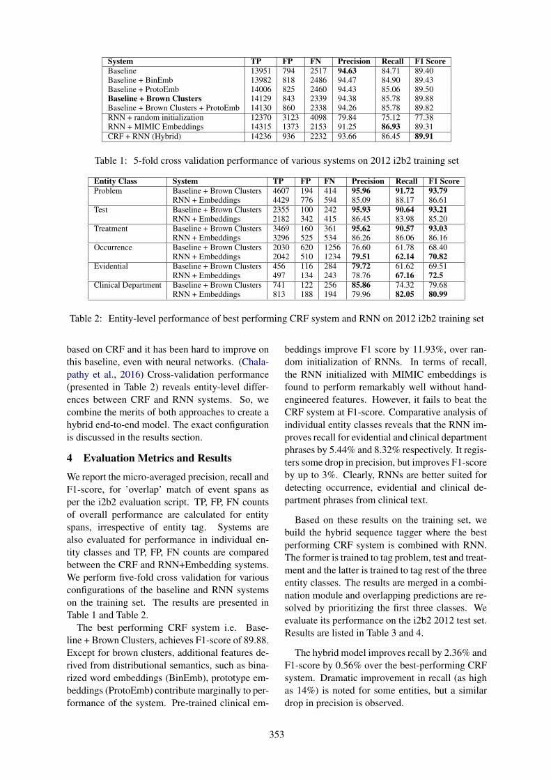
System TP FP FN Precision Recall F1 ScoreBaseline 13951 794 2517 94.63 84.71 89.40Baseline + BinEmb 13982 818 2486 94.47 84.90 89.43Baseline + ProtoEmb 14006 825 2460 94.43 85.06 89.50Baseline + Brown Clusters 14129 843 2339 94.38 85.78 89.88Baseline + Brown Clusters + ProtoEmb 14130 860 2338 94.26 85.78 89.82RNN + random initialization 12370 3123 4098 79.84 75.12 77.38RNN + MIMIC Embeddings 14315 1373 2153 91.25 86.93 89.31CRF + RNN (Hybrid) 14236 936 2232 93.66 86.45 89.91
Table 1: 5-fold cross validation performance of various systems on 2012 i2b2 training set
Entity Class System TP FP FN Precision Recall F1 ScoreProblem Baseline + Brown Clusters 4607 194 414 95.96 91.72 93.79
RNN + Embeddings 4429 776 594 85.09 88.17 86.61Test Baseline + Brown Clusters 2355 100 242 95.93 90.64 93.21
RNN + Embeddings 2182 342 415 86.45 83.98 85.20Treatment Baseline + Brown Clusters 3469 160 361 95.62 90.57 93.03
RNN + Embeddings 3296 525 534 86.26 86.06 86.16Occurrence Baseline + Brown Clusters 2030 620 1256 76.60 61.78 68.40
RNN + Embeddings 2042 510 1234 79.51 62.14 70.82Evidential Baseline + Brown Clusters 456 116 284 79.72 61.62 69.51
RNN + Embeddings 497 134 243 78.76 67.16 72.5Clinical Department Baseline + Brown Clusters 741 122 256 85.86 74.32 79.68
RNN + Embeddings 813 188 194 79.96 82.05 80.99
Table 2: Entity-level performance of best performing CRF system and RNN on 2012 i2b2 training set
based on CRF and it has been hard to improve onthis baseline, even with neural networks. (Chala-pathy et al., 2016) Cross-validation performance(presented in Table 2) reveals entity-level differ-ences between CRF and RNN systems. So, wecombine the merits of both approaches to create ahybrid end-to-end model. The exact configurationis discussed in the results section.
4 Evaluation Metrics and Results
We report the micro-averaged precision, recall andF1-score, for ’overlap’ match of event spans asper the i2b2 evaluation script. TP, FP, FN countsof overall performance are calculated for entityspans, irrespective of entity tag. Systems arealso evaluated for performance in individual en-tity classes and TP, FP, FN counts are comparedbetween the CRF and RNN+Embedding systems.We perform five-fold cross validation for variousconfigurations of the baseline and RNN systemson the training set. The results are presented inTable 1 and Table 2.
The best performing CRF system i.e. Base-line + Brown Clusters, achieves F1-score of 89.88.Except for brown clusters, additional features de-rived from distributional semantics, such as bina-rized word embeddings (BinEmb), prototype em-beddings (ProtoEmb) contribute marginally to per-formance of the system. Pre-trained clinical em-
beddings improve F1 score by 11.93%, over ran-dom initialization of RNNs. In terms of recall,the RNN initialized with MIMIC embeddings isfound to perform remarkably well without hand-engineered features. However, it fails to beat theCRF system at F1-score. Comparative analysis ofindividual entity classes reveals that the RNN im-proves recall for evidential and clinical departmentphrases by 5.44% and 8.32% respectively. It regis-ters some drop in precision, but improves F1-scoreby up to 3%. Clearly, RNNs are better suited fordetecting occurrence, evidential and clinical de-partment phrases from clinical text.
Based on these results on the training set, webuild the hybrid sequence tagger where the bestperforming CRF system is combined with RNN.The former is trained to tag problem, test and treat-ment and the latter is trained to tag rest of the threeentity classes. The results are merged in a combi-nation module and overlapping predictions are re-solved by prioritizing the first three classes. Weevaluate its performance on the i2b2 2012 test set.Results are listed in Table 3 and 4.
The hybrid model improves recall by 2.36% andF1-score by 0.56% over the best-performing CRFsystem. Dramatic improvement in recall (as highas 14%) is noted for some entities, but a similardrop in precision is observed.
353

System TP FP FN Precision Recall F1 ScoreTang et al. (2013) - - - 93.74 86.79 90.13Baseline + Brown Clusters 11664 647 1930 94.74 85.80 90.05Hybrid CRF-RNN 11985 875 1609 93.20 88.16 90.61
Table 3: Performance of best performing CRF and Hybrid CRF-RNN on 2012 i2b2 test set
Entity Class System TP FP FN Precision Recall F1 ScoreOccurrence Baseline + Brown Clusters 1509 489 991 75.53 60.36 67.10
Hybrid 1565 563 935 73.54 62.60 67.63Evidential Baseline + Brown Clusters 370 76 226 82.96 62.08 71.02
Hybrid CRF-RNN 446 177 150 71.59 74.83 73.17Clinical Department Baseline + Brown Clusters 557 109 176 83.63 75.99 79.63
Hybrid CRF-RNN 657 234 76 73.74 89.63 80.91
Table 4: Entity-level performance of best performing CRF and Hybrid CRF-RNN on 2012 i2b2 test set
5 Discussion
The hybrid architecture serves as a concept ex-traction model with a predisposition for higher re-call of clinical events, as compared to the CRFsystem which exhibits better precision in perfor-mance. On comparing errors, we found the %over-lap between false negatives of CRF and RNN sys-tems to be only about 52%. The CRF model is ableto exploit semantic, syntactic and orthographic in-formation among others, while RNNs are only ini-tialized with limited semantic information. Auto-matic learning of syntactic structure and finer se-mantic correlations is inherent to recurrent neuralarchitecture. However, this may be somewhat lim-ited by our small corpus. This situation leads tosubtle disparities in performance of both systems.
The RNN is able to detect clinical departments(which includes physician names, hospitals namesand clinical departments) with good recall value inspite of being trained with only 997 data points.CRF has lowest recall for clinical department,among all classes that contain more noun phrases.The RNN confuses higher percentage of Treat-ment concepts as Occurrence than CRF, mostlythose which are verb phrases like ’excised’, ’intu-bated’ etc. Instead of initializing all words withclinical embeddings, the performance of RNNmay be improved by selectively initializing clin-ical terms only. This can be done by filtering forcertain UMLS semantic groups/types and provid-ing only those words with a pre-trained word vec-tor. On the other hand, word embeddings help theRNN in handling unseen vocabulary effectively.For example, when RNN is trained to tag ’de-creased’ as occurrence, it tags the word ’weaned’correctly as occurrence in the test set. Under sim-
ilar conditions, CRF is unable to make the cor-rect decision. Word vectors derived from a largerbiomedical corpus may enable the RNN to makefiner semantic distinctions.
Unlike RNN, CRF fails to recognize the oc-casional long phrases such as ’normal appear-ing portal veins and hepatic arteries’, even underoverlap matching criteria. We expect the LSTMcells in RNN to capture long-term dependenciesfrom various ranges within a sentence, and ourhypothesis is confirmed by the test results. TheCRF operates within a pre-specified context win-dow and is limited by its linear chain framework.With a skip chain CRF, this situation can be reme-died.
6 Conclusion & Future Work
This paper evaluates various methods for usingneural architecture in clinical entity recognitionand minimizing feature engineering. Benefits areobserved when the merits of structured predic-tion model and RNN are fused into a hybrid ar-chitecture after analysis of their cross-validationperformance. The hybrid model’s recall and F1score surpass that of the state-of-art system wehave used for replication. Through error analysis,we highlight some of the situations where RNNsfare better such as longer concept length, unseenclinical terms, semantically similar generic words,proper nouns etc.
In future work, we will attempt to integratelong-term dependencies within a sentence by im-plementing the skip chain CRF model and explorethe efficient use of word embeddings for struc-tured prediction. This clinical entity recognitionmodel will also be extended to a temporal evalua-tion system.
354

ReferencesRaghavendra Chalapathy, Ehsan Zare Borzeshi, and
Massimo Piccardi. 2016. Bidirectional lstm-crffor clinical concept extraction. arXiv preprintarXiv:1611.08373 .
Jiang Guo, Wanxiang Che, Haifeng Wang, and TingLiu. 2014. Revisiting embedding features for simplesemi-supervised learning. In EMNLP. pages 110–120.
Abhyuday N Jagannatha and Hong Yu. 2016a. Bidi-rectional rnn for medical event detection in elec-tronic health records. In Proceedings of the con-ference. Association for Computational Linguistics.North American Chapter. Meeting. NIH Public Ac-cess, volume 2016, page 473.
Abhyuday N Jagannatha and Hong Yu. 2016b. Struc-tured prediction models for rnn based sequence la-beling in clinical text. In Proceedings of the Con-ference on Empirical Methods in Natural LanguageProcessing. Conference on Empirical Methods inNatural Language Processing. NIH Public Access,volume 2016, page 856.
Prateek Jindal and Dan Roth. 2013. Extraction ofevents and temporal expressions from clinical nar-ratives. Journal of biomedical informatics 46:S13–S19.
Alistair EW Johnson, Tom J Pollard, Lu Shen, Li-wei H Lehman, Mengling Feng, Mohammad Ghas-semi, Benjamin Moody, Peter Szolovits, Leo An-thony Celi, and Roger G Mark. 2016. Mimic-iii,a freely accessible critical care database. Scientificdata 3.
Guillaume Lample, Miguel Ballesteros, Sandeep Sub-ramanian, Kazuya Kawakami, and Chris Dyer. 2016.Neural architectures for named entity recognition.arXiv preprint arXiv:1603.01360 .
Naoaki Okazaki. 2007. Crfsuite: a fast im-plementation of conditional random fields (crfs).http://www.chokkan.org/software/crfsuite/.
Jeffrey Pennington, Richard Socher, and Christopher DManning. 2014. Glove: Global vectors for wordrepresentation. In EMNLP. volume 14, pages 1532–1543.
L Smith, Thomas Rindflesch, W John Wilbur, et al.2004. Medpost: a part-of-speech tagger for biomed-ical text. Bioinformatics 20(14):2320–2321.
Weiyi Sun, Anna Rumshisky, and Ozlem Uzuner. 2013.Evaluating temporal relations in clinical text: 2012i2b2 challenge. Journal of the American MedicalInformatics Association 20(5):806–813.
Buzhou Tang, Yonghui Wu, Min Jiang, Yukun Chen,Joshua C Denny, and Hua Xu. 2013. A hybrid sys-tem for temporal information extraction from clini-cal text. Journal of the American Medical Informat-ics Association 20(5):828–835.
Michael Tepper, Daniel Capurro, Fei Xia, Lucy Van-derwende, and Meliha Yetisgen-Yildiz. 2012. Sta-tistical section segmentation in free-text clinicalrecords. In LREC. pages 2001–2008.
Ozlem Uzuner, Brett R South, Shuying Shen, andScott L DuVall. 2011. 2010 i2b2/va challenge onconcepts, assertions, and relations in clinical text.Journal of the American Medical Informatics Asso-ciation 18(5):552–556.
Yonghui Wu, Jun Xu, Min Jiang, Yaoyun Zhang, andHua Xu. 2015. A study of neural word embed-dings for named entity recognition in clinical text.In AMIA Annual Symposium Proceedings. Ameri-can Medical Informatics Association, volume 2015,page 1326.
Yan Xu, Kai Hong, Junichi Tsujii, I Eric, and ChaoChang. 2012. Feature engineering combined withmachine learning and rule-based methods for struc-tured information extraction from narrative clinicaldischarge summaries. Journal of the American Med-ical Informatics Association 19(5):824–832.
Yan Xu, Yining Wang, Tianren Liu, Junichi Tsujii,I Eric, and Chao Chang. 2013. An end-to-end sys-tem to identify temporal relation in discharge sum-maries: 2012 i2b2 challenge. Journal of the Amer-ican Medical Informatics Association 20(5):849–858.
355

Proceedings of the BioNLP 2017 workshop, pages 356–364,Vancouver, Canada, August 4, 2017. c©2017 Association for Computational Linguistics
Extracting Personal Medical Events for User Timeline Construction usingMinimal Supervision
Aakanksha NaikLanguage Technologies
InstituteCarnegie Mellon [email protected]
Chris BogartInstitute for Software
ResearchCarnegie Mellon [email protected]
Carolyn RoseLanguage Technologies
InstituteCarnegie Mellon [email protected]
Abstract
In this paper, we describe a system for au-tomatic construction of user disease pro-gression timelines from their posts in on-line support groups using minimal super-vision. In recent years, several online sup-port groups have been established whichhas led to a huge increase in the amount ofpatient-authored text available. Creatingsystems which can automatically extractimportant medical events and create dis-ease progression timelines for users fromsuch text can help in patient health mon-itoring as well as studying links betweenmedical events and users’ participation insupport groups. Prior work in this domainhas used manually constructed keywordsets to detect medical events. In this work,our aim is to perform medical event detec-tion using minimal supervision in order todevelop a more general timeline construc-tion system. Our system achieves an accu-racy of 55.17%, which is 92% of the per-formance achieved by a supervised base-line system.
1 Introduction
In recent years, the steady shift towards aconsumer-centric paradigm in healthcare, in con-junction with the meteoric rise of social network-ing, has led to the establishment of several onlinesupport groups and an increasing amount of avail-able patient-authored text. Analyzing this text canprovide us an opportunity to study many impor-tant issues such as how important medical eventsaffect people’s lives and how important changesin their personal lives affect disease progression.We can also study how important medical events
affect users’ participation in these online commu-nities.
To perform such analyses on large-scale data,there is a need to develop automated methods toextract important personal medical events and as-sociate them with dates from user posts in on-line support groups. These extracted events anddates can then be used to construct medical eventtimelines for users and study links between userparticipation or posting behaviors in online sup-port groups and important personal medical events(Wen and Rose (2012)). Such automated methodscan also be used for patient health monitoring. Inthis work, we propose a novel unsupervised ap-proach to personal medical event extraction thatachieves an accuracy of 55.17%, which is 92% ofthe performance of the most similar supervised ap-proach on a cancer support forum corpus.
Prior work in personal medical event extraction(Wen and Rose (2012)) from user posts uses man-ually constructed sets of keywords to detect med-ical events from text. This limits the generality ofsuch systems, since using the system on a new cor-pus requires prior knowledge about types of medi-cal events, and the vocabulary used by users to de-scribe these events. To make them more general,we propose a data-driven personal medical eventextraction pipeline which detects medical eventswith minimal supervision. This makes our sys-tem independent of the corpus on which it is usedand reduces the manual effort required. We testthe performance of our system on the task of con-structing cancer event timelines from the datasetused by Wen and Rose (2012). In spite of being al-most completely unsupervised, our system reaches92% of the performance achieved by a supervisedbaseline system.
The rest of paper is organized as follows. Sec-tion 2 describes prior work in event extraction andtemporal resolution which we leverage, while sec-
356

tion 3 describes our datasets. Section 4 introducesthe architecture of our proposed system and sec-tion 5 talks about the system modules in more de-tail. Section 6 describes our experiments and eval-uation, while section 7 presents a brief error anal-ysis and describes possible future extensions. Sec-tion 8 concludes the paper.
2 Related Work
Event extraction is a well-studied topic in naturallanguage processing. This has resulted in the de-velopment of several off-the-shelf tools for eventextraction (Saurı et al. (2005), Chambers (2013),Derczynski et al. (2016)). All these tools havebeen developed for extraction of public eventsfrom news corpora. Some prior work has alsostudied extraction of public events from social me-dia (Sakaki et al. (2010), Becker et al. (2010), Rit-ter et al. (2012)). However, in this work, we wantto focus on extracting personal medical events forusers from their posts on online support groups us-ing minimal supervision.
There has been some prior work on personalevent extraction from social media, especiallytwitter )Li and Cardie (2014); Li et al. (2014)). Liet al. (2014) developed a system for personal eventextraction from twitter using minimal supervision.They used the presence of congratulations/ con-dolence speech acts to detect personal event men-tions in tweets and clustering based on the LatentDirichlet Algorithm (Blei et al. (2003)) to detectpersonal event types. However, they did not fo-cus specifically on medical events. While we alsowant to build a system for personal event extrac-tion from online support groups, our focus is onidentifying medical events. Hence, the techniquesused by Li et al. (2014) do not work very wellfor us. Online support groups are not as person-focused as twitter, so the presence of congratula-tions/ condolence speech acts is not a strong sig-nal for personal medical event detection. More-over, as we show in section 6, LDA is unable toperform well on personal medical event type de-tection. So, we use a different technique for eventtype detection, which is partly similar to the tech-nique used by Huang et al. (2016). Our overallsystem pipeline for data-driven medical event de-tection with minimal supervision is partly inspiredby Li et al. (2014).
On the other hand, there has not been exten-sive research on personal medical event extraction
from online support groups. Wen and Rose (2012)developed a system for medical event extractionfrom online support groups. Their system usedmanually constructed keyword sets for event ex-traction. We propose a minimally supervised med-ical event detection pipeline which can remove theneed to create these manual keyword sets.
Since we want to create event timelines forusers from their posts in online support groups,we also need to perform temporal expression de-tection and resolution as well as linking of tem-poral expressions to events. Temporal expressionextraction and normalization is also a well-studiedarea and several off-the-shelf systems are avail-able (Strotgen and Gertz (2010), Chang and Man-ning (2012), Derczynski et al. (2016)). More-over, some systems perform both temporal res-olution and linking of events with temporal ex-pressions (Chambers (2013)). However, most ofthese systems are developed for news data and donot work very well with the informal writing styleused on social media. But there have been someefforts to develop systems which work well forthis space. Wen et al. (2013) developed a tempo-ral tagger and resolver for informal temporal refer-ences on social media, but the system is not avail-able for use. The HeidelTime system Strotgenand Gertz (2010) also has a ”colloquial english”setting which works well for temporal resolutionfrom social media data. To link events with tem-poral expressions, we use the heuristics proposedby Wen and Rose (2012).
3 Dataset
We use two datasets in this paper. The firstdataset comprises of all posts from two groupscalled ”Knitters with Breast Cancer” and ”Begin-ners Knit-Along” from Ravelry1, a website forfiber arts enthusiasts. ”Knitters with Breast Can-cer” is one of the largest and most active breastcancer groups on Ravelry. This group was startedin December 2008. As of December 2016, it had426 members and 120,000 posts. ”Beginners Knit-Along” is a group for knitting enthusiasts whohave just started learning how to knit. This groupwas started in 2013. As of December 2016, it had3274 members and 70,000 posts. The data fromthese groups is used to create a list of medicalterms, based on vocabulary difference, which isused in the medical event extraction module. We
1https://www.ravelry.com/
357
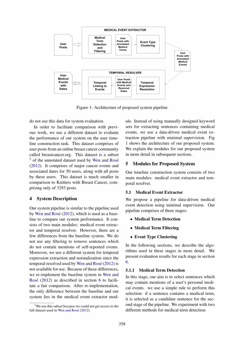
Medical Term
Detection and
Filtering
Event Type Clustering
MEDICAL EVENT EXTRACTOR
TEMPORAL RESOLVER
Temporal Expression Resolution
Temporal Linking to
Events
User Posts
User Posts with Annotated
Medical Terms
User Posts with Annotated
Medical Events
User Posts with Medical Events and Resolved
Dates
User Medical Events
with Dates
Figure 1: Architecture of proposed system pipeline
do not use this data for system evaluation.In order to facilitate comparison with previ-
ous work, we use a different dataset to evaluatethe performance of our system on the user time-line construction task. This dataset comprises ofuser posts from an online breast cancer communitycalled breastcancer.org. This dataset is a subset2 of the annotated dataset used by Wen and Rose(2012). It comprises of major cancer events andassociated dates for 50 users, along with all postsby these users. This dataset is much smaller incomparison to Knitters with Breast Cancer, com-prising only of 3293 posts.
4 System Description
Our system pipeline is similar to the pipeline usedby Wen and Rose (2012), which is used as a base-line to compare our system performance. It con-sists of two main modules: medical event extrac-tor and temporal resolver. However, there are afew differences from the baseline system. We donot use any filtering to remove sentences whichdo not contain mentions of self-reported events.Moreover, we use a different system for temporalexpression extraction and normalization since thetemporal resolved used by Wen and Rose (2012) isnot available for use. Because of these differences,we re-implement the baseline system in Wen andRose (2012) as described in section 6 to facili-tate a fair comparison. After re-implementation,the only difference between the baseline and oursystem lies in the medical event extractor mod-
2We use this subset because we could not get access to thefull dataset used in Wen and Rose (2012)
ule. Instead of using manually designed keywordsets for extracting sentences containing medicalevents, we use a data-driven medical event ex-traction pipeline with minimal supervision. Fig1 shows the architecture of our proposed system.We explain the modules for our proposed systemin more detail in subsequent sections.
5 Modules for Proposed System
Our timeline construction system consists of twomain modules: medical event extractor and tem-poral resolver.
5.1 Medical Event ExtractorWe propose a pipeline for data-driven medicalevent detection using minimal supervision. Ourpipeline comprises of three stages:
• Medical Term Detection
• Medical Term Filtering
• Event Type Clustering
In the following sections, we describe the algo-rithms used in these stages in more detail. Wepresent evaluation results for each stage in section6.
5.1.1 Medical Term DetectionIn this stage, our aim is to select sentences whichmay contain mentions of a user’s personal medi-cal events. we use a simple rule to perform thisselection: if a sentence contains a medical term,it is selected as a candidate sentence for the sec-ond stage of the pipeline. We experiment with twodifferent methods for medical term detection.
358

The first method uses ADEPT MacLean andHeer (2013), a medical term recognizer developedspecifically for patient-authored text, to detect thepresence of medical terms in sentences. All sen-tences containing at least one medical term, as de-tected by ADEPT, are chosen as candidate sen-tences. The second method is based on vocabu-lary difference between an online support groupand a non-illness related group (VOCAB). We cre-ate term vocabularies from two groups on Rav-elry: Knitters with Breast Cancer, a breast cancersupport group and Beginners’ Knit-Along, a nonillness-related group. We then create a list of termswhich occur at least once in Knitters with BreastCancer, but do not appear at all in Beginners’ Knit-Along. All terms in this list are now consideredto be medical terms. Choosing two groups fo-cusing on different interests from the same onlinecommunity to detect medical terms, mitigates theproblem of Ravelry-specific terms (such as Rav-eler, Ravatar etc.) being mistakenly included inthe list. Using this term list, we perform candi-date sentence extraction by choosing all sentenceswhich contain at least one of the terms from thelist.
Candidate sentences chosen by both methodscontain a lot of spurious sentences, since manyspurious terms are marked as medical terms bythese methods. Hence, the next stage in ourpipeline filters these candidate sentence sets.
5.1.2 Medical Term FilteringIn this stage, we filter out spurious terms to im-prove the quality of the candidate sentence set. Wefirst discuss major sources of errors for both medi-cal term detection methods and then discuss somestrategies we use to mitigate these errors. Thesestrategies are used to filter medical terms detectedby both systems, which in turn filters candidatesentences selected by both.
We face one major issue while running theADEPT system on our data. The system managesto correctly identify most important medical termsfrom the text, but it also marks several words usedin non-medical contexts as medical terms. For ex-ample, in the sentence ”I must learn to speak moreslowly than my brain thinks !”, the word ”brain”is marked as a medical term, even though it notbeing used in a medical context. Performing suchfiltering is difficult, but we observe that when usea combination of terms from both methods, someof these errors get mitigated.
k Vocab Size1 281365 658510 283320 1197
Table 1: Massive decrease medical term vocabu-lary size with increasing value of k (the frequencylimit for filtering)
While the vocabulary difference-based methoddoes not fall into such context-based errors, ithas its own drawbacks. Several terms in the listcreated via vocabulary difference are URLs, usernames, email addresses and telephone numbers.We observe that such spurious terms are very in-frequent. Hence, we perform filtering by remov-ing all terms which occur with a frequency lowerthan k in the Knitters with Breast Cancer group,from our medical term list. We experiment withdifferent values of k. Table 1 shows the mas-sive reduction in medical term vocabulary with in-creasing value of k.
For further comparison, we evaluate the perfor-mance of both methods on candidate sentence ex-traction. These experiments and results are dis-cussed further in section 6. Based on these results,we use a combination of both methods to performmedical event detection and filtering in the finalsystem.
5.1.3 Event Type ClusteringIn this stage, we use clustering to perform medi-cal event type detection. We consider all sentencesfrom the filtered set provided by the previous stageto be sentences containing mentions of medicalevents. This is an oversimplification since a sen-tence may contain a medical term which may notcorrespond to a medical event. For example, inthe sentence ”My onc gave me the choice, sayingshe would rather ovrtreat than undertreat”, thereare several medical terms (onc, overtreat, under-treat) but none of them are associated with med-ical events. However, we still perform clusteringon the entire set, since such medical terms whichdo not correspond to medical events form a sepa-rate set of clusters which are later discarded. Af-ter clustering, we manually label each cluster withthe medical event it corresponds to, and use theseclusters as keyword sets to only retain sentencescorresponding to each medical event. These setsof sentences for each medical event correspond to
359

what Wen and Rose (2012) call ”date sentences”and are used to extract the dates associated withthese events.
We experiment with two methods for clustering.The first method uses Latent Dirichlet Allocation(Blei et al. (2003)) to cluster the candidate set ofsentences. The use of this algorithm is motivatedby the observation that people use similar expres-sions to describe the same medical events. How-ever, as further discussed in section 6, we do notget good results using this algorithm.
The second method focuses on clustering med-ical terms instead of candidate sentences. Weuse a two-pass hierarchical clustering algorithmto cluster medical terms based on their Word2Vec(Mikolov et al. (2013)) embeddings. The wordvectors used are pretrained on biomedical arti-cles from Pubmed and PMC as well as EnglishWikipedia, in order to ensure enough domainspecificity 3. We also experiment with k-meansclustering, but use agglomerative clustering for thefinal system due to better performance. In the firstpass of agglomerative clustering, our main focusis on weeding out medical terms which are notlinked to major cancer events. Hence, we run ag-glomerative clustering on all medical terms in thispass and manually inspect the produced clusters,discarding those which do not contain any termscorresponding to major cancer events. Thus, af-ter the first pass, we are left with a list of terms,of which most are associated with major cancerevents. This list of terms is then clustered during asecond pass of agglomerative clustering. The finalclusters produced by this pass are inspected andlabeled with the cancer event that they correspondto. This method of clustering is able to identifybetter clusters, as discussed further in section 6.Hence, we use the keyword sets generated by thismethod for the final system.
5.2 Temporal Resolver
This module detects temporal expressions in ev-ery sentence, resolves those expressions to datesand then associates them with medical events. Ithas two phases: (1) temporal expression detec-tion and resolution and (2) linking temporal ex-pressions with events
3These pretrained word vectors are provided byhttp://bio.nlplab.org/
5.2.1 Temporal Expression Detection andResolution
We use HeidelTime (Strotgen and Gertz (2010)), astate-of-the-art temporal expression extractor andresolver to perform temporal expression detectionand resolution on all candidate sentences extractedby the medical event extraction module. We runthis system with the colloquial English setting,since our data comes from online support groups.Post timestamps are provided as document cre-ation times.
5.2.2 Linking Temporal Expressions withEvents
We use the rules of thumb proposed by Wen andRose (2012) to resolve temporal ambiguities, suchas multiple temporal expressions occurring in asingle sentence, for the baseline system. Whenmultiple temporal expressions occur in the samesentence, the expression nearest to the event wordin the sentence is chosen as the correct one. Whenan event is associated with multiple dates for thesame user, we choose the most frequent date asthe correct one.
6 Experimental Results and Evaluation
In this section, we first present our evaluationof each module for the proposed event detec-tion pipeline. We then describe the performanceachieved by our end-to-end system on the task ofconstructing cancer event timelines for users.
6.1 Evaluation of the Medical TermDetection Module
In this section, we evaluate the performance oftwo techniques (ADEPT-based term detection andvocabulary-based term detection) used in the med-ical term detection module. Since our aim is toreplace the supervised sentence extraction phasein Wen and Rose (2012) with our unsupervisedpipeline while incurring minimal performanceloss, we perform a comparative evaluation of thismodule. We use the sentence set extracted usingmanually defined keyword sets used by Wen andRose (2012) as our gold data. We measure perfor-mance by computing precision and recall of candi-date sentence sets extracted by both medical termdetection methods (ADEPT and VOCAB).Table2 presents the precision, recall and F1 scores forthese methods. We also present the scores for can-didate sentence extraction using our vocabulary-based method before frequency-based filtering to
360

Aug2009
Sep2009
Dec2009
Nov2009
Oct2009
Feb2010
Jan2010
Apr2010
Mar2010
Jun2010
May2010
Jul2010
Aug2010
DiagnosisChemotherapy,
Radiation
Figure 2: Sample cancer event timeline for a user constructed using events and dates extracted by oursystem
highlight the improvement achieved by filtering.As we can see from the table, each method hasits own merits. ADEPT has extremely high preci-sion but very poor recall, whereas our filtered termlist improves significantly on precision while los-ing on recall. Hence, we combine both methodsby only selecting sentences which contain termsmarked as medical terms by both methods. As wecan see from the table, this strategy works best,leading to an increase in precision without hurtingrecall 4. This method is used in the final system.
6.2 Evaluation of the Clustering Module
We evaluate the performance of both methods(LDA and Word2Vec-based agglomerative clus-tering) used in the clustering module manually.We look at the words in each cluster generated byboth clustering methods and label a cluster as cor-responding to a certain cancer event, if most ofthe words in the cluster are associated with thatevent. For example, a cluster containing mostdiagnosis-related words (”diagnose”, ”diagnosis”,”diagnosed” etc.) is labeled as the ”Diagnosis”event. On manual inspection of the clusters de-tected by LDA, we observe that only four impor-tant cancer events (chemotherapy, radiation, mas-tectomy and diagnosis) out of eight major eventsare identified. The main reason behind the poorperformance of this algorithm is that the candi-date sentences being clustered are very short anddo not provide enough contextual information forthe algorithm. However, we cannot perform clus-tering on the entire posts, since a single post maydescribe multiple events. Moreover, most cancerevents co-occur with similar words and this further
4Increase in recall is observed because case-insensitivematching is used to find common terms selected by bothADEPT and VOCAB. This leads to the presence of somewords selected only by one method in the final set. Suchwords however are case-variations of important words andmust not be discarded
hampers LDA performance. On the other hand,a manual inspection of the clusters detected byWord2Vec-based agglomerative clustering detectssix major cancer events (diagnosis, chemotherapy,radiation, reconstruction, metastasis, recurrence)very clearly. It also identifies a seventh eventwhich is a mixture of words related to lumpectomyand mastectomy (it combines both these eventsinto a single event). We present some keyword setsidentified by this clustering algorithm for somecancer events below:
• Chemotherapy: chemotherapy, adjuvant,neoadjuvant, chemo, adriamycin, carbo-platin, Taxol, herceptin, taxol, prednisone,Herceptin
• Mastectomy/ Lumpectomy: hysterectomy,lumpectomies, re-excision, mastectomy,Mastectomy, lumpectomy, mastectomies
As we can see from the above examples, these key-word sets are fairly coherent. 5
6.3 End-to-End System EvaluationTo evaluate our end-to-end system, we test it onthe user timeline construction task. As mentionedin section 3, we use a dataset consisting of all postsby a group of 50 users from breastcancer.org forthis experiment. This dataset also contains dateannotations for major cancer events for each user.However, this dataset is very small and only con-tains a total of 60 gold dates associated with cancerevents, since dates pertaining to all cancer eventsfor each user may not be available from their post-ing histories.
We compare the performance of our systemwith a re-implementation of the system describedby Wen and Rose (2012). We need to re-implement their system because we use different
5It is difficult to peform a quantitative evaluation of thekeyword sets since there is no gold standard
361
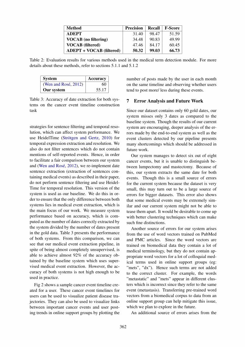
Method Precision Recall F-ScoreADEPT 31.40 98.47 51.59VOCAB (no filtering) 34.48 90.83 49.99VOCAB (filtered) 47.46 84.17 60.45ADEPT + VOCAB (filtered) 50.32 99.03 66.73
Table 2: Evaluation results for various methods used in the medical term detection module. For moredetails about these methods, refer to sections 5.1.1 and 5.1.2
System Accuracy(Wen and Rose, 2012) 60Our system 55.17
Table 3: Accuracy of date extraction for both sys-tems on the cancer event timeline constructiontask
strategies for sentence filtering and temporal reso-lution, which can affect system performance. Weuse HeidelTime (Strotgen and Gertz, 2010) fortemporal expression extraction and resolution. Wealso do not filter sentences which do not containmentions of self-reported events. Hence, in orderto facilitate a fair comparison between our systemand (Wen and Rose, 2012), we re-implement datesentence extraction (extraction of sentences con-taining medical events) as described in their paper,do not perform sentence filtering and use Heidel-Time for temporal resolution. This version of thesystem is used as our baseline. We do this in or-der to ensure that the only difference between bothsystems lies in medical event extraction, which isthe main focus of our work. We measure systemperformance based on accuracy, which is com-puted as the number of dates correctly extracted bythe system divided by the number of dates presentin the gold data. Table 3 presents the performanceof both systems. From this comparison, we cansee that our medical event extraction pipeline, inspite of being almost completely unsupervised, isable to achieve almost 92% of the accuracy ob-tained by the baseline system which uses super-vised medical event extraction. However, the ac-curacy of both systems is not high enough to beused in practice.
Fig 2 shows a sample cancer event timeline cre-ated for a user. These cancer event timelines forusers can be used to visualize patient disease tra-jectories. They can also be used to visualize linksbetween important cancer events and user post-ing trends in online support groups by plotting the
number of posts made by the user in each monthon the same timeline and observing whether userstend to post more/ less during these events.
7 Error Analysis and Future Work
Since our dataset contains only 60 gold dates, oursystem misses only 3 dates as compared to thebaseline system. Though the results of our currentsystem are encouraging, deeper analysis of the er-rors made by the end-to-end system as well as theevent clusters detected by our pipeline presentsmany shortcomings which should be addressed infuture work.
Our system manages to detect six out of eightcancer events, but it is unable to distinguish be-tween lumpectomy and mastectomy. Because ofthis, our system extracts the same date for bothevents. Though this is a small source of errorsfor the current system because the dataset is verysmall, this may turn out to be a large source oferrors for bigger datasets. This error also showsthat some medical events may be extremely sim-ilar and our current system might not be able totease them apart. It would be desirable to come upwith better clustering techniques which can makesuch fine distinctions.
Another source of errors for our system arisesfrom the use of word vectors trained on PubMedand PMC articles. Since the word vectors aretrained on biomedical data they contain a lot ofmedical terminology, but they do not contain ap-propriate word vectors for a lot of colloquial med-ical terms used in online support groups (eg:”mets”, ”dx”). Hence such terms are not addedto the correct cluster. For example, the words”metastatic” and ”mets” appear in different clus-ters which is incorrect since they refer to the sameevent (metastasis). Transferring pre-trained wordvectors from a biomedical corpus to data from anonline support group can help mitigate this issue,which we plan to explore in the future.
An additional source of errors arises from the
362

rules used to link temporal expressions to events.While we have rules which take care of the situa-tion in which multiple temporal expressions mayoccur in the same sentence as the event, we ig-nore scenarios in which multiple event words mayoccur in a sentence with a single temporal expres-sion. The current temporal rules will assign thatexpression to all events, which may be wrong incertain cases. For example, in the sentence ”Hadlumpectomy in November 2000, but because mar-gins were not clear, and another small tumor wasfound in the same breast, surgeon recommendedmodified radical mastectomy”, two cancer events(lumpectomy, mastectomy) are mentioned withonly one temporal expression (November 2000).The temporal expression will be linked to bothevents according to the current resolution rules,whereas it should only be linked to lumpectomy.Moreover, sometimes the sentences may containexactly one cancer event and one temporal expres-sion. However, the temporal expression still doesnot refer to the cancer event. For example, in thesentence ”He died in Oct ’04, right after my bc di-agnosis.”, the date October 2004 does not refer tothe user’s diagnosis event. These issues with tem-poral resolution impact the performances of bothour system and the baseline system. Improvingstrategies for linking events with temporal expres-sions should help in tackling these issues.
8 Conclusion
In this paper, we propose a novel data-drivenpipeline for personal medical event extractionfrom social media using minimal supervision,which is able to achieve 92% of the performanceachieved by a supervised baseline. The extractedmedical events can be used to study and identifylinks between user participation on online supportgroups and important medical events in their lives.While the results of our current system pipelinefor personal medical event extraction are encour-aging, there is a lot of scope for further improve-ment.
Acknowledgments
This research was supported in parts by NSF IIS1546393 and NHLBI R01 HL122639/. We wouldlike to acknowledge Miaomiao Wen and HyejuJang for providing access to the data from Wen andRose (2012) and Khyathi Chandu for her feedbackon earlier drafts of this paper. We would also like
to thank the anonymous reviewers for their con-structive feedback.
ReferencesHila Becker, Mor Naaman, and Luis Gravano. 2010.
Learning similarity metrics for event identificationin social media. In Proceedings of the third ACM in-ternational conference on Web search and data min-ing. ACM, pages 291–300.
David M Blei, Andrew Y Ng, and Michael I Jordan.2003. Latent dirichlet allocation. Journal of ma-chine Learning research 3(Jan):993–1022.
Nathanael Chambers. 2013. Navytime: Event and timeordering from raw text. Technical report, DTICDocument.
Angel X Chang and Christopher D Manning. 2012. Su-time: A library for recognizing and normalizing timeexpressions. In LREC. volume 2012, pages 3735–3740.
Leon Derczynski, Jannik Strotgen, Diana Maynard,Mark A Greenwood, and Manuel Jung. 2016. Gate-time: Extraction of temporal expressions and event.In 10th Language Resources and Evaluation Con-ference. European Language Resources Association(ELRA), pages 3702–3708.
Lifu Huang, T Cassidy, X Feng, H Ji, CR Voss, J Han,and A Sil. 2016. Liberal event extraction and eventschema induction. In Proceedings of the 54th An-nual Meeting of the Association for ComputationalLinguistics: Human Language Technologies (ACL-16).
Jiwei Li and Claire Cardie. 2014. Timeline genera-tion: Tracking individuals on twitter. In Proceed-ings of the 23rd international conference on Worldwide web. ACM, pages 643–652.
Jiwei Li, Alan Ritter, Claire Cardie, and Eduard HHovy. 2014. Major life event extraction from twitterbased on congratulations/condolences speech acts.In EMNLP. pages 1997–2007.
Diana Lynn MacLean and Jeffrey Heer. 2013. Iden-tifying medical terms in patient-authored text:a crowdsourcing-based approach. Journal ofthe American Medical Informatics Association20(6):1120–1127.
Tomas Mikolov, Kai Chen, Greg Corrado, and Jef-frey Dean. 2013. Efficient estimation of wordrepresentations in vector space. arXiv preprintarXiv:1301.3781 .
Alan Ritter, Oren Etzioni, Sam Clark, et al. 2012. Opendomain event extraction from twitter. In Proceed-ings of the 18th ACM SIGKDD international con-ference on Knowledge discovery and data mining.ACM, pages 1104–1112.
363

Takeshi Sakaki, Makoto Okazaki, and Yutaka Matsuo.2010. Earthquake shakes twitter users: real-timeevent detection by social sensors. In Proceedingsof the 19th international conference on World wideweb. ACM, pages 851–860.
Roser Saurı, Robert Knippen, Marc Verhagen, andJames Pustejovsky. 2005. Evita: a robust event rec-ognizer for qa systems. In Proceedings of the con-ference on Human Language Technology and Em-pirical Methods in Natural Language Processing.Association for Computational Linguistics, pages700–707.
Jannik Strotgen and Michael Gertz. 2010. Heideltime:High quality rule-based extraction and normaliza-tion of temporal expressions. In Proceedings ofthe 5th International Workshop on Semantic Eval-uation. Association for Computational Linguistics,pages 321–324.
Miaomiao Wen and Carolyn Penstein Rose. 2012. Un-derstanding participant behavior trajectories in on-line health support groups using automatic extrac-tion methods. In Proceedings of the 17th ACM in-ternational conference on Supporting group work.ACM, pages 179–188.
Miaomiao Wen, Zeyu Zheng, Hyeju Jang, Guang Xi-ang, and Carolyn Penstein Rose. 2013. Extractingevents with informal temporal references in personalhistories in online communities. In ACL (2). pages836–842.
364

Proceedings of the BioNLP 2017 workshop, pages 365–372,Vancouver, Canada, August 4, 2017. c©2017 Association for Computational Linguistics
Detecting mentions of pain and acute confusion in Finnish clinical text
Hans Moen 1,2∗, Kai Hakala1,3∗, Farrokh Mehryary1,3, Laura-Maria Peltonen2,4,Tapio Salakoski1,5, Filip Ginter1, Sanna Salantera2,4
1. Turku NLP Group, Department of Future Technologies, University of Turku, Finland.2. Department of Nursing Science, University of Turku, Finland.
3. The University of Turku Graduate School (UTUGS), University of Turku, Finland.4. Turku University Hospital, Finland.
5. Turku Centre for Computer Science (TUCS), [email protected]
Abstract
We study and compare two different ap-proaches to the task of automatic assign-ment of predefined classes to clinical free-text narratives. In the first approach thisis treated as a traditional mention-levelnamed-entity recognition task, while thesecond approach treats it as a sentence-level multi-label classification task. Per-formance comparison across these twoapproaches is conducted in the form ofsentence-level evaluation and state-of-the-art methods for both approaches are eval-uated. The experiments are done ontwo data sets consisting of Finnish clin-ical text, manually annotated with re-spect to the topics pain and acute confu-sion. Our results suggest that the mention-level named-entity recognition approachoutperforms sentence-level classificationoverall, but the latter approach still man-ages to achieve the best prediction scoreson several annotation classes.
1 Introduction
In relation to patient care in hospitals, cliniciansdocument the administrated care on a regular ba-sis. The documented information is stored as clin-ical notes in electronic health record (EHR) sys-tems. In many countries and hospital districts,a substantial portion of the information that clin-icians document concerning patient status, per-formed interventions, thoughts, uncertainties andplans are written in a narrative manner using (nat-ural) free text. This means that much of the pa-tient information is only found in free-text form,as opposed to structured or coded information (c.f.
∗These authors contributed equally.
standardized terminology, medications and diag-nosis codes).
When it comes to information retrieval, man-agement and secondary use, having the com-puter automatically identify and extract informa-tion from health records related to a given query ortopic is desirable. This could, for example, be in-formation about pain treatment given to a patient,or a patient group. Although free text is easy toproduce by humans and allows for great flexibilityand expressibility, it is challenging to have com-puters automatically classify and extract informa-tion from such text. The use of computers to auto-matically extract, label and structure informationin free text is referred to as information extraction(Meystre et al., 2008), with named-entity recogni-tion as a sub-task (Patawar Maithilee, 2015; Quim-baya et al., 2016). Due to the complexity of freetext, this task is commonly approached using man-ually annotated text as training data for machinelearning algorithms (see e.g. Velupillai and Kvist(2012)).
We present an ongoing work towards automatedannotation of text, i.e. labelling with pre-definedclasses/entity types, by first having the computerlearn from a set of manually annotated clinicalnotes. The annotations concern two topics rele-vant to clinical care: Pain and Acute Confusion.To get a better insight into these topics and howthis is being documented, two separate data setshave been manually annotated, one for each topic.For each of the two topics, a set of classes hasbeen initially identified that reflect the informationwhich the domain experts are interested in. An ex-ample sentence demonstrating the annotations ispresented in Figure 1. The ultimate aim of thisannotation work is to achieve improved documen-tation, assessment, handling and treatment of painand acute confusion in hospitals (Heikkila et al.,2016; Voyer et al., 2008). Now we want to inves-
365

tigate how to best train the computer to automati-cally detect and annotate mentions of these topicsin new, unseen text by exploring various machinelearning methods.
We address this by testing and comparing twodifferent overall approaches:
• Named-entity recognition (NER), where wehave the computer attempt to detect themention-level annotation boundaries.
• Sentence classification (SC), where we havethe computer attempt to label sentences basedon the contained annotations.
The motivation for comparing these two ap-proaches is that: (a) the experts are satisfied withhaving the computer identify and extract informa-tion on sentence level; and (b) we hypothesize thatseveral classes, in particular those reflecting themore complex concepts, are easier for the com-puter to identify when approached as a sentenceclassification task. Further, we are not aware ofany other work where a similar comparison hasbeen reported. The methods and algorithms thatwe explore are based on state-of-the-art machinelearning methods for NER and SC.
2 Data
Pain is something that most patients experienceto various degrees during or related to a hospitalstay. Pain experience is subjective and hence it canbe challenging for clinicians to properly assess if,how and to what extent patients are experiencingpain. Acute confusion is a mental state that pa-tients may enter as a result of serious illness, infec-tions, intense pain, anesthesia, surgery and/or druguse. When clearly evident, this is commonly diag-nosed as acute confusion or delirium (Fearing andInouye, 2009), which is identified as a mental dis-order that affects perception, cognitivity, memory,personality, mood, psychomotricity and the sleep-wake rhythm. However, it can be challenging toclearly identify acute confusion or delirium at thepoint of care, in particular the milder cases. Still,signs and symptoms can often be found in the freetext that clinicians document (Voyer et al., 2008),and the same goes for pain (Gunningberg and Id-vall, 2007).
Our annotated data consists of a random sam-ple of 280 care episodes that were gathered frompatients who had an open heart surgery and who
were admitted to one university hospital in Finlandduring the years 2005-2009. This sample includes1327 days of nursing narratives and 2156 noteswritten by physicians. The same sample was usedas data sets for both topics (i.e. pain and acute con-fusion). An ethical approval and an organizationalpermission from the hospital district was obtainedbefore the data collection.
Separate annotation schemes, reflecting theclasses and guidelines for the annotation work,were iteratively developed based on the literaturefor both topics. For pain the annotation schemehas 15 classes while the acute confusion schemehas 37 classes (see supplementary materials formore details). The annotation schemes were ini-tially tested and refined by having the annotatorsannotate a separate data set of another 100 careepisodes (not included in this study). The annota-tion task was conducted by four persons workingin pairs of two, so that all the text was annotated by(at least) two annotators. This team of annotatorsconsisted of two domain experts and two non do-main experts with an informatics background. Atthe end, the annotators analyzed the made anno-tations with respect to common consensus beforeproducing the final annotated data sets used in thisstudy. The annotations were conducted using thebrat annotation tool (Stenetorp et al., 2012).
The two data sets were individually dividedinto training (60%), development (20%) and test(20%) sets. As preprocessing of the data we to-kenize and enrich the text with linguistic infor-mation in the form of lemmas and part-of-speech(POS) tags for each token. For this we usethe Finnish dependency parser (Haverinen et al.,2014).
For training of word embeddings (word-levelsemantic vectors), we used a large corpus consist-ing of both physician and nursing narratives, ex-tracted from the same university hospital (in Fin-land). In total, this corpus consist of approxi-mately 0.5M nursing narratives and 0.4M physi-cian notes, which amounts to 136M tokens.
3 Experiment and Methods
Below (Section 3.1 and 3.2) we describe the meth-ods, algorithm implementations and hyper param-eters used in the two approaches, i.e., named-entity recognition (NER) and sentence classifica-tion (SC). In the Results section, Section 4, wecompare the scores achieved by these two ap-
366

Figure 1: An artificial English example of the used pain annotations.
proaches for each of the two topics (i.e. pain andacute confusion).
3.1 Named-entity recognition (NER)
In this approach we focus on methods for predict-ing word-level annotation spans. More preciselywe explore two such methods that have shownstate-of-the-art performance in NER.
NERsuite Conditional random fields (CRFs) area class of sequence modeling methods that haveshown state-of-the-art performance in learning toidentify biomedical named entities in text (Cam-pos et al., 2013). We use a named-entity recog-nition toolkit called NERsuite (Cho et al., 2010),which is built on top of CRFsuite (Okazaki, 2007).For each of the two topics, one NERsuite model istrained using the corresponding training sets andthe mentions are labeled using the common IOBtagging scheme. As training features, we use theoriginal tokens, lemmas and POS tags. AlthoughNERsuite allows the user to adjust regularizationand label weight parameters, for this initial studywe have used the default hyperparameters. It isworth noting that adjusting the regularization pa-rameter is not as crucial for CRFs as it is for in-stance for support vector machines and strong re-sults can be achieved even with the default values.
Several of the annotated entities have overlap-ping spans, e.g. the Finnish compound word rin-takipu (chest pain) includes both pain and locationmentions, but the standard CRF implementationsare not able to do multi-label classification. Thuswe form combination classes from the full spansof overlapping entities. This slightly distorts theannotated spans as the original mentions may havehad only partial overlaps. Another option wouldhave been to train separate models for each class,but as the number of classes is relatively high forboth topics, this would have been very impractical.
CNN-BiLSTM-CRF The second method thatwe explore is an end-to-end neural model follow-ing the approach by Ma and Hovy (2016), whichhas produced state-of-the-art results for generaldomain English NER tasks. This model uses aCRF layer for the final predictions, but instead of
relying on handcrafted features it utilizes a bidi-rectional recurrent neural network layer, with along short-term memory (LSTM) (Hochreiter andSchmidhuber, 1997; Gers et al., 2000) chain, overinput word embeddings. In addition to the inputword embeddings, a convolutional layer is usedover character embedding sequences to form an-other encoding for each token. Thus, this modelis often called CNN-BiLSTM-CRF network. Fortraining the model we use the example implemen-tation provided by the authors 1.
Training the CNN-BiLSTM-CRF is computa-tionally much more demanding then a standardCRF classifier and we have thus not ran an exhaus-tive hyperparameter search. Instead, we use thedefault values from the original paper except forsetting the LSTM state dimensionality to 100 andlearning rate to 0.05 as these produced slightly bet-ter results than the default values. The word em-beddings are initialized with a word2vec (Mikolovet al., 2013) model trained on the large clinicalFinnish text corpus.
3.2 Sentence classification (SC)In this approach, we regard the task as a multi-label text classification task in which a sentencecan be associated with multiple labels. For thistask, we rely on artificial neural networks (ANN)since they have been shown to achieve state-of-the-art performance in text classification tasks (seee.g. Zhang et al. (2015); Tang et al. (2015)).
Neural network architecture We tried severalneural network architectures, but report only thearchitecture that performed best. For both of thetwo topics, we apply a deep learning-based neuralnetwork architecture that use three separate LSTMchains: for the sequence of words, lemmas andPOS tags.
The network has three separate channels for thewords, lemmas and POS tags in the sentence. Eachchannel receives a sequence (words, lemmas orPOS tags) as input. The items in the sequence arethen mapped into their corresponding vector rep-resentations using a dedicated embedding look-uplayer. The sequence of vectors is then input to an
1https://github.com/XuezheMax/LasagneNLP
367

LSTM chain and the last step-wise output of thechain is regarded as the representation of the sen-tence based on its words (or lemmas or POS tags).
Next, the outputs of the three channels are con-catenated and the resulting vector is forwardedinto the classification (decision) layer, which has adimensionality equal to the number of annotationclasses. The sigmoid activation function is appliedon the output of the decision layer.
Training and optimization For implementationwe use the Keras deep learning library (Chollet,2015), with Theano tensor manipulation library(Bastien et al., 2012) as the back-end engine. Weuse binary cross-entropy as the objective functionand the Adam optimization algorithm (Kingmaand Ba, 2014) for training the network. We ini-tialize the embeddings for words and lemmas withpre-trained vectors, trained using word2vec on theFinnish clinical corpus. For hyper-parameter op-timization, we do a grid search and evaluate eachmodel on the development set. To detect the bestnumber of epochs needed for training, we usethe early stopping method. Optimization is doneagainst the micro-averaged F-score.
To avoid overfitting, we apply dropout (Srivas-tava et al., 2014) regularization with a rate of 20%on the input gates and with a rate of 1% on therecurrent connections of all LSTM units. In addi-tion, we have set the dimensionality of the word,lemma and POS tag embeddings to 300 and the di-mensionality of the LSTMs’ output are also set to300.
4 Results
We first evaluate the two NER methods on men-tion level using a strict offset matching criteria.The micro-averaged results are presented in Ta-ble 1. The NERsuite model achieves F-scores of73.10 and 48.11 on the test sets of pain and acuteconfusion data set, respectively. Surprisingly theCNN-BiLSTM-CRF model is not able to reach theperformance of the vanilla NERsuite on the paindataset even though it is able to utilize pre-trainedword embeddings. This might be due to the datasets being limited to open heart surgery patientsand thus to a rather narrow vocabulary. Conse-quently we do not train CNN-BiLSTM-CRF onthe confusion data. To analyse the performance ofthe NER approach in relation to the SC approach,we also convert the detected entity mentions tosentence-level predictions. For this the predictions
Approach Precision Recall F-scorePain
NERsuite 87.29 62.88 73.10CNN-BiLSTM-CRF 79.30 63.80 70.71
Acute confusionNERsuite 69.33 36.84 48.11
Table 1: Mention-level evaluation of the testedNER approaches on the test sets of the Pain andAcute confusion corpora. The reported numbersare micro-averaged over the various classes.
from the best performing method, i.e. NERsuite,is used.
Table 2 shows the sentence-level scores for boththe NER and SC approach. The best performingneural network used in the SC approach achievesslightly inferior results compared to the NER ap-proach (when evaluated on sentence level). Thisseems to somewhat falsify our hypothesis aboutsentence-level classification methods potentiallyperforming better than mention-level NER meth-ods when the task is approached as a sentence clas-sification task. Still, in Table 3 we see that the SCapproach achieves best overall prediction scoresfor several of the annotation classes (see also sup-plementary materials). Based on our analysis sofar, it is difficult to say whether these classes (i.e.the concepts they represents) are more “complex”than the others, or if there are some other factorsaffecting the results. In an attempt to achieve bet-ter insight into this, we calculated the average an-notation spans and vocabulary size associated withthe different classes. However, these numbers didnot show any clear trend.
Approach Pain Acute confusionNER 78.61 59.41SC 77.65 57.49
Table 2: Micro-averaged F-scores for the dif-ferent approaches on the test sets of the pain andacute confusion data sets. NERsuite was used toproduce the NER scores.
The actual pain mentions which are divided intoexplicit, implicit and potential pain subcategoriesall achieve relatively high performance, implicitpain being the hardest to predict (see supplemen-tary materials for more details). The other classes,which describe additional information about thepain mentions, are generally speaking harder todetect than the actual pain mentions. The acuteconfusion related entities seems to be much harder
368

Approach Pain Acute confusionNER 8 11SC 7 8Equal performance 0 18
Table 3: Counts showing the number of classesthat the various approaches performed best at pre-dicting.
to predict due to the vague and sparse nature ofthese concepts.
5 Discussion and Future Work
In this study we have gathered the initial resultsfor detecting mentions of pain and acute confu-sion in Finnish clinical text. We also use a re-laxed evaluation based on sentence level predic-tions and experiment with approaches designedspecifically for this definition. Surprisingly theNERsuite based mention-level approach outper-forms all other tested methods, showing strongperformance and being the best suited alternativefor real-world applications. However, it might bethat these two approaches are complementary.
As the used datasets are limited to open heartsurgery patients, a critical future work directionwill be assessing the generalizability of the trainedmodels on larger sets of patient health records, andfrom other hospital units. This study also revealsthat multiple classes in the annotation schemes, inparticular for acute confusion, need more manualannotation data, i.e. more training examples, in or-der to be reliably detected in an automatic manner.
As many of the classes can be considered as de-scriptive attributes of the pain and acute confusionmentions, but the relations have not been anno-tated explicitly, another future work direction is toinvestigate how often these relations are ambigu-ous and whether the relation extraction could besolved in an unsupervised fashion.
Acknowledgments
Funding sources for this research were Academyof Finland and Tekes (Raatali (“Tailor”) project).We would like to thank the annotators, PauliinaAnttila, Timo Viljanen, Satu Poikajarvi and Kris-tiina Heikkila. We would also like to thank JuhoHeimonen for assisting us in preprocessing theclinical text.
ReferencesFrederic Bastien, Pascal Lamblin, Razvan Pascanu,
James Bergstra, Ian Goodfellow, Arnaud Bergeron,Nicolas Bouchard, David Warde-Farley, and YoshuaBengio. 2012. Theano: New features and speed im-provements. arXiv preprint arXiv:1211.5590 (2012).
David Campos, Sergio Matos, and Jose Luıs Oliveira.2013. Gimli: open source and high-performancebiomedical name recognition. BMC Bioinformatics14(1):54.
HC Cho, N Okazaki, M Miwa, and J Tsujii. 2010. Ner-suite: a named entity recognition toolkit. http://nersuite.nlplab.org. Last visited 20thApril 2017.
Franois Chollet. 2015. Keras. https://github.com/fchollet/keras. Last visited 10th March2017.
Michael A Fearing and Sharon K Inouye.2009. Delirium. Focus 7(1):53–63.https://doi.org/10.1176/foc.7.1.foc53.
Felix A Gers, Jurgen Schmidhuber, and Fred Cummins.2000. Learning to forget: Continual prediction withLSTM. Neural Computation 12(10):2451–2471.
Lena Gunningberg and Ewa Idvall. 2007. The qualityof postoperative pain management from the perspec-tives of patients, nurses and patient records. Journalof Nursing Management 15(7):756–766.
Katri Haverinen, Jenna Nyblom, Timo Viljanen,Veronika Laippala, Samuel Kohonen, Anna Mis-sil, Stina Ojala, Tapio Salakoski, and Filip Gin-ter. 2014. Building the essential resources forfinnish: the turku dependency treebank. Lan-guage Resources and Evaluation 48:493–531.https://doi.org/10.1007/s10579-013-9244-1.
Kristiina Heikkila, Laura-Maria Peltonen, and SannaSalantera. 2016. Postoperative pain documentationin a hospital setting: A topical review. ScandinavianJournal of Pain 11:77–89.
Sepp Hochreiter and Jurgen Schmidhuber. 1997.Long short-term memory. Neural Computation9(8):1735–1780.
Diederik P. Kingma and Jimmy Ba. 2014. Adam:A method for stochastic optimization. CoRRabs/1412.6980. http://arxiv.org/abs/1412.6980.
Xuezhe Ma and Eduard Hovy. 2016. End-to-endsequence labeling via bi-directional LSTM-CNNs-CRF. arXiv preprint arXiv:1603.01354 .
Stephane M Meystre, Guergana K Savova, Karin CKipper-Schuler, and John F Hurdle. 2008. Extract-ing information from textual documents in the elec-tronic health record: A review of recent research.Yearbook of Medical Informatics 35:128–44.
369

Tomas Mikolov, Ilya Sutskever, Kai Chen, Greg S. Cor-rado, and Jeff Dean. 2013. Distributed representa-tions of words and phrases and their compositional-ity. In Advances in Neural Information ProcessingSystems 26, pages 3111–3119.
Naoaki Okazaki. 2007. Crfsuite: A fast implemen-tation of Conditional Random Fields (CRFs).http://www.chokkan.org/software/crfsuite/. Last visited 20th April 2017.
Potey M. A. Patawar Maithilee. 2015. Approaches tonamed entity recognition: A survey. InternationalJournal of Innovative Research in Computer andCommunication Engineering 3(12):12201–12208.
Alexandra Pomares Quimbaya, Alejandro SierraMnera, Rafael Andrs Gonzlez Rivera, JulinCamilo Daza Rodrguez, Oscar Mauricio Muoz Ve-landia, Angel Alberto Garcia Pea, and Cyril Labb.2016. Named entity recognition over electronichealth records through a combined dictionary-basedapproach. Procedia Computer Science 100:55 – 61.https://doi.org/http://dx.doi.org/10.1016/j.procs.2016.09.123.
Nitish Srivastava, Geoffrey Hinton, Alex Krizhevsky,Ilya Sutskever, and Ruslan Salakhutdinov.2014. Dropout: A simple way to preventneural networks from overfitting. Journal ofMachine Learning Research 15:1929–1958.http://jmlr.org/papers/v15/srivastava14a.html.
Pontus Stenetorp, Sampo Pyysalo, Goran Topic,Tomoko Ohta, Sophia Ananiadou, and Jun’ichi Tsu-jii. 2012. brat: a Web-based Tool for NLP-AssistedText Annotation. In Proceedings of the Demon-strations at the 13th Conference of the EuropeanChapter of the Association for Computational Lin-guistics. Association for Computational Linguistics,pages 102–107.
Duyu Tang, Bing Qin, and Ting Liu. 2015. Documentmodeling with gated recurrent neural network forsentiment classification. In Proceedings of the 2015Conference on Empirical Methods in Natural Lan-guage Processing. pages 1422–1432.
Sumithra Velupillai and Maria Kvist. 2012. Fine-grained certainty level annotations used for coarser-grained E-Health scenarios. In Alexander Gel-bukh, editor, Computational Linguistics and Intel-ligent Text Processing, Springer Berlin Heidelberg,volume 7182 of Lecture Notes in Computer Science,pages 450–461. https://doi.org/10.1007/978-3-642-28601-8 38.
Philippe Voyer, Martin G Cole, Jane McCusker,Sylvie St-Jacques, and Johanne Laplante. 2008.Accuracy of nurse documentation of deliriumsymptoms in medical charts. InternationalJournal of Nursing Practice 14(2):165–177.https://doi.org/10.1111/j.1440-172X.2008.00681.x.
Xiang Zhang, Junbo Zhao, and Yann LeCun. 2015.Character-level convolutional networks for text clas-sification. In C. Cortes, N. D. Lawrence, D. D. Lee,
M. Sugiyama, and R. Garnett, editors, Advances inNeural Information Processing Systems 28, CurranAssociates, Inc., pages 649–657.
A Supplemental Material
The supplementary material includes specific in-formation about the annotation classes for the painand acute confusion data sets, as well as the de-tailed evaluation of the studied methods.
370

English names Finnish names SC NERA recurrent situation Toistuva tilanne 83.60 86.10Care plan Suunnitelma 83.39 84.24Implicit pain Implisiittinen kipu 74.64 73.68Pain related issue Kipuun liittyva asia 54.69 54.51Location of pain Sijainti 83.36 87.23Pain Kipu 92.04 93.23Pain intensity Voimakkuus 75.29 80.80Pain management Kivunhoito 85.36 86.97Patient education Ohjeistus 33.33 0.00Potential pain Potentiaalinen kipu 93.69 95.58Procedure Toimenpide 64.73 63.90Quality of pain Laatu 59.33 71.07Success of treatment Hoidon onnistuminen 73.74 64.56Situation Tilanne 37.21 28.57Time Aika 79.49 72.41
Micro-average 77.65 78.61
Table 4: Comparison of SC and NER for sentence classification, for pain corpus test set, evaluated onmicro-averaged F1-scores.
English Names Finnish Names SC NERAbnormal level of consciousness Muu poikkeava tajunnan taso 28.57 0.00Aggressiveness Aggressiivisuus vihaisuus 20.00 64.00Appetite disturbance Ruokahalun hairio 57.35 59.02Calming activity Rauhoittelu 0.00 0.00Confusion Sekavuus 85.95 95.00Delirium Delirium 0.00 0.00Delusion Harhaisuus 34.29 27.59Dementia Dementia 0.00 0.00Desorientation Desorientaatio 66.67 89.86Diagnosed Diagnosoitu 0.00 0.00Disturbance in ability to focus Vaikea kiinnittaa huomiota 15.39 0.00Disturbance in the quality of speech Puheen laadun hairiot 40.00 29.41Drowsy Unelias 77.98 79.44Falls - fall out of bed Kaatuminen Sangysta tippuminen 0.00 0.00Hyper-alert Ylivalpas 0.00 0.00Hyperactivity Hyperaktiivisuus 68.71 70.23Hypoactivity Hypoaktiivisuus 26.67 22.22Infusion line detachment Letkun irtoaminen 20.00 20.00Memory disorder Muistiongelma 73.24 80.00Not awakable Ei herateltavissa 0.00 0.00Orientation to time and place Orientoiminen aikaan paikkaan 0.00 0.00Other abnormal behavior Muu poikkeava kayttaytyminen 0.00 0.00Other affective disturbance Muu tunnehairio 64.52 42.25Other care activity Muu hoitotoimenpide 0.00 0.00Other cognitive disturbance Muu kognitiivinen hairio 0.00 0.00Other disturbance of attention Muu tarkkaavaisuuden hairio 0.00 0.00Other incident Muu haittatapahtuma 0.00 0.00Other symptom Muu oire 0.00 0.00Pain management Kivunhoito 51.52 61.33Problems with motor functions Motoriikan ongelmat 59.56 59.79restraint - restraining Lepositeet sitominen 75.00 76.19Sleep-wake disorder Unirytmin valverytmin hairiot 54.32 48.65Slow rate of speech - Speechlessness Hidastunut puhe puhumattomuus 0.00 0.00Substance induced delirium Substance induced delirium 0.00 0.00Unappropriate behaviour Asiaankulumaton kayttaytyminen 9.52 10.26Uncertain Epavarma 0.00 0.00Unorganised thinking Ajatuksenkulun jarjestaytymattomyys 25.81 21.43
Micro-average 57.49 59.41
Table 5: Comparison of SC and NER for sentence classification, for acute confusion corpus test set,evaluated on micro-averaged F1-scores.
371

English Names Finnish Names Train Devel Test TotalA recurrent situation Toistuva tilanne 589 215 210 1014Care plan Suunnitelma 517 176 170 863Implicit pain Implisiittinen kipu 552 160 201 913Pain related issue Kipuun liittyva asia 1058 377 372 1807Location of pain Sijainti 1001 326 333 1660Pain Kipu 1655 536 549 2740Pain intensity Voimakkuus 1094 291 341 1726Pain management Kivunhoito 1158 368 419 1945Patient education Ohjeistus 11 3 4 18Potential pain Potentiaalinen kipu 752 222 255 1229Procedure Toimenpide 1423 478 468 2369Quality of pain Laatu 323 100 125 548Success of treatment Hoidon onnistuminen 226 75 102 403Situation Tilanne 286 85 82 453Time Aika 1257 386 426 2069
Overall 11902 3798 4057 19757Tokens 437935 147444 153975 739354Sentences 71390 23470 25123 119983Documents 2084 697 702 3483
Table 6: Pain annotation counts per class.
English Names Finnish Names Train Devel Test TotalAbnormal level of consciousness Muu poikkeava tajunnan taso 11 9 6 26Aggressiveness Aggressiivisuus vihaisuus 24 5 16 45Appetite disturbance Ruokahalun hairio 229 84 76 389Calming activity Rauhoittelu 6 4 6 16Confusion Sekavuus 131 45 60 236Delirium Delirium 4 1 1 6Delusion Harhaisuus 37 16 25 78Dementia Dementia 3 2 1 6Desorientation Desorientaatio 77 25 38 140Diagnosed Diagnosoitu 1 0 0 1Disturbance in ability to focus Vaikea kiinnittaa huomiota 29 8 12 49Disturbance in the quality of speech Puheen laadun hairiot 43 10 25 78Drowsy Unelias 275 88 115 478Falls - fall out of bed Kaatuminen Sangysta tippuminen 6 0 3 9Hyper-alert Ylivalpas 3 1 1 5Hyperactivity Hyperaktiivisuus 232 66 78 376Hypoactivity Hypoaktiivisuus 103 35 44 182Infusion line detachment Letkun irtoaminen 15 4 9 28Memory disorder Muistiongelma 92 40 41 173Not awakable Ei herateltavissa 15 7 6 28Orientation to time and place Orientoiminen aikaan paikkaan 6 0 0 6Other abnormal behavior Muu poikkeava kayttaytyminen 6 2 4 12Other affective disturbance Muu tunnehairio 109 52 52 213Other care activity Muu hoitotoimenpide 12 9 7 28Other cognitive disturbance Muu kognitiivinen hairio 23 4 5 32Other disturbance of attention Muu tarkkaavaisuuden hairio 10 1 3 14Other incident Muu haittatapahtuma 10 3 5 18Other symptom Muu oire 25 5 8 38Pain management Kivunhoito 118 39 40 197Problems with motor functions Motoriikan ongelmat 329 93 117 539restraint - restraining Lepositeet sitominen 25 8 13 46Sleep-wake disorder Unirytmin valverytmin hairiot 147 56 48 251Slow rate of speech - Speechlessness Hidastunut puhe puhumattomuus 25 11 11 47Substance induced delirium Substance induced delirium 1 0 0 1Unappropriate behaviour Asiaankulumaton kayttaytyminen 81 22 33 136Uncertain Epavarma 1 0 0 1Unorganised thinking Ajatuksenkulun jarjestaytymattomyys 62 17 24 103
Overall 2326 772 933 4031Tokens 434542 149387 155425 739354Sentences 71146 23797 25040 119983Documents 2080 698 705 3483
Table 7: Acute confusion annotation counts per class.
372

Proceedings of the BioNLP 2017 workshop, pages 373–380,Vancouver, Canada, August 4, 2017. c©2017 Association for Computational Linguistics
A Multi-strategy Query Processing Approach for Biomedical QuestionAnswering: USTB PRIR at BioASQ 2017 Task 5B
Zan-Xia Jin, Bo-Wen Zhang*, Fan Fang, Le-Le Zhang and Xu-Cheng Yin*Pattern Recognition and Information Retrieval lab (PRIR)
Department of Computer Scicene, University of Science and Technology [email protected], [email protected]
Abstract
This paper describes the participation ofUSTB PRIR team in the 2017 BioASQ5B on question answering, including doc-ument retrieval, snippet retrieval and con-cept retrieval task. We introduce differ-ent multimodal query processing strate-gies to enrich query terms and assign d-ifferent weights to them. Specifically, se-quential dependence model (SDM), pseu-do relevance feedback (PRF), fielded se-quential dependence model (FSDM) andDivergence from Randomness model (D-FRM) are respectively performed on dif-ferent fields of PubMed articles, sentencesextracted from relevant articles, the fiveterminologies or ontologies (MeSH, GO,Jochem, Uniprot and DO) to achieve bettersearch performances. Preliminary result-s show that our systems outperform othersin the document and snippet retrieval taskin the first two batches.
1 Introduction
Due to the continuous growth of information pro-duced in the biomedical domain, there is a particu-larly growing demand for biomedical QA from thegeneral public, medical students, health care pro-fessionals and biomedical researchers (Zweigen-baum, 2003). They consult knowledge about thenatures, the preventions or the treatments of dis-eases, or learn from research results of other re-searchers. To some extent, biomedical QA is oneof the most significant applications of the exist-ing real-world biomedical systems (Han and A-thenikos, 2010).
Since 2013, BioASQ organizers has proposed acommunity-based shared task which aims to eval-uate the current solutions of a variety of QA sub-
tasks. Several benchmarks have been provided forresearchers to evaluate their QA systems. BioASQ2017 Task 5B challenge (Tsatsaronis et al., 2015a)is the fifth edition of the question answering task,of which the phase A requires the evaluated sys-tem to (i) semantically annotate the questions withconcepts from a set of designated terminologiesand ontologies (MeSH, GO, Jochem, Uniprot andDO); and (ii) retrieve relevant articles, text s-nippets, and RDF triples from designated articlerepositories and ontologies (PubMed/MEDLINEarticles) with biomedical questions in natural lan-guage provided by biomedical professionals or re-searchers. The ground truth are manually anno-tated by these experts with some annotated tools.There are five batches of evaluation and in eachbatch participants are provided with 100 naturallanguage questions and required to return at most10 relevant documents, snippets, concepts to thequestions within 24 hours.
Over the past decade, a variety of approacheshave been proposed for biomedical question an-swering (Bauer and Berleant, 2012). Generally,a QA system typically consists of question pro-cessing, document processing, and answer pro-cessing phases, which are respectively in chargeof 1) converting natural language questions intoqueries, 2) searching relevant documents, and 3)extracting, ranking candidate answers and format-ting them into expected answer type. (Han andAthenikos, 2010; Holzinger et al., 2014). Thereare several studies concerning the improvementson query processing phase (Huang et al., 2006; Yuet al., 2005; Kobayashi and Shyu, 2006) and doc-ument processing phase (Cairns et al., 2011; Yuand Cao, 2008). However for answer processingphase, especially answer matching and ranking,only some simple approaches in previous BioASQchallenge have been proposed (Tsatsaronis et al.,2015a; Mao and Lu, 2015). According to the
373

above researches, the most challenges of biomed-ical QA are three main issues, specifically 1) howto generate query terms appropriately from natu-ral language questions, 2) how to match relevantdocuments or sentences when they use differen-t expressions (maybe synonyms of keywords) and3) how to measure and utilize the difference in im-portance of query terms.
In order to address these challenges, in this pa-per we propose a multi-strategy query processingapproach which combines several mature queryprocessing models according to the different char-acteristics of data sources, which is also actuallythe participation of our USTB PRIR team in theBioASQ Task 5B phase A challenge1. Specif-ically, in order to extract proper keywords andgenerate queries, we perform stop-words removal,noun extraction with Pos-of-Tagger (POS) andstemming. For the missing issue caused by ex-pressions, we utilize a thesaurus which is pro-duced through computing the similarities betweenthe vector representations of each pairs of word-s. Moreover for query keyword weighting, wetake the word sequences, different fields of appear-ance, TF-IDF, etc into consideration for differen-t BioASQ tasks. We evaluate our approach onthe BioASQ 2016 and 2017 benchmarks for docu-ment, snippet, concept retrieval and experimentalresults demonstrate our method outperforms thebaseline methods or other participants so far ondocument, snippet and concept retrieval tasks.
2 Related Work
The participants of previous BioASQ challengehave proposed several approaches for searchingrelevant documents, snippets and concepts forbiomedical QA. One of the participants(Choi,2015) proposed to utilize semantic concept en-riched dependence model where the recognisedUMLS concepts in the query are used as additionaldependence features for ranking documents. An-other team(Papanikolaou et al., 2014) developeda figure-inspired text retrieval method as a wayof retrieving documents and text passages frombiomedical publications. For matching relevant s-nippets, most participants works on similar meth-ods of searching articles. An exception is theframework proposed by NCBI(Mao et al., 2014),which directly compute the cosine similarities be-tween the questions and the sentences.
1http://bioasq.org
However, these methods focus on the match-ing function or the ranking process, which ignoresthe three challenges mentioned in the Introduc-tion section. The natural language questions aretoo raw to be regarded as query keywords and thedifference in importance of keywords should beconsidered. Some re-ranking or learning-to-rankbased approaches works not well either for thesame reason because they rely much on the initialranking results.
3 Task 5B Phase A: Document Retrieval
3.1 The Framework Architecture
The framework of searching relevant documents isshown in Figure 1, which includes document pre-processing, query pre-processing, several rank-ing models based on query expansion and termweighting strategies.
3.2 Pre-Processing
3.2.1 Document Pre-processingWe download the entire database of MEDLINEupdated in Feb 2017 through the FTP service ofNational Institutes of Health (NIH) which con-tains 26,759,010 citations. These documents arerepresented in JSON files which contains a vari-ety of information, including journal information,contents of title, author, abstract and keywords,similar articles and comments. We analyze theresources and select the following fields to rep-resent the documents: ArticleTitle, AbstractText,Title, MedlineTA, NameOfSubstance, Descriptor-Name, QualifierName, Keyword and ISOAbbrevi-ation. These fields are extracted from the docu-ment resources and indexed with Galago, an opensource search engine2, which is developed as animproved JAVA version of Indri. We also performstemming and stop-words removal work like otherIR applications, however unfortunately, the perfor-mances seems worse during the training process.As a result, we decide not to utilize these strate-gies for document pre-processing.
3.2.2 Query Pre-ProcessingAs is mentioned above, one of the challenges ishow to automatically generate the query termsfrom a natural language question. During querypre-processing, we carry out a series of work toextract the keywords of the user queries. There
2http://www.lemurproject.org/galago.php
374

Figure 1: The whole framework architecture of query generation method based on multimodal documentretrieval strategies
are several symbols which is unnecessary and un-related to the requests so we filter out the symbol-s in the first step. Note that the symbols whichmay be a part of named entity cannot be removed.Afterwards, stop words like “what” or “are” arecommon in natural language questions and are notsuitable to feed into search engine so they are re-moved according to a stop-words list. As usual,the query terms are case-folded and normalized. Inaddition, we used the Stanford-Postagger packageto identify nouns from queries and the MetaMap toidentify the biomedical concepts in query terms.
3.3 Ranking Models
3.3.1 Sequential Dependence ModelThe traditional IR techniques in biomedical do-main rely on a unigram Bag of Words (BoW) re-trieval model. Each document in the collection ofcandidates, as well as each query, is representedby a set of words and the corresponding frequen-cy based on the assumption that the appearance ofeach pair of words are independent. Different se-quence of queries is regarded as the same. Con-sider an example of two documents that containall query keywords. It is obvious that the doc-ument with the right sequence of terms appear-ing in query is more likely to meet the demand.Therefore, we introduce the Sequence Dependen-cy Model (SDM) (Bonnefoy et al., 2012) to takethe sequence information into account when com-puting the relevance between a document and aquery.
SDM is a special case of the Markov RandomField (MRF) (Metzler and Croft, 2005). In orderto capture the information of a sentence, this mod-el extracts the phrases in different ways, and givescorresponding weights to different types of phras-es to indicate their importance.
There are three features in the SDM to be con-sidered: single-word features (a collection consist-s of single-word, QT ), ordered bi-words phrasefeatures (the two words in a phrase appearing inorder,QO) and unordered window features (one orseveral words can be allowed appearing betweenthe two words, QU ). Generally, the potential func-tion for unigrams (single-word feature) looks asfollows:
fT (qi, D) = logP (qi|θD) = logtfqi,D + µ
cfqi|C|
|D|+ µ(1)
where qi is a query term, D is a document,tfqi,D is the frequency of qi in D, |D| is the doc-ument length, µ is a Dirichlet prior, that is usuallyset to the average document length in the collec-tion, cfqi is the collection frequency of qi and |C|is the total number of terms in the collection. Sim-ilarly, for ordered and unordered bi-grams, the po-tential functions are respectively as follows:
fO(qi, qi+1, D) = logP (#1(qi, qi+1)|θD)
= logtf#1(qi,qi+1) + µ
cf#1(qi,qi+1)
|C||D|+ µ
(2)
fU (qi, qi+1, D) = logP (#uwN(qi, qi+1)|θD)
= logtf#uwN(qi,qi+1) + µ
cf#1(qi,qi+1)
|C||D|+ µ
(3)
where #1(qi, qi+1) and #uwN(qi, qi+1) are re-spectively the appearances of the exact phraseqiqi+1 and the term qi, qi+1] within a window Nterms. Hence, the scoring function of a documen-t in SDM is the combination of the above threefunctions, shown as follows:
375

scoreSDM = scoreSDM(QT , QO, QU , D)
= λT
|Q|∑i=1
fT (qi, D)
+ λO
|Q|−1∑i=1
fO(qi, qi+1, D)
+ λU
|Q|−1∑i=1
fU (qi, qi+1, D)
(4)
Where Q is a sequence of keywords extractedfrom a user query, D is a candidate document,qi is the i-th query keyword of Q. fT ,fO,fU arethe maximum likelihood estimations of the corre-sponding feature terms in documentD. λT ,λO,λUare the features weights satisfy these conditions:
(1)0 ≤ λT , λO, λU ≤ 1 and λT + λO + λU = 1
(2)λT ≥ 0.6
(3)λO = 2λU
Often, λT = 0.85,λO = 0.1, λU = 0.05.
3.3.2 Fielded Sequential Dependence Model
As is mentioned, the candidate documents arestructured into several fields which contains dif-ferent types of information. One of the limitationsof standard SDM for structured document retrievalis that it considers term matches in different part-s of a document as equally important (i.e. havingthe same contribution to the final relevance scoreof a document), thus disregarding the documentstructure.
To adapt the MRF framework to multi-fieldedentity descriptions, we introduce (Zhiltsov et al.,2015)’s approach from their FSDM model to re-place a single document language model P (qi|θD)with a mixture of language models (MLM) foreach document field. Consequently, the potentialfunction for unigrams in case of FSDM is:
fT (qi, D) = log∑
j
wjP (qi|θj) (5)
where j represents the different fields, and theP (qi|θj) is the language model in each individualfield. Similarly, we can compute fO(qi, qi+1, D)and fO(qi, qi+1, D). Therefore, the scoring func-tion of FSDM is as follows:
scoreFSDM = scoreFSDM(QT , QO, QU , D)
= λT
|Q|∑i=1
fT (qi, D)
+ λO
|Q|−1∑i=1
fO(qi, qi+1, D)
+ λU
|Q|−1∑i=1
fU (qi, qi+1, D)
(6)
3.3.3 Pseudo Relevance Feedback
With the first-pass retrieval results, we assume thatthe initially retrieved top-K documents are rele-vant to questions, and their title and mesh fieldscontain relevant terms to the original query (Zhanget al., 2015a). Thus, for document retrieval, weuse the Pseudo Relevance Feedback (PRF) to en-rich query terms from the top-K document initiallyretrieved. The titles or mesh headings of the top-Kdocuments are extracted and then added to the o-riginal query term set. However, the performanceof PRF can be affected by the quality of the initialresult, the number of pseudo-relevant documents(top K), the number of expansion terms, and theterm re-weighting method applied. In our exper-iments, we use K = 3 and extract all the wordsin title or mesh headings as the expansion terms,which results in the best performance.
3.3.4 Multimodal Strategies Combination
Since there are several strategies to enrich queryterms and optimize their weights, the final scor-ing function is expected to make full use of thesestrategies and combine these strategies effective-ly. We take the importance of nouns, sequenceorders and crucial fields into consideration so ourweight optimization of query terms is based onto noun extraction, sequential dependence mod-el (SDM), Fielded sequential dependence model(FSDM), and Pseudo Relevance Feedback (PRF).According to massive experiments we find outthat for some questions, the original queries, nounqueries and enriched queries with PRF from rel-evant articles are all useful to some degree. Fur-thermore, we also find out that it is necessary toboth search in the full text of the document, and toassign different weights to different fields at mean-while. Hence, the final scoring function to searchrelevant documents is shown as follows:
376

Table 2: MAP performances compared withBioASQ Task 5B document retrieval participants.
System Batch 1 Batch 2sdm + NN + fsdm 0.1049 0.0850
sdm + NN + fsdm + PRF (mesh) 0.1086 0.0863sdm + fsdm + PRF (mesh) 0.1032 0.0859
sdm + w2v 0.0928 0.0874sdm 0.0952 0.0866
best of fdu 0.1072 0.0834best of UNCC 0.1080 -best of Olelo 0.0465 0.0318
best of KNU-SG 0.0413 0.0419best of HPI 0.0307 0.0329
best of Others 0.0437 0.0265
score(Q,D) = λ1scoreSDM(Q,D) + λ2scoreFSDM(Q′, D)
+ λ3scoreSDM(Q′′, D)(7)
where Q is the original query term set after querypre-processing, Q′ represents the noun query termset with noun extraction and the Q′′ stands for theenriched query term set with PRF.
3.4 Experments
We evaluate our proposed method by using boththe benchmark datasets from the previous BioASQchallenges and the current challenge. The opti-mization of all parameters, including the weight-ing paramters like wj in FSDM function andhyper-parameters (e.g. λT , λO, λU , λ1, λ2, λ3) areprocessed through tuning with the rules on train-ing set (when evaluated on BioASQ Task 4B, thetraining set includes 800 questions from BioASQ2B and 3B; for BioASQ Task 5B, the training setcontains 500 more questions on BioASQ 4B). Ta-ble 1 provides the results of our experiments inBioASQ task 4B, and Table 2 provides the result-s of our experiments in BioASQ Task 5B. Thesdm + w2v approach refers to our previous ap-proach in (Zhang et al., 2015b). Obviously, ourproposed method shows greater performance com-pared with baseline, SDM and FSDM and outper-form than other participants in current challenge.
4 Task 5B Phase A: Snippet Retrieval
4.1 The Framework Architecture
The framework of searching relevant snippets isshown in Figure 2, which includes pre-processing,some additional ranking models which is differentfrom document retrieval.
4.2 Pre-ProcessingThe query pre-processing for snippets retrievalis the same to the strategies for document re-trieval, which includes unnecessary symbol re-moval, stop-words removal, case-folding, nounextraction and concept extraction with Metamap.
For the snippet pre-processing, we choose thecandidate snippets from the top-K documents ofthe best performed document retrieval approachon the basis of results of document retrieval. Thesentences with the field ArticleTitle and the fieldabstract of these articles are separated throughsome specific rules, which can be regarded as “s-mall documents”. These sentences make up a pileof new files with unstructured text. They are thenindexed by Galago for search in the next step.
4.3 Ranking ModelsDifferent from document retrieval, the candidate s-nippets are represented in unstructured text, whichmakes some ranking models more difficult to uti-lize (e.g. FSDM). Moreover, since they are muchshorter in length, they are more likely expresssimilar meaning with different expressions (e.g.synonyms) which may emphasize the importanceof the issue of recognizing these relevant results.Furthermore, the PRF method generally providesmassive expansion query terms, which may affectthe search performance of the short text so we giveup applying PRF as query expansion method.
In addition, we introduce DFRM from (Clin-chant and Gaussier, 2011) as an additional termweigting model to optimize the most appropriateweight for query terms.
4.3.1 Divergence from Randomness ModelThe Divergence from Randomness models (D-FRM) are based on this simple idea: “Themore the divergence of the within-document term-frequency from its frequency within the collec-tion, the more the information carried by the wordt in the document d”. In other words the term-weight is inversely related to the probability ofterm-frequency within the document d obtained bya model M of randomness:
weight(t|d) ∝ − log ProbM (t ∈ d|Collection) (8)
where the subscriptM stands for the type of mod-el of randomness employed to compute the proba-bility. In order to choose the appropriate modelMof randomness, we can use different urn models.
377

Table 1: MAP performances of system components on BioASQ Task 4B document retrieval.Batch 1 Batch 2 Batch 3 Batch 4 Batch 5
baseline 0.2056 0.2593 0.228 0.2324 0.2516sdm 0.2214 0.2577 0.2436 0.2517 0.2935fsdm 0.2156 0.2621 0.2228 0.2469 0.2728
sdm + fsdm 0.2269 0.2768 0.2447 0.2608 0.2968sdm + NN + fsdm 0.2307 0.2741 0.2454 0.2632 0.2926
sdm + fsdm + PRF(title) 0.2337 0.2778 0.2455 0.265 0.2931sdm + fsdm + PRF(mesh) 0.2372 0.2863 0.2564 0.2762 0.3019
sdm + NN + fsdm + PRF(mesh) 0.2436 0.2859 0.2465 0.2773 0.3083sdm + NN + fsdm + PRF(title) 0.2377 0.2767 0.2429 0.2681 0.2985
sdm + NN + fsdm + mesh + PRF(mesh) 0.2440 0.2876 0.2505 0.2821 0.3059
Figure 2: The whole framework architecture of query generation method based on multimodal snippetretrieval strategies
Table 3: Basic DFR Models.D Divergence approximation of the binomialP Approximation of the binomialBE Bose-Einstein distributionG Geometric approximation of the Bose-Einstein
I(N) Inverse Document Frequency modelI(F ) Inverse Term Frequency modelI(ne) Inverse Expected Document Frequency model
There are many ways to choose M , each of theseprovides a basic DFR model. The basic modelsare derived in Table 4.
If the model M is the binomial distribution,then the basic model is P and the value can becomputed approximately as follows:
− log ProbP (t ∈ d|Collection) = − log(TFtf
)ptfqTF−tf
(9)
where TF is the term-frequency of the term t inthe collection, tf is the term-frequency of the ter-m t in the document d, N is the number of docu-ments in the collection, and p is 1
N and q = 1− p.
4.3.2 Multimodal Strategies CombinationSimilar to document retrieval, the final scoringfunction of snippet retrieval is expected to com-bine these strategies together effectively. Due tothe reason of shorter text length the FSDM modelcannot be used and the default IR language modelperforms not so satisfying for returning relevant s-nippets, we construct the merging scoring functionto optimize the query term weights according to
the Term Frequency−Inverse Document Frequen-cy (TF-IDF), sequential dependence model (SD-M) and Divergence from Randomness model (D-FRM). As mentioned above, we control the lengthof queries to guarantee the performance, thus weno longer use PRF for snippets retrieval whenmerging the strategies. As the length of the queriesdecreases, the divergence of importance of eachword becomes larger, so it is necessary to assignthe weights of query terms according to the differ-ent importance. So we apply the DFRM methodor the TF-IDF method along with SDM to achievethe results, which are respectively shown as fol-lows:
score(Q,D) =(1− λ1 − λ2)scoreSDM(Q,D)
+ λ1scoreTF-IDF(Q,D)
+ λ2scoreDFRM(Q,D)
(10)
where the terms are weighted according tocorresponding strategies through the followingweighting function:
scoreTF-IDF/DFRM(Q,D) =∑
t
scoreTF-IDF/DFRM(t,D) (11)
where t is the query term appearing in query Q.It is worth noting that when conducting the exper-iments we only consider λ1 = 0 or λ2 = 0 fortuning parameters.
378

Table 4: MAP performances of system compo-nents on BioASQ Task 4B snippet retrieval.
Batch 1 Batch 2 Batch 3baseline 0.1003 0.1361 0.1275
sdm 0.1047 0.1368 0.1338sdm + PRF 0.1044 0.1370 0.1327sdm + NN 0.1023 0.1402 0.1347
sdm + NN + PRF 0.1030 0.1357 0.1307sdm + DFRM 0.1193 0.1520 0.1469sdm + TF-IDF 0.1087 0.1424 0.1357
Table 5: MAP performances compared withBioASQ Task 5B snippet retrieval participants.
System Batch 1 Batch 2sdm + NN 0.0458 0.0811
sdm + NN + PRF(mesh) 0.0439 0.0716sdm + DFRM 0.0467 0.0898sdm + TF-IDF 0.0463 0.0874
sdm 0.0452 0.0736best of fdu - 0.0621
best of UNCC - -best of Olelo 0.0260 0.0318
best of KNU-SG 0.0181 0.0362best of HPI 0.0323 0.0335
best of Others 0.0249 0.0262
4.4 Experments
Similar to document retrieval, we evaluate themethod on the first 3 batches from the previ-ous BioASQ challenge and the current challenge.Similar to document retrieval, the optimization ofall parameters are processed through tuning withthe rules on training set. Table 4 provides the re-sults of our experiments in BioASQ task 4B, andTable 5 provides the results of our experiments inBioASQ Task 5B. Obviously, our proposed merg-ing strategy shows greater performance comparedwith various components and achieve better result-s than other particatants.
5 Task 5B Phase A: Concept Retrieval
Unlike the previous two tasks, the concept re-trieval task is more like a named entity recogni-tion task than an IR task. For each natural lan-guage question, participants are required to re-turn relevant concepts from five ontologies or ter-minologies: MeSH, GO, Jochem, Uniprot andDO. In other words, the task aims at recognizingrelevant biomedical concept within the questionand matching them with the concepts in the datasources.
Since we have few experience in named enti-ty recognition, we have to regard the task as anIR problem and design three query processing ap-
Table 6: MAP performances of system compo-nents on BioASQ Task 4B concept retrieval.
Batch 1 Batch 2 Batch 3 Batch 4 Batch 5Ours 0.1094 0.1124 0.1386 0.1174 0.1031fdu - - 0.1566 0.1319 0.1004HPI 0.0860 - 0.0863 0.0721 0.0439oaqa - - 0.1067 0.1332 0.0915auth 0.1433 0.0814 0.1361 0.1376 0.1066
proaches to generate appropriate query keywordsfor the web search services provided by BioASQofficials and implement the requested JSON fileaccording to the examples in the guidelines (N-eves, 2014). The five URLs of web services areutilized to post search requests for concepts andobtain search results. The request consists of t-wo basic elements: keywords, the query to feedinto search engine. Typically, this is a simple setof phrases separated by spaces acting as querieswhich may contain alphanumeric and punctuationcharacters; page and concepts-per-page, to con-trol the number of results since the search enginemay return thousands of concepts for one query.Thus, a pagination mechanism is used. Specif-ically, Page is a number representing the page(batch of concepts) to be retrieved, and concepts-per-page is a number representing the number ofconcepts per page (Tsatsaronis et al., 2015b).
For concept retrieval, noun extraction, synonymquery expansion and pseudo relevance feedbackare respectively used. On the purpose of obtain-ing the synonyms of query keywords, we down-load the vector representations of vocabulariesproduced through google word2vec tool (a wordembedding tool to train word vectors on corpora),provided by BioASQ officials. We compute thecosine similarity between each query keyword andthe word in the word list to find out the most se-mantic related words. These words are regardedas synonyms of the query keywords. We select thetop 10 concepts as the submitted results ordered bydescending predicted relevance score to the corre-sponding queries.
Since the results for this subtask will only beavailable after the manual assessment phase, weonly evaluate the proposed method on the BioASQ4B with other participants or any runs submittedoff the evaluation. Table 6 provides the results ofour experiments in BioASQ Task 4B and the s-tatistics indicate our approach shows fairly goodperformance on all batches.
379

6 Conclusion
In this paper, we describe how to utilize multi-modal query processing strategies for biomedicalquestion answering applied to the participation ofour USTB PRIR team on phase A of BioASQTask 5B. According to the official results, our sys-tem shows great robustness and effectiveness withcompetitive performance among the participatingsystems.
During the study of concept retrieval, we realizethat named entity recognition of biomedical con-cepts may be helpful for the other tasks and so wemay focus on utilizing this in the future.
ReferencesMichael A Bauer and Daniel Berleant. 2012. Usability sur-
vey of biomedical question answering systems. Humangenomics, 6(1):17.
Ludovic Bonnefoy, Romain Deveaud, Patrice Bellot,P Forner, J Karlgren, and C Womser-Hacker. 2012. Dosocial information help book search? In INEX, volume 12,pages 109–113.
Brian L Cairns, Rodney D Nielsen, James J Masanz, James HMartin, Martha S Palmer, Wayne H Ward, and Guergana KSavova. 2011. The mipacq clinical question answeringsystem. In AMIA Annual Symposium Proceedings, vol-ume 2011, page 171. American Medical Informatics As-sociation.
Sungbin Choi. 2015. Snumedinfo at CLEF bioasq 2015. InWorking Notes of CLEF 2015 - Conference and Labs ofthe Evaluation forum, Toulouse, France, September 8-11,2015.
Stphane Clinchant and Eric Gaussier. 2011. Bridging lan-guage modeling and divergence from randomness models:A log-logistic model for ir.
Hyoil Han and Sofia J Athenikos. 2010. Biomedical questionanswering: a survey. Computer Methods & Programs inBiomedicine, 99(1):1–24.
Andreas Holzinger, Matthias Dehmer, and Igor Jurisica.2014. Knowledge discovery and interactive data mining inbioinformatics-state-of-the-art, future challenges and re-search directions. BMC bioinformatics, 15(Suppl 6):I1.
X. Huang, J. Lin, and D Demnerfushman. 2006. Evaluationof pico as a knowledge representation for clinical ques-tions. AMIA ... Annual Symposium proceedings / AMIASymposium. AMIA Symposium, 2006:359–63.
T Kobayashi and C. R. Shyu. 2006. Representing clinicalquestions by semantic type for better classification. Pro-ceedings of the AMIA 2006 Symposium, 2006:987.
Yuqing Mao and Zhiyong Lu. 2015. NCBI at the 2015bioasq challenge task: Baseline results from mesh now.In Working Notes of CLEF 2015 - Conference and Labs ofthe Evaluation forum, Toulouse, France, September 8-11,2015.
Yuqing Mao, Chih-Hsuan Wei, and Zhiyong Lu. 2014.NCBI at the 2014 bioasq challenge task: Large-scalebiomedical semantic indexing and question answering. InWorking Notes for CLEF 2014 Conference, Sheffield, UK,September 15-18, 2014., pages 1319–1327.
Donald Metzler and W. Bruce Croft. 2005. A markov ran-dom field model for term dependencies. In SIGIR, pages472–479.
Mariana L Neves. 2014. Hpi in-memory-based database sys-tem in task 2b of bioasq. In CLEF (Working Notes), pages1337–1347.
Yannis Papanikolaou, Dimitrios Dimitriadis, Grigorios T-soumakas, Manos Laliotis, Nikos Markantonatos, andIoannis P. Vlahavas. 2014. Ensemble approaches forlarge-scale multi-label classification and question answer-ing in biomedicine. In Working Notes for CLEF 2014Conference, Sheffield, UK, September 15-18, 2014., pages1348–1360.
George Tsatsaronis, Georgios Balikas, Prodromos Malaka-siotis, Ioannis Partalas, Matthias Zschunke, Michael R.Alvers, Dirk Weissenborn, Anastasia Krithara, SergiosPetridis, Dimitris Polychronopoulos, Yannis Almirantis,John Pavlopoulos, Nicolas Baskiotis, Patrick Gallinar-i, Thierry Artieres, Axel Ngonga, Norman Heino, EricGaussier, Liliana Barrio-Alvers, Michael Schroeder, IonAndroutsopoulos, and Georgios Paliouras. 2015a. Anoverview of the BIOASQ large-scale biomedical seman-tic indexing and question answering competition. BMCBioinformatics, 16:138.
George Tsatsaronis, Georgios Balikas, Prodromos Malaka-siotis, Ioannis Partalas, Matthias Zschunke, Michael RAlvers, Dirk Weissenborn, Anastasia Krithara, SergiosPetridis, Dimitris Polychronopoulos, et al. 2015b. Anoverview of the bioasq large-scale biomedical semantic in-dexing and question answering competition. BMC bioin-formatics, 16(1):138.
H. Yu and Y. G. Cao. 2008. Automatically extracting infor-mation needs from ad hoc clinical questions. Amia AnnualSymposium Proceedings, 2008:96–100.
Hong Yu, Carl Sable, and Hai Ran Zhu. 2005. Classifyingmedical questions based on an evidence taxonomy. In Na-tional Conference on Artificial Intelligence.
Yanchun Zhang, S Peng, R You, Z Xie, B Wang, and Shan-feng Zhu. 2015a. The fudan participation in the 2015bioasq challenge: Large-scale biomedical semantic index-ing and question answering. In CEUR Workshop Proceed-ings, volume 1391. CEUR Workshop Proceedings.
Zhijuan Zhang, Tiantian Liu, Bo-Wen Zhang, Yan Li,Chun Hua Zhao, Shao-Hui Feng, Xu-Cheng Yin, and FangZhou. 2015b. A generic retrieval system for biomedicalliteratures: Ustb at bioasq2015 question answering task.In CLEF (Working Notes).
Nikita Zhiltsov, Alexander Kotov, and Fedor Nikolaev. 2015.Fielded sequential dependence model for ad-hoc entity re-trieval in the web of data. In International ACM SIGIRConference on Research and Development in InformationRetrieval, pages 253–262.
Pierre Zweigenbaum. 2003. Question answering inbiomedicine. In Proceedings Workshop on Natural Lan-guage Processing for Question Answering, EACL, volume2005, pages 1–4. Citeseer.
380

Author Index
Adams, Joel, 1Afzal, Zubair, 216Akinleye, Akintayo, 194Amiri, Hadi, 165Anand, Ashish, 316Ananiadou, Sophia, 117Apostolova, Emilia, 257Asada, Masaki, 9
Baker, Simon, 307Barker, Ken, 39Bedrick, Steven, 1Berzins, Rudolfs, 91Bethard, Steven, 165, 322Bhatia, Archna, 149Bhattacharyya, Pushpak, 302Birari, Nilesh, 302Björne, Jari, 80Bogart, Chris, 356Bornea, Mihaela, 39Bougiatiotis, Konstantinos, 48
Campillos Llanos, Leonardo, 333Carenini, Giuseppe, 232Cejuela, Juan Miguel, 91Chakraborti, Sutanu, 238Chandrasekar, Aditya, 58Chandu, Khyathi, 58Chatr-aryamontri, Andrew, 171Comeau, Donald, 171Conway, Mike, 282Cook, Helen, 91Coupet, Pascal, 216Cuffy, Clint, 272Curtin, Catherine, 200
Daelemans, Walter, 143Dai, Xiang, 328Daumé III, Hal, 126Dligach, Dmitriy, 322Doornenbal, Marius, 216Dorr, Bonnie, 149
Eckert, Fabian, 342Edwards, Erik, 159, 287
Fang, Fan, 373Fergadiotis, Gerasimos, 1Ferré, Arnaud, 99Field, Thalia, 232Finley, Greg, 159, 287Fiorini, Nicolas, 222Fivez, Pieter, 143Folkerts, Hendrik, 342Fosler-Lussier, Eric, 19
Ganesan, Devi, 238Ginter, Filip, 80, 365Golakiya, Mansi, 302Gonzalez, Graciela, 136Gorman, Kyle, 1Gregory, Michelle, 216Gupta, Niloy, 58Gupta, Samir, 206
Hakala, Kai, 80, 365Hassanzadeh, Hamedh, 328He, Daqing, 263Henry, Sam, 272Hernandez-Boussard, Tina, 200Hollingshead, Kristy, 149
Islamaj Dogan, Rezarta, 171
Jensen, Lars Juhl, 91Jin, Zan-Xia, 373Jones, Steven, 176
Kaewphan, Suwisa, 80Kakadiaris, Ioannis, 48Karimi, Sarvnaz, 328Katrenko, Sophia, 216Kayal, Subhradeep, 216Kim, Sun, 171, 222Klein, Ari, 136Knight, Kevin, 126Korhonen, Anna, 307Krithara, Anastasia, 48Kusa, Wojciech, 247
Lai, Albert, 19
381

Lever, Jake, 176Li, Gang, 184Li, Lei, 263Li, Maolin, 117Lin, Chen, 322Lu, Zhiyong, 29, 171, 222
Maharana, Adyasha, 351Mahmood, A.S.M. Ashique, 206Marcu, Daniel, 126Masrani, Vaden, 232McInnes, Bridget, 107, 272McKenzie, Barbara, 149Mehryary, Farrokh, 80, 365Miller, Mark, 159, 287Miller, Timothy, 165, 322Miwa, Makoto, 9Moen, Hans, 365Mohan, Sunil, 222Molla, Diego, 67Mowery, Danielle, 282Murray, Gabriel, 232
Naik, Aakanksha, 58, 356Nédellec, Claire, 99Nentidis, Anastasios, 48Neves, Mariana, 76, 342Newman-Griffis, Denis, 19Nguyen, Anthony, 328Nguyen, Nhung, 117Nyberg, Eric, 58
O’Connor, Karen, 136Ouatik El Alaoui, Said, 296
Paliouras, Georgios, 48Patel, Divya, 302Patel, Kevin, 302Patterson, Olga, 282Pedersen, Ted, 107Peltonen, Laura-Maria, 365Peng, Yifan, 29, 171Phillips, Samuel L., 149Polsley, Seth, 194
Rajani, Nazneen Fatema, 39Raju, Muppala, 194Rao, Sudha, 126Rodrıguez, Cristina Leal, 91Rose, Carolyn, 356Ross, Karen, 206Rosset, Sophie, 333Rouhizadeh, Masoud, 136
Sahu, Sunil, 316Salakoski, Tapio, 80, 365Salanterä, Sanna, 365Salloum, Wael, 159, 287Sarker, Abeed, 136Sarrouti, Mourad, 296Sasaki, Yutaka, 9Savova, Guergana, 165, 322South, Brett, 282Spranger, Michael, 247Steward, Duane, 194Suendermann-Oeft, David, 159, 287Suster, Simon, 143
Tahir, Atif, 194Tedesco, Dario, 200Tendulkar, Ashish V., 238Tsatsaronis, George, 216
Uflacker, Matthias, 342
V S S Patchigolla, Rahul, 316van Santen, Jan, 1Velez, Tom, 257Vijay-Shanker, K., 184, 206
Wei, Chih-Hsuan, 171Weissenborn, Dirk, 76Wiese, Georg, 76Wu, Cathy, 184, 206
Yang, Zi, 58Yetisgen, Meliha, 351Yim, Wen-wai, 200Yin, Xu-Cheng, 373
Zhang, Bo-Wen, 373Zhang, Danchen, 263Zhang, Le-Le, 373Zhao, Sanqiang, 263Zhu, Shu-Hong, 282Zweigenbaum, Pierre, 99, 333