EACL 2012

Proceedings of the Student Research Workshop at the 13thConference of the European Chapter of the Association for

Computational Linguistics

26 April 2012Avignon, France

c© 2012 The Association for Computational Linguistics

ISBN 978-1-937284-19-0

Order copies of this and other ACL proceedings from:

Association for Computational Linguistics (ACL)209 N. Eighth StreetStroudsburg, PA 18360USATel: +1-570-476-8006Fax: +1-570-476-0860acl@aclweb.org

ii

Introduction

On behalf of the Programme Committee, we are pleased to present the proceedings of the StudentResearch Workshop held at the 13th Conference of the European Chapter of the Association forComputational Linguistics, in Avignon, France, on April 26, 2012. Following the tradition of providing aforum for student researchers and the success of the previous workshops held in Bergen (1999), Toulouse(2001), Budapest (2003), Trento (2006) and Athens (2009), a panel of senior researchers will take partin the presentation of the papers, providing detailed comments on the work of the authors.

The Student Workshop will run as three parallel sessions, during which 10 papers will be presented.These high standard papers were carefully chosen from a total of 38 submissions coming from 20countries, and one of them will be awarded the EACL-2012 Best Student Paper.

We would like to take this opportunity to thank the many people that have contributed in various waysto the success of the Student Workshop: the members of the Programme Committee for their evaluationof the submissions and for taking the time to provide useful detailed comments and suggestions for theimprovement of papers; the nine panelists for providing detailed feedback on-site; and the students fortheir hard work in preparing their submissions.

We are also very grateful to the EACL for providing sponsorship for students who would otherwise beunable to attend the workshop and present their work. And finally, thanks to those who have givenus advice and assistance in planning this workshop (especially Laurence Danlos, Tania Jimenez, LluısMarquez, Mirella Lapata and Walter Daelemans).

We hope you enjoy the Student Research Workshop.

Pierre Lison, University of OsloMattias Nilsson, Uppsala UniversityMarta Recasens, Stanford University

EACL 2012 Student Research Workshop Co-Chairs

iii

Program Chairs:

Pierre Lison, University of Oslo (Norway)Mattias Nilsson, Uppsala University (Sweden)Marta Recasens, Stanford University (USA)

Faculty Advisor:

Laurence Danlos, University Paris 7 (France)

Program Committee:

Lars Ahrenberg, Linkoping University (Sweden)Gemma Boleda, Universitat Politecnica de Catalunya (Spain)Johan Bos, Rijksuniversiteit Groningen (Netherlands)Claire Cardie, Cornell University (USA)Michael Carl, Copenhagen Business School (Denmark)Benoit Crabbe, University of Paris 7 (France)Laurence Danlos, University of Paris 7 (France)Koenraad de Smedt, University of Bergen (Norway)Micha Elsner, Edinburgh University (UK)Cedrick Fairon, University of Louvain (Belgium)Caroline Gasperin, TouchType Ltd (UK)Nizar Habash, Columbia University (USA)Barry Haddow, University of Edinburgh (UK)Laura Hasler, University of Strathclyde (UK)Graeme Hirst, University of Toronto (Canada)Jerry Hobbs, University of Southern California (USA)Veronique Hoste, University College Gent (Belgium)Sophia Katrenko, Utrecht University (Netherlands)Jun’ichi Kazama, NICT (Japan)Dietrich Klakow, University of Saarland (Germany)Valia Kordoni, University of Saarland (Germany)Zornitsa Kozareva, University of Southern California (USA)Marco Kuhlmann, Uppsala University (Sweden)Sobha Lalitha Devi, AU-KBC Research Centre (India)Jan Tore Lønning, University of Oslo (Norway)M. Antonia Martı, University of Barcelona (Spain)Haitao Mi, Chinese Academy of Sciences (China)Marie-Francine Moens, K.U.Leuven (Belgium)Roser Morante, University of Antwerp (Belgium)Alessandro Moschitti, University of Trento (Italy)Costanza Navarretta, University of Copenhagen (Denmark)John Nerbonne, Rijksuniversiteit Groningen (Netherlands)Constantin Orasan, University of Wolverhampton (UK)Lilja Øvrelid, University of Oslo (Norway)Gerald Penn, University of Toronto (Canada)Adam Przepiorkowski, University of Warsaw (Poland)Sujith Ravi, Yahoo Research (USA)Jonathon Read, University of Oslo (Norway)Horacio Rodrıguez, Universitat Politecnica de Catalunya (Spain)

v

Dan Roth, University of Illinois at Urbana-Champaign (USA)Marta Ruiz Costa-jussa, Barcelona Media Research Center (Spain)David Schlangen, Bielefeld University (Germany)Anders Søgaard, University of Copenhagen (Denmark)Lucia Specia, University of Wolverhampton (UK)Caroline Sporleder, University of Saarland (Germany)Manfred Stede, University of Potsdam (Germany)Mariona Taule, University of Barcelona (Spain)Stefan Thater, University of Saarland (Germany)Antal van den Bosch, Tilburg University (Netherlands)Erik Velldal, University of Oslo (Norway)

Panelists:

Marco Baroni, University of Trento (Italy)Myroslava Dzikovska, University of Edinburgh (UK)Judith Eckle-Kohler, University of Stuttgart (Germany)Micha Elsner, University of Edinburgh (UK)Jesus Gimenez, Google (Ireland)Graeme Hirst, University of Toronto (Canada)Ivan Titov, Saarland University (Germany)Marco Turchi, Joint Research Centre – IPSC (Italy)Kalliopi Zervanou, Tilburg University (Netherlands)

vi

Table of Contents

Improving Pronoun Translation for Statistical Machine TranslationLiane Guillou . . . . . . . . . . . . . . . . . . . . . . . . . . . . . . . . . . . . . . . . . . . . . . . . . . . . . . . . . . . . . . . . . . . . . . . . . . . 1

Cross-Lingual Genre ClassificationPhilipp Petrenz . . . . . . . . . . . . . . . . . . . . . . . . . . . . . . . . . . . . . . . . . . . . . . . . . . . . . . . . . . . . . . . . . . . . . . . . . 11

A Comparative Study of Reinforcement Learning Techniques on Dialogue ManagementAlexandros Papangelis . . . . . . . . . . . . . . . . . . . . . . . . . . . . . . . . . . . . . . . . . . . . . . . . . . . . . . . . . . . . . . . . . . 22

Manually constructed context-free grammar for Myanmar syllable structureTin Htay Hlaing . . . . . . . . . . . . . . . . . . . . . . . . . . . . . . . . . . . . . . . . . . . . . . . . . . . . . . . . . . . . . . . . . . . . . . . . 32

What’s in a Name? Entity Type Variation across Two Biomedical SubdomainsClaudiu Mihaila and Riza Theresa Batista-Navarro . . . . . . . . . . . . . . . . . . . . . . . . . . . . . . . . . . . . . . . . . 38

Yet Another Language IdentifierMartin Majlis . . . . . . . . . . . . . . . . . . . . . . . . . . . . . . . . . . . . . . . . . . . . . . . . . . . . . . . . . . . . . . . . . . . . . . . . . . 46

Discourse Type Clustering using POS n-gram Profiles and High-Dimensional EmbeddingsChristelle Cocco . . . . . . . . . . . . . . . . . . . . . . . . . . . . . . . . . . . . . . . . . . . . . . . . . . . . . . . . . . . . . . . . . . . . . . . . 55

Hierarchical Bayesian Language Modelling for the Linguistically InformedJan A. Botha . . . . . . . . . . . . . . . . . . . . . . . . . . . . . . . . . . . . . . . . . . . . . . . . . . . . . . . . . . . . . . . . . . . . . . . . . . . 64

Mining Co-Occurrence Matrices for SO-PMI Paradigm Word CandidatesAleksander Wawer . . . . . . . . . . . . . . . . . . . . . . . . . . . . . . . . . . . . . . . . . . . . . . . . . . . . . . . . . . . . . . . . . . . . . . 74

Improving machine translation of null subjects in Italian and SpanishLorenza Russo, Sharid Loaiciga and Asheesh Gulati . . . . . . . . . . . . . . . . . . . . . . . . . . . . . . . . . . . . . . . 81

vii

Conference Program

Improving Pronoun Translation for Statistical Machine TranslationLiane Guillou

Cross-Lingual Genre ClassificationPhilipp Petrenz

A Comparative Study of Reinforcement Learning Techniques on Dialogue Manage-mentAlexandros Papangelis

Manually constructed context-free grammar for Myanmar syllable structureTin Htay Hlaing

What’s in a Name? Entity Type Variation across Two Biomedical SubdomainsClaudiu Mihaila and Riza Theresa Batista-Navarro

Yet Another Language IdentifierMartin Majlis

Discourse Type Clustering using POS n-gram Profiles and High-Dimensional Em-beddingsChristelle Cocco

Hierarchical Bayesian Language Modelling for the Linguistically InformedJan A. Botha

Mining Co-Occurrence Matrices for SO-PMI Paradigm Word CandidatesAleksander Wawer

Improving machine translation of null subjects in Italian and SpanishLorenza Russo, Sharid Loaiciga and Asheesh Gulati

ix

Proceedings of the EACL 2012 Student Research Workshop, pages 1–10,Avignon, France, 26 April 2012. c©2012 Association for Computational Linguistics

Improving Pronoun Translation for Statistical Machine Translation

Liane GuillouSchool of Informatics

University of EdinburghEdinburgh, UK, EH8 9AB

L.K.Guillou@sms.ed.ac.uk

Abstract

Machine Translation is a well–establishedfield, yet the majority of current systemstranslate sentences in isolation, losing valu-able contextual information from previ-ously translated sentences in the discourse.One important type of contextual informa-tion concerns who or what a coreferringpronoun corefers to (i.e., its antecedent).Languages differ significantly in how theyachieve coreference, and awareness of an-tecedents is important in choosing the cor-rect pronoun. Disregarding a pronoun’s an-tecedent in translation can lead to inappro-priate coreferring forms in the target text,seriously degrading a reader’s ability to un-derstand it.

This work assesses the extent to whichsource-language annotation of coreferringpronouns can improve English–Czech Sta-tistical Machine Translation (SMT). Aswith previous attempts that use this method,the results show little improvement. Thispaper attempts to explain why and to pro-vide insight into the factors affecting per-formance.

1 Introduction

It is well-known that in many natural languages,a pronoun that corefers must bear similar featuresto its antecedent. These can include similar num-ber, gender (morphological or referential), and/oranimacy. If a pronoun and its antecedent occur inthe same unit of translation (N-gram or syntactictree), these agreement features can influence thetranslation. But this locality cannot be guaranteedin either phrase-based or syntax-based StatisticalMachine Translation (SMT). If it is not within the

same unit, a coreferring pronoun will be trans-lated without knowledge of its antecedent, mean-ing that its translation will simply reflect local fre-quency. Incorrectly translating a pronoun can re-sult in readers/listeners identifying the wrong an-tecedent, which can mislead or confuse them.

There have been two recent attempts to solvethis problem within the framework of phrase-based SMT (Hardmeier & Federico, 2010; LeNagard & Koehn, 2010). Both involve anno-tation projection, which in this context meansannotating coreferential pronouns in the source-language with features derived from the transla-tion of their aligned antecedents, and then build-ing a translation model of the annotated forms.When translating a coreferring pronoun in a newsource-language text, the antecedent is identifiedand its translation used (differently in the two at-tempts cited above) to annotate the pronoun priorto translation.

The aim of this work was to better understandwhy neither of the previous attempts achievedmore than a small improvement in translationquality associated with coreferring pronouns.Only by understanding this will it be possible toascertain whether the method of annotation pro-jection is intrinsically flawed or the unexpectedlysmall improvement is due to other factors.

Errors can arise when:

1. Deciding whether or not a third person pro-noun corefers;

2. Identifying the pronoun antecedent;

3. Identifying the head of the antecedent, whichserves as the source of its features;

4. Aligning the source and target texts at thephrase and word levels.

1

Factoring out the first two decisions wouldshow whether the lack of significant improvementwas simply due to imperfect coreference resolu-tion. In order to control for these errors severaldifferent manually annotated versions of the PennWall Street Journal corpus were used, each pro-viding different annotations over the same text.The BBN Pronoun Coreference and Entity Typecorpus (Weischedel & Brunstein, 2005) was usedto provide coreference information in the source-language and exclude non-referential pronouns.It also formed the source-language side of theparallel training corpus. The PCEDT 2.0 cor-pus (Hajic et al., 2011), which contains a closeCzech translation of the Penn Wall Street Journalcorpus, provided reference translations for test-ing and the target-language side of the parallelcorpus for training. To minimise (although notcompletely eliminate) errors associated with an-tecedent head identification (item 3 above), theparse trees in the Penn Treebank 3.0 corpus (Mar-cus et al., 1999) were used. The gold stan-dard annotation provided by these corpora al-lowed me to assume perfect identification of core-ferring pronouns and coreference resolution andnear–perfect antecedent head noun identification.These assumptions could not be made if state-of-the-art methods had been used as they cannot yetachieve sufficiently high levels of accuracy.

The remainder of the paper is structured as fol-lows. The use of pronominal coreference in En-glish and Czech and the problem of anaphora res-olution are described in Section 2. The worksof Le Nagard & Koehn (2010) and Hardmeier& Federico (2010) are discussed in Section 3,and the source-language annotation projectionmethod is described in Section 4. The results arepresented and discussed in Section 5 and futurework is outlined in Section 6.

2 Background

2.1 Anaphora Resolution

Anaphora resolution involves identifying the an-tecedent of a referring expression, typically a pro-noun or noun phrase that is used to refer to some-thing previously mentioned in the discourse (itsantecedent). Where multiple referring expres-sions refer to the same antecedent, they are said tobe coreferential. Anaphora resolution and the re-lated task of coreference resolution have been the

subject of considerable research within NaturalLanguage Processing (NLP). Excellent surveysare provided by Strube (2007) and Ng (2010).

Unresolved anaphora can add significant trans-lation ambiguity, and their incorrect translationcan significantly decrease a reader’s ability to un-derstand a text. Accurate coreference in trans-lation is therefore necessary in order to produceunderstandable and cohesive texts. This justifiesrecent interest (Le Nagard & Koehn, 2010; Hard-meier & Federico, 2010) and motivates the workpresented in this paper.

2.2 Pronominal Coreference in English

Whilst English makes some use of case, it lacksthe grammatical gender found in other languages.For monolingual speakers, the relatively few dif-ferent pronoun forms in English make sentenceseasy to generate: Pronoun choice depends on thenumber and gender of the entity to which they re-fer. For example, when talking about ownershipof a book, English uses the pronouns “his/her”to refer to a book that belongs to a male/femaleowner, and “their” to refer to one with multi-ple owners (irrespective of their gender). Onesource of difficulty is that the pronoun “it” hasboth a coreferential and a pleonastic function. Apleonastic pronoun is one that is not referential.For example, in the sentence “It is raining”, “it”does not corefer with anything. Coreference res-olution algorithms must exclude such instances inorder to prevent the erroneous identification of anantecedent when one does not exist.

2.3 Pronominal Coreference in Czech

Czech, like other Slavic languages, is highly in-flective. It is also a free word order language, inwhich word order reflects the information struc-ture of the sentence within the current discourse.Czech has seven cases and four grammatical gen-ders: masculine animate (for people and animals),masculine inanimate (for inanimate objects), fem-inine and neuter. (With feminine and neuter gen-ders, animacy is not grammatically marked.) InCzech, a pronoun must agree in number, genderand animacy with its antecedent. The morpho-logical form of possessive pronouns depends notonly on the possessor but also the object in pos-session. Moreover, reflexive pronouns (both per-sonal and possessive) are commonly used. In ad-dition, Czech is a pro-drop language, whereby an

2

explicit subject pronoun may be omitted if it is in-ferable from other grammatical features such asverb morphology. This is in contrast with En-glish which exhibits relatively fixed Subject-Verb-Object (SVO) order and only drops subject pro-nouns in imperatives (e.g. “Stop babbling”) andcoordinated VPs.

Differences between the choice of coreferringexpressions used in English and Czech can beseen in the following simple examples:

1. The dog has a ball. I can see it playing out-side.

2. The cow is in the field. I can see it grazing.

3. The car is in the garage. I will take it to work.

In each example, the English pronoun “it”refers to an entity that has a different gender inCzech. Its correct translation requires identifyingthe gender (and number) of its antecedent and en-suring that the pronoun agrees. In 1 “it” refers tothe dog (“pes”, masculine, animate) and shouldbe translated as “ho”. In 2, “it” refers to the cow(“krava”, feminine) and should be translated as“ji”. In 3, “it” refers to the car (“auto”, neuter)and should be translated as “ho”.

In some cases, the same pronoun is used forboth animate and inanimate masculine genders,but in general, different pronouns are used. Forexample, with possessive reflexive pronouns inthe accusative case:

English: I admired my (own) dogCzech: Obdivoval jsme sveho psa

English: I admired my (own) castleCzech: Obdivoval jsme svuj hrad

Here “sveho” is used to refer to a dog (mascu-line animate, singular) and “svuj” to refer to a cas-tle (masculine inanimate, singular), both of whichbelong to the speaker.

Because a pronoun may take a large numberof morphological forms in Czech and becausecase is not checked in annotation projection, themethod presented here for translating coreferringpronouns does not guarantee their correct form.

3 Related Work

Early work on integrating anaphora resolutionwith Machine Translation includes the rule-based

approaches of Mitkov et al. (1995) and Lappin &Leass (1994) and the transfer-based approach ofSaggion & Carvalho (1994). Work in the 1990’sculminated in the publication of a special issueof Machine Translation on anaphora resolution(Mitkov, 1999). Work then appears to have beenon hold until papers were published by Le Na-gard & Koehn (2010) and Hardmeier & Federico(2010). This resurgence of interest follows ad-vances since the 1990’s which have made new ap-proaches possible.

The work described in this paper resembles thatof Le Nagard & Koehn (2010), with two main dif-ferences. The first is the use of manually anno-tated corpora to extract coreference informationand morphological properties of the target trans-lations of the antecedents. The second lies in thechoice of language pair. They consider English-French translation, focussing on gender-correcttranslation of the third person pronouns “it” and“they”. Coreference is more complex in Czechwith both number and gender influencing pronounselection. Annotating pronouns with both num-ber and gender further exacerbates the problem ofdata sparseness in the training data, but this can-not be avoided if the aim is to improve their trans-lation. This work also accommodates a widerrange of English pronouns.

In contrast, Hardmeier & Federico (2010) focuson English-German translation and model coref-erence using a word dependency module inte-grated within the log-linear SMT model as an ad-ditional feature function.

Annotation projection has been used elsewherein SMT. Gimpel & Smith (2008) use it to capturelong–distance phenomena within a single sen-tence in the source-language text via the extrac-tion of sentence-level contextual features, whichare used to augment SMT translation models andbetter predict phrase translation. Projection tech-niques have also been applied to multilingualWord Sense Disambiguation whereby the senseof a word may be determined in another language(Diab, 2004; Khapra et al., 2009).

4 Methodology

4.1 Overview

I have followed Le Nagard & Koehn (2010) in us-ing a two-step approach to translation, with anno-tation projection incorporated as a pre-processing

3

It stands on a hill.

The castle is old. Hrad je starý.

It stands on a hill.The castle is old.

Hrad je starý.

It.mascin.sg stands on a hill.

Masculine inanimate, singular

Translate:

Translate:

Input: The castle is old. It stands on a hill.

(1) Identification of coreferential pronoun

(2) Identification of antecedent head

(3) English – Czech mapping of antecedent head

(4) Extraction of number and gender of Czech word

(5) Annotation of English pronoun with number and gender of Czech word

Figure 1: Overview of the Annotation Process

task. In the first step, pronouns are annotated inthe source-language text before the text is trans-lated by a phrase-based SMT system in the secondstep. This approach leaves the translation pro-cess unaffected. In this work, the following pro-nouns are annotated: third person personal pro-nouns (except instances of “it” that are pleonasticor that corefer with clauses or VPs), reflexive per-sonal pronouns and possessive pronouns, includ-ing reflexive possessives. Relative pronouns areexcluded as they are local dependencies in bothEnglish and Czech and this work is concernedwith the longer range dependencies typically ex-hibited by the previously listed pronoun types.

Annotation of the English source-languagetext and its subsequent translation into Czech isachieved using two phrase-based translation sys-tems. The first, hereafter called the Baseline sys-tem, is trained using English and Czech sentence–aligned parallel training data with no annotation.The second system, hereafter called the Annotatedsystem, is trained using the same target data, butin the source-language text, each coreferring pro-noun has been annotated with number, gender andanimacy features. These are obtained from theexisting (Czech reference) translation of the headof its English antecedent. Word alignment of En-glish and Czech is obtained from the PCEDT 2.0alignment file which maps English words to theircorresponding t-Layer (deep syntactic, tectogram-matical) node in the Czech translation. Startingwith this t-Layer node the annotation layers of thePCEDT 2.0 corpus are traversed and the numberand gender of the Czech word are extracted fromthe morphological layer (m-Layer).

The Baseline system serves a dual purpose. Itforms the first stage of the two-step translationprocess, and as described in Section 5, it providesa baseline against which Annotated system trans-lations are compared.

The annotation process used here is shownin Figure 1. It identifies coreferential pronounsand their antecedents using the annotation in theBBN Pronoun Coreference and Entity Type cor-pus, and obtains the Czech translation of the En-glish antecedent from the translation producedby the Baseline system. Because many an-tecedents come from previous sentences, thesesentences must be translated before translating thecurrent sentence. Here I follow Le Nagard &Koehn (2010) in translating the complete source-language text using the Baseline system and thenextracting the (here, Czech) translations of the En-glish antecedents from the output. This providesa simple solution to the problem of obtaining theCzech translation prior to annotation. In contrastHardmeier & Federico (2010) translate sentenceby sentence using a process which was deemedto be more complex than was necessary for thisproject.

The English text is annotated such that allcoreferential pronouns whose antecedents have anidentifiable Czech translation are marked with thenumber and gender of that Czech word. The out-put of the annotation process is thus the same En-glish text that was input to the Baseline system,with the addition of annotation of the coreferen-tial pronouns. This annotated English text is thentranslated using the Annotated translation system,the output of which is the final translation.

4

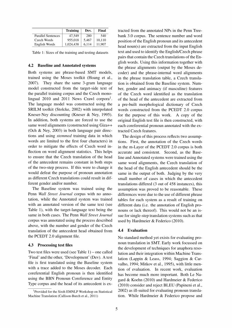
Training Dev. FinalParallel Sentences 47,549 280 540Czech Words 955,018 5,467 10,110English Words 1,024,438 6,114 11,907

Table 1: Sizes of the training and testing datasets

4.2 Baseline and Annotated systems

Both systems are phrase-based SMT models,trained using the Moses toolkit (Hoang et al.,2007). They share the same 3-gram languagemodel constructed from the target-side text ofthe parallel training corpus and the Czech mono-lingual 2010 and 2011 News Crawl corpora1.The language model was constructed using theSRILM toolkit (Stolcke, 2002) with interpolatedKneser-Ney discounting (Kneser & Ney, 1995).In addition, both systems are forced to use thesame word alignments (constructed using Giza++(Och & Ney, 2003) in both language pair direc-tions and using stemmed training data in whichwords are limited to the first four characters) inorder to mitigate the effects of Czech word in-flection on word alignment statistics. This helpsto ensure that the Czech translation of the headof the antecedent remains constant in both stepsof the two-step process. If this were to change itwould defeat the purpose of pronoun annotationas different Czech translations could result in dif-ferent gender and/or number.

The Baseline system was trained using thePenn Wall Street Journal corpus with no anno-tation, while the Annotated system was trainedwith an annotated version of the same text (seeTable 1), with the target-language text being thesame in both cases. The Penn Wall Street Journalcorpus was annotated using the process describedabove, with the number and gender of the Czechtranslation of the antecedent head obtained fromthe PCEDT 2.0 alignment file.

4.3 Processing test files

Two test files were used (see Table 1) – one called‘Final’ and the other, ‘Development’ (Dev). A testfile is first translated using the Baseline systemwith a trace added to the Moses decoder. Eachcoreferential English pronoun is then identifiedusing the BBN Pronoun Coreference and EntityType corpus and the head of its antecedent is ex-

1Provided for the Sixth EMNLP Workshop on StatisticalMachine Translation (Callison-Burch et al., 2011)

tracted from the annotated NPs in the Penn Tree-bank 3.0 corpus. The sentence number and wordposition of the English pronoun and its antecedenthead noun(s) are extracted from the input Englishtext and used to identify the English/Czech phrasepairs that contain the Czech translations of the En-glish words. Using this information together withthe phrase alignments (output by the Moses de-coder) and the phrase-internal word alignmentsin the phrase translation table, a Czech transla-tion is obtained from the Baseline system. Num-ber, gender and animacy (if masculine) featuresof the Czech word identified as the translationof the head of the antecedent are extracted froma pre-built morphological dictionary of Czechwords constructed from the PCEDT 2.0 corpusfor the purpose of this work. A copy of theoriginal English test file is then constructed, witheach coreferential pronoun annotated with the ex-tracted Czech features.

The design of this process reflects two assump-tions. First, the annotation of the Czech wordsin the m-Layer of the PCEDT 2.0 corpus is bothaccurate and consistent. Second, as the Base-line and Annotated systems were trained using thesame word alignments, the Czech translation ofthe head of the English antecedent should be thesame in the output of both. Judging by the verysmall number of cases in which the antecedenttranslations differed (3 out of 458 instances), thisassumption was proved to be reasonable. Thesedifferences were due to the use of different phrasetables for each system as a result of training ondifferent data (i.e. the annotation of English pro-nouns or lack thereof). This would not be an is-sue for single-step translation systems such as thatused by Hardmeier & Federico (2010).

4.4 Evaluation

No standard method yet exists for evaluating pro-noun translation in SMT. Early work focussed onthe development of techniques for anaphora reso-lution and their integration within Machine Trans-lation (Lappin & Leass, 1994; Saggion & Car-valho, 1994; Mitkov et al., 1995), with little men-tion of evaluation. In recent work, evaluationhas become much more important. Both Le Na-gard & Koehn (2010) and Hardmeier & Federico(2010) consider and reject BLEU (Papineni et al.,2002) as ill-suited for evaluating pronoun transla-tion. While Hardmeier & Federico propose and

5

use a strict recall and precision based metric forEnglish–German translation, I found it unsuitablefor English–Czech translation, given the highlyinflective nature of Czech.

Given the importance of evaluation to the goalof assessing the effectiveness of annotation pro-jection for improving the translation of corefer-ring pronouns, I carried out two separate typesof evaluation — an automated evaluation whichcould be applied to the entire test set, and an in-depth manual assessment that might provide moreinformation, but could only be performed on asubset of the test set. The automated evaluationis based on the fact that a Czech pronoun mustagree in number and gender with its antecedent.Thus one can count the number of pronouns in thetranslation output for which this agreement holds,rather than simply score the output against a sin-gle reference translation. To obtain these figures,the automated evaluation process counted:

1. Total pronouns in the input English test file.

2. Total English pronouns identified as corefer-ential, as per the annotation of the BBN Pro-noun Coreference and Entity Type corpus.

3. Total coreferential English pronouns that areannotated by the annotation process.

4. Total coreferential English pronouns that arealigned with any Czech translation.

5. Total coreferential English pronouns trans-lated as any Czech pronoun.

6. Total coreferential English pronouns trans-lated as a Czech pronoun corresponding toa valid translation of the English pronoun.

7. Total coreferential English pronouns trans-lated as a Czech pronoun (that is a validtranslation of the English pronoun) agreeingin number and gender with the antecedent.

The representation of valid Czech translationsof English pronouns takes the form of a list pro-vided by an expert in Czech NLP, which ignorescase and focusses solely on number and gender.

In contrast, the manual evaluation carried outby that same expert, who is also a native speakerof Czech, was used to determine whether devi-ations from the single reference translation pro-vided in the PCEDT 2.0 corpus were valid alter-natives or simply poor translations. The followingjudgements were provided:

1. Whether the pronoun had been translatedcorrectly, or in the case of a dropped pro-noun, whether pro-drop was appropriate;

2. If the pronoun translation was incorrect,whether a native Czech speaker would stillbe able to derive the meaning;

3. For input to the Annotated system, whetherthe pronoun had been correctly annotatedwith respect to the Czech translation of itsidentified antecedent;

4. Where an English pronoun was translateddifferently by the Baseline and Annotatedsystems, which was better. If both translatedan English pronoun to a valid Czech transla-tion, equal correctness was assumed.

In order to ensure that the manual assessorwas directed to the Czech translations alignedto the English pronouns, additional markup wasautomatically inserted into the English and Czechtexts: (1) coreferential pronouns in both Englishand Czech texts were marked with the headnoun of their antecedent (denoted by *), and(2) coreferential pronouns in the English sourcetexts were marked with the Czech translationof the antecedent head, and those in the Czechtarget texts were marked with the original Englishpronoun that they were aligned to:

English text input to the Baseline system: the u.s., claiming some success in its trade diplomacy , ...

Czech translation output by the Baseline system:usa , tvrdı nekterı jejı(its) obchodnı uspech v diplo-macii , ...

English text input to the Annotated system: theu.s.* , claiming some success in its(u.s.,usa).mascin.pltrade diplomacy , ...

Czech translation output by the Annotated sys-tem: usa ,* tvrdı nekterı uspechu ve sve(its.mascin.pl)obchodnı diplomacii , ...

5 Results and Discussion

5.1 Automated Evaluation

Automated evaluation of both “Development”and “Final” test sets (see Table 2) shows that evenfactoring out the problems of accurate identifica-tion of coreferring pronouns, coreference resolu-tion and antecedent head–finding, does not im-prove performance of the Annotated system muchabove that of the Baseline.

6

Dev. FinalBaseline Annotated Baseline Annotated

Total pronouns in English file 156 156 350 350Total pronouns identified as coreferential 141 141 331 331Annotated coreferential English pronouns – 117 – 278Coreferential English pronouns aligned with any Czech translation 141 141 317 317Coreferential English pronouns translated as Czech pronouns 71 75 198 198Czech pronouns that are valid translations of the English pronouns 63 71 182 182Czech pronouns that are valid translations of the English pronounsand that match their antecedent in number and gender

44 46 142 146

Table 2: Automated Evaluation Results for both test sets

Criterion Baseline System Better Annotated System Better Systems EqualOverall quality 9/31 (29.03%) 11/31 (35.48%) 11/31 (35.48%)Quality when annotation is correct 3/18 (16.67%) 9/18 (50.00%) 6/18 (33.33%)

Table 3: Manual Evaluation Results: A direct comparison of pronoun translations that differ between systems

Taking the accuracy of pronoun translation tobe the proportion of coreferential English pro-nouns having a valid Czech translation that agreesin both number and gender with their antecedent,yields the following on the two test sets:Baseline system:

Development — 44/141 (31.21%)Final — 142/331 (42.90%)

Annotated system:Development — 46/141 (32.62%)Final — 146/331 (44.10%)There are, however, several reasons for not tak-

ing this evaluation as definitive. Firstly, it relieson the accuracy of the word alignments output bythe decoder to identify the Czech translations ofthe English pronoun and its antecedent. Secondly,these results fail to capture variation between thetranslations produced by the Baseline and Anno-tated systems. Whilst there is a fairly high de-gree of overlap, for approximately 1/3 of the “De-velopment” set pronouns and 1/6 of the “Final”set pronouns, the Czech translation is different.Since the goal of this work was to understandwhat is needed in order to improve the transla-tion of coreferential pronouns, manual evaluationwas critical for understanding the potential capa-bilities of source-side annotation.

5.2 Manual Evaluation

The sample files provided for manual evaluationcontained 31 pronouns for which the translationsprovided by the two systems differed (differences)and 72 for which the translation provided by thesystems was the same (matches). Thus, the sam-

ple comprised 103 of the 472 coreferential pro-nouns (about 22%) from across both test sets. Ofthis sample, it is the differences that indicate therelative performance of the two systems. Of the31 pronouns in this set, 16 were 3rd-person pro-nouns, 2 were reflexive personal pronouns and 13were possessive pronouns.

The results corresponding to evaluation crite-rion 4 in Section 4.4 provide a comparison of theoverall quality of pronoun translation for both sys-tems. These results for the “Development” and“Final” test sets (see Table 3) suggest that the per-formance of the Annotated system is comparablewith, and even marginally better than, that of theBaseline system, especially when the pronoun an-notation is correct.

An example of where the Annotated systemproduces a better translation than the Baselinesystem is:

Annotated English: he said mexico could be one of thenext countries to be removed from the priority list because ofits.neut.sg efforts to craft a new patent law .

Baseline translation: rekl , ze mexiko by mohl byt jedenz dalsıch zemı , aby byl odvolan z prioritou seznam , protozejejı snahy podporit nove patentovy zakon .

Annotated translation: rekl , ze mexiko by mohl byt je-den z dalsıch zemı , aby byl odvolan z prioritou seznam ,protoze jeho snahy podporit nove patentovy zakon .

In this example, the English pronoun “its”,which refers to “mexico” is annotated as neuterand singular (as extracted from the Baseline trans-lation). Both systems translate “mexico” as“mexiko” (neuter, singular) but differ in theirtranslation of the pronoun. The Baseline systemtranslates “its” incorrectly as “jejı” (feminine, sin-gular), whereas the Annotated system produces

7

the more correct translation: “jeho” (neuter, sin-gular), which agrees with the antecedent in bothnumber and gender.

An analysis of the judgements on the remain-ing three evaluation criteria (outlined in Section4.4) for the 31 differences provides further infor-mation. The Baseline system appears to be moreaccurate, with 19 pronouns either correctly trans-lated (in terms of number and gender) or appro-priately dropped, compared with 17 for the An-notated system. Of those pronouns, the meaningcould still be understood for 7/12 for the Baselinesystem compared with 8/14 for the Annotated sys-tem. On the surface this may seem strange but itappears to be due to a small number of cases inwhich the translations produced by both systemswere incorrect but those produced by the Anno-tated system were deemed to be marginally better.Due to the small sample size it is difficult to forma complete picture of where one system may per-form consistently better than the other. The anno-tation of both number and gender was accurate for18 pronouns. Whilst this accuracy is not particu-larly high, the results (see Table 3) suggest thattranslation is more accurate for those pronounsthat are correctly annotated.

Whilst pro-drop in Czech was not explicitlyhandled in the annotation process, manual evalu-ation revealed that both systems were able to suc-cessfully ‘learn’ a few (local) scenarios in whichpro-drop is appropriate. This was unexpected butfound to be due to instances in which there areshort distances between the pronoun and verb inEnglish. For example, many of the occurrencesof “she” in English appear in the context of “shesaid...” and are translated correctly with the verbform “...rekla...”.

An example of where the Annotated systemcorrectly drops a pronoun is:

Annotated English: “ this is the worst shakeout ever inthe junk market , and it could take years before it.fem.sg ’s over , ” says mark bachmann , a senior vice president atstandard & poor ’ s corp . , a credit rating company .

Baseline translation: “ je to nejhorsı krize , kdy na trhus rizikovymi obligacemi , a to muze trvat roky , nez je to pryc, ” rıka mark bachmann , hlavnı viceprezident spolecnostistandard & poor ’s corp . , uverovy rating spolecnosti .

Annotated translation: “ je to nejhorsı krize , kdy natrhu s rizikovymi obligacemi , a to muze trvat roky , nezje !! pryc , ” rıka mark bachmann , hlavnı viceprezidentspolecnosti standard & poor ’s corp . , uverovy ratingspolecnosti .

In this example, the Baseline system trans-

lates “it” incorrectly as the neuter singular pro-noun “to”, whereas the Annotated system cor-rectly drops the subject pronoun (indicated by !!)— this is a less trivial example than “she said”. Inthe case of the Baseline translation “to” could beinterpreted as referring to the whole event, whichwould be correct, but poor from a stylistic pointof view.

An example of where the Annotated systemfails to drop a pronoun is:

Annotated English: taiwan has improved its.mascin.sg*standing with the u.s. by initialing a bilateral copyrightagreement , amending its.mascin.sg** trademark law andintroducing legislation to protect foreign movie producersfrom unauthorized showings of their.mascan.pl films .

Annotated translation: tchaj-wan zlepsenı svepostavenı s usa o initialing bilateralnıch autorskych prav najeho obchodnı dohody , uprava zakona a zavedenı zakonana ochranu zahranicnı filmove producenty z neopravneneshowings svych filmu .

Reference translation: tchaj-wan zlepsil svou reputaciv usa , kdyz podepsal bilateralnı smlouvu o autorskychpravech , pozmenil !! zakon o ochrannych znamkach azavedl legislativu na ochranu zahranicnıch filmovych produ-centu proti neautorizovanemu promıtanı jejich filmu .

In this example, the English pronoun “its”,which refers to “taiwan” is annotated as mascu-line inanimate and singular. The first occurrenceof “its” is marked by * and the second occurrenceby ** in the annotated English text above. Thesecond occurrence should be translated either asa reflexive pronoun (as the first occurrence is cor-rectly translated) or it should be dropped as in thereference translation (!! indicates the position ofthe dropped pronoun).

In addition to the judgements, the manual as-sessor also provided feedback on the evalua-tion task. One of the major difficulties encoun-tered concerned the translation of pronouns insentences which exhibit poor syntactic structure.This is a criticism of Machine Translation as awhole, but of the manual evaluation of pronountranslation in particular, since the choice of core-ferring form is sensitive to syntactic structure.Also the effects of poor syntactic structure arelikely to introduce an additional element of sub-jectivity if the assessor must first interpret thestructure of the sentences output by the transla-tion systems.

5.3 Potential Sources of Error

Related errors that may have contributed to theAnnotated system not providing a significant im-provement over the Baseline include: (1) incor-

8

rect identification of the English antecedent headnoun, (2) incorrect identification of the Czechtranslation of the antecedent head noun in theBaseline output due to errors in the word align-ments, and (3) errors in the PCEDT 2.0 align-ment file (affecting training only). While “per-fect” annotation of the BBN Pronoun Coreferenceand Entity Type, the PCEDT 2.0 and the PennTreebank 3.0 corpora has been assumed, errors inthese corpora cannot be completely ruled out.

6 Conclusion and Future Work

Despite factoring out three major sources of er-ror — identifying coreferential pronouns, findingtheir antecedents, and identifying the head of eachantecedent — through the use of manually anno-tated corpora, the results of the Annotated systemshow only a small improvement over the Baselinesystem. Two possible reasons for this are that thestatistics in the phrase translation table have beenweakened in the Annotated system as a result ofincluding both number and gender in the anno-tation and that the size of the training corpus isrelatively small.

However, more significant may be the avail-ability of only a single reference translation. Thisaffects the development and application of au-tomated evaluation metrics as a single referencecannot capture the variety of possible valid trans-lations. Coreference can be achieved without ex-plicit pronouns. This is true of both English andCzech, with sentences that contain pronouns hav-ing common paraphrases that lack them. For ex-ample,

the u.s. , claiming some success in its tradediplomacy , ...can be paraphrased as:

the u.s. , claiming some success in trade diplo-macy , ...

A target-language translation of the formermight actually be a translation of the latter, andhence lack the pronoun shown in bold. Given therange of variability in whether pronouns are usedin conveying coreference, the availability of onlya single reference translation is a real problem.

Improving the accuracy of coreferential pro-noun translation remains an open problem in Ma-chine Translation and as such there is great scopefor future work in this area. The investigation re-ported here suggests that it is not sufficient to fo-cus solely on the source-side and further opera-

tions on the target side (besides post-translationapplication of a target-language model) need alsobe considered. Other target–side operations couldinvolve the extraction of features to score multi-ple candidate translations in the selection of the‘best’ option – for example, to ‘learn’ scenar-ios in which pro-drop is appropriate and to selecttranslations that contain pronouns of the correctmorphological inflection. This requires identifica-tion of features in the target side, their extractionand incorporation in the translation process whichcould be difficult to achieve within a purely sta-tistical framework given that the antecedent of apronoun may be arbitrarily distant in the previousdiscourse.

The aim of this work was to better understandwhy previous attempts at using annotation projec-tion in pronoun translation showed less than ex-pected improvement. Thus it would be beneficialto conduct an error analysis to show the frequencyof the errors described in Section 5.3 appear.

I will also be exploring other directions re-lated to problems identified during the course ofthe work completed to date. These include, butare not limited to, handling pronoun dropping inpro-drop languages, developing pronoun-specificautomated evaluation metrics and addressing theproblem of having only one reference translationfor use with such metrics. In this regard, I will beconsidering the use of paraphrase techniques togenerate synthetic reference translations to aug-ment an existing reference translation set. Ini-tial efforts will focus on adapting the approach ofKauchak & Barzilay (2006) and back–translationmethods for extracting paraphrases (Bannard &Callison-Burch, 2005) to the more specific prob-lem of pronoun variation.

Acknowledgements

I would like to thank Bonnie Webber (Univer-sity of Edinburgh) who supervised this projectand Marketa Lopatkova (Charles University) whoprovided the much needed Czech language assis-tance. I am very grateful to Ondrej Bojar (CharlesUniversity) for his numerous helpful suggestionsand to the Institute of Formal and Applied Lin-guistics (Charles University) for providing thePCEDT 2.0 corpus. I would also like to thankWolodja Wentland and the three anonymous re-viewers for their feedback.

9

ReferencesColin Bannard and Chris Callison-Burch. 2005. Para-

phrasing with Bilingual Parallel Corpora. In Pro-ceedings of the 43rd Annual Meeting of the ACL,pages 597–604.

Chris Callison-Burch, Philipp Koehn, Christof Monzand Omar Zaidan. 2011. Findings of the 2011Workshop on Statistical Machine Translation. InProceedings of the Sixth Workshop on StatisticalMachine Translation, pages 22–64.

Mona Diab. 2004. An Unsupervised Approach forBootstrapping Arabic Sense Tagging. In Proceed-ings of the Workshop on Computational Approachesto Arabic Script-based Languages, pages 43–50.

Kevin Gimpel and Noah A. Smith. 2008. RichSource-Side Context for Statistical Machine Trans-lation. In Proceedings of the Third Workshop onStatistical Machine Translation, pages 9–17.

Barbara J. Grosz, Scott Weinstein and Aravind K.Joshi. 1995. Centering: A Framework for Mod-eling the Local Coherence Of Discourse. Computa-tional Linguistics, 21(2):203–225.

Christian Hardmeier and Marcello Federico. 2010.Modelling Pronominal Anaphora in Statistical Ma-chine Translation. In Proceedings of the 7th In-ternational Workshop on Spoken Language Trans-lation, pages 283–290.

Philipp Koehn, Hieu Hoang, Alexandra Birch,Chris Callison-Burch, Marcello Federico, NicolaBertoldi, Brooke Cowan, Wade Shen, ChristineMoran, Richard Zens. Chris Dyer, Ondrej Bojar,Alexandra Constantin and Evan Herbst. 2007.Moses: Open Source Toolkit for Statistical Ma-chine Translation. In Proceedings of the 45th An-nual Meeting of the ACL on Interactive Poster andDemonstration Sessions, pages 177–180.

Jerry R. Hobbs. 1978. Resolving Pronominal Refer-ences. Lingua, 44:311–338.

Jan Hajic, Eva Hajicova, Jarmila Panevova, Petr Sgall,Silvie Cinkova, Eva Fucıkova, Marie Mikulova,Petr Pajas, Jan Popelka, Jirı Semecky, JanaSindlerova, Jan Stepanek, Josef Toman, ZdenkaUresova and Zdenek Zabokrtsky. 2011. PragueCzech-English Dependency Treebank 2.0. Instituteof Formal and Applied Linguistics. Prague, CzechRepublic.

David Kauchak and Regina Barzilay. 2006. Para-phrasing For Automatic Evaluation. In Proceedingsof the Main Conference on Human Language Tech-nology Conference of the NAACL, June 5–7, NewYork, USA, pages 455–462.

Mitesh M. Khapra, Sapan Shah, Piyush Kedia andPushpak Bhattacharyya. 2009. Projecting Param-eters for Multilingual Word Sense Disambiguation.In Proceedings of the 2009 Conference on Empiri-cal Methods in Natural Language Processing, Au-gust 6–7, Singapore, pages 459–467.

Reinhard Kneser and Hermann Ney. 1995. Im-proved Backing-Off for M-gram Language Model-ing. IEEE International Conference on Acoustics,Speech, and Signal Processing, May 9–12, Detroit,USA, 1:181–184.

Shalom Lappin and Herbert J. Leass. 1994. An Algo-rithm for Pronominal Anaphora Resolution. Com-putational Linguistics, 20:535–561.

Ronan Le Nagard and Philipp Koehn. 2010. Aid-ing Pronoun Translation with Co-reference Resolu-tion. In Proceedings of the Joint Fifth Workshop onStatistical Machine Translation and MetricsMATR,pages 252–261.

Vincent Ng. 2010. Supervised Noun Phrase Corefer-ence Research: The first 15 years. In Proceedingsof the 48th Meeting of the ACL, pages 1396–1411.

Mitchell P. Marcus, Beatrice Santorini, Mary A.Marcinkiewicz and Ann Taylor. 1999. Penn Tree-bank 3.0 LDC Calalog No.: LDC99T42. LinguisticData Consortium.

Ruslan Mitkov, Sung-Kwon Choi and Randall Sharp.1995. Anaphora Resolution in Machine Transla-tion. In Proceedings of the Sixth International Con-ference on Theoretical and Methodological Issuesin Machine Translation, July 5-7, Leuven, Belgium,pages 5–7.

Ruslan Mitkov. 1999. Introduction: Special Issue onAnaphora Resolution in Machine Translation andMultilingual NLP. Machine Translation, 14:159–161.

Franz J. Och and Hermann Ney. 2003. A SystematicComparison of Various Statistical Alignment Mod-els. Computational Linguistics, 29(1):19–51.

Kishore Papineni, Salim Roukos, Todd Ward and Wei-Jing Zhu. 2002. BLEU: a method for automaticevaluation of machine translation. In Proceedingsof the 40th Annual Meeting of the ACL, pages 311–318.

Horacio Saggion and Ariadne Carvalho. 1994.Anaphora Resolution in a Machine Translation Sys-tem. In Proceedings of the International Con-ference on Machine Translation: Ten Years On,November, Cranfield, UK, 4.1-4.14.

Andreas Stolcke. 2002. SRILM — An ExtensibleLanguage Modeling Toolkit. In Proceedings of In-ternational Conference on Spoken Language Pro-cessing, September 16-20, Denver, USA, 2:901–904.

Michael Strube. 2007. Corpus-based and Ma-chine Learning Approaches to Anaphora Resolu-tion. Anaphors in Text: Cognitive, Formal andApplied Approaches to Anaphoric Reference, JohnBenjamins Pub Co.

Ralph Weischedel and Ada Brunstein. 2005. BBNPronoun Coreference and Entity Type Corpus LDCCalalog No.: LDC2005T33. Linguistic Data Con-sortium.

10

Proceedings of the EACL 2012 Student Research Workshop, pages 11–21,Avignon, France, 26 April 2012. c©2012 Association for Computational Linguistics

Cross-Lingual Genre Classification

Philipp PetrenzSchool of Informatics, University of Edinburgh10 Crichton Street, Edinburgh, EH8 9AB, UK

p.petrenz@sms.ed.ac.uk

Abstract

Classifying text genres across languagescan bring the benefits of genre classifi-cation to the target language without thecosts of manual annotation. This articleintroduces the first approach to this task,which exploits text features that can be con-sidered stable genre predictors across lan-guages. My experiments show this methodto perform equally well or better thanfull text translation combined with mono-lingual classification, while requiring fewerresources.

1 Introduction

Automated text classification has become stan-dard practice with applications in fields such asinformation retrieval and natural language pro-cessing. The most common basis for text clas-sification is by topic (Joachims, 1998; Sebas-tiani, 2002), but other classification criteria haveevolved, including sentiment (Pang et al., 2002),authorship (de Vel et al., 2001; Stamatatos et al.,2000a), and author personality (Oberlander andNowson, 2006), as well as categories relevant tofilter algorithms (e.g., spam or inappropriate con-tents for minors).

Genre is another text characteristic, often de-scribed as orthogonal to topic. It has been shownby Biber (1988) and others after him, that thegenre of a text affects its formal properties. It istherefore possible to use cues (e.g., lexical, syn-tactic, structural) from a text as features to pre-dict its genre, which can then feed into informa-tion retrieval applications (Karlgren and Cutting,1994; Kessler et al., 1997; Finn and Kushmer-ick, 2006; Freund et al., 2006). This is because

users may want documents that serve a particu-lar communicative purpose, as well as being ona particular topic. For example, a web search onthe topic “crocodiles” may return an encyclopediaentry, a biological fact sheet, a news report aboutattacks in Australia, a blog post about a safari ex-perience, a fiction novel set in South Africa, ora poem about wildlife. A user may reject manyof these, just because of their genre: Blog posts,poems, novels, or news reports may not containthe kind or quality of information she is seeking.Having classified indexed texts by genre would al-low additional selection criteria to reflect this.

Genre classification can also benefit LanguageTechnology indirectly, where differences in thecues that correlate with genre may impact sys-tem performance. For example, Petrenz andWebber (2011) found that within the New YorkTimes corpus (Sandhaus, 2008), the word “states”has a higher likelihood of being a verb in let-ters (approx. 20%) than in editorials (approx.2%). Part-of-Speech (PoS) taggers or statisticalmachine translation (MT) systems could benefitfrom knowing such genre-based domain varia-tion. Kessler et al. (1997) mention that parsingand word-sense disambiguation can also benefitfrom genre classification. Webber (2009) foundthat different genres have a different distributionof discourse relations, and Goldstein et al. (2007)showed that knowing the genre of a text can alsoimprove automated summarization algorithms, asgenre conventions dictate the location and struc-ture of important information within a document.

All the above work has been done within asingle language. Here I describe a new ap-proach to genre classification that is cross-lingual.Cross-lingual genre classification (CLGC) differs

11

from both poly-lingual and language-independentgenre classification. CLGC entails training agenre classification model on a set of labeled textswritten in a source language LS and using thismodel to predict the genres of texts written in thetarget language LT 6= LS . In poly-lingual classi-fication, the training set is made up of texts fromtwo or more languages S = LS1 , . . . , LSN

thatinclude the target language LT ∈ S. Language-independent classification approaches are mono-lingual methods that can be applied to any lan-guage. Unlike CLGC, both poly-lingual andlanguage-independent genre classification requirelabeled training data in the target language.

Supervised text classification requires a largeamount of labeled data. CLGC attempts to lever-age the available annotated data in well-resourcedlanguages like English in order to bring the afore-mentioned advantages to poorly-resourced lan-guages. This reduces the need for manual annota-tion of text corpora in the target language. Manualannotation is an expensive and time-consumingtask, which, where possible, should be avoidedor kept to a minimum. Considering the difficul-ties researchers are encountering in compiling agenre reference corpus for even a single language(Sharoff et al., 2010), it is clear that it would be in-feasible to attempt the same for thousands of otherlanguages.

2 Prior work

Work on automated genre classification was firstcarried out by Karlgren and Cutting (1994). LikeKessler et al. (1997) and Argamon et al. (1998)after them, they exploit (partly) hand-crafted setsof features, which are specific to texts in English.These include counts of function words such as“we” or “therefore”, selected PoS tag frequen-cies, punctuation cues, and other statistics derivedfrom intuition or text analysis. Similarly lan-guage specific feature sets were later explored formono-lingual genre classification experiments inGerman (Wolters and Kirsten, 1999) and Russian(Braslavski, 2004).

In subsequent research, automatically gener-ated feature sets have become more popular. Mostof these tend to be language-independent andmight work in mono-lingual genre classificationtasks in languages other than English. Examplesare the word based approaches suggested by Sta-matatos et al. (2000b) and Freund et al. (2006),

the image features suggested by Kim and Ross(2008), the PoS histogram frequency approach byFeldman et al. (2009), and the character n-gramapproaches proposed by Kanaris and Stamatatos(2007) and Sharoff et al. (2010). All of themwere tested exclusively on English texts. Whilelanguage-independence is a popular argument of-ten claimed by authors, few have shown empir-ically that this is true of their approach. Oneof the few authors to carry out genre classifica-tion experiments in more than one language wasSharoff (2007). Using PoS 3-grams and a vari-ation of common word 3-grams as feature sets,Sharoff classified English and Russian documentsinto genre categories. However, while the PoS 3-gram set yielded respectable prediction accuracyfor English texts, in Russian documents, no im-provement over the baseline of choosing the mostfrequent genre class was observed.

While there is virtually no prior work onCLGC, cross-lingual methods have been exploredfor other text classification tasks. The first toreport such experiments were Bel et al. (2003),who predicted text topics in Spanish and En-glish documents, using one language for train-ing and the other for testing. Their approach in-volves training a classifier on language A, using adocument representation containing only contentwords (nouns, adjectives, and verbs with a highcorpus frequency). These words are then trans-lated from language B to language A, so that textsin either language are mapped to a common rep-resentation.

Thereafter, cross-lingual text classification wastypically regarded as a domain adaptation prob-lem that researchers have tried to solve using largesets of unlabeled data and/or small sets of labeleddata in the target language. For instance, Rigutiniet al. (2005) present an EM algorithm in whichlabeled source language documents are translatedinto the target language and then a classifier istrained to predict labels on a large, unlabeledset in the target language. These instances arethen used to iteratively retrain the classificationmodel and the predictions are updated until con-vergence occurs. Using information gain scoresat every iteration to only retain the most predic-tive words and thus reduce noise, Rigutini et al.(2005) achieve a considerable improvement overthe baseline accuracy, which is a simple trans-lation of the training instances and subsequent

12

mono-lingual classification. They, too, were clas-sifying texts by topics and used a collection ofEnglish and Italian newsgroup messages. Simi-larly, researchers have used semi-supervised boot-strapping methods like co-training (Wan, 2009)and other domain adaptation methods like struc-tural component learning (Prettenhofer and Stein,2010) to carry out cross-lingual text classification.

All of the approaches described above rely onMT, even if some try to keep translation to aminimum. This has several disadvantages how-ever, as applications become dependent on par-allel corpora, which may not be available forpoorly-resourced languages. It also introducesproblems due to word ambiguity and morphol-ogy, especially where single words are translatedout of context. A different method is proposedby Gliozzo and Strapparava (2006), who use la-tent semantic analysis on a combined collectionof texts written in two languages. The ratio-nale is that named entities such as “Microsoft” or“HIV” are identical in different languages withthe same writing system. Using term correla-tion, the algorithm can identify semantically sim-ilar words in both languages. The authors exploitthese mappings in cross-lingual topic classifica-tion, and their results are promising. However,using bilingual dictionaries as well yields a con-siderable improvement, as Gliozzo and Strappar-ava (2006) also report.

While all of the methods above could techni-cally be used in any text classification task, the id-iosyncrasies of genres pose additional challenges.Techniques relying on the automated translationof predictive terms (Bel et al., 2003; Prettenhoferand Stein, 2010) are workable in the contexts oftopics and sentiment, as these typically rely oncontent words such as nouns, adjectives, and ad-verbs. For example, “hospital” may indicate atext from the medical domain, while “excellent”may indicate that a review is positive. Such termsare relatively easy to translate, even if not alwayswithout uncertainty. Genres, on the other hand,are often classified using function words (Karl-gren and Cutting, 1994; Stamatatos et al., 2000b)like “of”, “it”, or “in”. It is clear that translatingthese out of context is next to impossible. This istrue in particular if there are differences in mor-phology, since function words in one languagemay be morphological affixes in another.

Although it is theoretically possible to use the

bilingual low-dimension approach by Gliozzo andStrapparava (2006) for genre classification, it re-lies on certain words to be identical in two dif-ferent languages. While this may be the case fortopic-indicating named entities — a text contain-ing the words “Obama” and “McCain” will al-most certainly be about the U.S. elections in 2008,or at least about U.S. politics — there is little in-dication of what its genre might be: It could bea news report, an editorial, a letter, an interview,a biography, or a blog entry, just to name a few.Because topics and genres correlate, one wouldprobably reject some genres like instruction man-uals or fiction novels. However, uncertainty is stilllarge, and Petrenz and Webber (2011) show thatit can be dangerous to rely on such correlations.This is particularly true in the cross-lingual case,as it is not clear whether genres and topics corre-late in similar ways in a different language.

3 Approach

The approach I propose here relies on two strate-gies I explain below in more detail: Stable fea-tures and target language adaptation. The firstis based on the assumption that certain featuresare indicative of certain genres in more than onelanguage, while the latter is a less restricted wayto boost performance, once the language gap hasbeen bridged. Figure 1 illustrates this approach,which is a challenging one, as very little priorknowledge is assumed by the system. On theother hand, in theory it allows any resulting appli-cation to be used for a wide range of languages.

3.1 Assumption of prior knowledgeTypically, the aim of cross-lingual techniques is toleverage the knowledge present in one languagein order to help carry a task in another language,for which such knowledge is not available. In thecase of genre classification, this knowledge com-prises genre labels of the documents used to trainthe classification model. My approach requires nolabeled data in the target language. This is impor-tant, as some domain adaptation algorithms relyon a small set of labeled texts in the target do-main.

Cross-lingual methods also often rely on MT,but this effectively restricts them to languagesfor which MT is sufficiently developed. Apartfrom the fact that it would be desirable for across-lingual genre classifier to work for as many

13

Labelled

Set (LS)

Unlabelled

Set (LT)

Standardized

Stable Feature

Representation

Standardized

Stable Feature

Representation

SVM

Model

Prediction

Prediction

Prediction

Tar

get

Lan

gu

age

Ad

apta

tio

nS

tab

le F

eatu

res

Labelled

Set (LT)

Prediction

Confidence

Values

Labelled

Subset (LT)

Bag of Word

Representation &

Feature Selection

(Information Gain)

SVM

Model

(Labels

removed)

Tar

get

Lan

gu

age

Ad

apta

tio

n

Figure 1: Outline of the proposed method for CLGC.

languages as possible, MT only allows classi-fication in well-resourced languages. However,such languages are more likely to have genre-annotated corpora, and mono-lingual classifica-tion may yield better results. In order to bringthe advantages of genre classification to poorly-resourced languages, the availability of MT tech-niques, at least for the time being, must not beassumed. I only use them to generate baseline re-sults.

The same restriction is applied to other types ofprior knowledge, and I do not assume supervisedPoS taggers, syntactic parsers, or other tools areavailable. In future work however, I may exploreunsupervised methods, such as the PoS inductionmethods of Clark (2003), Goldwater and Griffiths(2007), or Berg-Kirkpatrick et al. (2010), as theydo not represent external knowledge.

There are a few assumptions that must be madein order to carry out any meaningful experiments.First, some way to detect sentence and paragraphboundaries is expected. This can be a simple rule-based algorithm, or unsupervised methods, suchas the Punkt boundary detection system by Kissand Strunk (2006). Also, punctuation symbolsand numerals are assumed to be identifiable assuch, although their exact semantic function is un-known. For example, a question mark will be

identified as a punctuation symbol, but its func-tion (question cue; end of a sentence) will not.Lastly, a sufficiently large, unlabeled set of textsin the target language is required.

3.2 Stable features

Many types of features have been used in genreclassification. They all fall into one of threegroups: Language-specific features are cueswhich can only be extracted from texts in one lan-guage. An example would be the frequency of aparticular word, such as “yesterday”. Language-independent features can be extracted in any lan-guage, but they are not necessarily directly com-parable. Examples would be the frequencies ofthe ten most common words. While these can beextracted for any language (as long as words canbe identified as such), the function of a word ona certain position in this ranking will likely differfrom one language to another. Comparable fea-tures, on the other hand, represent the same func-tion, or part of a function, in two or more lan-guages. An example would be type/token ratios,which, in combination with the document length,represent the lexical richness of a text, indepen-dent of its language. If such features prove tobe good genre predictors across languages, theymay be considered stable across those languages.Once suitable features are found, CLGC may beconsidered a standard classification problem, asoutlined in the upper part of Figure 1.

I propose an approach that makes use of suchstable features, which include mostly structural,rather than lexical cues (cf. Section 4). Stablefeatures lend themselves to the classification ofgenres in particular. As already mentioned, gen-res differ in communicative purpose, rather thanin topic. Therefore, features involving contentwords are only useful to an extent. While topicalclassification is hard to imagine without transla-tion or parallel/comparable corpora, genre classi-fication can be done without such resources. Sta-ble features provide a way to bridge the languagegap even to poorly-resourced languages.

This does not necessarily mean that the valuesof these attributes are in the same range acrosslanguages. For example, the type/token ratio willtypically be higher in morphologically-rich lan-guages. However, it might still be true that novelshave a richer vocabulary than scientific articles,whether they are written in English or Finnish. In

14

order to exploit such features cross-linguistically,their values have to be mapped from one languageto another. This can be done in an unsupervisedfashion, as long as enough data is present in bothsource and target language (cf. Section 3.1). Aneasy and intuitive way is to standardize values sothat each feature in both sets has a mean value ofzero mean and variance of one. This is achievedby subtracting from each feature value the meanover all documents and dividing it by the standarddeviation.

Note that the training and test sets have to bestandardized separately in order for both sets tohave the same mean and variance and thus becomparable. This is different from classificationtasks where training and test set are assumed tobe sampled from the same distribution. Althoughstandardization (or another type of scaling) is of-ten performed in such tasks as well, the scalingfactor from the training set would be used to scalethe test set (Hsu et al., 2000).

3.3 Target language adaptation

Cross-lingual text classification has often beenconsidered a special case of domain adap-tation. Semi-supervised methods, such asthe expectation-maximization (EM) algorithm(Dempster et al., 1977), have been employed tomake use of both labeled data in the source lan-guage and unlabeled data in the target language.However, adapting to a different language poses agreater challenge than adapting to different gen-res, topics, or sources. As the vocabularies havelittle (if any) overlap, it is not trivial to initiallybridge the gap between the domains. Typically,MT would be used to tackle this problem.

Instead, my use of stable features shifts the fo-cus of subsequent domain adaptation to exploitingunlabeled data in the target language to improveprediction accuracy. I refer to this as target lan-guage adaptation (TLA). The advantage of mak-ing this separation is that a different set of featurescan be used to adapt to the target language. Thereis no reason to keep the restrictions required forstable features once the language gap has beenbridged. In fact, any language-independent fea-ture may be used for this task. The assumption isthat the method described in Section 3.2 providesa good but enhanceable result, that is significantlybelow mono-lingual performance. The resultingdecent, though imperfect, labeling of target lan-

guage texts may be exploited to improve accuracy.A wide range of possible features lend them-

selves to TLA. Language-independent featureshave often been proposed in prior work on genreclassification. These include bag-of-words, char-acter n-grams, and PoS frequencies or PoS n-grams, although the latter two would have to bebased on the output of unsupervised PoS induc-tion algorithms in this scenario. Alternatively,PoS tags could be approximated by consideringthe most frequent words as their own tag, as sug-gested by Sharoff (2007). With appropriate fea-ture sets, iterative algorithms can be used to im-prove the labeling of the set in the target domain.

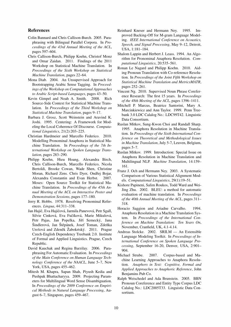
The lower part of Figure 1 illustrates the TLAprocess proposed for CLGC. In each iteration,confidence values obtained from the previousclassification model are used to select a subset oflabeled texts in the target language. Intuitively,only texts which can be confidently assigned toa certain genre should be used to train a newmodel. This is particularly true in the first iter-ation, after the stable feature prediction, as errorrates are expected to be high. The size of thissubset is increased at each iteration in the processuntil it comprises all the texts in the test set. Amulti-class Support Vector Machine (SVM) in ak genre problem is a combination of k×(k−1)

2 bi-nary classifiers with voting to determine the over-all prediction. To compute a confidence value forthis prediction, I use the geometric mean G =(∏n

i=1 ai)1/n of the distances from the decision

boundary ai for all the n binary classifiers, whichinclude the winning genre (i.e., n = k − 1). Thegeometric mean heavily penalizes low values, thatis small distances to the hyperplane separatingtwo genres. This corresponds to the intuition thatthere should be a high certainty in any pairwisegenre comparison for a high-confidence predic-tion. Negative distances from the boundary arecounted as zero, which reduces the overall confi-dence to zero. The acquired subset is then trans-formed to a bag of words representation. Inspiredby the approach of Rigutini et al. (2005), the in-formation gain for each feature is computed, andonly the highest ranked features are used. A newclassification model is trained and used to re-labelthe target language texts. This process continuesuntil convergence (i.e., labels in two subsequentiterations are identical) or until a pre-defined iter-ation limit is reached.

15

4 Experiments

4.1 Baselines

To verify the proposed approach, I carried out ex-periments using two publicly available corpora inEnglish and in Chinese. As there is no prior workon CLGC, I chose as baseline an SVM modeltrained on the source language set using a bag ofwords representation as features. This had pre-viously been used for this task by Freund et al.(2006) and Sharoff et al. (2010).1 The texts inthe test set were then translated from the targetinto the source language using Google translate2

and the SVM model was used to predict their gen-res. I also tested a variant in which the training setwas translated into the target language before thefeature extraction step, with the test set remaininguntranslated. Note that these are somewhat artifi-cial baselines, as MT in reasonable quality is onlyavailable for a few selected languages. They aretherefore not workable solutions to classify gen-res in poorly-resourced languages. Thus, even across-lingual performance close to these baselinescan be considered a success, as long as no MTis used. For reference, I also report the perfor-mances of a random guess approach and a classi-fier labeling each text as the dominant genre class.

With all experiments, results are reported forthe test set in the target language. I infer confi-dence intervals by assuming that the number ofmisclassifications is approximately normally dis-tributed with mean µ = e × n and standard devi-ation σ =

√µ× (1− e), where e is the percent-

age of misclassified instances and n is the size ofthe test set. I take two classification results to dif-fer significantly only if their 95% confidence in-tervals (i.e., µ± 1.96× σ) do not overlap.

4.2 Data

In line with some of the prior mono-lingual workon genre classification, I used the Brown corpusfor my experiments. As illustrated in Table 1,the 500 texts in the corpus are sampled from 15genres, which can be categorized more broadlyinto four broad genre categories, and even morebroadly into informative and imaginative texts.The second corpus I used was the Lancaster Cor-pus of Mandarin Chinese (LCMC). In creating the

1Other document representations, including character n-grams, were tested, but found to perform worse in this task.

2http://translate.google.com

Info

rmat

ive

Press Press: Reportage

(88 texts) Press: EditorialsPress: ReviewsReligion

Misc. Skills, Trades & Hobbies(176 texts) Popular Lore

Biographies & EssaysNon-Fiction Reports & Official Documents(110 texts) Academic Prose

Imag

inat

ive

General FictionMystery & Detective Fiction

Fiction Science Fiction(126 texts) Adventure & Western Fiction

Romantic FictionHumor

Table 1: Genres in the Brown corpus. Categories areidentical in the LCMC, except Western Fiction is re-placed by Martial Arts Fiction.

LCMC, the Brown sampling frame was followedvery closely and genres within these two corporaare comparable, with the exception of WesternFiction, which was replaced by Martial Arts Fic-tion in the LCMC. Texts in both corpora are tok-enized by word, sentence, and paragraph, and nofurther pre-processing steps were necessary.

Following Karlgren and Cutting (1994), Itested my approach on all three levels of granu-larity. However, as the 15-genre task yields rela-tively poor CLGC results (both for my approachand the baselines), I report and discuss only theresults of the two and four-genre task here. Im-proving performance on more fine-grained genreswill be subject of future work (cf. Section 6).

4.3 Features and Parameters

The stable features used to bridge the languagegap are listed in Table 2. Most are simply ex-tractable cues that have been used in mono-lingualgenre classification experiments before: Averagesentence/paragraph lengths and standard devia-tions, type/token ratio and numeral/token ratio.To these, I added a ratio of single lines in a text —that is, paragraphs containing no more than onesentence, divided by the sentence count. Theseare typically headlines, datelines, author names,or other structurally interesting parts. A distribu-tion value indicates how evenly single lines aredistributed throughout a text, with high values in-dicating single lines predominantly occurring atthe beginning and/or end of a text.

16

Features F N P M Features F N P MAverage Sentence −0.5 0.6 0.1 0.0 Type/Token 0.0 −0.9 0.6 0.3

Length −1.0 0.5 0.0 0.3 Ratio 0.0 −0.9 0.9 0.1Sentence Length −0.3 0.5 −0.1 0.0 Numeral/Token −0.3 0.6 −0.1 −0.1

Standard Deviation −0.5 0.4 0.0 0.1 Ratio −0.7 0.7 0.4 −0.1Average Paragraph −0.4 0.3 −0.1 0.1 Single Lines/ 0.3 0.1 −0.1 −0.2

Length −0.4 0.4 −0.6 0.4 Sentence Ratio 0.0 −0.3 1.1 −0.4Paragraph Length −0.4 0.4 −0.2 0.1 Single Line −0.3 0.2 0.0 0.1

Standard Deviation −0.1 0.4 −0.6 0.1 Distribution 0.1 −0.1 0.1 0.0Relative tf-idf values of 0.2 0.1 −0.1 0.0 Topic Average −0.4 0.8 −0.3 0.0

top 10 weighted words* 0.4 −0.2 −0.5 0.1 Precision −0.4 0.8 −0.2 −0.1

Table 2: Set of 19 stable features used to bridge the language gap. The numbers denote the mean values afterstandardization for each broad genre in the LCMC (upper values) and Brown corpus (lower values): Fiction,Non-Fiction, Press, and Miscellaneous. Negative/Positive numbers denote lower/higher average feature valuesfor this genre when compared to the rest of the corpus. *Relative tf-idf values are ten separate features. Thenumbers given are for the highest ranked word only.

The remaining features (cf. last row of Table2) are based on ideas from information retrieval.I used tf-idf weighting and marked the ten high-est weighted words in a text as relevant. I thentreated this text as a ranked list of relevant andnon-relevant words, where the position of a wordin the text determined its rank. This allowed me tocompute an average precision (AP) value. The in-tuition behind this value is that genre conventionsdictate the location of important content wordswithin a text. A high AP score means that the toptf-idf weighted words are found predominantly inthe beginning of a text. In addition, for the sameten words, I added the tf-idf value to the featureset, divided by the sum of all ten. These valuesindicate whether a text is very focused (a sharpdrop between higher and lower ranked words) ormore spread out across topics (relatively flat dis-tribution).

For each of these features, Table 2 shows themean values for the four broad genre classes inthe LCMC and Brown corpus, after the sets havebeen standardized to zero mean and unit variance.This is the same preprocessing process used fortraining and testing the SVM model, although thestatistics in Table 2 are not available to the clas-sifier, since they require genre labels. Each rowgives an idea of how suitable a feature might beto distinguish between these genres in Chinese(upper row) and English (lower row). Both rowstogether indicate how stable a feature is acrosslanguages for this task. Some features, such asthe topic AP value, seems to be both a good pre-dictor for genre and stable across languages. In

both Chinese and English, for example, the topi-cal words seem to be concentrated around the be-ginning of the text in Non-Fiction, but much lessso in Fiction. These patterns can be seen in otherfeatures as well. The type/token ratio is, on av-erage, highest in Press texts, followed by Miscel-laneous texts, Fiction texts, and Non-Fiction textsin both corpora. While this does not hold for allthe features, many such patterns can be observedin Table 2.

Since uncertainty after the initial prediction isvery high, the subset used to re-train the SVMmodel was chosen to be small. In the first iter-ation, I used up to 60% of texts with the highestconfidence value within each genre. To avoid animbalanced class distribution, texts were chosenso that the genre distribution in the new trainingset matched the one in the source language. To il-lustrate this, consider an example with two genreclasses A and B, represented by 80% and 20% oftexts respectively in the source language. Assum-ing that after the initial prediction both classes areassigned to 100 texts in a test set of size 200, the60 texts with the highest confidence values wouldbe chosen for class A. To keep the genre distribu-tion of the source language, only the top 15 textswould be chosen for class B.

In the second iteration, I simply used the top90% of texts overall. This number was increasedby 5% in each subsequent iteration, so that the fullset was used from the fourth iteration. No changeswere made to the genre distribution from the sec-ond iteration. To train the classification model,I used the 500 features with the highest informa-

17

0.4

0.5

0.6

0.7

0.8

0.9

1.0

Rand. PriorMT

Source

MT

TargetSF

SF +

TLA

t: zh 50.0% 74.8% 87.2% 83.2% 79.2% 87.6%

t: en 50.0% 74.8% 88.8% 95.8% 76.8% 94.6%

0.4

Figure 2: Prediction accuracies for the Brown / LCMCtwo genre classification task. Dark bars denote En-glish as source language and Chinese as target lan-guage (en→zh), light bars denote the reverse (zh→en).Rand.: Random classifier. Prior: Classifier always pre-dicting the most dominant class. The baselines MTSource and MT target use MT to translate texts intothe source and target language, respectively. SF: Sta-ble Features. TLA: Target Language Adaptation.

tion gain score for the selected training set in eachiteration. As convergence is not guaranteed theo-retically, I used a maximum limit of 15 iterations.In my experiments however, the algorithm alwaysconverged.

5 Results and Discussion

Figure 2 shows the accuracies for the two genretask (informative texts vs. imaginative texts) inboth directions: English as a source language withChinese being the target language (en→zh) andvice versa (zh→en). As the class distribution isskewed (374 vs. 126 texts), always predictingthe most dominant class yields acceptable perfor-mance. However, this is simplistic and might failin practice, where the most dominant class willtypically be unknown.

Full text translation combined with mono-lingual classification performs well. Stable fea-tures alone yield a respectable prediction accu-racy, but perform significantly worse than MTSource in both tasks and MT Target in the zh→entask. However, subsequent TLA significantly im-proves the accuracy on both tasks, eliminating anysignificant difference from baseline performance.

Figure 3 shows results for the four genre clas-sification task (Fiction vs. Non-Fiction vs. Pressvs. Misc.). Again, MT Source and MT Targetperform well. However, translating from Chineseinto English yields better results than the reverse.This might be due to the easier identification of

0.2

0.3

0.4

0.5

0.6

0.7

0.8

Rand. PriorMT

Source

MT

TargetSF

SF +

TLA

t: zh 25.0% 35.2% 64.4% 54.0% 54.2% 69.4%

t: en 25.0% 35.2% 51.0% 66.8% 59.2% 70.8%

0.2

Figure 3: Prediction accuracies for the Brown / LCMCfour genre classification task. Labels as in Figure 2.

words in English and thus a more accurate bagof words representation. TLA manages to signif-icantly improve the stable feature results. My ap-proach outperforms both baselines in this experi-ment, although the differences are only significantif texts are translated from English to Chinese.

These results are encouraging, as they showthat in CLGC tasks, equal or better performancecan be achieved with fewer resources, when com-pared the baseline of full text translation. The rea-son why TLA works well in this case can be un-derstood by comparing the confusion matrices be-fore the first iteration and after convergence (Ta-ble 3). While it is obvious that the stable fea-ture approach works better on some classes thanon others, the distributions of predicted and ac-tual genres are fairly similar. For Fiction, Non-Fiction, and Press, precision is above 50%, withcorrect predictions outweighing incorrect ones,which is an important basis for subsequent it-erative learning. However, too many texts arepredicted to belong to the Miscellaneous cate-gory, which reduces recall on the other genres.By using a different feature set and concentrat-ing on the documents with high confidence val-ues, TLA manages to remedy this problem to anextent. While misclassifications are still present,recalls for the Fiction and Non-Fiction genres areincreased significantly, which explains the higheroverall accuracy.

6 Conclusion and future work

I have presented the first work on cross-lingualgenre classification (CLGC). I have shown thatsome text features can be considered stable genrepredictors across languages and that it is possi-ble to achieve good results in CLGC tasks without

18

Fict. Non-Fict. Press Misc.Fiction 65 2 8 51Non-Fiction 4 59 2 45Press 5 8 31 44Miscellaneous 18 28 14 116Precision 0.71 0.61 0.56 0.45Recall 0.52 0.54 0.35 0.66

Fict. Non-Fict. Press Misc.Fiction 102 0 2 22Non-Fiction 0 83 0 27Press 2 8 27 51Miscellaneous 29 9 3 135Precision 0.77 0.83 0.84 0.57Recall 0.81 0.75 0.31 0.77

Table 3: Confusion Matrices for the four genre en→zh task. Left: After stable feature prediction, but beforeTLA. Right: After TLA convergence. Rows 2–5 denote actual numbers of texts, columns denote predictions.

resource-intensive MT techniques. My approachexploits stable features to bridge the language gapand subsequently applies iterative target languageadaptation (TLA) in order to improve accuracy.The approach performed equally well or betterthan full text translation combined with mono-lingual classification. Considering that Englishand Chinese are very dissimilar linguistically, Iexpect the approach to work at least equally wellfor more closely related language pairs.

This work is still in progress. While my resultsare encouraging, more work is needed to makethe CLGC approach more robust. At the moment,classification accuracy is low for problems withmany classes. I plan to remedy this by implement-ing a hierarchical classification framework, wherea text is assigned a broad genre label first and thenclassified further within this category.

Since TLA can only work on a sufficientlygood initial labeling of target language texts, sta-ble feature classification results have to be im-proved as well. To this end, I propose to focusinitially on features involving punctuation. Thiscould include analyses of the different punctu-ation symbols used in comparison with the restof the document set, their frequencies and devia-tions between sentences, punctuation n-gram pat-terns, as well as the analyses of the positions ofpunctuation symbols within sentences or wholetexts. Punctuation has frequently been used ingenre classification tasks and it is expected thatsome of the features based on such symbols arevaluable in a cross-lingual setting as well. As vo-cabulary richness seems to be a useful predictor ofgenres, experiments will also be extended beyondthe simple inclusion of type/token ratios in thefeature set. For example, hapax legomena statis-tics could be used, as well as the conformance totext laws, such as Zipf, Benford, and Heaps.

After this, I will examine text structure a pre-

dictor. While single line statistics and topic APscores already reflect text structure, more sophis-ticated pre-processing methods, such as text seg-mentation and unsupervised PoS induction, mightyield better results. The experiments using thetf-idf values of terms will be extended. Result-ing features may include the positions of highlyweighted words in a text, the amount of topicscovered, or identification of summaries.

TLA techniques can also be refined. An obvi-ous choice is to consider different types of fea-tures, as mentioned in Section 3.3. Different rep-resentations may even be combined to capture thenotion of different communicative purpose, sim-ilar to the multi-dimensional approach by Biber(1995). An interesting idea to combine differ-ent sets of features was suggested by Chaker andHabib (2007). Assigning a document to all genreswith different probabilities and repeating this fordifferent sets of features may yield a very flexi-ble classifier. The impact of the feature sets onthe final prediction could be weighted accordingto different criteria, such as prediction certaintyor overlap with other feature sets. Improvementsmay also be achieved by choosing a more reliablemethod for finding the most confident genre pre-dictions as a function of the distance to the SVMdecision boundary. Cross-validation techniqueswill be explored to estimate confidence values.

Finally, I will have to test the approach on alarger set of data with texts from more languages.To this end, I am working to compile a referencecorpus for CLGC by combining publicly availablesources. This would be useful to compare meth-ods and will hopefully encourage further research.

Acknowledgments

I thank Bonnie Webber, Benjamin Rosman, andthree anonymous reviewers for their helpful com-ments on an earlier version of this paper.

19

References

Shlomo Argamon, Moshe Koppel, and Galit Avneri.1998. Routing documents according to style. InProceedings of First International Workshop on In-novative Information Systems.

Nuria Bel, Cornelis Koster, and Marta Villegas. 2003.Cross-lingual text categorization. In Traugott Kochand Ingeborg Slvberg, editors, Research and Ad-vanced Technology for Digital Libraries, volume2769 of Lecture Notes in Computer Science, pages126–139. Springer Berlin / Heidelberg.

Taylor Berg-Kirkpatrick, Alexandre Bouchard-Cote,John DeNero, and Dan Klein. 2010. Painlessunsupervised learning with features. In HumanLanguage Technologies: The 2010 Annual Confer-ence of the North American Chapter of the Associa-tion for Computational Linguistics, HLT ’10, pages582–590, Stroudsburg, PA, USA. Association forComputational Linguistics.

Douglas Biber. 1988. Variation across Speech andWriting. Cambridge University Press, Cambridge.

Douglas Biber. 1995. Dimensions of Register Varia-tion. Cambridge University Press, New York.

Pavel Braslavski. 2004. Document style recognitionusing shallow statistical analysis. In Proceedings ofthe ESSLLI 2004 Workshop on Combining Shallowand Deep Processing for NLP, pages 1–9.

Jebari Chaker and Ounelli Habib. 2007. Genre cat-egorization of web pages. In Proceedings of theSeventh IEEE International Conference on DataMining Workshops, ICDMW ’07, pages 455–464,Washington, DC, USA. IEEE Computer Society.

Alexander Clark. 2003. Combining distributional andmorphological information for part of speech in-duction. In Proceedings of the tenth conference onEuropean chapter of the Association for Computa-tional Linguistics - Volume 1, EACL ’03, pages 59–66, Stroudsburg, PA, USA. Association for Compu-tational Linguistics.

O. de Vel, A. Anderson, M. Corney, and G. Mohay.2001. Mining e-mail content for author identifica-tion forensics. SIGMOD Rec., 30(4):55–64.

A. P. Dempster, N. M. Laird, and D. B. Rubin. 1977.Maximum Likelihood from Incomplete Data via theEM Algorithm. Journal of the Royal Statistical So-ciety. Series B (Methodological), 39(1):1–38.

S. Feldman, M. A. Marin, M. Ostendorf, and M. R.Gupta. 2009. Part-of-speech histograms forgenre classification of text. In Proceedings of the2009 IEEE International Conference on Acoustics,Speech and Signal Processing, pages 4781–4784,Washington, DC, USA. IEEE Computer Society.

Aidan Finn and Nicholas Kushmerick. 2006. Learn-ing to classify documents according to genre. J.Am. Soc. Inf. Sci. Technol., 57(11):1506–1518.

Luanne Freund, Charles L. A. Clarke, and Elaine G.Toms. 2006. Towards genre classification for IRin the workplace. In Proceedings of the 1st inter-national conference on Information interaction incontext, pages 30–36, New York, NY, USA. ACM.

Alfio Gliozzo and Carlo Strapparava. 2006. Exploit-ing comparable corpora and bilingual dictionariesfor cross-language text categorization. In Proceed-ings of the 21st International Conference on Com-putational Linguistics and the 44th annual meetingof the Association for Computational Linguistics,ACL-44, pages 553–560, Stroudsburg, PA, USA.Association for Computational Linguistics.

Jade Goldstein, Gary M. Ciany, and Jaime G. Car-bonell. 2007. Genre identification and goal-focused summarization. In Proceedings of the six-teenth ACM conference on Conference on informa-tion and knowledge management, CIKM ’07, pages889–892, New York, NY, USA. ACM.

Sharon Goldwater and Tom Griffiths. 2007. A fullyBayesian approach to unsupervised part-of-speechtagging. In Proceedings of the 45th Annual Meet-ing of the Association of Computational Linguistics,pages 744–751, Prague, Czech Republic, June. As-sociation for Computational Linguistics.

Chih-Wei Hsu, Chih-Chung Chang, and Chih-Jen Lin.2000. A Practical Guide to Support Vector Classifi-cation.

Thorsten Joachims. 1998. Text categorization withsuport vector machines: Learning with many rele-vant features. In Proceedings of the 10th EuropeanConference on Machine Learning, pages 137–142,London, UK. Springer-Verlag.

Ioannis Kanaris and Efstathios Stamatatos. 2007.Webpage genre identification using variable-lengthcharacter n-grams. In Proceedings of the 19th IEEEInternational Conference on Tools with AI, pages 3–10, Washington, DC.

Jussi Karlgren and Douglass Cutting. 1994. Recog-nizing text genres with simple metrics using dis-criminant analysis. In Proceedings of the 15th Con-ference on Computational Linguistics, pages 1071–1075, Morristown, NJ, USA. Association for Com-putational Linguistics.

Brett Kessler, Geoffrey Nunberg, and Hinrich Schutze.1997. Automatic detection of text genre. In Pro-ceedings of the 35th Annual Meeting of the Associ-ation for Computational Linguistics, pages 32–38,Morristown, NJ, USA. Association for Computa-tional Linguistics.

Yunhyong Kim and Seamus Ross. 2008. Examiningvariations of prominent features in genre classifica-tion. In Proceedings of the Proceedings of the 41stAnnual Hawaii International Conference on SystemSciences, HICSS ’08, pages 132–, Washington, DC,USA. IEEE Computer Society.

20

Tibor Kiss and Jan Strunk. 2006. Unsupervised multi-lingual sentence boundary detection. Comput. Lin-guist., 32:485–525, December.

Jon Oberlander and Scott Nowson. 2006. Whosethumb is it anyway?: classifying author person-ality from weblog text. In Proceedings of theCOLING/ACL on Main conference poster sessions,COLING-ACL ’06, pages 627–634, Morristown,NJ, USA. Association for Computational Linguis-tics.

Bo Pang, Lillian Lee, and Shivakumar Vaithyanathan.2002. Thumbs up?: sentiment classification usingmachine learning techniques. In Proceedings of theACL-02 conference on Empirical methods in natu-ral language processing - Volume 10, EMNLP ’02,pages 79–86, Morristown, NJ, USA. Associationfor Computational Linguistics.

Philipp Petrenz and Bonnie Webber. 2011. Stableclassification of text genres. Comput. Linguist.,37:385–393.

Peter Prettenhofer and Benno Stein. 2010. Cross-language text classification using structural corre-spondence learning. In Proceedings of the 48th An-nual Meeting of the Association for ComputationalLinguistics, ACL ’10, pages 1118–1127, Strouds-burg, PA, USA. Association for Computational Lin-guistics.

Leonardo Rigutini, Marco Maggini, and Bing Liu.2005. An em based training algorithm for cross-language text categorization. In Proceedings of theWeb Intelligence Conference, pages 529–535.

Evan Sandhaus. 2008. New York Times corpus: Cor-pus overview. LDC catalogue entry LDC2008T19.

Fabrizio Sebastiani. 2002. Machine learning in au-tomated text categorization. ACM Comput. Surv.,34:1–47, March.

Serge Sharoff, Zhili Wu, and Katja Markert. 2010.The Web Library of Babel: Evaluating genre collec-tions. In Proceedings of the Seventh conference onInternational Language Resources and Evaluation,pages 3063–3070, Valletta, Malta, may. EuropeanLanguage Resources Association (ELRA).

Serge Sharoff. 2007. Classifying web corpora intodomain and genre using automatic feature identifi-cation. In Proceedings of Web as Corpus Workshop.

E. Stamatatos, N. Fakotakis, and G. Kokkinakis.2000a. Text genre detection using common wordfrequencies. In Proceedings of the 18th conferenceon Computational linguistics, pages 808–814, Mor-ristown, NJ, USA. Association for ComputationalLinguistics.

Efstathios Stamatatos, George Kokkinakis, and NikosFakotakis. 2000b. Automatic text categorization interms of genre and author. Computational Linguis-tics, 26(4):471–495.

Xiaojun Wan. 2009. Co-training for cross-lingual sen-timent classification. In Proceedings of the Joint

Conference of the 47th Annual Meeting of the ACLand the 4th International Joint Conference on Nat-ural Language Processing of the AFNLP: Volume 1- Volume 1, ACL ’09, pages 235–243, Stroudsburg,PA, USA. Association for Computational Linguis-tics.

Bonnie Webber. 2009. Genre distinctions for dis-course in the Penn TreeBank. In Proceedings of theJoint Conference of the 47th Annual Meeting of theACL and the 4th International Joint Conference onNatural Language Processing of the AFNLP, pages674–682.

Maria Wolters and Mathias Kirsten. 1999. Exploringthe use of linguistic features in domain and genreclassification. In Proceedings of the ninth confer-ence on European chapter of the Association forComputational Linguistics, EACL ’99, pages 142–149, Stroudsburg, PA, USA. Association for Com-putational Linguistics.

21

Proceedings of the EACL 2012 Student Research Workshop, pages 22–31,Avignon, France, 26 April 2012. c©2012 Association for Computational Linguistics

A Comparative Study of Reinforcement Learning Techniques onDialogue Management

Alexandros PapangelisNCSR ”Demokritos”,Institute of Informatics& Telecommunications

andUniv. of Texas at Arlington,

Comp. Science and Engineeringalexandros.papangelis@mavs.uta.edu

Abstract

Adaptive Dialogue Systems are rapidly be-coming part of our everyday lives. As theyprogress and adopt new technologies theybecome more intelligent and able to adaptbetter and faster to their environment. Re-search in this field is currently focused onhow to achieve adaptation, and particularlyon applying Reinforcement Learning (RL)techniques, so a comparative study of therelated methods, such as this, is necessary.In this work we compare several standardand state of the art online RL algorithmsthat are used to train the dialogue managerin a dynamic environment, aiming to aid re-searchers / developers choose the appropri-ate RL algorithm for their system. This isthe first work, to the best of our knowledge,to evaluate online RL algorithms on the di-alogue problem and in a dynamic environ-ment.

1 Introduction

Dialogue Systems (DS) are systems that are ableto make natural conversation with their users.There are many types of DS that serve variousaims, from hotel and flight booking to provid-ing information or keeping company and forminglong term relationships with the users. Other in-teresting types of DS are tutorial systems, whosegoal is to teach something new, persuasive sys-tems whose goal is to affect the user’s attitude to-wards something through casual conversation andrehabilitation systems that aim at engaging pa-tients to various activities that help their rehabili-tation process. DS that incorporate adaptation totheir environment are called Adaptive DialogueSystems (ADS). Over the past few years ADS

have seen a lot of progress and have attracted theresearch community’s and industry’s interest.

There is a number of available ADS, apply-ing state of the art techniques for adaptation andlearning, such as the one presented by Young etal., (2010), where the authors propose an ADSthat provides tourist information in a fictitioustown. Their system is trained using RL and someclever state compression techniques to make itscalable, it is robust to noise and able to recoverfrom errors (misunderstandings). Cuayahuitl etal. (2010) propose a travel planning ADS, that isable to learn dialogue policies using RL, buildingon top of existing handcrafted policies. This en-ables the designers of the system to provide priorknowledge and the system can then learn the de-tails. Konstantopoulos (2010) proposes an affec-tive ADS which serves as a museum guide. It isable to adapt to each user’s personality by assess-ing his / her emotional state and current mood andalso adapt its output to the user’s expertise level.The system itself has an emotional state that is af-fected by the user and affects its output.

An example ADS architecture is depicted inFigure 1, where we can see several componentstrying to understand the user’s utterance and sev-eral others trying to express the system’s re-sponse. The system first attempts to convert spo-ken input to text using the Automatic SpeechRecognition (ASR) component and then tries toinfer the meaning using the Natural Language Un-derstanding (NLU) component. At the core liesthe Dialogue Manager (DM), a component re-sponsible for understanding what the user’s utter-ance means and deciding which action to take thatwill lead to achieving his / her goals. The DMmay also take into account contextual information

22

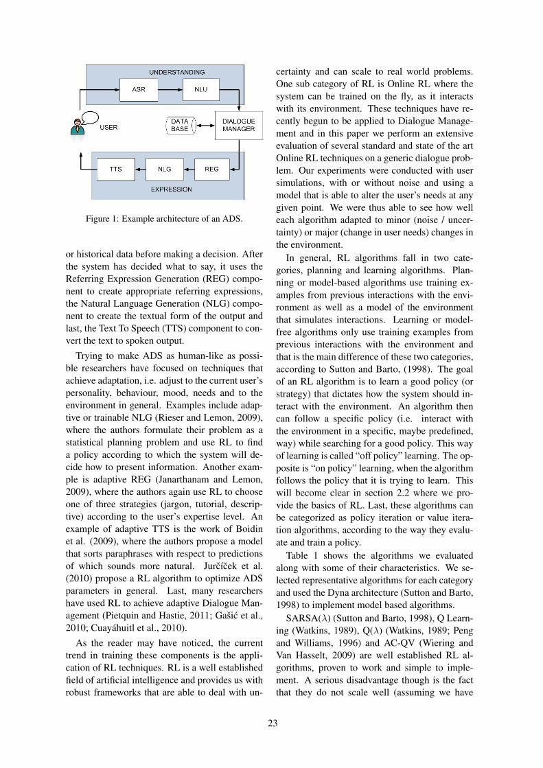
Figure 1: Example architecture of an ADS.

or historical data before making a decision. Afterthe system has decided what to say, it uses theReferring Expression Generation (REG) compo-nent to create appropriate referring expressions,the Natural Language Generation (NLG) compo-nent to create the textual form of the output andlast, the Text To Speech (TTS) component to con-vert the text to spoken output.

Trying to make ADS as human-like as possi-ble researchers have focused on techniques thatachieve adaptation, i.e. adjust to the current user’spersonality, behaviour, mood, needs and to theenvironment in general. Examples include adap-tive or trainable NLG (Rieser and Lemon, 2009),where the authors formulate their problem as astatistical planning problem and use RL to finda policy according to which the system will de-cide how to present information. Another exam-ple is adaptive REG (Janarthanam and Lemon,2009), where the authors again use RL to chooseone of three strategies (jargon, tutorial, descrip-tive) according to the user’s expertise level. Anexample of adaptive TTS is the work of Boidinet al. (2009), where the authors propose a modelthat sorts paraphrases with respect to predictionsof which sounds more natural. Jurcıcek et al.(2010) propose a RL algorithm to optimize ADSparameters in general. Last, many researchershave used RL to achieve adaptive Dialogue Man-agement (Pietquin and Hastie, 2011; Gasic et al.,2010; Cuayahuitl et al., 2010).

As the reader may have noticed, the currenttrend in training these components is the appli-cation of RL techniques. RL is a well establishedfield of artificial intelligence and provides us withrobust frameworks that are able to deal with un-

certainty and can scale to real world problems.One sub category of RL is Online RL where thesystem can be trained on the fly, as it interactswith its environment. These techniques have re-cently begun to be applied to Dialogue Manage-ment and in this paper we perform an extensiveevaluation of several standard and state of the artOnline RL techniques on a generic dialogue prob-lem. Our experiments were conducted with usersimulations, with or without noise and using amodel that is able to alter the user’s needs at anygiven point. We were thus able to see how welleach algorithm adapted to minor (noise / uncer-tainty) or major (change in user needs) changes inthe environment.

In general, RL algorithms fall in two cate-gories, planning and learning algorithms. Plan-ning or model-based algorithms use training ex-amples from previous interactions with the envi-ronment as well as a model of the environmentthat simulates interactions. Learning or model-free algorithms only use training examples fromprevious interactions with the environment andthat is the main difference of these two categories,according to Sutton and Barto, (1998). The goalof an RL algorithm is to learn a good policy (orstrategy) that dictates how the system should in-teract with the environment. An algorithm thencan follow a specific policy (i.e. interact withthe environment in a specific, maybe predefined,way) while searching for a good policy. This wayof learning is called “off policy” learning. The op-posite is “on policy” learning, when the algorithmfollows the policy that it is trying to learn. Thiswill become clear in section 2.2 where we pro-vide the basics of RL. Last, these algorithms canbe categorized as policy iteration or value itera-tion algorithms, according to the way they evalu-ate and train a policy.

Table 1 shows the algorithms we evaluatedalong with some of their characteristics. We se-lected representative algorithms for each categoryand used the Dyna architecture (Sutton and Barto,1998) to implement model based algorithms.

SARSA(λ) (Sutton and Barto, 1998), Q Learn-ing (Watkins, 1989), Q(λ) (Watkins, 1989; Pengand Williams, 1996) and AC-QV (Wiering andVan Hasselt, 2009) are well established RL al-gorithms, proven to work and simple to imple-ment. A serious disadvantage though is the factthat they do not scale well (assuming we have

23

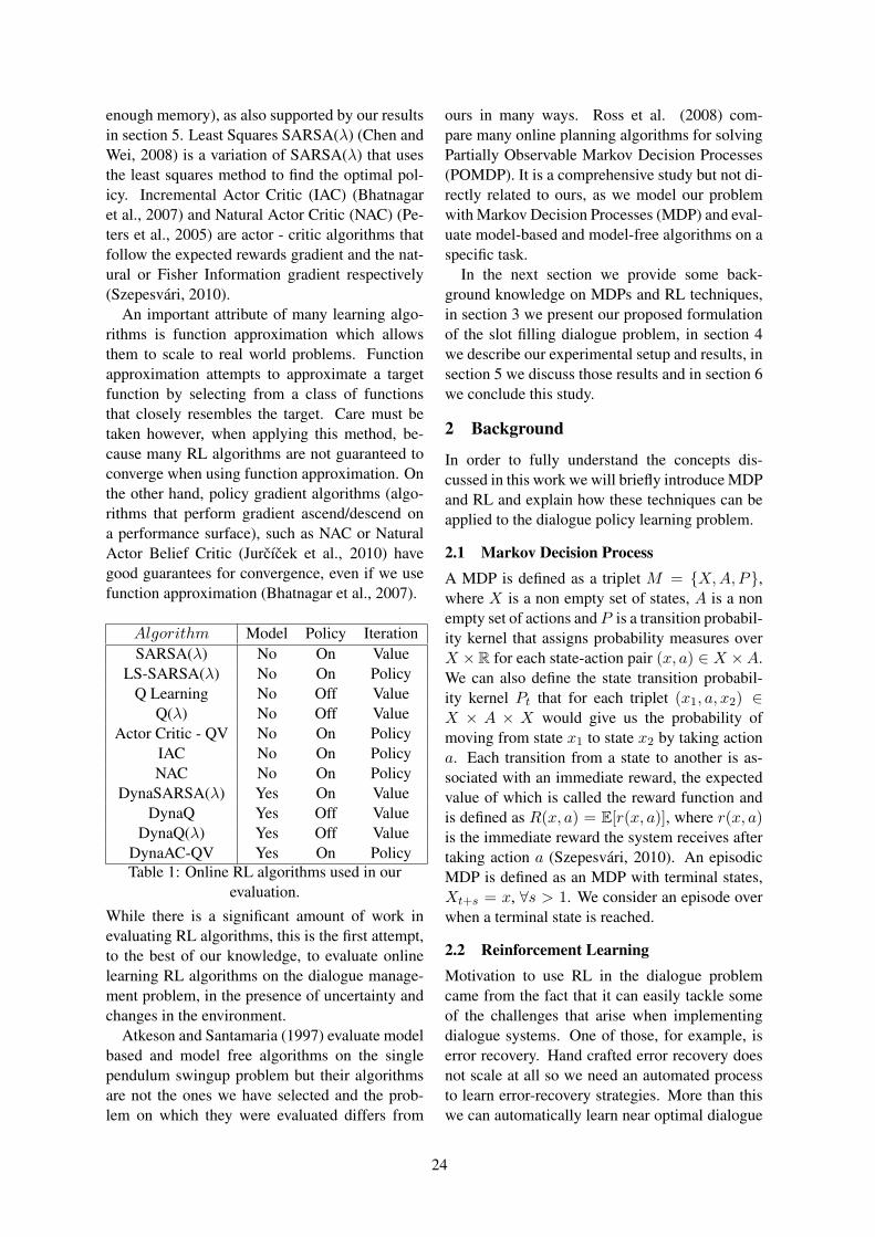
enough memory), as also supported by our resultsin section 5. Least Squares SARSA(λ) (Chen andWei, 2008) is a variation of SARSA(λ) that usesthe least squares method to find the optimal pol-icy. Incremental Actor Critic (IAC) (Bhatnagaret al., 2007) and Natural Actor Critic (NAC) (Pe-ters et al., 2005) are actor - critic algorithms thatfollow the expected rewards gradient and the nat-ural or Fisher Information gradient respectively(Szepesvari, 2010).

An important attribute of many learning algo-rithms is function approximation which allowsthem to scale to real world problems. Functionapproximation attempts to approximate a targetfunction by selecting from a class of functionsthat closely resembles the target. Care must betaken however, when applying this method, be-cause many RL algorithms are not guaranteed toconverge when using function approximation. Onthe other hand, policy gradient algorithms (algo-rithms that perform gradient ascend/descend ona performance surface), such as NAC or NaturalActor Belief Critic (Jurcıcek et al., 2010) havegood guarantees for convergence, even if we usefunction approximation (Bhatnagar et al., 2007).

Algorithm Model Policy IterationSARSA(λ) No On Value

LS-SARSA(λ) No On PolicyQ Learning No Off Value

Q(λ) No Off ValueActor Critic - QV No On Policy

IAC No On PolicyNAC No On Policy

DynaSARSA(λ) Yes On ValueDynaQ Yes Off Value

DynaQ(λ) Yes Off ValueDynaAC-QV Yes On PolicyTable 1: Online RL algorithms used in our

evaluation.While there is a significant amount of work inevaluating RL algorithms, this is the first attempt,to the best of our knowledge, to evaluate onlinelearning RL algorithms on the dialogue manage-ment problem, in the presence of uncertainty andchanges in the environment.

Atkeson and Santamaria (1997) evaluate modelbased and model free algorithms on the singlependulum swingup problem but their algorithmsare not the ones we have selected and the prob-lem on which they were evaluated differs from

ours in many ways. Ross et al. (2008) com-pare many online planning algorithms for solvingPartially Observable Markov Decision Processes(POMDP). It is a comprehensive study but not di-rectly related to ours, as we model our problemwith Markov Decision Processes (MDP) and eval-uate model-based and model-free algorithms on aspecific task.

In the next section we provide some back-ground knowledge on MDPs and RL techniques,in section 3 we present our proposed formulationof the slot filling dialogue problem, in section 4we describe our experimental setup and results, insection 5 we discuss those results and in section 6we conclude this study.

2 Background

In order to fully understand the concepts dis-cussed in this work we will briefly introduce MDPand RL and explain how these techniques can beapplied to the dialogue policy learning problem.

2.1 Markov Decision ProcessA MDP is defined as a triplet M = X,A,P,where X is a non empty set of states, A is a nonempty set of actions and P is a transition probabil-ity kernel that assigns probability measures overX ×R for each state-action pair (x, a) ∈ X ×A.We can also define the state transition probabil-ity kernel Pt that for each triplet (x1, a, x2) ∈X × A × X would give us the probability ofmoving from state x1 to state x2 by taking actiona. Each transition from a state to another is as-sociated with an immediate reward, the expectedvalue of which is called the reward function andis defined as R(x, a) = E[r(x, a)], where r(x, a)is the immediate reward the system receives aftertaking action a (Szepesvari, 2010). An episodicMDP is defined as an MDP with terminal states,Xt+s = x, ∀s > 1. We consider an episode overwhen a terminal state is reached.

2.2 Reinforcement LearningMotivation to use RL in the dialogue problemcame from the fact that it can easily tackle someof the challenges that arise when implementingdialogue systems. One of those, for example, iserror recovery. Hand crafted error recovery doesnot scale at all so we need an automated processto learn error-recovery strategies. More than thiswe can automatically learn near optimal dialogue

24

policies and thus maximize user satisfaction. An-other benefit of RL is that it can be trained usingeither real or simulated users and continue to learnand adapt with each interaction (in the case of on-line learning). To use RL we need to model thedialogue system using MDPs, POMDPs or SemiMarkov Desicion Processes (SMDP). POMDPstake uncertainty into account and model each statewith a distribution that represents our belief thatthe system is in a specific state. SMDPs add tem-poral abstraction to the model and allow for timeconsuming operations. We, however, do not dealwith either of those in an attempt to keep the prob-lem simple and focus on the task of comparing thealgorithms.

More formally, RL tries to maximize an objec-tive function by learning how to control the ac-tions of a system. A system in this setting is typ-ically formulated as an MDP. As we discussed insection 2.1 for every MDP we can define a pol-icy π, which is a mapping from states x ∈ X andactions α ∈ A to a distribution π(x, α) that repre-sents the probability of taking action α when thesystem is in state x. This policy dictates the be-haviour of the system. To estimate how good apolicy is we define the value function V :

V π(x) = E[∞∑t=0

γtRt+1|x0 = x], x ∈ X (1)

which gives us the expected cumulative rewardswhen beginning from state x and following policyπ, discounted by a factor γ ∈ [0, 1] that modelsthe importance of future rewards. We define thereturn of a policy π as:

Jπ =∞∑t=0

γtRt(xt, π(xt)) (2)

A policy π is optimal if Jπ(x) = V π(x), ∀x ∈X . We can also define the action-value functionQ:

Qπ(x, α) = E[

∞∑t=0

γtRt+1|x0 = x, a0 = α] (3)

where x ∈ X,α ∈ A, which gives us the ex-pected cumulative discounted rewards when be-ginning from state x and taking action α, againfollowing policy π. Note that Vmax = rmax

1−γ ,where R(x) ∈ [rmin, rmax].

The goal of RL therefore is to find the optimalpolicy, which maximizes either of these functions(Szepesvari, 2010).

3 Slot Filling Problem

We formulated the problem as a generic slot fill-ing ADS, represented as an MDP. This model hasbeen proposed in (Papangelis et al., 2012), and weextend it here to account for uncertainty. Formallythe problem is defined as: S =< s0, ..., sN >∈M,M = M0×M1× ...×MN ,Mi = 1, ..., Ti,where S are the N slots to be filled, each slot sican take values from Mi and Ti is the number ofavailable values slot si can be filled with. Dia-logue state is also defined as a vector d ∈ M ,where each dimension corresponds to a slot andits value corresponds to the slot’s value. We callthe set of all possible dialogue states D. Systemactions A ∈ 1, ..., |S| are defined as requestsfor slots to be filled and ai requests slot si. Ateach dialogue state di we define a set of availableactions ai ⊂ A. A user query q ⊂ S is definedas the slots that need to be filled so that the sys-tem will be able to accurately provide an answer.We assume action aN always means Give Answer.The reward function is defined as:

R(d, a) =

−1, if a 6= aN

−100, if a = aN ,∃qi|qi = ∅0, if a = aN ,¬∃qi|qi = ∅

(4)Thus, the optimal reward for each problem is−|q|since |q| < |S|.

Available actions for every state can be mod-elled as a matrix A ∈ 0, 1|D|×|A|, where:

Aij =

1, if aj ∈ ai0, if aj 6∈ ai

(5)

When designing A one must keep in mind thatthe optimal solution depends on A’s structureand must take care not to create an unsolvableproblem, i.e. a disconnected MDP. This can beavoided by making sure that each action is avail-able at some state and that each state has at leastone available action. We should now define thenecessary conditions for the slot filling problemto be solvable and the optimal reward be as de-fined before:

∃αij = 1, 1 ≤ i < |D|,∀j (6)

25

∃αij = 1, 1 < j < |A|,∀i (7)

Note that j > 1 since d1 is our starting state. Wealso allow Give Answer (which is aN ) to be avail-able from any state:

Ai,N = 1, 1 ≤ i ≤ |D| (8)

We define available action density to be the ra-tio of 1s over the number of elements of A:

Density =|(i, j)|Aij = 1||D| × |A|

We can now incorporate uncertainty in ourmodel. Rather than allowing deterministic transi-tions from a state to another we define a distribu-tion Pt(dj |di, am) which models the probabilityby which the system will go from state di to djwhen taking action am. Consequently, when thesystem takes action am from state di, it transits tostate dk with probability:

Pt(dk|di, am) =

Pt(dj |di, am), k = j

1−Pt(dj |di,am)|D|−1 , k 6= j

(9)assuming that under no noise conditions actionam would move the system from state di to statedj . The probability of not transiting to state djis uniformly distributed among all other states.Pt(dj |di, am) is updated after each episode witha small additive noise ν, mainly to model unde-sirable or unforeseen effects of actions. Anotherdistribution, Pc(sj = 1) ∈ [0, 1], models our con-fidence level that slot sj is filled:

sj =

1, Pc(sj = 1) ≥ 0.5

0, Pc(sj = 1) < 0.5(10)

In our evaluation Pc(sj) is a random number be-tween [1 − ε, 1] where ε models the level of un-certainty. Last, we can slightly alter A after eachepisode to model changes or faults in the avail-able actions for each state, but we did not in ourexperiments.

The algorithms selected for this evaluation arethen called to solve this problem online and findan optimal policy π? that will yield the highestpossible reward.

Algorithm α β γ λ

SARSA(λ) 0.95 - 0.55 0.4LS-SARSA(λ) 0.95 - 0.55 0.4

Q Learning 0.8 - 0.8 -Q(λ) 0.8 - 0.8 0.05

Actor Critic - QV 0.9 0.25 0.75 -IAC 0.9 0.25 0.75 -NAC 0.9 0.25 0.75 -

DynaSARSA(λ) 0.95 - 0.25 0.25DynaQ 0.8 - 0.4 -

DynaQ(λ) 0.8 - 0.4 0.05DynaAC-QV 0.9 0.05 0.75 -

Table 2: Optimized parameter values.

4 Experimental Setup

Our main goal was to evaluate how each algo-rithm behaves in the following situations:

• The system needs to adapt to a noise free en-vironment.

• The system needs to adapt to a noisy envi-ronment.

• There is a change in the environment and thesystem needs to adapt.

To ensure each algorithm performed to the bestof its capabilities we tuned each one’s parametersin an exhaustive manner. Table 2 shows the pa-rameter values selected for each algorithm. Theparameter ε in ε-greedy strategies was set to 0.01and model-based algorithms trained their modelfor 15 iterations after each interaction with theenvironment. Learning rates α and β and explo-ration parameter ε decayed as the episodes pro-gressed to allow better stability.

At each episode the algorithms need enough it-erations to explore the state space. At the initialstages of learning, though, it is possible that somealgorithms fall into loops and require a very largenumber of iterations before reaching a terminalstate. It would not hurt then if we bound the num-ber of iterations to a reasonable limit, provided itallows enough “negative” rewards to be accumu-lated when following a “bad” direction. In ourevaluation the algorithms were allowed 2|D| iter-ations, ensuring enough steps for exploration butnot allowing “bad” directions to be followed fortoo long.

To assess each algorithm’s performance andconvergence speed, we run each algorithm 100

26

times on a slot filling problem with 6 slots, 6 ac-tions and 300 episodes. The average reward overa high number of episodes indicates how stableeach algorithm is after convergence. User query qwas set to be s1, ..., s5 and there was no noisein the environment, meaning that the action ofquerying a slot deterministically gets the systeminto a state where that slot is filled. This can beformulated as: Pt(dj |di, am) = 1, Pc(sj) = 1∀j,ν = 0 and Ai,j = 1,∀i, j.

To evaluate the algorithms’ performance inthe presence of uncertainty we run each for 100times, on the same slot filling problem but withPt(dj |di, am) ∈ [1 − ε, 1], with varying ε andavailable action density values. At each run, eachalgorithm was evaluated using the same transitionprobabilities and available actions. To assess howthe algorithms respond to environmental changeswe conducted a similar but noise free experiment,where after a certain number of episodes the queryq was changed. Remember that q models the re-quired information for the system to be able to an-swer with some degree of certainty, so changing qcorresponds to requiring different slots to be filledby the user. For this experiment we randomly gen-erated two queries of approximately 65% of thenumber of slots. The algorithms then needed tolearn a policy for the first query and then adaptto the second, when the change occurs. Thiscould, for example, model scenarios where hotelbooking becomes unavailable or some airports areclosed, in a travel planning ADS. Last, we evalu-ated each algorithm’s scalability, by running eachfor 100 times on various slot filling problems, be-ginning with a problem with 4 slots and 4 actionsup to a problem with 8 slots and 8 actions. Wemeasured the return averaged over the 100 runseach algorithm achieved.

Despite many notable efforts, a standardizedevaluation framework for ADS or DS is still con-sidered an open question by the research commu-nity. The work in (Pietquin and Hastie, 2011)provides a very good survey of current techniquesthat evaluate several aspects of Dialogue Systems.When RL is applied, researchers typically usethe reward function as a metric of performance.This will be our evaluation metric as well, sinceit is common across all algorithms. As definedin section 2.3, it penalizes attempts to answer theuser’s query with incomplete information as wellas lengthy dialogues.

Algorithm Average RewardSARSA(λ) -10.5967

LS-SARSA(λ) -14.3439Q Learning -14.8888

Q(λ) -63.7588Actor Critic - QV -15.9245

IAC -10.5000NAC -5.8273

DynaSARSA(λ) -11.9758DynaQ -14.7270

DynaQ(λ) -17.1964DynaAC-QV -58.4576

Table 3: Average Total Reward without noise.

As mentioned earlier in the text we opted foruser simulations for our evaluation experimentsinstead of real users. This method has a number ofadvantages, for example the fact that we can veryquickly generate huge numbers of training exam-ples. One might suggest that since the system istargeted to real users it might not perform as wellwhen trained using simulations. However, as canbe seen from our results, there are online algo-rithms, such as NAC or SARSA(λ), that can adaptwell to environmental changes, so it is reasonableto expect such a system to adapt to a real user evenif trained using simulations. We can now presentthe results of our evaluation, as described aboveand in the next section we will provide insight onthe algorithms’ behaviour on each experiment.

Alg. E1 E2 E3 E4S(λ) -7.998 -13.94 -23.68 -30.01LSS -9.385 -12.34 -25.67 -32.33

Q -6.492 -15.71 -23.36 -30.56Q(λ) -22.44 -23.27 -27.04 -29.37AC -8.648 -17.91 -32.14 -38.46IAC -6.680 -18.58 -33.60 -35.39NAC -3.090 -9.142 -19.46 -21.33DS(λ) -8.108 -15.61 -38.22 -41.90

DQ -6.390 -13.04 -23.64 -28.69DQ(λ) -16.04 -17.33 -39.20 -38.42DAC -28.39 -32.25 -44.26 -45.01Table 4: Average Total Reward with noise.

4.1 Average reward without noiseTable 3 shows the average total reward each al-gorithm achieved (i.e. the average of the sum ofrewards for each episode), over 100 runs, eachrun consisting of 300 episodes. The problem had6 slots, 6 actions, a query q = s1, ..., s5 andno noise. In this scenario the algorithms need tolearn to request each slot only once and give the

27

answer when all slots are filled. The optimal re-ward in this case was −5. Remember that duringthe early stages of training the algorithms receivesuboptimal rewards until they converge to the op-timal policy that yields Jπ

∗= −5. The sum of re-

wards an algorithm received for each episode thencan give us a rough idea of how quickly it con-verged and how stable it is. Clearly NAC outper-forms all other algorithms with an average rewardof −5.8273 showing it converges early and is sta-ble from then on. Note that the differences in per-formance are statistically significant except be-tween LS-SARSA(λ), DynaSARSA(λ) and Dy-naQ Learning.

4.2 Average reward with noise

Table 4 shows results from four similar exper-iments (E1, E2, E3 and E4), with 4 slots, 4actions, q = s1, s2, s3 and 100 episodesbut in the presence of noise. For E1 we setPt(dj |di, am) = 1 and Density to 1, for E2 weset Pt(dj |di, am) = 0.8 and Density to 0.95, forE3 we set Pt(dj |di, am) = 0.6 and Density to0.9 and for E4 we set Pt(dj |di, am) = 0.4 andDensity to 0.8. After each episode we added asmall noise ν ∈ [−0.05, 0.05] to Pt(·). Remem-ber that each algorithm run for 2|D| iterations(32 in this case) for each episode, so an aver-age lower than −32 indicates slow convergenceor even that the algorithm oscillates. In E1, sincethere are few slots and no uncertainty, most algo-rithms, except for IAC, NAC and Q(λ) convergequickly and have statistically insignificant differ-ences with each other. In E2 we have less pairswith statistically insignificant differences, and inE3 and E4 we only have the ones mentioned inthe previous section. As we can see, NAC han-dles uncertainty better, by a considerable margin,than the rest algorithms. Note here that Q(λ) con-verges late while Q Learning, Dyna Q Learning,SARSA(λ) AC-QV and Dyna SARSA(λ) oscil-late a lot in the presence of noise. The optimalreward is −3, so it is evident that most algorithmscannot handle uncertainty well.

4.3 Response to change

In this experiment we let each algorithm run for500 episodes in a problem with 6 slots and 6actions. We generated two queries, q1 and q2,consisting of 4 slots each, and begun the algo-rithms with q1. After 300 episodes the query

was changed to q2 and the algorithms were al-lowed another 200 episodes to converge. Table5 shows the episode at which, on average, eachalgorithm converged after the change (after the300th episode). Note here that the learning ratesα and β were reset at the point of change. Differ-ences in performance, with respect to the averagereward collected during this experiment are statis-tically significant, except between SARSA(λ), QLearning and DynaQ(λ). We can see that NACconverges only after 3 episodes on average, withIAC converging after 4. All other algorithms re-quire many more episodes, from about 38 to 134.

Algorithm EpisodeSARSA(λ) 360.5

LS-SARSA(λ) 337.6Q Learning 362.8

Q(λ) 342.5Actor Critic - QV 348.7

IAC 304.1NAC 302.9

DynaSARSA(λ) 402.6DynaQ 380.2

DynaQ(λ) 384.6DynaAC-QV 433.3

Table 5: Average number of episodes requiredfor convergence after the change.

4.4 Convergence SpeedTo assess the algorithms’ convergence speed werun each algorithm 100 times for problems of “di-mension” 4 to 8 (i.e. 4 slots and 4 actions, 5 slotsand 5 actions and so on). We then marked theepisode at which each algorithm had convergedand averaged it over the 100 runs. Table 6 showsthe results. It is important to note here that LS-SARSA, IAC and NAC use function approxima-tion while the rest algorithms do not. We, how-ever, assume that we have enough memory forproblems up to 8 slots and 8 actions and are onlyinterested in how many episodes it takes eachalgorithm to converge, on average. The resultsshow how scalable the algorithms are with respectto computational power.

We can see that after dimension 7 many algo-rithms require much more episodes in order toconverge. LS-SARSA(λ), IAC and NAC onceagain seem to behave better than the others, re-quiring only a few more episodes as the prob-lem dimension increases. Note here however thatthese algorithms take much more absolute time to

28

converge compared to simpler algorithms (eg QLearning) who might require more episodes buteach episode is completed faster.

Algorithm 4 5 6 7 8S(λ) 5 23 29 42 101

LSS(λ) 10 22 27 38 51Q 11 29 47 212 816

Q(λ) 5 12 29 55 96AC 12 21 42 122 520IAC 7 14 29 32 39NAC 5 9 17 23 28DS(λ) 5 11 22 35 217

DQ 15 22 60 186 669DQ(λ) 9 13 55 72 128DAC 13 32 57 208 738

Table 6: Average number of episodes requiredfor convergence on various problem dimensions.

5 Discussion

SARSA(λ) performed almost equally to IACat the experiment with deterministic transitionsbut did not react well to the change in q. Aswe can see in Table 6, SARSA(λ) generally con-verges at around episode 29 for a problem with6 slots and 6 actions, therefore the 61 episodes ittakes it to adapt to change are somewhat many.This could be due to the fact that SARSA(λ) useseligibility traces which means that past state - ac-tion pairs still contribute to the updates, so even ifthe learning rate α is reset immediately after thechange to allow faster convergence, it seems notenough. It might be possible though to come upwith a strategy and deal with this type of situa-tion, for example zero out all traces as well as re-setting α. SARSA(λ) performs above average inthe presence of noise in this particular problem.

LS-SARSA(λ) practically is SARSA(λ) withfunction approximation. While this gives the ad-vantage of requiring less memory, it converges alittle slower than SARSA(λ) in the presence ofnoise or in noise free environments and it needsmore episodes to converge as the size of the prob-lem grows. It does, however, react better tochanges in the user’s goals, since it requires 38episodes to converge after the change, comparedto 27 it normally needs as we can see in Table 6.

Q Learning exhibits similar behaviour withthe only difference that it converges a little later.Again it takes many episodes to converge after the

change in the environment (compared to the 47that it needs initially). This could be explained bythe fact that Q Learning only updates one row ofQ(x, a) at each iteration, thus needing more itera-tions forQ(x, a) to reflect expected rewards in thenew environment. Like SARSA(λ), Q Learning isable to deal with uncertainty well enough on thedialogue task in the given time, but does not scalewell.

Q(λ) , quite opposite from SARSA(λ) and QLearning, is the slowest to initially converge, buthandles changes in the environment much better.In Q(λ) the update of Q(x, a) is (very roughly)based on the difference of Q(x, a′) − Q(x, a∗)where a∗ is the best possible action the algo-rithm can take, whereas in SARSA(λ) the updateis (again roughly) based on Q(x, a′) − Q(x, a).Also, in Q(λ) eligibility traces become zero if theselected action is not the best possible. These tworeasons help obsolete information in Q(x, a) bequickly updated. While it performs worse in thepresence of uncertainty, the average reward doesnot drop as steeply as for the rest algorithms.

AC-QV converges better than average, com-pared to the other algorithms, and seems to copewell with changes in the environment. Whileit needs 42 episodes, on average, to convergefor a problem of 6 slots and 6 actions, it onlyneeds around 49 episodes to converge again af-ter a change. Unlike SARSA(λ) and Q(λ) it doesnot have eligibility traces to delay the update ofQ(x, a) (or P (x, a) for Preferences in this case,see (Wiering and Van Hasselt, 2009)) while it alsokeeps track of V (x). The updates are then basedon the difference of P (x, a) and V (x) which,from our results, seems to make this algorithm be-have better in a dynamic environment. AC-QValso cannot cope with uncertainty very well onthis problem.

IAC is an actor - critic algorithm that fol-lows the gradient of cumulative discounted re-wards ∇Jπ. It always performs slightly worsethan NAC but in a consistent way, except in theexperiments with noise. It only requires approx-imately 4 episodes to converge after a changebut cannot handle noise as well as other algo-rithms. This can be in part explained by thepolicy gradient theorem (Sutton et al., 2000) ac-cording to which changes in the policy do not

29

affect the distribution of state the system visits(IAC and NAC perform gradient ascend in thespace of policies rather than in parameter space(Szepesvari, 2010)). Policy gradient methods ingeneral seem to converge rapidly, as supported byresults of Sutton et al. (2000) or Konda and Tsit-siklis (2001) for example.

NAC , as expected, performs better than anyother algorithm in all settings. It not only con-verges in very few episodes but is also very robustto noise and changes in the environment. Follow-ing the natural gradient has proven to be muchmore efficient than simply using the gradient ofthe expected rewards. There are many positiveexamples of NAC performance (or following thenatural gradient in general), such as (Bagnell andSchneider, 2003; Peters et al., 2005) and this workis one of them.

Dyna Algorithms except for DynaSARSA(λ), seem to perform worse than av-erage on the deterministic problem. In thepresence of changes, none of them seems toperform very well. These algorithms use amodel of the environment to update Q(x, a) orP (x, a), meaning that after each interaction withthe environment they perform several iterationsusing simulated triplets (x, a, r). In the presenceof changes this results in obsolete informationbeing reused again and again until sufficient realinteractions with the environment occur and themodel is updated as well. This is possibly themain reason why each Dyna algorithm requiresmore episodes after the change than its corre-sponding learning algorithm. Dyna Q Learningonly updates a single entry of Q(x, a) at eachsimulated iteration, which could explain whynoise does not corrupt Q(x, a) too much andwhy this algorithm performs well in the presenceof uncertainty. Noise in this case is added at asingle entry of Q(x, a), rather than to the wholematrix, at each iteration. Dyna SARSA(λ) andDyna Q(λ) handle noise slightly better than DynaAC-QV.

6 Concluding Remarks

NAC proved to be the best algorithm in our eval-uation. It is, however, much more complex to im-plement and run and thus each episode takes more(absolute) time to complete. One might suggestthen that a lighter algorithm such as SARSA(λ)

will have the opportunity to run more iterationsin the same absolute time. One should definitelytake this into account when designing a real worldsystem, when timely responses are necessary andresources are limited as, for example, in a mobilesystem. Note that SARSA(λ), Q-Learning, Q(λ)and AC-QV are significantly faster than the restalgorithms.

On the other hand, all algorithms except forNAC, IAC and LS-SARSA have the major draw-back of the size of the table representing Q(x, a)or P (x, a) that is needed to store state-action val-ues. This is a disadvantage that practically pro-hibits the use of these algorithms in high dimen-sional or continuous problems. Function approxi-mation might alleviate this problem, according toBertsekas (2007), if we reformulate the problemand reduce control space while increasing statespace. In such a setting function approximationperforms well, while in general it cannot deal withlarge control spaces. It becomes very expensiveas computation cost grows exponentially on thesize of the lookahead horizon. Also, according toSutton and Barto (1998) and Sutton et al. (2000),better convergence guarantees exist for online al-gorithms when combined with function approx-imation or for policy gradient methods (such asIAC or NAC) in general. Finally, one must takegreat care when selecting features to approximateQ(x, a) or V (x) as they are important to con-vergence and speed of the algorithm (Allen andFritzsche, 2011; Bertsekas, 2007).

To summarize, NAC outperforms the other al-gorithms in every experiment we conducted. Itdoes require a lot of computational power thoughand might not be suitable if it is limited. Onthe other hand, SARSA(λ) or Q Learning per-form well enough while requiring less computa-tional power but a lot more memory space. Theresearcher / developer then must make his / herchoice between them taking into account suchpractical limitations.

As future work we plan to implement these al-gorithms on the Olympus / RavenClaw (Bohusand Rudnicky, 2009) platform, using the resultsof this work as a guide. Our aim will be to cre-ate a hybrid state of the art ADS that will com-bine advantages of existing state of the art tech-niques. Moreover we plan to install our systemon a robotic platform and conduct real user trials.

30

ReferencesAllen, M., Fritzsche, P., 2011, Reinforcement Learn-

ing with Adaptive Kanerva Encoding for XpilotGame AI, Annual Congress on Evolutionary Com-putation, pp 1521–1528.

Atkeson, C.G., Santamaria, J.C., 1997, A comparisonof direct and model-based reinforcement learning,IEEE Robotics and Automation, pp 3557–3564.

Bagnell, J., Schneider, J., 2003, Covariant pol-icy search, Proceedings of the Eighteenth Interna-tional Joint Conference on Artificial Intelligence, pp1019–1024.

Bertsekas D.P., 2007, Dynamic Programming andOptimal Control, Athena Scientific, vol 2, 3rd edi-tion.

Bhatnagar, S, Sutton, R.S., Ghavamzadeh, M., Lee,M. 2007, Incremental Natural Actor-Critic Algo-rithms, Neural Information Processing Systems, pp105–112.

Bohus, D., Rudnicky, A.I., 2009, The RavenClaw di-alog management framework: Architecture and sys-tems, Computer Speech & Language, vol 23:3, pp332-361.

Boidin, C., Rieser, V., Van Der Plas, L., Lemon, O.,and Chevelu, J. 2009, Predicting how it sounds:Re-ranking dialogue prompts based on TTS qual-ity for adaptive Spoken Dialogue Systems, Pro-ceedings of the Interspeech Special Session Ma-chine Learning for Adaptivity in Spoken Dialogue,pp 2487–2490.

Chen, S-L., Wei, Y-M. 2008, Least-SquaresSARSA(Lambda) Algorithms for ReinforcementLearning, Natural Computation, 2008. ICNC ’08,vol.2, pp 632–636.

Cuayahuitl, H., Renals, S., Lemon, O., Shimodaira,H. 2010, Evaluation of a hierarchical reinforce-ment learning spoken dialogue system, ComputerSpeech & Language, Academic Press Ltd., vol 24:2,pp 395–429.

Gasic, M., Jurcıcek, F., Keizer, S., Mairesse, F.and Thomson, B., Yu, K. and Young, S, 2010,Gaussian processes for fast policy optimisation ofPOMDP-based dialogue managers, Proceedingsof the 11th Annual Meeting of the Special InterestGroup on Discourse and Dialogue, pp 201–204.

Geist, M., Pietquin, O., 2010, Kalman temporaldifferences, Journal of Artificial Intelligence Re-search, vol 39:1, pp 483–532.

Janarthanam, S., Lemon, O. 2009, A Two-Tier UserSimulation Model for Reinforcement Learning ofAdaptive Referring Expression Generation Policies,SIGDIAL Conference’09, pp 120–123.

Jurcıcek, F., Thomson, B., Keizer, S., Mairesse, F.,Gasic, M., Yu, K., Young, S 2010, Natural Belief-Critic: A Reinforcement Algorithm for ParameterEstimation in Statistical Spoken Dialogue Systems,International Speech Communication Association,vol 7, pp 1–26.

Konda, V.R., Tsitsiklis, J.N., 2001, Actor-Critic Al-gorithms, SIAM Journal on Control and Optimiza-tion, MIT Press, pp 1008–1014.

Konstantopoulos S., 2010, An Embodied DialogueSystem with Personality and Emotions, Proceedingsof the 2010 Workshop on Companionable DialogueSystems, ACL 2010, pp 3136.

Papangelis, A., Karkaletsis, V., Makedon, F., 2012,Evaluation of Online Dialogue Policy LearningTechniques, Proceedings of the 8th Conference onLanguage Resources and Evaluation (LREC) 2012,to appear.

Peng, J., Williams, R., 1996, Incremental multi-stepQ-Learning, Machine Learning pp 283–290.

Peters, J., Vijayakumar, S., Schaal, S. 2005, Naturalactor-critic , Machine Learning: ECML 2005, pp280–291.

Pietquin, O., Hastie H. 2011, A survey on metrics forthe evaluation of user simulations, The KnowledgeEngineering Review, Cambridge University Press(to appear).

Rieser, V., Lemon, O. 2009, Natural Language Gen-eration as Planning Under Uncertainty for SpokenDialogue Systems, Proceedings of the 12th Confer-ence of the European Chapter of the ACL (EACL2009), pp 683–691.

Ross, S., Pineau, J., Paquet, S., Chaib-draa, B., 2008,Online planning algorithms for POMDPs, Journalof Artificial Intelligence Research, pp 663–704.

Sutton R.S., Barto, A.G., 1998, Reinforcement Learn-ing: An Introduction, The MIT Press, Cambridge,MA.

Sutton, R.S.,Mcallester, D., Singh, S., Mansour, Y.2000, Policy gradient methods for reinforcementlearning with function approximation, In Advancesin Neural Information Processing Systems 12, pp1057–1063.

Szepesvari, C., 2010, Algorithms for ReinforcementLearning, Morgan & Claypool Publishers, Synthe-sis Lectures on Artificial Intelligence and MachineLearning, vol 4:1, pp 1–103.

Watkins C.J.C.H., 1989, Learning from delayed re-wards, PhD Thesis, University of Cambridge, Eng-land.

Wiering, M. A, Van Hasselt, H. 2009, The QVfamily compared to other reinforcement learningalgorithms, IEEE Symposium on Adaptive Dy-namic Programming and Reinforcement Learning,pp 101–108.

Young S., Gasic, M., Keizer S., Mairesse, F., Schatz-mann J., Thomson, B., Yu, K., 2010, The Hid-den Information State model: A practical frame-work for POMDP-based spoken dialogue manage-ment, Computer Speech & Language, vol 24:2, pp150–174.

31

Proceedings of the EACL 2012 Student Research Workshop, pages 32–37,Avignon, France, 26 April 2012. c©2012 Association for Computational Linguistics

Manually Constructed Context-Free Grammar

For Myanmar Syllable Structure

Tin Htay Hlaing

Nagaoka University of Technology

Nagaoka, JAPAN

tinhtayhlaing@gmail.com

Abstract

Myanmar language and script are unique and

complex. Up to our knowledge, considerable

amount of work has not yet been done in

describing Myanmar script using formal language

theory. This paper presents manually constructed

context free grammar (CFG) with “111”

productions to describe the Myanmar Syllable

Structure. We make our CFG in conformity with

the properties of LL(1) grammar so that we can

apply conventional parsing technique called

predictive top-down parsing to identify Myanmar

syllables. We present Myanmar syllable structure

according to orthographic rules. We also discuss

the preprocessing step called contraction for

vowels and consonant conjuncts. We make LL (1)

grammar in which “1” does not mean exactly one

character of lookahead for parsing because of the

above mentioned contracted forms. We use five

basic sub syllabic elements to construct CFG and

found that all possible syllable combinations in

Myanmar Orthography can be parsed correctly

using the proposed grammar.

1 Introduction

Formal Language Theory is a common way to

represent grammatical structures of natural

languages and programming languages. The

origin of grammar hierarchy is the pioneering

work of Noam Chomsky (Noam Chomsky,

1957). A huge amount of work has been done in

Natural Language Processing where Chomsky`s

grammar is used to describe the grammatical

rules of natural languages. However, formulation

rules have not been established for grammar for

Myanmar script. The long term goal of this study

is to develop automatic syllabification of

Myanmar polysyllabic words using regular

grammar and/or finite state methods so that

syllabified strings can be used for Myanmar

sorting.

In this paper, as a preliminary stage, we describe

the structure of a Myanmar syllable in context-

free grammar and parse the syllables using

predictive top-down parsing technique to

determine whether a given syllable can be

recognized by the proposed grammar or not.

Further, the constructed grammar includes

linguistic information and follows the traditional

writing system of Myanmar script.

2 Myanmar Script

Myanmar is a syllabic script and also one of the

languages which have complex orthographic

structures. Myanmar words are formed by

collection of syllables and each syllable may

contain up to seven different sub syllabic

elements. Again, each component group has its

own members having specific order.

Basically, Myanmar script has 33 consonants, 8

vowels (free standing and attached)1 , 2 diacritics,

11 medials, a vowel killer or ASAT, 10 digits

and 2 punctuation marks.

A Myanmar syllable consists of 7 different

components in Backus Normal Form (BNF) is as

follows.

S:= CMV[CK][D] | I[CK] | N

where

S = Syllable

1. C = Consonant

2. M = Medial or Consonant Conjunct or

attached consonant

1 Free standing vowel syllables (eg. ဣ )and attached vowel

symbols (eg. )

32

3. V = Attached Vowel

4. K = Vowel Killer or ASAT

5. D = Diacritic

6. I = Free standing Vowel

7. N = Digit

And the notation [ ] means 0 or 1 occurrence and

means 0 or more occurrence.

However, in this paper, we ignore digits, free

standing vowel and punctuation marks in writing

grammar for Myanmar syllable and we focus

only on basic and major five sub syllabic groups

namely consonants(C), medial(M), attached

vowels(V), a vowel killer (K) and diacritics(D).

The following subsection will give the details of

each sub syllabic group.

2.1 Brief Description of Basic Myanmar

Sub Syllabic Elements

Each Myanmar consonant has default vowel

sound and itself works as a syllable. The set of

consonants in Unicode chart is C=က, ခ, ဂ, ဃ,

င, စ, ဆ, ဇ, ဈ, ဉ , ည ,ဋ ,ဌ, ဍ, ဎ, ဏ, တ,

ထ ,ဒ ,ဓ ,န ,ပ ,ဖ, ဗ, ဘ ,မ ,ယ ,ရ, လ, ၀, သ, ဟ,

ဠ having 33 elements. But, the letter အ can act

as consonant as well as free standing vowel.

Medials or consonant conjuncts mean the

modifiers of the syllables` vowel and they are

encoded separately in the Unicode encoding.

There are four basic medials in Unicode chart

and it is represented as the set M= , , .

The set V of Myanmar attached vowel characters

in Unicode contains 8 elements ါ, , , , ,

, , . ( Peter and William, 1996)

Diacritics alter the vowel sounds of

accompanying consonants and they are used to

indicate tone level. There are 2 diacritical marks

, in Myanmar script and the set is

represented as D.

The asat, or killer, representing the set K=

is a visibly displayed sign. In some cases it

indicates that the inherent vowel sound of a

consonant letter is suppressed. In other cases it

combines with other characters to form a vowel

letter. Regardless of its function, this visible sign

is always represented by the character U+103A .2

[John Okell, 1994]

In Unicode chart, the diacritics group D and the

vowel killer or ASAT “K” are included in the

group named various signs.

2.2 Preprocessing of Texts - Contraction

In writing formal grammar for a Myanmar

syllable, there are some cases where two or more

Myanmar characters combine each other and the

resulting combined forms are also used in

Myanmar traditional writing system though they

are not coded directly in the Myanmar Unicode

chart. Such combinations of vowel and medials

are described in detail below.

Two or more Myanmar attached vowels are

combined and formed new three members ,

, in the vowel set.

Glyph Unicode for

Contraction

Description

+ 1031+102C Vowel sign E

+ AA

+

1031+102C+1

03A

Vowel sign E

+AA+ASAT

+ 102D + 102F Vowel sign I

+ UU

“Table 1. Contractions of vowels”

Similarly, 4 basic Myanmar medials combine

each other in some different ways and produce

new set of medials , , , , ,

, . [Tin Htay Hlaing and Yoshiki

Mikami, 2011]

Glyph Unicode for

Contraction

Description

+ 103B + 103D Consonant Sign

Medial YA + WA

103C + 103D Consonant Sign

Medial RA + WA

+ 103B + 103E Consonant Sign

Medial YA + HA

103C + 103E Consonant Sign

Medial RA + HA

2 http://www.unicode.org/versions/Unicode6.0.0/ch11.pdf

33

103D + 103E Consonant Sign

Medial WA + HA

+

+

103B + 103D +

103E

Consonant Sign

Medial YA+WA +

HA

+

103C + 103D +

103E

Consonant Sign

Medial YA+WA

+ HA

“Table 2. Contractions of Medials”

The above mentioned combinations of characters

are considered as one vowel or medial in

constructing the grammar. The complete sets of

elements for vowels and meidals used in writing

grammar are depicted in the table below.3

Name of Sub

Syllabic

Component

Elements

Medials or Conjunct

Consonants , , , , ,

, ,

Attached vowels အ, , , , , , ,

, , , ,

“Table 3. List of vowels and Medials”

2.3 Combinations of Syllabic Components

within a Syllable

As mentioned in the earlier sections, we choose

only 5 basic sub syllabic components namely

consonants (C), medial (M), attached vowels (V),

vowel killer (K) and diacritics (D) to describe

Myanmar syllable. As our intended use for

syllabification is for sorting, we omit stand-alone

vowels and digits in describing Myanmar

syllable structure. Further, according to the

sorting order of Myanmar Orthography, stand-

alone vowels are sorted as the syllable using the

above 5 sub syllabic elements having the same

pronunciation. For example, stand-alone vowel

“ဣ” is sorted as consonant “အ” and attached

vowel “ ” combination as “အ ”.

3 Sorting order of Medials and attached vowels in Myanmar

Orthography

In Myanmar language, a syllable with only one

consonant can be taken as one syllable because

Myanmar script is Abugida which means all

letters have inherent vowel. And, consonants can

be followed by vowels, consonant, vowel killer

and medials in different combinations.

One special feature is that if there are two

consonants in a given syllable, the second

consonant must be followed by vowel killer (K).

We found that 1872 combinations of sub-syllabic

elements in Myanmar Orthography [Myanmar

Language Commission, 2006]. The table below

shows top level combinations of these sub-

syllabic elements.

Conso-

nant

only

Consona-

nt

followed

by Vowel

Consona-

nt

followed

by

Consona-

nt

Consonant

followed by

Medial

C CV CCK CM

CVCK CCKD CMV

CVD CMVD

CVCKD CMVCK

CMVCKD

CMCK

CMCKD

“Table 4. Possible Combinations within a Syllable”

The combinations among five basic sub syllabic

components can also be described using Finite

State Automaton. We also find that Myanmar

orthographic syllable structure can be described

in regular grammar.

“Figure 1. FSA for a Myanmar Syllable”

5

6 7

1 2 C

3

4

M

C

V V

D

C

K

C

D

34

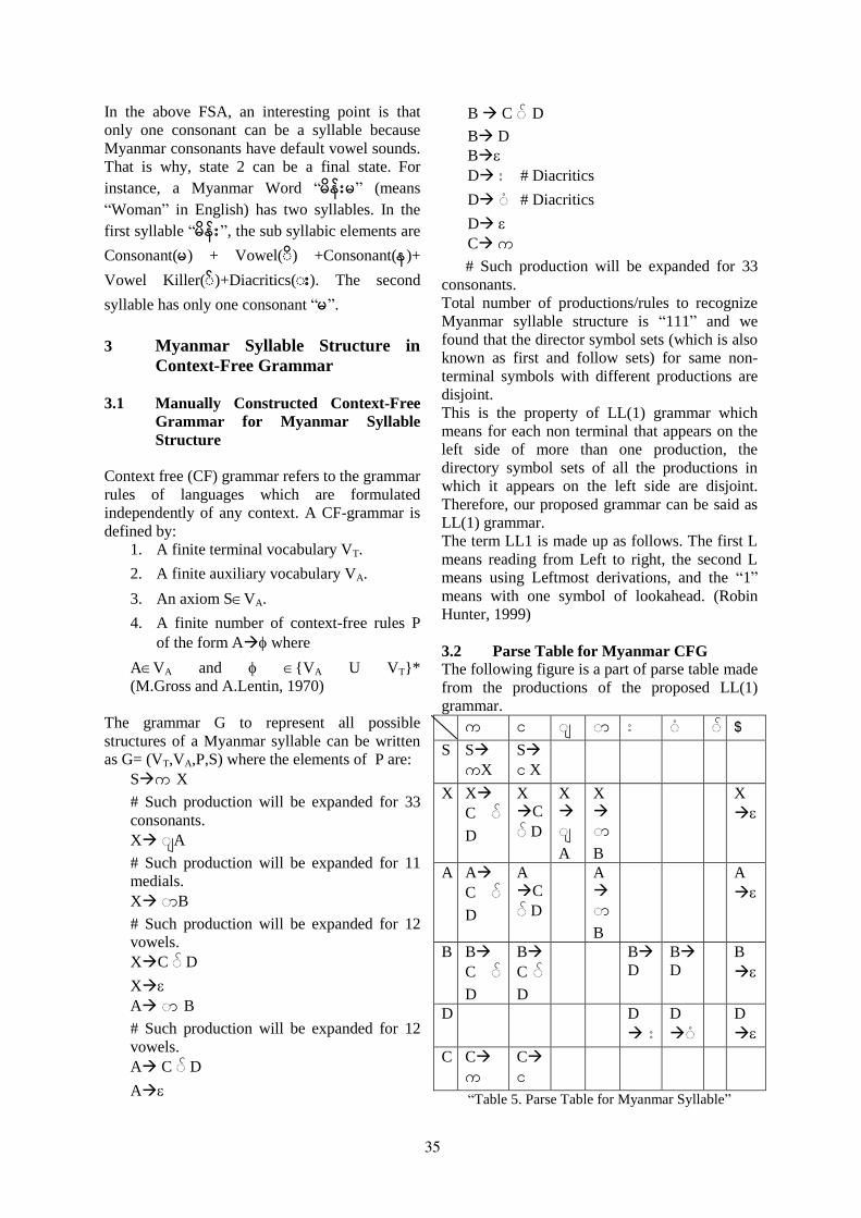
In the above FSA, an interesting point is that

only one consonant can be a syllable because

Myanmar consonants have default vowel sounds.

That is why, state 2 can be a final state. For

instance, a Myanmar Word “မ န မ” (means

“Woman” in English) has two syllables. In the

first syllable “မ န ”, the sub syllabic elements are

Consonant(မ) + Vowel( ) +Consonant(န)+

Vowel Killer( )+Diacritics( ). The second

syllable has only one consonant “မ”.

3 Myanmar Syllable Structure in

Context-Free Grammar

3.1 Manually Constructed Context-Free

Grammar for Myanmar Syllable

Structure

Context free (CF) grammar refers to the grammar

rules of languages which are formulated

independently of any context. A CF-grammar is

defined by:

1. A finite terminal vocabulary VT.

2. A finite auxiliary vocabulary VA.

3. An axiom SVA.

4. A finite number of context-free rules P

of the form A where

AVA and VA U VT*

(M.Gross and A.Lentin, 1970)

The grammar G to represent all possible

structures of a Myanmar syllable can be written

as G= (VT,VA,P,S) where the elements of P are:

Sက X

# Such production will be expanded for 33

consonants.

X A

# Such production will be expanded for 11

medials.

X B

# Such production will be expanded for 12

vowels.

XC D

X

A B

# Such production will be expanded for 12

vowels.

A C D

A

B C D

B D

B

D # Diacritics

D # Diacritics

D

C က # Such production will be expanded for 33

consonants.

Total number of productions/rules to recognize

Myanmar syllable structure is “111” and we

found that the director symbol sets (which is also

known as first and follow sets) for same non-

terminal symbols with different productions are

disjoint.

This is the property of LL(1) grammar which

means for each non terminal that appears on the

left side of more than one production, the

directory symbol sets of all the productions in

which it appears on the left side are disjoint.

Therefore, our proposed grammar can be said as

LL(1) grammar.

The term LL1 is made up as follows. The first L

means reading from Left to right, the second L

means using Leftmost derivations, and the “1”

means with one symbol of lookahead. (Robin

Hunter, 1999)

3.2 Parse Table for Myanmar CFG

The following figure is a part of parse table made

from the productions of the proposed LL(1)

grammar.

က င $

S S

ကX

S င X

X X

C D

X

C

D

X

A

X

B

X

A A

C D

A

C

D

A

B

A

B B

C D

B

C D

B

D

B

D

B

D D

D

D

C C က

C င

“Table 5. Parse Table for Myanmar Syllable”

35

In the above table, the topmost row represents

terminal symbols whereas the leftmost column

represents the non terminal symbols. The entries

in the table are productions to apply for each pair

of non terminal and terminal.

An example of Myanmar syllable having 4

different sub syllabic elements is parsed using

proposed grammar and the above parse table.

The parsing steps show proper working of the

proposed grammar and the detail of parsing a

syllable is as follows.

Input Syllable = က =က(C) + (M)+

(D)

Parse Stack Remaining Input Parser

Action

S $ က $ SကX

ကX $ က $ MATCH

က X $ က $ X A

က A $ က $ MATCH

က A $ က $ A B

က B $ က $ MATCH

က B $ က $ BD

က D $ က $ D က $ က $ MATCH

က $ $ SUCCESS

“Table 6. Parsing a Myanmar Syllable using

predictive top-down parsing method”

4 Conclusion

This study shows the powerfulness of

Chomsky`s context free grammar as it can apply

not only to describe the sentence structure but

also the syllable structure of an Asian script,

Myanmar. Though the number of productions in

the proposed grammar for Myanmar syllable is

large, the syntactic structure of a Myanmar

syllable is correctly recognized and the grammar

is not ambiguous.

Further, in parsing Myanmar syllable, it is

necessary to do preprocessing called contraction

for input sequences of vowels and consonant

conjuncts or medials to meet the requirements of

traditional writing systems. However, because of

these contracted forms, single lookahead symbol

in our proposed LL(1) grammar does not refer

exactly to one character and it may be a

combination of two or more characters in parsing

Myanmar syllable.

5 Discussion and Future Work

Myanmar script is syllabic as well as

aggulutinative script. Every Myanmar word or

sentence is composed of series of individual

syllables. Thus, it is critical to have efficient way

of recognizing syllables in conformity with the

rules of Myanmar traditional writing system.

Our intended research is the automatic

syllabification of Myanmar polysyllabic words

using formal language theory.

One option to do is to modify our current CFG to

recognize consecutive syllables as a first step.

We found that if the current CFG is changed for

sequence of syllables, the grammar can be no

longer LL(1). Then, we need to use one of the

statistical methods, for example, probabilistic

CFG, to choose correct productions or best parse

for finding syllable boundaries.

Again, it is necessary to calculate the probability

values for each production based on the

frequency of occurrence of a syllable in a

dictionary we referred or using TreeBank.

We need Myanmar corpus or a tree bank which

contains evidence for rule expansions for syllable

structure and such a resource does not yet exist

for Myanmar. And also, the time and cost for

constructing a corpus by ourselves came into

consideration.

Another approach is to construct finite state

transducer for automatic syllabification of

Myanmar words. If we choose this approach, we

firstly need to construct regular grammar to

recognize Myanmar syllables. We already have

Myanmar syllable structure in regular grammar.

However, for finite state syllabification using

weights, there is a lack of resource for training

database.

We still have many language specific issues to be

addressed for implementing Myanmar script

using CFG or FSA. As a first issue, our current

grammar is based on five basic sub-syllabic

elements and thus developing the grammar

which can handle all seven Myanmar sub

syllabic elements will be future study.

Our current grammar is based on the code point

values of the input syllables or words. Then, as a

second issue, we need to consider about different

presentations or code point values of same

character. Moreover, we have special writing

traditions for some characters, for example, such

36

as consonant stacking eg. ဗဒဓ (Buddha), မန တလေး (Mandalay, second capital of Myanmar),

consonant repetition eg. က (University),

kinzi eg. အငဂ (Cement), loan words eg.

ဘတ(စ) (bus). To represent such complex forms

in a computer system, we use invisible Virama

sign (U+1039). Therefore, it is necessary to

construct the productions which have conformity

with the stored character code sequence of

Myanmar Language.

References

John Okell. “ Burmese An Introduction to the Script”.

Northern Illinois University Press, 1994.

M.Gross, A.Lentin. “Introduction to Formal

Grammar”. Springer-Verlag, 1970.

Myanmar Language Commission. Myanmar

Orthography, Third Edition, University Press,

Yangon, Myanmar, 2006.

Noam Chomsky. “Syntactic Structures”. Mouton De

Gruyter, Berlin, 1957.

Peter T. Denials, William Bright. “World`s Writing

System”. Oxford University Press, 1996.

Robin Hunter. “The Essence of Compilers”. Prentice

Hall, 1999.

Tin Htay Hlaing, Yoshiki Mikami. “ Collation Weight

Design for Myanmar Unicode Texts” in Proceedings

of Human Language Technology for Development

organized by PAN Localization- Asia, AnLoc –

Africa, IDRC – Canada. May 2011, Alexandria,

EGYPT, Page 1- 6.

37

Proceedings of the EACL 2012 Student Research Workshop, pages 38–45,Avignon, France, 26 April 2012. c©2012 Association for Computational Linguistics

What’s in a Name?Entity Type Variation across Two Biomedical Subdomains

Claudiu Mihaila and Riza Theresa Batista-NavarroNational Centre for Text Mining

School of Computer Science, University of ManchesterManchester Interdisciplinary Biocentre,

131 Princess Street, M1 7DN, Manchester, UKclaudiu.mihaila@cs.man.ac.uk

riza.batista-navarro@cs.man.ac.uk

Abstract

There are lexical, syntactic, semantic anddiscourse variations amongst the languagesused in various biomedical subdomains. Itis important to recognise such differencesand understand that biomedical tools thatwork well on some subdomains may notwork as well on others. We report hereon the semantic variations that occur inthe sublanguages of two biomedical subdo-mains, i.e. cell biology and pharmacology,at the level of named entity information. Bybuilding a classifier using ratios of namedentities as features, we show that named en-tity information can discriminate betweendocuments from each subdomain. Morespecifically, our classifier can distinguishbetween documents belonging to each sub-domain with an accuracy of 91.1% F-score.

1 Introduction

Biomedical information extraction efforts in thepast decade have focussed on fundamental tasksneeded to create intelligent systems capableof improving search engine results and easingthe work of biologists. More specifically, re-searchers have concentrated mainly on named en-tity recognition, mapping them to concepts incurated databases (Krallinger et al., 2008) andextracting simple binary relations between enti-ties. Recently, an increasing number of resourcesthat facilitate the training of systems to extractmore detailed information have become available,e.g., PennBioIE (Kulick et al., 2004), GENE-TAG (Tanabe et al., 2005), BioInfer (Pyysalo etal., 2007), GENIA (Kim et al., 2008), GREC(Thompson et al., 2009) and Metaknowledge GE-NIA (Thompson et al., 2011). Moreover, several

other annotated corpora have been developed forshared task purposes, such as BioCreative I, II, III(Arighi et al., 2011) and BioNLP Shared Tasks2009 and 2011 (Cohen et al., 2009; Kim et al.,2011).

Many of the tools currently used for biomedi-cal language processing were trained and evalu-ated on such popular corpora, most of which con-sist of documents from the molecular biology sub-domain. However, previous studies (discussed inSection 2) have established that different biomed-ical sublanguages exhibit linguistic variations. Itfollows that tools which were developed and eval-uated on corpora derived from one subdomainmight not always perform as well on corpora fromother subdomains. Understanding these linguisticvariations is essential to the process of adaptat-ing natural language processing tools to new do-mains.

In this paper, we highlight the variations be-tween biomedical sublanguages by focussing onthe different types of named entities (NEs) thatare relevant to them. We show that the frequen-cies of different named entity types vary enoughto allow a classifier for scientific subdomains tobe built based upon them.

The study is performed on open access jour-nal articles present in the UK PubMed Central1

(UKPMC) (McEntyre et al., 2010), an articledatabase that extends the functionality of the orig-inal PubMed Central (PMC) repository2. Thisdatabase was chosen as our source, since most ofthe documents within it are already tagged withnamed entity information. We report here on theresults obtained for two biomedical subdomains,

1http://ukpmc.ac.uk/2http://www.ncbi.nlm.nih.gov/pmc

38

i.e. cell biology and pharmacology. Our focus onthese two particular subdomains is motivated byan increasing interest expressed by the biomedi-cal research community, according to recent find-ings that have shown their relevance to discover-ing possible causes and treatments for incurablediseases, such as cancer or Alzheimer’s Disease.

2 Related work

Harris (1968) introduced a formalisation of thenotion of sublanguage, which was defined as asubset of general language. According to thistheory, it is possible to process specialised lan-guages, since they have a structure that can be ex-pressed in a computable form. More recently, sev-eral works on the study of biomedical languagessubstantiated his theory.

For instance, Sager et al. (1987) worked onpharmacological literature and lipid metabolism,whereas Friedman et al. (2002) analysed the prop-erties of clinical and biomolecular sublanguages.

Other studies have investigated the differ-ences between general and biomedical lan-guages by focussing on specific linguistic aspects,such as verb-argument relations and pronomi-nal anaphora. For instance, Wattarujeekrit et al.(2004) analysed the predicate-argument structuresof 30 verbs used in biomedical articles. Their re-sults suggest that, in certain cases, a significantdifference exists in the predicate frames comparedto those obtained from analysing news articles inthe PropBank project (Palmer et al., 2005). Sim-ilarly, based on the GENIA and PennBioIE cor-pora, Cohen et al. (2008) performed a study ofargument realisation with respect to the nominal-isation and alternation of biomedical verbs. Theyconcluded that there is a high occurrence of thesephenomena in this semantically restricted do-main, and underline that this sublanguage modelapplies only to biomedical language.

Taking a different angle, Nguyen and Kim(2008) examined the differences in the use ofpronouns by studying general domains (MUCand ACE) and one biomedical domain (GENIA).They observed that compared to the MUC andACE corpora, the GENIA corpus has significantlymore occurrences of neutral and third-person pro-nouns, whilst first and second person pronounsare non-existent.

Verspoor et al. (2009) measured lexical andstructural variation in biomedical Open Access

journals and subscription-based journals, con-cluding that there are no significant differencesbetween them. Therefore, a model trained on oneof these sources can be used successfully on theother, as long as the subject matter is maintained.Furthermore, they compared a mouse genomicscorpus with two reference corpora, one composedof newswire texts and another of general biomed-ical articles. In this case, unsurprisingly, signifi-cant differences were found across many linguis-tic dimensions. Relevant to our study is the com-parison between the more specific mouse genomecorpus to the more general biomedical one: whilstsimilar from some points of view, such as nega-tion and passivisation, they differ in sentencelength and semantic features, such as the presenceof various named entities.

Our work is most similar to that of Lippincottet al. (2011), in which a clustering-based quantita-tive analysis of the linguistic variations across 38different biomedical sublanguages is presented.They investigated four dimensions relevant to theperformance of NLP systems, i.e. vocabulary,syntax, semantics and discourse structure. Withregard to semantic features, the authors induceda topic model using Latent Dirichlet Analysis foreach word, and then extended the model to docu-ments and subdomains according to observed dis-tributions. Their conclusion is that a machinelearning system is able to create robust clustersof subdomains, thus proving their hypothesis thatthe commonly used molecular biology subdomainis not representative of the domain as a whole.

In contrast, we examine the differences be-tween biomedical sublanguages at the semanticlevel, using only named entities. Furthermore,we choose to perform our analysis only on twosubdomains (i.e. cell biology and pharmacology),and try to classify these by using supervised ma-chine learning algorithms.

3 Methodology

We designed an experiment in which various ma-chine learning algorithms are trained and testedon data obtained from open access journal arti-cles. Firstly, a corpus of articles was created (Sec-tion 3.1), after which the documents were auto-matically annotated with named entities (Section3.2). We then extracted a number features rele-vant to the named entities present in the corpus(Section 3.3).

39

3.1 Corpus development

Our corpus was created by first searching theNLM Catalog3 for journals whose Broad Sub-ject Term attributes contain only cell biology orpharmacology, and then narrowing down the re-sults to those which are in English and avail-able via PubMed Central. Also, since we areconcentrating on full-text documents, we retainedonly those journals that are available within thePubMed Open Access subset4. According to thisprocedure, we obtained a final list of two journalsfor cell biology and six for pharmacology.

Using the PMC IDs of all articles publishedin the selected journals, we retrieved documentsfrom UK PubMed Central. This database waschosen as our source as the documents it containsare already tagged with named entity information.A total of 360 articles was retrieved for each cat-egory, i.e. cell biology and pharmacology.

The retrieved documents were encoded inXML format. Several unusable fragments wereremoved before converting them to plain text. Ex-amples of such fragments are article metadata (au-thors, their affiliations, publishing history, etc.),tables, figures and references. Table 1 shows thestatistics regarding the corpus following the ap-plication of the pre-processing step. In the caseof pharmacology, the document collection con-tains almost 1.4 million words, whilst the set ofcell biology articles consists of almost 2.5 millionwords. The ratio of named entities to the totalnumber of words is almost the same in the twocollections, i.e. about 10%.

Subdomain Cell biology PharmacologyNo. of docs. 360 360No. of words 2.49 m. 1.35 m.No. of NEs 231761 103484

Table 1: Named entity types and their source.

3.2 Tagging of Named Entities

To extract named entities from the corpus, weused a simple method that augments the namedentities present in the UKPMC articles with theoutput of two named entity recognition tools

3http://www.ncbi.nlm.nih.gov/nlmcatalog

4http://www.ncbi.nlm.nih.gov/pmc/tools/openftlist

(NERs), i.e. NeMine and OSCAR. The types ofentities in the output be each of the two tools, to-gether with the NE types present in the UKPMCarticles, are summarised in Table 2.

Named entities in the UKPMC database wereidentified using NeMine (Sasaki et al., 2008), adictionary-based statistical named entity recogni-tion system. This system was later extended andused by Nobata et al. (2009) to recognise moretypes, such as phenomena, processes, organs andsymptoms. We used this most recent version ofthe software as our second source of more diverseentity types.

The Open-Source Chemistry Analysis Rou-tines (OSCAR) software (Jessop et al., 2011) isa toolkit for the recognition of named entities anddata in chemistry publications. Currently in itsfourth version, it uses three types of chemical en-tity recognisers, namely regular expressions, pat-terns and Maximum Entropy Markov models.

In total, 20 different classes of entities wereconsidered in this study. However, due to thecombination of several NERs, some NE types areidentified by more than one NER. Furthermore,some of the NE types are more general and coverother more specific types, which are also anno-tated by one or mroe of the tools. This can lead todouble annotation. For instance, the Gene|Proteintype is more general than both Gene and Protein,whereas the Chemical molecule type is a hyper-nym of Gene, Protein, Drug and Metabolite. Inthe case of multiple annotations over the samespan of text, we removed the more general labels,so that each NE has only one label. Contradictorycases, where two NERs label one NE with com-pletely different tags, were not found.

After augmenting the existing NEs by runningthe two NER tools on the corpus, the outputs werecombined to give a single “silver” annotation list.This operation was performed by computing themathematical union of the three individual anno-tation sets, as shown in Equation 1.

ASilver = AUKPMC ∪ AOscar ∪ ANeMine (1)

Table 3 shows the ratios of named entities to thenumber of words in each subcorpus. The ≈ signindicates strictly positive percentages, but whichare rounded down to zero in this table for for-matting purposes. In the four places where it oc-curs, the percentages lie between 0% and 0.005%,

40

Type UKPMC NeMine OSCARGene X XProtein X XGene|Protein XDisease X XDrug X XMetabolite X XBacteria XDiagnostic process XGeneral phenomenon XHuman phenomenon XIndicator XNatural phenomenon XOrgan XPathologic function XSymptom XTherapeutic process XChemical molecule XChemical adjective XEnzyme XReaction X

Table 2: Named entity types and their source.

exclusively. It can be observed that some entitytypes have approximately the same percentages inthe two subdomains, e.g. phenomena and reac-tions. However, large differences can be observedin the case of some of the other entity types. Forinstance, chemical molecules occur twice as of-ten in pharmacology articles than in cell biology,whereas proteins appear almost three times moreoften in cell biology than in pharmacology.

3.3 Experimental setup

Using the corpus described previously, we cre-ated a training set for supervised machine learn-ing algorithms. Every document in the corpuswas transformed into a vector consisting of 20features. Each of these features corresponds toan entity type in Table 2, having a numeric valueranging from 0 to 1. This number represents theratio of the specific entity type to the total numberof named entities recognised in that document, asshown in Equation 2.

θ =ntype

N(2)

where ntype represents the number of NEs of acertain type in a document and N represents thetotal number of NEs in that document.

Furthermore, each vector was labelled with thesubdomain to which the respective document be-longs (i.e., cell biology or pharmacology).

Weka (Witten and Frank, 2005; Hall et al.,2009) was employed as the machine learningframework, due to its large variety of classifica-tion algorithms. We experimented with a largenumber of classifiers, ranging from Bayesian netsto functions, decision trees, decision rules andmeta-classifiers. The best performing classifiersare shown in Table 4. BayesNet is an implemen-tation of Bayesian Networks, SMO is an imple-mentation of Support Vector Machines, J48 is animplementation of decision trees, whilst Jrip is animplementation of decision rules. Random For-est is an ensemble classifier that consists of manydecision trees (in this study, J48 was used), out-putting the class that occurs most frequently in theoutput of individual trees.

The baseline that has been used is ZeroR, a sim-ple algorithm that classifies all instances as per-taining to the majority class. Since our classeshave equal numbers of instances, the F-score ofZeroR is 50%.

41

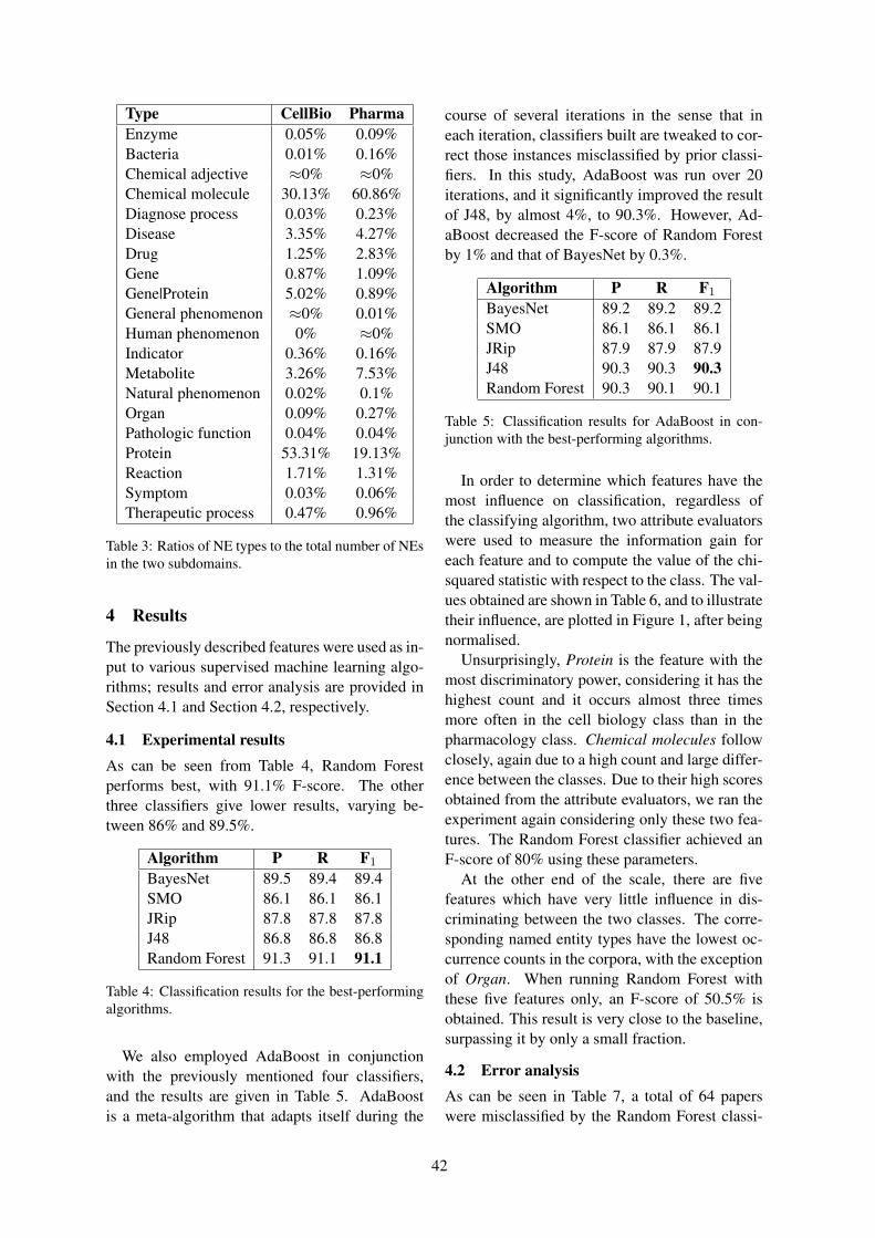
Type CellBio PharmaEnzyme 0.05% 0.09%Bacteria 0.01% 0.16%Chemical adjective ≈0% ≈0%Chemical molecule 30.13% 60.86%Diagnose process 0.03% 0.23%Disease 3.35% 4.27%Drug 1.25% 2.83%Gene 0.87% 1.09%Gene|Protein 5.02% 0.89%General phenomenon ≈0% 0.01%Human phenomenon 0% ≈0%Indicator 0.36% 0.16%Metabolite 3.26% 7.53%Natural phenomenon 0.02% 0.1%Organ 0.09% 0.27%Pathologic function 0.04% 0.04%Protein 53.31% 19.13%Reaction 1.71% 1.31%Symptom 0.03% 0.06%Therapeutic process 0.47% 0.96%

Table 3: Ratios of NE types to the total number of NEsin the two subdomains.

4 Results

The previously described features were used as in-put to various supervised machine learning algo-rithms; results and error analysis are provided inSection 4.1 and Section 4.2, respectively.

4.1 Experimental resultsAs can be seen from Table 4, Random Forestperforms best, with 91.1% F-score. The otherthree classifiers give lower results, varying be-tween 86% and 89.5%.

Algorithm P R F1

BayesNet 89.5 89.4 89.4SMO 86.1 86.1 86.1JRip 87.8 87.8 87.8J48 86.8 86.8 86.8Random Forest 91.3 91.1 91.1

Table 4: Classification results for the best-performingalgorithms.

We also employed AdaBoost in conjunctionwith the previously mentioned four classifiers,and the results are given in Table 5. AdaBoostis a meta-algorithm that adapts itself during the

course of several iterations in the sense that ineach iteration, classifiers built are tweaked to cor-rect those instances misclassified by prior classi-fiers. In this study, AdaBoost was run over 20iterations, and it significantly improved the resultof J48, by almost 4%, to 90.3%. However, Ad-aBoost decreased the F-score of Random Forestby 1% and that of BayesNet by 0.3%.

Algorithm P R F1

BayesNet 89.2 89.2 89.2SMO 86.1 86.1 86.1JRip 87.9 87.9 87.9J48 90.3 90.3 90.3Random Forest 90.3 90.1 90.1

Table 5: Classification results for AdaBoost in con-junction with the best-performing algorithms.

In order to determine which features have themost influence on classification, regardless ofthe classifying algorithm, two attribute evaluatorswere used to measure the information gain foreach feature and to compute the value of the chi-squared statistic with respect to the class. The val-ues obtained are shown in Table 6, and to illustratetheir influence, are plotted in Figure 1, after beingnormalised.

Unsurprisingly, Protein is the feature with themost discriminatory power, considering it has thehighest count and it occurs almost three timesmore often in the cell biology class than in thepharmacology class. Chemical molecules followclosely, again due to a high count and large differ-ence between the classes. Due to their high scoresobtained from the attribute evaluators, we ran theexperiment again considering only these two fea-tures. The Random Forest classifier achieved anF-score of 80% using these parameters.

At the other end of the scale, there are fivefeatures which have very little influence in dis-criminating between the two classes. The corre-sponding named entity types have the lowest oc-currence counts in the corpora, with the exceptionof Organ. When running Random Forest withthese five features only, an F-score of 50.5% isobtained. This result is very close to the baseline,surpassing it by only a small fraction.

4.2 Error analysisAs can be seen in Table 7, a total of 64 paperswere misclassified by the Random Forest classi-

42

Attribute InfoGain ChiSquareProtein 0.4482 386.5648Chemical molecule 0.3169 272.0111Gene|Protein 0.2265 211.8034Indicator 0.1805 170.0186Gene 0.1718 156.9504Metabolite 0.1667 155.8135Reaction 0.1545 144.6946Drug 0.1301 124.2604Therapeutic process 0.1259 111.4571Disease 0.1189 111.1882Chemical adjective 0.0642 55.5556Enzyme 0.0473 41.089Diagnostic process 0.0388 32.1161Bacteria 0.0297 26.0522Natural phenomenon 0.0227 20.8004Pathologic function 0 0Symptom 0 0General phenomenon 0 0Organ 0 0Human phenomenon 0 0

Table 6: Attribute selection output from two attributeevaluators.

fier, the best performing algorithm. Of these, 45(i.e. 70%) are cell biology papers which were in-correctly classified as belonging to pharmacology,whilst the remaining 19 belong to the pharmacol-ogy class and are classified as cell biology.

Labelled as Cell_bio PharmaCell_bio 315 19Pharma 45 341

Table 7: Confusion matrix for the Random Forest clas-sifier.

As previously mentioned, the two features thatachieved the highest information gain are the ra-tios for the Protein and Chemical molecule types.Accordingly, only these two features were consid-ered in this error analysis.

We firstly examined the features of the cellbiology documents which were incorrectly clas-sified as pharmacology papers. It was notice-able that the majority of the misclassified doc-uments in this case have a small percentage ofProteins (less than 0.35) and/or a large percent-age of Chemical molecules (greater than 0.58). Toconfirm this observation, a sample of documents

0

0.05

0.1

0.15

0.2

0.25

0.3

0.35

0.4

0.45InfoGain

ChiSquare

Pro

tein

Che

mic

al m

olec

ule

Gen

e|P

rote

inIn

dica

tor

Gen

eM

etab

olite

Rea

ctio

nD

rug

Ther

apeu

tic p

roce

ssD

isea

se

Che

mic

al a

djec

tive

Enz

yme

Dia

gnos

tic p

roce

ssB

acte

ria

Nat

ural

phe

nom

enon

Pat

holo

gic

func

tion

Sym

ptom

Gen

eral

phe

nom

enon

Org

an

Hum

an p

heno

men

on

Figure 1: Normalised attribute selection output fromtwo attribute evaluators.

was accessed via the PubMed Central page whichprovides links to identified entities such as com-pounds, substances, genes and proteins. For in-stance, the misclassified cell biology paper withPMCID 2755470 was found to have no proteins,whilst the one with PMCID 2679709 has quite alarge number of substances (chemical molecules).

We also analysed the features of papers in thepharmacology subdomain which were misclassi-fied as cell biology documents. In contrast tothe first type of misclassification, these documentshave a large percentage of Proteins and/or smallpercentage of Chemical molecules. For example,the pharmacology paper with PMCID 2817930contains many protein instances, whilst the onewith PMCID 2680808 has no mentions of chemi-cal molecules.

5 Conclusions and Future Work

We have shown that with the help of named en-tity identification, classifiers can be built that areable to distinguish between papers belonging todifferent biomedical subdomains. The RandomForest algorithm is able to discriminate betweencell biology and pharmacology open-access full-text articles with an F-score of 91%. This resultsupports the hypothesis that sublanguages used indifferent biomedical domains exhibit significantsemantic variations. Such variations should there-fore be considered when adapting automated tools

43

developed for a particular subdomain to new sub-domains.

One possible future direction is to analyse mul-tiple medical subdomains, such as neurology, vi-rology and critical care. This could enable themeasurement of the distance between various sub-domains with respect to specific named entitytypes. Furthermore, a comparison of the methoddescribed above with those using bag-of-wordsor other non-semantic features could further en-force the importance of named entities in doc-ument classification and sublanguage identifica-tion.

Acknowledgements

We would like to acknowledge the help givenby Dr. C.J. Rupp in obtaining the collection ofdocuments from the Open Access section of theUKMPC.

ReferencesCecilia Arighi, Zhiyong Lu, Martin Krallinger, Kevin

Cohen, W Wilbur, Alfonso Valencia, LynetteHirschman, and Cathy Wu. 2011. Overview ofthe BioCreative III Workshop. BMC Bioinformat-ics, 12(Suppl 8):S1.

Kevin Bretonnel Cohen, Martha Palmer, and LawrenceHunter. 2008. Nominalization and alternations inbiomedical language. PLoS ONE, 3(9):e3158, 09.

Kevin Bretonnel Cohen, Dina Demner-Fushman,Sophia Ananiadou, John Pestian, Jun’ichi Tsujii,and Bonnie Webber, editors. 2009. Proceedings ofthe BioNLP 2009 Workshop. Association for Com-putational Linguistics, Boulder, Colorado, June.

Carol Friedman, Pauline Kra, and Andrey Rzhetsky.2002. Two biomedical sublanguages: a descriptionbased on the theories of Zellig Harris. Journal ofBiomedical Informatics, 35(4):222–235.

Mark Hall, Eibe Frank, Geoffrey Holmes, BernhardPfahringer, Peter Reutemann, and Ian H. Witten.2009. The weka data mining software: An update.SIGKDD Explorations, 11(1).

Zellig Harris. 1968. Mathematical Structures of Lan-guage. John Wiley and Son, New York.

David Jessop, Sam Adams, Egon Willighagen, LezanHawizy, and Peter Murray-Rust. 2011. Oscar4:a flexible architecture for chemical text-mining.Journal of Cheminformatics, 3(1):41.

Jin-Dong Kim, Tomoko Ohta, and Jun’ichi Tsujii.2008. Corpus annotation for mining biomedi-cal events from literature. BMC Bioinformatics,9(1):10.

Jin-Dong Kim, Yue Wang, Toshihisa Takagi, and Aki-nori Yonezawa. 2011. Overview of genia eventtask in bionlp shared task 2011. In Proceedingsof BioNLP Shared Task 2011 Workshop, pages 7–15, Portland, Oregon, USA, June. Association forComputational Linguistics.

Martin Krallinger, Alexander Morgan, Larry Smith,Florian Leitner, Lorraine Tanabe, John Wilbur,Lynette Hirschman, and Alfonso Valencia. 2008.Evaluation of text-mining systems for biology:overview of the second biocreative communitychallenge. Genome Biology, 9(Suppl 2):S1.

Seth Kulick, Ann Bies, Mark Liberman, Mark Mandel,Ryan McDonald, Martha Palmer, Andrew Schein,and Lyle Ungar. 2004. Integrated annotation forbiomedical information extraction. In Proceedingsof the BioLINK 2004.

Thomas Lippincott, Diarmuid Seaghdha, and AnnaKorhonen. 2011. Exploring subdomain varia-tion in biomedical language. BMC Bioinformatics,12(1):212.

Johanna R. McEntyre, Sophia Ananiadou, StephenAndrews, William J. Black, Richard Boulderstone,Paula Buttery, David Chaplin, Sandeepreddy Che-vuru, Norman Cobley, Lee-Ann Coleman, PaulDavey, Bharti Gupta, Lesley Haji-Gholam, CraigHawkins, Alan Horne, Simon J. Hubbard, Jee-Hyub Kim, Ian Lewin, Vic Lyte, Ross MacIn-tyre, Sami Mansoor, Linda Mason, John Mc-Naught, Elizabeth Newbold, Chikashi Nobata,Ernest Ong, Sharmila Pillai, Dietrich Rebholz-Schuhmann, Heather Rosie, Rob Rowbotham, C. J.Rupp, Peter Stoehr, and Philip Vaughan. 2010.UKPMC: a full text article resource for the life sci-ences. Nucleic Acids Research.

Ngan L. T. Nguyen and Jin-Dong Kim. 2008. Explor-ing domain differences for the design of pronounresolution systems for biomedical text. In Proceed-ings of the 22nd International Conference on Com-putational Linguistics - Volume 1, COLING ’08,pages 625–632, Stroudsburg, PA, USA. Associationfor Computational Linguistics.

Chikashi Nobata, Yutaka Sasaki, Noaki Okazaki,C. J. Rupp, Jun’ichi Tsujii, and Sophia Ananiadou.2009. Semantic search on digital document reposi-tories based on text mining results. In InternationalConferences on Digital Libraries and the SemanticWeb 2009 (ICSD2009), pages 34–48.

Martha Palmer, Daniel Gildea, and Paul Kingsbury.2005. The proposition bank: An annotated cor-pus of semantic roles. Computational Linguistics,31(1):71–105.

Sampo Pyysalo, Filip Ginter, Juho Heimonen, JariBjorne, Jorma Boberg, Jouni Jarvinen, and TapioSalakoski. 2007. BioInfer: a corpus for infor-mation extraction in the biomedical domain. BMCBioinformatics, 8(1):50.

44

Naomi Sager, Carol Friedman, and Margaret Lyman.1987. Medical Language Processing: ComputerManagement of Narrative Data. Addison-Wesley,Reading, MA.

Yutaka Sasaki, Yoshimasa Tsuruoka, John McNaught,and Sophia Ananiadou. 2008. How to make themost of NE dictionaries in statistical NER. BMCBioinformatics, 9(Suppl 11):S5.

Lorraine Tanabe, Natalie Xie, Lynne Thom, WayneMatten, and W John Wilbur. 2005. GENETAG: atagged corpus for gene/protein named entity recog-nition. BMC Bioinformatics, 6(Suppl 1):S3.

Paul Thompson, Syed Iqbal, John McNaught, andSophia Ananiadou. 2009. Construction of an an-notated corpus to support biomedical informationextraction. BMC Bioinformatics, 10(1):349.

Paul Thompson, Raheel Nawaz, John McNaught, andSophia Ananiadou. 2011. Enriching a biomedi-cal event corpus with meta-knowledge annotation.BMC Bioinformatics, 12(1):393.

Karin Verspoor, Kevin Bretonnel Cohen, andLawrence Hunter. 2009. The textual characteristicsof traditional and open access scientific journals aresimilar. BMC Bioinformatics, 10(1):183.

Tuangthong Wattarujeekrit, Parantu Shah, and NigelCollier. 2004. PASBio: predicate-argument struc-tures for event extraction in molecular biology.BMC Bioinformatics, 5(1):155.

Ian Witten and Eibe Frank. 2005. Data Mining: Prac-tical Machine Learning Tools and Techniques (Sec-ond Edition). Morgan Kaufmann.

45

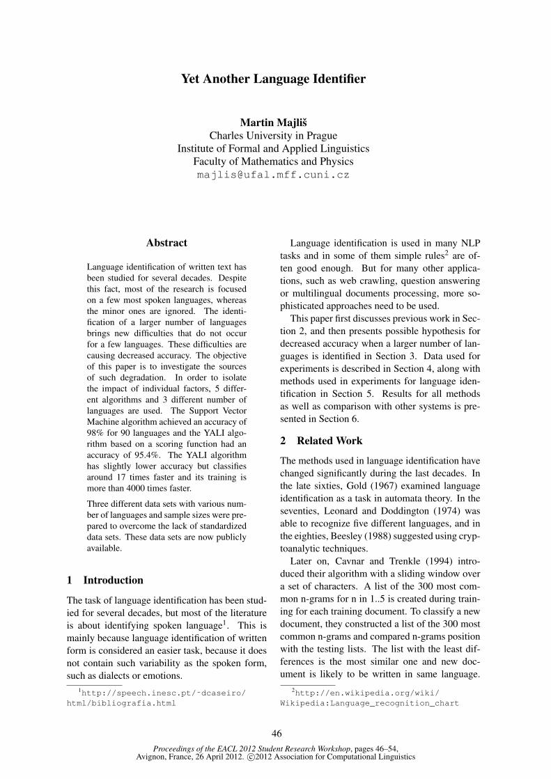
Proceedings of the EACL 2012 Student Research Workshop, pages 46–54,Avignon, France, 26 April 2012. c©2012 Association for Computational Linguistics

Yet Another Language Identifier

Martin MajlisCharles University in Prague

Institute of Formal and Applied LinguisticsFaculty of Mathematics and Physicsmajlis@ufal.mff.cuni.cz

Abstract

Language identification of written text hasbeen studied for several decades. Despitethis fact, most of the research is focusedon a few most spoken languages, whereasthe minor ones are ignored. The identi-fication of a larger number of languagesbrings new difficulties that do not occurfor a few languages. These difficulties arecausing decreased accuracy. The objectiveof this paper is to investigate the sourcesof such degradation. In order to isolatethe impact of individual factors, 5 differ-ent algorithms and 3 different number oflanguages are used. The Support VectorMachine algorithm achieved an accuracy of98% for 90 languages and the YALI algo-rithm based on a scoring function had anaccuracy of 95.4%. The YALI algorithmhas slightly lower accuracy but classifiesaround 17 times faster and its training ismore than 4000 times faster.

Three different data sets with various num-ber of languages and sample sizes were pre-pared to overcome the lack of standardizeddata sets. These data sets are now publiclyavailable.

1 Introduction

The task of language identification has been stud-ied for several decades, but most of the literatureis about identifying spoken language1. This ismainly because language identification of writtenform is considered an easier task, because it doesnot contain such variability as the spoken form,such as dialects or emotions.

1http://speech.inesc.pt/˜dcaseiro/html/bibliografia.html

Language identification is used in many NLPtasks and in some of them simple rules2 are of-ten good enough. But for many other applica-tions, such as web crawling, question answeringor multilingual documents processing, more so-phisticated approaches need to be used.

This paper first discusses previous work in Sec-tion 2, and then presents possible hypothesis fordecreased accuracy when a larger number of lan-guages is identified in Section 3. Data used forexperiments is described in Section 4, along withmethods used in experiments for language iden-tification in Section 5. Results for all methodsas well as comparison with other systems is pre-sented in Section 6.

2 Related Work

The methods used in language identification havechanged significantly during the last decades. Inthe late sixties, Gold (1967) examined languageidentification as a task in automata theory. In theseventies, Leonard and Doddington (1974) wasable to recognize five different languages, and inthe eighties, Beesley (1988) suggested using cryp-toanalytic techniques.

Later on, Cavnar and Trenkle (1994) intro-duced their algorithm with a sliding window overa set of characters. A list of the 300 most com-mon n-grams for n in 1..5 is created during train-ing for each training document. To classify a newdocument, they constructed a list of the 300 mostcommon n-grams and compared n-grams positionwith the testing lists. The list with the least dif-ferences is the most similar one and new doc-ument is likely to be written in same language.

2http://en.wikipedia.org/wiki/Wikipedia:Language_recognition_chart

46

They classified 3478 samples in 14 languagesfrom a newsgroup and reported an achieved accu-racy of 99.8%. This influenced many researchesthat were trying different heuristics for selectingn-grams, such as Martins and Silva (2005) whichachieved an accuracy of 91.25% for 12 languages,or Hayati (2004) with 93.9% for 11 languages.

Sibun and Reynar (1996) introduced a methodfor language detection based on relative entropy, apopular measure also known as Kullback-Leiblerdistance. Relative entropy is a useful measureof the similarity between probability distributions.She used texts in 18 languages from the EuropeanCorpus Initiative CD-ROM. She achieved a 100%accuracy for bigrams.

In recent years, standard classification tech-niques such as support vector machines also be-came popular and many researchers used themKruengkrai et al. (2005) or Baldwin and Lui(2010) for identifying languages.

Nowadays, language recognition is consideredas an elementary NLP task3 which can be usedfor educational purposes. McNamee (2005) usedsingle documents for each language from projectGutenberg in 10 European languages. He prepro-cessed the training documents – the texts werelower-cased, accent marks were retained. Then,he computed a so-called profile of each language.Each profile consisted of a percentage of the train-ing data attributed to each observed word. Fortesting, he used 1000 sentences per language fromthe Euro-parliament collection. To classify a newdocument, the same preprocessing was done andinner product based on the words in the documentand the 1000 most common words in each lan-guage was computed. Performance varied from80.0% for Portuguese to 99.5% for German.

Some researches such as Hughes et al. (2006)or Grothe et al. (2008) focused in their paperson the comparison of different approaches to lan-guage identification and also proposed new goalsin that field, such as as minority languages or lan-guages written non-Roman script.

Most of the researches in the past identifiedmostly up to twenty languages but in recentyears, language identification of minority lan-guages became the focus of Baldwin and Lui(2010), Choong et al. (2011), and Majlis (2012).All of them observed that the task became much

3http://alias-i.com/lingpipe/demos/tutorial/langid/read-me.html

harder for larger numbers of languages and accu-racy of the system dropped.

3 Hypothesis

The accuracy degradation with a larger number oflanguages in the language identification systemmay have many reasons. This section discussesthese reasons and suggests how to isolate them.In some hypotheses, charts involving data fromthe W2C Wiki Corpus are used, which are intro-duced in Section 4.

3.1 Training Data SizeIn many NLP applications, size of the availabletraining data influences overall performance ofthe system, as was shown by Halevy et al. (2009).

To investigate the influence of training datasize, we decided to use two different sizes of train-ing data – 1 MB and 4 MB. If the drop in accu-racy is caused by the lack of training data, thenall methods used on 4 MB should outperform thesame methods used on 1 MB of data.

3.2 Language DiversityThe increasing number of languages recognisedby the system decreases language diversity. Thismay be another reason for the observed dropin the accuracy. We used information aboutlanguage classes from the Ethnologue website(Lewis, 2009). The number of different languageclasses is depicted in Figure 1. Class 1 representsthe most distinguishable classes, such as Indo-European vs. Japonic, while Class 2 representsfiner classification, such as Indo-European, Ger-manic vs. Indo-European, Italic.

0

5

10

15

20

25

30

10 20 30 40 50 60 70 80 90

La

ng

ua

ge

Fa

mili

es

Languages

Class 1Class 2

Figure 1: Language diversity on Wikipedia. Lan-guages are sorted according to their text corpus size.

The first 52 languages belong to 15 differentClass 1 classes and the number of classes does not

47

change until the 77th language, when the Swahililanguage from class Niger-Congo appears.

3.3 ScalabilityAnother issue with increasing number of lan-guages is the scalability of used methods. Thereare several pitfalls for machine learning algo-rithms – a) many languages may require manyfeatures which may lead to failures caused bycurse-of-dimensionality, b) differences in lan-guages may shrink, so the classifier will be forcedto learn minor differences and will lose its abil-ity to generalise, and become overfitted, and c)the classifier may internally use only binary clas-sifiers which may lead up to quadratic complexity(Dimitriadou et al., 2011).

4 Data Sets

For our experiments, we decided to use the W2CWiki Corpus (Majlis, 2012) which contains arti-cles from Wikipedia. The total size of all textswas 8 GB and available material for various lan-guages differed significantly, as is displayed inFigure 2.

0

50

100

150

200

250

300

350

400

450

10 20 30 40 50 60 70 80 90

Siz

e in

MB

Language

W2C Wiki Corpus - Size in MB

Figure 2: Available data in the W2C Wiki Corpus.Languages are sorted according to their size in the cor-pus.

We used this corpus to prepare 3 different datasets. We used one of them for testing hypothesispresented in the previous section and the remain-ing two for comparison with other systems. Thesedata sets contain samples of length approximately30, 140, and 1000 bytes. The sample of length 30represents image caption or book title, the sampleof length 140 represents tweet or user comment,and sample of length 1000 represents newspaperarticle.

All datasets are available at http://ufal.mff.cuni.cz/˜majlis/yali/.

4.1 Long

The main purpose of this data set (yali-dataset-long) was testing hypothesis described in the pre-vious section.

To investigate the drop, we intended to coveraround 100 languages, but the amount of availabledata limited us. For example, the 80th languagehas 12 MB, whereas the 90th has 6 MB and tbe100th has only 1 MB of text. To investigate thehypothesis of the influence of training data size,we decided to build a 1 MB and 4 MB corpus foreach language, where the 1 MB corpus is a subsetof the 4 MB one.

Then, we divided the corpus for each languageinto chunks with 1000 bytes of text, so we gained1000 and 4000 chunks respectively. These chunkswere divided into training and testing sets in a90:10 ratio, thus we had 900 and 3600 train-ing chunks, respectively, and 100 and 400 testingchunks respectively.

To reduce the risk that the training and testingare influenced by the position from which theywere taken (the beginning or the end of the cor-pus), we decided to use every 10th sentence as atesting one and use the remaining ones for train-ing.

Then, we created an n-gram for n in 1..4 fre-quency list for each language, each corpus size.From each frequency list, we preserved only thefirst m = 100 most frequent n-grams. For exam-ple, from the raw frequency list – a: 5, b: 3, c: 1,d: 1, and m = 2, frequency list a: 5, b: 3 wouldbe created. We used this n-grams as features fortesting classifiers.

4.2 Small

The second data set (yali-dataset-small ) was pre-pared for comparison with Google Translate4

(GT). The GT is paid service capable of recog-nizing 50 different languages. This data set con-tains 50 samples of lengths 30 and 140 for 48 lan-guages, so it contains 4,800 samples in total.

4.3 Standard

The purpose of the third data sets is compari-son with other systems for language identifica-tion. This data set contains 700 samples of length30, 140, and 1000 for 90 languages, so it containsin total 189,000 samples.

4http://translate.google.com

48

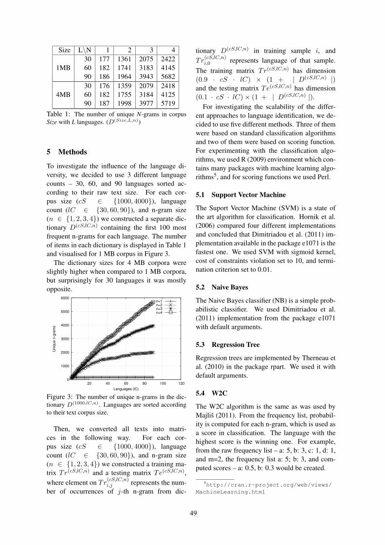
Size L\N 1 2 3 430 177 1361 2075 2422

1MB 60 182 1741 3183 414590 186 1964 3943 568230 176 1359 2079 2418

4MB 60 182 1755 3184 412590 187 1998 3977 5719

Table 1: The number of unique N-grams in corpusSize with L languages. (D(Size,L,n))

5 Methods

To investigate the influence of the language di-versity, we decided to use 3 different languagecounts – 30, 60, and 90 languages sorted ac-cording to their raw text size. For each cor-pus size (cS ∈ 1000, 4000), languagecount (lC ∈ 30, 60, 90), and n-gram size(n ∈ 1, 2, 3, 4) we constructed a separate dic-tionary D(cS,lC,n) containing the first 100 mostfrequent n-grams for each language. The numberof items in each dictionary is displayed in Table 1and visualised for 1 MB corpus in Figure 3.

The dictionary sizes for 4 MB corpora wereslightly higher when compared to 1 MB corpora,but surprisingly for 30 languages it was mostlyopposite.

0

1000

2000

3000

4000

5000

6000

20 40 60 80 100 120

Un

iqu

e n

-gra

ms

Languages (lC)

n=1n=2n=3n=4

Figure 3: The number of unique n-grams in the dic-tionary D(1000,lC,n). Languages are sorted accordingto their text corpus size.

Then, we converted all texts into matri-ces in the following way. For each cor-pus size (cS ∈ 1000, 4000), languagecount (lC ∈ 30, 60, 90), and n-gram size(n ∈ 1, 2, 3, 4) we constructed a training ma-trix Tr(cS,lC,n) and a testing matrix Te(cS,lC,n),where element on Tr

(cS,lC,n)i,j represents the num-

ber of occurrences of j-th n-gram from dic-

tionary D(cS,lC,n) in training sample i, andTr

(cS,lC,n)i,0 represents language of that sample.

The training matrix Tr(cS,lC,n) has dimension(0.9 · cS · lC) × (1 + | D(cS,lC,n) |)and the testing matrix Te(cS,lC,n) has dimension(0.1 · cS · lC)× (1 + | D(cS,lC,n) |).

For investigating the scalability of the differ-ent approaches to language identification, we de-cided to use five different methods. Three of themwere based on standard classification algorithmsand two of them were based on scoring function.For experimenting with the classification algo-rithms, we used R (2009) environment which con-tains many packages with machine learning algo-rithms5, and for scoring functions we used Perl.

5.1 Support Vector Machine

The Suport Vector Machine (SVM) is a state ofthe art algorithm for classification. Hornik et al.(2006) compared four different implementationsand concluded that Dimitriadou et al. (2011) im-plementation available in the package e1071 is thefastest one. We used SVM with sigmoid kernel,cost of constraints violation set to 10, and termi-nation criterion set to 0.01.

5.2 Naive Bayes

The Naive Bayes classifier (NB) is a simple prob-abilistic classifier. We used Dimitriadou et al.(2011) implementation from the package e1071with default arguments.

5.3 Regression Tree

Regression trees are implemented by Therneau etal. (2010) in the package rpart. We used it withdefault arguments.

5.4 W2C

The W2C algorithm is the same as was used byMajlis (2011). From the frequency list, probabil-ity is computed for each n-gram, which is used asa score in classification. The language with thehighest score is the winning one. For example,from the raw frequency list – a: 5, b: 3, c: 1, d: 1,and m=2, the frequency list a: 5; b: 3, and com-puted scores – a: 0.5, b: 0.3 would be created.

5http://cran.r-project.org/web/views/MachineLearning.html

49

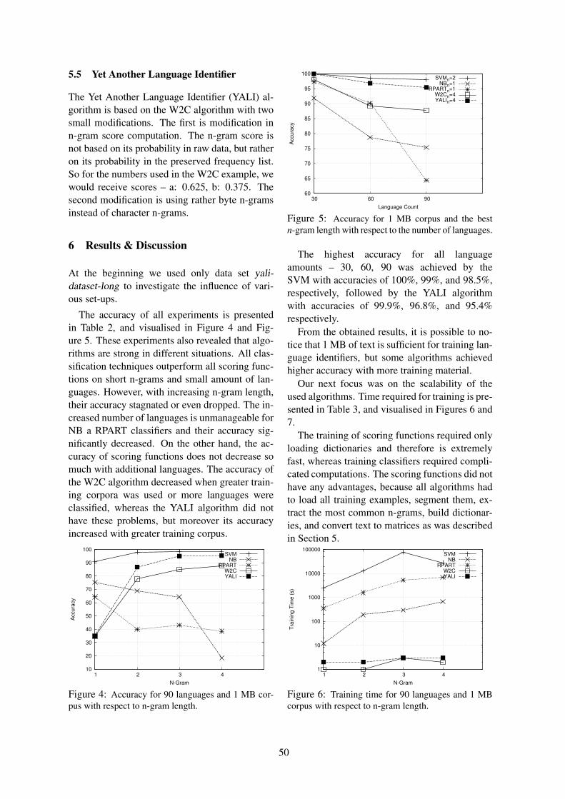
5.5 Yet Another Language Identifier

The Yet Another Language Identifier (YALI) al-gorithm is based on the W2C algorithm with twosmall modifications. The first is modification inn-gram score computation. The n-gram score isnot based on its probability in raw data, but ratheron its probability in the preserved frequency list.So for the numbers used in the W2C example, wewould receive scores – a: 0.625, b: 0.375. Thesecond modification is using rather byte n-gramsinstead of character n-grams.

6 Results & Discussion

At the beginning we used only data set yali-dataset-long to investigate the influence of vari-ous set-ups.

The accuracy of all experiments is presentedin Table 2, and visualised in Figure 4 and Fig-ure 5. These experiments also revealed that algo-rithms are strong in different situations. All clas-sification techniques outperform all scoring func-tions on short n-grams and small amount of lan-guages. However, with increasing n-gram length,their accuracy stagnated or even dropped. The in-creased number of languages is unmanageable forNB a RPART classifiers and their accuracy sig-nificantly decreased. On the other hand, the ac-curacy of scoring functions does not decrease somuch with additional languages. The accuracy ofthe W2C algorithm decreased when greater train-ing corpora was used or more languages wereclassified, whereas the YALI algorithm did nothave these problems, but moreover its accuracyincreased with greater training corpus.

10

20

30

40

50

60

70

80

90

100

1 2 3 4

Accu

racy

N-Gram

SVMNB

RPARTW2CYALI

Figure 4: Accuracy for 90 languages and 1 MB cor-pus with respect to n-gram length.

60

65

70

75

80

85

90

95

100

30 60 90

Accu

racy

Language Count

SVMn=2NBn=1

RPARTn=1W2Cn=4YALIn=4

Figure 5: Accuracy for 1 MB corpus and the bestn-gram length with respect to the number of languages.

The highest accuracy for all languageamounts – 30, 60, 90 was achieved by theSVM with accuracies of 100%, 99%, and 98.5%,respectively, followed by the YALI algorithmwith accuracies of 99.9%, 96.8%, and 95.4%respectively.

From the obtained results, it is possible to no-tice that 1 MB of text is sufficient for training lan-guage identifiers, but some algorithms achievedhigher accuracy with more training material.

Our next focus was on the scalability of theused algorithms. Time required for training is pre-sented in Table 3, and visualised in Figures 6 and7.

The training of scoring functions required onlyloading dictionaries and therefore is extremelyfast, whereas training classifiers required compli-cated computations. The scoring functions did nothave any advantages, because all algorithms hadto load all training examples, segment them, ex-tract the most common n-grams, build dictionar-ies, and convert text to matrices as was describedin Section 5.

1

10

100

1000

10000

100000

1 2 3 4

Tra

inin

g T

ime

(s)

N-Gram

SVMNB

RPARTW2CYALI

Figure 6: Training time for 90 languages and 1 MBcorpus with respect to n-gram length.

50

N-Gram L 1 2 3 4Method S 1MB 4MB 1MB 4MB 1MB 4MB 1MB 4MB

30 96.3% 96.7% 100.0% 99.9% 100.0% 99.9% 99.9% 99.9%SVM 60 91.5% 92.3% 98.5% 98.5% 99.0% 99.0% 98.6% 98.5%

90 90.8% 91.6% 98.0% 98.0% 98.5% - 98.3% -30 91.8% 94.2% 91.3% 90.9% 82.2% 93.3% 32.1% 59.9%

NB 60 78.7% 84.8% 70.6% 68.2% 71.7% 77.6% 25.7% 34.0%90 75.4% 82.7% 68.8% 66.5% 64.3% 71.0% 18.4% 17.5%30 97.3% 96.7% 98.8% 98.6% 98.4% 97.8% 97.7% 97.4%

RPART 60 90.2% 91.2% 67.3% 72.0% 67.2% 68.8% 65.5% 74.6%90 64.3% 55.9% 39.7% 39.6% 43.0% 44.0% 38.5% 39.6%30 38.0% 38.6% 89.9% 91.0% 96.2% 96.5% 97.9% 98.1%

W2C 60 34.7% 30.9% 83.0% 81.7% 86.0% 84.9% 89.1% 82.0%90 34.7% 30.9% 77.8% 77.6% 84.9% 83.4% 87.8% 82.7%30 38.0% 38.6% 96.7% 96.2% 99.6% 99.5% 99.9% 99.8%

YALI 60 35.0% 31.2% 86.1% 86.1% 95.7% 96.4% 96.8% 97.4%90 34.9% 31.1% 86.8% 87.8% 95.0% 95.6% 95.4% 96.1%

Table 2: Accuracy of classifiers for various corpora sizes, n-gram lengths, and language counts.

1

10

100

1000

10000

100000

30 60 90

Tra

inin

g T

ime

(s)

Language Count

SVMn=2NBn=1

RPARTn=1W2Cn=4YALIn=4

Figure 7: Training time for 1 MB corpus and the bestn-gram length with respect to the number of languages.

Time required for training increased dramat-ically for SVM and RPART algorithms whenthe number of languages or the corpora size in-creased. It is possible to use the SVM only withunigrams or bigrams, because training on trigramsrequired 12 times more time for 60 languagescompared with 30 languages. The SVM also hadproblems with increasing corpora sizes, because ittook almost 10-times more time when the corpussize increased 4 times. Scoring functions scaledwell and were by far the fastest ones. We ter-minated training the SVM on trigrams and quad-grams for 90 languages after 5 days of computa-tion.

Finally, we also measured time required forclassifying all testing examples. The results arein Table 4, and visualised in Figure 8 and Fig-ure 6. Times displayed in the table and charts rep-resents the number of seconds needed for classi-fying 1000 chunks.

0.1

1

10

100

1000

10000

1 2 3 4

Pre

dic

tio

n T

ime

(s/1

00

0 c

hu

nks)

N-Gram

SVMNB

RPARTW2CYALI

Figure 8: Prediction time for 90 languages and 1 MBcorpus with respect to n-gram length.

0

10

20

30

40

50

60

70

30 60 90

Pre

dic

tio

n T

ime

(s/1

00

0 c

hu

nks)

Language Count

SVMn=2NBn=1

RPARTn=1W2Cn=4YALIn=4

Prediction time for 1 MB corpus and the best n-gramlength with respect to the number of languages.The RPART algorithm was the fastest classifier

followed by both scoring functions, whereas NBwas the slowest one. All algorithms with 4 timesmore data achieved slightly higher accuracy, buttheir training took 4 times longer, with the ex-ception of the SVM which took at least 10 timeslonger. The SVM algorithm is the least scalable

51

N-Gram L 1 2 3 4Method S 1MB 4MB 1MB 4MB 1MB 4MB 1MB 4MB

30 215 1858 663 1774 627 7976 655 3587SVM 60 1499 13653 7981 87260 7512 44288 26943 207123

90 2544 24841 12698 267824 76693 - 27964 -30 5 19 27 83 40 144 54 394

NB 60 9 32 76 255 142 515 363 118790 12 56 188 683 298 1061 672 224530 44 189 144 946 267 1275 369 1360

RPART 60 162 1332 736 3447 1270 11114 2583 749390 351 1810 1578 7647 5139 23413 6736 1765930 1 1 0 1 0 1 1 1

W2C 60 1 2 1 2 2 1 2 290 1 1 1 1 3 1 2 130 1 1 1 1 1 1 1 1

YALI 60 2 2 2 2 2 2 2 090 2 1 2 1 3 1 3 2

Table 3: Training Time

Method 30 60 90Acc 100.0% 98.5% 98.0%

SVM Tre 663 7981 12698n=2 Pre 10.3 66.2 64.1

Acc 91.8% 78.7% 75.4%NB Tre 5 9 12n=1 Pre 13.0 18.2 22.2

Acc 97.3% 90.2% 64.3%RPART Tre 44 162 351

n=1 Pre 0.1 0.2 0.1Acc 97.9% 89.1% 87.8%

W2C Tre 1 2 2n=4 Pre 1.3 2.8 12.3

Acc 99.9% 96.8% 95.4%YALI Tre 1 2 3

n=4 Pre 1.3 2.7 3.6

Table 5: Comparison of classifiers with best param-eters. Label Acc represents accuracy, Tre representstraining time in seconds, and Pre represents predictiontime for 1000 chunks in seconds.

algorithm of all the examined – all the rest re-quired proportionally more time for training andprediction when the greater training corpus wasused or more languages were classified.

The comparison of all methods is presented inTable 5. For each model we selected the n-gramssize with the best trade-off between accuracy andtime required for training and prediction. The twomost accurate algorithms are SVM and YALI. TheSVM achieved the highest accuracy for all lan-guages but its training took around 4000 timeslonger and classification was around 17 timesslower than the YALI.

In the next step we evaluated the YALI algo-rithm for various size of selected n-grams. These

LanguagesSize 30 140 1000100 64.9% 85.7 % 93.8 %200 68.7% 87.3 % 93.9 %400 71.7% 88.0 % 94.0 %800 73.7% 88.5 % 94.0 %

1600 75.0% 88.8% 94.0%

Table 6: Effect of the number of selected 4-grams onaccuracy.

experiments were evaluated on the data set yali-dataset-standard. Achieved results are presentedin Table 6. The number of used n-grams increasedthe accuracy for short samples from 64.9% to75.0% but it had no effect on long samples.

As the last step in evaluation we decided tocompare the YALI with Google Translate (GT),which also provides language identification for 50languages through their API.6 For comparison weused data set yali-dataset-small which contains 50samples of length 30 and 140 for each language(4800 samples in total). Achieved results are pre-sented in Table 7. The GT and the YALI per-form comparably well on samples of length 30 onwhich they achieved accuracy 93.6% and 93.1%respectively, but on samples of length 140 GTwith accuracy 97.3% outperformed YALI with ac-curacy 94.8%.

7 Conclusions & Future Work

In this paper we compared 5 different algorithmsfor language identification – three based on the

6http://code.google.com/apis/language/translate/v2/using_rest.html

52

N-Gram L 1 2 3 4Method S 1MB 4MB 1MB 4MB 1MB 4MB 1MB 4MB

30 3.7 7.3 10.3 6.8 9.0 31.8 9.3 13.8SVM 60 13.3 30.1 66.2 189.7 59.8 92.8 236.7 375.2

90 16.1 36.7 64.1 381.4 414.9 - 133.4 -30 13.0 13.6 75.3 77.1 132.7 147.9 186.0 349.7

NB 60 18.2 18.8 155.3 162.0 291.5 297.4 860.3 676.090 22.2 24.7 318.1 251.9 546.3 469.3 1172.8 1177.830 0.1 0.1 0.3 0.1 0.1 0.2 0.7 0.2

RPART 60 0.2 0.1 0.2 0.0 0.2 0.4 0.8 0.290 0.1 0.1 0.2 0.1 0.4 0.3 1.2 0.330 0.7 0.8 1.7 1.6 3.3 1.5 1.3 2.2

W2C 60 1.3 1.3 2.2 2.4 2.7 2.5 2.8 2.990 2.1 1.8 4.0 3.2 4.4 3.8 12.3 5.830 0.7 0.8 1.0 1.2 2.0 1.9 1.3 2.2

YALI 60 1.3 1.5 1.8 2.2 2.5 2.2 2.7 2.590 2.2 1.8 2.7 2.9 4.4 3.5 3.6 3.7

Table 4: Prediction Time

Text Length30 140

SystemGoogle 93.6% 97.3%YALI 93.1% 94.8%

Table 7: Comparison of Google Translate and YALIon 48 languages.

standard classification algorithms (Support Vec-tor Machine (SVM), Naive Bayes (NB), and Re-gression Tree (RPART)) and two based on scoringfunctions. For investigating the influence of theamount of training data we constructed two cor-pora from the Wikipedia with 90 languages. Toinvestigate the influence of number if identifiedlanguages we created three sets with 30, 60, and90 languages. We also measured time required fortraining and classification.

Our experiments revealed that the standardclassification algorithms requires at most bi-grams while the scoring ones required quad-grams. We also showed that Regression Trees andNaive Bayes are not suitable for language identifi-cation because they achieved accuracy 64.3% and75.4% respectively.

The best classifier for language identificationwas the SVM algorithm which achieved accuracy98% for 90 languages but its training took 4200times more and its classification was 16 timesslower than the YALI algorithm with accuracy95.4%. This YALI algorithm has also potentialfor increasing accuracy and number of recognizedlanguages because it scales well.

We also showed that the YALI algorithm is

comparable with the Google Translate system.Both systems achieved accuracy 93% for sam-ples of length 30. On samples of length 140Google Translate with accuracy 97.3% outper-formed YALI with accuracy 94.8%.

All data sets as well as source codes areavailable at http://ufal.mff.cuni.cz/

˜majlis/yali/.In the future we would like to focus on using

described techniques not only on recognizing lan-guages but also on recognizing character encod-ings which is directly applicable for web crawl-ing.

Acknowledgments

The research has been supported by the grantKhresmoi (FP7-ICT-2010-6-257528 of the EUand 7E11042 of the Czech Republic).

References

[Baldwin and Lui2010] Timothy Baldwin and MarcoLui. 2010. Language identification: the long andthe short of the matter. Human Language Tech-nologies: The 2010 Annual Conference of the NorthAmerican Chapter of the Association for Computa-tional Linguistics, pp. 229–237.

[Beesley1988] Kenneth R. Beesley. 1988. Lan-guage identifier: A computer program for automaticnatural-language identification of on-line text. Lan-guages at Crossroads: Proceedings of the 29th An-nual Conferenceof the American Translators Asso-ciation, 12-16 October 1988, pp. 47-54.

[Cavnar and Trenkle1994] William B. Cavnar and JohnM. Trenkle. 1994. N-gram-based text categoriza-

53

tion. In Proceedings of Symposium on DocumentAnalysis and Information Retrieval.

[Choong et al.2011] Chew Yew Choong, YoshikiMikami, and Robin Lee Nagano. 2011. LanguageIdentification of Web Pages Based on Improved Ngram Algorithm. IJCSI, issue 8, volume 3.

[Dimitriadou et al.2011] Evgenia Dimitriadou, KurtHornik, Friedrich Leisch, David Meyer, and andAndreas Weingessel 2011. e1071: Misc Func-tions of the Department of Statistics (e1071), TUWien. R package version 1.5-27. http://CRAN.R-project.org/package=e1071.

[Gold1967] E. Mark Gold. 1967. Language iden-tification in the limit. Information and Control,5:447474.

[Grothe et al.2008] Lena Grothe, Ernesto William DeLuca, and Andreas Nrnberger. 2008. A Com-parative Study on Language Identification Meth-ods. Proceedings of the Sixth International Lan-guage Resources and Evaluation (LREC’08). Mar-rakech, 980-985.

[Halevy et al.2009] Alon Halevy, Peter Norvig, andFernando Pereira. 2009. The unreasonable effec-tiveness of data. IEEE Intelligent Systems, 24:8–12.

[Hayati 2004] Katia Hayati. 2004. Language Iden-tification on the World Wide Web. Master The-sis, University of California, Santa Cruz. http://lily-field.net/work/masters.pdf.

[Hornik et al.2006] Kurt Hornik, Alexandros Karat-zoglou, and David Meyer. 2006. Support Vec-tor Machines in R. Journal of Statistical Software2006., 15.

[Hughes et al.2006] Baden Hughes, Timothy Bald-win, Steven Bird, Jeremy Nicholson, and AndrewMackinlay. 2006. Reconsidering language identifi-cation for written language resources. Proceedingsof LREC2006, 485–488.

[Kruengkrai et al.2005] Canasai Kruengkrai, PrapassSrichaivattana, Virach Sornlertlamvanich, and Hi-toshi Isahara. 2005. Language identification basedon string kernels. In Proceedings of the 5th Interna-tional Symposium on Communications and Infor-mation Technologies (ISCIT2005), pages 896899,Beijing, China.

[Leonard and Doddington1974] Gary R. Leonard andGeorge R. Doddington. 1974. Automatic languageidentification. Technical report RADC-TR-74-200,Air Force Rome Air Development Center.

[Lewis2009] M. Paul Lewis. 2009. Ethnologue: Lan-guages of the World, Sixteenth edition. Dallas,Tex.: SIL International. Online version: http://www.ethnologue.com/

[McNamee2005] Paul McNamee. 2005. Languageidentification: a solved problem suitable for under-graduate instruction. J. Comput. Small Coll, vol-ume: 20, issue: 3, February 2005, 94–101. Consor-tium for Computing Sciences in Colleges, USA.

[Majlis2012] Martin Majlis, Zdenek Zabokrtsky.2012. Language Richness of the Web. In Proceed-ings of the Eight International Language Resourcesand Evaluation (LREC’12), Istanbul, Turkey, May2012.

[Majlis2011] Martin Majlis. 2011. Large Multilin-gual Corpus. Mater Thesis, Charles University inPrague.

[Martins and Silva2005] Bruno Martins and Mario J.Silva. 2005. Language identification in web pages.Proceedings of the 2005 ACM symposium on Ap-plied computing, SAC ’05, 764–768. ACM, NewYork, NY, USA. http://doi.acm.org/10.1145/1066677.1066852.

[R2009] R Development Core Team. 2009. R: A Lan-guage and Environment for Statistical Computing.R Foundation for Statistical Computing. ISBN 3-900051-07-0. http://www.R-project.org,

[Sibun and Reynar1996] Penelope Sibun and Jeffrey C.Reynar. 1996. Language identification: Examiningthe issues. In Proceedings of the 5th Symposium onDocument Analysis and Information Retrieval.

[Therneau et al.2010] Terry M. Therneau, Beth Atkin-son, and R port by Brian Ripley. 2010.rpart: Recursive Partitioning. R package ver-sion 3.1-48. http://CRAN.R-project.org/package=rpart.

54

Proceedings of the EACL 2012 Student Research Workshop, pages 55–63,Avignon, France, 26 April 2012. c©2012 Association for Computational Linguistics

Discourse Type Clustering using POS n-gram Profiles andHigh-Dimensional Embeddings

Christelle CoccoDepartment of Computer Science and Mathematical Methods

University of LausanneSwitzerland

Christelle.Cocco@unil.ch

Abstract

To cluster textual sequence types (discoursetypes/modes) in French texts, K-meansalgorithm with high-dimensional embed-dings and fuzzy clustering algorithm wereapplied on clauses whose POS (part-of-speech) n-gram profiles were previously ex-tracted. Uni-, bi- and trigrams were usedon four 19th century French short stories byMaupassant. For high-dimensional embed-dings, power transformations on the chi-squared distances between clauses were ex-plored. Preliminary results show that high-dimensional embeddings improve the qual-ity of clustering, contrasting the use of bi-and trigrams whose performance is disap-pointing, possibly because of feature spacesparsity.

1 Introduction

The aim of this research is to cluster textual se-quence types (named here discourse types)1, suchas narrative, descriptive, argumentative and so onin French texts, and especially in short storieswhich could contain all types.

For this purpose, texts were segmented intoclauses (section 2.1). To cluster the latter, n-gramPOS (part-of-speech) tag profiles were extracted(section 2.3). POS-tags were chosen because oftheir expected relation to discourse types.

Several authors have used POS-tags amongother features for various text classification tasks,such as Biber (1988) for text type detection, Karl-gren and Cutting (1994) and Malrieu and Rastier

1Sequence type is an appropriate name, because it refersto text passage type. However, it will be further mentionedas discourse types, a frequent French term. In English, astandard term is: discourse modes.

(2001) for genre classification, and Palmer et al.(2007) for situation entity classification. The lat-ter is an essential component of English discoursemodes (Smith, 2009). Moreover, previous work indiscourse type detection has shown a dependencybetween POS-tags and these types (Cocco et al.,2011).

In this paper, K-means algorithm with high-dimensional embeddings and fuzzy clustering al-gorithm were applied on uni-, bi- and trigramPOS-tag profiles (section 2.4) and results wereevaluated (section 2.5). Finally, results are givenin section 3.

2 Method

2.1 Expert assessment

The human expert, a graduate student in Frenchlinguistics, annotated 19th century French shortstories by Maupassant, using XML tags. Eachtext was first segmented into clauses, whoselength is typically shorter than sentences. Then,texts were annotated retaining the following sixdiscourse types: narrative, argumentative, de-scriptive, explicative, dialogal and injunctive.2

They resulted from an adaptation of the work ofAdam (2008a; 2008b) in text and discourse analy-sis, as well as Bronckart (1996) in psycholinguis-tics, concerning textual sequence types. The for-mer does not consider the injunctive type.

Let us briefly describe these types (Adam,2008a; Adam, 2008b; Bronckart, 1996), togetherwith the criteria finally adopted by the human ex-pert for this time-consuming task.

2Regarding English, there are five discourse modes ac-cording to Smith (2009): narrative, description, report, in-formation and argument.

55

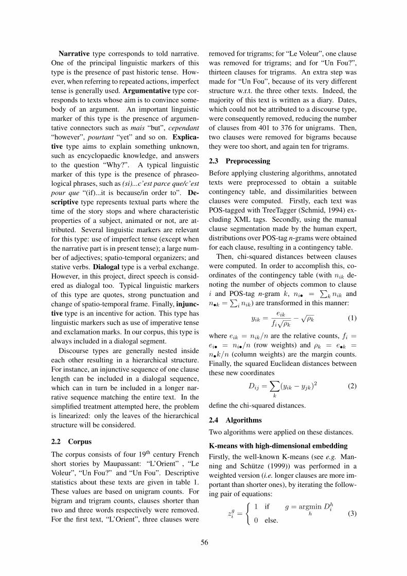
Narrative type corresponds to told narrative.One of the principal linguistic markers of thistype is the presence of past historic tense. How-ever, when referring to repeated actions, imperfecttense is generally used. Argumentative type cor-responds to texts whose aim is to convince some-body of an argument. An important linguisticmarker of this type is the presence of argumen-tative connectors such as mais “but”, cependant“however”, pourtant “yet” and so on. Explica-tive type aims to explain something unknown,such as encyclopaedic knowledge, and answersto the question “Why?”. A typical linguisticmarker of this type is the presence of phraseo-logical phrases, such as (si)...c’est parce que/c’estpour que “(if)...it is because/in order to”. De-scriptive type represents textual parts where thetime of the story stops and where characteristicproperties of a subject, animated or not, are at-tributed. Several linguistic markers are relevantfor this type: use of imperfect tense (except whenthe narrative part is in present tense); a large num-ber of adjectives; spatio-temporal organizers; andstative verbs. Dialogal type is a verbal exchange.However, in this project, direct speech is consid-ered as dialogal too. Typical linguistic markersof this type are quotes, strong punctuation andchange of spatio-temporal frame. Finally, injunc-tive type is an incentive for action. This type haslinguistic markers such as use of imperative tenseand exclamation marks. In our corpus, this type isalways included in a dialogal segment.

Discourse types are generally nested insideeach other resulting in a hierarchical structure.For instance, an injunctive sequence of one clauselength can be included in a dialogal sequence,which can in turn be included in a longer nar-rative sequence matching the entire text. In thesimplified treatment attempted here, the problemis linearized: only the leaves of the hierarchicalstructure will be considered.

2.2 CorpusThe corpus consists of four 19th century Frenchshort stories by Maupassant: “L’Orient” , “LeVoleur”, “Un Fou?” and “Un Fou”. Descriptivestatistics about these texts are given in table 1.These values are based on unigram counts. Forbigram and trigram counts, clauses shorter thantwo and three words respectively were removed.For the first text, “L’Orient”, three clauses were

removed for trigrams; for “Le Voleur”, one clausewas removed for trigrams; and for “Un Fou?”,thirteen clauses for trigrams. An extra step wasmade for “Un Fou”, because of its very differentstructure w.r.t. the three other texts. Indeed, themajority of this text is written as a diary. Dates,which could not be attributed to a discourse type,were consequently removed, reducing the numberof clauses from 401 to 376 for unigrams. Then,two clauses were removed for bigrams becausethey were too short, and again ten for trigrams.

2.3 PreprocessingBefore applying clustering algorithms, annotatedtexts were preprocessed to obtain a suitablecontingency table, and dissimilarities betweenclauses were computed. Firstly, each text wasPOS-tagged with TreeTagger (Schmid, 1994) ex-cluding XML tags. Secondly, using the manualclause segmentation made by the human expert,distributions over POS-tag n-grams were obtainedfor each clause, resulting in a contingency table.

Then, chi-squared distances between clauseswere computed. In order to accomplish this, co-ordinates of the contingency table (with nik de-noting the number of objects common to clausei and POS-tag n-gram k, ni• =

!k nik and

n•k =!

i nik) are transformed in this manner:

yik =eik

fi!

!k"!!k (1)

where eik = nik/n are the relative counts, fi =ei• = ni•/n (row weights) and !k = e•k =n•k/n (column weights) are the margin counts.Finally, the squared Euclidean distances betweenthese new coordinates

Dij ="

k

(yik " yjk)2 (2)

define the chi-squared distances.

2.4 AlgorithmsTwo algorithms were applied on these distances.

K-means with high-dimensional embeddingFirstly, the well-known K-means (see e.g. Man-ning and Schutze (1999)) was performed in aweighted version (i.e. longer clauses are more im-portant than shorter ones), by iterating the follow-ing pair of equations:

zgi =

#1 if g = argmin

hDh

i

0 else.(3)

56

Texts ! sent. ! clauses ! tokens ! types % discourse types according to the expertwith punct. w/o punct. word tag arg descr dial expl inj nar

L’Orient 88 189 1’749 1’488 654 27 4.23 20.11 25.93 19.05 2.65 28.04Le Voleur 102 208 1’918 1’582 667 29 4.81 12.02 13.94 4.81 2.88 61.54Un Fou? 150 314 2’625 2’185 764 28 18.15 10.51 14.65 14.65 8.28 33.76Un Fou 242 376 3’065 2’548 828 29 17.82 13.83 1.86 11.70 12.23 42.55

Table 1: Statistics of the annotated texts by Maupassant. For the text “Un Fou”, dates were initially removed fromthe text. Number of sentences as considered by TreeTagger (Schmid, 1994). Number of clauses as segmented bythe human expert. Number of tokens including punctuation and compounds as tagged by TreeTagger. Numberof tokens without punctuation and numbers, considering compounds as separated tokens. Number of wordformtypes. Number of POS-tag types. The last columns give the percentage of clauses for each discourse type (arg =argumentative, descr = descriptive, dial = dialogal, expl = explicative, inj = injunctive, nar = narrative).

Dgi =

"

j

fgj Dij "!g (4)

where zgi is the membership of clause i in group

g and Dgi is the chi-squared distance between

the clause i and the group g as resulting fromthe Huygens principle. In the equation 4, fg

j =(fizig)/!g = p(i|g), Dij is the chi-squared dis-tances between clauses given by the equation 2and !g = 1/2

!jk fg

j fgk Djk is the inertia of

group g. In addition, !g =!

i fizig = p(g) isthe relative weight of group g.

At the outset, the membership matrix Z waschosen randomly, and then the iterations werecomputed until stabilisation of the matrix Z or anumber of maximum iterations Nmax.

Besides the K-means algorithm, Schoenbergtransformations "(D) were also operated. Theytransform the original squared Euclidean dis-tances D into new squared Euclidean distances"(D) (Bavaud, 2011) and perform a high-dimensional embedding of data, similar to thoseused in Machine Learning. Among all Schoen-berg transformations, the simple componentwisepower transformation was used, i.e.

"(Dij) = (Dij)q (5)

where 0 < q # 1.In a nutshell, the K-means algorithm was ap-

plied on the four texts, for uni-, bi- and trigramsPOS-tags, with q in equation 5 varying from 0.1to 1 with steps of 0.05. Given that the aim wasto find the six groups annotated by the human ex-pert, the K-means algorithm was computed with anumber of groups m = 6. Moreover, Nmax = 400and for each q, calculations were run 300 times,and then the averages of the relevant quantities(see section 2.5) were computed.

Fuzzy clusteringSecondly, the same algorithm which was used ina previous work (Cocco et al., 2011) was appliedhere, i.e. the fuzzy clustering algorithm.

In brief, it consists of iterating, as for the K-means, the membership zg

i of clause i in group gdefined in the following way (Rose et al., 1990;Bavaud, 2009):

zgi =

!g exp("#Dgi )

m"

h=1

!h exp("#Dhi )

(6)

until stabilisation of the membership matrix Z(randomly chosen at the beginning as uniformlydistributed over the m groups) or after Nmax itera-tions. Dg

i is given by equation 4 and !g is the rela-tive weight of group g. Moreover, it turns out con-venient to set # := 1/(trel$!), the “inverse tem-perature” parameter, where ! := 1

2

!ij fifjDij

is the inertia and trel is the relative temperaturewhich must be fixed in advance.

The values of # controls for the bandwidthof the clustering, i.e. the number of groups: thehigher #, the larger the final number of groupsM (see figure 9). As a matter of fact, depend-ing of # values, group profiles are more or lesssimilar. Also, group whose profiles are simi-lar enough are aggregated, reducing the num-ber of groups from m (initial number of groupschosen at the beginning) to M . This aggrega-tion is made by adding memberships of clauses:z[g!h]i = zg

i + zhi . Two groups are considered

similar enough if $gh/$

$gg$hh % 1"10"5, with$gh =

!ni=1 fiz

gi zh

i which measures the overlapbetween g and h (Bavaud, 2010). Finally, eachclause is attributed to the most probable group.

For the application in this project, fuzzy clus-tering algorithm was computed on the four texts,

57

for uni- bi- and trigrams POS-tags. At the outset,the initial number of groups m was equal to thenumber of clauses for each text (see table 1 andsection 2.2), with a relative temperature trel from0.022 to 0.3 with steps of 0.001 (except for thetext “Un Fou” with trel min = 0.02, trel max = 0.3and trel step = 0.01). Besides this, Nmax = 400and for each trel, algorithm was run 20 times, andfinally the averages of the relevant quantities (seesection 2.5) were computed.

2.5 Evaluation criteriaThe clustering obtained by the two algorithms(K-means with high-dimensional embedding andfuzzy clustering) were compared to the classifi-cation made by the human expert. As clusteringinduces anonymous partitions, traditional indicessuch as precision, recall and Cohen’s Kappa can-not be computed.

Among the numerous similarity indices be-tween partitions, we have examined the Jaccardindex (Denœud and Guenoche, 2006; Younessand Saporta, 2004):

J =r

r + u + v(7)

whose values vary between 0 and 1, and thecorrected Rand index (Hubert and Arabie, 1985;Denœud and Guenoche, 2006):

RC =r " Exp(r)

Max(r)" Exp(r)(8)

whose the maximal value is 1. When this indexequals 0, it means that similarities between par-titions stem from chance. However, it can alsotake negative values when number of similaritiesis lower than the expectation (i.e. chance).

Both indices are based upon the contingencytable nij , defined by the number of objects at-tributed simultaneously to group i (w.r.t. thefirst partition) and to group j (w.r.t. the sec-ond partition). Moreover, in both indices, r =12

!ij nij(nij " 1) is the number of pairs si-

multaneously joined together, u = 12(

!j n2

•j "!ij n2

ij) (respectively v = 12(

!i n

2i•"

!ij n2

ij))is the number of pairs joined (respectively sep-arated) in the partition obtained with algorithmand separated (respectively joined) in the par-tition made by the human expert, Exp(r) =

12n(n"1)

!i ni•(ni• " 1)

!j n•j(n•j " 1) is the

expected number of pairs simultaneously joined

together by chance and Max(r) = 14

!i ni•(ni•"

1) +!

j n•j(n•j " 1).

3 Results

On the one hand, results obtained with the K-means algorithm and power (q) transformationsfor uni-, bi- and trigrams are presented in figures1 to 8. On the other hand, results obtained withfuzzy clustering for uni- bi- and trigrams are onlyshown for the text “Le Voleur” in figures 9 to 13.For the three other texts, results will be discussedbelow.

0.2 0.4 0.6 0.8 1.0

0.00

0.01

0.02

0.03

0.04

0.05

Power (q)

Co

rre

cte

d R

an

d I

nd

ex

Figure 1: “L’Orient” with K-means algorithm: cor-rected rand index as a function of power (q) (& = uni-grams, ! = bigrams and $ = trigrams). The standarddeviation is approximatively constant across q rangingfrom a minimum of 0.018 and a maximum of 0.024(unigrams); 0.0099 and 0.015 (bigrams); 0.0077 and0.013 (trigrams).

A first remark is that corrected Rand index andJaccard index behave differently in general. Thisdifference is a consequence of the fact that Jac-card index does not take into account the numberof pairs simultaneously separated in the two par-titions, a fact criticised by Milligan and Cooper(1986).

Regarding the texts “L’Orient”, “Le Voleur”and “Un Fou?” with K-means algorithm and thecorrected Rand index (figures 1, 3 and 5), un-igrams give the best results. Moreover, powertransformations (equation 5) tend to improvethem. For instance, for the text “L’Orient” (figure1), the best result is RC = 0.048 with q = 0.55,and for the text “Un Fou?” (figure 5), the best

58

0.2 0.4 0.6 0.8 1.0

0.11

0.12

0.13

0.14

0.15

0.16

0.17

Power (q)

Ja

cca

rd I

nd

ex

Figure 2: “L’Orient” with K-means algorithm: Jaccardindex as a function of power (q) (& = unigrams, ! =bigrams and $ = trigrams).

0.2 0.4 0.6 0.8 1.0

-0.05

0.00

0.05

0.10

0.15

Power (q)

Co

rre

cte

d R

an

d I

nd

ex

Figure 3: “Le Voleur” with K-means algorithm: cor-rected rand index as a function of power (q) (& = uni-grams, ! = bigrams and $ = trigrams).

0.2 0.4 0.6 0.8 1.0

0.14

0.16

0.18

0.20

0.22

Power (q)Ja

cca

rd I

nd

ex

Figure 4: “Le Voleur” with K-means algorithm: Jac-card index as a function of power (q) (& = unigrams, != bigrams and $ = trigrams).

0.2 0.4 0.6 0.8 1.0

-0.02

0.00

0.02

0.04

0.06

0.08

Power (q)

Co

rre

cte

d R

an

d I

nd

ex

Figure 5: “Un Fou?” with K-means algorithm: cor-rected rand index as a function of power (q) (& = uni-grams, ! = bigrams and $ = trigrams).

59

0.2 0.4 0.6 0.8 1.0

0.11

0.12

0.13

0.14

0.15

0.16

0.17

Power (q)

Ja

cca

rd I

nd

ex

Figure 6: “Un Fou?” with K-means algorithm: Jaccardindex as a function of power (q) (& = unigrams, ! =bigrams and $ = trigrams).

0.2 0.4 0.6 0.8 1.0

0.00

0.01

0.02

0.03

0.04

0.05

Power (q)

Co

rre

cte

d R

an

d I

nd

ex

Figure 7: “Un Fou” with K-means algorithm: cor-rected rand index as a function of power (q) (& = uni-grams, ! = bigrams and $ = trigrams).

result is RC = 0.072 with q = 0.85.Regarding the fuzzy clustering algorithm, fig-

ure 9 shows, for the text “Le Voleur”, the relationbetween the relative temperature and the num-ber of groups for uni- bi- and trigrams, i.e. num-ber of groups decreases when relative tempera-ture increases. Figure 10 (respectively figure 12)presents the corrected Rand index (respectivelythe Jaccard index) as a function of relative tem-perature, while figure 11 (respectively figure 13)shows, for each relative temperature, the averagenumber of groups on the x-axis and the average

0.2 0.4 0.6 0.8 1.0

0.12

0.14

0.16

0.18

Power (q)

Ja

cca

rd I

nd

ex

Figure 8: “Un Fou” with K-means algorithm: Jaccardindex as a function of power (q) (& = unigrams, ! =bigrams and $ = trigrams).

0.05 0.10 0.15 0.20 0.25 0.30

020

40

60

80

100

120

Relative Temperature

Nu

mb

er

of

Gro

up

s

Unigrams

Bigrams

Trigrams

Figure 9: “Le Voleur” with fuzzy clustering algorithm:average number of groups as a function of the relativetemperature. For unigrams, the thick line indicates theaverage and the two thin lines represent the standarddeviation. The other curves depict the average of thenumber of groups.

corrected Rand index (respectively Jaccard index)on the y-axis, over 20 clusterings. There is a re-markable peak for this text (RC = 0.31 (respec-tively J = 0.48)), when trel = 0.145 (respectively0.148), corresponding to M = 14.4 (respectively13.4). The same phenomenon appears with thetext “Un Fou?”, when trel = 0.158 and M = 7.8.However, the peak for the Jaccard index is lessimportant and it is not the highest value. More-

60

0.05 0.10 0.15 0.20 0.25 0.30

0.00

0.05

0.10

0.15

0.20

0.25

0.30

Relative Temperature

Co

rre

cte

d R

an

d I

nd

ex

Unigrams

Bigrams

Trigrams

Figure 10: “Le Voleur” with fuzzy clustering algo-rithm: corrected Rand index as a function of relativetemperature.

0 20 40 60 80 100 120

0.00

0.05

0.10

0.15

0.20

0.25

0.30

Number of Groups

Co

rre

cte

d R

an

d I

nd

ex

Unigrams

Bigrams

Trigrams

Figure 11: “Le Voleur” with fuzzy clustering algo-rithm: corrected Rand index as a function of numberof groups.

over, for the latter text, there is a higher peak,which occurs only with the corrected Rand index,for trel = 0.126 and M = 24.5.

For the two other texts, there are some peaks,but not as marked as in other texts. Besides,for these two texts, corrected Rand index takesnegative values, especially for “Un Fou”. Whilethe reason for these different behaviours is notknown, it should be noted that the structure ofthese texts is different from that of the two othertexts. Indeed, “Un Fou” is written as a diary anduses mainly the present tense, also in narrative and

0.05 0.10 0.15 0.20 0.25 0.30

0.0

0.1

0.2

0.3

0.4

0.5

Relative Temperature

Ja

cca

rd I

nd

ex

Unigrams

Bigrams

Trigrams

Figure 12: “Le Voleur” with fuzzy clustering algo-rithm: Jacccard index as a function of relative tem-perature.

0 20 40 60 80 100 120

0.0

0.1

0.2

0.3

0.4

0.5

Number of Groups

Co

rre

cte

d R

an

d I

nd

ex

Unigrams

Bigrams

Trigrams

Figure 13: “Le Voleur” with fuzzy clustering algo-rithm: Jaccard index as a function of number ofgroups.

descriptive parts; “L’Orient” contains several longmonologues mainly using the present tense too.

On figure 12, it appears that Jaccard index isconstant when one group remains, and the samephenomenon appears for all texts. Indeed, fromthe distribution of table 2, one finds from equa-tion 7: r = 8939, u = 0 and v = 12 589, imply-ing J = 0.415.

Overall, it is clear that results differ depend-ing on texts, no matter which algorithm or eval-uation criterion is used. Furthermore, they arealways better for “Le Voleur” than for the three

61

arg descr dial expl inj nar10 25 29 10 6 128

Table 2: Types distribution for the text “Le Voleur”.

other texts.Finally, in most case, unigrams give better

results than bi- and tri-grams. The relativelydisappointing performance of bi- and trigrams(w.r.t. unigrams) could be accounted for by thesparsity of the feature space and the well-knownassociated “curse of dimensionality”, in particularin clustering (see e.g. Houle et al. (2010)). Resultsare clearly different for “Un Fou”, and the reasonof this difference still needs to be investigated.

Certainly, as the sample is small and there is aunique annotator, all these results must be consid-ered with caution.

4 Conclusion and further development

A first conclusion is that the use of POS-tag n-grams does not seem to improve the solution ofthe problem exposed here. In contrast, high-dimensional embedding seems to improve results.Concerning evaluation criteria, results clearlyvary according to the selected index, which makesit difficult to compare methods. Another point isthat even choosing only short stories of one au-thor, text structures can be very different and cer-tainly do not give the same results.

These results are interesting and in general bet-ter than those found in a previous work (Coccoet al., 2011), but this is still work in progress,with much room for improvement. A next stepwould be to combine fuzzy clustering with high-dimensional embedding, which can both improveresults. Moreover, it could be interesting to addtypical linguistic markers, such as those men-tioned in section 2.1, or stylistic features. It wouldalso be possible to use lemmas instead of or withPOS-tags, if more data could be added to the cor-pus. Besides, Cordial Analyseur 3 could be usedinstead of TreeTagger, because it provides morefine-grained POS-tags. However, as for n-grams,it could imply a sparsity of the feature space. An-other idea would be to perform a supervised clas-sification with cross-validation. In this case, it

3http://www.synapse-fr.com/Cordial_Analyseur/Presentation_Cordial_Analyseur.htm

would be interesting to investigate feature selec-tion (see e.g. Yang and Pedersen (1997)). Also,the hierarchical structure of texts (cf. section 2.1)should be explored. Only the leaves were con-sidered here, but in reality, one clause belongs toseveral types depending on the hierarchical levelexamined. Therefore, it could be relevant to con-sider the dominant discourse type instead of theleaf discourse type. Similarly, since in our cor-pus, injunctive type is always included in dialo-gal type, the former could be removed to obtaina larger dialogal class. In addition, it would beuseful to find a better adapted measure of sim-ilarity between partitions. Finally, an importantimprovement would be to obtain more annotatedtexts, which should improve results, and a secondhuman expert, which would permit us to assessthe difficulty of the task.

AcknowledgmentsI would like to thank Francois Bavaud and ArisXanthos for helpful comments and useful discus-sions; Guillaume Guex for his help with techni-cal matters; and Raphael Pittier for annotating thegold standard.

ReferencesJean-Michel Adam. 2008a. La linguistique textuelle:

Introduction a l’analyse textuelle des discours. Ar-mand Colin, Paris, 2nd edition.

Jean-Michel Adam. 2008b. Les textes: types et proto-types. Armand Colin, Paris, 2nd edition.

Francois Bavaud. 2009. Aggregation invariance ingeneral clustering approaches. Advances in DataAnalysis and Classification, 3(3):205–225.

Francois Bavaud. 2010. Euclidean distances, softand spectral clustering on weighted graphs. InJose Balcazar, Francesco Bonchi, Aristides Gionis,and Michele Sebag, editors, Machine Learning andKnowledge Discovery in Databases, volume 6321of Lecture Notes in Computer Science, pages 103–118. Springer, Berlin; Heidelberg.

Francois Bavaud. 2011. On the Schoenberg transfor-mations in data analysis: Theory and illustrations.Journal of Classification, 28(3):297–314.

Douglas Biber. 1988. Variation across Speech andWriting. Cambridge University Press.

Jean-Paul Bronckart. 1996. Activite langagiere,textes et discours: Pour un interactionisme socio-discursif. Delachaux et Niestle, Lausanne; Paris.

Christelle Cocco, Raphael Pittier, Francois Bavaud,and Aris Xanthos. 2011. Segmentation and clus-tering of textual sequences: a typological approach.

62

In Proceedings of the International Conference Re-cent Advances in Natural Language Processing2011, pages 427–433, Hissar, Bulgaria, September.RANLP 2011 Organising Committee.

Guy de Maupassant. 1882. Le voleur. Gil Blas, June21. http://un2sg4.unige.ch/athena/selva/maupassant/textes/voleur.html. Thierry Selva. Accessed 2011, July 6.

Guy de Maupassant. 1883. L’orient. Le Gaulois,September 13. http://un2sg4.unige.ch/athena/selva/maupassant/textes/orient.html. Thierry Selva. Accessed 2011,March 5.

Guy de Maupassant. 1884. Un fou?. Le Figaro,September 1. http://un2sg4.unige.ch/athena/maupassant/maup_fou.html.Thierry Selva. Accessed 2011, February 7.

Guy de Maupassant. 1885. Un fou. Le Gaulois,September 2. http://un2sg4.unige.ch/athena/selva/maupassant/textes/unfou.html. Thierry Selva. Accessed 2011,April 26.

Lucile Denœud and Alain Guenoche. 2006. Com-parison of distance indices between partitions. InVladimir Batagelj, Hans-Hermann Bock, AnuskaFerligoj, and Ales Ziberna, editors, Data Scienceand Classification, Studies in Classification, DataAnalysis, and Knowledge Organization, pages 21–28. Springer Berlin Heidelberg.

Michael Houle, Hans-Peter Kriegel, Peer Kroger,Erich Schubert, and Arthur Zimek. 2010.Can shared-neighbor distances defeat the curseof dimensionality? In Michael Gertz andBertram Ludascher, editors, Scientific and Statisti-cal Database Management, volume 6187 of Lec-ture Notes in Computer Science, pages 482–500.Springer, Berlin; Heidelberg.

Lawrence Hubert and Phipps Arabie. 1985. Compar-ing partitions. Journal of Classification, 2(1):193–218.

Jussi Karlgren and Douglass Cutting. 1994. Recog-nizing text genres with simple metrics using dis-criminant analysis. In Proceedings of the 15th con-ference on Computational linguistics, volume 2 ofCOLING ’94, pages 1071–1075, Stroudsburg, PA,USA. Association for Computational Linguistics.

Denise Malrieu and Francois Rastier. 2001. Genres etvariations morphosyntaxiques. Traitement automa-tique des langues, 42(2):547–577.

Christopher D. Manning and Hinrich Schutze. 1999.Foundations of Statistical Natural Language Pro-cessing. The MIT Press, 1st edition, June.

Glenn W. Milligan and Martha C. Cooper. 1986. Astudy of the comparability of external criteria for hi-erarchical cluster analysis. Multivariate BehavioralResearch, 21(4):441–458.

Alexis Palmer, Elias Ponvert, Jason Baldridge, andCarlota Smith. 2007. A sequencing model for sit-uation entity classification. In Proceedings of the45th Annual Meeting of the Association of Compu-tational Linguistics, pages 896–903, Prague, CzechRepublic, June.

Kenneth Rose, Eitan Gurewitz, and Geoffrey C. Fox.1990. Statistical mechanics and phase transitionsin clustering. Physical Review Letters, 65(8):945–948.

Helmut Schmid. 1994. Probabilistic part-of-speechtagging using decision trees. In Proceedings of theInternational Conference on New Methods in Lan-guage Processing, pages 44–49.

Carlota S. Smith. 2009. Modes of Discourse: TheLocal Structure of Texts. Number 103 in Cambridgestudies in linguistics. Cambridge University Press,Cambridge, UK, digitally printed version edition.

Yiming Yang and Jan O. Pedersen. 1997. A compara-tive study on feature selection in text categorization.In Proceedings of the 14th International Conferenceon Machine Learning, pages 412–420.

Genane Youness and Gilbert Saporta. 2004. UneMethodologie pour la Comparaison de Partitions.Revue de Statistique Appliquee, 52(1):97–120.

63

Proceedings of the EACL 2012 Student Research Workshop, pages 64–73,Avignon, France, 26 April 2012. c©2012 Association for Computational Linguistics

Hierarchical Bayesian Language Modellingfor the Linguistically Informed

Jan A. BothaDepartment of Computer Science

University of Oxford, UKjan.botha@cs.ox.ac.uk

Abstract

In this work I address the challenge of aug-menting n-gram language models accord-ing to prior linguistic intuitions. I arguethat the family of hierarchical Pitman-Yorlanguage models is an attractive vehiclethrough which to address the problem, anddemonstrate the approach by proposing amodel for German compounds. In an em-pirical evaluation, the model outperformsthe Kneser-Ney model in terms of perplex-ity, and achieves preliminary improvementsin English-German translation.

1 IntroductionThe importance of effective language models inmachine translation (MT) and automatic speechrecognition (ASR) is widely recognised. n-grammodels, in particular ones using Kneser-Ney(KN) smoothing, have become the standardworkhorse for these tasks. These models are notideal for languages that have relatively free wordorder and/or complex morphology. The ability toencode additional linguistic intuitions into modelsthat already have certain attractive properties is animportant piece of the puzzle of improving ma-chine translation quality for those languages. Butdespite their widespread use, KN n-gram mod-els are not easily extensible with additional modelcomponents that target particular linguistic phe-nomena.

I argue in this paper that the family of hierarchi-cal Pitman-Yor language models (HPYLM) (Teh,2006; Goldwater et al., 2006) are suitable forinvestigations into more linguistically-informedn-gram language models. Firstly, the flexibilityto specify arbitrary back-off distributions makes iteasy to incorporate multiple models into a larger

n-gram model. Secondly, the Pitman-Yor processprior (Pitman and Yor, 1997) generates distribu-tions that are well-suited to a variety of power-law behaviours, as is often observed in language.Catering for a variety of those is important sincethe frequency distributions of, say, suffixes, couldbe quite different from that of words. KN smooth-ing is less flexibility in this regard. And thirdly,the basic inference algorithms have been paral-lelised (Huang and Renals, 2009), which shouldin principle allow the approach to still scale tolarge data sizes.

As a test bed, I consider compounding in Ger-man, a common phenomenon that creates chal-lenges for machine translation into German.

2 Background and Related Work

n-gram language models assign probabilities toword sequences. Their key approximation is thata word is assumed to be fully determined by n−1words preceding it, which keeps the number of in-dependent probabilities to estimate in a range thatis computationally attractive. This basic modelstructure, largely devoid of syntactic insight, issurprisingly effective at biasing MT and ASR sys-tems toward more fluent output, given a suitablechoice of target language.

But the real challenge in constructing n-grammodels, as in many other probabilistic settings, ishow to do smoothing, since the vast majority oflinguistically plausible n-grams will occur rarelyor be absent altogether from a training corpus,which often renders empirical model estimatesmisleading. The general picture is that probabilitymass must be shifted away from some events andredistributed across others.

The method of Kneser and Ney (1995) and

64

its later modified version (Chen and Goodman,1998) generally perform best at this smoothing,and are based on the idea that the number ofdistinct contexts a word appears in is an impor-tant factor in determining the probability of thatword. Part of this smoothing involves discount-ing the counts of n-grams in the training data;the modified version uses different levels of dis-counting depending on the frequency of the count.These methods were designed with surface worddistributions, and are not necessarily suitable forsmoothing distributions of other kinds of surfaceunits.

Bilmes and Kirchhoff (2003) proposed a moregeneral framework for n-gram language mod-elling. Their Factored Language Model (FLM)views a word as a vector of features, such that aparticular feature value is generated conditionalon some history of preceding feature values. Thisallowed the inclusion of n-gram models over se-quences of elements like PoS tags and semanticclasses. In tandem, they proposed more compli-cated back-off paths; for example, trigrams canback-off to two underlying bigram distributions,one dropping the left-most context word and theother the right-most. With the right combina-tion of features and back-off structure they gotgood perplexity reductions, and obtained someimprovements in translation quality by applyingthese ideas to the smoothing of the bilingualphrase table (Yang and Kirchhoff, 2006).

My approach has some similarity to the FLM:both decompose surface word forms into elementsthat are generated from unrelated conditional dis-tributions. They differ predominantly along twodimensions: the types of decompositions and con-ditioning possible, and my use of a particularBayesian prior for handling smoothing.

In addition to the HPYLM for n-gram lan-guage modelling (Teh, 2006), models based onthe Pitman-Yor process prior have also been ap-plied to good effect in word segmentation (Gold-water et al., 2006; Mochihashi et al., 2009) andspeech recognition (Huang and Renals, 2007;Neubig et al., 2010). The Graphical Pitman-Yorprocess enables branching back-off paths, whichI briefly revisit in §7, and have proved effectivein language model domain-adaptation (Wood andTeh, 2009). Here, I extend this general line ofinquiry by considering how one might incorpo-rate linguistically informed sub-models into the

HPYLM framework.

3 Compound Nouns

I focus on compound nouns in this work for tworeasons: Firstly, compounding is in general a veryproductive process, and in some languages (in-cluding German, Swedish and Dutch) they arewritten as single orthographic units. This in-creases data sparsity and creates significant chal-lenges for NLP systems that use whitespace toidentify their elementary modelling units. Aproper account of compounds in terms of theircomponent words therefore holds the potential ofimproving the performance of such systems.

Secondly, there is a clear linguistic intuition toexploit: the morphosyntactic properties of thesecompounds are often fully determined by the headcomponent within the compound. For example,in “Geburtstagskind” (birthday kid), it is “Kind”that establishes this compound noun as singularneuter, which determine how it would need toagree with verbs, articles and adjectives. In thenext section, I propose a model in the suggestedframework that encodes this intuition.

The basic structure of German compoundscomprises a head component, preceded by one ormore modifier components, with optional linkerelements between consecutive components (Gold-smith and Reutter, 1998).

Examples

• The basic form is just the concatenation of twonouns

Auto + Unfall = Autounfall (car crash)

• Linker elements are sometimes added be-tween components

Kuche + Tisch = Kuchentisch (kitchen table)

• Components can undergo stemming duringcomposition

Schule + Hof = Schulhof (schoolyard)

• The process is potentially recursive

(Geburt + Tag) + Kind = Geburtstag + Kind

= Geburtstagskind (birthday kid)

The process is not limited to using nouns ascomponents, for example, the numeral in Zwei-Euro-Munze (two Euro coin) or the verb “fahren”(to drive) in Fahrzeug (vehicle). I will treat allthese cases the same.

65

3.1 Fluency amid sparsity

Consider the following example from the trainingcorpus used in the subsequent evaluations:de: Die Neuinfektionen ubersteigen weiterhin die

Behandlungsbemuhungen.en: New infections continue to outpace treatment ef-

forts.

The corpus contains numerous other compoundsending in “infektionen” (16) or “bemuhungen”(117). A standard word-based n-gram modeldiscriminates among those alternatives using asmany independent parameters.

However, we could gauge the approximate syn-tactic fluency of the sentence almost as well if weignore the compound modifiers. Collapsing allthe variants in this way reduces sparsity and yieldsbetter n-gram probability estimates.

To account for the compound modifiers, a sim-ple approach is to use a reverse n-gram languagemodel over compound components, without con-ditioning on the sentential context. Such a modelessentially answers the question, “Given that theword ends in ‘infektionen’, what modifier(s), ifany, are likely to precede it?” The vast majority ofnouns will never occur in that position, meaningthat the conditional distributions will be sharplypeaked.

mit der Draht·seil·bahn

Figure 1: Intuition for the proposed generative pro-cess of a compound word: The context generates thehead component, which generates a modifier compo-nent, which in turn generates another modifier. (Trans-lation: “with the cable car”)

3.2 Related Work on Compounds

In machine translation and speech recognition,one approach has been to split compounds as apreprocessing step and merge them back togetherduring postprocessing, while using otherwise un-modified NLP systems. Frequency-based meth-ods have been used for determining how aggres-sively to split (Koehn and Knight, 2003), sincethe maximal, linguistically correct segmentationis not necessarily optimal for translation. Thisgave rise to slight improvements in machine trans-lation evaluations (Koehn et al., 2008), with fine-tuning explored in (Stymne, 2009). Similar ideas

have also been employed for speech recognition(Berton et al., 1996) and predictive-text input(Baroni and Matiasek, 2002), where single-tokencompounds also pose challenges.

4 Model Description4.1 HPYLM

Formally speaking, an n-gram model is an(n− 1)-th order Markov model that approxi-mates the joint probability of a sequence ofwords w as

P (w) ≈|w|∏i=1

P (wi|wi−n+1, . . . , wi−1),

for which I will occasionally abbreviate a con-text [wi, . . . , wj ] as u. In the HPYLM, the condi-tional distributions P (w|u) are smoothed by plac-ing Pitman-Yor process priors (PYP) over them.The PYP is defined through its base distribution,and a strength (θ) and discount (d) hyperparame-ter that control its deviation away from its mean(which equals the base distribution).

LetG[u,v] be the PYP-distributed trigram distri-bution P (w|u, v). The hierarchy arises by usingas base distribution for the prior of G[u,v] anotherPYP-distributedG[v], i.e. the distributionP (w|v).The recursion bottoms out at the unigram distri-bution G∅, which is drawn from a PYP with basedistribution equal to the uniform distribution overthe vocabularyW . The hyperparameters are tiedacross all priors with the same context length |u|,and estimated during training.

G0 = Uniform(|W|)G∅ ∼ PY (d0, θ0, G0)

...

Gπ(u) ∼ PY (d|π(u)|, θ|π(u)|, Gπ(π(u)))

Gu ∼ PY (d|u|, θ|u|, Gπ(u))

w ∼ Gu,

where π(u) truncates the context u by droppingthe left-most word in it.

4.2 HPYLM+c

Define a compound word w as a sequence ofcomponents [c1, . . . , ck], plus a sentinel symbol $marking either the left or the right boundary of theword, depending on the direction of the model. Tomaintain generality over this choice of direction,

66

let Λ be an index set over the positions, such thatcΛ1 always designates the head component.

Following the motivation in §3.1, I set up themodel to generate the head component cΛ1 condi-tioned on the word context u, while the remainingcomponents w \ cΛ1 are generated by some modelF , independently of u.

To encode this, I modify the HPYLM in twoways: 1) Replace the support with the reduced vo-cabularyM, the set of unique components c ob-tained when segmenting the items in W . 2) Addan additional level of conditional distributionsHu

(with |u| = n− 1) where items fromM combineto form the observed surface words:

Gu . . . (as before, except G0 =Uniform(|M|))

Hu ∼ PY (d|u|, θ|u|, Gu × F )

w ∼ Hu

So the base distribution for the prior of the wordn-gram distribution Hu is the product of a distri-bution Gu over compound heads, given the samecontext u, and another (n′-gram) language modelF over compound modifiers, conditioned on thehead component.

Choosing F to be a bigram model (n′=2) yieldsthe following procedure for generating a word:

cΛ1 ∼ Gu

for i = 2 to k

cΛi ∼ F (·|cΛi−1)

The linguistically motivated choice for condi-tioning in F is Λling = [k, k − 1, . . . , 1] such thatcΛ1 is the true head component; $ is drawn fromF (·|c1) and marks the left word boundary.

In order to see if the correct linguistic intuitionhas any bearing on the model’s extrinsic perfor-mance, we will also consider the reverse, sup-posing that the left-most component were actu-ally more important in this task, and letting theremaining components be generated left-to-right.This is expressed by Λinv = [1, . . . , k], where $this time marks the right word boundary and isdrawn from F (·|ck).

To test whether Kneser-Ney smoothing is in-deed sometimes less appropriate, as conjecturedearlier, I will also compare the case whereF = FKN , a KN-smoothed model, with the casewhere F = FHPY LM , another HPYLM.

Linker Elements In the preceding definition ofcompound segmentation, the linker elements donot form part of the vocabulary M. Regardinglinker elements as components in their own rightwould sacrifice important contextual informationand disrupt the conditionals F (·|cΛi−1). That is,given Kuche·n·tisch, we want P (Kuche|Tisch) inthe model, but not P (Kuche|n).

But linker elements need to be accountedfor somehow to have a well-defined generativemodel. I follow the pragmatic option of merg-ing any linkers onto the adjacent component – forΛling merging happens onto the preceding compo-nent, while for Λinv it is onto the succeeding one.This keeps the ‘head’ component cΛ1 in tact.

More involved strategies could be considered,and it is worth noting that for German the pres-ence and identity of linker elements between ciand ci+1 are in fact governed by the precedingcomponent ci (Goldsmith and Reutter, 1998).

5 TrainingFor ease of exposition I describe inference withreference to the trigram HPYLM+c model witha bigram HPYLM for F , but the general caseshould be clear.

The model is specified by the latent vari-ables (G[∅], G[v], G[u,v], H[u,v], F∅, Fc), whereu, v ∈ W , c ∈M, and hyperparameters Ω =di, θi ∪ d′j , θ′j ∪ d′′2, θ′′2, where i = 0, 1, 2,j = 0, 1, single primes designate the hyperpa-rameters in FHPY LM and double primes those ofH[u,v]. We can construct a collapsed Gibbs sam-pler by marginalising out these latent variables,giving rise to a variant of the hierarchical ChineseRestaurant Process in which it is straightforwardto do inference.

Chinese Restaurant Process A direct repre-sentation of a random variable G drawn from aPYP can be obtained from the so-called stick-breaking construction. But the more indirect rep-resentation by means of the Chinese RestaurantProcess (CRP) (Pitman, 2002) is more suitablehere since it relates to distributions over itemsdrawn from such a G. This fits the current set-ting, where wordsw are being drawn from a PYP-distributed G.

Imagine that a corpus is created in two phases:Firstly, a sequence of blank tokens xi is instanti-ated, and in a second phase lexical identities wiare assigned to these tokens, giving rise to the

67

observed corpus. In the CRP metaphor , the se-quence of tokens xi are equated with a sequenceof customers that enter a restaurant one-by-one tobe seated at one of an infinite number of tables.When a customer sits at an unoccupied table k,they order a dish φk for the table, but customersjoining an occupied table have to dine on the dishalready served there. The dish φi that each cus-tomer eats is equated to the lexical identity wi ofthe corresponding token, and the way in which ta-bles and dishes are chosen give rise to the charac-teristic properties of the CRP:

More formally, let x1, x2, . . . be draws fromG,while t is the number of occupied tables, c thenumber of customers in the restaurant, and ck thenumber of customers at the k-th table. Condi-tioned on preceding customers x1, . . . , xi−1 andtheir arrangement, the i-th customer sits at tablek = k′ according to the following probabilities:

Pr(k′| . . . ) ∝

ck′ − d occupied table k′

θ + dt unoccupied table t+ 1

Ordering a dish for a new table corresponds todrawing a value φk from the base distribution G0,and it is perfectly acceptable to serve the samekind of dish at multiple tables.

Some characteristic behaviour of the CRP canbe observed easily from this description: 1) Asmore customers join a table, that table becomesa more likely choice for future customers too.2) Regardless of how many customers there are,there is always a non-zero probability of joiningan unoccupied table, and this probability also de-pends on the number of total tables.

The dish draws can be seen as backing off tothe underlying base distribution G0, an importantconsideration in the context of the hierarchicalvariant of the process explained shortly. Note thatthe strength and discount parameters control theextent to which new dishes are drawn, and thusthe extent of reliance on the base distribution.

The predictive probability of a word w given aseating arrangement is given by

Pr(w| . . . ) ∝ cw − dtw + (θ + dt)G0(w)

In smoothing terminology, the first term can beinterpreted as applying a discount of dtw to theobserved count cw of w; the amount of dis-count therefore depends on the prevalence of theword (via tw). This is one significant way in

which the PYP/CRP gives more nuanced smooth-ing than modified Kneser-Ney, which only usesfour different discount levels (Chen and Good-man, 1998). Similarly, if the seating dynamicsare constrained such that each dish is only servedonce (tw = 1 for any w), a single discount levelis affected, establishing direct correspondence tooriginal interpolated Kneser-Ney smoothing (Teh,2006).

Hierarchical CRP When the prior of Gu hasa base distribution Gπ(u) that is itself PYP-distributed, as in the HPYLM, the restaurantmetaphor changes slightly. In general, each nodein the hierarchy has an associated restaurant.Whenever a new table is opened in some restau-rantR, another customer is plucked out of thin airand sent to join the parent restaurant pa(R). Thisinduces a consistency constraint over the hierar-chy: the number of tables tw in restaurant R mustequal the number of customers cw in its parentpa(R).

In the proposed HPYLM+c model usingFHPY LM , there is a further constraint of a simi-lar nature: When a new table is opened and servesdish φ = w in the trigram restaurant for H[u,v],a customer cΛ1 is sent to the corresponding bi-gram restaurant for G[u,v], and customers cΛ2:k

,$are sent to the restaurants for Fc′ , for contextsc′ = cΛ1:k−1

. This latter requirement is novel herecompared to the hierarchical CRP used to realisethe original HPYLM.

Sampling Although the CRP allows us to re-place the priors with seating arrangements S,those seating arrangements are simply latent vari-ables that need to be integrated out to get a truepredictive probability of a word:

p(w|D) =

∫S,Ω

p(w|S,Ω)p(S,Ω|D),

where D is the training data and, as before, Ω arethe parameters. This integral can be approximatedby averaging over m posterior samples (S,Ω)generated using Markov chain Monte Carlo meth-ods. The simple form of the conditionals in theCRP allows us to do a Gibbs update whereby thetable index k of a customer is resampled condi-tioned on all the other variables. Sampling a newseating arrangement S for the trigram HPYLM+cthus corresponds to visiting each customer in therestaurants for H[u,v], removing them while cas-cading as necessary to observe the consistency

68

across the hierarchy, and seating them anew atsome table k′.

In the absence of any strong intuitions about ap-propriate values for the hyperparameters, I placevague priors over them and use slice sampling1

(Neal, 2003) to update their values during gener-ation of the posterior samples:

d ∼ Beta(1, 1) θ ∼ Gamma(1, 1)

Lastly, I make the further approximation ofm = 1, i.e. predictive probabilities are informedby a single posterior sample (S,Ω).

6 ExperimentsThe aim of the experiments reported here is to testwhether the richer account of compounds in theproposed language models has positive effects onthe predictability of unseen text and the genera-tion of better translations.

6.1 Methods

Data and Tools Standard data preprocessingsteps included normalising punctuation, tokenis-ing and lowercasing all words. All data sets arefrom the WMT11 shared-task.2. The full English-German bitext was filtered to exclude sentenceslonger than 50, resulting in 1.7 million parallelsentences; word alignments were inferred fromthis using the Berkeley Aligner (Liang et al.,2006) and used as basis from which to extract aHiero-style synchronous CFG (Chiang, 2007).

The weights of the log-linear translation mod-els were tuned towards the BLEU metric ondevelopment data using cdec’s (Dyer et al.,2010) implementation of MERT (Och, 2003).For this, the set news-test2008 (2051 sen-tences) was used, while final case-insensitiveBLEU scores are measured on the official test setnewstest2011 (3003 sentences).

All language models were trained on the targetside of the preprocessed bitext containing 38 mil-lion tokens, and tested on all the German devel-opment data (i.e. news-test2008,9,10).

Compound segmentation To construct a seg-mentation dictionary, I used the 1-best segmenta-tions from a supervised MaxEnt compound split-ter (Dyer, 2009) run on all token types in bitext. Inaddition, word-internal hyphens were also taken

1Mark Johnson’s implementation, http://www.cog.brown.edu/˜mj/Software.htm

2http://www.statmt.org/wmt11/

as segmentation points. Finally, linker elementswere merged onto components as discussed in§4.2. Any token that is split into more than onepart by this procedure is regarded as a compound.The effect of the individual steps is summarisedin Table 1.

# Types Example

None 350998 Geburtstagskindpre-merge 201328 Geburtstag·kindmerge, Λling 150980 Geburtstags·kindmerge, Λinv 162722 Geburtstag·skind

Table 1: Effect of segmentation on vocabulary size.

Metrics For intrinsic evaluation of languagemodels, perplexity is a common metric. Given atrained model q, the perplexity over the words τin unseen test set T is exp

(− 1|T |∑

τ ln(q(τ))).

One convenience of this per-word perplexity isthat it can be compared consistently across dif-ferent test sets regardless of their lengths; its neatinterpretation is another: a model that achieves aperplexity of η on a test set is on average η-waysconfused about each word. Less confusion andtherefore lower test set perplexity is indicative ofa better model. This allows different models to becompared relative to the same test set.

The exponent above can be regarded as anapproximation of the cross-entropy between themodel q and a hypothetical model p from whichboth the training and test set were putatively gen-erated. It is sometimes convenient to use this asan alternative measure.

But a language model only really becomes use-ful when it allows some extrinsic task to be exe-cuted better. When that extrinsic task is machinetranslation, the translation quality can be assessedto see if one language model aids it more than an-other. The obligatory metric for evaluating ma-chine translation quality is BLEU (Papineni et al.,2001), a precision based metric that measures howclose the machine output is to a known correcttranslation (the reference sentences in the test set).Higher precision means the translation system isgetting more phrases right.

Better language model perplexities sometimeslead to improvements in translation quality, butit is not guaranteed. Moreover, even when realtranslation improvements are obtained, they are

69

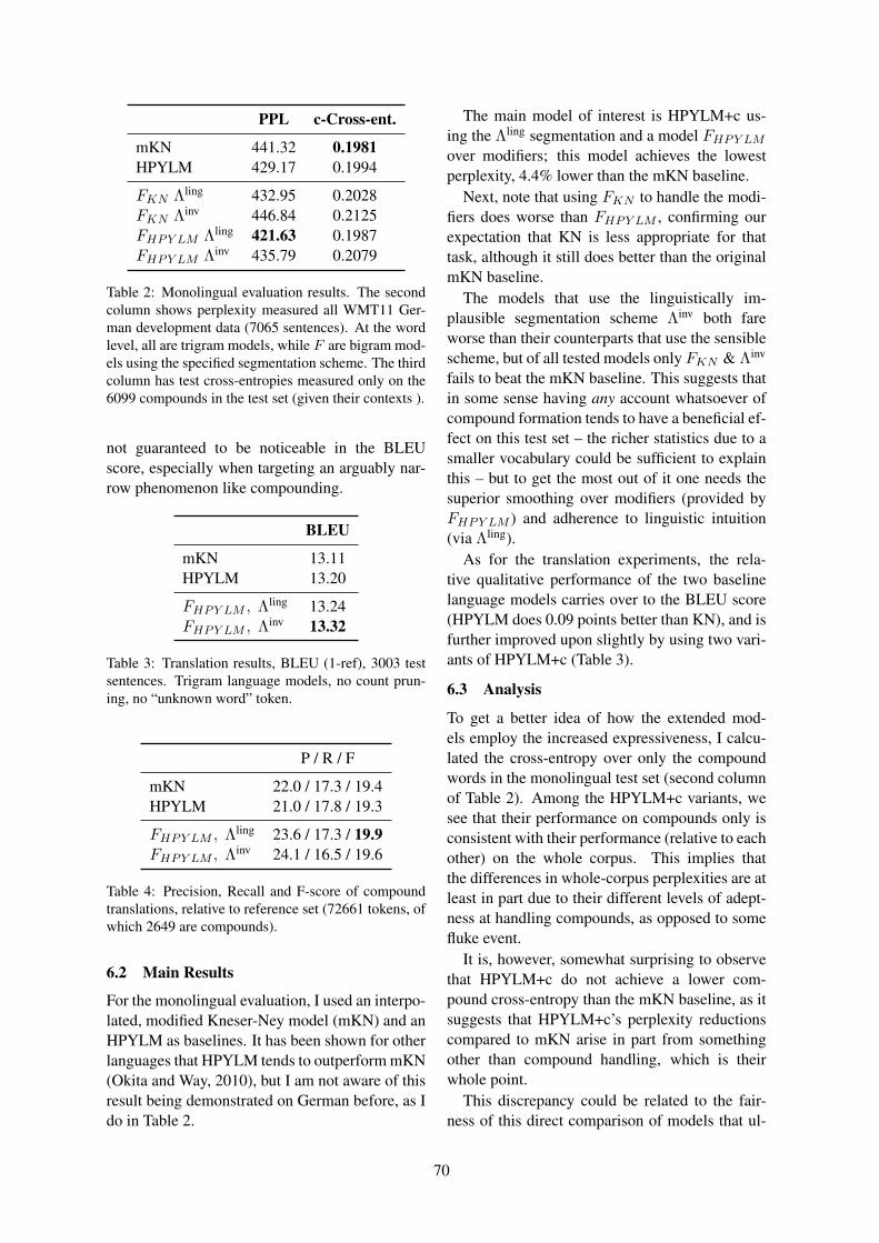
PPL c-Cross-ent.

mKN 441.32 0.1981HPYLM 429.17 0.1994

FKN Λling 432.95 0.2028FKN Λinv 446.84 0.2125FHPY LM Λling 421.63 0.1987FHPY LM Λinv 435.79 0.2079

Table 2: Monolingual evaluation results. The secondcolumn shows perplexity measured all WMT11 Ger-man development data (7065 sentences). At the wordlevel, all are trigram models, while F are bigram mod-els using the specified segmentation scheme. The thirdcolumn has test cross-entropies measured only on the6099 compounds in the test set (given their contexts ).

not guaranteed to be noticeable in the BLEUscore, especially when targeting an arguably nar-row phenomenon like compounding.

BLEU

mKN 13.11HPYLM 13.20

FHPY LM , Λling 13.24FHPY LM , Λinv 13.32

Table 3: Translation results, BLEU (1-ref), 3003 testsentences. Trigram language models, no count prun-ing, no “unknown word” token.

P / R / F

mKN 22.0 / 17.3 / 19.4HPYLM 21.0 / 17.8 / 19.3

FHPY LM , Λling 23.6 / 17.3 / 19.9FHPY LM , Λinv 24.1 / 16.5 / 19.6

Table 4: Precision, Recall and F-score of compoundtranslations, relative to reference set (72661 tokens, ofwhich 2649 are compounds).

6.2 Main Results

For the monolingual evaluation, I used an interpo-lated, modified Kneser-Ney model (mKN) and anHPYLM as baselines. It has been shown for otherlanguages that HPYLM tends to outperform mKN(Okita and Way, 2010), but I am not aware of thisresult being demonstrated on German before, as Ido in Table 2.

The main model of interest is HPYLM+c us-ing the Λling segmentation and a model FHPY LMover modifiers; this model achieves the lowestperplexity, 4.4% lower than the mKN baseline.

Next, note that using FKN to handle the modi-fiers does worse than FHPY LM , confirming ourexpectation that KN is less appropriate for thattask, although it still does better than the originalmKN baseline.

The models that use the linguistically im-plausible segmentation scheme Λinv both fareworse than their counterparts that use the sensiblescheme, but of all tested models only FKN & Λinv

fails to beat the mKN baseline. This suggests thatin some sense having any account whatsoever ofcompound formation tends to have a beneficial ef-fect on this test set – the richer statistics due to asmaller vocabulary could be sufficient to explainthis – but to get the most out of it one needs thesuperior smoothing over modifiers (provided byFHPY LM ) and adherence to linguistic intuition(via Λling).

As for the translation experiments, the rela-tive qualitative performance of the two baselinelanguage models carries over to the BLEU score(HPYLM does 0.09 points better than KN), and isfurther improved upon slightly by using two vari-ants of HPYLM+c (Table 3).

6.3 Analysis

To get a better idea of how the extended mod-els employ the increased expressiveness, I calcu-lated the cross-entropy over only the compoundwords in the monolingual test set (second columnof Table 2). Among the HPYLM+c variants, wesee that their performance on compounds only isconsistent with their performance (relative to eachother) on the whole corpus. This implies thatthe differences in whole-corpus perplexities are atleast in part due to their different levels of adept-ness at handling compounds, as opposed to somefluke event.

It is, however, somewhat surprising to observethat HPYLM+c do not achieve a lower com-pound cross-entropy than the mKN baseline, as itsuggests that HPYLM+c’s perplexity reductionscompared to mKN arise in part from somethingother than compound handling, which is theirwhole point.

This discrepancy could be related to the fair-ness of this direct comparison of models that ul-

70

timately model different sets of things: Accord-ing to the generative process of HPYLM+c (§4),there is no limit on the number of components ina compound: in theory, an arbitrary number ofcomponents c ∈ M can combine to form a word.HPYLM+c is thus defined over a countably infi-nite set of words, thereby reserving some prob-ability mass for items that will never be realisedin any corpus, whereas the baseline models aredefined only over the finite set W . These directcomparisons are thus lightly skewed in favour ofthe baselines. This bolsters confidence in the per-plexity reductions presented in the previous sec-tion, but the skew may afflict compounds morestarkly, leading to the slight discrepancy observedin the compound cross-entropies. What mattersmore is the performance among the HPYLM+cvariants, since they are directly comparable.

To home in still further on the compound mod-elling, I selected those compounds for whichHPYLM+c (FHPY LM ,Λling) does best/worst interms of the probabilities assigned, compared tothe mKN baseline (see Table 5). One pattern thatemerges is that the “top” compounds mostly con-sist of components that are likely to be quite com-mon, and that this improves estimates both for n-grams that are very rare (the singleton “senkun-gen der treibhausgasemmissionen” = decreases ingreen house gas emissions) or relatively common(158, “der hauptstadt” = of the capital).

n-gram ∆ C

gesichts·punkten 0.064 335700 milliarden us-·dollar 0.021 2

s. der treibhausgas·emissionen 0.018 1r. der treibhausgas·emissionen 0.011 3

ministerium fur land·wirtschaft 0.009 11bildungs·niveaus 0.009 14

newt ging·rich* -0.257 2nouri al-·maliki* -0.257 3

klerikers moqtada al-·sadr* -0.258 1nuri al-·maliki* -0.337 3

sankt peters·burg* -0.413 35nachtlichem flug·larm -0.454 2

Table 5: Compound n-grams in the test set for whichthe absolute difference ∆ = PHPYLM+c−PmKN is great-est. C is n-gram count in the training data. Asterisksdenote words that are not compounds, linguisticallyspeaking. Abbrevs: r. = reduktionen, s.= senkungen

On the other hand, the “bottom” compoundsare mostly ones whose components will be un-common; in fact, many of them are not truly com-pounds but artefacts of the somewhat greedy seg-mentation procedure I used. Alternative proce-dures will be tested in future work.

Since the BLEU scores do not reveal muchabout the new language models’ effect on com-pound translation, I also calculated compound-specific accuracies, using precision, recall andF-score (Table 4). Here, the precision for asingle sentence would be 100% if all the com-pounds in the output sentence occur in the ref-erence translation. Compared to the baselines,the compound precision goes up noticeably underthe HPYLM+c models used in translation, with-out sacrificing on recall. This suggests that thesemodels are helping to weed out incorrectly hy-pothesised compounds.

6.4 Caveats

All results are based on single runs and are there-fore not entirely robust. In particular, MERTtuning of the translation model is known to in-troduce significant variance in translation perfor-mance across different runs, and the small differ-ences in BLEU scores reported in Table 3 are verylikely to lie in that region.

Markov chain convergence also needs furtherattention. In absence of complex latent struc-ture (for the dishes), the chain should mix fairlyquickly, and as attested by Figure 2 it ‘converges’with respect to the test metric after about 20 sam-ples, although the log posterior (not shown) hadnot converged after 40. The use of a single poste-rior sample could also be having a negative effecton results.

7 Future Directions

The first goal will be to get more robust ex-perimental results, and to scale up to 4-grammodels estimated on all the available monolin-gual training data. If good performance can bedemonstrated under those conditions, this gen-eral approach could pass as a viable alternative tothe current Kneser-Ney dominated state-of-the artsetup in MT.

Much of the power of the HPYLM+c modelhas not been exploited in this evaluation, in par-ticular its ability to score unseen compounds con-sisting of known components. This feature was

71

0 10 20 30 40

Iteration

420

440

460

480

500

520

540

560P

erp

lexit

yKN Λling

HPYLM

HPYLM+c Λling

mKN-baseline

Figure 2: Convergence of test set perplexities.

not active in these evaluations, mostly due to thecurrent phase of implementation. A second areaof focus is thus to modify the decoder to gen-erate such unseen compounds in translation hy-potheses. Given the current low compound recallrates, this could greatly benefit translation quality.An informal analysis of the reference translationsin the bilingual test set showed that 991 of the1406 out-of-vocabulary compounds (out of 2692OOVs in total) fall into this category of unseen-but-recognisable compounds.

Ultimately the idea is to apply this modellingapproach to other linguistic phenomena as well.In particular, the objective is to model instancesof concatenative morphology beyond compound-ing, with the aim of improving translation intomorphologically rich languages. Complex agree-ment patterns could be captured by condition-ing functional morphemes in the target word onmorphemes in the n-gram context, or by stem-ming context words during back-off. Such ad-ditional back-off paths can be readily encoded inthe Graphical Pitman-Yor process (Wood and Teh,2009).

These more complex models may requirelonger to train. To this end, I intend to use thesingle table per dish approximation (§5) to reducetraining to a single deterministic pass through thedata, conjecturing that this will have little effecton extrinsic performance.

8 Summary

I have argued for further explorations into theuse of a family of hierarchical Bayesian modelsfor targeting linguistic phenomena that may notbe captured well by standard n-gram language

models. To ground this investigation, I focusedon German compounds and showed how thesemodels are an appropriate vehicle for encodingprior linguistic intuitions about such compounds.The proposed generative model beats the popu-lar modified Kneser-Ney model in monolingualevaluations, and preliminarily achieves small im-provements in translation from English into Ger-man. In this translation task, single-token Ger-man compounds traditionally pose challenges totranslation systems, and preliminary results showa small increase in the F-score accuracy of com-pounds in the translation output. Finally, I haveoutlined the intended steps for expanding this lineof inquiry into other related linguistic phenomenaand for adapting a translation system to get opti-mal value out of such improved language models.

AcknowledgementsThanks goes to my supervisor, Phil Blunsom, forcontinued support and advice; to Chris Dyer forsuggesting the focus on German compounds andsupplying a freshly trained compound splitter; tothe Rhodes Trust for financial support; and to theanonymous reviewers for their helpful feedback.

ReferencesMarco Baroni and Johannes Matiasek. 2002. Pre-

dicting the components of German nominal com-pounds. In ECAI, pages 470–474.

Andre Berton, Pablo Fetter, and Peter Regel-Brietzmann. 1996. Compound Words in Large-Vocabulary German Speech Recognition Systems.In Proceedings of Fourth International Conferenceon Spoken Language Processing. ICSLP ’96, vol-ume 2, pages 1165–1168. IEEE.

Jeff A Bilmes and Katrin Kirchhoff. 2003. Factoredlanguage models and generalized parallel back-off. In Proceedings of NAACL-HLT (short papers),pages 4–6, Stroudsburg, PA, USA. Association forComputational Linguistics.

Stanley F Chen and Joshua Goodman. 1998. AnEmpirical Study of Smoothing Techniques for Lan-guage Modeling. Technical report.

David Chiang. 2007. Hierarchical Phrase-Based Translation. Computational Linguistics,33(2):201–228, June.

Chris Dyer, Adam Lopez, Juri Ganitkevitch, JohnathanWeese, Ferhan Ture, Phil Blunsom, Hendra Se-tiawan, Vladimir Eidelman, and Philip Resnik.2010. cdec: A Decoder, Alignment, and Learningframework for finite-state and context-free trans-lation models. In Proceedings of the Association

72

for Computational Linguistics (Demonstration ses-sion), pages 7–12, Uppsala, Sweden. Associationfor Computational Linguistics.

Chris Dyer. 2009. Using a maximum entropy modelto build segmentation lattices for MT. In Proceed-ings of NAACL, pages 406–414. Association forComputational Linguistics.

John Goldsmith and Tom Reutter. 1998. AutomaticCollection and Analysis of German Compounds. InF. Busa F. et al., editor, The Computational Treat-ment of Nominals, pages 61–69. Universite de Mon-treal, Canada.

Sharon Goldwater, Thomas L. Griffiths, and MarkJohnson. 2006. Interpolating Between Types andTokens by Estimating Power-Law Generators. InAdvances in Neural Information Processing Sys-tems, Volume 18.

Songfang Huang and Steve Renals. 2007. Hierarchi-cal Pitman-Yor Language Models For ASR in Meet-ings. IEEE ASRU, pages 124–129.

Songfang Huang and Steve Renals. 2009. A paral-lel training algorithm for hierarchical Pitman-Yorprocess language models. In Proceedings of Inter-speech, volume 9, pages 2695–2698.

Reinhard Kneser and Hermann Ney. 1995. Improvedbacking-off for m-gram language modelling. InProceedings of the IEEE International Conferenceon Acoustics, Speech and SIgnal Processing, pages181–184.

Philipp Koehn and Kevin Knight. 2003. EmpiricalMethods for Compound Splitting. In Proceedingsof EACL, pages 187–193. Association for Compu-tational Linguistics.

Philipp Koehn, Abhishek Arun, and Hieu Hoang.2008. Towards better Machine Translation Qual-ity for the German – English Language Pairs. InThird Workshop on Statistical Machine Translation,number June, pages 139–142. Association for Com-putational Linguistics.

Percy Liang, Ben Taskar, and Dan Klein. 2006. Align-ment by Agreement. In Proceedings of the HumanLanguage Technology Conference of the NAACL,Main Conference, pages 104–111, New York City,USA, June. Association for Computational Linguis-tics.

Daichi Mochihashi, Takeshi Yamada, and NaonoriUeda. 2009. Bayesian unsupervised word seg-mentation with nested Pitman-Yor language mod-eling. In Proceedings of the Joint Conference ofthe 47th Annual Meeting of the ACL and the 4th In-ternational Joint Conference on Natural LanguageProcessing of the AFNLP: Volume 1 - ACL-IJCNLP’09, pages 100–108, Suntec, Singapore. Associa-tion for Computational Linguistics.

Radford M Neal. 2003. Slice Sampling. The Annalsof Statistics, 31(3):705–741.

Graham Neubig, Masato Mimura, Shinsuke Mori, andTatsuya Kawahara. 2010. Learning a LanguageModel from Continuous Speech. In Interspeech,pages 1053–1056, Chiba, Japan.

Franz Josef Och. 2003. Minimum Error Rate Trainingin Statistical Machine Translation. In Proceedingsof ACL, pages 160–167.

Tsuyoshi Okita and Andy Way. 2010. HierarchicalPitman-Yor Language Model for Machine Transla-tion. Proceedings of the International Conferenceon Asian Language Processing, pages 245–248.

Kishore Papineni, Salim Roukos, Todd Ward, Wei-jing Zhu, Thomas J Watson, and Yorktown Heights.2001. Bleu: A Method for Automatic Evaluation ofMachine Translation. Technical report, IBM.

J Pitman and M. Yor. 1997. The two-parameterPoisson-Dirichlet distribution derived from a sta-ble subordinator. The Annals of Probability,25:855–900.

J. Pitman. 2002. Combinatorial stochastic processes.Technical report, Department of Statistics, Univer-sity of California at Berkeley.

Sara Stymne. 2009. A comparison of merging strate-gies for translation of German compounds. Pro-ceedings of the 12th Conference of the EuropeanChapter of the Association for Computational Lin-guistics: Student Research Workshop, pages 61–69.

Yee Whye Teh. 2006. A hierarchical Bayesian lan-guage model based on Pitman-Yor processes. InProceedings of the 21st International Conferenceon Computational Linguistics and the 44th annualmeeting of the ACL, pages 985–992. Association forComputational Linguistics.

Frank Wood and Yee Whye Teh. 2009. A Hierarchi-cal Nonparametric Bayesian Approach to StatisticalLanguage Model Domain Adaptation. In Proceed-ings of the 12th International Conference on Arti-ficial Intelligence and Statistics (AISTATS), pages607–614, Clearwater Beach, Florida, USA.

Mei Yang and Katrin Kirchhoff. 2006. Phrase-basedBackoff Models for Machine Translation of HighlyInflected Languages. In Proceedings of the EACL,pages 41–48.

73

Proceedings of the EACL 2012 Student Research Workshop, pages 74–80,Avignon, France, 26 April 2012. c©2012 Association for Computational Linguistics

Mining Co-Occurrence Matrices for SO-PMI Paradigm WordCandidates

Aleksander WawerInstitute of Computer Science, Polish Academy of Science

ul. Jana Kazimierza 501-248 Warszawa, Polandaxw@ipipan.waw.pl

Abstract

This paper is focused on one aspect of SO-PMI, an unsupervised approach to senti-ment vocabulary acquisition proposed byTurney (Turney and Littman, 2003). Themethod, originally applied and evaluatedfor English, is often used in bootstrap-ping sentiment lexicons for European lan-guages where no such resources typicallyexist. In general, SO-PMI values are com-puted from word co-occurrence frequenciesin the neighbourhoods of two small sets ofparadigm words. The goal of this work isto investigate how lexeme selection affectsthe quality of obtained sentiment estima-tions. This has been achieved by compar-ing ad hoc random lexeme selection withtwo alternative heuristics, based on clus-tering and SVD decomposition of a wordco-occurrence matrix, demonstrating supe-riority of the latter methods. The work canbe also interpreted as sensitivity analysis onSO-PMI with regard to paradigm word se-lection. The experiments were carried outfor Polish.

1 Introduction

This paper seeks to improve one of the main meth-ods of unsupervised lexeme sentiment polarity as-signment. The method, introduced by (Turneyand Littman, 2003), is described in more detail inSection 2. It relies on two sets of paradigm words,positive and negative, which determine the polar-ity of unseen words.

The method is resource lean and therefore oftenused in languages other than English. Recent ex-amples include Japanese (Wang and Araki, 2007)and German (Remus et al., 2006).

Unfortunately, the selection of paradigm wordsrarely receives sufficient attention and is typicallydone in an ad hoc manner. One notable exampleof manual paradigm word selection method waspresented in (Read and Carroll, 2009).

In this context, an interesting variation of thesemantic orientation–pointwise mutual informa-tion (SO-PMI) algorithm for Japanese was sug-gested by (Wang and Araki, 2007). Authors, mo-tivated by excessive leaning toward positive opin-ions, proposed to modify the algorithm by intro-ducing balancing factor and detecting neutral ex-pressions. As will be demonstrated, this problemcan be addressed by proper selection of paradigmpairs.

One not entirely realistic, but nevertheless in-teresting theoretical possibility is to pick pairsof opposing adjectives with the highest loadingsidentified in Osgood’s experiments on semanticdifferential (Osgood et al., 1967). In the exper-iments, respondents were presented with a nounand asked to choose its appropriate position ona scale between two bipolar adjectives (for ex-ample: adequate-inadequate, valuable-worthless,hot-cold). Factor analysis of the results revealedthree distinctive factors, called Osgood dimen-sions. The first of the dimensions, often consid-ered synonymous with the notion of sentiment,was called Evaluative because its foundational ad-jective pair (one with the highest loading) is good-bad.

The first problem with using adjective pairs asexemplary for word co-occurrence distributionson the basis of their loadings, is the fact that fac-tor loadings as measured by Osgood et al. are notnecessarily reflected in word frequency phenom-ena.

74

The second problem is translation: an adjectivepair, central in English, may not be as stronglyassociated with a dimension (here: Evaluative) inother languages and cultures.

The approach we suggest in this paper assumesa latent structure behind word co-occurrence fre-quencies. The structure may be seen as a mix-ture of latent variables of unknown distributionsthat drives word selection. Some of the vari-ables are more likely to produce certain types ofhighly evaluative words (words with high senti-ment scores). We do not attempt to model thestructure in a generative way as in for exam-ple probabilistic latent semantic analysis (PLSA)or latent Dirichlet allocation (LDA). A gener-ative approximation is not feasible when usingcorpora such as the balanced, 300-million ver-sion of the National Corpus of Polish (NKJP)(Przepiórkowski et al., 2008; Przepiórkowski etal., 2012) 1 applied in the experiments describedin the next sections, which does not enable creat-ing a word-document matrix and organizing wordoccurrences by documents or narrowly specifiedtopics.

Therefore, we propose different techniques.We begin with a symmetric matrix of word co-occurences and attempt to discover as much ofits structure as possible using two well estab-lished techniques: Singular Value Decomposi-tion and clustering. The discovered structures arethen used to optimize the selection of words forparadigm sets used in SO-PMI.

The paper is organized as follows. In Section2 we define the SO-PMI measure and briefly for-mulate the problem. Section 3 describes obtainingthe set of sentiment word candidates, which arethen used to generate a symmetric co-occurencematrix as outlined in Section 4. Section 5 delin-eates the details of human word scoring, whichserves as a basis for evaluations in 9. Sections6, 7 and 8 describe three distinct approaches toparadigm sets generation.

2 Problem Statement. SO-PMI

When creating a sentiment lexicon, the strengthof association between candidate words and eachof the two polar classes (positive and negative,for instance) can be calculated using several mea-

1http://www.nkjp.pl/index.php?page=0&lang=1

sures. Perhaps most popular of them, employed inthis experiment after (Turney and Littman, 2003)and (Grefenstette et al., 2006) is Pointwise MutualInformation (PMI). The Pointwise Mutual Infor-mation (PMI) between two words, w1 and w2, isdefined as:

PMI(w1, w2) = log2

(p(w1&w2)

p(w1)p(w2)

)where p(w1 & w2) is the probability of co-

occurrence of (w1) and (w2). For the task of as-signing evaluative polarity, it is computed as num-ber of co-occurrences of candidate words witheach of the paradigm positive and negative words,denoted as pw and nw. Optimal selection of thesetwo sets of words is the subject of this paper.

Once the words are known, the semantic ori-entation PMI (SO-PMI) of each candidate word ccan be computed as:

SO-PMI(c) =

=∑

pw∈PW

PMI(c, pw)−∑

nw∈NW

PMI(c, nw)

The equation above demonstrates that opti-mization of both word lists, pw and nw, is of cru-cial importance for the performance of SO-PMI.

3 Generating Sentiment WordCandidates

This section describes the acquisition of senti-ment word candidates. The method we followedcould be substituted by any other technique whichresults in a set of highly sentimental lexemes, pos-sibly of varying unknown polarity and strength. Asimilar experiment for English has been describedby (Grefenstette et al., 2006).

The procedure can be described as follows. Inthe first step, a set of semi-manually defined lexi-cal patterns is submitted to a search engine to findcandidates for evaluatively charged terms. Then,the downloaded corpus is analyzed for patterncontinuations – lexemes immediately followingpattern matches, which are likely to be candidatesfor sentiment words. In the last step, candidateterms selected this way are tested for their senti-ment strength and polarity (in other words, howpositive or negative are the conotations). In origi-nal experiment described in the cited paper, wordswere evaluated using the SO-PMI technique.

75

The purpose of using extraction patterns is toselect candidates for evaluative words. In thisexperiment, 112 patterns have been created bygenerating all combinations of elements from twomanually prepared sets2, A and B:

• A: [0] wydawac sie, [1] wydawał sie, [2]wydawała sie, [3] czuc sie, [4] czułem sie,[5] czułam sie, [6] czułem, [7] byc 3

• B: [0] nie dosc, [1] niewystarczajaco, [2]niedostatecznie, [3] za mało, [4] prawie, [5]niemal, [6] tak, [7] taki, [8] zbyt, [9] zbyt-nio, [10] za bardzo, [11] przesadnie, [12]nadmiernie, [13] szczególnie 4

Each pattern (a combination of A and B) hasbeen wrapped with double quotes (“A B”) andsubmitted to Google to narrow the results to textswith exact phrases. The Web crawl yielded 17657web pages, stripped from HTML and other webtags to filter out non-textual content. Two patternsare grammatically incorrect due to gender dis-agreement, namely wydawała sie taki and czułamsie taki 5, thus did not generate any results.

The corpus of 17657 web pages has been an-alyzed using Spejd6, originally a tool for par-tial parsing and rule-based morphosyntactic dis-ambiguation, adapted in the context of this workfor the purpose of finding pattern continuations.Again, 112 patterns were constructed by gener-ating all combinations of elements from the twosets, A and B above. Spejd rules were written as“A B *” where the wildcard can be either an ad-jective or an adverb.

Parsing the web pages using the 112 patternsresulted in acquiring 1325 distinct base wordforms (lexemes) recognized by the morphologicanalyser and related dictionaries. This list is sub-sequently used for generating the co-occurrence

2Terms are translations of words listed in (Grefenstette etal., 2006). Many of the expressions denote either excess ordeficiency, as for example not enough or too much.

3English translations (morphosyntactic tags in parenthe-ses): [0] seem to (inf), [1] seemed to (sg,pri,perf,m), [2]seemed to (sg,pri,perf,f), [3] feel (inf), [4] felt (sg,pri,perf,m),[5] felt (sg,pri,perf,f), [7] to be (inf)

4items [0-3] are various ways of expressing not enough,items [4-5] almost, items [6-7] such, items [8-12] too much,item [13] especially

5seemed(f) so(m) and felt(f) so(m)6http://nlp.ipipan.waw.pl/Spejd/

(Przepiórkowski and Buczynski, 2007)

matrix as delineated in the next Section and forselecting paradigm words.

4 Word Co-Occurrence Matrix

Each word (base form) from the list was soughtin the balanced, 300 million segments7 version ofthe National Corpus of Polish (NKJP). For eachrow i and column j of the co-occurrence matrixm, its value was computed as follows:

mij =fij

fifj

where fij denotes the number of co-occurencesof word i within the window of 20 segments leftand right with word j, fi and fj denote the totalnumbers of occurrences of each word. The se-lection of a window of 20 follows the choice in(Turney and Littman, 2003).

This design has been found optimal after anumber of experiments with the singular value de-composition (SVD) technique described further.Without the denominator part, decompositions areheavily biased by word frequency. In this defni-tion, the matrix resembles the PMI form in (Tur-ney and Pantel, 2010), however we found that thelogarithm transformation flattens the eigenvaluedistribution and is not really necessary.

If the distributions of words i and j are statis-tically independent, then by the defnition of inde-pendence fifj = fij . The product fifj is what wewould expect for fij , if i occurs in the contexts ofj by the matter of a random chance. The opposingsituation happens when there exists a relationshipbetween i and j, for instance when both wordsare generated by the same latent topic variable,and we expect fij to be larger than in the case ofindependency.

5 Evaluating Word Candidates

In order to evaluate combinations of paradigmwords, one needs to compare the computed SO-PMI scores against a human made scoring. Ide-ally, such a scoring should not only inform aboutpolarity (indication whether a word is positive ornegative), but also about association strength (thedegree of positivity or negativity). Reliable and

7A segment usually corresponds to a word. Segmentsare not longer than orthographic words, but sometimesshorter. See http://nkjp.pl/poliqarp/help/ense1.html#x2-10001 for a detailed discussion

76

valid measurement of word associations on a mul-tipoint scale is not easy: the inter rater agreementis likely to decrease with the growing complexityof the scale.

Therefore, we decided that each lexeme was in-dependently scored by two humans using a fivepoint scale. Extreme values denoted very nega-tive or positive words, the central value denotedneutral words and remaining intermediate valueswere interpreted as somehow positive or nega-tive. Discrepancies between raters were solvedby arithmetic means of conflicting scores ratherthan introducing the third human (often called theGolden Annotator) to select one value of the two.Consequently, the 5-point scale extended to 10points.

Human word scores were used in evaluations ofmethods described in forthcoming sections.

6 Random Selection

The baseline method to compare against is to se-lect lexemes in a random fashion. In order to en-sure highest possible performance of the method,lexemes were selected only from those with atleast one extreme human score (very positive orvery negative) and at least 500 occurrences in thecorpus. The last condition renders this methodslightly favourable because in the case of SVD, inmany eigenvectors the highly loaded terms werenot as frequent and had to be selected despite rel-ative rarity.

7 SVD

The word co-occurrence matrix m (1325x1325)was the subject of singular value decomposition(SVD), a well-known matrix factorization tech-nique which decomposes a matrix A into threematrices:

A = UΣV T

where Σ is a matrix whose diagonals are thesingular values of A, U and V are left and righteigenvectors matrices.

The usage of SVD decompositions has a longand successful history of applications in extract-ing meaning from word frequencies in word-document matrices, as for example the well es-tablished algorithm of latent semantic indexing(LSI). More recently, the usability of analyzingthe structure of language via spectral analysis

of co-occurrence matrices was demonstrated bystudies such as (Mukherjee et al., 2009). The fo-cus was on phonology with the intention to dis-cover principles governing consonant inventoriesand quantify their importance. Our work, as webelieve, is the first to apply SVD in the context ofco-occurrence matrices and SO-PMI.

We suspect that the SVD technique can be help-ful by selecting lexemes that represent certainamounts of latent co-occurrence structure. Fur-thermore, the fact that 20 eigenvalues constitutesapproximately half of the norm of the spectrum(Horn and Johnson, 1990), as on Table 1, suggeststhat there may exist a small number of organiz-ing principles which could be potentially helpfulto improve the selection of lexemes into paradigmsets.

c m10 0.728 0.41020 0.797 0.498100 0.924 0.720

Table 1: Frobenius norm of the spectrum for 10, 20and 100 first eigenvalues.

Table 1 depicts also the problem of frequencybias, stronger in case of 10 and 20 eigenvaluesthan for 100. The values were computed for twomatrices: c contains only co-occurrence frequen-cies and m is the matrix described in section 4.Figure 1 plots the eigenvalue spectrum restrictedto the first 100 values.

""0 20 40 60 80 100

Eigenvalues

0.0000

0.0005

0.0010

0.0015

0.0020

0.0025

0.0030

0.0035

0.0040

Norm

of the spectrum

Figure 1: Eigenvalue distribution (limited to the first100).

In order to “discover” the principles behind theco-occurrences, we examine eigenvectors associ-

77

ated with the largest eigenvalues. Some of thevectors indeed appear to have their interpretationsor at least one could name common properties ofinvolved words. The meaning of vectors becomesusually apparent after examination of the first fewtop component weights.

The list below consits of four eigenvectors, topthree and the eighth one (as ordered accordingto their eigenvalues), along with five terms withhighest absolute weights and interpretations ofeach vector.

1 sztuczny (artificial), liryczny (lyrical), upi-orny (ghastly), zrzedliwy (grouchy), prze-jrzysty (lucid).⇒ abstract properties one could attribute toan actor or a play.

2 instynktowny (instinctive), odlotowo (su-per/cool), ostrozny (careful), bolesny(painful), przesadnie (excessively)⇒ physical and sensual experiences

3 wyemancypowac (emancipate), opuszczony(abandoned), przeszywac (pierce), wscibski(inquisitive), jednakowo (alike)⇒ unpleasant states and behaviours

8 gładki (smooth), kochany (beloved), staracsie (make efforts), niedołezny (infirm), in-tymnie (intimately)⇒ intimacy, caring, emotions

As it has been noted before, the eigenvectorsof pure co-occurrence matrix c did not deliveranything close in terms of conceivable interpreta-tions. It is also fairly clear that some of the eigen-vectors, as for example the third one, are more re-lated to sentiment than the others. This is also evi-dent by examination of average lexeme sentimentof top loaded terms of each vector, not disclosedin the paper.

The heuristic of SVD backed selection ofparadigm words maximizes three factors:

• corpus frequency: avoid rare words wherepossible;

• eigenvector component weights: selectwords that contribute the most to a giveneigenvector;

• sentiment polarity: select words with thehighest absolute human scores.

8 Affinity Propagation

Affinity Propagation (Frey and Dueck, 2007)method was selected because of two distinct ad-vantages for our task. First is the fact that itclusters data by diffusion in the similarity matrix,therefore does not require finding representationsin Euclidean space. Second advantage, especiallyover cluster analysis algorithms such as k-means,is that the algorithm automatically sets its numberof clusters and does not depend on initialization.

Affinity Propagation clusters data by exchang-ing real-valued messages between data points un-til a high-quality set of exemplars (representativeexamples, lexemes in our case) and correspondingclusters gradually emerges.

Interestingly, in each parameter setting the al-gorithm found exactly 156 clusters. It hints atthe fact that the number of “latent” variables be-hind the co-occurrences could indeed be over 100.This is further confirmed by the percentage ofnorm of the spectrum covered by top 100 eigen-values.

""0 20 40 60 80 100 120 140

Clusters

0

5

10

15

20

25

30

Frequency

Figure 2: Histogram of cluster counts.

The five most frequent clusters cover only 116words. We restrict the selection of paradigmwords to the same frequency and polarity condi-tions as in the case of random method. We pickone paradigm word from each most frequent clus-ter because we assume that it is sufficient to ap-proximate the principle which organizes that clus-ter. The heuristic is very similar to the one usedin case of SVD.

78

9 Evaluation

Using continous SO-PMI and multi point scalesfor human scoring facilitates formulating theproblem as a regression one, where goodness offit of the estimations can be computed using dif-ferent measures than in the case of classification.

This, however, demands a mapping such thatranges of the continuous SO-PMI scale corre-spond to discrete human scores. We propose tobase such a mapping on dividing the SO-PMIrange into 10 segments s0, ..., s10 of variouslength, each of which corresponds to one discretehuman value.

The choice of values (locations) of specificpoints is a subject of minimization where the errorfunction E over a set of words W is as follows:

E =∑

w∈W

dist(sc, se)

For each word w, the distance function dist re-turns the number of segments between the correctsegment sc and the estimated segment se usingthe SO-PMI. We minimize E and find optimumlocations for points separating each segment us-ing Powell’s conjugate direction method, deter-mined the most effective for this task. Powell’salgorithm is a non-gradient numerical optimiza-tion technique, applicable to a real valued func-tion which does not need not be differentiable(Powell, 1964).

10 Results

Table 2 presents E errors and extreme (min andmax) SO-PMI values computed over two indepen-dent samples of 500 lexemes. Error columns indi-cated as E denote errors computed either on non-optimized default (def ) or optimized segments(min). Each combination of paradigm words andeach sample required re-computing optimum val-ues of points dividing the SO-PMI scale into seg-ments.

Generally, the randomized selection methodperforms surprisingly well – most likely due tothe fact that the frequency and polarity conditionsare the key factors. In either case, the best re-sult was obtained using the selection of paradigmwords using the heuristic based on svd, closelyfollowed by aff . In one case, random selectionperformed better than the aff .

SO-PMI Esample min max def minS1 r1 -14 29 1226 908

r2 -15 23 1131 765r3 -18 8.6 844 710aff -9 25 1057 716svd -13 26 1002 701

S2 r1 -18 19 983 812r2 -17 15 910 756r3 -11 20 1016 789aff -13 28 1033 732svd -13 35 1028 724

Table 2: SO-PMI ranges and error (E) values on twoindependent random samples of N=500. 3 randomizedselections (r1 − r3), Affinity Propagation (aff ) andSVD (svd).

The small margin of a victory could be ex-plained by the fact that the size of each set ofparadigm SO-PMI words is limited to five lex-emes. Consequently, it is very difficult to repre-sent a space of over one hundred latent variables– because such appears to be the number indicatedby the distribution of eigenvalues in SVD and thenumber of clusters.

The ranges of SO-PMI values (in the columnsmin and max) were often non symmetric andleaned towards positive. This shift did not nec-essarily translate to higher error rates, especiallyafter optimizations.

11 Discussion and Future Work

The methods presented in this article, based on theassumption of latent word co-occurrence struc-tures, performed moderately better than the base-line of random selections. The result is ambigu-ous because it still requires a more in-depth un-derstanding of underlying mechanims.

The work will be continued in several aspects.One is to pre-determine lexeme type before it isactually evaluated against particular members ofparadigm word sets. This could be acheved us-ing a two-step model consisting of lexeme typeclassification (with regard to over one hundredlatent variables) followed by SO-PMI computa-tion, where the selection of paradigm words is notfixed, as in this paper, but dependens on previ-ously selected latent variables. Another promis-ing direction is to focus on explanations andword features: how adding or removing particu-

79

lar words change the SO-PMI, and more impor-tantly, why (in terms of features involved)? Whatare the features that change SO-PMI in specificdirections? How to extract them?

Acknowledgment

This research is supported by the POIG.01.01.02-14-013/09 project which is co-financed by the Eu-ropean Union under the European Regional De-velopment Fund

References

Brendan J. Frey and Delbert Dueck. 2007. Clusteringby passing messages between data points. Science,315:972–976.

Gregory Grefenstette, Yan Qu, David A. Evans, andJames G. Shanahan, 2006. Validating the Cover-age of Lexical Resources for Affect Analysis and Au-tomatically Classifying New Words along SemanticAxes. Springer. Netherlands.

Roger A. Horn and Charles R. Johnson. 1990. MatrixAnalysis. Cambridge University Press.

Animesh Mukherjee, Monojit Choudhury, and RaviKannan. 2009. Discovering global patterns in lin-guistic networks through spectral analysis: a casestudy of the consonant inventories. In Proceedingsof the 12th Conference of the European Chapterof the Association for Computational Linguistics,EACL ’09, pages 585–593, Stroudsburg, PA, USA.Association for Computational Linguistics.

Charles E. Osgood, George J. Suci, and Percy H. Tan-nenbaum. 1967. The Measurement of Meaning.University of Illinois Press.

M. J. D. Powell. 1964. An efficient method for findingthe minimum of a function of several variables with-out calculating derivatives. The Computer Journal,7(2):155–162, January.

Adam Przepiórkowski and Aleksander Buczynski.2007.spade: Shallow parsing and disambiguation engine.In Proceedings of the 3rd Language & TechnologyConference, Poznan.

Adam Przepiórkowski, Rafał L. Górski, BarbaraLewandowska-Tomaszczyk, and Marek Łazinski.2008. Towards the national corpus of polish. InThe proceedings of the 6th Language Resources andEvaluation Conference (LREC 2008), Marrakesh,Morocco.

Adam Przepiórkowski, Mirosław Banko, Rafał L.Górski, and Barbara Lewandowska-Tomaszczyk,editors. 2012. Narodowy Korpus Jezyka Polskiego.Wydawnictwo Naukowe PWN, Warsaw. Forthcom-ing.

J. Read and J. Carroll. 2009. Weakly supervisedtechniques for domain-independent sentiment clas-sification. In Proceedings of the 1st internationalCIKM workshop on Topic-sentiment analysis formass opinion, pages 45–52. ACM.

Robert Remus, Uwe Quasthoff, and Gerhard Heyer.2006. Sentiws: a publicly available german-language resource for sentiment analysis. In Pro-ceedings of LREC.

Peter Turney and Michael Littman. 2003. Measuringpraise and criticism: Inference of semantic orienta-tion from association. ACM Transactions on Infor-mation Systems, 21:315–346.

Peter D. Turney and Patrick Pantel. 2010. From fre-quency to meaning: vector space models of seman-tics. J. Artif. Int. Res., 37:141–188, January.

Guangwei Wang and Kenji Araki. 2007. Modifyingso-pmi for japanese weblog opinion mining by us-ing a balancing factor and detecting neutral expres-sions. In Human Language Technologies 2007: TheConference of the North American Chapter of theAssociation for Computational Linguistics; Com-panion Volume, Short Papers, NAACL-Short ’07,pages 189–192, Stroudsburg, PA, USA. Associationfor Computational Linguistics.

80

Proceedings of the EACL 2012 Student Research Workshop, pages 81–89,Avignon, France, 26 April 2012. c©2012 Association for Computational Linguistics

Improving Machine Translation of Null Subjects in Italian and Spanish

Lorenza Russo, Sharid Loaiciga, Asheesh GulatiLanguage Technology Laboratory (LATL)

Department of Linguistics – University of Geneva2, rue de Candolle – CH-1211 Geneva 4 – Switzerland

lorenza.russo, sharid.loaiciga, asheesh.gulati@unige.ch

Abstract

Null subjects are non overtly expressedsubject pronouns found in pro-drop lan-guages such as Italian and Spanish. Inthis study we quantify and compare the oc-currence of this phenomenon in these twolanguages. Next, we evaluate null sub-jects’ translation into French, a “non pro-drop” language. We use the Europarl cor-pus to evaluate two MT systems on theirperformance regarding null subject trans-lation: Its-2, a rule-based system devel-oped at LATL, and a statistical systembuilt using the Moses toolkit. Then weadd a rule-based preprocessor and a sta-tistical post-editor to the Its-2 translationpipeline. A second evaluation of the im-proved Its-2 system shows an average in-crease of 15.46% in correct pro-drop trans-lations for Italian-French and 12.80% forSpanish-French.

1 Introduction

Romance languages are characterized by somemorphological and syntactical similarities. Ital-ian and Spanish, the two languages we are inter-ested in here, share the null subject parameter,also called the pro-drop parameter, among othercharacteristics. The null subject parameter refersto whether the subject of a sentence is overtly ex-pressed or not (Haegeman, 1994). In other words,due to their rich morphology, Italian and Span-ish allow non lexically-realized subject pronouns(also called null subjects, zero pronouns or pro-drop).1

From a monolingual point of view, regardingSpanish, previous work by Ferrandez and Peral

1Henceforth, the terms will be used indiscriminately.

(2000) has shown that 46% of verbs in their testcorpus had their subjects omitted. Continuationof this work by Rello and Ilisei (2009) has foundthat in a corpus of 2,606 sentences, there were1,042 sentences without overtly expressed pro-nouns, which represents an average of 0.54 nullsubjects per sentence. As for Italian, many anal-yses are available from a descriptive and theoret-ical perspective (Rizzi, 1986; Cardinaletti, 1994,among others), but to the best of our knowledge,there are no corpus studies about the extent thisphenomenon has.2

Moreover, althought null elements have beenlargely treated within the context of AnaphoraResolution (AR) (Mitkov, 2002; Le Nagard andKoehn, 2010), the problem of translating fromand into a pro-drop language has only been dealtwith indirectly within the specific context of MT,as Gojun (2010) points out.

We address three goals in this paper: i) to com-pare the occurrence of a same syntactic feature inItalian and Spanish, ii) to evaluate the translationof null subjects into French, that is, a “non pro-drop” language; and, iii) to improve the transla-tion of null subjects in a rule-based MT system.Next sections follow the above scheme.

2 Null subjects in source corpora

We worked with the Europarl corpus (Koehn,2005) in order to have a parallel comparative cor-pus for Italian and Spanish. From this corpus,we manually analyzed 1,000 sentences in bothlanguages. From these 1,000 sentences (26,757words for Italian, 27,971 words for Spanish), weidentified 3,422 verbs for Italian and 3,184 for

2Poesio et al. (2004) and Rodrıguez et al. (2010), for in-stance, focused on anaphora and deixis.

81

Spanish. We then counted the occurrences ofverbs with pro-drop and classified them in twocategories: personal pro-drop3 and impersonalpro-drop4, obtaining a total amount of 1,041 pro-drop in Italian and 1,312 in Spanish. Table 1shows the results in percentage terms.

Total Pers. Impers. TotalVerbs pro-

droppro-drop

pro-drop

IT 3,422 18.41% 12.01% 30.42%ES 3,182 23.33% 17.84% 41.17%

Table 1: Results obtained in the detection of pro-drop.

Results show a higher rate of pro-drop in Span-ish (10.75%). It has 4.92% more personal pro-drop and 5.83% more impersonal pro-drop thanItalian. The contrast of personal pro-drop is due toa syntactic difference between the two languages.In Spanish, sentences like (1a.) make use of twopro-drop pronouns while the same syntactic struc-ture uses a pro-drop pronoun and an infinitiveclause in Italian (1b.), hence, the presence of morepersonal pro-drop in Spanish.

(1) a. ES pro le pido (1.sg) que pro inter-venga (3.sg) con el prestigio de sucargo.

b. IT pro le chiedo (1.sg) di intervenire(inf.) con il prestigio della sua carica.I ask you to intervene with the pres-tige of your position.

The difference of impersonal pro-drop, on theother hand, is due to the Spanish use of an im-personal construction (2a.) with the “se” parti-cle. Spanish follows the schema “se + finite verb+ non-finite verb”; Italian follows the schema “fi-nite verb + essere (to be) + past participle” (2b.).We considered this construction formed by onemore verb in Italian than in Spanish as shown inexamples (2a.) and (2b.). This also explains thedifference in the total amount of verbs (Table 1).

(2) a. ES Se podra corregir.b. IT Potra essere modificato.

It can be modified.

3Finite verbs with genuinely referential subjects (i.e. I,you, s/he, we, they).

4Finite verbs with non-referential subjects (i.e. it).

We found a total number of non-expressed pro-nouns in our corpus comparable to those obtainedby Rodrıguez et al. (2010) on the Live Memo-ries corpus for Italian and by Recasens and Martı(2010) on the Spanish AnCora-Co corpus (Table2). Note that in both of these studies, they wereinterested in co-reference links, hence they didnot annotate impersonal pronouns, claiming theyare rare. On the other hand, we took all the pro-drop pronouns into account, including impersonalones.

Corpus Language ResultOur corpus IT 3.89%Live Memories IT 4.5%Our corpus ES 4.69%AnCora-Co ES 6.36%

Table 2: Null-subjects in our corpus compared to LiveMemories and AnCora-Co corpora. Percentages arecalculated with respect to the total number of words.

3 Baseline machine translation of nullsubjects

The 1,000 sentences of our corpus were trans-lated from both languages into French (IT→FR;ES→FR) in order to assess if personal pro-dropand impersonal pro-drop were correctly identi-fied and translated. We tested two systems: Its-2(Wehrli et al., 2009), a rule-based MT system de-veloped at the LATL; and a statistical system builtusing the Moses toolkit out of the box (Koehn etal., 2007). The latter was trained on 55,000 sen-tence pairs from the Europarl corpus and tuned on2,000 additional sentence pairs, and includes a 3-gram language model.

Tables 3 and 4 show percentages of correct, in-correct and missing translations of personal andimpersonal null subjects calculated on the basis ofthe number of personal and impersonal pro-dropfound in the corpus.

We considered the translation correct when thenull pronoun is translated by an overt pronounwith the correct gender, person and number fea-tures in French; otherwise, we considered it in-correct. Missing translation refers to cases wherethe null pronoun is not generated at all in the tar-get language.

We chose these criteria because they allow usto evaluate the single phenomenon of null subject

82

Its-2Pair Pro-drop Correct Incorrect Missing

personal 66.34% 3.49% 30.15%IT→FR impersonal 16.78% 18.97% 64.23%

average 46.78% 9.6% 43.61%personal 55.79% 3.50% 40.70%

ES→FR impersonal 29.29% 11.40% 59.29%average 44.28% 6.93% 48.78%

Table 3: Percentages of correct, incorrect and missing translation of zero-pronouns obtained by Its-2. Average iscalculated on the basis of total pro-drop in corpus.

MosesPair Pro-drop Correct Incorrect Missing

personal 71.59% 1.11% 27.30%IT→FR impersonal 44.76% 11.43% 43.79%

average 61% 5.18% 33.81%personal 72.64% 2.02% 25.34%

ES→FR impersonal 54.56% 2.45% 42.98%average 64.78% 2.21% 33%

Table 4: Percentages of correct, incorrect and missing translation of zero-pronouns obtained by Moses. Averageis calculated on the basis of total pro-drop in corpus.

translation. BLEU and similar MT metrics com-pute scores over a text as a whole. For the samereason, human evaluation metrics based on ade-quacy and fluency were not suitable either (Koehnand Monz, 2006).

Moses generally outperforms Its-2 (Tables 3and 4). Results for the two systems demon-strate that instances of personal pro-drop are bet-ter translated than impersonal pro-drop for thetwo languages. Since rates of missing pronounstranslations are considerable, especially for Its-2,results also indicate that both systems have prob-lems resolving non-expressed pronouns for theirgeneration in French. A detailed description foreach system follows.

3.1 Results – Its-2

Its-2 obtains better results for IT→FR personalpro-drop (66.34%) than for ES→FR (55.79%),but worse for impersonal pro-drop translation(16.78% and 29.29% respectively, Table 3).

For IT→FR translation in particular, Its-2 usu-ally translates an Italian personal pro-drop withan overt pronoun of incorrect gender in French.In fact, it tends to translate a female personal pro-drop with a masculine overt pronoun. This prob-

lem is closely related with that of AR: as the sys-tem does not have any module for AR, it cannotdetect the gender of the antecedent, rendering thecorrect translation infeasible.

The number of correct translation of imper-sonal pro-drop is very low for both pairs. ES→FRreached 29.29%, while IT→FR only 16.78% (Ta-ble 3). The reason for these percentages is a reg-ular mistranslation or a missing translation. Asfor the mistranslation, in the case of Spanish,Its-2 translates the “se” pronoun in impersonalsentences by the French sequence qui est-ce que(who) (3). We attribute this behaviour to a lack ofgeneration rules.

(3) ES Por consiguiente, mi grupo so-licita que se suprima este punto deldıa.FR Par consequent, mon groupe sol-licite qu’on supprime ce point del’agenda.ITS-2 * Par consequent, mon groupesollicite qui est-ce que supprime cepoint du jour.Therefore, my group ask to delete thispoint from the agenda.

83

With respects to missing pronouns in the tar-get language (Table 3), percentages are quite highin both translation pairs (43.61% and 48.78% av-erage missing pronouns respectively), especiallywith impersonal pro-drop. Let us take the exem-ple of ES→FR translation (59.29% missing pro-nouns): Its-2 never generates the French expletivepronouns “ce, c’, ca” (it) (4a.). For IT→FR trans-lation (64.23% missing pronouns), it almost nevergenerates the French pronoun “il” (it) for the im-personal 3rd person pro-drop pronoun in Italian(4b.).

However, if the system generates the pronoun,it is likely to be a first or a second person singularpronoun (“je, tu” – I, you) in French, increasingthen the percentages of incorrectly translated im-personal pro-drop.

(4) a. ES No es pedir demasiado.FR Ce n’est pas trop demander.ITS-2 * Pas est demander trop.It is not too much to ask.

b. IT E vero che [. . . ].FR Il est vrai que [. . . ].ITS-2 * Vrai que [. . . ].It is true that [. . . ].

3.2 Results – Moses

Moses produces the highest percentage of cor-rect translations for both personal and impersonalpro-drop, particularly in ES→FR (72.64% and54.56% respectively, Table 4).

When translating personal pro-drop from Ital-ian, sometimes the system generates infinitiveforms instead of finite verbs (5).

(5) IT Naturalmente accettiamo questoemendamento.FR Bien sur, nous acceptons cetamendement.MOSES Bien sur accepter cetamendement.Of course, we accept this amend-ment.

When translating impersonal pro-drop fromItalian, it performs worse (44.76%) because ittends not to generate the expletive pronoun (6).

Furthermore, for both source languages, Mosestranslates the impersonal pro-drop usually corre-

(6) IT Vorrei, come mi e stato chiesto daalcuni colleghi, osservare un minutodi silenzio.FR J’aimerais, comme il m’a ete de-mande par certains collegues, ob-server une minute de silence.MOSES J’aimerais, comme m’a etedemande par certains collegues, ob-server une minute de silence.I would like, as some collegues askedme, to observe a minute of silence.

sponding to French pronoun “on” as the first plu-ral personal pronoun (“nous” – we) (7a. and 7b.).

(7) a. IT Io credo che si debba dare laprecedenza alla sicurezza.FR Je crois qu’on doit donner la pri-orite a la securite.MOSES Je crois que nous devonsdonner la priorite a la securite.I think that priority should be givento the safety.

b. ES Como han demostrado los even-tos recientes, queda mucho por hacersobre este tema.FR Comme l’ont montre lesevenements recents, on a encorebeaucoup a faire sur ce theme.MOSES Comme l’ont montre lesevenements recents, nous avons en-core beaucoup a faire sur ce theme.As it has been shown by recentevents, there is much left to do on thissubject.

4 Its-2 improvements

On the basis of this first evaluation, we tried to im-prove Its-2 pronoun generation when translatingfrom Italian and Spanish. Two new componentswere added to the translation pipeline: a rule-based preprocessor, and a statistical post-editor.This section presents them in detail, along withthe resources they rely on.

4.1 Rule-based preprocessingPreprocessing of input data is a very common taskin natural language processing. Statistical sys-tems often benefit from linguistic preprocessing

84

to deal with rich morphology and long distance re-ordering issues (Sadat and Habash, 2006; Habash,2007). In our case, the idea behind this first com-ponent is to help the translation process of a rule-based system by reducing the amount of zero pro-nouns in the source document5, ensuring that sub-ject pronouns get properly transferred to the targetlanguage.

In order to assess the effect of this approach, weimplemented a rule-based preprocessor taking asinput a document in Italian or Spanish and return-ing as output the same document with droppedsubject pronouns restored. It relies on two re-sources: a list of personal and impersonal verbs,and a part-of-speech tagging of the source docu-ment. We first present these two resources beforedescribing the approach in more detail.

List of personal and impersonal verbsThis list simply contains surface forms of

verbs. For our experiment, these forms wereextracted from a subset of the Europarl corpus,where pro-drop verbs were manually annotatedas taking a personal pronoun or an impersonalpronoun. This limits the coverage, but ensuresdomain-specific verb usage.

Part-of-speech tagging of the source documentIts-2, being a transfer-based system, relies on

a parser to construct the syntactic structure of thesource language and, from there, it transfers thesyntactic structure onto the target language. Its-2 uses Fips (Wehrli, 2007), a multilingual parseralso developed at LATL. Apart from the projec-tion of syntactic structures, Fips produces part-of-speech tagging.

Outline of the approachThese are the steps followed by the preproces-

sor:

1. Read a part-of-speech tagged sentence.

2. Whenever a verb with no subject is encoun-tered, check if it is a personal verb or an im-personal verb.

5In Italian and Spanish, even if a native speaker wouldnot use subject pronouns in a given sentence, the same sen-tence with overtly expressed subject pronouns is grammati-cal. There might be a pragmatic difference, as pronouns areused in these languages when emphasis or contrast is desired(Haegeman, 1994).

3. If it is a personal verb, generate the appropri-ate pronoun before the verb (the masculineform is generated for the third person); if itis an impersonal verb, do not generate anypronoun.

4. Check the sentence for reordering accordingto syntactic rules of the target language (e.g.move the generated pronoun before a pro-clitic already preceding the verb).

An example of preprocessed sentences is givenin Figure 1.

4.2 Statistical post-editing

Since the work of Simard et al. (2007a), statisti-cal post-editing (SPE) has become a very populartechnique in the domain of hybrid MT. The ideais to train a statistical phrase-based system in or-der to improve the output of a rule-based system.The statistical post-editing component is trainedon a corpus comprising machine translated sen-tences on the source side (translations producedby the underlying rule-based system), and theircorresponding reference translations on the targetside. In a sense, SPE “translates” from imperfecttarget language to target language. Both quantita-tive and qualitative evaluations have shown thatSPE can achieve significant improvements overthe output of the underlying rule-based system(Simard et al., 2007b; Schwenk et al., 2009).

We decided to incorporate a post-editing com-ponent in order to assess if this approach canspecifically address the issue of dropped subjectpronouns. We first present the training corpus be-fore describing the approach in more detail.

Training corpusTo train the translation model, we translated a

subset of the Europarl corpus using Its-2. Thetranslations were then aligned with correspond-ing reference translations, resulting in a paral-lel corpus for each language pair, composed of976 sentences for IT→FR and 1,005 sentencesfor ES→FR. We opted for machine translationsalso on the target side, rather than human refer-ence translations, in order to ascertain if a paral-lel corpus produced in such a way, with signif-icantly lesser cost and time requirements, couldbe an effective alternative for specific natural lan-guage processing tasks.

85

Source in Italian pro La ringrazio, onorevole Segni, pro lo faro volentieri.Preprocessed Io la ringrazio , onorevole Segni , io lo faro volentieri .

I thank you, Mr. Segni, I will do it willingly.Source in Spanish Todo ello, de conformidad con los principios que pro siempre hemos apoyado.Preprocessed Todo ello, de conformidad con los principios que nosotros siempre hemos

apoyado.All this, according to the principles we have always supported.

Figure 1: Output of the preprocessor: the pronoun in the first sentence is generated before the proclitic lo, andthe pronoun in the second sentence is generated before the adverb “siempre” (always).

We reused the language model trained for theMoses experiment of Section 3.

Outline of the approachWe trained the SPE component using the

Moses toolkit out of the box. With this setup, thefinal translation in French of a source sentence inItalian or Spanish can be obtained in two simplesteps:

1. Translate a sentence using Its-2.

2. Give the translated sentence as input to theSPE component; the output of the SPE com-ponent is the final translation.

An example of post-edited translations is givenin Figure 2.

4.3 Combination of preprocessing andpost-editing

The two components described in the previoussections can be used separately, or combined to-gether as the first and last elements of the sametranslation pipeline. With respect to the gen-eration of pronouns, error analysis showed thatthe setup producing the best translations was in-deed the combination of preprocessing and post-editing, which was therefore used in the full post-evaluation described in the next section. The ex-ample in Figure 3 illustrates progressive improve-ments (with respect to the generation of pronouns)achieved by using preprocessing and post-editingover the baseline Its-2 translation.

5 Post-evaluation

After adding the two components, we manuallyre-evaluated the translations of the same 1,000sentences. Table 5 show percentages of correct,incorrect and missing translation of null subjects

in a comparative way: the first columns show per-centages obtained by the baseline Its-2 system6

while the second columns show percentages ob-tained by the improved system.

Results show higher percentages of correct pro-drop translation for both language pairs, withan average increase of 15.46% for IT→FR, and12.80% for ES→FR. Specifically, percentagesof personal pro-drop translation for both pairsincreased almost the same rate: 13.18% forIT→FR; 13.34% for ES→FR. It was not the casefor impersonal pro-drop, where rates of the firstpair augmented (18.98%), while the latter de-creased (12.11%).

We explain this behaviour to a particular dif-ficulty encountered when translating from Span-ish, a language that largely prefers subjunctivemood clauses to other structures such as infinitiveclauses. The problem arises because subjunctivetenses have a less distinctive morphology, with thesame conjugation for the first and third person sin-gular (9).

(9) ES pro le pido (1.sg) que pro estudie(3.sg) un borrador de carta.FR Je vous demande d’etudier unbrouillon de lettre.ITS-2 *Je (1.sg) demande quej’etudie (1.sg) un brouillon de charte.I ask you to study a draft letter.

As a consequence of the improvement of per-sonal pro-drop, only incorrect impersonal pro-drop translations decreased (Table 5). Indeed,if we consider personal pro-drop translation, wethink that by means of restoring the pronouns forfinite verbs, we also amplified the issue of AR.For instance, Italian uses the third singular person

6These percentages have already been discussed in sec-tion 3 and, in particular, in Table 3.

86

Its-2 translation Vous invite a voter a faveur de l’amendement approuve a l’unanimite [. . . ].Post-edited Je vous invite a voter en faveur de l’amendement approuve a l’ unanimite [. . . ].

I invite you to vote in favour of the amendment unanimously approved [. . . ].Its-2 translation Je madame Presidente, voudrais reclamer l’attention sur un cas [. . . ].Post-edited Madame la Presidente, je voudrais reclamer l’attention sur un cas [. . . ].

Madam President, I would like to draw the attention on a case [. . . ].

Figure 2: Output of the post-editor: the pronoun in the first sentence is restored, and the pronoun in the secondsentence is moved to the correct position.

Source in Italian pro E’ la prima volta che pro intervengo in Plenaria e pro devo ammettere diessere molto emozionato [. . . ].

Preprocessed E’ la prima volta che io intervengo in Plenaria e io devo ammettere di esseremolto emozionato [. . . ].

Baseline Qu’est la premiere fois qu’intervient dans *Plenaria et admettre de m’estbeaucoup emus [. . . ].

Translation-after preprocessing Est la premiere fois que j’interviens dans *Plenaria et j’admettre d’est beau-

coup emus [. . . ].-with post-editing Qu ’est la premiere fois qu’ intervient en pleniere ont et admettre de s ’est

tres emus [. . . ].-using both C ’est la premiere fois que j’ interviens en pleniere ont et j ’admettre d’ est

tres emus [. . . ].It is the first time that I speak in the Plenary session and I admit to being[. . . ].

Figure 3: Comparison of translation outputs: preprocessing leads to a better analysis of the sentence by Fips,as suggested by the presence of the pronouns “j’” (I), absent in the baseline translation, and post-editing furtherrestores successfully the missing impersonal pronoun “C’” (It), whereas post-editing without preprocessing hasno effect on pronoun generation.

Baseline Its-2 Improved Its-2Pair Pro-drop Correct Incorrect Missing Correct Incorrect Missing

personal 66.34% 3.49% 30.15% 79.52% 5.87% 14.60%IT→FR impersonal 16.78% 18.97% 64.23% 35.76% 13.13% 51.09%

average 46.78% 9.6% 43.61% 62.24% 8.73% 29%personal 55.79% 3.50% 40.70% 69.13% 7.81% 23.04%

ES→FR impersonal 29.29% 11.40% 59.29% 41.40% 8.07% 50.52%average 44.28% 6.93% 48.78% 57.08% 7.92% 34.98%

Table 5: Percentages of correct, incorrect and missing translation of zero-pronouns. Results obtained by im-proved Its-2. Average is calculated on the basis of total pro-drop in corpus.

(“lei”) as a form of polite treatment, while Frenchuses the second plural person (“vous”); however,Its-2 translates a restored pronoun for a finite verbin the third singular person as a finite verb in thethird singular person in French too (8).

Gender discrepancies are an AR issue as well.For IT→FR, the problem of a female personalpro-drop translated by a masculine overt pronoun

in French still remains.

Finally, rates of missing pronouns also de-creased. In this case, improvements are signif-icant: we obtained a gain of 14.61% for theIT→FR pair and 13.8% for the ES→FR pair.Specifically, we obtained better improvementsfor personal pro-drop than for impersonal pro-drop. For the latter we think that rates decreased

87

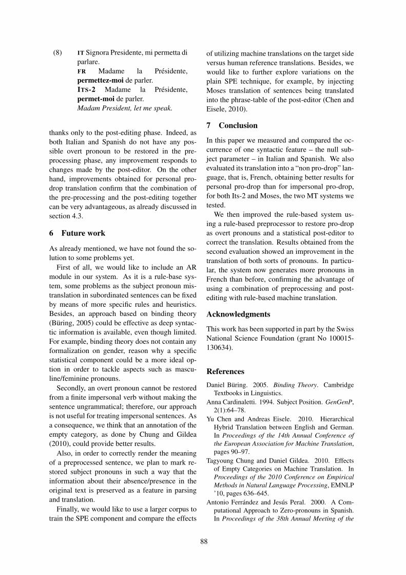
(8) IT Signora Presidente, mi permetta diparlare.FR Madame la Presidente,permettez-moi de parler.ITS-2 Madame la Presidente,permet-moi de parler.Madam President, let me speak.

thanks only to the post-editing phase. Indeed, asboth Italian and Spanish do not have any pos-sible overt pronoun to be restored in the pre-processing phase, any improvement responds tochanges made by the post-editor. On the otherhand, improvements obtained for personal pro-drop translation confirm that the combination ofthe pre-processing and the post-editing togethercan be very advantageous, as already discussed insection 4.3.

6 Future work

As already mentioned, we have not found the so-lution to some problems yet.

First of all, we would like to include an ARmodule in our system. As it is a rule-base sys-tem, some problems as the subject pronoun mis-translation in subordinated sentences can be fixedby means of more specific rules and heuristics.Besides, an approach based on binding theory(Buring, 2005) could be effective as deep syntac-tic information is available, even though limited.For example, binding theory does not contain anyformalization on gender, reason why a specificstatistical component could be a more ideal op-tion in order to tackle aspects such as mascu-line/feminine pronouns.

Secondly, an overt pronoun cannot be restoredfrom a finite impersonal verb without making thesentence ungrammatical; therefore, our approachis not useful for treating impersonal sentences. Asa consequence, we think that an annotation of theempty category, as done by Chung and Gildea(2010), could provide better results.

Also, in order to correctly render the meaningof a preprocessed sentence, we plan to mark re-stored subject pronouns in such a way that theinformation about their absence/presence in theoriginal text is preserved as a feature in parsingand translation.

Finally, we would like to use a larger corpus totrain the SPE component and compare the effects

of utilizing machine translations on the target sideversus human reference translations. Besides, wewould like to further explore variations on theplain SPE technique, for example, by injectingMoses translation of sentences being translatedinto the phrase-table of the post-editor (Chen andEisele, 2010).

7 Conclusion

In this paper we measured and compared the oc-currence of one syntactic feature – the null sub-ject parameter – in Italian and Spanish. We alsoevaluated its translation into a “non pro-drop” lan-guage, that is, French, obtaining better results forpersonal pro-drop than for impersonal pro-drop,for both Its-2 and Moses, the two MT systems wetested.

We then improved the rule-based system us-ing a rule-based preprocessor to restore pro-dropas overt pronouns and a statistical post-editor tocorrect the translation. Results obtained from thesecond evaluation showed an improvement in thetranslation of both sorts of pronouns. In particu-lar, the system now generates more pronouns inFrench than before, confirming the advantage ofusing a combination of preprocessing and post-editing with rule-based machine translation.

Acknowledgments

This work has been supported in part by the SwissNational Science Foundation (grant No 100015-130634).

ReferencesDaniel Buring. 2005. Binding Theory. Cambridge

Textbooks in Linguistics.Anna Cardinaletti. 1994. Subject Position. GenGenP,

2(1):64–78.Yu Chen and Andreas Eisele. 2010. Hierarchical

Hybrid Translation between English and German.In Proceedings of the 14th Annual Conference ofthe European Association for Machine Translation,pages 90–97.

Tagyoung Chung and Daniel Gildea. 2010. Effectsof Empty Categories on Machine Translation. InProceedings of the 2010 Conference on EmpiricalMethods in Natural Language Processing, EMNLP’10, pages 636–645.

Antonio Ferrandez and Jesus Peral. 2000. A Com-putational Approach to Zero-pronouns in Spanish.In Proceedings of the 38th Annual Meeting of the

88

Association for Computational Linguistics, pages166–172.

Anita Gojun. 2010. Null Subjects in Statistical Ma-chine Translation: A Case Study on Aligning En-glish and Italian Verb Phrases with Pronominalsubjects. Diplomarbeit, Institut fur MaschinelleSprachverarbeitung, University of Stuttgart.

Nizar Habash. 2007. Syntactic Preprocessing for Sta-tistical Machine Translation. In Proceedings of Ma-chine Translation Summit XI, pages 215–222.

Liliane Haegeman. 1994. Introduction to Governmentand Binding Theory. Blackwell Publishers.

Philipp Koehn and Christof Monz. 2006. Manualand Automatic Evaluation of Machine Translationbetween European Languages. In Proceedings onthe HTL-NAACL Workshop on Statistical MachineTranslation, pages 102–121. Association for Com-putational Linguistics.

Philipp Koehn, Hieu Hoang, Alexandra Birch, ChrisCallison-Burch, Marcello Federico, Nicola Bertoli,Brooke Cowan, Wade Shen, Christine Moran,Richard Zens, Christopher J. Dyer, Ondrej Bojar,Alexandra Constantin, and Evan Herbst. 2007.Moses: Open Source Toolkit for Statistical Ma-chine Translation. In Proceedings of the 45th An-nual Meeting of the Association for ComputationalLinguistics Companion Volume Proceedings of theDemo and Poster Sessions, pages 177–180. Associ-ation for Computational Linguistics.

Philipp Koehn. 2005. Europarl: A Parallel Corpus forStatistical Machine Translation. In Proceedings ofthe 10th Machine Translation Summit (MT SummitX).

Ronan Le Nagard and Philipp Koehn. 2010. AidingPronoun Translation with Co-Reference Resolution.In Proceedings of the Joint 5th Workshop on Statis-tical Machine Translation, pages 258–267.

Ruslan Mitkov. 2002. Anaphora Resolution. Long-man.

Massimo Poesio, Rodolfo Delmonte, Antonella Bris-tot, Luminita Chiran, and Sara Ronelli. 2004. TheVENEX corpus of anaphora and deixis in spokenand written Italian. In Manuscript.

Marta Recasens and M. Antonia Martı. 2010.AnCora-CO: Coreferentially Annotated Corporafor Spanish and Catalan. Language Resources andEvaluation, 44(4):315–345.

Luz Rello and Iustina Ilisei. 2009. A Rule-BasedApproach to the Identification of Spanish Zero Pro-nouns. In Proceedings of Student Research Work-shop, RANLP, pages 60–65.

Luigi Rizzi. 1986. Null Objects in Italian and theTheory of pro. Linguistic Inquiry, 17(3):501–557.

Kepa J. Rodrıguez, Francesca Delogu, Yannick Vers-ley, Egon W. Stemle, and Massimo Poesio. 2010.Anaphoric Annotation of Wikipedia and Blogsin the Live Memories Corpus. In Proceedings

of the Seventh International Conference on Lan-guage Resources and Evaluation (LREC), Valletta,Malta. European Language Resources Association(ELRA).

Fatiha Sadat and Nizar Habash. 2006. Combination ofArabic Preprocessing Schemes for Statistical Ma-chine Translation. In Proceedings of the 21st Inter-national Conference on Computational Linguisticsand 44th Annual Meeting of the ACL, pages 1–8.

Holger Schwenk, Sadaf Abdul-Rauf, Loıc Barrault,and Jean Senellart. 2009. SMT and SPE MachineTranslation Systems for WMT’09. In Proceedingsof the 4th Workshop on Statistical Machine Trans-lation, pages 130–134.

Michel Simard, Cyril Goutte, and Pierre Isabelle.2007a. Statistical Phrase-based Post-editing. InProceedings of NAACL HLT 2007, pages 508–515.

Michel Simard, Nicola Ueffing, Pierre Isabelle, andRoland Kuhn. 2007b. Rule-based Translation WithStatistical Phrase-based Post-editing. In Proceed-ings of the 2nd Workshop on Statistical MachineTranslation, pages 203–206, June.

Eric Wehrli, Luka Nerima, and Yves Scherrer. 2009.Deep Linguistic Multilingual Translation and Bilin-gual Dictionaries. In Proceedings of the FourthWorkshop on Statistical Machine Translation, pages90–94.

Eric Wehrli. 2007. Fips, a “Deep” Linguistic Multi-lingual Parser. In Proceedings of the Workshop onDeep Linguistic Processing, pages 120–127. Asso-ciation for Computational Linguistics.

89

Author Index

Batista-Navarro, Riza Theresa, 38Botha, Jan A., 64

Cocco, Christelle, 55

Guillou, Liane, 1Gulati, Asheesh, 81

Hlaing, Tin Htay, 32

Loaiciga, Sharid, 81

Majlis, Martin, 46Mihaila, Claudiu, 38

Papangelis, Alexandros, 22Petrenz, Philipp, 11

Russo, Lorenza, 81

Wawer, Aleksander, 74

91