ACL 2020

Innovative Use of NLP forBuilding Educational Applications

Proceedings of the 15th Workshop

July 10, 2020

Gold Sponsors

Silver Sponsors

c©2020 The Association for Computational Linguistics

Order copies of this and other ACL proceedings from:

Association for Computational Linguistics (ACL)209 N. Eighth StreetStroudsburg, PA 18360USATel: +1-570-476-8006Fax: +1-570-476-0860acl@aclweb.org

ISBN 978-1-952148-18-7

ii

Introduction

When we sent out our call for papers this year, we never imagined that the Workshop on Innovative Useof NLP for Building Educational Applications would be held virtually. While the circumstances are farfrom ideal, this will be an interesting experiment. We are pleased to host a set of innovative papers– even if virtually! Our papers this year include topics related to automated writing and speech andcontent evaluation, writing analytics, text revision analysis, building dialog resources, tracking writingproficient, neural models for writing evaluation tasks, and educational applications for languages otherthan English.

This year we received a total of 49 submissions and accepted 8 papers as oral presentations and 13 asposter presentations, for an overall acceptance rate of 43 percent. Each paper was reviewed by threemembers of the Program Committee who were believed to be most appropriate for each paper. Wecontinue to have a strong policy to deal with conflicts of interest. First, we continue to make a concertedeffort to resolve conflicts of interest - specifically, we do not assign papers to a reviewer if the paperhas an author from their institution. Second, organizing committee members recuse themselves fromdiscussions about papers if there is a conflict of interest.

Papers are accepted on the basis of several factors, including the relevance to a core educational problemspace, the novelty of the approach or domain, and the strength of the research. The accepted papers werehighly diverse – an indicator of the growing variety of foci in this field. We continue to believe that theworkshop framework designed to introduce work in progress and new ideas is important and we hopethat the breadth and variety of research accepted for this workshop is represented.

The BEA15 workshop has presentations on automated writing evaluation, readability, dialog, speech andgrammatical error correction, annotation and resources, and educational research that serves languagesother than English.

Automated Writing EvaluationGonzález-López et al’s Assisting Undergraduate Students in Writing Spanish Methodology Sectionsdiscusses a method that provides feedback to students with regard to how they have improved themethodology section of a paper; Ghosh et al’s An Exploratory Study of Argumentative Writing by YoungStudents: A Transformer-based Approach uses a transformer-based architecture (e.g., BERT) fine-tunedon a large corpus of critique essays from the college task to conduct a computational exploration ofargument critique writing by young students; Afrin et al’s Annotation and Classification of Evidence andReasoning Revisions in Argumentative Writing introduces an annotation scheme to capture the natureof sentence-level revisions of evidence use and reasoning and apply it to 5th- and 6th-grade students’argumentative essays. They show that reliable manual annotation can be achieved and that revisionannotations correlate with a holistic assessment of essay improvement in line with the feedback provided.They explore the feasibility of automatically classifying revisions according to their scheme; Wang etal’s Automated Scoring of Clinical Expressive Language Evaluation Tasks present a dataset consisting ofnon-clinically elicited responses for three related sentence formulation tasks, and propose an approach forautomatically evaluating their appropriateness. They use neural machine translation to generate correct-incorrect sentence pairs in order to create synthetic data to increase the amount and diversity of trainingdata for their scoring model and show how transfer learning improves scoring accuracy,

Automated Content Evaluation & Vocabulary AnalysisRiordan et al’s An Empirical Investigation of Neural Methods for Content Scoring of ScienceExplanations presents an empirical investigation of feature-based models, recurrent neural networkmodels, and pre-trained transformer models on scoring content in real-world formative assessmentdata. They demonstrate that recent neural methods can rival or exceed the performance of feature-based methods and provide evidence that different classes of neural models take advantage of different

iii

learning cues, and that pre-trained transformer models may be more robust to spurious, dataset-specificlearning cues, better reflecting scoring rubrics.; Cahill et al’s Context-based Automated Scoring ofComplex Mathematical Responses proposes a method for automatically scoring responses that containboth text and algebraic expressions. Their method not only achieves high agreement with human raters,but also links explicitly to the scoring rubric; Ehara’s Interpreting Neural CWI Classifiers’ Weights asVocabulary Size studies Complex Word Identification (CWI) – a task for the identification of words thatare challenging for second-language learners to read. The paper analyzes neural CWI classifiers andshows that some of their parameters can be interpreted as vocabulary size.

Writing Analytics and FeedbackDavidson et al’s Tracking the Evolution of Written Language Competence in L2 Spanish Learnerspresents an NLP-based approach for tracking the evolution of written language competence in L2Spanish learners using a wide range of linguistic features automatically extracted from students’written productions. The authors explore the connection between the most predictive features and theteaching curriculum, finding that their set of linguistic features often reflect the explicit instructions thatstudents receive during each course; Hellman et al’s Multiple Instance Learning for Content FeedbackLocalization without Annotation considers automated essay scoring as a Multiple Instance Learning(MIL) task. The authors show that such models can both predict content scores and localize contentby leveraging their sentence-level score predictions; Kerz et al’s Becoming Linguistically Mature:Modeling English and German Children’s Writing Development Across School Grades employs a novelapproach to advancing our understanding of the development of writing in English and German childrenacross school grades using classification tasks. Their experiments show that RNN classifiers trained oncomplexity contours achieve higher classification accuracy than one trained on text-average complexityscores; Mayfield and Black’s Should You Fine-Tune BERT for Automated Essay Scoring? investigateswhether, in automated essay scoring research, transformer-based models are an appropriate technologicalchoice. The authors conclude with a review of promising areas for research on student essays wherethe unique characteristics of transformers may provide benefits over classical methods to justify thecosts; Mathias and Bhattacharyya’s Can Neural Networks Automatically Score Essay Traits? shows howa deep-learning based system can outperform both feature-based machine learning systems and stringkernel-based systems when scoring essay traits.

Readability & Item Difficulty/SelectionDeutsch et al’s Linguistic Features for Readability Assessment combines linguistically-motivatedmachine learning and deep learning methods to improve overall readability model performance; Xue etal’s Predicting the Difficulty and Response Time of Multiple Choice Questions Using Transfer Learninginvestigates whether transfer learning can improve the prediction of the difficulty and response timeparameters for 18,000 multiple-choice questions from a high-stakes medical exam. The results indicatethat, for their sample, transfer learning can improve the prediction of item difficulty; Gao et al’sDistractor Analysis and Selection for Multiple-Choice Cloze Questions for Second-Language Learnersconsiders the problem of automatically suggesting distractors for multiple-choice cloze questionsdesigned for second-language learners. Based on their analyses, they train models to automaticallyselect distractors, and measure the importance of model components quantitatively.

Evaluation, Resources, Speech & DialogLoukina et al’s Using PRMSE to Evaluate Automated Scoring Systems in the Presence of Label Noisediscusses the effect that noisy labels have on system evaluation and propose the use of a new educationalmeasurement metric (PRMSE) to help address this issue; Raina et al’s Complementary Systems forOff-topic Spoken Response Detection examines one form of spoken language assessment; whether theresponse from the candidate is relevant to the prompt provided. The work focuses on the scenario whenthe prompt, and associated responses have not been seen in the training data, enabling the system tobe applied to new test scripts without the need to collect data or retrain the model; Maxwell-Smithet al’s Applications of Natural Language Processing in Bilingual Language Teaching: An Indonesian-

iv

English Case Study discusses methodological considerations for using automated speech recognition tobuild a corpus of teacher speech in an Indonesian language classroom; Stasaki et al’s Construction of aLarge Open Access Dialogue Dataset for Tutoring proposes a novel asynchronous method for collectingtutoring dialogue via crowdworkers that is both amenable to the needs of deep learning algorithms andreflective of pedagogical concerns. The CIMA dataset produced from this work is publicly available.

Grammatical Error CorrectionOmilianchuk et al’s GECToR – Grammatical Error Correction: Tag, Not Rewrite presents a simpleand efficient GEC sequence tagger using a transformer encoder; White & Rozovskaya’s A ComparativeStudy of Synthetic Data Generation Methods for Grammatical Error Correction compares techniquesfor generating synthetic data utilized by the two highest scoring submissions to the restricted and low-resource tracks in the BEA-2019 Shared Task on Grammatical Error Correction.

We wish to thank everyone who showed interest and submitted a paper, all of the authors for theircontributions, the members of the Program Committee for their thoughtful reviews, and everyone whois attending this workshop, virtually! We would especially like to thank our Gold Level sponsor, theNational Board of Medical Examiners.

Finally, our special thanks go to the emergency reviewers who stepped in to provide their expertiseand help ensure the highest level of feedback: we acknowledge the help of Beata Beigman Klebanov,Christopher Bryant, Andrew Caines, Mariano Felice, Yoko Futagi, Ananya Ganesh, Anastassia Loukina,and Marek Rei.

Jill Burstein, Educational Testing ServiceEkaterina Kochmar, University of CambridgeNitin Madnani, Educational Testing ServicesClaudia Leacock, GrammarlyIldikó Pilán, University of OsloHelen Yannakoudakis, King’s College LondonTorsten Zesch, University of Duisburg-Essen

v

Organizers:

Jill Burstein, Educational Testing ServiceEkaterina Kochmar, University of CambridgeNitin Madnani, Educational Testing ServicesClaudia Leacock, GrammarlyIldikó Pilán, University of OsloHelen Yannakoudakis, King’s College LondonTorsten Zesch, University of Duisburg-Essen

Program Committee:

Tazin Afrin, University of PittsburghDavid Alfter, University of GothenburgDimitris Alikaniotis, GrammarlyFernando Alva-Manchego, University of SheffieldRajendra Banjade, Audible (Amazon)Timo Baumann, Universität HamburgLee Becker, PearsonBeata Beigman Klebanov, Educational Testing ServiceLisa Beinbron, University of AmsterdamMaria Berger, German Research Center for Artificial IntelligenceKay Berkling, DHBW Cooperative State University KarlsruheDelphine Bernhard, Université de Strasbourg, FranceSameer Bhatnagar, Polytechnique MontrealSerge Bibauw, KU Leuven; UCLouvain; Universidad Central del EcuadorJoachim Bingel, University of CopenhagenKristy Boyer, University of FloridaChris Brew, Facebook AITed Briscoe, University of CambridgeChris Brockett, Microsoft Research AIJulian Brooke, University of British ColumbiaChristopher Bryant, University of CambridgeJill Burstein, Educational Testing ServiceAoife Cahill, Educational Testing ServiceAndrew Caines, University of CambridgeGuanliang Chen, Monash UniversityMei-Hua Chen, Department of Foreign Languages and LiteratureMartin Chodorow, City University of New YorkLeshem Choshen, Hebrew University of JerusalemMark Core, University of Southern CaliforniaLuis Fernando D’Haro, Universidad Politécnica de MadridVidas Daudaravicius, UAB VTeXOrphée De Clercq, LT3, Ghent UniversityKordula De Kuthy, Tübingen UniversityIria del Río Gayo, University of LisbonCarrie Demmans Epp, University of AlbertaAnn Devitt, Trinity College, Dublin

vii

Yo Ehara, Shizuoka Institute of Science and TechnologyNoureddine Elouazizi, Faculty of ScienceKeelan Evanini, Educational Testing ServiceMariano Felice, University of CambridgeMichael Flor Educational Testing ServiceThomas François, Université catholique de LouvainJennifer-Carmen Frey, Eurac ResearchYoko Futagi, Educational Testing ServiceMichael Gamon, Microsoft ResearchAnanya Ganesh, University of Massachusetts AmherstDipesh Gautam, University of MemphisSian Gooding, University of CambridgeCyril Goutte, National Research Council CanadaRoman Grundkiewicz, University of EdinburghMasato Hagiwara, Octanove Labs LLCJiangang Hao, Educational Testing ServiceHoma Hashemi, MicrosoftTrude Heift, Simon Fraser UniversityHeiko Holz, LEAD Graduate School and Research NetworkAndrea Horbach, University Duisburg-EssenRenfen Hu, Beijing Normal UniversityChung-Chi, Huang Frostburg State UniversityYi-Ting Huang, Academia SinicaRadu Tudor Ionescu, University of BucharestLifeng Jin, Ohio State UniversityMarcin Junczys-Dowmunt, MicrosoftTomoyuki Kajiwara, Osaka UniversityElma Kerz, RWTH Aachen UniversityFazel Keshtkar, St. John’s UniversityMamoru Komachi, Tokyo Metropolitan UniversityLun-Wei Ku, Academia SinicaKristopher Kyle, University of OregonJi-Ung Lee, UKP Lab, TU DarmstadtLung-Hao Lee, National Central UniversityJohn Lee, City University of Hong KongChee Wee (Ben) Leong, Educational Testing ServiceChen Liang, FacebookDiane Litman, University of PittsburghZitao Liu, TAL Education GroupPeter Ljunglöf, University of Gothenburg; Chalmers University of TechnologyAnastassia Loukina, Educational Testing ServiceLieve Macken, Ghent UniversityNabin Maharjan, Audible (Amazon)Montse Maritxalar, University of the Basque CountryJames Martin, University of Colorado BoulderIrina MaslowskiSandeep Mathias, IIT BombayNoboru Matsuda, North Carolina State UniversityJulie Medero, Harvey Mudd CollegeDetmar Meurers, University of Tübingen

viii

Michael Mohler, Language Computer CorporationNatawut Monaikul, University of Illinois at ChicagoFarah Nadeem, University of WahingtonCourtney Napoles, GrammarlyDiane Napolitano, RefinitivHwee Tou Ng, National University of SingaporeHuy Nguyen, LingoChampRodney Nielsen, University of North TexasYoo Rhee Oh, Electronics and Telecommunications Research Institute (ETRI)Robert Östling, Department of linguistics, Stockholm universityUlrike Pado, HFT StuttgartPatti Price, PPRICE Speech and Language TechnologyLong Qin, Singsound IncMengyang Qiu, University at BuffaloMartí Quixal, Universität TübingenVipul Raheja, GrammarlyZahra Rahimi Pandora MediaTaraka Rama, University of North TexasVikram Ramanarayanan, Educational Testing Service; University of California, San FranciscoHanumant Redkar, IIT BombayMarek Rei, University of CambridgeRobert Reynolds, Brigham Young UniversityBrian Riordan, Educational Testing ServiceAndrew Rosenberg, GoogleAlla Rozovskaya, City University of New YorkC. Anton Rytting, University of MarylandKeisuke Sakaguchi, Allen Institute for Artificial IntelligenceKatira Soleymanzadeh, EGE UniversitySwapna Somasundaran, Educational Testing ServiceHelmer Strik, Radboud University NijmegenJan Švec, University of West BohemiaAnaïs Tack, UCLouvain and KU LeuvenAlexandra Uitdenbogerd, RMIT UniversitySowmya Vajjala, National Research Council, CanadaPiper Vasicek, Brigham Young UniversityGiulia Venturi, Institute for Computational LinguisticsTatiana Vodolazova, University of AlicanteElena Volodina, University of Gothenburg, SwedenYiyi Wang, UIUC; Boston CollegeShuting Wang, FacebookZarah Weiss, University of TübingenMichael White, The Ohio State University; Facebook AIAlistair Willis, Open University, UKWei Xu, Ohio State UniversityKevin Yancey, DuolingoVictoria Yaneva, NBME; University of WolverhamptonSeid Muhie Yimam, University of HamburgMarcos Zampieri, Rochester Institute of TechnologyKlaus Zechner, Educational Testing ServiceFabian Zehner, DIPF, Leibniz Institute for Research and Information in EducationHaoran Zhang, University of Pittsburgh

ix

x

Table of Contents

Linguistic Features for Readability AssessmentTovly Deutsch, Masoud Jasbi and Stuart Shieber . . . . . . . . . . . . . . . . . . . . . . . . . . . . . . . . . . . . . . . . . . . . 1

Using PRMSE to evaluate automated scoring systems in the presence of label noiseAnastassia Loukina, Nitin Madnani, Aoife Cahill, Lili Yao, Matthew S. Johnson, Brian Riordan and

Daniel F. McCaffrey . . . . . . . . . . . . . . . . . . . . . . . . . . . . . . . . . . . . . . . . . . . . . . . . . . . . . . . . . . . . . . . . . . . . . . . . . 18

Multiple Instance Learning for Content Feedback Localization without AnnotationScott Hellman, William Murray, Adam Wiemerslage, Mark Rosenstein, Peter Foltz, Lee Becker

and Marcia Derr . . . . . . . . . . . . . . . . . . . . . . . . . . . . . . . . . . . . . . . . . . . . . . . . . . . . . . . . . . . . . . . . . . . . . . . . . . . . . 30

Complementary Systems for Off-Topic Spoken Response DetectionVatsal Raina, Mark Gales and Kate Knill . . . . . . . . . . . . . . . . . . . . . . . . . . . . . . . . . . . . . . . . . . . . . . . . . . 41

CIMA: A Large Open Access Dialogue Dataset for TutoringKatherine Stasaski, Kimberly Kao and Marti A. Hearst . . . . . . . . . . . . . . . . . . . . . . . . . . . . . . . . . . . . . 52

Becoming Linguistically Mature: Modeling English and German Children’s Writing Development AcrossSchool Grades

Elma Kerz, Yu Qiao, Daniel Wiechmann and Marcus Ströbel . . . . . . . . . . . . . . . . . . . . . . . . . . . . . . . . 65

Annotation and Classification of Evidence and Reasoning Revisions in Argumentative WritingTazin Afrin, Elaine Lin Wang, Diane Litman, Lindsay Clare Matsumura and Richard Correnti . . 75

Can Neural Networks Automatically Score Essay Traits?Sandeep Mathias and Pushpak Bhattacharyya . . . . . . . . . . . . . . . . . . . . . . . . . . . . . . . . . . . . . . . . . . . . . . 85

Tracking the Evolution of Written Language Competence in L2 Spanish LearnersAlessio Miaschi, Sam Davidson, Dominique Brunato, Felice Dell’Orletta, Kenji Sagae, Claudia

Helena Sanchez-Gutierrez and Giulia Venturi . . . . . . . . . . . . . . . . . . . . . . . . . . . . . . . . . . . . . . . . . . . . . . . . . . 92

Distractor Analysis and Selection for Multiple-Choice Cloze Questions for Second-Language LearnersLingyu Gao, Kevin Gimpel and Arnar Jensson . . . . . . . . . . . . . . . . . . . . . . . . . . . . . . . . . . . . . . . . . . . . 102

Assisting Undergraduate Students in Writing Spanish Methodology SectionsSamuel González-López, Steven Bethard and Aurelio Lopez-Lopez . . . . . . . . . . . . . . . . . . . . . . . . 115

Applications of Natural Language Processing in Bilingual Language Teaching: An Indonesian-EnglishCase Study

Zara Maxwelll-Smith, Simón González Ochoa, Ben Foley and Hanna Suominen . . . . . . . . . . . . . 124

An empirical investigation of neural methods for content scoring of science explanationsBrian Riordan, Sarah Bichler, Allison Bradford, Jennifer King Chen, Korah Wiley, Libby Gerard

and Marcia C. Linn . . . . . . . . . . . . . . . . . . . . . . . . . . . . . . . . . . . . . . . . . . . . . . . . . . . . . . . . . . . . . . . . . . . . . . . . . 135

An Exploratory Study of Argumentative Writing by Young Students: A transformer-based ApproachDebanjan Ghosh, Beata Beigman Klebanov and Yi Song . . . . . . . . . . . . . . . . . . . . . . . . . . . . . . . . . . 145

Should You Fine-Tune BERT for Automated Essay Scoring?Elijah Mayfield and Alan W Black . . . . . . . . . . . . . . . . . . . . . . . . . . . . . . . . . . . . . . . . . . . . . . . . . . . . . . 151

xi

GECToR – Grammatical Error Correction: Tag, Not RewriteKostiantyn Omelianchuk, Vitaliy Atrasevych, Artem Chernodub and Oleksandr Skurzhanskyi . 163

Interpreting Neural CWI Classifiers’ Weights as Vocabulary SizeYo Ehara . . . . . . . . . . . . . . . . . . . . . . . . . . . . . . . . . . . . . . . . . . . . . . . . . . . . . . . . . . . . . . . . . . . . . . . . . . . . . 171

Automated Scoring of Clinical Expressive Language Evaluation TasksYiyi Wang, Emily Prud’hommeaux, Meysam Asgari and Jill Dolata . . . . . . . . . . . . . . . . . . . . . . . . 177

Context-based Automated Scoring of Complex Mathematical ResponsesAoife Cahill, James H Fife, Brian Riordan, Avijit Vajpayee and Dmytro Galochkin . . . . . . . . . . . 186

Predicting the Difficulty and Response Time of Multiple Choice Questions Using Transfer LearningKang Xue, Victoria Yaneva, Christopher Runyon and Peter Baldwin . . . . . . . . . . . . . . . . . . . . . . . . 193

A Comparative Study of Synthetic Data Generation Methods for Grammatical Error CorrectionMax White and Alla Rozovskaya . . . . . . . . . . . . . . . . . . . . . . . . . . . . . . . . . . . . . . . . . . . . . . . . . . . . . . . . 198

xii

Conference Program

July, 10, 202008:30–09:00 Loading in of Oral Presentations06:00–06:10 Opening Remarks06:10–07:30 Session 107:30–08:00 Break08:00–09:10 Poster Session 109:10–10:10 Break10:10–11:30 Session 211:30–12:00 Break12:00–13:00 Poster Session 213:00–13:10 Closing Remarks

xiii

Proceedings of the 15th Workshop on Innovative Use of NLP for Building Educational Applications, pages 1–17July 10, 2020. c©2020 Association for Computational Linguistics

Linguistic Features for Readability Assessment

Tovly Deutsch Masoud Jasbi Stuart ShieberHarvard University

tdeutsch@college.harvard.edu, masoud jasbi@fas.harvard.edushieber@seas.harvard.edu

Abstract

Readability assessment aims to automaticallyclassify text by the level appropriate for learn-ing readers. Traditional approaches to thistask utilize a variety of linguistically motivatedfeatures paired with simple machine learningmodels. More recent methods have improvedperformance by discarding these features andutilizing deep learning models. However, it isunknown whether augmenting deep learningmodels with linguistically motivated featureswould improve performance further. This pa-per combines these two approaches with thegoal of improving overall model performanceand addressing this question. Evaluating ontwo large readability corpora, we find that,given sufficient training data, augmenting deeplearning models with linguistically motivatedfeatures does not improve state-of-the-art per-formance. Our results provide preliminary ev-idence for the hypothesis that the state-of-the-art deep learning models represent linguisticfeatures of the text related to readability. Fu-ture research on the nature of representationsformed in these models can shed light on thelearned features and their relations to linguis-tically motivated ones hypothesized in tradi-tional approaches.

1 Introduction

Readability assessment poses the task of identify-ing the appropriate reading level for text. Suchlabeling is useful for a variety of groups includ-ing learning readers and second language learners.Readability assessment systems generally involveanalyzing a corpus of documents labeled by editorsand authors for reader level. Traditionally, thesedocuments are transformed into a number of lin-guistic features that are fed into simple models likeSVMs and MLPs (Schwarm and Ostendorf, 2005;Vajjala and Meurers, 2012).

More recently, readability assessment models

utilize deep neural networks and attention mecha-nisms (Martinc et al., 2019). While such modelsachieve state-of-the-art performance on readabil-ity assessment corpora, they struggle to generalizeacross corpora and fail to achieve perfect classi-fication. Often, model performance is improvedby gathering additional data. However, readabil-ity annotations are time-consuming and expensivegiven lengthy documents and the need for quali-fied annotators. A different approach to improvingmodel performance involves fusing the traditionaland modern paradigms of linguistic features anddeep learning. By incorporating the inductive biasprovided by linguistic features into deep learningmodels, we may be able to reduce the limitationsposed by the small size of readability datasets.

In this paper, we evaluate the joint use of lin-guistic features and deep learning models. Weachieve this fusion by simply taking the outputof deep learning models as features themselves.Then, these outputs are joined with linguistic fea-tures to be further fed into some other model likean SVM. We select linguistic features based on abroad psycholinguistically-motivated compositionby Vajjala Balakrishna (2015). Transformers andHierarchical attention networks were selected asthe deep learning models because of their state-of-art performance in readability assessment. Mod-els were evaluated on two of the largest availablecorpora for readability assessment: WeeBit andNewsela. We also evaluate with different sizedtraining sets to investigate the use of linguistic fea-tures in data-poor contexts. Our results find that,given sufficient training data, the linguistic featuresdo not provide a substantial benefit over deep learn-ing methods.

The rest of this paper is organized as follows. Re-lated research is described in section 2. Section 3details our preprocessing, features, and model con-struction. Section 4 presents model evaluations on

1

two corpora. Section 5 discusses the implicationsof our results.

We provide a publicly available version of thecode used for our experiments.1

2 Related Work

Work on readability assessment has involvedprogress on three core components: corpora, fea-tures, and models. While early work utilized smallcorpora, limited feature sets, and simple models,modern research has experimented with a broad setof features and deep learning techniques.

Labeled corpora can be difficult to assemblegiven the time and qualifications needed to assigna text a readability level. The size of readabilitycorpora expanded significantly with the introduc-tion of the WeeklyReader corpus by Schwarm andOstendorf (2005). Composed of articles from aneducational magazine, the WeeklyReader corpuscontains roughly 2,400 articles. The WeeklyReadercorpus was then built upon by Vajjala and Meurers(2012) by adding data from the BBC Bitesize web-site to form the WeeBit corpus. This WeeBit cor-pus is larger, containing roughly 6,000 documents,while also spanning a greater range of readabilitylevels. Within these corpora, topic and readabilityare highly correlated. Thus, Xia et al. (2016) con-structed the Newsela corpus in which each articleis represented at multiple reading levels therebydiminishing this correlation.

Early work on readability assessment, such asthat of Flesch (1948), extracted simple textual fea-tures like character count. More recently, Schwarmand Ostendorf (2005) analyzed a broader set of fea-tures including out-of-vocabulary scores and syn-tactic features such as average parse tree height.Vajjala and Meurers (2012) assembled perhapsthe broadest class of features. They incorporatedmeasures shown by Lu (2010) to correlate wellwith second language acquisition measures, as wellas psycholinguistically relevant features from theCelex Lexical database and MRC PsycholinguisticDatabase (Baayen et al., 1995; Wilson, 1988).

Traditional feature formulas, like the Flesch for-mula, relied on linear models. Later work pro-gressed to more complex related models like SVMs(Schwarm and Ostendorf, 2005). Most recently,state-of-art-performance has been achieved on read-ability assessment with deep neural network incor-

1https://github.com/TovlyDeutsch/Linguistic-Features-for-Readability

porating attention mechanisms. These approachesignore linguistic features entirely and instead feedthe raw embeddings of input words, relying on themodel itself to extract any relevant features. Specif-ically, Martinc et al. (2019) found that a pretrainedtransformer model achieved state-of-the-art perfor-mance on the WeeBit corpus while a hierarchicalattention network (HAN) achieved state-of-the-artperformance on the Newsela corpus.

Deep learning approaches generally exclude anyspecific linguistic features. In general, a “feature-less” approach is sensible given the hypothesis that,with enough data, training, and model complexity,a model should learn any linguistic features thatresearchers might attempt to precompute. However,precomputed linguistic features may be useful indata-poor contexts where data acquisition is ex-pensive and error-prone. For this reason, in thispaper we attempt to incorporate linguistic featureswith deep learning methods in order to improvereadability assessment.

3 Methodology

3.1 Corpora

3.1.1 WeeBitThe WeeBit corpus was assembled by Vajjala andMeurers (2012) by combining documents from theWeeklyReader educational magazine and the BBCBitesize educational website. They selected classesto assemble a broad range of readability levels in-tended for readers aged 7 to 16. To avoid classifi-cation bias, they undersampled classes in order toequalize the number of documents in each class to625. We term this downsampled corpus “WeeBitdownsampled”. Following the methodologies ofXia et al. (2016) and Martinc et al. (2019), we ap-plied additional preprocessing to the WeeBit corpusin order to remove extraneous material.

3.1.2 NewselaThe Newsela corpus (Xia et al., 2016) consists of1,911 news articles each re-written up to 4 timesin simplified manners for readers at different read-ing levels. This simplification process means that,for any given topic, there exist examples of mate-rial on that topic suited for multiple reading levels.This overlap in topic should make the corpus morechallenging to label than the WeeBit corpus. In asimilar manner to the WeeBit corpus, the Newselacorpus is labeled with grade levels ranging fromgrade 2 to grade 12. As with WeeBit, these labels

2

can either be treated as classes or transformed intonumeric labels for regression.

3.1.3 Labeling ApproachesOften, readability classes within a corpus aretreated as unrelated. These approaches use rawlabels as distinct unordered classes. However, read-ability labels are ordinal, ranging from lower tohigher readability. Some work has addressed thisissue such as the readability models of Flor et al.(2013) which predict grade levels via linear regres-sion. To test different approaches to acknowledg-ing this ordinality, we devised three methods forlabeling the documents: “classification”, “age re-gression”, and “ordered class regression”.

The classification approach uses the classes orig-inally given. This approach does not suppose anyordinality of the classes. Avoiding such ordinalitymay be desirable for the sake of simplicity.

“Age regression” applies the mean of the ageranges given by the constituent datasets. For in-stance, in this approach Level 2 documents fromWeekly Reader would be given the label of 7.5as they are intended for readers of ages 7-8. Theadvantage of age regression over standard classifi-cation is that it provides more precise informationabout the magnitude of readability differences.

Finally, “ordered class regression” assigns theclasses equidistant integers ordered by difficulty.The least difficult class would be labeled “0”, thesecond least difficult class would be labeled “1”and so on. As with age regression, this labeling re-sults in a regression rather than classification prob-lem. This method retains the advantage of ageregression in demonstrating ordinality. However,ordered regression labeling removes informationabout the relative differences in difficulty betweenthe classes, instead asserting that they are equidis-tant in difficulty. The motivation behind this lossof information is that such age differences betweenclasses may not directly translate into differencesof difficulty. For instance, the readability differ-ence between documents intended for 7 or 8 year-olds may be much greater than between documentsintended for 15 or 16 year-olds because readingdevelopment is likely accelerated in younger years.

For final model inferences, we used the classifi-cation approach for comparison to previous work.For intermediary CNN models, all three approacheswere tested. As the different approaches with CNNmodels produced insubstantial differences, othermodel types were restricted to the simple classifi-

cation approach.

3.2 Features

Motivated by the success in using linguistic fea-tures for modeling readability, we considered alarge range of textual analyses relevant to readabil-ity. In addition to utilizing features posed in theexisting readability research, we investigated for-mulating new features with a focus on syntacticambiguity and syntactic diversity. This challengingaspect of language appeared to be underutilized inexisting readability literature.

3.2.1 Existing Features

To capture a variety of features, we utilized existinglinguistic feature computation software2 developedby Vajjala Balakrishna (2015) based on 86 featuredescriptions in existing readability literature. Giventhe large number of features, in this section wewill focus on the categories of features and theirpsycholinguistic motivations (where available) andproperties. The full list of features used can befound in appendix A.

Traditional Features The most basic features in-volve what Vajjala and Meurers (2012) refer to as“traditional features” for their use in long-standingreadability formulae. They include characters perword, syllables per word, and traditional formu-las based on such features like the Flesch-Kincaidformula (Kincaid et al., 1975).

Another set of feature types consists of countsand ratios of part-of-speech tags, extracted usingthe Stanford parser (Klein and Manning, 2003). Inaddition to basic parts of speech like nouns, somefeatures include phrase level constituent counts likenoun phrases and verb phrases. All of these countsare normalized by either the number of word to-kens or number of sentences to make them compa-rable across documents of differing lengths. Thesecounts are not provided with any psycholinguis-tic motivation for their use; however, it is not anunreasonable hypothesis that the relative usage ofthese constituents varies across reading levels. Em-pirically, these features were shown to have somepredictive power for readability. In addition toparts of speech counts, we also utilized word typecounts as a simple baseline feature, that is, count-ing the number of instances of each possible word

2This code can be found at https://bitbucket.org/nishkalavallabhi/complexity-features.

3

in the vocabulary. These counts are also divided bydocument length to generate proportions.

Becoming more abstract than parts of speech,some features count complex syntactic constituentlike clauses and subordinated clauses. Specifically,Lu (2010) found ratios involving sentences, clauses,and t-units3 that correlated with second languagelearners’ abilities to read a document. For manyof the multi-word syntactic constituents previouslydescribed, such as noun phrases and clauses, fea-tures were also constructed of their mean lengths.Finally, properties of the syntactic trees themselveswere analyzed such as their mean heights.

Moving beyond basic features from syntacticparses, Vajjala Balakrishna (2015) also incorpo-rated “word characteristic” features from linguis-tic databases. A significant source was the CelexLexical Database Baayen et al. (1995) which “con-sists of information on the orthography, phonology,morphology, syntax and frequency for more than50,000 English lemmas”. The database appears tohave a focus on morphological data such as whethera word may be considered a loan word and whetherit contains affixes. It also contains syntactic prop-erties that may not be apparent from a syntacticparse, e.g. whether a noun is countable. The MRCPsycholinguistic Database Wilson (1988) was alsoused with a focus on its age of acquisition ratingsfor words, an clear indicator of the appropriatenessof a document’s vocabulary.

3.2.2 Novel Syntactic FeaturesWe investigated additional syntactic features thatmay be relevant for readability but whose qualitieswere not targeted by existing features. These fea-tures were used in tandem with the existing linguis-tic features described previously; future work couldutilize these novel feature independently to investi-gate their particular effect on readability informa-tion extraction. For generating syntactic parses, weused the PCFG (probabilistic context-free gram-mar) parser (Klein and Manning, 2003) from theStanford Parser package.

Syntactic Ambiguity Sentences can have multi-ple grammatical syntactic parses. Therefore, syn-tactic parsers produce multiple parses annotatedwith parse likelihood. It may seem sensible to usethe number of parses generated as a measure of

3Defined by Vajjala and Meurers (2012) to be “one mainclause plus any subordinate clause or non-clausal structurethat is attached to or embedded in it”.

ambiguity. However, this measure is extremely sen-sitive to sentence length as longer sentences tend tohave more possible syntactic parses. Instead, if thislist of probabilities is viewed as a distribution, thestandard deviation of this distribution is likely tocorrelate with perceptions of syntactic ambiguity.

Definition 3.1. PDx

The parse deviation, PDx(s), of sentence s isthe standard deviation of the distribution of the xmost probable parse log probabilities for s. If s hasless than x valid parses, the distribution is takenfrom all the valid parses.

For large values of x, PDx(s) can be signif-icantly sensitive to sentence length: longer sen-tences are likely to have more valid syntactic parsesand thus create low probability tails that increasestandard deviation. To reduce this sensitivity, analternative involves measuring the difference be-tween the largest and mean parse probability.

Definition 3.2. PDMx

PDMx(s) is the difference between the largestparse log probability and the mean of the log proba-bilities of the x most probable parses for a sentences. If s has less than x valid parses, the mean istaken over all the valid parses.

As a compromise between parse investigationand the noise of implausible parses, we selectedPDM10, PD10, and PD2 as features to use in themodels of this paper.

Part-of-Speech Divergence To capture thegrammatical makeup of a sentence or document,we can count the usage of each part of speech(“POS”), phrase, or clause. The counts can becollected into a distribution. Then, the standarddeviation of this distribution, POSDdev, measuresa sentence’s grammatical heterogeneity.

Definition 3.3. POSDdev

POSDdev(d) is the standard deviation of thedistribution of POS counts for document d.

Similarly, we may want to measure how thisgrammatical makeup differs from the compositionof the document as a whole, a concept that mightbe termed syntactic uniqueness. To capture thisconcept, we measure the Kullback-Leibler diver-gence (Kullback and Leibler, 1951) between thesentence POS count distribution and the documentPOS count distribution.

Definition 3.4. POSdiv

4

Let P (s) be the distribution of POS counts forsentence s in document d. Let Q be the distribu-tion of POS counts for document d. Let |d| be thenumber of sentences in d.

POSdiv(d) =∑

s∈d

DKL(P (s) ‖‖ Q)

|d|

3.3 Models

A large range of model complexities were evalu-ated in order to ascertain the performance improve-ments, or lack thereof, of additional model com-plexity. In this section we will describe the specificconstruction and usage of these models for the ex-periments conducted in this paper, ordered roughlyby model complexity.

SVMs, Linear Models, and Logistic RegressionWe used the Scikit-Learn library (Pedregosa et al.,2011) for constructing SVM models. Hyper-parameter optimization was performed using theguidelines suggested by Hsu et al. (2003). Fromthe Scikit-Learn library, we also utilized the linearsupport vector classifier (an SVM with a linear ker-nel) and logistic regression classifier. As simplicitywas the aim for these evaluations, no hyperparam-eter optimization was performed. The logistic re-gression classifier was trained using the stochasticaverage gradient descent (“sag”) optimizer.

CNN Convolutional neural networks were se-lected for their demonstrated performance on sen-tence classification (Kim, 2014). The CNN modelused in this paper is based on the one describedby Kim (2014) and implemented using the Keras(Chollet and others, 2015), Tensorflow (Abadi et al.,2015), and Magpie libraries.

Transformer The transformer (Vaswani et al.,2017) is a neural-network-based model that hasachieved state-of-the-art results on a wide arrayof natural language tasks including readability as-sessment (Martinc et al., 2019). Transformers uti-lize the mechanism of attention which allows themodel to attend to specific parts of the input whenconstructing the output. Although they are formu-lated as sequence-to-sequence models, they canbe modified to complete a variety of NLP tasksby placing an additional linear layer at the endof the network and training that layer to producethe desired output. This approach often achievesstate-of-the-art results when combined with pre-training. In this paper, we use the BERT (Devlin

et al., 2019) transformer-based model that is pre-trained on BooksCorpus (800M words) (Zhu et al.,2015) and English Wikipedia. The model is thenfine-tuned on a specific readability corpus such asWeeBit. The pretrained BERT model is sourcedfrom the Huggingface transformers library (Wolfet al., 2019) and is composed of 12 hidden lay-ers each of size 768 and 12 self-attention heads.The fine-tuning step utilizes an implementationby Martinc et al. (2019). Among the pretrainedtransformers in the Huggingface library, there aretransformers that can accept sequences of size 128,256, and 512. The 128 sized model was chosenbased on the finding by Martinc et al. (2019) thatit achieved the highest performance on the WeeBitand Newsela corpora. Documents that exceededthe input sequence size were truncated.

HAN The Hierarchical attention network in-volves feeding the input through two bidirectionalRNNs each accompanied by a separate attentionmechanism. One attention mechanism attends tothe different words within each sentence while thesecond mechanism attends to the sentences withinthe document. These hierarchical attention mech-anisms are thought to better mimic the structureof documents and consequently produce superiorclassification results. The implementation of themodel used in this paper is identical to the originalarchitecture described by Yang et al. (2016) andwas provided by the authors of Martinc et al. (2019)based on code by Nguyen (2020).

3.4 Incorporating Linguistic Features withNeural Models

The neural network models thus far described takeeither the raw text or word vector embeddings ofthe text as input. They make no use of linguisticfeatures such as those described in section 3.2. Wehypothesized that combining these linguistic fea-tures with the deep neural models may improvetheir performance on readability assessment. Al-though these models theoretically represent sim-ilar features to those prescribed by the linguisticfeatures, we hypothesized that the amount of dataand model complexity may be insufficient to cap-ture them. This can be evidenced in certain mod-els failure to generalize across readability corpora.Martinc et al. (2019) found that the BERT modelperformed well on the WeeBit corpus, achievinga weighted F1 score of 0.8401, but performedpoorly on the Newsela corpus only achieving an F1

5

score of 0.5759. They posit that this disparity oc-curred “because BERT is pretrained as a languagemodel, [therefore] it tends to rely more on semanticthan structural differences during the classificationphase and therefore performs better on problemswith distinct semantic differences between readabil-ity classes”. Similarly a HAN was able to achievebetter performance than BERT on the Newsela butperformed substantially worse on the WeeBit cor-pus. Thus, under some evaluations the models havedeficiencies and fail to generalize. Given thesedeficiencies, we hypothesized that the inductivebias provided by linguistic features may improvegeneralizability and overall model performance.

In order to weave together the linguistic featuresand neural models, we take the simple approach ofusing the single numerical output of a neural modelas a feature itself, joined with linguistic features,and then fed into one of the simpler non-neuralmodels such as SVMs. SVMs were chosen as thefinal classification model for their simplicity andfrequent use in integrating numerical features. Theoutput of the neural model could be any of the labelapproaches such as grade classes or age regressionsdescribed in section 3.1. While all these labelingapproaches were tested for CNNs, insubstantialdifferences in final inferences led us to restrict in-termediary results to simple classification for othermodel types.

3.5 Training and Evaluation Details

All experiments involved 5-fold cross validation.All neural-network-based models were trained withthe Adam optimizer (Kingma and Ba, 2015) withlearning rates of 10−3,10−4, and 2−5 for the CNN,HAN, and transformer respectively. The HAN andCNN models were trained for 20 and 30 epochs.The transformer models were fine-tuned for 3epochs.

All results are reported as either a weighted F1 ormacro F1 score. To calculate weighted F1, first theF1 score is calculated for each class independently,as if each class was a case of binary classification.Then, these F1 score are combined in a weightedmean in which each class is weighted by the num-ber of samples in that class. Thus, the weightedF1 score treats each sample equally but prioritizesthe most common classes. The macro F1 is similarto the weighted F1 score in that F1 scores are firstcalculated for each class independently. However,for the macro F1 score, the class F1 scores are com-

Features Weighted F1HAN 0.8024SVM with HAN and linguisticfeatures

0.8014

SVM with HAN 0.7931SVM with linguistic features andFlesch Features

0.7694

SVM with transformer and lin-guistic features

0.7678

SVM with transformer, Fleschfeatures, and linguistic features

0.7627

SVM with Linguistic features 0.7582SVM with CNN age regressionand linguistic features

0.7281

SVM with CNN ordered classesregression and linguistic features

0.7231

SVM with transformer andFlesch features

0.7186

Transformer 0.5435CNN 0.3379

Table 1: Top 10 performing model results, transformer,and CNN on the Newsela corpus

bined in a mean without any weighting. Therefore,the macro F1 score treats each class equally butdoes not treat each sample equally, deprioritizingsamples from large classes and prioritizing samplesfrom small classes.

4 Results

In this section we report the experimental resultsof incorporating linguistic features into readabil-ity assessment models. The two corpora, WeeBitand Newsela, are analyzed individually and thencompared. Our results demonstrate that, givensufficient data, linguistic features provide little tono benefit compared to independent deep learn-ing models. While the corpus experiment resultsdemonstrate a portion of the approaches tested, thefull results are available in appendix B

4.1 Newsela Experiments

For the Newsela corpus, while linguistic featureswere able to improve the performance of somemodels, the top performers did not utilize linguis-tic features. The results from the top performingmodels are presented in table 1.

While the HAN performance was not surpassedby models with linguistic features, the transformermodels were. This improvement indicates that lin-

6

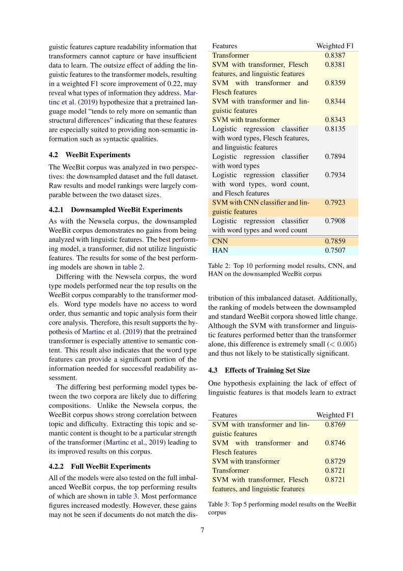
guistic features capture readability information thattransformers cannot capture or have insufficientdata to learn. The outsize effect of adding the lin-guistic features to the transformer models, resultingin a weighted F1 score improvement of 0.22, mayreveal what types of information they address. Mar-tinc et al. (2019) hypothesize that a pretrained lan-guage model “tends to rely more on semantic thanstructural differences” indicating that these featuresare especially suited to providing non-semantic in-formation such as syntactic qualities.

4.2 WeeBit Experiments

The WeeBit corpus was analyzed in two perspec-tives: the downsampled dataset and the full dataset.Raw results and model rankings were largely com-parable between the two dataset sizes.

4.2.1 Downsampled WeeBit ExperimentsAs with the Newsela corpus, the downsampledWeeBit corpus demonstrates no gains from beinganalyzed with linguistic features. The best perform-ing model, a transformer, did not utilize linguisticfeatures. The results for some of the best perform-ing models are shown in table 2.

Differing with the Newsela corpus, the wordtype models performed near the top results on theWeeBit corpus comparably to the transformer mod-els. Word type models have no access to wordorder, thus semantic and topic analysis form theircore analysis. Therefore, this result supports the hy-pothesis of Martinc et al. (2019) that the pretrainedtransformer is especially attentive to semantic con-tent. This result also indicates that the word typefeatures can provide a significant portion of theinformation needed for successful readability as-sessment.

The differing best performing model types be-tween the two corpora are likely due to differingcompositions. Unlike the Newsela corpus, theWeeBit corpus shows strong correlation betweentopic and difficulty. Extracting this topic and se-mantic content is thought to be a particular strengthof the transformer (Martinc et al., 2019) leading toits improved results on this corpus.

4.2.2 Full WeeBit ExperimentsAll of the models were also tested on the full imbal-anced WeeBit corpus, the top performing resultsof which are shown in table 3. Most performancefigures increased modestly. However, these gainsmay not be seen if documents do not match the dis-

Features Weighted F1Transformer 0.8387SVM with transformer, Fleschfeatures, and linguistic features

0.8381

SVM with transformer andFlesch features

0.8359

SVM with transformer and lin-guistic features

0.8344

SVM with transformer 0.8343Logistic regression classifierwith word types, Flesch features,and linguistic features

0.8135

Logistic regression classifierwith word types

0.7894

Logistic regression classifierwith word types, word count,and Flesch features

0.7934

SVM with CNN classifier and lin-guistic features

0.7923

Logistic regression classifierwith word types and word count

0.7908

CNN 0.7859HAN 0.7507

Table 2: Top 10 performing model results, CNN, andHAN on the downsampled WeeBit corpus

tribution of this imbalanced dataset. Additionally,the ranking of models between the downsampledand standard WeeBit corpora showed little change.Although the SVM with transformer and linguis-tic features performed better than the transformeralone, this difference is extremely small (< 0.005)and thus not likely to be statistically significant.

4.3 Effects of Training Set Size

One hypothesis explaining the lack of effect oflinguistic features is that models learn to extract

Features Weighted F1SVM with transformer and lin-guistic features

0.8769

SVM with transformer andFlesch features

0.8746

SVM with transformer 0.8729Transformer 0.8721SVM with transformer, Fleschfeatures, and linguistic features

0.8721

Table 3: Top 5 performing model results on the WeeBitcorpus

7

Figure 1: Performance differences across differenttraining set sizes on the downsampled WeeBit corpus

those features given enough data. Thus, perhaps inmore data-poor environments the linguistic featureswould prove more useful. To test this hypothesis,we evaluated two CNN-based models, one withlinguistic features and one without, with varioussized training subsets of the downsampled WeeBitcorpus. The macro F1 at these various dataset sizesis shown in figure 1. Across the trials at differ-ent training set sizes, the test set is held constantthereby isolating the impact of training set size.

The hypothesis holds true for extremely smallsubsets of training data, those with fewer than 200documents. Above this training set size, the ad-dition of linguistic features results in insubstan-tial changes in performance. Thus, either the pat-terns exposed by the linguistic features are learn-able with very little data or the patterns extractedby deep learning models differ significantly fromthe linguistic features. The latter appears morelikely given that linguistic features are shown toimprove performance for certain corpora (Newsela)and model types (transformers).

This result indicates that the use of linguisticfeatures should be considered for small datasets.However, the dataset size at which those featureslose utility is extremely small. Therefore, collect-ing additional data would often be more efficientthan investing the time to incorporate linguisticfeatures.

4.4 Effects of Linguistic Features

Overall, the failure of linguistic features to improvestate-of-the-art deep learning models indicates that,given the available corpora, model complexity, andmodel structures, they do not add information overand beyond what the state-of-the-art models havealready learned. However, in certain data-poor con-texts, they can improve the performance of deeplearning models. Similarly, with more diverse andmore accurately and consistently labeled corpora,the linguistic features could prove more useful. Itmay be the case that the best performing modelsalready achieve near the maximal possible perfor-mance on this corpus. The reason the maximal per-formance may be below a perfect score (an F1 scoreof 1) is disagreement and inconsistency in datasetlabeling. Presumably the dataset was assessed bymultiple labelers who may not have always agreedwith one another or even with themselves. Thus,if either a new set of human labelers or the origi-nal labelers are tasked with labeling readability inthis corpus, they may only achieve performancesimilar to the best performance seen in these exper-iments. Performing this human experiment wouldbe a useful analysis of corpus validity and consis-tency. Similarly, a more diverse corpus (differingin length, topic, writing style, etc.) may provemore difficult for the models to label alone withoutadditional training data; in this case, the linguis-tic features may prove more helpful in providinginductive bias.

Additionally, the lack of improvement fromadding linguistic features indicates that deep learn-ing models may already be representing those fea-tures. Future work could probe the models fordifferent aspects of the linguistic features, therebyinvestigating what properties are most relevant forreadability.

5 Conclusion

In this paper we explored the role of linguisticfeatures in deep learning methods for readabilityassessment, and asked: can incorporating linguis-tic features improve state-of-the-art models? Weconstructed linguistic features focused on syntacticproperties ignored by existing features. We incor-porated these features into a variety of model types,both those commonly used in readability researchand more modern deep learning methods. We eval-uated these models on two distinct corpora thatposed different challenges for readability assess-

8

ment. Additional evaluations were performed withvarious training set sizes to explore the inductivebias provided by linguistic features. While lin-guistic features occasionally improved model per-formance, particularly at small training set sizes,these models did not achieve state-of-the-art per-formance.

Given that linguistic features did not generallyimprove deep learning models, these models maybe already implicitly capturing the features thatare useful for readability assessment. Thus, futurework should investigate to what degree the modelsrepresent linguistic features, perhaps via probingmethods.

Although this work supports disusing linguisticfeatures in readability assessment, this assertion islimited by available corpora. Specifically, ambigu-ity in the corpora construction methodology limitsour ability to measure label consistency and valid-ity. Therefore, the maximal possible performancemay already be achieved by state-of-the-art models.Thus, future work should explore constructing andevaluating readability corpora with rigorous consis-tent methodology; such corpora may be assessedmost effectively using linguistic features. For in-stance, accuracy could be improved by averagingacross multiple labelers.

Overall, linguistic features do not appear to beuseful for readability assessment. While often usedin traditional readability assessment models, thesefeatures generally fail to improve the performanceof deep learning methods. Thus, this paper pro-vides a starting point to understanding the qualitiesand abilities of deep learning models in compari-son to linguistic features. Through this comparison,we can analyze what types of information thesemodels are well-suited to learning.

References

Martın Abadi, Ashish Agarwal, Paul Barham, EugeneBrevdo, Zhifeng Chen, Craig Citro, Greg S. Corrado,Andy Davis, Jeffrey Dean, Matthieu Devin, SanjayGhemawat, Ian Goodfellow, Andrew Harp, GeoffreyIrving, Michael Isard, Yangqing Jia, Rafal Jozefow-icz, Lukasz Kaiser, Manjunath Kudlur, Josh Leven-berg, Dandelion Mane, Rajat Monga, Sherry Moore,Derek Murray, Chris Olah, Mike Schuster, JonathonShlens, Benoit Steiner, Ilya Sutskever, Kunal Talwar,Paul Tucker, Vincent Vanhoucke, Vijay Vasudevan,Fernanda Viegas, Oriol Vinyals, Pete Warden, Mar-tin Wattenberg, Martin Wicke, Yuan Yu, and Xiao-qiang Zheng. 2015. TensorFlow: large-scale ma-

chine learning on heterogeneous systems. Technicalreport.

Rolf Harald Baayen, Richard Piepenbrock, and LeonGulikers. 1995. The CELEX lexical database.

Francois Chollet and others. 2015. Keras.

Jacob Devlin, Ming-Wei Chang, Kenton Lee, andKristina Toutanova. 2019. BERT: Pre-training ofDeep Bidirectional Transformers for Language Un-derstanding. In Proceedings of the 2019 Conferenceof the North American Chapter of the Associationfor Computational Linguistics: Human LanguageTechnologies, Volume 1 (Long and Short Papers),pages 4171–4186, Minneapolis, Minnesota. Associ-ation for Computational Linguistics.

Rudolph Flesch. 1948. A new readability yardstick.Journal of Applied Psychology, 32(3):221–233.

Michael Flor, Beata Beigman Klebanov, and Kath-leen M. Sheehan. 2013. Lexical tightness and textcomplexity. In Proceedings of the Workshop on Nat-ural Language Processing for Improving Textual Ac-cessibility, pages 29–38, Atlanta, Georgia. Associa-tion for Computational Linguistics.

Chih-wei Hsu, Chih-chung Chang, and Chih-Jen Lin.2003. A practical guide to support vector classifica-tion. Technical report.

Yoon Kim. 2014. Convolutional Neural Networksfor Sentence Classification. In Proceedings of the2014 Conference on Empirical Methods in NaturalLanguage Processing (EMNLP), pages 1746–1751,Doha, Qatar. Association for Computational Lin-guistics.

J. P. Kincaid, Jr. Fishburne, Rogers Robert P., ChissomRichard L., and Brad S. 1975. Derivation of NewReadability Formulas (Automated Readability In-dex, Fog Count and Flesch Reading Ease Formula)for Navy Enlisted Personnel:. Technical report, De-fense Technical Information Center, Fort Belvoir,VA.

Diederik P. Kingma and Jimmy Ba. 2015. Adam: Amethod for stochastic optimization. In 3rd Inter-national Conference on Learning Representations,ICLR 2015, San Diego, CA, USA, May 7-9, 2015,Conference Track Proceedings.

Dan Klein and Christopher D. Manning. 2003. Accu-rate unlexicalized parsing. In Proceedings of the41st Annual Meeting on Association for Computa-tional Linguistics - ACL ’03, volume 1, pages 423–430, Sapporo, Japan. Association for ComputationalLinguistics.

Solomon Kullback and Richard A. Leibler. 1951. OnInformation and Sufficiency. The Annals of Mathe-matical Statistics, 22(1):79–86.

9

Victor Kuperman, Hans Stadthagen-Gonzalez, andMarc Brysbaert. 2012. Age-of-acquisition ratingsfor 30,000 English words. Behavior Research Meth-ods, 44(4):978–990.

Xiaofei Lu. 2010. Automatic analysis of syntactic com-plexity in second language writing. InternationalJournal of Corpus Linguistics, 15(4):474–496.

Matej Martinc, Senja Pollak, and Marko Robnik-Sikonja. 2019. Supervised and unsupervised neuralapproaches to text readability. Computing ResearchRepository, arXiv:1503.06733. Version 2.

Viet Nguyen. 2020. Hierarchical Attention Networksfor Document Classification. Original-date: 2019-01-31T18:56:40Z.

Fabian Pedregosa, Gael Varoquaux, Alexandre Gram-fort, Vincent Michel, Bertrand Thirion, OlivierGrisel, Mathieu Blondel, Peter Prettenhofer, RonWeiss, Vincent Dubourg, Jake Vanderplas, Alexan-dre Passos, David Cournapeau, Matthieu Brucher,Matthieu Perrot, and Edouard Duchesnay. 2011.Scikit-learn: Machine Learning in Python. Journalof Machine Learning Research, 12:2825-2830.

Sarah E. Schwarm and Mari Ostendorf. 2005. ReadingLevel Assessment Using Support Vector Machinesand Statistical Language Models. In Proceedings ofthe 43rd Annual Meeting on Association for Com-putational Linguistics, ACL ’05, pages 523–530,Stroudsburg, PA, USA. Association for Computa-tional Linguistics. Event-place: Ann Arbor, Michi-gan.

Sowmya Vajjala and Detmar Meurers. 2012. On Im-proving the Accuracy of Readability Classificationusing Insights from Second Language Acquisition.In Proceedings of the Seventh Workshop on BuildingEducational Applications Using NLP, pages 163–173, Montreal, Canada. Association for Computa-tional Linguistics.

Sowmya Vajjala Balakrishna. 2015. Analyzing TextComplexity and Text Simplification: Connecting Lin-guistics, Processing and Educational Applications.Dissertation, Universitat Tubingen.

Ashish Vaswani, Noam Shazeer, Niki Parmar, JakobUszkoreit, Llion Jones, Aidan N Gomez, ŁukaszKaiser, and Illia Polosukhin. 2017. Attention is allyou need. In Advances in neural information pro-cessing systems 30, pages 5998–6008. Curran Asso-ciates, Inc.

Michael Wilson. 1988. MRC psycholinguisticdatabase: Machine-usable dictionary, version 2.00.Behavior Research Methods, Instruments, & Com-puters, 20(1):6–10.

Thomas Wolf, Lysandre Debut, Victor Sanh, JulienChaumond, Clement Delangue, Anthony Moi, Pier-ric Cistac, Tim Rault, R’emi Louf, Morgan Funtow-icz, and Jamie Brew. 2019. HuggingFace’s trans-formers: state-of-the-art natural language process-ing. Technical report.

Menglin Xia, Ekaterina Kochmar, and Ted Briscoe.2016. Text Readability Assessment for Second Lan-guage Learners. In Proceedings of the 11th Work-shop on Innovative Use of NLP for Building Edu-cational Applications, pages 12–22, San Diego, CA.Association for Computational Linguistics.

Zichao Yang, Diyi Yang, Chris Dyer, Xiaodong He,Alex Smola, and Eduard Hovy. 2016. HierarchicalAttention Networks for Document Classification. InProceedings of the 2016 Conference of the NorthAmerican Chapter of the Association for Computa-tional Linguistics: Human Language Technologies,pages 1480–1489, San Diego, California. Associa-tion for Computational Linguistics.

Yukun Zhu, Ryan Kiros, Richard Zemel, RuslanSalakhutdinov, Raquel Urtasun, Antonio Torralba,and Sanja Fidler. 2015. Aligning Books and Movies:Towards Story-like Visual Explanations by Watch-ing Movies and Reading Books. Computing Re-search Repository, arXiv:1506.06724.

10

A Feature Definitions

For the following definitions, if the a ratio is undefined (i.e. the denominator is zero) the result is treatedas zero. Vajjala and Meurers (2012) define complex nominals to be: “a) nouns plus adjective, possessive,prepositional phrase, relative clause, participle or appositive, b) nominal clauses, c) gerunds and infinitivesin subject positions.” Here polysyllabic means more than two syllables and “long words” means a wordwith seven or more characters. Descriptions of the norms of age of acquisition ratings can be found inKuperman et al. (2012).

Feature Name DefinitionPDx(s) The parse deviation, PDx(s), of sentence s is the standard deviation of the distribution

of the x most probable parse log probabilities for s. If s has less than x valid parses,the distribution is taken from all the valid parses.

PDMx PDMx(s) is the difference between the largest parse log probability and the mean ofthe log probabilities of the x most probable parses for a sentence s. If s has less thanx valid parses, the mean is taken over all the valid parses.

POSDdev POSDdev(d) is the standard deviation of the distribution of POS counts for documentd.

POSdiv Let P (s) be the distribution of POS counts for sentence s in document d. Let Q bethe distribution of POS counts for document d. Let |d| be the number of sentences ind. POSdiv(d) =

∑s∈d

DKL(P (s) ‖‖ Q)|d|

Table 4: Novel syntactic feature definitions

11

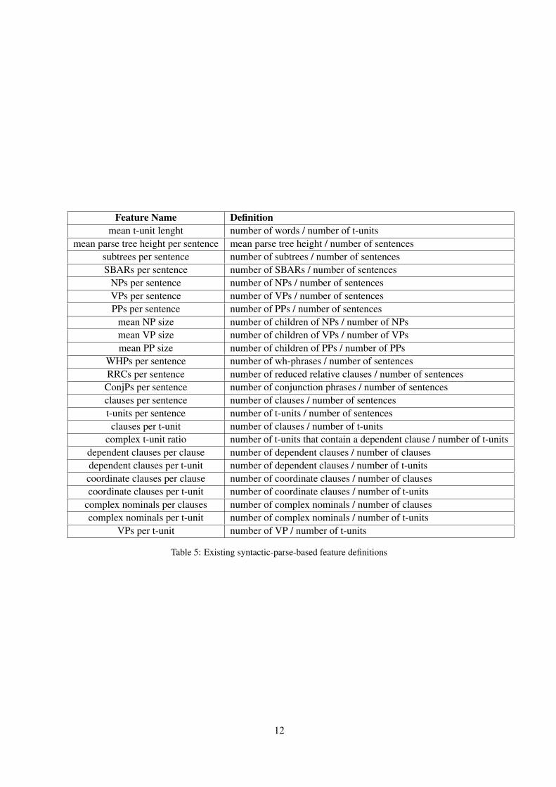
Feature Name Definitionmean t-unit lenght number of words / number of t-units

mean parse tree height per sentence mean parse tree height / number of sentencessubtrees per sentence number of subtrees / number of sentencesSBARs per sentence number of SBARs / number of sentences

NPs per sentence number of NPs / number of sentencesVPs per sentence number of VPs / number of sentencesPPs per sentence number of PPs / number of sentences

mean NP size number of children of NPs / number of NPsmean VP size number of children of VPs / number of VPsmean PP size number of children of PPs / number of PPs

WHPs per sentence number of wh-phrases / number of sentencesRRCs per sentence number of reduced relative clauses / number of sentences

ConjPs per sentence number of conjunction phrases / number of sentencesclauses per sentence number of clauses / number of sentencest-units per sentence number of t-units / number of sentencesclauses per t-unit number of clauses / number of t-units

complex t-unit ratio number of t-units that contain a dependent clause / number of t-unitsdependent clauses per clause number of dependent clauses / number of clausesdependent clauses per t-unit number of dependent clauses / number of t-unitscoordinate clauses per clause number of coordinate clauses / number of clausescoordinate clauses per t-unit number of coordinate clauses / number of t-units

complex nominals per clauses number of complex nominals / number of clausescomplex nominals per t-unit number of complex nominals / number of t-units

VPs per t-unit number of VP / number of t-units

Table 5: Existing syntactic-parse-based feature definitions

12

Feature Name Definitionnouns per word number of nouns / number of words

proper nouns per word number of proper nouns / number of wordspronouns per word number of pronouns / number of words

conjuctions per word number of conjuctions / number of wordsadjectives per word number of adjectives / number of words

verbs per word number of verbs / number of wordsadverbs per word number of adverbs / number of words

modal verbs per word number of modal verbs / number of wordsprepositions per word number of prepositions / number of wordsinterjections per word number of interjections / number of words

personal pronouns per word number of personal pronouns / number of wordswh-pronouns per word number of wh-pronouns / number of wordslexical words per word number of lexical words / number of words

function words per word number of function words / number of wordsdeterminers per word number of determiners / number of words

VBs per word number of base form verbs / number of wordsVBDs per word number of past tense verbs / number of wordsVBGs per word number of gerund or present participle verbs / number of wordsVBNs per word number of past participle verbs / number of wordsVBPs per word number of non-3rd person singular present verbs / number of

wordsVBZs per word number of 3rd person singular present verbs / number of wordsadverb variation number of adverbs / number of lexical words

adjective variation number of adjectives / number of lexical wordsmodal verb variation number of adverbs and adverbs / number of lexical words

noun variation number of nouns / number of lexical wordsverb variation-I number of verbs / number of unique verbsverb variation-II number of verbs / number of lexical words

squared verb variation-I (number of verbs)2 / number of unique verbscorrected verb variation-I number of verbs /

√2 ∗ number of unique verbs

Table 6: Existing POS-tag-based feature definitions

Feature Name DefinitionAoA Kuperman Mean age of acquisition of words (Kuperman database)

AoA Kuperman lemmas Mean age of acquisition of lemmasAoA Bird lemmas Mean age of acquisition of lemmas, Bird norm

AoA Bristol lemmas Mean age of acquisition of lemmas, Bristol normAoA Cortese and Khanna lemmas Mean age of acquisition of lemmas, Cortese and Khanna norm

MRC familiarity Mean word familiarity ratingMRC concreteness Mean word concreteness ratingMRC Imageability Mean word imageability rating

MRC Colorado Meaningfulness mean word Colorado norms meaningfulness ratingMRC Pavio Meaningfulness mean word Pavio norms meaningfulness rating

MRC AoA Mean age of acquisition of words (MRC database)

Table 7: Existing psycholinguistic feature definitions

13

Feature Name Definitionnumber of sentences number of sentencesmean sentence length number of words / number of sentencesnumber of characters number of charactersnumber of syllables number of syllables

Flesch-Kincaid Formula 11.8 ∗ syllables per word + 0.39 ∗ words per sentence− 15.59

Flesch Fomula 206.835− 1.015 ∗ words per sentence− 84.6 ∗ syllables per wordAutomated Readability Index 4.71 ∗ characters per word + 0.5 ∗ words per sentence− 21.43

Coleman Liau Formula −29.5873∗sentences per word+5.8799∗characters per word−15.8007SMOG Formula 1.0430 ∗ √30.0 ∗ polysyllabic words per sentence + 3.1291

Fog Fomula (words per sentence + proportion of words that are polysylabic) ∗ 0.4FORCAST Readability Formula 20− 15 ∗monosylabic words per word

LIX Readability Formula words per sentence + long words perword ∗ 100.0

Table 8: Existing traditional feature definitions

Feature Name Definitiontype token ratio number of word types / number of word tokens

corrected type token ratio number of word types /√2 ∗ number of word tokens

root type token ratio number of word types /√

number of word tokensbilogorathmic type token ratio log(number of word types)/log(number of word tokens)

uber index (log(number of word types))2/log(number of word tokensnumber of word types )

measure of textual lexical diversity (MTLD) see McCarthy and Jarvis, 2010number of senses total number of senses across all words / number of word tokens

hyeprnyms per word number of hypernyms / number of word tokenshyponyms per word total number of senses hyponyms / number of word tokens

Table 9: Existing traditional feature definitions

14

B Full Model Results

Features WeightedF1

Macro F1 SDweightedF1

SD macroF1

Linear classifier with Flesch Score 0.2147 0.2156 0.0347 0.0253Linear classifier with Flesch features 0.3973 0.3976 0.0154 0.0087SVM with HAN 0.5531 0.5499 0.1944 0.1928SVM with Flesch features 0.5908 0.5905 0.0157 0.0168SVM with CNN ordered class regression 0.6703 0.6700 0.0360 0.0334SVM with CNN age regression 0.6743 0.6742 0.0339 0.0314Linear classifier with word types 0.7202 0.7189 0.0063 0.0085SVM with CNN ordered classes regression,and linguistic features

0.7265 0.7262 0.0326 0.0297

Logistic regression classification with wordtypes, Flesch features, and linguistic features

0.7382 0.7376 0.0710 0.0684

SVM with CNN age regression and linguisticfeatures

0.7384 0.7376 0.0361 0.0346

HAN 0.7507 0.7501 0.0306 0.0302SVM with linguistic features and Flesch fea-tures

0.7664 0.7667 0.0109 0.0114

SVM with linguistic features 0.7665 0.7666 0.0146 0.0153CNN 0.7859 0.7852 0.0171 0.0166SVM with HAN and linguistic features 0.7862 0.7864 0.0631 0.0633SVM with CNN classifier 0.7882 0.7879 0.0217 0.0195Logistic regression with word types 0.7894 0.7887 0.0151 0.0202Logistic regression classification with wordtypes and word count

0.7908 0.7899 0.0130 0.0182

SVM with CNN classifier and linguistic fea-tures

0.7923 0.7919 0.0210 0.0193

Logistic regression classification with wordtypes, word count, and Flesch features

0.7934 0.7926 0.0135 0.0187

Logistic regression with word types, Fleschfeatures, and linguistic features

0.8135 0.8130 0.0131 0.0169

SVM with transformer 0.8343 0.8340 0.0131 0.0135SVM with transformer and linguistic features 0.8344 0.8347 0.0106 0.0091SVM with transformer and Flesch features 0.8359 0.8358 0.0151 0.0154SVM with transformer, Flesch features, andlinguistic features

0.8381 0.8377 0.0128 0.0118

Transformer 0.8387 0.8388 0.0097 0.0073

Table 10: WeeBit downsampled model results sorted by weighted F1 score

15

Features WeightedF1

Macro F1 SDweightedF1

SDMacro F1

Linear classifier with Flesch Score 0.3357 0.1816 0.0243 0.0079SVM with HAN 0.3625 0.2134 0.0400 0.0331Linear classifier with Flesch features 0.3939 0.2639 0.0239 0.0305SVM with Flesch features 0.4776 0.3609 0.0222 0.0190SVM with CNN age regression 0.7279 0.6431 0.0198 0.0205SVM with CNN ordered class regression 0.7316 0.6482 0.0142 0.0141SVM with CNN age regression and linguisticfeatures

0.7779 0.7088 0.0156 0.0194

SVM with CNN ordered classes regression,and linguistic features

0.7797 0.7114 0.0130 0.0120

Linear classifier with word types 0.7821 0.7109 0.0162 0.0127SVM with Linguistic features and Flesch fea-tures

0.7952 0.7367 0.0121 0.0157

SVM with Linguistic features 0.7952 0.7366 0.0130 0.0164HAN 0.8065 0.7435 0.0123 0.0220Logistic regression classification with wordtypes

0.8088 0.7497 0.0127 0.0152

Logistic regression classification with wordtypes and word count

0.8088 0.7497 0.0121 0.0148

Logistic regression classification with wordtypes, word count, and Flesch features

0.8098 0.7505 0.0130 0.0163

Logistic regression classification with wordtypes, Flesch features, and linguistic features

0.8206 0.7664 0.0428 0.0500

CNN 0.8282 0.7748 0.0211 0.0183SVM with CNN classifier and linguistic fea-tures

0.8286 0.7753 0.0222 0.0209

Logistic regression classification with wordtypes, Flesch features, and ling features

0.8293 0.7760 0.0152 0.0172

SVM with CNN classifier 0.8296 0.7754 0.0163 0.0136SVM with HAN and linguistic features 0.8441 0.7970 0.0643 0.0827SVM with transformer, Flesch features, andlinguistic features

0.8721 0.8273 0.0095 0.0121

Transformer 0.8721 0.8272 0.0071 0.0102SVM with transformer 0.8729 0.8288 0.0064 0.0090SVM with transformer and Flesch features 0.8746 0.8305 0.0054 0.0107SVM with transformer and linguistic features 0.8769 0.8343 0.0077 0.0129

Table 11: WeeBit model results sorted by weighted F1 score

16

Features WeightedF1

Macro F1 SDweightedF1

SDMacro F1

Linear classifier with Flesch Score 0.1668 0.0915 0.0055 0.0043SVM with Flesch score 0.2653 0.1860 0.0053 0.0086Logistic regression with word types 0.2964 0.2030 0.0144 0.0103Logistic regression with word types and wordcount

0.2969 0.2039 0.0145 0.0095

Logistic regression with word types, wordcount, and Flesch features

0.3006 0.2097 0.0139 0.0088

Linear classifier with Flesch features 0.3080 0.2060 0.0110 0.0077Logistic regression with word types, Fleschfeatures, and linguistic features

0.3333 0.2489 0.0118 0.0162

Linear classifier with word types 0.3368 0.2485 0.0089 0.0153CNN 0.3379 0.2574 0.0038 0.0111SVM with CNN classifier 0.3407 0.2616 0.0079 0.0142SVM with CNN ordered class regression 0.5207 0.4454 0.0092 0.0193SVM with CNN age regression 0.5223 0.4469 0.0149 0.0244SVM with transformer 0.5430 0.4711 0.0095 0.0258Transformer 0.5435 0.4713 0.0106 0.0264Linear classifier with linguistic features 0.5573 0.4748 0.0053 0.0140SVM with CNN classifier, and linguistic fea-tures

0.7058 0.5510 0.0079 0.0357

SVM with Flesch features 0.7177 0.6257 0.0079 0.0292SVM with transformer and Flesch features 0.7186 0.6305 0.0074 0.0282SVM with CNN ordered classes regressionand linguistic features

0.7231 0.6053 0.0062 0.0331

SVM with CNN age regression and linguisticfeatures

0.7281 0.6104 0.0057 0.0337

SVM with linguistic features 0.7582 0.6432 0.0089 0.0379SVM with transformer, Flesch features, andlinguistic features

0.7627 0.6263 0.0075 0.0301

SVM with transformer and linguistic features 0.7678 0.6656 0.0230 0.0385SVM with linguistic features and Flesch Fea-tures

0.7694 0.6446 0.0060 0.0406

SVM with HAN 0.7931 0.6724 0.0448 0.0449SVM with HAN and linguistic features 0.8014 0.6751 0.0263 0.0379HAN 0.8024 0.6775 0.1116 0.1825

Table 12: Newsela model results sorted by weighted F1 score

17

Proceedings of the 15th Workshop on Innovative Use of NLP for Building Educational Applications, pages 18–29July 10, 2020. c©2020 Association for Computational Linguistics

Using PRMSE to evaluate automated scoringsystems in the presence of label noise

Anastassia Loukina, Nitin Madnani, Aoife CahillLili Yao, Matthew S. Johnson, Brian Riordan, Daniel F. McCaffrey

{aloukina,nmadnani,acahill}@ets.orglili.yao@gmail.com, {msjohnson,briordan,dmccaffrey}@ets.org

Educational Testing Service, NJ, USA

Abstract

The effect of noisy labels on the performanceof NLP systems has been studied extensivelyfor system training. In this paper, we focuson the effect that noisy labels have on systemevaluation. Using automated scoring as an ex-ample, we demonstrate that the quality of hu-man ratings used for system evaluation have asubstantial impact on traditional performancemetrics, making it impossible to compare sys-tem evaluations on labels with different qual-ity. We propose that a new metric, proportionalreduction in mean squared error (PRMSE), de-veloped within the educational measurementcommunity, can help address this issue, andprovide practical guidelines on using PRMSE.

1 Introduction

NLP systems are usually trained and evaluated us-ing human labels. For automated scoring systems,these would be scores assigned by human raters.However, human raters do not always agree on thescores they assign (Eckes, 2008; Ling et al., 2014;Davis, 2016; Carey et al., 2011) and the inter-rateragreement can vary substantially across promptsas well as across applications. For example, in theASAP-AES data (Shermis, 2014), the agreementvaries from Pearson’s r=0.63 to r=0.85 across “es-say sets” (writing prompts) .

In many automated scoring studies, the data fortraining and evaluating the system are randomlysampled from the same dataset, which means thatthe quality of human labels may affect both systemtraining and evaluation. Notably, the effect of la-bel quality on training and evaluation may not bethe same. Previous studies (Reidsma and Carletta,2008; Loukina et al., 2018) suggest that when anno-tation noise is relatively random, a system trainedon noisier annotations may perform as well as asystem trained on clean annotations. On the otherhand, noise in the human labels used for evaluation

can have a substantial effect on the estimates ofsystem performance even if the noise is random.

In this paper, our focus is the effect of noise inhuman labels on system evaluation. How do wecompare two systems evaluated on datasets withdifferent quality of human labels? While there existseveral public data sets that can be used to bench-mark and compare automated scoring systems, inmany practical and research applications the scor-ing systems are customized for a particular task and,thus, cannot be evaluated appropriately on a publicdataset. As a result, the research community has torely on estimates of system performance to judgethe effectiveness of the proposed approach. In anindustry context, the decision to deploy a system isoften contingent on system performance meetingcertain thresholds which may even be codified ascompany- or industry-wide standards.

A typical solution to the problem of differ-ent human-human agreement across evaluationdatasets is to use human-human agreement itselfas a baseline when evaluating a system (Shermis,2014). In this case, the system can be evaluatedeither via a binary distinction (did its performancereach human-human agreement?) or by lookingat the differences in agreement metrics as mea-sured between two humans and between a singlehuman and the machine, known as “degradation”(Williamson et al., 2012). Yet how do we interpretthese numbers? Is a system that exceeds a human-human agreement of r=0.4 on one dataset betterthan another that performs just below a human-human agreement of r=0.9 on a different dataset?

In this paper, we use simulated data to demon-strate that the rate of human-human agreement hasa substantial effect on estimates of system perfor-mance, making it difficult to compare systems thatare evaluated on different datasets. We also showthat this problem cannot be resolved by simplylooking at the difference between human-human

18

and machine-human agreement. We then showthat one possible solution is to use proportionalreduction in mean squared error (PRMSE) (Haber-man, 2008), a metric developed in the educationalmeasurement community, which relies on classicaltest theory and can adjust for human error whencomputing estimates of system performance.

2 Related work

The effect of noisy labels on machine learning al-gorithms has been extensively studied in terms oftheir effect on system training in both general ma-chine learning literature (see, for example, Frénayand Verleysen (2014) for a comprehensive review),NLP (Reidsma and Carletta, 2008; Beigman Kle-banov and Beigman, 2009; Schwartz et al., 2011;Plank et al., 2014; Martínez Alonso et al., 2015;Jamison and Gurevych, 2015) and automated scor-ing (Horbach et al., 2014; Zesch et al., 2015).

One key insight that emerged from such work isthat the nature of the noise is extremely importantfor the system performance. Machine learning al-gorithms are greatly affected by systematic noisebut are less sensitive to random noise (Reidsma andCarletta, 2008; Reidsma and op den Akker, 2008).A typical case of random noise is when the labelingis done by multiple annotators which minimizesthe individual bias introduced by any single anno-tator. For example, in a study on crowdsourcingNLP tasks, Snow et al. (2008) showed that a systemtrained on a set of non-expert annotations obtainedfrom multiple annotators outperformed a systemtrained with labels from one expert, on average.

The studies discussed so far vary the model train-ing set, or training regime, or both while keepingthe evaluation set constant. Fewer studies have con-sidered how inter-annotator agreement may affectsystem evaluation when the training set is held con-stant. These studies have shown that in the caseof evaluation, the label quality is likely to have asubstantial impact on the estimates of system per-formance even if the annotation noise is random.

Reidsma and Carletta (2008) used simulated datato explore the effect of noisy labels on classifier per-formance. They showed that the performance of themodel, measured using Cohen’s Kappa, when eval-uated against the ‘real’ (or gold-standard) labelswas higher than the performance when evaluatedagainst the ‘observed’ labels with added randomnoise. This is because for some instances, the clas-sifier’s predictions were correct, but the ‘observed’

labels contained errors.

Loukina et al. (2018) used two different datasetsto train and evaluate an automated system for scor-ing spoken language proficiency. They showed thattraining an automated system on perfect labels didnot give any advantage over training the systemon noisier labels, confirming previous findings thatautomated scoring systems are likely to be robustto random noise in the data. At the same time, thechoice of evaluation set led to very different esti-mates of system performance regardless of whatdata was used to train the system.

Metrics such as Pearson’s correlation orquadratically-weighted kappa, commonly used toevaluate automated scoring systems (Williamsonet al., 2012; Yannakoudakis and Cummins, 2015;Haberman, 2019), compare automated scores to ob-served human scores without correcting for any er-rors in human scores. In order to account for differ-ences in human-human agreement, these are thencompared to the same metrics computed for the hu-man raters using measures such as “degradation”:the difference between human-human and human-machine agreement (Williamson et al., 2012).

In this paper, we build on findings from the edu-cational measurement community to explore analternative approach where estimates of systemperformance are corrected for measurement errorin the human labels. Classical test theory (Lordand Novick, 1968) assumes that the human holis-tic score is composed of the test’s true score andsome measurement error. A “true” score is de-fined as the expected score over an infinite numberof independent administrations of the test. Whilesuch true scores are latent variables, unobservablein real life, their underlying distribution and mea-surement error can be estimated if a subset of re-sponses is scored by two independently and ran-domly chosen raters. Haberman (2008); Habermanet al. (2015); Haberman and Yao (2015); Yao et al.(2019a,b); Zhang et al. (2019) proposed a new met-ric called proportional reduction in mean squarederror (PRMSE) which evaluates how well the ma-chine scores predict the true score, after adjustingfor the measurement error. The main contributionof this paper is a further demonstration of the utilityof this metric in the context of automated scoring.Outside of educational measurement, a similar ap-proach has been been explored in pattern recogni-tion by Lam and Stork (2003), for example, whoused estimated error rates in human labels to adjust

19

performance estimates.We further explore how agreement between hu-

man raters affects the evaluation of automated scor-ing systems. We focus on a specific case where thehuman rating process is organized in such a waythat annotator bias is minimized. In other words,the label noise can be considered random. We alsoassume that the scores produced by an automatedscoring system are on a continuous scale. This istypical for many automated scoring contexts includ-ing essay scoring (Shermis, 2014), speech scoring(Zechner et al., 2009) and, to some extent, con-tent scoring (Madnani et al., 2017a; Riordan et al.,2019) but, of course, not for all possible contexts:for example, some of the SemEval 2013 sharedtasks on short answer scoring (Dzikovska et al.,2016) use a different scoring approach.

3 Simulated data

In this paper, we use simulated gold-standard (or“true”) scores, human scores and system scores for aset of 10,000 responses. Since “true” scores are notavailable for real data, using simulated data allowsus to compare multiple raters and systems to theknown ground-truth.1 We focus on evaluation onlyand make no assumptions about the quality of thelabels in the training set or any other aspects ofsystem training. The only thing we know is thatdifferent human raters and different systems in ourdata set assign different scores and have differentperformances when evaluated against true scores.

As our gold-standard, we use a set of continu-ous scores simulated for each response and con-sider these to be the correct “true” score for theresponse. Note that the continuous nature of gold-standard scores allows us to capture the intuitionthat some responses fall between the ordinal scorepoints usually assigned by human raters. To createsuch gold-standard scores, we randomly sampled10,000 values from a normal distribution using themean and standard deviation of human scores ob-served in a large-scale assessment (mean=3.844,std=0.74). Since the scores in the large-scale as-sessment we use as reference varied from 1 to 6,the gold-standard scores below 1 and above 6 werealso truncated to 1 and 6 respectively.

Next, we simulated scores from 200 humanraters for each of these 10,000 “responses”. For

1cf. Reidsma and Carletta (2008); Yannakoudakis andCummins (2015) who also used simulated data to model sys-tem evaluation.

each rater, its score for a response was modeledas the gold-standard score for the response plus arandom error. We model different groups of raters:with low (inter-rater correlation r=0.4), moderate(r=0.55), average (r=0.65) and high (r=0.8) agree-ment. The correlations for different categories wereinformed by correlations we have observed in em-pirical data from various studies. The errors foreach rater were drawn from a normal distributionwith a mean of 0. We chose the standard devia-tion values used to sample the errors in order tocreate 4 categories of 50 raters, each defined bya specific average inter-rater correlation. Since inmost operational scenarios, human raters assignan integer score, all our simulated human scoreswere rounded to integers and truncated to lie in[1, 6], if necessary. Table 1 shows the correlationsbetween the simulated human rater scores withineach category.

Category # raters HH-corr mean stdLow 50 0.40 3.83 1.14Moderate 50 0.55 3.83 0.99Average 50 0.65 3.83 0.91High 50 0.80 3.83 0.83

Table 1: A description of the 4 categories of simulatedhuman raters used in this study. The table shows thelabel of each category, the number of raters in the cat-egory, the average correlation between pairs of raterswithin the category, and the mean and standard devia-tion of the scores assigned by raters in the category.

For each response, we also simulated 25 au-tomated scores. Like human scores, automatedscores were simulated as gold-standard scores plusrandom error. We chose the standard deviationvalues used to sample the random errors so as toobtain specific levels of performance against thegold-standard scores: the worst system had a RootMean Squared Error (RMSE) of 0.74 score pointswhile the best system had an error of 0.07 scorepoints. Since the interpretation of RMSE dependson the score scale, we chose these values as thepercentage of gold-standard score variance.

Table 2 summarizes different automated systemssimulated for this study. We created 5 categoriesof systems with 5 systems in each category. Forthe worst systems (“poor”), the mean squared errorwas equal to the variance of gold-standard scores(R2=0). In other words, in terms of scoring error,a system from the “poor” category performed no

20

better than a constant.2 For the best system (fromthe “perfect” category), the mean squared error wasonly 0.1% of gold-standard score variance withthe system achieving an R2 of 0.99. The systemswithin each category were very close in terms ofperformance as measured by mean squared errorbut the actual simulated scores for each systemwere different. These simulated systems will helpevaluate whether performance metrics can bothdifferentiate systems with different performanceand correctly determine when two systems havesimilar performance.

Category N R2 (GS) r (GS) r (‘Average’)Poor 5 0.01 0.71 0.57Low 5 0.40 0.79 0.64Medium 5 0.65 0.86 0.69High 5 0.80 0.91 0.74Perfect 5 0.99 1.00 0.80

Table 2: A description of the 5 categories of simulatedsystems used in this study. The table shows the labelof each category, the number of systems in the cate-gory, the average R2 of the systems within the cate-gory, and the r when evaluating the systems in the cate-gory against the gold-standard scores (“GS”). The lastcolumn shows the average correlation of the systems’scores with simulated rater scores from the “Average”category.

To summarize, the final simulated dataset con-sisted of 10,000 “responses”. Each response had 1“gold-standard” score, 200 “human” scores and 25“system” scores. 3

4 Problems with traditional metrics

4.1 Rating quality and performance

We first considered how the quality of human labelsaffects the estimates of the metrics that are typicallyused to evaluate automated scoring engines. Forthe analyses in this section, we used the scoresfrom one of our simulated systems from the “High”system category (R2 with gold-standard scores =

2R2 = 1 −∑

(yi−yi)2

∑(yi−y)2

where yi are the observed values(human scores), yi are the predicted values and y is the meanof observed score. R2 standardizes the MSE by the total vari-ance of the observed values leading to a more interpretablemetric that generally varies from 0 to 1, where 1 correspondsto perfect prediction and 0 indicates that the model is no moreaccurate than simply using mean value as the prediction.

3The data and the code are publicly available athttps://github.com/EducationalTestingService/prmse-simulations. We encourage the readers to use thiscode to run further simulations with varying input parameters.

0.8). We then randomly sampled 50 pairs of simu-lated raters from each rater category and evaluatedthe human-machine agreement for each pair. Weused both the score from the first rater in the pair aswell as the average of the the two rater scores in thepair as our reference score and computed four met-rics: Pearson’s r4, quadratically-weighted kappa(QWK)5,R2, and degradation (correlation betweenthe scores of the two humans minus the correlationbetween scores of our chosen system and the ref-erence human score). Figure 1 shows how thesemetrics for the same system vary depending on thehuman agreement in the evaluation dataset.

As the figure shows, the estimates of perfor-mance for the same set of scores vary drasticallydepending on the quality of human ratings whetherwe use the score from the first human rater or theaverage of the two scores. For example, estimatesof correlation vary from mean r = 0.69 when com-puted against the average scores of two raters withlow agreement to r = 0.86 when computed againstthe average score of two raters with high agreement.The difference between r = 0.69 and r = 0.86 isconsiderable and, at face value, could influenceboth deployment decisions in an industry contextas well as conclusions in a research context. Yet allit actually reflects is the amount of noise in humanlabels: both correlations were computed using thesame set of automated scores. Looking at degrada-tion does not resolve the issue: the degradation inour simulation varied from −0.05 to −0.30. It isobvious that the metrics improve when the human-human agreement goes from low to high, regardlessof which metric is used, and do not provide a sta-ble estimate of model performance. This pattern isconsistent across different sets of automated scores.

4.2 Rating quality and ranking

Given how much the estimates of system perfor-mance vary depending on the quality of humanratings, it is clear that the quality of human ratingswill also affect the comparison between differentsystems if they are evaluated on different datasets.

To demonstrate this, we randomly sampled 25pairs of simulated raters with different levels ofhuman-human agreement, the same as the numberof simulated systems in our data, and “assigned” adifferent pair to each system. Each pair of raters

4We use raw correlation coefficients, not z-transforms, asis the norm in automated scoring literature.

5QWK for continuous scores was computed cf. Haberman(2019) as implemented in RSMTool (Madnani et al., 2017b)

21

Figure 1: The effect of human-human agreement on the evaluation results for the same set of automated scoresagainst either the first human rater or the average of two human raters. Note that the metrics are on different scales.

is always sampled from the same rater categorybut different systems are evaluated on pairs fromdifferent rater categories. Thus, for example, 3 of5 systems in the “low” system category were eval-uated against rater pairs with “high” agreement,while the remaining two systems in that categorywere evaluated against rater pairs with “average”agreement. At the same time, for “medium” cate-gory systems, 3 out of 5 systems were evaluated onraters with “low” agreement (see also Table 1 in theAppendix). This simulation was designed to mimic,in a simplified fashion, a situation where differentresearch studies might evaluate their systems ondatasets with different quality of human ratings 6.

We then evaluated each system against their as-signed rater pairs using the standard agreementmetrics and ranked the systems based on each ofthe metrics. The results are presented in the firstfour subplots in Figure 2.7 For comparison, we alsoevaluated the systems against a single pair of ratersfrom the “average” rater category, i.e., using thesame rater pair for each system. The system rank-ing when systems are evaluated against this samerater pair are shown as red dots. The figure showsthat when different systems are evaluated againstthe same pair of raters, their ranking is consistentwith what we know to be the correct ranking in oursimulated dataset. However, when different sys-tems are evaluated against different pairs of raters,their ranking can vary depending on the quality ofthe ratings and the chosen metric. All metrics -except degradation - correctly ranked the worst per-forming systems (in the “poor” system category),

6Note that the random assignment between rater categoriesand systems is a key aspect of this simulation since we areexploring a situation where the system performance is inde-pendent of the quality of human labels used to evaluate suchsystems.

7The last subplot will be explained in §5.2.

but they could not reliably differentiate betweenthe other categories. In our simulated dataset, wesee substantial overlaps in R2 between systems inthe “medium“, “high“, and “perfect“ system cate-gories, with even larger overlaps for other metrics.

Notably, when rater quality differs across thedatasets used to evaluate a system, the degradationbetween human-human and system-human agree-ment, a common way to control for differences insaid rater quality, does not always provide accuratesystem rankings. In our simulated dataset, basedon degradation, some of the systems from the “per-fect“ system category ranked lower than some ofthe systems from the “medium” system category.

4.3 What if we had more than two raters?

Figure 1 showed that evaluating system scoresagainst the average of two raters leads to higherestimates of agreement than when the system isevaluated against a single rater. This is not sur-prising: in our simulated dataset, the rater error ismodeled as random and averaging across severalsimulated raters means that errors can cancel outwhen the number of raters is sufficiently large. Infact, we expect that evaluating the system againstthe average of multiple raters should provide perfor-mance estimates close to the known performanceagainst the gold-standard scores. In this section,we simulated a situation where each response isscored by up to 50 raters.

For each category of raters, we randomly orderedthe raters within this category and computed thecumulative average score of an increasing numberof raters. We then evaluated the same system fromthe “high” system category used in §4.1 against thiscumulative average score. The results are presentedin Figure 3. The red lines indicate the values whenevaluating the system’s performance against the

22

Figure 2: The ranking of systems from different categories when evaluated against randomly selected pairs of raterswith different human-human agreement levels. The X axis shows the known ranking of the simulated systems interms of their performance measured against the gold-standard scores. The red dots show the ranking when thesystems are evaluated against the same pair of raters.

Figure 3: The effect of number of raters on several common metrics. Each plot shows a different metric computedfor a randomly chosen system in our dataset against an increasing number of human raters. The red line indicatesthe metric value computed against the gold-standard scores & different colors indicate different rater categories.

gold-standard scores. As expected, for all rater cat-egories, the performance estimates for the systemapproach the known gold-standard performance asthe number of raters increases.

5 PRMSE with reference to true scores

The simulations in the previous sections demon-strate that the values of metrics usually used toevaluate automated scoring systems are directly de-pendent on the quality of human ratings used toevaluate the system. In fact, the effect of humanlabel quality can be so large such that two identi-cal systems may appear drastically different whilethe performance of two very different systems mayappear very similar. One possible solution is tocollect additional ratings for each response frommultiple raters as we showed in §4.3. This solu-tion is likely to be too expensive to be feasible: forexample, in our simulated dataset, we would needto collect at least 10 additional ratings for each re-

sponse in order to obtain stable estimates of systemperformance, more if the rater agreement is low.

The solution we propose comes from the educa-tional measurement community and draws on testtheory methods to adjust the system performanceestimates for measurement error.

5.1 The definition of PRMSE

The main idea behind PRMSE is to evaluate theautomated scores against the true scores ratherthan the observed human scores. Classical testtheory assumes that the human label H consists ofthe true score T and a measurement error E andVar(H) = Var(T ) + Var(E). While it is impos-sible to compare system scores to the latent truescores for each individual response, it is possibleto use the variability in human ratings to estimatethe rater error and to compute an overall measureof agreement between automated scores and truescores after subtracting the rater error from the vari-

23

ance of the human labels.Just like R2, PRMSE relies on the concepts of

mean squared error (MSE) and proportional reduc-tion in mean squared error (hence PRMSE), but inthis case, these measures are computed between theautomated score M and the true score T insteadof the human label H , where MSE = E(M − T )2

and PRMSE = 1− MSEVar(T ) .

Also similar to R2, PRMSE is expected to fallbetween 0 and 1. A value of 0 indicates that sys-tem scores explain none of the variance of the truescores, while a value of 1 implies that system scoresexplains all the variance of true scores. In general,the higher the PRMSE, the better the system scoresare at predicting the true scores.

We provide a detailed derivation for PRMSE inthe Appendix. A Python implementationof PRMSE is available in RSMTool in thersmtool.utils.prmse module8.

5.2 PRMSE and human-human agreement

In this section, we show how PRMSE can help ad-dress the issues discussed in §4. We first consid-ered the case where the same system is evaluatedagainst ratings of different quality. As shown in§4.1, all traditional metrics of system performanceare affected by human-human agreement and, there-fore, estimates for these metrics vary depending onwhich pair of raters is used to evaluate the sys-tem. Therefore, in this section, we only comparePRMSE to R2.

Figure 4: R2 with average human score and PRMSE forthe same system when evaluated against human ratingswith different levels of agreement. The red line showsthe value of R2 when evaluating system performanceagainst gold-standard scores.

We used the same pairs of raters and the samesystems as in §4.1 to compute PRMSE and then

8https://rsmtool.readthedocs.io/en/stable/api.html#prmse-api

compared its values to the values ofR2 for the samepair of raters. Both these metrics rely on comparingthe mean prediction error to the variance of gold-standard scores. For R2, the gold-standards scoresare the observed human-assigned scores that areavailable and can be used for computation. Thegold-standard scores for PRMSE are the latent truescores that cannot be used directly: the metric isinstead computed using the observed human scoresand the estimates of rater variance as explained inthe previous section.9 Figure 4 shows the valuesof R2 when evaluating the same system againstdifferent categories of human raters and the valuesof PRMSE for the same evaluations. While R2,as we have already seen, varies between 0.43 and0.71 depending on the quality of human ratings,PRMSE remains relatively stable between 0.76 and0.82. We also note that the values of PRMSE arecentered around the R2 between system scores andgold-standard scores (0.8 in this case), as expected.

Next, we considered whether PRMSE can helpobtain stable system rankings when systems areevaluated against human ratings with different qual-ities. We used the same combinations of simulatedrater pairs and systems as in §4.2 and computedPRMSE for each system and rater pair. We thenranked the systems based on their PRMSE values.The results are presented in the last subplot in Fig-ure 2. The figure shows that even though differ-ent systems were evaluated against human ratingsof different quality, their final ranking based onPRMSE was consistent with the known correct rank-ing based on the gold-standard scores.

In summary, PRMSE is more robust to the qualityof human ratings used for system evaluation andcan reliably rank systems regardless of the qualityof human labels used to evaluate them.

5.3 PRMSE and double-scoring

In §5.2, we considered a situation where all re-sponses are double-scored. In reality, often onlya subset of responses has several scores availableto compute inter-rater agreement. The formula forPRMSE presented in the Appendix also allows us tocompute PRMSE in such a situation: in this case, thevariance of human errors is computed using onlythe double-scored responses. The prediction error

9Although the true scores are known in our simulation,the values of PRMSE in this and the following sections arecomputed using observed human scores only following theformulas in the Appendix, without using the simulated truescores.

24

Figure 5: The distribution of PRMSE values depending on the percentage (left) or number (right) of double-scoredresponses. Different colors indicate levels of inter-rater agreement, i.e, rater category. The dotted line shows theknownR2 against gold-standard scores. Some PRMSE values for N=100 and “low” agreement were around 1.6 andare omitted for clarity. PRMSE values > 1 indicate that sample size is too small to reliably estimate error variance.

and variance are computed using all responses inthe sample and either the average of two scoreswhen available or the single available score. Thenumbers are adjusted for the percentage of the totalnumber of ratings available for each response.

To test how PRMSE values depend on the per-centage of double scored responses, we randomlysampled 50 pairs of raters from each rater categoryand created, for each of these 200 pairs, 7 newdatasets each with a different percentage of double-scored responses. We then computed PRMSE for arandomly selected system from the “high” categoryfor each of these 1,400 datasets. To check whetherit is the percentage of double-scored responses thatmatters or the number of double-scored responses,we also computed a second PRMSE value overonly the double-scored responses available in eachcase. For example, when simulating the scenariowhere we only have 10% of the responses double-scored, we compute two PRMSE values: (a) over thefull dataset (10,000 responses) with 10% (1,000)double-scored and 90% (9,000) single-scored re-sponses and (b) over a smaller dataset that onlyincludes the 1,000 double-scored responses. Theresults are shown in Figure 5 (see also Table 2 inthe Appendix). These results show that PRMSE val-ues are much more stable with a larger numberof double-scored responses and what matters isthe total number of double-scored responses, nottheir percentage in the sample. There is substantialvariability in PRMSE values when the number ofdouble-scored responses is low, especially whencomputed on human ratings with low inter-rateragreement. In our simulated experiments, consis-tent values of PRMSE (to the first decimal) wereachieved with 1,000 responses if the quality of

human ratings was moderate-to-high. More re-sponses would be necessary to reliably estimatePRMSE with low inter-rater agreement.

6 Discussion

The performance of automated systems is oftenlower on data with lower human-human agreement.While this may mean that responses harder to scorefor humans are also harder to score for machines,our analyses show that this is not always true. Fur-thermore, since subsets of the same dataset areoften used for both system training and evaluation,separating the effect of noisy labels on trainingfrom that on evaluation may be impossible.

In this paper, we showed that even for the sameset of automated scores, estimates of system perfor-mance depend directly on the the quality of the hu-man labels used to compute the agreement metrics.We also showed that using standard performancemetrics to compare two systems may be misleadingif the systems are evaluated against human scoreswith different inter-rater agreements. Comparingsystem performance to human-human agreementusing degradation does not resolve this issue.

We proposed that a new metric, PRMSE, devel-oped within the educational measurement commu-nity for evaluation is an effective way to obtainestimates of system performance that are adjustedfor human-human agreement. PRMSE provides sys-tem evaluation against ‘true’ scores, thus making itpossible to compare different systems on the samescale and offering a performance metric that is ro-bust to the quality of human labels.

We emphasize that PRMSE does not affect theevaluation results when the systems are evaluatedon the same set of human labels, for example, in

25

the context of a shared task or a benchmark dataset.However, it can help compare system performanceacross studies as well as within studies, for exam-ple, when the dataset includes multiple items withvarying levels of human-human agreement in theirrespective human scores.

The theory behind PRMSE makes certain assump-tions about the nature of the rater error: it is as-sumed to be random with a mean of 0 and finitevariance. Furthermore, the rater error is assumedto be independent of the item and its true score.There are several steps one can take to make surethe data meets these assumptions. For example,a standard way to randomize rater error is to setup the scoring process in a way such that multipleraters each score a different set of responses. Fur-thermore, one should additionally check whetherhuman ratings have similar mean and variance. Wenote that other models discussed in the NLP litera-ture (see §2), made other assumptions, for examplethat noisier labeling is more likely for some items(“hard” cases) than others. The performance ofPRMSE under such conditions remains subject forfuture studies.

Finally, while PRMSE can adjust estimates of sys-tem performance for human error, it does not fullyaddress the issue of different datasets. Users ofautomated scoring still need to use their judgement– or additional extrinsic criteria – to decide whethertwo systems can be deemed comparable.

7 Practical guidelines for PRMSE

We conclude with guidelines for using PRMSE.• PRMSE estimates of system performance are ro-

bust to human-human agreement and can be usedto compare systems across datasets.

• PRMSE computation assumes that the rating pro-cess is set up to randomize rater error: e.g. even ifmost responses only have a single score, the scor-ing process should involve multiple raters eachscoring a different set of responses to minimizeindividual rater bias.

• Both sets of human ratings used to estimatePRMSE should have similar mean and varianceand similar agreement with system scores.

• Responses selected for double-scoring must be arandom sample of all responses.

• We recommend a total of at least 1000 double-scored responses to reliably estimate the humanerror. For human-human correlations > 0.65,a smaller sample (such as 500) might suffice.

PRMSE values above 1 indicate that the double-scored sample is too small.

• PRMSE should be used in combination with othermetrics of human-machine agreement.

Acknowledgments

We thank Beata Beigman Klebanov, Oren Livne,Paul Deane and the three anonymous BEA review-ers for their comments and suggestions that greatlyimproved this paper.

ReferencesBeata Beigman Klebanov and Eyal Beigman. 2009.

From Annotator Agreement to Noise Models. Com-putational Linguistics, 35(4):495–503.

Michael D. Carey, Robert H. Mannell, and Peter K.Dunn. 2011. Does a Rater’s Familiarity with a Can-didate’s Pronunciation Affect the Rating in Oral Pro-ficiency Interviews? Language Testing, 28(2):201–219.

Larry Davis. 2016. The influence of training and ex-perience on rater performance in scoring spoken lan-guage. Language Testing, 33(1):117–135.

Myroslava O. Dzikovska, Rodney D. Nielsen, andClaudia Leacock. 2016. The joint student responseanalysis and recognizing textual entailment chal-lenge: making sense of student responses in educa-tional applications. Language Resources and Evalu-ation, 50(1):67–93.

Thomas Eckes. 2008. Rater types in writing perfor-mance assessments: A classification approach torater variability. Language Testing, 25(2):155–185.

Benoît Frénay and Michel Verleysen. 2014. Classifica-tion in the presence of label noise: A survey. IEEETransactions on Neural Networks and Learning Sys-tems, 25(5):845–869.

Shelby J. Haberman. 2008. When can subscores havevalue? Journal of Educational and BehavioralStatistics, 33:204–229.

Shelby J. Haberman. 2019. Measures of AgreementVersus Measures of Prediction Accuracy. ETS Re-search Report Series, 2019(1):1–23.

Shelby J. Haberman and L. Yao. 2015. Repeater anal-ysis for combining information from different as-sessments. Journal of Educational Measurement,52:223–251.

Shelby J. Haberman, L. Yao, and S. Sinharay. 2015.Prediction of true test scores from observed itemscores and ancillary data. British Journal of Math-ematical and Statistical Psychology, 68:363–385.

26

Andrea Horbach, Alexis Palmer, and Magdalena Wol-ska. 2014. Finding a Tradeoff between Accuracyand Rater’s Workload in Grading Clustered ShortAnswers. Proceedings of the Ninth InternationalConference on Language Resources and Evaluation(LREC’14), pages 588–595.

Emily K. Jamison and Iryna Gurevych. 2015. Noise oradditional information? Leveraging crowdsource an-notation item agreement for natural language tasks.In Proceedings of EMNLP 2015, pages 291–297,Lisbon, Portugal. Association for ComputationalLinguistics.

Chuck P. Lam and David G. Stork. 2003. Evaluatingclassifiers by means of test data with noisy labels.IJCAI International Joint Conference on ArtificialIntelligence, pages 513–518.

Guangming Ling, Pamela Mollaun, and Xiaoming Xi.2014. A Study on the Impact of Fatigue on Hu-man Raters when Scoring Speaking Responses. Lan-guage Testing, 31:479–499.

Frederic M. Lord and Melvin R. Novick. 1968. Statisti-cal Theories of Mental Test Scores. Addison Wesley,Reading, MA.

Anastassia Loukina, Klaus Zechner, James Bruno, andBeata Beigman Klebanov. 2018. Using exemplarresponses for training and evaluating automatedspeech scoring systems. In Proceedings of the Thir-teenth Workshop on Innovative Use of NLP for Build-ing Educational Applications, pages 1–12, Strouds-burg, PA, USA. Association for Computational Lin-guistics.

Nitin Madnani, Anastassia Loukina, and Aoife Cahill.2017a. A Large Scale Quantitative Exploration ofModeling Strategies for Content Scoring. In Pro-ceedings of the 12th Workshop on Innovative Use ofNLP for Building Educational Applications, pages457–467, Copenhagen, Denmark. Association forComputational Linguistics.

Nitin Madnani, Anastassia Loukina, Alina Von Davier,Jill Burstein, and Aoife Cahill. 2017b. Building Bet-ter Open-Source Tools to Support Fairness in Auto-mated Scoring. In Proceedings of the First Work-shop on ethics in Natural Language Processing, Va-lencia, Spain, April 4th, 2017, pages 41–52, Valen-cia. Association for Computational Linguistics.

Héctor Martínez Alonso, Barbara Plank, ArneSkjærholt, and Anders Søgaard. 2015. Learning toparse with IAA-weighted loss. In Proceedings ofthe 2015 Conference of the North American Chap-ter of the Association for Computational Linguis-tics: Human Language Technologies, pages 1357–1361, Denver, Colorado. Association for Computa-tional Linguistics.

Barbara Plank, Dirk Hovy, and Anders Søgaard. 2014.Learning part-of-speech taggers with inter-annotatoragreement loss. In Proceedings of the 14th Confer-ence of the European Chapter of the Association for

Computational Linguistics, pages 742–751, Gothen-burg, Sweden. Association for Computational Lin-guistics.

Dennis Reidsma and Rieks op den Akker. 2008. Ex-ploiting subjective annotations. In COLING 2008workshop on Human Judgments in ComputationalLinguistics, pages 8–16, Manchester, UK.

Dennis Reidsma and Jean Carletta. 2008. ReliabilityMeasurement without Limits. Computational Lin-guistics, 34(3):319–326.

Brian Riordan, Michael Flor, and Robert Pugh. 2019.How to account for mispellings: Quantifying thebenefit of character representations in neural contentscoring models. In Proceedings of the 14th Work-shop on Innovative Use of NLP for Building Educa-tional Applications (BEA).

Roy Schwartz, Omri Abend, Roi Reichart, and Ari Rap-poport. 2011. Neutralizing linguistically problem-atic annotations in unsupervised dependency parsingevaluation. In Proceedings of the 49th Annual Meet-ing of the Association for Computational Linguistics:Human Language Technologies - Volume 1, HLT ’11,pages 663–672, Stroudsburg, PA, USA. Associationfor Computational Linguistics.

Mark D. Shermis. 2014. State-of-the-art automated es-say scoring: Competition, results, and future direc-tions from a United States demonstration. AssessingWriting, 20:53–76.

Rion Snow, Brendan O’Connor, Daniel Jurafsky, andAndrew Y. Ng. 2008. Cheap and fast—but is itgood?: Evaluating non-expert annotations for natu-ral language tasks. In Proceedings of the Conferenceon Empirical Methods in Natural Language Process-ing, EMNLP ’08, pages 254–263, Stroudsburg, PA,USA. Association for Computational Linguistics.

David M. Williamson, Xiaoming Xi, and F. Jay Breyer.2012. A Framework for Evaluation and Use of Au-tomated Scoring. Educational Measurement: Issuesand Practice, 31(1):2–13.

Helen Yannakoudakis and Ronan Cummins. 2015.Evaluating the performance of Automated Text Scor-ing systems. In Proceedings of the 10th Workshopon Innovative Use of NLP for Building EducationalApplications, pages 213–223.

Lili Yao, Shelby J. Haberman, and Mo Zhang. 2019a.Penalized best linear prediction of true test scores.Psychometrika, 84 (1):186–211.

Lili Yao, Shelby J. Haberman, and Mo Zhang. 2019b.Prediction of writing true scores in automated scor-ing of essays by best linear predictors and penalizedbest linear predictors. ETS Research Report RR-19-13, ETS, Princeton, NJ.

Klaus Zechner, Derrick Higgins, Xiaoming Xi, andDavid M. Williamson. 2009. Automatic scoring ofnon-native spontaneous speech in tests of spoken En-glish. Speech Communication, 51(10):883–895.

27

Torsten Zesch, Michael Heilman, and Aoife Cahill.2015. Reducing Annotation Efforts in SupervisedShort Answer Scoring. In Proceedings of the TenthWorkshop on Innovative Use of NLP for Building Ed-ucational Applications, pages 124–132, Denver, Col-orado.

Mo Zhang, Lili Yao, Shelby J. Haberman, and Neil J.Dorans. 2019. Assessing scoring accuracy and as-sessment accuracy for spoken responses. In Au-tomated Speaking Assessment, pages 32–58. Rout-ledge.

A The distribution between system andrater categories

The table below shows how systems from differentcategories were assigned to different pairs of raters.

Human-human agreementSystem Low Moderate Average HighPoor 1 3 0 1Low 0 0 2 3Medium 3 0 1 1High 2 1 1 1Perfect 2 0 2 1

Table 3: The distribution between different systems anddifferent pairs of raters. The table shows how many sys-tems from each system category were evaluated usingpairs of raters from different rater categories.

B Deriving the PRMSE formula

Let• N denote the total number of responses in the

evaluation set• ci denote the number of human ratings for re-

sponse i,• Hij denote human rating j = 1, . . . , ci for re-

sponse i, and• Hi = 1

ci

∑cij=1Hij denote the average human

rating for response i.• H =

∑i ci Hi∑i ci

denote the average of all humanratings.

• Let Mi denote the predicted score for response i.The true human score model assumes a hypothet-

ical infinite population/sequence of human ratersthat could score responses and assumes that theraters a response actually receives are an unbiasedsample from this population. The raters Hij areassumed to have the same error variance and theerrors eij are uncorrelated. The model defines the

true human score by

Ti = limci→∞

1

ci

ci∑

j=1

Yij = E[Hij ] (1)

and the error εij as εij = Hij − Ti, or stateddifferently Hij = Ti + εij .

B.1 Estimating the error varianceIf we have only two ratings per response then weestimate the error variance by recognizing

Vε =1

2E[(Hi2 −Hi1)2] (2)

which can easily be estimated with the unbiasedestimator

Vε =1

2N

N∑

i=1

(Hi2 −Hi1)2 (3)

When we have more than two raters, the varianceof rater errors is computed as a pooled varianceestimator. We first calculate the within-subject vari-ance of human ratings Vi for each response i usingdenominator ci − 1:

Vi =

∑cj=1(Hi,j − Hi)

2

ci − 1(4)

We then take a weighted average of those within-responses variances:

Vε =

∑Ni=1 Vi ∗ (ci − 1)∑N

i=1(ci − 1)(5)

B.2 Estimating true score varianceAn unbiased estimator of the true score variance is

VT ≡ Var(T ) =

∑Ni=1 ci(Hi− H)2 − (N − 1)Vε

c· −∑N

i=1 c2i

c·(6)

where c· =∑N

i=1 ci is the total number of ob-served human scores.

B.3 Estimating mean squared errorWe estimate the mean squared error of the auto-mated scores Mi with the following unbiased esti-mator.

MSE(T |M) =1

c·

(N∑

i=1

ci(Hi −Mi)2 −NVε

)

(7)

28

B.4 Estimating PRMSE

With estimators for the MSE and the variance ofthe true score available, estimation of PRMSE issimple.

PRMSE = 1− MSE(T |M)

VT(8)

C Impact of double-scoring

Table 4 shows the range of PRMSE values we ob-served for different number of double-scored re-sponses and human-human agreement.

Human-human agreementN Low Moderate Average High100 1.01 0.41 0.26 0.12250 0.46 0.30 0.15 0.09500 0.33 0.17 0.12 0.071,000 0.24 0.13 0.08 0.062,500 0.18 0.09 0.07 0.035,000 0.08 0.07 0.04 0.0210,000 0.06 0.03 0.02 0.02

Table 4: The range of observed PRMSE values for differ-ent number double-scored responses and different lev-els of human-human agreement.

29

Proceedings of the 15th Workshop on Innovative Use of NLP for Building Educational Applications, pages 30–40July 10, 2020. c©2020 Association for Computational Linguistics

Multiple Instance Learning for Content Feedback Localizationwithout Annotation

Scott Hellman, William R. Murray, Adam Wiemerslage, Mark Rosenstein,Peter W. Foltz, Lee Becker and Marcia Derr

PearsonBoulder, CO

{scott.hellman, william.murray, adam.wiemerslage, mark.rosenstein, peter.foltz,lee.becker, marcia.derr}@pearson.com

Abstract

Automated Essay Scoring (AES) can be usedto automatically generate holistic scores withreliability comparable to human scoring. Inaddition, AES systems can provide formativefeedback to learners, typically at the essaylevel. In contrast, we are interested in pro-viding feedback specialized to the content ofthe essay, and specifically for the content ar-eas required by the rubric. A key objectiveis that the feedback should be localized along-side the relevant essay text. An importantstep in this process is determining where inthe essay the rubric designated points and top-ics are discussed. A natural approach to thistask is to train a classifier using manually an-notated data; however, collecting such datais extremely resource intensive. Instead, wepropose a method to predict these annotationspans without requiring any labeled annotationdata. Our approach is to consider AES as aMultiple Instance Learning (MIL) task. Weshow that such models can both predict con-tent scores and localize content by leveragingtheir sentence-level score predictions. This ca-pability arises despite never having access toannotation training data. Implications are dis-cussed for improving formative feedback andexplainable AES models.

1 Introduction

The assessment of writing is an integral compo-nent in the pedagogical use of constructed responseitems. Often, a student’s response is scored ac-cording to a rubric that specifies the components ofwriting to be assessed – such as content, grammar,and organization – and establishes an ordinal scaleto assign a score for each of those components.Furthermore, there is strong evidence of learningimprovements when instructors provide feedbackto their students (Graham et al., 2011). Their com-ments can take the form of holistic, document-levelfeedback, or more specific, targeted feedback that

addresses an error or praises an insight at relevantlocations in the paper.

As far back as the 1960s, computers have beenemployed in essay scoring (Page, 1966). Thus,automated essay scoring (AES) is a well-studiedarea, and with modern approaches, AES systemsare often as reliable as human scorers (Shermis andBurstein, 2003, 2013). However, many of thesesystems are limited to providing holistic scores– that is, they assign an ordinal value for everycomponent in the rubric.

Furthermore, some AES systems can providedocument-level feedback, but this requires studentsto interpret which parts of their text the feedbackrefers to. When an automated scoring system addi-tionally provides location information, students canleverage a more specific frame of reference to bet-ter understand the feedback. Indeed, students aremore likely to understand and implement revisionswhen given feedback that summarizes and localizesrelevant information (Patchan et al., 2016).

We are interested in automatically providing lo-calized feedback on the content of an essay. Thespecific kinds of feedback provided can vary, rang-ing from positive feedback reinforcing that a stu-dent correctly covered a specific topic, to feedbackindicating areas that the student could improve.This latter category includes errors such as domainmisconceptions or inadequate citations. We con-sider wholly omitted topics to be outside the scopeof localized feedback, as they represent an overallissue in the essay that is best addressed by essay-level feedback.

From a machine learning perspective, contentlocalization is difficult. Current automated local-ization is often very fine-grained, e.g., grammarcheckers can identify spelling or grammar mistakesat the word level. However, we view the contentof a student’s essay as primarily a sentence-levelaspect of student writing. Critically, to provide thistype of content feedback, we need to be able to

30

detect where in their essay a student is discussingthat particular content. One approach would be tocollect a corpus of training data containing essayswith annotations indicating text spans where topicsof interest were discussed. A supervised machinelearning classifier could be trained on this data, andthis localization model could then be integrated intoa full AES feedback system. For example, a scor-ing model could identify the degree of coverageof rubric-required topics t1, . . . , tn. A formativefeedback system could generate suggestions for in-adequately covered topics. Finally, the localizationsystem could identify where this formative feed-back should be presented. In this work, we addressthe localization part of this process.

While AES systems typically provide scoring ofseveral rubric traits, we are interested primarily inthe details of an essay’s content, and so our workhere focuses on a detailed breakdown of contentcoverage into individual topics. For example, con-sider a prompt that asks students to discuss howto construct a scientific study on the benefits ofaromatherapy. Each student answer is a short essay,and is scored on its coverage of six content topics.Examples of these topics include discussion of inde-pendent and dependent variables, defining a blindstudy, and discussing the difficulties in designinga blind study for aromatherapy. These kinds ofcontent topics are what our localization efforts arefocused on. Figure 1 shows a a screenshot from anannotation tool containing an example essay withhuman-provided annotations and scores.

The downside of building a localization classi-fier based on annotation data is that such anno-tation data is very expensive to collect. Holisticscoring data itself is expensive to collect, and ob-taining reliable annotations is even more difficultto orchestrate. Due to these issues, an approachthat eliminates annotation training data is desirable.We propose a weakly-supervised multiple instancelearning (MIL) approach to content localization,that relies on either document-level scoring infor-mation, or on a set of manually curated referencesentences. We show that both approaches can per-form well at the topic localization task, withouthaving been trained on localization data.

2 Automated Essay Scoring andFeedback

Automated Essay Scoring systems for providingholistic scoring are well studied (Shermis and

Burstein, 2003, 2013). Some systems are specifi-cally designed to provide formative feedback, withor without an accompanying overall score. Roscoeet al. (2012) presents an automated feedback sys-tem that measures attributes of the student responseand provides specific feedback if certain thresh-olds are met (e.g., “use larger words” when themean syllables per word is too low). In Foltz et al.(2000) an AES system is shown that uses LatentSemantic Analysis (LSA) to measure similaritiesbetween student sentences and reference sentences.Each required topic has a set of 1–3 reference sen-tences, and if no sentence in the student essay issimilar to any reference sentences for that topic,feedback encouraging the student to more fully de-scribe the topic is presented. Summary Street R©

provides students with content feedback during thesummarization task, and specifically uses a refer-ence document with LSA for semantic comparison(Steinhart, 2001; Franzke et al., 2005).

There has been effort toward providing studentswith localized feedback as well. Burstein et al.(2003) presents a system that uses an ensembleof supervised machine learning models to locateand provide feedback on discourse componentssuch as thesis statements. Similarly, Chukharev-Hudilainen and Saricaoglu (2016) presents a sys-tem that provides feedback on discourse structurein essays written by English language learners.

A major drawback of these more localized feed-back systems is the requirement that they be trainedon annotation data, which is expensive to gather.Our work, which removes this constraint, is in-spired by approaches that determine the contribu-tion of individual sentences to the overall essayscore. One such approach is described in Donget al. (2017), which presents a neural network thatgenerates an attention vector over the sentences ina response. This attention vector directly relates tothe importance of each individual sentence in thecomputation of the final predicted score.

Woods et al. (2017) attempts to localize feed-back based purely on the output of a holistic AESmodel. Specifically, they train an ordinal logisticregression model on a feature space consisting ofcharacter, word, and part-of-speech n-grams. Theyshow that this model performs well on the AEStask. They then propose a method for determin-ing the contribution of each sentence to the overallscore by measuring how much more likely a lower(or higher) score would be if that sentence was re-

31

Figure 1: Screenshot from an annotation tool containing an example essay with colored text indicating human-provided annotations (left), the color-coded annotation key (top right) and holistic scores (bottom right).

moved. They then use the Mahalanobis distance tocompute how much that sentence’s contribution dif-fers from a known distribution of sentence contribu-tions. Finally, they present feedback to the student,localized to sentences that were either noticeablybeneficial or detrimental to the overall essay.

We are interested in almost exactly the sametask as Woods et al. (2017) – the only difference isthat we aim to predict the locations humans wouldannotate, while their goal was to evaluate the effec-tiveness of their localized feedback. Specifically,we frame annotation prediction as a task with a setof essays and a set of labels, such that each sen-tence in each essay has a binary label indicatingwhether or not the specified topic was covered inthat sentence. The goal is to develop a model thatcan predict these binary labels given the essays.

Latent Dirichlet Allocation (LDA) is an unsuper-vised method for automatically identifying topicsin a document (Blei et al., 2003), and is relatedto our goal of identifying sentences that receivedhuman annotations. This requires an assumptionthat the human annotators identified sentences thatcould match a specific topic learned by LDA. Whilethere is some work on using LDA to aid in anno-tation (Camelin et al., 2011), we are unaware ofany attempts to extend it to the educational writingdomain. Our approach differs from LDA in that weuse supervised techniques whose predictions canbe transferred to the annotation domain, rather thanapproaching the problem as a wholly unsupervisedtask. Additionally, we are classifying sentencesby topics rather than explicitly creating word topicmodels for the topics.

If one views student essays as summaries (e.g.,of the section of the textbook that the writingprompt corresponds to), then summarization eval-uation approaches could be applicable. In particu-lar, the PEAK algorithm (Yang et al., 2016) buildsa hypergraph of subject-predicate-object triples,and then salient nodes in that graph are identified.These salient nodes are then collected into sum-mary content units (SCUs), which can be used toscore summaries. In our case, these SCUs wouldcorrespond to recurring topics in the student essays.One possible application of PEAK to our annota-tion prediction problem would be to run PEAK ona collection of high-scoring student essays. Simi-larity to the identified SCUs could then be used as aweak signal of the presence of a human annotationfor a given sentence. Our approach differs fromthis application of PEAK in that we not only utilizesimilarity to sentences from high-scoring essays,but also use sentences from low-scoring essays asnegative examples for a given topic.

3 Multiple Instance Learning

To accomplish our goal of predicting annotationswithout having access to annotation data, we ap-proach AES as a multiple instance learning regres-sion problem. Multiple instance learning is a su-pervised learning paradigm in which the goal isto label bags of items, where the number of itemsin a bag can vary. The items in a bag are also re-ferred to as instances. MIL is a well-studied areaof machine learning, with a broad literature intoits applications both in NLP (e.g., Bunescu andMooney (2007)) and in general settings (e.g., Diet-

32

terich et al. (1997)). The description provided hereis based on Carbonneau et al. (2016).

The standard description of MIL assumes thatthe goal is a binary classification. Intuitively, eachbag has a known binary label, and we can think ofthe instances in a bag as having unknown binarylabels. We then assume that the bag label is someaggregation of the unknown instance labels. Wefirst describe MIL in these terms, and then extendthose ideas to regression.

Formally, let X denote our collection of train-ing data, and let i denote an index over bags,such that each Xi ∈ X is of the form Xi ={xi,1, xi,2, . . . , xi,m}. Note that m can differamong the elements of X , that is, the cardinali-ties of two elementsXi, Xj ∈ X need not be equal.Let Y denote our training labels, such that each Xi

has a corresponding Yi ∈ {0, 1}. We assume thatthere is a latent label for each instance xi,j , denotedby yi,j . Note that, in our specific application, xi,jcorresponds to the j-th sentence of the i-th docu-ment in our corpus. The standard assumption inMIL asserts that

Yi =

{0 if ∀xi,j ∈ Xi, yi,j = 01 if ∃xi,j ∈ Xi, yi,j = 1

That is, the standard assumption holds that a bagis positive if any of its constituent instances arepositive. Another way of framing this assumptionis that a single instance is responsible for an entirebag being positive.

In contrast, the collective assumption holds thatYi is determined by some aggregation function overall of the instances in a bag. Thus, under the col-lective assumption, a bag’s label is dependent uponmore than one and possibly all of the instances inthat bag.

AES is usually approached as a regression task,so these notions must be extended to regression.We adapt the standard assumption, that a singleinstance determines the bag label, by using a func-tion that selects a single instance value from thebag. In this work, we use the maximum instancelabel. We adapt the collective assumption, that allinstance labels contribute to the bag label, by usinga function that aggregates across all instance labels.In this work, we use the mean instance label.

The application of MIL to natural language pro-cessing tasks is quite common. Wang et al. (2016)trains a convolutional neural network to aggregatepredictions across sentences in order to predict dis-cussion of events in written articles. By framing

this task as a MIL problem, not only can they learnto predict the types of events articles pertain to, theycan also predict which sentences specifically dis-cuss those events. A variety of similar approachesthat assign values to sentences and then use aggre-gation to create document scores have been usedfor sentiment analysis (Kotzias et al., 2015; Pappasand Popescu-Belis, 2017; Angelidis and Lapata,2018; Lutz et al., 2019).

To the best of our knowledge, applications ofMIL in educational domains are rare, and we arenot aware of any attempts to explicitly approachAES as a MIL task. The educational MIL workthat we are aware of uses MIL to determine overallstudent performance given their trajectory over theduration of a course (Zafra et al., 2011).

4 Automated Essay Scoring withMultiple Instance Learning

By framing AES as a MIL problem, the goal be-comes predicting, for each sentence, the score forthat sentence, and then aggregating those sentence-level predictions to create a document-level pre-diction. This goal requires determining both howto predict these sentence-level scores, and how toaggregate them into document-level scores. Notethat we perform this task independently for eachtopic t1, . . . , tn, but this discussion is limited to asingle topic for clarity.

We define the AES task as follows. Assumewe are given a collection of student essays D andcorresponding scores y. We assume these scoresare numeric and lie in a range defined by the rubric– we use integers, but continuous values could alsowork. For example, if the rubric for a conceptdefined the possible scores as Omitted/Incorrect,Partially Correct, and Correct, the correspondingentries in y could be drawn from {0, 1, 2}. TheAES task is to predict y given D.

The intuition for why MIL is appropriate forAES is that, for many kinds of topics, the content ofa single sentence is sufficient to determine a score.For example, consider a psychology writing promptthat requires students to include the definition ofa specific kind of therapy. If an essay includes asentence that correctly defines that type of therapy,then the essay as a whole will receive a high scorefor that topic.

We approach the sentence-level scoring task us-ing k-Nearest Neighbors (kNN) (Cover and Hart,1967). Denote the class label of a training example

33

a as ya. For each document in our training corpus,we project each sentence into a semantic vectorspace, generating a corresponding vector that wedenote as x. We assign to x the score of its parentdocument. We then train a kNN model on all ofthe sentences in the training corpus. We use theEuclidean distance as the metric for our nearestneighbor computations.

To predict the score of a new document using thismodel, we first split the document into sentences,project those sentences into our vector space, anduse the kNN model to predict the score of eachsentence. We define this sentence-level scoringfunction φ as

φ(x) =1

k

∑

a∈knn(x)

ya

where knn(x) denotes the set of k nearest neigh-bors of x. We aggregate these sentence-level scoresthrough a document-level scoring function θ:

θ(Xi) = aggxi,j∈Xi

(φ(xi,j))

where agg corresponds to either the maximum orthe mean – that is, agg determines whether we aremaking the standard or collective assumption.

We consider three semantic vector spaces. Wedefine our vocabulary V as the set of all wordsappearing in the training sentences. The first vec-tor space is a tf-idf space, in which each sentenceis projected into R|V | and each dimension in thatvector corresponds to the term frequency of thecorresponding vocabulary term multiplied by theinverse of the number of documents that containedthat term.

We also consider a pretrained latent semanticanalysis space. This space is constructed by us-ing the singular value decomposition of the tf-idfmatrix of a pretraining corpus to create a more com-pact representation of that tf-idf matrix (Landaueret al., 1998).

Finally, we consider embedding our sentencesusing SBERT (Reimers and Gurevych, 2019).SBERT is a version of BERT (Devlin et al., 2019)that has been fine-tuned on the SNLI (Bowmanet al., 2015) and Multi-Genre NLI (Williams et al.,2018) tasks. These tasks involves predicting howsentences relate to one another. Critically, thismeans that the SBERT network has been specifi-cally fine-tuned to embed individual sentences intoa common space.

5 Weakly Supervised Localization

While this kNN-MIL model is ultimately trained topredict document-level scores for essays, as a sideeffect, it also generates a score prediction for eachsentence. The central idea is that we can directlyuse these sentence-level scores as weak signals ofthe presence of annotation spans in the sentences.

Concretely, given our trained kNN-MIL modeland an essay Xi, we predict the presence of an-notations as follows. Assume that the minimumand maximum scores allowed by the rubric for thegiven topic are Smin and Smax, respectively. Weleverage the sentence-level scoring function φ tocompute an annotation prediction function α:

α(xi,j) =φ(xi,j)− Smin

Smax − Smin

That is, our annotation prediction function α is arescaling of φ such that it lies in [0, 1], allowingus to interpret it as a normalized prediction of asentence having an annotation.

As our goal is to predict annotation spans with-out explicit annotation data, we also consider amodification of this process. Rather than trainingour kNN-MIL model on a corpus of scored studentessays, we could instead use a set of manually cu-rated reference sentences to train the model. Weconsider two sources of reference sentences.

First, we consider reference sentences pulledfrom the corresponding rubric, labeled by the topicthey belong to. Rubrics often have descriptions ofideal answers and their key points, so generatingsuch a set is low-cost. However, sentences fromrubric descriptions may not discuss a topic in thesame way that a student would, or they may fail toanticipate specific correct student answers.

For these reasons, we also consider selecting ref-erence sentences by manually picking sentencesfrom the training essays. We consider all trainingessays that received the highest score on a topic ascandidates and choose one to a few sentences thatclearly address the topic. We specifically look forexemplars making different points and written indifferent ways. These identified sentences are man-ually labeled as belonging to the given topic, andeach one is used as a different reference sentencewhen training our kNN-MIL model. Typically, justa few exemplars per topic is sufficient (Foltz et al.,2000).

Whether we collect examples of formal wordingfrom the rubric or informal wording from student

34

answers, or both, we must then label the referencesentences for use in our kNN-MIL model. For agiven topic, the references drawn from other topicsprovide negative examples of it. To convert thesemanual binary topic labels into the integer spacethat we use for the AES task, we assign to each ref-erence sentence the maximum score for the topic(s)it was labeled as belonging to, and the minimumscore to it for all other topics.

The key benefit of our approach is that it neverrequires access to annotation training data. In-stead, given a collection of student essays for anew prompt, training a kNN-MIL model for thatprompt requires one of a few sources of data. Ifwe have human-provided document-level scoresfor the topics we are interested in, we can traina kNN-MIL model on those labeled documents.Otherwise, if the rubric contains detailed enoughreference sentences and descriptions for the vari-ous topics, we can train a kNN-MIL model usingreference sentences collected from the rubric. Andfinally, we can have a human expert collect exam-ples of the topics of interest from the essays, andthen train a kNN-MIL model using those examplesas reference sentences.

6 Datasets

To evaluate the performance of kNN-MIL, weneed student essays that have both document-levelscores and annotation spans. To the best of ourknowledge, there is no publicly available datasetthat contains both.

Thus, we make use of an existing Pearson propri-etary corpus developed to explore fine-grained con-tent assessment for formative feedback. This cor-pus consists of student responses to four university-level psychology writing prompts. While the es-says were originally written and scored againstholistic writing traits, a subsequent annotation ef-fort factored the content trait into multiple topicsthat represent core ideas or assertions an instructorwould expect a student to address within the essay.For example, the topic Comparing Egocentrismfrom a prompt about Piaget’s stages of develop-ment has the following reference answer:

A child in the pre-operational stage is unable to

see things from another person’s point of view,

whereas a child in the concrete operational stage

can.

Annotators were tasked with assigning an essay-level rating for each topic with a judgment of Com-

stages-of-sleepsensory

piaget-stages

exposure-therapy

0.2

0.0

0.2

0.4

0.6

0.8

corr

elat

ion

Inter-Annotator Agreement

stages-of-sleepsensory

piaget-stages

exposure-therapy

Inter-Topic Correlation

Figure 2: Box plots of inter-annotator correlationsof the sentence-level annotation labels for each topic(left) and correlation between scores for all topic pairs(right).

plete, Partial, Incorrect or Omitted. Additionally,they were asked to mark spans in the essay pertain-ing to the topic – these could be as short as a fewwords or as long as multiple sentences. Two psy-chology subject matter experts (SMEs) performedthe rating and span selection tasks. Ideally, rat-ing and span annotations would have also beenadjudicated by a third SME. However, due to timeand cost constraints, we lack adjudicated labels forthree of the four prompts. For this reason, we ranour experiments on both annotators separately.

As our techniques work at a sentence-level, butthe human annotations can be shorter or longerthan a single sentence, we frame the annotationprediction task as the task of predicting, for a givensentence, whether an annotation overlapped withthat sentence. We show the distribution of inter-annotator agreements for the topics in the fourprompts in the left panel of Figure 2, calculated asthe correlation between these sentence-level anno-tation labels. The annotators achieved reasonablereliability except on the Sensory prompt, where themedian correlation was below 0.5, and one topicin the Piaget prompt, where the annotators had acorrelation near 0.

The features of these four prompts are shownin Table 1. Essays had 5–8 topics and covered ar-eas such as the stages of sleep; the constructionof a potential experimental study on aromather-apy; Piaget’s stages of cognitive development; andgraduated versus flooding approaches to exposuretherapy for a hypothetical case of agoraphobia. Ta-ble 2 shows how many sentences were available fortraining the kNN-MIL models for each prompt.

Our approach assumes that the topic scores arenumeric. We convert the scores in this dataset bymapping both Omitted and Incorrect to 0, Partial

35

Prompt # of Essays # of Topics Mean Words Annotator 1 Annotator 2

Sleep Stages 283 7 361 9% 8%Sensory Study 348 6 395 7% 14%Piaget Stages 448 8 367 10% 6%Exposure Therapy 258 5 450 15% 9%

Table 1: Characteristics and summary statistics of prompts used in the experiments. The Annotator columnsindicate, for a specific topic, the average percentage of sentences annotated with that topic.

Prompt Rubric Student Training

Sleep Stages 15 19 4741Sensory Study 11 13 5362Piaget Stages 26 22 6342Exposure Therapy 20 48 5184

Table 2: Number of sentences available for kNN-MILtraining. The Rubric column shows the number of refer-ence sentences taken from the rubric, while the Studentcolumn shows the number manually chosen from thestudent essays. The Training column shows the totalnumber of sentences in the full set of essays.

to 1, and Complete to 2. As our approach usesthese topic scores to generate annotation predic-tions, its ability to predict different annotations fordifferent topics depends on the topic scores not be-ing highly correlated. The right panel of Figure2 shows the distribution of inter-topic correlationsfor each prompt. While there is considerable vari-ation between the prompts, we do see that, exceptfor one topic pair on the Piaget prompt, all inter-topic correlations are less than 0.8, and the mediancorrelations are all below 0.5.

7 Experiments

Our goal is to determine how well the kNN-MILapproaches perform on the annotation predictiontask. We also want to verify that our approachesperform reasonably well on the essay scoring task –while we are not directly interested in essay scor-ing, if our approaches are incapable of predictingessay scores, that would indicate that the underly-ing assumptions of our kNN-MIL approaches arelikely invalid.

For each prompt, we construct 30 randomizedtrain/test splits, holding out 20% of the data as thetest set. We then train and evaluate our models onthose splits, recording two key values: the corre-

lation of the model’s document-level scores to thehuman scorer, and the area under the ROC curve ofthe model’s sentence-level annotation predictions.

We compare results between three categories ofmodels. The first is the kNN-MIL model, trainedon the training set. We refer to this model as theBase kNN-MIL model. The second is the kNN-MIL model trained on a manually curated referenceset, which we refer to as the Manual kNN-MILmodel. Finally, we compare to the ordinal logis-tic regression-based approach presented in Woodset al. (2017), which we will refer to as the OLRmodel. Additionally, as a baseline for compari-son on the annotation prediction task, we train asentence-level kNN model directly on the humanannotation data, which we refer to as the Annota-tion kNN model. We consider the Annotation kNNmodel to provide a rough upper bound on how wellthe kNN-MIL approaches can perform. Finally, forour kNN-MIL models, we investigate how varyingk and the vector space impacts model performance.

We use the all-threshold ordinal logistic regres-sion model from mord (Pedregosa-Izquierdo, 2015)and the part of speech tagger from spaCy (Honnibaland Montani, 2017) in our implementation of theOLR model. The Mahalanobis distance computa-tion for this approach requires a known distributionof score changes, for this we use the distribution ofscore changes of the training set.

We use the kNN and tf-idf implementations fromscikit-learn (Pedregosa et al., 2011) and the LSAimplementation from gensim (Rehurek and Sojka,2010). Our pretrained LSA space is 300 dimen-sional, and is trained on a collection of 45,108English documents sampled from grade 3-12 read-ings and augmented with material from psychologytextbooks. (Landauer et al., 1998). After filteringvery common and uncommon words, this spaceincludes 37,013 terms, covering 85% of the termsappearing in the training data.

36

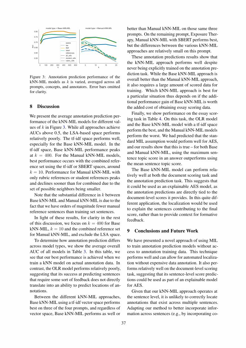
0 100 200 300 400 500 600k

0.55

0.60

0.65

0.70

0.75

0.80au

c

model type = Base kNN-MIL

spacelsatfidfsbertreferencesall_refsstudent_refsrubric_refs

5 10 15 20k

model type = Manual kNN-MIL

Figure 3: Annotation prediction performance of thekNN-MIL models as k is varied, averaged across allprompts, concepts, and annotators. Error bars omittedfor clarity.

8 Discussion

We present the average annotation prediction per-formance of the kNN-MIL models for different val-ues of k in Figure 3. While all approaches achieveAUCs above 0.5, the LSA-based space performsrelatively poorly. The tf-idf space performs well,especially for the Base kNN-MIL model. In thetf-idf space, Base kNN-MIL performance peaksat k = 400. For the Manual kNN-MIL models,best performance occurs with the combined refer-ence set using the tf-idf or SBERT spaces, aroundk = 10. Performance for Manual kNN-MIL withonly rubric references or student references peaksand declines sooner than for combined due to theset of possible neighbors being smaller.

Note that the substantial difference in k betweenBase kNN-MIL and Manual kNN-MIL is due to thefact that we have orders of magnitude fewer manualreference sentences than training set sentences.

In light of these results, for clarity in the restof this discussion, we focus on k = 400 for BasekNN-MIL, k = 10 and the combined reference setfor Manual kNN-MIL, and exclude the LSA space.

To determine how annotation prediction differsacross model types, we show the average overallAUC of all models in Table 3. In this table, wesee that our best performance is achieved when wetrain a kNN model on actual annotation data. Incontrast, the OLR model performs relatively poorly,suggesting that its success at predicting sentencesthat require some sort of feedback does not directlytranslate into an ability to predict locations of an-notations.

Between the different kNN-MIL approaches,Base kNN-MIL using a tf-idf vector space performsbest on three of the four prompts, and regardless ofvector space, Base kNN-MIL performs as well or

better than Manual kNN-MIL on those same threeprompts. On the remaining prompt, Exposure Ther-apy, Manual kNN-MIL with SBERT performs best,but the differences between the various kNN-MILapproaches are relatively small on this prompt.

These annotation predictions results show thatthe kNN-MIL approach performs well despitenever being explicitly trained on the annotation pre-diction task. While the Base kNN-MIL approach isoverall better than the Manual kNN-MIL approach,it also requires a large amount of scored data fortraining. Which kNN-MIL approach is best fora particular situation thus depends on if the addi-tional performance gain of Base kNN-MIL is worththe added cost of obtaining essay scoring data.

Finally, we show performance on the essay scor-ing task in Table 4. On this task, the OLR modeland the Base kNN-MIL model with a tf-idf spaceperform the best, and the Manual kNN-MIL modelsperform the worst. We had predicted that the stan-dard MIL assumption would perform well for AES,and our results show that this is true – for both Baseand Manual kNN-MIL, using the maximum sen-tence topic score in an answer outperforms usingthe mean sentence topic score.

The Base kNN-MIL model can perform rela-tively well at both the document scoring task andthe annotation prediction task. This suggests thatit could be used as an explainable AES model, asthe annotation predictions are directly tied to thedocument-level scores it provides. In this quite dif-ferent application, the localization would be usedto explain the sentences contributing to the finalscore, rather than to provide context for formativefeedback.

9 Conclusions and Future Work

We have presented a novel approach of using MILto train annotation prediction models without ac-cess to annotation training data. This techniqueperforms well and can allow for automated localiza-tion without expensive data annotation. It also per-forms relatively well on the document-level scoringtask, suggesting that its sentence-level score predic-tions could be used as part of an explainable modelfor AES.

Given that our kNN-MIL approach operates atthe sentence level, it is unlikely to correctly locateannotations that exist across multiple sentences.Adapting our method to better incorporate infor-mation across sentences (e.g., by incorporating co-

37

Model Space Exposure Therapy Piaget Stages Sensory Study Sleep Stages

Annotation kNNsbert 0.88 (0.04) 0.89 (0.08) 0.85 (0.06) 0.91 (0.03)tfidf 0.87 (0.04) 0.92 (0.07) 0.89 (0.06) 0.93 (0.02)

Base kNN-MILsbert 0.76 (0.08) 0.78 (0.09) 0.77 (0.09) 0.78 (0.06)tfidf 0.74 (0.06) 0.84 (0.10) 0.81 (0.09) 0.80 (0.07)

Manual kNN-MILsbert 0.78 (0.07) 0.73 (0.12) 0.70 (0.10) 0.78 (0.06)tfidf 0.74 (0.08) 0.77 (0.09) 0.68 (0.10) 0.75 (0.07)

OLR 0.55 (0.04) 0.63 (0.08) 0.63 (0.07) 0.61 (0.05)

Table 3: Area under the ROC curve on the annotation prediction task, averaged over all topics and annotators.Standard deviation shown in parentheses.

Model agg Space Exposure Therapy Piaget Stages Sensory Study Sleep Stages

Base kNN-MILmax

sbert 0.49 (0.14) 0.51 (0.18) 0.41 (0.15) 0.60 (0.11)tfidf 0.47 (0.12) 0.61 (0.19) 0.52 (0.17) 0.67 (0.12)

meansbert 0.39 (0.15) 0.44 (0.16) 0.36 (0.15) 0.61 (0.14)tfidf 0.40 (0.14) 0.52 (0.16) 0.46 (0.14) 0.63 (0.13)

Manual kNN-MILmax

sbert 0.41 (0.15) 0.30 (0.18) 0.25 (0.15) 0.37 (0.14)tfidf 0.38 (0.14) 0.40 (0.15) 0.23 (0.16) 0.34 (0.18)

meansbert 0.29 (0.15) 0.23 (0.15) 0.16 (0.15) 0.27 (0.14)tfidf 0.29 (0.16) 0.29 (0.13) 0.19 (0.16) 0.22 (0.20)

OLR 0.50 (0.18) 0.63 (0.16) 0.51 (0.18) 0.69 (0.14)

Table 4: Pearson correlation coefficients on the document-level scoring task, averaged over all topics. Standarddeviation shown in parentheses.

reference resolution) could help improve its overallperformance. Additionally, as the Base kNN-MILapproach uses topics as negative examples for eachother, we expect that it would not work well in situ-ations where the inter-topic score correlations werehigh. We expect the Manual kNN-MIL approachto be less sensitive to this issue. Determining otherways to include negative examples would allow theBase kNN-MIL approach to be applied to promptswhose topics were highly correlated.

In our current domain, psychology, and in thecontext of low-stakes formative feedback, incorrectanswers are uncommon compared to omitted or par-tial answers. In contrast, for domains that requirechained reasoning over more complex mental mod-els, such as accounting, cell biology, or computerscience, we expect the ability to correctly detectmisconceptions and errors to be far more important.In general, future work is required to determinehow well our approach will work in other domains,and which domains it is best suited to.

Determining where topics are discussed is onlyone step in the full formative feedback process.

More work is required to determine the path fromholistic scoring and topic localization to the mosthelpful kinds of feedback for a student. In partic-ular, we need to consider different kinds of peda-gogical feedback and how such feedback could beindividualized. Additionally, we could provide notjust text but also video, peer interaction, worked ex-amples, and other approaches from the full panoplyof potential pedagogical interventions. Finally, weneed to decide what actions will help the studentthe most, which relies on our pedagogical theoryof how to help a student achieve their current in-structional objectives.

Acknowledgements

We would like to thank Alok Baikadi, Julio Brad-ford, Jill Budden, Amy Burkhardt, Dave Farnham,Andrew Gorman and Jorge Roccatagliata for theirefforts in collecting the annotated dataset used inthis work.

38

ReferencesStefanos Angelidis and Mirella Lapata. 2018. Multi-

ple instance learning networks for Fine-Grained sen-timent analysis. Transactions of the Association forComputational Linguistics, 6:17–31.

David M Blei, Andrew Y Ng, and Michael I Jordan.2003. Latent dirichlet allocation. Journal of Ma-chine Learning Research., 3(Jan):993–1022.

Samuel R. Bowman, Gabor Angeli, Christopher Potts,and Christopher D. Manning. 2015. A large anno-tated corpus for learning natural language inference.In Proceedings of the 2015 Conference on EmpiricalMethods in Natural Language Processing (EMNLP).Association for Computational Linguistics.

Razvan Bunescu and Raymond Mooney. 2007. Learn-ing to extract relations from the web using mini-mal supervision. In Proceedings of the 45th An-nual Meeting of the Association of ComputationalLinguistics, pages 576–583.

Jill Burstein, Daniel Marcu, and Kevin Knight. 2003.Finding the write stuff: Automatic identification ofdiscourse structure in student essays. Intelligent Sys-tems, IEEE, 18:32 – 39.

Nathalie Camelin, Boris Detienne, Stephane Huet, Do-minique Quadri, and Fabrice Lefevre. 2011. Un-supervised concept annotation using latent dirichletallocation and segmental methods. In Proceedingsof the First workshop on Unsupervised Learning inNLP, pages 72–81.

Marc-Andre Carbonneau, Veronika Cheplygina, EricGranger, and Ghyslain Gagnon. 2016. Multiple in-stance learning: A survey of problem characteristicsand applications. Pattern Recognition.

Evgeny Chukharev-Hudilainen and Aysel Saricaoglu.2016. Causal discourse analyzer: improving auto-mated feedback on academic ESL writing. Com-puter Assisted Language Learning, 29(3):494–516.

T. Cover and P. Hart. 1967. Nearest neighbor patternclassification. IEEE Transactions on InformationTheory, 13(1):21–27.

Jacob Devlin, Ming-Wei Chang, Kenton Lee, andKristina Toutanova. 2019. BERT: pre-training ofdeep bidirectional transformers for language under-standing. In Proceedings of the 2019 Conferenceof the North American Chapter of the Associationfor Computational Linguistics: Human LanguageTechnologies, NAACL-HLT 2019, Minneapolis, MN,USA, June 2-7, 2019, Volume 1 (Long and Short Pa-pers), pages 4171–4186. Association for Computa-tional Linguistics.

Thomas G. Dietterich, Richard H. Lathrop, and TomasLozano-Perez. 1997. Solving the multiple instanceproblem with axis-parallel rectangles. Artificial In-telligence, 89(1–2):31–71.

Fei Dong, Yue Zhang, and Jie Yang. 2017. Attention-based recurrent convolutional neural network for au-tomatic essay scoring. In Proceedings of the 21stConference on Computational Natural LanguageLearning (CoNLL 2017), pages 153–162.

Peter W Foltz, Sara Gilliam, and Scott A Kendall.2000. Supporting Content-Based feedback in On-Line writing evaluation with LSA. InteractiveLearning Environments, 8(2):111–127.

Marita Franzke, Eileen Kintsch, Donna Caccamise,Nina Johnson, and Scott Dooley. 2005. Summarystreet R©: Computer support for comprehension andwriting. Journal of Educational Computing Re-search, 33:53–80.

Steve Graham, Karen Harris, and Michael Hebert.2011. Informing Writing: The Benefits of Forma-tive Assessment. A Report from Carnegie Corpora-tion of New York. Carnegie Corporation of NewYork.

Matthew Honnibal and Ines Montani. 2017. spaCy 2:Natural language understanding with Bloom embed-dings, convolutional neural networks and incremen-tal parsing. To appear.

Dimitrios Kotzias, Misha Denil, Nando de Freitas, andPadhraic Smyth. 2015. From group to individual la-bels using deep features. In Proceedings of the 21thACM SIGKDD International Conference on Knowl-edge Discovery and Data Mining, pages 597–606.ACM.

Thomas K Landauer, Peter W. Foltz, and Darrell La-ham. 1998. An introduction to latent semantic anal-ysis. Discourse processes, 25(2-3):259–284.

Bernhard Lutz, Nicolas Prollochs, and Dirk Neumann.2019. Sentence-level sentiment analysis of finan-cial news using distributed text representations andmulti-instance learning. In Proceedings of the 52ndHawaii International Conference on System Sci-ences.

Ellis B Page. 1966. The imminence of grading essaysby computer. The Phi Delta Kappan, 47(5):238–243.

Nikolaos Pappas and Andrei Popescu-Belis. 2017.Explicit document modeling through weightedmultiple-instance learning. Journal of Artificial In-telligenece Research., 58(1):591–626.

Melissa Patchan, Christian Schunn, and Richard Cor-renti. 2016. The nature of feedback: How peer feed-back features affect students’ implementation rateand quality of revisions. Journal of Educational Psy-chology, 108.

Fabian Pedregosa, Gael Varoquaux, Alexandre Gram-fort, Vincent Michel, Bertrand Thirion, OlivierGrisel, Mathieu Blondel, Peter Prettenhofer, RonWeiss, Vincent Dubourg, Jake Vanderplas, Alexan-dre Passos, David Cournapeau, Matthieu Brucher,

39

Matthieu Perrot, and Edouard Duchesnay. 2011.Scikit-learn: Machine Learning in Python. Journalof Machine Learning Research, 12(Oct):2825–2830.

Fabian Pedregosa-Izquierdo. 2015. Feature extractionand supervised learning on fMRI : from practice totheory. Theses, Universite Pierre et Marie Curie -Paris VI.

Radim Rehurek and Petr Sojka. 2010. Software Frame-work for Topic Modelling with Large Corpora. InProceedings of the LREC 2010 Workshop on NewChallenges for NLP Frameworks, pages 45–50, Val-letta, Malta. ELRA.

Nils Reimers and Iryna Gurevych. 2019. Sentence-bert: Sentence embeddings using siamese bert-networks. In Proceedings of the 2019 Conference onEmpirical Methods in Natural Language Processing.Association for Computational Linguistics.

Rod Roscoe, Danica Kugler, Scott A Crossley, Jen-nifer L Weston, and Danielle McNamara. 2012. De-veloping pedagogically-guided threshold algorithmsfor intelligent automated essay feedback. In Pro-ceedings of the 25th International Florida ArtificialIntelligence Research Society Conference, FLAIRS-25, pages 466–471.

Mark D. Shermis and Jill C. Burstein, editors. 2003.Automated essay scoring: A cross-disciplinary per-spective. Lawrence Erlbaum Associates, Inc., Mah-way, NJ.

Mark D. Shermis and Jill C. Burstein, editors. 2013.Handbook of automated essay evaluation: Currentapplications and new directions. Routledge, NewYork.

David J. Steinhart. 2001. Summary street: An intelli-gent tutoring system for improving student writingthrough the use of latent semantic analysis. Doc-tor of philosophy (thesis), University of Colorado atBoulder.

Wei Wang, Yue Ning, Huzefa Rangwala, and NarenRamakrishnan. 2016. A multiple instance learningframework for identifying key sentences and detect-ing events. In Proceedings of the 25th ACM Inter-national on Conference on Information and Knowl-edge Management, pages 509–518. ACM.

Adina Williams, Nikita Nangia, and Samuel Bowman.2018. A broad-coverage challenge corpus for sen-tence understanding through inference. In Proceed-ings of the 2018 Conference of the North AmericanChapter of the Association for Computational Lin-guistics: Human Language Technologies, Volume1 (Long Papers), pages 1112–1122, New Orleans,Louisiana. Association for Computational Linguis-tics.

Bronwyn Woods, David Adamson, Shayne Miel, andElijah Mayfield. 2017. Formative essay feedbackusing predictive scoring models. In Proceedings ofthe 23rd ACM SIGKDD International Conference on

Knowledge Discovery and Data Mining, KDD ’17,page 2071–2080, New York, NY, USA. Associationfor Computing Machinery.

Qian Yang, Rebecca J Passonneau, and GerardDe Melo. 2016. Peak: Pyramid evaluation via au-tomated knowledge extraction. In Thirtieth AAAIConference on Artificial Intelligence.

Amelia Zafra, Cristobal Romero, and Sebastian Ven-tura. 2011. Multiple instance learning for clas-sifying students in learning management systems.Expert Systems with Applications, 38(12):15020–15031.

40

Proceedings of the 15th Workshop on Innovative Use of NLP for Building Educational Applications, pages 41–51July 10, 2020. c©2020 Association for Computational Linguistics

Complementary Systems for Off-Topic Spoken Response Detection

Vatsal Raina, Mark J.F. Gales, Kate KnillDept. of Engineering, Cambridge University

Cambridge, UK{vr311, mjfg, kate.knill}@eng.cam.ac.uk

Abstract

Increased demand to learn English for busi-ness and education has led to growing interestin automatic spoken language assessment andteaching systems. With this shift to automatedapproaches it is important that systems reliablyassess all aspects of a candidate’s responses.This paper examines one form of spoken lan-guage assessment; whether the response fromthe candidate is relevant to the prompt pro-vided. This will be referred to as off-topicspoken response detection. Two forms ofpreviously proposed approaches are examinedin this work: the hierarchical attention-basedtopic model (HATM); and the similarity gridmodel (SGM). The work focuses on the sce-nario when the prompt, and associated re-sponses, have not been seen in the trainingdata, enabling the system to be applied to newtest scripts without the need to collect dataor retrain the model. To improve the perfor-mance of the systems for unseen prompts, dataaugmentation based on easy data augmenta-tion (EDA) and translation based approachesare applied. Additionally for the HATM, aform of prompt dropout is described. Thesystems were evaluated on both seen and un-seen prompts from Linguaskill Business andGeneral English tests. For unseen data theperformance of the HATM was improved us-ing data augmentation, in contrast to the SGMwhere no gains were obtained. The two ap-proaches were found to be complementary toone another, yielding a combined F0.5 score of0.814 for off-topic response detection wherethe prompts have not been seen in training.

1 Introduction

Spoken language assessment of English is onthe rise as English is the chosen language ofdiscourse for many situations. Businesses andacademic institutes demand rigorous assessmentmethods to ensure prospective employees and

students exceed a baseline standard for Englishproficiency so they can succeed and contributein their new environment. Standardised assess-ments such as IELTS (Cullen et al., 2014), PearsonTest of English Academic (Longman, 2010) andTOEFL (ETS, 2012) include “free speaking” taskswhere the candidate speaks spontaneously in re-sponse to a prompted question to ensure their speak-ing skills are fully assessed. A candidate mightattempt to achieve a higher grade by speaking apre-prepared response, irrelevant to the prompt.For scoring validity it is important that measuresare taken to detect any off-topic responses so theydo not influence the final grade. This is particu-larly true for automatic assessment systems whichare increasingly being deployed to cope with thegrowing demand for examinations and may see in-creased cheating if candidates are aware that a com-puterised system is responsible for grading them(e.g. (Mellar et al., 2018)). These systems are moresusceptible to inaccurate scoring due to empha-sis given to criteria such as fluency, pronunciationand language use, over topic relevance (Lochbaumet al., 2013; Higgins and Heilman, 2014).

Automatic off-topic spoken response detectionsystems based on attention (Malinin et al., 2017b,a)and similarity grid (Wang et al., 2019) models haveshown good performance for prompts seen in train-ing. For operational reasons it would be cost andtime effective to be able to use the same systemson responses to new prompts, unseen in training i.e.removing the need to collect new data and retrainmodels prior to deployment. Yoon et al. (2017) hashad some success with handling unseen prompts.This is still a challenging research problem, how-ever, with significant degradation observed on eventhe best performing hierarchical attention-basedtopic model (HATM) (Malinin et al., 2017a), andwith no assessment to date of Wang et al. (2019)’ssimilarity grid model (SGM) approach. This paper

41

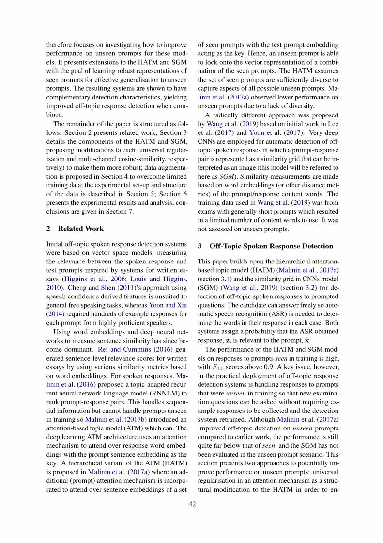
therefore focuses on investigating how to improveperformance on unseen prompts for these mod-els. It presents extensions to the HATM and SGMwith the goal of learning robust representations ofseen prompts for effective generalisation to unseenprompts. The resulting systems are shown to havecomplementary detection characteristics, yieldingimproved off-topic response detection when com-bined.

The remainder of the paper is structured as fol-lows: Section 2 presents related work; Section 3details the components of the HATM and SGM,proposing modifications to each (universal regular-isation and multi-channel cosine-similarity, respec-tively) to make them more robust; data augmenta-tion is proposed in Section 4 to overcome limitedtraining data; the experimental set-up and structureof the data is described in Section 5; Section 6presents the experimental results and analysis; con-clusions are given in Section 7.

2 Related Work

Initial off-topic spoken response detection systemswere based on vector space models, measuringthe relevance between the spoken response andtest prompts inspired by systems for written es-says (Higgins et al., 2006; Louis and Higgins,2010). Cheng and Shen (2011)’s approach usingspeech confidence derived features is unsuited togeneral free speaking tasks, whereas Yoon and Xie(2014) required hundreds of example responses foreach prompt from highly proficient speakers.

Using word embeddings and deep neural net-works to measure sentence similarity has since be-come dominant. Rei and Cummins (2016) gen-erated sentence-level relevance scores for writtenessays by using various similarity metrics basedon word embeddings. For spoken responses, Ma-linin et al. (2016) proposed a topic-adapted recur-rent neural network language model (RNNLM) torank prompt-response pairs. This handles sequen-tial information but cannot handle prompts unseenin training so Malinin et al. (2017b) introduced anattention-based topic model (ATM) which can. Thedeep learning ATM architecture uses an attentionmechanism to attend over response word embed-dings with the prompt sentence embedding as thekey. A hierarchical variant of the ATM (HATM)is proposed in Malinin et al. (2017a) where an ad-ditional (prompt) attention mechanism is incorpo-rated to attend over sentence embeddings of a set

of seen prompts with the test prompt embeddingacting as the key. Hence, an unseen prompt is ableto lock onto the vector representation of a combi-nation of the seen prompts. The HATM assumesthe set of seen prompts are sufficiently diverse tocapture aspects of all possible unseen prompts. Ma-linin et al. (2017a) observed lower performance onunseen prompts due to a lack of diversity.

A radically different approach was proposedby Wang et al. (2019) based on initial work in Leeet al. (2017) and Yoon et al. (2017). Very deepCNNs are employed for automatic detection of off-topic spoken responses in which a prompt-responsepair is represented as a similarity grid that can be in-terpreted as an image (this model will be referred tohere as SGM). Similarity measurements are madebased on word embeddings (or other distance met-rics) of the prompt/response content words. Thetraining data used in Wang et al. (2019) was fromexams with generally short prompts which resultedin a limited number of content words to use. It wasnot assessed on unseen prompts.

3 Off-Topic Spoken Response Detection

This paper builds upon the hierarchical attention-based topic model (HATM) (Malinin et al., 2017a)(section 3.1) and the similarity grid in CNNs model(SGM) (Wang et al., 2019) (section 3.2) for de-tection of off-topic spoken responses to promptedquestions. The candidate can answer freely so auto-matic speech recognition (ASR) is needed to deter-mine the words in their response in each case. Bothsystems assign a probability that the ASR obtainedresponse, z, is relevant to the prompt, x.

The performance of the HATM and SGM mod-els on responses to prompts seen in training is high,with F0.5 scores above 0.9. A key issue, however,in the practical deployment of off-topic responsedetection systems is handling responses to promptsthat were unseen in training so that new examina-tion questions can be asked without requiring ex-ample responses to be collected and the detectionsystem retrained. Although Malinin et al. (2017a)improved off-topic detection on unseen promptscompared to earlier work, the performance is stillquite far below that of seen, and the SGM has notbeen evaluated in the unseen prompt scenario. Thissection presents two approaches to potentially im-prove performance on unseen prompts: universalregularisation in an attention mechanism as a struc-tural modification to the HATM in order to en-

42

courage generalisation; multi-channel SGM basedon cosine distance (MSGM). Data augmentationstrategies to increase the number of prompts avail-able for training are presented in Section 4.

3.1 Attention-Based Model

Figure 1: Hierarchical Attention-based Topic Model(HATM).

The Hierarchical Attention-based Topic Model(HATM) (Malinin et al., 2017a) is depicted in Fig-ure 1. The system uses an encoding of the promptword sequence, hp, as the key for an attentionmechanism over an embedding of the response toyield a fixed length vector, h, that is used to predictthe probability, y, that the response was relevantto the prompt. To improve the robustness of theestimate of the prompt embedding an additional at-tention mechanism is run over all NT embeddingsof the prompts seen in training, h(1)

p , . . . , h(NT )p .

This attention mechanism uses an embedding ofthe test prompt, hp, as the key to yield hp. This ad-ditional attention mechanism over the prompts wasfound to improve the performance of the systemwhen the prompt had not been seen in the trainingdata (Malinin et al., 2017a). The same networkconfiguration as that used in Malinin et al. (2017a)was implemented in this work:

• bi-directional (Schuster and Paliwal, 1997)LSTMs (Hochreiter and Schmidhuber, 1997)were used as the encoders for both the promptsand the responses. Separate models were usedfor the prompt and response encoders1;

1More complex sentence and word embeddings, such asBERT (Devlin et al., 2019) were examined in initial experi-ments but were not found to yield performance gains.

• additive attention mechanisms were used forboth the attention mechanism over the trainingprompts and that over the responses;

• the classifier used ReLU activation functions.

The parameters of the network were optimisedusing cross-entropy training. For the training ofthe prompt attention mechanism, the actual promptwas excluded from the attention mechanism, oth-erwise the attention mechanism simply focuses onthe matched prompt embedding.

One of the issues observed with the HATMis that the performance of the system on unseenprompts is significantly poorer than the perfor-mance on seen prompts that have been seen, alongwith relevant responses, in the training data. Thismotivates the need for the model to improve thegeneralisation of the system to unseen prompts.Here, the prompt attention mechanism (see Fig-ure 1) is targeted. A specific form of dropout,where training prompt embeddings are excludedfrom the prompt attention mechanism, referred toas prompt-dropout, is proposed. Denoting αk =

Softmax[hp, h

(k)p , θpa

]as the attention weight

for the kth training prompt embedding, h(k)p , with

the test prompt embedding, hp, as the key, randomattention weights are set to zero during training inprompt-dropout such that

αk =

{0 w.p. 1− κSoftmax

[hp, h

(k)p , θpa

]w.p. κ

(1)where κ represents the keep-probability. The atten-tion weights must be re-normalised after prompt-dropout. Sampling κ from a probabilistic distribu-tion for each attention weight is motivated by Gar-nelo et al. (2018). In initial experiments this dis-tribution of dropout rate was found to outperformselecting a fixed dropout rate.

3.2 Similarity Grid Model

The Similarity Grid Model (SGM) (Wang et al.,2019) represents a prompt-response pair as a “sim-ilarity image”. This image is transformed by anInception network into a measure of the degreeof relevance between the test prompt and test re-sponse.

Initially all stop words are removed such that agiven prompt and response pair only consists of

43

Figure 2: Similarity Grid Model (SGM) where the grid“pixel” colours indicate the level of similarity.

content words2. After this pre-processing the simi-larity grid model for a prompt-response pair is asshown in Figure 2. For all content words in thetest prompt, {xi}NL

i=1, and test response, {zi}NRi=1,

word embeddings,{h(i)p

}NL

i=1and

{h(i)r

}NR

i=1, are

computed. These word embeddings are used to con-struct a similarity grid, S. This two-dimensionalgrid has NL columns and NR rows and the cellposition (i, j) holds an inverse similarity metricbetween the ith prompt word embedding, h(i)

p , andthe jth response word embedding, h(j)

r . S is thenresized to 180× 180 in order to make the similar-ity grid of standard size regardless of the numberof content words in the test prompt and response.Perceiving the similarity grid as an image, an In-ception network transforms the resized image to avalue 0 ≤ y ≤ 1, indicating the degree of relevancebetween the test prompt and test response.

The network configuration used in this work isclosely related to that used in Wang et al. (2019):

• context independent word embeddings arecomputed for each word in the prompt andthe response. The embeddings for both theprompt and response are tied;

• a cosine distance to compute the distance be-tween each prompt response word embeddingpair, followed by a bilinear transform wasused to resize the similarity grid;

2A comprehensive list of stop words is providedby nltk.corpus https://www.nltk.org/api/nltk.corpus.html.

• the Resnet-152 (He et al., 2016b) Inceptionnetwork was used.

The similarity grid has one channel i.e. onesingle measurement value per cell. This can beextended to multiple channels (MSGM), with dif-ferent forms of embeddings or distance functionsused to compute the grid in each channel. Wanget al. (2019) used cosine distances in the first chan-nel and inverse document frequency (IDF) valuesof the prompt and response words for the secondand third channel, respectively. For this paper aMSGM with three channels where each channelrepresents the cosine distance between prompt andresponse word embeddings with a different set ofword embeddings learnt for each channel is used3.The variety in the embeddings, and resulting chan-nel, is achieved by using different initialisationseeds with the same network configuration. Asthe Inception network filters over the channels aresimultaneously trained the resulting filters will becomplementary.

4 Data Augmentation

In general, the performance of off-topic responsesystems is limited by insufficient unique promptsbeing available for training. Data augmentation,where the training data is modified in some wayto create new examples, is regularly applied onlow resource tasks in areas such as speech recog-nition (e.g. (Cui et al., 2015)) and computer vision(e.g. (Shorten and Khoshgoftaar, 2019)) and hashad some success in NLP (e.g. (Zhang et al., 2015;Kafle et al., 2017; Wei and Zou, 2019)). This mo-tivates investigating if augmentation of the train-ing prompts such that multiple versions of eachprompt are generated can help improve robustness4.Prompt augmentation will permit the model to ex-plore the region around each unique prompt ratherthan being restricted to a discrete point in the high-dimensional prompt-space.

Both structured and unstructured data augmenta-tion techniques are considered here. Augmentationof prompts is performed on-the-fly during training.Note, the hierarchy of seen prompts of the HATM

3In this work, the use of IDF values in the second and thirdMSGM channels did not improve performance over the SGMso was not used.

4Data augmentation of training responses is also possible.This was found to degrade performance in initial experiments,possibly due to there being a large number of diverse responsesavailable for training without augmentation and issues withgenerating sensible back-translations on ASR output.

44

in the prompt attention mechanism (Figure 1) doesnot include the additional augmented prompts be-cause the expectation is that augmented promptswill not dramatically differ from the original uniqueprompts.

Easy Data Augmentation (EDA) techniqueswere trialled by Wei and Zou (2019). They pro-posed that different variants of any textual data canbe generated using a combination of synonym re-placement, random insertion, random swap and ran-dom deletion of words. A single hyper-parameter,α, controls the fraction of words that are modi-fied in the original text. Using the default value ofα = 0.1, prompts are augmented using the abovetechniques to replace, insert, swap or delete 10%of the words randomly in the original prompt. Thisstructured augmentation approach should enablethe model to learn a more robust representation ofeach unique prompt.

Back-translation is employed as an unstructuredmethod to augment the amount of available train-ing data. A machine translation model is employedto translate a given training prompt into a foreignlanguage by taking the maximum likelihood out-put. Then a reverse machine translation modeltakes the prompt in the foreign language and trans-lates it back into English. The expectation is thatthe original and final pair of English prompts willbe very similar in meaning but will have a differ-ent ordering and choice of specific words. There-fore, the back-translated prompt can be treated asa new prompt which can be paired with the orig-inal prompt’s response to generate a new prompt-response pair. The use of several different lan-guages permits the creation of several variants ofthe same prompt. Translation can be achieved us-ing standard machine translation packages.

5 Data and Experimental Set-Up

The HATM and SGM models and the proposedextensions were assessed on their ability to detectoff-topic responses to prompts in free speakingtests where the candidates can talk for up to oneminute in answering the question.

5.1 Training and evaluation data

Data from the Cambridge Assessment English Lin-guaskill Business and Linguaskill General Englishtests5 are used in the training and evaluation of the

5https://www.cambridgeenglish.org/exams-and-tests/linguaskill/

systems. The two tests are similar in format butwith different foci and therefore vary in the topicsdiscussed by candidates and their associated vo-cabularies. They are multi-level, global, tests - i.e.taken by candidates from across the CEFR levels,A1-C2, with a wide range of first languages (L1s)and variation in response proficiency.

Both Linguaskill speaking tests are comprisedof five parts. For this paper only prompts and corre-sponding responses from the three long free speak-ing parts are used. The candidate has 60 seconds inparts 3 and 4 to talk on a topic such as advice fora colleague/friend and discuss a picture or graph,respectively. Part 5 consists of 20 second responsesto a set of five contextualised prompts, such as start-ing a retail business, or talk about a hobby. Thediversity of these prompts is discussed by Malininet al. (2017a).

Data TRN SEEN UNS#Prompts 379 219 56

#Responses 257.2K 40.8K 85.0KAvg. prompt length 51 51 55

content words 28 28 29Avg. resp. length 48 43 42

content words 22 20 19

Table 1: Prompt/response statistics for training (TRN)and seen (SEEN) and unseen (UNS) evaluation datasets.

Table 1 outlines the statistics for the training(TRN) and two evaluation data sets (SEEN andUNS). TRN and SEEN are taken from the Lin-guaskill Business test and UNS from the Lin-guaskill General English test. There is no over-lap in speakers between any of the data sets. Theresponse texts are generated automatically fromthe 1-best hypotheses from an ASR system witha word error rate (WER) of 25.7% on BusinessEnglish data. TRN consists of a total of 257.2K re-sponses to 379 unique prompts, an average of 679responses per prompt compared with 186 for SEENand 1518 for UNS. The average number of wordsare similar across the 3 data sets, with prompts (51-55) being slightly longer than responses (42-48) onaverage. This reduces by about half when contentwords only are included. The HATM is trainedand evaluated using all the words in every textualprompt-response pair while the SGM is trained andevaluated using only the content words in everyprompt-response pair.

45

5.1.1 Training data construction

All responses are taken from tests assessed by hu-man examiners, which permits the assumption thatall responses in the data are on-topic. Thereforesynthetic off-topic responses have to be createdto train the systems. The off-topic data is gener-ated using a dynamic sampling mechanism; thismatches responses from one prompt with a differ-ent prompt. Balance is maintained such that theempirical distribution of topics in the on-topic ex-amples is mimicked in the generation of syntheticoff-topic examples. Off-topic examples for trainingdata are generated on-the-fly (Malinin et al., 2017a)instead of producing a fixed set of negative exam-ples prior to training as in Malinin et al. (2016)because dynamic sampling allows the diversity ofnegative examples to be efficiently increased. Foreach on-topic example, one off-topic example isgenerated.

For the data augmentation experiments the num-ber of prompts was increased by a factor of 10using EDA (Wei and Zou, 2019) or machine trans-lation, and 20 when both were applied. The defaultvalue of α = 0.1 was used in EDA to change 10%of words in the original prompt by replacing, insert-ing, swapping and/or deleting. Machine translationwas performed offline using the Babylon MT sys-tem 6. Back-translations were generated using 9different languages7.

5.1.2 Evaluation data construction

Due to the scarcity of real off-topic examples, nega-tive off-topic examples are generated by permutingon-topic examples for SEEN and UNS. Each on-topic example has ten off-topic examples generatedand duplicated ten times to maintain balance. Dataset SEEN is formed from prompts that have beenseen during training and negative responses thatcorrespond to a different set of prompts seen dur-ing training. Data set UNS consists of prompts thatare unseen during training and negative responsesthat correspond to prompts that are unseen duringtraining too. Forming negative examples by per-muting on-topic examples is reasonable becausereal off-topic examples by candidates are antici-pated to consist of responses to a different promptto that being answered.

6https://translation.babylon-software.com/english/Offline/

7Machine translation languages: Arabic, French, German,Greek, Hebrew, Hindi, Japanese, Korean, Russian.

5.2 Hyper-parameters and models

The HATM consists of two 400 dimensional BiL-STM encoders with 200 forward and backwardstates each and TanH non-linearities. 200 dimen-sional parameters are used for the prompt attentionmechanism. The binary classifier is a DNN with 2hidden layers of 200 rectified linear (ReLU) unitsand a 1-dimensional logistic output. Dropout reg-ularisation (Srivastava et al., 2014) with a keepprobability of 0.8 is applied to all layers exceptfor the LSTM recurrent connections and word em-beddings. The universal regularisation samples itskeep probability using κ ∼ U(0.05, 0.95). TheHATM is initialised from an attention-topic model(ATM) as described in Malinin et al. (2017a). It istrained for 3 epochs using an Adam optimizer, withan exponentially decaying learning rate initialisedat 1e-3 and decay factor of 0.85 per epoch. The firsttwo epochs train only the prompt attention mecha-nism and the final epoch is used to train the wholenetwork apart from the DNN binary classifier. Thisconfiguration was optimised using seen develop-ment data, similarly for the SGM. The ATM takesapproximately 3 hours to train and an additional1 hour for the HATM on an nVidia GTX 980Mgraphics card.

The SGM learns 200 dimensional word embed-dings for each word in the prompt and response.ResNet-152 (He et al., 2016a)8 with 152 residuallayers is used as the Inception network with a 1-dimensional logistic output. The SGM is trainedfor 1 epoch using an Adam optimizer with a learn-ing rate of 1e-3. It takes about 2 hours to train onan nVidia GTX 980M graphics card. The extendedHATM and the SGM were built in Tensorflow9.

The HATM and SGM results reported are com-puted on an ensemble of 15 models unless notedotherwise. Each model has an identical architectureand training parameters but each has a different ini-tial seed value, creating modeling diversity. Forthis work a large ensemble is reported to minimisevariance on the ensemble performance results. Noanalysis of efficiency is given. Approaches such asensemble distillation (Hinton et al., 2015) can bedirectly applied to reduce computational cost.

8Code available at https://github.com/KaimingHe/resnet-1k-layers.

9Code available at https://github.com/VatsalRaina/HATM.

46

5.3 Performance criteria

Following Wang et al. (2019), precision and re-call are used to assess performance except F0.5 ispreferred over F1 as there is a greater interest inachieving a higher precision compared to recall:a candidate’s response should not be mistakenlyclassified as off-topic as such responses are to beassigned a score of 0. This is a more standardmetric than the area under the curve (AUC) usedin Malinin et al. (2017a) and more intuitive in termsof test evaluation. Note, the results are given fora particular instance of permuting the off-topic ex-amples for evaluation.

6 Experimental Results

This section presents the results of experimentsperformed on SGM, MSGM and extended HATMsystems. Section 6.1 compares the performance ofthe baseline HATM with the MSGM on the unseen(UNS) and seen (SEEN) evaluation data sets. Sec-tion 6.2 explores the improvement in performancedue to extending the baseline HATM using universalregularisation and prompt augmentation strategies.Finally, 6.3 investigates the complementary natureof the MSGM and the extended HATM. The prompt-specific performance of the combined system isconsidered in Section 6.4.

6.1 Baseline systems

Model P R F0.5

SEEN

HATM — — 0.918±0.010

-ensemble 0.963 0.841 0.936MSGM — — 0.905

±0.009-ensemble 0.943 0.838 0.920

UNS

HATM — — 0.612±0.032

-ensemble 0.815 0.370 0.657MSGM — — 0.767

±0.019-ensemble 0.833 0.691 0.800

Table 2: Comparison of baseline HATM [B] and MSGM,for seen (SEEN) and unseen (UNS).

Table 2 shows the baseline performance for theHATM and MSGM models. There is a relatively lowvariance between individual system results but com-bining the outputs in an ensemble improves the F0.5

score in each case, with a larger gain (0.045/0.033vs 0.018/0.015) observed on the unseen data. The

HATM performs slightly better on the seen datathan the MSGM, with a higher F0.5 and a similarbut always slightly higher precision-recall curve(Figure 3). For unseen data, however, the reverse istrue with MSGM having a higher F0.5 score of 0.800compared to 0.657 for the baseline HATM. FromFigure 3 it can be seen that the precision-recallcurves for the HATM and SGM/MSGM systems onunseen data are quite different in shape. The HATMhas a higher precision at the lowest recall but thisdrops quickly as the threshold increases. The degra-dation in the MSGM precision is much more gradual.

Figure 3: Comparison of precision-recall curves forbaseline ensemble systems for HATM, SGM andMSGM for seen (SEEN) and unseen (UNS).

Figure 3 confirms that the focus should be on im-proving the performance on the unseen evaluationdata set. The use of multi-channels benefits the sim-ilarity grid model as can be seen in Figure 3, witha SGM F0.5 score of 0.908 on the seen and 0.768on the unseen data sets, respectively. These gainsare similar to those observed in Wang et al. (2019).Therefore, the results in the following sections willonly be presented for the unseen evaluation dataset and MSGM systems.

6.2 Regularisation and data augmentationUniversal regularisation and data augmentationwere applied to the HATM to see if they improveddetection performance. From Table 3 and Figure 4,it is evident that the universal regularisation on theprompt attention mechanism yields an increase inthe F0.5 score. Both the structured techniques andthe machine translation (MT) prompt data augmen-tation strategies produce a boost in performanceon the baseline HATM with universal regularisa-tion. MT yields a much larger gain but the struc-tured technique is shown to be complementary by

47

Model P R F0.5

B 0.815 0.370 0.657B ⊕ PD 0.846 0.386 0.683B ⊕ PD ⊕AE 0.790 0.464 0.693B ⊕ PD ⊕AM 0.877 0.529 0.775B ⊕ PD ⊕AE ⊕AM 0.891 0.524 0.782

Table 3: Impact of universal regularisation, PD, anddata augmentation (AE = structured techniques andAM = machine translation) on baseline HATM, B, forunseen (UNS).

a further improvement when prompts are gener-ated by both methods which was larger than ob-served when simply doubling the MT augmentedprompts. Hence, the extended HATM is defined asB ⊕ PD ⊕AE ⊕AM.

Figure 4: Impact of universal regularisation, PD, anddata augmentation (AE = structured techniques andAM = machine translation) on baseline HATM, B, onprecision-recall curves for unseen (UNS).

Experiments were also run on applying data aug-mentation to SGM. This led to significant drops inF0.5, probably as a result of the SGM over-fitting tothe training data.

6.3 Combining MSGM and extended HATMAs for the baseline HATM, the precision-recallcurve for the extended HATM displays differentcharacteristics to MSGM on the unseen data set asshown in Figure 5. These systems are comple-mentary; combining the systems by averaging theiroutputs yields precision-recall curves which boostthe precision at each recall level, giving a smallgain over the best individual system at each thresh-old. The individual F0.5 scores are boosted on theunseen data set from 0.782 and 0.800 to 0.814 andfrom 0.921 and 0.920 to 0.935 on the seen data set

Model P R F0.5

SEENHATM 0.956 0.802 0.921MSGM 0.943 0.838 0.920Comb 0.962 0.839 0.935

UNSHATM 0.891 0.524 0.782MSGM 0.833 0.691 0.800Comb 0.875 0.635 0.814

Table 4: Impact of combining models SGM and ex-tended HATM [B ⊕ PD ⊕AE ⊕AM] on seen (SEEN)and unseen (UNS). Comb = HATM & MSGM.

for the HATM and MSGM systems, respectively (Ta-ble 4). For comparison with Wang et al. (2019), thecombined system here has an F1 score of 0.922 and0.807 on the seen and unseen data sets respectively.

Figure 5: Impact of combining models MSGM and ex-tended HATM [B ⊕ PD ⊕AE ⊕AM] on seen (SEEN)and unseen (UNS).

6.4 Prompt-specific performance analysis

The performance of any off-topic response detec-tion system is expected to depend on both the na-ture of the prompts, and how “close” a test promptis to one seen in the training data. Yoon et al. (2017)found that performance varied substantially acrossdifferent prompts. In this work the 10 most com-mon, in the sense of having a large number of re-sponses, unseen prompts in UNS were used to anal-yse the prompt specific performance. These com-mon prompts should give robust per-prompt F0.5

scores. The average performance of the combinedMSGM and extended HATM system on this subsetof prompts was 0.832, with a standard deviation of0.048. This standard deviation across prompts isapproximately half of the value presented in Yoonet al. (2017). As the prompts for that data are not

48

available, however, it is unclear whether this reduc-tion is due to the nature of the prompts or improvedgeneralisation of the combined model.

From Table 4 there is a large F0.5 performancedifference between prompts seen during training,0.935, and those not seen, 0.814. Given this varia-tion in performance, it is interesting to see whetherthe performance of an individual test prompt canbe predicted given the set of training prompts. Forprompts that are expected to perform poorly itwould then be possible to collect training data.

Figure 6: Relationship between unseen prompt dis-tance to closest seen prompt and F0.5 performanceof MSGM & extended HATM [B ⊕ PD ⊕AE ⊕AM] onthe unseen prompts subsets.

In Malinin et al. (2017a) the entropy of theprompt attention mechanism was used to rank per-formance of the prompts based on area under thecurve metrics. From initial experiments this wasnot found to be a good predictor of F0.5 scoreon these unseen test prompts. In this work, thecosine distance from the test prompt embedding,hp, and each of the training prompt embeddings,h(i)p , was computed. The closest distance was then

used as the measure of similarity of the individ-ual test prompt to the training data prompts. Fig-ure 6 shows the individual F0.5 score against thisdistance again using the 10 most common unseenprompts. There is a strong negative correlation,an R2 statistic of 0.739, between the individualprompt performance and its distance to the closestseen prompt, showing the cosine distance betweenthe prompt embeddings is a good indicator of un-seen prompt performance.

From Figure 6 the cosine distance allows theunseen prompts to be partitioned into two distinctgroups, close and far prompts with respect to the

training prompts. The performance of all the un-seen prompts was then evaluated using a distancethreshold of 0.24 at the same operating point asTable 4. This yielded F0.5 of 0.833 for close, and0.777 for far prompts. Note for all distance thresh-olds examined, that resulted in a split of the unseenprompts, close always outperformed far.

7 Conclusion

This paper addresses the issue of off-topic detec-tion in the context of unconstrained spoken re-sponses to prompts. In particular, the problem ofrobustness to prompts unseen in training is con-sidered. The Hierarchical Attention-based TopicModel (HATM) (Malinin et al., 2017a) and Similar-ity Grid Model (Wang et al., 2019) are comparedand extended. Universal regularisation and dataaugmentation, from structured techniques and ma-chine translation, increased the HATM F0.5 by 19%relative to 0.782 on the unseen evaluation set. Thiscontrasts with a three channel SGM (MSGM) basedon cosine distances between prompt and responseembeddings which yielded F0.5 of 0.800.

The extended HATM and MSGM are shownto have very different precision-recall characteris-tics on unseen prompts, with the HATM having avery high precision at low recall but with a fairlysharp drop-off whilst the SGM’s precision does notreach quite the same level but degrades at a muchmore gradual rate. The best individual systemsare found to be complementary, with system com-bination boosting off-topic response detection onboth unseen and seen prompts, achieving the bestperformance of F0.5 of 0.814 on unseen and 0.935on seen prompts. This combined system closelyfollows, and slightly enhances, the envelope of thebest precision-recall path across the two individualsystems. Finally the distance between a test promptand the closest training is shown to predict the sys-tem performance, indicating which prompts mayrequire additional training data to be collected.

8 Acknowledgements

This paper reports on research supported byCambridge Assessment, University of Cambridge.Thanks to Cambridge English Language Assess-ment for support and access to the Linguaskill data.The authors would like to thank members of theALTA Speech Team for generating the ASR tran-scriptions for the responses, and the initial imple-mentation of the code from Malinin et al. (2017a).

49

ReferencesJ. Cheng and J. Shen. 2011. Off-topic detection in auto-

mated speech assessment applications. In Proc. IN-TERSPEECH 2011, pages 1597–1600.

X. Cui, V. Goel, and B. Kingsbury. 2015. Data aug-mentation for deep neural network acoustic model-ing. IEEE/ACM Transactions on Audio, Speech, andLanguage Processing, 23(9):1469–1477.

P. Cullen, A. French, and V. Jakeman. 2014. The Offi-cial Cambridge Guide to IELTS. Cambridge Univer-sity Press.

J. Devlin, M.-W. Chang, K. Lee, and K. Toutanova.2019. BERT: Pre-training of deep bidirectionaltransformers for language understanding. In Proc.2019 Conf. North American Chapter of the Associ-ation for Computational Linguistics: Human Lan-guage Technologies, Volume 1 (Long and Short Pa-pers), pages 4171–4186.

ETS. 2012. The Official Guide to the TOEFL R© Test,fourth edition edition. McGraw-Hill.

M. Garnelo, D. Rosenbaum, C. Maddison, T. Ramalho,D. Saxton, M. Shanahan, Y. W. Teh, D. JimenezRezende, and S. M. Ali Eslami. 2018. ConditionalNeural Processes. In Proc. 35th International Con-ference on Machine Learning, ICML, pages 1690–1699.

K. He, X. Zhang, S. Ren, and J. Sun. 2016a. Deepresidual learning for image recognition. In Proc.IEEE Conference on Computer Vision and PatternRecognition, CVPR 2016, pages 770–778.

K. He, X. Zhang, S. Ren, and J. Sun. 2016b. Identitymappings in deep residual networks. In Proc. Eu-ropean Conference Computer Vision (ECCV), pages630–645.

D. Higgins, J. Burstein, and Y. Attali. 2006. Identifyingoff-topic student essays without topic-specific train-ing data. Natural Language Engineering, 12:145 –159.

D. Higgins and M. Heilman. 2014. Managing what wecan measure: Quantifying the susceptibility of auto-mated scoring systems to gaming behavior. Educa-tional Measurement: Issues and Practice, 33(3):36–46.

G. E. Hinton, O. Vinyals, and J. Dean. 2015. Dis-tilling the knowledge in a neural network. CoRR,abs/1503.02531.

S. Hochreiter and J. Schmidhuber. 1997. Long short-term memory. Neural computation, 9:1735–80.

K. Kafle, M. Yousefhussien, and C. Kanan. 2017. Dataaugmentation for visual question answering. InProc. 10th International Conference on Natural Lan-guage Generation, pages 198–202.

C. H. Lee, S.-Y. Yoon, X. Wang, M. Mulholland,I. Choi, and K. Evanini. 2017. Off-topic spoken re-sponse detection using Siamese convolutional neu-ral networks. In Proc. INTERSPEECH 2017, pages1427–1431.

K. E. Lochbaum, M. Rosenstein, P. Foltz, and M. A.Derr. 2013. Detection of gaming in automated scor-ing of essays with the IEA. In Proc. 75th Annualmeeting of NCME.

P. Longman. 2010. The Official Guide to Pearson Testof English Academic. Pearson Education ESL.

A. Louis and D. Higgins. 2010. Off-topic essay detec-tion using short prompt texts. In Proc. NAACL HLT2010 Fifth Workshop on Innovative Use of NLP forBuilding Educational Applications, pages 92–95.

A. Malinin, R. C. van Dalen, K. Knill, Y. Wang, andM. J. F. Gales. 2016. Off-topic response detectionfor spontaneous spoken english assessment. In Proc.54th Annual Meeting of the Association for Compu-tational Linguistics, ACL 2016.

A. Malinin, K. Knill, and M. J. F. Gales. 2017a. A hi-erarchical attention based model for off-topic spon-taneous spoken response detection. In Proc. 2017IEEE Automatic Speech Recognition and Under-standing Workshop, ASRU, pages 397–403.

A. Malinin, K. Knill, A. Ragni, Y. Wang, and M. J. F.Gales. 2017b. An attention based model for off-topic spontaneous spoken response detection: Aninitial study. In Proc. 7th ISCA International Work-shop on Speech and Language Technology in Educa-tion, SLaTE 2017, pages 144–149.

H. Mellar, R. Peytcheva-Forsyth, S. Kocdar, A. Karad-eniz, and B. Yovkova. 2018. Addressing cheatingin e-assessment using student authentication and au-thorship checking systems: teachers’ perspectives.Int. J. Educ. Integr., 14(2).

Marek Rei and Ronan Cummins. 2016. Sentence simi-larity measures for fine-grained estimation of topicalrelevance in learner essays. In Proc. 11th Workshopon Innovative Use of NLP for Building EducationalApplications, BEA@NAACL-HLT 2016, pages 283–288.

M. Schuster and K. Paliwal. 1997. Bidirectional re-current neural networks. Signal Processing, IEEETransactions on, 45:2673 – 2681.

C. Shorten and T. M. Khoshgoftaar. 2019. A survey onimage data augmentation for deep learning. J. BigData, 6:60.

N. Srivastava, G. Hinton, A. Krizhevsky, I. Sutskever,and R. Salakhutdinov. 2014. Dropout: A simple wayto prevent neural networks from overfitting. J. Mach.Learn. Res., 15(1):1929–1958.

50

X. Wang, S.-Y. Yoon, K. Evanini, K. Zechner, andY. Qian. 2019. Automatic detection of off-topic spo-ken responses using very deep convolutional neu-ral networks. In Proc. INTERSPEECH 2019, pages4200–4204.

J. Wei and K. Zou. 2019. EDA: Easy data augmen-tation techniques for boosting performance on textclassification tasks. In Proc. 2019 Conference onEmpirical Methods in Natural Language Processingand the 9th International Joint Conference on Natu-ral Language Processing (EMNLP-IJCNLP), pages6382–6388.

Su-Youn Yoon, Chong Min Lee, Ikkyu Choi, XinhaoWang, Matthew Mulholland, and Keelan Evanini.2017. Off-topic spoken response detection withword embeddings. In Proc. INTERSPEECH 2017,pages 2754–2758.

Su-Youn Yoon and Shasha Xie. 2014. Similarity-based non-scorable response detection for auto-mated speech scoring. In Proc. Ninth Workshop onInnovative Use of NLP for Building Educational Ap-plications, pages 116–123.

X. Zhang, J. Zhao, and Y. LeCun. 2015. Character-level convolutional networks for text classification.In Advances in Neural Information Processing Sys-tems 28, page 649–657.

51

Proceedings of the 15th Workshop on Innovative Use of NLP for Building Educational Applications, pages 52–64July 10, 2020. c©2020 Association for Computational Linguistics

CIMA: A Large Open Access Dialogue Dataset for Tutoring

Katherine StasaskiUC Berkeley

katie stasaski@berkeley.edu

Kimberly KaoFacebook∗

kimkao957@gmail.com

Marti A. HearstUC Berkeley

hearst@berkeley.edu

Abstract

One-to-one tutoring is often an effectivemeans to help students learn, and recent exper-iments with neural conversation systems arepromising. However, large open datasets oftutoring conversations are lacking. To rem-edy this, we propose a novel asynchronousmethod for collecting tutoring dialogue viacrowdworkers that is both amenable to theneeds of deep learning algorithms and reflec-tive of pedagogical concerns. In this approach,extended conversations are obtained betweencrowdworkers role-playing as both studentsand tutors. The CIMA collection, which wemake publicly available, is novel in that stu-dents are exposed to overlapping groundedconcepts between exercises and multiple rel-evant tutoring responses are collected for thesame input.

CIMA contains several compelling propertiesfrom an educational perspective: student role-players complete exercises in fewer turns dur-ing the course of the conversation and tu-tor players adopt strategies that conform withsome educational conversational norms, suchas providing hints versus asking questions inappropriate contexts. The dataset enables amodel to be trained to generate the next tutor-ing utterance in a conversation, conditioned ona provided action strategy.

1 Introduction

There is a pressing societal need to help students ofall ages learn new subjects. One-on-one tutoring isone of the most effective techniques for producinglearning gains, and many studies support the effi-cacy of conversational tutors as educational aids(VanLehn et al., 2007; Nye et al., 2014; Graesser,2015; Ruan et al., 2019).

Tutoring dialogues should exhibit a number ofimportant properties that are not present in exist-

∗Research performed while at UC Berkeley.

ing open datasets. The conversation should begrounded around common concepts that both thestudent and the tutor recognize are the topics to belearned (Graesser et al., 2009). The conversationshould be extended, that is, long enough for the stu-dent to be exposed to new concepts, givin studentsthe opportunity to recall them in future interactions.The collection should contain varied responses, toreflect the fact that there is more than one valid wayfor a tutor to respond to a student at any given pointin the conversation. And lastly, the dialogue shouldnot contain personally identifiable information soit can be available as open access data.

We propose a novel method for creating a tutor-ing dialogue collection that exhibits many of theproperties needed for training a conversational tu-tor. In this approach, extended conversations areobtained between crowdworkers role-playing asboth students and tutors. Students work through anexercise, which involves translating a phrase fromEnglish to Italian. The workers do not conversedirectly, but rather are served utterances from priorrounds of interaction asynchronously in order toobtain multiple tutoring responses for the same con-versational input. Special aspects of the approachare:

• Each exercise is grounded with both an imageand a concept representation.

• The exercises are linked by subsets of sharedconcepts, thus allowing the student to poten-tially transfer what they learn from one exer-cise to the next.

• Each student conversational turn is assignedthree responses from distinct tutors.

• The exercises are organized into two datasets,one more complex (Prepositional Phrase) thanthe other (Shape).

• Each line of dialogue is manually labeled witha set of action types.

We report on an analysis of the Conversa-

52

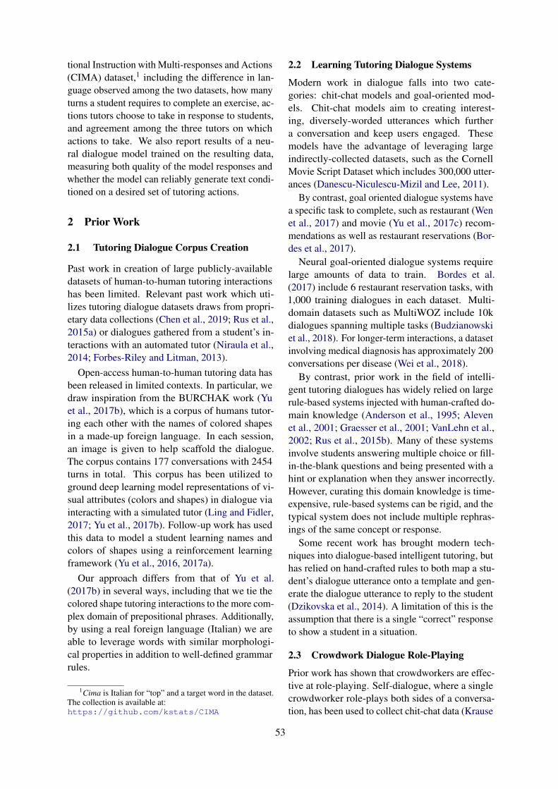
tional Instruction with Multi-responses and Actions(CIMA) dataset,1 including the difference in lan-guage observed among the two datasets, how manyturns a student requires to complete an exercise, ac-tions tutors choose to take in response to students,and agreement among the three tutors on whichactions to take. We also report results of a neu-ral dialogue model trained on the resulting data,measuring both quality of the model responses andwhether the model can reliably generate text condi-tioned on a desired set of tutoring actions.

2 Prior Work

2.1 Tutoring Dialogue Corpus Creation

Past work in creation of large publicly-availabledatasets of human-to-human tutoring interactionshas been limited. Relevant past work which uti-lizes tutoring dialogue datasets draws from propri-etary data collections (Chen et al., 2019; Rus et al.,2015a) or dialogues gathered from a student’s in-teractions with an automated tutor (Niraula et al.,2014; Forbes-Riley and Litman, 2013).

Open-access human-to-human tutoring data hasbeen released in limited contexts. In particular, wedraw inspiration from the BURCHAK work (Yuet al., 2017b), which is a corpus of humans tutor-ing each other with the names of colored shapesin a made-up foreign language. In each session,an image is given to help scaffold the dialogue.The corpus contains 177 conversations with 2454turns in total. This corpus has been utilized toground deep learning model representations of vi-sual attributes (colors and shapes) in dialogue viainteracting with a simulated tutor (Ling and Fidler,2017; Yu et al., 2017b). Follow-up work has usedthis data to model a student learning names andcolors of shapes using a reinforcement learningframework (Yu et al., 2016, 2017a).

Our approach differs from that of Yu et al.(2017b) in several ways, including that we tie thecolored shape tutoring interactions to the more com-plex domain of prepositional phrases. Additionally,by using a real foreign language (Italian) we areable to leverage words with similar morphologi-cal properties in addition to well-defined grammarrules.

1Cima is Italian for “top” and a target word in the dataset.The collection is available at:https://github.com/kstats/CIMA

2.2 Learning Tutoring Dialogue Systems

Modern work in dialogue falls into two cate-gories: chit-chat models and goal-oriented mod-els. Chit-chat models aim to creating interest-ing, diversely-worded utterances which furthera conversation and keep users engaged. Thesemodels have the advantage of leveraging largeindirectly-collected datasets, such as the CornellMovie Script Dataset which includes 300,000 utter-ances (Danescu-Niculescu-Mizil and Lee, 2011).

By contrast, goal oriented dialogue systems havea specific task to complete, such as restaurant (Wenet al., 2017) and movie (Yu et al., 2017c) recom-mendations as well as restaurant reservations (Bor-des et al., 2017).

Neural goal-oriented dialogue systems requirelarge amounts of data to train. Bordes et al.(2017) include 6 restaurant reservation tasks, with1,000 training dialogues in each dataset. Multi-domain datasets such as MultiWOZ include 10kdialogues spanning multiple tasks (Budzianowskiet al., 2018). For longer-term interactions, a datasetinvolving medical diagnosis has approximately 200conversations per disease (Wei et al., 2018).

By contrast, prior work in the field of intelli-gent tutoring dialogues has widely relied on largerule-based systems injected with human-crafted do-main knowledge (Anderson et al., 1995; Alevenet al., 2001; Graesser et al., 2001; VanLehn et al.,2002; Rus et al., 2015b). Many of these systemsinvolve students answering multiple choice or fill-in-the-blank questions and being presented with ahint or explanation when they answer incorrectly.However, curating this domain knowledge is time-expensive, rule-based systems can be rigid, and thetypical system does not include multiple rephras-ings of the same concept or response.

Some recent work has brought modern tech-niques into dialogue-based intelligent tutoring, buthas relied on hand-crafted rules to both map a stu-dent’s dialogue utterance onto a template and gen-erate the dialogue utterance to reply to the student(Dzikovska et al., 2014). A limitation of this is theassumption that there is a single “correct” responseto show a student in a situation.

2.3 Crowdwork Dialogue Role-Playing

Prior work has shown that crowdworkers are effec-tive at role-playing. Self-dialogue, where a singlecrowdworker role-plays both sides of a conversa-tion, has been used to collect chit-chat data (Krause

53

Figure 1: Example exercises as seen by a tutor (Left: Shape task, Right: Prepositional Phrase task). Shown are (A)the exercise with the correct answer that the student must produce, (B) knowledge in the form of information bulletpoints, (C) the image stimulus, and (D) the conversation so far. The student view is similar but does not includethe information bullet points or the correct answer.

et al., 2017). Crowdworkers have been effectiveparticipants in peer learning studies (Coetzee et al.,2015); multiple crowdworkers can confirm lexicalinformation within a dialogue (Ono et al., 2017).

3 Tutoring Dataset Creation

We create two dialogue datasets within CIMA:Shapes and Prepositional Phrases with colored ob-jects.

3.1 Stimuli

We constructed stimuli for the two tasks at differentlevels of complexity. The Shape task follows theBURCHAK (Yu et al., 2017b) format of learningthe words for adjective-noun modifiers when view-ing shapes of different colors (see Figure 1, left).The Prepositional Phrase stimuli involves pairs ofobjects in relation to one another, with the task oflearning the words for the prepositional phrase andits object, where the object is a noun with a colormodifier and a determiner (see Figure 1, right).

Each stimulus consists of an image, a set of infor-mation points, and a question and answer pair. Im-portantly, the stimuli across the two tasks are linkedby shared color terms. Intentionally including a setof common vocabulary words across datasets canpotentially aid with transfer learning experiments(both human and machine). Initial tests were alldone with English speakers learning the words inItalian. However, other language pairs can easilybe associated with the image stimuli.

Vocabulary for the Shape task includes six colors(red, blue, green, purple, pink, and yellow) and five

shapes (square, triangle, circle, star, and heart).There is only one grammar rule associated with thequestions: that adjectives follow nouns in Italian.

The Prepositional Phrase task includes 6 prepo-sitional phrases (on top of, under, inside of, nextto, behind, and in front of) with 10 objects (cat,dog, bunny, plant, tree, ball, table, box, bag, andbed). Additionally, the same six colors as the Shapedataset modify the objects. Students are not askedto produce the subjects or the verbs, only the prepo-sitional phrases. The full list of grammar rules(e.g. “l”’ (“the”) is prepended to the followingword when it begins with a vowel) appears in Ap-pendix A, and the full distribution of prepositionalphrases, objects, and colors is in Appendix B.

3.2 Dialogue Collection with Crowdworkers

We hired crowdworkers on Amazon MechanicalTurk to role-play both the the student and the tutor.(Throughout this paper we will refer to them asstudents and tutors; this should be read as peopletaking on these roles.) In order to collect multipletutoring responses at each point in a student conver-sation in a controllable way, student and tutor re-sponses are gathered asynchronously. A diagram ofthis process can be seen in Figure 2. We collect sev-eral student conversations from crowdworkers witha fixed collection of hand-crafted and crowdworker-generated tutor responses. Afterwards, we showthose student conversations to tutors to collect mul-tiple appropriate crowdworker-generated responses.We then feed the newly-collected responses intothe fixed collection of tutor responses for the next

54

Figure 2: Progression of data collection process. In the first round of data gathering (1A), the student is exposed to20 conversational responses from a hand-curated set of templates (shown in blue). After gathering data from 20-40students, each student conversation is subsequently sent to three tutors to gather responses (1B). These responses(shown in pink) are placed into the pool of tutor responses for subsequent rounds (ex: 2A).

Figure 3: Example student exercise progression, show-ing shared features across stimuli. In this case, the stu-dent sees images for the words for bed and on top oftwice within one session.

round of student data collection.Tutors are asked to construct a response to the

prior conversation with two outputs: the text of anutterance continuing the conversation and a dis-crete classification of the action(s) associated withthe utterance. A summary of these actions for boththe student and tutor can be seen in Table 1.

Similarly, students produce utterances whichthey label with actions as they work through ex-ercises (defined as a question and correspondinganswer, see (A) in Figure 1). Students complete as

many exercises as possible in a HIT, defined as thecrowdworking task consisting of a fixed numberof turns. Each turn is defined as a pair consistingof the student’s utterance and the most recent tutorresponse it is replying to. A conversation is definedas the set of utterances that comprise completionof an exercise.

Each participant can complete a maximum of100 combined responses as a tutor or student foreach task, to ensure diversity of responses. Forthe Shape task, students generate 5 responses perHIT. For the Prepositional Phrase task, however,we increase this to 20 responses per HIT due to themore complex domain.

To ensure response quality, crowdworkers wererequired to have 95% approval over at least 1,000HITs. A subset of responses from each crowd-worker were manually checked. We prohibitedworkers from copying from the prior conversationor writing a blank response. Crowdworkers werepaid the equivalent of $8/hour and were requirednot to know Italian to participate as a student.

3.3 The Student Role

Figure 3 shows an example student interaction pro-gression, in which students converse with the sys-tem to complete multiple exercises. Because thedata collection process is asynchronous, when astudent converses with the system, we serve a tu-tor response from a static collection to respond tothem instantly. There are four rounds of data col-lection; in each phase, the pool of tutor responses

55

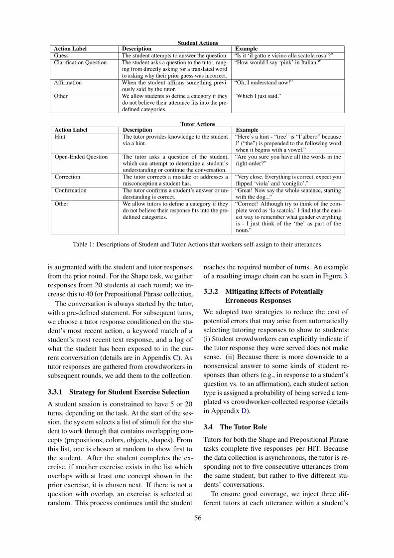
Student ActionsAction Label Description ExampleGuess The student attempts to answer the question “Is it ‘il gatto e vicino alla scatola rosa’?”Clarification Question The student asks a question to the tutor, rang-

ing from directly asking for a translated wordto asking why their prior guess was incorrect.

“How would I say ‘pink’ in Italian?”

Affirmation When the student affirms something previ-ously said by the tutor.

“Oh, I understand now!”

Other We allow students to define a category if theydo not believe their utterance fits into the pre-defined categories.

“Which I just said.”

Tutor ActionsAction Label Description ExampleHint The tutor provides knowledge to the student

via a hint.“Here’s a hint - “tree” is “l’albero” becausel’ (“the”) is prepended to the following wordwhen it begins with a vowel.”

Open-Ended Question The tutor asks a question of the student,which can attempt to determine a student’sunderstanding or continue the conversation.

“Are you sure you have all the words in theright order?”

Correction The tutor corrects a mistake or addresses amisconception a student has.

“Very close. Everything is correct, expect youflipped ‘viola’ and ‘coniglio’.”

Confirmation The tutor confirms a student’s answer or un-derstanding is correct.

“Great! Now say the whole sentence, startingwith the dog...”

Other We allow tutors to define a category if theydo not believe their response fits into the pre-defined categories.

“Correct! Although try to think of the com-plete word as ‘la scatola.’ I find that the easi-est way to remember what gender everythingis - I just think of the ‘the’ as part of thenoun.”

Table 1: Descriptions of Student and Tutor Actions that workers self-assign to their utterances.

is augmented with the student and tutor responsesfrom the prior round. For the Shape task, we gatherresponses from 20 students at each round; we in-crease this to 40 for Prepositional Phrase collection.

The conversation is always started by the tutor,with a pre-defined statement. For subsequent turns,we choose a tutor response conditioned on the stu-dent’s most recent action, a keyword match of astudent’s most recent text response, and a log ofwhat the student has been exposed to in the cur-rent conversation (details are in Appendix C). Astutor responses are gathered from crowdworkers insubsequent rounds, we add them to the collection.

3.3.1 Strategy for Student Exercise Selection

A student session is constrained to have 5 or 20turns, depending on the task. At the start of the ses-sion, the system selects a list of stimuli for the stu-dent to work through that contains overlapping con-cepts (prepositions, colors, objects, shapes). Fromthis list, one is chosen at random to show first tothe student. After the student completes the ex-ercise, if another exercise exists in the list whichoverlaps with at least one concept shown in theprior exercise, it is chosen next. If there is not aquestion with overlap, an exercise is selected atrandom. This process continues until the student

reaches the required number of turns. An exampleof a resulting image chain can be seen in Figure 3.

3.3.2 Mitigating Effects of PotentiallyErroneous Responses

We adopted two strategies to reduce the cost ofpotential errors that may arise from automaticallyselecting tutoring responses to show to students:(i) Student crowdworkers can explicitly indicate ifthe tutor response they were served does not makesense. (ii) Because there is more downside to anonsensical answer to some kinds of student re-sponses than others (e.g., in response to a student’squestion vs. to an affirmation), each student actiontype is assigned a probability of being served a tem-plated vs crowdworker-collected response (detailsin Appendix D).

3.4 The Tutor Role

Tutors for both the Shape and Prepositional Phrasetasks complete five responses per HIT. Becausethe data collection is asynchronous, the tutor is re-sponding not to five consecutive utterances fromthe same student, but rather to five different stu-dents’ conversations.

To ensure good coverage, we inject three dif-ferent tutors at each utterance within a student’s

56

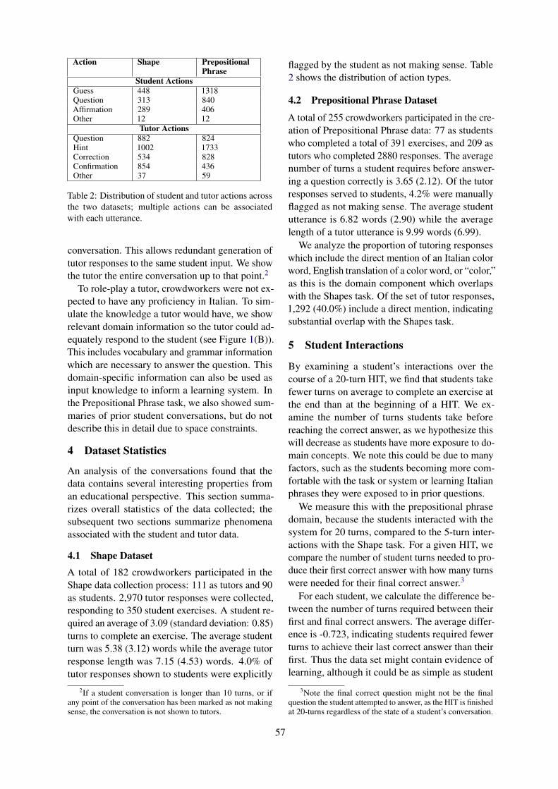
Action Shape PrepositionalPhrase

Student ActionsGuess 448 1318Question 313 840Affirmation 289 406Other 12 12

Tutor ActionsQuestion 882 824Hint 1002 1733Correction 534 828Confirmation 854 436Other 37 59

Table 2: Distribution of student and tutor actions acrossthe two datasets; multiple actions can be associatedwith each utterance.

conversation. This allows redundant generation oftutor responses to the same student input. We showthe tutor the entire conversation up to that point.2

To role-play a tutor, crowdworkers were not ex-pected to have any proficiency in Italian. To sim-ulate the knowledge a tutor would have, we showrelevant domain information so the tutor could ad-equately respond to the student (see Figure 1(B)).This includes vocabulary and grammar informationwhich are necessary to answer the question. Thisdomain-specific information can also be used asinput knowledge to inform a learning system. Inthe Prepositional Phrase task, we also showed sum-maries of prior student conversations, but do notdescribe this in detail due to space constraints.

4 Dataset Statistics

An analysis of the conversations found that thedata contains several interesting properties froman educational perspective. This section summa-rizes overall statistics of the data collected; thesubsequent two sections summarize phenomenaassociated with the student and tutor data.

4.1 Shape DatasetA total of 182 crowdworkers participated in theShape data collection process: 111 as tutors and 90as students. 2,970 tutor responses were collected,responding to 350 student exercises. A student re-quired an average of 3.09 (standard deviation: 0.85)turns to complete an exercise. The average studentturn was 5.38 (3.12) words while the average tutorresponse length was 7.15 (4.53) words. 4.0% oftutor responses shown to students were explicitly

2If a student conversation is longer than 10 turns, or ifany point of the conversation has been marked as not makingsense, the conversation is not shown to tutors.

flagged by the student as not making sense. Table2 shows the distribution of action types.

4.2 Prepositional Phrase Dataset

A total of 255 crowdworkers participated in the cre-ation of Prepositional Phrase data: 77 as studentswho completed a total of 391 exercises, and 209 astutors who completed 2880 responses. The averagenumber of turns a student requires before answer-ing a question correctly is 3.65 (2.12). Of the tutorresponses served to students, 4.2% were manuallyflagged as not making sense. The average studentutterance is 6.82 words (2.90) while the averagelength of a tutor utterance is 9.99 words (6.99).

We analyze the proportion of tutoring responseswhich include the direct mention of an Italian colorword, English translation of a color word, or “color,”as this is the domain component which overlapswith the Shapes task. Of the set of tutor responses,1,292 (40.0%) include a direct mention, indicatingsubstantial overlap with the Shapes task.

5 Student Interactions

By examining a student’s interactions over thecourse of a 20-turn HIT, we find that students takefewer turns on average to complete an exercise atthe end than at the beginning of a HIT. We ex-amine the number of turns students take beforereaching the correct answer, as we hypothesize thiswill decrease as students have more exposure to do-main concepts. We note this could be due to manyfactors, such as the students becoming more com-fortable with the task or system or learning Italianphrases they were exposed to in prior questions.

We measure this with the prepositional phrasedomain, because the students interacted with thesystem for 20 turns, compared to the 5-turn inter-actions with the Shape task. For a given HIT, wecompare the number of student turns needed to pro-duce their first correct answer with how many turnswere needed for their final correct answer.3

For each student, we calculate the difference be-tween the number of turns required between theirfirst and final correct answers. The average differ-ence is -0.723, indicating students required fewerturns to achieve their last correct answer than theirfirst. Thus the data set might contain evidence oflearning, although it could be as simple as student

3Note the final correct question might not be the finalquestion the student attempted to answer, as the HIT is finishedat 20-turns regardless of the state of a student’s conversation.

57

workers learning how to more efficiently ask ques-tions of the system.

6 Tutor Phenomena

We examine several characteristics about the tutorinteractions: (i) properties about the language tu-tors use in their responses, (ii) how tutors respondto different student action types, and (iii) character-izing if and how tutors agree when presented withidentical student input.

6.1 Tutoring Language

One feature of our dataset construction is the pro-gression from the relatively simple Shape task tothe linguistically richer Prepositional Phrase task.We analyze the resulting tutoring responses to see ifmore complex tutoring language emerges from thesyntactically richer domain. We measure complex-ity in terms of number of non-vocabulary terms(where vocabulary refers to the words that areneeded in the task, such as “rosa” for “pink”).

We examine the set of tutoring responses fromeach domain. For each utterance, we remove Italianvocabulary, English translations, and stop words.We further restrict the utterance to words includedin the English language4 to remove typos and mis-spellings.

We find an average of 2.34 non-domain wordsper utterance (of average length 9.99 words) inthe Prepositional Phrase dataset, compared to 0.40per utterance (of average length 7.15 words) in theShape dataset. While accounting for the averagedifference in length between the two datasets, thePrepositional Phrase dataset results in more non-domain English words than the Shape dataset.

This supports our hypothesis that the added do-main complexity makes the Prepositional Phrasecollection richer in terms of tutoring language thanrelated work such as Yu et al. (2017b).

6.2 Tutor Response to Student Actions

We additionally examine the tutor action distribu-tions conditioned on the student action taken imme-diately prior for the Prepositional Phrase dataset.We hypothesize if a student utterance is classifiedas a question, the tutor will be more likely to re-spond with the answer to the question (classifiedas a hint), conforming to conversational expecta-tions. This is supported by the distributions, seen

4Stopwords and English vocabulary as defined by NLTK’sstop words and English corpus, https://www.nltk.org/

Tutor Action(s) Agreement IndividualHint 81.1% 39.0%Question 5.7% 12.5%Correction 5.2% 12.1%Hint/Correction 2.8% 8.1%Confirmation 2.8% 6.2%Question/Hint 1.4% 7.5%Correction/Confirmation 0.9% 2.1%Total 212 2880

Table 3: Distribution of action sets agreed on by 3-tutorgroups. Included are the proportion of individual tutorutterances labeled with each set of actions over the en-tire dataset for comparison.

in Figure 4. For other student action type responses(e.g., guess, affirmation), we observe that the tutoractions are more evenly distributed.

6.3 Tutor Action Agreement

As there are three tutors responding to each studentutterance, we analyze the conditions in which thetutors agree on a unified set of actions to take inresponse to a student (in the Prepositional Phrasetask). In particular, when all three tutors take thesame set of action types we measure (i) which ac-tion(s) are they agreeing on and (ii) which action(s)the student took in the prior turn.

In 212 out of 1174 tutor tasks, all 3 tutors agreedon the same set of actions to take. We show thedistribution of these 212 cases over unified tutoraction sets in Table 3. There is a particularly highproportion of agreement on giving hints comparedto other action sets. While hint was the most com-mon action taken by tutors compared to the next-highest action by 26.5%, tutor agreement on hintwas the most common by 75.4% compared to thenext-highest category, a 2.8 times larger difference.

Additionally, we examine how a student’s mostrecent action might influence a group of tutor’spotential for action agreement. We measure theproportion of tutor agreement on a unified actionset per student action set (the analysis is restrictedto student action sets with at least 10 examples).Results can be seen in Table 4.

We note the highest agreement occurs after a stu-dent has made a Question or Question/Affirmation.This is consistent with (i) the high likelihood of atutor to give a hint in response to a question (Figure4) and (ii) the high proportion of tutor agreement onhints (Table 3). On the contrary, there is relativelylow agreement when a student makes a Guess, con-sistent with the more evenly-distributed tutor actiondistribution (Figure 4).

58

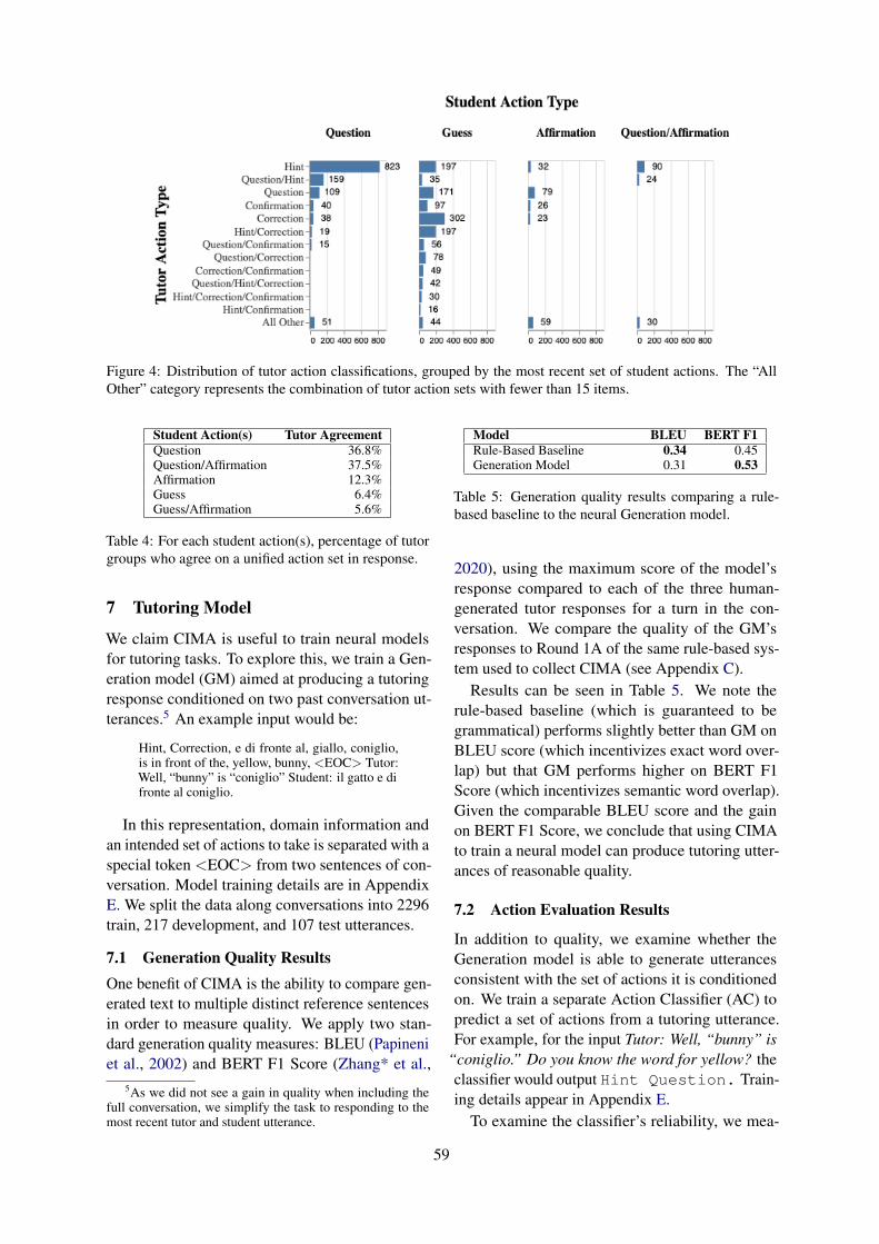
Figure 4: Distribution of tutor action classifications, grouped by the most recent set of student actions. The “AllOther” category represents the combination of tutor action sets with fewer than 15 items.

Student Action(s) Tutor AgreementQuestion 36.8%Question/Affirmation 37.5%Affirmation 12.3%Guess 6.4%Guess/Affirmation 5.6%

Table 4: For each student action(s), percentage of tutorgroups who agree on a unified action set in response.

7 Tutoring Model

We claim CIMA is useful to train neural modelsfor tutoring tasks. To explore this, we train a Gen-eration model (GM) aimed at producing a tutoringresponse conditioned on two past conversation ut-terances.5 An example input would be:

Hint, Correction, e di fronte al, giallo, coniglio,is in front of the, yellow, bunny, <EOC> Tutor:Well, “bunny” is “coniglio” Student: il gatto e difronte al coniglio.

In this representation, domain information andan intended set of actions to take is separated with aspecial token <EOC> from two sentences of con-versation. Model training details are in AppendixE. We split the data along conversations into 2296train, 217 development, and 107 test utterances.

7.1 Generation Quality ResultsOne benefit of CIMA is the ability to compare gen-erated text to multiple distinct reference sentencesin order to measure quality. We apply two stan-dard generation quality measures: BLEU (Papineniet al., 2002) and BERT F1 Score (Zhang* et al.,

5As we did not see a gain in quality when including thefull conversation, we simplify the task to responding to themost recent tutor and student utterance.

Model BLEU BERT F1Rule-Based Baseline 0.34 0.45Generation Model 0.31 0.53

Table 5: Generation quality results comparing a rule-based baseline to the neural Generation model.

2020), using the maximum score of the model’sresponse compared to each of the three human-generated tutor responses for a turn in the con-versation. We compare the quality of the GM’sresponses to Round 1A of the same rule-based sys-tem used to collect CIMA (see Appendix C).

Results can be seen in Table 5. We note therule-based baseline (which is guaranteed to begrammatical) performs slightly better than GM onBLEU score (which incentivizes exact word over-lap) but that GM performs higher on BERT F1Score (which incentivizes semantic word overlap).Given the comparable BLEU score and the gainon BERT F1 Score, we conclude that using CIMAto train a neural model can produce tutoring utter-ances of reasonable quality.

7.2 Action Evaluation Results

In addition to quality, we examine whether theGeneration model is able to generate utterancesconsistent with the set of actions it is conditionedon. We train a separate Action Classifier (AC) topredict a set of actions from a tutoring utterance.For example, for the input Tutor: Well, “bunny” is

“coniglio.” Do you know the word for yellow? theclassifier would output Hint Question. Train-ing details appear in Appendix E.

To examine the classifier’s reliability, we mea-

59

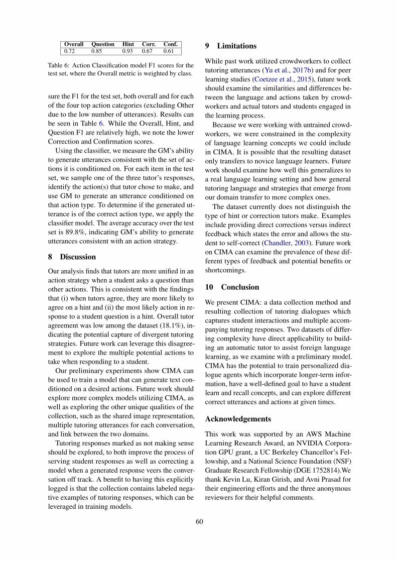
Overall Question Hint Corr. Conf.0.72 0.85 0.93 0.67 0.61

Table 6: Action Classification model F1 scores for thetest set, where the Overall metric is weighted by class.

sure the F1 for the test set, both overall and for eachof the four top action categories (excluding Otherdue to the low number of utterances). Results canbe seen in Table 6. While the Overall, Hint, andQuestion F1 are relatively high, we note the lowerCorrection and Confirmation scores.

Using the classifier, we measure the GM’s abilityto generate utterances consistent with the set of ac-tions it is conditioned on. For each item in the testset, we sample one of the three tutor’s responses,identify the action(s) that tutor chose to make, anduse GM to generate an utterance conditioned onthat action type. To determine if the generated ut-terance is of the correct action type, we apply theclassifier model. The average accuracy over the testset is 89.8%, indicating GM’s ability to generateutterances consistent with an action strategy.

8 Discussion

Our analysis finds that tutors are more unified in anaction strategy when a student asks a question thanother actions. This is consistent with the findingsthat (i) when tutors agree, they are more likely toagree on a hint and (ii) the most likely action in re-sponse to a student question is a hint. Overall tutoragreement was low among the dataset (18.1%), in-dicating the potential capture of divergent tutoringstrategies. Future work can leverage this disagree-ment to explore the multiple potential actions totake when responding to a student.

Our preliminary experiments show CIMA canbe used to train a model that can generate text con-ditioned on a desired actions. Future work shouldexplore more complex models utilizing CIMA, aswell as exploring the other unique qualities of thecollection, such as the shared image representation,multiple tutoring utterances for each conversation,and link between the two domains.

Tutoring responses marked as not making senseshould be explored, to both improve the process ofserving student responses as well as correcting amodel when a generated response veers the conver-sation off track. A benefit to having this explicitlylogged is that the collection contains labeled nega-tive examples of tutoring responses, which can beleveraged in training models.

9 Limitations

While past work utilized crowdworkers to collecttutoring utterances (Yu et al., 2017b) and for peerlearning studies (Coetzee et al., 2015), future workshould examine the similarities and differences be-tween the language and actions taken by crowd-workers and actual tutors and students engaged inthe learning process.

Because we were working with untrained crowd-workers, we were constrained in the complexityof language learning concepts we could includein CIMA. It is possible that the resulting datasetonly transfers to novice language learners. Futurework should examine how well this generalizes toa real language learning setting and how generaltutoring language and strategies that emerge fromour domain transfer to more complex ones.

The dataset currently does not distinguish thetype of hint or correction tutors make. Examplesinclude providing direct corrections versus indirectfeedback which states the error and allows the stu-dent to self-correct (Chandler, 2003). Future workon CIMA can examine the prevalence of these dif-ferent types of feedback and potential benefits orshortcomings.

10 Conclusion

We present CIMA: a data collection method andresulting collection of tutoring dialogues whichcaptures student interactions and multiple accom-panying tutoring responses. Two datasets of differ-ing complexity have direct applicability to build-ing an automatic tutor to assist foreign languagelearning, as we examine with a preliminary model.CIMA has the potential to train personalized dia-logue agents which incorporate longer-term infor-mation, have a well-defined goal to have a studentlearn and recall concepts, and can explore differentcorrect utterances and actions at given times.

Acknowledgements

This work was supported by an AWS MachineLearning Research Award, an NVIDIA Corpora-tion GPU grant, a UC Berkeley Chancellor’s Fel-lowship, and a National Science Foundation (NSF)Graduate Research Fellowship (DGE 1752814).Wethank Kevin Lu, Kiran Girish, and Avni Prasad fortheir engineering efforts and the three anonymousreviewers for their helpful comments.

60

ReferencesVincent Aleven, Octav Popescu, and Kenneth R

Koedinger. 2001. A tutorial dialogue system withknowledge-based understanding and classificationof student explanations. In Working Notes of 2ndIJCAI Workshop on Knowledge and Reasoning inPractical Dialogue Systems.

John R Anderson, Albert T Corbett, Kenneth RKoedinger, and Ray Pelletier. 1995. Cognitive tu-tors: Lessons learned. The journal of the learningsciences, 4(2):167–207.

Antoine Bordes, Y-Lan Boureau, and Jason Weston.2017. Learning end-to-end goal-oriented dialog.In 5th International Conference on Learning Rep-resentations, ICLR 2017, Toulon, France, April 24-26, 2017, Conference Track Proceedings. OpenRe-view.net.

Paweł Budzianowski, Tsung-Hsien Wen, Bo-HsiangTseng, Inigo Casanueva, Stefan Ultes, Osman Ra-madan, and Milica Gasic. 2018. Multiwoz - a large-scale multi-domain wizard-of-oz dataset for task-oriented dialogue modelling. In Proceedings of the2018 Conference on Empirical Methods in NaturalLanguage Processing, pages 5016–5026. Associa-tion for Computational Linguistics.

Jean Chandler. 2003. The efficacy of various kinds oferror feedback for improvement in the accuracy andfluency of l2 student writing. Journal of Second Lan-guage Writing, 12:267–296.

Guanliang Chen, David Lang, Rafael Ferreira, and Dra-gan Gasevic. 2019. Predictors of student satisfac-tion: A large-scale study of human-human onlinetutorial dialogues. In Proceedings of the 12th In-ternational Conference on Educational Data Mining,EDM 2019, Montreal, Canada, July 2-5, 2019. Inter-national Educational Data Mining Society (IEDMS).

D. Coetzee, Seongtaek Lim, Armando Fox, Bjorn Hart-mann, and Marti A. Hearst. 2015. Structuring inter-actions for large-scale synchronous peer learning. InProceedings of the 18th ACM Conference on Com-puter Supported Cooperative Work and Social Com-puting, CSCW ’15, page 1139–1152, New York, NY,USA. Association for Computing Machinery.

Cristian Danescu-Niculescu-Mizil and Lillian Lee.2011. Chameleons in imagined conversations: Anew approach to understanding coordination of lin-guistic style in dialogs. In Proceedings of the2nd Workshop on Cognitive Modeling and Compu-tational Linguistics, pages 76–87, Portland, Oregon,USA. Association for Computational Linguistics.

Myroslava O. Dzikovska, Natalie B. Steinhauser,Elaine Farrow, Johanna D. Moore, and Gwen-dolyn E. Campbell. 2014. Beetle ii: Deep natu-ral language understanding and automatic feedbackgeneration for intelligent tutoring in basic electricityand electronics. International Journal of ArtificialIntelligence in Education, 24:284–332.

Kate Forbes-Riley and Diane Litman. 2013. Whendoes disengagement correlate with performance inspoken dialog computer tutoring? Int. J. Artif. Intell.Ed., 22(1–2):39–58.

Arthur C. Graesser. 2015. Conversations with autotutorhelp students learn. International Journal of Artifi-cial Intelligence in Education, 26:124–132.

Arthur C Graesser, Sidney D’Mello, and Natalie Per-son. 2009. Meta-knowledge in tutoring. The edu-cational psychology series. Handbook of metacogni-tion in education, pages 361–382.

Arthur C. Graesser, Kurt VanLehn, Carolyn PensteinRose, Pamela W. Jordan, and Derek Harter. 2001.Intelligent tutoring systems with conversational di-alogue. AI Magazine, 22:39–52.

Jiatao Gu, Zhengdong Lu, Hang Li, and Victor O.K.Li. 2016. Incorporating copying mechanism insequence-to-sequence learning. In Proceedings ofthe 54th Annual Meeting of the Association for Com-putational Linguistics (Volume 1: Long Papers),pages 1631–1640, Berlin, Germany. Association forComputational Linguistics.

Diederik P. Kingma and Jimmy Ba. 2015. Adam: Amethod for stochastic optimization. In 3rd Inter-national Conference on Learning Representations,ICLR 2015, San Diego, CA, USA, May 7-9, 2015,Conference Track Proceedings.

Guillaume Klein, Yoon Kim, Yuntian Deng, Jean Senel-lart, and Alexander M. Rush. 2017. Opennmt:Open-source toolkit for neural machine translation.In Proc. ACL.

Ben Krause, Marco Damonte, Mihai Dobre, DanielDuma, Joachim Fainberg, Federico Fancellu, Em-manuel Kahembwe, Jianpeng Cheng, and BonnieWebber. 2017. Edina: Building an open domainsocialbot with self-dialogues. Alexa Prize Proceed-ings.

Huan Ling and Sanja Fidler. 2017. Teaching machinesto describe images via natural language feedback. InProceedings of the 31st International Conference onNeural Information Processing Systems, NIPS’17,page 5075–5085, Red Hook, NY, USA. Curran As-sociates Inc.

Nobal Niraula, Vasile Rus, Rajendra Banjade, Dan Ste-fanescu, William Baggett, and Brent Morgan. 2014.The DARE corpus: A resource for anaphora res-olution in dialogue based intelligent tutoring sys-tems. In Proceedings of the Ninth InternationalConference on Language Resources and Evalua-tion (LREC’14), pages 3199–3203, Reykjavik, Ice-land. European Language Resources Association(ELRA).

Benjamin D Nye, Arthur C Graesser, and Xiangen Hu.2014. Autotutor and family: A review of 17 years ofnatural language tutoring. International Journal ofArtificial Intelligence in Education, 24(4):427–469.

61

Kohei Ono, Ryu Takeda, Eric Nichols, Mikio Nakano,and Kazunori Komatani. 2017. Lexical acquisi-tion through implicit confirmations over multiple di-alogues. In Proceedings of the 18th Annual SIG-dial Meeting on Discourse and Dialogue, pages 50–59, Saarbrucken, Germany. Association for Compu-tational Linguistics.

Kishore Papineni, Salim Roukos, Todd Ward, and Wei-Jing Zhu. 2002. Bleu: a method for automatic eval-uation of machine translation. In Proceedings ofthe 40th Annual Meeting of the Association for Com-putational Linguistics, pages 311–318, Philadelphia,Pennsylvania, USA. Association for ComputationalLinguistics.

Jeffrey Pennington, Richard Socher, and ChristopherManning. 2014. Glove: Global vectors for word rep-resentation. In Proceedings of the 2014 Conferenceon Empirical Methods in Natural Language Process-ing (EMNLP), pages 1532–1543, Doha, Qatar. Asso-ciation for Computational Linguistics.

Sherry Ruan, Liwei Jiang, Justin Xu, Bryce Joe-KunTham, Zhengneng Qiu, Yeshuang Zhu, Elizabeth L.Murnane, Emma Brunskill, and James A. Landay.2019. Quizbot: A dialogue-based adaptive learn-ing system for factual knowledge. In Proceedingsof the 2019 CHI Conference on Human Factors inComputing Systems, CHI ’19, New York, NY, USA.Association for Computing Machinery.

Vasile Rus, Nabin Maharjan, and Rajendra Banjade.2015a. Unsupervised discovery of tutorial dialoguemodes in human-to-human tutorial data. In Proceed-ings of the Third Annual GIFT Users Symposium,pages 63–80.

Vasile Rus, Nobal B. Niraula, and Rajendra Banjade.2015b. Deeptutor: An effective, online intelligenttutoring system that promotes deep learning. In Pro-ceedings of the Twenty-Ninth AAAI Conference onArtificial Intelligence, AAAI’15, page 4294–4295.AAAI Press.

Kurt VanLehn, Arthur C Graesser, G Tanner Jackson,Pamela Jordan, Andrew Olney, and Carolyn P Rose.2007. When are tutorial dialogues more effectivethan reading? Cognitive science, 31(1):3–62.

Kurt VanLehn, Pamela W. Jordan, Carolyn PensteinRose, Dumisizwe Bhembe, Michael Bottner, AndyGaydos, Maxim Makatchev, Umarani Pappuswamy,Michael A. Ringenberg, Antonio Roque, StephanieSiler, and Ramesh Srivastava. 2002. The architec-ture of why2-atlas: A coach for qualitative physicsessay writing. In Proceedings of the 6th Inter-national Conference on Intelligent Tutoring Sys-tems, ITS ’02, page 158–167, Berlin, Heidelberg.Springer-Verlag.

Zhongyu Wei, Qianlong Liu, Baolin Peng, HuaixiaoTou, Ting Chen, Xuanjing Huang, Kam-Fai Wong,and Xiangying Dai. 2018. Task-oriented dialoguesystem for automatic diagnosis. In Proceedings of

the 56th Annual Meeting of the Association for Com-putational Linguistics (Volume 2: Short Papers),pages 201–207. Association for Computational Lin-guistics.

Tsung-Hsien Wen, David Vandyke, Nikola Mrksic,Milica Gasic, Lina M. Rojas-Barahona, Pei-Hao Su,Stefan Ultes, and Steve Young. 2017. A network-based end-to-end trainable task-oriented dialoguesystem. In Proceedings of the 15th Conference ofthe European Chapter of the Association for Compu-tational Linguistics: Volume 1, Long Papers, pages438–449, Valencia, Spain. Association for Computa-tional Linguistics.

Yanchao Yu, Arash Eshghi, and Oliver Lemon. 2016.Training an adaptive dialogue policy for interac-tive learning of visually grounded word meanings.In Proceedings of the 17th Annual Meeting of theSpecial Interest Group on Discourse and Dialogue,pages 339–349, Los Angeles. Association for Com-putational Linguistics.

Yanchao Yu, Arash Eshghi, and Oliver Lemon. 2017a.Learning how to learn: An adaptive dialogue agentfor incrementally learning visually grounded wordmeanings. In Proceedings of the First Workshopon Language Grounding for Robotics, pages 10–19,Vancouver, Canada. Association for ComputationalLinguistics.

Yanchao Yu, Arash Eshghi, Gregory Mills, and OliverLemon. 2017b. The BURCHAK corpus: a chal-lenge data set for interactive learning of visuallygrounded word meanings. In Proceedings of theSixth Workshop on Vision and Language, pages 1–10, Valencia, Spain. Association for ComputationalLinguistics.

Zhou Yu, Alan W. Black, and Alexander I. Rudnicky.2017c. Learning conversational systems that inter-leave task and non-task content. In Proceedingsof the 26th International Joint Conference on Artifi-cial Intelligence, IJCAI’17, page 4214–4220. AAAIPress.

Tianyi Zhang*, Varsha Kishore*, Felix Wu*, Kilian Q.Weinberger, and Yoav Artzi. 2020. Bertscore: Eval-uating text generation with bert. In InternationalConference on Learning Representations.

62

A Prepositional Phrase CollectionGrammar Rules

Listed below is the complete collection of Preposi-tional Phrase grammar rules:

• “il” (“the”) is used for when the followingword is masculine.

• “alla” (“to the”) is used when the followingword is feminine and a singular object. It is acontraction of a (“to”) and la (“the”).

• “al” (“to the”) is used when the followingword is masculine and a singular object. Itis a contraction of the words a (“to”) and il(“the”).

• “l”’ (“the”) is prepended to the following wordwhen it begins with a vowel.

• “all” (“to the” is prepended to the followingword when it begins with a vowel. This is acontraction of al (“to”) and l’ (“the”).

• “rossa” is the feminine form of red becausethe noun it modifies is feminine

• Adjectives (such as color words) follow thenoun they modify in Italian.

• Prepositional phrases separate the two nounphrases.

B Phrase Breakdown

Table 7 shows the coverage of Prepositional Phraseexercises over the potential objects, prepositionalphrase, and colors.

C Algorithm

Algorithmic specifications for data collection canbe viewed in Figure 5. In order to serve a tutor-crafted response to a student, we match the currentstudent utterance to a prior-collected student ut-terance which has been responded to by a tutor.The most similar student utterance is determinedby maximizing word overlap of the student’s mostrecent utterance to the prior-collected student utter-ances, excluding domain vocabulary words. TheEnglish and Italian words are replaced with theinformation relevant to the current exercise in theassociated tutor utterance before showing this tothe student.

D Hand-Crafted Response Probabilities

Throughout different rounds of data collection, webalance the probability of a student receiving a pre-made tutor response with a crowdworker-generatedresponse from a prior round of data collection. As

Category Number ofQuestions

First Object (students don’t translate these)‘the dog’ 134‘the cat’ 161‘the plant’ 49‘the bunny’ 129‘the ball’ 47‘the bag’ 28‘the box’ 17Prepositional phrases‘is in front of the’ 126‘is next to the’ 106‘is inside of the’ 74‘is under the’ 73‘is behind the’ 127‘is on top of the’ 59Colors‘green’ 88‘pink’ 77‘blue’ 100‘yellow’ 91‘red’ 101‘purple’ 108Second Object‘tree’ 128‘box’ 160‘plant’ 14‘cat’ 13‘bunny’ 49‘dog’ 23‘bed’ 69‘table’ 89‘bag’ 20

Table 7: Phrase Breakdown of Student conversations

we collect more tutoring responses in subsequentrounds, the probabilities shift from pre-made, safechoices to the crowd-worker generated responses,because with more data, the choices should be morelikely to more closely match a student utterance.The probabilities were manually set and can beseen in Table 8.

G Q A OShape 1.0 1.0 0.0 0.5PP R1 1.0 1.0 1.0 1.0PP R2 0.75 0.75 0.5 0.5PP R3 0.75 0.75 0.5 0.5PP R4 0.65 0.65 0.4 0.4

Table 8: Probabilities for serving hand crafted re-sponses instead of tutor-provided responses for theshape and the prepositional phrase task, rounds 1 - 4.for Guess, Question, Action, and Other student ques-tion types.

63

E Model Training Details

For the Generation Model, we use OpenNMT(Klein et al., 2017) to train a 4-layer LSTM ofsize 1000 with global attention. We use the Adamoptimizer (Kingma and Ba, 2015) with a learningrate of 0.001. We allow the model to have a copymechanism to copy relevant words (such as transla-tion information) from the input (Gu et al., 2016).We use 300-dimensional pre-trained GloVe embed-dings (Pennington et al., 2014), which are allowedto be updated throughout training. At decode time,we replace unknown words with the input wordwith the highest attention.

We train the Action Classification model usingOpenNMT (Klein et al., 2017). The model is a4-layer bidirectional LSTM with 1024 hidden statesize, general attention, a learning rate of 0.001,and batch size of 16. It utilizes pre-trained 300-dimensional GloVe embeddings (Pennington et al.,2014) which can be updated. This model is trainedon the same training set as the generation model,taking in the human-created utterances and predict-ing the corresponding classifications.

if Guess and Correct thenMove on to next question

else if Guess and Incorrect thenFlip a coin with probability = Gif Heads then

Compile a list of pre-defined responses containingvocabulary missing from the student responseRandomly select from this list

elseReturn the most similar past-tutor response from theset of responses of type G.

end ifend if

if Question thenFlip a coin with probability = Qif Heads then

Attempt to find words from a set list of pre-definedhints associated with each vocabulary word in thequestion.if Match is Found then

Serve that hintelse

Choose a random hint that the student has notseen and serve that.

end ifelse

Return the most similar past-tutor response from theset of responses of type Q.

end ifend if

if Affirmation or Other thenFlip a coin with probability = A / Oif Heads then

Flip a coin with probability = 0.5if Heads then

Ask the student for an attempt at a guess.else

Give a pre-defined hint for a vocabulary or gram-mar concept that the student has not yet seen.

end ifelse

Return the most similar past-tutor response from theset of responses of type A/O.

end ifend if

Figure 5: Algorithm for serving tutoring responses.

64

Proceedings of the 15th Workshop on Innovative Use of NLP for Building Educational Applications, pages 65–74July 10, 2020. c©2020 Association for Computational Linguistics

Becoming Linguistically Mature: Modeling English and GermanChildren’s Writing Development Across School Grades

Elma Kerz1, Yu Qiao1, Daniel Wiechmann 2, and Marcus Strobel1

1RWTH Aachen University, Germany2University of Amsterdam, Netherlands

{elma.kerz|marcus.stroebel}@ifaar.rwth.aachen.deyu.qiao@rwth-aachen.de d.wiechmann@uva.nl

Abstract

In this paper we employ a novel approach toadvancing our understanding of the develop-ment of writing in English and German chil-dren across school grades using classificationtasks. The data used come from two recentlycompiled corpora: The English data comefrom the the GiC corpus (983 school childrenin second-, sixth-, ninth- and eleventh-grade)and the German data are from the FD-LEXcorpus (930 school children in fifth- and ninth-grade). The key to this paper is the com-bined use of what we refer to as ‘complex-ity contours’, i.e. series of measurements thatcapture the progression of linguistic complex-ity within a text, and Recurrent Neural Net-work (RNN) classifiers that adequately capturethe sequential information in those contours.Our experiments demonstrate that RNN clas-sifiers trained on complexity contours achievehigher classification accuracy than one trainedon text-average complexity scores. In a sec-ond step, we determine the relative importanceof the features from four distinct categoriesthrough a Sensitivity-Based Pruning approach.

1 Introduction

There is growing recognition among researchers,educators and policymakers that literacy and thelanguage of schooling (other terms include aca-demic language, language of education, scientificlanguage) are key to children’s overall educationalsuccess and academic achievement (see, e.g., Com-mission, 2019; Lorenzo and Meyer, 2017). Chil-dren are expected to acquire the ability to com-prehend and produce complex clause and sentencestructures, sophisticated vocabulary and informa-tionally dense texts characteristic of language ofschooling as they progress through their schoolcareer (see, e.g., Berman, 2007; Snow, 2010, foroverviews). However, this ability is acquired grad-ually and for many school children only with diffi-

culty (Snow and Uccelli, 2009; Snow, 2010). Giventhe key role of academic language, it is somewhatsurprising that relatively little empirical researchhas been conducted on the development of aca-demic language skills across school grades in chil-dren’s first language, in particular in the area ofwriting (for exceptions, see, Crossley et al., 2011;Weiss and Meurers, 2019). This paper contributesto and expands the scant literature by investigat-ing the development of linguistic complexity inchildren’s writing from second-, sixth-, ninth- andeleventh-grade in English schools and fifth- andninth-grade in German schools. We employ a novelapproach to the automatic assessment of text com-plexity. In this approach, a series of scores for agiven complexity measure is obtained through asliding window technique, tracking the progressionof complexity within a text, captured in what werefer to as ‘complexity contours’ (Strobel, 2014;Strobel et al., 2020). These contours are then fedinto recurrent neural network (RNN) classifiers –adequate to take into account the sequential infor-mation in the contours – to perform grade-levelclassification tasks. We demonstrate the utilityof the approach by comparing the performanceof ‘contour-based’ RNN models against those of‘means-based’ RNN models trained on text-averageperformance scores. In a second step, we de-termine which features drive classification accu-racy through a Sensitivity-Based Pruning (SBP)approach. The remainder of the paper is organizedas follows: Section 2 provides a concise overviewof related work on automated assessment of textcomplexity in combination with machine learningtechniques in the language learning context. Sec-tion 3 presents the two data sets representing En-glish and German children’s school writing. Sec-tion 4 introduces our approach to assessment oftext complexity based on a sliding-window tech-nique, whereas Section 5 introduces the features

65

investigated in the paper. Sections 6 describes themodel architecture and the training procedure (Sec-tion 6.1) and the SBP method used to determinethe relative feature importance (Section 6.2). Sec-tions 7 presents the results and concluding remarksfollow in Section 8.

2 Related work

In recent years, there has been an increased interestin automated assessment of text complexity in au-thentic contextualized language samples in combi-nation with machine learning techniques (Meurers,2020, for a recent overview). As a valuable com-plement to experimental research, this research hasthe potential to advance our current understandingof (both first and second) language learning anddevelopment (Rebuschat et al., 2017; Ellis, 2019).Important steps have been made in this directionthrough both language input and language outputperspectives: Regarding the former, a number ofstudies have examined whether and to what ex-tent learning materials show an adequate level oflinguistic complexity considered to be of crucialimportance for successful learning outcomes (see,e.g., Francois and Fairon, 2012; Pilan et al., 2016;Xia et al., 2019; Chen and Meurers, 2018; Berendeset al., 2018). For example, Berendes et al. (2018)employ a text classification approach to examineto whether and to what extent reading complex-ity of school textbooks differ systematically acrossgrade levels in line with the so-called ‘systematiccomplexification assumption’. They build text clas-sification models using a Sequential Minimal Opti-mization (SMO) algorithm trained on a wide rangeof lexical, syntactic, morphological, and cohesion-related features to predict the grade level (fifth totenth grade) and school track (high vs. low). Thebest performing model reached a grade-level clas-sification accuracy of 53.7%, corresponding to a20.7% over the random baseline, providing onlypartial support for thee systematic complexificationassumption. In addition, they report significant dif-ferences across grade levels and tracks for someof the ten linguistic features. Regarding the latter,a rapidly growing body of research has focusedon language output aiming to determine to whatextent L2 writing and speaking differs from that oftheir L1 peers and expert writers/speakers, to dif-ferentiate levels of language proficiency, to predicthuman ratings of the quality of learner productions,and to examine to the relationship between L1 and

L2 writing complexity and speaking fluency (see,e.g., Crossley et al., 2014; Lu, 2017; Duran-Karaozand Tavakoli, 2020; Strobel et al., 2020). Muchresearch in this area has focused on English andon populations of upper intermediate to advancedL2 learners (but see Crossley et al., 2011; Durrantand Brenchley, 2019; Weiss and Meurers, 2019,for L1 English and German, respectively). Tworecent studies are particularly relevant for the pur-poses of the present study. Durrant and Brenchley(2019) zoom-in on the development of vocabularysophistication in English children’s writing acrosssecond-, sixth-, ninth- and eleventh grade. Theircorpus (also used in the present paper) consistsof 2,898 texts of children’s writing produced by983 children. Through a mixed-effects regressionmodeling approach, they assess the effects of gradelevel and genre on lexical sophistication - measuredthrough children’s use of low-frequency words andregister appropriate words. Their analysis revealsno significant differences with regard to the averagefrequency of the lexical words used by younger andolder children. However, with increasing age chil-dren’s writing display a shift from a more fiction-like vocabulary to a more academic-like vocabulary,reflecting a development towards more register ap-propriate word use. Weiss and Meurers (2019)focus on German children’s writing developmentthrough a text classification approach based on abroad range of complexity and accuracy measures.Their dataset includes 1,633 texts of writing from727 German elementary school children from firstto fourth grade and 906 secondary school studentsfrom fifth to eighth grade, who attended either abasic or an intermediate school track. Using SMOclassifiers with a linear kernel, their best perform-ing classification model employed a combination oflinguistic complexity features, error rate and metainformation on topic and school track to reach anaccuracy of 72.68% in classifying four grade levelcategories. Their analysis further revealed a shiftin the primary locus of development from accuracyto complexity within elementary school and an in-creasing linguistic complexity in secondary school,in particular in the lexical complexity domain.

3 Data

The data used in this study come from two recentlycompiled corpora representing school writing: TheEnglish data come from the the Growth in Gram-mar corpus (GIG, https://gigcorpus.com/) that

66

comprises 2,898 texts produced by 983 children in24 different schools from 14 cities in Great Britain.The texts in the GiG corpus were sampled at fourpoints that mark ‘key stages’ of the English schoolsystem: the ends of Key Stage (KS) 1 (Year 2,when children are 6-7 years old) and KS2 (Year9, when children are 10-11 years old), encompass-ing the primary phase of the school system, and theends of KS3 (Year 9, when children are 13-14 yearsold) and KS4 (Year 11, when children are 15-16years old), encompassing the secondary stage. Thetexts were classified into two text types (literaryand non-literary texts) on the basis of their over-all purpose. Approximately 13% of the texts werewritten by children categorized as speaking En-glish as an additional language. The German datacome from the Forschungsdatenbank Lernertexte(FD-LEX; https://fd-lex.Uni-koeln.de/), aresearch database of learner texts compiled in jointproject of the Mercator Institute for Language Pro-motion and German as a Second Language. Itcontains a total of 5,628 texts from two text types(report and argumentation) collected from a totalof 930 school children in grades five (when chil-dren are 10-11 years old) and nine (when childrenare 14-15 years old) at comprehensive and gram-mar schools in two German cities. These texts wereelicited using a narrative and an argumentative writ-ing prompt. The database contains information on anumber of learner background variables, includingthe learners language background distinguishingmonolingual German students from students whohave German as a their first language (L1) andknow at least one additional language and studentsfor whom German is not their first language. Table1 shows the distribution of texts along with descrip-tive statistics of text sizes across grade levels andregisters for each language.

4 Automatic Assessment of TextComplexity through a Sliding WindowTechnique

Text complexity of the writing samples in the twocorpora is automatically assessed using the Com-plexity Contour Generator (CoCoGen), a computa-tional tool that implements a sliding-window tech-nique to generate a series of measurements for agiven complexity measure (CM) (Strobel, 2014;Strobel et al., 2018; Strobel et al., 2020). This ap-proach enables a ‘local assessment’ of complexitywithin a text, in contrast to the standard approach

English data: GIGGrade Register N Texts M SD

2 lit 263 83.56 58.362 non-lit 376 71.18 43.094 lit 23 169.7 111.64 non-lit 26 151.58 96.656 lit 293 371.58 200.616 non-lit 575 208.68 104.539 lit 220 422.22 186.699 non-lit 584 277.25 187.95

11 lit 63 422.22 186.6911 non-lit 475 415.3 264.46

German data: FD-LEX5 arg 1462 49.26 27.945 nar 1460 67.65 32.689 arg 1282 70.67 32.249 nar 1305 80.69 32.54

Table 1: Composition of two corpora of children’sschool writing. ‘lit’ = literary, ‘non-lit’ = non-literary,‘arg’ = argumentative, ‘nar’ = narrative; M = mean num-ber of words, SD = standard deviation

that represents text complexity as a single score,providing a ‘global assessment’ of the complex-ity of a text. A sliding window can be conceivedof as a window with a certain size (ws) definedby the number of sentences it contains. The win-dow is moved across a text sentence-by-sentence,computing one complexity score per window for agiven CM. The series of measurements generatedby CoCoGen track the progression of linguisticcomplexity within a text captured in what we re-fer to as ‘complexity contours’. These contoursfaithfully represent that complexity is typically notuniformly distributed within a text but rather bycharacterized peaks and troughs and that complex-ity contours of individual measures may exhibitdifferent trajectories (see Figure 1. For a text com-prising n sentences, there are w = n � ws + 1windows.1 To compute the complexity score of agiven window, a measurement function is calledfor each sentence in the window and returns a frac-tion wnS/wdS , where wnS is the numerator of thecomplexity score for a sentence and wdS is the de-nominator of the complexity score for that sentence.If the window size is specified to be greater thanone sentences, the denominators and numeratorsof the fractions from the first to the last sentence

1Given the constraint that there has to be at least one win-dow, a text has to comprise at least as many sentences at thews is wide n � w.

67

in the window are added up to form the denom-inator and numerator of the resulting complexityscore of a given window (see Figure 3 in the Ap-pendix). The size of the window is user-definedparameter whose value depends on the goals of theanalysis: When windows is set to the minimum,i.e. complexity is measured at each sentence ofa text, the resulting complexity contour will typi-cally exhibit many sharp turns. By increasing thewindow size, i.e. the number of sentences in a win-dow, the complexity contour can be smoothenedakin to a moving average technique (see Figure4 in the Appendix). To compute the complexityscores, CoCoGen uses the Stanford CoreNLP suite(Manning et al., 2014) for performing tokenization,sentence splitting, part-of-speech tagging, lemmati-zation and syntactic parsing using the probabilisticcontext free grammar parsers for English (Kleinand Manning, 2003) and German (Rafferty andManning, 2008).

5 Features

In its current version CoCoGen features 57 com-plexity measures (CMs) for English of which 13are also available for German.2 These featurescover (1) surface measures, (2) measures of syn-tactic complexity, (3) measures of lexical rich-ness, (4) information theoretic measures, and (5)register-based n-gram frequency measures. The op-erationalizations of the syntactic and lexical CMsfollow those given in Lu (2011) and Lu (2012).For details on the operationalization of the infor-mation theoretic CMs, see Strobel (2014). Theoperationalization of the register-based n-gramfrequency measures is provided below. Surfacemeasures concern the length of production unitsand include Mean Length of Words in charac-ters (MLWc), Mean Length of Words in syllable(MLWs), Mean length of clause (MLC), Meanlength of sentence (MLS), and Mean length ofT-Unit (MLT). Syntactic complexity is typicallyquantified in terms of measures of the type andincidence of embeddings (Sentence complexityratio (C/S), T-Unit complexity ratio (C/T), Com-plex T-Unit ratio (CT/T), Dependent clause ratio(DC/C), Dependent clauses per T-Unit (DC/T), T-Units per Sentence (T/S), and Verb Phrases per

2CoCoGen was designed with extensibility in mind, sothat additional CMs can easily be added. It uses an abstractmeasure class for the implementation of CMs. Currently,additional CMs from the cognitive science (psycholinguistic)literature are being implemented for both English and German.

T-Unit (VP/T)), the types and number of coordina-tions between clauses and phrasal units (Coordinatephrases per clause (CP/C), Coordinate phrases perT-Unit (CP/T)), and the type of particular structures(Complex nominals per T-Unit(CN/T), Complexnominals per Clause (CN/C), Noun Phrase Premod-ification in words (NPpreW), Noun Phrase Post-modification in words (NPpostW)) (see Lu, 2017,for a recent overview). The lexical richness mea-sures fall into three distinct sub-types: (1) Lexicaldensity, i.e. the ratio of the number of lexical (asopposed to grammatical) words to the total num-ber of words in a text (Lexical Density (LD)), (2)Lexical variation, i.e. the range of a learner’s vo-cabulary as displayed in his or her language use(Number of Different Words (NDW), Type-TokenRatio (TTR), Log Type-Token Ratio (logTTR),Root Type-Token Ratio (rTTR), Corrected Type-Token Ratio (cTTR)) and (3) Lexical sophistica-tion, i.e. the proportion of relatively unusual or ad-vanced words in the learner’s text (words from theNew Academic Word List (NAWL), words fromthe New Academic Formula List (NAFL), wordsthat are not part of the New General Service List(NGSL), Lexical Sophistication BNC (LS.BNC),Lexical Sophistication ANC (LS.ANC)). The threeinformation-theoretic measures are KolmogorovDeflate (KolDef), Kolmogorov Deflate Syntactic(KolDefSyn), Kolmogorov Deflate Morphological(KolDefMor) (see Ehret and Szmrecsanyi, 2019,for the benefits of using these measures in theassessment of text complexity in the context oflanguage learning). These measures, use the De-flate algorithm (Deutsch and Gailly, 1996) to com-press a given text and obtain performance scoresby relating the size of the compressed file to thesize of the original file (Strobel, 2014). The fifthgroup of register-based n-gram frequency measureswas based on list of the top 100,000 most frequentngrams (for n 2 [1, 5]) from the five register sub-components of the COCA corpus3 (spoken, maga-zine, fiction, news, academic language). The gen-eral definition of these CMs is given in (1) and

3The Contemporary Corpus of American English (Davies,2008) is the largest genre-balanced corpus of American En-glish, which at the time the measures were derived comprised560 million words.

68

−1

0

1

2

3

4

0 10 20 30 40Sentence

Com

plex

ity s

core

(z−s

tand

ardi

zed)

GIG − Grade 2

−1

0

1

0 10 20Sentence

GIG − Grade 6

−2

−1

0

1

0.0 2.5 5.0 7.5 10.0 12.5Sentence

FD−LEX − Grade 5

−1

0

1

2

3

0 5 10 15Sentence

Com

plex

ity s

core

(z−s

tand

ardi

zed)

GIG − Grade 9

−2

−1

0

1

0 10 20 30Sentence

GIG − Grade 11

−1.0

−0.5

0.0

0.5

1.0

1.5

0 2 4 6 8Sentence

FD−LEX − Grade 9

Figure 1: Complexity contours for two different measures (red: Type Token Ratio, blue: Clauses per Sentence) forsix randomly selected texts from different grade levels for each language

(2):

Scoren,s,r =|Cn,s,r| · log

hQc2|Cn,s,r| freqn,r(c)

i

|Un,s|(1)

whereCn,s,r = An,s \Bn,r (2)

Let An,s be the list of n-grams (n 2 [0, 5])contained within a sentence s, Bn,r the list ofn-grams on the n-gram frequency list of a regis-ter r (r 2 {acad, acad, fic, mag, news, spok}) andCn,s,r = An,s \Bn,r the intersection list. Further-more, Un,s denotes the list of unique n-grams in s,and freqn,r(a) the frequency of n-gram a in then-gram frequency list of register r. The score of agiven n-gram-based CMs is thus obtained by mul-tiplying the number of n-grams in a sentence thatare on the n-gram list with the log of the productof the corresponding frequencies of those n-gramsdivided by the number of distinct n-grams in thesentence.

6 Classification Models

6.1 Model ArchitectureWe used a Recurrent Neural Network (RNN) classi-fier, specifically a dynamic RNN model with GatedRecurrent Unit (GRU) cells (Cho et al., 2014). Adynamic RNN was chosen as it can handle se-quences of variable length4. As shown in Figure 2,the input of the contour-based model is a sequenceX = (x1, x2, . . . , xl, xl+1, . . . , xn), where xi, the

4The lengths of the feature vector sequences depends onthe number of sentences of the texts in our corpus.

output of CoCoGen for the ith window of a doc-ument, is a 13 dimensional vector (for German)or a 57 dimensional vector (for English), l is thelength of the sequence, n 2 Z is a number, whichis greater or equal to the length of the longest se-quence in the dataset and xl+1, · · · , xn are padded0-vectors. The input of the contour-based model isbe fed into a RNN which consists of two layers ofGRU cells with 20 hidden units each. To predictthe class of a sequence, the last output of the RNN,i.e. the output of RNN right after the feeding ofxl, concatenated with the variables (text type andlearner background), which are encoded into one-hot vectors, is transformed through a feed-forwardneural network. The feed-forward neural-networkconsists of three fully connected layers, whose out-put dimensions are 512, 256, 1 (German) and 3(English). The Rectifier Linear Unit (ReLU) wasused as activation function. Two dropout layerswere added between fully connected layers 1 and2 and between layers 2 and 3, both with a dropoutrate of 0.3. Before the final output, a sigmoid layerwas applied. For the mean-based model, we usedthe same neural network as in the contour-basedmodel, except that the network was trained on vec-tors of text-average complexity scores. For thepurpose of comparison, we also built two baselinemodels based on the control variables and the priorprobability distribution. The first one is a statistics-based baseline model. We trained this model bygrouping the instances in the dataset by the controlvariables and computed the empirical distributionover grades for each group. For prediction, weclassified instances of the test set into grades by

69

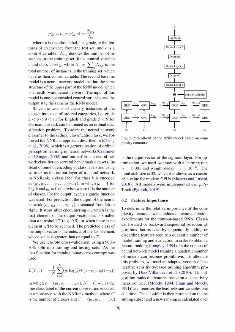
p(y|x, c) = p(y|c) =Nc,y

Nc

where y is the class label, i.e. grade, x the fea-tures of an instance from the test set, and c is acontrol variable. Nc,y denotes the number of in-stances in the training set, for a control variablec and class label y, while Nc =

XyNc,y is the

total number of instances in the training set, whichhas c as their control variable. The second baselinemodel is a neural network model that has the samestructure of the upper part of the RNN model whichis a feedforward neural network. The input of thismodel is one-hot encoded control variables and theoutput stay the same as the RNN model.

Since the task is to classify instances of thedataset into a set of ordered categories, i.e. grade2 < 6 < 9 < 11 for English and grade 5 < 9 forGerman, our task can be treated as an ordinal clas-sification problem. To adapt the neural networkclassifier to the ordinal classification task, we fol-lowed the NNRank approach described in (Chenget al., 2008), which is a gerneralization of ordinalperceptron learning in neural networks(Crammerand Singer, 2002) and outperforms a neural net-work classifier on serveral benchmark datasets. In-stead of one-hot encoding of class labels and usingsoftmax as the output layer of a neural network,in NNRank, a class label for class k is encodedas (y1, y2, . . . , yi, . . . , yC�1), in which yi = 1 fori k and yi = 0 otherwise, where C is the numberof classes. For the output layer, a sigmoid functionwas used. For prediction, the output of the neuralnetwork (o1, y2, . . . , oC�1) is scanned from left toright. It stops after encountering oi, which is thefirst element of the output vector that is smallerthan a threshold T (e.g. 0.5), or when there is noelement left to be scanned. The predicted class ofthe output vector is the index k of the last element,whose value is greater than or equal to T .

We use ten-fold cross-validation, using a 90%–10% split into training and testing sets. As theloss function for training, binary cross entropy wasused:

L(Y , c) = � 1

N

NX

i=1

(yi log(y)+(1�yi) log(1�y))

in which c = (y1, y2, . . . , yN ), N = C � 1 is thetrue class label of the current observation encodedin accordance with the NNRank method, where Cis the number of classes and Y = (y1, y2, . . . , yN )

GRU

GRU

x1

GRU

GRU

x2

h11

h21

· · ·

· · ·

h12

h22

GRU

GRU

xl

h1,l�1

h2,l�1

· · ·

· · ·

h1l

h2l

GRU

GRU

xn

h1,n�1

h2,n�1

L

Dense Layer 1

Dropout

Dense Layer 2

Dropout

Dense Layer 3

control variables

Sigmoid

y

Figure 2: Roll-out of the RNN model based on com-plexity contours

is the output vector of the sigmoid layer. For op-timization, we used Adamax with a learning rate⌘ = 0.001 and weight decay= 1 ⇥ 10�6. Theminibatch size is 32, which was shown as a reason-able value for modern GPUs (Masters and Luschi,2018). All models were implemented using Py-Torch (Pytorch, 2019).

6.2 Feature Importance

To determine the relative importance of the com-plexity features, we conducted feature ablationexperiments for the contour-based RNN. Classi-cal forward or backward sequential selection al-gorithms that proceed by sequentially adding ordiscarding features require a quadratic number ofmodel training and evaluation in order to obtain afeature ranking (Langley, 1994). In the context ofneural network model training a quadratic numberof models can become prohibitive. To alleviatethis problem, we used an adapted version of theiterative sensitivity-based pruning algorithm pro-posed by Dıaz-Villanueva et al. (2010). This al-gorithm ranks the features based on a ‘sensitivitymeasure’ (see, (Moody, 1994; Utans and Moody,1991)) and removes the least relevant variables oneat a time. The classifier is then retrained on the re-sulting subset and a new ranking is calculated over

70

the remaining features. This process is repeateduntil all features are removed (see Algorithm 1).In this fashion, rather than training n(n+1)

2 modelsrequired for sequential algorithms, the number ofmodels trained is reduced to n

m , where m is thenumber of features that can be removed at eachstep. We report the results obtained with m = 1,i.e. the results after the removal of a single fea-ture at each step. At step t, neural network modelsMt,n, n 2 {1, . . . , k} are trained on the trainingsets of a 10-fold cross-validation, where n is thefold ID. The training sets at step t consist of in-stances with feature set Ft = {f1, f2, . . . , fDt}where f1, . . . fDt are the remaining features at thecurrent step, whose importance rank is to be de-termined. We define Xt,n as the test set of thenth fold with feature set Ft and Xi

t,n as the samedataset as Xt,n except we set the ith feature fi

of each instance within the dataset to its average.Furthermore, we define g(X) as the classificationaccuracy of Mt,n for a dataset X . The sensitivityof feature fi on the nth fold at step t is obtainedfrom:

Si,t,n = g(Xt,n)� g(Xit,n)

The final sensitivity for a feature fi at step t is:

Si,t =1

k

kX

n=1

Si,t,n

The most important feature at step t can be foundby:

fi : i = arg maxi:fi2Ft

(Si,t)

Then we set the rank for feature fi:

Ranki = t

In the end, feature fi is dropped from Ft and thecorresponding columns in training and test datasetare also dropped simultaneously:

Ft+1 = Ft � {fi}

This procedure is repeated, until |Ft0 | = 1. Toincrease the robustness of the feature importancerank order, 10-fold cross-validation was applied.

7 Results

We report the results of classification with 10-foldcross-validation (see Figures 5 and 6 in the Ap-pendix for a visualization of model accuracy for the

means-based and contour-based models over 200epochs across the 10 cross-validation folds). Wefirst present the results of the experiments on theEnglish data, before moving to results for the Ger-man data. The performance metrics of the classifi-cation models for English (global accuracy, preci-sion, recall and macro F1 scores per grade level) arepresented in Table 2. Both the means-based and thecontour-based models achieved grade-level-basedclassification accuracy of > 75%, a substantial im-provement over the baseline model (28%, see Table4 in the Appendix for details). These findings indi-cate that text complexity increases with children’sage/competence level and provide further empiricalevidence in support of grade-level-based complexi-fication assumption (see the study by Berendes et al,2018 described above). The contour-based modeloutperforms the means-based model in terms ofboth precision and recall across all classes, result-ing in an increase in global classification accuracyof 6%, from 76% (means-based model) to 82%(contour-based model). Precision and recall ratesare found to be highest for grade 2, followed bygrades 6 and 11, and lowest for grade 11. Inspec-tion of the confusion matrix for the contour-basedmodel (see Table 7 in the Appendix) indicates thatmisclassified samples are close to the actual class,indicating that the model was sensitive to the gradeordering.5 These results suggest that the changein complexity was most pronounced in the earliergrades and decreased with increasing grade levels.The results of the feature importance analysis re-veal that classification is mainly driven by featuresrelated to vocabulary (the feature importance statis-tics for the top 30 measures can be found in Table 6in the Appendix). The top 14 of the 57 measures arerelated to lexical sophistication, word length andthe use of register-based n-grams. These findingsare consistent with the available body of researchsuggesting that the development of children’s writ-ing during adolescent years is primarily character-ized by higher proportions of unusual/advancedwords and words of greater surface length (com-pare same vs. equal vs. identical vs. tantamount)(see, Berman 2007) and replicate and extend thefindings reported in Durrant and Brenchley (2019)that the shift towards more academic vocabularycan also be observed in the use of multi-word se-quences. The information theoretic measures are

5We also examined all pairwise classification errors amongthe four grades (see Table 8).

71

Means-based Contour-basedM SD M SD

Accuracy 0.76 0.03 0.82 0.02Precision 2 0.87 0.06 0.90 0.07Recall 2 0.85 0.04 0.90 0.04F1 score 2 0.86 0.03 0.90 0.03Precision 6 0.78 0.02 0.82 0.04Recall 6 0.78 0.03 0.81 0.04F1 score 6 0.78 0.01 0.81 0.03Precision 9 0.72 0.04 0.76 0.06Recall 9 0.71 0.05 0.76 0.04F1 score 9 0.71 0.03 0.76 0.03Precision 11 0.71 0.09 0.82 0.06Recall 11 0.75 0.06 0.82 0.05F1 score 11 0.73 0.07 0.82 0.04

Table 2: Performance statistics of the means-based(left) and contour-based (right) RNN classifiers aggre-gated over 10 crossvalidation runs (English data). Base-line classification accuracy was 28%.

situated at ranks 15, 18 and 22. The group of lexi-cal diversity measures (NDW and variants of TTR)is located in the mid-field (ranks 34, 36, 37, 38,39). Syntactic complexity is found to play only asubsidiary role: with the exception of one measure(VP/T, rank 19) features from this class appearedonly after rank 30.

Even with a more restricted features set com-pared to English, grade-level-based classificationaccuracy on the German dataset displays consid-erable - albeit less pronounced - improvement of� 19% over the baseline model (51% classifica-tion accuracy) (see Table 5 in the appendix). Thesefindings thus provide additional, though somewhatweaker, empirical evidence in support of grade-level-based complexification assumption. As isthe case in the English data, the performance ofthe model based on complexity contours exceedsthat of the means-based model on the German databoth in terms of precision and recall across the twoschool grades, leading to an 4% increase in overallclassification accuracy from 70% to 74%. Table3 presents the performance statistics. The featureablation analysis reveals that the most importantfeatures are more evenly distributed across the fourgroups of CMs (see Table 9 in the Appendix): Thetop eight features include surface CMs pertainingto the length of production unit (MLWc, MLC,MLS), lexical diversity (NDW, RTTR, CTTR), syn-tactic complexity (Cl/S), and information density

Means-based Contour-basedM SD M SD

Accuracy 0.70 0.02 0.74 0.02Precision 5 0.71 0.02 0.75 0.02Recall 5 0.74 0.02 0.79 0.02F1 score 5 0.72 0.02 0.77 0.01Precision 9 0.69 0.03 0.74 0.03Recall 9 0.66 0.03 0.7 0.03F1 score 9 0.67 0.02 0.72 0.03

Table 3: Performance statistics of the means-based(left) and contour-based (right) RNN classifiers ag-gregated over 10 crossvalidation runs (German data).Baseline classification accuracy was 51%.

(KolDef). Within this set of eight CMs, the re-moval of individual CMs is associated with a rel-atively minor drop in classification accuracy ofless than 1.5%, suggesting that the network is ableto compensate for the loss of information froma given feature by relying on the other features.However, when the last feature of the top-8 groupis removed, classification accuracy drops by al-most 5%, indicating that the remaining featuresplayed subsidiary roles in the grade-level classifi-cation. These findings nicely complement thosereported in the paper by Weiss and Meurers (2019)described above focusing on basic (Hauptschule)and intermediate school tracks (Realschule) by as-sessing writing skills in the other two tracks ofthe German educational system: comprehensiveschool (Gesamtschule) and grammar school (Gym-nasium).

8 Conclusion and Outlook

In this paper, we demonstrated how the auto-matic assessment of text complexity through asliding window approach in combination with ma-chine learning techniques can provide valuable andunique insights into the development of children’swriting as they progress through their school edu-cation. Such an approach has the added advantageof capturing the progression of complexity withina text. In classification tasks on two data sets rep-resenting children’s school writing in L1 Englishand German, we showed that the inclusion of thissequential information can substantially increaseclassification performance across grade-levels. Wealso show that Sensitivity-Based Pruning is a vi-able complementary approach to other approachesaimed at assessing feature importance to identify

72

’criterial features’ that are characteristic and in-dicative of language competencies at a given level(Hawkins and Filipovic, 2012). More generally, thetype of research presented in this paper has the po-tential to advance our understanding of the develop-ment of literacy skills in children during adolescentyears, a key stage that is still not well understood.In future work, we intend to extend the approachpresented here to larger cross-sectional data setscovering additional school grades in search of validand reliable benchmarks and norms that can beused to inform school curricula and educationalstandards.

ReferencesKarin Berendes, Sowmya Vajjala, Detmar Meurers,

Doreen Bryant, Wolfgang Wagner, Maria Chinkina,and Ulrich Trautwein. 2018. Reading demands insecondary school: Does the linguistic complexityof textbooks increase with grade level and the aca-demic orientation of the school track? Journal ofEducational Psychology, 110(4):518.

Ruth A Berman. 2007. Developing linguistic knowl-edge and language use across adolescence.

Xiaobin Chen and Detmar Meurers. 2018. Word fre-quency and readability: Predicting the text-levelreadability with a lexical-level attribute. Journal ofResearch in Reading, 41(3):486–510.

Jianlin Cheng, Zheng Wang, and Gianluca Pollastri.2008. A neural network approach to ordinal regres-sion. In 2008 IEEE International Joint Conferenceon Neural Networks (IEEE World Congress on Com-putational Intelligence), pages 1279–1284. IEEE.

KyungHyun Cho, Bart van Merrienboer, Dzmitry Bah-danau, and Yoshua Bengio. 2014. On the propertiesof neural machine translation: Encoder-decoder ap-proaches. CoRR, abs/1409.1259.

European Commission. 2019. Proposal for a councilrecommendation on a comprehensive approach tothe teaching and learning of languages.

Koby Crammer and Yoram Singer. 2002. Prankingwith ranking. In Advances in neural informationprocessing systems, pages 641–647.

Scott A Crossley, Rod Roscoe, and Danielle S McNa-mara. 2014. What is successful writing? an investi-gation into the multiple ways writers can write suc-cessful essays. Written Communication, 31(2):184–214.

Scott A Crossley, Jennifer L Weston, Susan TMcLain Sullivan, and Danielle S McNamara. 2011.The development of writing proficiency as a func-tion of grade level: A linguistic analysis. WrittenCommunication, 28(3):282–311.

Peter Deutsch and Jean-Loup Gailly. 1996. Zlib com-pressed data format specification version 3.3. Tech-nical report, RFC 1950, May.

Wladimiro Dıaz-Villanueva, Francesc J Ferri, and Vi-cente Cerveron. 2010. Learning improved featurerankings through decremental input pruning for sup-port vector based drug activity prediction. In Inter-national Conference on Industrial, Engineering andOther Applications of Applied Intelligent Systems,pages 653–661. Springer.

Zeynep Duran-Karaoz and Parvaneh Tavakoli. 2020.Predicting L2 fluency from L1 fluency behavior:The case of L1 Turkish and L2 English speakers.Studies in Second Language Acquisition, pages 1–25.

Philip Durrant and Mark Brenchley. 2019. Develop-ment of vocabulary sophistication across genres inenglish children’s writing. Reading and Writing,32(8):1927–1953.

Katharina Ehret and Benedikt Szmrecsanyi. 2019.Compressing learner language: An information-theoretic measure of complexity in sla productiondata. Second Language Research, 35(1):23–45.

Nick C Ellis. 2019. Essentials of a theory of languagecognition. The Modern Language Journal, 103:39–60.

Thomas Francois and Cedrick Fairon. 2012. An ai read-ability formula for french as a foreign language. InProceedings of the 2012 Joint Conference on Empir-ical Methods in Natural Language Processing andComputational Natural Language Learning, pages466–477. Association for Computational Linguis-tics.

John A Hawkins and Luna Filipovic. 2012. Criterialfeatures in L2 English: Specifying the reference lev-els of the Common European Framework, volume 1.Cambridge University Press.

Dan Klein and Christopher D Manning. 2003. Accu-rate unlexicalized parsing. In Proceedings of the41st Annual Meeting on Association for Computa-tional Linguistics-Volume 1, pages 423–430. Associ-ation for Computational Linguistics.

Pat Langley. 1994. Selection of relevant features in ma-chine learning. In Proceedings of the AAAI Fall sym-posium on relevance, pages 1–5.

Francisco Lorenzo and Oliver Meyer. 2017. Special is-sue: Languages of schooling: explorations into dis-ciplinary literacies.

Xiaofei Lu. 2011. A corpus-based evaluation of syntac-tic complexity measures as indices of college-levelesl writers’ language development. Tesol Quarterly,45(1):36–62.

Xiaofei Lu. 2012. The relationship of lexical richnessto the quality of esl learners’ oral narratives. TheModern Language Journal, 96(2):190–208.

73

Xiaofei Lu. 2017. Automated measurement of syntac-tic complexity in corpus-based l2 writing researchand implications for writing assessment. LanguageTesting, 34(4):493–511.

Christopher Manning, Mihai Surdeanu, John Bauer,Jenny Finkel, Steven Bethard, and David McClosky.2014. The stanford corenlp natural language pro-cessing toolkit. In Proceedings of 52nd annual meet-ing of the association for computational linguistics:system demonstrations, pages 55–60.

Dominic Masters and Carlo Luschi. 2018. Revisitingsmall batch training for deep neural networks. arXivpreprint arXiv:1804.07612.

Detmar Meurers. 2020. Natural language processingand language learning. In Carol A. Chapelle, edi-tor, The Concise Encyclopedia of Applied Linguis-tics. Wiley.

John Moody. 1994. Prediction risk and architecture se-lection for neural networks. In From statistics toneural networks, pages 147–165. Springer.

Ildiko Pilan, David Alfter, and Elena Volodina. 2016.Coursebook texts as a helping hand for classify-ing linguistic complexity in language learners’ writ-ings. In Proceedings of the Workshop on Com-putational Linguistics for Linguistic Complexity(CL4LC), pages 120–126.

Pytorch. 2019. Pytorch: Tensors and dynamic neu-ral networks in python with strong gpu acceleration.https://github.com/pytorch/pytorch.

Anna N Rafferty and Christopher D Manning. 2008.Parsing three german treebanks: Lexicalized and un-lexicalized baselines. In Proceedings of the Work-shop on Parsing German, pages 40–46.

Patrick Emanuel Rebuschat, Meurers Detmar, andTony McEnery. 2017. Language learning researchat the intersection of experimental, computationaland corpus-based approaches. Language Learning,67(S1):6–13.

Catherine E Snow. 2010. Academic language and thechallenge of reading for learning about science. sci-ence, 328(5977):450–452.

Catherine E Snow and Paola Uccelli. 2009. The chal-lenge of academic language. The Cambridge hand-book of literacy, pages 112–133.

Marcus Strobel. 2014. Tracking complexity of l2 aca-demic texts: A sliding-window approach. Masterthesis. RWTH Aachen University.

Marcus Strobel, Elma Kerz, Daniel Wiechmann, andYu Qiao. 2018. Text genre classification based onlinguistic complexity contours using a recurrent neu-ral network. In MRC@ IJCAI, pages 56–63.

Marcus Strobel, Elma Kerz, and Daniel Wiechmann.2020. The relationship between first and second lan-guage writing: Investigating the effects of first lan-guage complexity on second language complexityin advanced stages of learning. Language Learning,n/a(n/a).

Joachim Utans and John Moody. 1991. Selecting neu-ral network architectures via the prediction risk: Ap-plication to corporate bond rating prediction. In Pro-ceedings First International Conference on ArtificialIntelligence Applications on Wall Street, pages 35–41. IEEE.

Zarah Weiss and Detmar Meurers. 2019. Analyzinglinguistic complexity and accuracy in academic lan-guage development of german across elementaryand secondary school. In Proceedings of the Four-teenth Workshop on Innovative Use of NLP for Build-ing Educational Applications, pages 380–393.

Menglin Xia, Ekaterina Kochmar, and Ted Briscoe.2019. Text readability assessment for second lan-guage learners. arXiv preprint arXiv:1906.07580.

74

Proceedings of the 15th Workshop on Innovative Use of NLP for Building Educational Applications, pages 75–84July 10, 2020. c©2020 Association for Computational Linguistics

Annotation and Classification of Evidence and Reasoning Revisions inArgumentative Writing

Tazin Afrin, Elaine Wang, Diane Litman, Lindsay C. Matsumura, Richard CorrentiLearning Research and Development Center

University of PittsburghPittsburgh, Pennsylvania 15260

tazinafrin@cs.pitt.edu, ewang@rand.org{dlitman,lclare,rcorrent}@pitt.edu

Abstract

Automated writing evaluation systems can im-prove students’ writing insofar as students at-tend to the feedback provided and revise theiressay drafts in ways aligned with such feed-back. Existing research on revision of argu-mentative writing in such systems, however,has focused on the types of revisions studentsmake (e.g., surface vs. content) rather than theextent to which revisions actually respond tothe feedback provided and improve the essay.We introduce an annotation scheme to capturethe nature of sentence-level revisions of evi-dence use and reasoning (the ‘RER’ scheme)and apply it to 5th- and 6th-grade students’argumentative essays. We show that reliablemanual annotation can be achieved and that re-vision annotations correlate with a holistic as-sessment of essay improvement in line withthe feedback provided. Furthermore, we ex-plore the feasibility of automatically classify-ing revisions according to our scheme.

1 Introduction

Automated writing evaluation (AWE) systems areintended to help improve students’ writing by pro-viding formative feedback to guide students’ essayrevision. Such systems are only effective if stu-dents attend to the feedback provided and revisetheir essays in ways aligned with such feedback.

To date, few AWE systems assess (and are as-sessed on) the extent to which students’ revisionsrespond to the feedback provided and thus improvethe essay in suggested ways. Moreover, we knowlittle about what students do when they do not re-vise in expected ways. For example, most naturallanguage processing (NLP) work on writing revi-sion focuses only on annotating and classifying re-vision purposes (Daxenberger and Gurevych, 2013;Zhang et al., 2017), rather than on assessing thequality of a revision in achieving its purpose. A few

studies do focus on revision quality, but withoutrelating revisions to feedback (Tan and Lee, 2014;Afrin and Litman, 2018).

In this study, we take a step towards advancingautomated revision analysis capabilities. First, wedevelop a sentence-level revision scheme to anno-tate the nature of students’ revision of evidenceuse and reasoning (hereafter, we refer to this as the‘RER scheme’) in a text-based argumentative essaywriting task. By evidence use, we refer to the selec-tion of relevant and specific details from a sourcetext to support an argument. By reasoning, wemean an explanation connecting the text evidenceto the claim and overall argument. Table 4 showsexamples of evidence and reasoning revisions fromfirst draft to second draft. Next, we demonstrateinter-rater reliability among humans in the use ofthe RER scheme. In addition, we show that onlydesirable revision categories in the scheme relate toa holistic assessment of essay improvement in linewith the feedback provided. Finally, we adapt wordto vector representation features to automaticallyclassify desirable versus undesirable evidence re-visions, and examine how automatically predictedevidence revisions relate to the holistic assessmentof essay improvement.

2 Related Work

Automated revision detection work has centered onclassifying edits on largely non-content level fea-tures of writing, such as spelling and morphosyn-tactic revisions (Max and Wisniewski, 2010), er-ror correction, paraphrase or vandalism detection(Daxenberger and Gurevych, 2013), factual ver-sus fluency edits (Bronner and Monz, 2012), anddocument- versus word-level revisions (Roscoeet al., 2015). Other research has focused on pat-terns of revision behavior, for example, the addi-tion, deletion, substitution, and reorganization of

75

information (Zhang, 2020). However, these cate-gories center on general writing features and behav-iors. In the context of AWE systems, this could beseen as a limitation because feedback is most use-ful to students and teachers alike when it is keyedto critical features of a genre – such as claims, rea-sons, and evidence use in argumentative writing –that are most challenging to teach and learn.

Some research has begun to take up the chal-lenge of investigating student revision for argumen-tative writing (Zhang and Litman, 2015; Zhanget al., 2017). Results show a high level of agree-ment for human annotation and some relationshipto essay improvement, though not at the level ofindividual argument elements (Zhang and Litman,2015). Existing schemes also lack in specificity,e.g., they do not distinguish between desirable andundesirable revisions for each argument element interms of improving essay quality.

Prior work on assessing revision quality has eval-uated revision in general terms (e.g., strength (Tanand Lee, 2014) or overall improvement (Afrin andLitman, 2018)), but without consideration of thefeedback students were provided. We instead fo-cus on analyzing revisions in response to feedbackfrom an AWE system. Although prior studies havefocused on all revision categories (e.g., claim, evi-dence, and word-usage (Zhang and Litman, 2015)),we focus on only evidence and reasoning revisionsthat correspond to the scope of the AWE system’sfeedback. Also, we focus not only on why the stu-dent made a revision (e.g., add evidence) but alsoanalyze if the revision was desirable or not (e.g.,relevant versus irrelevant evidence).

3 Corpus

Our corpus consists of the first draft (Draft1) andsecond draft (Draft2) of 143 argumentative essays.The corpus draws from our effort to develop anautomated writing evaluation system - eRevise, toprovide 5th- and 6th-grade students feedback on aresponse-to-text essay (Zhang et al., 2019; Wanget al., 2020). The writing task administration in-volved teachers reading aloud a text while studentsfollowed along with their copy. Then, studentswere given a writing prompt1 to write an argumen-tative essay.

1“Based on the article, did the author provide a convincingargument that winning the fight against poverty is achievablein our lifetime? Explain why or why not with 3-4 examplesfrom the text to support your answer.”

No Feedback Message1 Use more evidence from the article2 Provide more details for each piece of

evidence you use3 Explain the evidence4 Explain how the evidence connects to the

main idea & elaborate

Table 1: Top-level feedback from the AWE system.

Each student wrote Draft1 and submitted theiressay to the AWE system. Students then receivedfeedback focused specifically on the use of textevidence and reasoning. Table 1 shows the top-level feedback messages2 that the system provided.Finally, students were directed to revise their essayin response to the feedback, yielding Draft2.

As part of a prior exploration of students’ imple-mentation of the system’s feedback, this corpus of143 essays was coded holistically on a scale from0 to 3 for the extent to which use of evidence andreasoning improved from Draft1 to Draft 2 in linewith the feedback provided (Wang et al., 2020)3.A code, or score, of 0 indicated no attempt to imple-ment the feedback given; 1= no perceived improve-ment in evidence use or reasoning, 2= slight im-provement; and 3= substantive improvement. Noteagain that this score represents a subjective, holis-tic (i.e., not sentence-level) assessment of whetherDraft2 improved in evidence use and/or reasoningspecifically in alignment with the feedback thata particular student received. We refer to this as‘improvement score’ in the rest of the paper.

3.1 Preparing the corpus for annotation

On average, Draft1 essays contain 14 sentences and253 words, and Draft2 essays contain 18 sentencesand 334 words. To prepare the corpus for anno-tation, we first segmented each Draft1 and Draft2essay into sentences, then manually aligned themat sentence-level. For example, if a sentence isadded to Draft2, it is aligned with a null sentencein Draft1. If a sentence is deleted from Draft1,it is aligned with a null sentence in Draft2. Amodified sentence, or a sentence with no changein Draft2, is aligned with the corresponding sen-

2See (Zhang et al., 2019) for detailed feedback messages.3In the prior study, two researchers double-coded 35 of the

143 essays (24 percent). Cohen’s kappa was 0.77, indicating‘substantial’ agreement (McHugh, 2012).

76

#Sentence Draft2 #No Change #RevisionTotal 2652 1362 1475Avg. 18.545 9.524 10.315

Table 2: Essay statistics (N=143).

tence in Draft14. Based on this alignment, we thenextracted the 1475 sentence pairs where studentsmade either additions, deletions, or modificationsas revisions. The remaining 1362 aligned sentenceshad no changes between drafts and were thus notextracted as revisions.

Each revision was next manually annotated5

for its revision purpose according to the schemeproposed in (Zhang and Litman, 2015), whichcategorizes revisions into surface versus contentchanges. Surface revisions are changes to fluencyor word choice, convention or grammar, and orga-nization. Content revisions are meaningful textualchanges such as claim or thesis, evidence, reason-ing, counter-arguments etc. From among these re-visions, only evidence and reasoning revisions areused for the current study, due to their alignmentwith the AWE feedback messages in Table 1.

Table 2 shows the descriptive statistics of theessay corpus at the sentence-level. The secondcolumn shows the total and average number of sen-tences for Draft2. The third column shows that,on average, about 9 sentences per essay were un-changed. The final column shows that, on average,10 sentences per essay were revised6. Out of those10 sentences, only two to three sentences were re-vised with respect to evidence, and another twoto three sentences with respect to reasoning, onaverage over all 143 students. This indicates thatstudents engaged in very limited revisions of evi-dence and reasoning, even when provided feedbacktargeted to these argument elements.

Table 3 shows the statistics for the students whodid revise their essay. Note that out of 143 students,50 students (35%) did not make any evidence-userevisions; 32 students (22%) did not make any rea-soning revisions. Only 10 students (7%) did notmake any evidence or reasoning revisions. 4 stu-dents (3%) did not make any revision at all. Fromthese students we extracted 386 evidence revisionsand 389 reasoning revisions, a total of 775 sentence-

4Sentence order substitution is evaluated as deleted theninserted.

5Annotator Cohen’s kappa of 0.753.6#Revision also includes deleted sentences, hence #Revi-

sion + #No Change does not equal #Sentence in Draft2.

Evidence Reasoning Other#Revision (N=93) (N=111) (N=129)Total 386 389 700Min 0 0 0Max 36 17 21Avg. 4.151 3.505 5.426

Table 3: Revision statistics.

level revisions. We do not consider the other 700revisions (claim, word-usage, grammar mistakes,etc.) in this study.

To better understand how students did revise,whether their revisions were desirable, and whetherdesirable revisions relate to a measure of essay im-provement that includes alignment with feedback,we developed a revision categorization scheme andconducted the analysis described below.

4 Revision Categorization (RER Scheme)

We propose a new scheme for annotating revisionsof evidence use and reasoning (RER scheme) thatwill be useful for assessing the improvement ofthe essay in line with the feedback provided. Theinitial set of codes drew from the qualitative ex-ploration of students’ implementation of feedbackfrom our AWE system (Wang et al., 2020), in whichthe authors inductively and holistically coded howstudents successfully and unsuccessfully revisedtheir essays with respect to evidence use and rea-soning. For example, students sometimes addedevidence that repeated evidence they had alreadyprovided in Draft1. Or they successfully modifiedsentences to better link the evidence to the claim.

Both the initial set of codes and our AWE sys-tem’s feedback messages were informed by writingexperts and research suggesting that strong argu-ment writing generally features multiple pieces ofspecific evidence that are relevant to the argumentand clear explication (or reasoning) of how the ev-idence connects to the claim and helps to supportthe argument (see, for example, (De La Paz et al.,2012; O’Hallaron, 2014; Wang et al., 2018)).

For the present study, two annotators readthrough each extracted evidence or reasoning-related revision in the context of the entire essay.They labeled each instance of revision with a code.The annotators iteratively expanded or refined theinitial codes until they finalized a set of codes forevidence use revisions and another for reasoningrevisions (see sections 4.1 and 4.2). Together these

77

Draft1 Draft2 Operation Purpose RERcode

In the story, “A Brighter Fu-ture,” the author convincedme that “winning the fightagainst poverty is achiev-able in our life time.”

In the story, “A Brighter Fu-ture,” the author of the storyconvinced me that winning thefight against poverty is achiev-able in our lifetime.

Modify Fluency

I think that in Sauri, Kenya[where poverty is all around],people were in poverty.

Add Claim

In the story it states “TheYala sub-District Hospital hasmedicine.”

Add Evidence Relevant

For example, we have goodfood and clean water

Delete Evidence Irrelevant

This shows that there was achange at the hospital becausethey had medicine which isgood for the peoples healthwhen they get sick.

Add Reasoning Linked toClaim andEvidence

Table 4: Example revisions from aligned drafts of an essay and application of RER codes.

two sets comprise the RER scheme. Subsequently,the two annotators applied the RER scheme to allinstances of evidence use or reasoning-related re-visions in all 143 students’ essays.7 Annotatorsselected the best code; no sentence received morethan one code.

Table 4 presents an example of corpus prepara-tion (Operation and Purpose, section 3.1) and RERcoding (see below) as applied to an excerpted essayand its revision. Table 5 presents an example ofeach code, though for parsimony, we only presentadditive revisions – not deletions or modification,as these are less common. Table 6 shows the distri-bution for each RER code.

4.1 Revision of evidence use

Revisions related to evidence are characterized byone of the following five codes. All codes apply toadded, deleted, or modified revisions, except ‘Min-imal’, which only applies to modified evidence.Relevant applies to examples or details that sup-port (i.e., are appropriate and related to) the partic-ular claim. Irrelevant applies to examples or de-tails that are unnecessary, impertinent to, or discon-nected from the claim. They do not help with theargument. Repeat evidence applies to examples or

733 of the essays, or 23 percent, were double-coded forreliability, see Section 5 for kappa score.

details that were already present in Draft1; studentsare merely repeating the information. Non-textbased applies to examples or details outside of theprovided text. Minimal applies to minor modifi-cations to existing evidence that may add somespecificity, but do not affect the argument much.

4.2 Revision of reasoning

Reasoning revisions are characterized by one ofthe following six codes. All codes apply to added,deleted, or modified revisions, except ‘Minimal’,which only applies to modified reasoning. Linkedclaim-evidence (LCE) applies to an explanationthat connects the evidence provided with the claim.Not LCE applies to an explanation that does notconnect the evidence provided with the claim.Paraphrase evidence applies to an attempt at ex-planation that merely paraphrases the evidencerather than explain or elaborate upon it. Genericapplies to a non-specific explanation that is reusedmultiple times, after each piece of evidence (e.g.,“This is why I am convinced that we can endpoverty.”) Commentary applies to an explanationthat is unrelated to the main claim or source text;most of the time, it comes from the writer’s per-sonal experience. Minimal applies to minor modi-fications that do not affect the argument much.

78

Example of “Add” Revision (“Modify” for Minimal Revision)Evidence*Relevant To support the point that conditions in Sauri were bleak, a student added this new

example: “The hospitals don’t have the medicine for their sick patients so thereforethey can get even more ill and eventually die [if] the [immune] system is not strongenough.”

Irrelevant To support the claim that winning the fight against poverty is possible, the studentwrote, “Students could not attend school because they did not have enough money topay the school fee.” This does not support the claim.

Repeat Evidence “Malaria causes adults to get sick and cause children to die” was added as sentence#27 in a student’s Draft2, but sentence #5 already said, “Around 20,000 kids die aday from malaria and the adults get very ill from it.”

Non-Text-Based Student provided example of an uncle living in poverty, rather than draw fromexamples in the source text about poverty in Kenya.

Minimal In Draft1, the student wrote, “Now during the project there are no school fees, theschools serve the students lunch, and the attendance rate is way up.” In Draft 2, thestudent specified “Millennium Villages” project.

Reasoning*LCE The student argued that we can end poverty because Sauri has already made signif-

icant progress. After presenting the evidence about villagers receiving bednets toprotect against malaria, the student added, “This shows that the people of Sauri havemade progress and have taken steps to protect everyone using the bed nets and otherthings.”

Not LCE The student claims that Sauri is overcoming poverty. After presenting the evidencethat “Each net costs $5,” the student wrote, “This explain how low prices are but wemay not get people to lower them more.”

Paraphrase After presenting the evidence that “People’s crops were dying because they couldnot afford the necessary fertilizer,” the student added, “This evidence shows that thecrops were dying and the people could not get the food that they needed because thefarmers could not afford any fertilizer. . . ”

Generic After the first piece of evidence, the student added, “This evidence helps the statementthat there was a lot of poverty.” Then after the second piece of evidence, the studentadded almost the same generic sentence, “This statement also supports that therewere a lot of problems caused by poverty.”

Commentary After a piece of evidence, a student wrote, “We think that we are poor because wecan not get toys that we want, but we go to school and its not free.”

Minimal In Draft1, the student wrote, “I believe that because it states that we have enoughhands and feet to get down and dirty and help these kids that are suffering.”. InDraft2, the student only added “and are in poverty” to the end of the sentence.

* indicates desirable revision, as the revision has hypothesized utility in improving the assigned essay inalignment with provided feedback given in Table 1. Other codes may also be desirable given a differentwriting task with different feedback (e.g., students may be asked to provide non-text-based evidence fromtheir own experience).

Table 5: Example of each RER code.

79

RER Code Add Delete Modify TotalEvidence 265 63 58 386

Relevant 159 50 30 239Irrelevant 26 9 8 43Repeat Evidence 70 4 0 74Non-Text-Based 10 0 0 10Minimal 0 0 20 20

Reasoning 270 59 60 389LCE 90 18 13 121Generic 20 0 1 21Paraphrase 50 10 5 65Not LCE 62 11 12 85Commentary 48 20 7 75Minimal 0 0 22 22

Total 535 122 118 775

Table 6: RER code distribution (N=143).

5 Evaluation of the RER Scheme

We evaluated our annotated corpus to answer thefollowing research questions (RQ):

RQ1: What is the inter-rater reliability for anno-tating revisions of evidence use and reasoning?

RQ2: Is the number of each type of revisionrelated to essay ‘improvement score’?

RQ3: Is there any difference in the ‘improve-ment score’ based on the kinds of revisions?

RQ4: Is there a cumulative benefit to predictingessay ‘improvement score’ when students mademultiple types of revisions?

To answer RQ1, we calculated Cohen’s kappafor inter-rater agreement on the 33 essays (23 per-cent) that were double-coded. Our results showthat we were able to achieve substantial inter-rateragreement on reasoning (k = .719) and excellentinter-rater agreement for evidence use (k = .833)(see, e.g., (McHugh, 2012)).

To answer RQ2, we calculated the Pearson cor-relation between the raw number of revisions percode to the ‘improvement score’ described in Sec-tion 3. Table 7 shows that the total number ofevidence-related revisions was not significantly cor-related with ‘improvement score’ (r = .15), whilethe total number of reasoning revisions was (r =.30). Table 7 also shows that positive correlationswere found for added evidence or reasoning (r =.17 and .40, respectively), whereas deletions andmodification were not significantly correlated.

Looking at the correlations for our proposedRER codes (which sub-categorize the Evidence

and Reasoning codes (Zhang and Litman, 2015)),we see that the RER codes yield more and generallystronger results. We found that, as hypothesized,adding relevant pieces of evidence was significantlypositively correlated with the ‘improvement score’,while the addition of irrelevant evidence, non-textbased evidence or repeating prior evidence wereall unrelated to this score. Similarly, we foundthat adding reasoning that linked evidence to theclaim (LCE) was significantly correlated with the‘improvement score’ and so was paraphrasing ev-idence. Other reasoning codes, as expected, werenot significantly related to the ‘improvement score’.We did not initially consider paraphrases as a de-sirable type of revision; yet, this code showed asignificant positive correlation. While unexpected,we were not altogether surprised as two of the feed-back messages (shown in Table 1) did explicitly askfor students to put ideas into their own words (see(Zhang et al., 2019) for details). Although additionof evidence and reasoning revisions demonstratedcorrelation to the ‘improvement score’, deletionsand modifications did not show any intuitive corre-lation. We suspect that this is due to the compara-tively small number of delete and modify revisions.

To answer RQ3, we performed one-wayANOVAs for different levels of the ‘improvementscore’ (0=no attempt, 1=no improvement, 2=slightimprovement, 3=substantive improvement, alignedwith feedback provided) comparing means of thenumber of revisions added, modified, or deleted.ANOVAs showed overall significance for the cate-

80

RER Code Add Delete Modify TotalEvidence 0.17* 0.00 0.13 0.15

Relevant 0.25** 0.02 0.09 0.20*Irrelevant 0.05 -0.00 0.07 0.06Repeat Evidence 0.01 -0.06 – 0.00Non-Text-Based 0.07 – – 0.07Minimal – – 0.06 0.06

Reasoning 0.40** 0.09 -0.10 0.30**LCE 0.45** 0.05 0.09 0.41**Generic -0.03 – -0.04 -0.04Paraphrase 0.22** 0.09 0.02 0.22**Not LCE 0.09 0.00 -0.07 0.04Commentary -0.02 0.08 -0.08 0.01Minimal – – -0.14 -0.14

Table 7: Revision correlation to ‘Improvement Score’. (N=143, * p< .05, ** p< .01)

RER Code Add Modify TotalEvidence:

Relevant 3*>1 3*>2Reasoning:

LCE 3*>0,1,2 3*>1 3*>0,1,2Not LCE 2*>0,3 2*>0,3

Table 8: ANOVA results showing differences among‘Improvement Scores’ (coded as 0, 1, 2, 3). Only cate-gories with significant results are shown. All categorieswere tested. (N=143, * p< .05, ** p< .01)

gories shown in Table 8. Tukey post-hoc analysesshowed that students whose essays substantivelyimproved made more revisions in which they addedor modified relevant pieces of evidence. Studentswho substantively improved also added or modi-fied their reasoning linking evidence to their claims(LCE) more than students in all other groups. Fi-nally, students with slightly improved essays addedmore explanations not linking evidence to claim(Not-LCE) than did students who made no attemptat revision or whose essays substantively improved.

To answer RQ4, we examined three stepwiselinear regression models to understand whetheradding more revision codes had a cumulative in-fluence explaining more variance in ‘improvementscore’. Model E included only revisions relatedto evidence use. Model R included only revisionsrelated to reasoning. Model ER included all ev-idence use and reasoning revisions. As shown inTable 9, Model ER shows significant positive co-efficients for the addition of relevant evidence, rea-

Model Variables Coef. R2

Model E add Relevant 0.25** 0.06

Model Radd LCE 0.05**

0.25add Paraphrase 0.08**

Model ER

add LCE 0.45**

0.32add Paraphrase 0.20**add Relevant 0.29**del Relevant -0.21*

Table 9: Stepwise linear regression results predicting‘Improvement Score’. (N=143, * p< .05, ** p< .01)

soning that links evidence to the claim (LCE), andreasoning that paraphrases evidence. The positiverelationship shows that more of these kinds of revi-sions are more likely to lead to a higher ‘improve-ment score’. Note that the order of the coefficientsis related to the magnitude of the r-squared theyexplain - thus linked claim and evidence (LCE) hasthe strongest relationship with the score. Mean-while, deleting relevant pieces of evidence has anegative relationship when adjusting for the othercovariates in the model, which means that, all elsebeing equal, this is an undesirable revision.

6 Automatic RER Classification

The ultimate goal for developing the RER schemeis to implement it in an AWE system to providefeedback to students about revision outcome notonly at the essay-level but also at a more action-able, sentence-level. While the previous sectiondemonstrated the utility of the RER scheme, thissection explores its automatic classification. Since

81

Precision Recall F1-scoreMajority 0.309 0.500 0.377LogR 0.615** 0.622** 0.594**

Table 10: 10-fold cross-validation result for classifyingEvidence as ‘Relevant’ or not. (N=386, ** p< .01)

our overall revision dataset is small, we focus onthe simplified task of developing a binary classifierto predict whether an Evidence revision is ‘Rele-vant’ or not. ‘Relevant’ is both the most frequentRER code and relates positively to the improve-ment score.

The input is a revision sentence pair – the sen-tence from Draft1 (S1) and its aligned sentencefrom Draft2 (S2). The pair can have 3 variations:(null, S2) for added sentences, (S1, null) for deletedsentences, and (S1, S2) for modified sentences.Since we are focusing on ‘Relevant’ evidence pre-diction, and by our definition in Section 4.1 ‘Rele-vant’ evidence supports the claim, we also considerthe given source text (A) in extracting features.

Features. We explore Word2vec as features forour classification task8. We extract representationsof S1, S2, and A using the pre-trained GloVe wordembedding (Pennington et al., 2014). For eachword representation (w) we use the vector of dimen-sion 100, w = [v1, . . . , v100]. Then the sentenceor document vector (d) is calculated as the aver-age of all word vectors d = [d1, . . . , d100], wheredi = mean(v1i, . . . , vni), for n words in the doc-ument. Following this method we extract vectorsds1, ds2, and da for S1, S2, and A respectively.Finally, we take the average of those 3 vectors torepresent the feature vector, f = [f1, . . . , f100],where fj = mean(ds1j , ds2j , daj).

For machine learning, we use off-the-shelf Lo-gistic Regression (LogR) from the scikit-learntoolkit.9 We did not perform any parameter tuningor feature selection. In an intrinsic evaluation, wecompare whether there are significant differencesbetween the classifier’s performance and a majoritybaseline in terms of average un-weighted precision,recall and F1, using paired sample t-tests over 10-folds of cross-validation. In an extrinsic evaluation,we repeat the Pearson correlation study in Section 5for the predicted code, ‘Relevant’ evidence.

8We also explored n-gram features from a previous revi-sion classification task (Zhang and Litman, 2015). Our classi-fication algorithm performed better with word2vec features.

9We also explored Support Vector Machines (SVM) butLogistic Regression outperformed SVM in our experiment.

Add Delete Modify TotalGold 0.25** 0.02 0.09 0.20*Majority 0.17* 0.00 0.13 0.15LogR 0.17* -0.01 0.03 0.15

Table 11: Correlation of predicted ‘Relevant’ evidenceto ‘Improvement Score’. (N=143, * p< .05, ** p< .01)

Intrinsic evaluation. Table 10 presents the re-sults of the binary classifier predicting ‘Relevant’evidence. The results show that the logistic regres-sion classifier significantly outperforms the base-line using our features for all metrics.

Extrinsic evaluation. Table 11 shows the Pear-son correlation of ‘Relevant’ evidence to ‘Improve-ment Score’ using ‘Gold’ human labels (repeatedfrom Table 7) versus predicted labels from the ma-jority and logistic regression classifiers. First, thenumber of ‘Add Relevant’ revisions, whether goldor predicted, significantly correlates to improve-ment. While it is not surprising that the correlationis lower for LogR than for Gold (upper bound), it isunexpected that LogR and Majority (baseline) arethe same. This likely reflects the Table 7 result thatadding any type of Evidence, relevant or not, corre-lates with improvement. In contrast, the predictedmodels are not yet accurate enough to replicate thestatistical significance of the ‘Gold’ correlation be-tween improvement and ‘Total Relevant’ revisions.

7 Discussion

In our corpus, students revised only about half ofthe sentences from Draft1 to Draft2. Among therevisions, only a small proportion focused on ev-idence or reasoning, despite feedback targetingthese argument elements exclusively. This res-onates with writing research (though not in thecontext of AWE) showing that students often strug-gle to revise (Faigley and Witte, 1981; MacArthur,2018), and that novice writers – like our 5th- and6th-graders – tend to focus on local word- and sen-tence level problems rather than content or struc-ture (MacArthur et al., 2004; MacArthur, 2018).When novices do revise, their efforts frequentlyresult in no improvement or improvement only insurface features (Patthey-Chavez et al., 2004).

We knew of no revision schemes that assessedthe extent to which evidence use and reasoning-related revisions aligned with desirable features ofargumentative writing (i.e., showed responsivenessto system feedback to use more relevant evidence,

82

give more specific details, or provide explanationsconnecting evidence to the claim); hence, we devel-oped the RER scheme. The scheme – along withthe reliability we established and the positive corre-lations we demonstrated between its sentence-levelapplication and a holistic assessment of essay im-provement in line with provided feedback – is animportant contribution because the codes are keyedto critical features of the argument writing genre.Therefore, it is more useful than existing schemesthat focus on general revision purposes (surface vs.content) or operations (addition, deletion, modifica-tion) for assessing the quality of students’ revisions.

This assessment capability is important for atleast two related reasons. First, an AWE systemis arguably only effective if it helps to improvewriting in line with any feedback provided. It iseasier to attribute other types of revisions or im-provements to the general opportunity to revisitthe essay than to any inputs the system providesto students. For argument writing (and our AWEsystem), then, it is necessary, to be able to identifyspecific revision behaviors related to evidence useand reasoning. With the RER scheme, we wereable to distinguish among revision behaviors. Onthe whole, predictably undesirable revisions (e.g.,deleting relevant evidence) were not correlated withthe ‘improvement score’.

Second, gaining insight into how students specif-ically revise evidence use and reasoning can helphone the content of AWE feedback so that it bet-ter supports students to make desirable revisionsthat impact the overall argument quality. From ourcoding, we learned that students make deletion ormodification revisions less frequently; rather theytend to make additions, even if they do not im-prove the essay. We also learned that repeatingexisting evidence accounted for about 19 percentof the evidence-use revisions. We could refine ourfeedback to preempt students from making theseundesirable revisions. Or, once automated revi-sion detection is implemented, we could developa finer-grained set of feedback messages to pro-vide students to guide their second revision (i.e.,production of Draft 3).

Finally, our study takes a step towards advancingautomated revision detection for AWE by develop-ing a simple machine learning algorithm for classi-fying relevant evidence. However, it is importantto note that the classifier’s input is currently basedon the gold (i.e., human) alignments of the essay

drafts and the gold revision purpose labels (e.g.,Evidence). An actual end-to-end system wouldhave lower performance due to the propagation oferrors from both alignment and revision purposeclassification. In addition, due to the small sizeof our current corpus, our classification study wassimplified to focus on evidence rather than both ev-idence and reasoning, and to focus on binary ratherthan 5-way classification. Although our algorithmis thus limited to predicting only relevant evidence,the classifier nonetheless outperforms the baselinegiven little training data.

8 Conclusion and Future Work

We developed the RER scheme as a step towardsadvancing automated revision detection capabili-ties of students’ argument writing, which is criti-cal to supporting students’ writing development inAWE systems. We demonstrated that reliable man-ual annotation can be achieved and that the RERscheme correlates in largely expected ways with aholistic assessment of the extent to which revisionsaddress the feedback provided. We conclude thatthis scheme has promise in guiding the develop-ment of an automated revision classification tool.

Although the RER scheme was developed with aspecific corpus and writing assignment, we believesome of the categories (e.g., reasoning linked toclaim and evidence) can easily be adapted to datawe have from other revision tasks. With more data,we also plan to improve the current classificationmethod with state-of-the-art machine learning mod-els, and extend the classification for all categories.

Acknowledgments

The research reported here was supported, in wholeor in part, by the Institute of Education Sciences,U.S. Department of Education, through GrantR305A160245 to the University of Pittsburgh. Theopinions expressed are those of the authors and donot represent the views of the Institute or the U.S.Department of Education.

ReferencesTazin Afrin and Diane Litman. 2018. Annotation

and classification of sentence-level revision improve-ment. In Proceedings of the Thirteenth Workshop onInnovative Use of NLP for Building Educational Ap-plications, pages 240–246, New Orleans, Louisiana.

Amit Bronner and Christof Monz. 2012. User ed-its classification using document revision histories.

83

In Proceedings of the 13th Conference of the Euro-pean Chapter of the Association for ComputationalLinguistics, EACL ’12, pages 356–366, Avignon,France. Association for Computational Linguistics.

Johannes Daxenberger and Iryna Gurevych. 2013. Au-tomatically classifying edit categories in wikipediarevisions. In Proceedings of the 2013 Conference onEmpirical Methods in Natural Language Processing,EMNLP ’13, pages 578–589, Seattle, Washington,USA. Association for Computational Linguistics.

Susan De La Paz, Ralph Ferretti, Daniel Wissinger,Laura Yee, and Charles MacArthur. 2012. Ado-lescents’ disciplinary use of evidence, argumenta-tive strategies, and organizational structure in writ-ing about historical controversies. Written Commu-nication, 29(4):412–454.

Lester Faigley and Stephen Witte. 1981. Analyzing re-vision. College Composition and Communication,32(4):400–414.

Charles MacArthur, Steve Graham, and Karen Har-ris. 2004. Insights from Instructional Research onRevision with Struggling Writers, pages 125–137.Springer.

Charles A MacArthur. 2018. Evaluation and revision.Best practices in writing instruction, 287.

Aurelien Max and Guillaume Wisniewski. 2010. Min-ing naturally-occurring corrections and paraphrasesfrom Wikipedia’s revision history. In Proceedingsof the Seventh International Conference on Lan-guage Resources and Evaluation (LREC’10), Val-letta, Malta. European Language Resources Associ-ation (ELRA).

Mary McHugh. 2012. Interrater reliability: The kappastatistic. Biochem Med (Zagreb), 22:276–82.

Catherine L O’Hallaron. 2014. Supporting fifth-gradeells’ argumentative writing development. WrittenCommunication, 31(3):304–331.

Genevieve Patthey-Chavez, Lindsay Clare Matsumura,and Rosa Valdes. 2004. Investigating the processapproach to writing instruction in urban middleschools. Journal of Adolescent and Adult Literacy,47:462–477.

Jeffrey Pennington, Richard Socher, and Christopher D.Manning. 2014. Glove: Global vectors for word rep-resentation. In Empirical Methods in Natural Lan-guage Processing (EMNLP), pages 1532–1543.

Rod D Roscoe, Erica L Snow, Laura K Allen, andDanielle S McNamara. 2015. Automated detectionof essay revising patterns: Applications for intelli-gent feedback in a writing tutor. Technology, Instruc-tion, Cognition and Learning, 10(1):59–79.

Chenhao Tan and Lillian Lee. 2014. A corpus ofsentence-level revisions in academic writing: A step

towards understanding statement strength in commu-nication. In Proceedings of the 52nd Annual Meet-ing of the Association for Computational Linguistics,volume 2: Short Papers, pages 403–408, Baltimore,MD, USA.

Elaine Lin Wang, Lindsay Clare Matsumura, andRichard Correnti. 2018. Student writing acceptedas high-quality responses to analytic text-based writ-ing tasks. The Elementary School Journal, 118:357–383.

Elaine Lin Wang, Lindsay Clare Matsumura, RichardCorrenti, Diane Litman, Haoran Zhang, EmilyHowe, Ahmed Magooda, and Rafael Quintana. 2020.erevis(ing): Students’ revision of text evidence usein an automated writing evaluation system. Assess-ing Writing, 44:100449.

Fan Zhang, Homa Hashemi, Rebecca Hwa, and Di-ane Litman. 2017. A corpus of annotated revisionsfor studying argumentative writing. In Proceedingsof the 55th Annual Meeting of the Association forComputational Linguistics (Volume 1: Long Papers),pages 1568–1578. Association for ComputationalLinguistics.

Fan Zhang and Diane Litman. 2015. Annotation andclassification of argumentative writing revisions. InProceedings of the 10th Workshop on InnovativeUse of NLP for Building Educational Applications,pages 133–143, Denver, Colorado. Association forComputational Linguistics.

Haoran Zhang, Ahmed Magooda, Diane Litman,Richard Correnti, Elaine Lin Wang, Lindsay ClareMatsumura, Emily Howe, and Rafael Quintana.2019. erevise: Using natural language processing toprovide formative feedback on text evidence usagein student writing. In Proceedings of the AAAI Con-ference on Artificial Intelligence, volume 33, pages9619–9625.

Zhe Victor Zhang. 2020. Engaging with automatedwriting evaluation (AWE) feedback on l2 writing:Student perceptions and revisions. Assessing Writ-ing, 43:100439.

84

Proceedings of the 15th Workshop on Innovative Use of NLP for Building Educational Applications, pages 85–91July 10, 2020. c©2020 Association for Computational Linguistics

Can Neural Networks Automatically Score Essay Traits?

Sandeep Mathias and Pushpak BhattacharyyaCenter for Indian Language Technology

Department of Computer Science and EngineeringIndian Institute of Technology, Bombay{sam,pb}@cse.iitb.ac.in

Abstract

Essay traits are attributes of an essay that canhelp explain how well written (or badly writ-ten) the essay is. Examples of traits includeContent, Organization, Language, SentenceFluency, Word Choice, etc. A lot of research inthe last decade has dealt with automatic holis-tic essay scoring - where a machine rates an es-say and gives a score for the essay. However,writers need feedback, especially if they wantto improve their writing - which is why trait-scoring is important. In this paper, we showhow a deep-learning based system can outper-form feature-based machine learning systems,as well as a string kernel system in scoring es-say traits.

1 Introduction

An essay is a piece of text that is written in re-sponse to a topic, called a prompt. Writing a goodessay is a very useful skill. However, evaluatingthe essay consumes a lot of time and resources.Hence, in 1966, Ellis Page proposed a method ofevaluation of essays by computers (Page, 1966).The aim of automatic essay grading (AEG) is tohave machines, rather than humans, score the text.

An AEG system is a software that takes an es-say as input and returns a score as output. Thatscore could either be an overall score for the essay,or a trait-specific score, based on essay traits likecontent, organization, style, etc. To the best of ourknowledge, most of the systems today use featureengineering and ordinal classification / regressionto score essay traits.

From the late 1990s / early 2000s onwards, therewere many commercial systems that used auto-matic essay grading. Shermis and Burstein (2013)cover a number of systems that are used commer-cially, such as E-Rater (Attali and Burstein, 2006),Intelligent Essay Assessor (Landauer, 2003), Light-side (Mayfield and Rose, 2013), etc.

In 2012, Kaggle conducted a competition calledthe Automatic Student Assessment Prize (ASAP),which had 2 parts - the first was essay scoring, andthe second was short-answer scoring. The releaseof the ASAP AEG dataset1 led to a large number ofpapers on automatic essay grading using a numberof different techniques, from machine learning todeep learning. Section 3 lists the different work inautomatic essay grading.

In addition to the Kaggle dataset, another dataset- the International Corpus of Learner’s English(ICLE) - is also used in some trait-specific essaygrading papers (Granger et al., 2009). Our work,though, makes use of only the ASAP dataset, andthe trait specific scores provided by Mathias andBhattacharyya (2018a) for that dataset.

The rest of the paper is organized as follows. InSection 2, we give the motivation for our work. InSection 3, we describe related work done for trait-specific automatic essay grading. In Section 4, wedescribe the Dataset. In Section 5, we describe theexperiments, such as the baseline machine learningsystems, the string kernel and super word embed-dings, the Neural Network system, etc. We reportthe results and analyze them in Section 6, and con-clude our paper and describe future work in Section7.

2 Motivation

Most of the work dealing with automatic essaygrading either deals with providing an overallscore to the essay, but often doesn’t provide anymore feedback to the essay’s writer (Carlile et al.,2018).

One way to resolve this is by using trait-specificscoring, where we either do feature engineeringor construct a neural network, for individual traits.

1The dataset can be downloaded from https://www.kaggle.com/c/asap-aes/data

85

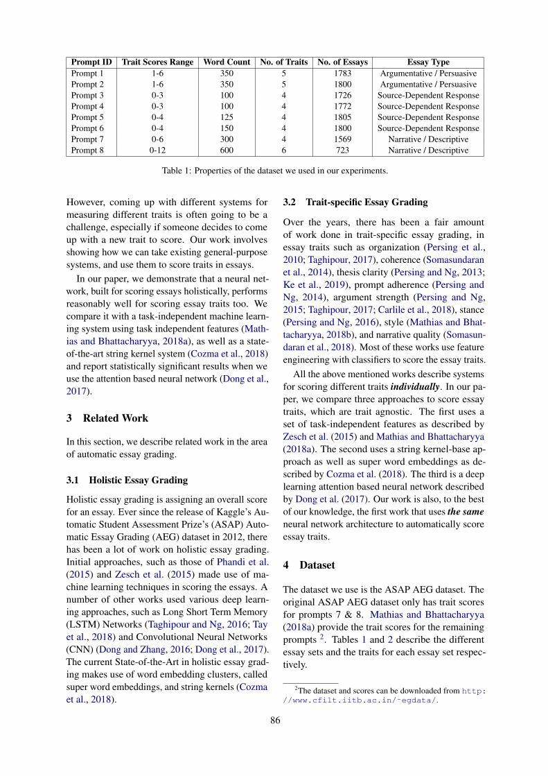
Prompt ID Trait Scores Range Word Count No. of Traits No. of Essays Essay TypePrompt 1 1-6 350 5 1783 Argumentative / PersuasivePrompt 2 1-6 350 5 1800 Argumentative / PersuasivePrompt 3 0-3 100 4 1726 Source-Dependent ResponsePrompt 4 0-3 100 4 1772 Source-Dependent ResponsePrompt 5 0-4 125 4 1805 Source-Dependent ResponsePrompt 6 0-4 150 4 1800 Source-Dependent ResponsePrompt 7 0-6 300 4 1569 Narrative / DescriptivePrompt 8 0-12 600 6 723 Narrative / Descriptive

Table 1: Properties of the dataset we used in our experiments.

However, coming up with different systems formeasuring different traits is often going to be achallenge, especially if someone decides to comeup with a new trait to score. Our work involvesshowing how we can take existing general-purposesystems, and use them to score traits in essays.

In our paper, we demonstrate that a neural net-work, built for scoring essays holistically, performsreasonably well for scoring essay traits too. Wecompare it with a task-independent machine learn-ing system using task independent features (Math-ias and Bhattacharyya, 2018a), as well as a state-of-the-art string kernel system (Cozma et al., 2018)and report statistically significant results when weuse the attention based neural network (Dong et al.,2017).

3 Related Work

In this section, we describe related work in the areaof automatic essay grading.

3.1 Holistic Essay Grading

Holistic essay grading is assigning an overall scorefor an essay. Ever since the release of Kaggle’s Au-tomatic Student Assessment Prize’s (ASAP) Auto-matic Essay Grading (AEG) dataset in 2012, therehas been a lot of work on holistic essay grading.Initial approaches, such as those of Phandi et al.(2015) and Zesch et al. (2015) made use of ma-chine learning techniques in scoring the essays. Anumber of other works used various deep learn-ing approaches, such as Long Short Term Memory(LSTM) Networks (Taghipour and Ng, 2016; Tayet al., 2018) and Convolutional Neural Networks(CNN) (Dong and Zhang, 2016; Dong et al., 2017).The current State-of-the-Art in holistic essay grad-ing makes use of word embedding clusters, calledsuper word embeddings, and string kernels (Cozmaet al., 2018).

3.2 Trait-specific Essay Grading

Over the years, there has been a fair amountof work done in trait-specific essay grading, inessay traits such as organization (Persing et al.,2010; Taghipour, 2017), coherence (Somasundaranet al., 2014), thesis clarity (Persing and Ng, 2013;Ke et al., 2019), prompt adherence (Persing andNg, 2014), argument strength (Persing and Ng,2015; Taghipour, 2017; Carlile et al., 2018), stance(Persing and Ng, 2016), style (Mathias and Bhat-tacharyya, 2018b), and narrative quality (Somasun-daran et al., 2018). Most of these works use featureengineering with classifiers to score the essay traits.

All the above mentioned works describe systemsfor scoring different traits individually. In our pa-per, we compare three approaches to score essaytraits, which are trait agnostic. The first uses aset of task-independent features as described byZesch et al. (2015) and Mathias and Bhattacharyya(2018a). The second uses a string kernel-base ap-proach as well as super word embeddings as de-scribed by Cozma et al. (2018). The third is a deeplearning attention based neural network describedby Dong et al. (2017). Our work is also, to the bestof our knowledge, the first work that uses the sameneural network architecture to automatically scoreessay traits.

4 Dataset

The dataset we use is the ASAP AEG dataset. Theoriginal ASAP AEG dataset only has trait scoresfor prompts 7 & 8. Mathias and Bhattacharyya(2018a) provide the trait scores for the remainingprompts 2. Tables 1 and 2 describe the differentessay sets and the traits for each essay set respec-tively.

2The dataset and scores can be downloaded from http://www.cfilt.iitb.ac.in/˜egdata/.

86

Essay Set List of Essay TraitsPrompt 1 Content, Organization, Word Choice, Sentence Fluency, & ConventionsPrompt 2 Content, Organization, Word Choice, Sentence Fluency, & ConventionsPrompt 3 Content, Prompt Adherence, Language, & NarrativityPrompt 4 Content, Prompt Adherence, Language, & NarrativityPrompt 5 Content, Prompt Adherence, Language, & NarrativityPrompt 6 Content, Prompt Adherence, Language, & NarrativityPrompt 7 Content, Organization, Style, & ConventionsPrompt 8 Content, Organization, Voice, Word Choice, Sentence Fluency & Conventions

Table 2: Traits that are present in each prompt in our dataset. The trait scores are taken from the original ASAPdataset, as well as from ASAP++ (Mathias and Bhattacharyya, 2018a).

5 Experiments

We use the following systems for our experiments:

1. Feature-Engineering System. This is amachine-learning system described by Math-ias and Bhattacharyya (2018a).

2. String Kernels and Superword Embed-dings. This is a state-of-the-art system onholistic essay grading developed by Cozmaet al. (2018) using string kernels and super-word embeddings.

3. Attention-based Neural Network. This is asystem for holistic automatic essay gradingdescribed by Dong et al. (2017), that we adaptfor trait-specific essay grading.

5.1 Baseline Feature-Engineering System

The baseline system we use is the one describedby Mathias and Bhattacharyya (2018a). Their sys-tem used a Random Forest classifier to score theessay traits. The features that they used are lengthbased features (word count, sentence count, sen-tence length, word length), punctuation features(counts of commas, apostrophes, quotations, etc.),syntax features (parse tree depth, number of clauses(denoted by SBAR in the parse tree), etc.), sytlis-tic features (formality, type-token ratio, etc.), co-hesion features (discourse connectives, entity grid(Barzilay and Lapata, 2008)), etc.

5.2 String Kernels and SuperwordEmbeddings

Cozma et al. (2018) showed that using string ker-nels and a bag of super word embeddings dras-tically improved on the state-of-the-art for essaygrading.

5.2.1 String KernelsA string kernel is a similarity function that oper-ates on a pair of strings a and b. The string ker-nel used is the histogram intersection string kernel(HISK(a, b)) that is given by the formula:

HISK(a, b) =∑

min(#x(a),#x(b)),

where HISK(a, b) is the histogram intersectionstring kernel between two strings a and b, and#x(a) and #x(b) is the number of occurrencesof the substring x in the strings a and b.

The string kernel is then normalized as follows:

k(i, j) = k(i,j)√k(i,i)×k(j,j)

,

where k(i, j) is the normalized value of the stringkernel k(i, j) between the strings i and j.

5.2.2 Super Word EmbeddingsA super word embedding is a word embeddingcreated by making a cluster of word embeddings(Cozma et al., 2018). The clusters are created usingthe k means algorithm, with k = 500. For eachessay, we use the count of words in each cluster asfeatures.

5.3 Attention-based Neural NetworkFigure 1 describes the architecture of Dong et al.(2017)’s neural network system. An essay is takenas input and the network outputs the grade for a par-ticular trait. The essay is first split into sentences.For each sentence, we get the embeddings from theword embedding layer. The 4000 most frequentwords are used as the vocabulary, with all the otherwords mapped to a special unknown token.

This sequence of words is given as input to a1-d CNN layer. The output from the CNN layer ispooled using an attention layer, which gets a word-level representation for every sentence in the essay.This is then sent through a sentence-level LSTM

87

Figure 1: Architecture of Dong et al. (2017) neural network system

layer for getting a sentence-level representation ofthe essay.

We send the sentence-level representation of theessay through a sentence-level attention poolinglayer, to get the representation for the essay. Theessay representation is then sent through a Denselayer to score the essay trait. As the scores wereconverted to the range of [0, 1], we use the sigmoidactivation function in the activation layer, mini-mizing the mean squared error loss To evaluatethe system, we convert the trait scores back to theoriginal score range.

We use the 50 dimension GloVe pre-trainedword embeddings (Pennington et al., 2014). We runthe experiments over a batch size of 100, for 100epochs, and set the learning rate as 0.001, and adropout rate of 0.5. The Word-level CNN layer hasa kernel size of 5, with 100 filters. The Sentence-level LSTM layer and modeling layer both have100 hidden units. We use the RMSProp Opti-mizer (Dauphin et al., 2015) with a momentumof 0.9.

5.4 Experimental SetupIn this section, we describe different experiments.

5.4.1 Evaluation MetricWe choose to use Cohen’s Kappa with quadraticweights (Cohen, 1968) - i.e. Quadratic WeightedKappa (QWK) - as the evaluation metric. We usethis as the evaluation metric because of the follow-

ing reasons. Unlike accuracy and F-Score, Kappatakes into account if the classification happened bychance. Secondly, the accuracy and F-score met-rics do not consider the fact that classes here areordered. Thirdly, using weights allows Kappa toconsider ordering among the classes. Lastly, by us-ing quadratic weights, we reward matches and pun-ish mismatches more than linear weights. Hence,we use QWK as the evaluation metric, rather thanaccuracy and F-score.

5.4.2 Evaluation MethodWe evaluate the systems using five-fold cross-validation, with 60% training data, 20% devel-opment data and 20% testing data for each fold.The folds that we use are the same as those used byTaghipour and Ng (2016).

6 Results and Analysis

Table 3 gives the results of the experiments usingthe different classification systems. In each cell, wecompare the results of each of the 3 systems for agiven trait and prompt. The bold value in each cellcorresponds to the system giving the best value outof all the 3 systems. Traits which are not applicableto different prompts are marked with a “—”.

We see that the attention-based neural networksystem is able to outperform both, the baselinesystem of Mathias and Bhattacharyya (2018a) andthe histogram intersection string kernel system of

88

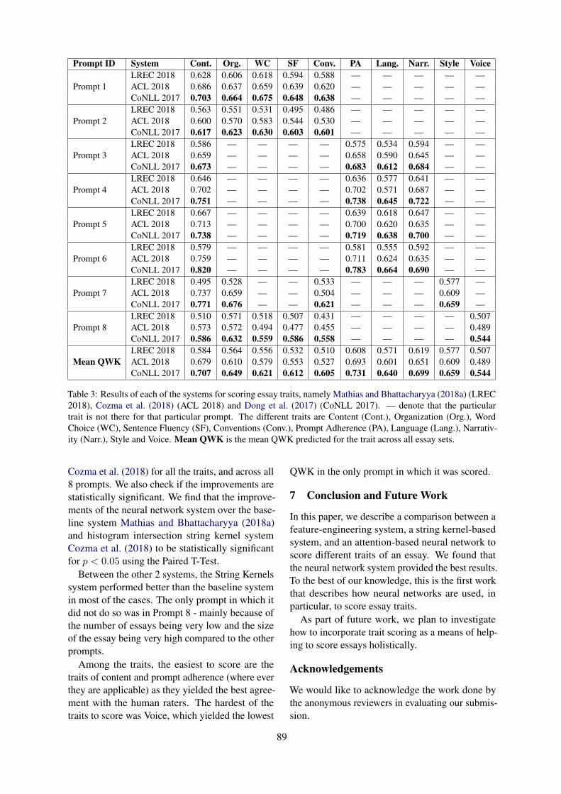
Prompt ID System Cont. Org. WC SF Conv. PA Lang. Narr. Style VoiceLREC 2018 0.628 0.606 0.618 0.594 0.588 — — — — —

Prompt 1 ACL 2018 0.686 0.637 0.659 0.639 0.620 — — — — —CoNLL 2017 0.703 0.664 0.675 0.648 0.638 — — — — —LREC 2018 0.563 0.551 0.531 0.495 0.486 — — — — —

Prompt 2 ACL 2018 0.600 0.570 0.583 0.544 0.530 — — — — —CoNLL 2017 0.617 0.623 0.630 0.603 0.601 — — — — —LREC 2018 0.586 — — — — 0.575 0.534 0.594 — —

Prompt 3 ACL 2018 0.659 — — — — 0.658 0.590 0.645 — —CoNLL 2017 0.673 — — — — 0.683 0.612 0.684 — —LREC 2018 0.646 — — — — 0.636 0.577 0.641 — —

Prompt 4 ACL 2018 0.702 — — — — 0.702 0.571 0.687 — —CoNLL 2017 0.751 — — — — 0.738 0.645 0.722 — —LREC 2018 0.667 — — — — 0.639 0.618 0.647 — —

Prompt 5 ACL 2018 0.713 — — — — 0.700 0.620 0.635 — —CoNLL 2017 0.738 — — — — 0.719 0.638 0.700 — —LREC 2018 0.579 — — — — 0.581 0.555 0.592 — —

Prompt 6 ACL 2018 0.759 — — — — 0.711 0.624 0.635 — —CoNLL 2017 0.820 — — — — 0.783 0.664 0.690 — —LREC 2018 0.495 0.528 — — 0.533 — — — 0.577 —

Prompt 7 ACL 2018 0.737 0.659 — — 0.504 — — — 0.609 —CoNLL 2017 0.771 0.676 — — 0.621 — — — 0.659 —LREC 2018 0.510 0.571 0.518 0.507 0.431 — — — — 0.507

Prompt 8 ACL 2018 0.573 0.572 0.494 0.477 0.455 — — — — 0.489CoNLL 2017 0.586 0.632 0.559 0.586 0.558 — — — — 0.544LREC 2018 0.584 0.564 0.556 0.532 0.510 0.608 0.571 0.619 0.577 0.507

Mean QWK ACL 2018 0.679 0.610 0.579 0.553 0.527 0.693 0.601 0.651 0.609 0.489CoNLL 2017 0.707 0.649 0.621 0.612 0.605 0.731 0.640 0.699 0.659 0.544

Table 3: Results of each of the systems for scoring essay traits, namely Mathias and Bhattacharyya (2018a) (LREC2018), Cozma et al. (2018) (ACL 2018) and Dong et al. (2017) (CoNLL 2017). — denote that the particulartrait is not there for that particular prompt. The different traits are Content (Cont.), Organization (Org.), WordChoice (WC), Sentence Fluency (SF), Conventions (Conv.), Prompt Adherence (PA), Language (Lang.), Narrativ-ity (Narr.), Style and Voice. Mean QWK is the mean QWK predicted for the trait across all essay sets.

Cozma et al. (2018) for all the traits, and across all8 prompts. We also check if the improvements arestatistically significant. We find that the improve-ments of the neural network system over the base-line system Mathias and Bhattacharyya (2018a)and histogram intersection string kernel systemCozma et al. (2018) to be statistically significantfor p < 0.05 using the Paired T-Test.

Between the other 2 systems, the String Kernelssystem performed better than the baseline systemin most of the cases. The only prompt in which itdid not do so was in Prompt 8 - mainly because ofthe number of essays being very low and the sizeof the essay being very high compared to the otherprompts.

Among the traits, the easiest to score are thetraits of content and prompt adherence (where everthey are applicable) as they yielded the best agree-ment with the human raters. The hardest of thetraits to score was Voice, which yielded the lowest

QWK in the only prompt in which it was scored.

7 Conclusion and Future Work

In this paper, we describe a comparison between afeature-engineering system, a string kernel-basedsystem, and an attention-based neural network toscore different traits of an essay. We found thatthe neural network system provided the best results.To the best of our knowledge, this is the first workthat describes how neural networks are used, inparticular, to score essay traits.

As part of future work, we plan to investigatehow to incorporate trait scoring as a means of help-ing to score essays holistically.

Acknowledgements

We would like to acknowledge the work done bythe anonymous reviewers in evaluating our submis-sion.

89

ReferencesYigal Attali and Jill Burstein. 2006. Automated essay

scoring with e-rater R© v. 2. The Journal of Technol-ogy, Learning and Assessment, 4(3).

Regina Barzilay and Mirella Lapata. 2008. Modelinglocal coherence: An entity-based approach. Compu-tational Linguistics, 34(1):1–34.

Winston Carlile, Nishant Gurrapadi, Zixuan Ke, andVincent Ng. 2018. Give me more Feedback: An-notating Argument Persuasiveness and Related At-tributes in Student Essays. In Proceedings of the56th Annual Meeting of the Association for Compu-tational Linguistics (Volume 1: Long Papers), pages621–631. Association for Computational Linguis-tics.

Jacob Cohen. 1968. Weighted kappa: Nominal scaleagreement provision for scaled disagreement or par-tial credit. Psychological bulletin, 70(4):213.

Madalina Cozma, Andrei Butnaru, and Radu TudorIonescu. 2018. Automated essay scoring with stringkernels and word embeddings. In Proceedings ofthe 56th Annual Meeting of the Association for Com-putational Linguistics (Volume 2: Short Papers),pages 503–509, Melbourne, Australia. Associationfor Computational Linguistics.

Yann Dauphin, Harm De Vries, and Yoshua Bengio.2015. Equilibrated adaptive learning rates for non-convex optimization. In Advances in neural infor-mation processing systems, pages 1504–1512.

Fei Dong and Yue Zhang. 2016. Automatic Featuresfor Essay Scoring – An Empirical Study. In Pro-ceedings of the 2016 Conference on Empirical Meth-ods in Natural Language Processing, pages 1072–1077, Austin, Texas. Association for ComputationalLinguistics.

Fei Dong, Yue Zhang, and Jie Yang. 2017. Attention-based Recurrent Convolutional Neural Network forAutomatic Essay Scoring. In Proceedings of the21st Conference on Computational Natural Lan-guage Learning (CoNLL 2017), pages 153–162,Vancouver, Canada. Association for ComputationalLinguistics.

Sylviane Granger, Estelle Dagneaux, Fanny Meunier,and Magali Paquot. 2009. International Corpus ofLearner English.

Zixuan Ke, Hrishikesh Inamdar, Hui Lin, and VincentNg. 2019. Give me more feedback II: Annotat-ing thesis strength and related attributes in studentessays. In Proceedings of the 57th Annual Meet-ing of the Association for Computational Linguis-tics, pages 3994–4004, Florence, Italy. Associationfor Computational Linguistics.

Thomas K Landauer. 2003. Automated scoring and an-notation of essays with the intelligent essay assessor.Automated Essay Scoring: A Cross-disciplinary Per-spective.

Sandeep Mathias and Pushpak Bhattacharyya. 2018a.ASAP++: Enriching the ASAP automated essaygrading dataset with essay attribute scores. In Pro-ceedings of the Eleventh International Conferenceon Language Resources and Evaluation (LREC-2018), Miyazaki, Japan. European Languages Re-sources Association (ELRA).

Sandeep Mathias and Pushpak Bhattacharyya. 2018b.Thank “Goodness”! A Way to Measure Style in Stu-dent Essays. In Proceedings of the 5th Workshop onNatural Language Processing Techniques for Edu-cational Applications, pages 35–41. Association forComputational Linguistics.

Elijah Mayfield and Carolyn Penstein Rose. 2013.LightSIDE: Open source machine learning for text.In Handbook of Automated Essay Evaluation, pages146–157. Routledge.

Ellis B Page. 1966. The imminence of... grading essaysby computer. The Phi Delta Kappan, 47(5):238–243.

Jeffrey Pennington, Richard Socher, and ChristopherManning. 2014. Glove: Global vectors for word rep-resentation. In Proceedings of the 2014 Conferenceon Empirical Methods in Natural Language Process-ing (EMNLP), pages 1532–1543, Doha, Qatar. Asso-ciation for Computational Linguistics.

Isaac Persing, Alan Davis, and Vincent Ng. 2010. Mod-eling Organization in Student Essays. In Proceed-ings of the 2010 Conference on Empirical Methodsin Natural Language Processing, pages 229–239.Association for Computational Linguistics.

Isaac Persing and Vincent Ng. 2013. Modeling The-sis Clarity in Student Essays. In Proceedings of the51st Annual Meeting of the Association for Compu-tational Linguistics (Volume 1: Long Papers), pages260–269, Sofia, Bulgaria. Association for Computa-tional Linguistics.

Isaac Persing and Vincent Ng. 2014. Modeling PromptAdherence in Student Essays. In Proceedings of the52nd Annual Meeting of the Association for Compu-tational Linguistics (Volume 1: Long Papers), pages1534–1543, Baltimore, Maryland. Association forComputational Linguistics.

Isaac Persing and Vincent Ng. 2015. Modeling Argu-ment Strength in Student Essays. In Proceedingsof the 53rd Annual Meeting of the Association forComputational Linguistics and the 7th InternationalJoint Conference on Natural Language Processing(Volume 1: Long Papers), pages 543–552, Beijing,China. Association for Computational Linguistics.

Isaac Persing and Vincent Ng. 2016. Modeling Stancein Student Essays. In Proceedings of the 54th An-nual Meeting of the Association for ComputationalLinguistics (Volume 1: Long Papers), pages 2174–2184, Berlin, Germany. Association for Computa-tional Linguistics.

90

Peter Phandi, Kian Ming A. Chai, and Hwee Tou Ng.2015. Flexible domain adaptation for automated es-say scoring using correlated linear regression. InProceedings of the 2015 Conference on EmpiricalMethods in Natural Language Processing, pages431–439, Lisbon, Portugal. Association for Compu-tational Linguistics.

Mark D Shermis and Jill Burstein. 2013. Handbook ofAutomated Essay Evaluation: Current Applicationsand New Directions. Routledge.

Swapna Somasundaran, Jill Burstein, and MartinChodorow. 2014. Lexical Chaining for MeasuringDiscourse Coherence Quality in Test-taker Essays.In Proceedings of COLING 2014, the 25th Inter-national Conference on Computational Linguistics:Technical Papers, pages 950–961. Dublin City Uni-versity and Association for Computational Linguis-tics.

Swapna Somasundaran, Michael Flor, MartinChodorow, Hillary Molloy, Binod Gyawali,and Laura McCulla. 2018. Towards evaluatingnarrative quality in student writing. Transactionsof the Association for Computational Linguistics,6:91–106.

Kaveh Taghipour. 2017. Robust Trait-Specific EssayScoring Using Neural Networks and Density Estima-tors. Ph.D. thesis, National University of Singapore.

Kaveh Taghipour and Hwee Tou Ng. 2016. A NeuralApproach to Automated Essay Scoring. In Proceed-ings of the 2016 Conference on Empirical Methodsin Natural Language Processing, pages 1882–1891,Austin, Texas. Association for Computational Lin-guistics.

Yi Tay, Minh Phan, Luu Anh Tuan, and Siu CheungHui. 2018. SkipFlow: Incorporating Neural Coher-ence Features for End-to-End Automatic Text Scor-ing. In Proceedings of the 32nd Annual AAAI Con-ference on Artificial Intelligence.

Torsten Zesch, Michael Wojatzki, and Dirk Scholten-Akoun. 2015. Task-independent features for auto-mated essay grading. In Proceedings of the TenthWorkshop on Innovative Use of NLP for Building Ed-ucational Applications, pages 224–232, Denver, Col-orado. Association for Computational Linguistics.

91

Proceedings of the 15th Workshop on Innovative Use of NLP for Building Educational Applications, pages 92–101July 10, 2020. c©2020 Association for Computational Linguistics

Tracking the Evolution of Written Language Competence in L2 SpanishLearners

Alessio Miaschi? �, Sam Davidson•, Dominique Brunato�,Felice Dell’Orletta�, Kenji Sagae•, Claudia H. Sánchez-Gutiérrez•, Giulia Venturi�

?Department of Computer Science, University of Pisa�ItaliaNLP Lab, Istituto di Linguistica Computazionale “Antonio Zampolli”, Pisa

•University of California Davisalessio.miaschi@phd.unipi.it, {ssdavidson,sagae,chsanchez}@ucdavis.edu,{dominique.brunato,felice.dellorletta,giulia.venturi}@ilc.cnr.it

Abstract

In this paper we present an NLP-based ap-proach for tracking the evolution of writtenlanguage competence in L2 Spanish learnersusing a wide range of linguistic features auto-matically extracted from students’ written pro-ductions. Beyond reporting classification re-sults for different scenarios, we explore theconnection between the most predictive fea-tures and the teaching curriculum, finding thatour set of linguistic features often reflects theexplicit instruction that students receive duringeach course.

1 Introduction

In the last few years, research on language acqui-sition has benefited from the use of Natural Lan-guage Processing (NLP) technologies applied tolarge–scale corpora of authentic texts produced bylearners, in both the first and second language con-text. The empirical evidence acquired from learnercorpora, complemented with the increased reliabil-ity of linguistic features extracted by computationaltools and machine learning approaches, has pro-moted a better understanding of learners’ languageproperties and how they change across time and in-creasing proficiency level (Crossley, 2020). A firstline of research has focused on providing automaticways of operationalizing sophisticated metrics oflanguage development to alleviate the laboriousmanual computation of these metrics by experts(Sagae et al., 2005; Lu, 2009). A second line ofresearch has taken the more challenging step ofimplementing completely data-driven approaches,which use a variety of linguistic features extractedfrom texts to automatically assign a learner’s lan-guage production to a given developmental level(Lubetich and Sagae, 2014).

A great amount of work has been carried outin the field of second language acquisition where

the study of L2 writings is seen as a proxy of lan-guage ability development (Crossley, 2020). Inthis respect, much related work is devoted to pre-dicting the degree of second language proficiencyaccording to expert–based evaluation (Crossley andMcNamara, 2012) or to modelling the evolution ofgrammatical structures’ competence with respect topredefined grades, such as the Common EuropeanFramework of Reference for Languages (CEFRL)(Zilio et al., 2018). Given the difficulty of defin-ing a unique indicator of linguistic complexity inthe context of L2 language development, a greatvariety of features from all linguistic levels havebeen used as input for supervised classification sys-tems trained on authentic learner data for differentL2s. Such is the case e.g. of Hancke and Meurers(2013) and Vajjala and Leo (2014), dealing withL2 German and L2 Estonian, respectively, and ofPilán and Volodina (2018), who also provided afeatures analysis focused on predictive features ex-tracted from both receptive and productive texts inSwedish L2.

This paper adopts this framework and presentsan innovative NLP-based stylometric approach tomodel writing development in learners of Spanishas a second and Heritage language. Our approachrelies on a wide set of linguistically motivated fea-tures extracted from students’ essays, which havealready been shown relevant for a number of tasksrelated to modelling the ‘form’ of a text rather thanthe content. While the majority of previous studieson the evolution of language proficiency in L2 usescross–sectional data, this study is the first, to ourknowledge, using a longitudinal corpus of SpanishL2 essays to model writing development. Interest-ingly, a similar approach resulted in the successfulprediction of the development of writing compe-tence in a L1 acquisition scenario for the Italianlanguage (Richter et al., 2015).

Contributions In this paper: (i) we present, to

92

the best of our knowledge, the first data–drivenstudy which uses linguistic features from studentdata to model the evolution of written languagecompetence in Spanish as a Second Language(SSL); (ii) we show that it is possible to automati-cally predict the relative order of two essays writtenby the same student at different course levels us-ing a wide spectrum of linguistic features; (iii) weinvestigate the importance of linguistic features inpredicting language growth at different course lev-els and whether they reflect the explicit instructionthat students receive during each course.

2 Motivation and Approach

Studies of L2 writing have focused on linguisticcomplexity as an indicator of writing development(Lu, 2011; Ortega, 2003). This construct, however,is still ill-defined, as evidenced by the divergentmeasures of complexity utilized in different stud-ies. Typical measures of complexity have beenthe length of the T-unit (Hunt, 1965), the numberof subordinate clauses in a text, or type to tokenratios, among others. Instead of considering theconstruct as being multidimensional (Norris andOrtega, 2009; Bulté and Housen, 2012) and, thus,encompassing an array of different features, moststudies have selected one or two of these measuresand used them as single indicators of complexity(Bulté and Housen, 2014). This has prevented thedevelopment of much needed research that asso-ciates different steps of linguistic and written devel-opment with specific sets of characteristics. Thissituation has also prevented the formation of an in-depth picture of how those specific aspects developin relation to the grammatical, lexical or stylis-tic content taught in classes at different languagecourse levels. This second objective of characteriz-ing writing at different proficiency levels may pro-vide useful insights into how writing samples couldbe used for placement tests or other assessments todetermine which language course is best suited tofurther develop a student’s linguistic skills.

In the concrete case of SSL, the literature indi-cates that one of the most difficult aspects to masterfor learners is the language’s complex verbal mor-phology (Blake and Zyzik, 2016; Salaberry, 1999),given that verbal inflections express a complexcluster of person, number, tense, aspect and mood.Therefore, SSL courses tend to propose a step-by-step introduction to these different aspects of verbalmorphology, generally following this order: (1) per-

son and number in the present indicative, (2) pasttenses (i.e., imperfect vs. preterite vs. pluperfect),and (3) mood (subjunctive vs. indicative). If thistypical instructional sequence had to influence stu-dents’ writing, it would be expected that learnersshow an increase in the variety of inflections thatthey are able to use over time. Nonetheless, sev-eral studies also indicate that a linguistic featurethat has been learned in class may be masteredin exercises that focus on explicit knowledge buttake additional time to unfold in tasks that requiremore implicit knowledge, such as free writing (El-lis and Shintani, 2013). This means that a simpleclassification of students’ proficiency based on thepresence or absence of features studied in a partic-ular course may not be accurate, as some studentsmay explicitly know the rules for a specific inflec-tional distinction but still be unable to use themaccurately in writing. Taking lack of use in writingas evidence for lack of explicit knowledge couldentail that students be mistakenly invited to enrollin courses where those features that do not show intheir writing are unnecessarily explained to themagain. A better approach would thus be to knowwhat students are able to do when they are enrolledin different courses and, only then, compare thoseabilities to see which match, or mismatch, the con-tents seen in that particular class. By using a largeset of linguistic features, it is possible to under-stand which phenomena change across proficiencylevels and whether they are explicitly related to theteaching guidelines.

This study aims at tackling some of the still openmethodological issues in the literature on Spanishacquisition by decomposing the problem into twomain research questions: (i) verify if it is possibleto predict the relative order of two essays writtenby the same student at different course levels usinga wide set of linguistic predictors automatically ex-tracted from Spanish L2 written productions; (ii)understand which typologies of language phenom-ena contribute more to the identification of writingskills’ evolution and whether such properties reflectthe teaching guidelines of the courses.

Following the approach devised in Richter et al.(2015) we addressed the first research question asa classification task: given a pair of essays writ-ten by the same student and ordered accordingto the course level (d1, d2), we classify whetherC(d2) > C(d1), where C(d1) and C(d2) cor-respond respectively to the course levels during

93

Course Level Essays Tokens StudentsBeginner (SPA 1-3) 2,058 485,435 1,130Intermediate (SPA 21-22) 445 120,102 244Composition (SPA 23-24) 536 151,197 287Heritage (SPA 31-33) 459 130,684 244Total 3,498 887,418 1,9051

Table 1: Summary of corpus composition.

Terms Enrolled Students Essays Tokens2 267 984 290,3993 111 612 179,3064 32 242 74,9565 5 48 13,977

Table 2: Longitudinal data summary.

which the student wrote d1 and d2. Specifically, wemodel the problem as a binary classification task,training a Linear Support Vector Machine (Lin-earSVM) to predict the relative order of two essayswritten by the same student using a wide range oflinguistic predictors automatically extracted fromthe POS tagged and dependency parsed essays.We rely on LinearSVM rather than more power-ful learning algorithms, such as Neural LanguageModels, in order to obtain meaningful explanationswhen the classifier outputs its predictions to anchorthe observed patterns of language development toexplicit linguistic evidence.

We further extracted and ranked the featureweights assigned by the linear model in order tounderstand which typology of linguistic featurescontributes more to the classification task at differ-ent course levels. The assumption is that the higherthe weight associated with a specific feature, thegreater its importance in solving the classificationtask and, consequently, in modeling the student’swritten language evolution.

3 Corpus and Features

3.1 The COWS-L2H Corpus

We analyzed development of student writing fromthe Corpus of Written Spanish of L2 and HeritageSpeakers, or COWS-L2H (Davidson et al., 2020).This corpus consists of 3,498 short essays writtenby students enrolled in one of ten lower-divisionSpanish courses at a single American university.Concretely, these courses are organized as follows:Spanish (SPA) 1, 2, and 3 are the introductory

1This number differs from the 1,370 unique participants,as students who participated in more than one category arerepresented twice.

courses, which exposes students to the basic mor-phosyntax of Spanish; SPA 21 and 22 are the in-termediate courses, focused on the developmentof reading and listening skills with a strong em-phasis on lexical development; SPA 23 and 24 aretwo courses that specifically aim at improving writ-ing skills with an emphasis on academic writingin Spanish; SPA 31, 32, and 33 are the Heritagespeakers courses. These courses are grouped intofour categories based on student proficiency andexperience, as shown in Table 1.

Student compositions in the corpus are writ-ten in response to one of four writing prompts,which are changed periodically. During each pe-riod (an academic quarter, which consists of tenweeks of instruction) of data collection, studentsare asked to submit two compositions, approxi-mately one month apart, in response to targetedwriting prompts. These composition themes aredesigned to be relatively broad, to allow for a widedegree of creative liberty and open-ended interpre-tation by the writer. Prompts are intended to beaccessible to writers at all levels of proficiency. Ad-ditionally, the use of broad themes invites the useof a variety of verb tenses and vocabulary. The useof specific writing prompts allows us to control forknown topic effects on syntactic complexity amongL2 learners (Yang et al., 2015).

The essays in the corpus were submitted by1,370 unique student participants, with 415 stu-dent participants having submitted compositions intwo or more academic terms (for a maximum ofeight writing samples from each student). Thus, thecorpus contains both cross-sectional and longitudi-nal data on the development of student writing inthe context of a university language program. Thedistribution of the essays across the levels is un-even due to the distribution of student enrollment inSpanish courses. Because more students enroll inbeginning Spanish courses than in advanced levels,a larger number of essays submitted to the corpuscome from these beginner-level courses. The L2Spanish learners are primarily L1 speakers of En-glish, but due to the diverse student population ofthe source university, a large number are L1 speak-ers of other languages such as Mandarin. However,as English is the university’s language of instruc-tion, all students are either L1 or fluent L2 speakersof English. Those students enrolled in the Heritagecourses (SPA 31 - 33) are, for the most part, L1speakers of Spanish, having learned Spanish from

94

a young age in the home, and L2 speakers of En-glish; these Heritage learners have had little-to-noacademic instruction in Spanish.

We focused our study on the longitudinal datain the COWS-L2H corpus. We were thus able tomodel the chronological development of L2 Span-ish writing by monitoring how the writing qualityof an individual student’s compositions increasewith time. Student participation is summarized inTable 2.

3.2 Linguistic Features

The set of linguistic features considered as predic-tors of L2 written competence evolution is basedon those described in Brunato et al. (2020). It in-cludes a wide range of text properties, from rawtext features, to lexical, morpho-syntactic and syn-tactic properties, which were extracted from dif-ferent levels of linguistic annotation. For this pur-pose, the COWS-L2H Corpus was automaticallyparsed using UDPipe (Straka et al., 2016) trainedon the Spanish Universal Dependency Treebank(GSD section), version 2.5. We rely on these fea-tures since it has been shown that they have a highpredictive power for several tasks all aimed at mod-elling the linguistic form of documents. This isthe case for example of the automatic readabilityassessment task (Dell’Orletta et al., 2011a), of theautomatic classification of the textual genre of doc-uments (Cimino et al., 2017), or also of the auto-matic identification of the L1 of a writer based onhis/her language production in a L2 (Cimino et al.,2018). Interestingly, for all mentioned tasks the setof linguistic features plays a very important role inthe classification not only of a whole document butalso of each single sentence. This is the reason why,as reported in the following sections, we modelledthe prediction of the development of writing skillsboth as document and sentence classification tasks.

Although we used a state–of–the art pipeline, itis well-acknowledged that the accuracy of statis-tical parsers decreases when tested against textsof a different typology from that used in training(Gildea, 2001). In this respect, learners’ data areparticularly challenging for general–purpose textanalysis tools since they can exhibit deviation fromcorrect and standard language; for instance, miss-ing or anomalous use of punctuation (especially in1st grade prompts) already impacts on the coarsestlevels of text processing, i.e. sentence splitting, andthus may affect all subsequent levels of annotation.

Nevertheless, if we can expect that the predictedvalue of a given feature might be different fromthe real one (especially for features extracted frommore complex levels of annotation such as syntax),we can also assume that the distributions of errorswill be almost similar, at least when parsing textsof the same domain. Note also that the reliability offeatures checked against automatically annotateddata was also empirically shown by Dell’Orlettaet al. (2011b), who compared morpho-syntacticand syntactic features extracted from a gold (i.e.manually annotated) and an automatically anno-tated corpus of the same domain (i.e. biomedicallanguage), showing that results are highly compa-rable.

As shown in Table 3, the considered featurescapture linguistic phenomena ranging from the av-erage length of document, sentences and words,to morpho-syntactic information such as parts ofspeech (POS) distribution and fine–grained featuresabout the inflectional properties of verbs. Morecomplex phenomena are derived from syntactic an-notation and model global and local properties ofparsed tree structure, with a focus on subtrees ofverbal heads, the order of subjects and objects withrespect to the verb, the distribution of Universal De-pendencies (UD) syntactic relations and featuresreferring to the use of subordination.

Since it is acknowledged that lexical profi-ciency plays an important role in predicting L2writing development (Crossley and McNamara,2012), we also decided to add a small subsetof features that model this property in termsof word frequency. Specifically, we consideredthe average class frequency of all word formsand lemmas in the essays (Words FrequencyClass), where the class frequency for each wordform/lemma was computed exploiting the Span-ish Wikipedia (dump of March 2020) using thefollowing measures: Ccw = blog2 freq(MFW )

freq(CW ) c,

Ccl = blog2 freq(MFL)freq(CL) c, where MFW and MFL

are the most frequent word form/lemma in the cor-pus and CW and CL are the considered ones.

A first overview of how and to what extent allthese features vary across the documents of theCOWS-L2H Corpus is provided in Table 4. Es-says written by students in the first course levelsare longer in terms of number of sentences butthey contain shorter sentences compared with thosewritten in the more advanced courses. As con-cerns the distribution of POS, essays written in the

95

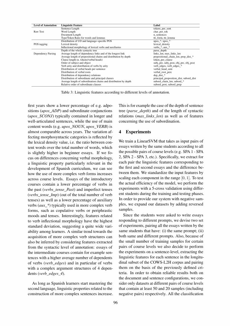
Level of Annotation Linguistic Feature Label

Raw TextSentence Length tokens_per_sentWord Length char_per_tokDocument Length n_sentencesType/Token Ratio for words and lemmas ttr_form, ttr_lemma

POS taggingDistribution of UD and language–specific POS upos_*, xpos_*Lexical density lexical_densityInflectional morphology of lexical verbs and auxiliaries verbs_*, aux_*

Dependency ParsingDepth of the whole syntactic tree parse_depthAverage length of dependency links and of the longest link links_len, max_links_lenAverage length of prepositional chains and distribution by depth prepositional_chain_len, prep_dist_*Clause length (n. tokens/verbal heads) token_per_clauseOrder of subject and object subj_pre, subj_post, obj_pre, obj_postVerb arity and distribution of verbs by arity verb_edges, verb_edges_*Distribution of verbal heads per sentence verbal_head_sentDistribution of verbal roots verbal_root_percDistribution of dependency relations dep_dist_*Distribution of subordinate and principal clauses principal_proposition_dist, subord_distAverage length of subordination chains and distribution by depth subord_chain_len, subord_*Relative order of subordinate clauses subord_post, subord_prep

Table 3: Linguistic features according to different levels of annotation.

first years show a lower percentage of e.g. adpo-sitions (upos_ADP) and subordinate conjunctions(upos_SCONJ) typically contained in longer andwell-articulated sentences, while the use of maincontent words (e.g. upos_NOUN, upos_VERB) isalmost comparable across years. The variation af-fecting morphosyntactic categories is reflected bythe lexical density value, i.e. the ratio between con-tent words over the total number of words, whichis slightly higher in beginner essays. If we fo-cus on differences concerning verbal morphology,a linguistic property particularly relevant in thedevelopment of Spanish curriculum, we can seehow the use of more complex verb forms increasesacross course levels. Essays of the introductorycourses contain a lower percentage of verbs inthe past (verbs_tense_Past) and imperfect tenses(verbs_tense_Imp) (out of the total number of verbtenses) as well as a lower percentage of auxiliaryverbs (aux_*) typically used in more complex verbforms, such as copulative verbs or periphrasticmoods and tenses. Interestingly, features relatedto verb inflectional morphology have the higheststandard deviation, suggesting a quite wide vari-ability among learners. A similar trend towards theacquisition of more complex verb structures canalso be inferred by considering features extractedfrom the syntactic level of annotation: essays ofthe intermediate courses contain for example sen-tences with a higher average number of dependentsof verbs (verb_edges) and in particular of verbswith a complex argument structures of 4 depen-dents (verb_edges_4).

As long as Spanish learners start mastering thesecond language, linguistic properties related to theconstruction of more complex sentences increase.

This is for example the case of the depth of sentencetree (parse_depth) and of the length of syntacticrelations (max_links_len) as well as of featuresconcerning the use of subordination.

4 Experiments

We train a LinearSVM that takes as input pairs ofessays written by the same students according to allthe possible pairs of course levels (e.g. SPA 1 - SPA2, SPA 2 - SPA 3, etc.). Specifically, we extract foreach pair the linguistic features corresponding tothe first and second essays and the difference be-tween them. We standardize the input features byscaling each component in the range [0, 1]. To testthe actual efficiency of the model, we perform theexperiments with a 5-cross validation using differ-ent students during the training and testing phases.In order to provide our system with negative sam-ples, we expand our datasets by adding reversedsamples.

Since the students were asked to write essaysresponding to different prompts, we devise two setof experiments, pairing all the essays written by thesame students that have: (i) the same prompt; (ii)both same and different prompts. Also, because ofthe small number of training samples for certainpairs of course levels we also decide to performthe experiments on a sentence-level, extracting thelinguistic features for each sentence in the longitu-dinal subset of the COWS-L2H corpus and pairingthem on the basis of the previously defined cri-teria. In order to obtain reliable results both onthe document and sentence configurations, we con-sider only datasets at different pairs of course levelsthat contain at least 50 and 20 samples (includingnegative pairs) respectively. All the classification

96

Features SPA 1 SPA 2 SPA 3 SPA 21 SPA 22 SPA 23 SPA 24 SPA 31 SPA 32 SPA 33Raw Text Properties

char_per_tok 4.3 ±.27 4.4 ±.27 4.42 ±.26 4.42 ±.26 4.43 ±.25 4.46 ±.23 4.41 ±.22 4.42 ±.25 4.42 ±.28 4.38 ±.3n_sentences 20.0 ±7.0 24.01 ±7.15 23.57 ±6.87 20.8 ±5.99 20.17 ±5.15 19.54 ±6.33 17.92 ±5.44 16.06 ±4.05 16.31 ±3.78 15.46 ±3.63tokens_per_sent 10.7 ±3.43 13.16 ±3.52 13.74 ±3.7 15.71 ±3.95 16.43 ±3.59 17.11 ±3.49 19.01 ±4.27 19.95 ±4.16 20.07 ±3.48 20.94 ±4.04

Morphosyntactic informationlexical_density .51 ±.05 .5 ±.04 .5 ±.04 .49 ±.03 .48 ±.04 .48 ±.03 .47 ±.03 .48 ±.04 .47 ±.04 .47 ±.04upos_ADJ .07 ±.03 .06 ±.02 .06 ±.02 .06 ±.02 .05 ±.02 .05 ±.02 .05 ±.02 .05 ±.02 .05 ±.02 .05 ±.02upos_ADP .09 ±.04 .1 ±.03 .11 ±.03 .11 ±.02 .11 ±.02 .12 ±.02 .12 ±.02 .13 ±.03 .12 ±.02 .13 ±.02upos_NOUN .16 ±.04 .16 ±.03 .16 ±.03 .16 ±.03 .16 ±.03 .17 ±.02 .17 ±.03 .17 ±.02 .16 ±.03 .16 ±.03upos_PRON .07 ±.04 .07 ±.03 .07 ±.03 .07 ±.03 .07 ±.03 .07 ±.03 .07 ±.03 .07 ±.03 .08 ±.04 .08 ±.04upos_PUNCT .14 ±.03 .13 ±.03 .12 ±.03 .12 ±.03 .11 ±.03 .11 ±.03 .11 ±.03 .09 ±.02 .09 ±.02 .09 ±.02upos_SCONJ .01 ±.01 .02 ±.01 .03 ±.01 .03 ±.02 .04 ±.02 .04 ±.01 .04 ±.02 .04 ±.02 .05 ±.02 .05 ±.02upos_VERB .12 ±.04 .12 ±.03 .12 ±.03 .12 ±.02 .12 ±.02 .12 ±.02 .12 ±.02 .13 ±.02 .13 ±.02 .13 ±.03

Inflectional morphologyaux_mood_Cnd .02 ±.09 .03 ±.09 .04 ±.12 .03 ±.07 .06 ±.11 .05 ±.11 .04 ±.08 .05 ±.09 .06 ±.12 .04 ±.11aux_mood_Ind .97 ±.14 .96 ±.12 .92 ±.15 .94 ±.14 .91 ±.13 .92 ±.14 .94 ±.1 .91 ±.16 .91 ±.12 .93 ±.12aux_mood_Sub .01 ±.04 .01 ±.04 .03 ±.07 .02 ±.05 .03 ±.05 .02 ±.08 .03 ±.06 .03 ±.06 .03 ±.06 .03 ±.05aux_tense_Imp .05 ±.16 .16 ±.25 .21 ±.26 .21 ±.25 .24 ±.25 .24 ±.26 .22 ±.24 .23 ±.28 .2 ±.27 .24 ±.29aux_tense_Past .02 ±.09 .1 ±.15 .09 ±.15 .12 ±.16 .12 ±.14 .11 ±.15 .12 ±.16 .11 ±.16 .12 ±.17 .11 ±.13aux_tense_Pres .92 ±.21 .73 ±.32 .69 ±.33 .65 ±.32 .63 ±.3 .65 ±.32 .66 ±.32 .63 ±.34 .66 ±.34 .63 ±.33verbs_tense_Imp .02 ±.06 .08 ±.12 .11 ±.13 .13 ±.13 .16 ±.14 .14 ±.15 .13 ±.13 .17 ±.15 .15 ±.15 .14 ±.14verbs_tense_Past .11 ±.19 .28 ±.23 .28 ±.22 .3 ±.2 .35 ±.22 .3 ±.22 .31 ±.19 .31 ±.21 .28 ±.18 .33 ±.19

Verbal Predicate Structureverb_edges 2.3 ±.36 2.5 ±.32 2.52 ±.3 2.62 ±.35 2.67 ±.28 2.63 ±.28 2.7 ±.32 2.71 ±.29 2.68 ±.26 2.76 ±.27verb_edges_4 .09 ±.08 .13 ±.07 .13 ±.07 .16 ±.07 .16 ±.07 .15 ±.08 .16 ±.07 .16 ±.06 .16 ±.06 .16 ±.07verbal_head_sent 1.52 ±.46 1.8 ±.53 1.92 ±.52 2.13 ±.54 2.26 ±.54 2.3 ±.51 2.54 ±.61 2.73 ±.58 2.86 ±.65 2.95 ±.66

Global and Local Parsed Tree Structuresparse_depth 2.88 ±.65 3.27 ±.62 3.37 ±.61 3.6 ±.63 3.78 ±.55 3.94 ±.64 4.21 ±.69 4.49 ±.65 4.59 ±.67 4.56 ±.62max_links_len .65 ±.44 .7 ±.45 .72 ±.42 .96 ±.74 .92 ±.43 .99 ±.42 1.2 ±.68 1.24 ±.53 1.21 ±.42 1.39 ±.725rtoken_per_clause 7.17 ±1.56 7.49 ±1.58 7.28 ±1.39 7.52 ±1.51 7.41 ±1.26 7.55 ±1.26 7.62 ±1.24 7.42 ±1.3 7.16 ±1.09 7.26 ±1.32

Order of elementsobj_post .67 ±.18 .68 ±.15 .67 ±.15 .64 ±.16 .65 ±.15 .69 ±.13 .69 ±.14 .6 ±.17 .64 ±.17 .6 ±.16obj_pre .33 ±.18 .32 ±.15 .33 ±.15 .35 ±.15 .35 ±.15 .31 ±.13 .31 ±.14 .39 ±.16 .36 ±.17 .4 ±.16subj_pre .8 ±.19 .84 ±.15 .82 ±.15 .84 ±.15 .84 ±.13 .84 ±.13 .83 ±.13 .81 ±.12 .78 ±.13 .79 ±.14

Use of Subordinationsubord_chain_len 1.06 ±.25 1.15 ±.16 1.18 ±.14 1.21 ±.18 1.24 ±.15 1.24 ±.14 1.26 ±.16 1.29 ±.23 1.33 ±.16 1.32 ±.2subord_2 .08 ±.14 .11 ±.11 .13 ±.1 .15 ±.11 .17 ±.1 .17 ±.11 .18 ±.11 .19 ±.11 .2 ±.1 .2 ±.1subord_dist .24 ±.14 .33 ±.13 .38 ±.12 .4 ±.12 .44 ±.12 .47 ±.12 .5 ±.12 .56 ±.12 .58 ±.08 .57 ±.1

Table 4: A subset of linguistic features extracted for each course level. For each feature it is reported the averagevalue and the standard deviation.

experiments are performed using the majority classclassifier as baseline and accuracy as the evaluationmetric.

4.1 Tracking Writing Skills’ Evolution

Table 5 reports the results obtained at both thedocument and sentence levels, pairing essays thathave the same prompt (Same columns) and boththe same and different prompts (All columns). As ageneral remark, we observe that best results arethose obtained with the document-level experi-ments. This is quite expected, since sentence-levelclassification is a more complex task that oftenrequires a higher number of features to gain com-parable accuracy (Dell’Orletta et al., 2014). If wefocus instead on the distinction between Same andAll results, we notice that higher scores are mainlyachieved considering pairs of essays that also havedifferent prompts. Again, this result is not sur-prising because adding pairs of essays with dif-ferent prompts within each datasets increases thenumber of training samples, thus leading to betterscores. Despite this, the results obtained accord-ing to the Same and All configurations are quitesimilar and this allows us to confirm that classifi-cation accuracy is not significantly harmed if thetwo essay’s prompts are the same, thus showing

that our system is actually focusing on written lan-guage competence evolution properties rather thanprompt-dependent characteristics.

More interestingly, we notice that consideringall the possible course level pairs at the same timeour system is able to achieve quite good results, es-pecially at document level classification (0.68 and0.70 of accuracy for Same and All configurationsrespectively), thus showing that it is possible to au-tomatically predict the chronological order of twoessays written by the same student by using a widespectrum of linguistic properties.

In general, our best scores are obtained by con-sidering all the experiments that include essayswritten by students in the Beginner category (SPA1, 2 and 3). This is particularly evident for theexperiments that compare essays written duringSPA 1 as one of the two considered course levels,most likely because the evolution from knowingnothing at all of a specific L2 to knowing enoughto start writing is actually bigger that the differ-ence between knowing a little and then learninga little more. Additionally, students at this begin-ning stage of L2 acquisition tend to use markedlyfewer words per sentence, and the words they userare shorter; these features are particularly salientfor the classifier. Observing instead the results ob-

97

Course Levels Documents SentencesSame All Same All

Score Samples Score Samples Score Samples Score SamplesAll Levels 0.68 2,208 0.7 5,536 0.59 1,047,156 0.61 2,570,366SPA 1 - SPA 2 0.88 280 0.9 624 0.7 143,660 0.71 316,264SPA 1 - SPA 3 0.97 178 0.95 440 0.75 85,032 0.75 209,048SPA 1 - SPA 21 # # 0.91 116 0.61 14,298 0.7 46,738SPA 2 - SPA 3 0.62 528 0.62 1,192 0.56 323,332 0.56 724,400SPA 2 - SPA 21 0.61 62 0.61 188 0.57 35,754 0.58 104,442SPA 2 - SPA 22 # # 0.59 68 0.55 8,048 0.63 29,670SPA 2 - SPA 23 # # 0.77 52 # # 0.58 27,420SPA 3 - SPA 21 0.59 158 0.55 364 0.53 82,104 0.54 190,596SPA 3 - SPA 22 0.61 64 0.58 186 0.54 31,886 0.6 93,486SPA 3 - SPA 23 # # 0.89 106 0.59 13,404 0.59 45,804SPA 3 - SPA 24 # # # # # # 0.68 11,276SPA 21 - SPA 22 0.59 132 0.62 302 0.52 57,326 0.54 132,454SPA 21 - SPA 23 0.52 58 0.74 154 0.54 27,038 0.57 67,634SPA 21 - SPA 24 # # 0.7 92 0.47 9,268 0.56 35,384SPA 22 - SPA 23 0.71 76 0.69 186 0.55 35,272 0.56 79,168SPA 22 - SPA 24 0.69 158 0.73 164 0.5 23,446 0.56 66,184SPA 23 - SPA 24 0.45 168 0.49 386 0.48 61,654 0.49 137,786SPA 31 - SPA 32 0.8 100 0.63 212 0.55 27,608 0.55 57,790SPA 31 - SPA 33 0.52 100 0.53 198 0.51 24,830 0.48 48,990SPA 32 - SPA 33 0.54 96 0.59 256 0.5 24,154 0.55 66,466

Table 5: Classification results in terms of accuracy obtained both at document and sentence levels along withnumber of samples for each dataset. Same and All columns report the results obtained by pairing essays that havesame prompt and both same and different prompts respectively. Since the labels within each dataset has beenbalanced, baseline accuracy is 0.50.

tained pairing student essays belonging to the otherthree course level categories (Intermediate, Com-position and Heritage), we notice a considerabledrop in classifier performance. For instance, if wecompare essays written by students in the Compo-sition category (SPA 23 - SPA 24) we can see thatall the classification results are below the majorityclass baseline classifier. A possible reason mightbe that these two courses are specifically aimed atimproving learners’ writing skills, with an empha-sis on academic writing in Spanish, thus involvingspecific properties, such as discourse-level charac-teristics, which are possibly not covered by our setof features.

4.2 Understanding Linguistic Predictors

Beyond classification results, we were interested inunderstanding which typologies of linguistic phe-nomena are more important for solving the classifi-cation task and whether such properties correlateto the teaching curriculum. To better explore thissecond research question, we perform a featureranking analysis along with the classification ex-periments, which allows us to establish a ranking ofthe most important features according to the differ-ent classification scenarios. That is, we evaluate theimportance of each linguistic property by extract-ing and ranking the feature weights assigned by the

LinearSVM. Table 6 reports the feature rankingsobtained with sentence-level classification results,including pairs of essays that have the same prompt(Same configuration). We considered in particularsix different course level pairs which are mostlyrepresentative of different stages of writing devel-opment. The focus on sentence-level results ratherthan document-level allows capturing more fine-grained linguistic phenomena.

Because the COWS-L2H corpus was collectedfrom a single university with set curriculum, weare able to compare the features utilized by theLinearSVM with the course curriculum. We findthat the feature rankings as obtained from the Lin-earSVM can in many cases be explained by dif-ferences in curriculum at each level. For example,from SPA 1 to SPA 2 the most important featuresused by the model are all related to verbal morphol-ogy, particularly morphology of auxiliary verbs.This can be explained by the fact that SPA 1 and2 are the courses where students are introducedfor the first time to the notions of verb tense andperson. SPA 1 is focused on managing the idea ofperson and number in a tense that is not particularlydifficult to understand for a speaker of English: thepresent tense. SPA 2, however, introduces the dif-ficult difference between the three tenses in thepast: imperfect, preterite and plus-perfect. This

98

SPA 1 - SPA 2 SPA 1 - SPA 3 SPA 2 - SPA 3 SPA 3 - SPA 21 SPA 22 - SPA 23 SPA 31 - SPA 32aux_mood_Ind lexical_density * aux_tense_dist_Pres * lexical_density upos_PUNCT upos_ADP *aux_tense_Pres * upos_ADP * aux_mood_Ind upos_DET dep_punct dep_case *aux_tense_Imp * upos_VERB * aux_tense_Imp * dep_punct upos_ADV verbal_head_sentaux_tense_Past * upos_NOUN * aux_tense_Past upos_VERB dep_advmod upos_PUNCTupos_ADP * upos_ADJ dep_punct * aux_tense_Pres upos_CCONJ upos_PRONverbs_tense_Past * upos_PRON upos_PUNCT * upos_ADJ dep_cc * dep_markupos_VERB * dep_det dep_nsubj * upos_NOUN upos_VERB dep_punctupos_INTJ * upos_PUNCT * dep_iobj dep_nsubj * dep_case aux_tense_Impverbal_head_sent * upos_PROPN upos_PRON upos_PRON aux_form_Part verbs_tense_Presverbs_tense_Imp * dep_case * verbal_head_sent * upos_SCONJ upos_ADP subord_distupos_ADJ * upos_SCONJ * dep_cop upos_ADV * dep_mark dep_copttr_form upos_AUX subj_post * upos_PUNCT dep_compound dep_ccupos_PRON * dep_punct * aux_form_Fin aux_form_Fin upos_INTJ * lexical_densityupos_PROPN * subord_dist * verbs_tense_Imp * dep_cc * dep_nsubj * upos_AUXupos_PUNCT * upos_CCONJ * upos_AUX aux_tense_Imp upos_AUX upos_ADV

Table 6: Feature rankings obtained with sentence-level (Same) classification results for six different course levelpairs. Features that vary in a statistically significant way with Wilcoxon Rank-Sum test are marked with *.

fact explains why distribution of past tense mainverbs (verbs_tense_Past) differs between essayswritten during SPA 1 and SPA 2. Additionally, SPA2 introduces composed verb tenses that require anauxiliary. Specifically, the auxiliary verbs “haber”,“estar”, and “ser” are introduced in SPA 2 as partof the past tense forms. Thus, it is not surprisingthat the top four features used by our classifier fordistinguishing between essays written in SPA 1 andSPA 2 are related to the use of auxiliary verbs.

Classification of essays written by students whileenrolled in SPA 2 and SPA 3 also relies largely ondifferences in verbal morphology. While the distri-bution of present tense auxiliary verbs is the mostimportant distinguishing feature, other compoundverb tenses play a role at these levels. For example,differences in the distribution of imperfect auxil-iary verbs (aux_tense_Imp) may be explained bythe use of the pluperfect tense.

Between SPA 1 and SPA 3, the most importantdiscriminating feature is lexical density. Whilethere is no specific focus on lexical density in thecourse curriculum, this feature is a natural exten-sion of increasing sentence complexity. David-son et al. (2019) shows that as students progressthrough the Spanish course sequence, lexical den-sity tends to decrease due to the increased use offunction words in more complex sentences. Addi-tionally, one of the final items covered in the SPA1 curriculum is the use of the prepositions “por”and “para”. Also, at all three beginning levels stu-dents are taught to use prepositions in constructingmore complex sentence structures. This may ex-plain why preposition usage (upos_ADP) is a keydiscriminating feature between essays written in

SPA 1 and SPA2, as well as between SPA 1 andSPA 3. The prominence of this feature indicatesthat students are learning to more confidently useprepositions as their writing skills develop. Thefact that (upos_ADP) is not a key discriminatingfeature between SPA 2 and SPA3 indicates thatthese changes are occurring primarily at the SPA 2level, which accords with the course curriculum.

In spite of the still reasonable accuracy in dis-criminating more advanced levels, making a directconnection between the features used by the SVMand the course curriculum becomes more difficult.At these more advanced levels students have de-veloped an individual writing style which resultsin a more complex relationship between the cur-riculum and the syntax used by students. At theSPA 3 - SPA 21 interval, the only three featureswhich vary in a statistically significant way arethe distributions of nominal subjects (dep_nsubj),adverbs (upos_ADV), and coordinating conjunc-tions (dep_cc). While the increased use of adverbsmay be seen as a general sign of increased writingcomplexity, coordinating conjunctions are taughtexplicitly during SPA 3. Conjunctions are alsopracticed intensively during both SPA 21 and SPA22 explaining their importance as a discriminatingfeature between these levels.

One of the clearest connections between curricu-lum and the features used by the LinearSVM occursat the Heritage levels SPA 31 and SPA 32. Heritagelearners of Spanish raised in an English-dominantcountry are known to use “English-like” preposi-tions in Spanish. For example, Pascual y Caboand Soler (2015) report on preposition stranding(which is grammatical in English by ungrammatical

99

in Spanish) among Heritage speakers of Spanishin the United States. We find that distributionaldifferences in the use of prepositions, representedby the features upos_ADP and dep_case, is the keydistinguishing feature between essays written bythe same student during SPA 31 and SPA 32. Thisdifference indicates that students are learning touse prepositions in a more “Spanish-like” manner,which is one of the major areas of feedback whichinstructors provide to Heritage students.

5 Conclusion

We present a first study aimed at modeling the evo-lution of written language competence in Span-ish as a Second and Heritage Language, usingdata from the COWS-L2H Corpus. We have de-scribed a rich set of linguistic features automat-ically extracted from student writing, and havedemonstrated that it is possible to automaticallypredict the relative order of two essays written bythe same student at different course levels usingthese features, especially when considering stu-dents enrolled in beginner-level Spanish courses.Finally, we have shown that the linguistic featuresmost important in predicting essay order often re-flect the explicit instruction that students receiveduring each course.

This work can help instructors and language re-searchers better understand the specific linguisticfactors which contribute to improved writing profi-ciency. Additionally, the appearance of features inthe LinearSVM ranking helps clarify the effect ofinstruction on writing performance, specifically oneffects such as the known delay between studentsbeing taught a concept and that concept appearingin the students’ writing. We also believe that thiswork may contribute to the development of betterlanguage assessment and placement tools.

In future work we intend to explore the influenceof student L1 on feature rankings, as L1 (and L2)transfer and interference effects may influence therate at which students acquire specific linguisticfeatures. Additionally we plan to conduct a cross-lingual analysis, investigating how the feature rank-ings we see in Spanish writing development relateto those seen in the acquisition of other languages.

Acknowledgments

Reported research started in the framework ofa Short Term Mobility program of internationalexchanges funded by CNR. This work was also

funded in part by the UC Davis Grant for Collabo-rative Interdisciplinary Research and by a gift fromMicrosoft Azure.

ReferencesRobert J Blake and Eve C Zyzik. 2016. El espanol y la

linguistica aplicada. Georgetown University Press.

Dominique Brunato, Andrea Cimino, FeliceDell’Orletta, Giulia Venturi, and SimonettaMontemagni. 2020. Profiling-ud: a tool for linguis-tic profiling of texts. In Proceedings of The 12thLanguage Resources and Evaluation Conference,pages 7147–7153, Marseille, France. EuropeanLanguage Resources Association.

Bram Bulté and Alex Housen. 2012. Defining andoperationalising L2 complexity. Dimensions of L2performance and proficiency: Complexity, accuracyand fluency in SLA, pages 23–46.

Bram Bulté and Alex Housen. 2014. Conceptualiz-ing and measuring short-term changes in L2 writ-ing complexity. Journal of second language writing,26:42–65.

Diego Pascual y Cabo and Inmaculada Soler. 2015.Preposition Stranding in Spanish as a Heritage Lan-guage. Heritage Language Journal, 12:186–209.

A. Cimino, F. Dell’Orletta, D. Brunato, and G. Ven-turi. 2018. Sentences and Documents in Native Lan-guage Identification. In Proceedings of 5th ItalianConference on Computational Linguistics (CLiC-it),pages 1–6, Turin.

A. Cimino, M. Wieling, F. Dell’Orletta, S. Monte-magni, and G. Venturi. 2017. Identifying Predic-tive Features for Textual Genre Classification: theKey Role of Syntax. In Proceedings of 4th ItalianConference on Computational Linguistics (CLiC-it),pages 1–6, Rome.

Scott Crossley. 2020. Linguistic features in writingquality and development: An overview. Journal ofWriting Research.

Scott A Crossley and Danielle S McNamara. 2012. Pre-dicting second language writing proficiency: Theroles of cohesion and linguistic sophistication. Jour-nal of Research in Reading, 35(2):115–135.

Sam Davidson, Aaron Yamada, Agustina Carando,Kenji Sagae, and Claudia Sánchez Gutiérrez. 2019.Word use and lexical diversity in second languagelearners and heritage speakers of spanish: A corpusstudy. In American Association for Applied Linguis-tics.

Sam Davidson, Aaron Yamada, Paloma Fer-nandez Mira, Agustina Carando, Claudia H.Sanchez Gutierrez, and Kenji Sagae. 2020. Devel-oping nlp tools with a new corpus of learner spanish.

100

In Proceedings of The 12th Language Resourcesand Evaluation Conference, pages 7240–7245,Marseille, France. European Language ResourcesAssociation.

F. Dell’Orletta, S. Montemagni, and G. Venturi. 2011a.READ-IT: assessing readability of Italian texts witha view to text simplification. In Proceedings of Sec-ond Workshop on Speech and Language Processingfor Assistive Technologies, pages 73–83, Edinburgh,UK.

Felice Dell’Orletta, Giulia Venturi, and SimonettaMontemagni. 2011b. Ulisse: an unsupervised algo-rithm for detecting reliable dependency parses. InCoNLL.

Felice Dell’Orletta, Martijn Wieling, Giulia Venturi,Andrea Cimino, and Simonetta Montemagni. 2014.Assessing the readability of sentences: which cor-pora and features? In Proceedings of the NinthWorkshop on Innovative Use of NLP for Building Ed-ucational Applications, pages 163–173.

Rod Ellis and Natsuko Shintani. 2013. Exploring lan-guage pedagogy through second language acquisi-tion research. Routledge.

Daniel Gildea. 2001. Corpus variation and parser per-formance. In Proceedings of the 2001 Conferenceon Empirical Methods in Natural Language Process-ing.

Julia Hancke and Detmar Meurers. 2013. ExploringCEFR classification for German based on rich lin-guistic modeling. In Proceedings of the LearnerCorpus Research (LCR) conference.

K. W. Hunt. 1965. Grammatical structures written atthree grade levels. (NCTE Research Report Number3). Urbana, IL: National Council of Teachers of En-glish.

Xiaofei Lu. 2009. Automatic measurement of syntacticcomplexity in child language acquisition. In Interna-tional Journal of Corpus Linguistics, 14(1):3–28.

Xiaofei Lu. 2011. A corpus-based evaluation of syntac-tic complexity measures as indices of college-levelESL writers’ language development. TESOL quar-terly, 45(1):36–62.

Shannon Lubetich and Kenji Sagae. 2014. Data-drivenmeasurement of child language development withsimple syntactic templates. In Proceedings of COL-ING 2014, the 25th International Conference onComputational Linguistics: Technical Papers, pages2151–2160.

John Norris and Lourdes Ortega. 2009. Measurementfor understanding: An organic approach to inves-tigating complexity, accuracy, and fluency in SLA.Applied Linguistics, 30(4):555–578.

Lourdes Ortega. 2003. Syntactic complexity measuresand their relationship to l2 proficiency: A researchsynthesis of college-level l2 writing. Applied lin-guistics, 24(4):492–518.

Ildikó Pilán and Elena Volodina. 2018. Investigat-ing the importance of linguistic complexity featuresacross different datasets related to language learning.In Proceedings of the Workshop on Linguistic Com-plexity and Natural Language Processing, pages 49–58, Santa Fe, New-Mexico. Association for Compu-tational Linguistics.

Stefan Richter, Andrea Cimino, Felice Dell’Orletta,and Giulia Venturi. 2015. Tracking the Evolutionof Written Language Competence: an NLP–basedApproach. CLiC it, page 236.

Kenji Sagae, Alon Lavie, and Brian MacWhinney.2005. Automatic measurement of syntactic devel-opment in child language. In Proceedings of the43rd Annual Meeting of the Association for Compu-tational Linguistics, pages 197–204. Association forComputational Linguistics.

M Rafael Salaberry. 1999. The development of pasttense verbal morphology in classroom L2 spanish.Applied Linguistics, 20(2):151–178.

M. Straka, J. Hajic, and J. Strakova. 2016. UD-Pipe: Trainable pipeline for processing CoNLL-Ufiles performing tokenization, morphological analy-sis, POS tagging and parsing. In Proceedings ofthe Tenth International Conference on Language Re-sources and Evaluation (LREC).

Sowmya Vajjala and Kaidi Leo. 2014. AutomaticCEFR Level Prediction for Estonian Learner Text.In NEALT Proceedings Series Vol. 22, pages 113–127.

Weiwei Yang, Xiaofei Lu, and Sara Cushing Weigle.2015. Different topics, different discourse: Rela-tionships among writing topic, measures of syntacticcomplexity, and judgments of writing quality. Jour-nal of Second Language Writing, 28:53–67.

Leonardo Zilio, Rodrigo Wilkens, and Cédrick Fairon.2018. An SLA corpus annotated with pedagogicallyrelevant grammatical structures. In Proceedings ofthe Eleventh International Conference on LanguageResources and Evaluation (LREC-2018), Miyazaki,Japan. European Languages Resources Association(ELRA).

101

Proceedings of the 15th Workshop on Innovative Use of NLP for Building Educational Applications, pages 102–114July 10, 2020. c©2020 Association for Computational Linguistics

Distractor Analysis and Selection for Multiple-Choice Cloze Questionsfor Second-Language Learners

Lingyu Gao1, Kevin Gimpel1, Arnar Jensson2

1Toyota Technological Institute at Chicago, 2Cooori Japan{lygao, kgimpel}@ttic.edu

Abstract

We consider the problem of automatically sug-gesting distractors for multiple-choice clozequestions designed for second-language learn-ers. We describe the creation of a dataset in-cluding collecting manual annotations for dis-tractor selection. We assess the relationshipbetween the choices of the annotators and fea-tures based on distractors and the correct an-swers, both with and without the surroundingpassage context in the cloze questions. Sim-ple features of the distractor and correct an-swer correlate with the annotations, though wefind substantial benefit to additionally usinglarge-scale pretrained models to measure thefit of the distractor in the context. Based onthese analyses, we propose and train models toautomatically select distractors, and measurethe importance of model components quantita-tively.

1 Introduction

Multiple-choice cloze questions (MCQs) arewidely used in examinations and exercises for lan-guage learners (Liang et al., 2018). The quality ofMCQs depends not only on the question and choiceof blank, but also on the choice of distractors, i.e.,incorrect answers. Distractors, which could bephrases or single words, are incorrect answers thatdistract students from the correct ones.

According to Pho et al. (2014), distractors tendto be syntactically and semantically homogeneouswith respect to the correct answers. Distractor se-lection may be done manually through expert cura-tion or automatically using simple methods basedon similarity and dissimilarity to the correct answer(Pino et al., 2008; Alsubait et al., 2014). Intuitively,optimal distractors should be sufficiently similarto the correct answers in order to challenge stu-dents, but not so similar as to make the questionunanswerable (Yeung et al., 2019). However, past

work usually lacks direct supervision for training,making it difficult to develop and evaluate auto-matic methods. To overcome this challenge, Lianget al. (2018) sample distractors as negative sam-ples for the candidate pool in the training process,and Chen et al. (2015) sample questions and usemanual annotation for evaluation.

In this paper, we build two datasets of MCQsfor second-language learners with distractor selec-tions annotated manually by human experts. Bothdatasets consist of instances with a sentence, ablank, the correct answer that fills the blank, and aset of candidate distractors. Each candidate distrac-tor has a label indicating whether a human annota-tor selected it as a distractor for the instance. Thefirst dataset, which we call MCDSENT, containssolely the sentence without any additional context,and the sentences are written such that they areunderstandable as standalone sentences. The sec-ond dataset, MCDPARA, contains sentences drawnfrom an existing passage and therefore also sup-plies the passage context.

To analyze the datasets, we design context-freefeatures of the distractor and the correct answer,including length difference, embedding similari-ties, frequencies, and frequency rank differences.We also explore context-sensitive features, suchas probabilities from large-scale pretrained modelslike BERT (Devlin et al., 2018). In looking at theannotations, we found that distractors are unchosenwhen they are either too easy or too hard (i.e., toogood of a fit in the context). Consider the examplesin Table 1. For the sentence “The large automobilemanufacturer has a factory near here.”, “beer” istoo easy and “corporation” is too good of a fit, soboth are rejected by annotators. We find that theBERT probabilities capture this tendency; that is,there is a nonlinear relationship between the dis-tractor probability under BERT and the likelihoodof annotator selection.

102

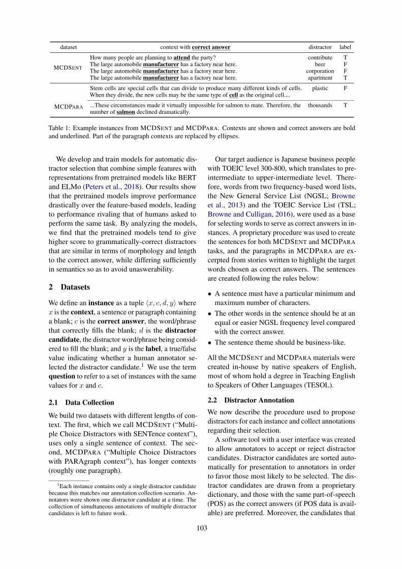
dataset context with correct answer distractor label

MCDSENT

How many people are planning to attend the party? contribute TThe large automobile manufacturer has a factory near here. beer FThe large automobile manufacturer has a factory near here. corporation FThe large automobile manufacturer has a factory near here. apartment T

MCDPARA

Stem cells are special cells that can divide to produce many different kinds of cells.When they divide, the new cells may be the same type of cell as the original cell....

plastic F

...These circumstances made it virtually impossible for salmon to mate. Therefore, thenumber of salmon declined dramatically.

thousands T

Table 1: Example instances from MCDSENT and MCDPARA. Contexts are shown and correct answers are boldand underlined. Part of the paragraph contexts are replaced by ellipses.

We develop and train models for automatic dis-tractor selection that combine simple features withrepresentations from pretrained models like BERTand ELMo (Peters et al., 2018). Our results showthat the pretrained models improve performancedrastically over the feature-based models, leadingto performance rivaling that of humans asked toperform the same task. By analyzing the models,we find that the pretrained models tend to givehigher score to grammatically-correct distractorsthat are similar in terms of morphology and lengthto the correct answer, while differing sufficientlyin semantics so as to avoid unaswerability.

2 Datasets

We define an instance as a tuple 〈x, c, d, y〉 wherex is the context, a sentence or paragraph containinga blank; c is the correct answer, the word/phrasethat correctly fills the blank; d is the distractorcandidate, the distractor word/phrase being consid-ered to fill the blank; and y is the label, a true/falsevalue indicating whether a human annotator se-lected the distractor candidate.1 We use the termquestion to refer to a set of instances with the samevalues for x and c.

2.1 Data Collection

We build two datasets with different lengths of con-text. The first, which we call MCDSENT (“Multi-ple Choice Distractors with SENTence context”),uses only a single sentence of context. The sec-ond, MCDPARA (“Multiple Choice Distractorswith PARAgraph context”), has longer contexts(roughly one paragraph).

1Each instance contains only a single distractor candidatebecause this matches our annotation collection scenario. An-notators were shown one distractor candidate at a time. Thecollection of simultaneous annotations of multiple distractorcandidates is left to future work.

Our target audience is Japanese business peoplewith TOEIC level 300-800, which translates to pre-intermediate to upper-intermediate level. There-fore, words from two frequency-based word lists,the New General Service List (NGSL; Browneet al., 2013) and the TOEIC Service List (TSL;Browne and Culligan, 2016), were used as a basefor selecting words to serve as correct answers in in-stances. A proprietary procedure was used to createthe sentences for both MCDSENT and MCDPARA

tasks, and the paragraphs in MCDPARA are ex-cerpted from stories written to highlight the targetwords chosen as correct answers. The sentencesare created following the rules below:

• A sentence must have a particular minimum andmaximum number of characters.• The other words in the sentence should be at an

equal or easier NGSL frequency level comparedwith the correct answer.• The sentence theme should be business-like.

All the MCDSENT and MCDPARA materials werecreated in-house by native speakers of English,most of whom hold a degree in Teaching Englishto Speakers of Other Languages (TESOL).

2.2 Distractor AnnotationWe now describe the procedure used to proposedistractors for each instance and collect annotationsregarding their selection.

A software tool with a user interface was createdto allow annotators to accept or reject distractorcandidates. Distractor candidates are sorted auto-matically for presentation to annotators in orderto favor those most likely to be selected. The dis-tractor candidates are drawn from a proprietarydictionary, and those with the same part-of-speech(POS) as the correct answers (if POS data is avail-able) are preferred. Moreover, the candidates that

103

have greater similarity to the correct answers arepreferred, such as being part of the same wordlearning section in the language learning courseand the same NGSL word frequency bucket. Thereis also preference for candidates that have not yetbeen selected as distractors for other questions inthe same task type and the same course unit.2 Afterthe headwords are decided through this procedure,a morphological analyzer is used to generate multi-ple inflected forms for each headword, which areprovided to the annotators for annotation. Both theheadwords and inflected forms are available whencomputing features and for use by our models.

Six annotators were involved in the annotation,all of whom are native speakers of English. Outof the six, four hold a degree in TESOL. Select-ing distractors involved two-step human selection.An annotator would approve or reject distractorcandidates suggested by the tool, and a differentannotator, usually more senior, would review theirselections. The annotation guidelines for MCD-SENT and MCDPARA follow the same criteria.The annotators are asked to select distractors thatare grammatically plausible, semantically implausi-ble, and not obviously wrong based on the context.Annotators also must accept a minimum numberof distractors depending on the number of timesthe correct answer appears in the course. Table 1shows examples from MCDSENT and MCDPARA

along with annotations.

2.3 Annotator Agreement

Some instances in the datasets have multiple anno-tations, allowing us to assess annotator agreement.We use the term “sample” to refer to a set of in-stances with the same x, c, and d. Table 2 shows thenumber of samples with agreement and disagree-ment for both datasets.3 Samples with only oneannotation dominate the data. Of the samples withmultiple annotations, nearly all show agreement.

2.4 Distractor Phrases

While most distractors are words, some are phrases,including 16% in MCDSENT and 13% in MCD-PARA. In most cases, the phrases are constructedby a determiner or adverb (“more”, “most”, etc.)and another word, such as “most pleasant” or

2More specific details about this process are included inthe supplementary material.

3We are unable to compute traditional inter-annotatoragreement metrics like Cohen’s kappa since we lack infor-mation about annotator identity for each annotation.

# anno. MCDSENT MCDPARAagree disagree total agree disagree total

1 - - 232256 - - 7340632 2553 122 2675 9680 152 98413 121 2 123 493 3 4964 17 0 17 62 0 625 10 0 10 12 0 126 0 0 0 2 0 2

Table 2: Numbers of samples for which annotatorsagree or disagree.

dataset type y train dev test

MCDSENTquestions - 2,713 200 200

instances T 30,737 1,169 1,046F 191,908 6,420 6,813

MCDPARAquestions - 14,999 1,000 1,000

instances T 49,575 597 593F 688,804 7,620 8,364

Table 3: Dataset sizes in numbers of questions (a“question” is a set of instances with the same x and c)and instances, broken down by label (y) and data split.

“more recently”. However, some candidates showother patterns, such as noun phrases “South Pole”,erroneously-inflected forms “come ed” and otherphrases (e.g. “Promises Of”, “No one”).

2.5 Dataset Preparation

We randomly divided each dataset into train, devel-opment, and test sets. We remind the reader thatwe define a “question” as a set of instances withthe same values for the context x and correct an-swer c, and in splitting the data we ensure that fora given question, all of its instances are placed intothe same set. The dataset statistics are shown inTable 3. False labels are much more frequent thantrue labels, especially for MCDPARA.

3 Features and Analysis

We now analyse the data by designing features andstudying their relationships with the annotations.

3.1 Features

We now describe our features. The dataset con-tains both the headwords and inflected forms ofboth the correct answer c and each distractor can-didate d. In defining the features below based onc and d for an instance, we consider separate fea-tures for the headword pair and the inflected formpair. For features that require embedding words,we use the 300-dimensional GloVe word embed-

104

dings (Pennington et al., 2014) pretrained on the 42billion token Common Crawl corpus. The GloVeembeddings are provided in decreasing order byfrequency, and some features below use the linenumbers of words in the GloVe embeddings, whichcorrespond to frequency ranks. For words that arenot in the GloVe vocabulary, their frequency ranksare |N | + 1, where N is the size of the GloVevocabulary. We use the four features listed below:

• length difference: absolute value of length dif-ference (in characters, including whitespace) be-tween c and d.

• embedding similarity: cosine similarity of theembeddings of c and d. For phrases, we averagethe embeddings of the words in the phrase.

• distractor frequency: negative log frequencyrank of d. For phrases, we take the max rank ofthe words (i.e., the rarest word is chosen).

• freq. rank difference: feature capturing fre-quency difference between c and d, i.e., log(1 +|rc − rd|) where rw is the frequency rank of w.

3.2 Label-Specific Feature Histograms

Figure 1 shows histograms of feature values foreach label.4 Since the data is unbalanced, the his-tograms are “label-normalized”, i.e., normalizedso that the sum of heights for each label is 1. So,we can view each bar as the fraction of that label’sinstances with feature values in the given range.

The annotators favor candidates that have ap-proximately the same length as the correct answers(Fig. 1, plot 1), as the true bars are much higher inthe first bin (length difference 0 or 1). Selected dis-tractors have moderate embedding similarity to thecorrect answers (Fig. 1, plot 2). If cosine similarityis very high or very low, then those distractors aremuch less likely to be selected. Such distractors arepresumably too difficult or too easy, respectively.

Selected distractors are moderately frequent(Fig. 1, plot 3). Very frequent and very infrequentdistractors are less likely to be selected. Distrac-tors with small frequency rank differences (thoseon the left of plot 4) are more likely to be chosen(Fig. 1, plot 4). Large frequency differences tend tobe found with very rare distractors, some of whichmay be erroneously-inflected forms.

We also computed Spearman correlations be-tween feature values and labels, mapping the T/F

4We show plots here for the inflected form pairs; those forheadword pairs are included in the supplementary material.

Figure 1: Label-specific feature histograms for MCD-SENT.

labels to 1/0. Aside from what are shown in thefeature histograms, we find that a distractor with arare headword but more common inflected form ismore likely to be selected, at least for MCDSENT.The supplementary material contains more detailon these correlations.

3.3 Probabilities of Distractors in Context

We use BERT (Devlin et al., 2018) to computeprobabilities of distractors and correct answers inthe given contexts in MCDSENT. We insert a masksymbol in the blank position and compute the prob-ability of the distractor or correct answer at thatposition.5 Figure 2 shows histograms for correctanswers and distractors (normalized by label). The

5For distractors with multiple tokens, we mask each posi-tion in turn and use the average of the probabilities.

105

Figure 2: Histograms of BERT log-probabilities ofselected distractors (“T”), unselected distractors (“F”),and correct answers (“c”) in MCDSENT.

correct answers have very high probabilities. Thedistractor probabilities are more variable and theshapes of the histograms are roughly similar for thetrue and false labels. Interestingly, however, whenthe probability is very high or very low, the distrac-tors tend to not be selected. The selected distractorstend to be located at the middle of the probabilityrange. This pattern shows that BERT’s distribu-tions capture (at least partially) the nonlinear rela-tionship between goodness of fit and suitability asdistractors.

4 Models

Since the number of distractors selected for each in-stance is uncertain, our datasets could be naturallytreated as a binary classification task for each dis-tractor candidate. We now present models for thetask of automatically predicting whether a distrac-tor will be selected by an annotator. We approachthe task as defining a predictor that produces ascalar score for a given distractor candidate. Thisscore can be used for ranking distractors for a givenquestion, and can also be turned into a binary clas-sification using a threshold. We define three typesof models, described in the subsections below.

4.1 Feature-Based Models

Using the features described in Section 3, we builda simple feed-forward neural network classifier thatoutputs a scalar score for classification. Only in-flected forms of words are used for features withoutcontexts, and all features are concatenated and usedas the input of the classifier. For features that useBERT, we compute the log-probability of the dis-tractor and the log of its rank in the distribution.For distractors that consist of multiple subwordunits, we mask each individually to compute theabove features for each subword unit, then use the

Figure 3: Illustration of the ELMo-based model MELMo,where semicolon refers to vector concatenation.

concatenation of mean, min, and max pooling ofthe features over the subword units. We refer tothis model as Mfeat.

4.2 ELMo-Based ModelsWe now describe models that are based onELMo (Peters et al., 2018) which we denoteMELMo. Since MCDPARA instances contain para-graph context, which usually includes more thanone sentence, we denote the model that uses thefull context by MELMo(`). By contrast, MELMo usesonly a single sentence context for both MCDSENT

and MCDPARA. We denote the correct answerby c, distractor candidate by d, the word sequencebefore the blank by wp, and the word sequence af-ter the blank by wn, using the notation rev(wn) toindicate the reverse of the sequence wn.

We use GloVe (Pennington et al., 2014) to ob-tain pretrained word embeddings for context words,then use two separate RNNs with gated recurrentunits (GRUs; Cho et al., 2014) to output hiddenvectors to represent wp and wn. We reverse wn

before passing it to its GRU, and we use the lasthidden states of the GRUs as part of the classifierinput. We also use ELMo to obtain contextualizedword embeddings for correct answers and distrac-tors in the given context, and concatenate them tothe input. An illustration of this model is presentedin Figure 3.

A feed-forward network (FFN) with 1 ReLUhidden layer is set on top of these features to getthe score for classification:

FFN (z) = max(0, zW1 + b1)W2 + b2

where z is a row vector representing the inputsshown in Figure 3. We train the model as a binaryclassifier by using a logistic sigmoid function on

106

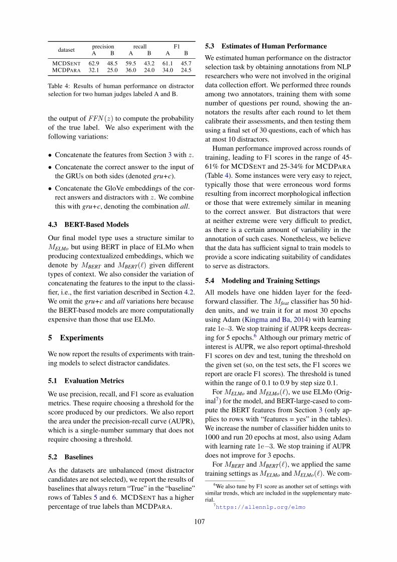
dataset precision recall F1A B A B A B

MCDSENT 62.9 48.5 59.5 43.2 61.1 45.7MCDPARA 32.1 25.0 36.0 24.0 34.0 24.5

Table 4: Results of human performance on distractorselection for two human judges labeled A and B.

the output of FFN (z) to compute the probabilityof the true label. We also experiment with thefollowing variations:

• Concatenate the features from Section 3 with z.

• Concatenate the correct answer to the input ofthe GRUs on both sides (denoted gru+c).

• Concatenate the GloVe embeddings of the cor-rect answers and distractors with z. We combinethis with gru+c, denoting the combination all.

4.3 BERT-Based Models

Our final model type uses a structure similar toMELMo but using BERT in place of ELMo whenproducing contextualized embeddings, which wedenote by MBERT and MBERT(`) given differenttypes of context. We also consider the variation ofconcatenating the features to the input to the classi-fier, i.e., the first variation described in Section 4.2.We omit the gru+c and all variations here becausethe BERT-based models are more computationallyexpensive than those that use ELMo.

5 Experiments

We now report the results of experiments with train-ing models to select distractor candidates.

5.1 Evaluation Metrics

We use precision, recall, and F1 score as evaluationmetrics. These require choosing a threshold for thescore produced by our predictors. We also reportthe area under the precision-recall curve (AUPR),which is a single-number summary that does notrequire choosing a threshold.

5.2 Baselines

As the datasets are unbalanced (most distractorcandidates are not selected), we report the results ofbaselines that always return “True” in the “baseline”rows of Tables 5 and 6. MCDSENT has a higherpercentage of true labels than MCDPARA.

5.3 Estimates of Human PerformanceWe estimated human performance on the distractorselection task by obtaining annotations from NLPresearchers who were not involved in the originaldata collection effort. We performed three roundsamong two annotators, training them with somenumber of questions per round, showing the an-notators the results after each round to let themcalibrate their assessments, and then testing themusing a final set of 30 questions, each of which hasat most 10 distractors.

Human performance improved across rounds oftraining, leading to F1 scores in the range of 45-61% for MCDSENT and 25-34% for MCDPARA

(Table 4). Some instances were very easy to reject,typically those that were erroneous word formsresulting from incorrect morphological inflectionor those that were extremely similar in meaningto the correct answer. But distractors that wereat neither extreme were very difficult to predict,as there is a certain amount of variability in theannotation of such cases. Nonetheless, we believethat the data has sufficient signal to train models toprovide a score indicating suitability of candidatesto serve as distractors.

5.4 Modeling and Training SettingsAll models have one hidden layer for the feed-forward classifier. The Mfeat classifier has 50 hid-den units, and we train it for at most 30 epochsusing Adam (Kingma and Ba, 2014) with learningrate 1e−3. We stop training if AUPR keeps decreas-ing for 5 epochs.6 Although our primary metric ofinterest is AUPR, we also report optimal-thresholdF1 scores on dev and test, tuning the threshold onthe given set (so, on the test sets, the F1 scores wereport are oracle F1 scores). The threshold is tunedwithin the range of 0.1 to 0.9 by step size 0.1.

For MELMo and MELMo(`), we use ELMo (Orig-inal7) for the model, and BERT-large-cased to com-pute the BERT features from Section 3 (only ap-plies to rows with “features = yes” in the tables).We increase the number of classifier hidden units to1000 and run 20 epochs at most, also using Adamwith learning rate 1e−3. We stop training if AUPRdoes not improve for 3 epochs.

For MBERT and MBERT(`), we applied the sametraining settings as MELMo and MELMo(`). We com-

6We also tune by F1 score as another set of settings withsimilar trends, which are included in the supplementary mate-rial.

7https://allennlp.org/elmo

107

model variant development set test set BERT features best thresholdprecision recall F1 AUPR precision recall F1 AUPR epoch

baseline 15.4 100 26.7 - 13.3 100 23.5 - - - - -

33.6 62.9 43.8 36.5 23.7 55.4 33.2 24.6 none yes 28 0.2Mfeat 44.5 57.1 50.0 46.1 28.2 70.9 40.3 32.4 base yes 25 0.2 (0.3)

36.4 77.8 49.6 47.0 30.0 71.3 42.2 34.5 large yes 22 0.2

none 43.2 87.5 57.8 59.0 41.4 88.0 56.3 54.6 - no 2 0.3gru+c 44.8 84.4 58.5 57.4 47.6 68.4 56.1 54.1 - no 2 0.3 (0.4)

MELMoall 47.2 88.9 61.7 61.2 48.3 75.0 58.7 55.8 - no 2 0.3 (0.4)

none 51.7 77.8 62.1 64.6 50.4 76.5 60.8 57.2 large yes 3 0.3gru+c 55.7 73.3 63.3 65.3 49.1 82.3 61.5 63.1 large yes 5 0.4 (0.3)all 56.2 74.4 64.0 66.5 49.8 80.8 61.6 58.8 large yes 5 0.4 (0.3)

47.9 78.1 59.4 60.8 44.8 81.0 57.7 55.7 base no 1 0.3

MBERT49.6 79.3 61.0 64.1 45.3 80.2 57.9 53.4 large no 1 0.350.6 83.9 63.2 65.3 44.8 78.5 57.0 53.8 base yes 12 0.153.8 73.1 62.0 66.5 49.7 73.9 59.4 56.3 large yes 2 0.4

Table 5: Results for MCDSENT. Boldface indicates the best F1/AUPR on dev/test for each model type. Weinclude the threshold tuned on the test set in parentheses when it differs from the threshold tuned on dev.

model development set test set BERT features best epoch thresholdprecision recall F1 AUPR precision recall F1 AUPR

baseline 7.3 100 13.5 - 6.6 100 12.4 - - - - -

15.3 63.1 24.6 17.3 14.5 63.6 23.6 15.5 - yes 23 0.1Mfeat 18.2 69.2 28.9 21.6 16.3 65.6 26.1 19.1 base yes 27 0.1

19.8 64.0 30.2 22.3 16.9 64.2 26.8 18.8 large yes 22 0.1

MELMo35.4 47.7 40.7 38.4 26.1 75.6 38.8 30.4 - no 5 0.3 (0.2)37.9 61.3 46.9 46.8 34.6 63.9 44.9 37.6 large yes 7 0.3

MELMo(`)30.5 61.1 40.7 36.6 29.1 61.6 39.5 33.2 - no 5 0.337.1 62.7 46.6 43.7 34.4 65.1 45.0 40.1 large yes 6 0.3

35.4 61.6 45.0 40.9 29.2 58.7 39.0 30.1 base no 2 0.2

MBERT33.0 63.7 43.5 40.9 29.1 65.1 40.2 32.4 large no 2 0.244.3 55.4 49.3 47.3 31.5 73.2 44.0 36.7 base yes 2 0.3 (0.2)35.6 66.0 46.2 45.0 35.5 54.5 43.0 36.6 large yes 2 0.2 (0.3)

MBERT(`)33.1 65.3 43.9 39.7 28.8 66.4 40.2 29.8 base no 2 0.237.4 67.3 48.1 46.0 31.3 69.1 43.1 37.0 base yes 2 0.2

Table 6: Results for MCDPARA.

pare the BERT-base-cased and BERT-large-casedvariants of BERT. When doing so, the BERT fea-tures from Section 3 use the same BERT variant asthat used for contextualized word embeddings.

For all models based on pretrained models, wekeep the parameters of the pretrained models fixed.However, we do a weighted summation of the 3layers of ELMo, and all layers of BERT except forthe first layer, where the weights are trained duringthe training process.

5.5 ResultsWe present our main results for MCDSENT in Ta-ble 5 and for MCDPARA in Table 6.

Feature-based models. The feature-basedmodel, shown as Mfeat in the upper parts of the

tables, is much better than the trivial baseline.Including the BERT features in Mfeat improvesperformance greatly (10 points in AUPR forMCDSENT), showing the value of using thecontext effectively with a powerful pretrainedmodel. There is not a large difference betweenusing BERT-base and BERT-large when computingthese features.

ELMo-based models. Even without features,MELMo outperforms Mfeat by a wide margin.Adding features to MELMo further improves F1 by2-5% for MCDSENT and 5-6% for MCDPARA.The F1 score for MELMo on MCDSENT is closeto human performance, and on MCDPARA theF1 score outperforms humans (see Table 4). For

108

MCDSENT, we also experiment with using the cor-rect answer as input to the context GRUs (gru+c),and additionally concatenating the GloVe embed-dings of the correct answers and distractors to theinput of the classifier (all). Both changes improveF1 on dev, but on test the results are more mixed.

BERT-based models. For MBERT, using BERT-base is sufficient to obtain strong results on this taskand is also cheaper computationally than BERT-large. Although MBERT with BERT-base has higherAUPR on dev, its test performance is close toMELMo. Adding features improves performancefor MCDPARA (3-5% F1), but less than the im-provement found for MELMo. While Mfeat is aidedgreatly when including BERT features, the fea-tures have limited impact on MBERT, presumablybecause it already incorporates BERT in its model.

Long-context models. We now discuss resultsfor the models that use the full context in MCD-PARA, i.e., MELMo(`) and MBERT(`). On dev,MELMo and MBERT outperform MELMo(`) andMBERT(`) respectively, which suggests that the ex-tra context for MCDPARA is not helpful. However,the test AUPR results are better when using thelonger context, suggesting that the extra contextmay be helpful for generalization. Nonetheless,the overall differences are small, suggesting thateither the longer context is not important for thistask or that our way of encoding the context is nothelpful. The judges in our manual study (Sec. 5.3)rarely found the longer context helpful for the task,pointing toward the former possibility.

5.6 Statistical Significance TestsFor better comparison of these models’ perfor-mances, a paired bootstrap resampling method isapplied (Koehn, 2004). We repeatedly sample withreplacement 1000 times from the original test setwith sample size equal to the corresponding test setsize, and compare the F1 scores of two models. Weuse the thresholds tuned by the development set forF1 score computations, and assume significance ata p value of 0.05.

• For MELMo, MELMo(`), MBERT and MBERT(`),the models with features are significantly betterthan their feature-less counterparts (p < 0.01).8

• When both models use features, MELMo(`) isalmost the same as MELMo (p = 0.477). How-8We only use BERT-base-cased for MBERT(`) due to com-

putational considerations.

ever, when both do not use features, MELMo(`)is significantly better (p < 0.01).• When using BERT-base-cased, MBERT(`) is bet-

ter than MBERT, but not significantly so (p = 0.4with features and 0.173 without features).• On MCDPARA, switching from BERT-base to

BERT-large does not lead to a significant differ-ence for MBERT without features (BERT-largeis better with p = 0.194) or MBERT with fea-tures (BERT-base is better with p = 0.504). ForMCDSENT, MBERT with BERT-large is betterboth with and without features (p < 0.2).• On MCDPARA, MBERT(`) outperformsMELMo(`) without features but not signifi-cantly. With features, MELMo(`) is better withp = 0.052.• On MCDSENT, MBERT without features (BERT-

large-cased) is better than MELMo without fea-tures, but not significantly so (p = 0.386). How-ever, if we add features or use MBERT withBERT-base-cased, MELMo is significantly better(p < 0.01).• On MCDPARA, MELMo is nearly significantly

better than MBERT when both use features (p =0.062). However, dropping the features for bothmodels makes MBERT significantly outperformMELMo (p = 0.044).

5.7 ExamplesFigure 4 shows an example question from MCD-SENT, i.e., “The bank will notify its customers ofthe new policy”, and two subsets of its distractors.The first subset consists of the top seven distractorsusing scores from MELMo with features, and the sec-ond contains distractors further down in the rankedlist. For each model, we normalize its distractorscores with min-max normalization.9

Overall, model rankings are similar across mod-els, with all distractors in the first set ranked higherthan those in the second set. The high-rankingbut unselected distractors (“spell”, “consult”, and“quit”) are likely to be reasonable distractors forsecond-language learners, even though they werenot selected by annotators.

We could observe the clustering of distractorranks with similar morphological inflected formin some cases, which may indicate that the modelmakes use of the grammatical knowledge of pre-trained models.

9Given original data x, we use (x−min(x))/(max(x)−min(x)) to normalize it.

109

Figure 4: Ranks of distractors for question “The bank will notify its customers of the new policy.” The colorsrepresent the normalized scores of the models and the numbers in the cells are the ranks of the candidates.

6 Related Work

Existing approaches to distractor selection useWordNet (Fellbaum, 1998) metrics (Mitkov andHa, 2003; Chen et al., 2015), word embedding sim-ilarities (Jiang and Lee, 2017), thesauruses (Sumitaet al., 2005; Smith et al., 2010), and phoneticand morphological similarities (Pino and Eskenazi,2009). Other approaches consider grammatical cor-rectness, and introduce structural similarities in anontology (Stasaski and Hearst, 2017), and syntac-tic similarities (Chen et al., 2006). When usingbroader context, bigram or n-gram co-occurrence(Susanti et al., 2018; Hill and Simha, 2016), contextsimilarity (Pino et al., 2008), and context sensitiveinference (Zesch and Melamud, 2014) have alsobeen applied to distractor selection.

Based on these heuristic features, Liang et al.(2018) assemble these features and apply neuralnetworks, training the model to predict the answerswithin a lot of candidates. Yeung et al. (2019)further applies BERT for ranking distractors bymasking the target word. As we have two manuallyannotated datasets that have different lengths ofcontexts, we adopt both word pair features and thecontext-specific distractor probabilities to build ourfeature-based models. Moreover, we build bothELMo-based and BERT-based models, combiningthem with our features and measuring the impactof these choices on performance.

7 Conclusion

We described two datasets with annotations of dis-tractor selection for multiple-choice cloze ques-tions for second-language learners. We designedfeatures and developed models based on pretrainedlanguage models. Our results show that the task

is challenging for humans and that the strongestmodels are able to approach or exceed human per-formance. The rankings of distractors providedby our models appear reasonable and can reduce agreat deal of human burden in distractor selection.Future work will use our models to collect addi-tional training data which can then be refined in asecond pass by limited human annotation. Otherfuture work can explore the utility of features de-rived from pretrained question answering modelsin scoring distractors.

ReferencesTahani Alsubait, Bijan Parsia, and Uli Sattler. 2014.

Generating multiple choice questions from ontolo-gies: Lessons learnt. In OWLED, pages 73–84. Cite-seer.

C. Browne and B. Culligan. 2016. The TOEIC ServiceList. http://www.newgeneralservicelist.org.

C. Browne, B. Culligan, and J. Phillips. 2013.The New General Service List. http://www.newgeneralservicelist.org.

Chia-Yin Chen, Hsien-Chin Liou, and Jason S Chang.2006. Fast–an automatic generation system forgrammar tests. In Proceedings of the COLING/ACL2006 Interactive Presentation Sessions, pages 1–4.

Tao Chen, Naijia Zheng, Yue Zhao, Muthu KumarChandrasekaran, and Min-Yen Kan. 2015. Interac-tive second language learning from news websites.In Proceedings of the 2nd Workshop on Natural Lan-guage Processing Techniques for Educational Appli-cations, pages 34–42.

Kyunghyun Cho, Bart van Merrienboer, Caglar Gul-cehre, Dzmitry Bahdanau, Fethi Bougares, HolgerSchwenk, and Yoshua Bengio. 2014. Learningphrase representations using RNN encoder–decoder

110

for statistical machine translation. In Proceedings ofthe 2014 Conference on Empirical Methods in Nat-ural Language Processing (EMNLP), pages 1724–1734, Doha, Qatar. Association for ComputationalLinguistics.

Jacob Devlin, Ming-Wei Chang, Kenton Lee, andKristina Toutanova. 2018. Bert: Pre-training of deepbidirectional transformers for language understand-ing. arXiv preprint arXiv:1810.04805.

Christiane Fellbaum, editor. 1998. WordNet: An Elec-tronic Lexical Database. Language, Speech, andCommunication. MIT Press, Cambridge, MA.

Jennifer Hill and Rahul Simha. 2016. Automatic gener-ation of context-based fill-in-the-blank exercises us-ing co-occurrence likelihoods and google n-grams.In Proceedings of the 11th Workshop on InnovativeUse of NLP for Building Educational Applications,pages 23–30.

Shu Jiang and John Lee. 2017. Distractor generationfor chinese fill-in-the-blank items. In Proceedingsof the 12th Workshop on Innovative Use of NLP forBuilding Educational Applications, pages 143–148.

Diederik P Kingma and Jimmy Ba. 2014. Adam: Amethod for stochastic optimization. arXiv preprintarXiv:1412.6980.

Philipp Koehn. 2004. Statistical significance testsfor machine translation evaluation. In Proceed-ings of the 2004 Conference on Empirical Meth-ods in Natural Language Processing, pages 388–395, Barcelona, Spain. Association for Computa-tional Linguistics.

Chen Liang, Xiao Yang, Neisarg Dave, Drew Wham,Bart Pursel, and C Lee Giles. 2018. Distractor gen-eration for multiple choice questions using learningto rank. In Proceedings of the thirteenth workshopon innovative use of NLP for building educationalapplications, pages 284–290.

Ruslan Mitkov and Le An Ha. 2003. Computer-aided generation of multiple-choice tests. In Pro-ceedings of the HLT-NAACL 03 workshop on Build-ing educational applications using natural languageprocessing-Volume 2, pages 17–22. Association forComputational Linguistics.

Jeffrey Pennington, Richard Socher, and Christopher D.Manning. 2014. Glove: Global vectors for word rep-resentation. In Empirical Methods in Natural Lan-guage Processing (EMNLP), pages 1532–1543.

Matthew Peters, Mark Neumann, Mohit Iyyer, MattGardner, Christopher Clark, Kenton Lee, and LukeZettlemoyer. 2018. Deep contextualized word rep-resentations. In Proceedings of the 2018 Confer-ence of the North American Chapter of the Associ-ation for Computational Linguistics: Human Lan-guage Technologies, Volume 1 (Long Papers), pages2227–2237, New Orleans, Louisiana. Associationfor Computational Linguistics.

Van-Minh Pho, Thibault Andre, Anne-Laure Ligozat,Brigitte Grau, Gabriel Illouz, and Thomas Francois.2014. Multiple choice question corpus analysisfor distractor characterization. In Proceedings ofthe Ninth International Conference on Language Re-sources and Evaluation (LREC’14).

Juan Pino and Maxine Eskenazi. 2009. Semi-automatic generation of cloze question distractors ef-fect of students’ l1. In International Workshop onSpeech and Language Technology in Education.

Juan Pino, Michael Heilman, and Maxine Eskenazi.2008. A selection strategy to improve cloze ques-tion quality. In Proceedings of the Workshop on In-telligent Tutoring Systems for Ill-Defined Domains.9th International Conference on Intelligent TutoringSystems, Montreal, Canada, pages 22–32.

Simon Smith, PVS Avinesh, and Adam Kilgarriff.2010. Gap-fill tests for language learners: Corpus-driven item generation. In Proceedings of ICON-2010: 8th International Conference on Natural Lan-guage Processing, pages 1–6. Macmillan Publishers.

Katherine Stasaski and Marti A Hearst. 2017. Multi-ple choice question generation utilizing an ontology.In Proceedings of the 12th Workshop on InnovativeUse of NLP for Building Educational Applications,pages 303–312.

Eiichiro Sumita, Fumiaki Sugaya, and Seiichi Ya-mamoto. 2005. Measuring non-native speakers’ pro-ficiency of english by using a test with automatically-generated fill-in-the-blank questions. In Proceed-ings of the second workshop on Building Educa-tional Applications Using NLP, pages 61–68.

Yuni Susanti, Takenobu Tokunaga, Hitoshi Nishikawa,and Hiroyuki Obari. 2018. Automatic distractor gen-eration for multiple-choice english vocabulary ques-tions. Research and Practice in Technology En-hanced Learning, 13(1):15.

Chak Yan Yeung, John SY Lee, and Benjamin K Tsou.2019. Difficulty-aware distractor generation for gap-fill items. In Proceedings of the The 17th AnnualWorkshop of the Australasian Language TechnologyAssociation, pages 159–164.

Torsten Zesch and Oren Melamud. 2014. Automaticgeneration of challenging distractors using context-sensitive inference rules. In Proceedings of theNinth Workshop on Innovative Use of NLP for Build-ing Educational Applications, pages 143–148.

111

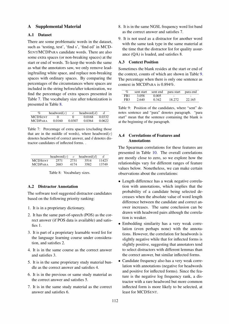
A Supplemental Material

A.1 Dataset

There are some problematic words in the dataset,such as ‘testing, test’, ‘find s’, ‘find ed’ in MCD-SENT/MCDPARA candidate words. There are alsosome extra spaces (or non-breaking spaces) at thestart or end of words. To keep the words the sameas what the annotators saw, we only remove lead-ing/trailing white space, and replace non-breakingspaces with ordinary spaces. By comparing thepercentages of the circumstances where spaces areincluded in the string before/after tokenization, wefind the percentage of extra spaces presented inTable 7. The vocabulary size after tokenization ispresented in Table 8.

% headword(c) c headword(d) dMCDSENT 0 0 0.0168 0.0332MCDPARA 0.0160 0.0307 0.0364 0.0622

Table 7: Percentage of extra spaces (excluding thosethat are in the middle of words), where headword(c)denotes headword of correct answer, and d denotes dis-tractor candidates of inflected forms. .

headword(c) c headword(d) dMCDSENT 2571 2731 3514 11423MCDPARA 2683 4174 3582 13749

Table 8: Vocabulary sizes.

A.2 Distractor Annotation

The software tool suggested distractor candidatesbased on the following priority ranking:

1. It is in a proprietary dictionary.

2. It has the same part-of-speech (POS) as the cor-rect answer (if POS data is available) and satis-fies 1.

3. It is part of a proprietary learnable word list forthe language learning course under considera-tion, and satisfies 2.

4. It is in the same course as the correct answerand satisfies 3.

5. It is in the same proprietary study material bun-dle as the correct answer and satisfies 4.

6. It is in the previous or same study material asthe correct answer and satisfies 5.

7. It is in the same study material as the correctanswer and satisfies 6.

8. It is in the same NGSL frequency word list bandas the correct answer and satisfies 7.

9. It is not used as a distractor for another wordwith the same task type in the same material atthe time that the distractor list for quality assur-ance (QA) is loaded, and satisfies 8.

A.3 Context PositionSometimes the blank resides at the start or end ofthe context, counts of which are shown in Table 9.The percentage when there is only one sentence ascontext in MCDPARA is 0.894%.

% sent start sent end para start para endFB1 3.058 0.005 - -FB3 2.640 0.342 18.272 22.165

Table 9: Position of the candidates, where “sent” de-notes sentence and “para” denotes paragraph. “parastart” mean that the sentence containing the blank isat the beginning of the paragraph.

A.4 Correlations of Features andAnnotations

The Spearman correlations for these features arepresented in Table 10. The overall correlationsare mostly close to zero, so we explore how therelationships vary for different ranges of featurevalues below. Nonetheless, we can make certainobservations about the correlations:

• Length difference has a weak negative correla-tion with annotations, which implies that theprobability of a candidate being selected de-creases when the absolute value of word lengthdifference between the candidate and correct an-swer increases. The same conclusion can bedrawn with headword pairs although the correla-tion is weaker.• Embedding similarity has a very weak corre-

lation (even perhaps none) with the annota-tions. However, the correlation for headwords isslightly negative while that for inflected forms isslightly positive, suggesting that annotators tendto select distractors with different lemmas thanthe correct answer, but similar inflected forms.• Candidate frequency also has a very weak corre-

lation with annotations (negative for headwordsand positive for inflected forms). Since the fea-ture is the negative log frequency rank, a dis-tractor with a rare headword but more commoninflected form is more likely to be selected, atleast for MCDSENT.

112

feature MCDSENT MCDPARAhead infl head infl

length difference -0.116 -0.171 -0.145 -0.173embedding similarity -0.018 0.026 -0.014 0.016candidate frequency -0.057 0.113 -0.062 0.028freq. rank difference -0.048 -0.161 -0.033 -0.091

Table 10: Spearman correlations with T/F choices,where “head” denotes headword pairs, and “infl” de-notes inflected form pairs.

• Frequency rank difference has a weak negativecorrelation with annotations, and this trend ismore significant with the inflected form pair.This implies that annotators tend to select distrac-tors in the same frequency range as the correctanswers.

The correlations are not very large in absoluteterms, however we found that there were strongerrelationships for particular ranges of these featurevalues and we explore this in the next section.

A.5 Label-Specific Feature HistogramsFigure 5 shows histograms of the feature values foreach label on headword pairs.

A.6 Results Tuned Based on F1We report our results tuned based on F1 in Table 11and 12.

A.7 Supplement for AnalysisThe example for MCDPARA is as below, and twosets of its distractors are shown in Figure 6.

• MCDPARA: A few years have passed sincethe Great Tohoku Earthquake occurred. It hasbeen extremely costly to rebuild the damagedareas from scratch, with well over $200 billiondollars provided for reconstruction. However,the availability of these funds has been limited.However, a large portion of the money has beenkept away from the victims due to a systemwhich favors construction companies....

Figure 5: Label-normalized feature histograms forMCDSENT (headword pairs).

113

model variant development set test set BERT features best thresholdprecision recall F1 AUPR precision recall F1 AUPR epoch

baseline 15.4 100 26.7 - 13.3 100 23.5 - - - - -

33.3 64.8 44.0 35.1 23.2 59.1 33.3 25.0 none yes 26 0.2Mfeat 42.1 67.0 51.7 45.4 31.5 57.4 40.7 32.3 base yes 26 0.2

41.3 67.1 51.1 46.7 32.4 56.6 41.2 33.9 large yes 25 0.3

none 49.0 79.1 60.5 58.5 46.5 75.7 57.6 53.9 - no 6 0.3gru+c 49.7 77.6 60.6 54.1 46.1 73.3 56.7 53.5 - no 3 0.4

MELMoall 52.9 75.8 62.3 60.4 48.0 75.9 58.8 57.6 - no 2 0.4

none 51.0 84.0 63.4 63.1 47.7 81.4 60.1 60.6 large yes 3 0.3gru+c 56.9 72.3 63.7 59.1 50.6 75.9 60.8 58.6 large yes 5 0.4all 53.5 80.8 64.4 63.4 50.8 75.5 60.8 59.6 large yes 3 0.4

48.8 85.5 62.1 56.6 43.8 82.8 57.3 51.5 base no 4 0.2

MBERT49.6 80.8 61.5 59.1 45.2 79.7 57.7 54.9 large no 3 0.351.5 84.2 63.9 61.7 46.0 78.6 58.0 55.0 base yes 6 0.251.4 81.1 62.9 64.7 46.4 79.8 58.7 57.5 large yes 6 0.2

Table 11: Results for MCDSENT tuned based on F1.

model development set test set BERT features best epoch thresholdprecision recall F1 AUPR precision recall F1 AUPR

baseline 7.3 100 13.5 - 6.6 100 12.4 - - - - -

17.1 53.1 25.9 15.9 15.6 51.3 23.9 15.0 - yes 14 0.1Mfeat 19.5 63.0 29.8 20.4 17.6 61.0 22.3 18.6 base yes 22 0.1

20.4 63.1 30.8 22.3 16.7 62.7 26.4 18.6 large yes 25 0.1

MELMo35.2 55.4 43.1 37.0 31.2 54.6 39.8 33.9 - no 5 0.340.2 61.3 48.5 43.8 34.1 59.4 43.3 35.2 large yes 5 0.3

MELMo(`)28.7 72.9 41.2 33.8 25.7 71.3 37.7 30.3 - no 2 0.236.2 67.3 47.1 40.8 31.0 65.6 42.1 37.3 large yes 7 0.3

35.8 64.2 46.0 39.3 28.9 64.3 39.9 34.5 base no 5 0.2

MBERT35.2 62.1 45.0 38.3 26.9 60.5 37.3 29.3 large no 6 0.144.3 55.4 49.3 47.3 34.6 56.2 42.8 36.7 base yes 2 0.337.8 63.3 47.4 44.0 32.7 66.1 43.7 38.1 large yes 3 0.2

MBERT(`)34.0 64.3 44.5 36.7 29.6 62.1 40.1 32.1 base no 5 0.243.3 57.5 49.4 45.4 33.3 60.9 43.1 35.8 base yes 3 0.3

Table 12: Results for MCDPARA tuned based on F1.

Figure 6: Ranks for distractor candidates of MCDPARA question “However, the availability of these funds hasbeen limited.” along with annotations.

114

Proceedings of the 15th Workshop on Innovative Use of NLP for Building Educational Applications, pages 115–123July 10, 2020. c©2020 Association for Computational Linguistics

Assisting Undergraduate Students in Writing Spanish MethodologySections

Samuel Gonzalez-LopezTechnological University of Nogales

Nogales, Sonora, Mexicosgonzalez@utnogales.edu.mx

Steven BethardUniversity of ArizonaTucson, Arizona, USA

bethard@email.arizona.edu

Aurelio Lopez-LopezNational Institute of Astrophysics, Optics and Electronics

Tonantzintla, Puebla, Mexicoallopez@inaoep.mx

Abstract

In undergraduate theses, a good methodologysection should describe the series of stepsthat were followed in performing the research.To assist students in this task, we developmachine-learning models and an app that usesthem to provide feedback while students write.We construct an annotated corpus that iden-tifies sentences representing methodologicalsteps and labels when a methodology containsa logical sequence of such steps. We trainmachine-learning models based on languagemodeling and lexical features that can identifysentences representing methodological stepswith 0.939 f-measure, and identify methodol-ogy sections containing a logical sequence ofsteps with an accuracy of 87%. We incorpo-rate these models into a Microsoft Office Add-in, and show that students who improved theirmethodologies according to the model feed-back received better grades on their method-ologies.

1 Introduction

In the Mexican higher education system, most un-dergraduate students write a thesis (tesis de licen-ciatura) before graduation. The academic advi-sor and the student are typically both involved.Throughout the process, the advisor spends timereviewing the draft that the student is building andgradually offering suggestions. This process be-comes a cycle until the document meets establishedstandards and/or institutional guidelines. This cy-cle is often slow due to the required changes inthe structure of the thesis. One of the key com-ponents of such a thesis is a methodology section,which contains the steps and procedures used todevelop the research. A methodology is supposedto provide a step-by-step explanation of the aspects

necessary to understand and replicate the researchincluding the techniques and procedures employed,the type of research, the population studied, thedata sample, the collection instruments, the dataselection process, the validation instrument, andthe statistical analysis process (Allen, 1976).

Natural language processing techniques have thepotential to assist students in writing such method-ologies, as several aspects of good methodologiesare visible from lexical and orthographic features ofthe text. A good methodology should have phrasesor sentences that represent a series of steps, whichmay be written in a numbered list or in prose withsequential connectives like next. Steps in a method-ology section should have a predicate that repre-sents the action of that step, like analyze or design.And the list of steps should be in a logical order,e.g., an explore step should typically appear before(not after) an implement step. Good methodologysections should of course have much more beyondthese simple features, but any methodology sectionthat is missing these basic components is clearly inneed of revision.

We thus focus on designing machine-learningmodels to detect and evaluate the quality ofsuch steps in a Spanish-language student-writtenmethodology section, and on incorporating suchmodels into an interactive application that gives stu-dents feedback on their writing. Our contributionsare the following:

• We annotate a small corpus of methodologysections drawn from Spanish information tech-nology theses for the presence of steps andtheir logical order.

• We design a model to detect sentences thatrepresent methodological steps, incorporatinglanguage model and verb taxonomy features,achieving 0.939 f-measure.

115

• We design a model to identify when a method-ology has a logical sequence of steps, incor-porating language model and content wordfeatures, achieving an accuracy of 87%.

• We incorporate the models into an Add-In forMicrosoft Word, and measure how the appli-cation’s feedback improves student writing.

2 Background

There is a long history of natural language pro-cessing research on interactive systems that assiststudent writing. Essay scoring has been a populartopic, with techniques ranging from syntactic anddiscourse analysis (Burstein and Chodorow, 1999),to list-wise learning-to-rank (Chen and He, 2013),to recurrent neural networks (Taghipour and Ng,2016). Yet the goal of such work is very differentfrom ours, as we aim not to assign an overall score,but rather to provide detailed feedback on aspectsof a good methodology that are present or absentfrom the draft.

Intelligent tutoring systems have been developedfor a wide range of topics, including mechani-cal systems (Di Eugenio et al., 2002), qualitativephysics (Litman and Silliman, 2004), learning anew language (Wang and Seneff, 2007), and in-troductory computer science (Fossati, 2008). Aswe focus on assisting students in writing thesismethodology sections, the most relevant prior workfocuses on analysis of essays. ETS Criterion (At-tali, 2004) uses features like n-gram frequency andsyntactic analysis to provide feedback for gram-matical errors, discourse structure, and undesirablestylistic features. The SAT system (Andersen et al.,2013) combines lexical and grammatical proper-ties with a perceptron learner to provide detailedsentence-by-sentence feedback about possible lex-ical and grammatical errors. Revision Assistant(Woods et al., 2017) uses logistic regression overlexical and grammatical features to provide feed-back on how individual sentences influence rubric-specific formative scores. All of these systems aimat general types of feedback, not the specific feed-back needed for methodology sections.

Other related work touches on issues of logicalorganization. Barzilay and Lapata (2008) proposetraining sentence ordering models to differentiatebetween the original order of a well-written textand a permuted sentence order. Cui et al. (2018)continue in this paradigm, training an encoder-decoder network to read a series of sentences and

reorder them for better coherence. Our goal isnot to reorder a student’s sentences, but to providemore detailed feedback on whether the right struc-tures (e.g., steps) are present in the methodology.More relevant work is Persing et al. (2010), whichcombines lexical heuristics with sequence align-ment models to score the organization of an essay.However, they provide only an overall score, anddo not integrate this into any intelligent tutoringsystem.

A final major difference between our work andprior work is that all the work above focused onthe English language, while we provide feedbackfor Spanish-language theses.

3 Data

A collection was created using the ColTyPi1 site.This site includes Spanish-language theses withinthe Information Technologies subject area. Thegraduate level is composed of Doctoral and Mastertheses. The Undergraduate level is composed ofBachelor and Advanced College-level Technician(TSU) theses. All theses and research proposals inthe collection have been reviewed at some point bya review committee.

3.1 Guidelines

A four-page guide was provided to the annotatorswith the instructions for labeling and a brief de-scription of the elements to identify. Annotatorsmarked each sentence (or text segment) that rep-resented a step in a series of steps. For each step,annotators marked the main predicate (typically averb). Finally, annotators judged whether or notthe steps of the methodology represented a logi-cal sequence.The guide included three examplesfor the annotators, the first one detailed a method-ology that accomplished a series of steps and alogical sequence, the second example only met aseries of steps, and the third example didn’t showany feature. The annotators did not have access tothe academic corresponding to each methodology.Figure 1 shows an annotated example.

3.2 Annotation

From ColTyPi, 160 methodologies were down-loaded, 40 at the PhD level, 60 at the Master level,40 at the Bachelor level, and 20 at the TSU level.Two professors in the computer area with expe-rience in reviewing graduate and undergraduate

1We used, http://coltypi.org/

116

Para desarrollar el trabajo propuesto se siguio un conjunto de pasos para asegurar el cumplimiento de cada uno de los objetivospresentados. A continuacion se enumeran las necesidades superadas en el desarrollo de la investigacion:

1. Recopilacion bibliografica y analisis detallado de los acercamientos de desambiguacion existentes.

2. Caracterizacion de las familias de lenguajes y su relacion con el lenguaje espanol.

3. Seleccionar el idioma que se empleara como lenguaje meta en los textos paralelos.

4. Comparar y aplicar diversas herramientas de alineacion a nivel de palabras sobre el corpus elegido.

5. Analizar diccionarios monolingues y bilingues disponibles.

6. Disenar un algoritmo para la adquisicion de etiquetas de sentidos extraıdas de la alineacion resultante.

To develop the proposed work, a set of steps was followed to ensure each of the objectives presented. Below are the tasksinvolved in this research:

1.Bibliographic compilation and detailed analysis of existing disambiguation approaches.

2.Characterize language families and their relationship with the Spanish language.

3. Select the language to be used as the target language in parallel texts.

4. Compare and apply various alignment tools at the word level on the chosen corpus.

5. Analyze monolingual and bilingual dictionaries available.

6. Design an algorithm for the acquisition of labels of senses extracted from the resulting alignment.

Figure 1: Part of a Spanish methodology tagged by the annotators (Spanish original above, English translationbelow). The series of steps is shaded in gray, the verbs identified are in italics, and the annotators marked thismethodology as “Yes” for the presence of logical sequence.

student theses, were recruited as annotators. Bothannotators tagged 160 methodology sections, andinter-annotator agreement was measured. For thetwo information extraction tasks, identifying stepsand identifying predicates, inter-annotator agree-ment was measured with F-score following Hripc-sak and Rothschild (2005). For logical sequence,which is a binary per-methodology judgment, inter-annotator agreement was measured with Cohen’sKappa (Landis and Koch, 1977). The annotatorsachieved 0.90 F-score on identifying steps, 0.89F-score on identifying predicates, and 0.46 Kappa(moderate agreement) on judging logical sequence.Identifying the logical sequence was a complicatedtask for the annotators since the objective was thata whole methodology evidenced a logical sequenceconcerning the verbs used. For instance, in the firststeps of the methodology, the student should useverbs like “identify” or “explore” and verbs like“implement” or “install” at the end of the methodol-ogy.

The annotated data was divided up for exper-iments. Only annotations that both annotatorsagreed on were considered. For the methodologi-cal step extraction task, we selected 300 sentencesannotated as representing a step, and 100 sentencesannotated as not representing a step, with the sen-tences selected to cover both graduate and under-graduate levels. For the logical sequence detectiontask, we selected 50 complete methodologies anno-

tated as having a logical sequence and 50 annotatedas not having a logical sequence.

4 Model: step identification

The model for identifying which sentences repre-sent steps (StepID) is a logistic regression2 thattakes a sentence as input, and predicts whether thatsentence is a methodology step or not. The modelconsiders the five types of features described in thefollowing sections.

4.1 Language model features

To measure how well the words in a Methodol-ogy match the typical sequence of words in a goodMethodology, we turn to language modeling tech-niques. We expected to capture facts like that thepresence of verbs “Select’, “Analyze” or “Com-pare” at the beginning of sentences is probablydescribing a series of steps. We preprocessed allsentences by extracting lemmas using FreeLing.3

Afterwards, two language models were built, thefirst (TM) with tokens (words, numbers, punctua-tion marks) and the second (GM) with grammaticalclasses. These language models were built only onthe sentences labeled as positive, i.e., on sentencesthat should be examples of good token/grammatical

2We used the implementation in Weka 3.6.13, https://www.cs.waikato.ac.nz/ml/weka/

3FreeLing4.1,http://nlp.lsi.upc.edu/freeling/

117

class sequences. We used the SRILM4 toolkit with4-grams and Kneser-Ney smoothing.5 To gener-ate these features for the 300 positive sentenceson which the language models were trained, weused 10-fold cross-validation, so as not to overes-timate the language model probabilities. The 100negative sentences were also processed separately,again with a 10-fold cross-validation.Perplexity val-ues from the language models were used as fea-tures. This component contributed 2 features to theStepID classifier.

4.2 Sentence location features

A methodology can begin immediately with se-quence of steps, or there may be a brief introduc-tion before the steps appear. Thus, location withinthe methodology may be a predictive feature. Weidentified whether the sentence under considerationis in the first third, second third, or final third ofthe methodology. This component contributed 3features to the StepID classifier.

4.3 Verb taxonomy features

This component captures the type of the verbs usedin the series of steps. We use a taxonomy basedon the cyclical nature of engineering education(CNEE; Fernandez-Sanchez et al., 2012), struc-tured in four successive levels. Categories of verbsinclude Knowledge and Comprehension, Applica-tion and Analysis, System Design, EngineeringCreation. In addition, we added a category to iden-tify verbs related to the writing process, as part ofthe steps to conclude the thesis.

We considered three ways of identifying suchverb categories in sentences.CNEE+Stem Each verb in the sentence is

stemmed, and compared against the 54 verbsof the CNEE taxonomy.

CNEE+FastText The 54 verbs in the CNEE tax-onomy are expanded to 540 verbs by tak-ing the 10 most similar words according topretrained word vectors from FastText (Bo-janowski et al., 2016)6. Each verb in the sen-tence is compared against these 540 verbs.

CNEE+Manual An expert annotator manually la-beled each verb with an appropriate one of thefive categories from the CNEE taxonomy.

4SRILM 1.7.3, http://www.speech.sri.com/projects/srilm/

5In preliminary experiments, we also tried using theTheanoLM toolkit, but performance was lower than SRILM.

6https://fasttext.cc/

For CNEE+Stem and CNEE+FastText, only thefirst verb category found is included as a fea-ture7. This component contributed 5 features tothe StepID classifier.

4.4 Sequencing element features

The online writing lab at Purdue University8 iden-tifies a category of words designed “to show se-quence” that includes words like first, second, next,then, after. We coupled the words from this cate-gory with a simple pattern to identify bullet pointsor numbered items to produce a rule that identifieswhether such sequencing elements are present inthe text. This component contributed 1 feature tothe StepID classifier.

5 Model: logical sequence detection

The model for detecting logical sequence (Log-icSeq) is a multilayer perceptron, with a singlehidden layer of size two plus the number of fea-tures (Weka’s a layer specifier), that takes an entiremethodology as input, and predicts whether it con-tains a logical sequence of steps or not. The modelconsiders the features described in the followingsection.

5.1 Language model features

We again incorporate language models to measurehow sequences of terms are used in well-writtenmethodologies. This component includes the sameGM and TM features as Section 4.1, except trainedon the 100 positive and negative methodologies,rather than on individual sentences. We also in-clude a third language model that considers onlythe nouns and verbs (NV) of the sentences of themethodology. Each token is followed by its partof speech in the language model input. The goalis to focus on just the words most likely to expressmethodological steps – characterize, select, com-pare, analyze, design, etc. – without restricting theanalysis to a specific lexicon of words.

We considered bigrams and/or 4-grams for theGM, TM, and NV features. This component con-tributed either 3 features to the LogicSeq classifier,or 6 features when both bigrams and 4-grams wereused.

7In preliminary experiments, we also tried using all verbcategories, but this did not improve performance.

8https://owl.purdue.edu/

118

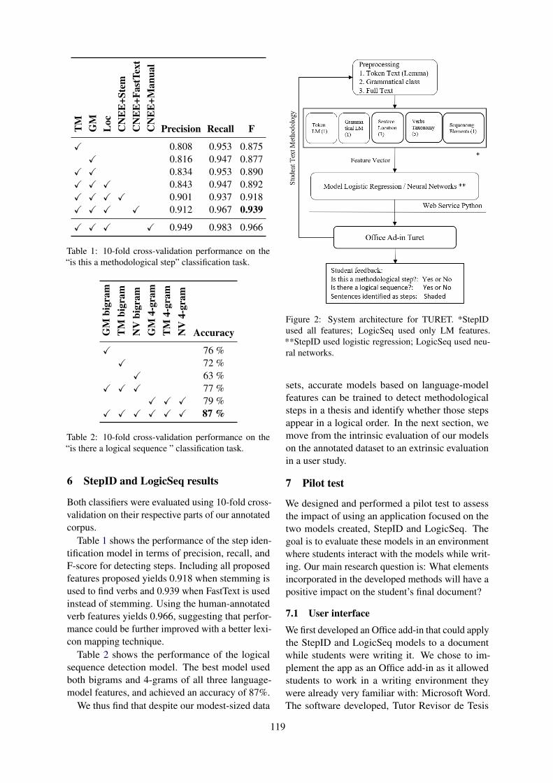
TM

GM

Loc

CN

EE

+Ste

mC

NE

E+F

astT

ext

CN

EE

+Man

ual

Precision Recall F

X 0.808 0.953 0.875X 0.816 0.947 0.877

X X 0.834 0.953 0.890X X X 0.843 0.947 0.892X X X X 0.901 0.937 0.918X X X X 0.912 0.967 0.939

X X X X 0.949 0.983 0.966

Table 1: 10-fold cross-validation performance on the“is this a methodological step” classification task.

GM

bigr

amT

Mbi

gram

NV

bigr

amG

M4-

gram

TM

4-gr

amN

V4-

gram

Accuracy

X 76 %X 72 %

X 63 %X X X 77 %

X X X 79 %X X X X X X 87 %

Table 2: 10-fold cross-validation performance on the“is there a logical sequence ” classification task.

6 StepID and LogicSeq results

Both classifiers were evaluated using 10-fold cross-validation on their respective parts of our annotatedcorpus.

Table 1 shows the performance of the step iden-tification model in terms of precision, recall, andF-score for detecting steps. Including all proposedfeatures proposed yields 0.918 when stemming isused to find verbs and 0.939 when FastText is usedinstead of stemming. Using the human-annotatedverb features yields 0.966, suggesting that perfor-mance could be further improved with a better lexi-con mapping technique.

Table 2 shows the performance of the logicalsequence detection model. The best model usedboth bigrams and 4-grams of all three language-model features, and achieved an accuracy of 87%.

We thus find that despite our modest-sized data

Figure 2: System architecture for TURET. *StepIDused all features; LogicSeq used only LM features.**StepID used logistic regression; LogicSeq used neu-ral networks.

sets, accurate models based on language-modelfeatures can be trained to detect methodologicalsteps in a thesis and identify whether those stepsappear in a logical order. In the next section, wemove from the intrinsic evaluation of our modelson the annotated dataset to an extrinsic evaluationin a user study.

7 Pilot test

We designed and performed a pilot test to assessthe impact of using an application focused on thetwo models created, StepID and LogicSeq. Thegoal is to evaluate these models in an environmentwhere students interact with the models while writ-ing. Our main research question is: What elementsincorporated in the developed methods will have apositive impact on the student’s final document?

7.1 User interface

We first developed an Office add-in that could applythe StepID and LogicSeq models to a documentwhile students were writing it. We chose to im-plement the app as an Office add-in as it allowedstudents to work in a writing environment theywere already very familiar with: Microsoft Word.The software developed, Tutor Revisor de Tesis

119

Figure 3: Application interface embedded in Office Ad-in

(TURET), was embedded in the Microsoft Wordprocessor through a component developed in theAzure platform for Office Add-ins. As part of thisdevelopment, we had to re-implement the StepIDand LogicSeq algorithms using Scikit-learn, butreused the same language model features createdwith the SRILM toolkit. Figure 2 shows the archi-tecture of the system. In the first stage the prepro-cessing was done sentence by sentence to computeeleven features established in the StepId method.For the LogicSeq method the entire methodologywas processed to extract six features.

Figure 3 shows an example methodology openin Microsoft Word with TURET enabled. Themethodology written by the student is shown onthe left side. After clicking, sentences that are iden-tified as being part of a series of steps are marked,and the student is also sent binary feedback indi-cating whether the methodology shows a series ofsteps and/or a logical sequence. Notice that themethodology shows seven steps, but the methodonly detects 3 of them as valid. This is most likelybecause words like implementation and connectare not generally appropriate at the beginning ofa methodology. Thus, this example shows an ab-sence of a logical sequence. The system correctlypredicts this, as shown in through the No in thefeedback frame.

7.2 Experimental design

The pilot test was conducted with two groups of 20(for a total of 40) undergraduate computer science

students. Each student received an introduction ex-plaining how to use the TURET application. Thenthe student was provided with a problem statementrelated to a computer science project and was askedto write a methodology that provides a solution.Students were encouraged to try to achieve posi-tive feedback from the system on two aspects: thatthe methodology had a logical sequence and thatthere was evidence of a series of steps. Studentshad access to the application for 1 month and wereexpected to use TURET at least twice (i.e., on afirst draft and a final draft) but could freely use theapplication more frequently if desired.

We also included a control group of 20 under-graduate computer science students who did notuse TURET, but still used Microsoft Word to writea methodology in response to the same problemstatements.

To validate the quality of the documents gener-ated by both the TURET students and the controlstudents, a teacher experienced in grading under-graduate theses evaluated both the first and thefinal draft. Each methodology received a rating ona scale of 1 to 10, where 10 is the best. The teacherwas not informed about the use of the TURET ap-plication; they graded the methodologies as theywould. Of the total number of students who startedthe pilot test, only 35 completed the entire process.

7.3 Statistical analysis

A multiple regression analysis was made on theresults obtained from the evaluation of the method-

120

Factor Coefficients P-values

Intercept 7.5552 0.0001N-Steps -0.1421 0.1263Steps? 0.2652 0.6946Logical Sequence? 1.2237 0.0096

Table 3: Coefficients of different final draft factorswhen predicting the final grade of a student.

ologies, with the teacher’s grade of the final draftas the dependent variable and the following factorsmeasured on their final draft:N-Steps A non-negative integer representing the

number of sentences of each methodology thatthe StepId model recognized as methodologi-cal steps.

Steps? A binary value, with a value of 1 when theStepId model recognized at least one sentenceas a methodological step, or a value of 0 ifthere was no such sentence.

Logical Sequence? A binary value, with a valueof 1 when the LogicSeq model recognizedthe methodology as having a logical sequence,and a value of 0 otherwise.

Table 3 shows that when predicting the grade as-signed to a student’s final draft, the LogicSeqmodel’s prediction is a statistically significant pre-dictor: drafts judged to have a logical sequencewere on average score 1.2237 higher than the otherdrafts.

We also explored a multiple regression designedto test how much changes in a student’s writingpredicted changes in their grade. Instead of consid-ering only the final draft, as above, we consider thedifference between the initial and the final for allfactors as well as the dependent variable. We thusre-define the factors as follows.N-Steps An integer representing the increase in

number of sentences recognized as method-ological steps by the StepId model when mov-ing from the draft to the final document.

Steps? An integer, with a value of 1 when theStepId model found no steps in the draft butat least one in the final, a value of 0 when thenumber of steps identified by StepId was un-changed between draft and final, and a valueof -1 when the StepId model found at leastone step in the draft but none in the final.

Logical Sequence? An integer, with a value of 1when the LogicSeq model found no logical

Items Coefficients P-values

Intercept 0.7768 0.0231N-Steps -0.3066 0.0097Steps? 1.0103 0.0342Logical Sequence? 0.6342 0.1270

Table 4: Coefficients of different (Final - Draft) factorswhen predicting the change in grade between Draft andFinal (i.e., the Final - Draft grade).

sequence in the draft but found one in the final,a value of 0 when there was no change in theprediction of the LogicSeq model betweendraft and final, and a value of -1 when theLogicSeq model found a logical sequence inthe draft but none in the final.

Table 4 shows that when predicting how much astudent’s grade will improve from draft to final, thechange in the number of steps identified by StepIdis a statistically significant predictor. Students thatwent from having no steps to having one or moresteps on average scored 1.0103 better than studentswith no change. Interestingly, having many stepswas not necessarily a good thing: for each addi-tional step, students on average lost 0.3066 fromtheir score. This suggests that students who addedtoo many more steps to their drafts were penalizedfor doing so.

Finally, we compared the TURET group of stu-dents against the control group of students. Onthe 20 problem statements that were common tothe TURET and control groups, the TURET stu-dents on average scored 7.85, while the controlstudents scored 6.8. The difference is significant(p = .041139) according to a t-test for two inde-pendent means (two tailed).

7.4 Satisfaction survey

To assess the opinion of the experimental groupon using the TURET Office Add-in, a satisfactionsurvey based on the Technology Acceptance Model(Davis et al., 1989) was conducted. Students wereasked about the usefulness, ease of use, adaptabilityand, their intention to use the system. For example,the “usefulness” questions were: Does the systemimprove your methodology? Did the system im-prove the performance of your learning? In general,do you think that the system was an advantage foryour learning to write arguments? As another exam-ple, the “ease of use” questions were: Was learningto use the system easy for you? Was the process

121

Measure Score

Usefulness 4.54Ease of use 4.85Adaptability 4.67Intention to use 4.50

Table 5: Satisfaction survey results TAM

of using the system clear and understandable?. Ingeneral, do you think the system was easy to use?

Student answers were based on a five-point Lik-ert scale ranging from 1 (“Strongly disagree”) to5 (“Strongly agree”), and the scores across eachcategory of question were averaged. Table 5 showsthat students rated the application above 4 points(“Agree”) for all aspects. The highest score was4.85 on ease of use, which we attribute to the useof a Microsoft Word Add-in, which takes advan-tage of students’ already existing familiarity withMicrosoft Word.

We also collected free-form comments from thestudents. Their biggest complaint was that TURETworks only in the online version of Microsoft Office(since it must communicate with a server), and theywould have liked to use it in offline mode.

8 Discussion

We have demonstrated that with a small amount oftraining data, several carefully engineered features,and standard supervised classification algorithms,we can construct models that can reliably (0.939F) detect the presence of steps in student-writtenSpanish methodology sections, and reliably (87%accuracy) determine whether those steps are pre-sented in a logical order. We have also shown thatincorporating these models into an Office Add-infor Microsoft Word resulted in a system that stu-dents found useful and easy to use, and that thedetections of the models were predictive of teacher-assigned essay grades.

There are some limitations to our study. First, be-cause of the success of our simple models, we didnot investigate more complex recent models likeBERT (Devlin et al., 2019). Such models mightyield improved predictive performance but at a sig-nificant additional computational cost. Second, theamount of data that we annotated was small, as itrequired a high level of expertise in the reviewingof Spanish-language methodology sections. (Werelied on Spanish-speaking professors in computer

science.) It would be good to expand the size ofthe dataset, but we take the high levels of perfor-mance of the models, and the fact that they makeuseful predictions on the unseen student-generatedmethodologies of the pilot test, as an indicationthat the dataset is already useful in its current size.Finally, the pilot study was a controlled experiment,where specific problem statements were given asprompts. It would be interesting to measure theutility of the application for students writing theirown theses.

In the future, we would like to explore integrat-ing other types of writing feedback into the TURETOffice Add-in, since students found its feedbackabout methodology steps both intuitive and help-ful. Though we focused on methodology sectionsin this article, our vision is a set of models thatcan provide useful feedback for all sections of aSpanish-language student thesis.

ReferencesGeorge R. Allen. 1976. The Graduate Students’ Guide

to Theses and Dissertations: A Practical Manual forWriting and Research, volume 1. Jossey-Bass Inc.,Publishers, 615 Montgomery Street, San Francisco.

Øistein E. Andersen, Helen Yannakoudakis, FionaBarker, and Tim Parish. 2013. Developing andtesting a self-assessment and tutoring system. InProceedings of the Eighth Workshop on Innova-tive Use of NLP for Building Educational Applica-tions, pages 32–41, Atlanta, Georgia. Associationfor Computational Linguistics.

Yigal Attali. 2004. Exploring the feedback and revi-sion features of criterion. Journal of Second Lan-guage Writing, 14:191–205.

Regina Barzilay and Mirella Lapata. 2008. Modelinglocal coherence: An entity-based approach. Compu-tational Linguistics, 34(1):1–34.

Piotr Bojanowski, Edouard Grave, Armand Joulin,and Tomas Mikolov. 2016. Enriching word vec-tors with subword information. arXiv preprintarXiv:1607.04606.

Jill Burstein and Martin Chodorow. 1999. Automatedessay scoring for nonnative English speakers. InComputer Mediated Language Assessment and Eval-uation in Natural Language Processing.

Hongbo Chen and Ben He. 2013. Automated essayscoring by maximizing human-machine agreement.In Proceedings of the 2013 Conference on Empiri-cal Methods in Natural Language Processing, pages1741–1752, Seattle, Washington, USA. Associationfor Computational Linguistics.

122

Baiyun Cui, Yingming Li, Ming Chen, and ZhongfeiZhang. 2018. Deep attentive sentence ordering net-work. In Proceedings of the 2018 Conference onEmpirical Methods in Natural Language Processing,pages 4340–4349, Brussels, Belgium. Associationfor Computational Linguistics.

Fred D. Davis, Richard P. Bagozzi, and Paul R. War-shaw. 1989. User acceptance of computer technol-ogy: A comparison of two theoretical models. Man-agement Science, 35(8):982–1003.

Jacob Devlin, Ming-Wei Chang, Kenton Lee, andKristina Toutanova. 2019. BERT: Pre-training ofdeep bidirectional transformers for language under-standing. In Proceedings of the 2019 Conferenceof the North American Chapter of the Associationfor Computational Linguistics: Human LanguageTechnologies, Volume 1 (Long and Short Papers),pages 4171–4186, Minneapolis, Minnesota. Associ-ation for Computational Linguistics.

Barbara Di Eugenio, Michael Glass, and Michael Tro-lio. 2002. The DIAG experiments: Natural lan-guage generation for intelligent tutoring systems. InProceedings of the International Natural LanguageGeneration Conference, pages 120–127, Harriman,New York, USA. Association for ComputationalLinguistics.

Pilar Fernandez-Sanchez, Angel Salaverrıa, and En-rique Mandado. 2012. Taxonomıa de los nivelesdel aprendizaje de la ingenierıa y su implementacionmediante herramientas informaticas. In X Congresode Tecnologıas Aplicadas en la Ensenanza de laElectronica, pages 522–527.

Davide Fossati. 2008. The role of positive feedback inIntelligent Tutoring Systems. In Proceedings of theACL-08: HLT Student Research Workshop, pages31–36, Columbus, Ohio. Association for Computa-tional Linguistics.

George Hripcsak and Adam S. Rothschild. 2005.Agreement, the f-measure, and reliability in infor-mation retrieval. Journal of the American MedicalInformatics Association, 12(3):296–298.

J. Richard Landis and Gary G. Koch. 1977. The mea-surement of observer agreement for categorical data.Biometrics, 33(1):159–174.

Diane J. Litman and Scott Silliman. 2004. ITSPOKE:An intelligent tutoring spoken dialogue system. InDemonstration Papers at HLT-NAACL 2004, pages5–8, Boston, Massachusetts, USA. Association forComputational Linguistics.

Isaac Persing, Alan Davis, and Vincent Ng. 2010. Mod-eling organization in student essays. In Proceedingsof the 2010 Conference on Empirical Methods inNatural Language Processing, pages 229–239, Cam-bridge, MA. Association for Computational Linguis-tics.

Kaveh Taghipour and Hwee Tou Ng. 2016. A neuralapproach to automated essay scoring. In Proceed-ings of the 2016 Conference on Empirical Methodsin Natural Language Processing, pages 1882–1891,Austin, Texas. Association for Computational Lin-guistics.

Chao Wang and Stephanie Seneff. 2007. Automaticassessment of student translations for foreign lan-guage tutoring. In Human Language Technologies2007: The Conference of the North American Chap-ter of the Association for Computational Linguistics;Proceedings of the Main Conference, pages 468–475, Rochester, New York. Association for Compu-tational Linguistics.

Bronwyn Woods, David Adamson, Shayne Miel, andElijah Mayfield. 2017. Formative essay feedbackusing predictive scoring models. In Proceedings ofthe 23rd ACM SIGKDD International Conference onKnowledge Discovery and Data Mining, KDD ’17,page 2071–2080, New York, NY, USA. Associationfor Computing Machinery.

123

Proceedings of the 15th Workshop on Innovative Use of NLP for Building Educational Applications, pages 124–134July 10, 2020. c©2020 Association for Computational Linguistics

Applications of Natural Language Processing in BilingualLanguage Teaching: An Indonesian-English Case Study

Zara Maxwell-Smith1 Ben Foley2 Simón González Ochoa1 Hanna Suominen1,3−4

1. The Australian National University / Canberra, ACT, Australia2. University of Queensland / Brisbane, QLD, Australia

3. Data61/Commonwealth Scientific and Industrial Research Organisation /Canberra, ACT, Australia

4. University of Turku / Turku, FinlandZara.Maxwell-Smith@anu.edu.au, b.foley@uq.edu.au,

Simon.Gonzalez@anu.edu.au, Hanna.Suominen@anu.edu.au

Abstract

Multilingual corpora are difficult to compileand a classroom setting adds pedagogy to themix of factors which make this data so rich andproblematic to classify. In this paper, we setout methodological considerations of using au-tomated speech recognition to build a corpusof teacher speech in an Indonesian languageclassroom. Our preliminary results (64% worderror rate) suggest these tools have the poten-tial to speed data collection in this context. Weprovide practical examples of our data struc-ture, details of our piloted computer-assistedprocesses, and fine-grained error analysis. Ourstudy is informed and directed by genuine re-search questions and discussion in both theeducation and computational linguistics fields.We highlight some of the benefits and risks ofusing these emerging technologies to analyzethe complex work of language teachers and ineducation more generally.

1 Introduction

Using quantitative methods to understand languagelearning and teaching is difficult work as limita-tions in the recording, transcribing, and analyzingof data continue to constrain the size of datasets.It is not surprising then, that quantitative studieslooking at second language1 acquisition have beencritiqued for their low statistical power (Plonsky,2013). Usage-based analyses of teacher corpora arean important next stage in understanding languageacquisition (Ellis, 2017). Given the magnitude ofworldwide investment in L2 teaching and learning,drawing on developments in automated methods ofcompiling this kind of speech data is timely.

Consequently, we sought to address the follow-ing main research question in this paper: How canautomated speech recognition (ASR) be adaptedfor this use? More specifically, i) How well do

1a.k.a. target language or L2

these speech-to-text tools perform on this type ofdata? and ii) How do these tools and datasets relateto the overall purpose of opening a window into thepractice of language teachers? Such an endeavorrequires careful consideration of how ASR modelsare built, and what the underlying training data anddesired output of such models might be. In thispaper we use the term ASR model to refer to sta-tistical models used to map speech sequences andsounds to respective text sequences (Jurafsky andMartin, 2009, pp. 38, 286, 287).

Our study is drawn from a project investigatingthe teaching of Indonesian. Data was collectedfrom a tertiary Indonesian language program at anAustralian university. A single teacher’s speechwas recorded throughout one semester of a second-year language program. In investigating Indone-sian language teaching, ideally various instancesof linguistic features and non-standard Indonesianwould be annotated to allow for analyzing varioustopics, including, for instance, the comprehensibil-ity of teachers’ speech, movement between the L2and assumed first language (L1), representations ofregional Indonesian languages, and non-standardvarieties and loanwords. Yet, the tools tend to re-strict the data structures for annotating the audio.As an example from the conclusions of this paper,the classification of data as belonging to the L2(Indonesian) or the L1 (English) quickly emergedas a very significant issue.

The paper is organized as follows: We begin bypresenting an overview of related work in transcrip-tion and ASR before describing our methodologicalapproach, with subsections on bilingual and class-room teacher data. This is followed by a more de-tailed description of our materials and methods totrain and evaluate ASR models. Finally, we presentexperimental results of our machine transcription,discuss them, and conclude the study.

124

2 Background

Transcription is a complex task traditionally seenby linguists from the perspective of linguistic the-ory and documentation of complex language struc-tures and phenomena. Linguists and their researchteams become extremely familiar with their dataduring the process of transcribing, and their pub-lications usually make reference to data-specificguidelines developed for their transcription teams(BNC-Consortium, 2007). Often these are adaptedfrom generic guidelines or rules for annotating lan-guage which aim to record the “most basic tran-scription information: the words and who theywere spoken by, the division of the stream of speechinto turns and intonation units, the truncation ofintonation units and words, intonation contours,medium and long pauses, laughter, and uncertainhearings or indecipherable words” (Du Bois et al.,1993). Most teams use sophisticated software tools,which provide a method for rich interlinear annota-tion of speech data by humans.2 These annotationsallow linguists to record more than ‘just’ the wordsused in human communication, but obviously can-not represent all characteristics of the audio data.

Acknowledging the time constraints and subjec-tivity or bias that enter the transcription processas transcription guidelines are developed is impor-tant. The purpose of these guidelines — namely,to create uniformity of practice from individual,and teams of transcribers — may not be achievable(Hovy and Lavid, 2010). In fact, experiments look-ing at the subjectivity of transcription led Lapadatand Lindsay (1998) to conclude that “the choicesresearchers make about transcription enact the theo-ries they hold and constrain the interpretations theydraw from their educational practice”. Moreover, atranscription survey carried out by the Centre of Ex-cellence for the Dynamics of Language, Transcrip-tion Acceleration Project (CoEDL TAP) team doc-umented a significant variety in the way linguistsgo about transcribing their data. The survey alsofound that each minute of data takes, on average,39 minutes for a linguist to transcribe, creating thewell-known ‘transcription bottleneck’ (Durantin,2017).

Advances in ASR and other natural languageprocessing (NLP) bring researchers closer to over-coming this bottleneck, but many open challengesremain (Hirschberg and Manning, 2015). ASR

2e.g., ELAN, Transana, and FLEx (last accessed on 4December 2019)

tools can help by providing a first-pass hypothe-sis of audio for languages with large datasets totrain the underlying models (Google, 2019; Nu-ance, 2019).3 However, financial and ethical re-strictions may prevent a study from using these off-the-shelf systems and cloud computing services.4

Existing solutions may also have insufficient cover-age of the domain-specific language used by speak-ers or not support a given L2.

Recognizing the potential benefit that integrat-ing ASR tools into a linguist’s workflow couldhave, the CoEDL TAP team has been building Elpis(Foley et al., 2018), an accessible interface for re-searchers to use the powerful but complex KaldiASR toolkit.5 According to Gaida et al. (2014)“Compared to the other recognizers, the outstandingperformance of Kaldi can be seen as a revolution inopen-source [ASR] technology”. This project con-stitutes an early use of the Elpis pipeline to preparetraining data, ready for Kaldi to build ASR models,which can then be used to “infer” a hypothesis forun-transcribed audio.

The interdisciplinary work involved in thisproject shines a spotlight on the limitations on thetype of data used by ASR systems; human tran-scribers often face difficult decisions as to whatshould and what should not be recorded in the train-ing data.6 Since bias and error may multiply inASR models and create unreliable and undesirableoutcomes, sharing the best practices and havingtransparent processes for creating training and eval-uation data and protocols is of utmost importance(Hovy and Lavid, 2010). ASR trained on carefullycompiled data can then be scientifically tested andvariations to the training data analysed for theirimpact (Baur et al., 2018).

3 Methodological Approach

Our methodological considerations addressed thefollowing: which ASR tool to use, how to preparetraining data for this tool, and how to best managethe bias of the training data inherent in all transcrip-tion processes. Kaldi’s orthographic transcription

3E.g., Google’s Cloud Speech-to-Text and Nuance’s ASRSelf-Service support 120 languages and 86 languages/dialects,respectively (last accessed on 4 December 2019).

4E.g., purchasing a license for all participating teachersand obtaining each participant’s informed consent for theirspeech data to be saved on a cloud owned by a private corpo-ration, possibly using them to develop their ASR and othercommercial products, may be infeasible or questionable.

5last accessed on 4 December 20196See our examples below for illustration.

125

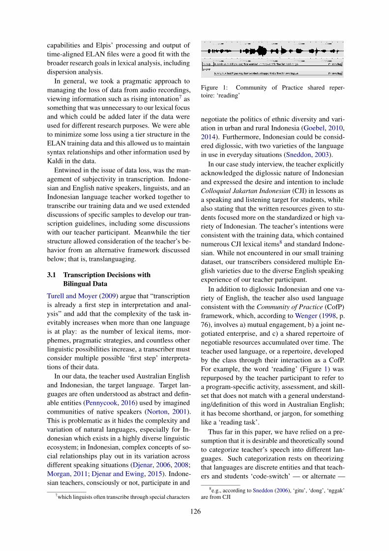
capabilities and Elpis’ processing and output oftime-aligned ELAN files were a good fit with thebroader research goals in lexical analysis, includingdispersion analysis.

In general, we took a pragmatic approach tomanaging the loss of data from audio recordings,viewing information such as rising intonation7 assomething that was unnecessary to our lexical focusand which could be added later if the data wereused for different research purposes. We were ableto minimize some loss using a tier structure in theELAN training data and this allowed us to maintainsyntax relationships and other information used byKaldi in the data.

Entwined in the issue of data loss, was the man-agement of subjectivity in transcription. Indone-sian and English native speakers, linguists, and anIndonesian language teacher worked together totranscribe our training data and we used extendeddiscussions of specific samples to develop our tran-scription guidelines, including some discussionswith our teacher participant. Meanwhile the tierstructure allowed consideration of the teacher’s be-havior from an alternative framework discussedbelow; that is, translanguaging.

3.1 Transcription Decisions withBilingual Data

Turell and Moyer (2009) argue that “transcriptionis already a first step in interpretation and anal-ysis” and add that the complexity of the task in-evitably increases when more than one languageis at play: as the number of lexical items, mor-phemes, pragmatic strategies, and countless otherlinguistic possibilities increase, a transcriber mustconsider multiple possible ‘first step’ interpreta-tions of their data.

In our data, the teacher used Australian Englishand Indonesian, the target language. Target lan-guages are often understood as abstract and defin-able entities (Pennycook, 2016) used by imaginedcommunities of native speakers (Norton, 2001).This is problematic as it hides the complexity andvariation of natural languages, especially for In-donesian which exists in a highly diverse linguisticecosystem; in Indonesian, complex concepts of so-cial relationships play out in its variation acrossdifferent speaking situations (Djenar, 2006, 2008;Morgan, 2011; Djenar and Ewing, 2015). Indone-sian teachers, consciously or not, participate in and

7which linguists often transcribe through special characters

Figure 1: Community of Practice shared reper-toire: ‘reading’

negotiate the politics of ethnic diversity and vari-ation in urban and rural Indonesia (Goebel, 2010,2014). Furthermore, Indonesian could be consid-ered diglossic, with two varieties of the languagein use in everyday situations (Sneddon, 2003).

In our case study interview, the teacher explicitlyacknowledged the diglossic nature of Indonesianand expressed the desire and intention to includeColloquial Jakartan Indonesian (CJI) in lessons asa speaking and listening target for students, whilealso stating that the written resources given to stu-dents focused more on the standardized or high va-riety of Indonesian. The teacher’s intentions wereconsistent with the training data, which containednumerous CJI lexical items8 and standard Indone-sian. While not encountered in our small trainingdataset, our transcribers considered multiple En-glish varieties due to the diverse English speakingexperience of our teacher participant.

In addition to diglossic Indonesian and one va-riety of English, the teacher also used languageconsistent with the Community of Practice (CofP)framework, which, according to Wenger (1998, p.76), involves a) mutual engagement, b) a joint ne-gotiated enterprise, and c) a shared repertoire ofnegotiable resources accumulated over time. Theteacher used language, or a repertoire, developedby the class through their interaction as a CofP.For example, the word ‘reading’ (Figure 1) wasrepurposed by the teacher participant to refer toa program-specific activity, assessment, and skill-set that does not match with a general understand-ing/definition of this word in Australian English;it has become shorthand, or jargon, for somethinglike a ‘reading task’.

Thus far in this paper, we have relied on a pre-sumption that it is desirable and theoretically soundto categorize teacher’s speech into different lan-guages. Such categorization rests on theorizingthat languages are discrete entities and that teach-ers and students ‘code-switch’ — or alternate —

8e.g., according to Sneddon (2006), ‘gitu’, ‘dong’, ‘nggak’are from CJI

126

Figure 2: ELAN tier structure

“between two languages or dialects of the samelanguage within the same conversation” (Boztepe,2003). Recent discussions of an alternative frame-work — translanguaging (Garcia and Wei, 2014)— propose that multilinguals employ only one, ex-panded repertoire of linguistic features. This reper-toire may contain two or more languages whichare officially and externally recognized as distinctsystems, but according to translanguaging theory,the distinction between the systems is not inter-nally valid.

By using several ELAN tiers to create parallelstructures for storing data (Figure 2), we balancedtechnological requirements without taking a partic-ular stance in relation to translanguaging nor theinternal mechanisms of bilinguals. The uppermost‘Everything’ tier included all orthographical anno-tations for the data. The next two tiers containeddata, which according to various phonological, syn-tactical, and morphological factors were separatedby our transcription team into Indonesian and En-glish according to a code-switch paradigm. Finally,we also created a tier labeled ‘Mixed’ to containannotations, which were difficult to separate.

While some researchers battle with technolo-gies to represent very different orthographies9, weworked with two languages that are both writtenin the Roman alphabet. This presented some chal-lenges of its own. Some words, for example, ‘sta-tus’ (status) and ‘level’ (level), were spelled identi-cally in both languages; meanwhile, names couldhave been represented in a number of differentways. Our decisions to use a certain orthographyin training data impacted statistical relationshipsbetween words and phonemes in the ASR models.We chose to approximate all names in the Indone-sian orthography as these proper nouns are some-what language independent.10 For example, our‘Indonesianized’ class list included ‘Jorj’ (George),‘Shantel’ (Chantelle), and ‘Medi’ (Maddy). This

9(e.g., Halai (2007) for Urdu and English)10They were also annotated in all tiers when they oc-

curred alone.

decision allowed us to maintain the names withinboth Indonesian and English sentences, however,it did require manual creation of a phonemic mapfor that lexical item.11 Similarly, we used only theIndonesian phonemic map for ‘status’ and ‘level’as our participant’s English incorporated Indone-sian phonological characteristics (accent), and ourintention was to strengthen our Indonesian compu-tational model.

Decisions about orthography and tier allocationswere very difficult and we made them only afterextensive discussion in our transcription team. Insome cases, within word changes between the typi-cal Indonesian phonology and English phonologyoccurred. For example, in one segment, the teacherproduced the first vowel of ‘status’ as [eI] (as in‘bait’), an English phoneme, but finished the wordwith the Indonesian /u/ (similar to ‘book’). Evenwith a common set of characters used for bilin-gual data, the decisions taken developing trainingdata had to be clearly documented and their impactconsidered in the ASR evaluation.

3.2 Toward Interpreting Teacher Speech

The complex bilingual transcription process out-lined above was further complicated by the tran-scriber’s interpretation of the educational setting.Given the conceivable criticism of a given teach-ers’ professional practice made possible throughthe creation of corpora, we carefully considered theimpacts of this scrutiny while developing our tran-scription guidelines and sought to minimize unfairor inaccurate treatment of teacher data. We alsowish to proclaim the limitations of corpus data inthis setting.

Although a full description and examination ofthese issues is beyond the scope of this paper, weidentified some pertinent methodological implica-tions of our own data structure. First, the taskof analyzing the teacher’s speech is likely to beover-simplified into binary L1 versus L2 catego-

11See Section 4 below.

127

Figure 3: Treatment of pauses in teacher speech

rization of teacher’s speech. The aforementionedmethodological difficulties of teasing apart speechdata and the questionable validity of delimiting lan-guages raised by the translanguaging frameworkwere central to our transcription guidelines. Wealso note that pauses in the teacher’s language andother easily overlooked phenomena might skewthe time counted towards a given language (Fig-ure 3). We assessed that L2 was vulnerable to thisskewing as the teacher extended pauses betweenwords unfamiliar to the students, thus expandingthe time counted as L2 speech. Conversely, cuttingthe L2 use apart when a teacher paused removedbetween-word-time from a cumulative L2 countand artificially shortened the time spent in the lan-guage.

Second, the goal of modifying sociolinguisticnorms which brings people to language classroomsprecipitated a level of variance and unpredictabilityunusual in other speech contexts as students learnand progress in their acquisition. We viewed varia-tion in teacher speech from a pedagogically ‘gen-erous’ perspective; for example, unusual linguisticforms were interpreted in line with research onlanguage simplification (Saito and Poeteren, 2012;O Dela Rosa and Arguelles, 2016) or identity workwith students (Norton and Toohey, 2011). How-ever, a transcriber might note that in the Australiansecond language teaching setting, teachers oftenhave less than ‘native’ proficiency in either the L2or classroom L1. A proficiency-focused transcribercould be particularly sensitive to the teacher’s pro-ductions of loanwords.12 Thus, a transcriber’s ownperception of proficiency and speech errors, as wellas their knowledge of, and stance on, pedagogicalapproaches are implicated in the interpretation ofteacher speech.

With so many possible interpretations, asking theteacher to comment on or transcribe their own data

12E.g., the Indonesian loanword ‘kelas’ (class) might be in-terpreted as English should it not meet a transcriber’s personalthreshold for an Indonesian production.

might seem useful. However, the intent of a teacherin using specific linguistic features is likely to behighly complex, as well as difficult to ascertain asthis work is often the result of internally reasoned,impromptu responses to student feedback (Borkoet al., 1990). With these features put together overthousands, possibly millions of teaching decisionseach lesson, we were cautious in our asking ourteacher participant to recall or explain what theywere doing in retrospect. We noted that any dis-parity in teacher intention and the recorded data,or inability to recall the purpose of specific inter-actions, language choices and other behaviors maycreate an air of scrutiny which could skew resultinginterpretation (Gangneux and Docherty, 2018).

Ensuring that teachers, their work, and their de-cisions are not misrepresented or misunderstoodwas important to us. We emphasized and are urg-ing caution in the use of corpora to assess teacherpractice until methodological questions have re-ceived prolonged and rigorous attention across awide-range of datasets, including at the minimumdifferent L1 and L2, teachers, pedagogical styles,and teaching situations.

4 Materials and Methods

The audio data was recorded in a second year ter-tiary Indonesian language program at an Australianuniversity (Ethics Approval No. 2017/889 of theAustralian National University Human ResearchCommittee for the Speech Recognition; BuildingDatasets from Indonesian Language Classroomsand Resources protocol). The teacher, who wasrecorded over the course of one semester, grew upusing Indonesian in school and public places, anda regional language at home. A semester of over32 hours of class was recorded.13

The teacher wore a head-mounted microphoneand wireless bodypack linked to a ZOOM recorderset to record 44.1 kHz, 36-bit WAV format audio.Because students were not the target of the study,the microphone settings were optimized to excludetheir voices. Three lessons of approximately 50minutes were chosen for transcription as trainingand test data for the ASR. The lessons were se-lected to contain a range of content, instructionalstyles, and activities. The remaining audio record-ings were held out from training and testing.14

13Excluded classes in which formal assessments took place,an introductory class, and some lesson segments where tech-nical problems resulted in loss of data.

14They were kept in reserve for future experiments and anal-

128

Model Training tiera Tokens intraining Languages n-gram WERb WER

full setc Correct Long text spansWords Text spans

Bilingual_1G Everything tier 6194English

IndonesianMixed

1 77%(56/73)

117%(117/100) 38/100 4

321

Bilingual_3G Everything tier 6194English

IndonesianMixed

3 89%(65/73)

133%(133/100) 34/100 3 2

Indonesian_3G Indonesian tier 3377 Indonesian 3 64%(23/36)

134%(134/100)

22/100d

22/51e43

11

a See Figure 2 for tier structureb Results when testing only with words found in training datac Results including training words and testing words not found in training datad In the full test sete Indonesian and non-language specific words in the test set

Table 1: Word Error Rates (WER) from 3 ASR Models

PRAAT auto-segmentation with settings at theminimum pitch of 70 Hz, silence threshold of -50Db, and minimum silent interval of 0.25 was usedto segment the data. Segments were then manu-ally edited to remove remnant student voices andextreme modality sounds15 to avoid confusing theKaldi acoustic training. Care was taken to find theboundaries between speech sounds and discrimi-nate between the languages used, with challengingsections examined in PRAAT by the transcriptionteam. Transcription was completed in ELAN andinitially all teacher speech was transcribed on onetier before being expanded onto other tiers (seeFigure 2).

To use the Kaldi toolkit, a lexicon with eachword’s phonemic representation was required. Dueto the bilingual dataset in this study, we built a lex-icon with consistent grapheme-to-phoneme (G2P)mapping across two orthographies. Our lexiconwas built by adding missing English words to theCarnegie Melon University (CMU) PronunciationDictionary. Although the pronunciations of this dic-tionary are based on American English, it was thebest available match with our teacher participant.We then merged this lexicon with an Indonesianlexicon, which was built using Elpis functionali-ties.16 The tools used the regular G2P mappingin Indonesian to generate a pronunciation dictio-nary based on the orthographical representation ofeach word.

We trained three models (Table 1) on two lessonsselected from the semester of teaching. We then

yses.15e.g. laughter, outbreaths, unintelligible whispers16incl. the Indonesianised names

used the three models to automatically transcribea 100-word17 test subset of data from a third les-son. We used the word error rate (WER)18 as theprimary evaluation measure in this analysis.

The two bilingual models, which were trainedon all parts of the audio recordings, are referred toas bilingual models for ease of reference. However,it should be noted that there was nothing binary inthese models:19 Bilingual_1G and Bilingual_3Gwere each a single model, where 1G and 3G referto n-grams.20 We chose the unigram and trigrammodels to assess the importance of word sequences.

5 Preliminary Results from AutomatedSpeech Recognition and Their Analysis

The WER of three models was from 64% to 89%(Table 1). This was large compared with those re-ported by major commercial ASR transcription ser-vices; however, this comparison requires interroga-tion.

The WER of the large commercial services istypically related monolingual tasks, usually on En-glish data, and outside the classroom context. In amonolingual Spanish classroom environment, animpressively small WER of 10% was reported us-ing a tailored, commercial ASR system with testdata of two 50-minute university lectures and one50-minute seminar with 10–16 year-old students(Iglesias et al., 2016). In contrast, for monolin-

17duration of approx. 1 minute18i.e., the number of deleted, inserted, and substituted

words, divided by the total number of words19No differentiation was made by the Kaldi toolkit be-

tween languages.20i.e., a sequence of n words

129

gual US English-speaking teachers’ speech, a WERfrom 44% to 100% was reported for five ASR sys-tems, which were free of cost to use and requiredno additional supervised learning to train the ASRmodel (Nathaniel et al., 2015).

In our results, we analyzed teacher speech phe-nomena, such as emphasized articulation. For ex-ample, an instance of ‘sma’, an acronym for a se-nior high school produced as the Indonesian namesof the letters, [es em ah] was hyper-articulated.Our Bilingual_3G and Indonesian_3G models pro-duced reasonable approximations: ‘ah sma aha’and ‘hasan aha’, respectively. Given the varia-tion this sort of phenomena introduced into lexicalitems, teacher speech characteristics seem likely tohave impacted our ASR performance.

ASR performance degrades in multilingual set-tings, but a range of techniques for reducing WERare available (see Yilmaz et al. (2016); Nakayamaet al. (2018); van der Westhuizen and Niesler(2019); Yue et al. (2019)). Many of these studiesnote their shortage of training data and some reportsuccess in using training data from high resourcelanguages to work with low resource languages.For example, Biswas et al. (2018) experimentedwith a new South African soap opera corpus inwhich five languages were present and found thatthe incorporation of monolingual, out-of-domaintraining data reduced their WER. Working withthe same corpus, Biswas et al. (2019) first trainedbilingual systems and a unified five-lingual system,and then experimented with adding convolutionalneural network layers to these models. Overallthey achieved WERs ranging from 43% to 64%for paired languages and from 26% to 78% forsingle languages.

While performance between different languagepairs might not be suitable for comparison due tothe interplay of language typologies interacting indistinctive ways, WERs from codeswitch bilingualdata were more similar to our WER, especiallygiven our small amount of training data. Yeong andTan (2014) studied Indonesian, Iban, and Malaycodeswitching in written work, however, to thebest of our knowledge, our work was the first workon spoken Indonesian–English data.

WER rates were useful in relating our resultswith the overall progress being made in ASR, butgiven our goal to expedite human transcription, forus, it was more fruitful to analyze the number andlength of correctly recognized text spans in the

ASR-based transcription. We theorized that thesetools could begin to change workflow or decreasecognitive load for human transcribers by generatinga draft transcript for revision.

The two 4-word and one 3-word correct textspans produced by our Bilingual_1G model wouldprobably be the most useful in speeding transcrip-tion (Table 1). However, the preliminary resultsproduced by the Indonesian_3G model were com-parable to the two bilingual models. This was im-pressive given that nearly 50% of the test data wasin English. Supposing a research interest in onlythe Indonesian spoken by the teacher, or the use ofan English language model for the other data, theIndonesian model could reasonably be assessed asscoring 22 correct words from the 51 Indonesianwords in the test data.

Proceeding to a more detailed study of the per-formance of the models, we undertook an erroranalysis to elucidate the type of errors occurring.We analyzed them as segments, from multiple per-spectives (Figure 4). There was a high incidenceof resyllabification21 in the machine transcription,as words were split, concatenated with the preced-ing or succeeding word(s), a middle consonant wasomitted, and/or an initial consonant was omitted.For example, ‘perguruan’ in the reference transcriptand ‘per keren’ by ASR accumulated three errors:resyllabification and two counts of substitution.22

Another example is, ‘it’ in the reference transcriptproduced as ‘old’ in the ASR output. This error wascoded for a vowel change and consonant change.23

Given the small test set, using this error analysis,we made the tentative note that the Bilingual_3Gmodel seemed slightly less likely to make errorsof insertion and deletion, indicating that the errorswere perhaps less ‘disruptive’ than the errors inthe other models. Thus, despite the model’s worseoverall performance, it might improve rapidly withmore training data.24

6 Discussion

As our principal result, we concluded that Kaldi, inconjunction with the Elpis interface, can expeditethe transcription of teacher corpora. The time takento transcribe speech can be extreme; in our project,

21word split22consonant g > k and vowel change monophthong > diph-

thong23monophthong > diphthong and t > d, respectively24Our analysis of the Indonesian excluded all English words,

reducing the test sample significantly.

130

Figure 4: Segment analysis showing the frequency of error types at the phonemic level

transcribers spent months familiarizing themselveswith the participants speech and setting up exten-sive transcription guidelines. Our final 51 minutesof test data took approximately 1, 024 minutes25 totranscribe.26 However, the use of Kaldi and Elpiswas also time-consuming and required significanttraining and expertise. The continued developmentof Elpis may make the tool more viable for ASR-assisted transcription in research.

Our detailed discussion of methodological issuesarising during human transcription of training datacannot prescribe a solution for all language teachercorpora; as Helm and Dooly (2017, p. 170) say oftheir own methodology paper examining the tran-scription of online language classroom data, theirmethods necessarily reflect “the research questionsand the situated context of the study”. However,we do hope to provide a baseline of discussion forthose developing training datasets with this kindof complex speech. Similarly to Helm and Dooly(2017, p. 181), we hope to “highlight how wecan try to be reflexive and critical in our researchpractices, increasing the transparency and account-ability of our work and opening it up for discussionwith others”. This is especially pertinent as we de-

25i.e., 17 hours26i.e., the turnaround of about 1:20

velop machine learning-based technologies, whichoften lack transparency and trustworthiness (Pyna-dath et al., 2018).

Beyond the goals of this study, our findings con-tribute to expanding bodies of research into theuse of ASR with small datasets (Gonzalez et al.,2018), in educational and classroom settings, aswell as ASR of multilingual data. Our results gavesome indication that while developing an initial(small) training dataset, using a simpler unigrammodel with less lexical information is better. Ofcourse, ASR could be enhanced with a larger train-ing dataset and supplementary text corpora fromteaching resources.

Data loss was inevitable when we converted en-acted classroom interactional phenomena into thelinear, rather two-dimensional written format oforthographic transcription. This loss of complexitycauses us to raise a cautionary flag; datasets pro-duced through these methods can be used to sup-port teacher reflection on their practice, but shouldnever be taken as the entirety of a teacher’s workand metrics derived from them should be viewedwith a careful understanding of how much they re-duce the complexity of the phenomena they record.Losing the context of data is not an “obscure prob-lem apparent to a few philosophers focused on cy-

131

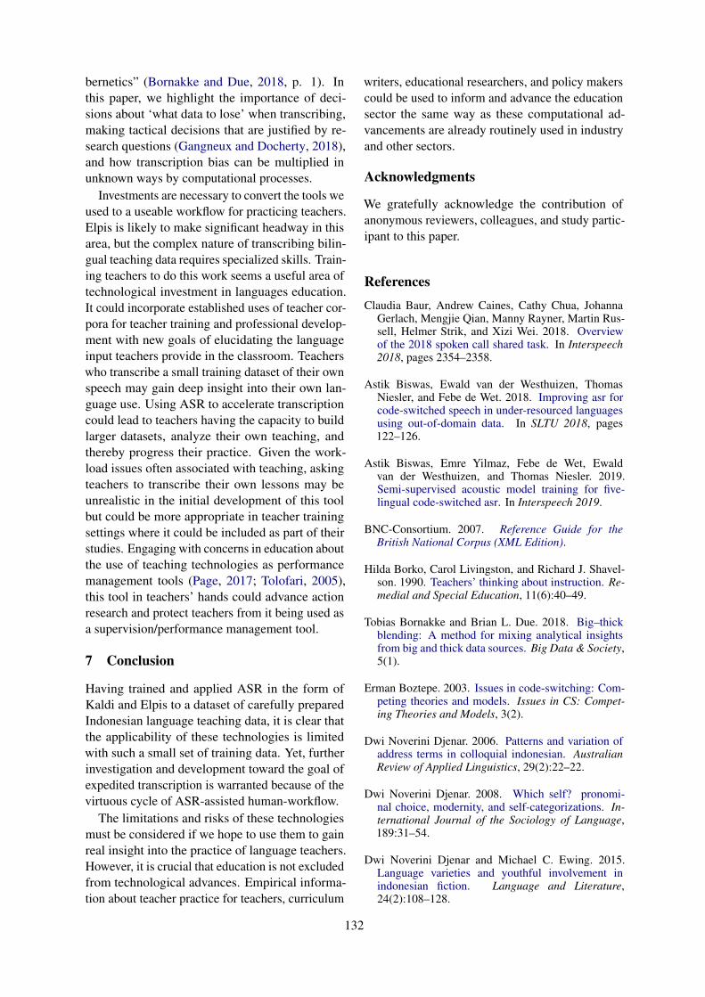
bernetics” (Bornakke and Due, 2018, p. 1). Inthis paper, we highlight the importance of deci-sions about ‘what data to lose’ when transcribing,making tactical decisions that are justified by re-search questions (Gangneux and Docherty, 2018),and how transcription bias can be multiplied inunknown ways by computational processes.

Investments are necessary to convert the tools weused to a useable workflow for practicing teachers.Elpis is likely to make significant headway in thisarea, but the complex nature of transcribing bilin-gual teaching data requires specialized skills. Train-ing teachers to do this work seems a useful area oftechnological investment in languages education.It could incorporate established uses of teacher cor-pora for teacher training and professional develop-ment with new goals of elucidating the languageinput teachers provide in the classroom. Teacherswho transcribe a small training dataset of their ownspeech may gain deep insight into their own lan-guage use. Using ASR to accelerate transcriptioncould lead to teachers having the capacity to buildlarger datasets, analyze their own teaching, andthereby progress their practice. Given the work-load issues often associated with teaching, askingteachers to transcribe their own lessons may beunrealistic in the initial development of this toolbut could be more appropriate in teacher trainingsettings where it could be included as part of theirstudies. Engaging with concerns in education aboutthe use of teaching technologies as performancemanagement tools (Page, 2017; Tolofari, 2005),this tool in teachers’ hands could advance actionresearch and protect teachers from it being used asa supervision/performance management tool.

7 Conclusion

Having trained and applied ASR in the form ofKaldi and Elpis to a dataset of carefully preparedIndonesian language teaching data, it is clear thatthe applicability of these technologies is limitedwith such a small set of training data. Yet, furtherinvestigation and development toward the goal ofexpedited transcription is warranted because of thevirtuous cycle of ASR-assisted human-workflow.

The limitations and risks of these technologiesmust be considered if we hope to use them to gainreal insight into the practice of language teachers.However, it is crucial that education is not excludedfrom technological advances. Empirical informa-tion about teacher practice for teachers, curriculum

writers, educational researchers, and policy makerscould be used to inform and advance the educationsector the same way as these computational ad-vancements are already routinely used in industryand other sectors.

Acknowledgments

We gratefully acknowledge the contribution ofanonymous reviewers, colleagues, and study partic-ipant to this paper.

ReferencesClaudia Baur, Andrew Caines, Cathy Chua, Johanna

Gerlach, Mengjie Qian, Manny Rayner, Martin Rus-sell, Helmer Strik, and Xizi Wei. 2018. Overviewof the 2018 spoken call shared task. In Interspeech2018, pages 2354–2358.

Astik Biswas, Ewald van der Westhuizen, ThomasNiesler, and Febe de Wet. 2018. Improving asr forcode-switched speech in under-resourced languagesusing out-of-domain data. In SLTU 2018, pages122–126.

Astik Biswas, Emre Yilmaz, Febe de Wet, Ewaldvan der Westhuizen, and Thomas Niesler. 2019.Semi-supervised acoustic model training for five-lingual code-switched asr. In Interspeech 2019.

BNC-Consortium. 2007. Reference Guide for theBritish National Corpus (XML Edition).

Hilda Borko, Carol Livingston, and Richard J. Shavel-son. 1990. Teachers’ thinking about instruction. Re-medial and Special Education, 11(6):40–49.

Tobias Bornakke and Brian L. Due. 2018. Big–thickblending: A method for mixing analytical insightsfrom big and thick data sources. Big Data & Society,5(1).

Erman Boztepe. 2003. Issues in code-switching: Com-peting theories and models. Issues in CS: Compet-ing Theories and Models, 3(2).

Dwi Noverini Djenar. 2006. Patterns and variation ofaddress terms in colloquial indonesian. AustralianReview of Applied Linguistics, 29(2):22–22.

Dwi Noverini Djenar. 2008. Which self? pronomi-nal choice, modernity, and self-categorizations. In-ternational Journal of the Sociology of Language,189:31–54.

Dwi Noverini Djenar and Michael C. Ewing. 2015.Language varieties and youthful involvement inindonesian fiction. Language and Literature,24(2):108–128.

132

John W. Du Bois, Stephan Schuetze-Coburn, SusannaCumming, and Danae Paolino. 1993. Outline of dis-course transcription. In Jane A. Edwards and Mar-tin D. Lampert, editors, Talking data: Transcriptionand coding in discourse research, pages 45–89. NJ:Erlbaum, Hillsdale.

Gautier Durantin. 2017. Early results from survey ex-ploring transcription processes.

Nick C. Ellis. 2017. Cognition, corpora, and comput-ing: Triangulating research in usage-based languagelearning. Language learning, 67(1):40–65.

Ben Foley, Josh Arnold, Gautier Durantin, T. Mark El-lison, Daan van Esch, Scott Heath, Nicholas Lam-bourne, Zara Maxwell-Smith, Ola Olsson, AnindaSaha, Nay San, Hywel Stoakes, and Janet Wiles.2018. Building speech recognition systems for lan-guage documentation: The coedl endangered lan-guage pipeline and inference system (elpis). In The6th International Workshop on Spoken LanguageTechnologies for Under-Resourced Languages.

Christian Gaida, Patrick Lange, Rico Petrick, PatrickProba, Ahmad Malatawy, and David Suendermann-Oeft. 2014. Comparing open-source speech recog-nition toolkits. In NLPCS 2014 : 11th Interna-tional Workshop on Natural Language Processingand Cognitive Science.

Justine Gangneux and Stevie Docherty. 2018. At closequarters: Combatting facebook design, features andtemporalities in social research. Big Data & Society,5(2).

Ofelia Garcia and Li Wei. 2014. Translanguaging:Language, Bilingualism and Education. PalgraveMacmillan, New York.

Zane Goebel. 2010. Identity and social conduct in atransient multilingual setting. Language in Society,39(02):203–240.

Zane Goebel. 2014. Doing leadership through sign-switching in the indonesian bureaucracy. Journalof Linguistic Anthropology, 24(2):193–215.

Simòn Gonzalez, Catherine E. Travis, James Grama,Danielle Barth, and Sunkulp Ananthanarayan. 2018.Recursive forced alignment: A test on a minoritylanguage. In 17th Speech Science and TechnologyConference.

Google. 2019. Google cloud speech-to-text api lan-guage support.

Nelofer Halai. 2007. Making use of bilingual interviewdata: Some experiences from the field. The Qualita-tive Report, 12(3):344–355.

Francesca Helm and Melinda Dooly. 2017. Challengesin transcribing multimodal data: A case study. Lan-guage Learning & Technology, 21(1):166–185.

Julia Hirschberg and Christopher D. Manning. 2015.Advances in natural language processing. Science,349(6245):261–266.

Eduard Hovy and Julia Lavid. 2010. Towards a ‘sci-ence’ of corpus annotation: A new methodologicalchallenge for corpus. International Journal of Trans-lation, 22(1):13–36.

Ana Iglesias, Javier Jimenèz, Pablo Revuelta, and Lour-des Moreno. 2016. Avoiding communication barri-ers in the classroom: the apeinta project. InteractiveLearning Environments, 24(4):829–843.

Daniel Jurafsky and James H. Martin. 2009. Speechand Language Processing (2nd Edition). Prentice-Hall, Inc, Upper Saddle River, NJ, USA.

Judith C. Lapadat and Anne C. Lindsay. 1998. Ex-amining transcription: A theory-laden methodology.Report, Social Sciences and Humanities ResearchCouncil of Canada, Ottawa (Ontario).

Anne-Marie Morgan. 2011. Me, myself, i: exploringconceptions of self and others in indonesian namesand pronouns with early learners. Babel, 45(2-3):26.

Sahoko Nakayama, Andros Tjandra, Sakriani Sakti,and Satoshi Nakamura. 2018. Speech chain forsemi-supervised learning of japanese-english code-switching asr and tts. In 2018 IEEE Spoken Lan-guage Technology Workshop (SLT), pages 182–189.

Blanchard Nathaniel, Michael Brady, Andrew M. Ol-ney, Marci Glaus, Xiaoyi Sun, Martin Nystrand,Borhan Samei, Sean Kelly, and Sidney D’Mello.2015. A study of automatic speech recognitionin noisy classroom environments for automated di-alog analysis. In Artificial Intelligence in Education,pages 23–33, Cham. Springer International Publish-ing.

Bonny Norton. 2001. Non-participation, imaginedcommunities and the language classroom. InM Breen, editor, Learner contributions to languagelearning: New directions in research, pages 159–171. Cascadilla Press.

Bonny Norton and Kelleen Toohey. 2011. Identity, lan-guage learning, and social change. Language Teach-ing, 44(4):412–446.

Nuance. 2019. Nuance recognizer language availabil-ity.

John Paul O Dela Rosa and Diana C. Arguelles. 2016.Do modification and interaction work? – a criticalreview of literature on the role of foreigner talk insecond language acquisition. i-Manager’s Journalon English Language Teaching, 6(3):46–60.

Damien Page. 2017. Conceptualising the surveillanceof teachers. British Journal of Sociology of Educa-tion, 38(7):991–1006.

Alastair Pennycook. 2016. Posthumanist applied lin-guistics. Applied Linguistics, 39(4):445–461.

133

Luke Plonsky. 2013. Study quality in sla: An assess-ment of designs, analyses, and reporting practicesin quantitative l2 research. Studies in Second Lan-guage Acquisition, 35(4):655–687.

David V. Pynadath, Michael J. Barnes, Ning. Wang,and Jessie Y.C. Chen. 2018. Transparency commu-nication for machine learning in human-automationinteraction. In J. Zhou and F. Chen, editors, Hu-man and Machine Learning, pages 75–90. Springer,Cham.

Kazuya Saito and Kim van Poeteren. 2012.Pronunciation-specific adjustment strategies forintelligibility in l2 teacher talk: results and implica-tions of a questionnaire study. Language Awareness,21(4):369–385.

James N. Sneddon. 2003. Diglossia in indonesian. Bi-jdragen tot de taal-, land- en volkenkunde / Journalof the Humanities and Social Sciences of SoutheastAsia, 159(4):519–549.

James N. Sneddon. 2006. Colloquial Jakartan Indone-sian, volume 581. Pacific Linguistics, ResearchSchool of Pacific and Asian Studies, Australian Na-tional University, Canberra.

Sowaribi Tolofari. 2005. New public management andeducation. Policy Futures in Education, 3(1):75–89.

Maria Teresa Turell and Melissa G. Moyer. 2009. Tran-scription. In Li Wei and Melissa Moyer, editors, TheBlackwell Guide to Research Methods in Bilingual-ism and Multilingualism, book section 11. Black-well Publishing Ltd, Carlton, Australia.

Etienne Wenger. 1998. Communities of Practice:Learning, Meaning, and Identity. Cambridge Uni-versity Press, Cambridge.

Ewald van der Westhuizen and Thomas R Niesler. 2019.Synthesised bigrams using word embeddings forcode-switched asr of four south african languagepairs. Computer Speech & Language, 54:151–175.

Yin-Lai Yeong and Tien-Ping Tan. 2014. Languageidentification of code switching sentences and mul-tilingual sentences of under-resourced languages byusing multi structural word information. In Inter-speech 2014, pages 3052–3055.

Emre Yilmaz, Henk van den Heuvel, and DavidVan Leeuwen. 2016. Investigating bilingual deepneural networks for automatic speech recognition ofcode-switching frisian speech. In 5th Workshop onSpoken Language Technology for Under-resourcedLanguages, SLTU 2016, volume 81, pages 159–166.

Xianghu Yue, Grandee Lee, Emre Yilmaz, Fang Deng,and Haizhou Li. 2019. End-to-end code-switchingasr for low-resourced language pairs. In IEEE ASRUWorkshop 2019.

AppendicesA Code Versions

This study used custom scripts for data preparation,along with the Elpis and Kaldi software projects totrain and apply ASR models.

Elpis is a wrapper for the Kaldi speech recogni-tion toolkit. At the time of the study, Kaldi was atversion 5.5.

The version of Elpis used was v0.3 of thekaldi_helpers code. The current version of Elpiscan be accessed at github.com/CoEDL/elpis. DOI:10.5281/zenodo.3833887

We have released the data preparation scriptsunder Apache License Version 2.0. These scriptshandled the generation of pronunciation lexiconsrequired by Kaldi, and the preparation of audiofiles for inferencing. The scripts can be down-loaded by following the respective DOIs. Version0.1 of kaldi-helpers-pron-lexicon was used to iden-tify and make pronunciations for English and In-donesian words. DOI: 10.5281/zenodo.3835586. Ascript, released as kaldi-helpers-segment-infer v0.1,was written to segment long audio into shorter seg-ments as required by Elpis v0.3. DOI: 10.5281/zen-odo.3834016

134

Proceedings of the 15th Workshop on Innovative Use of NLP for Building Educational Applications, pages 135–144July 10, 2020. c©2020 Association for Computational Linguistics

An empirical investigation of neural methods for content scoringof science explanations

Brian Riordan1, Sarah Bichler2, Allison Bradford2, Jennifer King Chen2,Korah Wiley2, Libby Gerard2, Marcia C. Linn2

1ETS2University of California-Berkeley

Abstract

With the widespread adoption of the NextGeneration Science Standards (NGSS), sci-ence teachers and online learning environ-ments face the challenge of evaluating stu-dents’ integration of different dimensions ofscience learning. Recent advances in represen-tation learning in natural language processinghave proven effective across many natural lan-guage processing tasks, but a rigorous evalua-tion of the relative merits of these methods forscoring complex constructed response forma-tive assessments has not previously been car-ried out. We present a detailed empirical inves-tigation of feature-based, recurrent neural net-work, and pre-trained transformer models onscoring content in real-world formative assess-ment data. We demonstrate that recent neuralmethods can rival or exceed the performanceof feature-based methods. We also provideevidence that different classes of neural mod-els take advantage of different learning cues,and pre-trained transformer models may bemore robust to spurious, dataset-specific learn-ing cues, better reflecting scoring rubrics.

1 Introduction

The Next Generation Science Standards (NGSS)call for the integration of three dimensions ofscience learning: disciplinary core ideas (DCIs),cross-cutting concepts (CCCs), and science andengineering practices (SEPs) (NGSS Lead States,2013). Science teachers can promote knowledgeintegration of these dimensions using constructedresponse (CR) formative assessments to help theirstudents build on productive ideas, fill in knowl-edge gaps, and reconcile conflicting ideas. How-ever, the time burden associated with reading andscoring student responses to CR assessment itemsoften leads to delays in evaluating student ideas.Such delays potentially make subsequent instruc-tional interventions less impactful on student learn-

ing. Effective automated methods to score studentresponses to NGSS-aligned CR assessment itemshold the potential to allow teachers to provide in-struction that addresses students’ developing under-standings in a more efficient and timely manner andcan increase the amount of time teachers have to fo-cus on classroom instruction and provide targetedstudent support.

In this study, we describe a set of CR forma-tive assessment items that call for students to ex-press and integrate ideas across multiple dimen-sions of the NGSS. We collected student responsesto each item in multiple middle school scienceclassrooms and trained models to automaticallyscore the content of responses with respect to aset of rubrics. This study explores the effective-ness of three classes of models for content scor-ing of science explanations with complex rubrics:feature-based models, recurrent neural networks,and pre-trained transformer networks. Specifically,we investigate the following questions:

(1) What is the relative effectiveness of automatedcontent scoring models from different modelclasses on scoring science explanations forboth (a) holistic knowledge integration and(b) NGSS dimensions?

(2) Do highly accurate model classes capture sim-ilar or different aspects of scoring rubrics?

2 Methods

2.1 BackgroundWe focus on constructed response (CR) items forformative assessments during science units for mid-dle school students accessed via an online class-room system (Gerard and Linn, 2016; Linn et al.,2014). In past research, items that assessed NGSSperformance expectations (PEs) were scored witha single knowledge integration (KI) rubric (Liu

135

et al., 2016). KI involves a process of buildingon and strengthening science understanding by in-corporating new ideas and sorting out alternativeperspectives using evidence. The KI rubric usedto score student short essays rewards students forlinking evidence to claims and for adding multipleevidence-claim links to their explanations (Linnand Eylon, 2011). In this study, we develop itemsthat solicit student reasoning about two or moreNGSS dimensions of DCIs, CCCs, and SEPs. Wescore each item for KI and NGSS “subscores” re-lating to the DCIs, CCCs, and practices.

3 Scoring item and rubric design

In this section we describe the design of the CRitems that comprise the datasets for the contentscoring models. The CR items formatively assessstudent understanding of multiple NGSS dimen-sions, namely, using SEPs while demonstratingintegrated understanding of DCIs and CCCs.

We designed formative assessment items andassociated rubrics for four units currently used inthe online classroom system: Musical Instruments(MI), Photosynthesis and Cellular Respiration (PS),Solar Ovens (SO), and Thermodynamics Challenge(TC).

Musical Instruments and the Physics of SoundWaves (MI). The Musical Instruments unit engagesstudents in testing and refining their ideas aboutthe properties of sound waves (wavelength, fre-quency, amplitude, and pitch) and guides them inapplying what they learn to design and build theirown instrument, a water xylophone. The CR itemwe designed aligns with the NGSS PE MS-PS4-2 PE and assesses students’ understanding of therelationship of pitch and frequency (DCI) and thecharacteristics of a sound wave when transmittedthrough different materials (CCC). Students areprompted to distinguish how the pitch of the soundmade by tapping a full glass of water compares tothe pitch made by tapping an empty glass. In theiranswer, they are asked to explain why they thinkthe pitch of the sound waves generated by strikingthe two glasses will be the same or different.

Photosynthesis and Cellular Respiration (PS).This unit engages students in exploring the pro-cesses of photosynthesis and cellular respiration byinteracting with dynamic models at the molecularlevel. We designed a CR item that aligns withNGSS performance expectation MS-LS1-6 thatasks students to express an integrated explanation

of how photosynthesis supports the survival of bothplants and animals. This item explicitly solicits stu-dents’ ideas related to the CCC of matter cycling(i.e. change) and energy flow (i.e. movement):“Write an energy story below to explain your ideasabout how animals get and use energy from thesun to survive. Be sure to explain how energy andmatter move AND how energy and matter change.”Successful responses demonstrate proficiency inthe SEP of constructing a scientific argument andreflect the synthesis of the DCIs and CCCs.

Solar Ovens (SO). The Solar Ovens unit asksstudents to collect evidence to agree or disagreewith a claim made by a fictional peer about thefunctioning of a solar oven. Students work with aninteractive model where they explore how differentvariables such as the size and capacity of a solaroven affect the transformation of energy from thesun. We designed a CR item that addresses NGSSPE MS-PS3-3 and assesses students for both theCCC of energy transfer and transformation andthe SEP of analyzing and interpreting data. Af-ter working with the interactive model, studentsrespond to the CR item with the prompt: “Explainwhy David’s claim is correct or incorrect using theevidence you collected from the model. Be sure todiscuss how the movement of energy causes onesolar oven to heat up faster than the other.”

Thermodynamics Challenge (TC). The Thermo-dynamics Challenge unit asks students to determinethe best material for insulating a cold beverage us-ing an online experimentation model. We designeda CR item that aligns with the NGSS PE MS-PS3-3and assesses student performance proficiency withthe targeted DCIs in the PE, understanding of theSEP of planning and carrying out an investigation,and the integration of both of these to constructa coherent and valid explanation. The CR itemprompts students to explain the rationale behindtheir experiment plans with the model, using bothkey conceptual ideas as well as their understandingof experimentation as a scientific practice: “Ex-plain WHY the experiments you [plan to test] arethe most important ones for giving you evidence towrite your report. Be sure to use your knowledgeof insulators, conductors, and heat energy transferto discuss the tests you chose as well as the onesyou didn’t choose.”

We designed three scoring rubrics for each itemcorresponding to two “subscores” representing thedegree to which the written responses expressed

136

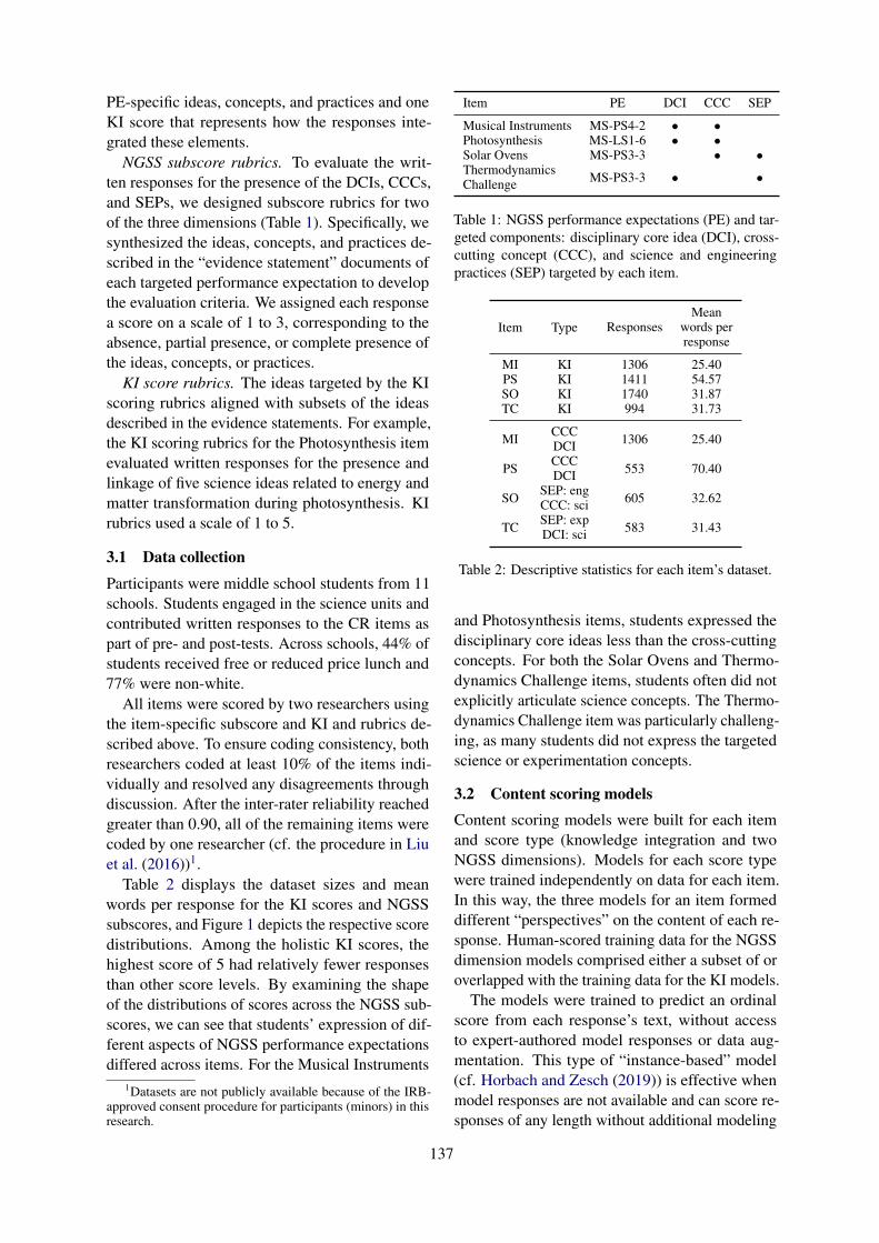
PE-specific ideas, concepts, and practices and oneKI score that represents how the responses inte-grated these elements.

NGSS subscore rubrics. To evaluate the writ-ten responses for the presence of the DCIs, CCCs,and SEPs, we designed subscore rubrics for twoof the three dimensions (Table 1). Specifically, wesynthesized the ideas, concepts, and practices de-scribed in the “evidence statement” documents ofeach targeted performance expectation to developthe evaluation criteria. We assigned each responsea score on a scale of 1 to 3, corresponding to theabsence, partial presence, or complete presence ofthe ideas, concepts, or practices.

KI score rubrics. The ideas targeted by the KIscoring rubrics aligned with subsets of the ideasdescribed in the evidence statements. For example,the KI scoring rubrics for the Photosynthesis itemevaluated written responses for the presence andlinkage of five science ideas related to energy andmatter transformation during photosynthesis. KIrubrics used a scale of 1 to 5.

3.1 Data collection

Participants were middle school students from 11schools. Students engaged in the science units andcontributed written responses to the CR items aspart of pre- and post-tests. Across schools, 44% ofstudents received free or reduced price lunch and77% were non-white.

All items were scored by two researchers usingthe item-specific subscore and KI and rubrics de-scribed above. To ensure coding consistency, bothresearchers coded at least 10% of the items indi-vidually and resolved any disagreements throughdiscussion. After the inter-rater reliability reachedgreater than 0.90, all of the remaining items werecoded by one researcher (cf. the procedure in Liuet al. (2016))1.

Table 2 displays the dataset sizes and meanwords per response for the KI scores and NGSSsubscores, and Figure 1 depicts the respective scoredistributions. Among the holistic KI scores, thehighest score of 5 had relatively fewer responsesthan other score levels. By examining the shapeof the distributions of scores across the NGSS sub-scores, we can see that students’ expression of dif-ferent aspects of NGSS performance expectationsdiffered across items. For the Musical Instruments

1Datasets are not publicly available because of the IRB-approved consent procedure for participants (minors) in thisresearch.

Item PE DCI CCC SEP

Musical Instruments MS-PS4-2 • •Photosynthesis MS-LS1-6 • •Solar Ovens MS-PS3-3 • •ThermodynamicsChallenge MS-PS3-3 • •

Table 1: NGSS performance expectations (PE) and tar-geted components: disciplinary core idea (DCI), cross-cutting concept (CCC), and science and engineeringpractices (SEP) targeted by each item.

Item Type ResponsesMean

words perresponse

MI KI 1306 25.40PS KI 1411 54.57SO KI 1740 31.87TC KI 994 31.73

MI CCCDCI 1306 25.40

PS CCCDCI 553 70.40

SO SEP: engCCC: sci 605 32.62

TC SEP: expDCI: sci 583 31.43

Table 2: Descriptive statistics for each item’s dataset.

and Photosynthesis items, students expressed thedisciplinary core ideas less than the cross-cuttingconcepts. For both the Solar Ovens and Thermo-dynamics Challenge items, students often did notexplicitly articulate science concepts. The Thermo-dynamics Challenge item was particularly challeng-ing, as many students did not express the targetedscience or experimentation concepts.

3.2 Content scoring modelsContent scoring models were built for each itemand score type (knowledge integration and twoNGSS dimensions). Models for each score typewere trained independently on data for each item.In this way, the three models for an item formeddifferent “perspectives” on the content of each re-sponse. Human-scored training data for the NGSSdimension models comprised either a subset of oroverlapped with the training data for the KI models.

The models were trained to predict an ordinalscore from each response’s text, without accessto expert-authored model responses or data aug-mentation. This type of “instance-based” model(cf. Horbach and Zesch (2019)) is effective whenmodel responses are not available and can score re-sponses of any length without additional modeling

137

0.0 0.2 0.4 0.6 0.8 1.0

TC

PS

SO

MI

Item

12345

(a)

0.0 0.2 0.4 0.6 0.8 1.0

TC exp

TC sci

PS CCC

PS DCI

SR eng

SR sci

MI CCC

MI DCI

Item

123

(b)

Figure 1: Score distributions for (a) knowledge integration scores and (b) NGSS subscores.

complexity. As we focus on content scoring, themodels do not consider grammatical or usage errorsthat do not relate to the content of each response.

The feature-based model is a nonlinear supportvector regression (SVR) model. The model istrained on a feature set of binarized word n-gramswith n in {1, 2}.

The RNN model uses a simple architecture withpre-trained word embeddings and pooling of hid-den states. Pre-trained word embeddings are pro-cessed by a bidirectional GRU encoder. The hiddenstates of the GRU are aggregated by a max poolingmechanism (Shen et al., 2018). The output of theencoder is aggregated in a fully-connected feedfor-ward layer with sigmoid activation that computesa scalar output for the predicted score. Despite itssimplicity, this architecture has achieved state-of-the-art performance on benchmark content scoringdatasets (Riordan et al., 2019).

For the pre-trained transformer model, we used astandard instance of the BERT model (Devlin et al.,2019). BERT is a bidirectional transformer modeltrained on the tasks of masked token prediction andnext sentence prediction across very large corpora(BooksCorpus and English Wikipedia). Duringtraining, a special token ‘[CLS]’ is added to thebeginning of each input sequence. To make predic-tions, the learned representation for this token isprocessed by an additional layer with nonlinear ac-tivation, outputting a score prediction. The modelwas ‘fine-tuned’ by training the additional layer’sweights on each item’s dataset.

3.3 Data preparation, model training, andhyperparameter optimization

SVR model. The SVR models used an RBF kernel.Hyperparameters C and gamma were tuned on thevalidation sets and were optimized by root meansquared error.

RNN model. Word tokens were embedded withGloVe 100 dimension vectors (Pennington et al.,2014) and fine-tuned during training. Word tokensthat were not found in the embeddings vocabularywere mapped to a randomly initialized UNK em-bedding. On conversion to tensors, responses werepadded to the same length in a batch; these paddingtokens are masked out during model training. Priorto training, responses were scaled to [0, 1] to formthe input to the networks. The scaled scores wereconverted back to their original range for evalua-tion.

The GRUs were 1 layer with a hidden state ofsize 250. The RNN models were trained with amean squared error loss. For this investigation, theRNN was optimized with RMSProp with ρ of 0.9,learning rate 0.001, batch size 32, and gradientclipping (10.0). We used an exponential movingaverage of the model’s weights for training (decayrate = 0.999) (Adhikari et al., 2019). In the tuningphase, models were trained for 50 epochs.

Pretrained transformer model. We used the bert-base-uncased pre-trained model (Wolf et al., 2019)and the Adam optimizer. On the Photosynthesisdataset, due to memory requirements, training re-quired a batch size of 8; all other datasets weretrained with a batch size 16. The learning ratewas tuned individually for each dataset with a gridof {2e-5, 3e-5, 5e-5}. Matching the RNN model,an exponential moving average over the model’sweights was employed during training. Hyperpa-rameters were tuned for 20 epochs.

For all experiments, we trained models with10-fold cross validation with train/validation/testsplits, evaluating on pooled (concatenated) predic-tions across folds. We split the data into 80% train,10% validation, and 10% test. For hyperparametertuning, we trained on each train split and evalu-ated performance on the validation split, retaining

138

Item Model Corr QWK MSE Sig.

MISVR 0.7804 0.7045 0.3298RNN 0.7989 0.7642 0.3058PT 0.8134 0.7733 0.2956

PSSVR 0.8296 0.7851 0.2098 RRNN 0.8215 0.7550 0.2285PT 0.8459 0.8246 0.1997 S,R

SOSVR 0.7491 0.6690 0.2737RNN 0.7612 0.7116 0.2619PT 0.7691 0.7127 0.2608 S,R

TCSVR 0.6856 0.6156 0.4777RNN 0.7106 0.6732 0.4465 SPT 0.7286 0.6791 0.4266 S

Table 3: Human-machine agreement for KnowledgeIntegration (KI) score models. QWK = quadratic-weighed kappa, MSE = mean squared error. SVR =support vector regression, RNN = recurrent neural net-work, PT = pre-trained Transformer. Sig. = signifi-cance by bootstrap replicability analysis; see main textfor details.

the predictions from the best performance acrossepochs and the epoch on which that performancewas observed. We pooled the predictions fromall folds on the validation sets, evaluated perfor-mance, and selected the best-performing configura-tion of hyperparameters. For final model training,we trained models on combined train and valida-tion splits, again with 10-fold cross-validation, tothe median best epoch across folds from the hy-perparameter tuning phase. Final performance wasevaluated on the pooled predictions from the testsplits. This training and evaluation procedure im-proves the stability of estimates of performanceduring both the tuning and final testing phases andmakes use of more data for training and evaluat-ing the final models, providing better estimates ofmodel performance.

3.4 Evaluation metrics

To evaluate the agreement of human scores andmachine scores, we report Pearson’s correlation,quadratic weighted kappa (QWK), and meansquared error (MSE). QWK is a measure of agree-ment that ranges between 0 and 1 and is motivatedby accounting for chance agreement (Fleiss andCohen, 1973). Correlation and MSE are computedover real-valued model predictions, while QWK iscomputed over rounded predictions.

Item Sub-score Model Corr QWK MSE Sig.

MI CCCSVR .7008 .6314 .3185RNN .7685 .7322 .2561 SPT .7730 .7542 .2557 S

MI DCISVR .7505 .7110 .1261RNN .7908 .7392 .1088PT .8230 .7970 .0953

PS CCCSVR .6992 .6050 .3102RNN .7379 .7187 .2772PT .7188 .6607 .2997 S

PS DCISVR .7410 .6956 .2245RNN .7795 .7471 .1955PT .8044 .7701 .1826

SO engSVR .6957 .5915 .2684RNN .7484 .7112 .2503PT .7662 .7263 .2428 S

SO sciSVR .5789 .4770 .1744RNN .6872 .5408 .1623PT .6480 .6038 .1834

TC expSVR .5323 .4705 .1926RNN .5916 .4675 .1724PT .6067 .5445 .1661

TC sciSVR .5038 .0000 .2262RNN .5090 .3897 .1835 SPT .5303 .4182 .1779 S

Table 4: Human-machine agreement for NGSS sub-score models. Sig. = significance by bootstrap repli-cability analysis; see main text.

4 Results

4.1 Human-machine agreementThe models for the KI scores showed mostly goodagreement with human scores (Table 3). QWKfor the Musical Instruments, Photosynthesis, andSolar Ovens items was substantially higher thanthe standard 0.7 recommended for human-machineagreement in real-word automated scoring applica-tions (Williamson et al., 2012).

For NGSS subscore models (Table 4), those withmore balanced score distributions (cf. Figure 1)showed good human-machine agreement, whilethe models trained on the most skewed data dis-tributions showed lower levels of human-machineagreement. Specifically, Solar Ovens-Science andthe Thermodynamics Challenge subscore modelswere trained on data where about 80% of responseshad the lowest score. Each of these models’ agree-ment with the human-scored data was relativelylow and significantly below the 0.7 QWK thresh-old.

Across both KI score models and NGSS sub-score models, the pre-trained transformer mod-els showed higher human-machine agreement thanboth the SVR and RNN models in almost all cases.On the KI score datasets, the performance improve-

139

ment from the PT models was relatively modest, ex-cept for the Photosynthesis dataset, where a largerimprovement was observed. On the NGSS sub-score datasets, the improvement from the PT mod-els was often larger. This may be the result ofstronger representations from the pretrained mod-els compensating from the smaller training datasetsizes. At the same time, RNN models also per-formed well on data-impoverished datasets such asPhotosynthesis-CCC and Solar Ovens-science.

The cross-validation training and evaluation pro-cedure employed here poses a challenge to statis-tically estimating the strengths of the differencesbetween methods since the folds are not indepen-dent. Here we employ replicability analysis formultiple comparisons (Reichart et al., 2018; Droret al., 2017). We use bootstrap-based significancetesting on each fold for the final model on eachdataset and then perform K-Bonferonni replicabil-ity analysis. We define significance as rejectingthe null hypothesis of no difference for at leasthalf of the folds. The results of these hypothesistests are shown in Tables 3 and 4. For example, Sindicates the model in that row (PT) performed sig-nificantly better than the SVR model (similarly forthe RNN models). Although this hypothesis testingframework is conservative, the results support theconclusion that the pre-trained transformer models’performance was strong.

5 Error analysis

In this section, we explore the differences in thetwo neural models (RNN and PT) in more detail bylooking at patterns of errors. We focus on instance-level saliency maps – gradient-based methods thatidentify the importance of tokens to the model byexamining the gradient of the loss. For each dataset,we sample 100 responses and generate saliencymaps for each. We use the simple gradient method(Simonyan et al., 2014) via AllenNLP (Wallaceet al., 2019). The item developers manually an-alyzed the generated saliency maps for each re-sponse and model.

We analyzed two sets of cases:

1. One neural model accurately predicted thehuman score while the other did not. How dothe error patterns in these cases illustrate howthe models each learned differently from thetraining data?

2. Both models incorrectly predicted the human

score, and moreover predicted the same incor-rect score. Do the models make the wrongprediction for the same or different reasons?

In the following, due to space constraints, wefocus on error analysis for the scoring model forthe Musical Instruments knowledge integrationdataset.

One correct, one incorrect. Cases where onemodel accurately predicted the human score whilethe other did not illuminated several differences inthe two neural models.

The RNN model tended to ignore or de-emphasize some keywords, while overemphasizinghigh frequency and function words. For example,Figure 2a shows a simple example where the RNNfails to emphasize the keyword pitch. The BERTmodel accurately registers this word as salient, andpredicts the correct score. Similarly, in Figure 2b,the RNN misses the keyphrase full glass while theBERT model catches it. In Figure 2c, the RNNspuriously treats the function words when and youas salient and over-predicts the score.

For its part, the BERT model may de-emphasizemany high frequency words but at the same timemay regard discourse markers as salient. An exam-ple is in Figure 3a, where the BERT model empha-sizes because since, and this may in part help themodel reach the correct prediction.

If the BERT model is able to better learn im-portant keywords (while ignoring more functionwords), it may sometimes “overlearn” the impor-tance of those tokens, leading to over-predictionof scores. There are several examples where themodel uses the word piece ##brate to overpredict ascore (Figure 3b).

Both incorrect with the same prediction. In manycases, the models made the same incorrect predic-tions for different reasons. An example is Figure3c, where the RNN emphasizes deeper and densewhile the BERT model focuses on because and cup.Overall, the same differences in the models identi-fied above held for these cases of making the sameincorrect prediction.

In general, although there was some variabilityacross models, both models correctly identified thekeywords necessary for scoring responses correctly,leading to good human-machine agreement. TheRNN model may be more sensitive to tokens thatare good indicators of the score in the training data(either high or low) but not in language in general,such as high frequency and function words, while

140

148053 score=3 prediction=2the pitch gets a lot lower148053 score=3 prediction=3[CLS] the pitch gets a lot lower [SEP]

(a)207529 score=3 prediction=2The tap of a full glass is more low pitched and an empty glass is morehigh pitched because there is no bellow207529 score=3 prediction=3[CLS] the tap of a full glass is more low pitched and an empty glass ismore high pitched because there is no bell ##ow [SEP]

(b)147925 score=2 prediction=3When you tap on a full glass the pitch stays the same as if you weretapping on an empty glass because you are still tapping on a glass thatis going to make a high pitched sound no matter if it is full or not .147925 score=2 prediction=2[CLS] when you tap on a full glass the pitch stays the same as if youwere tapping on an empty glass because you are still tapping on a glassthat is going to make a high pitched sound no matter if it is full or not. [SEP]

(c)

Figure 2: Error analysis: RNN model trends. In each example, the RNN model’s saliency map appears on top.

237142 score=3 prediction=2The pitch of the tapped full glass is lower than the pitch of the tappedempty glass because since there is water inside you are not going to beable to hear it as much .237142 score=3 prediction=3[CLS] the pitch of the tapped full glass is lower than the pitch of thetapped empty glass because since there is water inside you are not goingto be able to hear it as much . [SEP]

(a)148661 score=3 prediction=3The one taht is full will vibrate less so it will be higher than the onethat is empty .148661 score=3 prediction=4[CLS] the one ta ##ht is full will vi ##brate less so it will be higherthan the one that is empty . [SEP]

(b)176754 score=4 prediction=3the cup with water has a deeper sound because its changing throughthe dense water but the cup with no water stays the same because thesound wave does n’t have to go through anything or change anything .176754 score=4 prediction=3[CLS] the cup with water has a deeper sound because its changingthrough the dense water but the cup with no water stays the samebecause the sound wave doesn ’ t have to go through anything or changeanything . [SEP]

(c)

Figure 3: Error analysis: Pre-trained transformer model trends. In each example, the pre-trained transformermodel’s saliency map appears on the bottom.

141

BERT’s pre-training regime may equip it to reduceany reliance on such tokens.

Notably, however, while the models usuallymade good use of keyword evidence to arrive atcorrect scores, when the models made inaccuratepredictions, it was often because the response hadthe right vocabulary but the wrong science. For ex-ample, in the Musical Instruments item, a responsemight contain pitch, lower, density, and vibrations,but the response might attribute the lower pitch tothe empty glass. At least two issues were observedin cases of model mis-prediction: (1) students usedanaphoric it to refer to key concepts (e.g., full glassor empty glass), but the models do not incorpo-rate anaphora resolution capabilities; (2) modelsfail to associate the right keywords with the rightconcepts, in the way that human raters did.

6 Related work

The task of automated content scoring has recentlygained more attention (Kumar et al., 2017; Riordanet al., 2017; Burrows et al., 2015; Shermis, 2015).Our work is similar to Mizumoto et al. (2019), whodeveloped a multi-task neural model for assigningan overall holistic score as well as content-basedanalytic subscores. We leave a multi-task formula-tion of our application setting for future work.

Sung et al. (2019) demonstrated state-of-the-artperformance for similarity-based content scoringon the SemEval benchmark dataset (Dzikovskaet al., 2016). In this work, we use pre-trained trans-former models for instance-based content scoring(cf. Horbach and Zesch (2019)). That is, we usewhole responses as training data and fine-tune pre-trained representations for response tokens on thecontent score prediction task.

Recently, methods have been introduced to incor-porate “saliency” directly into the model trainingprocess (Ghaeini et al., 2019). The current workfocuses on interpreting the predictions of mod-els trained without additional annotations (for anoverview of interpretability in NLP, see Belinkovand Glass (2019). Exploring the contribution ofaugmented datasets and training algorithms is fu-ture work. To our knowledge, our work is the firstto to explore the relevance of the saliency in the pre-dictions of neural methods for the content scoringtask.

7 Conclusion

We described a set of constructed response itemsfor middle-school science curricula that simulta-neously assess students on expression of NGSSDisciplineary Core Ideas (DCIs), Cross-CuttingConcepts (CCCs), and Science and EngineeringPractices (SEPs), and the integrative linkages be-tween each, as part of engaging in scientific expla-nations and argumentation. We demonstrated thathuman and automated scoring of such CRs for theNGSS dimensions (via independent subscores) andthe integration of knowledge (via Knowledge Inte-gration scores) is feasible. We demonstrated thatautomated scoring can be developed with promis-ing accuracy.

Comparing feature-based, RNN, and pre-trainedtransformer models on these datasets, we observedthat the pre-trained transformer models obtainedhigher rates of human-machine agreement on mostholistic KI score and NGSS subscore datasets.While the RNN models were often competitivewith the pre-trained transformer models, an anal-ysis of the different kinds of errors made by eachmodel type indicated that the pre-trained trans-former models may be more robust to strongdataset-specific, but spurious, cues to score pre-diction.

Results showed that, in the formative settingtargeted by the online science learning environ-ment used in this study, students often scored at thelowest levels of all three rubrics, which increasedskewness in the datasets and likely contributed toreduced model accuracy. Future research will ex-plore more robust methods for learning scoringmodels from less data in formative settings, es-pecially from highly skewed score distributions,while continuing to provide accurate scoring.

Our findings demonstrate the ability to both de-velop and automatically score NGSS-aligned CRassessment items. With further refinement, we canprovide teachers with both the instructional andtechnological assistance they need to effectivelyand efficiently support their students to demonstratethe multidimensional science learning called for bythe NGSS.

Acknowledgments

We thank Aoife Cahill for many useful discussionsand three anonymous reviewers, Beata BeigmanKlebanov, Debanjan Ghosh, and Nitin Madnanifor helpful comments. This material is based upon

142

work supported by the National Science Founda-tion under Grant No. 1812660. Any opinions,findings, and conclusions or recommendations ex-pressed in this material are those of the author(s)and do not necessarily reflect the views of the Na-tional Science Foundation.

ReferencesAshutosh Adhikari, Achyudh Ram, Raphael Tang, and

Jimmy Lin. 2019. Rethinking Complex Neural Net-work Architectures for Document Classification. InProceedings of the 2019 Conference of the NorthAmerican Chapter of the Association for Computa-tional Linguistics: Human Language Technologies(NAACL-HLT).

Yonatan Belinkov and James Glass. 2019. AnalysisMethods in Neural Language Processing: A Survey.Transactions of the Association for ComputationalLinguistics.

Steven Burrows, Iryna Gurevych, and Benno Stein.2015. The Eras and Trends of Automatic Short An-swer Grading. International Journal of Artificial In-telligence in Education, 25(1):60–117.

Jacob Devlin, Ming-Wei Chang, Kenton Lee, andKristina Toutanova. 2019. BERT: Pre-training ofDeep Bidirectional Transformers for Language Un-derstanding. In Proceedings of the 2019 Conferenceof the North American Chapter of the Associationfor Computational Linguistics: Human LanguageTechnologies (NAACL-HLT).

Rotem Dror, Gili Baumer, Marina Bogomolov, andRoi Reichart. 2017. Replicability Analysis for Natu-ral Language Processing: Testing Significance withMultiple Datasets. Transactions of the Associationfor Computational Linguistics, 5:471–486.

Myroslava O. Dzikovska, Rodney D. Nielsen, andClaudia Leacock. 2016. The joint student responseanalysis and recognizing textual entailment chal-lenge: making sense of student responses in educa-tional applications. Language Resources and Evalu-ation, 50(1):67–93.

Joseph L. Fleiss and Jacob Cohen. 1973. The equiv-alence of weighted kappa and the intraclass corre-lation coefficient as measures of reliability. Educa-tional and psychological measurement, 33(3):613–619.

Libby F. Gerard and Marcia C. Linn. 2016. UsingAutomated Scores of Student Essays to SupportTeacher Guidance in Classroom Inquiry. Journal ofScience Teacher Education, 27(1):111–129.

Reza Ghaeini, Xiaoli Z. Fern, Hamed Shahbazi, andPrasad Tadepalli. 2019. Saliency Learning: Teach-ing the Model Where to Pay Attention. In Proceed-ings of the 2019 Conference of the North American

Chapter of the Association for Computational Lin-guistics: Human Language Technologies (NAACL-HLT).

Andrea Horbach and Torsten Zesch. 2019. The influ-ence of variance in learner answers on automaticcontent scoring. Frontiers in Education, 4:28.

Sachin Kumar, Soumen Chakrabarti, and Shourya Roy.2017. Earth Mover’s Distance Pooling over SiameseLSTMs for Automatic Short Answer Grading. InInternational Joint Conference on Artificial Intelli-gence (IJCAI).

Marcia C. Linn and Bat-Sheva Eylon. 2011. Sci-ence Learning and Instruction: Taking Advantageof Technology to Promote Knowledge Integration.Routledge, New York.

Marcia C. Linn, Libby Gerard, Kihyun Ryoo, KevinMcElhaney, Ou Lydia Liu, and Anna N Rafferty.2014. Computer-guided inquiry to improve sciencelearning. Science, 344(6180):155–156.

Ou Lydia Liu, Joseph A. Rios, Michael Heilman, LibbyGerard, and Marcia C. Linn. 2016. Validation of Au-tomated Scoring of Science Assessments. Journalof Research in Science Teaching, 53(2):215–233.

Tomoya Mizumoto, Hiroki Ouchi, Yoriko Isobe, PaulReisert, Ryo Nagata, Satoshi Sekine, and KentaroInui. 2019. Analytic Score Prediction and Justifica-tion Identification in Automated Short Answer Scor-ing. In 14th Workshop on Innovative Use of NLP forBuilding Educational Applications (BEA@ACL).

NGSS Lead States. 2013. Next Generation ScienceStandards: For States, By States. The NationalAcademies Press, Washington, D.C.

Jeffrey Pennington, Richard Socher, and ChristopherManning. 2014. Glove: Global Vectors for WordRepresentation. In Proceedings of the 2014 Con-ference on Empirical Methods in Natural LanguageProcessing (EMNLP).

Roi Reichart, Rotem Dror, Gili Baumer, and SegevShlomov. 2018. The Hitchhiker’s Guide to Test-ing Statistical Significance in Natural Language Pro-cessing. In Proceedings of the 56th Annual Meet-ing of the Association for Computational Linguistics(ACL).

Brian Riordan, Michael Flor, and Robert Pugh. 2019.How to account for mispellings: Quantifying thebenefit of character representations in neural contentscoring models. In Proceedings of the 14th Work-shop on Innovative Use of NLP for Building Educa-tional Applications (BEA@ACL).

Brian Riordan, Andrea Horbach, Aoife Cahill, TorstenZesch, and Chong Min Lee. 2017. Investigating neu-ral architectures for short answer scoring. In 12thWorkshop on Innovative Use of NLP for Building Ed-ucational Applications (BEA@EMNLP).

143

Dinghan Shen, Guoyin Wang, Wenlin Wang, Mar-tin Renqiang Min, Qinliang Su, Yizhe Zhang, Chun-yuan Li, Ricardo Henao, and Lawrence Carin. 2018.Baseline Needs More Love: On Simple Word-Embedding-Based Models and Associated PoolingMechanisms. In Proceedings of the 56th AnnualMeeting of the Association for Computational Lin-guistics (ACL).

Mark D Shermis. 2015. Contrasting state-of-the-artin the machine scoring of short-form constructed re-sponses. Educational Assessment, 20(1).

Karen Simonyan, Andrea Vedaldi, and Andrew Zis-serman. 2014. Deep Inside Convolutional Net-works: Visualising Image Classification Models andSaliency Maps. In International Conference onLearning Representations (ICLR).

Chul Sung, Tejas I. Dhamecha, and Nirmal Mukhi.2019. Improving Short Answer Grading UsingTransformer-Based Pre-training. In Proceedings ofthe 20th International Conference on Artificial Intel-ligence in Education (AIED).

Eric Wallace, Jens Tuyls, Junlin Wang, Sanjay Subra-manian, Matthew Gardner, and Sameer Singh. 2019.AllenNLP Interpret: A Framework for ExplainingPredictions of NLP Models. In Proceedings of the2019 Conference on Empirical Methods in NaturalLanguage Processing (EMNLP).

David M. Williamson, Xiaoming Xi, and F. Jay Breyer.2012. A framework for evaluation and use of au-tomated scoring. Educational measurement: issuesand practice, 31(1):2–13.

Thomas Wolf, Lysandre Debut, Victor Sanh, JulienChaumond, Clement Delangue, Anthony Moi, Pier-ric Cistac, Tim Rault, R’emi Louf, Morgan Funtow-icz, and Jamie Brew. 2019. HuggingFace’s Trans-formers: State-of-the-art Natural Language Process-ing. ArXiv, abs/1910.03771.

144

Proceedings of the 15th Workshop on Innovative Use of NLP for Building Educational Applications, pages 145–150July 10, 2020. c©2020 Association for Computational Linguistics

An Exploratory Study of Argumentative Writing by Young Students: ATransformer-based Approach

Debanjan Ghosh, Beata Beigman Klebanov, Yi SongEducational Testing Service

dghosh,bbeigmanklebanov,ysong@ets.org

Abstract

We present a computational exploration of ar-gument critique writing by young students.Middle school students were asked to criticizean argument presented in the prompt, focus-ing on identifying and explaining the reason-ing flaws. This task resembles an establishedcollege-level argument critique task. Lexicaland discourse features that utilize detailed do-main knowledge to identify critiques exist forthe college task but do not perform well onthe young students data. Instead, transformer-based architecture (e.g., BERT) fine-tuned ona large corpus of critique essays from the col-lege task performs much better (over 20% im-provement in F1 score). Analysis of the per-formance of various configurations of the sys-tem suggests that while children’s writing doesnot exhibit the standard discourse structure ofan argumentative essay, it does share basic lo-cal sequential structures with the more maturewriters.

1 Introduction

Argument and logic are essential in academic writ-ing as they enhance the critical thinking capacitiesof students. Argumentation requires systematicreasoning and the skill of using relevant examplesto craft a support for one’s point of view (Walton,1996). In recent times, the surge in AI-informedscoring systems has made it possible to assesswriting skills using automated systems. Recent re-search suggests the possibility of argumentation-aware automated essay scoring systems (Stab andGurevych, 2017b).

Most of the current work on computationalanalysis of argumentative writing in educationalcontext focuses on automatically identifying theargument structures (e.g., argument componentsand their relations) in the essays (Stab andGurevych, 2017a; Persing and Ng, 2016; Nguyen

and Litman, 2016) and by predicting essay scoresfrom features derived from the structures (e.g., thenumber of claims and premises and the number ofsupported claims) (Ghosh et al., 2016). Related re-search has also addressed the problem of scoring aparticular dimension of essay quality, such as rele-vance to the prompt (Persing and Ng, 2014), opin-ions and their targets (Farra et al., 2015), argumentstrength (Persing and Ng, 2015), among others.

While argument mining literature has addressedthe educational context, it has so far mainly fo-cused on analyzing college-level writing. For in-stance, Nguyen and Litman (2018) investigated ar-gument structures in TOEFL11 corpus (Blanchardet al., 2013); Beigman Klebanov et al. (2017) andPersing and Ng (2015) analyzed writing of uni-versity students; Stab and Gurevych (2017b) useddata from “essayforum.com”, where college en-trance examination is the largest forum. Compu-tational analysis of arguments in young students’writing has not yet been done, to the best of ourknowledge. Writing quality in essays by youngwriters has been addressed (Deane, 2014; Attaliand Powers, 2008; Attali and Burstein, 2006), butidentification of arguments was not part of thesestudies.

In this paper, we present a novel learning-and-assessment context where middle school studentswere asked to criticize an argument presented inthe prompt, focusing on identifying and explain-ing the reasoning flaws. Using a relatively smallpilot data collected for this task, our aim here isto automatically identify good argument critiquesin the young students’ writing, with the twin goalsof (a) exploring the characteristics of young stu-dents’ writing for this task, and (b) in view of po-tential scoring and feedback applications. We startwith describing and exemplifying the data, as wellas the argument critique annotation we performedon it (section 2). Experiments and results are pre-

145

Dear Editor,

Advertising aimed at children under 12 should be allowedfor several reasons.

First, one family in my neighbourhood sits down andwatches TV together almost every evening. The whole fam-ily learns a lot, which shows that advertising for children isalways a good thing because it brings families together.

Second, research shows that children can’t remember com-mercials well anyway, so they can’t be doing kids any harm.

Finally, the arguments against advertising aren’t very effec-tive. Some countries banned ads because kids thought theads were funny. But that’s not a good reason. Think aboutit: the advertising industry spends billions of dollars a yearon ads for children. They wouldn’t spend all the money ifthe ads weren’t doing some good. Let’s not hurt children bystopping a good thing.

If anyone doesn’t like children’s ads, the advertisers shouldjust try to make them more interesting. The ads are allowedto be shown on TV, so they shouldn’t be banned.

Table 1: The prompt of the argument critique task.

sented in section 3, followed by a discussion insection 4.

2 Dataset and Annotation

The data used in this study was collected as partof a pilot of a scenario-based assessment of ar-gumentation skills with about 900 middle schoolstudents (Song et al., 2017).1 Students engaged ina sequence of steps in which they researched andreflected on whether advertising to children underthe age of twelve should be banned. The test con-sists of four tasks; we use the responses to Task 3in which students are asked to review a letter to theeditor and evaluate problems in the letter’s reason-ing or use of evidence (see Table 1).

Students were expected to produce a written cri-tique of the arguments, demonstrating their abil-ity to identify and explain problems in the rea-soning or use of evidence. For example, the firstexcerpt below shows a well-articulated critique ofthe hasty generalization problem in the prompt:

(1) Just because it brings one family togetherto learn does not mean that it will bring allfamilies together to learn.

(2) The first one about the family in yourneighborhood is more like an opinion, not ac-tual information from the article.

1The data was collected under the ETS CBAL (Cogni-tively Based Assessment of, for, and as Learning) Initiative.

(3) Their claims are badly writtin [sic] andhave no good arguments. They need to supporttheir claims with SOLID evidence and onlyclaim arguments that can be undecicive [sic].

However, many students had difficulty explain-ing the reasoning flaws clearly. In the second ex-cerpt, the student thought that an argument fromthe family in the neighborhood is not strong, butdid not demonstrate an understanding of a weakgeneralization in his explanation. Other com-mon problems included students summarizing theprompt without criticizing, or providing a genericcritique that does not adhere to the particulars ofthe prompt (excerpt (3)).

The goal of the argument critique annotation(described next) was to identify where in a re-sponse good critiques are made, such as the onein the first excerpt.

Annotation of Critiques: We identified 11valid critiques of the arguments in the letter. Thesecritiques included: (1) overgeneralizing from asingle example; (2) example irrelevant to the ar-gument; (3) example misrepresenting what actu-ally happened; (4) misrepresenting the goal ofmaking advertisements; (5) misunderstanding theproblem; (6) neglecting potential side effects ofallowing advertising aimed at children; (7) mak-ing a wrong argument from sign; (8) argumentcontradicting authoritative evidence; (9) argumentcontradicting one’s own experience; (10) mak-ing a circular argument; (11) making contradic-tory claims. All sentences containing any ma-terial belonging to a valid critique were markedand henceforth denoted as Arg; the rest are de-noted as NoArg. Three annotators were em-ployed to annotate the sentences to mark them asArg/NoArg. We computed κ between each pairof annotators based on the annotation of 50 essays.Inter-annotator agreement for this sentence-levelArg/NoArg classification for each pair of anno-tators was 0.714, 0.714, and 0.811, respectivelyresulting in an average κ of 0.746.

Descriptive statistics: We split the data intotraining (585 response critiques) and test (252 re-sponse critiques). The training partition has 2,220sentences (515 Arg; 1,705 NoArg; average num-ber of words per sentence is 11 (std = 8.03)); testcontains 973 sentences.

146

3 Experiments and Results

3.1 BaselineIn this writing task, young students were askedto analyze the given prompt, focusing on iden-tifying and explaining its reasoning flaws. Thistask is similar to a well-established task for col-lege students previously discussed in the literature(Beigman Klebanov et al., 2017). Compared tothe college task, the prompt for children appearsto have more obvious reasoning errors. The tasksalso differ in the types of responses they elicit.While the college task elicits a full essay-lengthresponse, the current critique task elicits a shorter,less formal response.

As our baseline, we evaluate the features thatwere reported as being effective for identifying ar-gument critiques in the context of the college task.Beigman Klebanov et al. (2017) described a logis-tic regression classifier with two types of features:

• features capturing discourse structure, sinceit was found that argument critiques tended tooccupy certain consistent discourse roles thatare common in argumentative essays (such asthe SUPPORT, rather than THESIS or BACK-GROUND roles), as well as have a tendency toparticipate in roles that receive a lot of elabo-ration, such as a SUPPORT sentence followingor preceding another SUPPORT sentence, or aCONCLUSION sentence followed by anothersentence in the same role.

• features capturing content, based on hybridword and POS ngrams (see Beigman Kle-banov et al. (2017) for more detail).

Table 2 shows the results, with each of thetwo subsets of features separately and together.Clearly, the classifier performs quite poorly fordetecting Arg sentences in children’s data. Sec-ondly, it seems that whatever performance isachieved is due to the content features, whilethe structural features fail to detect Arg. Thus,the well-organized nature of the mature writing,where essays have identifiable discourse elementssuch as THESIS, MAIN CLAIM, SUPPORT, CON-CLUSION (Burstein et al., 2003), does not seem tocarry over to young students’ less formal writing.

3.2 Our systemAs the training dataset is relatively small, weleverage pre-trained language models that are

Features Category Precision Recall F1

Content NoArg 0.851 0.946 0.896Arg 0.611 0.338 0.436

Structure NoArg 0.799 1.00 0.889Arg 0 0 0

Structure + Content NoArg 0.852 0.940 0.894Arg 0.591 0.349 0.439

Table 2: Performance of baseline features. “Struc-ture" corresponds to the dr_pn feature set, “Content”corresponds to the 1-3gr ppos feature set, both fromBeigman Klebanov et al. (2017).

shown to be effective in various NLP applications.Particularly, we focus on BERT (Devlin et al.,2018), a bi-directional transformer (Vaswani et al.,2017) based architecture that has produced ex-cellent performance on argumentation tasks suchas argument component and relation identification(Chakrabarty et al., 2019) and argument cluster-ing (Reimers et al., 2019). The BERT model isinitially trained over a 3.3 billion word Englishcorpus on two tasks: (1) given a sentence con-taining multiple masked words predict the iden-tity of a particular masked word, and (2) given twosentences, predict whether they are adjacent. TheBERT model exploits a multi-head attention oper-ation to compute context-sensitive representationsfor each token in a sentence. During its training,a special token “[CLS]” is added to the beginningof each training utterance. During evaluation, thelearned representation for this “[CLS]” token isprocessed by an additional layer with nonlinearactivation. A standard pre-trained BERT modelcan be used for transfer learning when the modelis “fine-tuned” during training, i.e., on the classi-fication data of Arg and NoArg sentences (i.e.,training partition) or by first fine-tuning the BERTlanguage-model itself on a large unsupervised cor-pus from a partially relevant domain, such as acorpus of writings from advanced students andthen again fine-tuned on the classification data. Inboth the cases, BERT makes predictions via the“[CLS]” token.

Fine-tuning on classification data: We firstfine-tune a pre-trained BERT model (the “bert-base-uncased” version) with the training data.During training the class weights are proportionalto the numbers of Arg and NoArg instances. Un-less stated otherwise we kept the following param-eters throughout in the experiments: we utilize abatch size of 16 instances, learning_rate of 3e-5,warmup_proportion 0.1, and the Adam optimizer.

147

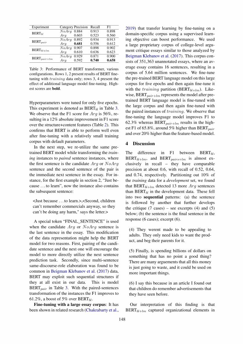
Experiment Category Precision Recall F1

BERTblNoArg 0.884 0.913 0.898Arg 0.603 0.523 0.560

BERTpairNoArg 0.892 0.934 0.913Arg 0.681 0.556 0.612

BERTbl+lmNoArg 0.907 0.898 0.902Arg 0.610 0.636 0.623

BERTpair+lmNoArg 0.929 0.871 0.900Arg 0.592 0.740 0.658

Table 3: Performance of BERT transformer, variousconfigurations. Rows 1, 2 present results of BERT fine-tuning with training data only; rows 3, 4 present theeffect of additional language model fine-tuning. High-est scores are bold.

Hyperparameters were tuned for only five epochs.This experiment is denoted as BERTbl in Table 3.We observe that the F1 score for Arg is 56%, re-sulting in a 12% absolute improvement in F1 scoreover the structure+content features (Table 2). Thisconfirms that BERT is able to perform well evenafter fine-tuning with a relatively small trainingcorpus with default parameters.

In the next step, we re-utilize the same pre-trained BERT model while transforming the train-ing instances to paired sentence instances, wherethe first sentence is the candidate Arg or NoArgsentence and the second sentence of the pair isthe immediate next sentence in the essay. For in-stance, for the first example in section 2, “Just be-cause . . . to learn”, now the instance also containsthe subsequent sentence:

<Just because . . . to learn.>,<Second, childrencan’t remember commercials anyway, so theycan’t be doing any harm," says the letter.>

A special token “FINAL_SENTENCE” is usedwhen the candidate Arg or NoArg sentence isthe last sentence in the essay. This modificationof the data representation might help the BERTmodel for two reasons. First, pairing of the candi-date sentence and the next one will encourage themodel to more directly utilize the next sentenceprediction task. Secondly, since multi-sentencesame-discourse-role elaboration was found to becommon in Beigman Klebanov et al. (2017) data,BERT may exploit such sequential structures ifthey at all exist in our data. This is modelBERTpair in Table 3. With the paired-sentencestransformation of the instances the F1 improves to61.2%, a boost of 5% over BERTbl.

Fine-tuning with a large essay corpus: It hasbeen shown in related research (Chakrabarty et al.,

2019) that transfer learning by fine-tuning on adomain-specific corpus using a supervised learn-ing objective can boost performance. We useda large proprietary corpus of college-level argu-ment critique essays similar to those analyzed byBeigman Klebanov et al. (2017). This corpus con-sists of 351,363 unannotated essays, where an av-erage essay contains 16 sentences, resulting in acorpus of 5.64 million sentences. We fine-tunethe pre-trained BERT language model on this largecorpus for five epochs and then again fine-tune itwith the training partition (BERTbl+lm). Like-wise, BERTpair+lm represents the model after pre-trained BERT language model is fine-tuned withthe large corpus and then again fine-tuned withthe paired instances of training. We observe thatfine-tuning the language model improves F1 to62.3% whereas BERTpair+lm results in the high-est F1 of 65.8%, around 5% higher than BERTpair

and over 20% higher than the feature-based model.

4 Discussion

The difference in F1 between BERTbl,BERTbl+lm, and BERTpairs+lm is almost ex-clusively in recall – they have comparableprecision at about 0.6, with recall of 0.52, 0.64,and 0.74, respectively. Partitioning out 10% ofthe training data for a development set, we foundthat BERTbl+lm detected 13 more Arg sentencesthan BERTbl in the development data. These fellinto two sequential patterns: (a) the sentenceis followed by another that further developsthe critique (7 cases) – see excerpts (4) and (5)below; (b) the sentence is the final sentence in theresponse (6 cases); excerpt (6).

(4) They werent made to be appealing toadults. They only need kids to want the prod-uct, and beg their parents for it.

(5) Finally, is spending billions of dollars onsomething that has no point a good thing?There are many arguements that all this moneyis just going to waste, and it could be used onmore important things.

(6) I say this because in an article I found outthat children do remember advertisements thatthey have seen before.

Our interpretation of this finding is thatBERTbl+lm captured organizational elements in

148

children’s writing that are similar to adult pat-terns. Beigman Klebanov et al. (2017) found thatadult writers often reiterate a previously statedcritique in an extended CONCLUSION and spreadcritiques across consecutive SUPPORT sentences.Thus, even though alignment of critiques with“standard" discourse elements such as CONCLU-SION and SUPPORT is not recognizable in chil-dren’s writing (as witnessed by the failure of thestructural features to detect critiques), some basiclocal sequential patterns do exist, and they aresufficiently similar to the ones in adult writing thata system with its language model tuned on adultcritique writing can capitalize on this knowledge.

Interestingly, BERTpairs learned similar se-quential patterns – indeed 7 of the 13 sentencesgained by BERTbl+lm over BERTbl are also re-called by BERTpairs. This further reinforces theconclusion that young writers exhibit certain localsequential patterns of discourse organization thatthey share with mature argument critique writers.

5 Conclusion and Future Work

We present a computational exploration of ar-gument critiques written by middle school chil-dren. A feature set designed for college-level cri-tique writing has poor recall of critiques whentrained on children’s data; a pre-trained BERTmodel fine-tuned on children’s data does better by18%. When BERT’s language model is addition-ally fine-tuned on a large corpus of college cri-tique essays, recall improves by further 20%, sug-gesting the existence of some similarity betweenyoung and mature writers. Performance analy-sis suggests that BERT capitalized on certain se-quential patterns in critique writing; a larger studyexamining patterns of argumentation in children’sdata is needed to confirm the hypothesis. In fu-ture, we plan to fine-tune our models on auxiliarydataset, such as the convincing argument datasetfrom Habernal and Gurevych (2016).

ReferencesYigal Attali and Jill Burstein. 2006. Automated essay

scoring with e-rater v.2. The Journal of Technology,Learning and Assessment, 4(3).

Yigal Attali and Don Powers. 2008. A developmen-tal writing scale. ETS Research Report Series,2008(1):i–59.

Beata Beigman Klebanov, Binod Gyawali, andYi Song. 2017. Detecting Good Arguments in a

Non-Topic-Specific Way: An Oxymoron? In Pro-ceedings of the 55th Annual Meeting of the Associa-tion for Computational Linguistics (Volume 2: ShortPapers), pages 244–249, Vancouver, Canada. Asso-ciation for Computational Linguistics.

Daniel Blanchard, Joel Tetreault, Derrick Higgins,Aoife Cahill, and Martin Chodorow. 2013. Toefl11:A corpus of non-native english. ETS Research Re-port Series, 2013(2):i–15.

Jill Burstein, Daniel Marcu, and Kevin Knight. 2003.Finding the WRITE Stuff: Automatic Identificationof Discourse Structure in Student Essays. IEEE In-telligent Systems, 18(1):32–39.

Tuhin Chakrabarty, Christopher Hidey, SmarandaMuresan, Kathleen Mckeown, and Alyssa Hwang.2019. Ampersand: Argument mining for persuasiveonline discussions. In Proceedings of the 2019 Con-ference on Empirical Methods in Natural LanguageProcessing and the 9th International Joint Confer-ence on Natural Language Processing (EMNLP-IJCNLP), pages 2926–2936.

Paul Deane. 2014. Using writing process and productfeatures to assess writing quality and explore howthose features relate to other literacy tasks. ETS Re-search Report Series, 2014(1):1–23.

Jacob Devlin, Ming-Wei Chang, Kenton Lee, andKristina Toutanova. 2018. Bert: Pre-training of deepbidirectional transformers for language understand-ing. arXiv preprint arXiv:1810.04805.

Noura Farra, Swapna Somasundaran, and Jill Burstein.2015. Scoring persuasive essays using opinions andtheir targets. In Proceedings of the Workshop on In-novative Use of NLP for Building Educational Ap-plications, pages 64–74.

Debanjan Ghosh, Aquila Khanam, Yubo Han, andSmaranda Muresan. 2016. Coarse-grained argu-mentation features for scoring persuasive essays. InProceedings of the 54th Annual Meeting of the As-sociation for Computational Linguistics (Volume 2:Short Papers), pages 549–554, Berlin, Germany. As-sociation for Computational Linguistics.

Ivan Habernal and Iryna Gurevych. 2016. Which ar-gument is more convincing? analyzing and predict-ing convincingness of web arguments using bidirec-tional lstm. In Proceedings of the 54th Annual Meet-ing of the Association for Computational Linguistics(Volume 1: Long Papers), pages 1589–1599.

Huy Nguyen and Diane Litman. 2016. Context-awareargumentative relation mining. In Proceedings ofthe 54th Annual Meeting of the Association for Com-putational Linguistics (Volume 1: Long Papers),pages 1127–1137.

Huy V Nguyen and Diane J Litman. 2018. Argumentmining for improving the automated scoring of per-suasive essays. In Thirty-Second AAAI Conferenceon Artificial Intelligence.

149

Isaac Persing and Vincent Ng. 2014. Modeling promptadherence in student essays. In Proceedings of the52nd Annual Meeting of the Association for Compu-tational Linguistics (Volume 1: Long Papers), pages1534–1543.

Isaac Persing and Vincent Ng. 2015. Modeling ar-gument strength in student essays. In Proceedingsof the 53rd Annual Meeting of the Association forComputational Linguistics and the 7th InternationalJoint Conference on Natural Language Processing(Volume 1: Long Papers), pages 543–552.

Isaac Persing and Vincent Ng. 2016. End-to-end ar-gumentation mining in student essays. In Proceed-ings of the 2016 Conference of the North Ameri-can Chapter of the Association for ComputationalLinguistics: Human Language Technologies, pages1384–1394.

Nils Reimers, Benjamin Schiller, Tilman Beck, Jo-hannes Daxenberger, Christian Stab, and IrynaGurevych. 2019. Classification and clustering ofarguments with contextualized word embeddings.arXiv preprint arXiv:1906.09821.

Yi Song, Paul Deane, and Mary Fowles. 2017. Exam-ining students’ ability to critique arguments and ex-ploring the implications for assessment and instruc-tion. ETS Research Report Series, 2017(16):1–12.

Christian Stab and Iryna Gurevych. 2017a. Parsing ar-gumentation structures in persuasive essays. Com-putational Linguistics, 43(3):619–659.

Christian Stab and Iryna Gurevych. 2017b. Recogniz-ing insufficiently supported arguments in argumen-tative essays. In Proceedings of the 15th Confer-ence of the European Chapter of the Associationfor Computational Linguistics: Volume 1, Long Pa-pers, pages 980–990, Valencia, Spain. Associationfor Computational Linguistics.

Ashish Vaswani, Noam Shazeer, Niki Parmar, JakobUszkoreit, Llion Jones, Aidan N Gomez, ŁukaszKaiser, and Illia Polosukhin. 2017. Attention is allyou need. In Advances in neural information pro-cessing systems, pages 5998–6008.

Douglas N Walton. 1996. Argumentation schemes forpresumptive reasoning. Psychology Press.

150

Proceedings of the 15th Workshop on Innovative Use of NLP for Building Educational Applications, pages 151–162July 10, 2020. c©2020 Association for Computational Linguistics

Should You Fine-Tune BERT for Automated Essay Scoring?

Elijah Mayfield and Alan W BlackLanguage Technologies Institute

Carnegie Mellon Universityelijah@cmu.edu, awb@cs.cmu.edu

Abstract

Most natural language processing researchnow recommends large Transformer-basedmodels with fine-tuning for supervised clas-sification tasks; older strategies like bag-of-words features and linear models have fallenout of favor. Here we investigate whether, inautomated essay scoring (AES) research, deepneural models are an appropriate technologicalchoice. We find that fine-tuning BERT pro-duces similar performance to classical modelsat significant additional cost. We argue thatwhile state-of-the-art strategies do match ex-isting best results, they come with opportunitycosts in computational resources. We concludewith a review of promising areas for researchon student essays where the unique charac-teristics of Transformers may provide benefitsover classical methods to justify the costs.

1 Introduction

Automated essay scoring (AES) mimics the judg-ment of educators evaluating the quality of studentwriting. Originally used for summative purposesin standardized testing and the GRE (Chen et al.,2016), these systems are now frequently foundin classrooms (Wilson and Roscoe, 2019), typi-cally enabled by training data scored on reliablerubrics to give consistent and clear goals for writ-ers (Reddy and Andrade, 2010).

More broadly, the natural language process-ing (NLP) research community in recent yearshas been dominated by deep neural network re-search, in particular, the Transformer architec-ture popularized by BERT (Devlin et al., 2019).These models use large volumes of existing textdata to pre-train multilayer neural networks withcontext-sensitive meaning of, and relations be-tween, words. The models, which often consist ofover 100 million parameters, are then fine-tuned toa specific new labeled dataset and used for classi-fication, generation, or structured prediction.

Research in AES, though, has tended to pri-oritize simpler models, usually multivariate re-gression using a small set of justifiable variableschosen by psychometricians (Attali and Burstein,2004). This produces models that retain di-rect mappings between variables and recognizablecharacteristics of writing, like coherence or lex-ical sophistication (Yannakoudakis and Briscoe,2012; Vajjala, 2018). In psychometrics more gen-erally, this focus on features as valid “constructs”leans on a rigorous and well-defined set of princi-ples (Attali, 2013). This approach is at odds withTransformer-based research, and so our core ques-tion for this work is: for AES specifically, is amove to deep neural models worth the cost?

The chief technical contribution of this work isto measure results for BERT when fine-tuned forAES. In section 3 we describe an experimentalsetup with multiple levels of technical difficultyfrom bag-of-words models to fine-tuned Trans-formers, and in section 5 we show that the ap-proaches perform similarly. In AES, human inter-rater reliability creates a ceiling for scoring modelaccuracy. While Transformers match state-of-the-art accuracy, they do so with significant tradeoffs;we show that this includes a slowdown in train-ing time of up to 100x. Our data shows that theseTransformer models improve on N -gram base-lines by no more than 5%. Given this result, insection 6 we describe areas of contemporary re-search on Transformers that show both promisingearly results and a potential alignment to educa-tional pedagogy beyond reliable scoring.

2 Background

In AES, student essays are scored either on a sin-gle holistic scale, or analytically following a rubricthat breaks out subscores based on “traits.” Thesescores are almost always integer-valued, and al-most universally have fewer than 10 possible scorepoints, though some research has used scales with

151

as many as 60 points (Shermis, 2014). In mostcontexts, students respond to “prompts,” a specificwriting activity with predefined content. Work innatural language processing and speech evaluationhas used advanced features like discourse coher-ence (Wang et al., 2013) and argument extraction(Nguyen and Litman, 2018); for proficient writersin professional settings, automated scaffolds likegrammatical error detection and correction alsoexist (Ng et al., 2014).

Natural language processing has historicallyused n-gram bag-of-words features to predict la-bels for documents. These were the standard rep-resentation of text data for decades and are still inwidespread use (Jurafsky and Martin, 2014). Inthe last decade, the field moved to word embed-dings, where words are represented not as a sin-gle feature but as dense vectors learned from largeunsupervised corpora. While early approaches todense representations using latent semantic anal-ysis have been a major part of the literature onAES (Foltz et al., 2000; Miller, 2003), these werecorpus-specific representations. In contrast, re-cent work is general-purpose, resulting in off-the-shelf representations like GloVe (Penningtonet al., 2014). This allows similar words to haveapproximately similar representations, effectivelymanaging lexical sparsity.

But the greatest recent innovation has been con-textual word embeddings, based on deep neuralnetworks and in particular, Transformers. Ratherthan encoding a word’s semantics as a staticvector, these models adjust the representation ofwords based on their context in new documents.With multiple layers and sophisticated attentionmechanisms (Bahdanau et al., 2015), these newermodels have outperformed the state-of-the-art onnumerous tasks, and are currently the most ac-curate models on a very wide range of tasks(Vaswani et al., 2017; Dai et al., 2019). Themost popular architecture, BERT, produces a 768-dimensional final embedding based on a networkwith over 100 million total parameters in 12 lay-ers; pre-trained models are available for opensource use (Devlin et al., 2019).

For document classification, BERT is “fine-tuned” by adding a final layer at the end of theTransformer architecture, with one output neuronper class label. When learning from a new set oflabeled training data, BERT evaluates the trainingset multiple times (each pass is called an epoch).

A loss function, propagating backward to the net-work, allows the model to learn relationships be-tween the class labels in the new data and thecontextual meaning of the words in the text. Alearning rate determines the amount of change to amodel’s parameters. Extensive results have shownthat careful control of the learning rate in a cur-riculum can produce an effective fine-tuning pro-cess (Smith, 2018). While remarkably effective,our community is only just beginning to identifyexactly what is learned in this process; research in“BERT-ology” is ongoing (Kovaleva et al., 2019;Jawahar et al., 2019; Tenney et al., 2019).

These neural models are just starting to beused in machine learning for AES, especially asan intermediate representation for automated es-say feedback (Fiacco et al., 2019; Nadeem et al.,2019). End-to-end neural AES models are in theirinfancy and have only seen exploratory studieslike Rodriguez et al. (2019); to our knowledge, nocommercial vendor yet uses Transformers as therepresentation for high-stakes automated scoring.

3 NLP for Automated Essay Scoring

To date, there are no best practices on fine-tuning Transformers for AES; in this section wepresent options. We begin with a classical baselineof traditional bag-of-words approaches and non-contextual word embeddings, used with NaıveBayes and logistic regression classifiers, respec-tively. We then describe three curriculum learn-ing options for fine-tuning BERT using AES databased on broader best practices. We end withtwo approaches based on BERT but without fine-tuning, with reduced hardware requirements.

3.1 Bag-of-Words Representations

The simplest features for document classificationtasks, “bag-of-words,” extracts surface N -gramsof length 1-2 with “one-hot” binary values indi-cating presence or absence in a document. Inprior AES results, this representation is surpris-ingly effective, and can be improved with simpleextensions: N -grams based on part-of-speech tags(of length 2-3) to capture syntax independent ofcontent, and character-level N -grams of length 3-4, to provide robustness to misspellings (Woodset al., 2017; Riordan et al., 2019). This high-dimensional representation typically has a cutoffthreshold where rare tokens are excluded: in ourimplementation, we exclude N -grams without at

152

least 5 occurrences in training data. Even afterthis reduction, this is a sparse feature space withthousands of dimensions. For learning with bag-of-words, we use a Naıve Bayes classifier withLaplace smoothing from Scikit-learn (Pedregosaet al., 2011), with part-of-speech tagging fromSpaCy (Honnibal and Montani, 2017).

3.2 Word Embeddings

A more modern representation of text uses word-level embeddings. This produces a vector, typi-cally of up to 300 dimensions, representing eachword in a document. In our implementation, werepresent each document as the term-frequency-weighted mean of word-level embedding vectorsfrom GloVe (Pennington et al., 2014). Unlike one-hot bag-of-words features, embeddings have densereal-valued features and Naıve Bayes models areinappropriate; we instead train a logistic regres-sion classifier with the LibLinear solver (Fan et al.,2008) and L2 regularization from Scikit-learn.

3.3 Fine-Tuning BERT

Moving to neural models, we fine-tune an uncasedBERT model using the Fast.ai library. This li-brary’s visibility to first-time users of deep learn-ing and accessible online learning materials1 meantheir default choices are the most accessible routefor practitioners.

Fast.ai recomends use of cyclical learning ratecurricula for fine-tuning. In this policy, an upperand lower bound on learning rates are established.lrmax is a hyperparameter defining the maximumlearning rate in one epoch of learning. In cyclicallearning, the learning rate for fine-tuning begins atthe lower bound, rises to the upper bound, then de-scends back to the lower bound. A high learningrate midway through training acts as regulariza-tion, allowing the model to avoid overfitting andavoiding local optima. Lower learning rates at thebeginning and end of cycles allow for optimizationwithin a local optimum, giving the model an op-portunity to discover fine-grained new informationagain. In our work, we set lrmax = 0.00001. Alower bound is then derived from the upper bound,lrmin = 0.04 ∗ lrmax; this again is default behav-ior in the Fast.ai library.

We assess three different curricula for cyclicallearning rates, visualized in Figure 1. In the de-fault approach, a maximum learning rate is set and

1https://course.fast.ai/

Figure 1: Illustration of cyclical (top), two-periodcyclical (middle, log y-scale), and 1-cycle (bottom)learning rate curricula over N epochs.

cycles are repeated until reaching a threshold; fora halting criterion, we measure validation set ac-curacy. Because of noise in deep learning train-ing, halting at any decrease can lead to prematurestops; it is preferable to allow some occasional,small drop in performance. In our implementa-tion we halt when accuracy on a validation set,measured in quadratic weighted kappa, decreasesby over 0.01. In the second, “two-rate” approach(Smith, 2018), we follow this algorithm, but whenwe would halt, we instead backtrack by one epochto a saved version of the network and restart train-ing with a learning rate of 1 × 10−6 (one order ofmagnitude smaller). Finally, in the “1-cycle” pol-icy, training is condensed into a single rise-and-fallpattern, spread over N epochs. Defining the exacttraining time N is a hyperparameter tuned on val-idation data. Finally, while BERT is optimized forsentence encoding, it is able to process documentsup to 512 words long. In our data, we truncate asmall number of essays longer than this maximum,mostly in ASAP dataset #2.

3.4 Feature Extraction from BERT

Fine-tuning is computationally expensive and canonly run on GPU-enabled devices. Many prac-

153

titioners in low-resource settings may not haveaccess to appropriate cloud computing environ-ments for these techniques. Previous work has de-scribed a compromise approach for using Trans-former models without fine-tuning. In Peters et al.(2019), the authors describe a new pipeline. Doc-ument texts are processed with an untuned BERTmodel; the final activations from network on the[CLS] token are then used directly as contex-tual word embeddings. This 768-dimensional fea-ture vector represents the full document, and isused as inputs for a linear classifier. In the edu-cation context, a similar approach was describedin Nadeem et al. (2019) as a baseline for evalua-tion of language-learner essays. This process al-lows us to use the world knowledge embedded inBERT without requiring fine-tuning of the modelitself, and without need for GPUs at training orprediction time. For our work, we train a logisticregression classifier as described in Section 3.2.

3.5 DistilBERT

Recent work has highlighted the extreme car-bon costs of full Transformer fine-tuning (Strubellet al., 2019) and the desire for Transformer-basedprediction on-device without access to cloud com-pute. In response to these concerns, Sanh et al.(2019) introduce DistilBERT, which they argue isequivalent to BERT in most practical aspects whilereducing parameter size by 40% to 66 million, anddecreasing model inference time by 60%. Thisis accomplished using a distillation method (Hin-ton et al., 2015) in which a new, smaller “stu-dent” network is trained to reproduce the behav-ior of a pretrained “teacher” network. Once thesmaller model is pretrained, interacting with it forthe purposes of fine-tuning is identical to interact-ing with BERT directly. DistilBERT is intendedfor use cases where compute resources are a con-straint, sacrificing a small amount of accuracy fora drastic shrinking of network size. Because ofthis intended use case, we only present results forDistilBERT with the “1-cycle” learning rate pol-icy, which is drastically faster to fine-tune.

4 Experiments

To test the overall impact of fine-tuning in theAES domain, we use five datasets from the ASAPcompetition, jointly hosted by the Hewlett Foun-dation and Kaggle.com (Shermis, 2014). This setof essay prompts was the subject of intense pub-

lic attention and scrutiny in 2012 and its pub-lic release has shaped the discourse on AES eversince. For our experiments, we use the origi-nal, deanonymized data from Shermis and Hamner(2012); an anonymized version of these datasets isavailable online2. In all cases, human inter-raterreliability (IRR) is an approximate upper boundon performance, but reliability above human IRRis possible, as all models are trained on resolvedscores that represent two scores plus a resolutionprocess for disagreements between annotators.

We focus our analysis on the five datasets thatmost closely resemble standard AES rubrics, dis-carding three datasets - prompts #1, 7, and 8 -with a scale of 10 or more possible points. Re-sults on these datasets are not representative ofoverall performance and can skew reported re-sults due to rubric idiosyncracies, making compar-ison to other published work impossible (see forexample (Alikaniotis et al., 2016), which groups60-point and 4-point rubrics into a single datasetand therefore produced correlations that cannot bealigned to results from any other published work).Prompts 2-6 are scored on smaller rubric scaleswith 4-6 points, and are thus generalizable to moreAES contexts. Note that nevertheless, each datasethas its own idiosyncracies; for instance, essaysin dataset #5 were written by younger students in7th and 8th grade, while dataset #4 contains writ-ing from high school seniors; datasets #3 and 4were responses to specific texts while others wereopen-ended; and scores in dataset #2 was actuallyscored on two separate traits, the second of whichis often discarded in followup work (as it is here).Our work here does not specifically isolate effectsof these differences that would lead to discrepan-cies in performance or in modeling behavior.

4.1 Metrics and Baselines

For measuring reliability of automated assess-ments, we use a variant of Cohen’s κ, withquadratic weights for “near-miss” predictions onan ordinal scale (QWK). This metric is standardin the AES community (Williamson et al., 2012).High-stakes testing organizations differ on exactcutoffs for acceptable performance, but thresholdvalues between 0.6 and 0.8 QWK are typicallyused as a floor for testing purposes; human reli-ability below this threshold is generally not fit forsummative student assessment.

2https://www.kaggle.com/c/asap-aes

154

In addition to measuring reliability, we alsomeasure training and prediction time, in seconds.As this work seeks to evaluate the practical trade-offs of the move to deep neural methods, this isan important secondary metric. For all experi-ments, training was performed on Google ColabPro cloud servers with 32 GB of RAM and anNVideo Tesla P100 GPGPU.

We compare the results of BERT against severalpreviously published benchmarks and results.

• Human IRR as initially reported in theHewlett Foundation study (Shermis, 2014).

• Industry best performance, as reported byeight commercial vendors and one open-source research team in the initial release ofthe ASAP study. (Shermis, 2014).

• An early deep learning approach using acombination CNN+LSTM architecture thatoutperformed most reported results at thattime (Taghipour and Ng, 2016).

• Two recent results using traditional non-neural models: Woods et al. (2017), whichuses n-gram features in an ordinal logistic re-gression, and Cozma et al. (2018), which usesa mix of string kernels and word2vec embed-dings in a support vector regression.

• Rodriguez et al. (2019), the one previously-published work that attempts AES with a va-riety of pretrained neural models, includingBERT and the similar XLNet (Yang et al.,2019), with numerous alternate configura-tions and training methods. We report theirresult with a baseline BERT fine-tuning pro-cess, as well as their best-tuned model afterextensive optimization.

4.2 Experimental Setup

Following past publications, we train a separatemodel on each dataset, and evaluate all dataset-specific models using 5-fold cross-validation.Each of the five datasets contains approximately1,800 essays, resulting in folds of 360 essayseach. Additionally, for measuring loss when fine-tuning BERT, we hold out an additional 20% ofeach training fold as a validation set, meaning thateach fold has approximately 1,150 essays used fortraining and 300 essays used for validation. We

report mean QWK across the five folds. For mea-surement of training and prediction time, we re-port the sum of training time across all five foldsand all datasets. For slow-running feature ex-traction, like N -gram part-of-speech features andword embedding-based features, we tag each sen-tence in the dataset only once and cache the re-sults, rather than re-tagging each sentence on eachfold. Finally, for models where distinguishingextraction from training time is meaningful, wepresent those times separately.

5 Results

5.1 Accuracy Evaluation

Our primary results are presented in Table 1. Wefind, broadly, that all approaches to machine learn-ing replicate human-level IRR as measured byQWK. Nearly eight years after the publication ofthe original study, no published results have ex-ceeded vendor performance on three of the fiveprompt datasets; in all cases, a naive N -gram ap-proach underperforms the state-of-the-art in indus-try and academia by 0.03-0.06 QWK.

Of particular note is the low performance ofGloVe embeddings relative to either neural or N -gram representations. This is surprising: whileword embeddings are less popular now than deepneural methods, they still perform well on a widerange of tasks (Baroni et al., 2014). Few publi-cations have noted this negative result for GloVein the AES domain; only Dong et al. (2017) usesGloVe as the primary representation of ASAPtexts in an LSTM model, reporting lower QWKresults than any baseline we presented here. Onesimple explanation for this may be that individ-ual keywords matter a great deal for model per-formance. It is well established that vocabulary-based approaches are effective in AES tasks (Hig-gins et al., 2014) and the lack of access to specificword-based features may hinder semantic vectorrepresentation. Indeed, only one competitive re-cent paper on AES uses non-contextual word vec-tors: Cozma et al. (2018). In this implementation,they do use word2vec, but rather than use wordembeddings directly they first cluster words intoa set of 500 “embedding clusters.” Words that ap-pear in texts are then counted in the feature vectoras the centroid of that cluster - in effect, creating a500-dimensional bag-of-words model.

Our results would suggest that fine-tuning withBERT also reaches approximately the same level

155

Table 1: Performance on each of ASAP datasets 2-6, inQWK. The final row shows the gap in QWK betweenthe best neural model and the N-gram baseline.

Model 2 3 4 5 6Human IRR .80 .77 .85 .74 .74Hewlett .74 .75 .82 .83 .78Taghipour .69 .69 .81 .81 .82Woods .71 .71 .81 .82 .83Cozma .73 .68 .83 .83 .83Rodriguez (BERT) .68 .72 .80 .81 .81Rodriguez (best) .70 .72 .82 .82 .82N-Grams .71 .71 .78 .80 .79Embeddings .42 .41 .60 .49 .36BERT-CLR .66 .70 .80 .80 .79BERT-1CYC .64 .71 .82 .81 .79BERT Features .61 .59 .75 .75 .74DistilBERT .65 .70 .82 .81 .79N-Gram Gap -.05 .00 .04 .01 .00

of performance as other methods, slightly un-derperforming previous published results. Thisis likely an underestimate, due to the complex-ity of hyperparameter optimization and curricu-lum learning for Transformers. Rodriguez et al.(2019) demonstrate that it is, in fact, possibleto improve the performance of neural models tomore closely approach (but not exceed) the state-of-the-art using neural models. Sophisticated ap-proaches like gradual unfreezing, discriminativefine-tuning, or greater parameterization throughnewer deep learning models in their work consis-tently produces improvements of 0.01-0.02 QWKcompared to the default BERT implementation.But this result emphasizes our concern: we donot claim our results are the best that could beachieved with BERT fine-tuning. We are, in fact,confident that they can be improved through opti-mization. What the results demonstrate instead isthat the ceiling of results for AES tasks lessens thevalue of that intensive optimization effort.

5.2 Runtime EvaluationOur secondary evaluation of models is based ontraining time and resource usage; those results arereported in Table 2. Here, we see that deep learn-ing approaches on GPU-enabled cloud computeproduce an approximately 30-100 fold increase inend-to-end training time compared to a naive ap-proach. In fact, this understates the gap, as approx-imately 75% of feature extraction and model train-ing time in the naive approach is due to part-of-

Table 2: Cumulative experiment runtime, in seconds,of feature extraction (F), model training (T), and pre-dicting on test sets (P), for ASAP datasets 2-6 with 5-fold cross-validation. Models with 1-cycle fine-tuningare measured at 5 epochs.

Model F T P TotalEmbeddings 93 6 1 100N-Grams 82 27 2 111BERT Features 213 10 1 224DistilBERT 1,972 108 2,080BERT-1CYC 2,956 192 3,148BERT-CLR 11,309 210 11,519

speech tagging rather than learning. Using BERTfeatures as inputs to a linear classifier is an in-teresting compromise option, producing slightlylower performance on these datasets but with onlya 2x slowdown at training time, all in feature ex-traction, and potentially retaining some of the se-mantic knowledge of the full BERT model. Fur-ther investigation should test whether additionalfeatures for intermediate layers, as explored in Pe-ters et al. (2019), is merited for AES.

We can look at this gap in training runtime moreclosely in Figure 2. Essays in the prompt 2 datasetare longer persuasive essays and are on average378 words long, while datasets 3-6 correspond toshorter, source-based content knowledge promptsand are on average 98-152 words long. The needfor truncation in dataset #2 for BERT, but not forother approaches, may explain the underperfor-mance of the model in that dataset. Additionally,differences across datasets highlight two key dif-ferences for fine-tuning a BERT model:

• Training time increases linearly with numberof epochs and with average document length.As seen in Figure 2, this leads to a longertraining for the longer essays of dataset 2,nearly as long as the other datasets combined.

• Performance converges on human inter-raterreliability more quickly for short content-based prompts, and performance begins todecrease due to overfitting in as few as 4epochs. By comparison, in the longer, per-suasive arguments of dataset 2, very smallperformance gains on held-out data contin-ued even at the end of our experiments.

Figure 2 also presents results for DistilBERT.Our work verifies prior published claims of speed

156

Figure 2: QWK (top) and training time (bottom, in sec-onds) and for 5-fold cross-validation of 1-cycle neuralfine-tuning on ASAP datasets 2-6, for BERT (left) andDistilBERT (right).

improvements both in fine-tuning and at predictiontime, relative to the baseline BERT model: train-ing time was reduced by 33% and prediction timewas reduced by 44%. This still represents at leasta 20x increase in runtime relative toN -gram base-lines both for training and prediction.

6 Discussion

For scoring essays with reliably scored, prompt-specific training sets, both classical and neural ap-proaches produce similar reliability, at approxi-mately identical levels to human inter-rater relia-bility. There is a substantial increase in techni-cal overhead required to implement Transformersand fine-tune them to reach this performance, withminimal gain compared to baselines. The pol-icy lesson for NLP researchers is that using deeplearning for scoring alone is unlikely to be justifi-able, given the slowdowns at both training and in-ference time, and the additional hardware require-ments. For scoring, at least, Transformer architec-tures are a hammer in search of a nail.

But it’s hardly the case that automated writingevaluation is limited to scoring. In this section wecover major open topics for technical researchersin AES to explore, focusing on areas where neuralmodels have proven strengths above baselines in

other domains. We prioritize three major areas:domain transfer, style, and fairness. In each wecite specific past work that indicates a plausiblepath forward for research.

6.1 Domain TransferA major challenge in AES is the inability ofprompt-specific models to generalize to new es-say topics (Attali et al., 2010; Lee, 2016). Col-lection of new prompt-specific training sets, withreliable scores, continues to be one of the ma-jor stumbling blocks to expansion of AES sys-tems in curricula (Woods et al., 2017). Rel-atively few researchers have made progress ongeneric essay scoring: Phandi et al. (2015) in-troduces a Bayesian regression approach that ex-tracts N -gram features then capitalizes on cor-related features across prompts. Jin et al.(2018) shows promising prompt-independent re-sults using an LSTM architecture with surface andpart-of-speech N -gram inputs, underperformingprompt-specific models by relatively small mar-gins across all ASAP datasets. But in implemen-tations, much of the work of practitioners is basedon workarounds for prompt-specific models; Wil-son et al. (2019), for instance, describes psycho-metric techniques for measuring generic writingability across a small sample of known prompts.

While Transformers are sensitive to the datathey were pretrained on, they are well-suited totransfer tasks in mostly unseen domains, as ev-idenced by part-of-speech tagging for historicaltexts (Han and Eisenstein, 2019), sentiment clas-sification on out-of-domain reviews (Myagmaret al., 2019), and question answering in new con-texts (Houlsby et al., 2019). This last result ispromising for content-based short essay prompts,in particular. Our field’s open challenge in scor-ing is to train AES models that can meaningfullyevaluate short response texts for correctness basedon world knowledge and domain transfer, ratherthan memorizing the vocabulary of correct, in-domain answers. Promising early results showthat relevant world knowledge is already embed-ded in BERT’s pretrained model (Petroni et al.,2019). This means that BERT opens up a poten-tially tractable path to success that was simply notpossible with N -gram models.

6.2 Style and VoiceSkepticism toward AES in the classroom comesfrom rhetoric and composition scholars, who ex-

157

press concerns about its role in writing pedagogy(NCTE, 2013; Warner, 2018). Indeed, the rela-tively “solved” nature of summative scoring thatwe highlight here is of particular concern to theseexperts, noting the high correlation between scoresand features like word count (Perelman, 2014).

Modern classroom use of AES beyond high-stakes scoring, like Project Essay Grade (Wilsonand Roscoe, 2019) or Turnitin Revision Assistant(Mayfield and Butler, 2018), makes claims of sup-porting student agency and growth; here, adapt-ing to writer individuality is a major current gap.Dixon-Roman et al. (2019) raises a host of ques-tions about these topics specifically in the contextof AES, asking how algorithmic intervention canproduce strong writers rather than merely good es-says: “revision, as adjudicated by the platform,is [...] a re-direction toward the predeterminedshape of the ideal written form [...] a puzzle-doerrecursively consulting the image on the puzzle-box, not that of author returning to their words tomake them more lucid, descriptive, or forceful.”

This critique is valid: research on machinetranslation, for instance, has shown that writerstyle is not preserved across languages (Rabi-novich et al., 2017). There is uncharted territoryfor AES to adapt to individual writer styles andgive feedback based on individual writing ratherthan prompt-specific exemplars. Natural languageunderstanding researchers now argue that “...styleis formed by a complex combination of differentstylistic factors” (Kang and Hovy, 2019); Style-specific natural language generation has shownpromise in other domains (Hu et al., 2017; Prab-humoye et al., 2018) and has been extended notjust to individual preferences but also to overlap-ping identities based on attitudes like sentimentand personal attributes like gender (Subramanianet al.). Early work suggests that style-specificmodels do see major improvements when shiftingto high-dimensionality Transformer architectures(Keskar et al., 2019). This topic bridges an im-portant gap: for assessment, research has shownthat “authorial voice” has measurable outcomes onwriting impact (Matsuda and Tardy, 2007), whileindividual expression is central to decades of peda-gogy (Elbow, 1987). Moving the field toward indi-vidual expression and away from prompt-specificdatasets may be a path to lending legitimacy toAES, and Transformers may be the technical leapnecessary to make these tasks work.

6.3 Fairness

Years ago, researchers suggested that demo-graphic bias is worth checking in AES systems(Williamson et al., 2012). But years later, thefield has primarily reported fairness experimentson simulated data, and shared toolkits for measur-ing bias, rather than results on real-world AES im-plementations or high-stakes data (Madnani et al.,2017; Loukina et al., 2019).

Prompted by social scientists (Noble, 2018),NLP researchers have seen a renaissance of fair-ness research based on the flaws in default im-plementations of Transformers (Bolukbasi et al.,2016; Zhao et al., 2017, 2018). These works typ-icallly seek to reduce the amplification of bias inpretrained models, starting with easy-to-measureproof that demographic bias can be “removed”from word embedding spaces. But iterating on in-puts to algorithmic classifiers – precisely the in-tended use case of formative eeedback for writ-ers! – can reduce the efficacy of “de-biasing” (Liuet al., 2018; Dwork and Ilvento, 2019). More re-cent research has shown that bias may simply bemasked by these approaches, rather than resolved(Gonen and Goldberg, 2019).

What these questions offer, though, is a well-spring of new and innovative technical research.Developers of learning analytics software, includ-ing AES, are currently encouraged to focus onscalable experimental evidence of efficacy forlearning outcomes (Saxberg, 2017), rather than fo-cus on specific racial or gender bias, or other eq-uity outcomes that are more difficult to achievethrough engineering. But Transformer architec-tures are nuanced enough to capture immenseworld knowledge, producing a rapid increase inexplainability in NLP (Rogers et al., 2020).

Meanwhile, in the field of learning analytics, aburgeoning new field of fairness studies are learn-ing how to investigate these issues in algorithmiceducational systems (Mayfield et al., 2019; Hol-stein and Doroudi, 2019). Outside of technol-ogy applications but in writing assessment morebroadly, fairness is also a rich topic with a historyof literature to learn from (Poe and Elliot, 2019).Researchers at the intersection of both these fieldshave an enormous open opportunity to better un-derstand AES in the context fairness, using the lat-est tools not just to build reliable scoring but toadvance social change.

158

ReferencesDimitrios Alikaniotis, Helen Yannakoudakis, and

Marek Rei. 2016. Automatic text scoring using neu-ral networks. In Proceedings of the Association forComputational Linguistics, pages 715–725.

Yigal Attali. 2013. Validity and reliability of auto-mated essay scoring. Handbook of automated es-say evaluation: Current applications and new direc-tions, page 181.

Yigal Attali, Brent Bridgeman, and Catherine Trapani.2010. Performance of a generic approach in auto-mated essay scoring. The Journal of Technology,Learning and Assessment, 10(3).

Yigal Attali and Jill Burstein. 2004. Automated essayscoring with e-rater R© v. 2.0. ETS Research ReportSeries, (2).

Dzmitry Bahdanau, Kyunghyun Cho, and Yoshua Ben-gio. 2015. Neural machine translation by jointlylearning to align and translate. In Proceedings ofthe International Conference on Learning Represen-tations.

Marco Baroni, Georgiana Dinu, and GermanKruszewski. 2014. Don’t count, predict! asystematic comparison of context-counting vs.context-predicting semantic vectors. In Proceedingsof the Association for Computational Linguistics,pages 238–247.

Tolga Bolukbasi, Kai-Wei Chang, James Y Zou,Venkatesh Saligrama, and Adam T Kalai. 2016.Man is to computer programmer as woman is tohomemaker? debiasing word embeddings. In D. D.Lee, M. Sugiyama, U. V. Luxburg, I. Guyon, andR. Garnett, editors, Advances in Neural InformationProcessing Systems 29, pages 4349–4357. CurranAssociates, Inc.

Jing Chen, James H Fife, Isaac I Bejar, and Andre ARupp. 2016. Building e-rater R© scoring models us-ing machine learning methods. ETS Research Re-port Series, 2016(1):1–12.

Madalina Cozma, Andrei Butnaru, and Radu TudorIonescu. 2018. Automated essay scoring with stringkernels and word embeddings. In Proceedings of theAssociation for Computational Linguistics.

Zihang Dai, Zhilin Yang, Yiming Yang, William WCohen, Jaime Carbonell, Quoc V Le, and RuslanSalakhutdinov. 2019. Transformer-xl: Attentive lan-guage models beyond a fixed-length context. In Pro-ceedings of the Association for Computational Lin-guistics.

Jacob Devlin, Ming-Wei Chang, Kenton Lee, andKristina Toutanova. 2019. Bert: Pre-training of deepbidirectional transformers for language understand-ing. In Proceedings of the NAACL HLT Conference.

Ezekiel Dixon-Roman, T. Philip Nichols, and AmaNyame-Mensah. 2019. The racializing forces of/inai educational technologies. Learning, Media &Technology Special Issue on AI and Education: Crit-ical Perspectives and Alternative Futures.

Fei Dong, Yue Zhang, and Jie Yang. 2017. Attention-based recurrent convolutional neural network for au-tomatic essay scoring. In Proceedings of the Confer-ence on Computational Natural Language Learning,pages 153–162.

Cynthia Dwork and Christina Ilvento. 2019. Fairnessunder composition. In Innovations in TheoreticalComputer Science Conference. Schloss Dagstuhl-Leibniz-Zentrum fuer Informatik.

Peter Elbow. 1987. Closing my eyes as i speak: Anargument for ignoring audience. College English,49(1):50–69.

Rong-En Fan, Kai-Wei Chang, Cho-Jui Hsieh, Xiang-Rui Wang, and Chih-Jen Lin. 2008. Liblinear: Alibrary for large linear classification. Journal of Ma-chine Learning Research, 9(Aug):1871–1874.

James Fiacco, Elena Cotos, and Carolyn Rose. 2019.Towards enabling feedback on rhetorical structurewith neural sequence models. In Proceedings of theInternational Conference on Learning Analytics &Knowledge, pages 310–319. ACM.

Peter W Foltz, Sara Gilliam, and Scott Kendall. 2000.Supporting content-based feedback in on-line writ-ing evaluation with lsa. Interactive Learning Envi-ronments, 8(2):111–127.

Hila Gonen and Yoav Goldberg. 2019. Lipstick on apig: Debiasing methods cover up systematic gen-der biases in word embeddings but do not removethem. Proceedings of the Association for Computa-tional Linguistics.

Xiaochuang Han and Jacob Eisenstein. 2019. Unsuper-vised domain adaptation of contextualized embed-dings: A case study in early modern english. arXivpreprint arXiv:1904.02817.

Derrick Higgins, Chris Brew, Michael Heilman, Ra-mon Ziai, Lei Chen, Aoife Cahill, Michael Flor,Nitin Madnani, Joel Tetreault, Daniel Blanchard,et al. 2014. Is getting the right answer just aboutchoosing the right words? the role of syntactically-informed features in short answer scoring. arXivpreprint arXiv:1403.0801.

Geoffrey Hinton, Oriol Vinyals, and Jeff Dean. 2015.Distilling the knowledge in a neural network. stat,1050:9.

Kenneth Holstein and Shayan Doroudi. 2019. Fairnessand equity in learning analytics systems (fairlak).in. In Companion Proceedings of the InternationalLearning Analytics & Knowledge Conference (LAK2019).

159

Matthew Honnibal and Ines Montani. 2017. spacy 2:Natural language understanding with bloom embed-dings, convolutional neural networks and incremen-tal parsing.

Neil Houlsby, Andrei Giurgiu, Stanislaw Jastrzebski,Bruna Morrone, Quentin De Laroussilhe, AndreaGesmundo, Mona Attariyan, and Sylvain Gelly.2019. Parameter-efficient transfer learning for nlp.In Proceedings of the International Conference onMachine Learning, pages 2790–2799.

Zhiting Hu, Zichao Yang, Xiaodan Liang, RuslanSalakhutdinov, and Eric P Xing. 2017. Toward con-trolled generation of text. In Proceedings of the In-ternational Conference on Machine Learning, pages1587–1596.

Ganesh Jawahar, Benoıt Sagot, and Djame Seddah.2019. What does bert learn about the structure oflanguage? In Proceedings of the Association forComputational Linguistics, pages 3651–3657.

Cancan Jin, Ben He, Kai Hui, and Le Sun. 2018.Tdnn: a two-stage deep neural network for prompt-independent automated essay scoring. In Proceed-ings of the Association for Computational Linguis-tics, pages 1088–1097.

Dan Jurafsky and James H Martin. 2014. Speech andlanguage processing, volume 3. Pearson London.

Dongyeop Kang and Eduard Hovy. 2019. xslue: Abenchmark and analysis platform for cross-style lan-guage understanding and evaluation. arXiv preprintarXiv:1911.03663.

Nitish Shirish Keskar, Bryan McCann, Lav R Varshney,Caiming Xiong, and Richard Socher. 2019. Ctrl: Aconditional transformer language model for control-lable generation. arXiv preprint arXiv:1909.05858.

Olga Kovaleva, Alexey Romanov, Anna Rogers, andAnna Rumshisky. 2019. Revealing the dark se-crets of bert. In Proceedings of Empirical Methodsin Natural Language Processing, volume 1, pages2465–2475.

Yong-Won Lee. 2016. Investigating the feasibility ofgeneric scoring models of e-rater for toefl ibt inde-pendent writing tasks. English Language Teaching,71.

Lydia T Liu, Sarah Dean, Esther Rolf, Max Sim-chowitz, and Moritz Hardt. 2018. Delayed impactof fair machine learning. In Proceedings of the In-ternational Conference on Machine Learning.

Anastassia Loukina, Nitin Madnani, and Klaus Zech-ner. 2019. The many dimensions of algorithmic fair-ness in educational applications. In Proceedings ofthe ACL Workshop on Innovative Use of NLP forBuilding Educational Applications.

Nitin Madnani, Anastassia Loukina, Alina von Davier,Jill Burstein, and Aoife Cahill. 2017. Building bet-ter open-source tools to support fairness in auto-mated scoring. In Proceedings of the ACL Workshopon Ethics in Natural Language Processing, pages41–52.

Paul Kei Matsuda and Christine M Tardy. 2007. Voicein academic writing: The rhetorical construction ofauthor identity in blind manuscript review. Englishfor Specific Purposes, 26(2):235–249.

Elijah Mayfield and Stephanie Butler. 2018. Dis-trictwide implementations outperform isolated useof automated feedback in high school writing. InProceedings of the International Conference ofthe Learning Sciences (Industry and CommercialTrack).

Elijah Mayfield, Michael Madaio, Shrimai Prab-humoye, David Gerritsen, Brittany McLaughlin,Ezekiel Dixon-Roman, and Alan W Black. 2019.Equity beyond bias in language technologies for ed-ucation. In Proceedings of ACL Workshop on Inno-vative Use of NLP for Building Educational Appli-cations.

Tristan Miller. 2003. Essay assessment with latent se-mantic analysis. Journal of Educational ComputingResearch, 29(4):495–512.

Batsergelen Myagmar, Jie Li, and Shigetomo Kimura.2019. Transferable high-level representations ofbert for cross-domain sentiment classification. InProceedings on the International Conference on Ar-tificial Intelligence (ICAI), pages 135–141.

Farah Nadeem, Huy Nguyen, Yang Liu, and MariOstendorf. 2019. Automated essay scoring withdiscourse-aware neural models. In Proceedings ofthe ACL Workshop on Innovative Use of NLP forBuilding Educational Applications, pages 484–493.

NCTE. 2013. Position statement on machine scoring.National Council of Teachers of English. Accessed2019-09-24.

Hwee Tou Ng, Siew Mei Wu, Ted Briscoe, ChristianHadiwinoto, Raymond Hendy Susanto, and Christo-pher Bryant. 2014. The conll-2014 shared taskon grammatical error correction. In Proceedingsof the Conference on Computational Natural Lan-guage Learning: Shared Task, pages 1–14.

Huy V Nguyen and Diane J Litman. 2018. Argumentmining for improving the automated scoring of per-suasive essays. In Proceedings of the AAAI Confer-ence on Artificial Intelligence.

Safiya Umoja Noble. 2018. Algorithms of oppression:How search engines reinforce racism. NYU Press.

Fabian Pedregosa, Gael Varoquaux, Alexandre Gram-fort, Vincent Michel, Bertrand Thirion, OlivierGrisel, Mathieu Blondel, Peter Prettenhofer, RonWeiss, Vincent Dubourg, et al. 2011. Scikit-learn:

160

Machine learning in python. Journal of MachineLearning Research, 12(Oct):2825–2830.

Jeffrey Pennington, Richard Socher, and ChristopherManning. 2014. Glove: Global vectors for wordrepresentation. In Proceedings of Empirical Meth-ods in Natural Language Processing, pages 1532–1543.

Les Perelman. 2014. When “the state of the art” iscounting words. Assessing Writing, 21:104–111.

Matthew E Peters, Sebastian Ruder, and Noah A Smith.2019. To tune or not to tune? adapting pretrainedrepresentations to diverse tasks. In Proceedings ofthe Workshop on Representation Learning for NLP(RepL4NLP-2019), pages 7–14.

Fabio Petroni, Tim Rocktaschel, Sebastian Riedel,Patrick Lewis, Anton Bakhtin, Yuxiang Wu, andAlexander Miller. 2019. Language models asknowledge bases? In Proceedings of EmpiricalMethods in Natural Language Processing, pages2463–2473.

Peter Phandi, Kian Ming A Chai, and Hwee Tou Ng.2015. Flexible domain adaptation for automated es-say scoring using correlated linear regression. InProceedings of Empirical Methods in Natural Lan-guage Processing, pages 431–439.

Mya Poe and Norbert Elliot. 2019. Evidence of fair-ness: Twenty-five years of research in assessingwriting. Assessing Writing, 42:100418.

Shrimai Prabhumoye, Yulia Tsvetkov, RuslanSalakhutdinov, and Alan W Black. 2018. Styletransfer through back-translation. In Proceedingsof the Association for Computational Linguistics,pages 866–876.

Ella Rabinovich, Raj Nath Patel, Shachar Mirkin, Lu-cia Specia, and Shuly Wintner. 2017. Personal-ized machine translation: Preserving original au-thor traits. In Proceedings of the European Chap-ter of the Association for Computational Linguistics,pages 1074–1084.

Y Malini Reddy and Heidi Andrade. 2010. A review ofrubric use in higher education. Assessment & evalu-ation in higher education, 35(4):435–448.

Brian Riordan, Michael Flor, and Robert Pugh. 2019.How to account for mispellings: Quantifying thebenefit of character representations in neural contentscoring models. In Proceedings of the ACL Work-shop on Innovative Use of NLP for Building Educa-tional Applications, pages 116–126.

Pedro Uria Rodriguez, Amir Jafari, and Christopher MOrmerod. 2019. Language models and automatedessay scoring. arXiv preprint arXiv:1909.09482.

Anna Rogers, Olga Kovaleva, and Anna Rumshisky.2020. A primer in bertology: What we know abouthow bert works. arXiv preprint arXiv:2002.12327.

Victor Sanh, Lysandre Debut, Julien Chaumond, andThomas Wolf. 2019. Distilbert, a distilled versionof bert: smaller, faster, cheaper and lighter. arXivpreprint arXiv:1910.01108.

Bror Saxberg. 2017. Learning engineering: the art ofapplying learning science at scale. In Proceedingsof the ACM Conference on Learning@ Scale. ACM.

Mark D Shermis. 2014. State-of-the-art automated es-say scoring: Competition, results, and future direc-tions from a united states demonstration. AssessingWriting, 20:53–76.

Mark D Shermis and Ben Hamner. 2012. Contrastingstate-of-the-art automated scoring of essays: Analy-sis. In Annual national council on measurement ineducation meeting, pages 14–16.

Leslie N Smith. 2018. A disciplined approach to neu-ral network hyper-parameters: Part 1–learning rate,batch size, momentum, and weight decay. arXivpreprint arXiv:1803.09820.

Emma Strubell, Ananya Ganesh, and Andrew McCal-lum. 2019. Energy and policy considerations fordeep learning in nlp. Proceedings of the Associationfor Computational Linguistics.

Sandeep Subramanian, Guillaume Lample,Eric Michael Smith, Ludovic Denoyer,Marc’Aurelio Ranzato, and Y-Lan Boureau.Multiple-attribute text style transfer. Age,18(24):65.

Kaveh Taghipour and Hwee Tou Ng. 2016. A neu-ral approach to automated essay scoring. In Pro-ceedings of Empirical Methods in Natural LanguageProcessing, pages 1882–1891.

Ian Tenney, Dipanjan Das, and Ellie Pavlick. 2019.Bert rediscovers the classical nlp pipeline. In Pro-ceedings of the Association for Computational Lin-guistics.

Sowmya Vajjala. 2018. Automated assessment of non-native learner essays: Investigating the role of lin-guistic features. International Journal of ArtificialIntelligence in Education, 28(1):79–105.

Ashish Vaswani, Noam Shazeer, Niki Parmar, JakobUszkoreit, Llion Jones, Aidan N Gomez, ŁukaszKaiser, and Illia Polosukhin. 2017. Attention is allyou need. In Advances in neural information pro-cessing systems, pages 5998–6008.

Xinhao Wang, Keelan Evanini, and Klaus Zechner.2013. Coherence modeling for the automated as-sessment of spontaneous spoken responses. In Pro-ceedings of the North American chapter of the Asso-ciation for Computational Linguistics: Human lan-guage technologies, pages 814–819.

John Warner. 2018. Why They Can’t Write: Killing theFive-Paragraph Essay and Other Necessities. JHUPress.

161

David M Williamson, Xiaoming Xi, and F Jay Breyer.2012. A framework for evaluation and use of au-tomated scoring. Educational measurement: issuesand practice, 31(1):2–13.

Joshua Wilson, Dandan Chen, Micheal P Sandbank,and Michael Hebert. 2019. Generalizability of auto-mated scores of writing quality in grades 3–5. Jour-nal of Educational Psychology, 111(4):619.

Joshua Wilson and Rod D Roscoe. 2019. Automatedwriting evaluation and feedback: Multiple metricsof efficacy. Journal of Educational Computing Re-search.

Bronwyn Woods, David Adamson, Shayne Miel, andElijah Mayfield. 2017. Formative essay feedbackusing predictive scoring models. In Proceedingsof ACM Conference on Knowledge Discovery andData Mining, pages 2071–2080. ACM.

Zhilin Yang, Zihang Dai, Yiming Yang, Jaime Car-bonell, Russ R Salakhutdinov, and Quoc V Le. 2019.Xlnet: Generalized autoregressive pretraining forlanguage understanding. In Advances in neural in-formation processing systems, pages 5754–5764.

Helen Yannakoudakis and Ted Briscoe. 2012. Model-ing coherence in esol learner texts. In Proceedingsof the ACL Workshop on Building Educational Ap-plications Using NLP, pages 33–43. Association forComputational Linguistics.

Jieyu Zhao, Tianlu Wang, Mark Yatskar, Vicente Or-donez, and Kai-Wei Chang. 2017. Men also likeshopping: Reducing gender bias amplification usingcorpus-level constraints. In Proceedings of Empiri-cal Methods in Natural Language Processing, pages2979–2989.

Jieyu Zhao, Yichao Zhou, Zeyu Li, Wei Wang, and Kai-Wei Chang. 2018. Learning gender-neutral wordembeddings. In Proceedings of Empirical Methodsin Natural Language Processing, pages 4847–4853.

162

Proceedings of the 15th Workshop on Innovative Use of NLP for Building Educational Applications, pages 163–170July 10, 2020. c©2020 Association for Computational Linguistics

GECToR – Grammatical Error Correction: Tag, Not Rewrite

Kostiantyn Omelianchuk Vitaliy Atrasevych∗ Artem Chernodub∗ Oleksandr Skurzhanskyi∗Grammarly

{firstname.lastname}@grammarly.com

Abstract

In this paper, we present a simple and ef-ficient GEC sequence tagger using a Trans-former encoder. Our system is pre-trainedon synthetic data and then fine-tuned in twostages: first on errorful corpora, and second ona combination of errorful and error-free par-allel corpora. We design custom token-leveltransformations to map input tokens to targetcorrections. Our best single-model/ensembleGEC tagger achieves an F0.5 of 65.3/66.5 onCoNLL-2014 (test) and F0.5 of 72.4/73.6 onBEA-2019 (test). Its inference speed is upto 10 times as fast as a Transformer-basedseq2seq GEC system. The code and trainedmodels are publicly available1.

1 Introduction

Neural Machine Translation (NMT)-based ap-proaches (Sennrich et al., 2016a) have become thepreferred method for the task of Grammatical Er-ror Correction (GEC)2. In this formulation, error-ful sentences correspond to the source language,and error-free sentences correspond to the targetlanguage. Recently, Transformer-based (Vaswaniet al., 2017) sequence-to-sequence (seq2seq) mod-els have achieved state-of-the-art performance onstandard GEC benchmarks (Bryant et al., 2019).Now the focus of research has shifted more to-wards generating synthetic data for pretrainingthe Transformer-NMT-based GEC systems (Grund-kiewicz et al., 2019; Kiyono et al., 2019). NMT-based GEC systems suffer from several issueswhich make them inconvenient for real world de-ployment: (i) slow inference speed, (ii) demand for

∗Authors contributed equally to this work, names are givenin an alphabetical order.

1https://github.com/grammarly/gector2http://nlpprogress.com/english/

grammatical_error_correction.html (Accessed1 April 2020).

large amounts of training data and (iii) interpretabil-ity and explainability; they require additional func-tionality to explain corrections, e.g., grammaticalerror type classification (Bryant et al., 2017).

In this paper, we deal with the aforementionedissues by simplifying the task from sequence gen-eration to sequence tagging. Our GEC sequencetagging system consists of three training stages:pretraining on synthetic data, fine-tuning on an er-rorful parallel corpus, and finally, fine-tuning ona combination of errorful and error-free parallelcorpora.

Related work. LaserTagger (Malmi et al., 2019)combines a BERT encoder with an autoregressiveTransformer decoder to predict three main edit op-erations: keeping a token, deleting a token, andadding a phrase before a token. In contrast, inour system, the decoder is a softmax layer. PIE(Awasthi et al., 2019) is an iterative sequence tag-ging GEC system that predicts token-level edit op-erations. While their approach is the most similarto ours, our work differs from theirs as describedin our contributions below:

1. We develop custom g-transformations:token-level edits to perform (g)rammatical errorcorrections. Predicting g-transformations insteadof regular tokens improves the generalization ofour GEC sequence tagging system.

2. We decompose the fine-tuning stage into twostages: fine-tuning on errorful-only sentences andfurther fine-tuning on a small, high-quality datasetcontaining both errorful and error-free sentences.

3. We achieve superior performance by incor-porating a pre-trained Transformer encoder in ourGEC sequence tagging system. In our experiments,encoders from XLNet and RoBERTa outperformthree other cutting-edge Transformer encoders(ALBERT, BERT, and GPT-2).

163

Dataset # sentences % errorful Trainingsentences stage

PIE-synthetic 9,000,000 100.0% ILang-8 947,344 52.5% IINUCLE 56,958 38.0% II

FCE 34,490 62.4% IIW&I+LOCNESS 34,304 67.3% II, III

Table 1: Training datasets. Training stage I is pretrain-ing on synthetic data. Training stages II and III are forfine-tuning.

2 Datasets

Table 1 describes the finer details of datasets usedfor different training stages.

Synthetic data. For pretraining stage I, we use9M parallel sentences with synthetically generatedgrammatical errors (Awasthi et al., 2019)3.

Training data. We use the following datasetsfor fine-tuning stages II and III: National Univer-sity of Singapore Corpus of Learner English (NU-CLE)4 (Dahlmeier et al., 2013), Lang-8 Corpus ofLearner English (Lang-8)5 (Tajiri et al., 2012), FCEdataset6 (Yannakoudakis et al., 2011), the publiclyavailable part of the Cambridge Learner Corpus(Nicholls, 2003) and Write & Improve + LOC-NESS Corpus (Bryant et al., 2019)7.

Evaluation data. We report results on CoNLL-2014 test set (Ng et al., 2014) evaluated by offi-cial M2 scorer (Dahlmeier and Ng, 2012), and onBEA-2019 dev and test sets evaluated by ERRANT(Bryant et al., 2017).

3 Token-level transformations

We developed custom token-level transformationsT (xi) to recover the target text by applying themto the source tokens (x1 . . . xN ). Transformationsincrease the coverage of grammatical error cor-rections for limited output vocabulary size for themost common grammatical errors, such as Spelling,Noun Number, Subject-Verb Agreement and VerbForm (Yuan, 2017, p. 28).

The edit space which corresponds to our de-fault tag vocabulary size = 5000 consists of 4971

3https://github.com/awasthiabhijeet/PIE/tree/master/errorify

4https://www.comp.nus.edu.sg/˜nlp/corpora.html

5https://sites.google.com/site/naistlang8corpora

6https://ilexir.co.uk/datasets/index.html

7https://www.cl.cam.ac.uk/research/nl/bea2019st/data/wi+locness_v2.1.bea19.tar.gz

basic transformations (token-independent KEEP,DELETE and 1167 token-dependent APPEND,3802 REPLACE) and 29 token-independent g-transformations.

Basic transformations perform the most com-mon token-level edit operations, such as: keep thecurrent token unchanged (tag $KEEP), delete cur-rent token (tag $DELETE), append new token t1next to the current token xi (tag $APPEND t1) orreplace the current token xi with another token t2(tag $REPLACE t2).

g-transformations perform task-specific oper-ations such as: change the case of the current to-ken (CASE tags), merge the current token and thenext token into a single one (MERGE tags) andsplit the current token into two new tokens (SPLITtags). Moreover, tags from NOUN NUMBER andVERB FORM transformations encode grammaticalproperties for tokens. For instance, these transfor-mations include conversion of singular nouns toplurals and vice versa or even change the form ofregular/irregular verbs to express a different num-ber or tense.

To obtain the transformation suffix for theVERB FORM tag, we use the verb conjugation dic-tionary8. For convenience, it was converted intothe following format: token0 token1 : tag0 tag1(e.g., go goes : V B V BZ). This means that thereis a transition from word0 and word1 to the re-spective tags. The transition is unidirectional, soif there exists a reverse transition, it is presentedseparately.

The experimental comparison of covering ca-pabilities for our token-level transformations is inTable 2. All transformation types with examplesare listed in Appendix, Table 9.

Preprocessing. To approach the task as asequence tagging problem we need to converteach target sentence from training/evaluationsets into a sequence of tags where each tag ismapped to a single source token. Below is abrief description of our 3-step preprocessing al-gorithm for color-coded sentence pair from Table 3:

Step 1). Map each token from source sentenceto subsequence of tokens from target sentence. [A7→ A], [ten 7→ ten, -], [years 7→ year, -], [old 7→old], [go 7→ goes, to], [school 7→ school, .].

8https://github.com/gutfeeling/word_forms/blob/master/word_forms/en-verbs.txt

164

Tagvocab. size

TransformationsBasic transf. All transf.

100 60.4% 79.7%1000 76.4% 92.9%5000 89.5% 98.1%

10000 93.5% 100.0%

Table 2: Share of covered grammatical errors inCoNLL-2014 for basic transformations only (KEEP,DELETE, APPEND, REPLACE) and for all transfor-mations w.r.t. tag vocabulary’s size. In our work, weset the default tag vocabulary size = 5000 as a heuristi-cal compromise between coverage and model size.

For this purpose, we first detect the mini-mal spans of tokens which define differences be-tween source tokens (x1 . . . xN ) and target tokens(y1 . . . yM ). Thus, such a span is a pair of selectedsource tokens and corresponding target tokens. Wecan’t use these span-based alignments, becausewe need to get tags on the token level. So then,for each source token xi, 1 ≤ i ≤ N we searchfor best-fitting subsequence Υi = (yj1 . . . yj2),1 ≤ j1 ≤ j2 ≤ M of target tokens by minimiz-ing the modified Levenshtein distance (which takesinto account that successful g-transformation isequal to zero distance).

Step 2). For each mapping in the list, find token-level transformations which convert source tokento the target subsequence: [A 7→ A]: $KEEP, [ten7→ ten, -]: $KEEP, $MERGE HYPHEN, [years7→ year, -]: $NOUN NUMBER SINGULAR,$MERGE HYPHEN], [old 7→ old]: $KEEP, [go7→ goes, to]: $VERB FORM VB VBZ, $AP-PEND to, [school 7→ school, .]: $KEEP, $AP-PEND {.}].

Step 3). Leave only one transforma-tion for each source token: A ⇔ $KEEP,ten ⇔ $MERGE HYPHEN, years ⇔$NOUN NUMBER SINGULAR, old ⇔$KEEP, go ⇔ $VERB FORM VB VBZ, school⇔ $APPEND {.}.

The iterative sequence tagging approach adds aconstraint because we can use only a single tag foreach token. In case of multiple transformations wetake the first transformation that is not a $KEEPtag. For more details, please, see the preprocessingscript in our repository9.

4 Tagging model architecture

Our GEC sequence tagging model is an encodermade up of pretrained BERT-like transformer

9https://github.com/grammarly/gector

Iteration # Sentence’s evolution # corr.Orig. sent A ten years old boy go school -Iteration 1 A ten-years old boy goes school 2Iteration 2 A ten-year-old boy goes to school 5Iteration 3 A ten-year-old boy goes to school. 6

Table 3: Example of iterative correction process whereGEC tagging system is sequentially applied at each it-eration. Cumulative number of corrections is given foreach iteration. Corrections are in bold.

stacked with two linear layers with softmax layerson the top. We always use cased pretrained trans-formers in their Base configurations. Tokeniza-tion depends on the particular transformer’s design:BPE (Sennrich et al., 2016b) is used in RoBERTa,WordPiece (Schuster and Nakajima, 2012) in BERTand SentencePiece (Kudo and Richardson, 2018)in XLNet. To process the information at the token-level, we take the first subword per token from theencoder’s representation, which is then forwardedto subsequent linear layers, which are responsiblefor error detection and error tagging, respectively.

5 Iterative sequence tagging approach

To correct the text, for each input token xi, 1 ≤i ≤ N from the source sequence (x1 . . . xN ), wepredict the tag-encoded token-level transformationT (xi) described in Section 3. These predicted tag-encoded transformations are then applied to thesentence to get the modified sentence.

Since some corrections in a sentence may de-pend on others, applying GEC sequence taggeronly once may not be enough to fully correct thesentence. Therefore, we use the iterative correc-tion approach from (Awasthi et al., 2019): we usethe GEC sequence tagger to tag the now modifiedsequence, and apply the corresponding transforma-tions on the new tags, which changes the sentencefurther (see an example in Table 3). Usually, thenumber of corrections decreases with each succes-sive iteration, and most of the corrections are doneduring the first two iterations (Table 4). Limit-ing the number of iterations speeds up the overallpipeline while trading off qualitative performance.

165

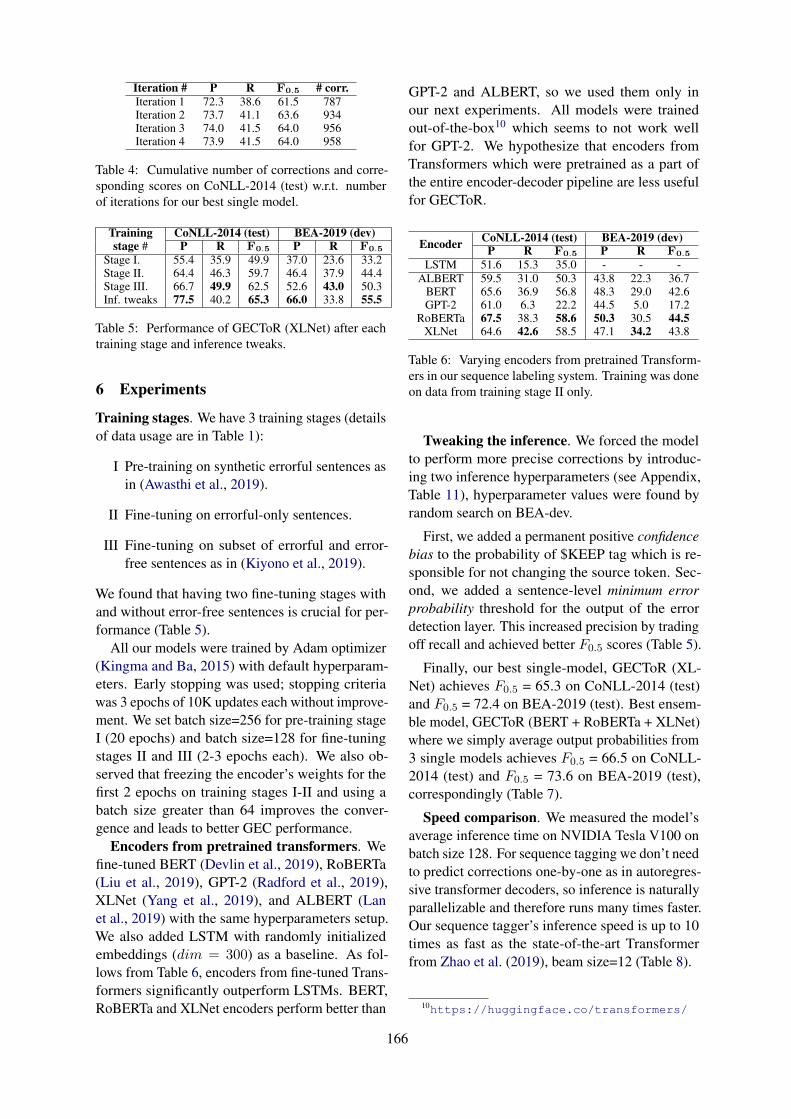
Iteration # P R F0.5 # corr.Iteration 1 72.3 38.6 61.5 787Iteration 2 73.7 41.1 63.6 934Iteration 3 74.0 41.5 64.0 956Iteration 4 73.9 41.5 64.0 958

Table 4: Cumulative number of corrections and corre-sponding scores on CoNLL-2014 (test) w.r.t. numberof iterations for our best single model.

Trainingstage #

CoNLL-2014 (test) BEA-2019 (dev)P R F0.5 P R F0.5

Stage I. 55.4 35.9 49.9 37.0 23.6 33.2Stage II. 64.4 46.3 59.7 46.4 37.9 44.4Stage III. 66.7 49.9 62.5 52.6 43.0 50.3Inf. tweaks 77.5 40.2 65.3 66.0 33.8 55.5

Table 5: Performance of GECToR (XLNet) after eachtraining stage and inference tweaks.

6 Experiments

Training stages. We have 3 training stages (detailsof data usage are in Table 1):

I Pre-training on synthetic errorful sentences asin (Awasthi et al., 2019).

II Fine-tuning on errorful-only sentences.

III Fine-tuning on subset of errorful and error-free sentences as in (Kiyono et al., 2019).

We found that having two fine-tuning stages withand without error-free sentences is crucial for per-formance (Table 5).

All our models were trained by Adam optimizer(Kingma and Ba, 2015) with default hyperparam-eters. Early stopping was used; stopping criteriawas 3 epochs of 10K updates each without improve-ment. We set batch size=256 for pre-training stageI (20 epochs) and batch size=128 for fine-tuningstages II and III (2-3 epochs each). We also ob-served that freezing the encoder’s weights for thefirst 2 epochs on training stages I-II and using abatch size greater than 64 improves the conver-gence and leads to better GEC performance.

Encoders from pretrained transformers. Wefine-tuned BERT (Devlin et al., 2019), RoBERTa(Liu et al., 2019), GPT-2 (Radford et al., 2019),XLNet (Yang et al., 2019), and ALBERT (Lanet al., 2019) with the same hyperparameters setup.We also added LSTM with randomly initializedembeddings (dim = 300) as a baseline. As fol-lows from Table 6, encoders from fine-tuned Trans-formers significantly outperform LSTMs. BERT,RoBERTa and XLNet encoders perform better than

GPT-2 and ALBERT, so we used them only inour next experiments. All models were trainedout-of-the-box10 which seems to not work wellfor GPT-2. We hypothesize that encoders fromTransformers which were pretrained as a part ofthe entire encoder-decoder pipeline are less usefulfor GECToR.

Encoder CoNLL-2014 (test) BEA-2019 (dev)P R F0.5 P R F0.5

LSTM 51.6 15.3 35.0 - - -ALBERT 59.5 31.0 50.3 43.8 22.3 36.7

BERT 65.6 36.9 56.8 48.3 29.0 42.6GPT-2 61.0 6.3 22.2 44.5 5.0 17.2

RoBERTa 67.5 38.3 58.6 50.3 30.5 44.5XLNet 64.6 42.6 58.5 47.1 34.2 43.8

Table 6: Varying encoders from pretrained Transform-ers in our sequence labeling system. Training was doneon data from training stage II only.

Tweaking the inference. We forced the modelto perform more precise corrections by introduc-ing two inference hyperparameters (see Appendix,Table 11), hyperparameter values were found byrandom search on BEA-dev.

First, we added a permanent positive confidencebias to the probability of $KEEP tag which is re-sponsible for not changing the source token. Sec-ond, we added a sentence-level minimum errorprobability threshold for the output of the errordetection layer. This increased precision by tradingoff recall and achieved better F0.5 scores (Table 5).

Finally, our best single-model, GECToR (XL-Net) achieves F0.5 = 65.3 on CoNLL-2014 (test)and F0.5 = 72.4 on BEA-2019 (test). Best ensem-ble model, GECToR (BERT + RoBERTa + XLNet)where we simply average output probabilities from3 single models achieves F0.5 = 66.5 on CoNLL-2014 (test) and F0.5 = 73.6 on BEA-2019 (test),correspondingly (Table 7).

Speed comparison. We measured the model’saverage inference time on NVIDIA Tesla V100 onbatch size 128. For sequence tagging we don’t needto predict corrections one-by-one as in autoregres-sive transformer decoders, so inference is naturallyparallelizable and therefore runs many times faster.Our sequence tagger’s inference speed is up to 10times as fast as the state-of-the-art Transformerfrom Zhao et al. (2019), beam size=12 (Table 8).

10https://huggingface.co/transformers/

166

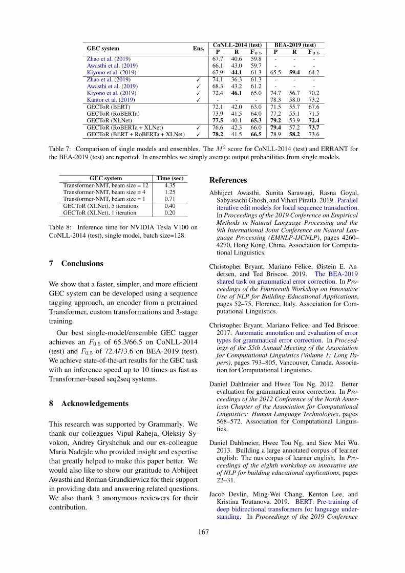
GEC system Ens. CoNLL-2014 (test) BEA-2019 (test)P R F0.5 P R F0.5

Zhao et al. (2019) 67.7 40.6 59.8 - - -Awasthi et al. (2019) 66.1 43.0 59.7 - - -Kiyono et al. (2019) 67.9 44.1 61.3 65.5 59.4 64.2Zhao et al. (2019) X 74.1 36.3 61.3 - - -Awasthi et al. (2019) X 68.3 43.2 61.2 - - -Kiyono et al. (2019) X 72.4 46.1 65.0 74.7 56.7 70.2Kantor et al. (2019) X - - - 78.3 58.0 73.2GECToR (BERT) 72.1 42.0 63.0 71.5 55.7 67.6GECToR (RoBERTa) 73.9 41.5 64.0 77.2 55.1 71.5GECToR (XLNet) 77.5 40.1 65.3 79.2 53.9 72.4GECToR (RoBERTa + XLNet) X 76.6 42.3 66.0 79.4 57.2 73.7GECToR (BERT + RoBERTa + XLNet) X 78.2 41.5 66.5 78.9 58.2 73.6

Table 7: Comparison of single models and ensembles. The M2 score for CoNLL-2014 (test) and ERRANT forthe BEA-2019 (test) are reported. In ensembles we simply average output probabilities from single models.

GEC system Time (sec)Transformer-NMT, beam size = 12 4.35Transformer-NMT, beam size = 4 1.25Transformer-NMT, beam size = 1 0.71GECToR (XLNet), 5 iterations 0.40GECToR (XLNet), 1 iteration 0.20

Table 8: Inference time for NVIDIA Tesla V100 onCoNLL-2014 (test), single model, batch size=128.

7 Conclusions

We show that a faster, simpler, and more efficientGEC system can be developed using a sequencetagging approach, an encoder from a pretrainedTransformer, custom transformations and 3-stagetraining.

Our best single-model/ensemble GEC taggerachieves an F0.5 of 65.3/66.5 on CoNLL-2014(test) and F0.5 of 72.4/73.6 on BEA-2019 (test).We achieve state-of-the-art results for the GEC taskwith an inference speed up to 10 times as fast asTransformer-based seq2seq systems.

8 Acknowledgements

This research was supported by Grammarly. Wethank our colleagues Vipul Raheja, Oleksiy Sy-vokon, Andrey Gryshchuk and our ex-colleagueMaria Nadejde who provided insight and expertisethat greatly helped to make this paper better. Wewould also like to show our gratitude to AbhijeetAwasthi and Roman Grundkiewicz for their supportin providing data and answering related questions.We also thank 3 anonymous reviewers for theircontribution.

ReferencesAbhijeet Awasthi, Sunita Sarawagi, Rasna Goyal,

Sabyasachi Ghosh, and Vihari Piratla. 2019. Paralleliterative edit models for local sequence transduction.In Proceedings of the 2019 Conference on EmpiricalMethods in Natural Language Processing and the9th International Joint Conference on Natural Lan-guage Processing (EMNLP-IJCNLP), pages 4260–4270, Hong Kong, China. Association for Computa-tional Linguistics.

Christopher Bryant, Mariano Felice, Øistein E. An-dersen, and Ted Briscoe. 2019. The BEA-2019shared task on grammatical error correction. In Pro-ceedings of the Fourteenth Workshop on InnovativeUse of NLP for Building Educational Applications,pages 52–75, Florence, Italy. Association for Com-putational Linguistics.

Christopher Bryant, Mariano Felice, and Ted Briscoe.2017. Automatic annotation and evaluation of errortypes for grammatical error correction. In Proceed-ings of the 55th Annual Meeting of the Associationfor Computational Linguistics (Volume 1: Long Pa-pers), pages 793–805, Vancouver, Canada. Associa-tion for Computational Linguistics.

Daniel Dahlmeier and Hwee Tou Ng. 2012. Betterevaluation for grammatical error correction. In Pro-ceedings of the 2012 Conference of the North Amer-ican Chapter of the Association for ComputationalLinguistics: Human Language Technologies, pages568–572. Association for Computational Linguis-tics.

Daniel Dahlmeier, Hwee Tou Ng, and Siew Mei Wu.2013. Building a large annotated corpus of learnerenglish: The nus corpus of learner english. In Pro-ceedings of the eighth workshop on innovative useof NLP for building educational applications, pages22–31.

Jacob Devlin, Ming-Wei Chang, Kenton Lee, andKristina Toutanova. 2019. BERT: Pre-training ofdeep bidirectional transformers for language under-standing. In Proceedings of the 2019 Conference

167

of the North American Chapter of the Associationfor Computational Linguistics: Human LanguageTechnologies, Volume 1 (Long and Short Papers),pages 4171–4186, Minneapolis, Minnesota. Associ-ation for Computational Linguistics.

Roman Grundkiewicz, Marcin Junczys-Dowmunt, andKenneth Heafield. 2019. Neural grammatical errorcorrection systems with unsupervised pre-trainingon synthetic data. In Proceedings of the FourteenthWorkshop on Innovative Use of NLP for Building Ed-ucational Applications, pages 252–263.

Yoav Kantor, Yoav Katz, Leshem Choshen, Edo Cohen-Karlik, Naftali Liberman, Assaf Toledo, AmirMenczel, and Noam Slonim. 2019. Learning to com-bine grammatical error corrections. In Proceedingsof the Fourteenth Workshop on Innovative Use ofNLP for Building Educational Applications, pages139–148, Florence, Italy. Association for Computa-tional Linguistics.

Diederik P Kingma and Jimmy Ba. 2015. Adam(2014), a method for stochastic optimization. InProceedings of the 3rd International Conferenceon Learning Representations (ICLR), arXiv preprintarXiv, volume 1412.

Shun Kiyono, Jun Suzuki, Masato Mita, Tomoya Mizu-moto, and Kentaro Inui. 2019. An empirical studyof incorporating pseudo data into grammatical er-ror correction. In Proceedings of the 2019 Confer-ence on Empirical Methods in Natural LanguageProcessing and the 9th International Joint Confer-ence on Natural Language Processing (EMNLP-IJCNLP), pages 1236–1242, Hong Kong, China. As-sociation for Computational Linguistics.

Taku Kudo and John Richardson. 2018. SentencePiece:A simple and language independent subword tok-enizer and detokenizer for neural text processing. InProceedings of the 2018 Conference on EmpiricalMethods in Natural Language Processing: SystemDemonstrations, pages 66–71, Brussels, Belgium.Association for Computational Linguistics.

Zhenzhong Lan, Mingda Chen, Sebastian Goodman,Kevin Gimpel, Piyush Sharma, and Radu Soricut.2019. Albert: A lite bert for self-supervised learn-ing of language representations. arXiv preprintarXiv:1909.11942.

Yinhan Liu, Myle Ott, Naman Goyal, Jingfei Du, Man-dar Joshi, Danqi Chen, Omer Levy, Mike Lewis,Luke Zettlemoyer, and Veselin Stoyanov. 2019.Roberta: A robustly optimized bert pretraining ap-proach. arXiv preprint arXiv:1907.11692.

Eric Malmi, Sebastian Krause, Sascha Rothe, DaniilMirylenka, and Aliaksei Severyn. 2019. Encode,tag, realize: High-precision text editing. In Proceed-ings of the 2019 Conference on Empirical Methodsin Natural Language Processing and the 9th Inter-national Joint Conference on Natural Language Pro-cessing (EMNLP-IJCNLP), pages 5054–5065, Hong

Kong, China. Association for Computational Lin-guistics.

Hwee Tou Ng, Siew Mei Wu, Ted Briscoe, ChristianHadiwinoto, Raymond Hendy Susanto, and Christo-pher Bryant. 2014. The conll-2014 shared task ongrammatical error correction. In Proceedings of theEighteenth Conference on Computational NaturalLanguage Learning: Shared Task, pages 1–14.

Diane Nicholls. 2003. The cambridge learner corpus:Error coding and analysis for lexicography and elt.In Proceedings of the Corpus Linguistics 2003 con-ference, volume 16, pages 572–581.

Alec Radford, Jeffrey Wu, Rewon Child, David Luan,Dario Amodei, and Ilya Sutskever. 2019. Languagemodels are unsupervised multitask learners. OpenAIBlog, 1(8):9.

Mike Schuster and Kaisuke Nakajima. 2012. Japaneseand korean voice search. In 2012 IEEE Interna-tional Conference on Acoustics, Speech and SignalProcessing (ICASSP), pages 5149–5152. IEEE.

Rico Sennrich, Barry Haddow, and Alexandra Birch.2016a. Edinburgh neural machine translation sys-tems for WMT 16. In Proceedings of the First Con-ference on Machine Translation: Volume 2, SharedTask Papers, pages 371–376, Berlin, Germany. As-sociation for Computational Linguistics.

Rico Sennrich, Barry Haddow, and Alexandra Birch.2016b. Neural machine translation of rare wordswith subword units. In Proceedings of the 54th An-nual Meeting of the Association for ComputationalLinguistics (Volume 1: Long Papers), pages 1715–1725, Berlin, Germany. Association for Computa-tional Linguistics.

Toshikazu Tajiri, Mamoru Komachi, and Yuji Mat-sumoto. 2012. Tense and aspect error correction foresl learners using global context. In Proceedingsof the 50th Annual Meeting of the Association forComputational Linguistics: Short Papers-Volume 2,pages 198–202. Association for Computational Lin-guistics.

Ashish Vaswani, Noam Shazeer, Niki Parmar, JakobUszkoreit, Llion Jones, Aidan N Gomez, ŁukaszKaiser, and Illia Polosukhin. 2017. Attention is allyou need. In Advances in neural information pro-cessing systems, pages 5998–6008.

Zhilin Yang, Zihang Dai, Yiming Yang, Jaime Car-bonell, Russ R Salakhutdinov, and Quoc V Le. 2019.Xlnet: Generalized autoregressive pretraining forlanguage understanding. In Advances in neural in-formation processing systems, pages 5754–5764.

Helen Yannakoudakis, Ted Briscoe, and Ben Medlock.2011. A new dataset and method for automaticallygrading esol texts. In Proceedings of the 49th An-nual Meeting of the Association for ComputationalLinguistics: Human Language Technologies-Volume1, pages 180–189. Association for ComputationalLinguistics.

168

Zheng Yuan. 2017. Grammatical error correction innon-native english. Technical report, University ofCambridge, Computer Laboratory.

Wei Zhao, Liang Wang, Kewei Shen, Ruoyu Jia, andJingming Liu. 2019. Improving grammatical errorcorrection via pre-training a copy-augmented archi-tecture with unlabeled data. In Proceedings of the2019 Conference of the North American Chapter ofthe Association for Computational Linguistics: Hu-man Language Technologies, Volume 1 (Long andShort Papers), pages 156–165, Minneapolis, Min-nesota. Association for Computational Linguistics.

169

A Appendix

id Coretransformation

Transformationsuffix Tag Example

basic-1 KEEP ∅ $KEEP . . . many people want to travel during the summer . . .basic-2 DELETE ∅ $DELETE . . . not sure if you are {you ⇒∅} gifting . . .basic-3 REPLACE a $REPLACE a . . . the bride wears {the ⇒ a} white dress . . .

. . . . . . . . . . . . . . .basic-3804 REPLACE cause $REPLACE cause . . . hope it does not {make ⇒ cause} any trouble . . .basic-3805 APPEND for $APPEND for . . . he is {waiting ⇒ waiting for} your reply . . .

. . . . . . . . . . . . . . .basic-4971 APPEND know $APPEND know . . . I {don’t ⇒ don’t know} which to choose. . .

g-1 CASE CAPITAL $CASE CAPITAL . . . surveillance is on the {internet ⇒ Internet} . . .g-2 CASE CAPITAL 1 $CASE CAPITAL 1 . . . I want to buy an {iphone ⇒ iPhone} . . .g-3 CASE LOWER $CASE LOWER . . . advancement in {Medical ⇒ medical} technology . . .g-4 CASE UPPER $CASE UPPER . . . the {it ⇒ IT} department is concerned that. . .g-5 MERGE SPACE $MERGE SPACE . . . insert a special kind of gene {in to ⇒ into} the cell . . .g-6 MERGE HYPHEN $MERGE HYPHEN . . . and needs {in depth ⇒ in-depth} search . . .g-7 SPLIT HYPHEN $SPLIT HYPHEN . . . support us for a {long-run ⇒ long run} . . .g-8 NOUN NUMBER SINGULAR $NOUN NUMBER SINGULAR . . . a place to live for their {citizen ⇒ citizens}g-9 NOUN NUMBER PLURAL $NOUN NUMBER PLURAL . . . carrier of this {diseases ⇒ disease} . . .g-10 VERB FORM VB VBZ $VERB FORM VB VBZ . . . going through this {make ⇒ makes} me feel . . .g-11 VERB FORM VB VBN $VERB FORM VB VBN . . . to discuss what {happen ⇒ happened} in fall . . .g-12 VERB FORM VB VBD $VERB FORM VB VBD . . . she sighed and {draw ⇒ drew} her . . .g-13 VERB FORM VB VBG $VERB FORM VB VBG . . . shown success in {prevent ⇒ preventing} such . . .g-14 VERB FORM VB VBZ $VERB FORM VB VBZ . . . a small percentage of people {goes ⇒ go} by bike . . .g-15 VERB FORM VBZ VBN $VERB FORM VBZ VBN . . . development has {pushes ⇒ pushed} countries to . . .g-16 VERB FORM VBZ VBD $VERB FORM VBZ VBD . . . he {drinks ⇒ drank} a lot of beer last night . . .g-17 VERB FORM VBZ VBG $VERB FORM VBZ VBG . . . couldn’t stop {thinks ⇒ thinking} about it . . .g-18 VERB FORM VBN VB $VERB FORM VBN VB . . . going to {depended ⇒ depend} on who is hiring . . .g-19 VERB FORM VBN VBZ $VERB FORM VBN VBZ . . . yet he goes and {eaten ⇒ eats} more melons . . .g-20 VERB FORM VBN VBD $VERB FORM VBN VBD . . . he {driven ⇒ drove} to the bus stop and . . .g-21 VERB FORM VBN VBG $VERB FORM VBN VBG . . . don’t want you fainting and {broken ⇒ breaking} . . .g-22 VERB FORM VBD VB $VERB FORM VBD VB . . . each of these items will {fell ⇒ fall} in price . . .g-23 VERB FORM VBD VBZ $VERB FORM VBD VBZ . . . the lake {froze ⇒ freezes} every year . . .g-24 VERB FORM VBD VBN $VERB FORM VBD VBN . . . he has been went {went ⇒ gone} since last week . . .g-25 VERB FORM VBD VBG $VERB FORM VBD VBG . . . talked her into {gave ⇒ giving} me the whole day . . .g-26 VERB FORM VBG VB $VERB FORM VBG VB . . . free time, I just {enjoying ⇒ enjoy} being outdoors . . .g-27 VERB FORM VBG VBZ $VERB FORM VBG VBZ . . . there still {existing ⇒ exists} many inevitable factors . . .g-28 VERB FORM VBG VBN $VERB FORM VBG VBN . . . people are afraid of being {tracking ⇒ tracked} . . .g-29 VERB FORM VBG VBD $VERB FORM VBG VBD . . . there was no {mistook ⇒ mistaking} his sincerity . . .

Table 9: List of token-level transformations (section 3). We denote a tag which defines a token-level transformationas concatenation of two parts: a core transformation and a transformation suffix.

Trainingstage #

CoNLL-2014 (test) BEA-2019 (dev)P R F0.5 P R F0.5

Stage I. 57.8 33.0 50.2 40.8 22.1 34.9Stage II. 68.1 42.6 60.8 51.6 33.8 46.7Stage III. 68.8 47.1 63.0 54.2 41.0 50.9Inf. tweaks 73.9 41.5 64.0 62.3 35.1 54.0

Table 10: Performance of GECToR (RoBERTa) after each training stage and inference tweaks. Results are givenin addition to results for our best single model, GECToR (XLNet) which are given in Table 5.

System name Confidence bias Minimum error probabilityGECToR (BERT) 0.10 0.41

GECToR (RoBERTa) 0.20 0.50GECToR (XLNet) 0.35 0.66

GECToR (RoBERTa + XLNet) 0.24 0.45GECToR (BERT + RoBERTa + XLNet) 0.16 0.40

Table 11: Inference tweaking values which were found by random search on BEA-dev.

170

Proceedings of the 15th Workshop on Innovative Use of NLP for Building Educational Applications, pages 171–176July 10, 2020. c©2020 Association for Computational Linguistics

Interpreting Neural CWI Classifiers’ Weights as Vocabulary Size

Yo EharaShizuoka Institute of Science and Technology / 2200-2, Toyosawa, Fukuroi, Shizuoka, Japan.

ehara.yo@sist.ac.jp

Abstract

Complex Word Identification (CWI) is a taskfor the identification of words that are chal-lenging for second-language learners to read.Even though the use of neural classifiers isnow common in CWI, the interpretation oftheir parameters remains difficult. This paperanalyzes neural CWI classifiers and shows thatsome of their parameters can be interpreted asvocabulary size. We present a novel formal-ization of vocabulary size measurement meth-ods that are practiced in the applied linguisticsfield as a kind of neural classifier. We alsocontribute to building a novel dataset for val-idating vocabulary testing and readability viacrowdsourcing.

1 Introduction

The readability of second-language learners hasattracted great interest in studies in the field of nat-ural language processing (NLP) (Beinborn et al.,2014; Pavlick and Callison-Burch, 2016). As NLPmainly addresses automatic editing of texts, read-ability assessment studies in this field have focusedon identifying complex parts by assuming that thewords identified are eventually simplified so thatlearners can read them. To this end, complex wordidentification (CWI) (Paetzold and Specia, 2016;Yimam et al., 2018) tasks have been studied exten-sively. Recently, a personalized CWI task has beenproposed, where the goal of the task is to predictwhether a word is complex for each learner in apersonalized manner (Paetzold and Specia, 2017;Lee and Yeung, 2018). Neural models are also em-ployed in these studies and have achieved excellentperformance.

The weights, or parameters, of a personalizedhigh-performance neural CWI, obviously includeinformation on how to measure the word difficultyand learner ability from a variety of features. Ifsuch information could be extracted from the modelin a form that is easy to interpret, it would not only

be use (Hoshino, 2009; Ehara et al., 2012, 2013,2014; Sakaguchi et al., 2013; Ehara et al., 2016,2018; Ehara, 2019). To this end, this paper pro-poses a method for interpreting the weights of per-sonalized neural CWI models. Let us suppose thatwe have a corpus and that its word frequency rank-ing reflects its word difficulty. Using our method, aword’s difficulty can be interpreted as the frequencyrank of the word in the corpus and a learner’s abil-ity can be interpreted as the vocabulary size withrespect to the corpus, i.e., the number of wordsknown to the learner when counted in a descendingorder of frequency in the corpus.

Our key idea is to compare CWI studies withvocabulary testing studies in applied linguistics(Nation, 2006; Laufer and Ravenhorst-Kalovski,2010). Second-language vocabulary is extensiveand occupies most of the time spent in learninga language. Vocabulary testing studies focus onmeasuring each learner’s second language vocab-ulary quickly. One of the major findings of thesestudies is that a learner needs to “know” at leastfrom 95% to 98% of the tokens in a target text toread. Here, to measure if a learner “knows” a word,vocabulary testing studies use the learner’s vocabu-lary size and word frequency ranking of a balancedcorpus. Hence, by formalizing the measurementmethod used in vocabulary testing studies as a neu-ral personalized CWI, we can interpret neural per-sonalized CWI models’ weights as vocabulary sizeand word frequency ranking.

Our contributions are summarized as follows:

1. To predict whether a learner knows a wordthrough the use of a vocabulary test result inhand, vocabulary size-based methods werepreviously used for vocabulary testing. Weshow that this method can represent a specialcase of typical neural CWI classifiers that takea specific set of features as input. Furthermore,we theoretically propose novel methods thatenable the weights of certain neural classifiers

171

to become explainable on the basis of the vo-cabulary size of a learner.

2. To validate the proposed models, we want adataset in which each learner/test-taker takesboth vocabulary and reading comprehensiontests. To this end, we build a novel dataset andmake it publicly available.

2 Related Work

2.1 Vocabulary size-based testing

Vocabulary size-based testing studies (Nation,2006; Laufer and Ravenhorst-Kalovski, 2010) mea-sure the vocabulary size of second-language learn-ers. Assuming that all learners memorize words inthe same order, i.e., that the difficulty of words isidentical for each learner, all words are ranked inone dimension using this method. Subsequently,it is determined whether or not a learner knows atarget word by checking if the vocabulary size ofthe learner is greater than the easiness rank of theword.

The vocabulary size-based method can be for-malized as follows. Let us consider the case inwhich we have J learners {l1, l2, . . . , lj , . . . , lJ}and I words {v1, v2, . . . , vi, . . . , vI}. j is the in-dex of the learners and i is the index of the words.When there is no ambiguity, we denote word vi asword i and learner lj as learner j, for the sake ofsimplicity. We write the rank of word vi as ri andthe vocabulary size of learner lj as sj . Then, todetermine whether learner lj knows word vi, thefollowing decision function f is used:

f(lj , vi) = sj − ri (1)

Interpretting Eq. 1 is simple: if f(lj , vi) ≥ 0,then learner lj knows word vi; if f(lj , vi) < 0,then learner lj does not know word vi.

The performance of Eq. 1 depends solely on howto determine the vocabulary size of learner lj , sj ,and the easiness rank of word vi, ri. As severalmethods have previously been proposed to estimatethis, we describe them in the following subsections.

2.1.1 Measuring rank of word viEasiness ranks of words are important in vocabu-lary size-based testing. To this end, word frequencyrankings from a balanced corpus, especially theBritish National Corpus (BNC Consortium, 2007),are used: the more frequent words in the corpus areranked higher and considered to be easier. Some

previous studies in the field manually adjust theBNC word frequency rankings to make them com-patible with language teachers’ intuitions. BNCcollects British English. Recent studies also takeinto account word frequency obtained from theCorpus of Contemporary American (COCA) En-glish (Davies, 2009) by simply adding the wordfrequencies of both corpora in order to obtain aword frequency ranking.

2.1.2 Measuring the vocabulary size oflearner lj

An intuitive and simple method for measuring thevocabulary size of learner lj is as follows. First, werandomly sample some words from a large vocab-ulary sample of the target language. Second, wetest whether learner lj knows each of the sampledwords and identify the ratio of words known to thelearner. Third, we estimate the learner’s vocabu-lary size as the ratio × the number of correctlyanswered questions.

This is how the Vocabulary Size Test (Beglar andNation, 2007) works. Using the frequency rankingof 20, 000 words from the BNC corpus, the wordsare first split into 20 levels, with each level consist-ing of 1, 000 words. It is assumed that the 1, 000words grouped in the same level have similar dif-ficulty. Then, from the 1, 000 words at each level,5 words are carefully sampled and a vocabularytest is built that consists of 100 words in total. Fi-nally, the number of words that learner lj correctlyanswered × 200 is estimated to be the vocabularysize of learner lj . This simple method was later val-idated by a study from another independent group(Beglar, 2010) and is widely accepted.

Examples of the Vocabulary Size Test are pub-licly available (Nation, 2007). Each question askslearners taking the test to choose the correct an-swer by selecting one of the four offered optionsthat has the same meaning as one of the underlinedwords in the question. It should be noted that, inthe Vocabulary Size Test, each word is placed in asentence to disambiguate the usage of each wordand each option can directly be replaced with theunderlined part without the need to grammaticallyrewrite the sentence, e.g., for singular/plural differ-ences. Although a typical criticism of vocabularytests relates to the fact that they do not take contextsinto account, each question in the Vocabulary SizeTest is specifically designed to account for suchcriticism by asking the meaning of a word within asentence.

172

−10 −5 0 5 10

0.0

0.2

0.4

0.6

0.8

1.0

Theta

Pro

babili

ty

a=1.0 a=0.5 a=2.0

Figure 1: Probability against θ when changing thevalue of a.

Figure 2: Neural network illustration of a vocabularysize-based prediction.

3 Proposed Formulation

The following notations are used. We haveJ learners {l1, l2, . . . , lj , . . . , lJ} and I words{v1, v2, . . . , vi, . . . , vI}. j is the index of the learn-ers and i is the index of the words. When thereis no ambiguity, we denote word vi as word i andlearner lj as learner j, for the sake of simplicity.Let Ki be the number of occurrences of word vi.While we do not use in our experiments, for gen-erality, we explicitly write the index for each ofthe occurrences, i.e., k. Let ui,k be the k-th occur-rence of word vi in the text. Let bj be the abilityof learner j and let di,k be the difficulty of the k-thoccurrence of word vi.

A dichotomous decision using a neural network-based formulation is typically modeled using a

probabilistic formulation. Let yj,i,k be a binaryrandom variable that takes 1 if learner lj knowsthe k-th occurrence of word vi, otherwise it takes0. Subsequently, it is typical to use a function thatmaps a real number to the [0, 1] range so that thereal number can be interpreted as a probability. Tothis end, typically σ is the logistic sigmoid function,i.e., σ(x) = 1

exp(−x)+1 is used. Then, the proba-bility that learner lj knows the k-th occurrence ofword vi, namely, ui,k, can be modeled as in Eq. 2.

p(yi,k,j = 1|ui,k, lj) = σ(a(bj − di,k)) (2)

Qualitative characteristics of Eq. 2 are explainedas follows. Let θ = a(bj − di,k). The logistic sig-moid function maps an arbitrary real number to the[0, 1] range and makes it possible to interpret thereal number as a probability. Here, θ is mapped tothe range. As θ increases, the larger the probabilitybecomes. We can see that a > 0 is the parameterthat determines the steepness of the slope. A largea results in a steep slope. When a is large enough,4.0 for example, numerically, the function is veryclose to the identity function that returns 0 if θ < 0and 1 if θ ≥ 0.

Probability in a dichotomous classification ismost ambiguous when it takes 0.5. By focusing onthe point the vertical line takes 0.5, we can see thatthe sign of bj − di,k determines whether or not theprobability is larger than 0.5.

3.1 Vocabulary size-based classification asneural classification

These characteristics of Eq. 2 enable it to expressthe decision function employed in the previous vo-cabulary size-based decision function Eq. 1 as itsspecial case. Let us consider the case when a islarge and the curve is very steep, say a = 10, forexample. Then, by setting bj = sj and di,k = rifor all k for word vi, the decision about whetherlearner j knows the k-th occurrence of word vi inEq. 1 is virtually identical to that of Eq. 2. In thismanner, the previous vocabulary size-based deci-sion functions for whether learner lj knows word viin applied linguistics can be converted to a neuralnetwork-based classifier and vice versa.

We can see that there exists a freedom in the pa-rameters. In the above example, we can achieve thesame setting by setting bj = 0.1sj , di,k = 0.1riand a = 100. In this way, the same vocabulary sizeclassification can be achieved by different parame-ter values.

173

This freedom in terms of parameters is the keyfor conversion: by setting an appropriate a, wecan convert neural classifier parameters as eachlearner’s vocabulary size and the rank of each word.

3.2 Rewriting parameters

While bj and di,k are parameters, we rewrite themusing one-hot vectors that are widely used to de-scribe neural network-based models. Let us intro-duce two types of feature functions: φl and φv.The former returns the feature vector of learner lj ,and the latter returns the feature vector of the k-thoccurrence of word vi, ui,k.

Then, the ability and difficulty parameters ofEq. 2 can be written as the inner product of a weightvector and a feature vector. Let us introduce wl asthe weight vector for φl. Let h be a function thatreturns the one-hot representation of the augment.We write hl(lj) to denote a function that returnsJ-dimensional one-hot vector, where only the j-thelement is 1 while the other elements are 0. Then,we can rewrite bj as the inner product of the weightvector and the one-hot vector as bj = w>l hl(lj).

In the same way, di,k can be rewritten as theinner product of its weight vector and feature vec-tor. Being reminded that Ki denotes the num-ber of occurrences of word vi, we consider avery long

∑Ii=1Ki-dimensional one-hot vector

hv(ui,k), where only one element that correspondsto the k-th element of word vi is 1 and all otherelements are 0. Then, by introducing a weight vec-tor wv that has the same dimension with hv(ui,k),we can rewrite di,k as di,k = w>v hv(ui,k). Usingthese expressions, Eq. 2 can be illustrated using atypical neural network illustration as in Fig. 2.

Overall, the equation using one-hot vector repre-sentation can be described as follows:

p(yi,k,j = 1|ui,k, lj)= σ(a(w>l hl(lj)−w>v hv(ui,k))) (3)

3.3 Weights as learner vocabulary sizes andword frequency ranks

Eq. 3 provides us with a hint to convert neuralclassifier weights into vocabulary sizes and wordfrequency rankings. To this end, we can do the fol-lowing. First, we use Eq. 3 to estimate parameters:a, wl, and wv. Typically, for a binary classificationsetting using the logistic sigmoid function, cross-entropy loss is chosen as the loss function. We

use L(a,wl,wv) to denote the sum of the cross-entropy loss function for each of the following: alldata, all learners, and all occurrences of all words.

From a, wl and wv, we can estimate the fre-quency rank of word vi as follows: aw>v hv(ui,k).Hence, by comparing the estimate with the ob-served ranking value ri of word vi, we can also tuneall parameters. We can simply employR(a,wv) =∑I

i=1

∑Kik=1 ||aw>v hv(ui,k)− ri||2 for a loss func-

tion that measures how distant the estimated rankand the observed rank are. Of course, we can com-pare aw>l hl(lj) and sj , the observed vocabularysize of learner lj . However, since the observed vo-cabulary size of each learner is usually much moreinaccurate than the ranking of a word, we do notuse this term. As ranks usually take large valuesbut never larger than 1, we can use the logarithm ofthe rank of word vi for ri instead of its raw values.

3.4 Proposed ModelPractically, it is important to note that the one-hotvector hv(ui,k) in L and R functions can be re-placed with any feature vector of ui,k or with thek-th occurrence of word vi. In our experiments, wesimply used this replacement.

We propose the following minimization problemthat simultaneously tunes both parameters. Welet the parameter γ ∈ [0, 1] be the parameter thattunes the two loss functions, namely, L and R.Note that, as the optimal value of a is different forterm L and for term R, we modeled the two termsseparately: a1 and a2, respectively. Since most ofEq. 4 consists of continuous functions, then Eq. 4can easily be optimized as a neural classifier using atypical deep learning framework, such as PyTorch.

mina1,a2,wl,wv

γL(a1,wl,wv) + (1− γ)R(a2,wv)

(4)For the input, we prepare the vocabulary test

results of J learners, the vocabulary feature func-tion h, and the vocabulary ranking ri. By preparingthese data for input, we can train the model throughestimating the w parameters by minimizing Eq. 4.The tuning of the γ value can be conducted us-ing validation data that are disjointed from boththe training and test data. Or, γ can also be tunedby jointly minimizing γ with other parameters inEq. 4. Finally, in the test phase, using the trainedparameter a1 and wl – we can estimate learner lj’svocabulary size as a1w>l hl(lj). Using the trainedparameter a2,wv, we can estimate the rank of the

174

first occurrence of a new word vi, which did notappear in the training data, as a2w>v hv(ui,1).

4 Dataset

4.1 Description

To evaluate Eq. 4, we need a real dataset that coversboth vocabulary size and reading comprehensiontests, assuming that the text coverage hypothesisof 98% holds true. To our knowledge, there isno such dataset widely available. There are cer-tain existing vocabulary test result datasets, suchas (Ehara, 2018), as well as many reading compre-hension test result datasets - however; we could notfind a dataset in which a second-language learnersubject is asked to provide both vocabulary sizeand reading comprehension test results.

To this end, this paper provides such a dataset.Following (Ehara, 2018), we used the Lancerscrowdsourcing service to collect 55 vocabulary testresults as well as answers to 1 long and 1 shortreading comprehension question from 100 learn-ers. We paid around 5 USD for each participant.In comparison to the dataset by (Ehara, 2018), thenumber of vocabulary test questions was reducedso that subjects would have enough time to solvethe reading comprehension test. For the vocabu-lary test part, we used the Vocabulary Size Test(Beglar and Nation, 2007). The reading compre-hension questions were taken from the sample setof the questions in the Appendix section in (Lauferand Ravenhorst-Kalovski, 2010). The correct op-tions for these questions are on a website that canalso be reached from the description of (Laufer andRavenhorst-Kalovski, 2010) 1.

In the same manner as (Ehara, 2018), all partici-pants were required to have ever taken the Test ofEnglish for International Communication (TOEIC)test provided by English Testing Services (ETS)and to write scores on a self-report basis. Thisrequirement filters out learners who have neverstudied English seriously but try to participate foreconomical merits.

In the dataset, each line describes all the re-sponses from a learner. The first columns, whichcontain the term TOEIC in their headings, provideTOEIC scores and dates. Then, the 55 vocabularytesting questions follow. The columns that startwith “l” denote the responses on the long reading

1For more detailed information for thedataset, refer to http://yoehara.com/vocabulary-prediction/.

Figure 3: Estimated LFRs against Gold LFRs.

comprehension test and those with “s” denote theresponses on the short one.

4.2 Preliminary Experiments

Finally, we show preliminary experiments by usingour dataset. We used 33 words from the dataset,i.e., 3, 300 responses. Hereafter, we simply denotethe logarithm of frequency ranks in a descendingorder as “LFR”. For ri, we used the LFR of theBNC corpus (BNC Consortium, 2007). For fea-tures of hv, we used the logarithm of the frequencyof the COCA corpus (Davies, 2009). We obtainedparameters by optimizing the minimization param-eters Eq. 4. Then, for 100 words disjoint from the33 training words, we plotted the estimated LFRvalues against the gold LFR values in Fig. 3. Wecan easily see that they have a good correlation.The Spearman’s correlation coefficient for Fig. 3was 0.70, which can be construed as a strong cor-relation (Taylor, 1990).

5 Conclusions

In this paper, we theoretically showed that previousvocabulary size-based classifiers can be seen as aspecial case of a neural classifier. We also built adataset necessary for this evaluation and made itpublicly available in the form of an attached dataset.Future work include more detailed experiments onlanguage learners’ second language vocabularies.

Acknowledgments

This work was supported by JST ACT-I GrantNumber JPMJPR18U8 and JSPS KAKENHI GrantNumber JP18K18118. We used the AI BridgingCloud Infrastructure (ABCI) by the National Insti-tute of Advanced Industrial Science and Technol-ogy (AIST), Japan. We thank anonymous reviewersfor their insightful and constructive comments.

175

ReferencesDavid Beglar. 2010. A Rasch-based validation of the

Vocabulary Size Test. Language Testing, 27(1):101–118.

David Beglar and Paul Nation. 2007. A vocabulary sizetest. The Language Teacher, 31(7):9–13.

Lisa Beinborn, Torsten Zesch, and Iryna Gurevych.2014. Predicting the Difficulty of Language Pro-ficiency Tests. Transactions of the Association forComputational Linguistics, 2:517–530.

The BNC Consortium. 2007. The British National Cor-pus, version 3 (BNC XML Edition).

Mark Davies. 2009. The 385+ million word corpus ofcontemporary american english (1990–2008+): De-sign, architecture, and linguistic insights. Interna-tional journal of corpus linguistics, 14(2):159–190.

Yo Ehara. 2018. Building an English Vocabu-lary Knowledge Dataset of Japanese English-as-a-Second-Language Learners Using Crowdsourcing.In Proc. of LREC.

Yo Ehara. 2019. Neural rasch model: How word em-beddings affect to word difficulty? In Proc. of the16th International Conference of the Pacific Associ-ation for Computational Linguistics (PACLING).

Yo Ehara, Yukino Baba, Masao Utiyama, and Ei-ichiro Sumita. 2016. Assessing Translation Abilitythrough Vocabulary Ability Assessment. In Proc. ofIJCAI.

Yo Ehara, Yusuke Miyao, Hidekazu Oiwa, Issei Sato,and Hiroshi Nakagawa. 2014. Formalizing WordSampling for Vocabulary Prediction as Graph-basedActive Learning. In Proc. of EMNLP, pages 1374–1384.

Yo Ehara, Issei Sato, Hidekazu Oiwa, and Hiroshi Nak-agawa. 2012. Mining Words in the Minds of Sec-ond Language Learners: Learner-Specific Word Dif-ficulty. In Proceedings of COLING 2012, pages799–814, Mumbai, India. The COLING 2012 Orga-nizing Committee.

Yo Ehara, Issei Sato, Hidekazu Oiwa, and Hiroshi Nak-agawa. 2018. Mining words in the minds of secondlanguage learners for learner-specific word difficulty.Journal of Information Processing, 26:267–275.

Yo Ehara, Nobuyuki Shimizu, Takashi Ninomiya,and Hiroshi Nakagawa. 2013. Personalized Read-ing Support for Second-language Web Documents.ACM Trans. Intell. Syst. Technol., 4(2):31:1–31:19.

Ayako Hoshino. 2009. Automatic Question Generationfor Language Testing and its Evaluation Criteria.Ph.D. thesis, Graduate School of InterdisciplinaryInformation Studies, The University of Tokyo.

Batia Laufer and Geke C. Ravenhorst-Kalovski. 2010.Lexical Threshold Revisited: Lexical Text Coverage,Learners’ Vocabulary Size and Reading Comprehen-sion. Reading in a Foreign Language, 22(1):15–30.

John Lee and Chak Yan Yeung. 2018. Personalizinglexical simplification. In Proceedings of the 27thInternational Conference on Computational Linguis-tics, pages 224–232, Santa Fe, New Mexico, USA.Association for Computational Linguistics.

I. Nation. 2006. How Large a Vocabulary is NeededFor Reading and Listening? Canadian Modern Lan-guage Review, 63(1):59–82.

I. Nation. 2007. Vocabulary size test. https://www.wgtn.ac.nz/lals/about/staff/paul-nation#vocab-tests.

Gustavo Paetzold and Lucia Specia. 2016. Collectingand Exploring Everyday Language for PredictingPsycholinguistic Properties of Words. In Proceed-ings of COLING 2016, the 26th International Con-ference on Computational Linguistics: Technical Pa-pers, pages 1669–1679, Osaka, Japan. The COLING2016 Organizing Committee.

Gustavo Paetzold and Lucia Specia. 2017. Lexical Sim-plification with Neural Ranking. In Proc. of EACL,pages 34–40, Valencia, Spain.

Ellie Pavlick and Chris Callison-Burch. 2016. SimplePPDB: A Paraphrase Database for Simplification. InProceedings of the 54th Annual Meeting of the As-sociation for Computational Linguistics (Volume 2:Short Papers), pages 143–148, Berlin, Germany. As-sociation for Computational Linguistics.

Keisuke Sakaguchi, Yuki Arase, and Mamoru Komachi.2013. Discriminative Approach to Fill-in-the-BlankQuiz Generation for Language Learners. In Proc.of the 51st Annual Meeting of the Association forComputational Linguistics (Volume 2: Short Pa-pers), pages 238–242, Sofia, Bulgaria. Associationfor Computational Linguistics.

Richard Taylor. 1990. Interpretation of the correlationcoefficient: a basic review. Journal of diagnosticmedical sonography, 6(1):35–39.

Seid Muhie Yimam, Chris Biemann, Shervin Malmasi,Gustavo H. Paetzold, Lucia Specia, Sanja Stajner,Anaıs Tack, and Marcos Zampieri. 2018. A Reporton the Complex Word Identification Shared Task2018. arXiv:1804.09132 [cs]. ArXiv: 1804.09132.

176

Proceedings of the 15th Workshop on Innovative Use of NLP for Building Educational Applications, pages 177–185July 10, 2020. c©2020 Association for Computational Linguistics

Automated Scoring of Clinical Expressive Language Evaluation Tasks

Yiyi Wang†, Emily Prud’hommeaux†, Meysam Asgari‡, and Jill Dolata‡† Boston College, Chestnut Hill MA, USA

‡ Oregon Health & Science University, Portland OR, USA{wangdil,prudhome}@bc.edu, {asgari,dolataj}@ohsu.edu

Abstract

Many clinical assessment instruments used todiagnose language impairments in children in-clude a task in which the subject must formu-late a sentence to describe an image using aspecific target word. Because producing sen-tences in this way requires the speaker to in-tegrate syntactic and semantic knowledge in acomplex manner, responses are typically eval-uated on several different dimensions of appro-priateness yielding a single composite scorefor each response. In this paper, we presenta dataset consisting of non-clinically elicitedresponses for three related sentence formula-tion tasks, and we propose an approach forautomatically evaluating their appropriateness.Using neural machine translation, we gener-ate correct-incorrect sentence pairs to serve assynthetic data in order to increase the amountand diversity of training data for our scoringmodel. Our scoring model uses transfer learn-ing to facilitate automatic sentence appropri-ateness evaluation. We further compare cus-tom word embeddings with pre-trained con-textualized embeddings serving as features forour scoring model. We find that transfer learn-ing improves scoring accuracy, particularlywhen using pre-trained contextualized embed-dings.

1 Introduction

It is estimated that between 5% and 10% of thepediatric population will experience a speech orlanguage impairment (Norbury et al., 2016; Rosen-baum and Simon, 2016). Diagnosing these im-pairments is complex, requiring the integration ofstructured assessments, medical history, and clini-cal observation, and there is evidence that languageimpairments are frequently misdiagnosed and un-derdiagnosed (Conti-Ramsden et al., 2006; Grimmand Schulz, 2014; Rosenbaum and Simon, 2016).As a result, there is a need for tools and technolo-

gies that can support efficient and remote screen-ing for language impairment. However, developingmethods for automatically scoring the subtests usedto diagnose language disorders can be challengingbecause of the very limited amount of labeled dataavailable for these subtests from these special pop-ulations.

In this paper, we focus on a task we have adaptedfrom the Formulated Sentences (FS) subtest of theClinical Evaluation of Language Fundamentals 4(CELF-4), one of the most widely used languagediagnostic instruments in the United States (Semelet al., 2003). In the CELF-4 Formulated Sentencestask, a child is presented with a target word and animage, and must use that word in a sentence aboutthat image. Poor performance on this subtest isstrongly correlated with expressive language im-pairments. Responses are scored on a scale from 0to 2; a sentence assigned a score of 2 must correctlyuse the target word, be a complete and grammat-ically correct sentence, and relate to the contentand activities shown in the image. Reliable man-ual scoring can be difficult and time-consumingbecause of the large of number of factors that mustbe considered. This degree of subjectivity, togetherwith the task’s important role in identifying expres-sive language impairments, make automatic scor-ing of the formulated sentences subtest particularlyworthwhile.

This paper makes the following contributions:

• We present a new data set of non-clinicallyelicited formulated sentence task responses,annotated for appropriateness evaluation(scores: 0, 1, and 2), which can be used asa benchmark and as a data source for futureautomated scoring of clinically elicited re-sponses. The dataset includes 2160 sentencesfrom three related sentence formulation tasks(Section 3).

177

• We develop a neural machine translationmodel trained on second language learner dataand generate two artificial datasets for trainingthe formulated sentences scoring classifier.

• We demonstrate that our transfer learningmodel has benefits for scoring formulated sen-tences.

• We systematically compare the use of cus-tom task-specific embeddings and pre-trainedgeneric contextualized embeddings for scor-ing formulated sentences.

2 Related Work

Scoring formulated sentences in terms of syntacticcorrectness can be analogous to the more commontask of Grammatical Error Detection (GED), inwhich points are deducted for each grammaticalerror detected in a sentence or text. The state-of-the-art approaches to GED use a supervised neuralsequence labeling setup to detect errors trainedon artificial data (Rei 2017; Kasewa et al. 2018).Performance on this task can generally benefit fromusing a large size of high-quality training data, butcollecting large quantities of such data is expensive.

Data augmentation can increase the amount anddiversity of training data, provide additional infor-mation about the representations of sentences, andimprove performance on the GED task. The currentstate-of-the-art GED trains on artificially generateddata produced via error induction. One traditionalway is to use the patterns learned from annotatedlearner corpora and apply them to grammaticallycorrect text to generate specific type of errors, suchas noun errors (Brockett et al., 2006) and article er-rors (Rozovskaya and Roth, 2010). More recently,artificial training data is typically generated by us-ing machine translation, where the source text iserror-free text and the target is ungrammatical text(Rei 2017).

Deploying vectorized representation of word andsentence is now a ubiquitous technique in mostNLP tasks. Incorporating word embeddings as fea-tures can provide another possible solution in low-resource scenarios. The current state of the art GEDis achieved by using BERT embeddings to capturethe contextual information. Bell et al. (2019) com-pare using ELMo, BERT and Flair embeddingson several publicly available GED datasets, andpropose an approach to effectively integrate suchrepresentations to detect grammatical errors.

Our work is inspired by this prior research onusing machine translation to generate artificial dataand comparing the influence of task-specific versusgeneric embeddings. Although these methods aretypically trained on second language learners’ datain essay writing tasks, our goal is to seek a gen-eral representation of the syntactic and semanticrepresentation of a single sentence in a constraineddomain by children who are L1 speakers but mayhave deficits in expressive language. Given the verylimited amount of clinical data, however, we makethe assumption that the types of errors languagelearners make can be leveraged to evaluate formu-lated sentences responses, an assumption that willbe empirically validated in future work with ourclinical dataset.

3 Data

In this section, we describe the non-clinical for-mulated sentences dataset we have collected, aswell as two other publicly accessible datasets, MS-COCO (Lin et al., 2014) and FCE (Yannakoudakiset al., 2011), which we use to train embeddings andgenerate artificial training data.

Formulated Sentences (FS) Dataset Using ourown stimuli designed to mimic the properties ofthe CELF-4 Formulated Sentences (FS) stimuli, wecollected 2160 sentences from Amazon Mechani-cal Turk workers and scored the responses accord-ing to the published guidelines for the CELF-4 FStask, which rely on syntactic grammaticality andsemantic appropriateness given the image. Eachof the 24 numbered stimulus words was manuallyselected by a speech language pathologist in orderto be comparable to the corresponding CELF-4 FSstimulus word in terms of part of speech, age ofacquisition, and phonological complexity. The par-ticipants were recruited on Amazon MechanicalTurk (AMT) and directed to take the test within theonline survey platform Qualtrics (Barnhoorn et al.,2015), as required by the affiliated university’s In-stitutional Review Board.

Our FS data collection effort is composed ofthree sub-tasks:

• Task 1: Formulating sentences from an imageand a target word. Participants view an imageand a target word and write a sentence usingthat word to describe that image.

• Task 2: Formulating sentence from targetword only (no image). Participants are asked

178

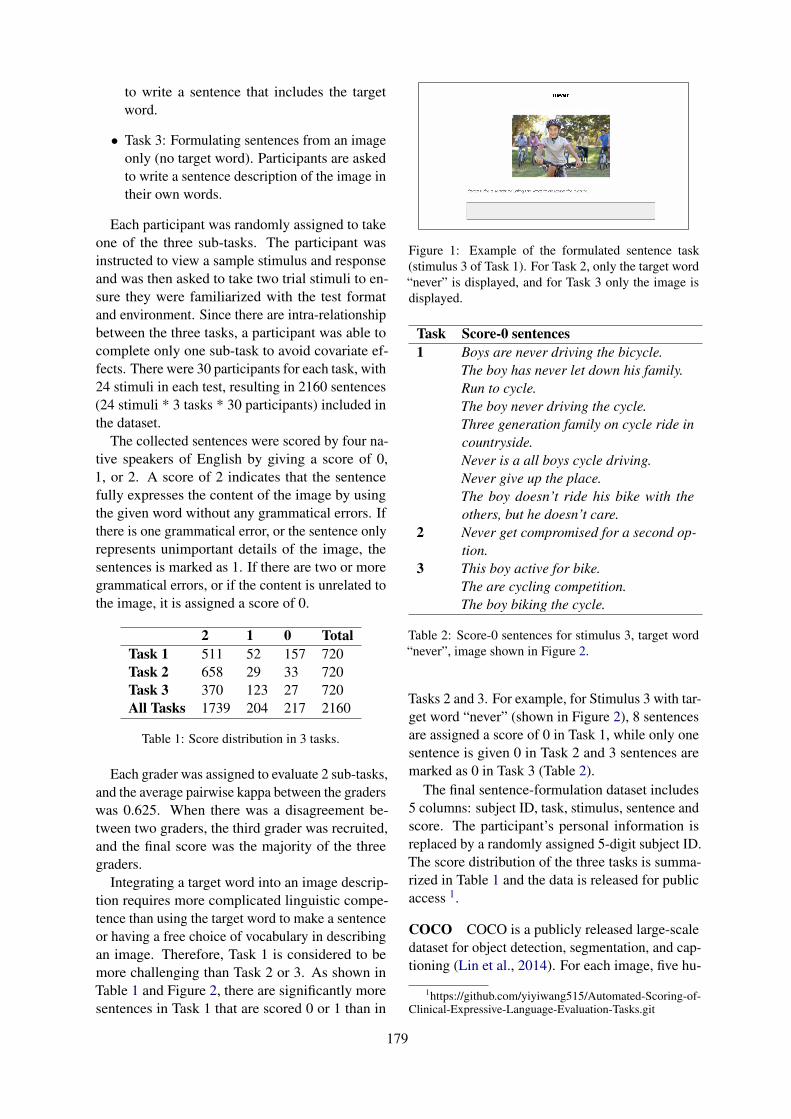
to write a sentence that includes the targetword.

• Task 3: Formulating sentences from an imageonly (no target word). Participants are askedto write a sentence description of the image intheir own words.

Each participant was randomly assigned to takeone of the three sub-tasks. The participant wasinstructed to view a sample stimulus and responseand was then asked to take two trial stimuli to en-sure they were familiarized with the test formatand environment. Since there are intra-relationshipbetween the three tasks, a participant was able tocomplete only one sub-task to avoid covariate ef-fects. There were 30 participants for each task, with24 stimuli in each test, resulting in 2160 sentences(24 stimuli * 3 tasks * 30 participants) included inthe dataset.

The collected sentences were scored by four na-tive speakers of English by giving a score of 0,1, or 2. A score of 2 indicates that the sentencefully expresses the content of the image by usingthe given word without any grammatical errors. Ifthere is one grammatical error, or the sentence onlyrepresents unimportant details of the image, thesentences is marked as 1. If there are two or moregrammatical errors, or if the content is unrelated tothe image, it is assigned a score of 0.

2 1 0 TotalTask 1 511 52 157 720Task 2 658 29 33 720Task 3 370 123 27 720All Tasks 1739 204 217 2160

Table 1: Score distribution in 3 tasks.

Each grader was assigned to evaluate 2 sub-tasks,and the average pairwise kappa between the graderswas 0.625. When there was a disagreement be-tween two graders, the third grader was recruited,and the final score was the majority of the threegraders.

Integrating a target word into an image descrip-tion requires more complicated linguistic compe-tence than using the target word to make a sentenceor having a free choice of vocabulary in describingan image. Therefore, Task 1 is considered to bemore challenging than Task 2 or 3. As shown inTable 1 and Figure 2, there are significantly moresentences in Task 1 that are scored 0 or 1 than in

Figure 1: Example of the formulated sentence task(stimulus 3 of Task 1). For Task 2, only the target word“never” is displayed, and for Task 3 only the image isdisplayed.

Task Score-0 sentences1 Boys are never driving the bicycle.

The boy has never let down his family.Run to cycle.The boy never driving the cycle.Three generation family on cycle ride incountryside.Never is a all boys cycle driving.Never give up the place.The boy doesn’t ride his bike with theothers, but he doesn’t care.

2 Never get compromised for a second op-tion.

3 This boy active for bike.The are cycling competition.The boy biking the cycle.

Table 2: Score-0 sentences for stimulus 3, target word“never”, image shown in Figure 2.

Tasks 2 and 3. For example, for Stimulus 3 with tar-get word “never” (shown in Figure 2), 8 sentencesare assigned a score of 0 in Task 1, while only onesentence is given 0 in Task 2 and 3 sentences aremarked as 0 in Task 3 (Table 2).

The final sentence-formulation dataset includes5 columns: subject ID, task, stimulus, sentence andscore. The participant’s personal information isreplaced by a randomly assigned 5-digit subject ID.The score distribution of the three tasks is summa-rized in Table 1 and the data is released for publicaccess 1.

COCO COCO is a publicly released large-scaledataset for object detection, segmentation, and cap-tioning (Lin et al., 2014). For each image, five hu-

1https://github.com/yiyiwang515/Automated-Scoring-of-Clinical-Expressive-Language-Evaluation-Tasks.git

179

Figure 2: Score distribution for each stimulus in three tasks. Each stimulus is represented by its associated targetword.

man generated captions were collected from AMT.In our work, we use the 2017 train dataset, whichincludes approximately 20k images with 600k cap-tions. Since some of the captions were either emptyor had likely incomplete sentences (fewer than 4words), we exclude those captions resulting in afinal dataset of 33,366 sentences.

The linguistic characteristics of COCO are anal-ogous to our sentence formulation task regardingchoice of lexicon, the use of syntactic structures,and the semantic context of the utterances. Wetherefore use COCO dataset for two purposes: (1)to train a task-specific Word2vec embedding to cap-ture meaning-related and syntactic relationships;and (2) to use as score-2 source input to machinetranslation models that are trained to generate arti-ficial errored (score-1 and score-0) sentences.

FCE First Certificate in English (FCE) (Yan-nakoudakis et al., 2011) is a publicly availabledataset, including 1244 essays written by non-native learners of English with different first lan-guage backgrounds. The FCE exam is used toassess English proficiency of upper-intermediatelevel learners. The essays are annotated by lan-guage assessment experts with types of errors andtheir corresponding corrections in XML. The origi-nal incorrect sentences in the essay and their cor-rected counterparts are extracted by sentence pairs.The sentences containing no errors or with a length(including punctuation) less than 5 are excludedfrom the final dataset used for training our models.

A label is added for each sentence. For all thecorrect sentences, label of 2 is added to mark theappropriateness of the sentence. A sentence withone error is assigned a label of 1, while a sentencewith two or more errors is assigned a label of 0.

The final dataset includes 10799 correct sentences,4810 sentences with one grammatical error, and5989 sentences with two or more errors. The FCEdata serves as training data for two neural machinetranslation models that we use to generate inappro-priate (score-1 and score-0) sentences by takingappropriate (score-2) sentences as input.

4 Experiments

4.1 Sentence EmbeddingThree types of sentence embeddings are used in thiswork: BERT, ELMo and Word2Vec embeddings(Devlin et al. 2018; Peters et al. 2017; Mikolov et al.2013). For context sensitive embeddings BERT andELMo, we use the publicly available pre-trainedmodels. We trained a Word2cvec embedding onthe 600,000 COCO captions.

BERT BERT can integrate information in rawcorpora (BooksCorpus and English Wikipedia)while considering task-specific information con-tained in the target dataset. Kaneko and Komachi(2019) use BERT contextualized representation toachieve state-of-the-art results for word-based GEDtasks. In addition to improving results in the GEDtask, BERT (Devlin et al., 2018) has been shownto be a powerful feature extractor for various othertasks. We employ BERT to generate pre-trainedcontextual representations. BERT pretrained em-beddings have two versions. We use a lighter ver-sion of BERT which yields 768 dimensions forsentence embeddings. The DistilBERT is smallerbut can roughly match the performance of usingthe full BERT (Sanh et al. 2019).

ELMo The ELMo pre-trained model we use istrained on the One Billion Word Benchmark cor-

180

pus. The sentence representation is learned by asequence labeler during training.

The BERT and ELMo models used here aretrained on formal published writings, such as booksand news articles. This is not a perfect domain orstylistic match for the evaluation of responses fromthe formulated sentences task. In order to betterrepresent the linguistic nature of our task, we alsotrain a task-specific Word2vec embedding.

Word2vec We train our Word2vec model usingthe Gensim Python library (Rehurek and Sojka,2010). We use skip-grams to train a word embed-ding model with 300 dimensions, again using theCOCO captions. Words occurring fewer than 5times are filtered out, and the maximum distancebetween a target word and its surrounding contentis set as 4. The number of threads used is 5. Asentence embedding is calculated as the mean ofthe component word embeddings. Since COCOcaptions share similar linguistic features with thesentence formulation tasks, this custom sentenceembedding is expected to capture a richer linguisticrepresentation of the task.

4.2 Data Augmentation

In our FS dataset, score-1 and score-0 sentencesaccount for around 20% of the total number of sen-tences. Since most of the classification algorithmsare sensitive to imbalance in predicting classes,such a dataset can bias the classification modeltowards score-2. In this case, a baseline majority-class classifier, which predicts score-2 for all thesentences, can achieve 0.8 accuracy (Table 1). Theunbalanced nature of this data requires us to syn-thesize additional score-1 and score-0 sentences toincrease the size and variety of training set.

We implement two LSTM machine translationmodels using OpenNMT (Klein et al., 2017). Thescore-2 (corrected) sentences from the FCE datasetare used as the source data, and the score-0 or score-1 (incorrect) sentences serve as the target data. Forexample, for the source-2 to target-1 (2-1) model,we trained the model on sentences pairs from FCEdataset containing only one grammatical error. TheLSTM model is a two-layer bidirectional LSTMwith 500 hidden units with a global attention layer.We set an early stop if the training accuracy scoredropped consistently for 10 epochs. Similarly, wetrain another source-2 to target-0 (2-0) model withthe same settings to generate score-0 sentences.

Having trained a NMT model, we then “trans-

late” 939 score-2 sentences from our formulatedsentences dataset and convert the sentences into thesame number of score-0/1 sentences by using the 2-0 and 2-1 machine translation models respectively.Eight hundred score-2 sentences were excludedfor synthesizing data to reserve for testing. The fi-nal synthesized formulated sentence (SFS) datasetused for training includes 2817 sentences. TheCOCO captions used for training word embeddingare further selected in this process serving as theerror-free input. A large number of COCO captionsare incomplete sentences with heavy noun phrasescontaining a long modifier. We remove such cap-tions in final training set to preserve sentence-levelgrammaticality. For example, “Man in apron stand-ing on front of oven with pans and bakeware” isexcluded, because the root of the dependency pars-ing tree (“man”) is not a verb. A subset of COCOcaptions containing 14017 sentences is selected us-ing parse information extracted using the SpaCylibrary (Honnibal and Montani, 2017). The finalsynthesized COCO (SCOCO) dataset used for train-ing includes 42051 sentences.

4.3 Transfer Learning

Transfer learning is a viable method for buildingNLP models in low-resource scenarios by lever-aging data from other related sources. The twoartificial data datasets, SFS and SCOCO, producedby applying machine translation to the FS datasetand the COCO captions, can provide a good basisfor transfer learning (Section 4.2). We implementa Multilayer Perceptron model (MLP) by usingKeras with tensorflow as the backend2. The MLPmodel has two hidden layers with five nodes ineach layer and uses Relu as the activation function.The output layer has three nodes, corresponding toeach score class with the softmax activation func-tion. The categorical cross-entropy loss function isminimized, and stochastic gradient descent is usedto learn the problem.

The two models are fit for 200 epochs on SFSand SCOCO datasets separately during training.We transfer the weights from the two standalonemodels to learn the initialize the weights for theformulated sentence evaluation tasks. The originalFS data is split proportionally into a training anda test sets in terms of task, stimulus, and scoredistribution. The training set used for tuning themodel includes 1160 sentences. The test set has

2https://github.com/keras-team/keras

181

1000 sentences, and the distribution of scores ispresented in Table 3.

Task 1 Task 2 Task 3 Total2 235 303 262 8001 25 14 61 1000 70 15 15 100Total 330 332 338 1000

Table 3: Score distribution in our formulated sentencestest set.

P R F1 AccBL1 Majority Class 0.80 0.80 0.80 0.80BL2 Target Word 0.82 0.82 0.82 0.82

W2V SFS 0.69 0.59 0.63 0.59SFS-FS 0.74 0.80 0.76 0.80SCOCO 0.67 0.70 0.68 0.70SCOCO-FS 0.72 0.73 0.72 0.73

ELMo SFS 0.78 0.63 0.68 0.63SFS-FS 0.79 0.75 0.77 0.75SCOCO 0.77 0.72 0.74 0.72SCOCO-FS 0.80 0.79 0.79 0.79

BERT SFS 0.80 0.78 0.77 0.78SFS-FS 0.76 0.85 0.81 0.85SCOCO 0.77 0.79 0.78 0.79SCOCO-FS 0.82 0.85 0.83 0.85

Table 4: Sentence evaluation precision, recall, F1 andaccuracy on the full three-task test set.

5 Results

Table 4 presents the results of integrating contex-tual embeddings with and without transfer learning,evaluating all the three sentence formulation taskstogether. The method of using transfer learning in-corporating BERT contextual embeddings achievesthe best performance in most of the cases, exceptfor transferring from SFS with BERT (Figure 3(a)).

The experiments demonstrate a marginal in-crease in precision and substantial improvementin recall for the sentence formulation tasks. Al-though the three tasks all involve making sentences,each task tests different aspects of linguistic knowl-edge. Therefore it is more valuable to investigatethe model performance on individual tasks, pre-sented in Table 5.

On the test sets of Task 1 and Task 2, the bestperforming model is transferred SFS (Task 1: F1 =0.81; Task 2: F1 = 0.92) with BERT. For Task 3, thebest model is trained on the larger SCOCO dataset

(F1 = 0.82) with BERT embeddings. Task 2 andTask 3 have marginal improvement compared withthe baseline. However, Task 1, which is the actualparallel to the CELF-4 Formulated Sentence taskused to diagnose language impairments in children,shows a substantial improvement in performance.The improvement by incorporating BERT embed-ding achieves the best performance in all the threetasks individually.

These experiments demonstrate that transferlearning provides a beneficial addition for eval-uating formulated sentence tasks. The languagerepresentations trained on a large general datasetallow the model to acquire a better representationof linguistic knowledge. Overall, we find that themodel with transfer learning and BERT embed-dings achieves the largest improvement across allthree tasks.

6 Discussion

Transfer learning is generally used in situations inwhich the related task has more training data thanthe problem of interest, and the two tasks share sim-ilarities in structure. In this paper, we train an MLPmodel on two artificial datasets (SFS and SCOCO)and improve the performance of formulated sen-tence scoring task. The two datasets are similarin terms of lexicon variations, syntactic structures,and semantic expressions. They are generated byusing the same machine translation models. Thedifference between these two sets is in the num-ber of sentences contained. Since the number ofcorrect sentences used for generated SCOCO is 14times larger than that used to generated the SFS set,the final data of SCOCO is much larger than SFS.

Although the SCOCO dataset is larger, the bestperformance on both Task 1 and Task 2 is achievedby using transfer learning from in-domain SFS data.One of the similarities between the two tasks is therequirement of applying stimuli words in the gen-erated sentences, whereas the test participants havea free choice of words in Task 3. This require-ment influences the grading of the sentences. If thetarget word is not included in a sentence, no mat-ter how grammatical the sentence is, it is markedwith a label 0 in Task 1 and Task 2. For all thescore-2 sentences in SFS, the target stimuli wordsare included; however this is not always the casein SCOCO. The lack of target word representa-tion information in SCOCO may cause the transferlearning results to be inferior to the SFS model.

182

0.3

0.4

0.5

0.6

0.7

0.8

0.9

Recall

W2V ELMo BERT0.5

0.6

0.7

0.8

0.9

1

Precision

0.3

0.4

0.5

0.6

0.7

0.8

0.9Recall

W2V ELMo BERT0.5

0.6

0.7

0.8

0.9

1

Precision

(a) (b)

without transfer

with transfer

SCOCOSFS

Figure 3: Precision and recall on full dataset using (a) SFS and (b) SCOCO with and without transfer learning.

Task 1 Task 2 Task 3P R F1 Acc P R F1 Acc P R F1 Acc

BL1 Majority Class 0.71 0.71 0.71 0.71 0.91 0.91 0.91 0.91 0.78 0.78 0.78 0.78BL2 Target Word 0.77 0.77 0.77 0.77 0.92 0.92 0.92 0.92 0.78 0.78 0.78 0.78

W2V SFS 0.66 0.63 0.64 0.63 0.84 0.43 0.56 0.43 0.69 0.71 0.70 0.71SFS-FS 0.71 0.75 0.71 0.75 0.84 0.86 0.85 0.86 0.75 0.78 0.73 0.78SCOCO 0.56 0.65 0.59 0.65 0.84 0.69 0.76 0.69 0.69 0.75 0.70 0.75SCOCO-FS 0.70 0.68 0.67 0.68 0.85 0.8 0.82 0.80 0.68 0.69 0.69 0.69

ELMo SFS 0.75 0.68 0.71 0.68 0.89 0.54 0.65 0.54 0.78 0.67 0.71 0.67SFS-FS 0.77 0.76 0.76 0.76 0.88 0.71 0.78 0.71 0.81 0.79 0.79 0.79SCOCO 0.74 0.72 0.73 0.72 0.86 0.69 0.76 0.69 0.79 0.75 0.76 0.75SCOCO-FS 0.80 0.78 0.78 0.78 0.87 0.80 0.83 0.80 0.80 0.80 0.80 0.80

BERT SFS 0.79 0.83 0.81 0.83 0.88 0.73 0.79 0.73 0.83 0.78 0.76 0.78SFS-FS 0.79 0.85 0.81 0.85 0.88 0.92 0.90 0.92 0.68 0.79 0.73 0.79SCOCO 0.78 0.77 0.76 0.77 0.86 0.80 0.83 0.80 0.76 0.79 0.76 0.79SCOCO-FS 0.80 0.82 0.80 0.82 0.89 0.91 0.90 0.91 0.84 0.82 0.80 0.82

Table 5: Sentence evaluation precision, recall, F1 and accuracy on individual tasks.

Embedding representations can capture under-lying meanings and relationships. Different em-beddings trained on distinct datasets may focus onparticular aspects of linguistic and context informa-tion. We use two pre-trained contextual embeddingand a customized embedding trained by using theCOCO captions, which is much more similar tothe data we intend to evaluate. The results showthat BERT generally outperforms others in all tasks.Word2vec embeddings achieve results comparableto those of using BERT and outperform ELMoon Task 2. For the tasks involving sentence-levelsemantic meanings, however, its performance isinferior to the two contextualized representations.

The results we have presented here point the wayto new approaches for automatically scoring tasksused in clinical diagnosis of language impairments,where labeled data for training models is typicallyscarce. In our future work, we will apply these mod-els to data we are currently collecting from childrenwith language disorders, autism spectrum disorder,ADHD, and typical development. Although thereare differences between the populations studied(MTurk workers vs. children) and the modalities inwhich the responses were (written vs. spoken), ourfindings demonstrate the robustness of our meth-ods even in the presence of domain or modalitymismatch.

183

Acknowledgements

We thank Beth Calame, Julie Bird, Kristin Hinton,Christine Yang, and Emily Fabius for their con-tributions to data collection and annotation. Thiswork was supported in part by NIH NIDCD awardsR01DC012033 and R21DC017000. Any opin-ions, findings, conclusions, or recommendationsexpressed in this publication are those of the au-thors and do not necessarily reflect the views of theNIH or NIDCD.

ReferencesJonathan S Barnhoorn, Erwin Haasnoot, Bruno R

Bocanegra, and Henk van Steenbergen. 2015.Qrtengine: An easy solution for running online re-action time experiments using qualtrics. Behaviorresearch methods, 47(4):918–929.

Samuel Bell, Helen Yannakoudakis, and Marek Rei.2019. Context is key: Grammatical error detec-tion with contextual word representations. arXivpreprint arXiv:1906.06593.

Chris Brockett, William B Dolan, and Michael Gamon.2006. Correcting esl errors using phrasal smt tech-niques. In Proceedings of the 21st InternationalConference on Computational Linguistics and the44th annual meeting of the Association for Compu-tational Linguistics, pages 249–256. Association forComputational Linguistics.

Gina Conti-Ramsden, Zoe Simkin, and Nicola Botting.2006. The prevalence of autistic spectrum disordersin adolescents with a history of specific language im-pairment (sli). Journal of Child Psychology and Psy-chiatry, 47(6):621–628.

Jacob Devlin, Ming-Wei Chang, Kenton Lee, andKristina Toutanova. 2018. Bert: Pre-training of deepbidirectional transformers for language understand-ing. arXiv preprint arXiv:1810.04805.

Angela Grimm and Petra Schulz. 2014. Specific lan-guage impairment and early second language acqui-sition: the risk of over-and underdiagnosis. ChildIndicators Research, 7(4):821–841.

Matthew Honnibal and Ines Montani. 2017. spaCy 2:Natural language understanding with Bloom embed-dings, convolutional neural networks and incremen-tal parsing. To appear.

Masahiro Kaneko and Mamoru Komachi. 2019. Multi-head multi-layer attention to deep language repre-sentations for grammatical error detection. arXivpreprint arXiv:1904.07334.

Sudhanshu Kasewa, Pontus Stenetorp, and SebastianRiedel. 2018. Wronging a right: Generating bet-ter errors to improve grammatical error detection.

In Proceedings of the 2018 Conference on Em-pirical Methods in Natural Language Processing,pages 4977–4983, Brussels, Belgium. Associationfor Computational Linguistics.

Guillaume Klein, Yoon Kim, Yuntian Deng, Jean Senel-lart, and Alexander Rush. 2017. OpenNMT: Open-source toolkit for neural machine translation. InProceedings of ACL 2017, System Demonstrations,pages 67–72, Vancouver, Canada. Association forComputational Linguistics.

Tsung-Yi Lin, Michael Maire, Serge Belongie, JamesHays, Pietro Perona, Deva Ramanan, Piotr Dollar,and C Lawrence Zitnick. 2014. Microsoft coco:Common objects in context. In European confer-ence on computer vision, pages 740–755. Springer.

Tomas Mikolov, Kai Chen, Greg Corrado, and Jef-frey Dean. 2013. Efficient estimation of wordrepresentations in vector space. arXiv preprintarXiv:1301.3781.

Courtenay Frazier Norbury, Debbie Gooch, CharlotteWray, Gillian Baird, Tony Charman, Emily Si-monoff, George Vamvakas, and Andrew Pickles.2016. The impact of nonverbal ability on prevalenceand clinical presentation of language disorder: ev-idence from a population study. Journal of ChildPsychology and Psychiatry, 57(11):1247–1257.

Matthew Peters, Waleed Ammar, Chandra Bhagavat-ula, and Russell Power. 2017. Semi-supervisedsequence tagging with bidirectional language mod-els. In Proceedings of the 55th Annual Meeting ofthe Association for Computational Linguistics (Vol-ume 1: Long Papers), pages 1756–1765, Vancouver,Canada. Association for Computational Linguistics.

Radim Rehurek and Petr Sojka. 2010. Software frame-work for topic modelling with large corpora. In InProceedings of the LREC 2010 Workshop on NewChallenges for NLP Frameworks. Citeseer.

Marek Rei. 2017. Semi-supervised multitask learn-ing for sequence labeling. In Proceedings of the55th Annual Meeting of the Association for Com-putational Linguistics (Volume 1: Long Papers),pages 2121–2130, Vancouver, Canada. Associationfor Computational Linguistics.

Sara Rosenbaum and Patti Simon. 2016. Speech andLanguage Disorders in Children: Implications forthe Social Security Administration’s SupplementalSecurity Income Program. ERIC.

Alla Rozovskaya and Dan Roth. 2010. Generating con-fusion sets for context-sensitive error correction. InProceedings of the 2010 conference on empiricalmethods in natural language processing, pages 961–970. Association for Computational Linguistics.

Victor Sanh, Lysandre Debut, Julien Chaumond, andThomas Wolf. 2019. Distilbert, a distilled versionof bert: smaller, faster, cheaper and lighter. arXivpreprint arXiv:1910.01108.

184

Eleanor Semel, Elizabeth Wiig, and Wayne Secord.2003. Clinical Evaluation of Language Fundamen-tals–Fouth Edition (CELF-4). NCS Pearson, Bloom-ington, MN.

Helen Yannakoudakis, Ted Briscoe, and Ben Medlock.2011. A new dataset and method for automaticallygrading ESOL texts. In Proceedings of the 49th An-nual Meeting of the Association for ComputationalLinguistics: Human Language Technologies, pages180–189, Portland, Oregon, USA. Association forComputational Linguistics.

185

Proceedings of the 15th Workshop on Innovative Use of NLP for Building Educational Applications, pages 186–192July 10, 2020. c©2020 Association for Computational Linguistics

Context-based Automated Scoring of Complex Mathematical Responses

Aoife Cahill, James H. Fife, Brian Riordan, Avijit Vajpayee, and Dmytro Galochkinacahill@ets.org, ejreed215@verizon.net,{briordan, avajpayee, dgalochkin} @ets.org

ETS, Princeton, NJ 08541, USA

Abstract

The tasks of automatically scoring either tex-tual or algebraic responses to mathematicalquestions have both been well-studied, albeitseparately. In this paper we propose a methodfor automatically scoring responses that con-tain both text and algebraic expressions. Ourmethod not only achieves high agreement withhuman raters, but also links explicitly to thescoring rubric – essentially providing explain-able models and a way to potentially providefeedback to students in the future.

1 Introduction

In this paper we present work on automaticallyscoring student responses to constructed-responsemathematics items where the response should con-tain both text and mathematical equations or ex-pressions. Existing work on automated scoring ofmathematics items has largely focused on itemswhere either only text is required (c.f. related workon automated short-answer-scoring (Galhardi andBrancher, 2018; Burrows et al., 2015)) or only anexpression or equation is required (Drijvers, 2018;Fife, 2017; Sangwin, 2004). This is the first work,to our knowledge, that attempts to automaticallyscore responses that contain both.

Items that elicit such responses could be algebra,trigonometry, or calculus items that ask the studentto solve a problem and/or provide an argument.Items at levels much below algebra most likelywould not require the student to include an equation– at least one that requires an equation editor forproper entry – in the text, and items at a higherlevel might require the student to include abstractmathematical expressions that would themselvespresent automated scoring difficulties. These kindsof items are quite common on paper-and-pencilalgebra exams. However, they are less commonon computer-delivered exams, primarily because

the technology of calling up an equation editor toinsert equations in text is new and not generallyused.

The challenge with automatically scoring thesekinds of responses, in a construct-valid way, isthat the system needs to be able to interpret thecorrectness of the equations and expressions in thecontext of the surrounding text.

Our goal is not just to achieve accurate scoringbut to also have explainable models. Explainablemodels have a number of advantages including (i)giving users evidence that the models are fair andunbiased; (ii) the ability to leverage the modelsfor feedback; and (iii) compliance with new laws,e.g. the General Data Protection Regulation (EU)2016/679 (GDPR) which requires transparency andaccountability of any form of automated process-ing of personal data. In this paper we present anapproach that not only achieves high agreementwith human raters, but also links explicitly to thescoring rubric – essentially providing explainablemodels and a way to potentially provide feedbackto students in the future.

2 Data

In this paper we use data from 3 pilot-study itemsthat elicited responses containing both textual ex-planations as well as equations and expressions.An example item is given in Figure 1, and a sampleresponse (awarded 2 points on a 0-3 point scale) isgiven in Figure 2.1 The pilot was administered aspart of a larger project in four high schools locatedin various regions of the United States. The itemsassumed one year of algebra and involved writingsolutions to algebra problems, similar to what a stu-dent would be expected to write on a paper-basedclassroom test. Responses were collected digitally;

1This item corresponds to Item 2 in our dataset. The scor-ing rubric is given in Appendix A.1.

186

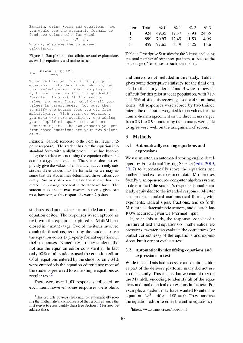
Explain, using words and equations, howyou would use the quadratic formula tofind two values of x for which

195 = −2x2 + 40x.You may also use the on-screencalculator.

Figure 1: Sample item that elicits textual explanationsas well as equations and mathematics.

x =−40+

√402−4(−2)(−195)

2(−2)

To solve this you must first put yourequation in standard form, which givesyou y=-2x+40x-195. You then plug youra, b, and c values into the quadraticformula. To start finding your xvalue, you must first multiply all yourvalues in parentheses. You must thensimplify the square root you get frommultiplying. With your new equation,you make two more equations, one addingyour simplified square root and onesubtracting it. The two answers you getfrom those equations are your two valuesof x.

Figure 2: Sample response to the item in Figure 1 (2-point response). The student has put the equation intostandard form with a slight error. −2x2 has become−2x; the student was not using the equation editor andcould not type the exponent. The student does not ex-plicitly give the values of a, b, and c, but correctly sub-stitutes these values into the formula, so we may as-sume that the student has determined these values cor-rectly. We may also assume that the student has cor-rected the missing exponent in the standard form. Thestudent talks about “two answers” but only gives oneroot, however, so this response is worth 2 points.

students used an interface that included an optionalequation editor. The responses were captured astext, with the equations captured as MathML en-closed in <math> tags. Two of the items involvedquadratic functions, requiring the student to usethe equation editor to properly format equations intheir responses. Nonetheless, many students didnot use the equation editor consistently. In factonly 60% of all students used the equation editor.Of all equations entered by the students, only 34%were entered via the equation editor since most ofthe students preferred to write simple equations asregular text.2

There were over 1,000 responses collected foreach item, however some responses were blank

2This presents obvious challenges for automatically scor-ing the mathematical components of the responses, since thefirst step is to even identify them (see Section 3.2 for how weaddress this).

Item Total % 0 % 1 % 2 % 31 924 49.35 19.37 6.93 24.352 889 70.97 12.49 11.59 4.953 859 77.65 3.49 3.26 15.6

Table 1: Descriptive Statistics for the 3 items, includingthe total number of responses per item, as well as thepercentage of responses at each score point.

and therefore not included in this study. Table 1gives some descriptive statistics for the final dataused in this study. Items 2 and 3 were somewhatdifficult for this pilot student population, with 71%and 78% of students receiving a score of 0 for thoseitems. All responses were scored by two trainedraters; the quadratic-weighted kappa values for thehuman-human agreement on the three items rangedfrom 0.91 to 0.95, indicating that humans were ableto agree very well on the assignment of scores.

3 Methods

3.1 Automatically scoring equations andexpressions

We use m-rater, an automated scoring engine devel-oped by Educational Testing Service (Fife, 2013,2017) to automatically score the equations andmathematical expressions in our data. M-rater usesSymPy3, an open-source computer algebra system,to determine if the student’s response is mathemat-ically equivalent to the intended response. M-ratercan process standard mathematical format, withexponents, radical signs, fractions, and so forth.M-rater is a deterministic system, and as such has100% accuracy, given well-formed input.

If, as in this study, the responses consist of amixture of text and equations or mathematical ex-pressions, m-rater can evaluate the correctness (orpartial correctness) of the equations and expres-sions, but it cannot evaluate text.

3.2 Automatically identifying equations andexpressions in text

While the students had access to an equation editoras part of the delivery platform, many did not useit consistently. This means that we cannot rely onthe MathML encoding to identify all of the equa-tions and mathematical expressions in the text. Forexample, a student may have wanted to enter theequation: 2x2 − 40x + 195 = 0. They may usethe equation editor to enter the entire equation, or

3https://www.sympy.org/en/index.html

187

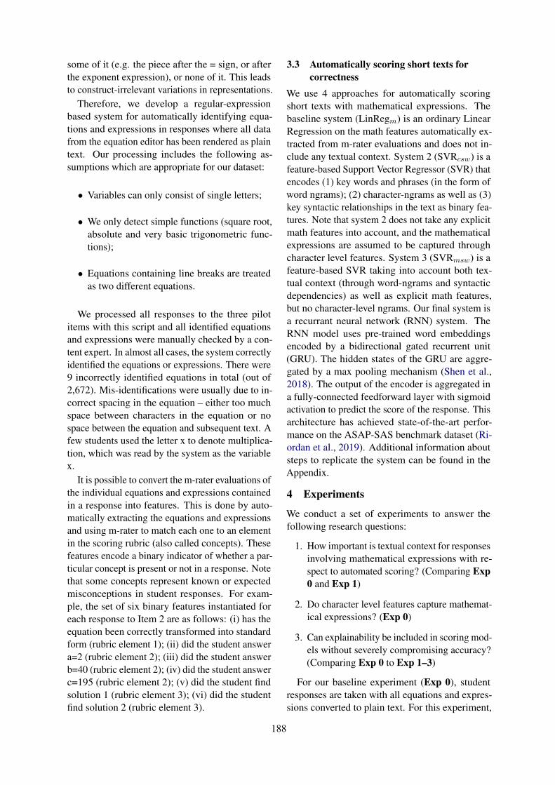
some of it (e.g. the piece after the = sign, or afterthe exponent expression), or none of it. This leadsto construct-irrelevant variations in representations.

Therefore, we develop a regular-expressionbased system for automatically identifying equa-tions and expressions in responses where all datafrom the equation editor has been rendered as plaintext. Our processing includes the following as-sumptions which are appropriate for our dataset:

• Variables can only consist of single letters;

• We only detect simple functions (square root,absolute and very basic trigonometric func-tions);

• Equations containing line breaks are treatedas two different equations.

We processed all responses to the three pilotitems with this script and all identified equationsand expressions were manually checked by a con-tent expert. In almost all cases, the system correctlyidentified the equations or expressions. There were9 incorrectly identified equations in total (out of2,672). Mis-identifications were usually due to in-correct spacing in the equation – either too muchspace between characters in the equation or nospace between the equation and subsequent text. Afew students used the letter x to denote multiplica-tion, which was read by the system as the variablex.

It is possible to convert the m-rater evaluations ofthe individual equations and expressions containedin a response into features. This is done by auto-matically extracting the equations and expressionsand using m-rater to match each one to an elementin the scoring rubric (also called concepts). Thesefeatures encode a binary indicator of whether a par-ticular concept is present or not in a response. Notethat some concepts represent known or expectedmisconceptions in student responses. For exam-ple, the set of six binary features instantiated foreach response to Item 2 are as follows: (i) has theequation been correctly transformed into standardform (rubric element 1); (ii) did the student answera=2 (rubric element 2); (iii) did the student answerb=40 (rubric element 2); (iv) did the student answerc=195 (rubric element 2); (v) did the student findsolution 1 (rubric element 3); (vi) did the studentfind solution 2 (rubric element 3).

3.3 Automatically scoring short texts forcorrectness

We use 4 approaches for automatically scoringshort texts with mathematical expressions. Thebaseline system (LinRegm) is an ordinary LinearRegression on the math features automatically ex-tracted from m-rater evaluations and does not in-clude any textual context. System 2 (SVRcsw) is afeature-based Support Vector Regressor (SVR) thatencodes (1) key words and phrases (in the form ofword ngrams); (2) character-ngrams as well as (3)key syntactic relationships in the text as binary fea-tures. Note that system 2 does not take any explicitmath features into account, and the mathematicalexpressions are assumed to be captured throughcharacter level features. System 3 (SVRmsw) is afeature-based SVR taking into account both tex-tual context (through word-ngrams and syntacticdependencies) as well as explicit math features,but no character-level ngrams. Our final system isa recurrant neural network (RNN) system. TheRNN model uses pre-trained word embeddingsencoded by a bidirectional gated recurrent unit(GRU). The hidden states of the GRU are aggre-gated by a max pooling mechanism (Shen et al.,2018). The output of the encoder is aggregated ina fully-connected feedforward layer with sigmoidactivation to predict the score of the response. Thisarchitecture has achieved state-of-the-art perfor-mance on the ASAP-SAS benchmark dataset (Ri-ordan et al., 2019). Additional information aboutsteps to replicate the system can be found in theAppendix.

4 Experiments

We conduct a set of experiments to answer thefollowing research questions:

1. How important is textual context for responsesinvolving mathematical expressions with re-spect to automated scoring? (Comparing Exp0 and Exp 1)

2. Do character level features capture mathemat-ical expressions? (Exp 0)

3. Can explainability be included in scoring mod-els without severely compromising accuracy?(Comparing Exp 0 to Exp 1–3)

For our baseline experiment (Exp 0), studentresponses are taken with all equations and expres-sions converted to plain text. For this experiment,

188

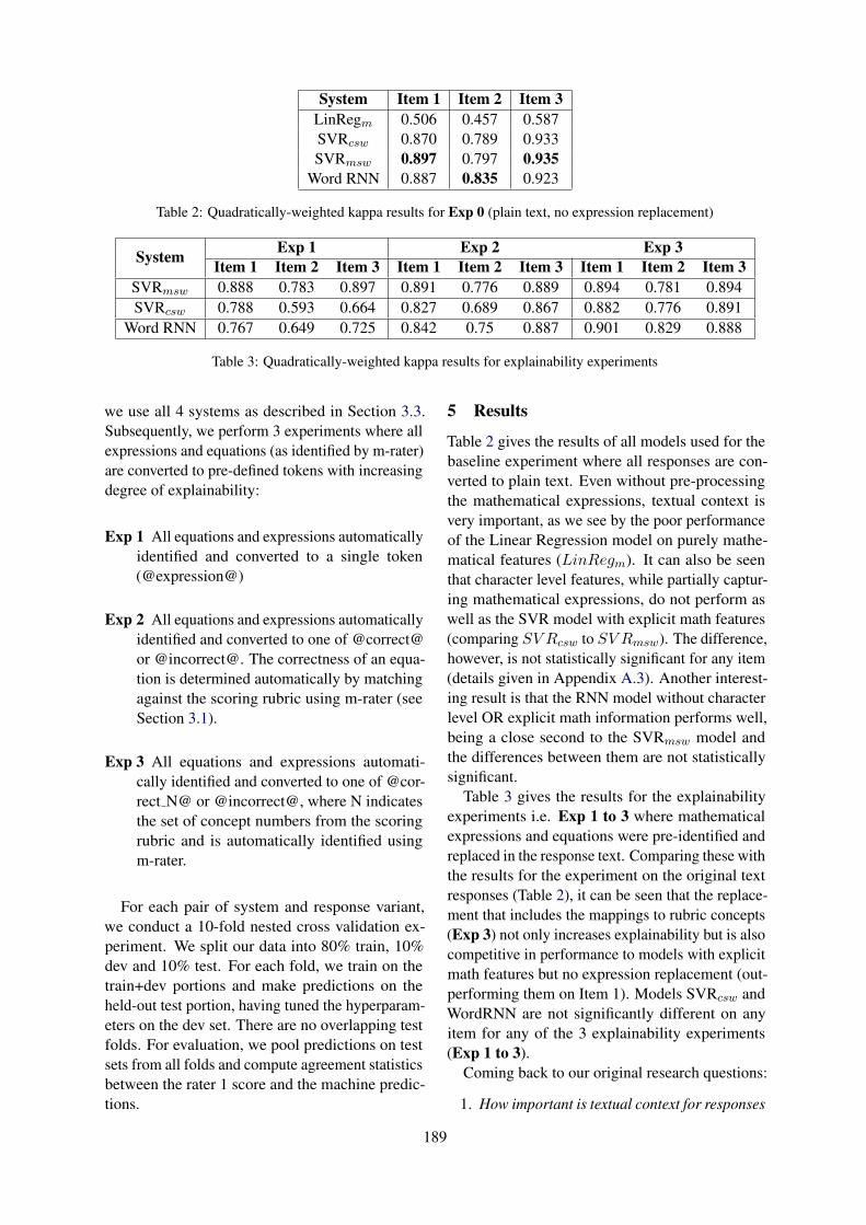
System Item 1 Item 2 Item 3LinRegm 0.506 0.457 0.587SVRcsw 0.870 0.789 0.933SVRmsw 0.897 0.797 0.935

Word RNN 0.887 0.835 0.923

Table 2: Quadratically-weighted kappa results for Exp 0 (plain text, no expression replacement)

System Exp 1 Exp 2 Exp 3Item 1 Item 2 Item 3 Item 1 Item 2 Item 3 Item 1 Item 2 Item 3

SVRmsw 0.888 0.783 0.897 0.891 0.776 0.889 0.894 0.781 0.894SVRcsw 0.788 0.593 0.664 0.827 0.689 0.867 0.882 0.776 0.891

Word RNN 0.767 0.649 0.725 0.842 0.75 0.887 0.901 0.829 0.888

Table 3: Quadratically-weighted kappa results for explainability experiments

we use all 4 systems as described in Section 3.3.Subsequently, we perform 3 experiments where allexpressions and equations (as identified by m-rater)are converted to pre-defined tokens with increasingdegree of explainability:

Exp 1 All equations and expressions automaticallyidentified and converted to a single token(@expression@)

Exp 2 All equations and expressions automaticallyidentified and converted to one of @correct@or @incorrect@. The correctness of an equa-tion is determined automatically by matchingagainst the scoring rubric using m-rater (seeSection 3.1).

Exp 3 All equations and expressions automati-cally identified and converted to one of @cor-rect N@ or @incorrect@, where N indicatesthe set of concept numbers from the scoringrubric and is automatically identified usingm-rater.

For each pair of system and response variant,we conduct a 10-fold nested cross validation ex-periment. We split our data into 80% train, 10%dev and 10% test. For each fold, we train on thetrain+dev portions and make predictions on theheld-out test portion, having tuned the hyperparam-eters on the dev set. There are no overlapping testfolds. For evaluation, we pool predictions on testsets from all folds and compute agreement statisticsbetween the rater 1 score and the machine predic-tions.

5 Results

Table 2 gives the results of all models used for thebaseline experiment where all responses are con-verted to plain text. Even without pre-processingthe mathematical expressions, textual context isvery important, as we see by the poor performanceof the Linear Regression model on purely mathe-matical features (LinRegm). It can also be seenthat character level features, while partially captur-ing mathematical expressions, do not perform aswell as the SVR model with explicit math features(comparing SV Rcsw to SV Rmsw). The difference,however, is not statistically significant for any item(details given in Appendix A.3). Another interest-ing result is that the RNN model without characterlevel OR explicit math information performs well,being a close second to the SVRmsw model andthe differences between them are not statisticallysignificant.

Table 3 gives the results for the explainabilityexperiments i.e. Exp 1 to 3 where mathematicalexpressions and equations were pre-identified andreplaced in the response text. Comparing these withthe results for the experiment on the original textresponses (Table 2), it can be seen that the replace-ment that includes the mappings to rubric concepts(Exp 3) not only increases explainability but is alsocompetitive in performance to models with explicitmath features but no expression replacement (out-performing them on Item 1). Models SVRcsw andWordRNN are not significantly different on anyitem for any of the 3 explainability experiments(Exp 1 to 3).

Coming back to our original research questions:

1. How important is textual context for responses

189

involving mathematical expressions with re-spect to automated scoring?Context is important for automatically scor-ing responses that integrate text and algebraicinformation. Evaluating the mathematical ex-pressions alone does not perform well (Exp0). Additionally, Exp 1 has no context for themathematical expressions, and we see lowerresults for the system that still includes math-ematical information as independent features,but out of context (SV Rmsw), compared tosystems that encode the mathematical infor-mation in some way in context.

2. Do character level features capture mathemat-ical expressions?Character level features certainly do capturea large portion of mathematical expressions.We see that in the Exp 0 results, where there isno interpretation of the mathematical expres-sions, that systems perform almost as well asthe systems that do explicit interpretation.

3. Can explainability be included in scoring mod-els without severely compromising accuracy?

Yes, we can include model interpretabilitywithout compromising scoring accuracy. Thedifferences between the best models from Exp0 and Exp3 ranged from -0.004 to +0.041).By explicitly linking aspects of the rubric toeach response, we yield interpretable modelsthat perform comparably to systems withoutthis interpretative layer. Although the over-all results are lower, they are not statisticallysignificantly lower.

6 Conclusion

To summarize, this work presented a hybrid scoringmodel using a deterministic system for evaluatingthe correctness (or partial correctness) of mathe-matical equations, in combination with text-basedautomated scoring systems for evaluating the appro-priateness of the textual explanation of a response.

We contribute the following:

1. Systems that produce extremely high agree-ment between an automated system and hu-man raters for the task of automatically scor-ing items that elicit both textual and algebraiccomponents

2. A method for linking rubric information tothe automated scoring system, resulting inan more interpretable model than one basedpurely on the raw response

Acknowledgments

We would like to thank the anonymous reviewersfor their valuable comments and suggestions. Wewould also like to thank Michael Flor, SwapnaSomasundaran and Beata Beigman-Klebanov fortheir helpful comments.

ReferencesAshutosh Adhikari, Achyudh Ram, Raphael Tang, and

Jimmy Lin. 2019. Rethinking Complex Neural Net-work Architectures for Document Classification. InProceedings of the 2019 Conference of the NorthAmerican Chapter of the Association for Compu-tational Linguistics: Human Language Technolo-gies, Volume 1 (Long and Short Papers), pages4046–4051, Minneapolis, Minnesota. Associationfor Computational Linguistics.

Steven Burrows, Iryna Gurevych, and Benno Stein.2015. The eras and trends of automatic short answergrading. International Journal of Artificial Intelli-gence in Education, 25(1):60–117.

Janez Demsar. 2006. Statistical comparisons of clas-sifiers over multiple data sets. Journal of Machinelearning research, 7(Jan):1–30.

Paul Drijvers. 2018. Digital assessment of mathemat-ics: Opportunities, issues and criteria. Mesure etevaluation en education, 41(1):41–66.

James H Fife. 2013. Automated scoring of mathemat-ics tasks in the Common Core era: Enhancements tom-rater in support of CBALTM, mathematics and theCommon Core assessments . ETS Research ReportSeries, 2013(2):i–35.

James H Fife. 2017. The m-rater Engine: Introductionto the Automated Scoring of Mathematics Items. Re-search Memorandum, ETS RM-17-02, pages 10–24.

Lucas Busatta Galhardi and Jacques Duılio Brancher.2018. Machine learning approach for automaticshort answer grading: A systematic review. InIbero-American Conference on Artificial Intelli-gence, pages 380–391. Springer.

Peter Nemenyi. 1963. Distribution-free multiple com-parisons,(mimeographed).

Brian Riordan, Michael Flor, and Robert Pugh. 2019.How to account for mispellings: Quantifying thebenefit of character representations in neural contentscoring models. In Proceedings of the 14th Work-shop on Innovative Use of NLP for Building Educa-tional Applications (BEA).

190

Chris Sangwin. 2004. Assessing mathematics auto-matically using computer algebra and the internet.Teaching Mathematics and Its Applications: An In-ternational Journal of the IMA, 23(1):1–14.

Dinghan Shen, Guoyin Wang, Wenlin Wang, Mar-tin Renqiang Min, Qinliang Su, Yizhe Zhang, Chun-yuan Li, Ricardo Henao, and Lawrence Carin.2018. Baseline needs more love: On simpleword-embedding-based models and associated pool-ing mechanisms. In Proceedings of the 56th An-nual Meeting of the Association for ComputationalLinguistics (Volume 1: Long Papers), pages 440–450, Melbourne, Australia. Association for Compu-tational Linguistics.

Sudhir Varma and Richard Simon. 2006. Bias in errorestimation when using cross-validation for model se-lection. BMC bioinformatics, 7(1):91.

A Appendices

A.1 Scoring Rubric for Item 2• 1 pt. for writing the equation as 2x2 − 40x+195 = 0 or −2x2 + 40x − 195 = 0. It’sacceptable to just write the expression 2x2 −40x+195 = 0 or−2x2+40x−195 = 0. It’salso acceptable to say something like “Move195 to the other side of the equation” if theyfind the correct values for a, b, and c (withcorrect signs).

• 1 pt. for determining the values of a, b, andc. a = 2, b = 40, c = 195 OR a = 2,b = 40, c = 195 0 pts. if they mix the valuesup (e.g., a = 2, b = 40, c = 195). 1 pt. ifthey implicitly complete this step by correctlysubstituting the correct values for a, b, and cinto the quadratic formula in the next step.

• 1 pt. for substituting the values of a, b,and c into the quadratic formula and ob-taining two solutions. Students do notneed to simplify the answers. Studentscan write any equivalent expressions forthe two values of x, including x =40+√402−4∗2∗1952∗2 and x = 40−

√402−4∗2∗1952∗2

OR x = −40+√402−4∗−2∗−1952∗−2 and x =

−40−√402−4∗−2∗−1952∗−2 . It’s also acceptable

for students to write x = 40±√402−4∗2∗1952∗2

to mean both solutions. Or students may writethat the two values of x are x = 11.5811. . . andx = 8.4188. . . , correct to at least one decimalplace, provided they arrive at these numbersthrough the quadratic formula and not by solv-ing the equation numerically.

• Max 2/3 for finding one correct solution.

• Max 2/3 for writing the two correct solutionswith no explanation of where the values of a,b, and c come from.

• 1/3 if the student provides an outline of thesolution without actually carrying out any ofthe steps.

A.2 Additional information for training theRNN model

The text is preprocessed with the spaCy tokenizerwith some minor postprocessing to correct tok-enization mistakes on noisy data. On conversion totensors, responses are padded to the same lengthin a batch; these padding tokens are masked outduring model training. Prior to training, responsesare scaled to [0, 1] to form the input to the net-works. The scaled scores are converted back totheir original range for evaluation. Word tokensare embedded with GloVe 100 dimension vectorsand fine-tuned during training. Word tokens notin the embeddings vocabulary are each assigneda unique randomly initialized vector. The GRUswere 1 layer with a hidden state of size 250. Thenetwork was trained with mean squared error loss.We optimized the network with RMSProp withhyperparameters set as follows: learning rate of0.001, batch size of 32, and gradient clipping setto 10.0. An exponential moving average of themodel’s weights is used during training (Adhikariet al., 2019).

A.3 Additional details on significance testingof results

Although nested cross-validation gives a fairly un-biased estimate of true error as shown by Varmaand Simon (2006), we performed statistical signif-icance testing to pair-wise compare 4 models forExp 0: no expression replacement and 2 mod-els for Exp 3: expressions replaced with incor-rect/correct along with concept numbers.

Friedman’s test as suggested by Demsar (2006)is run to compare 6 models (corresponding totreatments) across multiple repeated measures (10folds) for each item individually. Note that such asetup of comparing multiple models across 10 foldson a dataset has to be regarded as non-independentdata as even though the test folds will be distinct,the training data for each fold may partially over-lap. Hence Friedman’s test is appropriate here to

191

0 SVRcsw 0 SVRmsw 0 WordRNN 3 SVRcsw 3 WordRNN0 LinRegm 1 / 3 2 / 3 3 / 3 1 / 3 2 / 30 SVRcsw - 0 0 0 00 SVRmsw - 0 0 00 WordRNN - 1 / 3 03 SVRcsw - 0

Table 4: Pair-wise Comparisons of Models with fraction of datasets with significant difference between models

test whether any pair of models are statisticallydifferent.

Following Friedman’s test, we do pair-wisepost-hoc testing through Nemenyi’s test (Nemenyi,1963). Note that this testing is per-item and wereport the fraction of times the differences weresignificant in table 4.

192

Proceedings of the 15th Workshop on Innovative Use of NLP for Building Educational Applications, pages 193–197July 10, 2020. c©2020 Association for Computational Linguistics

Predicting the Difficulty and Response Time of Multiple Choice QuestionsUsing Transfer Learning

Kang Xue1 Victoria Yaneva2 Christopher Runyon2 Peter Baldwin2

1Department of Educational Psychology, University of Georgia, Athens, USAKangXue@uga.edu

2National Board of Medical Examiners, Philadelphia, USA{vyaneva, crunyon, pbaldwin}@nbme.org

AbstractThis paper reports on whether transfer learn-ing can improve the prediction of the difficultyand response time parameters for ≈ 18,000multiple-choice questions from a high-stakesmedical exam. The type of the signal that bestpredicts difficulty and response time is also ex-plored, both in terms of representation abstrac-tion and item component used as input (e.g.,whole item, answer options only, etc.). Theresults indicate that, for our sample, transferlearning can improve the prediction of item dif-ficulty when response time is used as an auxil-iary task but not the other way around. In ad-dition, difficulty was best predicted using sig-nal from the item stem (the description of theclinical case), while all parts of the item wereimportant for predicting the response time.

1 Introduction

The questions on standardized exams need to meetcertain criteria for the exam to be considered fairand valid. For example, it is often desirable to col-lect measurement information across a range of ex-aminee proficiencies but this requires that questiondifficulties span a similar range. Another consider-ation is the time required to answer each question:allocating too little time makes the exam speededwhereas allocating too much time makes it ineffi-cient. Typically, difficulty and response time mea-sures are needed before new questions can be usedfor scoring. Currently, these measures are obtainedby presenting new questions alongside scored itemson real exams; however, this process is time con-suming and costly. To address this challenge, thereis an emerging interest in predicting item param-eters based on item text (Section 2). The goal ofthis application is to filter out items that shouldnot be embedded in live exams—even as unscoreditems—because of their low probability of havingthe desired characteristics.

In practice, there may be situations where dataare available for one item parameter but not for

another. For example, when a pen-and-paper test isbeing migrated to a computer-based test, responsetime measures to individual questions will not beamong the historical pen-and-paper data whereasitem difficulty measures will be. In this scenario,the only available response-time data would bethose collected from the small sample of exami-nees who first piloted the computer-based test. Yet,since item characteristics like response time anddifficulty are often related (e.g., more difficult itemsmay require longer to solve), it is conceivable thatinformation stored while learning to predict oneparameter then could be used to improve the predic-tion of another. In this paper, we explore whetherapproaches from the field of transfer learning maybe useful for improving item parameter modeling.

We hypothesize that transfer learning (TL) canimprove the prediction of difficulty and responsetime parameters for a set of ≈18,000 multiple-choice questions (MCQs) from the United StatesMedical Licensing Examination (USMLE R©). Wepresent two sets of experiments, where learningto predict one parameter is used as an auxiliarytask for the prediction of the other and vice versa.In addition to our interest in parameter modeling,we investigate the type of signal that best predictsdifficulty and response time, which is done bothin terms of exploring potential differences in thelevel of representation abstraction required to pre-dict the two variables and in terms of the part ofthe item that contains information most relevant toeach parameter. This is accomplished by extractingtwo levels of item representations, embeddings andencodings, from various parts of the MCQ (answeroptions only, question only, whole item). Predic-tions are compared to i) the predictions for eachparameter without the use of an auxiliary task, andii) a ZeroR baseline. The results from the trans-fer learning experiments show the usefulness andlimitations of this approach for modeling item pa-rameters with a view to practical scenarios where

193

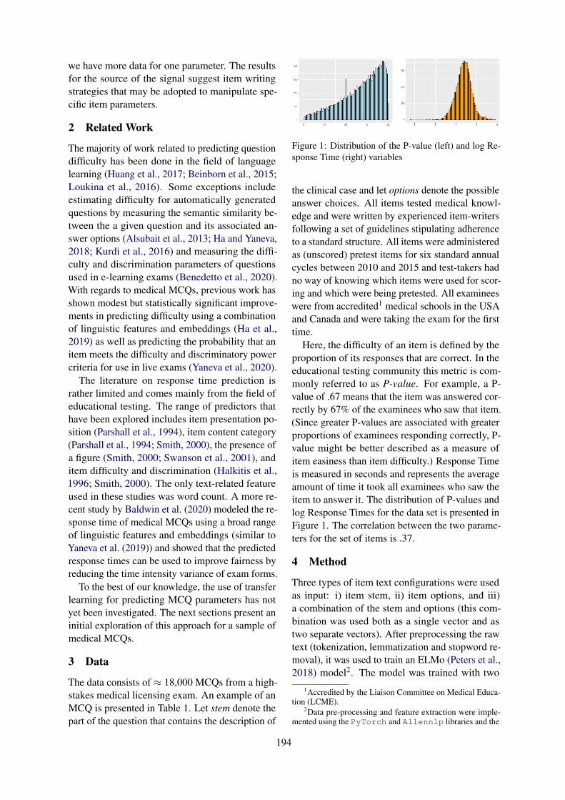
we have more data for one parameter. The resultsfor the source of the signal suggest item writingstrategies that may be adopted to manipulate spe-cific item parameters.

2 Related Work

The majority of work related to predicting questiondifficulty has been done in the field of languagelearning (Huang et al., 2017; Beinborn et al., 2015;Loukina et al., 2016). Some exceptions includeestimating difficulty for automatically generatedquestions by measuring the semantic similarity be-tween the a given question and its associated an-swer options (Alsubait et al., 2013; Ha and Yaneva,2018; Kurdi et al., 2016) and measuring the diffi-culty and discrimination parameters of questionsused in e-learning exams (Benedetto et al., 2020).With regards to medical MCQs, previous work hasshown modest but statistically significant improve-ments in predicting difficulty using a combinationof linguistic features and embeddings (Ha et al.,2019) as well as predicting the probability that anitem meets the difficulty and discriminatory powercriteria for use in live exams (Yaneva et al., 2020).

The literature on response time prediction israther limited and comes mainly from the field ofeducational testing. The range of predictors thathave been explored includes item presentation po-sition (Parshall et al., 1994), item content category(Parshall et al., 1994; Smith, 2000), the presence ofa figure (Smith, 2000; Swanson et al., 2001), anditem difficulty and discrimination (Halkitis et al.,1996; Smith, 2000). The only text-related featureused in these studies was word count. A more re-cent study by Baldwin et al. (2020) modeled the re-sponse time of medical MCQs using a broad rangeof linguistic features and embeddings (similar toYaneva et al. (2019)) and showed that the predictedresponse times can be used to improve fairness byreducing the time intensity variance of exam forms.

To the best of our knowledge, the use of transferlearning for predicting MCQ parameters has notyet been investigated. The next sections present aninitial exploration of this approach for a sample ofmedical MCQs.

3 Data

The data consists of ≈ 18,000 MCQs from a high-stakes medical licensing exam. An example of anMCQ is presented in Table 1. Let stem denote thepart of the question that contains the description of

Figure 1: Distribution of the P-value (left) and log Re-sponse Time (right) variables

the clinical case and let options denote the possibleanswer choices. All items tested medical knowl-edge and were written by experienced item-writersfollowing a set of guidelines stipulating adherenceto a standard structure. All items were administeredas (unscored) pretest items for six standard annualcycles between 2010 and 2015 and test-takers hadno way of knowing which items were used for scor-ing and which were being pretested. All examineeswere from accredited1 medical schools in the USAand Canada and were taking the exam for the firsttime.

Here, the difficulty of an item is defined by theproportion of its responses that are correct. In theeducational testing community this metric is com-monly referred to as P-value. For example, a P-value of .67 means that the item was answered cor-rectly by 67% of the examinees who saw that item.(Since greater P-values are associated with greaterproportions of examinees responding correctly, P-value might be better described as a measure ofitem easiness than item difficulty.) Response Timeis measured in seconds and represents the averageamount of time it took all examinees who saw theitem to answer it. The distribution of P-values andlog Response Times for the data set is presented inFigure 1. The correlation between the two parame-ters for the set of items is .37.

4 Method

Three types of item text configurations were usedas input: i) item stem, ii) item options, and iii)a combination of the stem and options (this com-bination was used both as a single vector and astwo separate vectors). After preprocessing the rawtext (tokenization, lemmatization and stopword re-moval), it was used to train an ELMo (Peters et al.,2018) model2. The model was trained with two

1Accredited by the Liaison Committee on Medical Educa-tion (LCME).

2Data pre-processing and feature extraction were imple-mented using the PyTorch and Allennlp libraries and the

194

A 55-year-old woman with small cell carcinoma of the lung is admitted to the hospital to undergo chemotherapy. Six daysafter treatment is started, she develops a temperature of 38C (100.4F). Physical examination shows no other abnormalities.Laboratory studies show a leukocyte count of 100/mm3 (5% segmented neutrophils and 95% lymphocytes). Which of thefollowing is the most appropriate pharmacotherapy to increase this patient’s leukocyte count?(A) Darbepoetin (B) Dexamethasone(C) Filgrastim (D) Interferon alfa(E) Interleukin-2 (IL-2) (F) Leucovorin

Table 1: An example of a practice item

Figure 2: Diagram of the proposed methods.

separate objectives: one was to predict P-value andthe other one was to predict Response Time. Tolearn the sequential information from the ELMoembedding output, an encoding layer was addedafter the ELMo embedding layers (Figure 2). Theencoding layer was constructed using a Bidirec-tional LSTM network (Graves et al., 2005). Thislayer allowed the extraction of encoding features,which captured more abstract information than theembeddings alone (the two are later compared).The encoding layer was followed by a dense layerin order to convert the feature vectors to the targetsthrough a non-linear combination of the elementsin the feature vectors.

As shown in Table 2, we used three differentELMo configurations (small, middle, and original),each with a different number of parameters. Sincethe number of parameters of these three ELMostructures was relatively large compared to thesize of our item pool, we used the parameters pre-trained on the 1 Billion Word Benchmark (Chelbaet al., 2013) as the initialization.

Two modeling approaches were applied. Thefirst approach (Method 1) used the pre-trainedELMo parameters as the initialization and trainedon the MCQ data with the aim of predicting the

prediction part was implemented using the scikit-learnlibrary. The NVIDIA Tesla M60 GPU was used to acceleratethe model training.

ELMo types Number of Output ParametersParameter dimension updating

Small 13.6 million 128 TuningMiddle 20.8 million 256 TuningOriginal 93.6 million 1024 Freezing

Table 2: ELMo architectures. Parameter tuning wasperformed for the Small and Middle models. Whentraining the Original ELMo structure, the parameterswere frozen (or not updated) because of the memorylimitations (6GB) of our NVIDIA Tesla M60 GPU plat-form.

item parameter of interest (either P-value or Re-sponse Time). In this scenario, the target variableused in the training procedure was the same asthe target variable in the prediction part. The sec-ond approach (Method 2) also used the pre-trainedELMo parameters as the initialization but thesewere updated when training on the auxiliary task.In other words, if the target variable in the predic-tion part was P-value, then the target variable in thetraining part was Response Time and vice-versa.Since we are also interested in understanding the ef-fects of different levels of abstraction on parameterprediction (as captured by the embeddings and en-codings), we used linear regression (LR) to predictthe item characteristics using the extracted featuresas input. The training set, the validation set andthe testing set consisted of 12,000 samples, 3,000samples, and 3,000 samples, respectively.

5 Results and Discussion

The results for the experiments are presented in Ta-ble 3. As can be seen, the models achieved a slightbut significant RMSE decrease compared to theZeroR baseline. In addition, Method 2 significantlyimproved the prediction of the Response Time vari-able (when predicting P-value is used as an auxil-iary task) but this was not the case the other wayaround (predicting P-value with Response Timeas an auxiliary task). A possible explanation forthis result is the fact that the models were muchbetter at predicting the Response Time component

195

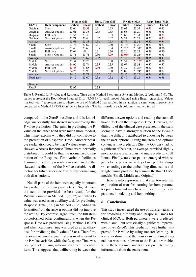
P-value (M1) Resp. Time (M1) P-value (M2) Resp. Time (M2)ELMo Item component Embed Encod Embed Encod Embed Encod Embed EncodOriginal Stem 23.60 23.32 0.31 0.33 23.62 23.33 0.31 0.33Original Answer options 23.61 23.35 0.35 0.35 23.63 23.29 0.35 0.35Original Full Item 23.55 23.43 0.31 0.33 23.60 23.34 0.31 0.34Original Stem + Options 23.71 23.40 0.32 0.32 24.24 23.27 0.32 0.33Average 23.61 23.38 0.32 0.33 23.77 23.31 0.32 0.34Small Stem 23.74 23.67 0.31 0.30 23.16* 23.20* 0.33 0.33Small Answer options 23.48 23.68 0.35 0.34 23.23* 23.31* 0.36 0.36Small Full Item 27.64 NA 0.31 0.30 23.20 23.23 0.38 0.70Small Stem + Options 23.71 23.71 0.30 0.29 23.04* 23.21* 0.34 0.33Average 24.64 23.69 0.32 0.31 23.16 23.24 0.35 0.43Middle Stem 23.54 23.73 0.31 0.30 23.32 23.16* 0.32 0.36Middle Answer options 24.90 23.74 0.35 0.35 23.67 23.38* 0.37 0.37Middle Full Item 23.45 23.65 0.30 0.30 23.39 23.22* 0.32 0.33Middle Stem + Options 24.76 23.95 0.31 0.30 23.82 23.24* 0.33 0.37Average 24.16 23.77 0.32 0.31 23.55 23.25 0.34 0.36Total aver. 24.17 23.60 0.32 0.32 23.49 23.26 0.34 0.38

BaselineZeroR 23.97 0.35

Table 3: Results for P-value and Response Time using Method 1 (columns 3-4) and Method 2 (columns 5-6). Thevalues represent the Root Mean Squared Error (RMSE) for each model obtained using linear regression. Valuesmarked with * represent cases, where the use of Method 2 has resulted in a statistically significant improvementcompared to Method 1 (95% Confidence Intervals). The best result in each column is marked in red.

compared to the ZeroR baseline and this knowl-edge successfully transferred into improving theP-value prediction. The gains in predicting the P-value on the other hand were much more modest,which may explain why they did not contribute tothe prediction of Response Time. Another possi-ble explanation could be that P-values were highlyskewed whereas Response Times were normallydistributed. It could be that the normalized distri-bution of the Response Time variable facilitateslearning of better representations compared to theskewed distribution of the P-value variable. A di-rection for future work is to test this by normalizingboth distributions.

Not all parts of the item were equally importantfor predicting the two parameters. Signal fromthe stem alone provided the best results for theP-value variable in Method 1 (23.32) and when P-value was used as an auxiliary task for predictingResponse Time (0.31) in Method 2 (i.e., adding in-formation from the answer options did not improvethe result). By contrast, signal from the full itemoutperformed other configurations when the Re-sponse Time was predicted using Method 1 (0.29)and when Response Time was used as an auxiliarytask for predicting the P-value (23.04). Therefore,the stem contained signal that was most relevant tothe P-value variable, while the Response Time wasbest predicted using information from the entireitem. This suggests that deliberating between the

different answer options and reading the stem allhave effects on the Response Time. However, thedifficulty of the clinical case presented in the stemseems to have a stronger relation to the P-valuethan the difficulty attributed to choosing betweenthe answer options. Using the stem and optionscontent as two predictors (Stem + Options) had nosignificant effects but, on average, provided slightlymore accurate results than the single predictor (FullItem). Finally, no clear pattern emerged with re-gards to the predictive utility of using embeddingsvs. encodings or the embedding dimensions andweight tuning produced by training the three ELMomodels (Small, Middle and Original).

These results represent a first step towards theexploration of transfer learning for item parame-ter prediction and may have implications for bothparameter modeling and item writing.

6 Conclusion

This study investigated the use of transfer learningfor predicting difficulty and Response Times forclinical MCQs. Both parameters were predictedwith a small but statistically significant improve-ment over ZeroR. This prediction was further im-proved for P-value by using transfer learning. Itwas also shown that the item stem contained sig-nal that was most relevant to the P-value variable,while the Response Time was best predicted usinginformation from the entire item.

196

References

Tahani Alsubait, Bijan Parsia, and Ulrike Sattler. 2013.A similarity-based theory of controlling mcq diffi-culty. In e-Learning and e-Technologies in Edu-cation (ICEEE), 2013 Second International Confer-ence on, pages 283–288. IEEE.

Peter Baldwin, Victoria Yaneva, Janet Mee, Brian EClauser, and Le An Ha. 2020. Using natural lan-guage processing to predict item response times andimprove test construction. Journal of EducationalMeasurement.

Lisa Beinborn, Torsten Zesch, and Iryna Gurevych.2015. Candidate evaluation strategies for improveddifficulty prediction of language tests. In Proceed-ings of the Tenth Workshop on Innovative Use ofNLP for Building Educational Applications, pages1–11.

Luca Benedetto, Andrea Cappelli, Roberto Turrin, andPaolo Cremonesi. 2020. R2de: a nlp approach toestimating irt parameters of newly generated ques-tions. In Proceedings of the Tenth International Con-ference on Learning Analytics & Knowledge, pages412–421.

Ciprian Chelba, Tomas Mikolov, Mike Schuster, Qi Ge,Thorsten Brants, Phillipp Koehn, and Tony Robin-son. 2013. One billion word benchmark for measur-ing progress in statistical language modeling. arXivpreprint arXiv:1312.3005.

Alex Graves, Santiago Fernandez, and Jurgen Schmid-huber. 2005. Bidirectional lstm networks for im-proved phoneme classification and recognition. InInternational Conference on Artificial Neural Net-works, pages 799–804. Springer.

Le An Ha and Victoria Yaneva. 2018. Automaticdistractor suggestion for multiple-choice tests usingconcept embeddings and information retrieval. InProceedings of the Thirteenth Workshop on Innova-tive Use of NLP for Building Educational Applica-tions, pages 389–398.

Le An Ha, Victoria Yaneva, Peter Baldwin, Janet Mee,et al. 2019. Predicting the difficulty of multiplechoice questions in a high-stakes medical exam. InProceedings of the Fourteenth Workshop on Innova-tive Use of NLP for Building Educational Applica-tions, pages 11–20.

Perry N Halkitis et al. 1996. Estimating testing time:The effects of item characteristics on response la-tency.

Zhenya Huang, Qi Liu, Enhong Chen, Hongke Zhao,Mingyong Gao, Si Wei, Yu Su, and Guoping Hu.2017. Question difficulty prediction for readingproblems in standard tests. In AAAI, pages 1352–1359.

Ghader Kurdi, Bijan Parsia, and Uli Sattler. 2016.An experimental evaluation of automatically gener-ated multiple choice questions from ontologies. InOWL: Experiences And directions–reasoner evalua-tion, pages 24–39. Springer.

Anastassia Loukina, Su-Youn Yoon, Jennifer Sakano,Youhua Wei, and Kathy Sheehan. 2016. Textualcomplexity as a predictor of difficulty of listeningitems in language proficiency tests. In Proceed-ings of COLING 2016, the 26th International Con-ference on Computational Linguistics: Technical Pa-pers, pages 3245–3253.

Cynthia G Parshall et al. 1994. Response latency: Aninvestigation into determinants of item-level timing.

Matthew E. Peters, Mark Neumann, Mohit Iyyer, MattGardner, Christopher Clark, Kenton Lee, and LukeZettlemoyer. 2018. Deep contextualized word repre-sentations. In Proc. of NAACL.

Russell Winsor Smith. 2000. An exploratory analysisof item parameters and characteristics that influenceitem level response time.

David B Swanson, Susan M Case, Douglas R Ripkey,Brian E Clauser, and Matthew C Holtman. 2001.Relationships among item characteristics, examinecharacteristics, and response times on usmle step 1.Academic Medicine, 76(10):S114–S116.

Victoria Yaneva, Peter Baldwin, Janet Mee, et al. 2019.Predicting the difficulty of multiple choice questionsin a high-stakes medical exam. In Proceedings ofthe Fourteenth Workshop on Innovative Use of NLPfor Building Educational Applications, pages 11–20.

Victoria Yaneva, Le An Ha, Peter Baldwin, and JanetMee. 2020. Predicting item survival for multiplechoice questions in a high-stakesmedical exam. InProceedings of the 12th Conference on LanguageResources and Evaluation (LREC 2020) , Marseille,11–16 May 2020, page 6814-6820.

197

Proceedings of the 15th Workshop on Innovative Use of NLP for Building Educational Applications, pages 198–208July 10, 2020. c©2020 Association for Computational Linguistics

A Comparative Study of Synthetic Data Generation Methods forGrammatical Error Correction

Maxwell White and Alla RozovskayaDepartment of Computer Science

Queens College, City University of New Yorkmaxwell.white94@qmail.cuny.edu,arozovskaya@qc.cuny.edu

Abstract

Grammatical Error Correction (GEC) is con-cerned with correcting grammatical errors inwritten text. Current GEC systems, namelythose leveraging statistical and neural machinetranslation, require large quantities of anno-tated training data, which can be expensive orimpractical to obtain. This research comparestechniques for generating synthetic data uti-lized by the two highest scoring submissionsto the restricted and low-resource tracks in theBEA-2019 Shared Task on Grammatical ErrorCorrection.

1 Introduction

Grammatical Error Correction (GEC) is the taskof automatically correcting grammatical errors inwritten text. More recently, significant progresshas been made, especially in English GEC, withinthe framework of statistical machine translation(SMT) and neural machine translation (NMT)approaches (Susanto et al., 2014; Yuan andBriscoe, 2016; Hoang et al., 2016; Chollampattet al., 2016; Junczys-Dowmunt and Grundkiewicz,2016; Mizumoto and Matsumoto, 2016; Jianshuet al., 2017; Chollampatt and Ng, 2018). The suc-cess of these approaches can be partially attributedto the availability of several large training sets.

In the most recent Building Educational Appli-cations (BEA) 2019 Shared Task (Bryant et al.,2019), which continued the tradition of earlierGEC competitions (Dale et al., 2012; Ng et al.,2014), all of the 24 participating teams appliedNMT and/or SMT approaches. One of the goalsof BEA-2019 was to re-evaluate the field aftera long hiatus, as recent GEC systems have be-come difficult to evaluate given a lack of stan-dardised experimental settings: Although signifi-cant progress has been made since the end of thelast CoNLL-2014 shared task, recent systems have

been trained, tuned and tested on different combi-nations of metrics and corpora. The BEA-2019Shared Task also introduced a new dataset thatrepresents a diverse cross-section of English lan-guage levels and domains (Bryant et al., 2019),and separate evaluation tracks, namely the Re-stricted, Unrestricted and Low Resource tracks.The Unrestricted track allowed the use of any re-sources; the Restricted track limited the use oflearner corpora to those that are publicly available,while the Low Resource track significantly limitedthe use of annotated data, to encourage develop-ment of systems that do not rely on large quantitiesof human-annotated data.

The two top scoring systems in the Restrictedand Low Resource tracks, UEDIN-MS (Grund-kiewicz et al., 2019) and Kakao&Brain (Choeet al., 2019), outperformed the other teams by alarge margin in both tracks; furthermore, both sys-tems made use of artificial data for training theirNMT systems, but they generated artificial datain different ways. Interestingly, in the RestrictedTrack, both of the systems scored on par, whilein the Low Resource Track Kakao&Brain exhib-ited a larger gap in performance (a drop of morethan 10 points compared to the Restricted track)vs. 4 points for UEDIN-MS. While both teamsused the same model architecture, transformer-based neural machine translation (NMT) (Vaswaniet al., 2017), in addition to the differences in thedata generation methods, the systems used differ-ent training scenarios, hyperpameter values, andtraining corpora of native data.

The goal of this paper is to compare the tech-niques for generating synthetic data used by theUEDIN-MS and Kakao&Brain systems. Themethod used in the UEDIN-MS system utilizesconfusion sets generated by a spellchecker, whilethe Kakao&Brain method relies on learner pat-terns extracted from a small annotated sample and

198

on POS-based confusions. Henceforth, we referto these as Inverted Spellchecker method and Pat-terns+POS method, respectively. To ensure a faircomparison of the methods, we control for theother variables, such as model choice, hyperpa-rameters, and the choice of native data. We trainNMT systems and evaluate our models on twolearner corpora, the W&I+LOCNESS corpus in-troduced in BEA-2019, and the FCE corpus (Yan-nakoudakis et al., 2011). Using the automatic errortype tool ERRANT (Bryant et al., 2017), we alsoshow performance evaluation by error type on thetwo corpora.

The paper makes the following contributions:(1) we provide a fair comparison of two methodsfor generating synthetic parallel data for GEC, us-ing two evaluation datasets; (2) we find that thetwo methods train different complementary sys-tems and target different types of errors: whilethe Inverted Spellchecker approach is good atidentifying spelling errors, the Patterns+POS ap-proach is better at correcting errors relating togrammar, such as noun number, verb agreement,and verb tense; (3) overall, the Patterns+POSmethod exhibits stronger results, compared to theInverted Spellchecker method in multiple trainingscenarios that include only synthetic parallel data,synthetic data augmented with in-domain learnerdata, and synthetic data augmented with out-of-domain learner data; (4) adding an off-the-shelfspellchecker is beneficial, and is especially help-ful for the Patterns+POS approach.

In the next section, we discuss relatedwork. Section 3 gives an overview of theW&I+LOCNESS and FCE learner datasets. Sec-tion 4 describes the error generation methods. Ex-periments are presented in section 5. Section 6 an-alyzes the results. Section 7 concludes the paper.

2 Related Work

Progress in English GEC Earlier GEC ap-proaches focused on English as a Second Lan-guage Learners and made use of linear machinelearning algorithms and developed classifiers forspecific error types, such as articles, prepositions,or noun number (Gamon, 2010; Rozovskaya andRoth, 2010, 2014; Dahlmeier and Ng, 2012). Theclassifiers can be trained on native English data,learner data, or a combination thereof.

The CoNLL shared tasks on English grammarcorrection provided a first large annotated corpus

of learner data for training (NUCLE, (Ng et al.,2014)), as well as two test sets. All the datawas produced by learners of English studying atthe National University of Singapore (majority ofwhich were native speakers of Chinese). The sta-tistical machine translation approach was shownto be successful in the CoNLL-2014 competitionfor the first time (Junczys-Dowmunt and Grund-kiewicz, 2014). Since then, the state-of-the-artresults on the CoNLL datasets were obtained us-ing SMT and NMT approaches. The systems aretypically trained on a combination of NUCLE andthe English part of the Lang-8 corpus (Mizumotoet al., 2012), even though the latter is known tocontain noise, as it is only partially corrected.Minimally-Supervised and Data-AugmentedGEC There has been a lot of work on generatingsynthetic training data for GEC. The approachescan be broken down into those that attempt tomake use of additional resources (e.g. Wikipediaedits) or noisify correct English data via artificialerrors. Boyd (2018) augmented training data withedits extracted from Wikipedia revision history inGerman. The edits were classified and only thoserelating to GEC were kept. Wikipedia edits areextracted from the revision history using Wiki Ed-its (Grundkiewicz and Junczys-Dowmunt, 2014).The contribution of the resulting edits is demon-strated using a multilayer convolutional encoder-decoder neural network model that we also usein this work. Mizumoto et al. (2011) extracteda Japanese learners corpus from the revision logof Lang-8 (about 1 million sentences) and im-plemented a character-based machine-translationmodel.

The other approach of generating parallel datacreates artificial errors in well-formed native data.This approach was shown to be effective withinthe classification framework (Rozovskaya andRoth, 2011; Dahlmeier and Ng, 2011; Felice andYuan, 2014).

3 The Learner Datasets

We make use of two publicly-available datasets oflearner texts for evaluation – the W&I+LOCNESSand the FCE – described below.

The BEA-2019 Shared Task introduced anew parallel corpus designed to represent awide range of English proficiency levels. TheW&I+LOCNESS corpus consists of hand-annotated data drawn from two sources. TheCambridge English Write & Improve (W&I) data

199

W&I+LOCNESSFCE (all) Training Dev

Type % % %ADJ 1.36 1.52 1.48ADJ:FORM 0.28 0.24 0.21ADV 1.94 1.51 1.51CONJ 0.67 0.51 0.58CONTR 0.32 0.30 0.39DET 10.86 11.25 10.43MORPH 1.90 1.85 2.07NOUN 4.57 4.36 4.30NOUN:INFL 0.50 0.12 0.13NOUN:NUM 3.34 4.05 3.29NOUN:POSS 0.51 0.60 0.87ORTH 2.94 4.77 4.61OTHER 13.26 12.76 12.84PART 0.29 0.84 0.79PREP 11.21 9.79 9.70PRON 3.51 2.64 2.33PUNCT 9.71 17.16 19.37SPELL 9.59 3.74 5.07UNK 3.13 2.59 2.24VERB 7.01 5.86 5.27VERB:FORM 3.55 3.56 3.09VERB:INFL 0.19 0.04 0.07VERB:SVA 1.52 2.23 1.94VERB:TENSE 6.04 6.07 6.20WO 1.82 1.64 1.25Total Edits 52,671 63,683 7,632

Table 1: Error distributions by type.

comes from a web-based platform that providesfeedback for non-native English students aroundthe world to improve their writing. LOCNESSwas compiled by researchers at the Centre forEnglish Corpus Linguistics at the University ofLouvain, and consists of essays written by nativeEnglish students.

W&I+LOCNESS contains 3,700 texts, consist-ing of 43,169 sentences or 801,361 tokens. 34,308sentences were made available for training and4,384 for development.

To provide an additional benchmark for eval-uation, we also evaluate on the test dataset fromthe FCE corpus (Yannakoudakis et al., 2011). TheFirst Certificate in English (FCE) corpus is a sub-set of the Cambridge Learner Corpus (CLC) thatcontains 1,244 written answers to the FCE exam,which assesses English at an upper-intermediatelevel. FCE was originally annotated accordingto a different error type framework, but was re-annotated automatically using ERRANT for use in

the shared task.A breakdown of error types for the

W&I+LOCNESS and FCE corpora can beseen in Table 1. The W&I+LOCNESS andthe FCE datasets have a similar percentage ofsome of the most common errors: determiner,preposition, noun and noun number, verb, verbform, and verb tense. Two notable exceptions arepunctuation errors (9.71% of all errors in the FCEcorpus, and between 17.16% and 19.37% in theW&I+LOCNESS training and development data);and spelling errors; almost 10% of all errors inFCE, and between 3.74-5.05 in W&I+LOCNESS.

4 Synthetic Data Generation Methods

In this section, we describe the two methods togenerate synthetic parallel data for training.

4.1 The Inverted Spellchecker Method

The method for generating unsupervised paral-lel data utilized in the system submitted by theUEDIN-MS team is characterized by usage ofconfusion sets extracted from a spellchecker. Thisartificial data is then used to pre-train a Trans-former sequence-to-sequence model.Noising method overview The InvertedSpellchecker method utilizes the Aspellspellchecker to generate a list of suggestionsfor a given word. Suggestions are sorted byweighted edit distance of the proposed word tothe input word and the distance between theirphonetic equivalents. The system then choosesthe top 20 suggestions to act as the confusion setfor the input word.

For each sentence, a number of words to changeis determined based on the word error rate of thedevelopment data set. For each chosen word, oneof the following operations is performed. Withprobability 0.7, the word is replaced with a wordrandomly chosen from the confusion set. Withprobability 0.1, the word is deleted. With prob-ability 0.1, a random word is inserted. With prob-ability 0.1, the word’s position is swapped withan adjacent word. Additionally, the above op-erations are performed at the character level for10% of words to introduce spelling errors. Itshould be emphasized that although the InvertedSpellchecker method uses confusion sets from aspellchecker, the idea of the method is to generatesynthetic noisy data for training a general-purposeGEC system to correct various grammatical errors.

200

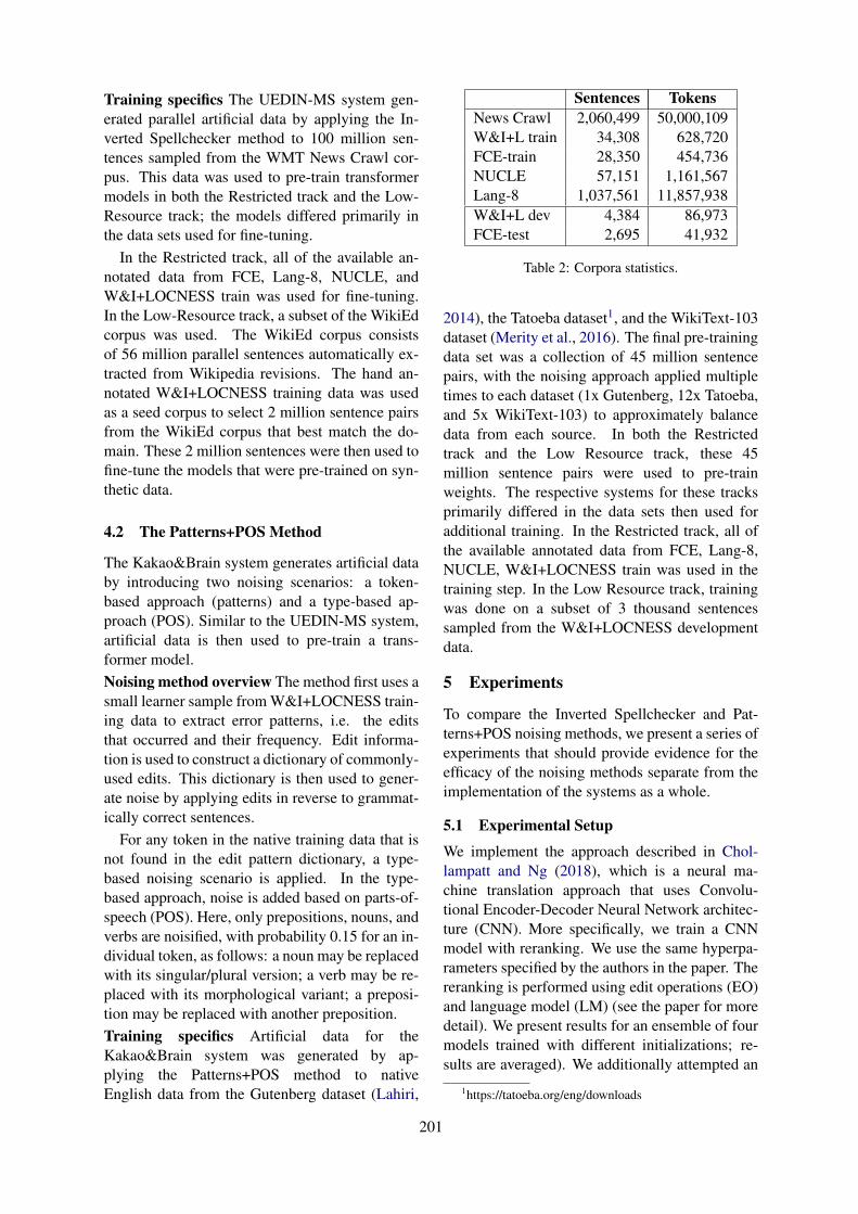
Training specifics The UEDIN-MS system gen-erated parallel artificial data by applying the In-verted Spellchecker method to 100 million sen-tences sampled from the WMT News Crawl cor-pus. This data was used to pre-train transformermodels in both the Restricted track and the Low-Resource track; the models differed primarily inthe data sets used for fine-tuning.

In the Restricted track, all of the available an-notated data from FCE, Lang-8, NUCLE, andW&I+LOCNESS train was used for fine-tuning.In the Low-Resource track, a subset of the WikiEdcorpus was used. The WikiEd corpus consistsof 56 million parallel sentences automatically ex-tracted from Wikipedia revisions. The hand an-notated W&I+LOCNESS training data was usedas a seed corpus to select 2 million sentence pairsfrom the WikiEd corpus that best match the do-main. These 2 million sentences were then used tofine-tune the models that were pre-trained on syn-thetic data.

4.2 The Patterns+POS Method

The Kakao&Brain system generates artificial databy introducing two noising scenarios: a token-based approach (patterns) and a type-based ap-proach (POS). Similar to the UEDIN-MS system,artificial data is then used to pre-train a trans-former model.Noising method overview The method first uses asmall learner sample from W&I+LOCNESS train-ing data to extract error patterns, i.e. the editsthat occurred and their frequency. Edit informa-tion is used to construct a dictionary of commonly-used edits. This dictionary is then used to gener-ate noise by applying edits in reverse to grammat-ically correct sentences.

For any token in the native training data that isnot found in the edit pattern dictionary, a type-based noising scenario is applied. In the type-based approach, noise is added based on parts-of-speech (POS). Here, only prepositions, nouns, andverbs are noisified, with probability 0.15 for an in-dividual token, as follows: a noun may be replacedwith its singular/plural version; a verb may be re-placed with its morphological variant; a preposi-tion may be replaced with another preposition.Training specifics Artificial data for theKakao&Brain system was generated by ap-plying the Patterns+POS method to nativeEnglish data from the Gutenberg dataset (Lahiri,

Sentences TokensNews Crawl 2,060,499 50,000,109W&I+L train 34,308 628,720FCE-train 28,350 454,736NUCLE 57,151 1,161,567Lang-8 1,037,561 11,857,938W&I+L dev 4,384 86,973FCE-test 2,695 41,932

Table 2: Corpora statistics.

2014), the Tatoeba dataset1, and the WikiText-103dataset (Merity et al., 2016). The final pre-trainingdata set was a collection of 45 million sentencepairs, with the noising approach applied multipletimes to each dataset (1x Gutenberg, 12x Tatoeba,and 5x WikiText-103) to approximately balancedata from each source. In both the Restrictedtrack and the Low Resource track, these 45million sentence pairs were used to pre-trainweights. The respective systems for these tracksprimarily differed in the data sets then used foradditional training. In the Restricted track, all ofthe available annotated data from FCE, Lang-8,NUCLE, W&I+LOCNESS train was used in thetraining step. In the Low Resource track, trainingwas done on a subset of 3 thousand sentencessampled from the W&I+LOCNESS developmentdata.

5 Experiments

To compare the Inverted Spellchecker and Pat-terns+POS noising methods, we present a series ofexperiments that should provide evidence for theefficacy of the noising methods separate from theimplementation of the systems as a whole.

5.1 Experimental Setup

We implement the approach described in Chol-lampatt and Ng (2018), which is a neural ma-chine translation approach that uses Convolu-tional Encoder-Decoder Neural Network architec-ture (CNN). More specifically, we train a CNNmodel with reranking. We use the same hyperpa-rameters specified by the authors in the paper. Thereranking is performed using edit operations (EO)and language model (LM) (see the paper for moredetail). We present results for an ensemble of fourmodels trained with different initializations; re-sults are averaged). We additionally attempted an

1https://tatoeba.org/eng/downloads

201

approach using a transformer architecture, but inpreliminary results it did not outperform the CNN.The language model (LM) is a 5-gram LM trainedon the publicly available WMT News Crawl cor-pus (233 million sentences), using the KenLMtoolkit (Heafield et al., 2013). We also use anoff-the-shelf speller (Flor, 2012; Flor and Futagi,2012) as a pre-processing step (prior to runningthe grammar correction system). We include re-sults with and without the use of the speller.

Most of the experiments (except experiment1, as shown below) are performed using 2 mil-lion sentences (50 million tokens) from the WMTNews Crawl corpus. We use this data to cre-ate artificially noised source data with the nois-ing techniques described above. For the InvertedSpellchecker method, we use the same error rateof 0.15 used by the authors in their original sys-tem (the error rate is chosen to simulate the er-ror rate of the learner data). The same probabil-ities for word-level and character-level modifica-tions are used as well (probability 0.7 to replacea token with another from the confusion set, and0.1 each to delete, insert, or swap with an adjacenttoken). For the Patterns+POS method, we use asample of 2,000 sentences from W&I+LOCNESStrain for the token-based portion of the noisingmethod. We also use the same error rates as theauthors in their original system: probability 0.9 toapply an edit in reverse if it appears in the edit dic-tionary, and probability 0.10 to apply a POS-basednoising scenario. For all models, the same 2,000sentences from W&I+LOCNESS train are used totrain the reranker.

All of the results are reported on the devel-opment section of the W&I+LOCNESS datasetand on the test section of the FCE corpus (theW&I+LOCNESS test data set has not been pub-licly released and the task participants were evalu-ated via CodaLab).

We address the following research questions:

• How do the two data generation methods com-pare on the FCE and W&I+LOCNESS evalua-tion datasets?

• How does the performance improve when thesynthetically-generated parallel data is aug-mented with parallel learner data from in-domain and out-of-domain?

• How do the two methods perform on differenterror types?

Experiments vary by the sources of additional

annotated learner data that were added to theartificially-generated data. Our goal in combiningsynthetic data with learner data is to evaluate tocontribution of synthetic data (generated in differ-ent ways) in various scenarios with in-domain andout-domain learner data available. The additionallearner training data comes from the publicly-available learner corpora of various sizes and vari-ous sources of data: the W&I+LOCNESS and theFCE training partitions (treated as in-domain forthe respective evaluation datasets), the Lang-8 cor-pus (Mizumoto et al., 2012), and the NUCLE cor-pus from the CoNLL-2014 shared task (Dahlmeieret al., 2013) (both treated as out-of-domain for thetwo datasets). These learner corpora were also al-lowed for use in the Restricted track. Statistics forthe amounts of data can be seen in Table 2.

The first experiment trains models on 50M to-kens of artificial data generated by each nois-ing method. The second experiment addsW&I+LOCNESS training data to the artificialdata. Experiment 3 adds the FCE training set tothe artificial data. In the fourth experiment, weadd the entirety of the annotated training corpora(FCE, Lang-8, and NUCLE) consisting of 13.5million tokens to the initial artificially-generatedtraining set, excluding W&I+LOCNESS trainingdataset. Finally, the fifth experiment modifiesthe fourth by also including the W&I+LOCNESStraining dataset.Experiment 1: Artificial data only For the firstexperiment, only artificial data generated by eitherrespective noising method is used to train models.The results can be viewed in Table 3.

Two observations can be made here. First,without adding the spellchecker, the Patterns+POSoutperforms the Inverted Spellchecker method bymore than 2 points on the W&I+LOCNESS cor-pus; however, on the FCE dataset, the InvertedSpellchecker method is superior (6 point differ-ence). Since the Patterns+POS method uses datafrom W&I+LOCNESS train to generate a tokenedit dictionary, this may explain the relativelyimproved results of this method on in-domainW&I+LOCNESS evaluation data. To explorethis hypothesis, we analyze these models’ perfor-mance with respect to ERRANT error types inSection 6.

We also note that, when a spellchecker is added,performance is improved substantially for the Pat-terns+POS methods (5 and 7 points, respectively,on W&I+LOCNESS and FCE datasets). In con-

202

W&I+L dev FCE testNoising method P R F0.5 P R F0.5Inverted Spellchecker 30.55 10.71 22.29 39.88 13.65 28.81Patterns+POS 33.93 12.24 25.05 32.43 10.05 22.43Inverted Spellchecker* 30.12 11.85 23.02 40.72 15.87 31.01Patterns+POS* 37.04 16.77 29.83 37.04 16.77 29.83

Table 3: Experiment 1 results: Ensemble of 4 models trained on 50 million tokens of artificial data and tuned witha sample of 2 thousand sentences from W&I+LOCNESS train (*speller applied during pre-processing).

W&I+L dev FCE testNoising method P R F0.5 P R F0.5Inverted Spellchecker 32.78 15.68 26.91 35.94 18.07 30.01Patterns+POS 41.56 15.41 31.03 35.57 12.46 25.95Inverted Spellchecker* 31.30 16.24 26.41 35.31 19.48 30.37Patterns+POS* 42.96 20.00 34.94 41.55 19.94 34.15

Table 4: Experiment 1 results continued: Ensemble of 4 models trained on 500 million tokens of artificial data(*speller applied during pre-processing).

W&I+L dev FCE testNoising method P R F0.5 P R F0.5Inverted Spellchecker 39.63 19.50 32.85 39.25 19.26 32.50Patterns+POS 42.57 22.07 35.90 38.88 18.84 32.06Inverted Spellchecker* 38.45 20.71 32.83 38.89 21.13 33.29Patterns+POS* 43.42 26.51 38.50 42.86 25.65 37.79

Table 5: Experiment 2 results: Ensemble of 4 models trained on 50 million tokens of artificial data with 600,000tokens from W&I+LOCNESS train added (*speller applied during pre-processing).

W&I+L dev FCE testNoising method P R F0.5 P R F0.5Inverted Spellchecker 33.38 13.89 26.06 44.88 20.73 36.40Patterns+POS 39.30 15.48 30.05 44.64 18.49 34.80Inverted Spellchecker* 32.34 14.76 26.12 44.57 22.47 37.24Patterns+POS* 40.51 19.54 33.35 47.09 23.68 39.32

Table 6: Experiment 3 results: Ensemble of 4 models trained on 50 million tokens of artificial data with 450,000tokens from FCE train added (*speller applied during pre-processing).

W&I+L dev FCE testNoising method P R F0.5 P R F0.5Inverted Spellchecker 44.80 22.97 37.65 52.43 31.02 46.07Patterns+POS 46.36 25.06 39.62 50.96 29.72 44.59Inverted Spellchecker* 42.65 23.64 36.74 50.16 31.81 44.97Patterns+POS* 45.78 28.13 40.68 50.44 32.69 45.50

Table 7: Experiment 4 results: Ensemble of 4 models trained on 50 million tokens of artificial data with 13.5million tokens from FCE train, Lang-8, and NUCLE (*speller applied during pre-processing).

203

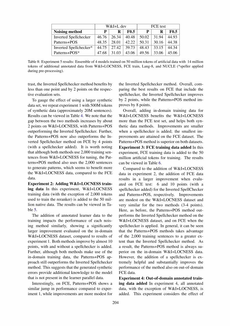
W&I+L dev FCE testNoising method P R F0.5 P R F0.5Inverted Spellchecker 46.76 26.34 40.48 50.02 31.94 44.93Patterns+POS 48.35 28.01 42.22 50.31 30.16 44.38Inverted Spellchecker* 44.75 27.42 39.73 48.43 33.15 44.34Patterns+POS* 47.68 31.03 43.06 49.56 33.06 45.06

Table 8: Experiment 5 results: Ensemble of 4 models trained on 50 million tokens of artificial data with 14 milliontokens of additional annotated data from W&I+LOCNESS, FCE train, Lang-8, and NUCLE (*speller appliedduring pre-processing).

trast, the Inverted Spellchecker method benefits byless than one point and by 2 points on the respec-tive evaluation sets.

To gauge the effect of using a larger syntheticdata set, we repeat experiment 1 with 500M tokensof synthetic data (approximately 20M sentences).Results can be viewed in Table 4. We note that thegap between the two methods increases by about2 points on W&I+LOCNESS, with Patterns+POSoutperforming the Inverted Spellchecker. Further,the Patterns+POS now also outperforms the In-verted Spellchecker method on FCE by 4 points(with a spellchecker added). It is worth notingthat although both methods use 2,000 training sen-tences from W&I+LOCNESS for tuning, the Pat-terns+POS method also uses the 2,000 sentencesto generate patterns, which seems to benefit morethe W&I+LOCNESS data, compared to the FCEdata.Experiment 2: Adding W&I+LOCNESS train-ing data In this experiment, W&I+LOCNESStraining data (with the exception of 2,000 tokensused to train the reranker) is added to the 50 mil-lion native data. The results can be viewed in Ta-ble 5.

The addition of annotated learner data to thetraining impacts the performance of each nois-ing method similarly, showing a significantlylarger improvement evaluated on the in-domainW&I+LOCNESS dataset, compared to results ofexperiment 1. Both methods improve by almost 10points, with and without a spellchecker is added.Further, although both methods make use of thein-domain training data, the Patterns+POS ap-proach still outperforms the Inverted Spellcheckermethod. This suggests that the generated syntheticerrors provide additional knowledge to the modelthat is not present in the learner parallel data.

Interestingly, on FCE, Patterns+POS shows asimilar jump in performance compared to exper-iment 1, while improvements are more modest for

the Inverted Spellchecker method. Overall, com-paring the best results on FCE that include thespellchecker, the Inverted Spellchecker improvesby 2 points, while the Patterns+POS method im-proves by 8 points.

Overall, adding in-domain training data forW&I+LOCNESS benefits the W&I+LOCNESSmore than the FCE test set, and helps both syn-thetic data methods. Improvements are smallerwhen a spellchecker is added; the smallest im-provements are attained on the FCE dataset. ThePatterns+POS method is superior on both datasets.Experiment 3: FCE training data added In thisexperiment, FCE training data is added to the 50million artificial tokens for training. The resultscan be viewed in Table 6.

Compared to the addition of W&I+LOCNESSdata in experiment 2, the addition of FCE dataresults in a larger improvement when evalu-ated on FCE test: 6 and 10 points (with aspellchecker added) for the Inverted SpellCheckerand Patterns+POS, respectively. Improvementsare modest on the W&I+LOCNESS dataset andvery similar for the two methods (3-4 points).Here, as before, the Patterns+POS method out-performs the Inverted Spellchecker method on theW&I+LOCNESS dataset, and on FCE when thespellchecker is applied. In general, it can be seenthat the Patterns+POS methods takes advantageof the 2,000 training sentences to a greater ex-tent than the Inverted Spellchecker method. Asa result, the Patterns+POS method is always su-perior on the in-domain W&I+LOCNESS data.However, the addition of a spellchecker is ex-tremely helpful and substantially improves theperformance of the method also on out-of-domainFCE data.Experiment 4: Out-of-domain annotated train-ing data added In experiment 4, all annotateddata, with the exception of W&I+LOCNESS, isadded. This experiment considers the effect of

204

out-of-domain learner data (out-of-domain rela-tive to the W&I+LOCNESS dataset). Results arein Table 7. Even though all of the datasets in-clude ESL data and most of them contain studentessays, we consider these data sets out-of-domainrelative to the W&I+LOCNESS set since they con-tain texts written on a different set of topics and bylearners of different proficiency levels .

Significant improvements over the previousexperiments can be observed, due to the vol-ume of additional data added. The InvertedSpellchecker method improves by 15 points onW&I+LOCNESS dev and 17 points on FCE test,compared to only using artificial data. The Pat-terns+POS method improves by 15 points onW&I+LOCNESS and 12 points on FCE test.We observe that the two methods are very closeon FCE , while the Patterns+POS method stilloutperforms the Inverted Spellchecker methodon W&I+Locness (by 2 and 4 points with andwithout the spellchecker added, respectively).This is interesting and suggests that the Pat-terns+POS method is especially useful when thereis no in-domain training data available, eventhough large amounts of out-of-domain learnerdata are available. It should also be noted thatadding a spellchecker does not improve InvertedSpellchecker models, while it is still useful for thePatterns+POS models.Experiment 5: All annotated training dataadded In experiment 5, all available annotateddata including the W&I+LOCNESS training data(approximately 14 million tokens) is added to theartificially generated data. Results can be viewedin Table 8. This model produces the best results onthe W&I+LOCNESS data, improving by 3 pointscompared to experiment 4, while on the FCEdataset there is no additional improvement. Thetwo methods perform similarly on the FCE test,and the Patterns+POS method outperforms the In-verted Spellchecker method on W&I+LOCNESSdata.

6 Discussion and Error Analysis

Results in the previous section indicate that thePatterns+POS method outperforms the InvertedSpellchecker method on W&I+LOCNESS, bothwhen used on its own, and when additionallearner training data is available, with and with-out a spellchecker. on the FCE dataset, thePatterns+POS method is superior only when aspellchecker is added. In general, the Pat-

terns+POS method benefits more from the addi-tion of a spellchecker in all experiments. Addingan off-the-shelf spellchecker to a GEC system isa common pre-processing step: a spellcheckeris developed to specifically target spelling errors,so a GEC system, which is typically more com-plex, can focus on other language misuse. Thegreater gap in performance between the methodson W&I+LOCNESS, compared to FCE, can be at-tributed to the utilization of in-domain data as partof the Patterns+POS noising approach.Evaluation by Error Type To examine the dis-crepancies in performance between the two nois-ing methods across the two evaluation datasets,we present an evaluation of performance by ER-RANT error type. Type-based evaluation resultsfor the top 10 most common error types for eachrespective evaluation dataset can be seen in Ta-bles 9 and 10 (note that these results do not in-clude the off-the-shelf spellchecker). The InvertedSpellchecker method significantly outperforms thePatterns+POS method on spelling errors on bothdatasets. As spelling errors make up approxi-mately 10% of errors in the FCE test set (dou-ble the relative frequency of spelling errors inW&I+LOCNESS), this may explain the improvedperformance of the Inverted Spellchecker methodwhen evaluated on FCE, compared to its own per-formance on W&I+LOCNESS.

In contrast, the Patterns+POS method outper-forms the Inverted Spellchecker method on verbtense errors and noun number errors. This makessense, since the POS-based confusion sets produceerrors that reflect misuse of these grammatical cat-egories. On the most common and notoriously dif-ficult errors – articles and prepositions – the twomethods exhibit similar performance. Finally, thePatterns+POS method outperforms the InvertedSpellchecker method by 25 points on punctuationerrors on the W&I+LOCNESS data, but is outper-formed by 2 points on FCE. This may be due tothe fact that the Patterns+POS method utilizes in-domain data as part of its noising process.Comparison with BEA-2019 results The high-est score achieved on W&I+LOCNESS data isF0.5 43.49 (experiment 5), obtained by the Pat-terns+POS method with all of the annotated dataadded to training, combined with the spellchecker(see Table 8). The model that only uses 2,000sentences for reranking and to generate the pat-terns table (experiment 1, Table 3) obtains ascore of 28.06 on W&I+LOCNESS and 30.98 on

205

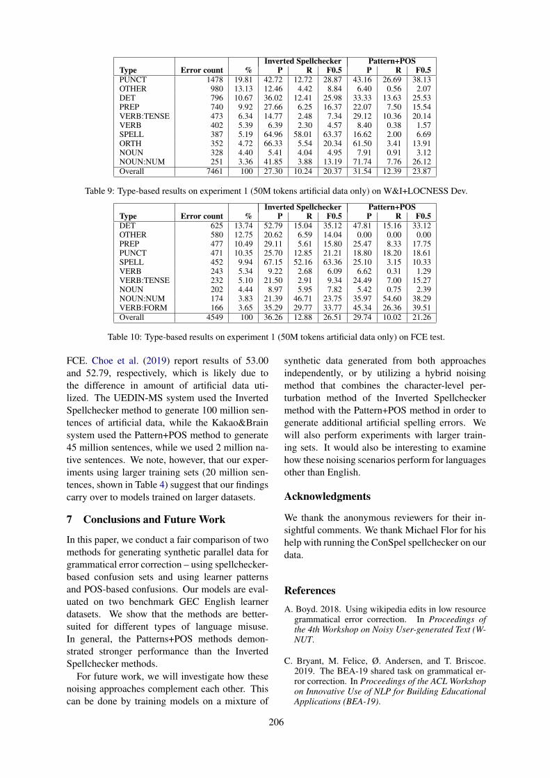
Inverted Spellchecker Pattern+POSType Error count % P R F0.5 P R F0.5PUNCT 1478 19.81 42.72 12.72 28.87 43.16 26.69 38.13OTHER 980 13.13 12.46 4.42 8.84 6.40 0.56 2.07DET 796 10.67 36.02 12.41 25.98 33.33 13.63 25.53PREP 740 9.92 27.66 6.25 16.37 22.07 7.50 15.54VERB:TENSE 473 6.34 14.77 2.48 7.34 29.12 10.36 20.14VERB 402 5.39 6.39 2.30 4.57 8.40 0.38 1.57SPELL 387 5.19 64.96 58.01 63.37 16.62 2.00 6.69ORTH 352 4.72 66.33 5.54 20.34 61.50 3.41 13.91NOUN 328 4.40 5.41 4.04 4.95 7.91 0.91 3.12NOUN:NUM 251 3.36 41.85 3.88 13.19 71.74 7.76 26.12Overall 7461 100 27.30 10.24 20.37 31.54 12.39 23.87

Table 9: Type-based results on experiment 1 (50M tokens artificial data only) on W&I+LOCNESS Dev.

Inverted Spellchecker Pattern+POSType Error count % P R F0.5 P R F0.5DET 625 13.74 52.79 15.04 35.12 47.81 15.16 33.12OTHER 580 12.75 20.62 6.59 14.04 0.00 0.00 0.00PREP 477 10.49 29.11 5.61 15.80 25.47 8.33 17.75PUNCT 471 10.35 25.70 12.85 21.21 18.80 18.20 18.61SPELL 452 9.94 67.15 52.16 63.36 25.10 3.15 10.33VERB 243 5.34 9.22 2.68 6.09 6.62 0.31 1.29VERB:TENSE 232 5.10 21.50 2.91 9.34 24.49 7.00 15.27NOUN 202 4.44 8.97 5.95 7.82 5.42 0.75 2.39NOUN:NUM 174 3.83 21.39 46.71 23.75 35.97 54.60 38.29VERB:FORM 166 3.65 35.29 29.77 33.77 45.34 26.36 39.51Overall 4549 100 36.26 12.88 26.51 29.74 10.02 21.26

Table 10: Type-based results on experiment 1 (50M tokens artificial data only) on FCE test.

FCE. Choe et al. (2019) report results of 53.00and 52.79, respectively, which is likely due tothe difference in amount of artificial data uti-lized. The UEDIN-MS system used the InvertedSpellchecker method to generate 100 million sen-tences of artificial data, while the Kakao&Brainsystem used the Pattern+POS method to generate45 million sentences, while we used 2 million na-tive sentences. We note, however, that our exper-iments using larger training sets (20 million sen-tences, shown in Table 4) suggest that our findingscarry over to models trained on larger datasets.

7 Conclusions and Future Work

In this paper, we conduct a fair comparison of twomethods for generating synthetic parallel data forgrammatical error correction – using spellchecker-based confusion sets and using learner patternsand POS-based confusions. Our models are eval-uated on two benchmark GEC English learnerdatasets. We show that the methods are better-suited for different types of language misuse.In general, the Patterns+POS methods demon-strated stronger performance than the InvertedSpellchecker methods.

For future work, we will investigate how thesenoising approaches complement each other. Thiscan be done by training models on a mixture of

synthetic data generated from both approachesindependently, or by utilizing a hybrid noisingmethod that combines the character-level per-turbation method of the Inverted Spellcheckermethod with the Pattern+POS method in order togenerate additional artificial spelling errors. Wewill also perform experiments with larger train-ing sets. It would also be interesting to examinehow these noising scenarios perform for languagesother than English.

Acknowledgments

We thank the anonymous reviewers for their in-sightful comments. We thank Michael Flor for hishelp with running the ConSpel spellchecker on ourdata.

References

A. Boyd. 2018. Using wikipedia edits in low resourcegrammatical error correction. In Proceedings ofthe 4th Workshop on Noisy User-generated Text (W-NUT.

C. Bryant, M. Felice, Ø. Andersen, and T. Briscoe.2019. The BEA-19 shared task on grammatical er-ror correction. In Proceedings of the ACL Workshopon Innovative Use of NLP for Building EducationalApplications (BEA-19).

206

C. Bryant, M. Felice, and T. Briscoe. 2017. Auto-matic annotation and evaluation of error types forgrammatical error correction. In Proceedings of the55th Annual Meeting of the Association for Compu-tational Linguistics (Volume 1: Long Papers), pages793–805, Vancouver, Canada. Association for Com-putational Linguistics.

Y. J. Choe, J. Ham, K. Park, and Y. Yoon. 2019. Aneural grammatical error correction system built onbetter pre-training and sequential transfer learning .In Proceedings of the ACL Workshop on InnovativeUse of NLP for Building Educational Applications(BEA-19).

S. Chollampatt and H. T. Ng. 2018. A multilayerconvolutional encoder-decoder neural network forgrammatical error correction. In Proceedings of theAAAI. Association for the Advancement of ArtificialIntelligence.

S. Chollampatt, K. Taghipour, and H. T. Ng. 2016.Neural network translation models for grammaticalerror correction. In IJCAI.

D. Dahlmeier and H. T. Ng. 2011. Grammatical er-ror correction with alternating structure optimiza-tion. In Proceedings of ACL.

D. Dahlmeier and H. T. Ng. 2012. A beam-search de-coder for grammatical error correction. In Proceed-ings of EMNLP-CoNLL.

D. Dahlmeier, H. T. Ng, and S. M. Wu. 2013. Build-ing a large annotated corpus of learner english: Thenus corpus of learner english. In Proceedings ofthe Eighth Workshop on Innovative Use of NLPfor Building Educational Applications, pages 22–31, Atlanta, Georgia. Association for ComputationalLinguistics.

R. Dale, I. Anisimoff, and G. Narroway. 2012. A reporton the preposition and determiner error correctionshared task. In Proceedings of the NAACL Workshopon Innovative Use of NLP for Building EducationalApplications.

M. Felice and Z. Yuan. 2014. Generating artifi-cial errors for grammatical error correction. InProceedings of the Student Research Workshop atEACL, Gothenburg, Sweden. Association for Com-putational Linguistics.

M. Flor. 2012. Four types of context for automaticspelling correction. Traitement Automatique desLangues (TAL), 53(3):61–99.

M. Flor and Y. Futagi. 2012. On using context for auto-matic correction of non-word misspellings in studentessays. In Proceedings of the 7th Workshop on Inno-vative Use of NLP for Building Educational Appli-cations. Association for Computational Linguistics.

M. Gamon. 2010. Using mostly native data to cor-rect errors in learners’ writing. In Proceedings ofNAACL.

R. Grundkiewicz and M. Junczys-Dowmunt. 2014.The Wiked error corpus: A corpus of correctivewikipedia edits and its application to grammaticalerror correction. In Advances in Natural LanguageProcessing – Lecture Notes in Computer Science,volume 8686, pages 478–490. Springer.

R. Grundkiewicz, M. Junczys-Dowmunt, andK. Heafield. 2019. Neural grammatical errorcorrection systems with unsupervised pre-trainingon synthetic data. In Proceedings of the ACLWorkshop on Innovative Use of NLP for BuildingEducational Applications (BEA-19).

K. Heafield, I. Pouzyrevsky, J. H. Clark, and P. Koehn.2013. Scalable modified Kneser-Ney languagemodel estimation. In ACL.

D.-T. Hoang, S. Chollampatt, and H.-T. Ng. 2016. Ex-ploiting n-best hypotheses to improve an SMT ap-proach to grammatical error correction. In IJCAI.

J. Jianshu, Q. Wang, K. Toutanova, Y. Gong, S. Truong,and Jianfeng J. Gao. 2017. A nested attention neuralhybrid model for grammatical error correction. InACL.

M. Junczys-Dowmunt and R. Grundkiewicz. 2014.The AMU system in the CoNLL-2014 shared task:Grammatical error correction by data-intensive andfeature-rich statistical machine translation. In Pro-ceedings of the Eighteenth Conference on Computa-tional Natural Language Learning: Shared Task.

M. Junczys-Dowmunt and R. Grundkiewicz. 2016.Phrase-based machine translation is state-of-the-artfor automatic grammatical error correction. InEMNLP.

S. Lahiri. 2014. Complexity of Word Collocation Net-works: A Preliminary Structural Analysis. In Pro-ceedings of the Student Research Workshop at the14th Conference of the European Chapter of the As-sociation for Computational Linguistics.

S. Merity, C. Xiong, J. Bradbury, and R. Socher.2016. Pointer sentinel mixture models. CoRR,abs/1609.07843.

T. Mizumoto, Y. Hayashibe, M. Komachi, M. Nagata,and Y. Matsumoto. 2012. The effect of learner cor-pus size in grammatical error correction of esl writ-ings. In COLING.

T. Mizumoto, M. Komachi, M. Nagata, and Y. Mat-sumoto. 2011. Mining revision log of languagelearning SNS for automated japanese error correc-tion of second language learners. In IJCNLP.

T. Mizumoto and Y. Matsumoto. 2016. Discriminativereranking for grammatical error correction with sta-tistical machine translation. In NAACL.

H. T. Ng, S. M. Wu, T. Briscoe, C. Hadiwinoto, R. H.Susanto, and C. Bryant. 2014. The conll-2014

207

shared task on grammatical error correction. In Pro-ceedings of the Eighteenth Conference on Compu-tational Natural Language Learning: Shared Task,pages 1–14, Baltimore, Maryland. Association forComputational Linguistics.

A. Rozovskaya and D. Roth. 2010. Training paradigmsfor correcting errors in grammar and usage. In Pro-ceedings of NAACL.

A. Rozovskaya and D. Roth. 2011. Algorithm selec-tion and model adaptation for ESL correction tasks.In Proceedings of ACL.

A. Rozovskaya and D. Roth. 2014. Building a State-of-the-Art Grammatical Error Correction System. InTransactions of ACL.

R. H. Susanto, P. Phandi, and H. T. Ng. 2014. Sys-tem combination for grammatical error correction.In EMNLP.

A. Vaswani, N. Shazeer, N. Parmar, J. Uszkoreit,L. Jones, A. N. Gomez, Ł. Kaiser, and I. Polosukhin.2017. 2017. Attention is all you need. In I. Guyon,U. V. Luxburg, S. Bengio, H. Wallach, R. Fergus, S.Vishwanathan, and R. Garnett, editors, Advances inNeural Information Processing Systems.

H. Yannakoudakis, T. Briscoe, and B. Medlock. 2011.A new dataset and method for automatically gradingesol texts. In Proceedings of the 49th Annual Meet-ing of the Association for Computational Linguis-tics: Human Language Technologies, pages 180–189, Portland, Oregon, USA. Association for Com-putational Linguistics.

Z. Yuan and T. Briscoe. 2016. Grammatical error cor-rection using neural machine translation. In NAACL.

208

Author Index

Afrin, Tazin, 75Asgari, Meysam, 177Atrasevych, Vitaliy, 163

Baldwin, Peter, 193Becker, Lee, 30Beigman Klebanov, Beata, 145Bethard, Steven, 115Bhattacharyya, Pushpak, 85Bichler, Sarah, 135Black, Alan W, 151Bradford, Allison, 135Brunato, Dominique, 92

C. Linn, Marcia, 135Cahill, Aoife, 18, 186Chernodub, Artem, 163Correnti, Richard, 75

Davidson, Sam, 92Dell’Orletta, Felice, 92Derr, Marcia, 30Deutsch, Tovly, 1Dolata, Jill, 177

Ehara, Yo, 171

Fife, James H, 186Foley, Ben, 124Foltz, Peter, 30

Gales, Mark, 41Galochkin, Dmytro, 186Gao, Lingyu, 102Gerard, Libby, 135Ghosh, Debanjan, 145Gimpel, Kevin, 102González-López, Samuel, 115González Ochoa, Simón, 124

Hearst, Marti A., 52Hellman, Scott, 30

Jasbi, Masoud, 1Jensson, Arnar, 102Johnson, Matthew S., 18

Kao, Kimberly, 52Kerz, Elma, 65King Chen, Jennifer, 135Knill, Kate, 41

Litman, Diane, 75Lopez-Lopez, Aurelio, 115Loukina, Anastassia, 18

Madnani, Nitin, 18Mathias, Sandeep, 85Matsumura, Lindsay Clare, 75Maxwelll-Smith, Zara, 124Mayfield, Elijah, 151McCaffrey, Daniel F., 18Miaschi, Alessio, 92Murray, William, 30

Omelianchuk, Kostiantyn, 163

Prud’hommeaux, Emily, 177

Qiao, Yu, 65

Raina, Vatsal, 41Riordan, Brian, 18, 135, 186Rosenstein, Mark, 30Rozovskaya, Alla, 198Runyon, Christopher, 193

Sagae, Kenji, 92Sanchez-Gutierrez, Claudia Helena, 92Shieber, Stuart, 1Skurzhanskyi, Oleksandr, 163Song, Yi, 145Stasaski, Katherine, 52Ströbel, Marcus, 65Suominen, Hanna, 124

Vajpayee, Avijit, 186Venturi, Giulia, 92

Wang, Elaine Lin, 75Wang, Yiyi, 177White, Max, 198Wiechmann, Daniel, 65

209

Wiemerslage, Adam, 30Wiley, Korah, 135

Xue, Kang, 193

Yaneva, Victoria, 193Yao, Lili, 18