Proceedings of the 2012 Workshop on Biomedical Natural ...
260
NAACL-HLT 2012 BioNLP 2012 Workshop on Biomedical Natural Language Processing Proceedings of the Workshop June 8, 2012 Montr´ eal, Canada
-
Upload
khangminh22 -
Category
Documents
-
view
1 -
download
0
Transcript of Proceedings of the 2012 Workshop on Biomedical Natural ...

NAACL-HLT 2012
BioNLP 2012
Workshop on Biomedical Natural Language Processing
Proceedings of the Workshop
June 8, 2012Montreal, Canada

Production and Manufacturing byOmnipress, Inc.2600 Anderson StreetMadison, WI 53707USA
c©2012 The Association for Computational Linguistics
Order copies of this and other ACL proceedings from:
Association for Computational Linguistics (ACL)209 N. Eighth StreetStroudsburg, PA 18360USATel: +1-570-476-8006Fax: [email protected]
ISBN13: 978-1-937284-20-6ISBN10: 1-937284-20-4
ii

iii
Introduction
BioNLP 2012 received 31 submissions exceeding even the traditionally high quality of the precedingeleven years of BioNLP. Due to uniformly positive reviews, eleven submissions were accepted as fullpapers and 19 as poster presentations.
The themes in this year’s papers and posters continue reflecting researchers’ growing interest in clinicaltext processing, while maintaining a steady mature work in biological language processing. This yearpresents a wide range of innovative methods applied to interesting problems in both domains.
Acknowledgments
We are profoundly grateful to the authors who chose BioNLP as venue for presenting their innovativeresearch.
The authors’ willingness to share their work through BioNLP consistently makes the workshop notonly noteworthy and stimulating, but also one of the largest, and some years the largest workshop, atACL/NAACL.
We are equally indebted to the program committee members (listed elsewhere in this volume) whoproduced three thorough reviews per paper on a tight review schedule and with an admirable level ofinsight.
iv

Organizers:
Kevin Bretonnel Cohen, University of Colorado School of MedicineDina Demner-Fushman, US National Library of MedicineSophia Ananiadou, University of Manchester and National Centre for Text Mining, UKJohn Pestian, Computational Medical Center, University of Cincinnati,Cincinnati Children’s Hospital Medical CenterJun’ichi Tsujii, University of Tokyoand Microsoft Research AsiaBonnie Webber,University of Edinburgh, UK
Program Committee:
Sophia AnaniadouGalia AngelovaEmilia ApostolovaAlan AronsonOlivier BodenreiderWendy ChapmanKevin CohenNigel CollierDina Demner-FushmanNoemie ElhadadMarcelo FiszmanFilip GinterSu JianJin-Dong KimZhiyong LuAurelie NeveolJon PatrickJohn PestianSampo PyysaloBastien RanceFabio RinaldiThomas RindfleschBrian RoarkAndrey RzhetskyDaniel RubinGuergana SavovaHagit ShatkayMatthew SimpsonPontus StenetorpYuka Tateisi
v

Jun’ichi TsujiiYoshimasa TsuruokaOzlem UzunerKarin VerspoorBonnie WebberPeter WhiteW. John WilburLimsoon WongAntonio YepesGuodong ZhouPierre Zweigenbaum
Invited Speaker:
Wendy W. Chapman, University of California San DiegoChallenges and Opportunities in Clinical Text Annotation
vi

Table of Contents
Graph-based alignment of narratives for automated neurological assessmentEmily Prud’hommeaux and Brian Roark . . . . . . . . . . . . . . . . . . . . . . . . . . . . . . . . . . . . . . . . . . . . . . . . . . 1
Bootstrapping Biomedical Ontologies for Scientific Text using NELLDana Movshovitz-Attias and William W. Cohen . . . . . . . . . . . . . . . . . . . . . . . . . . . . . . . . . . . . . . . . . . 11
Semantic distance and terminology structuring methods for the detection of semantically close termsMarie Dupuch, Laetitia Dupuch, Thierry Hamon and Natalia Grabar . . . . . . . . . . . . . . . . . . . . . . . . 20
Temporal Classification of Medical EventsPreethi Raghavan, Eric Fosler-Lussier and Albert Lai . . . . . . . . . . . . . . . . . . . . . . . . . . . . . . . . . . . . . 29
Analyzing Patient Records to Establish If and When a Patient Suffered from a Medical ConditionJames Cogley, Nicola Stokes, Joe Carthy and John Dunnion . . . . . . . . . . . . . . . . . . . . . . . . . . . . . . . 38
Alignment-HMM-based Extraction of Abbreviations from Biomedical TextDana Movshovitz-Attias and William W. Cohen . . . . . . . . . . . . . . . . . . . . . . . . . . . . . . . . . . . . . . . . . . 47
Medical diagnosis lost in translation – Analysis of uncertainty and negation expressions in English andSwedish clinical texts
Danielle L. Mowery, Sumithra Velupillai and Wendy W. Chapman. . . . . . . . . . . . . . . . . . . . . . . . . .56
A Hybrid Stepwise Approach for De-identifying Person Names in Clinical DocumentsOscar Ferrandez, Brett South, Shuying Shen and Stephane Meystre . . . . . . . . . . . . . . . . . . . . . . . . . 65
Active Learning for Coreference ResolutionTimothy Miller, Dmitriy Dligach and Guergana Savova . . . . . . . . . . . . . . . . . . . . . . . . . . . . . . . . . . . .73
PubMed-Scale Event Extraction for Post-Translational Modifications, Epigenetics and Protein Struc-tural Relations
Jari Bjorne, Sofie Van Landeghem, Sampo Pyysalo, Tomoko Ohta, Filip Ginter, Yves Van de Peer,Sophia Ananiadou and Tapio Salakoski . . . . . . . . . . . . . . . . . . . . . . . . . . . . . . . . . . . . . . . . . . . . . . . . . . . . . . . 82
An improved corpus of disease mentions in PubMed citationsRezarta Islamaj Dogan and Zhiyong Lu . . . . . . . . . . . . . . . . . . . . . . . . . . . . . . . . . . . . . . . . . . . . . . . . . . 91
New Resources and Perspectives for Biomedical Event ExtractionSampo Pyysalo, Pontus Stenetorp, Tomoko Ohta, Jin-Dong Kim and Sophia Ananiadou . . . . . 100
Combining Compositionality and Pagerank for the Identification of Semantic Relations between Biomed-ical Words
Thierry Hamon, Christopher Engstrom, Mounira Manser, Zina Badji, Natalia Grabar and SergeiSilvestrov . . . . . . . . . . . . . . . . . . . . . . . . . . . . . . . . . . . . . . . . . . . . . . . . . . . . . . . . . . . . . . . . . . . . . . . . . . . . . . . . 109
Domain Adaptation of Coreference Resolution for Radiology ReportsEmilia Apostolova, Noriko Tomuro, Pattanasak Mongkolwat and Dina Demner-Fushman . . . . 118
vii

What can NLP tell us about BioNLP?Attapol Thamrongrattanarit, Michael Shafir, Michael Crivaro, Bensiin Borukhov and Marie Meteer
122
A Prototype Tool Set to Support Machine-Assisted AnnotationBrett South, Shuying Shen, Jianwei Leng, Tyler Forbush, Scott DuVall and Wendy Chapman 130
MedLingMap: A growing resource mapping the Bio-Medical NLP fieldMarie Meteer, Borukhov Bensiin, Mike Crivaro, Michael Shafir and Attapol Thamrongrattanarit
140
Exploring Label Dependency in Active Learning for Phenotype MappingShefali Sharma, Leslie Lange, Jose Luis Ambite, Yigal Arens and Chun-Nan Hsu . . . . . . . . . . . 146
Evaluating Joint Modeling of Yeast Biology Literature and Protein-Protein Interaction NetworksRamnath Balasubramanyan, Kathryn Rivard, William W. Cohen, Jelena Jakovljevic and John L.
Woolford . . . . . . . . . . . . . . . . . . . . . . . . . . . . . . . . . . . . . . . . . . . . . . . . . . . . . . . . . . . . . . . . . . . . . . . . . . . . . . . . . 155
RankPref: Ranking Sentences Describing Relations between Biomedical Entities with an ApplicationCatalina Oana Tudor and K Vijay-Shanker . . . . . . . . . . . . . . . . . . . . . . . . . . . . . . . . . . . . . . . . . . . . . . 163
Finding small molecule and protein pairs in scientific literature using a bootstrapping methodYing Yan, Jee-Hyub Kim, Samuel Croset and Dietrich Rebholz-Schuhmann . . . . . . . . . . . . . . . . 172
Grading the Quality of Medical EvidenceBinod Gyawali, Thamar Solorio and Yassine Benajiba . . . . . . . . . . . . . . . . . . . . . . . . . . . . . . . . . . . 176
Classifying Gene Sentences in Biomedical Literature by Combining High-Precision Gene IdentifiersSun Kim, Won Kim, Don Comeau and W. John Wilbur . . . . . . . . . . . . . . . . . . . . . . . . . . . . . . . . . . . 185
Effect of small sample size on text categorization with support vector machinesPawel Matykiewicz and John Pestian . . . . . . . . . . . . . . . . . . . . . . . . . . . . . . . . . . . . . . . . . . . . . . . . . . . 193
PubAnnotation - a persistent and sharable corpus and annotation repositoryJin-Dong Kim and Yue Wang . . . . . . . . . . . . . . . . . . . . . . . . . . . . . . . . . . . . . . . . . . . . . . . . . . . . . . . . . . 202
Using Natural Language Processing to Extract Drug-Drug Interaction Information from Package In-serts
Richard Boyce, Gregory Gardner and Henk Harkema . . . . . . . . . . . . . . . . . . . . . . . . . . . . . . . . . . . . 206
Automatic Approaches for Gene-Drug Interaction Extraction from Biomedical Text: Corpus and Com-parative Evaluation
Nate Sutton, Laura Wojtulewicz, Neel Mehta and Graciela Gonzalez . . . . . . . . . . . . . . . . . . . . . . 214
A Preliminary Work on Symptom Name Recognition from Free-Text Clinical Records of TraditionalChinese Medicine using Conditional Random Fields and Reasonable Features
Yaqiang Wang, Yiguang Liu, Zhonghua Yu, Li Chen and Yongguang Jiang . . . . . . . . . . . . . . . . . 223
Scaling up WSD with Automatically Generated ExamplesWeiwei Cheng, Judita Preiss and Mark Stevenson . . . . . . . . . . . . . . . . . . . . . . . . . . . . . . . . . . . . . . . . 231
viii

Boosting the protein name recognition performance by bootstrapping on selected textYue Wang and Jin-Dong Kim . . . . . . . . . . . . . . . . . . . . . . . . . . . . . . . . . . . . . . . . . . . . . . . . . . . . . . . . . . 240
ix


Conference Program
Friday, June 8, 2012
8:40–8:50 Opening Remarks
Session 1: Alignment, similarity, classification
8:50–9:10 Graph-based alignment of narratives for automated neurological assessmentEmily Prud’hommeaux and Brian Roark
9:10–9:30 Bootstrapping Biomedical Ontologies for Scientific Text using NELLDana Movshovitz-Attias and William W. Cohen
9:30–9:50 Semantic distance and terminology structuring methods for the detection of seman-tically close termsMarie Dupuch, Laetitia Dupuch, Thierry Hamon and Natalia Grabar
9:50–10:10 Temporal Classification of Medical EventsPreethi Raghavan, Eric Fosler-Lussier and Albert Lai
10:10–10:30 Analyzing Patient Records to Establish If and When a Patient Suffered from a Med-ical ConditionJames Cogley, Nicola Stokes, Joe Carthy and John Dunnion
10:30–11:00 Morning coffee break
11:00–12:10 Invited Talk by Wendy Chapman
12:10–12:30 Alignment-HMM-based Extraction of Abbreviations from Biomedical TextDana Movshovitz-Attias and William W. Cohen
12:30–14:00 Lunch break
14:00–14:20 Medical diagnosis lost in translation – Analysis of uncertainty and negation expres-sions in English and Swedish clinical textsDanielle L. Mowery, Sumithra Velupillai and Wendy W. Chapman
14:20–14:40 A Hybrid Stepwise Approach for De-identifying Person Names in Clinical Docu-mentsOscar Ferrandez, Brett South, Shuying Shen and Stephane Meystre
xi

Friday, June 8, 2012 (continued)
14:40–15:00 Active Learning for Coreference ResolutionTimothy Miller, Dmitriy Dligach and Guergana Savova
15:00–15:20 PubMed-Scale Event Extraction for Post-Translational Modifications, Epigenetics andProtein Structural RelationsJari Bjorne, Sofie Van Landeghem, Sampo Pyysalo, Tomoko Ohta, Filip Ginter, Yves Vande Peer, Sophia Ananiadou and Tapio Salakoski
15:20–15:40 An improved corpus of disease mentions in PubMed citationsRezarta Islamaj Dogan and Zhiyong Lu
15:30–16:00 Afternoon coffee break
Poster Session (16:00–18:00)
New Resources and Perspectives for Biomedical Event ExtractionSampo Pyysalo, Pontus Stenetorp, Tomoko Ohta, Jin-Dong Kim and Sophia Ananiadou
Combining Compositionality and Pagerank for the Identification of Semantic Relationsbetween Biomedical WordsThierry Hamon, Christopher Engstrom, Mounira Manser, Zina Badji, Natalia Grabar andSergei Silvestrov
Domain Adaptation of Coreference Resolution for Radiology ReportsEmilia Apostolova, Noriko Tomuro, Pattanasak Mongkolwat and Dina Demner-Fushman
What can NLP tell us about BioNLP?Attapol Thamrongrattanarit, Michael Shafir, Michael Crivaro, Bensiin Borukhov andMarie Meteer
A Prototype Tool Set to Support Machine-Assisted AnnotationBrett South, Shuying Shen, Jianwei Leng, Tyler Forbush, Scott DuVall and Wendy Chap-man
MedLingMap: A growing resource mapping the Bio-Medical NLP fieldMarie Meteer, Borukhov Bensiin, Mike Crivaro, Michael Shafir and Attapol Thamrongrat-tanarit
Exploring Label Dependency in Active Learning for Phenotype MappingShefali Sharma, Leslie Lange, Jose Luis Ambite, Yigal Arens and Chun-Nan Hsu
Evaluating Joint Modeling of Yeast Biology Literature and Protein-Protein InteractionNetworksRamnath Balasubramanyan, Kathryn Rivard, William W. Cohen, Jelena Jakovljevic andJohn L. Woolford
xii

Friday, June 8, 2012 (continued)
RankPref: Ranking Sentences Describing Relations between Biomedical Entities with anApplicationCatalina Oana Tudor and K Vijay-Shanker
Finding small molecule and protein pairs in scientific literature using a bootstrappingmethodYing Yan, Jee-Hyub Kim, Samuel Croset and Dietrich Rebholz-Schuhmann
Grading the Quality of Medical EvidenceBinod Gyawali, Thamar Solorio and Yassine Benajiba
Classifying Gene Sentences in Biomedical Literature by Combining High-Precision GeneIdentifiersSun Kim, Won Kim, Don Comeau and W. John Wilbur
Effect of small sample size on text categorization with support vector machinesPawel Matykiewicz and John Pestian
PubAnnotation - a persistent and sharable corpus and annotation repositoryJin-Dong Kim and Yue Wang
Using Natural Language Processing to Extract Drug-Drug Interaction Information fromPackage InsertsRichard Boyce, Gregory Gardner and Henk Harkema
Automatic Approaches for Gene-Drug Interaction Extraction from Biomedical Text: Cor-pus and Comparative EvaluationNate Sutton, Laura Wojtulewicz, Neel Mehta and Graciela Gonzalez
A Preliminary Work on Symptom Name Recognition from Free-Text Clinical Records ofTraditional Chinese Medicine using Conditional Random Fields and Reasonable FeaturesYaqiang Wang, Yiguang Liu, Zhonghua Yu, Li Chen and Yongguang Jiang
Scaling up WSD with Automatically Generated ExamplesWeiwei Cheng, Judita Preiss and Mark Stevenson
Boosting the protein name recognition performance by bootstrapping on selected textYue Wang and Jin-Dong Kim
xiii


Proceedings of the 2012 Workshop on Biomedical Natural Language Processing (BioNLP 2012), pages 1–10,Montreal, Canada, June 8, 2012. c©2012 Association for Computational Linguistics
Graph-based alignment of narratives for automated neurological assessment
Emily T. Prud’hommeaux and Brian RoarkCenter for Spoken Language Understanding
Oregon Health & Science University{emilypx,roarkbr}@gmail.com
Abstract
Narrative recall tasks are widely used in neu-ropsychological evaluation protocols in or-der to detect symptoms of disorders suchas autism, language impairment, and demen-tia. In this paper, we propose a graph-basedmethod commonly used in information re-trieval to improve word-level alignments inorder to align a source narrative to narra-tive retellings elicited in a clinical setting.From these alignments, we automatically ex-tract narrative recall scores which can then beused for diagnostic screening. The signifi-cant reduction in alignment error rate (AER)afforded by the graph-based method resultsin improved automatic scoring and diagnos-tic classification. The approach described hereis general enough to be applied to almost anynarrative recall scenario, and the reductions inAER achieved in this work attest to the po-tential utility of this graph-based method forenhancing multilingual word alignment andalignment of comparable corpora for morestandard NLP tasks.
1 Introduction
Much of the work in biomedical natural languageprocessing has focused on mining information fromelectronic health records, clinical notes, and medicalliterature, but NLP is also very well suited for ana-lyzing patient language data, in terms of both con-tent and linguistic features, for neurological eval-uation. NLP-driven analysis of clinical languagedata has been used to assess language development(Sagae et al., 2005), language impairment (Gabani
et al., 2009) and cognitive status (Roark et al., 2007;Roark et al., 2011). These approaches rely on the ex-traction of syntactic features from spoken languagetranscripts in order to identify characteristics of lan-guage use associated with a particular disorder. Inthis paper, rather than focusing on linguistic fea-tures, we instead propose an NLP-based method forautomating the standard manual method for scoringthe Wechsler Logical Memory (WLM) subtest of theWechsler Memory Scale (Wechsler, 1997) with theeventual goal of developing a screening tool for MildCognitive Impairment (MCI), the earliest observableprecursor to dementia. During standard administra-tion of the WLM, the examiner reads a brief narra-tive to the subject, who then retells the story to theexaminer, once immediately upon hearing the storyand a second time after a 30-minute delay. The ex-aminer scores the retelling in real time by countingthe number of recalled story elements, each of whichcorresponds to a word or short phrase in the sourcenarrative. Our method for automatically extractingthe score from a retelling relies on an alignment be-tween substrings in the retelling and substrings inthe original narrative. The scores thus extracted canthen be used for diagnostic classification.
Previous approaches to alignment-based narra-tive analysis (Prud’hommeaux and Roark, 2011a;Prud’hommeaux and Roark, 2011b) have relied ex-clusively on modified versions of standard wordalignment algorithms typically applied to large bilin-gual parallel corpora for building machine transla-tion models (Liang et al., 2006; Och et al., 2000).Scores extracted from the alignments produced us-ing these algorithms achieved fairly high classifi-
1

cation accuracy, but the somewhat weak alignmentquality limited performance. In this paper, we com-pare these word alignment approaches to a new ap-proach that uses traditionally-derived word align-ments between retellings as the input for graph-based exploration of the alignment space in order toimprove alignment accuracy. Using both earlier ap-proaches and our novel method for word alignment,we then evaluate the accuracy of automated scoringand diagnostic classification for MCI.
Although the alignment error rates for our datamight be considered high in the context of buildingphrase tables for machine translation, the alignmentsproduced using the graph-based method are remark-ably accurate given the small size of our trainingcorpus. In addition, these more accurate alignmentslead to gains in scoring accuracy and to classificationperformance approaching that of manually derivedscores. This method for word alignment and scoreextraction is general enough to be easily adaptedto other tests used in neuropsychological evalua-tion, including not only those related to narrative re-call, such as the NEPSY Narrative Memory subtest(Korkman et al., 1998) but also picture descriptiontasks, such as the Cookie Theft picture descriptiontask of the Boston Diagnostic Aphasia Examination(Goodglass et al., 2001) or the Renfrew Bus Story(Glasgow and Cowley, 1994). In addition, this tech-nique has the potential to improve word alignmentfor more general NLP tasks that rely on small cor-pora, such as multilingual word alignment or wordalignment of comparable corpora.
2 Background
The act of retelling or producing a narrative taps intoa wide array of cognitive functions, not only mem-ory but also language comprehension, language pro-duction, executive function, and theory of mind. Theinability to coherently produce or recall a narrativeis therefore associated with many different cogni-tive and developmental disorders, including demen-tia, autism (Tager-Flusberg, 1995), and language im-pairment (Dodwell and Bavin, 2008; Botting, 2002).Narrative tasks are widely used in neuropsycholog-ical assessment, and many commonly used instru-ments and diagnostic protocols include a task in-volving narrative recall or production (Korkman et
al., 1998; Wechsler, 1997; Lord et al., 2002).In this paper, we focus on evaluating narrative re-
call within the context of Mild Cognitive Impair-ment (MCI), the earliest clinically significant pre-cursor of dementia. The cognitive and memoryproblems associated with MCI do not necessarilyinterfere with daily living activities (Ritchie andTouchon, 2000) and can therefore be difficult todiagnose using standard dementia screening tools,such as the Mini-Mental State Exam (Folstein et al.,1975). A definitive diagnosis of MCI requires anextensive interview with the patient and a familymember or caregiver. Because of the effort requiredfor diagnosis and the insensitivity of the standardscreening tools, MCI frequently goes undiagnosed,delaying the introduction of appropriate treatmentand remediation. Early and unobtrusive detectionwill become increasingly important as the elderlypopulation grows and as research advances in delay-ing and potentially stopping the progression of MCIinto moderate and severe dementia.
Narrative recall tasks, such as the test used in re-search presented here, the Wechsler Logical Mem-ory subtest (WLM), are often used in conjunctionwith other cognitive measures in attempts to identifyMCI and dementia. Multiple studies have demon-strated a significant difference in performance on theWLM between subjects with MCI and typically ag-ing controls, particularly in combination with testsof verbal fluency and memory (Storandt and Hill,1989; Peterson et al., 1999; Nordlund et al., 2005).The WLM can also serve as a cognitive indicator ofphysiological characteristics associated with symp-tomatic Alzheimers disease, even in the absence ofpreviously reported dementia (Schmitt et al., 2000;Bennett et al., 2006).
Some previous work on automated analysis of theWLM has focused on using the retellings as a sourceof linguistic data for extracting syntactic and pho-netic features that can distinguish subjects with MCIfrom typically aging controls (Roark et al., 2011).There has been some work on automating scoringof other narrative recall tasks using unigram overlap(Hakkani-Tur et al., 2010), but Dunn et al. (2002)are among the only researchers to apply automatedmethods to scoring the WLM for the purpose ofidentifying dementia, using latent semantic analysisto measure the semantic distance between a retelling
2

Dx n Age EducationMCI 72 88.7 14.9 yrNon-MCI 163 87.3 15.1 yr
Table 1: Subject demographic data.
and the source narrative. Although scoring automa-tion is not typically used in a clinical setting, theobjectivity offered by automated measures is par-ticularly important for tests like the WLM, whichare often administered by practitioners working in acommunity setting and serving a diverse population.
Researchers working on NLP tasks such as para-phrase extraction (Barzilay and McKeown, 2001),word-sense disambiguation (Diab and Resnik,2002), and bilingual lexicon induction (Sahlgren andKarlgren, 2005), often rely on aligned parallel orcomparable corpora. Recasting the automated scor-ing of a neuropsychological test as another NLP taskinvolving the analysis of parallel texts, however, is arelatively new idea. We hope that the methods pre-sented here will both highlight the flexibility of tech-niques originally developed for standard NLP tasksand attract attention to the wide variety of biomed-ical data sources and potential clinical applicationsfor these techniques.
3 Data
3.1 Subjects
The data examined in this study was collected fromparticipants in a longitudinal study on brain agingat the Layton Aging and Alzheimers Disease Cen-ter at the Oregon Health and Science University(OHSU), including 72 subjects with MCI and 163typically aging seniors roughly matched for age andyears of education. Table 1 shows the mean ageand mean years of education for the two diagnos-tic groups. There were no significant between-groupdifferences in either measure.
Following (Shankle et al., 2005), we assign a di-agnosis of MCI according to the Clinical DementiaRating (CDR) (Morris, 1993). A CDR of 0.5 corre-sponds to MCI (Ritchie and Touchon, 2000), whilea CDR of zero indicates the absence of MCI or anydementia. The CDR is measured via the Neurobe-havioral Cognitive Status Examination (Kiernan etal., 1987) and a semi-structured interview with the
patient and a family member or caregiver that allowsthe examiner to assess the subject in several key ar-eas of cognitive function, such as memory, orienta-tion, problem solving, and personal care. The CDRhas high inter-annotator reliability (Morris, 1993)when conducted by trained experts. It is crucial tonote that the calculation of CDR is completely inde-pendent of the neuropsychological test investigatedin this paper, the Wechsler Logical Memory subtestof the Wechsler Memory Scale. We refer readers tothe above cited papers for a further details.
3.2 Wechsler Logical Memory Test
The Wechsler Logical Memory subtest (WLM) ispart of the Wechsler Memory Scale (Wechsler,1997), a diagnostic instrument used to assess mem-ory and cognition in adults. In the WLM, the subjectlistens to the examiner read a brief narrative, shownin Figure 1. The subject then retells the narrative tothe examiner twice: once immediately upon hearingit (Logical Memory I, LM-I) and again after a 30-minute delay (Logical Memory II, LM-II). The nar-rative is divided into 25 story elements. In Figure 1,the boundaries between story elements are denotedby slashes. The examiner notes in real time whichstory elements the subject uses. The score that is re-ported under standard administration of the task isa summary score, which is simply the raw numberof story elements recalled. Story elements do notneed to be recalled verbatim or in the correct tempo-ral order. The published scoring guidelines describethe permissible substitutions for each story element.The first story element, Anna, can be replaced in theretelling with Annie or Ann, while the 16th storyelement, fifty-six dollars, can be replaced with anynumber of dollars between fifty and sixty.
An example LM-I retelling is shown in Figure 2.According to the published scoring guidelines, thisretelling receives a score of 12, since it contains thefollowing 12 elements: Anna, employed, Boston, asa cook, was robbed of, she had four, small children,reported, station, touched by the woman’s story,took up a collection, and for her.
3.3 Word alignment data
The Wechsler Logical Memory immediate and de-layed retellings for all of the 235 experimental sub-jects were transcribed at the word level. We sup-
3

Anna / Thompson / of South / Boston / em-ployed / as a cook / in a school / cafeteria /reported / at the police / station / that she hadbeen held up / on State Street / the night be-fore / and robbed of / fifty-six dollars. / Shehad four / small children / the rent was due /and they hadn’t eaten / for two days. / The po-lice / touched by the woman’s story / took upa collection / for her.
Figure 1: Text of WLM narrative segmented into 25 storyelements.
Ann Taylor worked in Boston as a cook. Andshe was robbed of sixty-seven dollars. Is thatright? And she had four children and reportedat the some kind of station. The fellow wassympathetic and made a collection for her sothat she can feed the children.
Figure 2: Sample retelling of the Wechsler narrative.
plemented the data collected from our experimentalsubjects with transcriptions of retellings from 26 ad-ditional individuals whose diagnosis had not beenconfirmed at the time of publication or who didnot meet the eligibility criteria for this study. Par-tial words, punctuation, and pause-fillers were ex-cluded from all transcriptions used for this study.The retellings were manually scored according topublished guidelines. In addition, we manually pro-duced word-level alignments between each retellingand the source narrative presented in Figure 1.
Word alignment for phrase-based machine trans-lation typically takes as input a sentence-alignedparallel corpus or bi-text, in which a sentence onone side of the corpus is a translation of the sen-tence in that same position on the other side of thecorpus. Since we are interested in learning how toalign words in the source narrative to words in theretellings, our primary parallel corpus must consistof source narrative text on one side and retellingtext on the other. Because the retellings containomissions, reorderings, and embellishments, we areobliged to consider the full text of the source narra-tive and of each retelling to be a “sentence” in theparallel corpus.
We compiled three parallel corpora to be used forthe word alignment experiments:
• Corpus 1: A roughly 500-line source-to-retelling corpus consisting of the source narra-
tive on one side and each retelling on the other.
• Corpus 2: A roughly 250,000-line pairwiseretelling-to-retelling corpus, consisting of ev-ery possible pairwise combination of retellings.
• Corpus 3: A roughly 900-line word identitycorpus, consisting of every word that appearsin every retelling and the source narrative.
The explicit parallel alignments of word identitiesthat compose Corpus 3 are included in order to en-courage the alignment of a word in a retelling to thatsame word in the source, if it exists.
The word alignment techniques that we use areentirely unsupervised. Therefore, as in the casewith most experiments involving word alignment,we build a model for the data we wish to evalu-ate using that same data. We do, however, use theretellings from the 26 individuals who were not ex-perimental subjects as a development set for tuningthe various parameters of our system, which is de-scribed below.
4 Word Alignment
4.1 Baseline alignment
We begin by building two word alignment modelsusing the Berkeley aligner (Liang et al., 2006), astate-of-the-art word alignment package that relieson IBM mixture models 1 and 2 (Brown et al., 1993)and an HMM. We chose to use the Berkeley aligner,rather than the more widely used Giza++ alignmentpackage, for this task because its joint training andposterior decoding algorithms yield lower alignmenterror rates on most data sets and because it offersfunctionality for testing an existing model on newdata and for outputting posterior probabilities. Thesmaller of our two Berkeley-generated models istrained on Corpus 1 (the source-to-retelling parallelcorpus described above) and ten copies of Corpus3 (the word identity corpus). The larger model istrained on Corpus 1, Corpus 2 (the pairwise retellingcorpus), and 100 copies of Corpus 3. Both modelsare then tested on the 470 retellings from our 235 ex-perimental subjects. In addition, we use both mod-els to align every retelling to every other retelling sothat we will have all pairwise alignments availablefor use in the graph-based model.
4
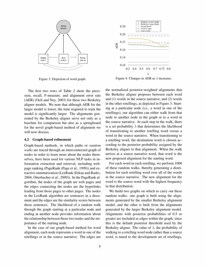
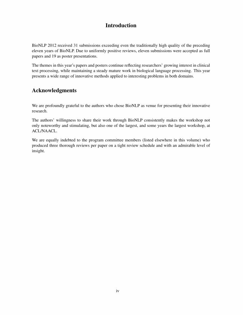
Figure 3: Depiction of word graph.
The first two rows of Table 2 show the preci-sion, recall, F-measure, and alignment error rate(AER) (Och and Ney, 2003) for these two Berkeleyaligner models. We note that although AER for thelarger model is lower, the time required to train themodel is significantly larger. The alignments gen-erated by the Berkeley aligner serve not only as abaseline for comparison but also as a springboardfor the novel graph-based method of alignment wewill now discuss.
4.2 Graph-based refinementGraph-based methods, in which paths or randomwalks are traced through an interconnected graph ofnodes in order to learn more about the nodes them-selves, have been used for various NLP tasks in in-formation extraction and retrieval, including web-page ranking (PageRank (Page et al., 1999)) and ex-tractive summarization (LexRank (Erkan and Radev,2004; Otterbacher et al., 2009)). In the PageRank al-gorithm, the nodes of the graph are web pages andthe edges connecting the nodes are the hyperlinksleading from those pages to other pages. The nodesin the LexRank algorithm are sentences in a docu-ment and the edges are the similarity scores betweenthose sentences. The likelihood of a random walkthrough the graph starting at a particular node andending at another node provides information aboutthe relationship between those two nodes and the im-portance of the starting node.
In the case of our graph-based method for wordalignment, each node represents a word in one of theretellings or in the source narrative. The edges are
Figure 4: Changes in AER as λ increases.
the normalized posterior-weighted alignments thatthe Berkeley aligner proposes between each wordand (1) words in the source narrative, and (2) wordsin the other retellings, as depicted in Figure 3. Start-ing at a particular node (i.e., a word in one of theretellings), our algorithm can either walk from thatnode to another node in the graph or to a word inthe source narrative. At each step in the walk, thereis a set probability λ that determines the likelihoodof transitioning to another retelling word versus aword in the source narrative. When transitioning toa retelling word, the destination word is chosen ac-cording to the posterior probability assigned by theBerkeley aligner to that alignment. When the walkarrives at a source narrative word, that word is thenew proposed alignment for the starting word.
For each word in each retelling, we perform 1000of these random walks, thereby generating a distri-bution for each retelling word over all of the wordsin the source narrative. The new alignment for theword is the source word with the highest frequencyin that distribution.
We build two graphs on which to carry out theserandom walks: one graph is built using the align-ments generated by the smaller Berkeley alignmentmodel, and the other is built from the alignmentsgenerated by the larger Berkeley alignment model.Alignments with posterior probabilities of 0.5 orgreater are included as edges within the graph, sincethis is the default posterior threshold used by theBerkeley aligner. The value of λ, the probability ofwalking to a retelling word node rather than a sourceword, is tuned to the development set of retellings,
5

Model P R F AERBerkeley-Small 72.1 79.6 75.6 24.5Berkeley-Large 78.6 80.5 79.5 20.5
Graph-Small 77.9 81.2 79.5 20.6Graph-Large 85.4 76.9 81.0 18.9
Table 2: Aligner performance comparison.
discussed in Section 3.3. Figure 4 shows how AERvaries according to the value of λ for the two graph-based approaches.
Each of these four alignment models produces,for each retelling, a set of word pairs containing oneword from the original narrative and one word fromthe retelling. The manual gold alignments for the235 experimental subjects were evaluated againstthe alignments produced by each of the four models.Table 2 shows the accuracy of word alignment us-ing these two graph-based models in terms of preci-sion, accuracy, F-measure, and alignment error rate,alongside the same measures for the two Berkeleymodels. We see that each of the graph-based modelsoutperforms the Berkeley model of the same size.The performance of the small graph-based model isespecially remarkable since it an AER comparableto the large Berkeley model while requiring signif-icantly fewer computing resources. The differencein processing time between the two approaches wasespecially remarkable: the graph-based model com-pleted in only a few minutes, while the large Berke-ley model required 14 hours of training.
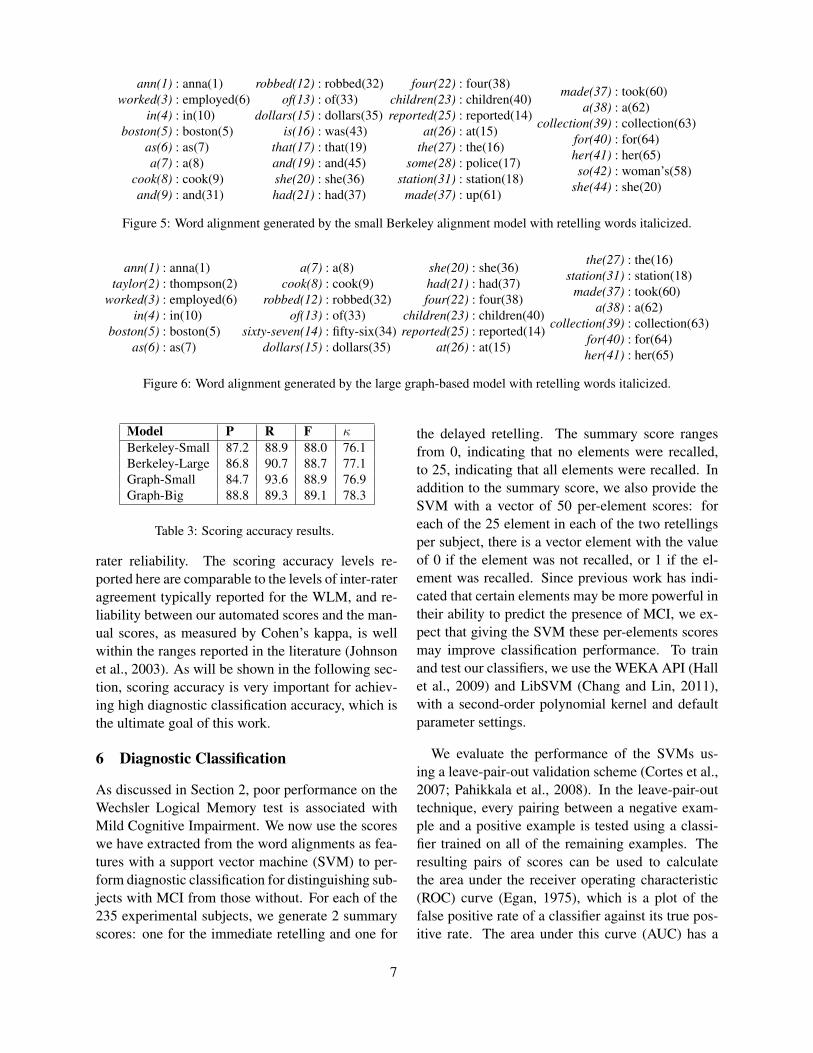
Figures 5 and 6 show the results of aligningthe retelling presented in Figure 2 using the smallBerkeley model and the large graph-based model,respectively. Comparing these two alignments, wesee that the latter model yields more precise align-ments with very little loss of recall, as is borne outby the overall statistics shown in Table 2.
5 Scoring
The published scoring guidelines for the WLM spec-ify the source words that compose each story ele-ment. Figure 7 displays the source narrative withthe element IDs (A− Y ) and word IDs (1− 65) ex-plicitly labeled. Element Q, for instance, consists ofthe words 39 and 40, small children. Using this in-formation, we extract scores from the alignments asfollows: for each word in the original narrative, if
[A anna1] [B thompson2] [C of3 south4][D boston5] [E employed6] [F as7 a8
cook9] [G in10 a11 school12] [H cafeteria13][I reported14] [J at15 the16 police17] [Kstation18] [L that19 she20 had21 been22 held23
up24] [M on25 state26 street27] [N the28
night29 before30] [O and31 robbed32 of33] [Pfifty-six34 dollars35] [Q she36 had37 four38][R small39 children40] [S the41 rent42 was43due44] [T and45 they46 had47 n’t48 eaten49][U for50 two51 days52] [V the53 police54] [Wtouched55 by56 the57 woman’s58 story59] [Xtook60 up61 a62 collection63] [Y for64 her65]
Figure 7: Text of Wechsler Logical Memory narrativewith story-element labeled bracketing and word IDs.
anna(1) : Athompson(2) : Bemployed(6) : E
boston(5) : Dcook(9) : F
robbed(32) : Ofifty-six(34) : P
four(38) : Qchildren(40) : Rreported(14) : I
station(18) : Ktook(60) : X
collection(63) : Xfor(64) : Yher(65) : Y
Figure 8: Source content words from the alignment inFigure 6 with corresponding story element IDs.
that word is aligned to a word in the retelling, thestory element that it is associated with is consideredto be recalled. Figure 8 shows the story elementsextracted from the word alignments in Figure 6.
When we convert alignments to scores in this way,any alignment can be mapped to an element, even analignment between function words such as the andof, which would be unlikely to indicate that the storyelement had been recalled. To avoid such scoring er-rors, we disregard any word-alignment pair contain-ing a source function word. The two exceptions tothis rule are the final two words, for her, which arenot content words but together make a single storyelement.
The element-level scores induced from the fourword alignments for all 235 experimental sub-jects were evaluated against the manual per-elementscores. We report the precision, recall, and f-measure for all four alignment models in Table 3. Inaddition, report Cohen’s kappa as a measure of reli-ability between our automated scores and the man-ually assigned scores. We see that as AER im-proves, scoring accuracy also improves, with thelarge graph-based model outperforming all othermodels in terms of precision, f-measure, and inter-
6
ann(1) : anna(1)worked(3) : employed(6)
in(4) : in(10)boston(5) : boston(5)
as(6) : as(7)a(7) : a(8)
cook(8) : cook(9)and(9) : and(31)
robbed(12) : robbed(32)of(13) : of(33)
dollars(15) : dollars(35)is(16) : was(43)
that(17) : that(19)and(19) : and(45)she(20) : she(36)had(21) : had(37)
four(22) : four(38)children(23) : children(40)reported(25) : reported(14)
at(26) : at(15)the(27) : the(16)
some(28) : police(17)station(31) : station(18)
made(37) : up(61)
made(37) : took(60)a(38) : a(62)
collection(39) : collection(63)for(40) : for(64)her(41) : her(65)so(42) : woman’s(58)
she(44) : she(20)
Figure 5: Word alignment generated by the small Berkeley alignment model with retelling words italicized.
ann(1) : anna(1)taylor(2) : thompson(2)
worked(3) : employed(6)in(4) : in(10)
boston(5) : boston(5)as(6) : as(7)
a(7) : a(8)cook(8) : cook(9)
robbed(12) : robbed(32)of(13) : of(33)
sixty-seven(14) : fifty-six(34)dollars(15) : dollars(35)
she(20) : she(36)had(21) : had(37)four(22) : four(38)
children(23) : children(40)reported(25) : reported(14)
at(26) : at(15)
the(27) : the(16)station(31) : station(18)
made(37) : took(60)a(38) : a(62)
collection(39) : collection(63)for(40) : for(64)her(41) : her(65)
Figure 6: Word alignment generated by the large graph-based model with retelling words italicized.
Model P R F κBerkeley-Small 87.2 88.9 88.0 76.1Berkeley-Large 86.8 90.7 88.7 77.1Graph-Small 84.7 93.6 88.9 76.9Graph-Big 88.8 89.3 89.1 78.3
Table 3: Scoring accuracy results.
rater reliability. The scoring accuracy levels re-ported here are comparable to the levels of inter-rateragreement typically reported for the WLM, and re-liability between our automated scores and the man-ual scores, as measured by Cohen’s kappa, is wellwithin the ranges reported in the literature (Johnsonet al., 2003). As will be shown in the following sec-tion, scoring accuracy is very important for achiev-ing high diagnostic classification accuracy, which isthe ultimate goal of this work.
6 Diagnostic Classification
As discussed in Section 2, poor performance on theWechsler Logical Memory test is associated withMild Cognitive Impairment. We now use the scoreswe have extracted from the word alignments as fea-tures with a support vector machine (SVM) to per-form diagnostic classification for distinguishing sub-jects with MCI from those without. For each of the235 experimental subjects, we generate 2 summaryscores: one for the immediate retelling and one for
the delayed retelling. The summary score rangesfrom 0, indicating that no elements were recalled,to 25, indicating that all elements were recalled. Inaddition to the summary score, we also provide theSVM with a vector of 50 per-element scores: foreach of the 25 element in each of the two retellingsper subject, there is a vector element with the valueof 0 if the element was not recalled, or 1 if the el-ement was recalled. Since previous work has indi-cated that certain elements may be more powerful intheir ability to predict the presence of MCI, we ex-pect that giving the SVM these per-elements scoresmay improve classification performance. To trainand test our classifiers, we use the WEKA API (Hallet al., 2009) and LibSVM (Chang and Lin, 2011),with a second-order polynomial kernel and defaultparameter settings.
We evaluate the performance of the SVMs us-ing a leave-pair-out validation scheme (Cortes et al.,2007; Pahikkala et al., 2008). In the leave-pair-outtechnique, every pairing between a negative exam-ple and a positive example is tested using a classi-fier trained on all of the remaining examples. Theresulting pairs of scores can be used to calculatethe area under the receiver operating characteristic(ROC) curve (Egan, 1975), which is a plot of thefalse positive rate of a classifier against its true pos-itive rate. The area under this curve (AUC) has a
7

Model Summ. (s.d.) Elem. (s.d.)Manual Scores 73.3 (3.76) 81.3 (3.32)Berkeley-Small 73.7 (3.74) 77.9 (3.52)Berkeley-Big 75.1 (3.67) 79.2 (3.45)Graph-Small 74.2 (3.71) 78.9 (3.47)Graph-Big 74.8 (3.69) 78.6 (3.49)
Table 4: Classification accuracy results (AUC).
value of 0.5 when the classifier performs at chanceand a value 1.0 when perfect classification accuracyis achieved.
Table 4 shows the classification results for thescores derived from the four alignment models alongwith the classification results using the examiner-assigned manual scores. It appears that, in all cases,the per-element scores are more effective than thesummary scores in classifying the two diagnosticgroups. In addition, we see that our automatedscores have classificatory power comparable to thatof the manual gold scores, and that as scoring ac-curacy increases from the small Berkeley model tothe graph-based models and bigger models, classifi-cation accuracy improves. This suggests both thataccurate scores are crucial for accurate classifica-tion and that pursuing even further improvements inword alignment is likely to result in improved di-agnostic differentiation. We note that although thelarge Berkeley model achieved the highest classi-fication accuracy, this very slight margin of differ-ence may not justify its significantly greater compu-tational requirements.
7 Conclusions and Future Work
The work presented here demonstrates the utilityof adapting techniques drawn from a diverse set ofNLP research areas to tasks in biomedicine. In par-ticular, the approach we describe for automaticallyanalyzing clinically elicited language data showspromise as part of a pipeline for a screening tool forMild Cognitive Impairment. Our novel graph-basedapproach to word alignment resulted in large reduc-tions in alignment error rate. These reductions in er-ror rate in turn led to human-level scoring accuracyand improved diagnostic classification.
As we have mentioned, the methods outlined hereare general enough to be used for other episodicrecall and description scenarios. Although the re-
sults are quite robust, several enhancements and im-provements should be made before we apply the sys-tem to other tasks. First, although we were able toachieve decent word alignment accuracy, especiallywith our graph-based approach, many alignment er-rors remain. As shown in Figure 4, the graph-basedalignment technique could potentially result in anAER of as low as 11%. We expect that our deci-sion to select as a new alignment the most frequentsource word over the distribution of source words atthe end of 1000 walks could be improved, since itdoes not allow for one-to-many mappings. In addi-tion, it would be worthwhile to experiment with sev-eral posterior thresholds, both during the decodingstep of the Berkeley aligner and in the graph edges.
In order to produce a viable clinical screeningtool, it is crucial that we incorporate speech recogni-tion in the pipeline. Our very preliminary investiga-tion into using ASR to generate transcripts for align-ment seems promising and surprisingly robust to theproblems that might be expected when working withnoisy audio. In our future work, we also plan to ex-amine longitudinal data for individual subjects to seewhether our techniques can detect subtle differencesin recall and coherence between a recent retellingand a series of earlier baseline retellings. Since themetric commonly used to quantify the progressionof dementia, the Clinical Dementia Rating, relies onobserved changes in cognitive function over time,longitudinal analysis of performance on the Wech-sler Logical Memory task may be the most promis-ing application for our research.
References
Regina Barzilay and Kathleen R. McKeown. 2001. Ex-tracting paraphrases from a parallel corpus. In Pro-ceeding of ACL.
D.A. Bennett, J.A. Schneider, Z. Arvanitakis, J.F. Kelly,N.T. Aggarwal, R.C. Shah, and R.S. Wilson. 2006.Neuropathology of older persons without cognitiveimpairment from two community-based studies. Neu-rology, 66:1837–844.
Nicola Botting. 2002. Narrative as a tool for the assess-ment of linguistic and pragmatic impairments. ChildLanguage Teaching and Therapy, 18(1).
Peter Brown, Vincent Della Pietra, Stephen Della Pietra,and Robert Mercer. 1993. The mathematics of statis-
8
tical machine translation: Parameter estimation. Com-putational Linguistics, 19(2):263–311.
Chih-Chung Chang and Chih-Jen Lin. 2011. LIBSVM:A library for support vector machines. ACM Transac-tions on Intelligent Systems and Technology, 2(27):1–27.
Corinna Cortes, Mehryar Mohri, and Ashish Rastogi.2007. An alternative ranking problem for search en-gines. In Proceedings of WEA2007, LNCS 4525,pages 1–21. Springer-Verlag.
Mona Diab and Philip Resnik. 2002. An unsupervisedmethod for word sense tagging using parallel corpora.In Proceedings of ACL.
Kristy Dodwell and Edith L. Bavin. 2008. Childrenwith specific language impair ment: an investigation oftheir narratives and memory. International Journal ofLanguage and Communication Disorders, 43(2):201–218.
John C. Dunn, Osvaldo P. Almeida, Lee Barclay, AnnaWaterreus, and Leon Flicker. 2002. Latent seman-tic analysis: A new method to measure prose recall.Journal of Clinical and Experimental Neuropsychol-ogy, 24(1):26–35.
James Egan. 1975. Signal Detection Theory and ROCAnalysis. Academic Press.
Gunes Erkan and Dragomir R. Radev. 2004. Lexrank:Graph-based lexical centrality as salience in text sum-marization. J. Artif. Intell. Res. (JAIR), 22:457–479.
M. Folstein, S. Folstein, and P. McHugh. 1975. Mini-mental state - a practical method for grading the cog-nitive state of patients for the clinician. Journal of Psy-chiatric Research, 12:189–198.
Keyur Gabani, Melissa Sherman, Thamar Solorio, andYang Liu. 2009. A corpus-based approach for theprediction of language impairment in monolingual En-glish and Spanish-English bilingual children. In Pro-ceedings of NAACL-HLT, pages 46–55.
Cheryl Glasgow and Judy Cowley. 1994. RenfrewBus Story test - North American Edition. CentrevilleSchool.
H Goodglass, E Kaplan, and B Barresi. 2001. BostonDiagnostic Aphasia Examination. 3rd ed. Pro-Ed.
Dilek Hakkani-Tur, Dimitra Vergyri, and Gokhan Tur.2010. Speech-based automated cognitive status as-sessment. In Proceedings of Interspeech, pages 258–261.
Mark Hall, Eibe Frank, Geoffrey Holmes, BernhardPfahringer, Peter Reutemann, and Ian H. Witten.2009. The WEKA data mining software: An update.SIGKDD Explorations, 11(1).
David K. Johnson, Martha Storandt, and David A. Balota.2003. Discourse analysis of logical memory recall innormal aging and in dementia of the alzheimer type.Neuropsychology, 17(1):82–92.
R.J. Kiernan, J. Mueller, J.W. Langston, and C. VanDyke. 1987. The neurobehavioral cognitive sta-tus examination, a brief but differentiated approach tocognitive assessment. Annals of Internal Medicine,107:481–485.
Marit Korkman, Ursula Kirk, and Sally Kemp. 1998.NEPSY: A developmental neuropsychological assess-ment. The Psychological Corporation.
Percy Liang, Ben Taskar, and Dan Klein. 2006. Align-ment by agreement. In Proceedings of HLT NAACL.
Catherine Lord, Michael Rutter, Pamela DiLavore, andSusan Risi. 2002. Autism Diagnostic ObservationSchedule (ADOS). Western Psychological Services.
John Morris. 1993. The clinical dementia rating(CDR): Current version and scoring rules. Neurology,43:2412–2414.
A Nordlund, S Rolstad, P Hellstrom, M Sjogren,S Hansen, and A Wallin. 2005. The goteborg mcistudy: mild cognitive impairment is a heterogeneouscondition. Journal of Neurology, Neurosurgery andPsychiatry, 76:1485–1490.
Franz Josef Och and Hermann Ney. 2003. A system-atic comparison of various statistical alignment mod-els. Computational Linguistics, 29(1):19–51.
Franz Josef Och, Christoph Tillmann, , and HermannNey. 2000. Improved alignment models for statisti-cal machine translation. In Proceedings of ACL, pages440–447.
Jahna Otterbacher, Gunes Erkan, and Dragomir R. Radev.2009. Biased lexrank: Passage retrieval using randomwalks with question-based priors. Inf. Process. Man-age., 45(1):42–54.
Lawrence Page, Sergey Brin, Rajeev Motwani, and TerryWinograd. 1999. The pagerank citation ranking:Bringing order to the web. Technical Report 1999-66, Stanford InfoLab, November. Previous number =SIDL-WP-1999-0120.
Tapio Pahikkala, Antti Airola, Jorma Boberg, and TapioSalakoski. 2008. Exact and efficient leave-pair-outcross-validation for ranking RLS. In Proceedings ofAKRR 2008, pages 1–8.
Ronald Peterson, Glenn Smith, Stephen Waring, RobertIvnik, Eric Tangalos, and Emre Kokmen. 1999. Mildcognitive impairment: Clinical characterizations andoutcomes. Archives of Neurology, 56:303–308.
Emily T. Prud’hommeaux and Brian Roark. 2011a.Alignment of spoken narratives for automated neu-ropsychological assessment. In Proceedings of ASRU.
Emily T. Prud’hommeaux and Brian Roark. 2011b. Ex-traction of narrative recall patterns for neuropsycho-logical assessment. In Proceedings of Interspeech.
Karen Ritchie and Jacques Touchon. 2000. Mild cogni-tive impairment: Conceptual basis and current noso-logical status. Lancet, 355:225–228.
9

Brian Roark, Margaret Mitchell, and Kristy Holling-shead. 2007. Syntactic complexity measures for de-tecting mild cognitive impairment. In Proceedings ofthe ACL 2007 Workshop on Biomedical Natural Lan-guage Processing (BioNLP), pages 1–8.
Brian Roark, Margaret Mitchell, John-Paul Hosom,Kristina Hollingshead, and Jeffrey Kaye. 2011. Spo-ken language derived measures for detecting mildcognitive impairment. IEEE Transactions on Audio,Speech and Language Processing, 19(7):2081–2090.
Kenji Sagae, Alon Lavie, and Brian MacWhinney. 2005.Automatic measurement of syntactic development inchild language. In Proceedings of ACL, pages 197–204.
Magnus Sahlgren and Jussi Karlgren. 2005. Automaticbilingual lexicon acquisition using random indexingof parallel corpora. Natural Language Engineering,11(3).
F.A. Schmitt, D.G. Davis, D.R. Wekstein, C.D. Smith,J.W. Ashford, and W.R. Markesbery. 2000. Preclini-cal ad revisited: Neuropathology of cognitively normalolder adults. Neurology, 55:370–376.
William R. Shankle, A. Kimball Romney, Junko Hara,Dennis Fortier, Malcolm B. Dick, James M. Chen,Timothy Chan, and Xijiang Sun. 2005. Methodsto improve the detection of mild cognitive impair-ment. Proceedings of the National Academy of Sci-ences, 102(13):4919–4924.
Martha Storandt and Robert Hill. 1989. Very mild seniledementia of the alzheimers type: Ii psychometric testperformance. Archives of Neurology, 46:383–386.
Helen Tager-Flusberg. 1995. Once upon a ribbit: Storiesnarrated by autistic children. British journal of devel-opmental psychology, 13(1):45–59.
David Wechsler. 1997. Wechsler Memory Scale - ThirdEdition Manual. The Psychological Corporation.
10

Proceedings of the 2012 Workshop on Biomedical Natural Language Processing (BioNLP 2012), pages 11–19,Montreal, Canada, June 8, 2012. c©2012 Association for Computational Linguistics
Bootstrapping Biomedical Ontologies for Scientific Text using NELL
Dana Movshovitz-AttiasCarnegie Mellon University
5000 Forbes AvenuePittsburgh, PA 15213 [email protected]
William W. CohenCarnegie Mellon University
5000 Forbes AvenuePittsburgh, PA 15213 [email protected]
Abstract
We describe an open information extractionsystem for biomedical text based on NELL(the Never-Ending Language Learner) (Carl-son et al., 2010), a system designed for ex-traction from Web text. NELL uses a cou-pled semi-supervised bootstrapping approachto learn new facts from text, given an initialontology and a small number of “seeds” foreach ontology category. In contrast to previ-ous applications of NELL, in our task the ini-tial ontology and seeds are automatically de-rived from existing resources. We show thatNELL’s bootstrapping algorithm is suscepti-ble to ambiguous seeds, which are frequent inthe biomedical domain. Using NELL to ex-tract facts from biomedical text quickly leadsto semantic drift. To address this problem, weintroduce a method for assessing seed qual-ity, based on a larger corpus of data derivedfrom the Web. In our method, seed qualityis assessed at each iteration of the bootstrap-ping process. Experimental results show sig-nificant improvements over NELL’s originalbootstrapping algorithm on two types of tasks:learning terms from biomedical categories,and named-entity recognition for biomedicalentities using a learned lexicon.
1 Introduction
NELL (the Never-Ending Language Learner) is asemi-supervised learning system, designed for ex-traction of information from the Web. The systemuses a coupled semi-supervised bootstrapping app-roach to learn new facts from text, given an initialontology and a small number of “seeds”, i.e., labeled
examples for each ontology category. The new factsare stored in a growing structured knowledge base.
One of the concerns about gathering data from theWeb is that it comes from various un-authoritativesources, and may not be reliable. This is especiallytrue when gathering scientific information. In con-trast to Web data, scientific text is potentially morereliable, as it is guided by the peer-review process.Open access scientific archives make this informa-tion available for all. In fact, the production rate ofpublicly available scientific data far exceeds the abil-ity of researchers to “manually” process it, and thereis a growing need for the automation of this process.
The biomedical field presents a great potential fortext mining applications. An integral part of life sci-ence research involves production and publication oflarge collections of data by curators, and as part ofcollaborative community effort. Prominent exam-ples include: publication of genomic sequence data,e.g., by the Human Genome Project; online col-lections of three-dimensional coordinates of proteinstructures; and databases holding data on genes. Animportant resource, initiated as a means of enforc-ing data standardization, are ontologies describingbiological, chemical and medical terms. These areheavily used by the research community. With thiswealth of available data the biomedical field holdsmany information extraction opportunities.
We describe an open information extraction sys-tem adapting NELL to the biomedical domain. Wepresent an implementation of our approach, namedBioNELL, which uses three main sources of infor-mation: (1) a public corpus of biomedical scientifictext, (2) commonly used biomedical ontologies, and
11
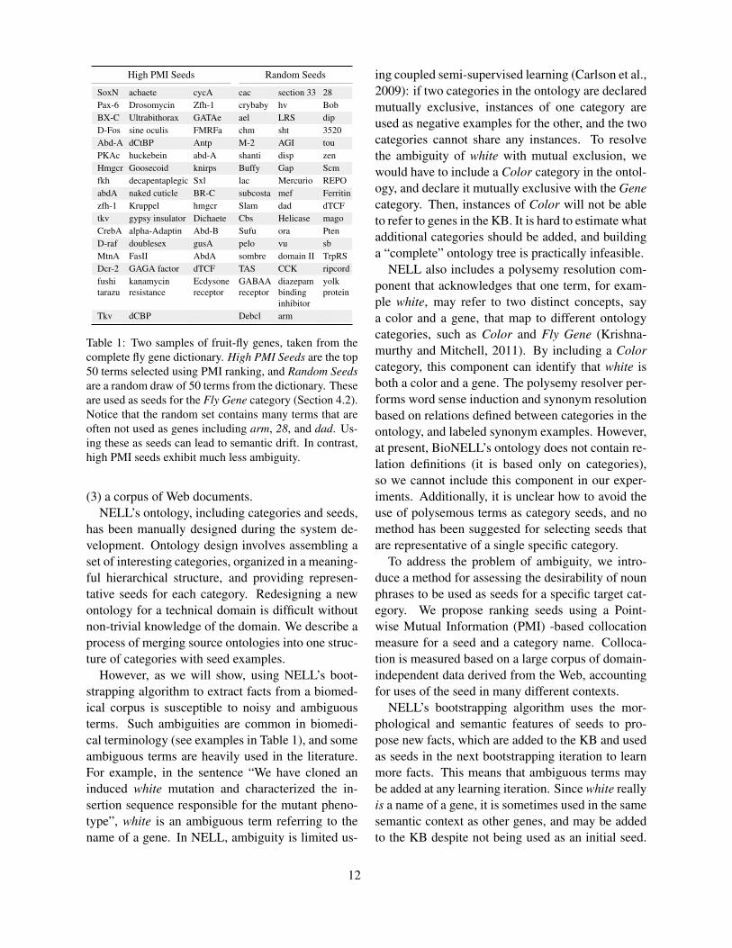
High PMI Seeds Random Seeds
SoxN achaete cycA cac section 33 28Pax-6 Drosomycin Zfh-1 crybaby hv BobBX-C Ultrabithorax GATAe ael LRS dipD-Fos sine oculis FMRFa chm sht 3520Abd-A dCtBP Antp M-2 AGI touPKAc huckebein abd-A shanti disp zenHmgcr Goosecoid knirps Buffy Gap Scmfkh decapentaplegic Sxl lac Mercurio REPOabdA naked cuticle BR-C subcosta mef Ferritinzfh-1 Kruppel hmgcr Slam dad dTCFtkv gypsy insulator Dichaete Cbs Helicase magoCrebA alpha-Adaptin Abd-B Sufu ora PtenD-raf doublesex gusA pelo vu sbMtnA FasII AbdA sombre domain II TrpRSDcr-2 GAGA factor dTCF TAS CCK ripcordfushitarazu
kanamycinresistance
Ecdysonereceptor
GABAAreceptor
diazepambindinginhibitor
yolkprotein
Tkv dCBP Debcl arm
Table 1: Two samples of fruit-fly genes, taken from thecomplete fly gene dictionary. High PMI Seeds are the top50 terms selected using PMI ranking, and Random Seedsare a random draw of 50 terms from the dictionary. Theseare used as seeds for the Fly Gene category (Section 4.2).Notice that the random set contains many terms that areoften not used as genes including arm, 28, and dad. Us-ing these as seeds can lead to semantic drift. In contrast,high PMI seeds exhibit much less ambiguity.
(3) a corpus of Web documents.NELL’s ontology, including categories and seeds,
has been manually designed during the system de-velopment. Ontology design involves assembling aset of interesting categories, organized in a meaning-ful hierarchical structure, and providing represen-tative seeds for each category. Redesigning a newontology for a technical domain is difficult withoutnon-trivial knowledge of the domain. We describe aprocess of merging source ontologies into one struc-ture of categories with seed examples.
However, as we will show, using NELL’s boot-strapping algorithm to extract facts from a biomed-ical corpus is susceptible to noisy and ambiguousterms. Such ambiguities are common in biomedi-cal terminology (see examples in Table 1), and someambiguous terms are heavily used in the literature.For example, in the sentence “We have cloned aninduced white mutation and characterized the in-sertion sequence responsible for the mutant pheno-type”, white is an ambiguous term referring to thename of a gene. In NELL, ambiguity is limited us-
ing coupled semi-supervised learning (Carlson et al.,2009): if two categories in the ontology are declaredmutually exclusive, instances of one category areused as negative examples for the other, and the twocategories cannot share any instances. To resolvethe ambiguity of white with mutual exclusion, wewould have to include a Color category in the ontol-ogy, and declare it mutually exclusive with the Genecategory. Then, instances of Color will not be ableto refer to genes in the KB. It is hard to estimate whatadditional categories should be added, and buildinga “complete” ontology tree is practically infeasible.
NELL also includes a polysemy resolution com-ponent that acknowledges that one term, for exam-ple white, may refer to two distinct concepts, saya color and a gene, that map to different ontologycategories, such as Color and Fly Gene (Krishna-murthy and Mitchell, 2011). By including a Colorcategory, this component can identify that white isboth a color and a gene. The polysemy resolver per-forms word sense induction and synonym resolutionbased on relations defined between categories in theontology, and labeled synonym examples. However,at present, BioNELL’s ontology does not contain re-lation definitions (it is based only on categories),so we cannot include this component in our exper-iments. Additionally, it is unclear how to avoid theuse of polysemous terms as category seeds, and nomethod has been suggested for selecting seeds thatare representative of a single specific category.
To address the problem of ambiguity, we intro-duce a method for assessing the desirability of nounphrases to be used as seeds for a specific target cat-egory. We propose ranking seeds using a Point-wise Mutual Information (PMI) -based collocationmeasure for a seed and a category name. Colloca-tion is measured based on a large corpus of domain-independent data derived from the Web, accountingfor uses of the seed in many different contexts.
NELL’s bootstrapping algorithm uses the mor-phological and semantic features of seeds to pro-pose new facts, which are added to the KB and usedas seeds in the next bootstrapping iteration to learnmore facts. This means that ambiguous terms maybe added at any learning iteration. Since white reallyis a name of a gene, it is sometimes used in the samesemantic context as other genes, and may be addedto the KB despite not being used as an initial seed.
12

To resolve this problem, we propose measuring seedquality in a Rank-and-Learn bootstrapping method-ology: after every iteration, we rank all the instancesthat have been added to the KB by their qualityas potential category seeds. Only high-ranking in-stances are used as seeds in the next iteration. Low-ranking instances are stored in the KB and “remem-bered” as true facts, but are not used for learningnew information. This is in contrast to NELL’s ap-proach (and most other bootstrapping systems), inwhich there is no distinction between acquired facts,and facts that are used for learning.
2 Related Work
Biomedical Information Extraction systems havetraditionally targeted recognition of few distinct bi-ological entities, focusing mainly on genes (e.g.,(Chang et al., 2004)). Few systems have been devel-oped for fact-extraction of many biomedical predi-cates, and these are relatively small scale (Wattaru-jeekrit et al., 2004), or they account for limited sub-domains (Dolbey et al., 2006). We suggest a moregeneral approach, using bootstrapping to extend ex-isting biomedical ontologies, including a wide rangeof sub-domains and many categories. The currentimplementation of BioNELL includes an ontologywith over 100 categories. To the best of our knowl-edge, such large-scale biomedical bootstrapping hasnot been done before.
Bootstrap Learning and Semantic Drift. Carl-son et al. (2010) use coupled semi-supervised boot-strap learning in NELL to learn a large set of cate-gory classifiers with high precision. One drawbackof using iterative bootstrapping is the sensitivity ofthis method to the set of initial seeds (Pantel et al.,2009). An ambiguous set of seeds can lead to se-mantic drift, i.e., accumulation of erroneous termsand contexts when learning a semantic class. Strictbootstrapping environments reduce this problem byadding boundaries or limiting the learning process,including learning mutual terms and contexts (Riloffand Jones, 1999) and using mutual exclusion andnegative class examples (Curran et al., 2007).
McIntosh and Curran (2009) propose a metricfor measuring the semantic drift introduced by alearned term, favoring terms different than the recentm learned terms and similar to the first n, (shown
for n=20 and n=100), following the assumption thatsemantic drift develops in late bootstrapping itera-tions. As we will show, for biomedical categories,semantic drift in NELL occurs within a handful ofiterations (< 5), however according to the authors,using low values for n produces inadequate results.In fact, selecting effective n and m parameters maynot only be a function of the data being used, butalso of the specific category, and it is unclear how toautomatically tune them.
Seed Set Refinement. Vyas et al. (2009) suggesta method for reducing ambiguity in seeds providedby human experts, by selecting the tightest seedclusters based on context similarity. The method isdescribed for an order of 10 seeds, however, in anontology containing hundreds of seeds per class, it isunclear how to estimate the correct number of clus-ters to choose from. Another approach, suggestedby Kozareva et al. (2010), is using only constrainedcontexts where both seed and class are present in asentence. Extending this idea, we consider a moregeneral collocation metric, looking at entire docu-ments including both the seed and its category.
3 Implementation
3.1 NELL’s Bootstrapping System
We have implemented BioNELL based on the sys-tem design of NELL. NELL’s bootstrapping algo-rithm is initiated with an input ontology structure ofcategories and seeds. Three sub-components oper-ate to introduce new facts based on the semantic andmorphological attributes of known facts. At everyiteration, each component proposes candidate facts,specifying the supporting evidence for each candi-date, and the candidates with the most strongly sup-ported evidence are added to the KB. The processand sub-components are described in detail by Carl-son et al. (2010) and Wang and Cohen (2009).
3.2 Text Corpora
PubMed Corpus: We used a corpus of 200K full-text biomedical articles taken from the PubMedCentral Open Access Subset (extracted in October2010)1, which were processed using the OpenNLPpackage2. This is the main BioNELL corpus and it
1http://www.ncbi.nlm.nih.gov/pmc/2http://opennlp.sourceforge.net
13

is used to extract category instances in all the exper-iments presented in this paper.
Web Corpus: BioNELL’s seed-quality colloca-tion measure (Section 3.4) is based on a domain-independent Web corpus, the English portion of theClueWeb09 data set (Callan and Hoy, 2009), whichincludes 500 million web documents.
3.3 OntologyBioNELL’s ontology is composed of six base on-tologies, covering a wide range of biomedical sub-domains: the Gene Ontology (GO) (Ashburner etal., 2000), describing gene attributes; the NCBI Tax-onomy for model organisms (Sayers et al., 2009);Chemical Entities of Biological Interest (ChEBI)(Degtyarenko et al., 2008), a dictionary focused onsmall chemical compounds; the Sequence Ontol-ogy (Eilbeck et al., 2005), describing biological se-quences; the Cell Type Ontology (Bard et al., 2005);and the Human Disease Ontology (Osborne et al.,2009). Each ontology provides a hierarchy of termsbut does not distinguish concepts from instances.
We used an automatic process for merging baseontologies into one ontology tree. First, we groupthe ontologies under one hierarchical structure, pro-ducing a tree of over 1 million entities, including856K terms and 154K synonyms. We then separatethese into potential categories and potential seeds.Categories are nodes that are unambiguous (have asingle parent in the ontology tree), with at least 100descendants. These descendants are the category’sPotential seeds. This results in 4188 category nodes.In the experiments of this paper we selected onlythe top (most general) 20 categories in the tree ofeach base ontology. We are left with 109 final cate-gories, as some base ontologies had less than 20 cat-egories under these restrictions. Leaf categories aregiven seeds from their descendants in the full tree ofall terms and synonyms, giving a total of around 1million potential seeds. Seed set refinement is de-scribed below. The seeds of leaf categories are laterextended by the bootstrapping process.
3.4 BioNELL’s Bootstrapping System3.4.1 PMI Collocation with the Category Name
We define a seed quality metric based on a largecorpus of Web data. Let s and c be a seed and a tar-get category, respectively. For example, we can take
s = “white”, the name of a gene of the fruit-fly, and c= “fly gene”. Now, let D be a document corpus (Sec-tion 3.2 describes the Web corpus used for ranking),and let Dc be a subset of the documents contain-ing a mention of the category name. We measurethe collocation of the seed and the category by thenumber of times s appears in Dc, |Occur(s, Dc)|.The overall occurrence of s in the corpus is givenby |Occur(s, D)|. Following the formulation ofChurch and Hanks (1990), we compute the PMI-rank of s and c as
PMI(s, c) =|Occur(s, Dc)||Occur(s, D)|
(1)
Since this measure is used to compare seeds of thesame category, we omit the log from the original for-mulation. In our example, as white is a highly am-biguous gene name, we find that it appears in manydocuments that do not discuss the fruit fly, resultingin a PMI rank close to 0.
The proposed ranking is sensitive to the descrip-tive name given to categories. For a more robustranking, we use a combination of rankings of theseed with several of its ancestors in the ontology hi-erarchy. In (Movshovitz-Attias and Cohen, 2012)we describe this hierarchical ranking in more detailand additionally explore the use of the binomial log-likelihood ratio test (BLRT) as an alternative collo-cation measure for ranking.
We further note that some specialized biomedicalterms follow strict nomenclature rules making themeasily identifiable as category specific. These termsmay not be frequent in general Web context, lead-ing to a low PMI rank under the proposed method.Given such a set of high confidence seeds from areliable source, one can enforce their inclusion inthe learning process, and specialized seeds can addi-tionally be identified by high-confidence patterns, ifsuch exist. However, the scope of this work involvesselecting seeds from an ambiguous source, biomed-ical ontologies, thus we do not include an analysisfor these specialized cases.
3.4.2 Rank-and-Learn BootstrappingWe incorporate PMI ranking into BioNELL using
a Rank-and-Learn bootstrapping methodology. Af-ter every iteration, we rank all the instances that havebeen added to the KB. Only high-ranking instances
14
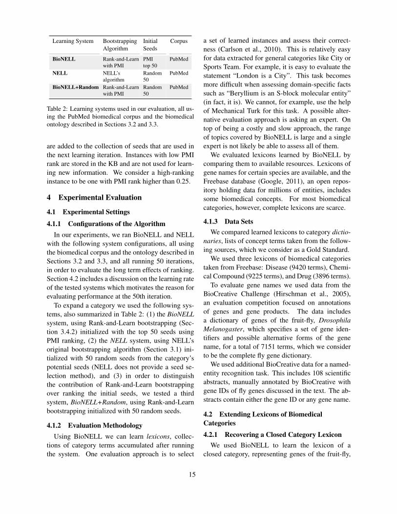
Learning System BootstrappingAlgorithm
InitialSeeds
Corpus
BioNELL Rank-and-Learnwith PMI
PMItop 50
PubMed
NELL NELL’salgorithm
Random50
PubMed
BioNELL+Random Rank-and-Learnwith PMI
Random50
PubMed
Table 2: Learning systems used in our evaluation, all us-ing the PubMed biomedical corpus and the biomedicalontology described in Sections 3.2 and 3.3.
are added to the collection of seeds that are used inthe next learning iteration. Instances with low PMIrank are stored in the KB and are not used for learn-ing new information. We consider a high-rankinginstance to be one with PMI rank higher than 0.25.
4 Experimental Evaluation
4.1 Experimental Settings
4.1.1 Configurations of the AlgorithmIn our experiments, we ran BioNELL and NELL
with the following system configurations, all usingthe biomedical corpus and the ontology described inSections 3.2 and 3.3, and all running 50 iterations,in order to evaluate the long term effects of ranking.Section 4.2 includes a discussion on the learning rateof the tested systems which motivates the reason forevaluating performance at the 50th iteration.
To expand a category we used the following sys-tems, also summarized in Table 2: (1) the BioNELLsystem, using Rank-and-Learn bootstrapping (Sec-tion 3.4.2) initialized with the top 50 seeds usingPMI ranking, (2) the NELL system, using NELL’soriginal bootstrapping algorithm (Section 3.1) ini-tialized with 50 random seeds from the category’spotential seeds (NELL does not provide a seed se-lection method), and (3) in order to distinguishthe contribution of Rank-and-Learn bootstrappingover ranking the initial seeds, we tested a thirdsystem, BioNELL+Random, using Rank-and-Learnbootstrapping initialized with 50 random seeds.
4.1.2 Evaluation MethodologyUsing BioNELL we can learn lexicons, collec-
tions of category terms accumulated after runningthe system. One evaluation approach is to select
a set of learned instances and assess their correct-ness (Carlson et al., 2010). This is relatively easyfor data extracted for general categories like City orSports Team. For example, it is easy to evaluate thestatement “London is a City”. This task becomesmore difficult when assessing domain-specific factssuch as “Beryllium is an S-block molecular entity”(in fact, it is). We cannot, for example, use the helpof Mechanical Turk for this task. A possible alter-native evaluation approach is asking an expert. Ontop of being a costly and slow approach, the rangeof topics covered by BioNELL is large and a singleexpert is not likely be able to assess all of them.
We evaluated lexicons learned by BioNELL bycomparing them to available resources. Lexicons ofgene names for certain species are available, and theFreebase database (Google, 2011), an open repos-itory holding data for millions of entities, includessome biomedical concepts. For most biomedicalcategories, however, complete lexicons are scarce.
4.1.3 Data SetsWe compared learned lexicons to category dictio-
naries, lists of concept terms taken from the follow-ing sources, which we consider as a Gold Standard.
We used three lexicons of biomedical categoriestaken from Freebase: Disease (9420 terms), Chemi-cal Compound (9225 terms), and Drug (3896 terms).
To evaluate gene names we used data from theBioCreative Challenge (Hirschman et al., 2005),an evaluation competition focused on annotationsof genes and gene products. The data includesa dictionary of genes of the fruit-fly, DrosophilaMelanogaster, which specifies a set of gene iden-tifiers and possible alternative forms of the genename, for a total of 7151 terms, which we considerto be the complete fly gene dictionary.
We used additional BioCreative data for a named-entity recognition task. This includes 108 scientificabstracts, manually annotated by BioCreative withgene IDs of fly genes discussed in the text. The ab-stracts contain either the gene ID or any gene name.
4.2 Extending Lexicons of BiomedicalCategories
4.2.1 Recovering a Closed Category LexiconWe used BioNELL to learn the lexicon of a
closed category, representing genes of the fruit-fly,
15

10 20 30 40 500
0.2
0.4
0.6
0.8
1
Iteration
Prec
isio
n
BioNELLNELLBioNELL+Random
(a) Precision
10 20 30 40 500
50
100
150
200
250
Iteration
Cum
ulat
ive
corre
ct le
xico
n ite
ms
BioNELLNELLBioNELL+Random
(b) Cumulative correct items
10 20 30 40 500
100
200
300
400
500
Iteration
Cum
ulat
ive
inco
rrect
lexi
con
item
s
BioNELLNELLBioNELL+Random
(c) Cumulative incorrect items
Figure 1: Performance per learning iteration for gene lexicons learned using BioNELL and NELL.
Learning System Precision Correct Total
BioNELL .83 109 132NELL .29 186 651BioNELL+Random .73 248 338
NELL by size 132 .72 93 130
Table 3: Precision, total number of instances (Total),and correct instances (Correct) of gene lexicons learnedwith BioNELL and NELL. BioNELL significantly im-proves the precision of the learned lexicon compared withNELL. When examining only the first 132 learned items,BioNELL has both higher precision and more correct in-stances than NELL (last row, NELL by size 132).
D. Melanogaster, a model organism used to studygenetics and developmental biology. Two samplesof genes from the full fly gene dictionary are shownin Table 1: High PMI Seeds are the top 50 dictio-nary terms selected using PMI ranking, and RandomSeeds are a random draw of 50 terms. Notice that therandom set contains many seeds that are not distinctgene names including arm, 28, and dad. In con-trast, high PMI seeds exhibit much less ambiguity.We learned gene lexicons using the test systems de-scribed in Section 4.1.1 with the high-PMI and ran-dom seed sets shown in Table 1. We measured theprecision, total number of instances, and correct in-stances of the learned lexicons against the full dic-tionary of genes. Table 3 summarizes the results.
BioNELL, initialized with PMI-ranked seeds, sig-nificantly improved the precision of the learnedlexicon over NELL (29% for NELL to 83% forBioNELL). In fact, the two learning systems us-ing Rank-and-Learn bootstrapping resulted in higherprecision lexicons (83%, 73%), suggesting that con-
strained bootstrapping using iterative seed rankingsuccessfully eliminates noisy and ambiguous seeds.
BioNELL’s bootstrapping methodology is highlyrestrictive and it affects the size of the learned lexi-con as well as its precision. Notice, however, thatwhile NELL’s final lexicon is 5 times larger thanBioNELL’s, the number of correctly learned items init are less than twice that of BioNELL. Additionally,BioNELL+Random has learned a smaller dictionarythan NELL (338 and 651 terms, respectively) with agreater number of correct instances (248 and 186).
We examined the performance of NELL after the7th iteration, when it has learned a lexicon of 130items, similar in size to BioNELL’s final lexicon (Ta-ble 3, last row). After learning 130 items, BioNELLachieved both higher precision (83% versus 72%)and higher recall (109 versus 93 correct lexiconinstances) than NELL, indicating that BioNELL’slearning method is overall more accurate.
After running for 50 iterations, all systems re-cover only a small portion of the complete gene dic-tionary (109-248 instances out of 7151), suggestingeither that, (1) more learning iterations are required,(2) the biomedical corpus we use is too small anddoes not contain (frequent) mentions of some genenames from the dictionary, or (3) some other limita-tions exist that prevent the learning algorithm fromfinding additional class examples.
Lexicons learned using BioNELL show persis-tently high precision throughout the 50 iterations,even when initiated with random seeds (Figure 1A).By the final iteration, all systems stop accumulatingfurther significant amounts of correct gene instances(Figure 1B). Systems that use PMI-based Rank-and-Learn bootstrapping also stop learning incorrect
16

Learning System Precision Correct Total
CC Drug Disease CC Drug Disease CC Drug Disease
BioNELL .66 .52 .43 63 508 276 96 972 624NELL .15 .40 .37 74 522 288 449 1300 782
NELL by size .58 .47 .37 58 455 232 100 968 623
Table 4: Precision, total number of instances (Total), and correct instances (Correct) of learned lexicons of ChemicalCompound (CC), Drug, and Disease. BioNELL’s lexicons have higher precision on all categories compared withNELL, while learning a similar number of correct instances. When restricting NELL to a total lexicon size similar toBioNELL’s, BioNELL has both higher precision and more correct instances (last row, NELL by size).
instances (BioNELL and BioNELL+Random; Fig-ure 1C). This is in contrast to NELL which continueslearning incorrect examples.
Interestingly, the highest number of correct geneinstances was learned using Rank-and-Learn boot-strapping with random initial seeds (248 items;BioNELL+Random). This may happen when therandom set includes genes that are infrequent inthe general Web corpus, despite being otherwisecategory-specific in the biomedical context. Assuch, these would result in low PMI rank (see notein Section 3.4.1). However, random seed selectiondoes not offer any guarantees on the quality of theseeds used, and therefore will result in unstable per-formance. Note that BioNELL+Random was initi-ated with the same random seeds as NELL, but dueto the more constrained Rank-and-Learn bootstrap-ping it achieves both higher recall (248 versus 186correct instances) and precision (73% versus 29%).
4.2.2 Extending Lexicons of Open Categories
We evaluated learned lexicons for three open cat-egories, Chemical Compound (CC), Drug, and Dis-ease, using dictionaries from Freebase. Since theseare open categories — new drugs are being devel-oped every year, new diseases are discovered, andvaried chemical compounds can be created — theFreebase dictionaries are not likely to contain com-plete information on these categories. For our evalu-ation, however, we considered them to be complete.
We used BioNELL and NELL to learn these cat-egories, and for all of them BioNELL’s lexiconsachieved higher precision than NELL (Table 4). Thenumber of correct learned instances was similar inboth systems (63 and 74 for CC, 508 and 522 forDrug, and 276 and 288 for Disease), however in
BioNELL, the additional bootstrapping restrictionsassist in rejecting incorrect instances, resulting in asmaller, more accurate lexicon.
We examined NELL’s lexicons when they reacheda size similar to BioNELL’s final lexicons (at the 8th,42nd and 39th iterations for CC, Drug, and Disease,respectively). BioNELL’s lexicons have both higherprecision and higher recall (more correct learned in-stances) than the comparable NELL lexicons (Ta-ble 4, NELL by size, last row).
4.3 Named-Entity Recognition using aLearned Lexicon
We examined the use of gene lexicons learned withBioNELL and NELL for the task of recognizingconcepts in free text, using a simple strategy ofmatching words in the text with terms from the lex-icon. We use data from the BioCreative challenge(Section 4.1.3), which includes text abstracts and theIDs of genes that appear in each abstract. We showthat BioNELL’s lexicon achieves both higher preci-sion and recall in this task than NELL’s.
We implemented an annotator for predicting whatgenes are discussed in text, which uses a gene lexi-con as input. Given sample text, if any of the termsin the lexicon appear in the text, the correspondinggene is predicted to be discussed in the text. Follow-ing BioCreative’s annotation format, the annotatoremits as output the set of gene IDs of the genes pre-dicted for the sample text.
We evaluated annotators that were given as in-put: the complete fly-genes dictionary, a filteredversion of that dictionary, or lexicons learned us-ing BioNELL and NELL. Using these annotators wepredicted gene mentions for all text abstracts in thedata. We report the average precision (over 108 text
17

Lexicon Precision Correct Total
BioNELL .90 18 20NELL .02 5 268BioNELL+Random .03 3 82
Complete Dictionary .09 153 1616Filtered Dictionary .18 138 675
Table 5: Precision, total number of predicted genes (To-tal), and correct predictions (Correct), in a named-entityrecognition task using a complete lexicon, a filtered lex-icon, and lexicons learned with BioNELL and NELL.BioNELL’s lexicon achieves the highest precision, andmakes more correct predictions than NELL.
abstracts) and number of total and correct predic-tions of gene mentions, compared with the labeledannotations for each text (Table 5).
Many gene names are shared among multiplevariants. For example, the name Antennapedia mayrefer to several gene variations, e.g., Dgua\Antp orDmed\Antp. Thus, in our precision measurements,we consider a prediction of a gene ID as “true” if itis labeled as such by BioCreative, or if it shares asynonym name with another true labeled gene ID.
First, we used the complete fly gene dictionaryfor the recognition task. Any dictionary gene thatis mentioned in the text was recovered, resultingin high recall. However, the full dictionary con-tains ambiguous gene names that contribute manyfalse predictions to the complete dictionary annota-tor, leading to a low precision of 9%.
Some ambiguous terms can be detected usingsimple rules, e.g., short abbreviations and numbers.For example, section 9 is a gene named after thefunctional unit to which it belongs, and abbreviatedby the symbol 9. Clearly, removing 9 from the fulllexicon should improve precision without great costto recall. We similarly filtered the full dictionary, re-moving one- and two-letter abbreviations and termscomposed only of non-alphabetical characters, leav-ing 6253 terms. Using the filtered dictionary, pre-cision has doubled (18%) with minor compromiseto recall. Using complete or manually refined genedictionaries for named-entity recognition has beenshown before to produce similar high-recall andlow-precision results (Bunescu et al., 2005).
We evaluated annotators on gene lexicons learnedwith BioNELL and NELL. BioNELL’s lexicon
achieved significantly higher precision (90%) thanother lexicons (2%-18%). It is evident that this lexi-con contains few ambiguous terms as it leads to only2 false predictions. Note also, that BioNELL’s lexi-con has both higher precision and recall than NELL.
5 Conclusions
We have proposed a methodology for an open infor-mation extraction system for biomedical scientifictext, using an automatically derived ontology of cat-egories and seeds. Our implementation is based onconstrained bootstrapping in which seeds are rankedat every iteration.
The benefits of iterative seed ranking have beendemonstrated, showing that our method leads to sig-nificantly less ambiguous lexicons for all the eval-uated biomedical concepts. BioNELL shows 51%increase over NELL in the precision of a learnedlexicon of chemical compounds, and 45% increasefor a category of gene names. Importantly, whenBioNELL and NELL learn lexicons of similar size,BioNELL’s lexicons have both higher precision andrecall. We have demonstrated the use of BioNELL’slearned gene lexicon as a high precision annotatorin an entity recognition task (with 90% precision).The results are promising, though it is currently dif-ficult to provide a similar quantitative evaluation fora wider range of concepts.
Many interesting improvements could be madein the current system, mainly discovery of relationsbetween existing ontology categories. In addition,we believe that Rank-and-Learn bootstrapping anditerative seed ranking can be beneficial in general,domain-independent settings, and we would like toexplore further use of this method.
Acknowledgments
This work was funded by grant 1R101GM081293from NIH, IIS-0811562 from NSF and by a gift fromGoogle. The opinions expressed in this paper aresolely those of the authors.
ReferencesM. Ashburner, C.A. Ball, J.A. Blake, D. Botstein, H. But-
ler, J.M. Cherry, A.P. Davis, K. Dolinski, S.S. Dwight,J.T. Eppig, et al. 2000. Gene ontology: tool for theunification of biology. Nature genetics, 25(1):25.
18

J. Bard, S.Y. Rhee, and M. Ashburner. 2005. An ontol-ogy for cell types. Genome Biology, 6(2):R21.
R. Bunescu, R. Ge, R.J. Kate, E.M. Marcotte, and R.J.Mooney. 2005. Comparative experiments on learninginformation extractors for proteins and their interac-tions. Artificial Intelligence in Medicine, 33(2).
J. Callan and M. Hoy. 2009. Clueweb09 data set.http://boston.lti.cs.cmu.edu/Data/clueweb09/.
A. Carlson, J. Betteridge, E.R. Hruschka Jr, T.M.Mitchell, and SP Sao Carlos. 2009. Coupling semi-supervised learning of categories and relations. Semi-supervised Learning for Natural Language Process-ing, page 1.
A. Carlson, J. Betteridge, B. Kisiel, B. Settles, E.R. Hr-uschka Jr, and T.M. Mitchell. 2010. Toward an ar-chitecture for never-ending language learning. In Pro-ceedings of the Twenty-Fourth Conference on ArtificialIntelligence (AAAI 2010), volume 2, pages 3–3.
J.T. Chang, H. Schutze, and R.B. Altman. 2004. Gap-score: finding gene and protein names one word at atime. Bioinformatics, 20(2):216.
K.W. Church and P. Hanks. 1990. Word associationnorms, mutual information, and lexicography. Com-putational linguistics, 16(1):22–29.
J.R. Curran, T. Murphy, and B. Scholz. 2007. Minimis-ing semantic drift with mutual exclusion bootstrap-ping. In Proceedings of the 10th Conference of thePacific Association for Computational Linguistics.
K. Degtyarenko, P. De Matos, M. Ennis, J. Hastings,M. Zbinden, A. McNaught, R. Alcantara, M. Darsow,M. Guedj, and M. Ashburner. 2008. Chebi: a databaseand ontology for chemical entities of biological inter-est. Nucleic acids research, 36(suppl 1):D344.
A. Dolbey, M. Ellsworth, and J. Scheffczyk. 2006.Bioframenet: A domain-specific framenet extensionwith links to biomedical ontologies. In Proceedingsof KR-MED, pages 87–94. Citeseer.
K. Eilbeck, S.E. Lewis, C.J. Mungall, M. Yandell,L. Stein, R. Durbin, and M. Ashburner. 2005. The se-quence ontology: a tool for the unification of genomeannotations. Genome biology, 6(5):R44.
Google. 2011. Freebase data dumps.http://download.freebase.com/datadumps/.
L. Hirschman, A. Yeh, C. Blaschke, and A. Valencia.2005. Overview of biocreative: critical assessment ofinformation extraction for biology. BMC bioinformat-ics, 6(Suppl 1):S1.
Z. Kozareva and E. Hovy. 2010. Not all seeds are equal:measuring the quality of text mining seeds. In HumanLanguage Technologies: The 2010 Annual Conferenceof the North American Chapter of the Association forComputational Linguistics, pages 618–626. Associa-tion for Computational Linguistics.
J. Krishnamurthy and T.M. Mitchell. 2011. Which nounphrases denote which concepts? In Proceedings of the49th Annual Meeting of the Association for Compu-tational Linguistics: Human Language Technologies.Association for Computational Linguistics.
T. McIntosh and J.R. Curran. 2009. Reducing seman-tic drift with bagging and distributional similarity. InProceedings of the Joint Conference of the 47th An-nual Meeting of the ACL and the 4th InternationalJoint Conference on Natural Language Processing ofthe AFNLP: Volume 1-Volume 1, pages 396–404. As-sociation for Computational Linguistics.
D. Movshovitz-Attias and W.W. Cohen. 2012. Boot-strapping biomedical ontologies for scientific text us-ing nell. Technical report, Carnegie Mellon Univer-sity, CMU-ML-12-101.
J. Osborne, J. Flatow, M. Holko, S. Lin, W. Kibbe,L. Zhu, M. Danila, G. Feng, and R. Chisholm. 2009.Annotating the human genome with disease ontology.BMC genomics, 10(Suppl 1):S6.
P. Pantel, E. Crestan, A. Borkovsky, A.M. Popescu, andV. Vyas. 2009. Web-scale distributional similarity andentity set expansion. In Proceedings of the 2009 Con-ference on Empirical Methods in Natural LanguageProcessing: Volume 2-Volume 2, pages 938–947. As-sociation for Computational Linguistics.
E. Riloff and R. Jones. 1999. Learning dictionaries forinformation extraction by multi-level bootstrapping.In Proceedings of the National Conference on Artifi-cial Intelligence (AAAI-99), pages 474–479.
E. W. Sayers, T. Barrett, D. A. Benson, S. H. Bryant,K. Canese, V. Chetvernin, D. M. Church, M. DiCuc-cio, R. Edgar, S. Federhen, M. Feolo, L. Y. Geer,W. Helmberg, Y. Kapustin, D. Landsman, D. J.Lipman, T. L. Madden, D. R. Maglott, V. Miller,I. Mizrachi, J. Ostell, K. D. Pruitt, G. D. Schuler,E. Sequeira, S. T. Sherry, M. Shumway, K. Sirotkin,A. Souvorov, G. Starchenko, T. A. Tatusova, L. Wag-ner, E. Yaschenko, and J. Ye. 2009. Database re-sources of the National Center for Biotechnology In-formation. Nucleic Acids Res., 37:5–15, Jan.
V. Vyas, P. Pantel, and E. Crestan. 2009. Helping edi-tors choose better seed sets for entity set expansion. InProceeding of the 18th ACM conference on Informa-tion and knowledge management. ACM.
R.C. Wang and W.W. Cohen. 2009. Character-level anal-ysis of semi-structured documents for set expansion.In Proceedings of the 2009 Conference on EmpiricalMethods in Natural Language Processing: Volume 3-Volume 3, pages 1503–1512. Association for Compu-tational Linguistics.
T. Wattarujeekrit, P. Shah, and N. Collier. 2004. Pasbio:predicate-argument structures for event extraction inmolecular biology. BMC bioinformatics, 5(1):155.
19

Proceedings of the 2012 Workshop on Biomedical Natural Language Processing (BioNLP 2012), pages 20–28,Montreal, Canada, June 8, 2012. c©2012 Association for Computational Linguistics
Semantic distance and terminology structuring methods for thedetection of semantically close terms
Marie DupuchCNRS UMR 8163 STL
Universite Lille 1&359653 Villeneuve d’Ascq, France
Laetitia DupuchUniversite Toulouse III Paul Sabatier
Thierry HamonLIM&BIO (EA3969) UFR SMBH
Universite Paris 13, [email protected]
Natalia GrabarCNRS UMR 8163 STL
Universite Lille 1&359653 Villeneuve d’Ascq, France
The identification of semantically similar lin-guistic expressions despite their formal differ-ence is an important task within NLP appli-cations (information retrieval and extraction,terminology structuring...) We propose to de-tect the semantic relatedness between biomed-ical terms from the pharmacovigilance area.Two approaches are exploited: semantic dis-tance within structured resources and termi-nology structuring methods applied to a rawlist of terms. We compare these methods andstudy their complementarity. The results areevaluated against the reference pharmacovigi-lance data and manually by an expert.
1 Introduction
When an automatic system is able to identify thatdifferent linguistic expressions convey the same orsimilar meanings, this is a positive point for severalapplications. For instance, when documents refer-ring to muscle pain or cephalgia are searched, in-formation retrieval system can also take advantageof the synonyms, like muscle ache or headache, toreturn more relevant documents and in this way toincrease the recall. This is also a great advantagefor systems designed for instance for text mining,terminology structuring and alignment, or for morespecific tasks such as pharmacovigilance.
The pharmacovigilance area covers the identifi-cation of adverse drug reactions (ADRs) in orderto improve the vigilance on the health products.Pharmacovigilance reports are traditionally encodedwith normalised terms from the dedicated termi-nologies, such as MedDRA (Medical Dictionary for
Drug Regulatory Activities) (Brown et al., 1999).MedDRA is a relatively fine-grained terminologywith nearly 90,000 terms. This means that a givenpharmacovigilance report can be coded with dif-ferent terms which have close meaning (Feschareket al., 2004), like muscle pain and muscle ache orheadache and cephalgia: although formally differ-ent the terms from these pairs have the same mean-ing. The difficulty is then to detect their semanticcloseness. Indeed, if this semantic information isavailable, reports from the phramacovigilance data-banks and mentionning similar adverse events canbe aggregated: the safety signal is intensified andthe safety regulation process is improved.
In order to aggregate the pharmacovigilance re-ports, several types of semantic information fromMedDRA are used: (1) different hierarchical levelsof MedDRA between the five levels available; (2)the SMQs (Standardized MedDRA Queries) whichgroup together terms associated to a given medicalcondition such as Acute renal failure, Angioedemaor Embolic and thrombotic events; and (3) specificresources (Bousquet et al., 2005; Iavindrasana et al.,2006; Alecu et al., 2008; Jaulent and Alecu, 2009).The SMQs are defined by groups of experts througha long and meticulous work consisting of the man-ual study of the MedDRA structure and of the anal-ysis of the scientific literature (CIOMS, 2004). 84SMQs have been created so far. They become thegold standard data of the pharmacovigilance area.However, the SMQs currently suffer from the lack ofexhausitivity (Pearson et al., 2009): the set of SMQsis not exhaustive because this is an ongoing work.We assume that automatic approaches can be ex-
20

ploited to systematize and accelerate the process ofrecruiting the semantically related MedDRA termsand to build the SMQs. We propose to exploit twoapproaches: methods dedicated to the terminologystructuring and semantic distance approaches. Wecompare and combine the generated results. For theevaluation, we compare the results with the existingSMQs and also analyse them manually with an ex-pert. Our work is different from previous work be-cause we exploit the whole set of the available Med-DRA terms, we apply several methods to cluster theterms and we perform several types of evaluation.
2 Material
We exploit two kinds of material: material issuedfrom MedDRA and specific to the pharmacovigi-lance area (sections 2.1 and 2.3), and linguistic re-sources issued from general and biomedical lan-guages (section 2.2). The MedDRA terms are struc-tured into five hierarchical levels: SOC (System Or-gan Class) terms belong to the first and the high-est level, while LLT (Lowest Level Terms) terms be-long to the fifth and the lowest level. Terms fromthe fourth level PT (Preferred Terms) are usually ex-ploited for the coding of the pharmacovigilance re-ports. They are also used for the creation of SMQs.A given PT term may belong to several SMQs.
2.1 Ontology ontoEIMontoEIM is an ontology of ADRs (Alecu et al.,2008) created through the projection of MedDRAto SNOMED CT (Stearns et al., 2001). This projec-tion is performed thanks to the UMLS (NLM, 2011),where an important number of terminologies are al-ready merged and aligned, among which MedDRAand SNOMED CT. The current rate of alignment ofthe PT MedDRA terms with SNOMED CT is weak(version 2011): 51.3% (7,629 terms). Projection ofMedDRA to SNOMED CT allows to improve therepresentation of the MedDRA terms:
• the structure of the MedDRA terms is parallelto that of SNOMED CT, which makes it morefine-grained (Alecu et al., 2008). The num-ber of hierarchical levels within the ontoEIMreaches 14, instead of five levels in MedDRA;
• the MedDRA terms receive formal defini-tions: semantic primitives which decompose
the meaning. MedDRA terms can be describedalong up to four axes from SNOMED CT, ex-emplified here through the term Arsenical ker-atosis: (1) Morphology (type of abnormal-ity): Squamous cell neoplasm; (2) Topogra-phy (anatomical localization): Skin structure;(3) Causality (agent or cause of the abnormal-ity): Arsenic AND OR arsenic compound; and(4) Expression (manifestation of the abnormal-ity): Abnormal keratinization. The formal def-initions are not complete. For instance, only12 terms receive formal definitions along thesefour axes and 435 along three axes. This is dueto the incomplete alignment of the MedDRAterms and to the fact these four elements arenot relevant for every term (their absence is notalways problematic).
2.2 Linguistic resourcesLinguistic resources provide three kinds of pairsof synonym words: (1) Medical synonyms ex-tracted from the UMLS 2011AA (n=228,542) andthen cleaned up (n=73,093); (2) Medical syn-onyms acquired from three biomedical terminolo-gies thanks to the exploitation of their composition-ality (Grabar and Hamon, 2010) (n=28,691); (3)Synonyms from the general language provided byWordNet (Fellbaum, 1998) (n=45,782). Amongthe pairs of words recorded in these resources, wecan find {accord, concordance}, {aceperone, ac-etabutone}, {adenazole, tocladesine}, {adrenaline,epinephrine} or {bleeding, hemorrhage}. The lasttwo pairs are provided by medical and general re-sources. However, the pair {accord, concordance}is provided only by medical resources.
2.3 Standardized MedDRA QueriesWe exploit 84 SMQs as reference data. Among theseSMQs, we distinguish 20 SMQs which are struc-tured hierarchically. We also exploit 92 sub-SMQs,which compose these 20 hierarchical SMQs.
3 Methods
Our method consists into four main steps (figure 1):(1) computing of the semantic distance and similar-ity between the MedDRA terms and their cluster-ing (section 3.1), (2) the application of the termi-nology structuring methods to acquire semantic re-
21
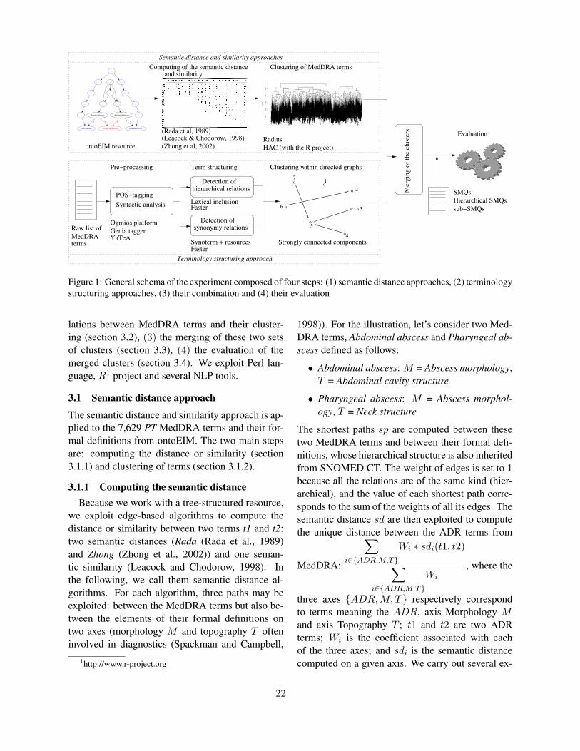
Abdominal abscess
Abdominal cavity
T
Abscess morphology
M
Pharyngal abscess
M
Neck structure
T
...
...
...
...
...
...
...
...
...
...
...
...
...
1o
o
o6
5
o 2
o 3
o7
4o
POS−tagging
Syntactic analysis
Detection ofhierarchical relations
Detection ofsynonymy relations
ontoEIM resource (Zhong et al, 2002)
(Leacock & Chodorow, 1998)
Computing of the semantic distance Clustering of MedDRA termsand similarity
Term structuring
Lexical inclusion
Synoterm + resources
Genia tagger
Ogmios platform
YaTeA
Pre−processing
Mer
gin
g o
f th
e cl
ust
ers
Clustering within directed graphs
EvaluationRadius
HAC (with the R project)
SMQs
Hierarchical SMQs
sub−SMQs
Semantic distance and similarity approaches
Terminology structuring approach
(Rada et al, 1989)
Strongly connected components
Faster
Faster
Raw list of
MedDRAterms
Figure 1: General schema of the experiment composed of four steps: (1) semantic distance approaches, (2) terminologystructuring approaches, (3) their combination and (4) their evaluation
lations between MedDRA terms and their cluster-ing (section 3.2), (3) the merging of these two setsof clusters (section 3.3), (4) the evaluation of themerged clusters (section 3.4). We exploit Perl lan-guage, R1 project and several NLP tools.
3.1 Semantic distance approach
The semantic distance and similarity approach is ap-plied to the 7,629 PT MedDRA terms and their for-mal definitions from ontoEIM. The two main stepsare: computing the distance or similarity (section3.1.1) and clustering of terms (section 3.1.2).
3.1.1 Computing the semantic distanceBecause we work with a tree-structured resource,
we exploit edge-based algorithms to compute thedistance or similarity between two terms t1 and t2:two semantic distances (Rada (Rada et al., 1989)and Zhong (Zhong et al., 2002)) and one seman-tic similarity (Leacock and Chodorow, 1998). Inthe following, we call them semantic distance al-gorithms. For each algorithm, three paths may beexploited: between the MedDRA terms but also be-tween the elements of their formal definitions ontwo axes (morphology M and topography T ofteninvolved in diagnostics (Spackman and Campbell,
1http://www.r-project.org
1998)). For the illustration, let’s consider two Med-DRA terms, Abdominal abscess and Pharyngeal ab-scess defined as follows:
• Abdominal abscess: M = Abscess morphology,T = Abdominal cavity structure
• Pharyngeal abscess: M = Abscess morphol-ogy, T = Neck structure
The shortest paths sp are computed between thesetwo MedDRA terms and between their formal defi-nitions, whose hierarchical structure is also inheritedfrom SNOMED CT. The weight of edges is set to 1because all the relations are of the same kind (hier-archical), and the value of each shortest path corre-sponds to the sum of the weights of all its edges. Thesemantic distance sd are then exploited to computethe unique distance between the ADR terms from
MedDRA:
∑i∈{ADR,M,T}
Wi ∗ sdi(t1, t2)∑i∈{ADR,M,T}
Wi
, where the
three axes {ADR,M, T} respectively correspondto terms meaning the ADR, axis Morphology Mand axis Topography T ; t1 and t2 are two ADRterms; Wi is the coefficient associated with eachof the three axes; and sdi is the semantic distancecomputed on a given axis. We carry out several ex-
22

headcomponent component
expansion headcomponent component
expansion
pain muscle ache muscle
Figure 2: Syntactically analyzed terms (muscle pain and muscle ache) into their head and expansion components
periments. Semi-matrices 7629*7629 with semanticdistance between the terms are built.
3.1.2 Clustering of termsAn unsupervised creation of clusters is applied to
the semi-matrices. We exploit two approaches:
• R radius approach: every MedDRA term isconsidered a possible center of a cluster and itsclosest terms are clustered with it. The thresh-olds tested correspond to the following inter-vals: 2 and 3 for Rada, [0; 5.059] for LCH and[0; 0.49] for Zhong. The intersection of theseclusters is not empty.
• HAC hierarchical ascendant classification isperformed through the R Project tools (hclustfunction). Iteratively, this function chooses thebest centers for terms and builds the hierar-chy of terms by progressively clustering thosewhich are closest to these centers. Then theunique cluster with all the terms is split up.Several splitting values between 100 and 7,000are tested. These clusters are exclusive.
Clusters created with the radius approach aremerged in order to eliminate smaller clusters in-cluded in bigger clusters and in order to aggregateclusters which have an important intersection be-tween them. For the intersection, we test several in-tersection values within the interval [10; 90], whichmeans that two compared clusters may have between10% and 90% of common terms.
3.2 Terminology structuring approachThe terminology structuring methods are applied toa raw list of 18,209 MedDRA PTs. They allowthe detection of semantic relations between theseterms. The POS-tagging is done with Genia tag-ger (Tsuruoka et al., 2005) and the syntactic analy-sis with the YATEA parser (Aubin and Hamon, 2006).Three kinds of methods are applied for the acquisi-tion of synonymy and hierarchical relations: lexicalinclusions (section 3.2.1), morpho-syntactic variants
(section 3.2.2) and compositionality (section 3.2.3).The terms are then clustered (section 3.2.4).
3.2.1 Lexical inclusion and hierarchyThe lexical inclusion hypothesis (Kleiber and
Tamba, 1990), which states that when a given termis lexically included at the head syntactic positionin another term there is a semantic subsumption be-tween them, allows to identify hierarchical relationsbetween terms. For instance, on figure 2, the shortterm pain is the hierarchical parent and the long termmuscle pain is its hierarchical child because pain isthe syntactic head of muscle pain. The lexical inclu-sions are computed on POS-tagged and syntacticallyanalyzed terms. We compute two kinds of lexical in-clusions:• syntactic dependencies on minimal syntactic
heads: the parent term corresponds to the short-est lexical form of the syntactic head. For in-stance, within the term kaolin cephalin clottingtime, the minimal head is time;• syntactic dependencies on maximal syntactic
heads: the parent term is the most complete lex-ical form of the syntactic head. Within the sameterm kaolin cephalin clotting time, the maximalhead is cephalin clotting time.
Parent and child terms have to be MedDRA terms.
3.2.2 Morpho-syntactic variantsWe exploit Faster (Jacquemin, 1996) for the in-
dentification of morpho-syntactic variants betweenthe PT terms. This tool applies several transforma-tion rules, such as insertion (cardiac disease/cardiacvalve disease), morphological derivation (arteryrestenosis/arterial restenosis) or permutation (aortacoarctation/coarctation of the aorta). Each transfor-mation rule is associated with hierarchical or syn-onymy relations: the insertion introduces a hierar-chical relation (cardiac valve disease is more spe-cific than cardiac disease), while the permutation in-troduces a synonymy relation. When several trans-formations are involved, the detected relations may
23

be ambiguous: gland abscess and abscess of sali-vary gland combines permutation (synonymy) andinsertion (hierarchy) rules. In such cases the hierar-chical relation prevails.
3.2.3 Compositionality and synonymyThe synonymy relations are acquired in two ways.
First, the synonymy relation is established betweentwo simple MedDRA terms if this relation is pro-vided by the linguitistic resources. Second, theidentification of synonym relations between com-plex terms relies on the semantic compositionality(Partee, 1984). Hence, two complex terms are con-sidered synonyms if at least one of their compo-nents at the same syntactic position (head or ex-pansion) are synonyms. For instance, on figure 2,given the synonymy relation between the two wordspain and ache, the terms muscle pain and muscleache are also identified as synonyms (Hamon andNazarenko, 2001). Three transformation rules areapplied: on the head component (figure 2), on theexpansion component and on both of them. We per-form several experiments: each medical synonymyresource is first used individually and then in com-bination with WordNet.
3.2.4 Clustering of termsThe sets of terms related through the lexical in-
clusions are considered as directed graphs: the termsare the nodes of the graph while the hierarchical re-lations are the directed edges. We partition these di-rected graphs and identify clusters of terms whichcould correspond to or be part of the SMQs. Amongconnected components and strongly connected com-ponents, we choose to generate the strongly con-nected components: they allow an intersection be-tween clusters which means that a given term maybelong to several clusters (this is also the case withthe SMQs). Thus, within the directed graphs G wehave to identify the maximal sub-graphs H of Gwhere for each pair {x, y} of the nodes from H ,there exists a directed edge from x to y (or from y tox). To improve the coverage of the obtained clusters,we also add the synonyms: if a term has a synonymyrelation with the term from a cluster then this termis also included in this cluster. From a graph theorypoint of view, the initial graph is augmented withtwo edges going from and to the synonyms.
Methods and relationships #relationsHierarchical relations
Maximal syntactic head 3,366Minimal syntactic head 3,816Morpho-syntactic variants 743
Medical synonyms3 biomedical terminologies 1,879UMLS/Filtered UMLS 190Morpho-syntactic variants 100
Medical synonyms and WordNet3 biomedical terminologies 1,939UMLS/Filtered UMLS 227
Table 1: Hierarchical and synonymy relations generatedby terminology structuring methods
3.3 Merging of clusters from two approachesWe merge the clusters generated by the two ap-proaches. The merging is performed on the inter-section between the clusters. As previously, we testintersection values within the interval [10; 90].
3.4 EvaluationWe give judgments on: (1) the correctness of thegenerated relations, (2) their relevance according tothe reference data, (3) their relevance according tothe manual evaluation by an expert. The evaluationis performed with three measures: precision P (per-centage of the relevant terms clustered divided bythe total number of the clustered terms), recall R(percentage of the relevant terms clustered dividedby the number of terms in the corresponding SMQ)and F-measure F1. The association between theSMQs and the clusters relies on the best F1.
4 Results
Semantic relations acquired with terminology struc-turing are indicated in table 1. There is a smalldifference between relations acquired through maxi-mal and minimal syntactic heads, although the influ-ence of medical resources for the acquisition of syn-onymy varies according to the resources. WordNetslightly increases the number of synonyms. Fastergenerates a large set of hierarchical and synonymyrelations. MedDRA terms have also been processedwith semantic distance and clustered. The bestthresholds with the radius clustering are 2 for Rada,
24

Approach Hierarchical SMQs SMQs and sub-SMQs#clusters interval mean #clusters interval mean
Semantic distance 2,667 [2; 1,206] 73 2,931 [2; 546] 17Structuring (hierarchical) 690 [1; 134] 3.69 748 [1; 117] 3.43Structuring (hierarchical+synonymy) 690 [1; 136] 4.11 748 [1; 119] 3.82Merging (hierarchical) 2,732 [1; 1,220] 72.40 2,998 [1; 563] 24.44Merging (hierarchical+synonymy) 2,732 [1; 1,269] 75.94 2,998 [1; 594] 26.03
Table 2: Number of clusters and their size (the interval and the mean number of terms per cluster) for individualapproaches and for their merging computed for hierarchical SMQs and also for SMQs and sub-SMQs
0
20
40
60
80
100
0 10 20 30 40 50 60 70 80
precisionrecall
f−measure
(a) Semantic distance
0
20
40
60
80
100
0 10 20 30 40 50 60 70 80
precisionrecall
f−measure
(b) Terminology structuring
Figure 3: Results (precision, recall and F-measure) for semantic distance and terminology structuring approaches
4.10 for LCH and 0 for Zhong. With the HAC, thebest results are obtained with 300 classes (number ofterms per class is within the interval [1; 98], meannumber of terms per class is 25.34). Our resultsshow that the best parameters for the semantic dis-tance are the Rada distance, radius approach and noformal definitions, while the best parameters for theterminology structuring are maximal syntactic headwith hierarchical relations by Faster augmented withsynonyms. For the merging of the clusters we apply50% intersection for hierarchical SMQs and 80% in-tersection for SMQs and sub-SMQs. We exploit anddiscuss these results. The percentage of the Med-DRA terms involved by the terminology structur-ing is the 32% with hierarchical relations, it reaches40% when the synonymy is also considered. Withsemantic distance, all the terms from ontoEIM (51%of the MedDRA) are used.
Table 2 provides information on clusters: num-
ber of clusters, number of terms per cluster (theirinterval and the mean number of terms per cluster).In table 2, we first indicate the results for the indi-vidual approaches, and then when the merging ofthe approaches is performed. We observe that themerging has a positive effect on the number and thesize of clusters: data generated by the individual ap-proaches (and by synonymy) are complementary.
4.1 Correctness of the semantic relationsA manual analysis of the generated hierarchical re-lations indicates that these relations are always cor-rect: the constraint involved through the syntac-tic analysis guarantees correct propositions. Nev-ertheless, we observed a small number of syntac-tic ambiguities. They appear within 144 pairs (5%)with maximal syntactic heads and correspond topairs like: {anticonvulsant drug level, drug level},{blood smear test, smear test}, {eye movement dis-order, movement disorder}. Thus, within the first
25
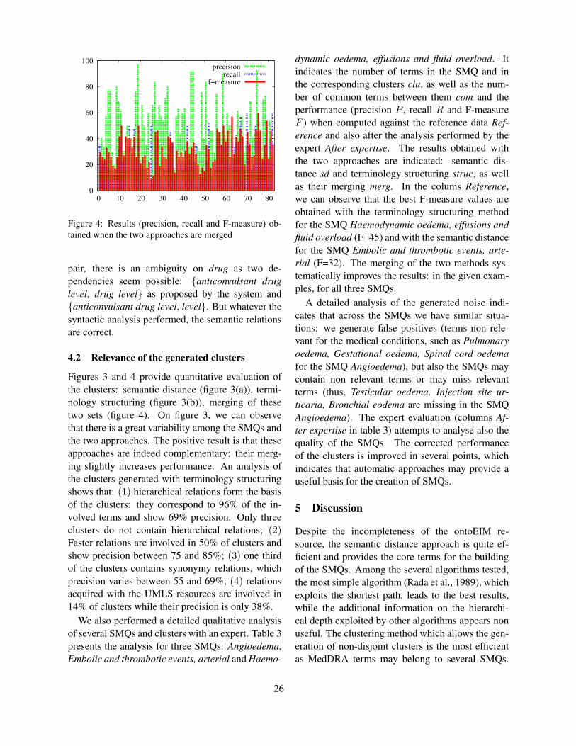
0
20
40
60
80
100
0 10 20 30 40 50 60 70 80
precisionrecall
f−measure
Figure 4: Results (precision, recall and F-measure) ob-tained when the two approaches are merged
pair, there is an ambiguity on drug as two de-pendencies seem possible: {anticonvulsant druglevel, drug level} as proposed by the system and{anticonvulsant drug level, level}. But whatever thesyntactic analysis performed, the semantic relationsare correct.
4.2 Relevance of the generated clusters
Figures 3 and 4 provide quantitative evaluation ofthe clusters: semantic distance (figure 3(a)), termi-nology structuring (figure 3(b)), merging of thesetwo sets (figure 4). On figure 3, we can observethat there is a great variability among the SMQs andthe two approaches. The positive result is that theseapproaches are indeed complementary: their merg-ing slightly increases performance. An analysis ofthe clusters generated with terminology structuringshows that: (1) hierarchical relations form the basisof the clusters: they correspond to 96% of the in-volved terms and show 69% precision. Only threeclusters do not contain hierarchical relations; (2)Faster relations are involved in 50% of clusters andshow precision between 75 and 85%; (3) one thirdof the clusters contains synonymy relations, whichprecision varies between 55 and 69%; (4) relationsacquired with the UMLS resources are involved in14% of clusters while their precision is only 38%.
We also performed a detailed qualitative analysisof several SMQs and clusters with an expert. Table 3presents the analysis for three SMQs: Angioedema,Embolic and thrombotic events, arterial and Haemo-
dynamic oedema, effusions and fluid overload. Itindicates the number of terms in the SMQ and inthe corresponding clusters clu, as well as the num-ber of common terms between them com and theperformance (precision P , recall R and F-measureF ) when computed against the reference data Ref-erence and also after the analysis performed by theexpert After expertise. The results obtained withthe two approaches are indicated: semantic dis-tance sd and terminology structuring struc, as wellas their merging merg. In the colums Reference,we can observe that the best F-measure values areobtained with the terminology structuring methodfor the SMQ Haemodynamic oedema, effusions andfluid overload (F=45) and with the semantic distancefor the SMQ Embolic and thrombotic events, arte-rial (F=32). The merging of the two methods sys-tematically improves the results: in the given exam-ples, for all three SMQs.
A detailed analysis of the generated noise indi-cates that across the SMQs we have similar situa-tions: we generate false positives (terms non rele-vant for the medical conditions, such as Pulmonaryoedema, Gestational oedema, Spinal cord oedemafor the SMQ Angioedema), but also the SMQs maycontain non relevant terms or may miss relevantterms (thus, Testicular oedema, Injection site ur-ticaria, Bronchial eodema are missing in the SMQAngioedema). The expert evaluation (columns Af-ter expertise in table 3) attempts to analyse also thequality of the SMQs. The corrected performanceof the clusters is improved in several points, whichindicates that automatic approaches may provide auseful basis for the creation of SMQs.
5 Discussion
Despite the incompleteness of the ontoEIM re-source, the semantic distance approach is quite ef-ficient and provides the core terms for the buildingof the SMQs. Among the several algorithms tested,the most simple algorithm (Rada et al., 1989), whichexploits the shortest path, leads to the best results,while the additional information on the hierarchi-cal depth exploited by other algorithms appears nonuseful. The clustering method which allows the gen-eration of non-disjoint clusters is the most efficientas MedDRA terms may belong to several SMQs.
26

Number of terms Reference After expertiseSMQs SMQ clu com P R F P R F
Angioedemasd 52 32 13 40 25 30 43 26 33Angioedemastruc 52 31 19 61 36 45 61 36 45Angioedemamerg 52 33 21 63 42 50 71 48 57Embolic and thrombotic events...sd 132 159 48 30 36 32 32 39 35.2Embolic and thrombotic events...struc 132 13 12 92 9 16 92 9 16Embolic and thrombotic events...merg 132 130 49 38 37 37.5 47 46 46.5Haemodynamic oedema, effusions...sd 36 22 7 32 20 24 54 33 41Haemodynamic oedema, effusions...struc 36 31 13 42 36 39 84 72 78Haemodynamic oedema, effusions...merg 36 35 16 46 44 45 86 83 84.5
Table 3: Comparison between the two approaches (semantic distance sd and terminology structuring struc) and themerging of the two approaches merg for three SMQs: Angioedema, Embolic and thrombotic events, arterial andHaemodynamic oedema, effusions and fluid overload
Traditionnal classification methods, which producedisjoint clusters, are less efficient for this task.
It has been surprising to observe that the contri-bution of the generated hierarchical relations is soimportant (table 1) and that these relations appear tobe so often correct for the creation of SMQs. In-deed, because PT terms belong to the same hierar-chical level of MedDRA, they should be hierarchi-cally equivalent between them. In reality, within acluster, we can find several hierarchical levels of thePT terms. This means that the hierarchical structureof MedDRA could be more fine-grained and that in-termediate hierarchical levels could be created. Asfor the generated synonymy relations, their numberis low and they contribute in a lesser way to thebuilding of the clusters: this means that the PTs aresemantically differentiated between them.
Finally, the merging of these two approaches isbeneficial for the generation of clusters: the per-formance is improved, although slightly. The twoapproaches provide indeed complementary results.The low recall and F-measure are due to the materialand methods exploited: ontoEIM contains only 51%of the MedDRA terms to be processed while the ex-ploited terminology structuring methods are not ableto detect more common features between the terms.
The difference between the results obtainedagainst the reference data and after the expert eval-uation (table 3) show that the reference data are notvery precise. In previous work, it has already beenobserved that some important PT terms can be miss-
ing in the SMQs (Pearson et al., 2009). With theproposed automatic methods we could find some ofthese terms. It has been also demonstrated that theSMQs are over-inclusive (Mozzicato, 2007; Pear-son et al., 2009). In the proposed analysis of theSMQs, we have also found terms which have toolarge meaning and which should not be included inthe SMQs.
6 Conclusion and Perspectives
We have applied two different approaches to theclustering of pharmacovigilance terms with simi-lar or close meaning. We performed a comparisonof the results obtained with these two approachesand analysed their complementarity. Several experi-ments have been carried out in order to test differentparameters which may influence the performance ofthe methods. Although the automatic creation of theSMQs is a difficult task, our results seem to indi-cate that the automatic methods may be used as abasis for the creation of new SMQs. The precisionof the clusters is often satisfactory, while their merg-ing leads to the improvement of their completeness.These approaches generate complementary data andtheir combination provides more performant results.
Future studies will lead to the identification ofother parameters which influence the quality of clus-ters and also other factors which may be exploitedfor the merging of clusters. More robust distancesand clustering methods will also be used in futurework, as well as approaches for a better acquisi-
27

tion and evaluation of the hierarchical structure ofSMQs. We plan also to design corpora-based meth-ods which may also to increase the recall of the re-sults. We will perform an exhaustive analysis of thenature of semantic relations which can be observedwithin the SMQs and propose other methods to fur-ther improve the coverage of the clusters. Differentfilters will be tested to remove the true false posi-tive relations between terms. The results will alsobe evaluation by several experts, which will allow toassess the inter-expert variation and its influence onthe results. Besides, the obtained clusters will alsobe evaluated through their impact on the pharma-covigilance tasks and through the exploring of thepharmacovigilance databases.
ReferencesI Alecu, C Bousquet, and MC Jaulent. 2008. A case
report: using snomed ct for grouping adverse drug re-actions terms. BMC Med Inform Decis Mak, 8(1):4–4.
S Aubin and T Hamon. 2006. Improving term extrac-tion with terminological resources. In FinTAL 2006,number 4139 in LNAI, pages 380–387. Springer.
C Bousquet, C Henegar, A Lillo-Le Louet, P Degoulet,and MC Jaulent. 2005. Implementation of auto-mated signal generation in pharmacovigilance using aknowledge-based approach. Int J Med Inform, 74(7-8):563–71.
EG Brown, L Wood, and S Wood. 1999. The medicaldictionary for regulatory activities (MedDRA). DrugSaf., 20(2):109–17.
CIOMS. 2004. Development and rational use of stan-dardised MedDRA queries (SMQs): Retrieving ad-verse drug reactions with MedDRA. Technical report,CIOMS.
C Fellbaum. 1998. A semantic network of english: themother of all WordNets. Computers and Humanities.EuroWordNet: a multilingual database with lexical se-mantic network, 32(2-3):209–220.
R Fescharek, J Kubler, U Elsasser, M Frank, andP Guthlein. 2004. Medical dictionary for regulatoryactivities (MedDRA): Data retrieval and presentation.Int J Pharm Med, 18(5):259–269.
N Grabar and T Hamon. 2010. Exploitation of linguis-tic indicators for automatic weighting of synonymsinduced within three biomedical terminologies. InMEDINFO 2010, pages 1015–9.
T Hamon and A Nazarenko. 2001. Detection of syn-onymy links between terms: experiment and results.In Recent Advances in Computational Terminology,pages 185–208. John Benjamins.
J Iavindrasana, C Bousquet, P Degoulet, and MC Jaulent.2006. Clustering WHO-ART terms using semanticdistance and machine algorithms. In AMIA Annu SympProc, pages 369–73.
Christian Jacquemin. 1996. A symbolic and surgical ac-quisition of terms through variation. In S. Wermter,E. Riloff, and G. Scheler, editors, Connectionist, Sta-tistical and Symbolic Approaches to Learning for Nat-ural Language Processing, pages 425–438, Springer.
MC Jaulent and I Alecu. 2009. Evaluation of an ontolog-ical resource for pharmacovigilance. In Stud HealthTechnol Inform, pages 522–6.
G Kleiber and I Tamba. 1990. L’hyperonymie revisitee :inclusion et hierarchie. Langages, 98:7–32, juin.
C Leacock and M Chodorow, 1998. Combining localcontext and WordNet similarity for word sense iden-tification, chapter 4, pages 305–332.
P Mozzicato. 2007. Standardised MedDRA queries:their role in signal detection. Drug Saf, 30(7):617–9.
NLM, 2011. UMLS Knowledge Sources Manual. Na-tional Library of Medicine, Bethesda, Maryland.www.nlm.nih.gov/research/umls/.
Barbara H. Partee. 1984. Compositionality. In F. Land-man and F. Veltman, editors, Varieties of formal se-mantics. Foris, Dordrecht.
RK Pearson, M Hauben, DI Goldsmith, AL Gould,D Madigan, DJ O’Hara, SJ Reisinger, andAM Hochberg. 2009. Influence of the Med-DRA hierarchy on pharmacovigilance data miningresults. Int J Med Inform, 78(12):97–103.
R Rada, H Mili, E Bicknell, and M Blettner. 1989. De-velopment and application of a metric on semanticnets. IEEE Transactions on systems, man and cyber-netics, 19(1):17–30.
K Spackman and K Campbell. 1998. Composi-tional concept representation using SNOMED: To-wards further convergence of clinical terminologies.In Journal of American Medical Informatics Associ-ation (JAMIA), pages 740–744.
MQ Stearns, C Price, KA Spackman, and AY Wang.2001. SNOMED clinical terms: overview of the de-velopment process and project status. In AMIA, pages662–666.
Y Tsuruoka, Y Tateishi, JD Kim, T Ohta, J McNaught,S Ananiadou, and J Tsujii. 2005. Developing a ro-bust part-of-speech tagger for biomedical text. LNCS,3746:382–392.
J Zhong, H Zhu, J Li, and Y Yu. 2002. Concep-tual graph matching for semantic search. In 10thInternational Conference on Conceptual Structures,ICCS2002, LNCS 2393, Springer Verlag, pages 92–106.
28

Proceedings of the 2012 Workshop on Biomedical Natural Language Processing (BioNLP 2012), pages 29–37,Montreal, Canada, June 8, 2012. c©2012 Association for Computational Linguistics
Temporal Classification of Medical Events
Preethi Raghavan∗, Eric Fosler-Lussier∗, and Albert M. Lai†∗Department of Computer Science and Engineering
†Department of Biomedical InformaticsThe Ohio State University, Columbus, Ohio, USA
{raghavap, fosler}@cse.ohio-state.edu, [email protected]
Abstract
We investigate the task of assigning medi-cal events in clinical narratives to discretetime-bins. The time-bins are defined to cap-ture when a medical event occurs relative tothe hospital admission date in each clinicalnarrative. We model the problem as a se-quence tagging task using Conditional Ran-dom Fields. We extract a combination of lexi-cal, section-based and temporal features frommedical events in each clinical narrative. Thesequence tagging system outperforms a sys-tem that does not utilize any sequence infor-mation modeled using a Maximum Entropyclassifier. We present results with both hand-tagged as well as automatically extracted fea-tures. We observe over 8% improvement inoverall tagging accuracy with the inclusion ofsequence information.
1 Introduction
There has been a lot of interest in building timelinesof medical events from unstructured patient narra-tives (Jung et al., 2011; Zhou and Hripcsak, 2007).Creating a timeline from longitudinal clinical textrequires learning temporal relations such as before,simultaneous, includes, overlaps, begins, ends andtheir inverses between medical events found withinand across patient narratives (Allen, 1981). How-ever, learning temporal relations for fine-grainedtemporal ordering of medical events in clinical textis challenging: the temporal cues typically found inclinical text may not always be sufficient for thistask.
An important characteristic of a clinical narrativeis that the medical events in the same narrative aremore or less semantically related by narrative dis-course structure. However, medical events in thenarrative are not ordered chronologically. Thus, theclinical narrative structure is not always temporallycoherent.
Moreover, extracting precise temporal featuresfor highly accurate temporal ordering of medicalevents is difficult as the temporal relationship be-tween medical events is varied and complicated.Zhou and Hripcsak (2007) identify six major cate-gories of temporal expressions from a corpus of dis-charge summaries: “date and time,” “relative dateand time,” “duration,” “event-dependent temporalexpression,” “fuzzy time,” and “recurring times.”Their study of temporal expressions in clinical textindicates that relative time (e.g., ever since theepisode 2 days ago) may be more prevalent than ab-solute time (e.g., 06/03/2007). Further, temporal ex-pressions may be fuzzy where “history of cocaineuse” may imply that cocaine use started 2 years agoor 10 years ago.
In this paper, we address a relatively simpler taskof assigning medical events to coarsely defined time-bins. The time-bins, way before admission, beforeadmission, on admission, after admission, after dis-charge, are defined based on the relative temporaldistance of the medical event from the admissiondate, which is the only explicit date almost alwaysfound in each clinical narrative. We extract fea-tures based on narrative structure as well as tempo-ral expressions to label a sequence of medical eventsfrom each clinical narrative with a highly probable
29

HISTORY PHYSICAL DATE: 06/03/2007
NAME: Smith Jack MR#: XXX-XX-XXXX
ATTENDING PHYSICIAN: Bill Payne MD DOB: 02/28/1960
CHIEF COMPLAINT
Chest pain and arm infection.
HISTORY OF PRESENT ILLNESS
Patient is a 48-year-old male with history of cocaine use hypertension who presents with chest pain
which started 2 days ago . He did not having chest pain yesterday but ever since the episode 2 days ago
he has felt a little weaker. He did have chest pain today and this is what prompted him to come to the
ER. He also notices that he has had some infections under his arms. He states that he had to have an
abscess I and D 3 or 4 months ago under his arm and 2 to 3 weeks ago he noticed some more spots and
these spots have now grown and now are under both arms. Currently he is chest pain free. His blood
pressure upon presentation was 189/106.
REVIEW OF SYSTEMS
On exam initial blood pressure was 189/106 current blood pressure 148/83 with heart rate of 74
respirations 16. Heart regular rhythm. No murmurs. Arms: He does have tender areas right greater
than left under the arm. Difficult to tell if there is any erythema but obvious cellulitis sludge abscess
under the right arm which is tender.
ASSESSMENT/PLAN
1. Chest pain history of cocaine with T-wave inversions in the inferior leads. Currently he is chest pain free. We will check a 2-D echocardiogram. Consult Cardiology for a stress test.
2. Axillary abscesses. Consult Surgery for I and D. We will place on IV vancomycin pain control.
3. Cocaine abuse. Encouraged to quit.
1
2
3
4
5
6
7
8
9
Figure 1: Excerpt from a de-identified clinical narrative(cn1) written for a patient in 2007. Medical events areunderlined. Enumerated events (in circles) are used as anexample later in Table 1.
sequence of time-bins using Conditional RandomFields (CRFs). The learned time-bins can be usedas an informative temporal feature for tasks suchas fine-grained temporal ordering of medical eventsand medical event coreference resolution.
2 Motivation
Clinical narratives are medical reports that containunstructured text documenting the medical historyof the patient. Medical events are temporally-relatedconcepts in clinical narratives that describe medicalconditions affecting the patient’s health, or tests andprocedures performed on a patient. Sample excerptsfrom two different clinical notes (cn1 and cn2) ofthe same patient, generated over time, are shown inFigures 1 and 2. We can see from the examples thatnarrative structure moves back and forth in time andis not temporally coherent. We use cn1 and cn2 asrunning examples throughout the paper.
The medical events assigned to time-bins in eachclinical narrative allow us to derive a coarse tempo-ral order between medical events within and acrossthe longitudinal medical history of the patient. Sincewe learn time-bins centered around admission ineach narrative and we also know the admission dateand perhaps the discharge dates in cn1 and cn2, wecan derive a coarse partial order across the medi-
HISTORY PHYSICAL DATE: 06/17/2007
NAME: Black Jack MR#: XXX-XX-XXXX
ATTENDING PHYSICIAN: Jack Payne MD DOB: 02/28/1960
He is a 48-year-old African American gentleman with a history of cocaine use and hypertension. He
has hidradenitis of both axilla resected. The patient is MRSA positive on IV antibiotics at the present
time. The patient's physical condition is excellent but he had MRSA in the axilla for hidradenitis that
was devastating. The wounds now are very large but he is wound vac and being changed to alginate.
Both axilla show major wounds of 20-25 cm in diameter and 4-5 cm deep in overall size and he has
excoriations on his chest from the tape. The plan is to change him from vac to alginate and see him
in a week.
Figure 2: Excerpt from another de-identified clinical nar-rative (cn2) for the same patient written in later in 2007.Medical events are underlined.
cal events in cn1 and cn2. This is shown in Fig-ure 3. Even if the discharge dates are not known,we still know that the admission date (A1) of cn1is 6/03/2007 and A2 of cn2 is 06/17/2007. Thus,A2 > A1, and all the time-bins in cn2 that are on orafter admission would have happened after A2. Thepartially ordered time-bins can now be used for taskssuch as medical concept coreference resolution.
In cross narrative coreference resolution tasks,we can prune the space of candidate pairs of med-ical events by ruling out portions of clinical nar-ratives that will not have any coreferring medicalevents. For example, in the timeline shown in Fig-ure 3, the medical events in time-bins admission, af-ter admission and discharge of cn2 will not coreferwith any medical event in cn1. Further, when men-tions of the same medical events occur in differenttime-bins, it could mean that they are the same in-stance of the medical event and they corefer. Forinstance, cocaine abuse and cocaine use. Similarly,MRSA positive is assigned to time-bin on admissionwhereas MRSA is assigned to before admission andboth mentions of MRSA corefer.
3 Related Work
The Timebank (Pustejovsky et al., 2003) corpus ofannotated newswire text is widely used for tempo-ral relation learning. The TempEval challenges haveoften focused on extracting different types of tempo-ral relations from Timebank (Verhagen et al., 2009).In Timebank, events are typically verbs that denotechange in state. Since the notion of an event in Time-bank is different from medical events in clinical text,it is not possible to directly train models on Time-bank and apply them to clinical text. The THYMEwork (Savova et al., 2009) extends TimeML to the
30

A1 D1
A2 D2
cocaine use hypertension
chest pain abscess
chest pain arm infection
heart regular rhythm
cellulitis
2-D echocardiogram
stress test
MRSA positive
hidradenitis of axilla resected MRSA in the axilla for hidradenitis
wounds
wound vac
IV antibiotics
alginate cocaine use hypertension
way before before admission after discharge
before admission after discharge way before
p1-cn1
p1-cn2
Figure 3: Medical events in clinical narratives cn1 and cn2 for patient p1 assigned to time-bins. A1 is the admissiondate in cn1 and D1 is the discharge date. Similarly A2 is the admission date in cn2 and D2 is the discharge date. Thus,we have, A1 < D1, D1 < A2, A2 < D2
medical domain to create layered annotation to beused for event linking. Boland et al. (2012) identifythe temporal knowledge representation requirementsof clinical eligibility criteria and develop a frame-based representation designed to support semanticannotation for temporal expressions in eligibility cri-teria. However, the nature of data found in eligibilitycriteria is different from clinical narratives.
Previous attempts at learning temporal relationsbetween medical events in clinical text include Junget al. (2011) and Zhou et al. (2006). Gaizauskas etal. (2006) learn the temporal relations before, after,is included between events from a corpus of clinicaltext much like the event-event relation TLINK learn-ing in Timebank (Pustejovsky et al., 2003). How-ever, the corpora used in these studies are not freelyavailable. A comprehensive survey of temporal rea-soning in medical data is provided by Zhou andHripcsak (2007).
The task addressed in this paper is at a higherlevel than the temporal relation learning or tempo-ral ordering task. Without getting into fine-grainedtemporal ordering, we define coarse time-bins andclassify medical events into one of the time-bins.
We work with a similar motivation of being ableto answer clinical trial eligibility criteria with tem-poral constraints. However, while they model thetemporal information in eligibility criteria, we pro-cess the temporal information and medical eventsin the clinical narrative to assign events to time-bins. The learned time-bins are a step towards fine-grained temporal ordering of medical events in clin-ical text. More importantly, we also demonstrate
how automatic feature extraction for this task givesus promising results, though not as good as usinghand-tagged features.
4 Problem Description
A patient could have multiple clinical narratives,generated over a period of time, representing the pa-tient’s longitudinal medical history. Returning to theexamples in Figures 1 and 2, in this section we de-scribe how such clinical narratives are translated intoa temporal-bin assignment problem.
4.1 Medical event representation
Medical events in clinical narratives often have atime duration with a corresponding start and stoptime, for example, history of hypertension (Zhou etal., 2006). In this example, hypertension started atsome point before admission and is present to thecurrent date. Time duration based representation isessential to learning the exact fine-grained tempo-ral order of medical events within and across clin-ical narratives. In order to keep the task of classi-fying medical events into coarse time-bins relativelysimple and easy to learn, we use a time-point nota-tion for representing medical events. Each mentionof a medical event is assigned to a time-bin with-out taking into consideration whether it denotes thebeginning or end of that event. We also do not dif-ferentiate between coreferences of the same medicalevent. Thus, if chest pain is mentioned in the pastmedical history and the same chest pain continuesto persist in the after admission time-bin, the twodifferent mentions of chest pain get anchored to dif-
31
ferent time-bins. Similarly, cocaine use started inthe history of the patient and cocaine abuse still per-sists. We assign the two different mentions of thismedical event into different time-bins.
4.2 Time-binsAs mentioned earlier, we learn to classify medicalevents into one of the following time-bins: way be-fore admission, before admission, on admission, af-ter admission, after discharge. The intuition behindeach time-bin label is as follows. The time-bin waybefore admission is intended to capture all medicalevents that happened in the past medical history ofthe patient but are not mentioned as being directlyrelated to the present illness. Before admission cap-tures events that occurred before admission and arerelated to the present illness. On admission capturesmedical events that occur on the day of admission.After admission captures medical events that occurbetween admission and discharge (during the hospi-tal stay or clinic visit). Finally, medical events thatare supposed to occur in the future after the patientis discharged belong to the class after discharge.
Further, the time duration of each time-bin variesbased on the patient. For instance, the hospital stayof a patient could be 4 days or 1 month or a year.This makes it very difficult to define exact time-binsbased on the intuitions described above. In orderto make the problem more precise and consistentacross different patients, we restrict way before ad-mission to events that happened more than a yearago and before admission to events that occurred inthe same year before admission. If it is unclear asto when in the past the medical event occurred, weassume it happened way before admission.
5 Learning time-bin assignmentsWe model the problem of classifying medical eventsto time-bins as a sequence tagging task using CRFs(Lafferty et al., 2001). CRFs are a joint model oflabel sequence conditioned on the observation.
For the task proposed in this paper, an observationsequence is composed of medical events in the orderin which they appear in a clinical narrative, and thestate sequence is the corresponding label sequenceof time-bins. Each label in the label sequence couldbe any one of the time-bins way before admission(wa), before admission (ba), on admission (a), after
admission (aa), after discharge (ad). Thus, givena sequence of medical events in narrative order welearn a corresponding label sequence of time-bins{wb, b, a, aa, ad}.
The probability of time-bin (label) sequence y,given a medical event (input) sequence x, is givenby,
P (Y |X) = exp∑
i
(S(x, y, i) + T (x, y, i)) (1)
where i is the medical event index and S and T arethe state and transition features respectively. Statefeatures S consider the label of a single medicalevent and are defined as,
S(x, y, i) =∑
j
λjsj(y, x, i) (2)
Transition features consider the mutual dependenceof labels yi−1 and yi (dependence between the time-bins of the current and previous medical event in thesequence) and are given by,
T (x, y, i) =∑
k
µktk(yi−1, yi, x, i) (3)
where sj and tk are the state and transition featurefunctions. Above, sj is a state feature function, andλj is its associated weight and tj is a transition func-tion, and µj is its associated weight. In contrast tothe state function, the transition function takes as in-put the current label as well as the previous label,in addition to the data. The mutual dependence be-tween the time-bins of the current and previous med-ical events is observed frequently in sections of thetext describing the history of the patient. Around40% of the medical events in gold standard corpusdemonstrate such dependencies.
The Maximum Entropy (MaxEnt) model (Bergeret al., 1996) estimates the probability of a time-bingiven the observed medical event. In this case, weare interested in finding the time-bin with the maxi-mum estimated probability.
6 Feature Space
We extract features from medical event sequencesfound in each clinical narrative. The extractedfeature-set captures narrative structure in terms ofthe narrative type, sections, section transitions, and
32

position in document. The medical event and thecontext in which it is mentioned is captured withthe help of lexical features. The temporal featuresresolve temporal references and associate medicalevents with temporal expressions wherever possible.
6.1 Section-based features
Determining the document-level structure of a clin-ical narrative is useful in mapping medical eventsto time-bins. This can be achieved by identifyingdifferent sections in different types of clinical narra-tives and relating them to different time-bins. Thesection in which the medical event is mentionedtells us something about when it occurred. Li et al.(2010) train a hidden Markov model (HMM) to mapa sequence of sections to 15 possible known sectiontypes in free-text narratives with high accuracy.
Commonly found sections in discharge sum-maries and history and physical reports include:“past medical history,” “history of present illness,”“findings on admission,” “physical examination,”“review of systems,” “impression,” and “assess-ment/plan.” On the other hand, radiology notes tendto have sections describing “indication,” “‘com-parison,” “findings” and “impression”. Similarly,pathology notes may have sections including “clini-cal history,” “specimen received,” “laboratory data”and “interpretation.” While some sections talk aboutpatient history, some other sections describe the pa-tient’s condition after admission, or plans after dis-charge. However, some clinical notes like cn2 inFigure 2 may not have any section information.
The combined feature representing the type ofclinical narrative along with the section can be infor-mative. Section transitions may also indicate a tem-poral pattern for medical events mentioned acrossthose sections. For instance, “past medical history”(way before admission), followed by “history ofpresent illness” (way before admission), followed by“findings on admission” (on admission), followedby “physical examination” (after admission), fol-lowed by “assessment/plan” (discharge). Medicalevents in different types of sections may also exhibitdifferent temporal patterns. A “history of present ill-ness” section may start with diseases and diagnoses30 years ago and then proceed to talk about them inthe context of a medical condition that happened fewyears ago and finally describe the patient’s condition
on admission.In addition to the section information, we also use
other features extracted from the clinical narrativestructure such as the position of the medical conceptin the section and in the narrative.
6.2 Lexical features
Bigrams are pairs of words that occur in close prox-imity to each other, and in a particular order. Thebigrams preceding the medical event in the narra-tive can be useful in determining when it occurred.For instance, “history of cocaine use and hyper-tension,” “presents with chest pain,” “have chestpain,” “since the episode,” etc. If the preceding bi-gram contains a verb, we also extract the tense of theverb as a feature. However, tense is not always help-ful in learning the time of occurrence of a medicalevent. Consider the following line from cn2 in Fig-ure 2, “He has hidradenitis of both axilla resected.”Though “has” is in present tense, the medical eventhas actually occurred in the history and is only beingobserved and noted now. Additionally, we also ex-plicitly include the preceding bigrams and the tenseof verb for the previous and next medical event as afeature for the current medical event.
Every medical event that occurs above a certainfrequency threshold in all the clinical narratives ofa particular patient is also represented as a binaryfeature. More frequent medical events tend to occurin the history of the patient, for example, cocaineuse. We use a threshold of 3 in our experiments.The medical event frequency in also calculated incombination with other features such as the type ofclinical narrative and section type.
6.3 Dictionary features
The UMLS1 includes a large Metathesaurus of con-cepts and terms from many biomedical vocabular-ies and a lexicon that contains syntactic, morpho-logical, and orthographic information for biomed-ical and common words in the English language.We map each medical event to the closest conceptin the UMLS Metathesaurus and extract its seman-tic category. The semantic categories in UMLS in-clude Finding, Disease or Syndrome, Therapeuticor Preventative procedure, Congenital abnormality,
1https://uts.nlm.nih.gov/home.html
33

and Pathologic Function. The intuition behind this isthat medical events associated with certain semanticcategories may be more likely to occur within cer-tain time-bins. For instance, a medical event classi-fied as “Congenital abnormality” may be more likelyto occur way before admission.
6.4 Temporal features
Temporal features are derived from any explicitdates that fall in the same sentence as the medicalconcept. The gold-standard corpus contains anno-tations for temporal anchors for events. Althoughthere are no explicit dates in cn1 and cn2, there maybe narratives where there are mentions of dates suchas fever on June 7th, 2007. In some cases, theremay also be indirect references to dates, which tellus when the medical event occurred. The referencedate with respect to which the indirect temporal ref-erence is made depends on the type of note. In caseof history and physical notes, the reference date isusually the admission date. For instance, chest painwhich started 2 days ago, this would mean chestpain which started 2 days before admission. Sincethe admission date is 06/03/2007, chest pain wouldhave started on 06/01/2007. Similarly, 3 to 4 monthsago resolves to February 2007 or March 2007 and 2to 3 weeks ago resolves to first or second week ofMay 2007. Whenever, the exact date is fuzzy, we as-sume the date that is farthest from the reference dateas accurate. So in case of these examples, February2007 and first week of May 2007 are assumed to becorrect. We also calculate the difference between ad-mission date and these dates associated with medicalevents. Another fuzzy temporal expression is “his-tory of,” where history could mean any time framebefore admission. We assume that any medical eventmentioned along with “history of” has occurred waybefore admission.
Other implicit temporal expressions can be foundin phrases such as upon presentation yesterday, to-day, at the present time, and now. Upon presen-tation, at the present time, today, and now resolveto the admission date 06/03/2007 and yesterdayresolves to the day before admission 06/02/2007.There are some other implicit temporal expressionsexpressed relative to medical events, for example,ever since the episode 2 days ago he has felt a littleweaker. Here, episode refers to chest pain and since
chest pain happened 2 days ago, ever since then upto the present time would resolve to the time periodbetween 06/01/2007 and 06/03/2007. This time pe-riod is associated with weaker.
7 Corpus
We use annotators that are students or recently grad-uated students from diverse clinical backgroundswith varying levels of clinical experience to anno-tate a corpus of clinical narratives from the medicalcenter. The corpus consists of narratives specificallyfrom MRSA cases and consists of admission notes,radiology and pathology reports, history and physi-cal reports and discharge summaries. The featuresmarked by the annotators include medical events;corresponding time-bin; corresponding UMLS con-cept identifier; the UMLS semantic category; tem-poral expressions; the link between temporal expres-sions and medical events, if any; and the section un-der which the medical event is mentioned, if any.The annotators marked 1854 medical events across5 patients and 51 clinical narratives. The annotationagreement across our team of annotators is high; allannotators agreed on 89.5% of the events and ouroverall inter-annotator Cohen’s kappa statistic (Con-ger, 1980) for medical events was 0.865.
While we found the inter-annotator agreementfor medical event UMLS concept identifiers to belower than for medical events and temporal expres-sions, agreement was still very high. We discov-ered that in many cases there was either a dis-crepancy in the granularity to which the medicalevents were coded or whether or not clinical judg-ment was used in selecting the concept identifier.For example, all of our annotators marked “B-CellCLL” as an event. Three of them coded this termas “C0023434: Chronic Lymphocytic Leukemia.”Two others coded this event as “C0475774: B-cellchronic lymphocytic leukemia variant.” While bothcould be considered correct annotations for “B-CellCLL,” C0475774 is the more specific term. Inanother example, all of the annotators marked thephrase “white blood cell count of 10,000.” For thissituation, one of them selected “C0750426: whiteblood cell count increased,” while another selected“C0023508: White Blood Cell count procedure.” Incontrast, the other three selected different concept
34

identifiers, applying clinical judgment to the medi-cal events. One other annotator selected “C0860797:differential white blood cell count normal.”
We use this gold-standard corpus for our exper-iments. We conduct two sets of experiments withthe clinical narratives in this corpus: 1) Medicalevent, Time-bin experiments using hand-tagged fea-tures from the corpus and 2) Medical event, Time-bin experiments using automatically extracted fea-tures from the corpus.
8 Experiments
We first conducted experiments using the hand-tagged features in our corpus. Based on thesefeatures, we generated the section-based, lexical,dictionary and temporal features described in theprevious sections. We used 10-fold cross vali-dation in all our experiments. We use the Mal-let2 implementation of CRFs and MaxEnt. CRFsare trained by Limited-Memory Broyden-Fletcher-Goldfarb-Shanno (BFGS) for our experiments. Theper-class accuracy values of both sequence taggingusing CRFs and using a MaxEnt model are indicatedin Table 3.
When modeled as a multi-class classification taskusing MaxEnt, we get an average precision of 81.2%and average recall of 71.4% whereas using CRFs weobtain an average precision of 89.4% and averagerecall of 79.2%. In order to determine the utilityof temporal features, we do a feature ablation studywith the temporal features removed. In this casethe average precision of the CRF is 79.5% and av-erage recall is 67.2%. Similarly, when we removethe section-based features, the average precision ofthe CRF is 82.7% and average recall is 72.3%. Thesection-based features seems to impact the precisionof the on admission and after admission time-binsthe most.
We compare our approach for classifying medi-cal events to time-bins with the following baselinemodel. We assign medical events to time-bins basedon the type of narrative, any explicit dates and sec-tion in which they occur. Each section is associatedwith a pre-defined time-bin. In the case of the sec-tions in cn1, any medical event under “history ofpresent illness” is before admission, “review of sys-
2http://mallet.cs.umass.edu/
Medical Event Baseline MaxEnt CRF Gold1©cocaine use ba wa wa wa2©hypertension ba wa wa wa3©chest pain ba ba ba ba4©episode ba ba ba ba5©chest pain ba ba a a6©infections ba wa ba ba7©abscess ba ba ba ba8©spots ba ba ba ba9©chest pain free ba wa a a
Table 1: Time-bin predictions by the section baselinemethod, MaxEnt model and CRF for a subset of medi-cal events marked in cn1 in Figure 1.
Class(time-bin) Section baselineP R
way before admission (wa) 56.3 61.4before admission (ba) 60.2 57.5on admission (a) 63.8 59.1after admission (aa) 57.5 68.2after discharge (ad) 52.3 55.1
Table 2: Per-class precision (P) and recall (R) for medicalevents, time-bins using hand-tagged extracted features.
tems” is after admission and “assessment/plan” isdischarge. If the narrative has a “past medical his-tory” or a similar section, the events mentioned un-der it would be assigned to way before admission.Partial results of (medical event, time-bin) assign-ment in cn2 as per this baseline can be seen in Table1. However, this baseline does not work for clinicalnarratives like cn2 that do not have any section in-formation. This model gives us an average precisionof 58.02% and average recall of 60.26% across the 5time-bins. Per-class predictions for the baseline areshown in Table 2.
The most common false positives for the beforeadmission class are medical events belonging to onadmission. This may be due to lack of temporal fea-tures to indicate that the event happened on the sameday as admission. Frequently, medical events thatbelong to the aa, ba and wa time-bin get classifiedas after discharge. One of the reasons for this couldbe misleading section information in case of histori-cal medical events mentioned in the assessment/plansection.
Next, we conduct experiments using automati-cally extracted features. This is done as follows. Themedical events are extracted using MetaMap, whichrecognizes medical concepts and codes them using
35

Class(time-bin) MaxEnt CRFP R P R
way before admission (wa) 72.4 63.5 79.8 66.7before admission (ba) 83.4 80.8 92.0 92.4on admission (a) 76.6 72.1 87.5 75.2after admission (aa) 88.6 82.1 93.6 99.1after discharge (ad) 85.2 58.7 94.3 62.5
Table 3: Per-class precision (P) and recall (R) for medicalevents, time-bins using hand-tagged extracted features.
UMLS (Aronson, 2001). Based on this UMLS code,we can extract the semantic category associated withthe code. Compared to the 1854 medical eventsmarked by the annotators, MetaMap identifies 1257medical events, which are a subset of the 1854. TheUMLS coding by the annotators is more contextu-ally relevant and precise. We use a rule-based al-gorithm to identify and extract document structurebased features such as sections from clinical narra-tives. The rules are formulated based on commonlyoccurring sections in our corpus. We extract linesthat are all upper-case, and longer than a word anduse their stemmed representation to sort them by fre-quency of occurrence in the corpus. While parsingthe text in each clinical narrative, on encounteringa line that matches a section title from the frequentlist, all subsequent lines are associated with that titleuntil a new section title is encountered. In case of thelexical features, we extract bigrams and calculate thetense of the verb preceding the medical event usingthe Stanford NLP software.3 The temporal featuresare extracted with the help of TimeText developedby Zhou and Hripcsak (2007) that automatically an-notates temporal expressions in clinical text. How-ever, it is not able to capture many of the implicittemporal references. Following this, a temporal ex-pression is linked to a medical event if it occurs inthe same sentence as the medical event.
The average precision and recall of the Max-Ent model using automatically extracted features is74.3% and 66.5% respectively. Sequence taggingusing CRFs gives us an average precision and recallof 79.6% and 69.7% respectively. Although the re-sults are not as good as using hand-tagged features,they are certainly promising. One reason for the lossin accuracy could be because the automatically cal-culated temporal features are not as precise as the
3http://nlp.stanford.edu/software/
Gold-standard FeaturesP R
ME 81.2 71.4CRF 89.4 79.2CRF(no temp. feats) 79.5 67.2CRF(no section feats) 82.7 72.3
Automatic FeaturesP R
ME 74.3 66.5CRF 79.6 69.7Baseline (P;R) 58.02 60.26
Table 4: Overall Result Summary: Average precision(P) and recall (R) with manually annotated gold-standardfeatures, automatically extracted features and the base-line.
hand-tagged ones. These results are summarized inTable 4.
9 Conclusion
We investigate the task of classifying medical eventsin clinical narratives to coarse time-bins. We de-scribe document structure based, lexical and tempo-ral features in clinical text and explain how thesefeature are useful in time-binning medical events.The extracted feature-set when used in a sequencetagging framework with CRFs gives us high accu-racy when compared with a section-based baselineor a MaxEnt model. The learned time-bins canbe used as an informative feature for tasks such asfine-grained ordering of medical events and medicalevent coreference resolution. We also experimentwith hand-tagged vs. automatically extracted fea-tures for this task and observe that while automati-cally extracted features show promising results, theyare not as good as using hand-tagged features for thistask.
AcknowledgmentsThe project described was supported by theNational Center for Research Resources,Grant UL1RR025755, KL2RR025754, andTL1RR025753, and is now at the NationalCenter for Advancing Translational Sciences,Grant 8KL2TR000112-05, 8UL1TR000090-05,8TL1TR000091-05. The content is solely the re-sponsibility of the authors and does not necessarilyrepresent the official views of the NIH.
36
ReferencesJames F. Allen. 1981. An interval-based representation
of temporal knowledge. In IJCAI, pages 221–226.Alan R. Aronson. 2001. Effective mapping of biomed-
ical text to the UMLS Metathesaurus: the MetaMapprogram. Proc of AMIA Symposium, pages 17–21.
Adam Berger, Stephen Della Pietra, and Vincent DellaPietra. 1996. A maximum entropy approach to nat-ural language processing. Computational Linguistics,22:39–71.
Mary Regina Boland, Samson W. Tu, Simona Carini, IdaSim, and Chunhua Weng. 2012. EliXR: An Approachto Eligibility Criteria Extraction and Representation.Proc of AMIA Clinical Research Informatics Summit.
Anthony J. Conger. 1980. Integration and generalizationof kappas for multiple raters. In Psychological Bul-letin Vol 88(2), pages 322–328.
Rob Gaizauskas, Henk Harkema, Mark Hepple, and An-drea Setzer. 2006. Task-oriented extraction of tem-poral information: The case of clinical narratives.In Proceedings of the Thirteenth International Sym-posium on Temporal Representation and Reasoning,TIME ’06, pages 188–195.
Hyuckchul Jung, James Allen, Nate Blaylock, Willde Beaumont, Lucian Galescu, and Mary Swift. 2011.Building timelines from narrative clinical records: ini-tial results based-on deep natural language under-standing. In Proceedings of BioNLP 2011 Workshop,BioNLP ’11, pages 146–154.
John D. Lafferty, Andrew McCallum, and Fernando C. N.Pereira. 2001. Conditional random fields: Probabilis-tic models for segmenting and labeling sequence data.In Proceedings of the Eighteenth International Con-ference on Machine Learning, ICML ’01, pages 282–289.
Ying Li, Sharon Lipsky Gorman, and Noemie Elhadad.2010. Section classification in clinical notes using su-pervised hidden markov model. In IHI, pages 744–750.
James Pustejovsky, Jose M. Castano, Robert Ingria,Roser Sauri, Robert J. Gaizauskas, Andrea Setzer,Graham Katz, and Dragomir R. Radev. 2003.TimeML: Robust specification of event and temporalexpressions in text. In New Directions in Question An-swering ’03, pages 28–34.
Guergana Savova, Steven Bethard, Will Styler, JamesMartin, Martha Palmer, James Masanz, and WayneWard. 2009. Towards temporal relation discoveryfrom the clinical narrative. Proc of AMIA Symposium,pages 568–572.
Marc Verhagen, Robert J. Gaizauskas, Frank Schilder,Mark Hepple, Jessica Moszkowicz, and James Puste-jovsky. 2009. The TempEval challenge: identifying
temporal relations in text. Language Resources andEvaluation, 43(2):161–179.
Li Zhou and George Hripcsak. 2007. Temporal rea-soning with medical data - a review with emphasison medical natural language processing. Journal ofBiomedical Informatics, pages 183–202.
Li Zhou, Genevieve B. Melton, Simon Parsons, andGeorge Hripcsak. 2006. A temporal constraint struc-ture for extracting temporal information from clinicalnarrative. Journal of Biomedical Informatics, pages424–439.
37

Proceedings of the 2012 Workshop on Biomedical Natural Language Processing (BioNLP 2012), pages 38–46,Montreal, Canada, June 8, 2012. c©2012 Association for Computational Linguistics
Analyzing Patient Records to Establish If and When a Patient Suffered froma Medical Condition
James Cogley, Nicola Stokes, Joe Carthy and John DunnionSchool of Computer Science and Informatics
University College DublinDublin, Ireland
[email protected] {Nicola.Stokes, Joe.Carthy, John.Dunnion}@ucd.ie
Abstract
The growth of digital clinical data has raisedquestions as to how best to leverage this datato aid the world of healthcare. Promising ap-plication areas include Information Retrievaland Question-Answering systems. Such sys-tems require an in-depth understanding of thetexts that are processed. One aspect of thisunderstanding is knowing if a medical con-dition outlined in a patient record is recent,or if it occurred in the past. As well as this,patient records often discuss other individu-als such as family members. This presentsa second problem - determining if a medi-cal condition is experienced by the patient de-scribed in the report or some other individ-ual. In this paper, we investigate the suitabil-ity of a machine learning (ML) based systemfor resolving these tasks on a previously unex-plored collection of Patient History and Phys-ical Examination reports. Our results showthat our novel Score-based feature approachoutperforms the standard Linguistic and Con-textual features described in the related litera-ture. Specifically, near-perfect performance isachieved in resolving if a patient experienceda condition. While for the task of establish-ing when a patient experienced a condition,our ML system significantly outperforms theConText system (87% versus 69% f-score, re-spectively).
1 IntroductionThe growth of the digitization of clinical docu-
ments has fostered interest in how to best lever-age this data in providing assistance in the worldof healthcare, including novel information re-trieval (Voorhees and Tong, 2010), question an-swering (Demner-Fushman and Lin, 2007; Patrick
and Li, 2011) and clinical summarization sys-tems (Feblowitz et al., 2011).
Given the richness of the language found in clin-ical reports, novel systems require a deeper under-standing of this textual data. One aspect of this un-derstanding is the assertion status of medical condi-tions (Demner-Fushman et al., 2011). The assertionstatus of a medical condition may refer to NegationResolution, Temporal Grounding (deciding if a con-dition is currently or historical, and Condition Attri-bution (deciding if a condition is experienced by thepatient described in the report or some other individ-ual). The focus of this paper rests on the latter twotasks of Temporal Grounding and Condition Attribu-tion as Negation has been satisfactorily addressed inChapman et al. (2007).
Several approaches, ranging in complexity, havebeen proposed for resolving temporal information.Hripcsak et al. (2005) modeled the task as a con-straint satisfaction problem. Another rule-based ap-proach that achieved moderate results uses regularexpressions matching occurrences of trigger terms(Chapman et al. 2007). A trigger term in this contextrefers to a term or phrase that provides strong evi-dence supporting the attribution (e.g., patient, fam-ily member) or temporality (e.g., current, past) ofa condition. Given the limitations of solely us-ing pre-composed trigger term lists, recent focushas been placed on the use of rule-based learningsystems with different feature sets (Mowery et al.,2009). Section headers, tense and aspect are investi-gated as features, with promising results for the tem-porality task achieving an accuracy score of 89%.However, the authors’ acknowledge that conclusionsdrawn must be tentative as a majority class classifierachieved an accuracy of 86.9% (only 13% of condi-tions in the dataset are historical).
38
This paper extends current work in the domain inthe following ways. The dataset used in these exper-iments is generated from a collection of previouslyunannotated History & Physical (H&P) Examina-tion reports. Prior work has focused on other reporttypes such as discharge summaries and emergencydepartment reports. In these cases the distributionof historical and recent conditions is often heavilyskewed in favour of descriptions of recent conditionsexperienced by the patient. As H&P reports aim toprovide a comprehensive picture of a patient’s pastand present state, a more uniform distribution of his-torical and recent conditions is present in this reporttype. This work extends previous work by exploringthe use of machine learning (ML) as an alternative tohand-crafted rule based systems and rule-based MLapproaches to resolving these tasks.
In this work, a comparative analysis of severalML algorithms from different paradigms are eval-uated, in order to determine the best approach forour tasks. Building on this, the performance of fourautomatically extracted feature sets are evaluated,identifying their contributions and also their interac-tions. This work also extends existing work by au-tomatically extracting features that were previouslyextracted manually as well as the proposal of a setof novel score-based features. The performance ofthe ML algorithms are compared to the rule-basedsystem - ConText. Our results show that the MLapproaches significantly outperform this rule-basedsystem on the Temporal Grounding task.
2 Related WorkNatural Language Processing techniques have
been shown to have many different uses in ClinicalText Analysis, such as in the representation (Sageret al., 1994) and understanding (Christensen, 2002)of clinical narratives, and frequently now in the con-text of more elaborate large-scale systems, such as aclinical decision support system (Demner-Fushmanet al., 2009).
Given the sensitive nature of clinical narrativesand the difficulty in obtaining data collections forexperimental purposes, evaluation and comparisonof NLP systems in this domain is difficult. However,recently anonymised data provided by the Biomedi-cal Language Understanding (BLU) Lab at the Uni-versity of Pittsburgh as well as datasets providedas part of the i2b2/VA 2010 challenge (Uzuner etal., 2011), has greatly aided NLP research into theprocessing of clinical narratives. The dataset pro-vided by BLU Lab and used in this work con-
sists of 101,711 reports of several different reporttypes ranging from discharge summaries to surgicalpathology reports. The report types differ in con-tent, technical language and structure. For example,surgical pathology reports are very technical and ex-plicit in the information that they convey, e.g. resultsof a biopsy, blood cell counts etc. In contrast, dis-charge summaries and consultation reports are moreexpressive, and aim to create a more complete pa-tient profile, e.g. including work and personal cir-cumstances. The BLU Lab have published a num-ber of papers on the topic of resolving the assertionstatus of medical conditions (Chapman et al., 2007;Harkema et al., 2009; Mowery et al., 2009). TheirConText algorithm (Chapman et al., 2007) useshandcrafted regular expressions, along with triggerterms and termination terms to determine character-istics of a condition mention in a text. The conditioncharacteristics investigated included negation, tem-porality (recent, historical, hypothetical) and experi-encer (patient, other). Their approach worked verywell on the negation and hypothetical temporality,achieving an f-score of 97% in determining nega-tion and an f-score of 88% in resolving hypotheticalconditions. However, the approach was less success-ful when determining historical conditions and theirexperiencer, with f-scores of 71% and 67%, respec-tively. These results were generated on emergencyroom reports only.
In more recent work, their algorithm was ap-plied to 5 other types of clinical document, namely:surgical pathology, operative procedure, radiol-ogy, echocardiogram and discharge summaries(Harkema et al., 2009). Results achieved on thesenew datasets were largely the same, with f-scoresfor negation ranging between 75% and 95%, and forhypothetical conditions ranging between 76% and96%. Again, a marked drop-off was seen for histor-ical conditions, with few occurrences of conditionsfor other experiencers annotated in the datasets (i.e.relatives) making it difficult to draw definitive con-clusions from this work.
Although this manual rule based approach hasperformed well and is advocated due to its ease ofimplementation (Meystre et al., 2008), Harkema etal. (2009) note its limitations in resolving historicalconditions, and encourage the possibility of statisti-cal classifiers in which information other than lexi-cal items, are considered as features. Further workinvestigating the use of Machine Learning (Uzuneret al., 2009; Mowery et al., 2009) has seen posi-
39

tive breakthroughs in resolving the assertion statusof medical conditions.
The 2010 i2b2 challenge (Uzuner et al., 2011)provided a rigid and standardized platform for eval-uating systems in resolving the assertion status ofmedical conditions found in Discharge Summaries.The challenge consisted of three subtasks:ConceptExtraction, Assertion and Relation Identification.The second subtask of Assertion involved the devel-opment of systems that resolved the assertion sta-tus of medical conditions. As part of the asser-tion task there were six possible assertion statuses:present, absent, uncertain, conditional, or not associ-ated with the patient. Systems submitted to this chal-lenge ranged from more simplistic pattern matchingtechniques to more complex supervised and semi-supervised approaches (de Bruijn et al., 2011; Clarket al., 2011). The datasets used in the 2010 i2b2challenge were not available to non-participants atthe time the experiments presented in this work wereconducted. We plan to explore these datasets infuture work. This research investigates patient vs.non-patient conditions as well as past vs. presentconditions in order to fine tune feature-sets that maybe generalized to further assertion statuses.
In the context of this paper, while the BLU Labclinical report collection is available, the medicalcondition annotations are not. As already stated, ourintention is to explore a machine learning approachto these tasks. For this purpose we annotated a por-tion of the consultation report section of the collec-tion. There were two reasons for this - firstly, theBLU Lab have not reported results on this reporttype so there is no duplication of annotation effortand secondly, it turns out that the consultation re-ports are a much richer source of historical condi-tions and condition attribution than any of the reporttypes annotated previously.
3 Method3.1 Corpus
For this task, 120 H&P reports were randomlyextracted from the BluLab’s NLP repository. Asalready stated, this report type’s fuller descriptionsmake it richer than previous datasets in instancesof condition attribution and temporal grounding. Abreakdown in the distributions of these annotationscan be seen in Tables 1 and 2.
H&P reports may vary in the organization of con-tent, but the content is mostly uniform, expressingthe same information about patients (Sager et al.,1987). As well as this, many reports feature head-
ings for different sections of the report (past medicalhistory, impression), information which can be usedas features in a classification task. Before annotat-ing conditions found in the text, preprocessing wasrequired in order to retain such information.
Table 1: Annotated Condition Attribution Occurrences
Class CountPatient 872Other 93Total 965
Table 2: Annotated Temporal Grounding Occurrences
Class CountHistorical 448
Recent 424Total 872
3.1.1 PreprocessingPreprocessing of the data consisted of a simple
Java program that extended Lingpipe1 tools in or-der to correctly split sentences on this dataset, andextract the heading for the section in which the sen-tence is contained.
The preprocessing outputs the sentence number,followed by a separator, the sentence’s contents andthe heading under which the sentence features. Sen-tences were split for ease of annotation and alsoto allow parsing and part-of-speech tagging by theC&C2 parsing tools. C&C was chosen for its scala-bilty, speed and the accuracy of its biomedical lan-guage models. A cursory analysis of its output in-dicates that its performance is acceptable. As C&Cdoes not provide a sentence splitter, Lingpipe’s split-ter was availed of for this task.3.1.2 Annotation
Annotation of the dataset was performed by twoannotators over a 60 hour period. The inter-annotator agreement was measured using the kappastatistic (Carletta, 1996). A kappa statistic of 0.78was achieved. The annotators were presented withthe collection, to annotate with an XML like tag“CONDITION”. This tag must have two attributes,“EXP” representing condition attribution and “HIST”
1http://alias-i.com/lingpipe/2http://svn.ask.it.usyd.edu.au/trac/
candc
40

representing the temporal grounding of the condi-tion.
• HIST: A value of 1 indicates the occurrence of ahistorical condition, where 0 describes a currentor recent condition. e.g. “The patient presentedwith <CONDITION NUM=“1” HIST=“0”> re-nal failure </CONDITION>” would indicate thecondition “renal failure” is current.• EXP: A value of 1 implies the expe-
riencer is the patient with 0 signifying“other”. e.g. “The patient has a fam-ily history of <CONDITION NUM=“1”EXP=“0”>hypertension </CONDITION>”signifies the condition “hypertension” is notexperienced by the patient.
3.2 Machine Learning AlgorithmsEarly work in the resolution of assertion status
primarily focused on the use of manually createdrule-based systems, with more recent work focusingon statistical and ML methods. However, the do-main of ML contains many sub-paradigms and vary-ing approaches to classification. In this paper, threeML methods that have not been previously appliedto this task are explored. These three classifiers,namely Naive Bayes, k-Nearest Neighbour and Ran-dom Forest represent the paradigms of probabilistic,lazy and ensemble learning, respectively.
Naive Bayes is a probabilistic classifier imple-menting Bayes Theorem. As a result, features im-plemented using this classifier are deemed to be in-dependent. Despite this strong assumption it hasbeen shown to be more than successful in text classi-fication tasks such as spam filtering (Provost, 1999).
k-Nearest Neighbour (kNN) (Cover and Hart,1967) is a simple pattern recognition algorithm thatclassifies an instance according to its distance to thek closest training instances. This algorithm has beenchosen to represent the paradigm of lazy learning,i.e. there is no training phase as all computationis performed at the classification stage. Despite itssimplicity, k-NN has often produce high accuracyresults in comparison to other approaches (Caruana,2006).
The final classifier chosen for this task representsthe state-of-the-art in machine learning, namely theRandom Forest algorithm (Breiman, 2001). A Ran-dom Forest consists of many different decision trees,combining bagging (Breiman, 1996), and randomfeature selection.
3.3 FeaturesIn this section, a list of features contributing to
this task are presented. All features are automati-cally extracted using a set of tools developed by theauthors. Section 3.3.1 presents score-based featuresthat are unique to this work. Section 3.3.2 describesthe implementation of features outlined in Chapmanet al (2007). Section 3.3.3 and Section 3.3.4 presentfeatures similar to those investigated in Mowery etal. (2009).3.3.1 Score based features
Scored based features used in this system extendand reinforce Trigger List features by computing anormalized score for the number of occurrences ofTrigger List terms3. This feature aims to add fur-ther granularity to the decision making of the ML al-gorithms, presenting a floating point number ratherthan a binary one.
The equation for computing these scores is de-fined as follows.
s =Nt
(Nw − Sw)(1)
Nt represents the number of trigger terms found inthe sentence that contains the condition, Nw is thetotal number of words in the sentence, with Sw beingthe number of stopwords4. These scores are calcu-lated for each type of trigger term. For example, fortrigger type relative mention, a score is calculatedusing mentions of relatives in the sentence.3.3.2 Trigger List Features• precededByHistTerm: This feature performs
a look-up for trigger terms from the historicalword list, checking if it directly precedes thecondition. An example historical trigger termwould be “history of” as in “a history of dia-betes”. If a condition, such as diabetes, is mod-ified by a historical trigger term, it will return 1,otherwise 0.• containsHistMention: This is a weaker
form of precededByHistTerm, checking sim-ply if a trigger term from the historical list oc-curs in the same sentence as the condition. Ifone does, it will return 1 otherwise 0.• hasRelativeMention: If the sentence which
contains the condition also contains a trigger3These trigger lists may be downloaded at http:
//csserver.ucd.ie/˜jcogley/downloads/wordlists.tar.gz
4The list of stopwords may be downloaded athttp://csserver.ucd.ie/˜jcogley/downloads/stopwords.txt
41

term from the experiencer list such as ‘mother’,‘father’ or ‘uncle’ it will return 1, otherwise 0.• hasPatientMention: 1 if the sentence men-
tions the patient, otherwise 0.• containsDeath: 1 if it contains the terms “de-
ceased”, “died” from the death trigger terms listotherwise 0. A sentence describing death is morelikely to refer to a relative, rather than the pa-tient.• mentionsCommunity: 1 if one of “area”,
“community” from the geographical trigger listis mentioned, otherwise 0. If a sentence de-scribes a community, as in “there has been a re-cent outbreak of flu in the area”, it is not refer-ring to the patient, therefore the condition shouldnot be attributed to the patient.• precededByWith: 1 if the condition is directly
preceded by “with”, otherwise 0. “with” wasfound to have higher frequency when describ-ing patients rather than individuals other than thepatient. e.g. ”Patient presented with high bloodpressure and fever.”• containsPseudoTerms: Pseudo-historical
terms or phrases may mention a term that isfound in the Historical list, but do not indicatethat a condition mention in the same sentence isbeing used in a historical context. For example,“poor history” is a pseudo-historical triggerterm. It uses a historical trigger term (“history”);however “poor history” refers to the incompletenature of the patient’s medical history, not thehistorical nature of their condition. This featurereturns 1 on the occurrence of a pseudo triggerterm, otherwise 0.
3.3.3 Contextual featuresIn resolving the textual context of conditions, it
is important to look at what surrounds the conditionbeyond the lexical items. With these contextual fea-tures, we can capture that section in which a sen-tence occurs, and how many conditions occur in thesentence.• isInFamHist: The importance of header infor-
mation is motivated by the assumption that con-ditions that fall under explicit headings, are morethan likely to have a greater affinity to the head-ing. This feature returns 1 if it is under FamilyHistory, 0 otherwise.• isInList: A binary feature denoting whether
a condition occurs as part of a list of conditions,with one condition per line. Returns 1 if it is a
member of such a list, otherwise 0.• numOfConditions: This feature represents the
number of conditions present in a given sen-tence. A higher number of conditions indicatesthat the condition may be part of a list. Sentencesthat contain a list of conditions tend to list pastconditions rather than recently suffered illnesses.
3.3.4 Linguistically motivated featuresThree features were designed to monitor the ef-
fect of the verb tense on a condition. This featurehas already been shown to aid the classification pro-cess (Mowery et al., 2009). For this task, linguisticfeatures were extracted from the output of the C&Cparsing tool, using both part-of-speech tags alongwith dependency information.
• hasPastTense: A binary feature with 1 indi-cating the sentence contains a past tense verb, 0otherwise. e.g. “The patient previously sufferedrenal failure” would return 1. If a condition ismodified by a past tense verb, it has occurred inthe past.• hasPresentTense: A binary feature with 1
indicating the sentence contains a present tenseverb, 0 otherwise. If a condition is modified by apresent tense verb, the condition is current. e.g.“the patient presents coughing”.• containsModalVerb: A binary feature with 1
indicating the sentence contains a modal verb,0 otherwise. e.g. “palpitations may have beencaused by anxiety”. The presence of the modal“may” following the condition indicates the con-dition is currently being examined and is there-fore recent.• tenseInClause: Analyzes the tense found in
the same syntactic clause as the condition beingexamined. For example, in “abdominal pain hasceased, but patient now complains of lower ex-tremity pain”, “abdominal pain” has a past tensewithin its clausal boundary, where the clausewhich contains “lower extremity pain” has apresent tense verb.• tenseChange: Determines whether the verb
tense used in the clause that contains the con-dition differs with the verb in another clause inthe sentence. e.g. “Migraines persist yet palpi-tations resolved”. This feature allows finer gran-ularity in resolving the tense surrounding condi-tions, such as the description of current condi-tions in the context of the patient’s history.
42
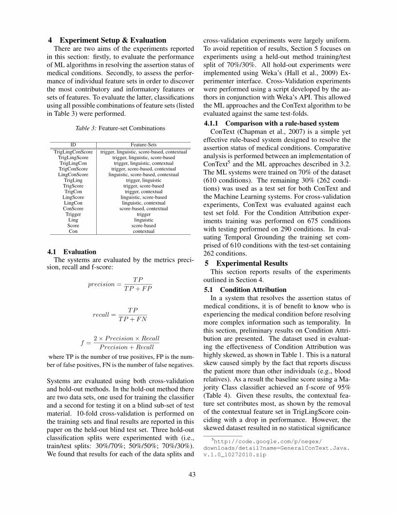
4 Experiment Setup & EvaluationThere are two aims of the experiments reported
in this section: firstly, to evaluate the performanceof ML algorithms in resolving the assertion status ofmedical conditions. Secondly, to assess the perfor-mance of individual feature sets in order to discoverthe most contributory and informatory features orsets of features. To evaluate the latter, classificationsusing all possible combinations of feature sets (listedin Table 3) were performed.
Table 3: Feature-set Combinations
ID Feature-SetsTrigLingConScore trigger, linguistic, score-based, contextual
TrigLingScore trigger, linguistic, score-basedTrigLingCon trigger, linguistic, contextualTrigConScore trigger, score-based, contextualLingConScore linguistic, score-based, contextual
TrigLing trigger, linguisticTrigScore trigger, score-basedTrigCon trigger, contextual
LingScore linguistic, score-basedLingCon linguistic, contextualConScore score-based, contextualTrigger trigger
Ling linguisticScore score-basedCon contextual
4.1 EvaluationThe systems are evaluated by the metrics preci-
sion, recall and f-score:
precision =TP
TP + FP
recall =TP
TP + FN
f =2× Precision×Recall
Precision + Recall
where TP is the number of true positives, FP is the num-ber of false positives, FN is the number of false negatives.
Systems are evaluated using both cross-validationand hold-out methods. In the hold-out method thereare two data sets, one used for training the classifierand a second for testing it on a blind sub-set of testmaterial. 10-fold cross-validation is performed onthe training sets and final results are reported in thispaper on the held-out blind test set. Three hold-outclassification splits were experimented with (i.e.,train/test splits: 30%/70%; 50%/50%; 70%/30%).We found that results for each of the data splits and
cross-validation experiments were largely uniform.To avoid repetition of results, Section 5 focuses onexperiments using a held-out method training/testsplit of 70%/30%. All hold-out experiments wereimplemented using Weka’s (Hall et al., 2009) Ex-perimenter interface. Cross-Validation experimentswere performed using a script developed by the au-thors in conjunction with Weka’s API. This allowedthe ML approaches and the ConText algorithm to beevaluated against the same test-folds.4.1.1 Comparison with a rule-based system
ConText (Chapman et al., 2007) is a simple yeteffective rule-based system designed to resolve theassertion status of medical conditions. Comparativeanalysis is performed between an implementation ofConText5 and the ML approaches described in 3.2.The ML systems were trained on 70% of the dataset(610 conditions). The remaining 30% (262 condi-tions) was used as a test set for both ConText andthe Machine Learning systems. For cross-validationexperiments, ConText was evaluated against eachtest set fold. For the Condition Attribution exper-iments training was performed on 675 conditionswith testing performed on 290 conditions. In eval-uating Temporal Grounding the training set com-prised of 610 conditions with the test-set containing262 conditions.5 Experimental Results
This section reports results of the experimentsoutlined in Section 4.5.1 Condition Attribution
In a system that resolves the assertion status ofmedical conditions, it is of benefit to know who isexperiencing the medical condition before resolvingmore complex information such as temporality. Inthis section, preliminary results on Condition Attri-bution are presented. The dataset used in evaluat-ing the effectiveness of Condition Attribution washighly skewed, as shown in Table 1. This is a naturalskew caused simply by the fact that reports discussthe patient more than other individuals (e.g., bloodrelatives). As a result the baseline score using a Ma-jority Class classifier achieved an f-score of 95%(Table 4). Given these results, the contextual fea-ture set contributes most, as shown by the removalof the contextual feature set in TrigLingScore coin-ciding with a drop in performance. However, theskewed dataset resulted in no statistical significance
5http://code.google.com/p/negex/downloads/detail?name=GeneralConText.Java.v.1.0_10272010.zip
43

between classifiers and feature-sets.
Table 4: Selected feature-sets (f-score) using Cross-Validation for the Condition Attribution task
ID RFor kNN NB Maj.TrigLingConScore 100% 100% 100% 95%
TrigLingScore 96% 96% 96% 95%TrigConScore 100% 100% 100% 95%
Con 100% 100% 100% 95%
In this task, ConText achieved an f-score of 99%.As there is little difference in scores achieved be-tween ConText and the approaches in Table 4 - amanual rule-based system can be considered ade-quate for this task.
Taking a closer look at the performance of the fea-ture sets, we see that the contextual feature set con-tributes most to the task with the removal of contex-tual features coinciding with a drop in performancee.g., TrigLingScore in Table 4. The strength of thisfeature set lies with the feature isInFamHist. Thisfeature simply checks if the condition occurs underthe heading “Family History”. Its highly influen-tial performance would indicate that its quite rarefor the mention of another individual anywhere elsein a clinical report. The Con run, which is solelycomposed of contextual features achieves near per-fect performance, an indication that the contributionof other features to the task of Condition Attribu-tion is minimal. Although this work used only H&Preports, this finding may be generalized to other re-port types such as Discharge Summaries which alsoexplicitly mark sections pertaining to other individ-uals.5.2 Temporal Grounding
The distribution of past and recent medical con-ditions is not skewed (as in the Condition Attribu-tion task), and hence it presents a more challeng-ing classification task. Despite the varying per-formance of individual classifiers and feature setsthe results obtained are again largely similar acrosscross-validation and hold-out methods, with the per-formance of each training set fitting the distribu-tion in Figure 1. Initial experiments investigated theuse of another state-of-the-art classifier, the SupportVector Machine using a polykernel, however due toits relatively poor performance (70% f-score, withits precision soundly beaten by other approaches) itwill not be discussed in further detail.
Random Forest proved to be the most effectiveclassifier across almost all feature sets. However,kNN was a very near second place - Random Forest
only significantly6 outperformed kNN on two occa-sions (TrigLingConScore, LingConScore). In con-strast, Naive Bayes performed poorly - despite hav-ing outperformed all other systems on the precisionmetric, it failed to outperform the baseline majorityclassifier on the recall.
Although the precision of ConText matches thatof the Random Forest and kNN (Table 5), it is alsolet down by its recall performance. As a result, thereis a statistical significant difference between its f-score and that of the Random Forest and kNN.
Table 5: Temporal Grounding ConText Comparison
System Precision Recall F-scorekNN 80% 80% 80%
RandomForest 82% 84% 83%NaiveBayes 91% 61% 72%ConText 80% 61% 69%Majority 55% 100% 71%
6 DiscussionThe distribution of recent and historical condi-
tions for the task of Temporal Grounding is moreevenly distributed than that used in Condition Attri-bution, allowing for a more interesting comparisonof the approaches and features employed.
Figure 1 shows the performance of each ML foreach feature-set combination. Random Forest wasexpectedly the best performing algorithm. However,more surprising was the comparative performanceof the often overlooked kNN algorithm. Both ap-proaches statistically significantly outperformed therule-based system ConText. Though the rule basedsystem matched the high performing ML systems interms of precision, it was significantly outperformedwith respect to recall.
The most contributory feature set in the ML runswas the novel score-based feature set. This featurecreates a normalized score for the occurrence of trig-ger terms in the same sentence as the medical con-dition in question. It was designed to reinforce theimportance of trigger terms, by providing a numericscore to support the binary Trigger List feature. Theaddition of score-based features to any of the fea-ture combinations coincided with a statistical signif-icant boost in performance, with Score (composedsolely of score-based features) outperforming half ofall other feature combinations as seen in Figure 1,.
On the contrary, the effect of contextual featureson the performance of the algorithms for Temporal
6Significance calculated by Paired T-Test with 95% confi-dence.
44

30%
40%
50%
60%
70%
80%
90%
100%
Trig
LingC
onSc
ore
Trig
LingS
core
Trig
LingC
on
Trig
ConSc
ore
LingC
onSc
ore
Trig
Ling
Trig
Scor
e
Trig
Con
LingS
core
LingC
on
ConSc
ore
Trig
Lin
g
Scor
e Con
Ran. Forest kNN Naive Bayes Maj. Class
Figure 1: Temporal Grounding f-score performance with 70% Training Data
Grounding is minimal, or even detrimental to thetask. For example, in Figure 1, the performanceof the kNN algorithm increases from TrigLingCon-Score to TrigLingScore with the removal of contex-tual features. The performance of the Random For-est is unaffected by such detrimental features as itperforms its own feature selection prior to classifi-cation. Though there are several feature set com-binations reaching a high level of performance, themost effective approach combines trigger list terms,linguistic and score based features with the RandomForest algorithm.
These experiments extend previous work by pro-viding a systematic, automated approach to featureextraction for the purpose of ML approaches to Tem-poral Grounding. They also indicate the high per-formance and contribution of our novel score-basedfeatures. These features are not designed to solelyclassify instances found in H&P reports and canbe applied to other clinical reports such as Dis-charge Summaries and Emergency Department re-ports. Previous work has involved the use of thelatter mentioned report types. Unfortunately, giventhe terms-of-use of these datasets they could not bemade available to authors to facilitate comparativeexperiments.7 Conclusion
In this paper, we proposed the use of machinelearning (ML) in resolving if and when a patientexperienced a medical condition. The implementedML algorithms made use of features comprising oftrigger terms, linguistic and contextual information,and novel score-based features. In an evaluation ofthese feature sets it was found that score-based fea-tures contributed to the task of resolving when a pa-tient experienced a medical condition.
The ML approaches were also evaluated against
the rule-based system ConText on a new annotateddataset of History & Physical (H&P) ExaminationReports. In this evaluation it was discovered that thetask of resolving if a condition was experienced bythe patient was adequately solved by the ConTextsystem, achieving an f-score of 99%. Although, theML approaches proposed achieved perfect perfor-mance, there is no statistical significance betweenthe result sets. However, the more challenging taskof deciding when a patient experienced a medicalcondition is deemed to be best suited to a ML ap-proach, with the top performing classifier RandomForest achieving an f-score of 87%, significantlyoutperforming ConText which achieved 69% on thesame dataset .
The results achieved in these tasks have paved theway for several avenues of future work. We be-lieve that the performance of these tasks is now suffi-ciently accurate to justify their inclusion in an Infor-mation Retrieval (IR) application. It is our intentionto use our medical condition analysis techniques toannotate clinical documents and build an advancedIR system capable of taking advantage of this markup in the context of the TREC Medical RecordsTrack 20127. With the availability of datasets suchas that of the i2b2 Shared Task 2010 data, furtherwork will include experimentation on these datasetsas well as an investigation into further assertion sta-tuses.
8 AcknowledgmentsWe are grateful to Dr Martina Naughton for her
advice on many aspects of this paper. We also wishto acknowledge the support of Science FoundationIreland, who fund this research under grant number10/RFP/CMS2836.
7http://groups.google.com/group/trec-med
45

ReferencesL. Breiman. 1996. Bagging predictors. Machine Learn-
ing, 24:123–140.L. Breiman. 2001. Random forests. Machine Learning,
45:5–32.J. Carletta. 1996. Assessing agreement on classification
tasks: the kappa statistic. Computational Linguistics,22(2):249 – 254.
R. Caruana. 2006. An empirical comparison of super-vised learning algorithms. In Proceedings of 23rd In-ternational Conference on Machine Learning.
W. W. Chapman, D. Chu, and J. N. Dowling. 2007. Con-text: An algorithm for identifying contextual featuresfrom clinical text. In BioNLP 2007: Biological, trans-lational, and clinical language processing, pages 81–88, June.
L. M. Christensen. 2002. Mplus: A probabilistic med-ical language understanding system. In Proceedingsof Workshop on Natural Language Processing in theBiomedical Domain, pages 29–36.
C. Clark, J. Aberdeen, M. Coarr, D. Tresner-Kirsch,B. Wellner, A. Yeh, and L. Hirschman. 2011. Mitresystem for clinical assertion status classification. Jour-nal of the American Medical Informatics Association.
T. Cover and P. Hart. 1967. Nearest neighbor patternclassification. Transactions on Information Theory.
B. de Bruijn, C. Cherry, S. Kiritchenko, J. Martin, andX. Zhu. 2011. Machine-learned solutions for threestages of clinical information extraction: the state ofthe art at i2b2 2010. Journal of the American MedicalInformatics Association.
D. Demner-Fushman and J. Lin. 2007. Answeringclinical questions with knowledge-based and statisti-cal techniques. In Computational Linguistics, pages63–103.
D Demner-Fushman, W W. Chapman, and C J. McDon-ald. 2009. What can natural language processing dofor clinical decision support? Journal of BiomedicalInformatics, 42:760–772.
D. Demner-Fushman, S. Abhyankar, A. Jimeno-Yepes,R. Loane, B. Rance, F. Lang, N. Ide, E. Apostolova,and A. R. Aronson. 2011. A knowledge-based ap-proach to medical records retrieval. In TREC 2011Working Notes.
J. Feblowitz, A. Wright, H. Singh, L. Samal, and D. Sit-tig. 2011. Summarization of clinical information: Aconceptual model. Biomedical Informatics.
M. Hall, F. Eibe, G. Holmes, B. Pfahringer, P. Reute-mann, and I. H. Witten. 2009. The weka data miningsoftware: An update. SIGKDD Explorations.
H. Harkema, J. N. Dowling, T. Thornblade, and W. W.Chapman. 2009. Context: An algorithm for identify-ing contextual features from clinical text. Journal ofBiomedical Informatics, 42(5):839–851.
G. Hripcsak, L. Zhou, S. Parsons, A. K. Das, and S. B.Johnson. 2005. Modeling electronic discharge sum-maries as a simple temporal constraint satisfactionproblem. Journal of the American Medical Informat-ics Association, 12(1):55–63, January.
S. M. Meystre, G. K. Savova, K. C. Kipper-Schuler, andJ. F. Hurdle. 2008. Extracting information from tex-tual documents in the electronic health record: a re-view of recent research. IMIA Yearbook of MedicalInformatics, pages 128–144.
D. L. Mowery, H Harkema, J. N. Dowling, J. L. Lust-garten, and W. W. Chapman. 2009. Distinguishinghistorical from current problems in clinical reports-which textual features help? In Proceedings of theWorkshop on Current Trends in Biomedical NaturalLanguage Processin, pages 10–18. Association forComputational Linguistics.
J. Patrick and M. Li. 2011. An ontolotgy for clinicalquestions about the contents of patients notes. Journalof Biomedical Informatics.
J. Provost. 1999. Naive-bayes vs. rule-learning in classi-fication of email. Technical report, The University ofTexas at Austin.
N. Sager, C. Friedman, and M.S. Lyman. 1987. Medi-cal Language Processing: Computer Management ofNarrative Data. Addison-Wesley.
N. Sager, M. Lyman, C. Bucknall, N. Nhan, and L. J.Tick. 1994. Natural language processing and the rep-resentation of clinical data. Journal of the AmericanMedical Informatics Association, 1:142–160.
O. Uzuner, X. Zhang, and T. Sibanda. 2009. Machinelearning and rule-based approaches to assertion classi-fication. Journal of the American Medical InformaticsAssociation, 16(1):109–115.
O. Uzuner, BR. South, S. Shen, and SL. DuVall. 2011.2010 i2b2/va challenge on concepts, assertions, and re-lations in clinical text. Journal of the American Medi-cal Informatics Association.
E. Voorhees and R. Tong. 2010. Overview of the trec2011 medical records track. preprint.
46

Proceedings of the 2012 Workshop on Biomedical Natural Language Processing (BioNLP 2012), pages 47–55,Montreal, Canada, June 8, 2012. c©2012 Association for Computational Linguistics
Alignment-HMM-based Extraction of Abbreviations from Biomedical Text
Dana Movshovitz-AttiasCarnegie Mellon University
5000 Forbes AvenuePittsburgh, PA 15213 [email protected]
William W. CohenCarnegie Mellon University
5000 Forbes AvenuePittsburgh, PA 15213 [email protected]
Abstract
We present an algorithm for extracting abbre-viation definitions from biomedical text. Ourapproach is based on an alignment HMM,matching abbreviations and their definitions.We report 98% precision and 93% recall ona standard data set, and 95% precision and91% recall on an additional test set. Our re-sults show an improvement over previously re-ported methods and our model has several ad-vantages. Our model: (1) is simpler and fasterthan a comparable alignment-based abbrevia-tion extractor; (2) is naturally generalizable tospecific types of abbreviations, e.g., abbrevia-tions of chemical formulas; (3) is trained on aset of unlabeled examples; and (4) associates aprobability with each predicted definition. Us-ing the abbreviation alignment model we wereable to extract over 1.4 million abbreviationsfrom a corpus of 200K full-text PubMed pa-pers, including 455,844 unique definitions.
1 Introduction
Abbreviations and acronyms are commonly used inthe biomedical literature for names of genes, dis-eases and more (Ambrus, 1987). Abbreviation def-initions are a source of ambiguity since they maychange depending on the context. The ability to rec-ognize and extract abbreviations and map them toa full definition can be useful for Information Ex-traction tasks (Yu et al., 2007) and for the completeunderstanding of scientific biomedical text.
Yu et al. (2002) distinguish the two follow-ing uses of abbreviations: (1) Common abbrevia-tions are those that have become widely accepted as
synonyms, such as 〈DNA, deoxyribonucleic acid〉or 〈AIDS, acquired immunodeficiency syndrome〉.These represent common fundamental and impor-tant terms and are often used, although not explic-itly defined within the text (Fred and Cheng, 2003).In contrast, (2) Dynamic abbreviations, are definedby the author and used within a particular article.Such definitions can often overlap, depending onthe context. For example, the term PBS most com-monly abbreviates Phosphate Buffered Saline, butin other contexts may refer to the following: PainBehavior Scale, Painful Bladder Syndrome, PairedDomain-Binding Site, Particle Based Simulation,Partitioned Bremer Support, Pharmaceutical Bene-fits Scheme, and more. Some abbreviations fall be-tween these two definitions in the sense that they arenormally defined in the text, however, they have be-come widely used, and therefore they do not nor-mally overlap with other abbreviations. An exam-ple for this is the term ATP which, almost exclu-sively, abbreviates adenosine triphosphate, and isonly rarely used in different contexts in biomedicine.
Gaudan et al. (2005) define two similar con-cepts, distinguishing Global and Local abbrevia-tions. Global abbreviations are not defined withinthe document, similar to common abbreviation. Lo-cal abbreviations appear in the document alongsidethe long form, similar to dynamic abbreviations.The contextual ambiguity of dynamic, or local, ab-breviations makes them an important target for ab-breviation recognition tasks.
There is a great deal of variation in the way thatdifferent authors produce abbreviations. Our defini-tion of abbreviation is quite flexible and can best be
47

represented by the set of examples described in Ta-ble 1. These include simple acronyms, in which thefirst letter of every word from the long form is rep-resented in the short form, as well as more complexcases such as: inner letter matches, missing shortform characters, and specific substitutions (such asof a chemical element and its symbol). We gener-ally assume that the abbreviated form contains somecontraction of words or phrases from the full form.This definition is consistent with the one defined bymany other extraction systems (see e.g., (Schwartzand Hearst, 2002) and (Chang et al., 2002)).
We describe a method for extracting dynamic ab-breviations, which are explicitly defined in biomed-ical abstracts. For each of the input texts, the taskis to identify and extract 〈short form, long form〉pairs of the abbreviations defined within the text. Wealso provide a mapping, formed as an alignment, be-tween the characters of the two forms, and the prob-ability of this alignment according to our model.
Our approach is based on dividing the abbrevia-tion recognition task into the following stages: (1)Parsing the text and extracting candidate abbrevia-tion pairs (long and short forms) based on textualcues, such as parentheses; (2) Recovering a validalignment between the short and long form candi-dates (valid alignments are defined in Section 3.2).We perform a sequential alignment based on a pair-HMM; (3) Extracting a final short and long formfrom the alignment.
We will show that our approach is fast and accu-rate: we report 98% precision and 93% recall on astandard data set, and 95% precision and 91% recallon a validation set. The alignment model: (1) is sim-pler and faster than a comparable alignment-basedabbreviation extractor; (2) is naturally generalizableto specific types of abbreviations; (3) is trained on aset of unlabeled examples; and (4) associates a prob-ability with each predicted definition.
2 Related Work
A wide variety of methods have been introducedfor recognizing abbreviations in biomedical context.Many utilize one of the following techniques: rule-based extraction, and extraction that relies on analignment of the abbreviation and full definition.Abbreviation extraction methods have been used in
two main contexts: to create online collections ofabbreviations, normally extracted from PubMed ab-stracts (Zhou et al., 2006; Gaudan et al., 2005; Adar,2004), and as part of larger learning frameworks,mainly for feature generation (Chowdhury et al.,2010; Huang et al., 2011).
Rule based extraction systems use a set of man-ually crafted pattern-matching rules to recognizeand extract the pair of abbreviation and defini-tion: Acrophile (Larkey et al., 2000) is an acronymrecognition system that exploits morphological rulesbased on the case of the characters in the definitions.Unlike many of the other available systems, it rec-ognized acronyms that are defined without paren-theses; The Alice system (Ao and Takagi, 2005) isbased on three extraction phases, each employingan elaborate set of over 15 rules, patterns and stopword lists. Liu and Friedman (2003) use a set ofstatistical rules to resolve cases in which an abbre-viation is defined more than once with several dif-ferent definitions. While these methods normallyachieve high performance results, their main draw-back is that they are difficult to implement and toextend. Rule development is normally based on athorough investigation of the range of targeted ab-breviations and the resulting heuristic patterns con-tain subtleties that are hard to recreate or modify.
Several extraction methods have been developedbased on some variant of the Longest Common Sub-sequence algorithm (LCS) (Schwartz and Hearst,2002; Chang et al., 2002; Taghva and Gilbreth,1999; Bowden et al., 1997). These systems searchfor at least one possible alignment of an abbrevia-tion and a full form definition.
The most widely used abbreviation extraction sys-tem is that presented by Schwartz and Hearst (2002).Their method scans the input text and extract pairsof candidate abbreviations from text surroundingparentheses. The algorithm scans the candidate defi-nition from right to left, and searches for an implicitalignment of the definition and abbreviation basedon few ad-hoc rules. This algorithm presents severalconstraints on the type of recognized abbreviations,the most restrictive being that every letter of the ab-breviation must be matched during the process ofscanning the definition. Of the variety of availableextraction systems, this remains a popular choicedue to its simplicity and speed. However, as the au-
48

Short Long Type of Abbreviation
AMS Associated Medical Services Acronym using the first letter of each long-form word.PS postsynaptic Inner letters are represented in the abbreviation.NTx cross-linked N-telopeptides 1. Phonetic substitution (cross→ x).
2. The short form is out-of-order.3. Words from the long form are missing in the short form (linked).
EDI-2 Eating Disorders Inventory Characters from the short form are missing in the long form (-2).NaB sodium butyrate Substitution of a chemical element by its symbol (sodium→ Na).MTIC 5-(3-N-methyltriazen-1-yl)-
imidazole-4-carboxamideChemical formula.
EBNA-1 Epstein-Barr virus (EBV) nuclearantigen 1
Recursive definition, in which the long form contains another ab-breviation definition.
3-D three-dimensional Substitution of a number name and symbol (three→ 3).A&E accident and emergency Substitution of a word and symbol (and→ &).anti-Tac antibody to the alpha subunit of the
IL-2 receptorSynonym: the short form commonly represents the long form, al-though it is not a direct abbreviation of it.
R.E.A.L. ’Revised European-American Clas-sification of Lymphoid Neoplasms’
The long- and/or short-forms contain characters that are not di-rectly related to the abbreviation (e.g., punctuation symbols).
Table 1: Examples of biomedical abbreviations.
thors report, this algorithm is less specific than otherapproaches and consequently results in lower recall.We will show that by performing an explicit align-ment of the abbreviation using an alignment-HMM,our model results in more accurate predictions, andthat the edit operations used in the alignment allowfor natural extensions of the abbreviations domain.
Another frequently used alignment based ap-proach is that of Chang et al. (2002), and it is closestto our approach. After calculating an abbreviationalignment, they convert the set of aligned terms intoa feature vector which is scored using a binary logis-tic regression classifier. Using a correct threshold onthe alignment scores produces a high performanceabbreviation extractor. However this approach hasseveral drawbacks. The run-time of this algorithmis fairly long (see Section 4.3), in part due to thesteps following the alignment recovery, i.e., calcu-lating a feature vector, and generating an alignmentscore. Additionally, choosing a score threshold maydepend on the genre of text, and different thresh-olds lead to a variety of quality in the results. Wewill show that presenting limitations on the range ofavailable alignments can produce correct alignmentsmore efficiently and quickly, maintaining high qual-ity results, without the need for threshold selection.Our alignment method distinguishes and penalizesinner and leading gaps in the alignment, and it ap-
plies a set of constraints on the range of legal align-ments. We will also show that relying solely on con-strained alignments still allows for flexibility in thedefinition of the range of desired abbreviations.
Ristad and Yianilos (1998) proposed a single statealignment-HMM for learning string-edit distancebased on matched strings. In later work, Bilenko andMooney (2003) extend this model to include affinegaps, by including in their model separate statesfor Matches, Deletions and Insertions. McCallumet al. (2005) describe a discriminative string editCRF, following a similar approach to that of Bilenkoand Mooney. The CRF model includes two disjointsets of states, each representing either “matching” or“mismatching” string pairs. Each of the sets is sim-ilar to the model described by Bilenko and Mooney.All of these models require labeled training exam-ples, and the CRF approach also requires negativetraining examples, which train the “mismatching”states of the model. We describe an alignment HMMthat is suited for aligning abbreviation long and shortforms, and does not require any labeling of the inputtext or training examples.
3 Method
In the following sections we describe a method forextracting candidate abbreviation definitions fromtext, and an alignment model with affine gaps for
49

Description Result
i. Input sentence: “anti-sperm antibodies were studied by indirect mixed anti-globulin reaction test (MAR)”
ii. Candidate: 〈MAR, by indirect mixed anti-globulin reaction test〉
iii. Alignment:HMM StatesShort FormLong Form
LG LG LG LG M M M M IG M M M IG
M A R
by indirect mixed anti - globulin reaction test
iv. Abbreviation: 〈MAR, mixed anti-globulin reaction test〉
Table 2: Example of the processing steps of a sample sentence. (i) Input sentence containing a single abbreviation.(ii) Candidate 〈short form, long form〉 pair extracted from the sentence (after truncating the long-form). (iii) Themost likely (Viterbi) alignment of the candidate pair, using our alignment model. Each state corresponds to a singleedit-operation, which consumed the corresponding short-form and long-form characters in the alignment. (iv) Finalabbreviation, extracted from the alignment by removing leading gaps.
matching the two forms of a candidate definition.Finally we describe how to extract the final abbre-viation prediction out of the alignment.
3.1 Extracting candidate abbreviations
The process described below scans the text for tex-tual cues and extracts a list of candidate abbreviationpairs, for every input document, in the form: 〈shortform, long form〉. The following text also describesthe restrictions and conditions of what we considerto be valid candidate pairs. The assumptions madein this work are generally less restrictive that thoseintroduced by previous extraction systems and theylead to a larger pool of candidate definitions. Wewill later show that false candidates normally pro-duce invalid alignment of their short and long forms,according to our alignment model, and so they areremoved and do not affect the final results.
The parsing process includes a search for bothsingle abbreviations, and abbreviation patterns. Anexample of a sentence with a single abbreviationcan be seen in Table 2(i). We consider the fol-lowing two cases of a single abbreviation defini-tion: (1) “long form (short form)”, and (2) “shortform (long form)”. Note that in some cases, theterm within the parenthesis is parsed, e.g., in thefollowing text, ELISA is extracted from the paren-thesis, by removing the text beyond the ’;’ symbol:“. . . human commercial enzyme-linked immunosor-bent assay (ELISA; BioGen, Germany) . . . ”.
We also consider abbreviation patterns which
define multiple abbreviations simultaneously, asdemonstrated by these examples:
• “anti-sperm (ASA), anti-phospholipid (APA),and antizonal (AZA) antibodies” – The mainnoun (antibodies) follows the pattern.
• “Epithelial-mesenchymal transition (EMT)and interaction (EMI)” – The main noun(Epithelial-mesenchymal) is at the head of thepattern.
Using textual cues (patterns and parentheses) weextract candidate short and long forms. Wheneverpossible, we consider the term within the parenthe-sis as the short form, and the text to the left of theparenthesis (until the beginning of the sentence) asthe candidate long form. We consider valid shortforms to be no longer than 3 words, having between1 and 15 characters, and containing at least one let-ter. In the case that the candidate short form wasfound to be invalid by these definitions, we switchthe assignment of long and short forms. The long-form string is truncated, following Park and Byrd(2001), to a length of min(|A|+ 5, |A| ∗ 2), where|A| is the length of the short form.
The length of the candidate long form is estimatedusing the Park and Byrd formula, and it is thereforenormally the case that the resulting candidate longform contains some leading characters that are notpart of the abbreviation definition. Next, we definean alignment between short and long form strings
50

<“CRF-BP”, “ligands for the corticotrophin-releasing factor binding protein”>
| | | | | |C | |R | |F | |-|B | |P | ligands| |for| |the| |corticotrophin|-|releasing| |factor| | |binding| |protein|
!"
#$"
%"
&$"
'"
Figure 1: Abbreviation alignment HMM model withstates: start (s), leading gaps (LG), match (M), inner gap(IG) and end (e).
EditOperation
SFMatch
LFMatch
ValidStates
LF deletion ε alpha-numericchar
LG, IG
LF deletion ε punct. symbol LG, MLF deletion ε word LG, IGSF deletion digit or punct. ε IGMatch char (partial) word MMatch char char MSubstitution ’&’ ’and’ MSubstitution ’1’-’9’ ’one’-’nine’ MSubstitution chem. symbol chemical name M
Table 3: Edit operations used in the alignment HMMmodel including, long form (LF) and short form (SF)deletions, matches and substitutions. We note the SF andLF characters consumed by each edit operation, and theHMM states in which it may be used.
which detects possible segments that are missing inthe alignment in either string (gaps).
3.2 Aligning candidate long and short forms
For each of the candidate pairs produced in the pre-vious step, we find the best alignment (if any) be-tween the short and the long form strings. We de-scribe an alignment HMM that is suited for abbrevi-ation alignments. The model is shown in Figure 1,and Table 2 shows the parsing process of a sam-ple sentence, including an alignment created for thissample using the model.
3.3 Abbreviation Alignment with AffineLeading and Inner Gaps
An alignment between a long and a short form of anabbreviation can be modeled as a series of edit oper-ations between the two strings, in which charactersfrom the short form may match a single or a seriesof characters from the long form. In previous work,Bilenko and Mooney (2003) describe a generative
model for string edit distance with affine gaps, andan Expectation Maximization algorithm for learningthe model parameters using a labeled set of match-ing strings. We propose a similar model for aligningthe short and long form of an abbreviation, using anaffine cost model for gaps
cost(g) = s+ e · l (1)
where s is the cost of starting a gap, e is the cost ofextending a gap and l is the length of the gap. In ourmethod, we use extracted candidate pairs (candidateshort and long forms) as training examples.
As described above, candidate long forms areformed by extracting text preceding parentheses andtruncating it to some length. This process may leadto candidate long forms that contain leading charac-ters that do not belong to the abbreviation, whichwill result in leading gaps in the final alignment.For example, the candidate long form presented inTable 2(ii) contains the leading text “by indirect “.While extra leading text is expected as an artifact ofour candidates extraction method, inner alignmentgaps are not expected to commonly appear in abbre-viation alignments, and are usually an indication of abad alignment. The example presented in Table 2 isof an abbreviation that does contain inner gaps (e.g.,globulin) despite being a valid definition.
We distinguish leading and inner alignment gapsusing a model with five states: Leading Gap (LG),Match (M), Inner Gap (IG), and two “dummy” statesfor the beginning and end of an alignment (Figure 1).Since leading and inner gaps are represented by dif-ferent states, their penalization is not coupled, i.e.,they are associated with different s, e and l costs.We use the EM algorithm to learn the model param-eters, based on a set of unlabeled candidate pairs,following the assumption that many false-candidateswill not produce a valid alignment, and will not af-fect training. This is in contrast to previous stringedit distance models, which require labeled trainingexamples.
The main effort in developing a successful ab-breviation alignment model involves generating ameaningful set of edit operations. The edit opera-tions used in our model,E = Ed∪Em∪Es, is shownin Table 3 and includes: Ed, deletions of charactersor words from the long form, or of single characters
51

from the short form; Em, matches of a full of par-tial word from the long form to a character in theshort form; and Es, word substitutions in which aword from the long form is replaced by a symbol inthe short form. Note that: (1) while all types of dele-tions from the long form are valid, deletions from theshort form are limited to digits and punctuation sym-bols, and (2) deletion of non-alpha-numeric charac-ters from the long form is not considered as openinga gap but as a match, as it is common for non-alpha-numeric characters to be missing in an abbreviation(i.e., be “matched” with the empty string, ε).
Let x = x1 . . . xT be the short form candidate,y = y1 . . . yV be the long form candidate, anda = 〈ap〉np=1, ap = (ep, qp, ixp, jyp), be a pos-sible alignment of the strings x and y. a repre-sents as a sequence of HMM transitions, ap, whereep ∈ E is an edit operation that consumes charac-ters from x (deletion from the long form), y (dele-tion from the short form), or both (match or substi-tution), up to position ixp in x and jyp in y, andis associated with a transition in the model to stateqp ∈ {LG,M, IG, e}. Let π(q, q′) be the transitionprobability between states q and q′, and let τ(q, e)be the emission probability of the edit operation e atstate q. Given a candidate abbreviation pair 〈x, y〉,and the model parameters π and τ , the probability ofan alignment is given by
p(a|x, y, π, τ) =
|a|∏p=1
π(qp−1, qp) · τ(qp, ep) (2)
where q0 is the start state. This probability can becalculated efficiently using dynamic programmingwith the forward-backward algorithm, and the mostlikely alignment corresponds to the Viterbi distancebetween x and y.
In our method, the model parameters, π and τ ,are estimated using the EM algorithm on an unla-beled training set of candidate pairs that have beenextracted from the text, without any further process-ing. At each EM iteration, we train on pairs that havevalid alignments (see below) with non-zero proba-bility under the model parameters at that iteration.
3.3.1 Valid AlignmentsGiven the edit operations defined above, the only
valid way of matching a letter from the short form
to the long form is by matching that letter to thebeginning of a full or partial word, or by matchingthat letter using a substitution operation. There isno edit operation for deleting letters from the shortform (only digits and punctuation symbols can bedeleted). This means that for some candidate pairsthere are no valid alignments under this model, inwhich case, no abbreviation will be predicted.
3.3.2 Extracting the Final AbbreviationGiven a valid alignment a between the candi-
date pair, x and y, we create a truncated alignment,a′, by removing from a initial transitions in whichqp = LG. We consider a′ valid if the number ofmatches in a′ = 〈a′p〉n
′p=1 is greater than the number
of deletions,
n′∑p=1
I(q′p = M) >n′∑
p=1
I(q′p = IG) (3)
where I is an indicator function.The final abbreviation prediction is given by the
portions of the x and y strings that are associatedwith a′, named x′ and y′, respectively. These may betruncated compared to x and y, as leading alignmentgaps are removed. The final alignment probability isgiven by p(a′|x′, y′, π, τ).
3.4 Substitution Edit OperationsIn contrast to rule-based extraction algorithms, inour model, it is easy to introduce new types of editoperations, and adjust the model to recognize a va-riety of abbreviation types. As an example, we haveadded a number of substitution operations (see Ta-ble 3), including an operation for the commonlyused convention of replacing a chemical elementname (e.g., Sodium) with its symbol (Na). Thesetypes of operations are not available using simplermodels, such as that presented by Schwartz andHearst (2002), making it impossible to recognizesome important biomedical entities, such as chem-ical compounds (e.g., 〈NaB, SodiumButyrate〉).In contrast, such additions are natural in our model.
4 Evaluation
4.1 Abbreviation Extraction AnalysisWe evaluated the alignment abbreviation model overtwo data sets (Table 4). The method was tuned using
52

Data Set Name Abstracts Abbreviations Testing Method
Development (D) Medstract 400 483 10-fold cross validation.Validation (V) PubMed Sample 50 76 Training on set D and testing on set V.
Table 4: Evaluation Data Sets.
Model D (average %) V (%)
P R F1 P R F1
Alignment HMM 98 93 96 95 91 93SH 96 88 91 97 83 89Chang 0.88 99 46 62 97 47 64Chang 0.14 94 89 91 95 91 93Chang 0.03 92 91 91 88 93 90Chang 0 49 92 64 53 93 67
Table 5: Results on validation (V) and development (D)sets. Average results are shown for D set, which wastested using 10-fold cross-validation (results rounded tonearest percent, all standard deviations were < 0.1)
10 fold cross-validation over the publicly availableMedstract corpus (Pustejovsky et al., 2002) whichincludes 400 Medline abstracts. The online versionof the corpus was missing the Gold Standard annota-tions throughout the development of our algorithm,nor was it possible to get them through communica-tion with the authors. We therefore hand-annotatedthe Medstract data, yielding 483 abbreviation defi-nitions in the form of 〈short form, long form〉 pairs.In order to be consistent with previous evaluationsover Medstract, our annotations include only defini-tions in which either the short or the long form ap-pear in parenthesis, and it is assumed that there areno trailing gaps in the term preceding the parenthe-sis, although our model does detect such gaps.
We compare our results with two algorithmsavailable for download: the Schwartz and Hearst(SH; (2002)) algorithm1, and the Chang et al. (2002)algorithm2 used at three score cutoffs reported intheir paper (0.88, 0.14, 0.03). We also use a fourthscore cutoff of 0 to account for any legal alignmentsproduced by the Chang model.
In Table 5 we report precision (P), recall (R) and
1Taken from http://biotext.berkeley.edu/software.html2Taken from http://abbreviation.stanford.edu
F1 scores for all methods, calculated by
P =correct predicted abbreviations
all predicted abbreviations(4)
R =correct predicted abbreviations
all correct abbreviations(5)
On the development set, our alignment modelachieves 98% precision, 93% recall and 96% F1 (av-erage values over cross-validation iterations, withstandard deviations all under 0.03).
To test the final model we used a validationdataset consisting of 50 abstracts, randomly selectedout of a corpus of 200K full-text biomedical articlestaken from the PubMed Central Open Access Sub-set (extracted in October 2010)3. These were hand-annotated, yielding 76 abbreviation definitions.
On the validation set, we predicted 69 out of 76abbreviations, with 4 false predictions, giving 95%precision, 91% recall and 93% F1. Our alignmentmodel results in higher F1 score over all baselinesin both datasets (with Chang0.14 giving equal resultson the validation set). Our results are most compa-rable with the Chang model at a score cutoff of 0.14,though our model does not require selecting a scorecutoff, and as we will show, it is considerably faster.Interestingly, our model results in lower recall thanprecision on both data sets. This may be due to alimited scope of edit operations.
In order to evaluate the usability of our method,we used it to scan the 200K full-text documents ofthe PubMed Central Open Access Subset corpus.The process completed in under 3 hours, yieldingover 1.4 million abbreviations, including 455,844unique definitions. A random sample of the ex-tracted abbreviations suggests a low rate of falsepositive predictions.
4.2 Error AnalysisOur model makes 4 incorrect predictions on the val-idation set, 3 of which are partial matches to the
3http://www.ncbi.nlm.nih.gov/pmc/
53
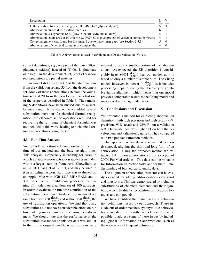
Description D V
Letters in short form are missing (e.g., 〈GlyRalpha2, glycine alpha2〉) 5 3Abbreviation missed due to extraction rules. 6 1Abbreviation is a synonym (e.g., 〈IRX-2, natural cytokine mixture〉) 5 1Abbreviation letters are out-of-order (e.g., 〈VSV-G, G glycoprotein of vesicular stomatitis virus〉) 4 1Correct alignment was found but it is invalid due to many inner gaps (see Section 3.3.1). 5 0Abbreviations of chemical formulas or compounds. 4 0
Table 6: Abbreviations missed in development (D) and validation (V) sets.
correct definitions, e.g., we predict the pair 〈GlOx,glutamate oxidase〉 instead of 〈GlOx, L-glutamateoxidase〉. On the development set, 3 out of 5 incor-rect predictions are partial matches.
Our model did not extract 7 of the abbreviationsfrom the validation set and 33 from the developmentset. Many of these abbreviations (6 from the valida-tion set and 29 from the development set) had oneof the properties described in Table 6. The remain-ing 5 definitions have been missed due to miscel-laneous issues. Note that while we added severalsubstitution operations for chemical formula recog-nition, the elaborate set of operations required forrecovering the full range of chemical formulas wasnot included in this work, leading to 4 chemical for-mula abbreviations being missed.
4.3 Run-Time Analysis
We provide an estimated comparison of the runtime of our method and the baseline algorithms.This analysis is especially interesting for cases inwhich an abbreviation extraction model is includedwithin a larger learning framework (Chowdhury etal., 2010; Huang et al., 2011), and may be used init in an online fashion. Run time was evaluated onan Apple iMac with 4GB 1333 MHz RAM, and a3.06 GHz Core i3, double-core processor, by run-ning all models on a random set of 400 abstracts.In order to evaluate the run time contribution of thesubstitution operations introduced in our model weran it both with (88 docs
sec ) and without (98 docssec ) the
use of substitution operations. We find that usingsubstitutions did not have considerable effect on runtime, adding under 1 ms for processing each docu-ment. We should note that the performance of thesubstitution-less model on this test data was similarto that of the original model, as substitutions were
relevant to only a smaller portion of the abbrevi-ations. As expected, the SH algorithm is consid-erably faster (6451 docs
sec ) than our model, as it isbased on only a number of simple rules. The Changmodel, however, is slower (4 docs
sec ) as it includesprocessing steps following the discovery of an ab-breviation alignment, which means that our modelprovides comparable results to the Chang model andruns an order-of-magnitude faster.
5 Conclusions and Discussion
We presented a method for extracting abbreviationdefinitions with high precision and high recall (95%precision, 91% recall and 93% F1 on a validationset). Our model achieves higher F1 on both the de-velopment and validation data sets, when comparedwith two popular extraction methods.
Our approach is based on a sequential genera-tive model, aligning the short and long form of anabbreviation. Using the proposed method we ex-tracted 1.4 million abbreviations from a corpus of200K PubMed articles. This data can be valuablefor Information Extraction tasks and for the full un-derstanding of biomedical scientific data.
The alignment abbreviation extractor can be eas-ily extended by adding edit-operations over shortand long forms. This was demonstrated by includingsubstitutions of chemical elements and their sym-bols, which facilitates recognition of chemical for-mulas and compounds.
We have identified the main classes of abbrevia-tion definitions missed by our approach. These in-clude out-of-order matches, synonym-like abbrevia-tions, and short forms with excess letters. It may bepossible to address some of these issues by includ-ing “global” information on abbreviations, such asthe occurrence of frequent definitions.
54

Acknowledgments
This work was funded by grant 1R101GM081293from NIH, IIS-0811562 from NSF and by a gift fromGoogle. The opinions expressed in this paper aresolely those of the authors.
ReferencesE. Adar. 2004. Sarad: A simple and robust abbreviation
dictionary. Bioinformatics, 20(4):527–533.JL Ambrus. 1987. Acronyms and abbreviations. Journal
of medicine, 18(3-4):134.H. Ao and T. Takagi. 2005. Alice: an algorithm to extract
abbreviations from medline. Journal of the AmericanMedical Informatics Association, 12(5):576–586.
M. Bilenko and R.J. Mooney. 2003. Adaptive duplicatedetection using learnable string similarity measures.In Proceedings of the ninth ACM SIGKDD interna-tional conference on Knowledge discovery and datamining, pages 39–48. ACM.
P.R. Bowden, P. Halstead, and T.G. Rose. 1997. Dic-tionaryless english plural noun singularisation usinga corpus-based list of irregular forms. LANGUAGEAND COMPUTERS, 20:339–352.
J.T. Chang, H. Schutze, and R.B. Altman. 2002. Cre-ating an online dictionary of abbreviations from med-line. Journal of the American Medical Informatics As-sociation, 9(6):612–620.
M. Chowdhury, M. Faisal, et al. 2010. Disease mentionrecognition with specific features. In Proceedings ofthe 2010 Workshop on Biomedical Natural LanguageProcessing, pages 83–90. Association for Computa-tional Linguistics.
H.L. Fred and T.O. Cheng. 2003. Acronymesis: theexploding misuse of acronyms. Texas Heart InstituteJournal, 30(4):255.
S. Gaudan, H. Kirsch, and D. Rebholz-Schuhmann.2005. Resolving abbreviations to their senses in med-line. Bioinformatics, 21(18):3658–3664.
M. Huang, J. Liu, and X. Zhu. 2011. Genetukit: a soft-ware for document-level gene normalization. Bioin-formatics, 27(7):1032–1033.
L.S. Larkey, P. Ogilvie, M.A. Price, and B. Tamilio.2000. Acrophile: an automated acronym extractor andserver. In Proceedings of the fifth ACM conference onDigital libraries, pages 205–214. ACM.
H. Liu, C. Friedman, et al. 2003. Mining terminologicalknowledge in large biomedical corpora. In Pac SympBiocomput, pages 415–426.
A. McCallum, K. Bellare, and F. Pereira. 2005. A condi-tional random field for discriminatively-trained finite-state string edit distance. In Conference on Uncer-tainty in AI (UAI).
Y. Park and R.J. Byrd. 2001. Hybrid text mining for find-ing abbreviations and their definitions. In Proceedingsof the 2001 conference on empirical methods in natu-ral language processing, pages 126–133.
J. Pustejovsky, J. Castano, R. Sauri, A. Rumshinsky,J. Zhang, and W. Luo. 2002. Medstract: creat-ing large-scale information servers for biomedical li-braries. In Proceedings of the ACL-02 workshopon Natural language processing in the biomedicaldomain-Volume 3, pages 85–92. Association for Com-putational Linguistics.
E.S. Ristad and P.N. Yianilos. 1998. Learning string-editdistance. Pattern Analysis and Machine Intelligence,IEEE Transactions on, 20(5):522–532.
A.S. Schwartz and M.A. Hearst. 2002. A simplealgorithm for identifying abbreviation definitions inbiomedical text. In Pacific Symposium on Biocomput-ing 2003: Kauai, Hawaii, 3-7 January 2003, page 451.World Scientific Pub Co Inc.
K. Taghva and J. Gilbreth. 1999. Recognizing acronymsand their definitions. International Journal on Docu-ment Analysis and Recognition, 1(4):191–198.
H. Yu, G. Hripcsak, and C. Friedman. 2002. Map-ping abbreviations to full forms in biomedical articles.Journal of the American Medical Informatics Associa-tion, 9(3):262–272.
H. Yu, W. Kim, V. Hatzivassiloglou, and W.J. Wilbur.2007. Using medline as a knowledge source for dis-ambiguating abbreviations and acronyms in full-textbiomedical journal articles. Journal of biomedical in-formatics, 40(2):150–159.
W. Zhou, V.I. Torvik, and N.R. Smalheiser. 2006. Adam:another database of abbreviations in medline. Bioin-formatics, 22(22):2813.
55
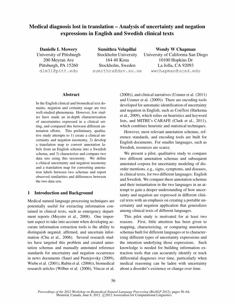
Proceedings of the 2012 Workshop on Biomedical Natural Language Processing (BioNLP 2012), pages 56–64,Montreal, Canada, June 8, 2012. c©2012 Association for Computational Linguistics
Medical diagnosis lost in translation – Analysis of uncertainty and negationexpressions in English and Swedish clinical texts
Danielle L MoweryUniversity of Pittsburgh
200 Meyran AvePittsburgh, PA [email protected]
Sumithra VelupillaiStockholm University
164 40 KistaStockholm, Sweden
Wendy W ChapmanUniversity of California San Diego
10100 Hopkins DrLa Jolla, CA 92093
Abstract
In the English clinical and biomedical text do-mains, negation and certainty usage are twowell-studied phenomena. However, few stud-ies have made an in-depth characterizationof uncertainties expressed in a clinical set-ting, and compared this between different an-notation efforts. This preliminary, qualita-tive study attempts to 1) create a clinical un-certainty and negation taxonomy, 2) developa translation map to convert annotation la-bels from an English schema into a Swedishschema, and 3) characterize and compare twodata sets using this taxonomy. We definea clinical uncertainty and negation taxonomyand a translation map for converting annota-tion labels between two schemas and reportobserved similarities and differences betweenthe two data sets.
1 Introduction and Background
Medical natural language processing techniques arepotentially useful for extracting information con-tained in clinical texts, such as emergency depart-ment reports (Meystre et al., 2008). One impor-tant aspect to take into account when developing ac-curate information extraction tools is the ability todistinguish negated, affirmed, and uncertain infor-mation (Chu et al., 2006). Several research stud-ies have targeted this problem and created anno-tation schemas and manually annotated referencestandards for uncertainty and negation occurrencein news documents (Saurı and Pustejovsky (2009),Wiebe et al. (2001), Rubin et al. (2006)), biomedicalresearch articles (Wilbur et al. (2006), Vincze et al.
(2008)), and clinical narratives (Uzuner et al. (2011)and Uzuner et al. (2009)). There are encoding toolsdeveloped for automatic identification of uncertaintyand negation in English, such as ConText (Harkemaet al., 2009), which relies on heuristics and keywordlists, and MITRE’s CARAFE (Clark et al., 2011),which combines heuristic and statistical techniques.
However, most relevant annotation schemas, ref-erence standards, and encoding tools are built forEnglish documents. For smaller languages, such asSwedish, resources are scarce.
We present a pilot, qualitative study to comparetwo different annotation schemas and subsequentannotated corpora for uncertainty modeling of dis-order mentions, e.g., signs, symptoms, and diseases,in clinical texts, for two different languages: Englishand Swedish. We compare these annotation schemasand their instantiation in the two languages in an at-tempt to gain a deeper understanding of how uncer-tainty and negation are expressed in different clini-cal texts with an emphasis on creating a portable un-certainty and negation application that generalizesamong clinical texts of different languages.
This pilot study is motivated for at least tworeasons. First, little attention has been given tomapping, characterizing, or comparing annotationschemas built for different languages or to character-izing different types of uncertainty expressions andthe intention underlying those expressions. Suchknowledge is needed for building information ex-traction tools that can accurately identify or trackdifferential diagnoses over time, particularly whenmedical reasoning can be laden with uncertaintyabout a disorder’s existence or change over time.
56

Second, building new resources for small lan-guages is time consuming. Utilizing existing toolsand techniques already developed for one language,such as English, could be an efficient way of devel-oping new useful tools for other less exploited lan-guages, such as Swedish.
Our overall goal is to move towards improving au-tomatic information extraction from clinical texts byleveraging language differences and similarities. Inorder to address this issue, our aims in this studyare to 1) create a taxonomy for deepened charac-terization of how uncertainty and negation is ex-pressed in clinical texts, 2) compare two existing un-certainty and negation annotation schemas from thisperspective, and 3) compare differences and similar-ities in expressions of uncertainty and negation be-tween two languages: English and Swedish.
2 Methods
In this pilot, qualitative comparison study, we usedgrounded theory (Strauss and Corbin, 1990) to in-ductively identify themes that characterize clini-cal uncertainty and negation expressed in both En-glish (University of Pittsburgh Medical Center) andSwedish (Karolinska University Hospital) researchdata sets derived from emergency department re-ports.
2.1 Uncertainty/negation annotation schemasTwo independently developed annotation schemaswere used to annotate disorder mentions in theclinical texts: a schema developed for English re-ports (Mowery et al. (2012)) and one for Swedish(Velupillai et al. (2011)). Each disorder mentionwas pre-annotated and constituted the input to a sep-arate set of annotators, who assigned values to a setof attributes defined in the schema. For instance, inthe sentence “Patient with possible pneumonia.”, an-notators for the English data set assigned values tofour attributes for the instance of pneumonia:
• Existence(yes, no): whether the disorder was ever present
• AspectualPhase(initiation, continuation, culmination, un-marked): the stage of the disorder in its progression
• Certainty(low, moderate, high, unmarked): amount of certaintyexpressed about whether the disorder exists
• MentalState(yes, no): whether an outward thought or feelingabout the disorder’s existence is mentioned
In the Swedish schema, annotators assigned val-ues to two attributes:
• Polarity(positive, negative): whether a disorder mention is in thepositive or negative polarity, i.e., affirmed (positive) or negated(negative)
• Certainty(possibly, probably, certainly): gradation of certaintyfor a disorder mention, to be assigned with a polarity value.
2.2 Data SetsThe English data set included 30 de-identified, full-length emergency department reports annotated with283 disorders related to influenza-like illnesses bya board-certified infectious disease physician. Eachdisorder was annotated with four attributes – exis-tence, aspectual phase, certainty and mental state –by two independent annotators (including DM) whocame to consensus after reviewing disagreements.
The Swedish data set included 1,297 assessmentsections from emergency department reports anno-tated with approx. 2,000 disorders, automaticallymarked from a manually created list of approx-imately 300 unique disorders by two physicians.The two physicians annotated each disorder mentionwith attributes of polarity and certainty. A randomsubset of approx. 200 annotated disorder mentionsfrom the data set were used for this qualitative study.
2.3 Study ProcessIn order to better understand how physicians de-scribe uncertainty of the presence or absence of adisorder, we evaluated the annotations from the twodata sets as follows: 1) created a clinical uncertaintyand negation taxonomy, 2) developed a translationmap for mapping attributes and values from the En-glish schema into the Swedish schema, and 3) char-acterized and compared both data sets and languagesusing the taxonomy.
To create the uncertainty and negation taxonomy,we conducted a literature review of recent annota-tion schemas (e.g. Vincze et al. (2008)), assignmentapplications (e.g. Uzuner et al. (2011), Harkemaet al. (2009), Clark et al. (2011), Chapman et al.(2011)), and observational studies (Lingard et al.,2003) about uncertainty or negation in the clinicaldomain. From our review, we created a clinical tax-onomy describing notable characteristics of uncer-tainty and negation, which were added to and re-fined using grounded theory, by inspecting the dis-order annotations in our data sets and documenting
57
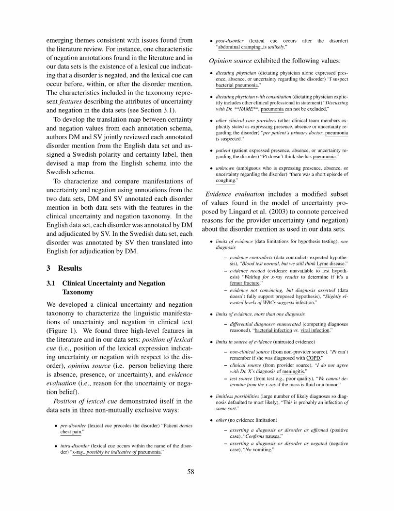
emerging themes consistent with issues found fromthe literature review. For instance, one characteristicof negation annotations found in the literature and inour data sets is the existence of a lexical cue indicat-ing that a disorder is negated, and the lexical cue canoccur before, within, or after the disorder mention.The characteristics included in the taxonomy repre-sent features describing the attributes of uncertaintyand negation in the data sets (see Section 3.1).
To develop the translation map between certaintyand negation values from each annotation schema,authors DM and SV jointly reviewed each annotateddisorder mention from the English data set and as-signed a Swedish polarity and certainty label, thendevised a map from the English schema into theSwedish schema.
To characterize and compare manifestations ofuncertainty and negation using annotations from thetwo data sets, DM and SV annotated each disordermention in both data sets with the features in theclinical uncertainty and negation taxonomy. In theEnglish data set, each disorder was annotated by DMand adjudicated by SV. In the Swedish data set, eachdisorder was annotated by SV then translated intoEnglish for adjudication by DM.
3 Results
3.1 Clinical Uncertainty and NegationTaxonomy
We developed a clinical uncertainty and negationtaxonomy to characterize the linguistic manifesta-tions of uncertainty and negation in clinical text(Figure 1). We found three high-level features inthe literature and in our data sets: position of lexicalcue (i.e., position of the lexical expression indicat-ing uncertainty or negation with respect to the dis-order), opinion source (i.e. person believing thereis absence, presence, or uncertainty), and evidenceevaluation (i.e., reason for the uncertainty or nega-tion belief).
Position of lexical cue demonstrated itself in thedata sets in three non-mutually exclusive ways:
• pre-disorder (lexical cue precedes the disorder) “Patient denieschest pain.”
• intra-disorder (lexical cue occurs within the name of the disor-der) “x-ray...possibly be indicative of pneumonia.”
• post-disorder (lexical cue occurs after the disorder)“abdominal cramping..is unlikely.”
Opinion source exhibited the following values:
• dictating physician (dictating physician alone expressed pres-ence, absence, or uncertainty regarding the disorder) “I suspectbacterial pneumonia.”
• dictating physician with consultation (dictating physician explic-itly includes other clinical professional in statement) “Discussingwith Dr. **NAME**, pneumonia can not be excluded.”
• other clinical care providers (other clinical team members ex-plicitly stated as expressing presence, absence or uncertainty re-garding the disorder) “per patient’s primary doctor, pneumoniais suspected.”
• patient (patient expressed presence, absence, or uncertainty re-garding the disorder) “Pt doesn’t think she has pneumonia.”
• unknown (ambiguous who is expressing presence, absence, oruncertainty regarding the disorder) “there was a short episode ofcoughing.”
Evidence evaluation includes a modified subsetof values found in the model of uncertainty pro-posed by Lingard et al. (2003) to connote perceivedreasons for the provider uncertainty (and negation)about the disorder mention as used in our data sets.
• limits of evidence (data limitations for hypothesis testing), onediagnosis
– evidence contradicts (data contradicts expected hypothe-sis), “Blood test normal, but we still think Lyme disease.”
– evidence needed (evidence unavailable to test hypoth-esis) “Waiting for x-ray results to determine if it’s afemur fracture.”
– evidence not convincing, but diagnosis asserted (datadoesn’t fully support proposed hypothesis), “Slightly el-evated levels of WBCs suggests infection.”
• limits of evidence, more than one diagnosis
– differential diagnoses enumerated (competing diagnosesreasoned), “bacterial infection vs. viral infection.”
• limits in source of evidence (untrusted evidence)
– non-clinical source (from non-provider source), “Pt can’tremember if she was diagnosed with COPD.”
– clinical source (from provider source), “I do not agreewith Dr. X’s diagnosis of meningitis.”
– test source (from test e.g., poor quality), “We cannot de-termine from the x-ray if the mass is fluid or a tumor.”
• limitless possibilities (large number of likely diagnoses so diag-nosis defaulted to most likely), “This is probably an infection ofsome sort.”
• other (no evidence limitation)
– asserting a diagnosis or disorder as affirmed (positivecase), “Confirms nausea.”
– asserting a diagnosis or disorder as negated (negativecase), “No vomiting.”
58

Figure 1: Uncertainty and negation taxonomy with features – Position of lexical cue, Opinion source and Evidence evaluation –with corresponding values (nested lines and sub-lines).
3.2 Translation MapIn order to compare annotations between the datasets, we developed a mapping procedure for convert-ing the four annotated attribute values from the En-glish schema into the two annotated attribute valuesfrom the Swedish schema. This mapping procedureuses two normalization steps, negation and certainty(see Figure 2).
Using Figure 2, we explain the mapping proce-dure to convert English annotations into Swedishannotations. Our steps and rules are applied withprecedence, top down and left to right. For “I haveno suspicion for bacterial infection for this patient”,English annotations are Existence(no) AND Aspec-tualPhase(null) AND Certainty(high) AND Men-talState(yes), and Swedish annotations are Polar-ity(negative) AND Certainty(probably). The map-ping procedure applies two normalization steps,negation and uncertainty, with the following rules.
The first step is negation normalization to convertExistence and Aspectual Phase into Polarity anno-tations. In this example, Existence(no) → Polar-ity(negative).
The second step is certainty normalization withup to two sub steps. For Certainty mapping, in sum-mary, map English NOT Certainty(unmarked) toSwedish Certainty level, e.g., Certainty(high)→ Certainty(probably). For MentalState
mapping, if English Certainty(unmarked) ANDMentalState(yes), map to either Swedish Cer-tainty(probably) OR Certainty(possibly) usingyour best judgment; otherwise, map to Cer-tainty(certainly). For our example sentence,Certainty mapping was sufficient to map from theEnglish to the Swedish Certainty levels.
We found that these two schemas were mappable.Despite the binary mapping splits from English Cer-tainty(Moderate) → Swedish Certainty(possibly)OR Certainty(probably) and judgment calls neces-sary for MentalState mapping, few annotations werenot easily mapped.
3.3 Characterization of English and SwedishData sets
In this study, we characterized our data sets accord-ing to a clinical uncertainty and negation taxonomycomprised of three concepts – position of lexicalcue, opinion source, and evidence evaluation.
3.3.1 Position of lexical cueIn Table 1, we show examples of phrases from eachdata set representing the Polarity and Certainty lev-els in the taxonomy. In our data set, we did notexplicitly annotate markers for the highest certaintylevels in the positive polarity, such as “definitelyhas”. We did not encounter any of these cases in the
59

Figure 2: Map between values for attributes in Swedish and English schemas. Bolded rules indicate the rules used to assign valuesto the example sentence (English sentence on top).
data set. We observed that most uncertainty expres-sions precede a disorder mention. Few expressionsboth precede and follow the disorder mention, orwithin the disorder mention itself. We observed thatmost expressions of uncertainty are conveyed usingpositive polarity gradations such as “probably” and“possibly”, for example “likely”, “appears to have”,“signs of”. Lexical cues of low levels of certainty inthe negative polarity were rare.
3.3.2 Opinion sourceIn Table 2, we report examples of the various in-dividuals – dictating physician, dictating physicianwith consultation, other clinical care providers, pa-tient, unknown – that are the source of the beliefstate for uncertainty about a disorder. We observedexplicit judgments or mental postulations e.g., “Ijudge” or implied speculations in which the physi-cian was not the subject and passive expressionswere used e.g., “patient appears to have”. In casesof dictating physician with consultation, the physi-cian speculated about the disorder using referencesto other providers consulted to strengthen the as-sessment e.g., “Discussing with Dr...”. In cases ofother clinical care providers, there was no owner-ship on the part of the dictating physician, but ofother members of the clinical care team e.g., “Con-
sulting Attending (Infection) thinks...”. In cases forpatient, the patient is conveying statements of con-fusion with respect to self-diagnosing e.g., “Pat. re-ports that she finds it difficult to discern...”. We ob-served no expressions of uncertainty owned by thepatient in the English data set or by a relative in theSwedish data set. In the unknown case, it is unclearfrom the context of the report whether the specu-lation is on the part of the physician to believe thesymptom reported or the relative unsure about re-porting the symptoms e.g., “there was apparently”.
3.3.3 Evidence evaluationBelow we list examples of the different rea-sons for uncertainties that were identified. Not alltypes were observed in both corpora (Not observed).
limits of evidence, one diagnosis
- evidence contradicts – English: “Likely upper GI bleedwith elevated bun, but normal h and h.”; Swedish: “Kon-sulterar infektionsjour som anser viros vara osannoliktmed tanke pa normalt leverstatus. (Consulting Attend-ing (infection) who thinks that virosis is improbable givennormal liver status.)”
- evidence needed – English: “chest x-ray was orderedto rule out TB.”; Swedish: “Diskuterar med RAH-jour;vi borjar utredning med CT-skalle med kontrast pa mis-stanke om metastaser och nagon form av epileptiskt anfall(Discussion with Attendant [CLINIC]; we start inves-
60

Table 1: Common lexical cues and their relative position to the disorder mention: Pre-disorder: uncertainty marker before disor-der, Intra-disorder: uncertainty marker inside disorder, Post-disorder: uncertainty marker after disorder, }= schema compatibil-ity/neutral case.
Table 2: Opinion source of uncertainty or negation types with English and Swedish examples.
tigation with CT-brain with contrast on suspicion formetastasis and some form of epileptic seizure.)”
- evidence not convincing, but diagnosis asserted – En-glish: Not observed; Swedish: “Formodligen en viroseftersom man kan se en viss lymfocytopeni i diff (Proba-bly a virosis since there is some lymphocyte in blood cellcount.)”
limits of evidence, more than one diagnosis
- differential diagnoses enumerated – English: “ques-tionable right-sided increased density on the right sideof the chest x-ray that could possibly be indicative ofa pneumonia versus increased pulmonary vasculature”;Swedish: “Forefaller neurologiskt, blodning? Infarkt?(Appears neurological, bleeding? Infarction?)”
limits in source of evidence
- non-clinical source – English: “I am not convinced thathe is perfectly clear on his situation..”; Swedish: “Pat
uppger att hon har svart att skilja pa panikangest och an-dra symtom. (Pat. reports that she finds it difficult todiscern panick disorder from other symptoms...)”
- clinical source – English: “there was no definite diagno-sis and they thought it was a viral syndrome of unknowntype..”; Swedish: Not observed
- test source – English: “..confusion was possible relateda TIA without much facial droop appreciated on myphysical exam”; Swedish: “Ter sig mest sannolikt somreumatoid artrit bade klinisk och lab-massigt (Seems likeit most probably is rheumatoid arthritis both clinicallyand lab-wise.)”
limitless possibilities – English: “I think this is probably aviral problem.”; Swedish: “Pat bedomes ha en forkylning,troligen virusinfektion. (Patient is evaluated as having a cold,probably a virus infection.)”
other
61

- asserting dx or disorder as affirmed – English: “I sus-pect that colon cancer is both the cause of the patient’sbleeding..”; Swedish: Not observed
- asserting dx or disorder as negated – English: “...herfever has abated.”; Swedish: Not observed
In many cases, the local context was sufficient forunderstanding the evidential origins for uncertainty.When a single disorder was mentioned, uncertaintywas due to data insufficient to make a definitive di-agnosis because it contradicted a hypothesis, wasunavailable, or was not convincing. For instance,data was to be ordered and the opportunity to inter-pret it had not presented itself, such as “..was or-dered to rule out TB” or “..start investigation withCT-brain with contrast..”. In few cases, more thanone diagnosis was being enumerated due to a lim-itation in the evidence or data gathered e.g., “Ap-pears neurological, bleeding? Infarction?”. We ob-served cases in which the source of the evidence pro-duced uncertainty including both non-clinical andclinical sources (care providers consulted and testsproduced). In cases of limitless possibilities, thephysician resorted to a common, default diagnosise.g., “probably a virus infection”. Limitations of ev-idence from a clinical source were not found in theSwedish data set and few were found in the Englishdata set. We expect that more examples of this cat-egory would be found in e.g. radiology reports inwhich the quality of the image is a critical factor inmaking an interpretation.
4 Discussion and Conclusion
From the resulting clinical taxonomy and charac-terization, we observe some general differences andsimilarities between the two data sets and languages.The Swedish assessment entries are more verbosecompared to the English medical records in termsof a more detailed account of the uncertainty andwhat is being done by whom to derive a diagnosisfrom a disorder mention. This might reflect culturaldifferences in how documentation is both producedand used. Differential diagnoses are often listed withquestion marks (“?”) in the Swedish set, e.g., “Dis-order 1? Disorder 2? Disorder 3?”, whereas in theEnglish data set enumerations are either listed orcompeting, e.g., “disorder 1 vs. disorder 2”. De-spite these differences, there are many similarities
between the two data sets.Mapping observations from the English schema
into the Swedish schema was not complicateddespite the difference in the modeled attributes.In most cases, we determined that designatingattribute-value rules for negation and certainty nor-malization steps was sufficient to accurately map ob-servations between the language schemas withoutchanging an observation’s semantics. This findingsuggests that simple heuristics can be used to trans-late annotations made from English trained toolsinto the Swedish schema values.
The majority of the lexical markers are pre-positioned in both languages, and the majority ofthese markers are similar across the two languages,e.g., “likely”, “possible”, “suspicion for”. How-ever, inflections and variants are more common inSwedish, and the language allows for free word or-der, this relation needs to be studied further. Thedefault case, i.e. affirmed, or certainly positive, wasrarely expressed through lexical markers.
When it comes to the opinion source of an un-certainty or negation, we observed a pattern in theuse of passive voice, e.g. “it was felt”, indicatingavoidance to commitment in a statement. Accurateextraction of the opinion source of an expressionhas important implications for a system that, for in-stance, tracks the reasoning about a patient case overtime by source. This has been recognized and incor-porated in other annotation efforts, for example fornews documents (Saurı and Pustejovsky, 2009). Inthe English data set, no cases of self-diagnosing arefound, i.e. a patient owning the expressed uncer-tainty. In both data sets, an implicit dictating physi-cian source is most common, i.e. there is no explicituse of pronouns indicating the opinion holder. Inmost cases it is clear that it is the writer’s (i.e. thedictating physician’s) opinion that is expressed, butin some cases, a larger context is needed for thisknowledge to be resolved.
Reviewing the evidential origins or reason for ex-pressed uncertainty, for both the Swedish and En-glish data sets, the category “limits of evidence” ismost common. This reflects a clinical reality, wheremany disorders require test results, radiology find-ings and other similar procedures before ascertain-ing a diagnosis. Although most cases of uncertaintyare manifested and strengthened through a lexical
62
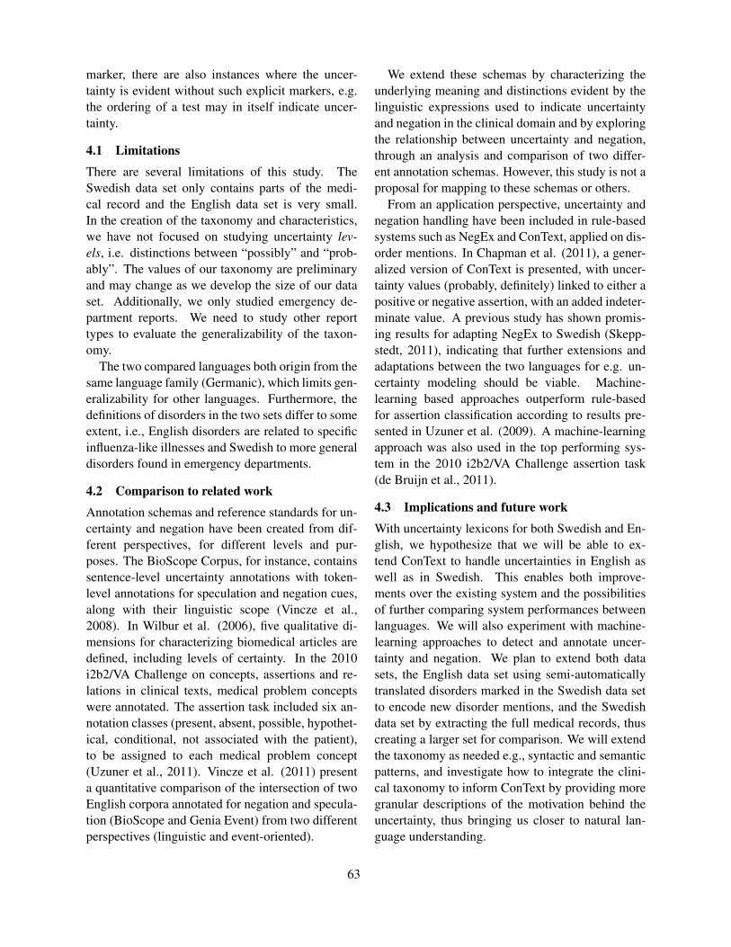
marker, there are also instances where the uncer-tainty is evident without such explicit markers, e.g.the ordering of a test may in itself indicate uncer-tainty.
4.1 Limitations
There are several limitations of this study. TheSwedish data set only contains parts of the medi-cal record and the English data set is very small.In the creation of the taxonomy and characteristics,we have not focused on studying uncertainty lev-els, i.e. distinctions between “possibly” and “prob-ably”. The values of our taxonomy are preliminaryand may change as we develop the size of our dataset. Additionally, we only studied emergency de-partment reports. We need to study other reporttypes to evaluate the generalizability of the taxon-omy.
The two compared languages both origin from thesame language family (Germanic), which limits gen-eralizability for other languages. Furthermore, thedefinitions of disorders in the two sets differ to someextent, i.e., English disorders are related to specificinfluenza-like illnesses and Swedish to more generaldisorders found in emergency departments.
4.2 Comparison to related work
Annotation schemas and reference standards for un-certainty and negation have been created from dif-ferent perspectives, for different levels and pur-poses. The BioScope Corpus, for instance, containssentence-level uncertainty annotations with token-level annotations for speculation and negation cues,along with their linguistic scope (Vincze et al.,2008). In Wilbur et al. (2006), five qualitative di-mensions for characterizing biomedical articles aredefined, including levels of certainty. In the 2010i2b2/VA Challenge on concepts, assertions and re-lations in clinical texts, medical problem conceptswere annotated. The assertion task included six an-notation classes (present, absent, possible, hypothet-ical, conditional, not associated with the patient),to be assigned to each medical problem concept(Uzuner et al., 2011). Vincze et al. (2011) presenta quantitative comparison of the intersection of twoEnglish corpora annotated for negation and specula-tion (BioScope and Genia Event) from two differentperspectives (linguistic and event-oriented).
We extend these schemas by characterizing theunderlying meaning and distinctions evident by thelinguistic expressions used to indicate uncertaintyand negation in the clinical domain and by exploringthe relationship between uncertainty and negation,through an analysis and comparison of two differ-ent annotation schemas. However, this study is not aproposal for mapping to these schemas or others.
From an application perspective, uncertainty andnegation handling have been included in rule-basedsystems such as NegEx and ConText, applied on dis-order mentions. In Chapman et al. (2011), a gener-alized version of ConText is presented, with uncer-tainty values (probably, definitely) linked to either apositive or negative assertion, with an added indeter-minate value. A previous study has shown promis-ing results for adapting NegEx to Swedish (Skepp-stedt, 2011), indicating that further extensions andadaptations between the two languages for e.g. un-certainty modeling should be viable. Machine-learning based approaches outperform rule-basedfor assertion classification according to results pre-sented in Uzuner et al. (2009). A machine-learningapproach was also used in the top performing sys-tem in the 2010 i2b2/VA Challenge assertion task(de Bruijn et al., 2011).
4.3 Implications and future work
With uncertainty lexicons for both Swedish and En-glish, we hypothesize that we will be able to ex-tend ConText to handle uncertainties in English aswell as in Swedish. This enables both improve-ments over the existing system and the possibilitiesof further comparing system performances betweenlanguages. We will also experiment with machine-learning approaches to detect and annotate uncer-tainty and negation. We plan to extend both datasets, the English data set using semi-automaticallytranslated disorders marked in the Swedish data setto encode new disorder mentions, and the Swedishdata set by extracting the full medical records, thuscreating a larger set for comparison. We will extendthe taxonomy as needed e.g., syntactic and semanticpatterns, and investigate how to integrate the clini-cal taxonomy to inform ConText by providing moregranular descriptions of the motivation behind theuncertainty, thus bringing us closer to natural lan-guage understanding.
63

Acknowledgments
For the English and Swedish data sets, we obtainedapproval from the University of Pittsburgh IRB andthe Regional Ethical Review Board in Stockholm(Etikprovningsnamnden i Stockholm). The study ispart of the Interlock project, funded by the Stock-holm University Academic Initiative and partiallyfunded by NLM Fellowship 5T15LM007059. Lex-icons and probabilities will be made available andupdated on the iDASH NLP ecosystem under Re-sources: http://idash.ucsd.edu/nlp/natural-language-processing-nlp-ecosystem.
ReferencesB. E. Chapman, S. Lee, H. Peter Kang, and W. W. Chap-
man. 2011. Document-level Classification of CT Pul-monary Angiography Reports Based on an Extensionof the ConText Algorithm. Journal of Biomedical In-formatics, 44:728–737.
D. Chu, J.N. Dowling, and WW Chapman. 2006. Eval-uating the Effectiveness of Four Contextual Featuresin Classifying Annotated Clinical Conditions in Emer-gency Department Reports. In AMIA Annu Symp Proc,pages 141–145.
C. Clark, J. Aberdeen, M. Coarr, D. Tresner-Kirsh,B. Wellner, A. Yeh, and L. Hirschman. 2011. MITREsystem for Clinical Assertion Status Classification. JAm Med Inform Assoc, 11(18):563–567.
B. de Bruijn, C. Cherry, S. Kiritchenko, J. Martin, andX. Zhu. 2011. Machine-learned Solutions for ThreeStages of Clinical Information Extraction: The State ofthe Art at i2b2 2010. Journal of the American MedicalInformatics Association, 18:557–562.
H. Harkema, J. N. Dowling, T. Thornblade, and W. W.Chapman. 2009. ConText: An Algorithm for De-termining Negation, Experiencer, and Temporal Statusfrom Clinical Reports. Journal of Biomedical Infor-matics, 42:839–851.
L. Lingard, K. Garwood, C. F. Schryer, and M. M. Spaf-ford. 2003. A Certain Art of Uncertainty: Case Pre-sentation and the Development of Professional Iden-tity. Social science medicine, 56(3):603–616.
S. M. Meystre, G. K. Savova, K. C. Kipper-Schuler, andJohn E. Hurdle. 2008. Extracting Information fromTextual Documents in the Electronic Health Record: AReview of Recent Research. IMIA Yearbook of Medi-cal Informatics 2008. 47 Suppl 1:138-154.
D. Mowery, P. Jordan, J.M. Wiebe, H. Harkema, andW.W. Chapman. 2012. Semantic Annotation of Clini-cal Text: A Pilot Study. Unpublished.
V. L. Rubin, E. D. Liddy, and N. Kando. 2006. Cer-tainty Identification in Texts: Categorization Modeland Manual Tagging Results. In Computing Affect andAttitutde in Text: Theory and Applications. Springer.
R. Saurı and J. Pustejovsky. 2009. FactBank: A CorpusAnnotated with Event Factuality. Language Resourcesand Evaluation, 43(3):227–268–268, September.
M. Skeppstedt. 2011. Negation Detection in SwedishClinical Text: An Adaptation of NegEx to Swedish.Journal of Biomedical Semantics, 2(Suppl. 3):S3.
A. L. Strauss and J. Corbin. 1990. Basics of Qual-itative Research: Grounded Theory Procedures andTechniques. Sage.
O. Uzuner, X. Zhang, and T. Sibanda. 2009. Ma-chine Learning and Rule-based Approaches to Asser-tion Classification. Journal of the American MedicalInformatics Association, 16(1):109–115.
O. Uzuner, B. R. South, S. Shen, and S. L. DuVall. 2011.2010 i2b2/VA Challenge on Concepts, Assertions, andRelations in Clinical Text. JAMIA, 18(5):552–556.
S. Velupillai, H. Dalianis, and M. Kvist. 2011. Factual-ity Levels of Diagnoses in Swedish Clinical Text. InA. Moen, S. K. Andersen, J. Aarts, and P. Hurlen, ed-itors, Proc. XXIII International Conference of the Eu-ropean Federation for Medical Informatics (User Cen-tred Networked Health Care), pages 559 – 563, Oslo,August. IOS Press.
V. Vincze, G. Szarvas, R. Farkas, G. Mora, and J. Csirik.2008. The BioScope Corpus: Biomedical Texts An-notated for Uncertainty, Negation and Their Scopes.BMC Bioinformatics, 9(S-11).
V. Vincze, G. Szarvas, G. M’ora, T. Ohta, and R. Farkas.2011. Linguistic Scope-based and Biological Event-based Speculation and Negation Annotations in theBioScope and Genia Event Corpora. Journal ofBiomedical Semantics, 2(Suppl. 5):S8.
J. Wiebe, R. Bruce, M. Bell, M. Martin, and T. Wilson.2001. A Corpus Study of Evaluative and Specula-tive Language. In Proceedings of the Second SIG-dial Workshop on Discourse and Dialogue - Volume16, SIGDIAL ’01, pages 1–10, Stroudsburg, PA, USA.Association for Computational Linguistics.
J. W. Wilbur, A. Rzhetsky, and H. Shatkay. 2006.New Directions in Biomedical Text Annotation: Def-initions, Guidelines and Corpus Construction. BMCBioinformatics, 7:356+, July.
64

Proceedings of the 2012 Workshop on Biomedical Natural Language Processing (BioNLP 2012), pages 65–72,Montreal, Canada, June 8, 2012. c©2012 Association for Computational Linguistics
A Hybrid Stepwise Approach for De-identifying Person Names in Clinical Documents
Oscar Ferrández1,2, Brett R. South1,2, Shuying Shen1,2, Stéphane M. Meystre1,2
1 Department of Biomedical Informatics, University of Utah, Salt Lake City, Utah, USA 2 IDEAS Center SLCVA Healthcare System, Salt Lake City, Utah, USA
[email protected], {brett.south,shuying.shen,stephane.meystre}@hsc.utah.edu
Abstract
As Electronic Health Records are growing ex-ponentially along with large quantities of un-structured clinical information that could be used for research purposes, protecting patient privacy becomes a challenge that needs to be met. In this paper, we present a novel hybrid system designed to improve the current strate-gies used for person names de-identification. To overcome this task, our system comprises several components designed to accomplish two separate goals: 1) achieve the highest re-call (no patient data can be exposed); and 2) create methods to filter out false positives. As a result, our system reached 92.6% F2-measure when de-identifying person names in Veteran’s Health Administration clinical notes, and considerably outperformed other existing “out-of-the-box” de-identification or named entity recognition systems.
1 Introduction
Electronic Healthcare Records are invaluable re-sources for clinical research, however they contain highly sensitive Protected Health Information (PHI) that must remain confidential. In the United States, patient confidentiality is regulated by the Health Insurance Portability and Accountability Act (HIPAA). To share and use clinical documents for research purposes without patient consent, HIPAA requires prior removal of PHI. More spe-cifically, the HIPAA “Safe Harbor”1 determines 18
1 GPO US: 45 C.F.R. § 164 Security and Privacy. http://www.access.gpo.gov/nara/cfr/waisidx_08/45cfr164_08.html Further details about the 18 HIPAA Safe Harbor PHI identifi-ers can be also found in (Meystre et al., 2010).
PHI categories that have to be obscured in order to consider clinical data de-identified.
An ideal de-identification system should recog-nize PHI accurately, but also preserve relevant non-PHI clinical data, so that clinical records can later be used for various clinical research tasks.
Of the 18 categories of PHI listed by HIPAA, one of the most sensitive is patient names, and all person names in general. Failure to de-identify such PHI involves a high risk of re-identification, and jeopardizes patient privacy.
In this paper, we describe our effort to satisfac-torily de-identify person names in Veteran’s Health Administration (VHA) clinical documents. We propose improvements in person names de-identification with a pipeline of processes tailored to the idiosyncrasies of clinical documents. This effort was realized in the context of the develop-ment of a best-of-breed clinical text de-identification system (nicknamed “BoB”), which will be released as an open source software pack-age, and it started with the implementation and evaluation of several existing de-identification and Named Entity Recognition (NER) systems recog-nizing person names. We then devised a novel methodology to better tackle this task and improve performance.
2 Background and related work
In many aspects de-identification resembles tradi-tional NER tasks (Grishman and Sundheim, 1996). NER involves detecting entities such as person names, locations, and organizations. Consequently, given the similar entities targeted by both tasks, NER systems can be relevant to de-identify docu-ments. However, most named entity recognizers were developed for newswire articles, and not for clinical narratives. Clinical records are character-
65

ized by fragmented and incomplete utterances, lack of punctuation marks and formatting, as well as domain specific language. These complications, in addition to the fact that some entities can appear both as PHI and non-PHI in the same document (e.g., “Mr. Epley” vs. “the Epley maneuver”), make clinical text de-identification a challenging task. Therefore, although person names de-identification is essentially NER, the unique char-acteristics of clinical texts make it more interesting and challenging than recognizing names in news articles, which also enhance the motivation for this study.
Several different approaches were proposed to deal with de-identification of clinical documents, and for named entity recognition of person names. These approaches are mainly focused on either pattern matching techniques, or statistical methods (Meystre et al., 2010), as exemplified below.
Beckwith et al. (2006) developed a de-identification system for pathology reports. This system implemented some patterns to detect dates, locations, and ID numbers, as well as a database of proper names and well-known markers such as ‘Mr.’ and ‘PhD’ to find person names.
Friedlin and McDonald (2008) described the Medical De-identification System (MeDS). It used a combination of methods including heuristics, pattern matching, and dictionary lookups to identi-fy PHI. Pattern matching through regular expres-sions was used to detect numerical identifiers, dates, addresses, ages, etc.; while for names, MeDS used lists of proper names, common usage words and predictive markers, as well as a text string nearness algorithm to deal with typograph-ical errors.
Neamatullah et al. (2008) proposed another rule-based de-identification approach focused on pat-tern matching via dictionary lookups, regular ex-pressions and context checks heuristics denoting PHI. Dictionaries made up of ambiguous names and locations that could also be non-PHI, as well as dictionaries of common words were used by this system to disambiguate PHI terms.
Other de-identification systems such as (Aberdeen et al., 2010; Gardner and Xiong, 2009) use machine learning algorithms to train models and predict new annotations. The key aspect of these systems is the selection of the learning algo-rithm and features. Both (Aberdeen et al., 2010) and (Gardner and Xiong, 2009) use an implemen-
tation of Conditional Random Fields (CRF) and a set of learning features based on the morphology of the terms and their context. One disadvantage of these systems is the need for large amounts of an-notated training examples.
As mentioned previously, for detecting person names, we could also use traditional newswire-trained NER systems. NER has long been studied by the research community and many different ap-proaches have been developed (Tjong Kim Sang and De Meulder, 2003; Doddington et al., 2004). One successful and freely available named entity recognizer is the Stanford NER system (Finkel et al., 2005), which provides an implementation of linear chain CRF sequence models, coupled with well-engineered feature extractors for NER, and trained with newswire documents.
3 Methods
As already mentioned, we first selected and ran several existing de-identification and NER systems detecting person names in our clinical documents. Afterwards, we devised and present here a novel pipeline of processes designed to improve the PHI recognition task.
3.1 Existing de-identification and NER sys-tems
Five available de-identification systems, as well as one newswire-trained named entity recognizer, were selected for an “out-of-the-box” evaluation. The aim of this evaluation was to compare the per-formance of the various methods and resources when de-identifying person names in our clinical documents.
We included three rule-based de-identification approaches: • HMS Scrubber (Beckwith et al., 2006); • MeDS (Friedlin and McDonald, 2008); and • MIT deid system (Neamatullah et al., 2008).
And two systems based on machine learning
classifiers: • The MITRE Identification Scrubber Toolkit
(MIST) (Aberdeen et al., 2010); and • The Health Information DE-identification
(HIDE) system (Gardner and Xiong, 2009).
66

Regarding NER systems, we chose the Stanford NER system (Finkel et al., 2005), which has re-ported successful results when detecting person names. These systems were described in Section 2, when we presented related work.
3.2 Our best-of-breed approach
Our names de-identification approach consists of a novel pipeline of processes designed to improve the current strategies for person names de-identification. This system is being developed as an Apache UIMA2 pipeline, with two main goals: 1) Obtain the highest recall (i.e., sensitivity), re-
gardless of the impact on precision; and 2) Improve overall precision by filtering out the
false positives produced previously. These goals correspond to the implementation of
the main components of our system. When we tested existing systems (we will present results for these systems in Table 1), we observed that recall was better addressed by rule-based approaches, while precision was higher applying machine learning-based algorithms. We therefore used this knowledge for the design of our system: goal#1 is then accomplished mainly using rule-based tech-niques, and goal#2 implementing machine learn-ing-based approaches.
Moreover, recall is of paramount importance in de-identification (patient PHI cannot be disclosed). And this was also a reason that motivated us to first focus on achieving high recall, and filtering out false positives afterwards as a separate proce-dure.
Unlike other de-identification and NER systems that tackle the classification problem from one per-spective (i.e., rule-based or machine learning-based) or from a limited combined approach (e.g., learning features extracted using regular expres-sions), the design of our system allows us to take advantage of the strong points of both techniques separately. And more importantly, our classifiers for filtering out false-positives (goal#2) are trained using correct and incorrect annotations derived from previous modules implemented in goal#1. Thus, they do not predict if every token in the doc-ument is or belongs to a PHI identifier, they in-stead decide if an actual annotation is a false or 2 http://uima.apache.org/
true positive. This design makes our classifiers better with less learning examples, which is a re-striction we have to deal with, and it also allows us to create methods that can be only focused on max-imizing recall regardless of the amount of false-positives introduced (goal#1). To the best of our knowledge, this perspective has not been exploited before, and as we will show in the evaluation sec-tion, it empirically demonstrates more robustness than previous approaches.
The design of our system integrates different components described below. Figure 1 depicts an overview of our system’s architecture and work-flow.
Figure 1. System’s architecture.
3.2.1 NLP preprocessing steps
This NLP preprocessing prepares the input for the main components of our system. It includes sen-tence segmentation, tokenization, part-of-speech tagging, chunking, and word normalization based
67

on Lexical Variant Generation (LVG)3. The output of this preprocessing will be used by subsequent pattern matching techniques and features for ma-chine learning algorithms. For these processes, we adapted several cTAKES (Savova et al., 2010) components.
3.2.2 Rules and dictionary lookups
We created a pattern matching component support-ed by contextual keyword searches (e.g., “Dr.”, “Mr.”, “M.D.”, “R.N.”, “L.C.S.W.”), dictionaries of person names4, and a simple disambiguation procedure based on a list of common words and the capitalization of the entity. We adapted some of the techniques implemented in (Beckwith et al., 2006; Friedlin and McDonald, 2008; Neamatullah et al., 2008) to our documents, and developed new patterns. For dictionary lookups, we used Lucene5 indexing, experimenting with keyword and fuzzy dictionary searches. Each word token is compared with our indexed dictionary of names (last and first names from the 1990 US Census4), considering all matches as candidate name annotations. However, candidates that also match with an entry in our dic-tionary of common words6 and do not contain an initial capital letter are discarded from this set of candidate name annotations.
With this component, we attempt to maximize recall, even if precision is altered.
3.2.3 CRF-based predictions
To further enhance recall, we created another com-ponent based on CRF models. We incorporated this component in our system considering that ma-chine learning classifiers are more generalizable and can detect instances of names that are not sup-ported by our rules or dictionaries. Therefore, alt-hough we knew the individual results of a CRF classifier at this level were not enough for de-identification, at this point our main concern is to obtain the highest recall. Thus, adding a machine learning classifier into this level we could help the system predicting the PHI formats and instances 3 http://lexsrv2.nlm.nih.gov/LexSysGroup/Projects/lvg/ current/web/index.html 4 Frequently Occurring Names from the 1990 Census. http://www.census.gov/genealogy/names. 5 http://lucene.apache.org/java/docs/index.html 6 We used the dictionary of common words from Neamatullah et al. (2008).
that could not be covered by our patterns and dic-tionaries.
To develop this component, we used the CRF classifier implementation provided by the Stanford NLP group7. We carried out a feature selection procedure using greedy forward selection. It pro-vided us with the best learning feature set, which consisted of: the target word, 2-grams of letters, position in the document, part-of-speech tag, lem-ma, widely-used word-shape features (e.g., initial capitals, all capitals, digits inside, etc.), features from dictionaries of names and common words, a 2-word context window, and combinations of words, word-shapes and part-of-speech tags of the word and its local context.
The learning features considered before and af-ter the selection procedure are shown in Table 1.
3.2.4 False-positive filtering
The two previous components’ objective is maxi-mal recall, producing numerous false positives. The last component of our pipeline was therefore designed to filter out these false positives and con-sequently increase overall precision. We built a machine learning classifier for this task, based on LIBSVM (Chang and Lin, 2001), a library for Support Vector Machines (SVM), with the RBF (Radial Basis Function) kernel. We then trained this classifier with reference standard text annota-tions, as well as the correct and incorrect annota-tions made by the previous components. We used our training document set (section 4.1) for this purpose. Features for the LIBSVM machine learning model were: the LVG normalized form of the target anno-tation, three words before and after, part-of-speech tags of the words within the annotation and the local context, number of tokens within the annota-tion, position in the document, 40 orthographic features (denoting capitals, digits, special charac-ters, etc.), features from dictionaries of names and common words, and the previous strategy used to make the annotation (i.e., rules, dictionary lookups or CRF-based predictions).
7 http://nlp.stanford.edu/software/corenlp.shtml
68
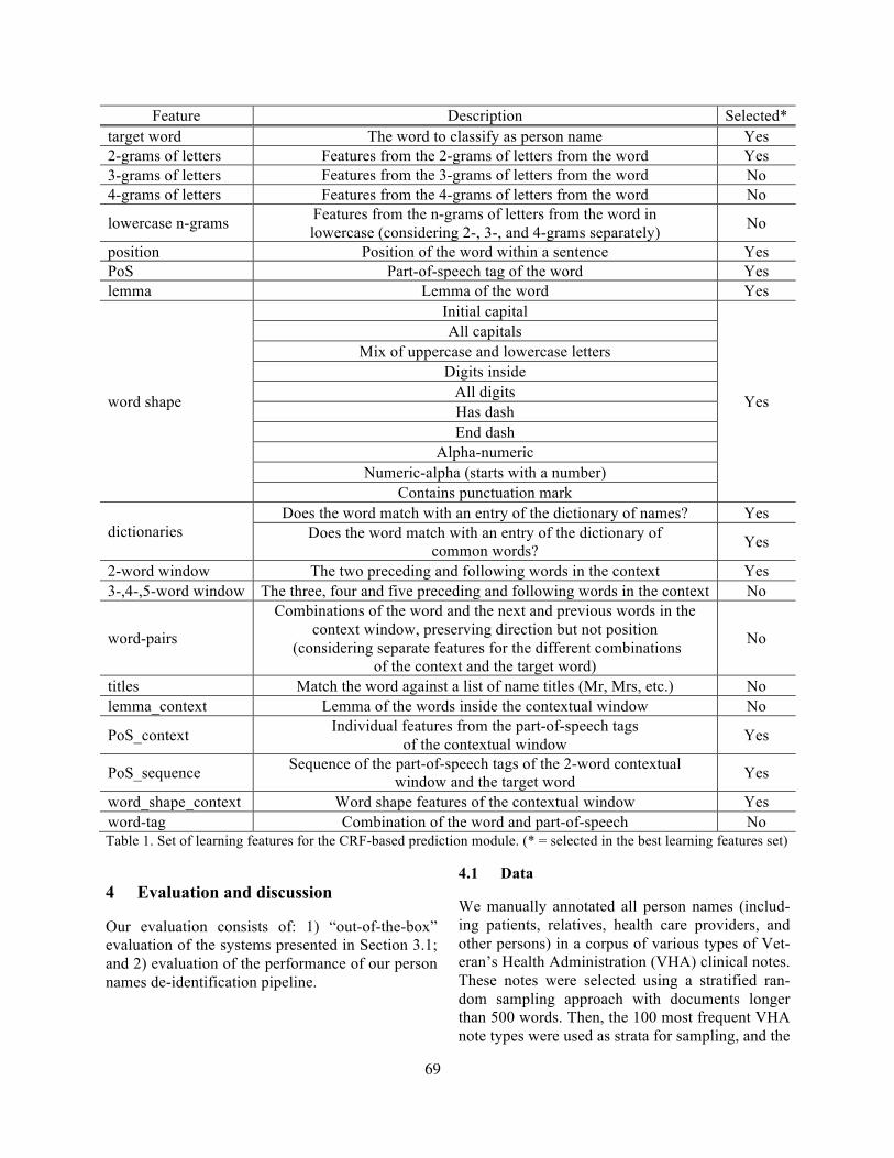
Feature Description Selected* target word The word to classify as person name Yes 2-grams of letters Features from the 2-grams of letters from the word Yes 3-grams of letters Features from the 3-grams of letters from the word No 4-grams of letters Features from the 4-grams of letters from the word No
lowercase n-grams Features from the n-grams of letters from the word in lowercase (considering 2-, 3-, and 4-grams separately) No
position Position of the word within a sentence Yes PoS Part-of-speech tag of the word Yes lemma Lemma of the word Yes
word shape
Initial capital
Yes
All capitals Mix of uppercase and lowercase letters
Digits inside All digits Has dash End dash
Alpha-numeric Numeric-alpha (starts with a number)
Contains punctuation mark
dictionaries Does the word match with an entry of the dictionary of names? Yes
Does the word match with an entry of the dictionary of common words? Yes
2-word window The two preceding and following words in the context Yes 3-,4-,5-word window The three, four and five preceding and following words in the context No
word-pairs
Combinations of the word and the next and previous words in the context window, preserving direction but not position
(considering separate features for the different combinations of the context and the target word)
No
titles Match the word against a list of name titles (Mr, Mrs, etc.) No lemma_context Lemma of the words inside the contextual window No
PoS_context Individual features from the part-of-speech tags of the contextual window Yes
PoS_sequence Sequence of the part-of-speech tags of the 2-word contextual window and the target word Yes
word_shape_context Word shape features of the contextual window Yes word-tag Combination of the word and part-of-speech No Table 1. Set of learning features for the CRF-based prediction module. (* = selected in the best learning features set)
4 Evaluation and discussion
Our evaluation consists of: 1) “out-of-the-box” evaluation of the systems presented in Section 3.1; and 2) evaluation of the performance of our person names de-identification pipeline.
4.1 Data
We manually annotated all person names (includ-ing patients, relatives, health care providers, and other persons) in a corpus of various types of Vet-eran’s Health Administration (VHA) clinical notes. These notes were selected using a stratified ran-dom sampling approach with documents longer than 500 words. Then, the 100 most frequent VHA note types were used as strata for sampling, and the
69

same number of notes was randomly selected in each stratum. Two reviewers independently anno-tated each document, a third reviewer adjudicated their disagreements, and a fourth reviewer eventu-ally examined ambiguous and difficult adjudicated cases.
The evaluation corpus presented here comprises a subset of 275 VHA clinical notes from the aforementioned corpus. For training, 225 notes were randomly selected (contained 748 person name annotations), and the remaining 50 notes (with 422 name annotations) were used for testing the systems.
4.2 Experiments and results
We present results in terms of precision, recall and F-measure (harmonic mean of recall and preci-sion). We used a weight of 2 when calculating the F2-measure giving recall more (twice) importance than precision (Jurafsky and Martin, 2009). This reflects our emphasis on recall for de-identification. To our understanding, due to legal and privacy issues, a good de-identification system should be tailored to prioritize recall, and conse-quently patient confidentiality. It is not the scope of this paper to judge or modify the development design adopted by other de-identification systems.
Moreover, we considered correct predictions at least overlapping with the entire PHI annotation in the reference standard (i.e., exact match with the reference annotation, or more than the exact match). We can therefore assure complete redac-tion of PHI.
Table 2 illustrates “out-of-the-box” evaluation results of the systems described in Section 3.1. For this evaluation, we trained MIST and HIDE with our 225 notes training corpus, while the Stanford NER was run using the trained models available with its distribution8. Testing was realized using our 50 notes testing corpus.
Table 3 shows the performance of our names de-identification approach. We provide results for dif-ferent configurations of our pipeline:
• Rules & Dictionaries. Results of the rules
and dictionary lookups component de-scribed in Section 3.2.2, in this case using a
8 Further details about these models can be found at http://nlp.stanford.edu/software/CRF-NER.shtml
keyword-search strategy for dictionary lookups.
• R&D with fuzzy searches. Results from the rules and dictionary lookups component us-ing Lucene’s Fuzzy Query engine for dic-tionary searches. It implements a fuzzy search based on the Levenshtein (edit dis-tance) algorithm9 (Levenshtein, 1966), which has to surpass a similarity threshold in order to produce a match. We carried out a greedy search on the training corpus for the best similarity threshold. We found 0.74 to be the best threshold.
• CRF-based w/FS. The CRF-based predic-tions component results after selecting the best set of features (see Section 3.2.3). The CRF classifier was trained using our 225-document training corpus.
• R&D + CRF w/FS. The cumulative results from the rules and dictionary lookups (not implementing fuzzy dictionary searches) and the CRF-based predictions components.
• R&D + CRF w/FS + FP-filtering. Includes all components together, adding the false-positive filtering component (Section 3.2.4) at the end of the pipeline. The SVM model for this last component was created using our training corpus.
System Prec. Rec. F2
HMS Scrubber 0.150 0.675 0.397 MeDS 0.149 0.768 0.419 MIT deid 0.636 0.893 0.826 MIST 0.865 0.319 0.356 HIDE 0.975 0.376 0.429 Stanford NER 0.692 0.723 0.716
Table 2. “Out-of-the-box” evaluation of existing de-identification and NER systems (Prec.=precision; Rec.=recall; F2= F2-measure).
System Prec. Rec. F2 Rules & Dictionaries 0.360 0.962 0.721 R&D + fuzzy 0.171 0.969 0.502 CRF-based w/FS 0.979 0.874 0.893 R&D + CRF w/FS 0.360 0.988 0.732 R&D + CRF w/FS + FP-filtering 0.774 0.974 0.926
Table 3. Cumulative results of our pipeline of processes.
9 http://www.merriampark.com/ld.htm
70

4.3 Analysis
Our novel names de-identification pipeline signifi-cantly outperforms all other systems we evaluated “out-of-the-box” or trained with our VHA notes corpus.
Among the five existing systems we evaluated (Table 1), only one achieved noteworthy recall around 89%. However, none of them obtained any remarkable F2-measure. Most errors produced by the pattern matching systems (i.e., HMS Scrubber, MeDS, and MIT deid system) were due to false positive annotations of medical eponyms (e.g., “Achilles”, “Guyon”, etc.), as well as acronyms denoting medical facilities (e.g., “ER” and “HCS”). The false negatives consisted of ambigu-ous person names (e.g., “Bill” and “Chase”), some formats not covered by the patterns (e.g., “[Last-Name], [FirstName] [Initial]”), and a few names not found in the dictionaries.
Among machine learning-based systems, the two de-identification applications (i.e., MIST and HIDE) obtained good precision, but quite low re-call. The size of our training corpus was somewhat limited, and these results probably indicate a need for more sophisticated learning features, as well as feature selection procedures (rather than using the “out-of-the-box” feature specification that comes with these systems) for better performance. With improved learning features, we could mitigate the relative lack of training examples. Interestingly, the NER system, which was trained on newswire documents, performed even better than some de-identification systems, although a need for im-provement is still present.
We acknowledge that the comparison with Stan-ford NER is not completely fair due to the different source of documents used for training. However, we considered it interesting information, and alt-hough clinical notes contain characteristics not present in newswire corpora, they also have simi-larities regarding person names (e.g., titles “Mr.”, “Dr.”, “PhD”, part-of-speech, verb tenses). There-fore, we think that only for names recognition, a newswire trained NER can provide interesting re-sults, and this was actually what we observed.
Table 2 points out that the combination of our components produces successful cumulative re-sults. Using the training corpus to create a simple component made up of rules, dictionary lookups, and few heuristics for disambiguation allowed for
recall values of 0.96. This demonstrates the need to adapt these techniques to the target documents, instead of employing systems “out-of-the-box”.
Our experiments with fuzzy dictionary lookups did not allow for a significant increase in recall, but caused a decrease in precision (-19%). It sug-gests that there was no need for considering person name misspellings.
The component based on CRF predictions alone achieved good performance, especially in preci-sion. It obtained the best F2-measure (0.89), clearly higher than the other “out-of-the-box” systems based on CRF models. It proves that selecting suit-able learning features mitigates to some extent the scarcity of training examples.
Our next experiment combined the rules and dictionaries and CRF components. It improved the overall recall to about 0.99, which means that CRF-based predictions recognized some person names that were missed by our pattern matching components, but didn’t increase the precision. We reached here our first goal of high recall or sensi-tivity.
Finally, we added the false-positive filtering component to our system. This component was able to filter out 622 (84%) false positives from a total of 742, improving the precision to 0.77 (+41%); but also causing a slight decrease in recall (-1.4%). This application of our pipeline was suc-cessful, reaching an F2-mesure of 0.93, and was an effective way of training the SVM model for false-positives filtering.
5 Conclusions
We designed and evaluated a novel person names de-identification system with VHA clinical docu-ments. We also presented an “out-of-the-box” evaluation of several available de-identification and NER systems; all of them were surpassed by our approach.
With our proposal, we showed that it is possible to improve the recognition of person names in clin-ical records, even when the corpus for training ma-chine learning classifiers is limited. Furthermore, the workflow of our pipeline allowed us to tackle the de-identification task from an intuitive but powerful perspective, i.e. facing the achievement of high recall and precision as two separate goals implementing specific techniques and components.
71

Packaging this two-step procedure as a boot-strapping learning or adding the rules to define learning features would not allow us to use the qualities of the R&D and CRF components (i.e., obtain the highest recall by any means). Moreover, considering the small size of our manually anno-tated examples, these approaches would not work much better than existing systems.
As future efforts, we plan to improve the preci-sion of the rules and dictionary lookups component by adding more sophisticated person names disam-biguation procedures. Such procedures should deal with the peculiar formatting of clinical records as well as integrate enriched knowledge from bio-medical resources. We also plan to evaluate the portability of our approach by using other sets of clinical documents, such as the 2006 i2b2 de-identification challenge corpus (Uzuner et al., 2007).
Acknowledgments Funding provided by the Department of Veterans Affairs Health Services Research & Development Services Consortium for Healthcare Informatics Research grant (HIR 08-374).
References John Aberdeen, Samuel Bayer, Reyyan Yeniterzi, Ben
Wellner, Cheryl Clark, David Hanauer, Bradley Ma-lin, and Lynette Hirschman. 2010. The MITRE Iden-tification Scrubber Toolkit: design, training, and assessment. International journal of medical infor-matics, 79 (12) (December): 849-59.
Bruce A. Beckwith, Rajeshwarri Mahaadevan, Ulysses J. Balis, and Frank Kuo. 2006. Development and evaluation of an open source software tool for deidentification of pathology reports. BMC medical informatics and decision making, 6 (1) (January): 12.
Chih-Chung Chang and Chih-Jen Lin. (2001). LIBSVM: a library for support vector machines. Computer, 1-30.
George Doddington, Alexis Mitchell, Mark Przybocki, Lance Ramshaw, Stephanie Strassel, and Ralph Weischedel. 2004. The Automatic Content Extraction (ACE) Program - Tasks, Data, and Evaluation. Pro-ceedings of LREC 2004: 837-840.
Jenny Rose Finkel, Trond Grenager, and Christopher Manning. 2005. Incorporating non-local information into information extraction systems by Gibbs sam-
pling. Proceedings of the 43rd Annual Meeting on Association for Computational Linguistics: 363-370.
F. Jeff Friedlin and Clement J. McDonald. 2008. A software tool for removing patient identifying infor-mation from clinical documents. Journal of the American Medical Informatics Association : JAMIA 15 (5) (January 1): 601-10.
James Gardner and Li Xiong. 2009. An integrated framework for de-identifying unstructured medical data. Data & Knowledge Engineering 68 (12) (De-cember): 1441-1451.
Ralph Grishman and Beth Sundheim. 1996. Message understanding conference-6: A brief history. Pro-ceedings of the 16th conference on Computational linguistics - Volume 1: 466-471. Association for Computational Linguistics, Copenhagen, Denmark.
Daniel Jurafsky and James H. Martin. 2009. Speech and Language Processing: An Introduction to Natural Language Processing, Speech Recognition, and Computational Linguistics. 2nd edition. Prentice-Hall. Upper Saddle River, NJ, USA.
V.I. Levenshtein. 1966. Binary Codes Capable of Cor-recting Deletions, Insertions and Reversals. Soviet Physics - Doklady 10: 707–710.
Stephane M. Meystre, F. Jeffrey Friedlin, Brett R. South, Shuying Shen, and Matthew H. Samore. 2010. Automatic de-identification of textual documents in the electronic health record: a review of recent re-search. BMC medical research methodology 10 (1) (January): 70.
Ishna Neamatullah, Margaret M. Douglass, Li-wei H. Lehman, Andrew Reisner, Mauricio Villarroel, Wil-liam J. Long, Peter Szolovits, George B. Moody, Roger G. Mark, and Gari D. Clifford. 2008. Auto-mated de-identification of free-text medical records. BMC medical informatics and decision making 8 (1) (January): 32.
Guergana K. Savova, James J. Masanz, Philip V. Ogren, Jiaping Zheng, Sunghwan Sohn, Karin C. Kipper-Schuler, and Christopher G. Chute. 2010. Mayo clin-ical Text Analysis and Knowledge Extraction System (cTAKES): architecture, component evaluation and applications. Journal of the American Medical In-formatics Association : JAMIA 17 (5): 507-13.
Erik F. Tjong Kim Sang, and Fien De Meulder. 2003. Introduction to the CoNLL-2003 Shared Task: Lan-guage-Independent Named Entity Recognition. In Proceedings of the seventh conference on Natural language learning at HLT-NAACL 2003 - Volume 4: 142-147.
Özlem Uzuner, Yuan Luo, and Peter Szolovits. 2007. Evaluating the State-of-the-Art in Automatic De-identification. Journal of the American Medical In-formatics Association : JAMIA 14(5):550-563.
72

Proceedings of the 2012 Workshop on Biomedical Natural Language Processing (BioNLP 2012), pages 73–81,Montreal, Canada, June 8, 2012. c©2012 Association for Computational Linguistics
Active Learning for Coreference Resolution
Timothy A. Miller and Dmitriy Dligach and Guergana K. Savova
Children’s Hospital Boston
and Harvard Medical School
300 Longwood Ave.
Enders 141
Boston, MA 02115, USA
{Timothy.Miller,Dmitriy.Dligach,Guergana.Savova}@childrens.harvard.edu
Abstract
Active learning can lower the cost of anno-
tation for some natural language processing
tasks by using a classifier to select informa-
tive instances to send to human annotators. It
has worked well in cases where the training in-
stances are selected one at a time and require
minimal context for annotation. However,
coreference annotations often require some
context and the traditional active learning ap-
proach may not be feasible. In this work we
explore various active learning methods for
coreference resolution that fit more realisti-
cally into coreference annotation workflows.
1 Introduction
Coreference resolution is the task of deciding which
entity mentions in a text refer to the same entity.
Solving this problem is an important part of the
larger task of natural language understanding in gen-
eral. The clinical domain offers specific tasks where
it is easy to see that correctly resolving coreference
is important. For example, one important task in the
clinical domain is template filling for the Clinical El-
ements Model (CEM).1 This task involves extracting
various pieces of information about an entity and fit-
ting the information into a standard data structure
that can be reasoned about. An example CEM tem-
plate is that for Disease with attributes for Body Lo-
cation, Associated Sign or Symptom, Subject, Nega-
tion, Uncertainty, and Severity. Since a given entity
may have many different attributes and relations, it
1http://intermountainhealthcare.org/cem
may be mentioned multiple times in a text. Coref-
erence resolution is important for this task because
it must be known that all the attributes and relations
apply to the same entity so that a single CEM tem-
plate is filled in for an entity, rather than creating a
new template for each mention of the entity.
2 Background
2.1 Coreference Resolution
Space does not permit a thorough review of coref-
erence resolution, but recent publications covered
the history and current state of the art for both the
general domain and the clinical domain (Ng, 2010;
Pradhan et al., 2011; Zheng et al., 2011).
The system used here (Zheng et al., 2012) is
an end-to-end coreference resolution system, mean-
ing that the algorithm receives no gold standard in-
formation about mentions, named entity types, or
any linguistic information. The coreference res-
olution system is a module of the clinical Tex-
tual Analysis and Knowledge Extraction System
(cTAKES) (Savova et al., 2010) that is trained on
clinical data. It takes advantage of named entity
recognition (NER) and categorization to detect en-
tity mentions, and uses several cTAKES modules
as feature generators, including the NER module,
a constituency parser module, and a part of speech
tagging module.
The system architecture is based on the pairwise
discriminative classification approach to the coref-
erence resolution problem. In that paradigm, pairs
of mentions are classified as coreferent or not, and
then some reconciliation must be done on all of the
73

links so that there are no conflicts in the clusters.
The system uses support vector machines (SVMs)
as the pairwise classifiers, and conflicts are avoided
by only allowing an anaphor to link with one an-
tecedent, specifically that antecedent the classifier
links with the highest probability.
There are separate pairwise classifiers for named
entity and pronominal anaphor types. In the domain
of clinical narratives, person mentions and personal
pronouns in particular are not especially challeng-
ing – the vast majority of person mentions are the
patient. In addition, pronoun mentions, while im-
portant, are relatively rare. Thus we are primarily
interested in named entity coreference classification,
and we use that classifier as the basis of the work de-
scribed here.
The feature set of this system is similar to that
used by Ng and Cardie (2002). That system in-
cludes features based on surface form of the men-
tions, shallow syntactic information, and lexical se-
mantics from WordNet. The system used here has
a similar feature set but uses Unified Medical Lan-
guage System (UMLS)2 semantic features as it is
intended for clinical text, and also incorporates sev-
eral syntactic features extracted from constituency
parses extracted from cTAKES.
To generate training data for active learning simu-
lations, mention detection is run first (cTAKES con-
tains a rule-based NER system) to find named en-
tities and a constituency parser situates entities in
a syntax tree). For each entity found, the system
works backwards through all other mentions within
a ten sentence window. For each candidate anaphor-
antecedent pair, a feature vector is extracted using
the features briefly described above.
2.2 Active Learning
Active Learning (AL) is a popular approach to se-
lecting unlabeled data for annotation (Settles, 2010)
that can potentially lead to drastic reductions in the
amount of annotation that is necessary for train-
ing an accurate statistical classifier. Unlike passive
learning, where the data is sampled for annotation
randomly, AL delegates data selection to the clas-
sifier. AL is an iterative process that operates by
first training a classifier on a small sample of the
2http://www.nlm.nih.gov/research/umls/
data known as the seed examples. The classifier
is subsequently applied to a pool of unlabeled data
with the purpose of selecting additional examples
the classifier views as informative. The selected data
is annotated and the cycle is repeated, allowing the
learner to quickly refine the decision boundary be-
tween classes. One common approach to assessing
the informativeness is uncertainty sampling (Lewis
and Gale, 1994; Schein and Ungar, 2007), in which
the learner requests a label for the instance it is most
uncertain how to label. In this work, we base our
instance selection on the distance to the SVM de-
cision boundary (Tong and Koller, 2002), assuming
that informative instances tend to concentrate near
the boundary.
Most AL work focuses on instance selection
where the unit of selection is one instance repre-
sented as a feature vector. In this paper we also
attempt document selection, where the unit of se-
lection is a document, typically containing multi-
ple coreference pairs each represented as a feature
vector. The most obvious way to extend a sin-
gle instance informativeness metric to the document
scenario is to aggregate the informativeness scores.
Several uncertainty metrics have been proposed that
follow that route to adapt single instance selection
to multiple instance scenarios (Settles et al., 2008;
Tomanek et al., 2009). We borrow some of these
metrics and propose several new ones.
To the best of our knowledge only one work
exists that explores AL for coreference resolution.
Gasperin (2009) experiments with an instance based
approach in which batches of anaphoric pairs are se-
lected on each iteration of AL. In these experiments,
AL did not outperform the passive learning baseline,
probably due to selecting batches of large size.
3 Active Learning Configurations
3.1 Instance Selection
The first active learning model we considered selects
individual training instances – putatively coreferent
mention pairs. This method is quite easy to simu-
late, and follows naturally from most of the theo-
retical active learning literature, but it has the draw-
back of being seemingly unrealistic as an annotation
paradigm. That is, since coreference can span across
an entire document, it is probably not practical to
74

have a human expert annotate only a single instance
at a time when a given instance may require many
sentences of reading in order to contextualize the in-
stance and properly label it. Moreover, even if such
an annotation scheme proved viable, it may result
in an annotated corpus that is only valuable for one
type of coreference system architecture.
Nonetheless, active learning for coreference at the
instance level is still useful. First, since this method
most closely follows the successful active learning
literature by using the smallest discrete problems, it
can serve as a proof of concept for active learning
in the coreference task – if it does not work well at
this level, it probably will not work at the document
level. Previous results (Gasperin, 2009) have shown
that certain multiple instance methods do not work
for coreference resolution, so testing on smaller se-
lection sizes first can ensure that active learning is
even viable at that scale. In addition, though in-
stance selection may not be feasible for real world
annotations, individual instances and metrics for se-
lecting them are usually used as building blocks for
more complex methods. In order for this to be pos-
sible it must be shown that the instances themselves
have some value.
3.2 Document Selection
Active learning with document selection is a much
more realistic representation of conventional anno-
tation methods. Conventionally, a set of documents
is selected, and each document is annotated exhaus-
tively for coreference (Pradhan et al., 2011; Savova
et al., 2011). Document selection fits into this work-
flow very naturally, by selecting the next document
to annotate exhaustively based on some metric of
which document has the best instances. In theory,
this method can save annotation time by only anno-
tating the most valuable documents.
Document selection is somewhat similar to the
concept of batch-mode active learning, wherein
multiple instances are selected at once, though
batch-mode learning is usually intended to solve a
different problem, that of an asymmetry between
classifier training speed and annotation speed (Set-
tles, 2010). A more important difference is that doc-
ument selection requires that all of the instances in
the batch must come from the same document. Thus,
one might expect a priori that document selection
for active learning will not perform as well as in-
stance selection. However, it is possible that even
smaller gains will be valuable for improving annota-
tion time, and the more robust nature of a corpus an-
notated in such a way will make the long term bene-
fits worthwhile.
In this work, we propose several metrics for se-
lecting documents to annotate, all of which are
based on instance level uncertainty. In the fol-
lowing descriptions, D is the set of documents, d
is a single document, d is the selected document,
Instances(d) is a function which returns the set of
pair instances in document d, i is an instance, dist(i)is a function which returns the distance of instance i
from the classification boundary, and I is the indica-
tor function, which takes the value 1 if its argument
is true and 0 otherwise. Note that high uncertainty
occurs when Abs(dist(i)) approaches 0.
• Best instance – This method uses the un-
certainty sampling criteria on instances, and
selects the document containing the in-
stance the classifier is least certain about.
d = argmind∈D
[mini∈Instances(d)Abs(dist(i))]
• Highest average uncertainty – This method
computes the average uncertainty of all
instances in a document, and selects the
document with the highest average uncertainty.
d = argmind∈D
1|Instances(d)|
∑i∈Instances(d)Abs(dist(i))
• Least bad example – This method uses
uncertainty sampling criteria to find the
document whose most certain example is
least certain, in other words the document
whose most useless example is least useless.
d = argmind∈D
maxi∈Instances(d)Abs(dist(i))
• Narrow band – This method creates an un-
certainty band around the discriminating
boundary and selects the document with
the most examples inside that narrow band.
d = argmaxd∈D
∑i∈Instances(d) I(Abs(dist(i) < 0.2))
• Smallest spread – This method computes the
distance between the least certain and most
certain instances and selects the document
minimizing that distance.
75

d = argmind∈D
[maxi∈Instances(d)(Abs(dist(i)))−
mini∈Instances(d)(Abs(dist(i)))]
• Most positives – This method totals the
number of positive predicted instances
in each document and selects the doc-
ument with the most positive instances.
d = argmaxd∈D
∑i∈Instances(d) I(dist(i) > 0)
• Positive ratio – This method calculates
the percentage of positive predicted in-
stances in each document and selects the
document with the highest percentage.
d = argmaxd∈D
∑i∈Instances(d) I(dist(i)>0)
|Instances(d)|
Many of these are straightforward adaptations of
the instance uncertainty criteria, but others deserve
a bit more explanation. The most positives and pos-
itive ratio metrics are based on the observation that
the corpus is somewhat imbalanced – for every posi-
tive instance there are roughly 20 negative instances.
These metrics try to account for the possibility that
instance selection focuses on positive instances. The
average uncertainty is an obvious attempt to turn in-
stance metrics into document metrics, but narrow
band and smallest spread metrics attempt to do the
same thing while accounting for skew in the distri-
bution of “good” and “bad” instances.
3.3 Document-Inertial Instance Selection
One of the biggest impracticalities of instance se-
lection is that labeling any given instance may re-
quire reading a fair amount of the document, since
the antecedent and anaphor can be quite far apart.
Thus, any time savings accumulated by only anno-
tating an instance is reduced since the reading time
per instance is probably increased.
It is also possible that document selection goes
too far in the other direction, and requires too
many useless instances to be annotated to achieve
gains. Therefore, we propose a hybrid method of
document-inertial instance selection which attempts
to combine aspects of instance selection and docu-
ment selection.
This method uses instance selection criteria to se-
lect new instances, but will look inside the current
document for a new instance within an uncertainty
threshold rather than selecting the most uncertain in-
stance in the entire training set. Sticking with the
same document for several instances in a row can
potentially solve the real world annotation problem
that marking up each instance requires some knowl-
edge of the document context. Instead, the context
learned by selecting one instance can be retained if
useful for annotating the next selected instance from
the same document.
This also preserves one of the biggest advantages
of instance selection, that of re-training the model
after every selected instance. In batch-mode selec-
tion and document selection, many instances are se-
lected according to criteria based on the same model
starting point. As a result, the selected instances
may be redundant and document scores based on
accumulated instance scores may not reflect reality.
Re-training the model between selected instances
prevents redundant instances from being selected.
4 Evaluation
Evaluations of the active learning models described
above took place in a simulation context. In active
learning simulations, a labeled data set is used, and
the unlabeled pool is simulated by ignoring or “cov-
ering” the labels for part of the data until the selec-
tion algorithm selects a new instance for annotation.
After selection the next data point is simply put into
the training data and its label is uncovered.
The data set used was the Ontology Development
and Information Extraction (ODIE) corpus (Savova
et al., 2011) used in the 2011 i2b2/VA Challenge on
coreference resolution.3 We used a set of 64 docu-
ments from the training set of the Mayo Clinic notes
for our simulations.
Instances were created by using the training
pipeline from the coreference system described in
Section 2.1. As previously mentioned, this work
uses the named entity anaphor classifier as it con-
tains the most data points. This training set resulted
in 6820 instances, with 311 positive instances and
6509 negative instances. Baseline ten-fold cross val-
idation performance on this data set using an SVM
with RBF kernel is an F-score of 0.48.
Simulations are performed using ten fold cross-
validation. First, each data point is assigned to one
3https://www.i2b2.org/NLP/Coreference/
76

of ten folds (this is done randomly to avoid any auto-
correlation issues). Then, for each iteration, one fold
is made the seed data, another fold is the validation
data, and the remainder are the unlabeled pool. Ini-
tially the labeled training data contains only the seed
data set. The model is trained on the labeled train-
ing data, tested on the validation set, then used to
select the next data point from the pool data set. The
selected data point is then removed from the pool
and added to the training data with its gold stan-
dard label(s), and the process repeats until the pool
of unlabeled data is empty. Performance is averaged
across folds to minimize the effects of randomness
in seed and validation set selection. Typically, active
learning is compared to a baseline of passive learn-
ing where the next data point to be labeled is selected
from the unlabeled pool data set randomly.
4.1 Instance Selection Experiments
Instance selection simulations follow the general
template above, with each instance (representing
a putative antecedent-anaphor pair) randomly as-
signed to a fold. After scoring on the validation set,
uncertainty sampling is used to select a single in-
stance from the unlabeled pool, and that instance is
added to the training set.
Figure 1 shows the results of active learning using
uncertainty selection on instances versus using pas-
sive learning (random selection). This makes it clear
that if the classifier is allowed to choose the data, top
performance can be achieved much faster than if the
data is presented in random order. Specifically, the
performance for uncertainty selection levels off at
around 500 instances into the active learning, out of
a pool set of around 5500 instances. In contrast, the
passive learning baseline takes basically the entire
dataset to reach the same performance.
This is essentially a proof of concept that there is
such a thing as a “better” or “worse” instance when
it comes to training a classifier for coreference. We
take this as a validation for attempting a document
selection experiment, with many metrics using in-
stance uncertainty as a building block.
4.2 Document Selection Experiments
Document selection follows similarly to the instance
selection above. The main difference is that instead
of assigning pair vectors to folds, we assign docu-
0 500 1000 1500 2000 2500 3000 3500 4000 4500 50000
0.1
0.2
0.3
0.4
0.5
0.6
0.7Active vs. Passive Learning on Pairwise Named Entity Coreference
Number of instances
F−
score
Random (Passive)
Uncertainty Sampling
Figure 1: Instance selection simulation results. The x-
axis is number of instances and the y-axis is ten-fold av-
eraged f-score of the pairwise named entity classifier.
ments to folds. To make a selection, each instance is
labeled according to the model, document level met-
rics described in Section 3.2 are computed per docu-
ment, and the document is selected which optimizes
the metric being evaluated. All of that document’s
instances and labels are added to the training data,
and the process repeats as before.
The results of these experiments are divided into
two plots for visual clarity. Figure 2 shows the
results of these experiments, roughly divided into
those that work as well as a random baseline (left)
and those that seem to work worse than a random
baseline (right). The best performing metrics (on
the left side of the figure) are Positive Ratio, Least
Worst,Highest Average, and Narrow Band, although
none of these performs noticeably better than ran-
dom. The remaining metrics (on the right) seem
to do worse than random, taking more instances to
reach the peak performance near the end.
The performance of document selection suggests
that it may not be a viable means of active learn-
ing. This may be due to a model of data distribution
in which useful instances are distributed very uni-
formly throughout the corpus. In this case, an aver-
age document will only have 8–10 useful instances
and many times as many that are not useful.
This was investigated by follow-up experiments
on the instance selection which kept track of which
77

0 1000 2000 3000 4000 5000 6000 70000
0.1
0.2
0.3
0.4
0.5
0.6
0.7
Number of instances
F−
sco
re
Document−level active learning
Passive
Least worst
Highest average
Pos/neg ratio
Narrow Band
0 1000 2000 3000 4000 5000 6000 70000
0.1
0.2
0.3
0.4
0.5
0.6
0.7
Number of instances
F−
sco
re
Document−level active learning
Passive
Best example
Most positives
Smallest spread
Figure 2: Two sets of document selection experiments.
document each instance came from. The experi-
ments tracked the first 500 instances only, which is
roughly the number of instances shown in Figure 1
to reach peak performance. Figure 3 (left) shows
a histogram with document indices on the x-axis
and normalized instance counts on the y-axis. The
counts are normalized by total number of document
vectors. In other words, we wanted to show whether
there was a distinction between “good” documents
containing lots of good instances and “bad” docu-
ments with few good instances.
The figure shows a few spikes, but most docu-
ments have approximately 10% of their instances
sampled, and all but one document has at least one
instance selected. Further investigation shows that
the spikes in the figure are from shorter documents.
Since shorter documents have few instances overall
but always at least one positive instance, they will be
biased to have a higher ratio of positive to negative
instances. If positive instances are more uncertain
(which may be the case due to the class imbalance),
then shorter documents will have more selected in-
stances per unit length.
We performed another follow-up experiment
along these lines using the histogram as a measure
of document value. In this experiment, we took the
normalized histogram, selected documents from it in
order of normalized number of items selected, and
used that as a document selection technique. Ob-
viously this would be “cheating” if used as a metric
for document selection, but it can serve as a check on
the viability of document selection. If the results are
better than passive document selection, then there is
some hope that a document level metric based on the
uncertainty of its instances can be successful.
In fact, the right plot on Figure 3 shows that the
“cheating” method of document selection still does
not look any better than random document selection.
4.3 Document-Inertial Instance Selection
Experiments
The experiments for document-inertial instance se-
lection were patterned after the instance selection
paradigm. However, each instance was bundled with
metadata representing the document from which it
came. In the first selection, the algorithm selects the
most uncertain instance, and the document it comes
from is recorded. For subsequent selections, the
document which contained the previously selected
instance is given priority when looking for a new
instance. Specifically, each instance in that docu-
ment is classified, and the confidence is compared
against a threshold. If the document contains in-
stances meeting the threshold, the most uncertain in-
stance was selected. After each instance, the model
is retrained as in normal instance selection, and the
new model is used in the next iteration of the selec-
tion algorithm. For these experiments, the threshold
is set at 0.75, where the distance between the classi-
fication boundary and the margin is 1.0.
Figure 4 shows the performance of this algorithm
compared to passive and uncertainty sampling. Per-
78

0 10 20 30 40 50 600
0.1
0.2
0.3
0.4
0.5
0.6
0.7
0.8
0.9
1Normalized document selection counts
Document index
% o
f ve
cto
rs s
ele
cte
d
0 1000 2000 3000 4000 5000 6000 70000
0.1
0.2
0.3
0.4
0.5
0.6
0.7
Number of instances
F−
sco
re
Document−level active learning
Passive
Cheating
Figure 3: Left: Percentage of instances selected from each document. Right: Performance of a document selection
algorithm that can ‘cheat’ and select the document with the highest proportion of good instances.
0 500 1000 1500 2000 2500 3000 3500 4000 4500 50000
0.1
0.2
0.3
0.4
0.5
0.6
0.7Active vs. Passive Learning on Pairwise Named Entity Coreference
Number of instances
F−
sco
re
Random (Passive)
Uncertainty Sampling
Sticky Instance Sampling
Figure 4: Document-inertial instance selection results.
formance using this algorithm is clearly better than
passive learning and is similar to standard uncer-
tainty selection ignoring document constraints.
5 Discussion and Conclusion
The results of these experiments paint a complex
picture of the way active learning works for this do-
main and model combination. The first experiments
with uncertainty selection indicate that the number
of instances required to achieve classifier perfor-
mance can be compressed. Selecting and training
on all the good instances first leads to much faster
convergence to the asymptotic performance of the
classifier given the features and data set.
Attempting to extend this result to document se-
lection met with mediocre results. Even the best per-
forming of seven attempted algorithms seems to be
about the same as random document selection. One
can interpret these results in different ways.
The most pessimistic interpretation is that docu-
ment selection simply requires too many useless in-
stances to be annotated, good instances are spread
too evenly, and so document selection will never be
meaningfully faster than random selection. This in-
terpretation seems to be supported by experiments
showing that even if document selection uses a
“cheating” algorithm to select the documents with
the highest proportion of good instances it still does
not beat a passive baseline.
One can also interpret these results to inspire fur-
ther work, first by noting that all of the selection
techniques attempt to build on the instance selec-
tion metrics. While our document selection metrics
were more sophisticated than simply taking the n-
best instances, Settles (2010) notes that some suc-
cessful batch mode techniques explicitly account for
diversity in the selections, which we do not. In ad-
dition, one could argue that our experiments were
unduly constrained by the small number of docu-
ments available in the unlabeled pool, and that with
a larger unlabeled pool, one would eventually en-
counter documents with many good instances. This
may be true, but may be difficult in practice as clin-
ical notes often need to be manually de-identified
79

before any research use, and so it is not simply a
matter of querying all records in an entire electronic
medical record system.
The document-inertial instance selection showed
that the increase in training speed can be main-
tained without switching documents for every in-
stance. This suggests that while good training in-
stances may be uniformly distributed, it is usually
possible to find multiple good enough instances in
the current document, and they can be found despite
not selecting instances in the exact best order that
plain instance selection would suggest.
Future work is mainly concerned with real world
applicability. Document level active learning can
probably be ruled out as being non-beneficial despite
being the easiest to work into annotation work flows.
Instance level selection is very efficient in achieving
classifier performance but the least practical.
Document-inertial seems to provide some com-
promise. It does not completely solve the prob-
lems of instance selection, however, as annotation
will still not be complete if done exactly as simu-
lated here. In addition, the assumption of savings
is based on a model that each instance takes a con-
stant amount of time to annotate. This assumption is
probably true for tasks like word sense disambigua-
tion, where an annotator can be presented one in-
stance at a time with little context. However, a better
model of annotation for tasks like coreference is that
there is a constant amount of time required for read-
ing and understanding the context of a document,
then a constant amount of time on top of that per
instance.While modeling annotation time may pro-
vide some insight, it will probably be most effective
to undertake empirical annotation experiments to in-
vestigate whether document-inertial instance selec-
tion actually provides a valuable time savings.
The final discussion point is that of producing
complete document annotations. For coreference
systems following the pairwise discriminative ap-
proach as in that described in Section 2.1, a corpus
annotated instance by instance is useful. However,
many recent approaches do some form of document-
level clustering or explicit coreference chain build-
ing, and are not natively able to handle incompletely
annotated documents.4
4Other recent unsupervised graphical model approaches us-
Future work will investigate this issue by quan-
tifying the value of complete gold standard annota-
tions versus the partial annotations that may be pro-
duced using document-inertial instance selection.
One way of doing this is in simulation, by training
a model on the 500 good instances that document-
inertial instance selection selects, and then classify-
ing the rest of the training instances using that model
to create a “diluted” gold standard. Then, a model
trained on the diluted gold standard will be used
to classify the validation set and performance com-
pared to the version trained on the full gold standard
corpus. Similar experiments can be performed using
other systems. The logic here is that if an instance
was not in the top 10% of difficult instances it can be
classified with high certainty. The fact that positive
instances are rare and tend to be most uncertain is a
point in favor of this approach – after all, high accu-
racy can be obtained by guessing in favor of negative
once the positive instances are labeled. On the other
hand, if document-inertial instance selection simply
amounts to labeling of positive instances, it may not
result in substantial time savings.
In conclusion, this work has shown that instance
selection works for coreference resolution, intro-
duced several metrics for document selection, and
proposed a hybrid selection approach that preserves
the benefits of instance selection while offering the
potential of being applicable to real annotation. This
work can benefit the natural language processing
community by providing practical methods for in-
creasing the speed of coreference annotation.
Acknowledgments
The project described was supported by award
number NLM RC1LM010608, the Strategic Health
IT Advanced Research Projects (SHARP) Program
(90TR002) administered by the Office of the Na-
tional Coordinator for Health Information Technol-
ogy, and Integrating Informatics and Biology to the
Bedside (i2b2) NCBO U54LM008748. The content
is solely the responsibility of the authors and does
not necessarily represent the official views of the
NLM/NIH/ONC.
ing Gibbs sampling (Haghighi and Klein, 2007) may be able to
incorporate partially annotated documents in semi-supervised
training.
80

References
Caroline Gasperin. 2009. Active learning for anaphora
resolution. In Proceedings of the NAACL HLT Work-
shop on Active Learning for Natural Language Pro-
cessing, pages 1–8.
Aria Haghighi and Dan Klein. 2007. Unsupervised
coreference resolution in a nonparametric bayesian
model. In Proceedings of the 45th Annual Meeting
of the Association of Computational Linguistics, pages
848–855.
David D. Lewis andWilliam A. Gale. 1994. A sequential
algorithm for training text classifiers. In Proceedings
of the ACM SIGIR Conference on Research and Devel-
opment in Information Retrieval, pages 3–12.
Vincent Ng and Claire Cardie. 2002. Improving machine
learning approaches to coreference resolution. In Pro-
ceedings of the 40th Annual Meeting of the Association
for Computational Linguistics (ACL).
Vincent Ng. 2010. Supervised noun phrase coreference
research: The first fifteen years. In Proceedings of the
48th Annual Meeting of the Association for Computa-
tional Linguistics (ACL-10).
Sameer Pradhan, Lance Ramshaw, Mitchell Marcus,
Martha Palmer, Ralph Weischedel, and Nianwen Xue.
2011. CoNLL-2011 shared task: Modeling unre-
stricted coreference in OntoNotes. In Proceedings of
the 15th Conference on Computational Natural Lan-
guage Learning: Shared Task, pages 1–27.
Guergana K. Savova, James J. Masanz, Philip V. Ogren,
Jiaping Zheng, Sunghwan Sohn, Karin C. Kipper-
Schuler, and Christopher G. Chute. 2010. Mayo
clinical text analysis and knowledge extraction sys-
tem (cTAKES): architecture, component evaluation
and applications. J Am Med Inform Assoc, 17(5):507–
513.
Guergana K. Savova, Wendy W. Chapman, Jiaping
Zheng, and Rebecca S. Crowley. 2011. Anaphoric
relations in the clinical narrative: corpus creation. J
Am Med Inform Assoc, 18:459–465.
A.I. Schein and L.H. Ungar. 2007. Active learning for
logistic regression: an evaluation. Machine Learning,
68(3):235–265.
B. Settles, M. Craven, and S. Ray. 2008. Multiple-
instance active learning. Advances in Neural Informa-
tion Processing Systems (NIPS), 20:1289–1296.
Burr Settles. 2010. Active learning literature survey.
Technical report, University of Wisconsin–Madison.
Katrin Tomanek, Florian Laws, Udo Hahn, and Hinrich
Schutze. 2009. On proper unit selection in active
learning: co-selection effects for named entity recog-
nition. In HLT ’09: Proceedings of the NAACL HLT
2009 Workshop on Active Learning for Natural Lan-
guage Processing, pages 9–17, Morristown, NJ, USA.
Association for Computational Linguistics.
S. Tong and D. Koller. 2002. Support vector machine
active learning with applications to text classification.
The Journal of Machine Learning Research, 2:45–66.
Jiaping Zheng, Wendy Webber Chapman, Rebecca S.
Crowley, and Guergana K. Savova. 2011. Coreference
resolution: A review of general methodologies and ap-
plications in the clinical domain. Journal of Biomedi-
cal Informatics, 44:1113–1122.
Jiaping Zheng, Wendy W Chapman, Timothy A Miller,
Chen Lin, Rebecca S Crowley, and Guergana K
Savova. 2012. A system for coreference resolution for
the clinical narrative. Journal of the American Medi-
cal Informatics Association.
81

Proceedings of the 2012 Workshop on Biomedical Natural Language Processing (BioNLP 2012), pages 82–90,Montreal, Canada, June 8, 2012. c©2012 Association for Computational Linguistics
PubMed-Scale Event Extraction for Post-Translational Modifications,Epigenetics and Protein Structural Relations
Jari Bjorne 1,2, Sofie Van Landeghem 3,4, Sampo Pyysalo 5, Tomoko Ohta 5,Filip Ginter 2, Yves Van de Peer 3,4, Sophia Ananiadou 5 and Tapio Salakoski 1,2
1Turku Centre for Computer Science (TUCS), Joukahaisenkatu 3-5B, 20520 Turku, Finland2Department of Information Technology, 20014 University of Turku, Finland
3Department of Plant Systems Biology, VIB, Technologiepark 927, 9052 Gent, Belgium4Department of Plant Biotechnology and Bioinformatics, Ghent University, Gent, Belgium
5National Centre for Text Mining and University of Manchester,Manchester Interdisciplinary Biocentre,131 Princess Street, Manchester, UK
Abstract
Recent efforts in biomolecular event extrac-tion have mainly focused on core event typesinvolving genes and proteins, such as geneexpression, protein-protein interactions, andprotein catabolism. The BioNLP’11 SharedTask extended the event extraction approachto sub-protein events and relations in the Epi-genetics and Post-translational Modifications(EPI) and Protein Relations (REL) tasks. Inthis study, we apply the Turku Event Ex-traction System, the best-performing systemfor these tasks, to all PubMed abstracts andall available PMC full-text articles, extract-ing 1.4M EPI events and 2.2M REL relationsfrom 21M abstracts and 372K articles. Weintroduce several entity normalization algo-rithms for genes, proteins, protein complexesand protein components, aiming to uniquelyidentify these biological entities. This nor-malization effort allows direct mapping ofthe extracted events and relations with post-translational modifications from UniProt, epi-genetics from PubMeth, functional domainsfrom InterPro and macromolecular structuresfrom PDB. The extraction of such detailedprotein information provides a unique textmining dataset, offering the opportunity to fur-ther deepen the information provided by ex-isting PubMed-scale event extraction efforts.The methods and data introduced in this studyare freely available from bionlp.utu.fi.
1 Introduction
Biomedical domain information extraction has in re-cent years seen a shift from focus on the extractionof simple pairwise relations (Pyysalo et al., 2008;
Tikk et al., 2010) towards the extraction of events,represented as structured associations of arbitrarynumbers of participants in specific roles (Ananiadouet al., 2010). Domain event extraction has been pop-ularized in particular by the BioNLP Shared Task(ST) challenges in 2009 and 2011 (Kim et al., 2009;Kim et al., 2011). While the BioNLP ST’09 em-phasized protein interactions and regulatory rela-tionships, the expressive event formalism can alsobe applied to the extraction of statements regardingthe properties of individual proteins. Accordingly,the EPI (Epigenetics and Post-Translational Modi-fications) subchallenge of the BioNLP ST’11 pro-vided corpora and competitive evaluations for thedetection of epigenetics and post-translational mod-ification (PTM) events, while the REL (Entity Re-lations) subchallenge covers structural and complexmembership relations of proteins (Ohta et al., 2011b;Pyysalo et al., 2011). The complex membershipsand domains define the physical nature of an indi-vidual protein, which is closely linked to its func-tion and biological activity. Post-translational mod-ifications alter and regulate this activity via struc-tural or chemical changes induced by the covalentattachment of small molecules to the protein. Inepigenetic regulation, gene expression is controlledby the chemical modification of DNA and the his-tone proteins supporting chromosomal DNA. All ofthese aspects are important for defining the biologi-cal role of a protein, and thus the EPI and REL tasksenable the development of text mining systems thatcan extract a more complete picture of the biomolec-ular reactions and relations than previously possible(cf. Table 1). Furthermore, previous work has shownpromising results for improving event extraction by
82

integration of “static” entity relations (Pyysalo et al.,2009), in particular for the previously only availablePTM event, phosphorylation (Van Landeghem et al.,2010).
Information on protein modifications is avail-able in general-purpose protein databases such asUniProt, and there are also a number of dedicateddatabase resources covering such protein modifica-tions (Wu and others, 2003; Lee et al., 2006; Li etal., 2009). While the automatic extraction of PTMsfrom text has also been considered in a number ofearlier studies, these have primarily involved singlePTM reactions extracted with special-purpose meth-ods (Hu et al., 2005; Yuan et al., 2006; Lee et al.,2008). The EPI task and associated work (Ohta etal., 2010) were the first to target numerous PTM re-actions in a general framework using retrainable ex-traction methods. The automatic detection of mod-ification statements using keyword matching-basedmethods has been applied also in support of DNAmethylation DB curation (Ongenaert et al., 2008;Fang et al., 2011). However, as for PTM, the EPItask and its preparatory efforts (Ohta et al., 2011a)were the first to consider DNA methylation using thegeneral event extraction approach. To the best of ourknowledge, the present study is the first to extend theevent extraction approach to PTM and DNA methy-lation event extraction to the scale of the entire avail-able literature.
The Turku Event Extraction System (TEES), firstintroduced for the BioNLP ST’09 (Bjorne et al.,2009), was updated and generalized for participa-tion in the BioNLP ST’11, in which it had the bestperformance on both the EPI and REL challenges(Bjorne and Salakoski, 2011). With an F-score of53.33% for the EPI and 57.7% for the REL task, itperformed over 16 pp better than the next best sys-tems, making it well suited for our study. We applythis system to the extraction of EPI events and RELrelations from all PubMed abstracts and all PMCopen access articles, using a pipeline of open sourcetext mining tools introduced in Bjorne et al. (2010).
We further process the result using a recentlycreated bibliome-scale gene normalization dataset1.This normalization effort connects protein and genementions in text to their database IDs, a prerequi-
1Data currently under review.
site for effective use of text mining results for mostbioinformatics applications. In addition to proteinnames, the EPI and REL challenges refer to theprotein substructures, modifications and complexes,which we also need to normalize in order to deter-mine the biological context of these events. In thiswork, we develop a number of rule-based algorithmsfor the normalization of such non-protein entities.
With both proteins and other entities normalized,we can align the set of events extracted from theliterature with biological databases containing an-notations on protein features, such as UniProt. Wecan determine how many known and unknown fea-tures we have extracted from text, and what percent-age of various protein feature annotations our textmining results cover. This association naturally alsoworks in the other direction, as we can take a gene orprotein and find yet unannotated post-translationalmodifications, domains, or other features from sci-entific articles, a promising use case for supportingbiomedical database curation.
2 Methods
2.1 PMC preprocessing
PMC full texts are distributed in an XML format thatTEES cannot use directly for event extraction. Weconvert this XML into a flat ASCII text format witha pipeline built on top of BioNLP ST’11 supportingresource tools (Stenetorp et al., 2011). This process-ing resolves embedded LATEX expressions, separatesblocks of text content (titles, sections, etc.) fromothers, maps non-ASCII characters to correspondingASCII sequences, and normalizes whitespace. Re-solving non-ASCII characters avoids increased errorrates from NLP tools trained on ASCII-only data.
2.2 Event Extraction
We use the Turku Event Extraction System for ex-tracting both REL relations and EPI events. TEES isa modular event extraction pipeline, that has recentlybeen extended for all the subtasks of the BioNLP’11ST, including EPI and REL (Bjorne and Salakoski,2011). TEES performs all supported tasks usinga shared graph scheme, which can represent bothevents and relations (Figure 1 D). The system alsoprovides confidence scores enabling selection of themost likely correct predictions. Before event extrac-
83

Event/relation type ExampleHydroxylation HIF-alpha proline hydroxylationPhosphorylation (D) siRNA-mediated ATM depletion blocks p53 Serine-15 phosphorylation.Ubiquitination K5 ubiquitinates BMPR-II on a Membrane-proximal LysineDNA methylation RUNX3 is frequently inactivated by P2 methylation in solid tumors.Glycosylation Also, two asparagine residues in alpha-hCG were glycosylated.Acetylation This interaction was regulated by Tat acetylation at lysine 50.Methylation Methylation of lysine 37 of histone H2B is conserved.Catalysis GRK2 catalyzed modest phosphorylation of BAC1.
Protein-Component Three enhancer elements are located in the 40 kb intron of the GDEP gene.Subunit-Complex The most common form is a heterodimer composed of the p65/p50 subunits.
Table 1: Sentences with examples of the eight EPI event and two REL relation types, with highlighted triggers, andprotein and site arguments. Relations have no trigger and Catalysis takes as an argument another event.
Protein
Serine
Phosphorylation
of
Catalysis
is
Protein
mediated by CKI .
Cause>
REL detectionD
C
B
parsing
phosphorylation T-bet
Entity
<Theme
<Site
E
named entity recognition and normalization BANNER + GenNorm
McCJ-parser + Stanford Conversion
TEES
sentence splitting GENIA Sentence Splitter
PubMed Article Data
conversion to ST format and database import
A
Theme>
Serine of is mediated by CKI .phosphorylation T-bet
ProteinEntity
<Protein-Component
Serine of is mediated by CKI .phosphorylation T-betNN VBN NN .NNNN VBZIN IN
<nn prep_of>
<nsubjpass
<auxpass agent>
Serine of is mediated by CKI .phosphorylation T-bet
Protein Protein
57765 27373
Serine of is mediated by CKI .phosphorylation T-bet
EPI detection
REL EPI
Figure 1: Event and relation extraction. Article text issplit into sentences (A), where gene/protein entities aredetected and normalized to their Entrez Gene IDs (B).Each sentence with at least one entity is then parsed(C). EPI events and REL relations are extracted fromthe parsed sentences (D) and following conversion tothe BioNLP ST format are imported into a database (E).(Adapted from Bjorne and Salakoski (2011)).
tion, protein/gene names are detected and sentencesare parsed. TEES handles all these preprocessingsteps via a pipeline of tool wrappers for the GE-NIA Sentence Splitter (Kazama and Tsujii, 2003),the BANNER named entity recognizer (Leaman andGonzalez, 2008), the McClosky-Charniak-Johnson(McCCJ) parser (Charniak and Johnson, 2005; Mc-Closky, 2010) and the Stanford tools (de Marneffeet al., 2006). For a detailed description of TEESwe refer to Bjorne and Salakoski (2011) and for thecomputational requirements of PubMed-scale eventextraction to Bjorne et al. (2010).
2.3 Entity normalization
The extraction of events and relations as described inthe previous sections is purely text-based and doesnot rely on any domain information from externalresources. This ensures generalizability of the meth-ods to new articles possibly describing novel inter-actions. However, practical use cases often requireintegration of text mining results with external re-sources. To enable such an integration, it is crucial tolink the retrieved information to known gene/proteinidentifiers. In this section, we describe how we linktext mining data to biomolecular databases by pro-viding integration with Entrez Gene, UniProt, Inter-Pro and the Protein Data Bank.
2.3.1 Protein annotationsA crucial step for integrating statements in do-
main text with data records is gene name normaliza-tion As part of a recent PubMed-scale effort,2 gene
2Data currently under review.
84
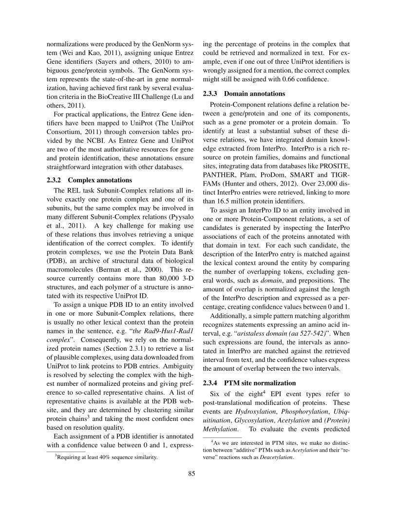
normalizations were produced by the GenNorm sys-tem (Wei and Kao, 2011), assigning unique EntrezGene identifiers (Sayers and others, 2010) to am-biguous gene/protein symbols. The GenNorm sys-tem represents the state-of-the-art in gene normal-ization, having achieved first rank by several evalua-tion criteria in the BioCreative III Challenge (Lu andothers, 2011).
For practical applications, the Entrez Gene iden-tifiers have been mapped to UniProt (The UniProtConsortium, 2011) through conversion tables pro-vided by the NCBI. As Entrez Gene and UniProtare two of the most authoritative resources for geneand protein identification, these annotations ensurestraightforward integration with other databases.
2.3.2 Complex annotationsThe REL task Subunit-Complex relations all in-
volve exactly one protein complex and one of itssubunits, but the same complex may be involved inmany different Subunit-Complex relations (Pyysaloet al., 2011). A key challenge for making useof these relations thus involves retrieving a uniqueidentification of the correct complex. To identifyprotein complexes, we use the Protein Data Bank(PDB), an archive of structural data of biologicalmacromolecules (Berman et al., 2000). This re-source currently contains more than 80,000 3-Dstructures, and each polymer of a structure is anno-tated with its respective UniProt ID.
To assign a unique PDB ID to an entity involvedin one or more Subunit-Complex relations, thereis usually no other lexical context than the proteinnames in the sentence, e.g. “the Rad9-Hus1-Rad1complex”. Consequently, we rely on the normal-ized protein names (Section 2.3.1) to retrieve a listof plausible complexes, using data downloaded fromUniProt to link proteins to PDB entries. Ambiguityis resolved by selecting the complex with the high-est number of normalized proteins and giving pref-erence to so-called representative chains. A list ofrepresentative chains is available at the PDB web-site, and they are determined by clustering similarprotein chains3 and taking the most confident onesbased on resolution quality.
Each assignment of a PDB identifier is annotatedwith a confidence value between 0 and 1, express-
3Requiring at least 40% sequence similarity.
ing the percentage of proteins in the complex thatcould be retrieved and normalized in text. For ex-ample, even if one out of three UniProt identifiers iswrongly assigned for a mention, the correct complexmight still be assigned with 0.66 confidence.
2.3.3 Domain annotationsProtein-Component relations define a relation be-
tween a gene/protein and one of its components,such as a gene promoter or a protein domain. Toidentify at least a substantial subset of these di-verse relations, we have integrated domain knowl-edge extracted from InterPro. InterPro is a rich re-source on protein families, domains and functionalsites, integrating data from databases like PROSITE,PANTHER, Pfam, ProDom, SMART and TIGR-FAMs (Hunter and others, 2012). Over 23,000 dis-tinct InterPro entries were retrieved, linking to morethan 16.5 million protein identifiers.
To assign an InterPro ID to an entity involved inone or more Protein-Component relations, a set ofcandidates is generated by inspecting the InterProassociations of each of the proteins annotated withthat domain in text. For each such candidate, thedescription of the InterPro entry is matched againstthe lexical context around the entity by comparingthe number of overlapping tokens, excluding gen-eral words, such as domain, and prepositions. Theamount of overlap is normalized against the lengthof the InterPro description and expressed as a per-centage, creating confidence values between 0 and 1.
Additionally, a simple pattern matching algorithmrecognizes statements expressing an amino acid in-terval, e.g. “aristaless domain (aa 527-542)”. Whensuch expressions are found, the intervals as anno-tated in InterPro are matched against the retrievedinterval from text, and the confidence values expressthe amount of overlap between the two intervals.
2.3.4 PTM site normalizationSix of the eight4 EPI event types refer to
post-translational modification of proteins. Theseevents are Hydroxylation, Phosphorylation, Ubiq-uitination, Glycosylation, Acetylation and (Protein)Methylation. To evaluate the events predicted
4As we are interested in PTM sites, we make no distinc-tion between “additive” PTMs such as Acetylation and their “re-verse” reactions such as Deacetylation.
85

from text, we compare these to annotated post-translational modifications in UniProt. UniProt isone of the largest manually curated databases forprotein knowledge, and contains annotations corre-sponding to each of the EPI PTM event types.
We use the reviewed and manually annotatedUniProtKB/Swiss-Prot dataset (release 2012 02) inXML format. We take for each protein all featureelements of types modified residue, cross-link andglycosylation site. Each of these feature elementsdefines the site of the modification, either a singleamino acid, or a sequence of amino acids. We selectonly annotations based on experimental findings,that is, features that do not have a non-experimentalstatus (potential, probable or by similarity) to avoide.g. features only inferred from the sequence.
The modified residue feature type covers the eventtypes Hydroxylation, Phosphorylation, Acetylationand Methylation. We determine the class of the mod-ification with the UniProt controlled vocabulary ofpost-translational modifications5. The descriptionattribute is the ID attribute of an entry in the vocabu-lary, through which we can determine the more gen-eral keyword (KW) for that description, if defined.These keywords can then be connected to the corre-sponding event types in the case of Hydroxylation,Phosphorylation, Acetylation and Methylation. ForUbiquitination events, we look for the presence ofthe string “ubiquitin” in the description attribute ofcross-link features. Finally, features correspondingto Glycosylation events are determined by their fea-ture element having the type glycosylation site.
The result of this selection process is a list of in-dividual modification features, which contain a typecorresponding to one of the EPI PTM event types,the UniProt ID of the protein, and the position andamino acid(s) of the modification site. This data canbe compared with extracted events, using their type,normalized protein arguments and modification sitearguments. However, we also need to normalize themodification site arguments.
PTM sites are defined with a modification typeand the numbered target amino acid residue. In EPIevents, these residues are defined in the site argu-ment target entities. To convert these into a formthat can be aligned with UniProt, we apply a set
5http://www.uniprot.org/docs/ptmlist/
Event Type Extracted PMC (%)Hydroxylation 14,555 34.17Phosphorylation 726,757 44.00Ubiquitination 74,027 70.46DNA methylation 140,531 52.27Glycosylation 154,523 42.31Acetylation 114,585 69.40Methylation 122,015 74.86Catalysis 45,763 67.86Total EPI 1,392,756 51.53Protein-Component 1,613,170 52.59Subunit-Complex 537,577 51.18Total REL 2,150,747 52.23
Table 2: Total number of EPI events and REL relationsextracted from PubMed abstracts and PMC full-text arti-cles, with the fractions extracted from PMC.
of rules that try to determine whether a site is anamino acid. We start from the main site token, andcheck whether it is of the form AA#, where AA is anamino acid name, or a one or three letter code, and# an optional site number, which can also be in a to-ken following the amino acid. For cases where thesite entity is the word “residue” or “residues”, welook for the amino acid definition in the precedingand following tokens. All strings are canonicalizedwith removal of punctuation, hyphens and parenthe-sis before applying the rules. In total, of the 177,994events with a site argument, 75,131 could be nor-malized to an amino acid, and 60,622 of these to aspecific residue number.
3 Results
The source for extraction in this work is the set of 21million PubMed abstracts and 372 thousand PMCopen-access full-text articles. From this dataset,1.4M EPI events and 2.2M REL relations were ex-tracted (Table 2). For both tasks, about half of theresults were extracted from PMC, confirming thatfull-text articles are an important source of infor-mation for these extraction targets. The total num-bers of events and relations are considerably lowerthan e.g. the 21.3M events extracted for the GENIAtask from PubMed abstracts (Bjorne et al., 2010;Van Landeghem et al., 2012), likely relating to thecomparatively low frequency with which EPI andREL extraction targets are discussed with respect tothe basic GENIA biomolecular reactions.
86

Event type UniProt Events Match Coverage Events (site) Match CoverageHydroxylation 1,587 14,555 1,526 19 4,298 130 5Phosphorylation 57,059 726,757 286,978 4,795 86,974 9,732 748Ubiquitination 792 74,027 4,994 143 10,562 54 20Glycosylation 6,708 154,523 18,592 897 22,846 68 31Acetylation 6,522 114,585 15,470 764 25,689 158 30Methylation 1,135 122,015 2,178 113 27,625 36 10Total 73,803 1,206,462 329,738 6,731 177,994 10,178 844
Table 3: PTM events. PTMs that are not marked with non-experimental qualifiers are taken from UniProt. TheEvents column lists the total number of predicted events, and the Events (site) the number of events that also have apredicted site-argument. For these groups, Match is the number of events that matches a known PTM from UniProt,and Coverage the number of UniProt PTMs for which at least one match exists. For Events matching takes into accountthe PTM type and protein id, for Events (site) also the amino acid and position of the modified residue.
Event type AA UP # Highest confidence event Article IDPhosphorylation S9 • 2 p53 isolated from ML1, HCT116 and RKO cells, after short
term genotoxic stress, were phosphorylated on Ser 6, Ser 9PMC:2777442
Acetylation S15 4 phosphorylated (Ser15), acetylated p53(Lys382) PMC:2557062Methylation S15 1 phosphorylation of p53 at serine 15 and acetylation PM:10749144Phosphorylation S15 • 238 Chk2, as well as p53 Ser(15) phosphorylation and its PM:16731759Phosphorylation T18 • 12 p53 stabilization and its phosphorylation in Thr18 PMC:3046209Phosphorylation S20 • 45 that phosphorylation of p53 at Ser20 leads to PMC:3050855Phosphorylation S33 • 14 phosphorylation of p53 at serine 33 may be part of PMC:35361Phosphorylation S37 • 20 serine 33 of p53 in vitro when serine 37 is already PMC:35361Phosphorylation S46 • 55 phosphorylation of p53, especially at Serine 46 by PMC:2634840Phosphorylation T55 • 7 that phosphorylation of p53 at Thr55 inhibits its PMC:3050855Phosphorylation S99 • 0Phosphorylation S183 • 0Phosphorylation S269 • 0Phosphorylation T284 • 0Ubiquitination K291 • 0Acetylation K292 • 0Ubiquitination K292 • 0Acetylation K305 • 0Phosphorylation S313 • 1 hyperphosphorylation of p53, particularly of Ser313 PM:8649812Phosphorylation S314 • 0Phosphorylation S315 • 6 to require phosphorylation of p53 at serine 315 (35) PMC:2532731Methylation K370 • 6 by methylating lysine 370 of p53 PMC:1636665Acetylation K372 1 for lysine 372 and 383 acetylated p53 (Upstate, PMC:1315280Methylation K372 • 5 methylation of p53 by the KMT7(SET7/9) methyltransferase
enzyme on Lys372PMC:2794343
Acetylation K373 • 16 p53 and acetylated p53 (lysine-373 and lysine-382) PMC:1208859Methylation K373 • 4 EHMT1-mediated p53 methylation at K373 PM:20588255Acetylation K381 • 0Acetylation K382 • 82 p53 acetylation at lysine 382 was found not PM:17898049Methylation K382 • 6 SET8 specifically monomethylates p53 at lysine 382 PM:17707234Methylation K386 • 1 that sumoylation of p53 at K386 blocks subsequent PM:19339993Phosphorylation S392 • 35 and phosphorylation of p53 at S392 PM:17237827
Table 4: Extracted and known PTM sites of p53. The type and site of the modification are in the first two columns.UP indicates whether the PTM is present in the UniProt annotation for p53. Column # shows the number of extractedevents, followed by the event with the highest confidence score and the PubMed abstract or PMC full-text article it hasbeen extracted from.
87

3.1 Extracted PTMs compared to UniProt
The EPI PTM events were compared to annotatedPTMs from UniProt (Table 3). The majority of ex-tracted PTM events (85%) have only a protein ar-gument, and no information about the modificationsite, so these can only be compared by the proteinid and PTM type. For the subset of proteins thatalso have a site, which can be normalized to anamino acid position, we can make a detailed com-parison with UniProt. Finding a match for thesenormalized amino acids is more difficult, and forboth categories, only a small fraction of proteinsfrom UniProt is covered. In part this may be dueto the limitations of the gene name normalization, asfinding the exact species-specific protein ID remainsa challenging task (Lu and others, 2011). How-ever, even if the overall coverage is limited, well-known protein modifications can be assigned to spe-cific residues, as we show in the next section.
3.2 Extracted PTMs for a single protein
For an in-depth example of PTM modifications, westudy the protein p53, a central tumor suppressorprotein that is the subject of many studies. p53 isalso among the proteins with the most UniProt PTMsites for which EPI events were predicted, making ita good example for a case study (see Table 4).
We take from UniProt all known p53 PTMs corre-sponding to our EPI event types and list the numberof predicted events for them (see Table 4). Whenthe number of predicted events is high, the mostconfident prediction is usually a correctly extracted,clear statement about the PTM. All events for PTMsknown in UniProt are correct except for the typeof K386. For events not in UniProt, the two S15ones are false positives, and K372 acetylation, whilecorrectly extracted, is most likely a typo in the arti-cle. For the PTMs for which no event was extracted,we checked the reference article from UniProt an-notation. K291, K292 ubiquitination, and K305 arefrom abstracts, and thus missed events. S183, S269and T284 are from a non-open access PMC article,while S99, K292 acetylation, K305, S314 and K381are from Excel or PDF format supplementary tables,sources outside our extraction input.
In total, we have extracted 561 PTM events re-lated to p53, 554 of which correspond to a PTM an-
Item PubMeth Extracted RecallPMID+UPID 2776 1698 61.2%UPID 392 363 92.6%PMID 1163 1120 96.3%
Table 5: Evaluation of DNA methylation event extractionrecall against PubMeth.
notated in UniProt. Of the 28 EPI-relevant PTMs onp53, 17 have at least one predicted event. The high-est confidence events are about equally often fromabstracts as from full texts.
3.3 DNA methylation analysisTwo recently introduced databases, PubMeth (On-genaert et al., 2008) and MeInfoText (Fang et al.,2011) provide manually curated information onDNA methylation, primarily as it relates to cancer.To evaluate the coverage of DNA methylation eventextraction, we focus here on PubMeth, as the fullcontent of this database could be directly used. EachPubMeth DB record provides the primary name ofthe methylated gene and the PMID of the publica-tion supporting the curation of the record. We usedthese two pieces of information to evaluate the recall6 of DNA methylation event extraction.
We mapped PubMeth entries to UniProt iden-tifiers (UPIDs), and extracted all unique (PMID,UPID) pairs from both PubMeth and the automat-ically extracted DNA methylation/demethylationevents. The results of comparison of these sets ofID pairs are given in Table 5. We find that for over60% of PubMeth entries, the system is able to re-cover the specific (document, gene) pair. This resultis broadly in line with the recall of the system asevaluated in the BioNLP ST. However, if the match-ing constraint is relaxed, asking either 1) can the sys-tem extract the methylation of each gene in PubMethsomewhere in the literature or, inversely, 2) can thesystem detect some DNA methylation event in eachdocument included in PubMeth as evidence, recallis over 90%. In particular, the evaluation indicatesthat the system shows very high recall for identify-ing documents discussing DNA methylation.
6As PubMeth does not aim for exhaustive coverage, preci-sion cannot be directly estimated in this way. For example, Pub-Meth covers fewer than 2,000 documents and DNA methylationevents were extracted from over 20,000, but due to differencesin scope, this does not suggest precision is below 10%.
88

REL Type Extracted Match (p) Match (e)Prot-Cmp 1613.1K 561.8K 150.7KSU-Cmplx 537.6K 226.5K 99.6K
Table 6: Numbers of extracted entity relations, with theprotein (p) or both protein and entity (e) identified.
3.4 REL statistics
Table 6 presents the amount of extracted entity re-lations and the coverage of the normalization algo-rithms assigning protein, domain and complex iden-tifiers. From a total of 537.6K Subunit-Complex re-lations, 226.5K (42%) involve a protein that could beunambiguously identified (Section 2.3.1). From thissubset, 99.6K relations (44%) could be assigned to aPDB complex identifier (Section 2.3.2), accountingfor 3800 representative 3D protein structures.
The Protein-Component relations are much morefrequent in the data (1.6M relations) and here 35%of the relations (561.8K) involve a normalized pro-tein mention. The assignment of InterPro domainsto these Protein-Component relations (Section 2.3.3)further covers 150.7K relations in this subset (27%),identifying 5500 distinct functional domains. Thevast majority of these annotations (99%) are pro-duced by matching the lexical context against theInterPro descriptions, and only a few cases (200)matched against the amino-acid pattern.
4 Conclusions
We have combined state-of-the-art methods forgene/protein name normalization together with thebest available methods for event-based extractionof protein post-translational modifications, reactionsrelating to the epigenetic control of gene expres-sion, and part-of relations between genes/proteins,their components, and complexes. These methodswere jointly applied to the entire available litera-ture, both PubMed abstracts and PMC full-text doc-uments, creating a text mining dataset unique in bothscope and breadth of analysis. We further performeda comprehensive analysis of the results of this au-tomatic extraction process against major biologicaldatabase resources covering various aspects of theextracted information. This analysis indicated thattext mining results for protein complexes, substruc-tures and epigenetic DNA methylation provides al-
ready quite extensive coverage of relevant proteins.For post-translational modifications, we note thatcoverage still needs to be improved, but concludethat the extracted events already provide a valuablelink to PTM related literature. In future work wehope to further extend the event types extracted byour PubMed-scale approach. The extraction meth-ods as well as all data introduced in this study arefreely available from bionlp.utu.fi.
Acknowledgments
We thank the Academy of Finland, the ResearchFoundation Flanders (FWO) and the UK BBSRC(reference number: BB/G013160/1) for funding,and CSC – IT Center for Science Ltd for compu-tational resources.
ReferencesSophia Ananiadou, Sampo Pyysalo, Jun’ichi Tsujii, and
Douglas B. Kell. 2010. Event extraction for sys-tems biology by text mining the literature. Trends inBiotechnology, 28(7):381–390.
Helen M. Berman, John Westbrook, Zukang Feng,Gary Gilliland, T. N. Bhat, Helge Weissig, Ilya N.Shindyalov, and Philip E. Bourne. 2000. The proteindata bank. Nucleic Acids Research, 28(1):235–242.
Jari Bjorne and Tapio Salakoski. 2011. Generalizingbiomedical event extraction. In Proceedings of theBioNLP Shared Task 2011 Workshop, pages 183–191.
Jari Bjorne, Juho Heimonen, Filip Ginter, Antti Airola,Tapio Pahikkala, and Tapio Salakoski. 2009. Extract-ing complex biological events with rich graph-basedfeature sets. In Proceedings of the BioNLP 2009 Work-shop, pages 10–18.
Jari Bjorne, Filip Ginter, Sampo Pyysalo, Jun’ichi Tsujii,and Tapio Salakoski. 2010. Scaling up biomedicalevent extraction to the entire PubMed. In Proceedingsof the BioNLP 2010 Workshop, pages 28–36.
Eugene Charniak and Mark Johnson. 2005. Coarse-to-fine n-best parsing and MaxEnt discriminative rerank-ing. In Proceedings of the 43rd Annual Meeting ofACL, pages 173–180.
Y.C. Fang, P.T. Lai, H.J. Dai, and W.L. Hsu. 2011. Me-infotext 2.0: gene methylation and cancer relation ex-traction from biomedical literature. BMC bioinformat-ics, 12(1):471.
Z. Z. Hu, M. Narayanaswamy, K. E. Ravikumar,K. Vijay-Shanker, and C. H. Wu. 2005. Literaturemining and database annotation of protein phospho-rylation using a rule-based system. Bioinformatics,21(11):2759–2765.
89

Sarah Hunter et al. 2012. Interpro in 2011: new devel-opments in the family and domain prediction database.Nucleic Acids Research, 40(D1):D306–D312.
Jun’ichi Kazama and Jun’ichi Tsujii. 2003. Evaluationand extension of maximum entropy models with in-equality constraints. In Proceedings of EMNLP 2003,pages 137–144.
Jin-Dong Kim, Tomoko Ohta, Sampo Pyysalo, Yoshi-nobu Kano, and Jun’ichi Tsujii. 2009. Overview ofBioNLP’09 shared task on event extraction. In Pro-ceedings of BioNLP 2009, pages 1–9.
Jin-Dong Kim, Sampo Pyysalo, Tomoko Ohta, RobertBossy, Ngan Nguyen, and Jun’ichi Tsujii. 2011.Overview of BioNLP Shared Task 2011. In Proceed-ings of the BioNLP Shared Task 2011, pages 1–6.
Robert Leaman and Graciela Gonzalez. 2008. BAN-NER: an executable survey of advances in biomedicalnamed entity recognition. Pacific Symposium on Bio-computing, pages 652–663.
Tzong-Yi Lee, Hsien-Da Huang, Jui-Hung Hung, Hsi-Yuan Huang, Yuh-Shyong Yang, and Tzu-Hao Wang.2006. dbPTM: an information repository of pro-tein post-translational modification. Nucleic acids re-search, 34(suppl 1):D622–D627.
Hodong Lee, Gwan-Su Yi, and Jong C. Park. 2008.E3Miner: a text mining tool for ubiquitin-protein lig-ases. Nucl. Acids Res., 36(suppl.2):W416–422.
Hong Li, Xiaobin Xing, Guohui Ding, Qingrun Li, ChuanWang, Lu Xie, Rong Zeng, and Yixue Li. 2009.SysPTM: A Systematic Resource for Proteomic Re-search on Post-translational Modifications. Molecular& Cellular Proteomics, 8(8):1839–1849.
Zhiyong Lu et al. 2011. The gene normalization taskin BioCreative III. BMC Bioinformatics, 12(Suppl8):S2+.
Marie-Catherine de Marneffe, Bill MacCartney, andChristopher Manning. 2006. Generating typed depen-dency parses from phrase structure parses. In Proceed-ings of LREC-06, pages 449–454.
David McClosky. 2010. Any domain parsing: auto-matic domain adaptation for natural language pars-ing. Ph.D. thesis, Department of Computer Science,Brown University.
Tomoko Ohta, Sampo Pyysalo, Makoto Miwa, Jin-DongKim, and Jun’ichi Tsujii. 2010. Event extractionfor post-translational modifications. In Proceedings ofBioNLP’10, pages 19–27.
Tomoko Ohta, Sampo Pyysalo, Makoto Miwa, andJun’ichi Tsujii. 2011a. Event extraction forDNA methylation. Journal of Biomedical Semantics,2(Suppl 5):S2.
Tomoko Ohta, Sampo Pyysalo, and Jun’ichi Tsujii.2011b. Overview of the epigenetics and post-translational modifications (EPI) task of BioNLP
Shared Task 2011. In Proceedings of BioNLP SharedTask 2011 Workshop, pages 16–25.
Mate Ongenaert, Leander Van Neste, Tim De Meyer,Gerben Menschaert, Sofie Bekaert, and WimVan Criekinge. 2008. PubMeth: a cancer methy-lation database combining text-mining and expertannotation. Nucl. Acids Res., 36(suppl 1):D842–846.
Sampo Pyysalo, Antti Airola, Juho Heimonen, and JariBjorne. 2008. Comparative analysis of five protein-protein interaction corpora. BMC Bioinformatics,9(Suppl. 3):S6.
Sampo Pyysalo, Tomoko Ohta, Jin-Dong Kim, andJun’ichi Tsujii. 2009. Static relations: a piece in thebiomedical information extraction puzzle. In Proceed-ings of the BioNLP 2009 Workshop, pages 1–9.
Sampo Pyysalo, Tomoko Ohta, and Jun’ichi Tsujii. 2011.Overview of the entity relations (REL) supporting taskof BioNLP Shared Task 2011. In Proceedings of theBioNLP Shared Task 2011 Workshop, pages 83–88.
Eric W. Sayers et al. 2010. Database resources of the na-tional center for biotechnology information. NucleicAcids Research, 38(suppl 1):D5–D16.
Pontus Stenetorp, Goran Topic, Sampo Pyysalo, TomokoOhta, Jin-Dong Kim, and Jun’ichi Tsujii. 2011.Bionlp shared task 2011: Supporting resources. InProceedings of BioNLP Shared Task 2011 Workshop,pages 112–120.
The UniProt Consortium. 2011. Ongoing and future de-velopments at the universal protein resource. NucleicAcids Research, 39(suppl 1):D214–D219.
Domonkos Tikk, Philippe Thomas, Peter Palaga, JorgHakenberg, and Ulf Leser. 2010. A comprehen-sive benchmark of kernel methods to extract protein-protein interactions from literature. PLoS ComputBiol, 6(7):e1000837, 07.
Sofie Van Landeghem, Sampo Pyysalo, Tomoko Ohta,and Yves Van de Peer. 2010. Integration of static re-lations to enhance event extraction from text. In Pro-ceedings of BioNLP’10, pages 144–152.
Sofie Van Landeghem, Kai Hakala, Samuel Ronnqvist,Tapio Salakoski, Yves Van de Peer, and Filip Ginter.2012. Exploring biomolecular literature with EVEX:Connecting genes through events, homology and indi-rect associations. Advances in Bioinformatics.
Chih-Hsuan Wei and Hung-Yu Kao. 2011. Cross-speciesgene normalization by species inference. BMC bioin-formatics, 12(Suppl 8):S5.
Cathy H. Wu et al. 2003. The Protein Information Re-source. Nucl. Acids Res., 31(1):345–347.
X. Yuan, ZZ Hu, HT Wu, M. Torii, M. Narayanaswamy,KE Ravikumar, K. Vijay-Shanker, and CH Wu. 2006.An online literature mining tool for protein phospho-rylation. Bioinformatics, 22(13):1668.
90

Proceedings of the 2012 Workshop on Biomedical Natural Language Processing (BioNLP 2012), pages 91–99,Montreal, Canada, June 8, 2012. c©2012 Association for Computational Linguistics
An improved corpus of disease mentions in PubMed citations
Rezarta Islamaj Doğan Zhiyong Lu National Center for Biotechnology Information National Center for Biotechnology Information
8600 Rockville Pike 8600 Rockville Pike
Bethesda, MD 20894, USA Bethesda, MD 20894, USA [email protected] [email protected]
Abstract
The latest discoveries on diseases and their di-
agnosis/treatment are mostly disseminated in
the form of scientific publications. However,
with the rapid growth of the biomedical litera-
ture and a high level of variation and ambigui-
ty in disease names, the task of retrieving
disease-related articles becomes increasingly
challenging using the traditional keyword-
based approach. An important first step for
any disease-related information extraction
task in the biomedical literature is the disease
mention recognition task. However, despite
the strong interest, there has not been enough
work done on disease name identification,
perhaps because of the difficulty in obtaining
adequate corpora. Towards this aim, we creat-
ed a large-scale disease corpus consisting of
6900 disease mentions in 793 PubMed cita-
tions, derived from an earlier corpus. Our cor-
pus contains rich annotations, was developed
by a team of 12 annotators (two people per
annotation) and covers all sentences in a
PubMed abstract. Disease mentions are cate-
gorized into Specific Disease, Disease Class,
Composite Mention and Modifier categories.
When used as the gold standard data for a
state-of-the-art machine-learning approach,
significantly higher performance can be found
on our corpus than the previous one. Such
characteristics make this disease name corpus
a valuable resource for mining disease-related
information from biomedical text. The NCBI
corpus is available for download at
http://www.ncbi.nlm.nih.gov/CBBresearch/Fe
llows/Dogan/disease.html.
1 Introduction
Identification of biomedical entities has been an
active area of research in recent years (Rinaldi et
al., 2011, Smith et al., 2008, Yeh et al., 2005). Au-
tomatic systems, both lexically-based and machine
learning-based, have been built to identify medi-
cally relevant concepts and/or their relationships.
Biomedical entity recognition research covers not
only gene/protein mention recognition (Tanabe et
al., 2005, Campos et al., 2012), but also other med-
ically relevant concepts such as disease names,
chemical/drug names, treatments, procedures etc.
Systems capable of achieving high performance on
these tasks are highly desirable as entity recogni-
tion precedes all other information extraction and
text mining tasks.
Disease information is sought very frequently in
biomedical search engines. Previous PubMed log
usage analysis (Islamaj Dogan et al., 2009) has
shown that disease is the most frequent non-
bibliographic information requested from PubMed
users. Furthermore, disease information was often
found to be queried together with Chemical/Drug
or Gene/Protein information. Automatic recogni-
tion of disease mentions therefore, is essential not
only for improving retrieval of relevant documents,
but also for extraction of associations between dis-
eases and genes or between diseases and drugs.
However, prior research shows that automatic dis-
ease recognition is a challenging task due to varia-
tions and ambiguities in disease names (Leaman et
al., 2009, Chowdhury and Lavelli 2010).
Lexically-based systems of disease name recog-
nition, generally refer to the Unified Medical Lan-
guage System (UMLS) (Burgun and Bodenreider
91
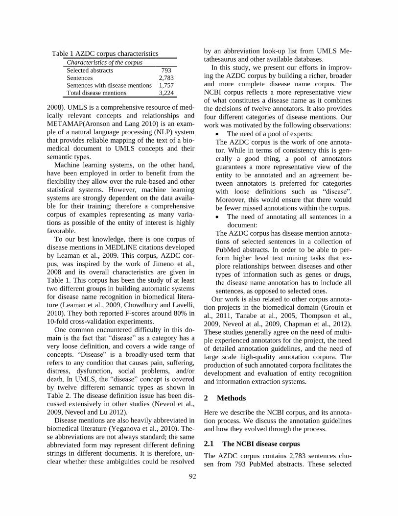
2008). UMLS is a comprehensive resource of med-
ically relevant concepts and relationships and
METAMAP(Aronson and Lang 2010) is an exam-
ple of a natural language processing (NLP) system
that provides reliable mapping of the text of a bio-
medical document to UMLS concepts and their
semantic types.
Machine learning systems, on the other hand,
have been employed in order to benefit from the
flexibility they allow over the rule-based and other
statistical systems. However, machine learning
systems are strongly dependent on the data availa-
ble for their training; therefore a comprehensive
corpus of examples representing as many varia-
tions as possible of the entity of interest is highly
favorable.
To our best knowledge, there is one corpus of
disease mentions in MEDLINE citations developed
by Leaman et al., 2009. This corpus, AZDC cor-
pus, was inspired by the work of Jimeno et al.,
2008 and its overall characteristics are given in
Table 1. This corpus has been the study of at least
two different groups in building automatic systems
for disease name recognition in biomedical litera-
ture (Leaman et al., 2009, Chowdhury and Lavelli,
2010). They both reported F-scores around 80% in
10-fold cross-validation experiments.
One common encountered difficulty in this do-
main is the fact that “disease” as a category has a
very loose definition, and covers a wide range of
concepts. “Disease” is a broadly-used term that
refers to any condition that causes pain, suffering,
distress, dysfunction, social problems, and/or
death. In UMLS, the “disease” concept is covered
by twelve different semantic types as shown in
Table 2. The disease definition issue has been dis-
cussed extensively in other studies (Neveol et al.,
2009, Neveol and Lu 2012).
Disease mentions are also heavily abbreviated in
biomedical literature (Yeganova et al., 2010). The-
se abbreviations are not always standard; the same
abbreviated form may represent different defining
strings in different documents. It is therefore, un-
clear whether these ambiguities could be resolved
by an abbreviation look-up list from UMLS Me-
tathesaurus and other available databases.
In this study, we present our efforts in improv-
ing the AZDC corpus by building a richer, broader
and more complete disease name corpus. The
NCBI corpus reflects a more representative view
of what constitutes a disease name as it combines
the decisions of twelve annotators. It also provides
four different categories of disease mentions. Our
work was motivated by the following observations:
The need of a pool of experts:
The AZDC corpus is the work of one annota-
tor. While in terms of consistency this is gen-
erally a good thing, a pool of annotators
guarantees a more representative view of the
entity to be annotated and an agreement be-
tween annotators is preferred for categories
with loose definitions such as “disease”.
Moreover, this would ensure that there would
be fewer missed annotations within the corpus.
The need of annotating all sentences in a
document:
The AZDC corpus has disease mention annota-
tions of selected sentences in a collection of
PubMed abstracts. In order to be able to per-
form higher level text mining tasks that ex-
plore relationships between diseases and other
types of information such as genes or drugs,
the disease name annotation has to include all
sentences, as opposed to selected ones.
Our work is also related to other corpus annota-
tion projects in the biomedical domain (Grouin et
al., 2011, Tanabe at al., 2005, Thompson et al.,
2009, Neveol at al., 2009, Chapman et al., 2012).
These studies generally agree on the need of multi-
ple experienced annotators for the project, the need
of detailed annotation guidelines, and the need of
large scale high-quality annotation corpora. The
production of such annotated corpora facilitates the
development and evaluation of entity recognition
and information extraction systems.
2 Methods
Here we describe the NCBI corpus, and its annota-
tion process. We discuss the annotation guidelines
and how they evolved through the process.
2.1 The NCBI disease corpus
The AZDC corpus contains 2,783 sentences cho-
sen from 793 PubMed abstracts. These selected
Table 1 AZDC corpus characteristics
Characteristics of the corpus
Selected abstracts 793
Sentences 2,783
Sentences with disease mentions 1,757
Total disease mentions 3,224
92

sentences were annotated for disease mentions,
resulting in 1,202 unique mentions and 3,224 total
mentions. The NCBI corpus starts with this origi-
nal corpus; however, it is expanded to cover all the
sentences in all the 793 PubMed abstracts.
2.2 Annotation guidelines
One fundamental problem in corpus annotation is
the definition of what constitutes an entity to be
tagged. Following the lead of the AZDC annota-
tions, the group of annotators working on the
NCBI corpus decided that a textual string would be
annotated as a disease mention if it could be
mapped to a unique concept in the UMLS Me-
tathesaurus, if it corresponded to at least one of the
semantic types listed in Table 2, and if it contained
information that would be helpful to physicians
and health care professionals.
Annotators were invited to use their common
knowledge, use public resources of the National
Library of Medicine such as UMLS or PubMed
Health, Disease Ontology (Warren et al., 2006) and
Wikipedia and consider the viewpoint of an aver-
age user trying to find information on diseases.
Initially, a set of 20 randomly chosen PubMed
abstracts was used as a practice set for the devel-
opment of annotation guidelines. After each anno-
tator worked individually on the set, the results
were shared and discussed among all annotators.
The final annotation guidelines are summarized
below and also made available at the corpus down-
load website.
What to annotate?
1. Annotate all specific disease mentions.
A textual string referring to a disease name may
refer to a Specific Disease, or a Disease Class.
Disease mentions that could be described as a
family of many specific diseases were annotated
with an annotation category called Disease
Class. The annotation category Specific Disease
was used for those mentions which could be
linked to one specific definition that does not in-
clude further categorization.
e.g. <Specific Disease> Diastrophic dysplasia
</> is an <Disease Class> autosomal recessive
disease</> characterized by short stature, very
short limbs and joint problems that restrict mo-
bility.
2. Annotate contiguous text strings.
A textual string may refer to two or more sepa-
rate disease mentions. Such mentions are anno-
tated with the Composite Mention category.
e.g. The text phrase “Duchenne and Becker
muscular dystrophy” refers to two separate dis-
eases. If this phrase is separated into two strings:
“Duchenne” and “Becker muscular dystrophy”,
it results in information loss, because the word
“Duchenne” on its own is not a disease mention.
3. Annotate disease mentions that are used as
modifiers for other concepts
A textual string may refer to a disease name, but
it may not be a noun phrase and this is better ex-
pressed with the Modifier annotation category.
e.g.: Although this mutation was initially de-
tected in four of 33 <Modifier> colorectal can-
cer </> families analysed from eastern England,
more extensive analysis has reduced the fre-
quency to four of 52 English <Modifier>
HNPCC </> kindreds analysed.
4. Annotate duplicate mentions.
Table 2 The set of UMLS semantic types that collectively cover concepts of the “disease” category
UMLS sematic types Disease name example
Acquired Abnormality Hernia, Varicose Veins
Anatomical Abnormality Bernheim aneurysm, Fistula of thoracic duct
Congenital Abnormality Oppenheim's Disease, Ataxia Telangiectasia
Cell or Molecular Dysfunction Uniparental disomy, Intestinal metaplasia
Disease or Syndrome Acute pancreatitis, Rheumatoid Arthritis
Experimental Model of Disease Collagen-Induced Arthritis, Jensen Sarcoma
Injury or Poisoning Contusion and laceration of cerebrum
Mental or Behavioral Dysfunction Schizophrenia, anxiety disorder, dementia
Neoplastic Process Colorectal Carcinoma, Burkitt Lymphoma
Pathologic Function Myocardial degeneration, Adipose Tissue Atrophy
Sign or Symptom Back Pain, Seizures, Skeletal muscle paralysis
Finding Abnormal or prolonged bleeding time
93
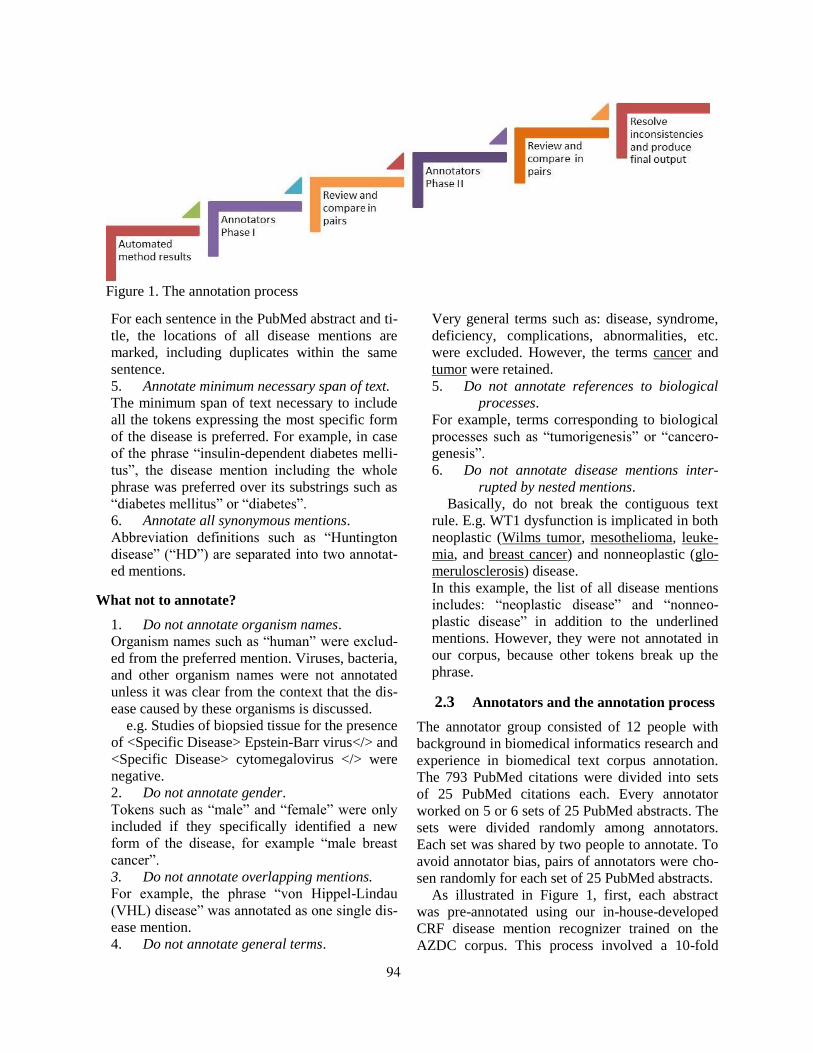
For each sentence in the PubMed abstract and ti-
tle, the locations of all disease mentions are
marked, including duplicates within the same
sentence.
5. Annotate minimum necessary span of text.
The minimum span of text necessary to include
all the tokens expressing the most specific form
of the disease is preferred. For example, in case
of the phrase “insulin-dependent diabetes melli-
tus”, the disease mention including the whole
phrase was preferred over its substrings such as
“diabetes mellitus” or “diabetes”.
6. Annotate all synonymous mentions.
Abbreviation definitions such as “Huntington
disease” (“HD”) are separated into two annotat-
ed mentions.
What not to annotate?
1. Do not annotate organism names.
Organism names such as “human” were exclud-
ed from the preferred mention. Viruses, bacteria,
and other organism names were not annotated
unless it was clear from the context that the dis-
ease caused by these organisms is discussed.
e.g. Studies of biopsied tissue for the presence
of <Specific Disease> Epstein-Barr virus</> and
<Specific Disease> cytomegalovirus </> were
negative.
2. Do not annotate gender.
Tokens such as “male” and “female” were only
included if they specifically identified a new
form of the disease, for example “male breast
cancer”.
3. Do not annotate overlapping mentions.
For example, the phrase “von Hippel-Lindau
(VHL) disease” was annotated as one single dis-
ease mention.
4. Do not annotate general terms.
Very general terms such as: disease, syndrome,
deficiency, complications, abnormalities, etc.
were excluded. However, the terms cancer and
tumor were retained.
5. Do not annotate references to biological
processes.
For example, terms corresponding to biological
processes such as “tumorigenesis” or “cancero-
genesis”.
6. Do not annotate disease mentions inter-
rupted by nested mentions.
Basically, do not break the contiguous text
rule. E.g. WT1 dysfunction is implicated in both
neoplastic (Wilms tumor, mesothelioma, leuke-
mia, and breast cancer) and nonneoplastic (glo-
merulosclerosis) disease.
In this example, the list of all disease mentions
includes: “neoplastic disease” and “nonneo-
plastic disease” in addition to the underlined
mentions. However, they were not annotated in
our corpus, because other tokens break up the
phrase.
2.3 Annotators and the annotation process
The annotator group consisted of 12 people with
background in biomedical informatics research and
experience in biomedical text corpus annotation.
The 793 PubMed citations were divided into sets
of 25 PubMed citations each. Every annotator
worked on 5 or 6 sets of 25 PubMed abstracts. The
sets were divided randomly among annotators.
Each set was shared by two people to annotate. To
avoid annotator bias, pairs of annotators were cho-
sen randomly for each set of 25 PubMed abstracts.
As illustrated in Figure 1, first, each abstract
was pre-annotated using our in-house-developed
CRF disease mention recognizer trained on the
AZDC corpus. This process involved a 10-fold
Figure 1. The annotation process
94

cross-validation scheme, where all sentences from
the same PubMed abstract were assigned to the
same split. The learning was performed on 9-folds
and then, the PubMed abstracts assigned to the
10th fold were annotated for disease mentions on a
sentence-by-sentence basis.
Annotation Phase I consisted of each pre-
annotated abstract in the corpus being read and
reviewed by two annotators working independent-
ly. Annotators could agree with the pre-annotation,
remove it, or adjust its text span. Annotators could
also add new annotations. After this initial round
of annotations, a summary document was created
highlighting the agreement and differences be-
tween two annotators in the annotations they pro-
duced for each abstract. This constituted the end of
phase I. The pair of annotators working on the
same set at this stage was given the summary doc-
ument and their own annotations of Phase I.
In annotation Phase II, each annotator examined
and edited his or her own annotations by reviewing
the different annotations reported in the Phase I
summary document. This resulted in a new set of
annotations. After this round, a second summary
document highlighting the agreement and differ-
ences between two annotators was created for each
pair of annotators to review.
After phase II, each pair of annotators organized
meetings where they reviewed, discussed and re-
solved their differences. After these meetings, a
reconciled set of annotations was produced for
each PubMed abstract. The final stage of the anno-
tation process consisted of the first author going
over all annotated segments and ensuring that an-
notations were consistent both in category and in
text span across different abstracts and different
annotation sets. For example if the phrase “classi-
cal galactosemia” was annotated in one abstract as
a Specific Disease mention, all occurrences of that
phrase throughout the corpus should receive con-
sistent annotation. Identified hard cases were dis-
cussed at a meeting where all annotators were
present and a final decision was made to reconcile
differences. The final corpus is available at:
http://www.ncbi.nlm.nih.gov/CBBresearch/Fellow
s/Dogan/disease.html
Figure 2. NCBI corpus annotation software. Each annotator selects a PubMed ID from the current
working set, and is directed to this screen. Annotation categories are: Specific Disease (highlighted in
yellow), Disease Class (green), Composite Mention (blue), or Modifier (purple). To annotate a disease
mention in text, annotators highlight the phrase and click on the appropriate label on top of the editor
screen. To delete a disease mention, annotators highlight the phrase and click on the Clear label on top
of the editor. Annotators can retrieve the last saved version of their annotations for each particular
document by clicking on “Last Saved” button. Annotators save their work by clicking on Submit but-
ton at the bottom of editor screen.
95

2.4 Annotation software
Annotation was done using a web interface (the
prototype of PubTator (Wei et al., 2012)), as
shown in Figure 2. Each annotator was able to log
into the system and work independently. The sys-
tem allowed flexibility to make annotations in the
defined categories, modify annotations, correct the
text span, delete as well as go back and review the
process as often as needed. At the end of each an-
notation phase, annotators saved their work, and
the annotation results were compared to find
agreement and consistency among annotations.
2.5 Annotation evaluation metrics
We measured the annotators’ agreement at phase I
and II of the annotation process. One way to meas-
ure the agreement between two annotators is to
measure their observed agreement on the sample of
annotated items, as specified in Equation (1).
Agreement statistics are measured for each an-
notator pair, for each shared annotation set. Then,
for each annotator pair the average agreement sta-
tistic is computed over all annotation sets shared
between the pair of annotators. The final agree-
ment statistic reflects the average and standard de-
viation computed over all annotator pairs. This is
repeated for both phases.
Agreement between two annotators is measured
on two levels: one, both annotators tag the same
exact phrase based on character indices as a dis-
ease mention, and two, both annotators tag the
same exact phrase based on character indices as a
disease mention of the same category.
2.6 Application of the NCBI corpus
To compare the two disease corpora with regard to
their intended primary use in training and testing
machine learning algorithms, we performed a 10-
fold cross validation experiment with BANNER
(Leaman et al, 2009). We evaluated BANNER per-
formance and compared Precision, Recall and F-
score values for BANNER when trained and tested
on AZDC corpus and the NCBI disease name cor-
pus, respectively. In these experiments, disease
mentions of all categories were included and are
discussed in the Results section.
To compare the effect of improvement in dis-
ease name recognition, the different disease cate-
gory annotations present in the NCBI corpus were
Figure 3 Inter-annotator annotation consistency measured at the span and span-category level
Table 3 The annotation results and corpus characteristics
Characteristics of the corpus NCBI corpus AZDC
Annotators 12 1
Annotated sentences in citation ALL Selected
PubMed Citations 793 793
Sentences 6,651 2,784
Sentences with disease annotations 3,752 1,757
Total disease mentions 6,900 3,228
Specific Disease 3,924 -
Disease Class 1029 -
Modifier 1,774 -
Composite Mention 173 -
96

Table 4 NCBI corpus as training, development and testing sets for disease name recognition
Corpus Characteristics Training set Development set Test set
PubMed Citations 593 100 100
Total disease mentions 5148 791 961
Specific Disease 2959 409 556
Disease Class 781 127 121
Modifier 1292 218 264
Composite Mention 116 37 20
flattened into only one single category. This made
the NCBI corpus compatible with the AZDC cor-
pus.
3 Results and Discussion
3.1 Results of Inter-Annotator Agreement
Figure 3 shows the inter-annotator agreement re-
sults after Phase I and Phase II of the annotations.
These statistics show a good agreement between
annotators, especially after phase II of annotations.
In particular, both span-consistency measure and
span-category consistency measure is above 80%
after phase II. These values show that our corpus
reflects a high quality of annotations and that our
two-stage annotation steps are effective in improv-
ing corpus consistency.
3.2 Agreement between automatic pre-
annotation and final annotation results
In our previous work (Neveol et al, 2009) we have
shown that automatic pre-annotation is found help-
ful by most annotators in assisting large-scale an-
notation projects with regard to speeding up the
annotation time and improving annotation con-
sistency while maintaining the high quality of the
final annotations. Thus, we again used pre-
annotation in this work. To demonstrate that hu-
man annotators were not biased towards the com-
puter-generated pre-annotation, we compared the
final annotation with the pre-annotation results.
There are a total of 3295 pre-annotated disease
mentions: 1750 were found also in the final corpus
while the remaining 1545 were either modified or
deleted. Furthermore, the final corpus consists of
additional 3605 new annotations. Overall, the
agreement between pre-annotation and final anno-
tation results is only 35%.
3.3 Statistics of the NCBI disease corpus
After two rounds of annotation, several annotator
meetings and resolving of inconsistencies, the
NCBI corpus contains 793 fully annotated PubMed
citations for disease mentions which are divided
into these categories: Specific Disease, Disease
Class, Composite Mention and Modifier. As shown
in Table 3, the NCBI corpus contains more than
6K sentences, of which more than half contain dis-
ease mentions. There are 2,161 unique disease
mentions total, which can be divided into these
categories: 1,349 unique Specific Disease men-
tions, 608 unique Disease Class mentions, 121
unique Composite Disease mentions, and 356
unique Modifier disease mentions. The NCBI dis-
ease name corpus is available for download and
can be used for development of disease name
recognition tools, identification of Composite Dis-
ease Mentions, Disease Class or Modifier disease
mention in biomedical text.
3.4 Characteristics of the NCBI corpus
This annotation task was initially undertaken for
purposes of creating a larger, broader and more
complete corpus for disease name recognition in
biomedical literature.
The NCBI corpus addresses the inconsistencies
of missed annotations by using a pool of experts
for annotation and creating the annotation envi-
ronment of multiple discussions and multiple
rounds of annotation. The NCBI corpus addresses
the problem of recognition of abbreviated disease
mentions by delivering annotations for all sentenc-
es in the PubMed abstract. Processing all sentences
in a document allows for recognition of an abbre-
viated form of a disease name. An abbreviated
term could be tagged for later occurrences within
the same document, if an abbreviation definition is
recognized in one of the preceding sentences.
NCBI corpus provides a richer level of annota-
tions characterized by four different categories of
disease mentions: Specific Disease, Disease Class,
(1)
s2Annotation12100
sAnnotation
AgreementyConsistenc
97

Composite Mention and Modifier. Specific Disease
mentions could be linked to one specific definition
without further categorization, allowing for future
normalization tasks. Composite Disease Mentions
identify intricate lexical strings that express two or
more disease mentions, allowing for future natural
language processing tasks to look at them more
closely. Modifier disease mentions identify non-
noun phrase mentions, again useful for other text
mining tasks.
Finally, the corpus can be downloaded and used
for development and testing for disease name
recognition and other tasks. To facilitate future
work, we have divided the corpus into training,
development and testing sets as shown in Table 4.
3.5 The NCBI corpus as training data for
disease mention recognition
We replicated the BANNER experiments by com-
paring their cross-validation results on the original
corpus (AZDC) and on the NCBI corpus. Our re-
sults reveal that BANNER achieves significantly
better performance on the NCBI corpus: a 10%
increase in F-score from 0.764 to 0.840. Table 5
shows detailed results for BANNER processing in
precision, recall and F-score, for both corpora.
In addition, we performed BANNER experi-
ments on the newly divided NCBI corpus with the
following results: BANNER achieves an F-score of
0.845 on a 10 fold cross-validation experiment on
the NCBI training set, an F-score of 0.819 when
tested on the NCBI development set, after trained
on the NCBI training set, and an F-score of 0.818
when tested on NCBI test set, after trained on
NCBI training set.
3.6 Limitations of this work
The NCBI corpus was annotated manually, thus
the tags assigned were judgment calls by human
annotators. Annotation guidelines were established
prior to the annotation process and they were re-
fined during the annotation process, however grey
areas still remained for which no explicit rules
were formulated. In particular, inclusion of qualita-
tive terms as part of the disease mention is a matter
of further investigation as illustrated by the follow-
ing example:
Acute meningococcal pericarditis – Consti-
tutes a disease mention and, exists as a
separate concept in UMLS, however
Acute Neisseria infection – May or may
not include the descriptive adjective.
Similarly:
Classical galactosemia – Includes the de-
scriptive adjective, because it corresponds
to a particular form of the disease.
Inherited spinocerebellar ataxia – May or
may not include the descriptive adjective.
Names containing conjunctions are difficult to
tag. Although it might seem excessive to require a
named entity recognizer to identify the whole ex-
pression for cases such as:
Adenomatous polyps of the colon and rec-
tum,
Fibroepithelial or epithelial hyperplasias,
Stage II or stage III colorectal cancer,
The NCBI disease name corpus rectifies this sit-
uation by annotating them as Composite Mention
disease name category, thus, allowing for future
NLP application to develop more precise methods
in identifying these expressions.
Moreover, sentences which contained nested
disease names require further attention, as the cur-
rent annotation rule of annotating only contiguous
phrases cannot select the outer mentions.
Finally, our current annotation guideline re-
quires that only one of the four categories be as-
signed to each disease mention. This is not ideal
because a disease mention may actually fit more
than one category. For instance, a mention can be
tagged as both “Modifier” and “Disease Class”. In
practice, for obtaining consistent annotations, the
priority was given in the order of “Modifier”,
“Composite Mention”, “Disease Class”, and “Spe-
cific Disease” when more than one category deems
appropriate. This aspect should be addressed at
future work.
4 Conclusions We have described the NCBI disease name corpus
of tagged disease mentions in 793 PubMed titles
and abstracts. The corpus was designed to capture
Table 5 BANNER evaluation results on AZDC
(original) corpus and on the NCBI corpus.
CRF-
order Corpus Precision Recall F-score
1 AZDC 0.788 0.743 0.764
1 NCBI 0.859 0.824 0.840
2 AZDC 0.804 0.752 0.776
2 NCBI 0.857 0.820 0.838
98

disease mentions in the most common sense of the
word, and is particularly relevant for biomedical
information retrieval tasks that involve diseases.
Annotations were performed for all sentences in a
document, facilitating the future applications of
complex information retrieval tasks connecting
diseases to treatments, causes or other types of in-
formation. Annotation guidelines were designed
with the goal of allowing flexible matching to
UMLS concepts, while retaining true meaning of
the tagged concept. A more detailed definition on
what constitutes a disease name, accompanied with
additional annotation rules, could help resolve
some existing inconsistencies. The current corpus
is reviewed several times by several annotators and
describes a refined scale of annotation categories.
It allows the separate definition and annotation of
Composite mentions, Modifiers and distinguishes
between Disease Class mentions versus Specific
Diseases. The corpus is available for download1.
Acknowledgments
Funding: This research was supported by the Intramural
Research Program of the NIH, National Library of Med-
icine.
We sincerely thank Robert Leaman and Graciela Gon-
zalez for their help with BANNER, and the whole team
of 12 annotators for their time and expertise on annota-
tion of this corpus.
References
Aronson, A., Lang, F. 2010. An overview of MetaMap:
historical perspective and recent advances. J Am Med
Inform Assoc, 17(3): 229-236.
Burgun, A., Bodenreider, O. 2008. Accessing and inte-
grating data and knowledge for biomedical research.
Yearb Med Inform, 91-101.
Campos, D., Matos, S., Lewin, I., Oliveira, J., Rebholz-
Schuhmann, D. 2012. Harmonisation of gene/protein
annotations: towards a gold standard MEDLINE. Bi-
oinformatics, 1;28(9):1253-61
Chapman, W.W., Savova, G.K., Zheng, J., Tharp, M.,
Crowley, R. 2012. Anaphoric reference in clinical re-
ports: Characteristics of an annotated corpus. J Bio-
med Inform
Chowdhury, F.M., Lavelli, A. 2010. Disease mention
recognition with specific features. BioNLP, 91-98.
Grouin, C., Rosset. S., Zweigenbaum, P., Fort, K., Gali-
bert, O., Quintard, L. 2011. Proposal for an extension
1
http://www.ncbi.nlm.nih.gov/CBBresearch/Fellows/Dogan/dis
ease.html
of traditional named entities: From guidelines to
evalua-tion, an overview. 5th law workshop, 92-100.
Islamaj Dogan, R., Murray, G. C., Neveol, A., Lu, Z.
2009. Understanding PubMed user search behavior
through log analysis. Database (Oxford): bap018.
Jimeno,A., Jimnez-Ruiz, E., Lee, V., Gaudan, S., Ber-
langa,R., Reholz-Schuhmann, D.2008. Assessment of
disease named entity recognition on a corpus of an-
no-tated sentences. BMC Bioinformatics, 9(S-3).
Leaman, R., Miller, C., Gonzalez, G. 2009. Enabling
Recognition of Diseases in Biomedical Text with
Ma-chine Learning: Corpus and Benchmark. Sympo-
sium on Languages in Biology and Medicine, 82-89.
Neveol, A., Li, J., Lu, Z. 2012. Linking Multiple Dis-
ease-related resources through UMLS. ACM Interna-
tional Health Informatics.
Neveol, A., Islamaj Dogan, R., Lu, Z. 2011. Semi-
automatic semantic annotation of PubMed Queries: a
study on quality, efficiency, satisfaction. J Biomed
Inform, 44(2):310-8.
Rinaldi, F., Kaljurand, K., Sætre, R. 2011. Terminologi-
cal resources for text mining over biomedical scien-
tific literature. Artificial intelligence in medicine
52(2)
Smith L., Tanabe L.K., Ando R.J., Kuo C.J., Chung I.F.,
Hsu C.N., Lin Y.S., Klinger R., Friedrich C.M.,
Ganchev K., Torii M., Liu H., Haddow B., Struble
C.A., Povinelli R.J., Vlachos A., Baumgartner W.A.
Jr., Hunter L., Carpenter B., Tsai R.T., Dai H.J., Liu
F., Chen Y., Sun C., Katrenko S., Adriaans P.,
Blaschke C., Torres R., Neves M., Nakov P., Divoli
A., Maña-López M., Mata J., Wilbur W.J.
2008.Overview of BioCreative II gene mention
recognition. Genome Biology, 9 Suppl 2:S2.
Tanabe, L., Xie, N., Thom, L., Matten, W., Wilbur, W.J.
2005. GENETAG: a tagged corpus for gene /protein
named entity recognition. BMC Bioinformatics, 6:S3.
Thompson, P., Iqbal, S.A., McNaught, J., Ananiadou, S.
2009. Construction of an annotated corpus to support
biomedical information extraction. BMC Bioinfor-
matics, 10:349. Warren A., Kibbe J.D.O., Wolf W.A., Smith M.E., Zhu L.,
Lin S., Chisholm R., Disease Ontology. 2006
Wei C., Kao, H., Lu, Z., 2012. PubTator: A PubMed-
like interactive curation system for document triage
and literature Curation. In proceedings of BioCrea-
tive workshop, 145-150.
Yeganova, L., Comeau, D.C., Wilbur, W.J. 2011. Ma-
chine learning with naturally labeled data for identi-
fying abbreviation definitions. BMC Bioinformatics.
S3:S6
Yeh, A., Morgan, A., Colosime, M., Hirschman, L.
2005. BioCreAtIvE Task 1A: gene mention finding
evaluation. BMC Bioinformatics, 6(Suppl 1):S2
99
Proceedings of the 2012 Workshop on Biomedical Natural Language Processing (BioNLP 2012), pages 100–108,Montreal, Canada, June 8, 2012. c©2012 Association for Computational Linguistics
New Resources and Perspectives for Biomedical Event Extraction
Sampo Pyysalo1, Pontus Stenetorp2, Tomoko Ohta1, Jin-Dong Kim3 and Sophia Ananiadou1
1National Centre for Text Mining and University of Manchester,Manchester Interdisciplinary Biocentre, 131 Princess Street, Manchester, UK
2Tokyo University, 7-3-1 Hongo, Bunkyo-ku, Tokyo, Japan3Database Center for Life Science, 2-11-16 Yayoi, Bunkyo-ku, Tokyo, Japan
AbstractEvent extraction is a major focus of re-cent work in biomedical information extrac-tion. Despite substantial advances, many chal-lenges still remain for reliable automatic ex-traction of events from text. We introduce anew biomedical event extraction resource con-sisting of analyses automatically created bysystems participating in the recent BioNLPShared Task (ST) 2011. In providing for thefirst time the outputs of a broad set of state-of-the-art event extraction systems, this resourceopens many new opportunities for studyingaspects of event extraction, from the identifi-cation of common errors to the study of ef-fective approaches to combining the strengthsof systems. We demonstrate these opportuni-ties through a multi-system analysis on threeBioNLP ST 2011 main tasks, focusing onevents that none of the systems can success-fully extract. We further argue for new per-spectives to the performance evaluation of do-main event extraction systems, considering adocument-level, “off-the-page” representationand evaluation to complement the mention-level evaluations pursued in most recent work.
1 Introduction
Biomedical information extraction efforts are in-creasingly focusing on event extraction using struc-tured representations that allow associations of arbi-trary numbers of participants in specific roles (e.g.Theme, Cause) to be captured (Ananiadou et al.,2010). Domain event extraction has been advancedin particular by the BioNLP Shared Task (ST) events(Kim et al., 2011a; Kim et al., 2011b), which haveintroduced common task settings, datasets, and eval-uation criteria for event extraction. Participants in
these shared tasks have introduced dozens of sys-tems for event extraction, and the resulting methodshave been applied to automatically analyse the entireavailable domain literature (Bjorne et al., 2010) andapplied in support of applications such as semanticliterature search (Ohta et al., 2010; Van Landeghemet al., 2011b) and pathway curation support (Kemperet al., 2010).
It is possible to assess recent advances in event ex-traction through results for a task considered both inthe BioNLP ST 2009 and 2011. By the primary eval-uation criteria, the highest performance achieved inthe 2009 task was 51.95% F-score, and a 57.46% F-score was reached in the comparable 2011 task (Kimet al., 2011b). These results demonstrate significantadvances in event extraction methods, but also indi-cate that the task continues to hold substantial chal-lenges. This has led to a call from task participantsfor further analysis of the data and results, accompa-nied by a proposal to release analyses from individ-ual systems to facilitate such analysis (Quirk et al.,2011).
In this study, we explore new perspectives into theanalyses and performance of event extraction meth-ods. We build primarily on a new resource compiledwith the support of the majority of groups participat-ing in the BioNLP ST 2011, consisting of analysesfrom systems for the three main tasks sharing thetext-bound event representation. We demonstratethe use of this resource through an evaluation fo-cusing on events that cannot be extracted even bythe union of combined systems, identifying partic-ular remaining challenges for event extraction. Wefurther propose and evaluate an alternate, document-level perspective to event extraction, demonstrat-ing that when only unique events are considered for
100

Figure 1: Example event annotations. The “crossed-out” event type identifies an event marked as negated. Eventillustrations created using the STAV visualization tool (Stenetorp et al., 2011).
each document, the measured performance and evenranking of systems participating in the shared task isnotably altered.
2 Background
In this work, we focus on the definition of theevent extraction task first introduced in the BioNLPShared Task 2009.1 The task targets the extrac-tion of events, represented as n-ary associations ofparticipants (entities or other events), each markedas playing a specific role such as Theme or Causein the event. Each event is assigned a type suchas BINDING or PHOSPHORYLATION from a fixed,task-specific set. Events are further typically associ-ated with specific trigger expressions that state theiroccurrence in text. As physical entities such as pro-teins are also identified in the setting with specificspans referring to the real-world entities in text, theoverall task is “text-bound” in the sense of requiringnot only the extraction of targeted statements fromtext, but also the identification of specific regions oftext expressing each piece of extracted information.Events can further be marked with modifiers iden-tifying additional features such as being explicitlynegated or stated in a speculative context. Figure 1shows an illustration of event annotations.
This BioNLP ST 2009 formulation of the eventextraction task was followed also in three 2011 maintasks: the GE (Kim et al., 2011c), ID (Pyysalo et al.,2011a) and EPI (Ohta et al., 2011) tasks. A vari-ant of this representation that omits event triggerswas applied in the BioNLP ST 2011 bacteria track(Bossy et al., 2011), and simpler, binary relation-type representations were applied in three support-ing tasks (Nguyen et al., 2011; Pyysalo et al., 2011b;Jourde et al., 2011). Due to the challenges of con-sistent evaluation and processing for tasks involv-
1While far from the only formulation proposed in the litera-ture, this specific task setting is the most frequently consideredand arguably a de facto standard for domain event extraction.
ing different representations, we focus in this workspecifically on the three 2011 main tasks sharing auniform representation: GE, ID and EPI.
3 New Resources for Event Extraction
In this section, we present the new collection of au-tomatically created event analyses and demonstrateone use of the data through an evaluation of eventsthat no system could successfully extract.
3.1 Data CompilationFollowing the BioNLP ST 2011, the MSR-NLPgroup called for the release of outputs from variousparticipating systems (Quirk et al., 2011) and madeanalyses of their system available.2 Despite the ob-vious benefits of the availability of these resources,we are not aware of other groups following this ex-ample prior to the time of this publication.
To create the combined resource, we approachedeach group that participated in the three targetedBioNLP ST 2011 main tasks to ask for their supportto the creation of a dataset including analyses fromtheir event extraction systems. This suggestion metwith the support of all but a few groups that wereapproached.3 The groups providing analyses fromtheir systems into this merged resource are summa-rized in Table 1, with references to descriptions ofthe systems used to create the included analyses. Wecompiled for each participant and each task both thefinal test set submission and a comparable submis-sion for the separate development set.
As the gold annotations for the test set are onlyavailable for evaluation through an online interface(in order to avoid overfitting and assure the compa-rability of results), it is important to provide also de-velopment set analyses to permit direct comparison
2http://research.microsoft.com/bionlp/3We have yet to hear back from a few groups, but none has
yet explicitly denied the release of their data. Should any re-maining group accept the release of their data, we will release anew, extended version of the resource.
101

Task SystemTeam GE EPI ID BB BI CO REL REN description
UTurku 1 1 1 1 1 1 1 1 Bjorne and Salakoski (2011)ConcordU 1 1 1 1 1 1 Kilicoglu and Bergler (2011)
UMass 1 1 1 Riedel and McCallum (2011)Stanford 1 1 1 McClosky et al. (2011)FAUST 1 1 1 Riedel et al. (2011)
MSR-NLP 1 1 Quirk et al. (2011)CCP-BTMG 1 1 Liu et al. (2011)BMI@ASU 1 Emadzadeh et al. (2011)
TM-SCS 1 Bui and Sloot (2011)UWMadison 1 Vlachos and Craven (2011)
HCMUS 1 1 Le Minh et al. (2011)PredX 1 -
VIBGhent 1 Van Landeghem et al. (2011a)
Table 1: BioNLP ST 2011 participants contributing to the combined resource.
EventsTask Gold FN Recall
GE (task 1) 3250 1006 69.05%EPI (CORE task) 601 129 78.54%ID (CORE task) 691 183 73.52%
Table 2: Recall for the union of analyses from systemsincluded in the combined dataset.
against gold annotations. The inclusion of both de-velopment and test set annotations also allows e.g.the study of system combination approaches wherethe combination parameters are estimated on devel-opment data for final testing on the test set (Kim etal., 2011a).
3.2 EvaluationWe demonstrate the use of the newly compileddataset through a manual evaluation of GE, EPI andID main task development set gold standard eventsthat are not extracted by any of the systems forwhich analyses were available.4 We perform eval-uation on the GE subtask 1 and the EPI and IDtask CORE subtasks, as all participating systems ad-dressed the extraction targets of these subtasks.
We first evaluated each of the analyses against thedevelopment set of the respective task using the of-ficial shared task evaluation software, using optionsfor the evaluation tools to list the sets of true posi-tive (TP), false positive (FP) and false negative (FN)
4The final collection includes analyses from the systems oftwo groups that agreed to the release of their data after the com-pletion of this analysis, but we expect the results to largely holdalso for the final collection.
events. We then selected for each of the three tasksthe set of events that were included in the FN listfor all systems. This gives the results for the re-call of the union of all systems shown in Table 2.The recall of the system union is approximately 30%points higher than that of any individual GE system(Kim et al., 2011c) and 25% points higher for EPIand ID (Ohta et al., 2011; Pyysalo et al., 2011a),suggesting potential remaining benefits from systemcombination. Nevertheless, a substantial fraction ofthe total set of gold events remains inaccessible alsoto this system union.
We then selected a random set of 100 events fromeach of the three sets of events that were not re-covered by any system (i.e. 300 events in total) andperformed a manual evaluation to identify frequentproperties of these events that could contribute toextraction failures. In brief, we first performed abrief manual evaluation to identify common charac-teristics of these events, and then evaluated the 300events individually to identify the set of these char-acteristics that apply to each event.
The results of the evaluation for common casesare shown in Table 3. We find that the most fre-quent property of the unrecoverable events is thatthey involve implicit arguments (Gerber and Chai,2010), a difficult challenge that has not been ex-tensively considered in domain event extraction. Aclosely related issue are events involving argumentsin a sentence different from that containing the trig-ger (“cross-sentence”), connected either implicitlyor through explicit coreference (“coreference”). Al-
102

Type GE EPI ID TotalImplicit argument 18 33 15 66
Cross-sentence 14 40 4 58Weak trigger 28 14 11 53Coreference 12 20 18 50
Static Relation 6 28 6 40Error in gold 17 4 9 30
Ambiguous type 2 9 11 22Shared trigger 2 12 1 15
Table 3: Manual evaluation results for features of eventsthat could not be recovered by any system.
though coreference was considered as as separatetask in BioNLP ST 2011 (Nguyen et al., 2011), it isclear that it involves many remaining challenges forevent extraction systems. Similarly, events whereexplicit arguments are connected to other argumentsthrough “static” relations such as part-of (e.g. “Abinds the X domain of B”) represent a known chal-lenge (Pyysalo et al., 2011b). These results sug-gest that further advances in event extraction perfor-mance could be gained by the integration of systemsfor the analysis of coreference and static relations,approaches for which some success has already beendemonstrated in recent efforts (Van Landeghem etal., 2010; Yoshikawa et al., 2011; Miwa et al., 2012).
“Weak” trigger expressions that must be inter-preted in context to determine whether they expressan event, as well as a related class of events whosetype must be disambiguated with reference to con-text (“ambiguous type”) are comparatively frequentin the three tasks, while EPI in particular involvesmany cases where a trigger is shared between mul-tiple events – an issue for approaches that assumeeach token can be assigned at most a single class.Finally, we noted a number of cases that we judgedto be errors in the gold annotation; the numberis broadly in line with the reported inter-annotatoragreement for the data (see e.g. Ohta et al. (2011)).
While there is an unavoidable subjective com-ponent to evaluations such as this, we note that asimilar evaluation performed following the BioNLPShared Task 2009 using test set data reached broadlycomparable results (Kim et al., 2011a). The newlycompiled dataset represents the first opportunity forthose without direct access to the test set data andsubmissions to directly assess the task results, asdemonstrated here. We hope that this resource will
encourage further exploration of both the data, thesystem analyses and remaining challenges in eventextraction.
4 New Perspectives to Event Extraction
As discussed in Section 2, the BioNLP ST event ex-traction task is “text-bound”: each entity and eventannotation is associated with a specific span of text.Contrasted to the alternative approach where anno-tations are document-level only, this approach hasa number of important benefits, such as allowingmachine learning methods for event extraction tobe directly trained on fully and specifically anno-tated data without the need to apply frequently error-prone heuristics (Mintz et al., 2009) or develop ma-chine learning methods addressing the mapping be-tween text expressions and document-level annota-tions (Riedel et al., 2010). Many of the most suc-cessful event extraction approaches involve directtraining of machine learning methods using the text-bound annotations (Riedel and McCallum, 2011;Bjorne and Salakoski, 2011; McClosky et al., 2011).However, while the availability of text-bound anno-tations in data provided to task participants is clearlya benefit, there are drawbacks to the choice of ex-clusive focus on text-bound annotations in systemoutput, including issues relating to evaluation andthe applicability of methods to the task. In the fol-lowing section, we discuss some of these issues andpropose alternatives to representation and evaluationaddressing them.
4.1 Evaluation
The evaluation of the BioNLP ST is instance-basedand text-bound: each event in gold annotation andeach event extracted by a system is considered in-dependently, separating different mentions of the“same” real-world event. This is the most detailed(sensitive) evaluation setting permitted by the data,and from a technical perspective a reasonable choicefor ranking systems performing the task.
However, from a practical perspective, this eval-uation setting arguably places excessively strict de-mands on systems, and may result in poor correla-tion between measured performance and the practi-cal value of systems. Our motivating observationsare that specific real-world events tend to be men-
103
tioned multiple times in a single publication – espe-cially the events that are of particular importance inthe study – and that there are few practical applica-tions for which it is necessary to find each such re-peated mention. For example, in literature search fore.g. pathway or database curation support, one typi-cal information need is to identify biomolecular re-actions involving a specific protein. Event extractioncan support such needs either by summarizing allevents involving the protein that could be extractedfrom the literature (Van Landeghem et al., 2011b), orby retrieving documents (perhaps showing relevanttext snippets) containing such events (Ohta et al.,2010). For the former to meet the information need,it may be sufficient that each different event is ex-tracted once from the entire literature; for the latter,once from each relevant document. For uses suchas these, there is no obvious need for, or, indeed,no very obvious benefit from the ability of extrac-tion systems to separately enumerate every mentionof every event in every publication. It is easy to en-vision other practical use cases where instance-levelextraction performance is at best secondary and, weargue, difficult to identify ones where it is of criticalimportance.
For applications such as these, the importantquestion is the reliability of the system at identify-ing events either on the level of documents or on thelevel of (a relevant subset of) the literature, ratherthan on the level of individual mentions. For a morecomplete and realistic picture of the practical valueof event extraction methods, measures other thaninstance-level should thus also be considered.
4.2 Task setting
While applications can benefit from the ability ofIE systems to identify a specific span of text sup-porting extracted information,5 the requirement ofthe BioNLP ST setting that the output of event ex-traction systems must identify specific text spans foreach entity and event makes it complex or impossi-ble to address the task using a number of IE methodsthat might otherwise represent feasible approachesto event extraction.
5For example, for curation support tasks, this allows the hu-man curator to easily check the correctness of extracted infor-mation and helps to select “evidence sentences”, as included inmany databases.
For example, Patwardhan and Riloff (2007) andChambers and Jurafsky (2011) consider an IE ap-proach where the extraction targets are MUC-4 styledocument-level templates (Sundheim, 1991), theformer a supervised system and the latter fully un-supervised. These methods and many like them fortasks such as ACE (Doddington et al., 2004) workon the document level, and can thus not be readilyapplied or evaluated against the existing annotationsfor the BioNLP shared tasks. Enabling the appli-cation of such approaches to the BioNLP ST couldbring valuable new perspectives to event extraction.
4.3 Alternative evaluationWe propose a new mode of evaluation that otherwisefollows the primary BioNLP ST evaluation criteria,but incorporates the following two exceptions:
1. remove the requirement to match trigger spans
2. only require entity texts, not spans, to match
The first alternative criterion has also been previ-ously considered in the GE task evaluation (Kim etal., 2011c); the latter has, to the best of our knowl-edge, not been previously considered in domainevent extraction. We additionally propose to con-sider only the minimal set of events that are uniqueon the document level (under the evaluation criteria),thus eliminating effects from repeated mentions of asingle event on evaluated performance. We createdtools implementing this mode of evaluation with ref-erence to the BioNLP ST 2011 evaluation tools.
While this type of evaluation has, to the best ofour knowledge, not been previously applied specif-ically in biomedical event extraction, it is closelyrelated (though not identical) to evaluation criteriaapplied in MUC, ACE, and the in-domain PPI re-lation extraction tasks in BioCreative (Krallinger etal., 2008).
4.4 Alternative representationA true conversion to a document-level, “off thepage” representation would require manual anno-tation efforts to identify the real-world entities andevents referred to in text (Doddington et al., 2004).However, it is possible to reasonably approximatesuch a representation through an automatic heuristicconversion.
104

BioNLP Shared TaskT1 Protein 0 5 CIITAT2 Protein 21 28 TAFII32T3 Binding 6 15 interactsE1 Binding:T3 Theme:T1 Theme2:T2T4 Protein 54 61 TAFII32T5 Protein 66 71 CIITAT6 Binding 33 45 interactionsE2 Binding:T6 Theme:T4 Theme2:T5
Document levelT1 Protein CIITAT2 Protein TAFII32 E1 Binding Theme:T1 Theme2:T2
CIITA interacts with TAFII32 ... interactions between TAFII32 and CIITA are
Pro Binding Protein Binding Protein ProTh Th2 Theme
Theme2
...
Figure 2: Illustration of BioNLP Shared Task annotation format and the proposed document-level (“off-the-page”)format.
We first introduce a non-textbound annotation for-mat that normalizes over differences in e.g. argu-ment order and eliminates duplicate events. The for-mat largely follows that of the shared task but re-moves any dependencies and references to text off-sets (see Figure 2). The conversion process into thisrepresentation involves a number of steps. First, wemerge duplicate pairs of surface strings and types,as different mentions of the same entity in differentparts of the text are no longer distinguishable in therepresentation. In the original format, equivalencerelations (Kim et al., 2011a) are annotated only forspecific mentions. When “raising” the annotationsto the document level, equivalence relations are rein-terpreted to cover the full document by extendingthe equivalence to all mentions that share the surfaceform and type with members of existing equivalenceclasses. Finally, we implemented an event equiv-alence comparison to remove duplicate annotationsfrom each document. The result of the conversionto this alternate representation is thus an “off-the-page” summary of the unique set of events in thedocument.
This data can then be used for training and com-parison of methods analogously to the original anno-tations, but without the requirement that all analysesinclude text-bound annotations.
4.5 Experimental Results
We next present an evaluation using the alternativedocument-level event representation and evaluation,comparing its results to those for the primary sharedtask evaluation criteria. As comparatively few of the
Primary criteria New criteriaGroup Rec. Prec. F Rec. Prec. F
FAUST 49.41 64.75 56.04 53.10 67.56 59.46UMass 48.49 64.08 55.20 52.55 66.57 58.74
UTurku 49.56 57.65 53.30 54.23 60.11 57.02MSR-NLP 48.64 54.71 51.50 53.55 58.24 55.80ConcordU 43.55 59.58 50.32 47.42 60.85 53.30
UWMadison 42.56 61.21 50.21 46.09 62.50 53.06Stanford 42.36 61.08 50.03 46.48 63.22 53.57
BMI@ASU 36.91 56.63 44.69 41.15 61.44 49.29CCP-BTMG 31.57 58.99 41.13 34.82 66.89 45.80
TM-SCS 32.73 45.84 38.19 38.02 50.87 43.51HCMUS 10.12 27.17 14.75 14.50 40.05 21.29
Table 4: Comparison of BioNLP ST 2011 GE task 1 re-sults.
shared task participants attempted subtasks 2 and 3for GE or the FULL task setting for EPI and ID, weconsider only GE subtask 1 and the EPI and ID taskCORE extraction targets in these experiments. Werefer to the task overviews for the details of the sub-tasks and the primary evaluation criteria (Kim et al.,2011c; Pyysalo et al., 2011a; Ohta et al., 2011).
Tables 4, 5 and 6 present the results for theGE, EPI and ID tasks, respectively. For GE, wesee consistently higher F-scores for the new crite-ria, in most cases reflecting primarily an increasein recall, but also involving increases in precision.The F-score differences range between 3-4% formost high-ranking systems, with more substantialincreases for lower-ranking systems. Notable in-creases in precision are seen for some systems (e.g.HCMUS), indicating that the systems comparativelyfrequently extract correct information, but associ-ated with the wrong spans of text.
105

Primary criteria New criteriaGroup Rec. Prec. F Rec. Prec. F
UTurku 68.51 69.20 68.86 74.20 69.14 71.58FAUST 59.88 80.25 68.59 67.04 76.82 71.60
MSR-NLP 55.70 77.60 64.85 59.24 77.66 67.21UMass 57.04 73.30 64.15 65.76 69.65 67.65
Stanford 56.87 70.22 62.84 62.74 67.12 64.86CCP-BTMG 45.06 63.37 52.67 54.62 63.17 58.58
ConcordU 40.28 76.71 52.83 48.41 76.57 59.32
Table 5: Comparison of BioNLP ST 2011 EPI COREtask results.
For EPI (Table 5), we find comparable differencesin F-score to those for GE, but there is a signifi-cant difference in the precision-recall balance: themajority of systems show over 5% points higher re-call under the new criteria, but many show substan-tial losses in precision, while for GE precision wasalso systematically increased. This effect was notunexpected: we judge this to reflect primarily theincreased number of opportunities to extract eachunique event (higher recall) combined with the com-paratively higher effect from errors from the reduc-tion in the total number of unique correct extractiontargets (lower precision). It is not clear from ouranalysis why a comparable effect was not seen forGE. Interestingly, most systems show a better pre-cision/recall balance under the new criteria than theold, despite not optimizing for these criteria.
For ID (Table 6), we find a different effect also onF-score, with all but one system showing reducedperformance under the new criteria, with some veryclear drops in performance; the only system to ben-efit is UTurku. Analysis suggests that this effecttraces primarily to a notable reduction in the numberof simple PROCESS events that take no arguments6
when considering unique events on the documentlevel instead of each event mention independently.7
Conversely, the Stanford system, which showed thehighest instance-level performance in the extractionof PROCESS type events (see Pyysalo et al. (2011a)),shows a clear loss in precision.
6The ID task annotation criteria call for mentions of somehigh-level biological processes such as “infection” to be anno-tated as PROCESS even if no explicit participants are mentioned(Pyysalo et al., 2011a).
7It is interesting to note that there was an error in theUTurku system implementation causing it to fail to output anyevents without arguments (Jari Bjorne, personal communica-tion), likely contributing to the effect seen here.
Primary criteria New criteriaGroup Rec. Prec. F Rec. Prec. F
FAUST 50.84 66.35 57.57 50.11 65.33 56.72UMass 49.67 62.39 55.31 49.34 60.98 54.55
Stanford 49.16 56.37 52.52 42.00 50.80 45.98ConcordU 50.91 43.37 46.84 43.42 37.18 40.06
UTurku 39.23 49.91 43.93 48.03 51.84 49.86PredX 23.67 35.18 28.30 20.94 30.69 24.90
Table 6: Comparison of BioNLP ST 2011 ID CORE taskresults.
The clear differences in performance and themany cases in which the system rankings under thetwo criteria differ demonstrate that the new evalua-tion criteria can have a decisive effect in which ap-proaches to event extraction appear preferred. Whilethere may be cases for which the original shared taskcriteria are preferred, there is at the very minimuma reasonable argument to be made that the emphasisthese criteria place on the extraction of each instanceof simple events is unlikely to reflect the needs ofmany practical applications of event extraction.
While these experimental results demonstrate thatthe new evaluation criteria emphasize substantiallydifferent aspects of the performance of the systemsthan the original criteria, they cannot per se serveas an argument in favor of one set of criteria overanother. We hope that these results and the accom-panying tools will encourage increased study anddiscussion of evaluation criteria for event extractionand more careful consideration of the needs of spe-cific applications of the technology.
5 Discussion and Conclusions
We have presented a new resource combining analy-ses from the systems participating in the GE, ID andEPI main tasks of the BioNLP Shared Task 2011,compiled with the collaboration of groups partic-ipating in these tasks. We demonstrated one useof the resource through an evaluation of develop-ment set events that none of the participating sys-tems could recover, finding that events involvingimplicit arguments, coreference and participants inmore than once sentence continue to represent chal-lenges to the event extraction systems that partici-pated in these tasks.
We further argued in favor of new perspectives tothe evaluation of domain event extraction systems,
106

emphasizing in particular the need for document-level, “off-the-page” representations and evaluationto complement the text-bound, instance-level eval-uation criteria that have so far been applied in theshared task evaluation. We proposed a variant ofthe shared task standoff representation for support-ing such evaluation, and introduced evaluation toolsimplementing the proposed criteria. An evaluationsupported by the introduced resources demonstratedthat the new criteria can in cases provide substan-tially different results and rankings of the systems,confirming that the proposed evaluation can serveas an informative complementary perspective intoevent extraction performance.
In future work, we hope to further extend the cov-erage of the provided system outputs as well as theiranalysis to cover all participants of all tasks in theBioNLP Shared Task 2011. We also aim to use thecompiled resource in further study of appropriatecriteria for the evaluation of event extraction meth-ods and deeper analysis of the remaining challengesin event extraction.
To encourage further study of all aspects of eventextraction, all resources and tools introduced in thisstudy are provided freely to the community fromhttp://2011.bionlp-st.org.
Acknowledgments
We wish to thank the members of all groups con-tributing to the combined resource, and in particularthe members of the MSR-NLP group for providingboth the initial suggestion for its creation as well asthe first publicly released analyses from their sys-tem. We would also like to thank the anonymousreviewers for their many insightful comments.
This work was funded in part by UK Biotechnol-ogy and Biological Sciences Research Council (BB-SRC) under project Automated Biological Event Ex-traction from the Literature for Drug Discovery (ref-erence number: BB/G013160/1), by the Ministry ofEducation, Culture, Sports, Science and Technologyof Japan under the Integrated Database Project andby the Swedish Royal Academy of Sciences.
ReferencesSophia Ananiadou, Sampo Pyysalo, Jun’ichi Tsujii, and
Douglas B. Kell. 2010. Event extraction for sys-
tems biology by text mining the literature. Trends inBiotechnology, 28(7):381–390.
Jari Bjorne and Tapio Salakoski. 2011. Generalizingbiomedical event extraction. In Proceedings of theBioNLP Shared Task 2011 Workshop.
Jari Bjorne, Filip Ginter, Sampo Pyysalo, Jun’ichi Tsujii,and Tapio Salakoski. 2010. Complex event extractionat PubMed scale. Bioinformatics, 26(12):i382–390.
Robert Bossy, Julien Jourde, Philippe Bessieres, Maartenvan de Guchte, and Claire Nedellec. 2011. BioNLPShared Task 2011 - Bacteria Biotope. In Proceedingsof BioNLP Shared Task 2011 Workshop, pages 56–64.
Quoc-Chinh Bui and Peter. M.A. Sloot. 2011. Extract-ing biological events from text using simple syntacticpatterns. In Proceedings of BioNLP Shared Task 2011Workshop, pages 143–146.
Nathanael Chambers and Dan Jurafsky. 2011. Template-based information extraction without the templates. InProceedings of the ACL-HLT 2011, pages 976–986.
George Doddington, Alexis Mitchell, Mark Przybocki,Lance Ramshaw, Stephanie Strassel, and RalphWeischedel. 2004. The automatic content extraction(ACE) program–tasks, data, and evaluation. In Pro-ceedings of LREC, volume 4, pages 837–840.
Ehsan Emadzadeh, Azadeh Nikfarjam, and GracielaGonzalez. 2011. Double layered learning for bio-logical event extraction from text. In Proceedings ofBioNLP Shared Task 2011 Workshop, pages 153–154.
Matthew Gerber and Joyce Chai. 2010. Beyond nom-bank: A study of implicit arguments for nominal predi-cates. In Proceedings of ACL 2010, pages 1583–1592.
Julien Jourde, Alain-Pierre Manine, Philippe Veber,Karen Fort, Robert Bossy, Erick Alphonse, andPhilippe Bessieres. 2011. BioNLP Shared Task2011 – Bacteria gene interactions and renaming. InProceedings of BioNLP Shared Task 2011 Workshop,pages 65–73.
Brian Kemper, Takuya Matsuzaki, Yukiko Matsuoka,Yoshimasa Tsuruoka, Hiroaki Kitano, Sophia Anani-adou, and Jun’ichi Tsujii. 2010. PathText: a text min-ing integrator for biological pathway visualizations.Bioinformatics, 26(12):i374–i381.
Halil Kilicoglu and Sabine Bergler. 2011. Adapting ageneral semantic interpretation approach to biologi-cal event extraction. In Proceedings of the BioNLPShared Task 2011 Workshop.
Jin-Dong Kim, Tomoko Ohta, Sampo Pyysalo, Yoshi-nobu Kano, and Jun’ichi Tsujii. 2011a. Extractingbio-molecular events from literature - the BioNLP’09shared task. Computational Intelligence, 27(4):513–540.
Jin-Dong Kim, Sampo Pyysalo, Tomoko Ohta, RobertBossy, Ngan Nguyen, and Jun’ichi Tsujii. 2011b.
107

Overview of BioNLP Shared Task 2011. In Proceed-ings of BioNLP Shared Task, pages 1–6.
Jin-Dong Kim, Yue Wang, Toshihisa Takagi, and AkinoriYonezawa. 2011c. Overview of the Genia Event taskin BioNLP Shared Task 2011. In Proceedings of theBioNLP Shared Task 2011 Workshop.
Martin Krallinger, Florian Leitner, Carlos Rodriguez-Penagos, Alfonso Valencia, et al. 2008. Overviewof the protein-protein interaction annotation extrac-tion task of BioCreative II. Genome Biology, 9(Suppl2):S4.
Quang Le Minh, Son Nguyen Truong, and Quoc Ho Bao.2011. A pattern approach for biomedical event anno-tation. In Proceedings of BioNLP Shared Task 2011Workshop, pages 149–150.
Haibin Liu, Ravikumar Komandur, and Karin Verspoor.2011. From graphs to events: A subgraph matchingapproach for information extraction from biomedicaltext. In Proceedings of the BioNLP Shared Task 2011Workshop.
David McClosky, Mihai Surdeanu, and Christopher Man-ning. 2011. Event extraction as dependency parsing.In Proceedings of ACL-HLT 2011, pages 1626–1635.
Mike Mintz, Steven Bills, Rion Snow, and Dan Juraf-sky. 2009. Distant supervision for relation extractionwithout labeled data. In Proceedings of ACL-IJCNLP2009, pages 1003–1011.
Makoto Miwa, Paul Thompson, and Sophia Ananiadou.2012. Boosting automatic event extraction from theliterature using domain adaptation and coreferenceresolution. Bioinformatics.
Ngan Nguyen, Jin-Dong Kim, and Jun’ichi Tsujii.2011. Overview of BioNLP 2011 Protein CoreferenceShared Task. In Proceedings of BioNLP Shared Task2011 Workshop, pages 74–82.
Tomoko Ohta, Takuya Matsuzaki, Naoaki Okazaki,Makoto Miwa, Rune Sætre, Sampo Pyysalo, andJun’ichi Tsujii. 2010. Medie and info-pubmed: 2010update. BMC Bioinformatics, 11(Suppl 5):P7.
Tomoko Ohta, Sampo Pyysalo, and Jun’ichi Tsujii. 2011.Overview of the Epigenetics and Post-translationalModifications (EPI) task of BioNLP Shared Task2011. In Proceedings of the BioNLP Shared Task 2011Workshop.
Siddharth Patwardhan and Ellen Riloff. 2007. Effec-tive information extraction with semantic affinity pat-terns and relevant regions. In Proceedings of EMNLP-CoNLL 2007, pages 717–727.
Sampo Pyysalo, Tomoko Ohta, Rafal Rak, Dan Sul-livan, Chunhong Mao, Chunxia Wang, Bruno So-bral, Jun’ichi Tsujii, and Sophia Ananiadou. 2011a.Overview of the Infectious Diseases (ID) task ofBioNLP Shared Task 2011. In Proceedings of theBioNLP Shared Task 2011 Workshop.
Sampo Pyysalo, Tomoko Ohta, and Jun’ichi Tsujii.2011b. Overview of the entity relations (REL) sup-porting task of BioNLP Shared Task 2011. In Pro-ceedings of BioNLP Shared Task 2011 Workshop,pages 83–88.
Chris Quirk, Pallavi Choudhury, Michael Gamon, andLucy Vanderwende. 2011. MSR-NLP entry inBioNLP Shared Task 2011. In Proceedings of BioNLPShared Task 2011 Workshop, pages 155–163.
Sebastian Riedel and Andrew McCallum. 2011. Fast androbust joint models for biomedical event extraction. InProceedings of EMNLP 2011, pages 1–12.
Sebastian Riedel, Limin Yao, and Andrew McCallum.2010. Modeling relations and their mentions withoutlabeled text. Machine Learning and Knowledge Dis-covery in Databases, pages 148–163.
Sebastian Riedel, David McClosky, Mihai Surdeanu, An-drew McCallum, and Chris Manning. 2011. Modelcombination for event extraction in BioNLP 2011. InProceedings of the BioNLP Shared Task 2011 Work-shop.
Pontus Stenetorp, Goran Topic, Sampo Pyysalo, TomokoOhta, Jin-Dong Kim, and Jun’ichi Tsujii. 2011.BioNLP Shared Task 2011: Supporting Resources. InProceedings of the BioNLP Shared Task 2011 Work-shop.
Beth M. Sundheim. 1991. Third message understandingevaluation and conference (MUC-3): Phase 1 statusreport. In Proceedings of the Speech and Natural Lan-guage Workshop, pages 301–305.
Sofie Van Landeghem, Sampo Pyysalo, Tomoko Ohta,and Yves Van de Peer. 2010. Integration of static re-lations to enhance event extraction from text. In Pro-ceedings of BioNLP 2010, pages 144–152.
Sofie Van Landeghem, Thomas Abeel, Bernard De Baets,and Yves Van de Peer. 2011a. Detecting entity rela-tions as a supporting task for bio-molecular event ex-traction. In Proceedings of BioNLP Shared Task 2011Workshop, pages 147–148.
Sofie Van Landeghem, Filip Ginter, Yves Van de Peer,and Tapio Salakoski. 2011b. Evex: a pubmed-scaleresource for homology-based generalization of textmining predictions. In Proceedings of BioNLP 2011Workshop, pages 28–37.
Andreas Vlachos and Mark Craven. 2011. Biomedicalevent extraction from abstracts and full papers usingsearch-based structured prediction. In Proceedings ofBioNLP Shared Task 2011 Workshop, pages 36–40.
Katsumasa Yoshikawa, Sebastian Riedel, Tsutomu Hi-rao, Masayuki Asahara, and Yuji Matsumoto. 2011.Coreference based event-argument relation extractionon biomedical text. Journal of Biomedical Semantics,2(Suppl 5):S6.
108
Proceedings of the 2012 Workshop on Biomedical Natural Language Processing (BioNLP 2012), pages 109–117,Montreal, Canada, June 8, 2012. c©2012 Association for Computational Linguistics
Combining Compositionality and Pagerank for the Identification ofSemantic Relations between Biomedical Words
Thierry HamonLIM&BIO UFR SMBH
Universite Paris 13, [email protected]
Christopher EngstromDivision of Applied Mathematics
Malardalen UniversityVasteras, Sweden
Mounira ManserLIM&BIO UFR SMBH
Universite Paris 13, France
Zina Badji and Natalia GrabarCNRS UMR 8163 STL
Universite Lille 1&359653 Villeneuve d’Ascq, France
Sergei SilvestrovDivision of Applied Mathematics
Malardalen UniversityVasteras, Sweden
Abstract
The acquisition of semantic resources and re-lations is an important task for several appli-cations, such as query expansion, informationretrieval and extraction, machine translation.However, their validity should also be com-puted and indicated, especially for automaticsystems and applications. We exploit the com-positionality based methods for the acquisi-tion of synonymy relations and of indicatorsof these synonyms. We then apply pager-ank-derived algorithm to the obtained seman-tic graph in order to filter out the acquired syn-onyms. Evaluation performed with two inde-pendent experts indicates that the quality ofsynonyms is systematically improved by 10 to15% after their filtering.
1 Introduction
Natural languages have extremely rich means to ex-press or to hide semantic relations: these can bemore or less explicit. Nevertheless, the semanticrelations are important to various NLP tasks withingeneral or specialized languages (i.e., query expan-sions, information retrieval and extraction, text min-ing or machine translation) and their decipheringmust be tackled by automatic approaches. We fo-cus in this work on synonymy relations. Thus, itis important to be able to decide whether two terms(i.e., anabolism and acetone anabolism, acetone an-abolism and acetone biosynthesis, replication of mi-tochondrial DNA and mtDNA replication) conveythe same, close or different meanings. According tothe ability of an automatic system to decipher such
relations, the answers of the system will be more orless exhaustive. Several solutions may be exploitedwhen deciphering the synonymy relations:
1. Exploitation of the existing resources in whichthe synonyms are already encoded. However,in the biomedical domain, such resources arenot well described. If the morphological de-scription is the most complete (NLM, 2007;Schulz et al., 1999; Zweigenbaum et al., 2003),little or no freely available synonym resourcescan be found, while the existing terminologiesoften lack the synonyms.
2. Exploitation and adaptation of the existingmethods (Grefenstette, 1994; Hamon et al.,1998; Jacquemin et al., 1997; Shimizu et al.,2008; Wang and Hirst, 2011).
3. Proposition of new methods specificallyadapted to the processed data.
Due to the lack of resources, we propose to ex-ploit the solutions 2 and 3. In either of these situ-ations, the question arises about the robustness andthe validity of the acquired relations. For instance,(Hamon and Grabar, 2008) face two problems: (1)contextual character of synonymy relations (Cruse,1986), i.e., two words are considered as synonymsif they can occur within the same context, whichmakes this relation more or less broad depending onthe usage; (2) ability of automatic tools to detect andcharacterize these relations, i.e., two words taken outof their context can convey different relations thanthe one expected. Our objective is to assess the relia-bility of synonymy resources. We propose to weightand to filter the synonym relations with the pager-ank-derived algorithm (Brin and Page, 1998). When
109

headcomponentcomponent
expansion
storagelipid
componentexpansionhead
component
retention lipids(of)
Figure 1: Parsing tree of the terms lipid storage and re-tention of lipids
processing textual data, this algorithm has been pre-viously applied in different contexts such as seman-tic disambiguation (Mihalcea et al., 2004; Sinha andMihalcea, 2007; Agirre and Soroa, 2009), summa-rization (Fernandez et al., 2009) and, more recently,for the identification of synonyms (Sinha and Mi-halcea, 2011). This last work takes into account theusage of a given word in corpora and its known syn-onyms from lexical resources. Other related workspropose also the exploitation of the random walk al-gorithm for the detection of semantic relatedness ofwords (Gaume, 2006; Hughes and Ramage, 2007)and of documents (Hassan et al., 2007). Our workis different from the previous work in several ways:(1) the acquisition of synonymy is done on resourcesprovided by a specialized domain; (2) the pager-ank algorithm is exploited for the filtering of seman-tic relations generated with linguistically-based ap-proaches; (3) the pagerank algorithm is adapted tothe small size of the processed data.
In the following of this paper, we present first thematerial (section 2), then the method we propose(section 3). We then describe the experiments per-formed and the results (section 4), as well as theirevaluation and discussion (section 5). Finally, weconclude and indicate some perspectives (section 6).
2 Material
We use the Gene Ontology (GO) as the original re-source from which synonym lexicon (or elementarysynonym relations) are induced. The goal of the GOis to produce a structured vocabulary for describingthe roles of genes and their products in any organ-ism. GO terms are structured with four types of re-lations: subsumption is-a, meronymy part-of,synonymy and regulates. The version used inthe current work is issued from the UMLS 2011AA.It provides 54,453 concepts and their 94,161 terms.The generated pairs of terms have 119,430 is-aand 101,254 synonymy relations.
3 Methods
Our method has several steps: preprocessing of GOterms (section 3.1), induction of elementary syn-onyms (section 3.2) and their characterization withlexical and linguistic indicators (section 3.3), anal-ysis of the synonymy graph, its weighting thanks tothe pagerank algorithm and its filtering (section 3.4).We also perform an evaluation of the generated andfiltered synonymy relations (section 3.5).
In the following, we call original synonyms thosesynonyms which are provided by GO, and we callelementary synonyms those synonyms which are in-duced by the compositionality based approach.
3.1 Preprocessing the GO terms: Ogmios NLPplatform
The aim of terminology preprocessing step is toprovide syntactic analysis of terms for computingtheir syntactic dependency relations. We use theOgmios platform1 and perform: segmentation intowords and sentences; POS-tagging and lemmatiza-tion (Tsuruoka et al., 2005); and syntactic analysis2.Syntactic dependencies between term componentsare computed according to assigned POS tags andshallow parsing rules. Each term is considered asa syntactic binary tree composed of two elements:head component and expansion component. For in-stance, lipid is the head component of the two termsanalyzed on figure 1.
3.2 Compositionality based induction ofsynonyms
GO terms present compositional structure (Verspooret al., 2003; Mungall, 2004; Ogren et al., 2005). Inthe example below (concept GO:0009073) the com-positionality can be observed through the substitu-tion of one of the components (underlined):
aromatic amino acid family biosynthesisaromatic amino acid family anabolismaromatic amino acid family formationaromatic amino acid family synthesis
We propose to exploit the compositionality for in-duction of synonym resources (i.e., biosynthesis, an-abolism, formation, synthesis in the given example).
1http://search.cpan.org/∼thhamon/Alvis-NLPPlatform/2http://search.cpan.org/∼thhamon/Lingua-YaTeA/
110

While the cited works are based on the string match-ing, our approach exploits their syntactic analysis,which makes it independent on their surface graphi-cal form (like examples on figure 1).
Compositionality assumes that the meaning of acomplex expression is fully determined by its syn-tactic structure, the meaning of its parts and the com-position function (Partee, 1984). This assumption isvery often true in specialized langages, which areknown to be compositional. On the basis of syntac-tically analysed terms, we apply a set of composi-tional rules: if the meaningM of two complex termsA rel B and A′ rel B, where A is its head and B itsexpansion components, is given as following:
M(A rel B) = f(M(A),M(B),M(rel))
M(A′ rel B) = f(M(A′),M(B),M(rel))
for a given composition function f , if A rel B andA′ rel B are complex synonym terms and if B com-ponents are identical (such as acetone within ace-tone catabolism and acetone breakdown), then thesynonymy relation between components A and A′
{catabolism, breakdown} can be induced. The mod-ification is also accepted on expansion componentB: from terms replication of mitochondrial DNAand mtDNA replication (fig. 1), we can induce syn-onymy between mitochondrial DNA and mtDNA.Finally, the modification is also accepted for bothcomponents A rel B and A′ rel B′, such as innicotinamide adenine dinucleotide catabolism andNAD breakdown, where one pair, i.e. {catabolism,breakdown}, can be known from previously pro-cessed synonyms and allow to induce the newpair {nicotinamide adenine dinucleotide, NAD}. Itshould noticed that rel depends on the original re-lations: if the original terms are synonyms then theelementary terms are also synonyms, if the originalterms are hierarchically related then the elementaryterms are also hierarchically related, etc.
3.3 Lexically-based profiling of the inducedelementary synonyms
In order to test and improve the quality of the in-duced synonymy relations, we confront these syn-onyms with approaches which allow to acquire thehyperonymy relations. All these resources are endo-geneously acquired from the same terminology GO:
• Each induced pair of synonyms is controlledfor the lexical inclusion (Kleiber and Tamba,1990; Bodenreider et al., 2001). If the test ispositive, like in the pair {DNA binding, bind-ing} this would suggest that this pair may con-vey a hierarchical relation. Indeed, it has beenobserved that lexical subsumption marks oftena hierarchical subsumption. Thus, in the pair{DNA binding, binding}, binding is the hierar-chical parent of DNA binding, while DNA bind-ing has a more specific meaning than binding.One can assume that the cooccurrence of syn-onymy with the lexical subsumption makes thesynonymy less reliable;
• The same compositional method, as describedin the previous section, is applied to originalGO term pairs related through is-a relations.In this way, we can also infer is-a elemen-tary relations. Thus, if a pair of induced syn-onyms is also induced through is-a relations,i.e. {binding, DNA binding}, this also makesthe synonymy relations less reliable.
In summary, an induced synonymy relation is con-sidered to be less reliable when it cooccurs witha lexical inclusion or with is-a relation. For in-stance, several edges from figure 2 present the cooc-currence of synonymy relations with the is-a rela-tions (such as, {holding, retention}, {retention, stor-age} or {retention, sequestering}).
3.4 Pagerank-derived filtering of the inducedelementary synonyms
The induced semantic relations can be representedas graphs where the nodes correspond to words andthe edges to one or more relations between given twowords. An example of what it can look like can beseen on figure 2: the induced synonymy relationsmay indeed cooccur with non-synonymy relations,like the hierarchical relations is-a. We propose touse a pagerank approach (Brin and Page, 1998) inorder to separate a given graph of synonym relationsinto subsets (or groups) within which all the wordsare considered as synonyms with each other but notwith any other word outside their subset. In ordernot to influence the results by the varying size ofthe graphs, we exploit a non-normalized version ofpagerank (Engstrom, 2011). Thus, given the usual
111

storage sequestering
holding
retention
sequestration
syn(3), is−a(1)
syn(1), is−a(3)syn(1), is−a(2)
syn(2) syn(2)
syn(2)
Figure 2: An example of graph generated thanks to theinduced semantic relations: pairs related with synonymyrelations syn may also be related with non-synonymyrelations (like hierarchical relation is-a)
normalized version P(1)Si
of pagerank:
Definition 1 P(1)S for system S is defined as the
eigenvector with eigenvalue one to the matrix
M = c(A + gvT )T + (1− c)v1T
where g is a n × 1 vector with zeros for nodes withoutgoing nodes and 1 for all dangling nodes, 0 <c < 1, A is the linkmatrix with sum of every rowequal to one, v is a non-negative weightvector withsum one.
As we mentioned, with the processed data wehave to use the non-normalized version of pagerank:
Definition 2 P(2)S for system S is defined as:
P(2)S =
P(1)S ||V ||1
d, with d = 1−
∑cAT P
(1)S
where V is the part of a global weightvector corre-sponding to the system S. We let V be the one vectorsuch that all words are weighted equally.
Looking at the example from figure 2, we startfrom any node and then randomly either stop by aprobability c or choose (possibly weighted by edge-weights) a new node by the probability 1 − c fromany of those linked to the chosen node. The page-rank of a node can then be seen as the sum of the
probabilities of all paths to the node in question(starting in every node once including itself).
Usually A is a two-dimensional matrix in whichthe sum of every row is equal to one and all non-zero elements are equal between them. In order touse different types of relations and different weightson these relations we calculate cA. Given B, whereB contains the weights of different edges and theirtype, we calculate A as:
Ai,j = (Bi,j,SY N/(Bi,j,OTHER + 1))/ni
where ni is the total number of edges connected tonode i. We treat all relations as symmetric relationsfor the filtering algorithm when creating B. Whilesome relations aren’t symmetric it seems reasonableto assume they affect the likelihood of synonyms inboth directions. We also do not distinguish non-synonym relations among them. However, we trya few variations on how to weight A such as assign-ing different weights to synonym and non-synonymrelations or using a logarithmic scale to decrease theeffect of very different weights in B.
Further to the weighting, the rows of A do notnecessarily sum to one. We propose then not tochoose a specific value for c, but to threshold thesum of every row in cA to 0.95. This means that formost of the rows we set crow = 1/
∑Arow · 0.95,
but for rows with a low sum we don’t increase thestrength of the links but rather keep them as theyare (crow = 1). Choosing the threshold can beseen as choosing c in the ordinary pagerank formu-lation. A low threshold means that only the immedi-ate surrounding of a node may impact its pagerank,while a high threshold means that distant nodes mayalso have an impact. Higher threshold is also use-ful to separate the pagerank of nodes and to makeslower the convergence when calculating the pager-ank. When the sum of all rows is less than one andall non-zero elements are positive we can guaranteethat the pagerank algorithm converges (Bryan andLeise, 2006). We also use the Power Method modi-fied for the non-normalized version of pagerank (En-gstrom, 2011). On the basis of these elements, weapply the following algorithm for segmenting thegraph into groups of nodes:
1. Calculate weighted linkmatrix;2. Calculate pagerank from uniform weightvector
vi;
112
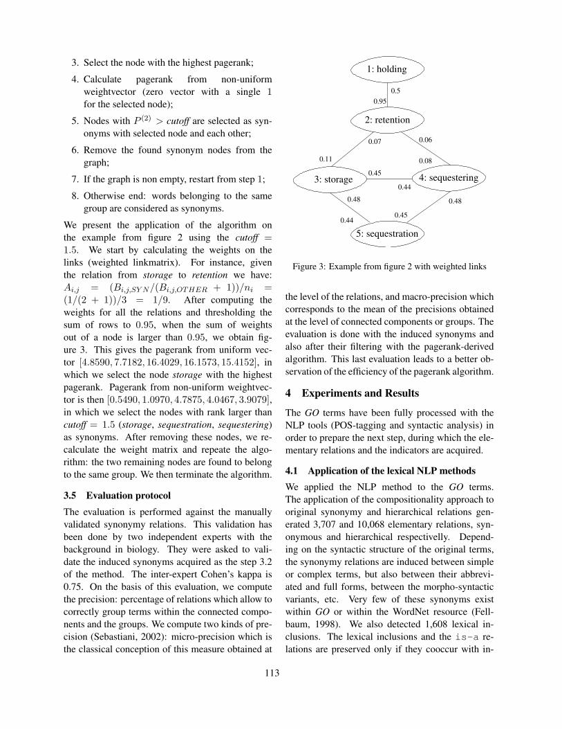
3. Select the node with the highest pagerank;
4. Calculate pagerank from non-uniformweightvector (zero vector with a single 1for the selected node);
5. Nodes with P (2) > cutoff are selected as syn-onyms with selected node and each other;
6. Remove the found synonym nodes from thegraph;
7. If the graph is non empty, restart from step 1;
8. Otherwise end: words belonging to the samegroup are considered as synonyms.
We present the application of the algorithm onthe example from figure 2 using the cutoff =1.5. We start by calculating the weights on thelinks (weighted linkmatrix). For instance, giventhe relation from storage to retention we have:Ai,j = (Bi,j,SY N/(Bi,j,OTHER + 1))/ni =(1/(2 + 1))/3 = 1/9. After computing theweights for all the relations and thresholding thesum of rows to 0.95, when the sum of weightsout of a node is larger than 0.95, we obtain fig-ure 3. This gives the pagerank from uniform vec-tor [4.8590, 7.7182, 16.4029, 16.1573, 15.4152], inwhich we select the node storage with the highestpagerank. Pagerank from non-uniform weightvec-tor is then [0.5490, 1.0970, 4.7875, 4.0467, 3.9079],in which we select the nodes with rank larger thancutoff = 1.5 (storage, sequestration, sequestering)as synonyms. After removing these nodes, we re-calculate the weight matrix and repeate the algo-rithm: the two remaining nodes are found to belongto the same group. We then terminate the algorithm.
3.5 Evaluation protocol
The evaluation is performed against the manuallyvalidated synonymy relations. This validation hasbeen done by two independent experts with thebackground in biology. They were asked to vali-date the induced synonyms acquired as the step 3.2of the method. The inter-expert Cohen’s kappa is0.75. On the basis of this evaluation, we computethe precision: percentage of relations which allow tocorrectly group terms within the connected compo-nents and the groups. We compute two kinds of pre-cision (Sebastiani, 2002): micro-precision which isthe classical conception of this measure obtained at
3: storage 4: sequestering
1: holding
2: retention
5: sequestration
0.060.07
0.5
0.44
0.480.48
0.45
0.11
0.45
0.08
0.95
0.44
Figure 3: Example from figure 2 with weighted links
the level of the relations, and macro-precision whichcorresponds to the mean of the precisions obtainedat the level of connected components or groups. Theevaluation is done with the induced synonyms andalso after their filtering with the pagerank-derivedalgorithm. This last evaluation leads to a better ob-servation of the efficiency of the pagerank algorithm.
4 Experiments and Results
The GO terms have been fully processed with theNLP tools (POS-tagging and syntactic analysis) inorder to prepare the next step, during which the ele-mentary relations and the indicators are acquired.
4.1 Application of the lexical NLP methodsWe applied the NLP method to the GO terms.The application of the compositionality approach tooriginal synonymy and hierarchical relations gen-erated 3,707 and 10,068 elementary relations, syn-onymous and hierarchical respectivelly. Depend-ing on the syntactic structure of the original terms,the synonymy relations are induced between simpleor complex terms, but also between their abbrevi-ated and full forms, between the morpho-syntacticvariants, etc. Very few of these synonyms existwithin GO or within the WordNet resource (Fell-baum, 1998). We also detected 1,608 lexical in-clusions. The lexical inclusions and the is-a re-lations are preserved only if they cooccur with in-
113
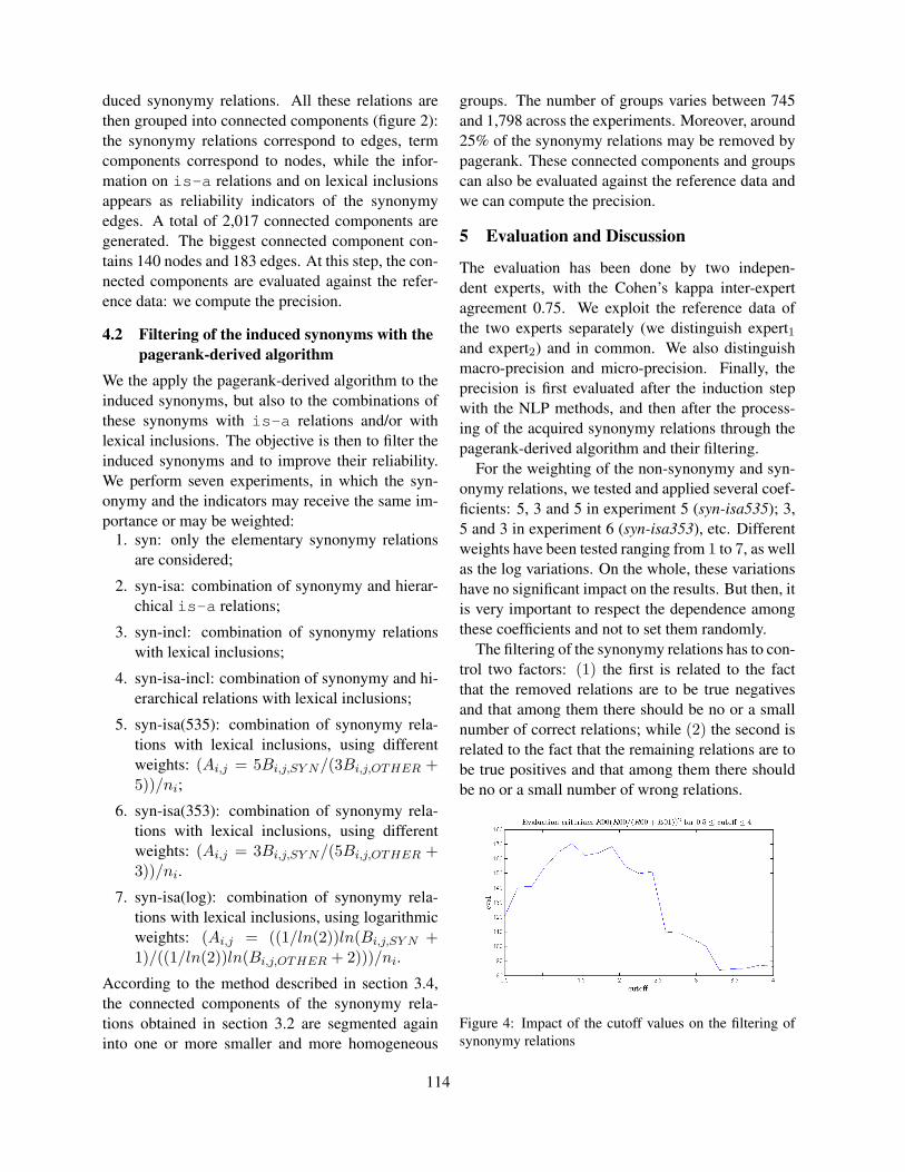
duced synonymy relations. All these relations arethen grouped into connected components (figure 2):the synonymy relations correspond to edges, termcomponents correspond to nodes, while the infor-mation on is-a relations and on lexical inclusionsappears as reliability indicators of the synonymyedges. A total of 2,017 connected components aregenerated. The biggest connected component con-tains 140 nodes and 183 edges. At this step, the con-nected components are evaluated against the refer-ence data: we compute the precision.
4.2 Filtering of the induced synonyms with thepagerank-derived algorithm
We the apply the pagerank-derived algorithm to theinduced synonyms, but also to the combinations ofthese synonyms with is-a relations and/or withlexical inclusions. The objective is then to filter theinduced synonyms and to improve their reliability.We perform seven experiments, in which the syn-onymy and the indicators may receive the same im-portance or may be weighted:
1. syn: only the elementary synonymy relationsare considered;
2. syn-isa: combination of synonymy and hierar-chical is-a relations;
3. syn-incl: combination of synonymy relationswith lexical inclusions;
4. syn-isa-incl: combination of synonymy and hi-erarchical relations with lexical inclusions;
5. syn-isa(535): combination of synonymy rela-tions with lexical inclusions, using differentweights: (Ai,j = 5Bi,j,SY N/(3Bi,j,OTHER +5))/ni;
6. syn-isa(353): combination of synonymy rela-tions with lexical inclusions, using differentweights: (Ai,j = 3Bi,j,SY N/(5Bi,j,OTHER +3))/ni.
7. syn-isa(log): combination of synonymy rela-tions with lexical inclusions, using logarithmicweights: (Ai,j = ((1/ln(2))ln(Bi,j,SY N +1)/((1/ln(2))ln(Bi,j,OTHER + 2)))/ni.
According to the method described in section 3.4,the connected components of the synonymy rela-tions obtained in section 3.2 are segmented againinto one or more smaller and more homogeneous
groups. The number of groups varies between 745and 1,798 across the experiments. Moreover, around25% of the synonymy relations may be removed bypagerank. These connected components and groupscan also be evaluated against the reference data andwe can compute the precision.
5 Evaluation and Discussion
The evaluation has been done by two indepen-dent experts, with the Cohen’s kappa inter-expertagreement 0.75. We exploit the reference data ofthe two experts separately (we distinguish expert1and expert2) and in common. We also distinguishmacro-precision and micro-precision. Finally, theprecision is first evaluated after the induction stepwith the NLP methods, and then after the process-ing of the acquired synonymy relations through thepagerank-derived algorithm and their filtering.
For the weighting of the non-synonymy and syn-onymy relations, we tested and applied several coef-ficients: 5, 3 and 5 in experiment 5 (syn-isa535); 3,5 and 3 in experiment 6 (syn-isa353), etc. Differentweights have been tested ranging from 1 to 7, as wellas the log variations. On the whole, these variationshave no significant impact on the results. But then, itis very important to respect the dependence amongthese coefficients and not to set them randomly.
The filtering of the synonymy relations has to con-trol two factors: (1) the first is related to the factthat the removed relations are to be true negativesand that among them there should be no or a smallnumber of correct relations; while (2) the second isrelated to the fact that the remaining relations are tobe true positives and that among them there shouldbe no or a small number of wrong relations.
Figure 4: Impact of the cutoff values on the filtering ofsynonymy relations
114

miP_Exp1 maP_Exp1 miP_Exp2 maP_Exp2
0.6
0.65
0.7
0.75
0.8
0.85
0.9
0.95
1
1 2 3 4 5 6 7
before Pagerank
maP_Exp1 and maP_Exp2before Pagerank
miP_Exp1
miP_Exp2 before Pagerank
(a) Connected components with terms
miP_Exp1 maP_Exp1 miP_Exp2 maP_Exp2
0.6
0.65
0.7
0.75
0.8
0.85
0.9
0.95
1
1 2 3 4 5 6 7
before Pagerank
maP_Exp1 and maP_Exp2before Pagerank
miP_Exp1
miP_Exp2 before Pagerank
(b) Groups of terms
Figure 5: Evaluation of the results in terms of micro-precision miP and of macro-precision maP for connectedcomponents and for groups of terms (performed according to the reference data provided by two experts)
On figure 4, we present the impact of the cut-off values on the selection and filtering of the syn-onyms. Like with other parameters, we have testedseveral values between 0.5 and 4. This figure illus-trates the distribution of the correctly removed rela-tions. The cutoff values have an important impacton the results: we can observe that the optimal cut-off values are set between 1.5 and 2 because theyallow to remove the highest number of the wrongrelations. We have set the cutoff value to 1.5. Thechoice of cutoff is an important factor for the defi-nition of the amount of the links that are to be re-moved: the higher the cutoff the higher the numberof clusters. On the data processed in this work, thecutoff value has been defined experimentally thanksto the observation of the processed data. For the gen-eralization of this method to new unknown but sim-ilar linguistic data (new terminology, new langage,new domain...), the cutoff will be either set in orderto remove a certain predefined number of links orwill be defined from a typical sample of the data.
Contrary to the cutoff values, the choice of thresh-old doesn’t greatly impact the results, although us-ing a lower threshold makes it harder to choose agood cutoff values since the ranking of differentnodes will be closer to each other.
As for the analysis of the precision and of therelations which are correctly kept within the con-nected components, let’s observe figure 5. On thisfigure, we present the evaluation results performedwithin the connected components with induced syn-
onyms (figure 5(a)) and within the groups of filteredsynonyms (figure 5(b)). On the y-axis we indicatethe precision values, and on the x-axis, we indicatethe different experiments performed as mentionedabove: 1 in which only synonyms are exploited, 2in which synonyms are combined with hierarchicalis-a relations, 3 in which synonyms are combinedwith lexical inclusions, etc. Horizontal lines corre-spond to the precision obtained before the applica-tion of the pagerank: they remain the same whateverthe experiment. These lines correspond to three ref-erence data provided by the expert1, the expert2 andby their common data. As for the points, they indi-cate the precision obtained further to the pagerank:it varies according to experiments and experts. Onthe basis of figure 5, we can observe that:
• the difference between the expert evaluations isvery low (0.02);
• the pagerank allows to increase the precision(between 0.10 and 0.15 for micro-precision,while macro-precision varies by 0.05);
• the consideration of synonymy alone providesperformant results;
• the consideration of is-a relations improvesthe results but lexical inclusions decrease them;
• the increased weight of some of the quality in-dicators has no effect on the evaluation;
• macro-precision is superior to micro-precisionbecause our data contain mainly small groups,
115
while the few large connected components havea very low precision;
• there is but a small difference between con-nected components (figure 5(a)) and groups(figure 5(b));
• the consideration of is-a relations and of lex-ical inclusions provides the best precision butthe amount of the remaining synonyms is thenthe lowest. As we explained, it is importantto keep the highest number of the correct re-lations, although when a lot of relations is re-moved, it is logical to obtain a higher precision.This means that the combination of is-a re-lations and of lexical inclusions is not suitablebecause it removes too much of synonyms.
In relation with this last observation, is should benoted that the balance between the removed and theremaining relations is a subtle parameter.
The obtained results indicate that the pagerank isindeed useful for the filtering of synonyms, althoughthe parameters exploited by this algorithm must bedefined accurately. Thus, it appears that synonymyalone may be sufficient for this filtering. When thequality indicators are considered, is-a relations aresuitable for this filtering because very often they pro-pose true hierarchical relations. However, the lex-ical inclusions have a negative effect of the filter-ing. We assume this is due to the fact that the lexicalinclusions are ambiguous: they may convey hierar-chical relations but also equivalence relations (Har-alambous and Lavagnino, 2011). Indeed, contextu-ally some terms may be shortened or may be subjectto an elision while their meaning is not impacted.
Currently, the pagerank is limited by the fact thatit is applied to a relatively small set of data whileit is designed to process very large data. Then, itcan be interesting to enrich the model and to be ableto take into account other quality indicators, such asfrequencies, productivity or other semantic relationsproposed within GO (part-of and regulates).Moreover, we can also give a lesser weight to someindicators (such as lexical inclusions) with penal-ties and keep the strong weight for other indicators.In the current model of the pagerank, we thresh-old rows to < 0.95. However, we assume that thealgorithm may have problems with very large andvery connected graphs: the pagerank may spread
out in the graph too much and possibly allow thefirst words with the highest pagerank to make groupswith only one word. This can be corrected if an addi-tional calculation is added and when the group con-tains only one word at step 5.
6 Conclusion and Perspectives
We propose an original approach for inducing syn-onyms from terminologies and for their filtering.The methods exploit the NLP methods, composi-tionality principle and pagerank-derived algorithm.This work is motivated by the fact that synonymyis a contextual relation and its validity and univer-sality are not guaranteed. We assume the seman-tic cohesiveness of synonymy relations should bequalified and quantified. The compositionality andNLP methods allow to acquire endogeneously thesynonymy relations and the quality indicators, whilethe pagerank-derived algorithm leads to the filteringof the acquired synonyms. Its functionning is basedupon the synonymy relations and also upon the ac-quired indicators (is-a relations and lexical inclu-sions). It appears that the synonymy relations aloneprovide good clues for their filtering. The is-a re-lations are also fruitful, while the use of the lexicalinclusions appears not to be suitable.
In the future, we plan to add and test other indi-cators. Other experiments will also be done with thepagerank approach. For instance, it will be inter-esting to propose a model which takes into accountthat, within a cluster, words may be synonym withsome cluster words but not with all the words of thecluster. This method can be adapted for the process-ing of corpora and also applied to terms from otherterminologies. The acquired and filtered synonymyrelations will be exploited within the NLP applica-tions in order to test the efficiency of these resourcesand also the usefulness and efficiency of their filter-ing. Moreover, the compositionality approach canbe adapted and exploited for the paraphrasing of thebiomedical terms and for the improvement of theirunderstanding by non expert people.
ReferencesE Agirre and A Soroa. 2009. Personalizing PageRank
for word sense disambiguation. In EACL 2009, pages33–41, Athens, Greece, March.
116

O Bodenreider, A Burgun, and TC Rindflesch. 2001.Lexically-suggested hyponymic relations among med-ical terms and their representation in the UMLS. InURI INIST CNRS, editor, Terminologie et Intelligenceartificielle (TIA), pages 11–21, Nancy.
S Brin and L Page. 1998. The anatomy of a large-scalehypertextual Web search engine. Computer Networksand ISDN Systems, 30(1–7):107–117.
K Bryan and T Leise. 2006. The $25, 000, 000, 000eigenvector: the linear algebra behind google. SIAMRev., 48(3):569–581.
David A. Cruse. 1986. Lexical Semantics. CambridgeUniversity Press, Cambridge.
C Engstrom. 2011. Pagerank as a solution to a lin-ear system, pagerank in changing systems and non-normalized versions of pagerank. Master’s thesis,Mathematics, Centre for Mathematical sciences, LundUniversity. LUTFMA-3220-2011.
C Fellbaum. 1998. A semantic network of english: themother of all WordNets. Computers and Humanities.EuroWordNet: a multilingual database with lexical se-mantic network, 32(2-3):209–220.
S Fernandez, E SanJuan, and JM Torres-Moreno. 2009.Resumes de texte par extraction de phrases, algo-rithmes de graphe et energie textuelle. In SocieteFrancophone de Classification, pages 101–104.
B Gaume. 2006. Cartographier la forme du sens dans lespetits mondes lexicaux. In JADT.
G Grefenstette. 1994. Explorations in automatic the-saurus discovery. Kluwer Academic Publishers.
T Hamon and N Grabar. 2008. Acquisition of elementarysynonym relations from biological structured termi-nology. In Computational Linguistics and IntelligentText Processing (5th International Conference on NLP,2006), number 4919 in LNCS, pages 40–51. Springer.
T Hamon, A Nazarenko, and C Gros. 1998. A steptowards the detection of semantic variants of termsin technical documents. In COLING-ACL’98, pages498–504.
Y Haralambous and E Lavagnino. 2011. La reduction determes complexes dans les langues de spcialite. TAL,52(1):37–68.
S Hassan, R Mihalcea, and C Banea. 2007. Random-walk term weighting for improved text classification.In ICSC, pages 242–249.
T Hughes and D Ramage. 2007. Lexical semantic relat-edness with random graph walks. In EMNLP-CoNLL,pages 581–589. Association for Computational Lin-guistics.
C Jacquemin, JL Klavans, and E Tzoukerman. 1997.Expansion of multi-word terms for indexing and re-trieval using morphology and syntax. In ACL/EACL97), pages 24–31, Barcelona, Spain.
G Kleiber and I Tamba. 1990. L’hyperonymie revisitee :inclusion et hierarchie. Langages, 98:7–32, juin.
R Mihalcea, P Tarau, and E Figa. 2004. Pagerank on se-mantic networks, with application to word sense dis-ambiguation. In COLING, pages 1126–1132.
CJ Mungall. 2004. Obol: integrating language andmeaning in bio-ontologies. Comparative and Func-tional Genomics, 5(6-7):509–520.
NLM, 2007. UMLS Knowledge Sources Manual. Na-tional Library of Medicine, Bethesda, Maryland.www.nlm.nih.gov/research/umls/.
PV Ogren, KB Cohen, and L Hunter. 2005. Implica-tions of compositionality in the Gene Ontology for itscuration and usage. In Pacific Symposium of Biocom-puting, pages 174–185.
BH Partee, 1984. Compositionality. F Landman and FVeltman.
S Schulz, M Romacker, P Franz, A Zaiss, R Klar, andU Hahn. 1999. Towards a multilingual morphemethesaurus for medical free-text retrieval. In MedicalInformatics in Europe (MIE), pages 891–4.
F Sebastiani. 2002. Machine learning in automated textcategorization. ACM Computing Surveys, 34(1):1–47.
N Shimizu, M Hagiwara, Y Ogawa, K Toyama, andH Nakagawa. 2008. Metric learning for synonym ac-quisition. In COLING, pages 793–800.
R Sinha and R Mihalcea. 2007. Unsupervised graph-based word sense disambiguation using measures ofword semantic similarity. In IEEE International Con-ference on Semantic Computing (ICSC 2007), pages363–369.
RS Sinha and RF Mihalcea. 2011. Using centrality algo-rithms on directed graphs for synonym expansion. InFLAIRS.
Y Tsuruoka, Y Tateishi, JD Kim, T Ohta, J McNaught,S Ananiadou, and J Tsujii. 2005. Developing a ro-bust part-of-speech tagger for biomedical text. LNCS,3746:382–392.
CM Verspoor, C Joslyn, and GJ Papcun. 2003. The GeneOntology as a source of lexical semantic knowledgefor a biological natural language processing applica-tion. In SIGIR workshop on Text Analysis and Searchfor Bioinformatics, pages 51–56.
T Wang and G Hirst. 2011. Exploring patterns in dictio-nary definitions for synonym extraction. Natural Lan-guage Engineering, 17.
P Zweigenbaum, R Baud, A Burgun, F Namer, E Jar-rousse, N Grabar, P Ruch, F Le Duff, B Thirion, andS Darmoni. 2003. Towards a Unified Medical Lexiconfor French. In Medical Informatics in Europe (MIE),pages 415–20.
117

Proceedings of the 2012 Workshop on Biomedical Natural Language Processing (BioNLP 2012), pages 118–121,Montreal, Canada, June 8, 2012. c©2012 Association for Computational Linguistics
Domain Adaptation of Coreference Resolution for Radiology Reports
Emilia Apostolova, Noriko Tomuro, Pattanasak Mongkolwat*, Dina Demner-Fushman∓College of Computing and Digital Media, DePaul University, Chicago, IL
*Department of Radiology, Northwestern University Medical School, Chicago, IL∓Communications Engineering Branch, National Library of Medicine, Bethesda, MD
[email protected], [email protected],[email protected], [email protected]
Abstract
In this paper we explore the applicability ofexisting coreference resolution systems to abiomedical genre: radiology reports. Analysisrevealed that, due to the idiosyncrasies of thedomain, both the formulation of the problemof coreference resolution and its solution needsignificant domain adaptation work. We refor-mulated the task and developed an unsuper-vised algorithm based on heuristics for coref-erence resolution in radiology reports. Thealgorithm is shown to perform well on a testdataset of 150 manually annotated radiologyreports.
1 Introduction
Coreference resolution is the process of determin-ing whether two expressions in natural language re-fer to the same entity in the world. General purposecoreference resolution systems typically cluster allmentions (usually noun phrases) in a document intocoreference chains according to the underlying ref-erence entity. A number of coreference resolutionalgorithms have been developed for general texts. Toname a few, Soon et al. (2001) employed machinelearning on the task and achieved an F-score of 62.6and 60.4 on the MUC-6 (1995) and MUC-7 (1997)coreference corpora respectively. Ng et al. (2002)improved this learning framework and achieved F-scores of 70.4 and 63.4 respectively on the samedatasets.
There are also a number of freely available off-the-shelf coreference resolution modules developed
for the general domain. For example, BART (Vers-ley et al., 2008) is an open source coreference reso-lution system which provides an implementation ofthe Soon et al. algorithm (2001). The Stanford De-terministic Coreference Resolution System (Raghu-nathan et al., 2010) uses an unsupervised sieve-likeapproach to coreference resolution. Similarly, theGATE Information Extraction system (Cunninghamet al., 2002) includes a rule-based coreference reso-lution module consisting of orthography-based pat-terns and a pronominal coreferencer (matching pro-nouns to the most recent referent).
While coreference resolution is a universal dis-course problem, both the scope of the problem andits solution could vary significantly across domainsand text genres. Newswire coreference resolutioncorpora (such as the MUC corpus) and general pur-pose tools do not always fit the needs of specific do-mains such as the biomedical domain well.
The importance and distinctive characteristics ofcoreference resolution for biomedical articles hasbeen recognized, for example (Castano et al., 2002;Gasperin, 2006; Gasperin et al., 2007; Su et al.,2008). Within the biomedical field, clinical textshave been noted as a genre that needs specializedcoreference corpora and methodologies (Zheng etal., 2011). The importance of the task for the clini-cal domain has been attested by the 2011 i2b2 NLPshared task (Informatics for Integrating Biology andthe Bedside1) which provided an evaluation plat-form for coreference resolution for clinical texts.
However, even within the clinical domain, coref-erence in different sub-genres could vary signifi-
1https://www.i2b2.org/NLP/Coreference/
118
cantly. In this paper we demonstrate the idiosyn-crasies of the task of coreference resolution in aclinical domain sub-genre, radiology reports, anddescribe an unsupervised system developed for thetask.
2 Coreference Resolution for RadiologyReports
Radiology reports have some unique characteristicsthat preclude the use of coreference resolution mod-ules or algorithms developed for the general biomed-ical domain or even for other types of clinical texts.The radiology report is a clinical text used to com-municate medical image findings and observationsto referring physicians. Typically, radiology reportsare produced by radiologists after examining medi-cal images and are used to describe the findings andobservations present in the accompanied images.
The radiology report accompanies an imagingstudy and frequently refers to artifacts present inthe image. In radiology reports, artifacts presentin the image exhibit discourse salience, and as aresult are often introduced with definite pronounsand articles. For example, consider the sentenceThe pericardial space is clear. The definite nounphrase the pericardial space does not represent ananaphoric (or cataphoric) discourse entity and hasno antecedent. In contrast, coreference resolutionin general texts typically considers definite nounphrases to be anaphoric discourse entities and at-tempts to find their antecedents.
Another important distinction between generalpurpose coreference resolution and the coreferenceresolution module needed by an NLP system forclinical texts is the scope of the task. General pur-pose coreference resolution systems typically clusterall mentions in a document into coreference chains.Such comprehensive mention clustering is often notnecessary for the purposes of clinical text NLP sys-tems. Biomedical Information Extraction systemstypically first identify named entities (medical con-cepts) and map them to unambiguous biomedicalstandard vocabularies (e.g. UMLS2 or RadLex3 inthe radiological domain). While multiple mentionsof the same named entity could exist in a document,
2http://www.nlm.nih.gov/research/umls/3http://www.radlex.org/
in most cases these mentions were previously as-signed to the same medical concept. For example,multiple report mentions of ‘the heart’ or ‘the lung’will normally be mapped to the same medical con-cept and clustering of these mentions into corefer-ence chains is typically not needed.
3 Task Definition
Analysis revealed that the coreference resolutiontask could be simplified and still meet the needs ofmost Information Extraction tasks relevant to the ra-diological domain. Due to their nature, texts de-scribing medical image finding and observations donot contain most pronominal references typicallytargeted by coreference resolution systems. For ex-ample, no occurrence of personal pronouns (e.g. he,I), possessive pronouns (e.g. his, my), and indefi-nite pronouns (e.g. anyone, nobody) was found inthe validation dataset. Demonstrative pronouns andnon-pleonastic ‘it’ mentions were the only pronom-inal references observed in the dataset4. The fol-lowing examples demonstrate the use of demonstra-tive pronouns and the non-pleonastic ‘it’ pronoun(shown in bold):
There is prominent soft tissue swelling involvingthe premaxillary tissues. This measures approxi-mately 15 mm in thickness and extends to the infe-rior aspect of the nose.
There is a foreign object in the proximal left main-stem bronchus on series 11 image 17 that was notpresent on the prior study. It has a somewhat ovoidto linear configuration.
Following these observations, the coreference res-olution task has been simplified as follows. Corefer-ence chains are assigned only for demonstrative pro-nouns and ‘it’ noun phrases. The coreference reso-lution task then involves selecting for each mentiona single best antecedent among previously annotatednamed entities (medical concepts) or the NULL an-tecedent.
4 Dataset
A total of 300 radiology reports were set aside forvalidation and testing purposes. The dataset consists
4Pleonastic ‘it’ refers to its use as a ‘dummy’ pronoun, e.g.It is raining, while non-pleonastic use of the pronoun refers toa specific entity.
119

Figure 1: A sample DICOM image from an imagingstudy described by the following radiology report snip-pet: . . . FINDINGS: Targeted sonography of the upper in-ner left breast was performed. At the site of palpable ab-normality, at the 11 o’clock position 3 cm from the nipple,there is an oval circumscribed, benign-appearing hypoe-choic mass measuring 2.0 x 1.6 x 1.4 cm. There is mildinternal blood flow. It is surrounded by normal appearingglandular breast tissue.. . .
of 100 Computed Tomography Chest reports, 100Ultrasound Breast reports, and 100 Magnetic Res-onance Brain reports, all randomly selected basedon their report types from a dataset of more than100,000 de-identified reports spanning a period of9 years5. These three types of reports representa diverse dataset covering representative imagingmodalities and body regions. Figure 1 shows a sam-ple Breast Ultrasound DICOM6 image and its asso-ciated radiology report.
The reports were previously tagged (using an au-tomated system) with medical concepts and theirsemantic types (e.g. anatomical entity, disorder,imaging observation, etc.). Half of the dataset (150reports) was manually annotated with coreferencechains using the simplified task definition describedabove. The other half of the dataset was used forvalidation of the system described next.
5 Method and Results
The coreference resolution task involves selectingfor each mention a single best antecedent amongpreviously annotated named entities or the NULLantecedent. Mentions are demonstrative pronounphrases or definite noun phrases containing previ-ously annotated named entities.
5The collection is a proprietary dataset belonging to North-western University Medical School.
6Digital Imaging and Communications in Medicine, c© TheNational Electrical Manufacturers Association.
We implemented an algorithm for the task de-scribed above which was inspired by the work ofHaghighi and Klein (2009). The algorithm first iden-tifies mentions within each report and orders themlinearly according to the position of the mentionhead. Then it selects the antecedent (or the NULLantecedent) for each mention as follows:
1. The possible antecedent candidates are first fil-tered based on a distance constraint. Only mentionsof interest belonging to the preceding two sentencesare considered. The rationale for this filtering step isthat radiology reports are typically very concise andless cohesive than general texts. Paragraphs oftendescribe multiple observations and anatomical enti-ties sequentially and rarely refer to mentions moredistant than the preceding two sentences.
2. The remaining antecedent candidates are thenfiltered based on a syntactic constraint: the co-referent mentions must agree in number (singular orplural based on the noun phrase head).
3. The remaining antecedent candidates are thenfiltered based on a semantic constraint. If the twomentions refer to named entities, the named entitiesneed to have the same semantic category7.
4. After filtering, the closest mention from the setof remaining possible antecedents is selected. If theset is empty, the NULL antecedent is selected.
Pairwise coreference decisions are consideredtransitive and antecedent matches are propagatedtransitively to all paired co-referents.
The algorithm was evaluated on the manually an-notated test dataset. Results (Table 1) were com-puted using the pairwise F1-score measure: preci-sion, recall, and F1-score were computed over allpairs of mentions in the same coreference cluster.
Precision Recall F1-score74.90 48.22 58.66
Table 1: Pairwise coreference resolution results.
The system performance is within the range ofstate-of-the-art supervised and unsupervised coref-erence resolution systems8. F1-scores could range
7The same semantic type in the case of UMLS concepts orthe same parent in the case of RadLex concepts.
8Source code for the described system will be made avail-able upon request.
120

between 39.8 and 67.3 for various methods andtest sets (Haghighi and Klein, 2009). The simpli-fication of the coreference resolution problem de-scribed above allowed us to focus only on corefer-ence chains of interest to clinical text InformationExtraction tasks and positively influenced the out-come. In addition, our goal was to focus on highprecision results as opposed to optimizing the over-all F1-score. This guarantees that coreference reso-lution errors will result in mostly omissions of coref-erence pairs and will not introduce information ex-traction inaccuracies.
6 Conclusion
In this paper, we presented some of the challengesinvolved in the task of adapting coreference resolu-tion for the domain of clinical radiology. We pre-sented a domain-specific definition of the corefer-ence resolution task. The task was reformulated andsimplified in a practical manner that ensures that theneeds of biomedical information extraction systemsare still met. We developed an unsupervised ap-proach to the task of coreference resolution of radi-ology reports and demonstrate state-of-the-art preci-sion and reasonable recall results. The developedsystem is made publicly available to the NLP re-search community.
References
J. Castano, J. Zhang, and J. Pustejovsky. 2002. Anaphoraresolution in biomedical literature. In InternationalSymposium on Reference Resolution. Citeseer.
D.H. Cunningham, D.D. Maynard, D.K. Bontcheva, andM.V. Tablan. 2002. GATE: A Framework and Graph-ical Development Environment for Robust NLP Toolsand Applications.
C. Gasperin, N. Karamanis, and R. Seal. 2007. Annota-tion of anaphoric relations in biomedical full-text arti-cles using a domain-relevant scheme. In Proceedingsof DAARC, volume 2007. Citeseer.
C. Gasperin. 2006. Semi-supervised anaphora resolutionin biomedical texts. In Proceedings of the Workshopon Linking Natural Language Processing and Biology:Towards Deeper Biological Literature Analysis, pages96–103. Association for Computational Linguistics.
A. Haghighi and D. Klein. 2009. Simple coreferenceresolution with rich syntactic and semantic features.In Proceedings of the 2009 Conference on Empirical
Methods in Natural Language Processing: Volume 3-Volume 3, pages 1152–1161. Association for Compu-tational Linguistics.
V. Ng and C. Cardie. 2002. Improving machine learn-ing approaches to coreference resolution. In Proceed-ings of the 40th Annual Meeting of the Association forComputational Linguistics, pages 104–111.
K. Raghunathan, H. Lee, S. Rangarajan, N. Chambers,M. Surdeanu, D. Jurafsky, and C. Manning. 2010. Amulti-pass sieve for coreference resolution. In Pro-ceedings of the 2010 Conference on Empirical Meth-ods in Natural Language Processing, pages 492–501.Association for Computational Linguistics.
W.M. Soon, H.T. Ng, and D.C.Y. Lim. 2001. A ma-chine learning approach to coreference resolution ofnoun phrases. Computational Linguistics, 27(4):521–544.
J. Su, X. Yang, H. Hong, Y. Tateisi, J. Tsujii, M. Ash-burner, U. Leser, and D. Rebholz-Schuhmann. 2008.Coreference resolution in biomedical texts: a machinelearning approach. Ontologies and Text Mining forLife Sciences 08.
Y. Versley, S.P. Ponzetto, M. Poesio, V. Eidelman,A. Jern, J. Smith, X. Yang, and A. Moschitti. 2008.Bart: A modular toolkit for coreference resolution. InProceedings of the 46th Annual Meeting of the Asso-ciation for Computational Linguistics on Human Lan-guage Technologies: Demo Session, pages 9–12. As-sociation for Computational Linguistics.
J. Zheng, W.W. Chapman, R.S. Crowley, and G.K.Savova. 2011. Coreference resolution: A review ofgeneral methodologies and applications in the clinicaldomain. Journal of biomedical informatics.
121

Proceedings of the 2012 Workshop on Biomedical Natural Language Processing (BioNLP 2012), pages 122–129,Montreal, Canada, June 8, 2012. c©2012 Association for Computational Linguistics
What can NLP tell us about BioNLP?
Attapol Thamrongrattanarit, Michael Shafir, Michael Crivaro, Bensiin Borukhov, Marie MeteerDepartment of Computer Science
Brandeis UniversityWaltham, MA 02453, USA
{tet, mshafir, mcrivaro, bborukhov, mmeteer}@brandeis.edu
Abstract
The goal of this work is to apply NLP tech-niques to the field of BioNLP in order to gaina better insight into the field and show connec-tions and trends that might not otherwise beapparent. The data we analyzed was the pro-ceedings from last decade of BioNLP work-shops. Our findings reveal the prominent re-search problems and techniques in the field,their progression over time, the approachesthat researchers are using to solve those prob-lems, insightful ways to categorize works inthe field, and the prominent researchers andgroups whose works are influencing the field.
1 Introduction
Thanks to improving technology and the discoveryof stronger statistical methods, natural language pro-cessing techniques have more power than ever togive us insights into real datasets too large for hu-mans to efficiently process. In the field of BioNLP,we see that natural language processing has a widerange of applications within the medical domainfrom analysis of clinical data to literature. Withthe increasing amount of publications in this grow-ing field, building a classification structure is help-ful both for categorizing papers in a sensible wayand for recognizing the trends that brought the fieldto where it is today. Understanding the current na-ture of the field can show us where the most effortis needed, while taking a look at where the field hasbeen can highlight successes and even unansweredquestions.
As the use of NLP in the medical domain has ex-panded in recent years so has the amount of freely-available online research. With this wealth of infor-mation comes a problem, however, as it is not trulyfeasible for humans to read through all the researchout there and classify it in a way that will capture theless-obvious trends and the finer relationships be-tween seemingly-disconnected works. Instead, wepropose that statistical methods can help us discoverboth the most reasonable way to partition the fieldand also see how the research has changed over thepast decade. The longer term goal for the work is tocontribute to a “map” of the field that can be a com-munity resource, such as www.medlingmap.org, de-scribed in Meteer, et al. (2012).
Schuemie et al. (2009) used clustering techniquesto analyze the domain of Medical Informatics. Theyprocessed a large number of Medline abstracts tofind a subset of the journals classified as “MedicalInformatics” whose content was sufficiently relatedto constitute a basis for the field. Using hierarchi-cal clustering, they determined that such a group ofjournals exists and, as we might expect, the rest ofthe journals were largely disconnected. They alsoused this cluster of journals as the basis for a topicmodeling task. Analyzing the articles from their newbasis of journals, they found three very strong, topic-based clusters, each comprised of three sub-clusters.Overall, Schuemie et al. (2009) demonstrated how itis possible to gain a great deal of insight into the na-ture of a field by using statistical methods over thatfield’s literature. More recently, Gupta and Manning(2011) used automatic methods to tag documents for”focus,” ”technique,” and ”domain” by examining
122
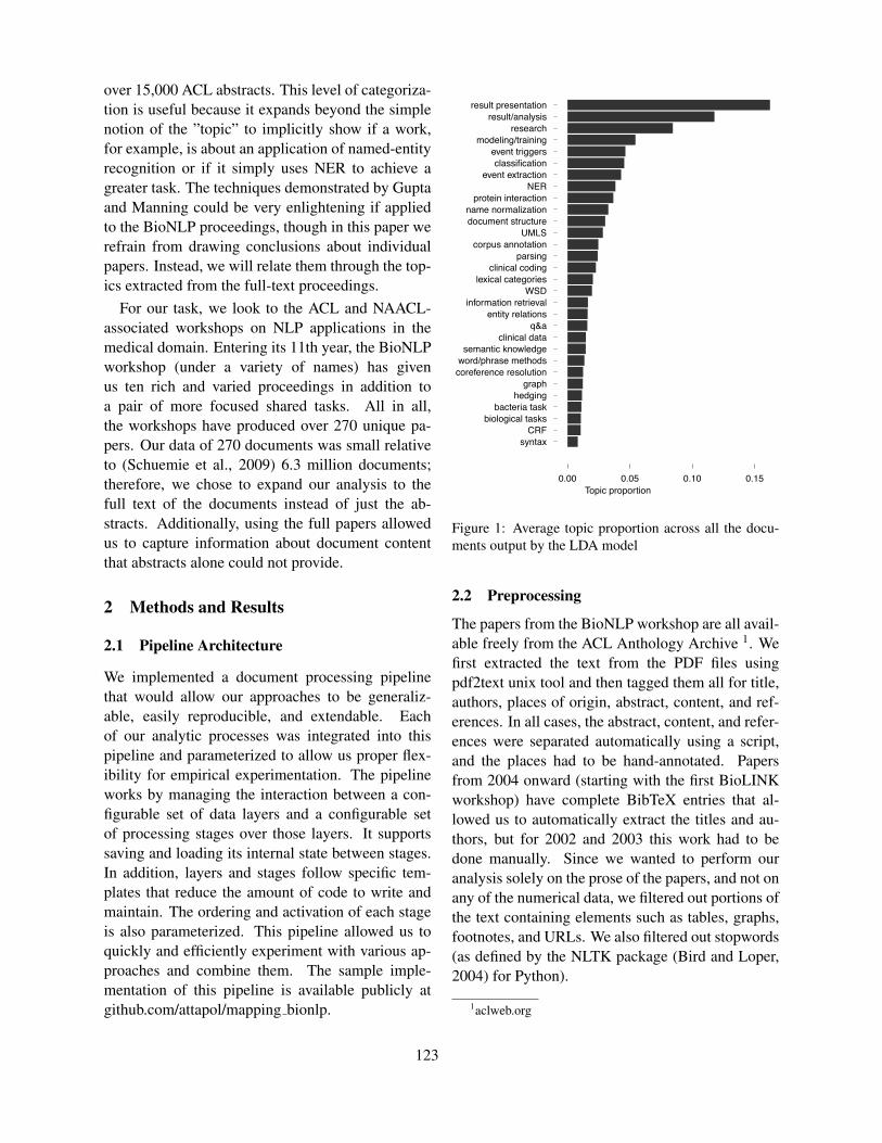
over 15,000 ACL abstracts. This level of categoriza-tion is useful because it expands beyond the simplenotion of the ”topic” to implicitly show if a work,for example, is about an application of named-entityrecognition or if it simply uses NER to achieve agreater task. The techniques demonstrated by Guptaand Manning could be very enlightening if appliedto the BioNLP proceedings, though in this paper werefrain from drawing conclusions about individualpapers. Instead, we will relate them through the top-ics extracted from the full-text proceedings.
For our task, we look to the ACL and NAACL-associated workshops on NLP applications in themedical domain. Entering its 11th year, the BioNLPworkshop (under a variety of names) has givenus ten rich and varied proceedings in addition toa pair of more focused shared tasks. All in all,the workshops have produced over 270 unique pa-pers. Our data of 270 documents was small relativeto (Schuemie et al., 2009) 6.3 million documents;therefore, we chose to expand our analysis to thefull text of the documents instead of just the ab-stracts. Additionally, using the full papers allowedus to capture information about document contentthat abstracts alone could not provide.
2 Methods and Results
2.1 Pipeline Architecture
We implemented a document processing pipelinethat would allow our approaches to be generaliz-able, easily reproducible, and extendable. Eachof our analytic processes was integrated into thispipeline and parameterized to allow us proper flex-ibility for empirical experimentation. The pipelineworks by managing the interaction between a con-figurable set of data layers and a configurable setof processing stages over those layers. It supportssaving and loading its internal state between stages.In addition, layers and stages follow specific tem-plates that reduce the amount of code to write andmaintain. The ordering and activation of each stageis also parameterized. This pipeline allowed us toquickly and efficiently experiment with various ap-proaches and combine them. The sample imple-mentation of this pipeline is available publicly atgithub.com/attapol/mapping bionlp.
Topic proportion
syntaxCRF
biological tasksbacteria task
hedginggraph
coreference resolutionword/phrase methodssemantic knowledge
clinical dataq&a
entity relationsinformation retrieval
WSDlexical categories
clinical codingparsing
corpus annotationUMLS
document structurename normalization
protein interactionNER
event extractionclassification
event triggersmodeling/training
researchresult/analysis
result presentation
0.00 0.05 0.10 0.15
Figure 1: Average topic proportion across all the docu-ments output by the LDA model
2.2 Preprocessing
The papers from the BioNLP workshop are all avail-able freely from the ACL Anthology Archive 1. Wefirst extracted the text from the PDF files usingpdf2text unix tool and then tagged them all for title,authors, places of origin, abstract, content, and ref-erences. In all cases, the abstract, content, and refer-ences were separated automatically using a script,and the places had to be hand-annotated. Papersfrom 2004 onward (starting with the first BioLINKworkshop) have complete BibTeX entries that al-lowed us to automatically extract the titles and au-thors, but for 2002 and 2003 this work had to bedone manually. Since we wanted to perform ouranalysis solely on the prose of the papers, and not onany of the numerical data, we filtered out portions ofthe text containing elements such as tables, graphs,footnotes, and URLs. We also filtered out stopwords(as defined by the NLTK package (Bird and Loper,2004) for Python).
1aclweb.org
123

2.3 Topic Modeling
Using the Mallet toolkit (McCallum, 2002), we wereable to generate topics from our cleaned data usingthe Latent Dirichlet Allocation (LDA) model. Thisapproach allows us to represent each document as avector of topic proportions instead of a bag of words,which prevents the problem of sparsity. When weset the number of topics to 30, the system output aset of distinct topics that seem to describe a rangeof tasks and methods within the domain of BioNLP.The topics generated by the LDA model reflect areasof study that are being pursued, techniques that arebeing applied, and resources that are being consultedin the field. A list of the generated topics along withthe associated keywords is shown in Table 1 and thedistributions of the topics across the entire documentset is displayed in Figure 1.
Additionally, we found that the topics generatedby LDA were more informative about the full con-tent of a work than those generated by TF-IDF asTF-IDF would often give too much weight to spe-cific examples over general concepts. For exam-ple, TF-IDF tended to select specific names of re-sources and ontologies rather than general terms.For example, it selected “Frame-net” instead “ontol-ogy” and “RadLex” instead of “lexicon”. We con-cluded that, while interesting, TF-IDF results werenot strongly suited for capturing an overall glimpseof the field. However, we think that TF-IDF can bemuch more useful in its more traditional capacity offinding document-specific keywords; we aim to usethese indices to partially automate keyword genera-tion for MedlingMap (Meteer et al., 2012), which isour accompanying project.
2.4 Topic Correlation
While looking at the topic proportions for each ofour LDA topics overall can help us paint a broadpicture of the field, it can also help to look at therelationship between these topics as they occur inthe documents. Some topics appear highly rankedin nearly all papers, such as the topic that is char-acterized by terms such as “system” and “results”,and the topic that includes “precision” and “recall”because they reflect the performance evaluation con-vention in the field. However, most topics are onlydominant in a small subset of the papers. Some
Topic
Cou
nt
0
2
4
6
8
10
12
14
parsing graph lexical categories semantic knowledge
Figure 2: The bar plot shows the frequency of the co-occurrences between the event extraction topic and someof the method-related topics.
topics refer to tasks (e.g. named-entity recognition,hedging) and others refer to techniques (e.g. CRFs,parsing). We can look at how often pairs of task-related topic and method-related topic co-occur tosee if researchers in the community are using certaintechniques in conjunction with solving certain prob-lems. We first turned a topic proportion vector into abinary vector where each element indicates whichtopic is discussed more extensively than average.Then, we counted the co-occurrences of tasks andmethods of interest. To demonstrate this, we com-puted the number of papers that substantially discussevent extraction in conjunction with parsing, graph,lexical categories, or semantic knowledge (Figure2). This topic comparison method provides a meansof visualizing how researchers in the field are ap-proaching BioNLP problems. It reveals that parsingand graph-based methods are commonly used in bio-logical event extraction, while lexical categories andsemantic knowledge are not as central to many of theapproaches to this task. Moving forward, trackinghow these correlations change over time will pro-vide an insightful reflection of the field’s progresson the task in a more meaningful way than evalu-ation scores alone. While a deeper analysis of allof such trends is beyond the scope of this paper, itcertainly warrants further investigation.
124

Table 1: The resulting topics and their associated keywords generated by LDA model with 30 topicsTopic Name KeywordsEvent Extraction event, task, extraction, types, data, annotationCoreference Resolution anaphora, resolution, referring, links, antecedentGraph graph, relationships, nodes, edges, path, constraint, semanicsClinical Coding medical, data, codes, patients, notes, reportsHedging negation, scope, cues, speculative, hedge, lexicalClinical Data condition, historical, clinical, temporal, reports, contextBacteria Task bacteria, names, location, organisms, taxonomic, host, roles, typeEntity Relations relations, entities, feature, static, renaming, annotated, pairsDocument Structure Analysis rst, classification, abstracts, identification, data, termsQ&A question, answer, structure, passage, evidence, purposeEvent Triggers triggers, dependency, binding, type, training, token, detectionSemantic Knowledge semantic, frame, structures, argument, patterns, domain, typesProtein Interaction protein, patterns, interaction, extraction, biologicalParsing dependency, parser, tree, syntactic, structures, grammar, linkName Normalization gene, names, dictionary, normalization, protein, database, synonymsNamed Entity Recognition entity, named, word, recognition, features, class, proteinInformation Retrieval search, queries, interface, text, retrieval, documentCorpus Annotation corpus, annotation, guidelines, agreement, papersLexical Categories semantic, categories, resources, simstring, lexical, gazetteer, featuresResearch text, figure, knowledge, domain, research, complex, processingCRF crf, skip, chain, linear, dependency, words, edges, sentenceResult Discussion system, based, results, set, table, test, shown, approachBiological Tasks species, disease, mutation, mentions, features, entities, acronymUMLS terms, semantic, phrases, umls, concepts, ontology, corpusWord/Phrase Methods words, measures, morphological, tag, token, chunking, formWSD disambiguation, sense, word, semantic, wsd, ambiguousResult Analysis found, number, precision, recall, cases, high, related, resultsClassification features, training, data, classification, set, learning, svmModeling/Training training, data, model, tagger, performance, corpus, annotatedSyntax attachment, pps, np, fragments, pp, noun, vp, nos, pattern
2.5 Trends within the subdisciplines inBiomedical NLP Literature
Our analysis of temporal trends builds on the ideaproposed by (Hall et al., 2008) in their analysis ofthe changing trends in the field of computational lin-guistics over time. In their approach, they attempted,among other things, to analyze which topics were upand coming in the field and which were becomingless popular. Given their sound results, we decidedto perform the same kind of trend analysis over theBioNLP topics. For many of our 30 topics, therewas little change in the topic frequency over time.Considering the relative youth of the BioNLP field,this result is not entirely surprising. We did, how-ever, find a few topics that have undergone notablechanges in these past ten years, as observable in Fig-ure 3. In particular, we found that two topics haveseen surges of activity in recent years, whereas therewere three topics that started out strong in the early
years but that have since petered off. The two top-ics that have gained popularity in the past few yearsboth involve biomedical events. Specifically, onesuch topic is primarily about event extraction tasks,and the other is about event triggers and the morefine-grained roles one needs to tag to categorize suchevents. The popularity of these two tasks is hardlysurprising, given that they were the focus of the 2009and 2011 shared tasks which were about workingwith events in both general and detailed ways. Wedo notice, however, that the growing trends continuein 2010 as well, when there was no shared task, andso we can see that events are of great interest inthe field at present even without the added incen-tive of the shared tasks. It is reasonable to suggestthat the 2009 BioNLP Shared Task in event extrac-tion generated interest in the topic that continuedthrough 2010 and 2011. Two more topics originallysaw their popularity rise in the early years, but have
125
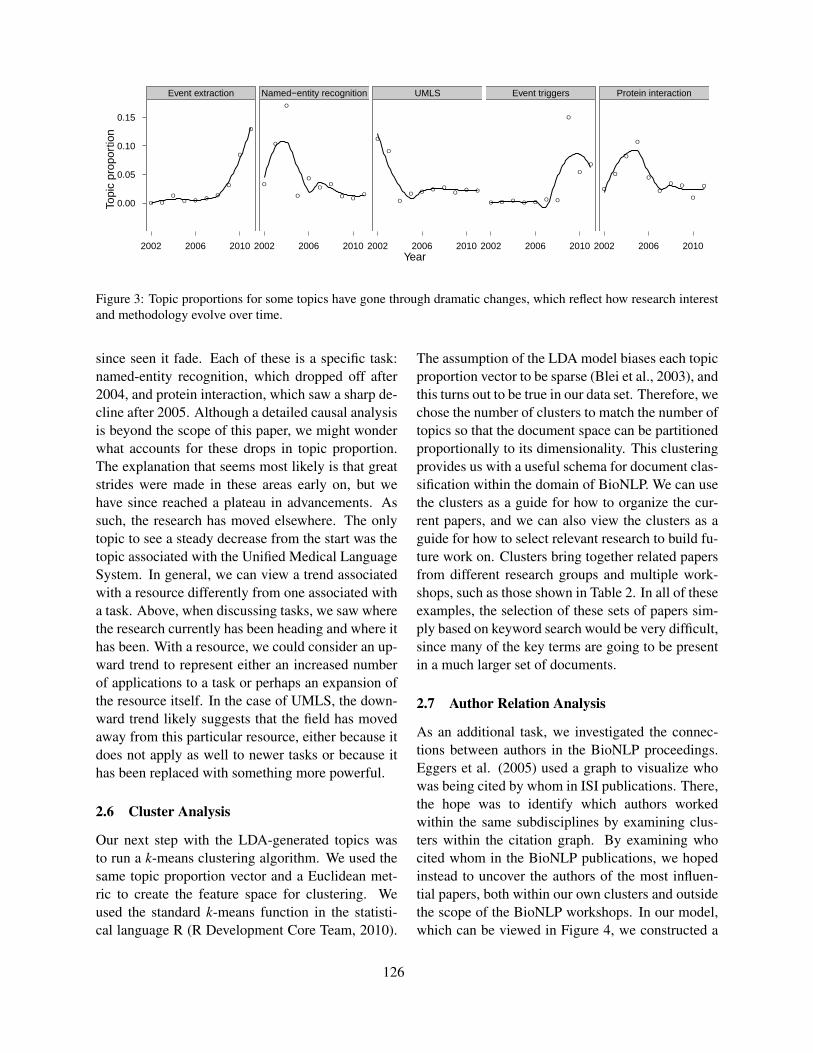
Year
Topi
c pr
opor
tion
0.00
0.05
0.10
0.15
Event extraction
O OO
O O O O
O
O
O
2002 2006 2010
Named−entity recognition
O
O
O
O
O
OO
O OO
2002 2006 2010
UMLS
O
O
OO O O O
O O O
2002 2006 2010
Event triggers
O O O O O O O
O
OO
2002 2006 2010
Protein interaction
O
O
O
O
O
OO O
O
O
2002 2006 2010
Figure 3: Topic proportions for some topics have gone through dramatic changes, which reflect how research interestand methodology evolve over time.
since seen it fade. Each of these is a specific task:named-entity recognition, which dropped off after2004, and protein interaction, which saw a sharp de-cline after 2005. Although a detailed causal analysisis beyond the scope of this paper, we might wonderwhat accounts for these drops in topic proportion.The explanation that seems most likely is that greatstrides were made in these areas early on, but wehave since reached a plateau in advancements. Assuch, the research has moved elsewhere. The onlytopic to see a steady decrease from the start was thetopic associated with the Unified Medical LanguageSystem. In general, we can view a trend associatedwith a resource differently from one associated witha task. Above, when discussing tasks, we saw wherethe research currently has been heading and where ithas been. With a resource, we could consider an up-ward trend to represent either an increased numberof applications to a task or perhaps an expansion ofthe resource itself. In the case of UMLS, the down-ward trend likely suggests that the field has movedaway from this particular resource, either because itdoes not apply as well to newer tasks or because ithas been replaced with something more powerful.
2.6 Cluster Analysis
Our next step with the LDA-generated topics wasto run a k-means clustering algorithm. We used thesame topic proportion vector and a Euclidean met-ric to create the feature space for clustering. Weused the standard k-means function in the statisti-cal language R (R Development Core Team, 2010).
The assumption of the LDA model biases each topicproportion vector to be sparse (Blei et al., 2003), andthis turns out to be true in our data set. Therefore, wechose the number of clusters to match the number oftopics so that the document space can be partitionedproportionally to its dimensionality. This clusteringprovides us with a useful schema for document clas-sification within the domain of BioNLP. We can usethe clusters as a guide for how to organize the cur-rent papers, and we can also view the clusters as aguide for how to select relevant research to build fu-ture work on. Clusters bring together related papersfrom different research groups and multiple work-shops, such as those shown in Table 2. In all of theseexamples, the selection of these sets of papers sim-ply based on keyword search would be very difficult,since many of the key terms are going to be presentin a much larger set of documents.
2.7 Author Relation Analysis
As an additional task, we investigated the connec-tions between authors in the BioNLP proceedings.Eggers et al. (2005) used a graph to visualize whowas being cited by whom in ISI publications. There,the hope was to identify which authors workedwithin the same subdisciplines by examining clus-ters within the citation graph. By examining whocited whom in the BioNLP publications, we hopedinstead to uncover the authors of the most influen-tial papers, both within our own clusters and outsidethe scope of the BioNLP workshops. In our model,which can be viewed in Figure 4, we constructed a
126

List of papers assigned to the cluster where the most discussed topic is parsing (44.74% on average)A Comparative Study of Syntactic Parsers for Event ExtractionAnalysis of Link Grammar on Biomedical Dependency Corpus Targeted at Protein-Protein InteractionsOn the unification of syntactic annotations under the Stanford dependency schemeA Transformational-based Learner for Dependency Grammars in Discharge SummariesA Study on Dependency Tree Kernels for Automatic Extraction of Protein-Protein Interaction
List of papers assigned to the cluster where the most discussed topic is clinical data (48.74% on average)Applying the TARSQI Toolkit to Augment Text Mining of EHRsTemporal Annotation of Clinical TextExtracting Distinctive Features of Swine (H1N1) Flu through Data Mining Clinical DocumentsConText: An Algorithm for Identifying Contextual Features from Clinical TextDistinguishing Historical from Current Problems in Clinical Reports – Which Textual Features Help?
Table 2: Two sample clusters from running k-means clustering algorithm on the corpus
Figure 4: Citation relation graph. Each node represents an author whose papers are either published in the BioNLPproceedings or are cited by one of the papers in the proceedings. Each edge represents a citation activity.
directed graph of author citations from the BioNLPworkshops and shared tasks. We disregarded the au-thor ordering within each paper and gave the sameweights for all authors whose names appear on thepaper. In this graph, a node points to another node ifthat author cited the other author at least three times.Additionally, a white node signifies an author whopublished in the BioNLP workshop between 2008and 2011, whereas a grey node is someone who didnot, but was cited in papers during that time span. Ascan be seen in Figure 4 above, which is itself onlya piece of the complete graph, this graph is ratherlarge and complex, showing us a large degree of in-
terconnectedness and interdependence in the field.Simply from the density of the lines, we can findsome of the most influential figures, such as Jun’ichiTsujii, shown in Region 3 and Yoshimasa Tsuruoka,shown in Region 2. Unsurprisingly, Tsujii’s node isbustling with activity, as a very large number of au-thors cite works with Tsujii as an author, and his ownprolific authorship (or co-authorship) naturally hashim citing a variety of authors. The white nodes nearhis own show the authors who published BioNLPpapers and primarily referenced his works, whereasthe grey nodes near his show people who didn’t pub-lish, but who Tsujii cited in the proceedings multiple
127
times. Thus, proximity can also be very telling in agraph like this. Since nodes with a heavier relianceon one another tend to end up closer to one another,we can also observe something of a “citation hierar-chy” in sections of the graph. Region 2 is a primeexample of this notion. We observe Ananiadou atthe bottom with a large number of incoming edges.Above her node, we see Korhonen, who cites Ana-niadou but is also cited by a number of other authorsherself. Finally, above Korhonen there are a seriesof single nodes who cite her (and Ananiadou) but arewithout incoming edges of their own. We can thinkof this as something of a “local hierarchy”, consist-ing of authors who are closely connected, with themore heavily-cited (and heavily-citing) easy to pickout.
3 Next Steps
The work described here provides a snapshot intothe field. Underlying the work is a toolset able toreproduce the results on new sets of data to continuetracking the trends, topics, and collaborations. How-ever, to be really useful to the research community,the results need to be captured in a way that can fa-cilitate searches in this domain and support ongoingresearch. In order to do this, we are in the process ofincorporating the results presented here in a contentmanagement system, MedLingMap (Meteer et al.,2012), which supports faceted indexing. Researchin search interface design has shown that techniqueswhich can create hierarchical faceted metadata stuc-tures of a domain significantly increase the ability ofusers to efficiently access documents in the collec-tion (Stoica et al., 2005). The techniques describedhere can be fed into MedLingMap to create muchof the metadata required to efficiently navigate thespace.
4 Conclusion
In this report, we have outlined a variety of meth-ods that can be used to gain a better understand-ing of BioNLP as a field. Our use of topic model-ing demonstrates that the field already has severalwell-defined tasks, techniques, and resources, andwe showed that we can use these topics to gain in-sight into the major research areas in the field andhow those efforts areas are progressing. We put forth
that this analysis could be powerful in recogniz-ing when a problem has been effectively “solved”,when a technique falls out of favor, and when a re-source grows outdated. At the same time, we cansee rising trends, such as how the 2009 shared taskspurred an obvious 2010 interest in event extraction,and the correlations in the field between certain ap-proaches and certain tasks. Through clustering, wewere able to show that these topics also can help usseparate the documents from the field into distinc-tive groups with a common theme, which can aid inbuilding a database for current documents and clas-sifying future ones. Finally, we ended with an anal-ysis of author relations based on citation frequencyand demonstrated how such a structure can be usefulin identifying influential figures through their works.
As a further benefit of this work, we propose touse it to create a more lasting resource for the com-munity that makes these results available to supportsearch and and navigation in the bio-medical NLPfield.
References
Andrew McCallum. 2002. MALLET: A Machine Learn-ing for Language Toolkit. http://mallet.cs.umass.edu.
David Blei, Andrew Ng, and Michael Jordan. 2003. La-tent Dirichlet allocation. Journal of Machine LearningResearch, 3:993-1022
David Hall, Dan Jurafsky, and Christopher D. Manning.2008. Studying the history of ideas using topic mod-els. In EMNLP.
MJ Schuemie, JL Talmon, PW Moorman, and JA Kors2009. Mapping the domain of medical informatics.Methods Inf Med 48:76-83.
Marie Meteer, Bensiin Borukhov, Michael Crivaro,Michael Shafir, and Attapol Thamrongrattanarit 2012.MedLingMap: Growing a resource for the Bio-Medical NLP field.
R Development Core Team 2010. R: A language andenvironment for statistical computing. http://www.R-project.org.
S. Eggers, Z. Huang, H. Chen, L. Yan, C. Larson, A.Rashid, M. Chau, and C. Lin. 2005 Mapping MedicalInformatics Research Medical Informatics: Knowl-edge Management and Data Mining in BioMedicine.Springer Science+Business Media, Inc.
S Gupta, and C. Manning 2011. Analyzing the dynam-ics of research by extracting key aspects of scientificpapers. Proceedings of IJCNLP.
128

Steven Bird, Edward Loper, and Ewan Klein. 2009. Nat-ural Language Processing with Python. OReilly Me-dia Inc.
Emilia Stoica, Marti A. Hearst, and Megan Richardson.2007. Automating creation of hierarchical facetedmetadata structure. Human Language Technologies:The Annual Conference of the North American Chap-ter of the Association for Computational Linguistics(NAACL-HLT 2007).
129

Proceedings of the 2012 Workshop on Biomedical Natural Language Processing (BioNLP 2012), pages 130–139,Montreal, Canada, June 8, 2012. c©2012 Association for Computational Linguistics
A Prototype Tool Set to Support Machine-Assisted Annotation
Brett R. South1,2, Shuying Shen1,2, Jianwei Leng2, Tyler B. Forbush4, Scott L. DuVall3,4, Wendy W. Chapman5
Departments of 1Biomedical Informatics, 2Internal Medicine, and 3Radiology University of Utah, Salt Lake City, Utah, USA
4IDEAS Center SLCVA Healthcare System, Salt Lake City, Utah, USA 5University of California, San Diego, Division of Biomedical Informatics, La Jolla, California, USA
[email protected], [email protected], [email protected], [email protected], [email protected],
Abstract
Manually annotating clinical document corpora to generate reference standards for Natural Language Processing (NLP) sys-tems or Machine Learning (ML) is a time-consuming and labor-intensive endeavor. Although a variety of open source annota-tion tools currently exist, there is a clear opportunity to develop new tools and assess functionalities that introduce efficiencies into the process of generating reference standards. These features include: man-agement of document corpora and batch as-signment, integration of machine-assisted verification functions, semi-automated cu-ration of annotated information, and sup-port of machine-assisted pre-annotation. The goals of reducing annotator workload and improving the quality of reference standards are important considerations for development of new tools. An infrastruc-ture is also needed that will support large-scale but secure annotation of sensitive clinical data as well as crowdsourcing which has proven successful for a variety of annotation tasks. We introduce the Ex-tensible Human Oracle Suite of Tools (eHOST) http://code.google.com/p/ehost that provides such functionalities that when coupled with server integration offer an end-to-end solution to carry out small or large scale as well as crowd sourced anno-tation projects.
1 Introduction
Supervised learning methods benefit from a ref-erence standard that is used to train and evaluate
the performance of Natural Language Processing (NLP) or Machine Learning (ML) systems for information extraction and classification. Ideal-ly, generating a reference standard involves the review of more than one annotator with an ac-companying adjudication step to resolve dis-crepancies (Roberts et al., 2007; Roberts et al., 2009). However, manual annotation of clinical, texts is time-consuming, expensive, and requires considerable effort. Reducing the time and costs required for manual annotation could be achieved by developing new tools that integrate methods to more efficiently annotate clinical texts and integrate a management interface that allows administration of large or small scale an-notation projects. Such a tool could also inte-grate methods to pre-annotate entities such as noun phrases or clinical concepts mapped to a standard vocabulary. Efficiencies could be real-ized via reduction in human workload, modifica-tion of annotation tasks that could include crowd sourcing, and implementation of machine-assisted approaches.
Typically annotation of clinical texts requires human reviewers to identify information classes of interest called “markables”. These tasks may also require reviewers to assign attributes to those information classes and build relations between spans of annotated text. For each anno-tation task there may be one or many types of markables and each markable class may be asso-ciated with one or more spans of text and may include single or even multiple tokens. These tasks may occur simultaneously, or may also be done in different steps and by multiple review-ers. Furthermore, these activities require written guidelines that clearly explicate what infor-
130
mation to annotate, specifics about each marka-ble class, such as how much information to in-clude in annotated spans, or syntactic rules to provide further guidance on annotated spans. Annotation tasks may benefit by incorporating rules or guidelines as part of the annotation task itself in the form of machine-assisted verifica-tion.
There are many annotation tools available, and the majority of them were designed for lin-guistic or gene annotation. Linguistic annotation tools such as Callisto and WordFreak are stand-alone clients suitable for small to medium scale tasks where collaborative effort is not empha-sized. Functionality integrated with eHOST was inspired by existing features of these tools with the intent of providing a more efficient means of reference standard generation in a large collabo-rative environment. One annotation tool called Knowtator, a plug-in for Protégé (Musen, M.A., et al, 1995) developed by Ogren (2006) has been widely used to annotate clinical texts and gener-ate reference standards. However, no stand-alone system exists that can provide end users with the ability to manually or semi-automatically edit, curate, and easily navigate annotated information. There are also specific functionalities that are missing from open source annotation tools in the clinical and biomedical domains that would introduce efficiencies into manual annotation tasks. These functionalities include: annotation of clinical texts along with database storage of stand-off annotations, the ability to interactively annotate texts in a way that allows users to react to either pre-annotations imported from NLP or ML systems or use exact string matching across an active corpus to identify similar spans of text to those already annotated. Additionally, these systems do not generally support crowd sourcing, ma-chine-assisted pre-annotation or verification ap-proaches integrated directly with the annotation tool.
This paper discusses development of a proto-type open source system designed to provide functionality that supports these activities and offers an end-to-end solution when coupled with server integration to reduce both annotator and administrative workload associated with refer-ence standard. We introduce the Extensible Hu-
man Oracle Suite of Tools (eHOST) created with these expectations in mind.
2 Background
Our goal for these development efforts was to build a prototype open source system that im-proves upon existing tools by including new functions and refining capabilities available in other annotation tools. The resulting GUI inter-face provides a means of visually representing annotated information, its attributes, and rela-tions between annotated mentions. These efforts also focused integrating various machine-assisted approaches that can be used to easily curate and navigate annotated information with-in a document corpus, pre-annotate information, and also verify annotations based on rules checks that correspond with annotation guide-lines or linguistic and syntactic cues. The eHOST provides basic functionality in-cluding manual annotation of information repre-senting markable classes and assignment of information attributes and relationships between markable classes. Annotations exported from eHOST are written using the XML format as Knowtator thus allowing integration of inputs and outputs to and from Knowtator and indirect-ly to Protégé 3.3.1. Coupling eHOST with an integrated server package such as the one under development by the VA Informatics and Com-puting Infrastructure (VINCI) called the Chart Administration Server for Patient Review (CASPR) provides one method of increasing efficiencies for small or large-scale annotation efforts that could also include crowd sourcing.
2.1 System Features Development
In the domains of computational linguistics and biomedical informatics various approaches that can be used to improve annotation efficiencies have been evaluated for a variety of tasks in-cluding information extraction and classifica-tion. While several methods may help reduce the time and costs required to create reference standards, one of the simplest approaches may include integrating machine-assisted methods to pre-annotate relevant spans of text allowing the annotator to add missing annotations, modify spans, or delete spurious annotations. Neveol (2011) evaluated use of automatic semantic pre-
131

annotation of PubMed queries. This study showed a significant reduction in the number of required annotations when using pre-annotations, reduction in annotation time with higher inter-annotator agreement. Pre-annotation using simple approaches such as regular expres-sions coupled with dictionaries (South et al., 2010a) based on the UMLS as a source of lexi-cal knowledge (Friedman, 2001) and pre-annotation of information representing protected health information (South et al., 2010b). In both cases finding that annotators preferred particular types of pre-annotation over others, but im-provements in reference standard quality occur when pre-annotation was provided. Others have explored the use of third party tools for the pre-annotation task for UMLS concepts (Savova, 2008) and pre-annotation using an algorithmic approach (Chapman, et al., 2007) combined with domain expert annotations reused for temporal relation annotation (Mowery, 2008). Savova (2008) suggests limited utility when a third party tool is used for pre-annotation and Mowery (2008) suggest that even with domain expert pre-annotations, additional features are required to discern temporality. Finally, Fort and Sagot (2008) evaluated using pre-annotation for part-of-speech tagging on the Penn Tree bank corpus and demonstrate a gain in quality and annotation speed even with a not so accurate tagger.
Semi-automated curation has been explored as a means to build custom dictionaries for in-formation extraction tasks (Riloff, 1993). More recently this approach was spurred on by the BioCreative II competition (Yeh et al., 2003). Alex et al., (2008), explored the use of NLP-assisted text mining to speed up curation of bi-omedical texts. Settles et al., (2008) estimates true labeling costs and provides a review of ac-tive and interactive learning approaches as a means of providing labels and reducing the cost of obtaining training data (Settles, 2010). Alt-hough eHOST does not yet include an active learning module it does provide one means of interactive annotation so these are important considerations for future development efforts.
In the biomedical informatics domain crowd sourcing has been evaluated as part of the 2009 i2b2 Medication Challenge (Uzuner, 2010). Nowak and Ruger (2010) provide estimates of annotation reliability from crowd sourcing of
image annotation. Hsueh et al., (2009) provide estimates of the quality of crowd sourcing for sentiment classification using both experts and non-expert annotators. In all three cases the re-sulting annotation set was of comparable quality to that derived from expert annotators. Wang et al., (2008) make general recommendations for best approaches to crowd sourcing that include closer interactions between human and machine methods in ways that more efficiently connect domain expertise with the annotation task.
Subsequent sections in this paper walk the reader through the various basic and advanced features eHOST provides. These features have been developed in a way that provides flexibility to add additional modules that support im-provements in annotation workflow and effi-ciency for a variety of annotation scenarios applicable to computational linguistics and bio-medical informatics. Some of these features may be useful for crowd-sourced efforts whereas oth-ers may simply represent an improvement in the way annotation is visualized or how manual ef-fort can be reduced. Figures in this paper use a set of synthetic clinical documents and a demon-stration annotation project based on the 2010 and 2011 i2b2/VA annotation tasks as examples available from http://code.google.com/p/ehost.
2.2 Systems Architecture
The eHOST is a client application that can run on most operating systems that supports Java including, most Microsoft Windows x86/x64 platforms, Apple Mac OS X, Sun Solaris, and Linux. The application uses standardized for-mats including a file folder system, and struc-tured XML inputs and outputs. These capabilities also support integration with other open source tools for annotation and knowledge management including Knowtator and Protégé. An Extract-Transform-Load process (ETL) is used by the system to import concept infor-mation from different sources, such as XML or Protégé PINS files. These inputs sources are normalized for loading into eHOST. All data that exists in the data pool can be transformed into various output formats. Raw input data doc-uments in a single text file or sequential text files in a file folder system.
Information representing an annotation in-
132

cluding concept attributes such as the annotated span, attributes, and relationships between anno-tations are inserted into a common data pool us-ing a dynamic structured storage space. The data pool ensures that eHOST has capabilities to add new functions easily without making major changes to system architecture.
2.3 Annotation Project Workspace
In eHOST each project has its own user assigned workspace that includes an annotation schema and document corpus. Annotation schema can also be imported from an existing Protégé PINS file. Project settings can be inherited from exist-ing projects for similar annotations tasks using eHOST. Other workspace functions include quickly switching between up to five of the most recently used workspaces. A workspace can be assigned for each annotation layer or document batch. In these situations, an annotator would receive a pre-compiled project that specifies all settings including any text documents and the annotation schema. Defining a workspace is a particularly useful function in situations where annotations may be crowd sourced and there may be multiple layers of annotation that are potentially fielded to many annotators.
2.3.1 Corpus Management
For any annotation task, the end user must man-age the document corpus, which can originate from a server or a file folder system that con-tains individual text files. Using the stand-alone eHOST client tool, corpus management is ac-complished via the current workspace (Figure 1). When the user initializes a new project, docu-ments are placed in a “corpus” folder that is as-sociated with the newly created annotation project. All text files, are copied to the “corpus” folder at the time of workspace assignment. Therefore, there is no risk of deleting the origi-nal documents associated with each new annota-tion project. This feature makes distribution of projects easier, because of the consistency be-tween the workspace, corpus assignment and annotation output folders. For crowd-sourced projects eHOST can be integrated with a backend server via web services using an admin-istrative module called CASPR.
Figure 1. eHOST corpus management
2.3.2 Viewer/Editor Panels
Figure 2 shows an annotation for “full body pain”, (shown with black bar above and below the active annotation) and information for that annotation including the annotated span, the class assignment and an assertion for the 2010 and 2011 i2b2/VA Challenge annotation tasks (Uzuner et al., 2011 and Uzuner et al., 2012). The result editor tab and its associated panels serve as the central place for basic annotation features. These functionalities include: assigning an annotator, creating new annotations or adjust-ing annotated spans of text and assignment of attributes or creating relationships between an-notated spans of text. Other functions in the re-sults editor tab include navigation between documents in the active corpus, resizing the text displayed in the document viewer, and “save” and “save as” functions that assigns a path for XML output files. The end user can easily re-move all annotations in a document or remove specific kinds of annotations by deleting a “markable” class as well as remove attributes, and relationships between all annotations.
From the navigator screen in the stand-alone eHOST client tool a user can build annotation schema specifying markable classes, their asso-ciated attributes, and any allowed relationships. The navigator interface allows the user to review all annotated spans either within the current document or across the entire document corpus, toggle the view of each class on or off, see counts for all unique annotations and all annota-tions for each class, and choose a class for a fast annotate mode.
An annotation editor panel allows the user to view more detailed information for each selected
133
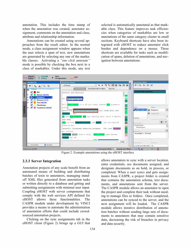
annotation. This includes the time stamp of when the annotation was created, annotator as-signment, comments on the annotation and class, attribute and relationship information.
Annotations can be created using several ap-proaches from the result editor. In the normal mode, a class assignment window appears when the user selects a span of text, new annotations are generated by selecting any one of the marka-ble classes. Activating a “one click annotate” mode is possible by checking the box next to a class of markables. Under this mode, any text
selected is automatically annotated as that mark-able class. This feature improves task efficien-cies when categories of markables are low or annotations of the same category cluster in small sections. Keyboard shortcuts have also been in-tegrated with eHOST to reduce annotator click burden and dependence on a mouse. These shortcuts are available for tasks such as modifi-cation of spans, deletion of annotations, and nav-igation between annotations.
Figure 2. Example annotations using the eHOST interface
2.3.3 Server Integration
Annotation projects of any scale benefit from an automated means of building and distributing batches of texts to annotators, managing stand-off XML files generated from annotation tasks or written directly to a database and getting and submitting assignments with minimal user input. Coupling eHOST with server components that comply with the web services API defined for eHOST allows these functionalities. The CASPR module under development by VINCI provides a means to automate the administration of annotation efforts that could include crowd-sourced annotation projects.
Clicking on the sync assignments tab in the eHOST client (Figure 2) brings up a GUI that
allows annotators to sync with a server location, enter credentials, see documents assigned, and designate documents as on hold, in process, or completed. When a user syncs and gets assign-ments from CASPR, a project folder is created that contains the annotation schema, text docu-ments, and annotations sent from the server. The CASPR module allows an annotator to open the project and complete their task without need-ing to manage files or folders. Once completed, annotations can be synced to the server, and the next assignment will be loaded. The CASPR module allows iterative distribution of annota-tion batches without sending large sets of docu-ments to annotators that may contain sensitive data, decreasing the risk of breaches in privacy and data security.
134

2.3.4 Additional Features
The document viewer panel employs visual cues to display relationships between annotations us-ing color coding representing a parent and child node and line indicator between them showing the relationship. An “annotation profiler” to the right of the scroll bar shows the density of anno-tations color-coded to their categories, as well as relative to their positions in the document. This type of data visualization is useful to see the rel-
ative location of annotations within a single document or across an en tire document corpus.
An adjudication mode is also included in the stand-alone eHOST client that allows difference matching and side-by-side comparison of anno-tations for efficient adjudication of discrepancies between annotations. Standard reporting metrics can be calculated including Inter-Annotator Agreement (IAA), Recall, Precision and F1-Measure.
Figure 3. eHOST adjudication mode showing discrepant annotations between annotators A7 and B4
In Adjudication mode discrepant annotations are shown using a wavy red underline in the editor window and by a red bolded outline in a side by side two panel view between the annotation edi-tor and comparator (Figure 3). These metrics and comparison tables between annotator results on the same documents can be output as HTML formatted reports that can be used by an adjudi-cator to quickly identify discrepancies between
annotators (Figure 4). These reports and the edi-tor window display can also be used to quickly train annotators on new clinical domains using a reference standard created by domain experts for training purposes. Using these features error analysis can also be done by importing outputs from an NLP system that have been converted into the XML format used by eHOST.
135

Figure 4. HTML Formatted report showing discrepant annotations between annotators A7 and B4 3 Advanced eHOST Features There are also other more advanced features that have been integrated with eHOST. These in-clude an “Oracle” mode that allows semi-automated annotation of similar spans of text across a document corpus, a means to easily and quickly curate annotated spans of text to create custom dictionaries, and machine-assisted pre-annotation integrated with the annotation tool itself.
3.1 Oracle Mode
Also implemented with eHOST is an “Oracle” mode which uses exact string matching allowing the user to annotate all spans of text that are
identical to a new annotation. The oracle lists where these candidate annotations are found along with the surrounding context. The annota-tor can then accept or reject candidate spans an-notated with the same markable class. Oracle mode can run within the current document or across the entire document corpus. This type of functionality is useful for annotation tasks that may involve identifying and marking spans of text that are repetitive or follow the same format For example, the 2011 i2b2/VA annotation task in which annotation of pronominal information was required for co-reference resolution (Figure 5).
Figure 5. Example annotations generated using the eHOST “Oracle” mode
136

3.2 Semi-Automated Curation and Dictionary Management
Using the navigator window users can navigate to all annotations in either a single document or across an entire document corpus (Figure 6). The end user can curate annotations directly, create classes on the fly, or add attributes to an-notations found from the navigator pane. These functions also allow users to easily identify spu-rious annotations introduced from machine-assisted approaches correct misclassification errors, and quickly curate all annotations within a single document or across an entire document corpus.
Figure 6. Semi-Automated curation within the
document corpus One task often associated with development of NLP systems involves manually creating or en-hancing some existing representation of lexical knowledge that can be used as a domain specific dictionary. Using eHOST users can export anno-tations to create a dictionary of terms, phrases, or individual tokens that have been identified by human annotators and assigned to markable in-formation classes. Once curated, annotated in-formation can be exported as a new dictionary. User created dictionaries can be integrated with
a database or exported and used in the creation of some ontologic representation of information using Protégé. Output from a dictionary manager is in the form of a delimited text file and can therefore be modified to fit any standardized information model or used to pre-annotate sub-sequent document batches.
3.3 Machine-Assisted Pre-Annotation
An interface is provided in eHOST that can be used for machine-assisted pre-annotation of documents in the active project corpus using either dictionaries or regular expressions based approaches. Users can import libraries of regular expressions or build their own regular expres-sions using a custom regular expression builder. Users can build and modify dictionaries created as part of annotation tasks that may include semi-automated curation steps. Dictionaries and regular expressions can also be coupled with the ConText algorithm (Chapman et al., 2007) to identify concept attributes such as negation, ex-periencer, and temporality. Pre-annotations de-rived from some external third party source such as an NLP system written as Knowtator XML outputs may also be imported into eHOST or passed to eHOST using CASPR.
Computational speed required for pre-annotation can be improved by selecting an op-tion to use an internal statistical dictionary in-dexing function. This feature is particularly useful in situations where pre-annotation dic-tionaries are extremely large, such as where a subset of some standard vocabulary may be used to pre-annotate documents. Using the result edi-tor and its associated functions annotators can add missed annotations, modifying existing an-notations and delete spurious annotations. Han-dling pre-annotations in this way allows troubleshooting and error analysis of NLP sys-tem outputs imported into eHOST that can be shown to a reviewer in context and also facili-tates interactive annotator training.
3.4 Machine-Assisted Verification
One of the more innovative features integrated with eHOST is the ability to verify and produce recommendations that help human annotators comply with syntactic and lexical rules that are specified by annotation task guidelines. Ma-
137

chine-Assisted verification is most useful when used on lexical or syntax rules to ensure that candidate phrases generated by automated sys-tems are similar to those marked by humans. These rules rely more on adherence to patterns than on decision-making, so the strengths of human review with machine approaches to semi-automated verification can be leveraged. When identifying medical concepts, it is common that noun phrases are marked as candidates. The de-termination of how much of a noun phrase to mark (inclusion of articles, adjectives, noun-modifiers, prepositional phrases) and at what granularity (simple nouns or complex noun phrases) may vary with each project.
The verifier allows portions of an annotation guideline to be programmed into rules that check for consistency. Rules check whether a word appears within a user-defined window before and after an annotation. Each rule can be linked to text that describes why the annotation was flagged. Annotators are then provided sugges-tions on the correct span based on the rule. Us-ing the surrounding text, the guideline text, and the suggestion, the annotator can determine the final span for an annotation. These machine-assisted verifier functions help support reference standard generation by providing the context of annotations that seem to fail syntactic and lexi-cal rules while allowing human annotators to focus on domain expertise required to identify and classify information found in clinical texts.
Conclusion
Our prototype system provides functionalities that have been created to more efficiently sup-port reference standard generation including ma-chine-assisted annotation approaches. It is our hope that these system features will serve as the basis for the further development efforts that will be part of an enterprise level system. Out-puts of such an annotation tool could be used as inputs for pipeline NLP systems or as one com-ponent of a common workbench of tools used for clinical NLP development tasks.
We have implemented and tested eHOST for the 2010 and 2011 i2b2/VA challenge annota-tion tasks and annotation projects for the Con-sortium for Healthcare Informatics Research (CHIR). The stand-alone eHOST client tool is
available from http://code.google.com/p/ehost along with a demonstration project, a users guide, API documentation, and source code. The eHOST/CASPR interfaces will be used to sup-port a large-scale crowd sourced annotation task used for annotation of disorders, temporal ex-pressions, uncertainty, and negation along with data standardization. These efforts will include more rigorous analysis and usability assessment of eHOST/CASPR for crowd sourcing and other small and large-scale annotation projects.
Acknowledgments Support and funding was provided by the VA Salt Lake City HealthCare System and the VA Consortium for Healthcare Informatics Research (CHIR), VA HSR HIR 08-374, the VA Infor-matics and Computing Infrastructure (VINCI), VA HIR 08-204, and NIH Grant U54 HL 108460 for integrating Data for Analysis, An-nonymization and Sharing (iDASH), NIGMS 7R01GM090187.
References Beatrice Alex, Claire Grover, Barry Haddow, Mijail
Kabadjov, Ewan Klein, Michael Matthews, Stuart Roebuck, Richard Tobin, and Xinglong Wang. 2008. Assisted curation: does text mining really help? In: Proceedings of the Pacific Symposium on Biocomputing.
Wendy W. Chapman, David Chu, John N. Dowling. 2007. ConText: An Algorithm for Identifying Contextual Features from Clinical Text. In: ACL-07 2007.
Carol Friedman, Hongfang Liu, Lyudmila Shagina, Stephen Johnson, George Hripcsak. 2001. Evaluat-ing the UMLS as a source of lexical knowledge for medical language processing. In: Proc AMIA Symp, 2001: 189-93.
Karen Fort and Saggot B. 2010. Influence of Pre-Annotation on POS-tagged Corpus Development. In: Proceedings of the Fourth Linguistic Annota-tion Workshop. ACL 2010: 56-63.
Pei-Yun Hsueh, Prem Melville, Vikas Sindhwani. 2009. Data Quality from Crowdsourcing: A study of Annotation Selection Criteria. In: Proceedings of the NAACL HLT Workshop on Active Learning for Natural Language Processing. June 2009: 27-35.
Danielle Mowery, Henk Harkema, Wendy W. Chap-man. 2008. Temporal Annotation of Clinical Text. In: ACL-08 2008.
138

Mark A. Musen, John Gennari, Henrik Eriksson, Samson W. Tu, and Angel R. Puerta. 1995. PROTEGE-II: computer support for development of intelligent systems from libraries of compo-nents. In: Medinfo 1995.
Aurélie Névéol, Rezarta Islamaj-Doğan, Zhiyong Lu. 2011. Semi-automatic semantic annotation of PubMed queries: a study on quality, efficiency, satisfaction. In: J Biomed Inform. 2011 Apr; 44(2):310-8.
Stefanie Nowak and Stefan Ruger. 2010. How Relia-ble are Annotations via Crowdsourcing? A Study about Inter-Annotator Agreement for Multi-label Image Annotation. In: MIR 10 2010.
Philip V. Ogren. 2006. Knowtator a protege plug-in for annotated corpus construction. In: Proceedings of the 2006 Conference of the North American Chapter of the Association for Computational Lin-guistics on Human Language Technology, 2006: 273-5.
Philip V. Ogren, Guergana K. Savova, Christopher G. Chute. 2008. Constructing Evaluation Corpora for Automated Clinical Named Entity Recogni-tion. In: Proceedings of the sixth international conference on Language Resources and Evalua-tion LREC 2008: 3143-3150.
Angus Roberts, Robert Gaizauskas, Mark Hepple, Neil Davis, George Demetriou, Yikun Guo, Jay Kola, Ian Roberts, Andrea Setzer, Archana Tapuria, Bill Wheeldin. 2007. The CLEF corpus: semantic annotation of clinical text. In: AMIA An-nu Symp Proc, 625-9.
Angus Roberts, Robert Gaizauskas, Mark Hepple, George Demetriou, Yikun Guo, Ian Roberts, An-drea Setzer. 2009. Building a semantically anno-tated corpus of clinical texts. In: J Biomed Inform, 42(5): 950-66.
Ellen Riloff. 1993. Automatically constructing a dic-tionary for information extraction tasks. In: Pro-ceedings of the Eleventh National Conference on Artificial Intelligence, 811-816.
Burr Settles, Mark Craven, and Lewis Friedland. 2008. Active Learning with Real Annotation Costs. In: Proceedings of the NIPS Workshop on Cost-Sensitive Learning. 2008.
Burr Settles. 2009. Active Learning Literature Sur-vey. In: Computer Sciences Technical Report 1648. University of Wisconsin-Madison. 2009.
Brett R. South, Shuying Shen, F. Jeff Friedlin, Mat-thew H. Samore, and Stephane M. Meystre. 2010. Enhancing Annotation of Clinical Text using Pre-Annotation of Common PHI. In: AMIA Annu Symp Proc. 2010.
Brett R. South, Shuying Shen, Robyn Barrus, Scott L. DuVall, Ozlem Uzuner, and Charlene Weir. 2011. Qualitative analysis of workflow modifications used to generate the reference standard for the 2010 i2b2/VA challenge. In: AMIA Annu Symp Proc. 2011.
Özlem Uzuner, Imre Solti, Fei Xia, and Eithon Cadag. 2010. Community annotation experiment for ground truth generation for the i2b2 medica-tion challenge. In: J Am Med Inform Assoc, 2010. 17(5):519-23.
Özlem Uzuner, Brett R. South, Shuying Shen, and Scott L. DuVall. 2011. 2010 i2b2/VA challenge on concepts, assertions, and relations in clinical text. In: JAMIA 18(5): 552-556.
Özlem Uzuner, Andreea Bodnari, Shuying Shen, Tyler B. Forbush, John Pestian, and Brett R. South. 2012. Evaluating the state of the art in co-reference resolution for electronic medical records. In: JAMIA doi: 10.1136/amiajnl-2011-000784.
Aobo Wang, Cong Duy Vu Hoang, and Min-Yen Kan. 2010. Perspectives on Crowdsourcing Anno-tations for Natural Language Processing. In: CSIDM Project No. CSIDM-200805.
Alexander S. Yeh, Lynette Hirschman, and Alexan-der A. Morgan. 2003. Evaluation of text data min-ing for database curation: Lessons learned from the KDD challenge cup. In: Bioinformatics, 19(Suppl 1): i331–339, 2003.
139
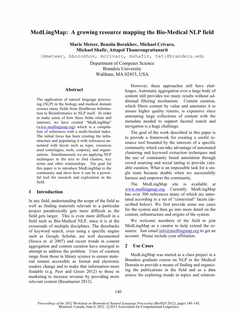
Proceedings of the 2012 Workshop on Biomedical Natural Language Processing (BioNLP 2012), pages 140–145,Montreal, Canada, June 8, 2012. c©2012 Association for Computational Linguistics
MedLingMap: A growing resource mapping the Bio-Medical NLP field
Marie Meteer, Bensiin Borukhov, Michael Crivaro, Michael Shafir, Attapol Thamrongrattanarit
{mmeteer, bborukhov, mcrivaro, mshafir, tet}@brandeis.edu
Department of Computer Science Brandeis University
Waltham, MA 02453, USA
Abstract
The application of natural language process-ing (NLP) in the biology and medical domain crosses many fields from Healthcare Informa-tion to Bioinformatics to NLP itself. In order to make sense of how these fields relate and intersect, we have created “MedLingMap” (www.medlingmap.org) which is a compila-tion of references with a multi-faceted index. The initial focus has been creating the infra-structure and populating it with references an-notated with facets such as topic, resources used (ontologies, tools, corpora), and organi-zations. Simultaneously we are applying NLP techniques to the text to find clusters, key terms and other relationships. The goal for this paper is to introduce MedLingMap to the community and show how it can be a power-ful tool for research and exploration in the field.
1 Introduction
In any field, understanding the scope of the field as well as finding materials relevant to a particular project paradoxically gets more difficult as the field gets larger. This is even more difficult in a field such as Bio-Medical NLP, since it is at the crossroads of multiple disciplines. The drawbacks of keyword search, even using a specific engine such as Google Scholar, are well documented (Stoica et. al 2007) and recent trends in content aggregation and content curation have emerged to attempt to address the problem. Uses of curation range from those in library science to ensure mate-rial remain accessible as format and electronic readers change and to make that information more findable (e.g. Peer and Green 2012) to those in marketing to increase revenue by providing more relevant content (Beaulaurier 2012).
However, these approaches still have chal-lenges. Automatic aggregation over a large body of content still provides too many results without ad-ditional filtering mechanism. Content curation, which filters content by value and annotates it to ensure higher quality returns, is expensive since annotating large collections of content with the metadata needed to support faceted search and navigation is a huge challenge.
The goal of the work described in this paper is to provide a framework for creating a useful re-source tool bounded by the interests of a specific community which can take advantage of automated clustering and keyword extraction techniques and the use of community based annotation through crowd sourcing and social tatting to provide valu-able curation. What is an impossible task for a sin-gle team because doable when we successfully harness and empower the community.
The MedLingMap site is available at www.medlingmap.org. Currently MedLingMap has over 300 references many of which are anno-tated according to a set of “contextual” facets (de-scribed below). We first provide some use cases for the system and then go into more detail on the content, infrastructure and origins of the system.
We welcome members of the field to join MedLingMap as a curator to help extend the re-source. Just email [email protected] to get an account. Please include your affiliation.
2 Use Cases
MedLingMap was started as a class project in a Brandeis graduate course on NLP in the Medical Domain to provide a means of finding and organiz-ing the publications in the field and as a data source for exploring trends in topics and relation-
140

ships among researchers. While there are many use cases for such a resource, three stand out.
The first is simply the ability to find material that meets very specific criteria. for example, to find papers using “MetaMap” for named entity extraction over clinical data. MedLingMap’s grow-ing collection of references and the necessary meta-data to make it useful is well suited to this task.
The second is to support the exploration of an area. If I’m interested in clinical coding, I can se-lect that subject area and am presented with a number of papers. I notice that Phil Resnik is on a number of papers and may want to follow up on his work. I also see many of the papers are tagged with AHIMA, including an entire proceedings that is worth exploring. I select a paper and see the
abstract mentions a particular challenge that is also worth following up on. We are in the process of developing a personal “workspace” that will let researchers record searches, annotate findings, and keep a queue of the “next directions” that might be worth following up.
The third use case gets back to one of the origi-nal premises of the work, which is that a “map” of a field goes beyond a collection of materials, it also provides context and can be used to see “hot spots” and trends. In order to provide this information and visualization, we have developed a set of tools applying a variety of NLP techniques, such as clus-tering, topic identification and tf-idf to the content of the papers. This work is described in more de-tail in (Thamrongrattanarit, et al, 2012).
Figure 1: MedLingMap site: www.medlingmap.org
3 Content and Context
The core content in MedLingMap are the refer-ences themselves. The underlying representation is based on bibtex and references can be added by either pasting in a single bibtex item or uploading
an entire file. A reference can be added through a form interface as well.
We have added BioNLP and related workshops dating back to 2002 as well as many other docu-ments. In addition to the references, there are en-tries for a variety of organizations and resources
141
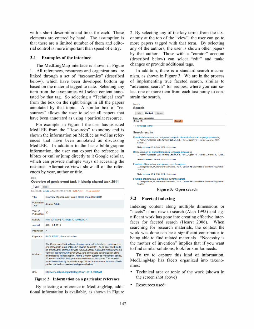
with a short description and links for each. These elements are entered by hand. The assumption is that there are a limited number of them and edito-rial control is more important than speed of entry.
3.1 Examples of the interface
The MedLingMap interface is shown in Figure 1. All references, resources and organizations are linked through a set of “taxonomies” (described below), which have been developed bottom up based on the material tagged to date. Selecting any item from the taxonomies will select content anno-tated by that tag. So selecting a “Technical area” from the box on the right brings in all the papers annotated by that topic. A similar box of “re-sources” allows the user to select all papers that have been annotated as using a particular resource.
For example, in Figure 1 the user has selected MedLEE from the “Resources” taxonomy and is shown the information on MedLee as well as refer-ences that have been annotated as discussing MedLEE. In addition to the basic bibliographic information, the user can export the reference in bibtex or xml or jump directly to it Google scholar, which can provide multiple ways of accessing the resource. Alternative views show all of the refer-ences by year, author or title.
Figure 2: Information on a particular reference
By selecting a reference in MedLingMap, addi-tional information is available, as shown in Figure
2. By selecting any of the key terms from the tax-onomy at the top of the “view”, the user can go to more papers tagged with that term. By selecting any of the authors, the user is shown other papers by that author. Those with a “curator” account (described below) can select “edit” and make changes or provide additional tags.
In addition, there is a standard search mecha-nism, as shown in Figure 3. We are in the process of implementing true faceted search, similar to “advanced search” for recipes, where you can se-lect one or more item from each taxonomy to con-strain the search.
Figure 3: Open search
3.2 Faceted indexing
Indexing content along multiple dimensions or “facets” is not new to search (Alan 1995) and sig-nificant work has gone into creating effective inter-faces for faceted search (Hearst 2006). When searching for research materials, the context the work was done can be a significant contributor to being able to find related materials. “Necessity is the mother of invention” implies that if you want to find similar solutions, look for similar needs.
To try to capture this kind of information, MedLingMap has facets organized into taxono-mies: • Technical area or topic of the work (shown in
the screen shot above)
• Resources used:
142

• Data: Corpora such as Genia, CRAFT, i2B2, BioInfer
• Lexical Resources, which are organized into dictionaries, and ontologies and include UMLS, PubMEd, MedLine, MeSH, and Medical Wordnet
• Tools, such as parsers, taggers, annotation toolkits and more complete systems, such as MedLee, GATE, and MIST
• Shared tasks, such as the BioNLP 2009 and 2011 shared tasks, BioCreative, and i2b2
• Institution the work was done in or is associated with in some way (e.g. funding, providing re-sources, etc)
As the project continues, these facets will grow and new ones will be added. Additional facets un-der consideration include the program (e.g. across multiple institutions, generally associated with a single funding source), target data (e.g. medical literature or clinical records).
4 Origins of MedLingMap
As mentioned above, MedLingMap was started as a class project in a graduate course NLP in the Medical Domain and the creation of the taxono-mies and population of the material was done as part of the class. However, the underlying architec-ture itself is based on a system that has been under development for speech recognition for the past two years (www.stcspeechmap.org) by author Marie Meteer as part of the Speech Technology Consortium’s effort to improve prior art research in non-patent literature.
The driving principle is that the “art” in any field (the papers, documentation, product descrip-tions, etc) can only be understood in terms of the context in which they were produced, contexts which show relations between them that is usually not available in the individual documents. For ex-ample, much of the early work in speech recogni-tion addressed the challenges of multimodal interfaces well before we had sophisticated mobile devices. Solutions are being reinvented and pat-ents applied for that would not considered novel if the original research were more readily available. Similar issues arise in multidisciplinary fields such as Bio-Medical NLP where different groups come
together who do not have the same historical con-text and may not know about previous research.
5 Infrastructure
MedLingMap and SpeechMap are built on Dru-pal1 an open architecture Content Management System (CMS), which underlies many web sites ranging from www.whitehouse.gov to BestBuy.
Using Drupal ensures that MedLingMap can be a living, growing resource. Drupal provides the following functionality:
• A database to store, retrieve, and maintain large documents sets and web pages, provid-ing multiple views into the contents.
• Specific content types for resources, organi-zations, authors, and references, all linked though a set of taxonomies.
• The capability to load in references in bibtex format either in a group or individually and annotate them with terms from the taxono-mies.
• Maintenance facilities, such as suggesting when multiple authors may be the same per-son and merging them.
• User profiles with different permission lev-els to accommodate viewers, contributors, social tagging, and private workspaces with the appropriate levels of security.
• The ability to integrate powerful search components, such as SOLR2, as well as spe-cific modules, such as the Bibliography module which provides automatic links to Google Scholar to retrieve those documents.
• Web-based to allow easy outside access and be more compatible with other systems.
• Extensibility both for more content, more content types, and more functionality. For example while there is a module that pro-duces a warning if a possible duplicate ref-erence, we are still looking for one that would search out potential duplicates and propose merges. If none exists, such a mod-ule can be written and easily integrated.
1 http://drupal.org/ 2 SOLR is an open-source search server based on the Lucene Java search library. http://lucene.apache.org/solr/
143

6 Value for Stakeholders
The value of MedLingMap varies with the audi-ence. We first talk about the value to the current community and contrast MedLingMap to similar resources already available. We then look at stakeholders outside or entering the community and the value MedLingMap brings to them.
6.1 BioMedical NLP community
For members of the community, a central reposi-tory for papers in the field is a “nice to have”. There is information that is surfaced by seeing the organization of the information and links to re-sources in one place, but if you have been attend-ing conferences and workshops regularly, this is not new information. You know the players and already follow the work you are interested in.
In addition, similar information is available elsewhere, though in a more distributed form. ACL has made all of the proceedings to confer-ences and workshops available3. Similarly ACM and IEEE Xplore provide access to all of the pa-pers they control. The significant difference is that in these collections even the advance search is re-lying on standard bibliographic elements, such as author and title, and keyword search and there is no segmentation of the material by field, which introduces significant ambiguity as the same term can mean different things in different fields. Simi-larly PubMed and GoPubMed offer documents and advanced search on a huge body of literature, but focused on biology and medicine, not the applica-tion of NLP techniques to those fields. MedLing-Map is designed to be focused on a smaller community with more like interests.
It is also important to note that MedLingMap is providing links to papers, not the actual papers, which are controlled by the publishers. While many papers are readily available using the links provided or can be found through the Google Scholar link for each reference, if you need a sub-scription to see the entire paper such as for IEEE, you still need to go through your standard method to get those papers.
LREC’s Resource Map is more similar in that it provides more in depth information that the aggre-gations described above, however the focus is on
3 http://aclweb.org/anthology-new/
mapping the resources themselves, not necessarily all of the publications that have taken advantage of those resources, though some of that information may be available by following the links. LREC is also using a crowd sourcing method for growing the resource by asking those who submit papers also submit the information about the resources they used. This is an interesting model in that it assures that those contributing have a stake in the result since they are members of the community by virtue of submitting a paper.
Organizations such as BioNLP.org and Sig-BioMed are also important resource aggregators for the community. Neither are focused on publi-cations and we hope that MedLingMap willl be-come one more resource they would point to.
6.2 From the outside
For students or those who come to the field from a neighboring field, the aggregation of the material in MedLingMap can save considerable time and provide overview or “map” of the field. Queries that are ambiguous in Google Scholar are more precise when the domain is limited. <example>
This increase in the ability of newcomers in the field to find what they are looking for actual turns into benefits for those in the field in two ways: First, one’s own papers become more findable, increasing citations and potential collaborations. Second, for those who teach, MedLingMap pro-vides a great environment for the students to do targeted research. Letting them loose in a con-strained search environment increases the likeli-hood they will find a rich body of material to learn from and build on without having to always hand select the papers.
7 Growing the resource
The real challenge for a community resource such as MedLingMap is how to grow it to be compre-hensive and keep it up to date, specifically how to:
• grow the number of references and resources
• increase high quality annotations that go be-yond what can be extracted automatically.
• provide visualizations that bring to light the connections in the material.
• maintain the quality of the data, for example by fining and merging duplicate entries and
144
ensuring information about resources and organizations is up to data.
The two choices for growing are automatic tech-niques and human annotation. We discuss the former in a related paper (Thamrongrattanarit 2012). Here we describe how manual annotation can be feasible.
7.1 Distributed Power
The key to high quality documents and tagging is community involvement. There are two comple-mentary approaches that are key to the MedLing-Map project: crowd sourcing and social tagging. Crowd sourcing involves the community in finding relevant resources, particularly those that are fairly obscure and predate the internet. The second is social tagging which lets individuals check on their own materials or materials in areas related to their own work and adding or adjusting the tags to make the content more searchable.
The key to making these tactics work is setting up the right support in the underlying system. For-tunately, the MedLingMap infrastructure allows for easy signup for those volunteering to contrib-ute. These technique have been used successfully in patent prior art search by Article One, Inc.4 which puts out a call to researchers to find art on a particular patent. If the client selects that art to support their case, the contributor is paid. The pat-ent office itself attempted something similar in the Peer to Patent program5, which depended on peo-ple’s desire to improve the quality of patents by letting them contribute art. It was moderately suc-cessful, but without the kind of specific reward the Article One provides, they did not get nearly as much material as they would have liked.
MedLingMap, SpeechMap and other efforts of its kind have the same problem: no one has enough time. So how do we address it? How do we create a convincing value proposition? Here are a couple suggestions:
Teaching: MedLingMap is a great teaching tool. Not only can students use it to do research on the material that’s in it, we as educators can enlist them to both tag material and go out on the web to find additional material to tag and add. In just one semester we have made considerable progress. If
4 http://www.articleonepartners.com/ 5 http://peertopatent.org/
everyone teaching a similar course enlisted their students, the students would gain and the resource would grow.
Research support: With the implementation of the personal workspace described above, the sys-tem will provide a unique service not available from other aggregators or content owners.
Funded project: Being able to hire student an-notators would accelerate the process. For the SpeechMap project we have a proposal into the US Patent Office for funding. We are open to sugges-tions about funding sources for MedLingMap.
Conclusion
With MedLingMap’s infrastructure in place and enough content to provide an exemplar of how it can grow, the challenge now is engaging the com-munity in what we see as an exiting experiment in harnessing the resources of the internet through crowd sourcing and social tagging to create a liv-ing resource that will benefit both the current and future members of the field. MedLingMap also provides a resource for exploring automated ways of annotating and organizing research materials. We also hope that this can be a map itself, to build similar “maps” in other subfields.
References Allen, RB. 1995. Retrieval from Facet Spaces, Elec-
tronic Publishing Chichester, Vol. 8(2 & 3), 247–257.
Beaulaurier, Joe. 2012. Content Curating for Fun and Profit, http://whatcommarketing.com/content-curating-for-fun-and-profit/.
Hearst, Marti. 2006. Design Recommendations for Hi-erarchical Faceted Search Interfaces. ACM SIGIR Workshop on Faceted Search, August, 2006
Peer, L. Green, A. 2012. Building an Open Data Reposi-tory for a Specialized Research Community: Process, Challenges and Lessons, International Journal of Digital Curation, Vol 7, No 1.
E. Stoica, M.A. Hearst, and M. Richardson. 2007. Au- tomating Creation of Hierarchical Faceted Metadata Structures. In Human Language Technologies: The Annual Conference of the North American Chapter of the Association for Computational Linguistics (NAACL-HLT 2007), pages 244–251.
Thamrongrattanarit, A., Shafir, M., Crivaro, M., Boruk-hov, B. , Meteer, M. What can NLP tell us about Bio NLP? BioNLP Workshop, Montreal, CA, 2012
145

Proceedings of the 2012 Workshop on Biomedical Natural Language Processing (BioNLP 2012), pages 146–154,Montreal, Canada, June 8, 2012. c©2012 Association for Computational Linguistics
Exploring Label Dependency in Active Learning for Phenotype Mapping
Shefali Sharma1, Leslie Lange2, Jose Luis Ambite1, Yigal Arens1, Chun-Nan Hsu1,3
1Information Sciences Institute, University of Southern California, Marina del Rey, CA 90292, USA2Department of Genetics, University of North Carolina, Chaple Hills, NC 27599, USA
3Institute of Information Sciences, Academia Sinica, Taipei 115, [email protected]
Abstract
Many genetic epidemiological studies of hu-man diseases have multiple variables relatedto any given phenotype, resulting from dif-ferent definitions and multiple measurementsor subsets of data. Manually mapping andharmonizing these phenotypes is a time-consuming process that may still miss themost appropriate variables. Previously, a su-pervised learning algorithm was proposed forthis problem. That algorithm learns to de-termine whether a pair of phenotypes is inthe same class. Though that algorithm ac-complished satisfying F-scores, the need tomanually label training examples becomes abottleneck to improve its coverage. Hereinwe present a novel active learning solutionto solve this challenging phenotype-mappingproblem. Active learning will make pheno-type mapping more efficient and improve itsaccuracy.
1 Introduction
Phenotypes are observable traits of an individual or-ganism resulting from the presence and interactionof its genotype with the environment. Phenotypespotentially related to human health are of interest ingenetics and epidemiology, including common clin-ical conditions, inheritance disorders, as well as var-ious risk factors such as diet. Substantial amountsof genomic data, including genome-wide genotyp-ing from GWAS (Genome-Wide Association Stud-ies) (Hardy and Singleton, 2009; Consortium, 2007)and sequencing, are being produced in conjunction
with the collection of carefully defined and mea-sured phenotypes to study the role of genetic vari-ations in a wide variety of inherited traits and disor-ders for many decades.
Recently, there is an emerging need to re-usethese valuable phenotype-genotype association datato boost the statistical power and improve sensitiv-ity and specificity of the search of associations be-tween various disorders and genetic variations. Newparadigms of genomic studies may be fostered oncea map of related phenotypes is easily accessible. Infact, one of such new paradigms, PheWAS (Phe-nome Wide Association Studies), has been devel-oped and producing interesting findings (Denny etal., 2010; Pendergrass et al., 2011) with the helpof phenotype mapping and harmonization. UnlikeGWAS, which focus on calculating the associationbetween the variation of hundreds of thousands ofgenotyped single nucleotide polymorphisms (SNPs)and a single or small number of phenotypes, Phe-WAS uses an extensive range of detailed pheno-typic measurements for comprehensively exploringthe association between genetic variations and phe-notypes. The investigation of a broad range of phe-notypes has the potential to identify pleiotropy, re-veal novel mechanistic insights, generate new hy-potheses, and define a more complete picture of ge-netic variations and their impact on human diseases.
To facilitate integration of genomic data sets, theresearch community needs to categorize compara-ble phenotype measurements and match them acrossmultiple genomic studies to identify data sets ofinterest as well as potential future collaborations.While the naming strategy for genetic variants is
146

largely standardized across studies (e.g. rs numbersfor single nucleotide polymorphisms or SNPs), thisis often not the case for phenotype variables. Dueto the lack of a standardized terminologies or othercontrolled vocabularies, it becomes increasingly dif-ficult to find studies with comparable phenotypes asthe genomic data accumulate. A researcher search-ing for the availability of comparable phenotypesacross multiple studies is confronted with a veritablemountain of variables to sift through. Even withina study, there are often numerous versions of se-mantically equivalent phenotypic variables. Manu-ally mapping and harmonizing these phenotypes is atime-consuming process that may still miss the mostappropriate variables.
Previously, (Hsu et al., 2011) have developed asupervised learning algorithm that learns to deter-mine whether a pair of phenotypes is semanticallyrelated from their descriptors. Though that algo-rithm accomplished satisfying F-scores, the need tomanually label training examples becomes a bottle-neck to improve its coverage. Moreover, the algo-rithm treats each pair independently, but pairs thatconsist of common phenotypes are not independent.Exploring this dependency may potentially improveits performance. In this paper, we investigate howto apply active learning to solve this challengingphenotype-mapping problem. Application of effec-tive active learning techniques will make pheno-type mapping more efficient and improve its accu-racy and, along with intuitive phenotype query tools,would provide a major resource for researchers uti-lizing these genomic data.
Active learning queries a user for labels of unla-beled phenotypes that may improve the learning ofphenotype mapping the most and thereby reduce theneed of labeling efforts. To select the most usefultraining examples to query, different selection strate-gies have been proposed in the past (Settles, 2010):
• Uncertainty Sampling In this strategy, an ac-tive learner chooses an instance that is the mostuncertain for the current model to label (Lewisand Catlett, 1994).
• Query-By-committee This strategy (Seung etal., 1992) is also known as maximum dis-agreement (Ayache and Quenot, 2007; Di andCrawford, 2011) because the idea is to choose
an instance for which a committee of modelsdisagrees the most among its members aboutits label.
• Expected Model Change The general princi-ple of this strategy is to choose an instance toquery when if its label is available, the modelwill be changed the most (Settles and Craven,2008).
• Expected Error Reduction Active learning isuseful when the selected instance reduce the er-ror the most and this strategy looks for an in-stance that can achieve this ultimate goal di-rectly.
• Variance Reduction Inspired by the bias-variance analysis of the generalization perfor-mance, the variance reduction principle seeksto query for instances that reduce the varianceof the model the most. A similar approach isapplied in the optimal experimental design instatistics (Federov, 1972). However, usuallythis also requires to solve expensive optimiza-tion problems.
• Density-Weighted Methods By consideringthe distribution of the instances, this strategyaddresses an issue of uncertainty sampling andquery-by-committee where outliers are likelyto be selected but contribute limitedly to im-proving the learning (Fujii et al., 1998; Das-gupta and Hsu, 2008).
The method reported here basically followsthe maximum disagreement principle of query-by-committee to select unlabeled pairs of phenotypesto query. A committee must be formed in order forthis strategy to be applied, but it has been shown thateven a small committee works well in practice. Vari-ous approaches can be applied to create committees.For example, co-testing (Muslea et al., 2006) appliesthis principle by combining forward and backwardparsing models for information extraction. A key tothe success of this strategy is that member modelsin the committee complement strengths and weak-nesses.
The idea of our method is to compare the match-or-not assignments by the model trained by super-vised learning and the class assignments derived
147
from exploring linkages of the labeled and unlabeledphenotypes. The most useful pairs to query are thosewhose assignments from the two different sourcesdisagree with the highest confidence.
Exploring linkages may improve classifier learn-ing when the classes of instances depend on eachother. This idea has been studied in the contextof classification of network data, such as pages onthe Web, co-reference resolution, word sense disam-biguation, and statistical relational learning (see e.g.,(Macskassy, 2007; McCallum and Wellner, 2005;Popescul et al., 2003)).
In this paper, we present an algorithm that im-plement our idea. This algorithm can be dividedinto two major steps. The first step of the algo-rithm explores the linkages and the second step pri-oritizes pairs of phenotypes to query. By identify-ing maximum disagreement pair instances betweenthe model classification results and exploring link-ages between labeled and unlabeled phenotype vari-ables, our active learner queries users for labels ofunlabeled phenotypes that may improve the map-ping the most and therefore will reduce the need oflabeling efforts. Our experimental results show thatexploring linkages can perfectly infer the match-or-not labels for a large number of pairs, and that ac-tive learning from maximum disagreement pairs im-proves the performance faster than from randomlyselected pairs, suggesting that active learning by ex-ploring linkages is a promising approach to the prob-lem of phenotype mapping.
2 Phenotype Mapping
2.1 Problem Definition
Phenotype mapping is a task of searching for alldatabases of participating studies to find a set of phe-notype variables that match a requested variable thatthe researcher is interested in. This is similar to thedefinition given in (Hsu et al., 2011) where the taskis defined as the assignment of every phenotype vari-able from each participating study to one of a setcategories, or classes, which corresponds to the “re-quested variable.”
Table 1 shows a fragment of the phenotype map-ping results of the phenotype variables that wematched manually from a consortium of cohort stud-ies for a set of 70 requested variables. In this frag-
ment, we show the phenotype variables assigned toone of the requested variables, the phenotype class‘hypertension’. The real ID of a phenotype ina Cohort is given in column Variable. In this ex-ample, seven cohort studies have a total of 13 phe-notype measurements related to hypertension.
Column Description is the main clue for au-tomatic matching. The variable descriptions usu-ally contain less than 10 words. As we can seein Table 1, the description contains abbreviations(e.g., ’HTN’, ’HBP’,dx), aliases (e.g., ’HighBlood Pressure’ vs. Hypertension), mea-surement criteria (e.g., DBP>90 MMHG, sys GE140, per JNC7, JNC VI), and tokens irrelevantto our task. As a result, word-by-word string sim-ilarity or sophisticated edit-distance based metricscan only match a small number of them. These ex-amples are phenotypes that share similar semanticsand are manually mapped to the same classes buttheir descriptions contain few or no common words.It is impossible for a model solely using the givendescriptions to figure out that they refer to relatedphenotypes without bringing to bear additional in-formation.
Other challenges of the phenotype problem in-clude: not knowing in advance how many classesthere are, unavailability of comprehensive catego-rization of phenotypes, and that the solution shouldscale well for a large number of phenotypes.
2.2 Supervised Learning for PhenotypeMapping
Here, we review the supervised learning method de-scribed in (Hsu et al., 2011), where phenotype map-ping was casted as a pair matching problem and ap-plied supervised learning to learn to tag a pair as amatch or not. A pair of phenotypes are considered asa match if they are assigned to the same class, other-wise it is not. 13 phenotype variables in Table 1 willyield 78 pairs of positive examples of matched pairs.A maximum entropy classifier (MaxEnt) (Hastie etal., 2009) was used as the model to estimate theprobability that a pair is a match. Two types of fea-tures were considered. The first type is based onstring similarity metrics to combine the strength ofa variety of string similarity metrics to measure theedit distance between the descriptions of a pair ofphenotypes and use the result to determine if they
148

RequestedCohort Variables Variable DescriptionARIC Hypertension HYPERT06 HYPERTENSION, DEFINITION 6CARDIA Hypertension Y01DBP HYPERTENSION BASED ON DBP> 90 MMHGCARDIA Hypertension Y01HTN HIGH BLOOD PRESSURECARDIA Hypertension Y01HTNTP TYPE OF HYPERTENSIONCFS Hypertension htn HTN: abnormal bp (sys GE 140 or dia GE 90) or medsCFS Hypertension htndx HTN: self report of MD dx of HTNCHS Hypertension HYPER CALCULATED HTN STATUSFHS Hypertension A70 HISTORY OF HYPERTENSIONFHS Hypertension B373 HYPERTENSION-ON TREAT OR ELEVATED BPFHS Hypertension C332 HBP statusJHS Hypertension HTN017 Hypertension Status Per JNC7MESA Hypertension HIGHBP1 HYPERTENSION: SELF-REPORTMESA Hypertension HTN1C Hypertension by JNC VI (1997) criteria
Table 1: Example variables of phenotype class ’hypertension’
match each other. The other type is the weightedJaccard where appearence of tokens and bi-gramsin both or one of the descriptions of a given phe-notype pair is used as the features. The training al-gorithm for MaxEnt will virtually assign to each to-ken or bi-gram a weight when it appears in the de-scriptions of an input phenotype pair. Weighted Jac-card is superior to string similarity features becausestring similarity metrics treat all tokens equally andthe information provided by these metrics is limited.Therefore weighted jaccard was shown to outper-form string similarity features by a large margin inthe experimental evaluation.
Before the feature extraction step, descriptionswill be augmented with the definitions given in theMerriam-Webster Medical Dictionary (2006)1. Forexample, ’hypertension’ will be augmentedwith its definition in the dictionary ’abnormallyhigh arterial blood pressure’ andconverted into ’hypertension abnormallyhigh arterial blood pressure’. Aug-mented ’hypertension’ will have many sharedtokens with ’high blood pressure’. Thisaugmentation step was proven to be effective inboosting recall, as semantically equivalent pairsdescribed by totally different sets of tokens can bematched.
(Hsu et al., 2011) also reported a transitive in-ference method to take advantage of the transitiverelationship of matched phenotype pairs. The ideais that if v1 and v2 are a match, so are v2 and v3,
1www.m-w.com/browse/medical/a.htm
then v1 and v3 must be a match, too. Applying tran-sitive inference did improve the performance, butwhen all possible transitive relations are explored,the performance degraded because false positivesaccumulated. The transitive inference method doesnot fully explore the dependency between pairs thatshare common phenotype variables. A more sophis-ticated approach is required.
3 Methods
Figure 1 illustrates our active learning idea. The ideais that, given a training set of phenotype variablesX manually matched with class labels and a test setof unlabeled phenotype variables, the first step is toinfer the class of each unlabeled variable by explor-ing the pairwise match scores assigned by the modeltrained by the training set. When we obtain a plausi-ble class assignment to each unlabeled variable, wecan classify each pair of unlabeled variables v1 andv2 by the trained model again to determine if theyare a match or not and compare the result with theirplausible class assignments.
If it turns out that the results agree with each other,we will move the pair to a set called sure pairs, oth-erwise, we will move the pair to a queue which willbe sorted in descreasing order by how much the re-sults disagree. Then we can query for true labels ofthe pairs in the queue to add to the training set themost useful examples and thus accomplish the activelearning.
149

Figure 1: Inferernce of match between unlabeled pheno-type variables by exploring their linkages to labeled pairs
3.1 Assigning Phenotype Categories
Procedure LabelA is to assign a class label to eachunlabeled test variable by matching them to labeledtraining variables. Let A denote the set of all pairsbetween a test variable and a training variable. Foreach variable, the output contains an element of thevariable, its assigned class label (may be null) anda score (log-likelihood). Function I(.) in line 2 isthe indicator function that returns 1 if its parameteris true and 0 otherwise. H is the model learned bycalling the supervised training procedure. In line 7,PH
vx is the probability that variables v and x are amatch estimated by H . In line 8, LabelA assigns vto a class c, which is the class of the training variablex that maximizes PH
vx. That is to assign the class ofx as that of v if PH
vx is the largest. Other selectioncan be used. For example, for each class c, we canestimate PH
vx for all training variables x in c, and se-lect c as the class of v if 1
n
∑log PH
vx, the geometricmean of the probabilities, is the largest. These selec-tion criteria are based on different assumptions andwe will empirically compare which one is a betterchoice. In fact, any type of average can potentiallybe considered here.
3.2 Prioritizing Unlabeled Pairs
Procedure LabelB orders pairs of test variables toquery for match-or-not and class labels. Let B bethe set of all pairs of test variables. LabelB alsogenerates a set called SurePairs. For each pairin B, LabelB checks if the model H considers thepair as a match (PH
vx ≥ 0.5) or not, and then checksif the pair is assigned by LabelA to the same class
Algorithm 1 Procedure LabelA1: Initialization
• Training variables X with their class anno-tated class(x) = c ∈ C,∀x ∈ X
• Test variables V with unknown classclass(v),∀v ∈ V
2: H ← Train({(x1, x2, m)|x1, x2 ∈ X, m =I(class(x1) = class(x2))})
3: A← {(v, x)|v ∈ V ∧ x ∈ X}4: procedure LABELA(A, H)5: Output← ∅6: for v ∈ V do7: ∀x ∈ X, PH
vx ← H(v, x)8: c← arg maxc(P
Hvx)
9: LHvx ← maxC(logPH
vx)10: if LH
vx < −2 then11: c← null,12: s← log(1− 2LH
vx)13: else14: s← LH
vx
15: end if16: Add (v, c, s) to Output17: end for18: Return Output19: end procedure
or not. If it is a match and assigned to the same class,or not a match and assigned to different classes, thatis, if H and LabelA agree, then the pair will bemoved to SurePairs, otherwise, the pair will bemoved to Queue. For a disagreed pair, LabelBalso estimate the degree of disagreement by the sumof the log-probabilities of the class assignments (LH
c1and LH
c2) and the match-or-not by the model (PHv1v2
).SurePairs can then be used for training.
We can then query for true labels of pairs inQueue. We can either query whether a pair is amatch or not or query for their class label. After acertain number of queries, we can repeat the pro-cedure to compute a new set of SurePairs andQueue, until all phenotypes are correctly assignedto a class.
150

Algorithm 2 Procedure LabelB1: Initialization2: H,A as in LabelA3: B ← {(v1, v2)|v1, v2 ∈ V }4: SurePairs← ∅; Queue← ∅5: ∀v1, v2 ∈ V, PH
v1v2← H(v1, v2)
6: (v, class(v), LHc ),∀v ∈ V ← LabelA(A,H)
7: procedure LABELB(B, A, H)8: for (v1, v2) ∈ B do9: if PH
v1,v2≥ 0.5 then
10: if c1 = c2 then11: Add (v1, v2, 1) to SurePairs12: else13: s← LH
c1 + LHc2 + log(1−PH
v1v2)
14: Add (v1, v2, s) to Queue15: end if16: else17: if c1 = c2 then18: s← LH
c1 + LHc2 + log PH
v1v2
19: Add (v1, v2, s) to Queue20: else21: Add (v1, v2, 0) to SurePairs22: end if23: end if24: end for25: Sort (v1, v2, m) in Queue by m26: Return Queue and SurePairs27: end procedure
4 Results
4.1 Data
We manually selected 1,177 phenotype variablesfrom a total of 35,041 in the databases of seven co-hort studies as shown in Table 1 and assigned themto one of 70 requested variables that are commontrait classes related to a large consortium study ofcardiovascular disorders. These seven cohorts in-clude ARIC (the Atherosclerosis Risk In Communi-ties study www.cscc.unc.edu/aric/), CAR-DIA (the Coronary Artery Risk In Young Adultsstudy www.cardia.dopm.uab.edu), CFS (theCleveland Family study dceweb1.case.edu/serc/collab/project_family.shtml),CHS (the Cardiovascular Heart Study www.chs-nhlbi.org/), FHS (Framingham HeartStudy www.framinghamheartstudy.org/),
Method / Model Precision Recall F-scoreString similarityMaxEnt 0.5557 0.0660 0.1179Weighted JaccardMaxEnt 0.8791 0.4848 0.6250w/ dictionary 0.9200 0.6104 0.7339w/ transitive infer. 0.7735 0.6612 0.7129w/ both 0.7728 0.8402 0.8051
Table 2: Performance results of supervised learning
JHS (Jackson Heart Study jhs.jsums.edu/jhsinfo/), and MEC (the Multi-Ethnic Cohortwww.crch.org/multiethniccohort/,www.uscnorris.com/mecgenetics/).
From these 1,177 phenotypes, 21,886 pairs areconsidered matches, that is, they are positive pairswith both phenotype variables in the same class.670,190 pairs are negatives.
4.2 Result of Supervised Learning
We divided all pairs in our data set by half into train-ing and test sets and evaluate different options of thesupervised learning algorithm with different optionsas described in (Hsu et al., 2011). The results asshown in Table 2 are consistent with the conclusionsgiven in (Hsu et al., 2011). That is, weighted Jaccardfeatures with dictionary augmentation plus transitiveinference yields the best performance.
We also performed a split-by-variable test, wherethe set of all variables is divided into three equalparts. Two of them are used for training and theother for testing. This is closer to the realistic appli-cation scenario and provides a better estimation ofthe generalization performance of a trained model.The results are given as the first two rows in Table 3.
4.3 Result of Active Learning
We implemented the two algorithms and evalu-ate the performance. We still applied split-by-variable to divide the data with 1
3 for testing and 23
for training. We measured the performance whenSurePairs produced by procedure LabelB wasadded to the training set, and then increasingly addmore pairs in Queue, also produced by LabelB,to the training set, and measured the performanceof the trained models to simulate an active learning
151

Method/Model Precision Recall F-scorew/o dictionary 0.8344 0.4106 0.5504w/ dictionary 0.6310 0.5287 0.5753Test on A 0.7956 0.5243 0.6321GM SurePairs(62622) 0.8772 0.5909 0.7061Model (62622) 0.9577 0.2936 0.4494MP SurePairs(74229) 0.8845 0.6196 0.7287Model (74229) 0.9660 0.2875 0.4431
Table 3: Performance results of splitting by variables.Numbers in the parentheses show the number of pairs inSurePairs.
query sequence.To ensure a fair comparison, we always use the set
A, the pairs between a labeled and unlabeled pheno-type variables, as the hold-out set for testing in allperformance evaluations. Note that pairs in the set Anever appear in either SurePairs or Queue, be-cause pairs in SurePairs or Queue are selectedfrom the set B, which contains the pairs betweenunlabeled phenotype variables. The third row of Ta-ble 3 shows the performance of the model testedonly on A.
We implemented two versions of procedureLabelA that are different in the methods they usedto assign a class to an unlabeled variable. The first,MP, is to use the maximum probability and the other,GM, is to use the maximum geometric mean of theprobabilities (see Section 3.1).
We start by evaluating the quality ofSurePairs. GM produced 62,622 pairs (1,642positives) while MP had 74,229 pairs (1,816positives). The match-or-not labels assigned byLabelB for both methods turn out to be perfectlycorrect, suggesting that combining model trainingand linkage exploration can effectively infer thematch-or-not labels.
Adding SurePairs to the training set boosts F-scores, as shown in Table 3, which also shows that,in contrast, if we add the same number of pairs tothe training set, but assign them match-or-not labelswith the trained model, they will degrade F-scores.
Next, we added pairs in Queue to the trainingset, 280 pairs at a time, and measured the F-scores
achieved by the resulting model. Figure 2 showsthe learning curves of three different ways to orderQueue produced with GM: descreasing, increasing,and random scores. The decreasing-score one per-formed the best by improving F-scores the fastest,confirming that higher-scored pairs are more useful.The end points of the three curves do not meet be-cause we have not exhausted all training examples.
Similarly, we evaluated decreasing and randomordering of Queue produced by applying MP.We note that MP already produced a large set ofSurePairs. As a result, less pairs are in Queuecompared to that by GM. Therefore, after 9 passes, allpairs are exhausted and no obvious difference can beobserved between decreasing and random orderingin the end.
Figure 2: Learning curves of active learning: class as-signment by maximum geometric mean of probabilities
Figure 3: Learning curves of active learning: class as-signment by maximum probabilities
5 Conclusions and Future Works
Despite the vast amounts of genomic data availablein repositories, identification of relevant datasets canbe challenging for researchers interested in specific
152

phenotypic measures. This paper presents our ac-tive learning approach that will be implemented as acomponent of new informatics tools for the researchcommunity to categorize phenotype measurementsfrom genomic studies.
We show that comparing class assignment by ex-ploring linkages and by the model can be effectivein both improving the match-or-not assignments andordering unlabeled pairs as queries for active learn-ing. It is interesting that when two sources of classassignment agree, the pairs’ match-or-not assign-ments are perfectly correct. How generalizable forthis result deserves further investigation. We notethat in order to perform a fair comparison, no pairbetween labeled and unlabeled phenotype variablesare used for training. In a real application, they canbe added to either SurePairs or Queue by ex-tending procedure LabelB to include them.
Acknowledgments
We thank Cheng-Ju Kuo and Congxing Cai for theirhelp in producing the results reported in Section 4.2.This research is supported by NHLBI-NIH grant1UH2HL108780-01.
ReferencesStephane Ayache and Georges Quenot. 2007. Evaluation
of active learning strategies for video indexing. SignalProcessing: Image Communication, 22(78):692 – 704.Special Issue on Content-Based Multimedia Indexingand Retrieval.
The Wellcome Trust Case Control Consortium. 2007.Genome-wide association study of 14,000 cases ofseven common diseases and 3,000 shared controls.Nature, 447(7145):661–678, June.
Sanjoy Dasgupta and Daniel Hsu. 2008. Hierarchicalsampling for active learning. In Machine Learning,Proceedings of the Twenty-Fifth International Confer-ence on Machine Learning (ICML-08), pages 208–215.
Joshua C. Denny, Marylyn D. Ritchie, Melissa A. Bas-ford, Jill M. Pulley, Lisa Bastarache, Kristin Brown-Gentry, Deede Wang, Dan R. Masys, Dan M. Ro-den, and Dana C. Crawford. 2010. Phewas: demon-strating the feasibility of a phenome-wide scan todiscover gene-disease associations. Bioinformatics,26(9):1205–1210.
Wei Di and Melba M. Crawford. 2011. View gen-eration for multiview maximum disagreement based
active learning for hyperspectral image classification.Geoscience and Remote Sensing, IEEE Transactionson, PP(99):1 –13.
Valerii V. Federov. 1972. Theory of Optimal Experi-ments. Academic Press.
Atsushi Fujii, Takenobu Tokunaga, Kentaro Inui, andHozumi Tanaka. 1998. Selective sampling forexample-based word sense disambiguation. Compu-tational Linguistics, 24(4):573–597.
John Hardy and Andrew Singleton. 2009. Genomewideassociation studies and human disease. New EnglandJournal of Medicine, 360(17):1759–1768.
Trevor Hastie, Robert Tibshirani, and Jerome H. Fried-mann. 2009. The Elements of Statistical Learning(2nd Edition). Springer-Verlag, New York, NY, USA.
Chun-Nan Hsu, Cheng-Ju Kuo, Congxing Cai, Sarah A.Pendergrass, Marylyn D. Ritchie, and Jose Luis Am-bite. 2011. Learning phenotype mapping for integrat-ing large genetic data. In Proceedings of BioNLP 2011Workshop, BioNLP ’11, pages 19–27, Portland, OR,USA. Association for Computational Linguistics.
David D. Lewis and Jason Catlett. 1994. Heterogeneousuncertainty sampling for supervised-learning. In Pro-ceedings of the International Conference on MachineLearning (ICML-94), pages 148–156.
Sofus A. Macskassy. 2007. Improving learning in net-worked data by combinng explicit and mined links. InProceedings of the National Conference on ArtificialIntelligence (AAAI-07), page 590.
Andrew McCallum and Ben Wellner. 2005. Conditionalmodels of identity uncertainty with application to nouncoreference. In Lawrence K. Saul, Yair Weiss, andLeon Bottou, editors, Advances in Neural InformationProcessing Systems 17, pages 905–912. MIT Press,Cambridge, MA.
Merriam-Webster. 2006. Medical Dictionary. Merriam-Webster, Springfield, MA, USA.
Ion Muslea, Steve Minton, and Craig A. Knoblock. 2006.Active learning with multiple views. Journal of Artifi-cial Intelligence Research, 27:203–233.
S. A. Pendergrass, K. Brown-Gentry, S. M. Dudek, E. S.Torstenson, J. L. Ambite, C. L. Avery, S. Buyske,C. Cai, M. D. Fesinmeyer, C. Haiman, G. Heiss,L. A. Hindorff, C. N. Hsu, R. D. Jackson, C. Kooper-berg, L. Le Marchand, Y. Lin, T. C. Matise, L. More-land, K. Monroe, A. P. Reiner, R. Wallace, L. R.Wilkens, D. C. Crawford, and M. D. Ritchie. 2011.The use of phenome-wide association studies (phewas)for exploration of novel genotype-phenotype relation-ships and pleiotropy discovery. Genetic Epidemiol-ogy, 35(5):410–422.
Alexandrin Popescul, Rin Popescul, and Lyle H. Ungar.2003. Statistical relational learning for link prediction.
153
In In Workshop on Learning Statistical Models fromRelational Data at the International Joint Conferenceon Articial Intelligence (IJCAI-2003).
Burr Settles and Mark Craven. 2008. An analysis ofactive learning strategies for sequence labeling tasks.In Proceedings of the Conference on Empirical Meth-ods in Natural Language Processing (EMNLP), pages1069–1078. ACL Press.
Burr Settles. 2010. Active learning literature survey.Computer Science Technical Report 1648, Universityof Wisconsin-Madison, January.
H. Sebastian Seung, Manfred Opper, and Haim Som-polinsky. 1992. Query by committee. In Proceed-ings of the Fifth Annual Workshop on ComputationalLearning Theory (COLT’92), pages 278–294.
154

Proceedings of the 2012 Workshop on Biomedical Natural Language Processing (BioNLP 2012), pages 155–162,Montreal, Canada, June 8, 2012. c©2012 Association for Computational Linguistics
Evaluating Joint Modeling of Yeast Biology Literature and Protein-ProteinInteraction Networks
Ramnath Balasubramanyan and Kathryn Rivard and William W. CohenSchool of Computer ScienceCarnegie Mellon University
rbalasub,krivard,[email protected]
Jelena Jakovljevic and John WoolfordDeparment of Biological Sciences
Carnegie Mellon Universityjelena,[email protected]
Abstract
Block-LDA is a topic modeling approach toperform data fusion between entity-annotatedtext documents and graphs with entity-entitylinks. We evaluate Block-LDA in the yeast bi-ology domain by jointly modeling PubMed R©
articles and yeast protein-protein interactionnetworks. The topic coherence of the emer-gent topics and the ability of the model to re-trieve relevant scientific articles and proteinsrelated to the topic are compared to that of atext-only approach that does not make use ofthe protein-protein interaction matrix. Eval-uation of the results by biologists show thatthe joint modeling results in better topic co-herence and improves retrieval performance inthe task of identifying top related papers andproteins.
1 Introduction
The prodigious rate at which scientific literatureis produced makes it virtually impossible for re-searchers to manually read every article to identifyinteresting and relevant papers. It is therefore crit-ical to have automatic methods to analyze the liter-ature to identify topical structure in it. The latentstructure that is identified can be used for differentapplications such as enabling browsing, retrieval ofpapers related to a particular sub-topic etc. Such ap-plications assist in common scenarios such as help-ing a researcher identify a set of articles to read (per-haps a set of well-regarded surveys) to familiarizeherself with a new sub-field; helping a researcher tostay abreast with the latest advances in his field byidentifying relevant articles etc.
In this paper, we focus on the task of organiz-ing a large collection of literature about yeast biol-ogy to enable topic oriented browsing and retrievalfrom the literature. The analysis is performed usingtopic modeling(Blei et al., 2003) which has, in thelast decade, emerged as a versatile tool to uncoverlatent structure in document corpora by identifyingbroad topics that are discussed in it. This approachcomplements traditional information retrieval taskswhere the objective is to fulfill very specific infor-mation needs.
In addition to literature, there often exist othersources of domain information related to it. In thecase of yeast biology, an example of such a resourceis a database of known protein-protein interactions(PPI) which have been identified using wetlab exper-iments. We perform data fusion by combining textinformation from articles and the database of yeastprotein-protein interactions, by using a latent vari-able model — Block-LDA (Balasubramanyan andCohen, 2011) that jointly models the literature andPPI networks.
We evaluate the ability of the topic models to re-turn meaningful topics by inspecting the top papersand proteins that pertain to them. We compare theperformance of the joint model i.e. Block-LDA witha model that only considers the text corpora by ask-ing a yeast biologist to evaluate the coherence oftopics and the relevance of the retrieved articles andproteins. This evaluation serves to test the utility ofBlock-LDA on a real task as opposed to an internalevaluation (such as by using perplexity metrics forexample). Our evaluaton shows that the joint modeloutperforms the text-only approach both in topic co-
155

herence and in top paper and protein retrieval asmeasured by precision@10 values.
The rest of the paper is organized as follows. Sec-tion 2 describes the topic modeling approach usedin the paper. Section 3 describes the datasets usedfollowed by Section 4 which details the setup of theexperiments. The results of the evaluation are pre-sented in Section 5 which is followed by the conclu-sion.
2 Block-LDA
The Block-LDA model (plate diagram in Figure 1)enables sharing of information between the compo-nent on the left that models links between pairs ofentities represented as edges in a graph with latentblock structure, and the component on the right thatmodels text documents, through shared latent topics.More specifically, the distribution over the entities ofthe type that are linked is shared between the blockmodel and the text model.
The component on the right, which is an extensionof the LDA models documents as sets of “bags of en-tities”, each bag corresponding to a particular typeof entity. Every entity type has a topic wise multi-nomial distribution over the set of entities that canoccur as an instance of the entity type. This modelis termed as Link-LDA(Nallapati et al., 2008) in theliterature.
The component on the left in the figure is a gen-erative model for graphs representing entity-entitylinks with an underlying block structure, derivedfrom the sparse block model introduced by Parkki-nen et al. (2009). Linked entities are generated fromtopic specific entity distributions conditioned on thetopic pairs sampled for the edges. Topic pairs foredges (links) are drawn from a multinomial definedover the Cartesian product of the topic set with it-self. Vertices in the graph representing entities there-fore have mixed memberships in topics. In con-trast to Mixed-membership Stochastic Blockmodel(MMSB) introduced by Airoldi et al. (2008), onlyobserved links are sampled, making this model suit-able for sparse graphs.
LetK be the number of latent topics (clusters) wewish to recover. Assuming documents consist of Tdifferent types of entities (i.e. each document con-tains T bags of entities), and that links in the graph
are between entities of type tl, the generative processis as follows.1. Generate topics: For each type t ∈ 1, . . . , T , andtopic z ∈ 1, . . . ,K, sample βt,z ∼ Dirichlet(γ), thetopic specific entity distribution.2. Generate documents. For every document d ∈{1 . . . D}:
• Sample θd ∼ Dirichlet(αD) where θd is thetopic mixing distribution for the document.
• For each type t and its associated set of entitymentions et,i, i ∈ {1, · · · , Nd,t}:
– Sample a topic zt,i ∼Multinomial(θd)– Sample an entity et,i ∼
Multinomial(βt,zt,i)
3. Generate the link matrix of entities of type tl:
• Sample πL ∼ Dirichlet(αL) where πL de-scribes a distribution over the Cartesian prod-uct of the set of topics with itself, for links inthe dataset.
• For every link ei1 → ei2, i ∈ {1 · · ·NL}:
– Sample a topic pair 〈zi1, zi2〉 ∼Multinomial(πL)
– Sample ei1 ∼Multinomial(βtl,zi1)
– Sample ei2 ∼Multinomial(βtl,zi2)
Note that unlike the MMSB model, this modelgenerates only realized links between entities.
Given the hyperparameters αD, αL and γ, thejoint distribution over the documents, links, theirtopic distributions and topic assignments is given by
p(πL,θ,β, z, e, 〈z1, z2〉, 〈e1, e2〉|αD, αL, γ) ∝
(1)K∏z=1
T∏t=1
Dir(βt,z|γt)×
D∏d=1
Dir(θd|αD)T∏t=1
Nd,t∏i=1
θz(d)t,i
d βet,i
t,z(d)t,i
×
Dir(πL|αL)
NL∏i=1
π〈zi1,zi2〉L βei1
tl,z1βei2tl,z2
156
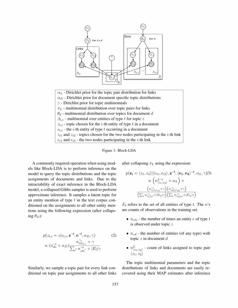
...
!d
!L!D
!L
NL
!
Dim: K x KDim: K
zi1 zi2
ei2ei1
Links
Docs
!t,zT
K
D
z1,i
e1,i
zT,i
eT,i
Nd,TNd,1
αL - Dirichlet prior for the topic pair distribution for linksαD - Dirichlet prior for document specific topic distributionsγ - Dirichlet prior for topic multinomialsπL - multinomial distribution over topic pairs for linksθd - multinomial distribution over topics for document dβt,z - multinomial over entities of type t for topic zzt,i - topic chosen for the i-th entity of type t in a documentet,i - the i-th entity of type t occurring in a documentzi1 and zi2 - topics chosen for the two nodes participating in the i-th linkei1 and ei2 - the two nodes participating in the i-th link
Figure 1: Block-LDA
A commonly required operation when using mod-els like Block-LDA is to perform inference on themodel to query the topic distributions and the topicassignments of documents and links. Due to theintractability of exact inference in the Block-LDAmodel, a collapsed Gibbs sampler is used to performapproximate inference. It samples a latent topic foran entity mention of type t in the text corpus con-ditioned on the assignments to all other entity men-tions using the following expression (after collaps-ing θD):
p(zt,i = z|et,i, z¬i, e¬i, αD, γ) (2)
∝ (n¬idz + αD)n¬iztet,i
+ γ∑e′ n¬izte′
+ |Et|γ
Similarly, we sample a topic pair for every link con-ditional on topic pair assignments to all other links
after collapsing πL using the expression:
p(zi = 〈z1, z2〉|〈ei1, ei2〉, z¬i, 〈e1, e2〉¬i, αL, γ)(3)
∝(nL¬i〈z1,z2〉 + αL
)×(
n¬iz1tlei1
+γ)(n¬i
z2tlei2+γ)
(∑e n
¬iz1tle
+|Etl|γ)(∑
e n¬iz2tle
+|Etl|γ)
Et refers to the set of all entities of type t. The n’sare counts of observations in the training set.
• nzte - the number of times an entity e of type tis observed under topic z
• nzd - the number of entities (of any type) withtopic z in document d
• nL〈z1,z2〉 - count of links assigned to topic pair〈z1, z2〉
The topic multinomial parameters and the topicdistributions of links and documents are easily re-covered using their MAP estimates after inference
157

using the counts of observations.
β(e)t,z =
nzte + γ∑e′ nzte′ + |Et|γ
, (4)
θ(z)d =
ndz + αD∑z′ ndz′ +KαD
and (5)
π〈z1,z2〉L =
n〈z1,z2〉 + αL∑z′1,z
′2n〈z′1,z′2〉 +K2αL
(6)
A de-noised form of the entity-entity link matrixcan also be recovered from the estimated parame-ters of the model. Let B be a matrix of dimensionsK × |Etl | where row k = βtl,k, k ∈ {1, · · · ,K}.Let Z be a matrix of dimensions K ×K s.t Zp,q =∑NL
i=1 I(zi1 = p, zi2 = q). The de-noised matrix Mof the strength of association between the entities inEtl is given by M = BTZB.
In the context of this paper, de-noising theprotein-protein interaction networks studied is animportant application. The joint model permits in-formation from the large text corpus of yeast publi-cations to be used to de-noise the PPI network andto identify potential interactions that are missing inthe observed network. While this task is importantand interesting, it is outside the scope of this paperand is a direction for future work.
3 Data
We use a collection of publications about yeast bi-ology that is derived from the repository of sci-entific publications at PubMed R©. PubMed R© is afree, open-access on-line archive of over 18 mil-lion biological abstracts and bibliographies, includ-ing citation lists, for papers published since 1948.The subset we work with consists of approximately40,000 publications about the yeast organism thathave been curated in the Saccharomyces GenomeDatabase (SGD) (Dwight et al., 2004) with anno-tations of proteins that are discussed in the publi-cation. We further restrict the dataset to only thosedocuments that are annotated with at least one pro-tein from the protein-protein interactions databasesdescribed below. This results in a protein annotateddocument collection of 15,776 publications. Thepublications in this set were written by a total of47,215 authors. We tokenize the titles and abstractsbased on white space, lowercase all tokens and elim-inate stopwords. Low frequency (< 5 occurrences)
terms are also eliminated. The vocabulary that is ob-tained consists of 45,648 words.
The Munich Institute for Protein Sequencing(MIPS) database (Mewes et al., 2004) includes ahand-crafted collection of protein interactions cover-ing 8000 protein complex associations in yeast. Weuse a subset of this collection containing 844 pro-teins, for which all interactions were hand-curated.
Finally, we use another dataset of protein-proteininteractions in yeast that were observed as a result ofwetlab experiments by collaborators of the authorsof the paper. This dataset consists of 635 interac-tions that deal primarily with ribosomal proteins andassembly factors in yeast.
4 Setup
We conduct three different evaluations of the emer-gent topics. Firstly, we obtain topics from onlythe text corpus using a model that comprises of theright half of Figure 1 which is equivalent to usingthe Link-LDA model. For the second evaluation,we use the Block-LDA model that is trained on thetext corpus and the MIPS protein-protein interac-tion database. Finally, for the third evaluation, wereplace the MIPS database with the interaction ob-tained from the wetlab experiments. In all the cases,we set K, the number of topics to be 15. In eachvariant, we represent documents as 3 sets of entitiesi.e. the words in the abstracts of the article, the setof proteins associated with the article as indicated inthe SGD database and finally the authors who wrotethe article. Each topic therefore consists of 3 differ-ent multinomial distributions over the sets of the 3kinds of entities described.
Topics that emerge from the different variants canpossibly be assigned different indices even whenthey discuss the same semantic concept. To com-pare topics across variants, we need a method todetermine which topic indices from the differentvariants correspond to the same semantic concept.To obtain the mapping between topics from eachvariant, we utilize the Hungarian algorithm (Kuhn,1955) to solve the assignment problem where thecost of aligning topics together is determined usingthe Jensen-Shannon divergence measure.
Once the topics are obtained, we firstly obtain theproteins associated with the topic by retrieving the
158
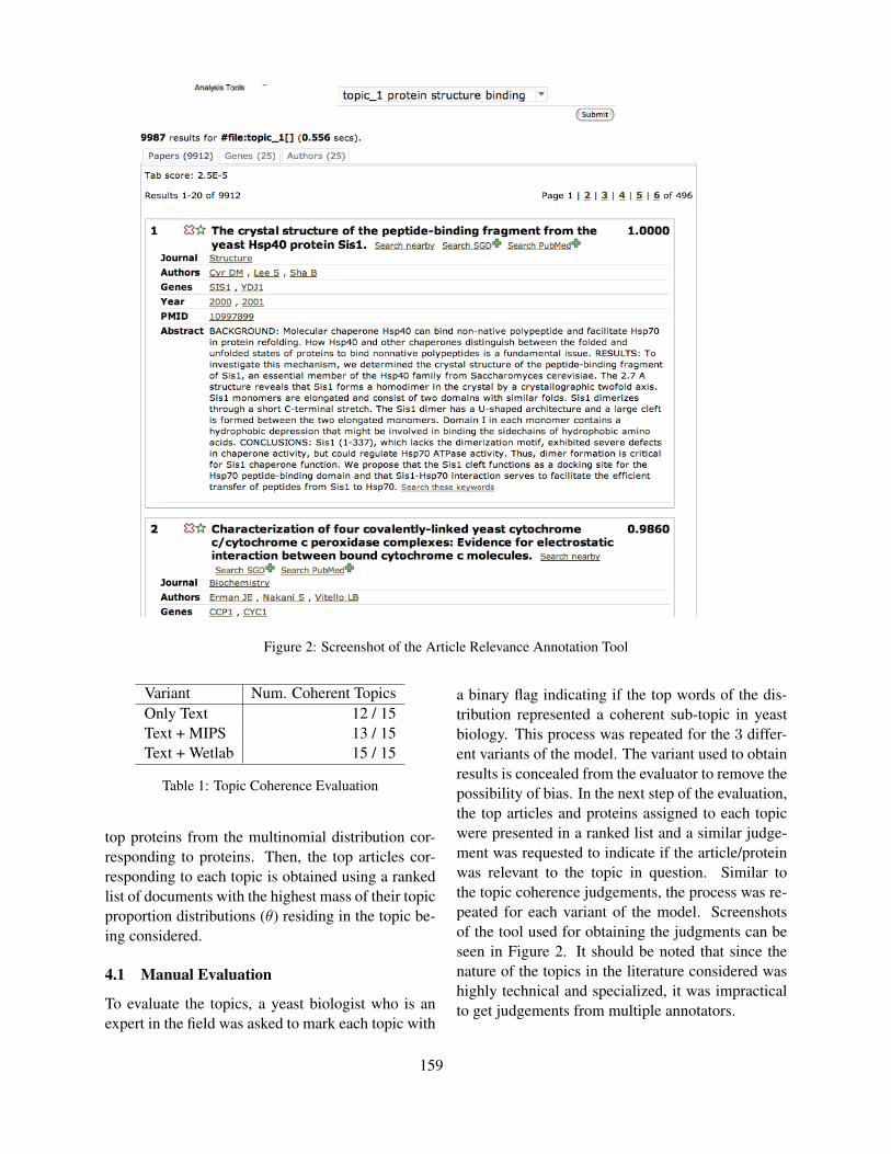
Figure 2: Screenshot of the Article Relevance Annotation Tool
Variant Num. Coherent TopicsOnly Text 12 / 15Text + MIPS 13 / 15Text + Wetlab 15 / 15
Table 1: Topic Coherence Evaluation
top proteins from the multinomial distribution cor-responding to proteins. Then, the top articles cor-responding to each topic is obtained using a rankedlist of documents with the highest mass of their topicproportion distributions (θ) residing in the topic be-ing considered.
4.1 Manual Evaluation
To evaluate the topics, a yeast biologist who is anexpert in the field was asked to mark each topic with
a binary flag indicating if the top words of the dis-tribution represented a coherent sub-topic in yeastbiology. This process was repeated for the 3 differ-ent variants of the model. The variant used to obtainresults is concealed from the evaluator to remove thepossibility of bias. In the next step of the evaluation,the top articles and proteins assigned to each topicwere presented in a ranked list and a similar judge-ment was requested to indicate if the article/proteinwas relevant to the topic in question. Similar tothe topic coherence judgements, the process was re-peated for each variant of the model. Screenshotsof the tool used for obtaining the judgments can beseen in Figure 2. It should be noted that since thenature of the topics in the literature considered washighly technical and specialized, it was impracticalto get judgements from multiple annotators.
159

Topic
Pre
cisi
on @
10
0.2
0.4
0.6
0.8
1.0 ● ● ● ●
●
● ● ● ● ● ● ●
Variant
● With MIPS interactions
Only Text
With Wetlab interactions
(a) Article Retrieval
Topic
Pre
cisi
on @
10
0.2
0.4
0.6
0.8
1.0 ●
●
●
● ● ● ● ● ●
Variant
● With MIPS interactions
Only Text
With Wetlab interactions
(b) Protein Retrieval
Figure 3: Retrieval Performance Evaluation (Horizontal lines indicate mean across all topics)
To evaluate the retrieval of the top articles andproteins, we measure the quality of the results bycomputing its precision@10 score.
5 Results
First we evaluate the coherence of the topics ob-tained from the 3 variants described above. Table1 shows that out of the 15 topics that were obtained,12 topics were deemed coherent from the text-onlymodel and 13 and 15 topics were deemed coherentfrom the Block-LDA models using the MIPS andwetlab PPI datasets respectively.
Next, we study the precision@10 values for eachtopic and variant for the article retrieval and proteinretrieval tasks, which is shown in Figure 3. The plots
also show horizontal lines representing the mean ofthe precision@10 across all topics. It can be seenfrom the plots that for both the article and proteinretrieval tasks, the joint models work better than thetext-only model on average. For the article retrievaltask, the model trained with the text + MIPS resultedin the higher mean precision@10 whereas for theprotein retrieval task, the text + Wetlab PPI datasetreturned a higher mean precision@10 value. Forboth the protein retrieval and paper retrieval tasks,the improvements shown by the joint models usingeither of the PPI datasets over the text-only model(i.e. the Link LDA model) were statistically sig-nificant at the 0.05 level using the paired Wilcoxonsign test. The difference in performance between the
160

Topic: Protein Structure & InteractionsTop articles using Publications Only Top articles using Block-LDA with Wetlab PPI* X-ray fiber diffraction of amyloid fibrils. * X-ray fiber diffraction of amyloid fibrils.* Molecular surface area and hydrophobic effect. * Scalar couplings across hydrogen bonds.* Counterdiffusion methods for macromolecularcrystallization.
* Dipolar couplings in macromolecular structuredetermination.
* Navigating the ClpB channel to solution. * Structure of alpha-keratin.* Two Rippled-Sheet Configurations of Polypep-tide Chains, and a Note about the Pleated Sheets.
* Stable configurations of polypeptide chains.
* Molecular chaperones. Unfolding protein fold-ing.
* The glucamylase and debrancher of S. diastati-cus.
* The molten globule state as a clue for under-standing the folding and cooperativity of globular-protein structure.
* A study of 150 cases of pneumonia.
* Unfolding and hydrogen exchange of proteins:the three-dimensional ising lattice as a model.
* Glycobiology.
* Packing of alpha-helices: geometrical con-straints and contact areas.
* The conformation of thermolysin.
Topic: DNA RepairTop articles using Publications Only Top articles using Block-LDA with Wetlab PPI* Passing the baton in base excision repair. * Telomeres and telomerase.* The bypass of DNA lesions by DNA and RNApolymerases.
* Enzymatic photoreactivation: overview.
* The glucamylase and debrancher of S. diastati-cus.
* High-efficiency transformation of plasmid DNAinto yeast.
* DNA replication fidelity. * The effect of ultraviolet light on recombinationin yeast.
* Base excision repair. * T-loops and the origin of telomeres.* Nucleotide excision repair. * Directed mutation: between unicorns and goats.* The replication of DNA in Escherichia Coli. * Functions of DNA polymerases.* DNA topoisomerases: why so many? * Immortal strands? Give me a break.
Table 2: Sample of Improvements in Article Retrieval
two joint models that used the two different PPI net-works were however insignificant which indicatesthat there is no observable advantage in using onePPI dataset over the other in conjunction with thetext corpus.
Table 2 shows examples of poor results of articleretrieval obtained using the publications-only modeland the improved set of results obtained using thejoint model.
5.1 TopicsTable 3 shows 3 sample topics that were retrievedfrom each variant described earlier. The table showsthe top words and proteins associated with the top-
ics. The topic label on the left column was assignedmanually during the evaluation by the expert anno-tator.
Conclusion
We evaluated topics obtained from the joint mod-eling of yeast biology literature and protein-proteininteractions in yeast and compared them to top-ics that were obtained from using only the litera-ture. The topics were evaluated for coherence andby measuring the mean precision@10 score of thetop articles and proteins that were retrieved for eachtopic. Evaluation by a domain expert showed that
161
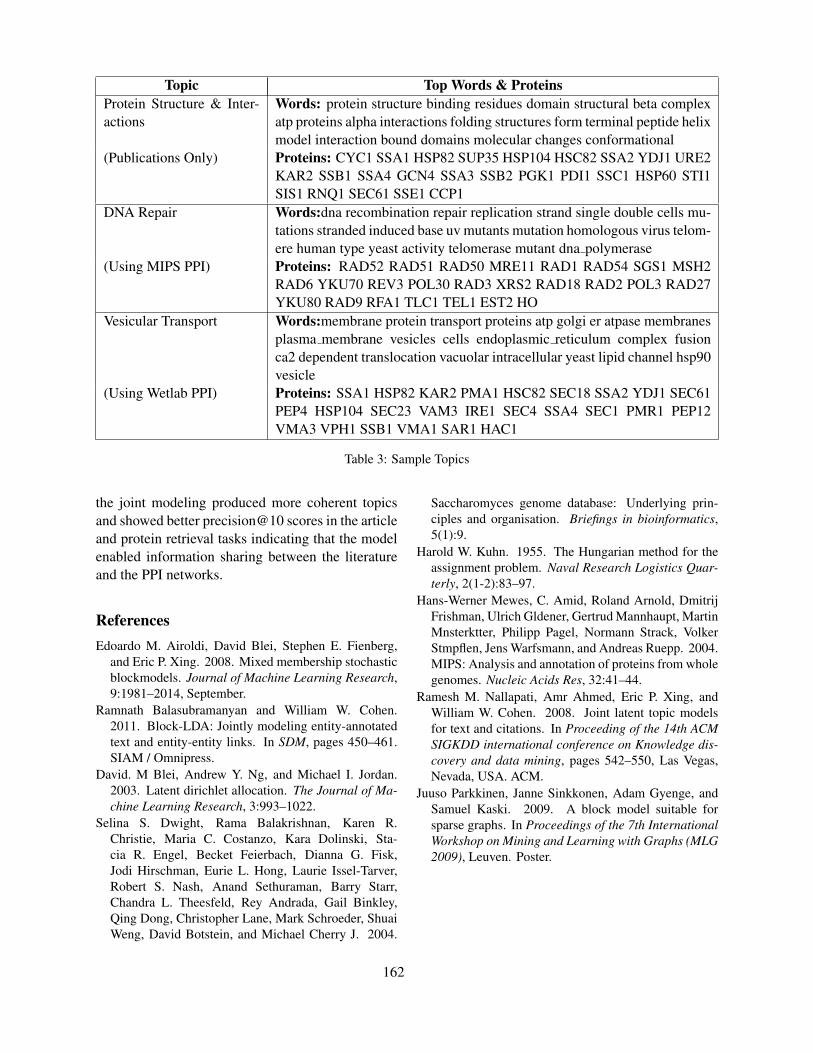
Topic Top Words & ProteinsProtein Structure & Inter-actions
Words: protein structure binding residues domain structural beta complexatp proteins alpha interactions folding structures form terminal peptide helixmodel interaction bound domains molecular changes conformational
(Publications Only) Proteins: CYC1 SSA1 HSP82 SUP35 HSP104 HSC82 SSA2 YDJ1 URE2KAR2 SSB1 SSA4 GCN4 SSA3 SSB2 PGK1 PDI1 SSC1 HSP60 STI1SIS1 RNQ1 SEC61 SSE1 CCP1
DNA Repair Words:dna recombination repair replication strand single double cells mu-tations stranded induced base uv mutants mutation homologous virus telom-ere human type yeast activity telomerase mutant dna polymerase
(Using MIPS PPI) Proteins: RAD52 RAD51 RAD50 MRE11 RAD1 RAD54 SGS1 MSH2RAD6 YKU70 REV3 POL30 RAD3 XRS2 RAD18 RAD2 POL3 RAD27YKU80 RAD9 RFA1 TLC1 TEL1 EST2 HO
Vesicular Transport Words:membrane protein transport proteins atp golgi er atpase membranesplasma membrane vesicles cells endoplasmic reticulum complex fusionca2 dependent translocation vacuolar intracellular yeast lipid channel hsp90vesicle
(Using Wetlab PPI) Proteins: SSA1 HSP82 KAR2 PMA1 HSC82 SEC18 SSA2 YDJ1 SEC61PEP4 HSP104 SEC23 VAM3 IRE1 SEC4 SSA4 SEC1 PMR1 PEP12VMA3 VPH1 SSB1 VMA1 SAR1 HAC1
Table 3: Sample Topics
the joint modeling produced more coherent topicsand showed better precision@10 scores in the articleand protein retrieval tasks indicating that the modelenabled information sharing between the literatureand the PPI networks.
ReferencesEdoardo M. Airoldi, David Blei, Stephen E. Fienberg,
and Eric P. Xing. 2008. Mixed membership stochasticblockmodels. Journal of Machine Learning Research,9:1981–2014, September.
Ramnath Balasubramanyan and William W. Cohen.2011. Block-LDA: Jointly modeling entity-annotatedtext and entity-entity links. In SDM, pages 450–461.SIAM / Omnipress.
David. M Blei, Andrew Y. Ng, and Michael I. Jordan.2003. Latent dirichlet allocation. The Journal of Ma-chine Learning Research, 3:993–1022.
Selina S. Dwight, Rama Balakrishnan, Karen R.Christie, Maria C. Costanzo, Kara Dolinski, Sta-cia R. Engel, Becket Feierbach, Dianna G. Fisk,Jodi Hirschman, Eurie L. Hong, Laurie Issel-Tarver,Robert S. Nash, Anand Sethuraman, Barry Starr,Chandra L. Theesfeld, Rey Andrada, Gail Binkley,Qing Dong, Christopher Lane, Mark Schroeder, ShuaiWeng, David Botstein, and Michael Cherry J. 2004.
Saccharomyces genome database: Underlying prin-ciples and organisation. Briefings in bioinformatics,5(1):9.
Harold W. Kuhn. 1955. The Hungarian method for theassignment problem. Naval Research Logistics Quar-terly, 2(1-2):83–97.
Hans-Werner Mewes, C. Amid, Roland Arnold, DmitrijFrishman, Ulrich Gldener, Gertrud Mannhaupt, MartinMnsterktter, Philipp Pagel, Normann Strack, VolkerStmpflen, Jens Warfsmann, and Andreas Ruepp. 2004.MIPS: Analysis and annotation of proteins from wholegenomes. Nucleic Acids Res, 32:41–44.
Ramesh M. Nallapati, Amr Ahmed, Eric P. Xing, andWilliam W. Cohen. 2008. Joint latent topic modelsfor text and citations. In Proceeding of the 14th ACMSIGKDD international conference on Knowledge dis-covery and data mining, pages 542–550, Las Vegas,Nevada, USA. ACM.
Juuso Parkkinen, Janne Sinkkonen, Adam Gyenge, andSamuel Kaski. 2009. A block model suitable forsparse graphs. In Proceedings of the 7th InternationalWorkshop on Mining and Learning with Graphs (MLG2009), Leuven. Poster.
162
Proceedings of the 2012 Workshop on Biomedical Natural Language Processing (BioNLP 2012), pages 163–171,Montreal, Canada, June 8, 2012. c©2012 Association for Computational Linguistics
RankPref: Ranking Sentences Describing Relationsbetween Biomedical Entities with an Application
Catalina O Tudor K Vijay-ShankerDepartment of Computer and Information Sciences
University of Delaware, Newark, DE, [email protected] [email protected]
Abstract
This paper presents a machine learning ap-proach that selects and, more generally, rankssentences containing clear relations betweengenes and terms that are related to them. Thisis treated as a binary classification task, wherepreference judgments are used to learn how tochoose a sentence from a pair of sentences.Features to capture how the relationship is de-scribed textually, as well as how central therelationship is in the sentence, are used in thelearning process. Simplification of complexsentences into simple structures is also appliedfor the extraction of the features. We show thatsuch simplification improves the results by upto 13%. We conducted three different evalu-ations and we found that the system signifi-cantly outperforms the baselines.
1 Introduction
Life scientists, doctors and clinicians often searchfor information relating biological concepts. For ex-ample, a doctor might be interested to know the im-pact of a drug on some disease. One source of infor-mation is the knowledge bases and ontologies thatare manually curated with facts from scientific arti-cles. However, the curation process is slow and can-not keep up with ongoing publications. Moreover,not all associations between biological concepts canbe found in these databases.
Another source of information is the scientificliterature itself. However, searching for biologicalfacts and how they might be related is often cumber-some. The work presented in this paper tries to au-tomate the process of finding sentences that clearly
describe relationships between biological concepts.We rank all sentences mentioning two concepts andpick the top one to show to the user. In this paper, wefocused on certain specific types of concepts (i.e.,genes1 and terms believed to be related to them), al-though our approach can be generalized.
Systems to facilitate knowledge exploration ofgenes are being built for the biomedical domain.One of them, eGIFT (Tudor et al., 2010), tries toidentify iTerms (informative terms) for a gene basedon frequency of co-occurrence (see Figure 1 for top15 terms selected for gene Groucho). iTerms areunigrams, bigrams, and exact matches of biomedi-cal terms gathered from various controlled vocabu-laries. Thus, iTerms can be of any type (e.g., pro-cesses, domains, drugs, other genes, etc.), the typesbeing determined by what is being described aboutthe gene in the literature. The iTerms for a geneare ranked based on a score that compares their fre-quencies of occurrence in publications mentioningthe gene in question with their frequencies in a back-ground set of articles about a wide variety of genes.
Previous evaluation of eGIFT by life scientistssuggested that there is almost always some kind ofrelationship between a gene and its iTerms. Theserelationships can be many and varied from one gene-term pair to another. Sometimes a user might makean erroneous assumption about a gene-term asso-ciation if sentences supporting the association arenot immediately inspected. For example, upon see-ing “co-repressor” in connection to gene Groucho,eGIFT users might correctly assume that Groucho is
1Throughout the paper, the word “gene” will be used forboth the gene and its products.
163

Figure 1: Top iTerms for gene Groucho, and sentences picked by RankPref for various iTerms.
a co-repressor (i.e., a protein that binds to transcrip-tion factors). However, upon seeing “wrpw motif”,a user might assume that this is a motif containedwithin gene Groucho, as this is typically the asso-ciation that we make between genes and informa-tion annotated for them in knowledge bases. Butthis would be a wrong assumption, since in actualitythe wrpw motif is contained within other genes thatinteract with Groucho, fact which is evident fromreading sentences containing the gene and the mo-tif. To get a quick overall understanding of a gene’sfunctionalities, users of eGIFT could be presentedwith terms extracted for the gene, as well as sen-tences clearly describing how they are related.
Our method selects sentences using a model thatis trained on preference judgments provided by biol-ogists. Example sentences chosen by our method areshown in Figure 1. While we evaluate our approachon sentences from eGIFT, this work could haveequally applied on other similar systems (Smal-heiser et al., 2008; Gladki et al., 2008; Kim et al.,2008; Kaczanowski et al., 2009). These systemsalso identify “important terms” from a set of doc-uments retrieved for a given search (either a genename or other biomedical concept).
The main contributions of this work are: (1) amethod for ranking sentences by employing ma-chine learning; (2) the use of preference judgments;(3) features to capture whether two terms are clearlyrelated and in focus in a sentence; (4) another appli-cation of sentence simplification, showing a signifi-cant gain in performance when utilized.
We continue with a description of our approach,which includes the use of preference judgments tolearn the models, how the features are extracted, andhow the sentence simplifier is used for this task. Theevaluation of the trained model and the system’s re-sults are presented in the following section. Re-lated work, conclusions, and future directions areprovided at the end of the manuscript.
2 Methods
Rather than pre-judging what is important for thistask and manually determining a weighting schemato automatically score sentences for a gene-termpair, we approached this task using machine learn-ing. We asked a group of annotators to rank sen-tences relating genes and iTerms, and we used theirannotations, together with features described in Sec-tion 2.3, to learn how to rank sentences.
164

2.1 Preference Judgments
For the annotation task, we presented biologists withsentences containing a gene-term pair and askedthem to specify which sentence they prefer. Oneway to do this is by employing the pointwise ap-proach, which requires absolute judgments (i.e. theannotator scores each sentence in a list or ranks thesentences based on their relevance to the given task).A second approach is the pairwise approach, whichrequires the iteration of preference judgments (i.e.,the annotator is presented with two sentences at atime, and is asked to chose one as more relevant tothe task than the other).
In order to simplify the annotator’s task, as wellas construct a more reliable training set, we used thepairwise approach. Our decision was influenced byCarterette et al. (2008), who showed that preferencejudgments are faster and easier to make than abso-lute judgments. Thus, we can obtain many annotatedinstances in a relatively short amount of time. More-over, since there are only two possible outcomes inchoosing one sentence, we need at most three judgesfor a majority vote. This will also ensure consistencyin the annotations. We discuss the model trained onpreference judgments in Section 2.2.
2.2 Learned Models: PrefSVM and RankPref
We used the preference judgments to learn a model,PrefSVM, that picks one sentence from a pair of sen-tences. This model was built using SVMLight witha linear kernel. The examples used in the learningprocess correspond to pairs of sentences. For eachpair, we constructed a vector of feature values, bysubtracting the feature values corresponding to thefirst sentence from the feature values correspondingto the second sentence. We assigned a positive valueto a pair vector if the first sentence was preferred anda negative value if the second one was preferred.
We can also use PrefSVM to design a system thatcan rank all the sentences containing a gene andan iTerm, by performing comparisons between sen-tences in the list. We call RankPref the system thatpicks one sentence from a group of sentences, andwhich also ranks the entire set of sentences. Thismethod recursively applies PrefSVM in the followingmanner: Two sentences are randomly picked froma given list of sentences. PrefSVM chooses one sen-
tence and discards the other. A third sentence is thenrandomly picked from the list, and PrefSVM makesits choice by comparing it to the sentence kept in theprevious step. This process of picking, comparingand discarding sentences is continued until there isonly one sentence left. We keep track of comparisonresults and apply transitivity, in order to speed up theprocess of ranking all the sentences.
2.3 Features
Each sentence is first chunked into base phrases. Weused Genia Tagger (Tsuruoka et al., 2005), whichprovides part-of-speech tags for every word in thesentence. We trained a chunker (i.e., shallow parserthat identifies base NPs) using the Genia corpus.
We considered typical features that are used inmachine learning approaches, such as distance be-tween gene and iTerm, length of sentence, etc.Moreover, we included additional groups of featuresthat we felt might be important for this task: onegroup to capture how the relationship is describedtextually, another group to capture how central therelationship is in terms of what is being described inthe sentence, and the last to capture whether the re-lation is stated as a conjecture or a fact. The weightsfor these features will be determined automaticallyduring the learning process and they will be depen-dent on whether or not the features were effective,given the annotation set.
The first type of features is to capture how therelationship is described textually. As an example,consider the sentence “Bmp2 stimulates osteoblas-tic differentiation”2, where the gene and the iTermare in subject and object (direct object or otherwise)positions, and the verb is a common biological verb.Thus, we constructed a set of lexico-syntactic pat-terns to capture the different kinds of argument re-lations served by the two concepts. We grouped 25lexico-syntactic patterns into 8 groups, correspond-ing to different relational constructions that can ex-ist between a gene and an iTerm. Example patternsare shown in Table 1 for each group, and the sym-bols used in these patterns are explained in Table 2.When a sentence matches a pattern group, the corre-sponding value is set to 1 for that feature.
2In our examples, the gene will be marked in italics and theiTerm will be marked in bold.
165

Group Example PatternG1 G VG+ IG2 G/I via/by/through I/GG3 G VG+ (NP/PP)* by/in VBG IG4 G/I by/in VBG I/GG5 G/I VB I/GG6 G/I of I/GG7 G/I other preposition I/GG8 including/such as/etc. G/I and I/G
Table 1: Examples of lexico-syntactic patterns
For example, the following sentence, in whichthe gene is Lmo2 and the iTerm is “erythropoiesis”,matches the pattern in G1: [G VG+ I].
While Tal1 has been shown to induce ery-throid differentiation , Lmo2 appears to sup-press fetal erythropoiesis.
where “Lmo2” matches G, “appears to suppress”matches VG+, and “fetal erythropoiesis” matches I.
Notice how the verb plays an important role inthe patterns of groups G1, G3, G4, and G5. We alsohave a verb type feature which differentiates groupsof verbs having the gene and the iTerm as arguments(e.g., “activates”, “is involved in”, “plays a role”,etc. are treated as different types).
The second type of features captures how cen-tral the relationship is in terms of what is being de-scribed in the sentence. The subject feature recordswhether the gene and iTerm appear in the subjectposition, as this will tell us if they are in focus inthe sentence. While we do not parse the sentence,we take a simplified sentence (see Section 2.4) andsee if the gene/term appear in a noun phrase pre-ceding the first tensed verb. Another feature, thegene-iTerm position, measures how close the geneand the term are to each other and to the beginningof the sentence, as this makes it easier for a readerto grasp the relation between them. For this, we addthe number of words occurring to the left of the seg-ment spanning the gene and iTerm, and half of thenumber of words occurring between them. Finally,we included a headedness feature. The idea here isthat if the gene/term are not the head of the noungroup, but rather embedded inside, then this poten-tially makes the relation less straightforward. These
Symb DefinitionNP a base noun phrasePP a preposition followed by a base noun phrase
VG+ a series of one or more verb groupsVBG a verb group in which the head is a gerund verbVBN a verb group in which the head is a participle verbVB a verb group in which the head is a base verbG, I base noun phrases, with 0 or more prepositional
phrases, containing the gene/iTerm
Table 2: Symbols used in the pattern notation
groups are denoted by G and I in the patterns shownin Table 1.
The third type of features captures informationabout the sentence itself. The sentence complexityfeature is measured in terms of the number of verbs,conjunctions, commas, and parentheticals that oc-cur in the sentence. We use a conjecture feature fordetecting whether the sentence involves a hypothe-sis. We have a simple rule for this feature, by see-ing if words such as “may”, “could”, “probably”,“potentially”, etc., appear in proximity of the geneand iTerm. Additionally, we have a negation featureto detect whether the relationship is mentioned in anegative way. We look for words such as “not”, “nei-ther”, etc., within proximity of the gene and iTerm.
Although the features and lexico-syntactic pat-terns were determined by analyzing a developmentset of sentences containing genes and their iTerms,we believe that these features and patterns can beused to rank sentences involving other biomedicalentities, not just genes.
2.4 Sentence Simplification
Notice that the lexico-syntactic patterns are writtenas sequences of chunks and lexical tags. If a sen-tence matches a pattern, then the sentence expressesa relation between the gene and the iTerm. However,sometimes it is not possible to match a pattern if thesentence is complex.
For example, consider sentence A in Table 3, forgene Cd63. Let us assume that the iTerm is “prota-somes”. Clearly, there is a relationship between thegene and the iTerm, namely that Cd63 was found inpc-3 cell-derived protasomes. However, none of thelexico-syntactic patterns is able to capture this rela-tion, because of all the extra information between
166
A Cd63, an integral membrane protein foundin multivesicular lysosomes and secretorygranules, was also found in pc-3 cell-derived protasomes.
S1 Cd63 was found in pc-3 cell-derived pro-tasomes.
S2 Cd63 is an integral membrane protein.
CS1 Cd63 is found in multivesicular lyso-somes.
CS2 Cd63 is found in secretory granules.
Table 3: Simplified sentences for gene Cd63. ExampleiTerms: “protasomes” and “secretory granules”.
the gene and the term. While we may have multi-ple patterns in each group, we cannot necessarily ac-count for each lexical variation at this level of gran-ularity.
We are using a sentence simplifier, built in-house,to ensure a match where applicable. The simpli-fier identifies appositions, relative clauses, and con-junctions/lists of different types, using regular ex-pressions to match chunked tags. In the sentenceof Table 3, the simplifier recognizes the apposition“an integral membrane protein”, the reduced relativeclause “found in multivesicular bodies/lysosomesand secretory granules” and the noun conjunction“multivesicular bodies/lysosome and secretory gran-ules”. It then produces several simplified sentencescontaining the gene. S1 and S2, shown in Table 3,are simplified sentences obtained from the simpli-fier. CS1 and CS2 are additional simplified sen-tences, which required the combination of multiplesimplifications: the appositive, the relative clause,and the noun conjunction.
Notice how each of the simplified sentencesshown in Table 3 is now matching a pattern group.If we are interested in the relationship between Cd63and “protasomes”, we can look at S1. Likewise, ifwe are interested in the relationship between Cd63and “secretory granules”, we can look at CS2.
We have a matching feature that tells whether thepattern was matched in the original sentence, a sim-plified sentence, or a combined sentence, and thisfeature is taken into account in the learning process.
3 Results and Discussion
We evaluated both PrefSVM and RankPref. Each re-quired a different set of annotated data. For theevaluation of PrefSVM, we used the preference judg-ments and leave-one-out cross validation. And forthe evaluation of RankPref, we asked the annota-tors to order a group of sentences mentioning gene-iTerm pairs. Six life science researchers, with grad-uate degrees, annotated both sets.
3.1 Evaluation of PrefSVM
First, we evaluated the performance of PrefSVM us-ing leave-one-out cross validation.
3.1.1 Annotation of Preference JudgementsWe started by selecting a group of pairs of sen-
tences. We randomly picked gene-iTerm combi-nations, and for each combination, we randomlypicked two sentences containing both the gene andthe term. To alleviate bias, the order of the sentenceswas chosen randomly before displaying them to theannotators. In our guidelines, we asked the annota-tors to choose sentences that clearly state the rela-tionship between the gene and the iTerm. Becausethe focus here is on the relationship between the twoterms, we also asked them to refrain from choos-ing sentences that describe additional information orother aspects. It is conceivable that, for other appli-cations, extra information might be an important de-termining factor, but for our task we wanted to focuson the relationship only.
For each pair of sentences, we wanted to havethree opinions so that we can have a majority vote.To alleviate the burden on the annotators, we startedby giving each pair of sentences to two annotators,and asked for an extra opinion only when they didnot agree. Each biologist was given an initial setof 75 pairs of sentences to annotate, and shared thesame amount of annotations (15) with each of theother biologists. 225 unique pairs of sentences werethus annotated, but six were discarded after the an-notators informed us that they did not contain thegene in question.
In 34 out of 219 pairs of sentences, the two biol-ogists disagreed on their annotations. These casesincluded pairs of similar sentences, or pairs of sen-tences that did not describe any relationship between
167

System Performance CorrectBaseline 1 65.75% 144Baseline 2 71.69% 157PrefSVM without Simp 72.14% 158PrefSVM with Simp 83.10% 182
Table 4: Results for PrefSVM
the gene and the iTerm. An example of sentences forwhich the annotators could not agree is:
1. The tle proteins are the mammalian ho-mologues of gro, a member of the drosophilanotch signaling pathway.2. In drosophila, gro is one of the neurogenicgenes that participates in the notch signallingpathway .
For these 34 pairs, we randomly selected anotherannotator and considered the majority vote.
3.1.2 BaselinesWe chose two baselines against which to com-
pare PrefSVM. The first baseline always choosesthe shortest sentence. For the second baseline, welooked at the proximity of the gene/term to the be-ginning of the sentence, as well as the proximity ofthe two to each other, and chose the sentence thathad the lowest accumulated proximity. The reasonfor this second baseline is because the proximity ofthe gene/term to the beginning of the sentence couldmean that the sentence focuses on the gene/term andtheir relation. Furthermore, the proximity of thegene to the iTerm could mean a clearer relation be-tween them.
3.1.3 ResultsWe evaluated PrefSVM by performing leave-one-
out cross validation on the set of 219 pairs of sen-tences. Each pair of sentences was tested by usingthe model trained on the remaining 218 pairs. Theresults are shown in Table 4.
The first baseline performed at 65.75%, correctlychoosing 144 of 219 sentences. The second base-line performed slightly better, at 71.69%. PrefSVMoutperformed both baselines, especially when thesentence simplifier was used, as this facilitated thematch of the lexico-syntactic patterns used as fea-tures. PrefSVM performed at 83.10%, which is
17.35% better than the first baseline, and 11.41%better than the second baseline.
3.2 Evaluation of RankPref
The previous evaluation showed how PrefSVM per-forms at picking a sentence from a pair of sentences.But ultimately, for the intended eGIFT application,the system needs to choose one sentence from many.We evaluated RankPref for this task.
3.2.1 Annotating Data for Sentence SelectionFor this evaluation, we needed to create a different
set of annotated data that reflects the selection of onesentence from a group of sentences.
Since a gene and an iTerm can appear in manysentences, it is too onerous a task for a human anno-tator to choose one out of tens or hundreds of sen-tences. For this reason, we limited the set of sen-tences mentioning a gene and an iTerm to only 10.We randomly picked 100 gene-term pairs and for thepairs that contained more than ten sentences, we ran-domly chose ten of them. On average, there were 9.4sentences per set.
We asked the same annotators as in the previousevaluation to participate in this annotation task. Be-cause the task is very time consuming, and becauseit is hard to decide how to combine the results frommultiple annotators, we assigned each set of sen-tences to only one annotator. We showed the sen-tences in a random order so that biasing them wouldnot be an issue.
We initially asked the annotators to order the sen-tences in the set. However, this task proved to be im-possible, since many sentences were alike. Instead,we asked the annotators to assign them one of threecategories:
(Cat.1) Any sentence in this category could beconsidered the “best” among the choices provided;
(Cat.2) These sentences are good, but there areother sentences that are slightly better;
(Cat.3) These sentences are not good or at leastthere are other sentences in this set that are muchbetter.
Classifying the sentences into these categorieswas less cumbersome, fact which was confirmed byour evaluators after a trial annotation.
Out of the total of 936 sentences, 322 (34.4%)were placed in the first category, 332 (35.5%) were
168
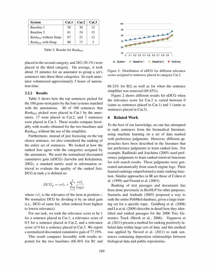
System Cat.1 Cat.2 Cat.3Baseline 1 58 30 12Baseline 2 61 24 15RankPref without Simp 67 21 12RankPref with Simp 80 17 3
Table 5: Results for RankPref
placed in the second category, and 282 (30.1%) wereplaced in the third category. On average, it tookabout 15 minutes for an annotator to group a set’ssentences into these three categories. So each anno-tator volunteered approximately 5 hours of annota-tion time.
3.2.2 ResultsTable 5 shows how the top sentences picked for
the 100 gene-term pairs by the four systems matchedwith the annotations. 80 of 100 sentences thatRankPref picked were placed in Cat.1 by the anno-tators, 17 were placed in Cat.2, and 3 sentenceswere placed in Cat.3. These results compare favor-ably with results obtained for the two baselines andRankPref without the use of the simplifier.
Furthermore, instead of just focussing on the topchoice sentence, we also considered the ranking ofthe entire set of sentences. We looked at how theranked lists agree with the categories assigned bythe annotators. We used the normalized discountedcumulative gain (nDCG) (Jarvelin and Kekalainen,2002), a standard metric used in information re-trieval to evaluate the quality of the ranked lists.DCG at rank p is defined as:
DCGp = rel1 +p∑
i=2
relilog2i
where reli is the relevance of the item at position i.We normalize DCG by dividing it by an ideal gain(i.e., DCG of same list, when ordered from highestto lowest relevance).
For our task, we took the relevance score to be 1for a sentence placed in Cat.1, a relevance score of0.5 for a sentence placed in Cat.2, and a relevancescore of 0 for a sentence placed in Cat.3. We reporta normalized discounted cumulative gain of 77.19%.
This result compares favorably with results re-ported for the two baselines (68.36% for B1 and
Figure 2: Distribution of nDCG for different relevancescores assigned to sentences placed in category Cat.2.
68.32% for B2) as well as for when the sentencesimplifier was removed (69.45%).
Figure 2 shows different results for nDCG whenthe relevance score for Cat.2 is varied between 0(same as sentences placed in Cat.1) and 1 (same assentences placed in Cat.3).
4 Related Work
To the best of our knowledge, no one has attemptedto rank sentences from the biomedical literature,using machine learning on a set of data markedwith preference judgments. However, different ap-proaches have been described in the literature thatuse preference judgments to learn ranked lists. Forexample, Radlinski and Joachims (2005) used pref-erence judgments to learn ranked retrieval functionsfor web search results. These judgments were gen-erated automatically from search engine logs. Theirlearned rankings outperformed a static ranking func-tion. Similar approaches in IR are those of Cohen etal. (1999) and Freund et al. (2003).
Ranking of text passages and documents hasbeen done previously in BioNLP for other purposes.Suomela and Andrade (2005) proposed a way torank the entire PubMed database, given a large train-ing set for a specific topic. Goldberg et al. (2008)and Lu et al. (2009) describe in detail how they iden-tified and ranked passages for the 2006 Trec Ge-nomics Track (Hersh et al., 2006). Yeganova etal. (2011) present a method for ranking positively la-beled data within large sets of data, and this methodwas applied by Neveol et al. (2011) to rank sen-tences containing deposition relationships betweenbiological data and public repositories.
169
Extraction of sentences describing gene functionshas also been applied for creating gene summaries(Ling et al., 2007; Jin et al., 2009; Yang et al., 2009).However, these methods differ in that their goal isnot to look for sentences containing specific termsand their relations with genes, but rather for sen-tences that fall into some predefined categories ofsentences typically observed in gene summaries.
Sentence simplification has been used to aid pars-ing (Chandrasekar et al., 1996; Jonnalagadda etal., 2009). Devlin and Tait (1998) and Carroll etal. (1998) use it to help people with aphasia. Sid-dharthan (2004) was concerned with cohesion andsuggested some applications.
The idea of using lexico-syntactic patterns toidentify relation candidates has also been applied inthe work of Banko et al. (2007), although their pat-terns are not used in the learning process.
5 Conclusion and Future Directions
We have developed a system which aims to identifysentences that clearly and succinctly describe the re-lation between two entities. We used a set of prefer-ence judgements, as provided by biologists, to learnan SVM model that could make a choice betweenany two sentences mentioning these entities.
The model compares favorably with baselines onboth the task of choosing between two sentences, aswell as ranking a set of sentences. The performancefor choosing between two sentences was 83.10%, ascompared to 65.75% and 71.69% for the two base-lines, respectively. For choosing one sentence froma list of sentences, the performance was 80%, ascompared to 58% and 61%. Furthermore, when theentire list of ranked sentences was evaluated, thesystem reported a nDCG of 77.19%, compared to68.36% and 68.32% for the two baselines.
The model’s performance was also shown tobe significantly better when sentence simplificationwas used. We were able to match relation patternson complex sentences, and observed an increase of10.96%, 13%, and 7.74% for the three evaluationsafore-mentioned, respectively. It is noteworthy that,without the simplification, the performance is onlyslightly better than the second baseline. This is be-cause the second baseline uses information that isalso used by our system, although this does not in-
clude the lexico-syntactic patterns that identify thetype of relation between the gene and the term.
Given that the full system’s performance is muchbetter than both baselines, and that the system’s per-formance without simplification is only slightly bet-ter than the second baseline, we believe that: (1) thepattern and type of relation determination are impor-tant, and (2) sentence simplification is crucial for thedetermination of the relationship type.
We are currently pursuing summaries for genes.Since iTerms have been shown in previous evalua-tions to represent important aspects of a gene’s func-tionality and behavior, we are investigating whetherthey are represented in gene summaries found in En-trezGene and UniProtKB. If so, an extractive sum-mary can be produced by choosing sentences for thegene and its iTerms. We are also considering de-veloping abstractive summaries. Our use of lexico-syntactic patterns can be extended to pick the exactrelation between a gene and the iTerm. For exam-ple, by using the lexico-syntactic patterns, coupledwith simplification, we can extract the following ex-act relations from the four sentences shown in Fig-ure 1: “Groucho is a corepressor”, “The wrpw motifrecruits groucho”, “Groucho is implicated in notchsignaling”, and “The eh1 repression domain bindsgroucho”. With these relations extracted, using textgeneration algorithms for textual realization and co-hesion, we can produce abstractive summaries.
We would also like to investigate how to general-ize this work to other pairs of entities, as well as howto generalize this work for other applications whichmay or may not require the same features as the oneswe used.
Acknowledgments
This work has been supported in part by USDAGrant 2008-35205-18734 and the Agriculture andFood Research Initiative Competitive USDA Grant2011-67015-3032. We thank Cecilia Arighi, KevinBullaughey, Teresia Buza, Fiona McCarthy, Lak-shmi Pillai, Carl Schmidt, Liang Sun, Hui Wang,and Qinghua Wang for participating in the anno-tation task and/or for various discussions. Wealso thank the anonymous reviewers for their com-ments and suggestions, which helped us improve themanuscript.
170

ReferencesMichele Banko, Michael J Cafarella, Stephen Soderland,
Matt Broadhead, and Oren Etzioni. 2007. Open In-formation Extraction from the Web. In Proceedings ofIJCAI.
John Carroll, Guido Minnen, Yvonne Canning, SiobhanDevlin, and John Tait. 1998. Practical simplificationof English newspaper text to assist aphasic readers.Proceedings of the AAAI98 Workshop on IntegratingAI and Assistive Technology, pages 7–10.
Ben Carterette, Paul N Bennett, David Maxwell Chicker-ing, and Susan T Dumais. 2008. Here or there: Pref-erence judgments for relevance. In Proceedings of theIR research, 30th European conference on Adv. in IR.
R Chandrasekar, Christine Doran, and B Srinivas. 1996.Motivations and methods for text simplification. InProceedings of the 16th conference on Computationallinguistics, volume 2, pages 1041–1044. Associationfor Computational Linguistics.
Wiliam W Cohen, Robert E Schapire, and Yoram Singer.1999. Learning to order things. Journal of ArtificialIntelligence Research, 10:243–270.
Siobhan Devlin and John Tait. 1998. The use of a psy-cholinguistic database in the simplification of text foraphasic readers. Linguistic Databases, pages 161–173.
Yoav Freund, Raj Iyer, Robert E Schapire, and YoramSinger. 2003. An efficient boosting algorithm forcombining preferences. Journal of Machine LearningResearch, 4:933–969.
Arek Gladki, Pawel Siedlecki, Szymon Kaczanowski,and Piotr Zielenkewicz. 2008. e-LiSe–an online toolfor finding needles in the ’Medline haystack’. Bioin-formatics, 24(8):1115–1117.
Andrew B Goldberg, David Andrzejewski, Jurgen VanGael, Burr Settles, Xiaojin Zhu, and Mark Craven.2008. Ranking biomedical passages for relevance anddiversity. In Proceedings of TREC.
William Hersh, Aaron M Cohen, Phoebe Roberts, andHari Krishna Rekapalli. 2006. TREC 2006 GenomicsTrack Overview.
Kalervo Jarvelin and Jaana Kekalainen. 2002. Cumu-lated gain-based evaluation of IR techniques. ACMTransactions on Information Systems, 20(4):422–446.
Feng Jin, Minlie Huang, Zhiyong Lu, and Xiaoyan Zhu.2009. Towards automatic generation of gene sum-mary. In Proceedings of the BioNLP 2009 Work-shop, pages 97–105. Association for ComputationalLinguistics, June.
Siddhartha Jonnalagadda, Luis Tari, Jorg Hakenberg,Chitta Baral, and Graciela Gonzalez. 2009. Towardseffective sentence simplification for automatic pro-cessing of biomedical text. In Proceedings of NAACLHLT 2009: Short Papers, pages 177–180.
Szymon Kaczanowski, Pawel Siedlecki, and Piotr Zie-lenkewicz. 2009. The high throughput sequenceannotation service (HT-SAS) - the shortcut from se-quence to true medline words. BMC Bioinformatics,10:148–154, May.
Jung-Jae Kim, Piotr Pezik, and Dietrich Rebholz-Schuhmann. 2008. MedEvi: Retrieving textual evi-dence of relations between biomedical concepts frommedline. Bioinformatics, 24(11):1410–1412.
Xu Ling, Jing Jiang, Xin He, Qiaozhu Mei, Chengxi-ang Zhai, and Bruce Schatz. 2007. Generating genesummaries from biomedical literature: A study ofsemi-structured summarization. Information Process-ing and Management, 43:1777–1791, March.
Yue Lu, Hui Fang, and Chengxiang Zhai. 2009. Anempirical study of gene synonym query expansionin biomedical information retrieval. Information Re-trieval, 12:51–68, February.
Aurelie Neveol, W John Wilbur, and Zhiyong Lu. 2011.Extraction of data deposition statements from the lit-erature: a method for automatically tracking researchresults. Bioinformatics, 27(23):3306–3312.
Filip Radlinski and Thorsten Joachims. 2005. Querychains: Learning to rank from implicit feedback. InProceedings of KDD’05.
Advaith Siddharthan. 2004. Syntactic Simplification andText Cohesion. Ph.D. thesis, University of Cambridge.
Neil R Smalheiser, Wei Zhou, and Vetle I Torvik. 2008.Anne O’Tate: A tool to support user-driven summa-rization, drill-down and browsing of PubMed searchresults. Journal of Biomedical Discovery and Collab-oration, 3(1):2–11.
Brian P Suomela and Miguel A Andrade. 2005. Rank-ing the whole MEDLINE database according to a largetraining set using text indexing. BMC Bioinformatics,6(75), March.
Yoshimasa Tsuruoka, Yuka Tateishi, Jing-Dong Kim,Tomoko Ohta, John McNaught, Sophia Ananiadou,and Jun’ichi Tsujii. 2005. Developing a robust part-of-speech tagger for biomedical text. In Advances inInformatics – 10th Panhellenic Conference on Infor-matics, LNCS 3746, pages 382–392.
Catalina O Tudor, Carl J Schmidt, and K Vijay-Shanker.2010. eGIFT: Mining Gene Information from the Lit-erature. BMC Bioinformatics, 11:418.
Jianji Yang, Aaron Cohen, and William Hersh. 2009.Evaluation of a gene information summarization sys-tem by users during the analysis process of microarraydatasets. BMC Bioinformatics, 10(Suppl 2):S5.
Lana Yeganova, Donald C Comeau, Won Kim, andW John Wilbur. 2011. Text Mining Techniques forLeveraging Positively Labeled Data. In Proceedingsof ACL Workshop BioNLP, pages 155–163.
171
Proceedings of the 2012 Workshop on Biomedical Natural Language Processing (BioNLP 2012), pages 172–175,Montreal, Canada, June 8, 2012. c©2012 Association for Computational Linguistics
Finding small molecule and protein pairs in scientific literature using a
bootstrapping method
Ying Yan, Jee-Hyub Kim, Samuel Croset, Dietrich Rebholz-Schuhmann
European Bioinformatics InstituteWellcome Trust Genome Campus
HinxtonCambridge
UK{yan, jhkim, croset, rebholz}@ebi.ac.uk
Abstract
The relationship between small moleculesand proteins has attracted attention from thebiomedical research community. In this pa-per a text mining method of extracting small-molecule and protein pairs from natural textis presented, based on a semi-supervised ma-chine learning approach. The technique hasbeen applied to the complete collection ofMEDLINE abstracts and pairs were extractedand evaluated. The results show the feasibilityof the bootstrapping system, which will subse-quently be further investigated and improved.
1 Introduction
Information extraction has become a major task intext-mining. A large number of studies have beencarried out with the objective of developing tech-niques to overcome the highly ambiguous and vari-able nature of natural language for the extraction ofinformation from scientific text (Song et al., 2006).Natural language processing (NLP) of biomedicaltext has been initiated and used for different knowl-edge discovery tasks such as the extraction of rela-tionships between different types of biological ob-jects.
Relationships between proteins and smallmolecules are of particular concern in the biomed-ical research domain. The importance of targetspecific small molecule research is vital in thescientific community’s understanding of numerousbiological processes with potential discoveriesyielding various translational benefits and outcomesto public health and industry. While there has been
a great number of traditional studies already com-pleted in this field, the underlying difficulty with thistype of research has been trying to understand howone molecule interacts with a target protein. Giventhe biological background, many researchers inCheminformatics and Metabolomics are attemptingto find the connections between small moleculesand other biological entities in order to bridge thechemical and biological domains.
Of the few reported text mining approaches to thisproblem, Temkin and Gilder (2003) was concernedwith the extraction of protein and small molecule in-teraction, and used a rule-based approach utilisinga lexical analyser and context free grammar. Jiaoand Wild (2009) presented a technique for detect-ing protein and small molecule interaction using amaximum entropy based learning method; this workalso uses corpus-based machine learning. The maindrawback of both of these studies is that they requirea fully annotated corpus which is difficult to gener-ate.
1.1 The bootstrapping method
At present a gold standard annotated corpus is notavailable, and constructing a reasonable annotatedcorpus would require an infeasible amount of man-ual work. Our proposed solution to this problemis to develop a semi-supervised machine learningmethod. In this paper a bootstrapping algorithm ispresented which requires only unannotated trainingtexts and a handful of protein small molecule pairs,known as seeds. The basic work of a bootstrap-ping system can be presented as an expansion en-gine which uses the initial seed pairs fed into the
172

system to generate patterns that are used, in turn, tofind more pairs. The operation of the algorithm iscontrolled by certain criteria that are delivered froma measurement of the quality or selectivity of pat-terns and discovered pairs.
Bootstrapping systems have been maturely usedfor information extraction purposes in other researchdomains, and it has been empirically shown to bea powerful method in learning lexico-syntactic pat-terns for extracting specific relations (Riloff andJones, 1999). Bootstrapping systems can operatewith a greatly reduced number of training examples.A bootstrapping system seems promising for thepurpose of relation extraction, making it a suitablecandidate method for protein and small moleculepair extraction.
2 Implementation
The typical bootstrapping method was tailored inorder to improve its suitability for our extractiontask, operating in the biomedical literature resourceMEDLINE. The bootstrapping architecture is pre-sented in Figure 1. The whole collection of MED-LINE was filtered using a co-occurrence approachand a named entity recogniser. In this way thesentences which contained both a protein and asmall molecule were selected. The structure of pat-terns which are suitable to extract protein and smallmolecule pairs from MEDLINE was defined. Eachsentence is tokenized and then normalised based onthe results of syntactic parsing in order to obtain amore generalised view of the pattern. In the fol-lowing sections, we describe in more detail these as-pects.
2.1 Protein and small molecule recognition
Two dictionary-based named entity recogniserswere used to detect the names of proteins and smallmolecules in the full collection of MEDLINE ab-stracts, with the two source dictionaries constructedusing the resources UniProt (Apweiler et al., 2004)and ChEBI (De Matos et al., 2006) respectively. Thefollowing example shows the two recognisers iden-tify a chemical object and a protein object in a sen-tence from a MEDLINE extract:
<chebi>Paracetamol</chebi>, 100 mg/kg, in-hibited <uniprot>COX-1</uniprot> in stomach
Figure 1: Extraction system architecture
mucosa ex vivo much less effectively than in othertissues.
2.2 Sentence analysis for normalisation
It was anticipated that variations in tense and otherlanguage characteristics would cause problems inpattern generation. We therefore applied a list ofnormalisation steps for pattern generation. The sur-rounding context in the biomedical text is not nor-mally useful and makes it difficult to identify the textand observe a clear sentence structure. The parsingresult normalises patterns by eliminating non-usefulcomponents in a sentence. The step of normalisationhence increases the quality of the pattern.
The complete list of normalisation steps is as fol-lows:
1. Replaced the representation of measurementunits, such as mg/L and ml/day.
2. Employed the part-of-speech (POS) tagger GE-NIA (Tsuruoka et al., 2005) to analyse each to-ken, and the tokens which are weakly related tothe sentence structure were removed. So that,the only remaining tokens are the head noun ofa noun phrase (NP), the verb phrase, and prepo-sitional phrase chunks.
3. Finally a simple rule to identify the head nounwas defined. In a general case, for a NP se-quence, the last token is considered as the headnoun. When the last token is a single character,the second last token is considered as the headnoun.
173

Table 1: An example of a generated patternSeed tuple: Paracetamol, COX-1Found string: “CHEBI, UNIT, inhibit UNIPROTin mucosa than in tissue.”Pattern: NP List1, UNIT, inhibit NP List2Constraints: NP List1=“CHEBI*”
NP List2=“UNIPROT*”Keywords: “,UNIT,inhibit”
The above example after these normalisationsteps becomes:
CHEBI*, UNIT, inhibit UNIPROT* in mucosathan in tissue.
where CHEBI* and UNIPROT* are the seeds incontext.
2.3 Bootstrapping
The bootstrapping system is applied to the nor-malised sentences. The process starts with 100high precision protein small molecule pairs col-lected from the ChEBI ontology. These pairs wereretrieved by querying the ChEBI sub-ontology forthe relation “has role”. From the resulting data weextracted small molecules that are enzyme inhibitorstogether with the name of the enzyme.
2.3.1 Pattern generation and pair extraction
The concept of a bootstrapping system is that us-ing a high precision seed pair to start the extrac-tion engine, the system can effectively learn the pat-tern construction rule and the pattern constraints.Searching for the seed pairs in the corpus returnsstrings which are candidate extraction patterns forother pairs. The candidate patterns are made up of‘slots’ and ‘context strings’, where the slots are ei-ther of type small-molecule or protein, and contextis the text connecting the slots and the words imme-diately before and after the pair. By analysing thesurrounding context of the slots new elements of thepattern are discovered, which can subsequently beused to search for new small-molecule protein pairs.The process of deriving a pattern from the above ex-ample is shown in Table 1.
The generated pattern can then be used to searchthe corpus and find other matching contexts. Newpairs are retrieved from the matching context bysimply locating the protein and small moleculenames from the same positions as they are in the pat-
tern.For instance, the pattern produced in Table 1 is
matched against a normalised sentence “data sug-gest CHEBI, UNIT, inhibit UNIPROT”, extractingthe new pair <trifluoperazine, CaMKII>.
2.3.2 Evaluating seeds and patterns
The quality of the pattern is critical since pat-terns that generate a bad pair can introduce morefalse positive seeds. Therefore, within a bootstrap-ping system it is necessary to have a stage of patternevaluation. Estimations of the confidence score ofa pattern can be used as one of the stopping criteria.We implemented an evaluation step for both patternsand pairs based on an evaluation method developedby Agichtein and Gravano (2000). Adapting the ap-proach to this work, if patterni predicts tuple t =<chemical, protein>, and there is already a tuplet� = <chemical, protein�> with high confidence,and chemical from t is same as chemical from t�,then we could define this as a positive match of pat-tern (Ppositive), otherwise the pattern is consideredas a negative match (Pnegative). So that the confi-dence score of pattern (P ) is estimated as:
Conf(P ) =Ppositive
Ppositive + Pnegative(1)
To evaluate the pairs we again employ the methoddescribed by Agichtein and Gravano (2000). Theconfidence of a particular pair is a function of thenumber of patterns that generate it. Equation 2shows how to calculate a confidence score for tupleT , where P is the set of patterns that derive T . Ci isthe context that also contains T , Match(Ci, Pi) isthe degree of match of Ci and Pi.
Conf(T ) = 1−�|P |
I=0 (1− (Conf (Pi) · Match (Ci, Pi)))
(2)
3 Results and discussion
Table 2 shows the top 10 generated patterns rankedby the frequency that they appear in MEDLINE. Ascan be seen the patterns all have very simple struc-tures. Simple patterns are more likely to be produc-tive, i.e the simpler the structure of the pattern, themore pairs it generates. However, simple structuresare also likely to generate more false negative pairs.
174
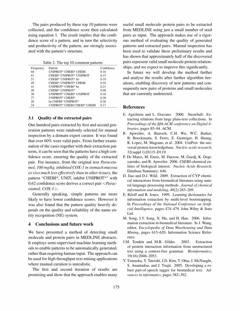
The pairs produced by these top 10 patterns werecollected, and the confidence score then calculatedusing equation 1. The result implies that the confi-dence score of a pattern, and in turn the selectivityand productivity of the pattern, are strongly associ-ated with the pattern’s structure.
Table 2: The top 10 comment patternsFrequency Pattern Confidence68 UNIPROT* CHEBI* CHEBI 0.1661 CHEBI* UNIPROT* UNIPROT 0.1551 CHEBI* UNIPROT* be 0.1049 CHEBI* UNIPROT* CHEBI 0.1041 UNIPROT* CHEBI* be 0.2140 CHEBI* UNIPROT* 0.0838 UNIPROT* CHEBI* UNIPROT 0.1637 UNIPROT* CHEBI* 0.3026 be CHEBI* UNIPROT* 0.2624 UNIPROT* CHEBI CHEBI* CHEBI 0.17
3.1 Quality of the extracted pairs
One hundred pairs extracted by first and second gen-eration patterns were randomly selected for manualinspection by a domain expert curator. It was foundthat over 60% were valid pairs. From further exami-nation of the cases together with their extraction pat-terns, it can be seen that the patterns have a high con-fidence score, ensuring the quality of the extractedpair. For instance, from the original text Paraceta-mol, 100 mg/kg, inhibited COX-1 in stomach mucosaex vivo much less effectively than in other tissues, thepattern “CHEBI*, UNIT, inhibit UNIPROT*” with0.62 confidence score derives a correct pair <Parac-etamol, COX-1>.
Generally speaking, simple patterns are morelikely to have lower confidence scores. However itwas also found that the pattern quality heavily de-pends on the quality and reliability of the name en-tity recognition (NE) system.
4 Conclusions and future work
We have presented a method of detecting smallmolecule and protein pairs in MEDLINE abstracts.It employs semi-supervised machine learning meth-ods to enable patterns to be automatically generated,rather than requiring human input. The approach canbe used for high throughput text mining applicationswhere manual curation is unrealistic.
The first and second iteration of results arepromising and show that the approach enables many
useful small molecule protein pairs to be extractedfrom MEDLINE using just a small number of seedpairs as input. The approach makes use of a rigor-ous method of evaluating the quality of generatedpatterns and extracted pairs. Manual inspection hasbeen used to validate these preliminary results andhas shown that approximately half of the discoveredpairs represent valid small molecule protein relation-ships, and we expect to improve this significantly.
In future we will develop the method furtherand analyse the results after further algorithm iter-ations, enabling discovery of new patterns and con-sequently new pairs of proteins and small moleculesthat are currently undetected.
References
E. Agichtein and L. Gravano. 2000. Snowball: Ex-tracting relations from large plain-text collections. InProceedings of the fifth ACM conference on Digital li-braries, pages 85–94. ACM.
R. Apweiler, A. Bairoch, C.H. Wu, W.C. Barker,B. Boeckmann, S. Ferro, E. Gasteiger, H. Huang,R. Lopez, M. Magrane, et al. 2004. UniProt: the uni-versal protein knowledgebase. Nucleic acids research,32(suppl 1):D115–D119.
P. De Matos, M. Ennis, M. Darsow, M. Guedj, K. Degt-yarenko, and R. Apweiler. 2006. ChEBI-chemical en-tities of biological interest. Nucleic Acids Research,Database Summary: 646.
D. Jiao and D.J. Wild. 2009. Extraction of CYP chemi-cal interactions from biomedical literature using natu-ral language processing methods. Journal of chemicalinformation and modeling, 49(2):263–269.
E. Riloff and R. Jones. 1999. Learning dictionaries forinformation extraction by multi-level bootstrapping.In Proceedings of the National Conference on Artifi-cial Intelligence, pages 474–479. John Wiley & SonsLtd.
M. Song, I.Y. Song, X. Hu, and H. Han. 2006. Infor-mation extraction in biomedical literature. In J. Wang,editor, Encyclopedia of Data Warehousing and DataMining, pages 615–620. Information Science Refer-ence.
J.M. Temkin and M.R. Gilder. 2003. Extractionof protein interaction information from unstructuredtext using a context-free grammar. Bioinformatics,19(16):2046–2053.
Y. Tsuruoka, Y. Tateishi, J.D. Kim, T. Ohta, J. McNaught,S. Ananiadou, and J. Tsujii. 2005. Developing a ro-bust part-of-speech tagger for biomedical text. Ad-vances in informatics, pages 382–392.
175

Proceedings of the 2012 Workshop on Biomedical Natural Language Processing (BioNLP 2012), pages 176–184,Montreal, Canada, June 8, 2012. c©2012 Association for Computational Linguistics
Grading the Quality of Medical Evidence
Binod Gyawali, Thamar SolorioCoRAL Lab
Department of Computer and Information SciencesUniversity of Alabama at Birmingham, AL, USA{bgyawali,solorio}@cis.uab.edu
Yassine BenajibaClinical Decision Support Solutions Department
Philips Research North America, Briarcliff Manor, NY, [email protected]
Abstract
Evidence Based Medicine (EBM) is the prac-tice of using the knowledge gained from thebest medical evidence to make decisions inthe effective care of patients. This medi-cal evidence is extracted from medical docu-ments such as research papers. The increas-ing number of available medical documentshas imposed a challenge to identify the ap-propriate evidence and to access the qualityof the evidence. In this paper, we presentan approach for the automatic grading of ev-idence using the dataset provided by the 2011Australian Language Technology Association(ALTA) shared task competition. With thefeature sets extracted from publication types,Medical Subject Headings (MeSH), title, andbody of the abstracts, we obtain a 73.77%grading accuracy with a stacking based ap-proach, a considerable improvement over pre-vious work.
1 Introduction
“Evidence Based Medicine (EBM) is the conscien-tious, explicit, and judicious use of current best evi-dence in making decisions about the care of individ-ual patients” (Sackett et al., 1996). EBM requires toidentify the best evidence, understand the method-ology and strength of the approaches reported inthe evidence, and bring relevant findings into clin-ical practice. Davidoff et al. (1995) express EBM interms of five related ideas. Their ideas imply thatthe conclusions should be derived based on the bestevidence available, the clinical decisions should be
made based on the conclusions derived, and the per-formance of the clinical decisions should be evalu-ated constantly. Thus, physicians practicing EBMshould be constantly aware of the new ideas andthe best methodologies available based on the mostrecent literature. But the amount of clinical docu-ments available is increasing everyday. For exam-ple, Pubmed, a service of the US National Library ofMedicine contains more than 21 million citations forbiomedical literature from MEDLINE, life sciencejournals, and online books (last updated on Decem-ber 7, 2011) 1. The abundance of digital informa-tion makes difficult the task of evaluating the qualityof results presented and the significance of the con-clusions drawn. Thus, it has become an importanttask to grade the quality of evidence so that the mostsignificant evidence is incorporated into the clinicalpractices.
There are several scale systems available to grademedical evidence. Some of them are: hierarchyof evidence proposed by Evans (2003), Grading ofRecommendations Assessment, Development, andEvaluation (GRADE) scale by GRADE (2004), andStrength of Recommendation Taxonomy (SORT)scale by Ebell et al. (2004). The SORT scale ad-dresses the quality, quantity, and consistency of evi-dence and proposes three levels of ratings: A, B, andC. Grade A is recommended based on the consistent,good-quality patient-oriented evidence, grade B isbased on the inconsistent or limited-quality patient-oriented evidence, and grade C is based on consen-sus, disease-oriented evidence, usual practice, ex-pert opinion or case studies.
1http://www.ncbi.nlm.nih.gov/books/NBK3827/
176
The Australasian Language Technology Associa-tion (ALTA) 2011 organized the shared task compe-tition2 to build an automatic evidence grading sys-tem for EBM based on the SORT grading scale. Wecarry out our experiments using the data set providedfor the competition and compare the accuracy ofgrading the evidence by applying basic approachesand an ensemble (stacking) based approach of clas-sification. We show that the later approach canachieve 73.77% of grading accuracy, a significantimprovement over the basic approaches. We furtherextend our experiments to show that, using featuresets generated from the method and conclusion sec-tions of the abstracts helps to obtain higher accuracyin evidence grading than using a feature set gener-ated from the entire body of the abstracts.
2 Related Work
To the best of our knowledge, automatic evidencegrading based on a grading scale was initiated bySarker et al. (2011). Their work was based on theSORT scale to grade the evidence using the corpusdeveloped by Molla-Aliod (2010). They showedthat using only publication types as features couldyield an accuracy of 68% while other informationlike publication types, journal names, publicationyears, and article titles could not significantly helpto improve the accuracy of the grading. Molla-Aliodand Sarker (2011) worked on the evidence gradingproblem of 2011 ALTA shared task and achievedan accuracy of 62.84% using three sequential clas-sifiers, each trained by one of the following featuresets: word n-grams from the abstract, publicationtypes, and word n-grams from the title. They ap-plied a three way classification approach where theinstances classified as A or C were removed fromthe test set and labeled as such, while instancesclassified as B were passed to the next classifier inthe pipeline. They repeated this process until theyreached the end of three sequential classifiers.
Most of the EBM related work is focused on ei-ther the identification of important statements fromthe medical abstracts or the classification of med-ical abstracts to facilitate the retrieval of impor-tant documents. Work by Demner-Fushman et al.(2006), Dawes et al. (2007), Kim et al. (2011) au-
2http://www.alta.asn.au/events/sharedtask2011
tomatically identify the key statements in the med-ical abstracts and classify them into different levelsthat are considered important for EBM practitionersin making decisions. Kilicoglu et al. (2009) workedon recognizing the clinically important medical ab-stracts using an ensemble learning method (stack-ing). They used different combinations of featurevectors extracted from documents to classify the ev-idence into relevant or non relevant classes. Theyapproached the problem as a binary classificationproblem without using any grading scales.
Systematic Reviews (SRs) are very importantto support EBM. Creating and updating SRs ishighly inefficient and needs to identify the best evi-dence. Cohen et al. (2010) used a binary classifica-tion system to identify the documents that are mostlikely to be included in creating and updating SRs.
In this work, we grade the quality of evidencebased on the SORT scale, that is different from mostof the existing works related to classification of ab-stracts and identification of key statements of ab-stracts. We work on the same problem as by Molla-Aliod and Sarker (2011) but, we undertake the prob-lem with a different approach and use different setsof features.
3 Dataset
We use the data of 2011 ALTA shared task compe-tition that contains three different sets: training, de-velopment and test set. The number of evidence in-stances present in each set is shown in Table 1. Eachdata set consists of instances with grades A, B, or Cbased on the SORT scale. The distribution of evi-dence grades is shown in Table 2.
Data Set No. of Evidence InstancesTraining Set 677Development Set 178Test Set 183
Table 1: Evidence per data set
The evidence instances were obtained from thecorpus developed by Molla-Aliod and Santiago-Martinez (2011). The corpus was generated basedon the question and the evidence based answer forthe question along with SOR grade obtained fromthe “Clinical Inquiries” section of the Journal of
177

Grades Trainingset (%)
Developmentset (%)
Test set(%)
A 31.3 27.0 30.6B 45.9 44.9 48.6C 22.7 28.1 20.8
Table 2: Evidence distribution per grade
Family Practice (JFP). A sample question from theJFP Clinical Inquiries section is “How does smokingin the home affect children with asthma?”. Each ev-idence contains at least one or more publications de-pending upon from which publications the evidencewas generated. Each publication is an XML file con-taining information such as abstract title, abstractbody, publication types, and MeSH terms. Eachpublication is assigned at least one publication typeand zero or more MeSH terms. The MeSH termsvocabulary 3 is developed and maintained by theNational Library of Medicine and is used in rep-resentation, indexing and retrieval of medical doc-uments. Some of the medical document retrievalwork emphasizes the use of MeSH terms in the ef-ficient retrieval of documents (Trieschnigg et al.,2009; Huang et al., 2011). MeSH terms are alsoused in document summarization (Bhattacharya etal., 2011).
Figure 1: Sample data file
Each data set contains an additional grade filewith the information related to the evidence in-stances, their grades, and the publications. A sam-ple of the file is shown in Figure 1. The first columncontains the evidence id, the second column containsthe grades A, B, or C of the evidence based on theSORT scale, and the remaining columns show thepublication id of each publication in the evidence.
3http://www.nlm.nih.gov/mesh
The problem in this task is to analyze the publica-tions in each evidence provided and classify theminto A, B or C.
The dataset available for our research has ab-stracts in two different formats. One of them con-tains abstracts divided into sections: background,objective, method, result, and conclusion. The otherformat contains abstracts with all the information ina single block without any sections. A sample of anabstract having only four sections in the given datais shown below:
Objectives: To determine the effectiveness of a musclestrengthening program compared to a stretching program inwomen with fibromyalgia (FM).
Methods: Sixty-eight women with FM were randomly as-signed to a 12 week, twice weekly exercise program consistingof either muscle strengthening or stretching. Outcome measuresincluded muscle strength (main outcome variable), flexibility,weight, body fat, tender point count, and disease and symptomseverity scales.
Results: No statistically significant differences betweengroups were found on independent t tests. Paired t tests revealedtwice the number of significant improvements in the strengthen-ing group compared to the stretching group. Effect size scoresindicated that the magnitude of change was generally greater inthe strengthening group than the stretching group.
Conclusions: Patients with FM can engage in a speciallytailored muscle strengthening program and experience an im-provement in overall disease activity, without a significant exer-cise induced flare in pain. Flexibility training alone also resultsin overall improvements, albeit of a lesser degree.
In the abstract above, we see that the approachesapplied for the study are described in the methodsection, and the outcome and its effectiveness aredescribed in the conclusion section.
4 Proposed Methodology
In this paper we propose a system to identify thecorrect grade of an evidence given publications inthe evidence. We deal with the problem of evi-dence grading as a classification problem. In evi-dence grading, basic approaches have been shownto have poor performance. Molla-Aliod and Sarker(2011) showed that a basic approach of using simplebag-of-word features and a Naive Bayes classifierachieved 45% accuracy and proposed a sequentialapproach to improve the accuracy at each step. Ourpreliminary studies of applying the simple classifi-cation approach also showed similar results. Here,we propose a stacking based approach (Wolpert,
178

1992) of evidence grading. Stacking based approachbuilds a final classifier by combining the predictionsmade by multiple classifiers to improve the predic-tion accuracy. It involves two steps. In the first step,multiple base-level classifiers are trained with dif-ferent feature sets extracted from a dataset and theclassifiers are used to predict the classes of a sec-ond dataset. Then, a higher level classifier is trainedusing the predictions made by the base-level clas-sifiers on the second dataset and used to predict theclasses of the actual test data. In this approach, base-level classifiers are trained independent of each otherand allowed to predict the classes. Based on thepredictions made by these base-level classifiers, thehigher level classifier learns from those predictionsand makes a new prediction that is the final class.
Our stacking based approach of classification usesfive feature sets. In the first step of classification, wetrain five classifiers using different feature sets perclassifier and use the classifiers to predict the gradesof the development dataset. Thus, at the end of thefirst step, five different predictions on the develop-ment dataset are obtained. In the second step, a newclassifier is trained using the grades predicted by thefive classifiers as features. This new classifier is thenused to predict the grades of the test dataset.
5 Features
We extracted six sets of features from the publica-tions to perform our experiments. They are as fol-lows:
1. Publication types2. MeSH terms3. Abstract title4. Abstract body5. Abstract method section6. Abstract conclusion section
For feature set 1, we extracted 30 distinct publi-cation types from the training data. For the MeSHterms feature set, we selected 452 unique MeSHterms extracted from the training data. The publi-cations contained the descriptor name of the MeSHterms having an attribute “majortopicyn” with value‘Y’ or ‘N’. As MeSH terms feature set, we selectedonly those MeSH term descriptor names having ma-jortopicyn=‘Y’.
We extracted the last four sets of features fromthe title, body, method, and conclusion sections ofthe abstracts. Here, the body of an abstract meansthe whole content of the abstract, that includes back-ground, objective, method, result, and conclusionsections. We applied some preprocessing steps togenerate these feature sets. We also applied a featureselection technique to reduce the number of featuresand include only the high informative features fromthese feature sets. The details about preprocess-ing and feature selection techniques are described inSection 6.
We performed all the experiments on the basis ofevidence, i.e. we created a single feature vector perevidence. If an evidence contained more than onepublication, we generate its features as the union ofthe features extracted from all its publications.
The grades of the evidence in the SORT scaleare based on the quality of evidence, basis of ex-periments, the methodologies used, and the types ofanalysis done. Grades also depend upon the effec-tiveness of the approach used in the experiments.The method section of an abstract contains the in-formation related to the basis of the experiments,such as randomized controlled trails, systematic re-view, cohort studies, and the methods used in theirresearch. The conclusion section of the abstractusually contains the assertion statements about howstrongly the experiment supports the claims. Anal-ysis of the contents of abstracts shows that the in-formation needed for grading on SORT scale is typ-ically available in the method and conclusion sec-tions, more than in the other sections of the abstracts.Thus, we used the method and conclusion sectionsof the abstracts to generate two different feature setsso that only the features more likely to be importantin grading using the SORT rating would be included.
Separating method and conclusion sections ofthe abstracts
In order to extract features from the method and con-clusion sections, we should separate them from thebody of abstracts, which is a challenging task forthose abstracts without section headers. Of the to-tal number of abstracts, more than one-third of theabstracts do not contain the section headers. In or-der to separate these sections, we used a very simpleapproach based on the number of sentences present
179

in the method and conclusion sections, and the bodyof the abstracts. We used the following informationto separate the method and conclusion sections fromthese abstracts: i) Order of sections in the abstracts,ii) Average number of sentences in the method andconclusion sections of the abstracts having sections,and iii) Average number of sentences in the entirebody of the abstracts not having sections. All the ab-stracts having section headers contained the sectionsin the same order: background, objective, method,result and conclusion. From the available trainingdataset, we calculated:
i. The average number of sentences in the method(4.14) and conclusion (2.11) sections of the abstracts di-vided into sections
ii. The average number of sentences (8.78) of the ab-stracts not having sections
Based on these values, we fragmented the ab-stracts that do not have the section headers and sepa-rated the method and conclusion sections from them.Table 3 shows how the method and conclusion sec-tions of those abstracts were generated. For exam-ple, the fourth row of the table says that, if an ab-stract without section headers has 6, 7 or 8 sentences(let it be n), then the 3rd, 4th and 5th sentences wereconsidered as the method section, and the nth sen-tence was considered as the conclusion section.
Total sentences inAbstracts(n)
Method Conclusion
1 None 12 or 3 1 n4 or 5 2 and 3 n6 or 7 or 8 2, 3 and 4 nMore than 8 3, 4 and 5 n-1 and n
Table 3: Selecting method and conclusion of the abstractshaving a single block
6 Experiments and Results
This section describes the two sets of experimentsperformed to compare the performance of the stack-ing based approach and the effectiveness of the base-level classifiers used. The first set of experimentswas done to provide a baseline comparison againstour stacking based approach. The second set con-sists of five experiments to evaluate different con-
figurations of stack based classifiers. The basic ap-proach of classification implies the use of a singleclassifier trained by using a single feature vector.
We applied preprocessing steps to generate fea-ture sets from the title, body, method and conclusionsections of the abstracts. The preprocessing stepswere: detecting sentences using OpenNLP SentenceDetector4, stemming words in each sentence usingPorter Stemmer (Porter, 1980), changing the sen-tences into lower-case, and removing punctuationcharacters from the sentences. After the preprocess-ing step, we generated features from the unigrams,bigrams and trigrams in each part. We removedthose features from the feature sets that containedthe stopwords listed by Pubmed5 or contained anytoken having a length less than three characters. Toremove the less informative features, we calculatedthe information gain of the features in the trainingdata using Weka (Hall et al., 2009) and selected onlythe top 500 high informative features for each fea-ture set. We used the Weka SVM classifier for all theexperiments. Based on the best result obtained af-ter a series of experiments run with different kernelfunctions and regularization parameters, we chosethe SVM classifier with a linear kernel and regular-ization parameter equals 1 for all the experiments.We used a binary weight for all the features.
6.1 First set of experimentsIn the first set, we performed nine experiments usingthe basic classification approach and one experimentusing the stacking based approach. The details ofthe experiments and the combinations of the featuresused in them are as shown in Table 4.
The first six experiments in the table were imple-mented by applying a basic approach of classifica-tion and each using only a single set of features. Ex-periments 7, 8, and 9 were similar to the first sixexperiments except, they used more than one set offeatures to create the feature vector. Each feature inthe experiments 7, 8, and 9 encode the section of itsorigin. For example, if feature abdomen is presentin method as well as conclusion sections, it is rep-resented as two distinct features conc abdomen andmethod abdomen. In experiment 10, we applied
4http://incubator.apache.org/opennlp5http://www.ncbi.nlm.nih.gov/books/NBK3827
/table/pubmedhelp.T43/?report=objectonly)
180

the stacking approach of classification using fivebase-level classifiers. The base-level classifiers inthis experiment are the basic classifiers used in ex-periments 1 to 5.
Exp.No.
Features used Exp. type
1. Publication types
Basic approach
2. MeSH terms3. Abstract title4. Abstract method5. Abstract conclusion6. Abstract body
7. Publication types,MeSH terms
8.
Publication types,MeSH terms,Abstract title,Abstract body
9.
Publication types,MeSH terms,Abstract title,Abstract method,Abstract conclusion
10.
Publication types
Stacking basedapproach
MeSH termsAbstract titleAbstract methodAbstract conclusion
Table 4: Experiments to compare basic approaches to astacking based approach
Figure 2 shows the results of the 10 experimentsdescribed in Table 4 in the same order, from 1st to10th place and the result of the experiment by Molla-Aliod and Sarker (2011). The results show thatthe stacking based approach gives the highest ac-curacy (73.77%), outperforming all the basic ap-proaches applying any combination of feature sets.The stacking based approach outperforms the base-line of a single layered classification approach (Exp9) that uses all the five sets of features. Molla-Aliodand Sarker (2011) showed that a simple approach ofusing a single classifier and bag-of-words featurescould not achieve a good accuracy (45.9%) and pro-posed a new approach of using a sequence of classi-fiers to achieve a better result. Similar to their simpleapproach, our basic approaches could not achievegood results, but their performance is comparableto Molla-Aliod and Sarker (2011)’s baseline system.The result of our stacking based approach shows thatour approach has a better accuracy than the sequen-cial classification approach (62.84%) proposed by
Figure 2: Comparison of accuracy of basic approaches toa stacking based approach. X-axis shows the experimentsand Y-axis shows the accuracy of the experiments. Thefirst nine experiments are based on the basic approachand the tenth experiment is based on the stacking basedapproach.
Molla-Aliod and Sarker (2011).Our stacking based approach works on two lev-
els. In the first level, the base-level classifiers pre-dict the grades of the evidence. In the next level,these predictions are used to train a new classifierthat learns from the predictions to identify the gradescorrectly. Moreover, the five feature sets used in ourexperiments were unrelated to each other. For ex-ample, the features present in MeSH headings weredifferent from the features used in publication types,and similarly, the features present in the method sec-tion of the abstract were different from the featurespresent in the conclusion section. Each base-levelclassifier trained by one of these feature sets is spe-cialized in that particular feature set. Thus, usingthe predictions made by these specialized base-levelclassifiers to train a higher level classifier helps tobetter predict the grades, this cannot be achieved bya single classifier trained by a set of features (Exp.1, 2, 3, 4, 5, 6), or a group of different feature sets(Exp. 7, 8, 9).
6.2 Second set of experiments
In the second set of experiments, we compared fiveexperiments performed varying the base-level clas-sifiers used in our stack based approach. Experi-ments 1 and 2 were performed using a single base-level classifier, that means that the second classifieris trained on only one feature. Experiments 3 and 4were performed by using four base-level classifiers,and experiment 5 was performed using five base-
181

level classifiers. The 5th experiment in this set issame as the 10th experiment in the first set. The de-tails about the feature sets used in each experimentare shown in Table 5.
Exp.No.
Features used No. of Base levelclassifiers
1.
Publication types,
1MeSH terms,Abstract title,Abstract body
2.
Publication types,
1MeSH terms,Abstract title,Abstract method,Abstract conclusion
3.
Publication types
4MeSH termsAbstract titleAbstract body
4.
Publication types
4MeSH termsAbstract titleAbstract method,Abstract conclusion
5.
Publication types
5MeSH termsAbstract titleAbstract methodAbstract conclusion
Table 5: Experiments to compare stacking based ap-proach
Figure 3 shows the accuracy of the five experi-ments shown in Table 5 in the same order. It showsthat the accuracy of 1st and 2nd experiments is lowerthan the accuracy of 3rd, 4th, and 5th experiments.In these two experiments, a feature vector generatedfrom the prediction of a single base-level classifieris used to train the higher level classifier, that is notsufficient to make a correct decision.
Experiments 3, 4, and 5 show a considerable im-provement in the accuracy of the grading. Compar-ing the results of experiments 3 and 4, we see thatthe 4th experiment has higher accuracy than the 3rd
one. The difference between these experiments wasthe use of features from the method and conclusionsections of the abstracts in the 4th experiment, whileusing features from the entire body of abstracts inthe 3rd experiment. The higher accuracy in the 4th
experiment shows that the method and conclusionsections of the experiment contain high informativetext that is important for evidence grading, while
Figure 3: Comparison of accuracy of the stacking basedapproaches. X-axis shows the experiments and Y-axisshows the accuracy of the experiments. 1st and 2nd ex-periments use only one base-level classifier, 3rd and 4th
experiment are based on four base-level classifiers and5th one uses five base-level classifiers.
the body of abstracts may contain some informationthat is not relevant to the task. The same analysiscan also be inferred from the results of experiment8 and 9 in the first set of experiments. The high-est accuracy obtained in the 5th experiment of apply-ing 5 base-level classifiers shows that identifying thesections of the abstracts containing high informativefeatures and using a sufficient number of base-levelclassifiers can help to achieve a good accuracy in ev-idence grading.
7 Error Analysis
The result obtained by the stacking based approach(5th experiment in Table 5) using five base-level clas-sifiers gave a higher error rate in predicting gradesA and C, compared to the error rate in predict-ing grade B. Most of the error is the misclassifica-tion of A to C and vice versa. One of the possi-ble reasons of this might be due to the use of thefeature set extracted from the conclusion section.Among the five base-level classifiers used in the ex-periment, the one trained by the features extractedfrom the conclusion sections has the lowest accu-racy (5th experiment in Figure 2). We evaluated thetext contained in the conclusion section of the ab-stracts in our dataset. The section mostly containsthe assertion statements having the words showingstrong positive/negative meanings. Conclusion of Agrade evidence mostly contains the information thatstrongly asserts the claim (e.g. emollient treatment
182

significantly reduced the high-potency topical cor-ticosteroid consumption in infants with AD), whilethat of C grade evidence is not strong enough to as-sert the claim (e.g. PDL therapy should be consid-ered among the better established approaches in thetreatment of warts, although data from this trial sug-gest that this approach is probably not superior). Itseems that the problem might be because of not pro-cessing the negations appropriately. So, in order topreserve some negation information present in theconclusion sections, we performed another experi-ment by merging words no, not, nor with their suc-cessor word to create a single token from the twowords. This approach still could not reduce the mis-classification. Thus, the simple approach of extract-ing unigram, bigram, and trigram features from theconclusion section might not be sufficient and mightneed to include higher level analysis related to as-sertion/certainty of the statements to reduce the mis-classification of the evidence.
Other possible reasons of the misclassificationof the evidence might be the imbalanced data set.Our dataset (Table 2) contains higher number of in-stances with grade B than those with grades A and C.Moreover, the number of publications per evidenceis not uniform, that ranges from 1 to 8 publicationsper evidence in the test data. Analyzing the results,we found that misclassification of evidence havingonly one publication is higher than that of the evi-dence having more than one publication. If an ev-idence contains only one publication, the featuresof the evidence extracted from a single publicationmight not be sufficient to accurately grade the evi-dence and might lead to misclassification.
In order to evaluate the appropriateness of ourapproach in extracting the method and conclusionsections, we performed a manual inspection of ab-stracts. We could not revise all the abstracts to ver-ify the approach. Thus, we randomly selected 25abstracts without section headers from the test dataand viewed the content in them. We found that theconclusion section was appropriately extracted in al-most all abstracts, while the selection of method sec-tion was partially effective. Our approach was basedon the assumption that all the abstracts having manysentences have all the sections (background, objec-tive, method, result, and conclusion). But we foundthat the abstracts do not follow the same format, and
the start sentence of the method section is not con-sistent. Even a long abstract might sometimes startwith the method section, and sometimes the objec-tive section might not be present in the abstracts.This could lead to increase the error in our gradingsystem.
8 Conclusion
This paper presents an approach of grading the med-ical evidence applying a stacking based classifierusing the features from publication types, MeSHterms, abstract body, and method, and conclusionsections of the abstracts. The results show thatthis approach achieves an accuracy of 73.77%, thatis significantly better than the previously reportedwork. Here, we present two findings: 1) We showthat the stacking based approach helps to obtain abetter result in evidence grading than the basic ap-proach of classification. 2) We also show that themethod and conclusion sections of the abstracts con-tain important information necessary for evidencegrading. Using the feature sets generated from thesetwo sections helps to achieve a higher accuracy thanby using the feature set generated from the entirebody of the abstracts.
In this work, all the information available in themethod and conclusion sections of the abstracts istreated with equal weight. Evidence grading shouldnot depend upon specific disease names and syn-dromes, but should be based on how strong the factsare presented. We would like to extend our ap-proach by removing the words describing specificdisease names, disease syndromes, and medications,and giving higher weight to the terms that describethe assertion of the statements. In our current work,we apply a simple approach to extract the methodand conclusion sections from the abstracts not hav-ing sections. Improving the approach by using a ma-chine learning algorithm that can more accuratelyextract the sections might help to increase the accu-racy of grading. Including the information about thestrength of assertions made in the conclusion sec-tions could also help in boosting the accuracy. Fu-ture work would also include testing the effective-ness of our approach on other diverse data sets hav-ing complex structures of the evidence, or on a dif-ferent grading scale.
183

References
Sanmitra Bhattacharya, Viet HaThuc, and Padmini Srini-vasan. 2011. Mesh: a window into full text for doc-ument summarization. Bioinformatics, 27(13):i120–i128.
Aaron M. Cohen, Kyle Ambert, and Marian McDon-agh. 2010. A Prospective Evaluation of an Au-tomated Classification System to Support Evidence-based Medicine and Systematic Review. AMIA AnnuSymp Proc., 2010:121 – 125.
Frank Davidoff, Brian Haynes, Dave Sackett, andRichard Smith. 1995. Evidence based medicine.BMJ, 310(6987):1085–1086, 4.
Martin Dawes, Pierre Pluye, Laura Shea, Roland Grad,Arlene Greenberg, and Jian-Yun Nie. 2007. The iden-tification of clinically important elements within med-ical journal abstracts: Patient-Population-Problem,Exposure-Intervention, Comparison, Outcome, Dura-tion and Results (PECODR). Informatics in PrimaryCare, 15(1):9–16.
Dina Demner-Fushman, Barbara Few, Susan E. Hauser,and George Thoma. 2006. Automatically IdentifyingHealth Outcome Information in MEDLINE Records.Journal of the American Medical Informatics Associa-tion, 13(1):52 – 60.
M. H. Ebell, J. Siwek, B. D. Weiss, S. H. Woolf, J. Sus-man, B. Ewigman, and M. Bowman. 2004. Strengthof recommendation taxonomy (SORT): a patient-centered approach to grading evidence in the medi-cal literature. American Family Physician, 69(3):548–56+.
David Evans. 2003. Hierarchy of evidence: a frame-work for ranking evidence evaluating healthcare inter-ventions. Journal of Clinical Nursing, 12(1):77–84.
GRADE. 2004. Grading quality of evidence and strengthof recommendations. BMJ, 328(7454):1490, 6.
Mark Hall, Eibe Frank, Geoffrey Holmes, BernhardPfahringer, Peter Reutemann, and Ian H. Witten.2009. The WEKA data mining software: an update.SIGKDD Explor. Newsl., 11(1).
Minlie Huang, Aurlie Nvol, and Zhiyong Lu. 2011. Rec-ommending MeSH terms for annotating biomedicalarticles. Journal of the American Medical Informat-ics Association, 18(5):660–667.
Halil Kilicoglu, Dina Demner-Fushman, Thomas C Rind-flesch, Nancy L Wilczynski, and R Brian Haynes.2009. Towards Automatic Recognition of Scientif-ically Rigorous Clinical Research Evidence. Jour-nal of the American Medical Informatics Association,16(1):25–31.
Su Kim, David Martinez, Lawrence Cavedon, and LarsYencken. 2011. Automatic classification of sentences
to support Evidence Based Medicine. BMC Bioinfor-matics, 12(Suppl 2):S5.
Diego Molla-Aliod and Maria Elena Santiago-Martinez.2011. Development of a Corpus for Evidence BasedMedicine Summarisation. In Proceedings of theAustralasian Language Technology Association Work-shop.
Diego Molla-Aliod and Abeed Sarker. 2011. AutomaticGrading of Evidence: the 2011 ALTA Shared Task.In Proceedings of Australasian Language TechnologyAssociation Workshop, pages 4–8.
Diego Molla-Aliod. 2010. A Corpus for EvidenceBased Medicine Summarisation. In Proceedings of theAustralasian Language Technology Association Work-shop, volume 8.
MF Porter. 1980. An algorithm for sufx stripping. Pro-gram, 14(3):130–137.
David L Sackett, William M C Rosenberg, J A Muir Gray,R Brian Haynes, and W Scott Richardson. 1996. Ev-idence based medicine: what it is and what it isn’t.BMJ, 312(7023):71–72, 1.
Abeed Sarker, Diego Molla-Aliod, and Cecile Paris.2011. Towards automatic grading of evidence. In Pro-ceedings of LOUHI 2011 Third International Work-shop on Health Document Text Mining and Informa-tion Analysis, pages 51–58.
Dolf Trieschnigg, Piotr Pezik, Vivian Lee, Franciskade Jong, Wessel Kraaij, and Dietrich Rebholz-Schuhmann. 2009. MeSH Up: effective MeSH textclassification for improved document retrieval. Bioin-formatics, 25(11):1412–1418.
David H. Wolpert. 1992. Stacked generalization. NeuralNetworks, 5(2):241 – 259.
184

Proceedings of the 2012 Workshop on Biomedical Natural Language Processing (BioNLP 2012), pages 185–192,Montreal, Canada, June 8, 2012. c©2012 Association for Computational Linguistics
Classifying Gene Sentences in Biomedical Literature by Combining High-Precision Gene Identifiers
Sun Kim, Won Kim, Don Comeau, and W. John Wilbur National Center for Biotechnology Information
National Library of Medicine, National Institutes of Health Bethesda, MD 20894, USA
{sun.kim,won.kim,donald.comeau,john.wilbur}@nih.gov
Abstract
Gene name identification is a fundamental step to solve more complicated text mining problems such as gene normalization and pro-tein-protein interactions. However, state-of-the-art name identification methods are not yet sufficient for use in a fully automated sys-tem. In this regard, a relaxed task, gene/protein sentence identification, may serve more effectively for manually searching and browsing biomedical literature. In this pa-per, we set up a new task, gene/protein sen-tence classification and propose an ensemble approach for addressing this problem. Well-known named entity tools use similar gold-standard sets for training and testing, which results in relatively poor performance for un-known sets. We here explore how to combine diverse high-precision gene identifiers for more robust performance. The experimental results show that the proposed approach out-performs BANNER as a stand-alone classifier for newly annotated sets as well as previous gold-standard sets.
1 Introduction
With the rapidly increasing biomedical literature, text mining has become popular for finding bio-medical information in text. Among others, named entity recognition (NER) for bio-entities such as genes and proteins is a fundamental task because
extracting biological relationships begins with enti-ty identification. However, NER in biomedical literature is challenging due to the irregularities and ambiguities in bio-entities nomenclature (Yang et al., 2008). In particular, compound entity names make this problem difficult because it also requires deciding word boundaries.
Recent bio-text competitions such as JNLPBA (Kim et al., 2004) and BioCreative (Lu et al., 2011; Smith et al., 2008) have evaluated NER systems for gene mentions. Even though progress has been made in several areas, gene identification methods are not yet sufficient for real-world use without human interaction (Arighi et al., 2011). Thus, at the present, a realistic suggestion is to use these algorithms as an aid to human curation and infor-mation retrieval (Altman et al., 2008).
In this paper, we define a new task, gene/protein sentence classification. A gene or protein sentence means a sentence including at least one specific gene or protein name. This new task has ad-vantages over gene mention identification. First, gene name boundaries are not important at the sen-tence level and human judges will agree more in their judgments. Second, highlighting gene sen-tences may be more useful in manual search and browsing environments since this can be done more accurately and with less distraction from in-correct annotations.
To classify gene/protein sentences, we here pro-pose an ensemble approach to combine different NER identifiers. Previous NER approaches are mostly developed on a small number of gold-
185

standard sets including GENIA (Kim et al., 2003) and BioCreative (Smith et al., 2008) corpora. The-se sets help to find regular name patterns in a lim-ited set of articles, but also limit the NER performance for real-world use. In the proposed approach, we use a Semantic Model and a Priority Model along with BANNER (Leaman and Gonzalez, 2008). The Semantic and Priority Mod-els are used to provide more robust performance on gene/protein sentence classification because they utilize larger resources such as SemCat and Pub-Med○R to detect gene names.
For experiments, we created three new gold-standard sets to include cases appearing in the most recent publications. The experimental results show that our approach outperforms machine learning classifiers using unigrams and substring features as well as stand-alone BANNER classification on five gold-standard datasets.
The paper is organized as follows. In Section 2, the ensemble approach for gene/protein sentence classification is described. Section 3 explains the gold-standard sets used for our experiments. Sec-tion 4 presents and discusses the experimental re-sults. Conclusions are drawn in Section 5.
2 Methods
Figure 1. Method Overview.
Figure 1 shows the overall framework for our pro-posed approach. We basically assume that a main NER module works as a strong predictor, i.e., the majority of outputs obtained from this module are correct. We here use BANNER (Leaman and Gonzalez, 2008) as the main NER method because it adopts features and methods which are generally known to be effective for gene name recognition. While BANNER shows good performance on
well-known gold-standard sets, it suffers from rela-tively poor performance on unknown examples. To overcome this problem, we combine BANNER with two other predictors, a Sematic Model and a Priority Model. First, the Semantic Model and the Priority Model do not use previous gold-standard sets for training. Second, these two models learn name patterns in different ways, i.e., semantic rela-tionships for the Semantic Model and positional and lexical information for the Priority Model. This combination of a strong predictor and two weaker but more general predictors can respond better to unknown name patterns.
As described above, the proposed method main-ly relies on outputs from different NER methods, whereas word features can still provide useful evi-dence for discriminating gene and non-gene sen-tences. Hence, we alternatively utilize word features such as unigrams and substrings along with NER features. For NER features only, the output is the sum of binary decisions from three NER modules. For word and NER features, the Huber classifier (Kim and Wilbur, 2011) is trained to combine the features. The parameter set in the Huber classifier is optimized to show the best clas-sification performance on test sets. The following subsections describe each feature type used for gene sentence classification.
2.1 Word Features
Unigrams are a set of words obtained from to-kenizing sentences on white space. All letters in unigrams are converted to lower case.
Substrings are all contiguous substrings of a sen-tence, sized three to six characters. This substring feature may help reduce the difference between distributions on training and test sets (Huang et al., 2008). Substrings encode the roots and morpholo-gy of words without identifying syllables or stems. They also capture neighboring patterns between words.
2.2 BANNER
BANNER is a freely available tool for identifying gene mentions. Due to its open-source policy and Java implementation, it has become a popular tool.
BANNER uses conditional random fields (CRF) as a discriminative method and utilizes a set of fea-ture types that are known to be good for identify-ing gene names. The feature sets used are
186

orthographic, morphological and shallow syntax features (Leaman and Gonzalez, 2008): (1) The part of speech (POS) of a token in a sen-tence. (2) The lemma of a word. (3) 2, 3 and 4-character prefixes and suffixes. (4) 2 and 3 character n-grams including start-of-token and end-of-token indicators. (5) Word patterns by converting upper-case letters, lower-case letters and digits to their corresponding representative characters (A, a, 0). (6) Numeric normalization by converting digits to “0”s. (7) Roman numerals. (8) Names of Greek letters.
Even though BANNER covers most popular feature types, it does not apply semantic features or other post-processing procedures such as abbrevia-tion processing. However, these features may not have much impact for reducing performance since our goal is to classify gene sentences, not gene mentions.
2.3 Semantic Model
The distributional approach to semantics (Harris, 1954) has become more useful as computational power has increased, and we have found this ap-proach helpful in the attempt to categorize entities found in text. We use a vector space approach to modeling semantics (Turney and Pantel, 2010) and compute our vectors as described in (Pantel and Lin, 2002) except we ignore the actual mutual in-formation and just include a component of 1 if the dependency relation occurs at all for a word, else the component is set to 0. We constructed our vec-tor space from all single tokens (a token must have an alphabetic character) throughout the titles and abstracts of the records in the whole of the Pub-Med database based on a snapshot of the database taken in January 2012. We included only tokens that occurred in the data sufficient to accumulate 10 or more dependency relations. There were just over 750 thousand token types that satisfied this condition and are represented in the space. We de-note this space by h. We then took all the single tokens and all head words from multi-token strings in the categories “chemical”, “disease”, and “gene/protein” from an updated version of the
SemCat database (Tanabe et al., 2006) and placed all the other SemCat categories similarly processed into a category we called “other”. We consider on-ly the tokens in these categories that also occur in our semantic vector space h and refer to these sets as
Chemicalh , Diseaseh ,
inGene/Proteh , Otherh . Table 1 shows
the size of overlaps between sets. Chemicalh Diseaseh inGene/Proteh Otherh
Chemicalh 54478 209 4605 5495
Diseaseh 8801 1139 169
inGene/Proteh 76440 9466
Otherh 127337 Table 1. Pairwise overlap between sets representing the different categories.
Class '
Chemicalh 'Diseaseh
'inGene/Proteh
'Otherh
Strings 49800 7589 70832 113815 Ave. Prec. 0.8680 0.7060 0.9140 0.9120 Table 2. Row two contains the number of unique strings in the four different semantic classes studied. The last row shows the mean average precisions from a 10-fold cross validation to learn how to distinguish each class from the union of the other three.
In order to remove noise or ambiguity in the training set, we removed the tokens that appeared in more than one semantic class as follows.
inGene/ProteDiseaseChemicalOther
'Other
DiseaseChemicalinGene/Prote'
inGene/Prote
inGene/ProteChemicalDisease'Disease
inGene/ProteDiseaseChemical'Chemical
hhhhh
hhhh
hhhh
hhhh
(1)
We then applied Support Vector Machine learn-ing to the four resulting disjoint semantic classes in a one-against-all strategy to learn how to classify into the different classes. We used 31064.1 C based upon the size of the training set. As a test of this process we applied this same learning with 10-fold cross validation on the training data and the results are given in the last row of Table 2.
This Semantic Model is an efficient and general way to identify words indicating gene names. Un-like other NER approaches, this model decides a target class solely based on a single word. Howev-er, evaluating all tokens from sentences may in-crease incorrect predictions. A dependency parser analyzes a sentence as a set of head- and depend-
187

ent-word combinations. Since gene names likely appear in describing a relationship with other enti-ties, a name indicating a gene mention will be mostly placed in a dependent position. Thus, we first apply the C&C CCG parser (Curran et al., 2007), and evaluate words in dependent positions only.
2.4 Priority Model
The Semantic Model detects four different catego-ries for a single word. However, the Priority Model captures gene name patterns by analyzing the order of words and the character strings making up words. Since gene names are noun phrases in gen-eral, we parse sentences and identify noun phrases first. These phrases are then evaluated using the Priority Model.
The Priority Model is a statistical language model for named entity recognition (Tanabe and Wilbur, 2006). For named entities, a word to the right is more likely to be the word determining the nature of the entity than a word to the left in gen-eral.
Let T1 be the set of training data for class C1 and T2 for class C2. Let At denote the set of all to-
kens used in names contained in 21 TT . For each
token tα, A , it is assumed that there are associ-ated two probabilities pα and qα, where pα is the probability that the appearance of the token tα in a name indicates that name belongs to class C1 and qα is the probability that tα is a more reliable indi-cator of the class of a name than any token to its left. Let )()2()1( ktttn be composed of the
tokens on the right in the given order. Then the probability of n belonging to class C1 can be com-puted as follows.
k
i
k
ijjii
k
jj qpqqpnCp
2 1)()()(
2)()1(1 11|
(2)
A limited memory BFGS method (Nash and
Nocedal, 1991) and a variable order Markov model (Tanabe and Wilbur, 2006) are used to obtain pα and qα. An updated version of SemCat (Tanabe and Wilbur, 2006) was used to learn gene names.
2.5 Semantic and Priority Models for High-Precision Scores
The Semantic and Priority Models learn gene names and other necessary information from the SemCat database, where names are semantically categorized based on UMLS○R (Unified Medical Language System) Semantic Network. Even though the Semantic and Priority Models show good performance on names in SemCat, they can-not avoid noise obtained from incorrect pre-processing, e.g., parsing errors. The use of a gen-eral category for training may also limit perfor-mance. To obtain high-precision scores for our ensemble approach, it is important to reduce the number of false positives from predictions. Hence, we apply the Semantic and Priority Models on training sets, and mark false positive cases. These false positives are automatically removed from predictions on test sets. These false positive cases tend to be terms for entities too general to warrant annotation.
Table 3 shows the classification performance with and without false positive corrections on training data. For both Semantic and Priority Mod-els, precision rates are increased by removing false positives. Even though recall drops drastically, this does not cause a big problem in our setup since these models try to detect gene names which are not identified by BANNER.
SEM SEMFP PM PMFP
Accuracy 0.7907 0.7773 0.7805 0.8390 Precision 0.7755 0.8510 0.7405 1.0000 Recall 0.8323 0.6852 0.8799 0.6856 F1 0.8029 0.7592 0.8042 0.8135
Table 3. Performance changes on training set for the Semantic Model (SEM) and the Priority Model (PM). FP indicates that learned false positives were removed from predictions.
3 Datasets
For experiments, we rigorously tested the proposed method on gene mention gold-standard sets and newly annotated sets. GENETAG (Smith et al., 2008) is the dataset released for BioCreative I and BioCreative II workshops. Since it is well-known for a gene mention gold-standard set, we used GENETAG as training data.
For test data, two previous gold-standard sets were selected and new test sets were also built for gene sentence classification. YAPEX (Franzen et al., 2002) and JNLPBA (Kim et al., 2004) are con-sidered of moderate difficulty because they are
188

both related to GENIA corpus, a well-known gold-standard set. However, Disease, Cell Line and Reptiles are considered as more difficult tasks be-cause they represent new areas and contain recent-ly published articles. The annotation guideline for new test sets basically followed those used in GENETAG (Tanabe et al., 2005), however do-mains, complexes, subunits and promoters were not included in new sets.
(1) “Disease” Set: This set of 60 PubMed docu-ments was obtained from two sources. Fifty of the documents were obtained from the 793 PubMed documents used to construct the AZDC (Leaman et al., 2009). They are the fifty most recent among these records. In addition to these fifty documents, ten documents were selected from PubMed on the topic of maize to add variety to the set and because one of the curators who worked with the set had experience studying the maize genome. These ten were chosen as recent documents as of early March 2012 and which contained the text word maize and discussed genetics. The whole set of 60 docu-ments were annotated by WJW to produce a gold standard.
(2) “CellLine” Set: This set comprised the most recent 50 documents satisfying the query “cell line[MeSH]” in PubMed on March 15, 2012. This query was used to obtain documents which discuss cell lines, but most of these documents also discuss genes and for this reason the set was expected to be challenging. The set was annotated by WJW and DC and after independently annotating the set they reconciled differences to produce a final gold standard.
(3) “Reptiles” Set: This set comprised the most recent 50 documents satisfying the query “reptiles AND genes [text]” in PubMed on March 15, 2012. This set was chosen because it would have little about human or model organisms and for this rea-son it was expected to be challenging. The set was annotated by WJW and DC and after independent-ly annotating the set they reconciled differences to produce a final gold standard.
For both “CellLine” and “Reptiles” Sets, the most recent data was chosen in an effort to make the task more challenging. Presumably such docu-ments will contain more recently created names
and phrases that do not appear in the older training data. This will then pose a more difficult test for NER systems.
Table 4 shows all datasets used for training and testing. The new sets, “Disease”, “CellLine” and “Reptiles” are also freely available at http://www.ncbi.nlm.nih.gov/CBBresearch/Wilbur/IRET/bionlp.zip
Positives Negatives Total GENETAG 10245 9755 20000 YAPEX 1298 378 1676 JNLPBA 17761 4641 22402 Disease 345 251 596 CellLine 211 217 428 Reptiles 179 328 507
Table 4. Datasets. “GENETAG” was used for training data and others were used for test data. “YAPEX” and “JNLPBA” were selected from previous gold-standard corpora. “Disease”, “Cell Line” and “Reptiles” are new-ly created from recent publications and considered as difficult sets.
4 Results and Discussion
In this paper, our goal is to achieve higher-prediction performance on a wide range of gene sentences by combining multiple gene mention identifiers. The basic assumption here is that there is a strong predictor that performs well for previ-ously known gold-standard datasets. For this strong predictor, we selected BANNER since it includes basic features that are known to give good performance.
Accuracy Precision Recall F1 GENETAG 0.9794 0.9817 0.9779 0.9799 YAPEX 0.9051 0.9304 0.9483 0.9392 JNLPBA 0.8693 0.9349 0.8976 0.9159 Disease 0.8591 0.9223 0.8261 0.8716 Cell Line 0.8925 0.9146 0.8626 0.8878 Reptiles 0.8994 0.8478 0.8715 0.8595
Table 5. Performance of BANNER on training and test datasets.
Table 5 presents the gene sentence classification
performance of BANNER on training and test sets. We emphasize that performance here means that if BANNER annotates a gene/protein name in a sen-tence, that sentence is classified as positive, other-wise it is classified as negative. BANNER used GENETAG as training data, hence it shows excel-lent classification performance on the same set.
189

Unigrams Substrings BANNER Ensemble Uni+Ensemble Sub+EnsembleYAPEX 0.9414 0.9491 0.9685 0.9704 0.9624 0.9678 JNLPBA 0.9512 0.9504 0.9584 0.9651 0.9625 0.9619 Disease 0.8255 0.8852 0.9238 0.9501 0.9573 0.9610 CellLine 0.8174 0.9004 0.9281 0.9539 0.9429 0.9496 Reptiles 0.6684 0.7360 0.8696 0.9049 0.9001 0.8937
Table 6. Average precision results on test sets for different feature combinations.
Unigrams Substrings BANNER Ensemble Uni+Ensemble Sub+EnsembleYAPEX 0.8735 0.8819 0.9321 0.9196 0.9298 0.9336 JNLPBA 0.8902 0.8938 0.9111 0.9197 0.9262 0.9264 Disease 0.7449 0.7884 0.8479 0.8894 0.8957 0.9043 CellLine 0.7346 0.8057 0.8698 0.9017 0.9052 0.8957 Reptiles 0.6257 0.6816 0.8499 0.8199 0.8547 0.8547
Table 7. Breakeven results on test sets for different feature combinations.
Just one fiber gene was revealed in this strain.
This transcription factor family is characterized by
a DNA-binding alpha-subunit harboring the Runt domain and a secondary subunit, beta, which binds to the Runt domain and enhances its interaction with DNA.
Figure 2. False positive examples including misleading words. YAPEX and JNLPBA are gold-standard sets that partially overlap the GENIA corpus. Since BANNER utilizes features from previous research on GENETAG, YAPEX and JNLPBA, we expect good performance on these data sets. For that rea-son, we created the three additional gold-standard sets to use in this study, and we believe the per-formance on these sets is more representative of what could be expected when our method is ap-plied to cases recently appearing in the literature.
Table 6 show average precision results for the different methods and all the test sets. GENETAG is left out because BANNER is trained on GENETAG. We observe improved performance of the ensemble methods over unigrams, substrings and BANNER. The improvement is small on YAPEX and JNLPBA, but larger for Disease, CellLine and Reptiles. We see that unigrams and substrings tend to add little to the plain ensemble.
The MAP (Mean Average Precision) values in Table 6 are in contrast to the breakeven results in Table 7, where we see that unigrams and sub-strings included with the ensemble generally give improved results. Some of the unigrams and sub-strings are specific enough to detect gene/protein
names with high accuracy, and improve precision in top ranks in a way that cannot be duplicated by the annotations coming from Semantic or Priority Models or BANNER. In addition, substrings may capture more information than unigrams because of their greater generality.
Some of our errors are due to false positive NER identifications. By this we mean a token was clas-sified as a gene/protein by BANNER or the Se-mantic or Priority Models. This often happens when the name indeed represents a gene/protein class, which is too general to be marked positive (Figure 2). A general way in which this problem could be approached is to process a large amount of literature discussing genes or proteins and look for names that are marked as positives by one of the NER identifiers, and which appear frequently in plural form as well as in the singular. Such names are likely general class names, and have a high probability to be false positives.
Another type of error will arise when unseen to-kens are encountered. If such tokens have string similarity to gene/protein names already encoun-tered in the SemCat data, they may be recognized by the Priority Model. But there will be completely new strings. Then one must rely on context and this may not be adequate. We think there is little that can be done to solve this short of better lan-guage understanding by computers.
There is a benefit in considering whole sentenc-es as opposed to named entities. By considering whole sentences, name boundaries become a non-issue. For this reason, one can expect training data to be more accurate, i.e., human judges will tend to agree more in their judgments. This may allow for improved training and testing performance of ma-
190

chine learning methods. We believe it beneficial that human users are directed to sentences that con-tain the entities they seek without necessity of viewing the less accurate entity specific tagging which they may then have to correct.
5 Conclusions
We defined a new task for classifying gene/protein sentences as an aid to human curation and infor-mation retrieval. An ensemble approach was used to combine three different NER identifiers for im-proved gene/protein sentence recognition. Our ex-periments show that one can indeed find improved performance over a single NER identifier for this task. An additional advantage is that performance at this task is significantly more accurate than gene/protein NER. We believe this improved accu-racy may benefit human users of this technology. We also make available to the research community three gold-standard gene mention sets, and two of these are taken from the most recent literature ap-pearing in PubMed.
Acknowledgments
This work was supported by the Intramural Re-search Program of the National Institutes of Health, National Library of Medicine.
References
R. B. Altman, C. M. Bergman, J. Blake, C. Blaschke, A. Cohen, F. Gannon, L. Grivell, U. Hahn, W. Hersh, L. Hirschman, L. J. Jensen, M. Krallinger, B. Mons, S. I. O'donoghue, M. C. Peitsch, D. Rebholz-Schuhmann, H. Shatkay, and A. Valencia. 2008. Text mining for biology - the way forward: opinions from leading scientists. Genome Biol, 9 Suppl 2:S7.
C. N. Arighi, Z. Lu, M. Krallinger, K. B. Cohen, W. J. Wilbur, A. Valencia, L. Hirschman, and C. H. Wu. 2011. Overview of the BioCreative III workshop. BMC Bioinformatics, 12 Suppl 8:S1.
J. R. Curran, S. Clark, and J. Bos. 2007. Linguistically motivated large-scale NLP with C&C and boxer. In Proceedings of the 45th Annual Meeting of the ACL on Interactive Poster and Demonstration Sessions, pages 33-36.
K. Franzen, G. Eriksson, F. Olsson, L. Asker, P. Liden, and J. Coster. 2002. Protein names and how to find them. Int J Med Inform, 67:49-61.
Z. S. Harris. 1954. Distributional structure. Word, 10:146-162.
M. Huang, S. Ding, H. Wang, and X. Zhu. 2008. Mining physical protein-protein interactions from the literature. Genome Biol, 9 Suppl 2:S12.
J.-D. Kim, T. Ohta, Y. Tateisi, and J. Tsujii. 2003. GENIA corpus - semantically annotated corpus for bio-textmining. Bioinformatics, 19 Suppl 1:i180-i182.
J.-D. Kim, T. Ohta, Y. Tsuruoka, Y. Tateisi, and N. Collier. 2004. Introduction to the bio-entity recognition task at JNLPBA. In Proceedings of the International Joint Workshop on Natural Language Processing in Biomedicine and its Applications, pages 70-75.
S. Kim and W. J. Wilbur. 2011. Classifying protein-protein interaction articles using word and syntactic features. BMC Bioinformatics, 12 Suppl 8:S9.
R. Leaman and G. Gonzalez. 2008. BANNER: an executable survey of advances in biomedical named entity recognition. In Proceedings of the Pacific Symposium on Biocomputing, pages 652-663.
R. Leaman, C. Miller, and G. Gonzalez. 2009. Enabling recognition of diseases in biomedical text with machine learning: corpus and benchmark. In 2009 Symposium on Languages in Biology and Medicine.
Z. Lu, H. Y. Kao, C. H. Wei, M. Huang, J. Liu, C. J. Kuo, C. N. Hsu, R. T. Tsai, H. J. Dai, N. Okazaki, H. C. Cho, M. Gerner, I. Solt, S. Agarwal, F. Liu, D. Vishnyakova, P. Ruch, M. Romacker, F. Rinaldi, S. Bhattacharya, P. Srinivasan, H. Liu, M. Torii, S. Matos, D. Campos, K. Verspoor, K. M. Livingston, and W. J. Wilbur. 2011. The gene normalization task in BioCreative III. BMC Bioinformatics, 12 Suppl 8:S2.
S. G. Nash and J. Nocedal. 1991. A numerical study of the limited memory BFGS method and the truncated-Newton method for large scale optimization. SIAM Journal on Optimization, 1:358-372.
P. Pantel and D. Lin. 2002. Discovering word senses from text. In Proceedings of the Eighth ACM SIGKDD International Conference on Knowledge Discovery and Data Mining, pages 613-619.
L. Smith, L. K. Tanabe, R. J. Ando, C. J. Kuo, I. F. Chung, C. N. Hsu, Y. S. Lin, R. Klinger, C. M. Friedrich, K. Ganchev, M. Torii, H. Liu, B. Haddow, C. A. Struble, R. J. Povinelli, A. Vlachos, W. A. Baumgartner, Jr., L. Hunter, B. Carpenter, R. T. Tsai, H. J. Dai, F. Liu, Y. Chen, C. Sun, S. Katrenko, P. Adriaans, C. Blaschke, R. Torres, M. Neves, P. Nakov, A. Divoli, M. Mana-Lopez, J. Mata, and W. J. Wilbur. 2008. Overview of BioCreative II gene mention recognition. Genome Biol, 9 Suppl 2:S2.
L. Tanabe, L. H. Thom, W. Matten, D. C. Comeau, and W. J. Wilbur. 2006. SemCat: semantically categorized entities for genomics. In AMIA Annu Symp Proc, pages 754-758.
191

L. Tanabe and W. J. Wilbur. 2006. A priority model for named entities. In Proceedings of the Workshop on Linking Natural Language Processing and Biology: Towards Deeper Biological Literature Analysis, pages 33-40.
L. Tanabe, N. Xie, L. H. Thom, W. Matten, and W. J. Wilbur. 2005. GENETAG: a tagged corpus for gene/protein named entity recognition. BMC Bioinformatics, 6 Suppl 1:S3.
P. D. Turney and P. Pantel. 2010. From frequency to meaning: vector space models of semantics. Journal of Artificial Intelligence Research, 37:141-188.
Z. Yang, H. Lin, and Y. Li. 2008. Exploiting the contextual cues for bio-entity name recognition in biomedical literature. J Biomed Inform, 41:580-587.
192

Proceedings of the 2012 Workshop on Biomedical Natural Language Processing (BioNLP 2012), pages 193–201,Montreal, Canada, June 8, 2012. c©2012 Association for Computational Linguistics
Effect of small sample size on text categorization with support vectormachines
Paweł MatykiewiczBiomedical Informatics
Cincinnati Children’s Hospital3333 Burnet Ave
Cincinnat, OH 45220, [email protected]
John PestianBiomedical Informatics
Cincinnati Children’s Hospital3333 Burnet Ave
Cincinnat, OH 45220, [email protected]
Abstract
Datasets that answer difficult clinical ques-tions are expensive in part due to the need formedical expertise and patient informed con-sent. We investigate the effect of small samplesize on the performance of a text categoriza-tion algorithm. We show how to determinewhether the dataset is large enough to trainsupport vector machines. Since it is not pos-sible to cover all aspects of sample size cal-culation in one manuscript, we focus on howcertain types of data relate to certain proper-ties of support vector machines. We show thatnormal vectors of decision hyperplanes canbe used for assessing reliability and internalcross-validation can be used for assessing sta-bility of small sample data.
1 Introduction
Every patient visit generates data, some on paper,some stored in databases as structured form fields,some as free text. Regardless of how they arestored, all such data are to be used strictly for pa-tient care and for billing, not for research. Patienthealth records are maintained securely according tothe provisions of the Health Insurance Portabilityand Accountability Act (HIPAA). Investigators mustobtain informed consent from patients whose datawill be used for other purposes. This means defin-ing which data will be used and how they will beused. In addition to writing protocols and obtain-ing consent from patients, medical experts must ei-ther manually codify important information or teacha machine how to do it. All of these labor-intensive
tasks are expensive. No one wants to collect moredata than is necessary.
Our research focuses on answering difficult neu-ropsychiatric questions such as, “Who is at higherrisk of dying by suicide?” or “Who is a goodcandidate for epilepsy surgery evaluation?” Largeamounts of data that might answer these questionsexist in the form of text dictated by clinicians orwritten by patients and thus unavailable. Parallelto the collection of such data, we explored whethersmall datasets can be used to build reliable methodsof making this information available. Here, we in-vestigate how text classification training size relatesto certain aspects of linear support vector machines.We hypothesize that a sufficiently large training sub-set will generate stable and reliable performance es-timates of a classifier. On the other hand, if thedataset is too small, then even small changes tothe training size will change the performance of aclassifier and manifest unstable and unreliable esti-mates. We introduce quantitive definitions for sta-bility and reliability and give empirical evidence onhow they work.
2 Background
How much data is needed for reliable and stableanalysis? This question has been answered for mostunivariate problems, and a few solutions exist formultivariate problems, but no widely accepted an-swer is available for sparse and high-dimensionaldata. Nonetheless, we will review the few samplesize calculation methods that have been used for ma-chine learning.
193

Hsieh et al. (1998) described a method for calcu-lating the sample size needed for logistic and lin-ear regression models. The multivariate problemwas simplified to a series of univariate two-sample t-tests on the input variables. A variance inflation fac-tor was used to correct for the multi-dimensionalitywhich quantifies the severity of multicollinearity inthe least squares regression: collinearity deflatesand non-collinearity inflates sample size estima-tion. Computer simulations were done on low-dimensional and continuous data, so it is not knownwhether the method is applicable to text categoriza-tion.
Guyon et al. (1998) addressed the problem of de-termining what size test set guarantees statisticallysignificant results in a character recognition task, asa function of the expected error rate. This methoddoes not assume which learner will be used. Instead,it requires specific parameters that describe hand-writing data collection properties such as between-writers variance and within-writer variance. Thedownside of this method is that it must assume theworst-case scenario: a large variance in data and alow error rate for the classifier. For this reason largerdatasets are recommended.
Dobbin et al. (2008) and Jianhua Hu (2005) fo-cused only on sample size for a classifier that learnsfrom gene expression data. No assumptions weremade about the classifier, only about the data struc-ture. All gene expressions were measured on a con-tinuous scale that denotes some luminescence cor-responding to the relative abundance of nucleic acidsequences in the target DNA strand. The data, re-gardless of size, can be qualified using just one pa-rameter, fold change, which measures changes in theexpression level of a gene under two different con-ditions. Furthermore, the fold change can be stan-dardized for compatibility with other biological ex-periments: with a lower standardized fold change,more samples are needed, and with more genes,more samples are needed. There is a strong assump-tion about data makeup, but no assumption is madeabout the classifier. This solution allows for smallsample sizes but does not generalize to text classifi-cation data.
Way et al. (2010) evaluated the performance ofvarious classifiers and featured a selection techniquein the presence of different training sample sizes.
Experiments were conducted on synthetic data, withtwo classes drawn from multivariate Gaussian dis-tributions with unequal means and either equal orunequal covariance matrices. The conclusion wasthat support vector machines with a radial kernelperformed slightly better than the LDA when thetraining sample size was small. Only certain combi-nations of feature selection and classification meth-ods work well with small sample sizes. We will usesimilar assumptions for sparse and high-dimensionaldata.
Most recently, Juckett (2012) developed a methodfor determining the number of documents needed fora gold standard corpus. The sample size calculationwas based on the concept of capture probabilities.It is defined as the normalized sum of probabilitiesover all words of interest. For example, if the re-quired capture probability is 0.95 for a set of med-ical words, when using larger corpora that containthese words, it must first be calculated how manydocuments are needed to capture the same probabil-ity in the target corpus. This method is specific tolinguistic research on annotated corpora, where theprobabilities of individual words in the sought cor-pora must match the probabilities of words in thetarget domain. This method focuses solely on thedata structure and does not assume an algorithm orthe task that it will serve. The downside is a highersample size.
When reviewing various methods for sample sizecalculation, we found that as more assumptions canbe made, fewer data are needed for meaningful anal-ysis. Assumptions can be made about data structureand quality, the task the data serve, feature selection,and the classifier. Our approach exploits a scenariowhere the task, the feature selection, and the classi-fier are known.
3 Data
We used four data sets to test our hypothesis: ver-sicolor and virginica samples from the Iris dataset(VV), newswires about corn and wheat from theModApte split of the Reuters-21578 dataset (WCTand WCE), suicide notes reprinted in Shneidmanand Farberow (1957) (SN), and ubiquitous question-naire patient interviews (UQ). Properties of thesedata are summarized in Table 1.
194

The first dataset was created by Anderson (1935)and introduced to the world of statistics by Fisher(1936). Since then it has been used on countless oc-casions to benchmark machine learning algorithms.Each row of data has four variables to describe theshape of an iris calyx: sepal length, sepal width,petal length, and petal width. The dataset contains50 measurements for each of three subspecies of theiris flower: setosa, versicolor, and virginica. Allmeasurements of the setosa calyx are separable fromthe rest of the data and thus were not used in our ex-periments. Instead, we used data corresponding toversicolor and virginica (VV), which is more inter-esting because of a small class overlap. The noise isintroduced mostly by sepal width and sepal length.
The second dataset was created by Lewis andRinguette (1994) and is the one most commonlyused to benchmark text classification algorithms.The collection is composed of 21,578 short newsstories from the Reuters news agency. Some storieshave manually assigned topics, like “earn,” “acq,” or“money-fx,” and others do not. In order to make thedataset comparable across different uses, a “Modi-fied Apte” (“ModApte”) split was proposed by Apteet al. (1994). It has 9,603 training and 3,299 exter-nal testing documents, a total of 135 distinct topics,with at least one topic per document. The most fre-quent topic is “earn,” which appears in 3,964 docu-ments. Here, we used only the “wheat” and “corn”categories, which appear 212 and 181 times in thetraining set along with 71 and 56 cases in the testset. These topics are semantically related, so it isno surprise that 59 documents in the training setand 22 documents in test set have both labels. Thisgives a total of 335 unique training instances and105 unique test instances. Interestingly, it is eas-ier to distinguish “corn” news from “not corn justwheat” news than it is to distinguish “wheat” from“not wheat just corn.” The latter seems to be a gooddataset for benchmarking sample size calculation.We will refer to the “wheat” versus “not wheat”training set as WCT and the “wheat” versus “notwheat” external test set as WCE.
The third dataset was extracted from the appendixin Shneidman and Farberow (1957). It contains 66suicide notes (SN) organized into two categories: 33genuine and 33 simulated. The authors of the noteswere matched in both groups by gender (male), race
(white), religion (Protestant), nationality (native-born U.S. citizens), and age (25-59). Authors of thesimulated suicide notes were screened for personal-ity disorders or tendencies toward morbid thoughtsthat would exclude them from the study. Individu-als enrolled in the study were asked to write a sui-cide note as if they were going to take their own life.Notes were anonymized, digitized, and prepared fortext processing (Pestian et al., 2010).
The fourth dataset was collected in a clinical con-trolled trial at Cincinnati Children’s Hospital Med-ical Center Emergency Department. Sixty patientswere enrolled, 30 with suicidal behavior and 30 con-trols from the orthopedic service. The suicidal be-havior group comprised 15 females and 15 maleswith an average age of ≈ 15.7 years (SD ≈ 1.15).The control group included 15 females and 15 maleswith an average age of ≈ 14.3 years (SD ≈ 1.21).The interview consisted of five open-ended ubiqui-tous questions (UQ): “Does it hurt emotionally?”“Do you have any fear?” “Are you angry?” “Doyou have any secrets?” and “Do you have hope?”The interviews were recorded in an audio format,transcribed by a medical transcriptionist, and pre-pared for analysis by removing the sections of theinterview where the questions were asked. To pre-serve the UQ structure, n-grams from each of thefive questions were separated (Pestian et al., 2012).
VV SN UQ WCT WCESamples (m) 100 66 60 335 105Classes 2 2 2 2 2Class balance 100% 100% 100% 58% 48%Min row freq 100 2 2 3 0Max row freq 100 66 60 335 105Min cell value 1 0 0 0 0Max cell value 7.9 102.045 64 117 892Features (n) 4 60 7,282 7,132 7,132Sparsity 0% 60% 92.3% 97% 98%
Table 1: Four very different benchmark data: versicolorand virginica (VV) from iris data, representing a dense,low-dimensional dataset; suicide notes (SN) from Cluesto Suicide (Shneidman and Farberow, 1957), represent-ing a mildly sparse, high-dimensional dataset; ubiquitousquestionnaires, (UQ) representing a sparse, extremelyhigh-dimensional dataset; and “wheat” versus “not wheatjust corn” (WCT and WCE) from the “ModApte” splitof Reuters-21578 data, representing an unbalanced, ex-tremely sparse, high-dimensional dataset.
195

4 Methods
Feature extraction. Every text classification algo-rithm starts with feature engineering. Documentsin the UQ, WCT, and WCE sets were representedby a bag-of-n-grams model (Manning and Schuetze,1999; Manning et al., 2008). Every document wastokenized, and frequencies of unigrams, bigrams,and trigrams were calculated. All digit numbersthat appeared in a document were converted to thesame token (”NUMB”). Documents become rowvectors and n-grams become column vectors in alarge sparse matrix. Each n-gram has its own dimen-sion, with the exception of UQ data, where n-gramsare represented separately for each of the five ques-tions. Neither stemming nor a stop word list wereapplied to the textual data. Suicide notes (SN) werenot represented by n-grams. In previous studies, wefound that the structure of the note and its emotionalcontent are indicative of suicidality, not its seman-tic content. Hence, the SN dataset is representedby the frequency of 23 emotions assigned by men-tal health professionals, the frequency of 34 parts ofspeech, and by three readability scores: Flesch, Fog,and Kincaid.
Feature weighting. Term weighting was chosenad hoc. UQ, WCT, and WCE had a logarithmicterm frequency (log-tf) as local weighting and an in-verse document frequency (idf) as global weightingbut were derived only from the training data (Saltonand Buckley, 1988; Nakov et al., 2001).
Feature selection. To speed up calculations, theleast frequent features were removed from the SN,UQ, WCT, and WCE datasets (see minimum rowfrequency in Table 1). Further optimization of thefeature space was done using an information gainfilter (Guyon and Elisseeff, 2003; Yang and Peder-sen, 1997). Depending on the experiment, some ofthe features with the lowest information gain wereremoved. For example, IG = 0.4 means that 40%of the features, those with a higher information gain,were kept, and the other 60%, those with a lower in-formation gain, were removed. Lastly, all row vec-tors in UQ, WCT, and WCE were normalized tounit length (Joachims, 1998).
Learning algorithm. We used linear support vec-tor machines (SVM) to learn from the data. Sup-port vector machines are described in great detail in
Figure 1: Normal vector w of a hyperplane.
Schlkopf and Smola (2001). We will focus on justtwo aspects: properties of the normal vector of de-cision hyperplane (see Figure 1) and internal cross-validation (see Figure 2). SVM is in essence a sim-ple linear classifier:
f(x) = sgn(〈w,x〉+ b) (1)
where x is an input vector that needs to be classified,〈·, ·〉 is the inner product, w is a weight vector withthe same dimensionality as x, and b is a scalar. Thefunction f outputs +1 if x belongs to the first classor −1 if x belongs to the second class. SVM differsfrom other linear classifiers on how w is computed.Contrary to other classifiers, it does not solve w di-rectly. Instead, it uses convex optimization to findvectors from the training set that can be used for cre-ating the largest margin between training examplesfrom the first and second class. Hence, the solutionto w is in the form of the linear combination of co-efficients and training vectors:
w =
m∑i=1
αiyixi (2)
where m is the number of training vectors, αi ≥ 0are Lagrange multipliers, yi ∈ {−1, 1} are numer-ical codes for class labels, and xi are training rowvectors. Vector w is perpendicular to the decisionboundary, and its proper name in the context ofSVM is the normal vector of decision hyperplane1
(see Figure 1). One of the properties of SVM is thatoutlying training vectors are not used in w. Thesevectors have the corresponding coefficient αi = 0.In fact, these vectors can be removed from the train-ing set and the convex optimization procedure will
1If R with SVM from the e1071 package is used,the command to obtain the normal vector is w =c(t(model$coefs)% ∗ %model$SV).
196
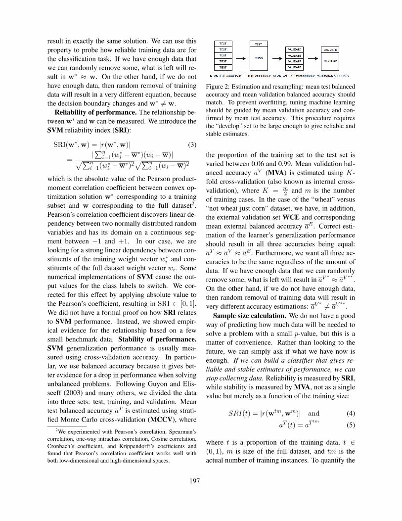
result in exactly the same solution. We can use thisproperty to probe how reliable training data are forthe classification task. If we have enough data thatwe can randomly remove some, what is left will re-sult in w∗ ≈ w. On the other hand, if we do nothave enough data, then random removal of trainingdata will result in a very different equation, becausethe decision boundary changes and w∗ 6= w.
Reliability of performance. The relationship be-tween w∗ and w can be measured. We introduce theSVM reliability index (SRI):
SRI(w∗,w) = |r(w∗,w)| (3)
=|∑n
i=1(w∗i −w∗)(wi −w)|√∑n
i=1(w∗i −w∗)2
√∑ni=1(wi −w)2
which is the absolute value of the Pearson product-moment correlation coefficient between convex op-timization solution w∗ corresponding to a trainingsubset and w corresponding to the full dataset2.Pearson’s correlation coefficient discovers linear de-pendency between two normally distributed randomvariables and has its domain on a continuous seg-ment between −1 and +1. In our case, we arelooking for a strong linear dependency between con-stituents of the training weight vector w∗i and con-stituents of the full dataset weight vector wi. Somenumerical implementations of SVM cause the out-put values for the class labels to switch. We cor-rected for this effect by applying absolute value tothe Pearson’s coefficient, resulting in SRI ∈ [0, 1].We did not have a formal proof on how SRI relatesto SVM performance. Instead, we showed empir-ical evidence for the relationship based on a fewsmall benchmark data. Stability of performance.SVM generalization performance is usually mea-sured using cross-validation accuracy. In particu-lar, we use balanced accuracy because it gives bet-ter evidence for a drop in performance when solvingunbalanced problems. Following Guyon and Elis-seeff (2003) and many others, we divided the datainto three sets: test, training, and validation. Meantest balanced accuracy aT is estimated using strati-fied Monte Carlo cross-validation (MCCV), where
2We experimented with Pearson’s correlation, Spearman’scorrelation, one-way intraclass correlation, Cosine correlation,Cronbach’s coefficient, and Krippendorff’s coefficients andfound that Pearson’s correlation coefficient works well withboth low-dimensional and high-dimensional spaces.
Figure 2: Estimation and resampling: mean test balancedaccuracy and mean validation balanced accuracy shouldmatch. To prevent overfitting, tuning machine learningshould be guided by mean validation accuracy and con-firmed by mean test accuracy. This procedure requiresthe “develop” set to be large enough to give reliable andstable estimates.
the proportion of the training set to the test set isvaried between 0.06 and 0.99. Mean validation bal-anced accuracy aV (MVA) is estimated using K-fold cross-validation (also known as internal cross-validation), where K = m
2 and m is the numberof training cases. In the case of the “wheat” versus“not wheat just corn” dataset, we have, in addition,the external validation set WCE and correspondingmean external balanced accuracy aE . Correct esti-mation of the learner’s generalization performanceshould result in all three accuracies being equal:aT ≈ aV ≈ aE . Furthermore, we want all three ac-curacies to be the same regardless of the amount ofdata. If we have enough data that we can randomlyremove some, what is left will result in aV ∗ ≈ aV ∗∗
.On the other hand, if we do not have enough data,then random removal of training data will result invery different accuracy estimations: aV ∗ 6= aV ∗∗
.Sample size calculation. We do not have a good
way of predicting how much data will be needed tosolve a problem with a small p-value, but this is amatter of convenience. Rather than looking to thefuture, we can simply ask if what we have now isenough. If we can build a classifier that gives re-liable and stable estimates of performance, we canstop collecting data. Reliability is measured by SRI,while stability is measured by MVA, not as a singlevalue but merely as a function of the training size:
SRI(t) = |r(wtm,wm)| and (4)
aT (t) = aT tm(5)
where t is a proportion of the training data, t ∈(0, 1), m is size of the full dataset, and tm is theactual number of training instances. To quantify the
197

ability of the dataset to produce classification mod-els with reliable and stable performance estimates,we need two more measures: sample dispersion ofSRI and sample dispersion of MVA:
cSRI(t ≥ p) =sSRI(t≥p)
SRI(t ≥ p)and (6)
cMV A(t ≥ p) =saT (t≥p)
aT (t ≥ p)(7)
defined as the coefficient of variation of all SRI orMVA measurements for training data sizes greaterthan pm. For example, we want to know if our 10-fold cross-validation (CV) for a dataset that has 400training samples is reliable and stable. 10-fold CVis 0.9 of training data, so we need to measure SRIand MVA for different proportions of training data,t = {0.90, 0.91, . . . , 0.99}, and then calculate dis-persion for cSRI(t ≥ 0.9) and cMV A(t ≥ 0.9). Nu-merical calculations will give us sense of good andbad dispersion across different datasets.
5 Results
Do I have enough data? The first set of experi-ments was done with untuned algorithms. We set theSVM parameter to C = 1 and did not use any fea-ture selection. Figure 3 shows four examples of howSVM performance depends on the training set size.The performance was measured using mean test bal-anced accuracy, MVA, and SRI. Numerical calcu-lations showed that VV needs at least 30 randomlyselected training examples to produce reliable andstable results with high accuracy. cSRI(t ≥ 0.75)is 0.005 and cMV A(t ≥ 0.75) is 0.016. SN wasnot encouraging regarding the estimated accuracy;SRI dropped, suggesting that the SVM decision hy-perplanes are unreliable. Mental health profession-als can distinguish between genuine and simulatednotes about 63% of time. Machine learning doesit correctly about 73% of time if text structure andemotional content are used. Even so, the samplesize calculation yields high dispersion (cSRI(t ≥0.75) = 0.134 and cMV A(t ≥ 0.75) = 0.082).UQ is small and high-dimensional, and yet the re-sults were reliable and stable (cSRI(t ≥ 0.75) =0.015 and cMV A(t ≥ 0.75) = 0.023). Patientsenrolled in the UQ study also received the Sui-cide Ideation Questionnaire (Raynolds, 1987) and
the Columbia-Suicide Severity Rating Scale (Pos-ner et al., 2011). We found that UQ was no dif-ferent from the structured questionnaires. UQ de-tects suicidality mostly by emotional pain and hope-lessness, which were mildly present in four controlpatients. Other instruments returned errors becausethe same few teenagers reported risky behavior andmorbid thoughts. WCT produced reliable and sta-ble accuracy estimates, but no large amounts of datacould be removed (cSRI(t ≥ 0.75) = 0.010 andcMV A(t ≥ 0.75) = 0.053). It seems that WCEis somehow different from WCT, or it might be acase of overfitting, which causes the mean test ac-curacy to diverge from MVA as the training datasetgets smaller. Algorithm tuning. No results shouldbe regarded as satisfactory until a thorough param-eter space search has been completed. Each step ofa text classification algorithm can be improved. Toattempt a complete description of the dependencyof a minimal viable sample size on text classifica-tion would be both impossible and futile, since newmethods are discovered every day. However, to startsomewhere, we focused only on the feature selectionand SVM parameter C 3. Feature selection removesnoise from data. Parameter C informs the convexoptimization process about the expected noise level.If both parameters are set correctly, we should seean improvement in the reliability and stability ofthe results. There are several methods for tuningSVM; the most commonly used but computation-ally expensive is internal cross-validation (Duan etal., 2003; Chapelle et al., 2002). Figure 5 showsthe results of the parameter tuning procedure. VVand SN are not extremely high-dimensional, so wetuned just parameter C. MVA maxima were foundat C = 0.45 with VV, C = 0.05 with SN, C = 0.4and IG = 0.1584 with UQ, and C = 2.5 andIG = 0.8020 with WCT. Do I have enough dataafter algorithm tuning? Internal cross-validation(MVA) did not improve dispersion universally (seeTable 2). VV improved on reliability but not stabil-ity. SN scored much better on both measures, butwe do not yet know what the cutoff for having alow enough dispersion is. UQ did worse on all mea-sures after tuning. WCT improved greatly on mean
3Please note that most SVM implementations do not allowfor simultaneous feature selection and internal cross-validation.
198

VV SN UQ WCT and WCE
Figure 3: SRI index (S), MVA accuracy (V) and mean test accuracy (T) averaged over 120 repetitions and differenttraining data sizes. Linear SVM with C = 1 and no feature selection. VV (cSRI(t ≥ 0.75) = 0.005 and cMV A(t ≥0.75) = 0.016), UQ (cSRI(t ≥ 0.75) = 0.015 and cMV A(t ≥ 0.75) = 0.023), and WCT (cSRI(t ≥ 0.75) = 0.010and cMV A(t ≥ 0.75) = 0.053) gave stable and reliable estimates, but SN did not (cSRI(t ≥ 0.75) = 0.134 andcMV A(t ≥ 0.75) = 0.082).
VV SN UQ WCT
Figure 4: MVA (internal cross-validation) parameter tuning results. Maxima were found at C = 0.45 with VV,C = 0.05 with SN, C = 0.4 and IG = 0.1584 with UQ, and C = 2.5 and IG = 0.8020 with WCT.
VV SN UQ WCT and WCE
Figure 5: SRI index (S), MVA accuracy (V), and mean test accuracy (T) averaged over 60 repetitions and differenttraining data sizes. Tuned classification algorithms: VV with C = 0.45 and no feature selection, SN with C = 0.05and no feature selection, UQ with C = 0.4 and IG = 0.1584, and WCT with C = 2.5 and IG = 0.8020. Stabilityand reliability: VV had cSRI(t ≥ 0.75) = 0.003 and cMV A(t ≥ 0.75) = 0.018), SN had cSRI(t ≥ 0.75) = 0.085and cMV A(t ≥ 0.75) = 0.075, UQ had cSRI(t ≥ 0.75) = 0.025 and cMV A(t ≥ 0.75) = 0.024, and WCT hadcSRI(t ≥ 0.75) = 0.025 and cMV A(t ≥ 0.75) = 0.011.
199

test accuracy, mean external validation, and stabilitydispersion (see Figure 5). It would be interesting tosee if improvement on both reliability dispersion andstability dispersion would bring mean test accuracyand mean external validation even closer together.
aT (t ≥ 0.75) cSRI(t ≥ 0.75) cMV A(t ≥ 0.75)VV no tuning 0.965 0.005 0.016SN no tuning 0.744 0.134 0.082UQ no tuning 0.946 0.015 0.023WCT no tuning 0.862 0.010 0.053VV with tuning 0.970 0.003 0.018SN with tuning 0.755 0.085 0.075UQ with tuning 0.941 0.025 0.024WCT with tuning 0.946 0.025 0.011
Table 2: Sample size calculation before and after tuningwith internal cross-validation (MVA). Even though meantest accuracy (aT (t ≥ 0.75)) improved for VV, SN, andWCT, reliability and stability did not improve univer-sally. Internal cross-validation alone might not be ade-quate for tuning classification algorithms for all data.
6 Discussion
Sample size calculation data for a competitionand for problem-solving. In general, there might betwo conflicting objectives when calculating whetherwhat we have collected is a large enough dataset. Ifthe objective is to have a shared task with many par-ticipants and, thus, many unknowns, the best courseof action is to assume the weakest classifier: uni-grams with no feature weighting or selection trainedusing the simplest logistic regression. On the otherhand, if the problem is to be solved with only oneclassifier and the least amount of data, then thestrongest assumptions about the data and the algo-rithm are required.
The fallacy of untuned algorithms. After yearsof working with classification algorithms to solvedifficult patient care problems, we have found thata large amount of data is not needed; usually sam-ples measured in the hundreds will suffice, but thisis only possible when a thorough parameter spacesearch is conducted. It seems that reliability andstability dispersions are good measures of how wellthe algorithm is tuned to the data without overfitting.Moreover, we now have a new direction for thinkingabout optimizing classification algorithms: insteadof focusing solely on accuracy, we can also measurethe dispersion and see whether this is a better indi-
cator of what would happen with unevaluated data.There is a great deal of data available, but very littlethat can be used for training.
What to measure? VC-bound, span-bound, ac-curacy, F1, reliability, and stability dispersions arejust a few examples of indicators of how well ourmodels fit. What we have outlined here is howone of the many properties of SVM, the propertyof the normal vector, can be used to obtain insightsinto data. Normal vectors are constructed using La-grangian multipliers and support vectors; accuracyis constructed using a sign function on decision val-ues. It is feasible that other parts of SVM may bemore suited to algorithm tuning and calculation ofminimum viable training size.
7 Conclusion
Power and sample size calculations are very impor-tant in any domain that requires extensive expertise.We do not want to collect more data than necessary.There is, however, a scarcity of research in samplesize calculation for machine learning. Nonetheless,the existing results are consistent: the more that canbe assumed about the data, the problem and the al-gorithm, the fewer data are needed.
We proposed two independent measures for eval-uating whether available datasets are sufficientlylarge: reliability and stability dispersions. Reliabil-ity dispersion measures indirectly whether the deci-sion hyperplane is always similar and how much itvaries, while stability dispersion measures how wellwe are generalizing and how much variability thereis. If the sample size is large enough, we shouldalways get the same decision hyperplane with thesame generalization accuracy.
With little empirical evidence, we can concludethat classifier performance measured by just a singleK in a cross-validation test is not sufficient. K mustbe be varied, and other measures must be present,such as the SVM reliability index, that support orcontradict the generalization accuracy estimates. Wesuggest that other measures for sample size calcula-tion and algorithm tuning may exist and there is stillmuch to be learned about the mechanics of supportvector machines.
200

References
Edgar Anderson. 1935. The irises of the gaspe peninsula.Bulletin of the American Iris Society, 59:2–5.
Chidanand Apte, Fred Damerau, and Sholom M. Weiss.1994. Automated learning of decision rules for textcategorization. ACM Trans. Inf. Syst., 12(3):233–251,July.
Olivier Chapelle, Vladimir Vapnik, Olivier Bousquet, andSayan Mukherjee. 2002. Choosing multiple parame-ters for support vector machines. Machine Learning,46:131–159.
Kevin K. Dobbin, Yingdong Zhao, and Richard M. Si-mon. 2008. How large a training set is needed to de-velop a classifier for microarray data? Clinical cancerresearch : an official journal of the American Associ-ation for Cancer Research, 14(1):108–114, January.
Kaibo Duan, S. Sathiya Keerthi, and Aun Neow Poo.2003. Evaluation of simple performance measuresfor tuning svm hyperparameters. Neurocomputing,51:41–59.
Ronald A. Fisher. 1936. The use of multiple measure-ments in taxonomic problems. Annals of Eugenics,7:179–188.
Isabelle Guyon and Andre Elisseeff. 2003. An introduc-tion to variable and feature selection. J. Mach. Learn.Res., 3:1157–1182, March.
Isabelle Guyon, John Makhoul, Richard Schwartz, andVladimir Vapnik. 1998. What size test set gives gooderror rate estimates? Pattern Analysis and MachineIntelligence, IEEE Transactions on, 20(1):52–64, Jan-uary.
Fushing Y. Hsieh, Daniel A. Bloch, and Michael D.Larsen. 1998. A simple method of sample size cal-culation for linear and logistic regression. Statistics inMedicine, 17(14):1623–1634, December.
Fred A. Wright Jianhua Hu, Fei Zou. 2005. Practical fdr-based sample size calculations in microarray experi-ments. Bioinformatics, 21(15):3264–3272, August.
Thorsten Joachims. 1998. Text categorization with sup-port vector machines: Learning with many relevantfeatures. In Claire Ndellec and Cline Rouveirol, ed-itors, Machine Learning: ECML-98, volume 1398,pages 137–142. Springer-Verlag, Berlin/Heidelberg.
David Juckett. 2012. A method for determining the num-ber of documents needed for a gold standard corpus.Journal of Biomedical Informatics, page In Press, Jan-uary.
David D. Lewis and Marc Ringuette. 1994. A com-parison of two learning algorithms for text categoriza-tion. In Third Annual Symposium on Document Anal-ysis and Information Retrieval, pages 81–93.
Christopher D. Manning and Hinrich Schuetze. 1999.Foundations of Statistical Natural Language Process-ing. The MIT Press, 1 edition, June.
Christopher D. Manning, Prabhakar Raghavan, and Hin-rich Schtze. 2008. Introduction to Information Re-trieval. Cambridge University Press, 1 edition, July.
Preslav Nakov, Antonia Popova, and Plamen Mateev.2001. Weight functions impact on lsa performance.In EuroConference RANLP’2001 (Recent Advances inNLP), pages 187–193.
John Pestian, Henry Nasrallah, Pawel Matykiewicz, Au-rora Bennett, and Antoon Leenaars. 2010. Suicidenote classification using natural language processing:A content analysis. Biomedical Informatics Insights,pages 19–28, August.
John Pestian, Jacqueline Grupp-Phelan, PawelMatkiewicz, Linda Richey, Gabriel Meyers,Christina M. Canter, and Michael Sorter. 2012.Suicidal thought markers: A controlled trail exam-ining the language of suicidal adolescents. To BeDetermined, In Preparation.
Kelly Posner, Gregory K. Brown, Barbara Stanley,David A. Brent, Kseniya V. Yershova, Maria A.Oquendo, Glenn W. Currier, Glenn A. Melvin, Lau-rence Greenhill, Sa Shen, and J. John Mann. 2011.The ColumbiaSuicide severity rating scale: Initial va-lidity and internal consistency findings from three mul-tisite studies with adolescents and adults. The Amer-ican Journal of Psychiatry, 168(12):1266–1277, De-cember.
William M. Raynolds, 1987. Suicidal Ideation Question-naire - Junior. Odessa, FL: Psychological AssessmentResources.
Gerard Salton and Christopher Buckley. 1988. Term-weighting approaches in automatic text retrieval. In-formation Processing & Management, 24(5):513–523.
Bernhard Schlkopf and Alexander J. Smola. 2001.Learning with Kernels: Support Vector Machines,Regularization, Optimization, and Beyond. The MITPress, 1st edition, December.
Edwin S. Shneidman and Norman Farberow. 1957.Clues to Suicide. McGraw Hill Paperbacks.
Ted W. Way, Berkman Sahiner, Lubomir M. Hadjiiski,and Heang-Ping Chan. 2010. Effect of finite samplesize on feature selection and classification: a simula-tion study. Medical Physics, 37(2):907–920, February.
Yiming Yang and Jan O. Pedersen. 1997. A compara-tive study on feature selection in text categorization.In Proceedings of the Fourteenth International Con-ference on Machine Learning, ICML ’97, pages 412–420, San Francisco, CA, USA. Morgan KaufmannPublishers Inc.
201
Proceedings of the 2012 Workshop on Biomedical Natural Language Processing (BioNLP 2012), pages 202–205,Montreal, Canada, June 8, 2012. c©2012 Association for Computational Linguistics
PubAnnotation - a persistent and sharable corpus and annotation repository
Jin-Dong Kim and Yue WangDatabase Center for Life Science (DBCLS),
Research Organization of Information and Systems (ROIS),2-11-16, Yayoi, Bunkyo-ku, Tokyo, 113-0032, Japan
{jdkim|wang}@dbcls.rois.ac.jp
Abstract
There has been an active development of cor-pora and annotations in the BioNLP commu-nity. As those resources accumulate, a newissue arises about the reusability. As a solu-tion to improve the reusability of corpora andannotations, we presentPubAnnotation, a per-sistent and sharable repository, where variouscorpora and annotations can be stored togetherin a stable and comparable way. As a positionpaper, it explains the motivation and the coreconcepts of the repository and presents a pro-totype repository as a proof-of-concept.
1 Introduction
Corpora with high-quality annotation is regarded in-dispensable for the development oflanguage pro-cessing technology (LT), e.g.natural language pro-cessing (NLP)or textmining. Biology is one of thefields which have strong needs for LT, due to thehigh productivity of new information, most of whichis published in literature. There have been thus anactive development of corpora and annotations fortheNLP for biology (BioNLP). Those resources arecertainly an invaluable asset of the community.
As those resources accumulate, however, a newissue arises about the reusability: the corpora andannotations need to be sharable and comparable. Forexample, there are a number of corpora that claim tohave annotations for protein or gene names, e.g, Ge-nia (Kim et al., 2003), Aimed (Bunescu et al., 2004),and Yapex (Franzen et al., 2002). To reuse them, auser needs to be able to compare them so that theycan devise a strategy on how to use them. It is how-ever known that often the annotations in different
corpora are incompatible to each other (Wang et al.,2010): while one is considered as a protein name ina corpus, it may not be the case in another.
A comparison of annotations in different corporacould be made directly or indirectly. If there is anoverlap between two corpora, a direct comparisonof them would be possible. For example, there areone1, two2 and three3 PubMed abstracts overlappedbetween Genia - Yapex, Genia - Aimed, and Yapex- Aimed corpora, respectively. When there is no orinsufficient overlap, an indirect comparison could betried (Wang et al., 2010). In any case, there are anumber of problems that make it costly and trouble-some, though not impossible, e.g. different formats,different ways of character encoding, and so on.
While there have been a few discussions aboutthe reusability of corpora and annotations (Cohen etal., 2005; Johnson et al., 2007; Wang et al., 2010;Campos et al., 2012), as a new approach, we presentPubAnnotation, a persistent and sharable storage orrepository, where various corpora and annotationscan be stored together in a stable and comparableway. In this position paper, after the motivation andbackground are explained in section 1, the initial de-sign and a prototype implementation of the storageare presented in section 2 and 3, respectively and fu-ture works are discussed in section 4.
2 Design
Figure 1 illustrates the current situation of cor-pus annotation in the BioNLP community, whichwe consider problematic. In the community, there
1PMID-103578182PMID-8493578, PMID-89103983PMID-9144171, PMID-10318834, PMID-10713102
202
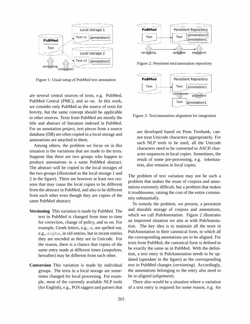
Figure 1: Usual setup of PubMed text annotation
are several central sources of texts, e.g. PubMed,PubMed Central (PMC), and so on. In this work,we consider only PubMed as the source of texts forbrevity, but the same concept should be applicableto other sources. Texts from PubMed are mostly thetitle and abstract of literature indexed in PubMed.For an annotation project, text pieces from a sourcedatabase (DB) are often copied in a local storage andannotations are attached to them.
Among others, the problem we focus on in thissituation is the variations that are made to the texts.Suppose that there are two groups who happen toproduce annotations to a same PubMed abstract.The abstract will be copied to the local storages ofthe two groups (illustrated as the local storage 1 and2 in the figure). There are however at least two rea-sons that may cause the local copies to be differentfrom the abstract in PubMed, and also to be differentfrom each other even though they are copies of thesame PubMed abstract:
Versioning This variation is made by PubMed. Thetext in PubMed is changed from time to timefor correction, change of policy, and so on. Forexample, Greek letters, e.g.,α, are spelled out,e.g.,alpha, in old entries, but in recent entriesthey are encoded as they are in Unicode. Forthe reason, there is a chance that copies of thesame entry made at different times (snapshots,hereafter) may be different from each other.
Conversion This variation is made by individualgroups. The texts in a local storage are some-times changed for local processing. For exam-ple, most of the currently available NLP tools(for English), e.g., POS taggers and parsers that
Figure 2: Persistent text/annotation repository
Figure 3: Text/annotation alignment for integration
are developed based on Penn Treebank, can-not treat Unicode characters appropriately. Forsuch NLP tools to be used, all the Unicodecharacters need to be converted to ASCII char-acter sequences in local copies. Sometimes, theresult of some pre-processing, e.g. tokeniza-tion, also remains in local copies.
The problem of text variation may not be such aproblem that makes the reuse of corpora and anno-tations extremely difficult, but a problem that makesit troublesome, raising the cost of the entire commu-nity substantially.
To remedy the problem, we present, a persistentand sharable storage of corpora and annotations,which we callPubAnnotation. Figure 2 illustratesan improved situation we aim at with PubAnnota-tion. The key idea is to maintain all the texts inPubAnnotation in their canonical form, to which allthe corresponding annotations are to be aligned. Fortexts from PubMed, the canonical form is defined tobe exactly the same as in PubMed. With the defini-tion, a text entry in PubAnnotation needs to be up-dated (uptodatein the figure) as the correspondingtext in PubMed changes (versioning). Accordingly,the annotations belonging to the entry also need tobe re-aligned (alignment).
There also would be a situation where a variationof a text entry is required for some reason, e.g. for
203

Figure 4: Text/annotation alignment example
application of an NLP tool that cannot handle Uni-code characters. Figure 3 illustrates a required pro-cess to cope with such a situation: first, the text isexported in a desired form (conversionin the fig-ure); second, annotations are made to the text; andthird, the annotations are aligned back to the text inits canonical form in the repository.
Figure 4 shows an example of text conversionand annotation alignment that are required when theEnju parser (Miyao and Tsujii, 2008) needs to beused for the annotation of protein names. The ex-ample text includes a Greek letter,ε, which Enjucannot properly handle. As Enju expects Greekletters to be spelled out with double equal signson both sides, the example text is converted as sowhen it is exported into a local storage. Basedon the pre-processing by Enju, the two text spans,CD==epsilon== andCD4, are annotated as pro-tein names. When they are imported back to PubAn-notation, the annotations are re-aligned to the canon-ical text in the repository. In this way, the textsand annotations can be maintained in their canon-ical form and in alignment respectively in PubAn-notation. In the same way, existing annotations, e.g.Genia, Aimed, Yapex, may be imported in the repos-itory, as far as their base texts are sufficiently similarto the canonical entries so that they can be alignedreliably. In this way, various existing annotationsmay be integrated in the repository,
To enable all the processes described so far, anytwo versions of the same text need to be aligned, sothat the places of change can be detected. Text align-ment is therefore a key technology of PubAnnota-tion. In our implementation of the prototype repos-itory, the Hunt-McIlroy’s longest common subse-quence (LCS) algorithm (Hunt and McIlroy, 1976),as implemented in thediff-lcs ruby gem pack-age, is used for the alignment.
Figure 5: DB schema of persistent annotation repository
3 Prototype implementation
As a proof-of-concept, a prototype repository hasbeen implemented. One aspect considered seriouslyis thescalability, as repository is intended to be “per-sistent”. Therefore it is implemented on a relationaldatabase (Ruby on Rails with PostgreSQL 9.1.3), in-stead of relying on a plain file system.
Figure 5 shows the database schema of the reposi-tory.4 Three tables are created fordocuments, anno-tations, and (annotation)contexts, respectively. Theannotations are stored in a stand-off style, each ofwhich belongs to adocumentand also to ananno-tation context(context, hereafter). A context rep-resents a set of annotations sharing the same set ofmeta-data, e.g., the type of annotation and the an-notator. For brevity, we only considered PubMed asthe source DB, and named entity recognition (NER)-type annotations, which may be simply representedby the attributes,begin, end, andlabel.
The prototype repository provides a RESTful in-terface. Table 1 shows some example which can beaccessed with the standard HTTP GET method. Anew entry can be created in the repository using aHTTP POST method with data in JSON format. Fig-ure 6 shows an example of JSON data for the cre-ation of annotations in the repository. Note that, thebase text of the annotations needs to be passed to-gether with the annotations, so that the text can becompared to the canonical one in the repository. If adifference is detected, the repository will try to alignthe annotations to the text in the repository.
4Although not shown in the figure, all the records are storedwith the date of creation.
204

http://server url/pmid/8493578to retrieve the document record of a specific PMID
http://server url/pmid/8493578.asciisame as above, but in US-ASCII encoding (Unicode characters are converted to HTML entities).
http://server url/pmid/8493578/annotationsto retrieve all the annotations to the specific document.
http://server url/pmid/8493578/contextsto retrieve all the annotation contexts created to the specific document.
http://server url/pmid/8493578/annotations?context=genia-proteinto retrieve all the annotations that belong to genia-protein context.
http://server url/pmid/8493578/annotations.json?context=genia-proteinthe same as above, but in JSON format.
Table 1: Examples of RESTful interface of the prototype repository
{"document":
{"pmid":"8493578","text":"Regulation ..."},
"context":{"name":"genia-protein"},
"annotations":[
{"begin":51,"end":56,"label":"Protein",{"begin":75,"end":97,"label":"Protein",
]}
Figure 6: The JSON-encoded data for the creation of twoprotein annotations to the document of PMID:8493578.
4 Discussions and conclusions
The current state of the design and the prototypeimplementation are largely incomplete, and there isa much room for improvement. For example, thedatabase schema has to be further developed to storetexts from various source DBs, e.g., PMC, and torepresent various types of annotations, e.g., relationsand events. The issue of governance is yet to bediscussed. We, however, hope the core conceptspresented in this position paper to facilitate discus-sions and collaborations of the community and theremaining issues to be addressed in near future.
Acknowledgments
This work was supported by the “IntegratedDatabase Project” funded by the Ministry of Edu-cation, Culture, Sports, Science and Technology ofJapan.
References
Razvan Bunescu, Ruifang Ge, Rohit J. Kate, Edward M.Marcotte, Raymond J. Mooney, Arun K. Ramani, andYuk Wah Wong. 2004. Comparative experimentson learning information extractors for proteins andtheir interactions.Artificial Intelligence in Medicine,33(2):139–155.
David Campos, Srgio Matos, Ian Lewin, Jos Lus Oliveira,and Dietrich Rebholz-Schuhmann. 2012. Harmoniza-tion of gene/protein annotations: towards a gold stan-dard medline.Bioinformatics, 28(9):1253–1261.
K. Bretonnel Cohen, Philip V Ogren, Lynne Fox, andLawrence Hunter. 2005. Empirical data on corpus de-sign and usage in biomedical natural language process-ing. In AMIA annual symposium proceedings, pages156–160.
Kristofer Franzen, Gunnar Eriksson, Fredrik Olsson, LarsAsker, Per Liden, and Joakim Coster. 2002. Proteinnames and how to find them.International Journal ofMedical Informatics, 67(13):49 – 61.
James W. Hunt and M. Douglas McIlroy. 1976. An Al-gorithm for Differential File Comparison. TechnicalReport 41, Bell Laboratories Computing Science, July.
Helen Johnson, William Baumgartner, Martin Krallinger,K Bretonnel Cohen, and Lawrence Hunter. 2007.Corpus refactoring: a feasibility study.Journal ofBiomedical Discovery and Collaboration, 2(1):4.
Jin-Dong Kim, Tomoko Ohta, Yuka Tateisi, and Jun’ichiTsujii. 2003. GENIA corpus - a semantically an-notated corpus for bio-textmining.Bioinformatics,19(suppl. 1):i180–i182.
Yusuke Miyao and Jun’ichi Tsujii. 2008. Feature forestmodels for probabilistic hpsg parsing.ComputationalLinguistics, 34(1):35–80, March.
Yue Wang, Jin-Dong Kim, Rune Sætre, Sampo Pyysalo,Tomoko Ohta, and Jun’ichi Tsujii. 2010. Improvingthe inter-corpora compatibility for protein annotations.Journal of Bioinformatics and Computational Biology,8(5):901–916.
205

Proceedings of the 2012 Workshop on Biomedical Natural Language Processing (BioNLP 2012), pages 206–213,Montreal, Canada, June 8, 2012. c©2012 Association for Computational Linguistics
Using Natural Language Processing to Identify Pharmacokinetic Drug-Drug Interactions Described in Drug Package Inserts
Richard Boyce, PhD University of Pittsburgh
5607 Baum Avenue Pittsburgh, PA 15206, USA
Gregory Gardner, MS University of Pittsburgh
5607 Baum Avenue Pittsburgh, PA 15206, USA
Henk Harkema, PhD University of Pittsburgh
6425 Penn Ave. Pittsburgh, PA 15206
Abstract
The package insert (aka drug product label) is the only publicly-available source of infor-mation on drug-drug interactions (DDIs) for some drugs, especially newer ones. Thus, an automated method for identifying DDIs in drug package inserts would be a potentially important complement to methods for identi-fying DDIs from other sources such as the scientific literature. To develop such an algo-rithm, we created a corpus of Federal Drug Administration approved drug package insert statements that have been manually annotated for pharmacokinetic DDIs by a pharmacist and a drug information expert. We then evalu-ated three different machine learning algo-rithms for their ability to 1) identify pharmacokinetic DDIs in the package insert corpus and 2) classify pharmacokinetic DDI statements by their modality (i.e., whether they report a DDI or no interaction between drug pairs). Experiments found that a support vector machine algorithm performed best on both tasks with an F-measure of 0.859 for pharmacokinetic DDI identification and 0.949 for modality assignment. We also found that the use of syntactic information is very helpful for addressing the problem of sentences con-taining both interacting and non-interacting pairs of drugs.
1 Introduction
Package inserts (PIs, aka drug product label) are the primary source of information for newly ap-proved drugs and a potentially authoritative source of drug information from a medical-legal stand-
point (Marroum & Gobburu 2002). Among the information provided by PIs are drug-drug interac-tions (DDIs): known and predicted drug combina-tions that could lead to a clinically meaningful alteration in the effect of one of the drugs. The United States Federal Drug Administration (FDA) mandates that PIs for FDA-approved drugs include both observed and predicted clinically significant DDIs, as well as the results of pharmacokinetic studies that establish the absence of effect (FDA. 2010). Moreover, the PI is the only publically-available source of information on DDIs for some drugs, especially newer ones (Dal-Ré et al. 2010). Hence, an automated method for identifying DDIs from drug PIs would be an important complement to methods for identifying DDIs from other sources such as the scientific literature. In this pa-per we describe the creation of a new corpus of FDA-approved drug package insert statements that have been manually annotated for pharmacokinetic DDIs. We then discuss how three different ma-chine learning algorithms were evaluated for their ability to 1) identify pharmacokinetic DDIs in drug package inserts and 2) classify pharmacokinetic DDI statements by their modality (i.e., whether they report a DDI or that a drug pair does not in-teract).
2 Materials and Methods
2.1 The DDI Corpus and Schema
A corpus of annotated statements derived from FDA-approved drug PIs was created for use as training and test data while developing automated DDI extraction algorithms. The statements were derived from PIs using a strategy that ensured there
206

would be a representative sample of statements that 1) unambiguously identified interacting drug pairs, 2) unambiguously identified non-interacting drug pairs, and 3) included no mention of interact-ing drug pairs. Previous experience by our research group suggested that the manner in which DDI statements are described in PIs has changed over time in response to changing FDA regulations. Most notably, an FDA guidance document issued in 1999 was (to our knowledge) the first to explic-itly suggest the inclusion of brief descriptions of pharmacokinetic DDI studies within specific sec-tions of drug PIs (FDA. 1999). To account for this, investigators selected 64 PIs using a strategy that ensured the corpus would have a balanced sample of statements from drugs marketed before and after 2000. For the purpose of this study we designated all PIs for drugs marketed prior to 2000 as “older” and those for drugs marketed in or after 2000 as “newer.” PIs were downloaded from the DailyMed website,1 and the entire “Drug Interactions” and “Clinical Pharmacology” sections were selected as text sources from “newer” PIs. For “older” PIs, which often lacked these two sections, investiga-tors chose a section containing an apparent interac-tion statement and one randomly-selected section.
DDIs are typically classified as occurring by either pharmacodynamic or pharmacokinetic mechanisms. A pharmacodynamic DDI involves the additive or synergistic amplification of a drug’s effect. In a pharmacokinetic (PK) DDI, one drug, called a precipitant, affects (inhibits or induces) the absorption, distribution, metabolism, or excre-tion of another drug, called the object. To simplify our task, we decided to focus specifically on PK DDIs. Prior to annotating the PI statements, a schema was created for the entities that the investi-gators considered important components of a PK DDI. The schema modeled drugs as having two characteristics, type and role. The type of drug could be active ingredient (e.g., simvastatin), drug product (e.g., Zocor), or metabolite (e.g., beta-OH-simvastatin). Drugs annotated as metabolite also referred to the active ingre-dient parent compound. The role of a drug could be either an object or a precipitant. Two oth-er properties were provided to model each PK DDI: 1) whether the statement from which the DDI was identified suggested an observed effect or a 1 http://dailymed.nlm.nih.gov/
lack of an observed effect between two coadminis-tered drugs (i.e., positive vs negative modali-ty statements), and 2) whether the statement included quantitative or qualitative data in describ-ing an interaction or non-interaction between a drug pair (i.e., quantitative vs qualitative statements). Finally, the segment of text in which the interaction claim was made was annotated as an interaction phrase. With the corpus and schema in place, drugs and PK DDIs present in the PI statements were then annotated by two inde-pendent reviewers using Knowtator, an annotation tool integrated with the Protégé ontology editor (Ogren 2006).
One annotator was a pharmacist and DDI expert, and the other a librarian specializing in drug information retrieval. To help the annotators, co-investigator RB ran the NCBO Annotator (Jon-quet, Shah & Musen 2009) over the corpus using the RxNorm drug terminology (Nelson et al. 2011) to pre-annotate as many active ingredients and drug products as possible. The annotators reviewed these “pre-annotations” while identifying entities that missed during the pre-annotation process. Co-investigator HH used Knowtator to calculate inter-annotator agreement statistics from the annotators’ initial annotation sets. RB then worked with the two annotators to achieve consensus on the final corpus of annotated DDI statements.
2.2 Setting up the DDI statement extraction experiment
Once the set of DDI annotations was compiled, we devised two machine learning tasks. The first task was to determine whether two drugs mentioned in a statement taken from a PI are noted as either in-teracting or not interacting with each other by pharmacokinetic mechanisms (i.e., does the state-ment report a PK DDI with the drug pair of either a positive or negative modality?). The second task was to determine the modality of a given PK DDI. The first task did not include determining the roles of the drugs if an interaction is found, i.e., which member of the pair of drug mentions is the precipi-tant and which one is the object. To enable the ex-ploration of the performance of multiple machine learning methods, we divided two-thirds of the annotated PI statements into a development set and one-third into a blind test set. PI statements anno-tated as reporting DDIs were stratified within the
207
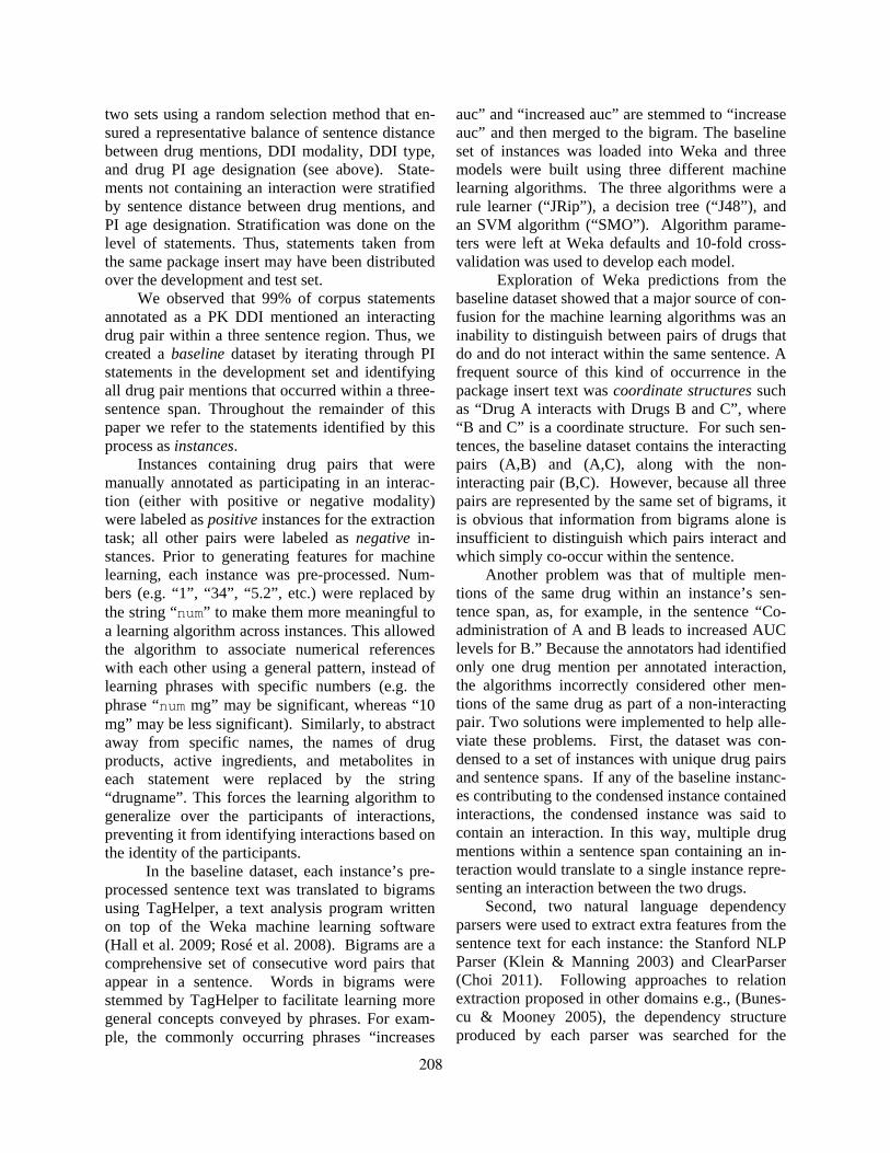
two sets using a random selection method that en-sured a representative balance of sentence distance between drug mentions, DDI modality, DDI type, and drug PI age designation (see above). State-ments not containing an interaction were stratified by sentence distance between drug mentions, and PI age designation. Stratification was done on the level of statements. Thus, statements taken from the same package insert may have been distributed over the development and test set.
We observed that 99% of corpus statements annotated as a PK DDI mentioned an interacting drug pair within a three sentence region. Thus, we created a baseline dataset by iterating through PI statements in the development set and identifying all drug pair mentions that occurred within a three-sentence span. Throughout the remainder of this paper we refer to the statements identified by this process as instances.
Instances containing drug pairs that were manually annotated as participating in an interac-tion (either with positive or negative modality) were labeled as positive instances for the extraction task; all other pairs were labeled as negative in-stances. Prior to generating features for machine learning, each instance was pre-processed. Num-bers (e.g. “1”, “34”, “5.2”, etc.) were replaced by the string “num” to make them more meaningful to a learning algorithm across instances. This allowed the algorithm to associate numerical references with each other using a general pattern, instead of learning phrases with specific numbers (e.g. the phrase “num mg” may be significant, whereas “10 mg” may be less significant). Similarly, to abstract away from specific names, the names of drug products, active ingredients, and metabolites in each statement were replaced by the string “drugname”. This forces the learning algorithm to generalize over the participants of interactions, preventing it from identifying interactions based on the identity of the participants.
In the baseline dataset, each instance’s pre-processed sentence text was translated to bigrams using TagHelper, a text analysis program written on top of the Weka machine learning software (Hall et al. 2009; Rosé et al. 2008). Bigrams are a comprehensive set of consecutive word pairs that appear in a sentence. Words in bigrams were stemmed by TagHelper to facilitate learning more general concepts conveyed by phrases. For exam-ple, the commonly occurring phrases “increases
auc” and “increased auc” are stemmed to “increase auc” and then merged to the bigram. The baseline set of instances was loaded into Weka and three models were built using three different machine learning algorithms. The three algorithms were a rule learner (“JRip”), a decision tree (“J48”), and an SVM algorithm (“SMO”). Algorithm parame-ters were left at Weka defaults and 10-fold cross-validation was used to develop each model.
Exploration of Weka predictions from the baseline dataset showed that a major source of con-fusion for the machine learning algorithms was an inability to distinguish between pairs of drugs that do and do not interact within the same sentence. A frequent source of this kind of occurrence in the package insert text was coordinate structures such as “Drug A interacts with Drugs B and C”, where “B and C” is a coordinate structure. For such sen-tences, the baseline dataset contains the interacting pairs (A,B) and (A,C), along with the non-interacting pair (B,C). However, because all three pairs are represented by the same set of bigrams, it is obvious that information from bigrams alone is insufficient to distinguish which pairs interact and which simply co-occur within the sentence.
Another problem was that of multiple men-tions of the same drug within an instance’s sen-tence span, as, for example, in the sentence “Co-administration of A and B leads to increased AUC levels for B.” Because the annotators had identified only one drug mention per annotated interaction, the algorithms incorrectly considered other men-tions of the same drug as part of a non-interacting pair. Two solutions were implemented to help alle-viate these problems. First, the dataset was con-densed to a set of instances with unique drug pairs and sentence spans. If any of the baseline instanc-es contributing to the condensed instance contained interactions, the condensed instance was said to contain an interaction. In this way, multiple drug mentions within a sentence span containing an in-teraction would translate to a single instance repre-senting an interaction between the two drugs.
Second, two natural language dependency parsers were used to extract extra features from the sentence text for each instance: the Stanford NLP Parser (Klein & Manning 2003) and ClearParser (Choi 2011). Following approaches to relation extraction proposed in other domains e.g., (Bunes-cu & Mooney 2005), the dependency structure produced by each parser was searched for the
208

shortest path between the pair of drug mentions of the instance. The words on this path were stemmed using the Stanford NLP Tools stemmer (Stanford NLP 2011), and added to the dataset as the instance’s “syntactic path”.
Once a statement is classified as describing a PK DDI between two drugs, it is important to know if there is an observed effect or a lack of ef-fect between two coadministered drugs (i.e., posi-tive vs negative modality statements). To present the learning algorithms with the most relevant training data, modality prediction was treated as a separate task from interaction prediction. Devel-opment and test sets were created in the same manner as for interaction prediction, however in-stances that did not represent interactions were ex-cluded. Only bigram features were used for modality prediction. Model training and testing proceeded in the same manner as for interaction prediction.
3 Results
A total of 208 multi-sentence sections were ex-tracted from 64 PIs. Prior to consensus, inter-annotator agreement between the two annotators on PK DDI, active ingredient, drug product, me-tabolite mentions and was found to be 60%, 96.3%, 99.5%, and 60.8% respectively. The major-ity of disagreements about DDIs were due to a ten-dency of one annotator to incorrectly annotate some pharmacodynamic DDIs as PK DDIs. Also, one annotator incorrectly assumed that all metabo-lites had been pre-annotated and so did not actively attempt to annotate metabolite entities. These and other minor issues were corrected and full consen-sus was reached by both annotators. The final drug package insert PK DDI corpus contains 592 PK DDIs, 3,351 active ingredient mentions, 234 drug product mentions, and 201 metabolite mentions.2
Tables 1 and 2 provide more details on the mo-dality and drug types present in the 592 consensus PK DDI statements. Table 1 shows that 388 state-
2 http://purl.org/NET/nlprepository/PI-PK-DDI-Corpus
ments indicated that a PK DDI would occur be-tween a drug pair, while 204 statements indicated that an interaction would not occur. The table also shows that 204 statements reported quantitative measures while 388 did not. Table 2 shows that the majority (86%) of PK DDI statements reported interactions by stating the two active ingredients involved in the DDI, with a much smaller propor-tion using a drug product in the description. Also, 35 DDI statements reported an effect on a drug metabolite.
A total of 11,048 PI instances were generated for the baseline dataset. This was reduced to 5,015 instances after condensing the instances down to unique drug pairs and sentence spans. In the final dataset, about a third of instances were drug pairs within the same sentence (1,583). The rest were split between drug pairs in adjacent sentences (1,717), and drug pairs with two sentences of sepa-ration (1,715). The dataset included 542 interac-tions of which 493 included the drug pair within a single sentence. 355 interactions were positive modality and 187 negative; 360 were qualitative, 182 quantitative. 1,636 instances were categorized as “new” based on drug release data while 3,379 were classified as “old”.
Results for interaction and modality prediction are shown in Table 3. For both the interaction and modality prediction tasks, the SVM algorithm (SMO) outperformed the rule learner (Jrip) and decision tree (J48). On the test set which was not used in training, the SVM classifier identified PK DDIs with an F-measure of 0.859 vs 0.762 for the rule learner and 0.802 for the decision tree algo-rithm. All algorithms performed quite well on the modality classification task but the SVM algorithm performed best with an F-measure of 0.949 vs 0.929 (rule learner) and 0.917 (decision tree).
4 Discussion
The automatic identification of DDIs in unstruc-tured text is a topic that is gaining much interest. This work makes an important contribution to the field by being the first to demonstrate that machine learning can be applied quite effectively to the task of extracting PK DDIs from FDA-approved PIs.
Interaction Type Modality Qualitative Quantitative Total Negative 202 2 204 Positive 186 202 388 Total 388 204 592
Table 1. PK DDI statement modality shown by in-teraction type.
209
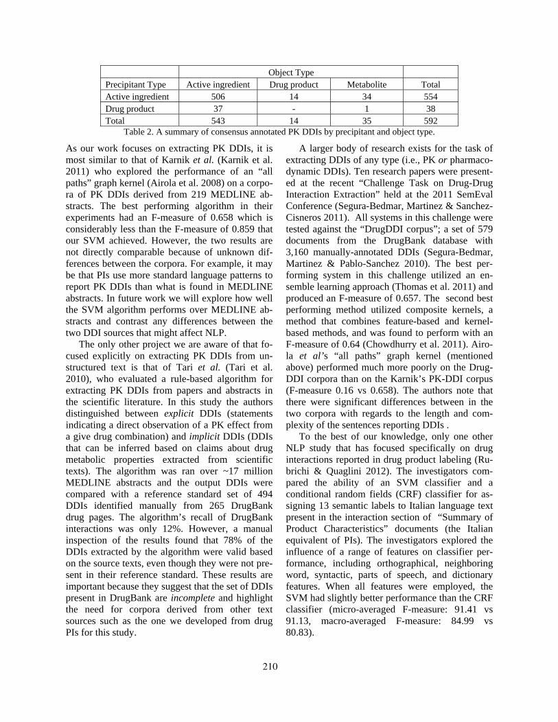
Object Type Precipitant Type Active ingredient Drug product Metabolite Total Active ingredient 506 14 34 554 Drug product 37 - 1 38 Total 543 14 35 592
Table 2. A summary of consensus annotated PK DDIs by precipitant and object type.
As our work focuses on extracting PK DDIs, it is most similar to that of Karnik et al. (Karnik et al. 2011) who explored the performance of an “all paths” graph kernel (Airola et al. 2008) on a corpo-ra of PK DDIs derived from 219 MEDLINE ab-stracts. The best performing algorithm in their experiments had an F-measure of 0.658 which is considerably less than the F-measure of 0.859 that our SVM achieved. However, the two results are not directly comparable because of unknown dif-ferences between the corpora. For example, it may be that PIs use more standard language patterns to report PK DDIs than what is found in MEDLINE abstracts. In future work we will explore how well the SVM algorithm performs over MEDLINE ab-stracts and contrast any differences between the two DDI sources that might affect NLP.
The only other project we are aware of that fo-cused explicitly on extracting PK DDIs from un-structured text is that of Tari et al. (Tari et al. 2010), who evaluated a rule-based algorithm for extracting PK DDIs from papers and abstracts in the scientific literature. In this study the authors distinguished between explicit DDIs (statements indicating a direct observation of a PK effect from a give drug combination) and implicit DDIs (DDIs that can be inferred based on claims about drug metabolic properties extracted from scientific texts). The algorithm was ran over ~17 million MEDLINE abstracts and the output DDIs were compared with a reference standard set of 494 DDIs identified manually from 265 DrugBank drug pages. The algorithm’s recall of DrugBank interactions was only 12%. However, a manual inspection of the results found that 78% of the DDIs extracted by the algorithm were valid based on the source texts, even though they were not pre-sent in their reference standard. These results are important because they suggest that the set of DDIs present in DrugBank are incomplete and highlight the need for corpora derived from other text sources such as the one we developed from drug PIs for this study.
A larger body of research exists for the task of extracting DDIs of any type (i.e., PK or pharmaco-dynamic DDIs). Ten research papers were present-ed at the recent “Challenge Task on Drug-Drug Interaction Extraction” held at the 2011 SemEval Conference (Segura-Bedmar, Martinez & Sanchez-Cisneros 2011). All systems in this challenge were tested against the “DrugDDI corpus”; a set of 579 documents from the DrugBank database with 3,160 manually-annotated DDIs (Segura-Bedmar, Martinez & Pablo-Sanchez 2010). The best per-forming system in this challenge utilized an en-semble learning approach (Thomas et al. 2011) and produced an F-measure of 0.657. The second best performing method utilized composite kernels, a method that combines feature-based and kernel-based methods, and was found to perform with an F-measure of 0.64 (Chowdhurry et al. 2011). Airo-la et al’s “all paths” graph kernel (mentioned above) performed much more poorly on the Drug-DDI corpora than on the Karnik’s PK-DDI corpus (F-measure 0.16 vs 0.658). The authors note that there were significant differences between in the two corpora with regards to the length and com-plexity of the sentences reporting DDIs .
To the best of our knowledge, only one other NLP study that has focused specifically on drug interactions reported in drug product labeling (Ru-brichi & Quaglini 2012). The investigators com-pared the ability of an SVM classifier and a conditional random fields (CRF) classifier for as-signing 13 semantic labels to Italian language text present in the interaction section of “Summary of Product Characteristics” documents (the Italian equivalent of PIs). The investigators explored the influence of a range of features on classifier per-formance, including orthographical, neighboring word, syntactic, parts of speech, and dictionary features. When all features were employed, the SVM had slightly better performance than the CRF classifier (micro-averaged F-measure: 91.41 vs 91.13, macro-averaged F-measure: 84.99 vs 80.83).
210

Jrip J48 SMO
Model (dataset) Prec Recall F Prec Recall F Prec Recall F
Baseline (development) 0.588 0.656 0.62 0.584 0.573 0.578 0.639 0.677 0.658 Stanford Parser (develop-ment) 0.762 0.68 0.719 0.809 0.804 0.807 0.851 0.815 0.833
ClearParser (development) 0.787 0.793 0.79 0.822 0.791 0.806 0.828 0.887 0.856
Stanford Parser (test) 0.778 0.665 0.717 0.828 0.832 0.83 0.843 0.838 0.84
ClearParser (test) 0.764 0.76 0.762 0.85 0.76 0.802 0.836 0.883 0.859
Modality (test) 0.963 0.897 0.929 0.887 0.948 0.917 0.941 0.957 0.949 Table 3. Results for interaction prediction on the baseline, development, and blind test set. Also shown are re-sults for modality prediction for the blind test set (results over the development set are similar but not shown).
One key difference between the Rubrichi study and ours is that the task of tagging unstructured text with semantic elements that describe a DDI is not the same as classifying whether or not a state-ment containing a drug pair is reporting a DDI be-tween the drugs. The difference is especially apparent when considering coordinate structures such as “Drug A interacts with Drugs B and C”, Semantic tagging would be useful for identifying the drug entities but is not useful (on its own) for identifying which of the three drug pairs interact with each other.
It is interesting to note that most recent work on DDI extraction had not made the distinction be-tween PK and pharmacodynamic DDIs that is standard in the fields of pharmacology and phar-macy. This distinction might be relevant to DDI extraction because the two types of interactions are discovered in distinct ways that might lead to sig-nificant differences in how they are described in scientific documents. For example, there is a fairly standard set of in vitro experiments and clinical trials that have been a routine part of drug devel-opment for more than a decade (FDA. 1999). The same is not true for pharmacodynamic DDIs, which are more challenging to study because they involve additive and synergistic effects that are not necessarily related to a drug’s dose or clearance. Since it is reasonable that the methods used to in-vestigate a DDI strongly influences its description, we think future work should examine if PK and pharmacodynamic DDI descriptions are different enough to warrant distinct DDI extraction efforts.
An error analysis of the final dataset suggested some reasons for cases where the machine learning algorithms misclassified instances. Instances that were not interactions, but were classified as such, contained a large number of sentences with de-
scriptions of studies or biochemical processes and measurements. These types of statements may share a number of features with actual interactions (e.g. numerical data, changing levels of drug, etc.) without containing an interaction. There also re-main cases where several drug names occur and the classifiers were unable to differentiate between the interacting pair and non-interacting pairs. Un-fortunately, no such clear pattern was apparent for instances that descrived interactions, but were clas-sified as containing no interaction statement. A number of large sentences were observed in these instances, suggesting sentence complexity may play a role, increasing the difficulty of natural lan-guage parsing.
Analysis of the attribute weights assigned by the SVM algorithm (SMO) after training for inter-action prediction shows some commonality regard-less of whether the data was processed by the Stanford Parser or the ClearParser. For example, 19 out of the 20 most significant features identified by the algorithm from the dataset when processed by the Stanford Parser were words on the syntactic path; one less than when the dataset was processed by the ClearParser. Common significant features include words such as “coadminister”, “auc”, “pharmacokinetic”, and “absorption”. The algo-rithm placed greater importance on the words “in-crease” and “decrease” when the dataset was processed by the Stanford Parser, while the words “reduce” and “enhance” received greater attribute weights when the data was processed by the ClearParser. A similar analysis of the SVM algo-rithm developed for PK DDI modality prediction shows that bigrams with the words “no” or “not” are clearly the features of most importance to the model.
211
We also note that the algorithm’s performance on the test set of PI statements is very similar to the algorithm’s performance over the development set (see Table 3). We think that this finding is largely due to the careful stratification approach we used when creating the development and test sets. It might also be possible that the features in the unstructured PI text do not vary greatly be-tween PIs regardless of their age. However, Table 2 shows that our PK DDI corpora had considerable variation in terms of quantitative vs qualitative and positive vs negative DDI statements. Thus, we an-ticipate that the SVM algorithm’s performance will be maintained when ran against a much larger PI corpus and future work will test how well the algo-rithm generalizes to other sets of PIs.
5 Conclusion
We created a new, publically available, corpus of FDA-approved drug PI statements that have been manually annotated for PK DDIs by a pharmacist and a drug information expert. Also, we evaluated three different machine learning algorithms for their ability to 1) identify PK DDIs in drug PIs and 2) classify PK DDI statements by their modality (i.e., whether they report a DDI or no interaction between drug pairs). Experiments found that an SVM algorithm performed best on both tasks with an F-measure of 0.859 for PK DDI identification and 0.949 for modality assignment. We found that the use of syntactic information is very helpful for addressing the problem of sentences containing both interacting and non-interacting pairs of drugs. The strong performance of our algorithm for PK DDIs suggests that approaching pharmacokinetic and pharmacodynamic interactions as different NLP tasks is a potentially promising approach for advancing automated DDI extraction. Given the marked difference in performance between our extraction methods and previous work, we are planning further experiments to establish whether this difference reflects the comparative simplicity of the extraction task represented by our corpus, some specific strength of the applied extraction methods, or some other factor.
Acknowledgement
This project was funded by grant K12-HS019461 from the Agency for Healthcare Research and
Quality (AHRQ). The content is solely the respon-sibility of the authors and does not represent the official views of AHRQ. We also thank John Horn, PharmD (University of Washington) and Mr. Rob Guzman (University of Pittsburgh) for their work annotating the corpus and identifying related re-search.
References
Airola, Antti, Sampo Pyysalo, Jari Björne, Tapio Pahikkala, Filip Ginter & Tapio Salakoski. 2008. All-paths graph kernel for protein-protein interaction extraction with evaluation of cross-corpus learning. BMC Bioinformatics 9(Suppl 11). S2. doi:10.1186/1471-2105-9-S11-S2 (3 May, 2012).
Bunescu, Razvan C. & Raymond J. Mooney. 2005. A shortest path dependency kernel for relation extraction. Proceedings of the conference on Human Language Technology and Empirical Methods in Natural Language Processing, 724–731. (HLT ’05). Stroudsburg, PA, USA: Association for Computational Linguistics. doi:10.3115/1220575.1220666. http://dx.doi.org/10.3115/1220575.1220666 (2 May, 2012).
Choi, Jinho. 2011. ClearParser GoogleCode page. clearparser. http://code.google.com/p/clearparser/ (10 De-cember, 2011).
Chowdhurry, Md. Faisal Mahbub, Asma Ben Abacha, Alberto Lavelli & Pierre Zweigenbaum. 2011. Two Different Machine Learning Techniques for Drug-Drug Interaction Extraction. 1st Chal-lenge task on Drug-Drug Interaction Extrac-tion (DDIExtraction 2011), 19–26. Huelva, Spain.
Dal-Ré, R., A. Pedromingo, M. García-Losa, J. Lahuer-ta & R. Ortega. 2010. Are results from phar-maceutical-company-sponsored studies available to the public? European Journal of Clinical Pharmacology 66(11). 1081–1089. doi:10.1007/s00228-010-0898-y (5 August, 2011).
FDA. 1999. FDA Guideline: In Vivo Drug Metabo-lism/Drug Interaction Studies – Study Design, Data Analysis, and Implications for Dosing and Labeling. Rockville, MD: Food and Drug Administration. http://www.fda.gov/downloads/Drugs/GuidanceComplianceRegulatoryInfor-mation/Guidances/ucm072119.pdf.
FDA. 2010. CFR - Code of Federal Regulations Title 21.
212

http://www.accessdata.fda.gov/scripts/cdrh/cfdocs/cfcfr/CFRSearch.cfm?fr=201.57 (7 June, 2011).
Hall, Mark, Eibe Frank, Geoffrey Holmes, Bernhard Pfahringer, Peter Reutemann & Ian H Witten. 2009. The WEKA data mining software: an update. SIGKDD Explorations 11(1). 10–18.
Jonquet, Clement, Nigam H Shah & Mark A Musen. 2009. The open biomedical annotator. Summit on Translational Bioinformatics 2009. 56–60. (10 December, 2011).
Karnik, Shreyas, Abhinita Subhadarshini, Zhiping Wang, Luis M Rocha & Lang Li. 2011. Extrac-tion Of Drug-Drug Interactions Using All Paths Graph Kernel. 1st Challenge task on Drug-Drug Interaction Extraction (DDIExtrac-tion 2011). Huelva, Spain.
Klein, Dan & Christopher D Manning. 2003. Fast Exact Inference with a Factored Model for Natural Language Parsing. (Ed.) S Thrun S Becker & Keditors Obermayer. Science 15. 3–10.
Marroum, P.J. & J. Gobburu. 2002. The product label: how pharmacokinetics and pharmacodynamics reach the prescriber. Clinical Pharmacokinetics 41(3). 161–169. (7 June, 2011).
Nelson, Stuart J, Kelly Zeng, John Kilbourne, Tammy Powell & Robin Moore. 2011. Normalized names for clinical drugs: RxNorm at 6 years. Journal of the American Medical Informatics Association: JAMIA 18(4). 441–448. doi:10.1136/amiajnl-2011-000116 (10 Decem-ber, 2011).
Ogren, Philip V. 2006. Knowtator: a Protégé plug-in for annotated corpus construction. Proceedings of the 2006 Conference of the North American Chapter of the Association for Computational Linguistics on Human Language Technology, 273–275. Morristown, NJ, USA: Association for Computational Linguistics. doi:http://dx.doi.org/10.3115/1225785.1225791.
Rosé, Carolyn, Yi-Chia Wang, Yue Cui, Jaime Arguel-lo, Karsten Stegmann, Armin Weinberger & Frank Fischer. 2008. Analyzing collaborative learning processes automatically: Exploiting the advances of computational linguistics in computer-supported collaborative learning. In-ternational Journal of Computer-Supported Collaborative Learning 3(3). 237–271. doi:10.1007/s11412-007-9034-0 (10 Decem-ber, 2011).
Rubrichi, S & S Quaglini. 2012. Summary of Product Characteristics content extraction for a safe drugs usage. Journal of Biomedical Informatics 45(2). 231–239. doi:10.1016/j.jbi.2011.10.012 (3 May, 2012).
Segura-Bedmar, Isabel, Paloma Martinez & Cesar Pablo-Sanchez. 2010. Extracting drug-drug in-teractions from biomedical texts. Workshop on Advances in Bio Text Mining, vol. 11 Suppl 5, 9. Madrid, Spaim: BMC Bioinformatics. http://www.biomedcentral.com/1471-2105/11/S5/P9.
Segura-Bedmar, Isabel, Paloma Martinez & Daniel Sanchez-Cisneros (eds.). 2011. Proceedings of the First Challenge Task: Drug-Drug Interac-tion Extraction 2011. Huelva, Spain. http://sunsite.informatik.rwth-aachen.de/Publications/CEUR-WS/Vol-761/ (9 December, 2011).
Stanford NLP. 2011. The Stanford NLP (Natural Lan-guage Processing) Group. http://nlp.stanford.edu/software/ (10 December, 2011).
Tari, Luis, Saadat Anwar, Shanshan Liang, James Cai & Chitta Baral. 2010. Discovering drug-drug in-teractions: a text-mining and reasoning ap-proach based on properties of drug metabolism. Bioinformatics (Oxford, England) 26(18). i547–553. doi:10.1093/bioinformatics/btq382 (9 December, 2011).
Thomas, Philippe, Mariana Neves, Illes Solt, Domonkos Tikk & Ulf Leser. 2011. Relation Extraction for Drug-Drug Interactions using Ensemble Learning. 1st Challenge task on Drug-Drug In-teraction Extraction (DDIExtraction 2011), 11–18. Huelva, Spain.
213

Proceedings of the 2012 Workshop on Biomedical Natural Language Processing (BioNLP 2012), pages 214–222,Montreal, Canada, June 8, 2012. c©2012 Association for Computational Linguistics
Automatic Approaches for Gene-Drug Interaction Extraction
from Biomedical Text: Corpus and Comparative Evaluation
Nate Sutton, Laura Wojtulewicz, Neel Mehta, Graciela Gonzalez
Department of Biomedical Informatics
Arizona State University, Tempe, Arizona, USA {nate.sutton, whitz, nbmehta2, graciela.gonzalez}@asu.edu
Abstract
Publications that report genotype-drug inte-
raction findings, as well as manually curated
databases such as DrugBank and PharmGKB
are essential to advancing pharmacogenomics,
a relatively new area merging pharmacology
and genomic research. Natural language
processing (NLP) methods can be very useful
for automatically extracting knowledge such
as gene-drug interactions, offering researchers
immediate access to published findings, and
allowing curators a shortcut for their work.
We present a corpus of gene-drug interac-
tions for evaluating and training systems to
extract those interactions. The corpus in-
cludes 551 sentences that have a mention of a
drug and a gene from about 600 journals
found to be relevant to pharmacogenomics
through an analysis of gene-drug relationships
in the PharmGKB knowledgebase.
We evaluated basic approaches to auto-
matic extraction, including gene and drug co-
occurrence, co-occurrence plus interaction
terms, and a linguistic pattern-based method.
The linguistic pattern method had the highest
precision (96.61%) but lowest recall (7.30%),
for an f-score of 13.57%. Basic co-occurrence
yields 68.99% precision, with the addition of
an interaction term precision increases slightly
(69.60%), though not as much as could be ex-
pected. Co-occurrence is a reasonable base-
line method, with pattern-based being a prom-
ising approach if enough patterns can be gen-
erated to address recall. The corpus is availa-
ble at http://diego.asu.edu/index.php/projects
1 Introduction
Pharmacogenomics is a relatively new area of
biomedical research that merges pharmacology and
molecular genomics, among other disciplines, and
focuses on studying the effects of genetic variabili-
ty on drug toxicity and efficacy, on the discovery
of novel genomic targets for drug development,
and on the identification and functional characteri-
zation of polymorphisms relevant to drug action.
Thus, publications that report genotype-drug find-
ings and manually curated databases that collect
such findings, like PharmGKB and DrugBank
(Hewett et al., 2002; Wishart, 2006) are of para-
mount importance to the field. However, manual
curation is expensive and time consuming, and
cannot keep up with the ever increasing number of
publications. Natural language processing (NLP)
methods can be very useful for automatically ex-
tracting such gene-drug interactions, offering re-
searchers immediate access to published findings,
and allowing curators a shortcut for their work.
Consider for example a sentence contain-
ing an interaction NLP can help extract: ―Only the
epsilon4 allele of APOE was found to make a sig-
nificant (P = 0.002) but small contribution to war-
farin dose requirement.‖ (PMID: 16847429). We
can easily see that in the sentence, an APOE allele
interacts with the drug warfarin in its dose re-
quirement. Furthermore, at a higher level of ab-
straction, the sentence can help researchers infer
that APOE affects the metabolic processes targeted
by the drug warfarin.
NLP researchers attacking an interaction
extraction project such as this one, will usually
start by identifying the entities involved in the ex-
tractions and the terms that indicate such interac-
tions. Assuming named entity recognition (NER)
systems exist for the entities in question (or a dic-
tionary is available for direct match), the main
concern becomes extracting true interactions. A
gold standard corpus would then need to be identi-
fied or created in order to evaluate and develop
interaction extraction approaches, starting with the
214
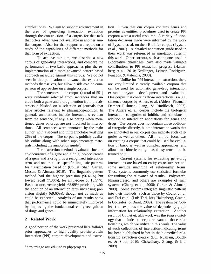
simplest ones. We aim to support advancement in
the area of gene-drug interaction extraction
through the construction of a corpus for that task
that offers advantages not available in another sim-
ilar corpus. Also for that support we report on a
study of the capabilities of different methods for
that form of extraction.
To achieve our aim, we describe a new
corpus of gene-drug interactions, and compare the
performance of two basic approaches plus the re-
implementation of a more advanced pattern-based
approach measured against this corpus. We do not
seek in this publication to advance the extraction
methods themselves, but allow a side-to-side com-
parison of approaches on a single corpus.
The sentences in the corpus (a total of 551)
were randomly selected from sentences that in-
clude both a gene and a drug mention from the ab-
stracts published on a selection of journals that
have articles relevant to pharmacogenomics. In
general, annotations include interactions evident
from the sentence, if any, also noting when men-
tioned genes or drugs are not involved in interac-
tions. All sentences were annotated by the main
author, with a second and third annotator verifying
26% of the corpus. The corpus is publicly availa-
ble online along with other supplementary mate-
rials including the annotation guide1.
The extraction methods evaluated include
co-occurrence of a gene and a drug, co-occurrence
of a gene and a drug plus a recognized interaction
term, and one that uses specific linguistic patterns
for classification based on (Coulet, Shah, Garten,
Musen, & Altman, 2010). The linguistic pattern
method had the highest precision (96.61%) but
lowest recall (7.30%), for an f-score of 13.57%.
Basic co-occurrence yields 68.99% precision, with
the addition of an interaction term increasing pre-
cision slightly (69.60%), though not as much as
could be expected. Analysis of our results show
that performance could be immediately improved
by improving the fundamental entity-recognition
of drugs and genes.
2 Related Work
A good portion of the work presented here follows
prior approaches to high quality protein-protein
interaction (PPI) corpora development and extrac-
1 http://diego.asu.edu/index.php/projects
tion. Given that our corpus contains genes and
proteins as entities, procedures used to create PPI
corpora were a useful resource. A variety of anno-
tation decisions made were informed by the work
of Pyysalo et. al. on their BioInfer corpus (Pyysalo
et al., 2007). A detailed annotation guide used in
their work was referenced in annotation rules in
this work. Other corpora, such as the ones used in
Biocreative challenges, have also made valuable
contributions to PPI extraction progress (Haken-
berg et al., 2010; Krallinger, Leitner, Rodriguez-
Penagos, & Valencia, 2008).
Unlike for PPI interaction extraction, there
are very limited currently available corpora that
can be used for automatic gene-drug interaction
extraction system development and evaluation.
One corpus that contains those interactions is a 300
sentence corpus by Ahlers et al. (Ahlers, Fiszman,
Demner-Fushman, Lang, & Rindflesch, 2007).
The Ahlers et. al. corpus include the biological
interaction categories of inhibit, and stimulate in
addition to interaction annotations for genes and
drugs. Our corpus does not contain those addition-
al categories directly, but the interaction words that
are annotated in our corpus can indicate such cate-
gories as well as others. All in all, our focus was
on creating a corpus that could be used for evalua-
tion of basic as well as complex approaches, and
allow machine-learning based systems to be
trained on it.
Current systems for extracting gene-drug
interactions are based on entity co-occurrence and
some include matching of relationship terms.
Those systems commonly use statistical formulas
for ranking the relevance of results. Polysearch,
Pharmspresso, and others are examples of such
systems (Cheng et al., 2008; Garten & Altman,
2009). Some systems integrate linguistic patterns
into their methods, such as those by Coulet et. al.
and Tari et. al. (Luis Tari, Jörg Hakenberg, Gracie-
la Gonzalez, & Baral, 2009). The system by Cou-
let et al. explores the value of dependency graph
information for relationship extraction. Another
result of Coulet et. al.'s work was the Phare ontol-
ogy that includes concepts relevant to those rela-
tionships, which we utilize in this work. The value
of such collections of interaction-indicating terms
has been highlighted before in the biomedical rela-
tionship extraction context (Bui, Nualláin, Bouch-
er, & Sloot, 2010; Chowdhary, Zhang, & Liu,
2009).
215

3 Materials and Methods
3.1 Corpus design.
The purpose for the creation of the new corpus was
to create a resource that NLP developers can use to
train and test gene-drug interaction extraction sys-
tems. The corpus was based on articles from jour-
nals that are known to contain pharmacogenomic
relationships. Genes and drugs were automatically
tagged and then 551 sentences that contain both a
gene and drug were randomly selected for annota-
tion. The corpus and sentence selection process is
described in the following subsections.
Journal Selection. A list of journals relevant to
pharmacogenomics was generated by extracting
the journal names from articles that have been cu-
rated in PharmGKB as containing evidence of
gene-drug relationships. This list was generated
from their downloadable ―relationships‖ file,
which contains the abstract IDs of articles with
manually curated gene-drug relationships. 591
journal names were obtained this way. The goal of
using only those journals is to make the corpus
representative of typical sentences containing a
gene and drug from literature known to report
pharmacogenomic findings.
Sentence processing. All abstracts in PubMed from
the relevant journal names were downloaded. A
sentence splitter program from OpenNLP was used
to extract sentences from the abstracts (―The
OpenNLP Homepage,‖ n.d.). A total of
22,601,402 sentences were processed.
Identification of entites. Previous work in pharma-
cogenomics relationship extraction has shown ef-
fective results by classifying relationships after
identifying sentences with entities of interest
through dictionary matching techniques (Garten &
Altman, 2009; Rebholz-Schuhmann et al., 2007).
Our work takes a similar approach, but utilizes a
machine-learning based method, BANNER, for
gene recognition, as it was shown to have better
performance than a dictionary-based method
(Leaman & Gonzalez, 2008). Drugs were recog-
nized through the use of dictionary matching. The
dictionaries used for drugs were based on drug
names available at DrugBank. Exact full token
matching of drug terms was used to identify them
in sentences. Although incorrectly tagged (false
entity) genes and drugs were corrected by annota-
tors, they did not add entities missed by NER rec-
ognition. A second round of annotation will correct
this when we shift focus to NER.
Terms indicative of an interaction for add-
ing to basic co-occurrence relationship extraction
were extracted from the Phare ontology. The
terms acquired were from rdfs labeled text in the
―object properties‖ in the ontology. Object proper-
ties are elements of the ontology that describe rela-
tionships between classes such as gene and drugs,
yielding 168 unique terms after stemming.
Sentence selection. The initial annotation effort
that is the focus of this paper was aimed at com-
pleting around 500 sentences as a proof of concept,
with a total of 1,500 to be completed in the second
phase of this project. Random selection of sen-
tences that include a gene and a drug, in contrast to
balanced positive and negative selection, was used
to make the corpus reflect typical sentences poten-
tially containing an interaction that can be easily
extracted from the source articles after simple
(drug and gene) concept tagging, which is the most
basic approach to interaction extraction. The ran-
domized ratio of positive and negative interactions
in the corpus is useful for training classification
systems that operate on similarly pre-processed
sentences to account for that naturally occurring
ratio.
3.2 Annotation.
An annotation tool named STAV was used to
create annotations (―stav,‖ n.d.). Customization of
the tool was performed to match the types of anno-
tations needed for the corpus. The identified enti-
ties were formatted for use with the tool. Annota-
tions created with the tool were stored in the Bi-
oNLP shared task file format. That format is com-
patible with a variety of existing systems for rela-
tionship extraction.
Annotation guidelines. Based on a review of litera-
ture on related annotation guidelines for relation-
ships such as PPIs, an initial annotation guideline
was created based on a small sample of sentences.
The guide was iteratively refined through annota-
tion of additional sentences, until considered suffi-
ciently stable for release to additional annotators.
The guideline was refined to achieve a bal-
ance of complexity and clarity to assist annotators.
216

Only a few (5-10) example sentences per annotator
have been discussed in person. The explicit writ-
ten instructions in the guide were relied on more
than in-person example sentence discussions to
train annotators to handle the complicated content
of the corpus and avoid over-influencing the anno-
tators, as noted that is possible with the overuse of
those examples (Hovy & Lavid, 2008).
The first annotator, a student with a Bache-
lor of Science (BS) in Biology, was the main anno-
tator and author of the guidelines. The second and
third annotators are PhD students in Biomedical
Informatics, the second with a BS in Biology and
10 years nursing experience, and the other with a
Bachelor of Technology in Bioinformatics. Week-
ly annotation meetings were done on individual
bases. A short checklist of things to look for in
annotations was distributed in addition to the
guidelines.
Annotations. The following describes major anno-
tation categories and subcategories in the corpus:
Interaction Genes and drugs are annotated
simply as ―having an interaction‖ broadly un-
derstood as having an ―action, effect, or influ-
ence‖ on each other. All gene-drug interac-
tions annotated must have at least one interac-
tion term that helps explain the interaction.
Additional properties that were annotated and
a brief explanation of their purpose include:
o Direct/Indirect: Describes the complexi-
ty in the interaction statements. An ―indi-
rect‖ interaction is one where the presence
of an intermediary entity is needed for se-
mantic understanding of the interaction.
o Explicit/Inferred: Records if an infe-
rence had to be made on whether the inte-
raction was present because an interaction
was not explicitly stated.
Non-interaction o Shared Entity: An entity connected to
both a gene and a drug that don't interact
with each other. In contrast to an interme-
diary entity.
Interaction Term Terms that are descriptive
of the interaction (as defined earlier). These
terms are helpful for capturing more specifical-
ly the type of interaction present.
Intermediary Entity These are non-gene,
non-drug entities that are closely connected to
the interaction. They are entities that are
needed for understanding of the full semantic
meaning of gene-drug interactions. These enti-
ties are not annotated themselves but they are
used to determine the indirectness property.
Examples of these categories can be seen in the
sentence: ―Using standard steady-state kinetic
analysis, it was demonstrated that paclitaxel was a
possible uncompetitive inhibitor to NAT activity in
cytosols based on the decrease in apparent values
of K(m) and V(max).‖ (PMID: 11955677). This
sentence includes an interaction between the drug
paclitaxel and gene NAT. An interaction term that
helps establish that the interaction is present is ―in-
hibitor‖. ―Cytosols‖ is where the NAT inhibition
activity can occur and represents an intermediary
entity that is needed in the semantic meaning of the
interaction.
The broad definition of interaction was
used to make progress toward annotations includ-
ing, and in turn being representative of, the most
general form of gene-drug interaction that is de-
scribed in the source abstracts. We chose to first
concentrate on getting good inter-annotator agree-
ment using the general definition before consider-
ing additionally annotating specific biological inte-
raction types. Annotated interactions are required
to have at least one annotated interaction term (al-
though terms do not have to be from the predefined
list) to ensure that specific and identifiable lan-
guage is present that justifies the annotation.
The subcategories included were added to
record the linguistic complexity in which the inte-
ractions and non-interactions are described. Re-
cording that complexity can help system develop-
ers handle its presence when trying to automatical-
ly recognize interaction statements. Additionally,
the annotation properties of speculation, negation,
and nesting were allowed but not separately anno-
tated in interaction annotations.
Each annotator reported annotation time
estimates. Total time spent on annotations includ-
ing meetings but not other work (e.g. guideline
development) was approximately 80 hours for the
primary annotator and 20 hours combined for other
annotators. Hard sentences to annotate required
research into source articles and entities described.
217

Evaluation of the Corpus. Around 26% of the cor-
pus was annotated by a second and third annotator.
A program was created for IAA scoring, account-
ing for nested entities and equivalent entities in-
cluding abbreviations. Manual review was used to
verify the program’s scores. Example sentences
from the corpus discussed with annotators were not
used for IAA scoring.
3.3 Relationship Extraction methods.
Three basic methods for extracting interactions
were implemented for evaluation. The basic me-
thod, co-occurrence, is inherent to the corpus as all
sentences are selected based on both entities being
present in them. Thus, in co-occurrence, any men-
tion of a gene and a drug together in a sentence
represents an interaction between those entities.
Co-occurrence plus interaction terms, the
second method tried, identifies that interactions are
present only when sentences contain an interaction
word from a predefined list. The list of interaction
terms obtained from the Phare ontology was fil-
tered by removing common stop words. Also, a
filter was applied to only use terms greater than
two letters in size. Those filters were used to avoid
unneeded matches from common words.
The linguistic pattern based extraction me-
thod developed for this evaluation was based on
the work by Coulet et. al. Specific linguistic pat-
terns described in that work were used to classify
the presence of interactions between genes and
drugs. A program named Graph Spider was used
to match the specified patterns within sentences
(Shepherd & Clegg, 2008). The Stanford Parser
was used to generate dependency graphs for use
with the pattern recognition in Graph Spider.
The dependency rules designed by Coulet.
et. al. were entered into Graph Spider using the
metapattern language (MPL) designed by the
Graph Spider authors. MPL is a pattern formalism
that can be used to match dependency subgraph
patterns in dependency parsed text. After depen-
dency graphs were generated for processing in
Graph Spider, text representing genes and drugs in
the graphs were converted to general tags for those
entity types. Those conversions were made to al-
low the patterns in MPL to be generalizable.
Java programs were created to reformat
and score the subgraph pattern match results made
by Graph Spider. Scoring used text character posi-
tions (spans) of entities included in annotations.
True positives were recorded when pairs of entity
spans in Graph Spider subgraph results matched
annotated pairs of entity spans labeled as having
interactions. False positives and false negatives
were similarly assessed using entity spans. A ma-
nual evaluation of pattern matched output com-
pared to annotations was performed to ensure ac-
curacy.
A condition applied in the pattern based
system was that the patterns can match up to four
modifier words for each individual gene and drug
in interaction pattern matches. Those words are
additional words that modify the meaning of the
gene or drug in the interaction. The limit was in-
cluded for practical reasons, as hand coding of pat-
terns in MPL is complex. The rules described by
Coulet et. al. did not specify any limit on modifier
words but the difference in results by including a
realistic limit is predicted to be negligible.
4 Results
A total of 551 sentences are annotated, with 781
interactions present in them. There are 351 in-
stances of non-interactive entities in the same set.
The average length of sentences is 28.1 words.
Table 1 describes further properties of the corpus.
Annotation Analysis. The inter-annotator agree-
ment scores are reported as accuracy and Cohen’s
kappa. Kappa was chosen due to its widespread
use and therefore comparability with other work in
corpus creation. Accuracy is found by the number
of instances agreed on divided by the total in-
stances annotated. A total of 144 sentences were
used for the scoring. Annotators 1 and 2, 1 and 3,
and 2 and 3 were compared using 92, 52, and 61
sentences respectively. IAA results with the main
categories of interaction vs. non-interaction are
shown in Table 2.
Sentences Tokens (with
punctuation)
Words (tokens with
no punctuation)
551 18,585 15,464
Table 1. Statistics describing corpus properties.
1 & 2 1 & 3 2 & 3
Accuracy 81.1% 74.2% 73.0%
Kappa 45.7% 30.5% 11.4%
Table 2. Inter-annotator agreement results.
218

IAA scores were found for all annotated
subcategories. Those subcategories are DirectEx-
plicit, IndirectExplicit, IndirectInferred for interac-
tions and SharedEntity for non-interactions. Their
ranges of scores with all annotator pair groups us-
ing accuracy scores are 72-79%, 40-69%, 62-82%,
50-60% and kappa scores are 31-58%, 1-27%, -4-
31%, 0-4% respectively. Those scores are created
by selecting main category inter-annotator matches
(e.g. interaction) and calculating the IAA between
the annotated subcategories.
In some sentences, annotators missed
doing annotations for gene-drug instances that the
other annotator added. IAA scores did not include
annotations made by only one annotator. Confir-
mation with annotators was made that annotations
not made were not intended to represent non-
interactions. The percentage of missed inter-
annotator instances was approximately 20%. Fu-
ture work will be to improve the inter-annotator
annotation process so that those instances are not
missed for IAA scoring. While some annotations
were missed in IAA scoring, annotations by the
primary annotator that are included in the corpus
contain all instances (none missed) from the source
text to our knowledge.
I
D
Contents Agree
ment
Sentence text
A One direct expli-
cit interaction
Y This suggests that galantamine (GAL), a cholinesterase inhibitor, could be
effective when seeking to prolong abstinence in recently detoxified alcohol-
ics. (PMID: 16328375)
B One indirect ex-
plicit and four
shared entity
non-interactions
Y They are widely distributed and mediate all of the known biologic effects of
angiotensin II (AngII) through a variety of signal transduction systems, in-
cluding activation of phospholipases C and A2, inhibition of adenylate cyc-
lase, opening of calcium channels, and activation of tyrosine kinases. (PM-
ID: 9892138)
C One indirect ex-
plicit interaction
N The results of studies of perfused rat hearts with completely inhibited crea-
tine kinase show significantly decreased work capacity and respectively,
energy fluxes, in these hearts in spite of significant activation of adenylate
kinase system (Dzeja et al. this volume). (PMID: 9746326)
Table 3. Example sentences from the corpus.
Table 4. Extraction system performances.
Note that sentences were selected based on co-
occurrence of a gene and a drug, thus recall is
100% for that method, as it essentially defines
the corpus.
The scoring methods used were instance
level scoring instead of sentence level scoring. In
the instance level scoring each gene-drug instance
counted in performance scores.
A caveat about the pattern-based system
scoring should be noted. That caveat was that the
Graph Spider software used was unable to process
approximately 10% (around 50) of the sentences in
the corpus due to errors. The pattern-based system
is likely to have scored slightly higher if it could
have processed those sentences.
5 Discussion
5.1 Analyses of interaction extraction methods
performance.
Interaction
Extractor Type
Precision
(TP/TP+FP)
Recall
(TP/TP+
FN)
F1-Score
(2*((P*R)/(
P+R)))
Co-occurrence 68.99%
(781/1132)
100.00%
(781/781)
81.65%
Co-occurrence
plus int. terms
69.60%
(664/954)
85.02%
(664/781)
76.54%
Pattern-based 96.61%
(57/59)
7.30%
(57/781)
13.57%
219

The f-score of co-occurrence with and without in-
teraction terms showed better performance than the
pattern-based interaction extractions, which was
expected. Pattern based methods, particularly those
where the patterns were manually created, are typi-
cally very high in precision and very low in recall,
as they are highly dependant on the specific pat-
terns included for recognition. Although recall was
low, users who want very high confidence interac-
tion predictions or interactions of a very specific
type can benefit from the pattern-based system’s
demonstrated high precision. Co-occurrence can
suit users who want to focus on recall.
Coulet et al. reported their system scored a
precision of 70% for exact match and 87.7% for
exact or incomplete match but true classification.
Our results are similar to their 87.7% results in
both percentage and scoring method. The method
that allows incompleteness accepts matches that
accurately identify core pharmacogenomic rela-
tionships but don’t need to correctly match modifi-
er words. Our scoring is similar in not needing to
match modifier words. The similarity in results
indicates that we correctly implemented the system
that Coulet et al. designed. That indication does
have the limitation that the 10% of sentences una-
ble to be processed may have affected the results.
An example of a more complex interaction
that was matched by co-occurrence with an inte-
raction term but not the pattern-based method was
―Moreover, S-nitrosylation of thioredoxin was also
significantly augmented after atorvastatin treat-
ment.‖ (PMID: 15289372). In that sentence, an
interaction occurred where thioredoxin's (gene) S-
nitrosylation was augmented by atorvastatin
(drug). Analysis of the dependency graphs used by
the pattern-based system revealed some reasons
why it was unable to identify the interaction.
The pattern-based system uses a rule that
applies to that sentence: a potential pattern se-
quence match can be ―interrupted‖ by a dependen-
cy that does not fit accepted patterns. In the non-
classified sentence, the entities ―was‖ and ―aug-
mented‖ were terms that caused the pattern match-
ing to be interrupted. Both ―was‖ and ―aug-
mented‖ are not nouns or prepositions. They both
also are needed in the dependency subgraph that
connects the gene and drug together. Those parts
of speech are not allowed to be chained together in
the pattern-based system's patterns. That deviation
from the allowed patterns caused the system to
miss that interaction.
Adding patterns with more diversity in al-
lowed parts of speech in series of interaction terms
that connect genes and drugs in interactions can
improve recall performance. A review of parts of
speech (POS) in missed matches showed that some
misses were due to no verb POS tags being present
in interaction descriptions. That can occur when
verbs are in their nominalized form or other situa-
tions. Mining the corpus for both part of speech
and dependency graph patterns can identify pat-
terns that are able to correct those misses. Also,
the POS tagger included with the parser mis-
tagged a variety of words. Using a higher perfor-
mance tagger or one trained on biomedical text
may help with pattern matches.
Ahlers et. al. also reported relationship ex-
traction performance from a new system with their
gene-drug corpus. That system achieved a preci-
sion of 73% and recall of 50% extracting an anno-
tation category including gene-drug relationships.
The system is built upon an earlier system and an
important part of its capabilities comes from spe-
cialized linguistic rules it uses. The corpus in-
cluded in this work can be useful for further devel-
opment of systems that integrate such rules with
other methods to improve extraction performances.
Some characteristics were notable about
the results of the methods using co-occurrence
with and without interaction terms. The perfor-
mances found of those methods may be specific to
an increased amount of gene-drug interactions
found in the journals used compared to other jour-
nals. Also, the use of interaction terms from the
Phare ontology was expected to increase precision
because they were found from predicted pharma-
cogenomic relationships. The co-occurrence with
interaction terms method resulted in only approx-
imately equaling the precision of basic co-
occurrence. One possible reason for that is the
terms were originally found partly with disease
relationships. They therefore can be less relevant
to gene-drug interactions.
5.2 Analyses of annotations
Table 2 includes that the general interaction anno-
tations had the kappa values 46%, 30%, 11%
which are considered only moderate to low scores
by common rating methods. Some IAA scores,
such as kappa, include a correction for chance
220
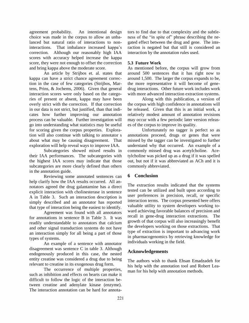
agreement probability. An intentional design
choice was made in the corpus to allow an unba-
lanced but natural ratio of interactions to non-
interactions. That imbalance increased kappa’s
correction. Although our reasonably high IAA
scores with accuracy helped increase the kappa
score, they were not enough to offset the correction
and bring kappa above the moderate score.
An article by Strijbos et. al. states that
kappa can have a strict chance agreement correc-
tion in the case of few categories (Strijbos, Mar-
tens, Prins, & Jochems, 2006). Given that general
interaction scores were only based on the catego-
ries of present or absent, kappa may have been
overly strict with the correction. If that correction
in our data is not strict, but justified, than that indi-
cates how further improving our annotation
process can be valuable. Further investigation will
go into understanding what statistics may be useful
for scoring given the corpus properties. Explora-
tion will also continue with talking to annotator s
about what may be causing disagreement. That
exploration will help reveal ways to improve IAA.
Subcategories showed mixed results in
their IAA performances. The subcategories with
the highest IAA scores may indicate that those
subcategories are more clearly defined than others
in the annotation guide.
Reviewing some annotated sentences can
help clarify how the IAA results occurred. All an-
notators agreed the drug galantamine has a direct
explicit interaction with cholinesterase in sentence
A in Table 3. Such an interaction description is
simply described and an annotator has reported
that type of interaction being the easiest to identify.
Agreement was found with all annotators
for annotations in sentence B in Table 3. It was
readily understandable to annotators that calcium
and other signal transduction systems do not have
an interaction simply for all being a part of those
types of systems.
An example of a sentence with annotator
disagreement was sentence C in table 3. Although
endogenously produced in this case, the nested
entity creatine was considered a drug due to being
relevant to creatine in its exogenous drug form.
The occurrence of multiple properties,
such as inhibition and effects on hearts can make it
difficult to follow the logic of the interaction be-
tween creatine and adenylate kinase (enzyme).
The interaction annotation can be hard for annota-
tors to find due to that complexity and the subtle-
ness of the ―in spite of‖ phrase describing the ne-
gated effect between the drug and gene. The inte-
raction is negated but that still is considered an
interaction by the annotation rules used.
5.3 Future Work
As mentioned before, the corpus will grow from
around 500 sentences that it has right now to
around 1,500. The larger the corpus expands to be,
the more representative it will become of gene-
drug interactions. Other future work includes work
with more advanced interaction extraction systems.
Along with this publication, a version of
the corpus with high confidence in annotations will
be released. Given that this is an initial work, a
relatively modest amount of annotation revisions
may occur with a few periodic later version releas-
es of the corpus to improve its quality.
Unfortunately no tagger is perfect so as
annotations proceed, drugs or genes that were
missed by the tagger can be investigated to further
understand why that occurred. An example of a
commonly missed drug was acetylcholine. Ace-
tylcholine was picked up as a drug if it was spelled
out, but not if it was abbreviated as ACh and it is
commonly abbreviated.
6 Conclusion
The extraction results indicated that the systems
tested can be utilized and built upon according to
user preferences in precision, recall, or specific
interaction terms. The corpus presented here offers
valuable utility to system developers working to-
ward achieving favorable balances of precision and
recall in gene-drug interaction extractions. The
growth of that corpus will also increasingly benefit
the developers working on those extractions. That
type of extraction is important to advancing work
in pharmacogenomics by retrieving knowledge for
individuals working in the field.
Acknowledgements
The authors wish to thank Ehsan Emadzadeh for
his help with the annotation tool and Robert Lea-
man for his help with annotation methods.
221

References
Ahlers, C., Fiszman, M., Demner-Fushman, D.,
Lang, F.-M., & Rindflesch, T. (2007). Extracting
semantic predications from Medline citations for
pharmacogenomics. Pacific Symposium on Bio-
computing. Pacific Symposium on Biocomputing,
209–220.
Bui, Q.-C., Nualláin, B. O., Boucher, C. A., &
Sloot, P. M. A. (2010). Extracting causal relations
on HIV drug resistance from literature. BMC Bio-
informatics, 11, 101. doi:10.1186/1471-2105-11-
101
Cheng, D., Knox, C., Young, N., Stothard, P., Da-
maraju, S., & Wishart, D. S. (2008). PolySearch: a
web-based text mining system for extracting rela-
tionships between human diseases, genes, muta-
tions, drugs and metabolites. Nucleic Acids Re-
search, 36(Web Server issue), W399–405.
doi:10.1093/nar/gkn296
Chowdhary, R., Zhang, J., & Liu, J. S. (2009).
Bayesian inference of protein-protein interactions
from biological literature. Bioinformatics (Oxford,
England), 25(12), 1536–1542.
doi:10.1093/bioinformatics/btp245
Coulet, A., Shah, N. H., Garten, Y., Musen, M., &
Altman, R. B. (2010). Using text to build semantic
networks for pharmacogenomics. Journal of Bio-
medical Informatics, 43(6), 1009–1019.
doi:10.1016/j.jbi.2010.08.005
Garten, Y., & Altman, R. B. (2009). Pharmspresso:
a text mining tool for extraction of pharmacoge-
nomic concepts and relationships from full text.
BMC Bioinformatics, 10 Suppl 2, S6.
doi:10.1186/1471-2105-10-S2-S6
Hakenberg, J., Leaman, R., Vo, N. H., Jonnalagad-
da, S., Sullivan, R., Miller, C., Tari, L., et al.
(2010). Efficient extraction of protein-protein inte-
ractions from full-text articles. IEEE/ACM Trans-
actions on Computational Biology and Bioinfor-
matics / IEEE, ACM, 7(3), 481–494.
doi:10.1109/TCBB.2010.51
Hewett, M., Oliver, D. E., Rubin, D. L., Easton, K.
L., Stuart, J. M., Altman, R. B., & Klein, T. E.
(2002). PharmGKB: The Pharmacogenetics Know-
ledge Base. Nucleic Acids Research, 30(1), 163–
165. doi:10.1093/nar/30.1.163
Krallinger, M., Leitner, F., Rodriguez-Penagos, C.,
& Valencia, A. (2008). Overview of the protein-
protein interaction annotation extraction task of
BioCreative II. Genome Biology, 9 Suppl 2, S4.
doi:10.1186/gb-2008-9-s2-s4
Leaman, R., & Gonzalez, G. (2008). BANNER: an
executable survey of advances in biomedical
named entity recognition. Pacific Symposium on
Biocomputing. Pacific Symposium on Biocomput-
ing, 652–663.
Luis Tari, Jörg Hakenberg, Graciela Gonzalez, &
Baral, C. (2009). Querying parse tree database of
medline text to synthesize user-specific biomolecu-
lar networks. CiteSeerX. Retrieved from
http://citeseerx.ist.psu.edu/viewdoc/summary?doi=
10.1.1.140.8574
Pyysalo, S., Ginter, F., Heimonen, J., Björne, J.,
Boberg, J., Järvinen, J., & Salakoski, T. (2007).
BioInfer: a corpus for information extraction in the
biomedical domain. BMC Bioinformatics, 8, 50.
doi:10.1186/1471-2105-8-50
Rebholz-Schuhmann, D., Kirsch, H., Arregui, M.,
Gaudan, S., Riethoven, M., & Stoehr, P. (2007).
EBIMed—text Crunching to Gather Facts for Pro-
teins from Medline. Bioinformatics, 23(2), e237–
e244. doi:10.1093/bioinformatics/btl302
Sconce, E. A., Daly, A. K., Khan, T. I., Wynne, H.
A., & Kamali, F. (2006). APOE genotype makes a
small contribution to warfarin dose requirements.
Pharmacogenetics and Genomics, 16(8), 609–611.
doi:10.1097/01.fpc.0000220567.98089.b5
Shepherd, A. J., & Clegg, A. B. (2008). Syntactic
pattern matching with GraphSpider and MPL. Pro-
ceedings of the Third International Symposium on
Semantic Mining in Biomedicine SMBM 2008 Tur-
ku Finland, 129–132.
stav. (n.d.).GitHub. Retrieved March 26, 2012,
from https://github.com/TsujiiLaboratory/stav
Strijbos, J.-W., Martens, R. L., Prins, F. J., & Jo-
chems, W. M. G. (2006). Content analysis: What
are they talking about? Computers & Education,
46(1), 29–48. doi:10.1016/j.compedu.2005.04.002
T1.pdf. (n.d.). Retrieved from http://www.lrec-
conf.org/proceedings/lrec2008/workshops/T1.pdf
The OpenNLP Homepage. (n.d.). Retrieved March
26, 2012, from
http://opennlp.sourceforge.net/projects.html
Wishart, D. S. (2006). DrugBank: a comprehensive
resource for in silico drug discovery and explora-
tion. Nucleic Acids Research, 34(90001), D668–
D672. doi:10.1093/nar/gkj067
222
Proceedings of the 2012 Workshop on Biomedical Natural Language Processing (BioNLP 2012), pages 223–230,Montreal, Canada, June 8, 2012. c©2012 Association for Computational Linguistics
A Preliminary Work on Symptom Name Recognition from Free-Text
Clinical Records of Traditional Chinese Medicine using Conditional
Random Fields and Reasonable Features
Yaqiang Wang, Yiguang Liu, Zhonghua Yu*, Li Chen Yongguang Jiang
Department of Computer Science Department of Preclinical Medicine
Sichuan University Chengdu University of TCM
Chengdu, Sichuan 610064, China Chengdu, Sichuan 610075, China [email protected],[email protected],
[email protected],[email protected]
Abstract
A preliminary work on symptom name recog-
nition from free-text clinical records (FCRs)
of traditional Chinese medicine (TCM) is de-
picted in this paper. This problem is viewed as
labeling each character in FCRs of TCM with
a pre-defined tag (“B-SYC”, “I-SYC” or “O-
SYC”) to indicate the character’s role (a be-
ginning, inside or outside part of a symptom
name). The task is handled by Conditional
Random Fields (CRFs) based on two types of
features. The symptom name recognition F-
Measure can reach up to 62.829% with recog-
nition rate 93.403% and recognition error rate
52.665% under our experiment settings. The
feasibility and effectiveness of the methods
and reasonable features are verified, and sev-
eral interesting and helpful results are shown.
A detailed analysis for recognizing symptom
names from FCRs of TCM is presented
through analyzing labeling results of CRFs.
1 Introduction*
Traditional Chinese medicine (TCM), a comple-
mentary medical theory to western medicine, pro-
vides a distinct way to view our human life (Pal,
2002; Barnes, et al., 2004; Molassiotis, et al.,
2005). Moreover, it has shown that TCM
knowledge, which is accumulated in clinical prac-
tice, has become one of the most important sources
of modern biomedical research (Zhou, et al., 2010).
*Corresponding author
In recent years, Data Mining and Machine
Learning have been more than ever before applied
to TCM clinical research, such as establishing
TCM diagnosis expert systems for supporting deci-
sion making (Wang, et al., 2004; Huang and Chen,
2007; Zhang, et al., 2008). However, most of the
works are based on manually well-structured da-
tasets.
Because of the high cost of manually structuring
and maintaining free-text clinical records (FCRs)
of TCM, large volume of such datasets has not
been exploited effectively (Zhou, et al., 2010), alt-
hough they are significant for discovering new
knowledge or capturing medical regularities.
Therefore, developing appropriate information ex-
traction methods for handling FCRs of TCM is an
urgent need to reduce the manual labor for re-
searchers.
Automatically extracting meaningful infor-
mation and knowledge from FCRs of TCM is chal-
lenging in Data Mining and Machine Learning
fields (Zhou, et al., 2010). As the basis, symptom
name recognition or extraction from FCRs of TCM
is in an early stage. To the best of our knowledge,
there has little work to solve this problem (Wang,
et al., 2010; Wang, et al., 2012). Symptom name
recognition from FCRs of TCM was firstly at-
tempted in (Wang, et al., 2010) through normaliz-
ing the symptom names in clinical records based
on literal similarity and remedy-based similarity
methods but not directly recognizing original clini-
cal symptom names from FCRs of TCM. In 2012,
Wang, et al. proposed a framework of automatic
diagnosis of TCM for practice. Symptom name
recognition is one part of the framework and simp-
223

ly attempted through a literal similarity method
without detailed analysis (summarized procedures
for the previous wok are shown in figure 1).
Figure 1. Simple Conclusions of the Previous Work.
Named Entity Recognition (NER) has been
widely studied. There have been lots of methods
for Chinese NER (Zhang, et al., 2003; Wu, et al.,
2003; Gao, et al., 2005; Fu and Luke, 2005; Zhou,
2006; Duan and Zhang, 2011). However, these
methods cannot be directly applied on symptom
name recognition from FCRs of TCM due to big
differences of characteristics of the corpus (Wang,
et al., 2012). There are also several related work on
English NER, but Chinese NER has more chal-
lenges because of the distinct characteristics of
Chinese (Wu, et al., 2003).
In this paper, the task of symptom name recog-
nition from FCRs of TCM is studied. The symp-
tom names are recognized through finding their
description boundaries from FCRs of TCM, and
the method is described in section 2. Several rea-
sonable and helpful features are introduced for
CRFs to label the characters in FCRs of TCM with
pre-defined boundary tags to indicate their roles (a
beginning, inside or outside part of a symptom
name) (presented in section 3). At last, several in-
teresting and valuable experimental results are
shown in section 4 and a conclusion is given in
section 5.
2 Symptom Name Recognition from FCRs
of TCM
The task of symptom name recognition from FCRs
of TCM can be treated as detecting the boundaries
of the symptom name descriptions in the sentences
of FCRs of TCM. Therefore, this task can be
viewed as labeling each tagging unit (e.g. word) in
the sentences with a pre-defined tag indicating
whether the unit is a beginning, inside, or outside
part of a symptom name.
Generally, the tagging unit is word (Ramshaw
and Marcus, 1995). However, there is no natural
segmentation for words in Chinese sentences.
Therefore, Chinese word segmentation problem
has to face up firstly (Gao, et al., 2005). Because of
the characteristics of FCRs of TCM (Wang, et al.,
2012), automatically segmenting FCRs of TCM
into words is not trivial and common Chinese word
segmentation methods are not suitable. In order to
tackle this problem, Chinese character is settled as
the basic tagging unit. An example sentence of the
labeling task is shown in figure 2.
Figure 2. An Example Sentence of the Symptom Name
Recognition Task.
In figure 2, each character is labeled with a pre-
defined tag (“B-SYC”, “I-SYC” or “O-SYC”). The
meaning of each tag is defined in table 1.
Tag Meaning
B-SYC Beginning of a TCM symptom name
I-SYC Inside a TCM symptom name
O-SYC Outside the TCM symptom names
Table 1. Meanings of the Pre-defined Tags.
Consequently, a recognized symptom name
should start with a character labeled with “B-SYC”
and end before the character whose corresponding
label changes from “I-SYC” to “B-SYC” or “O-
SYC” for the first time. The labeling task can be
formulated as follows:
Given a FCR 1 2x ,x ,...,xnx , where x i is a
Chinese character, the goal is to build a annotator
p to accurately label x with the credible corre-
sponding tag sequence ( )py x , where
1 2= y ,y ,..., yny and y {B-SYC,I-SYC,O-SYC}n .
This task can be effectively done by CRFs (Sha
and Pereira, 2003) based on a training dataset
which is consisted of pairs of sequences ( , )x y .
224
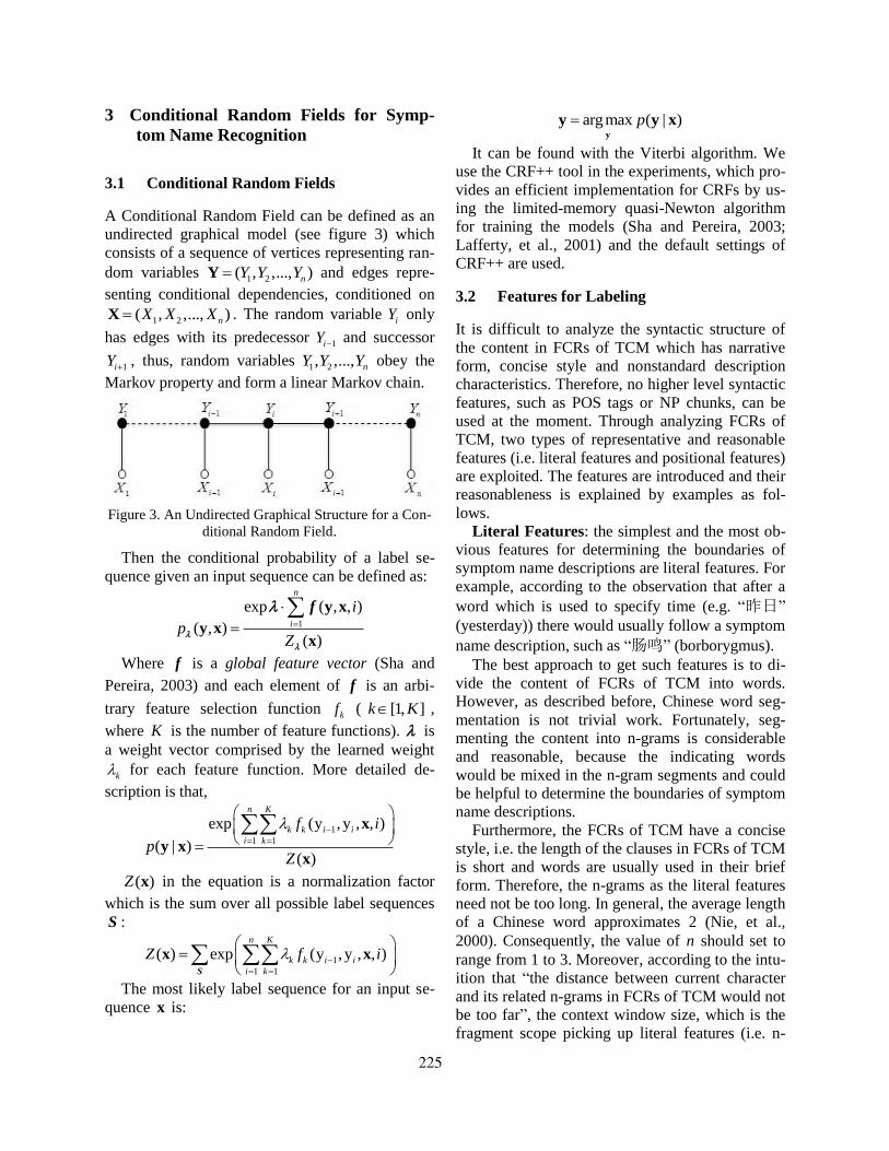
3 Conditional Random Fields for Symp-
tom Name Recognition
3.1 Conditional Random Fields
A Conditional Random Field can be defined as an
undirected graphical model (see figure 3) which
consists of a sequence of vertices representing ran-
dom variables 1 2( , ,..., )nY Y YY and edges repre-
senting conditional dependencies, conditioned on
1 2( , ,..., )nX X XX . The random variable iY only
has edges with its predecessor 1iY and successor
1iY , thus, random variables
1 2, ,..., nY Y Y obey the
Markov property and form a linear Markov chain.
Figure 3. An Undirected Graphical Structure for a Con-
ditional Random Field.
Then the conditional probability of a label se-
quence given an input sequence can be defined as:
1
exp ( , , )
( , )( )
n
i
i
pZ
y x
y xx
f
Where f is a global feature vector (Sha and
Pereira, 2003) and each element of f is an arbi-
trary feature selection function kf ( [1, ]k K ,
where K is the number of feature functions). is
a weight vector comprised by the learned weight
k for each feature function. More detailed de-
scription is that,
1
1 1
exp (y , y , , )
( | )( )
n K
k k i i
i k
f i
pZ
x
y xx
( )Z x in the equation is a normalization factor
which is the sum over all possible label sequences
S :
1
1 1
( ) exp (y ,y , , )n K
k k i i
i k
Z f i
x x
S
The most likely label sequence for an input se-
quence x is:
argmax ( | )py
y y x
It can be found with the Viterbi algorithm. We
use the CRF++ tool in the experiments, which pro-
vides an efficient implementation for CRFs by us-
ing the limited-memory quasi-Newton algorithm
for training the models (Sha and Pereira, 2003;
Lafferty, et al., 2001) and the default settings of
CRF++ are used.
3.2 Features for Labeling
It is difficult to analyze the syntactic structure of
the content in FCRs of TCM which has narrative
form, concise style and nonstandard description
characteristics. Therefore, no higher level syntactic
features, such as POS tags or NP chunks, can be
used at the moment. Through analyzing FCRs of
TCM, two types of representative and reasonable
features (i.e. literal features and positional features)
are exploited. The features are introduced and their
reasonableness is explained by examples as fol-
lows.
Literal Features: the simplest and the most ob-
vious features for determining the boundaries of
symptom name descriptions are literal features. For
example, according to the observation that after a
word which is used to specify time (e.g. “昨日”
(yesterday)) there would usually follow a symptom
name description, such as “肠鸣” (borborygmus).
The best approach to get such features is to di-
vide the content of FCRs of TCM into words.
However, as described before, Chinese word seg-
mentation is not trivial work. Fortunately, seg-
menting the content into n-grams is considerable
and reasonable, because the indicating words
would be mixed in the n-gram segments and could
be helpful to determine the boundaries of symptom
name descriptions.
Furthermore, the FCRs of TCM have a concise
style, i.e. the length of the clauses in FCRs of TCM
is short and words are usually used in their brief
form. Therefore, the n-grams as the literal features
need not be too long. In general, the average length
of a Chinese word approximates 2 (Nie, et al.,
2000). Consequently, the value of n should set to
range from 1 to 3. Moreover, according to the intu-
ition that “the distance between current character
and its related n-grams in FCRs of TCM would not
be too far”, the context window size, which is the
fragment scope picking up literal features (i.e. n-
225

grams (see examples in table 2)) in FCRs of TCM,
would not be too large. Otherwise it would bring
about noisy information, thereby reducing the la-
beling precision. The context window size in our
experiment is specified smaller then 4.
Feature
Type
Context Window
Size (CWS)
Literal feature examples
under different CWS
Unigram
Features
(Uni)
1 Ci-1, Ci, Ci+1
2 Ci-2, Ci-1, Ci, Ci+1, Ci+2
3 Ci-3, Ci-2, Ci-1, Ci,
Ci+1, Ci+2, Ci+3
4 Ci-4, Ci-3, Ci-2, Ci-1,
Ci, Ci+1, Ci+2, Ci+3, Ci+4
Bigram
Features
(Big)
1 Ci-1Ci, Ci Ci+1
2 Ci-2Ci-1, Ci-1Ci,
CiCi+1, Ci+1Ci+2
3 Ci-3Ci-2, Ci-2Ci-1, Ci-1Ci,
CiCi+1, Ci+1Ci+2, Ci+2Ci+3
4
Ci-4Ci-3, Ci-3Ci-2, Ci-2Ci-1,
Ci-1Ci, CiCi+1, Ci+1Ci+2,
Ci+2Ci+3, Ci+3Ci+4
Trigram
Features
(Tri)
1 Ci-1CiCi+1
2 Ci-2Ci-1Ci, Ci-1CiCi+1,
CiCi+1Ci+2
3
Ci-3Ci-2Ci-1, Ci-2Ci-1Ci,
Ci-1CiCi+1, CiCi+1Ci+2,
Ci+1Ci+2Ci+3
4
Ci-4Ci-3Ci-2Ci-1,
Ci-3Ci-2Ci-1Ci,
Ci-2Ci-1CiCi+1,
Ci-1CiCi+1Ci+2,
CiCi+1Ci+2Ci+3,
Ci+1Ci+2Ci+3Ci+4
Table 2. Literal Feature Examples Used in the Experi-
ments. Ci is the character at current position i in one
clause.
Positional Features: positions of characters in
FCRs of TCM are also helpful. They are assistant
features to determine the boundaries of symptom
name descriptions.
The start of a sentence would be usually a com-
mon character (i.e. its corresponding label is “O-
SYC”) rather than the beginning of a symptom
name description. On the contrary, the starting po-
sitions of the following clauses have higher proba-
bilities to be labeled with “B-SYC”. Taking the
FCR “昨日肠鸣, 失气多, 心中不适” (Yesterday,
the patient had borborygmus and more farting, and
his/her heart was uncomfortable) as an example, it
starts with a common word “昨日” (yesterday)
followed by a symptom name “肠鸣” (borboryg-
mus). And at the same time, following clauses all
start with symptom name descriptions.
The example of positional features is shown in
figure 4.
Figure 4. Example of Positional Features.
In figure 4, one “[SubSID-POS]” represents a
positional feature, and SubSID is the index of cur-
rent clause in a FCR and POS indicates the posi-
tion of a character in current clause.
4 Experiments
In this section, the proposed method for symptom
name recognition from TCM FCRs is evaluated,
and the usefulness of the introduced features is
verified based on a TCM clinical dataset. The re-
sults are depicted bellow.
4.1 Experimental Datasets
In this paper, a clinical record dataset (CRD) is
used. It contains 11613 FCRs of TCM and was
collected by TCM doctors during their routine di-
agnostic work. The Chinese characters in FCRs of
CRD are annotated with tags “B-SYC”, “I-SYC”,
and “O-SYC”. The number of each type of tags is
69193, 104243 and 142860, respectively. There are
4235 unique symptom names in CRD, and the
amount of annotated symptom names is 69193.
Training
Data
Test
Data
Number of Unique Symptom
Names 1813 3463
Amount of Symptom Names 17339 51854
Number of Each Type of Tags
(“B-SYC”, “I-SYC”, “O-SYC”)
17339,
25738,
35995
51854,
78505,
106865
Table 3. Detailed Information of the Training and Test
Datasets.
CRD is divided into two sub-datasets (i.e. a
training dataset (3483 FCRs, 25% of CRD) and a
test dataset (8130 FCRs, 75% of CRD)). For con-
226

venience, all numbers (e.g. integers, decimals and
fractions, etc.) in CRD are uniformly replaced by a
English character “N” in advance. Detailed infor-
mation of training and test datasets is listed in table
3.
4.2 Evaluation Metrics
A new method for symptom name recognition
from FCRs of TCM is proposed and two types of
features are introduced. To evaluate the feasibility
and effectiveness of the method and features, two
groups of evaluation metrics are designed: (1) for
assessing the ability of symptom name recognition,
symptom name recognition rate, recognition error
rate and recognition F-Measure are defined; (2) for
giving a detailed analysis, the labeling precision,
recall, and F-Measure are exercised. The detailed
explanations of these metrics are described below.
Symptom name recognition rate (RRdet),
recognition error rate (RERdet) and recognition
F-Measure (RFMdet): these metrics are designed
for assessing capability of the proposed method for
symptom name recognition from TCM FCRs. If
and only if the boundary of a symptom name is
labeled accurately (i.e. starting with “B-SYC” and
ending with the first change from “I-SYC” to “B--
SYC” or “O-SYC”), the recognized symptom
name is correct. Higher RRdet and lower RERdet are
achieved; better symptom name recognition per-
formance RFMdet would be obtained. RRdet, RERdet
and RFMdet are formulated as follows.
| |
| |det
NSDCRR
NCS
| | | |
| |det
SD NSDCRER
SD
2 (1 )
1
det detdet
det det
DR DERRFM
DR DER
Where | |NSDC is the number of symptom
name recognized correctly from the test dataset,
| |NCS is the number of clinical symptom names
in the test dataset, and | |SD is the number of
symptom name recognized.
Labeling precision (Prelab), recall (Reclab) and
F-Measure (FMlab): the metrics (Prelab, Reclab and
FMlab) are used to evaluate the performance of la-
beling Chinese character sequences of FCRs of
TCM for giving a detailed analysis. They are de-
fined below.
| |
| |lab
NCLCPre
NCL
| |
| |lab
NCLRec
NC
2 lab lablab
lab lab
Pre RecFM
Pre Rec
Where | |NCLC is the number of characters la-
beled correctly with their corresponding tags,
| |NCL is the number of characters labeled with
tags, and | |NC is the number of characters should
be labeled.
4.3 Evaluation of Symptom Name Recogni-
tion Ability
Comprehensive evaluations of symptom name
recognition ability using CRFs with reasonable
features are shown in figure 5, 6 and 7. These fig-
ures show that CRFs with reasonable features for
symptom name recognition from FCRs of TCM is
feasible. The best RFMdet 62.829% (RRdet 93.403%
and RERdet 52.665%) is achieved under settings
CWS 3 and features Uni+Big+Tri used.
Figure 5. Symptom Name Recognition Rate.
It obviously shows in figures 5, 6 and 7 that lit-
eral features and positional features are helpful to
symptom name recognition from FCRs of TCM.
More types of features are used; better recognition
performance would be obtained in most cases.
When CWS 1 and referred features changed
from unigram literal features to the combination of
unigram and bigram literal features, the highest
growth about 3.925% of RFMdet is achieved (the
227

RRdet increases from 87.586% to 93.034% and the
RERdet decreases from 56.173% to 53.118%).
Figure 6. Symptom Name Recognition Error Rate.
Figure 7. Symptom Name Recognition F-Measure.
As described previously, the context information
is helpful to symptom name recognition. However,
the context window size should not be too large. In
figures 5, 6 and 7, it clearly shows that when CWS
increase RRdet and RFMdet are improved and
RFMdet is reduced. When CWS grows too large
(larger than 3 here), RRdet and RFMdet begin, never-
theless, to descend and RERdet is raised in most
every cases.
Moreover, positional features are complemen-
tary features to literal features for symptom name
recognition from FCRs of TCM. It vividly shows
in figures 5, 6 and 7 that RRdet and RFMdet would
be improved and RERdet would be reduced more or
less when literal features combined with positional
features. The highest elevation can reach 0.297% if
the combination features of trigram literal features
and positional features are used and CWS 1 .
4.4 Evaluation of Labeling Performance and
Detailed Analysis for Symptom Name
Recognition
In this part, firstly, an evaluation for labeling per-
formance is given, and then a detailed analysis for
symptom name recognition from FCRs of TCM
using CRFs with reasonable features would be de-
scribed.
The results of Prelab and FMlab under different
situations are shown in figure 8 and 9, respectively.
The Reclab here are all 100%. It can be seen from
these figures that the FMlab can reach nearly up to
97.596% with corresponding Prelab 95.305%. The
results can also demonstrate the feasibility of the
proposed method for symptom name recognition
from FCRs of TCM and the worth of the repre-
sentative and reasonable features introduced in this
paper. The properties of literal features and posi-
tional features, which are just described in section
4.3, are also reflected in figures 8 and 9.
Figure 8. Results of Prelab under Different Situations.
Figure 9. Results of FMlab under Different Situations.
Although RRdet can achieve a very high perfor-
mance, however, RERdet is also too high. In figures
8 and 9, high labeling results was gotten. It implies
that the probable position of the symptom name
can be found in TCM FCRs, but the exact bounda-
ries of the symptom name descriptions cannot be
detected accurately yet.
More careful results are listed in table 4. In this
table, the average labeling Prelab of labels “B-
228
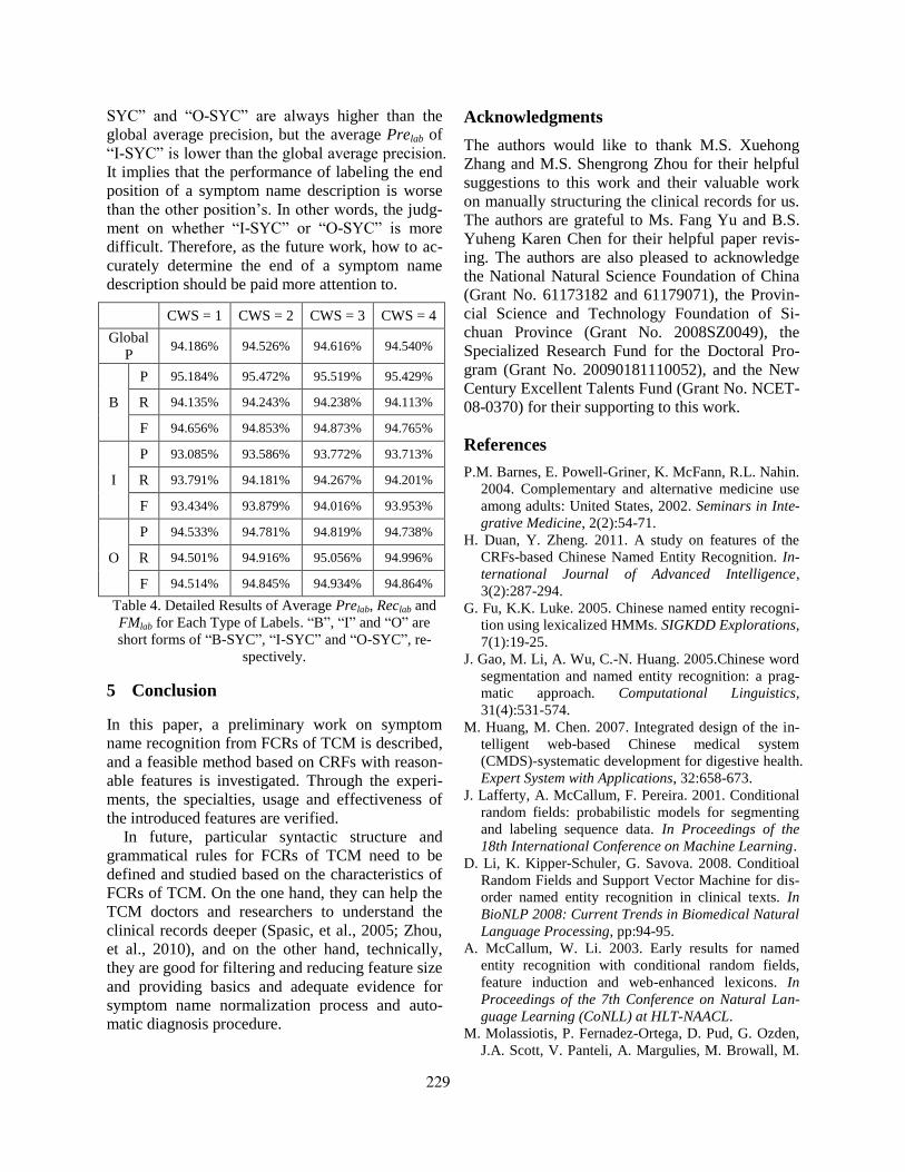
SYC” and “O-SYC” are always higher than the
global average precision, but the average Prelab of
“I-SYC” is lower than the global average precision.
It implies that the performance of labeling the end
position of a symptom name description is worse
than the other position’s. In other words, the judg-
ment on whether “I-SYC” or “O-SYC” is more
difficult. Therefore, as the future work, how to ac-
curately determine the end of a symptom name
description should be paid more attention to.
CWS = 1 CWS = 2 CWS = 3 CWS = 4
Global
P 94.186% 94.526% 94.616% 94.540%
B
P 95.184% 95.472% 95.519% 95.429%
R 94.135% 94.243% 94.238% 94.113%
F 94.656% 94.853% 94.873% 94.765%
I
P 93.085% 93.586% 93.772% 93.713%
R 93.791% 94.181% 94.267% 94.201%
F 93.434% 93.879% 94.016% 93.953%
O
P 94.533% 94.781% 94.819% 94.738%
R 94.501% 94.916% 95.056% 94.996%
F 94.514% 94.845% 94.934% 94.864%
Table 4. Detailed Results of Average Prelab, Reclab and
FMlab for Each Type of Labels. “B”, “I” and “O” are
short forms of “B-SYC”, “I-SYC” and “O-SYC”, re-
spectively.
5 Conclusion
In this paper, a preliminary work on symptom
name recognition from FCRs of TCM is described,
and a feasible method based on CRFs with reason-
able features is investigated. Through the experi-
ments, the specialties, usage and effectiveness of
the introduced features are verified.
In future, particular syntactic structure and
grammatical rules for FCRs of TCM need to be
defined and studied based on the characteristics of
FCRs of TCM. On the one hand, they can help the
TCM doctors and researchers to understand the
clinical records deeper (Spasic, et al., 2005; Zhou,
et al., 2010), and on the other hand, technically,
they are good for filtering and reducing feature size
and providing basics and adequate evidence for
symptom name normalization process and auto-
matic diagnosis procedure.
Acknowledgments
The authors would like to thank M.S. Xuehong
Zhang and M.S. Shengrong Zhou for their helpful
suggestions to this work and their valuable work
on manually structuring the clinical records for us.
The authors are grateful to Ms. Fang Yu and B.S.
Yuheng Karen Chen for their helpful paper revis-
ing. The authors are also pleased to acknowledge
the National Natural Science Foundation of China
(Grant No. 61173182 and 61179071), the Provin-
cial Science and Technology Foundation of Si-
chuan Province (Grant No. 2008SZ0049), the
Specialized Research Fund for the Doctoral Pro-
gram (Grant No. 20090181110052), and the New
Century Excellent Talents Fund (Grant No. NCET-
08-0370) for their supporting to this work.
References
P.M. Barnes, E. Powell-Griner, K. McFann, R.L. Nahin.
2004. Complementary and alternative medicine use
among adults: United States, 2002. Seminars in Inte-
grative Medicine, 2(2):54-71.
H. Duan, Y. Zheng. 2011. A study on features of the
CRFs-based Chinese Named Entity Recognition. In-
ternational Journal of Advanced Intelligence,
3(2):287-294.
G. Fu, K.K. Luke. 2005. Chinese named entity recogni-
tion using lexicalized HMMs. SIGKDD Explorations,
7(1):19-25.
J. Gao, M. Li, A. Wu, C.-N. Huang. 2005.Chinese word
segmentation and named entity recognition: a prag-
matic approach. Computational Linguistics,
31(4):531-574.
M. Huang, M. Chen. 2007. Integrated design of the in-
telligent web-based Chinese medical system
(CMDS)-systematic development for digestive health.
Expert System with Applications, 32:658-673.
J. Lafferty, A. McCallum, F. Pereira. 2001. Conditional
random fields: probabilistic models for segmenting
and labeling sequence data. In Proceedings of the
18th International Conference on Machine Learning.
D. Li, K. Kipper-Schuler, G. Savova. 2008. Conditioal
Random Fields and Support Vector Machine for dis-
order named entity recognition in clinical texts. In
BioNLP 2008: Current Trends in Biomedical Natural
Language Processing, pp:94-95.
A. McCallum, W. Li. 2003. Early results for named
entity recognition with conditional random fields,
feature induction and web-enhanced lexicons. In
Proceedings of the 7th Conference on Natural Lan-
guage Learning (CoNLL) at HLT-NAACL.
M. Molassiotis, P. Fernadez-Ortega, D. Pud, G. Ozden,
J.A. Scott, V. Panteli, A. Margulies, M. Browall, M.
229

Magri, S. Selvekerova, E. Madsen, L. Milovics, I.
Bruyns, G. Gudmundsdottir, S. Hummerston, A. M.-
A. Ahmad, N. Platin, N. Kearney, E. Pariraki. 2005.
Use of complementary and alternative medicine in
cancer patients: a European survey. Annals of Oncol-
ogy, 16(4):655-663.
J.-J. Nie, J. Gao, J. Zhang, M. Zhou. 2000. On the use of
words and n-grams for Chinese information retrieval.
In Proceedings of the fifth international workshop on
Information Retrieval with Asian Languages.
S.K. Pal. 2002. Complementary and alternative medi-
cine: an overview. Current Science, 82(5):518-524.
L.A. Ramshaw, M.P. Marcus. 1995. Text chunking us-
ing transformation-based learning. In Proceedings of
the Third Workshop on Very Large Corpora. ACL.
F. Sha, F. Pereira. 2003. Shallow parsing with condi-
tional random fields. Proceedings of the 2003 Con-
ference of the North American Chapter of the
Association of Computer Linguistics on Human Lan-
guage Technology.
I. Spasic, S. Ananiadou, J. McNaught, A. Kumar. 2005.
Text mining and ontologies in biomedicine: making
sense of raw text. Briefings in Bioinformatics,
6(3):239-251.
X. Wang, H. Qu, P. Liu. 2004. A self-learning expert
system for diagnosis in traditional Chinese medicine.
Expert System with Applications, 26:557-566.
Y. Wang, Z. Yu, Y. Jiang, K. Xu, X. Chen. 2010. Au-
tomatic symptom name normalization in clinical rec-
ords of traditional Chinese medicine. BMC
Bioinformatics, 11:40.
Y. Wang, Z. Yu, Y. Jiang, Y. Liu, L. Chen, Y. Liu.
2012. A framework and its empirical study of auto-
matic diagnosis of traditional Chinese medicine uti-
lizing raw free-text clinical records. Journal of
Biomedical Informatics, 45:210-223.
Y. Wu, J. Zhao, B. Xu. 2003. Chinese named entity
recognition combining a statistical model with hu-
man knowledge. In Proceedings of the ACL 2003
Workshop on Multilingual and Mixed-Language
Named Entity Recognition (MultiNER’03), pp:65-72.
K. Yoshida, J. Tsujii. 2007. Reranking for biomedical
named-entity recognition. In BioNLP 2007: Biologi-
cal, translational, and clinical language processing,
pp:209-216.
H.-P. Zhang, Q. Liu, H.-K. Yu, X.-Q. Cheng, S. Bai.
2003. Chinese named entity recognition using role
model. Computational Linguistics and Chinese Lan-
guage Processing, 8(2):29-60.
N.L. Zhang, S. Yuan, Y. Wang. 2008. Latent tree mod-
els and diagnosis in traditional Chinese medicine. Ar-
tificial Intelligence in Medicine, 42:229-245.
J. Zhou, L. He, X. Dai, J. Chen. 2006. Chinese named
entity recognition with a multi-phase model. In Pro-
ceedings of the fifth Workshop on Chinese Language
Processing, pp:213-216.
X. Zhou, Y. Peng, B. Liu. 2010. Text mining for tradi-
tional Chinese medical knowledge discovery: a sur-
vey. Joural of Biomedical Informatics, 43:650-660.
G.D. Zhou, J. Su. 2002. Named entity recognition using
an HMM-based Chunk Tagger. In Proceedings of the
40th Annual Meeting of the Association for Computa-
tional Linguistics.
230
Proceedings of the 2012 Workshop on Biomedical Natural Language Processing (BioNLP 2012), pages 231–239,Montreal, Canada, June 8, 2012. c©2012 Association for Computational Linguistics
Scaling up WSD with Automatically Generated Examples
Weiwei Cheng, Judita Preiss and Mark StevensonDepartment of Computer Science,
Sheffield University,Regent Court, 211 Portobello,
Sheffield, S1 4DPUnited Kingdom
{W.Cheng, J.Preiss, M.Stevenson}@dcs.shef.ac.uk
Abstract
The most accurate approaches to Word SenseDisambiguation (WSD) for biomedical docu-ments are based on supervised learning. How-ever, these require manually labeled trainingexamples which are expensive to create andconsequently supervised WSD systems arenormally limited to disambiguating a small setof ambiguous terms. An alternative approachis to create labeled training examples automat-ically and use them as a substitute for manu-ally labeled ones. This paper describes a largescale WSD system based on automatically la-beled examples generated using informationfrom the UMLS Metathesaurus. The labeledexamples are generated without any use of la-beled training data whatsoever and is thereforecompletely unsupervised (unlike some previ-ous approaches). The system is evaluated ontwo widely used data sets and found to outper-form a state-of-the-art unsupervised approachwhich also uses information from the UMLSMetathesaurus.
1 Introduction
The information contained in the biomedical liter-ature that is available in electronic formats is use-ful for health professionals and researchers (West-brook et al., 2005). The amount is so vast thatit is difficult for researchers to identify informa-tion of interest without the assistance of automatedtools (Krallinger and Valencia, 2005). However,processing these documents automatically is madedifficult by the fact that they contain terms thatare ambiguous. For example, “culture” can mean
“laboratory procedure” (e.g. “In peripheral bloodmononuclear cell culture”) or “anthropological cul-ture” (e.g. “main accomplishments of introducing aquality management culture”). These lexical ambi-guities are problematic for language understandingsystems.
Word sense disambiguation (WSD) is the processof automatically identifying the meanings of am-biguous terms. Some WSD systems for the biomed-ical domain are only able to disambiguate a smallnumber of ambiguous terms (see Section 2). How-ever, for WSD systems to be useful in applicationsthey should be able to disambiguate all ambiguousterms. One way to create such a WSD system is toautomatically create the labeled data that is used totrain supervised WSD systems. Several approaches(Liu et al., 2002; Stevenson and Guo, 2010; Jimeno-Yepes and Aronson, 2010) have used informationfrom the UMLS Metathesaurus1 to create labeledtraining data that have successfully been used to cre-ate WSD systems.
A key decision for any system that automaticallygenerates labeled examples is the number of exam-ples of each sense to create, known as the bias of thedata set. It has been shown that the bias of a set of la-beled examples affects the performance of the WSDsystem it is used to train (Mooney, 1996; Agirre andMartınez, 2004b). Some of the previous approachesto generating labeled data relied on manually anno-tated examples to determine the bias of the data setsand were therefore not completely unsupervised.
This paper describes the development of a largescale WSD system that is able to disambiguate all
1http://www.nlm.nih.gov/research/umls/
231

terms that are ambiguous in the UMLS Metathe-saurus. The system relies on labeled examples thatare created using information from UMLS. Variousbias options are explored, including ones that do notmake use of information from manually labeled ex-amples, and thus we can create a completely unsu-pervised system. Evaluation is carried out on twostandard datasets (the NLM-WSD and MSH-WSDcorpora). We find that WSD systems can be cre-ated without using any information from manuallylabeled examples and that their performance is bet-ter than a state-of-the-art unsupervised approach.
The remainder of this paper is organized as fol-lows. Previous approaches to WSD in biomedicaldocuments are described in the next Section. Section3 presents the methods used to identify bias in thelabeled examples and WSD system. Experiments inwhich these approaches are compared are describedin Section 4 and their results in Section 5.
2 Background
Many WSD systems for the biomedical domain arebased on supervised learning (McInnes et al., 2007;Xu et al., 2007; Stevenson et al., 2008; Yepes andAronson, 2011). These systems require labeledtraining data, examples of an ambiguous term la-beled with the correct meaning. Some sets of labeleddata have been developed for the biomedical domain(Weeber et al., 2001; Savova et al., 2008; Jimeno-Yepes et al., 2011). However, these data sets onlycontain examples for a few hundred terms and canonly be used to develop WSD systems to identifythe meanings of those terms. The process of creat-ing labeled examples is extremely time-consumingand difficult (Artstein and Poesio, 2008), making itimpractical to create labeled examples of all possibleambiguous terms found in biomedical documents.
Two alternative approaches have been explored todevelop systems which are able to disambiguate allambiguous terms in biomedical documents. The firstmakes use of unsupervised WSD algorithms (seeSection 2.1) and the second creates labeled data au-tomatically and uses it to train a supervised WSDsystem (see Section 2.2).
2.1 Unsupervised WSD
Unsupervised WSD algorithms make use of infor-mation from some knowledge source, rather than re-lying on training data.
Humphrey et al. (2006) describe an unsupervisedsystem which uses semantic types in UMLS to dis-tinguish between the possible meanings of ambigu-ous words. However, it cannot disambiguate be-tween senses with the same semantic type, i.e., itis not possible for the system to recognise all sensedistinctions.
The Personalised Page Rank (PPR) system(Agirre et al., 2010; Jimeno-Yepes and Aronson,2010) relies on a a graph-based algorithm similarto the Page Rank algorithm originally developed foruse in search engines (Brin, 1998). It performsWSD by converting the UMLS Metathesaurus intoa graph in which the possible meanings of ambigu-ous words are nodes and relations between them areedges. Disambiguation is carried out by providingthe algorithm with a list of senses that appear in thetext that is being disambiguated. This information isthen combined with the graph and a ranked list of thepossible senses for each ambiguous word generated.
Unsupervised systems have the advantage of be-ing able to disambiguate all ambiguous terms. How-ever, the performance of unsupervised systems thathave been developed for biomedical documents islower than that of supervised ones.
2.2 Automatic Generation of Labeled Data
Automatic generation of labeled data for WSD com-bines the accuracy of supervised approaches withthe ability of unsupervised approaches to disam-biguate all ambiguous terms. It was first suggestedby Leacock et al. (1998). Their approach is basedon the observation that some terms in a lexicon oc-cur only once and, consequently, there is no doubtabout their meaning. These are referred to as beingmonosemous. Examples for each possible meaningof an ambiguous term are generated by identifyingthe closest monosemous term (the monosemous rel-ative) in the lexicon and using examples of that term.Variants of the approach have been applied to thebiomedical domain using the UMLS Metathesaurusas the sense inventory.
232

Liu et al. (2002) were the first to apply themonosemous relatives approach to biomedical WSDand use it to disambiguate a set of 35 abbreviations.They reported high precision but low recall, indicat-ing that labeled examples could not be created formany of the abbreviations. Jimeno-Yepes and Aron-son (2010) applied a similar approach and foundthat it performed better than a number of alternativeapproaches on a standard evaluation resource (theNLM-WSD corpus) but did not perform as well assupervised WSD. Stevenson and Guo (2010) com-pared two techniques for automatically creating la-beled data, including the monosemous relatives ap-proach. They found that the examples which weregenerated were as good as manually labeled exam-ples when used to train a supervised WSD system.However, Stevenson and Guo (2010) relied on la-beled data to determine the number of examples ofeach sense to create, and therefore the bias of thedata set. Consequently their approach is not com-pletely unsupervised since it could not be applied toambiguous terms that do not have labeled trainingdata available.
3 Approach
3.1 WSD System
The WSD system is based on a supervised approachthat has been adapted for the biomedical domain(Stevenson et al., 2008). The system was tested onthe NLM-WSD corpus (see Section 4.1) and foundto outperform alternative approaches.
The system can exploit a wide range of fea-tures, including several types of linguistic informa-tion from the context of an ambiguous term, MeSHcodes and Concept Unique Identifiers (CUIs) fromthe UMLS Metathesaurus. However, computingthese features for every example is a time consum-ing process and to make the system suitable for largescale WSD it was restricted to using a smaller setof features. Previous experiments (Stevenson et al.,2008) showed that this only leads to a small drop indisambiguation accuracy while significantly reduc-ing the computational cost of generating features.
3.1.1 FeaturesTwo types of context words are used as features:
the lemmas of all content words in the same sen-
tence as the ambiguous word and the lemmas of allcontent words in a±4-word window around the am-biguous term. A list of corpus-specific stopwordswas created containing terms that appear frequentlyin Medline abstracts but which are not useful for dis-ambiguation (e.g. “abstract”, “conclusion”). Anylemmas found in this list were not used as features.
3.1.2 Learning algorithmDisambiguation is carried out using the Vector
Space Model, a memory-based learning algorithmin which each occurrence of an ambiguous word isrepresented as a vector created using the features ex-tracted to represent it (Agirre and Martınez, 2004a).The Vector Space Model was found to outperformother learning algorithms when evaluated using theNLM-WSD corpus (Stevenson et al., 2008).
During the algorithm’s training phase a singlecentroid vector, ~Csj , is generated for each possiblesense, sj . This is shown in equation 1 where T isthe set of training examples for a particular term andsense(~t) is the sense associated with the vector ~t.
~Csj =
∑~ti ε T :sense(~ti)=sj
~ti
|~ti ε T : sense(~ti) = sj |(1)
Disambiguation is carried out by comparing thevector representing the ambiguous word, ~a, againstthe centroid of each sense using the cosine metric,shown in equation 2, and choosing the one with thehighest score.
score(sj ,~a) = cos( ~Csj ,~a) =~Csj .~a
| ~Csj ||~a|(2)
Note that the learning algorithm does not ex-plicitly model the prior probability of each possi-ble sense, unlike alternative approaches (e.g. NaiveBayes), since it was found that including this infor-mation did not improve performance.
3.2 Automatically generating trainingexamples
The approaches used for generating training exam-ples used here are based on the work of Stevensonand Guo (2010), who describe two approaches:
1. Monosemous relatives
2. Co-occurring concepts
233

Both approaches are provided with a set of ambigu-ous CUIs from the UMLS Metathesaurus, whichrepresent the possible meanings of an ambiguousterm, and a target number of training examples to begenerated for each CUI. Each CUI is associated withat least one term and each term is labeled with a lex-ical unique identifier (LUI) which represents a rangeof lexical variants for a particular term. The UMLSMetathesaurus contains a number of data files whichare exploited within these techniques, including:
AMBIGLUI: a list of cases where a LUI is linkedto multiple CUIs.
MRCON: every string or concept name in theMetathesaurus appears in this file.
MRCOC: co-occuring concepts.
For the monosemous relatives approach, thestrings of monosemous LUIs of the target CUIand its relatives are used to search Medline to re-trieve training examples. The monosemous LUIs re-lated to a CUI are defined as any LUIs associatedwith the CUI in the MRCON table and not listed inAMBIGLUI table.
The co-occurring concept approach works differ-ently. Instead of using strings of monosemous LUIsof the target CUI and its relatives, the strings associ-ated with LUIs of a number of co-occurring CUIs ofthe target CUI and its relatives found in MRCOC ta-ble are used. The process starts by finding the LUIsof the top n co-occurring CUIs of the target CUI.These LUIs are then used to form search queries.The query is quite restrictive in the beginning and re-quires all terms appear in the Medline citations files.Subsequently queries are made less restrictive by re-ducing the number of required terms in the query.
These techniques were used to generate labeledexamples for all terms that are ambiguous in the2010 AB version of the UMLS Metathesaurus.2 Theset of all ambiguous terms was created by analysingthe AMBIGLUI table, to identify CUIs that are asso-ciated with multiple LUIs. The Medline BaselineRepository (MBR)3 was also analysed and it wasfound that some terms were ambiguous in this re-source, in the sense that more than one CUI had been
2Stevenson and Guo (2010) applied them to a small set ofexamples from the NLM-WSD data set (see Section 4.1).
3http://mbr.nlm.nih.gov
assigned to an instance of a term, but could not beidentified from the AMBIGLUI table. The final listof ambiguous CUIs was created by combining thoseidentified from the AMBIGLUI table and those findin the MBR. This list contained a total of 103,929CUIs.
Both techniques require large number of searchesover the Medline database and to carry this out ef-ficiently the MBR was indexed using the LuceneInformation Retrieval system4 and all searches ex-ecuted locally.
Examples were generated using both approaches.The monosemous relatives approach generated ex-amples for 98,462 CUIs and the co-occurring con-cepts for 98,540. (Examples generated using themonosemous relatives approach were preferred forthe experiments reported later.) However, neithertechnique was able to generate examples for 5,497CUIs, around 5% of the total. This happened whennone of the terms associated with a CUI returnedany documents when queried against the MBR andthat CUI does not have any monosemous relatives.An example is C1281723 “Entire nucleus pulpo-sus of intervertebral disc of third lumbar vertebra”.The lengthy terms associated with this CUI do notreturn any documents when used as search termsand, in addition, it is only related to one other CUI(C0223534 “Structure of nucleus pulposus of inter-vertebral disc of third lumbar vertebra”) which is it-self only connected to C1281723. Fortunately thereare relatively few CUIs for which no examples couldbe generated and none of them appear in the MBR,suggesting they refer to UMLS concepts that do nottend to be mentioned in documents.
3.3 Generating Bias
Three different techniques for deciding the numberof training examples to be generated for each CUI(i.e. the bias) were explored.
Uniform Bias (UB) uses an equal number oftraining examples to generate centroid vectors foreach of the possible senses of the ambiguous term.
Gold standard bias (GSB) is similar to the uni-form bias but instead of being the same for all pos-sible CUIs the number of training examples for eachCUI is determined by the number of times it appears
4http://lucene.apache.org/
234

in a manually labeled gold standard corpus. Assumet is an ambiguous term and Ct is the set of possiblemeanings (CUIs). The number of training examplesused to generate the centroid for that CUI, Ec, iscomputed according to equation 3 where Gc is thenumber of instances in the gold standard corpus an-notated with CUI c and n is a constant which is setto 100 for these experiments.5
Ec =Gc∑
ci ε CtGci,t
.n (3)
The final technique, Metamap Baseline Repos-itory Bias (MBB), is based on the distribution ofCUIs in the MBR. The number of training examplesare generated in a similar way to the gold standardbias with MBR being used instead of a manually la-beled corpus and is shown in equation 4 whereMc isthe number of times the CUI c appears in the MBR.
Ec =Mc∑
ci ε CtMci
.n (4)
For example, consider the three possible CUIs as-sociated with term “adjustment” in the NLM-WSDcorpus: C0376209, C0456081 and C06832696.The corpus contains 18 examples of C0376209,62 examples of C0456081 and 13 of C0683269.Using equation 3, the number of training exam-ples when GSB is applied for C0376209 is 20,67 for C0456081 and 14 for C0683269. In theMetamap Baseline Repository files, C0376209 hasa frequency count of 98046, C0456081 a count of292809 and C0683269 a count of 83530. Thereforethe number of training examples used for the threesenses when applying MBB is: 21 for C0376209, 62for C0456081 and 18 for C0683269.
4 Evaluation
4.1 Data sets
We evaluate our system on two datasets: the NLM-WSD and MSH-WSD corpora.
5Small values for Ec are rounded up to ensure that any rareCUIs have at least one training example.
6These CUIs are obtained using the mappings from NLM-WSD senses to CUIs available on the NLM website: http://wsd.nlm.nih.gov/collaboration.shtml
The NLM-WSD corpus7 (Weeber et al., 2001) hasbeen widely used for experiments on WSD in thebiomedical domain, for example (Joshi et al., 2005;Leroy and Rindflesch, 2005; McInnes et al., 2007;Savova et al., 2008). It contains 50 ambiguous termsfound in Medline with 100 examples of each. Theseexamples were manually disambiguated by 11 an-notators. The guidelines provided to the annotatorsallowed them to label a senses as “None” if noneof the concepts in the UMLS Metathesaurus seemedappropriate. These instances could not be mappedonto UMLS Metathesaurus and were ignored for ourexperiments.
The larger MSH-WSD corpus (Jimeno-Yepes etal., 2011) contains 203 strings that are associatedwith more than one possible MeSH code in theUMLS Metathesaurus. 106 of these are ambiguousabbreviations, 88 ambiguous terms and 9 a combi-nation of both. The corpus contains up to 100 ex-amples for each possible sense and a total of 37,888examples of ambiguous strings taken from Medline.Unlike the NLM-WSD corpus, all of the instancescan be mapped to the UMLS Metathesaurus andnone was removed from the dataset for our exper-iments.
The two data sets differ in the way the numberof instances of each sense was determined. Forthe NLM-WSD corpus manual annotation is used todecide the number of instances that are annotatedwith each sense of an ambiguous term. However,the NLM-MSH corpus was constructed automati-cally and each ambiguous term has roughly the samenumber of examples of each possible sense.
4.2 Experiments
The WSD system described in Section 3 was testedusing each of the three techniques for determiningthe bias, i.e. number of examples generated for eachCUI. Performance is compared against various alter-native approaches.
Two supervised approaches are included. Thefirst, most frequent sense (MFS) (McCarthy et al.,2004), is widely used baseline for supervised WSDsystems. It consists of assigning each ambiguousterm the meaning that is more frequently observedin the training data. The second supervised approach
7http://wsd.nlm.nih.gov
235

is to train the WSD system using manually labeledexamples from the NLM-WSD and MSH-WSD cor-pora. 10-fold cross validation is applied to evaluatethis approach.
Performance of the Personalised Page Rank ap-proach described in Section 2.1 is also provided toallow comparison with an unsupervised algorithm.Both Personalised Page Rank and the techniqueswe employ to generate labeled data, base disam-biguation decisions on information from the UMLSMetathesaurus.
The performance of all approaches is measuredin terms of the percentage of instances which arecorrectly disambiguated for each term with the av-erage across all terms reported. Confidence inter-vals (95%) computed using bootstrap resampling(Noreen, 1989) are also shown.
5 Results
Results of the experiments are shown in Table 1where the first three rows show performance of theapproach described in Section 3 using the threemethods for computing the bias (UB, MMB andGSB). MFS and Sup refer to the Most FrequentSense supervised baseline and using manually la-beled examples, respectively, and PPR to the Per-sonalised PageRank approach.
When the performance of the approaches us-ing automatically labeled examples (UB, MMB andGSB) is compared it is not surprising that the best re-sults are obtained using the gold standard bias sincethis is obtained from manually labeled data. Resultsusing this technique for computing bias always out-perform the other two, which are completely unsu-pervised and do not make use of any informationfrom manually labeled data. However, the improve-ment in performance varies according to the corpus,for the NLM-WSD corpus there is an improvementof over 10% in comparison to UB while the corre-sponding improvement for the MSH-WSD corpus isless than 0.5%.
A surprising result is that performance obtainedusing the uniform bias (UB) is consistently betterthan using the bias obtained by analysis of the MBR(MMB). It would be reasonable to expect that in-formation about the distribution of CUIs in this cor-pus would be helpful for WSD but it turns out that
making no assumptions whatsoever about their rel-ative frequency, i.e., assigning a uniform baseline,produces better results.
The relative performance of the supervised (MFS,Sup and GSB) and unsupervised approaches (UB,MMB and PPR) varies according to the corpus. Un-surprisingly using manually labeled data (Sup) out-performs all other approaches on both corpora. Thesupervised approaches also outperform the unsuper-vised ones on the NLM-WSD corpus. However, forthe MSH-WSD corpus all of the unsupervised ap-proaches outperform the MFS baseline.
A key reason for the differences in these results isthe different distributions of senses in the two cor-pora, as shown by the very different performance ofthe MFS approach on the two corpora. This is dis-cussed in more detail later (Section 5.2).
Comparison of the relative performance of the un-supervised approaches (UB, MMB and PPR) showsthat training a supervised system with the automat-ically labeled examples using a uniform bias (UB)always outperforms PPR. This demonstrates thatthis approach outperforms a state-of-the-art unsu-pervised algorithm that relies on the same infor-mation used to generate the examples (the UMLSMetathesaurus).
5.1 Performance by Ambiguity Type
The MSH-WSD corpus contains both ambiguousterms and abbreviations (see Section 4.1). Perfor-mance of the approaches on both types of ambiguityare shown in Table 2.
MSH-WSD Ambiguity TypeApproach Abbreviation Term
UB 91.40 [91.00, 91.75] 72.68 [72.06, 73.32]
MMB 84.43 [83.97, 84.89] 69.45 [68.86, 70.10]
GSB 90.82 [90.45, 91.22] 73.96 [73.40, 74.62]
MFS 52.43 [51.73, 53.05] 51.76 [51.11, 52.36]
Sup. 97.41 [97.19, 97.62] 91.54 [91.18, 91.94]
PPR 86.40 [86.00, 86.85] 68.40 [67.80, 69.14]
Table 2: WSD evaluation results for abbreviations andterms in the MSH-WSD data set.
The relative performance of the different ap-proaches on the terms and abbreviations is similar tothe entire MSH-WSD data set (see Table 1). In par-
236
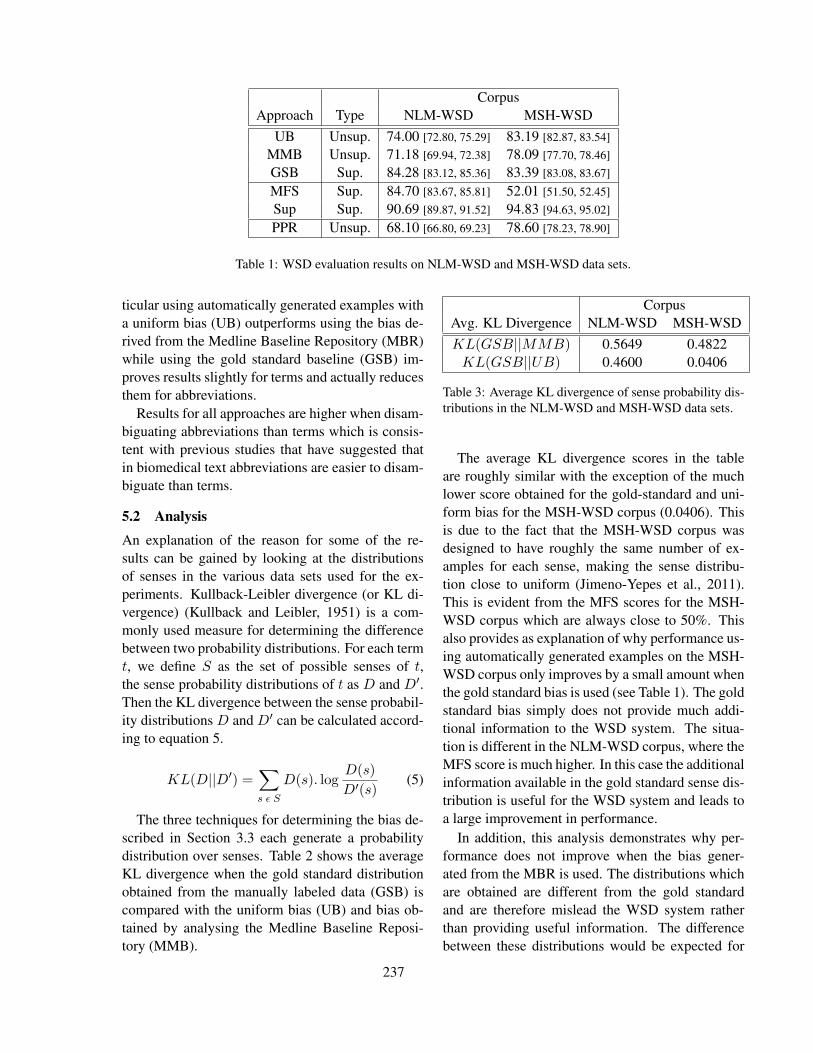
CorpusApproach Type NLM-WSD MSH-WSD
UB Unsup. 74.00 [72.80, 75.29] 83.19 [82.87, 83.54]
MMB Unsup. 71.18 [69.94, 72.38] 78.09 [77.70, 78.46]
GSB Sup. 84.28 [83.12, 85.36] 83.39 [83.08, 83.67]
MFS Sup. 84.70 [83.67, 85.81] 52.01 [51.50, 52.45]
Sup Sup. 90.69 [89.87, 91.52] 94.83 [94.63, 95.02]
PPR Unsup. 68.10 [66.80, 69.23] 78.60 [78.23, 78.90]
Table 1: WSD evaluation results on NLM-WSD and MSH-WSD data sets.
ticular using automatically generated examples witha uniform bias (UB) outperforms using the bias de-rived from the Medline Baseline Repository (MBR)while using the gold standard baseline (GSB) im-proves results slightly for terms and actually reducesthem for abbreviations.
Results for all approaches are higher when disam-biguating abbreviations than terms which is consis-tent with previous studies that have suggested thatin biomedical text abbreviations are easier to disam-biguate than terms.
5.2 Analysis
An explanation of the reason for some of the re-sults can be gained by looking at the distributionsof senses in the various data sets used for the ex-periments. Kullback-Leibler divergence (or KL di-vergence) (Kullback and Leibler, 1951) is a com-monly used measure for determining the differencebetween two probability distributions. For each termt, we define S as the set of possible senses of t,the sense probability distributions of t as D and D′.Then the KL divergence between the sense probabil-ity distributions D and D′ can be calculated accord-ing to equation 5.
KL(D||D′) =∑s ε S
D(s). logD(s)D′(s)
(5)
The three techniques for determining the bias de-scribed in Section 3.3 each generate a probabilitydistribution over senses. Table 2 shows the averageKL divergence when the gold standard distributionobtained from the manually labeled data (GSB) iscompared with the uniform bias (UB) and bias ob-tained by analysing the Medline Baseline Reposi-tory (MMB).
CorpusAvg. KL Divergence NLM-WSD MSH-WSDKL(GSB||MMB) 0.5649 0.4822KL(GSB||UB) 0.4600 0.0406
Table 3: Average KL divergence of sense probability dis-tributions in the NLM-WSD and MSH-WSD data sets.
The average KL divergence scores in the tableare roughly similar with the exception of the muchlower score obtained for the gold-standard and uni-form bias for the MSH-WSD corpus (0.0406). Thisis due to the fact that the MSH-WSD corpus wasdesigned to have roughly the same number of ex-amples for each sense, making the sense distribu-tion close to uniform (Jimeno-Yepes et al., 2011).This is evident from the MFS scores for the MSH-WSD corpus which are always close to 50%. Thisalso provides as explanation of why performance us-ing automatically generated examples on the MSH-WSD corpus only improves by a small amount whenthe gold standard bias is used (see Table 1). The goldstandard bias simply does not provide much addi-tional information to the WSD system. The situa-tion is different in the NLM-WSD corpus, where theMFS score is much higher. In this case the additionalinformation available in the gold standard sense dis-tribution is useful for the WSD system and leads toa large improvement in performance.
In addition, this analysis demonstrates why per-formance does not improve when the bias gener-ated from the MBR is used. The distributions whichare obtained are different from the gold standardand are therefore mislead the WSD system ratherthan providing useful information. The differencebetween these distributions would be expected for
237

the MSH-WSD corpus, since it contains roughly thesame number of examples for each possible senseand does not attempt to represent the relative fre-quency of the different senses. However, it is sur-prising to observe a similar difference for the NLM-WSD corpus, which does not have this constraint.The difference suggests the information about CUIsin the MBR, which is generated automatically, hassome limitations.
Table 4 shows a similar analysis for the MSH-WSD corpus when abbreviations and terms are con-sidered separately and supports this analysis. Thefigures in this table show that the gold standard anduniform distributions are very similar for both ab-breviations and terms, which explains the similar re-sults for UB and GSB in Table 2. However, the goldstandard distribution is different from the one ob-tained from the MBR. The drop in performance ofMMB compared with GBS in Table 2 is a conse-quence of this.
Ambiguity TypeAvg. KL Divergence Abbreviation TermKL(GSB||MMB) 0.4554 0.4603KL(GSB||UB) 0.0544 0.0241
Table 4: Average KL divergence for abbreviations andterms in the MSH-WSD data set.
6 Conclusion
This paper describes the development of a largescale WSD system based on automatically labeledexamples. We find that these examples can be gener-ated for the majority of CUIs in the UMLS Metathe-saurus. Evaluation on the NLM-WSD and MSH-WSD data sets demonstrates that the WSD systemoutperforms the PPR approach without making anyuse of labeled data.
Three techniques for determining the number ofexamples to use for training are explored. It isfound that a supervised approach (which makes useof manually labeled data) provides the best results.Surprisingly it was also found that using informationfrom the MBR did not improve performance. Anal-ysis showed that the sense distributions extractedfrom the MBR were different from those observedin the evaluation data, providing an explanation for
this result.Evaluation showed that accurate information
about the bias of training examples is useful forWSD systems and future work will explore other un-supervised ways of obtaining this information. Al-ternative techniques for generating labeled exampleswill also be explored. In addition, further evaluationof the WSD system will be carried out, such as ap-plying it to an all words task and within applications.
Acknowledgements
This research has been supported by the Engineer-ing and Physical Sciences Research Council and aGoogle Research Award.
ReferencesE. Agirre and D. Martınez. 2004a. The Basque Country
University system: English and Basque tasks. In RadaMihalcea and Phil Edmonds, editors, Proceedings ofSenseval-3, pages 44–48, Barcelona, Spain.
E. Agirre and D. Martınez. 2004b. Unsupervised WSDBased on Automatically Retrieved Examples: TheImportance of Bias. In Proceedings of EMNLP-04,Barcelona, Spain.
E. Agirre, A. Sora, and M. Stevenson. 2010. Graph-based word sense disambiguation of biomedical docu-ments. Bioinformatics, 26(22):2889–2896.
R. Artstein and M. Poesio. 2008. Inter-Coder Agree-ment for Computational Linguistics. ComputationalLinguistics, 34(4):555–596.
S. Brin. 1998. Extracting Patterns and relations from theWord-Wide Web. In Proceedings of WebDB’98.
S. Humphrey, W. Rogers, H. Kilicoglu, D. Demner-Fushman, and T. Rindflesch. 2006. Word SenseDisambiguation by Selecting the Best Semantic TypeBased on Journal Descriptor Indexing: Preliminary ex-periment. Journal of the American Society for Infor-mation Science and Technology, 57(5):96–113.
A. Jimeno-Yepes and A. Aronson. 2010. Knowledge-based biomedical word sense disambiguation: com-parison of approaches. BMC Bioinformatics,11(1):569.
A. Jimeno-Yepes, B. McInnes, and A. Aronson. 2011.Exploiting MeSH indexing in MEDLINE to generatea data set for word sense disambiguation. BMC Bioin-formatics, 12(1):223.
M. Joshi, T. Pedersen, and R. Maclin. 2005. A Com-parative Study of Support Vector Machines Applied tothe Word Sense Disambiguation Problem for the Med-ical Domain. In Proceedings of IICAI-05, pages 3449–3468, Pune, India.
238

M. Krallinger and A. Valencia. 2005. Text mining andinformation retrieval services for molecular biology.Genome Biology, 6(7):224.
S. Kullback and R. A. Leibler. 1951. On Information andSufficiency. The Annals of Mathematical Statistics,22(1):79–86.
C. Leacock, M. Chodorow, and G. Miller. 1998. Us-ing Corpus Statistics and WordNet Relations for SenseIdentification. Computational Linguistics, 24(1):147–165.
G. Leroy and T. Rindflesch. 2005. Effects of Informationand Machine Learning algorithms on Word Sense Dis-ambiguation with Small Datasets. International Jour-nal of Medical Informatics, 74(7-8):573–585.
H. Liu, S. Johnson, and C. Friedman. 2002. Au-tomatic Resolution of Ambiguous Terms Based onMachine Learning and Conceptual Relations in theUMLS. Journal of the American Medical InformaticsAssociation, 9(6):621–636.
D. McCarthy, R. Koeling, J. Weeds, and J. Carroll.2004. Finding Predominant Word Senses in UntaggedText. In Proceedings of ACL-2004, pages 280–287,Barcelona, Spain.
B. McInnes, T. Pedersen, and J. Carlis. 2007. UsingUMLS Concept Unique Identifiers (CUIs) for WordSense Disambiguation in the Biomedical Domain. InProceedings of the AMIA Symposium, pages 533–537,Chicago, IL.
R. Mooney. 1996. Comparative Experiments on Disam-biguating Word Senses: An Illustration of the Role ofBias in Machine Learning. In Proceedings of EMNLP-96, pages 82–91, Philadelphia, PA.
E. W. Noreen. 1989. Computer-Intensive Methods forTesting Hypotheses. John Wiley & Sons.
G. Savova, A. Coden, I. Sominsky, R. Johnson, P. Ogren,C. de Groen, and C. Chute. 2008. Word Sense Disam-biguation across Two Domains: Biomedical Literatureand Clinical Notes. Journal of Biomedical Informat-ics, 41(6):1088–1100.
M. Stevenson and Y. Guo. 2010. Disambiguation of Am-biguous Biomedical Terms using Examples Generatedfrom the UMLS Metathesaurus. Journal of Biomedi-cal Informatics, 43(5):762–773.
M. Stevenson, Y. Guo, R. Gaizauskas, and D. Martinez.2008. Disambiguation of biomedical text using di-verse sources of information. BMC Bioinformatics,9(Suppl 11):S7.
M. Weeber, J. Mork, and A. Aronson. 2001. Developinga Test Collection for Biomedical Word Sense Disam-biguation. In Proceedings of AMIA Symposium, pages746–50, Washington, DC.
J. Westbrook, E. Coiera, and A. Gosling. 2005. Do On-line Information Retrieval Systems Help Experienced
Clinicians Answer Clinical Questions? Journal of theAmerican Medical Informatics Association, 12:315–321.
H. Xu, J. Fan, G. Hripcsak, E. Mendonca, Markatou M.,and Friedman C. 2007. Gene symbol disambigua-tion using knowledge-based profiles. Bioinformatics,23(8):1015–22.
A. Jimeno Yepes and A. Aronson. 2011. Self-trainingand co-training in biomedical word sense disambigua-tion. In Proceedings of BioNLP 2011 Workshop, pages182–183, Portland, Oregon, USA, June.
239

Proceedings of the 2012 Workshop on Biomedical Natural Language Processing (BioNLP 2012), pages 240–243,Montreal, Canada, June 8, 2012. c©2012 Association for Computational Linguistics
Boosting the protein name recognition performance
by bootstrapping on selected text
Yue Wang and Jin-Dong Kim
Database Center for Life Science,
Research Organization of Information and Systems
2-11-16 Yayoi, Bunkyo-ku, Tokyo, Japan 113-0032
{wang,jdkim}@dbcls.rois.ac.jp
Abstract
When only a small amount of manually anno-
tated data is available, application of a boot-
strapping method is often considered to com-
pensate for the lack of suf�cient training ma-
terial for a machine-learning method. The
paper reports a series of experimental results
of bootstrapping for protein name recogni-
tion. The results show that the performance
changes signi�cantly according to the choice
of text collection where the training samples
to bootstrap, and that an improvement can be
obtained only with a well chosen text collec-
tion.
1 Introduction
While machine learning-based approaches are be-
coming more and more popular for the development
of natural language processing (NLP) systems, cor-
pora with annotation are regarded as a critical re-
source for the training process. Nonetheless, the cre-
ation of corpus annotation is an expensive and time-
consuming work (Cohen et al., 2005), and it is of-
ten the case that lack of suf�cient annotation hinders
the development of NLP systems. Bootstrapping
method (Becker et al., 2005; Vlachos and Gasperin,
2006) can be considered as a way to automatically
in�ate the amount of corpus annotation to comple-
ment the lack of suf�cient annotation.
In this study, we report the experimental results on
the effect of bootstrapping for the training of protein
name recognizers, particularly in the situation when
we have only a small amount of corpus annotations.
In summary, we begin with a small corpus with
manual annotation for protein names. A named en-
tity tagger trained on the small corpus is applied to
a big collection of text, to obtain more annotation.
We hope the newly created annotation to be precise
enough so that the training of a protein tagger can
bene�t from the increased training material.
We assume that the accuracy of a bootstrapping
method (Ng, 2004) depends on two factors: the ac-
curacy of the bootstrap tagger itself and the similar-
ity of the text to the original corpus. While accuracy
of the bootstrap tagger may be maximized by �nd-
ing the optimal parameters of the applied machine
learning method, the choice of text where the origi-
nal annotations will bootstrap may also be a critical
factor for the success of the bootstrapping method.
Experimental results presented in this paper con-
�rm that we can get a improvement by using a boot-
strapping method with a well chosen collection of
texts.
The paper is organized as follows. Section 2 intro-
duces the two datasets used in this paper. Following
that, in Section 3, we brie�y introduce the experi-
ments performed in our research. The experimental
results are demonstrated in Section 4. The research
is concluded in Section 5 and in the meanwhile, fu-
ture work is discussed.
2 Datasets
2.1 The cyanobacteria genome database
Cyanobacteria are prokaryotic organisms that have
served as important model organisms for studying
oxygenic photosynthesis and have played a signi�-
240

cant role in the Earthfs history as primary producers
of atmospheric oxygen (Nakao et al., 2010).
The cyanobacteria genome database (abbreviated
to CyanoBase1) includes the annotations to the
PubMed text. In total, 39 species of the cyanobacte-
ria are covered in the CyanoBase.
In our cyanobacteria data (henceforth, the Kazusa
data for short), 270 abstracts were annotated by two
independent annotators. We take the entities, about
which both of the annotators agreed with each other.
In total, there are 1,101 entities in 2,630 sentences.
The Kazusa data was split equally into three sub-
sets and the subsets were used in turn as the training,
development and testing sets in the experiments.
2.2 The BioCreative data
The BioCreative data, which was used for the
BioCreative II gene mention task2, is described as
the tagged gene/protein names in the PubMed text.
The training set is used in the research, and totally
there are 15,000 sentences in the dataset.
Unlike other datasets, the BioCreative data was
designed to contain sentences both with and without
protein names, in a variety of contexts. Since the
collection is made to explicitly compile positive and
negative examples for protein recognition, there is a
chance that the sample of text is not comprehensive,
and gray-zone expressions may be missed.
The reason that we chose the BioCreative data
for the bootstrapping is that, the BioCreative data
(henceforth, the BC2 data for short) is the collection
for the purpose of training and evaluation of protein
name taggers.
3 Experiment summary
In the following experiments, the NERSuite3, a
named entity tagger based on Conditional Random
Fields (CRFs) (Lafferty et al., 2001; Sutton and Mc-
Callum, 2007), is used. The NERSuite is executable
open-source and serves as a machine learning sys-
tem for named entity recognition (NER). The sigma
value for the L2-regularization is optimizable and in
our experiments, we tune the sigma value between
10−1 to 104.
1http://genome.kazusa.or.jp/cyanobase2http://www.biocreative.org/3http://nersuite.nlplab.org/
As mentioned in Section 2.1, the three subsets of
Kazusa data are used for training, tuning and testing
purposes, in turn. We experimented with all the six
combinations.
Experiments were performed to compare three
different strategies. First, with the baseline strat-
egy, the protein tagger is trained only on the Kazusa
training set. The sigma value is optimized on the
tuning set, and the performance is evaluated on the
test set. It is the most typical strategy particularly
when it is believed there is a suf�cient training ma-
terial.
Second, with the bootstrapping strategy, the
Kazusa training set is used as the seed data. A tag-
ger for bootstrapping (bootstrap tagger, hereafter) is
trained on the seed data, and applied to the BC2 data
to bootstrap the training examples. Another pro-
tein tagger (application tagger) is then trained on the
bootstrapped BC2 data together with the seed data.
The Kazusa tuning set is used to optimize the two
sigma values for the two protein taggers, and the
performance is evaluated on the test set. With this
strategy, we wish the bootstrapped examples com-
plement the lack of suf�cient training examples.
Experiment Seed BT BT+SS
E1 368 647 647 (1,103)
E2 368 647 647 (1,103)
E3 366 759 759 (1,200)
E4 366 769 590 (1,056)
E5 367 882 558 (1,068)
E6 367 558 558 (1,068)
Table 1: The number of positive examples used in each
experiment. The �BT� column shows the number of posi-
tive examples obtained by the bootstrapping in the 15,000
BC2 sentences. In the last column, the �gures in paren-
theses are the number of the selected sentences.
Third, the bootstrapping with sentence selection
strategy is almost the same with the bootstrapping
strategy, except that the second tagger is trained after
the non-relevant sentences are �ltered out from the
BC2 data. Here, non-relevant sentences mean those
that are not tagged by the the bootstrap tagger. With
this strategy, we wish an improvement with the boot-
strapping by removing noisy data. Table 1 shows the
number of the seed and bootstrapped examples used
for the three strategies. It is observed that the seed
241

Training Tuning Testing Baseline BT BT+SS
E1 A B C 63.7/29.2/40.0 [102] 61.3/25.9/36.4 [104-101] 61.7/38.2/47.1 [104-104]
E2 A C B 65.2/36.9/47.1 [103] 67.7/35.0/46.1 [104-101] 61.7/46.7/53.2 [104-104]
E3 B C A 75.3/36.4/49.1 [102] 75.2/31.3/44.2 [102-101] 67.1/40.0/50.1 [102-101]
E4 B A C 68.5/33.8/45.3 [102] 70.2/28.9/40.9 [104-101] 66.7/36.5/47.2 [101-102]
E5 C B A 77.7/35.1/48.3 [101] 71.8/27.7/40.0 [104-102] 70.9/38.3/49.7 [100-101]
E6 C A B 73.0/39.1/50.9 [101] 76.1/32.2/45.3 [100-102] 67.7/41.8/51.7 [100-102]
Table 2: Experimental results of using the Kazusa and BC2 data (Precision/Recall/F-score). �BT� and �SS� represent
the bootstrapping and sentence selection strategies, respectively. The �gures in square brackets are the sigma values
optimized in the experiments.
annotation bootstrap only on a small portion of the
BC2 data set, e.g., 1,103 vs. 15,000 sentences in the
case of E1 (less than 10%), suggesting that a large
portion of the data set may be irrelevant to the origi-
nal data set.
4 Experimental results
The experimental results of all the six combinations
are shown in Table 2. The use of the three subsets,
denoted by A, B, C, of the Kazusa data set for train-
ing, tuning and testing in each experiment is spec-
i�ed in �training�, �tuning� and �testing� columns.
The results of the baseline strategy that uses only
the Kazusa data are shown in the �baseline� column,
whereas the results with the bootstrapping methods
with and without sentence selection are shown in the
last two columns. As explained in Section 3, the
sigma values are optimized using the tuning set for
each experiment. Note that for bootstrapping, we
need two sigma values for the bootstrapping tagger
and the application tagger. See section 3.
The performance of named entity recognition is
measured in terms of precision, recall and F-score.
For matching criterion, in order to avoid underesti-
mation, instead of the exact matching, system per-
formance is evaluated under a soft matching, the
overlapping matching criterion. That is, if any part
of the annotated protein/gene names is recognized
by the NER tagger, we will regard that as a correct
answer.
4.1 Results with the bootstrapping strategy
Comparing the two columns, �baseline� and �BT�,
we observe that the use of bootstrapping may lead
to a degradation of the performance. Note that the
sigma values are optimized on the development set
for each experiment, and the text for bootstrapping
is BC2 corpus which is expected to be similar to the
Kazusa corpus, but still it is observed that the boot-
strapping does not work, suggesting that the text col-
lection may not yet similar enough.
4.2 Results with bootstrapping with sentence
selection
Comparing the last column (the �BT+SS� column)
to the �baseline� column, we observe that the appli-
cation of the bootstrapping method with sentence se-
lection consistently improves the performance. The
improvement is sometimes signi�cant, e.g., 7.1% of
difference in F-score in the case of E1, but some-
times not, e.g., only 0.8% in the case of E6, but the
performance is improved in the every experiments.
The results con�rm our assumption that the choice
of text for bootstrapping is important, and that the
sentence selection is a stable method for the choice
of text.
5 Conclusion and future work
In order to compensate for the lack of suf�cient
training data for a CRF-based protein name recog-
nizer, the potential of a bootstrapping method has
been explored through a series of experiments. The
BC2 data was chosen for the bootstrapping as the
data set was one collected for protein name recogni-
tion.
Our initial experiment showed that the seed anno-
tations bootstrapped only on a very small portion of
the BC2 data set, suggesting that a big portion of the
data set might be less relevant to the seed corpus.
From a series of experiments, it was observed that
the performance of protein name recognition was al-
ways improved with bootstrapping by selecting only
242

the sentences where the seed annotations bootstrap,
and by using them as an additional training data.
The goal was to be able to predict more possible
protein mentions (recall) at a relatively satisfactory
level of the quality (precision). The experimental
results suggest us, in order to achieve the goal, the
choice of text collection is important for the success
of the use of a bootstrapping method.
For the future work, we would like to take use of
the original annotations in the BC2 data. A �ltering
strategy (Wang, 2010) will be performed. Instead of
completely using the output of the Kazusa-trained
tagger, we compare the output of the Kazusa-trained
tagger with the BioCreative annotations. If the en-
tity is recognized by the tagger and also annotated
in the BioCreative data, then the annotation to this
entity will be kept. The entity will be regarded as
a true positive according to the BioCreative annota-
tions. Otherwise, we will remove the annotation to
the entity from the BioCreative annotations.
Further, we also would like to combine the boot-
strapping with the �ltering. Besides keeping the true
positives, we also want to include some false pos-
itives from the bootstrapping. Because these false
positives helps in improving the recall, when the tag-
ger is applied to the Kazusa testing subset. To dis-
criminate this strategy from the bootstrapping and
�ltering strategies, different sigma value should be
used.
Acknowledgement
We thank Shinobu Okamoto for providing the
Kazusa data and for many useful discussion. This
work was supported by the �Integrated Database
Project� funded by the Ministry of Education, Cul-
ture, Sports, Science and Technology (MEXT) of
Japan.
References
K. Bretonnel Cohen, Lynne Fox, Philip Ogren and
Lawrence Hunter. 2005. Empirical data on corpus
design and usage in biomedical natural language pro-
cessing. Proceedings of the AMIA Annual Symposium,
38�45.
Markus Becker, Ben Hachey, Beatrice Alex, Claire
Grover. 2005. Optimising Selective Sampling for
Bootstrapping Named Entity Recognition. Proceed-
ings of the Workshop on Learning with Multiple Views,
5�11.
Andreas Vlachos and Caroline Gasperin. 2006. Boot-
strapping and Evaluating Named Entity Recognition
in the Biomedical domain. Proceedings of the BioNLP
Workshop, 138�145.
Andrew Ng. 2004. Feature selection, L1 vs. L2 regu-
larization, and rotational invariance. Proceedings of
the 21st International Conference on Machine Learn-
ing (ICML).
Mitsuteru Nakao, Shinobu Okamoto, Mitsuyo Kohara,
Tsunakazu Fujishiro, Takatomo Fujisawa, Shusei
Sato, Satoshi Tabata, Takakazu Kaneko and Yasukazu
Nakamura. 2010. CyanoBase: the cyanobacteria
genome database update 2010. Nucleic Acids Re-
search, 38:D379�D381.
John Lafferty, Andrew McCallum, and Fernando Pereira.
2001. Conditional Random Fields: Probabilistic Mod-
els for Segmenting and Labeling Sequence Data. Pro-
ceedings of the 18th International Conference on Ma-
chine Learning, 282�289.
Charles Sutton and Andrew McCallum. 2007. An Intro-
duction to Conditional Random Fields for Relational
Learning. Introduction to Statistical Relational Learn-
ing, MIT Press.
Yue Wang. 2010. Developing Robust Protein Name
Recognizers Based on a Comparative Analysis of Pro-
tein Annotations in Different Corpora. University of
Tokyo, Japan, PhD Thesis.
243


Author Index
Ambite, Jose Luis, 146Ananiadou, Sophia, 82, 100Apostolova, Emilia, 118Arens, Yigal, 146
Badji, Zina, 109Balasubramanyan, Ramnath, 155Benajiba, Yassine, 176Bensiin, Borukhov, 140Bjorne, Jari, 82Borukhov, Bensiin, 122Boyce, Richard, 206
Carthy, Joe, 38Chapman, Wendy, 130Chapman, Wendy W., 56Chen, Li, 223Cheng, Weiwei, 231Cogley, James, 38Cohen, William W., 155Comeau, Don, 185Crivaro, Michael, 122Crivaro, Mike, 140Croset, Samuel, 172
Demner-Fushman, Dina, 118Dligach, Dmitriy, 73Dunnion, John, 38Dupuch, Laetitia, 20Dupuch, Marie, 20DuVall, Scott, 130
Engstrom, Christopher, 109
Ferrandez, Oscar, 65Forbush, Tyler, 130Fosler-Lussier, Eric, 29
Gardner, Gregory, 206Ginter, Filip, 82
Gonzalez, Graciela, 214Grabar, Natalia, 20, 109Gyawali, Binod, 176
Hamon, Thierry, 20, 109Harkema, Henk, 206Hsu, Chun-Nan, 146
Islamaj Dogan, Rezarta, 91
Jakovljevic, Jelena, 155Jiang, Yongguang, 223
Kim, Jee-Hyub, 172Kim, Jin-Dong, 100, 202, 240Kim, Sun, 185Kim, Won, 185
Lai, Albert, 29Lange, Leslie, 146Leng, Jianwei, 130Liu, Yiguang, 223Lu, Zhiyong, 91
Manser, Mounira, 109Matykiewicz, Pawel, 193Mehta, Neel, 214Meteer, Marie, 122, 140Meystre, Stephane, 65Miller, Timothy, 73Mongkolwat, Pattanasak, 118Movshovitz-Attias, Dana, 11, 47Mowery, Danielle L., 56
Ohta, Tomoko, 82, 100
Pestian, John, 193Preiss, Judita, 231Prud’hommeaux, Emily, 1Pyysalo, Sampo, 82, 100
245

Raghavan, Preethi, 29Rebholz-Schuhmann, Dietrich, 172Rivard, Kathryn, 155Roark, Brian, 1
Salakoski, Tapio, 82Savova, Guergana, 73Shafir, Michael, 122, 140Sharma, Shefali, 146Shen, Shuying, 65, 130Silvestrov, Sergei, 109Solorio, Thamar, 176South, Brett, 65, 130Stenetorp, Pontus, 100Stevenson, Mark, 231Stokes, Nicola, 38Sutton, Nate, 214
Thamrongrattanarit, Attapol, 122, 140Tomuro, Noriko, 118Tudor, Catalina Oana, 163
Van de Peer, Yves, 82Van Landeghem, Sofie, 82Velupillai, Sumithra, 56Vijay-Shanker, K, 163
W. Cohen, William, 11, 47Wang, Yaqiang, 223Wang, Yue, 202, 240Wilbur, W. John, 185Wojtulewicz, Laura, 214Woolford, John L., 155
Yan, Ying, 172Yu, Zhonghua, 223