Proceedings of the 29th International Workshop on ...

Proceedings of the

29th International Workshop onConcurrency, Specification and

Programming (CS&P 2021)

Berlin, September 27-28, 2021

Holger Schlingloff, Thomas Vogel (Eds.)

Preface of the 29th International Workshop onConcurrency, Specification and Programming(CS&P 2021)Holger Schlingloff1, Thomas Vogel1

1Humboldt Universität zu Berlin, Germany

The 29th International Workshop on Concurrency, Specification, and Programming 2021(CS&P’21) is one of a series of seminars formerly organized every even year by HumboldtUniversität zu Berlin and every odd year by Warsaw University. Due to the corona pandemic,this order has now been inverted. CS&P deals with the formal specification of concurrent andparallel systems, mathematical models for describing such systems, and programming andverification concepts for their implementation.

The workshop has a tradition dating back to the mid-seventies; since 1993 it was namedCS&P. During almost 30 years, CS&P has become an important forum for researchers fromEuropean and Asian countries.

In 2020, the tradition was interrupted; there was no CS&P conference, and CS&P’20 waspostponed to September 2021 and renamed to be CS&P’21. The event was held hybrid, both asan online event and as an on-site conference with physical meeting of the participants. Theon-site meeting took place at GFaI e.V., the society for the advancement of applied informatics(Gesellschaft zur Förderung der angewandten Informatik), in Berlin-Adlershof, Germany.

This volume contains the 16 talks selected by the program committee, plus abstracts of thetwo invited talks of the workshop. The program of CS&P’21 reflects the current trends in its field:there are “classical” contributions on the theory of concurrency, specification and programmingsuch as event/data-based systems, cause-effect structures, granular computing, and time Petrinets. However, more and more papers are also concerned with artificial intelligence and machinelearning techniques, e.g., in the set of pairs of objects, or with sparse neural networks. Moreover,application areas such as the prediction of football games results, the classification of dry beans,or the care for honeybees are in the focus of attention. Furthermore, this volume containsseveral papers on software quality assurance, e.g., fault localization and automated testing ofsoftware-based systems. Altogether, we hope that you will find the collection to constitute aninteresting read and to offer many connecting factors for further research.

Berlin, in September 2021Holger Schlingloff and Thomas Vogel

29th International Workshop on Concurrency, Specification and Programming (CS&P’21)$ [email protected] (H. Schlingloff); [email protected] (T. Vogel)� http://www.informatik.hu-berlin.de/~hs (H. Schlingloff); https://thomas-vogel.github.io/ (T. Vogel)� 0000-0002-7127-352X (T. Vogel)

© 2021 Copyright for this paper by its authors. Use permitted under Creative Commons License Attribution 4.0 International (CC BY 4.0).CEURWorkshopProceedings

http://ceur-ws.orgISSN 1613-0073 CEUR Workshop Proceedings (CEUR-WS.org)

i

Table of Contents

Specifying Event/Data-based Systems (keynote) 1Alexander Knapp

Evaluating Fault Localization Techniques with Bug Signatures and JoinedPredicates 2Roman Milewski, Simon Heiden, Lars Grunske

NLP-Based Requirements Formalization for Automatic Test Case Generation 18Robin Gropler, Viju Sudhi, Emilio Jose Calleja Garcıa, Andre Bergmann

Cause-Effect Structures Behaving like Reaction Systems 31Ludwik Czaja

Interactive Granular Computing Connecting Abstract and Physical Worlds:An Example 46Soma Dutta, Andrzej Skowron

On Semantics for Testing in Time Petri Nets 60Elena Bozhenkova, Irina Virbitskaite

Left Recursion by Recursive Ascent 72Roman R. Redziejowski

Process Opacity and Insertion Functions 83Damas P. Gruska, M. Carmen Ruiz

Attack Trees with Time Constraints 93Aliyu Tanko Ali, Damas Gruska

Extended Abstract: Simulation of Interactions between Beehives 106Volha Taliaronak, Heinrich Mellmann, Verena V. Hafner

Extended Abstract: A Novel Mobile App for the Next Generation of Beekeepers 113Eugen Puzynin, Heinrich Mellmann, Verena V. Hafner

Efficient Machine Learning Methods over Pairwise Space (keynote) 117Hung Son Nguyen

Influence of Data Dimension Reduction, Feature Scaling and ActivationFunction on Machine Learning Performance (short paper) 120Grzegorz S lowinski

Sorting by Decision Trees with Hypotheses (extended abstract) 126Mohammad Azad, Igor Chikalov, Shahid Hussain, Mikhail Moshkov

On Reliable Wireless Streaming of Real-time Sensor Data 131Agnieszka Boruta, Pawel Gburzynski, Ewa Kuznicka

Graph-based Sparse Neural Networks for Traffic Signal Optimization 145Lukasz Skowronek, Pawel Gora, Marcin Mozejko, Arkadiusz Klemenko

Prediction of Football Games Results 156Roman Nestoruk, Grzegorz S lowinski

Dry Beans Classification Using Machine Learning (short paper) 166Grzegorz S lowinski

ii

Specifying Event/Data-based Systems (keynote)Alexander Knapp

Augsburg University, Germany

AbstractEvent/data-based systems are controlled by events, their local data state may change in reaction to events.Numerous methods and notations for specifying such reactive systems have been designed, thoughwith varying focus on the different development steps and their refinement relations. We first brieflyreview some of such methods, like temporal/modal logic, TLA, UML state machines, symbolic transitionsystems, CSP, synchronous languages, and Event-B with their support for parallel composition andrefinement. We then present E↓-logic for covering a broad range of abstraction levels of event/data-basedsystems from abstract requirements to constructive specifications in a uniform foundation. E↓-logic usesdiamond and box modalities over structured events adopted from dynamic logic, for recursive processspecifications it offers (control) state variables and binders from hybrid logic. The semantic interpretationrelies on event/data transition systems; specification refinement is defined by model class inclusion.Constructive operational specifications given by state transition graphs can be characterised by a singleE↓-sentence. Also a variety of implementation constructors is available in E↓-logic to support, amongothers, event refinement and parallel composition. Thus the whole development process can rely onE↓-logic and its semantics as a common basis.

Acknowledgments: Joint work with Rolf Hennicker and Alexandre Madeira.

29th International Workshop on Concurrency, Specification and Programming (CS&P’21)$ [email protected] (A. Knapp)� https://www.uni-augsburg.de/de/fakultaet/fai/informatik/prof/swtsse/ (A. Knapp)� 0000-0002-4050-3249 (A. Knapp)



1

Evaluating Fault Localization Techniques with BugSignatures and Joined PredicatesRoman Milewski1, Simon Heiden1 and Lars Grunske1

1Software Engineering, Humboldt-Universität zu Berlin, Germany

AbstractPredicate-based fault localization techniques have an advantage over other approaches by not onlydetermining the location of a fault but also potentially giving the developer additional information tounderstand it. In this paper, we evaluate the accuracy of predicate-based bug signatures based on theDefects4J benchmark. Additionally, we try to improve the predicate-based approach by extending itwith joined predicates, a technique for combining multiple predicates, to extract even more information.To validate our results, we compare our approaches with established spectrum-based fault localizationmethods.

KeywordsSBFL, predicate-based fault localization, bug signatures

1. Introduction

Searching for bugs, debugging, and fixing bugs are important parts of the software developmentcycle. A lot of time and effort is spent on minimizing the amount of bugs in a program, but thisis usually a costly and difficult process [1].

While some bugs can be found by static analysis, e.g., compilers fail to compile a program, alot of bugs only manifest under special conditions or are simply not detectable at all by compilersor static analysis [2]. For those bugs, the only detection approach is dynamic analysis, e.g.,extracting information about the program during execution. Basic methods for findings bugsinclude the usage of print statements to extract information about the state of variables orthe path taken through the program. More advanced methods include using a debugger orslicing [3]. All these methods give the programmer more information about the program stateswhich lead to the bug, or reduce the amount of code that needs to be examined, thus helpingthe programmer to identify the faulty code.

There have been multiple approaches to automate parts of the fault localization process.A popular approach, shared by most techniques, is collecting data during correct and faultyexecutions of the program code and then analyzing it to produce information about the possiblebug locations [4]. Tarantula, one of the first automated fault localization techniques, comparesthe executed lines in failed and successful program executions and assigns lines executed bymore failed runs a higher score [5]. There exist more advanced statistics-based approaches

29th international Workshop on Concurrency, Specification and Programming (CS&P’21)" [email protected] (R. Milewski); [email protected] (S. Heiden);[email protected] (L. Grunske)



2

that use, e.g., path spectra [6, 7], def-use pairs [8, 9], information-flow pairs [9], dependencechains [10], (potential) invariants [11, 12, 13, 14, 15, 16], predicates [17, 18, 19, 20], predicatepairs [21] or method call sequences [22]. Many of these techniques provide the user with moreinformation than only the potential locations of the bug and, thus, provide more context to helpthe user understand the cause of the bug.

One leading the way to providing this context is statistical debugging, a technique introducedby Liblit et al. [17], to isolate bugs by profiling several runs of the buggy program and then usingstatistical analysis to pinpoint the likely cause of failure. It uses predicates to provide extrainformation, as each predicate can hold information about a state of the program or informationabout the control flow of the program. Predicates can be used to generate bug signatures [23],which are sets of said predicates, providing information about the cause or effect of a bug orother information helpful for debugging. This provides the context for where and how the bugoccurs and, thus, can be used to understand and locate the bug itself.

As an example, when confronted with a bug which leads to a program crash, the usual entrypoint for the programmer is the stack trace (a report of the active stack frames) and, thus, thelocation the program failed in. Often, the programmer is now presented with a scenario, inwhich it is obvious why the code failed at this location (e.g., a null-reference) but not how theprogram managed to arrive at this state. The programmer now has to work backwards throughthe stack trace, trying to find the location of the bug that caused the failure. However, oftenthe bug is not directly part of the stack-trace. It may be in a function that manipulated somevariables but already returned or – in a multi-threaded scenario – had happened in anotherthread.

A bug signature tries to explain a bug by showing the programmer a set of relevant predicatesthat have been observed during the execution of the program prior to the crash. These sets areextracted by comparing failed program executions to normal executions (i.e., without a crash)and have a high chance of being correlated to the cause of the program failure [23]. This givesthe programmer additional entry points into the code, at locations with some relevance to thebug, and may thus expedite the process of identifying the bug. Additionally, the bug signaturesproposed by Hsu et al. [23] consist of predicates which provide information about either thestate of the program, its control flow or its data flow prior to the crash. This is additionalinformation that the programmer can use to reconstruct the program execution more easilyand which may help them locate the bug.

In this paper, we want to explore the usage of predicates in a java environment. We imple-mented a tool for instrumenting the java bytecode to collect the predicate data during execution,a mining algorithm that can find the top-k bug signatures from this data and, finally, comparethe bug localization performance of our approaches with a state-of-the-art bug localizationapproach. Additionally, we explore the idea of joined predicates, i.e., predicate chains consistingof one or more predicates, as an improvement for predicated bug signatures.

RQ1: Can a bug signature based approach be used for bug localization?

RQ2: Can a bug signature based approach be enhanced by using joined predicates?

3

2. Background

In this section, we explain important concepts of predicates, itemsets and generators used inthis work.

2.1. Predicates

Predicates are part of an approach developed by Liblit et al. [17]. Here, a program is instrumentedat prior defined instrumentation sites. At each of these sites, one or multiple predicates areevaluated (as true or false) and the evaluation results are tracked. Liblit et al. [17] used thefollowing instrumentations:

branches: At each conditional statement, one predicate tracks whether the true branchis taken at runtime, and one predicate tracks the false branch.

returns: Sometimes, function return values are used to track success or failure (eitherdirectly as boolean or with a numeric value). At each scalar returning method call, sixpredicates are used: < 0, ≤ 0, = 0 = 0, ≥ 0, > 0.

scalar pairs: At each assignment to a scalar variable 𝑥, for each other in scope scalarvariable 𝑦𝑖 the following six predicates are possible: 𝑥 < 𝑦𝑖, 𝑥 ≤ 𝑦𝑖, 𝑥 = 𝑦𝑖, 𝑥 = 𝑦𝑖,𝑥 ≥ 𝑦𝑖 and 𝑥 > 𝑦𝑖.

Additionally, we define and track the following predicates:

nullness: At each assignment of an object to a variable, we track whether the objectequals null.

2.2. Itemsets, Generators and Gr-Tree

In this work, we will use the following terminology for itemsets and generators:

• An itemset 𝐼 is an unordered set of distinct items 𝐼 = {𝑖1, 𝑖2, ..., 𝑖𝑚}.

• A transaction 𝑡 is a set of items, and 𝑡 ⊆ 𝐼 .

• A transaction database 𝑇 is a set of transactions 𝑇 = {𝑡1, 𝑡2, ..., 𝑡𝑛}.

• A frequent itemset is an itemset that appears in at least 𝑥 transactions from a transactiondatabase.

• The support of an itemset is the number of transactions in a transaction database thatcontain the itemset.

• A generator is an itemset 𝑋 such that there does not exist an itemset 𝑌 strictly includedin 𝑋 that has the same support.

4

Frequent itemset mining algorithms are a data mining technique used to find all frequentitemsets for a given transaction database. In a naive approach, the search space is exponentialto the number of items in the transaction database. Starting with the Apriori algorithm [24],better algorithms for finding frequent itemsets have been developed. One important differencebetween most frequent itemset mining algorithms and the one used by our approach basedon [25] is the specification of support as positive support and negative support. A transactionhas positive support if it is the result of a successful run, and it has negative support if it is theresult of a failed run.

Gr-trees (generator trees) and a depth-first Gr-growth algorithm for mining frequent gen-erators were introduced in [26]. A Gr-tree is a typical trie structure, providing a compactrepresentation of a transaction database. Each Gr-tree has a prefix that is the distinct itemsetprefixing all items in the Gr-tree. In [25] and [27], the authors provide improved algorithms,albeit still using a Gr-tree as basis. We base our implementation on the work done in [25].

3. Fault Localization with Mined Bug Signatures via Predicatesand Joined Predicates

3.1. Generating Predicates

In this first step, the goal is to modify the existing java code in such a way that we can gatherpredicate information during later execution.

3.1.1. Instrumentation with ASM

The ASM library1 [28] is one of the more popular frameworks for instrumenting java code. Weused its ability to manipulate the bytecode of already compiled java classes to instrument javaprograms and to generate predicate data if the program is run afterward. The core ASM libraryprovides an event-based representation of a compiled java class, with each element of the classbeing represented by an event. The core ASM library uses the visitor design pattern in whicheach class is passed to one (or multiple) ClassVisitors which can modify and transform it.The same happens for fields and methods. We implement our own visitors, which react to theevents emitted by ASM while parsing the bytecode. Now, when ASM is reading a class andvisits a relevant instruction, we can generate predicates and insert instructions for triggeringthe evaluation of those predicates: if the predicate evaluates as true during the execution of thecode, the program saves this information.

3.1.2. Joined Predicates

In addition to the predicates introduced in [17], our approach aims to evaluate the usefulnessof joined predicates. In our context, joined predicates are composed of multiple ”traditional”predicates and carry information about their order of appearance in the program flow.

As a motivating example, in the buggy code shown in Listing 1, a classical approach wouldplace predicates in lines 3 and 5, among others. The included bug only manifests if both branches

1https://asm.ow2.io

5

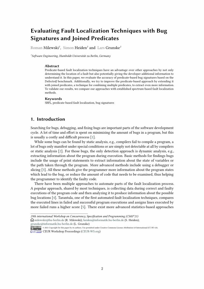
Listing 1: Example code with tests

1 private boolean anyTrue(boolean first, boolean second) {2 int x = 0;3 if (first)4 x++;5 if (second)6 x++;7 return x == 1; // bug, should be: x >= 18 }9 public Test1() { assert(!anyTrue(false,false)); }

10 public Test2() { assert(anyTrue(true,false)); assert(anyTrue(false,true)); }11 public Test3() { assert(anyTrue(true,true)); } // this fails

at line 3 and 5 are true, but not in any other combination. If we run all example tests from Listing 1,the predicate database would contain the same predicates L:3[true] and L:5[true] after runningeither test 2 or test 3, making them impossible to distinguish based on only this information.Our approach would now generate 4 additional joined predicates: 1) L:3[true] ≻ L:5[true],2) L:3[false] ≻ L:5[true], 3) L:3[true] ≻ L:5[false], and 4) L:3[false] ≻ L:5[false].

These joined predicates are different from the two separate predicates, as they additionallyencode the order of execution. For example, L:3[true] ≻ L:5[true] means: the branch at line 3was evaluated to true, and then, the next branch statement was at line 5 and was true, as well.This joined predicate is only evaluated to true in the failed test case, allowing us to distinguishit from the other test cases.

3.2. Gathering execution data

In the next step, we execute the instrumented code to generate the trace data. During execution,we collect predicate execution data for, e.g, each test in a test suite, while also classifying eachtrace as successful or failed, depending on the test outcome. The approach expects multipleexecution profiles and at least one failed execution to work correctly.

The current prototype of our approach uses a simple rule for generating joined predicates:each pair of two simple predicates is a possible joined predicate. During execution of theinstrumented code, each time a predicate gets evaluated, we dynamically create a new joinedpredicate from the last evaluated simple predicate and the currently triggered one and add itto our list of joined predicates, if it has not been encountered, previously. It is possible to usemore complex rules for the creation of joined predicates, e.g., using the previous two predicatesto create a joined predicate consisting of three simple ones or even only considering specifictypes of predicates.

During the execution of tests, all predicates for an instrumented location are directly evaluatedby the executing code, and the results are stored in a list. This list contains all predicates andjoined predicates that got triggered during a run and is exported at the end of the run.

6

3.3. Mining bug signatures

In this step, we try to find the top-k discriminative bug signatures. For this, we use an adaptationof the mining algorithm presented in [25].

The input is a database of transactions with each transaction containing a single run ofthe program and the information if that run was successful. A Gr-tree (see subsection 2.2) isconstructed from the database. The Gr-tree stores all its items in its head table and links themto their corresponding nodes in the tree structure. The output is a list containing the top-kdiscriminative signatures.

Our mining algorithm implements the pseudo code mining algorithm described in [25]. Mostdifferences stem from the java implementation and do not alter the basic idea. The algorithmalso has some parameters controlling the size of the mined bug signatures, the cutoff point forsignificance, and k, the size of the returned list. We used the same default parameters as definedin [25].

4. Experimental Setup

4.1. Choosing a base for a comparison

The result of bug signature identification is different from other fault localization techniques.Other fault localization techniques output a list of program elements ordered by suspiciousness,while a bug signature approach instead returns a ranked list of bug signatures. Each bugsignature consists of one or multiple program elements, describing a supposed bug context.The advantage of this additional information is difficult to quantify, as each programmer mayprocess the information from such a bug context in a unique way and most likely different thana program would. A bug signature can therefore consist of program elements that do not havean immediately obvious relation to the bug under examination.

We decided to quantitatively compare our approaches to spectrum-based fault localization(SBFL), a popular fault localization technique. Thus, we compare the following approaches:

SBFL state-of-the-art SBFL as implemented in BugLoRD2, using JaCoCo3to collect ex-ecution profiles (test coverage data) and using the DStar metric [29] to calculatesuspiciousness scores

Predicates our approach using predicates

Joined Predicates our approach using predicates and joined predicates (see subsubsection 3.1.2)

4.2. The scoring algorithm

The result of our approach, described in section 3, is a ranked list of bug signatures. The resultof SBFL is a ranked list of source code lines. As a bug signature can contain information aboutone or more code locations (note that a bug signature may also contain additional information

2https://github.com/hub-se/BugLoRD3https://www.eclemma.org/jacoco/index.html

7

that has no equivalent in SBFL), we developed an algorithm to calculate suspiciousness scoresfor a bug signature. A scoring approach for fault localization experiments is a metric, firstproposed by Renieres and Reiss in [30] and used by others [31, 32], based on static programdependencies. In the first step, a program dependence graph (PDG), a graph that contains a nodefor each expression in the program, is constructed from the source code. Next, nodes in thePDG get marked ”faulty” for being related to the bug under inspection. Using the results of thefault localization, for each prediction, one or more nodes can be marked as ”reported” if theycontain the predicted program element. Now, a score can be calculated as the fraction of thePDG that would need to be examined to get from a ”reported” node to a ”faulty” one by shortestpath.

We used Soot4 [33, 34] to generate intra-procedural PDGs. Soot stores the code for eachmethod in a Body. Each Body contains a chain of Units which represent the actual code insideof a method. Each Unit represents a statement in the original source code. We now define acodelocation as the line of code in the source code and all following lines not belonging toanother Unit.

Definition 1 - codelocation

Given a reference to a line of java source code (e.g., MyClass:7) and a corresponding java methodin a Soot representation, a codelocation is the source code line of a Unit corresponding tothe referenced line and all lines after that, until the next Unit or the end of its method.

The result of our algorithm is a ranked list of bug signatures. Each bug signature containsone or multiple predicates. Each predicate has a reference to the line of source code, whereit was evaluated. Now, we can generate codelocations from a bug signature by using allreferences to lines of source code inside the bug signature. We generate the codelocations

for the bug under examination (using the source code lines associated with the bug) and thecodelocations from the bug signatures reported by our algorithm (or the SBFL results).

Definition 2 - path cost

The path cost is the sum of all edge costs on the shortest path between two codelocations.

In our setting, each edge between two classes weighs 25, each edge between two methodsweighs 10 and each edge between two Units inside a method weighs 1. The higher cost of classand method transitions represents the additional mental effort while debugging. The numbersare chosen based on personal experience and can be adjusted.

Both SBFL and our approach rank their output by an internal suspiciousness score (see [25]for a definition of discriminative significance (DS) and [35] for a definition of the used SBFLmetrics). Often, multiple elements get assigned the exact same score, due to the nature ofthe used formulas, the limited availability of diverse enough execution data (i.e., test caseswith diverse execution profile) or simply due to identical execution behavior that is dictatedby the implementation itself. Even worse (from an evaluation approach), a bug signature, by

4https://soot-oss.github.io/soot/

8

definition, usually contains multiple predicates and/or joined predicates and thus containsmultiple codelocations. This means that the actual position of a codelocation in a rankingis nondeterministic. For each of such cases, we therefore have a best and worst case. In the bestcase, the codelocation that will lead to the smallest score is evaluated first, and in the worstcase, it is evaluated last among all codelocations with the same suspiciousness score.

𝑚𝑖𝑛𝐶𝑜𝑑𝑒𝐿𝑜𝑐𝑎𝑡𝑖𝑜𝑛𝑠𝑏𝑒𝑓𝑜𝑟𝑒(𝑐𝑖) = |{𝑐𝑗 ∈ 𝐶 | 𝑠𝑢𝑠𝑝𝐷𝑆(𝑐𝑗) > 𝑠𝑢𝑠𝑝𝐷𝑆(𝑐𝑖)}|𝑚𝑎𝑥𝐶𝑜𝑑𝑒𝐿𝑜𝑐𝑎𝑡𝑖𝑜𝑛𝑠𝑏𝑒𝑓𝑜𝑟𝑒(𝑐𝑖) = |{𝑐𝑗 ∈ 𝐶 | 𝑠𝑢𝑠𝑝𝐷𝑆(𝑐𝑗) ≥ 𝑠𝑢𝑠𝑝𝐷𝑆(𝑐𝑖)}|

An alternative, more correct, definition for 𝑚𝑎𝑥𝐶𝑜𝑑𝑒𝐿𝑜𝑐𝑎𝑡𝑖𝑜𝑛𝑠𝑏𝑒𝑓𝑜𝑟𝑒(𝑐𝑖) would subtract 1 tonot count 𝑐𝑖 twice. Now, by combining the path cost and codelocation, we can define ourEvaluationScore:

𝑆𝑐𝑜𝑟𝑒𝑏𝑒𝑠𝑡 = 𝑚𝑖𝑛𝐶𝑜𝑑𝑒𝐿𝑜𝑐𝑎𝑡𝑖𝑜𝑛𝑠𝑏𝑒𝑓𝑜𝑟𝑒 +(𝑝𝑎𝑡ℎ𝐶𝑜𝑠𝑡 *

√𝑚𝑖𝑛𝐶𝑜𝑑𝑒𝐿𝑜𝑐𝑎𝑡𝑖𝑜𝑛𝑠𝑏𝑒𝑓𝑜𝑟𝑒 + 1

)

𝑆𝑐𝑜𝑟𝑒𝑤𝑜𝑟𝑠𝑡 = 𝑚𝑎𝑥𝐶𝑜𝑑𝑒𝐿𝑜𝑐𝑎𝑡𝑖𝑜𝑛𝑠𝑏𝑒𝑓𝑜𝑟𝑒 +(𝑝𝑎𝑡ℎ𝐶𝑜𝑠𝑡 *

√𝑚𝑎𝑥𝐶𝑜𝑑𝑒𝐿𝑜𝑐𝑎𝑡𝑖𝑜𝑛𝑠𝑏𝑒𝑓𝑜𝑟𝑒 + 1

)

𝑆𝑐𝑜𝑟𝑒𝑎𝑣𝑔 =1

2* (𝑆𝑐𝑜𝑟𝑒𝑏𝑒𝑠𝑡 + 𝑆𝑐𝑜𝑟𝑒𝑤𝑜𝑟𝑠𝑡)

Note that 𝑆𝑐𝑜𝑟𝑒𝑎𝑣𝑔 is just the average of 𝑆𝑐𝑜𝑟𝑒𝑏𝑒𝑠𝑡 and 𝑆𝑐𝑜𝑟𝑒𝑤𝑜𝑟𝑠𝑡. To calculate a real averageEvaluationScore, one would use 𝑎𝑣𝑒𝑟𝑎𝑔𝑒𝑀𝑖𝑛𝐶𝑜𝑑𝑒𝐿𝑜𝑐𝑎𝑡𝑖𝑜𝑛𝑠𝑏𝑒𝑓𝑜𝑟𝑒 and path cost. In ourdefinition, the path cost is also included in the average.

The EvaluationScore is based on the usefulness of a bug prediction to a programmer whiledebugging. The EvaluationScore is 0, a perfect score, if the first reported codelocation isexactly the line of source code associated with the bug. The EvaluationScore grows by one forevery additional codelocation to check. Additionally, the EvaluationScore is scaled with thenumber of codelocations already checked, as a programmer checking the first few locationswill be motivated to look deeper, but when having already looked at multiple locations before,might stop his investigation sooner. So, while there might be an incredibly long path in theUnit-graph linking the suspected codelocation and the bug location, it is highly unlikely thatthis connection would be useful to the programmer. I.e., the more the path cost between codelocations and bug increases, the less likely it is to track down the bug.

4.3. Evaluation Subjects

The Defects4J Benchmark5 [36] is a collection of open source projects with each being availablein multiple buggy versions. Each buggy version consists of the respective source code and achange set with changes exclusively related to the bug. This omission of other changes (e.g.,refactorings) in the change set makes it more reliable as a source for the lines of code related tothe bug. Sobreira et al. [37] did an analysis of many Defects4J bugs and showed a method forlinking a bug to lines of code. The big number of real (not artificially created) bugs from manydifferent projects make this a sensible benchmark choice for our purposes.

We used the bugs in the version 2.0.0 from the projects in Table 1. From the original set ofbugs, we had to exclude 21 bugs from our final results. The most common reasons were problems

5https://github.com/rjust/defects4j

9

Table 1Used projects from the Defects4J Benchmark

project size[loc] #bugs

jfreechart (Chart) 96k 26

commons-cli (Cli) 2k 39

commons-codec (Codec) 3k 18

commons-csv (Csv) 1k 16

gson (Gson) 6k 18

commons-lang (Lang) 22k 64

commons-math (Math) 84k 106

joda-time (Time) 90k 26

Total 313

Applicable after

Instrumentation 292

Applicable after

Runtime Eval. 162

with compilation of the source code, crashes of the instrumenter and JVM crashes during testexecution. During the runtime evaluation, we encountered some additional problems, becausewe could not relate the Unit containing the line of source code to the given bug/prediction, orbecause the evaluation produced a time out. This leaves us with 162 bugs which were used forthe following graphs.

5. Results

In Figure 1, we see that 𝑆𝑐𝑜𝑟𝑒𝑏𝑒𝑠𝑡 (EvaluationScore if the reported location is examined firstamong all locations ranked equally; see section 4 for more details) for both joined predicates andpredicates is lower (better) than for SBFL. 𝑆𝑐𝑜𝑟𝑒𝑤𝑜𝑟𝑠𝑡 is more similar for all three approaches,with the joined predicates being significantly worse than simple predicates. If we look at theincluded p-values, we can see that the EvaluationScores for both predicate approaches aresignificantly different in our data set. The only non significant difference is between the worstEvaluationScore for joined predicates and SBFL.

In Table 2, we can see the mean values for 𝑆𝑐𝑜𝑟𝑒𝑏𝑒𝑠𝑡 and 𝑆𝑐𝑜𝑟𝑒𝑤𝑜𝑟𝑠𝑡. For a better visualization,we can look at Figure 3(left), where the total EvaluationScores for each approach are summedup. Both predicate approaches have significantly lower total EvaluationScores than the SBFLapproach when comparing 𝑆𝑐𝑜𝑟𝑒𝑏𝑒𝑠𝑡. When comparing 𝑆𝑐𝑜𝑟𝑒𝑤𝑜𝑟𝑠𝑡, the results are more even,with only simple predicates being significantly different than the other two. If we look at themedian values in Table 2, we can see the very small difference between all three approachesfor 𝑆𝑐𝑜𝑟𝑒𝑏𝑒𝑠𝑡. This shows us that a lot of bugs have similar, very small scores and most of the

10

p = 0.01

p = 0.004

p = 5e−05

p = 3.8e−20

p = 0.15

p = 0.0063

0

200

400

Joined Predicates Predicates SBFL

Eval

uatio

nSco

reScore Type

BestWorst

p−values from Wilcoxon Signed Rank Tests (paired)

Figure 1: Summary of results

differences stem from a few bugs with high (i.e. bad) scores. When comparing the medians for𝑆𝑐𝑜𝑟𝑒𝑤𝑜𝑟𝑠𝑡, the median for joined predicates is nearly double as big as the medians of the otherapproaches.

In Figure 3(right), we further split up our results regarding the different Defects4J projectsused. It shows the different mean values for 𝑆𝑐𝑜𝑟𝑒𝑎𝑣𝑔 separated by project. Here, we can seethat both predicate approaches have lower (i.e., better) results for nearly all projects, with only’cli’ in favor of SBFL.

Because a lot of the scores are close to or equal to 0, i.e., the best result, we additionallylooked at the density of scores. Figure 2 shows the density distribution of 𝑆𝑐𝑜𝑟𝑒𝑎𝑣𝑔 from 0 to75. The dashed lines show the mean values for each approach. Here, we see that the simplepredicate approach has the highest density in the 0-10-range. This represents a lot of verylow 𝑆𝑐𝑜𝑟𝑒𝑎𝑣𝑔 results – results where the correct codelocation was highly ranked, while nothaving too many similarly ranked codelocations. SBFL seems to have both very good scores,but also a lot of very bad ones, leading to a significantly worse mean value.

Table 2Mean and median values for 𝑆𝑐𝑜𝑟𝑒𝑏𝑒𝑠𝑡 and 𝑆𝑐𝑜𝑟𝑒𝑤𝑜𝑟𝑠𝑡

Approach 𝑆𝑐𝑜𝑟𝑒𝑏𝑒𝑠𝑡 ˜𝑆𝑐𝑜𝑟𝑒𝑏𝑒𝑠𝑡 𝑆𝑐𝑜𝑟𝑒𝑤𝑜𝑟𝑠𝑡˜𝑆𝑐𝑜𝑟𝑒𝑤𝑜𝑟𝑠𝑡

Joined Predicates 3.97 0 41.25 26.33

Predicates 2.94 0 26.14 12.50

SBFL 18.94 1 48.34 13.50

11

0.00

0.02

0.04

0 20 40 60Average

Type Joined Predicates SBFLPredicates

Den

sity

Figure 2: Density plot for 𝑆𝑐𝑜𝑟𝑒𝑎𝑣𝑔 with x-axis limited to 75

Best Worst

Joined Predicates

Predicates SBFL

0

2000

4000

6000

8000

Tota

l Eva

luat

ionS

core Defects4J

projectchartclicodeccsvgsonlangmathtime

Joined Predicates

Predicates SBFL

17.4

17.7

23.7

10.5

18.2

11.4

31.3

30.8

34

2.8

26.5

42.3

28.3

18.7

46.9

51

18.2

10.4

20.6

7

10.4

8.1

17.6

20.9

chart

cli

codec

csv

gson

lang

math

time

Joine

d Pred

icates

Predica

tesSBFL

1020304050

Avg

Figure 3: Left: Best and Worst EvaluationScore, Right: Mean values for 𝑆𝑐𝑜𝑟𝑒𝑎𝑣𝑔 , separated byDefects4J project

5.1. Spread and Path Cost

Next, we analyze the EvaluationScore in more detail to better understand the differencesbetween the predicate based and SBFL approaches. For this, we split up the EvaluationScore

into its two main components:

12

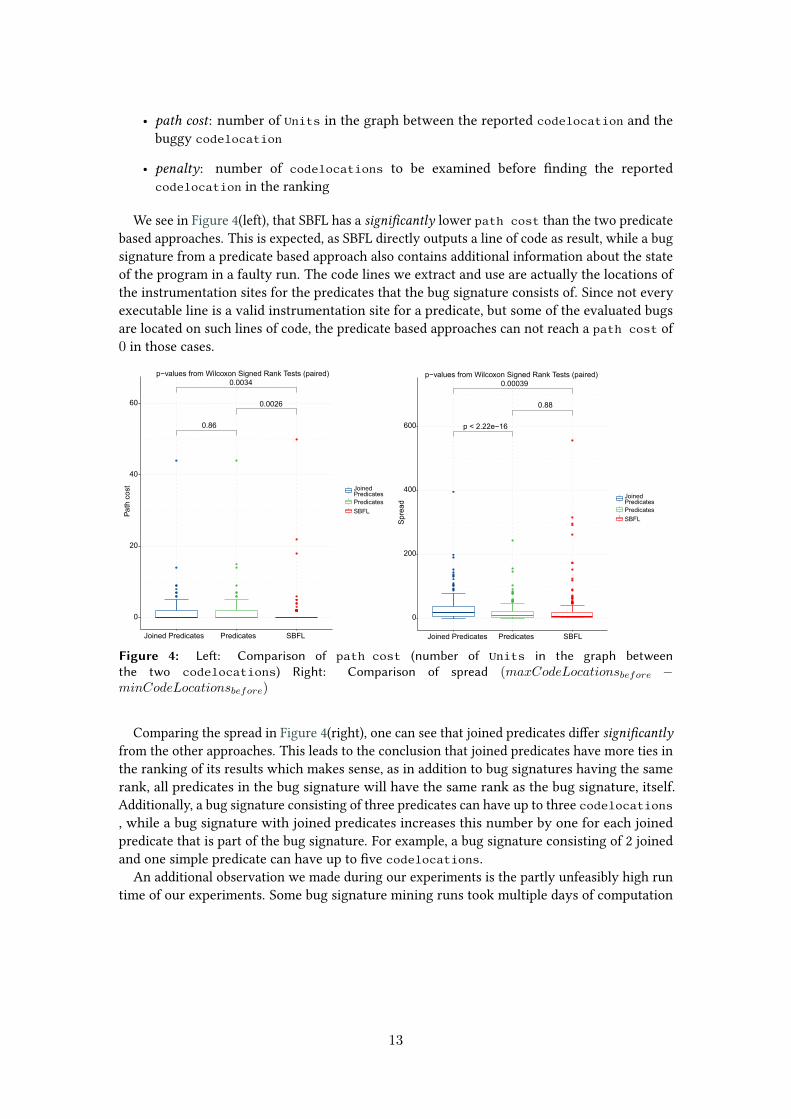
• path cost: number of Units in the graph between the reported codelocation and thebuggy codelocation

• penalty: number of codelocations to be examined before finding the reportedcodelocation in the ranking

We see in Figure 4(left), that SBFL has a significantly lower path cost than the two predicatebased approaches. This is expected, as SBFL directly outputs a line of code as result, while a bugsignature from a predicate based approach also contains additional information about the stateof the program in a faulty run. The code lines we extract and use are actually the locations ofthe instrumentation sites for the predicates that the bug signature consists of. Since not everyexecutable line is a valid instrumentation site for a predicate, but some of the evaluated bugsare located on such lines of code, the predicate based approaches can not reach a path cost of0 in those cases.

0.86

0.0034

0.0026

0

20

40

60


Path

cos

t


Joined

SBFLPredicatesPredicates

p < 2.22e−16

0.00039

0.88

0

200

400

600


Spre

ad


Joined

SBFLPredicatesPredicates

Figure 4: Left: Comparison of path cost (number of Units in the graph betweenthe two codelocations) Right: Comparison of spread (𝑚𝑎𝑥𝐶𝑜𝑑𝑒𝐿𝑜𝑐𝑎𝑡𝑖𝑜𝑛𝑠𝑏𝑒𝑓𝑜𝑟𝑒 −𝑚𝑖𝑛𝐶𝑜𝑑𝑒𝐿𝑜𝑐𝑎𝑡𝑖𝑜𝑛𝑠𝑏𝑒𝑓𝑜𝑟𝑒)

Comparing the spread in Figure 4(right), one can see that joined predicates differ significantlyfrom the other approaches. This leads to the conclusion that joined predicates have more ties inthe ranking of its results which makes sense, as in addition to bug signatures having the samerank, all predicates in the bug signature will have the same rank as the bug signature, itself.Additionally, a bug signature consisting of three predicates can have up to three codelocations, while a bug signature with joined predicates increases this number by one for each joinedpredicate that is part of the bug signature. For example, a bug signature consisting of 2 joinedand one simple predicate can have up to five codelocations.

An additional observation we made during our experiments is the partly unfeasibly high runtime of our experiments. Some bug signature mining runs took multiple days of computation

13

time, making the approach in its current form largely unusable in a real world scenario – atleast without further optimization.

6. Conclusions

After having analyzed the data from section 5, we summarize the following conclusions:

RQ1: Can a bug signature based approach be used for bug localization?

Yes, as we have seen in, e.g., Figure 1 and Figure 3(left), a bug signature (predicate) basedapproach consistently gets a lower EvaluationScore than SBFL.

These are welcome results, because while we expected it, as bug signature approaches havebeen shown as effective in other languages, e.g., [23, 25] showed predicate based approaches inC, there were multiple additional, java-specific difficulties with regard to the instrumentation.

RQ2: Can a bug signature based approach be enhanced by using joined predicates?

Maybe, but we did not manage to find any significant improvement by using our (rather simple)joined predicate approach over the single predicate approach. In our studies, we only evaluatedjoined predicate with a simple ”two-following” generation rule, and we did not exhaust otherpossible rules for generating joined predicates, yet. While a three-following rule might deemtoo time-intensive, we have many ideas for more elaborate rules concerning two predicates.Another factor could be our definition of the EvaluationScore. As we discussed in section 4,we did not find a way to use an established scoring algorithm to evaluate bug signatures. Whilethe problems we faced were beyond the scope of this project, most of them could be solved inthe future, allowing for a new evaluation of our results or future results.

We still strongly believe that a bug signature based approach can be enhanced by using joinedpredicates, but with other joined predicates beyond a simple combination of two followingpredicates into a joined one.

Another point is the differences between SBFL and predicate approaches visible in Fig-ure 4(left). SBFL has a significantly lower average path cost than the two predicate approaches.We can explain this with the different output formats used by the two techniques. The factthat the predicate based approaches still get better overall scores thus must mean they performbetter in the non path cost part of our EvaluationScore.

Furthermore, the bug signature mining algorithm described in [25] which our approachesare based on, too, actually has a parameter for controlling how many predicates can be part of asingle bug signature. A bigger size limit significantly increases the computation time, which iswhy we used a size limit of 3, as recommended in [25]. This could have been chosen too small,as in the joined predicate approach, the joined predicates now compete with the others for aspot inside a bug signature. On the one hand, while a bigger bug signature may potentiallybe more helpful to a real programmer, it would negatively impact our score, as it does notdifferentiate between processing multiple predicates inside one bug signature or multiple smallbug signatures containing the same predicates. Even worse for our evaluation (and likely any

14

other based on lines of source code), just one ”correct” predicate inside a bug signature is allthat is needed to score it positively, while ignoring all the others inside the bug signature. Onthe other hand, in [25], the authors noted that increasing the size of the mined bug signaturesincreases the predictive power but increases the computation time.

Especially noteworthy is that all the extra information a programmer is supposed to get outof a bug signature, e.g., it containing a predicate with 𝑣𝑎𝑟 = 𝑛𝑢𝑙𝑙 for a 𝑣𝑎𝑟 where 𝑛𝑢𝑙𝑙 is notexpected, can lead to another investigation path than just the information to investigate thatline. An evaluation method considering those aspects could have completely different resultsthan ours.

Acknowledgements Lars Grunske would like to thank the intensive care unit of the Achen-bach hospital in Königs Wusterhausen for the tremendous help during his Covid-19 case.

References

[1] M. Zhivich, R. K. Cunningham, The real cost of software errors, IEEE Security & PrivacyMagazine 7 (2009) 87–90. doi:10.1109/msp.2009.56.

[2] N. Ayewah, W. Pugh, D. Hovemeyer, J. D. Morgenthaler, J. Penix, Using static analysis tofind bugs, IEEE Software 25 (2008) 22–29. doi:10.1109/ms.2008.130.

[3] M. Perscheid, B. Siegmund, M. Taeumel, R. Hirschfeld, Studying the advancement indebugging practice of professional software developers, Software Quality Journal 25 (2016)83–110. doi:10.1007/s11219-015-9294-2.

[4] W. E. Wong, R. Gao, Y. Li, R. Abreu, F. Wotawa, A survey on software fault localization,IEEE Transactions on Software Engineering 42 (2016) 707–740. doi:10.1109/tse.2016.2521368.

[5] J. A. Jones, M. J. Harrold, Empirical evaluation of the tarantula automatic fault-localizationtechnique, in: Proceedings of the 20th IEEE/ACM international Conference on Automatedsoftware engineering - ASE '05, ACM Press, 2005, pp. 273–282. doi:10.1145/1101908.1101949.

[6] T. Reps, T. Ball, M. Das, J. Larus, The use of program profiling for software maintenancewith applications to the year 2000 problem, ACM SIGSOFT Software Engineering Notes22 (1997) 432–449. doi:10.1145/267896.267925.

[7] T. M. Chilimbi, B. Liblit, K. Mehra, A. V. Nori, K. Vaswani, Holmes: Effective statisticaldebugging via efficient path profiling, in: 2009 IEEE 31st International Conference onSoftware Engineering, IEEE, IEEE, 2009, pp. 34–44. doi:10.1109/icse.2009.5070506.

[8] R. Santelices, J. A. Jones, Y. Yu, M. J. Harrold, Lightweight fault-localization using multiplecoverage types, in: 2009 IEEE 31st International Conference on Software Engineering,IEEE, IEEE, 2009, pp. 56–66. doi:10.1109/icse.2009.5070508.

[9] W. Masri, Fault localization based on information flow coverage, Software Testing,Verification and Reliability 20 (2009) 121–147. doi:10.1002/stvr.409.

[10] R. A. Assi, W. Masri, Identifying Failure-Correlated Dependence Chains, in: 2011 IEEEFourth International Conference on Software Testing, Verification and Validation Work-shops, 2011, pp. 607–616. doi:10.1109/ICSTW.2011.42.

[11] T. B. Le, D. Lo, C. L. Goues, L. Grunske, A learning-to-rank based fault localization

15

approach using likely invariants, in: Proceedings of the 25th International Symposiumon Software Testing and Analysis, ISSTA 2016, ACM, 2016, pp. 177–188. doi:10.1145/2931037.2931049.

[12] M. D. Ernst, J. Cockrell, W. G. Griswold, D. Notkin, Dynamically discovering likely programinvariants to support program evolution, IEEE Transactions on Software Engineering 27(2001) 99–123. doi:10.1109/32.908957.

[13] S. Hangal, M. S. Lam, Tracking down software bugs using automatic anomaly detection,in: Proceedings of the 24th International Conference on Software Engineering, ICSE ’02,Association for Computing Machinery, New York, NY, USA, 2002, pp. 291–301. doi:10.1145/581339.581377.

[14] B. Pytlik, M. Renieris, S. Krishnamurthi, S. P. Reiss, Automated fault localization usingpotential invariants, CoRR cs.SE/0310040 (2003). arXiv:preprintcs/0310040.

[15] S. K. Sahoo, J. Criswell, C. Geigle, V. Adve, Using likely invariants for automated softwarefault localization, in: Proceedings of the eighteenth international conference on Archi-tectural support for programming languages and operating systems, 2013, pp. 139–152.doi:10.1145/2451116.2451131.

[16] M. A. Alipour, A. Groce, Extended program invariants: applications in testing and faultlocalization, in: Proceedings of the Ninth International Workshop on Dynamic Analysis,2012, pp. 7–11. doi:10.1145/2338966.2336799.

[17] B. Liblit, M. Naik, A. X. Zheng, A. Aiken, M. I. Jordan, Scalable statistical bug isolation,ACM SIGPLAN Notices 40 (2005) 15–26. doi:10.1145/1064978.1065014.

[18] C. Liu, X. Yan, L. Fei, J. Han, S. P. Midkiff, Sober: Statistical model-based bug lo-calization, in: Proceedings of the 10th European software engineering conferenceheld jointly with 13th ACM SIGSOFT international symposium on Foundations of soft-ware engineering - ESEC/FSE-13, Proceedings of 13th ACM SIGSOFT InternationalSymposium on Foundations of Software Engineering, ACM Press, 2005, pp. 286–295.doi:10.1145/1081706.1081753.

[19] C. Liu, L. Fei, X. Yan, J. Han, S. P. Midkiff, Statistical debugging: A hypothesis testing-basedapproach, IEEE Transactions on Software Engineering 32 (2006) 831–848. doi:10.1109/TSE.2006.105.

[20] P. A. Nainar, T. Chen, J. Rosin, B. Liblit, Statistical debugging using compound booleanpredicates, in: D. S. Rosenblum, S. G. Elbaum (Eds.), Proceedings of the 2007 internationalsymposium on Software testing and analysis - ISSTA '07, ACM Press, 2007, pp. 5–15.doi:10.1145/1273463.1273467.

[21] Z. You, Z. Qin, Z. Zheng, Statistical fault localization using execution sequence, in: 2012International Conference on Machine Learning and Cybernetics, volume 3, IEEE, IEEE,2012, pp. 899–905. doi:10.1109/icmlc.2012.6359473.

[22] V. Dallmeier, C. Lindig, A. Zeller, Lightweight defect localization for java, in: ECOOP2005 - Object-Oriented Programming, Springer Berlin Heidelberg, 2005, pp. 528–550.doi:10.1007/11531142_23.

[23] H.-Y. Hsu, J. A. Jones, A. Orso, Rapid: Identifying bug signatures to support debuggingactivities, in: 2008 23rd IEEE/ACM International Conference on Automated SoftwareEngineering, IEEE, IEEE, 2008, pp. 439–442. doi:10.1109/ase.2008.68.

[24] R. Agrawal, R. Srikant, Fast algorithms for mining association rules in large databases,

16

in: VLDB’94, Proceedings of 20th International Conference on Very Large Data Bases,September 12-15, 1994, Santiago de Chile, Chile, Morgan Kaufmann, 1994, pp. 487–499.URL: http://www.vldb.org/conf/1994/P487.PDF. doi:10.5555/645920.672836.

[25] C. Sun, S.-C. Khoo, Mining succinct predicated bug signatures, in: Proceedings of the 20139th Joint Meeting on Foundations of Software Engineering - ESEC/FSE 2013, ACM Press,2013, pp. 576–586. doi:10.1145/2491411.2491449.

[26] J. Li, H. Li, L. Wong, J. Pei, G. Dong, Minimum description length principle: Generatorsare preferable to closed patterns., in: Proceedings of the 21st National Conference onArtificial Intelligence - Volume 1, volume 1 of AAAI’06, 2006, pp. 409–414.

[27] Z. Zuo, S.-C. Khoo, C. Sun, Efficient predicated bug signature mining via hierarchicalinstrumentation, in: Proceedings of the 2014 International Symposium on SoftwareTesting and Analysis - ISSTA 2014, ACM Press, 2014, pp. 215–224. doi:10.1145/2610384.2610400.

[28] E. Bruneton, ASM 4.0 A Java bytecode engineering library, 2007.[29] W. E. Wong, V. Debroy, R. Gao, Y. Li, The DStar method for effective software fault

localization, IEEE Transactions on Reliability 63 (2014) 290–308. doi:10.1109/tr.2013.2285319.

[30] M. Renieres, S. Reiss, Fault localization with nearest neighbor queries, in: 18th IEEEInternational Conference on Automated Software Engineering, 2003. Proceedings., ASE’03,IEEE Comput. Soc, 2003, pp. 30–39. doi:10.1109/ase.2003.1240292.

[31] H. Cleve, A. Zeller, Locating causes of program failures, in: Proceedings of the 27thinternational conference on Software engineering - ICSE '05, ICSE ’05, ACM Press, 2005,pp. 342–351. doi:10.1145/1062455.1062522.

[32] P. A. Nainar, T. Chen, J. Rosin, B. Liblit, Statistical debugging using compound booleanpredicates, in: D. S. Rosenblum, S. G. Elbaum (Eds.), Proceedings of the 2007 internationalsymposium on Software testing and analysis - ISSTA '07, ACM Press, 2007, pp. 5–15.doi:10.1145/1273463.1273467.

[33] R. Vallée-Rai, P. Co, E. Gagnon, L. Hendren, P. Lam, V. Sundaresan, Soot, in: CASCONFirst Decade High Impact Papers on - CASCON '10, ACM Press, Mississauga, Ontario,Canada, 2010, p. 13. doi:10.1145/1925805.1925818.

[34] P. Lam, E. Bodden, O. Lhoták, L. Hendren, The soot framework for java program analysis:a retrospective, in: Cetus Users and Compiler Infastructure Workshop (CETUS 2011),volume 15, 2011, p. 35.

[35] S. Heiden, L. Grunske, T. Kehrer, F. Keller, A. Hoorn, A. Filieri, D. Lo, An evaluation of purespectrum-based fault localization techniques for large-scale software systems, Software:Practice and Experience 49 (2019) 1197–1224. doi:10.1002/spe.2703.

[36] R. Just, D. Jalali, M. D. Ernst, Defects4j: a database of existing faults to enable controlledtesting studies for java programs, in: Proceedings of the 2014 International Symposium onSoftware Testing and Analysis - ISSTA 2014, ACM Press, 2014, pp. 437–440. doi:10.1145/2610384.2628055.

[37] V. Sobreira, T. Durieux, F. Madeiral, M. Monperrus, M. de Almeida Maia, Dissection ofa bug dataset: Anatomy of 395 patches from defects4j, in: 2018 IEEE 25th InternationalConference on Software Analysis, Evolution and Reengineering (SANER), IEEE, 2018, pp.130–140. doi:10.1109/saner.2018.8330203.

17

NLP-Based Requirements Formalization forAutomatic Test Case GenerationRobin Gröpler1, Viju Sudhi1, Emilio José Calleja García2 and Andre Bergmann2

1ifak Institut für Automation und Kommunikation e.V., 39106 Magdeburg, Germany2AKKA Germany GmbH, 80807 München, Germany

AbstractDue to the growing complexity and rapid changes of software systems, the assurance of their qualitybecomes increasingly difficult. Model-based testing in agile development is a way to overcome thesedifficulties. However, major effort is still required to create specification models from a large set offunctional requirements provided in natural language. This paper presents an approach for a machine-aided requirements formalization technique based on Natural Language Processing (NLP) to be used foran automatic test case generation. The goal of the presented method is to automate the process of modelcreation from requirements in natural language by utilizing appropriate algorithms, thus reducing costand effort. The application of our procedure will be demonstrated using an industry example from thee-mobility domain. In this example, requirement models are generated for a charging approval systemwithin a larger vehicle battery charging application. Additionally, existing tools for automated modelsynthesis and test case generation are applied to our models to evaluate whether valid test cases can begenerated.

KeywordsRequirements analysis, natural language processing, test generation

1. Introduction

In the life cycle of a device, component or system in industrial use, a rapidly changing andgrowing number of requirements and the associated increase in features and feature changesinevitably lead to an increasing effort for verifying requirements and testing of the implemen-tation. To manage test complexity and reduce necessary test effort and cost, agile methodsfor model-based testing have been developed [1]. The effectiveness of model-based testinghighly depends on the quality of the used specification model. The creation and maintenanceof well-defined specification models is therefore crucial and usually comes with high effort andcost. This is especially true in agile development, where requirements are subject to frequentchanges.

In this context, an approach for requirements-based testing was developed that enablesefficient test processes, see Fig. 1. Model synthesis and model-based test generation methods areused to systematically and efficiently create a test suite that contains suitable test cases. Thisapproach is based on behavioral requirements that serve as input for model synthesis. The only

29th International Workshop on Concurrency, Specification and Programming (CS&P’21)Envelope-Open [email protected] (R. Gröpler); [email protected] (V. Sudhi); [email protected] (E. J. CallejaGarcía); [email protected] (A. Bergmann)



18

Requirements

Formalization

(semi-automated)

Model

Synthesis

(automated)

Test Case

Generation

(automated)

ModGen TCG

Sequence

models

Req. 1 Req. 2 Req. n

Specification

model

UML state machine

TC6TC5TC4TC3TC2TC1

Generated

test cases

Abstract test cases

Functional

requirements

Text documents

ReForm

Figure 1: Toolchain for requirements-based test case generation.

time-consuming manual step is the creation of requirement models from textual requirementsdocuments.

Recent advances in natural language processing show promising results to organize andidentify desired information from raw text. As a result, NLP techniques show a growing interestin automating various software development activities like test case generation. Several NLPapproaches and tools have been investigated in recent years aiming to generate test cases frompreliminary requirements documents [2, 3, 4]. A major drawback of existing methods is the useof controlled natural language or templates that force the requirements engineer or designernot only to concentrate on the content but also on the syntax of the requirement. Furthermore,those algorithms are in general not applicable to existing requirements.

In this work, we propose a new, semi-automated technique for requirements-based model gen-eration that reduces human effort and supports frequent requirements changes and extensions.The aim of our approach is to develop a method that

1) can handle an extended range of domains and formats of requirements, i.e. it is not limitedto a specific template or controlled natural language, and

2) provides enhanced but easily interpretable intermediate results in the form of a textualand graphical representation of UML sequence diagrams.

Our approach utilizes an existing NLP parser to obtain basic syntactic information about thewords and their relationship to each other. Based upon this information, several rule-basedsteps are performed in order to identify relevant syntactic entities which are then mapped tosemantic entities. Finally, these entities are used to form requirement models as UML sequencediagrams. The main contributions of this work are

1) the development of a rule-based approach based on NLP information that automates thevarious steps involved in deriving requirement models, and

2) the evaluation on an industrial use case using meaningful metrics that demonstrates thegood quality of our approach.

The paper is structured as follows. In Section 2, we briefly outline related work on NLP-based requirements formalization methods. In Section 3, we present the individual steps of our

19

methodology for deriving requirement models from textual descriptions. The method is appliedto the battery charging approval system presented in Section 4. In Section 5, we define severalevaluation metrics and demonstrate the results of the application. Finally, a conclusion andoutlook is given in Section 6.

2. Related work

In order to circumvent the challenges of analyzing highly complex requirements, many authorsrestrict their NLP approaches to a specific domain or a prescribed format. In [5], the authorspropose an algorithm creating activity diagrams from requirements following a predefinedstructure. They consider the SOPHIST method which performs a refinement and formalizationof structured texts by introducing text templates with a defined syntactical structure [6]. In [7], asmall set of structural rules was developed to address common requirement problems includingambiguity, complexity and vagueness. In [8], requirements are expected to be written in acontrolled natural language and are supposed to be from Data-Flow Reactive Systems (DFRS).The approach in [9] is to generate test cases from use cases or user stories, both of whichhave to comply with a specified format. In [10], requirements engineers shall be supportedwith formalization of use case descriptions by writing pre-conditions and post-conditions in apredefined format from which test cases can be generated automatically. Likewise [11] aims tofind and complete missing test cases by parsing exceptional behaviors from Javadoc commentswritten in natural language, provided the documentation is in a specified template. [12] relieson the artifacts that the programmers create while developing the product which belong to asmaller subset of specifications.

Even for simple syntactical structures of requirements it is still necessary to enable therequirements engineer to review the intermediate results, i.e. the generated model artifacts, andto adjust them where necessary. The toolchain of [13] involves eliciting requirements accordingto Restricted Use Case Modeling (RUCM) specifications. This applies to the work of [14], wherethe authors attempt to generate executable test cases from a Restricted Test Case Modeling(RTCM) language which restricts the style of writing test cases. This becomes an additionaloverhead to the requirement engineers who draft formal requirements. Additionally, the usersare expected to inspect the generated OCL constraints before proceeding to test case generation.Similarly, in [15] the authors explore the possibility of test case generation using Petri Netsimulation; however the interpretability of Colored Petri Nets as proposed in the approachmay vary depending on the user’s level of expertise. These intermediate results may not beeasily understood by the user and it may be cumbersome for him to fine-tune or modify thepredictions before generating reliable test cases.

A notable work from the authors of [16] makes use of recursive dependency matching toformulate test cases. Though our approach aligns with theirs in this step, we attempt to generatetest cases from a broader set of functional requirements while they restrict themselves withuser stories from which a cause-effect relationship can be learnt.

20

3. Methodology

We utilize an existing NLP parser and use a rule-based algorithm to perform the transformationfrom requirements written in natural language to requirement models. Our rule set tries toconceive all relevant rules that could satisfactorily parse the input behavioral requirement andextract its semantic content.

3.1. Linguistic pre-processing

The behavioral requirements are, in general, complex by nature. In order to reliably extract thesyntactic and semantic content of these requirements, a thorough linguistic pre-processing isindispensable. For this stage, we rely on spaCy (v2.1.8) [17] - a free, open-source library foradvanced Natural Language Processing. We follow the basic NLP pipeline including tokenization,lemmatization, part-of-speech (POS) tagging and dependency parsing in various stages of thealgorithm.

3.1.1. Pronoun resolution

Though the formal requirements tend to avoid first person (I, me, etc.) or second person (you,your, etc.) pronouns, they may contain third person neutral pronouns (it, they, etc.) [18].These pronouns are identified and resolved with the farthest subject, inline with the algorithmproposed in [19] and [20]. Owing to the simplicity of the task, we assume there is no particularneed to use more sophisticated algorithms checking grammatical gender and person whileresolving pronouns. However, we attempt to resolve pronouns only if the grammatical numberof the pronoun agrees with that of the antecedent. Since pleonastic pronouns (pronouns withouta direct antecedent) do not affect the algorithm, they are cited but not replaced.

Example: Consider the requirement ”If the temperature of the battery is below Tmin or itexceeds Tmax, charging approval has to be withdrawn”. Here, the pronoun it is resolved withits antecedent the temperature of the battery.

3.1.2. Decomposition

Textual requirements with multiple conditions and conjunctions are hard to be transformedand mapped to individual relations. This demands decomposition of complex requirementsinto simple clauses [21]. Multiple conditions (sentences with multiple if s, whiles, etc.), rootconjunctions (sentences with multiple roots connected with a conjunction) and noun phraseconjunctions (sentences with multiple subjects and/or objects connected with a conjunction)are decomposed to simple primitive clauses.

We resort to the syntactic dependencies obtained from the parser to decompose requirements.The algorithm considers the token(s) with dependency mark to decompose multiple conditionsand dependency conj for decomposing root and noun phrase conjunctions. The span of thesub-requirement can then be defined by identifying the edges (for e.g. the left-most edge refersto the token towards the left of the dependency graph with which the parent token holds asyntactic dependency) of the token of interest.

21

Example: In the requirement ”If the temperature of the battery is below Tmin or the tempera-ture of the battery exceeds Tmax, charging approval has to be withdrawn”, the root conjunction(arising from the two roots is and exceeds) and the subsequent multiple conditions (arisingfrom if ) are decomposed to three sub-requirements as ”[if the temperature of the battery isbelow Tmin] or [if the temperature of the battery exceeds Tmax], [charging approval has to bewithdrawn]”.

3.2. Syntactic entity identification

Almost all behavioral requirements describe a particular action (linguistically, verb) done by anagent (linguistically, subject) on the system of interest (linguistically, object). This motivatesthe idea of identifying syntactic entities from the requirements. The algorithm identifies thesesyntactic entities by checking the dependencies of tokens with the root.

1) Action: The main action verb in the requirement (mostly, with the dependency ROOT )is identified and called an action. The algorithm particularly distinguishes the type ofactions as: Nominal action which has a noun and a verb together (e.g. send a message),Boolean action which can take a Boolean constraint (e.g. is withdrawn) and Simple actionwhich has only an action verb (e.g. send).In addition, the algorithm also tries to identify the verb type(s) (transitive, dative, preposi-tional, etc.) as suggested in [21] to supplement the syntactic significance of action types.This is essential particularly when we rely on action types for relation formulation.

2) Subjects and Objects: The tokens with dependencies subj and obj (and their variantslike nsubj, pobj, dobj, etc.) are identified mostly as Subjects and Objects, respectively.They can be noun chunks (e.g. temperature of the battery), compound nouns (e.g. batterytemperature) or single tokens (e.g. battery) in the requirement.

Also, we noted that there are several requirements involving a logical comparison (identified asan adjective or an adverb) between the expressed quantities. In order to identify comparisons(e.g. greater than, exceeds, etc.) in the requirement, we utilize the exhaustive synonym hyperlinksfrom Roget’s Thesaurus [22] and map them to the corresponding equality (=), inequality (!=),inferiority (<, <=) and superiority (>, >=) symbols.

Example: From the sub-requirements ”[if the temperature of the battery is below Tmin] or[if the temperature of the battery exceeds Tmax], [charging approval has to be withdrawn]”,the system identifies Battery_Temperature and Charging_Approval as Subjects, Tmin and Tmaxas Objects and withdrawn as a Boolean Action. Also, the comparison term below is mapped as <and exceeds is mapped as >.

3.3. Semantic entity identification

Semantic entities are tightly coupled with the end application which translates the parsedsyntactic information to sequence diagrams and then to abstract test cases. The semantic

22

Table 1Mapping of syntactic to semantic entities

Syntactic entities Semantic entitiesAction SignalAction constraints AttributesSubject / Object Actor / Component

entities are defined from the perspective of interactions in a sequence diagram and are outlinedbelow. The algorithm derives these entities from their syntactic counterparts1.

1) Actor or Component: The participants involved in an interaction are defined as actorsand components. To differentiate other participants from the system under test (SUT),component is always considered as the SUT.

2) Signal: The interaction between different participants is defined as a signal.3) Attributes: The variables holding the status at different points of interaction are defined

as attributes.4) State: This refers to the initial, intermediate and final states of an interaction.

Semantic entities demand additional details for completeness. For example, if the value of anattribute is not given, it can not be initialized in its corresponding test case. Likewise, for eachsignal the corresponding actor needs to be identified. For each requirement, the direction ofcommunication (incoming: towards the system under test or outgoing: from the system undertest) should be identified. In cases where the algorithm lacks the desired ontology information,user input is demanded to update these values.

It is worth noting that the separation of the entities as syntactic (application independent butgrammar dependent) and semantic (application dependent but grammar independent) givesmore flexibility to the algorithm to be used in parts also in a different environment than thedescription language considered here. However, the mapping from the syntactic entities to theirsemantic counterparts can be completely automated with stricter rules or can be accomplishedwith user intervention and validation.

Example: From the sub-requirements ”[if the temperature of the battery is below Tmin] or[if the temperature of the battery exceeds Tmax], [charging approval has to be withdrawn]”,the identified Subjects (Battery_Temperature and Charging_Approval) are mapped as Signals andthe identified Objects (Tmin and Tmax) are mapped as Attributes. Here, the identified Actionwithdrawn is also considered as an Attribute owing to the semantics of its corresponding BooleanSignal. Additionally, we can arrive at the Actor for Battery_Temperature as battery. However,the Actor of Charging_Approval is ambiguous (or rather unknown). Likewise, Attribute valuesshould either be passed by the user or they remain uninitialized in the resulting test case.

1Note that the algorithm maps syntactic to semantic entities with more complex rules (including action typesand verb types). In Table 1, we have presented only the most primitive ones for brevity. This difference is alsodetailed in the example where an Action is considered as an Attribute and a Subject is mapped to a Signal.

23

3.4. Transformation to requirement model

For the description of the formal requirements a simple text-based domain-specific language(DSL) is used, the ifak requirements description language (IRDL) [23]. This notation for require-ment models was developed on the basis of UML sequence diagrams and is specially adapted tothe needs of describing requirements as sequences. The IRDL defines a series of model elements(e.g. components, messages) with associated attributes (name, description, recipient, sender,etc.) and special model structures (behavior based on logical operators or time). Functional,behavior-based requirements are described textually using IRDL and can then be visualizedgraphically as sequence diagrams (Fig. 2).

Once the entities are mapped and validated, the algorithm forms IRDL relations for eachclause and then combines them together to form relations for the whole requirement. IRDLdefines mainly two types of relations:

1) Incoming messages: SUT receives these messages provided the guard expression evaluatesto be true and then continues to the next sequence in an interaction. IRDL defines thisclass of messages as ’Check’.

2) Outgoing messages: SUT sends these messages to other interaction participants with thecontent defined in the signal. In IRDL, these messages are denoted as ’Message’.

Check(Actor->Component): Signal[guard expression];Message(Component->Actor): Signal(signal content);

As an intermediate result, the user is shown the formulated IRDL relations along withthe sequence diagram corresponding to the requirement and is asked if the IRDL and thecorresponding sequence diagram are correct. In case the user wants to further modify therelation formulation, the algorithm repeats from the mapping of syntactic entities to semanticentities. This continues until the user confirms the model is satisfactory.

Example: IRDL relations for the example requirement ”If the temperature of the batteryis below Tmin or it exceeds Tmax, charging approval has to be withdrawn”, after the above-mentioned steps is shown in Fig. 2.

Textual representation (IRDL) Graphical representation

State iState_001 at system;

Check(battery->system):Battery_Temperature

[msg.value < Tmin || msg.value > Tmax];

Message(system->unknown_actor):

Charging_Approval(false);

State fState_001 at system;

Battery_Temperature

Charging_Approval

iState_001

system battery unknown_actor

fState_001

Figure 2: Visualization of a requirement model in IRDL and as sequence diagram.

24

3.5. Model synthesis and test generation

The formalized requirements of the SUT can be combined to a specification model using existingmethods for model synthesis [23]. The sequence elements described before, are transformedusing a rule-based algorithm into equivalent elements of a UML state machine.

After model synthesis, test cases can be automatically generated from the state machineusing an existing method for model-based test generation [24]. Selecting a specific graph-basedcoverage criteria such as ”all paths”, ”all decisions”, ”all places” or ”all transitions”, the statemachine is transformed into a special form of a Petri net from which abstract test cases in theform of sequence diagrams can be generated. In this way, the approach allows modeling ofeven complex system behavior and applying graph-based coverage criteria to the entire systemmodel.

4. Application

The toolchain for requirements-based model and test case generation presented in the previoussection is applied to an industrial use case from the e-mobility domain. The use case describesa system for charging approval of an electric vehicle in interaction with a charging station.The industrial use case was defined by AKKA and aims to provide a typical basic scenario anddevelopment workflow in software development for an automotive electronic control unit (ECU).It does so by defining requirements, using model-based software development and deployingthe functionality on an ECU.

The use case has to be seen in the context of an electric car battery that is supposed to becharged. The function “charging approval” implements a simple function, which decides uponspecific input signals, if the charging process of the battery is allowed or not. For example,charging approval is given or withdrawn depending on the battery temperature, voltage or stateof charge, the requested current is adjusted according to the battery temperature, and errorbehavior is handled for certain conditions. This is a continuous process, i.e. the signal valuesmay change over time. A more detailed technical description of the industrial use case can befound in [25]. To fulfill the requirement of model-based software development, the module isimplemented in Matlab Simulink. Matlab Simulink Coder is used to generate C/C++ code thatcan be compiled and deployed to the target. A Raspberry Pi is used to simulate some but not allaspects of an ECU. A basic overview of the charging approval system and its interfaces to theenvironment is given in Fig. 3.

Environment Velocity

Parking brake

Ignition

Charging

ApprovalEnvironment

Charging Approval

State of Charge

Temperature of Battery

Figure 3: Process overview of charging approval system.

25

5. Results

The battery charging approval system described in the former section is used to evaluate theproposed method. We first define the used evaluation metrics and then demonstrate the results.To our knowledge, there are no available tools with similar input and output properties as ourtool that enable a direct comparison.

5.1. Evaluation metrics

Let 𝑅 be the set of textual requirements. For a requirement 𝑟 ∈ 𝑅, let 𝑋𝑟 be the set of expectedartifacts and 𝑌𝑟 be the set of generated artifacts. Here, artifacts refer to all the semantic entitiesincluding the relation indicators. Let 𝑋 = ⋃𝑟∈𝑅 𝑋𝑟 denote the set of expected artifacts in allrequirements and 𝑌 = ⋃𝑟∈𝑅 𝑌𝑟 the set of generated artifacts in all requirements. Then we definethe following metrics to measure the performance of the method.

1) Completeness: For an individual requirement, this metric denotes the number of ex-pected artifacts 𝑥 ∈ 𝑋𝑟 for which a corresponding (not necessarily identical) generatedartifact 𝑦 ∈ 𝑌𝑟 exists, in relation to the total number of expected artifacts |𝑋𝑟|.

2) Correctness: For an individual requirement, this metric denotes the number of gener-ated artifacts 𝑦 ∈ 𝑌𝑟 for which a corresponding, semantically identical (up to namingconventions) expected artifact 𝑥 ∈ 𝑋𝑟 exists, in relation to the total number of generatedartifacts |𝑌𝑟|.

3) Consistency: This metric denotes the number of generated artifacts 𝑦 ∈ 𝑌 for which acorresponding expected artifact 𝑥 ∈ 𝑋 exists and is used identically in all requirements𝑟 ∈ 𝑅, in relation to the total number of generated artifacts |𝑌 |.

The macro average for completeness and correctness, respectively, is then given by the meanvalue of all individual percentage values for all 𝑟 ∈ 𝑅. The micro average is given by the sum ofall values in the numerator divided by the sum of all values in the denominator for all 𝑟 ∈ 𝑅.

Example: In order to assert the evaluation metrics in detail, consider the requirement clause’if the SoC of the battery is below SoC_max’.

Expected: Check(charging_management->system): Battery_SoC[msg.Ialue < SoC_max];

Generated: Check(battery->system): battery_SoC[msg.value < SoC_max];

For the metric completeness, we check if all the expected artifacts (i.e. Check, charging_man-agement, Battery_SoC, etc.) are generated by the algorithm. In this case, we can see that allof them were generated. For obtaining the correctness, we check if those generated artifactsare semantically correct. In this case, though we expect the actor charging_management, thealgorithm generates battery. This reduces the value of correctness. If the algorithm generatesbattery_SoC for every occurrence of ’SoC of battery’ across all the requirements, it is consideredconsistent for this artifact.

26

Table 2Evaluation of the algorithm on the charging approval system

without domain knowledge with domain knowledgemacro avg. micro avg. macro avg. micro avg.

Completeness 78.2% 79.8% 81.4% 84.1%Correctness 74.9% 78.8% 78.3% 82.1%Consistency 94.1% 96.4%

5.2. Requirements formalization

As part of the demonstrated use case, AKKA has provided functional requirement documentsdescribing the expected behavior for the relevant SUT. To apply the NLP-based requirementsformalization method, each statement is treated as a separate entity for which a well-definedrequirement model is created. Overall, the charging approval SUT is described by 14 separaterequirement statements.

The results of our evaluation are shown in Table 2. We have determined the individualcorrectness and completeness values and calculated the macro and micro average for them.We avoided double counting of identical entity detections as not to skew the results. Asmentioned above, if an actor or value of an attribute is not explicitly mentioned in the textualrequirement, it cannot be detected by the algorithm. Therefore we also show the results usingdomain knowledge, which could be in the form of a predefined list of signals, attributes, etc. orintegrated by direct user interaction from an expert with knowledge about the system.

As one can observe, the method shows good results, most of the signals and other artifactswere detected correctly and completely. Having a list of artifact declarations in advanceproduces even more accurate predictions. Thus, our NLP-based approach shows a good qualityand supports the generation of the formal requirement model to a significant extent.

A comparison of the time for its creation, both with and without the provided tool is notmeasured directly. However, from our experience of former and the presented use case it takesa lot of time for a requirements engineer to get into the description language for sequencediagrams by reading documentations and having discussions, to create the logical structureand to add all the details to the model manually. The new semi-automated approach supportsthe user in a great manner. It gives a first proposal of the requirement model in a textual andgraphical view and provides options for handeling unclear points. This should therefore save alot of time, even though a manual review of the created model is still required.

5.3. Model synthesis and test generation

For the next step, the requirement models of the charging approval system were used as theinput for model synthesis using ifak’s prototypical tool ModGen. Since the NLP-based approachtreats every requirement as a separate entity, it is also necessary to connect each requirement bymodelling the boundaries explicitly. As a result, a graph-based representation of the functionalityas described by the requirements was generated in the form of a UML state machine (Fig. 4).The generated model contains 6 states and 20 transitions with appropriate signals, guards andactions. The semantic as well as syntactic validity of the generated UML state machine could

27

Figure 4: UML state machine of charging approval (left) and a test case visualized as a sequencediagram (right).

be confirmed by a thorough evaluation based on the initial requirement documents and bychecking for deadlocks and livelocks. It could be shown that no further manual editing of themodel is required for a full description of the behavior of the system.

In this evaluation, ifak’s prototypical tool TCG with the coverage criteria “all-paths” wasselected, which ensures that each possible path in the utilized model is covered by at least onetest case. By utilizing the existing algorithm for test generation, a total of 73 test cases weregenerated. In Fig. 4, one of the generated test cases is visualized in the form of a sequencediagram. Here, a test system (TS) interacts with the SUT (charging approval) and provides anumber of parameters, upon which the system decides if charging approval is given.

Overall, it can be shown that valid abstract test cases are generated based on the specificationmodel. Using an appropriate framework for test case execution and a suitable test adapter, thegenerated test cases could be used for validation of the functional behavior of the SUT.

6. Conclusion

In this work, an NLP-based method for machine-aided model generation from textual require-ments is presented. The method is designed to cover a wide range of requirements formulationswithout being restricted to a specific domain or format. Further, the generated requirementmodels are given in a user-friendly, comprehensible textual and graphical representation in theform of sequence diagrams.

We evaluated our approach on the industrial use case of a battery charging approval systemand showed that the algorithm can produce complete, correct and consistent artifacts to a highdegree. We have also shown how these artifacts are then used to create sequence diagrams

28

for each requirement and transformed into a state machine for the entire specification modelto finally generate abstract test cases. With the proposed semi-automated approach, we aimto reduce the human effort of creating test cases from textual requirements to validating thegenerated requirement models. In future versions of this prototypical implementation, we intendto refine the rule-based approach further, thus reducing the need for manual modifications. Onepossible solution to this regard could be training a Named Entity Recognition (NER) algorithmto identify the semantic entities, however at the cost of intensive labelling work. Anothersolution could be to rely on (pre-trained) Semantic Role Labels (SRL).

This study is still research-in-progress, since even more complex textual requirements haveto be considered for future applications. The use of the methodology is also conceivable inother domains, such as in rail, industrial communication and automotive. In future work, wetherefore intend to analyze how we can improve the method to cover more application domains.

Acknowledgments

This research was funded by the German Federal Ministry of Education and Research (BMBF)within the ITEA 3 projects TESTOMAT under grant no. 01IS17026G and XIVT under grantno. 01IS18059E. We thank our former colleague Martin Reider and our research assistant LibinKutty from ifak for the valuable contributions to this paper. We also thank AKKA GermanyGmbH for providing an industrial use case for the evaluation of the presented method.

References

[1] P. Ammann, J. Offutt, Introduction to Software Testing, 2nd ed., Cambridge UniversityPress, 2017.

[2] M. J. Escalona, J. J. Gutierrez, M. Mejías, G. Aragón, I. Ramos, J. Torres, F. J. Domínguez,An overview on test generation from functional requirements, Journal of Systems andSoftware 84 (2011) 1379–1393.

[3] I. Ahsan, W. H. Butt, M. A. Ahmed, M. W. Anwar, A comprehensive investigation ofnatural language processing techniques and tools to generate automated test cases, in:ICC, 2017, pp. 1–10.

[4] V. Garousi, S. Bauer, M. Felderer, NLP-assisted software testing: A systematic mapping ofthe literature, Information and Software Technology 126 (2020).

[5] M. Riebisch, M. Hubner, Traceability-Driven Model Refinement for Test Case Generation,in: ECBS, 2005, pp. 113–120.

[6] C. Rupp, Requirements-Engineering und -Management: Aus der Praxis von klassisch bisagil, 6th ed., Hanser, 2014.

[7] A. Mavin, P. Wilkinson, A. Harwood, M. Novak, Easy Approach to Requirements Syntax(EARS), in: RE, 2009, pp. 317–322.

[8] G. Carvalho, F. Barros, A. Carvalho, A. Cavalcanti, A. Mota, A. Sampaio, NAT2TEST Tool:From Natural Language Requirements to Test Cases Based on CSP, in: SEFM, 2015, pp.283–290.

29

[9] S. C. Allala, J. P. Sotomayor, D. Santiago, T. M. King, P. J. Clarke, Towards TransformingUser Requirements to Test Cases Using MDE and NLP, in: COMPSAC, 2019, pp. 350–355.

[10] C. Nebut, F. Fleurey, Y. Le Traon, J.-M. Jezequel, Automatic test generation: A use casedriven approach, IEEE Transactions on Software Engineering 32 (2006) 140–155.

[11] A. Goffi, A. Gorla, M. D. Ernst, M. Pezzè, Automatic generation of oracles for exceptionalbehaviors, in: ISSTA, 2016, pp. 213–224.

[12] A. Blasi, A. Goffi, K. Kuznetsov, A. Gorla, M. D. Ernst, M. Pezzè, S. D. Castellanos, Trans-lating code comments to procedure specifications, in: ISSTA, 2018, pp. 242–253.

[13] C. Wang, F. Pastore, A. Goknil, L. Briand, Automatic Generation of Acceptance Test Casesfrom Use Case Specifications: an NLP-based Approach, IEEE Transactions on SoftwareEngineering (2020) 1–38.

[14] T. Yue, S. Ali, M. Zhang, RTCM: a natural language based, automated, and practical testcase generation framework, in: ISSTA, 2015, pp. 397–408.

[15] B. C. F. Silva, G. Carvalho, A. Sampaio, Test Case Generation from Natural LanguageRequirements Using CPN Simulation, in: SBMF, 2015, pp. 178–193.

[16] J. Fischbach, A. Vogelsang, D. Spies, A. Wehrle, M. Junker, D. Freudenstein, Specmate:Automated creation of test cases from acceptance criteria, in: ICST, 2020, pp. 321–331.

[17] spaCy, Industrial-strength Natural Language Processing in Python, 2020. URL: https://spacy.io/.

[18] H. Yang, A. de Roeck, V. Gervasi, A. Willis, B. Nuseibeh, Analysing anaphoric ambiguityin natural language requirements, Requirements Engineering 16 (2011) 163–189.

[19] S. Lappin, H. J. Leass, An algorithm for pronominal anaphora resolution, ComputationalLinguistics 20 (1994) 535–561.

[20] L. Qiu, M.-Y. Kan, T.-S. Chua, A Public Reference Implementation of the RAP AnaphoraResolution Algorithm, in: LREC, 2004, pp. 291–294.

[21] D. K. Deeptimahanti, R. Sanyal, An Innovative Approach for Generating Static UMLModels from Natural Language Requirements, in: ASEA, 2008, pp. 147–163.

[22] Roget’s Hyperlinked Thesaurus, Categories of notions, 2020. URL: http://www.roget.org/scripts/hier.php/?class=I&division=0&section=III.

[23] S. Magnus, T. Ruß, J. Krause, C. Diedrich, Modellsynthese für die Testfallgenerierungsowie Testdurchführung unter Nutzung von Methoden zur Netzwerkanalyse, at - Automa-tisierungstechnik 65 (2017) 73–86.

[24] J. Krause, Testfallgenerierung aus modellbasierten Systemspezifikationen auf der Basisvon Petrinetzentfaltungen, Ph.D. thesis, Otto-von-Guericke-Universität Magdeburg, 2012.

[25] D. Grujic, T. Henning, E. J. C. García, A. Bergmann, Testing a Battery Management Systemvia Criticality-based Rare Event Simulation, preprint, arXiv:2107.00530 [cs.SE], 2021.

30

Cause-Effect Structures Behaving like ReactionSystemsLudwik Czaja1,2

1Vistula University, Warsaw, Poland2Institute of Informatics, The University of Warsaw, Poland

AbstractCause-effect (c-e) structures, a net-like algebraic formalism for describing and analysing systems, pri-marily parallel, may be adapted to work as Reaction Systems. This is acquired by a simple modificationof the c-e structures’ semantics

Keywordscause-effect structure, reaction system, quasi semiring

1. Summary of elementary cause-effect structures

Cause-effect structures (c-e) are objects of an algebraic calculus called a quasi-semiring1, fordescribing and analysing systems built up as nets. Among a number of similarities to Petri nets,the noticeable is graphic presentation of systems’ dynamics. The complete presentation of c-estructures is in [Cza 2019].

Definition 1.1 (set F [X], quasi-semiring of formal polynomials)

Let X be a non-empty enumerable set. Its elements, called nodes, are counterparts of places inPetri nets. 𝜃 /∈ X is a symbol called neutral. It plays role of neutral element for operations onterms, called formal polynomials over X. The names of nodes, symbol 𝜃, operators +, ∙, calledaddition and multiplication, and parentheses are symbols out of which formal polynomialsare formed. A node’s name and 𝜃 is a formal polynomial; if 𝐾 and 𝐿 are formal polynomials,then (𝐾 + 𝐿) and (𝐾 ∙ 𝐿) are too. Their set is denoted by F [X]. Assume stronger binding of ∙than +, which allows for dropping some parentheses. Addition and multiplication of formalpolynomials is defined as follows: 𝐾 ⊕𝐿 = (𝐾 +𝐿), 𝐾 ⊙𝐿 = (𝐾 ∙𝐿). To simplify notation,let us use + and ∙ instead of ⊕ and ⊙. It is required that the system ⟨F [X],+, ∙, 𝜃⟩ obeys thefollowing equality axioms for all 𝐾,𝐿,𝑀 ∈ F [X], 𝑥 ∈ X:(+) 𝜃 + 𝐾 = 𝐾 + 𝜃 = 𝐾 (∙) 𝜃 ∙𝐾 = 𝐾 ∙ 𝜃 = 𝐾

29th International Workshop on Concurrency, Specification and Programming (CS&P’21)" [email protected] (L. Czaja)� 0000-0003-4675-816X (L. Czaja)



1This calculus differs from the standard semiring by restricted distributivity law: 𝑎 · (𝑏 + 𝑐) = 𝑎 · 𝑏 + 𝑎 · 𝑐satisfied provided that 𝑏 = 𝜃 if and only if 𝑐 = 𝜃 where 𝜃 is a neutral element for both operations (simultaneityand nondeterministic choice). Hence the preposition "quasi". Note that due to the conditional distributivity, thecalculus neither reduces to the single element 𝜃, nor makes both operations coincide.

31

(++) 𝐾 + 𝐾 = 𝐾 (∙∙) 𝑥 ∙ 𝑥 = 𝑥(+++) 𝐾 + 𝐿 = 𝐿 + 𝐾 (∙ ∙ ∙) 𝐾 ∙ 𝐿 = 𝐿 ∙𝐾(++++) 𝐾 + (𝐿 + 𝑀) = (𝐾 + 𝐿) + 𝑀 (∙ ∙ ∙∙) 𝐾 ∙ (𝐿 ∙𝑀) = (𝐾 ∙ 𝐿) ∙𝑀(+∙) If 𝐿 = 𝜃 ⇔𝑀 = 𝜃 then 𝐾 ∙ (𝐿 + 𝑀) = 𝐾 ∙ 𝐿 + 𝐾 ∙𝑀

Algebraic system which obeys these axioms will be referred to as a quasi-semiring of formalpolynomials. □

Definition 1.2 (cause-effect structure, carrier, set CE[X])

A cause-effect structure (c-e structure) over X is a pair 𝑈 = ⟨𝐶,𝐸⟩ of total functions:

𝐶 : X→ F [X] (cause function; nodes occuring in 𝐶(𝑥) are causes of 𝑥)𝐸: X→ F [X] (effect function; nodes occuring in 𝐸(𝑥) are effects of 𝑥)

such that 𝑥 occurs in the formal polynomial 𝐶(𝑦) iff 𝑦 occurs in 𝐸(𝑥). Carrier of 𝑈 is theset 𝑐𝑎𝑟(𝑈) = {𝑥 ∈ X : 𝐶(𝑥) = 𝜃∨ 𝐸(𝑥) = 𝜃}. 𝑈 is of finite carrier iff |𝑐𝑎𝑟(𝑈)| < ∞ (|...|denotes cardinality). The set of all c-e structures over X is denoted by CE[X]. Since X is fixed,we write just CE. □

𝐶 and 𝐸 are total, thus each c-e structure comprises all nodes from X, also the isolated ones- those from outside of its carrier. In presenting c-e structures graphically, only their carriersare drawn. A representation of a c-e structure 𝑈 = ⟨𝐶,𝐸⟩ as a set of annotated nodes is{𝑥𝐶(𝑥)

𝐸(𝑥) : 𝑥 ∈ 𝑐𝑎𝑟(𝑈)}. 𝑈 is also presented as a directed graph with 𝑐𝑎𝑟(𝑈) as set of vertices

labelled with objects of the form 𝑥𝐶(𝑥)𝐸(𝑥) (𝑥 ∈ 𝑐𝑎𝑟(𝑈)); there is an edge from 𝑥 to 𝑦 iff 𝑦 occurs

in the polynomial 𝐸(𝑥). Fig. 1 (a) and (b) depict two graphical presentations of the same c-estructure with carrier {𝑎, 𝑏, 𝑐, 𝑑, 𝑒, 𝑓, 𝑔, ℎ}; in (a) the encircled nodes comprise groups makingproducts in formal polynomials in (b), where the sums of the products create families of thegroups. This c-e structure is the set {𝑎𝜃𝑒, 𝑏𝜃𝑒, 𝑐𝜃𝑒, 𝑑𝜃𝑒, 𝑒𝑎+𝑏·𝑐+𝑐·𝑑

𝑓 ·𝑔+ℎ , 𝑓𝑒𝜃 , 𝑔

𝑒𝜃, ℎ

𝑒𝜃}. Sometimes the empty

subscript/superscript 𝜃 by node names is omitted.

Figure 1: (a) Predecessors and successors of the node 𝑒, grouped into families:{{𝑎}, {𝑏, 𝑐}, {𝑐, 𝑑}} and {{𝑓, 𝑔}, {ℎ}}. (b) Notation by means of polynomials; the arrows are redun-dant: used only for graphic presentation of c-e structures.

32

Definition 1.3 (addition and multiplication, monomial c-e structure)

For c-e structures 𝑈 = ⟨𝐶𝑈 , 𝐸𝑈 ⟩, 𝑉 = ⟨𝐶𝑉 , 𝐸𝑉 ⟩ define:𝑈 + 𝑉 = ⟨𝐶𝑈+𝑉 , 𝐸𝑈+𝑉 ⟩ = ⟨𝐶𝑈 + 𝐶𝑉 , 𝐸𝑈 + 𝐸𝑉 ⟩ where(𝐶𝑈 + 𝐶𝑉 )(𝑥) = 𝐶𝑈 (𝑥) + 𝐶𝑉 (𝑥) and similarly for 𝐸𝑈 ∙ 𝑉 = (𝐶𝑈∙𝑉 , 𝐸𝑈∙𝑉 ) = (𝐶𝑈 ∙ 𝐶𝑉 , 𝐸𝑈 ∙ 𝐸𝑉 ) where(𝐶𝑈 ∙ 𝐶𝑉 )(𝑥) = 𝐶𝑈 (𝑥) ∙ 𝐶𝑉 (𝑥) and similarly for 𝐸

(The same symbols "+" and "∙" are used for operations on c-e structures and formal polynomials).𝑈 is a monomial c-e structure iff each polynomial 𝐶𝑈 (𝑥) and 𝐸𝑈 (𝑥) is a monomial, i.e. doesnot comprise non-reducible (relative to equations in Definition 1.1) operation “+“. □

Apart from the representation of c-e structures as a set{𝑥𝐶(𝑥)

𝐸(𝑥) : 𝑥 ∈ 𝑐𝑎𝑟(𝑈)}, their linear notation is used as the so-called "arrow-expressions":

{𝑥𝜃𝑦, 𝑦𝑥𝜃 } is an arrow, denoted as 𝑥→ 𝑦 and, consequently, {𝑥𝜃𝑦, 𝑦𝑥𝜃 }∙{𝑦𝜃𝑧 , 𝑧𝑦𝜃}∙{𝑧𝜃𝑢, 𝑢𝑧𝜃}..... =

{𝑥𝜃𝑦, 𝑦𝑥𝑧 , 𝑧𝑦𝑢, 𝑢𝑧.........} is a chain, denoted as 𝑥→ 𝑦 → 𝑧 → 𝑢.... . Bidirectional arrow 𝑥↔ 𝑦denotes 𝑥 → 𝑦 → 𝑥 (equivalent to 𝑦 → 𝑥 → 𝑦), that is, the close cycle {𝑥𝑦𝑦, 𝑦𝑥𝑥}. Chainsand arrows in particular, may be combined into “arrow expressions” representing some c-estructures. For instance c-e structure {𝑎𝜃𝑥+𝑦, 𝑏

𝜃𝑥∙𝑦, 𝑥

𝑎∙𝑏𝜃 , 𝑦𝑎∙𝑏𝜃 } may be written as

(𝑎→ 𝑥 + 𝑎→ 𝑦) ∙ (𝑏→ 𝑥) ∙ (𝑏→ 𝑦).

The set CE with addition, multiplication and a distinguished element denoted also by 𝜃 andunderstood as the empty c-e structure (𝜃, 𝜃), where 𝜃 is a constant function 𝜃(𝑥) = 𝜃 for all𝑥 ∈ X, makes an algebraic system similar to that in Definition 1.1, the quasi-semiring of c-estructures. Therefore the Proposition 1.1:

Proposition 1.1 The system ⟨CE[X],+, ∙, 𝜃⟩ obeys the following equations for all 𝑈, 𝑉,𝑊 ∈CE[X], 𝑥, 𝑦 ∈ X:

(+) 𝜃 + 𝑈 = 𝑈 + 𝜃 = 𝑈 (∙) 𝜃 ∙ 𝑈 = 𝑈 ∙ 𝜃 = 𝑈(++) 𝑈 + 𝑈 = 𝑈 (∙∙) (𝑥→ 𝑦) ∙ (𝑥→ 𝑦) = 𝑥→ 𝑦(+++) 𝑈 + 𝑉 = 𝑈 + 𝑉 (∙ ∙ ∙) 𝑈 ∙ 𝑉 = 𝑉 ∙ 𝑈(++++) 𝑈 + (𝑉 + 𝑊 ) = (𝑈 + 𝑉 ) + 𝑊 (∙ ∙ ∙∙) 𝑈 ∙ (𝑉 ∙𝑊 ) = (𝑈 ∙ 𝑉 ) ∙𝑊(+∙) If 𝐶𝑉 (𝑥) = 𝜃 ⇔ 𝐶𝑊 (𝑥) = 𝜃 and 𝐸𝑉 (𝑥) = 𝜃 ⇔ 𝐸𝑊 (𝑥) = 𝜃 then

𝑈 ∙ (𝑉 + 𝑊 ) = 𝑈 ∙ 𝑉 + 𝑈 ∙𝑊 □

Definition 1.4 (partial order ≤; substructure, set SUB[𝑉 ], firing component, set FC, pre-setand post-set)

For 𝑈, 𝑉 ∈ CE let 𝑈 ≤ 𝑉 ⇔ 𝑉 = 𝑈 + 𝑉 ; ≤ is a partial order in CE. If 𝑈 ≤ 𝑉 then 𝑈 is asubstructure of 𝑉 ; SUB[𝑉 ]= {𝑈 : 𝑈 ≤ 𝑉 } is the set of all substructures of 𝑉 . For 𝐴 ⊆CE:𝑉 ∈ 𝐴 is minimal (wrt ≤) in 𝐴 iff ∀𝑊 ∈ 𝐴: (𝑊 ≤ 𝑉 ⇒𝑊 = 𝑉 ).A minimal in CE∖{𝜃} c-e structure 𝑄 = ⟨𝐶𝑄, 𝐸𝑄⟩ is a firing component iff 𝑄 is a monomial c-estructure and 𝐶𝑄(𝑥) = 𝜃 ⇔ 𝐸𝑄(𝑥) = 𝜃 for any 𝑥 ∈ 𝑐𝑎𝑟(𝑄). The set of all firing components

33

is denoted by FC, thus the set of all firing components of 𝑈 ∈CE is FC[𝑈 ] = SUB[𝑈 ] ∩ FC.Let for 𝑄 ∈ FC and 𝐺 ⊆ FC:

∙𝑄 = {𝑥 ∈ 𝑐𝑎𝑟(𝑄) : 𝐶𝑄(𝑥) = 𝜃} (pre-set or causes of 𝑄)𝑄∙ = {𝑥 ∈ 𝑐𝑎𝑟(𝑄) : 𝐸𝑄(𝑥) = 𝜃} (post-set or effects of 𝑄)∙𝑄∙ = ∙𝑄 ∪𝑄∙∙𝐺 =

⋃𝑄∈𝐺

∙𝑄 (pre-set or causes of 𝐺)

𝐺∙ =⋃

𝑄∈𝐺𝑄∙ (post-set or effects of 𝐺)

∙𝐺∙ = ∙𝐺 ∪𝐺∙ □

Thus, the firing component is a connected graph, due to the required minimality. Elements ofthe pre-set are its causes and elements of the post-set are its effects.

Definition 1.5 (salvo - pairwise detached firing components; family FCS)

Firing components 𝑄 and 𝑃 are detached if and only if ∙𝑄∙∩ ∙𝑃 ∙ = ∅. Any set 𝐺 ⊆FC ofpairwise detached firing components is called their salvo. The family of salvos is denoted byFCS. So, if 𝐺 ⊆FC[𝑈 ] then FCS[𝑈 ] ⊆ 2FC[𝑈 ] for a c-e structure 𝑈 , denotes a collection ofsalvos in 𝑈 . The intention is that firing components in a salvo are capable of acting ("firing")simultaneously. This notion will be used in definition of parallel semantics of c-e structures.□

Definition 1.6 (state of elementary c-e structures)

A state is a subset of the set of nodes: 𝑠 ⊆ X. The set of all states: S = 2X. A node 𝑥 isactive in the state 𝑠 iff 𝑥 ∈ 𝑠 and passive otherwise. As in case of Petri nets, we say ”𝑥 holds atoken” when 𝑥 is active. Obviously, the state might be defined equivalently as a two-valuedfunction 𝑠: X→{0, 1}. □

Definition 1.7 (sequential and parallel semantics of elementary c-e structures)

Sequential. For 𝑄 ∈FC[𝑈 ] , 𝑠 ∈ S, let [[𝑄]] ⊆ S× S be a binary relation defined as:(𝑠, 𝑡) ∈ [[𝑄]] iff ∙𝑄 ⊆ 𝑠 ∧ 𝑄∙ ∩ 𝑠 = ∅ ∧ 𝑡 = (𝑠∖∙𝑄) ∪ 𝑄∙ (𝑄 transforms state 𝑠 into 𝑡).Semantics [[𝑈 ]] of 𝑈 ∈CE is: [[𝑈 ]] =

⋃𝑄∈FC [𝑈 ]

[[𝑄]]. [[𝑈 ]]* is its reflexive and transitive

closure, that is (𝑠, 𝑡) ∈ [[𝑈 ]]* if and only if 𝑠 = 𝑡 or there exists a sequence of states𝑠0, 𝑠1, ..., 𝑠𝑛 with 𝑠 = 𝑠0, 𝑡 = 𝑠𝑛 and (𝑠𝑗 , 𝑠𝑗+1) ∈ [[𝑈 ]] for 𝑗 = 0, 1, ..., 𝑛− 1. State 𝑡 isreachable from 𝑠 in semantics [[ ]] and the sequence 𝑠0, 𝑠1, ..., 𝑠𝑛 is a computation performedby 𝑈 .Parallel. For a salvo 𝐺 ∈FCS[𝑈 ], 𝐺 = ∅, relations [[𝐺]] and [[𝑈 ]]𝑝𝑎𝑟 are defined in thesame way as [[𝑄]] and [[𝑈 ]] in the sequential case but with 𝑄 replaced with 𝐺 and FC[𝑈 ]replaced with FCS[𝑈 ]. Closure [[𝑈 ]]*𝑝𝑎𝑟, reachability and computation are defined as in thesequential case. □

Note that [[𝑈 ]] = ∅ iff FC[𝑈 ] = ∅. Behaviour of elementary c-e structures may be thoughtof as a token game: if each node in a firing component’s pre-set holds a token and none in

34

its post-set does, then remove tokens from the pre-set and put them in the post-set. This isillustrated in Fig. 2. Properties inferred from above definitions are proved in [Cza 2019].

Figure 2: Example of activity (successive transformations) of elementary c-e structure. Its linear nota-tion as an "arrow expression" is the following:(𝑎→ 𝑏) + (𝑏→ 𝑐) ∙ (𝑏→ 𝑑) + (𝑏→ 𝑒) + (𝑐→ 𝑒) + (𝑐→ 𝑑) + (𝑒→ 𝑑) + (𝑒→ 𝑎).

2. Summary of extended cause-effect structures

The structure of extended c-e structures, their firing component in particular, is the sameas in Definitions 1.1 - 1.4. The extensions consist in redefining the state, treating the pre andpost sets of firing components as multisets, and redefining semantics. It is assumed that with agiven c-e structure 𝑈 ∈CE[X] (i.e. already constructed by operations introduced in Definition1.3) and the set of its firing components FC[𝑈 ] = SUB[𝑈 ]∩FC, some additional information isassociated. The following extensions of elementary c-e structures with this information will beobtained: multi-valued nodes, capacity of nodes and coefficients of monomials in polynomialsannotating nodes (counterparts of weight of arrows in Petri nets), in particular a coefficient 𝜔which represents inhibiting. To this end, a notation for multisets is convenient: let N be the setof natural numbers including 0 and N𝜔 = N ∪ {𝜔}, where the value 𝜔 means infinity, thatis 𝜔 > 𝑛 for each 𝑛 ∈ N. A multiset over a base set 𝑋 is a (total) function 𝑓 : 𝑋 → N𝜔 . Ifthe set {𝑥: 𝑓(𝑥) = 0} is finite then the linear-form notation is adopted for multisets , e.g.𝑋 𝑎 𝑏 𝑐 𝑑 𝑒

𝑓(𝑋) 2 0 3 1 𝜔is denoted by 2 ⊗ 𝑎 + 3 ⊗ 𝑐 + 𝑑 + 𝜔 ⊗ 𝑒. A multiset is zero

O, when O(𝑥) = 0 for all 𝑥. Addition, subtraction and multiplication on multisets is defined:(𝑓+𝑔)(𝑥) = 𝑓(𝑥)+𝑔(𝑥), (𝑓−𝑔)(𝑥) = 𝑓(𝑥)−𝑔(𝑥) for 𝑓(𝑥) ≥ 𝑔(𝑥), (𝑓 ·𝑔)(𝑥) = 𝑓(𝑥)·𝑔(𝑥),comparison of multisets: 𝑓 ≤ 𝑔 iff 𝑓(𝑥) ≤ 𝑔(𝑥) for all 𝑥. Assume the customary arithmeticof 𝜔: 𝜔 + 𝑛 = 𝜔, 𝜔 − 𝑛 = 𝜔, 𝜔 + 𝜔 = 𝜔 and additionally 0− 𝜔 = 0.

Definition 2.1 (state of extended c-e structures)

A state of extended c-e structure 𝑈 is a total function 𝑠 : 𝑐𝑎𝑟(𝑈)→ N, thus a multiset over𝑐𝑎𝑟(𝑈). The set of all states of 𝑈 is denoted by S. □

Definition 2.2. (weights of monomials and capacity of nodes)

For a c-e structure 𝑈 = ⟨𝐶,𝐸⟩ and its firing component 𝑄 ∈FC[𝑈 ], let with the pre-set ∙𝑄and post-set 𝑄∙ of 𝑄, some multisets ∙𝑄: ∙𝑄→ N𝜔 and 𝑄∙: 𝑄∙ → N𝜔 be given as additionalinformation. The value ∙𝑄(𝑥) is a weight (or multiplicity) of monomial 𝐸𝑄(𝑥) and the value

35

𝑄∙(𝑥) - a weight (or multiplicity) of monomial 𝐶𝑄(𝑥). For 𝐸𝑄(𝑥) = 𝜃 or 𝐶𝑄(𝑥) = 𝜃assume respectively ∙𝑄(𝑥) = 0 or 𝑄∙(𝑥) = 0 and additionally let ∙𝑄(𝑥) = 0 for 𝑥 /∈ ∙𝑄and 𝑄∙(𝑥) = 0 for 𝑥 /∈ 𝑄∙. Let 𝑐𝑎𝑝(𝑈) be a total function 𝑐𝑎𝑝(𝑈) : 𝑐𝑎𝑟(𝑈) → N𝜔∖{0},assigning a capacity to nodes in the set 𝑐𝑎𝑟(𝑈). A c-e structure endowed with such informationis a c-e structure-with-weighted monomials and capacity of nodes. Note that this definitionextends directly from the firing components onto their salvos. Indeed, For any non-empty salvo𝐺 ∈FCS[𝑈 ] and any 𝑥 ∈ ∙𝐺∙ there exists exactly one firing component 𝑄 ∈ 𝐺, with 𝑥 ∈∙𝑄∙ (because firing components in 𝐺 are pairwise detached). Thus one may define ∙𝐺 = ∙𝑄and 𝐺∙ = 𝑄∙. It should also be noticed that weights of cause or effect monomials in identicalfiring components appearing in different c-e structures, may be different. □

An effect monomial 𝐸𝑄(𝑎) of a node 𝑎 ∈ ∙𝑄, with weight ∙𝑄(𝑎), is denoted by ∙𝑄(𝑎)⊗𝐸𝑄(𝑎).Similarly for a cause monomial 𝐶𝑄(𝑥) of a node 𝑥 ∈ 𝑄∙ with weight 𝑄∙(𝑥): 𝑄∙(𝑥)⊗ 𝐶𝑄(𝑥).The coefficient representing weights will be abandoned if they are 1.

Definition 2.3 (inhibitors)

For a firing component 𝑄 ∈FC[𝑈 ], let 𝑖𝑛ℎ[𝑄] = {𝑥 ∈ ∙𝑄 : ∙𝑄(𝑥) = 𝜔}, thus a set of nodesin the pre-set of 𝑄, whose effect monomials 𝐸𝑄(𝑥) are of weight 𝜔. The nodes in 𝑖𝑛ℎ[𝑄] willplay role of inhibiting nodes of firing component 𝑄. In accordance with the note in Definition1.5 (pairwise detached firing components in salvos), the concept of inhibiting nodes extendsdirectly onto the salvos: 𝑖𝑛ℎ[𝐺] = {𝑥 ∈ ∙𝐺 : ∙𝐺(𝑥) = 𝜔} where 𝐺 ∈FCS[𝑈 ]. The inhibitingnodes will be called inhibitors. □

Definition 2.4. (enabled firing components and enabled salvos)

For a firing component 𝑄 ∈FC[𝑈 ] and state 𝑠 let us define the formula: 𝑒𝑛𝑎𝑏𝑙𝑒𝑑[𝑄](𝑠) if andonly if:

∀𝑥 ∈ 𝑖𝑛ℎ[𝑄] : 𝑠(𝑥) = 0∧∀𝑥 ∈ ∙𝑄∖𝑖𝑛ℎ[𝑄] : 𝑠(𝑥) > 0 ∧ ∙𝑄(𝑥) ≤ 𝑠(𝑥) ≤ 𝑐𝑎𝑝(𝑈)(𝑥)∧∀𝑥 ∈ 𝑄∙ : 𝑄∙(𝑥) + 𝑠(𝑥) ≤ 𝑐𝑎𝑝(𝑈)(𝑥)

So, 𝑄 is enabled in the state 𝑠 iff none of inhibiting nodes 𝑥 ∈ ∙𝑄 contains a token and eachremaining node in ∙𝑄 contains, with no fewer tokens than is the weight of its effect monomial𝐸𝑄(𝑥) and no more than capacity of each 𝑥 ∈ ∙𝑄. Moreover, none of 𝑥 ∈ 𝑄∙ holds moretokens than their number when increased by the weight of the cause monomial 𝐶𝑄(𝑥), exceedscapacity of 𝑥. Evidently, for a salvo 𝐺 ∈FCS[𝑈 ], the formula 𝑒𝑛𝑎𝑏𝑙𝑒𝑑[𝐺](𝑠) is defined asabove by replacing 𝑄 with 𝐺 and FC[𝑈 ] with FCS[𝑈 ]. □

Definition 2.5. (Sequential and parallel semantics of extended c-e structures)

Sequential. For 𝑄 ∈FC[𝑈 ] , let [[𝑄]] ⊆ S× S be a binary relation defined as:

36

(𝑠, 𝑡) ∈ [[𝑄]] iff 𝑒𝑛𝑎𝑏𝑙𝑒𝑑[𝑄](𝑠) ∧ 𝑡 = (𝑠 − ∙𝑄) + 𝑄∙ ≤ 𝑐𝑎𝑝(𝑈) (𝑄 transforms state 𝑠 into𝑡). Semantics [[𝑈 ]] of 𝑈 ∈CE is [[𝑈 ]] =

⋃𝑄∈FC[𝑈 ]

[[𝑄]]. Closure [[𝑈 ]]* and reachability and

computation are defined as in Definition 1.7.Parallel. For a salvo 𝐺 ∈FCS[𝑈 ], 𝐺 = ∅, the relations [[𝐺]] and [[𝑈 ]]𝑝𝑎𝑟 are defined inthe same way as [[𝑄]] and [[𝑈 ]] in the sequential case, but with 𝑄 replaced with 𝐺 and FC[𝑈 ]replaced with FCS[𝑈 ]. Closure [[𝑈 ]]*𝑝𝑎𝑟, reachability and computation are defined as in thesequential case. □

An example of using inhibitor is in Fig. 3. The weight of one effect (i.e. subscript) monomial𝜔 ⊗ 𝑧 of the node 𝑇 is 𝜔, thus traversing arrow from 𝑇 to 𝑧 would require infinite numberof tokens at 𝑇 , which is impossible. Thus, 𝑇 is the inhibiting node in firing component 𝑄0

and ordinary - in firing component 𝑄1. In accordance with aforesaid notation of multisets, theweighted monomials are denoted by 𝑤 ⊗𝑀 , where 𝑤 is the weight of 𝑀 - an unweightedmonomial. The weight is skipped if 𝑤 = 1. The corresponding arrows are dashed in the figuresif 𝑤 = 𝜔. In all graphic presentations of c-e structures, nodes of unbounded capacity 𝜔, forstoring data (sets of tokens), will be drawn as bigger circles with double edge. Remaining nodes,the "control", are of capacity 1 and drawn as smaller circles.

Figure 3: Construction of c-e structure 𝑄0 +𝑄1 implementing "test zero". A token at the node 𝑖 startstesting contents of 𝑇 ; on termination, the token appears at 𝑧 (zero) if 𝑇 is empty and at 𝑛 (not zero)otherwise. The tested node 𝑇 plays two roles: inhibiting in 𝑄0 and ordinary in 𝑄1. Capacity of 𝑇 isinfinite, whereas of remaining nodes is 1. The empty subscript/superscript 𝜃 is skipped. In the Petri netcounterpart, the inhibiting arrow enters the left transition.

3. Basic notions of reaction systems

This outline of reaction systems [Ehr 2007], [Ehr 2017] is limited to the primary definitions,not their extensions, generalizations and properties established in this theory. The outlineserves only as a reference base for the next section concerned with a translation of reactionsystems into a version of cause-effect structures. That is why the original (in the literature)denotation of certain constituents of reaction systems, has been somewhat changed, in order toavoid naming collision with the cause-effect structures. But the new presentation is completelyequivalent to original and only tailored to the purpose of the next section. The reaction systemswill be referred to as RE. The reaction systems as well as cause-effect structures, though devisedto describe interactions or cooperation in a network of active objects, both are certain models

37

of computing - in the broadest meaning of this word. Reaction systems are very inspiring newmodel of computing, if "computing" is to encompass interaction, not only "number crunching".That is why a certain attempt to translate the reaction systems into c-e structures is undertaken,though for a price of modifying semantics of the latter, but retaining their structure. There havebeen also other endeavours to relate reaction systems with some formal models, for instance[Kle 2011], [Dut 2018], [Bar 2018], [Gor 2018].

Definition 3.1 (reaction system)

A reaction system 𝐴 is created of two sets: 𝐴 = (B,R) where B is a set called a background(intended to comprise the so-called entities), R is a set of reactions, each reaction 𝑟 ∈ Rcreated of three sets 𝑟 = (𝑅𝑟, 𝐼𝑟, 𝑃𝑟) where 𝑅𝑟 ⊆ B is a set of reactants, 𝐼𝑟 ⊆ B is a setof inhibitors with 𝑅𝑟 ∩ 𝐼𝑟 = ∅ and 𝑃𝑟 ⊆ B is a set of products. The initial state of thesystem 𝐴 is a set S0 ⊆ B. □

In the literature, all the sets in Definition 3.1 are required to be finite. Though the concept of"entity" has not been formally adopted in the definitions, for the purpose of this section it will beunderstood as an object associated in a given state with an element of the background, likewisea "token", an abstract object, of intuitive, informal status in the c-e structures or Petri nets.Hence, the set phrase "entity present in..." in writings on the reaction systems. Since the notionof "state" of reaction systems is analogous to that in elementary Petri nets (and elementary c-estructures), meaning of the word "entity" may be thought of as an element of state.

Definition 3.2 (state and enabled reactions)

A state S of reaction system 𝐴 is a subset of its background: S ⊆ B. The intention is that S bethe set of those background’s members, which comprise entities. A reaction 𝑟 = (𝑅𝑟, 𝐼𝑟, 𝑃𝑟)is enabled in a state S iff 𝑅𝑟 ⊆ S and 𝐼𝑟 ∩ S = ∅. □

Definition 3.3 (semantics of reaction systems - change of state)

The result of a reaction 𝑟 in a state S is the set 𝑃𝑟 if 𝑟 is enabled at S and the empty set ∅otherwise. This result is denoted by 𝑟𝑒𝑠𝑟(S). The result of the reaction system 𝐴 in a state Sis the union of all its reactions in this state:

𝑟𝑒𝑠𝐴(S) =⋃𝑟∈R

𝑟𝑒𝑠𝑟(S)

□

Note that on completion (if it exists) of reaction system work, the entities in the difference of setsS∖𝑟𝑒𝑠𝐴(S) disappear. Note also two features differing the reaction systems from cause-effectstructures (or Petri nets): the lack of conflicts and possible absorption of reactants by products.

38

These features will be taken into account in definition of semantics of reaction c-e structures inthe next section.

Example 3.1 (test zero)

The "test zero" task (Fig. 3) may be realized in the reaction system 𝐴 = (B,R) with B ={𝑖, 𝑧, 𝑛, 𝑇},R ={𝑟1, 𝑟2} where 𝑟1 = ({𝑖}, {𝑇}, {𝑧}), 𝑟2 = ({𝑖, 𝑇},∅, {𝑛}). Result of this system’swork depends on the initial state S0 (i.e. what the environment supplies): if S0 = {𝑖, 𝑇}then the result is {𝑛} ("not zero" - presence of entity at 𝑇 ), if S0 = {𝑖} then the result is {𝑧}("zero" - absence of entity at 𝑇 ). Reactant 𝑖 initiates work of the system, while 𝑇 is tested forpresence/absence of entity. Evolution of the system 𝐴 = ({𝑖, 𝑧, 𝑛, 𝑇}, {𝑟1, 𝑟2}) with initialstate {𝑖, 𝑇} is the following:

𝑟𝑒𝑠𝑟1({𝑖, 𝑇}) = ∅ (because {𝑖} ⊆ {𝑖, 𝑇} and {𝑇} ∩ {𝑖, 𝑇} = ∅)𝑟𝑒𝑠𝑟2({𝑖, 𝑇}) = {𝑛} (because {𝑖, 𝑇} ⊆ {𝑖, 𝑇} and ∅ ∩ {𝑖, 𝑇} = ∅) thus𝑟𝑒𝑠𝐴({𝑖, 𝑇}) = 𝑟𝑒𝑠𝑟1({𝑖, 𝑇}) ∪ 𝑟𝑒𝑠𝑟2({𝑖, 𝑇}) = {𝑛} ("not zero")

Evolution of the system 𝐴 with initial state {𝑖} is the following:

𝑟𝑒𝑠𝑟1({𝑖}) = {𝑧} (because {𝑖} ⊆ {𝑖} and {𝑇} ∩ {𝑖} = ∅)𝑟𝑒𝑠𝑟2({𝑖}) = ∅ (because {𝑖, 𝑇} ⊈ {𝑖} and ∅ ∩ {𝑖} = ∅) thus𝑟𝑒𝑠𝐴({𝑖}) = 𝑟𝑒𝑠𝑟1({𝑖}) ∪ 𝑟𝑒𝑠𝑟2({𝑖}) = {𝑧} ("zero")

More complex example of evolution of a reaction system, that is its consecutive state changes,is in section 4.

4. Cause-effect structures working similarly to reaction systems

The objective is to build a system structurally identical with c-e structures but working likereaction systems. Let us call them "reaction c-e structures" and denote by RECE. The evidentcounterparts of some objects in reaction c-e structures and reaction systems are the following:

nodes←→elements of background,firing components←→reactions,causes in a firing component←→reactants in a reaction,effects in a firing component←→products in a reaction,inhibitors in a firing component←→inhibitors in a reaction,tokens←→entities.

The state of reaction c-e structures is a restriction of the state introduced in Definition 2.1 withadded "𝜔" to the range (codomain).

Definition 4.1 (state)

A state of reaction c-e structure 𝑈 is a total function 𝑠 : 𝑐𝑎𝑟(𝑈) → {0,1,𝜔}. The set of allstates of 𝑈 is denoted by S. In the following, symbols 0 and 1 will be treated as logical values

39

of false and true respectively and operations of propositional calculus on them will be applied.Moreover, operations ∨, ∧ on 𝜔, are defined as: 0 ∨ 𝜔 = 𝜔 ∨ 0 = 𝜔, 0 ∧ 𝜔 = 𝜔 ∧ 0 = 0,1∨𝜔 = 𝜔 ∨ 1 = 𝜔, 1∧𝜔 = 𝜔 ∧ 1 = 1, 𝜔 ∨𝜔 = 𝜔 ∧𝜔 = 𝜔, ¬𝜔 = 0. As formerly, 𝜔 will beused for inhibiting actions. Interpretation of 0 and 1 as false and true is justified by absorptionproperty of entities in reaction systems and will be made formal in Definition 4.6. □

The lack of conflicts requires introducing for reaction c-e structures concept called here "volley",to differ it from "salvo" for c-e structures introduced in Definition 1.5.

Definition 4.2 (weights of monomials and inconsistent firing components)

Given a c-e structure 𝑈 = ⟨𝐶,𝐸⟩ and its firing component 𝑄 ∈FC[𝑈 ], let along with thepre-set ∙𝑄 and post-set 𝑄∙ of 𝑄, some functions∙𝑄: ∙𝑄 → {0,1,𝜔} and 𝑄∙: 𝑄∙ → {0,1,𝜔} be given as additional information. The value∙𝑄(𝑥) is called a weight of monomial 𝐸𝑄(𝑥) and the value 𝑄∙(𝑥) - a weight of monomial𝐶𝑄(𝑥). For 𝐸𝑄(𝑥) = 𝜃 or 𝐶𝑄(𝑥) = 𝜃 assume respectively ∙𝑄(𝑥) = 0 or 𝑄∙(𝑥) = 0.Additionally, ∙𝑄(𝑥) = 0 for 𝑥 /∈ ∙𝑄 and 𝑄∙(𝑥) = 0 for 𝑥 /∈ 𝑄∙. As formerly, 𝜔 isinterpreted as a "disable signal" and used for defining inhibiting nodes. Firing components 𝑄and 𝑃 are inconsistent if for a certain 𝑥 ∈ ∙𝑄∙ ∩ ∙𝑃 ∙, weights ∙𝑄(𝑥) and ∙𝑃 (𝑥) or 𝑄∙(𝑥)and 𝑃 ∙(𝑥) are different: ∙𝑄(𝑥) = ∙𝑃 (𝑥) or 𝑄∙(𝑥) = 𝑃 ∙(𝑥). Note that detached 𝑄 and 𝑃(Definition 1.5) are not inconsistent. □

Remark. Inconsistency of firing components must be avoided so that to obtain free of conflictsbehaviour of the reaction c-e structures. The inconsistency is exemplified by the following c-estructure: 𝑈 = {𝑥0⊗𝑦+𝑧, 𝑦

𝑥, 𝑧𝑥} containing two firing components: 𝑄 = {𝑥0⊗𝑦, 𝑦𝑥}, 𝑃 =

{𝑥𝑧 𝑧𝑥}, thus ∙𝑄(𝑥) = 0, ∙𝑃 (𝑥) = 1. In the initial state 𝑠 with 𝑠(𝑥) = 1, 𝑠(𝑦) = 𝑠(𝑧) = 0the parallel execution of the set of firing components 𝐺 = {𝑄,𝑃} yields undeterminedstate of node 𝑥: it might be either 1 or 0. 𝑈 is a direct translation of the reaction system({𝑥, 𝑦, 𝑧}, {𝑄,𝑃}, {𝑥}) with 𝑄 = ({𝑥},∅, {𝑥, 𝑦}), 𝑃 = ({𝑥},∅, {𝑧}), which performsstate transformation {𝑥} → {𝑥, 𝑦, 𝑧}. The same transformation of state is performed by thereaction c-e structure 𝑉 = {𝑥0⊗𝑦+0⊗𝑧, 𝑦

𝑥, 𝑧𝑥}, leading to 𝑡(𝑥) = 𝑡(𝑦) = 𝑡(𝑧) = 1.

Definition 4.3 (volley - simultaneous firing, family FCV, extension of weight functions)

Any set 𝐺 ⊆FC without inconsistent firing components is called their volley. The family ofvolleys is denoted by FCV. So, if 𝐺 ⊆FC[𝑈 ] then FCV [𝑈 ] ⊆ 2FC[𝑈 ] for a c-e structure 𝑈 ,denotes a collection of volleys in 𝑈 . The pre-set ∙𝐺 and post-set 𝐺∙ of a volley 𝐺 are defined asin Definition 1.4. Extension of the weight functions ∙𝑄 and 𝑄∙ onto the volley 𝐺 are definedas follows:

∙𝐺(𝑥) =

{ ∙𝑄(𝑥) for arbitrary 𝑄 if it belongs to 𝐺0 else

𝐺∙(𝑥) =

{𝑄∙(𝑥) for arbitrary 𝑄 if it belongs to 𝐺0 else

40

This is a correct definition, since for any firing components 𝑄 and 𝑃 in 𝐺: ∙𝑄(𝑥) = ∙𝑃 (𝑥) if𝑥 ∈ ∙𝐺 and 𝑄∙(𝑥) = 𝑃 ∙(𝑥) if 𝑥 ∈ 𝐺∙. Functions ∙𝐺 and 𝐺∙ will be used in definition ofreaction c-e structures semantics. □

Definition 4.4 (inhibitors)

As in Definition 2.3, for a firing component 𝑄 ∈FC[𝑈 ], the set 𝑖𝑛ℎ[𝑄] = {𝑥 ∈ ∙𝑄 : ∙𝑄(𝑥) =𝜔} comprises all nodes in the pre-set of 𝑄, whose effect monomials 𝐸𝑄(𝑥) are of weight 𝜔.This also extends onto the volleys: 𝑖𝑛ℎ[𝐺] = {𝑥 ∈ ∙𝐺 : ∙𝐺(𝑥) = 𝜔} where 𝐺 ∈FCV [𝑈 ]. □

Definition 4.5 (enabled firing components and enabled volleys)

For a firing component 𝑄 ∈ FC[𝑈 ] and state 𝑠 let the formula 𝑒𝑛𝑎𝑏𝑙𝑒𝑑[𝑄](s) be defined as:

∀𝑥 ∈ 𝑖𝑛ℎ[𝑄] : 𝑠(𝑥) = 0 ∧ ∀𝑥 ∈ ∙𝑄∖𝑖𝑛ℎ[𝑄] : 𝑠(𝑥) = 1

For a volley 𝐺 ∈FCV [𝑈 ], the formula 𝑒𝑛𝑎𝑏𝑙𝑒𝑑[𝐺](𝑠) is defined as above by replacing 𝑄 with𝐺 and FC[𝑈 ] with FCV [𝑈 ].

In the "token game" metaphor, 𝑄 (or 𝐺) is enabled in the state 𝑠 iff none of inhibiting nodes𝑥 ∈ ∙𝑄 (or 𝑥 ∈ ∙𝐺) contains a token and each remaining node contains. As formerly, theinhibiting nodes will be called inhibitors. □

Definition 4.6 (semantics [[ ]] of reaction c-e structures)

For a volley 𝐺 ∈FCV [𝑈 ], 𝐺 = ∅ let [[𝐺]] ⊆ S× S be a binary relation defined as:(𝑠, 𝑡) ∈ [[𝐺]] iff 𝑒𝑛𝑎𝑏𝑙𝑒𝑑[𝐺](𝑠) ∧ ∀𝑥 ∈ 𝑐𝑎𝑟(𝑈) : 𝑡(𝑥) = (𝑠(𝑥) ∧ ¬∙𝐺(𝑥)) ∨𝐺∙(𝑥)(say: 𝐺 transforms state 𝑠 into 𝑡). Semantics [[𝑈 ]] of 𝑈 ∈RECE is

⋃𝐺∈FCV [𝑈 ]

[[𝐺]], for any

maximal volley 𝐺, i.e. if 𝐺 ⊆ 𝐺′∈FCV [𝑈 ] and(𝑠, 𝑡) ∈ [[𝐺′]] then 𝐺 = 𝐺′. Closure [[𝑈 ]]* and reachability and computation are defined asin Definition 1.7. □

In Definition 4.6, if 𝑥 ∈ ∙𝐺 then ∙𝐺(𝑥) = 𝜔, because the volley 𝐺 is enabled in the state 𝑠thus ∙𝐺(𝑥) is 0 or 1. If 𝑥 /∈ ∙𝐺∙ then ∙𝐺(𝑥) = 0 and 𝐺∙(𝑥) = 0 hence ¬∙𝐺(𝑥) = 1, thus𝑡(𝑥) = 𝑠(𝑥) (strictly, "=" means equivalence). Evidently, formula (𝑠(𝑥) ∧ ¬∙𝐺(𝑥)) ∨𝐺∙(𝑥)is equivalent to (𝑠(𝑥)⇒ ∙𝐺(𝑥))⇒ 𝐺∙(𝑥). Note also that description of semantics by meansof this propositional formula is justified by the property of reaction systems: presence of token("entity") at a node absorbs another token arriving in this node. Another property of reactionsystems, the lack of conflicts between different reactions, takes place in reaction c-e structuresdue to the lack of inconsistent firing components in 𝐺 ∈FCV [𝑈 ].

Example 4.1 (reaction c-e structure assembling a chemical molecule)

41

A description of creating some chemical molecules presents the reaction system

𝐴 = ({𝐶,𝐻,𝑂,𝑈, 𝑉,𝑊,𝑋, 𝑌, 𝑍}, {𝑟1, 𝑟2, 𝑟3, 𝑟4, 𝑟5, 𝑟6}),

starting with initial state {𝐶,𝐻,𝑂} and with reactions defined as follows:

𝑟1 = ({𝐶,𝐻},∅, {𝑈}) 𝑈 contains molecule 𝐶𝐻 (methylidyne)𝑟2 = ({𝑈,𝐶,𝐻},∅, {𝑉 }) 𝑉 contains molecule 𝐶2𝐻2 (acetylene)𝑟3 = ({𝑉,𝐻},∅, {𝑊}) 𝑊 contains molecule 𝐶2𝐻3 (ethylenyl)𝑟4 = ({𝑊,𝐻},∅, {𝑋}) 𝑋 contains molecule 𝐶2𝐻4 (ethylene)𝑟5 = ({𝑋,𝐻,𝑂},∅, {𝑌 }) 𝑌 contains molecule 𝐶2𝐻5𝑂 (ethoxide)𝑟6 = ({𝑌,𝐻},∅, {𝑍}) 𝑍 contains molecule 𝐶2𝐻5𝑂𝐻 (ethanol)

A diagram of the final result, that is the ethanol molecule, is in Fig. 4 and a certain translationof this reaction system into a reaction c-e structure is depicted in Fig. 5. Successive steps of thereaction system evolution are the following:

𝑟𝑒𝑠𝑟1({𝐶,𝐻,𝑂}) = {𝑈} (since {𝐶,𝐻} ⊆ {𝐶,𝐻,𝑂} and ∅ ∩ {𝐶,𝐻,𝑂} = ∅)𝑟𝑒𝑠𝑟2({𝐶,𝐻,𝑂}) = 𝑟𝑒𝑠𝑟3({𝐶,𝐻,𝑂}) = 𝑟𝑒𝑠𝑟4({𝐶,𝐻,𝑂}) = 𝑟𝑒𝑠𝑟5({𝐶,𝐻,𝑂}) =𝑟𝑒𝑠𝑟6({𝐶,𝐻,𝑂}) = ∅ thus𝑟𝑒𝑠𝐴({𝐶,𝐻,𝑂}) = {𝑈}

𝑟𝑒𝑠𝑟1({𝐶,𝐻,𝑂,𝑈}) = {𝑈} (since {𝐶,𝐻} ⊆ {𝐶,𝐻,𝑂,𝑈} and∅ ∩ {𝐶,𝐻,𝑂,𝑈} = ∅)𝑟𝑒𝑠𝑟2({𝐶,𝐻,𝑂,𝑈}) = {𝑉 } (since {𝐶,𝐻,𝑈} ⊆ {𝐶,𝐻,𝑂,𝑈} and∅ ∩ {𝐶,𝐻,𝑂,𝑈} = ∅)𝑟𝑒𝑠𝑟3({𝐶,𝐻,𝑂,𝑈}) = 𝑟𝑒𝑠𝑟4({𝐶,𝐻,𝑈}) = 𝑟𝑒𝑠𝑟5({𝐶,𝐻,𝑂,𝑈}) =𝑟𝑒𝑠𝑟6({𝐶,𝐻,𝑂,𝑈}) = ∅ thus𝑟𝑒𝑠𝐴({𝐶,𝐻,𝑂,𝑈}) = {𝑈, 𝑉 }

𝑟𝑒𝑠𝑟1({𝐶,𝐻,𝑂,𝑈, 𝑉 }) = {𝑈} (since {𝐶,𝐻} ⊆ {𝐶,𝐻,𝑂,𝑈, 𝑉 } and∅ ∩ {𝐶,𝐻,𝑂,𝑈, 𝑉 } = ∅)𝑟𝑒𝑠𝑟2({𝐶,𝐻,𝑂,𝑈, 𝑉 }) = {𝑉 } (since {𝐶,𝐻,𝑈} ⊆ {𝐶,𝐻,𝑂,𝑈, 𝑉 } and∅ ∩ {𝐶,𝐻,𝑂,𝑈, 𝑉 } = ∅)𝑟𝑒𝑠𝑟3({𝐶,𝐻,𝑂,𝑈, 𝑉 }) = {𝑊} (since {𝐻,𝑉 } ⊆ {𝐶,𝐻,𝑂,𝑈, 𝑉 } and∅ ∩ {𝐶,𝐻,𝑂,𝑈, 𝑉 } = ∅)𝑟𝑒𝑠𝑟4({𝐶,𝐻,𝑂,𝑈, 𝑉 }) = 𝑟𝑒𝑠𝑟5({𝐶,𝐻,𝑂,𝑈, 𝑉 }) = 𝑟𝑒𝑠𝑟6({𝐶,𝐻,𝑂,𝑈, 𝑉 }) = ∅ thus𝑟𝑒𝑠𝐴({𝐶,𝐻,𝑂,𝑈, 𝑉 }) = {𝑈, 𝑉,𝑊}

𝑟𝑒𝑠𝑟1({𝐶,𝐻,𝑂,𝑈, 𝑉,𝑊}) = {𝑈} (since {𝐶,𝐻} ⊆ {𝐶,𝐻,𝑂,𝑈, 𝑉,𝑊} and ∅∩{𝐶,𝐻,𝑂,𝑈, 𝑉,𝑊} =∅)𝑟𝑒𝑠𝑟2({𝐶,𝐻,𝑂,𝑈, 𝑉,𝑊}) = {𝑉 } (since {𝐶,𝐻,𝑈} ⊆ {𝐶,𝐻,𝑂,𝑈, 𝑉,𝑊} and ∅ ∩{𝐶,𝐻,𝑂,𝑈, 𝑉,𝑊} = ∅)

42

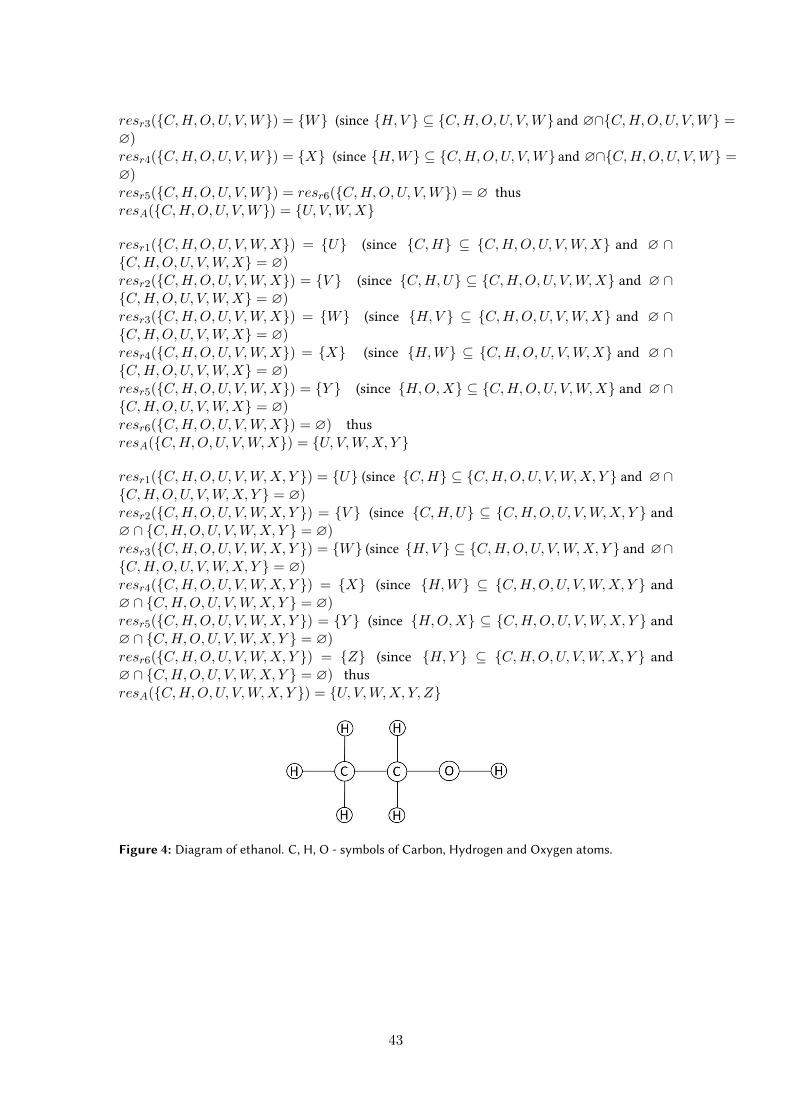
𝑟𝑒𝑠𝑟3({𝐶,𝐻,𝑂,𝑈, 𝑉,𝑊}) = {𝑊} (since {𝐻,𝑉 } ⊆ {𝐶,𝐻,𝑂,𝑈, 𝑉,𝑊} and ∅∩{𝐶,𝐻,𝑂,𝑈, 𝑉,𝑊} =∅)𝑟𝑒𝑠𝑟4({𝐶,𝐻,𝑂,𝑈, 𝑉,𝑊}) = {𝑋} (since {𝐻,𝑊} ⊆ {𝐶,𝐻,𝑂,𝑈, 𝑉,𝑊} and ∅∩{𝐶,𝐻,𝑂,𝑈, 𝑉,𝑊} =∅)𝑟𝑒𝑠𝑟5({𝐶,𝐻,𝑂,𝑈, 𝑉,𝑊}) = 𝑟𝑒𝑠𝑟6({𝐶,𝐻,𝑂,𝑈, 𝑉,𝑊}) = ∅ thus𝑟𝑒𝑠𝐴({𝐶,𝐻,𝑂,𝑈, 𝑉,𝑊}) = {𝑈, 𝑉,𝑊,𝑋}

𝑟𝑒𝑠𝑟1({𝐶,𝐻,𝑂,𝑈, 𝑉,𝑊,𝑋}) = {𝑈} (since {𝐶,𝐻} ⊆ {𝐶,𝐻,𝑂,𝑈, 𝑉,𝑊,𝑋} and ∅ ∩{𝐶,𝐻,𝑂,𝑈, 𝑉,𝑊,𝑋} = ∅)𝑟𝑒𝑠𝑟2({𝐶,𝐻,𝑂,𝑈, 𝑉,𝑊,𝑋}) = {𝑉 } (since {𝐶,𝐻,𝑈} ⊆ {𝐶,𝐻,𝑂,𝑈, 𝑉,𝑊,𝑋} and ∅ ∩{𝐶,𝐻,𝑂,𝑈, 𝑉,𝑊,𝑋} = ∅)𝑟𝑒𝑠𝑟3({𝐶,𝐻,𝑂,𝑈, 𝑉,𝑊,𝑋}) = {𝑊} (since {𝐻,𝑉 } ⊆ {𝐶,𝐻,𝑂,𝑈, 𝑉,𝑊,𝑋} and ∅ ∩{𝐶,𝐻,𝑂,𝑈, 𝑉,𝑊,𝑋} = ∅)𝑟𝑒𝑠𝑟4({𝐶,𝐻,𝑂,𝑈, 𝑉,𝑊,𝑋}) = {𝑋} (since {𝐻,𝑊} ⊆ {𝐶,𝐻,𝑂,𝑈, 𝑉,𝑊,𝑋} and ∅ ∩{𝐶,𝐻,𝑂,𝑈, 𝑉,𝑊,𝑋} = ∅)𝑟𝑒𝑠𝑟5({𝐶,𝐻,𝑂,𝑈, 𝑉,𝑊,𝑋}) = {𝑌 } (since {𝐻,𝑂,𝑋} ⊆ {𝐶,𝐻,𝑂,𝑈, 𝑉,𝑊,𝑋} and ∅ ∩{𝐶,𝐻,𝑂,𝑈, 𝑉,𝑊,𝑋} = ∅)𝑟𝑒𝑠𝑟6({𝐶,𝐻,𝑂,𝑈, 𝑉,𝑊,𝑋}) = ∅) thus𝑟𝑒𝑠𝐴({𝐶,𝐻,𝑂,𝑈, 𝑉,𝑊,𝑋}) = {𝑈, 𝑉,𝑊,𝑋, 𝑌 }

𝑟𝑒𝑠𝑟1({𝐶,𝐻,𝑂,𝑈, 𝑉,𝑊,𝑋, 𝑌 }) = {𝑈} (since {𝐶,𝐻} ⊆ {𝐶,𝐻,𝑂,𝑈, 𝑉,𝑊,𝑋, 𝑌 } and ∅ ∩{𝐶,𝐻,𝑂,𝑈, 𝑉,𝑊,𝑋, 𝑌 } = ∅)𝑟𝑒𝑠𝑟2({𝐶,𝐻,𝑂,𝑈, 𝑉,𝑊,𝑋, 𝑌 }) = {𝑉 } (since {𝐶,𝐻,𝑈} ⊆ {𝐶,𝐻,𝑂,𝑈, 𝑉,𝑊,𝑋, 𝑌 } and∅ ∩ {𝐶,𝐻,𝑂,𝑈, 𝑉,𝑊,𝑋, 𝑌 } = ∅)𝑟𝑒𝑠𝑟3({𝐶,𝐻,𝑂,𝑈, 𝑉,𝑊,𝑋, 𝑌 }) = {𝑊} (since {𝐻,𝑉 } ⊆ {𝐶,𝐻,𝑂,𝑈, 𝑉,𝑊,𝑋, 𝑌 } and ∅∩{𝐶,𝐻,𝑂,𝑈, 𝑉,𝑊,𝑋, 𝑌 } = ∅)𝑟𝑒𝑠𝑟4({𝐶,𝐻,𝑂,𝑈, 𝑉,𝑊,𝑋, 𝑌 }) = {𝑋} (since {𝐻,𝑊} ⊆ {𝐶,𝐻,𝑂,𝑈, 𝑉,𝑊,𝑋, 𝑌 } and∅ ∩ {𝐶,𝐻,𝑂,𝑈, 𝑉,𝑊,𝑋, 𝑌 } = ∅)𝑟𝑒𝑠𝑟5({𝐶,𝐻,𝑂,𝑈, 𝑉,𝑊,𝑋, 𝑌 }) = {𝑌 } (since {𝐻,𝑂,𝑋} ⊆ {𝐶,𝐻,𝑂,𝑈, 𝑉,𝑊,𝑋, 𝑌 } and∅ ∩ {𝐶,𝐻,𝑂,𝑈, 𝑉,𝑊,𝑋, 𝑌 } = ∅)𝑟𝑒𝑠𝑟6({𝐶,𝐻,𝑂,𝑈, 𝑉,𝑊,𝑋, 𝑌 }) = {𝑍} (since {𝐻,𝑌 } ⊆ {𝐶,𝐻,𝑂,𝑈, 𝑉,𝑊,𝑋, 𝑌 } and∅ ∩ {𝐶,𝐻,𝑂,𝑈, 𝑉,𝑊,𝑋, 𝑌 } = ∅) thus𝑟𝑒𝑠𝐴({𝐶,𝐻,𝑂,𝑈, 𝑉,𝑊,𝑋, 𝑌 }) = {𝑈, 𝑉,𝑊,𝑋, 𝑌, 𝑍}

Figure 4: Diagram of ethanol. C, H, O - symbols of Carbon, Hydrogen and Oxygen atoms.

43

Figure 5: A c-e structure with initial state 𝑠(𝐶) = 𝑠(𝐻) = 𝑠(𝑂) = 1 (and empty remaining nodes)imitating behaviour of reaction system 𝐴 specified in Example 4.1. Regarding it as a translation of 𝐴,note that nodes 𝑐1, 𝑐2, ℎ1, ℎ2, ℎ3, ℎ4, ℎ5, ℎ6 are some "artifacts" of this fairly liberal translation andhave no counterparts in 𝐴. Intuitively, they might be seen as holding single atoms of elements 𝐶 and𝐻 .

References

[Bar 2018] Barbutti R., Bove P., Gori R., Levi F., Milazzo P., Simulating Gene Regulatory Networksusing Reaction Systems, Proceedings of Concurrency, Specification and Programming 2018, pp.119-132

[Cza 2019] Czaja L. Cause-Effect Structures. An Algebra of Nets with Examples of Application,Lecture Notes in Networks and Systems 45, Springer 2019

[Dut 2018] Dutta S., Jankowski A., Rozenberg G., Skowron A., Linking Reaction Systems withRough Sets. Fundamenta Informaticae 165(3-4): 283-302 (2019)

[Ehr 2007] Ehrenfeucht A., Rozenberg G.: Reaction systems. Fundamenta Informaticae 75 (2007),pp. 263-280

[Ehr 2017] Ehrenfeucht A, Petre I., Rozenberg G., Reaction Systems: A Model of ComputationInspired by the Functioning of the Living Cell, in: The Role of Theory in Computer Science, EssaysDedicated to Janusz Brzozowski, edited by Stavros Konstantinidis, Nelma Moreira, Rogério Reisand Jeffrey Shallit, World Scientific 2017, pp.1-32

[Gor 2018] Gori R., Gruska D., Milazzo P., Hidden States in Reaction Systems, Proceedings ofConcurrency, Specification and Programming 2018, pp. 133-144

44

[Kle 2011] Kleijn J., Kountny M., Rozenberg G., Modelling Reaction Systems with Petri Nets, in:Proc. of the International Workshop on Biological Processes & Petri Nets (BioPPN 2011), pp.36–52

45

Interactive Granular Computing ConnectingAbstract and Physical Worlds: An ExampleSoma Dutta1, Andrzej Skowron2,3

1University of Warmia and Mazury in Olsztyn, Słoneczna 54, 10-710 Olsztyn, Poland2Systems Research Institute, Polish Academy of Sciences, Newelska 6, 01-447 Warsaw, Poland3Digital Science and Technology Centre, UKSW, Wóycickiego 1/3; b. 21, 01-938 Warsaw, Poland

AbstractThis short paper is an attempt to clarify the role of Interactive Granular Computing (IGrC) as a com-putation model which respects that a real cognition about a real physical complex phenomenon andmaking decisions based on that cannot be formalized only being in the language of mathematics. In thisregard, the paper focuses on presenting a real life example of computation where in order to move for-ward, without stumbling over the obstacles, a blind person needs to explore and learn the surroundingenvironment through interactions with the environment. The paper simply describes different compo-nents and features of IGrC model in the light of the concerned example and explains how this computingmodel has the potential to handle the grounding problem by bridging a connection between the abstractmathematical modeling and the real physical semantics.

Keywordsinteractions, granular computing, perception, knowledge specification, implementational language, com-plex granule, informational granule, grounding problem, dynamic transition relation

1. Introduction

In a few of our previous papers [8, 9, 19] we already put forward our arguments in favour of aneed to develop a model for computing and reasoning which is not purely mathematical andisolated from its real physical semantics, and which has the possibility to learn from the realphysical environment through real physical interactions. That such an endeavour is necessaryfor building an intelligent system, dealing with complex phenomenon, is supported by severalopinions of different researchers from different fields of research [1, 2, 3, 4, 6, 7, 10, 11, 12, 13,16, 18]. Without repeating many such inspiring thoughts of different researchers let us startwith citing one from [18].

[. . .] the often implicit stand one takes with regard to the question of the bridgebetween physical and symbolic descriptions determines in a fundamental way howone views the problems of cognition. A primary question here is, Exactly what kindof function is carried out by that part of the organism which is variously called the

29th International Workshop on Concurrency, Specification and Programming (CS&P’21)" [email protected] (S. Dutta); [email protected] (A. Skowron)� 0000-0002-7670-3154 (S. Dutta); 0000-0002-5271-6559 (A. Skowron)



46

sensor, the transducer, or in the case of Gibson, the “information pickup”? One’s an-swer to this question determines the shape of any theory of perception and cognitionone subsequently constructs. As I shall argue, unlike the symbolic processes that char-acterize cognition, the function performed by the transducer cannot be described asa computation, that is, by a purely symbol-manipulation function. Like all primitiveoperations of the functional architecture, the transducer fundamentally is a physicalprocess; that is, its behavior is explainable (its regularities can be captured) in termsof its intrinsic properties - physical, chemical, biological, and so on. Thus, typicallyit does not come under study by cognitive psychologists who simply presuppose thatan organism is equipped with certain transducer functions. The task of discoveringthese mechanisms is left for others, for example, “sensory encoding neurophysiologists,biophysicists, and engineers.

Let us also cite the opinion concerning the need of a new computing model in Cyber-PhysicalSystems (CPS) [5].

The inherent cross-disciplinary nature of CPS requires distinct modelling techniquesto be employed, thus prompting for a common background formalism that enablescommunication between all specialities. However, to this date, no such single super-formalism exists to support the multiple dimensions of the design of a CPS. Indeed, toeffectively design a CPS, engineers (in the role of modellers) either need to be versedin multiple formalisms, or a fundamentally new modelling approach has toemerge.

According to the view of Edmund Husserl, the founder of phenomenology [7], non-standardmodels of computation such as natural computing, reaction systems, Harel’s algorithmics andGurevich’s abstract state machines, or neural network computing are closed in the abstractspace, in the mathematical manifold.

Husserl was frustrated by the idea that science and mathematics were increasinglyconducted on an abstract plane [treating nature itself as a “mathematical mani-fold"] that was disconnected from human experience and human understanding,independently of questions of truth and applicability. He felt that the sciencesincreasingly dealt with idealized entities and internal abstractions a world apartfrom the concrete phenomena of daily life.

Till now, in different works (see, e.g., [8, 9, 14, 19, 20]), we tried to introduce what do we meanby Interactive Granular Computing (IGrC) and how it is different from other existing theoriesfrom the perspective of modeling computations in a complex system. In a very brief description,Interactive symbolizes interaction between the abstract world and the real physical world, andGranular Computing symbolizes computation over imperfect, partial, granulated informationabstracted about the real physical world. Here, once again we take the opportunity to explainbriefly the notion of complex granule (c-granule), the basic building block of IGrC.

A c-granule is composed of three parts, known as soft_suit, link_suit and hard_suit. Thesethree parts correspond to three sets of physical objects, together which determines the scope of

47

that particular c-granule1. The soft_suit represents the objects from the physical reality whichare directly accessible or about which already some information is obtained. The hard_suitcorresponds to those objects which are in the scope of the c-granule but not yet accessed orare not in the direct reach at that point of time of the c-granule. The link_suit represents achain of objects that creates a communication channel between the soft_suit and the hard_suit.A c-granule, when associated with an information layer with it, is known as informationalc-granule, in short ic-granule. The information layer of an ic-granule contains different formsof information, such as specification of the already perceived properties of the objects from itssoft_suit, specifications of the windows describing where and how some specific part from thescope of the ic-granule can be accessed or reached etc. Based on the purposes and types of theinformation specifications of an ic-granule there can be different types of ic-granules, such asic-granule representing perception of the objects from the scope (perception based ic-granule), ic-granule representing domain knowledge (knowledge based ic-granule), ic-granule representingplan of actions (planner ic-granule), ic-granule representing plan into an implementationallevel language (implementational ic-granule) etc. Here to be emphasized that the ic-granule,responsible for implementation of a plan of actions, serves the task of connecting between theabstract and the real worlds.

A computation process over a c-granule is described by a network of ic-granules lyingwithin the scope of the concerned c-granule. The informational layer of all these ic-granulesconstitutes the domain knowledge of the control of the c-granule, may be also called control ofthe computation process; this informational content is endowed with a reasoning mechanism.The information content and the reasoning mechanism together designs the control mechanismof a computation process. More specifically, the whole information layer is clustered basedon the information relevant to different sub-scopes of the whole scope of the c-granule. Forexample, in the ic-granules representing the domain knowledge, there can be different sub-clusters in the informational layer corresponding to different aspects of the domain knowledge.That is, an ic-granule may contain several other ic-granules inside its scope. On the otherhand the reasoning mechanism of the control of a c-granule is responsible for aggregating,deleting, or generating information from the existing clustered of information layers. Thus newinformation layers are generated over time based on (i) initial (partial) perception and domainknowledge of the concerned fragment of the environment (ii) initiation of interactions throughalready accessible objects to access the information about the not directly reachable objects(iii) perception of the physical world after interactions and (iv) verification of the perceivedproperties of the newly obtained configuration with the expected specifications of the targetenvironment.

Having this much of preliminary relevant details about a computation process over a c-granule, in this paper our target is to present a real life example through which different aspectsof computation over a c-granule can be visualised.

In this regard, Section 2 presents an example of computing along with an explanation of howsuch a real life computation can be modeled in the framework of IGrC. Section 3 presents theconcluding remarks explaining how different components and features of IGrC incorporate a

1The scope of a c-granule at a given moment 𝑡 of the local time of the c-granule is the part of the physical spacecorresponding to the formal specifications of all spatio-temporal windows active at 𝑡.

48

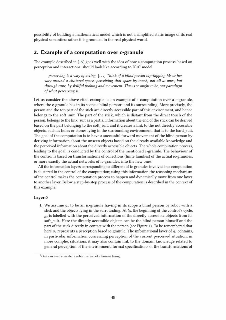
possibility of building a mathematical model which is not a simplified static image of its realphysical semantics; rather it is grounded in the real physical world.

2. Example of a computation over c-granule

The example described in [15] goes well with the idea of how a computation process, based onperception and interactions, should look like according to IGrC model.

perceiving is a way of acting. [. . .] Think of a blind person tap-tapping his or herway around a cluttered space, perceiving that space by touch, not all at once, butthrough time, by skillful probing and movement. This is or ought to be, our paradigmof what perceiving is.

Let us consider the above cited example as an example of a computation over a c-granule,where the c-granule has in its scope a blind person2 and its surrounding. More precisely, theperson and the top part of the stick are directly accessible part of this environment, and hencebelongs to the soft_suit. The part of the stick, which is distant from the direct touch of theperson, belongs to the link_suit as a partial information about the end of the stick can be derivedbased on the part belonging to the soft_suit, and it creates a link to the not directly accessibleobjects, such as holes or stones lying in the surrounding environment, that is to the hard_suit.The goal of the computation is to have a successful forward movement of the blind person byderiving information about the unseen objects based on the already available knowledge andthe perceived information about the directly accessible objects. The whole computation process,leading to the goal, is conducted by the control of the mentioned c-granule. The behaviour ofthe control is based on transformations of collections (finite families) of the actual ic-granules,or more exactly the actual networks of ic-granules, into the new ones.

All the information layers corresponding to different of ic-granules involved in a computationis clustered in the control of the computation; using this information the reasoning mechanismof the control makes the computation process to happen and dynamically move from one layerto another layer. Below a step-by-step process of the computation is described in the context ofthis example.

Layer:0

1. We assume 𝑔𝑠 to be an ic-granule having in its scope a blind person or robot with astick and the objects lying in the surrounding. At 𝑡0, the beginning of the control’s cycle,𝑔𝑠 is labelled with the perceived information of the directly accessible objects from itssoft_suit. Here the directly accessible objects can be the blind person himself and thepart of the stick directly in contact with the person (see Figure 1). To be remembered thathere 𝑔𝑠 represents a perception based ic-granule. The informational layer of 𝑔𝑠 contains,in particular information concerning perception of the current perceived situation; inmore complex situations it may also contain link to the domain knowledge related togeneral perception of the environment, formal specifications of the transformations of

2One can even consider a robot instead of a human being.

49

informational objects

physical objects

L

S

H

informationallabel

A blind person or robotwith directly accessiblestick in the soft_suit (S)

A link created in the link_suit (L) through the stick interacting

with other objects connectingthe hole.

A hole in the hard_suit (H)

Part of realphysical

objects andtheir dynamicsare captured

in ic-granule gs.The informationlayer at the topconsists of the

perceivedproperties in the

scope of gs.

gs

Figure 1: ic-granule operating on a particular scope of the physical world.

the ic-granules within its scope, database with rules for selection of transformation of ic-granules for realisation, etc. In our illustrative example we discuss only a very simplifiedversion of 𝑔𝑠.

2. Let the description of the general goal of the computation be attached as the informationlayer of a planner ic-granule 𝑔0. So, here 𝑔0 corresponds to those particular cells of ahuman brain where the goal description is set. So, for 𝑔0 the soft_suit, link_suit and thehard_suit can be like different layers of those brain cells where the reachability to moredeeper layer in the hard_suit happens through the directly reachable layer in the soft_suitand reactions of the brain cells propagating from the soft_suit to the hard_suit.

3. The role of the knowledge base is represented by another ic-granule 𝑔𝑘𝑏. Here, 𝑔𝑘𝑏 can beconsidered as the brain parts related to the memory locations. The information layer of𝑔𝑘𝑏 is labelled with the addresses of different relevant properties of different fragmentsof the c-granule. The soft_suit of 𝑔𝑘𝑏 consists of the objects which form the outer boxof the memory location whose address is attached to the information layer; in orderto access the detailed information about some fragments some more inner boxes, lyingin the hard_suit, are to be opened. Such ic-granules representing knowledge base maybe called information granules. Their physical parts create local memories for storingand transmitting information. One may also look on 𝑔𝑘𝑏 as on a compound ic-granulerepresenting a network of ic-granules determining the structure of 𝑔𝑘𝑏.

4. Now based on the information gathered from the informational layers of 𝑔𝑠, 𝑔0 and𝑔𝑘𝑏, the control with its reasoning mechanism aims to better understand the perceivedsituation necessary for decomposition; this leads to construction of a more detailed planof actions. This detailed plan is represented in informational layer of the ic-granule 𝑔1 atthe next time point 𝑡1. For a visual representation the readers are referred to Figure 2.

In our simplified illustrative example, we mention only one mechanism for enriching the

50

label of ic-granule

I: informational objects

P: physical objects

S

L

H

Layer:0

g0 gkb g s

Layer:1

g1 gkb gs 1

gi

info expansion info translation

Figure 2: Computation over ic-granules passing from layer-0 to layer-1.(i) 𝑔𝑠: Current perception of some objects of P at time 𝑡0, indicating the scope. S contains directlyperceivable objects, L contains objects creating communication channel to the objects in H wheresome actions are to be performed.(ii) 𝑔𝑘𝑏: Relevant information about general laws related to objects in 𝑔𝑠 and specifications ofwhere this information is stored. Here S contains directly accessible part of the storage memoryand L contains the objects linking to the directory at H.(iii) 𝑔0: Relevant information regarding a goal that to be implemented in the H part of 𝑔𝑠. Thisspecification of goal is stored in some object in the H of 𝑔0, and is accessible by some object lyingin the S of 𝑔0.(iv) info expansion denotes decomposition of the plan available at 𝑔0 to a more detailed plan.

informational layer of 𝑔𝑠. In a more realistic example, one should consider other mechanisms, e.g.,measuring different parameters by sensors (e.g., stick in our example), recording the perceivedresults of measurements in the corresponding informational layers of ic-granules etc. In a moregeneral case, a sequence of steps of reasoning is realised, which are based on transformationsof ic-granules, leading to better understanding of the currently perceived situation. It shouldbe also noted that in general decomposition problems are challenging and they are related, inparticular to the idea of information granulations and computing with words [23, 24, 25, 26].

Layer:1

1. From the perspective of the example, at 𝑡0 the information attached to 𝑔0 encodes thegeneral goal of the blind person that primarily gets registered in his brain, i.e., in thesoft_suit of 𝑔0. At time 𝑡0 the hard_suit of 𝑔0, such as more deep analytical brain cells,remains still unaccessed. Based on the collected information of 𝑔𝑠 and 𝑔𝑘𝑏, at time 𝑡1 theperson ponders more analytically; this in a sense activates interaction with the previouslyunaccessed part of 𝑔0. This gradually gives access to the hard_suit of 𝑔0, and thus at time

51

𝑡1 the hard_suit of 𝑔0 becomes the soft_suit of 𝑔1, labelled with a more detailed plan forthe person.

2. Now in order to implement the abstract description of the plan available at 𝑔1 throughreal physical actions, the plan needs to be transformed from the abstract level to animplementational level language. From the perspective of our example, this can be atranslation of the plan from the person’s analytical brain cells to a language of actuators,like hands, legs, and the stick of the person. So, a new ic-granule is manifested at this layer.We call it as 𝑔𝑖1 , an implementational ic-granule. To be noted that 𝑔𝑖1 does not concernabout the actual actuators; rather it is like another hard-drive in the brain of the personwhere the action plan can be stored in the language of actuators. The information layer of𝑔𝑖1 also contains the specification of the conditions for initiating the implementation planthrough a real actuator. Figure 3 presents the computation process described in layer-1.

Layer:0

g0 gkb gs

Layer:1

g1 gkb gs 1ig

info expansion info translation

Layer:2

g2

gs 2ig

info embedding

Figure 3: Computation over ic-granules passing from layer-1 to layer-2.(i) 𝑔1: at time 𝑡1 specification of the plan of 𝑔0 is expanded. Detailed specification is generatedbased on 𝑔𝑠, 𝑔𝑘𝑏 and 𝑔0 of Layer:0. In particular the H part of 𝑔0 can be now the S of 𝑔1 which isgradually reached through the L part of 𝑔0.(ii) 𝑔𝑖1 : Specification of how the abstract plan of 𝑔1 can be implemented in 𝑔𝑠, that is the specifi-cation of the plan in a lower level language which can be implemented via physical objects. Thislower level language is also a built-in language of a hardware lying at the H part of 𝑔𝑖1 .(iii) info translation denotes translation of the plan from the level of abstract description to thelevel of implementational language.(iv) 𝑔2: Specification in lower level language is embedded to a physical object lying in the S partof 𝑔2, which prepares the ground to run the plan via a physical object in H part of 𝑔2.(v) info embedding represents embedding the plan of actions on a real physical object.

Layer:21. The specification of the plan of implementation of 𝑔𝑖1 is now realized through a physical

object at time 𝑡2. Let this object belong to the scope of the ic-granule 𝑔2. In case of the

52

example, it can be the stick of the blind person on which the abstract implementationplan is embedded, and 𝑔2 represents the ic-granule containing the stick in its scope. Thephysical interaction of the stick with other objects in 𝑔2 is encoded in the informationlayer of 𝑔2. If this information matches to a significant level to the condition for initiatingimplementation plan stored at 𝑔𝑖1 then an action compilation signal is passed to the nextimplementation granule, may be named as 𝑔𝑖2 .

2. With the action compilation specification of 𝑔𝑖2 the objects lying in its link_suit andhard_suit propagate actions to realize a desired configuration in the hard_suit of 𝑔𝑠. Inthe context of our example, 𝑔𝑖2 represents the ic-granule which specifies how to movethe stick forward until it touches a stone on its way. This chain of objects between thestick and a stone creates a communication channel.

3. Through this communication channel the computation process enters into the hard_suitof 𝑔𝑠, which was inaccessible at time 𝑡0. The initiation of the action compilation via 𝑔𝑖2creates a link to the hard_suit of 𝑔𝑠. This new interaction gives access to the hard_suit of𝑔𝑠 which was previously inaccessible.

4. A new cycle starts by perceiving properties of the newly accessible part of 𝑔𝑠.

Here to be noted, that in the example we only have mentioned about the decomposition ofthe plan of actions from the initial stage 𝑔0 to a stage 𝑔1, from where it gets translated tothe implementational level language. But in practice decomposition of the action plan, say𝛼 : 𝑔0 ⇒ 𝛽 : 𝑔1 available in the information layer of 𝑔0 specifying the target ic-granule 𝑔1 withproperty 𝛽 can have several layers of decomposition in between. For a visual representationthe readers are referred to the Figure 4, which will be discussed in Section 3. One should alsoconsider that some actions are lunched in the process of perception while the other ones arerelated to the main decisions.

The above described idea of computation over a c-granule is in the line of the idea that LucSteels has characterised in [21]; complex dynamical systems (complex systems, for short) areconsidered as systems consisting of a set of interacting elements

[. . .] where the behavior of the total is an indirect, non-hierarchical consequence ofthe behavior of the different parts. Complex systems differ in that sense from strictlyhierarchical systems [...] where the total behavior is a hierarchical composition of thebehavior of the parts. In complex systems, global coherence is reached despite purelylocal non-linear interactions. There is no central control source. Typically the systemis open.

3. Beyond pure mathematical modeling: a concluding remark

From the above exemplification of the process of computation over a c-granule, moving from aconfiguration of ic-granules to another, it is quite clear that the process deals with a set of hunksof real physical matter associated with their information layers; the information layers indicatewhere, when and how they can be touched, or their properties can be achieved or verified. So,this already clarifies how in the model of IGrC by a c-granule both abstract world, that is theinformation layer, and the real physical semantics, that is the three-layered hunk of objects,

53

together are referred to. One more point, that needs to be clarified, is how the model designs itsreal physical implementation by lifting the static description of a process to the level of actions.

The implementational ic-granules create a specific interface between the abstract and thephysical world. In particular, at some level of the implementational phase the control of thec-granule launches actions linking the abstract world associated to the informational layer ofthe control of the c-granule with the real physical world. These actions are not from abstractmathematical space and the model of IGrC keep those action functions free from mathematicalformalizations. Their syntactic descriptions can be formalised in the informational layers of thecontrol of the c-granule. However, their implementation should be realised in the real physicalworld and the model only can mathematically formalize their performance quality by perceivingthe changes in the world after initiation of the actions. Of course, the expected properties ofthe real physical environment, after the implementation of the actions, also can be formalizedwithin the description of the action specification.

Thus the IGrC model keeps the possibility of mismatch between expected and real physicaloutcome open as we never can a priori formalize all possible outcomes of an action, which issupposed to be initiated in the physical world based on an abstract description of the actionspecification. We can only expect a desired outcome, specified in the information layer. So,after each implementational phase of a computation over a c-granule the control starts a newcycle again by perceiving the properties of the objects lying in its scope. Then those observedproperties are verified with the expected properties. Hence, accordingly there is a need tomodify the induced models based on their comparisons with the recorded data.

In Figure 4 we illustrate the idea of decomposition of the description of the action plan inorder to transform an ic-granule with a given property, say 𝛼, into another one with the property𝛽. After several levels of decomposition it reaches a level at which the relevant actions arelaunched by the control so that the expected realisation of the whole chain of actions can leadto a situation satisfying, to a satisfactory degree, the property 𝛽. Though the conditions of thechain of actions and the expected properties after the actions are specified by 𝛼’s and 𝛽’s, theactual actions 𝑎𝑐1, . . . 𝑎𝑐𝑘 are not in the realm of mathematical formulation. The model of IGrCkeeps this juncture between abstract and physical bridging free from mathematical formulation.Instead, IGrC proposes to formalize the results of actions by perceiving the properties of outcomeconfigurations and verifying them with the expected property 𝛽.

Let us outline a scheme of the behaviour of the control of a c-granule.Often the control aims at achieving its target goal, expressed in the information layer of the

ic-granule 𝑔0, using complex vague concepts, e.g., related to safeness of the perceived situation,from a natural language. Below, we assume that for a given specification a set of rules forselection of the relevant transformations of ic-granules was learned by the control or is given apriori. The pre-condition of each rule is a condition. The degree of matching of this conditionby the current status of the perceived situation determines selection of the transformation ofic-granules from the post-condition of the rule.3

The outline of the general procedure of a computation in IGrC, realised by the controlof a c-granule, is based on searching for relevant transformations of ic-granules and their

3Note that other learning paradigms such as lazy learning can be used in inducing models of complex vagueconcepts different from the discussed here.

54

0: :

trg g

...

...1

ac kac:plan

Transformation specification tr from an ic-granule with property to an ic-granule with property available at the planner ic-granule g0

∝: 𝑔𝑜 ⟹𝑡𝑟1 𝛼1: 𝑔1 𝛼1: 𝑔1 ⟹𝑡𝑟2 𝛽: 𝑔

∝: 𝑔𝑜 ⟹𝑡𝑟1 𝛼1: 𝑔1 … 𝛼𝑘−1: 𝑔𝑘−1 ⟹𝑡𝑟𝑘 𝛽: 𝑔

Figure 4: Illustration of a simple case of decomposition of transformation.

implementations; it looks as follows.

perceive accessible parts of the abstract and physical world to understand (up to asatisfactory degree) the current situation for making decision concerning the selection ofthe formal specification of transformation of ic-granules for implementation; the currentstatus of perception is represented in the informational layer of 𝑔𝑠; this is realised by the

control in several steps and one of them is listed below⇓

consult domain knowledge and required goal of computation (𝑔𝑘𝑏, 𝑔0) to enrich theinformation about the status of currently perceived situation

⇓. . .

(it may be necessary to perform several steps of reasoning before having a satisfactoryunderstanding of the perceived situation; it can be achieved by allowing the control to

select the relevant formal specification of transformation of ic-granules forimplementation; some of these steps may be related, e.g., to measurements (by sensors)

of features of the perceived physical objects in the scope of active ic-granules4

. . .

⇓select (from the proper knowledge base) the relevant formal specification of the

transformation of the ic-granules for implementation5

⇓

4It should be noted that the mentioned steps of reasoning are also realised by transformations of some ic-granules.

5This step is especially compound; details will be discussed in an extended version of our paper.

55

. . .the selected formal specification may require several decomposition steps before the

proper level for the direct implementation can be achieved (embedding in the physicalworld)

⇓after reaching the satisfactory level of decomposition generate the formal specification of

the action plan; in the simplest case such a plan is represented by a linear order ofic-granules which can be implemented by the considered control of the c-granule in the

physical world6

⇓initiate (in proper order) implementational granules from the plan responsible for

implementation of actions of plan⇓

during plan realisation, perceive the relevant accessible parts of the physical world(through the implementational granules) and store the perceived data in informational

layers of the relevant ic-granules⇓

follow the same loop as above taking, in particular into account the results of matchingthe expected results with the perceived ones7.

The discussed above issues of decomposition and implementation should be treated as anillustrative example only. In the real-life projects one should take into account many otherissues.

Here to be noted that the transition from one configuration of ic-granules to the other,as described above in the general plan of computation, by creating and accessing differentic-granules and their information layers is not also purely mathematical. Usually, the statetransition relation is presented by a given family of sets {𝑋𝑖}𝑖∈𝐼 where a transition relation isrepresented as a relation 𝑡𝑟𝑖 ⊆ 𝑋𝑖 ×𝑋𝑖. Here, this cannot be purely mathematical as we needto incorporate the components which can specify (i) how elements of 𝑋𝑖 are perceived in thereal physical environment, and (ii) how the transition relation 𝑡𝑟𝑖 is implemented in the realphysical world. This reasoning mechanism, as described in the Introduction, is conducted bythe control of the c-granule over which the computation process is running.

So, in contrary to a static transition relation, in IGrC the control of a c-granule incorporatesthe possibility of dynamic as well as not purely mathematical formulation of a state transitionrelation. The structure of a control is designed to have two interacting modules, called theabstract module (AM) and the physical module (PM) (see Figure 5).

Communication between AM and PM is designed by two mechanisms. The first one providesa possibility of encoding given information from AM by a relevant state of a set of physicalobjects from PM, and the second one provides a possibility of encoding the considered state of

6Plans may be generated on different levels of decomposition, e.g., for better understanding the perceivedsituation helping the control to generate the high quality plans for realisation of the target goals.

7In a more compound case of the control of a c-granule, strategies for adaptation of the previously used planto the new situation are used. Moreover, the decision about the necessity of plan adaptation may be taken oftenduring of the actual plan.

56

AM PM

Figure 5: Interacting abstract (AM) and physical (PM) modules in control of c-granules.

a set of physical objects from PM by a relevant information represented in the language of AM.These two mechanisms can be implemented by atomic actions.

AM module sends to PM a formal specification of a transformation of a ic-granule as well asformal specifications of some spatio-temporal windows. Some of them are labelled by alreadyperceived information or properties from the scope of the c-granule and others are labelled byformal specifications of the required information from PM. In case when the delivered specifica-tion can be directly embedded by PM in the physical world then PM, by creating a network ofinteracting ic-granules, aims to deliver a network of physical pointers matching information,perceived by AM, with the expected properties, expressed formally in AM. Otherwise, PM sendsto AM a message about the necessity of the specification decomposition.

AM may send to PM messages consisting of formal specification(s) of the required trans-formation(s) of ic-granules together with the expected results provided by AM. The messagessent by AM are encoded by the states of some physical objects in PM. In this way, atomicactions changing states of physical objects to the ones specified by the given information areimplemented. However, it is to be noted that the modeling of the behaviour of AM and commu-nication of AM with PM can be based on mathematical modeling; whereas PM is composed outof physical objects which, being from the real world, are outside of the abstract mathematicalmodeling. However, partial information about properties of these objects and their interactionsmay be communicated to AM through interaction of PM with AM. Thus, IGrC incorporatesboth dynamic as well as mathematical modeling grounded in the real physical world.

References

[1] Hyo-Sung Ahn: Formation Control Approaches for Distributed Agents. Studies in Systems,Decision and Control 205. SpringerHyo-Sung , Cwitzerland (2020) doi:10.1007/978-3-030-15187-4

[2] Lawrence W. Barsalou: Perceptual symbol systems. Behavioral & Brain Sciences 22 (1999)577–660 (doi:10.1017/S0140525X99002149)

[3] Franz Brentano: Psychologie vom empirischen Standpunkte. Dunker & Humboldt, Leipzig(1874) (https://archive.org/details/psychologievome02brengoog/page/n4/mode/2up)

[4] Frederick P. Brooks: The Mythical Man-Month: Essays on Software Engineering. Addison-Wesley, Boston (1975) (extended Anniversary Edition in 1995)

[5] Paulo Carreira, Vasco Amaral, Hans Vangheluwe: Multi-paradigm modelling for cyber-physical systems: Foundations. In: Paulo Carreira, Vasco Amaral, Hans Vangheluwe (eds.),

57

Foundations of Cyber-Physical Systems Multi-Paradigm Modelling for Cyber-PhysicalSystems. Springer, Cham, Switzerland, pp. 1-14 (2020) (doi:10.1007/978-3-030-43946-0)

[6] David Deutsch, Artur Ekert, Rossella Lupacchini: Machines, logic and quantum physics.Neural Computation 6 (2000) 265–283 (doi:10.2307/421056)

[7] Paul Dourish: Where the Action Is. The Foundations of Embodied Interaction. The MITPress Cambridge, MA, London (2004)

[8] Soma Dutta, Andrzej Skowron: Toward a computing model dealing with complex phe-nomena: Interactive granular computing. In: Ngoc Than Nguyen et al (eds): ICCCI 2021Proceedings, Springer (2021) (to appear)

[9] Soma Dutta, Andrzej Skowron: Interactive Granular Computing Model for IntelligentSystems. In: Shi, Z., Chakraborty, M., Kar, S. (eds): Intelligence Science III. 4th IFIP TC12 International Conference, ICIS 2020, Durgapur, India, February 24-27, 2021, RevisedSelected Papers. IFIP Advances in Information and Communication Technology (IFIPAICT)book series 623, Springer, Cham, Switzerland, pp. 37-48 (2021) doi:10.1007/978-3-030-74826-5_4

[10] Sean Gerrish: How Smart Machines Think. MIT Press, Cambridge, MA (2018)[11] Stevan Harnad: The symbol grounding problem. Physica D42 (1990) 335–346

(doi:10.1016/0167-2789(90)90087-6)[12] Mark Heller: The Ontology of Physical Objects. Four dimensional hunks of matter. Cam-

bridge Studies in Philosophy , Cambridge University Press, Cambridge, UK (1990)[13] Andrew Hodges: Alan Turing, Logical and Physical. In: Cooper, S.B., Löwe, B., Sorbi, A.,

New Computational Paradigms. Changing Conceptions of What is Computable. Springerand Business Media, New York, N.Y., pp. 3-15 (2008) (doi:10.1007/978-0-387-68546-5_1)

[14] Andrzej Jankowski: Interactive Granular Computations in Networks and Systems En-gineering: A Practical Perspective. Lecture Notes in Networks and Systems. Springer,Heidelberg (2017) (doi:10.1007/978-3-319-57627-5)

[15] Alva Nöe: Action in perception. MIT Press, Cambridge, MA (2004)[16] Charles L. Ortiz Jr.: Why we need a physically embodied Turing test and what it might

look like. AI Magazine 37 (2016) 55–62 (doi:10.1609/aimag.v37i1.2645 )[17] Pawlak, Z.: Rough sets. International Journal of Computer and Information Sciences 11

(1982) 341–356 (doi:10.1007/BF01001956)[18] Zenon W. Pylyshyn: Computation and Cognition. Toward a Foundation for Cognitive

Science. The MIT Press Cambridge, MA (1884)[19] Andrzej Skowron, Andrzej Jankowski, Soma Dutta: Interactive granular computing.

Granular Computing 1(2) (2016) 95–113 (doi:10.1007/s41066-015-0002-1)[20] Andrzej Skowron, Andrzej Jankowski: Rough sets and interactive granular computing.

Fundamenta Informaticae 147 (2016) 371–385 (doi:10.3233/FI-2016-1413)[21] Luc Steels: The synthetic modeling of language origins. Evolution of Communication 1(1)

(1997) 1–34 (doi:10.1075/eoc.1.1.02ste)[22] Lotfi A. Zadeh: Fuzzy sets. Information and Control 8(3) (1965) 338–353 (doi:10.1016/S0019-

9958(65)90241-X)[23] Lotfi A. Zadeh: Toward a theory of fuzzy information granulation and its central-

ity in human reasoning and fuzzy logic. Fuzzy Sets and Systems 90 (1997) 111–127(doi:10.1016/S0165-0114(97)00077-8)

58

[24] Lotfi A. Zadeh: From computing with numbers to computing with words – frommanipulation of measurements to manipulation of perceptions. IEEE Transactions onCircuits and Systems I: Fundamental Theory and Applications 45(1) 105–119 (1999)(doi:10.1109/81.739259)

[25] Lotfi A. Zadeh: Foreword. In: Pal, S.K., Polkowski, L., Skowron, A. (eds.), Rough-Neuralcomputing: Techniques for Computing with Words, Heidelberg, Springer, pp. ix-xi(2004) (doi:10.1007/978-3-642-18859-6)

[26] Lotfi A. Zadeh: Computing with Words: Principal Concepts and Ideas. Studies in Fuzzinessand Soft Computing 277, Springer, Heidelberg (2012) (doi:10.1007/978-3-642-27473-2)

59

On Semantics for Testing in Time Petri NetsElena Bozhenkova1, Irina Virbitskaite1

1A.P. Ershov Institute of Informatics Systems, SB RAS; 6, Lavrentiev av., Novosibirsk, 630090, Russian Federation

AbstractDense-Time Petri Nets (TPNs) are now a well-established model to describe and study real time (quanti-tative) and functional (qualitative) properties of safety-critical, computer-controlled systems. Testingequivalences, used to compare systems’ behaviors (processes) and reduce the structure of systems, aredefined in terms of tests that processes may or must pass. The intention of the paper is to establishthe interrelations between various semantics for must-testing equivalences with extended tests, in theframework of TPNs. This allows for studying in detail the timing behavior in addition to the degree ofrelative concurrency of processes generated when systems are functioning.

1. Introduction

Dense-Time Petri Nets (TPNs) are suitable for qualitative and quantitative modelling and verify-ing of safety-critical, computer-controlled, real-time systems. Several semantics (behaviors) areexplored in the literature for TPNs, that can be classified according to interleaving – partial orderdichotomy. The classical interleaving behavior of the TPN is described by runs — sequences ofchanges in states by time elapsings and/or transition firings. The semantics allows for analyzingsome safety and liveness properties of systems, however concurrency between net transitionsis reduced to non-deterministic choice between sequences of transitions firings in any possibleorder. Step semantics of TPNs generalizes the interleaving approach by allowing several con-current transitions (forming a step) to fire simultaneously. Partial order semantics of TPNs ismost often represented by means of the so-called causal net processes which include eventsand conditions related by causal dependence (the absence of causality means concurrency)and equipped with timing information. Causal tree semantics summarizes the interleavingand partial order approaches by representing the behavior of the TPN in the form of a treewith nodes corresponding to runs, and edges labeled by actions with their times and causalpredecessors.

Testing equivalences [1] are explicitly based on a framework of extracting information aboutthe systems’ behaviors (processes) by testing them. Two processes are considered equivalent ifthere is no test that can distinguish them. In the realm of untimed models, interleaving testingwas thoroughly investigated and well-understood in the setting of models of transition systems(see [2, 3] among many others). Interleaving, step and partial order testing equivalences forelementary net systems (safe Petri nets without loops) were studied in [4]. There, the authors

29th International Workshop on Concurrency, Specification and Programming (CS&P’21)$ [email protected] (E. Bozhenkova); [email protected] (I. Virbitskaite)� https://pdb.iis.nsk.su/en/person/220 (E. Bozhenkova); https://persons.iis.nsk.su/en/virbitskaite (I. Virbitskaite)� 0000-0002-9291-7451 (E. Bozhenkova); 0000-0002-4475-3480 (I. Virbitskaite)



60

indicated the location of the testings among other behavioral equivalences from linear time –branching time spectrum, providing their hierarchies for the model under consideration withand without invisible actions. Partial order and non-deterministic semantics for different classesof Petri nets are often represented by means of various models of event structures. In theframework of the models, testing equivalences within interleaving – partial order dichotomywere developed and compared in the papers [5, 6, 7]. Moreover, in [7] special attention was paidto the relationships between partial order and causal tree semantics in the context of testingequivalences. To the best of authors’ knowledge, causal tree semantics in the framework ofPetri nets has not been studied yet.

As safety-critical applications often require verification of real time characteristics, testingequivalences are expanded in concurrent models with time. In the papers [8, 9, 10, 11], alternativecharacterizations of timed testing are provided for timed generalizations of interleaving models.In [12], the testing relations along with their alternative characterization and discretizationwere proposed in the framework of Petri nets with time intervals associated to arcs from placesto transitions. At the same time, to the best of our knowledge, there are only few mentionsof a fusion of timing and partial order semantics, in testing scenario. In this regard, the work[13] is a welcome exception, where time-sensitive testing is investigated within linear time –branching time spectrum, in the setting of event structure models with time characteristics.Also, our origin is the paper [14] the main result of which is the coincidence of poset and causaltree testing equivalences, with the tests as direct extensions of the experiments, in the settingof TPNs. In this paper, we expand the results of [14] to step, poset and causal tree semanticswith extended tests1, and demonstrate the discriminating/matching power of the semantics inthe framework of testing equivalences on contact-free TPNs. The results obtained can be usefulin formal verification of systems since partial order semantics allows for reducing the numberof systems’ states to be analyzed.

2. Syntax and Different Semantics of TPNs

In this section, some terminology concerning the model of Petri nets with timing constraints(time intervals on the firings of transitions) and its concurrent semantics in terms of interleav-ing/step firing sequences, causal net processes and causal trees are defined.

2.1. Syntax and Interleaving/Step Semantics of TPNs

We start with recalling the definitions of the structure and interleaving/step behavior of timePetri nets [15, 16]. We use 𝐴𝑐𝑡 as an alphabet of actions and 𝐴𝑐𝑡N as a set of multisets over𝐴𝑐𝑡. Let the domain T of time values be the set of rational numbers. We denote by [𝜏1, 𝜏2] theclosed interval between two time values 𝜏1, 𝜏2 ∈ T. Infinity is allowed at the upper bounds ofintervals. Let 𝐼𝑛𝑡𝑒𝑟𝑣 be the set of all such intervals.

Definition 1. • A (labeled over 𝐴𝑐𝑡) time Petri net is a pair 𝒯 𝒩 = (𝒩 , 𝐷), where 𝒩 = (𝑃 ,𝑇 , 𝐹 , 𝑀0, 𝐿) is a (labeled over 𝐴𝑐𝑡) underlying Petri net (with a finite set 𝑃 of places, a

1Testing equivalence with extended tests checks, after the executions of the experiments, the tests that arecontinuations of the experiments with steps/posets of actions, not with single actions.

61

finite set 𝑇 of transitions such that 𝑃 ∩ 𝑇 = ∅ and 𝑃 ∪ 𝑇 = ∅, a flow relation 𝐹 ⊆(𝑃 ×𝑇 )∪ (𝑇 ×𝑃 ), an initial marking ∅ = 𝑀0 ⊆ 𝑃 , a labeling function 𝐿 : 𝑇 → 𝐴𝑐𝑡) and𝐷 : 𝑇 → 𝐼𝑛𝑡𝑒𝑟𝑣 is a static timing function associating with each transition a time interval.For a transition 𝑡 ∈ 𝑇 , the boundaries of the interval 𝐷(𝑡) ∈ 𝐼𝑛𝑡𝑒𝑟𝑣 are called the earliestfiring time 𝐸𝑓𝑡 and latest firing time 𝐿𝑓𝑡 of 𝑡. For 𝑥 ∈ 𝑃 ∪ 𝑇 , let ∙𝑥 = {𝑦 | (𝑦, 𝑥) ∈ 𝐹}and 𝑥∙ = {𝑦 | (𝑥, 𝑦) ∈ 𝐹} be the preset and postset of 𝑥, respectively. For 𝑋 ⊆ 𝑃 ∪ 𝑇 ,define ∙𝑋 =

⋃𝑥∈𝑋

∙𝑥 and 𝑋∙ =⋃

𝑥∈𝑋 𝑥∙.

• A marking 𝑀 of 𝒯 𝒩 is any subset of 𝑃 . A transition 𝑡 ∈ 𝑇 is enabled at a marking𝑀 if ∙𝑡 ⊆ 𝑀 . Let 𝐸𝑛(𝑀) be the set of transitions enabled at 𝑀 . A non-empty subset∅ = 𝑈 ⊆ 𝑇 is a step enabled at a marking 𝑀 , if (∀𝑡 ∈ 𝑈 ◇ 𝑡 ∈ 𝐸𝑛(𝑀)) and (∀𝑡 = 𝑡′ ∈𝑈 : (∙𝑡 ∪ 𝑡∙) ∩ (∙𝑡′ ∪ 𝑡′∙) = ∅).

A state of 𝒯 𝒩 is a pair (𝑀, 𝐼), where 𝑀 is a marking and 𝐼 : 𝐸𝑛(𝑀) −→ T is a dynamictiming function. The initial state of 𝒯 𝒩 is a pair 𝑆0 = (𝑀0, 𝐼0), where 𝑀0 is the initialmarking and 𝐼0(𝑡) = 0, for all 𝑡 ∈ 𝐸𝑛(𝑀0).

A step 𝑈 enabled at a marking 𝑀 can fire from a state 𝑆 = (𝑀, 𝐼) after a delay time𝜃 ∈ T if (𝐸𝑓𝑡(𝑡) ≤ 𝐼(𝑡) + 𝜃), for all 𝑡 ∈ 𝑈 , and (𝐼(𝑡′) + 𝜃 ≤ 𝐿𝑓𝑡(𝑡′)), for all 𝑡′ ∈ 𝐸𝑛(𝑀).

The firing of a step 𝑈 that can fire from a state 𝑆 = (𝑀, 𝐼) after a delay time 𝜃 leads to the

new state 𝑆′ = (𝑀 ′, 𝐼 ′) (denoted 𝑆(𝑈,𝜃)−→ 𝑆′) given by:

(𝑎) 𝑀𝑈−→ 𝑀 ′,

(𝑏) ∀𝑡′ ∈ 𝑇 ◇ 𝐼 ′(𝑡′) =

⎧⎨⎩

𝐼(𝑡′) + 𝜃, if 𝑡′ ∈ 𝐸𝑛(𝑀 ∖ ∙𝑡),0, if 𝑡′ ∈ 𝐸𝑛(𝑀 ′) ∖ 𝐸𝑛(𝑀 ∖ ∙𝑡),undefined, otherwise.

Then, we write 𝑆(𝐴,𝜃)−→ 𝑆′, if 𝐴 = 𝐿(𝑈) = Σ𝑡∈𝑈𝐿(𝑡) ∈ 𝐴𝑐𝑡N, i.e. 𝐴 is a multiset

over the set {𝑎 ∈ 𝐴𝑐𝑡 | 𝑎 = 𝐿(𝑡) and 𝑡 ∈ 𝑈}. We use the notation 𝑆𝜎−→ 𝑆′ iff

𝜎 = (𝑈1, 𝜃1) . . . (𝑈𝑘, 𝜃𝑘) and 𝑆 = 𝑆0 (𝑈1,𝜃1)−→ 𝑆1 . . . 𝑆𝑘−1 (𝑈𝑘,𝜃𝑘)−→ 𝑆𝑘 = 𝑆′ (𝑘 ≥ 0). In thiscase, 𝜎 is a step firing sequence of 𝒯 𝒩 from 𝑆 (to 𝑆′), and 𝑆′ is a reachable state of 𝒯 𝒩from 𝑆. Whenever | 𝑈𝑖 |= 1 for all 1 ≤ 𝑖 ≤ 𝑘, we call 𝜎 an interleaving firing sequenceof 𝒯 𝒩 . Let ℱ𝒮𝑠(𝑖)(𝒯 𝒩 ) be the set of all step (interleaving) firing sequences of 𝒯 𝒩 from𝑆0, and 𝑅𝑆(𝒯 𝒩 ) be the set of all reachable states of 𝒯 𝒩 from 𝑆0. For 𝜎 = (𝑈1, 𝜃1) . . .(𝑈𝑘, 𝜃𝑘) ∈ ℱ𝒮𝑠(𝑖)(𝒯 𝒩 ), 𝐿(𝜎) = (𝐴1, 𝜃1) . . . (𝐴𝑘, 𝜃𝑘) iff 𝐴𝑖 = 𝐿(𝑈𝑖) for all 1 ≤ 𝑖 ≤ 𝑘.

We call 𝒯 𝒩 𝑇 -restricted iff ∙𝑡 = ∅ = 𝑡∙, for all transitions 𝑡 ∈ 𝑇 ; contact-free iff whenevera step 𝑈 can fire from the state 𝑆 = (𝑀, 𝐼) after some delay time 𝜃, then (𝑀 ∖∙𝑈)∩𝑈∙ = ∅,for all 𝑆 ∈ 𝑅𝑆(𝒯 𝒩 ). In what follows, we shall consider only 𝑇 -restricted and contact-freetime Petri nets.

Example 1. A (labeled over 𝐴𝑐𝑡 = {𝑎, 𝑏, 𝑐}) time Petri net 𝒯 𝒩 is shown in Figure 1. Here,the places are represented by circles, and transitions — by bars; the names are depicted near thenet elements, the flow relation is drawn by the arcs, the initial marking is represented as the setof the places with tokens (bold points), and the values of the labeling and timing functions are

62

𝑝1𝑝2

𝑝3

𝑝4 𝑝5

𝑏, 𝑡3[1, 3] 𝑎, 𝑡2[1, 3]

𝑎, 𝑡1[0, 1]𝑎, 𝑡4[0, 2]

𝑐, 𝑡5[0, 2]

Figure 1: The TPN 𝒯 𝒩 .

printed next to the transitions. It is not difficult to check that 𝑡1, 𝑡2 and 𝑡4 are transitions enabledat the initial marking 𝑀0 = {𝑝1, 𝑝2}, and, moreover, {𝑡1, 𝑡4} and {𝑡2, 𝑡4} are steps enabledat 𝑀0. The steps can fire from the initial state 𝑆0 = (𝑀0, 𝐼0) after time delay 𝜃1 = 1, where

𝐼0(𝑡) =

{0, if 𝑡 ∈ {𝑡1, 𝑡2, 𝑡4},𝑢𝑛𝑑𝑒𝑓𝑖𝑛𝑒𝑑, otherwise. The sequence 𝜎 = ({𝑡1, 𝑡4}, 0.5) (𝑡3, 1) (𝑡2, 2)

(𝑡5, 2) is a step firing sequence of 𝒯 𝒩 from 𝑆0. Also, we have 𝐿(𝜎) = (2′𝑎, 0.5) (𝑏, 1) (𝑎, 2)

(𝑐, 2). Furthermore, it is easy to see that 𝒯 𝒩 is really 𝑇 -restricted and contact-free.

2.2. Causal Net Process Semantics of TPNs

In this subsection, the concept of causality-based net processes is presented in the context ofTPNs.

We start with the definition of time causal nets, whose events and conditions are related bycausal dependence and concurrency (absence of causality), and whose timing function associateswith the events their occurrence times.

Definition 2. A (labeled over 𝐴𝑐𝑡) time causal net is a finite, acyclic net 𝑇𝑁 = (𝐵,𝐸,𝐺, 𝑙, 𝜏)with a set 𝐵 of conditions; a set 𝐸 of events; a flow relation 𝐺 ⊆ (𝐵 × 𝐸) ∪ (𝐸 ×𝐵) such that| ∙𝑏 |≤ 1 ≥| 𝑏∙ |, for all 𝑏 ∈ 𝐵, and ∙𝐵 = 𝐸 = 𝐵∙; a labeling function 𝑙 : 𝐸 → 𝐴𝑐𝑡, and atiming function 𝜏 : 𝐸 → T such that 𝑒 𝐺+ 𝑒′ ⇒ 𝜏(𝑒) ≤ 𝜏(𝑒′).

For a time causal net 𝑇𝑁 = (𝐵, 𝐸, 𝐺, 𝑙, 𝜏) and 𝑒, 𝑒′ ∈ 𝐸, define:

• 𝑇𝑁∙ = {𝑏 ∈ 𝐵 | 𝑏∙ = ∅};

• ≺= 𝐺+, ⪯= 𝐺* (causality);

• 𝑃𝑟𝑒𝑑𝑒𝑐(𝑒) = {𝑒′ ∈ 𝐸 | 𝑒′ ≺ 𝑒} (causal predecessors of 𝑒), 𝐸𝑎𝑟𝑙𝑖𝑒𝑟(𝑒) = {𝑒′ ∈𝐸 | 𝜏(𝑒′) < 𝜏(𝑒)} (time predecessors of 𝑒), and 𝐶𝑢𝑡(𝑒) = (𝐸𝑎𝑟𝑙𝑖𝑒𝑟(𝑒)∙ ∪ ∙𝑇𝑁) ∖∙𝐸𝑎𝑟𝑙𝑖𝑒𝑟(𝑒);

• 𝐸′ is a downward-closed subset of 𝐸 iff 𝐸′ ⊂ 𝐸 and 𝑃𝑟𝑒𝑑𝑒𝑐(𝑒′) ⊆ 𝐸′, for all 𝑒′ ∈ 𝐸′; atimely sound subset of 𝐸 iff 𝐸′ ⊂ 𝐸 and 𝐸𝑎𝑟𝑙𝑖𝑒𝑟(𝑒′) ⊆ 𝐸′, for all 𝑒′ ∈ 𝐸′;

• 𝑒 ⌣ 𝑒′ ⇐⇒ ¬((𝑒 ≺ 𝑒′) ∨ (𝑒′ ≺ 𝑒)) (concurrency); ∅ = 𝑉 ⊆ 𝐸 is a step iff 𝑒 ⌣ 𝑒′

and 𝜏(𝑒) = 𝜏(𝑒′) for all 𝑒 = 𝑒′ ∈ 𝑉 . Let 𝜏(𝑉 ) = 𝜏(𝑒) for some 𝑒 ∈ 𝑉 (time of 𝑉 );

63

• a sequence 𝜌 = 𝑉1 . . . 𝑉𝑘 (𝑘 ≥ 0) of steps of𝑇𝑁 is an s-linearization of𝑇𝑁 iff⋃

1≤𝑖≤𝑘 𝑉𝑖 =𝐸 and

⋂1≤𝑖≤𝑘>1 𝑉𝑖 = ∅ (i.e. every event of 𝑇𝑁 appears in the sequence exactly once),

and for all 1 ≤ 𝑖 < 𝑗 ≤ 𝑘 it holds:⋃

1≤𝑙≤𝑖 𝑉𝑙 is a downward-closed and timely sound sub-set of

⋃1≤𝑚≤𝑗 𝑉𝑚 (i.e. both causal and time order are preserved: for all 1 ≤ 𝑖 < 𝑗 ≤ 𝑘,

¬((𝑒′ ≺ 𝑒) ∨ (𝜏(𝑒′) < 𝜏(𝑒))), for all 𝑒 ∈ 𝑉𝑖, 𝑒′ ∈ 𝑉𝑗). Whenever | 𝑉𝑖 | = 1 for all1 ≤ 𝑖 ≤ 𝑘, 𝜌 is an 𝑖-linearization;

• 𝜂(𝑇𝑁) = (𝐸𝑇𝑁 ,⪯𝑇𝑁 ∩(𝐸𝑇𝑁 × 𝐸𝑇𝑁 ), 𝑙𝑇𝑁 , 𝜏𝑇𝑁 ) is a time poset2. For time posets𝜂 = (𝐸,⪯, 𝑙, 𝜏) and 𝜂′ = (𝐸′,⪯′, 𝑙′, 𝜏 ′), 𝜂 is a pos-extension of 𝜂′ iff 𝐸′ is a downward-closed and timely sound subset of 𝐸, ⪯′=⪯ ∩𝐸′ × 𝐸′, 𝑙′ = 𝑙 |𝐸′ , and 𝜏 ′ = 𝜏 |𝐸′ .

We are now ready to define the concept of causal net based processes of TPNs, proposed in[15].

Definition 3. Given a time Petri net 𝒯 𝒩 = ((𝑃 , 𝑇 , 𝐹 , 𝑀0, 𝐿), 𝐷) and a time causal net𝑇𝑁 = (𝐵,𝐸,𝐺, 𝑙, 𝜏),

• a mapping 𝜙 : 𝐵 ∪ 𝐸 → 𝑃 ∪ 𝑇 is a homomorphism from 𝑇𝑁 to 𝒯 𝒩 iff the followinghold:

– 𝜙(𝐵) ⊆ 𝑃 , 𝜙(𝐸) ⊆ 𝑇 ;

– the restriction of 𝜙 to ∙𝑒 is a bijection between ∙𝑒 and ∙𝜙(𝑒), and the restriction of 𝜙to 𝑒∙ is a bijection between 𝑒∙ and 𝜙(𝑒)∙, for all 𝑒 ∈ 𝐸;

– the restriction of 𝜙 to ∙𝑇𝑁 is a bijection between ∙𝑇𝑁 and 𝑀0;

– 𝑙(𝑒) = 𝐿(𝜙(𝑒)), for all 𝑒 ∈ 𝐸.

• a pair 𝜋 = (𝑇𝑁,𝜙) is a time process of a time Petri net 𝒯 𝒩 iff 𝑇𝑁 is a time causal netand 𝜙 is a homomorphism from 𝑇𝑁 to 𝒯 𝒩 ;

• a time process 𝜋 = (𝑇𝑁,𝜙) of 𝒯 𝒩 is correct iff for all 𝑒 ∈ 𝐸 it holds:

(a) 𝜏(𝑒) ≥ TOE𝜋(∙𝑒, 𝜙(𝑒)) + 𝐸𝑓𝑡(𝜙(𝑒)),

(b) ∀𝑡 ∈ 𝐸𝑛(𝜙(𝐶𝑢𝑡(𝑒))) ◇ 𝜏(𝑒) ≤ TOE𝜋(𝐶𝑢𝑡(𝑒), 𝑡) + 𝐿𝑓𝑡(𝑡).

Here, for a subset 𝐵′ ⊆ 𝐵𝑇𝑁 and a transition 𝑡 ∈ 𝐸𝑛(𝜙(𝐵′)), the time of enabling (TOE)of 𝑡, i.e. the latest global time moment when tokens appear in all input places of 𝑡, isdefined as follows: TOE𝜋(𝐵′, 𝑡) = max

({𝜏𝑇𝑁 (∙𝑏) | 𝑏 ∈ 𝐵′

[𝑡] ∖ ∙𝑇𝑁} ∪ {0})

, where𝐵′

[𝑡] = {𝑏 ∈ 𝐵′ | 𝜙𝑇𝑁 (𝑏) ∈ ∙𝑡}.Let 𝒞𝒫(𝒯 𝒩 ) denote the set of correct time processes of 𝒯 𝒩 .

We now present for the time Petri net the relationships between its correct time processesand its interleaving/step firing sequences from the initial state.

Proposition 1. [15, 16] Let 𝒯 𝒩 be a time Petri net. Then,2A (labeled over 𝐴𝑐𝑡) time poset (partially ordered set) is a tuple 𝜂 = (𝑋,⪯, 𝜆, 𝜏) consisting of a finite set 𝑋

of elements; a reflexive, antisymmetric and transitive relation ⪯; a labeling function 𝑙 : 𝑋 → 𝐴𝑐𝑡; and a timingfunction 𝜏 : 𝑋 → T such that 𝑥 ⪯ 𝑥′ ⇒ 𝜏(𝑥) ≤ 𝜏(𝑥′).

64

(i) for any 𝜋 = (𝑇𝑁,𝜙) ∈ 𝒞𝒫(𝒯 𝒩 ) with an 𝑠(𝑖)-linearization 𝜌 = 𝑉1 . . . 𝑉𝑘 of 𝑇𝑁 , thereis a unique step (interleaving) firing sequence 𝐹𝑆𝜋(𝜌) = (𝜙(𝑉1), 𝜏(𝑉1) − 0) . . . (𝜙(𝑉𝑘),𝜏(𝑉𝑘) − 𝜏(𝑉𝑘−1)) ∈ ℱ𝒮𝑠(𝑖)(𝒯 𝒩 );

(ii) for any step (interleaving) firing sequence 𝜎 ∈ ℱ𝒮𝑠(𝑖)(𝒯 𝒩 ), there is a unique (up toan isomorphism3) correct time process 𝜋𝜎 = (𝑇𝑁,𝜙) ∈ 𝒞𝒫(𝒯 𝒩 ) with a unique 𝑠(𝑖)-linearization 𝜌𝜎 of 𝑇𝑁 such that 𝐹𝑆𝜋𝜎(𝜌𝜎) = 𝜎.

For correct time processes 𝜋 = (𝑇𝑁,𝜙), 𝜋′ = (𝑇𝑁 ′, 𝜙′) ∈ 𝒞𝒫(𝒯 𝒩 ), we say that 𝜋 is a𝑝𝑜𝑠-extension of 𝜋′ in 𝒯 𝒩 iff 𝜂(𝑇𝑁) is 𝑝𝑜𝑠-extension of 𝜂(𝑇𝑁 ′), 𝐵′ ⊂ 𝐵, 𝐺′ = 𝐺 ∩ (𝐵′ ×𝐸′ ∪ 𝐸′ ×𝐵′), and 𝜙′ = 𝜙 |𝐵′∪𝐸′ .

We expand the above results to 𝑝𝑜𝑠-extensions of correct time processes of TPNs.

Lemma 1. Given a time Petri net 𝒯 𝒩 , 𝜎 ∈ ℱ𝒮𝑠(𝑖)(𝒯 𝒩 ), and 𝜋 ∈ 𝒞𝒫(𝒯 𝒩 ) such that 𝜎 =𝐹𝑆𝜋(𝜌), where 𝜌 is an 𝑠(𝑖)-linearization of 𝑇𝑁𝜋 ,

(i) if 𝜋 is a 𝑝𝑜𝑠-extension of 𝜋 in 𝒯 𝒩 , then there is 𝜎𝜎′ ∈ ℱ𝒮𝑠(𝑖)(𝒯 𝒩 ) such that 𝜎𝜎′ =𝐹𝑆𝜋(𝜌𝜌′), where 𝜌𝜌′ is an 𝑠(𝑖)-linearization of 𝑇𝑁𝜋 ;

(ii) if 𝜎𝜎′ ∈ ℱ𝒮𝑠(𝑖)(𝒯 𝒩 ), there is 𝜋 ∈ 𝒞𝒫(𝒯 𝒩 ) such that 𝜋 is a 𝑝𝑜𝑠-extension of 𝜋 in 𝒯 𝒩and 𝜎𝜎′ = 𝐹𝑆𝜋(𝜌𝜌′), where 𝜌𝜌′ is an 𝑠(𝑖)-linearization of 𝑇𝑁𝜋 .

2.3. Causal Tree Semantics of TPNs

Causal trees [17] are synchronisation trees which carry in their labels additional informationabout causes of actions thus providing us with an interleaving description of concurrent pro-cesses, which faithfully expresses causality. Time causal trees are generalizations of causaltrees by adding timing. In the time causal tree of the TPN, the nodes are the interleaving firingsequences of the TPN, and an edge exists between two nodes if the second one is a directextension of the first one. The causes in the edge labels are calculated based on the causalityrelations in the correct time processes of the TPN corresponding to the nodes (the interleavingfiring sequences).

Definition 4. The time causal tree of the TPN 𝒯 𝒩 , 𝑇𝐶𝑇 (𝒯 𝒩 ), is a tree (ℱ𝒮𝑖(𝒯 𝒩 ), 𝐸𝑑, 𝜑),where ℱ𝒮𝑖(𝒯 𝒩 ) is the set of nodes with the root 𝜖; 𝐸𝑑 = {(𝜎, 𝜎(𝑡, 𝜃)) | 𝜎, 𝜎(𝑡, 𝜃) ∈ ℱ𝒮(𝒯 𝒩 )}is the set of edges; 𝜑 is the labeling function such that 𝜑(𝜖) = 𝜖 and 𝜑(𝜎, 𝜎(𝑡, 𝜃)) = (𝐿𝒯 𝒩 (𝑡), 𝜃,𝐾), with 𝜎 = 𝐹𝑆𝜋𝜎(𝜌𝜎 = 𝑒1 . . . 𝑒𝑛), 𝜎(𝑡, 𝜃) = 𝐹𝑆𝜋𝜎(𝑡,𝜃)

(𝜌𝜎(𝑡,𝜃) = 𝑒1 . . . 𝑒𝑛𝑒), 𝐾 = {𝑛− 𝑙+1 |𝑒𝑙 ≺𝑇𝑁𝜋𝜎(𝑡,𝜃)

𝑒}. Let 𝑝𝑎𝑡ℎ(𝜎) be the path starting from the root and finishing in the node 𝜎 of𝑇𝐶𝑇 (𝒯 𝒩 )4.

3Time processes 𝜋 = (𝑇𝑁,𝜙) and 𝜋′ = (𝑇𝑁 ′, 𝜙′) ∈ 𝒞𝒫(𝒯 𝒩 ) are isomorphic (denoted 𝜋 ≃ 𝜋′) iff there existsa bijective mapping 𝛽 : 𝐵 ∪𝐸 → 𝐵′ ∪𝐸′ such that (i) 𝛽(𝐵) = 𝐵′ and 𝛽(𝐸) = 𝐸′; (ii) 𝑥 𝐺 𝑦 ⇐⇒ 𝛽(𝑥)𝐺′ 𝛽(𝑦),for all 𝑥, 𝑦 ∈ 𝐵 ∪ 𝐸; (iii) 𝑙(𝑒) = 𝑙′(𝛽(𝑒)), for all 𝑒 ∈ 𝐸; (iv) 𝜏(𝑒) = 𝜏 ′(𝛽(𝑒)), for all 𝑒 ∈ 𝐸; (v) 𝜙(𝑥) = 𝜙′(𝛽(𝑥)),for all 𝑥 ∈ 𝐵 ∪ 𝐸.

4We assume 𝑝𝑎𝑡ℎ(𝜖) = 𝜖. Notice that in 𝑇𝐶𝑇 (𝒯 𝒩 ), for any node 𝜎 ∈ ℱ𝒮𝑖(𝒯 𝒩 ), there is a path startingfrom the root and finishing in 𝜎.

65

Example 2. Consider the time Petri net 𝒯 𝒩 (see Figure 1) and its interleaving firing sequence𝜎 = (𝑡1, 0.5) (𝑡4, 0) (𝑡3, 1) (𝑡2, 2) (𝑡5, 2) ∈ ℱ𝒮𝑖(𝒯 𝒩 ). It is easy to get that 𝜑(𝑝𝑎𝑡ℎ(𝜎)) =(𝑎, 0.5, ∅) (𝑎, 0.5, ∅) (𝑏, 1, {2}) (𝑎, 2, {1}) (𝑐, 2, {1, 3}).

We finally establish some relationships between correct time processes and labeled paths inthe time causal trees of two time Petri nets.

Proposition 2. Let 𝒯 𝒩 , 𝒯 𝒩 ′ be time Petri nets. Then,

(i) for any 𝜋 ∈ 𝒞𝒫(𝒯 𝒩 ) and 𝜋′ ∈ 𝒞𝒫(𝒯 𝒩 ′) with an isomorphism 𝑓 : 𝜂(𝑇𝑁𝜋) → 𝜂(𝑇𝑁𝜋′),𝜑(𝑝𝑎𝑡ℎ(𝐹𝑆𝜋(𝜌))) = 𝜑′(𝑝𝑎𝑡ℎ(𝐹𝑆𝜋′(𝑓(𝜌)))), for any 𝑖-linearization 𝜌 of 𝑇𝑁𝜋 ;

(ii) for any 𝜎 ∈ ℱ𝒮𝑖(𝒯 𝒩 ) and 𝜎′ ∈ ℱ𝒮𝑖(𝒯 𝒩 ′) such that 𝜑(𝑝𝑎𝑡ℎ(𝜎)) = 𝜑′(𝑝𝑎𝑡ℎ(𝜎′)), thereis an isomorphism 𝑓 : 𝜂(𝑇𝑁𝜋𝜎) → 𝜂(𝑇𝑁𝜋𝜎′ ) such that 𝑓(𝜌𝜎) = 𝜌𝜎′ .

3. Testing Equivalences

Interleaving testing equivalence deals with the experiments on the TPN — sequences of actionswith their times — and the behaviors which are tested for after the experiments — sets of actionswith their times. So, it checks whether actions with times, given as a test, can be executed aftera sequence of actions with times, specified as an experiment. Here, both the experiments andtests represent interleaving semantics.

Definition 5. Given time Petri nets 𝒯 𝒩 and 𝒯 𝒩 ′,

• for a sequence 𝑤 ∈ (𝐴𝑐𝑡 × T)* and a set 𝑊 ⊆ (𝐴𝑐𝑡 × T), 𝒯 𝒩 after 𝑤 MUST𝑖𝑛𝑡𝑖𝑛𝑡 𝑊

iff for all firing sequences 𝜎 ∈ ℱ𝒮𝑖(𝒯 𝒩 ) such that 𝐿(𝜎) = 𝑤, there exists an element(𝑎, 𝜃) ∈ 𝑊 and a firing sequence 𝜎(𝑡, 𝜃) ∈ ℱ𝒮𝑖(𝒯 𝒩 ) such that 𝐿(𝜎(𝑡, 𝜃)) = 𝑤(𝑎, 𝜃);

• 𝒯 𝒩 and 𝒯 𝒩 ′ are interleaving testing equivalent (denoted 𝒯 𝒩 ∼𝑖𝑛𝑡𝑖𝑛𝑡 𝒯 𝒩 ′) iff for all

sequences 𝑤 ∈ (𝐴𝑐𝑡× T)* and for all sets 𝑊 ⊆ (𝐴𝑐𝑡× T), it holds:

𝒯 𝒩 after 𝑤 MUST𝑖𝑛𝑡𝑖𝑛𝑡 𝑊 ⇐⇒ 𝒯 𝒩 ′ after 𝑤 MUST𝑖𝑛𝑡

𝑖𝑛𝑡 𝑊.

In step testing, the experiments on the TPN are sequences of multisets over sets of actionswith their times and the tests checked after the experiments are sets of multisets over sets ofactions with their times. So, it checks whether multisets over sets of actions with times, givenas a test, can be executed after a sequence of multisets over sets of actions with times, specifiedas an experiment. Thereby, both the experiments and tests respect step semantics.


• for a sequence 𝑤 ∈ (𝐴𝑐𝑡N × T)* and a set 𝑊 ⊆ (𝐴𝑐𝑡N × T), 𝒯 𝒩 after 𝑤 MUST𝑠𝑡𝑒𝑝𝑠𝑡𝑒𝑝

𝑊 iff for all firing sequences 𝜎 ∈ ℱ𝒮𝑠(𝒯 𝒩 ) such that 𝐿(𝜎) = 𝑤, there exists an element(𝐴, 𝜃) ∈ 𝑊 and a firing sequence 𝜎(𝑈, 𝜃) ∈ ℱ𝒮𝑠(𝒯 𝒩 ) such that 𝐿(𝜎(𝑈, 𝜃)) = 𝑤(𝐴, 𝜃);

66

𝒯 𝒩 1 :

𝑎[1, 1] 𝑏[1, 2]

𝑏[0, 0] 𝑏[0, 1] 𝑎[0, 0]

𝒯 𝒩 2 :

𝑎[1, 1] 𝑏[1, 1]

Figure 2: The ∼𝑖𝑛𝑡𝑖𝑛𝑡–equivalent but neither ∼𝑠𝑡𝑒𝑝

𝑠𝑡𝑒𝑝– nor ∼𝑝𝑜𝑠𝑝𝑜𝑠–equivalent TPNs 𝒯 𝒩 1 and 𝒯 𝒩 2.

𝒯 𝒩 3 :

𝑏[0, 0] 𝑏[0, 0]

𝑎[2, 3] 𝑎[2, 3] 𝑎[2, 3]

𝒯 𝒩 4 :

𝑏[0, 0] 𝑏[0, 0]

𝑎[2, 3] 𝑎[2, 3]

Figure 3: The ∼𝑠𝑡𝑒𝑝𝑠𝑡𝑒𝑝–equivalent but not ∼𝑝𝑜𝑠

𝑝𝑜𝑠–equivalent TPNs 𝒯 𝒩 3 and 𝒯 𝒩 4.

• 𝒯 𝒩 and 𝒯 𝒩 ′ are step testing equivalent (denoted 𝒯 𝒩 ∼𝑠𝑡𝑒𝑝𝑠𝑡𝑒𝑝 𝒯 𝒩 ′) iff for all sequences

𝑤 ∈ (𝐴𝑐𝑡N × T)* and for all sets 𝑊 ⊆ (𝐴𝑐𝑡N × T), it holds:

𝒯 𝒩 after 𝑤 MUST𝑠𝑡𝑒𝑝𝑠𝑡𝑒𝑝 𝑊 ⇐⇒ 𝒯 𝒩 ′ after 𝑤 MUST𝑠𝑡𝑒𝑝

𝑠𝑡𝑒𝑝 𝑊.

The idea of partial order testing is that the experiments on the TPN are time posets and thetests, that are examined after the experiments, are sets of 𝑝𝑜𝑠-extensions of the experiments.This contrasts with partial order based testing investigated in the paper in [14], where the testscontain sets of time posets extending the experiments by single actions with their times. Fromnow on, we denote 𝑝𝑜𝑠-extensions of a time poset 𝑇𝑃 by TP𝑇𝑃 .


• for a time poset 𝑇𝑃 and a set TP ⊆ TP𝑇𝑃 , 𝒯 𝒩 after 𝑇𝑃 MUST𝑝𝑜𝑠𝑝𝑜𝑠 TP iff for all

time processes 𝜋 = (𝑇𝑁,𝜙) ∈ 𝒞𝒫(𝒯 𝒩 ) and for all isomorphisms 𝑓 : 𝜂(𝑇𝑁) −→ 𝑇𝑃 ,

67

𝒯 𝒩 5 :

𝑏[0, 0] 𝑏[0, 0]

𝑐[1, 4] 𝑎[1, 4] 𝑎[1, 4]

𝒯 𝒩 6 :

𝑏[0, 0] 𝑏[0, 0]

𝑐[1, 4] 𝑎[1, 4] 𝑎[4, 4]𝑎[1, 4]

Figure 4: The ∼⋆⋆–equivalent TPNs 𝒯 𝒩 5 and 𝒯 𝒩 6, for ⋆ ∈ {𝑖𝑛𝑡, 𝑠𝑡𝑒𝑝, 𝑝𝑜𝑠}.

there exists a time poset 𝑇𝑃 ′ ∈ TP, a time process 𝜋′ = (𝑇𝑁 ′, 𝜙′) ∈ 𝒞𝒫(𝒯 𝒩 ), and anisomorphism 𝑓 ′ : 𝜂(𝑇𝑁 ′) −→ 𝑇𝑃 ′, such that 𝜋′ is a 𝑝𝑜𝑠-extension of 𝜋 and 𝑓 ⊂ 𝑓 ′;

• 𝒯 𝒩 and 𝒯 𝒩 ′ are poset testing equivalent (denoted 𝒯 𝒩 ∼𝑝𝑜𝑠𝑝𝑜𝑠 𝒯 𝒩 ′) iff for all time posets

𝑇𝑃 and for all sets TP ⊆ TP𝑇𝑃 , it holds:

𝒯 𝒩 after 𝑇𝑃 MUST𝑝𝑜𝑠𝑝𝑜𝑠TP ⇐⇒ 𝒯 𝒩 ′ after 𝑇𝑃 MUST𝑝𝑜𝑠

𝑝𝑜𝑠TP.

Theorem 1. Given time Petri nets 𝒯 𝒩 and 𝒯 𝒩 ′,

𝒯 𝒩 ∼𝑝𝑜𝑠𝑝𝑜𝑠 𝒯 𝒩 ′ =⇒ 𝒯 𝒩 ∼𝑠𝑡𝑒𝑝

𝑠𝑡𝑒𝑝 𝑇𝑁 =⇒ 𝒯 𝒩 ∼𝑖𝑛𝑡𝑖𝑛𝑡 𝒯 𝒩 ′.

The implications in the theorem above do not hold in the opposite directions, as demonstratedin the example below.

Example 3. The time Petri nets 𝒯 𝒩 1 and 𝒯 𝒩 2, shown in Figure 2, are ∼𝑖𝑛𝑡𝑖𝑛𝑡–equivalent but

they are neither ∼𝑠𝑡𝑒𝑝𝑠𝑡𝑒𝑝– nor ∼𝑝𝑜𝑠

𝑝𝑜𝑠–equivalent. First, check that 𝒯 𝒩 1 and 𝒯 𝒩 2 are not ∼𝑠𝑡𝑒𝑝𝑠𝑡𝑒𝑝–

equivalent. It is easy to see that 𝒯 𝒩 1 after 𝑤 = (1′𝑎 + 1′𝑏, 1) MUST𝑠𝑡𝑒𝑝𝑠𝑡𝑒𝑝 𝑊 = ∅, because

in ℱ𝒮𝑠(𝒯 𝒩 1) there is no firing sequence 𝜎 such that 𝐿(𝜎) = 𝑤. However, this is not thecase in 𝒯 𝒩 2, since in ℱ𝒮𝑠(𝒯 𝒩 2) there exists a firing sequence 𝜎 such that 𝐿(𝜎) = 𝑤 and itis impossible to find any element (𝐴, 𝜃) of 𝑊 so as to locate in ℱ𝒮𝑠(𝒯 𝒩 2) a firing sequence𝜎(𝑈, 𝜃) such that 𝐿(𝜎(𝑈, 𝜃)) = 𝑤(𝐴, 𝜃). Hence, it hods that ¬(𝒯 𝒩 2 after 𝑤 = (1′𝑎 + 1′𝑏, 1)MUST𝑠𝑡𝑒𝑝

𝑠𝑡𝑒𝑝 𝑊 = ∅). Second, verify that 𝒯 𝒩 1 and 𝒯 𝒩 2 are not ∼𝑝𝑜𝑠𝑝𝑜𝑠–equivalent. Define

a poset 𝑇𝑃 = ({𝑥1, 𝑥2}, ⪯, 𝜆, 𝜏) (with ⪯= {(𝑥1, 𝑥1), (𝑥2, 𝑥2)}, 𝜆(𝑥1) = 𝑎, 𝜆(𝑥2) = 𝑏,𝜏(𝑥1) = 𝜏(𝑥2) = 1). For any time process 𝜋1 = (𝑇𝑁1, 𝜙1) ∈ 𝒞𝒫(𝒯 𝒩 1), there is no isomorphism𝑓1 : 𝜂(𝑇𝑁1) −→ 𝑇𝑃 . So, it is true that 𝒯 𝒩 1 after 𝑇𝑃 MUST𝑝𝑜𝑠

𝑝𝑜𝑠 TP = ∅. However, this isnot the case in 𝒯 𝒩 2 because there is a time process 𝜋2 = (𝑇𝑁2, 𝜙2) ∈ 𝒞𝒫(𝒯 𝒩 2), with 𝐸𝑇𝑁2

containing two concurrent events labeled by 𝑎 and 𝑏, both with time value 1, and an isomorphism𝑓2 : 𝜂(𝑇𝑁2) −→ 𝑇𝑃 , and we cannot find any 𝑝𝑜𝑠-extension of 𝑇𝑃 in TP. Hence, it hods that¬(𝒯 𝒩 2 after 𝑇𝑃 MUST𝑝𝑜𝑠

𝑝𝑜𝑠 TP = ∅).

68

The time Petri nets 𝒯 𝒩 3 and 𝒯 𝒩 4, shown in Figure 3, are ∼𝑠𝑡𝑒𝑝𝑠𝑡𝑒𝑝–equivalent but not ∼𝑝𝑜𝑠

𝑝𝑜𝑠–equivalent. Let’s make sure of the latter. Define posets 𝑇𝑃 = ({𝑥1}, ⪯, 𝜆, 𝜏) (with ⪯= {(𝑥1, 𝑥1)},𝜆(𝑥1) = 𝑏, 𝜏(𝑥1) = 0) and 𝑇𝑃 ′ = ({𝑥1, 𝑥2, 𝑥3, 𝑥4}, ⪯′, 𝜆′, 𝜏 ′) (with ⪯′= {(𝑥𝑖, 𝑥𝑖) | 1 ≤𝑖 ≤ 4} ∪ {(𝑥2, 𝑥3)}, 𝜆′(𝑥1) = 𝜆′(𝑥2) = 𝑏, 𝜆′(𝑥3) = 𝜆′(𝑥4) = 𝑎, 𝜏 ′(𝑥1) = 𝜏 ′(𝑥2) = 0,and 𝜏 ′(𝑥3) = 𝜏 ′(𝑥4) = 2.9. It is easy to see that 𝑇𝑃 ′ is a 𝑝𝑜𝑠-extension of 𝑇𝑃 . For anytime process 𝜋1 = (𝑇𝑁1, 𝜙1) ∈ 𝒞𝒫(𝒯 𝒩 3), with 𝐸𝑇𝑁1 consisting of an event with label 𝑏and time value 0, and any isomorphism 𝑓1 : 𝜂(𝑇𝑁1) −→ 𝑇𝑃 , we can find a 𝑝𝑜𝑠-extension𝜋′1 = (𝑇𝑁 ′

1, 𝜙′1) ∈ 𝒞𝒫(𝒯 𝒩 1), with 𝐸𝑇𝑁 ′

1consisting of two concurrent events, both with label 𝑏

and time value 0, and two concurrent events, both with label 𝑎 and time value 2.9, and, moreover,one of the two events labeled by 𝑎 is causally preceded by the added event labeled by 𝑏, and anisomorphism 𝑓 ′

1 : 𝜂(𝑇𝑁 ′1) −→ 𝑇𝑃 ′ such that 𝑓1 ⊂ 𝑓 ′

1. But this is not the case in 𝒯 𝒩 4.The time Petri nets 𝒯 𝒩 5 and 𝒯 𝒩 6, depicted in Figure 4, are ∼⋆

⋆–equivalent, for ⋆ ∈ {𝑖𝑛𝑡, 𝑠𝑡𝑒𝑝,𝑝𝑜𝑠}. □

At last, the definition of testing equivalence based on the causal trees of TPNs is developed.In doing so the experiments are considered as sequences over the alphabet (𝐴𝑐𝑡 × T × 2N)(corresponding to labeled paths from the roots in the causal trees) and the tests are specified assets of non-empty sequences over the same alphabet (corresponding to sets of extensions of thelabeled paths in the causal trees). In the paper [14], the tests directly extend the experiments bysingle elements, not by sequences of elements, from the set (𝐴𝑐𝑡× T× 2N).

Definition 8. Given time Petri nets 𝒯 𝒩 and 𝒯 𝒩 ′ with their time causal trees 𝑇𝐶𝑇 (𝒯 𝒩 ) and𝑇𝐶𝑇 (𝒯 𝒩 ′), respectively,

• for a sequence 𝑤 ∈ (𝐴𝑐𝑡×T× 2N)* and a set W ⊆ (𝐴𝑐𝑡×T× 2N)+, we say 𝑇𝐶𝑇 (𝒯 𝒩 )after 𝑤 MUST𝑒𝑥𝑡

𝑐𝑡 W iff for all paths 𝑢 in 𝑇𝐶𝑇 (𝒯 𝒩 ) from its root to a node 𝑛 suchthat 𝜑(𝑢) = 𝑤, there exists 𝑤′ ∈ W and a path 𝑢′ starting from the node 𝑛, such that𝜑(𝑢′) = 𝑤′;

• 𝒯 𝒩 and 𝒯 𝒩 ′ are causal tree testing equivalent (𝒯 𝒩 ∼𝑒𝑥𝑡𝑐𝑡 𝒯 𝒩 ′) iff for all sequences

𝑤 ∈ (𝐴𝑐𝑡× T× 2N)* and sets W ⊆ (𝐴𝑐𝑡× T× 2N)+, it holds:

𝑇𝐶𝑇 (𝒯 𝒩 ) after 𝑤 MUST𝑒𝑥𝑡𝑐𝑡 W ⇐⇒ 𝑇𝐶𝑇 (𝒯 𝒩 ′) after 𝑤 MUST𝑒𝑥𝑡

𝑐𝑡 W.

We finally expand the main result of [14] by establishing the coincidence of poset and causaltree testing equivalences with extended tests, in the setting of TPNs.

Theorem 2. Given time Petri nets 𝒯 𝒩 and 𝒯 𝒩 ′,

𝒯 𝒩 ∼𝑝𝑜𝑠𝑝𝑜𝑠 𝒯 𝒩 ′ ⇐⇒ 𝒯 𝒩 ∼𝑒𝑥𝑡

𝑐𝑡 𝒯 𝒩 ′.

4. Concluding Remarks

We have specified and studied several testing equivalences based on concurrent semantics, inthe setting of contact-free time Petri nets. In doing so, we dealt with various conceptions of the

69

behavior of the time Petri net: interleaving/step firing sequences, time processes, from causalnets of which partial orders are derived, and time causal tree, constructed from interleavingfiring sequences and partial orders. We have demonstrated that interleaving testing equivalence(with the experiments as labeled interleaving firing sequences and with the tests as experimentsextensions by single actions with their times) is coarser than step testing (with the experimentsas labeled step firing sequences and the tests as sequences extensions by steps of concurrentactions with their times), which, in turn, is coarser than poset testing (with time posets asexperiments and their 𝑝𝑜𝑠-extensions as tests). As the main result, the latter equivalence hasbeen established to coincide with causal tree testing (based on labeled paths and their extensionsin time causal trees of TPNs).

As for future work, we plan to investigate the equivalences and semantics under considerationin the framework of Petri nets with weak timing policy [18]. Also, it would be interesting tosee whether open intervals in the specification of TPNs influence the results obtained here.

References

[1] R. de Nicola, M. Hennessy, Testing equivalence for processes, in: J. Díaz (Ed.), Automata,Languages and Programming, 10th Colloquium, Barcelona, Spain, July 18-22, 1983, Pro-ceedings, volume 154 of Lecture Notes in Computer Science, Springer, 1983, pp. 548–560.URL: https://doi.org/10.1007/BFb0036936. doi:10.1007/BFb0036936.

[2] R. de Nicola, Extensional equivalences for transition systems, Acta Informatica 24 (1987)211–237. URL: https://doi.org/10.1007/BF00264365. doi:10.1007/BF00264365.

[3] R. Cleaveland, M. Hennessy, Testing equivalence as a bisimulation equivalence, FormalAspects Comput. 5 (1993) 1–20. URL: https://doi.org/10.1007/BF01211314. doi:10.1007/BF01211314.

[4] L. Pomello, G. Rozenberg, C. Simone, A survey of equivalence notions for net basedsystems, in: G. Rozenberg (Ed.), Advances in Petri Nets 1992, The DEMON Project,volume 609 of Lecture Notes in Computer Science, Springer, 1992, pp. 410–472. URL: https://doi.org/10.1007/3-540-55610-9_180. doi:10.1007/3-540-55610-9\_180.

[5] L. Aceto, History preserving, causal and mixed-ordering equivalence over stable eventstructures, Fundam. Informaticae 17 (1992) 319–331.

[6] L. Aceto, R. de Nicola, A. Fantechi, Testing equivalences for event structures, in: M. V. Zilli(Ed.), Mathematical Models for the Semantics of Parallelism, Advanced School, Rome, Italy,September 24 - October 1, 1986, Proceedings, volume 280 of Lecture Notes in ComputerScience, Springer, 1986, pp. 1–20. URL: https://doi.org/10.1007/3-540-18419-8_9. doi:10.1007/3-540-18419-8\_9.

[7] U. Goltz, H. Wehrheim, Causal testing, in: W. Penczek, A. Szalas (Eds.), Mathemat-ical Foundations of Computer Science 1996, 21st International Symposium, MFCS’96,Cracow, Poland, September 2-6, 1996, Proceedings, volume 1113 of Lecture Notes in Com-puter Science, Springer, 1996, pp. 394–406. URL: https://doi.org/10.1007/3-540-61550-4_165.doi:10.1007/3-540-61550-4\_165.

[8] R. Cleaveland, A. E. Zwarico, A theory of testing for real-time, in: Proceedings of theSixth Annual Symposium on Logic in Computer Science (LICS ’91), Amsterdam, The

70

Netherlands, July 15-18, 1991, IEEE Computer Society, 1991, pp. 110–119. URL: https://doi.org/10.1109/LICS.1991.151635. doi:10.1109/LICS.1991.151635.

[9] M. Hennessy, T. Regan, A process algebra for timed systems, Inf. Comput. 117 (1995)221–239. URL: https://doi.org/10.1006/inco.1995.1041. doi:10.1006/inco.1995.1041.

[10] F. Corradini, W. Vogler, L. Jenner, Comparing the worst-case efficiency of asynchronoussystems with PAFAS, Acta Informatica 38 (2002) 735–792. URL: https://doi.org/10.1007/s00236-002-0094-3. doi:10.1007/s00236-002-0094-3.

[11] L. F. L. Díaz, D. de Frutos-Escrig, Denotational semantics for timed testing, in: M. Bertran,T. Rus (Eds.), Transformation-Based Reactive Systems Development, 4th InternationalAMAST Workshop on Real-Time Systems and Concurrent and Distributed Software,ARTS’97, Palma, Mallorca, Spain, May 21-23, 1997, Proceedings, volume 1231 of Lec-ture Notes in Computer Science, Springer, 1997, pp. 368–382. URL: https://doi.org/10.1007/3-540-63010-4_25. doi:10.1007/3-540-63010-4\_25.

[12] E. Bihler, W. Vogler, Timed Petri nets: Efficiency of asynchronous systems, in: M. Bernardo,F. Corradini (Eds.), Formal Methods for the Design of Real-Time Systems, InternationalSchool on Formal Methods for the Design of Computer, Communication and SoftwareSystems, SFM-RT 2004, Bertinoro, Italy, September 13-18, 2004, Revised Lectures, volume3185 of Lecture Notes in Computer Science, Springer, 2004, pp. 25–58. URL: https://doi.org/10.1007/978-3-540-30080-9_2. doi:10.1007/978-3-540-30080-9\_2.

[13] M. V. Andreeva, I. B. Virbitskaite, Observational equivalences for timed stable eventstructures, Fundam. Informaticae 72 (2006) 1–19. URL: http://content.iospress.com/articles/fundamenta-informaticae/fi72-1-3-02.

[14] E. N. Bozhenkova, I. B. Virbitskaite, Testing equivalences of time Petri nets, Program.Comput. Softw. 46 (2020) 251–260. URL: https://doi.org/10.1134/S0361768820040040. doi:10.1134/S0361768820040040.

[15] T. Aura, J. Lilius, A causal semantics for time Petri nets, Theor. Comput. Sci. 243 (2000) 409–447. URL: https://doi.org/10.1016/S0304-3975(99)00114-0. doi:10.1016/S0304-3975(99)00114-0.

[16] I. B. Virbitskaite, D. Bushin, E. Best, True concurrent equivalences in time Petri nets,Fundam. Informaticae 149 (2016) 401–418. URL: https://doi.org/10.3233/FI-2016-1454.doi:10.3233/FI-2016-1454.

[17] P. Darondeau, P. Degano, Refinement of actions in event structures and causal trees,Theor. Comput. Sci. 118 (1993) 21–48. URL: https://doi.org/10.1016/0304-3975(93)90361-V.doi:10.1016/0304-3975(93)90361-V.

[18] P. Reynier, A. Sangnier, Weak time Petri nets strike back!, in: M. Bravetti, G. Zavattaro(Eds.), CONCUR 2009 - Concurrency Theory, 20th International Conference, CONCUR 2009,Bologna, Italy, September 1-4, 2009. Proceedings, volume 5710 of Lecture Notes in ComputerScience, Springer, 2009, pp. 557–571. URL: https://doi.org/10.1007/978-3-642-04081-8_37.doi:10.1007/978-3-642-04081-8\_37.

71

Left Recursion by Recursive AscentRoman R. Redziejowski

AbstractRecursive-descent parsers can not handle left recursion, and several solutions to this problem have beensuggested. This paper presents yet another solution. The idea is to modify recursive-descent parser sothat it reconstructs left-recursive portions of syntax tree bottom-up, by "recursive ascent".

Keywordsparsing, recursive descent, left recursion

1. Introduction

Recursive-descent parser is a collection of "parsing procedures" that correspond to differentsyntactic units and call each other recursively. Some of these procedures must choose whatto call next, and the choice is made by looking at the input ahead, on depth-first basis. Thisprocess does not work if the grammar is left-recursive: the procedure may indefinitely call itself,facing the same input. One suggested solution [1] counts the number of recursive calls of eachprocedure and stops when it reaches a pre-set bound. The process is repeated with the boundstarting with 1 and gradually increased. Another solution [2, 3] saves the input consumed byinvocations of parsing procedures and tricks the parser to use the saved result instead of makingrecursive call. The third idea sees parsing as reconstruction of input’s syntax tree. The classicalprocess builds that tree top-down, but [4] suggests that portions of the tree involved in leftrecursion can be reconstructed starting from the bottom. We present here an approach based onthis idea. To reconstruct portions of the tree bottom-up we use procedures that call each otherrecursively. These procedures can be regarded as new parsing procedures. We incorporate theminto the recursive-descent parser, and the result is recursive-descent parser for a new grammar,referred to as the "dual grammar". The dual grammar is (normally) not left-recursive and definesthe same language as the original one.

After the necessary definitions in Section 2, Section 3 gives an example of recursive ascent,and shows that the procedures performing it can be seen as parsing procedures for new non-terminals. Section 4 incorporates these new non-terminals into the original grammar, thusobtaining the dual grammar. Two Propositions state the essential properties of that grammar.Section 5 discusses handling choice expressions, and Section 6 discusses the elements omittedto simplify the presentation. Section 7 contains some final remarks: relation to other solutionsand unsolved problems. Proofs of the Propositions are given in the Appendix.

29th international Workshop on Concurrency, Specification and Programming (CS&P’21), September 2021, Berlin,Germany" [email protected] (R. R. Redziejowski)~ http://www.romanredz.se (R. R. Redziejowski)



72

2. Basic concepts

We consider a BNF-like grammar 𝐺 = (N,Σ,E, ℰ , 𝑁𝑠) with finite set N of non-terminals, finiteset Σ of terminals, finite set E of expressions, function ℰ from non-terminals to expressions, andthe start symbol 𝑁𝑠.An expression is one of these:

• 𝑎 ∈ Σ ("terminal"),• 𝑁 ∈ N ("non-terminal"),• 𝑒1 . . . 𝑒𝑛 ("sequence"),• 𝑒1| . . . |𝑒𝑛 ("choice"),

where each of 𝑒𝑖 is an expression. The function ℰ is defined by a set of rules of the form𝑁 → 𝑒, where 𝑒 is the expression assigned by ℰ to non-terminal 𝑁 . We often write 𝑁 → 𝑒 tomean 𝑒 = ℰ(𝑁). To simplify the presentation, we did not include the empty string 𝜀 amongexpressions. In the following, expressions 𝑎 ∈ Σ and 𝑁 ∈ N will be viewed as special cases ofchoice expression with 𝑛 = 1.

Non-terminal 𝑁 → 𝑒1 . . . 𝑒𝑛 derives the string 𝑒1 . . . 𝑒𝑛 of symbols, while 𝑁 → 𝑒1| . . . |𝑒𝑛derives one of 𝑒1, . . . , 𝑒𝑛. The derivation is repeated to obtain a string of terminals. This processis represented by syntax tree.

Figures 1 and 2 are examples of grammar 𝐺, showing syntax trees of strings derived fromthe start symbol. The set of all strings derived from 𝑁 ∈ N is called the language of 𝑁 and isdenoted by ℒ(𝑁).

N = {Z,A,A1,B,B1,B2}Σ = {a,b,x,y}𝑁𝑠 = Z

Z → x A yA → A1 | aA1→ B aB → B1 | B2 | bB1→ A bB2→ B b

Z��

xHH

yA

A1�� HH

aB

B1�� HH

bA

a

Figure 1: Example of grammar 𝐺 and syntax tree of ’xabay’

For 𝑁 ∈ N and 𝑒 ∈ N ∪ Σ, define 𝑁 first−→ 𝑒 to mean that parsing procedure for 𝑁 may call thatfor 𝑒 on the same input. We have thus:

• If 𝑁 → 𝑒1 . . . 𝑒𝑛, 𝑁 first−→ 𝑒1.

• If 𝑁 → 𝑒1| . . . | 𝑒𝑛, 𝑁 first−→ 𝑒𝑖 for 1 ≤ 𝑖 ≤ 𝑛.

Let First−→ be the transitive closure of first−→. Non-terminal 𝑁 ∈ N is recursive if 𝑁 First−→ 𝑁 . The setof all recursive non-terminals of 𝐺 is denoted by R. All non-terminals in Figure 1 except Z, andall non-terminals in Figure 2 are recursive.

73

N = {E,E1,F,F1}Σ = {a,b,x,z}𝑁𝑠 = E

E → E1 | FE1→ E + FF → F1 | aF1→ F * a

E

E1�� HH

E + F

F F1�� HH

F1 F * a�� HHF * a a

a

Figure 2: Example of grammar 𝐺 and syntax tree of ’a*a+a*a’

Define relation between recursive 𝑁1, 𝑁2 ∈ R that holds if 𝑁1First−→ 𝑁2

First−→ 𝑁1. This is anequivalence relation that partitions R into equivalence classes. We call them recursion classes.The recursion class of 𝑁 is denoted by C(𝑁). All non-terminals in Figure 1 belong to the sameclass; the grammar of Figure 2 has two recursion classes: {E,E1} and {F,F1}.

In syntax tree, the leftmost path emanating from any node is a chain of nodes connected

by first−→. Suppose 𝑁1 and 𝑁2 belonging to the same recursion class C appear on the sameleftmost path. Any non-terminal 𝑁 between them must also belong to C, which follows fromthe fact that 𝑁1

First−→ 𝑁First−→ 𝑁2

First−→ 𝑁1. It means that members of C appearing on the sameleftmost path must form an uninterrupted sequence. We call such sequence a recursion path ofclass C. The only recursion path in Figure 1 is the whole leftmost path from the first A withoutfinal a. The syntax tree in Figure 2 has two recursion paths, one starting with E and anotherwith F.

Let 𝑁 → 𝑒1 . . . 𝑒𝑛 be on a recursion path. The next item on the leftmost path is 𝑒1, and itmust belong to C(𝑁) to ensure 𝑁 First−→ 𝑁 . It follows that the last item on a recursion path mustbe 𝑁 → 𝑒1| . . . |𝑒𝑛 where at least one of 𝑒𝑖 is not a member of C(𝑁). Such 𝑁 is called an exitof C(𝑁), and its alternatives outside C(𝑁) are the seeds of C(𝑁). In Figure 1, both A and B areexits, and the seeds are a and b. In Figure 2, E and F are exits of their respective classes, and thecorresponding seeds are F and a.

A recursive 𝑁 that appears in expression for a non-terminal outside C(𝑁), or is the startsymbol, is an entry of its recursion class. It is the only non-terminal that can be first in arecursion path. The recursion class of Figure 1 has entry A, and recursion classes of Figure 2have E and F as their respective entries.To simplify presentation, we assume that each class has only one entry.

74

3. Recursive ascent

Recursive descent constructs the syntax tree implicitly, as the structure of its procedure calls. Weassume that to serve any purpose, this tree has to be somehow registered. Thus, we assume thatparsing procedures include "semantic actions" that actually build data structure representingthe tree.

We suggest that parsing procedure for entry𝐸 builds its syntax tree in a special way, illustratedbelow by parsing the string ’xabay’ from Figure 1. The parsing starts with procedure fornon-recursive Z that, in the usual way, calls the procedures for ’x’, A, and ’y’. After consuming’x’, Z applies A to ’abay’. The procedure for entry A is not the usual choice between A1 and a;instead, it reconstructs the subtree A as follows:

1. The recursion path from A must end with a seed. The seeds are a and b. Decide to try a.2. Apply expression a to ’abay’. It consumes ’a’, leaving ’bay’. Use a as start of the

tree.3. The only possible parent of seed a in the syntax tree is its exit A. Add A on top of the tree,

with a as child.4. We have a tree for A, but decide to continue.5. A appears only in B1→A b, so B1 is the only possible parent of A.6. The tree for A is already constructed. Complete B1 by applying expression b to the

remaining ’bay’. It consumes b, leaving ’ay’. Add B1 on top of the tree, with A,b aschildren.

7. B1 appears only in B→B1|B2|b, so B is the only possible parent of B1.8. Add B on top of the tree, with B1 as child.9. The possible parents of B are A1→B a and B2→B b. Decide for A1.

10. The tree for B is already constructed. Complete A1 by applying expression a to ’ay’. Itconsumes ’a’, leaving ’y’. Add A1 on top of the tree with B,a as children.

11. The only possible parent of A1 is A→A1.12. Add A on top of the tree, with A1 as child.13. We have a tree for A, and decide to stop. Return the tree of the consumed ’aba’ to Z,

which continues to consume y and constructs the tree for ’xabay’.

In general, the procedure for entry 𝐸 chooses and executes one of procedures that correspondto different seeds. In the example, the choice is made in step 1, and the selected procedureconsists of steps 2-13. The procedure for seed 𝑆 starts with constructing the tree for 𝑆 andfollows by executing a procedure that adds node for the containing exit 𝑋 ; then it proceeds togrow the resulting tree towards 𝐸. These are the steps 2 respectively 3-13 in our example. Thismay be seen as parsing procedure that implements a new expression for 𝐸:

𝐸 → 𝑆1 $𝑋1| . . . |𝑆𝑛 $𝑋𝑛 (1)

where 𝑆𝑖 are all the seeds of C(𝐸) and 𝑋𝑖 are the exits containing them.We can see $𝑋 as a special case of procedure $𝑅 that adds a new node 𝑅 on top of previously

constructed tree. This is the case in steps 6, 8, 10, and 12 of our example. The procedure thencontinues to build the tree, which is in each case done in the subsequent steps up to the step 13.

75

𝑅 → 𝑇𝑒2 . . . 𝑒𝑚 𝑅 → 𝑒1| . . . |𝑇 | . . . |𝑒𝑛𝑅 𝑅

�� TTHHH

𝑇 𝑇 𝑒2 . . . 𝑒𝑚 𝑇�� TT - �� TT �� TT �� TT �� TT𝑥 𝑥 𝑥2 . . . 𝑥𝑚 𝑥

Figure 3: Adding R

The way of adding 𝑅 on top of tree 𝑇 depends on 𝑅 as illustrated in Figure 3.If 𝑅 → 𝑒1𝑒2 . . . 𝑒𝑚 (where 𝑒1 = 𝑇 ), $𝑅 builds the trees for 𝑒2, . . . , 𝑒𝑚, binds them with 𝑇

into the tree for 𝑅. The whole procedure can be seen as parsing procedure for new non-terminal:

$𝑅 → 𝑒2 . . . 𝑒𝑚 #𝑅 (2)

where 𝑒2, . . . , 𝑒𝑚 are procedures for these expressions and #𝑅 continues the growing.If 𝑅 → 𝑒1| . . . |𝑒𝑚 (where 𝑇 = 𝑒𝑖 for some 𝑖), the procedure just adds 𝑅 on top of 𝑇 and

proceeds to grow that tree. This can be seen as parsing procedure for:

$𝑅 → #𝑅 . (3)

Procedure #𝑅 consists of choosing a possible parent of node 𝑅 and adding that parent tothe tree. This can be seen as parsing procedure for another new non-terminal:

#𝑅 → $𝑃1| . . . |$𝑃𝑛 (4)

where 𝑃𝑖 are all members of C such that 𝑃𝑖first−→ 𝑅.

In our example, the choice (4) is performed in steps 5, 7, 9, and 11.If 𝑅 is identical to 𝐸, #𝑅 can choose to terminate building of the tree. Therefore, #𝐸 must

have an alternative to allow that:

#𝐸 → $𝑃1| . . . |$𝑃𝑛|$𝜀 (5)

where procedure $𝜀 returns the tree constructed for𝐸. It was not chosen in step 4, but terminatedthe process in step 13.

4. The dual grammar

As shown above, parsing procedure for an entry expression can be implemented by a set ofprocedures that reconstruct portion of syntax tree bottom-up, by "recursive ascent". Theseprocedures can be seen as parsing procedures for new non-terminals. We can add these non-terminals to the original grammar. The result for the grammar of Figure 1 is shown in Figure 4.Here we replaced the expression for entry A by (1), and added the new non-terminals appearingin it, and in their expressions. The other left-recursive non-terminals are no longer used, so theyare omitted. The non-recursive non-terminals, here represented by Z, are left unchanged. This

76

Z → x A zA → a $A | b $B$A → #A$A1 → a #A1#A → $B1 | $𝜀#A1 → $A

$B → #B$B1 → b #B1$B2 → b #B2#B → $A1 | $B2#B1 → $B#B2 → $B

Figure 4: Dual grammar for grammar of Figure 1

E → F $E$E → #E$E1 → + F #E1#E → $E1 | $𝜀#E1 → $E

F → a $F$F → #F$F1 → * a #F1#F → $F1 | $𝜀#F1 → $F

Figure 5: Dual grammar for grammar of Figure 2

is the "dual grammar" of the grammar in Figure 1. Figure 5 shows the dual grammar obtained ina similar way for the grammar of Figure 2.

In general, the dual grammar is obtained as follows:

• For each entry 𝐸 replace ℰ(𝐸) by 𝑆1 $𝑋1| . . . |𝑆𝑛 $𝑋𝑛

where 𝑆1, . . . , 𝑆𝑛 are all seeds of C(𝐸), and 𝑋𝑖 is the exit containing 𝑆𝑖.• Replace each recursive 𝑅 → 𝑒1𝑒2 . . . 𝑒𝑛 by $𝑅 → 𝑒2 . . . 𝑒𝑛 #𝑅.• Replace each recursive 𝑅 → 𝑒1| . . . |𝑒𝑛 by $𝑅 → #𝑅.• For each 𝑅 ∈ R create:

– #𝑅 → $𝑃1| . . . |$𝑃𝑛 if 𝑅 = 𝐸,– #𝑅 → $𝑃1| . . . |$𝑃𝑛|$𝜀 if 𝑅 = 𝐸,

where 𝑃1, . . . , 𝑃𝑛 are all members of C(𝑅) such that 𝑃𝑖first−→ 𝑅, and 𝐸 is the entry of C.

The dual grammar is an n-tuple 𝐷 = (N𝑑,Σ,E𝑑, ℰ𝑑, 𝑁𝑠). Its set N𝑑 consists of:

• The non-recursive members of N;• The entries to recursion classes;• The $-expressions;• The #-expressions.

In the following, the set of all non-recursive members of N is denoted by R, and the set of allentries by RE. They appear as non-terminals in both 𝐺 and 𝐷. The set R∪RE of these commonsymbols is denoted by N𝑐. Functions ℰ and ℰ𝑑 assign the same expressions to members of R.

The two important facts about the dual grammar are:

Proposition 1. The dual grammar is left-recursive only if the original grammar contains a cycle,that is, a non-terminal that derives itself.

Proof is found in the Appendix.

77

Proposition 2. ℒ𝐷(𝑁) = ℒ(𝑁) for all 𝑁 ∈ N𝑐.

Proof is found in the Appendix.

The start symbol 𝑁𝑠 is either non-recursive or an entry, so it appears in both grammars, andthus both grammars define the same language. It means that recursive-descent parser for thedual grammar is a correct parser for the original grammar, and its "semantic actions" buildsyntax tree for the original grammar.

5. Implementing the choices

The construction of dual grammar introduces a number of choice expressions. We assume thatthey are treated in the same way as those originally present in the grammar. If dual grammarhas the LL(𝑘) property, the choice can be made by looking at the next 𝑘 input terminals. Thedual grammar of Figure 4 is LL(1), so decisions in steps 1, 5, 10, and 14 of the example couldwell be made by looking at the next terminal.

If the dual grammar is not LL(𝑘), the possible option is trial-and-error with backtracking. Asthis may result in exponential processing time, the practical solution is limited backtracking,recently being popular as the core of Parsing Expression Grammar (PEG) [5]. (As a matter offact, the three solutions named in the Introduction are all suggested as modifications to PEG.)

The problem with limited backtracking is that it may fail to accept some legitimate inputstrings. For some grammars, which may be called "PEG-complete", limited backtracking doesaccept all legitimate strings. Thus, if the dual grammar is PEG-complete, it provides a correctparser for the original grammar.

There exist a sufficient condition that may be used to check if the dual grammar is PEG-complete [6].

The checks for LL(𝑘) and PEG-completeness are carried on dual grammar. It is the subject offurther research how they can be replaced by checks applied to the original grammar.

6. Towards full grammar

We made here two simplifying assumptions. First, we did not include empty string 𝜀 in thegrammar. Second, we assumed a unique entry to each recursion class.

The result of adding 𝜀 is that some expressions may derive empty string. These expressionsare referred to as nullable, and can be identified as such by analyzing the grammar.

Nullable 𝑒1 in 𝑁 → 𝑒1 . . . 𝑒𝑛 invalidates the whole analysis in Section 2. Nullable 𝑒2 . . . 𝑒𝑛in recursive 𝑁 → 𝑒1𝑒2 . . . 𝑒𝑛 invalidates the proof of Proposition 1. Except for these two cases,our approach seems to work with empty string.

The assumption of unique entry per recursion class is not true for many grammars; forexample, the class of Primary in Java has four entries.

The exit alternative $𝜀 must appear in #𝐸 for the entry 𝐸 that actually started the ascent.This can be solved by having a separate version of #𝐸 and $𝐸 for each entry, multiplying thenumber of these non-terminals by the number of entries.

78

A practical shortcut can exploit the fact that the ascents are nested. One can keep the stack ofentries for active ascents and modify the procedure for #𝑇 to check if 𝑇 is the entry to currentascent.

7. Final remarks

The traditional way of eliminating left recursion is to rewrite the grammar so that left recursionis replaced by right recursion. It can be found, for example, in [7], page 177. The process iscumbersome and produces large results; most important, it loses the spirit of the grammar. Ourrewriting is straightforward and produces correct syntax tree for the original grammar.

The methods described in [1, 2, 3] use memoization tables and special code to handle them.The procedures are repeatedly applied to the same input. Our approach is in effect just anotherrecursive-descent parser.Our idea of recursive ascent is in principle the same as that of [4], but this latter uses speciallycoded "grower" to interpret data structures derived from the grammar.

As indicated in Section 6, our method does not handle some cases of nullable expressions.Among them is the known case of "hidden" left recursion: 𝐴 → 𝑒1𝑒2 . . . 𝑒𝑛 becomes leftrecursive when 𝑒1 derives 𝜀. Another unsolved problem is 𝐸 → 𝐸+𝐸 |𝑛, which results in aright-recursive parse for 𝐸.

References

[1] S. Medeiros, F. Mascarenhas, R. Ierusalimschy, Left recursion in Parsing Expression Gram-mars, Science of Computer Programming 96 (2014) 177–190.

[2] A. Warth, J. R. Douglass, T. D. Millstein, Packrat parsers can support left recursion, in:Proceedings of the 2008 ACM SIGPLAN Symposium on Partial Evaluation and Semantics-based Program Manipulation, PEPM 2008, San Francisco, California, USA, January 7-8, 2008,pp. 103–110.

[3] L. Tratt, Direct left-recursive parsing expression grammars, Technical Report EIS-10-01,School of Engineering and Information Sciences, Middlesex University, 2010.

[4] O. Hill, Support for Left-Recursive PEGs, 2010.https://github.com/orlandohill/peg-left-recursion.

[5] B. Ford, Parsing expression grammars: A recognition-based syntactic foundation, in: N. D.Jones, X. Leroy (Eds.), Proceedings of the 31st ACM SIGPLAN-SIGACT Symposium onPrinciples of Programming Languages, POPL 2004, ACM, Venice, Italy, 2004, pp. 111–122.

[6] R. R. Redziejowski, More about converting BNF to PEG, Fundamenta Informaticae 133(2014) 177–191.

[7] A. V. Aho, R. Sethi, J. D. Ullman, Compilers, Principles, Techniques, and Tools, Addison-Wesley, 1987.

79

A. Proof of Proposition 1

For 𝑁 ∈ N𝑑 and 𝑒 ∈ N𝑑 ∪ Σ, define 𝑁firstD−→ 𝑒 to mean that parsing procedure 𝑁 may call

parsing procedure 𝑒 on the same input:

(a) For 𝑁 ∈ R, firstD−→ is the same as first−→.

(b) For 𝑁 ∈ RE, 𝑁 firstD−→ 𝑆 for each seed 𝑆 of C(𝑁).

(c) For $𝑅 → 𝑒2 . . . 𝑒𝑛#𝑅, $𝑅 firstD−→ 𝑒2.

(d) For $𝑅 → #𝑅, $𝑅 firstD−→ #𝑅.

(e) #𝑅firstD−→ $𝑃𝑖 for each 𝑃𝑖 ∈ C(𝑅) such that 𝑃𝑖

first−→ 𝑅.

Grammar 𝐷 is left-recursive if 𝑁 FirstD−→ 𝑁 for some 𝑁 ∈ N𝑑, whereFirstD−→ is the transitive closureof firstD−→.

Suppose 𝐷 is left-recursive, that is, exist 𝑁1, 𝑁2, . . . , 𝑁𝑘 ∈ N𝑑 such that 𝑁1FirstD−→ 𝑁2

FirstD−→. . .

FirstD−→ 𝑁𝑘 and 𝑁𝑘 = 𝑁1. We start by showing that none of them can be in N𝑐.

Assume, by contradiction, that 𝑁1 ∈ N𝑐. We show that in this case 𝑁2 ∈ N𝑐 and 𝑁1First−→ 𝑁2.

(Case 1) 𝑁1 ∈ R. Because ℰ𝑑(𝑁1) = ℰ(𝑁1), 𝑁2 is in N, and thus in N𝑐. We have 𝑁1first−→ 𝑁2.

(Case 2) 𝑁1 ∈ RE. According to (b), 𝑁2 is a seed of C(𝑁1), which is either non-recursive or an

entry, and thus is in N𝑐. For a seed 𝑁2 of C(𝑁1) holds 𝑁1First−→ 𝑁2.

(Conclusion) The above can be repeated with 𝑁2, . . . , 𝑁𝑘−1 to show that if any of 𝑁𝑖 is in N𝑐,then for all 𝑖, 1 ≤ 𝑖 ≤ 𝑛 𝑁𝑖 ∈ N𝑐 and 𝑁𝑖

First−→ 𝑁𝑖. Thus, all 𝑁𝑖 belong to R and are all in thesame recursion class. As none of 𝑁𝑖 belongs to R, they must all be in RE. Then, in particular,𝑁1 ∈ RE. But, according to (b), 𝑁2 is a seed of C(𝑁1), that cannot be a member of C(𝑁1).Thus, 𝑁1 /∈ N𝑐.

It follows that each 𝑁𝑖 is $𝑅𝑖 or #𝑅𝑖 for some 𝑅𝑖 ∈ R. If 𝑅𝑖 → 𝑒2 . . . 𝑒𝑛, we have from (c)$𝑅𝑖

firstD−→ 𝑒2, and 𝑒2 ∈ N𝑐. That means all 𝑅𝑖 are choice expressions. Thus, the sequence of 𝑁𝑖

is a repetition of $𝑅𝑖,#𝑅𝑖+1, $𝑅𝑖+2 where, according to (d), 𝑅𝑖+1 = 𝑅𝑖, and according to (e),𝑅𝑖+2 → . . . |𝑅𝑖+1| . . . . That means 𝑅𝑖+2 derives 𝑅𝑖, and in 𝑘/2 steps derives itself. □

B. Proof of Proposition 2

The proof is in terms of syntax trees. We write 𝑒◁𝑥 for syntax tree of 𝑥 with root 𝑒. We write𝑒◁ [𝑒1◁𝑥1+· · ·+𝑒𝑛◁𝑥𝑛]𝑥 to represent syntax tree with root 𝑒 and children 𝑒1◁𝑥1, . . . , 𝑒𝑛◁𝑥𝑛where 𝑥1 . . . 𝑥𝑛 = 𝑥.

To distinguish between the trees according to grammar 𝐺 (𝐺-trees) and those according togrammar 𝐷 (𝐷-trees) we use the symbols ◁𝐺 respectively ◁𝐷 .

Assuming that a terminal derives itself, we show that every string 𝑥 derived from 𝑒 ∈ N𝑐 ∪Σaccording to 𝐺 can be also derived from 𝑒 according to 𝐷 and vice-versa. The proof is byinduction on height of syntax trees.

80

(Induction base) Syntax tree of height 0. This is the syntax tree of a terminal. The terminals andtheir syntax trees are identical in both grammars.

(Induction step) Assume that the stated property holds for all strings 𝑤 having syntax tree ofheight ℎ ≥ 0 or less. Lemmas 1 and 2 below show that it holds then for syntax trees of heightℎ + 1.

Lemma 1. Assume that for each 𝑒◁𝐺𝑤 of height ℎ ≥ 0 with 𝑒 ∈ N𝑐 ∪ Σ exists 𝑒◁𝐷𝑤. Then thesame holds for each 𝑒◁𝐺𝑤 of height ℎ + 1.

Proof. Take any 𝑁◁𝐺𝑤 of height ℎ + 1 where 𝑁 ∈ N𝑐.

(Case 1) 𝑁 ∈ R. It means 𝑁 → 𝑒1 . . . 𝑒𝑛 or 𝑁 → 𝑒1| . . . |𝑒𝑛.We have 𝑁◁𝐺 [𝑒1◁𝐺𝑤1 + · · · + 𝑒𝑛◁𝐺𝑤𝑛]𝑤 respectively 𝑁◁𝐺 [𝑒𝑗◁𝐺𝑤]𝑤. Each of the subtrees𝑒𝑖◁𝐺𝑤𝑖 has height ℎ or less and each 𝑒𝑖 is in N𝑐 ∪ Σ. By assumption, exists 𝑒𝑖◁𝐷𝑤𝑖 for each 𝑖.The required 𝐷-tree is 𝑁◁𝐷 [𝑒1◁𝐷𝑤1 + · · · + 𝑒𝑛◁𝐷𝑤𝑛]𝑤 respectively 𝑁◁𝐷 [𝑒𝑗◁𝐷𝑤]𝑤.

(Case 2) 𝑁 ∈ RE. The tree 𝑁◁𝐺𝑤 has the leftmost path 𝑅𝑛first−→ . . .

first−→ 𝑅1first−→ 𝑅0 where

𝑅𝑛 = 𝑁 , 𝑅𝑖 ∈ C(𝑁) for 𝑛 ≥ 𝑖 > 0, and 𝑅0 is a seed of C(𝑁). Define 𝑥𝑖 to be the stringderived by 𝐺 from 𝑅𝑖, for 0 ≤ 𝑖 ≤ 𝑛. We have thus 𝑤 = 𝑥𝑛.

Define 𝑤0 be the string derived by 𝐺 from 𝑅0, so the subtree for 𝑅0 is 𝑅0◁𝐺𝑤0.Let 1 ≤ 𝑖 ≤ 𝑛. If 𝑅𝑖 → 𝑒1𝑒2 . . . 𝑒𝑚, the subtree for 𝑅𝑖 is 𝑅𝑖◁𝐺 [𝑅𝑖−1◁𝐺𝑥𝑖−1 + 𝑒2◁𝐺𝑣2 + · · · +𝑒𝑚◁𝐺𝑣𝑚]𝑥𝑖. Define 𝑤𝑖 = 𝑣2 . . . 𝑣𝑚, so 𝑥𝑖 = 𝑥𝑖−1𝑤𝑖.if 𝑅𝑖 → 𝑒1| . . . |𝑒𝑚, the subtree for 𝑅𝑖 is 𝑅𝑖◁𝐺 [𝑅𝑖−1◁𝐺𝑥𝑖−1]𝑥𝑖 Define 𝑤𝑖 = 𝜀, so we have again𝑥𝑖 = 𝑥𝑖−1𝑤𝑖.One can easily see that 𝑤 = 𝑥𝑛 = 𝑤0 . . . 𝑤𝑛.

Define 𝑦𝑖 to be the string derived by 𝐷 from $𝑅𝑖, and 𝑧𝑖 to be the string derived by 𝐷 from#𝑅𝑖, for 0 ≤ 𝑖 ≤ 𝑛.

For entry 𝑅𝑛 exists the tree #𝑅𝑛◁𝐷𝜀. If $𝑅𝑛 → #𝑅𝑛, exists the tree $𝑅𝑛◁𝐷 [#𝑅𝑛◁𝐷𝜀]𝜀 = 𝑤𝑛.If $𝑅𝑛 → 𝑒2 . . . 𝑒𝑛#𝑅𝑛, exists by assumption D-tree for each of 𝑒𝑗 , deriving, respectively, 𝑣𝑗 .Thus, exists the tree $𝑅𝑛◁𝐷 [𝑒2◁𝐷𝑣2 + 𝑑𝑜𝑡𝑠 + 𝑒𝑚◁𝐷𝑣𝑚 + #𝑅𝑛◁𝐷𝜀]𝑣2 . . . 𝑣𝑚𝜀 = 𝑤𝑛. Define𝑦𝑛 = 𝑤𝑛.

Suppose that exists the tree $𝑅𝑖◁𝐷𝑦𝑖. Then exists the tree #𝑅𝑖−1[◁𝐷$𝑅𝑖◁𝐷𝑦𝑖]𝑦𝑖. By construc-tion similar to the above, w find the D-tree for $𝑅𝑖−1 deriving 𝑦𝑖−1 = 𝑤𝑖−1𝑦𝑖. At the end, wefind the D-tree for $𝑅1 deriving 𝑦1 = 𝑤1𝑦2.By assumption there exists D-tree for the seed 𝑅0 deriving 𝑤0. For entry 𝑅𝑛 we have 𝑅𝑛 →𝑅0$𝑅1, which gives the D-tree 𝑅𝑛◁𝐷 [𝑅0◁𝐷𝑤0 + $𝑅𝑖◁𝐷𝑦1]𝑤0𝑦1. One can easily see that𝑦1 = 𝑤1 . . . 𝑤𝑛, so we have a D-tree for 𝑁 = 𝑅𝑛 deriving 𝑤 = 𝑤0 . . . 𝑤𝑛. □

Lemma 2. Assume that for each 𝑒◁𝐷𝑤 of height ℎ ≥ 0 with 𝑒 ∈ N𝑐 ∪ Σ exists 𝑒◁𝐺𝑤. Then thesame holds for each 𝑒◁𝐷𝑤 of height ℎ + 1.

Proof. Take any 𝑁◁𝐷𝑤 of height ℎ + 1 where 𝑁 ∈ N𝑐.

(Case 1) 𝑁 ∈ R. It means 𝑁 → 𝑒1 . . . 𝑒𝑛 or 𝑁 → 𝑒1| . . . |𝑒𝑛. We have 𝑁◁𝐷 [𝑒1◁𝐷𝑤1 + · · · +𝑒𝑛◁𝐷𝑤𝑛]𝑤 respectively 𝑁◁𝐷 [𝑒𝑗◁𝐷𝑤]𝑤. Each of the subtrees 𝑒𝑖◁𝐷𝑤𝑖 has height ℎ or less

81

and each 𝑒𝑖 is in N𝑐 ∪ Σ. By assumption, exists 𝑒𝑖◁𝐺𝑤𝑖 for each 𝑖. The required 𝐺-tree is𝑁◁𝐺 [𝑒1◁𝐺𝑤1 + · · · + 𝑒𝑛◁𝐺𝑤𝑛]𝑤 respectively 𝑁◁𝐺 [𝑒𝑗◁𝐺𝑤]𝑤.

(Case 2) 𝑁 ∈ RE. The D-tree of 𝑁 has root 𝑁 , node 𝑆 for seed of C(𝑁),and nodes $𝑅𝑖, #𝑅𝑖

for 1 ≤ 𝑖 ≤ 𝑛. Denote 𝑅𝑛 = 𝑁 and 𝑅0 = 𝑆. Denote 𝑦𝑖 the string derived by $𝑅𝑖 and 𝑧𝑖 thatderived by #𝑅𝑖. We have 𝑧𝑖 = 𝑦𝑖+1 for 𝑖 < 𝑛 and 𝑧𝑛 = 𝜀. Denote by 𝑤0 the string derived by𝑅0 and by 𝑤 one derived by 𝑁 = 𝑅𝑛.The D-tree for 𝑅𝑛 is 𝑅𝑛◁𝐷 [𝑅0◁𝐷𝑤0 + $𝑅1◁𝐷𝑦1]𝑤0𝑦1 = 𝑤.If $𝑅𝑖 → 𝑒2 . . . 𝑒𝑛#𝑅𝑖, we have 𝑦𝑖 = 𝑣2 . . . 𝑣𝑚𝑧𝑖. where 𝑣𝑗 is the string derived by 𝑒𝑗 . Defining𝑤𝑖 = 𝑣2 . . . 𝑣𝑚 by 𝑤𝑖, we have 𝑦𝑖 = 𝑤𝑖𝑧𝑖.If $𝑅𝑖#𝑅𝑖, we have 𝑦𝑖 = 𝑧𝑖. Defining 𝑤𝑖 = 𝜀, we have again 𝑦𝑖 = 𝑤𝑖𝑧𝑖.We have 𝑧𝑖 = 𝑦(𝑖 + 1) for 𝑖 < 𝑛 and 𝑧𝑛 = 𝜀, so 𝑦𝑖 = 𝑤𝑖𝑦(𝑖 + 1) for 𝑖 < 𝑛 and 𝑦𝑛 = 𝑤𝑛. Onecan easily see that 𝑤 = 𝑤0 . . . 𝑤𝑛.

By assumption exists G-tree 𝑅0◁𝐺𝑤0. Suppose we have the G-tree for 𝑅𝑖−1 where 1 ≤ 𝑖 ≤ 𝑛that derives 𝑥𝑖−1.Suppose 𝑅𝑖 → 𝑅(𝑖 − 1)𝑒2 . . . 𝑒𝑚. By assumption exist G-trees that derive 𝑣2 . . . 𝑣𝑚 from𝑒2 . . . 𝑒𝑚, so exists G-tree for 𝑅𝑖 deriving 𝑥𝑖 = 𝑥(𝑖 − 1)𝑣2 . . . 𝑣𝑚 = 𝑥(𝑖 − 1)𝑤𝑖. Suppose𝑅𝑖 → 𝑅(𝑖− 1). Then exists G-tree deriving 𝑥𝑖 = 𝑥(𝑖− 1)𝜀 = 𝑥(𝑖− 1)𝑤𝑖. One can easily seethat the string 𝑥𝑛 derived by 𝑅𝑛 is 𝑤0 . . . 𝑤𝑛 = 𝑤 □

82

Process Opacity and Insertion FunctionsDamas P. Gruska1, M. Carmen Ruiz2

1Comenius University, Slovak Republic2Universidad de Castilla-La Mancha, Spain

AbstractTime insertion functions as a way how to guarantee state-based security with respect to timing attacksare proposed and studied. As regards the security property, we work with the property called processopacity. First, we define timing attacks and later we show how security with respect to them can beenforced by such functions. The time insertion function can alter the time behaviour of the originalsystem by inserting some time delays to guarantee its security. We investigate conditions under whichsuch functions do exist and also some of their properties.

Keywordsstate-based security, process opacity, process algebras, information flow, insertion function, timing at-tack

1. Introduction

Formal methods allows us, in many cases, to show, even prove, that a given system is not secure.Then we have a couple of options what to do. We can either re-design its behavior, what mightbe costly, difficult or even impossible, in the case that it is already part of a hardware solution,proprietary firmware and so on, or we can use supervisory control (see [1]) to restrict system’sbehaviour in such a way that the system becomes secure. A supervisor can see (some) system’sactions and can control (disable or enable) some set of system’s action. In this way it restrictssystem’s behaviour to guarantee its security (see also [2]). This is a trade-off between securityand functionality. Situation is different in the case of timing attacks. They, as side channelattacks, represent serious threat for many systems. They allow intruders “break” “unbreakable”systems, algorithms, protocols, etc. For example, by carefully measuring the amount of timerequired to perform private key operations, attackers may be able to find fixed Diffie-Hellmanexponents, factor RSA keys, and break other cryptosystems (see [3]). This idea was developedin [4] were a timing attack against smart card implementation of RSA was conducted. In [5], atiming attack on the RC5 block encryption algorithm is described. The analysis is motivatedby the possibility that some implementations of RC5 could result in data-dependent rotationstaking a time that is a function of the data. In [6], the vulnerability of two implementations ofthe Data Encryption Standard (DES) cryptosystem under a timing attack is studied. It is showedthat a timing attack yields the Hamming weight of the key used by both DES implementations.Moreover, the attack is computationally inexpensive. A timing attack against an implementationof AES candidate Rijndael is described in [7], and the one against the popular SSH protocol in

29th International Workshop on Concurrency, Specification and Programming (CS&P’21)" [email protected] (D. P. Gruska); [email protected] (M. C. Ruiz)



83

[8]. Even relatively recently discovered possible attacks on most of currently used processors(Meltdown and Spectre) also belong to timing attacks. To protect systems against timing attackswe propose application of inserting functions (see [9, 10, 11, 12]). Such functions can add someidling between actions to enforce process’s security. In this paper we investigate conditionsunder which such functions do exist and also their properties.

As regards formalism, we will work with a timed process algebra and opacity, which isthe security property based on an absence of information flow. This formalism enables us toformalize timing attacks. In [13] we have introduced time insertion functions to guaranteelanguage-based security and showed some of their properties. In [14] we studied conditionsunder which there exists a timed insertion function for a given process and security language-based security property and we have presented some decidability and undecidability results.In this paper we define and study time insertion functions for state-based security propertyprocess opacity.

The paper is organized as follows. In Section 2 we describe the timed process algebra TPAwhich will be used as a basic formalism and information flow state-based security processopacity. The next section is devoted to time insertion functions as a way how to guarantee statethis security property with respect to timing attacks.

2. Working Formalism

In this section we briefly recall Timed Process Algebra, TPA for short (for more details see [15]).TPA is based on Milner’s Calculus of Communicating Systems (for short, CCS, see [16]) butthe special time action 𝑡 which expresses elapsing of (discrete) time is added and hence the setof actions is extended from 𝐴𝑐𝑡 to 𝐴𝑐𝑡𝑡. The presented language is a slight simplification ofTimed Security Process Algebra (tSPA) introduced in [17]. We omit an explicit idling operator𝜄 used in tSPA and instead of this we allow implicit idling of processes. Hence processes canperform either "enforced idling" by performing 𝑡 actions which are explicitly expressed in theirdescriptions or "voluntary idling" (i.e. for example, the process 𝑎.𝑁𝑖𝑙 can perform 𝑡 actiondespite the fact that this action is not formally expressed in the process specification). Butin both cases internal communications have priority to action 𝑡 in the parallel composition.Moreover we do not divide actions into private and public ones as it is in tSPA. TPA differsalso from the tCryptoSPA (see [18]). TPA does not use value passing and strictly preserves timedeterminancy in case of choice operator + what is not the case of tCryptoSPA (see [15]).

To define the language TPA, we first assume a set of atomic action symbols 𝐴 not containingsymbols 𝜏 and 𝑡, and such that for every 𝑎 ∈ 𝐴 there exists 𝑎 ∈ 𝐴 and 𝑎 = 𝑎. We define𝐴𝑐𝑡 = 𝐴 ∪ {𝜏}, 𝐴𝑡 = 𝐴 ∪ {𝑡}, 𝐴𝑐𝑡𝑡 = 𝐴𝑐𝑡 ∪ {𝑡}. We assume that 𝑎, 𝑏, . . . range over 𝐴,𝑢, 𝑣, . . . range over 𝐴𝑐𝑡, and 𝑥, 𝑦 . . . range over 𝐴𝑐𝑡𝑡.

We give a structural operational semantics of terms by means of labeled transition systems.The set of terms represents a set of states, labels are actions from 𝐴𝑐𝑡𝑡. The transition relation→ is a subset of TPA ×𝐴𝑐𝑡𝑡× TPA. We write 𝑃

𝑥→ 𝑃 ′ instead of (𝑃, 𝑥, 𝑃 ′) ∈ → and 𝑃 𝑥→ ifthere is no 𝑃 ′ such that 𝑃 𝑥→ 𝑃 ′. The meaning of the expression 𝑃

𝑥→ 𝑃 ′ is that the term 𝑃can evolve to 𝑃 ′ by performing action 𝑥, by 𝑃

𝑥→ we will denote that there exists a term 𝑃 ′

such that 𝑃 𝑥→ 𝑃 ′. We define the transition relation as the least relation satisfying the inference

84

rules for CCS plus the following inference rules:

𝑁𝑖𝑙𝑡→ 𝑁𝑖𝑙

𝐴1𝑢.𝑃

𝑡→ 𝑢.𝑃𝐴2

𝑃𝑡→ 𝑃 ′, 𝑄 𝑡→ 𝑄′, 𝑃 | 𝑄 𝜏→𝑃 | 𝑄 𝑡→ 𝑃 ′ | 𝑄′

𝑃𝑎𝑃

𝑡→ 𝑃 ′, 𝑄 𝑡→ 𝑄′

𝑃 + 𝑄𝑡→ 𝑃 ′ + 𝑄′

𝑆

For 𝑠 = 𝑥1.𝑥2. . . . .𝑥𝑛, 𝑥𝑖 ∈ 𝐴𝑐𝑡 we write 𝑃𝑠→ instead of 𝑃 𝑥1→𝑥2→ . . .

𝑥𝑛→ and we say that𝑠 is a trace of 𝑃 . The set of all traces of 𝑃 will be denoted by 𝑇𝑟(𝑃 ). By 𝜖 we denote theempty sequence and by 𝑀* we denote the set of sequences of elements from 𝑀 . We use 𝑥⇒ fortransitions including 𝜏 actions (see [16]). By 𝑠|𝐵 we will denote the sequence obtained from 𝑠by removing all actions not belonging to 𝐵. By 𝐿(𝑃 ) we will denote a set of actions which canbe performed by 𝑃 , i.e. 𝐿(𝑃 ) = {𝑥|𝑃 𝑠.𝑥→, 𝑠 ∈ 𝐴𝑐𝑡𝑡*}.

We define two behavior equivalences trace equivalence and weak bisimulation, respectively(see [16]).

Definition 1. The set of weak traces of process 𝑃 is defined as 𝑇𝑟𝑤(𝑃 ) = {𝑠 ∈ 𝐴𝑡⋆|∃𝑃 ′.𝑃 𝑠⇒𝑃 ′}.

Two processes 𝑃 and 𝑄 are weakly trace equivalent iff 𝑇𝑟𝑤(𝑃 ) = 𝑇𝑟𝑤(𝑄).

Definition 2. Let (TPA, 𝐴𝑐𝑡,→) be a labelled transition system (LTS). A relationℜ ⊆ TPA×TPAis called a weak bisimulation if it is symmetric and it satisfies the following condition: if (𝑃,𝑄) ∈ℜ and 𝑃

𝑥→ 𝑃 ′, 𝑥 ∈ 𝐴𝑐𝑡𝑡 then there exists a process 𝑄′ such that 𝑄 𝑥⇒ 𝑄′ and (𝑃 ′, 𝑄′) ∈ ℜ.Two processes 𝑃,𝑄 are weakly bisimilar, abbreviated 𝑃 ≈ 𝑄, if there exists a weak bisimulationrelating 𝑃 and 𝑄.

To formalize an information flow we do not divide actions into public and private ones at thesystem description level, as it is done for example in [18], but we use a more general concept ofobservation and opacity. This concept was exploited in [19] and [20] in a framework of PetriNets and transition systems, respectively. Firstly we define observation function on sequencesfrom 𝐴𝑐𝑡⋆. Various variants of observation functions differs according to contexts which theytake into account. For example, an observation of an action can depend on the previous actions.

Definition 3 (Observation). Let Θ be a set of elements called observables. Any function 𝒪 :𝐴𝑐𝑡𝑡⋆ → Θ⋆ is an observation function. It is called static /dynamic /orwellian / m-orwellian(𝑚 ≥ 1) if the following conditions hold respectively (below we assume 𝑤 = 𝑥1 . . . 𝑥𝑛):

• static if there is a mapping 𝒪′ : 𝐴𝑐𝑡𝑡 → Θ ∪ {𝜖} such that for every 𝑤 ∈ 𝐴𝑐𝑡⋆ it holds𝒪(𝑤) = 𝒪′(𝑥1) . . .𝒪′(𝑥𝑛),

• dynamic if there is a mapping 𝒪′ : 𝐴𝑐𝑡𝑡⋆ → Θ ∪ {𝜖} such that for every 𝑤 ∈ 𝐴𝑐𝑡𝑡⋆ itholds 𝒪(𝑤) = 𝒪′(𝑥1).𝒪′(𝑥1.𝑥2) . . .𝒪′(𝑥1 . . . 𝑥𝑛),

• orwellian if there is a mapping 𝒪′ : 𝐴𝑐𝑡𝑡×𝐴𝑐𝑡𝑡⋆ → Θ∪{𝜖} such that for every 𝑤 ∈ 𝐴𝑐𝑡𝑡⋆

it holds 𝒪(𝑤) = 𝒪′(𝑥1, 𝑤).𝒪′(𝑥2, 𝑤) . . .𝒪′(𝑥𝑛, 𝑤),

85

• m-orwellian if there is a mapping 𝒪′ : 𝐴𝑐𝑡𝑡 × 𝐴𝑐𝑡𝑡⋆ → Θ ∪ {𝜖} such that for every 𝑤 ∈𝐴𝑐𝑡𝑡⋆ it holds 𝒪(𝑤) = 𝒪′(𝑥1, 𝑤1).𝒪′(𝑥2, 𝑤2) . . .𝒪′(𝑥𝑛, 𝑤𝑛) where𝑤𝑖 = 𝑥𝑚𝑎𝑥{1,𝑖−𝑚+1}.𝑥𝑚𝑎𝑥{1,𝑖−𝑚+1}+1 . . . 𝑥𝑚𝑖𝑛{𝑛,𝑖+𝑚−1}.

In the case of the static observation function each action is observed independently fromits context. In the case of the dynamic observation function an observation of an actiondepends on the previous ones, in the case of the orwellian and m-orwellian observation functionan observation of an action depends on the all and on 𝑚 previous actions in the sequence,respectively. The static observation function is the special case of m-orwellian one for 𝑚 = 1.Note that from the practical point of view the m-orwellian observation functions are the mostinteresting ones. An observation expresses what an observer - eavesdropper can see from asystem behavior and we will alternatively use both the terms (observation - observer) with thesame meaning. Note that the same action can be seen differently during an observation (exceptstatic observation function) and this express a possibility to accumulate some knowledge byintruder. For example, an action not visible at the beginning could become somehow observable.From now on we will assume that Θ ⊆ 𝐴𝑐𝑡𝑡.

Now let us assume hat an intruder is interested whether a given process has reached astate with some given property which is expressed by a (total) predicate. This property mightbe process deadlock, capability to execute only traces with some given actions, capability toperform at the same actions form a given set, incapacity to idle (to perform 𝜏 action ) etc. Wedo not put any restriction on such predicates but we only assume that they are consistent withsome suitable behavioral equivalence. The formal definition follows.

Definition 4. We say that the predicate 𝜑 over processes is consistent with respect to relation ∼=if whenever 𝑃 ∼= 𝑃 ′ then 𝜑(𝑃 ) ⇔ 𝜑(𝑃 ′).

As the consistency relation ∼= we could take bisimulation, weak bisimulation, weak traceequivalence or any other suitable equivalence.

An intruder cannot learn validity of predicate 𝜑 observing process’s behaviour iff there aretwo traces, undistinguished for him (by observation function 𝒪), where one leads to a statewhich satisfy 𝜑 and another one leads to a state for which ¬𝜑 holds. The formal definitionfollows.

Definition 5 (Process Opacity). Given process𝑃 , a predicate𝜑 over processes is process opaquew.r.t. the observation function 𝒪 whenever 𝑃

𝑤→ 𝑃 ′ for

𝑤 ∈ 𝐴𝑐𝑡𝑡* and 𝜑(𝑃 ′) holds then there exists 𝑃 ′′ such that 𝑃 𝑤′→ 𝑃 ′′ for some 𝑤′ ∈ 𝐴𝑐𝑡𝑡*

and ¬𝜑(𝑃 ′′) holds and moreover 𝒪(𝑤) = 𝒪(𝑤′). The set of processes for which the predicate 𝜑is process opaque w.r.t. to the 𝒪 will be denoted by 𝑃𝑂𝑝𝜑𝒪 .

3. Insertion functions

Timing attacks belong to powerful tools for attackers who can observe or interfere with systemsin real time. On the other side these techniques is useless for off-line systems and hence theycould be consider safe with respect to attackers who cannot observe (real) time behaviour. By

86

the presented formalism we have a way how to distinguish these two cases. First we defineuntimed version of an observation function, i.e. a function which does not take into account timeinformation. From now on we will consider observation functions 𝒪 : 𝐴𝑐𝑡𝑡⋆ → 𝐴𝑐𝑡𝑡⋆ for whichthere exists untimed variants 𝒪𝑡 . Function 𝒪𝑡 is untimed variant of 𝒪 iff 𝒪(𝑤) = 𝒪𝑡(𝑤|𝐴𝑐𝑡),i.e. untimed variant represents an observer who does not see elapsing of time since both traces,with and without actions 𝑡, are seen equally. Now we can formally describe situation when aprocess could be jeopardized by a timing attack i.e. is secure only if an observer cannot seeelapsing of time.

Definition 6 (Timinig Attacks). We say that process 𝑃 is prone to timing attacks with respectto 𝜑 and 𝒪 iff 𝑃 ∈ 𝑃𝑂𝑝𝜑𝒪 but 𝑃 ∈ 𝑃𝑂𝑝𝜑𝒪𝑡

.

Example 1. Let us assume an intruder who tries to learn whether a private action ℎ was per-formed by a given process while (s)he can observe only public action 𝑙 but not ℎ itself. Thenprocess 𝑃 = 𝑎.𝑡.𝑅 + 𝑏.𝑡.𝑡.𝑄 is not opaque for static observation function 𝒪(𝑥) = 𝜖 for 𝑥 = 𝑡,𝒪(𝑡) = 𝑡 and 𝜑(𝑅),¬𝜑(𝑄) hold, i.e. 𝑃 ∈ 𝑃𝑂𝑝𝜑𝒪 . But if an observer cannot see elapsing of timethis process is opaque, i.e. 𝑃 ∈ 𝑃𝑂𝑝𝜑𝒪𝑡

.

From now on we will consider only processes which are prone to timing attacks (see Definition6) and moreover we will assume that predicate 𝜑 is decidable. There are basically three wayshow to solve vulnerability to timing attacks except putting a system off-line. First, redesignthe system, put some monitor or supervisor which prevents dangerous behavior which couldleak some classified information (see, for example, [2]) or hide this leakage by inserting sometime delays between system’s action (see [12, 10] for general insertion functions for non-deterministic finite automata). Now we will define and study this possibility. First we needsome notation. For 𝑤,𝑤′ ∈ 𝐴𝑐𝑡𝑡* and 𝑤 = 𝑥1.𝑥2 . . . 𝑥𝑛 we will write 𝑤 ≪𝑆 𝑤′ for 𝑆 ⊂ 𝐴𝑐𝑡𝑡iff 𝑤′ = 𝑥1.𝑖1.𝑥2 . . . 𝑥𝑛.𝑖𝑛 where 𝑖𝑘 ∈ 𝑆* for every 𝑘, 1 ≤ 𝑘 ≤ 𝑛. In general, an insertionfunction inserts additional actions between original process’s actions (given by trace 𝑤) suchthat for the resulting trace 𝑤′ we have 𝑤 ≪𝑆 𝑤′ and 𝑤′ is still a possible trace of the process.In our case we would consider insertion functions (called time insertion functions) which insertonly time actions i.e. such functions that 𝑤 ≪{𝑡} 𝑤′. Results of an insertion function dependson previous process behaviour. We can define this dependency similarly as it is defined forobservation functions.

Definition 7 (Time Insertion function). Any function ℱ : 𝐴𝑐𝑡𝑡⋆ → 𝐴𝑐𝑡𝑡⋆ is an insertionfunction iff for every 𝑤 ∈ 𝐴𝑐𝑡𝑡* we have 𝑤 ≪{𝑡} ℱ(𝑤). It is called static /dynamic /orwellian / m-orwellian (𝑚 ≥ 1) if the following conditions hold respectively (below we assume 𝑤 = 𝑥1 . . . 𝑥𝑛):

• static if there is a mapping 𝑓 : 𝐴𝑐𝑡𝑡 → {𝑡}* such that for every 𝑤 ∈ 𝐴𝑐𝑡𝑡⋆ it holdsℱ(𝑤) = 𝑥1.𝑓(𝑥1).𝑥2.𝑓(𝑥2) . . . 𝑥𝑛.𝑓(𝑥𝑛),

• dynamic if there is a mapping 𝑓 : 𝐴𝑐𝑡𝑡⋆ → {𝑡}* such that for every 𝑤 ∈ 𝐴𝑐𝑡⋆ it holdsℱ(𝑤) = 𝑥1.𝑓(𝑥1).𝑥2.𝑓(𝑥1.𝑥2) . . . 𝑥𝑛.𝑓(𝑥1. . . . .𝑥𝑛),

• orwellian if there is a mapping 𝑓 ′ : 𝐴𝑐𝑡𝑡×𝐴𝑐𝑡𝑡⋆ → {𝑡}* such that for every 𝑤 ∈ 𝐴𝑐𝑡𝑡⋆ itholds ℱ(𝑤) = 𝑥1.𝑓(𝑥1, 𝑤).𝑥2.𝑓(𝑥2, 𝑤) . . . 𝑥𝑛.𝑓(𝑥𝑛, 𝑤),

87

• m-orwellian if there is a mapping 𝑓 ′ : 𝐴𝑐𝑡𝑡×𝐴𝑐𝑡𝑡⋆ → {𝑡}* such that for every𝑤 ∈ 𝐴𝑐𝑡𝑡⋆ itholds ℱ(𝑤) = 𝑥1.𝑓(𝑥1, 𝑤1).𝑥2.𝑓(𝑥2, 𝑤2) . . . 𝑥𝑛.𝑓(𝑥𝑛, 𝑤𝑛),𝑤𝑖 = 𝑥𝑚𝑎𝑥{1,𝑖−𝑚+1}.𝑥𝑚𝑎𝑥{1,𝑖−𝑚+1}+1 . . . 𝑥𝑚𝑖𝑛{𝑛,𝑖+𝑚−1}.

Note that contrary to general insertion function (see [12, 10]) inserting time actions is muchsimpler due to transition rules 𝐴1, 𝐴2, 𝑆. The purpose of time insertion function is to guarantysecurity with respect to process opacity. Let 𝑃 ∈ 𝑃𝑂𝑝𝜑𝒪 but 𝑃 ∈ 𝑃𝑂𝑝𝜑𝒪𝑡

, i.e. the process 𝑃 isprone to timing attack with respect to 𝒪 and 𝜑. If 𝒪 and 𝜑 is clear from a context we will omitit. Now we define what it means that process can be immunized by a time insertion function.

Definition 8. We say that process 𝑃 can be immunized for process opacity with respect to apredicate 𝜑 over 𝐴𝑐𝑡𝑡⋆ and the observation function 𝒪 if for every 𝑃 ′, 𝑃 𝑤→ 𝑃 ′ such that 𝜑(𝑃 ′)

holds and there does not exists 𝑃 ′′ such that 𝑃 𝑤′→ 𝑃 ′′ for some 𝑤′ such that 𝒪(𝑤) = 𝒪(𝑤′) and

𝜑(𝑃 ′′) does not hold, there exist 𝑤𝑡, 𝑤 ≪{𝑡} 𝑤𝑡 such that 𝑃 𝑤𝑡→ 𝑃 ′′ and and there exists 𝑃 ′′′ and

𝑤′′, such that 𝑃 𝑤′′→ 𝑃 ′′′ such that ¬𝜑(𝑃 ′′′) holds and 𝒪(𝑤𝑡) = 𝒪(𝑤′′).

In Fig. 1 process immunization is depicted.

𝑃𝑤

=⇒ 𝜑(𝑃 ′) 𝒪(𝑤)

𝑃 𝑤′

=⇒ ¬𝜑(𝑃 ′′) 𝒪(𝑤′)

‖

𝑃𝑤𝑡=⇒ 𝜑(𝑃 ′) 𝒪(𝑤𝑡)

𝑃𝑤′′=⇒ ¬𝜑(𝑃 ′′′) 𝒪(𝑤′′)

‖

Figure 1: Process immunization

Now we will study an existence of time insertion functions. First we need some notations.We begin with observational functions which do not see 𝜏 actions.

Definition 9. We say that observational function 𝒪 is not sensitive to 𝜏 action iff 𝒪(𝑤) =𝒪(𝑤|𝐴𝑡) for every 𝑤 ∈ 𝐴𝑐𝑡*. Otherwise we say that 𝒪 is sensitive to 𝜏 action.

Example 2. Process 𝑃, 𝑃 = 𝑡.𝑅+(𝑎.𝑄|��.𝑁𝑖𝑙)∖{𝑎}, cannot be immunized if 𝒪 is sensitive to 𝜏action and 𝜑(𝑅), ¬𝜑(𝑄) hold. An immunization should put a time delay into the trace performedby the right part of the process 𝑃 but this subprocess cannot perform 𝑡 action due to the inferencerule 𝑃𝑎 before communication by means of channel 𝑎.

Lemma 1. Let 𝑃 is prone to timing attack with respect to 𝒪 and 𝜑. Let 𝜏 ∈ 𝐿(𝑃 ), 𝑃 is sequential(i.e. does not contain parallel composition) and 𝒪 is static. Then 𝑃 can be immunized.

Another problem, which causes that processes cannot be immunized, is related to observationof time, namely, if this observation is context sensitive, as it is stated by the following example.

88

Example 3. Process 𝑃, 𝑃 = ℎ.𝑅.𝑁𝑖𝑙+ 𝑡.𝑄.𝑁𝑖𝑙 cannot be immunized for dynamic 𝒪 such that𝒪(𝑤.ℎ.𝑡*.𝑤′) = 𝒪(𝑤.𝑤′), 𝒪(𝑤.𝑙.𝑤′) = 𝒪(𝑤).𝑙.𝒪(𝑤′), if 𝑤 does not end with action ℎ we have𝒪(𝑤.𝑡.𝑤′) = 𝒪(𝑤).𝑡.𝒪(𝑤′), and 𝜑(𝑅), ¬𝜑(𝑄) hold.

Now we define time contextuality formally.

Definition 10. We say that observational function 𝒪 is time non-contextual if 𝒪𝑡(𝑤) = 𝒪𝑡(𝑤′)

for every 𝑤,𝑤′ such that 𝑤 ≪{𝑡} 𝑤′.

Proposition 1. Let process𝑃 is prone to timing attacks with respect to 𝜑 and time non-contextualobservation function 𝒪 which does not see 𝜏 . Then 𝑃 can be immunized for opacity with respectto timing attacks.

Proof 1. The main idea. Let 𝑃 ∈ 𝑃𝑂𝑝𝜑𝒪 but 𝑃 ∈ 𝑃𝑂𝑝𝜑𝒪𝑡. This means that there exists a

sequence 𝑤 and 𝑃 ′ such that 𝑃 𝑤→ 𝑃 ′, 𝜑(𝑃 ′) holds and there does not exist 𝑃 ′′ such that 𝑃 𝑤′→ 𝑃 ′′

for some 𝑤′ such that 𝒪(𝑤) = 𝒪(𝑤′) and 𝜑(𝑃 ′′) does not hold.Suppose that 𝑃 cannot be immunized, i.e. for every 𝑤𝑡, 𝑤 ≪{𝑡} 𝑤𝑡 if 𝑃 𝑤𝑡→ 𝑃 ′′′, 𝜑(𝑃 ′′′) holds,

there does not exist 𝑃 ′′′′′ such that 𝑃 𝑤′′→ 𝑃 ′′′′ for some 𝑤′′ such that 𝒪(𝑤𝑡) = 𝒪(𝑤′′′). But due

to our assumption we have 𝒪𝑡(𝑤𝑡) = 𝒪𝑡(𝑤) and hence it is with contradiction that 𝑃 is prone totiming attacks.

Corollary 1. Let 𝒪 is a static observation function such that 𝒪(𝜏) = 𝜖 and 𝒪(𝑡) = 𝑡. Thenprocess 𝑃 which is prone to timing attacks with respect to 𝜑 and observation function 𝒪 canbe immunized for process opacity with respect to timing attacks.

Under some special conditions time insertion functions can be computed effectively a it isstated by the following proposition.

Proposition 2. Let process𝑃 is prone to timing attacks with respect to 𝜑 and time non-contextualobservation function 𝒪 which does not see 𝜏 . Then 𝑃 can be immunized for opacity with respectto timing attacks by a m-orwellian insertion function, moreover such one, which can be emulatedby finite state process.

Proof 2. Sketch. The prove follows an idea from Proposition 3 and Theorem 4.10 and Lemma4.5.in [13], where insertion functions are modeled by processes run in parallel with 𝑃 .

No we define what it means that a predicate is time sensitive.

Definition 11. We say that predicate 𝜑 is time sensitive iff whenever 𝜑(𝑃 ) holds for 𝑃 then thereexists 𝑛, 𝑛 > 0 such that 𝑃 𝑡𝑛→ 𝑃 ′ and 𝜑(𝑃 ′) does not hold.

Proposition 3. Let process 𝑃 is prone to timing attacks with respect to time sensitive predicate¬𝜑 and time non-contextual observation function 𝒪 which does not see 𝜏 . Then 𝑃 can be immu-nized for opacity with respect to timing attacks, 𝒪 and 𝜑.

89

Proof 3. Sketch. By inserting some time actions after performing a sequence we can always reacha state for which 𝜑 holds and hence 𝑃 becomes safe with respect to 𝑃𝑂𝑝¬𝜑𝒪 .

Corollary 2. Let process 𝑃 is prone to timing attacks with respect 𝜑 and time non-contextualobservation function 𝒪 which does not see 𝜏 . Let ¬𝜑 is not time sensitive predicate then 𝑃 canbe immunized for opacity with respect to timing attacks and 𝒪 and𝜑.

In general, we cannot decide whether process can be immunized as it is stated by thefollowing proposition. Fortunately, it is decidable for the most important static and m-orwellianobservation functions.

Proposition 4. Immunizability is undecidable i.e. it cannot be decided whether 𝑃 can be immu-nized for opacity with respect to timing attacks.

Proof 4. Sketch. Let 𝑇𝑖 represents i-th Turing machine under some numeration of all Turingmachines. We start with generalized process from Example 3. Let 𝑃 = ℎ.𝑙.𝑅 +

∑𝑖∈𝑁 𝑡𝑖.𝑙.𝑄.

Let 𝒪(𝑤.ℎ.𝑡𝑖.𝑤′) = 𝒪(𝑤.𝑤′) whenever 𝑇𝑖 halts with the empty tape and 𝒪(𝑤.ℎ.𝑡𝑖.𝑤′) =𝒪(𝑤).𝑡𝑖.𝒪(𝑤′) otherwise. It is easy to check that immunization of 𝑃 is undecidable.

Proposition 5. Immunizability is decidable for static and m-orwellian observation function 𝒪.

Proof 5. According to Proposition 3 it is enough to show that observation function 𝒪 is time non-contextual observation function and it does not see 𝜏 . Clearly both these properties are decidablefor static and m-orwellian observation functions.

4. Conclusions

We have investigated time insertion functions for timed process algebra which enforce thesecurity with respect to timing attack formalized process opacity. Time insertion functionsadd some delays to system’s behaviour to prevent a timing attack. We study an existence ofan insertion function for a given process, given observational function and a predicate overprocesses. In future work we plan to investigate minimal insertion functions, i.e. such functionswhich add as little as possible time delays to guarantee process’s security with respect to timingattacks. The presented approach allows us to exploit also process algebras enriched by operatorsexpressing other "parameters" (space, distribution, networking architecture, power consumptionand so on). Hence we could obtain security properties which have not only theoretical butalso practical value. Moreover, we can use similar techniques as in [21] to minimize time,as well as other resources, added to process’s behaviour. Moreover, we plan to model bothobservation functions as well as predicates over processes by processes themselves, to obtainsome complexity results as it was done in [13] for trace based variant of opacity.

Acknowledgement

This work was supported by the Slovak Research and Development Agency under the Contractno. APVV-19-0220 (ORBIS) and by the Slovak VEGA agency under Contract no. 1/0778/18(KATO).

90

References

[1] P. Ramadge, W. Wonham, The control of discrete event systems, Proceedings of the IEEE77 (1989) 81–98. doi:10.1109/5.21072.

[2] D. P. Gruska, M. C. Ruiz, Opacity-enforcing for process algebras, in: B. Schlingloff, S. Akili(Eds.), Proceedings of the 27th International Workshop on Concurrency, Specification andProgramming, Berlin, Germany, September 24-26, 2018, volume 2240 of CEUR WorkshopProceedings, CEUR-WS.org, 2018. URL: http://ceur-ws.org/Vol-2240/paper1.pdf.

[3] P. C. Kocher, Timing attacks on implementations of diffie-hellman, rsa, dss, and othersystems, in: N. Koblitz (Ed.), Advances in Cryptology — CRYPTO ’96, Springer BerlinHeidelberg, Berlin, Heidelberg, 1996, pp. 104–113.

[4] J.-F. Dhem, F. Koeune, P.-A. Leroux, P. MestrÃ©, J.-J. Quisquater, J.-L. Willems, A practicalimplementation of the timing attack, volume 1820, 1998, pp. 167–182. doi:10.1007/10721064_15.

[5] H. Handschuh, H. M. Heys, A timing attack on rc5, in: Proceedings of the Selected Areasin Cryptography, SAC ’98, Springer-Verlag, Berlin, Heidelberg, 1998, p. 306–318.

[6] A. Hevia, M. Kiwi, Strength of two data encryption standard implementations undertiming attacks, ACM Trans. Inf. Syst. Secur. 2 (1999) 416–437. URL: https://doi.org/10.1145/330382.330390. doi:10.1145/330382.330390.

[7] F. Koeune, F. Koeune, J.-J. Quisquater, J. jacques Quisquater, A timing attack againstRijndael, Technical Report, 1999.

[8] D. X. Song, D. Wagner, X. Tian, Timing analysis of keystrokes and timing attacks on ssh,in: Proceedings of the 10th Conference on USENIX Security Symposium - Volume 10,SSYM’01, USENIX Association, USA, 2001.

[9] R. Jacob, J.-J. Lesage, J.-M. Faure, Overview of discrete event systems opacity: Models,validation, and quantification, Annual Reviews in Control 41 (2016) 135–146. URL: https://www.sciencedirect.com/science/article/pii/S1367578816300189. doi:https://doi.org/10.1016/j.arcontrol.2016.04.015.

[10] C. Keroglou, L. Ricker, S. Lafortune, Insertion functions with memory for opacity enforce-ment, IFAC-PapersOnLine 51 (2018) 394–399. URL: https://www.sciencedirect.com/science/article/pii/S240589631830661X. doi:https://doi.org/10.1016/j.ifacol.2018.06.331, 14th IFAC Workshop on Discrete Event Systems WODES 2018.

[11] C. Keroglou, S. Lafortune, Embedded insertion functions for opacity enforcement,IEEE Transactions on Automatic Control 66 (2021) 4184–4191. doi:10.1109/TAC.2020.3037891.

[12] Y.-C. Wu, S. Lafortune, Enforcement of opacity properties using insertion functions, in:2012 IEEE 51st IEEE Conference on Decision and Control (CDC), 2012, pp. 6722–6728.doi:10.1109/CDC.2012.6426760.

[13] D. P. Gruska, Security and time insertion, Proceedings of the 23rd Pan-Hellenic Conferenceon Informatics (2019).

[14] D. P. Gruska, Time insertion functions, in: Proceedings CSMML 2021, to appear, 2021.[15] D. P. Gruska, Process opacity for timed process algebra, in: A. Voronkov, I. B. Virbit-

skaite (Eds.), Perspectives of System Informatics - 9th International Ershov InformaticsConference, PSI 2014, St. Petersburg, Russia, June 24-27, 2014. Revised Selected Papers,

91

volume 8974 of Lecture Notes in Computer Science, Springer, 2014, pp. 151–160. URL: https://doi.org/10.1007/978-3-662-46823-4_13. doi:10.1007/978-3-662-46823-4\_13.

[16] R. Milner, Communication and Concurrency, Prentice-Hall, Inc., USA, 1989.[17] R. Focardi, R. Gorrieri, F. Martinelli, Information flow analysis in a discrete-time process

algebra, in: Proceedings 13th IEEE Computer Security Foundations Workshop. CSFW-13,2000, pp. 170–184. doi:10.1109/CSFW.2000.856935.

[18] R. Gorrieri, F. Martinelli, A simple framework for real-time cryptographic protocolanalysis with compositional proof rules, Science of Computer Programming 50 (2004)23–49. doi:10.1016/j.scico.2004.01.001.

[19] J. W. Bryans, M. Koutny, P. Y. Ryan, Modelling opacity using petri nets, Electronic Notesin Theoretical Computer Science 121 (2005) 101–115. URL: https://www.sciencedirect.com/science/article/pii/S1571066105000277. doi:https://doi.org/10.1016/j.entcs.2004.10.010, proceedings of the 2nd International Workshop on Security Issues withPetri Nets and other Computational Models (WISP 2004).

[20] J. Bryans, M. Koutny, L. Mazare, P. Ryan, Opacity generalised to transition systems,volume 7, 2008, pp. 421–435. doi:10.1007/11679219_7.

[21] Y. Ji, X. Yin, S. Lafortune, Enforcing opacity by insertion functions un-der multiple energy constraints, Automatica 108 (2019) 108476. URL: https://www.sciencedirect.com/science/article/pii/S0005109819303243. doi:https://doi.org/10.1016/j.automatica.2019.06.028.

92

Attack Trees with Time ConstraintsAliyu Tanko Ali, Damas Gruska

Comenius University, Mlynska Dolina 842 48, Bratislava, Slovak Republic

AbstractWe propose how attack trees formalism can be extended with time constraints. An attack tree is a basicdescription of how an attacker can compromise an asset, we refine this basic description by adding timeconstraints which can prevent an attacker from reaching the root node, if the attack actions performedcannot be completed within the defined time constraint. Adding time to attack trees causes an infinitenumber of possible states, to overcome this problem, we translate the tree into (an extended version of)timed automata and later use UPPAAL verification tool to analyse.

KeywordsAttack trees, timed attack trees, cyber-physical systems, security, threat modelling, timed automata,reachability

1. Introduction

Attack tree’s security. The revolution that brought the introduction of assets such as IoTs, CPS,and industrial control systems etc., in the last decades also brought many security challenges.At its inception, attack trees are used to model how an asset (mostly static) may be compromisedand allow a security engineer to plan on how to address the potential security threats. Forexample, in its early days, attack trees were used to model how to gain access (open) to securedocuments, how a PGP encrypted file or password can be cracked, potential ways to infect asystem files with a virus, how unauthorized users can obtain admin privileges, and how to gainremote access to a system [1, 2, 3] etc. In recent days, attack trees are used for security andrisk assessment of assets such as SCADA systems [4], IoT systems [5], CPS [6], and medicalequipment [7] etc. It is important to note that while attack trees remain a powerful graphicalsecurity tool that can be used to identify how an asset may be compromised, the shift in thedynamics of the assets i.e. from modelling and analysing single static systems to dealing withcomplex and dynamic (sometimes run concurrently) raised some questions in the effectivenessof using attack trees to analyse certain assets.

The settings of (traditional) attack trees are to depict (static) varying ways an asset may becompromised. However, most assets nowadays have erratic behaviour and can interact withother (sub)systems. This makes their vulnerabilities change according to the threat environments.Therefore, to capture such dynamism using attack trees, the estimated annotations (i.e. nodes)need to be updated regularly. Attempts have been made to extend attack trees through theintroduction of attack-defence trees [8], attack protection trees [9], sequential and parallel attack

29th International Workshop on Concurrency, Specification and Programming (CS&P’21)" [email protected] (A. T. Ali); [email protected] (D. Gruska)



93

trees [10], and attack countermeasure trees [11] etc. These proposed extensions introducedhow potential threats can be refuted. For example, if an attack tree models potential ways anasset may be attacked (i.e. access to a secure sever room), the security engineer having goodknowledge of the assets surroundings, will design a security defence (hidden or open) to defendthe asset. These concepts are proven effective to assets that can be modelled with finite numberof nodes (states). The asset is modelled with an attack tree, and all possible attack paths areblocked with defence or attack countermeasures. However, for a large and complex asset thathas infinitely many states, this concept is ineffective. Another important point is that; mostassets nowadays are safety-critical. They do require a timely response to threats. This meansapart from identifying possible ways an asset may be compromised, the model has to alsoprovide a means to slow down or prevent the attack. In previous papers [9, 12], we investigatedthe concept of attack trees for stand-alone assets. In [9] we proposed the use of protection nodesas an alternative to defence nodes. However, we realised that such a method is less effective toCPS assets even with a small number of states. The challenge here is, CPS assets interact with awide range of objects (i.e. routing signs, cameras, buildings) and respond accordingly. Each ofthese objects has its characteristics, and an attacker can manipulate these objects in differentways (e.g. blur, blocked, add) to compromise the asset (e.g. DoS, message falsification attacks).As such, a single pre-defined countermeasures or defence nodes is not enough to stop potentialattacks. In [12] we explored informally an idea to introduce time constraints in the set of parentnodes in addition to the associated gates refinement. In this idea, we assume that even if thethreat environment of an asset changed, new vulnerabilities that emerged are connected to anexisting parent nodes. Although these vulnerabilities might not be refuted with the alreadyexisting defence or protection nodes for other vulnerabilities, the time constraints defined onthe parent node will still be apply to the new vulnerabilities that connect to the parent node.

In this paper we push forward our approach, we formally defined attack trees with timeconstraints, we provided a case study to highlight situations where such model is applicable.Also, we translated the concept into a (weighted) timed automata, and use a formal verificationtool UPPAAL to analyse. Let 𝑞 be a parent node that is associated with a gate refinement,assume we want to prevent an attacker from achieving the parent node. We introduce a set ofconstant time intervals 𝜏 that is represented by a constant pair < 𝑏, 𝑓 >, with 𝑏 marking thestart of an attack and 𝑓 marking the end of the attack on a parent node. 𝑏, 𝑓 ∈ Q, and 𝑏 ≤ 𝑓 .We associate the set of attack actions 𝐴𝑐𝑡 with a set of attack time 𝑇 . An attack time definesthe attack execution time for each action. To reach to the parent node, the attack time 𝑡 ∈ 𝑇 foreach action on a given child node under attack has to be less than or equal to the interval. Inother words, if the attack time for child node(s) is more than the interval, the attacker cannotreach to the parent node. We formalized this idea and translated the parent node reachability tostate reachability of timed automata.

Related work. Currently, threat modelling methods commonly used in industry mainlyinclude graphical models, such as attack trees [1], and attack graph [13]. Among them, attacktree is a systematic attack scenario modelling method proposed by Schneier [1] and formallydefined by Mauw and Oostdijk [2]. Since attack tree is a static model (and considered asemiformal model), several analysis frameworks have been proposed to establish its analysis

94

method based on formal methods. These analysis frameworks have been developed based ontimed automata [14], petri nets [15], and stochastic games [16] etc. The authors of [17] developeda stochastic framework for quantitative analysis of ADTrees. The framework adopts ADTreemethodology to represent attack scenarios in a simple graphical representation and performsquantitative assessment using CTMC analytical approach. The authors of [18] introduced amulti-objective optimization framework for attack trees whereby the leaves of the attack treeswere enriched with various parameters such as cost, time, skills and resources. The frameworksupports the computation of a wide range of security metrics such as attack values, attack paths,and ranking. They translated each attack tree gate and leaf into a priced timed automata andanalyse the framework via UPPAAL CORE. In another effort, the work in [19] developed amodelling framework for expressing the temporal behaviour of an attacker as a boolean formula,and use a model checking tools to perform fully automated analyses of the modelled systemby performing both qualitative (boolean) and quantitative (probabilistic) analysis. The authorsdemonstrated an example using UPPAAL tool, a network of timed automata that shows themodel of a thief who wants to enter a house while the resident is not at home. The work in[20] defined the semantics for arbitrary attackers in an attack-defence tree using schematictimed automata (STA), and implemented the model by translating it into UPPAAL SMC. Theauthors modelled the encoding of an AD-Tree with one automaton modelling the defender, oneautomaton modelling the attacker and a separate one modelling the environment of an outcome,and coordinated their behaviour through synchronising channels. Other related works are[21, 22, 11, 8].

Unlike the works mentioned here, our work focus on traditional attack trees without consid-ering defence nodes/actions. In our view, as mentioned earlier, defence actions are effectiveonly to pre-identified vulnerabilities. As such cannot be applied to a (new) set of attack surfacethat emerged as a result of a change in the vulnerabilities landscape of the asset; modelled in anattack tree. Therefore, we shift our focus on preventing attacks by introducing a set of timeconstraints at the parent nodes; in addition to the gate refinement of the tree. We introduce aset of time constraints 𝜏 that is represented by a constant pair < 𝑏, 𝑓 >, with 𝑏 marking thestart of an attack and 𝑓 marking the end of the attack on a parent node. 𝑏, 𝑓 ∈ Q, and 𝑏 ≤ 𝑓 .We associate the set of attack actions 𝐴𝑐𝑡 with a set of attack time 𝑇 . An attacker can achievethe parent node if and only if the attack action(s) together with the attack time can be executedwithin the defined constant time intervals. To model the time constraints, we translate the treeinto a parallel composition of weighted timed automata (WTA). The sets of nodes of the attacktrees are translated to a set of locations in the weighted timed automata. For each leaf node inthe attack tree, we have an automaton that represents a linear path from the leaf to the rootnode. Altogether their areas many WTAs as the leaf nodes in the attack tree. Each location thatrepresents a leaf has a clock that is activated when there is an attack in the corresponding leafin the tree. A transition is enabled only if a simple attack is successful in the attack tree.

The paper is organized as follows. In Section 2 we describe attack trees formalism. In Section3 we present the motivation for enhanced restrictions on attack trees model, and why timeconstraint is a good option. In Section 4 we present time constraint as a form of security in attacktrees, and Section 5 timed automata and the translation of attack trees with time constraint into(weighted) timed automata. Section 6 contains discussions and plans for future work.

95

2. Attack trees formalism

In this section, we describe and define attack trees. An attack tree is a graphical way of describingvarying ways an asset may be compromised by a malicious user (an attacker). The structureof attack trees we use in this paper is based on the existing model introduced by Schneier [1]but here we introduce a set of attacker’s actions 𝐴𝑐𝑡 (explain later) over the tree. (𝒬, ℰ) is atree, where 𝒬 = {𝑞0} ∪ 𝒬𝑆 ∪ 𝒬𝐿. {𝑞0} is the root node of the tree, it represents attackersultimate goal, 𝒬𝑆 is a set of internal nodes which we will refer to as sub-goal (also called parentnodes), they represent the decomposition of the root node into smaller units that are easier tosolve, and 𝒬𝐿 is a set of leaf nodes (also called child nodes). The leaf nodes represent atomicnodes or end nodes (vulnerability), indicating an attack step. These sets of nodes are connectedby a set of edges ℰ ⊆ 𝒬 ×𝒬. Each node in the attack tree (except for leaf nodes) has a gaterefinement. A gate indicates (the fashion) how a node can be achieved (compromised). Theinterpretation of this fashion is on a node at a level above the current node. For this work, wemake use of the 𝐴𝑁𝐷 and 𝑂𝑅 gates refinement. Informally, for a (parent) node with 𝐴𝑁𝐷gate, it is said to have a set of (child) nodes, that are linked to the parent node by a set ofedges and all these (child) nodes must be achieved first before the parent node is reached. For a(parent) node with 𝑂𝑅 gate, a single node from the set of child nodes when achieved is enoughfor the parent node to be reached. Formally we associate nodes with gates by the mapping𝒢 : {𝑞0} ∪ 𝒬𝑆 → {𝐴𝑁𝐷,𝑂𝑅}.

Definition 1. An attack tree is a tuple 𝒯 = (𝒬, 𝑞0,𝒬𝑆 ,𝒬𝐿, ℰ ,𝒢) where, 𝒬 is a finite set ofnodes, 𝑞0 is the root node of the tree, 𝒬𝑆 ,𝒬𝐿 ⊆ 𝒬 are two subsets such that 𝒬𝑆 ∪ 𝒬𝐿 = 𝒬and 𝒬𝑆 ∩ 𝒬𝐿 = ∅, ℰ ⊆ 𝒬 × 𝒬 is a set of edges, connecting the nodes, and 𝒢 : {𝑞0} ∪ 𝒬𝑆 →{𝐴𝑁𝐷,𝑂𝑅} is a mapping that associate some nodes to a gate.

Steal a car attack tree (A) An attack tree with time constraint (B)

Figure 1: Simple attack trees of how to steal a car that could be extended with time restriction

Note, to compromise nodes in the tree, an attacker needs to perform a set of attack actions.These set of (possible) actions are denoted by 𝐴𝑐𝑡, and we defined an attack as a mapping𝒜 : 𝒬𝐿 → 𝐴𝑐𝑡 ∪ {𝑁𝑖𝑙} such that 𝐴(𝑙) = 𝑎 means that an attacker can compromises leaf node𝑙 ∈ 𝒬𝐿 by executing an action 𝑎 ∈ 𝐴𝑐𝑡, 𝒜(𝑙) = Nil when no action is performed. We say thatattack 𝒜 is simple if 𝒜(𝑙) = Nil only for one leaf i.e. only one leaf is attacked. Practically, theseset of attack actions are aided by the use of tools or/and techniques to carry out the attack.

96

Therefore, in this work, we will name a tool that can aid an attacker in executing the attackwhen referring to attack process in the working examples.

Example 1. Shown in Figure.1 (A) is a simple attack tree that depicts possible ways to steal a car.The car can be stolen by achieving the sub-goal obtain key or short-circuit. To obtain the key, thesub-goal is of 𝑂𝑅 refinement and therefore, an attacker must either steal the key or make a copy.While to achieve short-circuit, the sub-goal is of 𝐴𝑁𝐷 refinement and the attacker must get accessinterior, find ignition cable, and connect the cable. Since the nodes must be achieved sequentially,in this case the 𝐴𝑁𝐷 gate is said to be extended to 𝑆𝐴𝑁𝐷 (sequential 𝐴𝑁𝐷). Linked with dottedlines (below the tree) are a set of aided tools or/and techniques, and an attack is performed whena tool is mapped to a node i.e. 𝒜(make copy) = key cutter.

To model the attack propagation (i.e. from leaf nodes, through sub-goals to root), we define astate of attack tree, denoted by 𝑠 i.e. state after an attacker has performed some actions from𝐴𝑐𝑡. A state of attack tree is defined as a set of nodes, and for each successful execution ofattack actions (depending on the gate refinement of the target state), an attacker progresses toanother state. An initial state is denoted by 𝑠0. Let 𝑠 be a state of an attack tree, and let 𝒜 bean attack. The transition 𝛿 : (𝑠,𝒜) → 𝑠

′defines a change in state from 𝑠, when an attack 𝒜

is performed, to state 𝑠′. We define this for simple attacks but it can be extended for arbitrary

ones.

Definition 2. Let 𝒜 be a simple attack such that 𝒜(𝑙𝑖) = 𝑏 and let 𝑠 be an attack state. Thenthe next state 𝑠′ after attack 𝒜 is defined as 𝑠

′= 𝑟(𝑠 ∪ 𝑙𝑖) where operation 𝑟 on the set of nodes

is defined as follows: 𝑡′

= 𝑟(𝑡) iff 𝑡′ is the smallest set with the following properties

• 𝑡 ⊆ 𝑡′

• if 𝑞 is a sub-goal that is associated with 𝐴𝑁𝐷 gate and all its child nodes are in 𝑟(𝑡) then𝑞 ∈ 𝑟(𝑡)

• if 𝑞 is a sub-goal that is associated with𝑂𝑅 gate and at least one of its child node is containedin 𝑟(𝑡) then 𝑞 ∈ 𝑟(𝑡),

A state is called final if it contains the root node. The transitive closure of 𝛿 defines reachabilityand will consider only states reachable from 𝑠0 by some attacks. Henceforth, we will use the

notation 𝑠𝒜→ 𝑠′ instead of 𝛿 : (𝑠,𝒜) → 𝑠

′. In the following lemma, we can see that an attack

can be decomposed into simple attacks, however, the order of executing the attacks is importantin succeeding.

Lemma 1. Given an attack tree 𝑇 . Let 𝒜1,𝒜2 be two simple attacks and 𝑠 is a state. Then𝑠

𝒜1𝒜2→ 𝑠′ = 𝑠𝒜2𝒜1→ 𝑠′, i.e. attacks are asymmetry.

Proof 1. By example. State 𝑠 is composed of all the nodes needed to reach 𝑠′, while 𝑠′ containsall the nodes attacked by 𝒜1 and 𝒜2. As we can see from example 1, it is impossible to connectthe cable before accessing the interior and/or before finding the ignition cable. As such ordering ofattacks has influences on multiple simple attacks.

Example 2. Let 𝑠, 𝑠′

be a state and its successor respectively. Suppose from Fig.1 (A) to access theinterior, an attacker needs a plier. Then a transition 𝑠

𝒜→ 𝑠′ iff 𝒜(access interior) = plier.

97

3. Motivation for enhanced restrictions

In this section, we will present motivations for a new security concept that will be formallyintroduced in the next section. We start by presenting why it is important to have enhancedrestrictions in attack trees that will serve as a form of security in addition to identifying varyingways an asset (modelled with attack trees) may be compromised. But first, we start by explainingenhanced restriction and why it is needed.

An attack tree is a basic description of how an attacker may compromise an asset, withoutthe description of how to prevent or repel the attack. This can play well into potential attackers;by analysing an asset using attack trees to identify the set of vulnerabilities. The gates describean order (restriction) that guides how a set of parent nodes can be achieved. For example, the𝐴𝑁𝐷 gate refinement required an attacker to execute attack on all the child nodes (link to aparent node) before the attack succeeds. A more restrictive version of this was proposed in [10],where the attacker is required to achieve the (child) nodes in sequential order. Failing to achieve“all” the child nodes or “ accordingly”, will result in the attack process failing. Mechanisms likethis can be added (hidden) to components that will help prevent an attack. However, assetssuch as CPS (i.e. interaction with objects from the physical environment which can be observedby the attacker), this can be uncovered easily. The following scenario motivates the need forextending attack trees (gates refinement) with time constraints.

Attack Scenario: Assume that an auto company developed an app tool that connects itscustomers with the service centre for

• technical analysis: whereby, some sensors in the vehicle can send data back to the manu-facturer for intelligent and autonomous vehicle studies,

• threat analysis: whereby, safety or/and varying ways a vehicle can be in danger is identi-fied and cautions message sent to the user.

Combined this, a security threat analysis of the vehicle can be carried out based on the threatenvironment (i.e. vehicle moving or parked), at each instance; an attack tree identifies potentialthreats and display either in the vehicles’ onboard TFT LCD screen display or/and the usermobile phone as a notification. For each identified possible threat/fault, the app indicates theoriginating location (leaf node), other components in the vehicle that can be affected (sub-goals)and the resultant effect/damage (attack goal). Potential adversaries to the vehicle are classifiedas follows:

• an insider: someone with close relation to the auto company i.e. rough employee thatdirectly/indirectly misuses his/her privileges,

• generic attacker : someone with the intention to exploit vulnerabilities, that can result inputting the vehicle to harm,

• component failure: part of vehicle components with rust/ware-out that can lead to dam-ages.

For this paper, we will model working examples from a single threat environment i.e. thevehicle is at a parked position, and in our future work, we will consider working with a dynamic

98

threat environment. Now, consider the vehicle user who is notified (by the app) of potentialdanger. Even though the attack tree can (correctly) show the originating point and target, theuser cannot prevent or slow down the attack process.

Example 3. Let us revisit example 1. let us assume a case whereby an attacker has already madesome progress with the attack (i.e. access interior and locate ignition cable) and (s)he is interrupted.By the settings of traditional attack trees model, the attacker is not restricted from returning laterin time to complete the attack, or with the previous knowledge, restart the attack process.

It is important that, apart from identifying possible ways the attacker can achieve the target,a security measure is defined that will constrain the attacker from unlimited attempts.

4. Time constraints and security

In this section, we extend the set of gates refinement with a set of time constraints. The timeconstraints is an addition to the already existing gate refinement that is associated with eachparent node. We also associate each attack action with an attack time, indicating the timeneeded for an attacker to complete executing the action.

Given a set of attack actions 𝐴𝑐𝑡, we introduce a set of attack time 𝑇 . 𝑇 is the time needed tocomplete an action that can result in compromising a node, denoted simply by (𝑎, 𝑡) ∈ 𝐴𝑐𝑡× 𝑇(see Figure.1 (B)). By doing so, we are extending the attack definition (defined in section 2) by𝒜 : 𝒬𝐿 → (𝐴𝑐𝑡× 𝑇 ) ∪ {𝑁𝑖𝑙}. The set of gates refinements mapping is also extended with aset of time constraints 𝜏 that is represented by a constant pair ⟨𝑏, 𝑓⟩, with 𝑏 marking the startof an attack and 𝑓 marking the (expected) end of attack on the parent node such that 𝑏, 𝑓 ∈ Q,and 𝑏 ≤ 𝑓 . This allows us to redefine the gates refinement mapping as 𝒢 : {𝑞0} ∪ 𝒬𝑆 →{𝑂𝑅,𝐴𝑁𝐷} × 𝜏 . For the sake of simplicity, we denote this as ⟨𝑏, 𝑓⟩. From the graphicalrepresentation shown in Figure.1 (B), one can easily derive these time extensions whereby⟨𝑏0, 𝑓0⟩, ⟨𝑏1, 𝑓1⟩, and ⟨𝑏2, 𝑓2⟩ is added to the parent nodes (root node and sub-goals), meaningthey can only be reached if an attacker can execute the attack within the interval respectively.Also, below with the dotted lines, attack time 𝑡𝑖 is added to each action, where 𝑖 ∈ {1 . . . 6}.Regardless of the gates refinement i.e. 𝑂𝑅,𝐴𝑁𝐷, an attack can only succeed if the action(s)execution time does not exceed the time intervals at the gates of the (parent) node.

Example 4. Let us consider attack tree shown in Figure.1(B), the parent nodes are extended withtime intervals represented as pairs ⟨𝑏0, 𝑓0⟩ for the root node, ⟨𝑏1, 𝑓1⟩ for the 𝑂𝑅 sub-goal, and⟨𝑏2, 𝑓2⟩ for the 𝐴𝑁𝐷 sub-goal. The attack actions (represented by tools) are also extended withattack time. Each time indicates the time needed to complete the attack. From the initial attackattempt, an attacker has until elapsed of 𝑡𝑖 to complete the attack, otherwise the whole attackprocess is consider failed. If 𝑡𝑖 is larger than the constant time interval for the connected sub-goal,the attack cannot succeed.

Definition 3. Attack trees with time constraint. Let (𝒬, ℰ) be a tree, an attack tree withtime constraint is a tuple 𝒯𝑟 = (𝒬, 𝑞0,𝒬𝑆 ,𝒬𝐿, ℰ , 𝜏,𝒢, 𝑇,𝒜), where, 𝒬 is a finite set of nodes,𝑞0 is the root node of the tree that represents the attack target, 𝒬𝑆 ,𝒬𝐿 ⊆ 𝒬 are two subsets suchthat 𝒬𝑆 ∪ 𝒬𝐿 = 𝒬 and 𝒬𝑆 ∩ 𝒬𝐿 = ∅, ℰ ⊆ 𝒬×𝒬 is a set of edges that connect the nodes, 𝜏 is

99

a set of time constraints, 𝒢 : {𝑞0} ∪𝒬𝑆 → {𝐴𝑁𝐷,𝑂𝑅}× 𝜏 is the mapping that associate somenodes to a gate and time constraint, 𝑇 is a set of attack time, and 𝒜 : 𝒬𝐿 → (𝐴𝑐𝑡× 𝑇 )∪ {𝑁𝑖𝑙}.

Definition 4. Given an attack tree with time constraint 𝒯𝑟 , an attack over the tree that can reachto the root node is defined as (assuming 𝑎 ∈ 𝐴𝑐𝑡, 𝑙 ∈ 𝒬𝐿 and 𝑡 ∈ 𝑇 )

• If the tree has 𝐴𝑁𝐷 gates, ∀𝒜1 . . .𝒜𝑛 : ∀𝑡𝑖 . . . 𝑡𝑛 are less than or equal to the constanttime interval on the parent node,

• If the tree has 𝑂𝑅 gates, ∃𝒜𝑖 : 𝑡𝑖 is less than or equal to the constant time interval on theparent node.

As an example, let us consider a sub-goal short-circuit from Figure. 1 (B), an attacker cansucceed in achieving the sub-goal if and only if the summation of attack time 𝑡3 + 𝑡4 + 𝑡5 doesnot exceed the time interval defined at ⟨𝑏, 𝑓⟩.

From Figure.1 (B), 𝒜(𝒬𝐿) = Nil if the attacker cannot complete the attack within the timeconstraint at the gates. The following lemma guarantees that under some conditions a parentnode remains unreachable to a potential attacker regardless of the gate refinement associatedwith the parent node.

Lemma 2. Given a sub-goal 𝑆, a set of time constraint defined at the gate refinement ⟨𝑏, 𝑓⟩, anda set of attack (actions) 𝑋 ⊆ 𝐴𝑐𝑡 required to compromise 𝑆. The sub-goal is unreachable to anattacker if the attack execution time ∀𝑖 ∈ 𝑋 exceeds the attack time defined at the gate refinement.

Proof 2. Since each action has an attack time, we need to show that this attack time for all thechild nodes of 𝑆 exceeds the time constraint at the gate. Now if this action cannot be executedwithin the attack time, the sub-goal cannot be achieved.

4.1. Enhanced restrictions and security

There are some relations between time constraint on the gates refinement and improved securityfor different kinds of systems; in general. For example, the use of idle time outs for web sessionis a common practice in the development of high-risk applications such as online bankingplatforms. Other instances where time constraint is used to improve the security of asset can befound on e-locks (eg. car central locking system) that can automatically locked itself after aspecified passage of time [23]. The implementation of time restriction such as action time-outin assets such as ATMs [15], and SMART-doors [24] are further good examples.

In addition to other extensions of attack trees with security mechanism such as defence nodesor attack countermeasures, time constraint can be used to model and analyse different kinds ofattack scenarios for different kinds of assets.

5. Timed automata

As in [12], we now consider the use of a weighted timed automata to analyse our model.A weighted timed automata (WTA) is an extension of timed automata [14] with cost/price

100

information on both locations and edges that can be used to solve several interesting problems.There exists a formal verification tool UPPAAL [25] that accepts WTA as its modelling language.Before we explain further, we first recall the definition of a timed automata. (henceforth, werefer to a location of timed automata by 𝑙).

Definition 5. A timed automaton is a tuple 𝑇𝐴 = (ℒ,ℒ0,E, 𝒞, ℐ, 𝑇, 𝑓), where ℒ is a finite setof locations, ℒ0 ⊆ ℒ is a set of initial locations, E is a finite set of synchronization actions (events),𝒞 is a finite set of clocks, ℐ : ℒ → Φ(𝒞) is an invariant, assigning to every location 𝑙 ∈ ℒ a clockconstraint, 𝑇 ⊆ ℒ × E × Φ(𝒞) × 2𝒞 × ℒ is a set of transition relations such that ⟨𝑙, 𝑎, 𝜑, 𝑐, 𝑙′⟩represents an edge from location 𝑙 to location 𝑙

′on symbol 𝑎. 𝜑 is a clock constraint, 𝑐 ⊆ 𝒞 is a set

of clocks to be reset, and 𝑓 is a final location.

The semantics of a timed automaton 𝑇𝐴 is defined by associating a (labelled) transitionsystem 𝑇𝐴𝐿𝑇𝑆 (defined in section 1) with it. A state in 𝑇𝐴𝐿𝑇𝑆 consists of a pair (𝑙, 𝑣) whereby𝑙 is a location of 𝑇𝐴 and 𝑣 indicates that for a clock 𝑐, 𝑣 satisfies the label constraint ℐ(𝑙).

5.1. Weighted time automata and attack trees translation

In this subsection, we introduce the basics of a WTA and give the translation of attack treeswith time constraint into a WTA.

A Weighted timed automata, otherwise known as price timed automata (PTA), is an extendedversion of timed automata (TA) with weight/cost information added on both locations andedges. To arrive at a location, the weight value defined at that location has to be satisfied, also,to enabled a transition via an edge, the weight value at that edge has to be satisfied. At thefinal/desired location, a global weight/cost which is the accumulated weight/cost along the runis calculated. With this accumulative weight/cost value, it is easy to calculate the distance orcost of travelling from point 𝐴 to point 𝐵 in different case studies. Formally, a weighted timedautomata is defined as follows [25].

Definition 6. The tuple 𝑊𝑇𝐴 = (ℒ,ℒ0,E, 𝒞, ℐ,𝒲,𝒲𝒫, 𝑇 𝑓) is a weighted timed automaton,where ℒ is a finite set of locations, ℒ0 ⊆ ℒ is a set of initial locations, E is a finite set of synchro-nization actions (events), 𝒞 is a finite set of clocks, ℐ : ℒ → Φ(𝒞) is an invariant, assigning toevery location 𝑙 ∈ ℒ a clock constraint, 𝒲 : ℒ∪E → N𝑛

≥0 is a function that assigns weight valueto location and edge, 𝑤 : 𝒲𝒫 → Q is a set of weight parameters that updates the weight value𝛼 : 𝒲 → (𝒲 ∪𝒲𝒫), 𝑇 is a set of transitions such that ⟨𝑙, 𝜑, 𝑎, 𝑐, 𝛼, 𝑙′⟩, where 𝑙, 𝑙

′ ∈ ℒ are thesource and target locations, 𝜑 is a clock constraint, 𝑎 ∈ E, 𝑐 ⊆ 𝒞 is a set of clocks to be reset, and𝛼 is a parametric weight update, and finally 𝑓 is a final location.

The trace of a weighted timed automata is a sequence of states with the transitions acrossthe states given as 𝜋 = 𝑙0

𝑎0−→𝑐0

𝛼0𝑙1

𝑎1−→𝑐1

𝛼1𝑙2... such that

• there is always an initial location 𝑙0 with an initial clock valuation 𝑐0 = 0,• for every 𝑖 ∈ {1, .., 𝑘}, there is some transition (𝑙𝑖, 𝜑, 𝑎𝑖, 𝑐𝑖, 𝛼𝑖, 𝑙𝑖+1) ∈ 𝑇 ,• a transition is enables only if; for every clock valuation 𝑣, there exists a constraint 𝜑 such

that 𝑣 satisfies 𝜑,

101

• for every successful transition, a new clock valuation 𝑐𝑖+1 is obtained by increasing everyclock variable in 𝑐𝑖 by a transition 𝑖 and resetting all previous clocks 0.

Now, in other to analyse attack trees with time constraint using UPPAAL, we translate thetree into a parallel composition of weighted timed automata. The sets of nodes of the attacktrees are translated to a set of locations in the weighted timed automata. For each leaf nodein the attack tree, we have a WTA that represents a linear path from the leaf to the root node.Altogether there are as many WTAs as the leaf nodes in the attack tree. Each location thatrepresents a leaf which has a clock that is activated when there is an attack in the correspondingleaf in the tree. An attack on a node in the tree represents an enabled transition in the WTA.Initially, clocks become active when events synchronized, and end with either a success or failsynchronization action.

More general, an attack tree is translated into a parallel composition of weighted timedautomata 𝑊𝑇𝐴1 . . .𝑊𝑇𝐴𝑛 that represents linear path from the leaf to the root node. Givenan attack tree with time constraint 𝒯𝑟 , the semantics of successfully reaching the root node thatsatisfies the weighted timed automata WTA can be given as J𝒯𝑟K ⊆ WTA if

• J𝑞0K = WTA, a final location 𝑓 ∈ WTA is always satisfied,• J𝒬K𝑂𝑅 = {WTA1 . . .WTA𝑛}such that at least WTA𝑖 reached the

final location 𝑓𝑖,• J𝒬K𝐴𝑁𝐷 = {WTA1 . . .WTA𝑛}such that for all A𝑖, the final location 𝑓𝑖 reached.

Lemma 3. Let 𝒯𝑟 be an attack tree with time constraint and let 𝑊𝑇𝐴 be the equivalent productof weighted timed automata. Suppose 𝑆 is a (target) node, and location 𝑙 is the (equivalent) trans-lation in 𝑊𝑇𝐴. The number of the active clock(s) in 𝑊𝑇𝐴 to reach 𝑙, is the same as the numberof (attack) actions carried out by an attacker before reaching 𝑆.

Proof 3. We know that a clock is reset for each enabled transition in WTA, therefore, since thelocations of 𝑊𝑇𝐴 corresponds to the nodes in the attack trees, each enabled clock indicates anactive attack on a node. As such, the number of attack executed will correspond to the number ofclock(s) reset for events in the 𝑊𝑇𝐴.

Theorem 1. Let 𝑊𝑇𝐴 be a product of weighted timed automata for the translation of 𝒯𝑟 . Fora transition (𝑙𝑖, 𝜑, 𝑎𝑖, 𝑐𝑖, 𝛼𝑖, 𝑙𝑖+1), the clock 𝑐𝑖 is inactive for a corresponding node 𝑞 ∈ 𝒬 in thetree, if there is no active attack process on that node.

Proof 4. Directly from lemma 3.

We can model an attack 𝒜 as a special weighted timed automata, and denote it as 𝒜𝑊𝑇𝐴,this weighted timed automata shows the attackers’ action and time when they are performedon the attack tree. We use this in the following theorem to check the attack target (root node)reachability for both the attack tree and the WTA.

Theorem 2. Given an attack tree with time constraint 𝒯𝑟 and a time automata 𝑊𝑇𝐴, an at-tacker 𝐴 can only reach the root node of the tree {𝑞0} iff corresponding 𝑊𝑇𝐴 plus 𝒜𝑊𝑇𝐴running with the attack path in the tree can reach the final location.

102

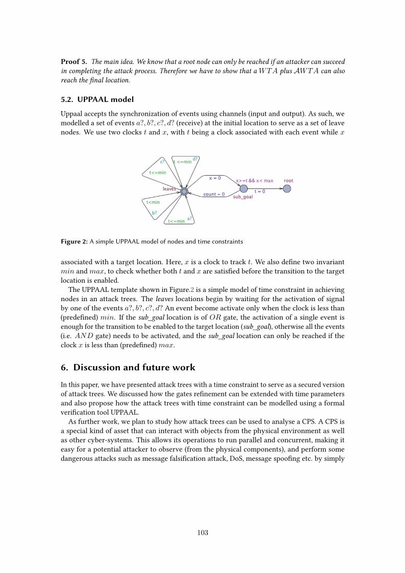
Proof 5. The main idea. We know that a root node can only be reached if an attacker can succeedin completing the attack process. Therefore we have to show that a 𝑊𝑇𝐴 plus 𝒜𝑊𝑇𝐴 can alsoreach the final location.

5.2. UPPAAL model

Uppaal accepts the synchronization of events using channels (input and output). As such, wemodelled a set of events 𝑎?, 𝑏?, 𝑐?, 𝑑? (receive) at the initial location to serve as a set of leavenodes. We use two clocks 𝑡 and 𝑥, with 𝑡 being a clock associated with each event while 𝑥

Figure 2: A simple UPPAAL model of nodes and time constraints

associated with a target location. Here, 𝑥 is a clock to track 𝑡. We also define two invariant𝑚𝑖𝑛 and 𝑚𝑎𝑥, to check whether both 𝑡 and 𝑥 are satisfied before the transition to the targetlocation is enabled.

The UPPAAL template shown in Figure.2 is a simple model of time constraint in achievingnodes in an attack trees. The leaves locations begin by waiting for the activation of signalby one of the events 𝑎?, 𝑏?, 𝑐?, 𝑑? An event become activate only when the clock is less than(predefined) 𝑚𝑖𝑛. If the sub_goal location is of 𝑂𝑅 gate, the activation of a single event isenough for the transition to be enabled to the target location (sub_goal), otherwise all the events(i.e. 𝐴𝑁𝐷 gate) needs to be activated, and the sub_goal location can only be reached if theclock 𝑥 is less than (predefined) 𝑚𝑎𝑥.

6. Discussion and future work

In this paper, we have presented attack trees with a time constraint to serve as a secured versionof attack trees. We discussed how the gates refinement can be extended with time parametersand also propose how the attack trees with time constraint can be modelled using a formalverification tool UPPAAL.

As further work, we plan to study how attack trees can be used to analyse a CPS. A CPS isa special kind of asset that can interact with objects from the physical environment as wellas other cyber-systems. This allows its operations to run parallel and concurrent, making iteasy for a potential attacker to observe (from the physical components), and perform somedangerous attacks such as message falsification attack, DoS, message spoofing etc. by simply

103

adding, blocking or blurring the objects from the physical environment. This kind of threatscannot be captured using attack trees alone. We plan to investigate opacity, a security propertyformalizing the information leakage of a system to an external observer, namely intruder andstudy how it can be used with attack trees.

Acknowledgement

This work was supported by the Slovak Research and Development Agency under the Contractno. APVV-19-0220 (ORBIS) and by the Slovak VEGA agency under Contract no. 1/0778/18(KATO).

References

[1] B. Schneier, Attack trees, Dr. Dobb’s journal 24 (1999) 21–29.[2] S. Mauw, M. Oostdijk, Foundations of attack trees, in: International Conference on

Information Security and Cryptology, Springer, 2005, pp. 186–198.[3] B. Kordy, L. Piètre-Cambacédès, P. Schweitzer, Dag-based attack and defense modeling:

Don’t miss the forest for the attack trees, Computer science review 13 (2014) 1–38.[4] C.-W. Ten, C.-C. Liu, G. Manimaran, Vulnerability assessment of cybersecurity for scada

systems, IEEE Transactions on Power Systems 23 (2008) 1836–1846.[5] D. Beaulaton, N. B. Said, I. Cristescu, S. Sadou, Security analysis of iot systems using attack

trees, in: International Workshop on Graphical Models for Security, Springer, 2019, pp.68–94.

[6] F. Xie, T. Lu, X. Guo, J. Liu, Y. Peng, Y. Gao, Security analysis on cyber-physical systemusing attack tree, in: 2013 Ninth International Conference on Intelligent InformationHiding and Multimedia Signal Processing, IEEE, 2013, pp. 429–432.

[7] M. A. Siddiqi, R. M. Seepers, M. Hamad, V. Prevelakis, C. Strydis, Attack-tree-based threatmodeling of medical implants., in: PROOFS@ CHES, 2018, pp. 32–49.

[8] A. Roy, D. S. Kim, K. S. Trivedi, Attack countermeasure trees (act): towards unifying theconstructs of attack and defense trees, Security and Communication Networks 5 (2012)929–943.

[9] A. T. Ali, D. P. Gruska, Attack protection tree., in: CS&P, 2019.[10] F. Arnold, D. Guck, R. Kumar, M. Stoelinga, Sequential and parallel attack tree modelling,

in: International Conference on Computer Safety, Reliability, and Security, Springer, 2014,pp. 291–299.

[11] X. Ji, H. Yu, G. Fan, W. Fu, Attack-defense trees based cyber security analysis for cpss,in: 2016 17th IEEE/ACIS International Conference on Software Engineering, ArtificialIntelligence, Networking and Parallel/Distributed Computing (SNPD), IEEE, 2016, pp.693–698.

[12] A. T. Ali, Simplified timed attack trees, in: International Conference on Research Challengesin Information Science, Springer, 2021, pp. 653–660.

[13] X. Ou, A. Singhal, Attack graph techniques, in: Quantitative Security Risk Assessment ofEnterprise Networks, Springer, 2012, pp. 5–8.

104

[14] R. Alur, Timed automata, in: International Conference on Computer Aided Verification,Springer, 1999, pp. 8–22.

[15] B. Berthomieu, M. Diaz, Modeling and verification of time dependent systems using timepetri nets, IEEE transactions on software engineering 17 (1991) 259.

[16] L. S. Shapley, Stochastic games, Proceedings of the national academy of sciences 39 (1953)1095–1100.

[17] K. Lounis, S. Ouchani, Modeling attack-defense trees’ countermeasures using continuoustime markov chains, in: International Conference on Software Engineering and FormalMethods, Springer, 2020, pp. 30–42.

[18] R. Kumar, E. Ruijters, M. Stoelinga, Quantitative attack tree analysis via priced timedautomata, in: International Conference on Formal Modeling and Analysis of TimedSystems, Springer, 2015, pp. 156–171.

[19] O. Gadyatskaya, R. R. Hansen, K. G. Larsen, A. Legay, M. C. Olesen, D. B. Poulsen, Modellingattack-defense trees using timed automata, in: International Conference on FormalModeling and Analysis of Timed Systems, Springer, 2016, pp. 35–50.

[20] R. R. Hansen, P. G. Jensen, K. G. Larsen, A. Legay, D. B. Poulsen, Quantitative evaluationof attack defense trees using stochastic timed automata, in: International Workshop onGraphical Models for Security, Springer, 2017, pp. 75–90.

[21] I. A. Tøndel, M. G. Jaatun, M. B. Line, Threat modeling of ami, in: Critical InformationInfrastructures Security, Springer, 2013, pp. 264–275.

[22] A. E. M. AL-Dahasi, B. N. A. Saqib, Attack tree model for potential attacks against thescada system, in: 2019 27th Telecommunications Forum (TELFOR), IEEE, 2019, pp. 1–4.

[23] D. Ray, The time structure of self-enforcing agreements, Econometrica 70 (2002) 547–582.[24] J. Padhye, V. Firoiu, D. Towsley, J. Kurose, Modeling tcp throughput: A simple model

and its empirical validation, in: Proceedings of the ACM SIGCOMM’98 conference onApplications, technologies, architectures, and protocols for computer communication,1998, pp. 303–314.

[25] P. Bulychev, A. David, K. G. Larsen, M. Mikučionis, D. B. Poulsen, A. Legay, Z. Wang,Uppaal-smc: Statistical model checking for priced timed automata, arXiv preprintarXiv:1207.1272 (2012).

105

Extended Abstract: Simulation of Interactionsbetween BeehivesVolha Taliaronak1, Heinrich Mellmann1 and Verena V. Hafner1

1Humboldt University of Berlin, Unter den Linden 6, Berlin, 10117, Germany

AbstractThe interdisciplinary EU project HIVEOPOLIS aims to develop a new generation of intelligent beehivewhich might help bees in coping with adverse environmental factors. As a part of the HIVEOPOLISproject, this extended abstract reports on our ongoing work on the simulation of a decision-makingprocess based on interactions between HIVEOPOLIS units and bee colonies which are not equippedwith HIVEOPOLIS systems using the Mesa simulation framework.

KeywordsMulti-agent systems, Bio-hybrid systems, HIVEOPOLIS

1. Introduction

The impact of humans on the environment is difficult to exaggerate. Habitats of different specieshave been reduced, transformed or damaged as a result of monocultural agriculture, pesticidepollution, etc [1]. These changes in addition to colony diseases dramatically affect insectsincluding bees. As a result, one of the concerning issues has become the sharing of valuablefood sources, such as pollen and nectar as well as the limited habitat between native bee speciesand honeybees, as invasive species [2, 3].

The interdisciplinary EU project HIVEOPOLIS aims to develop a new generation of intelligentbeehive which might help bees in coping with these adverse environmental factors and providea synergistic added value to the colony, to its owner, and to the ecosystem in general [4, 5]. Theintelligent beehives will form connected bio-hybrid systems. One concrete example is an activeselection of foraging grounds, which could enable a mutually beneficial distribution of resourcesamong several beehives and avoidance of areas affected by pesticides. Bees communicatebeneficial foraging locations through a specific waggle dance [5, 6]. A HIVEOPOLIS beehive willbe equipped with a technology, which enables decoding, suppressing and imitating such dancesand allows the system to actively influence the foraging locations of the bees [5, 6]. A prototypeof such robot, called RoboBee, was introduced in [6]. And as observed in [7], HIVEOPOLIS unitmay incorporate one or more dancing robots which interact with honeybees to communicatethem directions to floral resources. From that perspective a bio-hybrid HIVEOPOLIS beehivecan be seen as an autonomous robot making autonomous decisions and negotiating with other

CS&P 2021: 29th International Workshop on Concurrency, Specification and Programming" [email protected] (V. Taliaronak); [email protected] (H. Mellmann);[email protected] (V. V. Hafner)� 0000-0001-8150-024X (V. Taliaronak)



106

beehives, e.g., send the bees to a particular region or, potentially, prevent them from harvestingin another.

Bees are able to exhibit complex swarm behaviors like decentralized target selection andworkload balancing [8]. A decision mechanism steering the behavior of a whole bee swarmrequires a model describing how waggle dances generated by robots which mimic honeybeeswould influence the behavior of the bees and their interaction with the environment. The firstresults of such modeling experiments for foraging choices in a bee swarm were introduced in[7] where the authors investigate the effect of robots on the hive’s foraging decisions using amathematical model. Further, such models can form a basis for a decision process based onanticipation as described in [9].

In this paper we introduce a proof of concept rule-based decision-making process and simu-late behavior of bees’ colonies and their interaction with the environment using agent basedmodeling approach. We aim to simulate different scenarios and study direct and indirectinteractions between native bee colonies and honeybee colonies with integrated external regu-lation mechanisms and gain insights about possible competitive factors as well as cooperativestrategies.

2. Modeling Methods

Behavior and interactions are the two key issues for modeling ecosystem organization. Usingthe Mesa framework [10], we direct our attention on a simulation of a decision-making processbased on the interactions between agents (bees) and the environment, while bee agents’ behavioris reduced to honeybees’ foraging behavior, and the surrounding landscape is modeled as asimplified forage map [11].

2.1. Mesa

In comparison to the other well-known simulation tools, like NetLogo [12] and Mason [13],this framework has several competitive advantages. First of all, it is python-based and can beextended with modern python libraries and other python-based tools (e.g., Jupyter Notebookand Pandas tools) in order to create more complex simulations or analyse collected data. Thecollected data can be stored in a JSON or Pandas DataFrame format for further analysis. Second,Mesa consists of decoupled components, which can be replaced or used independently fromeach other. Third, visualization is browser-based, which provides additional opportunities forsharing of visualisation via the Internet. Since all components in the Mesa framework aredecoupled, visualisation modules can be customized, extended, replaced, or removed.

2.2. Simulation

The environment of our simulations is discrete, modeled as a squared grid, with three types ofagents: bee, beehive, and field. The beehives are modeled as hierarchical multi-agent systemwhich consists of two levels: bees’ level and beehives’ (or colonies’) level. A bee swarm isconsidered to be a multi-agent system with a non-hierarchical structure, where every bee ismodeled as a separate agent. On the other hand, every beehive itself is considered an agent.

107

Despite the fact that HIVEOPOLIS unit has been conceived and, in reality, may be designed as arobotic honeybee imitating waggle dancing, in our simulations we implemented HIVEOPOLISunit on the beehives’ level as a separate type of beehive agent. Figure 1 (Right) demonstratesone of our simulations, which consists of two beehives ((1) is a beehive with an integratedHIVEOPOLIS unit and (2) is a wild beehive) with bees (e.g., (6), (7)) and three possible foodsources ((3), (4), (5)), green-colored cells represent field agents without available food sources. Forthe sake of simplicity, we do not model the whole complex social organisation of an individualcolony, ignore the diversity of bees’ casts (workers, drones, queen) and food sources (nectar,pollen, water). Bee and beehive agents are described with a limited number of parameters (e.g.,maximum flying distance, collected amount of food, coordinates of a known field, abundanceof a field, etc). Floral sources are described using only three relevant parameters: amount ofavailable resources, blooming tag, flowering period. We simulate agents’ movements as discreteevents. An activation order of agents is randomized in order to reduce its impact on the model.

Figure 1: Simulation of the environment with two beehives. Left: graphs of collected food for eachbeehive. Right: a 2D view of the environment.

We implemented two foraging strategies for bees agents: random foraging search and targetedforaging on the known floral patch. We also considered two different interaction strategies be-tween agents. The first one, a direct interaction, occurs on the bees’ level, when the informationabout known foraging resources is communicated between simulated bees from one colony. So,for instance, the wild bees start with the random search strategy, as seen in Figure 1 (Right).After a discovery of a field with available floral resources (e.g., field (3) in Figure 1 (Right)), thebees return back to the hive and share the information about the found floral resource withother bees which are also in the hive. Bees might follow the communicated directions, in thiscase, they switch to the targeted foraging strategy, but might also ignore this information aboutthe found food sources. The second one, an indirect interaction, occurs on the beehives’ level,where the internal robot is supposed to define the most optimal food source and communicateit to the bees. This type of interactions is implemented only in the beehives with HIVEOPOLISunits. We assume that it will make autonomous decisions regarding optimal foraging sources

108

based on information about the surrounding landscape, weather and other information receivedfrom the external sources as well as its predictions about behavior of the other beehives fromthe surroundings. The implementation details of the HIVEOPOLIS’ interior robot are outsidethe scope of this work. In our simulations, the optimal fields are determined using rule-baseddecision-making approach which is based on three parameters: a distance parameter, a floweringperiod of fields, and an abundance of fields. In every simulation step, it is checked if thereare any bees in the hive. If there are any, then a new optimal field is being calculated on thebeehive’s level and communicated to the bees on the bees’ level. Also a decision, to follow thecommunicated coordinates or ignore them is being simulated on the bees’ level. Data generatedduring simulation is displayed in the real-time mode in the live chart (see Figure 1 (Left)), the xaxis shows the number of simulation steps, the y axis – the foraging dynamics of the modeledhives.

3. Results and Discussion

Bees are not only important pollinators but also a prime example of swarm intelligence [8]. Suchmodeling tools, like BEESCOUT [11] and BEEHAVE [14], can be useful for better understandingand exploration of the possible realistic scenarios of colony natural dynamics, bees’ searchingbehavior in habitats with different landscape configuration as well as interactions betweenbees. Nevertheless, these tools are NetLogo based and cannot be applied for simulations ofinteractions between several colonies.We are not the first, who is aiming to simulate decision-making processes in bees’ swarms.A multi-agent simulation able to simulate the dynamics of honeybee nectar foraging wasconducted using NetLogo tool and introduced in [8]. The authors implemented experimentsreported in [15] and other works of T. Seeley, who investigated decision-making mechanismswithin bee swarm.Nonetheless, in our work, we aim to model and simulate decision-making processes not onlywithin one colony, as it was done in [15, 8], but in a system of beehives and HIVEOPOLISunits. For this reason, we examined the factors relevant for a selection process of foragingsources. In [15] the authors highlighted three main factors, which are being considered during aprocess of choosing nectar sources: distance, quality and the abundance of the food. The factorsdetermining the quality of food sources are, for instance, difficulty of feeding at the source,direction in relation to the wind, and the colony’s need for food, etc [15]. In our first attempt ofsimulations, we focus on a distance from hive and abundance of patches. We also added onemore parameter, which was not mentioned by [15], but can be relevant for our purposes, –flowering period of floral patches. Quality of food resources is a complex factor which is hardto capture and implement without any real data. Nonetheless, we hope to find a way how tointegrate this parameter in our further simulation scenarios.A HIVEOPOLIS bio-hybrid system could serve as a mechanism for implementing interactionson the beehive level and having an influence on the colony decisions regarding chosen foodresources. Such centralized control mechanism might be beneficial for cases in which severalbee colonies have to share limited floral resources, floral resources are difficult to discover dueto the morphology of the beehive surrounding area, or a gentle way to redirect the bees to

109

the desired fields is required. It might be a feasible path to make safer or ecologically moreimportant food sources more attractive to bees, even if these sources are energetically lessprofitable [7].Our simulations don’t capture the whole complexity of a decision-making process yet. We aregoing to continue our work on simulations with different combinations of possible competitivefactors such as a food diversity. We consider evaluation of collected data to be a non-trivial task,which will require expertise from other scientific fields. The collected data are strongly affectedby the parameters (e.g., number of bees per hive), which are relative values. Nevertheless,all parameters can be changed without much extra effort. Simulation experiments have lowcomputational cost and can be run repeatedly.

4. Conclusion

Mesa is a convenient, powerful tool, which provides a solid base functionality for easy andcomfortable simulation implementations as well as enough capabilities for customization ofcreated models and their visualisation. Since the framework is based on Python, it might beadvantageous and handy for a wide range of researchers.Multi-agent systems are useful for problems integrating social and spatial aspects and suitablefor simulation of complex systems. Models and simulations of beehives have been studied for along time, so that we can draw experience from a rich library of literature. The novel directionof this work is the study of the simulation scenarios as a basis for a decision mechanism, whichwould allow a bio-hybrid beehive to act autonomously in a way beneficial to itself and itsenvironment. Our preliminary results have shown coherent behaviors of the whole simulation,nevertheless, the model parameters require further tuning and scientific justification. Ourfurther work will be focused on extension and improving of the existing simulation model. Inorder to increase credibility of our simulations, we aim to utilise geospatial data. The goal is tointegrate an augmented map of a landscape and model the distribution of the floral resourcesand landscape features more precisely. Further, we are planning on collecting additional dataand storing it in DataFrame format for further analysis using modern data science libraries.

Acknowledgments

This work was supported by the EU H2020 program under grant agreement No. 824069(HIVEOPOLIS).

References

[1] O. Komasilova, V. Komasilovs, A. Kviesis, N. Bumanis, H. Mellmann, A. Zacepins, Modelfor the bee apiary location evaluation, Agronomy Research 18 (2020) 1350–1358. doi:10.15159/AR.20.090.

[2] A. Hudewenz, A.-M. Klein, Competition between honey bees and wild bees and the role ofnesting resources in a nature reserve, Journal of Insect Conservation 17 (2013) 1275–1283.doi:10.1007/s10841-013-9609-1.

110

[3] C. Rasmussen, Y. L. Dupont, H. B. Madsen, P. Bogusch, D. Goulson, L. Herbertsson, K. P.Maia, A. Nielsen, J. M. Olesen, S. G. Potts, S. P. M. Roberts, M. A. K. Sydenham, P. Kryger,Evaluating competition for forage plants between honey bees and wild bees in denmark,PLOS ONE 16 (2021) 1–19. doi:10.1371/journal.pone.0250056.

[4] CORDIS, Futuristic beehives for a smart metropolis, 2019. URL: https://cordis.europa.eu/project/id/824069.

[5] A. Ilgün, K. Angelov, M. Stefanec, S. Schönwetter-Fuchs, V. Stokanic, J. Vollmann, D. N.Hofstadler, M. H. Kärcher, H. Mellmann, V. Taliaronak, A. Kviesis, V. Komasilovs, M. A.Becher, M. Szopek, D. M. Dormagen, R. Barmak, E. Bairaktarov, M. Broisin, R. Thenius,R. Mills, S. C. Nicolis, A. Campo, A. Zacepins, S. Petrov, J.-L. Deneubourg, F. Mondada,T. Landgraf, V. V. Hafner, T. Schmickl, Bio-hybrid systems for ecosystem level effects, in:Proceedings of the ALIFE 2021: The 2021 Conference on Artificial Life, MIT Press Direct,Virtual (formerly Prague), Czech Republic, 2021. doi:10.1162/isal_a_00396.

[6] T. Landgraf, D. Bierbach, A. Kirbach, R. Cusing, M. Oertel, K. Lehmann, U. Greggers,R. Menzel, R. Rojas, Dancing honey bee robot elicits dance-following and recruits foragers,2018. URL: https://arxiv.org/abs/1803.07126.

[7] D. Lazic, T. Schmickl, Can robots inform a honeybee colony’s foraging decision-making?,in: Proceedings of the ALIFE 2021: The 2021 Conference on Artificial Life, MIT PressDirect, Virtual (formerly Prague), Czech Republic, 2021. doi:10.1162/isal_a_00397.

[8] T. Schmickl, K. Crailsheim, Costs of environmental fluctuations and benefits of dynamicdecentralized foraging decisions in honey bees, in: C. Anderson, T. Balch (Eds.), The 2ndInternational Workshop on the Mathematics and algorithms of Social Insects Proceedings,Georgia Institute of Technology, Atlanta, GA, 2003, pp. 145–152.

[9] H. Mellmann, B. Schlotter, L. Musiolek, V. V. Hafner, Anticipation as a mechanism forcomplex behavior in artificial life, in: Proceedings of the ALIFE 2020: The 2020 Conferenceon Artificial Life, MIT Press Direct, Virtual (formerly Prague), Czech Republic, 2020, pp.157–159. doi:10.1162/isal_a_00314.

[10] J. Kazil, D. Masad, A. Crooks, Utilizing python for agent-based modeling: The mesaframework, in: R. Thomson, H. Bisgin, C. Dancy, A. Hyder, M. Hussain (Eds.), Social,Cultural, and Behavioral Modeling, volume 12268 of Lecture Notes in Computer Science,Springer, Cham, 2020, pp. 308–317. doi:10.1007/978-3-030-61255-9_30.

[11] M. A. Becher, V. Grimm, J. Knapp, J. Horn, G. Twiston-Davies, J. L. Osborne, Beescout: Amodel of bee scouting behaviour and a software tool for characterizing nectar/pollen land-scapes for beehave, Ecological Modelling 340 (2016) 126–133. doi:10.1016/j.ecolmodel.2016.09.013.

[12] S. Tisue, U. Wilensky, Netlogo: A simple environment for modeling complexity, in:C. Anderson, T. Balch (Eds.), The International Conference on Complex Systems, Boston,MA, USA, 2004.

[13] S. Luke, C. Cioffi-Revilla, L. Panait, K. M. Sullivan, G. Balan, Mason: A multi-agentsimulation environment, SIMULATION 81 (2005) 517–527.

[14] M. A. Becher, V. G. P. Thorbek, J. Horn, P. J. Kennedy, J. L. Osborne, Beehave: a systemsmodel of honeybee colony dynamics and foraging to explore multifactorial causes of colonyfailure, Journal of Applied Ecology 51 (2014) 470–482. doi:10.1111/1365-2664.12222.

[15] T. Seeley, S. Camazine, J. Sneyd, Collective decision-making in honey bees: How colonies

111

choose among nectar sources, Behavioral Ecology and Sociobiology 28 (1991) 277–290.doi:10.1007/BF00175101.

112

Extended Abstract: A Novel Mobile App for the NextGeneration of BeekeepersEugen Puzynin1, Heinrich Mellmann1 and Verena V. Hafner1

1Humboldt University of Berlin, Unter den Linden 6, Berlin, 10117, Germany

AbstractIn this extended abstract, the authors report the ongoing work on a new mobile app for beekeepers. It isvery important for beekeepers - especially for those who are in search of new locations for their beehives- to know the current situation in the immediate vicinity. This work presents a mobile applicationsuitable for beekeepers to view weather and air quality data and, in particular, what people in thenearby area have annotated.

KeywordsBeekeeping, Mobile App, Prototype, HIVEOPOLIS

1. Introduction

Beekeepers pollinate many crop plants with their bees. Most important crops depend to somedegree of pollination from the most important species for crop pollination: the western honeybee. Honey production is also an important source of income in many rural communities[1]. Often forgotten are the wild bees, who are responsible for pollinating garden plants andwildflowers. Honey bees are linked to the spread of diseases to wild pollinators via sharedflowers. They can also out-compete with native pollinators for resources and food [2]. Othermodern challenges for bees are pesticides, parasites, climate change and a lack of flowers [3].According to the World Health Organization, an estimated seven million people die each yearfrom air pollution [4]. Since bees rely on their sense of smell to identify different flowers, airpollution is affecting them too. Air pollution masks the scent molecules from plants. This makesbees forage longer leading them to become ineffective pollinators because of the decreasedreproductive output and the amount of pollen flow in flowering plants [5]. Another studyobserved a reduction in pollinator survival as well as significant molecular and physiologicalchanges [6]. In order to fight these challenges, the authors created a prototype in the form of amobile app. Beekeepers should monitor climate and air conditions to keep bees and themselveshealthy. Managed honey bee hives should not be placed in protected areas, where a risk wouldexist of wild bees being driven away or attacked. More plants are required to address the plantshortage and help wild insects. The map-based app uses current technologies, with whichnon-beekeepers can help beekeepers by marking spots on the map. The whole utilization

CS&P 2021: 29th International Workshop on Concurrency, Specification and Programming" [email protected] (E. Puzynin); [email protected] (H. Mellmann);[email protected] (V. V. Hafner)



113

process is simplified for all users with features such as identifying plant species via photos andshowing which plants are suitable for bees.

The development of a new app is part of the HIVEOPOLIS project [7, 8]. HIVEOPOLIS intendsto provide honeybee colonies with technology (internet, databases, satellite data and robots)that would otherwise be unavailable to them.

2. Methodology

The goals of developing the app consists of three main components:

1. An interactive augmented map shows key elements of weather and air quality for bee-keepers.

2. Users must be able to make inputs and help beekeepers with it.3. It should be simple and swiftly to use.

The application was developed as a native iOS app in the programming language Swift withthe integrated development environment Xcode. One reason mobile app development waspreferred is access to the camera for various functions, such as photographing plants for plantidentification. Furthermore, GPS data is required in case a user of the app wants to get directionsto the next destination of his hives. Apple’s MapKit was used natively for the app’s interactivemap. This allows users to see the map as a satellite view in 2D or 3D. OpenWeather provideswith its API the current and forecast weather as well as air pollution data for all coordinates.The air pollution values are currently based on the European Air Quality Index. A pretrainedconvolutional neural network was used for the flower recognition function: Oxford’s 102 FlowerDataset with 102 categories, each 40 - 200 images, allows to take a picture of any flower andit tries to recognise the flower’s name [9]. Users can have their own account with email andpassword, which are stored and encrypted on Google’s Firestore servers. The cloud database isinstantly accessible, which means saved data is instantly available for other users. For example,registered users are able to send chat messages and save annotations. An API from Wikipediawas used to retrieve flower data, allowing users to look up information about any flower.

3. Results and Discussion

A preliminary user evaluation had been created as an online survey. A total of 26 peopleparticipated in it, 15 were beekeepers and 11 were non-beekeepers. They assisted in revisingthe design and generated ideas for new functionalities. After this evaluation an alpha test wasmade. Sergey Petrov from the company Pollenity asked 22 Bulgarian beekeepers to test the appon an iPhone and give feedback. Each member of the group spent between 1 and 10 minutestesting the app. The methodology of the test included a short verbal presentation and a videotutorial on how to use the app. In the following pictures, you can see the app. Figure 1 depictsan impression of the app. (Left) shows markers on the map that have theoretically been set byusers. Potential beekeeping locations are depicted here, along with plants of interest to bees. Forexample, a beekeeper can see where other beekeepers are in the vicinity, if they have marked achosen location as already been occupied by the beekeeper, and where beekeepers should pay

114

attention to the protection of wild bees. (Right) shows the current weather with temperature,humidity, air speed, UV index, as well as the current air quality values.

Figure 1: View of the application. Left: overview with annotations. Buttons: hamburger menu withmore functions; set focus to a specific city; adding and deleting annotations. Right: Slide up menu withcurrent weather and pollution data. Buttons here are the search button for displaying information ofa specific plant; camera for shooting pictures; tomorrow for future weather and air quality; current forweather and air quality at the moment.

4. Conclusion

The preliminary user evaluation and the alpha test confirmed that such an app could be of interestto beekeepers and environmentalists. The next steps would be to define some corrections tothe design and then test it again as a beta version to get further constructive feedback. Furtherevaluation is needed to collect more meaningful reactions and constructive criticism frombeekeepers to be able to improve the app. Current ideas for improvements are: The mostimportant point is the implementation of Android. Another important point is localization,so that the app works all over the world without language barriers. The authors are alsoconsidering how gamification can be integrated to motivate users and bind them to the app.Furthermore, there are still a lot of functions that could be implemented. For example, the

115

flowering times of the respective plants, so that beekeepers know when the flowers are usablefor them. And uploadable images so that users can see more of what the location looks like.After some testing and improvements, the app could be made available to the public.

Acknowledgments

This work was supported by the EU H2020 program under grant agreement No. 824069(HIVEOPOLIS).

References

[1] Ashley N. Mortensen at el. European honey bee apis mellifera linnaeus and subspecies(insecta: Hymenoptera: Apidae). UF/IFAS Extension, EENY568, August 2013

[2] Jonas Geldmann and Juan P. González-Varo. Conserving honey bees does not help wildlife.Science, 359(6374):392–393, January 2018

[3] Dave Goulson at el. Bee declines driven by combined stress from parasites, pesticides, andlack of flowers. Science, 347(6229), March 2015

[4] Air pollution in the Western Pacific https://www.who.int/westernpacific/health-topics/air-pollution Last access 1 July 2021

[5] Quinn S. McFrederick et al. Air pollution modifies floral scent trails. Atmospheric Environ-ment, 42(10):2336–2348, March 2008

[6] Geetha G. Thimmegowda et al. A field-based quantitative analysis of sublethal effects ofair pollution on pollinators. Proceedings of the National Academy of Sciences, 117(34),August 2020

[7] Futuristic Beehives For A Smart Metropolis https://cordis.europa.eu/project/id/824069 Lastaccess 1 July 2021

[8] Asya Ilgün et al. Bio-Hybrid Systems for Ecosystem Level Effects in Proceedings of theArtificial Life Conference 2021 (ALIFE 2021) (to appear)

[9] Nilsback, M-E. and Zisserman, A. Automated flower classification over a large number ofclasses Proceedings of the Indian Conference on Computer Vision, Graphics and ImageProcessing (2008) https://www.robots.ox.ac.uk/~vgg/data/flowers/102/

116

Efficient Machine Learning Methodsover Pairwise Space (keynote)Hung Son Nguyen

University of Warsaw

KeywordsRough sets, Support Vector Machine, Factorization Machine, Distance Metric Learning, Context-AwareRecommendation

Extended Abstract

In recent years many machine learning concepts and methods were developed on the set ofpairs of objects. In this paper, the set of all pairs of objects is called the pairwise space. Let usnotice that if the set of objects 𝒳 = {x1,x2, . . . ,x𝑛} consists of 𝑛 instances, then the pairwisespace contains 𝑂(𝑛2) pairs. Thus why the straightforward implementations of those methodsare not applicable for big data sets with millions of objects.

The main concepts in rough set theory (RS) such as reducts, lower and upper approximations,decision rules or discretizations have been defined in term of the discernibility matrix, whichis a form of the pairwise space [1]. For example, in minimal decision reduct problem, we arelooking for the minimal subset of features that preserves the discernibility between objectsfrom different decision classes [2].

Support Vector Machine (SVM) is also a classification method described as an optimizationproblem over the pairwise space [3]. The initial idea of looking for the linear classifier withthe maximal margin were transformed into the problem of looking for a set of coefficients𝛼 = (𝛼1, 𝛼2, · · · , 𝛼𝑛) related to objects that maximizes an objective function

𝑊 (𝛼) =∑

𝑖

𝛼𝑖 −1

2

∑

𝑖,𝑗

𝑦𝑖𝑦𝑗𝛼𝑖𝛼𝑗𝐾(𝑥𝑖, 𝑥𝑗).

defined on the set of dot products of all pairs of objects. In the above formula 𝑦𝑖 denotes thedecision class of the object x𝑖 and 𝐾 is a kernel function chosen by the user.

Distance Metric Learning (DML) [4] is a machine learning discipline that looks for the bestdistance function (also divergence or similarity ) from certain available information aboutsimilarity measures between different pairs or triplets of data. These similarities are determined

29th International Workshop on Concurrency, Specification and Programming (CS&P’21)$ [email protected] (H. S. Nguyen)� 0000-0002-3236-5456 (H. S. Nguyen)



117

by the sets

𝑆 = {(x𝑖,x𝑗) ∈ 𝒳 × 𝒳 : x𝑖 and x𝑗 are similar.}𝐷 = {(x𝑖,x𝑗) ∈ 𝒳 × 𝒳 : x𝑖 and x𝑗 are not similar.}𝑅 = {(x𝑖,x𝑗 ,x𝑙) ∈ 𝒳 × 𝒳 × 𝒳 : x𝑖 is more similar to x𝑗 than to x𝑙.}

With these data and similarity constraints, the problem to is to look for those distance functions(belonging to a predefined family of distances 𝒟) that minimize a certain loss function ℓdetermined on the base of the sets 𝑆,𝐷 and 𝑅. In other words, the objective of DML is to solvethe optimization problem

min𝑑∈𝒟

ℓ(𝑑, 𝑆,𝐷,𝑅)

In recent years, many efficient implementations for the mentioned above disciplines havebeen proposed and developed. Most of them are based either on the approximation idea [5], [6]or deep learning [7].

Context aware recommendation systems is another machine learning concept that weredefined on the pairwise space which was in fact defined as a regression problem over the set oftransaction pairs [8].

In this talk we compare different techniques for the mentioned above machine learningconcepts and we will pay an attention on application of factorization machine (FM). Thismethod has been successfully applied for context aware recommendation systems [9]. Themain idea is to transform the optimization problem established on the pairwise space intoan equivalent problem where the time complexity for each iteration has been reduced fromquadratic time into linear time [10]. We will show that factorization machine can be also appliedfor some problems in rough set theory, SVM or distance metric learning.

References

[1] Z. Pawlak, Rough sets, International Journal of Information and Computer Sciences 11(1982) 341–356.

[2] Z. Pawlak, A. Skowron, Rudiments of rough sets, Information Sciences 177 (2007) 3–27.[3] C. Cortes, V. Vapnik, Support vector networks, Machine Learning 20 (1995) 273–297.[4] J.-L. Suárez, S. García, F. Herrera, A tutorial on distance metric learning: Mathematical

foundations, algorithms, experimental analysis, prospects and challenges, Neurocomputing425 (2021) 300–322.

[5] H. S. Nguyen, Approximate Boolean Reasoning: Foundations and Applications in DataMining, Springer-Verlag, Berlin, Heidelberg, 2006, p. 334–506.

[6] T. Joachims, Learning to Classify Text Using Support Vector Machines – Methods, Theory,and Algorithms, Kluwer/Springer, 2002.

[7] P. H. Barros, F. Queiroz, F. Figueredo, J. A. dos Santos, H. S. Ramos, A new similarityspace tailored for supervised deep metric learning, CoRR abs/2011.08325 (2020). URL:https://arxiv.org/abs/2011.08325. arXiv:2011.08325.

118

[8] S. Rendle, Z. Gantner, C. Freudenthaler, L. Schmidt-Thieme, Fast context-aware rec-ommendations with factorization machines, in: Proceedings of the 34th InternationalACM SIGIR Conference on Research and Development in Information Retrieval, SIGIR’11, Association for Computing Machinery, New York, NY, USA, 2011, p. 635–644. URL:https://doi.org/10.1145/2009916.2010002. doi:10.1145/2009916.2010002.

[9] X. Xin, B. Chen, X. He, D. Wang, Y. Ding, J. Jose, Cfm: Convolutional factorizationmachines for context-aware recommendation, in: Proceedings of the Twenty-EighthInternational Joint Conference on Artificial Intelligence, IJCAI-19, International JointConferences on Artificial Intelligence Organization, 2019, pp. 3926–3932. URL: https://doi.org/10.24963/ijcai.2019/545. doi:10.24963/ijcai.2019/545.

[10] S. Rendle, Factorization machines with libfm, ACM Trans. Intell. Syst. Technol. 3 (2012)57:1–57:22. URL: http://doi.acm.org/10.1145/2168752.2168771. doi:10.1145/2168752.2168771.

119

Influence of Data Dimension Reduction, Feature Scaling andActivation Function on Machine Learning Performance

Grzegorz Słowiński

University of Technology and Economics, ul. Jagiellońska 82f, 03-301 Warsaw, Poland

Abstract

A dataset containing over 13k samples of dry beans geometric features is beinganalysed using machine learning (ML) and deep learning (DL) techniques withthe goal to automatically classify the bean specie. The obtained geometrical datahas quite a lot redundancy. Many features are strongly correlated. This workanalyses the influence of data dimension reduction (DDR) (elimination of excessstrongly correlated features) and features scaling (FS), often callednormalization, on the machine learning performance (measured in terms ofaccuracy and approximate training time). Additionally also an influence ofactivation function (sigmoid vs. ReLU) on artificial neural network performancehas been checked.

Keywords 1

machine learning, deep learning, data dimension reduction, features scaling, activationfunction

1. Introduction

Classification of dry beans is of some economic importance. Manual classification is labourintensive, etc. Over 13 k samples of dry beans of 7 various species were photographed and theirgeometry was measured via computer vision techniques in [1]. Then the set was analysed via severalmachine learning (or data science) and deep learning (or artificial neural network) techniques. Theoverall accuracy obtained was 87.92-93.13%, depending on technique used.

The dataset used in [1] has been published in the UCI machine learning repository [2]. In thiswork, a collection of beans was used as material for investigation how machine learning process isinfluenced by the following factors: 1) data dimension reduction, 2) features scaling (or datanormalization) and 3) in case of neural networks, how their performance depends on activationfunction used (ReLU vs. sigmoid).

The research question examined in this work is: How do data dimension reduction, feature scalingand activation function influence machine learning performance? The above question is related toconcurency, specification and programming in the following way. Among topics of CS&P 2021 onecan find: Model checking and testing - this work checks different ML models, knowledge discoveryand data mining - machine learning belong to this field, soft computing - artificial neural networks areare categorized as a kind of soft-computing.

1.1. Data Dimension Reduction

129th International Workshop on Concurrency, Specification and Programming (CS&P'21)EMAIL: [email protected] ORCID: 0000-0001-9770-5063

© 2021 Copyright for this paper by its author.Use permitted under Creative Commons License Attribution 4.0 International (CC BY 4.0).

CEUR Workshop Proceedings (CEUR-WS.org) CEURWorkshopProceedings

http://ceur-ws.orgISSN 1613-0073

120

In the work [1] data dimension has not been reduced, although many features are stronglycorrelated. This work investigates the effect of data dimension reduction on performance (computingtime and accuracy).

1.2. Feature scaling

In the handbook [4], page 72 Aurelien Geron, states: "One of the most important transformationsyou need to apply to your data is feature scaling. With few exceptions, Machine Learning algorithmsdon’t perform well when the input numerical attributes have very different scales." This work verifiesthis statement and investigates what ML methods really needs feature scaling.

1.3. Activation Function

In work [1] ANN with sigmoid activation in hidden layers has been applied. This workinvestigates how ANN performance depends on activation function used. Two activation function arecompared: ReLU and sigmoid.

2. Tools

The entire analysis was done using Python and its ML frameworks: numpy, pandas, matplotlib,seaborn, scikit-learn and keras. Google Colab a free cloud version of jupyter notebook was used. Thereader can find the Python scripts under link [3]. Parameters of compute engine used were: Intel(R)Xeon(R) CPU @ 2.30GHz, 12,69 GB RAM, no graphical processing unit (GPU) acceleration.Majority of experiments performed were shallow learning that do not need GPU support. As the drybeans dataset is relatively simple, the artificial neural network (ANN) applied was also rather simpleand GPU support was not crucial for ANN training. Training times were in range from milliseconds toa few minutes.

3. Data

The dataset under study consists of 13611 samples. A sample amounts to 16 geometrical featuresand a label identifying the specie of the bean. The species are as follows: Barbunya, Bombay, Cali,Dermason, Horoz, Seker, and Sira. The features are: Area, Perimeter, MajorAxisLength,MinorAxisLength, AspectRatio, Eccentricity, ConvexArea, EquivDiameter, Extent, Solidity,Roundness, Compactness, ShapeFactor1, ShapeFactor2, ShapeFactor3, and ShapeFactor4. A detailedexplanation how the features were calculated is presented in [1].

Table 1.Correlation between beans features

Area Extent Solidity

Area 1.000 0.967 0.932 0.952 0.242 0.267 1.000 0.985 0.054 -0.197 -0.358 -0.268 -0.848 -0.639 -0.272 -0.356

Perimeter 0.967 1.000 0.977 0.913 0.385 0.391 0.968 0.991 -0.021 -0.304 -0.548 -0.407 -0.865 -0.768 -0.408 -0.429

MajorAxisLength 0.932 0.977 1.000 0.826 0.550 0.542 0.933 0.962 -0.078 -0.284 -0.596 -0.568 -0.774 -0.859 -0.568 -0.483

MinorAxisLength 0.952 0.913 0.826 1.000 -0.009 0.020 0.951 0.949 0.146 -0.156 -0.210 -0.015 -0.947 -0.471 -0.019 -0.264

AspectRatio 0.242 0.385 0.550 -0.009 1.000 0.924 0.243 0.304 -0.370 -0.268 -0.767 -0.988 0.025 -0.838 -0.979 -0.449

Eccentricity 0.267 0.391 0.542 0.020 0.924 1.000 0.269 0.319 -0.319 -0.298 -0.722 -0.970 0.020 -0.860 -0.981 -0.449

ConvexArea 1.000 0.968 0.933 0.951 0.243 0.269 1.000 0.985 0.053 -0.206 -0.362 -0.270 -0.848 -0.641 -0.274 -0.362

EquivDiameter 0.985 0.991 0.962 0.949 0.304 0.319 0.985 1.000 0.028 -0.232 -0.436 -0.328 -0.893 -0.713 -0.330 -0.393

Extent 0.054 -0.021 -0.078 0.146 -0.370 -0.319 0.053 0.028 1.000 0.191 0.344 0.354 -0.142 0.238 0.348 0.149

Solidity -0.197 -0.304 -0.284 -0.156 -0.268 -0.298 -0.206 -0.232 0.191 1.000 0.607 0.304 0.153 0.344 0.308 0.702

Roundness -0.358 -0.548 -0.596 -0.210 -0.767 -0.722 -0.362 -0.436 0.344 0.607 1.000 0.768 0.230 0.783 0.763 0.472

Compactness -0.268 -0.407 -0.568 -0.015 -0.988 -0.970 -0.270 -0.328 0.354 0.304 0.768 1.000 -0.009 0.869 0.999 0.484

ShapeFactor1 -0.848 -0.865 -0.774 -0.947 0.025 0.020 -0.848 -0.893 -0.142 0.153 0.230 -0.009 1.000 0.469 -0.008 0.249

ShapeFactor2 -0.639 -0.768 -0.859 -0.471 -0.838 -0.860 -0.641 -0.713 0.238 0.344 0.783 0.869 0.469 1.000 0.873 0.530

ShapeFactor3 -0.272 -0.408 -0.568 -0.019 -0.979 -0.981 -0.274 -0.330 0.348 0.308 0.763 0.999 -0.008 0.873 1.000 0.484

ShapeFactor4 -0.356 -0.429 -0.483 -0.264 -0.449 -0.449 -0.362 -0.393 0.149 0.702 0.472 0.484 0.249 0.530 0.484 1.000

Peri-meter

Major Axis

Length

Minor Axis

LengthAspect Ratio

Eccentri-city

ConvexArea

Equiv Diameter

Round-ness

Compact-ness

Shape Factor 1

Shape Factor 2

Shape Factor 3

Shape Factor 4

121

Correlation analysis (see table 1) has shown that several of the features are strongly (positively ornegatively) correlated. This is due to the fact that basically all of them are kind of geometricmeasures. In the original work [1] the issue of strong correlation between features has not beenaddressed. Generally strongly (over 0,9) features bring little extra information, so its eliminationshould reduce computational complexity (speed up training) with little if any loss in classificationaccuracy.

It is also sometimes suggested that feature scaling (often called normalization) can improveperformance [4], pages 72-73. This is also investigated. To give a brief visualisation of beans dataset,the pair-plot with selected features (less correlated) has been done, see figure 1.

Figure 1: Pair-plot of selected (low corelated) bean features.

4. Shallow learning results

The methods tried were: Naive Bayes Classifier, Decision Tree, Random Forest, Support VectorClassifier.

4.1.Naive Bayes Classifier

Results for Gaussian naive Bayes classifier are shown in table 2. One can see that DDR or FS hassmall effect on training time. Using DDR or FS (or both) significantly increased accuracy from77.23% to 89.83-91.00%.

122

Table 2. Gaussian naive Bayes classifier performance

Data Accuracy Approx. training time

Full, not scaled 77.23% 18.2 msDimension reduced, not scaled 91.00% 16.3 ms

Full, scaled 89.83% 17.0 msDimension reduced, scaled 90.78% 15.8 ms

4.2.Decision tree

Results for decision tree are shown in table 3. Decision tree applied was limited to 16 leaf nodesand maximum depth of 5. One can see that FS has no effect on accuracy and little effect on trainingtime. This probably connected with the fact that DT analyses one feature at the time, so it not careswhat is the ratio of specific feature range to other features. DDR shorten training time with limitedaccuracy decrease.

Table 3.Decision tree classifier performance


Full, not scaled 88.87% 128 msDimension reduced, not scaled 88.24% 71 ms

Full, scaled 88.87% 129 msDimension reduced, scaled 88.24% 70 ms

Decision tree is known to be sensitive for data “rotation”, see [4] p 188. DT analyses only onefeature at the time. Strongly correlated features gives little extra information, but can presentinformation in a slightly different manner, suitable for decision tree.

4.3.Random Forest Classifier

Results for the random forest (RF) are shown in table 4. The random forest consisted of 150 trees.No limits (max leaves, max depth and etc.) were put on trees. One can observe that training times arelonger that for single decision tree (which is reasonable as here we have a set of decision trees). Theaccuracies are high. DDR shortened training time and allowed for slightly higher accuracy (0,14-0,18% point). This is quite interesting that although DDR slightly reduced accuracy on single tree itimproved accuracy on RF. Similarly to decision tree, SF practically has little effect on training time.

Table 4. Random forest classifier performance


Full, not scaled 93.06% 4.69 sDimension reduced, not scaled 93.24% 2.69 s

Full, scaled 93.10% 4.79 sDimension reduced, scaled 93.24% 2.59 s

4.4.Support Vector Classifier

Results for support vector classifier (SVC) is shown in table 5. Polynomial kernel has been used.Generally SVC is much more “heavier” model than gaussian classifier, decision tree or random forest.Training times much longer. One can see that DDR or FS has small effect on SVC accuracy. DDR on

123

not scaled features reduced training time. Feature scaling significantly increased training time andincreased accuracy a little (about 1% point). The longest training time was observed for DDR and SFdata. The training time was 9 times longer than for DDR and not SF data. The author cannotexplained this effect.

Table 5. Support vector classifier performance


Full, not scaled 91.81% 42 sDimension reduced, not scaled 91.81% 29 s

Full, scaled 93.24% 88 sDimension reduced, scaled 92.95% 266 s

5. Artificial neural network

For an artificial neural network (ANN) the data needs additional treatment. First, the names ofbean species were labelled with numbers and then these numbers 0-6 were codded as so called ”one-hot”. The reason of using ”one-hot” encoding is well explained for example in [5] p. 376 or [6] pp.190-194.

Three experiments has been performed to analyse: 1) influence of data dimension reduction,2) influence of features scaling and 3) influence of activation function (sigmoid vs. ReLU). The ANNarchitecture was kept similar (as much as possible) to described in [1]. All ANNs had 3 hidden layerswith 17, 12, 3, neurons respectively. However here ReLU function has be used as “default” option.Output layer consisted of 7 neurons with softmax activation function – one for each class. Generallytraining lasted for 16 epochs. However, as it was obvious that ANN with sigmoid activation isundertrained, this net was trained for 48 epochs. The training process is presented in figure 2. Theperformance summary is presented in table 6.

Table 6.ANNs performance, 17-12-3 architecture, Adam optimiser, 16 epochs

Data Activationfunction in

hidden layers

Epochs oftraining

Approx. trainingtime

Accuracy

16 features, scaled ReLU 16 14 s 92.66%8 features, scaled ReLU 16 8 s 93.24%8 features, not scaled ReLU 16 9 s 26.74%

8 features, scaled sigmoid 48 41 s 88.14%

It can be visible that:1. feature scaling (or data normalisation) is very important for ANN’s. An attempt to train

without prior data scaling failed. Only 55,82% accuracy has been obtained. Perhaps biggernetwork can manage this issue by rescaling data in a few first layers, but it will influencetraining time and accuracy.

2. ReLU works significantly better than sigmoid function as an activation function. ReLUnetwork trains faster and reaches better accuracy.

3. Data dimension reduction shortens training time nearly by half and increases accuracy byabout 0,58 % point.

124

Figure 2: Training of different ANNs

6. Conclusions

Influence of data dimension reduction, data scaling (or normalisation) and activation function hasbeen investigated. The influence depends on machine learning technique used.

Generally data dimension reduction reduces training time with rather limited influence on accuracyData scaling is a must in case of artificial neural network. Omitting data scaling decreased accuracyfrom about 93% to about 56%. In case of shallow learning techniques its influence is smaller, itsometimes help a little with accuracy, sometimes not.

Generally scaling had no effect on decision tree and random forest performance. In case of supportvector classifier scaling resulted in huge training time increase. Author cannot explain this effect.

The highest accuracy observed was 93,24%. It was obtained 3 times with: 1) random forest with 8features (scaled and not scaled), 2) ANN, 8 features, scaled and 3) SVC, 16 features, scaled. It is quiteintriguing that exactly the same, maximum result repeated 3 time.

7. References

[1] Murat Koklu, Ilker Ali Ozkan, Multiclass classification of dry beans using computer vision andmachine learning techniques, Computers and Electronics in Agriculture 174 (2020) 105507

[2] Dry beans dataset at UCI repository: https://archive.ics.uci.edu/ml/datasets/Dry+Bean+Dataset,access 23.06.2021

[3] Colab notebook containing computation scripts for this work:https://colab.research.google.com/drive/1l5lH1QgesDX8CbbkqcnmlbqwcXfksGQB?usp=sharing

[4] Aurelien Geron, Hands-on Machine Learning with Scikit-Learn, Keras & TensorFlow, O’Reilly,2019

[5] Jake VanderPlass, Python Data Science Handbook, O’Reilly, 2017[6] Francois Chollet, Deep Learning with Python, Manning Publications, 2018

125

Sorting by Decision Trees with Hypotheses (extendedabstract)Mohammad Azad1, Igor Chikalov2, Shahid Hussain3 and Mikhail Moshkov4

1Jouf University, Sakaka 72441, Saudi Arabia2Intel Corporation, 5000 W Chandler Blvd, Chandler, AZ 85226, USA3Institute of Business Administration, University Road, Karachi 75270, Pakistan4King Abdullah University of Science and Technology (KAUST), Thuwal 23955-6900, Saudi Arabia

AbstractIn this paper, we consider decision trees that use both queries based on one attribute each and queriesbased on hypotheses about values of all attributes. Such decision trees are similar to ones studied inexact learning, where not only membership but also equivalence queries are allowed. For 𝑛 = 3, . . . , 6,we compare decision trees based on various combinations of attributes and hypotheses for sorting 𝑛pairwise different elements from linearly ordered set.

Keywordsdecision tree, hypothesis, dynamic programming, sorting

1. Introduction

Decision trees are widely used in many areas of computer science, for example, test theory(initiated by Chegis and Yablonskii [1]), rough set theory (initiated by Pawlak [2, 3, 4]), andexact learning (initiated by Angluin [5, 6]). These theories are closely related: attributes fromrough set theory and test theory correspond to membership queries from exact learning. Exactlearning also studies equivalence queries. The notion of “minimally adequate teacher” usingboth membership and equivalence queries was discussed by Angluin in [7]. Relations betweenexact learning and PAC learning proposed by Valiant [8] were considered in [5].

In [9, 10, 11], we added the notion of a hypothesis (an analog of equivalence queries) to themodel considered in both rough set theory and test theory and proposed dynamic programmingalgorithms for the optimization of the decision trees with hypotheses. Note that the dynamicprogramming algorithms for the optimization of the conventional decision trees that do not usehypotheses were proposed earlier [12].

In the present paper, we consider an application of the dynamic programming algorithmsfrom [9, 10, 11] to the study of the problem of sorting. We compare the complexity of five typesof optimal (relative to the depth and relative to the number of realizable nodes) decision trees

29th International Workshop on Concurrency, Specification and Programming (CS&P’21)" [email protected] (M. Azad); [email protected] (I. Chikalov); [email protected] (S. Hussain);[email protected] (M. Moshkov)� 0000-0001-9851-1420 (M. Azad); 0000-0002-1010-6605 (I. Chikalov); 0000-0002-1698-2809 (S. Hussain);0000-0003-0085-9483 (M. Moshkov)



126

based on various combinations of attributes and hypotheses for sorting 𝑛 pairwise differentelements from linearly ordered set, 𝑛 = 3, . . . , 6. Results obtained for the conventional decisiontrees are known – see book [12]. Results obtained for the decision trees with hypotheses arecompletely new.

Note that in the present paper we follow [11] when discuss the notions related to the decisiontrees with hypotheses. Complete definitions of these notions can be found in the same paper.

2. Five Types of Decision Trees and Their Optimization

Let 𝑇 be a decision table with 𝑛 conditional attributes 𝑓1, . . . , 𝑓𝑛 that have values from theset 𝜔 = {0, 1, 2, . . .}. Rows of this table are pairwise different and each row is labeled with adecision. For a given row of 𝑇 , we should recognize the decision attached to it. To this end,we will use decision trees based on two types of queries. We can ask about the value of aconditional attribute 𝑓𝑖 ∈ {𝑓1, . . . , 𝑓𝑛} on the given row. As a result, we obtain an answer ofthe kind 𝑓𝑖 = 𝛿, where 𝛿 is the number in the intersection of the given row and the column 𝑓𝑖.We can also ask if a hypothesis {𝑓1 = 𝛿1, . . . , 𝑓𝑛 = 𝛿𝑛} is true, where the numbers 𝛿1, . . . , 𝛿𝑛belong to the columns 𝑓1, . . . , 𝑓𝑛, respectively. Either this hypothesis is confirmed or we obtaina counterexample of the kind 𝑓𝑖 = 𝜎, where 𝑓𝑖 ∈ {𝑓1, . . . , 𝑓𝑛} and 𝜎 is a number from thecolumn 𝑓𝑖 that is different from 𝛿𝑖. We will say that this hypothesis is proper if (𝛿1, . . . , 𝛿𝑛) is arow of the table 𝑇 .

We study the following five types of decision trees:

1. Decision trees based on attributes only.2. Decision trees based on hypotheses only.3. Decision trees based on both attributes and hypotheses.4. Decision trees based on proper hypotheses only.5. Decision trees based on both attributes and proper hypotheses.

As time complexity of a decision tree we consider its depth, which is equal to the maximumnumber of queries in a path from the root to a terminal node of the tree. We consider thenumber of realizable relative to 𝑇 nodes in a decision tree as its space complexity. A node iscalled realizable relative to 𝑇 if the computation in the tree will pass through this node for somerow and some choice of counterexamples. We use the following notation:

• ℎ(𝑘)(𝑇 ) denotes the minimum depth of a decision tree of the type 𝑘 for 𝑇 , 𝑘 = 1, . . . , 5.• 𝐿(𝑘)(𝑇 ) denotes the minimum number of nodes realizable relative to 𝑇 in a decision tree

of the type 𝑘 for 𝑇 , 𝑘 = 1, . . . , 5.

In [9] and [10], dynamic programming algorithms for the optimization of decision trees ofall five types relative to the depth and the number of realizable nodes were proposed (see alsojournal extension [11] of these papers that considers additionally two cost functions: the numberof realizable terminal nodes and the number of nonterminal nodes). Note that algorithms forthe minimization of the depth and number of nodes for decision trees of the type 1 wereconsidered in [12] for decision tables with one-valued decisions and in [13] for decision tableswith many-valued decisions.

127

Table 1Experimental results for the depth

𝑛 ℎ(1)(𝑇𝑛) ℎ(2)(𝑇𝑛) ℎ(3)(𝑇𝑛) ℎ(4)(𝑇𝑛) ℎ(5)(𝑇𝑛)

3 3 2 2 2 24 5 4 4 4 45 7 6 6 6 66 10 9 9 9 9

Table 2Experimental results for the number of realizable nodes

𝑛 𝐿(1)(𝑇𝑛) 𝐿(2)(𝑇𝑛) 𝐿(3)(𝑇𝑛) 𝐿(4)(𝑇𝑛) 𝐿(5)(𝑇𝑛)

3 11 13 9 14 94 47 253 39 254 395 239 15,071 199 15,142 1996 1,439 2,885,086 1,199 2,886,752 1,199

Dynamic programming optimization algorithms are applicable to medium-sized decisiontables. These algorithms first construct a directed acyclic graph (DAG) whose nodes are somesubtables of the original decision table given by conditions of the type “attribute = value”. Thenthey pass through all the nodes of the DAG, starting with the simplest subtables, and for eachsubtable they find the minimum value of the considered cost function.

In the present paper, we use algorithms proposed in [9, 10, 11] to study decision trees of allfive types optimal relative to the depth and relative to the number of realizable nodes for thesorting problem. Results for decision trees of the type 1 were obtained earlier [12]. Results fordecision trees of the types 2–5 are new.

3. Problem of Sorting

In this paper, we study the problem of sorting 𝑛 elements. Let 𝑥1, . . . , 𝑥𝑛 be pairwise differentelements from a linearly ordered set. We should find a permutation (𝑝1, . . . , 𝑝𝑛) from the set𝑃𝑛 of all permutations of the set {1, . . . , 𝑛} for which 𝑥𝑝1 < · · · < 𝑥𝑝𝑛 . To this end, we useattributes 𝑥𝑖 : 𝑥𝑗 such that 𝑖, 𝑗 ∈ {1, . . . , 𝑛}, 𝑖 < 𝑗, 𝑥𝑖 : 𝑥𝑗 = 1 if 𝑥𝑖 < 𝑥𝑗 , and 𝑥𝑖 : 𝑥𝑗 = 0 if𝑥𝑖 > 𝑥𝑗 .

The problem of sorting 𝑛 elements can be represented as a decision table 𝑇𝑛 with 𝑛(𝑛 −1)/2 conditional attributes 𝑥𝑖 : 𝑥𝑗 , 𝑖, 𝑗 ∈ {1, . . . , 𝑛}, 𝑖 < 𝑗, and 𝑛! rows corresponding topermutations from 𝑃𝑛. For each permutation (𝑝1, . . . , 𝑝𝑛), the corresponding row of 𝑇𝑛 islabeled with this permutation as the decision. This row is filled with values of attributes 𝑥𝑖 : 𝑥𝑗such that 𝑥𝑖 : 𝑥𝑗 = 1 if and only if 𝑖 stays before 𝑗 in the tuple (𝑝1, . . . , 𝑝𝑛).

For 𝑛 = 3, . . . , 6 and 𝑘 = 1, . . . , 5, we find values of ℎ(𝑘)(𝑇𝑛) and 𝐿(𝑘)(𝑇𝑛) using dynamicprogramming algorithms described in [9, 10, 11] – see results in Tables 1 and 2.

From the obtained experimental results it follows that the decision trees of the types 2–5 can

128

have less depth than the decision trees of the type 1. Decision trees of the types 3 and 5 canhave less number of realizable nodes than the decision trees of the type 1. Decision trees of thetypes 2 and 4 have too many nodes.

4. Conclusions

In this paper, we found the minimum depth and the minimum number of realizable nodes offive types of decision trees for sorting 𝑛 elements, 𝑛 = 3, . . . , 6.

In the future, we are planning to study joint behavior of the depth and the number of nodes insuch decision trees. It would be also interesting to compare the complexity of optimal decisiontrees of the considered five types constructed by dynamic programming algorithms and thecomplexity of decision trees constructed by entropy-based greedy algorithm proposed in [14].

Acknowledgments

Research reported in this publication was supported by King Abdullah University of Scienceand Technology (KAUST). The authors are indebted to the anonymous reviewers for interestingcomments.

References

[1] I. A. Chegis, S. V. Yablonskii, Logical methods of control of work of electric schemes,Trudy Mat. Inst. Steklov (in Russian) 51 (1958) 270–360.

[2] Z. Pawlak, Rough sets, Int. J. Parallel Program. 11 (1982) 341–356.[3] Z. Pawlak, Rough Sets - Theoretical Aspects of Reasoning about Data, volume 9 of Theory

and Decision Library: Series D, Kluwer, 1991.[4] Z. Pawlak, A. Skowron, Rudiments of rough sets, Inf. Sci. 177 (2007) 3–27.[5] D. Angluin, Queries and concept learning, Mach. Learn. 2 (1988) 319–342.[6] D. Angluin, Queries revisited, Theor. Comput. Sci. 313 (2004) 175–194.[7] D. Angluin, Learning regular sets from queries and counterexamples, Inf. Comput. 75

(1987) 87–106.[8] L. G. Valiant, A theory of the learnable, Commun. ACM 27 (1984) 1134–1142.[9] M. Azad, I. Chikalov, S. Hussain, M. Moshkov, Minimizing depth of decision trees with

hypotheses (to appear), in: International Joint Conference on Rough Sets (IJCRS 2021),19–24 September 2021, Bratislava, Slovakia, 2021.

[10] M. Azad, I. Chikalov, S. Hussain, M. Moshkov, Minimizing number of nodes in decisiontrees with hypotheses (to appear), in: 25th International Conference on Knowledge-Basedand Intelligent Information & Engineering Systems (KES 2021), 8–10 September 2021,Szczecin, Poland, 2021.

[11] M. Azad, I. Chikalov, S. Hussain, M. Moshkov, Optimization of decision trees with hy-potheses for knowledge representation, Electronics 10 (2021) 1580. URL: https://doi.org/10.3390/electronics10131580.

129

[12] H. AbouEisha, T. Amin, I. Chikalov, S. Hussain, M. Moshkov, Extensions of DynamicProgramming for Combinatorial Optimization and Data Mining, volume 146 of IntelligentSystems Reference Library, Springer, 2019.

[13] F. Alsolami, M. Azad, I. Chikalov, M. Moshkov, Decision and Inhibitory Trees and Rules forDecision Tables with Many-valued Decisions, volume 156 of Intelligent Systems ReferenceLibrary, Springer, 2020.

[14] M. Azad, I. Chikalov, S. Hussain, M. Moshkov, Entropy-based greedy algorithm for decisiontrees using hypotheses, Entropy 23 (2021) 808. URL: https://doi.org/10.3390/e23070808.

130

On Reliable Wireless Streaming of Real-time SensorDataAgnieszka Boruta1, Pawel Gburzynski2 and Ewa Kuznicka1

1Warsaw University of Live Sciences, ul. Nowoursynowska 166, 02-787 Warsaw, Poland2Vistula University, ul. Stokłosy 3, 02-787 Warsaw, Poland

AbstractWe discuss a practical problem related to wireless transmission of a continuous stream of readings froma sensor. The problem arose in the context of a contraption devised for monitoring the behavior patternsof working canines with the intention of spotting signs of their stress, exhaustion, or any indication ofthe animal’s fatigue or discomfort that would call for the attention of its human companion. The devicehas been (is being) designed primarily as a vehicle for research in collaboration between the University ofLive Sciences and Vistula University. The point we are trying to make is this paper is that tiny embeddedsystems aimed at specific applications within the realm of the so-called Internet of Things (IoT) comeout best when built following a “holistic” approach. By “holistic” we mean taking into account, fromthe very bottom, the idiosyncratic aspect of the application instead of blindly relying on ready, layered,standardized, library solutions. In addition to reducing the footprint of the application, and enabling itto run in a cheaper and resource-frugal device, such an approach also translates into better performance.With the right selection of tools, it may in fact speed up the development process while resulting in abetter quality of the product.

Keywordswireless communication, remote sensing, wireless telemetry, streaming

1. The context

This paper deals with a subset of the technical aspects of a wider project aiming at researchingsimple and reliable automated methods for assessing the well-being of working dogs, includingservice dogs (military, police, disaster-response) as well as assistance dogs (guide, therapy).While the goals of our research probably need no long arguments in defense of their compas-sionate motivation, there are also solid remunerative reasons why an effective assessment of theanimal’s “quality” in providing its service matters. The dog training process is lengthy, complex,and expensive [1, 2] and good quality service/assistance dogs are extremely valuable [3, 4]. Thisstimulates studies along two lines: (1) to establish reliable criteria for early assessment of a dog’ssuitability for a particular kind of work/service [5, 6, 7, 8]; (2) to make sure that the animal iswell taken care of and, in particular, any problems related to its work stress and generally healthare quickly detected, diagnosed, and addressed [9, 10]. The latter issue can be reformulated as

29th International Workshop on Concurrency, Specification and Programming (CS&P’21)Envelope-Open [email protected] (A. Boruta); [email protected] (P. Gburzynski);[email protected] (E. Kuznicka)Orcid 0000-0002-3471-025X (A. Boruta); 0000-0002-1844-6110 (P. Gburzynski); 0000-0002-3760-1622 (E. Kuznicka)



131

that of an effective communication in the animal-to-human direction [11], as opposed to themore popular direction inherent in dog training.

While anomalies in a dog’s behavior indicative of deficiencies in its well-being can be spottedby an expert human (veterinarian, behaviorist) through direct observation, our primary interestis in harnessing to this task sensing devices that, ideally, should be able to detect such problemsautomatically and signal them to the human supervisor. The issue can be viewed as falling underthemore general domain of sensor-based diagnostics, e.g., similar to taking and interpreting ECGreadings [12]. While it is obviously possible to subject the animal to extensive and authoritativeveterinary assessments, including tests and sensor data collection interpreted by a human expert,we are interested in completely automated monitoring carried out by an inconspicuous and(basically) maintenance-free device being (basically) unnoticeable by the animal. Such a device,a wearable Tag, would be permanently carried by the dog, e.g., attached to a collar, and wouldconvey wirelessly sensor data to a nearby access point for automated interpretation [13, 14].

The unobtrusiveness premise of the sensing/monitoring device trades off against the overtinformation content of the data that it can possibly collect. For example, it may seemworthwhileto try to obtain an EKG/ECG chart of the animal, which is a valuable source of informationabout the heart activity. One can expect such a chart to reasonably easily translate into arepresentation of the dog’s tiredness or stress. While there exist experimental techniquesfor collecting this kind of data through “wearable” sensors [15], they overtax our premise byrequiring direct access to the animal’s skin. Even the less ambitious task of taking reliable heartrate without skin contact proves challenging [16].

Our long-term goal is to investigate how much one can accomplish with a completelyunobtrusive device, requiring no skin contact and, preferably, no rigid attachment to theanimal (in a specific position or place). The most natural sensor to try in this context isthe Inertial Measurement Unit (IMU) being a combination of an accelerometer, a gyro, and acompass. Previous studies have reported various degrees of success in using the sensor (mostnotably the accelerometer component) for diagnosing various behavioral anomalies/problemsin dogs [10, 17, 18]. We want to establish criteria for the classification of IMU data into simplesignals indicative of some threshold levels of the animal’s well-being in relation to its level offatigue or stress that can be easily communicated to the human companion. The next step willbe to built an actual practical device and application based on the outcome of our studies.

2. The setup

Our end goal being to fabricate a practically useful device, it makes sense to start with a viewof the target application in mind. Ideally, we should use the same hardware for the experimentsand for the final application. As the classification of the animal’s activity patterns will be carriedout based on the indications of an IMU, the embodiment of the sensor (the weight of the deviceand the mode of its attachment to the animal) is likely to matter because of its own (inherent)inertia component which will tend to influence the readings. This aspect of the project makes itsimilar to one of our earlier endeavors [19] where a series of research experiments carried outwith an IMU-based sensor provided data to drive the design of a classification algorithm thatcould be subsequently implanted into the same device to a more practical end.

132

Having agreed that the experimental device should be identical to the target one, we stillhave to understand that the experimental version of the application (the software run by thedevice) is going to be drastically different from its target version. The role of the experiments isbasically raw data collection. We want to amass a large amount of sensor readings, taken at themaximum rate that we can afford, from various representative animals acting under controllableconditions where experts can annotate the collected data with authoritative labels indicative ofthe dog’s state. That data will be later used off-line to search for patterns that can guide theclassification algorithms to be applied on the data collected by the target incarnation of thedevice. That part of the research methodology is beyond the scope of the present paper; wemerely want to clarify the technical requirements for the experimental guise of the application.

The nature of the experiments, demanding that the animals act within environments ap-pearing as close to their natural work conditions as possible, is an additional argument forthe experimental devices being identical to the target ones, and it obviously precludes wiredconnectivity of the devices to external equipment. The footprint of the target device makes itimpossible to store large volumes of data directly on it. Besides, the data must be annotatedin real time, which makes it natural to use an external computer (a laptop or a tablet) for theactual collection and simultaneous annotation. Therefore, the sensor device is going to streamits readings wirelessly to the external computer. The streaming protocol is the aspect of theapplication discussed in the remainder of this paper.

The device used for data collection (and envisioned for the target application) is the CC1350SensorTag1 manufactured by Texas Instruments and featuring an ARM-based CC1350 microcon-troller [20]. The SensorTag comes equipped with a number of sensors including the MPU9250IMU by TDK InvenSense.2 The complete device weights ca. 20 g (including a CR 2032 battery)and its dimensions are 44×32×6mm. When attached to a dog’s collar, it is not more obtrusivethan a (slightly oversized) name tag.

The experimental setup consists of a pair of CC1350-based devices, one of them being theTag worn by the dog, the other a CC1350 LaunchPad,3 dubbed the Peg, connected over USB tothe computer and acting as the RF access point (data sink) for the Tag. While the RF module ofCC1350 can be configured to operate in Bluetooth mode, thus eliminating the need for a specialaccess point, we opt for the so-called proprietary mode of the radio which gives us access tothe raw channel. We prefer to circumvent the Bluetooth standard to: 1) increase the range ofcommunication (to provide for a larger separation between the animal and the access point),2) implement our private reliability scheme to increase the delivery fraction of the collecteddata. The proprietary mode operates within the 915 MHz ISM band offering parameterizabletransmission power up to 14 dBm and (raw) transmission rates up to 500 kbps. Data exchangedover the RF channel is organized into packets with the maximum packet length (practically)limited to 60 bytes. The Bluetooth capability of the device will become handy in the targetapplication where the device will be able to communicate directly with a smartphone. Theessential classification will then be carried out in the Tag [19], so there will be no need forreliable streaming of large volumes of readings to the access point.

1https://dev.ti.com/cc1350stk2https://invensense.tdk.com/products/motion-tracking/9-axis/mpu-9250/3http://dev.ti.com/launchxl-CC1350

133

3. The problem

In its most general formulation, independent of the hardware and application context, theproblem is that of implementing reliable communication across an unreliable channel. We dealwith an asymmetric link where the Tag continuously sends a stream of data to the Peg. Ideally,we would like all the data generated by the Tag to (eventually) reach the Peg, in the properorder, such that the complete, timed, and annotated stream of sensor readings produced by theTag is stored at the collection computer.

Figure 1: The channel model

Standard solutions to this problem involve a feedback channel operating in the Peg-to-Tagdirection, as shown in Figure 1. The simplest of them has been known as the AlternatingBit Protocol [21, 22] and consists in explicitly acknowledging every single packet received bythe Peg from the Tag. Various generalizations and improvements upon this simple scheme,including the one underlying TCP, are known under the name of ARQ protocols [23, 24]. Theirprimary objectives are: 1) to reduce the amount of feedback traffic, 2) to improve the continuityof the forward traffic when the losses are low and/or the bandwidth-delay product of the link islarge [25].

The problem of absolutely reliable data transmission primarily concerns information whoseutmost integrity is essential, i.e., the transmission of files. With streaming, the data is assumedto be created continuously and the problem of its reliable delivery receives a different flavor.In many cases the information is not stored at the source in the form of a complete file whosemissing fragments could be requested at random by the recipient and retransmitted later. Buteven if this happens to be the case, the issue of its reliable delivery is conditioned by the real-timecharacter of the reception where the data often become obsolete and useless if not deliveredwithin a certain time window (like in streaming of voice and/or video). Consequently, whilestandard streaming applications may insist on high-quality of delivery, they typically are (andusually must be) prepared to deal with acceptable (innate) data loss [26, 27].

Our problem is specific in that: 1) the information collected by the Tag cannot be entirelystored at the source, so the availability of its undelivered fragments is restricted; 2) there is noissue of real-time playback at the recipient (unlike in streaming audio or video); 3) we can beprepared to deal with (acceptable) losses (and seemingly have to because of 1). The problem isreminiscent of one we dealt with before [28] (the hardware context was similar), and it maybe worthwhile to emphasize the difference. In the case of [28] the entire collected data setwas stored at the source Tag, and the problem was formulated as minimizing the time of itscomplete delivery to the Peg (the completeness of delivery was essential, so we were basicallyinterested in reliable and fast file transfers). In the present case, we are inclined to deal withoccasional data loss (the stream is infinite for all practical purposes) and the issue is to maximizethe delivery fraction thus maximizing the feasible data collection rate.

134

If losses are unavoidable, one can often simplify the solution by eliminating the feedbackchannel altogether focusing instead on enhancing the reliability of communication in thephysical layer, e.g., through forward error correction (FEC) techniques [29]. The proprietarymode of the RF module of CC1350 comes with a number of options that can be applied to thisend. They effectively trade the transmission range and bit rate for reliability and amount toan important set of parameters that have to be tuned for best performance regardless of anyother tools. However, depending solely on them would be too restrictive from our point ofview. The dynamic nature of the propagation environment, including the variable distancebetween the Tag and the Peg, would lock the channel into a conservative setting, offering anacceptable (or passable) loss rate for the worst case scenario, while unnecessarily reducing theopportunities for collecting more data in a friendlier environment. Our hope is to achieve amuch better flexibility with a properly designed feedback scheme: the bandwidth to be sacrificedfor reliability will only be sacrificed when needed.

In a high-level discussion of ARQ schemes (and in many implementations of such schemesin the wired world) it is assumed that the feedback channel (Figure 1) is separate from theforward (data) channel. This is to say that the feedback messages do not disrupt the data streamand, in particular, they can be sent at any rate up to some maximum with their impact beingsolely positive. This is seldom true in wireless communication. Even if the two channels are infact separate, which they mostly aren’t, they will tend to interfere. Generally, setting aside asizable portion of the RF bandwidth for a “frivolous” feedback channel makes that bandwidthunavailable for the proper use which is transmitting data. For example, in Bluetooth, e.g., withinthe framework of an ACL link [30], the essentially single channel must be partitioned (time-divided) into two parts to provide for two-way communication. Realizing that the feedbackchannel is going to directly coexist with the forward data channel, we would like to make itflexible and, in particular, avoid a rigid, time-division-based pre-allocation of bandwidth for thetwo channels. Our goal is to try to reduce the impact of the feedback channel on data bandwidthto the minimum needed by the application and demanded dynamically by the temperamentalRF medium.

4. The solution

We propose a protocol for improving the reliability of conveying sensor data from the Tagto the Peg. The improvement will be evaluated in reference to the reliability achievable withpurely hardware means, by assuming a unidirectional data channel (no feedback). The solutionillustrates how application constraints can influence the design of low-level communicationschemes stimulating a holistic approach to programming the application.

Owing to the lack of real-time requirements, the possibility of unrecoverable losses resultssolely from the finite buffers at the Tag. Whatever buffer space is available will be allocated to ashifting window of the collected data. The Peg will be able to request retransmission of thoselost packets that are still present within the window.

The Tag side of the protocol is described by two threads: the generator of blocks of sensorreadings (dubbed the generator thread) and the transmitter of those blocks on the RF channel.The blocks are stored in a singly-linked queue, denoted by 𝑄 and depicted in Figure 2, whose

135

Figure 2: The block queue

size is limited. The queue is represented by two pointers: 𝑄ℎ (the head), and 𝑄𝑡 (the tail). When𝑄 is empty, we have 𝑄ℎ = 𝑄𝑡 = n𝑢𝑙𝑙. One block contains readings to be expedited in a single RFpacket. In addition to the readings (whose number is the same for all blocks), a block 𝑏 containsa link to the next block in 𝑄 (or null if the block is the tail one) and the sequence number ofthe block in the stream, which we shall denote by 𝑏→𝑛. This number starts with 1 (for the firstblock generated in a session) and is incremented by 1 for every new block issued by the thread,as explained below. The maximum size of the queue (i.e., the maximum number of blocks that itcan contain at a time) is determined by the amount of storage available at the Tag and denotedby Q𝑆m𝑎𝑥. Q𝑆m𝑎𝑥 can be assumed to be (roughly) equal to𝑀/𝑠)where𝑀 is total amount of RAMavailable at the Tag for storing 𝑄 and 𝑠 is the (fixed) block size. When the streaming operationstarts, 𝑄 is initialized to empty and 𝑁 (the current block number) is initialized to 1.

4.1. The generator thread

Every 1/𝑓𝑠 seconds, where 𝑓𝑠 is the sampling frequency, a sensor reading is taken. The readingis stored in the current buffer denoted by CB. CB is filled by consecutive readings (𝑓𝑠 times persecond) until it becomes complete (its capacity is reached).

When CB becomes complete, the thread executes a function named add_CB which sets C𝐵→𝑛to 𝑁, increments 𝑁 by 1, and appends CB at the end of 𝑄 (updating 𝑄𝑡 and possibly 𝑄ℎ as needed).Before adding the new block to the queue the function makes sure that, after the addition of CB,𝑄 will not exceed its two limitations (of which both are necessary). Limitation 1 says that thetotal number of blocks in the queue is never bigger than Q𝑆m𝑎𝑥. Limitation 2 requires that𝑄𝑡→𝑛 − 𝑄ℎ→𝑛, i.e., the difference between the first and the last block number in the queue, beless than or equal to 𝑂𝑚𝑎𝑥 which we call the maximum block offset. The first limitation simplymakes sure that 𝑄 never exceeds its allotted storage. The second limitation constrains the agedifference of the blocks kept in the queue. This is needed for two reasons. The first (informal)reason is that, in the face of the storage limitations, it makes little sense to keep around oldblocks that (for one reason or another) have not made it to the collection point. The secondreason is that we want to be able to reference past blocks relative to the current place (blocknumber) within the session, for which we want to restrict the range of requisite offsets.

Note the CB is appended at the tail of 𝑄 becoming new 𝑄𝑡. To enforce the limitations, add_CB

136

examines the block at the front of 𝑄 (pointed to by 𝑄ℎ) and discards it for as long as any of thetwo limitations is violated when CB is included the queue. One invariant of the queue is thatthe numbers of blocks stored in it are strictly increasing (they need not be consecutive as weshall shortly see). Thus, looking at 𝑄ℎ and the total number of blocks stored in 𝑄 is enough toverify the limitations. Having added CB to 𝑄, the function opens a new empty version of CBwhich the thread will now be filling from scratch.

The blocks stored in 𝑄 will be transmitted to the Peg by the second thread (as explainedbelow), but not immediately discarded, unless new blocks, containing most recent readings,cannot be accommodated into 𝑄 because of the limitations. When that happens, the samplingthread will be removing blocks from the front of the queue thus giving preference to freshreadings.

4.2. The transmitter thread

The thread operates in rounds where it transmits a train of blocks to the Peg and then reverses thechannel for a short while [28] to allow the Peg to acknowledge the train. Once the transmissionof a train is started, it is carried out back-to-back with a minimum inter-packet spacing, just toenable the recipient to accept the individual packets from the channel.

A train always consists of the same number of packets (blocks) which we shall denote by 𝑇.When commencing a train, the thread starts by scanning consecutive packets from 𝑄 (beginningfrom 𝑄ℎ) and transmitting them in sequence. When the last packet (the one pointed to by 𝑄𝑡)has been handled and the train is still incomplete, the transmitter thread will simply wait untilthe generator thread delivers the next block, i.e., the remaining packets in the train will be sentas new blocks materialize in 𝑄. Note that the blocks are not removed from 𝑄 as they are beingtransmitted.

A train packet contains the block number 𝑏→𝑛 of the block carried by the packet, andthe packaged sensor readings copied from the block. The block number always allows thePeg to authoritatively place the contents of a received packet within the complete stream ofreadings, regardless of how many packets have been lost and how the received packets havebeen misordered with respect to the original stream.

Having completed the current train, the transmitter thread enters a loop in which it expectsto receive a response (an acknowledgment packet) from the Peg. Within that loop, the threadperiodically sends a short EOT (end of train) packet (to make sure that the Peg has recognizedthat the train has ended and a response is expected) and waits for a short while for the ACK(which should normally arrive after a minimum delay). The EOT packet carries three items ofinformation: the train number modulo 256 (a single byte) used to match trains to acknowledg-ments, the number of the last block transmitted in the train (denoted by 𝐿), and the back offset(𝑂𝑏) from 𝐿 to the oldest packet still held in 𝑄 (𝑂𝑏 = 𝐿 − 𝑄ℎ→𝑛 + 1).

The idea is that having received an EOT packet, the Peg can assess which blocks have beenmissing (it knows the number of the last block sent by the Tag) and it also knows the minimumnumber of the block that it can still ask the Tag to retransmit. The reason why the latter isspecified as an offset with respect to 𝐿 is technical: the offset information can be conveyedin two bytes instead of four (needed for a full block number). It illustrates one practical andseemingly mundane aspect of real life in the embedded world where it always makes sense to

137

try to save on individual bytes. Note that the generator thread enforces a limitation reducingthe maximum difference between the numbers of blocks stored in 𝑄.

The number of the oldest block still available in 𝑄 conveyed by the Tag in the EOT packetreflects the state of 𝑄 at the moment the EOT packet is constructed and scheduled for trans-mission. This information may become outdated by the time the Peg builds and transmits itsresponse and, more importantly, by the time that response arrives and is interpreted by theTag, because 𝑄 can be trimmed by the generator thread independently of the transmitter thread.This is OK. The possibility that a block may be irretrievably lost is factored into the scheme. Itcan happen that the Peg asks for the retransmission of a block that is no longer available. Atthe end of the next train the Peg will learn (from the new EOT packet) that the block is no more,so it will know that it makes no sense to keep asking for it.

The transmitter thread will keep retransmitting the EOT packet (possibly updating its param-eters) until an acknowledgment arrives from the Peg. Normally this should happen right away,but in a pathological scenario, if the connectivity has been broken for a long time, the contentsof 𝑄 may evolve to the point where 𝐿 is no longer available. This is why the minimum value of𝑂𝑏 for the situation when 𝑄 still contains the block number 𝐿 is 1. When 𝑂𝑏 in an EOT packet is0, it means that none of the blocks up to (and including) the end of the last train is available anymore, so the Peg need not ask for any retransmissions.

4.3. The acknowledgment

The role of the acknowledgment (ACK) packet is to indicate to the Tag which blocks havebeen missing with respect to the end of the last train and relative to the Peg’s knowledgeregarding the blocks that it can still hope to receive. Again, mundane technical constraintsforce us to be frugal about the representation of information within the ACK. For one thing,the entire message should fit into a single packet whose useful (payload) size is limited to 60bytes. Organizing the ACK message into multiple packets would introduce obscure reassemblyproblems complicating things beyond practical [28]. Consequently, the ACK format shouldallow the Peg to maximize the population of (independent) block numbers that it can specifyin a single packet to cover worst-case scenarios and, more generally, to minimize the size ofthe (typical) ACK packet. As the ACK traffic interferes with an otherwise smooth series ofback-to-back transmissions of useful data (causing channel reversals [28]), its impact (and theincurred reduction of bandwidth) should be minimized.

One mandatory item carried in an ACK packet is the train number (modulo 256) to whichthe acknowledgment applies. Any other data included in the packet pertain to the blocks thatthe transmitter thread of the Tag should retain in 𝑄 before commencing the next train. In otherwords, these are the blocks that the Peg wants retransmitted. If the ACK contains no databeyond the single mandatory byte (which is the ideal case), the message to the Tag is simple:erase 𝑄 up to and including 𝐿, i.e., the end of the last train.

The structure of an ACK packet is best explained by the way the information is interpretedby the Tag upon its arrival. The interpretation is carried out by function handle_ACK invokedby the transmitter thread. Following the train number stored as the first byte of the packet, thefunction interprets consecutive bytes as descriptors of the blocks that have been missing by thePeg and, if possible, should be retransmitted. Those blocks are specified within the ACK packet

138

Figure 3: Descriptors of missing blocks

in the increasing order of their numbers.While interpreting the descriptors, the function stores in 𝑟 the last block number mentioned

by a previous descriptor, to be used as a reference. The value of 𝑟 is initialized to 𝐿 − 𝑂𝑚𝑎𝑥 − 1where 𝑂𝑚𝑎𝑥 is the maximum legal difference between block numbers in 𝑄 (see above). The ACKbytes are interpreted in the following way (see Figure 3):

1. If the two most significant bits of the byte are zero, then its remaining six bits areinterpreted as a forward offset from 𝑟 minus 1, i.e., 𝑟 is incremented by the nonnegativeinteger value stored on those bits plus 1, and block number 𝑟 is marked to be retained in𝑄. Note that the minimum sensible value of an offset is 1.

2. If the two most significant bits of the byte are 01, then the remaining six bits of the byteare prepended (on the left) to the next byte and the two bytes form together a 14-bit(forward) offset from 𝑟 minus 1.

3. If the most significant bit of the byte is 1, then the remaining seven bits are treated as abit map, each bit indicating an individual block relative to the value of 𝑟. For this purpose,the bits are numbered from 1 to 7 (right to left), and when bit number 𝑖 is set, the blocknumber 𝑟 + 𝑖 is marked to be retained. At the end of processing the byte, 𝑟 is set to 𝑟 + 7,i.e., the last block number covered by the bit map, regardless of whether the block wasmarked as retained or not.

The important point is that the interpretation of the consecutive bytes, starting from the frontof the packet’s payload, produces increasing values of 𝑟 which eases the operation of updating𝑄. The queue is scanned in place, in the most natural manner, starting from 𝑄ℎ, and any blockswhose numbers are not mentioned in the ACK are discarded. Before interpreting the first byteof the ACK, handle_ACK initializes 𝑟 to 𝐿 − 𝑂𝑚𝑎𝑥 − 1 to provide a sensible, default, initial value(so the first byte of the ACK can be a forward offset). It might seem natural to initialize 𝑟 to𝐿 − 𝑂𝑏 (based on the value of 𝑂𝑏 passed in the EOT packet), which would make the range ofthe initial offset better contained. However, while the value of 𝐿 is nailed to the train, 𝑂𝑏 maychange in the different (retransmitted) versions of the EOT packet for the same train. As theTag cannot know which particular copy of EOT served the Peg as the basis for its ACK, 𝑂𝑏 isnot a well-known value that both parties can always agree on.

Following the reception of an ACK packet from the Peg, the transmitter thread will startthe next train with a trimmed-down version of 𝑄. The queue will have been emptied of allblocks that 1) have numbers less than or equal to 𝐿 from the previous train, and 2) have notbeen mentioned in the ACK packet.4

4Strictly speaking, the packet carries a negative acknowledgement.

139

Table 1A tentative setting of protocol parameters

Parameter Value Units

Channel transmission rate 50 kbpsSamples per block 12 3-vectorsMax. 𝑄 size: 𝑄𝑆𝑚𝑎𝑥 128 blocksTrain length: 𝑇 64 packetsMax. block offset: 𝑂𝑚𝑎𝑥 2047 blocksPacket space (within train) 5 msEnd of train space (for the ACK) 20 ms

4.4. The Peg

The device passes the received blocks to the computer, locally keeping track of the holes inthe received sequence, down to the maximum negative offset from the end of the last train.The blocks are tallied in a bit map whose fixed size covers the interval 𝑂𝑚𝑎𝑥. For the ease ofcalculations, the actual momentary coverage of the map is described by the current base blocknumber 𝐵 which is shifted to the newest value of 𝐿 − 𝑂𝑏 learned by the Peg. As 𝐵 is updated,the (logical) beginning of the bit map shifts automatically (in a circular fashion), so the bit mapitself is not shifted (no copying is involved), except for clearing the obsolete entries at the tail.

Having received an EOT packet, the Peg updates the base of its bit map to 𝐿 − 𝑂𝑏, sets itsreference block number 𝑟 to 𝐿 − 𝑂𝑚𝑎𝑥 − 1, and begins constructing the consecutive bytes of theACK packet. Given the next missing block to be accounted for, there are these possibilitieswhich are greedily examined in this order: 1) the last entry in the ACK packet is a bit map byteand the block number falls under its coverage, 2) the block number is within a bit-map rangefrom the current value of 𝑟, 3) the block number can be represented by a short offset from 𝑟,4) a long (two byte) offset is needed. In the first case, the block is simply added to the bit mapbyte without extending the ACK packet. In the second case, if the difference between the blocknumber and 𝑟 is less than 7, a new bit map byte is added to the packet. Note that a bit map bytecomes at the same storage expense as a short offset from 𝑟, so there is no point in looking ahead(a greedy approach works fine). Preference is given to the bit map when, based on the currentblock number alone, the map stands a chance of accommodating at least one more block.

In the unlikely case when the ACK packet becomes filled up to the limit of its size, thereceiving Tag will assume that all the blocks falling behind the last block number represented inthe ACK are implicitly marked as missing. Note that this will only happen in highly abnormalconditions where pessimistic assumptions regarding the unknown are probably warranted.

5. Performance

The first implementation of our scheme addresses a planned series of experiments with animalsaimed at collecting 128 acceleration samples per second. Our intention was to tune the parame-ters of the protocol until we get a satisfying performance for the task at hand. Table 1 lists thenumerical values of the parameters assumed for the initial tests.

140

While the values in Table 1 must be treated as tentative, they were produced by confrontingour expectations with the parameters and capabilities of hardware. One sample of accelerationamounts to three scalars which we pack into 30 bits (10 bits per value). With some modestcreativity, a 50-byte packet encodes 12 samples plus the 32-bit block number. The collection rateof 128 samples per second translates into about 11 packets per second, the total (transmitted)length of every packet being 60 bytes. This implies the (continuous) rate of 5280 bits per secondand clearly suggests that the raw RF channel bandwidth of 50 kbps is more than sufficient toaccommodate the transfers.

Our experiments have demonstrated, at first sight somewhat surprisingly, that it is virtuallyimpossible to lose data in a streaming session for as long as the session operates within theframework of raw technical feasibility. We can easily cater to sampling frequencies up to 512samples per second (which is just one notch below the maximum capacity of the the sensor)without increasing the channel rate, and up to the maximum of 1024 samples per second at aslight increase of the channel rate, practically without losing any samples!

This can be argued quite formally. Let 𝑅 denote the raw rate at which blocks can be transmit-ted, back-to-back, assuming smooth operation and no errors (we shall ignore the ACKs for awhile). Let 𝑟𝑎 denote the target effective rate corresponding to the frequency at which we wouldlike to reliably collect samples of sensor readings. Let 𝑟𝑒 be the block error rate of the channel.The system can be modeled as a server shown in Figure 4.

Figure 4: The performance model

The bottom path represents the traffic incurred by errors and the consequent retransmissionsrequested by the Peg in its acknowledgments. This is what the queue 𝑄 is really for: toaccommodate blocks that have to be retransmitted because of errors.

Consider the system at equilibrium and note that the upper path is stable and deterministic:blocks arrive at a steady rate 𝑟𝑎, their processing time is fixed, and they leave the server at thesame rate. Consequently, we can ignore the dynamics of the upper part assuming that its impactconsists in removing from 𝑅 a fixed portion amounting to 𝑟𝑎. Whatever is left, i.e., 𝑅 − 𝑟𝑎 can betreated as the bandwidth available for the bottom part of the traffic, i.e., for retransmissions.

Suppose that the errors are independent and they occur at the same probability 𝑃𝑒 for everytransmitted block. Then we have:

𝑟𝑒 = 𝑟𝑎 ×∞∑𝑖=1

𝑃𝑒𝑖 =𝑟𝑎 × 𝑃𝑒1 − 𝑃𝑒

(1)

The bottom part of the service can be approximated as an M/D/1 queue where 𝜌 = 𝑟𝑒/(𝑅 − 𝑟𝑎)(the utilization parameter) indicates the fraction of the spare bandwidth (whatever remains after

141

accounting for 𝑟𝑎) taken by the retransmissions. The expected occupancy of the queue is then:

𝐶 = 𝜌 + 12(

𝜌2

1 − 𝜌) (2)

The graph of 𝐶 versus 𝜌 (Figure 5) is quite illuminating. It shows that unless the utilizationfactor becomes very close to unity, i.e., the retransmissions fill all the bandwidth left to them,the demand for queue space is extremely modest. Consequently, to see the queue overflow (forany size above the train length 𝑇), and actual losses start to materialize, we have to bring thesystem to the very edge of its equilibrium. Then, of course, there is no surprise that the systemrefuses to cooperate: it could not possibly do any better under the best possible scheme.

Figure 5: 𝐶 = the average occupancy of 𝑄 versus the utilization factor 𝜌

The above model is oversimplified a bit by its abstraction from the acknowledgments. Theirmain impact is in stealing a fraction of 𝑅 proportional to the total portion of the bandwidthused by the trains. To factor them in, we should express the utilization parameter as:

𝜌 =𝑟𝑒

𝑅 − 𝑟𝑎 − 𝑓𝐴 × (𝑟𝑒 + 𝑟𝑎)(3)

where 𝑓𝐴 is the amount of bandwidth (expressed in blocks) used up by the exchange of oneacknowledgment.

6. Summary

We have presented a protocol for reliable streaming of telemetric data over an unreliable wirelesschannel. Our scheme seems to make a good use of the available bandwidth, especially in thespecific context of its inspiring application. On the sender’s side, this is accomplished by anefficient organization of storage for the outstanding (unacknowledged) packets. The feedbacksent by the recipient is minimized to reduce the impact of channel reversals on the bandwidthavailable for the forward traffic. The proposed scheme is intended for small-footprint wirelesssensing devices where the amount of memory for packet buffers is drastically limited.

142

References

[1] B. J. Cooke, L. B. Hill, D. P. Farrington, W. D. Bales, A beastly bargain: A cost-benefitanalysis of prison-based dog-training programs in Florida, The Prison Journal 101 (2021)239–261.

[2] R. A. Yount, M. D. Olmert, M. R. Lee, Service dog training program for treatment ofposttraumatic stress in service members., US Army Medical Department Journal (2012).

[3] G. Lippi, G. Cervellin, M. Dondi, G. Targher, Hypoglycemia alert dogs: a novel, costeffectiveapproach for diabetes monitoring?, Alternative therapies in health and medicine 22 (2016)14.

[4] R. Schoenfeld-Tacher, P. Hellyer, L. Cheung, L. Kogan, Public perceptions of service dogs,emotional support dogs, and therapy dogs, International journal of environmental researchand public health 14 (2017) 642.

[5] G. S. Berns, A. M. Brooks, M. Spivak, K. Levy, Functional MRI in awake dogs predictssuitability for assistance work, Scientific reports 7 (2017) 43704.

[6] E. E. Bray, K. M. Levy, B. S. Kennedy, D. L. Duffy, J. A. Serpell, E. L. MacLean, Predictivemodels of assistance dog training outcomes using the canine behavioral assessment andresearch questionnaire and a standardized temperament evaluation, Frontiers in veterinaryscience 6 (2019) 49.

[7] C. Byrne, J. Zuerndorfer, L. Freil, X. Han, A. Sirolly, S. Cilliland, T. Starner, M. Jackson,Predicting the suitability of service animals using instrumented dog toys, Proceedings ofthe ACM on Interactive, Mobile, Wearable and Ubiquitous Technologies 1 (2018) 1–20.

[8] J. M. Slabbert, J. S. Odendaal, Early prediction of adult police dog efficiency—a longitudinalstudy, Applied Animal Behaviour Science 64 (1999) 269–288.

[9] M. Brložnik, V. Avbelj, A case report of long-term wireless electrocardiographic moni-toring in a dog with dilated cardiomyopathy, in: 2017 40th International Convention onInformation and Communication Technology, Electronics and Microelectronics (MIPRO),IEEE, 2017, pp. 303–307.

[10] G. J. Jenkins, C. H. Hakim, N. N. Yang, G. Yao, D. Duan, Automatic characterization ofstride parameters in canines with a single wearable inertial sensor, PloS one 13 (2018)e0198893.

[11] J. M. Alcaidinho, The internet of living things: enabling increased information flow indog-human interactions, Ph.D. thesis, Georgia Institute of Technology, 2017.

[12] M. Brložnik, Š. Likar, A. Krvavica, V. Avbelj, A. Domanjko Petrič, Wireless body sensor forelectrocardiographic monitoring in dogs and cats, Journal of Small Animal Practice 60(2019) 223–230.

[13] Pet Pace Pets Remote Monitoring System, User Manual, PetPace Ltd., 2020. URL: https://petpace.com/.

[14] Animo Quick Start Guide, SureFlap Ltd., 2019. URL: https://www.surepetcare.com/en-au/animo.

[15] M. Foster, R. Brugarolas, K. Walker, S. Mealin, Z. Cleghern, S. Yuschak, J. Condit, D. Adin,J. Russenberger, M. Gruen, et al., Preliminary evaluation of a wearable sensor system forheart rate assessment in guide dog puppies, IEEE Sensors Journal (2020).

[16] M. Foster, S. Mealin, M. Gruen, D. L. Roberts, A. Bozkurt, Preliminary evaluation of a

143

wearable sensor system for assessment of heart rate, heart rate variability, and activitylevel in working dogs, in: 2019 IEEE SENSORS, IEEE, 2019, pp. 1–4.

[17] F. M. Duerr, A. Pauls, C. Kawcak, K. K. Haussler, G. Bertocci, V. Moorman, M. King,Evaluation of inertial measurement units as a novel method for kinematic gait evaluationin dogs, Veterinary and Comparative Orthopaedics and Traumatology 29 (2016) 475–483.

[18] M. Foster, J. Wang, E. Williams, D. L. Roberts, A. Bozkurt, Inertial measurement basedheart and respiration rate estimation of dogs during sleep for welfare monitoring, in:Proceedings of the Seventh International Conference on Animal-Computer Interaction,2020, pp. 1–6.

[19] E. Kuźnicka, P. Gburzyński, Automatic detection of suckling events in lamb throughaccelerometer data classification, Computers and Electronics in Agriculture 138 (2017)137–147.

[20] Texas Instruments, CC1350 SimpleLink Ultra-Low-Power Dual-Band Wireless MCU, 2019.URL: http://www.ti.com/lit/ds/symlink/cc1350.pdf, technical document SWRS183B.

[21] K. A. Bartlett, R. A. Scantlebury, P. T.Wilkinson, A note on reliable full-duplex transmissionover half-duplex links, Communications of the ACM 12 (1969) 260–261.

[22] W. Lynch, Reliable full-duplex transmission over half-duplex telephone lines, Communi-cations of the ACM 11 (1968) 407–410.

[23] J. F. Kurose, K. W. Ross, Computer Networking: A Top-Down Approach Featuring theInternet, Addison-Wesley, 2004.

[24] S. Lin, D. Costello, M. Miller, Automatic-repeat-request error-control schemes, IEEECommunications Magazine 22 (1984) 5–17.

[25] T. Lakshman, U. Madhow, The performance of TCP/IP for networks with high bandwidth-delay products and random loss, IEEE/ACM transactions on networking 5 (1997) 336–350.

[26] C. Baransel, W. Dobosiewicz, P. Gburzyński, Routing in multi-hop switching networks:Gbps challenge, IEEE Network Magazine (1995) 38–61.

[27] R. Pereira, E. G. Pereira, Video streaming considerations for internet of things, in: 2014International Conference on Future Internet of Things and Cloud, IEEE, 2014, pp. 48–52.

[28] P. Gburzynski, B. Kaminska, A. Rahman, On reliable transmission of data over simplewireless channels, Journal of Computer Systems, Networks, and Communications 2009(2009).

[29] A. Nafaa, T. Taleb, L. Murphy, Forward error correction strategies for media streamingover wireless networks, IEEE Communications Magazine 46 (2008) 72–79.

[30] Bluetooth SIG, Bluetooth technology, 2020.

144

Graph-based Sparse Neural Networks for TrafficSignal OptimizationLukasz Skowronek2, Pawel Gora1,2, Marcin Mozejko2 and Arkadiusz Klemenko2

1Faculty of Mathematics, Informatics and Mechanics,University of Warsaw, Poland2TensorCell

AbstractWe investigate the performance of sparsely connected neural networks, with connectivity determinedby road network graphs, for solving the Traffic Signal Setting optimization problem. We conductedexperiments on three realistic road network topologies and found these types of graph neural networkssuperior to fully connected ones, both in terms of generalization properties on fixed test sets and - moreimportantly - near target function minima obtained in the gradient descent optimization process. Weadditionally confirm the soundness of our method by showing that random perturbations of the actualgraph lead to consistent deterioration of model performance.

Keywordstraffic optimization, graph neural networks, Traffic Signal Setting problem, surrogate modelling

1. Introduction

Traffic optimization problems have a natural underlying graph structure, determined by thetopology of the corresponding road network. In this paper, we introduce a neural networkarchitecture based on a road network graph adjacency matrix to solve the so-called TrafficSignal Setting (TSS) problem, in which the goal is to find the optimal traffic signal settings forgiven traffic conditions (as defined in [1]). Some variants of this problem were proven to beNP-hard even for very simple traffic models ([2]), and therefore, heuristics and approximationshave been used to solve it ([1]), but the existing approaches still have some drawbacks. Forexample, evaluating the quality of traffic signal settings using accurate traffic simulations (whichis a standard evaluation method) can be too time-consuming, especially for large-scale roadnetworks and/or online evaluation ([3, 4]). Also, the size of the space of possible solutions isso large that it turns out infeasible, in any reasonable time, to obtain global minima (or even arelatively good signal settings) of the simulator output by checking all the possible solutions ordoing a random search ([1]), as most points in the input space are far from the optimal solutions.

A strategy used for solving these two difficulties was presented in [1] and consists of generat-ing a reasonably sized training set using a traffic simulator and then fitting a machine learning

29th International Workshop on Concurrency, Specification and Programming (CS&P’21)" [email protected] (P. Gora)~ https://www.mimuw.edu.pl/~pawelg (P. Gora)� 0000-0002-8037-5704 (P. Gora)



145

model to approximate the outcomes of traffic simulations very fast and accurately. The output ofthese models can be then minimized using an optimization algorithm, such as gradient descent,in hope to obtain close to optimal traffic signal settings. This strategy turned out to be quitesuccessful ([1, 5, 4]), yet the models’ accuracy degraded close to points considered as minimaby the optimization algorithm and the model, making further optimization far more difficult([3, 4]).

In this paper, we show that the graph-based neural networks (GNN) that we use, built based onroad network graphs, can outperform feed-forward fully connected neural networks (FCNN) onthis task. Comparing to the standard FCNNs, the introduced GNNs have most of the connectionsdeleted, keeping only the crucial connections between neurons (making the information flowcorresponding to the traffic flow in the road network), which makes this architecture relativelysparse, easier to train and generalize. As a consequence, GNNs have better accuracy on the testset, as well as close to the local optima found using gradient descent optimization applied tothe TSS problem. We also prove that GNN architectures work better than analogous ones builtbased on perturbed adjacency matrices.

The rest of the paper is organized as follows. Section 2 puts our work in the context ofa research in the domain of building surrogate models for complex processes, solving TSSproblem and using graph neural networks. Section 3 presents the two types of graph neuralnetwork architectures we used. In Section 4, we describe the setup of our main experimentsincluding a description of the used datasets and their generation. Section 5 summarizes ourmain experiment results showing that neural network architectures introduced in this paperoutperform other models used in such a task. In Section 6, we summarize the results of several’sanity checks’ we performed in order to confirm that our results were not obtained by chance.Moreover, the results in Section 6 can be especially interesting for researchers in graph neuralnetworks, e.g. we show that out-of-sample performance of graph-based sparse neural netsdecreases (almost) monotonously as a function of the distance of the adjacency matrix we usefor constructing the network from the true adjacency matrix. We summarize the presentedresearch in Section 7, outlining some possible future research directions.

2. Related works

Complex processes, such as road traffic in cities, are difficult to study due to large numberof interacting components (e.g., vehicles), nondeterminism or sensitive dependence on initialconditions. Very often, the only reasonable method to accurately predict the behaviour of suchsystems is to apply computer simulations which can be time-consuming and usually can’t besimplified due to computational irreducibility. However, in many tasks related to complexprocesses it is not necessary to obtain very accurate predictions, it can be sufficient to getapproximate outcomes but as fast as possible (due to stochasticity or sensitive dependence oninitial conditions, it may be impossible to predict the exact value anyway). Therefore, in suchcases it is natural to build the so-called surrogate models (metamodels) approximating outcomesof simulations very fast and with a good accuracy ([6]). Such applications are especially commonin the case of optimization tasks, in which quite often it is necessary to run multiple simulationsin order to evaluate many different input settings ([7, 8, 9]). This is the case of traffic optimization

146

problems [10], such as the TSS problem. Many such surrogate models are based on machinelearning methods, such as neural networks [7, 8], and also some previous works on solvingTSS [1, 5, 3, 4] use various machine learning techniques (e.g., based on neural networks orgradient boosted decision trees) to build metamodels of traffic simulations, which were used toevaluate quality of traffic signal settings. Such metamodels were able to approximate outputs ofsimulations (the total times of waiting on red signals) with a very good accuracy (e.g., valuesof the MAPE metrics were at the level 1 − 2%) and a few orders of magnitude faster than byrunning microscopic simulations [1, 5]. Thanks to that, it was possible to use optimizationalgorithms such as genetic algorithms or gradient descent, to find heuristically optimal signalsettings without performing extensive parameter space searches that would take weeks tocomplete [1, 5, 3, 4]. However, information about the road network structure has never beenused in those experiments, even though it should naturally be relevant when optimizing traffic.

Introducing the direct connection between the network architecture and the graph structurecan help to leverage additional information represented by a graph. Similarly to our work, [11]introduces a graph NN layer in which each vertex has specific parameters assigned to combineinformation from its neighbors. However, differently to our method, this layer uses only anoriginal graph matrix and skips the dual graph structure when performing computations. Thenotable usage of a dual structure can be found in [12], where it is compressed to a PPMI matrixusing aggregated statistics from a random graph walk procedure. This aggregation is used tointroduce a vertex neighborhood context similarly to a popular T-SNE method [13]. [14] providesan extensive overview of different graph neural networks architectures and applications.

Due to their capability to capture a road-network structure, GNNs were used in multipletraffic applications. In [15, 16, 17] authors used spatio-temporal GNNs for a traffic situationprediction, whereas [18] used the same technique in order to predict the TAXI demand. However,our application of graph neural networks in the traffic optimization domain and the TrafficSignal Setting problem seems to be the first such approach.

3. Network architecture

The key idea in defining our sparse graph-based neural network architecture is an intuitivelycompelling rule that information/signal should propagate locally between the net layers. Bylocality, we mean the presence of only those neuron connections that have a corresponding non-zero entry in the adjacency matrix of the corresponding graph. In the case of the road network,in order to implement such a rule, the neurons in the successive layers of the neural networkshould be linked to the neurons corresponding to vertices and/or edges of the correspondinggraph. Thus, we propose the following general ways to build a graph neural network (seeSection 1 of Supplementary materials ([19]) for mathematical formulas):

1. Neurons in the even numbered layers, starting with the input layer as layer 0, correspondto graph vertices (in our case - road crossings). Neurons in the odd numbered layerscorrespond to graph edges (in our case - road segments). An exception should be the finallayer with just one neuron. Connections from a vertex-localized layer to an edge-localizedlayer should only be present if a given vertex is an end of a given edge in the corre-sponding road network graph. There are exactly two such connections for every edge

147

neuron. Connections from an edge-localized layer to a vertex-localized layer should onlybe present if the edge has the vertex as its end in the corresponding road network graph.The number of such connections is equal to the number of particular vertex neighbors.

or2. Neurons in all layers, with the exception of the output layer, correspond to road network

graph vertices. Connections from a neuron in one layer to a neuron in the next oneshould only be present if the corresponding vertices are neighbors in the road networkgraph. The number of connections for the vertex node is equal to the number of thevertex neighbors.

Although architecture 2 might seem to be more basic, architecture 1 appears to naturallymodel a traffic flow through the road networks (see Supplementary materials ([19]), Section 2,for a detailed explanation). In the rest of this paper, we focus solely on GNNs of the architecturetype 1.

It should also be pointed out that GNNs can have multiple channels at each edge/vertex. Thenumber of channels in each layer is a hyperparameter of the network. In the following part, wealways assume the number of channels to be constant across the hidden layers of the network.

One may also notice a similarity between our GNN architecture 2 and the graph neuralnetworks proposed by Thomas Kipf [20]. However, we do not share any weights in our model,as we aim to focus on local patterns connected to roads / crossroads. Theoretically, we couldintroduce some weight sharing in the ’edge’ layers of GNNs of type 1, but our first experimentsusing this approach led to highly disappointing results.

In typical ML literature terminology, our GNNs should likely be called ‘NNs with a fixedsparse connectivity mask’. In case of multi-channel networks, sparsity is applied in the ‘spacial’,but not in the ‘channel’ dimension.

4. Experiment setup

In order to train the surrogate models, it was necessary to generate datasets first. For this task,we simulated vehicular traffic on 3 realistic road networks, corresponding to selected districtsin Warsaw: Centrum, Ochota and Mokotów, including 11, 21 and 42 intersections with trafficsignals, respectively. The simulations were run using a microscopic traffic simulator, TrafficSimulation Framework [21], for which a road network description for Warsaw was obtainedfrom the OpenStreetMap service [22]. The inputs to the simulator were vectors of lengths 11,21 and 42, respectively. Each position in a vector represented an offset of a traffic signal on acorresponding intersection. The offsets are shifts with respect to a global two minute trafficsignal cycle start - times from the beginning of the simulation to the first switch from the greensignal state to the red signal state (it was assumed for simplicity that the duration of a greensignal phase is always equal to 58 seconds, while duration of a red signal phase is equal to 62,constituting a 120-second cycle). The offsets were provided as integers, measured in seconds,hence they ranged from 0 to 119 (note the periodicity of these variables). The simulator outputin each case was the total waiting time on red signals, summed for all the cars participating inthe simulation on a considered area (finding the inputs minimizing this output value was theoptimization goal of the considered TSS problem instance).

148

Each simulation lasted 10 minutes and consisted of 42000 cars on the whole road network ofWarsaw. The datasets for Ochota, Mokotów and Centrum were generated using approximately100000 randomly selected inputs for the TSF simulator (the input offset values from the set{0, 1, . . . , 119} were sampled from the uniform distribution independently). These datasets arepublicly available to enable further research ([23]).

After preparing the datasets, we trained GNN and FCNN networks as metamodels to solveTSS using gradient descent. Before training, we scaled the inputs to [−1, 1] using the followingmappring 𝑥 ↦→ sin (2𝜋𝑥/120) and 𝑥 ↦→ cos (2𝜋𝑥/120), thus doubling the input size (actually,increasing the number of input channels). This is motivated by the periodicity of the problem -the neural network may learn that the offsets are periodic and values 0 and 120 correspond tothe same setting and this can improve the training [3, 4]. For the output, we used a standardscaler that divides the data by its standard deviation and shifts the mean to zero.

For each of the 3 considered road networks, we tested 9 different GNN architectures and 9FCNN architectures. The 9 selected GNN architectures corresponded to all combinations ofvalues from the following parameter sets:

• number of hidden GNN layers: 2, 3, 4 (not counting input and output layers);• number of channels per layer: 3, 4, 5.

The activation function we used was tanh, indicated as superior to ReLU in preliminaryexperiments and in previous works [4].

For comparison, we also tested 9 FCNN architectures with tanh activation function, coveringall combinations of parameter values from the following sets:

• number of hidden layers: 2, 3, 4

• number of neurons per layer: 20, 40, 100

For each of the 3 datasets, we used the same 90/10 train/test split for each of the considered18 hyperparameter settings (9 GNN architectures and 9 FCNN architecture). For each of thearchitectures, we ran the following procedure:

1. Train a model on the training set for about 1100 epochs (concretely, minimize on 105

random mini-batches of size 997 (997 is the closest prime to 1000 - a prime number waschosen to assure better randomization, although it was not expected to have any realeffect) using Adam optimizer ([24]) and a learning rate of 0.0035).

2. Evaluate the trained model on the test set using the mean relative error with respect tothe original outputs as the core metrics.

3. Generate 100 gradient descent trajectories of the trained model output with respect to itsinputs (in the original input space, backpropagating through the sin/cos transformation).Gradients were evaluated at inputs rounded in the original parameter space (our trafficsimulator (TSF) accepts only integer inputs). Nesterov updater ([25]) with a learning rateof 0.01 and momentum of 0.9 is used. Each trajectory had 3000 steps. This is similar toapproach used in [4].

4. Every 30 steps, transform the current trajectory point to the original parameter space,round and send to the TSF simulator. Save the inputs and the simulator outputs to a new‘simulation’ test set.

149

5. Evaluate the trained model on the ‘simulation’ test set using various metrics (cf. thediscussion in Section 5).

All the experiments were run on virtual machines in the Azure cloud (NC6 with NVIDIATesla K80 ([26])). The code used in the experiments can be found at ([27]). All of the modelstrained for the main experiment and all the out-of-sample simulation datasets can be found at[28]. The core dataset can be obtained at [23].

5. Experiment results

Table 1Core results for the three best GNN and the three best FCNN architectures according to the accuracy(MAPE) on the test set (i.e. gradient descent results did not affect the selection of these models).

Measure Model Ochota Mokotów Centrum

Min. MAPE GNN 1.33% 0.76% 0.80%on the test set FCNN 1.71% 0.94% 0.87%

Min. simulation output GNN 32,205 265,129 63,606FCNN 32,587 266,237 63,553

Avg MAPE on the lowest GNN 1.26% 0.53% 0.76%5% sim. outputs FCNN 5.35% 3.04% 2.49%



The key results of our experiments with GNNs are shown in Table 1, as well as in Figure 1,complemented by the tables and figures in Section 3 of Supplementary Materials [19]. Table 1shows a summary of core performance measures, calculated for three top GNN and three FCNN,ranked based on the average accuracy on the test set (MAPE). The core measures presented are:

• Minimum MAPE (mean absolute percentage error) on the test set. This number can beobtained before doing gradient descent. The minimum is taken among the 3 top rankedGNNs or FCNNs (according to the row description). Because of the model selectioncriterion we use for Table 1, this minimum is global within the respective 9-elementmodel universe (GNN or FCNN).

• Minimum simulation output obtained when doing gradient descent (note that while beinginteresting from a traffic optimization perspective, this measure lacks robustness, as itcan be distorted by a single data point).

• Average MAPE on 𝑥% (for 𝑥 = 5, 10, 15) gradient descent trajectory ends, selectedaccording to the corresponding simulator output value (sorted lowest first). An averageis taken over the three models selected, GNN or FCNN, according to the row description.

First, let us note that the results of Table 1 show a better performance of GNNs comparing toFCNNs, particularly in terms of minimum MAPE of the test set and average MAPE on the lowest

150

points from the gradient descent trajectory according to the simulation. The improvement isvisible for all the 3 road maps (Ochota, Mokotów, Centrum) and all the 5 core measures (withthe exception of the minimum simulation output value obtained for Centrum, where one FCNNturned out to yield slightly (less than 0.1%) lower result than all the GNNs).

To summarize, the core improvement areas are:

• Much lower error on the test set.• Lower minimum simulator output value obtained when doing the gradient descent (except

for Centrum, for which we can count a draw).• Much lower approximation error obtained on the trajectory ends corresponding to 5%,

10% and 15% lowest simulator output values.

Figure 1 as well as similar figures for Ochota and Mokotów (see Section 3 of SupplementaryMaterials [19]) show the density of gradient descent trajectory points as heatmap plots. Thehorizontal axis corresponds to gradient descent trajectory point number (recorded every 30steps), and the vertical axis corresponds to the simulator output. Each trajectory had 3000 steps,but we recorded points every 30 steps. The plots show a heatmap of these points on the (pointnumber, simulator output) plane. Thus, the more points in some area, the brighter the color.Also, if one architecture reaches a lower minimum than another, the resulting heatmap is taller.

Besides confirming some of the quantitative conclusions from Table 1, the heatmaps alsoshow that in many cases, the gradient descent is less ‘noisy’ for GNN, suggesting a smootherfunction surface, less prone to overfit noise (this is best visible in the plots in Section 3 of [19]).

6. Consistency checks

The findings of the previous section call for some careful consistency checks before reachingfinal conclusions. In particular, it is not fully clear that the actual adjacency matrix gives anyvalue. Perhaps, any similar graph, even not related to the problem at hand, can do equally well.

To address that question, we decided to fix the number of layers to 3 and the number ofchannels to 4 per layer (for GNN of type 1), and built our nets using random graphs withvarious degrees of resemblance to the true problem graph (we repeated this for all the threeroad networks we considered). As a measure of graph similarity, we used the symmetricdifference between the sets of graph edges. The random graphs were generated in two ways.The first method (referred later as ‘Edge/Non-edge switching’) used random edge insertionsand deletions, with the desired value of the symmetric difference kept fixed. The second method(referred later as ‘Vertex label permutation’) used random permutations of the vertex labelswhile keeping the connection graph structure exactly the same. Graphs generated by thismethod were isomorphic, but not identical to the original one.

It is worth mentioning that although the first method generates truly random graphs similarto the original one, the new graph might not represent a plausible road network. The secondmethod, on the contrary, always keeps the same, realistic road network graph structure, but itprovides spurious insights to the training algorithm as crossroads are switched.

Results obtained by the two methods are shown in Figure 2, including Ochota, Mokotów andCentrum. The plots show that the mean relative error achieved on the test sets by neural nets

151

Figure 1: Gradient descent trajectory density plots for Warsaw Ochota for the 3 best GNN and FCNNmodels. Horizontal axis corresponds to trajectory point number (recorded every 30 steps), vertical axisto simulator output value.

based on random graphs, after roughly 330 epochs of training, as a function of the distance ofthe graph used for constructing the net to the true graph. The distance was measured using thesymmetric difference between the respective edge sets.

As we can see, the median of the mean relative error, denoted with a red dot, grows almostmonotonously as a function of the distance of the graph we use to the actual problem graph.This is visible for both graph sampling methods. The minimum average relative error attainedfor a particular value of the distance also grows, perhaps with a bit more of noise.

152

(a) Edge/Non-edge switching (b) Vertex label permutation

Figure 2: Mean relative error achieved by a GNN on test set after roughly 330 epochs of training,shown as a function of the distance of a random graph to the true one. In subfigure 2(a), edge/non-edge switching (described in the text) was used for generating random graphs. In subfigure 2(b), vertexlabel permutation was used. Red dots denote median result. Errorbars correspond to 5% quantiles.

7. Conclusions

We demonstrated the usefulness of sparsely connected neural networks, with sparsity based onan adjacency graph, in a problem from the traffic optimization domain. GNN consistently out-performed FCNN on fixed test sets for the three realistic road networks we considered (Ochota,Mokotów and Centrum districts in Warsaw). More importantly, GNN achieved approximationquality far superior to FCNN near unseen simulator output value minima. By using randomlyperturbed graphs, we also showed that the choice of the proper graph when constructing aGNN is important for achieving good results on a test set.

153

The kind of NN sparsity considered in this paper, where only some of the connections areallowed, may be regarded as a kind of a regularizer based on the problem graph. It is similarto L1 regularization of a fully connected neural network in that it keeps only some weightsnon-zero in the trained model. The resulting networks have much fewer parameters thananalogous fully connected networks and turn out to generalize significantly better than anyarchitecture we considered so far for solving the TSS problem.

Acknowledgments

The presented research was supported by Microsoft’s “AI for Earth” computational grant.

References

[1] P. Gora, K. Kurach, Approximating traffic simulation using neural networks and itsapplication in traffic optimization, in: NIPS 2016 Workshop on Nonconvex Optimizationfor Machine Learning: Theory and Practice, 2016.

[2] C. Yang, Y. Yeh, The model and properties of the traffic light problem, in: Proc. ofInternational Conference on Algorithms, 1996, pp. 19–26.

[3] P. Gora, M. Brzeski, M. Możejko, A. Klemenko, A. Kochański, Investigating performanceof neural networks and gradient boosting models approximating microscopic traffic simu-lations in traffic optimization tasks, in: "NeurIPS 2018 Workshop "Machine Learning forIntelligent Transportation Systems", 2018.

[4] M. Możejko, M. Brzeski, L. Madry, L. Skowronek, P. Gora, Traffic signal settings optimiza-tion using gradient descent, Schedae Informaticae 27 (2018).

[5] P. Gora, M. Bardoński, Training neural networks to approximate traffic simulation out-comes, in: 2017 5th IEEE International Conference on Models and Technologies forIntelligent Transportation Systems (MT-ITS), IEEE, 2017, pp. 889––894.

[6] J. Zhang, S. Chowdhury, J. Zhang, A. Messac, L. Castillo, Adaptive hybrid surrogatemodeling for complex systems, AIAA J (2013) 643–656.

[7] D. Rijnen, J. Rhuggenaath, P. R. d. O. d. Costa, Y. Zhang, Machine learning based simulationoptimisation for trailer management, in: 2019 IEEE International Conference on Systems,Man and Cybernetics (SMC), 2019, pp. 3687–3692. doi:10.1109/SMC.2019.8914329.

[8] R. D. Hurrion, A sequential method for the development of visual interactive meta-simulation models using neural networks, The Journal of the Operational Research Society51 (2000) 712–719.

[9] R. R. Barton, M. Meckesheimer, Chapter 18 metamodel-based simulation optimization, in:S. G. Henderson, B. L. Nelson (Eds.), Simulation, volume 13 of Handbooks in OperationsResearch and Management Science, Elsevier, 2006, pp. 535 – 574.

[10] C. Osorio, M. Bierlaire, A surrogate model for traffic optimization of congested networks:an analytic queueing network approach, in: EPFL-REPORT-152480, 2009.

[11] A. Micheli, Neural network for graphs: A contextual constructive approach, IEEETransactions on Neural Networks 20 (2009) 498–511.

[12] C. Zhuang, Q. Ma, Dual graph convolutional networks for graph-based semi-supervised

154

classification, in: Proceedings of the 2018 World Wide Web Conference, WWW ’18,International World Wide Web Conferences Steering Committee, Republic and Cantonof Geneva, CHE, 2018, p. 499–508. URL: https://doi.org/10.1145/3178876.3186116. doi:10.1145/3178876.3186116.

[13] L. van der Maaten, G. Hinton, Visualizing data using t-SNE, Journal of Machine LearningResearch 9 (2008) 2579–2605. URL: http://www.jmlr.org/papers/v9/vandermaaten08a.html.

[14] Z. Wu, S. Pan, F. Chen, G. Long, C. Zhang, P. S. Yu, A comprehensive survey ongraph neural networks, CoRR abs/1901.00596 (2019). URL: http://arxiv.org/abs/1901.00596.arXiv:1901.00596.

[15] Y. Li, R. Yu, C. Shahabi, Y. Liu, Graph convolutional recurrent neural network: Data-driventraffic forecasting, CoRR abs/1707.01926 (2017). URL: http://arxiv.org/abs/1707.01926.arXiv:1707.01926.

[16] B. Yu, H. Yin, Z. Zhu, Spatio-temporal graph convolutional neural network: A deeplearning framework for traffic forecasting, CoRR abs/1709.04875 (2017). URL: http://arxiv.org/abs/1709.04875. arXiv:1709.04875.

[17] S. Guo, Y. Lin, N. Feng, C. Song, H. Wan, Attention based spatial-temporal graph convolu-tional networks for traffic flow forecasting, in: AAAI, 2019.

[18] H. Yao, F. Wu, J. Ke, X. Tang, Y. Jia, S. Lu, P. Gong, J. Ye, Z. Li, Deep multi-view spatial-temporal network for taxi demand prediction, CoRR abs/1802.08714 (2018). URL: http://arxiv.org/abs/1802.08714. arXiv:1802.08714.

[19] Supplementary, Supplementary materials, 2021. URL: https://drive.google.com/file/d/1sba_cunGhao4z4-loIfQYV7u4cXCdnWk/view?usp=sharing.

[20] T. Kipf, M. Welling, Semi-supervised classification with graph convolutional networks, in:5th International Conference on Learning Representations, ICLR 2017, Conference TrackProceedings, 2017.

[21] P. Gora, Traffic simulation framework - a cellular automaton based tool for simulatingand investigating real city traffic, in: Recent Advances in Intelligent Information Systems,2009, pp. 641–653.

[22] OSM, Openstreetmap, 2021. URL: https://www.openstreetmap.org.[23] Dataset, Dataset used for experiments, 2021. URL: https://drive.google.com/file/d/

1aLUL3QPxGxeUVmqds6HWeGnVnQ5O4Mxr/view?usp=sharing.[24] D. Kingma, J. Ba, Adam: A method for stochastic optimization, in: Proceedings of the 3rd

International Conference on Learning Representations (ICLR), 2015.[25] Y. Nesterov, A method for unconstrained convex minimization problem with the rate of

convergence o (1/𝑘2), Doklady AN USSR 269 (1983) 543—-547.[26] VMs, Description of virtual machines used in experiments, 2021. URL: https://docs.

microsoft.com/en-us/azure/virtual-machines/sizes-gpu.[27] Code, Zipped repository of the code used in our experiments, 2021. URL: https://drive.

google.com/file/d/1FF6q8GTJljkYjKSNMYsL5neoXbOqPIcm/view?usp=sharing.[28] Models, Models trained for the main experiment and all the out-of-sample sim-

ulation datasets, 2021. URL: https://drive.google.com/file/d/1mPnFt1Y1wGLGE-ha2_JiYsuJEebnfBYx/view?usp=sharing.

155

© 2021 Copyright for this paper by its authors. Use permitted under Creative Commons License Attribution 4.0 International (CC BY 4.0)

Prediction of Football Games Results

Roman Nestoruk 1 and Grzegorz Słowiński 2

1 Sollers Consulting Sp. z o.o., ul. Koszykowa 54, Warsaw 00-675, Poland 2 University of Technology and Economics, Engineering Department, ul. Jagiellońska 82f, Warsaw 03-301, Poland

Abstract

For creation of 3 machine learning models, dataset of 50, 100 and 200 games are being used. All the models are

built, using deep learning (DL) and machine technology (ML) technique with the goal to prove, that even ML

algorithms can be used to predict football games result. The data set consists of different real games results,

collected from the most recognizable tournaments, such as: English Premier League, Italian Seria A, German

Bundesliga, Spanish La Liga and French League 1. The target values of the work are prediction of exact game

score (Average accuracy obtained after the last wave of testing – 11.6%) and prediction of game result (Average

accuracy obtained after the last wave of testing – 39%).

Keywords

machine learning, football games prediction, deep learning

1. Introduction

Mainly, the regular person thinking that football is unpredictable and sometimes, analogical game, but we

are living in the 21st century, where technologies have become one of the biggest parts of our lives.

We are using virtual assistance, image and voice recognition, autopilots, we almost meet the era of self-

driving cars. The brain of all these discoveries is Artificial Intelligence, with neural networks inside. We

think these technologies are very helpful for achieving the main target of this work – proving that even

football, where every match consists of thousands of different moments, can be predicted by Artificial

Intelligence better than by benchmark.

2. Used Tools and technology

As football statistic is not available in the format of data files, or API communication response, scraping

algorithm is needed. To not enhance existing stack with extra languages, scrapping algorithm was written

in Python and with use of Selenium Web Driver framework & BeautifulSoup4 library. For machine learning

processes TensorFlow and keras frameworks has been used and CSV library for storing data.

3. Data for training and validation

One of the most recognized kinds of statistics in football games are possession and shots, but for this

algorithm, some more data are also useful:

• Average game mark: Shows the performance of the team, during the season.

• The average amount of goals, per game: Result of dividing the number of goals, scored by the look

at team, by the number of played games.

• Average possession: Average percentage of possession of the ball during the games.

• Pass accuracy: Counting by diving number of all successfully completed passes, by the number of

all passes of the team.

• Shots per game: Anyone, who is connected to football knows, that goals are mainly the result of

shots.

• Average players mark from most possible starting line up: Shows the performance of every single

player, during the season.

156

[Введите текст]

Figure 1: Table with player’s mark

4. Model creation

For this experiment, model with 3 dense layers is being used. As shown on figure 2, model is consisting of:

Figure 2: Model summary

• Hidden layer 1

Consist of 56 units, with RELU activation.

• Hidden layer 2

Consist of 28 units, with RELU activation.

• Output layer

Consist just of 2 units, with Linear activation.

157


Figure 3: ReLU activation function graph [Source: 8]

For the first two layers, RELU activation helps to decrease all negative values, as team can not score -1

goals.

4.1. Data preparation

Considering that almost never in football one team is scoring more than 10 goals, expected result was

transformed to the format of 0-1 value by dividing it by 10. For example: Actual score: 1:3, score after

transformation: 0.1:0.3.

To be able, to better validate the result, extra 10% of the data was used for testing and validation of the

model.

5. Models structure and usage

As a result of experiment, 3 models where created:

• Model 1: Trained on 50 examples of games with no unexpected result and validated on 5 extra

examples.

• Model 2: Trained on 100 examples of games with no unexpected result and validated on 10

extra examples.

• Model 3: Trained on 200 examples and validated on 20 extra examples.

To make a summary, how effective are models in daily games prediction. Upcoming days games statistic

were taken as input data for model.

Figure 4: Example of information, used for the result prediction

To simplify the process of validation, result of models prediction is stored table with following format:

• Team playing home as t1

• Team playing away as t1

• Number of goals predicted by the first model, for the home teams as m1t1

• Number of goals predicted by the first model, for the away teams as m1t2

• Number of goals predicted by the second model, for the home teams as m2t1

• Number of goals predicted by the second model, for the away teams as m2t2 158


• Number of goals predicted by the last model, for the home teams as m3t1

• Number of goals predicted by the last model, for the away teams as m3t2

Figure 5: Data stored into the “results” variable.

6. Models evaluation

After all matches, we were interested in, have been finished. We can start comparing our predictions with

the actual result. To simplify the result verification, we should transfer output of DL model to the integer,

for that purpose, values where multiplied by. As a standard for this transformation, regular rules of rounding

where used:

• Values are less than integer and half will be rounded to closes lower integer. For example: 1.5252-

>2, 2.9842->3, 0.5->1

• Values are less then integer and half, will be rounded to closes lower integer. For example: 0.4999-

>0, 1.1->1, 2.332->2.

Following these rules, a result like 0.5 vs 0.49 will be considered as 1 vs 0, but a result of 1.49 vs 0.5 will

be considered as 1 vs 1.

The most known kind of prediction is a white guessing. Considering that probability of randomly guessing

the result of any football game is 1 by the amount of possible – 3 (Winning of the home team, draw, or

winning of away team), technically it is 33.3%.

The possibility of predicting the exact score of the game is more complicated because all possible

combinations of the score should be considered. The chance of scoring more than 4 goals is too small, to

be considered. So, to calculate the chance of predicting the exact score of the game, we should calculate

the combination of 5 elements (score from 0 to 4) into 2 places (for 2 playing teams, home and away). We

can calculate it by using the formula 6 – 1. The result of this calculation gives as 15 and the chance of

prediction of the exact score of the game is 1 by 15 or 6.7%.

𝐶(𝑛 + 𝑟 − 1, 𝑟) =(𝑛 + 𝑟 − 1)!

𝑟! (𝑛 − 1)!

Formula 6: Combination with repetition

6.1. Model 1 evaluation

As mentioned in Chapter 6, model 1 was trained on the smallest amount of real data – 50 games.

• The average percentage of the predicted exact score of the games is on the level 10.3%. It's around

1.5 times more than mathematical chances to predict it. Of course, 0 predicted games for the 02-

07-20 is looking not promising, but we had a very small amount of data to predict. Next days, this

amount increased and was more than 2 times greater than the mathematical probability.

• The average percentage of the predicted winner or draw category is much higher. Of course, in

Picture 8.2 we can see that the first day was failed again. Next days we can see results 4 and 3 times

higher than on the 02-07-20, but this time average is below mathematical.

159


Figure 7: Statistic of prediction from model 1

Figure 8: Diagram for the statistic of prediction from model 1


Model 2 was trained on the higher amount of real data – 100 games.

• This time we can see good progress on the average percent of predicted games, mainly because of

the predicted games from day 02-07-20. The average percentage for the exact score category was

much more stable and stands on the level 2 times more than mathematical probability.

• For the Predicted winner or draw category we can again see a big difference on the first row, but

almost similar results on the day two and three. The average prognosis stands on the level 44.2%,

it's now 33% more effective than mathematical probably for games prediction.


160


Figure 10: Diagram for the statistic of prediction from model 2


Model 3 was trained on the highest amount of real data – 200 games.

• The last model, we are taking into the evaluation shows a very interesting result. The average

percentage of predicting the exact score is above the mathematical chances, average percentage

against stands on the level of around 10%, but much more stable than the first model.

• On the Predicted winner or draw category we can see a big difference in percentages, the first day

was amazingly predicted with 6 out of 8 games. This is more than two times higher than the random

guess probably. But after the checking next two days we can see, that this percentage drops so

much to an extremely low level.


Figure 12: Diagram for statistic of prediction from model 3

161


6.4. Models comparison

For the model's comparison, we are using predictions, they made for real games. To discuss mainly the

advantages and disadvantages of the model, we will be concentrated only on those 3 dates: 02-07-20, 11-

07-20 and 12-07-20

All of them are very useful, in terms of finding the problems, which can be improved during the training of

the future model.

6.4.1. First day of experiment

After the first look at the model's result, we can be somehow disappointed about their prediction for the

first day. Two of them were doing very well and predicted more than 60% of the games, but one completely

failed the experiment. To find the reason for this situation we should look at the games, we were trying to

predict Figure 15.

Figure 13: Games, took place at the date of the experiment (02-07-20)

Most of these games were very important because it was games between the table "place mates". The

difference between the data was very small, but for almost all the games, except the game Roma vs Udinese,

we have seen the success of a team, having a little bit better statistic.

After this analysis, we can assume that our model 1 is having a very small amount of data with different

quality, which impacts a bigger range of possible results. For example:

Let's imagine the ball falls to the ground, we need to predict the height at which the ball will rise after

falling. If we have seen too few examples, with different results we will think like this: The ball might have

small pressure and will raise only for 40% of the initial height or this ball might have different materials

and jump for 60% or even higher. Neural networks trying to consider as most data, as it can, so some of the

examples from the data set can make only mistakes in prediction.

Now, we can investigate model 3, For the first day we have an amazing result, but why we have such a big

drop for the next days? The problem is very similar to the one above. Because we have a big amount of

data, saying for example: "Ball almost every time jumps to the 50% of the initial height", the model will

162


ignore extra data and always trying to make a prediction without caring about extra data. This problem is

usually called overtraining.

Let us finally discuss model 2. There we have an average amount of data, so after the training model

"thinks", usually the ball jumps for 50% of the initial height, but let us consider materials, this ball was

created from, etc. This is the reason, why this model is not failing very much during all the games.

6.4.2. Second day of experiment

After reviewing day 2, we can see, how the overtraining problem having an impact on forecasting.

According to our statistics, the best prediction for this day was made by the first model. To make the right

conclusion about this day, we should investigate the games and their results (Figure 15) from football

analytics way. Some of them finished with the surprising and hardly predictable result even for the

specialists in analytics, like draw in the game between the English champion and the team, from the second

part of the table.


The first model showed us the best result 12 out of 25 or 48% of correct predictions for the "Predicted

winner or draw" category, while the second model was working also well, with 40% of predicted games.

The worst result was shown by the third model. 7 out of 25 and 28%, which is also fine if it happens rarely.

6.4.3. Third day of experiment

All of the models having similar results, but they have predicted different games. Because of 20 games with

different kinds of teams, we can see a very good percent of exact prediction on the 10-15%. But as well this

variety of teams is having a big impact on the amount of predicted winner/draw. All of them are on the 25-

30%. For this day, as well as the previous one, we can see the worst result is made by model 3.

163



7. Summary

The main idea of this work – is to create a new kind of working model, for football result prediction. While

other peoples are trying to predict the winner of the game, we decided to look more for trying to predict the

number of goals each team should score.

After the following experiments, we can conclude that amount of data, taken for the training is not having

the main impact on successful predictions. Mainly the quality of the data and a little bit of luck are making

success in this field. For getting these 3 different neural networks, we have done more than 500 tries to fit

them, because, for such kind of sport like football, the models should have some understanding about the

usability of every component and not every time we can receive the same result even with the same statistic.

164


8. References

[1] Maureen Caudill, Neural Network Primer: Part I", February 1989

[2] Francois Chollet, Deep Learning with Python Paperback, 10 January 2018

[3] Andreas C. Müller, Sarah Guido, Introduction to Machine Learning with Python: A Guide for Data

Scientists, 2015

[4] Sebastian Raschka, Vahid Mirjalili, Python Machine Learning: Machine Learning and Deep Learning

with Python, scikit-learn, and TensorFlow, 2 December 2019

[5] Yann LeCun, Gökhan BakIr, Thomas Hofmann, Bernhard ,Alexander J. Smola, Predicting Structured

Data (Neural Information Processing series), July 2007

[6] David J. Livingstone, Artificial Neural Networks, 2009

[7] https://medium.com/@toprak.mhmt/activation-functions-for-deep-learning-13d8b9b20e Access date:

11.07.2021

165

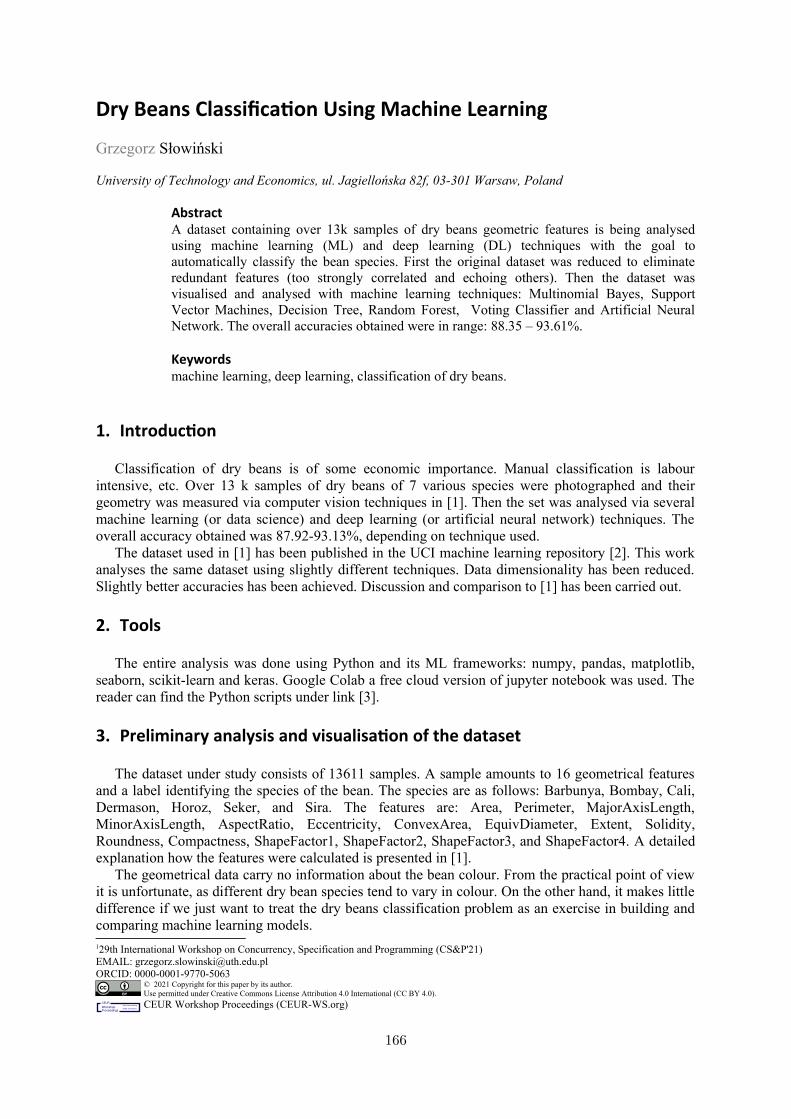
Dry Beans Classification Using Machine Learning

Grzegorz Słowiński

University of Technology and Economics, ul. Jagiellońska 82f, 03-301 Warsaw, Poland

Abstract A dataset containing over 13k samples of dry beans geometric features is being analysedusing machine learning (ML) and deep learning (DL) techniques with the goal toautomatically classify the bean species. First the original dataset was reduced to eliminateredundant features (too strongly correlated and echoing others). Then the dataset wasvisualised and analysed with machine learning techniques: Multinomial Bayes, SupportVector Machines, Decision Tree, Random Forest, Voting Classifier and Artificial NeuralNetwork. The overall accuracies obtained were in range: 88.35 – 93.61%.

Keywords 1

machine learning, deep learning, classification of dry beans.

1. Introduction

Classification of dry beans is of some economic importance. Manual classification is labourintensive, etc. Over 13 k samples of dry beans of 7 various species were photographed and theirgeometry was measured via computer vision techniques in [1]. Then the set was analysed via severalmachine learning (or data science) and deep learning (or artificial neural network) techniques. Theoverall accuracy obtained was 87.92-93.13%, depending on technique used.

The dataset used in [1] has been published in the UCI machine learning repository [2]. This workanalyses the same dataset using slightly different techniques. Data dimensionality has been reduced.Slightly better accuracies has been achieved. Discussion and comparison to [1] has been carried out.

2. Tools

The entire analysis was done using Python and its ML frameworks: numpy, pandas, matplotlib,seaborn, scikit-learn and keras. Google Colab a free cloud version of jupyter notebook was used. Thereader can find the Python scripts under link [3].

3. Preliminary analysis and visualisation of the dataset

The dataset under study consists of 13611 samples. A sample amounts to 16 geometrical featuresand a label identifying the species of the bean. The species are as follows: Barbunya, Bombay, Cali,Dermason, Horoz, Seker, and Sira. The features are: Area, Perimeter, MajorAxisLength,MinorAxisLength, AspectRatio, Eccentricity, ConvexArea, EquivDiameter, Extent, Solidity,Roundness, Compactness, ShapeFactor1, ShapeFactor2, ShapeFactor3, and ShapeFactor4. A detailedexplanation how the features were calculated is presented in [1].

The geometrical data carry no information about the bean colour. From the practical point of viewit is unfortunate, as different dry bean species tend to vary in colour. On the other hand, it makes littledifference if we just want to treat the dry beans classification problem as an exercise in building andcomparing machine learning models.129th International Workshop on Concurrency, Specification and Programming (CS&P'21)EMAIL: [email protected] ORCID: 0000-0001-9770-5063

© 2021 Copyright for this paper by its author.Use permitted under Creative Commons License Attribution 4.0 International (CC BY 4.0).

CEUR Workshop Proceedings (CEUR-WS.org) CEURWorkshopProceedings

http://ceur-ws.orgISSN 1613-0073

166

3.1. Correlation analysis and feature reduction

Correlation analysis has shown that several of the features are strongly (positively or negatively)correlated. This is due to the fact that basically all of them are kind of geometric measures. Thedecision was taken to drop some features to avoid correlations over 0.9 (or negative correlationbelow -0.9) between them. The benefits of such a decision should be: 1) a significant reduction of thecomputational complexity 2) a lower risk of overfitting 3) ease of visualisation. The disadvantage is alimited risk of loosing some valuable information and, as a result, a decrease in accuracy.

Table 1Correlation between selected beans features

MajorAxisLength

MinorAxisLength

Aspect-Ratio

Extent Solidity Roundness ShapeFactor2

ShapeFactor4

MajorAxisLength

1.0000 0.8261 0.5503 -0.0781 -0.2843 -0.5964 -0.8592 -0.4825

MinorAxisLength

0.8261 1.0000 -0.0092 0.1460 -0.1558 -0.2103 -0.4713 -0.2637

AspectRatio 0.5503 -0.0092 1.0000 -0.3702 -0.2678 -0.7670 -0.8378 -0.4493Extent -0.0781 0.1460 -0.3702 1.0000 0.1914 0.3444 0.2380 0.1485Solidity -0.2843 -0.1558 -0.2678 0.1914 1.0000 0.6072 0.3436 0.7022

Roundness -0.5964 -0.2103 -0.7670 0.3444 0.6072 1.0000 0.7828 0.4721Shape-Factor2

-0.8592 -0.4713 -0.8378 0.2380 0.3436 0.7828 1.0000 0.5299

Shape-Factor4

-0.4825 -0.2637 -0.4493 0.1485 0.7022 0.4721 0.5299 1.0000

Thus, in this work it was decided to limit the set of features list to these 8 members:MajorAxisLength, MinorAxisLength, AspectRatio, Extent, Solidity, Roundness, ShapeFactor2,ShapeFactor4, and to exclude: Area, Perimeter, Eccentricity, ConvexArea, EquivDiameter,Compactness, ShapeFactor1, ShapeFactor3. The issue of high correlations among some features wasnot addressed in [1]. The visualisation of the data was done by pair-plot, and is presented in figure 1.

It shows that the Bombay species is trivial to classify as its beans are significantly bigger thanothers. the classification of other species seems to be much more difficult, and we can expect moreerrors. The correlations between pairs of the selected features are listed in Table 1.

4. Machine Learning techniques used and results

In this work the following techniques were used: Multinomial Gaussian Classifier, Support VectorClassifier, Decision Tree, Random Forest, Voting Classifier, Artificial Neural Network (MultilayerPerceptron or MLP).

The full dataset was divided into the training and test subsets. 80% of samples were used fortraining and 20% for testing. Division of all available samples into the training and test subsets iscrucial for a correct methodology. The aim of all ML or DL methods is to achieve a ”generalization”ability. Thus it is important to check the accuracy of classifying new samples, ones that have not beenused during training. Otherwise, there is a very serious risk that the model will suffer form overfitting.Overfitted models perform very well on the training data but much worse on new data. Overfitting (asone of the most important issues in ML) is widely discussed in ML handbooks [4-6].

4.1. Multinomial Naive Bayes classifier

Naive Bayes models are based on Bayes's theorem. They are extremely fast and simple, but on theother hand, their performance is usually limited. They can be used as a baseline for classificationproblems (see [4], p. 382).

The overall accuracy obtained with Multinomial Bayes Classifier was 64,30 %. The problem wasto classify into 7 different classes. Thus the blind (random) classification should result in about 1/7 =

167

14,29% accuracy. As one can see, classification is more difficult if there are more classes. Randomclassification should give accuracy equal to about 1/(number of classes). Thus we can see that eventhis simple model perform about 50 percent points better than the random approach.

Figure 1: The selected features of dry beans (pairplot)

4.2. Support Vector Classifier

Support vector machines (SVM), which can be used as regressors or classifiers, are considered avery powerful and flexible algorithms. On the other hand. they may need a lot of computing power(see [4] p.405). The SVM principle is to partition the classes by ”drawing a line” (or plane) in a waythat maximises the margin between classes. As straight lines (or planes) do not usually produce thebest solution, SVC can apply different kernels (polynomial, radial and others). SVC is widerexplained in [4,5]. SVCs with different kernels were tried. Table 2 presents the parameters used andthe accuracy obtained.

The results are quite similar for all kernels. The accuracy can be further improved to some extent(tenths of %, maybe 1%) by increasing C, but this will also significantly increase the training time.

168

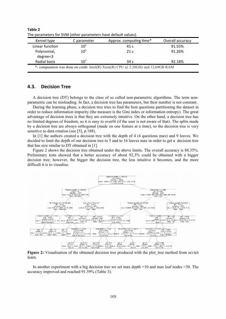
Table 2The parameters for SVM (other parameters have default values).

Kernel type C parameter Approx. computing time* Overall accuracyLinear function 105 41 s 91.55%

Polynomial,degree=3

105 21 s 91.26%

Radial basis 107 34 s 92.18%*- computation was done on colab: Intel(R) Xeon(R) CPU @ 2.20GHz and 12,69GB RAM

4.3. Decision Tree

A decision tree (DT) belongs to the class of so called non-parametric algorithms. The term non-parametric can be misleading. In fact, a decision tree has parameters, but their number is not constant.

During the learning phase, a decision tree tries to find the best questions partitioning the dataset inorder to reduce information impurity (the measure is the Gini index or information entropy). The greatadvantage of decision trees is that they are extremely intuitive. On the other hand, a decision tree hasno limited degrees of freedom, so it is easy to overfit (if the user is not aware of that). The splits madeby a decision tree are always orthogonal (made on one feature at a time), so the decision tree is verysensitive to data rotation (see [5], p.188).

In [1] the authors created a decision tree with the depth of 4 (4 questions max) and 9 leaves. Wedecided to limit the depth of our decision tree to 5 and to 16 leaves max in order to get a decision treethat has size similar to DT obtained in [1].

Figure 2 shows the decision tree obtained under the above limits. The overall accuracy is 88.35%.Preliminary tests showed that a better accuracy of about 92,3% could be obtained with a biggerdecision tree; however, the bigger the decision tree, the less intuitive it becomes, and the moredifficult it is to visualise.

Figure 2: Visualisation of the obtained decision tree produced with the plot_tree method from sci-kitlearn.

In another experiment with a big decision tree we set max depth =10 and max leaf nodes =30. Theaccuracy improved and reached 91.59% (Table 3).

169

Table 3Decision trees parameters and performance

Decision tree Max depth Max leaf nodes Overall accuracysmall 5 16 88.35%

big 10 30 91.59%

It can be seen that to obtain an accuracy similar to that reported in [1] with a decision tree, the treewould have to be much bigger (losing the main advantage of decision trees, i.e., the intuitiveinterpretation). One should keep in mind that in this work the amount of features has been reducedfrom 16 to 8. The excluded features were highly correlated to the retained features (being othergeometrical measures of the same beans), so they accounted for little additional information.However, they present this information in a slightly different manner (”rotated”), making the taskeasier for the decision tree.

To see this better, assume that in some dataset we have two parameters A and B, and theclassification is obvious, but it depends on the A/B ratio that is not explicitly present in the dataset.This can be hard for a decision tree to solve. The addition of an extra column, A/B, will add no newinformation to the dataset, but it will help the decision tree quite a bit. It can be supposed that in thedry bean case, the 8 removed categories contained little extra information, but they presentedessentially the same information in a way more appropriate for the decision tree.

4.4. Random Forest

The random forest idea is as follows: take many decision trees (employing some randomness, sothe trees differ) and let them vote. So the classification decision taken by a random forest is a decisiontaken by the most numerous group of decision trees in a random set of trees.

Usually a random forest performs better than a single decision tree. However, a random forest isconsidered a ”black-box” model being very hard to interpret.

A random forest of 150 decision trees was created. No restrictions on trees were applied. Theaccuracy obtained was 93.61%, the best so-far, better than the best accuracy reported in [1]. Inaddition, the training process was fast and took about 2 s, which 10-20 times faster than for SVC.

4.5. Voting Classifier

The idea of ”voting”, which by default is used in random forests, can be applied to any classifiers.There are 2 main ways of voting: ”hard” (straightforward, direct voting) and ”soft” (the votes areweighted depending on how confident the classifier is with its choice). Like in the case of a randomforest, there is a good chance that the voting result will be more accurate than for any particularclassifier.

The hard voting classifier was implemented using 3 classifiers described above: the radial kernelSVC, the ”big” decision tree, and the random forest.

The obtained accuracy was 92.80%. Thus in this case it is worse than for the random forest. Thisgives us a clue that voting should be used carefully and preferably with models exhibiting similarperformance; otherwise ”stupid” models can outvote ”smart” models. It seems that this flaw ofdemocracy does not only apply to human societies, but is more universal in nature.

4.6. Artificial Neural Network

Besides the (shallow) machine learning/data science methods presented above, a deep learningtechnique, the so-called dense artificial neural network, has also been tried.

For an artificial neural network the data needs additional treatment. First, the names of beanspecies were labelled with numbers and then these numbers 0-6 were codded as so called ”one-hot”.

170

The reason of using ”one-hot” encoding is well explained for example in [4] p. 376 or [6] pp. 190-194. The other operation is scaling, a standardisation or normalisation of the training data. The data(each feature) is centred around zero (by subtracting the average) and normalised (by dividing by thestandard deviation). Standardisation is said to ease the training process and tends to bring inimprovement in performance [5] p. 72.

Two architectures of ANN were tried. The first one is similar to the one described in [1], exceptthat the input layer size in our case is 8 not 16. The network has 3 hidden layers with 17, 12, 3,neurons, respectively. Rectified Linear Unit was used as an activation function in hidden layers. Theoutput layer has 7 neurons, one for each bean species. Sigmoid is the activation function for the outputlayer. The optimiser used was: RMSprop, and the loss function was the categorical cross entropy. Thevalidation set was 20% of training set. The network was trained for 24 epochs. The architecture of thisnetwork and the training process are presented in figure 3.

Figure 3. The architecture (left) and the training process (right) of the first ANN.

The overall accuracy was 92.58%. In an attempt to improve it, another ”bigger” ANN was tried.Besides the normal layers, a dropout layer was added. A dropout layer only works during the trainingand randomly ”cuts off” (sets to zero) some inputs. It is expected that dropout layers reduce the risk ofoverfitting [6] p.109. The architecture of the network and its training are shown in figure 4. The sameoptimiser and loss function were used: RMSprop and the categorical cross entropy, respectively. Thenetwork was also trained for 24 epochs. The overall accuracy was 92.77%, thus the improvement wasnot much.

5. Results and Conclusions

The dry beans dataset has been analysed by different machine learning and deep learningtechniques. Table 4 shows the summary results.

It can be seen that in general the task of beans classification is a relatively simple task in terms ofthe necessary computing power. All training times were shorter than 1 minute using a free google-colab computer.

171

The accuracy of Naive Bayes is much worse than for the other methods. This is not surprising, asthis method is known to be fast but not very accurate, and is suggested as a preliminary method tocheck if there is „something” in the data, rather than to do a full analysis. The other methods giveaccuracy in a relatively close range of 88.3-93.6%. This is comparable to [1] where the accuracy wasin range 87.9-93.13%.

The authors in [1] trained their models with all 16 features. Here, some strongly correlated featureswere eliminated. The results show that this elimination has not decreased the accuracy.

The only technique, that suffered from this elimination to some extend seems to be decision tree.This is due to the fact that decision tree operates on one feature at a time and cannot ”combine”features. See also the discussion in p. 4.3 devoted to the decision tree section.

Figure 4. The architecture (left) and the training process (right) of the second ANN.

One can see that the models vary strongly in the terms of the computing time. SVC and ANN (andalso Voting Classifier, because it includes SVC) are the slowest learners. Random forest seems to bethe best method in this case, as it perform best and its training time is also reasonable.

Confusion matrices provide a comfortable way to visualise results in more details and compareactual values with predicted ones. The confusion matrix for the random forest classifier (the bestperformer) will be discussed further. It is presented in figure 5. The most frequent mistakes werebetween Dermason and Sira (38 + 44). On the other hand, Bombay was classified perfectly which isnot surprising. It is easy to notice that Bombay beans are significantly bigger than other species.

The dry beans dataset appeared to be an interesting dataset to demonstrate and compare MLtechniques. Two ideas for further research:

172

Deeper insight how and if the elimination of correlated features influences the ML trainingprocess. This study shows that there is little, if any, performance decrease. One may try toinvestigate if the elimination reduces the training time and how much. Despite ”manual” feature reduction, as done in this work, on may try to use PCA (the primarycomponent analysis) to reduce the dimensionality of data and also analyse its influence on modelperformance (accuracy and training time)

Figure 5. Test subset confusion matrix for the random forest classifier.

6. References

[1] Murat Koklu, Ilker Ali Ozkan, Multiclass classification of dry beans using computer vision andmachine learning techniques, Computers and Electronics in Agriculture 174 (2020) 105507

[2] Dry beans dataset at UCI repository: https://archive.ics.uci.edu/ml/datasets/Dry+Bean+Dataset,access 23.06.2021

[3] Colab notebook containing computation scripts for this work: https://colab.research.google.com/drive/11X6VevSMybenGkRqK1Xj_1EJmU3vomFB?usp=sharing

[4] Jake VanderPlass, Python Data Science Handbook, O’Reilly, 2017[5] Aurelien Geron, Hands-on Machine Learning with Scikit-Learn, Keras & TensorFlow, O’Reilly,

2019[6] Francois Chollet, Deep Learning with Python, Manning Publications, 2018

173

Author Index

AliAliyu Tanko, 93

AzadMohammad, 126

BergmannAndre, 18

BorutaAgnieszka, 131

BozhenkovaElena, 60

Calleja GarcıaEmilio Jose, 18

ChikalovIgor, 126

CzajaLudwik, 31

DuttaSoma, 46

GburzynskiPawel, 131

GoraPawel, 145

GrunskeLars, 2

GruskaDamas, 83, 93

GroplerRobin, 18

HafnerVerena V., 106, 113

HeidenSimon, 2

HussainShahid, 126

KlemenkoArkadiusz, 145

Knapp

Alexander, 1

Kuznicka

Ewa, 131

Mellmann

Heinrich, 106, 113

Milewski

Roman, 2

Moshkov

Mikhail, 126

Mozejko

Marcin, 145

Nestoruk

Roman, 156

Nguyen

Hung Son, 117

Puzynin

Eugen, 113

Redziejowski

Roman R., 72

Ruiz

M. Carmen, 83

Skowron

Andrzej, 46

Skowronek

Lukasz, 145

Sudhi

Viju, 18

S lowinski

Grzegorz, 120, 156, 166

Taliaronak

Volha, 106

Virbitskaite

Irina, 60

Proceedings of the 29th International Workshop on ...

Documents

Transcript of Proceedings of the 29th International Workshop on ...