DISSERTATION

PROBLEMS ON DECISION MAKING UNDER UNCERTAINTY

Submitted by

Yugandhar Sarkale

Department of Electrical and Computer Engineering

In partial fulfillment of the requirements

For the Degree of Doctor of Philosophy

Colorado State University

Fort Collins, Colorado

Fall 2019

Doctoral Committee:

Advisor: Edwin K. P. Chong

Peter YoungJ. Rockey LuoYongcheng Zhou

Copyright by Yugandhar Sarkale 2019

All Rights Reserved

ABSTRACT

PROBLEMS ON DECISION MAKING UNDER UNCERTAINTY

Humans and machines must often make rational choices in the face of uncertainty. Determin-

ing decisions, actions, choices, or alternatives that optimize objectives for real-world problems is

computationally difficult. This dissertation proposes novel solutions to such optimization problems

for both deterministic and stochastic cases; the proposed methods maintain near-optimal solution

quality. Even though the applicability of the techniques developed in our work cannot be limited

to a few examples, the applications addressed in our work include post-hazard large-scale real-

world community recovery management, path planning of UAVs by incorporating feedback from

intelligence assets, and closed-loop, urban target tracking in challenging environments. As an il-

lustration of the properties shared by the solutions developed in this dissertation, we will describe

the example of community recovery in depth.

In the work associated with community recovery, we handle both deterministic and stochastic

recovery decisions. For the deterministic problems (outcome of recovery actions is deterministic

but we handle the uncertainty in the underlying models), we develop a sequential discrete-time

decision-making framework and compute the near-optimal decisions for a community modeled

after Gilroy, California. We have designed stochastic models to calculate the damage to the infras-

tructures systems within the community after an occurrence of an earthquake. Our optimization

framework to compute the recovery decisions, which is hazard agnostic (the hazard could be a

nuclear explosion or a disruptive social event), is based on an approximate dynamic programming

paradigm of rollout; we have modeled the recovery decisions as string of actions. We design sev-

eral base heuristics pertaining to the problem of community recovery to be used as a base heuristic

in our framework; in addition, we also explore the performance of random heuristics. In addition

to modeling the interdependence between several networks and the cascading effect of a single

ii

recovery action on these networks, we also fuse the traditional optimization approaches, such as

simulated annealing, to compute efficient decisions, which mitigates the simultaneous spatial and

temporal evolution of the recovery problem.

For the stochastic problems, in addition to the previous complexities, the outcome of the de-

cisions is stochastic. Inclusion of this single complexity in the problem statement necessitates an

entirely novel way of developing solutions. We formulate the recovery problem in the powerful

framework of Markov Decision Processes (MDPs). In contrast to the conventional matrix-based

representation, we have formulated our problem as a simulation-based MDP. Classical solutions

to solve an MDP are inadequate; therefore, approximation to compute the Q-values (based on

Bellman’s equation) is necessary. In our framework, we have employed Approximate Policy Im-

provement to circumvent the limitation with the classical techniques. We have also addressed the

risk-attitudes of the policymakers and the decisionmakers, who are a key stakeholder in the recov-

ery process. Despite the use of a state-of-the-art computational platform, additional optimization

must be made to the resultant stochastic simulation optimization problem owing to the massive size

of the recovery problem. Our solutions are calculated using one of the best performing simulation

optimization method of Optimal Computing Budget Allocation. Further, in the stochastic setting,

scheduling of decisions for the building portfolio recovery is even more computationally difficult

than some of the other coarsely-modeled networks like Electric Power Networks (EPN). Our work

proposes a stochastic non-preemptive scheduling framework to address this challenging problem

at scale.

For the stochastic problems, one of the major highlights of this dissertation is the decision-

automation framework for EPN recovery. The novel decision-making-under-uncertainty algo-

rithms developed to plan sequential decisions for EPN recovery demonstrate a state-of-the-art

performance; our algorithms should be of interest to practitioners in several fields—those that

deal with real-world large-scale problem of selecting a single choice given a massive number of al-

ternatives. The quality of recovery decisions calculated using the decision-automation framework

does not deteriorate despite a massive increase in the size of the recovery problem. Even though

iii

the focus of this dissertation is primarily on application to recovery of communities affected by

hazards, our algorithms contributes to the general problem of MDPs with massive action spaces.

The primary objective of our work in the community recovery problem is to address the issue

of food security. Particularly, we address the objective of making the community food secure to

the pre-hazard levels in minimum amount of time or schedule the recovery actions so that maxi-

mum number of people are food secure after a sequence of decisions. In essence, our framework

accommodates the stochastic hazard models, handles the stochastic nature of outcome of human or

machine repair actions, has lookahead, does not suffer from decision fatigue, and incorporates the

current policies of the decision makers. The decisions calculated using our framework have been

aided by the free availability of a powerful supercomputer.

iv

ACKNOWLEDGEMENTS

In my advisor Prof. Chong, I found someone who abides by the philosophy, “take care of

your students, and the research will take care of itself." As a result, completing my PhD under

his tutelage has been a very rich and enjoyable experience, and I am strongly convinced about the

merit of his approach. His support, guidance, and immense patience throughout my research at

Colorado State University is incomparable. I would specifically like to acknowledge his selfless

investment in my research aspirations and his distinctive quality of providing me the freedom and

the opportunity to pursue topics of my interest, which include a variety of challenging research

problems. I will always carry deep reverence for him—not only because he is an exceptional

scholar but also a caring mentor. I genuinely feel that his aura exceeds that of all his students,

colleagues, and peers combined because he is an institution in himself.

I would also like to express my sincere thanks to my committee members. The courses on

nonlinear and robust control systems taught by Prof. Peter Young are some of the best courses in

CSU. The clarity in his exposition is truly captivating. The rich ideas expressed through concise

and crisp mathematical expressions in the information theory course taught by Prof. Rockey Luo

formed the bedrock of my research pursuit in related topics, although I now miss not having studied

his principles of digital communications class. Researchers working in applied math have to often

deal with real-world problems where the size of computation is large. I would like to acknowledge

Prof. Yongcheng Zhou for training me in numerical analysis, which is one of the fundamental

skills necessary for applied-math researchers; I was always fascinated by his ability to explain

complex ideas in a simple fashion. Learning under their expert guidance was a truly enriching

experience, and the concepts assimilated in the respective courses have impacted several aspects

of my research.

The research on post-hazard community recovery planning is a collaborative effort with De-

partment of Civil and Environmental Engineering, CSU; specifically, I would like to acknowledge

v

the contribution of Dr. Saeed Nozhati and Prof. Bruce Ellingwood who are my co-authors on sev-

eral papers.

The research on orchestrated management of sensors to incorporate feedback from humans

partly uses the code provided by Prof. Shankarachary Ragi, which was developed during his PhD

work at CSU. The work included in this dissertation is an independent continuation of his research.

The research on tracking in urban terrain, included in the dissertation, is primarily the work of

Dr. Patricia Barbosa during her pursuit of PhD at CSU (which was included in her dissertation),

but it remained unpublished in a peer-reviewed journal before additional revisions were performed

by me. I would like to thank Prof. Edwin Chong, Dr. Patricia Barbosa, and other collaborators

associated with the project for providing me an opportunity to revise the work and being my co-

authors on the published journal manuscript.

My graduate studies have immensely benefitted through generous financial support from the

CSU Department of Electrical and Computer Engineering, Naval Postgraduate School via As-

sistance Agreement No. N00244-14-1-0038, CSU Energy Institute, ISTeC at CSU, and National

Science Foundation under Grant CMMI-1638284. In addition to these generous funding sources,

I would like to acknowledge (among others) Citibank, Chase Bank, Capital One Financial Cor-

poration, American Express, and Bank of America for providing me further financial flexibility

through their programs.

Special thanks also goes to the members of our research group Dr. Yajing Liu, Tushar Ganguli,

Pranav Damale, Apichart Vasutapituks, and Fateh El Sherif for their support and stimulating dis-

cussions. During my pursuit of PhD, I have had the opportunity to live with several people. I would

like to acknowledge the following people for providing me a peaceful and conducive environment

to meditate on my research while sharing the burden of mundane household chores (in chrono-

logical order): Cheryl Smith, Arun Vardhan Modali, Vihari Roy Surabhi, Tushar Jagtap, Pranav

Devalla, Tushar Ganguli, Marvin Antony, Sanket Mane, Karan Khot, Ronil Pala, Mary Maisner,

Kunal Vichare, Gitesh Kulkarni, Noel Varghese, Leanne Seguin, Sarah Gardner, and Ilyana Cole-

mann.

vi

I am truly blessed to have a large set of close friends. Even though acknowledging every-

one here is not feasible, the ones that immediately come to my mind are Siddharth Chougule,

Vivek Varma Sagi, Karan Naik, Nikhil Bhosale, Rohit Yadav, Sanket Shah, Yogesh Oswal, Vadiraj

Haribal, and Akshay Kapoor. I will always be indebted to them for the positive impact they have

had in my life.

I would like to thank my immediate family (my parents and my sister) for selflessly supporting

me in every endeavour that I have undertaken. Words cannot adequately describe their countless

sacrifices.

vii

DEDICATION

I would like to dedicate this dissertation to my family, my adviser and my PhD committee

members, my research collaborators, my teachers, and my friends.

viii

TABLE OF CONTENTS

ABSTRACT . . . . . . . . . . . . . . . . . . . . . . . . . . . . . . . . . . . . . . . . . . . iiACKNOWLEDGEMENTS . . . . . . . . . . . . . . . . . . . . . . . . . . . . . . . . . . . vDEDICATION . . . . . . . . . . . . . . . . . . . . . . . . . . . . . . . . . . . . . . . . . viiiLIST OF TABLES . . . . . . . . . . . . . . . . . . . . . . . . . . . . . . . . . . . . . . . xiiLIST OF FIGURES . . . . . . . . . . . . . . . . . . . . . . . . . . . . . . . . . . . . . . . xiii

Chapter 1 Introduction . . . . . . . . . . . . . . . . . . . . . . . . . . . . . . . . . . . 1

Chapter 2 Scheduling of Electric Power Network Recovery Post-Hazard . . . . . . . . . 82.1 Introduction . . . . . . . . . . . . . . . . . . . . . . . . . . . . . . . . . 82.2 System Resilience . . . . . . . . . . . . . . . . . . . . . . . . . . . . . . 102.3 Description of Case Study . . . . . . . . . . . . . . . . . . . . . . . . . . 122.4 Hazard and Damage Assessment . . . . . . . . . . . . . . . . . . . . . . . 13

2.4.1 Earthquake Simulation . . . . . . . . . . . . . . . . . . . . . . . . . . 132.4.2 Fragility Function and Restoration . . . . . . . . . . . . . . . . . . . . 17

2.5 Optimization Problem Description . . . . . . . . . . . . . . . . . . . . . . 182.5.1 Introduction . . . . . . . . . . . . . . . . . . . . . . . . . . . . . . . . 182.5.2 Optimization Problem Formulation . . . . . . . . . . . . . . . . . . . . 19

2.6 Optimization Problem Solution . . . . . . . . . . . . . . . . . . . . . . . 212.6.1 Approximate Dynamic Programming . . . . . . . . . . . . . . . . . . . 222.6.2 Rollout Algorithm . . . . . . . . . . . . . . . . . . . . . . . . . . . . . 24

2.7 Results . . . . . . . . . . . . . . . . . . . . . . . . . . . . . . . . . . . . 282.7.1 Discussion . . . . . . . . . . . . . . . . . . . . . . . . . . . . . . . . . 282.7.2 Computational Efforts . . . . . . . . . . . . . . . . . . . . . . . . . . . 39

2.8 Concluding Remarks . . . . . . . . . . . . . . . . . . . . . . . . . . . . . 412.9 Funding and Support . . . . . . . . . . . . . . . . . . . . . . . . . . . . . 41

Chapter 3 Planning for Community-Level Food Security Following Disasters . . . . . . 423.1 Introduction . . . . . . . . . . . . . . . . . . . . . . . . . . . . . . . . . 423.2 Preliminaries . . . . . . . . . . . . . . . . . . . . . . . . . . . . . . . . . 43

3.2.1 Simulated Annealing . . . . . . . . . . . . . . . . . . . . . . . . . . . 433.3 Case Study . . . . . . . . . . . . . . . . . . . . . . . . . . . . . . . . . . 44

3.3.1 Water Networks . . . . . . . . . . . . . . . . . . . . . . . . . . . . . . 443.3.2 Highway Bridges . . . . . . . . . . . . . . . . . . . . . . . . . . . . . 44

3.4 Policy Optimization for Food Security . . . . . . . . . . . . . . . . . . . . 443.5 Results and Discussion . . . . . . . . . . . . . . . . . . . . . . . . . . . . 473.6 Conclusion . . . . . . . . . . . . . . . . . . . . . . . . . . . . . . . . . . 503.7 Funding and Support . . . . . . . . . . . . . . . . . . . . . . . . . . . . . 51

ix

Chapter 4 Optimal Stochastic Dynamic Scheduling for Managing Community Recov-ery from Natural Hazards . . . . . . . . . . . . . . . . . . . . . . . . . . . . 52

4.1 Introduction . . . . . . . . . . . . . . . . . . . . . . . . . . . . . . . . . 524.2 Technical Preliminaries . . . . . . . . . . . . . . . . . . . . . . . . . . . 54

4.2.1 MDP Framework . . . . . . . . . . . . . . . . . . . . . . . . . . . . . 554.2.2 Simulation-based MDP . . . . . . . . . . . . . . . . . . . . . . . . . . 564.2.3 Approximate Dynamic Programming . . . . . . . . . . . . . . . . . . . 574.2.4 Rollout . . . . . . . . . . . . . . . . . . . . . . . . . . . . . . . . . . . 57

4.3 Community Testbed . . . . . . . . . . . . . . . . . . . . . . . . . . . . . 594.4 Post-hazard Recovery Formulation . . . . . . . . . . . . . . . . . . . . . 60

4.4.1 Markov Decision Process Formulation . . . . . . . . . . . . . . . . . . 614.5 Results and Discussion . . . . . . . . . . . . . . . . . . . . . . . . . . . . 64

4.5.1 Mean-based Stochastic Optimization . . . . . . . . . . . . . . . . . . . 654.5.2 Worst-case Stochastic Optimization . . . . . . . . . . . . . . . . . . . . 71

4.6 Conclusion . . . . . . . . . . . . . . . . . . . . . . . . . . . . . . . . . . 754.7 Funding and Support . . . . . . . . . . . . . . . . . . . . . . . . . . . . . 76

Chapter 5 Solving Markov Decision Processes for Water Network Recovery of Com-munity Damaged by Earthquake . . . . . . . . . . . . . . . . . . . . . . . . 77

5.1 Introduction . . . . . . . . . . . . . . . . . . . . . . . . . . . . . . . . . 775.2 Testbed Case Study . . . . . . . . . . . . . . . . . . . . . . . . . . . . . . 785.3 Problem Description and Solution . . . . . . . . . . . . . . . . . . . . . . 78

5.3.1 MDP Framework . . . . . . . . . . . . . . . . . . . . . . . . . . . . . 785.3.2 MDP Solution . . . . . . . . . . . . . . . . . . . . . . . . . . . . . . . 795.3.3 Simulation-Based Representation of MDP . . . . . . . . . . . . . . . . 805.3.4 Problem Formulation . . . . . . . . . . . . . . . . . . . . . . . . . . . 815.3.5 Rollout . . . . . . . . . . . . . . . . . . . . . . . . . . . . . . . . . . . 835.3.6 Optimal Computing Budget Allocation . . . . . . . . . . . . . . . . . . 85

5.4 Simulation Results . . . . . . . . . . . . . . . . . . . . . . . . . . . . . . 865.5 Funding and Support . . . . . . . . . . . . . . . . . . . . . . . . . . . . . 90

Chapter 6 Stochastic Scheduling for Building Portfolio Restoration Following Disasters 916.1 Introduction . . . . . . . . . . . . . . . . . . . . . . . . . . . . . . . . . 916.2 Testbed Case Study . . . . . . . . . . . . . . . . . . . . . . . . . . . . . . 936.3 Seismic Hazard and Damage Assessment . . . . . . . . . . . . . . . . . . 936.4 Markov Decision Process Framework . . . . . . . . . . . . . . . . . . . . 946.5 Building Portfolio Recovery . . . . . . . . . . . . . . . . . . . . . . . . . 966.6 Conclusion . . . . . . . . . . . . . . . . . . . . . . . . . . . . . . . . . . 976.7 Funding and Support . . . . . . . . . . . . . . . . . . . . . . . . . . . . . 98

Chapter 7 A Method for Handling Massive Discrete Action Spaces of MDPs: Applica-tion to Electric Power Network Recovery . . . . . . . . . . . . . . . . . . . 99

7.1 Introduction . . . . . . . . . . . . . . . . . . . . . . . . . . . . . . . . . 997.2 The Assignment Problem . . . . . . . . . . . . . . . . . . . . . . . . . . 101

x

7.2.1 Problem Setup: The Gilroy Community, Seismic Hazard Simulation,and Fragility and Restoration Assessment of EPN . . . . . . . . . . . . 101

7.2.2 Problem Formulation . . . . . . . . . . . . . . . . . . . . . . . . . . . 1027.3 Problem Solution . . . . . . . . . . . . . . . . . . . . . . . . . . . . . . . 108

7.3.1 MDP Solution: Exact Methods . . . . . . . . . . . . . . . . . . . . . . 1087.3.2 Rollout: Dealing with Massive S . . . . . . . . . . . . . . . . . . . . . 1097.3.3 Linear Belief Model: Dealing with Massive A . . . . . . . . . . . . . . 1127.3.4 Adaptive Sampling: Utilizing Limited Simulation Budget . . . . . . . . 116

7.4 Simulation Results: Modeling Gilroy Recovery . . . . . . . . . . . . . . . 1207.5 Conclusion . . . . . . . . . . . . . . . . . . . . . . . . . . . . . . . . . . 1267.6 Funding and Support . . . . . . . . . . . . . . . . . . . . . . . . . . . . . 127

Chapter 8 Dynamic UAV Path Planning Incorporating Feedback from Humans for Tar-get Tracking . . . . . . . . . . . . . . . . . . . . . . . . . . . . . . . . . . . 128

8.1 Introduction . . . . . . . . . . . . . . . . . . . . . . . . . . . . . . . . . 1288.2 Problem Formulation . . . . . . . . . . . . . . . . . . . . . . . . . . . . . 1308.3 NBO Approximation Method . . . . . . . . . . . . . . . . . . . . . . . . 1338.4 Incorporating Feedback from Intelligence Assets . . . . . . . . . . . . . . 136

8.4.1 The Complete Optimization Problem . . . . . . . . . . . . . . . . . . . 1368.4.2 Feedback from Intelligence Assets . . . . . . . . . . . . . . . . . . . . 138

8.5 Simulation Results . . . . . . . . . . . . . . . . . . . . . . . . . . . . . . 1408.6 Conclusions . . . . . . . . . . . . . . . . . . . . . . . . . . . . . . . . . 1478.7 POMDP Review . . . . . . . . . . . . . . . . . . . . . . . . . . . . . . . 1478.8 Funding and Support . . . . . . . . . . . . . . . . . . . . . . . . . . . . . 149

Chapter 9 A Novel Closed Loop Framework for Controlled Tracking in Urban Terrain . 1509.1 Introduction . . . . . . . . . . . . . . . . . . . . . . . . . . . . . . . . . 1509.2 Literature Review . . . . . . . . . . . . . . . . . . . . . . . . . . . . . . 1529.3 Problem Assumptions and Modeling . . . . . . . . . . . . . . . . . . . . 154

9.3.1 Clutter and Multipath in Urban Terrain . . . . . . . . . . . . . . . . . . 1559.3.2 Signals for Active Sensing in Urban Terrain . . . . . . . . . . . . . . . 1579.3.3 Models for Target Motion in Urban Terrain . . . . . . . . . . . . . . . . 159

9.4 Closed-Loop Active Sensing Platform . . . . . . . . . . . . . . . . . . . . 1629.4.1 From Signal Detection to Discrete Measurements . . . . . . . . . . . . 1629.4.2 Multitarget-Multisensor Tracker . . . . . . . . . . . . . . . . . . . . . 1659.4.3 Waveform Scheduling . . . . . . . . . . . . . . . . . . . . . . . . . . . 170

9.5 Simulation Results . . . . . . . . . . . . . . . . . . . . . . . . . . . . . . 1719.6 Concluding Remarks . . . . . . . . . . . . . . . . . . . . . . . . . . . . . 1759.7 Funding and Support . . . . . . . . . . . . . . . . . . . . . . . . . . . . . 175

Chapter 10 Summary . . . . . . . . . . . . . . . . . . . . . . . . . . . . . . . . . . . . 179

Bibliography . . . . . . . . . . . . . . . . . . . . . . . . . . . . . . . . . . . . . . . . . . 181

xi

LIST OF TABLES

2.1 The main food retailers of Gilroy . . . . . . . . . . . . . . . . . . . . . . . . . . . . 132.2 Restoration times based on the level of damage . . . . . . . . . . . . . . . . . . . . . 18

4.1 The expected repair times (Unit:days) . . . . . . . . . . . . . . . . . . . . . . . . . . 594.2 Performance of rollout vs. base policy for the 1st objective function for the individual

retailers . . . . . . . . . . . . . . . . . . . . . . . . . . . . . . . . . . . . . . . . . . 664.3 The performance of policies in different cases for the worse-case optimization (Unit:

average No. of people per day) . . . . . . . . . . . . . . . . . . . . . . . . . . . . . . 72

6.1 Age distribution of Gilroy [1]. . . . . . . . . . . . . . . . . . . . . . . . . . . . . . . 93

8.1 Weights are assigned to the N-W targets . . . . . . . . . . . . . . . . . . . . . . . . . 1418.2 Weights are assigned to the N-E targets . . . . . . . . . . . . . . . . . . . . . . . . . . 147

xii

LIST OF FIGURES

2.1 Schematic representation of resilience concept (adopted from [2, 3]) . . . . . . . . . . 112.2 Map of Gilroy’s population over the defined grids . . . . . . . . . . . . . . . . . . . . 122.3 Gilroy’s main food retailers . . . . . . . . . . . . . . . . . . . . . . . . . . . . . . . . 142.4 The modeled electrical power network of Gilroy . . . . . . . . . . . . . . . . . . . . . 152.5 The map of shear velocity at Gilroy area . . . . . . . . . . . . . . . . . . . . . . . . . 162.6 The simulation of median of peak ground acceleration field . . . . . . . . . . . . . . . 172.7 Electrical Power Network of Gilroy . . . . . . . . . . . . . . . . . . . . . . . . . . . 302.8 Electrical Power Network Tree . . . . . . . . . . . . . . . . . . . . . . . . . . . . . . 322.9 Electrical power network recovery due to base heuristicH with one standard deviation

band . . . . . . . . . . . . . . . . . . . . . . . . . . . . . . . . . . . . . . . . . . . . 332.10 Comparison of base heuristic (H) vs. rollout algorithm with 1-step heuristic vs. rollout

algorithm with N-step heuristic for multiple scenarios for objective 2. . . . . . . . . . 342.11 Histogram of F2(X) with Base (H), rollout with 1-step and rollout with N-step heuris-

tic for multiple scenarios . . . . . . . . . . . . . . . . . . . . . . . . . . . . . . . . . 352.12 Comparison of base heuristic (H) vs. rollout algorithm with 1-step heuristic vs. rollout

algorithm with N-step heuristic for multiple scenarios for objective 2. . . . . . . . . . 362.13 Cumulative moving average plot for objective 1 where γ = .8 with base heuristic (H)

and rollout algorithm . . . . . . . . . . . . . . . . . . . . . . . . . . . . . . . . . . . 372.14 Comparison of base heuristic (H) vs rollout algorithm . . . . . . . . . . . . . . . . . . 382.15 Comparison of base heuristic (H) vs. rollout algorithm for multiple scenarios for ob-

jective 1. . . . . . . . . . . . . . . . . . . . . . . . . . . . . . . . . . . . . . . . . . . 392.16 Comparison of base heuristic (H) vs. rollout algorithm for multiple scenarios for ob-

jective 2. . . . . . . . . . . . . . . . . . . . . . . . . . . . . . . . . . . . . . . . . . . 40

3.1 The modeled water network of Gilroy . . . . . . . . . . . . . . . . . . . . . . . . . . 453.2 Comparison of base and rollout with simulated annealing policies . . . . . . . . . . . 473.3 Histogram of F(X) for base and rollout with simulated annealing policies . . . . . . . . 49

4.1 Decision graph of a MDP . . . . . . . . . . . . . . . . . . . . . . . . . . . . . . . . . 564.2 Performance of rollout vs. base policy for the first objective function . . . . . . . . . . 664.3 Performance of rollout vs. base policy for the second objective function . . . . . . . . 684.4 The performance of policies to provide electricity for household units . . . . . . . . . 694.5 The performance of policies to provide electricity for household units and retailers . . 704.6 The performance of policies to provide potable water for household units . . . . . . . . 704.7 The performance of policies to provide potable water for household units and retailers . 714.8 Performance of rollout vs. base policy in the worst-case optimization for the second

objective function . . . . . . . . . . . . . . . . . . . . . . . . . . . . . . . . . . . . . 734.9 The performance of policies to provide electricity for household units . . . . . . . . . 734.10 The performance of policies to provide electricity for household units and retailers . . 744.11 The performance of policies to provide potable water for household units . . . . . . . . 744.12 The performance of policies to provide potable water for household units and retailers . 75

xiii

5.1 Performance comparison of rollout vs base policy for 3 units of resources. . . . . . . . 875.2 Performance comparison of rollout vs base policy for 5 unit of resources. . . . . . . . 885.3 Performance comparison of uniform rollout (TEA), rollout with OCBA and base policy

for 3 units of resources. . . . . . . . . . . . . . . . . . . . . . . . . . . . . . . . . . . 89

6.1 Housing units over the defined grids. . . . . . . . . . . . . . . . . . . . . . . . . . . 946.2 Different numbers of people based on age with inhabitable structures. . . . . . . . . . 986.3 Number of people with inhabitable houses a) following the earthquake b) after 100

days c) after 600 days. . . . . . . . . . . . . . . . . . . . . . . . . . . . . . . . . . . 98

7.1 A cumulative moving average plot for the number of days required to provide elec-tricity to 80% of the population with respect to the total number of scenarios usingAlgorithm 5. . . . . . . . . . . . . . . . . . . . . . . . . . . . . . . . . . . . . . . . . 122

7.2 Average (of 25 recovery paths) recovery path using base policy and uniform rolloutwith linear belief for Objective 2. . . . . . . . . . . . . . . . . . . . . . . . . . . . . . 124

7.3 A cumulative moving average plot for the number of days required to provide elec-tricity to 80% of the population with respect to the total number of scenarios usingAlgorithm 6. . . . . . . . . . . . . . . . . . . . . . . . . . . . . . . . . . . . . . . . . 124

7.4 Performance comparison of adaptive rollout w/ linear belief vs. base policy for thesecond objective. . . . . . . . . . . . . . . . . . . . . . . . . . . . . . . . . . . . . . 125

8.1 3 UAVs track 2 Targets . . . . . . . . . . . . . . . . . . . . . . . . . . . . . . . . . . 1418.2 Track location error for target moving towards N-W, MSE 1.6743m . . . . . . . . . . 1428.3 Track location error for target moving towards N-E, MSE 2.2767m . . . . . . . . . . . 1438.4 3 UAVs track 2 Targets . . . . . . . . . . . . . . . . . . . . . . . . . . . . . . . . . . 1448.5 Track location error for target moving towards N-W, MSE 1.5544m . . . . . . . . . . 1458.6 Track location error for target moving towards N-E, MSE 2.8098m . . . . . . . . . . . 146

9.1 Systems-level architecture of the proposed closed-loop active sensing platform. . . . . 1519.2 A simple transmitter-clutter-receiver path. . . . . . . . . . . . . . . . . . . . . . . . . 1579.3 The simulated urban terrain. The start and end trajectory points are shown as ; re-

ceivers are shown as©; the transmitter is shown as; and clutter discretes are shownas +. . . . . . . . . . . . . . . . . . . . . . . . . . . . . . . . . . . . . . . . . . . . . 173

9.4 Number of confirmed tracks for close-loop and open-loop systems. . . . . . . . . . . . 1769.5 Position RMSE for closed-loop and open-loop systems. . . . . . . . . . . . . . . . . . 1779.6 Motion model probabilities in the closed-loop system. . . . . . . . . . . . . . . . . . . 178

xiv

Chapter 1

Introduction

This dissertation addresses planning of decisions in real-world post-hazard community recov-

ery, path planning for autonomous Unmanned Aerial Vehicles (UAVs) to track multiple targets,

and the problem of tracking targets in the urban terrain. In all these problems, the world (physical

model of the problem) is dynamic and evolves spatially and temporally. The underlying theme that

connects our solutions of these distinct problems is that decisions in each problem are calculated

sequentially and in a closed-loop fashion to optimize an objective function. Our techniques have

several common attractive features, lookahead being one of them. Our methods handle uncertainty

in both the model and the outcome of the decisions.

Network-level decision-making algorithms need to solve large-scale optimization problems

that pose computational challenges. The complexity of the optimization problems increases when

various sources of uncertainty are considered. In Chapter 2, we introduce a sequential discrete

optimization approach, as a decision-making framework at the community level for recovery man-

agement. The proposed mathematical approach leverages approximate dynamic programming

along with heuristics for the determination of recovery actions. The methodology proposed in

this chapter overcomes the curse of dimensionality and manages multi-state, large-scale infrastruc-

ture systems following disasters [4]. In this chapter, we assume that the outcome of the recovery

decisions is deterministic.

In the aftermath of an extreme natural hazard, community residents must have access to func-

tioning food retailers to maintain food security. Food security is dependent on supporting critical

infrastructure systems, including electricity, potable water, and transportation. An understanding

of the response of such interdependent networks and the process of post-disaster recovery is the

cornerstone of an efficient emergency management plan. In Chapter 3, we model the intercon-

nectedness among different critical facilities, such as electrical power networks, water networks,

highway bridges, and food retailers. In this chapter, we consider various sources of uncertainty

1

and complexity in the recovery process of a community to capture the stochastic behavior of the

spatially distributed infrastructure systems. The work in this chapter is an extension of the work

in Chapter 2, where networks in addition to EPN are considered simultaneously [5]. Just like in

Chapter 2, the outcome of the recovery decisions are assumed to be deterministic.

Stochastic scheduling (outcome of decisions is uncertain) for several interdependent infrastruc-

ture systems is a difficult control problem with huge decision spaces. The Markov decision process

(MDP)-based optimization approach proposed in Chapter 4 incorporates different sources of un-

certainties to compute the restoration policies. The computation of optimal scheduling schemes

using our framework employs the rollout algorithm, which provides an effective computational

tool for optimization problems dealing with real-world large-scale networks and communities. In

this chapter, we also investigate the applicability of the proposed method to address different risk

attitudes of policymakers, which include risk-neutral and risk-averse attitudes in the community

recovery management [6].

In Chapter 5, we draw upon established tools from multiple research communities to provide

an effective solution to stochastic scheduling of community recovery post-hazard. A simulation-

based representation of MDPs is utilized in conjunction with rollout; however, in contrast to the

techniques in Chapter 4, the Optimal Computing Budget Allocation (OCBA) algorithm is em-

ployed to address the resulting stochastic simulation optimization problem to manage simulation

budget. We show, through simulation results, that rollout fused with OCBA performs competitively

with respect to rollout with total equal allocation (TEA) at a meager simulation budget of 5–10%

of rollout with TEA, which is a crucial step towards addressing large-scale community recovery

problems following natural disasters [7].

To address food security issues following a natural disaster, the recovery of several elements

of the built environment within a community, including its building portfolio, must be consid-

ered. Building portfolio restoration is one of the most challenging elements of recovery owing to

the complexity and dimensionality of the problem. Chapter 6 introduces a stochastic scheduling

algorithm for the identification of optimal building portfolio recovery strategies. The proposed

2

approach provides a computationally tractable formulation to manage multi-state, large-scale in-

frastructure systems [8]. Like Chapter 2, we consider a single type of network (building structures).

Unlike Chapter 3, we address the issue of food security when the outcome of the building restora-

tion actions is stochastic.

As described in the abstract, Chapter 7 is one of the major highlights of this dissertation. The

combinatorial assignment problem under uncertainty for assigning limited resource units (RUs) to

damaged components of the community is known to be NP-hard. In this chapter, we propose a

novel decision technique that addresses the massive number of assignment options resulting from

removing the restriction on the available number of RUs—which is a common assumption in all

the community recovery problems addressed in Chapters 2 to 6. Owing to the restriction on the

number of available RUs, the problem size in Chapters 2 to 6 is relatively smaller than the com-

munity recovery problem in this chapter. To address the massive increase in the problem size, the

techniques developed in this work are significantly sophisticated than their counterparts in Chap-

ters 2 to 6. Our decision-automation framework (developed in this chapter) features an experiential

learning component that adaptively determines the utilization of the computational resources based

on the performance of a small number of choices. To this end, we leverage the theory of regres-

sion analysis, Markov decision processes (MDPs), multi-armed bandits, and stochastic models of

community damage from natural disasters to develop the decision-automation framework for near-

optimal recovery of communities. Our work contributes to the general problem of MDPs with

massive action spaces with application to recovery of communities affected by hazards [9, 10].

Just like in Chapter 5, we consider a single type of network, namely EPN, and the outcome of the

sequential decisions is stochastic.

In Chapter 8, we develop a method for autonomous management of multiple heterogeneous

sensors mounted on unmanned aerial vehicles (UAVs) for multitarget tracking. The main contri-

bution of the work presented in the chapter is incorporating feedback received from intelligence

assets (humans) on priorities assigned to specific targets. We formulate the problem as a partially

observable Markov decision processes (POMDP) where information received from assets is cap-

3

tured as a penalty on the cost function. The resulting constrained optimization problem is solved

using an augmented Lagrangian method. Information obtained from sensors and assets is fused

centrally for guiding the UAVs to track these targets [11].

Chapter 9 investigates the challenging problem of integrating detection, signal processing, tar-

get tracking, and adaptive waveform scheduling with lookahead in urban terrain. We propose a

closed-loop active sensing system to address this problem by exploiting three distinct levels of

diversity: (1) spatial diversity through the use of coordinated multistatic radars; (2) waveform

diversity by adaptively scheduling the transmitted waveform; and (3) motion model diversity by

using a bank of parallel filters matched to different motion models. Specifically, at every radar

scan, the waveform that yields the minimum trace of the one-step-ahead error covariance matrix is

transmitted; the received signal goes through a matched-filter, and curve fitting is used to extract

range and range-rate measurements that feed the LMIPDA-VSIMM algorithm for data association

and filtering. Monte Carlo simulations demonstrate the effectiveness of the proposed system in an

urban scenario contaminated by dense and uneven clutter, strong multipath, and limited line-of-

sight [12].

All the chapters are based on our work, which is published in [4–12]. In Chapters 2 to 6, the

case study of Gilroy, California has been described briefly. Additional details can be found in our

papers [4–12] and in [13].

Even though we have provided a brief gist of our major contributions in the abstract, we present

a more systematic list of the contributions below. The important contributions in the solution of

the recovery problem are:

• We have successfully planned the recovery of a real-world community; our recovery plan

significantly outperforms the recovery planned by the existing techniques.

• We achieve this by incorporating the preferences of the existing policymakers into the solu-

tion.

4

• We incorporate uncertainty at multiple levels; specifically, the uncertainty is incorporated in

the outcome of the decisions and in the models themselves.

• Several novel concepts are introduced to manage the computational complexity associated

with the scale of the problem. While the work on this is forthcoming through future publi-

cations (see [9]), even the already published techniques will be immediately helpful for the

community planners.

• Our methods outperform the existing methods, which can be partly attributed to two impor-

tant features in the designed framework, namely lookahead and a closed-loop design.

• We have successfully modeled the cascading effect of the outcome of single recovery action

on a small component within any network (among several interdependent networks) on the

temporal and spatial evolution of the world.

• Our stochastic damage models of the community following an earthquake are based on the

state-of-the-art techniques; in fact, the parameters of these models are themselves chosen to

mimic past real-world events.

The important contributions for the solution of dynamic UAV path planning problem are:

• In the modern target-tracking applications, humans can function as an important sensor and

communicate relevant information. Often times, it is physically impossible for a sensor to

assign a specific value to the importance of the target or for the decision-making algorithm

to interpret such a value in a physically meaningful way.

• Our work, for the first time, shows a technique to incorporate information obtained from

a human into an automated decision-making framework without sacrificing on the perfor-

mance. This novel work leverages the capabilities of a human and a machine jointly to

compute control actions for UAVs to track targets of interest.

Finally, the list of our novel contributions for target tracking in an urban terrain are:

5

• We propose a novel active sensing platform that simultaneously addresses signal processing,

detection, estimation, and tracking. This is a first work that simultaneously integrates all the

components in a closed-loop system for urban target tracking.

• The framework described in Fig. 9.1 is novel. The principle appealing feature of our frame-

work is a closed-loop system that incorporates the uncertainty in the outcome of the controls

(adaptive selection of waveforms) into the decision-making process via lookahead.

• Conventionally, each sensing system is considered separately; however, our work is the first

step towards understanding how all these elements fit together, from a systems perspective,

into an integrated “tracker” that operates in the urban environment. The only previous related

work that resembles our work from an active closed-loop sensing perspective is the work

in [14]. Otherwise, the integration aspect is largely ignored in the research community.

• The design of each sub-system in the framework in Fig. 9.1 can vary greatly and can be tuned

to a particular urban setting; nevertheless, exploiting the levels of diversity is possible in our

framework owing to the closed-loop design in any possible variation of the sub-systems. The

method implemented in our work shows just one way of exploiting the different modes of

diversity.

• We consider a realistic urban setting for the simulations. Before we test our framework on a

real-world simulator or a real urban intersection to evaluate the performance of the proposed

method, we demonstrate how to account for such challenging case study by incorporating

elements like ground targets that move with enough speed to cause non-negligible Doppler

shift; we also analyze the effect of competition among motion models with the inclusion

of an acceleration model in the filter design. Waveforms are scheduled using an improved

approximation of the mean-squared error.

• We consider a representative scenario that allows the tracker to experience the main technical

challenges observed in practice: multipath ambiguities, lack of continuous target visibility,

and measurement-to-track uncertainty owing to clutter.

6

• We not only address signal design to exploit spatial diversity for improved coverage by

adding up-sweep and down-sweep chirped waveforms of different pulse durations to the

waveform library but also demonstrate how we can incorporate multiple motion models in

the proposed framework.

7

Chapter 2

Scheduling of Electric Power Network Recovery

Post-Hazard

2.1 Introduction

In the modern era, the functionality of infrastructure systems is of significant importance in pro-

viding continuous services to communities and in supporting their public health and safety. Natural

and anthropogenic hazards pose significant challenges to infrastructure systems and cause undesir-

able system malfunctions and consequences. Past experiences show that these malfunctions are not

always inevitable despite design strategies like increasing system redundancy and reliability [15].

Therefore, a sequential rational decision-making framework should enable malfunctioned systems

to be restored in a timely manner after the hazards. Further, post-event stressors and chaotic cir-

cumstances, time limitations, budget and resource constraints, and complexities in the community

recovery process, which are twinned with catastrophe, highlight the necessity for a comprehensive

risk-informed decision-making framework for recovery management at the community level. A

comprehensive decision-making framework must take into account indirect and delayed conse-

quences of decisions (also called the post-effect property of decisions), which requires foresight or

planning. Such a comprehensive decision-making system must also be able to handle large-scale

scheduling problems that encompass large combinatorial decision spaces to make the most rational

plans at the community level.

Developing efficient computational methodologies for sequential decision-making problems

has been a subject of significant interest [16–19]. In the context of civil engineering, several stud-

ies have utilized the framework of dynamic programming for management of bridges and pave-

ment maintenance [20–24]. Typical methodological formulations employ principles of dynamic

programming that utilize state-action pairs. In this study, we develop a powerful and relatively un-

8

explored methodological framework of formulating large infrastructure problems as string-actions,

which will be described in Section 2.5.2. Our formulation does not require an explicit state-space

model; therefore, it is shielded against the common problem of state explosion when such method-

ologies are employed. The sequential decision-making methodology presented here not only man-

ages network-level infrastructure but also considers the interconnectedness and cascading effects

in the entire recovery process that have not been addressed in the past studies.

Dynamic programming formulations frequently suffer from the curse of dimensionality. This

problem is further aggravated when we have to deal with large combinatorial decision spaces

characteristic of community recovery. Therefore, using approximation techniques in conjunction

with the dynamic programming formalism is essential. There are several approximation techniques

available in the literature [25–28]. Here, we use a promising class of approximation techniques

called rollout algorithms. We show how rollout algorithms blend naturally with our string-action

formulation. Together, they form a robust tool to overcome some of the limitations faced in the

application of dynamic programming techniques to massive real-world problems. The proposed

approach is able to handle the curse of dimensionality in its analysis and management of multi-

state, large-scale infrastructure systems and data sources. The proposed methodology is also able

to consider and improve the current recovery policies of responsible public and private entities

within the community.

Among infrastructure systems, electrical power networks (EPNs) are particularly critical inso-

far as the functionality of most other networks, and critical facilities depend on EPN functionality

and management. Hence, the method is illustrated in an application to recovery management of the

modeled EPN in Gilroy, California following a severe earthquake. The illustrative example shows

how the proposed approach can be implemented efficiently to identify near-optimal recovery de-

cisions. The computed near-optimal decisions restored the EPN of Gilroy in a timely manner, for

residential buildings as well as main food retailers, as an example of critical facilities that need

electricity to support public health in the aftermath of hazards.

9

The remainder of this study is structured as follows. In Section 2.2, we introduce the back-

ground of system resilience and the system modeling used in this study. In Section 2.3, we in-

troduce the case study used in this chapter. In Section 2.4, we describe the earthquake modeling,

fragility, and restoration assessments. In Section 2.5, we provide a mathematical formulation of our

optimization problem. In Section 2.6, we describe the solution method to solve the optimization

problem. In Section 2.7, we demonstrate the performance of the rollout algorithm with the string-

action formulation through multiple simulations. In Section 2.8, we present a brief conclusion of

this research.

2.2 System Resilience

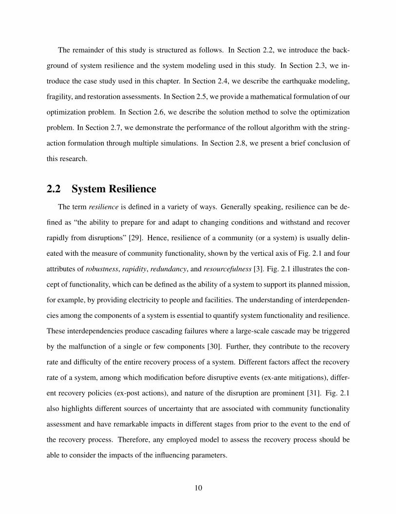
The term resilience is defined in a variety of ways. Generally speaking, resilience can be de-

fined as “the ability to prepare for and adapt to changing conditions and withstand and recover

rapidly from disruptions” [29]. Hence, resilience of a community (or a system) is usually delin-

eated with the measure of community functionality, shown by the vertical axis of Fig. 2.1 and four

attributes of robustness, rapidity, redundancy, and resourcefulness [3]. Fig. 2.1 illustrates the con-

cept of functionality, which can be defined as the ability of a system to support its planned mission,

for example, by providing electricity to people and facilities. The understanding of interdependen-

cies among the components of a system is essential to quantify system functionality and resilience.

These interdependencies produce cascading failures where a large-scale cascade may be triggered

by the malfunction of a single or few components [30]. Further, they contribute to the recovery

rate and difficulty of the entire recovery process of a system. Different factors affect the recovery

rate of a system, among which modification before disruptive events (ex-ante mitigations), differ-

ent recovery policies (ex-post actions), and nature of the disruption are prominent [31]. Fig. 2.1

also highlights different sources of uncertainty that are associated with community functionality

assessment and have remarkable impacts in different stages from prior to the event to the end of

the recovery process. Therefore, any employed model to assess the recovery process should be

able to consider the impacts of the influencing parameters.

10

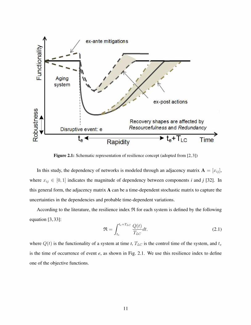
Figure 2.1: Schematic representation of resilience concept (adopted from [2, 3])

In this study, the dependency of networks is modeled through an adjacency matrix A = [xij],

where xij ∈ [0, 1] indicates the magnitude of dependency between components i and j [32]. In

this general form, the adjacency matrix A can be a time-dependent stochastic matrix to capture the

uncertainties in the dependencies and probable time-dependent variations.

According to the literature, the resilience index R for each system is defined by the following

equation [3, 33]:

R =

∫ te+TLC

te

Q(t)

TLCdt. (2.1)

where Q(t) is the functionality of a system at time t, TLC is the control time of the system, and te

is the time of occurrence of event e, as shown in Fig. 2.1. We use this resilience index to define

one of the objective functions.

11

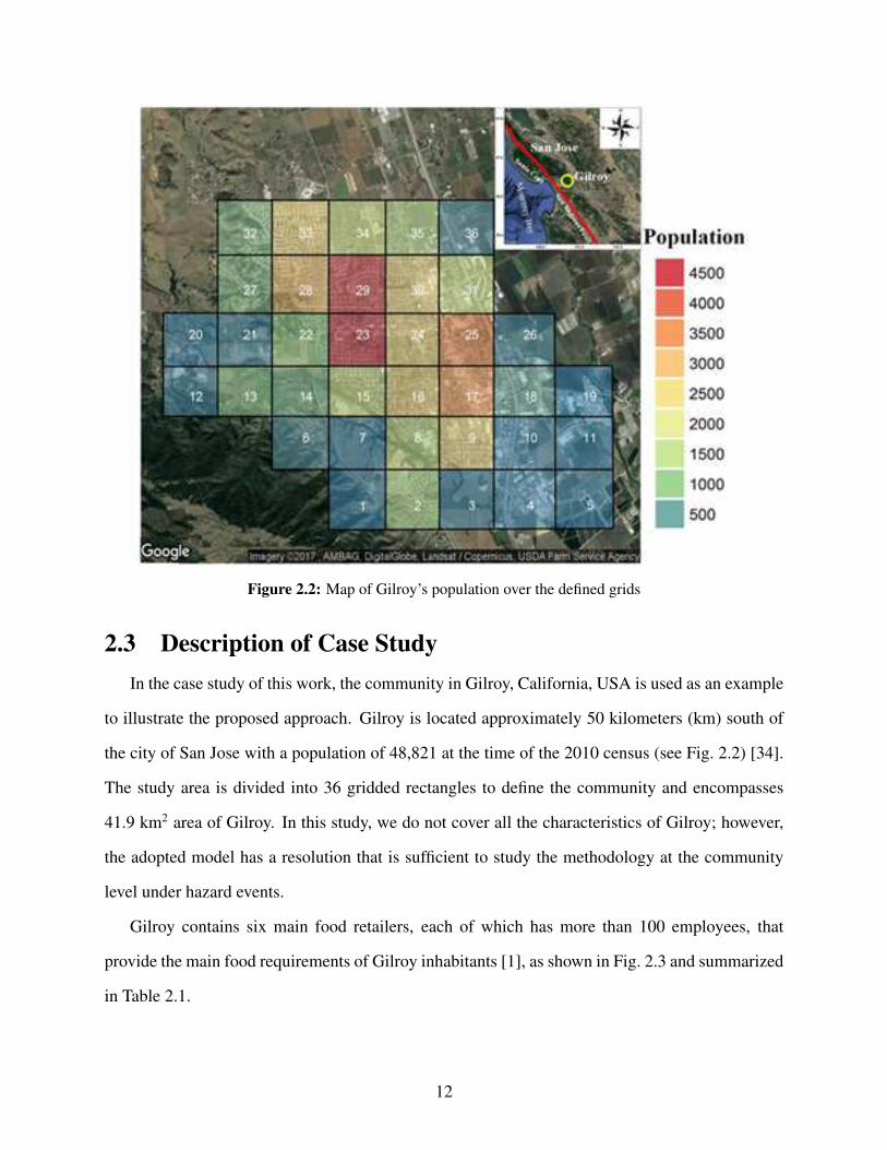
Figure 2.2: Map of Gilroy’s population over the defined grids

2.3 Description of Case Study

In the case study of this work, the community in Gilroy, California, USA is used as an example

to illustrate the proposed approach. Gilroy is located approximately 50 kilometers (km) south of

the city of San Jose with a population of 48,821 at the time of the 2010 census (see Fig. 2.2) [34].

The study area is divided into 36 gridded rectangles to define the community and encompasses

41.9 km2 area of Gilroy. In this study, we do not cover all the characteristics of Gilroy; however,

the adopted model has a resolution that is sufficient to study the methodology at the community

level under hazard events.

Gilroy contains six main food retailers, each of which has more than 100 employees, that

provide the main food requirements of Gilroy inhabitants [1], as shown in Fig. 2.3 and summarized

in Table 2.1.

12

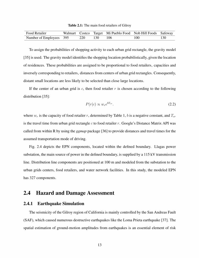
Table 2.1: The main food retailers of Gilroy

Food Retailer Walmart Costco Target Mi Pueblo Food Nob Hill Foods SafewayNumber of Employees 395 220 130 106 100 130

To assign the probabilities of shopping activity to each urban grid rectangle, the gravity model

[35] is used. The gravity model identifies the shopping location probabilistically, given the location

of residences. These probabilities are assigned to be proportional to food retailers‚ capacities and

inversely corresponding to retailers‚ distances from centers of urban grid rectangles. Consequently,

distant small locations are less likely to be selected than close large locations.

If the center of an urban grid is c, then food retailer r is chosen according to the following

distribution [35]:

P (r|c) ∝ wrebTcr . (2.2)

where wr is the capacity of food retailer r, determined by Table 1, b is a negative constant, and Tcr

is the travel time from urban grid rectangle c to food retailer r. Google’s Distance Matrix API was

called from within R by using the ggmap package [36] to provide distances and travel times for the

assumed transportation mode of driving.

Fig. 2.4 depicts the EPN components, located within the defined boundary. Llagas power

substation, the main source of power in the defined boundary, is supplied by a 115 kV transmission

line. Distribution line components are positioned at 100 m and modeled from the substation to the

urban grids centers, food retailers, and water network facilities. In this study, the modeled EPN

has 327 components.

2.4 Hazard and Damage Assessment

2.4.1 Earthquake Simulation

The seismicity of the Gilroy region of California is mainly controlled by the San Andreas Fault

(SAF), which caused numerous destructive earthquakes like the Loma Prieta earthquake [37]. The

spatial estimation of ground-motion amplitudes from earthquakes is an essential element of risk

13

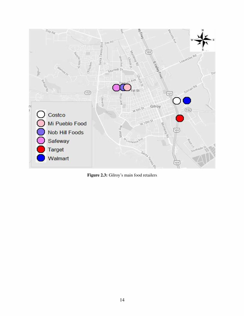
Figure 2.3: Gilroy’s main food retailers

14

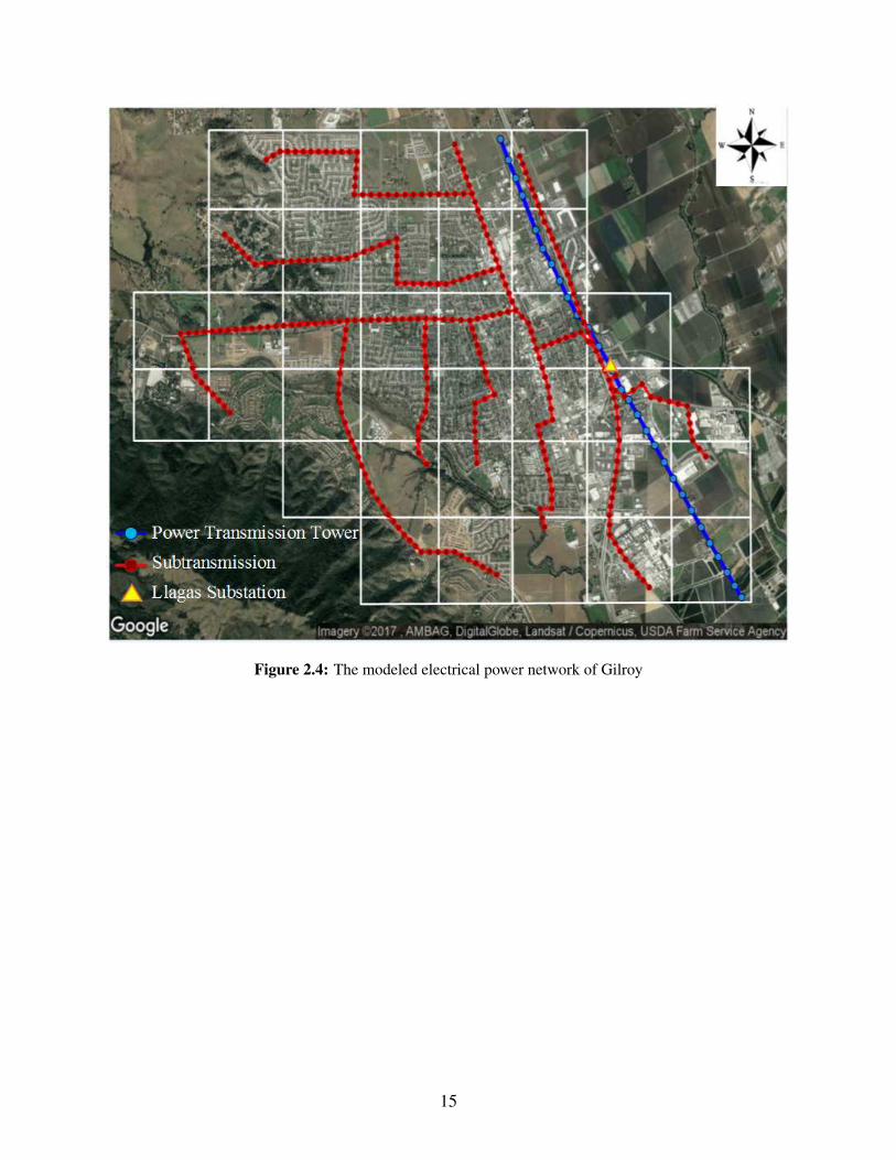
Figure 2.4: The modeled electrical power network of Gilroy

15

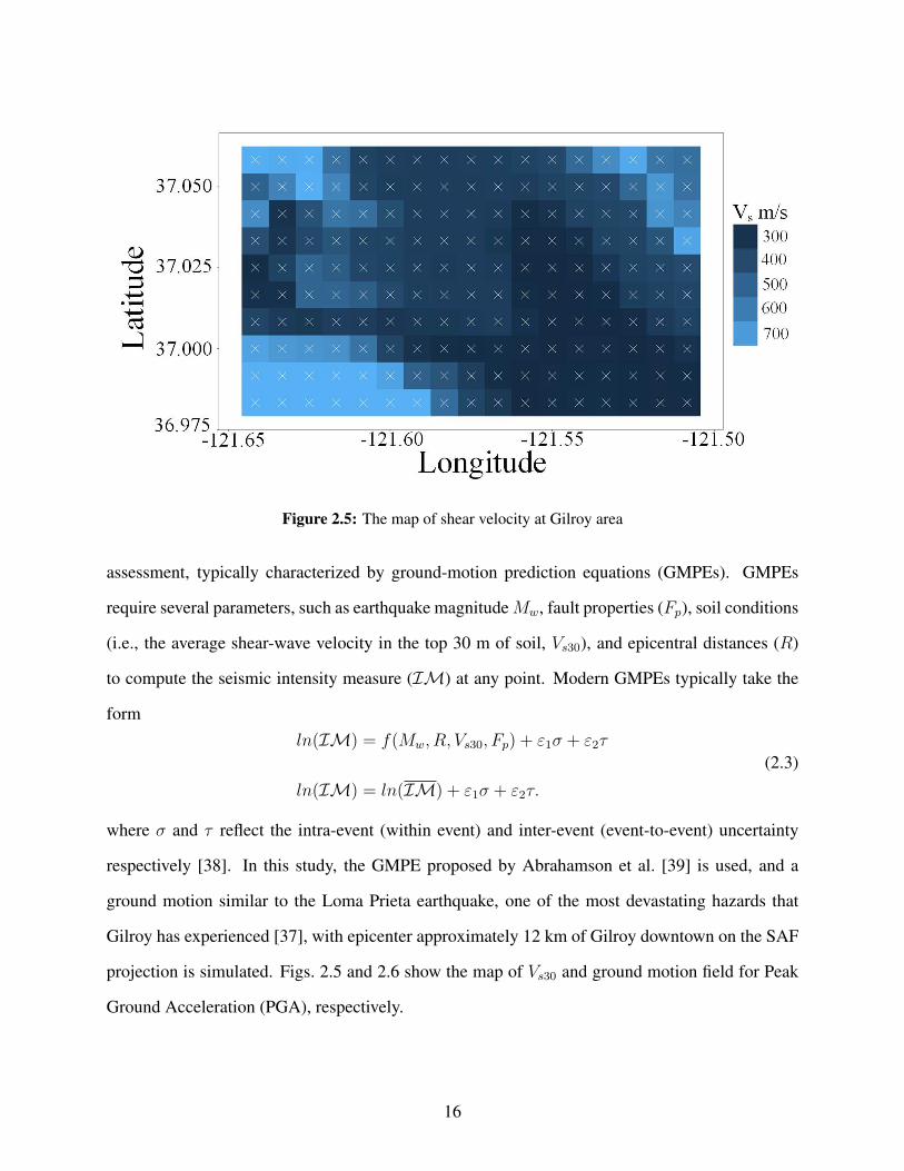
Figure 2.5: The map of shear velocity at Gilroy area

assessment, typically characterized by ground-motion prediction equations (GMPEs). GMPEs

require several parameters, such as earthquake magnitudeMw, fault properties (Fp), soil conditions

(i.e., the average shear-wave velocity in the top 30 m of soil, Vs30), and epicentral distances (R)

to compute the seismic intensity measure (IM) at any point. Modern GMPEs typically take the

form

ln(IM) = f(Mw, R, Vs30, Fp) + ε1σ + ε2τ

ln(IM) = ln(IM) + ε1σ + ε2τ.

(2.3)

where σ and τ reflect the intra-event (within event) and inter-event (event-to-event) uncertainty

respectively [38]. In this study, the GMPE proposed by Abrahamson et al. [39] is used, and a

ground motion similar to the Loma Prieta earthquake, one of the most devastating hazards that

Gilroy has experienced [37], with epicenter approximately 12 km of Gilroy downtown on the SAF

projection is simulated. Figs. 2.5 and 2.6 show the map of Vs30 and ground motion field for Peak

Ground Acceleration (PGA), respectively.

16

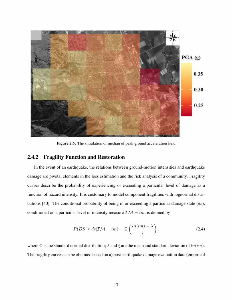
Figure 2.6: The simulation of median of peak ground acceleration field

2.4.2 Fragility Function and Restoration

In the event of an earthquake, the relations between ground-motion intensities and earthquake

damage are pivotal elements in the loss estimation and the risk analysis of a community. Fragility

curves describe the probability of experiencing or exceeding a particular level of damage as a

function of hazard intensity. It is customary to model component fragilities with lognormal distri-

butions [40]. The conditional probability of being in or exceeding a particular damage state (ds),

conditioned on a particular level of intensity measure IM = im, is defined by

P (DS ≥ ds|IM = im) = Φ

(

ln(im)− λ

ξ

)

. (2.4)

where Φ is the standard normal distribution; λ and ξ are the mean and standard deviation of ln(im).

The fragility curves can be obtained based on a) post-earthquake damage evaluation data (empirical

17

curves) [41] b) structural modeling (analytical curves) [42] c) expert opinions (heuristics curves)

[43]. In the present study, the seismic fragility curves included in [44, 45] are used for illustration.

To restore a network, a number of available resource units, N , as a generic single number in-

cluding equipment, replacement components, and repair crews are considered for assignment to

damaged components, and each damaged component is assumed to require only one unit of re-

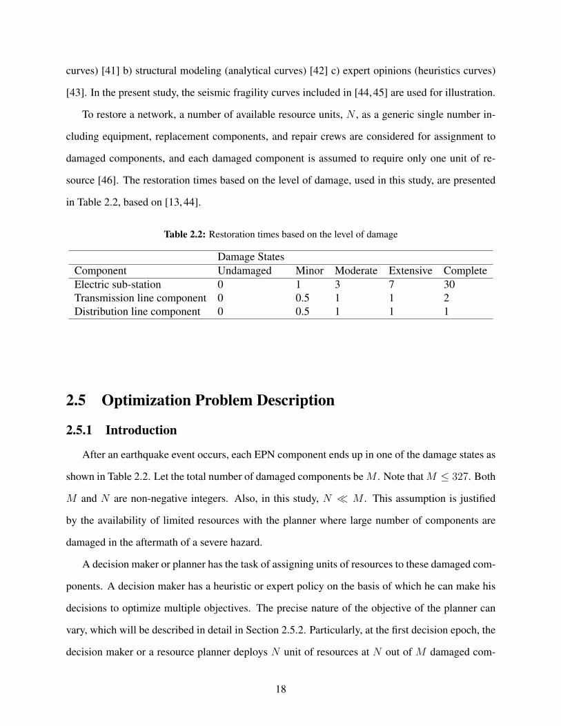
source [46]. The restoration times based on the level of damage, used in this study, are presented

in Table 2.2, based on [13, 44].

Table 2.2: Restoration times based on the level of damage

Damage StatesComponent Undamaged Minor Moderate Extensive CompleteElectric sub-station 0 1 3 7 30Transmission line component 0 0.5 1 1 2Distribution line component 0 0.5 1 1 1

2.5 Optimization Problem Description

2.5.1 Introduction

After an earthquake event occurs, each EPN component ends up in one of the damage states as

shown in Table 2.2. Let the total number of damaged components beM . Note thatM ≤ 327. Both

M and N are non-negative integers. Also, in this study, N ≪ M . This assumption is justified

by the availability of limited resources with the planner where large number of components are

damaged in the aftermath of a severe hazard.

A decision maker or planner has the task of assigning units of resources to these damaged com-

ponents. A decision maker has a heuristic or expert policy on the basis of which he can make his

decisions to optimize multiple objectives. The precise nature of the objective of the planner can

vary, which will be described in detail in Section 2.5.2. Particularly, at the first decision epoch, the

decision maker or a resource planner deploys N unit of resources at N out of M damaged com-

18

ponents. Each unit of resource is assigned to a distinct damaged component. At every subsequent

decision epoch, the planner must have an option of reassigning some or all of the resources to new

locations based on his heuristics and objectives. He must have the flexibility of such a reassign-

ment even if the repair work at the currently assigned locations is not complete. At every decision

epoch, it is possible to forestall the reassignment of the units of resource that have not completed

the repair work; however, we choose to solve the more general problem of preemptive assignment,

where non-preemption at few or all the locations is a special case of our problem. The preemptive

assignment problem is a richer decision problem than the non-preemptive case in the sense that the

process of optimizing the decision actions is a more complex task because the size of the decision

space is bigger.

In this study, we assume that the outcome of the decisions is fully predictable. We improve

upon the solutions offered by heuristics of the planner by formulating our optimization problem as

a dynamic program, and solving it using the rollout approach.

2.5.2 Optimization Problem Formulation

Suppose that the decision maker starts making decisions and assigning repair locations to dif-

ferent units of resource. The number of such non-trivial decisions to be made is less than or equal

to M − N . When M becomes less than or equal to N (because of sequential application of re-

pair actions to the damaged components), the assignment of units of resource becomes a trivial

problem in our setting because each unit can simply be assigned one to one, in any order, to the

damaged components. Consequently, a strict optimal assignment can be achieved in the trivial

case. The size of this trivial assignment problem reduces by one for every new decision epoch

until all the remaining damaged components are repaired. The additional units of resources retire

because deploying more than one unit of resource to the same location does not decrease the repair

time associated with that damaged component. Henceforth, we focus on the non-trivial assignment

problem.

19

Let the variable t denote the decision epoch, and let Dt be the set of all damaged compo-

nents before a repair action xt is performed. Let tend denote the decision epoch at which re-

pair action xtendis selected so that |Dtend+1| ≤ N . Note that t ∈ A := (1, 2, . . . , tend). Let

X = (x1, x2, . . . , xtend) represent the string of actions owing to the non-trivial assignment. We say

that a repair action is completed when at least one out of the N damaged components is repaired.

Let P(Dt) be the powerset of Dt. Let,

PN(Dt) = C ∈ P(Dt) : |C| = N. (2.5)

so that xt ∈ PN(Dt). Let Rt be the set of all repaired components after the repair action xt is

completed. Note that Dt+1 = Dt\Rt, ∀t ∈ A, where 1 ≤ |Dtend+1| ≤ N , and the decision-

making problem moves into the trivial assignment problem previously discussed.

We wish to calculate a string X of repair actions that optimizes our objective functions F (X).

We deal with two objective functions in this study denoted by mapping F1 and F2.

• Objective 1: Let the variable p represent the population of Gilroy and γ represent a constant

threshold. Let X1 = (x1, . . . , xi) be the string of repair actions that results in restoration

of electricity to γ × p number of people. Here, xi ∈ PN(Di), where Di is the number of

damaged component at the ith decision epoch. Let n represent the time required to restore

electricity to γ × p number of people as a result of repair actions X1. Formally,

F1 (X1) = n. (2.6)

Objective 1 is to compute the optimal solution X∗1 given by

X∗1 = argmin

X1

F1(X1). (2.7)

We explain the precise meaning of restoration of electricity to people in more detail in Sec-

tion 2.7.1. To sum up, in objective 1, our aim is to find a string of actions that minimizes the

20

number of days needed to restore electricity to a certain fraction (γ) of the total population

of Gilroy.

• Objective 2: We define the mapping F2 in terms of number of people who have electricity

per unit of time; our objective is to maximize this mapping over a string of repair actions.

Let the variable kt denote the total time elapsed between the completion of repair action xt−1

and xt, ∀t ∈ A\1; k1 is the time elapsed between the start and completion of repair action

x1. Let ht be the total number of people that have benefit of EPN recovery after the repair

action xt is complete. Then,

F2(X) =1

kttot

tend∑

t=1

ht × kt, (2.8)

where kttot =∑tend

v=1 ktv . We are interested in the optimal solution X∗ given by

X∗ = argmaxX

F2(X). (2.9)

Note that our objective function in the second case F2(X) mimics the resilience index and can

be interpreted in terms of (2.1). Particularly, the integral in (2.1) is replaced by a sum because of

discrete decision epochs, Q(t) is replaced by the product ht × kt, ktendis analogous to TLC , and

the integral limits are changed to represent the discrete decision epochs.

2.6 Optimization Problem Solution

Calculating X∗ or X∗1 is a sequential optimization problem. The decision maker applies the

repair action xt at the decision epoch t to maximize or minimize a cumulative objective function.

The string of actions, as represented inX orX1, are an outcome of this sequential decision-making

process. This is particularly relevant in the context of dynamic programming where numerous

solution techniques are available for the sequential optimization problem. Rollout is one such

method that originated in dynamic programming. It is possible to use the dynamic programming

21

formalism to describe the method of rollout, but here we accomplish this by starting from first

principles [47]. We will draw comparisons between rollout with first principles and rollout in

dynamic programming at suitable junctions. The description of the rollout algorithm is inherently

tied with the notion of approximate dynamic programming.

2.6.1 Approximate Dynamic Programming

Let’s focus our attention on objective 1. The extension of this methodology to objective 2

is straightforward; we need to adapt notation used for objective 2 in the methodology presented

below, and a maximization problem replaces a minimization problem. Recall that we are interested

in the optimal solution X∗1 given by (2.7). This can be calculated in the following manner:

First calculate x∗1 as follows:

x∗1 ∈ argminx1

J1(x1), (2.10)

where the function J1 is defined by

J1(x1) = minx2,...,xi

F1(X1). (2.11)

Next, calculate x∗2 as:

x∗2 ∈ argminx2

J2(x∗1, x2), (2.12)

where the function J2 is defined by

J2(x1, x2) = minx3,...,xi

F1(X1). (2.13)

Similarly, we calculate the α-solution as follows:

x∗α ∈ argminxα

Jα(x∗1, . . . , x

∗α−1, xα), (2.14)

where the function Jα is defined by

22

Jα(x1, . . . , xα) = minxα+1,...,xi

F1(X1). (2.15)

The functions Jα are called the optimal cost-to-go functions and are defined by the following

recursion:

Jα(x1, . . . , xα) = minxα+1

Jα+1(x1, . . . , xα+1), (2.16)

where the boundary condition is given by:

Ji(X1) = F1(X1). (2.17)

Note that J is a standard notation used to represent cost-to-go functions in the dynamic program-

ming literature.

The approach discussed above to calculate the optimal solutions is typical of the dynamic pro-

gramming formulation. However, except for very special problems, such a formulation cannot be

solved exactly because calculating and storing the optimal cost-to-go functions Jα can be numeri-

cally intensive. Particularly, for our problem, let |PN(Dt)| = βt; then the storage of Jα requires a

table of size

Sα =α∏

t=1

βt, (2.18)

where α ≤ i for objective 1, and α ≤ tend for objective 2. In the dynamic programming literature,

this is called as the curse of dimensionality. If we consider objective 2 and wish to calculate Jα such

that α = M − N (we assume for the sake of this example that only a single damaged component

is repaired at each t), then for 50 damaged components and 10 unit of resources, Sα ≈ 10280. In

practice, Jα in (2.14) is replaced by an approximation denoted by Jα. In the literature, Jα is called

as a scoring function or approximate cost-to-go function [48]. One way to calculate Jα is with the

aid of a heuristic; there are several ways to approximate Jα that do not utilize heuristic algorithms.

All such approximation methods fall under the category of approximate dynamic programming.

The method of rollout utilizes a heuristic in the approximation process. We provide a more

detailed discussion on the heuristic in Section 2.6.2. Suppose that a heuristicH is used to approx-

23

imate the minimization in (2.15), and let Hα(x1, . . . , xα) denote the corresponding approximate

optimal value; then rollout yields the suboptimal solution by replacing Jα with Hα in (2.14):

xα ∈ argminxα

Hα(x1, . . . , xα−1, xα). (2.19)

The heuristic used in the rollout algorithm is usually termed as the base heuristic. In many

practical problems, rollout results in a significant improvement over the underlying base heuristic

to solve the approximate dynamic programming problem [48].

2.6.2 Rollout Algorithm

It is possible to define the base heuristicH in several ways:

(i) The current recovery policy of regionally responsible public and private entities,

(ii) The importance analyses that prioritize the importance of components based on the consid-

ered importance factors [49],

(iii) The greedy algorithm that computes the greedy heuristic [50, 51],

(iv) A random policy without any pre-assumption,

(v) A pre-defined empirical policy; e.g., base heuristic based on the maximum node and link

betweenness (shortest path), as for example, used in the studies of [46, 52].

The rollout method described in Section 2.6.1, using first principles and string-action formula-

tion, for a discrete, deterministic, and sequential optimization problem has interpretations in terms

of the policy iteration algorithm in dynamic programming. The policy iteration algorithm (see [53]

for the details of the policy iteration algorithm including the definition of policy in the dynamic

programming sense) computes an improved policy (policy improvement step), given a base pol-

icy (stationary), by evaluating the performance of the base policy. The policy evaluation step is

typically performed through simulations [7]. Rollout policy can be viewed as the improved policy

calculated using the policy iteration algorithm after a single iteration of the policy improvement

24

step. For a discrete and deterministic optimization problem, the base policy used in the policy it-

eration algorithm is equivalent to the base heuristic, and the rollout policy consists of the repeated

application of this heuristic. This approach was used by the authors in [48] where they provide per-

formance guarantees on the basic rollout approach and discuss variations to the rollout algorithm.

Henceforth, for our purposes, base policy and base heuristic will be considered indistinguishable.

On a historical note, the term rollout was first coined by Tesauro in reference to creating com-

puter programs that play backgammon [54]. An approach similar to rollout was also shown much

earlier in [55].

Ideally, we would like the rollout method to never perform worse than the underlying base

heuristic (guarantee performance). This is possible under each of the following three cases [48]:

1. The rollout method is terminating (called as optimized rollout).

2. The rollout method utilizes a base heuristic that is sequentially consistent (called as rollout).

3. The rollout method is terminating and utilizes a base heuristic that is sequentially improving

(extended rollout and fortified rollout).

A sequentially consistent heuristic guarantees that the rollout method is terminating. It also guar-

antees that the base heuristic is sequentially improving. Therefore, 3 and 1 are the special cases of

2 with a less restrictive property imposed on the base heuristic (that of sequential improvement or

termination). When the base heuristic is sequentially consistent, the fortified and extended rollout

method are the same as the rollout method.

A heuristic must posses the property of termination to be used as a base heuristic in the rollout

method. Even if the base heuristic is terminating, the rollout method need not be terminating.

Apart from the sequential consistency of the base heuristic, the rollout method is guaranteed to be

terminating if it is applied on problems that exhibit special structure. Our problem exhibits such

a structure. In particular, a finite number of damaged components in our problem are equivalent

to the finite node set in [48]. Therefore, the rollout method in this study is terminating. In such a

25

scenario, we could use the optimized rollout algorithm to guarantee performance without putting

any restriction on the base heuristic to be used in the proposed formulation; however, a wiser base

heuristic can potentially enhance further the computed rollout policy. Nevertheless, our problem

does not require any special structure on the base heuristic for the rollout method to be sequentially

improving, which is justified later in this section.

In the terminology of dynamic programming, a base heuristic that admits sequential consis-

tency is analogous to the Markov or stationary policy. Similarly, the terminating rollout method

defines a rollout policy that is stationary.

Two different base heuristics are considered in this study. The first base heuristic is a random

heuristic denoted byH. The idea behind consideration of this heuristic is that in actuality there are

cases where there is no thought-out strategy or the computation of such a scheme is computation-

ally expensive. We will show though simulations that the rollout formulation can accept a random

base policy at the community level from a decision maker and improve it significantly. The second

base heuristic is called a smart heuristic because it is based on the importance of components and

expert judgment, denoted by H. The importance factors used in prioritizing the importance of

the components can accommodate the contribution of each component in the network. This base

heuristic is similar in spirit to the items (ii) and (v) listed above. More description on the assign-

ment of units of resources based on H and H is described in Section 2.7.1. We also argue there

thatH and H are sequentially consistent. Therefore, in this study, and for our choice of heuristics,

the extended, fortified, and rollout method are equivalent.

Let H be any heuristic algorithm; the state of this algorithm at the first decision epoch is j1,

where j1 = (x1). Similarly, the state of the algorithm at the αth decision epoch is the α-solution

given by jα = (x1, . . . , xα), i.e., the algorithm generates the path of the states (j1, j2, . . . , jα). Note

that j0 is the dummy initial state of the algorithm H. The algorithm H terminates when α = i for

objective 1, and α = tend for objective 2. Henceforth, in this section, we consider only objective

1 without any loss of generality. Let Hα(jα) denote the cost-to-go starting from the α-solution,

generated by applying H (i.e., H is used to evaluate the cost-to-go). The cost-to-go associated

26

with the algorithm H is equal to the terminal reward, i.e., Hα(jα) = F1(X1). Therefore, we have:

H1(j1) = H2(j2) = . . . = Hi(ji). We use this heuristic cost-to-go in (2.14) to find an approximate

solution to our problem. This approximation algorithm is termed as “Rollout on H” (RH) owing

to its structure that is similar to the approximate dynamic programming approach rollout. TheRH

algorithm generates the path of the states (j1, j2, . . . , ji) as follows:

jα = arg minδ∈N(jα−1)

J(δ), α = 1, . . . , i (2.20)

where, jα−1 = (x1, . . . , xα−1), and

N(jα−1) = (x1, . . . , xα−1, x)|x ∈ PN(Dα). (2.21)

The algorithm RH is sequentially improving with respect to H and outperforms H (see [56] for

the details of the proof).

The RH algorithm described above is termed as one-step lookahead approach because the re-

pair action at any decision epoch t (current step) is optimized by minimizing the cost-to-go given

the repair action at t (see (2.20)). It is possible to generalize this approach to incorporate multi-step

lookahead. Suppose that we optimize the repair actions at any decision epoch t and t + 1 (current

and the next step combined) by minimizing the cost-to-go given the repair actions for the current

and next steps. This can be viewed as a two-step lookahead approach. Note the similarity of this

approach with the dynamic programming formulation from first principles in Section 2.6.1, except

for the difficulty of estimating the cost-to-go values J exactly. Also, note that a two-step lookahead

approach is computationally more intensive than the one-step approach. In principle, it is possible

to extend it to step size λ, where 1 ≤ λ ≤ i. However, as λ increases, the computational com-

plexity of the algorithm increases exponentially. Particularly, when λ is selected equal to i at the

first decision epoch, the RH algorithm finds the exact optimal solution by exhaustively searching

through all possible combinations of repair action at each t, with computational complexity O(Si).

27

Also, note thatRH provides a tighter upper bound on the optimal objective value compared to the

bound obtained from the original heuristic approach.

2.7 Results

2.7.1 Discussion

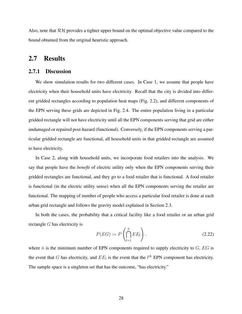
We show simulation results for two different cases. In Case 1, we assume that people have

electricity when their household units have electricity. Recall that the city is divided into differ-

ent gridded rectangles according to population heat maps (Fig. 2.2), and different components of

the EPN serving these grids are depicted in Fig. 2.4. The entire population living in a particular

gridded rectangle will not have electricity until all the EPN components serving that grid are either

undamaged or repaired post-hazard (functional). Conversely, if the EPN components serving a par-

ticular gridded rectangle are functional, all household units in that gridded rectangle are assumed

to have electricity.

In Case 2, along with household units, we incorporate food retailers into the analysis. We

say that people have the benefit of electric utility only when the EPN components serving their

gridded rectangles are functional, and they go to a food retailer that is functional. A food retailer

is functional (in the electric utility sense) when all the EPN components serving the retailer are

functional. The mapping of number of people who access a particular food retailer is done at each

urban grid rectangle and follows the gravity model explained in Section 2.3.

In both the cases, the probability that a critical facility like a food retailer or an urban grid

rectangle G has electricity is

P (EG) := P

(

n⋂

l=1

EEl

)

. (2.22)

where n is the minimum number of EPN components required to supply electricity to G, EG is

the event that G has electricity, and EEl is the event that the lth EPN component has electricity.

The sample space is a singleton set that has the outcome, “has electricity.”

28

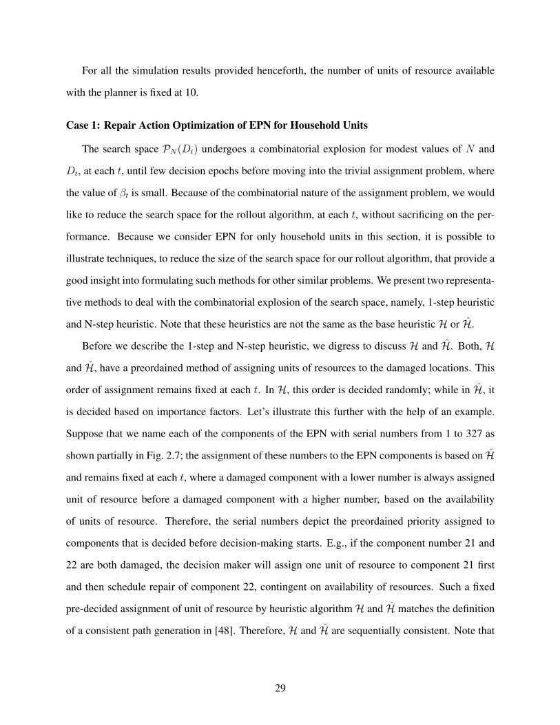
For all the simulation results provided henceforth, the number of units of resource available

with the planner is fixed at 10.

Case 1: Repair Action Optimization of EPN for Household Units

The search space PN(Dt) undergoes a combinatorial explosion for modest values of N and

Dt, at each t, until few decision epochs before moving into the trivial assignment problem, where

the value of βt is small. Because of the combinatorial nature of the assignment problem, we would

like to reduce the search space for the rollout algorithm, at each t, without sacrificing on the per-

formance. Because we consider EPN for only household units in this section, it is possible to

illustrate techniques, to reduce the size of the search space for our rollout algorithm, that provide a

good insight into formulating such methods for other similar problems. We present two representa-

tive methods to deal with the combinatorial explosion of the search space, namely, 1-step heuristic

and N-step heuristic. Note that these heuristics are not the same as the base heuristicH or H.

Before we describe the 1-step and N-step heuristic, we digress to discuss H and H. Both, H

and H, have a preordained method of assigning units of resources to the damaged locations. This

order of assignment remains fixed at each t. In H, this order is decided randomly; while in H, it

is decided based on importance factors. Let’s illustrate this further with the help of an example.

Suppose that we name each of the components of the EPN with serial numbers from 1 to 327 as

shown partially in Fig. 2.7; the assignment of these numbers to the EPN components is based on H

and remains fixed at each t, where a damaged component with a lower number is always assigned

unit of resource before a damaged component with a higher number, based on the availability

of units of resource. Therefore, the serial numbers depict the preordained priority assigned to

components that is decided before decision-making starts. E.g., if the component number 21 and

22 are both damaged, the decision maker will assign one unit of resource to component 21 first

and then schedule repair of component 22, contingent on availability of resources. Such a fixed

pre-decided assignment of unit of resource by heuristic algorithmH and H matches the definition

of a consistent path generation in [48]. Therefore, H and H are sequentially consistent. Note that

29

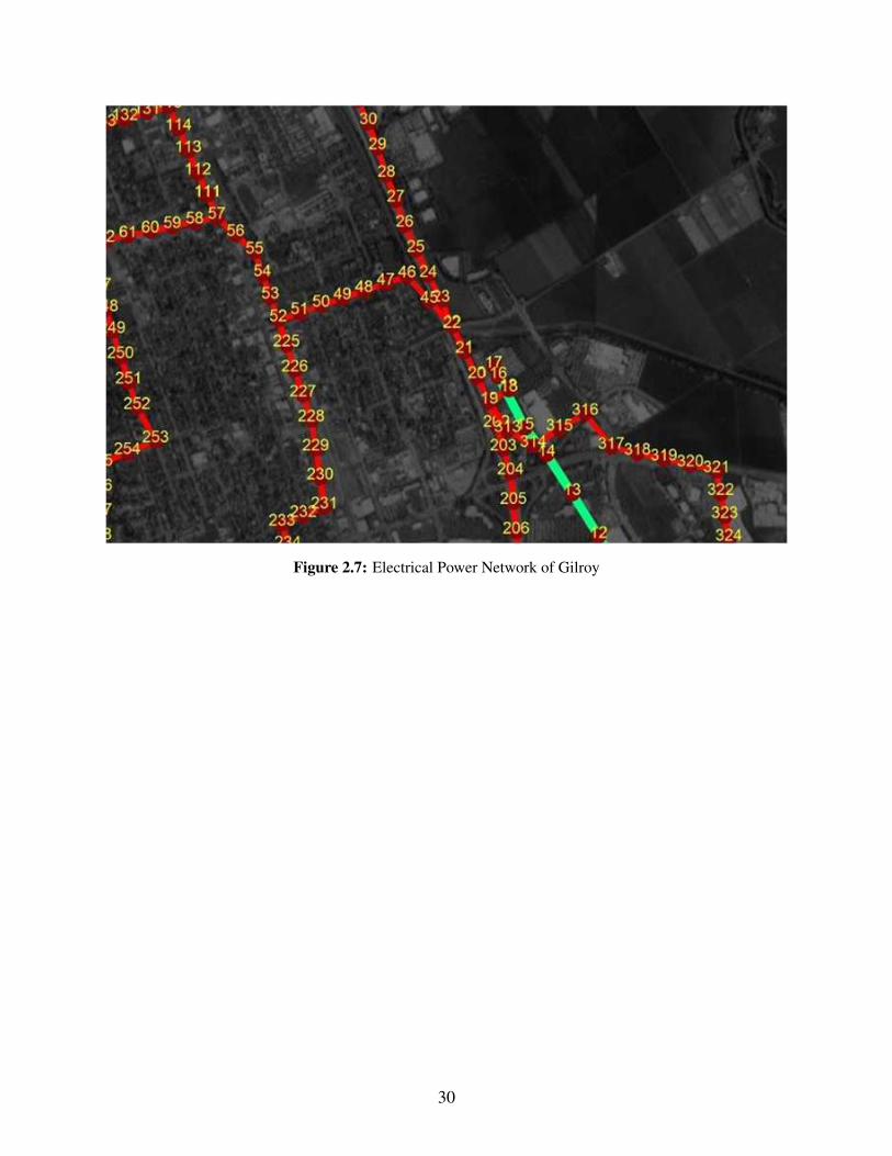
Figure 2.7: Electrical Power Network of Gilroy

30

the assignment of numbers 1 to 327 in Fig. 2.7 is assumed only for illustration purposes; the rollout

method can incorporate a different preordained order defined byH and H.

We now discuss the 1-step and N-step heuristic. In Fig. 2.7, note that each successive EPN

component (labeled 1-327), is dependent upon the prior EPN component for electricity. E.g.,

component 227 is dependent upon component 50. Similarly, component 55 is dependent upon

component 50. The components in the branch 53-57 and 225-231 depend upon the component 52

for electricity. We exploit this serial nature of an EPN by representing the EPN network as a tree

structure as shown in Fig. 2.8. Each number in the EPN tree represents an EPN component; each

node represents a group of components determined by the label of the node, and the arcs of the

tree capture the dependence of the nodes.

If the number of damaged components in the root node of the EPN tree is greater than N , then

it would be unwise to assign a unit of resource at the first decision epoch to the fringe nodes of our

EPN tree because we do not get any benefit until we repair damaged components in the root node.

As soon as the number of damaged components in the root node of the EPN tree becomes less than

N , only then we explore the assignment problem at other levels of the EPN tree.

1-step Heuristic: We increase the pool of candidate damaged components, where the assign-

ment of units of resources must be considered, to all the damaged components of the next level of

the EPN tree if and only if the number of damaged components at the current level of the EPN tree

is less than N . Even after considering the next level of the EPN tree, if the number of damaged

components is less than N , we take one more step and account for all damaged components two

levels below the current level. We repeat this until the pool of candidate damaged components is

greater than or equal to N , or the levels of EPN tree are exhausted.

N-step Heuristic: Note that it might be possible to ignore few nodes at each level of the EPN

tree and assign units of resources to only some promising nodes. This is achieved in the N-step

heuristic (here N in N-step is not same as N -number of workers). Specifically, if the number of

the damaged components at the current level of the EPN tree is less than N , then the algorithm

searches for a node at the next level that has the least number of damaged components, adds

31

Figure 2.8: Electrical Power Network Tree

32

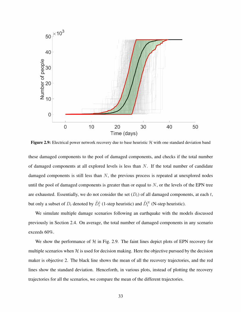
Figure 2.9: Electrical power network recovery due to base heuristicH with one standard deviation band

these damaged components to the pool of damaged components, and checks if the total number

of damaged components at all explored levels is less than N . If the total number of candidate

damaged components is still less than N , the previous process is repeated at unexplored nodes

until the pool of damaged components is greater than or equal to N , or the levels of the EPN tree

are exhausted. Essentially, we do not consider the set (Dt) of all damaged components, at each t,

but only a subset of Dt denoted by D1t (1-step heuristic) and DN

t (N-step heuristic).

We simulate multiple damage scenarios following an earthquake with the models discussed

previously in Section 2.4. On average, the total number of damaged components in any scenario

exceeds 60%.

We show the performance of H in Fig. 2.9. The faint lines depict plots of EPN recovery for

multiple scenarios whenH is used for decision making. Here the objective pursued by the decision

maker is objective 2. The black line shows the mean of all the recovery trajectories, and the red

lines show the standard deviation. Henceforth, in various plots, instead of plotting the recovery

trajectories for all the scenarios, we compare the mean of the different trajectories.

33

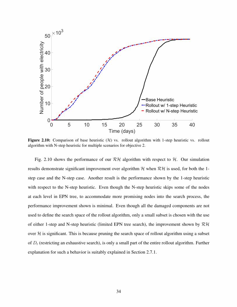
0 5 10 15 20 25 30 35 40

Time (days)

0

10

20

30

40

50N

um

ber

of people

with e

lectr

icity

103

Base Heuristic

Rollout w/ 1-step Heuristic

Rollout w/ N-step Heuristic

Figure 2.10: Comparison of base heuristic (H) vs. rollout algorithm with 1-step heuristic vs. rolloutalgorithm with N-step heuristic for multiple scenarios for objective 2.

Fig. 2.10 shows the performance of our RH algorithm with respect to H. Our simulation

results demonstrate significant improvement over algorithm H when RH is used, for both the 1-

step case and the N-step case. Another result is the performance shown by the 1-step heuristic

with respect to the N-step heuristic. Even though the N-step heuristic skips some of the nodes

at each level in EPN tree, to accommodate more promising nodes into the search process, the

performance improvement shown is minimal. Even though all the damaged components are not

used to define the search space of the rollout algorithm, only a small subset is chosen with the use

of either 1-step and N-step heuristic (limited EPN tree search), the improvement shown by RH

over H is significant. This is because pruning the search space of rollout algorithm using a subset

of Dt (restricting an exhaustive search), is only a small part of the entire rollout algorithm. Further

explanation for such a behavior is suitably explained in Section 2.7.1.

34

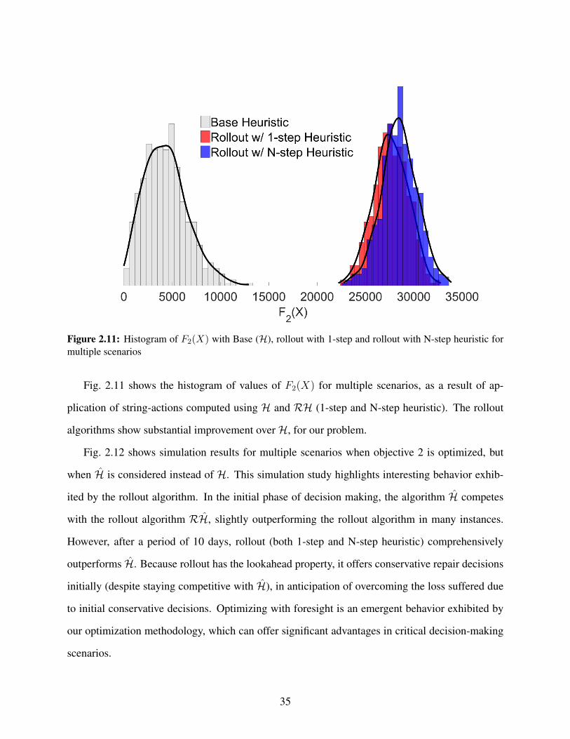
Figure 2.11: Histogram of F2(X) with Base (H), rollout with 1-step and rollout with N-step heuristic formultiple scenarios

Fig. 2.11 shows the histogram of values of F2(X) for multiple scenarios, as a result of ap-

plication of string-actions computed using H and RH (1-step and N-step heuristic). The rollout

algorithms show substantial improvement overH, for our problem.

Fig. 2.12 shows simulation results for multiple scenarios when objective 2 is optimized, but

when H is considered instead of H. This simulation study highlights interesting behavior exhib-

ited by the rollout algorithm. In the initial phase of decision making, the algorithm H competes

with the rollout algorithm RH, slightly outperforming the rollout algorithm in many instances.

However, after a period of 10 days, rollout (both 1-step and N-step heuristic) comprehensively

outperforms H. Because rollout has the lookahead property, it offers conservative repair decisions

initially (despite staying competitive with H), in anticipation of overcoming the loss suffered due

to initial conservative decisions. Optimizing with foresight is an emergent behavior exhibited by

our optimization methodology, which can offer significant advantages in critical decision-making

scenarios.

35

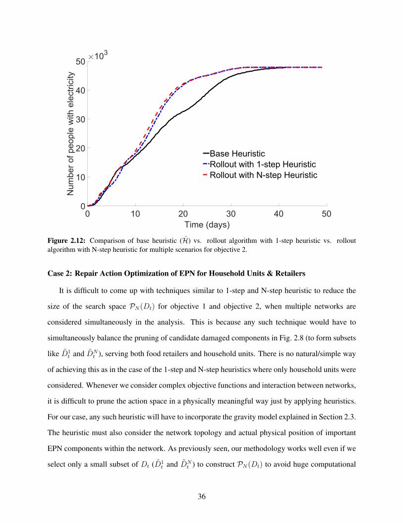
0 10 20 30 40 50

Time (days)

0

10

20

30

40

50N

um

be

r o

f p

eo

ple

with

ele

ctr

icity

103

Base Heuristic

Rollout with 1-step Heuristic

Rollout with N-step Heuristic

Figure 2.12: Comparison of base heuristic (H) vs. rollout algorithm with 1-step heuristic vs. rolloutalgorithm with N-step heuristic for multiple scenarios for objective 2.

Case 2: Repair Action Optimization of EPN for Household Units & Retailers

It is difficult to come up with techniques similar to 1-step and N-step heuristic to reduce the

size of the search space PN(Dt) for objective 1 and objective 2, when multiple networks are

considered simultaneously in the analysis. This is because any such technique would have to

simultaneously balance the pruning of candidate damaged components in Fig. 2.8 (to form subsets

like D1t and DN

t ), serving both food retailers and household units. There is no natural/simple way

of achieving this as in the case of the 1-step and N-step heuristics where only household units were

considered. Whenever we consider complex objective functions and interaction between networks,

it is difficult to prune the action space in a physically meaningful way just by applying heuristics.

For our case, any such heuristic will have to incorporate the gravity model explained in Section 2.3.

The heuristic must also consider the network topology and actual physical position of important

EPN components within the network. As previously seen, our methodology works well even if we

select only a small subset of Dt (D1t and DN

t ) to construct PN(Dt) to avoid huge computational

36

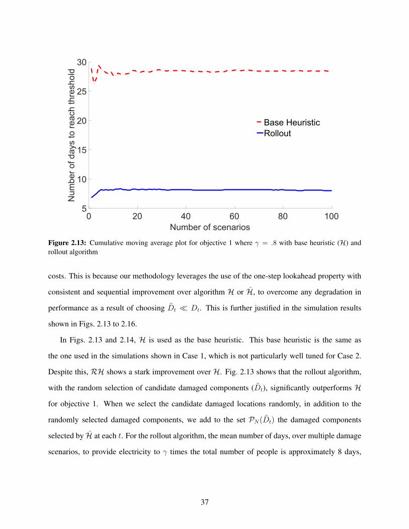
0 20 40 60 80 100

Number of scenarios

5

10

15

20

25

30N

um

be

r o

f d

ays to

re

ach

th

resh

old

Base Heuristic

Rollout

Figure 2.13: Cumulative moving average plot for objective 1 where γ = .8 with base heuristic (H) androllout algorithm

costs. This is because our methodology leverages the use of the one-step lookahead property with

consistent and sequential improvement over algorithm H or H, to overcome any degradation in

performance as a result of choosing Dt ≪ Dt. This is further justified in the simulation results

shown in Figs. 2.13 to 2.16.

In Figs. 2.13 and 2.14, H is used as the base heuristic. This base heuristic is the same as

the one used in the simulations shown in Case 1, which is not particularly well tuned for Case 2.

Despite this, RH shows a stark improvement over H. Fig. 2.13 shows that the rollout algorithm,

with the random selection of candidate damaged components (Dt), significantly outperforms H

for objective 1. When we select the candidate damaged locations randomly, in addition to the

randomly selected damaged components, we add to the set PN(Dt) the damaged components

selected by H at each t. For the rollout algorithm, the mean number of days, over multiple damage

scenarios, to provide electricity to γ times the total number of people is approximately 8 days,

37

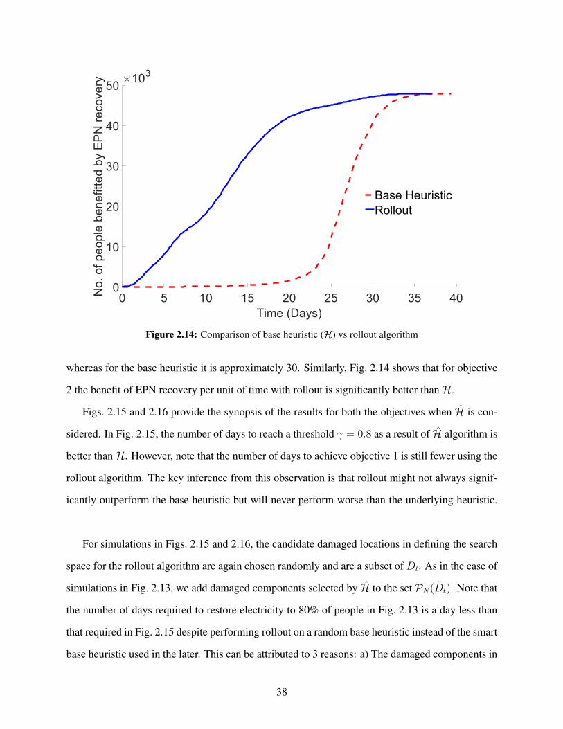
0 5 10 15 20 25 30 35 40

Time (Days)

0

10

20

30

40

50N

o. of pe

op

le b

en

efitte

d b

y E

PN

re

co

ve

ry 103

Base Heuristic

Rollout

Figure 2.14: Comparison of base heuristic (H) vs rollout algorithm

whereas for the base heuristic it is approximately 30. Similarly, Fig. 2.14 shows that for objective

2 the benefit of EPN recovery per unit of time with rollout is significantly better thanH.

Figs. 2.15 and 2.16 provide the synopsis of the results for both the objectives when H is con-

sidered. In Fig. 2.15, the number of days to reach a threshold γ = 0.8 as a result of H algorithm is

better thanH. However, note that the number of days to achieve objective 1 is still fewer using the

rollout algorithm. The key inference from this observation is that rollout might not always signif-

icantly outperform the base heuristic but will never perform worse than the underlying heuristic.

For simulations in Figs. 2.15 and 2.16, the candidate damaged locations in defining the search

space for the rollout algorithm are again chosen randomly and are a subset of Dt. As in the case of

simulations in Fig. 2.13, we add damaged components selected by H to the set PN(Dt). Note that

the number of days required to restore electricity to 80% of people in Fig. 2.13 is a day less than

that required in Fig. 2.15 despite performing rollout on a random base heuristic instead of the smart

base heuristic used in the later. This can be attributed to 3 reasons: a) The damaged components in

38

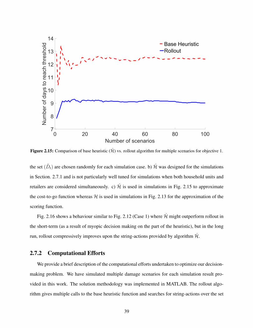
0 20 40 60 80 100

Number of scenarios

7

8

9

10

11

12

13

14N

um

be

r o

f d

ays to

re

ach

th

resh

old Base Heuristic

Rollout

Figure 2.15: Comparison of base heuristic (H) vs. rollout algorithm for multiple scenarios for objective 1.

the set (Dt) are chosen randomly for each simulation case. b) H was designed for the simulations

in Section. 2.7.1 and is not particularly well tuned for simulations when both household units and

retailers are considered simultaneously. c) H is used in simulations in Fig. 2.15 to approximate

the cost-to-go function whereas H is used in simulations in Fig. 2.13 for the approximation of the

scoring function.

Fig. 2.16 shows a behaviour similar to Fig. 2.12 (Case 1) where H might outperform rollout in

the short-term (as a result of myopic decision making on the part of the heuristic), but in the long

run, rollout compressively improves upon the string-actions provided by algorithm H.

2.7.2 Computational Efforts

We provide a brief description of the computational efforts undertaken to optimize our decision-

making problem. We have simulated multiple damage scenarios for each simulation result pro-

vided in this work. The solution methodology was implemented in MATLAB. The rollout algo-

rithm gives multiple calls to the base heuristic function and searches for string-actions over the set

39

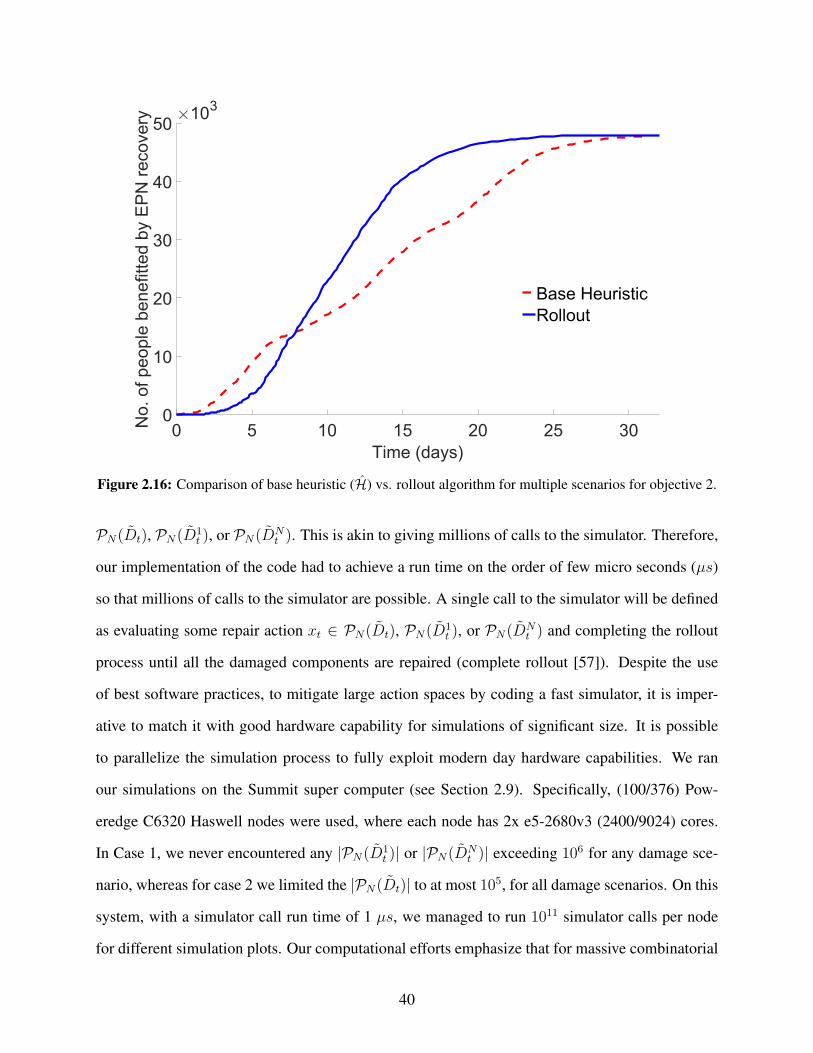
0 5 10 15 20 25 30

Time (days)

0

10

20

30

40

50N

o. of pe

op

le b

en

efitte

d b

y E

PN

re

co

ve

ry 103

Base Heuristic

Rollout

Figure 2.16: Comparison of base heuristic (H) vs. rollout algorithm for multiple scenarios for objective 2.

PN(Dt), PN(D1t ), or PN(DN

t ). This is akin to giving millions of calls to the simulator. Therefore,

our implementation of the code had to achieve a run time on the order of few micro seconds (µs)

so that millions of calls to the simulator are possible. A single call to the simulator will be defined

as evaluating some repair action xt ∈ PN(Dt), PN(D1t ), or PN(DN

t ) and completing the rollout

process until all the damaged components are repaired (complete rollout [57]). Despite the use

of best software practices, to mitigate large action spaces by coding a fast simulator, it is imper-

ative to match it with good hardware capability for simulations of significant size. It is possible

to parallelize the simulation process to fully exploit modern day hardware capabilities. We ran

our simulations on the Summit super computer (see Section 2.9). Specifically, (100/376) Pow-

eredge C6320 Haswell nodes were used, where each node has 2x e5-2680v3 (2400/9024) cores.

In Case 1, we never encountered any |PN(D1t )| or |PN(DN

t )| exceeding 106 for any damage sce-

nario, whereas for case 2 we limited the |PN(Dt)| to at most 105, for all damage scenarios. On this

system, with a simulator call run time of 1 µs, we managed to run 1011 simulator calls per node

for different simulation plots. Our computational efforts emphasize that for massive combinatorial

40

decision-making problems, it is possible to achieve near-optimal performance with our methodol-

ogy by harnessing powerful present day computational systems and implementing sound software

practices.

2.8 Concluding Remarks

In this study, we proposed an optimization formulation based on the method of rollout, for the

identification of near-optimal community recovery actions, following a disaster. Our methodology

utilizes approximate dynamic programming algorithms along with heuristics to overcome the curse

of dimensionality in its analysis and management of large-scale infrastructure systems. We have

shown that the proposed approach can be implemented efficiently to identify near-optimal recov-

ery decisions following a severe earthquake for the electrical power serving Gilroy. Different base

heuristics, used at the community-level recovery, are used in the simulation studies. The intended

methodology and the rollout policies significantly enhanced these base heuristics. Further, the ef-

ficient performance of the rollout formulation in optimizing different common objective functions

for community resilience is demonstrated. We believe that the methodology is adaptable to other

infrastructure systems and hazards.

2.9 Funding and Support

“The research herein has been funded by the National Science Foundation under Grant CMMI-

1638284. This support is gratefully acknowledged. Any opinions, findings, conclusions, or recom-

mendations presented in this material are solely those of the authors and do not necessarily reflect

the views of the National Science Foundation.”

“This work utilized the RMACC Summit supercomputer, which is supported by the National

Science Foundation (awards ACI-1532235 and ACI-1532236), the University of Colorado Boul-

der and Colorado State University. The RMACC Summit supercomputer is a joint effort of the

University of Colorado Boulder and Colorado State University.”

41

Chapter 3

Planning for Community-Level Food Security

Following Disasters

3.1 Introduction

A resilient food supply is necessary for securing and maintaining an adequate food stock for

urban inhabitants before and following extreme hazard events, such as earthquakes and hurricanes.

Food security issues are exacerbated during the chaotic circumstances following disruptive hazard

events [58]. Such events can damage food systems, household units, and utility and transportation

systems, thereby endangering public health and community food security. Main food retailers

play a pivotal role in ensuring community food security, and their functionality, along with the

functionality of household units, is a critical concern of community leaders. Even though numerous

efforts have been undertaken to mitigate the challenging problem of food shortage, very few studies

address this problem from a systems perspective where the interaction between various network is

considered simultaneously. We propose a holistic approach that not only considers the interactions

between the critical networks that contribute towards food security but also provide a method

to compute the near-optimal recovery actions at the community level following the occurrence of

extreme natural hazards. The proposed decision-making algorithm can handle large-scale networks

and provides robust and anticipatory decisions. To this end, we leverage the approximate dynamic

programming (ADP) paradigm to calculate the near-optimal actions periodically and employ a

simulated annealing algorithm to guide the ADP method in selecting the most promising recovery

actions. This fusion enables us to calculate the recovery actions in a limited time, which is usually

not possible because of large candidate solutions. The testbed community modeled after Gilroy,

California, is employed to illustrate how the proposed approach can be implemented efficiently to

find the optimal decisions. Our approach provides policies to restore the critical Electrical Power

42

Networks (EPN), Water Networks (WN), and highway bridges of Gilroy, in the aftermath of a

severe earthquake, in a timely fashion. Specifically, we find a near-optimal sequence of decisions

such that the main utilities of electricity and potable water are restored to the main food retailers

and household units in (approximately) the shortest amount of time. Additionally, we also make

sure that functional food retailers are accessible to community residents. This study pursues the

Sustainable Development Goals (SDGs), a collection of 17 global goals set by the United Nations.

For example, a result of this study is trying to make communities and human settlements inclusive,

safe, resilient and sustainable (SDG 11). We aim to guide community leaders and risk-informed

decision makers in reducing adverse food-insecurity impacts from extreme natural hazards.

3.2 Preliminaries

In this section, we briefly describe the method of simulated annealing. The fusion of simulated

annealing with approximate dynamic programming to obtain near-optimal recovery actions for our

problem is illustrated in our case study in Section 3.4. For a description on approximate dynamic

programming, see Chapter 2.

3.2.1 Simulated Annealing

Simulated annealing (SA) is a random-search technique for global optimization problems. De-

terministic search and gradient-based methods often get trapped at local optima during the search

process. However, the SA method overcomes this limitation and converges to a globally optimal

solution, provided enough iterations are performed and a sufficiently slow cooling schedule is em-

ployed. The underlying Markov chain in SA not only accepts changes that improve the objective

function but also keeps some changes that are not ideal [59]. The likelihood of acceptance of

a worse solution decreases with the difference in objective function values. More precisely, the

probability of acceptance of a worse solution is given by

P = e− ∆f

kBT (3.1)

43

where ∆f is the change in objective function, T is a positive real number representing the current

temperature, and kB is Boltzmann’s constant. The search process would be a greedy search pro-

vided that T → 0 and P → 0, because in this case it only accepts better solutions. On the other

hand, the search process would be a random selection process provided that T → ∞ and P → 1,

because here it accepts any solution.

3.3 Case Study

For the description of the modeled Gilroy city, EPN, food retailers, and the seismic hazard

simulation, see Chapter 2.

3.3.1 Water Networks

The functionality of the potable water network is of great significance, especially following

disasters, to support inhabitants’ health, firefighting, and industrial processes. The major compo-

nents of the WN in Gilroy are illustrated in Fig. 3.1. The WN consists of six water wells, two

booster pump stations (BPS), three water tanks (WT), and the main pipelines.

3.3.2 Highway Bridges

The critical facilities and residence units not only must have essential utilities but also should

be accessible. Gilroy is at the intersection of two main highways: U.S. 101, which extends through

the City in a north/south route, and SR 152, which extends in an east/west direction. Several

highway bridges must be operable to serve the transportation of the community and accessibility,

especially for the main food retailers of Costco, Walmart, and Target.

3.4 Policy Optimization for Food Security

We will recap some of the terms introduced in Chapter 2. We illustrate the performance of

the method using a customary objective in community resilience: the number of people whose

residence units have electricity and potable water (main utilities for short), and who have access to

44

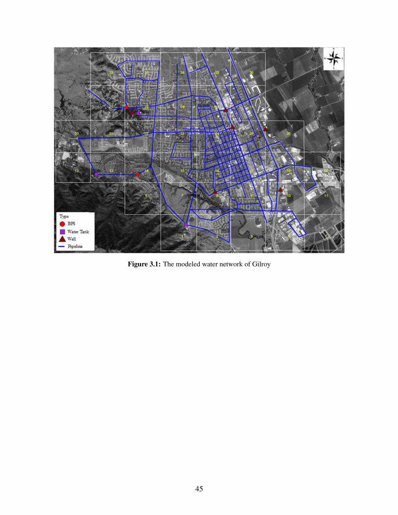
Figure 3.1: The modeled water network of Gilroy

45

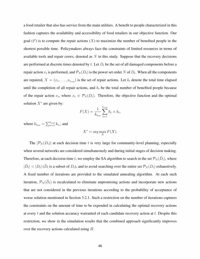
a food retailer that also has service from the main utilities. A benefit to people characterized in this

fashion captures the availability and accessibility of food retailers in our objective function. Our

goal (F ) is to compute the repair actions (X) to maximize the number of benefited people in the

shortest possible time. Policymakers always face the constraints of limited resources in terms of

available tools and repair crews, denoted as N in this study. Suppose that the recovery decisions

are performed at discrete times denoted by t. LetDt be the set of all damaged components before a

repair action xt is performed, andPN(Dt) is the power set orderN ofDt. When all the components

are repaired, X = (x1, . . . , xtend) is the set of repair actions. Let kt denote the total time elapsed

until the completion of all repair actions, and ht be the total number of benefited people because

of the repair action xt, where xt ∈ PN(Dt). Therefore, the objective function and the optimal

solution X∗ are given by:

F (X) =1

kttot

tend∑

t=1

ht × kt,

where kttot =∑tend

v=1 ktv , and

X∗ = argmaxX

F (X).

The |PN(Dt)| at each decision time t is very large for community-level planning, especially

when several networks are considered simultaneously and during initial stages of decision making.

Therefore, at each decision time t, we employ the SA algorithm to search in the set PN(Dt), where

|Dt| < |Dt| (Dt is a subset of Dt), and to avoid searching over the entire set PN(Dt) exhaustively.

A fixed number of iterations are provided to the simulated annealing algorithm. At each such

iteration, PN(Dt) is recalculated to eliminate unpromising actions and incorporate new actions

that are not considered in the previous iterations according to the probability of acceptance of

worse solution mentioned in Section 3.2.1. Such a restriction on the number of iterations captures

the constraints on the amount of time to be expended in calculating the optimal recovery actions

at every t and the solution accuracy warranted of each candidate recovery action at t. Despite this

restriction, we show in the simulation results that the combined approach significantly improves

over the recovery actions calculated using H .

46

Figure 3.2: Comparison of base and rollout with simulated annealing policies

3.5 Results and Discussion

Once we subject Gilroy, California to the simulated earthquake, we calculate the damage to

the individual components and initiate the recovery process. In this study, H is chosen to be

a random base restoration policy without any pre-assumption to show the effectiveness of the

proposed method. Thereafter, the recovery actions are calculated using the fused method explained

previously.

The rollout algorithm sequentially and consistently improves the underlying H , and the SA

algorithm guides the rollout search to find the near-optimal actions at each stage non-exhaustively.

This non-exhaustive guidance helps in limiting the amount of computations that results in increased

solution speeds without affecting the performance of the rollout approach.

Fig. 3.2 shows the performance of the proposed fused algorithm in the restoration of the defined

community. Recall that the number of food-secure people are defined to be people who have func-

tional main utilities and have accessible and available food retailers. The colored plots presented

here are average (and one-standard-deviation band) of recovery for multiple damage scenarios, and

47

the recovery in each such damage scenario is represented by the faint lines in Fig. 3.2. Note how

the rollout with simulated annealing (Rollout w/ SA) policy results in recovery actions that benefit

a larger number of people per-time than the underlying base heuristic (Base). This is validated

by calculating the area under the average plots (represented by the dotted blue and dark red lines)

owing to Rollout w/ SA and Base. The area under the curve measures the benefit or impact of

the recovery actions. The larger the area, the bigger the impact/benefit (normalized by the total

recovery time). In the plots depicted in the Fig. 3.2, it is obvious that the area under the curve of

recovery owing to rollout w/ SA (average curve) is greater than the area under the recovery owing

to Base (average curve). However, such a drastic improvement might not be realistic in all the

cases. We attribute such a stark improvement in performance of the Rollout w/ SA algorithm to

the fact that the performance of Rollout w/ SA is validated by comparing it with the performance

of a random base heuristic, which does not offer a good performance in itself. Nonetheless, note

that our algorithm utilizes this random base heuristic and improves its performance drastically;

therefore, a comparison with the Base performance is justified. When other types of base heuris-

tics are considered, both the average plots (Base and Rollout w/ SA) might intersect each other at

multiple places, like in the study of [4]. In all such scenarios, instead of focusing on individual

sections of the average recovery, we must calculate the area under the recovery owing to Rollout

and compare this calculated value with area under the recovery owing to Base (normalized by the

total recovery time). This is in accordance with the definition of our optimization objective func-

tion. Similarly, the one-standard deviation plots might intersect with each other; the area under

the upper one-standard-deviation curve owing to Rollout w/ SA must be compared to the upper

one-standard-deviation curve owing to Base. This is further illustrated in the Fig. 3.3.

Fig. 3.3 demonstrates the efficiency of the proposed methodology in terms of the final com-

puted rewards, where reward is as defined in the optimization objective. Such a plot provides an

alternative perspective on the interpretation of the results. These rewards are calculated for mul-

tiple scenarios and are the area under the curve divided by the total recovery time for each of the

faint plots depicted in the Fig. 3.2. The computed near-optimal repair actions using the Rollout

48

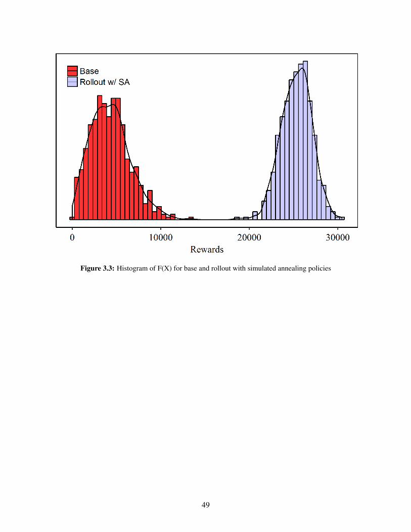
Figure 3.3: Histogram of F(X) for base and rollout with simulated annealing policies

49

w/ SA approach result in greater rewards than Base. This is validated by the separation between

the two histograms shown in Fig. 3.3. When the underlying base heuristic is no longer random,

the two plots will intersect with each other; therefore, the performance evaluation because of the

separation between the two histograms might not be apparent. In this situation, we extend the

benefit analogy described for Fig. 3.2. Particularly, we can calculate the benefit by using Fig. 3.3

as follows: Count the number of samples in each bin for recovery owing to Base. Multiply the

samples and the rewards for that bin. Repeat this for all the bins. Sum all these values to get the

total impact owing to Base. A similar procedure can be followed for Rollout w/ SA and the two

calculated values for Rollout w/ SA and Base can be compared to evaluate the performance of our

method. As discussed previously, for the simulation results in Fig. 3.2 and Fig. 3.3, the benefit

owing to Rollout w/ SA is more than that owing to Base; as can be seen by the separation between

the maximum bin of Base histogram and the minimum bin of Rollout w/ SA histogram along the

X-axis of Fig. 3.3 (given that the total sum of samples, which is the number of scenarios is same

for both the histograms). Therefore, in the Fig. 3.3, we omit plotting the sample count along the

Y-axis.

3.6 Conclusion

We proposed an optimization formulation based on the approximate dynamic programming

approach fused with the simulated annealing algorithm to determine near-optimal recovery policies

in urban communities. To show the efficiency of the applicability of the method on the food

security of realistic communities, the community of Gilroy (California) was modeled. Because the

availability of utilities for people and retailers degrades the food security issues following a severe

natural hazard event, the methodology optimizes the recovery of EPN, WN, and highway bridges

so that a maximum number of people and main food retailers benefit from the prompt restoration

of the main utilities.

50

3.7 Funding and Support

This work was supported by the National Science Foundation under Grant CMMI-1638284.

This support is gratefully acknowledged. Any opinions, findings, conclusions, or recommenda-

tions presented in this material are solely those of the authors and do not necessarily reflect the

views of the National Science Foundation.

51

Chapter 4

Optimal Stochastic Dynamic Scheduling for

Managing Community Recovery from Natural

Hazards

4.1 Introduction

Natural and man-made hazards pose significant challenges to civil infrastructure systems. Al-

though proactive mitigation planning may lessen catastrophic effects, efficacious recovery schedul-

ing can yield significant post-event benefits to restore functionality of critical systems to a level of

normalcy in a timely fashion, thereby minimizing wastage of limited resources and disaster-related

societal disorders. During the recovery process, the decision maker (also called “agent”) must se-

lect recovery actions sequentially to optimize the objectives of the community. There are several

characteristics of a rational agent and selecting a decision-making approach can become compli-

cated. The most important characteristics of a rational decision-making approach include:

(i) The agent must balance the desire for low present cost with the undesirability of high future

costs [17] (also referred as “non-myopic agent” or look-ahead property);

(ii) The agent must consider different sources of uncertainties;

(iii) The agent must make decisions periodically to not only take advantage of information that

becomes available when recovery actions are in progress but also to adapt to disturbances

over the recovery process;

(iv) The agent must be able to handle a large decision-making space, which is typical for the

problems at the community level. This decision-making space can cause an agent to suffer

from decision fatigue. Decision fatigue concerns to the degenerating quality of decisions

52

made by a human decision-maker after a long spell of decision making. It indicates no

matter how rational and high-minded an agent tries to be, one cannot make decision after

decision without paying a cost [60].

(v) The agent must consider different types of dependencies and interdependencies among net-

works, because a single decision can trigger cascading effects in multiple networks at the

community level.

(vi) The agent must be able to handle multi-objective tasks, which are common in real-world

domains. The interconnectedness among networks and probable conflicts among competing

objectives complicate the decision-making procedure.

(vii) The agent must consider different constraints, such as time constraints, limited budget and

repair crew, and current regional entities’ policies.

(viii) External factors, like the available resources and the type of community and hazard, shape

the risk attitude of the agent. The different risk behaviors must be considered.

Community-level decision makers would benefit from an algorithmic framework that empow-

ers them to take rational decisions and that accounts for the characteristics above. Markov Decision

Processes (MDPs) address stochastic dynamic decision-making problems efficiently and offer an

agent the means to identify optimal sequential post-event restoration policies.

This study introduces a stochastic scheduling formulation based on MDP to identify near-

optimal recovery actions following extreme natural hazards. This approach can support ratio-

nal risk-informed decision making at the community level. The proposed approach possesses all

mentioned properties (i-viii). To this end, we leverage the ADP paradigm to address large-scale

scheduling problems in a way that overcomes the notorious curse of dimensionality that challenges

the practical use of Bellman’s equation [61]. We employ a promising class of approximation tech-

niques called rollout algorithms. The application of ADP and rollout algorithms, along with the

MDP formulation, provides not only a robust and computationally tractable approach but also the

53

flexibility of incorporating current organizational recovery policies. In addition, we show how to

treat current restoration policies as heuristics in the rollout mechanism.

As an illustrative example, we consider critical infrastructure systems within a community

modeled after Gilroy, California, which is susceptible to severe earthquakes emanating from the

San Andreas Fault. We model the Electrical Power Network (EPN), Water Network (WN), and

main food retailers, including interconnectedness within and between networks. The EPN is par-

ticularly critical because the restoration and operation of most other vital systems need electricity.

Additionally, the WN and food retailers supply water, food (e.g., ready-to-eat meals), and prescrip-

tion medications that are essential for human survival following disasters. The functionality of the

WN not only depends on its physical performance but also on the operation of the EPN, where a

working EPN provides electricity for pumping station and water tanks. The serviceability of food

retailers depends heavily on the WN and EPN. We consider these interdependencies and define

two decision-making objective functions for optimization: to minimize the number of days needed

to restore networks to an arbitrary level of service and to maximize number of people who have

utilities per unit of time. We show how the proposed approach enables the agent (decision maker)

to compute near-optimal recovery strategies to provide the three essential services — electricity,

potable water, and food — to urban inhabitants and food retailers following a severe earthquake.

We discuss the integrated recovery policies that consider multiple networks and objectives simul-

taneously, which can remarkably outperform the conventional isolated policies. Finally, we also

discuss how risk-averse decision makers can utilize the proposed method.

4.2 Technical Preliminaries

In this section, we present the mathematical setting for the MDP. A detailed treatment of the

subject is available in [62].

54

4.2.1 MDP Framework

A Markov decision process (MDP) is defined by the six-tuple (X,A,A(.), P, R, γ), where X

denotes the state space, A denotes the action space, A(x) ⊂ A is the set of admissible actions in

state x, P (y|x, a) is the probability of transitioning from state x ∈ X to state y ∈ X when action

a ∈ A(x) is taken, R(x, a) is the reward obtained when action a ∈ A(x) is taken in state x ∈ X ,

and γ is the discount factor. Let Π be the set of Markovian policies (π), where π : X → A is a

function such that π(x) ∈ A(x) for each x ∈ X . Our goal is to compute a policy π that optimizes

the expected total discounted reward given by

V π(x) := E

[

∞∑

t=0

γtR(xt, π(xt))|x0 = x)

]

. (4.1)

The optimal value function for a given state x ∈ X is connoted as V π∗

: X → R given by

V π∗

= maxπ∈Π

V π(x). (4.2)

The optimal policy is given by

π∗ = argmaxπ∈Π

V π(x). (4.3)

Note that the optimal policy is independent of the initial state x0. Also, note that we maximize

over policies π, where at each time t the action taken is at = π(xt). The optimal policy π∗ can be

computed using different methods, which include linear programming and dynamic programing.

The methods of value iteration, policy iteration, policy search, etc., can find a strict optimal policy.

We briefly discuss the Bellman’s optimality principle, useful for defining the Q-value function,

which plays a pivotal role in the description of the rollout algorithm. The Bellman’s optimality

principle states that V π∗

(x) satisfies

V π∗

(x) := maxa∈A(x)

R(x, a)) + γ∑

y∈X

P (y|x, a)V π∗

(y)

. (4.4)

55

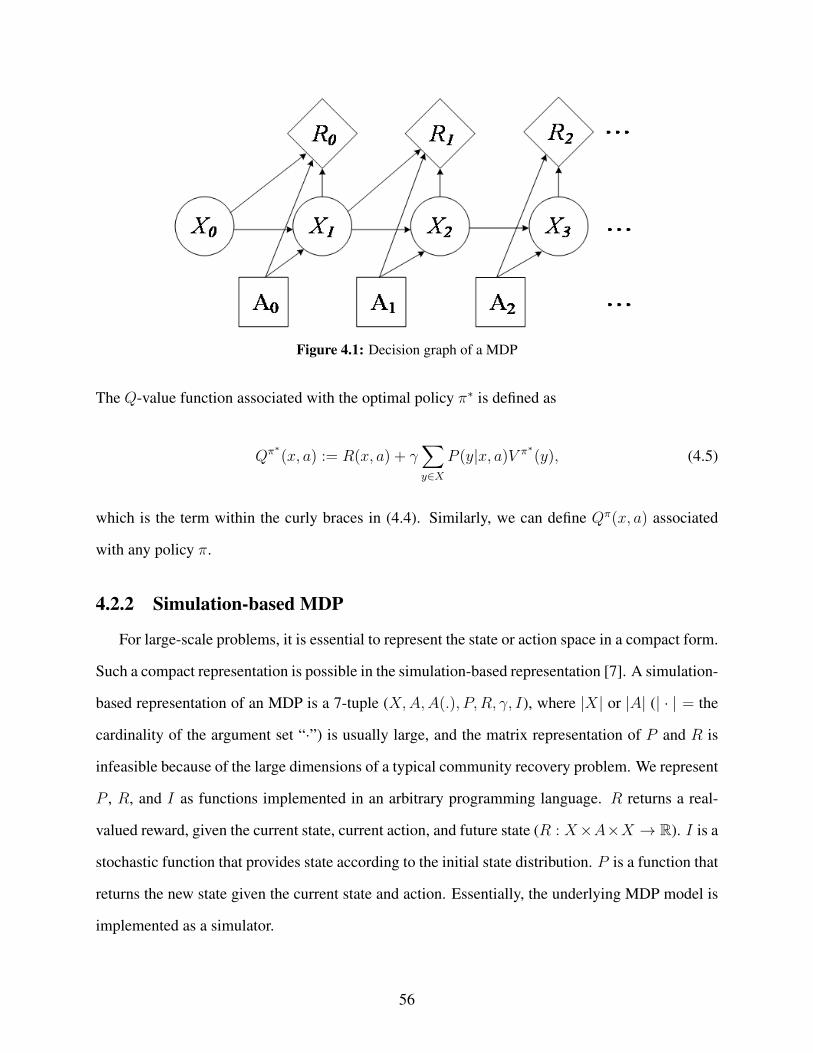
Figure 4.1: Decision graph of a MDP

The Q-value function associated with the optimal policy π∗ is defined as

Qπ∗

(x, a) := R(x, a) + γ∑

y∈X

P (y|x, a)V π∗

(y), (4.5)

which is the term within the curly braces in (4.4). Similarly, we can define Qπ(x, a) associated

with any policy π.

4.2.2 Simulation-based MDP

For large-scale problems, it is essential to represent the state or action space in a compact form.

Such a compact representation is possible in the simulation-based representation [7]. A simulation-

based representation of an MDP is a 7-tuple (X,A,A(.), P, R, γ, I), where |X| or |A| (| · | = the

cardinality of the argument set “·”) is usually large, and the matrix representation of P and R is

infeasible because of the large dimensions of a typical community recovery problem. We represent

P , R, and I as functions implemented in an arbitrary programming language. R returns a real-

valued reward, given the current state, current action, and future state (R : X×A×X → R). I is a

stochastic function that provides state according to the initial state distribution. P is a function that

returns the new state given the current state and action. Essentially, the underlying MDP model is

implemented as a simulator.

56

4.2.3 Approximate Dynamic Programming

Calculating an optimal policy using the methods above is usually infeasible owing to the di-

mensions of the state and/or action spaces. The size of the state/action space grows exponentially

with the number of state/action variables, a phenomenon referred to by Bellman as the curse of di-

mensionality. The computational costs of running a single iteration of the value iteration and policy

iteration algorithm areO(|X|2|A|) andO(|X|2|A|+|X|3), respectively. The computational cost of

finding the optimal policy by directly solving the linear system provided by the Bellman equation

is O(|X|3|A|3). Additionally, the computational cost of an exhaustive direct policy search algo-

rithm, for a single trajectory consisting of K simulation steps, is 3(

∑Kk=1 |X|

k)

|A||X||X| [63],

which is prohibitive for even small-sized problems.

These computationally intractable algorithms cannot be used for large problems involving re-

silience assessment or recovery of a real-size community and approximate solutions are neces-

sary. To this end, several algorithms have been developed in the realm of Approximate Dynamic

Programming (ADP) that result in tractable computations for finding the near-optimal restoration

policies. One popular class of algorithms involves approximating the Q-value function in (5).

However, it often is difficult in practice to identify a suitable approximation to the Q-value func-

tion for practical, large-scale problems. In the following, we pursue a promising class of ADP

algorithms known as rollout that sidesteps these difficulties by avoiding an explicit representation

of the Q-value function.

4.2.4 Rollout

While computing an optimal policy for an MDP is often quite difficult because of the curse of

dimensionality, policies based on heuristics (termed as base policies) can be readily designed in

many cases. The principal idea behind the rollout technique is to improve upon the performance

of the base policy through various means. Therefore, the base policy does not have to be close

to optimal. In this study, we focus on improvement of the base policy through simulation. The

base policy is generally some heuristic, and the rollout policy is computed with the repeated ap-

57

plication of this heuristic. The base policy can be defined in various ways like experts’ judgments,

importance analyses, greedy algorithms, etc [4].

The idea was first proposed for stochastic scheduling problems by Bertsekas and Castanon [64].

Instead of the classical DP scheme [17], the agent “rolls out” or simulates the available policy over

a selected finite horizon H < ∞; thereafter, the agent implements the most “promising” action

in an on-line fashion. In the on-line methods, unlike the classical off-line techniques, optimal

decisions are computed only for the states realized in the real-world (reachable states); the idea is

to preserve computational effort on the unreachable states. Conversely, in off-line computations

the policy is pre-computed for all the states and collected; then, the agent selects an optimal action

from the collected policy corresponding to the observed evolution of the system [62].

Monte Carlo (MC) simulations assess the Q-value function on demand. To estimate the Q-

value function ( Qπ(x, a) represents the estimate) of a given state-action pair (x, a), we simulate

NMC number of trajectories, where each trajectory is generated using the policy π, has length H ,

and starts from the pair (x, a). The assessed Q-value function is typically taken as the average of

the sample returns obtained along these trajectories:

Qπ(x, a) =1

NMC

NMC∑

i0=1

[

R(x, a, xi0,1) +H∑

k=1

R(xi0,k, π(xi0,k), xi0,k+1)

]

. (4.6)

For each trajectory i0, we fix the first state-action pair to (x, a); the simulator provides the next

state xi0,1 when the current action a in state x is completed. Thereafter, we choose actions using

the base policy. Note that if the simulator is deterministic, a single trajectory suffices, while in the

stochastic case, a sufficient number of trajectories (NMC) should be pursued to approximate theQ-

value function. In this study, we focus on the rollout policy computed with single-step look-ahead.

An agent can consider multistep look-ahead, at an added computational cost, to extract maximum

performance out of our solution technique. The number of look-ahead steps mainly depends on the

scale of the problem, computational budget, real-time constraints, and agent’s preferences. This

study focuses on the application of the proposed rollout algorithm following a disaster. In an on-

58

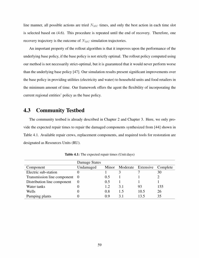
line manner, all possible actions are tried NMC times, and only the best action in each time slot

is selected based on (4.6). This procedure is repeated until the end of recovery. Therefore, one

recovery trajectory is the outcome of NMC simulation trajectories.

An important property of the rollout algorithm is that it improves upon the performance of the

underlying base policy, if the base policy is not strictly optimal. The rollout policy computed using

our method is not necessarily strict-optimal, but it is guaranteed that it would never perform worse

than the underlying base policy [47]. Our simulation results present significant improvements over

the base policy in providing utilities (electricity and water) to household units and food retailers in

the minimum amount of time. Our framework offers the agent the flexibility of incorporating the

current regional entities’ policy as the base policy.

4.3 Community Testbed

The community testbed is already described in Chapter 2 and Chapter 3. Here, we only pro-

vide the expected repair times to repair the damaged components synthesized from [44] shown in

Table 4.1. Available repair crews, replacement components, and required tools for restoration are

designated as Resources Units (RU).

Table 4.1: The expected repair times (Unit:days)

Damage StatesComponent Undamaged Minor Moderate Extensive CompleteElectric sub-station 0 1 3 7 30Transmission line component 0 0.5 1 1 2Distribution line component 0 0.5 1 1 1Water tanks 0 1.2 3.1 93 155Wells 0 0.8 1.5 10.5 26Pumping plants 0 0.9 3.1 13.5 35

59

4.4 Post-hazard Recovery Formulation

Following an earthquake, the EPN and WN systems and components either remain undamaged

or exhibit a level of damage, which is determined from the seismic fragility curves. Suppose that

an agent must restore a community that includes several networks, which function as a System of

Systems (SoS). Let L′ be the total number of damaged components at time t, and let tc denote

the decision time at which all the damaged components are repaired (L′ = 0). The agent has

only a limited number of RUs that can be assigned, usually much less than L′, especially in severe

disasters that impact large communities. The RUs differ from network to network because of the

skill of repair crews and qualities of the required tools. The problem is to assign the available

RUs to L′ damaged components in a manner that best achieves the community objectives and

policymakers’ preferences.

We make the following assumptions:

• The agent has access to all the damaged component for repair purposes;

• A damaged component only needs one RU to be repaired and assigning more than one RU

would not reduce the repair time [46];

• The agent has limited RUs for each network and cannot assign a RU of one network to

another (e.g., a WN RU cannot be assigned to the EPN);

• The agent can preempt the assigned RUs from completing their work and reassign them at

different locations to maximize the beneficial outcomes.

• Once a damaged component is repaired, all assigned RUs are available for re-assignment

even if their assigned components are not fully repaired. It is also possible to let the RU

continue the repair work at the same location in the next time slot according to the objectives

of the agent. We refer to such assignment as preemptive scheduling, which allows the agent

to be flexible in planning and is particularly useful when a central stakeholder manages an

infrastructure system; see [8] for a discussion on non-preemptive scheduling.

60

• The agent can deal with stochastic scheduling, where the outcome of the repair actions is

not fully predictable and can be quantified probabilistically. The unpredictability mainly

arises from the randomness in the repair times (see Table 4.1). The MDP simulator exhibits

stochastic behavior owing to the random repair times.

4.4.1 Markov Decision Process Formulation

Suppose that xEt and xWt , respectively, represent the damage state of the EPN and WN at time

t. xEt is a vector of length LEt , where LEt is the number of damaged components in the EPN.

Each element of the vector xEt is in one of the five damage states (counting no damage as one

state) in Table 4.1. Similarly, we define xWt of length LWt , where LWt is the number of damaged

components in the WN at time slot t. Let NE and NW denote the available RUs for the EPN and

WN, respectively, withNE ≤ LEt andNW ≤ LWt . We can define the tuples of our MDP framework

as follows:

• States X: xt denotes the state of the damaged components in the community at time slot t as

the stack of two vectors, xEt and xWt as follows:

xt := (xEt , xWt ) s.t. |xt| = LEt + LWt . (4.7)

• Actions A: at denotes the repair actions to be carried out on the damaged components at

time slot t, as the stack of two vectors, aEt and aWt ,

at := (aEt , aWt ) s.t. |at| = LEt + LWt , (4.8)

where both aEt and aWt are binary vectors of length LEt and LWt , respectively, where a value

of zero means no repair and one means carry out repair action. aEt and aWt represent the

actions (no repair, repair) to be performed on the damaged components of the EPN and WN.

61

• Set of Admissible Actions A(xt): The set of admissible repair actions A(xt) for the state xt

is the set of all possible binary combinations of integers one and zero such that each element

of this set is of size LEt + LWt , and each element has NE number of ones in the first LEt

locations and NW number of ones at the remaining locations. The interdependence between

networks explodes the size of the set of admissible actions as follows: Let DEt be the set of

all damaged components of the EPN before a repair action at is performed. P(DEt ) denotes

the powerset of DEt ;

PNE(DE

t ) :=

C ∈ P(DEt ) : |C| = NE

, (4.9)

where∣

∣PNE(DE

t )∣

∣ represents the size of the set of admissible actions for the EPN. We can

also define PNW(DW

t ) similarly. The size of the set of admissible actions, at any time t, is

the product of the size of set of admissible actions for EPN and WN:

|A(xt)| :=∣

∣PNE(DE

t )∣

∣×∣

∣PNW(DW

t )∣

∣ (4.10)

Therefore, when multiple networks are considered simultaneously, the size of A(xt) grows

very quickly. Searching exhaustively over the entire set A(xt) for calculating the optimal

solution is not possible; therefore, we employ the rollout technique.

• Simulator P : Given, xt and at, the simulator P provides the new state xt+1. P is a generative

model that can be implemented as a simulator, without any explicit knowledge of the actual

transitions. It considers the interconnectedness within and between networks to compute the

cascading effects of at through the whole community and recovery process. As we alluded to

before, a compact representation of P is important for large-scale problems. In our problem

formulation, as soon as at least one of the damaged components is repaired, the repair action

at is considered complete. Define this completion time at every t by tt. Recall that the repair

time is exponentially distributed. The completion time is the minimum of the repair time at

one or more damaged locations, where a repair action is being performed. The minimum

62

of exponential random variables is exponentially distributed; therefore, the completion time

is also exponentially distributed [65]. The sojourn time (a.k.a. the holding time) is the

amount of time that the system spends in a specific state. For an MDP, the sojourn time,

ts, is exponentially distributed. Note that for our MDP formulation, tt is equal to ts. A

natural question that arises is “does this formulation work when the repair times are non-

exponential?” In that case, the completion time is not exponentially distributed. However,

in our present problem formulation, the completion time is the same as the sojourn time.

Thus, the sojourn time would not be exponentially distributed, which is inconsistent with

the Markovian assumption. This can be remedied simply by incorporating the lifetime of

the damaged component into the state definition. The lifetime of the damaged component is

the time required for the damaged component to be repaired after the occurrence of hazard.

With this new definition of the state space, the sojourn time is different from the completion

time tt, and the sojourn time is exponentially distributed. Here the completion time tt is still

the minimum of the repair time at one or more damaged locations but with any underlying

distribution of the repair times. Thus, our framework is sufficiently flexible to accommodate

repair times with any underlying distribution.

• Rewards R: In this study, we pursue two different objectives for the agent. The first objec-

tive (hereinafter Obj. 1) is to optimally plan decisions so that a certain percentage of the

total inhabitants (denoted by threshold α) are benefitted from the recovery of utilities in the

shortest period of time, implying that household units not only have electricity and water but

also have access to a functional retailer that has electricity and water. Conversely, even if a

household unit has electricity and water and has access to a retailer that has electricity but

not water, the household unit does not benefit from the recovery actions. The mapping of

people in the gridded rectangle to a food retailer is determined by the gravity model. We aim

to optimally plan the repair actions to minimize the time it takes to achieve the benefit from

utilities to α percent of people. The reward function for the first objective is defined as:

63

R1(xt, at, xt+1) = tt. (4.11)

The second objective (hereinafter Obj. 2) is to optimally plan decisions so that maximum

number of inhabitants are benefited from recovery of utilities per unit of time (days, in our

case). Therefore, in the second case, there are two objectives embedded in our reward as

follows:

R2(xt, at, xt+1) =r

trep(4.12)

where r is the number of people deriving benefit from utilities after the completion of at,

and trep is the total repair time to reach xt+1 from any initial state x0 (i.e., trep =∑

tt). Note

that the reward function is stochastic because the outcome of the repair action is stochastic.

• Initial State I: The initial damage states associated with the components will be provided by

the stochastic damage model of the EPN and WN components.

• Discount factor γ: In this study, we set the discount factor to be 0.99. This is a measure of

how “far-sighted” the agent is in considering its decisions. The discount factor weighs the

future stochastic rewards at each discrete time t.

4.5 Results and Discussion

We divide the presentation of our simulation results into two sections. The first section caters to

risk-neutral decision makers, and the second section caters to risk-averse decision makers [66,67].

Each of these sections is further divided into two sub-sections to demonstrate the performance

of our method on two separate objectives functions. When Objective 1 is considered, the reward

function in our MDP is given by (7.4), while for Objective 2, the reward function of our MDP is

given by (7.5). For all the simulation results presented henceforth, we selected NMC in 4.6 so that

the standard deviation of the estimated Q-value Qπ(x, a) is below 0.05.

As mentioned in Section 4.2.4, the most feasible base policy for community recovery planning

often is the current recovery strategy of regional responsible companies or organizations. However,

64

there is no restriction on the selection of a policy as a base policy. We proposed the alternatives

for the definition of base policies for recovery management problems in [4]. In this study, the base

policy is defined based on expert judgment and importance analyses that prioritize the importance

of components owing to their contribution to the overall risk. Specifically, the restoration sequence

defined by our base policy for EPN is transmission line, power substation, and distribution lines to

downtown and water pumps; similarly, the base policy for WN involves water wells, water tanks,

BPS, and pipelines to downtown and food retailers.

4.5.1 Mean-based Stochastic Optimization

The mean-based optimization is suited to risk-neutral decision makers [20]. In this approach,

the optimal policy is determined based on the optimization of the Q-value function, where the esti-

mate of the Q-value function Qπ(x, a) is based on the mean of NMC trajectories, as demonstrated

in (4.6). Calculating the Q-value based on the expected Q-value of NMC trajectories may not al-

ways be appropriate, especially in the case of risk-averse decision makers. However, it has been

shown that the mean-based stochastic optimization approach can be appropriate when the objec-

tive function properly encodes the risk preferences of policymakers. Nevertheless, we demonstrate

the performance of our method when the decision maker has risk-averse attitude to planning in

Section 4.5.2.

Implementation of Rollout Algorithm for Objective 1

The rollout algorithm with respect to Obj. 1 identifies recovery strategies to minimize the

time it takes to provide the utilities to α percent of people in the community. In this formulation,

the selection of α depends on the preferences of policymakers. For our simulation, we selected

α = 0.8, implying that we want to provide the benefit of the utility recoveries to 80% of people

in minimum amount of time. Fig. 4.2 shows the performance of the rollout and base polices

for Objective 1. The rollout algorithm optimizes the restoration of two networks, EPN and WN,

simultaneously to provide utilities for 80% of people in 19.3 days following the earthquake, while

the base policy completes this task in 26.1 days. This 35% improvement over the entire recovery

65

0 5 10 15 20 25 30

Time (days)

0

10

20

30

40N

um

ber

of benefite

d p

eople

103

Rollout

Base policy

Figure 4.2: Performance of rollout vs. base policy for the first objective function

period signifies the performance of rollout at the community level. Fig. 4.2 also highlights the

look-ahead property of rollout. Although the base policy showed a better performance during the

first 15 days following the earthquake, the rollout algorithm outperformed the base policy in the

whole recovery. By selecting conservative repair decisions initially, rollout can balance the desire

for low present cost with the undesirability of high future costs.

The performance of rollout on the individual food retailers is summarized in Table 4.2. Note

that the base policy restored EPN and WN to Safeway, Nob Hill Foods, and Mi Pueblo Food faster

than the rollout policy; however, the base policy is incapable of determining the recovery actions to

balance the rewards so that 80% of people benefit from restoration of utilities (our true objective).

Table 4.2: Performance of rollout vs. base policy for the 1st objective function for the individual retailers

Policy Recovery time Costco Walmart Target Safeway Nob Hill Foods Mi Pueblo FoodBase 26.06 0.31 0.31 21.02 5.91 5.91 2.76Rollout 19.23 0.31 0.31 15.95 18.33 18.33 8.01

66

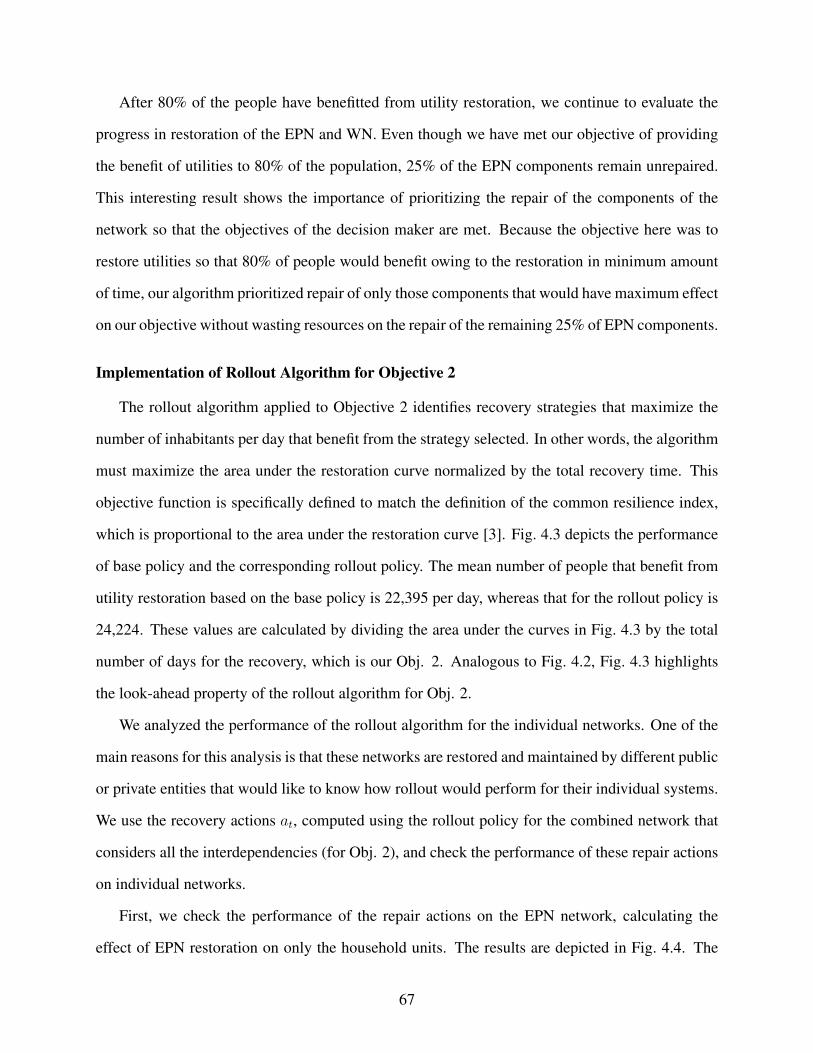
After 80% of the people have benefitted from utility restoration, we continue to evaluate the

progress in restoration of the EPN and WN. Even though we have met our objective of providing

the benefit of utilities to 80% of the population, 25% of the EPN components remain unrepaired.

This interesting result shows the importance of prioritizing the repair of the components of the

network so that the objectives of the decision maker are met. Because the objective here was to

restore utilities so that 80% of people would benefit owing to the restoration in minimum amount

of time, our algorithm prioritized repair of only those components that would have maximum effect

on our objective without wasting resources on the repair of the remaining 25% of EPN components.

Implementation of Rollout Algorithm for Objective 2

The rollout algorithm applied to Objective 2 identifies recovery strategies that maximize the

number of inhabitants per day that benefit from the strategy selected. In other words, the algorithm

must maximize the area under the restoration curve normalized by the total recovery time. This

objective function is specifically defined to match the definition of the common resilience index,

which is proportional to the area under the restoration curve [3]. Fig. 4.3 depicts the performance

of base policy and the corresponding rollout policy. The mean number of people that benefit from

utility restoration based on the base policy is 22,395 per day, whereas that for the rollout policy is

24,224. These values are calculated by dividing the area under the curves in Fig. 4.3 by the total

number of days for the recovery, which is our Obj. 2. Analogous to Fig. 4.2, Fig. 4.3 highlights

the look-ahead property of the rollout algorithm for Obj. 2.

We analyzed the performance of the rollout algorithm for the individual networks. One of the

main reasons for this analysis is that these networks are restored and maintained by different public

or private entities that would like to know how rollout would perform for their individual systems.

We use the recovery actions at, computed using the rollout policy for the combined network that

considers all the interdependencies (for Obj. 2), and check the performance of these repair actions

on individual networks.

First, we check the performance of the repair actions on the EPN network, calculating the

effect of EPN restoration on only the household units. The results are depicted in Fig. 4.4. The

67

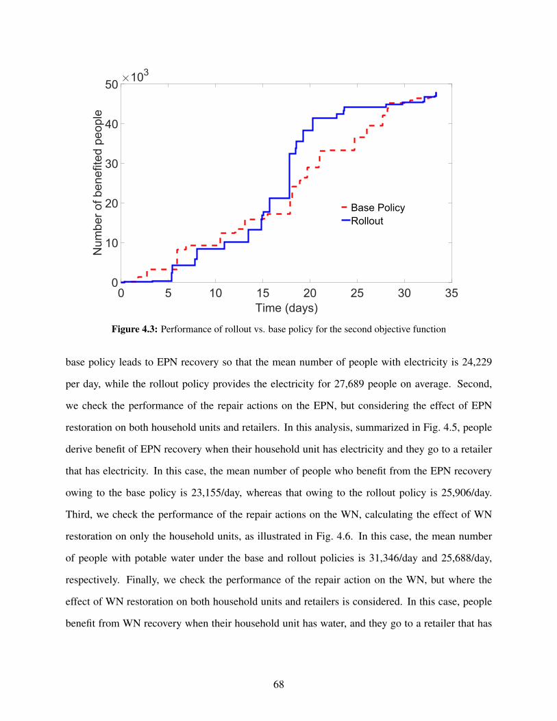
0 5 10 15 20 25 30 35

Time (days)

0

10

20

30

40

50N

um

ber

of benefite

d p

eople

103

Base Policy

Rollout

Figure 4.3: Performance of rollout vs. base policy for the second objective function

base policy leads to EPN recovery so that the mean number of people with electricity is 24,229

per day, while the rollout policy provides the electricity for 27,689 people on average. Second,

we check the performance of the repair actions on the EPN, but considering the effect of EPN

restoration on both household units and retailers. In this analysis, summarized in Fig. 4.5, people

derive benefit of EPN recovery when their household unit has electricity and they go to a retailer

that has electricity. In this case, the mean number of people who benefit from the EPN recovery

owing to the base policy is 23,155/day, whereas that owing to the rollout policy is 25,906/day.

Third, we check the performance of the repair actions on the WN, calculating the effect of WN

restoration on only the household units, as illustrated in Fig. 4.6. In this case, the mean number

of people with potable water under the base and rollout policies is 31,346/day and 25,688/day,

respectively. Finally, we check the performance of the repair action on the WN, but where the

effect of WN restoration on both household units and retailers is considered. In this case, people

benefit from WN recovery when their household unit has water, and they go to a retailer that has

68

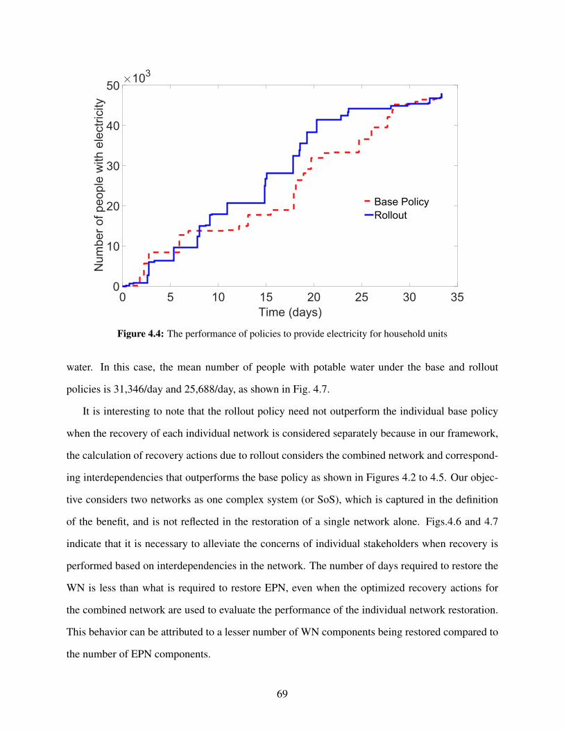
0 5 10 15 20 25 30 35

Time (days)

0

10

20

30

40

50N

um

ber

of people

with e

lectr

icity

103

Base Policy

Rollout

Figure 4.4: The performance of policies to provide electricity for household units

water. In this case, the mean number of people with potable water under the base and rollout

policies is 31,346/day and 25,688/day, as shown in Fig. 4.7.

It is interesting to note that the rollout policy need not outperform the individual base policy

when the recovery of each individual network is considered separately because in our framework,

the calculation of recovery actions due to rollout considers the combined network and correspond-

ing interdependencies that outperforms the base policy as shown in Figures 4.2 to 4.5. Our objec-

tive considers two networks as one complex system (or SoS), which is captured in the definition

of the benefit, and is not reflected in the restoration of a single network alone. Figs.4.6 and 4.7

indicate that it is necessary to alleviate the concerns of individual stakeholders when recovery is

performed based on interdependencies in the network. The number of days required to restore the

WN is less than what is required to restore EPN, even when the optimized recovery actions for

the combined network are used to evaluate the performance of the individual network restoration.

This behavior can be attributed to a lesser number of WN components being restored compared to

the number of EPN components.

69

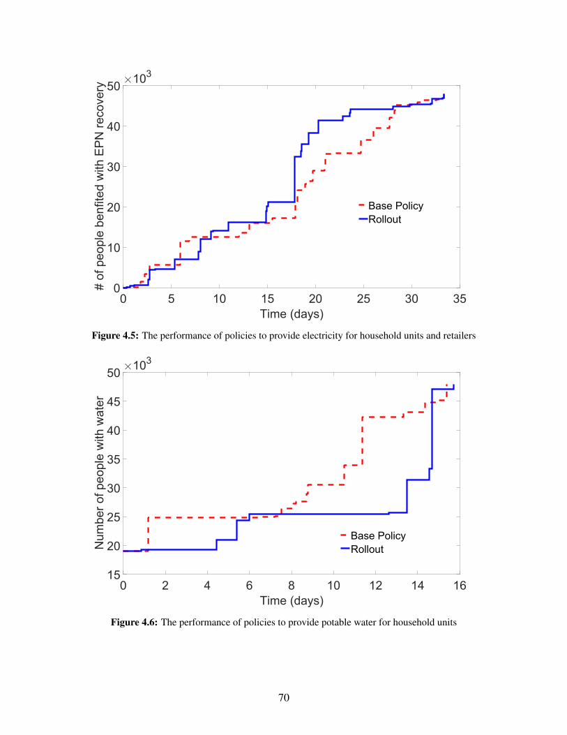
0 5 10 15 20 25 30 35

Time (days)

0

10

20

30

40

50# o

f people

benfite

d w

ith E

PN

recovery

103

Base Policy

Rollout

Figure 4.5: The performance of policies to provide electricity for household units and retailers

0 2 4 6 8 10 12 14 16

Time (days)

15

20

25

30

35

40

45

50

Num

ber

of people

with w

ate

r

103

Base Policy

Rollout

Figure 4.6: The performance of policies to provide potable water for household units

70

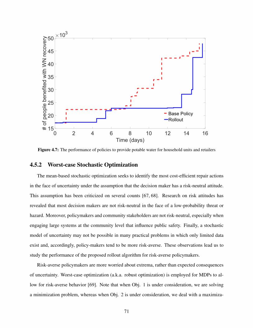
0 2 4 6 8 10 12 14 16

Time (days)

15

20

25

30

35

40

45

50# o

f people

benefite

d w

ith W

N r

ecovery

103

Base Policy

Rollout

Figure 4.7: The performance of policies to provide potable water for household units and retailers

4.5.2 Worst-case Stochastic Optimization

The mean-based stochastic optimization seeks to identify the most cost-efficient repair actions

in the face of uncertainty under the assumption that the decision maker has a risk-neutral attitude.

This assumption has been criticized on several counts [67, 68]. Research on risk attitudes has

revealed that most decision makers are not risk-neutral in the face of a low-probability threat or

hazard. Moreover, policymakers and community stakeholders are not risk-neutral, especially when

engaging large systems at the community level that influence public safety. Finally, a stochastic

model of uncertainty may not be possible in many practical problems in which only limited data

exist and, accordingly, policy-makers tend to be more risk-averse. These observations lead us to

study the performance of the proposed rollout algorithm for risk-averse policymakers.

Risk-averse policymakers are more worried about extrema, rather than expected consequences

of uncertainty. Worst-case optimization (a.k.a. robust optimization) is employed for MDPs to al-

low for risk-averse behavior [69]. Note that when Obj. 1 is under consideration, we are solving

a minimization problem, whereas when Obj. 2 is under consideration, we deal with a maximiza-

71

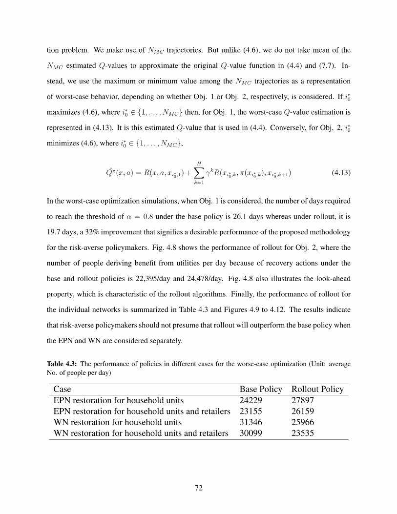
tion problem. We make use of NMC trajectories. But unlike (4.6), we do not take mean of the

NMC estimated Q-values to approximate the original Q-value function in (4.4) and (7.7). In-

stead, we use the maximum or minimum value among the NMC trajectories as a representation

of worst-case behavior, depending on whether Obj. 1 or Obj. 2, respectively, is considered. If i∗0

maximizes (4.6), where i∗0 ∈ 1, . . . , NMC then, for Obj. 1, the worst-case Q-value estimation is

represented in (4.13). It is this estimated Q-value that is used in (4.4). Conversely, for Obj. 2, i∗0

minimizes (4.6), where i∗0 ∈ 1, . . . , NMC,

Qπ(x, a) = R(x, a, xi∗0,1) +H∑

k=1

γkR(xi∗0,k, π(xi∗0,k), xi∗0,k+1) (4.13)

In the worst-case optimization simulations, when Obj. 1 is considered, the number of days required

to reach the threshold of α = 0.8 under the base policy is 26.1 days whereas under rollout, it is

19.7 days, a 32% improvement that signifies a desirable performance of the proposed methodology

for the risk-averse policymakers. Fig. 4.8 shows the performance of rollout for Obj. 2, where the

number of people deriving benefit from utilities per day because of recovery actions under the

base and rollout policies is 22,395/day and 24,478/day. Fig. 4.8 also illustrates the look-ahead

property, which is characteristic of the rollout algorithms. Finally, the performance of rollout for

the individual networks is summarized in Table 4.3 and Figures 4.9 to 4.12. The results indicate

that risk-averse policymakers should not presume that rollout will outperform the base policy when

the EPN and WN are considered separately.

Table 4.3: The performance of policies in different cases for the worse-case optimization (Unit: averageNo. of people per day)

Case Base Policy Rollout PolicyEPN restoration for household units 24229 27897EPN restoration for household units and retailers 23155 26159WN restoration for household units 31346 25966WN restoration for household units and retailers 30099 23535

72

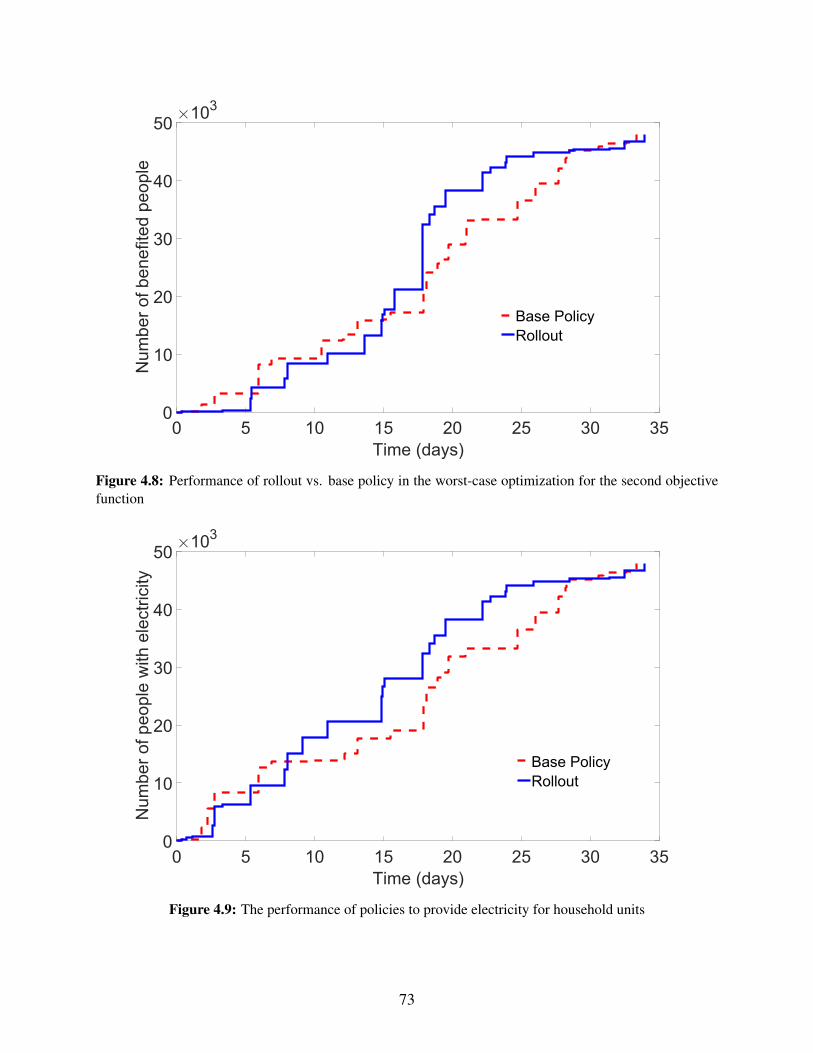
0 5 10 15 20 25 30 35

Time (days)

0

10

20

30

40

50N

um

ber

of benefite

d p

eople

103

Base Policy

Rollout

Figure 4.8: Performance of rollout vs. base policy in the worst-case optimization for the second objectivefunction

0 5 10 15 20 25 30 35

Time (days)

0

10

20

30

40

50

Num

ber

of people

with e

lectr

icity

103

Base Policy

Rollout

Figure 4.9: The performance of policies to provide electricity for household units

73

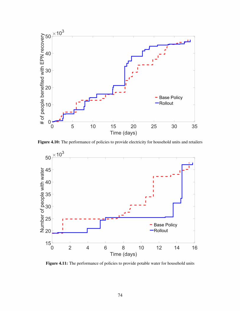
0 5 10 15 20 25 30 35

Time (days)

0

10

20

30

40

50# o

f people

benefite

d w

ith E

PN

recovery 10

3

Base Policy

Rollout

Figure 4.10: The performance of policies to provide electricity for household units and retailers

0 2 4 6 8 10 12 14 16

Time (days)

15

20

25

30

35

40

45

50

Num

ber

of people

with w

ate

r

103

Base Policy

Rollout

Figure 4.11: The performance of policies to provide potable water for household units

74

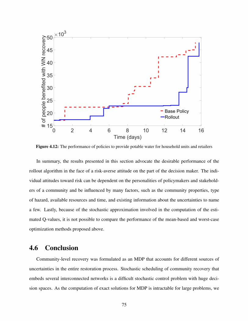
0 2 4 6 8 10 12 14 16

Time (days)

15

20

25

30

35

40

45

50# o

f people

benefite

d w

ith W

N r

ecovery

103

Base Policy

Rollout

Figure 4.12: The performance of policies to provide potable water for household units and retailers

In summary, the results presented in this section advocate the desirable performance of the

rollout algorithm in the face of a risk-averse attitude on the part of the decision maker. The indi-

vidual attitudes toward risk can be dependent on the personalities of policymakers and stakehold-

ers of a community and be influenced by many factors, such as the community properties, type

of hazard, available resources and time, and existing information about the uncertainties to name

a few. Lastly, because of the stochastic approximation involved in the computation of the esti-

mated Q-values, it is not possible to compare the performance of the mean-based and worst-case

optimization methods proposed above.

4.6 Conclusion

Community-level recovery was formulated as an MDP that accounts for different sources of

uncertainties in the entire restoration process. Stochastic scheduling of community recovery that

embeds several interconnected networks is a difficult stochastic control problem with huge deci-

sion spaces. As the computation of exact solutions for MDP is intractable for large problems, we

75

utilized rollout algorithms, which fall under the broad umbrella of approximate dynamic program-

ming techniques, for scheduling community-level recovery actions. The proposed methodology

considers interdependent electrical and water networks in the community and treats them as one

complex system. We tested the feasibility of the proposed method through a real case study involv-

ing a real community susceptible to severe earthquakes with respect to different objective functions

that are popular for policymakers in the community resilience problems. We also considered the

performance of the method for policymakers with different risk attitudes. The performance of

the rollout policies appears to be near-optimal and is substantially better than the performance

of their underlying base policies. The proposed rollout approach has the all characteristics of a

comprehensive framework, mentioned in Section 4.1. Furthermore, the rollout policy treats the

community as a system of systems and provides the optimal strategies for the whole community.

These strategies are not necessarily optimal for the individual networks and surely outperforms

their underlying base policies. Noted that the mentioned properties are the properties of the ratio-

nal decision-making approach for our particular problem and cannot be generalized as a universal

panacea.

4.7 Funding and Support

The research herein has been funded by the National Science Foundation under CRISP Collab-

orative Research Grant CMMI-1638284. This support is gratefully acknowledged. Any opinions,

findings, conclusions, or recommendations presented in this material are solely those of the au-

thors, and do not necessarily reflect the views of the National Science Foundation.

76

Chapter 5

Solving Markov Decision Processes for Water

Network Recovery of Community Damaged by

Earthquake

5.1 Introduction

Natural disasters have a significant impact on the economic, social, and cultural fabric of af-

fected communities. Moreover, because of the interconnected nature of communities in the modern

world, the adverse impact is no longer restricted to the locally affected region, but it has ramifi-

cations on national or international scale. Among other factors, the occurrence of such natural

disasters is on the rise owing to population growth and economic development in hazard-prone ar-

eas. Keeping in view the increased frequency of natural disasters, there is an urgent need to address

the problem of community recovery post-hazard. Typically, the resources available to post-disaster

planners are limited and relatively small compared to the impact of the damage. Under these sce-

narios, it becomes imperative to assign limited resources to various damaged components in the

network optimally to support community recovery. Such an assignment must also consider multi-

ple objectives and cascading effects due to the interconnectedness of various networks within the

community and must also successfully adopt previous proven methods and practices developed

by expert disaster-management planners. Holistic approaches addressing various uncertainties for

network-level management of limited resources must be developed for maximum effect. Civil

infrastructure systems, including power, transportation, and water networks, play a critical part

in post-disaster recovery management. In this study, we focus on one such critical infrastructure

system, namely the water networks (WN), and compute near-optimal recovery actions, in the af-

termath of an earthquake, for the WN of a test-bed community.

77

Markov decision processes (MDPs) offer a convenient framework for representation and solu-

tion of stochastic decision-making problems. Exact solutions are intractable for problems of even

modest size; therefore, approximate solution methods have to be employed. We can leverage the

rich theory of MDPs to model recovery action optimization for large state-space decision-making

problems such as our. In this study, we employ a simulation-based representation and solution of

MDP. The near-optimal solutions are computed using an approximate solution technique known

as rollout. Even though state-of-the-art hardware and software practices are used to implement the

solution to our problem, we are faced with the additional dilemma of computing recovery actions

on a fixed simulation budget without affecting the solution performance. Therefore, any prospec-

tive methodology must incorporate such a limitation in its solution process. We incorporate the

Optimal Computing Budget Allocation (OCBA) algorithm into our MDP solution process [70,71]

to address the limited simulation budget problem.

5.2 Testbed Case Study

The details for the modeled WN of Gilroy, CA and the hazard simulation model are already

presented in Chapters 2 to 4.

5.3 Problem Description and Solution

5.3.1 MDP Framework

We provide a brief description of MDP [72] for the sake of completeness. An MDP is a con-

trolled dynamical process useful in modelling of wide range of decision-making problems. It

can be represented by the 4-tuple 〈S,A, T,R〉. Here, S represents the set of states, and A repre-

sents the set of actions. Let s, s′ ∈ S and a ∈ A; then T is the state transition function, where

T (s, a, s′) = P (s′ | s, a) is the probability of going into state s′ after taking action a in state s. R

is the reward function, where R(s, a, s′) is the reward received after transitioning from s to s′ as a

result of action a. In this study, we assume that |S| and |A| are finite; R is bounded and real-valued

and a deterministic function of s, a and s′. Implicit in our presentation are also the following as-

78

sumptions: First order Markovian dynamics (history independence), stationary dynamics (reward

function is not a function of absolute time), and full observability of the state space (outcome of

an action in a state might be random, but we know the state reached after action is completed). In

our study, we assume that we are allowed to take recovery actions (decisions) indefinitely until all

the damaged components of our modeled problem are repaired (infinite-horizon planning). In this

setting, we have a stationary policy π, which is defined as π : S → A. Suppose that decisions are

made at discrete-time t; then π(s) is the action to be taken in state s (regardless of time t). Our

objective is to find an optimal policy π∗. For the infinite-horizon case, π∗ is defined as

π∗ = argmaxπ

V π(s0), (5.1)

where

V π(s0) = E

[

∞∑

t=0

γ tR(st, π(st), st+1)

]

(5.2)

is called the value function for a fixed policy π, and 0 < γ < 1 is the discount factor. Note that the

optimal policy is independent of the initial state s0. Also, note that we maximize over policies π,

where at each time t the action taken is at = π(st). Stationary optimal policies are guaranteed to

exist for discounted infinite-horizon optimization criteria [53]. To summarize, our presentation is

for infinite-horizon discrete-time MDPs with the discounted value as our optimization criterion.

5.3.2 MDP Solution

A solution to an MDP is the optimal policy π∗. We can obtain π∗ with linear programming or

dynamic programming. In the dynamic programming regime, there are several solution strategies,

namely value iteration, policy iteration, modified policy iteration, etc. Unfortunately, such exact

solution algorithms are intractable for large state and actions spaces. We briefly mention here the

method of value iteration because it illustrates the Bellman’s equation [73]. Studying Bellman’s

equation is useful for defining Q value function. Q value function will play a critical role in

describing the rollout algorithm. Let V π∗

denote the optimal value function for some π∗; Bellman

79

showed that V π∗

satisfies:

V π∗

(s) = maxa∈A(s)

γ ·∑

s′

P (s′ | s, a) ·[

V π∗

(s′) +R(s, a, s′)]

. (5.3)

Equation (5.3) is known as the Bellman’s optimality equation, where A(s) is the set of possible ac-

tions in any state s. The value iteration algorithm solves (5.3) by using Bellman backup repeatedly,

where Bellman backup is given by:

Vi+1(s) = maxa∈A(s)

γ∑

s′

P (s′ | s, a) · [Vi(s′) +R(s, a, s′)]

. (5.4)

Bellman showed that limi→∞ Vi = V π∗

, where V0 is initialised arbitrarily.1 Next, we define the Q

value function of policy π:

Qπ(s, a) = γ ·∑

s′

P (s′ | s, a) · [V π(s′) +R(s, a, s′)] . (5.5)

The Q value function of any policy π gives the expected discount reward in the future after starting

in some state s, taking action a and following policy π thereafter. Note that this is the inner term

in (5.3).

5.3.3 Simulation-Based Representation of MDP

We now briefly explain the simulation-based representation of an MDP [76]. Such a repre-

sentation serves well for large state and action spaces, which is a characteristic feature of many

real-world problems. When |S| or |A| is large, it is not feasible to represent T and R in a matrix

form. A simulation-based representation of an MDP is a 5-tuple 〈S,A,R, T, I〉, where S andA are

as before, except |S| and |A| are large. Here, R is a stochastic real-valued bounded function that

stochastically returns a reward r when input s and a are provided, where a is the action applied in

1On a historical note, Lloyd Shapely’s paper [74] included the value iteration algorithm for MDPs as a specialcase, but this was recognised only later on [75].

80

state s. T is a simulator that stochastically returns a state s′ when state s and action a are provided

as inputs. I is the stochastic initial state function that stochastically returns a state according to

some initial state distribution. R, T , and I can be thought of as any callable library functions that

can be implemented in any programming language.

5.3.4 Problem Formulation

After an earthquake event occurs, the components of the water network remain undamaged or

exhibit one of the damage states as shown in Table 2.1. Let L′ be the total number of damaged

component at t. Let tc represent the decision time when all components are repaired. There is

a fixed number of resource units (M ) available to the decision maker. At each discrete-time t,

the decision maker has to decide the assignment of unit of resource to the damaged locations;

each component cannot be assigned more than one resource unit. When the number of damaged

locations is less than the number of units of resources (because of sequential application of repair

actions, or otherwise), we retire the extra unit of resources so that M is equal to the number of

damaged locations.

• States S: Let st be the state of the damaged components of the system at time t; then st is a

vector of length L′, st = (s1t , . . . , sL′

t ), and slt is one of the damaged state in Table 2.1 where

l ∈ 1, . . . , L′.

• Actions A: Let at denote the repair action to be carried out at time t. Then, at is a vector of

length L′, at = (a1t , . . . , aL′

t ), and alt ∈ 0, 1 ∀l, t. When alt = 0, no repair work is to be

carried out at l. Similarly, when alt = 1, repair work is carried out at l.

• Simulator T: The repair time associated with each damaged location depends on the state of

the damage to the component at that location (see Table 2.1). This repair time is random and

is exponentially distributed with expected repair times shown in Table 2.1. Given st and at,

T gives us the new state st+1. We say that a repair action is complete as soon as at least one of

the locations where repair work is carried out is fully repaired. Let’s denote this completion

time at every t by tt. Note that it is possible for the repair work at two or more damaged

81

locations to be completed simultaneously. Once the repair action is complete, the units of

resources at remaining locations, where repair work was not complete, are also available for

reassignment along with unit of resources where repair was complete. The new repair time

at such unrepaired locations is calculated by subtracting t from the time required to repair

these locations. It is also possible to reassign the unit of resource at the same unrepaired

location if it is deemed important for the repair work to be continued at that location by

the planner. Because of this reason, preemption of repair work during reassignment is not a

restrictive assumption, on the contrary, it allows greater flexibility to the decision maker for

planning. Because the repair times are random, the outcomes of repair actions are random

as not the same damaged component will be repaired first even if the same repair action

at is applied in st (We would like to stress again that the state-dependent random repair

time is exponentially distributed with expected repair times shown in Table 2.1). Hence,

our simulator T is stochastic. Alternative formulation where outcome of repair action is

deterministic is also an active area of research [4, 5, 77].

• Rewards R: We wish to optimally plan decisions so that maximum people will get water in

minimum amount of time. We combine these two competing objectives to define our reward

as:

R(st, at, st+1) =r

trep, (5.6)

where r is the number of people who have water after action at is completed, and trep is the

total repair time (days) required to reach st+1 from any initial state s0. Note that the total

repair time trep, after an action at is completed, is the sum of the completion time tt, at each

t. Therefore, the state-action dependent definition of the reward function in (5.6) is based

on the time period required to complete an action (completion time tt), and captures the

time-critical aspect of the recovery actions in its definition, which plays an important part in

post-hazard recovery problems. Also, note that our reward function is stochastic because the

outcome of our action at is random.

82

• Initial State I: We have already described the stochastic damage model of the components

for the modeled network in Chapters 2 to 4. The initial damage states associated with the

components will be provided by these models.

• Discount factor γ: In our simulation studies, γ is fixed at 0.99.

5.3.5 Rollout

The rollout algorithm was first proposed for stochastic scheduling problems by Bertsekas and

Castanon [64]. Instead of the dynamic programming formalism, we motivate the rollout algorithm

in relation to the simulation-based representation of our MDP. Suppose that we have access to a

non-optimal policy π, and our aim is to compute an improved policy π′. Then, we have:

π′(st) = argmaxat

Qπ(st, at), (5.7)

where the Q function is as defined in (7.7). If the policy defined in (7.8) π′ is non-optimal, it is a

strict improvement over π [53]. This result is termed as policy improvement theorem. Note that

the improved policy π′ is generated as a greedy policy w.r.t. Qπ. Unlike the exact solution meth-

ods described in Section 7.3.1, we are interested here in computing π′ only for the current state.

Methods that use (7.8) as the basis for updating the policy suffer from the curse of dimensionality.

Before performing the policy improvement step in (7.8), we have to first calculate the value of Qπ.

Calculating the value of Qπ in (7.8) is known as policy evaluation. Policy evaluation is intractable

for large or continuous state and action spaces. Approximation techniques alleviate this problem

by calculating an approximate Q value function. Rollout is one such approximation technique that

utilises monte-carlo simulations. Particularly, rollout can be formulated as an approximate policy

iteration algorithm [76, 78]. An implementable (programming sense) stochastic function (simu-

lator) SimQ(st, at, π, h) is defined in such a way that its expected value is Qπ(st, at, h), where

h is a finite number representing horizon length. In the rollout algorithm, SimQ is implemented

by simulating action at in state st and following π thereafter for h − 1 steps. This is done for all

83

the actions at ∈ A(st). A finite horizon approximation of Qπ(st, at) (termed as Qπ(st, at, h)), is

required; our simulation would never finish in the infinite horizon case because we would have to

follow policy π indefinitely. However, V π(st), and consequently Qπ(st, at), is defined over the

infinite horizon. It is easy to show the following:

|Qπ(st, at)−Qπ(st, at, h)| =γ hRmax

1− γ. (5.8)

The approximation error in (7.9) reduces exponentially fast as h grows. Therefore, the h-horizon

results apply to the infinite horizon setting, for we can always choose h such that the error in (7.9)

is negligible. To summarize, the rollout algorithm can be presented in the following fashion for

our problem:

Algorithm 1 Uniform Rollout (π,h,α,st)

for i = 1 to n do

for j = 1 to α do

ai,j ← SimQ(st, ai,jt , π, h) ⊲ See algorithm 2

end for

end for

ait ← Mean(ai,j)k ← argmax aitreturn akt

Algorithm 2 Simulator SimQ(st, ai,jt , π, h)

st+1 ← T (st, ai,jt )

r ← R(st, ai,jt , st+1)

for p = 1 to h− 1 do

st+1+p ← T (st+p, π(st+p))r ← r + γ pR(st+p, π(st+p), st+1+p)

end for

return r

In Algorithm 3, n denotes |A(st)|. Note that Algorithm 8.5 returns the discounted sum of

rewards. When h = tc, we term the rollout as complete rollout, and when h < tc, the rollout is

84

called truncated rollout. It is possible to analyse the performance of uniform rollout in terms of

uniform allocation α and horizon depth h [76, 79].

5.3.6 Optimal Computing Budget Allocation

In the previous section, we presented the rollout method for solving our MDP problem. In

the case of uniform rollout, we allocate a fixed rollout sampling budget α to each action, i.e., we

obtain α number of rollout samples per candidate action to estimate the Q value associated with

the action. In the simulation optimization community, this is analogous to total equal allocation

(TEA) [80] with a fixed budget α for each simulation experiment (a single simulation experiment

is equivalent to one rollout sample). In practice, we are only interested in the best possible action,

and we would like to direct our search towards the most promising candidates. Also, for large

real-world problems, the simulation budget available is insufficient to allocate α number of rollout

samples per action. We would like to get a rough estimate of the performance of each action and

spend the remaining simulation budget in refining the accuracy of the best estimates. This is the

classic exploration vs. exploitation problem faced in optimal learning and simulation optimization

problems.

Instead of a uniform allocation α for each action, non-uniform allocation methods have been

explored in the literature pertaining to Algorithm 3 called as adaptive rollout [81]. An analysis of

performance guarantees for adaptive rollout remains an active area of research [81–83]. These non-

uniform allocation methods guarantee performance without a constraint on the budget of rollouts.

Hence, we explore an alternative non-uniform allocation method that would not only fuse well into

our solutions (adaptively guiding the stochastic search) but would also incorporate the constraint

of simulation budget in its allocation procedure. Numerous techniques have been proposed in

the simulation optimization community to solve this problem. We draw upon one of the best

performers [84] that naturally fits into our solution framework—OCBA. Moreover, the probability

of correct selection PCS of an alternative in OCBA mimics finding the best candidate action at

each stage in Algorithm 3. Formally, the OCBA problem [85] for Section 7.2.2 can be stated as :

85

maxN1,...,Nn

PCS such thatn∑

i=1

Ni = B, (5.9)

where B represents the simulation budget for determining optimal at for st at any t, and Ni is

the simulation budget for the ith action at a particular t. At each OCBA allocation step (for the

definition of the allocation step, see variable l in [85]), barring the best alternative, the OCBA

solution assigns an allocation that is directly proportional to the variance of each alternative and

inversely proportional to the squared difference between the mean of that alternative and the best

alternative.

Here, we only provide information required to initialize the OCBA algorithm. For a detailed

description of OCBA, including the solution to the problem in (5.9), see [85]. The key initialization

variables, for the OCBA algorithm [85], are k, T (not to be confused with T in this work), ∆, and

n0. The variable k is equal to variable n in our problem. The value of n changes at each t and

depends on the number of damaged components and units of resources. The variable T is equal

to per-stage budget B in our problem. More information about the exact value assigned to B is

described in Section 7.4. We follow the guidelines specified in [86] to select n0 and ∆; n0 in the

OCBA algorithm is selected equal to 5, and ∆ is kept at 15% of n (within rounding).

5.4 Simulation Results

We simulate 100 different initial damage scenarios for each of the plots presented in this sec-

tion. There will be a distinct recovery path for each of the initial damage scenarios. All the plots

presented here represent the average of 100 such recovery paths. Two different simulation plots

of rollout fused with OCBA are provided in Fig. 7.2 and Fig. 7.3. They are termed as rollout

with OCBA1 and rollout with OCBA2. The method applied is the same for both cases; only the

per-stage simulation budget is different. A per-stage budget (budget at each decision time t) of

B = 5 · n + 5000 is assigned for rollout with OCBA1 and B = 5 · n + 10000 for rollout with

OCBA2. Fig. 7.2 compares the performance of rollout fused with OCBA and base policy. The

rollout algorithm is known to have the “lookahead property" [64]. This behavior of the rollout al-

86

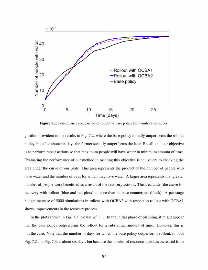
0 5 10 15 20 25

Time (days)

0

10

20

30

40

Num

ber

of people

with w

ate

r

103

Rollout with OCBA1

Rollout with OCBA2

Base policy

Figure 5.1: Performance comparison of rollout vs base policy for 3 units of resources.

gorithm is evident in the results in Fig. 7.2, where the base policy initially outperforms the rollout

policy, but after about six days the former steadily outperforms the later. Recall, that our objective

is to perform repair actions so that maximum people will have water in minimum amount of time.

Evaluating the performance of our method in meeting this objective is equivalent to checking the

area under the curve of our plots. This area represents the product of the number of people who

have water and the number of days for which they have water. A larger area represents that greater

number of people were benefitted as a result of the recovery actions. The area under the curve for

recovery with rollout (blue and red plots) is more than its base counterpart (black). A per-stage

budget increase of 5000 simulations in rollout with OCBA2 with respect to rollout with OCBA1

shows improvements in the recovery process.

In the plots shown in Fig. 7.3, we use M = 5. In the initial phase of planning, it might appear

that the base policy outperforms the rollout for a substantial amount of time. However, this is

not the case. Note that the number of days for which the base policy outperforms rollout, in both

Fig. 7.2 and Fig. 7.3, is about six days, but because the number of resource units has increased from

87

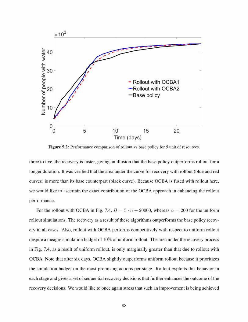
0 5 10 15 20

Time (days)

0

10

20

30

40

Num

ber

of people

with w

ate

r

103

Rollout with OCBA1

Rollout with OCBA2

Base policy

Figure 5.2: Performance comparison of rollout vs base policy for 5 unit of resources.

three to five, the recovery is faster, giving an illusion that the base policy outperforms rollout for a

longer duration. It was verified that the area under the curve for recovery with rollout (blue and red

curves) is more than its base counterpart (black curve). Because OCBA is fused with rollout here,

we would like to ascertain the exact contribution of the OCBA approach in enhancing the rollout

performance.

For the rollout with OCBA in Fig. 7.4, B = 5 · n + 20000, whereas α = 200 for the uniform

rollout simulations. The recovery as a result of these algorithms outperforms the base policy recov-

ery in all cases. Also, rollout with OCBA performs competitively with respect to uniform rollout

despite a meagre simulation budget of 10% of uniform rollout. The area under the recovery process

in Fig. 7.4, as a result of uniform rollout, is only marginally greater than that due to rollout with

OCBA. Note that after six days, OCBA slightly outperforms uniform rollout because it prioritizes

the simulation budget on the most promising actions per-stage. Rollout exploits this behavior in

each stage and gives a set of sequential recovery decisions that further enhances the outcome of the

recovery decisions. We would like to once again stress that such an improvement is being achieved

88

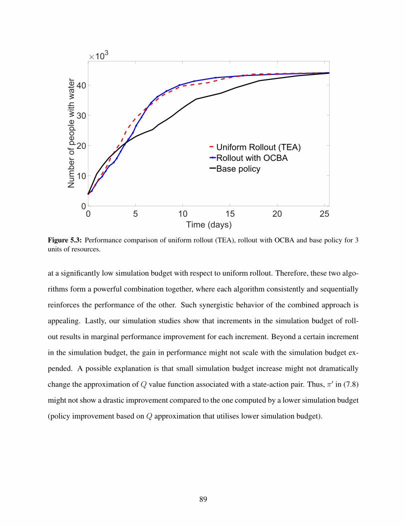
0 5 10 15 20 25

Time (days)

0

10

20

30

40

Num

ber

of people

with w

ate

r

103

Uniform Rollout (TEA)

Rollout with OCBA

Base policy

Figure 5.3: Performance comparison of uniform rollout (TEA), rollout with OCBA and base policy for 3units of resources.

at a significantly low simulation budget with respect to uniform rollout. Therefore, these two algo-

rithms form a powerful combination together, where each algorithm consistently and sequentially

reinforces the performance of the other. Such synergistic behavior of the combined approach is

appealing. Lastly, our simulation studies show that increments in the simulation budget of roll-

out results in marginal performance improvement for each increment. Beyond a certain increment

in the simulation budget, the gain in performance might not scale with the simulation budget ex-

pended. A possible explanation is that small simulation budget increase might not dramatically

change the approximation of Q value function associated with a state-action pair. Thus, π′ in (7.8)

might not show a drastic improvement compared to the one computed by a lower simulation budget

(policy improvement based on Q approximation that utilises lower simulation budget).

89

5.5 Funding and Support

“The research herein has been funded by the National Science Foundation under Grant CMMI-

1638284. This support is gratefully acknowledged. Any opinions, findings, conclusions, or recom-

mendations presented in this material are solely those of the authors and do not necessarily reflect

the views of the National Science Foundation.”

90

Chapter 6

Stochastic Scheduling for Building Portfolio

Restoration Following Disasters

6.1 Introduction

One of the principal objectives of the United Nations (UN) Sustainable Development Goals is

achieving food security. The Food and Agriculture Organization (FAO) describes food security

as: “a situation that exists when all people, at all times, have physical, social and economic ac-

cess to sufficient, safe and nutritious food that meets their dietary needs and food preferences for

an active and healthy life” [87]. Securing an adequate food supply to all community inhabitants

requires a food distribution system that is resilient to natural and man-made hazards. The growth

of population in hazard-prone regions and climate change pose numerous challenges to achiev-

ing a resilient food system around the world. The resiliency concept applied to food distribution

systems can be evaluated with respect to two different time-frames, namely in “normal” times

(i.e., prior to disasters) and in the aftermath of hazards. Several studies have investigated different

approaches to enhance the resilience of agri-food systems [88]. These studies have focused on re-

silience in terms of biophysical capacity to increase food production, diversity of modern domestic

food production, and the role played by social status and income in the impact of food deficits.

To mitigate food security issues, the United States Department of Agriculture (USDA) Food and

Nutrition Service (FNS) supplies 15 domestic food and nutrition assistance programs. The three

largest are the Supplemental Nutrition Assistance Program (SNAP - formerly the Food Stamp Pro-

gram), the National School Lunch Program, and the Special Supplemental Nutrition Program for

Women, Infants, and Children (WIC) [89]. However, household food security following extreme

natural hazard events is also contingent on interdependent critical infrastructure systems, such as

transportation, energy, water, household units, and retailer availability. This study focuses on the

91

connection between failures in food distribution and food retail infrastructure and disruption in

civil infrastructure and structures. Household food security issues are considerably worsened fol-

lowing natural disasters. For example, Hurricanes Rita, Wilma, and Katrina, which occurred in

2005, caused disaster-related food programs to serve 2.4 million households and distributed $928

million in benefits to households [90]. Three dimensions of food security - accessibility, availabil-

ity, and affordability - are particularly relevant for the nexus between infrastructure and household

food security. Affordability captures the ability of households to buy food from food retailers,

and is a function of household income, assets, credit, and perhaps even participation in food as-

sistance programs. Accessibility is concerned with the households’ physical access to food retail

outlets. Because at least one functional route must be available between a household unit and a

functioning food retailer, transportation networks are a major factor in accessibility. Availability

is concerned with the functionality of the food distribution infrastructure, beginning with whole-

salers, extending to retailers, and ultimately ending with the household as the primary consumer.

The functionality of food retailers and household units depends not only on the functionality of

their facilities but also the availability of electricity and water. Therefore, the electrical power net-

work (EPN), water network (WN), and the buildings housing retailers and household units must

be considered simultaneously to address availability. As is evident from the preceding discussion,

food security relies on a complex supply-chain system. If such a system is disrupted, community

resilience and the food security will be threatened [91]. In this work, we focus only on household

unit structures, which forms the largest entity in community restoration. In this work, we focus

on household unit buildings, which usually form the largest element of the built environment in

community restoration. A literature review [92] shows that the recovery of building portfolios has

been studied far less than the recovery of other infrastructure systems. Building portfolio restora-

tion is an essential element of availability and plays a major role towards addressing food security

issues. Effective emergency logistics demand a comprehensive decision-making framework that

addresses and supports policymakers’ preferences by providing efficient recovery plans. In this

study, we employ Markov decision processes (MDPs) along with an approximate dynamic pro-

92

gramming (ADP) technique to provide a practical framework for representation and solution of

stochastic large-scale decision-making problems. The scale and complexity of building portfolio

restoration is captured by the proposed simulation-based representation and solution of the MDP.

The near-optimal solutions are illustrated for the building portfolio of a testbed community mod-

eled after Gilroy, California, United States.

6.2 Testbed Case Study

As an illustration, this study considers the building portfolio of Gilroy, California, USA. The

City of Gilroy is a moderately sized growing city in southern Santa Clara County, California, with

a population of 48,821 at the time of the 2010 census. The study area is divided into 36 rectangular

regions organized as a grid to define the properties of the community with an area of 42 km2 and

a population of 47,905. Household units are growing at a faster pace in Gilroy than in Santa Clara

County and the State of California [1]. The average number of people per household in Gilroy in

2010 was 3.4, greater than the state and county average. Approximately 95% of Gilroy’s housing

units are occupied. A heat map of household units in the grid is shown in Fig. 6.1. Age distribution

of Gilroy is tabulated in Table 6.1.

Table 6.1: Age distribution of Gilroy [1].

Age Group PercentChildren (0-17 years) 30.60Adults (18-64 years) 61

Senior Citizen (65+ years) 8.40

6.3 Seismic Hazard and Damage Assessment

For details on the seismic hazard and damage model, see Chapter 2.

93

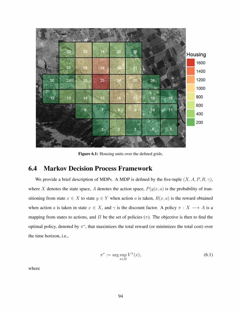
Figure 6.1: Housing units over the defined grids.

6.4 Markov Decision Process Framework

We provide a brief description of MDPs. A MDP is defined by the five-tuple (X,A, P,R, γ),

where X denotes the state space, A denotes the action space, P (y|x, a) is the probability of tran-

sitioning from state x ∈ X to state y ∈ Y when action a is taken, R(x, a) is the reward obtained

when action a is taken in state x ∈ X , and γ is the discount factor. A policy π : X −→ A is a

mapping from states to actions, and Π be the set of policies (π). The objective is then to find the

optimal policy, denoted by π∗, that maximizes the total reward (or minimizes the total cost) over

the time horizon, i.e.,

π∗ := arg supπ∈Π

V π(x), (6.1)

where

94

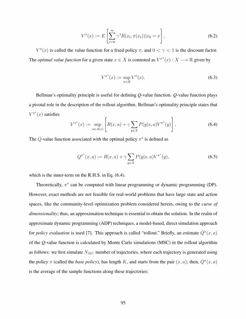
V π(x) := E

[

∞∑

t=0

γ tR(xt, π(xt))|x0 = x

]

, (6.2)

V π(x) is called the value function for a fixed policy π, and 0 < γ < 1 is the discount factor.

The optimal value function for a given state x ∈ X is connoted as V π∗

(x) : X −→ R given by

V π∗

(x) := supπ∈Π

V π(x). (6.3)

Bellman’s optimality principle is useful for defining Q-value function. Q-value function plays

a pivotal role in the description of the rollout algorithm. Bellman’s optimality principle states that

V π∗

(x) satisfies

V π∗

(x) := supa∈A(x)

[

R(x, a) + γ∑

y∈X

P (y|x, a)V π∗

(y)

]

, (6.4)

The Q-value function associated with the optimal policy π∗ is defined as

Qπ∗

(x, a) := R(x, a) + γ∑

y∈X

P (y|x, a)V π∗

(y), (6.5)

which is the inner-term on the R.H.S. in Eq. (6.4).

Theoretically, π∗ can be computed with linear programming or dynamic programming (DP).

However, exact methods are not feasible for real-world problems that have large state and action

spaces, like the community-level optimization problem considered herein, owing to the curse of

dimensionality; thus, an approximation technique is essential to obtain the solution. In the realm of

approximate dynamic programming (ADP) techniques, a model-based, direct simulation approach

for policy evaluation is used [7]. This approach is called “rollout.” Briefly, an estimate Qπ(x, a)

of the Q-value function is calculated by Monte Carlo simulations (MSC) in the rollout algorithm

as follows: we first simulate NMC number of trajectories, where each trajectory is generated using

the policy π (called the base policy), has length K, and starts from the pair (x, a); then, Qπ(x, a)

is the average of the sample functions along these trajectories:

95

Qπ(x, a) =1

NMC

NMC∑

i0=1

[

R(x, a, xi0,1) +K∑

k=1

γkR(xi0,k, π(xi0,k, xxi0,k+1))

]

. (6.6)

For each trajectory i0, we fix the first state-action pair to (x, a); the next state xi0,1 is calculated

when the current action a in state x is completed. Thereafter, we choose actions using the base

policy.

6.5 Building Portfolio Recovery

Each household unit and retailer building remains undamaged or exhibits one of the damage

states (i.e., Minor, Moderate, Major, and Collapse) based on the level of intensity measure and

the seismic fragility curves. There is a limited number of RUs (defined earlier) available to the

decision maker for the repair of the buildings in the community. In this study, we also limit the

number of RUs for each urban grid so that the number of available RUs for each grid RUg is 20

percent of the number of damaged buildings in each region of the grid. Therefore, the number of

RUs varies over the community in proportion to the density of the damaged buildings.

Let xt be the state of the damaged structures of the building portfolio at time t; xt is a vector,

where each element represents the damage state of each building in the portfolio based on the level

of intensity measure and the seismic fragility curves. Let agt denote the repair action to be carried

out on the damaged structures in the gth region of the grid at time t; each element of agt is either

zero or a one, where zero means do not repair and one means carry out repair. Note that the sum

of elements of agt is equal to RUg. The repair action for the entire community at time t, at, is the

stack of the repair action agt . The assignment of RUs to damaged locations is non − preemptive

in the sense that the decision maker cannot preempt the assigned RUs from completing their work

and reassign them to different locations at every decision epoch t. This type of scheduling is

more suitable when the decision maker deals with non-central stakeholders and private owners,

which is the case for a typical building portfolio. We wish to plan decisions optimally so that a

maximum number of inhabitants have safe household unit structures per unit of time (day in our

case). Therefore, the reward function embeds two objectives as follows:

96

R(xt, at, xt+1) =r

trep, (6.7)

where r is the number of people benefited from household units after the completion of at, and

trep is the total repair time to reach xt+1 from any initial state x0. Note that the reward function is

stochastic because the outcome of the repair action is stochastic. In this study, we set the discount

factor to be 0.99, implying that the decision maker is “far-sighted” in the consideration of the future

rewards.

We simulated NMC number of trajectories to reach a low (0.1 in this study) dispersion in

Eq. (6.6). As Eq. (6.6) shows, we addressed the mean-based optimization that is suited to risk-

neutral decision-makers. However, this approach can easily address different risk aversion be-

haviors. Fig. 6.2 shows the total number of people with inhabitable structures (undamaged or

repaired) over the community. We also computed the different numbers of children, adults, and

senior citizens that have safe buildings over the recovery. Different age groups have different levels

of vulnerability to food insecurity; for example, children are a vulnerable group and must be paid

more attention during the recovery process.

Fig. 6.3 depicts the spatio-temporal evolution of the community for people with inhabitable

structurally-safe household units. This figure shows that for urban grids with a high density of

damaged structures, complete recovery is prolonged despite availability of additional RUs. The

spatio-temporal analysis of the community is informative for policy makers whereby they can

identify the vulnerable areas of the community across time.

6.6 Conclusion

The building portfolio restoration is one of the most challenging ingredients to address food

security issues in the aftermath of disasters. Our stochastic dynamic optimization approach, based

on the method of rollout, successfully plans a near-optimal building portfolio recovery following

a hazard. Our approach shows how to overcome the curse of dimensionality in optimizing large-

scale building portfolio recovery post-diaster.

97

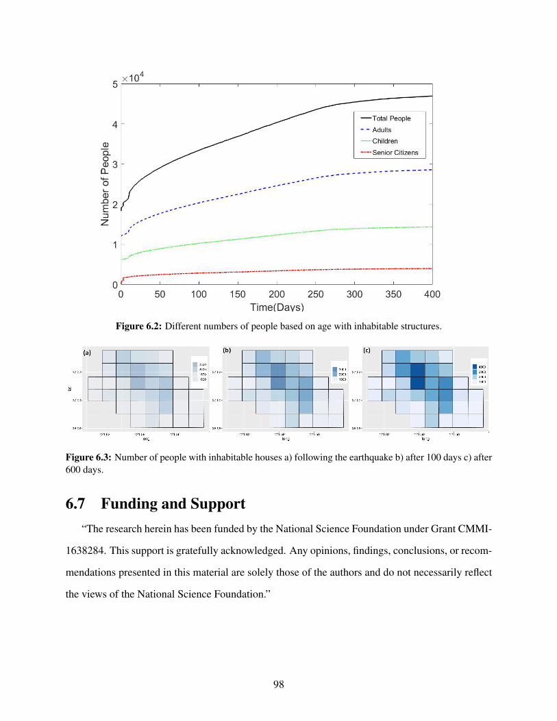
Figure 6.2: Different numbers of people based on age with inhabitable structures.

Figure 6.3: Number of people with inhabitable houses a) following the earthquake b) after 100 days c) after600 days.

6.7 Funding and Support

“The research herein has been funded by the National Science Foundation under Grant CMMI-

1638284. This support is gratefully acknowledged. Any opinions, findings, conclusions, or recom-

mendations presented in this material are solely those of the authors and do not necessarily reflect

the views of the National Science Foundation.”

98

Chapter 7

A Method for Handling Massive Discrete Action

Spaces of MDPs: Application to Electric Power

Network Recovery

7.1 Introduction

Automatic control systems have had a wide impact in multiple fields, including finance, robotics,

manufacturing, and automobiles. Decision automation has gained relatively little attention, espe-

cially when compared to decision support systems where the primary aim is to aid humans in the

decision-making process. In practice, decision automation systems often do not eliminate human

decision makers entirely but rather optimize decision making in specific instances where the au-

tomation system can surpass human performance. In fact, human decision makers play a very

important role in the selection of models, determining the set of rules, and developing methods

that automate the decisions. Nonetheless, decision automation systems remain indispensable in

applications where humans are unable to make rational decisions, whether because of the sheer

complexity of the system, the enormity of the set of alternatives, or the massive amount of data

that must be processed.

Our focus in this work is to develop a framework that automates decisions for post-disaster

recovery of communities. Designing such a framework is ambitious given that it should ideally

possess several key properties such as the ability to incorporate sources of uncertainty in the mod-

els, information gained at periodic intervals during the recovery process, current policies of the

decision-maker, and multiple decision objectives under resource constraints [6]. Our framework

possesses these desired properties; in addition, our framework uses reasonable computational re-

sources even for massive problems, has the lookahead property, and does not suffer from decision

fatigue.

99

Civil infrastructure systems, including building infrastructure, power, transportation, and water

networks, play a major role in the welfare of any community. The interdependence between the re-

covery of these networks post-hazard and community welfare addressing the issue of food-security,

has been studied in [5, 8, 93]. In this study, we focus on electric power networks (EPNs) because

almost all other infrastructure systems rely heavily on the availability of this network. In this study,

a stochastic model characterizes the damage to the components of the EPN after an earthquake;

similarly, the repair times associated with the repair actions are also given by a stochastic model.

The assignment of limited resources, including repair crews composed of humans and ma-

chines, to the damaged components of the EPN after a hazard can be posed as the generalized

assignment problem (as defined in [94]), which is known to be NP-hard. Several heuristic methods

have been demonstrated in the literature to address this problem [95].

Our Contribution: Instead of these classical methods, we employ Markov decision processes

(MDPs) for the representation and solution of our stochastic decision-making problem, which nat-

urally extends its appealing properties to our framework. In our framework, the solution to the

assignment problem formulated as a MDP is computed in an online fashion using an approximate

dynamic programming method known as rollout [64,96]. This approach addresses the curse of di-

mensionality associated with large state spaces [61]. Furthermore, in our framework, the massive

action space is handled by using a linear belief model, where a small number of candidate actions

are used to estimate the parameters in the model based on a least-squares solution. Our method

also employs adaptive sampling inspired by solutions to multi-armed bandit problems to carefully

expend the limited simulation budget—a limit on the simulation budget is often a constraint while

dealing with large real-world problems. Our approach successfully addresses the goal of develop-

ing a technique to deal with problems when the state and actions spaces of the MDP are jointly

exceptionally large.

100

7.2 The Assignment Problem

7.2.1 Problem Setup: The Gilroy Community, Seismic Hazard Simulation,

and Fragility and Restoration Assessment of EPN

The details for the modeled EPN of Gilroy, CA, the hazard simulation model, and fragility and

restoration assessment of EPN are already presented in Chapters 2 to 4. For additional details,

see [9].

Challenges

The total number of modeled EPN components is equal to 327, denoted by L. On average,

about 60% of these components are damaged after the simulated earthquake event. At each deci-

sion epoch t = 0, 1, 2, . . . , the decision maker has to select the assignment of RUs to the damaged

components; each component cannot be assigned more than one RU. Note that the symbol t is used

to denote a discrete-index representing decision-epoch and is not to be confused with the actual

time for recovery. Let the total number of damaged components at any t be represented by Mt, and

let the total number of RUs be equal to N , where N ≪Mt (typically, the number of resource units

for repair is significantly less than the damaged components). Then, the total number of possible

choices for the assignment at any t is(

Mt

N

)

. For 196 damaged components and 29 RUs (15% of the

damaged components), the possible choices at the first decision epoch is approximately 1034. In

addition, the reassignment of all RUs is done when one component gets repaired so that the total

number of choices at the second decision epoch is(

19529

)

≈ 1034.

Note that the repair time associated with a damaged component will depend on the level of

damage, as determined from the fragility analysis described in Chapter 2 to 4. This repair time is

random and is exponentially distributed with expected repair times shown in Table 4.1. Therefore,

the outcomes of the repair actions are also random. It is difficult for a human decision maker to

anticipate the outcome of repair actions when the outcomes are uncertain; therefore, planning with

foresight is difficult. In fact, the problem is difficult to such an extent that assignment of RUs at the

101

first decision epoch itself is challenging. Further, an additional layer of complexity to the problem

is manifested owing to the level of damage at each location specified by a probabilistic model [44].

Because of the extraordinarily large number of choices, stochastic initial conditions, and the

stochastic behavior of the outcome of the repair actions, our problem has a distinct flavor compared

to the generalized assignment problem, and the classical heuristic solutions are not well-suited

to this problem. In addition to dealing with these issues, the decision maker has to incorporate

the dynamics and the sequential nature of decision making during recovery; thus, our problem

represents a stochastic sequential decision-making problem. Last, we would also like our solution

to admit most of the desirable properties previously discussed in the Section 7.1. Our framework

addresses all these issues.

7.2.2 Problem Formulation

In this section, we briefly discuss MDPs and the simulation-based representation pertaining to

our problem, previously described in Chapter 5, and repeated here for the sake of continuity and

completeness. We then specify the components of the MDP for our problem.

MDP Framework and Simulation-Based Representation

An MDP is a controlled stochastic dynamical process, widely used to solve disparate decision-

making problems. In the simplest form, it can be represented by the 4-tuple 〈S,A, T,R〉. Here, S

represents the set of states, and A represents the set of actions. The state makes a transition to a

new state at each decision epoch (represented by discrete-index t) as a result of taking an action.

Let s, s′ ∈ S and a ∈ A; then T is the state transition function, where T (s, a, s′) = P (s′ | s, a)

is the probability of transitioning to state s′ after taking action a in state s, and R is the reward

function, where R(s, a, s′) is the reward received after transitioning from s to s′ as a result of

action a. In our problem, |S| and |A| are finite; R is real-valued and a stochastic function of s

and a (deterministic function of s, a, and s′). Implicit in our presentation are also the following

assumptions [72]: First-order Markovian dynamics (history independence), stationary dynamics

(transition function is not a function of absolute time), and full observability of the state space

102

(outcome of an action in a state might be random, but the state reached is known after the action is

completed). The last assumption simplifies our presentation in that we do not need to take actions

specifically to reinforce or modify our belief about the underlying state. We assume that recovery

actions (decisions) can be taken indefinitely as needed, e.g., until all the damaged components are

repaired (infinite-horizon planning). In this setting, we define a stationary policy as a mapping

π : S → A. Our objective is to find an optimal policy π∗. For the infinite-horizon case, π∗ is

defined as

π∗ = argmaxπ

V π(s0), (7.1)

where

V π(s0) = E

[

∞∑

t=0

γ tR(st, π(st), st+1)

∣

∣

∣

∣

∣

s0

]

(7.2)

is called the value function for a fixed policy π, and γ ∈ (0, 1] is the discount factor. Note that

in (7.1) we maximize over policies π, where at each decision epoch t the action taken is at = π(st).

Stationary optimal policies are guaranteed to exist for the discounted infinite-horizon optimization

criterion [53]. To summarize, our framework is built on discounted infinite-horizon discrete-time

MDPs with finite state and action spaces, though the role γ is somewhat tangential in our applica-

tion.

We now briefly explain the simulation-based representation of an MDP [76]. Such a represen-

tation serves well for large state, action, and outcome spaces, which is a characteristic feature of

many real-world problems; it is infeasible to represent T and R in a simple matrix form for such

problems. A simulation-based representation of an MDP is a 4-tuple 〈S,A, R, T 〉, where S and A

are as before. Here, R is a stochastic real-valued function that stochastically returns a reward when

input s and a are provided, where a is the action applied in state s; T is a simulator, which stochas-

tically returns a state sample s′ when state s and action a are provided as inputs. We can think of

R and T as callable library functions that can be implemented in any programming language.

103

MDP Specification for EPN Recovery Problem

States: Let st denote the state of our MDP at discrete decision epoch t: st = (s1t , . . . , sLt , ρ

1t , . . . , ρ

Lt ),

slt is the damage state of the lth damaged EPN component (the possible damage states are Undam-

aged, Minor, Moderate, Extensive, and Complete, as shown in Table 4.1); and ρlt is the remaining

repair time associated with the lth damaged component, where l ∈ 1, . . . , L. The state transition,

and consequently the calculation of ρlt and slt at each t, is explained in the description of simulator

T below.

Actions: Let at denote the repair action to be carried out at decision epoch t: at = (a1t , . . . , aLt ),

and alt ∈ 0, 1 ∀l, t. When alt = 0, no repair work is to be carried out at lth component. Con-

versely, when alt = 1, repair work is carried out at the lth component. Note that∑

l alt = N , and

alt = 0 for all l where slt is equal to Undamaged. Let Dt be the set of all damaged components

before a repair action at is performed. Let P(Dt) be the powerset of Dt. The total number of

possible choices at any decision epoch t is given by |PN(Dt)|, where

PN(Dt) = C ∈ P(Dt) : |C| = N, (7.3)

|Dt| =Mt, and |PN(Dt)| =(

Mt

N

)

.

Initial State: The stochastic damage model, previously described in Chapters 2 to 4, is used to

calculate the initial damage state sl0. Once the initial damage states of the EPN components are

known, depending on the type of the damaged EPN component, the repair times ρl0 associated with

the damaged components are calculated using the mean restoration times provided in Table 4.1.

Simulator T : Given st and at, T gives us the new (stochastic) state st+1. We define a repair

completion as the instant when at least one of the locations where repair work is carried out is fully

repaired. The decision epochs occur at these repair-completion times. A damaged component

is fully repaired when the damage state of the component changes from any of the four damage

states (except the Undamaged state) in Table 4.1 to the Undamaged state. Let us denote the inter-

104

completion time by rt, which is the time duration between decision epochs t and t + 1, and let

∆t = ρlt : l ∈ 1, . . . , L, ρ

lt > 0. Then, rt = min∆t and ρlt+1 = max(ρlt−rt, 0). Note that it is

possible in principle for the repair work at two or more locations to be completed simultaneously,

though this virtually never happens in simulation or in practice. When a damaged component is

in any of the Minor, Moderate, Extensive, or Complete states, it can only transition directly to

the Undamaged state. Instead of modeling the effect of repair via inter-transitions among damage

states, the same effect is captured by the remaining repair time ρt.

Once a damaged component is restored to the Undamaged state, the RUs previously assigned

to it become available for reassignment to other damaged components. Moreover, the RUs at

remaining locations, where repair work is unfinished, are also available for reassignment—the

repair of a component is preemptive. It is also possible for a RU to remain at its previously assigned

unrepaired location if we choose so. Because of this reason, preemption of repair work during

reassignment is not a restrictive assumption; on the contrary, it allows greater flexibility to the

decision maker for planning. Preemptive assignment is known to be particularly useful when an

infrastructure system is managed by a central authority, an example of which is EPN [6].

Even if the same assignment is applied repeatedly to the same system state (let us call this the

current system state), the system state at the subsequent decision epoch could be different because

different components might be restored in the current system state, because of random repair times;

i.e., our simulator T is stochastic. WhenMt eventually becomes less than or equal toN because of

the sequential application of the repair actions (say at decision epoch ta), the extra RUs are retired

so that we have Mt = N ∀t ≥ ta+1, and the assignment problem is trivial. The evolution of the

state of the community as a result of the nontrivial assignments is therefore given by (s0, . . . , sta).

Rewards: We define two reward functions corresponding to two different objectives:

In the first objective, the goal is to minimize the days required to restore electricity to a certain

fraction (ζ) of the total population (p); recall that for our region of study in Gilroy, p = 47905. We

capture this objective by defining the corresponding reward function as follows:

105

R1(st, at, st+1) = rt, (7.4)

where we recall that rt is the inter-completion time between the decision epochs t and t+1. Let tc

denote the decision epoch at which the outcome of repair action atc−1 results in the restoration of

electricity to ζ · p number of people. The corresponding state reached resulting from action atc−1

is stc , called the goal state for the first objective.

In the second objective, the goal is to maximize the sum (over all the discrete decision epochs

t) of the product of the total number of people with electricity (nt) after the completion of a repair

action at and the per-action time, defined as the time required (rt) to complete the repair action at,

divided by the total number of days (ttot) required to restore electricity to p people. We capture this

objective by defining our second reward function as:

R2(st, at, st+1) =nt · rtttot

. (7.5)

The terms in (7.5) have been carefully selected so that the product of the terms nt and rt/ttot cap-

tures the impact of automating a repair action at each decision epoch t, in the spirit of maximizing

electricity benefit in a minimum amount of time. Let tc denote the decision epoch at which the

outcome of repair action atc−1 results in the restoration of electricity to the entire population. Then

the corresponding goal state is stc .

Note that both tc and tc need not belong to the set 0, . . . , ta−1, i.e., both stc and stc need

not be reached only with a nontrivial assignment. Also, note that our reward function is stochastic

because the outcome of each action is random.

Discount factor γ: A natural consequence of sequential decision making is the problem of in-

tertemporal choice [97]. The problem consists in balancing the rewards and costs at different

decision epochs so that the uncertainty in the future choices can be accounted for. To deal with

the problem, the MDP model, specifically for our formulation, accommodates a discounted utility,

which has been the preferred method of tackling this topic for over a century. In this study, the

discount factor γ is fixed at 0.99. We have selected a value closer to one because of the use of

106

sophisticated stochastic models described in Chapters 2 to 4; the uncertainty in the outcome of the

future choices is modeled precisely via these models, and therefore we can evaluate the value of

the decisions several decision-epochs in the future accurately to estimate the impact of the current

decision. In our framework, it is possible to select a value closer to zero if the decision automa-

tion problem demands the use of simpler models. Moreover, the discounting can be done based

on rt—the real time required for repair in days (the inter-epoch time)—rather than the number of

decision epochs, but this distinction is practically inconsequential for our purposes because of our

choice of γ being very close to one.

Next we highlight the salient features of our MDP framework; in particular, we discuss the

successful mitigation of the challenges previously discussed in Section 7.2.1

Recall that we have a probability distribution for the initial damage state of the EPN compo-

nents for a simulated earthquake. We generate multiple samples from this distribution to initialize

s0 and optimize the repair actions for each of the initial states separately. The outcomes of the

optimized repair action for each initial state constitutes a distinct stochastic unfolding of recovery

events (recovery path or recovery trajectory). We average over these recovery paths to evaluate

the performance of our methods. In our framework, as long as sufficient samples (with respect

to some measure of dispersion) are generated, we can appropriately deal with the probabilistic

damage-state model.

Our sequential decision-making formulation also includes modeling the uncertainty in the out-

come of repair actions. Thus, our framework can handle both stochastic initial conditions and

stochastic repair actions.

We have formulated the impact of the current decisions on the future choices with exponential

discounting. In addition, our sequential decision-making framework addresses the issue of making

restoration decisions in stages, where feedback (information) gathered at each stage can play an

important role in successive decision making. This is essentially a closed-loop design to compute

decisions at each decision epoch.

107

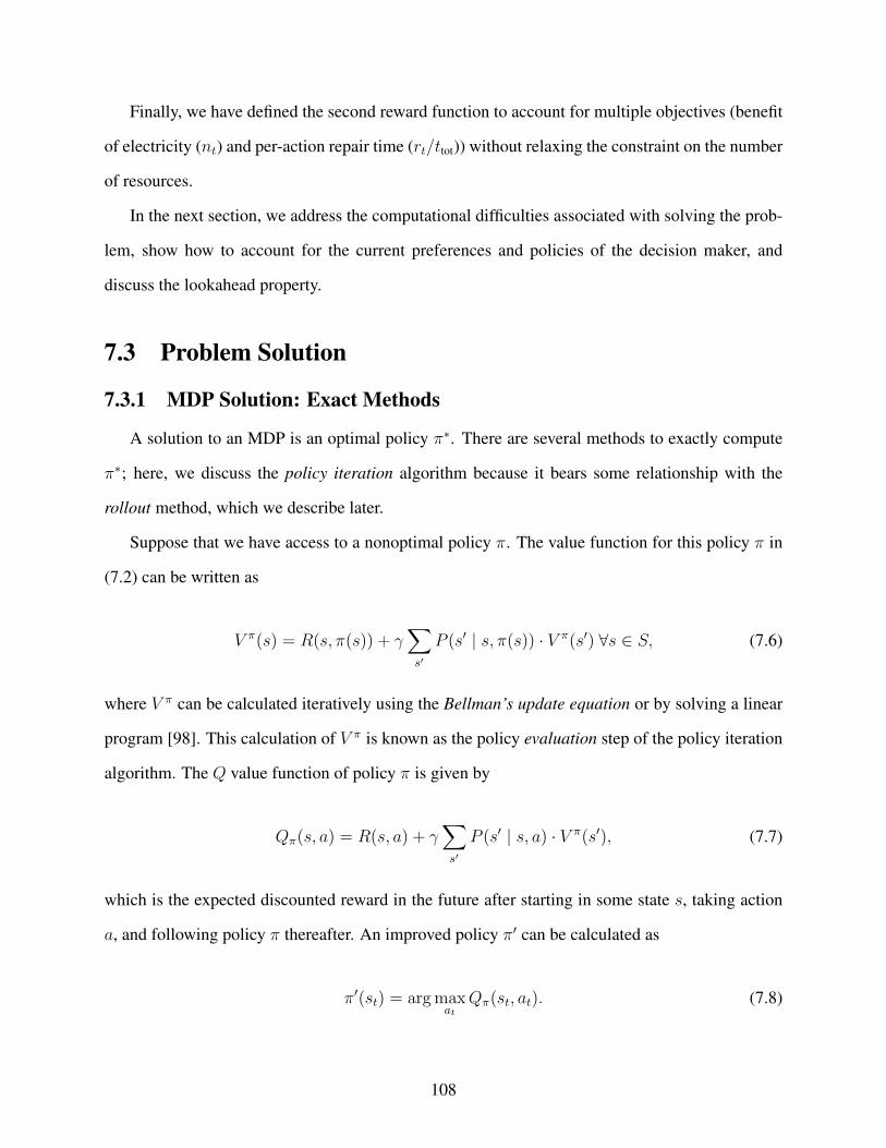
Finally, we have defined the second reward function to account for multiple objectives (benefit

of electricity (nt) and per-action repair time (rt/ttot)) without relaxing the constraint on the number

of resources.

In the next section, we address the computational difficulties associated with solving the prob-

lem, show how to account for the current preferences and policies of the decision maker, and

discuss the lookahead property.

7.3 Problem Solution

7.3.1 MDP Solution: Exact Methods

A solution to an MDP is an optimal policy π∗. There are several methods to exactly compute

π∗; here, we discuss the policy iteration algorithm because it bears some relationship with the

rollout method, which we describe later.

Suppose that we have access to a nonoptimal policy π. The value function for this policy π in

(7.2) can be written as

V π(s) = R(s, π(s)) + γ∑

s′

P (s′ | s, π(s)) · V π(s′) ∀s ∈ S, (7.6)

where V π can be calculated iteratively using the Bellman’s update equation or by solving a linear

program [98]. This calculation of V π is known as the policy evaluation step of the policy iteration

algorithm. The Q value function of policy π is given by

Qπ(s, a) = R(s, a) + γ∑

s′

P (s′ | s, a) · V π(s′), (7.7)

which is the expected discounted reward in the future after starting in some state s, taking action

a, and following policy π thereafter. An improved policy π′ can be calculated as

π′(st) = argmaxat

Qπ(st, at). (7.8)

108

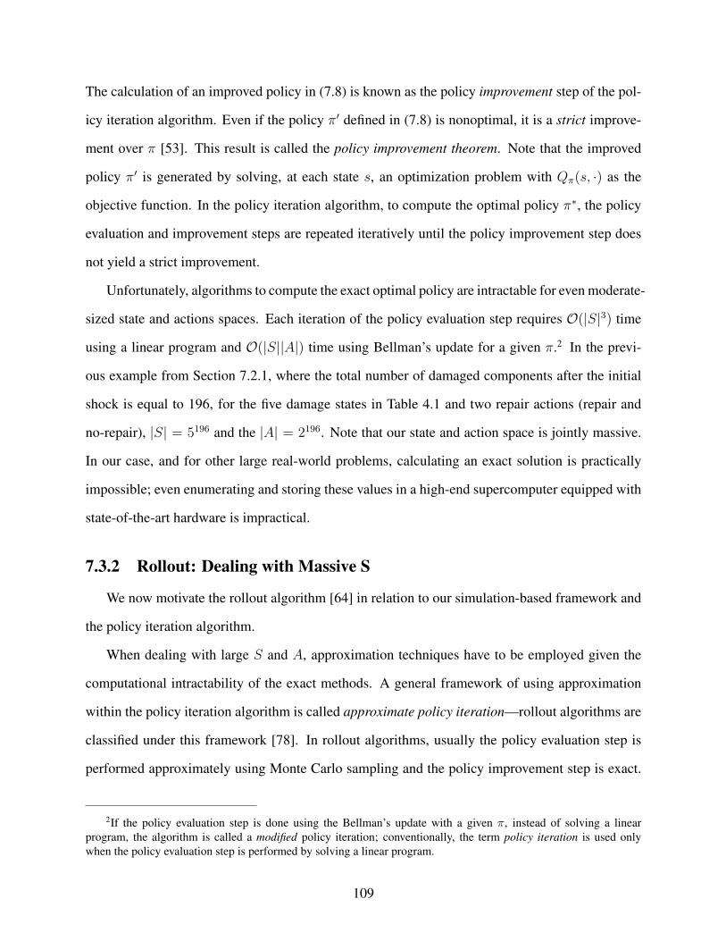
The calculation of an improved policy in (7.8) is known as the policy improvement step of the pol-

icy iteration algorithm. Even if the policy π′ defined in (7.8) is nonoptimal, it is a strict improve-

ment over π [53]. This result is called the policy improvement theorem. Note that the improved

policy π′ is generated by solving, at each state s, an optimization problem with Qπ(s, ·) as the

objective function. In the policy iteration algorithm, to compute the optimal policy π∗, the policy

evaluation and improvement steps are repeated iteratively until the policy improvement step does

not yield a strict improvement.

Unfortunately, algorithms to compute the exact optimal policy are intractable for even moderate-

sized state and actions spaces. Each iteration of the policy evaluation step requires O(|S|3) time

using a linear program and O(|S||A|) time using Bellman’s update for a given π.2 In the previ-

ous example from Section 7.2.1, where the total number of damaged components after the initial

shock is equal to 196, for the five damage states in Table 4.1 and two repair actions (repair and

no-repair), |S| = 5196 and the |A| = 2196. Note that our state and action space is jointly massive.

In our case, and for other large real-world problems, calculating an exact solution is practically

impossible; even enumerating and storing these values in a high-end supercomputer equipped with

state-of-the-art hardware is impractical.

7.3.2 Rollout: Dealing with Massive S

We now motivate the rollout algorithm [64] in relation to our simulation-based framework and

the policy iteration algorithm.

When dealing with large S and A, approximation techniques have to be employed given the

computational intractability of the exact methods. A general framework of using approximation

within the policy iteration algorithm is called approximate policy iteration—rollout algorithms are

classified under this framework [78]. In rollout algorithms, usually the policy evaluation step is

performed approximately using Monte Carlo sampling and the policy improvement step is exact.

2If the policy evaluation step is done using the Bellman’s update with a given π, instead of solving a linearprogram, the algorithm is called a modified policy iteration; conventionally, the term policy iteration is used onlywhen the policy evaluation step is performed by solving a linear program.

109

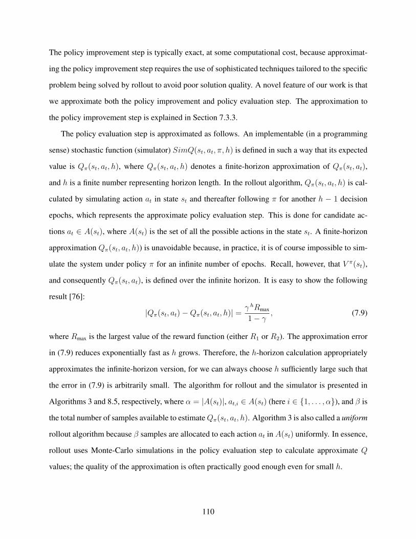
The policy improvement step is typically exact, at some computational cost, because approximat-

ing the policy improvement step requires the use of sophisticated techniques tailored to the specific

problem being solved by rollout to avoid poor solution quality. A novel feature of our work is that

we approximate both the policy improvement and policy evaluation step. The approximation to

the policy improvement step is explained in Section 7.3.3.

The policy evaluation step is approximated as follows. An implementable (in a programming

sense) stochastic function (simulator) SimQ(st, at, π, h) is defined in such a way that its expected

value is Qπ(st, at, h), where Qπ(st, at, h) denotes a finite-horizon approximation of Qπ(st, at),

and h is a finite number representing horizon length. In the rollout algorithm, Qπ(st, at, h) is cal-

culated by simulating action at in state st and thereafter following π for another h − 1 decision

epochs, which represents the approximate policy evaluation step. This is done for candidate ac-

tions at ∈ A(st), where A(st) is the set of all the possible actions in the state st. A finite-horizon

approximation Qπ(st, at, h)) is unavoidable because, in practice, it is of course impossible to sim-

ulate the system under policy π for an infinite number of epochs. Recall, however, that V π(st),

and consequently Qπ(st, at), is defined over the infinite horizon. It is easy to show the following

result [76]:

|Qπ(st, at)−Qπ(st, at, h)| =γ hRmax

1− γ, (7.9)

where Rmax is the largest value of the reward function (either R1 or R2). The approximation error

in (7.9) reduces exponentially fast as h grows. Therefore, the h-horizon calculation appropriately

approximates the infinite-horizon version, for we can always choose h sufficiently large such that

the error in (7.9) is arbitrarily small. The algorithm for rollout and the simulator is presented in

Algorithms 3 and 8.5, respectively, where α = |A(st)|, at,i ∈ A(st) (here i ∈ 1, . . . , α), and β is

the total number of samples available to estimateQπ(st, at, h). Algorithm 3 is also called a uniform

rollout algorithm because β samples are allocated to each action at in A(st) uniformly. In essence,

rollout uses Monte-Carlo simulations in the policy evaluation step to calculate approximate Q

values; the quality of the approximation is often practically good enough even for small h.

110

Algorithm 3 Uniform_Rollout(π, h, β, st, A(st))

for i = 1 to α do

for j = 1 to β do

Qi,j ← SimQ(st, at,i, π, h) ⊲ See algorithm 2end for

Qt(i)← Average(Qi,j) ⊲ With respect to jend for

k ← argmaxiQt

return at,k

Algorithm 4 Simulator SimQ(st, at,i, π, h)

t′ = 0s′0 ← sts′t′+1 ← T (s′t′ , at,i)

r ← R(s′t′ , at,i, s′t′+1)

for λ = 1 to h− 1 do

s′t′+1+λ ← T (s′t′+λ, π(s′t′+λ))

r ← r + γ λR(s′t′+λ, π(s′t′+λ), s

′t′+1+λ)

end for

return r

Rollout fits well in the paradigm of online planning. In online planning, the optimal action is

calculated only for the current state st, reducing the computational effort associated with a large

state space. Similarly, in our problem, we need to calculate repair actions for the current state of

the EPN without wasting computational resources on computing repair actions for the states that

are never encountered during the recovery process. Therefore, the property of online planning

associated with Algorithm 3 is important for recovery, and even if the policy π (called the base

policy in the context of Algorithm 3) is applied repeatedly (“rolled out”) for h−1 decision epochs,

we focus only on the encountered states as opposed to dealing with all the possible states (cf.,

(7.6)). In essence, for the recovery problem, rollout can effectively deal with large sizes of the

state space because the calculation of the policy is amortized over time.

Consider the following example. In the context of online planning, for the sake of argument

suppose that the action space has only a single action. Even for such a superficially trivial example,

the outcome space can be massive. However, the representation of the problem in our framework

111

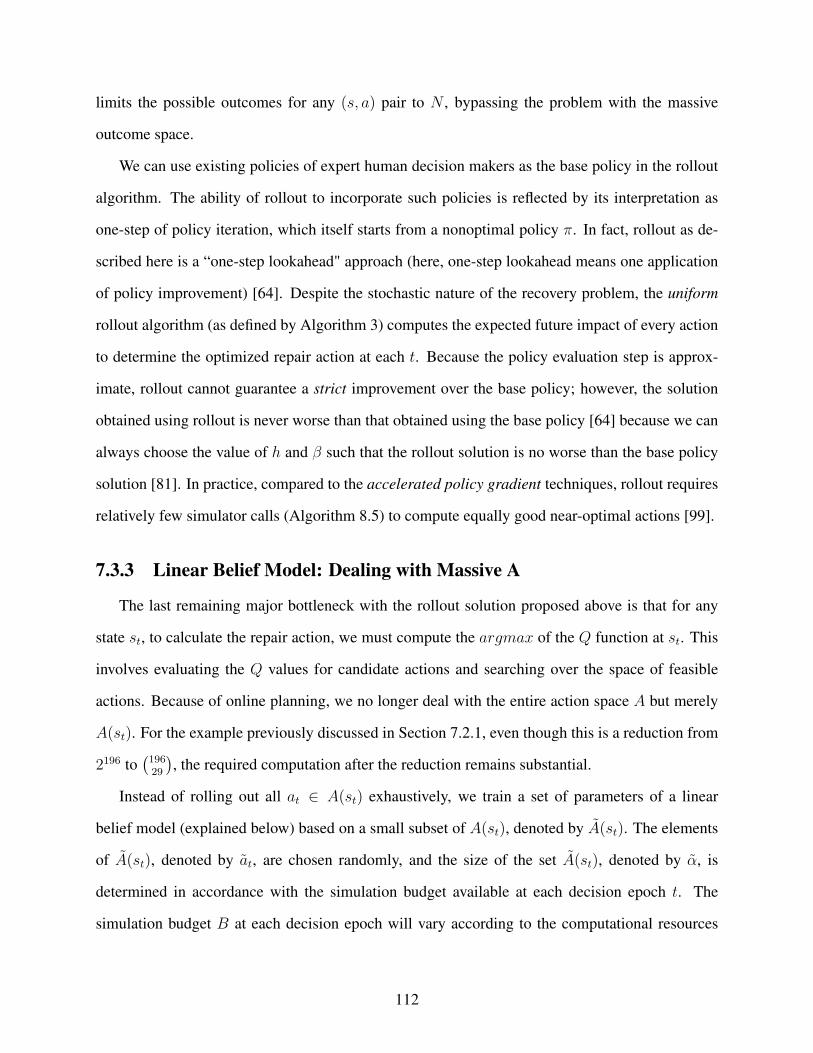
limits the possible outcomes for any (s, a) pair to N , bypassing the problem with the massive

outcome space.

We can use existing policies of expert human decision makers as the base policy in the rollout

algorithm. The ability of rollout to incorporate such policies is reflected by its interpretation as

one-step of policy iteration, which itself starts from a nonoptimal policy π. In fact, rollout as de-

scribed here is a “one-step lookahead" approach (here, one-step lookahead means one application

of policy improvement) [64]. Despite the stochastic nature of the recovery problem, the uniform

rollout algorithm (as defined by Algorithm 3) computes the expected future impact of every action

to determine the optimized repair action at each t. Because the policy evaluation step is approx-

imate, rollout cannot guarantee a strict improvement over the base policy; however, the solution

obtained using rollout is never worse than that obtained using the base policy [64] because we can

always choose the value of h and β such that the rollout solution is no worse than the base policy

solution [81]. In practice, compared to the accelerated policy gradient techniques, rollout requires

relatively few simulator calls (Algorithm 8.5) to compute equally good near-optimal actions [99].

7.3.3 Linear Belief Model: Dealing with Massive A

The last remaining major bottleneck with the rollout solution proposed above is that for any

state st, to calculate the repair action, we must compute the argmax of the Q function at st. This

involves evaluating the Q values for candidate actions and searching over the space of feasible

actions. Because of online planning, we no longer deal with the entire action space A but merely

A(st). For the example previously discussed in Section 7.2.1, even though this is a reduction from

2196 to(

19629

)

, the required computation after the reduction remains substantial.

Instead of rolling out all at ∈ A(st) exhaustively, we train a set of parameters of a linear

belief model (explained below) based on a small subset of A(st), denoted by A(st). The elements

of A(st), denoted by at, are chosen randomly, and the size of the set A(st), denoted by α, is

determined in accordance with the simulation budget available at each decision epoch t. The

simulation budget B at each decision epoch will vary according to the computational resources

112

employed and the run-time of Algorithm 8.5. Thereafter, at is calculated using the estimated

parameters of the linear belief model.

Linear belief models are popular in several fields, especially in drug discovery [100]. Given an

action at,i selected from A(st), the linear belief model can be represented as

Qi,j =N∑

n=1

M∑

m=1

Xmn ·Θmn + ηmn, (7.10)

where

Xmn =

1 if nth RU is assigned to mth location

0 otherwise,

(7.11)

i ∈ 1, . . . , α, j ∈ 1, . . . , β, Qi,j are the Q values corresponding to at,i obtained with Algo-

rithm 8.5, and ηmn represents noise. Let Qi = 1β

∑βj=1 Q

i,j . In this formulation, each parameter

Θmn additively captures the impact on the Q value of assigning a RU (indexed by n) to a damaged

component (indexed by m). In particular, the contribution of each parameter is assumed to be in-

dependent of the presence or absence of the other parameters (see the discussion at the end of this

section). Typically, linear belief models include an additional parameter: the constant intercept

term Θ0 so that (7.10) would be expressed as

Qi,j = Θ0 +N∑

n=1

M∑

m=1

Xmn ·Θmn + ηmn. (7.12)

However, our model excludes Θ0 because it would carry no corresponding physical significance

unlike the other parameters.

The linear belief model in (7.10) can be equivalently written as

y = H · θ + η, (7.13)

where y (of size α × 1) is a vector of the Qi values calculated for all the actions at ∈ A(st), H

(of size α × (Mt · N)) is a binary matrix where the entries are in accordance with (7.10), (7.11),

113

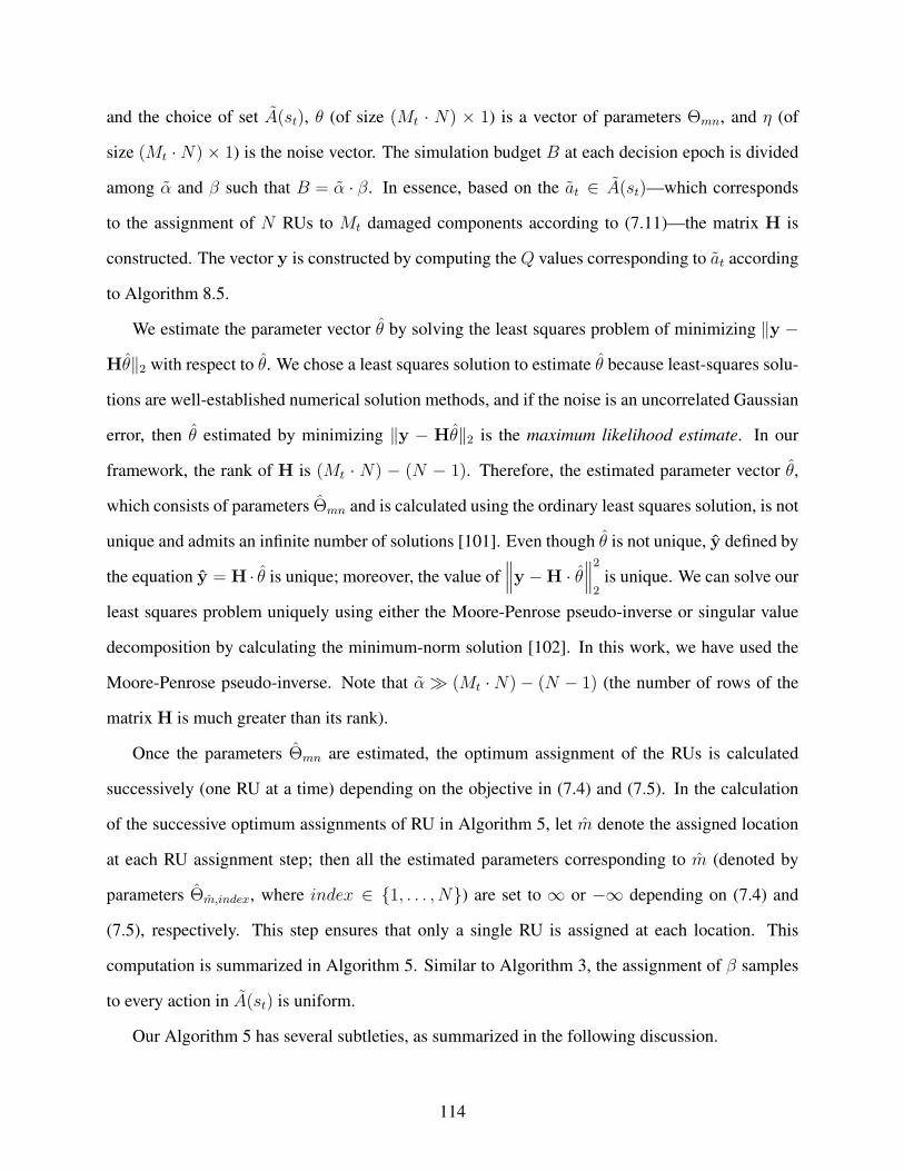
and the choice of set A(st), θ (of size (Mt · N) × 1) is a vector of parameters Θmn, and η (of

size (Mt ·N)× 1) is the noise vector. The simulation budget B at each decision epoch is divided

among α and β such that B = α · β. In essence, based on the at ∈ A(st)—which corresponds

to the assignment of N RUs to Mt damaged components according to (7.11)—the matrix H is

constructed. The vector y is constructed by computing the Q values corresponding to at according

to Algorithm 8.5.

We estimate the parameter vector θ by solving the least squares problem of minimizing ‖y −

Hθ‖2 with respect to θ. We chose a least squares solution to estimate θ because least-squares solu-

tions are well-established numerical solution methods, and if the noise is an uncorrelated Gaussian

error, then θ estimated by minimizing ‖y − Hθ‖2 is the maximum likelihood estimate. In our

framework, the rank of H is (Mt · N) − (N − 1). Therefore, the estimated parameter vector θ,

which consists of parameters Θmn and is calculated using the ordinary least squares solution, is not

unique and admits an infinite number of solutions [101]. Even though θ is not unique, y defined by

the equation y = H · θ is unique; moreover, the value of∥

∥

∥y −H · θ∥

∥

∥

2

2is unique. We can solve our

least squares problem uniquely using either the Moore-Penrose pseudo-inverse or singular value

decomposition by calculating the minimum-norm solution [102]. In this work, we have used the

Moore-Penrose pseudo-inverse. Note that α≫ (Mt ·N)− (N − 1) (the number of rows of the

matrix H is much greater than its rank).

Once the parameters Θmn are estimated, the optimum assignment of the RUs is calculated

successively (one RU at a time) depending on the objective in (7.4) and (7.5). In the calculation

of the successive optimum assignments of RU in Algorithm 5, let m denote the assigned location

at each RU assignment step; then all the estimated parameters corresponding to m (denoted by

parameters Θm,index, where index ∈ 1, . . . , N) are set to ∞ or −∞ depending on (7.4) and

(7.5), respectively. This step ensures that only a single RU is assigned at each location. This

computation is summarized in Algorithm 5. Similar to Algorithm 3, the assignment of β samples

to every action in A(st) is uniform.

Our Algorithm 5 has several subtleties, as summarized in the following discussion.

114

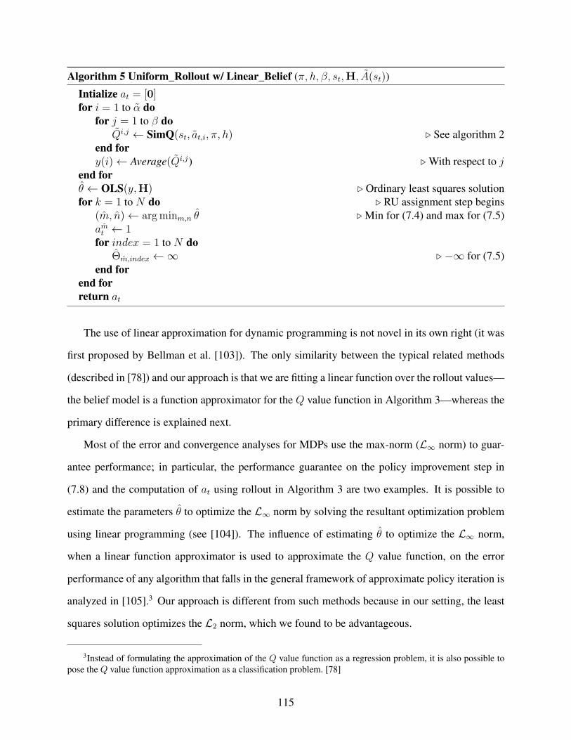
Algorithm 5 Uniform_Rollout w/ Linear_Belief (π, h, β, st,H, A(st))

Intialize at = [0]for i = 1 to α do

for j = 1 to β do

Qi,j ← SimQ(st, at,i, π, h) ⊲ See algorithm 2end for

y(i)← Average(Qi,j) ⊲ With respect to jend for

θ ← OLS(y,H) ⊲ Ordinary least squares solutionfor k = 1 to N do ⊲ RU assignment step begins

(m, n)← argminm,n θ ⊲ Min for (7.4) and max for (7.5)amt ← 1for index = 1 to N do

Θm,index ←∞ ⊲ −∞ for (7.5)end for

end for

return at

The use of linear approximation for dynamic programming is not novel in its own right (it was

first proposed by Bellman et al. [103]). The only similarity between the typical related methods

(described in [78]) and our approach is that we are fitting a linear function over the rollout values—

the belief model is a function approximator for the Q value function in Algorithm 3—whereas the

primary difference is explained next.

Most of the error and convergence analyses for MDPs use the max-norm (L∞ norm) to guar-

antee performance; in particular, the performance guarantee on the policy improvement step in

(7.8) and the computation of at using rollout in Algorithm 3 are two examples. It is possible to

estimate the parameters θ to optimize the L∞ norm by solving the resultant optimization problem

using linear programming (see [104]). The influence of estimating θ to optimize the L∞ norm,

when a linear function approximator is used to approximate the Q value function, on the error

performance of any algorithm that falls in the general framework of approximate policy iteration is

analyzed in [105].3 Our approach is different from such methods because in our setting, the least

squares solution optimizes the L2 norm, which we found to be advantageous.

3Instead of formulating the approximation of the Q value function as a regression problem, it is also possible topose the Q value function approximation as a classification problem. [78]

115

Indeed, our solution shows promising performance. Three commonly used statistics to validate

the use of the linear-belief model and the least squares solution in Algorithm 5 are as follows:

residual standard error (RSE), R-squared (R2), and F-statistic. The RSE for our model is 10−5,

which indicates that the linear model satisfactorily fits the Q values computed using rollout. The

R2 value for our model is 0.99, which indicates that the computed features/predictors (θ) can ef-

fectively predict the Q values. The F-statistic is 4 (away from 1) for a large α (α = 106; whereas,

at each t, the rank of H is never greater than 5850), which indicates that the features/predictors de-

fined in (7.10) and (7.11) are statistically significant. We can increase the number of predictors by

including the interactions between the current predictors at the risk of overfitting the Q values with

the linear model [106]. As the authors in [78] aptly point out, “increasing expressive power can

lead to a surprisingly worse performance, which can make feature engineering a counterintuitive

and tedious task."

7.3.4 Adaptive Sampling: Utilizing Limited Simulation Budget

Despite implementing best software practices to code fast simulators and deploying the simu-

lators on modern supercomputers, the simulation budget B is a precious resource, especially for

massive real-world problems. A significant amount of research has been done in the simulation-

based optimization literature [107–110] to manage simulation budget. The related methods have

also been demonstrated on real-world problems [7, 111].

A classic simulation-based approach such as optimal computing budget allocation [85] is not

employed here to manage budget, instead the techniques in our study are inspired by solutions

to the multi-armed bandit problems [112–115], which are topical in the computer science and

artificial intelligence community, especially in research related to reinforcement learning. The

problem of (managing budget) expending limited resources is studied in reinforcement learning,

although in a completely different context, where few optimal choices must be selected among a

large number of options to optimize a stochastic objective function.

116

It has been our observation that two independent research communities—simulation-based op-

timization and computer science—have worked on similar problems in isolation. In this work, our

solutions have been inspired by the later approach and will serve to bridge the gap between the

work in the two research communities.

Algorithm 3, and consequently also Algorithm 5, is not only directly dependent upon the speed

of Algorithm 8.5 (simulator) but also requires an accurate Q value function estimate to guarantee

performance. Therefore, typically a huge sampling budget in the form of large β is allocated

uniformly to every action at ∈ A(st). This naive approach decreases the value of α (which is

the size of the set A(st));4 consequently, the parameter vector θ is trained on a smaller number

of Q values. In practice, we would like to get a rough estimate of the Q value associated with

every action in the set A(st) and adaptively spend the remaining simulation budget in refining the

accuracy of the Q values corresponding to the best-performing actions; this is the exploration vs.

exploitation problem in optimal learning and simulation optimization problems [116]. Spending

the simulation budgetB in a nonuniform, adaptive fashion in the estimation of theQ value function

would not only train the parameter vector θ on a larger size of the set A(st) via the additive model

in (7.10) but also train the parameters Θmn on Q values corresponding to superior actions (this

is because in an adaptive scheme, B is allocated in refining the accuracy of only those actions

that show promising performance), consequently refining the accuracy of the parameters. The

nonuniform allocation of simulation budget is the experiential learning component of our method,

which further enhances Algorithm 5.

An interesting closed-loop sequential method pertaining to drug discovery that bears some

resemblance to the experiential learning component of our method is described in [117], where the

alternatives (actions are called alternatives in their work) are selected adaptively using knowledge

gradient (KG). Further, in their work, KG is combined with a linear-belief model, and the results

are demonstrated on a moderate-sized problem. Unfortunately, the algorithms proposed in [117]

4Note that B is fixed and depends on the simulator runtime and the computational platform on which the algorithmruns. Recall that B = α · β, and the larger the value of β required to guarantee performance, the smaller the value ofα.

117

are not directly applicable to our problem because the algorithms in [117] necessitate sampling

over the actions in A(st), instead of A(st).

Instead of uniformly allocating β samples to each action in Algorithm 3, nonuniform allocation

methods have been explored in the literature to manage the rollout budget [81]. An analysis of

performance guarantees for nonuniform allocation of the rollout samples remains an active area of

research [79]. However, we extend the ideas in [81] and [79], pertaining to nonuniform allocation,

to Algorithm 5 based on the theory of multi-armed bandits.

In bandit problems, the agent has to sequentially allocate resources among a set of bandits,

each one having an unknown reward function, so that a bandit objective [112] is optimized. There

is a direct overlap between managing B and the resource allocation problem in multi-armed bandit

theory; the allocation of the simulation budgetB∗ defined by the equationB∗ = B−α sequentially

to the state-action pair (st, at) during rollout is equivalent to a variant of the classic multi-armed

bandit problem [81].

In this study, we consider two bandit objectives: probable approximate correctness (PAC) and

cumulative regret. In the PAC setting, the goal is to allocate budget B∗ sequentially so that we

find a near-optimal (ǫ of optimal) action at with high probability (1 − δ) when the budget B∗ is

exhausted. Algorithm 3 is PAC optimal when h and β are selected in accordance with the fixed

algorithm in [79]. For our decision-automation problem, the value of β required to guarantee

performance is typically large. Nonuniform allocation algorithms like median elimination are PAC

optimal [113] (the median elimination algorithm is asymptotically optimal, so no other nonuniform

resource-allocation algorithm can outperform the median elimination algorithm in the worst case).

However, the choice of (ǫ, δ) for the PAC objective is arbitrary; therefore, the PAC objective is not

well-suited to our decision automation problem. Further, the parameters of the median elimination

algorithm that guarantee performance are directly dependent on the (ǫ, δ) pair.

The second common objective function in bandits problems mentioned earlier, cumulative re-

gret is well-suited to our problem. During the optimization of cumulative regret, the budget B∗ is

allocated sequentially in such a way that when the budget is exhausted, the expected total reward

118

is very close to the best possible reward (called minimizing the cumulative regret). An algorithm

in [114] called UCB1 minimizes the cumulative regret; in fact, no other algorithm can achieve

a better cumulative expected regret (in the sense of scaling law). Usually, cumulative regret is

not an appropriate objective function to be considered in nonuniform rollout allocation [115] be-

cause almost all common applications require finding the best (approximately) action at, whereas

in our problem, we would like to allocate the budget nonuniformly so that the parameter vector

θ in Algorithm 5 is estimated in the most efficient way. Therefore, it is natural to allocate the

computing budget so that the expected cumulative reward over all the at (Q values in the vector y

in Algorithm 5) is close to the optimal value.

Based on the simulator runtime, the underlying computational platform, and the actual time

provided by the decision maker to our automation system, suppose that we fix B and in turn the

size of the set A(st). We exhaust a budget of α samples (one per action) from B on getting rough

estimates of the Q value function for the entire set A(st); the remaining budget B− α (denoted by

B∗) is allocated adaptively using the UCB1 algorithm. This scheme of adaptively managing B∗ in

Algorithm 5 is summarized in Algorithm 6.

Algorithm 6 alleviates the shortcomings of Algorithm 5 by embedding the experiential learning

component using the UCB1 algorithm. The UCB1 algorithm assumes that the rewards lie in the

interval [0,1]. Satisfying this condition is trivial in our case because the rewards are bounded and

thus can be always normalized so that they lie in the interval [0,1]; it is important to implement

the normalization of R in Algorithm 8.5 when we use Algorithm 6. In Algorithm 6, not only

is B∗ ≫ β, but we can also select α larger than that in Algorithm 5 and train the parameter

vector θ on a larger size of the set A(st), which in turn will yield better estimates of θ. Note

that Algorithm 6 does not merely manage the budget B∗ adaptively (adaptive rollout), but it also

handles massive action spaces through the linear belief model described in Section 7.3.3 (this is

because Algorithm 6 is Algorithm 5 with the UCB1 step appended).

In essence, Algorithm 6 has three important steps: First, Q values corresponding to α actions

in the set A(st) are computed. Second, the estimates for the Q values corresponding to the most

119

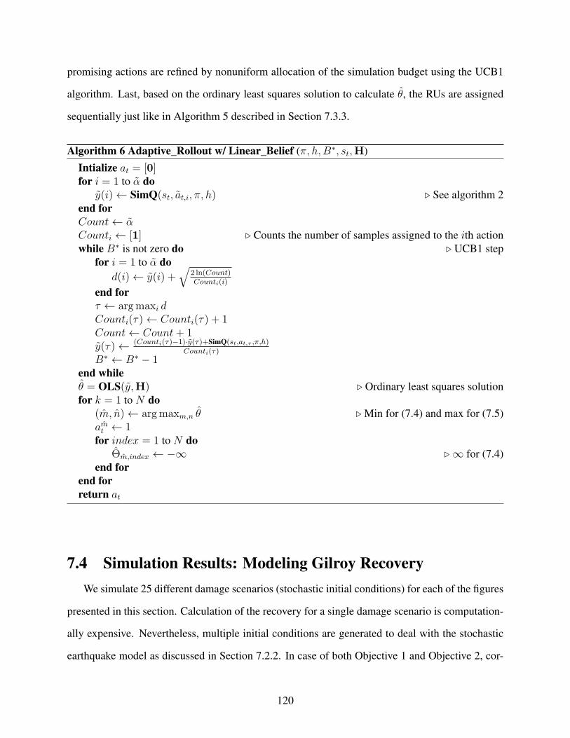
promising actions are refined by nonuniform allocation of the simulation budget using the UCB1

algorithm. Last, based on the ordinary least squares solution to calculate θ, the RUs are assigned

sequentially just like in Algorithm 5 described in Section 7.3.3.

Algorithm 6 Adaptive_Rollout w/ Linear_Belief (π, h,B∗, st,H)

Intialize at = [0]for i = 1 to α do

y(i)← SimQ(st, at,i, π, h) ⊲ See algorithm 2end for

Count← αCounti ← [1] ⊲ Counts the number of samples assigned to the ith actionwhile B∗ is not zero do ⊲ UCB1 step

for i = 1 to α do

d(i)← y(i) +√

2 ln(Count)Counti(i)

end for

τ ← argmaxi dCounti(τ)← Counti(τ) + 1Count← Count+ 1y(τ)← (Counti(τ)−1)·y(τ)+SimQ(st,at,τ ,π,h)

Counti(τ)

B∗ ← B∗ − 1end while

θ = OLS(y,H) ⊲ Ordinary least squares solutionfor k = 1 to N do

(m, n)← argmaxm,n θ ⊲ Min for (7.4) and max for (7.5)amt ← 1for index = 1 to N do

Θm,index ← −∞ ⊲∞ for (7.4)end for

end for

return at

7.4 Simulation Results: Modeling Gilroy Recovery

We simulate 25 different damage scenarios (stochastic initial conditions) for each of the figures

presented in this section. Calculation of the recovery for a single damage scenario is computation-

ally expensive. Nevertheless, multiple initial conditions are generated to deal with the stochastic

earthquake model as discussed in Section 7.2.2. In case of both Objective 1 and Objective 2, cor-

120

responding to R1 and R2 respectively, there will be a distinct recovery path for each of the initial

damage scenarios. To present the results for Objective 1, we do not explicitly show the recovery

trajectories. We are only interested in the number of days it takes to provide maximum benefit in

the sense of optimizing R1. Therefore, the results are presented in terms of a cumulative moving

average plot. In Objective 2, for both Algorithm 5 and Algorithm 6, the recovery computed using

these algorithms outperform the base policy for every single scenario.

There are several candidates for determining the base policy to be used in the simulation. For

a detailed discussion on these candidates in post-hazard recovery planning, see [4]. For the simu-

lations presented in this study, a random base policy is used. The total number of RUs are capped

at 15% of the damaged components for each scenario. The maximum number of damaged com-

ponents in any scenario encountered in this study is 205, i.e., the size of the assignment problem

at any t is less than 1037. The simulators have a runtime of 10−5 s when h = 1, and this runtime

varies with the parameter h. The deeper we rollout the base policy in any variation of the rollout

algorithm, the larger the simulation time per-action and the smaller the action space covered to

train our parameters.

For Algorithm 5 and the computational platform (AMD EPYC 7451, 2.3 GHz, and 96 cores),

the value of β is capped at 100 and the value of α is capped at 106. Note that it is possible to

parallelize Algorithm 5 at two levels. The recovery of each damage scenario can be computed

on a different processor, and then their average can be calculated. Further, Algorithm 5 offers

the opportunity to parallelize over A(st) because a uniform budget can be allocated to a separate

processor to return the average Q value for each a(st). On the contrary, the allocation of budget

B∗ in Algorithm 6 is sequential, and only a single Q value corresponding to the allocated sample

is evaluated (see the UCB1 step in Algorithm 6). Based on the updated Q value (calculation of

y(τ) in Algorithm 6), further allocation is continued until the budget (B∗) is exhausted. Therefore,

barring the rough estimates at the first iteration, Algorithm 6 cannot be parallelized for allocation.

However, just like Algorithm 5, each processor can compute the recovery for a distinct initial

condition (s0) separately. Because of reduction in the parallelization in Algorithm 6, the solutions,

121

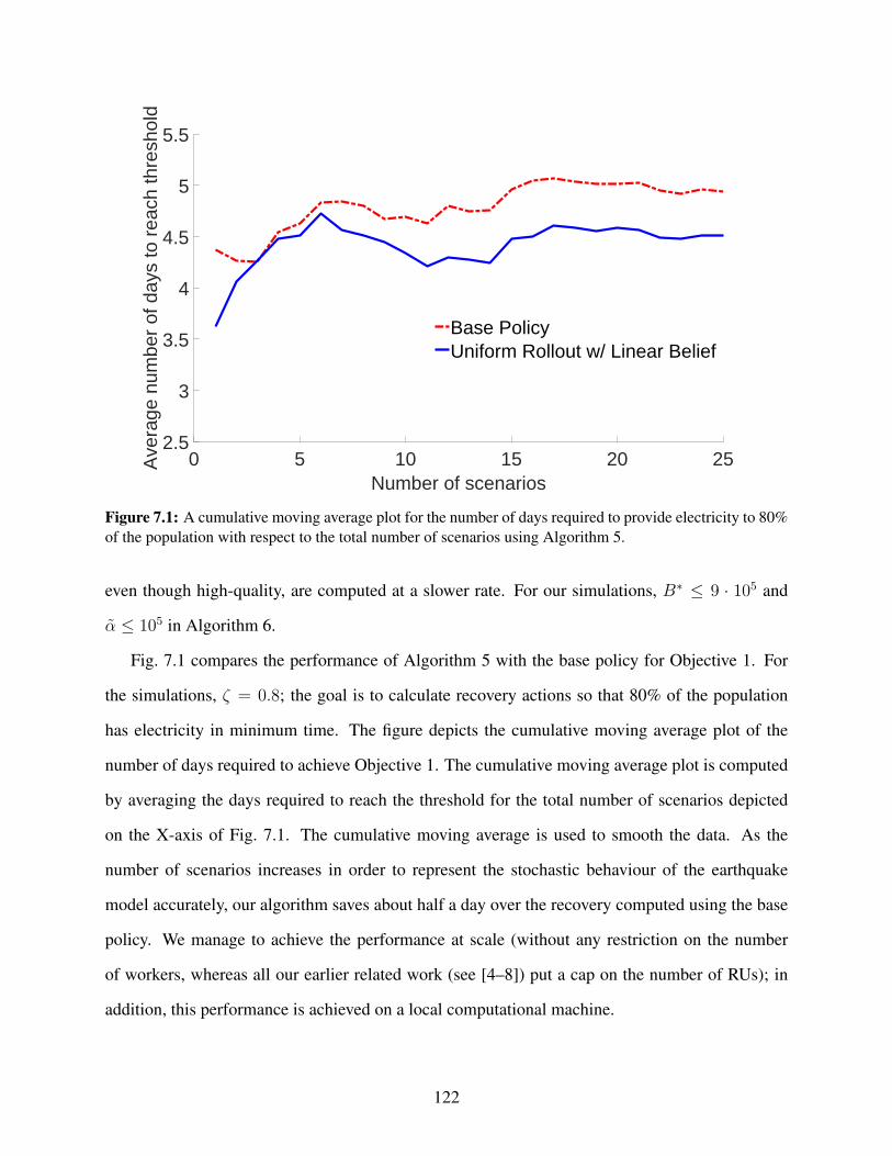
0 5 10 15 20 25Number of scenarios

2.5

3

3.5

4

4.5

5

5.5A

vera

ge n

umbe

r of

day

s to

rea

ch th

resh

old

Base PolicyUniform Rollout w/ Linear Belief

Figure 7.1: A cumulative moving average plot for the number of days required to provide electricity to 80%of the population with respect to the total number of scenarios using Algorithm 5.

even though high-quality, are computed at a slower rate. For our simulations, B∗ ≤ 9 · 105 and

α ≤ 105 in Algorithm 6.

Fig. 7.1 compares the performance of Algorithm 5 with the base policy for Objective 1. For

the simulations, ζ = 0.8; the goal is to calculate recovery actions so that 80% of the population

has electricity in minimum time. The figure depicts the cumulative moving average plot of the

number of days required to achieve Objective 1. The cumulative moving average plot is computed

by averaging the days required to reach the threshold for the total number of scenarios depicted

on the X-axis of Fig. 7.1. The cumulative moving average is used to smooth the data. As the

number of scenarios increases in order to represent the stochastic behaviour of the earthquake

model accurately, our algorithm saves about half a day over the recovery computed using the base

policy. We manage to achieve the performance at scale (without any restriction on the number

of workers, whereas all our earlier related work (see [4–8]) put a cap on the number of RUs); in

addition, this performance is achieved on a local computational machine.

122

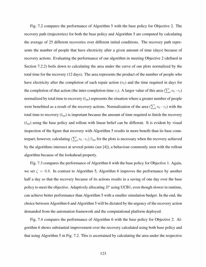
Fig. 7.2 compares the performance of Algorithm 5 with the base policy for Objective 2. The

recovery path (trajectories) for both the base policy and Algorithm 5 are computed by calculating

the average of 25 different recoveries over different initial conditions. The recovery path repre-

sents the number of people that have electricity after a given amount of time (days) because of

recovery actions. Evaluating the performance of our algorithm in meeting Objective 2 (defined in

Section 7.2.2) boils down to calculating the area under the curve of our plots normalized by the

total time for the recovery (12 days). The area represents the product of the number of people who

have electricity after the completion of each repair action (nt) and the time required in days for

the completion of that action (the inter-completion time rt). A larger value of this area (∑

t nt · rt)

normalized by total time to recovery (ttot) represents the situation where a greater number of people

were benefitted as a result of the recovery actions. Normalization of the area (∑

t nt · rt) with the

total time to recovery (ttot) is important because the amount of time required to finish the recovery

(ttot) using the base policy and rollout with linear belief can be different. It is evident by visual

inspection of the figure that recovery with Algorithm 5 results in more benefit than its base coun-

terpart; however, calculating (∑

t nt · rt)/ttot for the plots is necessary when the recovery achieved

by the algorithms intersect at several points (see [4]), a behaviour commonly seen with the rollout

algorithm because of the lookahead property.

Fig. 7.3 compares the performance of Algorithm 6 with the base policy for Objective 1. Again,

we set ζ = 0.8. In contrast to Algorithm 5, Algorithm 6 improves the performance by another

half a day so that the recovery because of its actions results in a saving of one day over the base

policy to meet the objective. Adaptively allocatingB∗ using UCB1, even though slower in runtime,

can achieve better performance than Algorithm 5 with a smaller simulation budget. In the end, the

choice between Algorithm 6 and Algorithm 5 will be dictated by the urgency of the recovery action

demanded from the automation framework and the computational platform deployed.

Fig. 7.4 compares the performance of Algorithm 6 with the base policy for Objective 2. Al-

gorithm 6 shows substantial improvement over the recovery calculated using both base policy and

that using Algorithm 5 in Fig. 7.2. This is ascertained by calculating the area under the respective

123

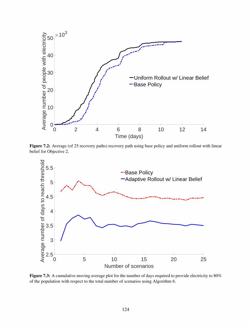
0 2 4 6 8 10 12 14Time (days)

0

10

20

30

40

50A

vera

ge n

umbe

r of

peo

ple

with

ele

ctric

ity 103

Uniform Rollout w/ Linear BeliefBase Policy

Figure 7.2: Average (of 25 recovery paths) recovery path using base policy and uniform rollout with linearbelief for Objective 2.

0 5 10 15 20 25Number of scenarios

2.5

3

3.5

4

4.5

5

5.5

Ave

rage

num

ber

of d

ays

to r

each

thre

shol

d

Base PolicyAdaptive Rollout w/ Linear Belief

Figure 7.3: A cumulative moving average plot for the number of days required to provide electricity to 80%of the population with respect to the total number of scenarios using Algorithm 6.

124

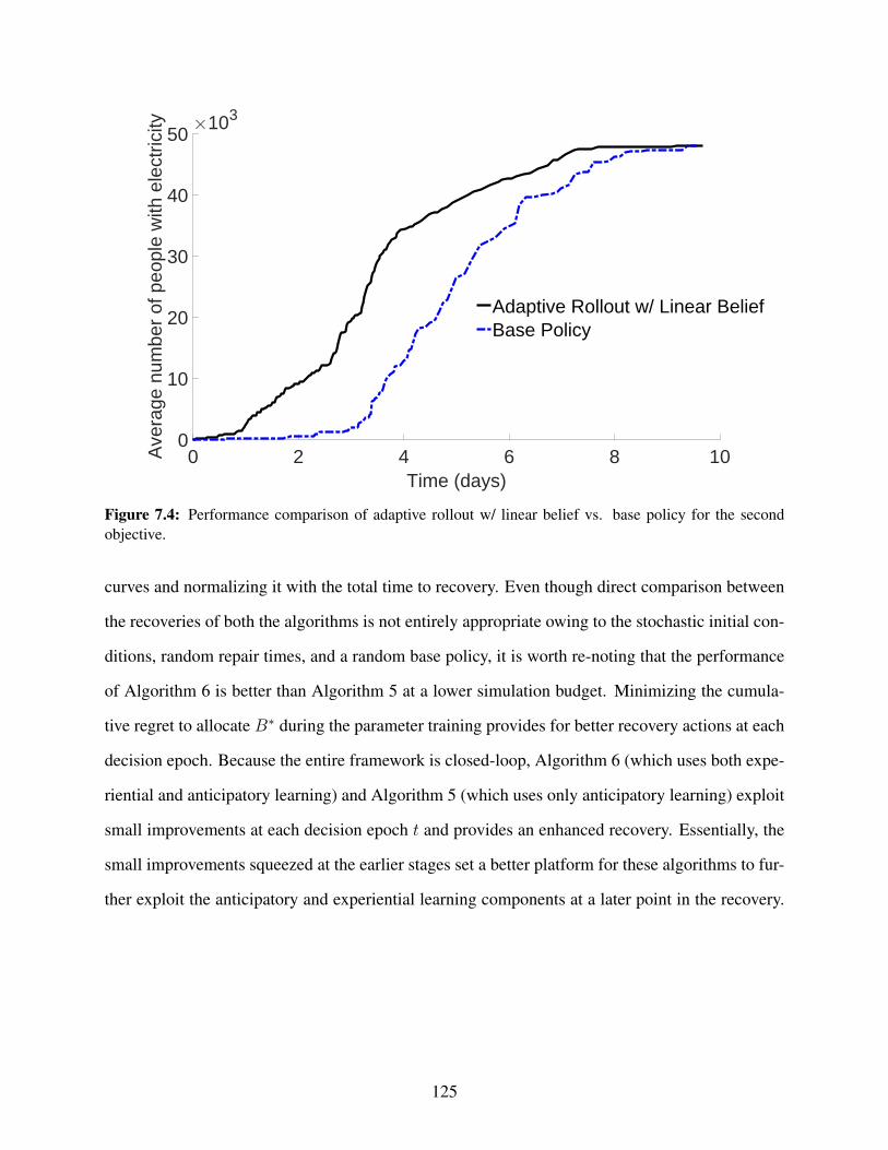
0 2 4 6 8 10Time (days)

0

10

20

30

40

50A

vera

ge n

umbe

r of

peo

ple

with

ele

ctric

ity 103

Adaptive Rollout w/ Linear BeliefBase Policy

Figure 7.4: Performance comparison of adaptive rollout w/ linear belief vs. base policy for the secondobjective.

curves and normalizing it with the total time to recovery. Even though direct comparison between

the recoveries of both the algorithms is not entirely appropriate owing to the stochastic initial con-

ditions, random repair times, and a random base policy, it is worth re-noting that the performance

of Algorithm 6 is better than Algorithm 5 at a lower simulation budget. Minimizing the cumula-

tive regret to allocate B∗ during the parameter training provides for better recovery actions at each

decision epoch. Because the entire framework is closed-loop, Algorithm 6 (which uses both expe-

riential and anticipatory learning) and Algorithm 5 (which uses only anticipatory learning) exploit

small improvements at each decision epoch t and provides an enhanced recovery. Essentially, the

small improvements squeezed at the earlier stages set a better platform for these algorithms to fur-

ther exploit the anticipatory and experiential learning components at a later point in the recovery.

125

7.5 Conclusion

In this work, we presented a novel, systematic approach to MDPs that have jointly massive

finite state and action spaces. When the action space consists of large number of discrete actions,

the method of choice has been to embed these actions in continuous action spaces [118], where

deep reinforcement learning techniques have shown promising performance on |A| ≈ 106. In

contrast, in this study, we present a unique approach to address the problem, where the size of the

discrete action space that we consider is significantly large than that in [118].

We studied an intricate real-world problem, modeled it in our framework, and demonstrated

the powerful applicability of our algorithm on this challenging problem. The community recovery

problem is a stochastic combinatorial decision-making problem, and the solution to such decision-

making problems is critically tied with the welfare of communities in the face of ever-increasing

natural and anthropogenic hazards. Our modeling of the problem is general enough to accom-

modate the uncertainty in the hazard models and the outcome of repair actions. Ultimately, we

would like to test the techniques developed in this work on other real-world problems, e.g., large

recommender systems (like those in use with the organizations YouTube and Amazon) and large

industrial control systems.

Ongoing Work: In our work on post-hazard community management (see [?, 4–6,8]), includ-

ing this study, we have been focusing on obtaining solutions by the use of a single base policy.

Currently, we are developing a framework where we leverage the availability of multiple base po-

lices in the aftermath of hazards. Two algorithms are particularly appealing in this regard: parallel

rollout and policy switching [119]. In parallel rollout, just like in [117], the optimization is done

over the entire set A(st). In our ongoing work, we are formulating a non-preemptive stochastic

scheduling framework, where the size of set A(st) grows linearly with the number of RUs, which

circumvents the issue of large action spaces. In addition, we are also exploring heuristic search

algorithms to guide the stochastic search, i.e., adaptively select the samples of the parallel rollout

algorithm. There, we consider several infrastructure systems in a community, such as building

126

structures, EPN, WN, and food retailers simultaneously (all these systems are inter-connected),

and we compute the recovery of the community post-hazard.

7.6 Funding and Support

“The research herein has been funded by the National Science Foundation under Grant CMMI-

1638284. This support is gratefully acknowledged. Any opinions, findings, conclusions, or recom-

mendations presented in this material are solely those of the authors and do not necessarily reflect

the views of the National Science Foundation.”

127

Chapter 8

Dynamic UAV Path Planning Incorporating

Feedback from Humans for Target Tracking

8.1 Introduction

We develop a method for autonomous management of multiple heterogeneous sensors for a

multitarget tracking problem. We adopt a non-myopic (long-term) method known as partially

observable Markov decision process (POMDP) to formulate the problem. POMDP incorporates

long-term decision making, effective for managing limited resources, and accounts for uncertain-

ties arising from noisy measurements. We have included a brief introduction to POMDP in Sec-

tion 8.7. The main contribution of the work is incorporation of feedback received from intelligence

assets (humans) on priorities assigned to specific targets into the decision-making process. Infor-

mation received from assets is captured as a penalty on the cost function. The resulting constrained

optimization problem is solved using an augmented Lagrangian method (ALM). The cost function

is the mean squared error between the tracks and target states. The suite of sensors consists of

sensors on board multiple unmanned aerial vehicles (UAVs). Each sensor collects measurements

of the locations of multiple targets; moreover, each sensor is controllable in the sense that we can

control the motion of the UAVs. Information obtained from sensors and assets is fused together

for guiding the UAVs to track these targets. The motion of the UAVs is subject to dynamic con-

straints, and the error statistics associated with the sensor measurements are spatially varying. The

following gives a detailed breakdown of the problem specification and the ensuing assumptions.

Motion of the targets: The targets follow a 2-D motion, i.e., they move in a plane on the

ground. The motion of these targets follows a linear model.

Motion of the UAVs: The UAVs follow a 2-D motion model, i.e., they are assumed to fly at a

fixed altitude over the ground.

128

Sensors on board UAVs: A simplified visual sensor (camera plus image processing ) is as-

sumed, which implies that angular resolution is much better than range resolution. The measure-

ment by the sensors on UAVs have random errors.

Perfect Tracker: We assume that there are no missed detection and false alarms.

Dynamic Constraints on motion of UAVs: The UAVs fly with variable speed and there are

constraints on the motion of the UAVs, specified in terms of maximum and minimum acceleration

and maximum and minimum heading angle. Adaptive long term sensing has a clear advantage

under constrained resource environments over short term sensing (using a greedy strategy) [120].

Spatially varying error measurement: Depending on the location of the UAVs and the posi-

tion of the targets, we incorporate a spatially varying error. The precise nature of this is explained

later. This spatially varying error is what makes the sensor placement problem meaningful.

Tracking objective: The performance objective is related to maintaining optimal tracks on the

targets. Normally, this means minimizing the mean squared error between tracks and targets.

Fusion Center: The algorithm runs on a central fusion node (preferably on one of the UAVs

itself) which collects measurements generated by all sensors of different UAVs, constructs tracks

from those measurements, plans the future motion of the UAVs to maximize tracking performance,

and sends motion commands back to the UAVs based on the plans.

Section 8.2 describes how our problem is formulated in the POMDP framework. POMDPs

are intractable to solve exactly. We use an approximation technique known as nominal belief state

optimization (NBO), which is known to be computationally efficient and well suited for target

tracking applications. Section 8.3 contains a description of the NBO method. Section 8.4 features

the solution to our main problem, incorporating feedback from intelligence assets into the sensor

management problem. In Section 8.5 we provide simulations to illustrate our scheme. Finally, in

Section 8.6 we provide conclusions and discuss future work. Section 8.7 gives a brief introduction

to POMDP.

129

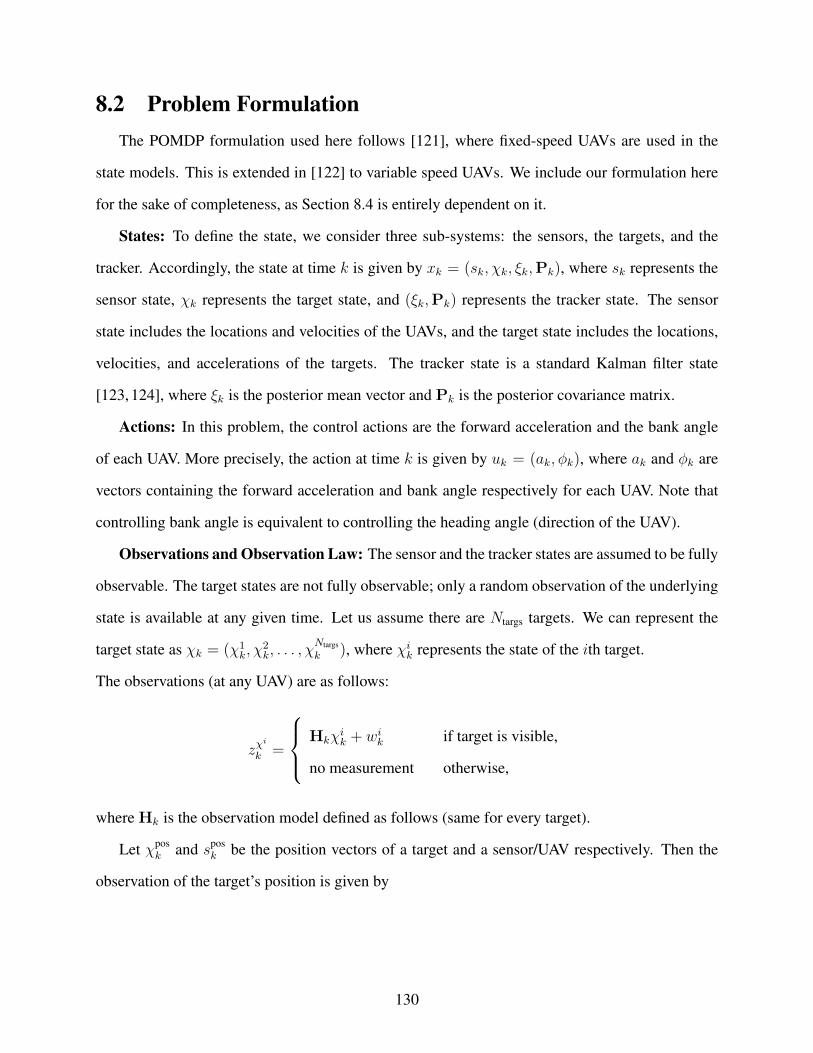
8.2 Problem Formulation

The POMDP formulation used here follows [121], where fixed-speed UAVs are used in the

state models. This is extended in [122] to variable speed UAVs. We include our formulation here

for the sake of completeness, as Section 8.4 is entirely dependent on it.

States: To define the state, we consider three sub-systems: the sensors, the targets, and the

tracker. Accordingly, the state at time k is given by xk = (sk, χk, ξk,Pk), where sk represents the

sensor state, χk represents the target state, and (ξk,Pk) represents the tracker state. The sensor

state includes the locations and velocities of the UAVs, and the target state includes the locations,

velocities, and accelerations of the targets. The tracker state is a standard Kalman filter state

[123, 124], where ξk is the posterior mean vector and Pk is the posterior covariance matrix.

Actions: In this problem, the control actions are the forward acceleration and the bank angle

of each UAV. More precisely, the action at time k is given by uk = (ak, φk), where ak and φk are

vectors containing the forward acceleration and bank angle respectively for each UAV. Note that

controlling bank angle is equivalent to controlling the heading angle (direction of the UAV).

Observations and Observation Law: The sensor and the tracker states are assumed to be fully

observable. The target states are not fully observable; only a random observation of the underlying

state is available at any given time. Let us assume there are Ntargs targets. We can represent the

target state as χk = (χ1k, χ

2k, . . . , χ

Ntargs

k ), where χik represents the state of the ith target.

The observations (at any UAV) are as follows:

zχi

k =

Hkχik + wik if target is visible,

no measurement otherwise,

where Hk is the observation model defined as follows (same for every target).

Let χposk and spos

k be the position vectors of a target and a sensor/UAV respectively. Then the

observation of the target’s position is given by

130

zχk =

χposk + wk if target is visible,

no measurement otherwise,(8.1)

According to this model, only the position of the target is observed. The state of the ith target (χik)

includes its 2-D position coordinates (xk, yk), its velocities (vxk , vyk) and accelerations (axk, a

yk) in x

and y directions, i.e., χik = [xk, yk, vxk , v

yk , a

xk, a

yk]

T. Therefore, the observation model is of the form

Hk = [I2×2,04×4].

We formulate the spatially varying error described earlier using the formulation from [125].

The measurement error wk is distributed according to the normal distribution N (0,Rk (χk, sk)),

where Rk captures both range and angular uncertainty. If rk is the distance between the target and

the sensor at time k, then the standard deviations corresponding to the range (σrange(k)) and the

angle (σangle(k)) are written as σrange(k) = (p/100) ∗ rk and σangle(k) = q ∗ rk. The information

matrix depends on the inverse of the measurement covariance matrix, which depends on the dis-

tance between the sensor and the target. Therefore, the information matrix blows up when the UAV

is exactly on top of the target (i.e., when rk = 0 the sensor’s location overlaps with the target’s

location in our 2-D environment). To address this problem, we define the effective distance (reff)

between the sensor and the target as follows: reff(k) =√

r2k + b2, where rk is the actual distance

between the target and the sensor and b is some non-zero real value. If θk is the angle between the

target and the sensor at time k, then Rk is calculated as follows:

Rk =Mk

σ2range(k) 0

0 σ2angle(k)

MT

k , where Mk =

cos(θk) − sin(θk)

sin(θk) cos(θk)

.

State-Transition Law: The state transition law specifies the next state distribution given the

action at the current distribution. We will define state transition for sensors, target, and trackers

separately. The sensor state evolves according to sk+1 = ψ(sk, uk). The state of the ith UAV

at time k is given by sik = (pik, qik, V

ik , θ

ik) , where (pik, q

ik) represents the position coordinates,

V ik represents the speed, and θik represents the heading angle. Let aik be the forward acceleration

131

(control variable) and φik be the bank angle (control variable) of the UAV, i.e., uik = (aik, φik).

The mapping function ψ can be specified as a collection of simple kinematic equations as given

in [126]. This is the same mapping function used in [122, 125]. The speed is updated according to

V ik+1 =

[

V ik + aikT

]Vmax

Vmin, where [v]Vmax

Vmin= max Vmin,min(Vmax, v) ,

where Vmin and Vmax are the minimum and the maximum limits on the speed of the UAVs. The

heading angle is updated according to

θik+1 = θik + (gT tan(φik)/Vik ),

where g is the acceleration due to gravity and T is the length of the time-step. The position

coordinate are updated according to

pik+1 = pik + V ikT cos(θik) andqik+1 = qik + V i

kT sin(θik).

The target state evolves according to

χk+1 = f(χk) + vk,

where we use linearized target motion model with zero mean noise to model the target state dy-

namics, as given next:

χik+1 = Fkχik + vik, v

ik ∼ N (0,Qk) , i ∈ 1, . . . , Ntargs. (8.2)

We adopt the constant velocity (CV) model [123,124] for target dynamics (8.2), which defines Fk.

The tracker state evolves according to the Kalman filter equations with a data association tech-

nique called joint probabilistic data association (JPDA) [123, 127]. Let the track state be ξk =

132

(ξ1k, . . . , ξNtargs

k ) and Pk = (P1k, . . . ,P

Ntargs

k ), where (ξik, Pik) is the track state corresponding to the

ith target.

Cost Function: The cost function specifies the cost of taking an action in a given state. We

use the mean-squared error between the tracks and the targets as the cost function:

C(xk, uk) = Evk,wk+1

[

||χk+1 − ξk+1||2∣

∣ xk, uk]

.

Belief State update: The belief state is the posterior distribution of the underlying state, which

is updated at each iteration using Bayes rule given the observations. The belief state at time k is

given by bk = (bsk, bχk , b

ξk, b

P

k ). We have already noted that the sensor and tracker states are fully

observable; thus we have bsk = δ(s − sk), bξk = δ(ξ − ξk), bPk = δ(P − Pk). Since we assumed

Gaussian distributions in the target motion model and observation model we can approximate the

belief state of the target as bχi

k (χ) = N (χ− ξik,Pik).

8.3 NBO Approximation Method

A POMDP gives rise to an optimization problem where the objective is to find actions over

a time horizon H such that the expected cumulative cost is minimized. The expected cumulative

cost, to be minimized over the action sequence u0, u1, . . . , uH−1, is given by

JH = E

[

H−1∑

k=0

C(xk, uk)

]

. (8.3)

The action chosen at time k should be allowed to depend on the history of all observable quantities

till time k − 1. It turns out that if an optimal choice of such actions exist, then there exists an

optimal sequence of actions that depend only on the “belief-state feedback” [120]. Indeed, the

objective function JH can be written in terms of the belief states as follows:

JH = E

[

H−1∑

k=0

c(bk, uk)

∣

∣

∣

∣

∣

b0

]

, (8.4)

133

where c(bk, uk) =∫

C(x, uk)bk(x) dx and b0 is the given initial belief state. Given the optimization

problem, the goal is to find, at each time k, an optimal policy π∗k : B → U such that if the action

uk = π∗k(bk) is performed at time k, the objective function (8.4) is minimized. According to

Bellman’s principle of optimality [128], the optimal objective function value can be written in the

following form:

J∗H(b0) = min

u

c(b0, u) + E[

J∗H−1(b1)

∣

∣ b0, u]

, (8.5)

where b1 is the random next belief state, J∗H−1 is the optimal cumulative cost over the horizon

k = 1, 2, . . . , H − 1, and E[·|b0, u] is the conditional expectation given the current belief state b0

and an action u taken at time k = 0. Define the Q-value of taking an action u given the current

belief state b0 is as follows:

QH(b0, u) = c(b0, u) + E[

J∗H−1(b1)

∣

∣ b0, u]

. (8.6)

An optimal policy (from Bellman’s principle) at time k = 0 is given by

π∗0(b0) = argmin

uQH(b0, u). (8.7)

More generally, an optimal policy at time k is given by

π∗k(bk) = argmin

uQH−k(bk, u). (8.8)

In practice, the second term in the Q function is hard to obtain exactly. Thus we use approxi-

mate methods to solve the problem. Other reasons to use approximations are: we have continuous

state space and in a stochastic control problem, dynamics are properly understood in terms of

belief states (distributions over the state space), which are infinite dimensional. We have to repre-

sent these distributions in some (parametric/non-parametric) form to convert the distribution into a

finite-dimensional quantity. To solve our POMDP problem we use nominal belief state optimiza-

tion (NBO). For a detailed description of the method see [121]. According to the NBO method,

134

the objective function is approximated as follows:

JH(b0) ≈H−1∑

k=0

c(bk, uk), (8.9)

where b1, b2, . . . , bH−1 is a nominal belief-state sequence and the optimization is over the action

sequence u1, u2, . . . , uH−1. This approximation is valid under the assumptions that we have a

correct tracking model, correct data association, and Gaussian statistics [121]. The nominal belief-

state sequence for the ith target can be identified with the nominal tracks (ξik, Pik), which are

obtained from the Kalman filter equations [123, 124] with exactly zero-noise sequence as follows:

bχi

k (χ) = N(

χ− ξik, Pik

)

, ξik+1 = Fkξik,

and

Pik+1 =

[

[Pik+1|k]

−1 + Sik+1

]−1if measurement available,

Pik+1|k otherwise,

(8.10)

where

Pik+1|k = FkP

ikF

Tk +Qk,

Sik+1 = HTk+1

[

Rk+1

(

ξik+1, sk+1

)]−1

Hk+1

and sk+1 = ψ(sk, uk). In equation (8.10), the nominal error covariance matrix Pik+1 depends on

the the observations in the future time, which are unavailable. Therefore, we set the location of the

target at time k + 1 as ξi,posk+1 (component of nominal track-state corresponding to the ith target at

time k + 1) and use this to check its line of sight from the sensor location sposk+1. The cost function,

i.e., the mean-squared error between the tracks and the targets, can be written as

c(bk, uk) =

Ntargs∑

i=1

Tr Pik+1.

135

Therefore, the goal is to find an action sequence (u0, u1, . . . , uH−1) that minimizes the cumulative

cost function (truncated horizon [121])

JH(b0) =H−1∑

k=0

Ntargs∑

i=1

Tr Pik+1,

where Pik+1 represents the nominal error covariance matrix of the ith target at time k+1. Here, we

adopt an approach called “receding horizon control,” according to which we optimize the action

sequence for H time steps at the current time-step and implement only the action corresponding

to the current time-step and again optimize the action sequence for H time-steps in the next time-

step. When there are multiple UAVs, the nominal covariance matrix for the ith target (based on

data fusion techniques) at time k + 1 is expressed as follows:

Pik+1 =

[

Nsens∑

j=1

(

Pi,jk+1

)−1]−1

,

where Nsens represents the number of UAVs and Pi,jk+1 is the nominal covariance matrix of the the

ith target computed at the jth sensor [125].

NBO should perform well in our tracking problem as long as the target motion model is pre-

dicted reasonably by the tracking algorithm within the chosen planning horizon [121].

8.4 Incorporating Feedback from Intelligence Assets

8.4.1 The Complete Optimization Problem

As seen in the previous section, our goal is to obtain an optimal policy, one that minimizes

the objective function in (8.4). We also note that using the method of NBO we approximate our

objective function as in (8.9). In other words using the NBO method to get the optimal policy boils

down to minimizingH−1∑

k=0

c(bk, uk)

136

with respect to u0, . . . , uH−1. Furthermore, we have already noted that for our problem, the cost

function, i.e., the mean-squared error between the tracks and the targets, can be written as

c(bk, uk) =

Ntargs∑

i=1

Tr Pik+1,

where for multiple UAVs the nominal covariance matrix for the ith target (based on data fusion

techniques) at time k + 1 is expressed as :

Pik+1 =

[

Nsens∑

j=1

(

Pi,jk+1

)−1]−1

,

where Nsens represents the number of UAVs and Pi,jk+1 is the nominal covariance matrix of the ith

target computed at the jth sensor. Therefore, for our problem the complete representation of the

cost function is

JH(b0) ≈H−1∑

k=0

c(bk, uk) =H−1∑

k=0

Ntargs∑

i=1

Tr

[

Nsens∑

j=1

(

Pi,jk+1

)−1]−1

. (8.11)

Minimizing (8.11) would have been an unconstrained optimization problem, but we have con-

straints on the controls u as mentioned in the Section 1, where dynamic constraints are imposed

by specifying the maximum and minimum bank angle and forward acceleration. Therefore (8.11)

is a bound constrained optimization problem [129]. The feedback received from intelligence as-

sets is also captured as a constraint on this cost function. The method to formulate this constraint

based on the received feedback is explained in detail later. The resulting problem then becomes a

constrained non-linear optimization problem with bounds on the optimization variables. If we let

ci represent the per-stage constraints, then the constrained optimization problem is

argminu

H−1∑

k=0

c(bk, uk) subject toH−1∑

k=0

ci(bk, uk) ≤ 0 ∀i and L ≤ uk ≤ U. (8.12)

137

Here L and U are vectors of appropriate size. This constrained optimization problem is solved

using an augmented Lagrangian method (ALM) [129]. ALM has many advantages over typical

penalty methods [102] used to solve constrained non-linear optimization problems, the major ad-

vantage being that the penalty parameter need not go to∞ to solve the optimization problem, thus

avoiding ill-conditioning, at little extra computational cost. There are different formulations of

practical ALM methods: Bound-Constrained Formulation, Linearly Constrained Formulation, and

Unconstrained Formulations. For details on these methods, see [129]. The unconstrained formu-

lation has never been tested in a commercial package and the linearly constrained formulation is

computationally costlier. We intend to use this algorithm several times in simulations and therefore

we use the bound constrained formulation. The bound constrained formulation is the basis of the

commercial package LANCELOT [130].

8.4.2 Feedback from Intelligence Assets

Now we show how to formulate the feedback received from the intelligence asset into con-

straints in the cost function. Consider the case of 2 targets. Suppose that the intelligence assets

decide that one target is δ times as important as another target in a sense that the mean squared

error (MSE) of one target is 1δ

times the mean squared error of the other target. The total mean

squared error for target 1 is given by

H−1∑

k=0

Tr

[

Nsens∑

j=1

(

P1,jk+1

)−1]−1

.

Let us call this term T1. Similarly the total mean squared error for target 2 is given by

H−1∑

k=0

Tr

[

Nsens∑

j=1

(

P2,jk+1

)−1]−1

.

Let us call this term T2. Assuming that target 2 is δ times as important as target 1, we must have

δ × T2 = T1. Therefore, our constraint for the problem becomes c1 = δ × T2 − T1 = 0. Similarly

138

we can formulate other constraints as desired, including inequality constraints. Under the bound

constrained formulation (BCALM), we convert inequality constraints into equality constraints by

introduction of slack variables. Hence, it suffices to consider only the case of equality constraints.

Therefore, (8.12) becomes

argminu

H−1∑

k=0

c(bk, uk) subject toH−1∑

k=0

ci(bk, uk) = 0 ∀i and L ≤ uk ≤ U. (8.13)

The above problem is solved using ALM. Under BCALM (8.13) becomes

LA(u, λ;µ) =H−1∑

k=0

(c(bk, uk) +µ

2

∑

i

ci(bk, uk)2 −

∑

i

λici(bk, uk))

where µ and λi are updated as described in [129]. This is step 1 of BCALM. The bound constraints

are enforced explicitly in the subproblem, which has the form

argminuLA(u, λ;µ) subject to L ≤ uk ≤ U.

This subproblem is solved in MATLAB using the function fmincon. This is the step 2 of BCALM.

The optimization problem using the BCALM for 2 target case with single constraint is

argminu

[

T1 + T2 +µ

2(δT2 − T1)

2 − λ (δT2 − T1)]

subject to L ≤ uk ≤ U.

This can be rewritten as

argminu

H−1∑

k=0

Tr

[

Nsens∑

j=1

(

P1,jk+1

)−1]−1

+ Tr

[

Nsens∑

j=1

(

P2,jk+1

)−1]−1

+µ

2

δTr

[

Nsens∑

j=1

(

P2,jk+1

)−1]−1

− Tr

[

Nsens∑

j=1

(

P1,jk+1

)−1]−1

2

139

−λ

δTr

[

Nsens∑

j=1

(

P2,jk+1

)−1]−1

− Tr

[

Nsens∑

j=1

(

P1,jk+1

)−1]−1

subject to L ≤ uk ≤ U. (8.14)

8.5 Simulation Results

We set H = 4 and assume a 10% range uncertainty and 0.01π radian angular uncertainty. We

run 10 iterations of the step 1 of BCALM to solve the constrained optimization problem posed in

the previous section. We set the initial value of µ = 2 and λ = 1. The sensitivity parameter or

stopping criterion for the algorithm is kept at eps = 10−1.

Case 1: First, we do not assign any weights to the targets; this will help us in evaluating the

performance of our algorithm once weights are assigned to targets. Fig. 8.1 shows the simula-

tion of the scenario with 3 UAVs and 2 targets. Both targets start at the bottom, and as simula-

tion progresses, one target moves towards the north-east, and the other target moves towards the

north-west. The targets move at a constant speed. The POMDP framework enables the UAVs to

coordinate so as to achieve maximum coverage of the targets. There is no explicit assignment of

any UAV to any particular target; the implicit assignment of UAVs to targets is an emergent feature

of the algorithm. Figs. 8.2 and 8.3 show the average location error for each target.

Case 2: Next, we decide that target moving towards north-west is 8 times important than target

moving towards north-east. Therefore, we expect the MSE for target moving N-W to be 1/8 times

of the MSE for target moving N-E. Fig. 8.4 shows the simulation of the scenario with 3 UAVs and

2 targets. Figs. 8.5 and 8.6 show the average location error for each target.

As can be noted the target location error for the N-W target is almost half of the target location

error for N-E target after 10 simulation runs of step 1 of BCALM. But we have assigned δ = 8, so

we would expect the error for the N-W target to be 1/8 that of the N-E target. The reason for this

discrepancy is that the MSE values that are achievable are not arbitrary. We will say more about

this below.

140

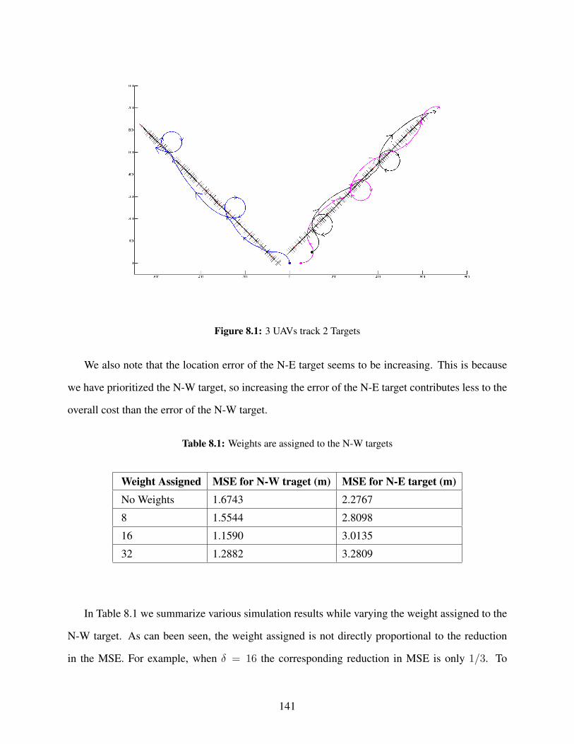
Figure 8.1: 3 UAVs track 2 Targets

We also note that the location error of the N-E target seems to be increasing. This is because

we have prioritized the N-W target, so increasing the error of the N-E target contributes less to the

overall cost than the error of the N-W target.

Table 8.1: Weights are assigned to the N-W targets

Weight Assigned MSE for N-W traget (m) MSE for N-E target (m)

No Weights 1.6743 2.2767

8 1.5544 2.8098

16 1.1590 3.0135

32 1.2882 3.2809

In Table 8.1 we summarize various simulation results while varying the weight assigned to the

N-W target. As can been seen, the weight assigned is not directly proportional to the reduction

in the MSE. For example, when δ = 16 the corresponding reduction in MSE is only 1/3. To

141

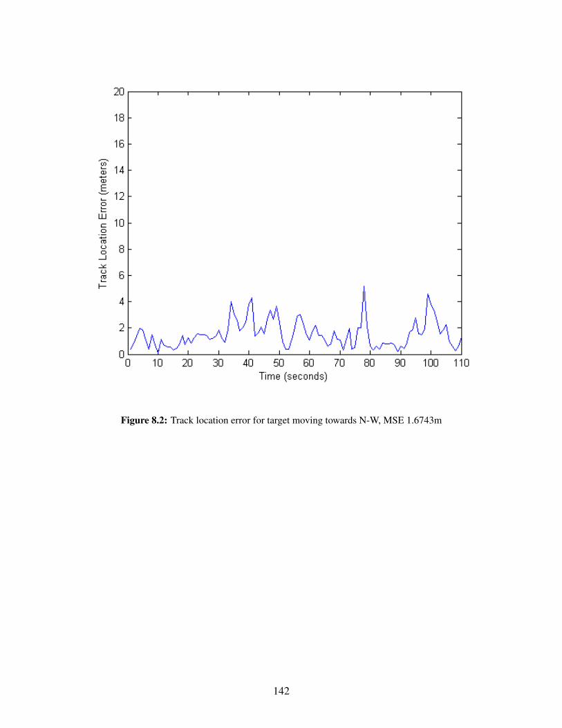
Figure 8.2: Track location error for target moving towards N-W, MSE 1.6743m

142

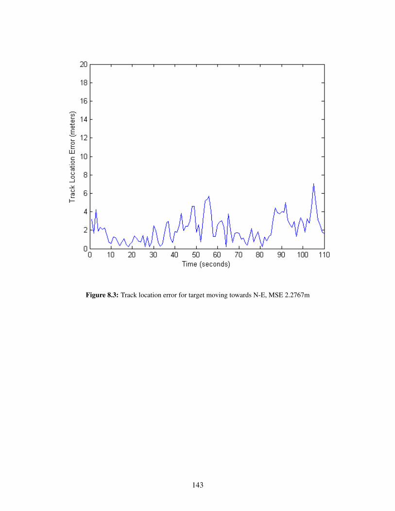
Figure 8.3: Track location error for target moving towards N-E, MSE 2.2767m

143

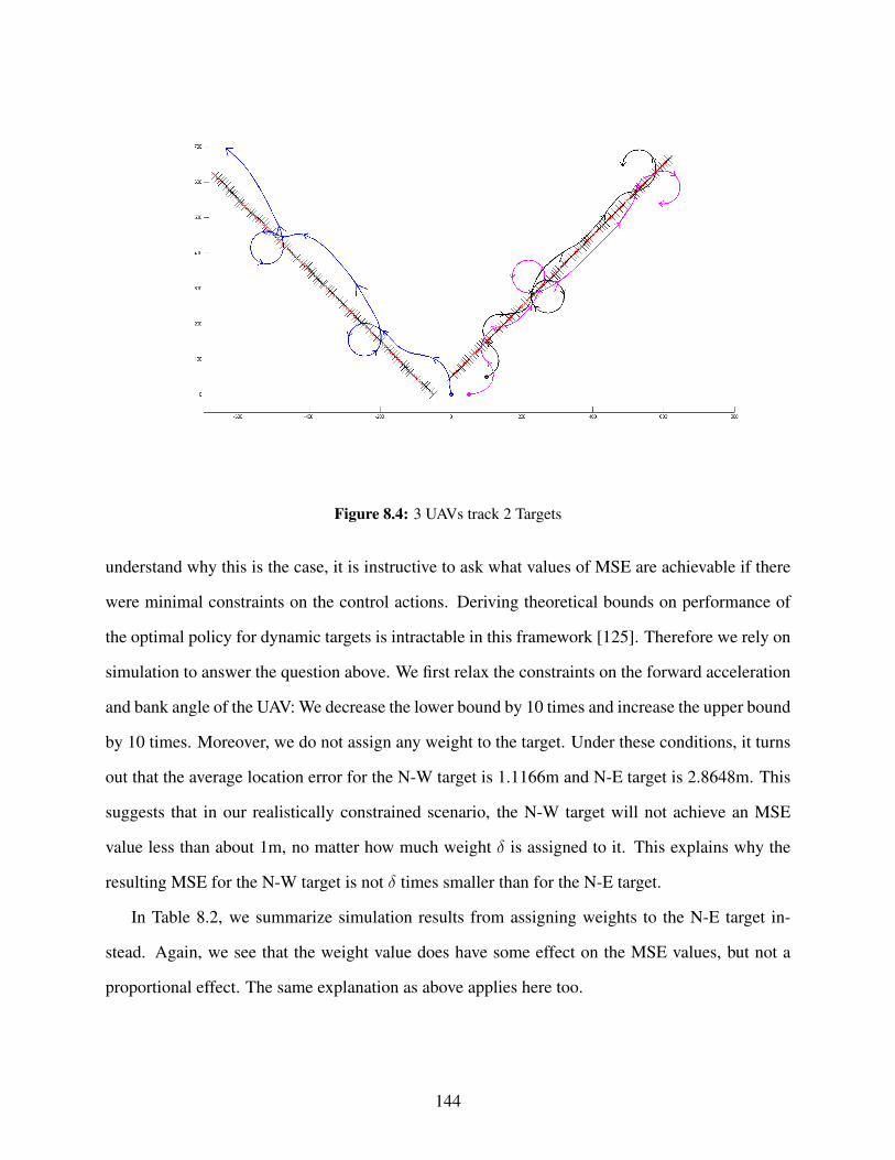
Figure 8.4: 3 UAVs track 2 Targets

understand why this is the case, it is instructive to ask what values of MSE are achievable if there

were minimal constraints on the control actions. Deriving theoretical bounds on performance of

the optimal policy for dynamic targets is intractable in this framework [125]. Therefore we rely on

simulation to answer the question above. We first relax the constraints on the forward acceleration

and bank angle of the UAV: We decrease the lower bound by 10 times and increase the upper bound

by 10 times. Moreover, we do not assign any weight to the target. Under these conditions, it turns

out that the average location error for the N-W target is 1.1166m and N-E target is 2.8648m. This

suggests that in our realistically constrained scenario, the N-W target will not achieve an MSE

value less than about 1m, no matter how much weight δ is assigned to it. This explains why the

resulting MSE for the N-W target is not δ times smaller than for the N-E target.

In Table 8.2, we summarize simulation results from assigning weights to the N-E target in-

stead. Again, we see that the weight value does have some effect on the MSE values, but not a

proportional effect. The same explanation as above applies here too.

144

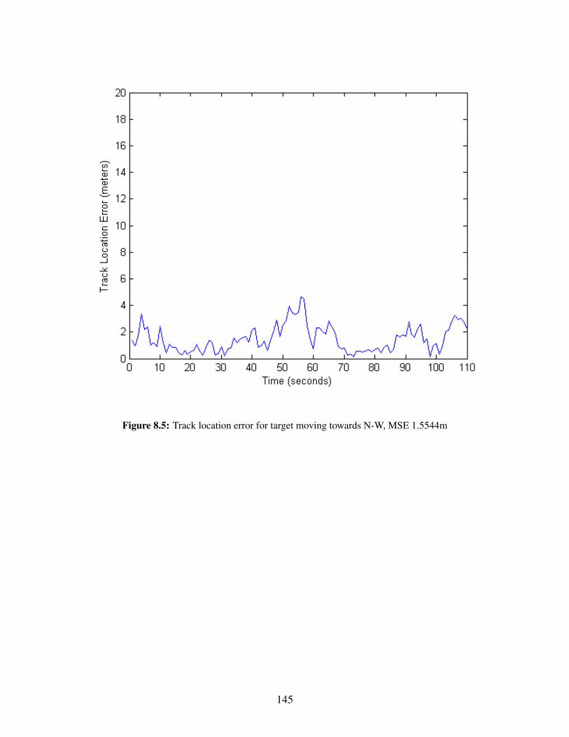
Figure 8.5: Track location error for target moving towards N-W, MSE 1.5544m

145

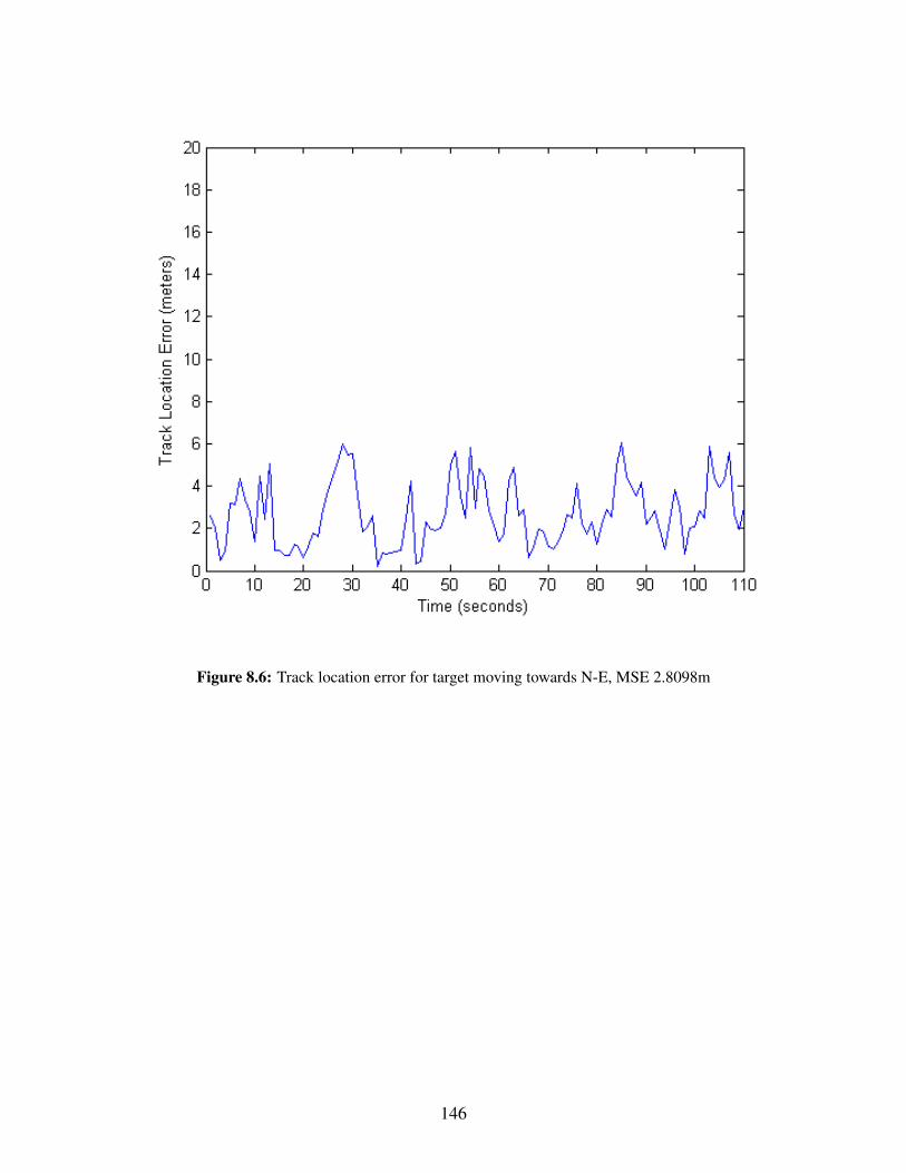
Figure 8.6: Track location error for target moving towards N-E, MSE 2.8098m

146

Table 8.2: Weights are assigned to the N-E targets

Weight Assigned MSE for N-W target (m) MSE for N-E target (m)

No Weights (Dynamic Constraints relaxed) 1.6743 2.2767

4 1.9404 2.4939

8 2.1971 2.1100

16 2.1732 2.1329

8.6 Conclusions

Our method incorporates feedback from intelligence assets as weights in the constraints. In-

corporating this feedback will not always result in lower MSE for the target to which weight is

assigned. We can similarly impose other constraint on the cost function, such as the cost to switch

on a sensor, and use the method proposed.

8.7 POMDP Review

Partially observable Markov decision process (POMDP) [120] is a mathematical framework

useful for solving resource control problems. A POMDP can also be viewed as a controlled hidden

Markov reward process. In general, a POMDP is hard to solve exactly. Therefore, the literature

on POMDP methods has focused on approximation methods [120]. A POMDP evolves in discrete

time-steps; in this study we assume that the length of each time-step is T seconds. We use k as

the discrete-time index. For a full treatment of POMDPs and related algorithms see [131]. The

following are the key components of a POMDP:

States:

The states are the features of the system that possibly evolve over time and are relevant to the

problem of interest. Let xk ∈ X represent the state of the system at time k, where X be the set of

all possible states.

Actions:

The actions are the controllable aspects of the system, i.e., the transition of the system from the

147

current state to the next state depends on the current actions. Let ak ∈ A represent the actions at

time k, where A is the set of all possible actions.

State-Transition Law:

The state-transition law defines the conditional probability distribution over the next state xk+1

given the current state xk and the current action ak, i.e.,

xk+1 ∼ pk(·|xk, ak),

where pk represents a conditional probability distribution over the state space X .

Observations and Observation-Law:

Let zk ∈ Z be the observation at time k, where Z is the observation space. The observation law

specifies the condition distribution over the observation space Z given the current state xk and

possibly the current action ak, i.e.,

zk ∼ qk(·|xk, ak),

where qk represents a conditional probability distribution over the observation space Z.

Cost Function:

The cost function at time k represents the cost (a real number) of taking an action ak given the

current state xk. Let Ck : X × A→ R represent the cost function at time k.

Belief State:

The belief-state at any given time is the posterior distribution over the state space X given the

history of observations and actions. Let bk ∈ B represent the belief-state at time k, where B is

the set of all distributions over the state space X . The POMDP process begins at time k = 0 at a

(random) initial state. As the process evolves, the state transitions to a (random) next state from

the current state according to the state-transition law given the action. An action taken at a given

state incurs a cost, which is given by the cost function. At every time-step, the system generates an

observation, which depends on the current state and action. At every time-step, this observation is

used to infer the actual underlying state. However, there will be some uncertainty in the knowledge

148

of the underlying state; this uncertainty is represented by the belief state. The belief state is the

posterior distribution over the underlying state, which is updated according to the Bayes’ rule. A

POMDP can be viewed as a fully-observable Markov decision process (MDP) with state space B.

8.8 Funding and Support

This work was supported by the Naval Postgraduate School Assistance Agreement No. N00244-

14-1-0038 awarded by the Naval Supply Systems Command (NAVSUP) Fleet Logistics Center

San Diego (NAVSUP FLC San Diego). It has not been formally reviewed by NPS. The views

and conclusions contained in this document are those of the authors and should not be interpreted

as necessarily representing the official policies, either expressed or implied, of the NPS or NAV-

SUP FLC San Diego. The NPS and NAVSUP FLC San Diego do not endorse any products or

commercial services mentioned in this publication.

149

Chapter 9

A Novel Closed Loop Framework for Controlled

Tracking in Urban Terrain

9.1 Introduction

Tracking airborne targets using sensors has been a well-researched field. Historically, the early

efforts began before the advent of World War II and gained precedence in the actual period of

war. The field has evolved to incorporate new advancements, and the technology has matured

in the ensuing decades. While lot of work has been done in tracking airborne targets, tracking

ground targets has drawn sustained attention in the past two decades. Moreover, tracking ground

targets in urban terrain poses a new set of challenges and remains relatively unexplored. Target

mobility is constrained by road networks, and the quality of measurements is affected by dense

and uneven clutter, strong multipath, and limited line-of-sight. In addition, targets can perform

evasive maneuvers or undergo a track swap owing to congested environments [125].

Traditionally, the approach to tracking systems design has been to treat sensing and tracking

sub-systems as two completely separate entities. While many of the problems involved in the

design of such sub-systems have been individually examined in the literature from a theoretical

point-of-view, very little attention has been devoted to the challenges involved in the design of an

active sensing platform that simultaneously addresses detection, signal processing, tracking, and

scheduling in an integrated fashion.

In this work, we intend to fill this gap by proposing a closed-loop active sensing system for

the urban terrain that integrates multitarget detection and tracking, multistatic radar signal process-

ing, and adaptive waveform scheduling with a one-step-lookahead [121]. The proposed system

simultaneously exploits three distinct levels of diversity: (1) spatial diversity through the use of

coordinated multistatic radars; (2) waveform diversity by adaptively scheduling the transmitted

150

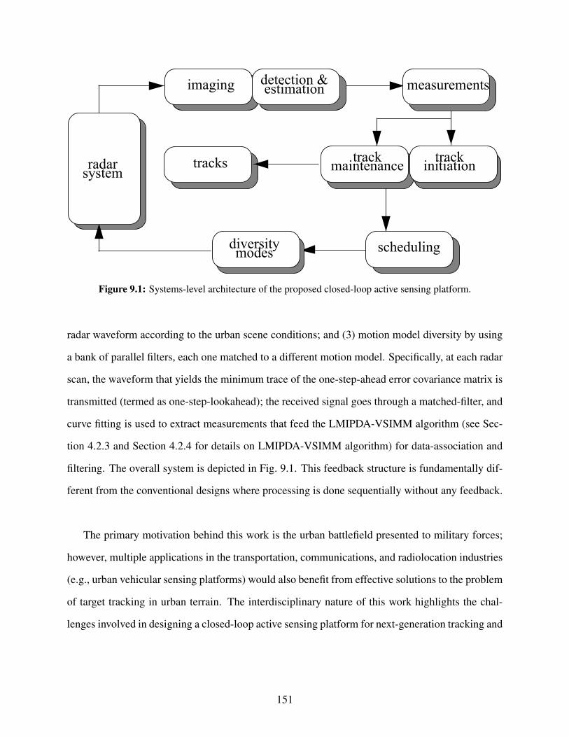
imaging

tracks

estimation measurements

initiationtrack

maintenancetrack

schedulingmodesdiversity

systemradar

detection &

Figure 9.1: Systems-level architecture of the proposed closed-loop active sensing platform.

radar waveform according to the urban scene conditions; and (3) motion model diversity by using

a bank of parallel filters, each one matched to a different motion model. Specifically, at each radar

scan, the waveform that yields the minimum trace of the one-step-ahead error covariance matrix is

transmitted (termed as one-step-lookahead); the received signal goes through a matched-filter, and

curve fitting is used to extract measurements that feed the LMIPDA-VSIMM algorithm (see Sec-

tion 4.2.3 and Section 4.2.4 for details on LMIPDA-VSIMM algorithm) for data-association and

filtering. The overall system is depicted in Fig. 9.1. This feedback structure is fundamentally dif-

ferent from the conventional designs where processing is done sequentially without any feedback.

The primary motivation behind this work is the urban battlefield presented to military forces;

however, multiple applications in the transportation, communications, and radiolocation industries

(e.g., urban vehicular sensing platforms) would also benefit from effective solutions to the problem

of target tracking in urban terrain. The interdisciplinary nature of this work highlights the chal-

lenges involved in designing a closed-loop active sensing platform for next-generation tracking and

151

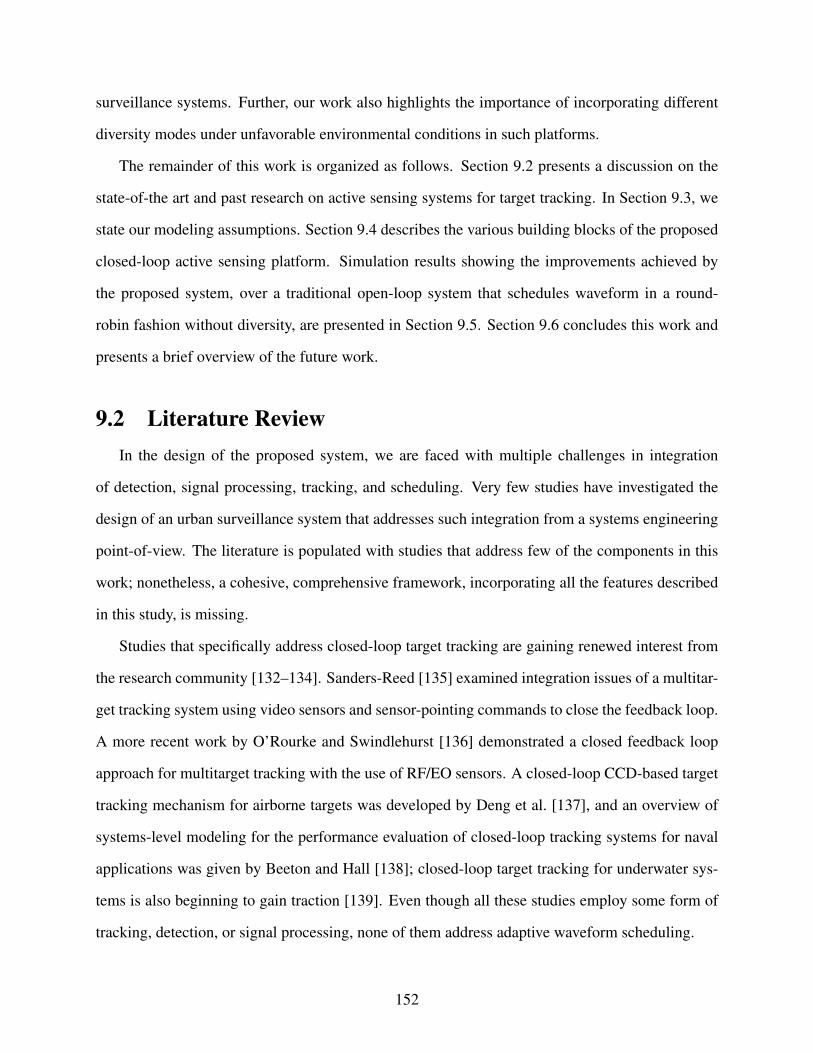
surveillance systems. Further, our work also highlights the importance of incorporating different

diversity modes under unfavorable environmental conditions in such platforms.

The remainder of this work is organized as follows. Section 9.2 presents a discussion on the

state-of-the art and past research on active sensing systems for target tracking. In Section 9.3, we

state our modeling assumptions. Section 9.4 describes the various building blocks of the proposed

closed-loop active sensing platform. Simulation results showing the improvements achieved by

the proposed system, over a traditional open-loop system that schedules waveform in a round-

robin fashion without diversity, are presented in Section 9.5. Section 9.6 concludes this work and

presents a brief overview of the future work.

9.2 Literature Review

In the design of the proposed system, we are faced with multiple challenges in integration

of detection, signal processing, tracking, and scheduling. Very few studies have investigated the

design of an urban surveillance system that addresses such integration from a systems engineering

point-of-view. The literature is populated with studies that address few of the components in this

work; nonetheless, a cohesive, comprehensive framework, incorporating all the features described

in this study, is missing.

Studies that specifically address closed-loop target tracking are gaining renewed interest from

the research community [132–134]. Sanders-Reed [135] examined integration issues of a multitar-

get tracking system using video sensors and sensor-pointing commands to close the feedback loop.

A more recent work by O’Rourke and Swindlehurst [136] demonstrated a closed feedback loop

approach for multitarget tracking with the use of RF/EO sensors. A closed-loop CCD-based target

tracking mechanism for airborne targets was developed by Deng et al. [137], and an overview of

systems-level modeling for the performance evaluation of closed-loop tracking systems for naval

applications was given by Beeton and Hall [138]; closed-loop target tracking for underwater sys-

tems is also beginning to gain traction [139]. Even though all these studies employ some form of

tracking, detection, or signal processing, none of them address adaptive waveform scheduling.

152

Next-generation multifunctional and waveform-agile radars demand innovative resource man-

agement techniques to achieve a common sensing goal while satisfying resource constraints. Re-

source allocation for target tracking has been studied from different perspectives. Adaptive sens-

ing for single target tracking was previously considered by He and Chong [140], where the sensor

scheduling problem was formulated as a partially observable Markov decision process (POMDP).

Multitarget results using the same solution framework were presented by Li et al. [141]. Kershaw

and Evans [142] investigated the problem of one-step-ahead waveform scheduling for tracking

systems, while the multi-step-ahead case was considered by Suvorova et al. [143]. The problem

of airborne tracking of ground targets was further studied by Miller et al. [121], where a POMDP

framework was used in the coordinated guidance of autonomous unmanned aerial vehicles (UAVs)

for multitarget tracking. This work was further expanded by Ragi and Chong [125] to accommo-

date track swap avoidance, target evasion, and threat-motion model for UAVs; the more general

framework of decentralised POMDP (Dec-POMDP) was also studied in [144]. A method to in-

corporate information received from human intelligence assets into the UAV decision making for

target tracking was demonstrated by Sarkale and Chong [11] using the POMDP framework. Al-

location of other sensor resources such as target revisit interval and radar steering angle were

examined by Kirubarajan et al. [145].

A case study of urban operations for counter-terrorism, which was analyzed using a probability

of attack integrated into a multitarget tracking system, was proposed by Sathyan et al. [146]. Guerci

and Baranoski [147] provided an overview of a knowledge-aided airborne adaptive radar system

for tracking ground targets in an urban environment. A lookahead sensor scheduling approach

was presented but, as the authors acknowledged, they were “merely scratching the surface" of a

possible solution. Research studies focusing on target tracking in the urban environment have been

on the rise ever since. Multipath exploitation for enhanced target tracking in urban terrain was

studied by Chakrabortay et al. [148]. In the following year, Chakrabortay et al. [149] studied target

tracking in urban terrain in presence of high clutter. As opposed to the single target tracking cases

considered in the previous two works, an integrated method to exploit multipath and mitigate high

153

clutter simultaneously for multitarget tracking was done by Zhou et al. [150]. A light detection

and ranging (LIDAR)-based approach to track targets at urban intersections was demonstrated

recently by Chen et al. [151], where simulation results are provided for real urban intersections.

The results in the study suggests that substantial amount of work remains to be done in this field.

A data fusion framework for UAVs tracking a single target in an urban terrain was demonstrated

by Ramirez-Paredes et al. [152]. Machine learning techniques to track multiple targets in an urban

setting have been making a steady progress. Many new ideas in this domain are currently being

pursued [153].

As is amply justified by the previous studies, a holistic approach that manages all the crucial

components involved in target tracking (in urban terrain) is the need of the hour. The only other

work that is close in spirit to our work in addressing this problem from a systems perspective is

the study by Nielsen and Goodman [14], where they combine signal processing, detection, and

waveform scheduling for tracking a target. However, our approach significantly differs from the

method in that research work. Specifically, we expand upon our previous work [154] and analyze

the performance of the proposed closed-loop system under more realistic urban conditions. Ground

targets move with enough speed to cause non-negligible Doppler shift; thus, a time-delay versus

Doppler image is used to extract range and range-rate measurements. In addition, we analyze the

effect of competition among motion models with the inclusion of an acceleration model in the filter

design. Waveforms are scheduled based on the trace of the one-step-ahead error covariance matrix,

which is proportional to the perimeter of the rectangular region enclosing the covariance ellipsoid.

This results in a better approximation of the mean square error than the previously considered

matrix determinant. We also add up-sweep and down-sweep chirped waveforms of different pulse

durations to the waveform library available for scheduling.

9.3 Problem Assumptions and Modeling

The first step in designing an active sensing platform for target tracking in an urban environ-

ment is to model the various elements that are part of this environment. Even though this process

154

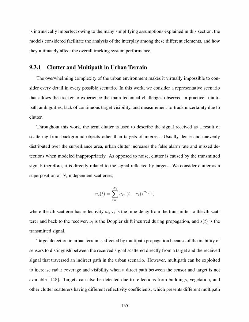
is intrinsically imperfect owing to the many simplifying assumptions explained in this section, the

models considered facilitate the analysis of the interplay among these different elements, and how

they ultimately affect the overall tracking system performance.

9.3.1 Clutter and Multipath in Urban Terrain

The overwhelming complexity of the urban environment makes it virtually impossible to con-

sider every detail in every possible scenario. In this work, we consider a representative scenario

that allows the tracker to experience the main technical challenges observed in practice: multi-

path ambiguities, lack of continuous target visibility, and measurement-to-track uncertainty due to

clutter.

Throughout this work, the term clutter is used to describe the signal received as a result of

scattering from background objects other than targets of interest. Usually dense and unevenly

distributed over the surveillance area, urban clutter increases the false alarm rate and missed de-

tections when modeled inappropriately. As opposed to noise, clutter is caused by the transmitted

signal; therefore, it is directly related to the signal reflected by targets. We consider clutter as a

superposition of Nc independent scatterers,

nc(t) =Nc∑

i=1

ais (t− τi) e2πjνi ,

where the ith scatterer has reflectivity ai, τi is the time-delay from the transmitter to the ith scat-

terer and back to the receiver, νi is the Doppler shift incurred during propagation, and s(t) is the

transmitted signal.

Target detection in urban terrain is affected by multipath propagation because of the inability of

sensors to distinguish between the received signal scattered directly from a target and the received

signal that traversed an indirect path in the urban scenario. However, multipath can be exploited

to increase radar coverage and visibility when a direct path between the sensor and target is not

available [148]. Targets can also be detected due to reflections from buildings, vegetation, and

other clutter scatterers having different reflectivity coefficients, which presents different multipath

155

conditions. A high clutter can inflict severe loss on the SNR of the multipath returns [149]. There-

fore, addressing high clutter and exploiting multipath in an integrated fashion is crucial for urban

target tracking.

Using prior knowledge of the terrain, a physical scattering model can be derived. We assume

reflective surfaces are smooth, reflectivity coefficients are constant, and the angle of incidence

equals the angle of reflection. We further assume that the strength of the radar return is negligible

after three reflections.

For an unobstructed target, the direct path can be described as follows. Let p and q be vectors

corresponding to the paths from transmitter to target and from target to receiver, respectively. The

length of the direct path is the sum of the lengths of p and q; azimuth is the angle between the

receiver and q; and the Doppler shift is the sum of the projected target velocity onto p and q. In

all other cases, path length, azimuth, and Doppler shift can be calculated once the reflection point

on the clutter scatterer has been determined. For instance, let (xc, yc) be the incidence point of the

transmitted signal on the clutter scatterer, (xk, yk) the target position at time step k, and (xr, yr) the

receiver location, as shown in Fig. 9.2. Using simple geometry and the line equation, the reflection

point (xc, yc) can be found solving the equations below:

yc = mxc + c

[−m(xr − xc) + yr − yc]2

(xr − xc)2 + (yr − yc)2=

[−m(xk − xc) + yk − yc]2

(xk − xc)2 + (yk − yc)2,

where m is the slope and c is the y-intercept in the line equation representing the clutter scatterer.

Both m and c are assumed to be known. Note that such a point may not exist due to possible

obscuration and the finite dimensions of scatterers. Equations above refer to the transmitter-target-

clutter-receiver path, and the approach is analogous for other paths.

156

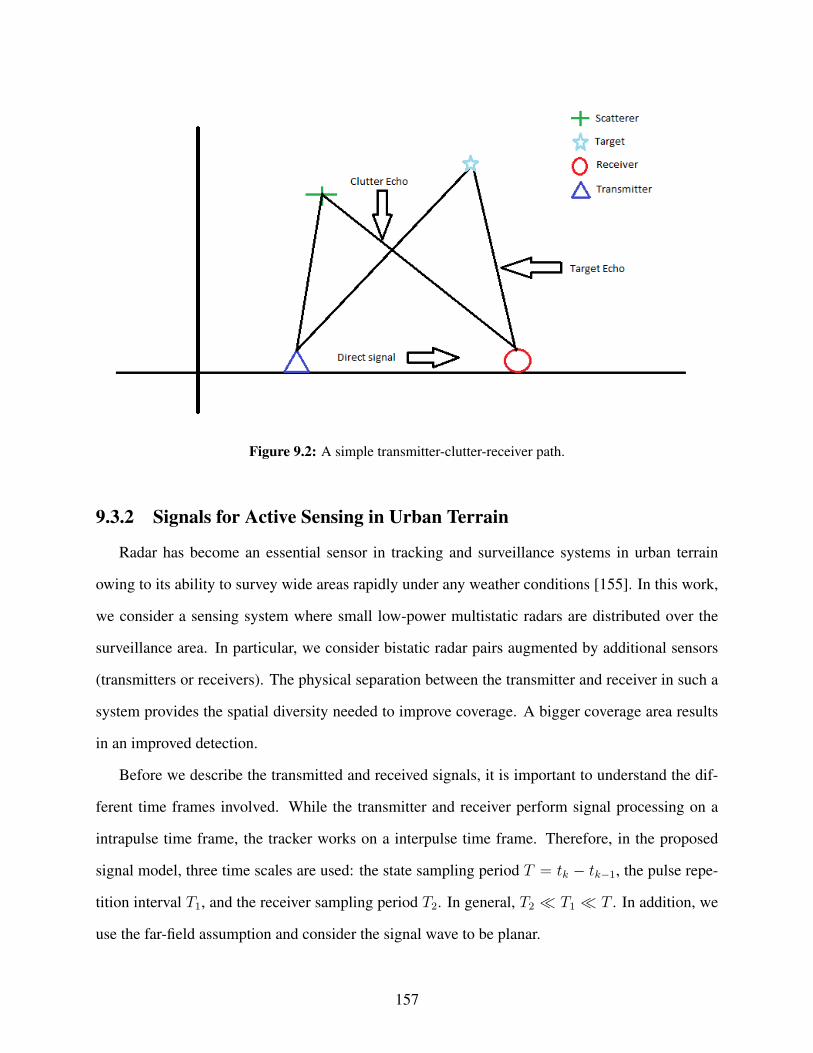
Figure 9.2: A simple transmitter-clutter-receiver path.

9.3.2 Signals for Active Sensing in Urban Terrain

Radar has become an essential sensor in tracking and surveillance systems in urban terrain

owing to its ability to survey wide areas rapidly under any weather conditions [155]. In this work,

we consider a sensing system where small low-power multistatic radars are distributed over the

surveillance area. In particular, we consider bistatic radar pairs augmented by additional sensors

(transmitters or receivers). The physical separation between the transmitter and receiver in such a

system provides the spatial diversity needed to improve coverage. A bigger coverage area results

in an improved detection.

Before we describe the transmitted and received signals, it is important to understand the dif-

ferent time frames involved. While the transmitter and receiver perform signal processing on a

intrapulse time frame, the tracker works on a interpulse time frame. Therefore, in the proposed

signal model, three time scales are used: the state sampling period T = tk − tk−1, the pulse repe-

tition interval T1, and the receiver sampling period T2. In general, T2 ≪ T1 ≪ T . In addition, we

use the far-field assumption and consider the signal wave to be planar.

157

At time tk, a series of pulses is transmitted at periods of T1 seconds. Assuming Gaussian-

windowed up-sweep and down-sweep chirp signals of unit energy, the signal transmitted by the

nth transmitter (n = 1, . . . , N) at time tk is given by:

sk,n(t) =

(B−1)/2∑

b=−(B−1)/2

exp

[±jγ − 1/(2κ2)] (t− bT1)2

(πκ2B2)1/4, (9.1)

where t ∈ R, B is the number of pulses transmitted, κ represents the pulse duration, and γ is the

chirp rate. The complex exponential is positive or negative according to the waveform scheduled

for transmission: up-sweep chirp or down-sweep chirp, respectively.

The mth receiver (m = 1, . . . ,M) is a uniform linear array of Lm sensor elements; the sensor

elements Lm at each receiver are separated by distance dm, where the direction of arrival of the

signal sent by the nth transmitter is θn,m. We assume coherent processing, i.e., radar returns that

arrive at different receiver sampling intervals can be processed jointly. In other words, we are

assuming that radar returns can be stored, aligned, and subsequently fed to the receiver for fusion.

The received signal is a summation of reflections from targets of interest and clutter scatterers.

Let Pk,n,m be the total number of reflections received by the mth receiver at time tk that originated

from the nth transmitter. Signals from the pth path (p = 1, . . . , Pk,n,m) are subject to a random

phase shift φpn,m that are uniformly distributed in (−π, π]. Hence, the signal received by the lth

element (l = 1, . . . , Lm) of the mth sensor array at time tk + uT2 can be written as:

yk,m,l(u) =N∑

n=1

Pk,n,m∑

p=1

ejφpn,mgpn,m (xk; uT2) + e(u), (9.2)

where u = (0, . . . , U − 1) is the sample index, and e(u) is a complex white Gaussian process. We

can write gpn,m (xk; uT2) as:

158

gpn,m (xk; uT2) = (9.3)

αpn,m (xk) · sk,n(

uT2 − τpn,m (xk)

)

·

e2πjνpn,m(xk)uT2−j(lm−1)dm[cos(θpn,m(xk))] ·

e−2πjνpn,m(xk)uT2+j(lm−1)dm[sin(θpn,m(xk))θpn,m(xk)uT2],

where dm = dm/λ for the carrier signal wavelength λ, and sk,n(

uT2 − τpn,m (xk)

)

is the delayed

replica of the transmitted signal given in (9.1). In addition, the following received signal param-

eters are defined for the pth path between the nth transmitter and mth receiver: αpn,m (xk) is the

magnitude of the radar return, including transmitted signal strength and path attenuation; τ pn,m (xk)

is the time-delay incurred during propagation; νpn,m (xk) represents the Doppler shift; and θpn,m (xk)

is the direction of arrival, where θpn,m (xk) is its rate of change. Note that, because clutter is in-

dependent of the target state, gpn,m(xk; uT2) = gpn,m(uT2) in (9.2). The parameters above can be

computed for each target state xk, given prior knowledge of the urban scenario.

9.3.3 Models for Target Motion in Urban Terrain

Target motion in urban terrain can be described by a large number of models that can be com-

bined in various ways. It is not the objective of this work to design novel motion models for targets

in urban terrain. Instead, we adopt existing models in the literature. For a comprehensive survey

emphasizing the underlying ideas and assumptions of such models, we refer the reader to Li and

Jilkov [156].

Let the target state vector at time tk be

xk = [xk, xk, yk, yk, xk, yk]⊤ ,

where ⊤ denotes matrix transpose, [xk, yk]⊤ is the velocity vector, and [xk, yk]

⊤ is the acceleration

vector.

Motion models can be divided into two categories: uniform motion (or non-maneuvering)

models and maneuvering models. The most commonly used non-maneuvering motion model is

159

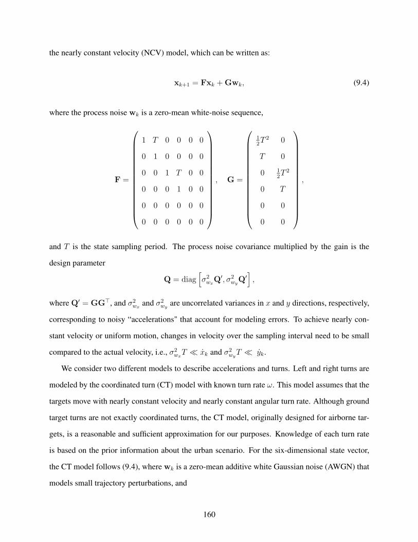
the nearly constant velocity (NCV) model, which can be written as:

xk+1 = Fxk +Gwk, (9.4)

where the process noise wk is a zero-mean white-noise sequence,

F =

1 T 0 0 0 0

0 1 0 0 0 0

0 0 1 T 0 0

0 0 0 1 0 0

0 0 0 0 0 0

0 0 0 0 0 0

, G =

12T 2 0

T 0

0 12T 2

0 T

0 0

0 0

,

and T is the state sampling period. The process noise covariance multiplied by the gain is the

design parameter

Q = diag[

σ2wxQ′, σ2

wyQ′]

,

where Q′ = GG⊤, and σ2wx

and σ2wy

are uncorrelated variances in x and y directions, respectively,

corresponding to noisy “accelerations" that account for modeling errors. To achieve nearly con-

stant velocity or uniform motion, changes in velocity over the sampling interval need to be small

compared to the actual velocity, i.e., σ2wxT ≪ xk and σ2

wyT ≪ yk.

We consider two different models to describe accelerations and turns. Left and right turns are

modeled by the coordinated turn (CT) model with known turn rate ω. This model assumes that the

targets move with nearly constant velocity and nearly constant angular turn rate. Although ground

target turns are not exactly coordinated turns, the CT model, originally designed for airborne tar-

gets, is a reasonable and sufficient approximation for our purposes. Knowledge of each turn rate

is based on the prior information about the urban scenario. For the six-dimensional state vector,

the CT model follows (9.4), where wk is a zero-mean additive white Gaussian noise (AWGN) that

models small trajectory perturbations, and

160

F =

1 sinωTω

0 −1−cosωTω

0 0

0 cosωT 0 − sinωT 0 0

0 1−cosωTω

1 sinωTω

0 0

0 sinωT 0 cosωT 0 0

0 0 0 0 0 0

0 0 0 0 0 0

.

As in the NCV model, Q = σ2wdiag [Q

′,Q′], Q′ = GG⊤, and σ2w is the process noise variance.

However, contrary to the NCV model, x and y directions are now coupled.

Accelerations and decelerations are described by the Wiener-sequence acceleration model,

where

F =

1 T 0 0 12T 2 0

0 1 0 0 T 0

0 0 1 T 0 12T 2

0 0 0 1 0 T

0 0 0 0 1 0

0 0 0 0 0 1

and

G =

12T 2 0

T 0

0 12T 2

0 T

1 0

0 1

.

For this model, the process noise wk in (9.4) is a zero-mean white-noise sequence with uncor-

related variances in the x and y directions. We consider σ2wxT ≪ xk and σ2

wyT ≪ yk; under

these assumptions, the Wiener-sequence acceleration model is also known as the nearly constant

acceleration (NCA) model.

161

9.4 Closed-Loop Active Sensing Platform

In this section, we outline the main aspects of each component of our closed-loop active sensing

platform depicted in Fig. 9.1.

9.4.1 From Signal Detection to Discrete Measurements

Under the modeling assumption of AWGN, the optimal signal detection is the correlator re-

ceiver, or equivalently, the matched-filter [157]. The signal received by the lth element of the mth

sensor array, given in (9.2), is compared to a template signal by computing a correlation sum of

sampled signals. The template signal is a time-shifted, time-reversed, conjugate, and scaled replica

of the signal transmitted by the nth transmitter at time tk:

hk,n(t) = as∗k,n (td − t) , (9.5)

where td is the time-delay incurred during propagation, ∗ represents complex conjugate, and a is

the scaling factor assumed to be unity.

In the general multistatic setting with N transmitters and M receivers, we consider the case

where the mth receiver is a uniform linear array of Lm sensor elements. Therefore, we need

to combine the signals received by each of the sensor array elements to obtain the total signal

received by the mth receiver at time tk, which can be written as:

yk,m =U−1∑

u=0

T1∑

t=1

Lm∑

l=1

yk,m,l(u)hk,n (uT2 − t) , (9.6)

where yk,m,l is given by (9.2), and hk,n is given by (9.5).

Before range and range-rate measurements that feed the tracker can be extracted, pre-processing

the radar intensity image is necessary. Assuming each target is a point object (as opposed to an ex-

tended object with spatial shape), we use peak detection to locate a point source corresponding to

a received power peak on a time-delay versus Doppler image. Because of the strong local (but lack

of global) similarities exhibited by urban clutter, image processing techniques aimed to suppress

162

this type of clutter should be based on segmentation analysis, where each image segment must be

processed individually in order to distinguish between targets of interest and background scatter-

ers [158]. However, this could be extremely computationally intensive; therefore, we use a more

standard form of clutter suppression. Specifically, we calculate a background model prior to track-

ing using the average of radar intensity images over time to approximate the true urban scenario.

The average background image is then subtracted from each image formed using radar returns dur-

ing the tracking process. For each time-delay τ and Doppler shift ν, the average magnitude of the

radar return A(τ, ν) is given by:

A(τ, ν) =1

J

J∑

j=1

Aj(τ, ν),

where j indexes times during which the urban scenario was under surveillance prior to tracking,

Aj(τ, ν) is the average magnitude at time step j, and

Ak(τ, ν) = A−k (τ, ν)− A(τ, ν)

is the magnitude of the radar return for time-delay τ and Doppler shift ν at time step tk during

tracking. Note that it is also possible to reduce the image noise, using several image processing

techniques, if further improvements on the contrast between background and targets of interest are

needed.

Peak detection is implemented iteratively. For each peak(

τ peakk , νpeakk

)

found in Ak(τ, ν), a

nonlinear optimization algorithm is used to find a curve that fits the underlying image within a

window centered at the peak. When performing curve fitting, we are interested in estimating the

measurement error covariance matrix. Since noise sources are assumed to be AWGN, Gaussian

curve fitting has been widely used in target detection [159]. Note that a Gaussian can be ap-

proximated by a quadratic locally within a window centered at the peak. In this work, we fit a

two-dimensional quadratic function to each peak in the underlying image. Specifically, at every

time step tk, we solve the following optimization problem:

163

minστ ,σν

∑

τ

∑

ν

∣

∣ fστ ,σν (τ, ν)− Ak(τ, ν)∣

∣

2,

where for ǫ > 0, the window containing time-delay and Doppler values is defined by

τ ∈(

τ peakk − ǫ, τ peakk + ǫ)

and ν ∈(

νpeakk − ǫ, νpeakk + ǫ)

, and

fστ ,σν (τ, ν) = σ2ττ

2 + 2στσντν + σ2νν

2.

We define a scan as the set of measurements generated by a radar receiver from an individual

look over the entire surveillance area. The kth scan by the mth receiver corresponding to its kth

look is denoted by:

Zk,m =

z1k,m, z2k,m, . . . , z

Nk,m

k,m

,

whereNk,m is the total number of measurements in scanZk,m. In this work, the jth (j = 1, . . . , Nk,m)

measurement in the kth scan of the mth receiver is the following two-dimensional vector of range

and range-rate:

zjk,m =

rjk,m

rjk,m

,

where(

rjk,m, rjk,m

)

corresponds to the location of the jth peak in the time-delay and Doppler image

from receiver m by trivial transformation. Associated with each measurement vector zjk,m is an

error covariance matrix

Rjk,m(ψ) =

σ2rjk,m

ρrr

(

σrjk,mσrj

k,m

)

ρrr

(

σrjk,mσrj

k,m

)

σ2rjk,m

,

where ψ is the vector of parameters that characterize the waveform transmitted at tk, and ρrr is the

correlation coefficient between range and range-rate measurement errors. The vector ψ is included

in the measurement noise covariance matrix description to show the explicit dependence of this

matrix on the transmitted waveform. In particular, transmitted waveforms defined by (9.1) are

characterized by pulse duration κ and chirp rate γ; hence, in this case,

164

ψ =

κ

γ

.

The correlation coefficient between measurement errors ρrr also depends on the transmitted wave-

form and can be calculated using the waveform’s ambiguity function [160]. In particular, the cor-

relation coefficient for the up-sweep and down-sweep chirp waveforms, considered in this work,

are strongly negative and positive, respectively.

In state estimation, the measurement model describing the relationship between the target state

at time tk and the kth radar scan can be written as:

zjk,m = H (xk) + vk,

where H is a vector-valued function that maps the target state xk to its range and range-rate, and

vk is the zero-mean Gaussian measurement noise vector with covariance matrix Rjk,m(ψ).

9.4.2 Multitarget-Multisensor Tracker

We consider a tracker implemented as a sequential filter that weighs measurements in each

scan. In addition, tracks are initiated, maintained, and terminated in an integrated fashion. Note

that we use the word track instead of target because we have no a priori knowledge of the number

of targets in the urban scenario. There are several techniques in the literature that address target

tracking for an unknown number of targets; the number of targets can also vary over time. For a

discussion on these techniques, see [161]. Also, algorithms discussed in this section have been pre-

viously presented in the literature. Hence, rather than deriving each algorithm below, we highlight

their main features related to the design of a closed-loop active sensing system for urban terrain.

Automatic Track Initiation and Termination

The goal in track initiation is to estimate tentative tracks from raw measurements without any

prior information about how many targets are present in the surveillance area.

165

We follow the two-point differencing algorithm, according to which it takes two time steps (or

two radar scans) for a track to be initiated [162]. For each receiver m (m = 1, . . . ,M), a tentative

track is initiated for every declared detection, i.e., for every peak in the time-delay versus Doppler

image exceeding a given detection threshold and that cannot be associated with an existing track.

In particular, at t1 a tentative track x(j)1 is initiated for each measurement j = 1, . . . , N1,m in scan

Z1,m. Assuming the velocity of a target along the x and y coordinates lies within the intervals[

−xmaxk−1 , xmaxk−1

]

and[

−ymaxk−1 , ymaxk−1

]

, respectively, a track is initiated at (xk, yk) when

xk ∈[(

−xmaxk−1 − 2σxk−1

)

T,(

xmaxk−1 + 2σxk−1

)

T]

and

yk ∈[(

−ymaxk−1 − 2σyk−1

)

T,(

ymaxk−1 + 2σyk−1

)

T]

,

where T = tk − tk−1 is the state sampling period, and σxk−1and σyk−1

are the standard deviations

of target velocities in x and y directions, respectively. Each measurement that falls into the track

initiation area yields an initial position and velocity from which a track is initiated. Measurements

can then be associated with this new track starting at tk > 2, and the target’s acceleration can then

be estimated at the filtering stage of the tracker, described in Section 9.4.2.

The usual approach to track termination is to declare a track terminated if such a track has

not been associated with any new measurements for two consecutive time steps. We adopt a

more integrated approach and use a probability of track existence, defined in Section 9.4.2, that

is initialized for every initiated track. Specifically, a track is terminated if the probability of track

existence falls below a given track termination threshold.

Measurement Validation

For each initiated track x(t)k , t = 1, . . . ,Tk, we define a gate in the measurement space within

which measurements to be associated with track x(t)k are expected to lie. Only those measurements

that lie within the gate are said to be validated; therefore, only such measurements are associated

to track x(t)k . The size and shape of the gate can be defined in several different ways. We use the

166

ellipsoidal validation gating [163] and apply the following statistical test:

[

zik − z(t)k

]⊤ (

S(t)k

)−1 [

zik − z(t)k

]

< g2,

where zik represents the ith measurement in the kth scan, z(t)k is the predicted measurement for

track x(t)k , S(t)

k represents the innovation covariance at scan k, and g is a threshold computed from

Chi-square distribution tables, such that, if a target is detected, its measurement is validated with

gating probability PG. The number of degrees of freedom of g is equal to the dimension of the mea-

surement vector. In the two-dimensional case, the area of the validation ellipse is g2π det(S(t)k )1/2,

where det is the matrix determinant.

Filtering

The tracking algorithm needs to be adaptive in order to handle a time-varying number of tar-

gets and dynamic urban conditions. We show in Section 9.5 that the variable structure interacting

multiple model (VS-IMM) estimator is effective under such conditions [164, 165]. The VS-IMM

estimator implements a separate filter for each model in its model set, which is determined adap-

tively according to the underlying terrain conditions. Specifically, at each time step tk, the model

set is updated to:

Mk =

rk ∈Mtotal

∣

∣ I,x(t,r)k−1,P

(t,r)k−1, rk−1 ∈Mk−1

,

where x(t,r)k−1 and P

(t,r)k−1 are the mean and covariance of track t in the filter matched to model r at tk−1,

I represents prior information about the urban scenario, andMtotal is the set of all possible motion

models. Changes in track trajectory are modeled as a Markov chain with transition probabilities

given by:

πij = P rk = i|rk−1 = j , i, j ∈Mtotal.

In this work, we consider the unscented Kalman filter (UKF) algorithm. Initially proposed by

Julier and Uhlmann [166], the UKF represents the state distribution by a set of deterministically

167

chosen sample points. Each UKF filter, matched to a different motion model, runs in parallel in

the VS-IMM framework. The estimated mean and covariance from each model-matched filter

are mixed (Gaussian mixture) before the next filtering time step. The overall output of the VS-

IMM estimator is then calculated by probabilistically combining the individual estimates of each

filter [167].

Data Association

We consider the linear multitarget integrated probabilistic data association (LMIPDA) algo-

rithm for data association [168,169]. An extension of the single-target integrated probabilistic data

association [170], LMIPDA models the notion of track existence as a Markov chain. Let χk denote

the event that a track exists at tk. The a priori probability that a track exists at tk is given by:

ψk|k−1 , P

χk

∣

∣

∣

∣

k−1⋃

i=1

Zi

,

where Zk is the set of measurements from all receivers at time tk, i.e., Zk = ∪Mm=1Zk,m. The

evolution of track existence over time satisfies the following equations:

ψk|k−1 = p11ψk−1|k−1 + p21(

1− ψk−1|k−1

)

1− ψk|k−1 = p12ψk−1|k−1 + p22(

1− ψk−1|k−1

)

,

where pij , i, j = 1, 2, are the corresponding transition probabilities.

The central ideal behind the LMIPDA algorithm is the conversion of a single-target tracker in

clutter into a multitarget tracker in clutter by simply modifying the clutter measurement density

according to the predicted measurement density of other tracks. The modified clutter density of

track x(t)k given the ith measurement can be written as:

Ω(t)i = ρ

(t)i +

Tk∑

s=1,s 6=t

p(s)i

P(s)i

1− P (s)i

,

168

where ρ(t)i is the clutter density in the validation gate of track x(t)k given the ith measurement in the

kth scan zik, P (t)i is the a priori probability that zik is the true measurement for track x

(t)k , i.e.,

P(t)i = PDPGψ

(t)k|k−1

p(t)i /ρ

(t)i

∑N(t)k

i=1 p(t)i /ρ

(t)i

,

where ψ(t)k|k−1 is the probability of existence of track x

(t)k , p(t)i is the a priori measurement likelihood

(Gaussian density), and N (t)k is the total number of measurements associated with track x

(t)k at time

tk. The probability of track existence is calculated as follows:

ψ(t)k|k =

(

1− δ(t)k

)

ψ(t)k|k−1

1− δ(t)k ψ(t)k|k−1

,

where

δ(t)k = PDPG

1−

N(t)k∑

i=1

p(t)i

Ω(t)i

.

For each model r ∈Mk, we define the following probabilities of data association:

β(t,r)k,0 =

1− PDPG

1− δ(t,r)k

for clutter measurements, and for each target measurement i > 0,

β(t,r)k,i =

1− PDPGp(t,r)i

(

1− δ(t,r)k

)

Ω(t)i

,

where p(t,r)i is the a priori likelihood of measurement i assuming association with track x(t)k that

follows motion model r, i.e.,

p(t)i =

∑

r∈Mk

p(t,r)i ,

and

169

δ(t,r)k = PDPG

1−

N(t)k∑

i=1

p(t,r)i

Ω(t)i

.

Finally, the motion model for each track x(t)k is updated according to the following model

probabilities:

µ(t,r)k = µ

(t,r)k|k−1

1− δ(t,r)k

1− δ(t)k,

for r ∈Mk.

9.4.3 Waveform Scheduling

Many modern airborne radars have a waveform scheduler implemented. Ideally, the scheduler

would use a library of waveforms especially designed to improve detection and the overall tracking

performance.

We consider the general waveform selection problem, which in the multitarget tracking case

can be written as:

minψ∈Ψ

1

Tk

Tk∑

t=1

E

‖x(t)k − x

(t)k ‖

2∣

∣ Zk

,

where Ψ represents the waveform library, xk is the tracking state estimate, and Tk is the total

number of tracks at tk.

In particular, we consider the one-step ahead (or myopic) waveform scheduling problem, where

the waveform selected for transmission at tk+1 is given by:

ψk+1 = argminψk+1∈Ψ

1

Tk

Tk∑

t=1

Tr

P(t)k+1 (ψk+1)

, (9.7)

where Tr is the matrix trace and P(t)k+1 is the posterior state error covariance matrix corresponding

to track x(t)k . For a detailed discussion on the advantages of incorporating lookahead in sensing, see

Miller et al. [?]. The performance measure in (9.7) is equivalent to minimizing the mean square

tracking error over all existing tracks. The posterior state covariance error matrix P(t)k+1 defines a

170

six-dimensional ellipsoid centered at x(t)k that is a contour of constant probability of error [171],

and its trace is proportional to the perimeter of the rectangular region enclosing this ellipsoid.

In order to evaluate (9.7), we first approximate the measurement error covariance matrix by the

Fisher information matrix J(ψ) corresponding to the measurement using waveform ψ [142, 171].

Specifically,

R(ψ) = UJ(ψ)−1U⊤,

where U is the transformation matrix between the time-delay and Doppler measured by the receiver

and the target’s range and range-rate. In particular, for the up-sweep Gaussian chirp with pulse

duration κ, chirp rate γ, and wavelength λ defined by (9.1), we have:

R(ψ) =1

η

c2κ2

2−2πc2γκ2

λ

−2πc2γκ2

λ

(

2πcλ

)2 ( 12κ2

+ 2γ2κ2)

,

where η is the signal-to-noise ratio (SNR). A similar expression can be obtained for the down-

sweep Gaussian chirp.

The posterior state error covariance matrix can then be calculated for each waveform ψ ∈ Ψ

using the UKF’s covariance update equations.

Coherent signal processing across spatially distributed transmitters and receivers is an appeal-

ing feature of our sensing platform. The transmission of phase synchronization information for

coherent signal processing and waveform scheduling is now possible owing to the advancements

in the wireless communications technology, which might have not been possible just a decade

before.

9.5 Simulation Results

Monte Carlo simulations are used to evaluate the effectiveness of the proposed closed-loop

system in urban terrain.

171

A number of terrain factors have major impact on the overall system performance. Different

road classes (e.g., highways, arterial roads, residential streets, and alleys) impose different con-

straints on ground vehicles. In addition, different construction materials (e.g., glass, concrete,

brick, and wood) have different reflectivity coefficients; therefore, they have different multipath

conditions. Any urban environment encompasses multiple components like bridges, footbridges,

fences of various types, and round poles etc. Moreover, the structural design of the buildings can

vary. The modeling assumptions and the models described in Section 9.3 and Section 9.4 might

not be able to incorporate every fine detail in an urban environment; nevertheless, they are general

enough to accommodate any generic representative urban scenario with adequate detail. For the

simulation purposes, we consider a scenario that is representative of the urban conditions to be

likely faced by an active sensing tracking system. E.g., we will use vegetation in the simulations

to represent the clutter in the urban scenario.

The simulated scenario is depicted in Fig. 9.3, which shows four building structures at an

intersection. The uneven nature of urban clutter is represented by the ‘+’, indicating vegetation on

the center median and sidewalks. The overall clutter density is assumed to be 2.5e−4m2. A radar

transmitter, represented by ‘’, is located at (2085,1470.5); whereas two radar receivers, each with

three sensor array elements, are located at (2088,1475) and (2078,1467), both represented by ‘©’.

The maximum sensor range is 300 meters, and the SNR experienced is 0.2.

Although in reality the transmitted signal can be reflected by multiple scatterers, we assume

that the strength of the radar return is negligible after three reflections; therefore, we restrict

our simulation to the following paths: transmitter-target-receiver (direct path), transmitter-clutter-

receiver, transmitter-target-clutter-receiver, transmitter-clutter-target-receiver, transmitter-clutter-

clutter-receiver, transmitter-clutter-target-clutter-receiver, transmitter-target-clutter-clutter-receiver,

and transmitter-clutter-clutter-target-receiver.

The simulation experiment consisted of 100 runs, each with a total of 140 radar scans, where a

radar scan takes 0.25 seconds. Two targets, 10 seconds apart from each other, are simulated using

the same trajectory as follows. Starting at (1950,1500), each target moves at constant velocity of

172

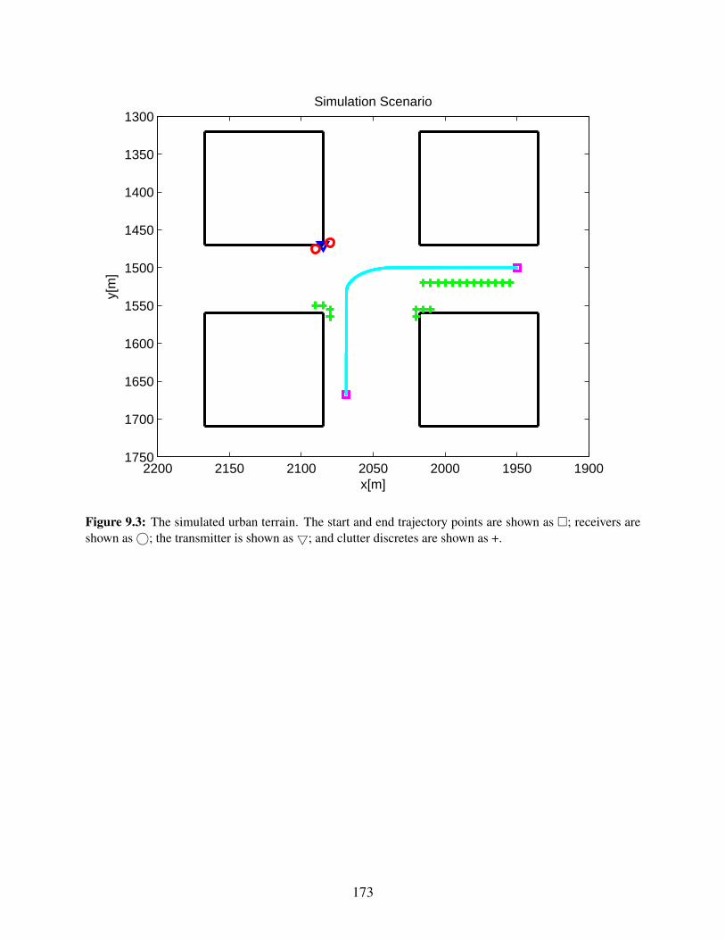
1900195020002050210021502200

1300

1350

1400

1450

1500

1550

1600

1650

1700

1750

Simulation Scenario

x[m]

y[m

]

Figure 9.3: The simulated urban terrain. The start and end trajectory points are shown as ; receivers areshown as©; the transmitter is shown as; and clutter discretes are shown as +.

173

10 m/s in the x direction for 10 seconds; as they approach the intersection, they start decelerating at

constant rate of 1 m/s2 for 5 seconds; they enter a left turn with constant turn rate of π/20 rad/s for

10 seconds; after completing the turn, each target accelerates for 5 seconds at 1 m/s2 rate; finally,

they end their trajectories with constant velocity at (2068.8,1667.8).

Two model sets are used during the motion model adaptation. In the vicinity of intersections,

a set consisting of NCA, left-turn CT, and right-turn CT is used. Both the left and right turn CT

model are assumed to have a turn rate of π/20 rad/s. This model set is used between scans 20 and

100. During the remaining radar scans, a set containing the NCA and NCV motion models is used

instead. The motion model transition probability matrix is given by

0.99 0.01 0 0

0.1 0.7 0.1 0.1

0 0.1 0.99 0

0 0.1 0 0.99

.

A waveform library consisting of four different Gaussian-windowed chirp signals is consid-

ered. Waveforms vary in pulse duration κ. In particular, radar sensors considered in the simulation

experiment are assumed to support the following pulse durations: κ = 0.5 µs, and κ = 1.375 µs.

In general, longer pulses return more power; however, finer details may be lost. In addition, wave-

forms of each pulse duration can be either an up-sweep or down-sweep chirp. Pulses are repeated

at every 10 milliseconds, and waveforms operate at 4 GHz with 40 MHz of bandwidth.

A more traditional open-loop system, which does not support any diversity modes and that

schedules the waveforms in a round-robin fashion, is used as a baseline for comparison. In the

baseline implementation, a single UKF using the NCV motion model is considered.

Note that the simulation parameters used in this work do not represent any particular system,

and were chosen exclusively for illustration purposes.

Simulation results in Fig. 9.4 and Fig. 9.5 show that the closed-loop system clearly outperforms

its open-loop counterpart. The average number of confirmed tracks is increased by approximately

174

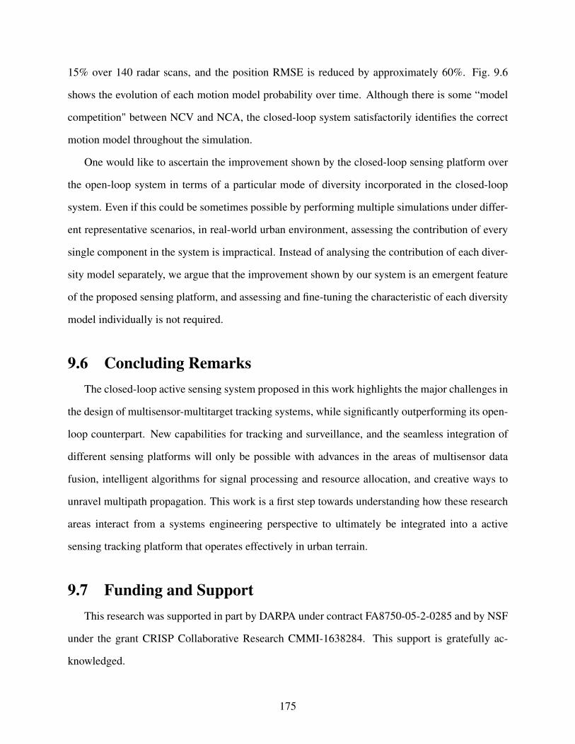
15% over 140 radar scans, and the position RMSE is reduced by approximately 60%. Fig. 9.6

shows the evolution of each motion model probability over time. Although there is some “model

competition" between NCV and NCA, the closed-loop system satisfactorily identifies the correct

motion model throughout the simulation.

One would like to ascertain the improvement shown by the closed-loop sensing platform over

the open-loop system in terms of a particular mode of diversity incorporated in the closed-loop

system. Even if this could be sometimes possible by performing multiple simulations under differ-

ent representative scenarios, in real-world urban environment, assessing the contribution of every

single component in the system is impractical. Instead of analysing the contribution of each diver-

sity model separately, we argue that the improvement shown by our system is an emergent feature

of the proposed sensing platform, and assessing and fine-tuning the characteristic of each diversity

model individually is not required.

9.6 Concluding Remarks

The closed-loop active sensing system proposed in this work highlights the major challenges in

the design of multisensor-multitarget tracking systems, while significantly outperforming its open-

loop counterpart. New capabilities for tracking and surveillance, and the seamless integration of

different sensing platforms will only be possible with advances in the areas of multisensor data

fusion, intelligent algorithms for signal processing and resource allocation, and creative ways to

unravel multipath propagation. This work is a first step towards understanding how these research

areas interact from a systems engineering perspective to ultimately be integrated into a active

sensing tracking platform that operates effectively in urban terrain.

9.7 Funding and Support

This research was supported in part by DARPA under contract FA8750-05-2-0285 and by NSF

under the grant CRISP Collaborative Research CMMI-1638284. This support is gratefully ac-

knowledged.

175

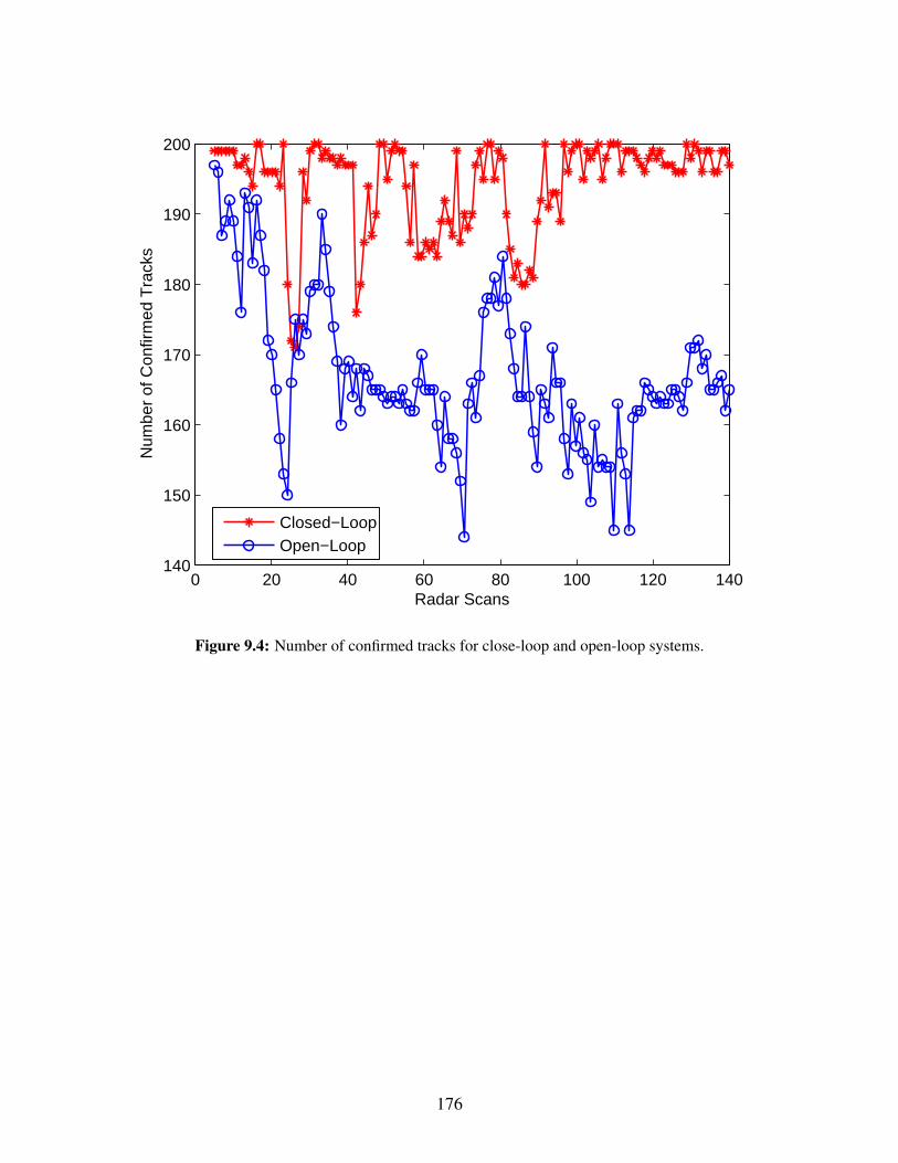
0 20 40 60 80 100 120 140140

150

160

170

180

190

200

Radar Scans

Num

ber

of C

onfir

med

Tra

cks

Closed−LoopOpen−Loop

Figure 9.4: Number of confirmed tracks for close-loop and open-loop systems.

176

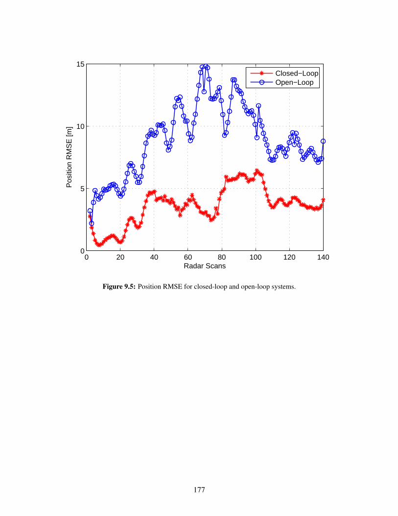
0 20 40 60 80 100 120 1400

5

10

15

Radar Scans

Pos

ition

RM

SE

[m]

Closed−LoopOpen−Loop

Figure 9.5: Position RMSE for closed-loop and open-loop systems.

177

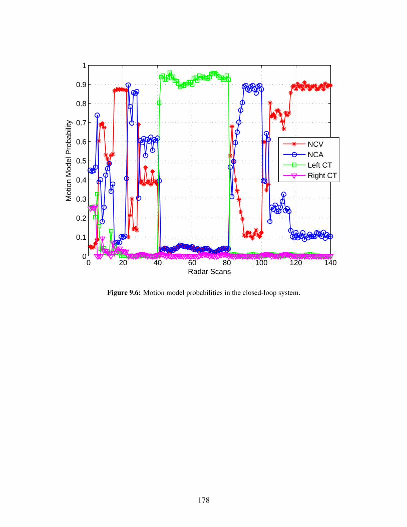
0 20 40 60 80 100 120 1400

0.1

0.2

0.3

0.4

0.5

0.6

0.7

0.8

0.9

1

Radar Scans

Mot

ion

Mod

el P

roba

bilit

y

NCVNCALeft CTRight CT

Figure 9.6: Motion model probabilities in the closed-loop system.

178

Chapter 10

Summary

Detailed conclusion and remarks have already been given at the end of each chapter. Here we

provide a brief summary of the dissertation.

In Chapter 2, we demonstrated the near-optimal EPN recovery for households and retailers

in a real-world community post-hazard. We assumed that the outcome of the recovery decisions

was deterministic. In Chapter 3, we showed that when the recovery of several interdependent in-

frastructures is considered simultaneously, the goal of food security post-hazard can be addressed

from the dimensions of availability and accessibility. Again, the outcome of recovery decision

was assumed to be deterministic. In Chapter 4, we efficiently addressed the more challenging

problem of the outcome of recovery decisions being uncertain for several interdependent infras-

tructure systems. Note that the methods introduced in Chapters 2 to 4 rely on an accurate model

of the world. This model is then implemented as a simulator in an arbitrary computer program-

ming language. For a large-scale planning problem, computational constraints limit the size of the

simulator. Therefore, efficient utilization of simulation budget is important. In contrast to Chap-

ters 2 to 4, which shows the planning of the recovery optimally by searching over all the candidate

recovery decisions exhaustively, Chapter 5 proposes a method to adaptively allocate a limited sim-

ulation budget so that even larger community recovery problems can be handled. We demonstrated

this on the water networks of a real-world community; however, when multiple networks are con-

sidered simultaneously, and the size of the damaged components within the networks along with

the size of the resource units increases, the approach fails. In Chapter 6, we introduced a simple

bypass to this problem by studying building portfolio recovery, where the decisions are planned

non-preemptively, but this approach is not suitable for other infrastructure networks, like EPN and

WN, and when all the networks are considered simultaneously. In Chapter 7, we developed novel

techniques to compute recovery solutions that scale with the size of network and the number of

resource units. Scaling of solutions to massive decision-making problems is non-trivial; in fact,

179

a highly ambitious and difficult problem that is being worked upon by some of the top software

companies in the world. We demonstrated, for the first time, simultaneous management of massive

discrete state, action, and outcome spaces of MDPs. In Chapter 8, we developed solutions to plan

the motion of UAVs with sensors on-board to track multiple targets. Several uncertainties in the

motion of UAVs and the target were considered. We successfully incorporated the feedback from

intelligence assets (can be humans and machines) into the solutions to adaptively plan UAV con-

trols. In Chapter 9, we developed a closed loop framework to track targets in an urban terrain. Ours

is the first, among a rare group of publicly available works, to propose several tracking features

jointly, in an urban environment, in a closed-loop fashion.

180

Bibliography

[1] Mintier Harnish. 2015-2023 HOUSING ELEMENT POLICY DOCUMENT AND BACK-

GROUND REPORT, Dec 2014.

[2] Therese McAllister. Research Needs for Developing a Risk-Informed Methodology for

Community Resilience. J. Struct. Eng., 142(8), 2015.

[3] Michel Bruneau, Stephanie E Chang, Ronald T Eguchi, George C Lee, Thomas D

O’Rourke, Andrei M Reinhorn, Masanobu Shinozuka, Kathleen Tierney, William A Wal-

lace, and Detlof Von Winterfeldt. A Framework to Quantitatively Assess and Enhance the

Seismic Resilience of Communities. Earthq. Spectra, 19(4):733–752, 2003.

[4] Saeed Nozhati, Yugandhar Sarkale, Bruce Ellingwood, Edwin K. P. Chong, and Hussam

Mahmoud. Near-optimal planning using approximate dynamic programming to enhance

post-hazard community resilience management. Reliab. Eng. & Syst. Saf., 181:116 – 126,

2019.

[5] S. Nozhati, Y. Sarkale, B. R. Ellingwood, E. K. P. Chong, and H. Mahmoud. A modified

approximate dynamic programming algorithm for community-level food security following

disasters. In Proc. 9th Int. Congr. Environ. Model. and Softw. (iEMSs 2018), Ft. Collins,

CO, Jun 2018.

[6] Saeed Nozhati, Yugandhar Sarkale, Edwin K. P. Chong, and Bruce R. Ellingwood. Opti-

mal stochastic dynamic scheduling for managing community recovery from natural hazards.

Reliab. Eng. & Syst. Saf., 193, 2020.

[7] Y. Sarkale, S. Nozhati, E. K. P. Chong, B. R. Ellingwood, and H. Mahmoud. Solving markov

decision processes for network-level post-hazard recovery via simulation optimization and

rollout. In 2018 IEEE 14th Int. Conf. Autom. Sci. and Eng.(CASE), pages 906–912, Aug

2018.

181

[8] S. Nozhati, Y. Sarkale, B. R. Ellingwood, E. K. P. Chong, and H. Mahmoud. An approximate

dynamic programming approach to food security of communities following hazards. In

Proc. 13th Int. Conf. Appl. Stat. and Probab. and Civ. Eng. (ICASP 13), Seoul, S. Korea,

May 2019.

[9] Yugandhar Sarkale, Saeed Nozhati, Edwin K. P. Chong, and Bruce R. Ellingwood. Decision

automation for electric power network recovery. arXiv preprint arXiv:1910.00699, 2019.

[10] Y. Sarkale, S. Nozhati, E. K. P. Chong, and B. R. Ellingwood. A parametric simulation

optimization method for decision automation. In 2019 IEEE 15th Int. Conf. Autom. Sci. and

Eng.(CASE) (Special Session on Simulation Optimization in New Information Age), 2019.

[11] Yugandhar Sarkale and Edwin K. P. Chong. Orchestrated management of heterogeneous

sensors incorporating feedback from intelligence assets. In Proc. SPIE Signal Process.,

Sens./Inf. Fusion, and Target Recognit. XXIV, volume 9474, page 94740A. Int. Soc. for Opt.

and Photonics, 2015.

[12] Patricia R Barbosa, Yugandhar Sarkale, Edwin K. P. Chong, Yun Li, Sofia Suvorova, and

Bill Moran. Controlled tracking in urban terrain: Closing the loop. Asian J Control,

21(4):1630–1643, 2019.

[13] S Nozhati, B. R. Ellingwood, H Mahmoud, and J. W. van de Lindt. Identifying and Ana-

lyzing Interdependent Critical Infrastructure in Post-Earthquake Urban Reconstruction. In

Proc. 11th Natl. Conf. Earthq. Eng., Los Angeles, CA, Jun 2018. Earthq. Eng. Res. Inst.

[14] P. Nielsen and N. A. Goodman. Integrated detection and tracking via closed-loop radar with

spatial-domain matched illumination. In 2008 Int. Conf. Radar, pages 546–551, Sep 2008.

[15] Joel A Nachlas. Reliability Engineering: Probabilistic Models and Maintenance Methods.

CRC Press, 2017.

[16] Mykel J Kochenderfer. Decision Making Under Uncertainty: Theory and Application. MIT

Press, 2015.

182

[17] Dimitri P Bertsekas. Dynamic Programming and Optimal Control, volume 1. Athena Sci.

Belmont, MA, 1995.

[18] Konstantinos G Papakonstantinou and Masanobu Shinozuka. Planning structural inspection

and maintenance policies via dynamic programming and markov processes. Part II: POMDP

implementation. Reliab. Eng. & Syst. Saf., 130:214–224, 2014.

[19] Konstantinos G Papakonstantinou and Masanobu Shinozuka. Planning structural inspection

and maintenance policies via dynamic programming and markov processes. Part I: Theory.

Reliab. Eng. & Syst. Saf., 130:202–213, 2014.

[20] Hadi Meidani and Roger Ghanem. Random Markov decision processes for sustainable

infrastructure systems. Struct. and Infrastruct. Eng., 11(5):655–667, 2015.

[21] Dan M Frangopol, Maarten Jan Kallen, and Jan M Van Noortwijk. Probabilistic models

for life-cycle performance of deteriorating structures: review and future directions. Prog.

Struct. Eng. and Mater., 6(4):197–212, 2004.

[22] Hugh Ellis, Mingxiang Jiang, and Ross B Corotis. Inspection, Maintenance, and Repair

with Partial Observability. J. Infrastruct. Syst., 1(2):92–99, 1995.

[23] Ross B Corotis, J Hugh Ellis, and Mingxiang Jiang. Modeling of risk-based inspection,

maintenance and life-cycle cost with partially observable Markov decision processes. Struct.

and Infrastruct. Eng., 1(1):75–84, 2005.

[24] Ehsan Fereshtehnejad and Abdollah Shafieezadeh. A randomized point-based value itera-

tion POMDP enhanced with a counting process technique for optimal management of multi-

state multi-element systems. Struct. Saf., 65:113–125, 2017.

[25] Dimitri P. Bertsekas and John N. Tsitsiklis. Neuro-Dynamic Programming. Athena Sci., 1st

edition, 1996.

183

[26] Kenneth D Kuhn. Network-Level Infrastructure Management Using Approximate Dynamic

Programming. J. Infrastruct. Syst., 16(2):103–111, 2009.

[27] Aditya Medury and Samer Madanat. Incorporating network considerations into pavement

management systems: A case for approximate dynamic programming. Transp. Res. Part C:

Emerg. Technol., 33:134–150, 2013.

[28] Lucian Busoniu, Robert Babuska, Bart De Schutter, and Damien Ernst. Reinforcement

Learning and Dynamic Programming Using Function Approximators, volume 39. CRC

Press, 2010.

[29] Office of the Press Secretary, The White House. Presidential Policy Directive – Critical

Infrastructure Security and Resilience, Feb 2013.

[30] Sergey V Buldyrev, Roni Parshani, Gerald Paul, H Eugene Stanley, and Shlomo Havlin.

Catastrophic cascade of failures in interdependent networks. Nat., 464(7291):1025, 2010.

[31] A Barabadi and Y. Z Ayele. Post-disaster infrastructure recovery: Prediction of recovery

rate using historical data. Reliab. Eng. & Syst. Saf., 169:209–223, 2018.

[32] Duncan J Watts and Steven H Strogatz. Collective dynamics of ‘small-world’ networks.

Nat., 393(6684):440, 1998.

[33] Gian Paolo Cimellaro, D Solari, V Arcidiacono, Chris S Renschler, AM Reinhorn, and

Michel Bruneau. Community resilience assessment integrating network interdependencies.

Earthq. Eng. Res. Inst., Jul 2014.

[34] The Association of Bay Area Governments (City of Gilroy Annex), 2011.

[35] Abhijin Adigaa, Aditya Agashea, Shaikh Arifuzzamana, Christopher L. Barretta, Richard

Beckmana, Keith Bisseta, Jiangzhuo Chena, Youngyun Chungbaeka, Stephen Eubanka, Eep

Guptaa, Maleq Khana, Chris J. Kuhlmana, Henning S. Mortveita, Eric Nordberga, Caitlin

184

Riversa, Paula Stretza, Samarth Swarupa, A Wilsona, and Dawen Xiea. Generating a syn-

thetic population of the United States. Technical report, Jan 2015.

[36] David Kahle and Hadley Wickham. ggmap: Spatial Visualization with ggplot2. The R J.,

5:144—-162, 2013.

[37] National Research Council. Practical Lessons from the Loma Prieta Earthquake. The Natl.

Acad. Press, Washington, DC, 1994.

[38] Nirmal Jayaram and Jack W Baker. Correlation model for spatially distributed ground-

motion intensities. Earthq. Eng. & Struct. Dyn., 38(15):1687–1708, 2009.

[39] Norman Alan Abrahamson, Walter Joseph Silva, and Ronnie Kamai. Update of the AS08

ground-motion prediction equations based on the NGA-West2 data set. Pac. Earthq. Eng.

Res. Cent., 2013.

[40] R. P Kennedy and M. K Ravindra. Seismic fragilities for nuclear power plant risk studies.

Nucl. Eng. and Des., 79(1):47–68, 1984.

[41] Miriam Colombi, Barbara Borzi, Helen Crowley, Mauro Onida, Fabrizio Meroni, and Rui

Pinho. Deriving vulnerability curves using Italian earthquake damage data. Bull. Earthq.

Eng., 6(3):485–504, 2008.

[42] Ajay Singhal and Anne S Kiremidjian. Method for Probabilistic Evaluation of Seismic

Structural Damage. J. Struct. Eng., 122(12):1459–1467, 1996.

[43] KS Jaiswal, W Aspinall, D Perkins, D Wald, and KA Porter. Use of Expert Judgment

Elicitation to Estimate Seismic Vulnerability of Selected Building Types. In Proc. 15th

World Conf. Earthq. Eng., Lisbon, Portugal, Sep 2012.

[44] Department of Homeland Security, Emergency Preparedness and Response Directorate,

FEMA, Mitigation Division. Multi-hazard Loss Estimation Methodology, Earthquake

Model: HAZUS-MH MR1, Advanced Engineering Building Module. Wash., DC, Jan 2003.

185

[45] Liyu Xie, Jue Tang, Hesheng Tang, Qiang Xie, and Songtao Xue. Seismic Fragility Assess-

ment of Transmission Towers via Performance-based Analysis. In Proc. 15th World Conf.

Earthq. Eng., Lisbon, Portugal.

[46] Min Ouyang, Leonardo Dueñas-Osorio, and Xing Min. A three-stage resilience analysis

framework for urban infrastructure systems. Struc. Saf., 36:23–31, 2012.

[47] Dimitri P. Bertsekas. Rollout Algorithms for Discrete Optimization: A Survey, pages 2989–

3013. Springer-Verlag New York, 2013.

[48] Dimitri P. Bertsekas, John N. Tsitsiklis, and Cynara Wu. Rollout Algorithms for Combina-

torial Optimization. J. Heuristics, 3(3):245–262, Dec 1997.

[49] Nikolaos Limnios. Fault Trees. Wiley-ISTE, Mar 2013.

[50] Yanfeng Ouyang and Samer Madanat. Optimal scheduling of rehabilitation activities for

multiple pavement facilities: exact and approximate solutions. Transportation Res. Part A:

Policy and Pract., 38(5):347–365, 2004.

[51] Yajing Liu, Edwin K. P Chong, and Ali Pezeshki. Bounding the greedy strategy in finite-

horizon string optimization. In 2015 IEEE 54th Annu. Conf. Decis. and Control (CDC),

pages 3900–3905. IEEE, 2015.

[52] Hassan Masoomi and John W van de Lindt. Restoration and functionality assessment of a

community subjected to tornado hazard. Struct. and Infrastruct. Eng., 14(3):275–291, 2018.

[53] R. A. Howard. Dynamic Programming and Markov Processes. MIT Press, Camb., MA,

1960.

[54] Gerald Tesauro and Gregory R. Galperin. On-line Policy Improvement using Monte-Carlo

Search. In M. C. Mozer, M. I. Jordan, and T. Petsche, editors, Advances in Neural Informa-

tion Processing Systems 9, pages 1068–1074. MIT Press, 1997.

186

[55] B. Abramson. Expected-Outcome: A General Model of Static Evaluation. IEEE Trans.

Pattern Anal. and Mach. Intell., 12(2):182–193, Feb 1990.

[56] S. Ragi, H. D. Mittelmann, and E. K. P. Chong. Directional Sensor Control: Heuristic

Approaches. IEEE Sens. J., 15(1):374–381, Jan 2015.

[57] Dimitri P. Bertsekas. Rollout Algorithms for Constrained Dynamic Programming. Technical

report, Lab. Inf. & Decis. Syst., Apr 2005.

[58] Erin Biehl, Sarah Buzogany, Alice Huang, Gwen Chodur, and Roni Neff. Baltimore food

system resilience advisory report. Baltimore, MD: Johns Hopkins Center for a Livable

Future and Baltimore Office of Sustainability, 2017.

[59] Xin-She Yang. Engineering optimization: an introduction with metaheuristic applications.

John Wiley & Sons, 2010.

[60] Roy Baumeister. The psychology of irrationality: Why people make foolish, self-defeating

choices. The psychology of economic decisions, 1:3–16, 2003.

[61] Warren B Powell. Approximate Dynamic Programming: Solving the curses of dimensional-

ity, volume 703. John Wiley & Sons, 2007.

[62] Hyeong Soo Chang, Jiaqiao Hu, Michael C Fu, and Steven I Marcus. Simulation-based

algorithms for Markov decision processes. Springer Science & Business Media, 2013.

[63] Lucian Busoniu, Robert Babuska, Bart De Schutter, and Damien Ernst. Reinforcement

learning and dynamic programming using function approximators. CRC press, 2017.

[64] Dimitri P. Bertsekas and David A. Castanon. Rollout algorithms for stochastic scheduling

problems. J. Heuristics, 5(1):89–108, Apr 1999.

[65] Louis JM Aslett. MCMC for inference on phase-type and masked system lifetime models.

PhD thesis, Trinity College Dublin, 2012.

187

[66] Amos Tversky and Daniel Kahneman. Advances in prospect theory: Cumulative represen-

tation of uncertainty. Journal of Risk and uncertainty, 5(4):297–323, 1992.

[67] Eun Jeong Cha and Bruce R Ellingwood. Risk-averse decision-making for civil infrastruc-

ture exposed to low-probability, high-consequence events. Reliability Engineering & System

Safety, 104:27–35, 2012.

[68] Arnab Nilim and Laurent El Ghaoui. Robust control of markov decision processes with

uncertain transition matrices. Operations Research, 53(5):780–798, 2005.

[69] Garud N Iyengar. Robust dynamic programming. Mathematics of Operations Research,

30(2):257–280, 2005.

[70] Tao Sun, Qianchuan Zhao, and Peter B. Luh. A Rollout Algorithm for Multichain Markov

Decision Processes with Average Cost. In Rafael Bru and Sergio Romero-Vivó, editors,

Posit. Syst. Springer Berl. Heidelb., 2009.

[71] Laurent Péret and Frédérick Garcia. Online Resolution Techniques. Markov Decis. Process.

in Artif. Intell., pages 153–184, 2010.

[72] Martin L. Puterman. Markov Decision Processes: Discrete Stochastic Dynamic Program-

ming. John Wiley & Sons, Inc., N. Y., NY, USA, 1st edition, 1994.

[73] Richard Bellman. Dynamic Programming. Princet. Univ. Press, Princet., NJ, USA, 1 edition,

1957.

[74] L. S. Shapley. Stochastic games. Proc. of the Nat. Acad. of Sci., 39(10):1095–1100, 1953.

[75] Lodewijk Kallenberg. Finite state and action MDPs. In Handb. of Markov Decis.Process.,

pages 21–87. Springer, 2003.

[76] Alan Fern, Sungwook Yoon, and Robert Givan. Approximate policy iteration with a policy

language bias: Solving relational Markov decision processes. J. Artif. Intell. Res., 25:75–

118, 2006.

188

[77] Saeed Nozhati, Bruce Ellingwood, Hussam Mahmoud, Yugandhar Sarkale, Edwin K. P.

Chong, and Nathanael Rosenheim. An approximate dynamic programming approach to

community recovery management. In Eng. Mech. Inst. Conf. (EMI 2018), Camb. - Boston,

MA, May – Jun 2018.

[78] Michail G Lagoudakis and Ronald Parr. Reinforcement learning as classification: Leverag-

ing modern classifiers. In Proc. of the 20th Int. Conf. on Mach. Learn. (ICML-03), pages

424–431, 2003.

[79] Christos Dimitrakakis and Michail G. Lagoudakis. Algorithms and bounds for rollout sam-

pling approximate policy iteration. In Sertan Girgin, Manuel Loth, Rémi Munos, Philippe

Preux, and Daniil Ryabko, editors, Recent Adv. in Reinf. Learn., pages 27–40, Berl., Hei-

delb., 2008. Springer Berl. Heidelb.

[80] M. C. Fu, C. H. Chen, and L. Shi. Some topics for simulation optimization. In 2008 Winter

Simul. Conf., pages 27–38, Dec 2008.

[81] Christos Dimitrakakis and Michail G. Lagoudakis. Rollout sampling approximate policy

iteration. Mach. Learn., 72(3):157–171, Sep 2008.

[82] Christos Dimitrakakis and Michail G. Lagoudakis. Algorithms and bounds for rollout sam-

pling approximate policy iteration. CoRR, abs/0805.2015, 2008.

[83] Alessandro Lazaric, Mohammad Ghavamzadeh, and Rémi Munos. Analysis of

classification-based policy iteration algorithms. J. of Mach. Learn. Res., 17(19):1–30, 2016.

[84] Jürgen Branke, Stephen E. Chick, and Christian Schmidt. Selecting a selection procedure.

Manage. Sci., 53(12):1916–1932, 2007.

[85] Chun-Hung Chen, Jianwu Lin, Enver Yücesan, and Stephen E. Chick. Simulation budget

allocation for further enhancing the efficiency of ordinal optimization. Discret. Event Dyn.

Syst., 10(3):251–270, Jul 2000.

189

[86] Chun-Hung Chen, S. D. Wu, and L. Dai. Ordinal comparison of heuristic algorithms using

stochastic optimization. IEEE Trans. Robot. Autom., 15(1):44–56, Feb 1999.

[87] FAO. The state of food insecurity in the world (rome: Fao), 2001.

[88] David Seekell, Joel Carr, Jampel Dell’Angelo, Paolo D’Odorico, Marianela Fader, Jessica

Gephart, Matti Kummu, Nicholas Magliocca, Miina Porkka, Michael Puma, et al. Re-

silience in the global food system. Environmental Research Letters, 12(2):025010, 2017.

[89] V. Oliveira. The food assistance landscape: Fy 2016 annual report, 2017.

[90] Food Research and Action Center. An advocate’s guide to the disaster supplemental nutri-

tion assistance program, 2017.

[91] Rebekah Paci-Green and Gigi Berardi. Do global food systems have an achilles heel? the

potential for regional food systems to support resilience in regional disasters. Journal of

Environmental Studies and Sciences, 5(4):685–698, 2015.

[92] Peihui Lin and Naiyu Wang. Stochastic post-disaster functionality recovery of community

building portfolios i: Modeling. Structural Safety, 69:96–105, 2017.

[93] Saeed Nozhati, Nathanael Rosenheim, Bruce R. Ellingwood, Hussam Mahmoud, and Maria

Perez. Probabilistic framework for evaluating food security of households in the aftermath

of a disaster. Struct. Infrastructure Eng., 15(8):1060–1074, 2019.

[94] Marshall L. Fisher, R. Jaikumar, and Luk N. Van Wassenhove. A multiplier adjustment

method for the generalized assignment problem. Manag. Sci., 32(9):1095–1103, 1986.

[95] David B. Shmoys and Éva Tardos. An approximation algorithm for the generalized assign-

ment problem. Math. Program., 62(1):461–474, Feb 1993.

[96] David Silver and Joel Veness. Monte-Carlo planning in large POMDPs. In J. D. Lafferty,

C. K. I. Williams, J. Shawe-Taylor, R. S. Zemel, and A. Culotta, editors, Adv. Neural Inf.

Process. Syst. 23, pages 2164–2172. Curran Associates, Inc., 2010.

190

[97] Gregory S Berns, David Laibson, and George Loewenstein. Intertemporal choice–toward

an integrative framework. Trends Cogn. Sci., 11(11):482–488, 2007.

[98] Milos Hauskrecht and Branislav Kveton. Linear program approximations for factored

continuous-state Markov decision processes. In S. Thrun, L. K. Saul, and B. Schölkopf,

editors, Adv. Neural Inf. Process. Syst. 16, pages 895–902. MIT Press, 2004.

[99] Yangchen Pan, Adam White, and Martha White. Accelerated gradient temporal difference

learning. In Proc. 31st AAAI Conf. Artif. Intell., AAAI’17, pages 2464–2470. AAAI Press,

2017.

[100] Spencer M. Free and James W. Wilson. A mathematical contribution to structure-activity

studies. J. Medicinal Chem., 7(4):395–399, 1964.

[101] Thomas Kailath, Ali H Sayed, and Babak Hassibi. Linear Estimation. Number EPFL-

BOOK-233814. Prentice Hall, 2000.

[102] Edwin K. P. Chong and Stanislaw H. Zak. An Introduction to Optimization, Fourth Edition.

John Wiley & Sons, Inc., New York, USA, 2013.

[103] Richard Bellman, Robert Kalaba, and Bella Kotkin. Polynomial approximation-a new com-

putational technique in dynamic programming - I. Allocation processes. Technical report,

RAND Corp. Santa Monica, CA, 1962.

[104] E. Stiefel. Note on Jordan elimination, linear programming and Tchebycheff approximation.

Numer. Math., 2(1):1–17, December 1960.

[105] Carlos Guestrin, Daphne Koller, and Ronald Parr. Max-norm projections for factored MDPs.

In Proc. 17th Int. Jt. Conf. Artif. Intell. - Volume 1, IJCAI’01, pages 673–680, San Francisco,

CA, USA, 2001. Morgan Kaufmann Publishers Inc.

[106] Anselm Blumer, Andrzej Ehrenfeucht, David Haussler, and Manfred K. Warmuth. Occam’s

razor. Inf. Process. Lett., 24(6):377 – 380, 1987.

191

[107] Q. Jia. Efficient computing budget allocation for simulation-based policy improvement.

IEEE Trans. Autom. Sci. Eng., 9(2):342–352, April 2012.

[108] W. Chen, S. Gao, C. Chen, and L. Shi. An optimal sample allocation strategy for partition-

based random search. IEEE Trans. Autom. Sci. Eng., 11(1):177–186, Jan 2014.

[109] H. Xiao, L. H. Lee, and K. M. Ng. Optimal computing budget allocation for complete

ranking. IEEE Trans. Autom. Sci. Eng., 11(2):516–524, April 2014.

[110] F. Gao, S. Gao, H. Xiao, and Z. Shi. Advancing constrained ranking and selection with

regression in partitioned domains. IEEE Trans. Autom. Sci. Eng., 16(1):382–391, Jan 2019.

[111] Y. Liu, G. Pedrielli, H. Li, L. H. Lee, C. Chen, and J. F. Shortle. Optimal computing

budget allocation for stochastic N–k problem in the power grid system. IEEE Trans. Reliab.,

68(3):778–789, Sep. 2019.

[112] Sébastien Bubeck and Nicolò Cesa-Bianchi. Regret analysis of stochastic and nonstochastic

multi-armed bandit problems. Found. Trends R© Mach. Learn., 5(1):1–122, 2012.

[113] Eyal Even-Dar, Shie Mannor, and Yishay Mansour. PAC bounds for multi-armed bandit and

Markov decision processes. In Jyrki Kivinen and Robert H. Sloan, editors, Computational

Learning Theory, COLT ’02, pages 255–270, Berlin, Heidelberg, 2002. Springer Berlin

Heidelberg.

[114] Peter Auer, Nicolò Cesa-Bianchi, and Paul Fischer. Finite-time analysis of the multiarmed

bandit problem. Mach. Learn., 47(2):235–256, May 2002.

[115] Sébastien Bubeck, Rémi Munos, and Gilles Stoltz. Pure exploration in multi-armed bandits

problems. In Ricard Gavaldà, Gábor Lugosi, Thomas Zeugmann, and Sandra Zilles, edi-

tors, Algorithmic Learning Theory, pages 23–37, Berlin, Heidelberg, 2009. Springer Berlin

Heidelberg.

192

[116] Y. Peng, C. Chen, E. K. P. Chong, and M. C. Fu. A review of static and dynamic optimization

for ranking and selection. In 2018 Winter Simul. Conf. (WSC), pages 1909–1920, Dec 2018.

[117] Diana M Negoescu, Peter I Frazier, and Warren B Powell. The knowledge-gradient algo-

rithm for sequencing experiments in drug discovery. INFORMS J. Comput., 23(3):346–363,

2011.

[118] Gabriel Dulac-Arnold, Richard Evans, Hado van Hasselt, Peter Sunehag, Timothy Lillicrap,

Jonathan Hunt, Timothy Mann, Theophane Weber, Thomas Degris, and Ben Coppin. Deep

reinforcement learning in large discrete action spaces. arXiv preprint arXiv:1512.07679,

2015.

[119] Hyeong Soo Chang, Robert Givan, and Edwin K. P. Chong. Parallel rollout for online

solution of partially observable Markov decision processes. Discret. Event Dyn. Syst.,

14(3):309–341, Jul 2004.

[120] E. K. P. Chong, C. Kreucher, and A. O. Hero. Partially observable Markov decision process

approximations for adaptive sensing. Discrete Event Dynamic Systems, 19:377–422, 2009.

[121] S. A. Miller, Z. A. Harris, and E. K. P. Chong. A POMDP framework for coordinated

guidance of autonomous UAVs for multitarget tracking. EURASIP Journal on Advances in

Signal Processing, 2009, 2009.

[122] S. Ragi and E. K. P. Chong. Dynamic UAV path planning for multitarget tracking. In Proc.

2012 American Control Conference, pages 3845–3850, Montreal, Canada, June 2012.

[123] S. Blackman and R. Popoli. Design and Analysis of Modern Tracking Systems. Artech

House, Boston, MA, 1999.

[124] Y. Bar-Shalom, X. R. Li, and T. Kirubarajan. Estimation with Applications to Tracking and

Navigation. Wiley-Interscience, NY, 2001.

193

[125] S. Ragi and E. K. P. Chong. UAV path planning in a dynamic environment via partially

observable Markov decision process. IEEE Trans. Aerosp. Electron. Syst., 49:2397–2412,

2013.

[126] B. R. Geiger, J. F. Horn, A. M. DeLullo, and L. N. Long. Optimal path planning of UAVs

using direct collocation with nonlinear programming. In Proc. AIAA Guidance, Navigation,

and Control Conf., Keystone, CO, 2006.

[127] Y. Bar-Shalom and T. E. Fortmann. Tracking and Data Association. Academic Press Inc.,

London, UK, 1988.

[128] R. Bellman. Dynamic Programming. Princeton University Press, Princeton, New Jersey,

USA, 1957.

[129] J. Nocedal and S. J. Wright. Numerical Optimization, Second Edition. Springer, 2006.

[130] A. R. Conn, G. I. .M .Gould, and P. L. Toint. LANCELOT: A FORTRAN package for large-

scale nonlinear optimization (Release A). Springer-Verlag, New York, 1992.

[131] D. P. Bertsekas. Dynamic Programming and Optimal Control vol. 2. Athena Scientific,

Belmont, Massachusetts, USA, 2007.

[132] T. Oliveira, A. P. Aguiar, and P. Encarnação. Moving Path Following for Unmanned Aerial

Vehicles With Applications to Single and Multiple Target Tracking Problems. IEEE Trans.

Robot., 32(5):1062–1078, Oct 2016.

[133] J. Yan, H. Liu, B. Jiu, B. Chen, Z. Liu, and Z. Bao. Simultaneous Multibeam Resource Al-

location Scheme for Multiple Target Tracking. IEEE Trans. Signal Process., 63(12):3110–

3122, Jun 2015.

[134] J. Yan, H. Liu, W. Pu, S. Zhou, Z. Liu, and Z. Bao. Joint Beam Selection and Power

Allocation for Multiple Target Tracking in Netted Colocated MIMO Radar System. IEEE

Trans. Signal Process., 64(24):6417–6427, Dec 2016.

194

[135] John N Sanders-Reed. Multitarget multisensor closed-loop tracking. In Proc. SPIE Acquis.,

Track., and Pointing XVIII, volume 5430, pages 94–113. Int. Soc. for Opt. and Photonics,

2004.

[136] S. M. O’Rourke and A. L. Swindlehurst. Closed-loop tracking using multimodal RF/EO

sensors. In 2010 Conf. Rec. 44th Asilomar Conf. Signals, Syst. and Comput., pages 1662–

1666, Nov 2010.

[137] C. Deng, Y. Mao, W. Ren, and G. Ren. Feedforward control based on orthogonal least square

for a charge-coupled device-based tracking loop. In 2017 Chin. Autom. Congr. (CAC), pages

6877–6881. IEEE, Oct 2017.

[138] L. J. Beeton and S. L. Hall. Closed loop tracking systems for naval applications. In The IEE

Semin. Target Track.: Algorithms and Appl. (Ref. No. 2006/11359), pages 115–122, Mar

2006.

[139] Khoshnam Shojaei and Mehdi Dolatshahi. Line-of-sight target tracking control of underac-

tuated autonomous underwater vehicles. Ocean Eng., 133:244 – 252, 2017.

[140] Ying He and Edwin K. P. Chong. Sensor scheduling for target tracking: A Monte Carlo

sampling approach. Digit. Signal Process., 16(5):533 – 545, 2006. Special Issue on DASP

2005.

[141] Y. Li, L.W. Krakow, Edwin K. P. Chong, and K.N. Groom. Approximate stochastic dy-

namic programming for sensor scheduling to track multiple targets. Digit. Signal Process.,

19(6):978 – 989, 2009. DASP’06 - Def. Appl. of Signal Process.

[142] D. J. Kershaw and R. J. Evans. Optimal waveform selection for tracking systems. IEEE

Trans. on Inf. Theory, 40(5):1536–1550, Sep 1994.

[143] S. Suvorova, D. Musicki, B. Moran, S. Howard, and B. La Scala. Multi step ahead beam

and waveform scheduling for tracking of manoeuvering targets in clutter. In Proc. IEEE Int.

195

Conf. Acoust., Speech, and Signal Process., 2005. (ICASSP ’05)., volume 5, pages 889–892,

Mar 2005.

[144] Shankarachary Ragi and Edwin K. P. Chong. Decentralized Guidance Control of UAVs

with Explicit Optimization of Communication. J. Intell. Robot. Syst., 73(1-4):811–822, Jan

2014.

[145] T. Kirubarajan, Y. Bar-Shalom, W. D. Blair, and G. A. Watson. IMMPDA solution to bench-

mark for radar resource allocation and tracking in the presence of ECM. In 1997 Eur. Con-

trol Conf. (ECC), pages 2967–2972, July 1997.

[146] T Sathyan, K Bharadwaj, A Sinha, and T Kirubarajan. Intelligence-aided multitarget track-

ing for urban operations - a case study: counter terrorism. In Proc. SPIE Sens., and Com-

mand, Control, Commun., and Intell. (C3I) Technol. Homel. Secur. and Homel. Def. V,

volume 6201, page 62010M. Int. Soc. for Opt. and Photonics, 2006.

[147] J. R. Guerci and E. J. Baranoski. Knowledge-aided adaptive radar at DARPA: an overview.

IEEE Signal Process. Mag., 23(1):41–50, Jan 2006.

[148] B. Chakraborty, Y. Li, J. J. Zhang, T. Trueblood, A. Papandreou-Suppappola, and D. Mor-

rell. Multipath exploitation with adaptive waveform design for tracking in urban terrain. In

2010 IEEE Int. Conf. Acoust., Speech and Signal Process., pages 3894–3897, Mar 2010.

[149] B. Chakraborty, J. J. Zhang, A. Papandreou-Suppappola, and D. Morrell. Urban terrain

tracking in high clutter with waveform-agility. In 2011 IEEE Int. Conf. Acoust., Speech and

Signal Process. (ICASSP), pages 3640–3643, May 2011.

[150] M. Zhou, J. J. Zhang, and A. Papandreou-Suppappola. Multiple Target Tracking in Urban

Environments. IEEE Trans. Signal Process., 64(5):1270–1279, Mar 2016.

[151] Jiun-Fu Chen, Chieh-Chih Wang, and Cheng-Fu Chou. Multiple target tracking in occlusion

area with interacting object models in urban environments. Robot. and Auton. Syst., 103:68

– 82, 2018.

196

[152] J. P. Ramirez-Paredes, E. A. Doucette, J. W. Curtis, and N. R. Gans. Urban target search and

tracking using a UAV and unattended ground sensors. In 2015 Am. Control Conf. (ACC),

pages 2401–2407, Jul 2015.

[153] Patrick Emami, Panos M Pardalos, Lily Elefteriadou, and Sanjay Ranka. Machine Learn-

ing Methods for Solving Assignment Problems in Multi-Target Tracking. arXiv preprint:

1802.06897, 2018. submitted to ACM Compute. Surv.

[154] Patricia R. Barbosa, Edwin K. P. Chong, Sofia Suvorova, and Bill Moran. Multitarget-

multisensor tracking in an urban environment: A closed-loop approach. In Proc. SPIE

Signal and Data Process. Small Targets, volume 6969, page 69690W. Int. Soc. for Opt. and

Photonics, 2008.

[155] Phani Chavali and Arye Nehorai. Compressive Sensing for Urban Radar, chapter 10, page

327. CRC Press, 2017.

[156] X. Rong Li and V. P. Jilkov. Survey of maneuvering target tracking. Part i. Dynamic models.

IEEE Trans. Aerosp. and Electron. Syst., 39(4):1333–1364, Oct 2003.

[157] John Proakis and Massoud Salehi. Digital Communications. McGraw Hill, 5th edition,

2008.

[158] Tetsuo Asano, Danny Z. Chen, Naoki Katoh, and Takeshi Tokuyama. Polynomial-time So-

lutions to Image Segmentation. In Proc. 7th Annu. ACM-SIAM Symp. Discret. Algorithms,

SODA ’96, pages 104–113, Phila., PA, USA, 1996. Soc. for Ind. and Appl. Math.

[159] Kevin J Sangston, Fulvio Gini, and Maria S Greco. Coherent radar target detection in heavy-

tailed compound-Gaussian clutter. IEEE Trans. on Aerosp. and Electron. Syst., 48(1):64–77,

2012.

[160] Ruixin Niu, Peter Willett, and Y Bar-Shalom. System level performance of radar wave-

forms. In Proc. 1999 Mediterr. Conf. Control and Autom., 1999.

197

[161] H. Sidenbladh. Multi-target particle filtering for the probability hypothesis density. In Proc.

6th Int. Conf. Inf. Fusion, volume 2, pages 800–806, July 2003.

[162] Y. Bar-Shalom. Multitarget-multisensor tracking: Advanced applications. Norwood, MA,

Artech House, 1990.

[163] X. Rong Li and Y. Bar-Shalom. Tracking in clutter with nearest neighbor filters: Analysis

and performance. IEEE Trans. Aerosp. and Electron. Syst., 32(3):995–1010, Jul 1996.

[164] T. Kirubarajan, Y. Bar-Shalom, K. R. Pattipati, and I. Kadar. Ground target tracking with

variable structure IMM estimator. IEEE Trans. Aerosp. and Electron. Syst., 36(1):26–46,

Jan 2000.

[165] X. Rong Li and V. P. Jilkov. Survey of maneuvering target tracking. Part V. Multiple-model

methods. IEEE Trans. Aerosp. and Electron. Syst., 41(4):1255–1321, Oct 2005.

[166] S. J. Julier and J. K. Uhlmann. Unscented filtering and nonlinear estimation. Proc. IEEE,

92(3):401–422, Mar 2004.

[167] Yong-Shik Kim and Keum-Shik Hong. An IMM algorithm for tracking maneuvering vehi-

cles in an adaptive cruise control environment. Int. J. Control, Autom., and Syst., 2(3):310–

318, 2004.

[168] D. Musicki and S. Suvorova. Tracking in clutter using IMM-IPDA-based algorithms. IEEE

Trans. Aerosp. and Electron. Syst., 44(1):111–126, Jan 2008.

[169] D. Musicki and B. La Scala. Multi-target tracking in clutter without measurement assign-

ment. IEEE Trans. Aerosp. and Electron. Syst., 44(3):877–896, Jul 2008.

[170] D. Musicki, R. Evans, and S. Stankovic. Integrated probabilistic data association. IEEE

Trans. Autom. Control, 39(6):1237–1241, Jun 1994.

[171] Harry L. Van Trees, K. L. Bell, and Z. Tian (with). Detection Estimation and Modulation

Theory, Part I: Detection, Estimation, and Filtering Theory. Wiley, 2nd edition, Apr 2013.

198