Uncertainty Quantification for Decision Making in Early Design ...

Uncertainty quantification for decision making in earlydesign phase for passive and active vibration isolation

R. Platz 1, C. Melzer 2

1 Fraunhofer Institute for Structural Durability and SystemReliability LBF,Bartningstrasse 47, D-64289 Darmstadt, Germanye-mail: : [email protected]

2Technische Universitat Darmstadt, System Reliability and Machine Acoustics SzM,Magdalenenstrasse 4, D-64289 Darmstadt, Germany

AbstractThe authors compare direct probability and non-probability parametric uncertainty analysis for decisionmaking in early design phase of passive and active vibrationisolation in suspension struts. A simplemathematical one degree of freedom linear model of an automobile’s suspension leg with harmonic basepoint excitation and subject to passive and active vibration isolation is used as an example to answer threebasic questions: which simple and direct yet adequate methodological tool to quantify data uncertaintyanalysis is reasonable for decision making in early design phase? What is the difference between uncertaintyin the passive and in the active vibration isolation approach and what is the confidence level analyzing thedifference? Is the data uncertainty quantification in earlydesign sufficient and to what extend it is needed toquantify model uncertainty for decision making?

1 Introduction

The evaluation of uncertainty becomes predominant for decision making in defining the product’s propertiesin early design phases. The more ambitious new and innovative ideas are, the less experience and, therefore,less knowledge about similar concepts is available, there is an information gap, [1]. Decision makers needadequate tools, simple but sufficient enough to chose between different concepts in the early design phasewhere knowledge is, in most cases, limited. One approach to evaluate uncertainty in early developmentphase could be the representation of uncertainty in processchains for its qualitative disclosure within theproducts lifetime, [2] and [3]. However, a quantitative approach would lead to more assurances, especiallyfor decision making in early design phase. For example, if a decision has to be made between passive,active or semi-active designs today, the authors observe that the active approach is favored many timesbecause of its increasing manifoldness and popularity using smart materials and systems that are usedin active systems. However, increasing possibility and popularity may overlook advantages of the moreconventional, and often less expensive and more reliable passive alternatives with similar good performance,for example for vibration attenuation with energy absorbing material or compensators [4]. Active systemsbecome more complex, e. g. additional electric energy for actuators, sensors, and control, [5]. The activesystem’s functionality is versatile, however, it depends on these additional features with additional functionaluncertainty compared to the, in most cases, more simple passive approach. Favoring active over passivesolutions should be built on solid ground, taking also into account evaluation and comparison of uncertaintyfor both approaches like in [6]. It is the general desire thatuncertainty decreases when going active. However,

4501

the increasing callbacks for complex and often active systems for example in the automotive industry tellanother story, [7].

In [8], the authors showed analytically that active controlmay lead to a vibration isolation ability withless deviation in amplitude and phase responses than with passive control using direct MONTE CARLO

simulation. This was seen throughout the range of the exciting frequencyΩ when sweeping through theundamped angular resonance frequencyΩ = ω0 until angular excitation frequencies are beyond the angularisolation frequency withΩ > ωiso =

√2ω0. However, this was only a first and rough analytical approach

that did not go deeper into the comparison between passive and active vibration attenuation potential underparametric uncertainty at various significant dynamic properties. The authors looked at amplitudes at thedamped angular eigenfrequencyωD, at the angular isolation frequencyωiso, at an amplitude attenuationof -15 dB and at the ability for a fast decaying time to reach damped steady state vibrations after initialexcitation. Though, the authors neglected to look closely to the quality of MONTE CARLO simulations interms of confidence levels when using assumed sample trails.

In a second contribution [9], the authors used theχ2-Test to validate normal distribution assumptions of themodel’s input parameters and evaluate the computational adequacy when using 100 samples and10 000 persample trials as well as the simulation’s practicability with respect to computational cost in time. Variationsof characteristic properties in frequency and in time domain of vibration isolation caused by the varyingmodel input parameters were studied for six different casesat certain characteristic frequency ranges like atresonance or isolation frequency for passive and active vibration isolation. The contribution showed that,generally, the tendency of varying standard deviations forpassive and active vibration isolation approacheswith respect to characteristic amplitudes and angular frequencies due to the damping properties is notrelevantly affected by using low or high sampling rates, with 100 or 10 000 samples. What is more, highactive damping results in high amplitude deviation at the angular isolation frequency, but results in lessdeviation at angular frequencies beyond the isolation point compared to the passive approach. Also, thedeviation of the amplitude attenuation beyond the angular isolation frequency is less with the active approach.As far as the numerical comparison of uncertainty in passiveand active vibration isolation is concerned, theactive approach is not necessarily accompanied with less uncertainty throughout a wide angular frequencyrange even beyond the isolation starts. Especially close atthe angular frequency when vibration isolationstarts, the active approach appears to be uncertain with increasing active damping.

Now, in this third contribution and before validating the mathematical preliminary work with experimentalresults, the authors compare the direct probabilistic approach conducted in [8] and [9] with also directnon-probabilistic approaches using direct interval and fuzzy as well as simplified worst case analysis. Theauthors concentrate only on uncertainty for

– varying amplitudes and phase shifts at the excitation frequency beyond the passive system’s fixedisolation frequency,

– varying vibration amplitudes and phase shifts at the undamped resonance frequency and

– varying amplitudes and phase shifts for -15 dB isolation attenuation.

The quality and confidence of predictions of the dynamic responses via probabilistic and non-probabilisticanalyses and the computational cost conducting the approaches are discussed.

4502 PROCEEDINGS OF ISMA2016 INCLUDING USD2016

2 Linear mathematical model of a mass-damper-spring system forpassive and active vibration isolation

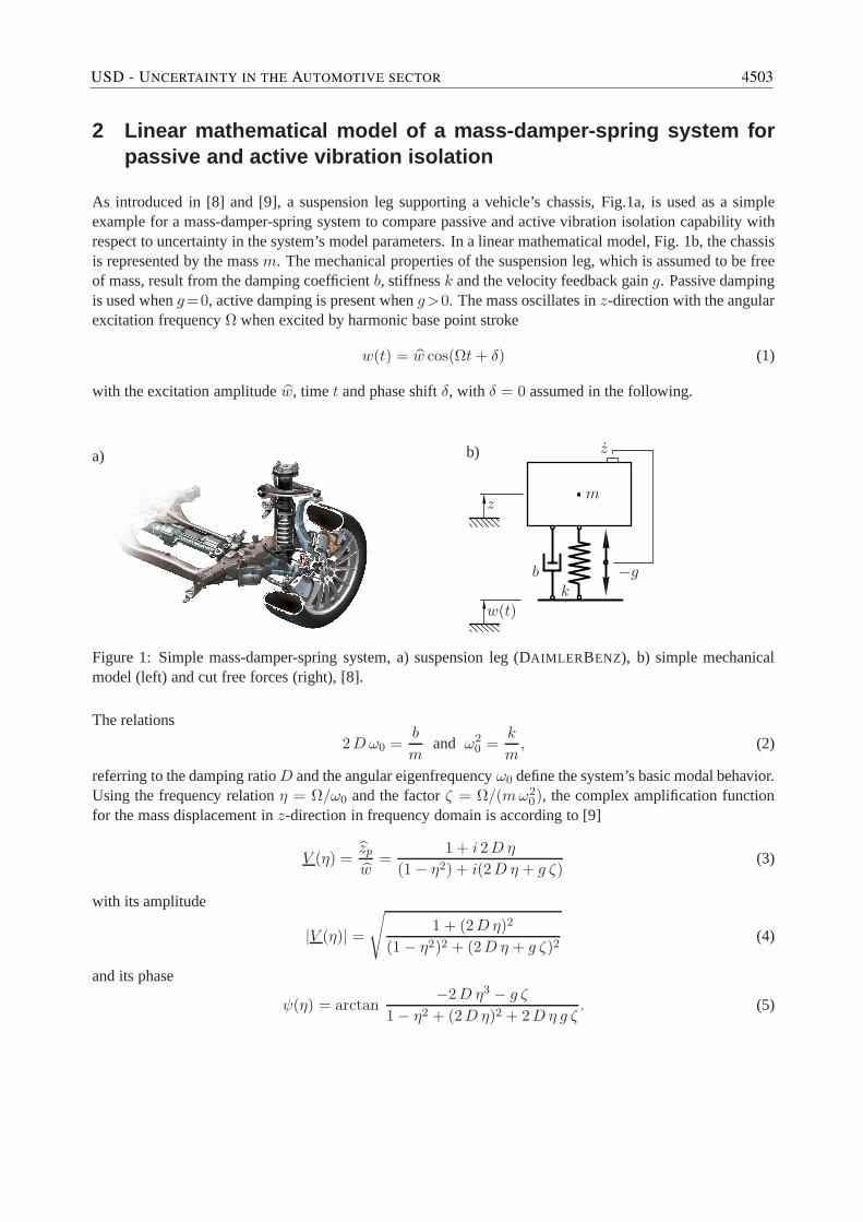
As introduced in [8] and [9], a suspension leg supporting a vehicle’s chassis, Fig.1a, is used as a simpleexample for a mass-damper-spring system to compare passiveand active vibration isolation capability withrespect to uncertainty in the system’s model parameters. Ina linear mathematical model, Fig. 1b, the chassisis represented by the massm. The mechanical properties of the suspension leg, which is assumed to be freeof mass, result from the damping coefficientb, stiffnessk and the velocity feedback gaing. Passive dampingis used wheng=0, active damping is present wheng>0. The mass oscillates inz-direction with the angularexcitation frequencyΩ when excited by harmonic base point stroke

w(t) = w cos(Ωt+ δ) (1)

with the excitation amplitudew, time t and phase shiftδ, with δ = 0 assumed in the following.

a) b)

w(t)

z

bk

−g

z

m

Figure 1: Simple mass-damper-spring system, a) suspensionleg (DAIMLER BENZ), b) simple mechanicalmodel (left) and cut free forces (right), [8].

The relations

2Dω0 =b

mand ω2

0 =k

m, (2)

referring to the damping ratioD and the angular eigenfrequencyω0 define the system’s basic modal behavior.Using the frequency relationη = Ω/ω0 and the factorζ = Ω/(mω2

0), the complex amplification functionfor the mass displacement inz-direction in frequency domain is according to [9]

V (η) =zpw

=1 + i 2D η

(1− η2) + i(2D η + g ζ)(3)

with its amplitude

|V (η)| =√

1 + (2Dη)2

(1− η2)2 + (2D η + g ζ)2(4)

and its phase

ψ(η) = arctan−2D η3 − g ζ

1− η2 + (2D η)2 + 2Dη g ζ. (5)

USD - UNCERTAINTY IN THE AUTOMOTIVE SECTOR 4503

3 Deterministic and non-deterministic amplitude and phaserepresentation for passive and active vibration isolation

3.1 Deterministic amplitude and phase representation

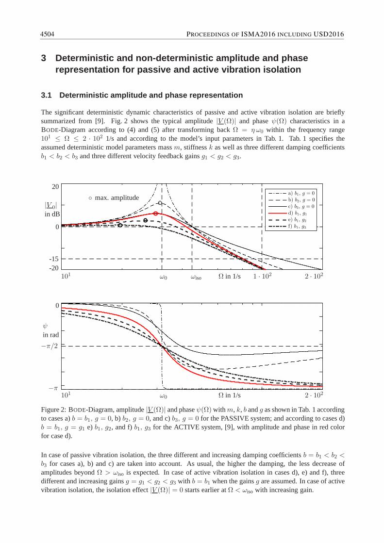
The significant deterministic dynamic characteristics of passive and active vibration isolation are brieflysummarized from [9]. Fig. 2 shows the typical amplitude|V (Ω)| and phaseψ(Ω) characteristics in aBODE-Diagram according to (4) and (5) after transforming backΩ = η ω0 within the frequency range101 ≤ Ω ≤ 2 · 102 1/s and according to the model’s input parameters in Tab. 1. Tab. 1 specifies theassumed deterministic model parameters massm, stiffnessk as well as three different damping coefficientsb1 < b2 < b3 and three different velocity feedback gainsg1 < g2 < g3.

a) b1, g = 0

b) b2, g = 0

c) b3, g = 0

d) b1, g1e) b1, g2f) b1, g3

max. amplitude

20

|V 0|in dB

0

-15-20

101 ω0 ωiso 1 · 102 2 · 102Ω in 1/s

0

ψ

in rad

−π/2

−π101 ω0 2 · 102Ω in 1/s

Figure 2: BODE-Diagram, amplitude|V (Ω)| and phaseψ(Ω) withm, k, b andg as shown in Tab. 1 accordingto cases a)b = b1, g = 0, b) b2, g = 0, and c)b3, g = 0 for the PASSIVE system; and according to cases d)b = b1, g = g1 e) b1, g2, and f)b1, g3 for the ACTIVE system, [9], with amplitude and phase in red colorfor case d).

In case of passive vibration isolation, the three differentand increasing damping coefficientsb = b1 < b2 <b3 for cases a), b) and c) are taken into account. As usual, the higher the damping, the less decrease ofamplitudes beyondΩ > ωiso is expected. In case of active vibration isolation in cases d), e) and f), threedifferent and increasing gainsg = g1 < g2 < g3 with b = b1 when the gainsg are assumed. In case of activevibration isolation, the isolation effect|V (Ω)| = 0 starts earlier atΩ < ωiso with increasing gain.


For the two particular cases c) and d) in Fig. 2, damping and gain are selected to beb = b3 with g = 0for passive vibration isolation andb = b1 with g = g1 for active vibration isolation. As a result, similaramplitudes occur until approximately the undamped angulareigenfrequencyΩ = ω0 is reached. Withfurther increasingΩ, though, the amplitude due to active vibration isolation ind) decreases faster than in c),isolation begins earlier atΩ < ωiso. Typical for passive vibration isolation, same phase shiftψ(ω0) = −π/2for different passive damping for cases a) to c) at the undamped angular eigenfrequencyω0 does not occur.For high angular excitation frequencies, the phases tend towardsψ(Ω ≫ ω0) = −π/2 for all cases a) to f).For passive vibration isolation, the phase shift−π/2 is reached much earlier for passive vibration isolationwith b ≫ b1 andg = 0 in cases b) and c) than for active vibration isolation withb = b1 andg 6= 0 incases d), e) and f). Additionally and in case of an active approach in cases d), e) and f), Fig. 2 shows thatfor different active damping at the undamped angular eigenfrequencyω0, same phase shiftψ(ω0) = −π/2does occur. Eventually, for high angular excitation frequenciesΩ ≫ 2 · 102 1/s, the phases also tend towardsψ(Ω ≫ ω0) = −π/2. As a result, cases c) and d) lead to same amplitudes until resonance, however, nosimilarities in phase shift are seen.

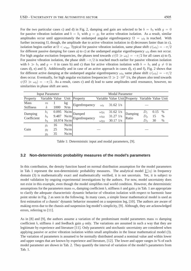
Input Parameter Modal ParameterProperty Variable Value UnitProperty Variable Value UnitProperty Variable Value UnitMass m 1 kgStiffness k 1000 N/m

Eigenfrequency ω0 31.62 1/s —

b1 0.095 Ns/m ωD1 31.62 1/s D1 0.15 %Damping

b2 9.487 Ns/mDamped

ωD2 31.27 1/sDamping

D2 15 %Coefficient

b3 18.974 Ns/mEigenfrequency

ωD3 30.17 1/sRatio

D3 30 %g1 16 Ns/m

Gain g2 25 Ns/m — —g3 35 Ns/m

Table 1: Deterministic input and modal parameters, [9].

3.2 Non-deterministic probability measures of the model’s parameters

In this contribution, the density function based on normal distribution assumption for the model parametersin Tab. 1 represent the non-deterministic probability measures. The analytical modelV (η) in frequencydomain (3) is mathematically exact and mathematically verified, it is not uncertain. Yet, it is subject tomodel validation by ongoing experimental investigations by the authors. For now, model uncertainty doesnot exist in this example, even though the model simplifies real world condition. However, the deterministicassumptions for the parameters massm, damping coefficientb, stiffnessk and gaing in Tab. 1 are appropriateto clarify the adequate characteristic dynamic behavior ofvibration isolation with respect to harmonic basepoint stroke in Fig. 2 as seen in the following. In many cases,a simple linear mathematical model is used asfirst estimation of a chassis’ dynamic behavior mounted on a suspension leg, [10]. The authors are aware ofmaking erros due to the chassis and suspension leg model’s simplicity, [9]. Although, they are acknowledgederrors, referring to [11].

As in [8] and [9], the authors assume a variation of the predominant model parameters massm dampingcoefficientb, stiffnessk and feedback gaing only. The variations are assumed in such a way that they arelegitimate by experience and literature [11]. Only parametric and stochastic uncertainty are considered whenapplying passive or active vibration isolation within small amplitudes in the linear mathematical model (3).The variation of parameters is assumed to be normally distributed around a nominal value and within lowerand upper ranges that are known by experience and literature, [12]. The lower and upper ranges in % of eachmodel parameter are shown in Tab. 2. They quantify the interval of variation of the model’s parameters fromTab. 1.


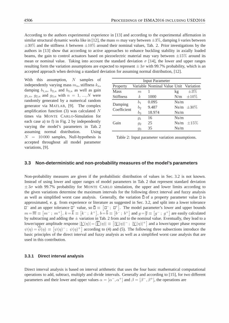
According to the authors experimental experience in [13] and according to the experimental affirmation insimilar structural dynamic works like in [12], the massmmay vary between±3%, dampingb varies between±30% and the stiffnessk between±10% around their nominal values, Tab. 2. Prior investigations by theauthors in [13] show that according to active approaches to enhance buckling stability in axially loadedbeams, the gain to control actuators based on piezoelectricmaterial may vary between±15% around itsmean or nominal value. Taking into account the standard deviation σ [14], the lower and upper rangesresulting form the variation assumptions are expected to represent± 3σ with 99.7% probability, which is anaccepted approach when deriving a standard deviation for assuming normal distribution, [12].

With this assumption, N samples ofindependently varying massmn, stiffnesskn,dampingb1,n, b2,n and b3,n as well as gaing1,n, g2,n and g3,n with n = 1, ..., N wererandomly generated by a numerical randomgenerator via MATLAB , [9]. The complexamplification function (3) was calculatedNtimes via MONTE CARLO-Simulation foreach case a) to f) in Fig. 2 by independentlyvarying the model’s parameters in Tab. 2assuming normal distribution. UsingN = 10000 samples, Null-hypothesis isaccepted throughout all model parametervariations, [9].

Input ParameterProperty Variable Nominal Value Unit VariationMass m 1 kg ±3%Stiffness k 1000 N/m ±10%

b1 0.095 Ns/mDamping

b2 9.487 Ns/m ±30%Coefficient

b3 18.974 Ns/mg1 16 Ns/m

Gain g2 25 Ns/m ±15%g3 35 Ns/m

Table 2: Input parameter variation assumptions.

3.3 Non-deterministic and non-probability measures of the model’s parameters

Non-probability measures are given if the probabilistic distribution of values in Sec. 3.2 is not known.Instead of using lower and upper ranges of model parameters in Tab. 2 that represent standard deviation± 3σ with 99.7% probability for MONTE CARLO simulation, the upper and lower limits according tothe given variations determine the maximum intervals for the following direct interval and fuzzy analysisas well as simplified worst case analysis. Generally, the variation of a property parameter valueisapproximated, e. g. from experience or literature as suggested in Sec. 3.2, and split into a lower tolerance− and an upper tolerance+ value, so ≡

[− ; +

]. The model parameter’s lower and upper bounds

m=m ≡[m− ; m+

], k=k ≡

[k− ; k+

], b= b ≡

[b− ; b+

]andg= g ≡

[g− ; g+

]are easily calculated

by subtracting and adding the± variation in Tab. 2 from and to the nominal value. Eventually, they lead to alower/upper amplitude response|V (η)|= |V (η)| ≡

[|V (η)|− ; |V (η)|+

]and a lower/upper phase response

ψ(η) = ψ(η) ≡[ψ(η)− ; ψ(η)+

]according to (4) and (5). The following three subsections introduce the

basic principles of the direct interval and fuzzy analysis as well as a simplified worst case analysis that areused in this contribution.

3.3.1 Direct interval analysis

Direct interval analysis is based on interval arithmetic that uses the four basic mathematical computationaloperations to add, subtract, multiply and divide intervals. Generally and according to [15], for two differentparameters and their lower and upper valuesα = [α−, α+] andβ = [β−, β+], the operations are


α+ β =[α− + β−, α+ + β+]

α− β =[α− − β+, α+ − β−]

α · β =[min(α− · β−, α− · β+, α+ · β−, α+ · β+),

max(α− · β−, α− · β+, α+ · β−, α+ · β+)]

α/β =[min(α−/β−, α−/β+, α+/β−, α+/β+),

min(α−/β−, α−/β+, α+/β−, α+/β+)]; with β 6= 0.

(6)

To calculate the lower/upper amplitude response|V (η)|= |V (η)| and a lower/upper phase responseψ(η)=ψ(η), each arithmetic operation in (4) and (5) follows the interval arithmetic (6) in a serial manner and leadsto an equivalent total amount of calculation operations. For example, the relationk/m in (2) needs at leastfour operations to divide four times and two operations to find minimum and maximum values from thedevisions according to the ruleα/β in (6). For the deterministic approach, only two calculations fork/mand

√in (2) to calculate a single deterministic value are necessary. The results of the direct interval analysis

are equal to a worst case analysis.

3.3.2 Direct fuzzy analysis

An overview of fuzzy stochastic methods suitable for the analysis of uncertainty in engineering applicationsis presented in [16] and applied fuzzy arithmetic can be found in [17]. Fuzzy set theory based on fuzzyarithmetic is discussed in [18]. Fuzzy numbers are described by membership functions and types of fuzzynumbers are especially triangular, gaussian, exponentialor crisp fuzzy numbers. The direct fuzzy arithmeticused in this contribution is based on interval arithmetic according to (6). Instead of giving the probabilitythat a value lies within the±3σ range in Sec. 3.2, fuzzy interval analysis gives a possibility that a valuelies within an interval or not via membership functionµ( ), with 0 ≤ µ( ) ≤ 1 and with the value ofthe property parameterm, b, k or g. In this contribution, the triangluar shaped membership function’s toprepresents the deterministic valueµ( ) = 1 and widens to the lower and upper values≡

[− ; +

]≡ ±3σ

with µ( −, +) = µ(±3σ) = 0, Fig. 3. That means the grade of membership of the deterministic value isone and the grade of membership of the lower and upper values−, + or, respectively,±3σ is zero.

3.3.3 Simplified worst case analysis

The simplified worst case approach gives a chance to quickly evaluate the predicted variations withoutcomplex calculations as introduced in Sec. 3.3.1 and Sec. 3.3.2. However, this approach needs a decisionfor choosing an adequate amount of model parameters that hassignificant and relevant influence on theprediction, for example by an individual sensitivity analysis. In this contribution, variations of modelparameter massm and stiffnessk that lead to sensitive variations of the angular eigenfrequency ω0 forthe undamped system according to (2) are taken into account.The amount of calculations for the varyingcomplex amplification functionV (η) in (3) is reduced to four calulation operations and two operations tofind the minimum and maximum values of only the mass-stiffness relation

[ω2−

0;ω2+

0

]=[min(k−/m−, k−/m+, k+/m−, k+/m+);

min(k−/m−, k−/m+, k+/m−, k+/m+)], with m 6= 0.(7)


4 Comparing direct probability and direct non-probability measures

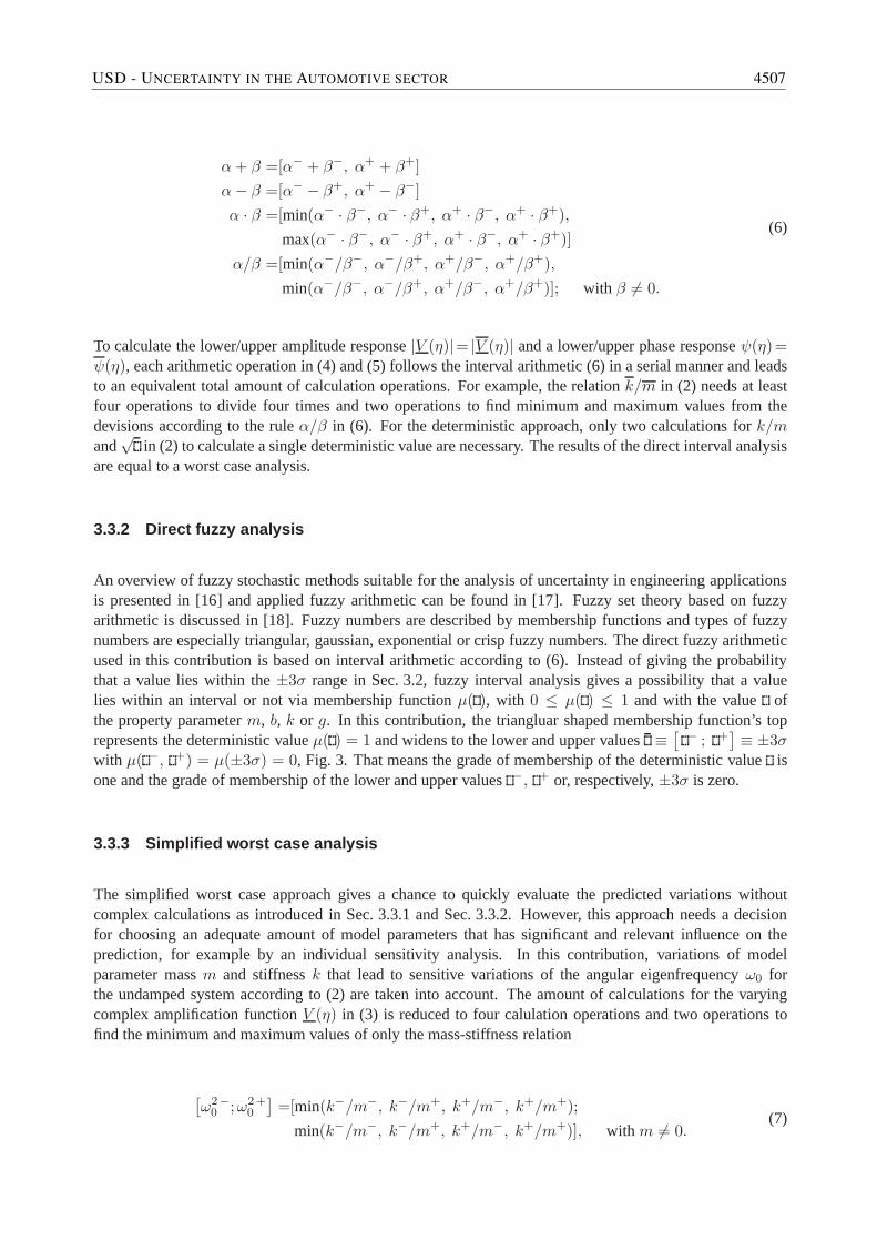
In this chapter the authors suggest a simple visual way to compare the ability of direct probability andnon-probability measures in predicting the dynamic isolation behavior of the mass-damper-spring systemin early design phase. Exemplary, normalized density function p

(), membership functionµ

() and worst

case interval[

− ; +]

of any model parameter or state variableare shown in Fig. 3. In there, a solidcircle represents the deterministic value, the solid curverepresents the density function for MONTE CARLO

simulation, the dashed line represents the membership function for fuzzy analyses based on interval arithmeticwith circles atµ(±3σ) = 0 and brackets represent the interval due to simplified worst case analysis. Theauthors are aware of the fact that normalizing the density function does not increase the understanding forthis comparison with respect to absolute frequency distribution. It has been normalized only for the sakeof comparing the maximum bandwidth of variation due to different non-deterministic measures in one plot,Fig. 3. It has been included especially to depict theµ(±3σ) interval for comparability reasons.

Fig. 3 shows an ideal case with, on the onehand, the mean value of the density functionequal to the deterministic value and, on theother hand, with the deviation±3σ equalto the membershipµ(±3σ) = 0 as wellas lower/upper interval values from worstcase assumption. The following Fig. 4 andFig. 5 show amplitude|V (Ω)| and phaseψ(Ω) of the amplification function (3)for three characteristic points seen in theBODE-Diagram in Fig. 2:

– within isolation atΩ = 100 1/s> ωiso,– before isolation atΩ = ω0 < ωiso and– for a -15 dB vibration attenuation

for passive and active vibration isolation.

1

norm

aliz

edde

nsity

func

tionp(

)m

embe

rshi

pfu

nctio

nµ(

)

wor

stca

sein

terv

al[−

;+]

0

µ(±3σ)=0

model parameter or state variable

Figure 3: Exemplary normalized density function (solidline), deterministic value (solid circle), membershipfunction (dashed line) and worst case interval (brackets)of model parameters or state variables.

The amplitudes|V (Ω)| and phasesψ(Ω) in Fig. 4 and Fig. 5 are given in terms of crisp deterministic resultof (3), density functionsp

(|V (Ω)|

)andp

(ψ(Ω)

)based on MONTE CARLO simulation with 10 000 samples,

membership functionsµ(|V (Ω)|

)andµ

(ψ(Ω)

)based on direct fuzzy-analysis using interval-arithmetic, and

lower/upper values[|V (Ω)|− ; |V (Ω)|+

]and

[ψ(Ω)− ; ψ(Ω)+

]based on the simplified worst case analysis.

Deterministic assumptions as well as variations and limitsof input parameters are taken from Tab. 2 for casec) with b3 andg= 0 representing the PASSIVE system and for case d) withb= b1 andg= g1 representingthe ACTIVE system. The expelled grades of membershipµ(±3σ) from the direct fuzzy-analysis show theaffiliation to the MONTE CARLO simulation.

It is seen in Fig. 4 that, generally, the active system’s amplitude |V (100)| within isolation forΩ = 100 1/s> ωiso for cases c) and d) is lower and has relatively less deviationthan the passive system’s amplitude.The direct fuzzy and simplified worst case intervals are inside the normalized density function’s standarddeviation values±3σ from the MONTE CARLO simulation for the active and outside for the passive system.As expected and well known, the latter approach leads to a deviation overestimation via direct fuzzy andsimplified worst case analysis compared to the standard deviation values±3σ. The grade of membershipfor an equivalent±3σ interval is roughlyµ(±3σ)≈ 0,45. It is used as a threshold measure after which atlower grades the possibility of the value’s occurrence getsoverestimated compared to direct MONTE CARLO

simulation. Similar relations occur withµ(±3σ)≈0,52 for the passive system.


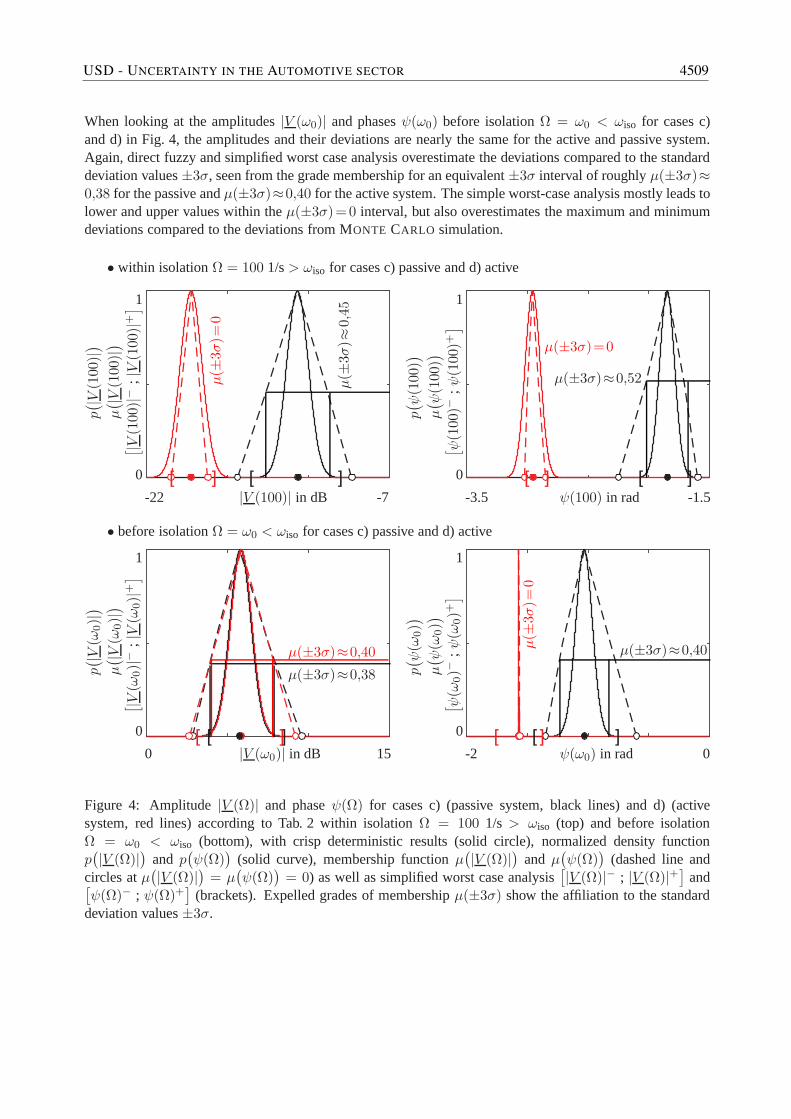
When looking at the amplitudes|V (ω0)| and phasesψ(ω0) before isolationΩ = ω0 < ωiso for cases c)and d) in Fig. 4, the amplitudes and their deviations are nearly the same for the active and passive system.Again, direct fuzzy and simplified worst case analysis overestimate the deviations compared to the standarddeviation values±3σ, seen from the grade membership for an equivalent±3σ interval of roughlyµ(±3σ)≈0,38 for the passive andµ(±3σ)≈0,40 for the active system. The simple worst-case analysis mostly leads tolower and upper values within theµ(±3σ)=0 interval, but also overestimates the maximum and minimumdeviations compared to the deviations from MONTE CARLO simulation.

[ ][ ]

[ ][ ]

[ ][ ]

[ ]][

• within isolationΩ = 100 1/s> ωiso for cases c) passive and d) active

1

p( |V

(100

)|)

µ( |V

(100

)|)[ |V

(100

)|−;|V

(100

)|+]

0

µ(±

3σ)=

0

µ(±

3σ)≈

0,45

-22 |V (100)| in dB -7

1

p( ψ

(100

))

µ( ψ

(100

))[ ψ

(100

)−;ψ

(100

)+]

0

µ(±3σ)=0

µ(±3σ)≈0,52

-3.5 ψ(100) in rad -1.5

• before isolationΩ = ω0 < ωiso for cases c) passive and d) active

1

p( |V

(ω0)|)

µ( |V

(ω0)|)

[ |V(ω

0)|−

;|V

(ω0)|+

]

0

µ(±3σ)≈0,38

µ(±3σ)≈0,40

0 |V (ω0)| in dB 15

1

p( ψ

(ω0))

µ( ψ

(ω0))

[ ψ(ω

0)−

;ψ

(ω0)+

]

0

µ(±

3σ)=

0

µ(±3σ)≈0,40

-2 ψ(ω0) in rad 0

Figure 4: Amplitude|V (Ω)| and phaseψ(Ω) for cases c) (passive system, black lines) and d) (activesystem, red lines) according to Tab. 2 within isolationΩ = 100 1/s > ωiso (top) and before isolationΩ = ω0 < ωiso (bottom), with crisp deterministic results (solid circle), normalized density functionp(|V (Ω)|

)and p

(ψ(Ω)

)(solid curve), membership functionµ

(|V (Ω)|

)and µ

(ψ(Ω)

)(dashed line and

circles atµ(|V (Ω)|

)= µ

(ψ(Ω)

)= 0) as well as simplified worst case analysis

[|V (Ω)|− ; |V (Ω)|+

]and[

ψ(Ω)− ; ψ(Ω)+]

(brackets). Expelled grades of membershipµ(±3σ) show the affiliation to the standarddeviation values±3σ.


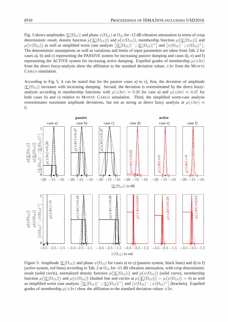
Fig. 5 shows amplitudes|V (Ω15)| and phaseψ(Ω15) atΩ15 for -15 dB vibration attenuation in terms of crispdeterministic result, density functionp

(|V (Ω15)|

)andp

(ψ(Ω15)

), membership functionµ

(|V (Ω15)|

)and

µ(ψ(Ω15)

)as well as simplified worst case analysis

[|V (Ω15)|− ; |V (Ω15)|+

]and

[ψ(Ω15)

− ; ψ(Ω15)+].

The deterministic assumptions as well as variations and limits of input parameters are taken from Tab. 2 forcases a), b) and c) representing the PASSIVE system for increasing passive damping and cases d), e) and f)representing the ACTIVE system for increasing active damping. Expelled grades of membershipµ(±3σ)from the direct fuzzy-analysis show the affiliation to the standard deviation values±3σ from the MONTE

CARLO simulation.

According to Fig. 5, it can be stated that for the passive cases a) to c), first, the deviation of amplitude|V (Ω15)| increases with increasing damping. Second, the deviation is overestimated by the direct fuzzy-analysis according to membership functions withµ(±3σ) ≈ 0,20 for case a) andµ(±3σ) ≈ 0,47 forboth cases b) and c) relative to MONTE CARLO simulation. Third, the simplified worst-case analysisoverestimates maximum amplitude deviations, but not as strong as direct fuzzy analysis atµ(±3σ) ≈0.

•

passivecase a) case b) case c)

activecase d) case e) case f)

1

p( |V

(Ω15)|)

µ( |V

(Ω15)|)

[ |V(Ω

15)|−

;|V

(Ω15)|+

]

0

µ(±

3σ)≈

0,2

0

µ(±

3σ)≈

0,4

7

µ(±

3σ)≈

0,4

7

µ(±

3σ)≈

0,0

2

µ(±

3σ)≈

0

µ(±

3σ)=

0

−20 −15 −10 −20 −15 −10 −20 −15 −10 −20 −15 −10 −20 −15 −10 −20 −15 −10

|V (Ω15)| in dB

1

p( ψ

(Ω15))

µ( ψ

(Ω15))

[ ψ(Ω

15)−

;ψ(Ω

15)+

]

0

µ(±

3σ)=

0

µ(±

3σ)≈

0,4

8

µ(±

3σ)≈

0,4

8

µ(±

3σ)≈

0,6

4

µ(±

3σ)≈

0,5

8

µ(±

3σ)≈

0,6

4

−3.5 −2.5−1.5 −3.5−2.5−1.5 −3.5−2.5−1.5 −3.5−2.5−1.5 −3.5−2.5−1.5 −3.5−2.5−1.5

ψ(Ω15) in rad

Figure 5: Amplitude|V (Ω15)| and phaseψ(Ω15) for cases a) to c) (passive system, black lines) and d) to f)(active system, red lines) according to Tab. 2 atΩ15 for -15 dB vibration attenuation, with crisp deterministicresult (solid circle), normalized density functionp

(|V (Ω15)|

)and p

(ψ(Ω15)

)(solid curve), membership

functionµ(|V (Ω15)|

)andµ

(ψ(Ω15)

)(dashed line and circles atµ

(|V (Ω15)|

)= µ

(ψ(Ω15)

)= 0) as well

as simplified worst case analysis[|V (Ω15)|− ; |V (Ω15)|+

]and

[ψ(Ω15)

− ; ψ(Ω15)+]

(brackets). Expelledgrades of membershipµ(±3σ) show the affiliation to the standard deviation values±3σ.


For the active cases d) to f), increasing damping does not lead to higher deviation of amplitudes, nor doesthe direct fuzzy-analysis lead to overestimated deviations atµ(±3σ)≈ 0. The simplified worst-case study,however, does overestimate the amplitude deviation relative to MONTE CARLO simulation, this time evenhigher than the direct fuzzy analysis.

The deviation of the phase shiftψ(Ω15) for the passive cases a) to c) also rises with increasing damping.Overestimation by direct fuzzy- and simplified worst-case analyses is seen. Higher differences in phaseslopes at the corresponding frequencies for an equal -15 dB vibration attenuation than in amplitude slopesin all cases are the reason, since the sensitivity at this frequency range increases. For the active cases d) tof), higher sensitivity also appears to be the reason for overestimating the phase shift deviation for both directfuzzy- and simplified worst-case analysis, with grades of membership0, 58 . µ(±3σ) . 0,64.

5 Computational costs

Computational costs depend on the computer’s capability and on the skill and ability of the programmingengineer, so costs are always relative. This contribution takes into account the amount of calculations neededto compute the non-deterministic output of the complex amplification function (3) according to the assumedderivations of input model parameter in Tab. 2. As a reference, the amount of the deterministic calculationof (3) is assumed to be 1,Ndet = 1. The MONTE CARLO simulation in this paper needs the 10 000-foldamount,NMCS = 10000. As for the direct fuzzy-analysis based on interval analysis and for the simplifiedworst case analysis, the amount of calculations varies due to the amount of variables and operations (6)used in the complex amplification function (3). In any case, the amount of calculations for direct fuzzy andsimplified worst case analyses is less then a hundred calculations,Nint < 100.

6 Conclusion

This contribution suggests a combined analytical and numerical way to predict uncertainty in passive andactive vibration isolation due to model parameter variations in a simple manner for decision making inearly design phase. For that, the authors compare vibrationamplitudes and phases before and after thecharacteristic isolation frequency of a basic single mass-damper-spring system due to harmonic base pointstroke via non-deterministic probability and non-probability measures. The probability measure is basedon normalized direct MONTE CARLO simulation, the non-probability measures are based on direct fuzzyanalysis via interval arithmetic and simplified worst case analysis. The active concept follows the idea ofan absolute velocity feedback control of the mass’ vibration. The results confirm that, on the one hand, theactive control approach attenuates the vibration more effectively then the passive approach in the frequencyrange before and after the characteristic isolation frequency with less uncertainty in amplitude and phasevariations. On the other hand, the direct comparison between the probabilistic and non-probabilistic confirmsthat the trustworthiness of direct MONTE CARLO simulation is higher then the direct fuzzy and simplifiedworst case approach, the latter overestimates the possiblevariations. However, for the fuzzy approach itis possible to derivate an equivalent grade of membership representing the standard deviation values±3σfrom the MONTE CARLO simulation. If the interrelation between the grade of membership and the standarddeviation is known, the computational cost to predict uncertainty in early design phase can be reduced in amanifold manner when using the direct fuzzy approach. That leads to the conclusion that for this example,first, the active vibration isolation approach should be favored against the passive approach due to a greaterattenuation potential throughout a wide frequency range and due to less expected uncertainty in amplitude anphase variation. Second, using the direct fuzzy approach isan effective way to predict uncertainty withoutgreater computational cost if the equivalent grade of membership for intervals is known that relates to the


±3σ standard deviation. These findings are subject of current experimental validation with an adequate testrig along with a comprehensive sensitivity analysis.

Acknowledgements

The authors like to thank the German Research Foundation DFGfor funding this research within the SFB805.

References

[1] Ben Haim, Y.: Robustness of model-based fault diagnosis: decisions withinformation-gap models ofuncertainty, International Journal of Systems Science, 2000, 31: 1511-1518

[2] Eifler, T., Enss, G.C., Haydn, M., Mosch, L., Platz, R., Hanselka, H.: Approach for a consistentdescription of uncertainty in process chains of load carrying mechanical systems, in Proceedings of theFirst International Conference on Uncertainty in Mechanical Engineering (ICUME), 14.-15.11.2011,Darmstadt, Germany, Journal of Applied Mechanics and Materials Vol. 104 (2012), Trans TechPublications, pp 133-144, 2011

[3] Hanselka, H., Platz, R.:Ansatze und Maßnahmen zur Beherrschung von Unsicherheit in lasttragendenSystemen des Maschinenbaus – Controlling Uncertainties inLoad Carrying Systems, Konstruktion, Vol.11/12, pp. 55–62, 2010.

[4] VDI 2062: Vibration Insulation – Insulation elements, Part 2, Verein Deutscher Ingenieure, Beuth VerlagBerlin, 2007

[5] VDI 2064: Aktive Schwingungsisolierung – Active vibration isolation, Verein Deutscher Ingenieure,Beuth Verlag Berlin, 2010

[6] Enss, G.C; Platz, R.:Evaluation of uncertainty in experimental active bucklingcontrol of a slenderbeam-column with disturbance forces using Weibull analysis, Mechanical Systems and Signal Processing79 (2016) 123131

[7] Auto-Institut: Callbacks in US Automotive Industry 2015,http://www.auto-institut.de/performancestudien.htm, last cited June 24, 2016

[8] Platz, R., Ondoua, S., Enss, G.C., Melz, T.:Approach to Evaluate Uncertainty in Passive andActive Vibration Reduction, in H.S. Atamturktur et al. (eds.),Model Validation and UncertaintyQuantification, Volume 3: Proceedings of the 32nd IMAC, A Conference and Exposition on StructuralDynamics, 2014, Conference Proceedings of the Society for Experimental Mechanics Series, DOI10.1007/978-3-319-04552-834, pp. 345-352, 2014

[9] Platz, R., Enss, G.C.:Comparison of uncertainty in passive and active vibration isolation, in H.S.Atamturktur et al. (eds.),Model Validation and Uncertainty Quantification, Volume 3,ConferenceProceedings of the Society for Experimental Mechanics Series, DOI 10.1007/978-3-319-15224-02, pp.15-25, 2015

[10] Voth, S.: Dynamik schwingungsfahiger Systeme – Dynamics of vibrations systems, Vieweg & SohnVerlag, Wiesbaden, Germany, 2006

[11] Oberkampf, W.L., DeLand, S.M., Rutherford, B.M., Diegert, K.V., Alvin, K.F.: Error and uncertaintyin modeling and simulation, Reliability Engineering and System Safety 75, pp. 333–357, 2002


[12] Schueller, G.I.:On the treatment of uncertainties in structural mechanics and analysis, Computers andStructures 85, pp. 235–243, 2007

[13] Platz, R., Enss, G.C., Ondoua, S., Melz, T.:Active stabilization of a slender beam-column under staticaxial loading and estimated uncertainty in actuator properties, in Second International Conference onVulnerability and Risk Analysis and Management (ICVRAM) and the sixth International Symposium onUncertainty Modeling and Analysis (ISUMA), July 13.-16.2014, Liverpool, UKpp 235-245, 2014

[14] Bronstein, I.N., Semendjajew, K.A.:Taschenbuch der Mathematik – Handbook of Mathematics, VerlagHarri Deutsch, 25, 1991

[15] Alefeld, G., Mayer, G.: Interval analysis: theory and applications, Journal of Computational andApplied Mathematics, Volume 121, 2000, pp. 421-464

[16] Moller, B., Reuter. U.:Uncertainty Forecasting in Engineering, Springer-Verlag Berlin Heidelberg,2007

[17] Hanss, M.:Applied Fuzzy Arithmetic, Springer, 2005

[18] Zadeh, L. A.:Fuzzy Sets, Journal of Information and Control, 1965


Uncertainty Quantification for Decision Making in Early Design ...

Documents

Transcript of Uncertainty Quantification for Decision Making in Early Design ...