Response Surface Designs for Scenario Management and Uncertainty Quantification in Reservoir...

P1: KEE

Mathematical Geology [mg] PP1377-matg-496107 November 19, 2004 5:44 Style file version June 25th, 2002

Mathematical Geology, Vol. 36, No. 8, November 2004 ( C© 2004)

Response Surface Designs for ScenarioManagement and Uncertainty Quantification

in Reservoir Production1

Astrid Jourdan2 and Isabelle Zabalza-Mezghani2

Response surface experimental designs provide a framework for evaluating sensitivities and assessinguncertainties in reservoir-production forecasts for continuous parameters (i.e. permeability, flow rate,etc.). In this paper, the method is extended in order to integrate both continuous and discrete parameters(i.e. fault status: open/close, injection scheme: SWAG/WAG, etc.). This paper presents an appropriateexperimental designs approach, notably the regression models associated with, and the statisticalinterpretation (sensitivity study, Monte Carlo simulations, etc.). The method has been successfullyapplied to a reservoir oil-production simulation problem. The objective was to define the best productionscheme by optimizing the well-completion level. This application has highlighted the advantages of thisnew approach, both in terms of decreasing simulation cost and improving the interpretation quality.

KEY WORDS: discrete parameter, production scheme optimization, risk analysis, sensitivity,composite design.

INTRODUCTION

The well-known methodology of experimental designs is widely used to manageuncertainties in reservoir oil production (Damsleth and Hage, 1991; Dejean andBlanc, 2000). The principle of the method consists of running a few reservoirsimulations by varying all the uncertain parameters simultaneously. The simulationresults are then used to fit a simple polynomial regression model, which will replacethe time-consuming fluid-flow simulator. The model is then used to:

– identify the uncertain parameters that really influence the production (sen-sitivity analysis),

– estimate their impact on oil-production forecasts (risk analysis),– optimize the reservoir-production scheme.

1Received 25 June 2003; accepted 28 May 2004.2Reservoir Engineering Department - IFP - 92852 Rueil Malmaison Cedex – France; e-mail:[email protected] or [email protected]

965

0882-8121/04/1100-0965/1 C© 2004 International Association for Mathematical Geology

P1: KEE


966 Jourdan and Zabalza-Mezghani

At the present time, this method is applicable for continuous parameters,i.e. parameters that can take all possible values between a minimum and maxi-mum value. The treatment of discrete parameters, i.e. parameters that take only afixed number of qualitative levels, is not satisfactory with the standard method ofexperimental designs.

However, handling discrete parameters is essential for comparing differentproduction scenarios. For example, the fault status is a discrete parameter at twolevels, one for the scenario the fault is closed, and another for the scenario, thefault is open. This finite number of levels is incompatible with standard response-surface designs, which require five (or three) quantitative levels. At present, themethod to deal with discrete parameters (called the classical approach hereafter)consists of repeating a standard experimental design for the continuous parameters,once for each scenario. The simulation cost for this solution can be prohibitive.Furthermore, this method does not allow estimation of the impact on the productionof the discrete parameters and their interactions with continuous parameters sinceeach scenario is studied separately from the others.

We propose here an innovative approach (called the new approach hereafter),which integrates discrete parameters in response-surface experimental designs(Section Methodology). The objective of this new method is to be less expen-sive with equal or better quality than the classical method. Furthermore, the newmethod will allow estimation of the impact of discrete parameters and their possibleinteractions with continuous parameters.

In order to highlight the main advantages of the new approach, a comparisonwith the classical approach is performed by means of a synthetic reservoir simu-lation problem (Section Application to Risk Evalution in the Petroleum Industry).The aim is to compare two production scenarios by varying the level of completionof a producing well. This case study proves the necessity of integrating discreteparameters in response-surface designs and of a global interpretation of the results.

METHODOLOGY

Classical Approach

The classical approach for dealing with several possible scenarios in the pres-ence of other continuous uncertainty parameters is to build a classical experimentaldesign, which involves the continuous uncertainty parameters and to repeat it asmany times as the number of scenarios.

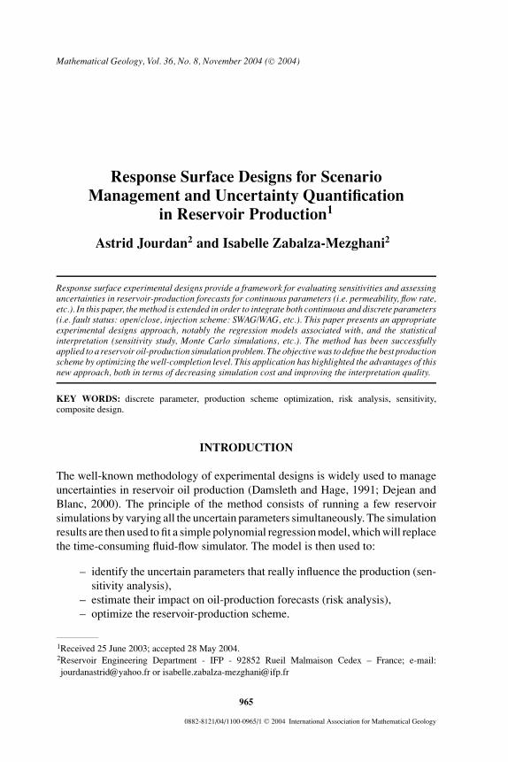
For instance, two discrete parameters at two levels, z and w, lead to fourdistinct scenarios. As an illustration, to deal with three continuous parameters x1,x2, x3, the classical approach implies four repetitions of the classical experimentaldesign in Figure 1.

P1: KEE


Response Surface Designs for Scenario Management and Uncertainty Quantification 967

Figure 1. Central composite design.

This experimental design requires 15 simulations for each of the four scenar-ios, resulting in 60 simulations. It allows a fit for each scenario of a second orderpolynomial model:

E(y|z = −1, w = −1) = α0 +3∑

i=1αi xi + ∑

1≤i< j≤3αi j xi x j +

3∑i=1

αi i x2i

E(y|z = −1, w = +1) = β0 +3∑

i=1βi xi + ∑

1≤i< j≤3βi j xi x j +

3∑i=1

βi i x2i

E(y|z = +1, w = −1) = γ0 +3∑

i=1γi xi + ∑

1≤i< j≤3γi j xi x j +

3∑i=1

γi i x2i

E(y|z = +1, w = +1) = θ0 +3∑

i=1θi xi + ∑

1≤i< j≤3θi j xi x j +

3∑i=1

θi i x2i

, (1)

We can notice that only the continuous parameters x1, x2, x3, are involvedin those models to describe the response y. The discrete parameters, z and w, aretaken into account through the consideration of four distinct models.

Remark. For a sensitivity analysis, the experimental design will consist onlyin its factorial part, and the resulting polynomial model will include only the mainterms (xi ) and the interaction terms (xi x j , j > i).

Classically, the polynomial models are used for a statistical analysis: screen-ing, Monte Carlo sampling, optimization, etc.

As explained above, each scenario is described by a model and no link existsbetween the models. Thus, the classical approach consists of conducting as manyindependent studies as scenarios, so the comparison of scenarios together is notpossible. Moreover, repeating experimental designs implies a prohibitive cost interms of number of simulations. In this context, we present a new method ofexperimental design, which allows us to tackle simultaneously continuous anddiscrete parameters while preserving a reasonable cost.

P1: KEE



New Approach

Contrary to the classical approach, a single experimental design is used tostudy simultaneously all scenarios. This experimental design explicitly includesboth continuous and discrete parameters.

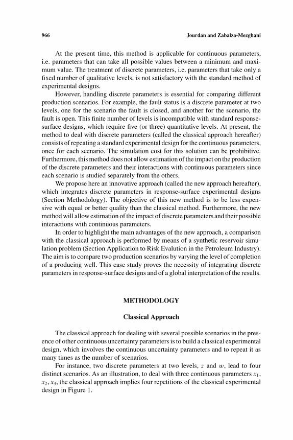
The new experimental designs are constructed using a classical compositedesign for the continuous parameters x1, x2, . . . , xd . The discrete parameters aretaken into account by adding to the initial composite design as many columns asthe number of discrete parameters (Fig. 2).

Draper and John (1988) first introduced this kind of design, and their methodwas developed by Wu and Ding (1998) and more recently by Jourdan (2002). Wuand Ding suggest an algorithm of construction, and Jourdan gives a list of designs.

The main properties of these designs are the number of estimable modelsassociated with each design. As an illustration, we present a design for two discrete

Figure 2. Composite design with discrete parameter.

P1: KEE



parameters at two levels, z and w, and the seven models associated with thisdesign.

The additional columns are defined in order to satisfy the following objectives:

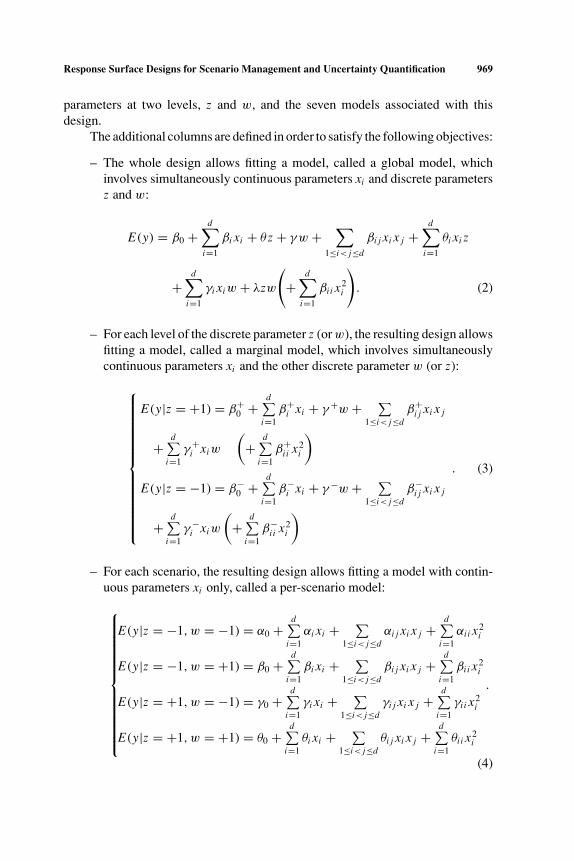
– The whole design allows fitting a model, called a global model, whichinvolves simultaneously continuous parameters xi and discrete parametersz and w:

E(y) = β0 +d∑

i=1

βi xi + θ z + γw +∑

1≤i< j≤d

βi j xi x j +d∑

i=1

θi xi z

+d∑

i=1

γi xiw + λzw

(+

d∑i=1

βi i x2i

). (2)

– For each level of the discrete parameter z (or w), the resulting design allowsfitting a model, called a marginal model, which involves simultaneouslycontinuous parameters xi and the other discrete parameter w (or z):

E(y|z = +1) = β+0 +

d∑i=1

β+i xi + γ +w + ∑

1≤i< j≤dβ+

i j xi x j

+d∑

i=1γ +

i xiw

(+

d∑i=1

β+i i x2

i

)

E(y|z = −1) = β−0 +

d∑i=1

β−i xi + γ −w + ∑

1≤i< j≤dβ−

i j xi x j

+d∑

i=1γ −

i xiw

(+

d∑i=1

β−i i x2

i

). (3)

– For each scenario, the resulting design allows fitting a model with contin-uous parameters xi only, called a per-scenario model:

E(y|z = −1, w = −1) = α0 +d∑

i=1αi xi + ∑

1≤i< j≤dαi j xi x j +

d∑i=1

αi i x2i

E(y|z = −1, w = +1) = β0 +d∑

i=1βi xi + ∑

1≤i< j≤dβi j xi x j +

d∑i=1

βi i x2i

E(y|z = +1, w = −1) = γ0 +d∑

i=1γi xi + ∑

1≤i< j≤dγi j xi x j +

d∑i=1

γi i x2i

E(y|z = +1, w = +1) = θ0 +d∑

i=1θi xi + ∑

1≤i< j≤dθi j xi x j +

d∑i=1

θi i x2i

.

(4)

P1: KEE



For instance, if we again consider three continuous parameters x1, x2, x3 andtwo discrete parameters at two levels, z and w, the experimental design providedby the new approach can be the design in Figure 2.

This experimental design takes into account both discrete and continuousparameters simultaneously and requires only 26 simulations for studying the fourdistinct scenarios.

The construction technique is presented in more detail in Wu and Ding (1998)and Jourdan (2002).

Comparison

As with the classical approach, this new method provides a model for eachscenario [models (1) and (4)]. The main advantage of the new approach is theadditional information provided by the global and marginal models.

First, each marginal model (3) allows study of the influence of the continuousparameters and of one of the discrete parameters while the other is fixed. Thus, wecan better catch distinct behaviours due to one discrete parameter.

Moreover, the global model (2) allows understanding of the whole phenomenaof the behaviour by testing simultaneously the impact of continuous and discreteparameters. In particular, considering discrete and continuous parameters explicitlyin the same model allows us to compare and rank the influential parameters.

This new approach provides more information about the physical phenomenathan the classical method and reduces the simulation cost significantly: in case ofthree continuous parameters and two discrete parameters at two levels, the classicalapproach requires 60 simulations against 26 for the new approach.

APPLICATION TO RISK EVALUATION INTHE PETROLEUM INDUSTRY

Case Description

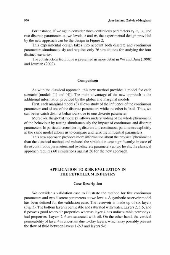
We consider a validation case to illustrate the method for five continuousparameters and two discrete parameters at two levels. A synthetic reservoir modelhas been defined for the validation case. The reservoir is made up of six layers(Fig. 3). The bottom layer is permeable and saturated with water. Layers 2, 3, 5, and6 possess good reservoir properties whereas layer 4 has unfavourable petrophys-ical properties. Layers 2–6 are saturated with oil. On the other hand, the verticalpermeability of layer 4 is uncertain due to clay layers, which may possibly preventthe flow of fluid between layers 1-2-3 and layers 5-6.

P1: KEE



Figure 3. Description of the validation case.

We assume that significant uncertainties remain for the field. The five follow-ing continuous uncertainty parameters have been selected for this study:

– x1 the horizontal permeability KHi of layers 1, 2, 3, 5, and 6,– x2, x3, x4, x5 four relative permeability curve parameters (SORW, SORG,

KRWM, KRGM).

SORW represent the residual oil saturation after a waterflood production phaseand SORG represent the residual oil saturation after a gasflood production phase.KRWM represents the water relative permeability at the maximum water satura-tion value. KRGM represent the gas relative permeability at the maximum gassaturation value. In other words, SORW and KRWM are parameters that will act(favour/disfavour) on oil production in presence of a water phase and SORG andKRGM are parameters that will act (favour/disfavour) on oil production in presenceof a gas phase.

In addition, significant uncertainty remains on the vertical permeability oflayer 4. Thus, a discrete parameter at two levels, z, is introduced to take into accountthe two possible status for layer 4: permeable (coded z = +1) or impermeable(coded z = −1).

In order to produce from this reservoir, we suggest putting a producing wellin the reservoir top and an injection well in layer 1. The layers, which are to beperforated for production in the well, remain uncertain. We hesitate to perforatebelow layer 4 in order to drain the bottom part of the reservoir if layer 4 is imper-meable, due to the risk of early arrival of the water at the producing well (whichpenalizes the total production of oil). Consequently, a discrete parameter at twolevels, w, is introduced to take into account the two possible production scenar-ios: perforation in layers 5 and 6 (coded w = +1) or in layers 3, 5, and 6 (codedw = −1).

Remark. Note that taking the vertical permeability of layer 4 as a discreteparameter, whereas the other uncertain permeabilities are considered as continuous

P1: KEE



parameters is mainly due to the order of magnitude of the uncertainty. In fact, thevertical permeability on layer 4 is assumed to vary from 0.01 mD to 10 mD. Thisvariation may change drastically the physical phenomena, and leads then to twodistinct scenarios: permeable against impermeable.

Thus, the context of this case is to study five continuous uncertainty param-eters for four distinct scenarios:

1. Layer 4 permeable/Perforation in layers 5 and 6 (z = +1, w = +1)2. Layer 4 impermeable/Perforation in layers 5 and 6 (z = −1, w = +1)3. Layer 4 permeable/Perforation in layers 3, 5, and 6 (z = +1, w = −1)4. Layer 4 impermeable/Perforation in layers 3, 5, and 6 (z = −1, w = −1)

Goal of the Study

The response we will focus on is the cumulative oil production (COS) after4 years of production. The goal of this study is mainly to:

– identify the main influential parameters (either continuous or discrete)through a sensitivity analysis,

– forecast the production by taking into account the remaining uncertaintieson parameters through a risk analysis (Monte Carlo sampling),

– determine the perforation level (optimal w), which minimizes water pro-duction and maximizes oil production.

This statistical analysis will provide us with information about the respectiveinfluence of each parameter on oil production. This can be crucial in recommendinga new phase of characterization of some petrophysical parameters in order to reducethe remaining uncertainty on production. On the other hand, this statistical analysiswill be useful for decision-making on the production scheme by optimizing theproduction parameters (in this case perforation level).

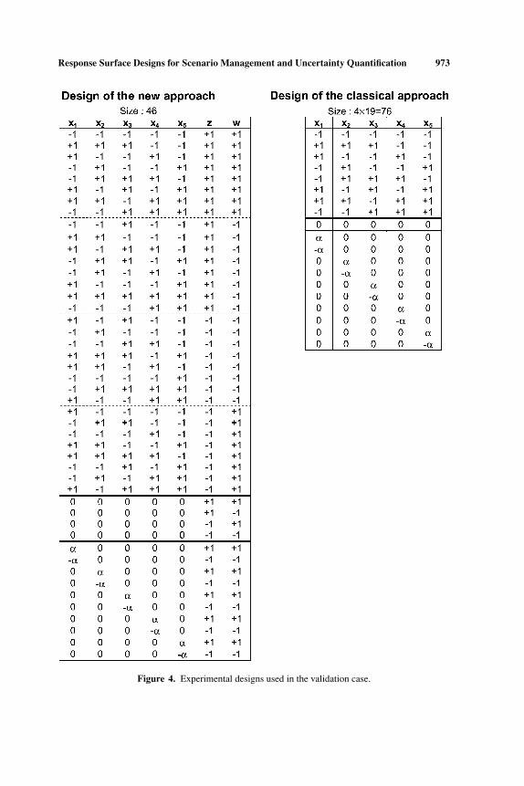
In accordance with these goals, we present the comparison between the clas-sical approach, which requires 4 × 19 = 76 simulations, and the new approachthat requires only 46 simulations (Fig. 4).

Qualitative Sensitivity Study

The aim of sensitivity analysis is to detect which parameters or interactionsinfluence the response.

For the sensitivity study, only simulations defined by the factorial part of theexperimental design are required. Thus, the quadratic terms will not be estimated

P1: KEE



Figure 4. Experimental designs used in the validation case.

P1: KEE



during this part of the analysis whatever the approach we consider (either classicalor new).

Analysis for Each Scenario

The experimental design we consider (using either the classical or new ap-proach) (Fig. 4) allows to fit, for each scenario, a model of the followingstructure:

E(y) = β0 +5∑

i=1

βi xi + β12x1x2 + β15x1x5. (5)

The other interactions are not involved in the model to keep the estimability ofcoefficientsβi , but are taken into account though main effects xi or interactions x1x2

and x1x5. We have the following aliases: x1 = x3x4, x2 = x3x5, x3 = x1x4 = x2x5,x4 = x1x3, x5 = x2x3, x1x2 = x4x5 and x1x5 = x2x4. It means that, for example,the influence of interaction x1x2 in the model represents in fact the influence ofthe group of interactions x1x2 and x4x5. For more details about experimental de-sign methodology (estimability, influential terms, aliasing. . .) see Box and Draper(1987).

Figure 5 represents the influential terms in the model and highlights therelative influence of the continuous parameters and their possible interactions.

Two main conclusions can be made according to these results:

– for all the scenarios, the parameters associated with gas, KRGM and SORG,are influential. SORG is significantly the most influential parameter on theoil production. KRGM and SORG have always a negative effect, that is theoil production decreases when KRGM or SORG increases.

– two distinct behaviors appear through the scenarios: in scenarios 1, 3,and 4, the parameters associated with water, KRWM, and SORW, are sig-nificantly influential whereas they are negligible for scenario 2. This re-sult reinforces our intuition concerning the presence of water in layers2 and 3. In fact, the negative influence of KRWM and SORW, for sce-narios 1, 3, and 4 indicates the early arrival of water in the produc-ing well. This result is consistent, since for scenario 2, layer 4 is im-permeable and the well perforation is done on layers 5 and 6 (abovelayer 4). Thus the producing zone is completely isolated from the waterzone.

For the sensitivity analysis, the classical approach leads only to these results,whereas the new approach provides also additional information related to themarginal and the global behaviors of the cumulative oil production.

P1: KEE



Fig

ure

5.C

ontin

uous

para

met

ers

influ

ence

for

each

scen

ario

.

P1: KEE



Additional Information Thanks to the New Approach

Marginal Models. The experimental design of the new approach allows fit-ting not only the models per scenario, but also the marginal models described asfollows:

E(y/z = +1) = β+0 +

5∑i=1

β+i xi + γ +w + β+

12x1x2 + β+15x1x5 +

5∑i=1

γ +i xiw

E(y/z = −1) = β−0 +

5∑i=1

β−i xi + γ −w + β−

12x1x2 + β−15x1x5 +

5∑i=1

γ −i xiw

(6)

with aliases: x1x2 = x4x5, x1x5 = x2x4, x1w = x3x4, x2w = x3x5, x3w = x2x5 =x1x4, x4w = x1x3, x5w = x2x3.

E(y/w = +1) = β+0 +

5∑i=1

β+i xi + γ +z + β+

12x1x2 + β+15x1x5

+ β+24x2x4 + β+

45x4x5 +5∑

i=1γ +

i xi z

E(y/w = −1) = β−0 +

5∑i=1

β−i xi + γ −z + β−

12x1x2 + β−15x1x5

+ β−24x2x4 + β−

45x4x5 +5∑

i=1γ −

i xi z

(7)

with aliases: x2 = x3x5, x3 = x2x5, x5 = x2x3, x1x5 = x3x4, x3z = x1x4, x4z =x1x3.

Note that the interaction terms x2x4 and x4x5 belong to the marginal models(7) whereas they are not involved in the per-scenarios models (5) provided by theclassical approach. This improvement is due to the construction technique of theexperimental design in the new approach (Jourdan, 2002).

The two Pareto plots confirm the results already obtained in studying eachscenario: SORG and KRGM are always influential parameters. Moreover, as shownin Figure 6, the marginal models on z (z fixed respectively to −1 or 1) allow alsostudy in more detail of the impact of the perforation level w.

If layer 4 is permeable (z = +1), w is nearly negligible. In this case, thechoice of the way to perforate seems not decisive.

If layer 4 is impermeable (z = −1), w has a large positive effect, which meansthat perforation in the top is favorable to oil production. Moreover, we can noticethat some w × xi interactions have an impact on the response. This confirms the

P1: KEE


Fig

ure

6.Pa

ram

eter

sin

fluen

cefo

rz

mar

gin.

977

P1: KEE



importance of w and indicates that continuous parameters do not have the sameimpact if w = +1 or w = −1 (Fig 7).KRGM and SORG are still influential regardless of the level of perforation.

If the perforation is in the top only (w = +1), the oil production dependslogically on the vertical permeability of layer 4 (effect of z and its interactions).The negative effect of z is contrary to our expectation. In fact, we expected that ahigh vertical permeability would have favoured oil production, due to the drainageof layers 2 and 3. The results we obtain however show a low oil production for ahigh permeability. This most likely indicates that water has invaded layers 2 and3 from layer 1.

If the perforation is in layers 3, 5, and 6 (w = −1), the role of vertical per-meability of layer 4 is less significant. In fact, whatever the status of layer 4, thewhole reservoir can be produced through the three perforations. On the other hand,the water-related parameters (SORW and KRWM) have a significant impact on oilproduction. Thus, the presence of water in layers 2 and 3 seems confirmed.

To conclude the analysis of the two margins, it appears that:

– perforating in the top (layers 5, 6) is the best solution to improve oilrecovery when layer 4 is impermeable,

– considering two distinct status for the vertical permeability of layer 4 isessential to capture the physical phenomena. In fact, the significant impactof z shows that from one value of z to the other we have two completelydistinct kinds of reservoirs.

– oil production can be strongly penalized by an early arrival of water inthe well.

Global Model. The experimental design of the new approach allows us to fitnot only the models per scenario, but also the global model described as follows:

E(y) = β0 +5∑

i=1

βi xi + θ z + γw +5∑

j=2

β1 j x1x j +5∑

j=2, j =4

β4 j x4x j

+5∑

i=1

θi xi z+5∑

i=1

γi xiw + λzw. (8)

with aliases: x2w = x3x5 and x3w = x2x5.The construction technique of the new experimental design allows us to in-

tegrate more interaction terms xi x j in the global model than in the marginal orper-scenario models (for instance SORG × KRWM) (Jourdan, 2002). In addition,the fact that both z and w are simult aneously involved in the global model impliesa capability to compare their relative influence.

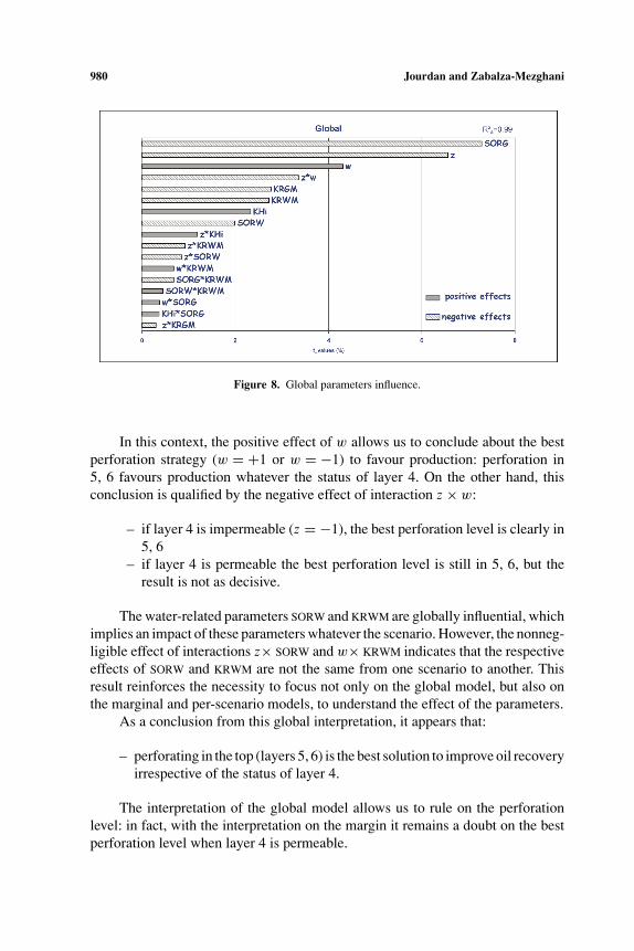
The Pareto plot (Fig. 8) confirms the global influence of KRGM and SORG. Themain advantage of this global interpretation is to be able to study both together butindependently the two discrete parameters z and w.

P1: KEE


Fig

ure

7.Pa

ram

eter

sin

fluen

cefo

rw

mar

gin.

979

P1: KEE



Figure 8. Global parameters influence.

In this context, the positive effect of w allows us to conclude about the bestperforation strategy (w = +1 or w = −1) to favour production: perforation in5, 6 favours production whatever the status of layer 4. On the other hand, thisconclusion is qualified by the negative effect of interaction z × w:

– if layer 4 is impermeable (z = −1), the best perforation level is clearly in5, 6

– if layer 4 is permeable the best perforation level is still in 5, 6, but theresult is not as decisive.

The water-related parameters SORW and KRWM are globally influential, whichimplies an impact of these parameters whatever the scenario. However, the nonneg-ligible effect of interactions z× SORW and w× KRWM indicates that the respectiveeffects of SORW and KRWM are not the same from one scenario to another. Thisresult reinforces the necessity to focus not only on the global model, but also onthe marginal and per-scenario models, to understand the effect of the parameters.

As a conclusion from this global interpretation, it appears that:

– perforating in the top (layers 5, 6) is the best solution to improve oil recoveryirrespective of the status of layer 4.

The interpretation of the global model allows us to rule on the perforationlevel: in fact, with the interpretation on the margin it remains a doubt on the bestperforation level when layer 4 is permeable.

P1: KEE



Quantitative Risk Study

Risk Analysis Modeling

The experimental design used for risk-analysis purposes is the full compositedesign (Fig. 2) composed with a factorial part, a central part, and an axial part.This design allows fitting a more accurate model than for sensitivity study, whichincludes not only the main terms and interactions terms but also quadratic terms.

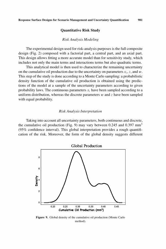
This analytical model is then used to characterize the remaining uncertaintyon the cumulative oil production due to the uncertainty on parameters xi , z, and w.This step of the study is done according to a Monte Carlo sampling: a probabilisticdensity function of the cumulative oil production is obtained using the predic-tions of the model at a sample of the uncertainty parameters according to givenprobability laws. The continuous parameters xi have been sampled according to auniform distribution, whereas the discrete parameters w and z have been sampledwith equal probability.

Risk Analysis Interpretation

Taking into account all uncertainty parameters, both continuous and discrete,the cumulative oil production (Fig. 9) may vary between 0.245 and 0.397 mm3

(95% confidence interval). This global interpretation provides a rough quantifi-cation of the risk. Moreover, the form of the global density suggests different

Figure 9. Global density of the cumulative oil production (Monte Carlomethod).

P1: KEE



Figure 10. Marginal density of the cumulative oil production per level ofperforation (Monte Carlo method).

behaviors, most likely due to the effect of the discrete parameters (two populationsappear on Fig. 9). In order to explore further this interpretation in depth, a studyon margins and scenarios is necessary.

The cumulative oil densities on w margins (Fig. 10) allow selection of the bestlevel of perforation. The mean cumulative production is only 0.28 × 106 m3 withthe 95% confidence interval [0.23 × 106 m3, 0.33 × 106 m3] if the perforationis in layers 3, 5, and 6, compared with 0.33 with the 95% confidence interval[0.25 × 106 m3, 0.4 × 106 m3] if perforation is in layers 5 and 6.

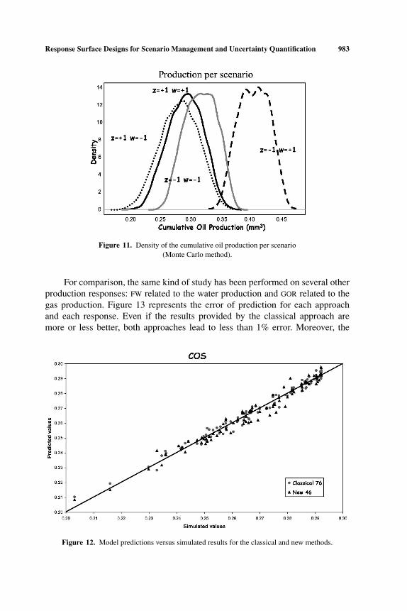
However, in the case of perforation in layers 5 and 6, a large uncertaintyremains. In fact, the dominating influence of the vertical permeability of layer 4(z) generates two distinct populations of equal importance. The studies by scenarios(Fig. 11) highlight the role played by z for a given perforation.

Comparison Between Classical and New Approach

To quantify the adding value of using this statistical approach to tackle dis-crete parameters, we present a comparison between the classical approach, whichrequires 4 times 19, i.e. 76 simulations, and this new approach, which requiresonly 46 simulations.

In order to compare the two approaches, we use a set of validation simulations(i.e. simulations not involved in the two experimental designs). Figure 12 representsthe model predictions versus the simulated results either for the new or the classicalapproaches. The two models provide good prediction accuracy. This result showsthe reliability and the consistency of the new approach.

P1: KEE



Figure 11. Density of the cumulative oil production per scenario(Monte Carlo method).

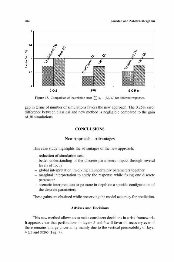
For comparison, the same kind of study has been performed on several otherproduction responses: FW related to the water production and GOR related to thegas production. Figure 13 represents the error of prediction for each approachand each response. Even if the results provided by the classical approach aremore or less better, both approaches lead to less than 1% error. Moreover, the

Figure 12. Model predictions versus simulated results for the classical and new methods.

P1: KEE



Figure 13. Comparison of the relative error (∑ |yi − yi |/yi ) for different responses.

gap in terms of number of simulations favors the new approach. The 0.25% errordifference between classical and new method is negligible compared to the gainof 30 simulations.

CONCLUSIONS

New Approach—Advantages

This case study highlights the advantages of the new approach:

– reduction of simulation cost– better understanding of the discrete parameters impact through several

levels of focus– global interpretation involving all uncertainty parameters together– marginal interpretation to study the response while fixing one discrete

parameter– scenario interpretation to go more in-depth on a specific configuration of

the discrete parameters

These gains are obtained while preserving the model accuracy for prediction.

Advises and Decisions

This new method allows us to make consistent decisions in a risk framework.It appears clear that perforations in layers 5 and 6 will favor oil recovery even ifthere remains a large uncertainty mainly due to the vertical permeability of layer4 (z) and SORG (Fig. 7).

P1: KEE



In order to reduce this remaining uncertainty, we suggest better characterizingthose two parameters z and SORG, for instance, by constraining the fluid-flow modelto new production data.

REFERENCES

Box, G. E. P., and Draper, N. R., 1987, Empirical model building and response surfaces: Wiley, NewYork, 669 p.

Damsleth, E., and Hage, A., 1991, Maximum information at minimum cost: A North Sea field devel-opment study using experimental design, in Offshore European Conference, Aberdeen, Scotland3–6 September 1991. SPE paper no. 23139.

Dejean, J.-P., and Blanc, G., 1999, Managing uncertainties on production prediction using integratedstatistical methods, in SPE Annual Technical Conference and Exhibition, Houston, TX, 3–6October 1999, SPE paper no. 56696.

Draper, N. R., and John, J. A., 1988, Response-surface designs for quantitative and qualitative variables:Technometrics, v. 30, p. 423–428.

Jourdan, A., 2002, Methode pour quantifier les incertitudes liees a des parametres continus et discretsdescriptifs d’un milieu par construction de plans d’experience et analyse statistique, IFP, Patentno. 02/04109.

Wu, C. F. J., and Ding, Y., 1998, Construction of response surface designs for qualitative and quantitativefactors: J. Stat. Plann. Inference, v. 71, p. 331–348.

Response Surface Designs for Scenario Management and Uncertainty Quantification in Reservoir...

Documents

Transcript of Response Surface Designs for Scenario Management and Uncertainty Quantification in Reservoir...