arX

iv:1

202.

1015

v2 [

quan

t-ph

] 3

Jun

201

2

Probability-based comparison of quantum states

Sergey N. Filippov1 and Mario Ziman2,31Moscow Institute of Physics and Technology, Moscow Region, Russia

2Institute for Theoretical Physics, ETH Zurich, 8093 Zurich, Switzerland3Institute of Physics, Slovak Academy of Sciences, Bratislava, Slovakia

We address the following state comparison problem: is it possible to design an experiment enablingus to unambiguously decide (based on the observed outcome statistics) on the sameness or differenceof two unknown state preparations without revealing complete information about the states? Wefind that the claim “the same” can never be concluded without any doubts unless the information iscomplete. Moreover, we prove that a universal comparison (that perfectly distinguishes all states)also requires complete information about the states. Nevertheless, for some measurements, theprobability distribution of outcomes still allows one to make an unambiguous conclusion regardingthe difference between the states even in the case of incomplete information. We analyze an efficiencyof such a comparison of qudit states when it is based on the SWAP-measurement. For qubit states,we consider in detail the performance of special families of two-valued measurements enabling usto successfully compare at most half of the pairs of states. Finally, we introduce almost universalcomparison measurements which can distinguish almost all non-identical states (up to a set ofmeasure zero). The explicit form of such measurements with two and more outcomes is found inany dimension.

PACS numbers: 03.67.-a, 03.65.Wj

I. INTRODUCTION

The exponential scaling of the number of parametersdescribing multipartite quantum systems stands behindthe potential power of quantum information processing.However, the same feature makes a complete character-ization (tomography) of unknown quantum devices in-tractable. Therefore, it is of practical interest to under-stand which properties of physical systems require thefull tomography for their determination and for which ofthem such a complete knowledge is redundant. In thispaper we analyze the resources needed for a comparisonof quantum states. Suppose a given pair of quantumsystems in unknown states. The question is what ex-periments (if any) are capable either of revealing withcertainty the difference between the states, or confirmingtheir sameness as long as the the probability distributionof measurement outcomes is identified.

By the very nature of quantum theory, the events weobserve in quantum experiments are random. That is,both quantum predictions and quantum conclusions arenaturally formulated in terms of probabilities and uncer-tainty. Therefore, it is surprising that there are (very spe-cific) situations (including special instances of the com-parison problem) in which individual clicks enable us tomake a nontrivial unambiguous prediction, or conclusion.For example, if we are given a promise that the states arepure, then (with a nonzero probability) the difference ofstates can be confirmed unambiguously from a single ex-perimental click [1, 2]. This result can be also generalizedto the comparison of many pure states [3–5], the compar-ison of ensembles of pure states [6], and the comparisonof some pure continuous-variable states [7, 8] (see alsothe review [9]). Unfortunately, such single-shot (non-statistical) comparison strategy fails for general mixed

states [5, 10]. The reason is simple. The probability ofany outcome is strictly nonvanishing provided that a bi-partite system is in the completely mixed state, for whichthe subsystems are in the same state. That is, for anyoutcome there is a situation in which the systems are thesame, hence the difference cannot be concluded unam-biguously. In such a case any error-free conclusions needto be based on the observed probabilities of outcomes.Probability-based strategies were not considered in pre-vious studies of quantum state comparison. Our aim inthis paper is to introduce this concept and provide basicresults in this area.Trivially, if the experimentally measured probabilities

provide complete information on quantum states of bothsystems individually, then they also contain all the infor-mation needed for the comparison. The question of ourinterest is whether the complete tomography is necessary.Our main goal is to design a comparison experiment pro-viding as little redundant information as possible.In Sec. II, we introduce the necessary mathematical

notation and formulate the problem. In Sec. III, we ad-dress the existence of a universal comparison measure-ment. Sec. IV investigates the comparison performanceof two-outcome measurements. Almost universal two-valued and many-valued comparison measurements arepresented in Sec. V and conclusions are the content ofSec. VI.

II. PROBLEM FORMULATION

Any quantum state is associated with the density oper-ator ∈ S(H) such that ≥ O and tr[] = 1. Hereafter,S(H) stands for the set of all states of a system associ-ated with the Hilbert space H. The statistical features

2

POVM

p1

p2

pn

...E

pn

p1

p2

10

1

1 P+

P

E

E

FIG. 1: (Color online) Illustration of probability-based com-parison. If the observed probability distribution belongs toP−

E\ P+

E, then states and ξ are for sure different.

of quantum measurements are fully captured by meansof a positive operator-valued measure (POVM) that isa collection E of positive operators (acting on H andcalled effects) E1, . . . , En summing up to the identity,i.e.

∑nj=1Ej = I. For each state ∈ S(H) the measure-

ment E assigns a probability distribution {pj}nj=1 ≡ ~pE,

where pj = tr[Ej] ≥ 0 and∑n

j=1 pj = 1.Let us now move on to the set of bipartite factorized

states Sfac = { ⊗ ξ : , ξ ∈ S(H)} ⊂ S(H ⊗H), wherethe parties and ξ are the states to be compared. For afixed measurement E we can ask how much informationit reveals concerning the comparison of the subsystems.Denote by S+ the subset of twin-identical states, i.e.

S+ = {η ⊗ η : η ∈ S(H)} ⊂ S(H ⊗ H). Similarly, letus denote by S− the subset of non-identical states, i.e.S− = {⊗ξ : , ξ(6= ) ∈ S(H)} ⊂ S(H⊗H). Obviously,Sfac = S+∪S−. The goal of comparison is then to distin-guish between sets of states S+ and S−. This goal can beachieved in our approach by considering two sets of prob-ability distributions P±

E= {~p : pj = tr[Ejω], ω ∈ S±}. In

other words, since the measurement E performs the map-ping S± 7→ P±

E, one can unambiguously conclude that a

bipartite state ω belongs to the set S± if the observedprobability distribution ~pE ∈ P±

E\ P∓

E(see Fig. 1).

For a fixed POVM E on H⊗H we may introduce thefollowing quantities:

DE(⊗ ξ,S+) = infη⊗η∈S+

n∑

j=1

|tr[Ej(⊗ ξ − η ⊗ η)]| ,(1)

DE(η ⊗ η,S−) = inf⊗ξ∈S−

n∑

j=1

|tr[Ej(⊗ ξ − η ⊗ η)]| .(2)

While DE(⊗ξ,S+) quantifies how different the states and ξ are (with respect to measurement E), the valueof DE(η⊗ η,S−) tells us to which extent the equivalenceof twin-identical states can be confirmed.Before we proceed further let us make one important

observation: for all ǫ > 0 and any state η⊗ η there existsa state ⊗ ξ such that |tr[E(η ⊗ η − ⊗ ξ)]| ≤ ǫ for anyPOVM effect E. In other words, in order to concludethat the states are the same no uncertainty in the spec-ification of the probabilities pE(ω) = tr[Eω] is allowed.Such an infinite precision is practically not achievable,

however, for our purposes we will assume the probabil-ities are specified exactly. The proof of the statementabove is relatively straightforward. Let us set = η andξ = (1− ǫ

2 )η+ǫ2dI, i.e. η⊗η−⊗ξ = ǫ

2η⊗(η− 1dI). Since

|tr[EX ]| ≤ maxE∈E tr[|EX |] ≤ tr[|X |], it follows that

|tr[E(η ⊗ η − ⊗ ξ)]| ≤ ǫ 12 tr[|η ⊗ (η − 1

dI)|] ≤ ǫ . (3)

In the last inequality we used the fact that the tracedistance of states is bounded from above by one. For-mula (3) is valid for any POVM-effect Ej , therefore∑n

j=1 |tr[Ej(⊗ ξ − η ⊗ η)]| ≤ nǫ → 0 when ǫ → 0. By

definition of the greatest lower bound (infimum), the dis-tance (2) vanishes for an arbitrary η ∈ S(H).Our observation implies that for any measurement E

we have DE(η ⊗ η,S−) = 0. This seems to be in contra-diction with measurements which provide us with com-plete information on the states of individual systems. Wewill refer to such measurements as locally information-

ally complete (LIC) measurements. Clearly, in case ofan ideal LIC measurement the sameness can be verified.Where is the problem? Topologically, in the set of fac-torized states Sfac with the trace-distance metrics, thesubset S+ is closed and does not contain any interiorpoint (therefore the distance (2) vanishes), however, itdoes not mean that the subset S+ is empty.Remark. The subset S+ is closed because the set S(H)

is closed. To prove that S+ does not contain any interiorpoint, assume the converse. Let η0 ⊗ η0 be an interiorpoint of S+, then there exists a neighborhood Oε(η0⊗η0)such that Oε(η0 ⊗ η0) ⊂ S+. Choose an arbitrary pointη⊗η ∈ Oε(η0⊗η0) with η 6= η0, then a nontrivial convexcombination [λη0⊗η0+(1−λ)η⊗η] ∈ Oε(η0⊗η0) ⊂ S+,i.e. λη0 ⊗ η0 + (1 − λ)η ⊗ η = ζ ⊗ ζ for some ζ ∈ S(H).Taking partial trace over the first subsystem, we obtainλη0 + (1 − λ)η = ζ. In view of this, ζ ⊗ ζ = λ2η0 ⊗ η0 +λ(1−λ)(η0⊗η+η⊗η0)+(1−λ)2η⊗η. Subtracting the twoexpressions obtained for ζ⊗ζ yields (η−η0)⊗(η−η0) = 0,i.e. η = η0, which contradicts the choice η 6= η0. Thus,S+ does not contain any interior point.The vanishing value of the distance considered (2) is

not completely relevant if one thinks about the idealerror-free experiments. In practice, experimental noiseis unavoidable; hence, from the practical point of view aconclusion on the sameness of states can never be errorfree.

III. UNIVERSAL COMPARISON

MEASUREMENT

We say the measurement E implements the compar-ison whenever DE( ⊗ ξ, S+) > 0 for some pairs , ξ.The state comparison measurement E is universal ifDE( ⊗ ξ, S+) > 0 for all , ξ(6= ). This is, for in-stance, achieved in case of the ideal LIC measurements:even though the value of DE(⊗ξ, S+) can be arbitrarilysmall, it always remains strictly positive. As before, this

3

situation is not very realistic in practice, because any er-ror in the identification of outcome probabilities makesthe conclusions (in some cases of and ξ) ambiguous.However, assuming the infinite precision in the specifi-cation of probabilities, the universality can be achievedand in what follows we will assume that probabilities areidentified perfectly. The potential errors can be viewedas modifications of the sets S+ and S− we are aiming todistinguish. Nevertheless, our goal is to analyze the idealcase.

Let us now demonstrate that a universal comparisoncan be implemented if and only if the measurement isLIC.

To start with, we are reminded that any POVM E witheffects Ej linearly maps a state ω ∈ S(H ⊗H) into theprobability vector ~p = (p1, p2, . . .), where pj = tr[Ejω].For LIC measurements the induced mapping ⊗ ξ 7→ ~πis bijective. That proves the sufficiency. To prove thenecessity let us assume the converse, i.e. suppose themeasurement E is not an LIC measurement but imple-ments a universal comparison. Since E is not LIC, theprobability assignment ⊗ ξ 7→ ~pE is injective. Let usdenote by Π± and Π the images of S± and Sfac undersome LIC measurement, respectively, and by PE denotethe image of Sfac under the measurement E. Clearly, therelation between ~π(⊗ ξ) and ~pE(⊗ ξ) is linear and in-jective, i.e. there exist probability vectors ~π1 ∈ Π and~π2 ∈ Π transformed into the same probability distribu-tion ~pE( ⊗ ξ) ∈ PE. The distributions ~πj transformedinto the same probability vector ~pE( ⊗ ξ) span a linearsubspace (hyperplane) H⊗ξ in the linear span of Π.

Consider an internal point η ∈ S(H), then the image~π(η ⊗ η) is an interior point of Π on the probability sim-plex. There exists ǫ0 > 0 such that for all 0 < ǫ ≤ ǫ0 theneighborhoodOǫ(~π(η⊗η)) belongs to Π (on the simplex).Moreover, the intersection Oǫ(~π(η ⊗ η)) ∩ Hη⊗η cannotbe a subset of Π+ only, because Π+ does not containany interior point on the simplex (if it did, the distanceDE(η ⊗ η,S−) would not vanish for all states η). Thus,Oǫ(~π(η⊗η))∩Hη⊗η∩Π− is not empty and contains points

of the form ~π(˜⊗ξ) such that ˜ 6= ξ. As both ~π(η⊗η) and~π(˜⊗ ξ) belong to Hη⊗η, we have ~pE(˜⊗ ξ) = ~pE(η ⊗ η)

and formula (1) yields D(˜⊗ ξ,S+) = 0, i.e. E is not auniversal comparison measurement (by definition). Thiscontradiction concludes the proof of the necessity.

Let us summarize two main conclusions:

(i) In any locally informationally incomplete measure-ment the sameness of states cannot be confirmed.

(ii) Universal comparison (concluding universally andunambiguously the difference of states) requires a locallyinformationally complete measurement.

A question that remains open is how to evaluate theoverall performance of (universal or non-universal) com-parison experiments. There are several options. We canuse the volume of the subset S−

comp of states in S− thatcan be successfully compared, or the average value ofDE(⊗ ξ,S+) with respect to some measure on the state

space. In particular, these quantities read

|S−comp|E =

∫∫

S−

µ(d)µ(dξ)h(DE(⊗ ξ,S+)) , (4)

〈DE〉 =

∫∫

S−

µ(d)µ(dξ)DE(⊗ ξ,S+) , (5)

where h(x) is the Heaviside function and µ(d) = µ(dξ)is a measure on the state space of individual subsystems.Quite common choices for the measure µ on density oper-ators are the ones induced by metrics, namely, by Buresdistance and Hilbert–Schmidt distance (see, e.g., [12, 13]and references therein). Let us stress that |S−

comp|E = 1does not imply the comparison is universal, because therecan be a set of measure zero for which DE(⊗ξ, S+) = 0.In such case we say that the comparison measurementis almost universal. It is of great interest to investigatewhether there exist some almost universal comparison ex-periments and, in particular, how many outcomes suchmeasurements require.

IV. TWO-VALUED COMPARISON

EXPERIMENTS

Let us start our investigation with the simplest case oftwo-valued POVMs described by the effects E and I−E.In such a case,

DE(⊗ ξ,S+) = 2DE(⊗ ξ,S+) , (6)

where DE(⊗ ξ,S+) = minη⊗η∈S+ |tr[E(⊗ ξ− η⊗ η)]|.Two-valued measurements cannot be LIC, because theyprovide the only informative real number (the probabilitypE , pI−E = 1− pE) whereas the state ⊗ ξ is defined by2(d2 − 1) ≥ 6 real numbers. Thus, two-valued measure-ments are necessarily non-universal comparators. Never-theless, it is of practical interest to understand how goodtheir comparison performance is.

Let us consider a geometry of comparable states. Sup-pose = 1

d(I + r · Λ) and ξ = 1

d(I + k · Λ), where

Λ = (Λ1, . . . ,Λd2−1) is a vector formed of traceless Her-mitian operators Λj such that tr[ΛjΛk] = dδjk, and

r,k ∈ Rd2−1 are Bloch-like vectors which necessarily sat-

isfy |r|, |k| ≤√d− 1 (see, e.g., [14]). Using this notation,

let us find such vectors r that the states are comparablewith a fixed state ξ (the POVM-effect E is fixed as well).The trace tr[E⊗ ξ] = 1

d(tr[EI ⊗ ξ] + r ·K), where K =

tr[EΛ⊗ ξ]. Therefore the inequality DE( ⊗ ξ,S+) > 0boils down to either

1dr ·K > max

η⊗η∈S+tr[Eη ⊗ η]− 1

dtr[EI ⊗ ξ], (7)

or

1dr ·K < min

η⊗η∈S+tr[Eη ⊗ η]− 1

dtr[EI ⊗ ξ]. (8)

4

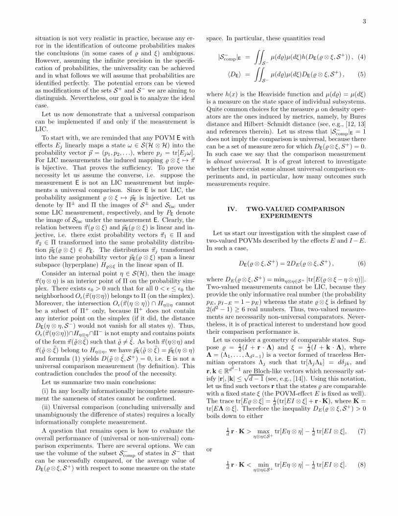
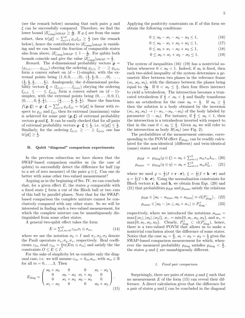
FIG. 2: (Color online) Body B(κ0), i.e. the region of parameters (κ1,κ2,κ3) when (15) is a true POVM effect. Parameter κ0

takes values 14, 3

8, 1

2, and 3

4for figures from left to right. The union ∪

κ0∈[0,1]B(κ0) is a rhombododecahedron and is depictedby solid lines. POVM effects Easym, Esym, Ez± are vertices and POVM effects Exy± are face centers of this convex polytope.

These inequalities define two nonintersecting half-spaces

in Rd2−1 separated by the distance

L =d

|K|

(

maxη⊗η∈S+

tr[Eη ⊗ η]− minη⊗η∈S+

tr[Eη ⊗ η]

)

.

(9)Thus, for any fixed ξ the set of successfully comparableBloch-like vectors r is given by an intersection of twohalf-spaces with the state space.

A. SWAP-based comparison

As we have already mentioned in Sec. I, if we restrictourselves only to pure states, then there exists a strategyto perform an unambiguous comparison (via the SWAPmeasurement). In such an approach, the sameness of thestates cannot be concluded and this is related to the ab-sence of the universal NOT-operation [11]. However, thestrategy (if successful) can reveal the difference betweenthe states in a single shot, hence, no collection of statis-tics is needed.The key observation for such a conventional strategy

is that the support of twin-identical pure states spansonly the symmetric subspace of H ⊗ H. Suppose pro-jections Esym, Easym onto symmetric and antisymmetricsubspaces of H⊗H. Since Esym + Easym = I they forma two-valued POVM ESWAP. Let us note that Esym =12 (I+S), Easym = 1

2 (I−S), where S is the SWAP opera-tor acting as S(|ψ⊗ϕ〉) = |ϕ⊗ψ〉 for all |ψ〉, |ϕ〉 ∈ H. Itis straightforward to see that for any twin-identical purestate |ϕ⊗ϕ〉 one has tr[Easym|ϕ⊗ϕ〉〈ϕ⊗ϕ|] = 0, howevertr[Easym|ϕ⊗ψ〉〈ϕ⊗ψ|] = 1

2 (1−|〈ϕ|ψ〉|2) > 0 if |ψ〉 6= |ϕ〉.Therefore, recording an outcome Easym allows us to un-ambiguously conclude that the states are different. Nostatistics is needed.Let us see how this strategy works in the case of general

mixed states. A direct calculation yields

psym = tr[Esym⊗ ξ] = 12 (1 + tr[ξ]) , (10)

pasym = tr[Easym⊗ ξ] = 12 (1− tr[ξ]) , (11)

where we used the identity tr[S⊗ξ] = tr[ξ]. The purityof a state, tr[η2], is bounded from below by 1/d, whered = dimH. Thus,

psym(⊗ ξ) ∈ [ 12 , 1) ≡ P−sym , (12)

psym(η ⊗ η) ∈ [d+12d , 1] ≡ P+

sym , (13)

where P±sym is the image of S± under the POVM ef-

fect Esym. It follows that by measuring the probabilitypsym < (d+1)/2d we can with certainty conclude that thestates are different. In particular, DSWAP( ⊗ ξ,S+) =max{0, 1

d− tr[ξ]}.

Associating and ξ with the Bloch-like vectors r,k ∈R

d2−1 as above (|r|, |k| ≤√d− 1), for the SWAP-based

measurement we obtain K± = tr[(I ± S)Λ ⊗ ξ] =±k. Also, we find explicitly tr[(I ± S)I ⊗ ξ] = d ± 1,maxη⊗η∈S+ tr[(I+S)η⊗η] = 2, maxη⊗η∈S+ tr[(I−S)η⊗η] = 1 − 1

d, minη⊗η∈S+ tr[(I + S)η ⊗ η] = 1 + 1

d, and

minη⊗η∈S+ tr[(I − S)η ⊗ η] = 0. Then it is straightfor-ward to see that, for the SWAP-based measurement, oneof inequalities (7) and (8) is never fulfilled and the otherone reduces to r · k < 0. That is, for each fixed k(6= 0)the set of successfully comparable Bloch-like vectors r isgiven by an intersection of a single half-space with thestate space. Let us stress that for qubits (d = 2) thestate space is exactly the Bloch ball |r| ≤ 1, so the set ofcomparable vectors r is the hemisphere. Thus, for qubits|S−

comp|SWAP = 12 (see the next paragraph). In other

words, the difference of states from the same hemisphereis not detected in the SWAP measurement. This impliesthat the approximate universality is lost.Due to unitary invariance of the measure µ we can

always treat one of the states in DE(⊗ ξ,S+) as diago-

nal, say . Then tr[ξ] =∑d

j=1 jjξjj and the integration

area of |S−comp|SWAP is split into d! subsets labeled by the

permutation of the labels j1, . . . , jd identifying the order-ing j1j1 ≥ · · · ≥ jdjd of eigenvalues of . The (normal-ized) volume of each of these subsets is 1

d! . If and ξ arefrom mutually opposite subsets (labeled as j1, . . . , jd and

jd, . . . , j1, respectively), then tr[ξ] =∑d

j=1 jjξjj ≤ 1d

5

(see the remark below) meaning that such pairs andξ can be successfully compared. Therefore, we find thelower bound |S−

comp|SWAP ≥ 1d! . If , ξ are from the same

subset, then tr[ξ] =∑d

j=1 jjξjj ≥ 1d(see the remark

below), hence the contribution to |S−comp|SWAP is vanish-

ing and we can bound the fraction of comparable statesalso from above, |S−

comp|SWAP ≤ 1 − 1d! . For qubits both

bounds coincide and give the value |S−comp|SWAP = 1

2 .Remark. The d-dimensional probability vectors =

(j1j1 , . . . , jdjd) obeying the ordering j1j1 ≥ · · · ≥ jdjdform a convex subset on (d − 1)-simplex, with the ex-tremal points being (1, 0, 0, . . . , 0), (12 ,

12 , 0, . . . , 0), . . . ,

( 1d, 1d, 1d, . . . , 1

d). Analogously, the d-dimensional proba-

bility vectors ξ = (ξj1j1 , . . . , ξjdjd) obeying the orderingξj1j1 ≤ · · · ≤ ξjdjd form a convex subset on (d − 1)-simplex, with the extremal points being (0, . . . , 0, 0, 1),(0, . . . , 0, 12 ,

12 ), . . . , (

1d, . . . , 1

d, 1d, 1d). Since the function

f(, ξ) = · ξ =∑d

j=1 jjξjj = tr[ξ] is linear with re-

spect to jj and ξjj , then its extremal (maximum) valueis achieved for some pair (, ξ) of extremal probabilityvectors and ξ. It can be easily checked that for all pairsof extremal probability vectors · ξ ≤ 1

d, i.e. tr[ξ] ≤ 1

d.

Similarly, for the ordering ξj1j1 ≥ · · · ≥ ξjdjd one hastr[ξ] ≥ 1

d.

B. Qubit “diagonal” comparison experiments

In the previous subsection we have shown that theSWAP-based comparison enables us (in the case ofqubits) to successfully detect the difference for half (upto a set of zero measure) of the pairs ⊗ ξ. Can one dobetter with some other two-valued measurement?Arguing as in the beginning of Sec. IV, we can conclude

that, for a given effect E, the states comparable witha fixed state ξ form a cut of the Bloch ball or two cutsof this ball by parallel planes. Note that for the SWAP-based comparison the complete mixture cannot be con-clusively compared with any other state. So we will beinterested in finding such a two-valued measurement, forwhich the complete mixture can be unambiguously dis-tinguished from some other states.A general two-qubit effect takes the form

E =∑3

l,m=0 εlmσl ⊗ σm, (14)

where we use the notation σ0 = I and σ1, σ2, σ3 denotethe Pauli operators σx, σy , σz, respectively. Real coeffi-cients εlm read εlm = 1

4 tr[Eσl ⊗ σm] and satisfy the theconstraints O ≤ E ≤ I.For the sake of simplicity let us consider only the diag-

onal case, i.e. we will assume εlm = δlmκm, with κm ∈ R

for all m = 0, . . . , 3. Then

Ediag =

κ0 + κ3 0 0 κ1 − κ2

0 κ0 − κ3 κ1 + κ2 00 κ1 + κ2 κ0 − κ3 0

κ1 − κ2 0 0 κ0 + κ3

.

(15)

Applying the positivity constraints on E of this form weobtain the following conditions:

0 ≤ κ0 − κ1 − κ2 − κ3 ≤ 1, (16)

0 ≤ κ0 − κ1 + κ2 + κ3 ≤ 1, (17)

0 ≤ κ0 + κ1 − κ2 + κ3 ≤ 1, (18)

0 ≤ κ0 + κ1 + κ2 − κ3 ≤ 1. (19)

The system of inequalities (16)–(19) has a nontrivial so-lution whenever 0 < κ0 < 1. Indeed, if κ0 is fixed, theneach two-sided inequality of the system determines a ge-ometric fiber between two planes in the reference frame(κ1,κ2,κ3), with the distance between the planes beingequal to 1√

3. If 0 < κ0 ≤ 1

4 , then four fibers intersect

to yield a tetrahedron. The intersection becomes a trun-cated tetrahedron if 1

4 < κ0 <12 and finally transforms

into an octahedron for the case κ0 = 12 . If κ0 ≥ 1

2then the solution is a body obtained by the inversion(κ1,κ2,κ3) → (−κ1,−κ2,−κ3) of the body labeled byparameter (1 − κ0). For instance, if 3

4 ≤ κ0 < 1, thenthe intersection is a tetrahedron inverted with respect tothat in the case 0 < κ0 ≤ 1

4 . Given κ0 we will refer tothe intersection as body B(κ0) (see Fig. 2).The probabilities of the measurement outcome, corre-

sponding to the POVM effect Ediag, can be readily calcu-lated for the non-identical (different) and twin-identical(same) states and read

pdiff = pdiag(⊗ ξ) = κ0 +∑3

m=1 κmrmkm , (20)

psame = pdiag(η ⊗ η) = κ0 +∑3

m=1 κmh2m , (21)

where we used = 12 (I + r · σ), ξ = 1

2 (I + k · σ) and

η = 12 (I +h ·σ). Using the normalization constraints for

Bloch vectors r, k, and h, we obtain from Eqs. (20) and(21) that probabilities pdiff and psame satisfy the relations

pdiff ∈ [κ0 − κmax,κ0 + κmax] ≡ cl(P−diag) , (22)

psame ∈ [κ0 − |κ−|,κ0 + κ+] ≡ P+diag , (23)

respectively, where we introduced the notations κmax =max{|κ1|, |κ2|, |κ3|}, κ− = min{0,κ1,κ2,κ3}, and κ+ =max{0,κ1,κ2,κ3}. Clearly, P+

diag ⊂ cl(P−diag), hence,

there is a two-valued POVM that allows us to make anontrivial conclusion about the difference of some states.Notice that the case κ0 = 3

4 , κ1 = κ2 = κ3 = 14 gives the

SWAP-based comparison measurement for which, when-ever the measured probability pdiag satisfies pdiag <

34 ,

the states and ξ are unambiguously different.

1. Fixed pair comparison

Surprisingly, there are pairs of states and ξ such thatno measurement E of the form (15) can reveal their dif-ference. A direct calculation gives that the difference fora pair of states and ξ can be concluded in the diagonal

6

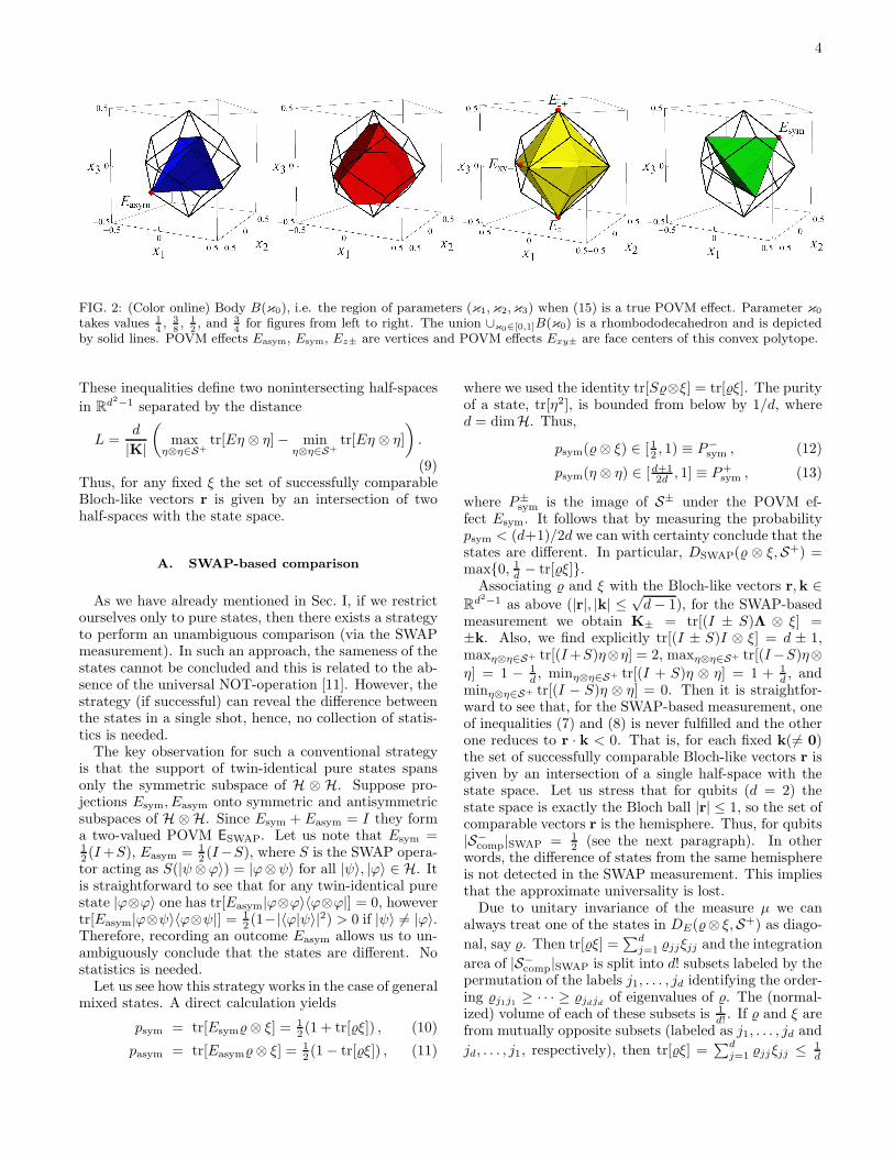
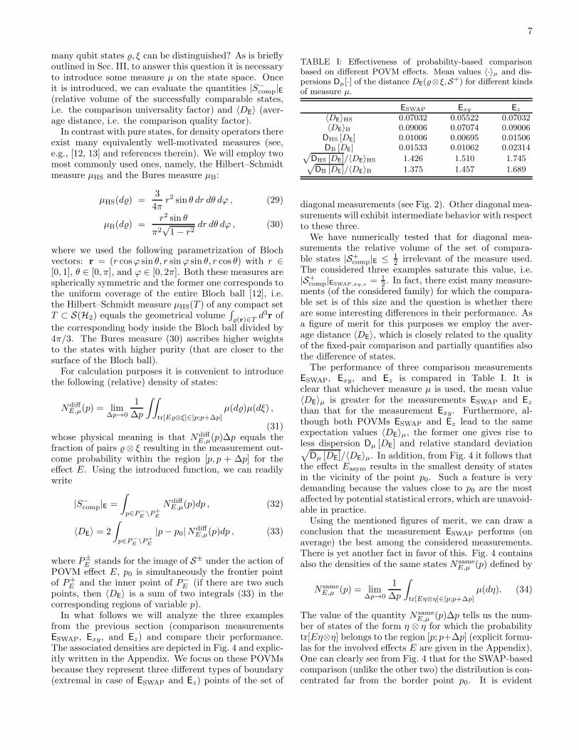
FIG. 3: (Color online) States in the Bloch ball (determined by vectors r) which can be distinguished from a fixed state ξ(given by vector k) by using measurement ESWAP (a), Exy (b), and Ez (c).

comparison experiment if

Ddiag(⊗ ξ,S+) = min|h|≤1

∣

∣

∣

∑3m=1 κm(rmkm − h2m)

∣

∣

∣ > 0 .

(24)Suppose that rmkm is nonnegative for all m. Settinghm =

√rmkm the distance (24) is vanishing for arbitrary

measurement of the considered diagonal form. Let usstress that the requirement of positivity of rmkm for allm means that signs of the Bloch vector components co-incide, hence, k and r belong to the same octant of theBloch ball. Let us stress, however, that the octants de-pend on the choice of the axes (Pauli operators), and fora given pair of states we can always fix the coordinatesystem in such a way that they belong to two differentoctants. The only exceptions are collinear vectors k andr = ck for c ≥ 0. In fact, a pair of parallel Bloch vec-tors (pointing in the same direction) is indistinguishableby any diagonal measurement irrelevant of the choice ofcoordinate system. In particular, it follows that none ofthese measurements is capable of distinguishing (in thecomparison sense) the complete mixture = 1

2I from any

other state, because pdiff(12I⊗ ξ) = psame(

12I⊗ 1

2I) = κ0.It is natural to ask for which pairs , ξ their difference

can be identified by a suitably selected E of the consid-ered diagonal form and whether there are some “non-diagonal” measurements enabling us to compare a pairof states containing the complete mixture.In order to get an insight into the power of diagonal

measurements, let us assume that κm ≥ 0, m = 1, 2, 3and fix k. Define a new vector K = (κ1k1,κ2k2,κ3k3).If K · r > 0, then we can find h such that K · r =∑3

m=1 κmh2m, hence Ddiag( ⊗ ξ,S+) = 0. If K · r < 0,

then Ddiag( ⊗ ξ,S+) = |K · r| + ∑3m=1 κmh

2m > 0 for

any h 6= 0. Therefore, the minimum is achieved forη ⊗ η = 1

2I ⊗ 12I and the distance reads

Ddiag(⊗ ξ,S+) =

{

0 if K · r ≥ 0,|K · r| otherwise.

(25)

In other words, the considered diagonal measurement Eenables us to verify the difference between and ξ for all satisfying the inequality K · r < 0. The condition K · r =0 determines a plane containing the complete mixture(center of the Bloch ball), hence, for any measurement ofthe considered type and any state ξ the set of successfullycomparable states is exactly a hemisphere of the Blochball. Fig. 3 illustrates this situation for the followingchoices of the diagonal measurements (POVMs):

ESWAP ={

Esym = 14

(

3 · I ⊗ I +∑3

m=1 σm ⊗ σm)

,

Easym = 14 (I ⊗ I −∑3

m=1 σm ⊗ σm)}

; (26)

Exy ={

Exy+ = 14

(

3 · I ⊗ I +∑2

m=1 σm ⊗ σm)

,

Exy− = 14

(

I ⊗ I −∑2m=1 σm ⊗ σm

)}

; (27)

Ez ={

Ez± = 12 (I ⊗ I ± σ3 ⊗ σ3)

}

. (28)

In particular, for ESWAP the “comparable hemisphere”is orthogonal to the vector k. For Exy the “comparable”hemisphere is orthogonal to the vector k‖ = (k1, k2, 0)being a projection of k onto the xy plane. Finally, for Ez

any state from the northern hemisphere is “comparable”with any state from the southern hemisphere.It is worth noting that we have restricted ourselves to

the specific form of POVM effects (15). However, evenfor such a simplified problem the solution looks rathersophisticated.

2. Average performance

The fact that for any given diagonal two-valued mea-surement the states within the same octant are not com-parable means that none of them is universal neither inan approximative way. Nevertheless, it is of interest tounderstand which of them perform better than the othersand which do not perform at all. In particular, we areinterested in the answer to the following question: How

7

many qubit states , ξ can be distinguished? As is brieflyoutlined in Sec. III, to answer this question it is necessaryto introduce some measure µ on the state space. Onceit is introduced, we can evaluate the quantities |S−

comp|E(relative volume of the successfully comparable states,i.e. the comparison universality factor) and 〈DE〉 (aver-age distance, i.e. the comparison quality factor).In contrast with pure states, for density operators there

exist many equivalently well-motivated measures (see,e.g., [12, 13] and references therein). We will employ twomost commonly used ones, namely, the Hilbert–Schmidtmeasure µHS and the Bures measure µB:

µHS(d) =3

4πr2 sin θ dr dθ dϕ , (29)

µB(d) =r2 sin θ

π2√1− r2

dr dθ dϕ , (30)

where we used the following parametrization of Blochvectors: r = (r cosϕ sin θ, r sinϕ sin θ, r cos θ) with r ∈[0, 1], θ ∈ [0, π], and ϕ ∈ [0, 2π]. Both these measures arespherically symmetric and the former one corresponds tothe uniform coverage of the entire Bloch ball [12], i.e.the Hilbert–Schmidt measure µHS(T ) of any compact setT ⊂ S(H2) equals the geometrical volume

∫

(r)∈Td3r of

the corresponding body inside the Bloch ball divided by4π/3. The Bures measure (30) ascribes higher weightsto the states with higher purity (that are closer to thesurface of the Bloch ball).For calculation purposes it is convenient to introduce

the following (relative) density of states:

NdiffE,µ(p) = lim

∆p→0

1

∆p

∫∫

tr[E⊗ξ]∈[p;p+∆p]

µ(d)µ(dξ) ,

(31)whose physical meaning is that Ndiff

E,µ(p)∆p equals thefraction of pairs ⊗ ξ resulting in the measurement out-come probability within the region [p, p + ∆p] for theeffect E. Using the introduced function, we can readilywrite

|S−comp|E =

∫

p∈P−E

\P+

E

NdiffE,µ(p)dp , (32)

〈DE〉 = 2

∫

p∈P−E\P+

E

|p− p0|NdiffE,µ(p)dp , (33)

where P±E stands for the image of S± under the action of

POVM effect E, p0 is simultaneously the frontier pointof P+

E and the inner point of P−E (if there are two such

points, then 〈DE〉 is a sum of two integrals (33) in thecorresponding regions of variable p).In what follows we will analyze the three examples

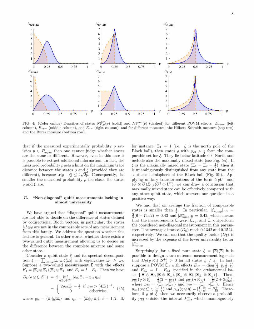
from the previous section (comparison measurementsESWAP, Exy, and Ez) and compare their performance.The associated densities are depicted in Fig. 4 and explic-itly written in the Appendix. We focus on these POVMsbecause they represent three different types of boundary(extremal in case of ESWAP and Ez) points of the set of

TABLE I: Effectiveness of probability-based comparisonbased on different POVM effects. Mean values 〈·〉µ and dis-persions Dµ[·] of the distance DE(⊗ξ,S+) for different kindsof measure µ.

ESWAP Exy Ez

〈DE〉HS 0.07032 0.05522 0.07032〈DE〉B 0.09006 0.07074 0.09006

DHS [DE] 0.01006 0.00695 0.01506DB [DE] 0.01533 0.01062 0.02314

√

DHS [DE]/〈DE〉HS 1.426 1.510 1.745√

DB [DE]/〈DE〉B 1.375 1.457 1.689

diagonal measurements (see Fig. 2). Other diagonal mea-surements will exhibit intermediate behavior with respectto these three.We have numerically tested that for diagonal mea-

surements the relative volume of the set of compara-ble states |S+

comp|E ≤ 12 irrelevant of the measure used.

The considered three examples saturate this value, i.e.|S+

comp|ESWAP,xy,z= 1

2 . In fact, there exist many measure-ments (of the considered family) for which the compara-ble set is of this size and the question is whether thereare some interesting differences in their performance. Asa figure of merit for this purposes we employ the aver-age distance 〈DE〉, which is closely related to the qualityof the fixed-pair comparison and partially quantifies alsothe difference of states.The performance of three comparison measurements

ESWAP, Exy, and Ez is compared in Table I. It isclear that whichever measure µ is used, the mean value〈DE〉µ is greater for the measurements ESWAP and Ez

than that for the measurement Exy. Furthermore, al-though both POVMs ESWAP and Ez lead to the sameexpectation values 〈DE〉µ, the former one gives rise toless dispersion Dµ [DE] and relative standard deviation√

Dµ [DE]/〈DE〉µ. In addition, from Fig. 4 it follows thatthe effect Easym results in the smallest density of statesin the vicinity of the point p0. Such a feature is verydemanding because the values close to p0 are the mostaffected by potential statistical errors, which are unavoid-able in practice.Using the mentioned figures of merit, we can draw a

conclusion that the measurement ESWAP performs (onaverage) the best among the considered measurements.There is yet another fact in favor of this. Fig. 4 containsalso the densities of the same states N same

E,µ (p) defined by

N sameE,µ (p) = lim

∆p→0

1

∆p

∫

tr[Eη⊗η]∈[p;p+∆p]

µ(dη). (34)

The value of the quantity N sameE,µ (p)∆p tells us the num-

ber of states of the form η ⊗ η for which the probabilitytr[Eη⊗η] belongs to the region [p; p+∆p] (explicit formu-las for the involved effects E are given in the Appendix).One can clearly see from Fig. 4 that for the SWAP-basedcomparison (unlike the other two) the distribution is con-centrated far from the border point p0. It is evident

8

FIG. 4: (Color online) Densities of states NdiffE,µ(p) (solid) and N same

E,µ (p) (dashed) for different POVM effects: Easym (leftcolumn), Exy− (middle column), and Ez− (right column); and for different measures: the Hilbert–Schmidt measure (top row)and the Bures measure (bottom row).

that if the measured experimentally probability p sat-isfies p ∈ P+

asym then one cannot judge whether statesare the same or different. However, even in this case itis possible to extract additional information. In fact, themeasured probability p sets a limit on the maximum tracedistance between the states and ξ (provided they aredifferent), because tr|− ξ| ≤ 2

√2p. Consequently, the

smaller the measured probability p the closer the states and ξ are.

C. “Non-diagonal” qubit measurements lacking in

almost universality

We have argued that “diagonal” qubit measurementsare not able to decide on the difference of states definedby codirectional Bloch vectors, in particular, the states12I⊗ are not in the comparable sets of any measurementfrom this family. We address the question whether thisfeature is general. In other words, whether there exists atwo-valued qubit measurement allowing us to decide onthe difference between the complete mixture and someother state.Consider a qubit state ξ and its spectral decomposi-

tion ξ =∑

i=1,2 Ξi|Ξi〉〈Ξi| with eigenvalues Ξ1 ≥ Ξ2.Suppose a two-valued measurement E with the effectsE1 = |Ξ2⊗Ξ1〉〈Ξ2⊗Ξ1| and E2 = I−E1. Then we have

DE(⊗ ξ,S+) = 2 infη⊗η∈S+

|22Ξ1 − η11η22|

=

{

222Ξ1 − 12 if 22 > (4Ξ1)

−1,0 otherwise,

(35)

where ii = 〈Ξi||Ξi〉 and ηii = 〈Ξi|η|Ξi〉, i = 1, 2. If,

for instance, Ξ1 = 1 (i.e. ξ is the north pole of theBloch ball), then states with 22 >

14 form the com-

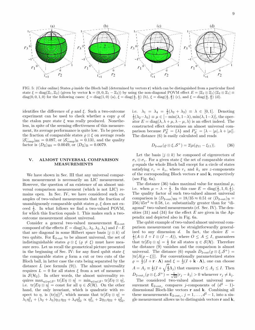
parable set for ξ. They lie below latitude 60◦ North andinclude also the maximally mixed state (see Fig. 5a). Ifξ is the maximally mixed state (Ξ1 = Ξ2 = 1

2 ), then itis unambiguously distinguished from any state from thesouthern hemisphere of the Bloch ball (Fig. 5b). Ap-plying unitary transformations of the form UU † and(U ⊗ U)E1,2(U

† ⊗ U †), we can draw a conclusion thatmaximally mixed state can be effectively compared withany other qubit state, which answers our question in apositive way.

We find that on average the fraction of comparablestates is smaller than 1

2 . In particular, |S−comp|HS =

38 (6 − 7 ln 2) = 0.43 and |S−

comp|B = 0.42, which meansthat the measurements ESWAP, Exy, and Ez outperformthe considered non-diagonal measurement in this param-eter. The average distance 〈DE〉 reads 0.1342 and 0.1524,respectively. We can see that the quality factor 〈DE〉 isincreased by the expense of the lower universality factor|S−

comp|.Surprisingly, for a fixed pure state ξ = |Ξ〉〈Ξ| it is

possible to design a two-outcome measurement EΞ suchthat DΞ( ⊗ ξ,S+) > 0 for all states 6= ξ. In fact,suppose a POVM EΞ with effects EΞ1 = diag(14 ,

38 ,

18 ,

58 )

and EΞ2 = I − EΞ1 specified in the orthonormal ba-sis {|Ξ ⊗ Ξ〉, |Ξ ⊗ Ξ⊥〉, |Ξ⊥ ⊗ Ξ〉, |Ξ⊥ ⊗ Ξ⊥〉}. Then,pΞ1( ⊗ ξ) = 1

8 (2 − 22) and pΞ1(η ⊗ η) = 18 (2 + 3η222),

where 22 = 〈Ξ⊥||Ξ⊥〉 and η22 = 〈Ξ⊥|η|Ξ⊥〉. HencepΞ1(⊗ ξ) ∈ [ 18 ,

14 ) and pΞ1(η⊗η) = [ 14 ,

58 ] ≡ P+

Ξ1. There-fore, if 6= ξ, then we necessarily observe a probabil-ity pΞ1 outside the interval P+

Ξ1, which unambiguously

9

FIG. 5: (Color online) States inside the Bloch ball (determined by vectors r) which can be distinguished from a particular fixedstate ξ = diag(Ξ1,Ξ2) (given by vector k = (0, 0,Ξ1 − Ξ2)) by using the non-diagonal POVM effect E = |Ξ2 ⊗ Ξ1〉〈Ξ2 ⊗ Ξ1| ≡diag(0, 0, 1, 0) for the following cases: ξ = diag(1, 0) (a), ξ = diag( 1

2, 12) (b), ξ = diag( 1

3, 23) (c), and ξ = diag( 1

4, 34) (d).

identifies the difference of and ξ. Such a two-outcomeexperiment can be used to check whether a copy ofthe etalon pure state ξ was really produced. Nonethe-less, in spite of the seeming effectiveness of this measure-ment, its average performance is quite low. To be precise,the fraction of comparable states ⊗ ξ on average reads|S−

comp|HS = 0.097, or |S−comp|B = 0.131, and the quality

factor is 〈DΞ〉HS = 0.0049, or 〈DΞ〉B = 0.0079.

V. ALMOST UNIVERSAL COMPARISON

MEASUREMENTS

We have shown in Sec. III that any universal compar-ison measurement is necessarily an LIC measurement.However, the question of an existence of an almost uni-versal comparison measurement (which is not LIC) re-mains open. In Sec. IV, we have considered such ex-amples of two-valued measurements that the fraction ofunambiguously comparable qubit states , ξ does not ex-ceed 1

2 . In what follows we find a two-valued POVM,for which this fraction equals 1. This makes such a two-outcome measurement almost universal.Consider a general two-valued measurement E2-out

composed of the effects E = diag(λ1, λ2, λ3, λ4) and I−Ethat are diagonal in some Hilbert space basis |j ⊗ k〉 oftwo qubits. For E2-out to be almost universal, the set ofindistinguishable states ⊗ ξ ( 6= ξ) must have mea-sure zero. Let us recall the geometrical picture presentedin the beginning of Sec. IV: for any fixed qubit state ξthe comparable states form a cut or two cuts of theBloch ball, in latter case the cuts being separated by thedistance L (see formula (9)). The almost universalityrequires L = 0 for all states ξ from a set of measure 1in S(H2). In other words, the almost universality re-quires maxη⊗η∈S+ tr[Eη ⊗ η] = minη⊗η∈S+ tr[Eη ⊗ η],i.e. tr[Eη ⊗ η] = const for all η ∈ S(H). On the otherhand, the only invariant, which is quadratic with re-spect to η, is (tr[η])2, which means that tr[Eη ⊗ η] =λ1η

211 + (λ2 + λ3)η11η22 + λ4η

222 ∝ η211 + 2η11η22 + η222,

i.e. λ1 = λ4 = 12 (λ2 + λ3) ≡ λ ∈ [0, 1]. Denoting

12 (λ2−λ3) ≡ µ ∈ [−min(λ, 1−λ),min(λ, 1−λ)], the oper-ator E = diag(λ, λ+ µ, λ− µ, λ) is an effect indeed. Theconstructed effect determines an almost universal com-parison because P+

E = {λ} and P−E = [λ − |µ|, λ + |µ|].

The distance (6) is easily calculated and reads

D2-out(⊗ ξ,S+) = 2|µ(11 − ξ11)|. (36)

Let the basis |j ⊗ k〉 be composed of eigenvectors ofσz ⊗ σz . For a given state ξ the set of comparable states equals the whole Bloch ball except for a circle of statessatisfying rz = kz, where rz and kz are z-componentsof the corresponding Bloch vectors r and k, respectively(see Fig. 6a).The distance (36) takes maximal value for maximal µ,

i.e. when µ = λ = 12 . In this case E = diag(12 , 1, 0,

12 ).

The quality factor of such two-valued almost universalcomparison is 〈D2-out〉HS = 18/35 ≈ 0.51 or 〈D2-out〉B =256/45π2 ≈ 0.58, i.e. substantially greater than for “di-agonal” two-valued measurements (cf. Sec. IV). The den-sities (31) and (34) for the effect E are given in the Ap-pendix and depicted also in Fig. 6a.The qubit example of two-valued almost universal com-

parison measurement can be straightforwardly general-ized to any dimension d. In fact, the choice E =12 (A ⊗ I + I ⊗ (I − A)), where O ≤ A ≤ I, guarantees

that tr[Eη ⊗ η] = 12 for all states η ∈ S(H). Therefore

the distance (9) vanishes and the comparison is almostuniversal. The distance (6) equals D2-out( ⊗ ξ,S+) =|tr[A(− ξ)]|. For conventionally parameterized states = 1

d(I + r · Λ) and ξ = 1

d(I + k · Λ), one can choose

A = Aj ≡ 12 (I +

√

2dΛj) that ensures O ≤ Aj ≤ I. Then

D2-outj (⊗ ξ,S+) = 1√2d|rj − kj | > 0 whenever rj 6= kj .

The considered two-valued almost universal mea-surement E2-outj compares j-components of (d2 − 1)-dimensional Bloch-like vectors r and k. Combining allthese measurements E2-outj , j = 1, . . . , d2 − 1, into a sin-gle measurement allows us to distinguish vectors r and k,

10

i.e. performing universal comparison measurements with2(d2 − 1) effects. Such a measurement will be LIC, intotal agreement with the results of Sec. III.Although a measurement with two outcomes can be al-

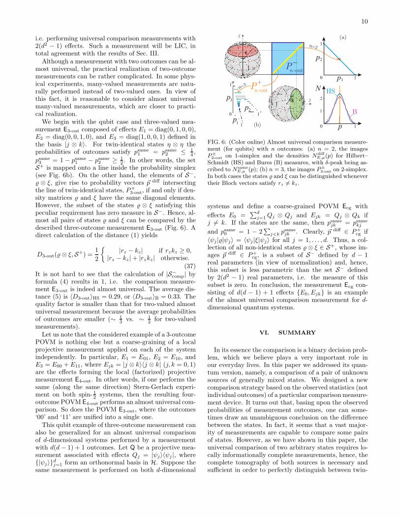
most universal, the practical realization of two-outcomemeasurements can be rather complicated. In some phys-ical experiments, many-valued measurements are natu-rally performed instead of two-valued ones. In view ofthis fact, it is reasonable to consider almost universalmany-valued measurements, which are closer to practi-cal realization.We begin with the qubit case and three-valued mea-

surement E3-out composed of effects E1 = diag(0, 1, 0, 0),E2 = diag(0, 0, 1, 0), and E3 = diag(1, 0, 0, 1) defined inthe basis |j ⊗ k〉. For twin-identical states η ⊗ η theprobabilities of outcomes satisfy psame

1 = psame2 ≤ 1

4 ,

psame3 = 1 − psame

1 − psame2 ≥ 1

2 . In other words, the setS+ is mapped onto a line inside the probability simplex(see Fig. 6b). On the other hand, the elements of S−, ⊗ ξ, give rise to probability vectors ~p diff intersectingthe line of twin-identical states, P+

3-out, if and only if den-sity matrices and ξ have the same diagonal elements.However, the subset of the states ⊗ ξ satisfying thispeculiar requirement has zero measure in S−. Hence, al-most all pairs of states and ξ can be compared by thedescribed three-outcome measurement E3-out (Fig. 6). Adirect calculation of the distance (1) yields

D3-out(⊗ ξ,S+) =1

2

{

|rz − kz| if rzkz ≥ 0,|rz − kz |+ |rzkz| otherwise.

(37)It is not hard to see that the calculation of |S−

comp| byformula (4) results in 1, i.e. the comparison measure-ment E3-out is indeed almost universal. The average dis-tance (5) is 〈D3-out〉HS = 0.29, or 〈D3-out〉B = 0.33. Thequality factor is smaller than that for two-valued almostuniversal measurement because the average probabilitiesof outcomes are smaller (∼ 1

3 vs. ∼ 12 for two-valued

measurements).Let us note that the considered example of a 3-outcome

POVM is nothing else but a coarse-graining of a localprojective measurement applied on each of the systemindependently. In particular, E1 = E01, E2 = E10, andE3 = E00 + E11, where Ejk = |j ⊗ k〉〈j ⊗ k| (j, k = 0, 1)are the effects forming the local (factorized) projectivemeasurement E4-out. In other words, if one performs thesame (along the same direction) Stern-Gerlach experi-ment on both spin- 12 systems, then the resulting four-outcome POVM E4-out performs an almost universal com-parison. So does the POVM E3-out, where the outcomes‘00’ and ‘11’ are unified into a single one.This qubit example of three-outcome measurement can

also be generalized for an almost universal comparisonof d-dimensional systems performed by a measurementwith d(d − 1) + 1 outcomes. Let Q be a projective mea-surement associated with effects Qj = |ψj〉〈ψj |, where{|ψj〉}dj=1 form an orthonormal basis in H. Suppose thesame measurement is performed on both d-dimensional

r

z

zk

P+

n -out

Pn -out

n=3

0 p1

p2

1

1

0 p

2

1

1

N

B

HS

(a)

(b)

1

p2

0

1

p1

1

p3

n=2

FIG. 6: (Color online) Almost universal comparison measure-ment (for qubits) with n outcomes: (a) n = 2, the imagesP±

2-out on 1-simplex and the densities NdiffE,µ(p) for Hilbert–

Schmidt (HS) and Bures (B) measures, with δ-peak being as-cribed to N same

E,µ (p); (b) n = 3, the images P±3-out on 2-simplex.

In both cases the states and ξ can be distinguished whenevertheir Bloch vectors satisfy rz 6= kz.

systems and define a coarse-grained POVM Ecg with

effects E0 =∑d

j=1Qj ⊗ Qj and Ejk = Qj ⊗ Qk ifj 6= k. If the states are the same, then psame

jk = psamekj

and psame0 = 1 − 2

∑

j<k psamejk . Clearly, ~p diff ∈ P+

cg if

〈ψj ||ψj〉 = 〈ψj |ξ|ψj〉 for all j = 1, . . . , d. Thus, a col-lection of all non-identical states ⊗ ξ ∈ S+, whose im-ages ~p diff ∈ P+

cg, is a subset of S− defined by d − 1real parameters (in view of normalization) and, hence,this subset is less parametric than the set S− definedby 2(d2 − 1) real parameters, i.e. the measure of thissubset is zero. In conclusion, the measurement Ecg con-sisting of d(d − 1) + 1 effects {E0, Ejk} is an exampleof the almost universal comparison measurement for d-dimensional quantum systems.

VI. SUMMARY

In its essence the comparison is a binary decision prob-lem, which we believe plays a very important role inour everyday lives. In this paper we addressed its quan-tum version, namely, a comparison of a pair of unknownsources of generally mixed states. We designed a newcomparison strategy based on the observed statistics (notindividual outcomes) of a particular comparison measure-ment device. It turns out that, basing upon the observedprobabilities of measurement outcomes, one can some-times draw an unambiguous conclusion on the differencebetween the states. In fact, it seems that a vast major-ity of measurements are capable to compare some pairsof states. However, as we have shown in this paper, theuniversal comparison of two arbitrary states requires lo-cally informationally complete measurements, hence, thecomplete tomography of both sources is necessary andsufficient in order to perfectly distinguish between twin-

11

identical states η⊗η and non-identical states ⊗ξ ( 6= ξ).

Furthermore, we analyzed the comparison performanceof two-valued qubit measurements. We defined the fam-ily of “diagonal” measurements including the so-calledSWAP-based comparison measurement, which is knownto be useful for the single-shot unambiguous compari-son of pure states. We have shown that none of thesediagonal measurements is able to decide on the differ-ence of a completely mixed state from any other mixedstate. Consequently, the fraction of comparable states,|S−

comp|E, is at most 12 for diagonal measurements. We

compared in detail the average performance of three diag-onal measurements ESWAP,Exy, and Ez that are bound-ary (extremal in case of ESWAP and Ez) points of diagonalmeasurements. Although for all of these measurements|S−

comp|E = 12 , we found differences in the distribution

of distances DE( ⊗ ξ,S+). Using these considerations,we concluded that the SWAP-based comparison performs(on average) better than the other two examples.

We also provided non-diagonal comparison measure-ments enabling us to decide on the difference between anarbitrary state ξ and the complete mixture 1

2I or betweena pure state ξ and any other state (in both cases the mea-surement depends on ξ). In this sense, for a given ξ themeasurements of this kind overcome the performance ofany diagonal measurement. However, their average per-formance over the set of all states results in |S−

comp|E < 12 .

Despite this shortcoming, any pair of qubit states can becompared in a suitable non-diagonal two-valued measure-ment.

In the remaining part we presented the almost univer-sal comparison measurements in any dimension, i.e. suchmeasurements that the size of the comparable set is max-imal, |S−

comp|E = 1, but there are still some pairs of states(forming a subset of measure zero) for which their differ-ence cannot be certified. The almost universal compari-son can even be realized by two-outcome measurements.For qubits, the constructed two-valued almost universalmeasurement is shown to exhibit the best average per-formance. We succeeded in finding the explicit form oftwo-valued almost universal comparators in any dimen-sion. Nonetheless, many-outcome almost universal com-parison measurements may turn out to be more feasiblefor practical implementation than two-valued ones. Ford-dimensional systems we theoretically constructed suchmeasurements with d(d − 1) + 1 outcomes (3 in case ofqubits). Each measurement is just a coarse-graining ofa local measurement, where both systems are measuredby the same (d-valued) projective measurement (e.g., theStern-Gerlach apparatus oriented along z-direction in thecase of spin particles).

In summary, we have shown that the universal compar-ison of states (in the considered settings) is not possible,but that there still exist simple almost universal com-parators. In particular, two-outcome measurements arealready sufficient (in any dimension) for almost universal-ity. A nice feature of the proposed many-outcome almostuniversal comparison measurements is their experimental

simplicity. We left many open questions, especially con-cerning an optimality of the almost universal comparisonmeasurements. As concerns the universal comparison, anoptimality is directly related to the optimal complete to-mography.

Acknowledgments

The authors appreciate fruitful discussions with TomasRybar and thank the anonymous referee for insight-ful and constructive comments. This research was ini-tiated while S.N.F. was visiting at the Research Cen-ter for Quantum Information, Institute of Physics, Slo-vak Academy of Sciences. S.N.F. is grateful for theirvery kind hospitality. This work was supported by EUintegrated project 2010-248095 (Q-ESSENCE), APVVDO7RP-0002-10, and VEGA 2/0092/11 (TEQUDE).S.N.F. thanks the Russian Foundation for Basic Research(projects 10-02-00312 and 11-02-00456), the DynastyFoundation, and the Ministry of Education and Scienceof the Russian Federation (projects 2.1.1/5909, Π558,2.1759.2011, and 14.740.11.1257). M.Z. acknowledgesthe support of SCIEX Fellowship 10.271 and GACRP202/12/1142.

Appendix A: Densities of states

The densities of states NdiffE,µ(p) and N

sameE,µ (p) are intro-

duced in Eqs. (31) and (34), respectively. It is worth not-ing that the domain of functions Ndiff

E,µ(p) and N sameE,µ (p)

is P−E and P+

E , respectively. Below we present the ex-plicit formulas of these densities for the effects Easym,Exy−, and Ez− specified in Eqs. (26)–(28). We calculatethe densities by using either the Hilbert–Schmidt mea-sure (29) or the Bures measure (30) and the obtaineddensities are depicted in Fig. 4.As far as POVM effect Easym is concerned, P−

asym =

(0, 12 ] and P+asym = [0, 14 ], consequently p0 = 1

4 and the

density of states Ndiffasym,µ(p) is symmetrical with respect

to the point p0. The density of states can be calculatedexplicitly in the corresponding domains for the Hilbert–Schmidt measure and expressed in quadratures for theBures measure, namely,

Ndiffasym,HS(p) =

9

2

[

1 + (4p− 1)2(2 ln |4p− 1| − 1)]

,

Ndiffasym,B(p) =

32

π2

∫ 1

|4p−1|

√

r2 − (4p− 1)2

1− r2dr ,

N sameasym,HS(p) = 6

√

1− 4p ,

N sameasym,B(p) =

4√1− 4p

π√p

.

Similarly, for the effect Exy− we have P−xy− = (0, 12 ],

P+xy− = [0, 14 ], and p0 = 1

2 but the densities of states

12

differ from those obtained above and in the correspondingdomains they read

Ndiffxy−,HS(p) =

9

2

[

(1 + 2(4p− 1)2) arccos |4p− 1|

−3|4p− 1|√

1− (4p− 1)2]

,

Ndiffxy−,B(p) =

16

π2

∫ π−arcsin |4p−1|

arcsin |4p−1|dθ

×∫ 1

|4p−1|sin θ

√

r2 sin2 θ − (4p− 1)2

(1− r2) sin2 θdr,

N samexy−,HS(p) = 12

√p,

N samexy−,B(p) = 4.

The effect Ez− is characterized by regions P−z− = (0, 1],

P+z− = [0, 12 ], p0 = 1

2 and gives rise to the following den-sities of states:

Ndiffz−,HS(p) =

9

4

[

(1 + (2p− 1)2)(1 − ln |2p− 1|)− 2]

,

Ndiffz−,B(p) =

16

π2

∫ 1

|2p−1|

√

(r2z − (2p− 1)2)(1− r2z)

r2zdrz ,

N samez−,HS(p) =

3p√1− 2p

,

N samez−,B(p) =

4√2p

π√1− 2p

.

Also, we present the calculated densities (31) and (34)for the effect E = diag(12 , 1, 0,

12 ) of the almost universal

two-valued comparison measurement from Sec. V. Theresult is

NdiffE,HS(p) =

12

5(1 − |2p− 1|)3(|2p− 1|2 + 3|2p− 1|+ 1)

NdiffE,B(p) =

16

π2

1−2|2p−1|∫

−1

√

(1− r2z)[1 − (rz + 2|2p− 1|)2] drz ,

N sameE,HS(p) = N same

E,B (p) = δ(

p− 12

)

.

[1] S. M. Barnett, A. Chefles, and I. Jex, Phys. Lett. A 307,189 (2003).

[2] E. Andersson, M. Curty, and I. Jex, Phys. Rev. A 74,022304 (2006).

[3] I. Jex, E. Andersson, and A. Chefles, J. Mod. Opt. 51,505 (2004).

[4] A. Chefles, E. Andersson, and I. Jex, J. Phys. A: Math.Gen. 37, 7315 (2004).

[5] M. Kleinmann, H. Kampermann, and D. Bruß, Phys.Rev. A 72, 032308 (2005).

[6] M. Sedlak, M. Ziman, V. Buzek, and M. Hillery, Phys.Rev. A 77, 042304 (2008).

[7] M. Sedlak, M. Ziman, O. Pribyla, V. Buzek, and M.Hillery, Phys. Rev. A 76, 022326 (2007).

[8] S. Olivares, M. Sedlak, P. Rapcan, M. G. A. Paris, andV. Buzek, Phys. Rev. A 83, 012313 (2011).

[9] M. Sedlak, Acta Physica Slovaca 59, 653 (2009).[10] S. Pang and S. Wu, Phys. Rev. A 84, 012336 (2011).[11] S. M. Barnett, J. Mod. Opt. 57, 227 (2010).[12] M. J. W. Hall, Phys. Lett. A 242, 123 (1998).

[13] I. Bengtsson and K. Zyczkowski, Geometry of Quan-

tum States. An Introduction to Quantum Entanglement

(Cambridge University Press, New York, 2006).[14] T. Heinosaari and M. Ziman, The Mathematical Lan-

guage of Quantum Theory (Cambridge University Press,Cambridge, 2012).