Non-Gaussian Quantum States and Where to Find Them
69
HAL Id: hal-03216896 https://hal.archives-ouvertes.fr/hal-03216896 Submitted on 29 Sep 2021 HAL is a multi-disciplinary open access archive for the deposit and dissemination of sci- entific research documents, whether they are pub- lished or not. The documents may come from teaching and research institutions in France or abroad, or from public or private research centers. L’archive ouverte pluridisciplinaire HAL, est destinée au dépôt et à la diffusion de documents scientifiques de niveau recherche, publiés ou non, émanant des établissements d’enseignement et de recherche français ou étrangers, des laboratoires publics ou privés. Distributed under a Creative Commons Attribution| 4.0 International License Non-Gaussian Quantum States and Where to Find Them Mattia Walschaers To cite this version: Mattia Walschaers. Non-Gaussian Quantum States and Where to Find Them. PRX Quantum, APS Physics, 2021, 2, pp.030204. hal-03216896
-
Upload
khangminh22 -
Category
Documents
-
view
1 -
download
0
Transcript of Non-Gaussian Quantum States and Where to Find Them

HAL Id: hal-03216896https://hal.archives-ouvertes.fr/hal-03216896
Submitted on 29 Sep 2021
HAL is a multi-disciplinary open accessarchive for the deposit and dissemination of sci-entific research documents, whether they are pub-lished or not. The documents may come fromteaching and research institutions in France orabroad, or from public or private research centers.
L’archive ouverte pluridisciplinaire HAL, estdestinée au dépôt et à la diffusion de documentsscientifiques de niveau recherche, publiés ou non,émanant des établissements d’enseignement et derecherche français ou étrangers, des laboratoirespublics ou privés.
Distributed under a Creative Commons Attribution| 4.0 International License
Non-Gaussian Quantum States and Where to FindThem
Mattia Walschaers
To cite this version:Mattia Walschaers. Non-Gaussian Quantum States and Where to Find Them. PRX Quantum, APSPhysics, 2021, 2, pp.030204. �hal-03216896�
PRX QUANTUM 2, 030204 (2021)Tutorial
Non-Gaussian Quantum States and Where to Find Them
Mattia Walschaers *
Laboratoire Kastler Brossel, Sorbonne Université, CNRS, ENS-Université PSL, Collège de France, 4 placeJussieu, Paris F-75252, France
(Received 2 May 2021; published 28 September 2021)
Gaussian states have played an important role in the physics of continuous-variable quantum systems.They are appealing for the experimental ease with which they can be produced, and for their compactand elegant mathematical description. Nevertheless, many proposed quantum technologies require us togo beyond the realm of Gaussian states and introduce non-Gaussian elements. In this Tutorial, we providea roadmap for the physics of non-Gaussian quantum states. We introduce the phase-space representationsas a framework to describe the different properties of quantum states in continuous-variable systems. Wethen use this framework in various ways to explore the structure of the state space. We explain how non-Gaussian states can be characterized not only through the negative values of their Wigner function, but alsovia other properties such as quantum non-Gaussianity and the related stellar rank. For multimode systems,we are naturally confronted with the question of how non-Gaussian properties behave with respect toquantum correlations. To answer this question, we first show how non-Gaussian states can be createdby performing measurements on a subset of modes in a Gaussian state. Then, we highlight that thesemeasured modes must be correlated via specific quantum correlations to the remainder of the system tocreate quantum non-Gaussian or Wigner-negative states. On the other hand, non-Gaussian operations arealso shown to enhance or even create quantum correlations. Finally, we demonstrate that Wigner negativityis a requirement to violate Bell inequalities and to achieve a quantum computational advantage. At the endof the Tutorial, we also provide an overview of several experimental realizations of non-Gaussian quantumstates in quantum optics and beyond.
DOI: 10.1103/PRXQuantum.2.030204
CONTENTS
I. INTRODUCTION 2II. CONTINUOUS-VARIABLE QUANTUM
STATES 3A. Fock space 3B. Phase space 5C. Discrete and continuous variables 11D. Gaussian states 12
III. NON-GAUSSIAN QUANTUM STATES 15A. Gaussian versus Non-Gaussian 15B. Examples of non-Gaussian states 18C. Quantum non-Gaussianity 20D. Stellar rank 22E. Wigner negativity 24
IV. CREATING NON-GAUSSIAN STATES 26A. Deterministic methods 26
Published by the American Physical Society under the terms ofthe Creative Commons Attribution 4.0 International license. Fur-ther distribution of this work must maintain attribution to theauthor(s) and the published article’s title, journal citation, andDOI.
B. Conditional methods 271. General framework 282. An example: photon subtraction 29
V. NON-GAUSSIAN STATES ANDQUANTUM CORRELATIONS 32A. Quantum correlations: a crash course 32
1. Correlations 322. Quantum entanglement 333. Quantum steering 344. Bell nonlocality 36
B. Non-Gaussianity through quantumcorrelations 361. Quantum non-Gaussianity and
entanglement 372. Wigner negativity and
Einstein-Podolsky-Rosen steering 39C. Quantum correlations through
non-Gaussianity 391. Entanglement measures on phase space 402. Entanglement increase 413. Purely non-Gaussian quantum
entanglement 43D. Non-Gaussianity and Bell inequalities 46
2691-3399/21/2(3)/030204(68) 030204-1 Published by the American Physical Society
MATTIA WALSCHAERS PRX QUANTUM 2, 030204 (2021)
VI. NON-GAUSSIAN QUANTUMADVANTAGES 48
VII. EXPERIMENTAL REALIZATIONS 52A. Quantum optics experiments 52B. Other experimental setups 54
VIII. CONCLUSIONS AND OUTLOOK 55ACKNOWLEDGMENTS 57APPENDIX: MATHEMATICAL REMARKS 571. Topological vector spaces 572. Span 58REFERENCES 58
I. INTRODUCTION
Gaussian states have a long history in quantum physics,which dates back to Schrödinger’s introduction of thecoherent state as a means to study the harmonic oscilla-tor [1]. In later times, Gaussian states rose to prominencedue to their importance in the description of Bose gases[2–4] and in the theory of optical coherence [5,6]. With theadvent of quantum-information theory, the elegant mathe-matical structure of Gaussian states made them importantobjects in the study of continuous-variable (CV) quantum-information theory [7–9]. In this Tutorial, we focus onbosonic systems, which means that the continuous vari-ables of interest are field quadratures. Gaussian quantumstates are then defined as the states for which measurementstatistics of these field quadratures is Gaussian.
Gaussian states can be fully described by their meanfield and covariance matrix, and, due to Williamson’sdecomposition [10], the latter can be studied using a rangeof tools from symplectic vector spaces. As such, one candirectly relate quadrature squeezing to Gaussian entangle-ment via the Bloch-Messiah decomposition [11]. In thefull state space of CV systems, Gaussian states are fur-thermore known to play a specific role: of all possiblestates with the same covariance matrix, the Gaussian statewill always have the weakest entanglement [12] and thehighest entropy [13]. From a theoretical point of view,Gaussian quantum states provide, thus, an elegant andhighly relevant framework for quantum-information the-ory. On an experimental level, CV quantum informationhas long been motivated by advances in quantum optics,due to the capability of on-demand generation of everlarger entangled states using either spatial modes [14–16]or time-frequency modes [17–22]. Furthermore, Gaussianstates also play a key role in the recent demonstration ofa quantum advantage with Gaussian Boson sampling [23].These developments have made the CV quantum optics animportant platform for quantum computation [24].
Regardless of all the experimental and theoretical suc-cesses of Gaussian states, they have a major shortcom-ing in the context of quantum technologies: all Gaussianmeasurements of such states can be efficiently simulated[25]. In pioneering work on CV quantum computation,
it is already argued that a non-Gaussian operation isnecessary to implement a universal quantum computerin CV [26]. Later works that laid the groundwork forCV measurement-based quantum computing have left thequestion of this non-Gaussian operation somewhat in theopen [27–29]. Common schemes, based on the cubic phasegate, turn out to be particularly hard to implement in realis-tic setups [30]. Furthermore, these protocols require highlynon-Gaussian states, such as Gottesman-Kitaev-Preskill(GKP) states [31], to encode information. Even thoughsuch states could also serve as a non-Gaussian resource forimplementing non-Gaussian gates [32], these states remainnotoriously challenging to produce. In spite of the prac-tical problems involved with non-Gaussian states, one isobliged to venture into non-Gaussian territory to reach aquantum computational advantage in the CV regime [33].This emphasizes the importance of a general understandingof non-Gaussian states and their properties. In this Tuto-rial, we attempt to provide a roadmap to navigate withinthis quickly developing field.
In Sec. II, we take an unusual start to introduce CVsystems. We first present some elements of many-bosonphysics, by treating Fock space. This mathematical envi-ronment is probably familiar to most readers to describephotons. We then explain how such a Fock space canalso be described in phase space, which is the more nat-ural framework from CV quantum optics. We introducephase-space representations of states and observables inCV systems such as the Wigner function, and to famil-iarize the reader with the language of multimode systems.By first reviewing the basics of Fock space, we can makeinteresting connections between what is known as thediscrete-variable (DV) approach and the CV approach toquantum optics. We see that there is often a shady regionbetween these two frameworks, where techniques that aretypically associated with one framework can be applied inthe other. We finally argue that the main distinction lies inwhether one measures photons (DV) or field quadratures(CV).
In Sec. III, we provide the reader with an introduction tosome of the different structures that can be identified in thespace of CV quantum states. When pure states are consid-ered, all non-Gaussian states are known to have a nonposi-tive Wigner function [34,35], but this no longer holds whenmixed states enter the game [36]. In the entirety of the statespace, non-Gaussian states occupy such a vast territory thatit is impossible to describe all of them within one singleformalism. Nevertheless, there has recently been consider-able progress in the classification of non-Gaussian states[37,38]. We introduce some key ideas behind quantumnon-Gaussianity, the stellar rank, and Wigner negativity astools to characterize non-Gaussian states.
Section IV introduces two main families of techniquesto create non-Gaussian states starting from Gaussianinputs. The first approach concentrates on deterministic
030204-2

NON-GAUSSIAN QUANTUM STATES... PRX QUANTUM 2, 030204 (2021)
methods, which rely on the implementation of non-Gaussian unitary transformations. We show how suchtransformations can be built by using a specific non-Gaussian gate. We then introduce the second class oftechniques, which are probabilisitic and rely on performingnon-Gaussian measurements on a Gaussian state and con-ditioning on a certain measurement result. We introduceour recently developed approach to describe these systems[39] and present mode-selective photon subtraction as acase study.
Then all the pieces are set to discuss the interplaybetween non-Gaussian effects and quantum correlations inSec. V. First, we consider the resources that are requiredto conditionally prepare certain non-Gaussian states. Theconditional scheme relies on performing a non-Gaussianmeasurement on one part of a bipartite Gaussian state, andwill show that the nature of the quantum correlations in thisbipartite state is essential. We show that we can only gen-erate quantum non-Gaussian states if the initial bipartitestate is entangled. Furthermore, to conditionally generateWigner negativity we even require quantum steering. Inthe second part of Sec. V, we show how non-Gaussianoperations can in return enhance or create quantum corre-lations. Finally, we show that Wigner negativity (in eitherthe state or the measurement) is necessary to violate Bellinequalities in CV systems.
In a similar fashion, we spend most of Sec. VI explain-ing the result of Ref. [33], which shows that Wigner neg-ativity is also necessary to reach a quantum advantage. Toshow this, we explicitly construct a protocol to efficientlysimulate the measurement outcomes of a setup with states,operations, and detectors that are described by positiveWigner functions. In the remainder of the section, we pro-vide comments on the quantum computational advantagereached with Gaussian Boson sampling.
Finally, in Sec. VII, we provide a quick overview of non-Gaussian states in CV experiments. Due to the author’sbackground, the first half of this overview focuses onquantum optics. In the second part, we also discuss somekey developments in other branches of experimental quan-tum physics. Readers should be warned that this is by nomeans an extensive review of all the relevant experimentalprogress. A more general conclusion and outlook on whatthe future may have in store is presented in Sec. VIII.
II. CONTINUOUS-VARIABLE QUANTUM STATES
Before we can start our endeavor to classify non-Gaussian states of CV systems and study their properties,we must develop some basic formalism for dealing withmultimode bosonic systems. At the root of bosonic systemslies the canonical commutation relation, [x, p] ∼ i1, whichcan be traced back to the early foundations of quantummechanics. The study of the algebra of such noncom-muting observables has given birth to rich branches of
mathematics and mathematical physics that ponder on thesubtleties of these observables and their associated states.In this Tutorial, we keep a safe distance from the repre-sentation theory of the associated C∗ algebras that describebosonic field theories in their most general sense. We dorefer interested readers to a rich but technical literature[4,40–42].
In this Tutorial, we do exclusively work within the Fockrepresentation, which implies that we consider systemswith a finite expectation value for the number of parti-cles. In quantum optics, this assumption translates to thelogical requirement that energies remain finite. There aremany approaches to mathematically construct such sys-tems (luckily for us they are all equivalent [43–46]). Here,we briefly present two such approaches that nicely cap-ture one of the key dualities on quantum physics. First wetake the particle approach by introducing the Fock spacethat describes identical bosonic particles in Sec. A. Sub-sequently, in Sec. B, we take the approach that starts outfrom a wave picture, by concentrating on the phase-spacerepresentation of the electromagnetic field. Here we alsointroduce the phase-space representations of CV quantumstates that proves to be crucial tools in the remainder ofthis Tutorial. We show how these approaches are quite nat-urally two sides of the same coin. In Sec. C, we brieflydiscuss the concept of modes and the role they play inCV quantum systems. This subsection is both intended toprovide some clarification about common jargon and toeliminate common misconceptions. We finish this sectionby presenting a brief case study of Gaussian states in Sec.D, reviewing some key results. After all, it is difficult toappreciate the subtleties of non-Gaussian states withouthaving a flavor from their Gaussian counterparts.
A. Fock space
In typical quantum mechanics textbooks, the story ofidentical particles usually starts by considering a set ofn particles, which are each described by a quantum statevector in a single-particle Hilbert space H, thus for theith particle we ascribe a state vector |ψi〉 ∈ H. The jointstate of these n particles is then given by the tensor prod-uct of the state vectors |ψ1〉 , . . . , |ψn〉. However, if theparticles are identical in all their internal degrees of free-dom, we should be free to permute them without changingthe observed physics. Formally, such permutation is imple-mented by a unitary operator Uσ , for the permutation σ ∈Sn, which acts as
Uσ |ψ1〉 ⊗ · · · ⊗ |ψn〉 = ∣∣ψσ(1)⟩ ⊗ · · · ⊗ ∣∣ψσ(n)
⟩. (1)
Invariance of physical observables under such permuta-tions can be achieved by either imposing the n-particlestate vector to be fully symmetric (bosons) or fully anti-symmetric (fermions) under these permutations of parti-cles. In this Tutorial, we focus exclusively on bosons, and
030204-3

MATTIA WALSCHAERS PRX QUANTUM 2, 030204 (2021)
thus the condition that must be imposed to obtain a bosonicn-particle state is
Uσ
∣∣�(n)⟩ = ∣∣�(n)⟩ . (2)
Because these are the only states that are permitted todescribe the bosonic system, we commonly use the Hilbertspace H(n)
s , which is a subspace of H⊗n that contains onlythose states that fulfil Eq. (2). It is usually convenient togenerate these spaces with a set of elementary tensors,known as Fock states, which we define as
|ψ1〉 ∨ · · · ∨ |ψn〉 :=∑
σ∈Sn
∣∣ψσ(1)⟩ ⊗ . . .
∣∣ψσ(n)⟩, (3)
such that
H(n)s = span
{ |ψ1〉 ∨ · · · ∨ |ψn〉 | |ψi〉 ∈ H}, (4)
where we refer to the Appendix for some further details onthe span. This fully describes a system of n bosonic parti-cles in what is often referred to as first quantization. It isinteresting to note that these identical particles appear tobe entangled with respect to the tensor product structure ofH⊗n. There is still debate on whether this is a mathemati-cal artefact of our description or rather a genuine physicalfeature of identical particles. Even though there is stilldebate about how to exactly define entanglement betweenindistinguishable particles [47,48], several authors haveshown how these symmetrizations can [49–52] induce use-ful entanglement. Furthermore, it is undeniable that thisstructure leads to physical interference phenomena that donot exist for distinguishable particles [53].
The name “first quantization” suggests the existence of asecond quantization, which turns out to be more appropri-ate for this Tutorial. Second quantization finds its origins inmodels where particle numbers are not fixed or conserved.This formalism is largely based on creation and annihila-tion operators, denoted a† and a, respectively, that add orremove particles. To accommodate these operators in ourmathematical framework, we must equip our Hilbert spaceto describe a varying number of particles. Therefore, weintroduce the Fock space
�(H) := H(0)s ⊕ H(1)
s ⊕ H(2)s ⊕ . . . , (5)
where the single-particle Hilbert space is given by H(1)s =
H. Furthermore, we retrieve a peculiar component H(0)s ,
which describes the fraction of the system that contains noparticles at all. On its own, H(0)
s is thus populated by asingle state |0〉 that we refer to as the vacuum. This impliesthat technically H(0)
s∼= C the zero-particle Hilbert space is
just described by a complex number that corresponds to theoverlap of the state with the vacuum. A general pure state
in Fock space |�〉 ∈ �(H) can then be described using thestructure, Eq. (5), as
|�〉 = �(0) ⊕�(1) ⊕�(2) ⊕ . . . , (6)
where �(i) ∈ H(i)s are non-normalized vectors (and there-
fore we omit the |.〉) in the i-particle Hilbert space. Because|�〉 is a state, we must impose the normalization condition‖�‖2 = ∑∞
i=0‖�(i)‖2 = 1We can now define a creation operator a†(ϕ) for every
ϕ ∈ H [54], which acts as
a†(ϕ) |�〉 = 0 ⊕ (�(0) |ϕ〉) ⊕ (|ϕ〉 ∨�(1))
⊕ (|ϕ〉 ∨�(2)) ⊕ . . . (7)
In the same spirit, it is possible to provide an explicit con-struction of the annihilation operators a(ϕ), but here wecontent ourselves by just introducing the annihilation oper-ator as the hermitian conjugate of the creation operator.Just as the creation operator that literally adds a particleto the system, the annihilation operator literally removesone. One additional property of the annihilation operatorsis that they destroy the vacuum state:
a(ϕ) |0〉 = 0. (8)
We can now use creation and annihilation operators tobuild an arbitrary Fock state by creating particles on thevacuum state
|ψ1〉 ∨ · · · ∨ |ψn〉 = a†(ψ1)a†(ψ2) . . . a†(ψn) |0〉 (9)
and by considering superpositions of such Fock states, wecan ultimately generate the entire Fock space. By consid-ering any basis of the single-particle Hilbert space H andconstructing all possible Fock states of all possible lengthsthat can be formed by generating particles in these basisvectors we construct a basis of the Fock space �(H). Werefer to this basis as the Fock basis.
The beauty of second quantization lies in the naturalappearance of states, which have no fixed particle number.The most important example is the coherent state
|α〉 := e− ‖α‖28
∞∑
j =0
[a†(α)]j
2j j !|0〉 , (10)
where α ∈ H is a non-normalized vector in the single par-ticle Hilbert space. One can, indeed, simply generalise (7)to non-normalized vectors in H which we use explicitlyin Eq. (10). Second, we note that an unusual factor 2 isincluded to make the definition consistent with Eq. (62).
In quantum optics, these coherent states are crucialobjects as they describe perfectly coherent light [5]. It is
030204-4

NON-GAUSSIAN QUANTUM STATES... PRX QUANTUM 2, 030204 (2021)
important to remark that a coherent state is always gener-ated by a single vector in the single-particle Hilbert space.Coherent states often provide a good approximation forthe state that is produced by a single-mode laser far abovethreshold [55]. More generally, the study of laser light isa whole field in its own right and often the light deviatesfrom the fully coherent approximation.
The creation and annihilation operators are not onlyimportant objects because they populate the Fock space;they are also of key importance for describing observablesin a many-boson system. These operators are the genera-tors of the algebra of observables that represents the canon-ical commutation relations on Fock space. This impliesthat any observable can ultimately be approximated by apolynomial of creation and annihilation operators. At theheart of this mathematical formalism lies the canonicalcommutation relation (CCR):
[a(ϕ), a†(ψ)] = 〈ϕ | ψ〉, (11)
which describes the algebra of observables. Note that thisrelation holds for any vectors |ϕ〉 and |ψ〉 in the single-particle Hilbert space H. These vectors should not forma basis, nor should they be orthogonal. When |ϕ〉 = |ψ〉,we find that [a(ψ), a†(ψ)] = 1. On the other hand, whenthe single-particle states |ϕ〉 and |ψ〉 are fully orthogonal,we find that [a(ϕ), a†(ψ)] = 0. In these cases we recoverthe typical creation and annihilation operators for har-monic oscillators. However, by introducing the creationsand annihilation operators through Eq. (7), we can alsodeal with more general cases. Furthermore, all definitionsand the form of the CCR are still valid when ϕ and ψ areunnormalized vectors in H. A more detailed discussion canbe found in Ref. [56].
When we leave the realm of pure states, the descriptionof quantum states becomes tedious. Commonly, one usesa density operator ρ with tr ρ = 1 to formally describe astate. However, we can generally think of these densityoperators as infinite-dimensional matrices with an infi-nite number of components in the Fock basis. In otherwords, this is not necessarily a convenient description. Inan operational sense, any state is considered to be charac-terized when we know all the moments of all the possibleobservables. Because the creation and annihilation opera-tors generate the algebra, one knows all the moments ofall the observables if one knows all the correlation func-tions tr[ρ a†(ψ1) . . . a†(ψn)a(ϕ1) . . . a(ϕm)], for all possi-ble lengths n and m. Even though this might seem likean equally challenging endeavor, much of quantum statis-tical mechanics boils down to finding expressions of thecorrelation functions for relevant classes of states.
B. Phase space
In the previous subsection, we started our analysis byextending a system of one quantum particle to a system of
many quantum particles. Here we follow a different route,where we start by considering the classical electric field.With some effort, we can apply such an analysis to anybosonic field, but in this Tutorial we focus on quantumoptics as our main field of application. For a more exten-sive introduction from a quantum optics perspective werecommend Refs. [55,57,58], whereas a general introduc-tion to quantum physics in phase space can be found inRef. [59].
A traveling electromagnetic wave is described by a solu-tion of Maxwell’s equations. As is commonly the case inoptics, we focus on the complex representation of the elec-tric field, which is generally given by E(+)(r, t). It is relatedto the real-valued electric field E(r, t) that is encoun-tered in standard electrodynamics textbooks by E(r, t) =E(+)(r, t)+ [
E(+)(r, t)]∗. To express the electric field, it is
useful to introduce an orthonormal mode basis {ui(r, t)}.These modes are solutions to Maxwell’s equations
∇ · ui(r, t) = 0, (12)(− 1
c2
∂2
∂t2
)ui(r, t) = 0. (13)
The orthogonalization property is implemented by thefollowing condition:
1V
∫
Vd3r [ui(r, t)]∗ uj (r, t) = δi,j , (14)
where V is some large volume that contains the entire phys-ical system. This assumption serves the practical purposeof allowing us to consider a discrete mode basis and on topit makes physical sense. Note that we do not integrate overt, which implies that at every instant of time t we considera mode basis that is normalized with respect to the spatialdegrees of freedom. It is practical to assume that all rele-vant physics can be described by a (possibly large) finitenumber of modes m. These modes now form a basis inwhich we can expand any solution to Maxwell’s equationsand thus we may write
E(+)(r, t) =m∑
j =1
Ej uj (r, t), (15)
where Ei are a set of complex numbers, which can bewritten in terms of the real and imaginary parts
Ej = E(x)j + iE(p)j . (16)
These real and imaginary parts of the field are known asthe amplitude and phase quadrature, respectively. We caninterpret these quantities E := (E(x)1 , E(p)1 , . . . , E(x)m , E(p)m ) ∈R2m as the coordinate in optical phase space that describesthe light field.
030204-5
MATTIA WALSCHAERS PRX QUANTUM 2, 030204 (2021)
The space of solutions of Maxwell’s equations formsa Hilbert space, which we call the mode space M andthe mode basis chosen to describe this space is far fromunique. As with all Hilbert spaces, we can define unitarytransformations and use them to change from one basis toanother. As such, let us introduce the unitary operator U tochange between bases
ui(r, t) =m∑
j =1
Ujivj (r, t), (17)
vi(r, t) =m∑
j =1
U†jiuj (r, t), (18)
where we can in principle obtain U as an infinite-dimensional matrix with
Uji = 1V
∫
Vd3r
[vj (r, t)
]∗ ui(r, t), (19)
which remarkably does not depend on time due to thenormalization properties of the mode bases. We can analo-gously expand the electric field in the new mode basis
E(+)(r, t) =∑
i
E ′i vi(r, t), (20)
where E ′i = ∑
j Uij Ej . This observation is of great impor-tance when we quantize the electric field. The change ofmode basis also imposes a change of coordinates in theoptical phase space. Like in Eq. (16) the new componentscan also be divided in real and imaginary parts, which leadsto a new coordinate E′. Because the coordinate vectors inoptical phase space are real 2m-dimensional vectors, weobtain
E′ = O E, (21)
where O is an orthonormal transformation. However, theorthogonal transformation O on the phase space must cor-respond to the unitary transformation U on the modes,which imposes the constraint
O2i−1,2j −1 = 12(Uij + U∗
ij ), (22)
O2i−1,2j = − 12i(Uij − U∗
ij ), (23)
O2i,2j −1 = 12i(Uij − U∗
ij ), (24)
O2i,2j = 12(Uij + U∗
ij ). (25)
This imposes a symplectic structure to the transformationO such that the optical phase space, just like the phase
space of analytical mechanics, can be treated as a symplec-tic space. The conserved symplectic structure associatedwith this space is given by
� =m⊕
j =1
ω, with ω =(
0 −11 0
), (26)
such that OT�O = �. Note that � can be interpreted as amatrix representation of the imaginary i, in the sense thatit has the properties �T = −� and �2 = −1 [60].
In quantum optics, the electric field of light is treated asa quantum observable E
(+)(r, t). In this quantization, the
modes, i.e., the normalized solutions to Maxwell’s equa-tions, remain classical objects and all the quantum featuresare absorbed in the coefficients. We can thus write
E(+)(r, t) =
∑
i
E (1)ixi + ipi
2ui(r, t), (27)
where E (1)i is a constant that carries the dimensions of thefield, which can be interpreted as the electric field of asingle photon. Glossing over many subtleties of the quan-tization of the electromagnetic field, we remind the readerthat any system that is described on phase space can bequantized through canonical quantization. The quadratureoperators xj and pk therefore follow the canonical com-mutation relations [xj , pk] = 2iδj ,k, such that they satisfythe Heisenberg relationxp � 1. As they are introducedabove, the quadrature operators are specifically related tothe specific mode basis. Indeed, xj and pj are the quadra-ture operators that describe the field in mode uj (r, t). Thus,when we change the basis of modes, we should changethe quadrature operators accordingly in line with Eq. (21).To overcome these difficulties, it is often convenient tointroduce a basis-independent expression for the quadra-ture operators, which can be done by mapping any pointin the optical phase space f ∈ R2m to an observable q( f ),given by
q( f ) :=m∑
j =1
f2j −1xj + f2j pj . (28)
These quadrature operators follow a generalized version ofthe CCR, given by
[q( f1), q( f2)] = −2i f T1 �
f2, for all f1, f2 ∈ R2m. (29)
We highlight the particular case where [q( f ), q(� f )] =2i‖ f ‖2, such that we recover the typical form of theCCR for ‖ f ‖ = 1. This highlights that � maps an ampli-tude quadrature to its associated phase quadrature. Froma mathematical point of view, everything is perfectly well
030204-6
NON-GAUSSIAN QUANTUM STATES... PRX QUANTUM 2, 030204 (2021)
defined for arbitrary f ∈ R2m and no normalization con-ditions have to be imposed. From Eq. (28) we can seethat the norm of f can be factored out, such that it servesas a general rescaling factor of the quadrature operator.In a physical context, when a quadrature is measured, itis common to renormalize measurements to units of vac-uum noise, which practically means that we set ‖ f ‖ = 1.Unless explicitly stated otherwise, we assume that ‖ f ‖ =1 throughout this Tutorial. We can use these generalquadrature operators to express electric field operator as
E(+)(r, t) =
m∑
j =1
E (1)jq( ej )+ iq(� ej )
2uj (r, t), (30)
and we can use the basis transformation (21) to equiva-lently express the electric field operator in a different modebasis as
E(+)(r, t) =
m∑
j =1
E (1)jq(O ej )+ iq(�O ej )
2vj (r, t). (31)
This procedure shows us that optical elements, that changethe mode basis, change the associated quadrature operatorsaccordingly.
Equation (30) shows us explicitly that quadrature oper-ators q( f ) and q(� f ) correspond to the same mode,regardless of the mode basis. This reflects the fact that f generates one axis in the optical phase space and � fgenerates the second axis that corresponds to the samemode. As such, any arbitrary mode comes with an associ-ated two-dimensional phase space that mathematically canbe denoted as span( f ,� f ). Because this phase space isuniquely associated with a specific mode, we introduce thenotation
f = span( f ,� f ), (32)
and we refer to this as “mode f.” This allows us to concen-trate on the multimode quantum states within this Tutorial,while the specifications of the modes can be left ambigu-ous. The modes can be seen as the physical implementa-tions of the quantum system and are of major importancein the experimental setting as multimode quantum opticsexperiments rely on the manipulation of these modes.
Multimode quantum states define expectation values ofthe field, and when we consider CV quantum optics, weprimarily focus on the expectation values of the quadra-ture operators q( f ). These operators are unbounded andhave a continuous spectrum. The measurement of a fieldquadrature thus leads to a continuum of possible outcomesand the continuous-variable approach to quantum opticsimplies that this characterizes quantum properties of lightthrough the measurement of such quadrature operators.
Formally, we can again describe a quantum state onsuch a system by a density operator ρ but this descrip-tion is rather inconvenient. It turns out that the quadratureoperators q( f ) generate the algebra of observables for thequantum system that is comprised within our multimodelight. In other words, any observable can be approximatedby a polynomial of quadrature operators. This generallyimplies that we can fully characterize the quantum stateρ by correlation functions of the type tr[ρq( f1) . . . q( fn)].When we know these correlation functions for all lengthsn and normalized vectors in phase space, we have fullycharacterized the state.
To go beyond the information that is contained in cor-relation functions, it is often convenient to consider proba-bility distributions as a whole. For a single quadrature q( f )we can introduce the characteristic function for any λ ∈ R
as
χ(λ) = tr[ρeiλq( f )] =∞∑
n=0
(iλ)n
n!tr[ρq( f )n], (33)
which is clearly related to the moments tr[ρq( f )n]. Thecharacteristic function is the Fourier transform of the prob-ability distribution of the outcomes of observable q( f ). Wecan thus obtain the probability distribution as
p(x) = 12π
∫
R
dλ χ(λ)e−ixλ. (34)
This approach can be readily generalized to the joint prob-ability distribution for a set of commuting quadrature oper-ators. We thus consider f1, . . . fn with [q( fj ), q( fk)] = 0 forall j , k, and we define for all λ = λ1 f1 + λ2 f2 + · · · + λn fn(note that λ is not normalized). We can then use theproperties of the quadrature operators to construct q( λ) =∑n
k=1 λkq( fk) and define the function
χ( λ) = tr[ρeiq( λ)]. (35)
This function generates all the correlations betweenobservables q( f1), . . . , q( fn) and it can be used to obtain themultivariate probability distribution
p( x) = 1(2π)n
∫
Rnd λ χ( λ)e−i λT x, (36)
where d λ = dλ1 . . . dλn. The function p( x) describes theprobability density to jointly obtain x1, . . . , xn as measure-ment outcomes for the measurements of q( f1), . . . , q( fn),respectively. This approach relies on the fact that com-muting observables can be jointly measured and what wepresented to derive Eqs. (34) and (36) is ultimately justclassical probability theory. However, not all quadratureoperators commute such that joint measurements are not
030204-7

MATTIA WALSCHAERS PRX QUANTUM 2, 030204 (2021)
always possible. This implies that a quantum state cannotbe straightforwardly defined by a probability distributionof the optical phase space.
Intriguingly, we can carry out the same procedure for afull multimode system over a set of m modes. To this goal,let us define the quantum characteristic function
χ : R2m → C : λ �→ χ( λ) := tr[ρeiq( λ)]. (37)
This function, defined on the full optical phase space, canbe used to generate all correlation functions between allquadrature operators. As such, it does characterize the fullquantum state, but it is common practice to rather study itsinverse Fourier transform, which is known as the Wignerfunction [61–63]
W( x) := 1(2π)2m
∫
R2md λ χ( λ)e−i λT x. (38)
This function has many appealing properties even thoughit is not a probability distribution but rather a quasiproba-bility distribution. First of all, the Wigner function is nor-malized, i.e.,
∫R2m d x W( x) = 1. Furthermore, its marginals
consistently describe all the joint probability distributionsfor sets of commuting quadratures in the system. Formally,this implies that p( x) of Eq. (36) can be obtained by inte-grating over all the phase-space axes that are not containedwithin span( f1, . . . fn). To do so, let us introduce the n-dimensional vector xM that is associated with the measuredquadratures, and the 2m − n dimensional vectors xc, whichdescribe all other axes in phase space. An arbitrary point inphase space can thus be written as x = xM ⊕ xc. Then wefind that
P( xM ) =∫
R2m−nd xc W( xM ⊕ xc). (39)
Finally, the Wigner function also produces the correctexpectation values
∫
R2md x f T
1 x . . . f Tn xW( x) = Re{tr[ρq( f1) . . . q( fn)]}. (40)
Note that considering the real part of tr[ρq( f1) . . . q( fn)] isessentially equivalent to considering symmetric orderingof the operators. Regardless of these nice properties theWigner function is by itself not a well-defined probabil-ity distribution. Due to complementarity, the function canreach negative values for some states. This Wigner nega-tivity is consistent with the impossibility to jointly describethe measurement statistics of all quadratures while alsocomplying with the laws of quantum physics (notably theHeisenberg relation). The profound relation between neg-ativity of the Wigner functions and joint measurability isperhaps most strikingly illustrated by its connection to con-textuality [64]. The formalism of Wigner functions can be
used to construct phase-space representations of arbitraryobservables by introducing
χA( λ) = tr[Aeiq( λ)], (41)
such that the Wigner representation is given by
WA( x) = 1(2π)2m
∫
R2md λ χA( λ)e−i λT x. (42)
These Wigner representations have the appealing propertythat
tr[Aρ] = (4π)m∫
R2md x W∗
A( x)W( x). (43)
When A is an observable and thus has A = A†, its Wignerfunction will be real such that W∗
A( x) = WA( x). However, it
may sometimes be useful to extend the formalism to moregeneral operators. As such the entire theory of continuous-variable quantum systems can be developed using Wignerfunctions.
Several aspects of the phase-space representations inthis section are reminiscent of earlier results in Sec. A,which was fully developed in a language of particles (alsoknown as a discrete-variable approach). Indeed, the alge-bra of operators that is generated by the creation andannihilation operators is actually the same as the alge-bra generated by the quadrature operators. To formalizethis, we must first stress that the optical phase space isisomorphic to an m-dimensional complex Hilbert space,which can equally be interpreted as the single-particleHilbert space of a photon. Formally, this equivalence isconstructed through the bijection (see also the Appendix)
f ∈ R2m �→
∑
j
(f2j −1 + if2j )∣∣ϕj
⟩ ∈ H, (44)
where {∣∣ϕj⟩} is an arbitrary basis of H. We can introduce
the operators
a( f ) = 12
[q( f )+ iq(� f )],
a†( f ) = 12
[q( f )− iq(� f )].(45)
By using Eq. (44), we can naturally associate these oper-ators to creation and annihilation operators on the single-particle Hilbert space. We retrieve the canonical commuta-tion relation
[a( f1), a†( f2)] = f T1
f2 − i f T1 �
f2, (46)
which can be connected to the inner product on the Hilbertspace H via Eq. (44).
030204-8

NON-GAUSSIAN QUANTUM STATES... PRX QUANTUM 2, 030204 (2021)
The definition of creation and annihilation operatorsallows us to make sense of the vacuum state in our phase-space picture. The vacuum state is completely character-ized by the property
a( f ) |0〉 = 0, for all f ∈ R2m. (47)
This simple fact can be used to evaluate the quantumcharacteristic function
χ0( λ) = tr(|0〉 〈0| ei[a†( λ)+a( λ)]) (48)
=∞∑
n=0
in
n!〈0| [a†( λ)+ a( λ)]n |0〉 (49)
=∞∑
n=0
−‖ λ‖2n
2nn!(50)
= exp
[
−‖ λ‖2
2
]
. (51)
To obtain Eq. (50) we need a considerable amount of com-binatorics to evaluate 〈0| [a†( λ)+ a( λ)]n |0〉. In general, itcan be shown that 〈0| a†( λ1) . . . a†( λk)a( λk+1) . . . a( λk+l)
|0〉 = 0. Thus it suffices to cast [a†( λ)+ a( λ)]n in nor-mal ordering and extract the term proportional to iden-tity. Even though straightforward, this calculation is quitecumbersome and thus we do not present the details.
From Eq. (51) the Wigner function can be obtained viaan inverse Fourier transformation that leads to
W0( x) = e− 12 ‖ x‖2
2π. (52)
This Wigner function describes a Gaussian distribution onthe phase space with unit variance along every axis. Wecan thus use Eq. (40) to see that the vacuum state saturatesHeisenberg’s inequality, i.e., q( f )q(� f ) = 1.
The quadrature operators thus generate the same algebraof observables as the creation and annihilation operators.However, both sets of observables tend to cause mathe-matical problems because they are unbounded operators[42,65–67]. The unboundedness means that, when |�〉 iscontained in the Fock space, there is no guarantee thatq( f ) |�〉 will also be contained in the Fock space. Oneway of solving this problem explicitly is by only con-sidering states for which 〈�| q( f )2 |�〉 < ∞, such thatq( f ) |�〉 is a well-defined state. Physically this assump-tion makes sense, as it ultimately implies that we consideronly states with finite energies. However, the unbound-edness of quadrature operators also disqualifies them aswell-defined generators of the C∗ algebra of observables(since elements of such algebras must be bounded). C∗algebras are essential tools as they allow reconstruction
of the whole framework of Hilbert spaces based on repre-sentation theory of abstract algebras (which is essentiallythe idea of canonical quantization). A highly formal anddetailed treatment that considers all these subtleties forbosonic systems is found in Ref. [41]. The key idea is torather consider a set of bounded operators that describesthe same algebra of observables [65,66] and are known asthe displacement operators:
D( α) = e−iq(� α)/2, (53)
where α ∈ R2m need not be normalized. Again, we can usethe isomorphism (44) to identify the displacement operatoron the quantized phase space to a displacement operator onthe Fock space. These operators can be seen as generatorsof the quadrature operators and they act in a very naturalway on them:
D†( α)q( f )D( α) = q( f )+ αT f , (54)
which means that the value αT f is added to the measure-ment outcomes of q( f ). The displacement operator can becombined according to the rule
D( α1)D( α2) = D( α1 + α2)ei4 αT
1� α2 . (55)
This rule is yet another representation of the canonicalcommutation relation and it generates the same algebraof observables. This implies that any observable A canbe written as a linear combination of displacement opera-tors. We use the Hilbert-Schmidt inner product 〈A, B〉HS =tr[A†B] to make this explicit
A =∫
R2md λ 〈D(2� λ), A〉HSD(2� λ),
=∫
R2md λ tr[AD(−2� λ)]D(2� λ), (56)
and we can readily identify that
tr[AD(−2� λ)] = χ∗A(
λ). (57)
It can then directly be seen that
tr[Aρ] =∫
R2md λχ∗
A( λ)tr[D(2� λ)ρ], (58)
=∫
R2md λχ∗
A( λ)χ( λ). (59)
And we immediately obtain Eq. (43) via Plancherel’stheorem [67,68].
The displacement operators also implement a unitaryoperation on a quantum state. This unitary operation has aremarkably simple effect when it is expressed on the level
030204-9

MATTIA WALSCHAERS PRX QUANTUM 2, 030204 (2021)
of the Wigner function. Via the property, Eq. (55), we cancalculate that
ρ �→ D( α)ρD†( α) =⇒ χ( λ) �→ χ( λ)e−i αT λ. (60)
Performing the inverse Fourier transform of these quantumcharacteristic functions leads to
W( x) D( α)�→ W( x − α). (61)
The displacement operator thus literally implements a dis-placement of the Wigner function by a vector α ∈ R2m inphase space.
Displacement operators are also well known as the gen-erators of the coherent states that were introduced in Eq.(10). We can combine the bijection between phase spaceand Hilbert space, Eq. (44), the expression of creation andannihilation operators in terms of quadratures, Eq. (45),and the definition of the displacement operator, Eq. (53),to derive that
| α〉 = D( α) |0〉 . (62)
By combining Eqs. (52) and (61), we immediately see thatthe Wigner function for such a coherent state is given by
Wα( x) = W0( x − α) = e− 12 ‖ x− α‖2
2π. (63)
We emphasize that there is a slight difference betweenthe coherent states as defined here, and coherent states assometimes introduced in the literature. The difference is afactor of 2, which appears because we normalized the shotnoise to 1 rather than to 1/2. As such, our coherent stateshave an energy in mode f, which is given by
〈 α| a†( f )a( f ) | α〉 = 14
[( αT f )2 + ( αT� f )2]. (64)
The coherent states lead us to two other representationsof quantum states and observables: the Q function and Pfunction. The definition of the P function is related to theidea that coherent states form an overcomplete basis ofFock space. This implies, notably, that for a m-dimensionalsingle-particle Hilbert space
1(4π)m
∫
R2md α | α〉 〈 α| = 1, (65)
with 1 the identity operator. We can then show that anyobservable can be written as [5,6]
A = 1(4π)m
∫
R2md αPA( α) | α〉 〈 α| , (66)
where we refer to PA( α) as the P function of the observ-able A. Similarly, we can represent a density of operator ρ
by its P function P( α). The reader should be warned that Pfunctions often have rather unpleasant mathematical prop-erties. In particular, they often are not actual functions andcan be highly singular.
The P function naturally comes with a dual representa-tion that is known as the Q function. As often in quantumphysics, what actually counts is the expectation value of anobservable in a specific state. We can use the P function towrite
tr[Aρ] = 1(4π)m
∫
R2md αPA( α) 〈 α| ρ | α〉 (67)
= 1(4π)m
∫
R2md αP( α) 〈 α| A | α〉 . (68)
This naturally introduces the Q function, given by
QA( α) = 1(4π)m
〈 α| A | α〉 , (69)
and, in particular, for the quantum state ρ we find that
Q( α) = 1(4π)m
〈 α| ρ | α〉 . (70)
The latter is of particular interest because it represents thequantum state ρ as an actual probability distribution. Thisleads us to the general identity that
tr[AB] =∫
R2md αPA( α)QB( α) =
∫
R2md αQA( α)PB( α).
(71)
Thus finishing our introduction to the various descriptionsof the quantum states and observables of bosonic many-particle systems.
The Q function has a clear physical interpretation. Itis directly proportional to the fidelity of the state ρ withrespect to a target coherent state | α〉. Furthermore, it isalways positive, which implies that it is a well-definedprobability distribution. Because we can write 〈 α| ρ | α〉 =tr[ρ | α〉 〈 α|], we can use Eqs. (43) and (52) to express theQ function in terms of the Wigner function as
Q( α) =∫
R2md x W( x)W0( x − α). (72)
To satisfy both Eqs. (43) and (71), we find that
W( x) = 1(4π)m
∫
R2md α P( α)W0( x − α), (73)
= 1(4π)m
∫
R2md α P( α)e
− 12 ‖ x− α‖2
(2π)m. (74)
030204-10
NON-GAUSSIAN QUANTUM STATES... PRX QUANTUM 2, 030204 (2021)
In turn, this implies that
Q( α) = 1(8π)m
∫
R2md β P( β)e
− 14 ‖ β− α‖2
(2π)m. (75)
These results thus show that all these phase-space repre-sentations are ultimately related to one another throughconvolution or deconvolution with a Gaussian [recall thatthe Wigner function of the vacuum Eq. (52) is a Gaus-sian distribution on phase space]. One can now followRef. [69] to define a continuous family of phase-spacerepresentations Wσ for σ ∈ [−1, 1]
Wσ ( α) =(
14π [1 − σ ]
)m ∫
R2md β P( β)e
− 12[1−σ ] ‖ β− α‖2
(2π)m,
(76)
where we convolute the P function with an ever-increasingGaussian, smoothening its features. We can then see that
tr[Aρ] = (4π)m∫
R2md αWA,−σ ( α)Wσ ( α). (77)
We find, notably, that W( x) = Wσ=0( x), Q( α) = Wσ=−1( α), and P( α) = (4π)mWσ=1( α). This shows that thephase-space representation becomes more regular whendecreasing σ . Other generalized probability distributionshave been considered in the literature [70,71], often to cir-cumvent the unappealing properties of the P function. Inthis Tutorial, we mainly use the Wigner function and (toa lesser extent) the Q function, as they are suitable toolsto classify non-Gaussian quantum states. The P functionis often used in the literature to characterize the nonclas-sicality of a state, where the intuition is that classical lightis a mixture of coherent states (and thus its P function is aprobability distribution) [5,6].
Before we close this introductory section on the phase-space description of CV quantum systems, we introduceone final tool that often comes in handy. The Wigner func-tion can itself be obtained as the expectation value of anoperator [72]. Formally, we write
W( x) = 1(2π)m
tr[ρ( x)]. (78)
Using linearity and Eq. (38), we obtain the special case
( 0) = 1(2π)m
∫
R2md λ eiq( λ). (79)
By using techniques based on Eqs. (54) and (55), we canshow that
( 0)q( f )( 0) = −q( f ). (80)
This means that ( 0) is the parity operator. Its eigenstatesare the Fock states, since
( 0)a†( f1) . . . a†( fn) |0〉 = (−1)na†( f1) . . . a†( fn) |0〉 .(81)
Thus we can formally identify
( 0) = (−1)N , (82)
where N is the number operator. We define this opera-tor by introducing a mode basis { e1,� e1, . . . , em,� em} ofthe optical phase space, such that N := ∑m
j =1 a†( ej )a( ej ).This definition can be combined with the properties of thedisplacement operator to obtain that
( x) = D(− x)(−1)N D( x). (83)
Note that what we just obtained is the operator equivalentof a δ function, which becomes even more explicit whenwe explicitly write down its Wigner representation
W( x′)( x) = 1(4π)m
δ( x − x′), (84)
which follows directly from Eqs. (43) and (78).This result may seem somewhat artificial, but it turns out
to be extremely useful. The observable ( x) can be mea-sured experimentally by counting photons, which meansthat the combination of photon counting and displacementsdirectly allows us to reconstruct the Wigner function of thequantum state [73]. Until recently, the lack of good photon-number-resolving detectors in the optical frequency rangehas long made this method unfeasible for most states. Eventhough there was an early demonstration of the method forcoherent states [74], it is only due to recent developmentsin detector technologies that the method can be applied tomore general states [75,76]. The idea was also applied inother settings [77], and was used in pioneering CV exper-iments with trapped ions, such as Ref. [78], and in cavityQED [79,80].
C. Discrete and continuous variables
In Sec. A, we have introduced a many-boson system,regardless of the physical realization of these bosons. Sucha many-boson system and its Fock space are built upon thestructure that is determined by the single-particle Hilbertspace H. The Fock space that is constructed accordinglyhas a rich structure that is further explored in the Tutorial[56]. In optics, the bosons that we consider are photons,and quantum optics can thus be seen as the theory of amany-boson system in the context of Sec. A. This approachto quantum optics is referred to as the DV approach.
030204-11

MATTIA WALSCHAERS PRX QUANTUM 2, 030204 (2021)
In Sec. B, we contrast this with the CV approach toquantum optics. This approach relies on the measurementof the field quadratures, and can thus be seen as a bosonicquantum field theory. Therefore we started this approachby introducing the classical electric field and its modes,which we subsequently quantized through canonical quan-tization. We introduced the notion of optical phase spaceas a general way of describing CV quantum systems. Thephase space is directly related to the modes of the fieldand manipulations of the modes also cause changes in theoptical phase space. Nevertheless, any system with a phasespace can be described by these techniques.
Both of these approaches are ultimately equivalent.Bosonic creation and annihilation operators describe thesame algebra of observables as bosonic quadrature oper-ators, which means that on the level of mathematicalstructure, both approaches can be interchanged and evenmixed. This is strikingly clear when the Wigner function,i.e., the phase-space representation of quantum states andobservables that is most naturally associated with fieldquadratures, turns out to be directly measurable by count-ing photons. Notably, this implies that when it comes tomathematical structures, bosonic particles such as atomscan also be described on phase space.
The real difference between CV and DV approaches isof an experimental nature. What is important is not theobservables that are technically present in the quantum sys-tem, but the observables that are practically measured inthe lab. For the CV approach we typically use homodynedetection to measure quadratures [7,81], whereas in DVapproaches we count photons [82].
A common source of misunderstanding between the DVand CV community stems from the role they attribute tothe single-particle Hilbert space and optical phase space,respectively. As we argued, both spaces are (at least fora finite-dimensional number of modes) isomorphic, seethe Appendix for some additional mathematical intuition.However, the Hilbert space of a photon, which is inher-ently a quantum particle, is often interpreted as a quantumobject. At the same time, the optical phase space repre-sents the field quadratures of optical modes and is thusrather considered to be a classical object. The origin ofthis confusion lies in the fact that the optical modes, i.e.,normalized solutions of Maxwell’s equations, also forma Hilbert space that has its origins entirely in classicalphysics.
The optical modes are the vessels that contain pho-tons much in the same way as a set of electrons containsspins. The crucial difference is that optical modes arenot uniquely defined, we can manipulate them, transformthem from one mode basis to another with an interfer-ometer and thus consider new superpositions of modes.In typical experimental settings, one would not considera superposition of two electrons a new well-defined elec-tron.
Because creation and displacement operators always actin one specific mode (i.e., they are generated by a singlevector on the single-photon Hilbert space), single-photonstates and coherent states are always single-mode states.We may expand this single mode in a different mode basis,which can even be done physically by sending the statethrough a beam splitter, to create some form of entangle-ment in the quantum states. However, this entanglement isjust a manifestation of the fact that we are not consider-ing the optimal mode basis. In the CV approach, this hasled to the notion of “intrinsic” properties [58], which arethose properties of quantum states that are independent ofthe chosen mode basis. The purity and entropy of a stateare notable examples, but one can also introduce a notionof “intrinsic entanglement” to refer to a state that is entan-gled in any possible mode basis. In the next subsection,we introduce Gaussian states, which will later be shown tonever be intrinsically entangled.
D. Gaussian states
Now that we have introduced phase-space representa-tions for states and observables of CV quantum systems,we still need one building block before we can tacklemultimode non-Gaussian states: a good understanding ofGaussian states. It is not the goal of this subsection to delvedeep into decades worth of research on Gaussian states. Werather highlight a few key results that set apart Gaussianquantum states from the rest of the vast states’ space. Formore extended reviews, we refer the reader to Refs. [8,9].These states are also extensively studied in the mathemat-ical physics literature under the name “quasifree states ofthe CCR algebra.”
Gaussian states are by definition states that have aWigner function, which is a Gaussian:
WG( x) = e− 12 ( x− ξ)TV−1( x− ξ)
(2π)m√
det V, (85)
where ξ is referred to as the mean field (or displacement)and V is known as the covariance matrix. With Eq. (40),we can verify that the mean field indeed corresponds to theexpectation value of the field quadrature
tr[ρq( f )] = ξT f , (86)
similarly, we find for the covariance matrix
tr[ρq( f1)q( f2)] − tr[ρq( f1)]tr[ρq( f2)]= f T
1 V f2 − i f T1 �
f2. (87)
These quantities can thus be obtained for arbitrary quan-tum states, but for Gaussian states the covariance matrixand the mean field also determine all higher-order expec-tation values. The most elegant way to see this is via the
030204-12
NON-GAUSSIAN QUANTUM STATES... PRX QUANTUM 2, 030204 (2021)
multivariate cumulants (also known as truncated correla-tion functions), which vanish beyond order two [4]. Thisfact implies that all properties of Gaussian states can ulti-mately be deduced from their mean field and—often moreimportantly—from their covariance matrix.
Hitherto, we have encountered the vacuum state |0〉 andthe coherent states | α〉 as examples of Gaussian states.Both of the examples have a covariance matrix V = 1.However, there is a much larger range of possible covari-ance matrices available and they have to satisfy certainconstraints [83]. At first instance, we note that a covari-ance matrix must be positive. An additional constraint isobtained by imposing that the variance 2q( f ) � 0 forall f in phase space. Equation (87) then directly yieldsthat f T(V − i�) f � 0, which implies that V � 0 and sug-gests that (V − i�) � 0. However, the latter is not obvious,since f are real vectors, whereas (V − i�) is a complexmatrix. We thus need an additional ingredient: the Heisen-berg inequality. Formally, this inequality can be obtainedthrough Robertson’s more general inequality [84], suchthat we find
2q( f1)2q( f2) � 14
∣∣∣tr{ρ[q( f1), q( f2)]}∣∣∣2
. (88)
We can now apply the CCR (29) to obtain the general form
2q( f1)2q( f2) �∣∣∣ f T
1 � f2
∣∣∣2
. (89)
On the other hand, the definition (87) of the covariancematrix can be used to translate this result to
f T1 V f1 f T
2 V f2 �∣∣∣ f T
1 � f2
∣∣∣2
. (90)
This identity can then be used to prove ( f T1 − i f T
2 )(V −i�)( f1 + i f2) � 0 for all f1, f2 ∈ R2m. As a consequence, wefind that
V − i� � 0, (91)
an important constraint on the covariance matrix V, whichcan be understood as combining the positivity conditionsand the Heisenberg inequality.
To further understand the structure of covariance matri-ces and the Gaussian states that they describe, we highlightsome important results on symplectic matrices. The first ofthese results is Williamson’s decomposition [10], whichstates that any positive-definite real matrix V can be diag-onalized by a symplectic matrix S (i.e., a matrix withST�S = �):
V = STNS, with N = diag[ν1, ν1, ν2, ν2, . . . , νm, νm].(92)
The values ν1, . . . νm are also known as the symplec-tic spectrum of V. From Heisenberg’s relation, we then
find the additional constraint that ν1, . . . , νm � 1, in otherwords, the values in the symplectic spectrum are largerthan shot noise. It now becomes straightforward to see theHeisenberg’s relation also implies that
det V � 1. (93)
It thus becomes apparent that the Heisenberg inequality issaturated when det V = 1. The states for which this is thecase must have a covariance matrix V = STS.
The Gaussian states for which the Heisenberg inequal-ity is saturated turn out to be the pure Gaussian states.Recall that the purity of a quantum state is given by μ =tr[ρ2]. This quantity can be directly calculated from theWigner function via Eq. (43). We then find for an arbitraryGaussian state
μG = (4π)m∫
R2md x WG( x)2 = 1√
det V. (94)
Alternatively, we may use the symplectic spectrum toexpress μG = ∏m
k=1 ν−1k . This shows us that a Gaussian
state is pure if and only if its covariance matrix is a positivesymplectic matrix, i.e., it can be written as V = STS.
The class of states with a covariance matrix given byV = STS is much larger than just the vacuum and coher-ent states with V = 1. The additional states turn out tohave asymmetric noise in their quadratures, and becausethe Heisenberg inequality is saturated this implies thatsome quadratures have less noise than the vacuum state.The states with such covariance matrices are thereforeknown as squeezed states. To formalize this intuition,we consider the Bloch-Messiah decomposition (which isknown in mathematics and classical mechanics as Euler’sdecomposition) [11,85]. Any symplectic matrix S can bedecomposed as follows:
S = O1KO2, with K = diag[s1/21 , s−1/2
1 , . . . , s1/2m , s−1/2
m ],(95)
where O1 and O2 are orthogonal symplectic matrices, i.e.,OT
j Oj = 1 and OTj �Oj = �. We can then see that for any
pure Gaussian state, we find
V = STS = OTK2O. (96)
We have already encountered orthogonal symplectic trans-formations in Eq. (21), where we associated them withtransformations of mode bases. Thus, if we find a set ofoptical modes that are prepared in a pure Gaussian state,we can always find a different mode basis in which the state
030204-13

MATTIA WALSCHAERS PRX QUANTUM 2, 030204 (2021)
is given by
V′ = O VOT =
⎛
⎜⎜⎜⎜⎝
s11/s1
. . .sm
1/sm
⎞
⎟⎟⎟⎟⎠
. (97)
This means that we can always find a set of symplec-tic eigenvectors { e1,� e1, . . . , em,� em} of a pure Gaus-sian state’s covariance matrix, which have the propertiesthat 2q( ej ) = sj and 2q(� ej ) = 1/sj , such that theHeisenberg relation is saturated: 2q( ej )
2q(� ej ) = 1.At the same time, we find that clearly either 2q( ej )
of 2q(� ej ) is smaller than one (and thus below shotnoise).
Gaussian states naturally come with the notion of Gaus-sian channels [86], they are the completely positive trace-preserving transformations that map Gaussian states intoother Gaussian states. We have already seen that the dis-placement operators are unitary transformations that ful-fil this condition. Because any Gaussian transformation� preserves the general shape of the Wigner function(85), we can simply describe the Gaussian channel � interms of its actions on the mean field and the covariancematrix:
V��→ XVX T + Vc, (98)
ξ ��→ X ξ + α. (99)
The vector α simply serves to displace the entire Gaus-sian to a different location in phase space. On the levelof the covariance matrix, X transforms and reshapesthe initial covariance matrix, whereas Vc describes theaddition of Gaussian classical noise. Both can a prioribe any real matrices, as long as they satisfy the con-straint
Vc − i�+ iX�X T � 0. (100)
This constraint derives from the demand that XVX T +Vc is a well-defined covariance matrix, and there-fore XVX T + Vc − i� � 0. Because V is a well-definedcovariance matrix, X (V − i�)X T � 0 and thus it canbe seen that XVX T + Vc is also a well-defined covari-ance matrix whenever Eq. (100) holds. This sim-ple argument proves Eq. (100) is a sufficient con-dition for � to transform the covariance matrix ofthe initial state into a new bona fide covariancematrix.
An important case is obtained when we impose that �conserves the purity of the state and is thus a unitary trans-formation. It then immediately follows that Vc = 0, sincethere cannot be any classical noise. The displacement α is
simply implemented by a displacement operator, and theconstraint (100), combined with the demand that purity isconserved implies that X is a symplectic matrix. In otherwords, a Gaussian unitary transformation UG satisfies V �→STVS. Another relevant example is the case of uniformGaussian losses, where we set X = √
1 − η1, Vc = η1
and α = 0, with the positive value η � 1 denoting theamount of loss.
More generally, the action of a Gaussian channel onan arbitrary state can be understood from its action onexp[iq( λ)], which can be proven to take the form
exp[iq( λ)] ��→ exp[
iq(X T λ)+ i αT λ− 12 λTVc λ
]. (101)
We can then calculate the quantum characteristic functionand use some properties of Fourier transforms to find thatthe Wigner function transforms as
W( x) ��→∫
R2md y W(X −1 x − y)e
− 12 ( y− α)TV−1
c ( y− α)
(2π)m√
det Vc. (102)
For Gaussian unitary transformations we find the appeal-ing result that W( x) �→ W[S−1( x − α)]. This means thata Gaussian unitary transformation is simply a coordinatetransformation on phase space.
Proving that any completely positive Gaussian channel� is of the form Eq. (102) with condition (100), is a chal-lenging task. The result was first obtained in Refs. [87,88],using the language of C∗ algebras. The proof is rathertechnical and we do not go into details here.
The paradigm of Gaussian channels is also useful tostructure general Gaussian states. One may, for example,wonder which Gaussian channel would transform the vac-uum state into the Gaussian state with covariance matrix V.In general, there is no unique solution to this question, butthere is a straightforward route to find an answer. First, takeany symplectic matrix S that satisfies V − STS � 0 (theWilliamson decomposition guarantees that this is alwayspossible). This implies that there is a positive-definitematrix Vc such that V = STS + Vc. As such, an arbitraryGaussian state can always be decomposed as
WG( x) =∫
R2md y W0(S−1 x − y)e− 1
2 ( y− α)TV−1c ( y− α). (103)
The symplectic operation that is applied to the vacuumis known as multimode squeezing in optics. These trans-formations are fully equivalent to Bogoliubov transforma-tions that are regularly used in condensed-matter physics[4,8]. Combined with a displacement, this operation pro-vides the most general operation that maps quadratureoperators into well-defined quadrature operators.
Now that we have introduced the basic concepts ofGaussian states, we are equipped to start exploring their
030204-14
NON-GAUSSIAN QUANTUM STATES... PRX QUANTUM 2, 030204 (2021)
non-Gaussian counterparts. Several other important prop-erties of Gaussian states will be introduced along theway to stress just how peculiar these Gaussian states arecompared to the rest of state space.
III. NON-GAUSSIAN QUANTUM STATES
Contrary to Gaussian states with their elegant Wignerfunction and properties that can be nicely deduced fromthe covariance matrix, the set of non-Gaussian states is vastand wild. Literally all states with Wigner functions that arenot Gaussian are contained within this class. To give anidea of the enormous variety, one can consider that highlyexotic states such as Gottesman-Kitaev-Preskill states [31]and Schrödinger cat states inhabit the set of non-Gaussianstates together with the states that describe single pho-tons and even certain convex mixtures of Gaussian states.Throughout the years, there have been considerable effortsto structure the set of non-Gaussian states. We introducethe notion of quantum non-Gaussian states [89] and thenextend it to a hierarchy based on stellar rank [38]. A differ-ent approach is provided by considering that the negativityof the Wigner function can be used as a genuine signa-ture of nonclassicality [90]. However, before we attackthese different measures to structure non-Gaussian quan-tum states, we contrast some properties of Gaussian andnon-Gaussian states.
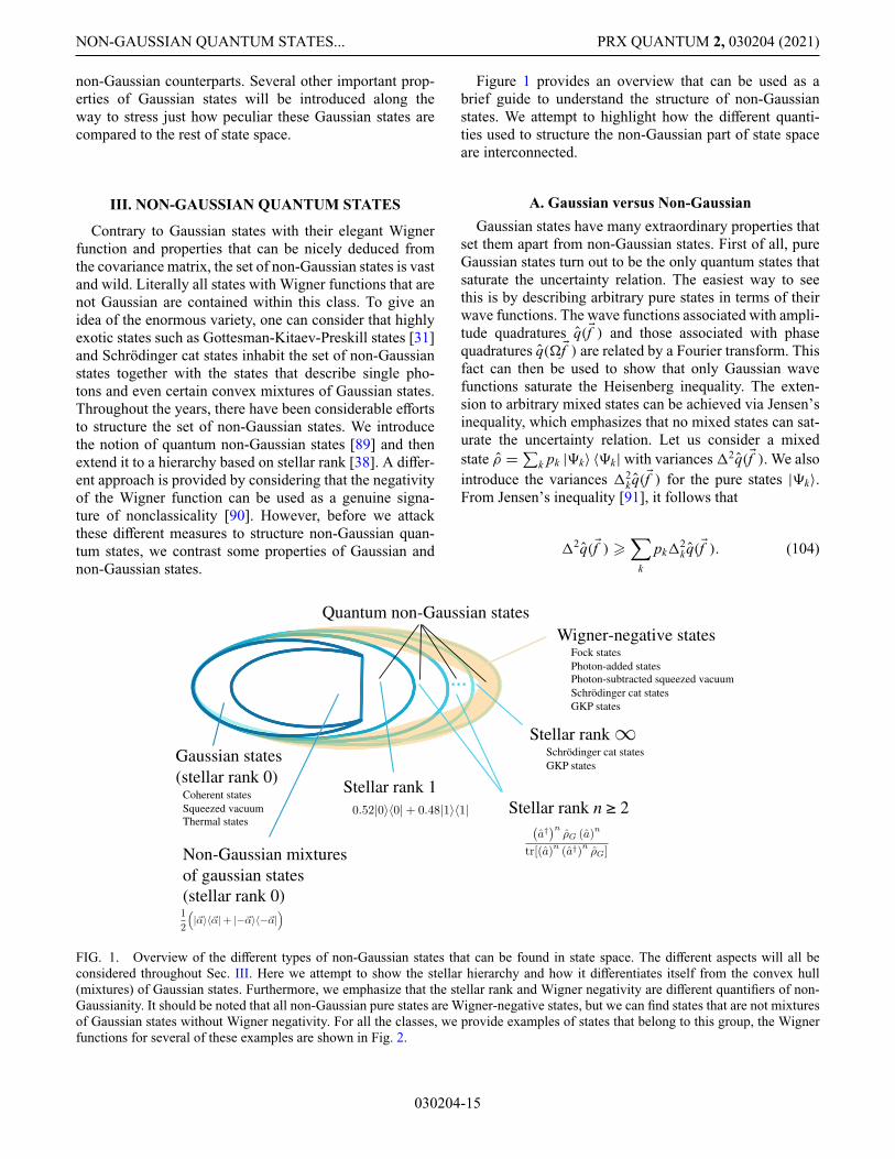
Figure 1 provides an overview that can be used as abrief guide to understand the structure of non-Gaussianstates. We attempt to highlight how the different quanti-ties used to structure the non-Gaussian part of state spaceare interconnected.
A. Gaussian versus Non-Gaussian
Gaussian states have many extraordinary properties thatset them apart from non-Gaussian states. First of all, pureGaussian states turn out to be the only quantum states thatsaturate the uncertainty relation. The easiest way to seethis is by describing arbitrary pure states in terms of theirwave functions. The wave functions associated with ampli-tude quadratures q( f ) and those associated with phasequadratures q(� f ) are related by a Fourier transform. Thisfact can then be used to show that only Gaussian wavefunctions saturate the Heisenberg inequality. The exten-sion to arbitrary mixed states can be achieved via Jensen’sinequality, which emphasizes that no mixed states can sat-urate the uncertainty relation. Let us consider a mixedstate ρ = ∑
k pk |�k〉 〈�k| with variances2q( f ). We alsointroduce the variances 2
k q( f ) for the pure states |�k〉.From Jensen’s inequality [91], it follows that
2q( f ) �∑
k
pk2k q( f ). (104)
Gaussian states(stellar rank 0)
Non-Gaussian mixtures of gaussian states(stellar rank 0)
Coherent statesSqueezed vacuumThermal states
Stellar rank 10.52|0 0| + 0.48|1 1| Stellar rank n 2
a† nρG (a)n
tr[(a)n (a†)nρG]
Stellar rank ∞
GKP states
Wigner-negative statesFock statesPhoton-added statesPhoton-subtracted squeezed vacuum
GKP states
12
| | + |− |
…
Quantum non-Gaussian states
FIG. 1. Overview of the different types of non-Gaussian states that can be found in state space. The different aspects will all beconsidered throughout Sec. III. Here we attempt to show the stellar hierarchy and how it differentiates itself from the convex hull(mixtures) of Gaussian states. Furthermore, we emphasize that the stellar rank and Wigner negativity are different quantifiers of non-Gaussianity. It should be noted that all non-Gaussian pure states are Wigner-negative states, but we can find states that are not mixturesof Gaussian states without Wigner negativity. For all the classes, we provide examples of states that belong to this group, the Wignerfunctions for several of these examples are shown in Fig. 2.
030204-15

MATTIA WALSCHAERS PRX QUANTUM 2, 030204 (2021)
For Heisenberg’s inequality, we calculate
2q( f )2q(� f ) �∑
k
p2k
2k q( f )2
k q(� f )
+∑
k �=l
pkpl2k q( f )2
l q(� f )
� 1. (105)
The presence of cross terms highlights that even when allthe pure states in the mixture saturate the inequality, themixture does not. The only possible exception is the casewhere the state is pure.
That only pure Gaussian states saturate the Heisenberginequality may seem like an innocent observation, but ithas an important implication for non-Gaussian states. TheHeisenberg inequality can be formulated entirely in termsof the covariance matrix. We showed in Eq. (92) that theinequality is saturated if and only if the covariance matrixis symplectic, i.e., V = STS. Furthermore, we showed inEq. (94) that a Gaussian state is pure if and only if itscovariance matrix is symplectic V = STS. The fact thatno non-Gaussian states can saturate the inequality thusimplies that non-Gaussian states can never have a sym-plectic covariance matrix V = STS. This is a first hint ofthe special role played by Gaussian states.
A more general result along these lines states that for allstates ρ with the same covariance matrix V, the Gaussianstate always has the highest von Neumann entropy [13].First of all, note that entropy −tr[ρ log ρ] is conservedunder unitary transformations. Due to the Williamsondecomposition (92), we can write any Gaussian state as
ρG = UG
m⊗
j =1
ρnj U†G, (106)
where ρnj is a thermal state of the Hamiltonian a†j aj with
average particle number nj = (νj − 1)/2. From statisticalmechanics, we know that thermal states are the quantumstates that maximize the von Neumann entropy for a giventemperature (here fixed by the occupations nj ).
It turns out that Gaussian states are limiting cases formany quantities [12]. This result shows that for a rangeof functionals f on the state space, we find that f (ρ) �f (ρG), where ρG is the Gaussian state with the samecovariance matrix as ρ. Apart from some more technicalaspects such as continuity, f must have two important fea-tures: it must be conserved under (a certain class of) unitaryoperations f (UρU†) = f (ρ) and it must be strongly super-additive f (ρ) � f (ρ1)+ f (ρ2) (note that ρ1 and ρ2 aremarginals of ρ). The equality must be saturated for productstates, i.e., f (ρ1 ⊗ ρ2) = f (ρ1)+ f (ρ2). For strongly sub-additive functions with f (ρ) � f (ρ1)+ f (ρ2) the sameresult implies f (ρ) � f (ρG), (after all, in that case −f
is a strongly superadditive function). It is clear that thevon Neumann entropy fulfils the latter conditions and ismaximized for Gaussian states. For superadditive entan-glement measures, this result can be used to show thatfor all states with the same covariance matrix, Gaussianstates are the least entangled ones (entanglement is muchmore extensively discussed in Sec. V). However, severalcommon entanglement measures, e.g., the logarithmic neg-ativity [92] and the entanglement of formation [93], are notsuperadditive.
At the heart of these extremal properties lies the cen-tral limit theorem [4,94–96]. There are many versions ofthe central limit theorem in quantum physics, but we stickto what is probably the simplest one. As always, we con-sider our optical phase space R2m, but this time, we takeN copies of it, which implies that we are dealing witha phase space R2Nm = R2m ⊕ · · · ⊕ R2m for the full sys-tem. We can then embed a vector λ ∈ R2m in the j th ofthese N copies via λj := 0 ⊕ · · · ⊕ 0 ⊕ λ⊕ 0 · · · ⊕ 0 andintroduce the new averaged operator
qN ( λ) := 1√
N
N∑
j =1
q( λj ). (107)
It is rather straightforward to see that these observablesfollow the canonical commutation relation. We can nowrestrict ourselves to studying the algebra that is generatedentirely by such averaged quadrature operators. When wethen assume that the different copies of the system are“independently and identically distributed” we must setthe overall state to be ρ(N ) = ρ⊗N . We then find the char-acteristic function of the algebra of averaged observablesby
χN ( λ) = tr[ρ⊗N eiqN ( λ)]. (108)
The following pointwise convergence can be shown:
χN ( λ) N→∞→ χG( λ), (109)
where χG( λ) is the characteristic function of the Gaussianstate ρG that has the same covariance matrix as ρ. Thismeans that the non-Gaussian features in any state ρ can becoarse grained away by averaging sufficiently many copiesof the state. Note that this result considers N copies of anarbitrary m-mode state. The single-mode version of thisresult was proven in Ref. [94], whereas a much more gen-eral versions are derived in Refs. [95,96]. In Ref. [12] thecentral limit theorem is combined with invariance underlocal unitary transformations to prove the final extremalityresult, we do not review these points in detail.
The extremality of Gaussian states and the associatedcentral limit theorem highlight why Gaussian states areimportant in quantum-information theory and quantum
030204-16

NON-GAUSSIAN QUANTUM STATES... PRX QUANTUM 2, 030204 (2021)
statistical mechanics. It also shows that Gaussian stateshave some particular properties compared to non-Gaussianstates. It thus should not come as a surprise that someof these properties can be used to measure the degree ofnon-Gaussianity of the state [97–99]. As we mentionedbefore, for a fixed covariance matrix V the von Neumannentropy is maximized by the Gaussian state. This suggestthat we can use the difference in von Neumann entropy asa measure for non-Gaussianity. To formalize things, let usconsider an arbitrary state ρ with covariance matrix V andmean field ξ (this quantities can be derived, respectively,for the second and first moments of the quadrature opera-tors). We then construct a Gaussian state σV, which has thesame covariance matrix and the mean field. In the spirit ofextremality, we then define
δ(ρ) = S(σV)− S(ρ), (110)
where S(ρ) := −tr[ρ log ρ]. Because von Neumannentropy is constant under unitary transformations, for aGaussian state it depends only on the symplectic spectrumν1, . . . , νm. In other words, we can calculate S(σV) directlyby using the Williamson decomposition (92) on V. We findfrom Ref. [13] that
S(σV) =m∑
j =1
[νj + 1
2log
νj + 12
− νj − 12
logνj − 1
2
].
(111)
However, it should be noted that the entropy of the non-Gaussian states S(ρ) is generally harder to calculate unlesswe can accurately approximate the state by a finite densitymatrix in the Fock basis. Furthermore, if the state ρ is pure,we simply find that δ(ρ) = S(σV).
Due to extremality of Gaussian states it directly followsthat δ(ρ) � 0, but this does not necessarily mean that δ(ρ)is a good measure for non-Gaussianity. References [13,98]establish that
δ(ρ) = S(ρ | |σV), (112)
where S(ρ || σV) := tr[ρ(log ρ − log σV)] is the quantumrelative entropy between ρ and reference state σV. Thequantum relative entropy allows us to connect δ(ρ) to arange of interesting properties, as shown in Ref. [98]. Forexample, it directly follow that δ(ρ) = 0 if and only ifρ = σV. Furthermore, the measure δ(ρ) inherits convex-ity and monotonicity properties from the relative entropy.These are exactly the properties that made this measurea useful ingredient in the resource theory for quantumnon-Gaussianity presented in Ref. [100].
Thus, the connection between Eq. (110) and relativeentropy shows that δ(ρ) can indeed be used as a measurefor non-Gaussianity in the sense that it measures “entropic
distance” between ρ and σV. Yet, there is one importantquestion that remains to be answered: is σV indeed theclosest Gaussian state to ρ? An affirmative answer to thisquestion was provided in Ref. [101], where it was shownthat
δ(ρ) = minρG
S(ρ | |ρG), (113)
where we minimise over all possible Gaussian states ρG.The main idea of the proof is to show that S(ρ || ρG)−S(ρ || σV) = S(σV || ρG) � 0 such that the smallest rela-tive entropy in indeed achieved for σV. For the technicaldetails, we refer the interested reader to Ref. [101]. Fur-thermore, we note that a similar non-Gaussianity measurewas introduced by using the Wehrl entropy (based on theQ function) rather than the von Neumann entropy [102].
We have thus shown that Gaussian states are specialin the sense that they minimize entanglement and maxi-mize entropy as compared to other states with the samecovariance matrix. Another profound distinction can befound when comparing pure Gaussian states to pure non-Gaussian states. In this case, there is a seminal result byHudson [34] that was extended by Soto and Claverie tomultimode systems [35], which states that a pure state canhave a non-negative Wigner function if and only if the stateis Gaussian. In other words, all non-Gaussian pure statesexhibit Wigner negativity.
Here, we follow the approach of Ref. [103] to prove thisresult. First of all, we introduce the function
F��( α) := 〈 α | �〉e 1
8 ‖ α‖2, (114)
such that the Q function (70) of the state |�〉 is given by
Q( α) = 1(4π)m
∣∣F��( α)
∣∣2 e− 14 ‖ α‖2
. (115)
From Eq. (114), we directly find that
∣∣F��( α)
∣∣2 � e14 ‖ α‖2
. (116)
Next, we observe that a Q function that reaches zeroimplies a negative Wigner function, which can be seenfrom Eq. (72). Thus, demanding that the state has a pos-itive Wigner function implies demanding that Q( α) > 0,and thus that F�
�( α) has no zeros. Using the equiva-lence between 2m-dimensional phase space and a complexm-dimensional Hilbert space, we can use the multidimen-sional but restricted version of the Hadamard theorem[35], which states that any entire function f : Cm �→ C
without any zeros and with order of growth [104] r isan exponential f (z) = exp g(z), where g(z) is a polyno-mial of degree s � r. We then note that F�
� is an entirefunction of maximal growth r = 2 as given by Eq. (116).
030204-17
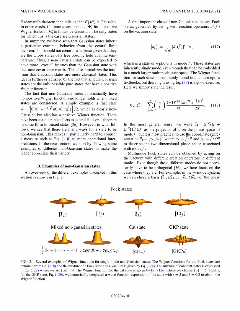
MATTIA WALSCHAERS PRX QUANTUM 2, 030204 (2021)
Hadamard’s theorem then tells us that F��( α) is Gaussian.
In other words, if a pure quantum state |�〉 has a positiveWigner function F�
�( α) must be Gaussian. The only statesfor which this is the case are Gaussian states.
In summary, we have seen that Gaussian states inherita particular extremal behavior from the central limittheorem. This should not come as a surprise given that theyare the Gibbs states of a free bosonic field at finite tem-perature. Thus, a non-Gaussian state can be expected tohave more “exotic” features than the Gaussian state withthe same covariance matrix. This also formalizes the intu-ition that Gaussian states are more classical states. Thisidea is further established by the fact that all pure Gaussianstates are the only possible pure states that have a positiveWigner function.
The fact that non-Gaussian states automatically havenonpositive Wigner functions no longer holds when mixedstates are considered. A simple example is that stateρ = [
∣∣∣0〉〈0| + a†( f )|0〉〈0|a( f )]/2, which is clearly non-
Gaussian but also has a positive Wigner function. Therehave been considerable efforts to extend Hudson’s theoremin some form to mixed states [36]. However, in what fol-lows, we see that there are many ways for a state to benon-Gaussian. This makes it particularly hard to connecta measure such as Eq. (110) to more operational inter-pretations. In the next section, we start by showing someexamples of different non-Gaussian states to make thereader appreciate their variety.
B. Examples of non-Gaussian states
An overview of the different examples discussed in thissection is shown in Fig. 2.
A first important class of non-Gaussian states are Fockstates, generated by acting with creation operators a†( f )on the vacuum state
∣∣nf⟩
:= 1√n!
[a†( f )]n |0〉 , (117)
which is a state of n photons in mode f . These states areinherently single mode, even though they can be embeddedin a much larger multimode state space. The Wigner func-tion for such states is commonly found in quantum opticstextbooks, but deriving it using Eq. (38) is a good exercise.Here we simply state the result:
Wnf ( x) =n∑
k=0
(nk
)(−1)n+k‖ xf‖2k
k!e− 1
2 ‖ x‖2
2π. (118)
In the most general sense, we write xf = ( f T x) f +( f T� x)� f as the projector of x on the phase space ofmode f , but it is most practical to use the coordinate repre-sentation xf = (xf , pf )
T where xf = f T x and pf = f T� xto describe the two-dimensional phase space associatedwith mode f .
Multimode Fock states can be obtained by acting onthe vacuum with different creation operators in differentmodes. Even though these different modes do not neces-sarily have to be orthogonal [56], we here focus on thecase where they are. For example, in the m-mode system,we can chose a basis { e1,� e1, . . . , em,� em} of the phase
Fock states
Mixed non-gaussian states Cat state GKP state
12
(| | + |− |) |cat− |GKP0
FIG. 2. Several examples of Wigner functions for single-mode non-Gaussian states. The Wigner functions for the Fock states areobtained from Eq. (118) and the mixture of a Fock state and a vacuum is given by Eq. (124). The mixture of coherent states is expressedin Eq. (122) where we set ‖ α‖ = 4. The Wigner function for the cat state is given by Eq. (126) where we choose ‖ α‖ = 6. Finally,for the GKP state, Eq. (130), we numerically integrated a wave-function expression of the state with s = 2 and δ = 0.3 to obtain theWigner function.
030204-18
NON-GAUSSIAN QUANTUM STATES... PRX QUANTUM 2, 030204 (2021)
space R2m and define multimode Fock states as∣∣ne1
⟩ ⊗ · · · ⊗ ∣∣nem
⟩
:= 1√n1! . . . nm!
[a†( e1)]n1 . . . [a†( em)]nm |0〉 , (119)
where the kth mode in the basis contains nk photons. Notethat for nk = 0 we have a vacuum mode. For the Wignerfunction, this implies
Wne1 ,...,nem ( x) = Wne1( xe1) . . .Wnem ( xef). (120)
Here we use that the phase-space point x can be expressedas x = xe1 ⊕ · · · ⊕ xem , where xek is the phase-space coor-dinate within the subspace spanned by ek and � ek. We cannote xek = (xk, pk)
T, such that we find the coordinate rep-resentation x = (x1, p1, . . . , xm, pm)
T in the chosen basis ofphase space.
Non-Gaussian states do not necessarily have to be pure,they can also come in the form of statistical mixtures. Themost basic example of such as state is a non-Gaussian mix-ture of Gaussian states. As a simple example, let is considera mixture of two coherent states
ρ = 12(| α〉 〈 α| + |− α〉 〈− α|) . (121)
Even though this is a highly classical state, it is still non-Gaussian as clearly seen from its Wigner function
W( x) = 14π
(e− 1
2 ‖ x− α‖2 + e− 12 ‖ x+ α‖2
). (122)
Another important example of a non-Gaussian mixed stateis
ρλ = λ |0〉 〈0| + (1 − λ)∣∣1f
⟩ ⟨1f
∣∣ . (123)
In the mode f , the Wigner function of the state behaves as
Wλ( x) = [(1 − λ)‖ xf‖2 + 2λ− 1]e− 1
2 ‖ x‖2
2π. (124)
This Wigner function reaches negative values as long asλ < 1/2 and subsequently becomes positive. Nevertheless,it will remain non-Gaussian until λ = 1. As we see inSec. C, even when the Wigner function is positive, it isnot always possible to describe this state as a mixture ofGaussian states.
Generally speaking, non-Gaussian states can come in awide variety of shapes, which can be much more exoticthan the examples discussed above. A popular class ofGaussian states is obtained by taking coherent superposi-tions of Gaussian states. As we see in Sec. VII, there hasbeen a strong experimental focus on two specific types of
such states: Schrödinger’s cat states [105] and GKP states[31]. The former are obtained by coherently superposingtwo coherent states, and often are split in even |cat+〉 andodd |cat−〉 cat states:
|cat±〉 := 1N (| α〉 ± |− α〉) , (125)
where N =√
2(1 ± exp[−‖ α‖2]) is the normalizationcoefficient, which depends on the displacement α. The lat-ter is often referred to as “the size of the cat.” The Wignerfunction of these states resembles that of Eq. (122) but hasan additional interference term
Wcat±( x) = e− 12 ‖ x− α‖2 + e− 1
2 ‖ x+ α‖2 ± cos(√
2 αT x)e− 12 ‖ x‖2
4π(1 ± e−‖ α‖2)
.
(126)
The appearance of these interference terms creates sev-eral regions in phase space where the Wigner functionattains negative values. The term “Schrödinger’s cat state”has historically grown from the idea that coherent statesdescribe classical electromagnetic fields and can thus beconsidered “macroscopic,” in particular, for large values of‖ α‖. However, one should honestly admit that they fail tocapture an important point of Schrödinger’s thought exper-iment [106]: the entanglement with a microscopic quantumsystem (i.e., the decay event that triggers the smashing ofthe vial of poison). Nevertheless, the term “cat state” hasestablished itself firmly in the CV jargon, and now also liesat the basis of derived concepts such “cat codes” for errorcorrection [107,108].
Finally, there are the GKP states. In their idealizedform, they rely on eigenvectors of the quadrature operators(sometimes also known as infinitely squeezed states). Tokeep notation simple, we restrict to the single mode withquadrature operators x and p . The eigenvectors of theseoperators are then formally written as
x |x〉 = x |x〉 , and p |p〉 = p |p〉 . (127)
Furthermore, we have the relations 〈x′ | x〉 = δ(x′ −x), 〈p ′ | p〉 = δ(p ′ − p), and 〈p | x〉 = e−ipx/
√2π . GKP
states are constructed by considering a grid of such statesto create a qubit, by identifying the two following GKPvectors:
∣∣GKP0
⟩:=
∑
k∈Z
∣∣x = 2k√π
⟩, (128)
∣∣GKP1
⟩:=
∑
k∈Z
∣∣x = (2k + 1)√π
⟩. (129)
Clearly, these states are not normalizable and not phys-ical as they would require infinite energy to be created.Thus, it is common to construct approximate GKP states,
030204-19
MATTIA WALSCHAERS PRX QUANTUM 2, 030204 (2021)
by replacing the states |x〉 with displaced squeezed states,and by truncating the summation by adding a Gaussianenvelope:
|GKP0〉 := N0
∑
k∈Z
e−2π [kδ]2D[2k
√π ] |s〉 , (130)
|GKP1〉 := N1
∑
k∈Z
e−2π [(k+1/2)δ]2D[(2k + 1)
√π ] |s〉 .
(131)
Here N0,1 are normalization constants and |s〉 is a single-mode squeezed vacuum, which implies that its Wignerfunction is given by Eq. (85) with ξ = (0, 0)T and V =diag[1/s, s] for s > 1. To get a good GKP state for quan-tum error correction, we generally need that s � √
π . TheWigner function of an ideal GKP state is a grid of deltafunctions, which again highlights that it is a nonphysi-cal state. The more realistic states |GKP0〉 and |GKP1〉have well-defined Wigner functions, even though they arenot very insightful to write down explicitly. In Fig. 2, weplot an example that was calculated numerically by takinginto account only the first few terms around k = 0 in thesum.
GKP states may seem a little artificial at first glance,but they have been developed with a very clear pur-pose: to encode a qubit in a harmonic oscillator [31].This encoding implies a notion of fault tolerance asthese states are designed to be very efficient at cor-recting displacement errors. The more realistic incar-nations of these states, Eq. (130), are therefore oftenproposed as candidates for encoding the information inCV quantum computation protocols [29]. Furthermore,it was shown that these states can also be used as thesole non-Gaussian resource to implement a CV quantumcomputer [32]
Once we progress into the realm of multimode states,the class of non-Gaussian states becomes even more vast.In Sec. 2, we present a dedicated introduction to mul-timode photon-subtracted states, which is a useful stateto illustrate several of the concepts treated in this Tuto-rial. Furthermore, these states have a particular importancein CV quantum optics experiments. As a final example,we introduce another class of multimode non-Gaussianstates, which have been highly relevant for quantummetrology: N00N states [109–111]. Even though thesestates are very promising for quantum sensing with opti-cal setups, the general idea that underlies these stateswas first introduced for fermions [112] in an attempt tomimic the advantage that is provided by squeezing inoptics.
N00N states are two-mode entangled states defined ina pair of orthogonal modes g1 and g2. The state containsexactly N photons, and is a superposition of a state withall photons being mode g1 and a state with all photons in
mode g2:
|N00N 〉 := 1√2
(∣∣Ng1
⟩ + ∣∣Ng2
⟩). (132)
Here we recall that the state∣∣Ng1
⟩can be trivially embed-
ded to the full multimode space by adding vacuum inall other modes. We study these states in more detail forN = 2 in our discussion of the Hong-Ou-Mandel effectsurrounding Eq. (165). However, here we highlight alreadythat the Wigner function of |N00N 〉 is not simply the sumof Wigner functions of the form Eq. (118). The entangle-ment will create additional interference terms, just like wesaw in Eq. (126). In the present case, these interferencesare genuinely multimode, and thus related to quantumcorrelations.
Experimentally, these states have been created and ana-lyzed using a DV approach [113]. As we highlighted inSec. C, the distinction between DV and CV is somewhatsubtle and mainly depends on what is measured. BecauseN00N states are built from Fock states and have a well-defined total photon number, they are most natural toanalyze using photon-number-resolving detectors.
C. Quantum non-Gaussianity
Non-Gaussian states come in a wide variety, whichmeans also that some of them are more exotic than oth-ers. Non-Gaussian states that are of limited interest, arethose which are convex combinations of Gaussian states.Gaussian states do not form a convex set, after all, we canimmediately see that, e.g., [W0( x − α1)+ W0( x − α2)]/2is not a Gaussian function even though it is a convexcombination of Gaussian states.
The fact that the set of non-Gaussian states containsmixtures of Gaussian states may lead one to suspect thatany mixed state with a positive Wigner function can bewritten as a well-chosen mixture of Gaussian states. Afterall, Gaussian states are the only pure states with posi-tive Wigner functions. This intuition turns out to be false[89], which means that the set of states with a nonpositiveWigner function is not the same as the set of states thatlie outside of the convex hull of Gaussian states G. Moreformally, let us define
G :={ρ | ρ =
∫dγ p(γ )ρG(γ )
}, (133)
where γ is some arbitrary way of labelling Gaussian statesρG(γ ) and p(γ ) is a probability distribution on theselabels. Note that Eq. (103) tells us that we can generateall Gaussian states by taking convex combinations of dis-placed squeezed states, and thus we can limit ourselves toρG(γ ) = |�G(γ )〉 〈�G(γ )| in the definition of G.
Any quantum state ρ that is not contained in the con-vex hull of Gaussian states, i.e., ρ /∈ G, is referred to
030204-20

NON-GAUSSIAN QUANTUM STATES... PRX QUANTUM 2, 030204 (2021)
as a “quantum non-Gaussian” state. The intuition behindthis terminology is that Gaussian pure states are lessquantum than non-Gaussian pure states that boast a non-positive Wigner function. A mixed state that is quantumnon-Gaussian may have a positive Wigner function, butit cannot be created without adding states with nonposi-tive Wigner functions into the pure-state decomposition.Hence, these states are more quantum than the states thatare in the convex hull of Gaussian states G.
Next, one may wonder how to differentiate betweenstates that are quantum non-Gaussian and states which arein the convex hull G. Throughout the last decade, manymethods have been developed to answer this question. Westart by introducing the main idea of Ref. [114] becauseit is based on the Wigner function. The key idea is thatGaussian distributions have tails, which means that we cantake an arbitrary pure Gaussian state W0[S−1( x − α)], andevaluate the Wigner function at to origin of phase space:
W0(S−1 α) = e− 12 ‖S−1 α‖2
(2π)2. (134)
Clearly, when ‖S−1 α‖2 → ∞, we do find that W0(S1 α) →0. This limit essentially corresponds to a system with infi-nite energy. It is thus natural to try to bound the value of theWigner function in the origin by a function that depends onthe energy N of the state. For an arbitrary pure Gaussianstate, we find that
N =m∑
j =1
tr[ρa†( ej )a( ej )] = 14
(tr[STS − 1] + ‖ α‖2)
.
(135)
Using the properties of the operator norm, we write‖S−1 α‖2 = ‖S−1O α‖2, where O is a symplectic orthog-onal transformation. Furthermore, we note that ‖ α‖2 =‖O α‖2. It is then useful to explicitly write the coordi-nate representation of the vector O α = (α
(x)1 ,α(p)1 , . . . ,α(x)m ,
α(p)m )T, such that
N =m∑
j =1
14
(sj + 1
sj+ (α
(x)j )2 + (α
(p)j )2 − 2
)(136)
=m∑
j =1
nj . (137)
At the same time, we expand
‖S−1 α‖2 =m∑
j =1
sj (α(x)j )2 + (α
(p)j )2
sj, (138)
and with a little algebra we can show that
12‖S−1 α‖2 �
m∑
j =1
4nj (2nj + 1) � 4N (2N + 1), (139)
such that
W0(S−1 α) � 1(2π)m
e−4N (2N+1). (140)
This means that the value of the Wigner function of a pureGaussian state in the origin of phase space is bounded frombelow by a function of the average number of particles N .However, it is not obvious that we can extend this boundto arbitrary mixtures of Gaussian states. Let us assume thatρ ∈ G, then the Wigner function in the origin is given by
W( 0) =∫
dγ p(γ )W0(S−1γ αγ ), (141)
where we saw that W0(S−1γ αγ ) is the value of a pure
Gaussian state’s Wigner function in the origin and γ issome arbitrary label for the Gaussian states in the mix-ture. Therefore we can bound the states in the convexcombination
W( 0) � 1(2π)m
∫ ∞
0dN γ p(N γ )e−4Nγ (2Nγ+1), (142)
where we introduce a probability distribution p on theaverage particle numbers of the pure Gaussian states inthe mixture. The overall average number of particles in thestate ρ is then given by N = ∫ ∞
0 dN γ p(N γ )N γ . The finalelement that we require is the fact that exp[−4N γ (2N γ +1)] is a convex function, such that we can apply Jensen’sinequality to find that
ρ ∈ G =⇒ W( 0) � 1(2π)m
e−4N (2N+1). (143)
This means that we can simply use the total energyof the state to construct a witness for quantum non-Gaussianity. This clearly shows that there are quantumnon-Gaussian states with positive Wigner functions. Anexplicit example can be constructed by tuning the γ
in the state [(1 − γ ) |0〉 〈0| + γ |1 f 〉〈1 f |] to 1/2 > γ >
1/2 − e−4γ (2γ+1) (where we use that γ is also the averageparticle number in this particular state).
Nevertheless, there are many quantum non-Gaussianstates that do not violate inequality (143). After all, whywould the origin of phase space be the most interestingpoint? A first solution is provided in Ref. [114], where it is
030204-21

MATTIA WALSCHAERS PRX QUANTUM 2, 030204 (2021)
argued that
ρ ∈ G =⇒ W�( 0) � 1(2π)m
e−4N�(2N�+1), (144)
for all Gaussian channels � that act on the Wigner func-tion of ρ as W( x) ��→ W�( x). Recall that the action of aGaussian channel was defined in Eq. (102). The quantityN� then denotes the average number of particles in thestate �(ρ). Further generalizations of this scheme havebeen worked out in Ref. [115]. Moreover, Ref. [116]has considered combinations of the value of the Wignerfunction in several points to reach better witnesses forquantum non-Gaussianity. Further progress has been madeby identifying observables that are more easily measurablewith typical CV techniques [117]. Others have consideredother phase-space representations of the state to identifywitnesses of quantum non-Gaussianity [118,119].
Quantum non-Gaussianity has been investigated witha wide range of tools. In this Tutorial we have limitedourselves to phase-space methods in the spirit of the CVapproach. However, there is also a significant body ofwork on quantum non-Gaussianity using techniques thatare more typical in DV quantum optics. The earliest workson the subject used photon statistics to distinguish quantumnon-Gaussian states from convex mixtures of Gaussianstates [89]. This research line has been continued in recentyears to uncover new aspects of quantum non-Gaussianstates, such as the “non-Gaussian depth” [120] and tech-niques to differentiate different types of multiphoton states[121]. Ultimately, these photon-counting techniques wereextended to develop a whole hierarchy of quantum non-Gaussian states [37]. These ideas have been further for-malized and generalized through the notion of the “stellarrank” of a quantum state.
D. Stellar rank
An interesting starting point to introduce the stellarrepresentation is the method [103] to prove Hudson’stheorem. We recall the definition
F��( α) := 〈 α | �〉e 1
8 ‖ α‖2,
of what we henceforth refer to as the stellar function. Toavoid technical complications, let us now restrict ourselvesto single-mode systems such that the optical phase space isR2. Note that, in a single-mode system, there is only onecreation operator a† with associated annihilation operatorsa. We can then follow Ref. [38] to introduce the stellar rep-resentation of single-mode quantum states. Note that somesimilar ideas are also present in other works [122].
First, we develop the stellar representation for purestates, which will then be used to generalize the frameworkto mixed states in Eq. (148). We use the definition of the
displacement operator to show that
|�〉 = F��(a
†) |0〉 , (145)
which immediately implies that the stellar representation isunique. In other words, if F�
� = F�� it follows that |�〉 =
|�〉 up to a phase. In our proof of Hudson’s theorem,we have already highlighted that F�
� satisfies the property(116), which means that it is an entire function with growthorder r = 2. Because in this single-mode setting F�
� canbe interpreted as a function of a single complex variable,the Hadamard-Weierstrass theorem implies that F�
� can befully represented by its zeros (one can consider this as ageneralization of the fundamental theorem of calculus).This thus implies that a single-mode state is completelydetermined by the zeros of the F�
� , and thus by the zeros ofthe Q function in Eq. (115).
It is thus natural to use these zeros in order to classifypure single-mode quantum states and thus the stellar rankis introduced. Ultimately, the stellar rank is simply givenby the number of zeros of F�
� or alternatively the numberof zeros of the Q function. Because in practice zeros maycoincide, one should also consider the multiplicity of thezeros. We thus define the stellar rank r�(�) of |�〉 as thenumber of zeros of F�
� : C �→ C counted with multiplicity.Alternatively one may count the zeros of the Q functionwith multiplicity and divide by two.
The fact that a state is fully characterized by its stellarrepresentation F�
� can be made more explicit by consider-ing the roots { α1, . . . , αr�(�)} of the Q function, which rep-resents |�〉 [note that we use (44) to interchange betweenphase-space representation and complex Hilbert-space rep-resentation]. The single-mode state |�〉 can then be used toexpress
|�〉 = 1N
r�(�)∏
j =1
D†( αj )a†D( αj ) |�G〉 , (146)
where |�G〉 is a pure Gaussian state and N a normalizationconstant. We can then use the stellar rank to induce somefurther structure in the set of states by defining
RN := {|�〉 | r�(�) = N }. (147)
that groups all states of stellar rank N . Note that theHadamard-Weierstrass theorem also considers functionswith an infinite amount of zeros and the case N = ∞ isthus mathematically well defined. It turns out that this caseis not just a pathological limit. An evaluation of the Qfunction shows that Gottesman-Kitaev-Preskill states andSchrödinger cat states inhabit the set R∞.
Clearly, all that was introduced so far only works forpure states. We can naturally extend this result via a convex
030204-22
NON-GAUSSIAN QUANTUM STATES... PRX QUANTUM 2, 030204 (2021)
roof construction, by defining
r�(ρ) := inf{p(γ ),|�(γ )〉}
supγ
{r�[�(γ )]}, (148)
where the infimum is considered of all probability dis-tributions on the set of pure states that lead to ρ =∫
dγ p(γ ) |�(γ )〉 〈�(γ )|. In words, there are many waysto decompose the state ρ in pure states and we consider allof them. For each decomposition, we define the stellar rankas the highest rank of the states in the decomposition. Thenwe minimize these values over all possible decompositionsto arrive at the stellar rank of ρ.
Convex roof constructions are commonly used to treatmixed states as they are easy and natural to formally define.However, they are often much harder to calculate in prac-tice. This is where the stellar representation unveils itsmost remarkable property: stellar robustness. To formalizethis idea, Ref. [38] introduced the robustness as the tracedistance between the state and the nearest possible state oflower stellar rank.
R�(�) := infr�(ρ)<r�(�)
12
tr√(|�〉 〈�| − ρ)2. (149)
And it can be shown that
R�(�) =√
1 − supr�(ρ)<r�(�)
〈�| ρ |�〉, (150)
where 〈�| ρ |�〉 is the fidelity of ρ with target state|�〉. Remarkably, it can be shown that R�(�) > 0 whenr�(�) < ∞ [38]. This means that any state that is suffi-ciently close to a pure state of r�(�) is also of rank r�(�)or higher.
The idea of stellar robustness can be generalized [123]by introducing k robustness. For any k < r�(�), we define
R�k(�) := infr�(�)�k
√1 − |〈� | �〉|2, (151)
and show subsequently that
R�k(�) =√
1 − supr�(ρ)�k
〈�| ρ |�〉. (152)
The k robustness can thus be interpreted as the nearest dis-tance from a state |�〉 at which we can find any state ofstellar rank k, provided k < r�(�). Beyond showing thatR�k(�) is nonzero when |�〉 is of finite stellar rank, Ref.[123] also provides an explicit method to calculate R�k(�).Thus, for whichever state ρ is available in an experimentone can attempt to find a pure target state |�〉 for which〈�| ρ |�〉 > 1 − R�k(�)
2 to prove that ρ is at least of stellarrank k.
We note that for pure states r�(�) = 0 implies that thestate is Gaussian (this is essentially what is proven in Hud-son’s theorem). From the definition (148) we can thendeduce that
r�(ρ) = 0 ⇐⇒ ρ ∈ G, (153)
where G denotes, again, the convex hull of Gaussian states.On the other hand, states for which r�(ρ) > 0 cannotbe written as a mixture of Gaussian states and are thusquantum non-Gaussian.
This idea can be extended by using the stellar k robust-ness, Eq. (152), as a witness of quantum non-Gaussianity.When we want to check whether ρ is quantum non-Gaussian, it suffices to find a pure target state |�〉 suchthat ρ is closer to |�〉 than the 1 robustness R�k(�). Moreformally written, whenever a pure state |�〉 exists with thefollowing property:
〈�| ρ |�〉 > 1 − R�1(�)2 =⇒ ρ /∈ G, (154)
and ρ is quantum non-Gaussian. This may seem like acomplicated challenge, but for a single-photon state |�〉 =|1〉 we find that 1 − R�1(�)
2 ≈ 0.478 [123]. This meansthat any state that has a fidelity of more than 0.478 withrespect to a Fock state is quantum non-Gaussian. This ideacan be extended to higher stellar ranks: whenever we finda target state |�〉 such that 〈�| ρ |�〉 > 1 − R�k(�)
2, thestate ρ is at least of stellar rank k. Note that the fidelity ofan experimentally generated state ρ with any pure targetstate |�〉 can be calculated from double homodyne mea-surements on ρ [123]. There is no need to experimentallycreate the pure state |�〉, the latter is just theoretical inputneeded to analyze the data.
Obviously, the stellar rank imposes a lot of additionalstructure on the state space. It rigorously orders all statesthat can be achieved by combining a finite number of cre-ation operators and Gaussian transformations. The creationoperator serves as a tool to increase the stellar rank by oneand the stellar rank actually corresponds to the minimalnumber of times the creation operator must be applied toobtain the state, together with Gaussian operations. Thestellar rank remains unchanged under Gaussian unitarytransformations, which makes sense for a measure of thenon-Gaussian character of the state, and thus it falls withinthe set of intrinsic properties of a state as discussed inSec. C. Furthermore, the class of states with infinite stellarrank can be understood as the set that contains the mostexotic states. However, it is lonely at the top as it canbe shown that R�∞(�) = 0 for states of infinite rank. Thismeans that we can find states of finite stellar rank arbitrar-ily close to a state of infinite stellar rank. As stressed in Ref.[38], this implies that finite-rank states are dense in the fullFock space and any state of infinite rank can be arbitrarilywell approximated by finite-rank states. Whereas a finite
030204-23

MATTIA WALSCHAERS PRX QUANTUM 2, 030204 (2021)
stellar rank k of any experimental state can be certified byachieving a sufficiently high fidelity to a target state |�〉to fall within the range given by its k robustness R�k(�),a similar procedure is impossible for infinite stellar ranks.This means, in practice, that genuinely infinite-rank statesare impossible to certify in experiments because one neverachieves perfect fidelity. Nevertheless, different states ofinfinite rank may differ significantly in the values R�k(�)for k < ∞.
Many of the results on stellar rank rely on theHadamard-Weierstrass theorem that allows one to uniquelyfactorize F�
�( α) as a Gaussian and a polynomial, wherethe roots of the polynomial are the roots of F�
� and thusalso the roots of the Q function. Sadly, this theorem cannotbe straightforwardly generalized to a multimode setting,which is known in mathematics as Cousin’s second prob-lem [124]. Notable progress was made in Ref. [125] whereone studies multimode stellar functions, which are poly-nomials and it was shown that there is no straightforwardgeneralization of Eq. (146).
E. Wigner negativity
Hudson’s theorem shows us that all pure non-Gaussianstates have nonpositive Wigner functions, which sets themapart from normal probability distributions of phase space.For mixed states, this no longer holds and thus we spentthe previous two sections developing methods to charac-terize the non-Gaussian features of these states. Whetherit is through quantum non-Gaussianity or the more refinedstellar rank, these methods focus on characterizing the non-Gaussian resources that are required to generate a certainstate. In this subsection, we change the perspective andfocus rather on negative values of the Wigner function(“Wigner negativity” in short) as a resource of interest.
Wigner negativity has the advantage of being a clearquantum feature, it reflects that different quadratures inthe same mode cannot be jointly measured and thus goeshand in hand with the principle of complementarity. Moreformally, it has even been connected to the principle ofquantum contextuality [64]. Indeed, in Sec. VI we elab-orate on the fact that Wigner negativity is a necessaryresource for reaching a quantum advantage, i.e., perform-ing a task that cannot be efficiently simulated by a classicalcomputer. However, the idea of using Wigner negativity asa signature of nonclassicality was already around beforeit was connected to a quantum computational advantage.An important step to formalize this idea was the introduc-tion of a measure for Wigner negativity [90], which lies atthe basis of recent resource theories of Wigner negativity[100,126].
A priori, there are several natural measures than canbe used for Wigner negativity. It is therefore useful toconsider some desirable properties that are required fora measure of Wigner negativity. First of all, we want the
measure to be zero if and only if the Wigner functionis positive. It seems natural to demand that, furthermore,Wigner negativity remains unchanged under Gaussian uni-tary transformations. It is then tempting to simply considerthe absolute value of the lowest possible value of theWigner function, but this would have some unnatural out-comes. It would mean that a single-photon state wouldhave more Wigner negativity than a two-photon state. Wethus need to look for a different measure.
The starting point of Ref. [90] is that the normalizationof the Wigner function implies that
∫
R2md x |W( x)| � 1, (155)
and that the inequality is strict whenever there is Wignernegativity. Furthermore, Liouville’s theorem implies thatintegrals over phase space are unchanged by Gaussiantransformations. A first possible way of measuring Wignernegativity is through the negativity volume
N (ρ) :=∫
R2md x |W( x)| − 1. (156)
This measure has the major advantage of being convexdue to the triangle inequality, which means that for ρ =∫
dγ p(γ )ρ(γ ) we find that
N (ρ) �∫
dγ p(γ )N [ρ(γ )]. (157)
However, this measure is not additive, i.e., N (ρ1 ⊗ ρ2) �=N (ρ1)+ N (ρ2). To circumvent this shortcoming, anothermeasure for Wigner negativity has been introduced [100,126,127]:
N(ρ) := log∫
R2md x |W( x)| . (158)
Clearly, N(ρ1 ⊗ ρ2) = N(ρ1)+ N(ρ2) making this mea-sure additive. However, the introduction of the logarithmdestroys the convexity of the measure. Note that the twomeasures are closely related by N(ρ) = log[N (ρ)+ 1].Thus when N (ρ1) > N (ρ2), we also find that N(ρ1) >
N(ρ2).The single-mode examples that are considered in Ref.
[90] lead to some interesting observations. First of all,they show that for Fock states Wigner negativity increaseswith the photon number. Furthermore, they show that forSchrödinger cat states the integral is bounded from aboveby a value smaller than the Wigner negativity of a two-photon state. Even though Fock states of increasing stellarrank have increasing Wigner negativity, there is no clearrelation between stellar rank and Wigner negativity formore general classes of states. For example, Schrödinger
030204-24

NON-GAUSSIAN QUANTUM STATES... PRX QUANTUM 2, 030204 (2021)
cat states are of infinite stellar rank, suggesting that theyare in this regard the most exotic states, but they manifestonly a limited amount of Wigner negativity.
As a case study, let us briefly concentrate on the Wignernegativity of Fock states, Eq. (117). One can now evaluatethe Wigner negativity of such states to find that
N (|1〉) ≈ 0.426 12 and N(|1〉) ≈ 0.354 959, (159)
N (|2〉) ≈ 0.728 99 and N(|2〉) ≈ 0.547 537, (160)
N (|3〉) ≈ 0.976 67 and N(|3〉) ≈ 0.681 415, (161)
which shows that the negativity does not simply increaselinearly with the number of photons even for the addi-tive measure N. However, let us now look at a multimoden-photon state where each photon occupies a differentmode, i.e., a Fock state generated by creation operators in f1, . . . , fn with span{ fj ,� fj } �= span{ fk,� fk} for all j �= k,
a†( f1) . . . a†( fn) |0〉 = ∣∣1f1
⟩ ⊗ · · · ⊗ ∣∣1fn⟩. (162)
The Wigner function for this state can be shown to be[showing this based on (38) is again a good exercise]
W1f1 ,...,1fn( xf1 ⊕ · · · ⊕ xfn) =
n∏
k=1
W1fk( xfk). (163)
Either by explicitly using the expression of the Wignerfunction, or by using the additivity property, we find that
N(∣∣1f1
⟩ ⊗ · · · ⊗ ∣∣1fn⟩) = nN(|1〉). (164)
Numerically, we can show that nN(|1〉) > N(|n〉) and thuswe can generally conclude that n photons in differentmodes hold more Wigner negativity than n photons in thesame mode.
Let us now concentrate on the case where n = 2. Weshowed that two photons in different modes are moreWigner negative than two photons in the same mode, andnow we combine this finding with the idea that Wignernegativity remains unchanged under Gaussian transforma-tions. A particularly simple Gaussian transformation is abalanced beam splitter, which ultimately just implements achange in mode basis that we describe by an orthonormaltransformation OBS. When we mix two photons, preparedin orthogonal modes f1 and f2 by such a balanced beamsplitter, we see the Hong-Ou-Mandel effect in action (moredetails can be found in Ref. [56] where a similar notationis used):
∣∣1f1
⟩ ⊗ ∣∣1f2
⟩ OBS�→ 1√2
(∣∣2g1
⟩ − ∣∣2g2
⟩):= |HOM〉 , (165)
where f1, f2 and g1, g2 are the input and output modes ofthe beam splitter, respectively. The Hong-Ou-Mandel out-put state |HOM〉 is thus a superposition of two photons in
mode g1 and two photons in mode g2. We can now usethe simple fact that Wigner negativity is unchanged underGaussian unitary transformations to show that
N (|HOM〉) = N(∣∣1f1
⟩ ⊗ ∣∣1f2
⟩) = 2N(|1〉) > N(|2〉),(166)
this then also implies that N (|HOM〉) > N (|2〉). At firstsight, this is somewhat of a peculiar finding: by tak-ing a superposition of two states with the same Wignernegativity one finds a state with a higher Wigner negativity.
An explicit look at the Wigner function of the Hong-Ou-Mandel state |HOM〉 provides some insight. We find thatthis Wigner function can be written as (yet again a goodexercise to show this explicitly)
WHOM( xg1 ⊕ xg2) =12
[W2g1( xg1)+ W2g2
( xg2)]
+ Wint( xg1 ⊕ xg2), (167)
where Wint is the contribution to the Wigner function thatcontains all the interference terms that are induced by thesuperposition. We can calculate that
N(
12
[W2g1( xg1)+ W2g2
( xg2)])
� N (|2〉), (168)
and thus, by additionally applying the triangle inequal-ity, we can understand that the additional negativity in theHong-Ou-Mandel state is due to the term Wint.
In the Hong-Ou-Mandel effect, it is common to talkabout interference between particles, but in a more gen-eral CV language this interference will be equivalent tosome form of entanglement, which is exactly describedby the Wigner-function contribution Wint. In other words,the superposition between
∣∣2g1
⟩and
∣∣2g2
⟩has more Wigner
negativity than each of its two constituents because it cre-ates entanglement between the modes g1 and g2. This isa first indication that there is a connection between quan-tum correlations and non-Gaussian features of the Wignerfunction. We explore this connection in further detail inSec. V.
Even though Wigner negativity is an important non-Gaussian feature, it is often hard to witness [128]. The mostcommon experimental technique is homodyne tomogra-phy [129] to fully reconstruct the quantum state. Thesemethods come with the inconvenience that it is hard toset good error bars. Techniques to circumvent the needfor a full tomography have been developed based onhomodyne [130] and double-homodyne (or heterodyne)measurements [123,128]. These methods come with theadvantage of permitting to put a degree of confidence onthe proclaimed Wigner negativity.
030204-25
MATTIA WALSCHAERS PRX QUANTUM 2, 030204 (2021)
IV. CREATING NON-GAUSSIAN STATES
In Sec. III we have discussed the many ways of charac-terizing non-Gaussian quantum states and their properties.In this section, we explore the different theoretical frame-works for creating these states. An overview of someimportant experimental advances to put these theoreticaltechniques into practice is left for Sec. VII.
Gaussian quantum states can in some sense be under-stood as naturally occurring states. The foundational workof Planck that lies at the basis of all of quantum mechan-ics provides a first description of the thermal states of lightthat describe black-body radiation. In a more modern lan-guage, we refer to this as the thermal states of an ensembleof quantum harmonic oscillators or a free bosonic field.It has long been understood that these states are Gaussian[2–4]. Creating this kind of Gaussian states of light is thusliterally as simple as switching on a light bulb.
When we turn towards more sophisticated light sourcessuch as lasers, we can encounter coherent light that isdescribed by coherent states [5,6]. Generating squeezedlight becomes much harder and typically requires nonlin-ear optics [131]. Nevertheless, pumping a nonlinear crystalwith a coherent pump generally suffices to deterministi-cally create a squeezed state [132]. Recall from the endof Sec. D that from a theoretical point of view all thesepure Gaussian states can be created by applying Gaussianunitary transformation to the vacuum state.
From an experimental point of view, the creation of non-Gaussian states is much harder than the creation of theirGaussian counterparts. Nevertheless, we start by introduc-ing an ideal theoretical approach that is not too differentfrom Gaussian states. In essence, it suffices to apply anon-Gaussian unitary operation to the state to create anon-Gaussian state. In Sec. A we dig deeper into thedesired structure of such non-Gaussian unitary transforma-tions that would in principle allow for the deterministicgeneration of non-Gaussian quantum states. In experi-ments (in particular, those in optics) such non-Gaussianunitary transformations are hard to come by, which iswhy one very often uses different preparation schemes.In Sec. B, we provide a general introduction into theconditional preparation of non-Gaussian quantum states,where one measures part of the system and conditions ona certain measurement outcome. This process projects theremainder of the system into a new non-Gaussian state.
A. Deterministic methods
To introduce some further structure in the sets of Gaus-sian and non-Gaussian unitary transformations, it is usefulto take a quantum computation approach that is inspiredby Ref. [26,133]. The central idea of this work is thatGaussian unitary transformations are always generated by“Hamiltonians” that are at most quadratic in the quadratureoperators (or equivalently in the creation and annihilation
operators). Let us denote that as
UG = exp{iP2(q)} (169)
where the polynomials P2(q) are generated by combiningterms of the types 1, q( f ), and q( f1)q( f2). A remarkableproperty of these three types of observables is that theyare closed under the action of a commutator. Indeed, usingthe canonical commutation relation (29) and the generalproperties of commutators, we can show that
[q( f1), q( f2)] ∼ 1, (170)
[q( f1), q( f2)q( f3)] ∼ q( f ′), (171)
[q( f1)q( f2), q( f3)q( f4)] ∼∑
q( f ′1 )q( f ′
2 ). (172)
Thus, we can use the Baker-Campbell-Hausdorff formulato show that the combination of two Gaussian unitariesUGU′
G is again a Gaussian unitary.This notion lies at the basis of universal gate sets in the
CV approach. Using typical techniques from Lie groups,we can look for a minimal set of Gaussian unitaries thancan be combined to generate all possible Gaussian unitarytransformations. Generally, such a set is clearly not unique,but there are some natural choices. For example, we pre-viously saw that a Gaussian unitary transformation is acombination of displacement operations and symplectictransformations. Furthermore, the Bloch-Messiah decom-position (95) shows us that any symplectic transformationcan be decomposed into a combination of multimodeinterferometers and single-mode squeezing. In turn, inter-ferometers can be decomposed as a combination of beamsplitters and phase shifters [134]. Indeed, we can choosethe set of Gaussian gates to be
UD( λ) := D( λ), (173)
US( λ) := exp i[q( λ)q(� λ)+ q(� λ)q( λ)], (174)
UP( λ) := exp i[q( λ)2 + q(� λ)2], (175)
UBS( λ1, λ2) := exp i[q( λ1)q( λ2)+ q(� λ1)q(� λ2)],(176)
where we note that λ, λ1, λ2 ∈ R2m are not normalized and λ1 ⊥ λ2. These unitary operators describe a displacement,a squeezer, a phase shifter, and a beam splitter, respec-tively. We note that all these operations act on a singlemode, except for the beam splitter, which connects a pairof modes. These transformations are referred to as a Gaus-sian gate set; when we can implement all these gates in allthe modes of some mode basis, we can generate any mul-timode Gaussian transformation, and thus any Gaussianstate.
To generate non-Gaussian unitary transformations andthus non-Gaussian states, we need to add more unitary
030204-26

NON-GAUSSIAN QUANTUM STATES... PRX QUANTUM 2, 030204 (2021)
gates to the Gaussian gate set. The relevant question is thushow many gates one should add and which gates are thebest choices. The answer to the first question is surprising:one needs to add just one single gate [27]. The argument issimple, when we consider the operators q( λ)3, we find that
[q( λ1)3, q( λ2)
n] =q( λ1)2[q( λ1), q( λ2)
n]
+ [q( λ1), q( λ2)n]q( λ1)
2
+ q( λ1)[q( λ1), q( λ2)n]q( λ1). (177)
With the canonical commutation relations we can showthat [q( λ1), q( λ2)
n] ∼ q( λ2)n−1, which can be inserted into
Eq. (177) to obtain
[q( λ1)3, q( λ2)
n] ∼q( λ1)2q( λ2)
n−1 + q( λ2)n−1q( λ1)
2
+ q( λ1)q( λ2)n−1q( λ1). (178)
This calculation thus shows that commutation with theoperators q( λ)3 increases the order of the quadrature oper-ators. Thus, with the quadratic Hamiltonians to generateall operations that conserve the order of polynomials ofquadrature operators and q( λ)3 to increase the order ofthe polynomial by one, we can ultimately generate the fullalgebra of observables. On the level of unitary gates, thisimplies that a full universal gate set is given by
U ={UD( λ), US( λ), UP( λ), UBS( λ1, λ2), UC( λ)}, (179)
with UC := exp iq( λ)3. (180)
In other words, combining sufficiently many of these gatesallows us to built any arbitrary unitary transformationgenerated by a Hamiltonian, which is polynomial in thequadrature operators.
The non-Gaussian gate UC is known as the cubic phasegate. The argument above shows that any experiment thatcan implement Gaussian transformations and a cubic phasegate can in principle generate any arbitrary non-Gaussianstate. Even though many protocols have been proposed toexperimentally realize a cubic phase gate [28,135–138],any convincing implementations have yet to be demon-strated. One of the key problems is that experimentalimperfections and finite squeezing are detrimental for themost commonly proposed methods [30].
In principle, there is no particular reason to limit ourattention to cubic phase gates. Already in the very firstwork on the subject it is argued that essentially any Hamil-tonian of a higher than quadratic order can be used as agenerator [26]. Thus, optical processes that perform pho-ton triplet generation can also be used as a non-Gaussiangate, which can even be converted into the cubic phasegate [139]. This requires well-controlled high χ(3) nonlin-earities, which are generally only achieved by using exotic
nonlinear crystals or well-controlled individual atoms.Handling such setups with a sufficient degree of con-trol to actually implement a quantum gate is extremelychallenging.
Other CV systems are more appropriate for the imple-mentation of non-Gaussian unitary transformations. Inparticular, the systems used in circuit QED have such non-Gaussian contributions in their Hamiltonians [140,141],which suggests that they may be more capable of determin-istically generating non-Gaussian states than their opticalcounterparts. Still, the characterization, detection, and con-trol of such states is expected to be challenging. Recently,some important progress was made by demonstratingtriplet generation in these systems [142].
B. Conditional methods
The experimental difficulties that are encountered whentrying to implement non-Gaussian unitary transformationscan be circumvented by abandoning the demand of unitar-ity. This implies that we no longer consider operations thatcan be implemented deterministically, but rather resort towhat can be broadly referred to as conditional operations.This idea was formalized by Kraus when characterizing themost general ways of manipulating quantum states [143].
In the most general sense, we can implement a condi-tional operation by taking a set of linear operators on Fockspace X1, X2, . . . and acting on the state in the followingway:
ρ �→∑
j Xj ρX †j
tr[ρ∑
j X †j Xj ]
. (181)
This formalism is typically implemented by performingsome form of generalized measurement on the state ρ[144]. When ρ is a deterministically generated Gaus-sian state, the action of a well-chosen set of operatorsX1, X2, . . . can turn it into a non-Gaussian state. In optics,two of the most well-known examples of this technique aresingle-photon addition and subtraction. In both cases, thereis only a single operator X1. For photon addition, we imple-ment X1 = a†( f ), whereas photon subtraction requires therealization of a case where X1 = a( f ).
In many physical setups, and, in particular, in optics,the problem is that measurements are destructive and ameasurement effectively removes the measured mode fromthe system. Therefore, it is common to prepare large mul-timode Gaussian states of which a subset of modes ismeasured in order to conditionally prepare a non-Gaussianstate in the remaining modes. We now introduce a generalframework to describe the non-Gaussian Wigner functionsthat are created accordingly [39].
030204-27

MATTIA WALSCHAERS PRX QUANTUM 2, 030204 (2021)
Sourceg
WA(xg)
W (x)Wf |A(xf )
f
FIG. 3. Sketch representation of the conditional preparationscheme for creating the non-Gaussian states described by Eq.(190). Note that both f and g can be highly multimode. TheWigner function shown on the right is obtained by a conditionalprotocol shown in Ref. [39].
1. General framework
First of all, let us consider a general multimode phasespace and separate it into two subsystems, i.e., R2m =R2l ⊕ R2l′ , where we perform some generalized measure-ment on the l′ modes and leave the remaining l modesuntouched. This introduces a general structure in the pointsof phase space x ∈ R2m, which can now be written as x = xf ⊕ xg with xf ∈ R2l and xg ∈ R2l′ . The general pro-cedure is schematically outlined in Fig. 3 and we presentthe details step by step.
Any state ρ on this system then comes with a Wignerfunction W( x) = W( xf ⊕ xg) that is defined on the globalphase space. This state can be reduced to one of the twosubsystems by tracing out the other subsystem, which canbe described on the level of the Wigner function by thefollowing integrals:
Wf( xf) :=∫
R2l′d xgW( xf ⊕ xg), (182)
Wg( xg) :=∫
R2ld xfW( xf ⊕ xg). (183)
When the state is Gaussian and the Wigner function isgiven by Eq. (85), the structure of the phase space isreflected in the mean field vector ξ and in the covariancematrix V:
ξ = ξf ⊕ ξg, (184)
V =(
Vf VfgVgf Vg
), (185)
with Vfg = VTgf. The matrices Vf and Vg describe all the
variances and correlations of the modes within R2l andR2l′ , respectively. In addition, the submatrix Vgf containsall the correlations between the modes in the differentsubspaces, which will be important for conditional statepreparation. One can show that for such Gaussian states,the reduced states are also Gaussian, for the modes in R2l
given by
Wf( xf) = e− 12 ( xf− ξf)TV−1
f ( xf− ξf)
(2π)m√
det Vf, (186)
and analogously for the modes in R2l′ . As Gaussian statesare the states that are least challenging to produce, theyform the starting point of the conditional state preparationscheme.
As a next step, we must implement some form of oper-ation on the modes that correspond to the phase spaceR2l′ . To do so, we consider the action of a general posi-tive operator-valued measure (POVM) element A � 0 thatcorresponds to a specific measurement outcome. We canthen obtain a conditional state via
ρf|A := trg[Aρ]
tr[Aρ]. (187)
The partial trace trg[Aρ] runs only over the modes in R2l′
because the other modes are left untouched. The denom-inator tr[Aρ] renormalizes the state and gives the prob-ability of actually obtaining the measurement result thatcorresponds to A. In an actual experiment, this operationis implemented by many repeated measurements of themodes in R2l′ and A corresponds to a specific detector out-put of these measurements. The nonmeasured part of thestate is only used when the detector indicates this specificoutput, otherwise it is simply discarded. This conditionalselection of the state significantly changes the propertiesof the state in a way that is strongly influenced by A.
As we described in Eq. (42), the operator A comes withan associated phase-space representation WA( xg), whichcan be used to formally describe the phase-space represen-tation of ρf|A:
Wf|A( xf) =∫
R2l′ d xgWA( xg)W( xf ⊕ xg)∫R2l′ d xgWA( xg)Wg( xg)
. (188)
There is a more practical way of expressing this Wignerfunction by exploiting the fact that the initial multi-mode Wigner function W( xf ⊕ xg) is positive and there-fore describes a well-defined probability distribution onphase space. This implies that the conditional probabilitydistribution
W( xg | xf) := W( xf ⊕ xg)
Wf( xf), (189)
is also a well-defined probability distribution, which isobtained when we fix one point in phase space xf ∈ R2l
and look at the probability distribution for the remainingmodes in R2l′ . We can then use this conditional probabilitydistribution to write W( xf ⊕ xg) = W( xg | xf)Wf( xf), whichcan be inserted in Eq. (188) to find
Wf|A( xf) = 〈A〉g| xf
〈A〉Wf( xf), (190)
030204-28
NON-GAUSSIAN QUANTUM STATES... PRX QUANTUM 2, 030204 (2021)
where we define
〈A〉 := (4π)l′∫
R2l′d xgWA( xg)Wg( xg), (191)
〈A〉g| xf := (4π)l′∫
R2l′d xgWA( xg)W( xg | xf). (192)
The quantity 〈A〉 is simply the expectation value of theobservable A in the state ρ. 〈A〉g| xf , on the other hand,is the expectation value of the function WA( xg) where xg is distributed according to the distribution W( xg | xf),which makes 〈A〉g| xf a function of the selected phase-spacepoint xf. However, even though W( xg | xf) is a well-definedprobability distribution on phase space, it does not neces-sarily correspond to a quantum state. Indeed, W( xg | xf)
may violate the Heisenberg inequality, which will be ofvital importance in Sec. V as it is narrowly connected toquantum steering.
In the specific case where W( xf ⊕ xg) is Gaussian, wefind that W( xg | xf) is also a Gaussian probability distribu-tion, given by
W( xg | xf) =exp
[− 1
2 ( xg − ξg| xf)TV−1
g| xf( xg − ξg| xf)
]
(2π)l′√
det Vg| xf
.
(193)
Using the notation of Eq. (185), we express its covariancematrix
Vg| xf = Vg − VgfV−1f VT
gf, (194)
and mean field vector
ξg| xf = ξg + VgfV−1f ( xf − ξf). (195)
The covariance matrix Vg| xf is known in the mathematicsliterature [145] as the Schur complement of V. The Schurcomplement has interesting properties, for example, V is apositive matrix if and only if the same holds for the Schurcomplement Vg| xf . This immediately implies that the Gaus-sian probability distribution in Eq. (193) is well defined.Furthermore, the Schur complement also plays an impor-tant role in the theory of Gaussian quantum correlations[146]. It should be noted that Vg| xf does not actually dependon the chosen value for xf. Thus, the conditional expecta-tion value 〈A〉g| xf depends only on the phase-space point xf
through the displacement ξg| xf . This is a particular featureof Gaussian states.
Finally, remark that the derivation of Eq. (190) holdstrue for all initial states with a positive Wigner function.Whenever the initial multimode Wigner function W( xf ⊕ xg) is positive, it follows that Wf( xf) is also positive.Furthermore, given that 〈A〉 is the quantum expectation
value of a positive semidefinite operator it clearly also isa positive quantity. Hence, Wigner negativity is entirelycontained with 〈A〉g| xf . The fact that 〈A〉g| xf can take neg-ative values is exactly due to W( xg | xf) not being theWigner function of a quantum state. Furthermore, Eq.(192) teaches us that the conditionally generated Wignerfunction Wf|A( xf) can only achieve negative value whenWA( xg) is nonpositive.
Thus, in order to conditionally prepare a state withWigner negativity, one faces strict requirements, on boththe POVM element A that is conditioned upon and onthe conditional probability distribution W( xg | xf) that isobtained from the initial multimode state. We discuss thispoint in greater detail in Sec. B. For a more experimentallyinclined perspective on the production of non-Gaussianstates, we refer to Ref. [81].
Before we move on to consider photon subtraction asan example of conditional creation of non-Gaussian states,let us take for a moment the opposite process: Gaussifi-cation. The authors of Ref. [147] consider several copiesof an initial non-Gaussian state, which are mixed throughlinear optics and subsequently some output modes aremeasured with on-off detectors. The conditioning is doneof the events where no photons are detected, and such thatwe can interpret A as a projector in vacuum. By repeatingseveral iterations of this scheme (assuming many success-ful conditioning events), the initial non-Gaussian state isconverted into a Gaussian state. The Gaussification pro-cess thus relies on starting from a non-Gaussian state andconditioning by projecting on a Gaussian state: the vac-uum. This point of view nicely complements our approachto create non-Gaussian states.
2. An example: photon subtraction
Single-photon subtracted states are theoretically obtainedby acting with an annihilation operator on the state. Theirdensity matrices are given by
ρ− = a( b)ρa†( b)tr[a†( b)a( b)ρ]
, (196)
if the photon is subtracted in one specific mode b. In prac-tice [129,148,149], we can implement this operation onthe state ρ through a mode-selective beam splitter U =exp{θ [a†( g)a( b)− a†( b)a( g)]}, that couples the mode b toan auxiliary mode g, which is prepared in a vacuum state.We thus describe the action of the beam splitter on the sys-tem of interest and the auxiliary mode as U(ρ ⊗ |0〉 〈0|)U†.As a next step, we mount a photon detector on one of theoutput modes of the beam splitter. This detector is cru-cial to make sure that no information is lost, without it wewould effectively trace out the mode and the beam split-ter would simply induce losses. In contrast, we conditionon the specific events where the detector counts a single
030204-29
MATTIA WALSCHAERS PRX QUANTUM 2, 030204 (2021)
photon, we generate the state
ρ−θ = trg[U(ρ ⊗ |0〉 〈0|)U†(1 ⊗ |1〉 〈1|)]
tr[U(ρ ⊗ |0〉 〈0|)U†(1 ⊗ |1〉 〈1|)] . (197)
The reader can now recognize Eq. (187). As a next step, weassume that the beam splitter is transmitting nearly all theincoming light, such that θ → 0. We can then approximateU ≈ 1 + θ [a†( g)a( b)− a†( b)a( g)]. Then, when we insertthis approximation in the expression for ρ−
θ , we find thatonly the terms proportional to θ2 survive such that
ρ− = limθ→0
ρ−θ = a( b)ρa†( b)
tr[a†( b)a( b)ρ]. (198)
A much more detailed analysis of multimode photon sub-traction with imperfect mode selectivity can be found inRef. [150]. We note that through this approach, photon sub-traction can be understood as a weak measurement of thenumber of photons [151].
We can now derive the Wigner function of a single-photon-subtracted state through Eq. (193) by following theidea of Eq. (197). We initially start from a Gaussian statewith covariance matrix Vf and one auxiliary mode that isprepared in the vacuum
Vini =(
Vf 00 1
). (199)
We then implement a mode-selective beam splitter thatmixes one specific mode b with the auxiliary vacuummode, following the scheme outlined in Fig. 4. An effec-tive way to describe such a transformation is by designinga new mode basis B, which has b as one of the modes inthe mode basis. We complete the basis with complemen-tary modes bc
1, . . . bcm−1, such that the modes basis of phase
space is given by B = { bc1,� bc
1, . . . , bcm−1,� bc
m−1, b,� b}.Thus, we can perform such a basis change as
(Vf 00 1
)�→
(OT
B 00 1
) (Vf 00 1
) (OB 00 1
), (200)
where the matrix of basis change is given by
OB =⎛
⎝| | | | | | bc
1 � bc1 . . . bc
m−1 � bcm−1
b � b| | | | | |
⎞
⎠ .
(201)
It is now instructive to explicitly write the rows andcolumns corresponding to mode b:
OTBVfOB =
(Vc
f Vcbf
Vbcf Vb
f
). (202)
Note that Vbf is the 2 × 2 matrix that describes the ini-
tial state covariances of mode b, while Vcf is the (m −
1)× (m − 1) that describes all the covariances in the com-plementary modes. The rectangular matrices Vcb
f and Vbcf
contain all the correlations between the mode b and thecomplementary modes in the basis. Now, we mix the modeb and the auxiliary vacuum mode on a beam splitter. Thisbeam splitter is implemented by the transformation
V(B)BS = O(B)BS
⎛
⎝Vc
f Vcbf 0
Vbcf Vb
f 00 0 1
⎞
⎠ O(B)BS
T, (203)
where O(B)BS is given by
O(B)BS =
⎛
⎝1 0 00 cos θ1 − sin θ10 sin θ1 cos θ1
⎞
⎠ . (204)
As a final step, we change the basis back to the originalbasis, such that the final state’s covariance matrix becomes
V =(
OB 00 1
)V(B)BS
(OT
B 00 1
). (205)
We can now rewrite this entire transformation such that thematrix V in Eq. (185) is given by
V = OBSViniOTBS, (206)
with
OBS =(
OB 00 1
)O(B)
BS
(OT
B 00 1
)
=((cos θ − 1)BBT + 1 sin θ B
− sin θ BT cos θ1
). (207)
We introduce the 2m × 2 matrix B, which implements themode selectivity of the beam splitter in mode b and isdefined as
B =⎛
⎝| | b � b| |
⎞
⎠ . (208)
Hence, we can simply use OBS as a mode-selective beamsplitter that mixes one specific mode of a multimode statewith the auxiliary mode. We should highlight that OBS ulti-mately turns out to be independent of the complementarymodes bc
1, . . . bcm−1. This means that the finer details of the
interferometer OB are not important for the final OBS, thekey point is that OB changes towards a mode basis in which b and � b are basis vectors of the phase space.
For the particular case of photon subtraction, we con-sider a very weak beam splitter, such that we consider thelimit θ → 0. In this case, we can express the conditional
030204-30

NON-GAUSSIAN QUANTUM STATES... PRX QUANTUM 2, 030204 (2021)
OTB OB
O(B)BS
f
b
f
OBS
g
WA(xg)
FIG. 4. Schematic representation of an implementation ofmode-selective photon subtraction. See main text for details. Forillustration, the initial state on the left is a product of single-mode squeezed vacuum states, but the protocol can in principlebe applied to any Gaussian state.
mean field, Eq. (195), and covariance matrix, Eq. (194), ofthe auxiliary mode g by
ξg| xf ≈ θ(Vbf − BT)V−1f ( xf − ξf)+ θ ξb
= θBT(1 − V−1f )( xf − ξf)+ θ ξb (209)
Vg| xf ≈ 1 + θ2 [Vb − 1 − (Vbf − BT)V−1
f (Vfb − B)]
,
= 1 + θ2 (1 − BTV−1
f B)
, (210)
where we introduce the matrices Vb = BTVfB, Vb f = BTVf,and Vfb = VfB as well as the vector ξb = BT ξf. We can thenuse these quantities to evaluate that
W( xg | xf) ≈ e− 12 ‖ xg‖
(2π)m
(1 + θ xT
g · BT(1 − V−1f )( xf − ξf)
+ θ xTg · ξb + θ2
2[( xT
g · BT(1 − V−1f )( xf − ξf)
+ xTg · ξb)
2 − ‖BT(1 − V−1f )( xf − ξf)+ ξb‖2
+ xTg
(1 − BTV−1
f B) xg
] + O(θ3))
. (211)
As a next step, we must choose a POVM element A to mea-sure. In the case of photon subtraction, we mount a photoncounter on the auxiliary mode and for single-photon sub-traction we condition on the event where this detectordetects exactly one photon. Because we use a very weaklyreflective beam splitter, the probability of obtaining suchan event is small but when it occurs, we have created aphoton subtracted state on the remaining modes.
On a theoretical level, mounting a photon counter andconditioning on a single photon is translated to choosing
A = ∣∣1g⟩ ⟨
1g∣∣. We already encountered the corresponding
Wigner function in Eq. (118), and thus we can combinethis with Eq. (211) to obtain
〈A〉g| xf = 4π∫
R2d xgW1 g ( xg)W( xg | xf)
≈ θ2
2
(‖BT(1 − V−1
f )( xf − ξf)+ ξb‖2
+ tr[1 − BTV−1
f B] )
+ O(θ3), (212)
and in a similar fashion we find that
0〈A〉 = 4π∫
R2d xgW1 g ( xg)Wg( xg)
≈ θ2
2
(tr [Vb − 1] + ‖ ξb‖2
)+ O(θ3). (213)
The actual evaluation of these integrals is not completelystraightforward. As a key idea, we use that the integraltakes the form of a polynomial multiplied by a Gaussian.We can thus evaluate the expectation value of the polyno-mial with respect to this Gaussian distribution. In essence,this boils down to calculating a set of moments of a Gaus-sian probability distribution. We see rather quickly that thelowest orders in θ vanish, such that the leading order is θ2.Putting everything together, we find that
limθ→0
Wf|A( xf) = limθ→0
〈A〉g| xf
〈A〉Wf( xf)
= ‖BT(1 − V−1f )( xf − ξf)+ ξb‖2 + tr
[1 − BTV−1
f B]
tr (Vb − 1)+ ‖ ξb‖2
Wf( xf). (214)
As such, we obtain the Wigner function for a multi-mode photon-subtracted state. This Wigner function canbe obtained using several different methods, ranging fromalgebraic [152,153] to analytical [154]. The differencebetween those approaches and our method here is that wedo not directly use the properties of the annihilation oper-ator, but rather model the exact experimental setup, whilerelying entirely on phase-space representations.
The methods presented here for treating photon-subtracted states can straightforwardly be extended to thesubtraction of multiple photons in different modes andwe can easily replace photon-number-resolving detectionwith an on-off detector by setting A = 1 − |0〉 〈0|. Thetechniques used in the calculations remain essentially thesame and it yields the same result in the θ → 0 limit(doing this calculation may prove to be a good exercisefor the motivated reader). However, any real implementa-tion of a photon-subtraction experiment will use a beamsplitter with finite reflectivity, such that there will be a
030204-31

MATTIA WALSCHAERS PRX QUANTUM 2, 030204 (2021)
difference between on-off detectors and photon-number-resolving detectors due to the small contributions of higherorder terms in θ . In practice, one chooses the reflectivity ofthe beam splitter with respect to the energy content of theinitial state to effectively suppress all higher-order termsin Eq. (211). In the single-mode case, an early thoroughanalysis of the implementation of photon subtraction canbe found in Ref. [155]. There are also proposals in theliterature to use a photon-subtraction setup with larger val-ues of θ to gain an additional advantage in quantum statepreparation [156–158].
As a final note, we point out that a similar treatment canbe used to describe photon-added states, which are alsorelevant in experiments [159,160]. It is perhaps surprisingthat such a state can be obtained by performing a measure-ment on a part of a Gaussian state, but it suffices to replacethe beam splitter in Eq. (197) with a two-mode squeezer. Inother words, we set U = exp{θ [a†( g)a†( b)− a( b)a( g)]},and consider again the limit where the parameter θ is small,i.e., weak squeezing. Even though this is a simple step intheory, it is much harder in an actual experimental setting.Photon subtraction can be implemented with a passive lin-ear optics element, while photon addition always requiressqueezing and thus a nonlinear optics implementation.
V. NON-GAUSSIAN STATES AND QUANTUMCORRELATIONS
In this section, we explore the interplay between non-Gaussian effects and quantum correlations. First, in Sec.A, we provide a crash course to introduce the unfamiliarreader to the most important types of quantum correla-tions: entanglement, steering, and Bell nonlocality. In Sec.B we subsequently highlight how certain types of quan-tum correlations can be used to create certain types ofnon-Gaussian states via the methods of Sec. B. In Sec. C,we then explore how non-Gaussian operations can createor enhance quantum correlations by focusing on photon-subtracted states. Finally, we explore the role that is playedby non-Gaussian states in Bell inequalities in Sec. D.
A. Quantum correlations: a crash course
We start by giving a quick introduction to the differ-ent kinds of common quantum correlations. Readers whowant to get a more thorough overview on these subjects arereferred to Refs. [161–163] as natural starting points.
In this Tutorial, we solely consider bipartite quantumcorrelations. This implies that we structure the system ina similar way as in Sec. B and divide the m-mode sys-tem in two parts, each with their own phase space, i.e.,R2m = R2l ⊕ R2l′ . It is noteworthy that the correspondingFock space takes the structure �(Hm) = �(Hl)⊗ �(Hl′),where we again use the mapping, Eq. (44), between thephase space R2k and the k-dimension Hilbert space Hk.
These structures are crucial to understand quantum corre-lations.
1. Correlations
To better understand quantum correlations, it is useful tostart by generally defining what a correlations is. In a statis-tical sense, two stochastic variables X and Y are correlatedwhen the expectation values have the following property:
E(XY) �= E(X )E(Y). (215)
This can be translated to the level of probability distri-butions by stating that the joint probability distributionfor outcomes X = x and Y = y is not the product of themarginals
P(x, y) �= P(x)P(y), (216)
where
P(x) =∫
Ydy P(x, y), and P(y) =
∫
Xdx P(x, y). (217)
Here, X and Y denote the possible outcomes of thestochastic variables X and Y, respectively [164].
When we talk about quantum systems, there are gener-ally many observables that can be considered. When weconsider a global multimode system with phase space R2m
and two subsystems with phase spaces R2l and R2l′ , thereis a whole algebra of observables involved. The role ofthe stochastic observables X and Y will be taken up bylocal observables X and Y that are contained in the observ-able algebra generated by, respectively, q( f ) and q( g),with f ∈ R2l and g ∈ R2l′ . These local observables arecorrelated when
tr(X ⊗ Yρ) �= tr(X ρf)tr(Yρg), (218)
where ρf and ρg are the marginals (or reduced states) of ρfor the subsystems R2l and R2l′ .
When we talk about correlated systems rather than cor-related observables, we consider that there exists a pairof local observables such that Eq. (218) holds. Thus, iftwo systems are not correlated, it follows that for all pos-sible observables tr(X ⊗ Yρ) = tr(X ρf)tr(Yρg). This lackof correlations can be expressed on the level of the quan-tum state by the identity ρ = ρf ⊗ ρg. On the level ofWigner functions, we can therefore say that a state containscorrelations if the Wigner function satisfies
W( xf ⊕ xg) �= Wf( xf)Wg( xg), (219)
where the marginal Wigner functions are defined as in Eqs.(182), (183).
030204-32
NON-GAUSSIAN QUANTUM STATES... PRX QUANTUM 2, 030204 (2021)
It is clear that correlations between systems can occur,both, in the context of classical probability theory andin quantum theory. However, we already established thatquantum physics imposes additional constraints on thestatistics of observables, which ultimately make it impossi-ble to describe CV quantum systems in terms of probabilitydistributions on phase space. Similarly, quantum physicsleads to new features for the correlations of subsystems.Thus, in our study of quantum correlations we explore cor-related systems, in the sense of Eq. (219), and we seekto differentiate between correlations that are of classicalorigin and those that can be attributed to a quantum origin.
2. Quantum entanglement
Quantum entanglement is probably the most well-known type of quantum correlation. The notion of entan-glement derives directly from the structure of the quantumstate space and is related to the contrast between pure statesin classical and quantum physics.
To understand this contrast, we loosely follow the ideaof Ref. [165]. Let us be a bit more precise as to whatis meant with pure states in classical physics in the con-text of CV systems. Classically, in a context of statisticalmechanics, any CV system can be described by a prob-ability distribution on phase space. From a mathematicalpoint of view, this means that the space containing all thepossible classical states is a convex set because any con-vex combination of two probability distributions is againa probability distribution. Pure states are formally definedas the extreme points of the convex set, i.e., the statesthat cannot be decomposed as being a convex combina-tion of two other states. In a classical theory, where statescan unambiguously be represented by probability distribu-tions on phase space, the pure states are delta functionscentered on the different points of phase space. From aphysical point of view, this corresponds to the intuitionthat pure states are “the least noisy” states, which simplycorresponds to a single point in phase space.
For our phase space R2m = R2l ⊕ R2l′ these delta func-tions factorize with respect to the subsystems, i.e., δ( x − x′) = δ( xf − x′
f)δ( xg − x′g), with x, x′ ∈ R2m, xf, x′
f ∈ R2l,and xg, x′
g ∈ R2l′ . In the light of Eq. (216) we thus concludethat pure states of classical systems are always uncorre-lated [166]. Any correlations that are present in classicalstates are thus obtained by taking a convex combination ofuncorrelated pure states.
In quantum systems, pure states are represented by statevectors in a Hilbert space (in our case Fock space). Theyalso can be seen as the extreme points of a convex set ofstates that contains all density matrices ρ. As we saw in theexample where we discussed the Hong-Ou-Mandel state|HOM〉 in Eq. (165), pure quantum states can actually becorrelated in the sense of Eq. (219). This crucial difference
between classical and quantum pure states lies at the basisof quantum entanglement.
The notion of entanglement derives directly from thestructure of the quantum state and is defined as the oppositeof a separable state. For pure states, separable states |�〉 ∈�(Hm) are the pure states that are uncorrelated and canthus be written as |�〉 = |�l〉 ⊗ |�l′ 〉 with |�l〉 ∈ �(Hl)
and |�l′ 〉 ∈ �(Hl′). All other pure states are said to beentangled. They possess correlations that are not due tosome type of convex combination of uncorrelated states,something which is impossible for classical pure states.
The situation is more subtle when considering mixedstates, i.e., convex combinations of pure states. Convexmixtures of classical pure states can also show correlations,and it is therefore crucial to make a distinction between thistype of classical correlations and quantum correlations.Due to the structure of classical pure states, we find thatany classical joint probability distribution on phase spacecan be written as a convex combination of local probabilitydistributions
P( xf ⊕ xg) =∫
dγ p(γ )P(γ )( xf)P(γ )( xg), (220)
where γ is some arbitrary way of labeling states, dis-tributed according to distribution p(γ ). This notion ofclassical correlations can directly be generalized to quan-tum states [167], and thus a mixed state is said to beseparable when all of its correlations are classical, i.e.,when it is a convex mixture of product states
ρ =∫
dγ p(γ )ρ(γ )f ⊗ ρ(γ )g . (221)
In the language of Wigner functions, the separability con-dition translates to
W( xf ⊕ xg) =∫
dγ p(γ )W(γ )
f ( xf)W(γ )g ( xg), (222)
where we again use the definitions of Eqs. (182), (183).Quantum states that cannot be described by a Wigner func-tion of the form Eq. (222) are not separable and are said tobe entangled.
Hence, quantum entanglement describes the origin ofthe quantum correlations rather than their properties. Nev-ertheless, the set of separable states is a convex set and thusthe Hahn-Banach separation theorem [168,169] teaches usthat it is in principle possible to use observables to dis-tinguish between separable and entangled states. In thissense the difference between entangled and separable statesis measurable. For the sake of uniformity, we highlightthat separable states lead to the following measurement
030204-33
MATTIA WALSCHAERS PRX QUANTUM 2, 030204 (2021)
statistics of local observables X and Y:
P(x, y) =∫
dγ p(γ )P(γ )ρ(x)P(γ )
ρ(y). (223)
It is crucial to emphasize that the distributions of measure-ment outcomes P(γ )
ρ(x) and P(γ )
ρ(y) are governed by the
laws of quantum physics. Formally, we can use the spectraltheorem to write
X =∫
Xdx xEx, and Y =
∫
Ydy yEy , (224)
such that Ex and Ey are the POVM elements that cor-respond to the measurement outcomes x and y for themeasurement of the (generalized) observables X and Y,respectively. The probability distribution P(γ )
ρ(x) is then
given by
P(γ )ρ(x) = tr[Exρ
(γ )
f ] = (4π)l∫
R2ld xf WEx( xf)Wf( xf),
(225)
and analogously for P(γ )ρ(y).
For separable states, Eq. (223) with local probability dis-tribution given by Eq. (225) holds for any arbitrary pairof local observables. The model that is described by theseequations is known as a local hidden variable model forquantum entanglement, where γ is the hidden variable. Wemay not necessarily know the origins and behavior of γ ,but the model generally captures two important elements.First, all correlations are induced by the common vari-able γ that governs the convex mixture. Second, the localprobability distributions P(γ )
ρ(x) and P(γ )
ρ(y) have a quan-
tum origin. For CV systems the latter point, for example,implies that these local probability distributions must sat-isfy the Heisenberg inequality. These quantum constraintson the local probability distributions P(γ )
ρ(x) and P(γ )
ρ(y)
are typically useful for the falsification of the local hiddenvariable model, Eq. (223), and thus prove the presence ofquantum entanglement [170,171].
3. Quantum steering
In a formal sense, quantum steering is a rather recentaddition to the family of quantum correlations. Neverthe-less, it is exactly this phenomenon that lies at the basisof the Einstein-Podolsky-Rosen (EPR) paradox [172].Schrödinger’s response to the EPR paper [173,174] lies atthe basis of what we now call quantum steering, but thebroader implications of these results were only sporadi-cally discovered and formalized [175,176].
Just like for quantum entanglement, a system is saidto be steerable if the measurement statistics cannot beexplained in terms of a local hidden variable model. A
peculiarity of quantum steering is that it involves a cer-tain directionality, where one of the subsystems is saidto “steer” the other subsystem. This asymmetry is repre-sented in the local hidden variable model, which takes thefollowing form:
P(x, y) =∫
dγ p(γ )P(γ )(x)P(γ )ρ(y), (226)
where we emphasize the striking resemblance to Eq. (223).Note that, contrary to the case of quantum entanglement,we now allow the probability distribution P(γ )(x) for thefirst subsystem to be arbitrary and thus do not impose anyconstraints of quantum theory on it. If there exist observ-ables X and Y for which the probability distribution is notconsistent with the model, Eq. (226), the subsystems withphase space R2l is able to steer the subsystem with phasespace R2l′ .
Quantum steering is perhaps most logically explainedin terms of conditional states and probability distributions.For nonsteerable states, the local hidden variable model,Eq. (226), must hold for all observables, which in turnimposes conditions on the level of states. Here these con-ditions manifest on the level of conditional states of thetype Eq. (187). To see this, we consider the conditionalprobability distribution associated with Eq. (226):
P(y | x) =∫
dγ p(γ )P(γ )(x)P(γ )ρ(y)
P(x), (227)
where the probability to obtain a certain outcome X = x isgiven by
P(x) =∫
dγ p(γ )P(γ )(x). (228)
Note that for any x the function
P(γ | x) := p(γ )P(γ )(x)P(x)
(229)
is a well-defined probability distribution. Furthermore, ifwe demand that Eq. (227) holds for all observables Y, wefind the following condition for the conditional state:
ρg|X =x =∫
dγ P(γ | x)ρ(γ )g . (230)
Because quantum steering is a property of the state, weagain require Eq. (230) to hold for all observables X for astate to not be steerable.
The local hidden variable model, Eq. (226), and the con-sequence for the conditional state, Eq. (230), may seemstringent, but it is often intricate to formally prove thatsuch a model cannot explain observed data. It turns out
030204-34
NON-GAUSSIAN QUANTUM STATES... PRX QUANTUM 2, 030204 (2021)
that computational methods based on semidefinite pro-gramming [177] are well suited to prove that the set of allpossible conditional states is inconsistent with Eq. (230).A more physical point of view is based on developingsteering inequalities [178]. As a notable example, onecan derive a type of conditional Heisenberg inequalityfor states of the form Eq. (230). The local hidden vari-able model, Eq. (226), assumes that the laws of quantumphysics constrain the measurement statistics in the secondsubsystem. We can then define the conditional variance ofan arbitrary observable Y
2(Y | X = x) := tr[Y2ρg|X =x] − tr[Yρg|X =x]2, (231)
which leads to the “average inference variance”
2inf(Y) :=
∫
XdxP(x)2(Y | X = x), (232)
that characterizes the precision with which we can infer themeasurement outcome of Y, given a measurement outcomeof X . Under the assumption that Eq. (230) holds, we canthan prove the inference Heisenberg inequality [178]
2inf(Y1)
2inf(Y2) � 1
2
∫
X3
dxP(x)∣∣∣tr
([Y1, Y2]ρg|X3=x
)∣∣∣2
,
(233)
where 2inf(Y1) and 2
inf(Y2) can be conditioned on anyobservables X1 and X2, respectively.
Thus, whenever one performs a series of condi-tional measurements that violate the inference Heisenberginequality (233), the assumption (230) cannot hold andthus the measurements in the subsystem with phase spaceR2l have steered those in the subsystem with phase spaceR2l′ . In more colloquial terms, the inequality (233) setsa limit on the precision with which classical correlationsbetween observables can be used to infer measurement out-comes of one quantum subsystem, based on measurementoutcome of the other subsystem (regardless of whether itis quantum or not). Quantum correlations allow us to out-perform these bounds and provide better inference thanclassically possible, and this phenomenon is the essenceof quantum steering.
Now let us now express Eq. (233) for quadrature opera-tors:
2inf[q( g1)]2
inf[q( g2)] �∣∣ gT
1� g2∣∣2 , (234)
where g1, g2 ∈ R2l′ . As a next step, we must understand theproperties of the average inference variance 2
inf[q( g1)],which we obtain by conditioning on a quadrature observ-able in the other subsystem’s phase space R2l. More specif-ically let us assume that we condition on measurements of
q( f1), such that we must evaluate the conditional variance2[q( g1) | q( f1) = x]. The conditional variance2[q( g1) |q( f1) = x] is then given by the matrix element of thecovariance matrix that describes W( xg | x f1) as defined inEq. (193):
2[q( g1) | q( f1) = x] = gT1
[
Vg − Vg f f1 f T1 Vfg
f T1 Vf f1
]
g1,
(235)
because the quantity does not depend on the actual out-come that is postselected upon, we find that
2inf[q( g1)] = gT
1
[
Vg − Vg f f1 f T1 Vfg
f T1 Vf f1
]
g1, (236)
2inf[q( g2)] = gT
2
[
Vg − Vg f f2 f T2 Vfg
f T2 Vf f2
]
g2. (237)
From Eqs. (236) and (237) we can deduce that2
inf[q( g)] � gTVg| xf g for all g ∈ R2l′ regardless of theq( f ) that is conditioned upon. Thus, if Vg| xf satisfies theHeisenberg inequality the inference Heisenberg inequality(234) is also satisfied.
The setting with homodyne measurements, or more gen-eral Gaussian measurements, is close to the system that isdiscussed in Ref. [172]. For this reason, we refer to quan-tum steering with Gaussian measurements as EPR steeringin contrast to more general quantum steering. This type ofsteering has been studied extensively in the literature, e.g.,[176,179–181] and will be a key element in Sec. 2.
Note that both subsystems clearly play a very differentrole in this setting. The first subsystem simply producesmeasurement results of different observables. The infor-mation of these measurements in the first subsystem isthen used to infer measurement results in the second sub-system, which is assumed to be a quantum system. In aquantum communication context, this asymmetry corre-sponds to a level of trust: we position ourselves in thesteered system and trust that our system is a well-behavedquantum system, but we do not trust the party that controlsthe other subsystem (up to a point where we do not evenwant to assume that the data that are communicated to uscome from an actual quantum system). The violation of asteering inequality practically allows verification in such asetting that there is indeed a quantum correlation betweenthe two subsystems [182].
The inference Heisenberg inequality (233) shows thatquantum steering describes certain properties of the quan-tum correlations. States that can perform quantum steeringthus possess correlations that can be used to infer mea-surement outcomes better than any classical correlations
030204-35

MATTIA WALSCHAERS PRX QUANTUM 2, 030204 (2021)
could. These correlations cannot be described by a hid-den variable model of the form Eq. (226), which is moregeneral than the model, Eq. (223). Thus, all states that pro-duce statistics consistent with Eq. (223) are also consistentwith Eq. (226) such that states that can perform steeringmust be entangled. However, there are states that producestatistics that is consistent with Eq. (226), but inconsistentwith Eq. (223). In other words, not all entangled states canbe used to perform quantum steering. In this sense, quan-tum steering can be said to be “stronger” than quantumentanglement.
4. Bell nonlocality
To date, the seminal work of John S. Bell on theEinstein-Podolsky-Rosen paradox [183] is probably one ofthe most remarkable findings on the foundations of quan-tum physics. What most had long taken for granted, theexistence of local hidden variables to explain the proba-bilistic nature of quantum physics, turned out to be incon-sistent with the theoretical quantum formalism. It is herethat we find the real historical origin of the concept ofquantum correlations as something fundamentally differentfrom classical ones.
As for quantum entanglement and steering, the storyof Bell nonlocality starts from a local hidden variablemodel that bears a strong resemblance to Eqs. (223) and(226). In this case, the model attempts to describe the jointmeasurement statistics of X and Y as
P(x, y) =∫
dγ p(γ )P(γ )(x)P(γ )(y). (238)
The key observation is that now all the quantum constraintson the probability distributions have been dropped andboth the P(γ )(x) and P(γ )(y) can be any mathematicallywell-defined probability distributions. Even though the dif-ference between Eqs. (223) and (226) on the one hand,and Eq. (238) on the other hand, may appear small, theimpact of dropping the constraints on the local distribu-tions is enormous. Think, for example, of the Hahn-Banachseparation theorem that is invoked to define entanglementwitnesses, this crucially relies on the Hilbert-space struc-ture of the state space. Think for example of (233) whichcrucially depends on the fact that quantum probabilities areconstrained by the Heisenberg inequality. Abandoning allconnections that tie probabilities to operator algebras onHilbert spaces deprives quantum mechanics of their tool-box. Nevertheless, it turns out that some quantum statesinduce statistics that is inconsistent with Eq. (238).
Again, we note that states that can be described by themodels, Eqs. (223) or (226), can also be described by themodel, Eq. (238). Bell’s local hidden variable model, Eq.(238), is thus the most general one and the class of statesthat lead to measurement statistics that cannot be describedby it is the smallest. Therefore, we say that the correlations
that lead to a violation of the mode, Eq. (238), also knownas Bell nonlocality, are the strongest types of quantumcorrelations.
The key insight of Bell’s work [183,184] is that Eq.(238) puts constraints on the correlations of different com-binations of observables in the subsystems. These con-straints, cast in the form of Bell inequalities can be violatedby certain quantum states. The inconsistency of quantumphysics with the model, Eq. (238), can in itself be seenas a special case of contextuality [185]. Over the decades,many different kinds of Bell inequalities have been derived(see, for example, Ref. [186]). Here we restrict to pre-senting one of the most commonly used incarnations: theClauser-Horne-Shimony-Holt (CHSH) inequality [187].This inequality relies on the measurement of four observ-ables: X and X ′ on the first subsystem and Y and Y′on the second subsystem. Furthermore, we consider thatthe observables can take two possible values: −1 or 1.Assuming the model in Eq. (238) it is then possible toderive
∣∣∣〈X Y〉−〈X Y′〉+〈X ′Y〉+〈X ′Y′〉∣∣∣ � 2, (239)
where 〈.〉 denotes the expectation value. In this Tutorialwe skip the derivation of this result, but the interestedreader is referred to Ref. [188] for a detailed discussion.Remarkably, certain highly entangled states can violatethis inequality.
The experimental violation of Bell’s inequalities for-mally shows that quantum correlations are profoundlydifferent than classical correlations [189–192]. However,one needs clever combinations of several observables inboth subsystems to actually observe the difference. Withmost experimental loopholes now closed [193–197], Bellinequalities can now in principle be used to impose adevice-independent level of security on various quantumprotocols [198].
As a concluding remark, it is interesting to highlight theexistence of a semidevice-independent framework for test-ing quantum correlations [199,200]. The key idea is thatnothing is assumed about the measurement devices norabout the states, much like in the scenario of Bell inequali-ties. Yet, in the framework of Refs. [199,200] one does addan additional level of trust in the sense that one assumesthat the inputs of the measurement device can be controlledand trusted. In a way, this additional intermediate level oftrust is somewhat reminiscent of quantum steering. Thisframework was very recently extended to the CV setting[201].
B. Non-Gaussianity through quantum correlations
In Sec. B, we explained how conditional operationscan be used to create non-Gaussian quantum states. Thepresence of correlations plays an essential role in this
030204-36

NON-GAUSSIAN QUANTUM STATES... PRX QUANTUM 2, 030204 (2021)
framework. Indeed, in the absence of correlations the com-bination of Eqs. (222) and (189) implies that W( xg | xf) =Wg( xg). As a consequence, we see from Eq. (192) for theconditional expectation value 〈A〉g| xf = 〈A〉, and thus fromEq. (190) that Wf|A( xf) = Wf( xf). In other words, the con-ditional operation has no effect whatsoever and gives thesame result as tracing out the modes in R2l′ .
A closer look at the explicit expressions
Wf|A( xf) = 〈A〉g| xf
〈A〉Wf( xf),
and
〈A〉g| xf := (4π)l′∫
R2l′d xgWA( xg)W( xg | xf),
shows that whenever there are correlations, and thus〈A〉g| xf �= 〈A〉, the conditional Wigner function is a priorinon-Gaussian. When we use explicitly that the initial stateis Gaussian and thus that W( xg | xf) is given by Eq. (193),this condition can be translated to the existence of nonzerocomponents in Vgf in Eq. (185). The precise properties ofthe resulting non-Gaussian quantum state depend on theconditional expectation value 〈A〉g| xf .
In the literature, some attention has been devotedto proposing different types of measurements for suchheralding procedures. One may think of using on-offdetectors [202], photon-number-resolving detectors [156],parity detectors [203], and more exotic multimode setups
[204,205]. However, these works usually assume that theinitial quantum state is a pure Gaussian state obtained byan idealized source of multimode squeezed vacuum states.As we saw in Sec. 2, for pure-state correlations automat-ically imply entanglement, and it even turns out that allcorrelated pure states violate a Bell inequality [206]. Inother words, for pure states all correlations are quantumcorrelations and all these quantum correlations are of thestrongest type. When we no longer make such assumptionson the initial multimode Gaussian state, we see that 〈A〉g| xf
will not only depend on the chosen POVM A, but also onthe properties of W( xg | xf). In Secs. 1 and 2, we explainthat certain types of non-Gaussian features can only beachieved through certain types of quantum correlations inthe initial Gaussian state. An overview of the results of thissection is provided in Fig. 5.
1. Quantum non-Gaussianity and entanglement
To understand the role of quantum entanglement in aconditional preparation scheme, we contrast it to a systemwith only classical correlations. In that regard, let us sup-pose that the initial quantum state is separable such thatits Wigner function can be cast in the form Eq. (222). Byinserting this form in Eq. (188), we find that
Wf|A( xf) =∫
dγ p(γ )
∫R2l′ d xgWA( xg)W
(γ )g ( xg)∫
R2l′ d xgWA( xg)Wg( xg)W(γ )
f ( xf).
(240)
Uncorrelated states
(Correlated)separable states
Nonsteerableentangled states
Steerable states
Bell nonlocal states
Gaussian states
Non-Gaussian mixtures of gaussian states
Quantum non-gaussian states
Wigner-negative states
INITIAL STATECONDITIONAL STATE
FIG. 5. Different types of quantum correlations are required to be present in the initial Gaussian state W( x) to create conditional statesWf|A( xf), as described in Eq. (190), that belong to a certain class. We thus show how the typical hierarchy of quantum correlations(right) can be connected to the structure of the CV state space that was introduced previously in Fig. 1. Throughout Sec. B, we provethat these different types of quantum correlations are necessary resources to achieve different types of states.
030204-37
MATTIA WALSCHAERS PRX QUANTUM 2, 030204 (2021)
As a next step, we define
pA(γ ) := p(γ )
∫R2l′ d xgWA( xg)W
(γ )g ( xg)∫
R2l′ d xgWA( xg)Wg( xg), (241)
and show that pA(γ ) is a well-defined probability distribu-tion. First, we use the definition of the reduced state
Wg( xg) =∫
R2ld xfW( xf ⊕ xg) (242)
=∫
dγ p(γ )W(γ )g ( xg), (243)
and thus we immediately find that∫
dγ pA(γ ) = 1. Fur-thermore, we note that W(γ )
g ( xg) is the Wigner function ofa well-defined quantum state ρ(γ )g and thus
∫
R2l′d xgWA( xg)W(γ )
g ( xg) = tr[ρ(γ )g A] � 0. (244)
The final inequality follows from the fact that A is a posi-tive semidefinite operator. As a consequence, we find thatpA(γ ) � 0 for every possible γ . Thus, we find that for aseparable initial state
Wf|A( xf) =∫
dγ pA(γ )W(γ )
f ( xf). (245)
Up to this point, we assumed only that the initial stateis separable. As we saw in Sec. C, a mixed quantumstate with a positive Wigner function cannot necessarilybe decomposed in states with positive Wigner functions.Therefore, we can generally not infer much about theproperties of the Wigner function W(γ )
f ( xf) in Eq. (245).As a next step, we use the fact that the initial state is
also a Gaussian state. Recall from Eq. (103) that any mixedGaussian state can be decomposed as a mixture of pureGaussian states. A priori, however, it is not trivial that thisdecomposition is consistent with decomposition in sepa-rable states, Eq. (222). Thus, it remains to show that forGaussian separable states the Wigner functions W(γ )
f ( xf)
and W(γ )g ( xg) in Eq. (222) are also Gaussian.
We start from a crucial observation on covariance matri-ces that was made in Ref. [207]: whenever an m-mode statewith covariance matrix V is separable, there are covariancematrices V′
f and V′g such that
V �(
V′f 0
0 V′g
)= V′
f ⊕ V′g. (246)
Note that V′f and V′
g are covariance matrices on the phasespaces R2l and R2l′ , respectively. Nevertheless, V′
f andV′
g are generally not the same as the covariance matrices
Vf and Vg of Eq. (185) that describe the marginal distri-butions. We should emphasize that the Williamson, Eq.(92), and Bloch-Messiah, Eq. (95), decompositions offerthe necessary tools to explicitly construct V′
f and V′g (we
come back to this point in Sec. C). This allows us to usesimilar techniques as in Eq. (103). Let us first define
W′f( xf) := e− 1
2 xTf V′
f−1 xf
(2π)m√
det V′f
, (247)
W′g( xg) := e− 1
2 xTg V′
g−1 xg
(2π)m√
det V′g
. (248)
We can then use Eq. (246) to define a positive definitematrix Vc := V − V′
f ⊕ V′g, such that a decomposition of
the type Eq. (103) gives us
W( xf ⊕ xg) =∫
R2md y W′
f( xf − yf)W′g( xg − yg)
× e− 12 ( y− ξ)TV−1
c ( y− ξ)
(2π)m√
det Vc, (249)
where we again impose the structure of the bipartitionon y = yf ⊕ yg, with yf ∈ R2l and yg ∈ R2l′ . Furthermore,recall that ξ is the mean field of the initial Gaussian stateW( xf ⊕ xg). The structure we obtain in Eq. (249) exactlycorresponds to Eq. (222), where y now labels the statesand thus plays the role of the abstract variable γ .
We can then use the structure Eq. (249) in the derivationEq. (245) and then we find that
Wf|A( xf) =∫
R2ld yfW′
f( xf − yf)pA( yf). (250)
In any concrete choice of A, one can use Eq. (241) to derivean explicit expression for pA( yf), which will generally be anon-Gaussian probability distribution, such that Wf|A( xf)
describes a non-Gaussian state. However, the resultingconditional state, Eq. (250), is clearly a statistical mix-ture of Gaussian states and thus lies in the convex hullof Gaussian states. In the language of Sec. C this meansthat the conditional state is non-Gaussian but not quantumnon-Gaussian and has a stellar rank 0.
In summary, we have assumed that our initial state withWigner function W( xf ⊕ xg) is a separable Gaussian state.Without making any assumptions on the POVM elementA of the conditional operation, we retrieve that the condi-tional state always is a convex combination of Gaussianstates, given by Eq. (250). Thus, when the initial state isGaussian, entanglement is a necessary resource to producequantum non-Gaussian states via conditional operations.
030204-38

NON-GAUSSIAN QUANTUM STATES... PRX QUANTUM 2, 030204 (2021)
2. Wigner negativity and Einstein-Podolsky-Rosensteering
In Sec. E, we explained that Wigner negativity isa “stronger” non-Gaussian feature than quantum non-Gaussianity. Here, we show that also stronger types ofquantum correlations are required to conditionally createWigner negativity. To understand how Wigner negativitycan be achieved through a conditional preparation scheme,it suffices to understand when the conditional expectationvalue 〈A〉g| xf in Eq. (192) reaches negative values.
Regardless of the chosen POVM, WA( xg) is the Wignerfunction of a positive semidefinite operator A as definedby Eq. (42). Thus, whenever there is a quantum stateρ ′ that has W( xg | xf) as associated Wigner function, Eq.(43) implies that 〈A〉g| xf = tr[ρ ′A] � 0. Hence, to con-ditionally create a nonpositive Wigner function (190)the conditional probability distribution W( xg | xf) can-not be a well-defined Wigner function. This observationholds whenever the initial state has a positive Wignerfunction.
When in addition we assume that the initial state isGaussian, we find that W( xg | xf) is a Gaussian distribu-tion (193). Whether the conditional probability distributionEq. W( xg | xf) describes a Gaussian quantum state dependsentirely in the properties of its covariance matrix, i.e.,the Schur complement Vg| xf . Indeed, W( xg | xf) describesa quantum state if and only if Vg| xf satisfies the Heisenberginequality. Because Vg| xf does not depend on the choice xf ∈ R2l, it follows that W( xg | xf) corresponds to a quan-tum state either for all xf ∈ R2l [if the Schur complementEq. (194) satisfies the Heisenberg inequality] or for noneof the xf ∈ R2l [if the Schur complement Eq. (194) violatesthe Heisenberg inequality].
If Vg| xf satisfies the Heisenberg inequality, the condi-tional state’s Wigner function Wf|A( xf) must thus be pos-itive. To better understand the physical resources requiredto conditionally create Wigner negativity, one must com-prehend what it means for Vg| xf to violate Heisenberg’sinequality in terms of quantum correlations. It turnsout that this condition is closely related to the origi-nal argument of the EPR paper [172]. The violation ofHeisenberg’s inequality by the Schur complement Vg| xfcorresponds to Gaussian quantum steering in the stateW( xg ⊕ xf).
To understand the connection between the conditionalcovariance matrix Vg| xf and quantum steering, we firstexpress the Wigner function obtained by conditioning ona Gaussian measurement, such that the associated POVMelement has a Wigner function WG( xf):
Wg|G( xg) =∫
R2l d xfWG( xf)W( xf | xg)∫R2l d xfWG( xf)Wf( xf)
Wg( xg). (251)
In a very similar way, we can also show that
Wg|G( xg) =∫
R2ld xf
WG( xf)Wf( xf)∫R2l d xfWG( xf)Wf( xf)
W( xg | xf).
(252)
Hence, when W( xg | xf) is a bona fide Wigner functionfor every xf this expression is an explicit manifestationof the local hidden variable model Eq. (230). In otherwords, whenever W( xg | xf) describes a quantum state, themodes in g cannot be steered by Gaussian measurementson the modes f. Note that we can generalize Gaussianmeasurements to any measurement with a positive Wignerfunction.
The remarkable feature of EPR steering is that theinverse statement also holds: when W( xg | xf) is not a bonafide Wigner function Gaussian measurements can steer thestate. Let us assume that Eq. (230) holds for Gaussianmeasurements. It then follows that a well-defined covari-ance matrix U exists such that the covariance matrix Vg|Gof the conditional state Wg|G( xg) satisfies Vg|G � U forall Gaussian measurements. Furthermore, U is physicaland satisfies the Heisenberg inequality. Reference [176]shows that the existence of such a U implies that the fullcovariance matrix of the system satisfies V + 0f ⊕ i�g �0, which in turn implies that Vg| xf , the Schur complementof V, satisfies the Heisenberg inequality.
This shows that we can only generate Wigner negativ-ity through Eq. (190) if the initial state can be steered byGaussian measurements on the subsystem associated withphase space R2l. Note that the creation of Wigner nega-tivity occurs in the opposite direction to the steering: Wecan produce Wigner negativity in the modes f by per-forming a measurement on the modes g if the modes gcan be steered by performing Gaussian measurements onthe modes f. Somewhat counterintuitively, it turns out thatthe created Wigner negativity volume, Eq. (156), is notdirectly proportional to the strength of EPR steering [208].
As a final remark, we note that, in a multimode con-text, EPR steering is constrained by monogamy relations[209–211]. Notably, this implies that when a single modeg can be steered by a single other mode f , it is impossi-ble for any other mode to also steer g. This naturally hasprofound consequences for the conditional generation ofWigner negativity that we discussed in this section. Themonogamy relations for quantum steering can be used toderive similar monogamy relations [208] for the createdWigner negativity volume (156).
C. Quantum correlations through non-Gaussianity
In Sec. B, we extensively considered the use of quantumcorrelations as a resource to create non-Gaussian effects.In this subsection, we focus on the opposite idea wherenon-Gaussian operations increase or even create quantum
030204-39
MATTIA WALSCHAERS PRX QUANTUM 2, 030204 (2021)
correlations. The subject of entanglement in non-Gaussianstates is generally difficult to study, for some states itmay be sufficient to evaluate lower-order moments [212]and when the density matrix in the Fock representationis available one can apply DV approaches to character-ize entanglement [213]. However, these methods cannotalways be applied and there are no universally applica-ble entanglement criteria that are practical to evaluate forarbitrary CV quantum states.
1. Entanglement measures on phase space
In Sec. 2, we argued that any pure state that manifestscorrelations between subsystems contains entanglement.Measuring entanglement in this case becomes equivalentto measuring the amount of correlation within the purestate. In particular, for pure states, one finds a wide rangeof entanglement measures in the literature [161]. In thecase of CV systems, some measures are more appropriatethan others, and here we focus on one particularly intuitivemeasure that is based on purity.
When we consider an arbitrary bipartite pure quantumstate with Wigner function W( xf ⊕ xg) (with xf ∈ R2l and xg ∈ R2l′), we find that its purity is μ = 1 by definition.However, this is not necessarily true for the subsystems fand g. We can use Eq. (94) to evaluate the purity of anystate based on its Wigner function, and we define
μf =∫
R2ld xf[Wf( xf)]2, and μg =
∫
R2l′d xg[Wg( xg)]2,
(253)
where we again use the definitions (182), (183). Becausethe global state with Wigner function W( xf ⊕ xg) is pure,we always find that μf = μg (this is a general conse-quence of the existence of a Schmidt decomposition forpure states). Furthermore, if the pure state is separable,we find W( xf ⊕ xg) = Wf( xf)Wg( xg) and as a consequencewe obtain that μf = μg = 1. However, when μf = μg < 1there must be correlations between the subsystems f and gand the smaller the purity of the subsystems, the strongerthese correlations are. Without delving into the details, westress that the opposite notion also holds: when there isa correlation between the subsystems, the purity of thesubsystems is smaller than one.
To convert this quantity into an entanglement mea-sure [214], it is useful to define the Rényi-2 entropy forsubsystem f
SR := − logμf. (254)
We then find that SR � 0 and SR = 0 if and only if the stateis separable. Furthermore, it should be clear that SR cannotbe increased by local unitary operations on the subsys-tems f and g. We can thus define an entanglement measure
for the pure state |�〉 with Wigner function W( xf ⊕ xg) bysetting
ER(|�〉) := SR. (255)
This constitutes a well-defined entanglement measure forany chosen bipartition and any pure state on the phasespace.
To extend this measure to mixed states, we followRef. [214] and construct a convex roof. Any mixedstate ρ can be decomposed in pure states as ρ =∫
dγ p(γ )∣∣�(γ )
⟩ ⟨�(γ )
∣∣, we abbreviate this decompositionas the ensemble {p(γ ), ∣∣�(γ )
⟩}. For each pure state in thisensemble, we can evaluate the entanglement ER(
∣∣�(γ )⟩)
and subsequently average all of these values accordingto p(γ ). However, the decomposition of ρ in pure statesis far from unique and different ensembles {p(γ ), ∣∣�(γ )
⟩}generally lead to a different value of entanglement eventhough they are all constrained to produce the same stateρ. Therefore, it is common to define
ER(ρ) := inf{p(γ ),|�(γ )〉}
∫dγ p(γ )ER
(∣∣�(γ )⟩)
(256)
as the general “Rényi-2 entanglement” of the state ρ.Formally, this is an elegant definition that can in prin-
ciple be calculated directly from the Wigner function.However, in practice it is nearly impossible to actuallyidentify all possible decompositions {p(γ ), ∣∣�(γ )
⟩}, whichmakes this measure notoriously hard to evaluate for mixedstates. This has sparked some alternative definitions ofentanglement measures for Gaussian states, where anyGaussian state can be decomposed in an ensemble of Gaus-sian states, Eq. (103). Thus, one can define “GaussianRényi-2 entanglement” by restricting Eq. (256) to onlyGaussian decompositions [215]. In this sense, GaussianRényi-2 entanglement is by construction an upper boundto the general Rényi-2 entanglement.
As an alternative to entanglement measures, it is com-mon to use entanglement witnesses. These have beenparticularly successful for Gaussian states [146,216–220],where one commonly applies methods based on the covari-ance matrix of the state. Due to the extremality of Gaussianstates [12] these results also provide witnesses for entan-glement if the state is non-Gaussian. However, there areseveral examples of non-Gaussian entangled states forwhich no entanglement can be detected from the covari-ance matrix. Notable progress was made by developingentanglement witnesses for non-Gaussian states with spe-cific structure in their Wigner function [221].
It is noteworthy to emphasize that the positive-partialtranspose (PPT) criterion of Ref. [216] can in principle beimplemented on the level of Wigner functions. To makethis apparent, let us first define the transposition opera-tor T that implements ρ �→ ρT. When W( x) with x ∈ R2m
030204-40

NON-GAUSSIAN QUANTUM STATES... PRX QUANTUM 2, 030204 (2021)
denotes the Wigner function of the state ρ, we can writethe Wigner function of ρT as W(T x). The matrix T can bewritten as
T =m⊕ (
1 00 −1
), (257)
which can be derived from the definition of the Wignerfunction [222]. The concept of partial transposition inentanglement theory relies on the simple idea that onecan apply a transpose only on one of the two subsys-tems in the bipartition. In our context, this means that theWigner function changes as W( xf ⊕ xg) �→ W( xf ⊕ T xg)
(where T is now taken only on the l′ modes of subsystemg). The PPT criterion is based on the idea that, in absenceof entanglement, the function W( xf ⊕ T xg) still gives awell-defined Wigner function of a quantum state. How-ever, there are entangled states for which this is no longertrue and W( xf ⊕ T xg) becomes unphysical. This lack ofphysicality is expressed by the fact there exist positivesemidefinite operators A for which
(4π)m∫
R2md x WA( x)W( xf ⊕ T xg) < 0. (258)
Finding such observables A � 0 for a non-Gaussian stateW( xf ⊕ xg) is generally a very hard task. For Gaussianstates, on the other hand, the physicality of W( xf ⊕ T xg) issimply checked through Heisenberg’s inequality. For moregeneral non-Gaussian states, this is insufficient and oneshould check a full hierarchy of inequalities instead [212].Nevertheless, one may yet uncover more direct methods tocheck the properties of W( xf ⊕ T xg).
2. Entanglement increase
One of the most well-known protocols for increasingentanglement is entanglement distillation. In this proto-col, one acts with local operations on a large numberof mixed entangled states that are shared by two partiesand concentrates the entanglement in a smaller number ofmaximally entangled pairs [223]. When the initial statesare pure and the local operation serves only to increasethe entanglement and not the purity, we speak of entan-glement concentration [224]. Conditional operations playan important role in these protocols, and we can alterna-tively think of entanglement distillation as the idea thata conditional operation can increase the entanglement ofa state. For Gaussian quantum states, there is a notori-ous no-go theorem that states that Gaussian measurements(or Gaussian operations in general) cannot increase bipar-tite entanglement [225–227]. It was quickly realized thatthese no-go results can be circumvented by even the mostbasics non-Gaussian states: those created through a non-Gaussian noise process [228,229]. On the other hand, if
one wants to distill entanglement in a CV system start-ing from initial Gaussian states one really requires non-Gaussian operations. One such example is given in Refs.[230,231], where the authors propose to use a Kerr non-linearity to distill entanglement for mixed Gaussian states.In contrast, conditional schemes have also been proposed[147,232,233], avoiding the need for optical nonlinearities.In those protocols, one first uses conditional operations tocreate non-Gaussian states and subsequently uses Gaus-sification to obtain states with higher entanglement. Anarrowly related protocol [234] relies on the implemen-tation of noiseless linear amplification [235], where thenon-Gaussian element is injected in the form of auxiliaryFock states.
The realization that photon subtraction and additioncan be used to increase the entanglement of a Gaussianinput state was developed reasonably early [236–238] andwas further formalized in works such as Refs. [239–241].Remarkably, all of these works explicitly assume that theinitial state under consideration is a two-mode squeezedstate and the approach strongly relies on the structure ofthis type of state in the Fock basis. Beyond the two modesetting, the class of CV graph states has also been studiedin the context of entanglement increase [242,243]. Herewe provide an alternative approach, based on phase-spacerepresentations to understand entanglement increase due tothe subtraction of a single photon.
Our approach relies on the fact that we can easily applythe entanglement measure (256) when the global state ispure. This means that we are focusing on a context ofentanglement concentration. Furthermore, when we per-form photon subtraction on a pure Gaussian state, theresulting photon-subtracted state is also pure, as we sawin Sec. 2. The starting point is the Wigner function of thephoton-subtracted state, Eq. (214), which we rewrite as
W−( x) = W( x)tr (Vb − 1)+ ‖ ξb‖2
(‖BT(1 − V−1)( x − ξ)
+ ξb‖2 + tr[1 − BTV−1B
] ). (259)
The state W−( x) is thus obtained by subtracting a pho-ton from the Gaussian state W( x). As we consider a puretwo-mode state we assume that the state has a 4 × 4 covari-ance matrix of the form V = STS, where S is a symplecticmatrix. We assume that the photon is locally subtracted inone of the modes of the mode basis, such that
B =
⎛
⎜⎝
0 00 01 00 1
⎞
⎟⎠ . (260)
However, to assess the entanglement in the system, wemust obtain the Wigner function for the reduced state asso-ciated to either of the two modes. When we focus on mode
030204-41
MATTIA WALSCHAERS PRX QUANTUM 2, 030204 (2021)
b where the photon is subtracted, we can simply obtain thereduced photon subtracted state W−
b ( xb) by subtracting aphoton from the reduced Gaussian state Wb( xb). As such,we obtain
W−b ( xb) = ‖(1 − V−1
b ) xb + V−1b
ξb‖2 + tr[1 − V−1
b
]
tr (Vb − 1)+ ‖ ξb‖2
Wb( xb). (261)
This is now a single-mode photon subtracted state, but it isno longer pure. This lack of purity is notably reflected byVb, which is no longer symplectic. Nevertheless, we canuse the Williamson decomposition, Eq. (92), and write
Vb = ν
(r 00 r−1
), (262)
where we set the phase such that the squeezing coincideswith one of the axes of phase space. What remains is for usto calculate the purity
μ−b = 4π
∫
R2d xb[W−
b ( xb)]2. (263)
The final expression for the purity is not very insightful.When on top we use that the purity μb of the Gaussianstate Wb( xb) is given by μb = 1/ν, an explicit calculationof μ−
b makes it possible to prove (the motivated reader canuse a combination of patience and software for symbolicalgebra to do so) that
μ−b
μb� 1
2. (264)
In other words, photon subtraction reduces the purity atmost by a factor of 2.
When we use Eq. (256) to define the entanglement ofthe two-mode photon-subtracted state, Eq. (259), we findthat it is given by
ER(∣∣�−⟩
) = − logμ−b , (265)
because the two-mode state is pure. The entanglement ofthe initial Gaussian state is given by ER(|�G〉) = − logμb,such that we can use Eq. (264) to find that
ER := ER(∣∣�−⟩
)− ER(|�G〉) � log 2. (266)
In other words, photon subtraction can increase the Rényi-2 entanglement of an arbitrary Gaussian state, but at mostby an amount log 2. It turns out that this result can be gen-eralized to all bipartitions of Gaussian pure states of anarbitrary number of modes [244]. Furthermore, the samework shows that when the entanglement measure ER(|�G〉)is replaced with the Gaussian Rényi-2 entropy of Ref.
[215], the result holds for all bipartitions of all Gaussianstates (including mixed ones).
For the particular case of a two-mode pure Gaussianstate, we can directly evaluate ER for some importantexamples. Say, for example, that we consider the EPR statethat is obtained by mixing two oppositely squeezed vac-uum states on a balanced beam splitter. In this case ξ = 0and V is given by
V = 12
⎛
⎜⎝
1 0 1 00 1 0 1
−1 0 1 00 −1 0 1
⎞
⎟⎠
T ⎛
⎜⎜⎝
ss−1
s−1
s
⎞
⎟⎟⎠
×
⎛
⎜⎝
1 0 1 00 1 0 1
−1 0 1 00 −1 0 1
⎞
⎟⎠
= 12s
⎛
⎜⎜⎝
s2 + 1 0 s2 − 1 00 s2 + 1 0 1 − s2
s2 − 1 0 s2 + 1 00 1 − s2 0 s2 + 1
⎞
⎟⎟⎠ . (267)
We then extract directly that
Vb = s2 + 12s
1, (268)
such that we find that the parameters in Eq. (262) are set tor = 1 and ν = (s2 + 1)/(2s). And thus we directly obtain
ER = log(2)− log
(s4 + 6s2 + 1
(s2 + 1
)2
)
. (269)
We clearly see that the entanglement increase vanishes inabsence of squeezing, whereas we achieve the log(2) limitfor s → ∞. Adding a mean field with ξb �= 0 immediatelycomplicates the problem. As can be seen in Fig. 6, wherewe plot the case ξb = (0, 1)T, the presence of a mean fieldin the mode of photon subtraction lowers the entanglementincrease ER. Nevertheless, in the limit s → ∞ we reachthe limit log(2) regardless of the displacement.
This example clearly shows that photon subtraction canbe used as a tool to increase entanglement. The setting cor-responds to the case that is typically studied in most workson CV entanglement distillation such as Refs. [239–241].It turns out that one can further increase entanglement insuch systems by subtracting more photons. Furthermore,photon addition and the combination of addition and sub-traction on both modes have also been considered. Themethods we use in this Tutorial are not easily generalizedto the subtraction and addition of many photons, but inreturn they can be applied to a much wider class of initialGaussian states.
030204-42
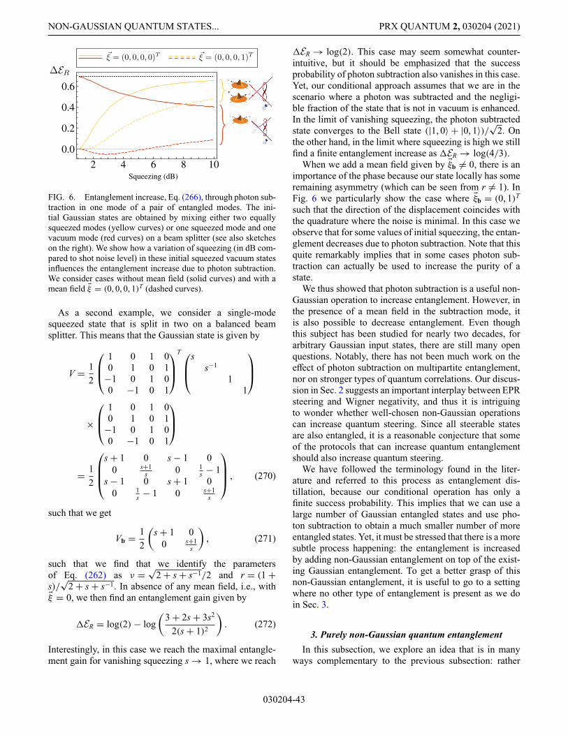
NON-GAUSSIAN QUANTUM STATES... PRX QUANTUM 2, 030204 (2021)
2 4 6 8 10
0.0
0.2
0.4
0.6
Squeezing (dB)
ΔER
ξ = (0, 0, 0, 1)Tξ = (0, 0, 0, 0)T
FIG. 6. Entanglement increase, Eq. (266), through photon sub-traction in one mode of a pair of entangled modes. The ini-tial Gaussian states are obtained by mixing either two equallysqueezed modes (yellow curves) or one squeezed mode and onevacuum mode (red curves) on a beam splitter (see also sketcheson the right). We show how a variation of squeezing (in dB com-pared to shot noise level) in these initial squeezed vacuum statesinfluences the entanglement increase due to photon subtraction.We consider cases without mean field (solid curves) and with amean field ξ = (0, 0, 0, 1)T (dashed curves).
As a second example, we consider a single-modesqueezed state that is split in two on a balanced beamsplitter. This means that the Gaussian state is given by
V = 12
⎛
⎜⎝
1 0 1 00 1 0 1
−1 0 1 00 −1 0 1
⎞
⎟⎠
T ⎛
⎜⎝
ss−1
11
⎞
⎟⎠
×
⎛
⎜⎝
1 0 1 00 1 0 1
−1 0 1 00 −1 0 1
⎞
⎟⎠
= 12
⎛
⎜⎜⎝
s + 1 0 s − 1 00 s+1
s 0 1s − 1
s − 1 0 s + 1 00 1
s − 1 0 s+1s
⎞
⎟⎟⎠ , (270)
such that we get
Vb = 12
(s + 1 0
0 s+1s
), (271)
such that we find that we identify the parametersof Eq. (262) as ν = √
2 + s + s−1/2 and r = (1 +s)/
√2 + s + s−1. In absence of any mean field, i.e., with
ξ = 0, we then find an entanglement gain given by
ER = log(2)− log(
3 + 2s + 3s2
2(s + 1)2
). (272)
Interestingly, in this case we reach the maximal entangle-ment gain for vanishing squeezing s → 1, where we reach
ER → log(2). This case may seem somewhat counter-intuitive, but it should be emphasized that the successprobability of photon subtraction also vanishes in this case.Yet, our conditional approach assumes that we are in thescenario where a photon was subtracted and the negligi-ble fraction of the state that is not in vacuum is enhanced.In the limit of vanishing squeezing, the photon subtractedstate converges to the Bell state (|1, 0〉 + |0, 1〉)/√2. Onthe other hand, in the limit where squeezing is high we stillfind a finite entanglement increase as ER → log(4/3).
When we add a mean field given by ξb �= 0, there is animportance of the phase because our state locally has someremaining asymmetry (which can be seen from r �= 1). InFig. 6 we particularly show the case where ξb = (0, 1)T
such that the direction of the displacement coincides withthe quadrature where the noise is minimal. In this case weobserve that for some values of initial squeezing, the entan-glement decreases due to photon subtraction. Note that thisquite remarkably implies that in some cases photon sub-traction can actually be used to increase the purity of astate.
We thus showed that photon subtraction is a useful non-Gaussian operation to increase entanglement. However, inthe presence of a mean field in the subtraction mode, itis also possible to decrease entanglement. Even thoughthis subject has been studied for nearly two decades, forarbitrary Gaussian input states, there are still many openquestions. Notably, there has not been much work on theeffect of photon subtraction on multipartite entanglement,nor on stronger types of quantum correlations. Our discus-sion in Sec. 2 suggests an important interplay between EPRsteering and Wigner negativity, and thus it is intriguingto wonder whether well-chosen non-Gaussian operationscan increase quantum steering. Since all steerable statesare also entangled, it is a reasonable conjecture that someof the protocols that can increase quantum entanglementshould also increase quantum steering.
We have followed the terminology found in the liter-ature and referred to this process as entanglement dis-tillation, because our conditional operation has only afinite success probability. This implies that we can use alarge number of Gaussian entangled states and use pho-ton subtraction to obtain a much smaller number of moreentangled states. Yet, it must be stressed that there is a moresubtle process happening: the entanglement is increasedby adding non-Gaussian entanglement on top of the exist-ing Gaussian entanglement. To get a better grasp of thisnon-Gaussian entanglement, it is useful to go to a settingwhere no other type of entanglement is present as we doin Sec. 3.
3. Purely non-Gaussian quantum entanglement
In this subsection, we explore an idea that is in manyways complementary to the previous subsection: rather
030204-43
MATTIA WALSCHAERS PRX QUANTUM 2, 030204 (2021)
than using a local non-Gaussian operation to increasealready existing entanglement, we now use a nonlocalnon-Gaussian operation to create entanglement betweenunentangled modes.
Let us again assume that our state is initially Gaussianas described by Eq. (85), and we induce the non-Gaussianfeatures through the conditional methods of Sec. B. Themean field of the initial state is given by ξ = ξf ⊕ ξg, and
V =(
Vf VfgVgf Vg
), with Vf = Vf1 ⊕ Vf2 . (273)
Here, we have introduced the modes of interest, labeled byf and a set of auxiliary modes g upon which a measurementwill be performed to induce non-Gaussian features in themodes f. In the initial state, we consider a bipartition inthe modes f without any direct correlations, hence Vf =Vf1 ⊕ Vf2 . In other words, the modes in f1 are completelyuncorrelated to the modes in f2.
To induce non-Gaussian effects, we resort to the condi-tional framework by acting with a POVM element A uponthe auxiliary modes g, and we rewrite Eq. (190) as
Wf|A( xf1 ⊕ xf2) =〈A〉g| xf1⊕ xf2
〈A〉Wf1( xf1)Wf2( xf2), (274)
and the conditional expectation value 〈A〉g| xf1⊕ xf2is again
given by Eq. (192). The entanglement in the resultingstate thus crucially depends on the exact properties of〈A〉g| xf1⊕ xf2
.First of all, note that Wf1( xf1) and Wf2( xf2) are generally
not pure states and as a consequence Wf|A( xf1 ⊕ xf2) is nota pure state either. Even though the specific structure ofthe Wigner function makes it a suitable case to apply themethods of Ref. [221], we follow a different route in thisTutorial by focusing on a particular example for which wecan assume that Wf1( xf1) and Wf2( xf2) are pure.
Just as in Sec. 2, we concentrate on photon subtraction.To get a conceptual idea of such a setup in this specificscenario, we present two equivalent schemes in (a) and (b)of Fig. 7. Note that the equivalence stems from the factthat the beam splitters that subtract the light from the sig-nal beams to send it to the photodetector are of extremelylow reflectivity. In this limit, we can be sure that there isat most one photon in the path and when it is detected,we herald a single-photon-subtracted state. In Fig. 7(a),the combination of this heralding process and the presenceof at most one photon avoids that the unmeasured outputcauses any losses or impurities. Nevertheless, the unmea-sured output will practically change the success probabilityof the heralding process, such that for practical implemen-tations Fig. 7(b) may be the preferential setup. Recall thatthe Wigner function for a state with a photon subtracted in
a particular mode b was given by Eq. (259), which herebecomes
W−( xf1 ⊕ xf2) = Wf1( xf1)Wf2( xf2)
tr (Vb − 1)+ ‖ ξb‖2
×(‖BT(1 − V−1
f1⊕ V−1
f2)( xf1 ⊕ xf2
− ξ1 ⊕ ξ2)+ ξb‖2
+ tr[1 − BT(V−1
f1⊕ V−1
f2)B
] ). (275)
Because we consider a limit where the state is completelytransmitted by the beam splitter and only a negligibleamount is sent to the photon counter to subtract the photon,we can indeed assume that the state is pure. For simplicity,we also assume that f1 and f2 are single modes. As we didbefore, we now calculate the reduced state
W−1 ( xf1) =
∫
R2d xf2W−( xf1 ⊕ xf2). (276)
The integral is rather tedious to evaluate, therefore weimmediately jump to the result (see Ref. [153] for an alter-native method that circumvents the explicit calculation ofintegrals):
W−1 ( xf1) = Wf1( xf1)
tr (Vb − 1)+ ‖ ξb‖2
(‖BTF1(1 − V−1
f1)( xf1 − ξ1)
+ ξb‖2 + tr[BTF1(1 − V−1
f1)FT
1 B]
+ tr[BTF2(Vf2 − 1)FT
2 B] )
, (277)
where we introduce the matrices Fk, given by
Fk =⎛
⎝| | fk � fk| |
⎞
⎠ , (278)
such that we can use the properties of the symplectic form� to obtain
BTFk =( bT fk bT� fk
− bT� fk bT fk
). (279)
If mode b is orthogonal to mode f1, we find that BTF1 =0 such that W−
1 ( xf1) = Wf1( xf1). On the other hand, whenmode b is exactly the same as f1 we find that BTF1 = 1
such that the photon is only subtracted there. In this caseW−
1 ( xf1) is a pure state and no entanglement is created. Inthis case, one can check that W−
2 ( xf2) = W2( xf2).To create entanglement, we are thus interested in the
case where b is a superposition of the two modes f1 and f2.To keep things simple, let us assume that b = cos θ f1 +
030204-44

NON-GAUSSIAN QUANTUM STATES... PRX QUANTUM 2, 030204 (2021)
(a)(c) (d)
(b)
FIG. 7. Entanglement creation through photon subtraction in asuperposition of uncorrelated modes f1 and f2. (a),(b) Sketchesof two equivalent setups to implement a photon subtraction inthe mode b, with b = cos θ f1 + sin θ f2. In (c),(d), we show thecreated entanglement, as measure through the Rényi entropy, Eq.(256), for varying values of θ . The initial Gaussian states arepure, with covariance matrices Vf1 = diag[s1, 1/s1] and Vf2 =diag[s2, 1/s2] for modes f1 and f2, respectively. The global meanfield, i.e., displacement, is varied ξ = 0 (solid curves), ξ =(1, 0, 0, 0)T (dotted curves), and ξ = (0, 0, 1, 0)T (dotted curves).(c) The particular case where the squeezing is balanced, i.e., s1 =s2 = 2. (d) An unbalanced example where s1 = 4 and s2 = 2.All squeezing values s1 and s2 are measured in units of vacuumnoise.
sin θ f2. Because the modes f1 and f2 are orthogonal, wecan use that f T
1 f2 = 0 and thus we find that BTF1 = cos θ 1
and BTF2 = sin θ 1. Nevertheless, the general expressionfor W−
1 ( xf1) does not simplify much.To acquire additional insight, let us now assume that
both modes f1 and f2 have exactly the same squeezing inthe same quadrature:
Vf1 = Vf2 =(
s 00 1
s
). (280)
Furthermore, let us assume that there is no mean field, suchthat ξ = 0. In this particular case, we find the expression
W−1 (xf1 , pf1) = W1(xf1 , pf1)
×[
p2f1
s + x2f1
s+ cos(2θ)
(
p2f1
s + x2f1
s− 2
)]
.
(281)
In particular, it turns out that the purity takes a simple form,such that we can quantify the entanglement for this state as
ER = log(2)− log(
cos(4θ)+ 32
). (282)
This shows that the maximal entanglement is reached forθ = π/4 and—as expected—the entanglement vanisheswhen θ = 0 and θ = π/2, i.e., when we subtract entirelyin either mode f1 and f2.
More general settings are shown in Fig. 7, where weshow the entanglement creation for unbalanced squeezing,by setting
Vf1 =(
s1 00 1
s1
), and Vf2 =
(s2 00 1
s2
). (283)
We compare the case with s1 = s2 to the case with s1 �= s2and find that in absence of a mean field one can reachthe same maximal amount of entanglement. However, themaximum is attained at a different value of θ when thesqueezing is unbalanced. From Eq. (282) we know thatin absence of a mean field, the curve for s1 = s2 does notdepend on the actual value of squeezing.
Figure 7 also shows the effect of an existing mean field,by probing a mean field in mode f1 with ξ = (1, 0, 0, 0)T
and in mode f2 with ξ = (0, 0, 1, 0)T. Generally speak-ing, we observe that the mean field reduces the createdentanglement. Nevertheless, the unbalance of squeezing(s1 �= s2) also unbalances the effect of the mean field. Thehigher squeezing in mode f1 makes the entanglement cre-ation more resilient to displacements, but a mean field inmode f2 will reduce the maximal attainable amount ofentanglement to the same level as in the balanced case[because in both (c) and (d) mode f2 is squeezed withs2 = 2]. In the presence of a mean field, we also findthat unbalanced squeezing shifts the value θ for whichmost entanglement is created. In other words, to achievemaximal entanglement upon photon subtraction in twomodes with unequal squeezing, one must subtract in anunbalanced superposition of these modes.
Through this example, we showed that entanglementbetween previously uncorrelated Gaussian states can becreated by a non-Gaussian operation. This entanglementhas some additional peculiarities. For example, a quickglance at how this procedure affects Eq. (190) shows thatwe can split the state in a Gaussian, i.e., Wf( xf), and a non-Gaussian part, i.e., 〈A〉g| xf/〈A〉. In this case of Eq. (259) theGaussian part of the state clearly remains fully separable.This means that, in this representation, all entanglement isoriginating from the non-Gaussian part of the state. Nev-ertheless, the decomposition, Eq. (190), of the state intoa Gaussian and a non-Gaussian part most probably is notunique for mixed states, making it challenging to studysuch non-Gaussian entanglement in its most general sense.
Yet, common tools that rely on the covariance matrix,such as Refs. [216,217], to characterize entanglement inthe photon subtracted states, Eq. (259), are doomed tofail. In Ref. [152] it is explicitly shown that the covari-ance matrix of a photon-subtracted state is given by thecovariance matrix of the initial Gaussian state with a posi-tive matrix added to it. This means that photon subtractionjust adds correlated noise to the covariance matrix and ifwe consider a Gaussian state that has exactly this covari-ance matrix we can decompose it using Eq. (103). In other
030204-45

MATTIA WALSCHAERS PRX QUANTUM 2, 030204 (2021)
words, when there is no entanglement visible in the covari-ance matrix of the initial Gaussian state, we do not witnessany entanglement based on the covariance matrix of thephoton-subtracted state. In this case, the non-Gaussianentanglement is thus genuinely non-Gaussian in the sensethat it cannot be detected through Gaussian witnesses.Hence, rather than decomposing the states in a Gaussianand non-Gaussian part, as was done in Eq. (190), it may bemore fruitful to define non-Gaussian entanglement as anyentanglement that cannot be witnessed based solely on thecovariance matrix of the state. This approach also offers anatural connection to the framework of Gaussian passivityon quantum thermodynamics [245].
Another peculiarity that was presented in Refs. [152,153] is the intrinsic nature of this non-Gaussian entan-glement. When we transform the system into a differentmode basis, there will still be entanglement in the system.The entanglement is said to be intrinsic because the stateis entangled in every possible mode basis. As we saw inEq. (249) Gaussian entanglement is never intrinsic as therealways exists a basis in which a Gaussian state is separable.
Figure 7(b) gives a rather interesting approach to under-standing the intrinsic nature of non-Gaussian entangle-ment. In this sketch, the second beam splitter is intendedto undo the superposition θ and return to the initial modebasis with modes f1 and f2. Changing this beam split-ter thus implies a basis change. If we remove this beamsplitter entirely, we find ourselves in the entanglementdistillation scenario of Sec. 2. In this case, the photonsubtraction is fully local, but it happens on a state withGaussian entanglement. The photon subtraction can thenincrease the Rényi entanglement by a maximal amount oflog 2. When we change to a mode basis where there isno Gaussian entanglement and the entanglement is cre-ated through a nonlocal photon subtraction, we create amaximal amount of Rényi entanglement given by log 2.Changing the mode basis in a different way will combinethe physics of these two extreme cases such that there willalways be entanglement, regardless of the basis.
Extending these ideas to more general non-Gaussianoperations on more general Gaussian mixed states is a hardand currently open problem. This reflects the general statusof entanglement theory in CV systems: we lack a struc-tured theoretical understanding of this phenomenon and asa consequence we also lack good tools to detect it.
D. Non-Gaussianity and Bell inequalities
In this final subsection of our study of quantum corre-lations in non-Gaussian states, we study Bell inequalities.First of all, we argue that it is impossible to violate Bellinequalities when both of the states and all the mea-surements involved can be described by positive Wignerfunctions. Then, we show that the Wigner function of the
state can itself be used to formulate a Bell inequality whenwe allow for nonpositive Wigner functions.
The general setup for studying nonlocality in CVrevolves around a multimode state with Wigner functionW( xf ⊕ xg) defined on a phase space R2m = R2l ⊕ R2l′ .Bell nonlocality entails that some measurements on thisstate cannot be described by a local hidden variable modelof the type, Eq. (238). In a quantum framework, the localmeasurements with POVM elements {Aj } (on the modesin f) and {Bj } (on the modes in g) can also be describedby Wigner functions WAj ( xf) and WBj ( xg). Because we aredealing with a POVM, we find that
(4π)l∑
j
WAj ( xf) = (4π)l′ ∑
j
WBj ( xg) = 1. (284)
Note that this equality holds for all possible coordinates xfand xg. Here we assume that the measurement outcomes Ajand Bj are discrete, but by correctly defining resolutions ofthe identity we can also deal with more general probabilitydistributions, e.g., homodyne measurements.
The probability to get the joint measurement result(Aj , Bk) is given by
P(Aj , Bk) = (4π)m∫
R2l
∫
R2l′d xfd xgW( xf ⊕ xg)WAj ( xf)
WBk ( xg). (285)
Now let us assume that all these Wigner functions are posi-tive. Because they are normalized, this implies that W( xf ⊕ xg) is a probability distribution on the entire phase spaceR2m, and WAj ( xf) and WBj ( xg) are probability distributionson the reduced phase spaces R2l and R2l′ , respectively.However, the model, Eq. (238), does not require probabil-ity distributions on phase space, but rather on the possiblemeasurement outcomes.
This is where Eq. (284) comes into play. BecauseWAj ( xf) and WBj ( xg) are positive, more than just treatthem as probability distributions in phase space wecan also consider P xf(Aj ) = (4π)lWAj ( xf) and P xg(Bj ) =(4π)l
′WBj ( xg) as the probability of getting the measure-
ment outcomes Aj and Bk, respectively. Because of Eq.(284) we find that these probabilities are correctly normal-ized
∑
j
P xf(Aj ) =∑
j
P xg(Bj ) = 1, (286)
and because the Wigner functions are positive, we alsofind that P xf(Aj ), P xg(Bj ) � 0. Note that the phase-spacecoordinates xf and xg are no longer treated as the vari-able, but rather as a label. The set {P xf(Aj ) | xf ∈ R2l}denotes a family of different probability distributions on
030204-46

NON-GAUSSIAN QUANTUM STATES... PRX QUANTUM 2, 030204 (2021)
the space of measurement outcomes {A1, A2, . . . }. The set{P xg(Bj ) | xg ∈ R2l′ } can be interpreted analogously.
We can thus recast Eq. (285) in the following form:
P(Aj , Bk) =∫
d xfd xgW( xf ⊕ xg)P xf(Aj )P xg(Bk). (287)
Because W( xf ⊕ xg) is a positive and normalized Wignerfunction, it is a joint probability distribution on the coordi-nates xf and xg. These coordinates label families of proba-bility distributions {P xf(Aj ) | xf ∈ R2l} and {P xg(Bj ) | xg ∈R2l′ } for the measurement outcomes. The expression (287)is thus fully consistent with Bell’s local hidden variablemodel, Eq. (238). As a consequence, we cannot violate anyBell inequalities when the system is prepared in a state witha positive Wigner function and when we only have accessto POVM that have Wigner representations with positiveWigner functions.
Let us emphasize that there is generally no reason toassume that the probabilities P xf(Aj ) and P xg(Bj ) are alsoconsistent with quantum mechanics. In other words, thereis not necessarily any state ρ such that P xf(Aj ) = tr[ρAj ].However, because we are dealing with Bell nonlocality, wedo not need this to be the case, since Eq. (238) allows forarbitrary local probability distributions.
To make a long story short, we have shown that Wignernegativity is necessary for witnessing Bell nonlocality. Theinterested reader can consult works such as Ref. [64] thatrelate Wigner negativity to the more general concept ofquantum contextuality. However, the topic of contextualityin CV systems is still a matter of scientific debate [246].
There has been a significant body of work about the vio-lation of Bell inequalities in CV setups [247–249]. It isevident that this is an arduous task once one approachesa realistic experimental setting [250]. Here, we focus onone particular suggestion to test Bell nonlocality based ona state’s Wigner function [251,252].
The starting point of this approach is the CHSH inequal-ity
∣∣∣〈X Y〉−〈X Y′〉+〈X ′Y〉+〈X ′Y′〉∣∣∣ � 2.
As we discussed in Sec. 4, this inequality relies on someassumptions for the observables X , X ′, Y, and Y′. In par-ticular, we must assume that the measurement outcomesare either −1 or 1. In a CV setting, where we generallydeal with a continuum of possible measurement outcomes,this seems like a serious constraint. Nevertheless, wehave already encountered some natural examples duringthis Tutorial. For example, photon counters yield a dis-crete number of possible measurement outcomes. Here, wechoose a related observable that takes us all the way backto Sec. B, where we encountered the observable
( x) = D(− x)(−1)N D( x).
This displaced parity operator has a rich structure, butwhen it comes to actual measurement outcomes is willreturn either −1 or 1. This means that we can chooseX , X ′, Y, and Y′ to be parity operators. First of all, let usnote that
( xf ⊕ xg) = ( xf)⊗ ( xg). (288)
To see this, one can first show that (−1)Nm =(−1)Nl+Nl′ = (−1)Nl ⊗ (−1)Nl′ and subsequently useD( xf ⊕ xg) = D( xf)⊗ D( xg) (displacements in differentmodes are independent from each other).
Now we can identify the observables as follows:
X = ( xf), X ′ = ( x′f),
Y = ( xg), Y′ = ( x′g),
(289)
and therefore the CHSH inequality is transformed into∣∣∣〈( xf ⊕ xg)〉−〈( xf ⊕ x′
g)〉+〈( x′f ⊕ xg)〉+〈( x′
f ⊕ x′g)〉
∣∣∣
� 2. (290)
As a next step, we use Eq. (78) to write
〈( xf ⊕ xg)〉=(2π)mW( xf ⊕ xg), (291)
such that the inequality (290) can be recast as∣∣∣W( xf ⊕ xg)− W( xf ⊕ x′
g)+ W( x′f ⊕ xg)+ W( x′
f ⊕ x′g)
∣∣∣
� 2(2π)m
. (292)
Any state with a Wigner function that violates this inequal-ity for some choice of coordinates xf, x′
f, xg, and x′g pos-
sesses some form of Bell nonlocality. In Refs. [251,252]it is argued that the inequality (292) can be violated bysending a single photon through a beam splitter, but alsoby an EPR state. The fact that a Gaussian Wigner func-tion suffices to violate Eq. (292) sometimes comes as asurprise, because we previously argued that one needsWigner negativity to violate Bell inequalities. The reasonwhy one can detect Bell nonlocality with this inequalityeven when the Wigner function is positive stems from ourchoice of observable ( xf ⊕ xg). The POVM elements thatcorrespond to the measurement outcomes 1 and −1 haveWigner functions that are strongly Wigner negative. As aconsequence the necessary Wigner negativity is baked intoEq. (292) by construction.
In practice, the inequality (292) is highly sensitive toimpurities and can often be hard to violate with experimen-tally reconstructed Wigner functions. The hunt for goodnew techniques to show Bell nonlocality in CV systems
030204-47

MATTIA WALSCHAERS PRX QUANTUM 2, 030204 (2021)
is therefore still open. However, this subsection clearlyshowed us that Wigner negativity is necessary to observeone of the most exotic features in quantum physics. Thisnegativity might be baked into the state, but it could just aswell be induced by measurements. The conditional meth-ods of Sec. B also highlight this duality, where Wignernegativity in the measurement is used to induce Wignernegativity in the state. It should come as no surprise thatWigner negativity is also a necessary ingredient for themost exotic quantum protocols. However, it should also behighlighted that even with a little extra trust, it is possibleto design protocols that do not require Wigner negativity towitness quantum correlations [201]. In the next section, wediscuss its importance for reaching a quantum advantagewith CV systems.
VI. NON-GAUSSIAN QUANTUM ADVANTAGES
It has been long known that systems that are entirelybuilt with Gaussian building blocks are easy to simulate[25]. It should perhaps not come as a surprise that efficientnumerical tools exist to sample numbers from a multivari-ate Gaussian distribution. The discrete variable analog ofthis result comes across as less intuitive and goes by thename “Gottesman-Knill theorem” [253]. Yet, it turns outthat something stronger than mere non-Gaussian elementsis required to render a system hard to simulate.
In Sec. D, we encountered the power of Wigner neg-ativity by realizing that it is a necessary requirement forBell nonlocality. This connection between Wigner nega-tivity and the most exotic types of quantum correlationsshows us that Wigner negativity is key to giving CV sys-tems their most prominent quantum features. It is thenperhaps not a surprise that such Wigner negativity is alsoa necessary requirement for implementing any type ofprotocol that cannot be efficiently simulated by a classi-cal computer [33,254,255]. We thus start our discussionof quantum advantages by explaining the result of Ref.[33]. To show the necessity of Wigner negativity, weshow an explicit simulation algorithm for general quantumprotocols without Wigner negativity.
Any quantum protocol ultimately relies on the mea-surement of a certain set of measurement operators {Ej }(typically a POVM) of a system prepared on a state ρ. In aWigner function formalism, we then find
pj = (4π)m∫
R2md x WEj ( x)W( x). (293)
Furthermore, the fact that the set {Ej } forms a POVMimplies that
(4π)m∑
j
WEj ( x) = 1. (294)
As we already discussed in Sec. D, surrounding Eq. (284),it is crucial that the normalization condition (294) holds forany phase-space coordinate x. In the present context, wewant to show that there is an efficient method for a classicaldevice to sample values from the probability distribution{pj } when all involved Wigner functions are positive.
Let us start by assuming that the Wigner functions thatdescribe the POVM elements are all positive. When com-bined with the POVM condition (294), this implies that wecan identify a set of probabilities P x(ej ) = (4π)mWEj ( x)as the probability to obtain the measurement outcomeej , associated with the POVM element Ej . These P x(ej )
depend on a parameter x, we can thus form a family ofprobability distributions {P x(ej ) | x ∈ R2m} that describethe probability of obtaining the different results ej , depend-ing on a chosen phase-space point. The normalizationcondition (294) now states that
∑j P x(ej ) = 1 for all x. Let
us emphasize that this family of probabilities would not bewell defined if WEj ( x) were not positive Wigner functions,as some of the probabilities would be negative.
Going back to the initial Eq. (293), we now find that
pj =∫
R2md x P x(ej )W( x). (295)
To find the actual probability of getting the j th outcomeis thus given by “averaging” the probabilities P x(ej ) overthe different phase-space coordinates. Generally speaking,this is not a real average, unless the Wigner function W( x)of the state is an actual probability distribution on phasespace. The latter is exactly the case when W( x) is posi-tive. Then, we can simply think of the probability pj forobtaining event ej as pj = EW[P x(ej )], where EW is theexpectation value over the probability distribution W( x).
Hence, when all Wigner functions are positive, thealgorithm to simulate our relevant quantum process cansimply be expressed by the following steps:
1. Sample a phase-space coordinate x from the proba-bility distribution W( x).
2. Construct the probability distribution P x(ej ) for thesampled value x.
3. Sample an outcome ej from the probability distribu-tion P x(ej ).
Even though this is the general idea behind our samplingprotocol, there are some major hidden assumptions. First,we assume here that the Wigner function for the state andthe measurement are known. Furthermore, we also assumethat we can simply sample points from any distributionon phase space and from any distribution of measurementoutcomes P x(ej ). In particular, for the sampling aspects itis not at all clear that these are reasonable assumptions tomake. Standard sampling protocols for multivariate prob-ability distributions tend to get highly inefficient once the
030204-48
NON-GAUSSIAN QUANTUM STATES... PRX QUANTUM 2, 030204 (2021)
probability distributions become too exotic such that it isdangerous to assume that we can “just sample.”
To address this point Ref. [33] makes more assump-tions on the exact setup we are trying to simulate. First,we assume that the detection is done by a series of single-mode detectors, such that our label j now become a tuplej = (j1, j2, . . . , jm)where jk denotes the outcome e(k)jk for thedetector on the kth mode. We can thus write the POVMelement as Ej = E(1)j1 ⊗ · · · ⊗ E(m)jm , such that
WEj( x) = WE(1)j1(x1, p1)WE(2)j2
(x2, p2) . . .WE(m)jm(xm, pm).
(296)
We assume that each detector has been accurately cal-ibrated, such that all the individual Wigner functionsare known. This implies that for a given point in phasespace x = (x1, p1, . . . , xm, pm)
T, we can simply evaluatethe probabilities for each detector to produce a certainoutcome. Thus, we calculate the probability distributionsP(xk ,pk)(e
(k)j ) = 4πWE(k)j
(xk, pk) for all the possible mea-
surement outcomes for that specific mode. We assume thatsampling outcomes e(k)j from these probability distribu-tions P(xk ,pk)(e
(k)j ) is a feasible task. For typical detectors
in quantum optics experiments this is a very reasonableassumption.
The Wigner function W( x) that describes the state ismore subtle as it also includes all correlations betweenmodes. If the state is Gaussian, a measurement of thecovariance matrix would be sufficient to know the fullWigner function. Because of its Gaussian features, thereare efficient tools to directly sample phase-space points.Yet, for more general non-Gaussian positive Wigner func-tions this sampling may be much harder. Therefore, Ref.[33] makes an essential assumption: it assumes that weknow a protocol that combines local operations to designthe state W( x) from a known initial state with no correla-tions between the modes. The notion of “locality” shouldhere be understood in the sense of acting on a smallset of modes while leaving the others fully untouched.These local operations are also supposed to be representedby positive Wigner functions, which depend only on thephase-space coordinates of the subset of modes on whichthey act.
Generally speaking, such Wigner positive operations� : Hin → Hout map a state ρ to a new state �[ρ]. In Ref.[33], the Choi representation [256,257] is used to repre-sent� as a state on a larger Hilbert space Hin ⊗ Hout. Thisbecomes particularly appealing when we go to a Wignerrepresentation, where the Choi representation of� is givenby a Wigner function W�( x in ⊕ x out). The action of � on
a state with Wigner function W( x in) is then given by
Wout( x out) = (4π)m∫
R2md x in W�( x in ⊕ T x out)W( x in),
(297)
where m is the number of modes of the input state. Fortechnical reasons, we must include the transposition oper-ator T, Eq. (257), in the action of the channel. Becausethis operation must be trace preserving, we on top get theproperty that
(4π)m∫
R2md x out W�( x in ⊕ T x out) = 1. (298)
When we now assume that the operation � has a Wigner-Choi representation W�( x in ⊕ x out), which is a positivefunction, it immediately follows that the operation �
turns a Wigner positive initial state W( x in) into a Wignerpositive output state Wout( x out).
It is useful to note that such operations, Eq. (297), can betrivially embedded in a larger space. Let us assume that weconsider a state W( xf ⊕ xg), we can simply let the operationact on the modes g by taking
Wout( xf ⊕ x outg ) = (4π)l
′∫
R2l′d xin
g W�( x ing ⊕ T x out
g )
× W( xf ⊕ x ing ). (299)
Notationally, this may seem a little complicated, but, inessence, we just carry out the integration over a subset ofthe full phase space. We call these operations local Wignerpositive operations.
In our simulation protocol, we thus assume that W( x) iscreated by a series of such local Wigner positive operationsof �1, . . . ,�t on a noncorrelated input state Win( xin) =W(1)
in (x1, p1)W(2)in (x2, p2) . . .W
(m)in (xm, pm).
W( x) = (4π)mt∫
R2md xt . . .
∫
R2ld xtW�t( xt ⊕ T x) . . .
× W�2( x1 ⊕ T x2)W�1( xin ⊕ T x1)
× Win( xin). (300)
We assume on top that each operation is local over a smallnumber of modes l � m. To model this with Eq. (299),it suffices to split xtk−1 = xl
tk−1⊕ xl′
tk−1and xtk = xl
tk ⊕ xl′tk ,
such that
(4π)mW�tk( xtk−1 ⊕ T xtk )
= (4π)lW�tk( x l
tk−1⊕ T x l
tk )δ( xl′tk−1
− xl′tk ). (301)
Even though the notation is complicated, it simplydescribes that we act on an l-mode subspace with theoperation �tk and leave the other l′ modes untouched.
030204-49

MATTIA WALSCHAERS PRX QUANTUM 2, 030204 (2021)
The normalization condition (298) now has an impor-tant consequence, since it allows us to identify aprobability distribution on phase space P xtk−1
( xtk ) =(4π)mW�tk
( xtk−1 ⊕ T xtk ). It gives us the probability ofchoosing a phase space value xtk , given that we know xtk−1 .Because the operations are local, Eq. (301) allows us tokeep most of the phase-space coordinates constant fromstep to step. Furthermore, the first step is simple. Everypair (xk, pk) of the initial coordinate xin can be sampledindependently because Win( xin) factorizes. This now givesus the following new algorithm:
1. Take the initial Wigner function Win( x in) =W(1)
in (x1, p1)W(2)in (x2, p2) . . .W
(m)in (xm, pm) and sample
a pair (xk, pk) from every single-mode probabilitydistribution W(k)
in (xk, pk). Put all these pairs togetherto obtain x in = (x1, p1, . . . , xm, pm).
2. Update the coordinate by sampling new coor-dinates based on P xtk−1
( xtk ) = (4π)mW�tk( xtk−1 ⊕
T xtk ). Because �tk are local operations, it sufficesto only locally update coordinates. Let us makethis clear through an example. Say we have xtk−1
= (x(k−1)1 , p (k−1)
1 , . . . , x(k−1)m , p (k−1)
m )T and operation�tk acts locally on modes with labels 2, 5, and7. Take x l
tk−1= (x(k−1)
2 , p (k−1)2 , x(k−1)
5 , p (k−1)5 , x(k−1)
7 ,
p (k−1)7 ) and use it to evaluate P xtk−1
( x ltk )= (4π)lW�tk
( x ltk−1
⊕ T x ltk ). Now sample a new vector x l
tk =(x(k)2 , p (k)2 , x(k)5 , p (k)5 , x(k)7 , p (k)7 ) from this probabilitydistribution. Then construct the new vector xtk bytaking xtk−1 and updating the coordinates associ-ated to modes 2, 5, and 7 to the newly sampledcoordinates
3. After the operations �1, . . . ,�t have been imple-mented by updating the phase-space coordi-nate, take the final phase-space coordinate x =(x1, p1, . . . , xm, pm)
T and the Wigner function describ-ing the detectors WEj( x) = WE(1)j1
(x1, p1)WE(2)j2(x2, p2)
. . .WE(m)jm(xm, pm). For each detector k, use the phase-
space coordinate x to generate the probability distri-bution P(xk ,pk)(e
(k)j ) = WE(k)j
(xk, pk).
4. Sample an outcome e(k)j from the distributionP(xk ,pk)(e
(k)j ) for every detector.
Sampling the final phase-space coordinate x by using aMonte-Carlo-style update rule is time consuming, but ifthe operations are local it can be done efficiently. This pro-cedure implicitly assumes that we do not just know thestate we are sampling from, but that we know the cir-cuit of local operations that is used to create the statefrom local resources. Ultimately, when one considers thecircuit representation of quantum algorithms, this is alsohow a quantum algorithm works. For example, Sec. A
exactly shows that any unitary CV circuit can be built withsingle- and two-mode gates. The algorithm outlined in thissection shows that we can efficiently simulate any protocolwhere the local input state, the circuit’s operations, and themeasurements are described by positive Wigner functions.
One may wonder whether any positive Wigner functionW( x) can be constructed through such a circuit and, if so,whether there is an efficient way to design such a circuitwhen we know the Wigner function. If we assume that notonly the state W( x) but also all its marginals are known,it is possible to construct a stepwise sampling procedurethrough the chain rule of probability theory:
W( x) = W(xm, pm | xm−1, pm−1, . . . x1, p1)× . . .
W(x3, p3 | x2, p2, x1, p1)W(x2, p2 | x1, p1)W(x1, p1).(302)
This process effectively executes a type of random walkwith memory. In each step of this walk, we then samplethe phase-space coordinates for one mode. Nevertheless,this process only works when we have access to all theseconditional probabilities, which practically implies havingaccess to all the marginals of the distribution. In practi-cal setups, this will often not be the case. Nevertheless,it is quickly seen that this setup can be efficiently usedto sample from Gaussian Wigner functions where theseconditional distributions have a particularly simple form.
Thus, we have shown that it is impossible to obtaina quantum computational advantage by using only localstates, measurements, and operations with positive Wignerfunctions. This means that Wigner negativity is necessaryto reach a quantum advantage in such setups. However,Wigner negativity is certainly not sufficient since thereare many setups of quantum systems that involve negativeWigner functions that can be efficiently simulated [258].It is thus interesting to take the opposite approach andexplore a setup that is known to lead to a quantum advan-tage. In the spirit of CV setups, the most logical choice forsuch a discussion is Gaussian boson sampling [259]. In theliterature, this setup has been studied mainly from the pointof view of complexity theory [260,261], but here we ratherfocus on its physical building blocks.
Boson sampling [262] is a problem in which one injectsa set of N bosons (generally photons) into an m-modeinterferometer. On the output ports of this interferome-ter, photodetectors are mounted to count the particles atthe output. Simulating this type of quantum Galton boardis a computationally hard task, implying that a quantumadvantage could be reached by implementing the setup ina quantum optics experiment. On the other hand, it turnsout that the required number of photons to implement suchan experiment is also hard to come by. This was the moti-vation for developing a new approach, where the inputphotons are replaced by squeezed states that are injected
030204-50

NON-GAUSSIAN QUANTUM STATES... PRX QUANTUM 2, 030204 (2021)
in each of the interferometer inputs. Because an interfer-ometer, built out of phase shifters and beam splitters, is aGaussian transformation the output state will remain Gaus-sian. We can thus effectively say that we are samplingphotons from a state with Wigner function WG( x). In addi-tion, there is no mean field in the setup such that the entirestate is characterized by its covariance matrix V.
When we assume that the detectors resolve photon num-bers, the probability to detect a string of counts n =(n1, . . . , nm) can we written as
P(n) = (4π)m∫
R2md x Wn( x)WG( x). (303)
We can then use Eq. (118) to write
Wn( x) = Wn1(x1, p1) . . .Wnm(xm, pm). (304)
Even though the integral (303) is hard to compute, it isinsightful in the light of Eq. (295) and our discussionregarding the necessity of Wigner negativity. Indeed, wesee immediately that the detectors form a crucial ele-ment in rendering the setup hard to simulate. The sameholds when we replace the number-resolving detectorswith their on-off counterparts [263] such that nk = {0, 1}and the Wigner functions are given by Wnk (xk, pk) = {1 −2 exp[−(x2
k + p2k )/2]}/(4π).
When we stick with number-resolving detectors thatproject on Fock states, it is practical to reformulate theproblem in terms of P functions and Q functions, such that
P(n) =∫
R2md x Pn( x)QG( x). (305)
For the detailed calculation, we refer to Ref. [259]. It turnsout that the probabilities P(n) can be expressed in termsof the Hafnian of a matrix [264], which establishes a con-nection to the problem of finding perfect matchings ingraph theory. This connection has led to several suggestedapplications for Gaussian Boson sampling [265–267].
In the light of this Tutorial, the most interesting appli-cation of Gaussian Boson sampling is its potential role inquantum state engineering [205]. When only a subset ofmodes are measured, we can see Gaussian Boson samplingas a generalization of photon subtraction (and even as ageneralization of “generalized photon subtraction” [157]).The idea is reasonably simply explained in the light of Sec.B: when we split the system in two parts R2m = R2l ⊕ R2l′ ,such that the Gaussian state that comes out of the interfer-ometer now takes the form WG( xf ⊕ xg), we can postselecton a measurement outcome n = (n1, . . . nl′) for the secondsubsystem. We thus project on a state Wn( xg), which is aproduct of l′ Fock states, and from Eq. (190), we obtainthat the conditional state on the remaining modes is given
by
Wf|n( xf) = 〈[|n1〉 〈n1| ⊗ · · · ⊗ |nl′ 〉 〈nl′ |]〉g| xf
〈[|n1〉 〈n1| ⊗ · · · ⊗ |nl′ 〉 〈nl′ |]〉 Wf( xf),
(306)
with Wf( xf) defined by Eq. (182). From Eq. (192) we recallthe expression
〈[|n1〉 〈n1| ⊗ · · · ⊗ |nl′ 〉 〈nl′ |]〉g| xf
= (4π)l′∫
R2l′d xg Wn( xg)WG( xg | xf), (307)
and because the initial state WG( xf ⊕ xg) is Gaus-sian, we find that the conditional probability distribu-tion WG( xg | xf) is given by Eq. (193). Ironically, toevaluate 〈[|n1〉 〈n1| ⊗ · · · ⊗ |nl′ 〉 〈nl′ |]〉g| xf and 〈[|n1〉 〈n1| ⊗· · · ⊗ |nl′ 〉 〈nl′ |]〉 we must essentially solve the same hardproblem as for the implementation of Gaussian Bosonsampling itself. Therefore, the exact description of theresulting states is generally complicated.
Nevertheless, in idealized scenarios, even small Gaus-sian Boson sampling circuits can be used to prepare inter-esting non-Gaussian states [205]. In particular, the capacityof Gaussian Boson sampling to produce GKP states hastaken up a prominent place in a recent blueprint for pho-tonic quantum computation [24]. Furthermore, the resultsin Sec. C suggest that states created by performing Gaus-sian Boson sampling on a subset of modes can haveadditional non-Gaussian entanglement. Yet, to be able touse this procedure to produce highly resourceful Wignernegative states, Sec. 2 highlights that the initial Gaussianstate needs to be such that the modes in f can steer themodes in g. This condition can be seen as a basic qualityrequirement for the Gaussian Boson samplers that are usedin Ref. [24].
Finally, the experimental imperfections are also detri-mental for the quantum advantage that is produced inGaussian Boson sampling. Clearly, when the Gaussianstate WG( x) can be written as a Gaussian mixture of coher-ent states (meaning that no mode basis exists in which thequadrature noise is below vacuum noise), the samplingcan be simulated efficiently. Because multimode coher-ent states are always just a tensor product of single-modecoherent states, it suffices to sample a coherent state fromthe mixture, calculate all the individual probabilities for theoutput detectors, and sample independent detector outputsaccording to these probabilities. The presence of entan-glement in the Gaussian state from which we sample isthus crucial. In addition, detector efficiencies must be suf-ficiently high such that their Wigner functions remainnonpositive, otherwise the protocol of Ref. [33] rendersthe setup easy to simulate (as explained in the first part
030204-51

MATTIA WALSCHAERS PRX QUANTUM 2, 030204 (2021)
of this section). A more thorough analysis of how dif-ferent experimental imperfections render Gaussian Bosonsampling easier to simulate can be found in Ref. [268].
There are clearly still many aspects of the relationbetween non-Gaussian features of quantum states on theone hand, and the ability to achieve a quantum computa-tional advantage on the other hand, that are not yet fullyunderstood. The Gaussian Boson sampling setup clearlyemphasizes the importance of entanglement in combina-tion with Wigner negativity. Furthermore, there is theimplicit fact that a simulation scheme such as Ref. [33]requires knowledge of the actual circuit of local operationsthat was used to create the state. It does make sense toassume that we actually have some ideas of the quantumprotocol that we are attempting to simulate, but yet onemay wonder whether there could be a reasonable setting(in the sense that we are actually implementing a well-controlled protocol) in which the assumptions of Ref. [33]do not hold. This clearly shows that many fundamental the-oretical aspects of CV quantum computation remain to beuncovered.
VII. EXPERIMENTAL REALIZATIONS
Now that we have provided an overview of some theo-retical aspects of non-Gaussian quantum states, we inter-pret the “where to find them” part of the title in a very lit-eral sense. Non-Gaussian states are generally rather fragile,as one should expect from quantum central limit theoremand the fact that thermal states in free bosonic theories areGaussian. Producing and analyzing non-Gaussian states ina laboratory setting is indeed challenging, but neverthelessit has been done numerous times. Our main focus in Sec.A is quantum optics, which is the historical testbed for CVquantum physics. However, in recent years there has beenincreased attention for CV approaches in other setting suchas optomechanics, superconducting circuits, and trappedions.
A. Quantum optics experiments
This section provides an overview of some of the mostimportant milestones in the generation of non-Gaussianstates in optics. For more details, we refer the reader toa specialized review [81].
Historically, one might argue that the first experimentalrealizations of non-Gaussian states in optical setups reliedon sufficiently sensitive photon detectors. Initial demon-strations primarily used photoemission of atoms [269,270],which are prepared in excited states (e.g., by electron bom-bardment) or via resonance fluorescence in ions [271]. Thedevelopment of spontaneous parametric down-conversion(SPDC) made it possible to create a single-photon stateusing only bulk optical elements [202]. However, allthese early non-Gaussian states were characterized through
counting statistics, which means that we generally classifythem as DV experiments.
It is perhaps intriguing to note that SPDC is also theprocess that lies at the basis of the creation of squeezedstates of light [272], which are Gaussian. These states playa key role in the generation of single-photon states, simplybecause a weakly squeezed vacuum is mainly a super-position of vacuum and a photon pair. By detecting onephoton of the pair, the presence of the second photon isheralded. Hence, the approach of Ref. [202] is a basicimplementation of a conditional scheme for the generationof non-Gaussian states as presented in Sec. B.
A genuine CV treatment of such non-Gaussian stateswould only be achieved much later in a work that presentsthe first tomographic reconstruction of a state with Wignernegativity in optics [273]. Due to the developments of aneasily implementable maximum-likelihood algorithm forstate reconstruction, homodyne tomography became oneof the main tools to study non-Gaussian states in CV quan-tum optics [274]. It did not take long before this also led tothe reconstruction of a displaced single-photon Fock state[275] and a two-photon Fock state [276]. The combinationof increased squeezing with type-II SPDC and an array ofphoton detectors to increase the number of heralded pho-tons more recently made it possible to resolve the Wignerfunction of a three-photon Fock state [277]. Similar ideasof multiplexed photon detection have also been used togenerate superpositions of Fock states [278].
For non-Gaussian states beyond Fock states, photonsubtraction, as described in Sec. 2, is a common experi-mental tool. Its first experimental implementation success-fully showed the capability of generating non-Gaussianstatistics in the homodyne measurements, but it failed todemonstrate Wigner negativity [148]. Later experimentsimproved the quality of the generated states, demonstrat-ing Wigner negativity and creating so-called “Schrödingerkittens” [129,279,280]. The terminology is chosen becausethese states resemble cat states proportional to |α〉 − |−α〉for small values of the mean field α. Even though suchSchrödinger kittens are ultimately not very different fromsqueezed single-photon states, the nomenclature makesmore sense in the context of experiments that “breed” catstates [281]. Here, one mixes two Schrödinger kittens ona beam splitter and performs homodyne detection on oneoutput port. By conditioning on instances where this homo-dyne detector registers values close to zero, one effectivelyheralds a larger cat state (the value of α has increased). Avariation of photon subtraction has also been used to createa type of CV qubit [282].
As an alternative to photon subtraction, one can alsoadd a photon [159]. Even though this operation theoreti-cally equates to applying a creation operator on the state,it is experimentally much harder to implement than pho-ton subtraction as it requires nonlinear optics. However,photon subtraction can only produce Wigner negativity
030204-52

NON-GAUSSIAN QUANTUM STATES... PRX QUANTUM 2, 030204 (2021)
when the initial state is squeezed. Photon addition, onthe other hand, provides the advantage of always creat-ing a Wigner negative state. A simple way to see thisis by applying a creation operator to the state and eval-uating the Q function (70). When a photon is added tothe mode g, the Q function after photon addition has theproperty Q+( α) ∼ ( αT g)2QG( α), where QG( α) is the Qfunction of the initial Gaussian state. This relation impliesautomatically that the Q function will be exactly zerofor α = 0, and a zero of the Q function implies Wignernegativity. This means that one can apply photon addi-tion to highly classical states, such as a coherent state ora thermal state, and still end up creating Wigner nega-tivity. Such photon-added coherent states were also usedto experimentally measure [283] non-Gaussianity δ(ρ)
as defined in Eq. (110). Remarkably, combining photonaddition and photon subtraction operations in both pos-sible orders provides a way to experimentally verify thecanonical commutation relations [a, a†] = 1, as was shownin Ref. [160].
The above methods are all based on Gaussian states asinitial resources to generate non-Gaussian states. The non-Gaussian states that are created as such can in turn serveas useful resources to create more intricate non-Gaussianstates. Fock states are a commonly used type of inputstate, for example, in the first demonstration of a largeSchrödinger’s cat state [284]. Intriguingly, by using non-Gaussian initial states, it suffices to use homodyne detec-tion as the conditional operation. This setup can then beextended to a cat breeding scheme [285]. Another methodto create large cat states in optics relies on making the lightfield interact with an atom [286]. The presence of entan-glement between the “macroscopic” coherent state and the“microscopic” atomic degrees of freedom make for anexperiment that resembles Schrödinger’s original thoughexperiment [106]. Once the atom and the coherent lightare entangled, a spin rotation of the atom is followed by ameasurement to project the state of the light field in eitheran even or an odd cat state. This reflects the general ideathat atoms still induce much larger nonlinearities than non-linear crystals. These nonlinearities are the direct source ofnon-Gaussian effect, but they are also much harder to con-trol. At present, experiments that rely on such higher-ordernonlinearities to create non-Gaussian states remain rare inthe optical regime.
The above methods all focus on the creation of single-mode non-Gaussian states. For multimode systems, muchof the experimental progress has concentrated on two-mode systems. As we extensively discussed throughoutthis tutorial, an important feature in such multimode sys-tems are quantum correlations. Some of the first exper-imental demonstrations of non-Gaussian quantum corre-lations were based on the Bell inequality (292). Homo-dyne tomography and a single photon, delocalized over
two modes by a beam splitter, suffices to violate theinequality [287,288]. However, these works also teach usthat extreme high purities are required to do so.
Motivated by photon-subtraction experiments and chal-lenged by the no-go theorem of [225–227], entanglementdistillation soon became a new focus for non-Gaussianquantum optics experiments. Some of these experimentshave focused on adding some form of non-Gaussian noiseon the initial state to circumvent the no-go theorem [228,229]. Entanglement distillation through local photon sub-traction from the entangled modes of a Gaussian input statewould later be demonstrated in Ref. [289]. Earlier, it hadalready been shown that Gaussian entanglement can beincreased by photon subtraction in a superposition of theentangled mode [290]. Interestingly, in the latter case, thephoton is effectively subtracted in a nonentangled modesuch that the setup is essentially equivalent to mixing asqueezed vacuum and a photon-subtracted squeezed vac-uum on a beam splitter. A similar photon subtraction in acoherent superposition of modes was later carried out toentangle two Schrödinger kittens [291]. This can proba-bly be seen as the first realizations of purely non-Gaussianentanglement in CV.
Photon addition has also been considered as a tool forcreating entanglement between pairs of previously uncor-related modes [292]. The resulting state can be seen as ahybrid entangled state proportional to |0〉 |α〉 + |1〉 |−α〉,such states have also been produced using techniques sim-ilar to photon subtraction [293]. For two modes, photonaddition can be implemented in a mode-selective way[294]. This setup is particularly useful to create entan-glement between coherent states by adding a photon in asuperposition of displaced modes.
Going beyond two modes has always remained a chal-lenging task. For mode-selective photon subtraction froma multimode field, one must abandon the typical imple-mentation based on a beam splitter. For two modes, suchan alternative photon subtraction scheme was, for exam-ple, realized in the time-frequency domain, by subtractinga photon from a sideband [295]. Yet, going to a gen-uine multimode scenario required the design of a wholenew photon subtractor based on sum-frequency generation[296,297]. This finally permitted the first demonstration ofmultimode non-Gaussian state in a CV setting, demonstrat-ing non-Gaussian features in up to four entangled modes[298].
Such highly multimode states of more than two modesare confronted with a considerable problem: the exponen-tial scaling of the required number of measurements fora full state tomography. This makes it highly challeng-ing to demonstrate non-Gaussian features such as Wignernegativity in multimode non-Gaussian states. For single-photon-subtracted states, it has been pointed out that goodanalytical models can be used to train machine-learning
030204-53
MATTIA WALSCHAERS PRX QUANTUM 2, 030204 (2021)
algorithms to recognize Wigner negativity based on single-mode measurements [299]. Furthermore, the techniques ofRef. [128] combined with Ref. [300] should also make itpossible to use multiplexed double homodyne detection towitness Wigner negativity in certain classes of multimodestates.
In multimode systems, we are confronted with the lim-itations of homodyne tomography. Recently, it has beenshown that machine-learning techniques can be used toimplement an improved form of CV tomography basedon homodyne measurements [301]. Even though this setupis computationally heavy in single-mode setups, it usesa smaller set of states as a basis for state reconstruction,which might make multimode versions of the protocolmore scalable. Alternatively, one can also bypass homo-dyne measurements all together. Photon-number-resolvingdetectors such as transition edge sensors [302] make itpossible to use the identity, Eq. (78), to directly measurethe Wigner function [76]. Intriguingly, this implies thata photon-number-resolving detector and a setup to gen-erate displacements of the state in arbitrary modes makesit possible to directly measure the full multimode Wignerfunction. Nevertheless, such a multimode protocol has sofar not been realized in any experiment.
B. Other experimental setups
Given all the experimental work in CV quantum optics,it is perhaps surprising that the first experimental demon-strations of quantum states with Wigner negativity hap-pened in different fields. The very first realization of sucha state was achieved with trapped ions. Even though oneoften uses the atomic transitions in these systems to iso-late qubits for potential quantum computers, trapped ionsalso have interesting motional degrees of freedom. Byexploiting a Jaynes-Cummings type interaction betweenthe atom and the trapping field, it is possible to use theions’ internal atomic degrees of freedom to create well-controlled non-Gaussian states such as a Fock state [78]and a Schrödinger’s cat state [303] in the motional degreesof freedom.
Mathematically, this setup is equivalent to cavity QED,where it was shown that photons in a cavity can be manip-ulated through interactions with atoms [304] and the Rabioscillations of the injected Rydberg atoms can in turn beused to probe the field within the cavity [305]. These meth-ods would then be combined to experimentally generate asingle-photon Fock state of the microwave field in a cav-ity [306], confirm its Wigner negativity [79], and probe itsfull Wigner function [80]. A few years later, similar tech-niques were used to finally generate Schrödinger cat statesand higher-order Fock states [307].
A third setup with very similar physics is found incircuit QED. In this field, the macroscopic microwavecavities are replaced by superconducting circuits, and
nonlinearities are induced by Josephson junctions ratherthan atoms [140]. Even though these setups are often usedin a DV approach, the microwave fields involved canequally be treated in a CV approach. The large nonlineari-ties rather naturally create non-Gaussian states, but gettinga good sense of control over them can be challenging. Nev-ertheless, a wide range of non-Gaussian states such as Fockstate [308] and large Schrödinger cat states [309] havebeen experimentally realized. The latter have furthermorebeen stabiized by engineering the decoherence processesin the system [310]. Very recently these systems have alsobeen used to demonstrate the deterministic generation ofphoton triplets [142].
In recent years, both, trapped ions [311] and super-conducting circuits [312] were used to achieve anotherimportant milestone in CV quantum computing: the exper-imental generation of a GKP state. These highly non-Gaussian states are useful for encoding a fault-tolerantqubit in a CV degree of freedom. By exploiting the redun-dancy that is offered by the infinite dimension Hilbert spaceof a CV system, one can create a qubit with a certain degreeof robustness. This effectively makes it possible to imple-ment error-correction routines, as shown in Ref. [312]. Inother words, these systems have managed to generate CVstates that are so non-Gaussian that they can be effectivelyused as fault-tolerant DV states.
A final field that has shown much potential over thelast decades is cavity optomechanics. Here, an optical fieldis injected into a cavity with one moving mirror (moregenerally also other types of “dynamic cavities” can beused). The goal is to cool this mirror to its ground state toobserve its quantum features. This way, one hopes to createnonclassical states of motion in reasonably large objects.A wide variety of such optomechanical devices exist[313]. Several theoretical schemes have been proposed togenerate non-Gaussian states in such an optomechanicalsetup [314,315]. Even though quantum features such asphoton-phonon entanglement have been demonstrated insuch systems [316,317], it remains highly challenging toobtain good experimental control over the motional quan-tum state. Nevertheless, some CV non-Gaussian statesstates in the form of superpositions between vacuum anda single-phonon Fock state have been experimentally real-ized [318].
A common problem in these setups is the creation ofentanglement between the CV degrees of freedom in dif-ferent modes. Some degree of such CV entanglement hasbeen experimentally achieved in trapped ion [319] andcircuit QED setups [320]. However, the number of entan-gled modes is much lower than what has been achievedin optics [18–21,220], where even non-Gaussian entangledstates of more than two modes have been created [298].This shows clearly how different experimental setups havedifferent strengths and weaknesses. Optics comes withthe advantage of spatial, temporal, and spectral mode
030204-54
NON-GAUSSIAN QUANTUM STATES... PRX QUANTUM 2, 030204 (2021)
manipulations, which allows the creation of large entan-gled states. However, the resilience of optical setups todecoherence is due to limited interaction with the envi-ronment. The latter implies that it is also difficult tofind controlled ways to make these systems strongly non-Gaussian. On the other hand, the other setups, which wediscussed, require much more significant shielding fromenvironmental degrees of freedom. When this coupling toother degrees of freedom can be controlled, it providesthe means to create non-Gaussian quantum states. In thiscontext, it is appealing to combine the advantages of differ-ent regimes. Optomechanics offers a potential pathway toachieve this by converting between microwave and opticaldegrees of freedom [321,322].
As a last remark, it is interesting to mention that phase-space descriptions and non-Gaussian states also appearin atomic ensembles. This framework relies on the factthat an ensemble of a large number of atoms can bedescribed by collective observables that behave very simi-lar to bosonic systems. The associated phase space behavesdifferently from the optical phase space, in the sense that itis compact. More specifically, the phase space will covera sphere and the radius of this sphere will depend onthe number of atoms. Effectively, we would recover abosonic system in the limit of an infinite number of atoms.However, the compactness of phase space for a finiteensemble comes with interesting side effects: a sufficientlyhigh amount of spin squeezing can create non-Gaussianstates. We do not go into details for these systems, but itshould nevertheless be highlighted that non-Gaussian spinstates have received considerable attention in the literature[323] and have been produced in a range of experiments[324–327].
VIII. CONCLUSIONS AND OUTLOOK
In this Tutorial, we have presented a frameworkbased on phase-space representations to study continuous-variable quantum systems. We then focused on the variousaspects of non-Gaussian states, where we first representeddifferent ways to structure the space of continuous-variablestates in a single mode in Fig. 1. Whenever possible, wegeneralized results from the literature to a multimode set-ting. However, for certain properties such as the stellarrank, these generalizations become insufficient to classifyall possible quantum states.
We introduced two paradigms to create non-Gaussianstates, where one is a deterministic approach based on uni-tary transformations, reminiscent of the circuit approachfor quantum-information processing. The second approachis conditional, in the sense that it relies on condition-ing one part of a state on measurement outcomes foranother part of a state, which is more narrowly relatedto a measurement-based approach to quantum protocols.Throughout the remainder of the Tutorial, we have largely
focused on conditional operations, since it is the most com-monly used approach in experiments. It also provides anatural avenue to start studying the relation between quan-tum correlations and non-Gaussian features. We show howthe conditional approach requires certain correlations inthe initial Gaussian state to be able to induce certain typeof non-Gaussianity in the conditional state, as summarizedin Fig. 5.
On the other hand, non-Gaussian operations can alsocreate a type of non-Gaussian entanglement as introducedin Sec. C. This kind of entanglement is particular as itcan not be identified with typical techniques that relyon the state’s covariance matrix. Nevertheless, we useRényi-2 entanglement as a measure to illustrate the exis-tence of such purely non-Gaussian quantum correlationsin photon-subtracted states. Even though its existence isknown from pure-state examples, it has only received lim-ited attention in both theoretical and experimental work.One possible reason is the difficulty of studying this type ofentanglement for mixed states, since convex roof construc-tions tend to become highly intractable for non-Gaussianstates.
As a final theoretical aspect of the Tutorial, we high-light the need of Wigner negativity to achieve some of themost striking features in quantum technologies. On the onehand, we show that Wigner negativity in either the state orthe measurement is necessary to violate a Bell inequality.This observation can be understood in the broader con-text of nonlocality and contextuality: Wigner negativity isoften seen as a manifestation of the contextual behavior ofquantum systems, and nonlocality can be understood as atype of contextuality of measurements on different subsys-tems. On the other hand, we also present results that showhow Wigner negativity is a requirement to achieve a quan-tum computational advantage. Intuitively, it is perhaps notsurprising that states, operations, and measurements thatcan all be described by probability distributions on phasespace can be efficiently simulated on a classical computer.However, as we showed in Sec. VI, the actual simula-tions protocol contains many subtle points. Here, too, weconclude that there are still many open questions surround-ing the physics of quantum computational advantages incontinuous-variable setups.
As a last step of this Tutorial, we provided anoverview of the experimental realizations of non-Gaussianstates with continuous variables. Quantum states of lightare indeed the usual suspects for continuous-variablequantum-information processing, but it turns out to beremarkably challenging to engineer highly non-Gaussianstates in such setups. We highlighted how trapped ions,cavity QED, and circuit QED have proven to be bet-ter equipped for this task, but in return they are con-fronted with other problems. Optomechanics presents itselfas an ideal translator between these two regimes, whichmay soon make it possible to combine the scalability of
030204-55
MATTIA WALSCHAERS PRX QUANTUM 2, 030204 (2021)
optical setups with the high nonlinearities of themicrowave domain.
In a more general sense, there are definitely many openquestion to be resolved in the domain of continuous-variable quantum physics. In this Tutorial, we havefocused extensively on questions related to non-Gaussianfeatures, notably in multimode systems. In the greaterscheme of things, this is only one of the many challengesin the field. The recent demonstration of a quantum com-putational advantage with Gaussian Boson sampling hasset an important milestone for continuous-variable quan-tum technologies [23], but we are still far away fromuseful computational protocols as set out in the roadmapof Ref. [24]. Even though the quest for a Gottesman-Kitaev-Preskill state [31] is one of the main experimentalpriorities, there are still many open challenges in designingthe Gaussian operations that form the basis of such a setup[328,329].
Beyond universal fault-tolerant quantum computers,there are many other potential applications for continuous-variable systems. They are widely used in quantum com-munications for quantum key distribution [330] and andsecret sharing [331]. These protocols are largely basedon Gaussian states and measurements, such that alsothe best possible attacks to these systems are Gaussian[332]. Nevertheless, non-Gaussian protocols for quantumkey distribution, based on photon subtraction, have beenproposed [333]. Such non-Gaussian quantum computa-tion protocols and their security still involve many openquestions.
Continuous-variable systems also provide a natural linkto other bosonic systems, which is why they have been sug-gested as a platform to simulate molecular vibronic spectra[334]. The continuous-variable approach also plays animportant role in quantum algorithms for other chemistry-related problems such as drug discovery through moleculardocking [335] and the simulation of electron transport[336].
Furthermore, the continuous-variable setting is also suit-able to implement certain elements for quantum machinelearning such as quantum neural networks [337]. Eventhough this is a promising platform for tackling a widerange of problems, the proposal is highly ambitious on sev-eral points. In the context of this Tutorial, we emphasizethe need of non-Gaussian unitary transformations. In prin-ciple, neural networks require linear couplings betweendifferent “neurons,” which each implement some form ofnonlinear operation. Non-Gaussian operations play the roleof this nonlinear element, making them a crucial step inthe scheme. To implement such continuous-variable neuralnetworks we thus require either new developments on theimplementation of non-Gaussian operations, or theoreticalmodifications in the protocol to make it fit for imple-mentable conditional non-Gaussian operations. It shouldbe highlighted that other machine-learning approaches
exist, such as reservoir computing, which can be entirelybased on Gaussian states [338].
A final quantum technology that may benefit from theuse of non-Gaussian states is quantum metrology, as wasrecently demonstrated with motional Fock states of trappedions [339]. Even though early work has shown that there isno clear benefit in using non-Gaussian operations such asphoton subtraction for parameter estimation [154], theremay still be other settings where such states are beneficial.Non-Gaussian entanglement could, for example, have aformal metrological advantage that is reflected in the quan-tum Fisher information [340]. On the other hand, ideasfrom quantum metrology also provide a possible approachfor measuring non-Gaussian quantum steering [341]. Theeffects of non-Gaussian features on the sensitivity of thestate can in principle be captured by higher moments ofthe quadrature operators [342]. It was recently shown thatpostselected measurements could, indeed, offer a quantumadvantage for metrology [343]. This result is narrowly con-nected to the field of weak measurements and makes aconnection to yet another phase-space representation: theKirkwood-Dirac distribution [70,344]. Hence, we circleback to the fundamental physics of continuous-variablesystems and conclude that there are still many connectionsto be made.
Beyond the technological applications that continuous-variable systems may have to offer, there is an importantdown-to-earth perspective that must be emphasized. Withthe improvement of detectors throughout the years, wehave reached a point where theory and experiment canbe considered mature to tackle single-mode problems. Inmultimode systems, the same cannot be said. With theexponential scaling of standard homodyne tomography,experimental tools for studying large multimode statesbeyond the Gaussian regime are limited. We may haveto accept that the full quantum state is out of reachfor experimental measurements. Even theoretically, highlymultimode Wigner functions quickly become cumbersometo handle. Treating them with numerical integration tech-niques becomes a near-impossible task, once the number ofmodes is drastically increased. This makes even numericalsimulations challenging. How then can we understand andeven detect the non-Gaussian features of these systems?
One clear and important future research goal in thisfield is to provide an answer to this question. For quan-tum technologies, this may provide us with new ways tobenchmark our systems, but more fundamentally it mightteach us something new about the physics of these systems.One place where one might look for inspiration is the fieldof statistical mechanics, where statistical methods showthat even highly complex systems can produce clear emer-gent signatures. We recently took a first step in exploringsuch ideas by looking at emergent network structures forcontinuous-variable non-Gaussian states [345]. The mostexciting lesson from such preliminary work is that there
030204-56

NON-GAUSSIAN QUANTUM STATES... PRX QUANTUM 2, 030204 (2021)
is still much to be learned about non-Gaussian quantumstates.
ACKNOWLEDGMENTS
First, I want to express sincere gratitude to the anony-mous referees for providing very thorough reports andmany useful suggestions that significantly improved theclarity and completeness of this Tutorial. I also thankM. Genoni for several useful suggestions. More gener-ally speaking, the content of this text was influenced bystimulating discussions throughout the years with manycolleagues, notably F. Grosshans, R. Filip, Q. He, M. Gess-ner, and G. Ferrini. Furthermore, I am very grateful to M.Fannes for teaching me the mathematical foundations thatlie at the basis bosonic quantum systems. This point ofview was complemented by colleagues in the multimodequantum optics group of the Laboratoire Kastler Brossel,V. Parigi, N. Treps, and C. Fabre, who have introduced meto the wonderful world of experimental quantum optics.Still, the main source of inspiration for this Tutorial are themany excellent students and postdocs that I have workedwith in the last few years. Their questions and struggleshave been essential to highlight the barriers that I try toovercome in this Tutorial. Among these students and post-docs, I want to express explicit gratitude to U. Chabaud, G.Sorelli, and D. Barral for their careful and detailed read-ing of the Tutorial and for their useful comments. I alsoacknowledge the many useful discussions with K. Zhang,who notably made me aware of the possibility of reducingentanglement through photon subtraction (here shown inFig. 7). Last but not least, I want to express special thanksto C. Lopetegui, who started reading this Tutorial as a new-comer to the field of CV quantum optics and thus had theperfect point of view to help fine tune the content.
APPENDIX: MATHEMATICAL REMARKS
Here we present some important well-known mathemat-ical concepts that are regularly used in the Tutorial to makethe text more self-contained. The comments and defini-tions given here are not very rigorous and mainly aim atgiving the reader an intuitive understanding, for a moreformal introduction one should consult a standard textbook[41,346,347].
1. Topological vector spaces
Throughout this Tutorial, we often deal implicitly withtopological vector spaces. Vector spaces are well knownfrom linear algebra and can be thought of as sets of mathe-matical objects called vectors, which can be added togetherin a commutative way and multiplied by scalars. When weconsider a vector space V on a field F , this means thatfor any v1, v2 ∈ V and any α1,α2 ∈ F the object α1 v1 +α2 v2 ∈ V . This means that the vector space is closed under
addition and scalar multiplication. In this Tutorial, the fieldF is either identified as R (for phase space) or C (forHilbert spaces).
The spaces that are considered in the Tutorial have muchmore structure than what is given by the vector space.First of all, we generally deal with normed spaces, whichmeans that our vector spaces are topological vector spacesin the sense that there is a notion of distance defined uponthem. Generally speaking, topological vector spaces canbe equipped with exotic topologies, but here we simplydeal with norms. On top, we again add an additional struc-ture when we assume that these norms are generated byinner products (depending on exact properties, these innerproducts go by different names such as “positive-definitesesquilinear form”, which is what we typically consider inquantum mechanics).
As we deal with infinite-dimensional spaces to describebosonic quantum states and Fock space, it is importantto set some terminology straight. When we talk about aHilbert space, there is the assumption that the space is com-plete. In an infinite-dimensional inner-product space, wecan define sequences of elements in V . If we consider asequence ( vj )j ∈N such that for any ε we can find a valueN > 0 such that ‖ vj − vk‖ < ε for all j , k > N , we callthe sequence a Cauchy sequence. In other words, the dis-tance between elements in the Cauchy sequence shrinksas we proceed further into the sequence. The fact that aHilbert space is closed means that all Cauchy sequencesconverge in the sense that limj →∞ vj = v ∈ V . Finite-dimensional inner-product spaces automatically have thisproperty, but for infinite-dimensional spaces it must beimposed explicitly.
Another class of structured vector space, that is oftenencountered in the Tutorial, is a real symplectic space.These spaces appear when we consider phase space, andthey are given by a real vector space with an additionalsymplectic form σ instead of the usual inner product. Inthe mathematical literature, one often encounters the nota-tion (V , σ) for a symplectic space, where the symplecticform has the following properties: we consider v1. v2 ∈ Vand find that σ( v1, v2) ∈ R, σ is bilinear, and σ( v1, v2) =−σ( v2, v1). In all cases in this Tutorial, we also considerthat σ is nondegenerate, which means that σ( v1, v2) = 0for all v1 ∈ V if and only if v2 = 0. When the symplecticspace is finite dimensional, it is often practical to representthe symplectic form in terms of a matrix. In the Tutorialthis is done by associating σ( v1, v2) = vT
1� v2.In principle, a real symplectic space is all that is needed
to develop the mathematical framework of the CCR alge-bra. However, it is often natural when dealing with bosonicsystems to include an additional structure in the form of aninner product. In the Tutorial, this is done implicitly by alsousing the standard inner product vT
1 v2 on phase space. Thisallows us to ultimately get the isomorphism (44). In thequantum statistical mechanics literature, it is common to
030204-57
MATTIA WALSCHAERS PRX QUANTUM 2, 030204 (2021)
see references to a “pre-Hilbert space”, rather than a phasespace or a symplectic space. When we refer to a pre-Hilbertspace, we consider an inner-product space, which is notnecessarily complete and one must consider the closure tobe guaranteed to obtain a full Hilbert space. The reason isthat phase space, as a real vector space V with an innerproduct, given by a bilinear form s(., .), and a symplecticform σ(., .) is equivalent to a complex pre-Hilbert spaceH. For finite-dimensional spaces, the equivalence betweenthe vector spaces is obtained via isomorphism (44):
f ∈ V �→ ∣∣ψf⟩ =
∑
j
(f2j −1 + if2j )∣∣ϕj
⟩ ∈ H, (A1)
where∣∣ϕj
⟩for a basis of H. As we are talking about an iso-
morphism between structured vectors spaces, we also needan identity between additional structures, which is givenby
〈ψf1 | ψf2〉=s( f1, f2)− iσ( f1, f2). (A2)
This isomorphism holds very generally and can beextended to infinite-dimensional spaces. It provides avery formal connection between the single-particle Hilbertspace for a many-boson system and its phase space asso-ciated with the modes of the bosonic field. Technically,we note that the phase space is equivalent to a pre-Hilbertspace, and the closure of this space is the single-particleHilbert space. Whenever the phase space (and thus thesingle-particle Hilbert space) is finite dimensional, the pre-Hilbert space is closed such that phase space and single-particle Hilbert space really are equivalent. For a veryrigorous treatment on all these points, we refer to Ref. [42].
2. Span
Throughout the Tutorial, we often refer to the “span” ofa certain set of vectors. These vectors can be members of avector space, symplectic space, topological vectors space,pre-Hilbert space, or Hilbert space, the definition of thespan is always the same. Let us here assume that V denotesany type of vector space over a field F and consider a set v1, . . . vn ∈ V . We can now define the span of this set ofvectors as the set of all linear combinations that can bemade with these vectors
span{ v1, . . . vn} := {α1 v1 + · · · + αn vn | α1, . . . ,αn ∈ F}.(A3)
We emphasize that there is no need for the set v1, . . . vn toform a basis, nor for the vectors to be linearly independent,nor for the vectors to be normalized, nor for the vectors tobe orthogonal to one another.
Throughout the Tutorial, the vector spaces we encounterare either real (in the case of phase space) such that F = R
or complex (in the case of Hilbert spaces for quantum sys-tems) such that F = C. In the case where the vector spaceshave some topological structure (which we can colloqui-ally understand as a mathematical sense of distance thatallows limits to be defined), it can make sense to considerthe closure of a span, denoted by
span{ v1, . . . vn}, (A4)
such that any convergent sequence built with elements ofthe span has its limit also included in the closure.
[1] E. Schrödinger, Der stetige übergang von der mikro- zurmakromechanik, Naturwissenschaften 14, 664 (1926).
[2] H. Araki and E. J. Woods, Representations of the canon-ical commutation relations describing a nonrelativisticinfinite free bose gas, J. Math. Phys. 4, 637 (1963).
[3] D. W. Robinson, The ground state of the Bose gas,Commun.Math. Phys. 1, 159 (1965).
[4] A. Verbeure, Many-Body Boson Systems: Half a CenturyLater, Theoretical and mathematical physics (Springer,London ; New York, 2011).
[5] R. J. Glauber, Coherent and incoherent states of theradiation field, Phys. Rev. 131, 2766 (1963).
[6] E. C. G. Sudarshan, Equivalence of Semiclassical andQuantum Mechanical Descriptions of Statistical LightBeams, Phys. Rev. Lett. 10, 277 (1963).
[7] S. L. Braunstein and P. van Loock, Quantum informa-tion with continuous variables, Rev. Mod. Phys. 77, 513(2005).
[8] C. Weedbrook, S. Pirandola, R. García-Patrón, N. J. Cerf,T. C. Ralph, J. H. Shapiro, and S. Lloyd, Gaussian quan-tum information, Rev. Mod. Phys. 84, 621 (2012).
[9] G. Adesso, S. Ragy, and A. R. Lee, Continuous variablequantum information: Gaussian states and beyond, OpenSyst. Inf. Dynamics 21, 1440001 (2014).
[10] J. Williamson, On the algebraic problem concerning thenormal forms of linear dynamical systems, American J.Math. 58, 141 (1936).
[11] S. L. Braunstein, Squeezing as an irreducible resource,Phys. Rev. A 71, 055801 (2005).
[12] M. M. Wolf, G. Giedke, and J. I. Cirac, Extremality ofGaussian Quantum States, Phys. Rev. Lett. 96, 080502(2006).
[13] A. S. Holevo, M. Sohma, and O. Hirota, Capacity ofquantum gaussian channels, Phys. Rev. A 59, 1820 (1999).
[14] M. Yukawa, R. Ukai, P. van Loock, and A. Furu-sawa, Experimental generation of four-mode continuous-variable cluster states, Phys. Rev. A 78, 012301 (2008).
[15] X. Su, Y. Zhao, S. Hao, X. Jia, C. Xie, and K. Peng,Experimental preparation of eight-partite cluster state forphotonic qumodes, Opt. Lett. 37, 5178 (2012).
[16] D. Barral, M. Walschaers, K. Bencheikh, V. Parigi, J. A.Levenson, N. Treps, and N. Belabas, Versatile PhotonicEntanglement Synthesizer in the Spatial Domain, Phys.Rev. Appl. 14, 044025 (2020).
030204-58

NON-GAUSSIAN QUANTUM STATES... PRX QUANTUM 2, 030204 (2021)
[17] J. Roslund, R. M. de Araújo, S. Jiang, C. Fabre, and N.Treps, Wavelength-multiplexed quantum networks withultrafast frequency combs, Nat Photon 8, 109 (2014).
[18] M. Chen, N. C. Menicucci, and O. Pfister, ExperimentalRealization of Multipartite Entanglement of 60 Modes of aQuantum Optical Frequency Comb, Phys. Rev. Lett. 112,120505 (2014).
[19] Y. Cai, J. Roslund, G. Ferrini, F. Arzani, X. Xu, C.Fabre, and N. Treps, Multimode entanglement in recon-figurable graph states using optical frequency combs, Nat.Commun. 8, 15645 (2017).
[20] W. Asavanant, Y. Shiozawa, S. Yokoyama, B. Charoen-sombutamon, H. Emura, R. N. Alexander, S. Takeda,J.-i. Yoshikawa, N. C. Menicucci, H. Yonezawa, and A.Furusawa, Generation of time-domain-multiplexed two-dimensional cluster state, Science 366, 373 (2019).
[21] M. V. Larsen, X. Guo, C. R. Breum, J. S. Neergaard-Nielsen, and U. L. Andersen, Deterministic generationof a two-dimensional cluster state, Science 366, 369(2019).
[22] Z. Yang, M. Jahanbozorgi, D. Jeong, S. Sun, O. Pfister,H. Lee, and X. Yi, A squeezed quantum microcomb on achip, arXiv:2103.03380 [physics.optics] (2021).
[23] H.-S. Zhong et al., Quantum computational advantageusing photons, Science 370, 1460 (2020), https://science.sciencemag.org/content/370/6523/1460.full.pdf.
[24] J. E. Bourassa, R. N. Alexander, M. Vasmer, A. Patil, I.Tzitrin, T. Matsuura, D. Su, B. Q. Baragiola, S. Guha,G. Dauphinais, K. K. Sabapathy, N. C. Menicucci, andI. Dhand, Blueprint for a scalable photonic fault-tolerantquantum computer, Quantum 5, 392 (2021).
[25] S. D. Bartlett, B. C. Sanders, S. L. Braunstein, and K.Nemoto, Efficient Classical Simulation of ContinuousVariable Quantum Information Processes, Phys. Rev. Lett.88, 097904 (2002).
[26] S. Lloyd and S. L. Braunstein, Quantum ComputationOver Continuous Variables, Phys. Rev. Lett. 82, 1784(1999).
[27] N. C. Menicucci, P. van Loock, M. Gu, C. Weedbrook, T.C. Ralph, and M. A. Nielsen, Universal Quantum Compu-tation with Continuous-Variable Cluster States, Phys. Rev.Lett. 97, 110501 (2006).
[28] M. Gu, C. Weedbrook, N. C. Menicucci, T. C. Ralph,and P. van Loock, Quantum computing with continuous-variable clusters, Phys. Rev. A 79, 062318 (2009).
[29] N. C. Menicucci, Fault-Tolerant Measurement-BasedQuantum Computing with Continuous-Variable ClusterStates, Phys. Rev. Lett. 112, 120504 (2014).
[30] F. Arzani, N. Treps, and G. Ferrini, Polynomial approxi-mation of non-gaussian unitaries by counting one photonat a time, Phys. Rev. A 95, 052352 (2017).
[31] D. Gottesman, A. Kitaev, and J. Preskill, Encoding a qubitin an oscillator, Phys. Rev. A 64, 012310 (2001).
[32] B. Q. Baragiola, G. Pantaleoni, R. N. Alexander, A.Karanjai, and N. C. Menicucci, All-Gaussian Universalityand Fault Tolerance with the Gottesman-Kitaev-PreskillCode, Phys. Rev. Lett. 123, 200502 (2019).
[33] A. Mari and J. Eisert, Positive Wigner Functions RenderClassical Simulation of Quantum Computation Efficient,Phys. Rev. Lett. 109, 230503 (2012).
[34] R. Hudson, When is the Wigner quasi-probability densitynon-negative?, Rep. Math. Phys. 6, 249 (1974).
[35] F. Soto and P. Claverie, When is the Wigner function ofmultidimensional systems nonnegative?, J. Math. Phys.24, 97 (1983).
[36] A. Mandilara, E. Karpov, and N. J. Cerf, Extending Hud-son’s theorem to mixed quantum states, Phys. Rev. A 79,062302 (2009).
[37] L. c. v. Lachman, I. Straka, J. Hloušek, M. Ježek, and R.Filip, Faithful Hierarchy of Genuine n-Photon QuantumNon-Gaussian Light, Phys. Rev. Lett. 123, 043601 (2019).
[38] U. Chabaud, D. Markham, and F. Grosshans, Stellar Rep-resentation of Non-Gaussian Quantum States, Phys. Rev.Lett. 124, 063605 (2020).
[39] M. Walschaers, V. Parigi, and N. Treps, Practical frame-work for conditional non-gaussian quantum state prepara-tion, PRX Quantum 1, 020305 (2020).
[40] D. Petz, An Invitation to the Algebra of Canonical Comu-tation Relations, Leuven notes in mathematical and the-oretical physics Series A No. 2 (Leuven Univ. Press,Leuven, 1990).
[41] O. Bratteli and D. W. Robinson, Operator Algebras andQuantum Statistical Mechanics 1 (Springer Berlin Heidel-berg, Berlin, Heidelberg, 1987).
[42] O. Bratteli and D. W. Robinson, Operator Algebras andQuantum Statistical Mechanics Equilibrium States. Mod-els in Quantum Statistical Mechanics (Springer, Berlin,1997).
[43] M. H. Stone, Linear transformations in Hilbert space: III.Operational methods and group theory, PNAS 16, 172(1930).
[44] J. von Neumann, Die eindeutigkeit der Schrödingerschenoperatoren, Math. Ann. 104, 570 (1931).
[45] M. H. Stone, On one-parameter unitary groups in Hilbertspace, Ann. Math. 33, 643 (1932).
[46] J. von Neumann, Über einen satz von herrn M. H. Stone,Ann. Math. 33, 567 (1932).
[47] M. C. Tichy, F. Mintert, and A. Buchleitner, Essentialentanglement for atomic and molecular physics, J. Phys.B: At. Mol. Opt. Phys. 44, 192001 (2011).
[48] F. Benatti, R. Floreanini, F. Franchini, and U. Marzolino,Entanglement in indistinguishable particle systems, Phys.Rep. 878, 1 (2020), entanglement in indistinguishableparticle systems.
[49] N. Killoran, M. Cramer, and M. B. Plenio, ExtractingEntanglement from Identical Particles, Phys. Rev. Lett.112, 150501 (2014).
[50] N. Killoran, F. E. S. Steinhoff, and M. B. Plenio, Convert-ing Nonclassicality Into Entanglement, Phys. Rev. Lett.116, 080402 (2016).
[51] R. Lo Franco and G. Compagno, Indistinguishability ofElementary Systems as a Resource for Quantum Informa-tion Processing, Phys. Rev. Lett. 120, 240403 (2018).
[52] B. Morris, B. Yadin, M. Fadel, T. Zibold, P. Treutlein, andG. Adesso, Entanglement between Identical Particles is aUseful and Consistent Resource, Phys. Rev. X 10, 041012(2020).
[53] M. C. Tichy, Interference of identical particles from entan-glement to boson-sampling, J. Phys. B: At. Mol. Opt.Phys. 47, 103001 (2014).
030204-59

MATTIA WALSCHAERS PRX QUANTUM 2, 030204 (2021)
[54] Note that the notation is not a coincidence, we can indeedconstruct a formal linear map from the single-particleHilbert space into the operator algebra of linear operatorson the Fock space. This mapping takes single-particle statevectors ψ ∈ H and maps them to a creation operators.The mapping is linear in the sense that a†(xψ + yϕ) =xa†(ψ)+ ya†(ϕ), for all x, y ∈ C.
[55] L. Mandel and E. Wolf, Optical Coherence and QuantumOptics (Cambridge University Press, Cambridge, 1995).
[56] M. Walschaers, Signatures of many-particle interference,J. Phys. B: At. Mol. Opt. Phys. 53, 043001 (2020).
[57] W. P. Schleich, Quantum Optics in Phase Space (WileyVCH, Berlin, 2001).
[58] C. Fabre and N. Treps, Modes and states in quantumoptics, Rev. Mod. Phys. 92, 035005 (2020).
[59] A. M. O. de Almeida, The weyl representation in classicaland quantum mechanics, Phys. Rep. 295, 265 (1998).
[60] In the literature, one will encounter various differ-ent choices for the symplectic structure, which corre-spond to different forms of ordering the amplitude andphase quadratures. In general, any matrix J that satisfiesthe conditions J T = −J and J 2 = −1 defines a sym-plectic structure. A popular alternative to the ordering(E(x)1 , E(p)1 , . . . , E(x)m , E(p)m ) that we follow in this Tutorialis the ordering (E(x)1 , . . . , E(x)m , E(p)1 , . . . , E(p)m ). The choicein this Tutorial is motivated by the study of entanglement,where it is more convenient to group the quadratures thatcorrespond to the same modes together.
[61] E. Wigner, On the quantum correction for thermodynamicequilibrium, Phys. Rev. 40, 749 (1932).
[62] M. Hillery, R. O’Connell, M. Scully, and E. Wigner, Dis-tribution functions in physics: Fundamentals, Phys. Rep.106, 121 (1984).
[63] W. P. Schleich, in Quantum Optics in Phase Space (JohnWiley and Sons, Ltd, 2001), Chap. 3, p. 67.
[64] R. W. Spekkens, Negativity and Contextuality are Equiv-alent Notions of Nonclassicality, Phys. Rev. Lett. 101,020401 (2008).
[65] J. von Neumann, Mathematical Foundations of QuantumMechanics (Princeton University Press, Berlin, Heidel-berg, 1955).
[66] H. Weyl, Quantenmechanik und gruppentheorie,Zeitschrift für Physik 46, 1 (1927).
[67] J. B. Conway, in A Course in Functional Analysis(Springer New York, New York, NY, 1985), p. 310.
[68] M. Plancherel, Contribution à l’étude de la représen-tation d’une fonction arbitraire par des intégralesdéfinies, Rendiconti del Circolo Matematico di Palermo(1884-1940) 30, 289 (1910).
[69] K. E. Cahill and R. J. Glauber, Density operatorsand quasiprobability distributions, Phys. Rev. 177, 1882(1969).
[70] P. A. M. Dirac, On the analogy between classicaland quantum mechanics, Rev. Mod. Phys. 17, 195(1945).
[71] J. Sperling and W. Vogel, Quasiprobability distribu-tions for quantum-optical coherence and beyond, PhysicaScripta 95, 034007 (2020).
[72] A. Royer, Wigner function as the expectation value of aparity operator, Phys. Rev. A 15, 449 (1977).
[73] K. Banaszek and K. Wódkiewicz, Direct Probing of Quan-tum Phase Space by Photon Counting, Phys. Rev. Lett. 76,4344 (1996).
[74] K. Banaszek, C. Radzewicz, K. Wódkiewicz, and J. S.Krasinski, Direct measurement of the wigner function byphoton counting, Phys. Rev. A 60, 674 (1999).
[75] K. Laiho, K. N. Cassemiro, D. Gross, and C. Silberhorn,Probing the Negative Wigner Function of a Pulsed Sin-gle Photon Point by Point, Phys. Rev. Lett. 105, 253603(2010).
[76] R. Nehra, A. Win, M. Eaton, R. Shahrokhshahi, N. Srid-har, T. Gerrits, A. Lita, S. W. Nam, and O. Pfister,State-independent quantum state tomography by photon-number-resolving measurements, Optica 6, 1356 (2019).
[77] L. G. Lutterbach and L. Davidovich, Method for DirectMeasurement of the Wigner Function in Cavity qed andion Traps, Phys. Rev. Lett. 78, 2547 (1997).
[78] D. Leibfried, D. M. Meekhof, B. E. King, C. Monroe, W.M. Itano, and D. J. Wineland, Experimental Determinationof the Motional Quantum State of a Trapped Atom, Phys.Rev. Lett. 77, 4281 (1996).
[79] G. Nogues, A. Rauschenbeutel, S. Osnaghi, P. Bertet, M.Brune, J. M. Raimond, S. Haroche, L. G. Lutterbach, andL. Davidovich, Measurement of a negative value for thewigner function of radiation, Phys. Rev. A 62, 054101(2000).
[80] P. Bertet, A. Auffeves, P. Maioli, S. Osnaghi, T. Meunier,M. Brune, J. M. Raimond, and S. Haroche, Direct Mea-surement of the Wigner Function of a One-Photon FockState in a Cavity, Phys. Rev. Lett. 89, 200402 (2002).
[81] A. I. Lvovsky, P. Grangier, A. Ourjoumtsev, V. Parigi,M. Sasaki, and R. Tualle-Brouri, Production andapplications of non-gaussian quantum states of light,arXiv:2006.16985 [quant-ph] (2020).
[82] F. Flamini, N. Spagnolo, and F. Sciarrino, Photonic quan-tum information processing: A review, Rep. Prog. Phys.82, 016001 (2018).
[83] R. Simon, N. Mukunda, and B. Dutta, Quantum-noisematrix for multimode systems: U(n) invariance, squeez-ing, and normal forms, Phys. Rev. A 49, 1567 (1994).
[84] H. P. Robertson, The uncertainty principle, Phys. Rev. 34,163 (1929).
[85] Arvind, B. Dutta, N. Mukunda, and R. Simon, The realsymplectic groups in quantum mechanics and optics,Pramana 45, 471 (1995).
[86] J. Eisert and M. M. Wolf, in Quantum Information withContinuous Variables of Atoms and Light (World Scien-tific, 2007), p. 23.
[87] B. Demoen, P. Vanheuverzwijn, and A. Verbeure, Com-pletely positive maps on the CCR-algebra, Lett Math Phys2, 161 (1977).
[88] B. Demoen, P. Vanheuverzwijn, and A. Verbeure, Com-pletely positive quasi-free maps of the CCR-algebra, Rep.Math. Phys. 15, 27 (1979).
[89] R. Filip and L. Mišta, Detecting Quantum States with aPositive Wigner Function beyond Mixtures of GaussianStates, Phys. Rev. Lett. 106, 200401 (2011).
[90] A. Kenfack and K. Zyczkowski, Negativity of the wignerfunction as an indicator of non-classicality, J. Opt. B:Quantum Semiclassical Opt. 6, 396 (2004).
030204-60
NON-GAUSSIAN QUANTUM STATES... PRX QUANTUM 2, 030204 (2021)
[91] J. L. W. V. Jensen, Sur les fonctions convexes et les iné-galités entre les valeurs moyennes, Acta Math. 30, 175(1906).
[92] G. Vidal and R. F. Werner, Computable measure of entan-glement, Phys. Rev. A 65, 032314 (2002).
[93] M. B. Hastings, Superadditivity of communication capac-ity using entangled inputs, Nat. Phys. 5, 255 (2009).
[94] C. D. Cushen and R. L. Hudson, A quantum-mechanicalcentral limit theorem, J. Appl. Probab. 8, 454 (1971).
[95] J. Quaegebeur, A noncommutative central limit theoremfor ccr-algebras, J. Funct. Anal. 57, 1 (1984).
[96] D. Goderis, A. Verbeure, and P. Vets, Non-commutativecentral limits, Probab. Theory Relat. Fields 82, 527(1989).
[97] M. G. Genoni, M. G. A. Paris, and K. Banaszek, Measureof the non-gaussian character of a quantum state, Phys.Rev. A 76, 042327 (2007).
[98] M. G. Genoni, M. G. A. Paris, and K. Banaszek, Quan-tifying the non-gaussian character of a quantum stateby quantum relative entropy, Phys. Rev. A 78, 060303(2008).
[99] M. G. Genoni and M. G. A. Paris, Quantifying non-gaussianity for quantum information, Phys. Rev. A 82,052341 (2010).
[100] F. Albarelli, M. G. Genoni, M. G. A. Paris, and A. Ferraro,Resource theory of quantum non-gaussianity and wignernegativity, Phys. Rev. A 98, 052350 (2018).
[101] P. Marian and T. A. Marian, Relative entropy is an exactmeasure of non-gaussianity, Phys. Rev. A 88, 012322(2013).
[102] J. S. Ivan, M. S. Kumar, and R. Simon, A measure of non-gaussianity for quantum states, Quantum Inf. Process. 11,853 (2012).
[103] N. Lütkenhaus and S. M. Barnett, Nonclassical effects inphase space, Phys. Rev. A 51, 3340 (1995).
[104] A function f is said to have an order of growth rwhen there are constant a, b ∈ C such that |f (z)| �a e xp(b |z|r) for all z ∈ C.
[105] B. Yurke and D. Stoler, Generating Quantum MechanicalSuperpositions of Macroscopically Distinguishable Statesvia Amplitude Dispersion, Phys. Rev. Lett. 57, 13 (1986).
[106] E. Schrödinger, Die gegenwärtige situation in der quan-tenmechanik, Naturwissenschaften 23, 807 (1935).
[107] P. T. Cochrane, G. J. Milburn, and W. J. Munro, Macro-scopically distinct quantum-superposition states as abosonic code for amplitude damping, Phys. Rev. A 59,2631 (1999).
[108] Z. Leghtas, G. Kirchmair, B. Vlastakis, R. J. Schoelkopf,M. H. Devoret, and M. Mirrahimi, Hardware-EfficientAutonomous Quantum Memory Protection, Phys. Rev.Lett. 111, 120501 (2013).
[109] B. C. Sanders, Quantum dynamics of the nonlinear rotatorand the effects of continual spin measurement, Phys. Rev.A 40, 2417 (1989).
[110] A. N. Boto, P. Kok, D. S. Abrams, S. L. Braunstein, C.P. Williams, and J. P. Dowling, Quantum InterferometricOptical Lithography: Exploiting Entanglement to Beat theDiffraction Limit, Phys. Rev. Lett. 85, 2733 (2000).
[111] H. Lee, P. Kok, and J. P. Dowling, A quantum rosetta stonefor interferometry, J. Mod. Opt. 49, 2325 (2002).
[112] B. Yurke, Input States for Enhancement of FermionInterferometer Sensitivity, Phys. Rev. Lett. 56, 1515(1986).
[113] Y. Israel, I. Afek, S. Rosen, O. Ambar, and Y. Silber-berg, Experimental tomography of noon states with largephoton numbers, Phys. Rev. A 85, 022115 (2012).
[114] M. G. Genoni, M. L. Palma, T. Tufarelli, S. Olivares,M. S. Kim, and M. G. A. Paris, Detecting quantum non-Gaussianity via the Wigner function, Phys. Rev. A 87,062104 (2013).
[115] C. Hughes, M. G. Genoni, T. Tufarelli, M. G. A. Paris, andM. S. Kim, Quantum non-Gaussianity witnesses in phasespace, Phys. Rev. A 90, 013810 (2014).
[116] J. Park, J. Zhang, J. Lee, S.-W. Ji, M. Um, D. Lv,K. Kim, and H. Nha, Testing Nonclassicality and Non-Gaussianity in Phase Space, Phys. Rev. Lett. 114, 190402(2015).
[117] L. Happ, M. A. Efremov, H. Nha, and W. P. Schle-ich, Sufficient condition for a quantum state to be gen-uinely quantum non-Gaussian, New J. Phys. 20, 023046(2018).
[118] B. Kühn and W. Vogel, Quantum non-Gaussianity andquantification of nonclassicality, Phys. Rev. A 97, 053823(2018).
[119] M. Bohmann, E. Agudelo, and J. Sperling, Probing non-classicality with matrices of phase-space distributions,Quantum 4, 343 (2020).
[120] I. Straka, A. Predojevic, T. Huber, L. c. v. Lachman, L.Butschek, M. Miková, M. Micuda, G. S. Solomon, G.Weihs, M. Ježek, and R. Filip, Quantum Non-GaussianDepth of Single-Photon States, Phys. Rev. Lett. 113,223603 (2014).
[121] I. Straka, L. Lachman, J. Hloušek, M. Miková, M. Micuda,M. Ježek, and R. Filip, Quantum non-Gaussian multipho-ton light, Npj Quantum Inf. 4, 4 (2018).
[122] C. N. Gagatsos and S. Guha, Efficient representation ofGaussian states for multimode non-Gaussian quantumstate engineering via subtraction of arbitrary number ofphotons, Phys. Rev. A 99, 053816 (2019).
[123] U. Chabaud, G. Roeland, M. Walschaers, F. Grosshans,V. Parigi, D. Markham, and N. Treps, Certification ofnon-Gaussian states with operational measurements, PRXQuantum 2, 020333 (2021).
[124] P. Lelong and L. Gruman, Entire Functions of SeveralComplex Variables (Springer-Verlag Berlin Heidelberg,1986).
[125] U. Chabaud, G. Ferrini, F. Grosshans, and D. Markham,Classical simulation of Gaussian quantum circuits withnon-Gaussian input states, Phys. Rev. Res. 3, 033018(2021).
[126] R. Takagi and Q. Zhuang, Convex resource theory of non-Gaussianity, Phys. Rev. A 97, 062337 (2018).
[127] V. Veitch, S. A. H. Mousavian, D. Gottesman, and J.Emerson, The resource theory of stabilizer quantum com-putation, New J. Phys. 16, 013009 (2014).
[128] U. Chabaud, P.-E. Emeriau, and F. Grosshans, WitnessingWigner negativity, Quantum 5, 471 (2021).
[129] A. Ourjoumtsev, R. Tualle-Brouri, J. Laurat, and P. Grang-ier, Generating optical Schrödinger kittens for quantuminformation processing, Science 312, 83 (2006).
030204-61

MATTIA WALSCHAERS PRX QUANTUM 2, 030204 (2021)
[130] A. Mari, K. Kieling, B. M. Nielsen, E. S. Polzik, andJ. Eisert, Directly Estimating Nonclassicality, Phys. Rev.Lett. 106, 010403 (2011).
[131] R. Loudon and P. Knight, Squeezed light, J. Mod. Opt. 34,709 (1987).
[132] L.-A. Wu, H. J. Kimble, J. L. Hall, and H. Wu, Genera-tion of Squeezed States by Parametric Down Conversion,Phys. Rev. Lett. 57, 2520 (1986).
[133] D. P. DiVincenzo, Quantum computation, Science 270,255 (1995).
[134] M. Reck, A. Zeilinger, H. J. Bernstein, and P. Bertani,Experimental Realization of any Discrete Unitary Oper-ator, Phys. Rev. Lett. 73, 58 (1994).
[135] P. Marek, R. Filip, and A. Furusawa, Deterministic imple-mentation of weak quantum cubic nonlinearity, Phys. Rev.A 84, 053802 (2011).
[136] K. Marshall, R. Pooser, G. Siopsis, and C. Weed-brook, Repeat-until-success cubic phase gate for universalcontinuous-variable quantum computation, Phys. Rev. A91, 032321 (2015).
[137] K. Miyata, H. Ogawa, P. Marek, R. Filip, H. Yonezawa,J.-i. Yoshikawa, and A. Furusawa, Implementation of aquantum cubic gate by an adaptive non-Gaussian mea-surement, Phys. Rev. A 93, 022301 (2016).
[138] R. Yanagimoto, T. Onodera, E. Ng, L. G. Wright, P. L.McMahon, and H. Mabuchi, Engineering a Kerr-BasedDeterministic Cubic Phase Gate via Gaussian Operations,Phys. Rev. Lett. 124, 240503 (2020).
[139] Y. Zheng, O. Hahn, P. Stadler, P. Holmvall, F. Quijandría,A. Ferraro, and G. Ferrini, Gaussian conversion protocolsfor cubic phase state generation, PRX Quantum 2, 010327(2021).
[140] D. Vion, A. Aassime, A. Cottet, P. Joyez, H. Pothier, C.Urbina, D. Esteve, and M. H. Devoret, Manipulating thequantum state of an electrical circuit, Science 296, 886(2002).
[141] M. H. Devoret and R. J. Schoelkopf, Superconducting cir-cuits for quantum information: An outlook, Science 339,1169 (2013).
[142] C. W. S. Chang, C. Sabín, P. Forn-Díaz, F. Quijandría, A.M. Vadiraj, I. Nsanzineza, G. Johansson, and C. M. Wil-son, Observation of Three-Photon Spontaneous Paramet-ric Down-Conversion in a Superconducting ParametricCavity, Phys. Rev. X 10, 011011 (2020).
[143] K. Kraus, General state changes in quantum theory, Ann.Phys. (N. Y) 64, 311 (1971).
[144] Statistics of quantum measurements, in Statistical Struc-ture of Quantum Theory (Springer Berlin Heidelberg,Berlin, Heidelberg, 2001) p. 39.
[145] R. A. Horn and C. R. Johnson, Matrix Analysis (Cam-bridge University Press, New York, NY, 2017), 2nd ed.corrected reprint ed.
[146] L. Lami, A. Serafini, and G. Adesso, Gaussian entangle-ment revisited, New J. Phys. 20, 023030 (2018).
[147] D. E. Browne, J. Eisert, S. Scheel, and M. B. Plenio, Driv-ing non-Gaussian to Gaussian states with linear optics,Phys. Rev. A 67, 062320 (2003).
[148] J. Wenger, R. Tualle-Brouri, and P. Grangier, Non-Gaussian Statistics from Individual Pulses of SqueezedLight, Phys. Rev. Lett. 92, 153601 (2004).
[149] A. Zavatta, V. Parigi, M. S. Kim, and M. Bellini, Subtract-ing photons from arbitrary light fields: Experimental testof coherent state invariance by single-photon annihilation,New J. Phys. 10, 123006 (2008).
[150] V. Averchenko, C. Jacquard, V. Thiel, C. Fabre, and N.Treps, Multimode theory of single-photon subtraction,New J. Phys. 18, 083042 (2016).
[151] H. M. Wiseman and G. J. Milburn, Quantum Measurementand Control (Cambridge University Press, Cambridge,2009).
[152] M. Walschaers, C. Fabre, V. Parigi, and N. Treps,Entanglement and Wigner Function Negativity of Multi-mode Non-Gaussian States, Phys. Rev. Lett. 119, 183601(2017).
[153] M. Walschaers, C. Fabre, V. Parigi, and N. Treps, Sta-tistical signatures of multimode single-photon-added and-subtracted states of light, Phys. Rev. A 96, 053835(2017).
[154] D. Braun, P. Jian, O. Pinel, and N. Treps, Preci-sion measurements with photon-subtracted or photon-added gaussian states, Phys. Rev. A 90, 013821(2014).
[155] K. Mølmer, Non-Gaussian states from continuous-waveGaussian light sources, Phys. Rev. A 73, 063804 (2006).
[156] M. Dakna, T. Anhut, T. Opatrný, L. Knöll, and D.-G.Welsch, Generating Schrödinger-cat-like states by meansof conditional measurements on a beam splitter, Phys.Rev. A 55, 3184 (1997).
[157] K. Takase, J.-i. Yoshikawa, W. Asavanant, M. Endo, andA. Furusawa, Generation of optical Schrödinger cat statesby generalized photon subtraction, Phys. Rev. A 103,013710 (2021).
[158] A. O. C. Davis, M. Walschaers, V. Parigi, and N. Treps,Conditional preparation of non-Gaussian quantum opti-cal states by mesoscopic measurement, New J. Phys. 23,063039 (2021).
[159] A. Zavatta, S. Viciani, and M. Bellini, Quantum-to-classical transition with single-photon-added coherentstates of light, Science 306, 660 (2004).
[160] V. Parigi, A. Zavatta, M. Kim, and M. Bellini, Probingquantum commutation rules by addition and subtractionof single photons to/from a light field, Science 317, 1890(2007).
[161] R. Horodecki, P. Horodecki, M. Horodecki, and K.Horodecki, Quantum entanglement, Rev. Mod. Phys. 81,865 (2009).
[162] R. Uola, A. C. S. Costa, H. C. Nguyen, and O.Gühne, Quantum steering, Rev. Mod. Phys. 92, 015001(2020).
[163] N. Brunner, D. Cavalcanti, S. Pironio, V. Scarani, andS. Wehner, Bell nonlocality, Rev. Mod. Phys. 86, 419(2014).
[164] One could introduce more general and rigorous nota-tion based on measure theory, but here we restrict to asimpler, though less general, formulation for pedagogicalpurposes.
[165] R. Jozsa, Quantum effects in algorithms, Chaos, SolitonsFractals 10, 1657 (1999).
[166] This is true for general “states” in classical probability the-ory, but in the CV context of this Tutorial it is appealing to
030204-62

NON-GAUSSIAN QUANTUM STATES... PRX QUANTUM 2, 030204 (2021)
phrase the argument in terms of probability distributionsof phase space.
[167] R. F. Werner, Quantum states with einstein-podolsky-rosen correlations admitting a hidden-variable model,Phys. Rev. A 40, 4277 (1989).
[168] J. B. Conway, in A Course in Functional Analysis(Springer New York, New York, NY, 2007), p. 63.
[169] Sohail and U. Sen, Witnessing nonseparability of bipartitequantum operations, Phys. Lett. A 404, 127411 (2021).
[170] H. F. Hofmann and S. Takeuchi, Violation of local uncer-tainty relations as a signature of entanglement, Phys. Rev.A 68, 032103 (2003).
[171] O. Gittsovich, O. Gühne, P. Hyllus, and J. Eisert, Unify-ing several separability conditions using the covariancematrix criterion, Phys. Rev. A 78, 052319 (2008).
[172] A. Einstein, B. Podolsky, and N. Rosen, Can quantum-mechanical description of physical reality be consideredcomplete?, Phys. Rev. 47, 777 (1935).
[173] E. Schrödinger, Discussion of probability relationsbetween separated systems, Math. Proc. Cambridge Philo-sophical Soc. 31, 555 (1935).
[174] E. Schrödinger, Probability relations between separatedsystems, Math. Proc. Cambridge Philosophical Soc. 32,446 (1936).
[175] M. D. Reid, Demonstration of the einstein-podolsky-rosenparadox using nondegenerate parametric amplification,Phys. Rev. A 40, 913 (1989).
[176] H. M. Wiseman, S. J. Jones, and A. C. Doherty, Steering,Entanglement, Nonlocality, and the Einstein-Podolsky-Rosen Paradox, Phys. Rev. Lett. 98, 140402 (2007).
[177] D. Cavalcanti and P. Skrzypczyk, Quantum steering: Areview with focus on semidefinite programming, Rep.Prog. Phys. 80, 024001 (2017).
[178] E. G. Cavalcanti, S. J. Jones, H. M. Wiseman, and M. D.Reid, Experimental criteria for steering and the einstein-podolsky-rosen paradox, Phys. Rev. A 80, 032112(2009).
[179] I. Kogias, A. R. Lee, S. Ragy, and G. Adesso, Quantifica-tion of Gaussian Quantum Steering, Phys. Rev. Lett. 114,060403 (2015).
[180] Q. Y. He, Q. H. Gong, and M. D. Reid, ClassifyingDirectional Gaussian Entanglement, Einstein-Podolsky-Rosen Steering, and Discord, Phys. Rev. Lett. 114, 060402(2015).
[181] X. Deng, Y. Xiang, C. Tian, G. Adesso, Q. He, Q. Gong,X. Su, C. Xie, and K. Peng, Demonstration of MonogamyRelations for Einstein-Podolsky-Rosen Steering in Gaus-sian Cluster States, Phys. Rev. Lett. 118, 230501 (2017).
[182] C. Branciard, E. G. Cavalcanti, S. P. Walborn, V. Scarani,and H. M. Wiseman, One-sided device-independent quan-tum key distribution: Security, feasibility, and the connec-tion with steering, Phys. Rev. A 85, 010301 (2012).
[183] J. S. Bell, On the einstein podolsky rosen paradox, PhysicsPhysique Fizika 1, 195 (1964).
[184] J. S. BELL, On the problem of hidden variables in quan-tum mechanics, Rev. Mod. Phys. 38, 447 (1966).
[185] N. D. Mermin, Hidden variables and the two theorems ofjohn bell, Rev. Mod. Phys. 65, 803 (1993).
[186] A. Peres, All the bell inequalities, Found. Phys. 29, 589(1999).
[187] J. F. Clauser, M. A. Horne, A. Shimony, and R. A.Holt, Proposed Experiment to Test Local Hidden-VariableTheories, Phys. Rev. Lett. 23, 880 (1969).
[188] J. F. Clauser and M. A. Horne, Experimental conse-quences of objective local theories, Phys. Rev. D 10, 526(1974).
[189] S. J. Freedman and J. F. Clauser, Experimental Test ofLocal Hidden-Variable Theories, Phys. Rev. Lett. 28, 938(1972).
[190] A. Aspect, P. Grangier, and G. Roger, Experimental Testsof Realistic Local Theories via Bell’s Theorem, Phys. Rev.Lett. 47, 460 (1981).
[191] A. Aspect, J. Dalibard, and G. Roger, Experimental Test ofBell’s Inequalities Using Time-Varying Analyzers, Phys.Rev. Lett. 49, 1804 (1982).
[192] G. Weihs, T. Jennewein, C. Simon, H. Weinfurter, andA. Zeilinger, Violation of Bell’s Inequality under StrictEinstein Locality Conditions, Phys. Rev. Lett. 81, 5039(1998).
[193] B. Hensen, H. Bernien, A. E. Dréau, A. Reiserer, N.Kalb, M. S. Blok, J. Ruitenberg, R. F. L. Vermeulen, R.N. Schouten, C. Abellán, W. Amaya, V. Pruneri, M. W.Mitchell, M. Markham, D. J. Twitchen, D. Elkouss, S.Wehner, T. H. Taminiau, and R. Hanson, Loophole-freebell inequality violation using electron spins separated by1.3 kilometres, Nature 526, 682 (2015).
[194] M. Giustina et al., Significant-Loophole-Free Test ofBell’s Theorem with Entangled Photons, Phys. Rev. Lett.115, 250401 (2015).
[195] L. K. Shalm et al., Strong Loophole-Free Test of LocalRealism, Phys. Rev. Lett. 115, 250402 (2015).
[196] C. Abellán et al., T. B. B. T. Collaboration, Challenginglocal realism with human choices, Nature 557, 212 (2018).
[197] D. Rauch, J. Handsteiner, A. Hochrainer, J. Gallicchio,A. S. Friedman, C. Leung, B. Liu, L. Bulla, S. Ecker, F.Steinlechner, R. Ursin, B. Hu, D. Leon, C. Benn, A. Ghe-dina, M. Cecconi, A. H. Guth, D. I. Kaiser, T. Scheidl, andA. Zeilinger, Cosmic Bell Test Using Random Measure-ment Settings from High-Redshift Quasars, Phys. Rev.Lett. 121, 080403 (2018).
[198] A. Acín, N. Brunner, N. Gisin, S. Massar, S. Pironio,and V. Scarani, Device-Independent Security of QuantumCryptography against Collective Attacks, Phys. Rev. Lett.98, 230501 (2007).
[199] F. Buscemi, All Entangled Quantum States are Nonlocal,Phys. Rev. Lett. 108, 200401 (2012).
[200] C. Branciard, D. Rosset, Y.-C. Liang, and N. Gisin,Measurement-Device-Independent EntanglementWitnesses for all Entangled Quantum States, Phys. Rev.Lett. 110, 060405 (2013).
[201] P. Abiuso, S. Bäuml, D. Cavalcanti, and A. Acín,Measurement-Device-Independent Entanglement Detec-tion for Continuous-Variable Systems, Phys. Rev. Lett.126, 190502 (2021).
[202] C. K. Hong and L. Mandel, Experimental Realization ofa Localized One-Photon State, Phys. Rev. Lett. 56, 58(1986).
[203] G. S. Thekkadath, B. A. Bell, I. A. Walmsley, and A. I.,Engineering Schrödinger cat states with a photonic even-parity detector, Quantum 4, 239 (2020).
030204-63

MATTIA WALSCHAERS PRX QUANTUM 2, 030204 (2021)
[204] M. Eaton, R. Nehra, and O. Pfister, Non-gaussian andgottesman–kitaev–preskill state preparation by photoncatalysis, New J. Phys. 21, 113034 (2019).
[205] D. Su, C. R. Myers, and K. K. Sabapathy, Conver-sion of gaussian states to non-gaussian states usingphoton-number-resolving detectors, Phys. Rev. A 100,052301 (2019).
[206] S. Yu, Q. Chen, C. Zhang, C. H. Lai, and C. H. Oh, AllEntangled Pure States Violate a Single Bell’s Inequality,Phys. Rev. Lett. 109, 120402 (2012).
[207] R. F. Werner and M. M. Wolf, Bound Entangled GaussianStates, Phys. Rev. Lett. 86, 3658 (2001).
[208] Y. Xiang, S. Liu, J. Guo, Q. Gong, N. Treps, Q. He,and M. Walschaers, Quantification of wigner negativityremotely generated via einstein-podolsky-rosen steering,arXiv:2104.00451 [quant-ph] (2021).
[209] M. D. Reid, Monogamy inequalities for the einstein-podolsky-rosen paradox and quantum steering, Phys. Rev.A 88, 062108 (2013).
[210] S.-W. Ji, M. S. Kim, and H. Nha, Quantum steeringof multimode gaussian states by gaussian measurements:monogamy relations and the peres conjecture, J. Phys. A:Math. Theor. 48, 135301 (2015).
[211] X. Deng, Y. Xiang, C. Tian, G. Adesso, Q. He, Q. Gong,X. Su, C. Xie, and K. Peng, Demonstration of MonogamyRelations for Einstein-Podolsky-Rosen Steering in Gaus-sian Cluster States, Phys. Rev. Lett. 118, 230501 (2017).
[212] E. Shchukin and W. Vogel, Inseparability Criteria for Con-tinuous Bipartite Quantum States, Phys. Rev. Lett. 95,230502 (2005).
[213] J. Sperling and W. Vogel, Verifying continuous-variableentanglement in finite spaces, Phys. Rev. A 79, 052313(2009).
[214] J. S. Kim and B. C. Sanders, Monogamy of multi-qubitentanglement using rényi entropy, J. Phys. A: Math.Theor. 43, 445305 (2010).
[215] G. Adesso, D. Girolami, and A. Serafini, Measuring Gaus-sian Quantum Information and Correlations Using therényi Entropy of Order 2, Phys. Rev. Lett. 109, 190502(2012).
[216] R. Simon, Peres-Horodecki Separability Criterion forContinuous Variable Systems, Phys. Rev. Lett. 84, 2726(2000).
[217] L.-M. Duan, G. Giedke, J. I. Cirac, and P. Zoller, Insepa-rability Criterion for Continuous Variable Systems, Phys.Rev. Lett. 84, 2722 (2000).
[218] P. van Loock and A. Furusawa, Detecting genuine mul-tipartite continuous-variable entanglement, Phys. Rev. A67, 052315 (2003).
[219] P. Hyllus and J. Eisert, Optimal entanglement witnessesfor continuous-variable systems, New J. Phys. 8, 51(2006).
[220] S. Gerke, J. Sperling, W. Vogel, Y. Cai, J. Roslund, N.Treps, and C. Fabre, Full Multipartite Entanglement ofFrequency-Comb Gaussian States, Phys. Rev. Lett. 114,050501 (2015).
[221] A. A. Valido, F. Levi, and F. Mintert, Hierarchies of multi-partite entanglement for continuous-variable states, Phys.Rev. A 90, 052321 (2014).
[222] Note that there is also a more profound connectionbetween the transpose and time reversal through Wigner’stheorem. The latter is here effectively implemented bychanging the sign of the momentum variables. However,this connection is beyond the scope of this Tutorial andinterested readers are invited to indulge in the literature onquantum chaos instead.
[223] C. H. Bennett, G. Brassard, S. Popescu, B. Schumacher,J. A. Smolin, and W. K. Wootters, Purification of NoisyEntanglement and Faithful Teleportation via Noisy Chan-nels, Phys. Rev. Lett. 76, 722 (1996).
[224] C. H. Bennett, H. J. Bernstein, S. Popescu, and B. Schu-macher, Concentrating partial entanglement by local oper-ations, Phys. Rev. A 53, 2046 (1996).
[225] J. Eisert, S. Scheel, and M. B. Plenio, Distilling GaussianStates with Gaussian Operations is Impossible, Phys. Rev.Lett. 89, 137903 (2002).
[226] J. Fiurášek, Gaussian Transformations and Distillation ofEntangled Gaussian States, Phys. Rev. Lett. 89, 137904(2002).
[227] G. Giedke and J. Ignacio Cirac, Characterization of gaus-sian operations and distillation of gaussian states, Phys.Rev. A 66, 032316 (2002).
[228] R. Dong, M. Lassen, J. Heersink, C. Marquardt, R. Filip,G. Leuchs, and U. L. Andersen, Experimental entangle-ment distillation of mesoscopic quantum states, Nat. Phys.4, 919 (2008).
[229] B. Hage, A. Samblowski, J. DiGuglielmo, A. Franzen, J.Fiurášek, and R. Schnabel, Preparation of distilled andpurified continuous-variable entangled states, Nat. Phys.4, 915 (2008).
[230] L.-M. Duan, G. Giedke, J. I. Cirac, and P. Zoller, Entan-glement Purification of Gaussian Continuous VariableQuantum States, Phys. Rev. Lett. 84, 4002 (2000).
[231] L.-M. Duan, G. Giedke, J. I. Cirac, and P. Zoller, Physicalimplementation for entanglement purification of gaus-sian continuous-variable quantum states, Phys. Rev. A 62,032304 (2000).
[232] J. Fiurášek, Distillation and purification of symmetricentangled gaussian states, Phys. Rev. A 82, 042331(2010).
[233] E. T. Campbell, M. G. Genoni, and J. Eisert, Continuous-variable entanglement distillation and noncommutativecentral limit theorems, Phys. Rev. A 87, 042330 (2013).
[234] J. Dias and T. C. Ralph, Quantum repeaters usingcontinuous-variable teleportation, Phys. Rev. A 95,022312 (2017).
[235] G. Y. Xiang, T. C. Ralph, A. P. Lund, N. Walk,and G. J. Pryde, Heralded noiseless linear amplificationand distillation of entanglement, Nat. Photonics 4, 316(2010).
[236] T. Opatrný, G. Kurizki, and D.-G. Welsch, Improvementon teleportation of continuous variables by photon sub-traction via conditional measurement, Phys. Rev. A 61,032302 (2000).
[237] P. T. Cochrane, T. C. Ralph, and G. J. Milburn, Telepor-tation improvement by conditional measurements on thetwo-mode squeezed vacuum, Phys. Rev. A 65, 062306(2002).
030204-64

NON-GAUSSIAN QUANTUM STATES... PRX QUANTUM 2, 030204 (2021)
[238] S. Olivares, M. G. A. Paris, and R. Bonifacio, Telepor-tation improvement by inconclusive photon subtraction,Phys. Rev. A 67, 032314 (2003).
[239] A. Kitagawa, M. Takeoka, M. Sasaki, and A. Chefles,Entanglement evaluation of non-gaussian states generatedby photon subtraction from squeezed states, Phys. Rev. A73, 042310 (2006).
[240] Y. Yang and F.-L. Li, Entanglement properties of non-gaussian resources generated via photon subtraction andaddition and continuous-variable quantum-teleportationimprovement, Phys. Rev. A 80, 022315 (2009).
[241] C. Navarrete-Benlloch, R. García-Patrón, J. H. Shapiro,and N. J. Cerf, Enhancing quantum entanglement by pho-ton addition and subtraction, Phys. Rev. A 86, 012328(2012).
[242] T. Das, R. Prabhu, A. Sen(De), and U. Sen, Superiorityof photon subtraction to addition for entanglement in amultimode squeezed vacuum, Phys. Rev. A 93, 052313(2016).
[243] M. Walschaers, S. Sarkar, V. Parigi, and N. Treps, Tai-loring Non-Gaussian Continuous-Variable Graph States,Phys. Rev. Lett. 121, 220501 (2018).
[244] K. Zhang, J. Jing, N. Treps, and M. Walschaers, Maximalentanglement distillation with single-photon subtraction,arXiv:2103.09197 [quant-ph] (2021).
[245] E. G. Brown, N. Friis, and M. Huber, Passivity and prac-tical work extraction using gaussian operations, New J.Phys. 18, 113028 (2016).
[246] R. S. Barbosa, T. Douce, P.-E. Emeriau, E. Kashefi, and S.Mansfield, Continuous-variable nonlocality and contextu-ality, arXiv:1905.08267 [quant-ph] (2019).
[247] A. Acín, N. J. Cerf, A. Ferraro, and J. Niset, Tests ofmultimode quantum nonlocality with homodyne measure-ments, Phys. Rev. A 79, 012112 (2009).
[248] R. García-Patrón, J. Fiurášek, N. J. Cerf, J. Wenger, R.Tualle-Brouri, and P. Grangier, Proposal for a Loophole-Free Bell Test Using Homodyne Detection, Phys. Rev.Lett. 93, 130409 (2004).
[249] D. Klyshko, The bell and ghz theorems: A possiblethree-photon interference experiment and the question ofnonlocality, Phys. Lett. A 172, 399 (1993).
[250] W. N. Plick, F. Arzani, N. Treps, E. Diamanti, and D.Markham, Violating bell inequalities with entangled opti-cal frequency combs and multipixel homodyne detection,Phys. Rev. A 98, 062101 (2018).
[251] K. Banaszek and K. Wódkiewicz, Nonlocality of theeinstein-podolsky-rosen state in the wigner representation,Phys. Rev. A 58, 4345 (1998).
[252] K. Banaszek and K. Wódkiewicz, Testing Quantum Non-locality in Phase Space, Phys. Rev. Lett. 82, 2009 (1999).
[253] S. Aaronson and D. Gottesman, Improved simulation ofstabilizer circuits, Phys. Rev. A 70, 052328 (2004).
[254] V. Veitch, N. Wiebe, C. Ferrie, and J. Emerson, Efficientsimulation scheme for a class of quantum optics exper-iments with non-negative wigner representation, New J.Phys. 15, 013037 (2013).
[255] S. Rahimi-Keshari, T. C. Ralph, and C. M. Caves, Suf-ficient Conditions for Efficient Classical Simulation ofQuantum Optics, Phys. Rev. X 6, 021039 (2016).
[256] M.-D. Choi, Completely positive linear maps on complexmatrices, Linear Algebra Appl. 10, 285 (1975).
[257] A. S. Holevo, The choi–jamiolkowski forms of quantumgaussian channels, J. Math. Phys. 52, 042202 (2011).
[258] L. García-Álvarez, C. Calcluth, A. Ferraro, and G. Fer-rini, Efficient simulatability of continuous-variable cir-cuits with large wigner negativity, Phys. Rev. Res. 2,043322 (2020).
[259] C. S. Hamilton, R. Kruse, L. Sansoni, S. Barkhofen, C.Silberhorn, and I. Jex, Gaussian Boson Sampling, Phys.Rev. Lett. 119, 170501 (2017).
[260] R. Kruse, C. S. Hamilton, L. Sansoni, S. Barkhofen, C.Silberhorn, and I. Jex, Detailed study of gaussian bosonsampling, Phys. Rev. A 100, 032326 (2019).
[261] A. Deshpande, A. Mehta, T. Vincent, N. Quesada, M.Hinsche, M. Ioannou, L. Madsen, J. Lavoie, H. Qi, J. Eis-ert, D. Hangleiter, B. Fefferman, and I. Dhand, Quantumcomputational supremacy via high-dimensional gaussianboson sampling, arXiv:2102.12474 [quant-ph] (2021).
[262] S. Aaronson and A. Arkhipov, The computational com-plexity of linear optics, Theory of Computing 9, 143(2013).
[263] N. Quesada, J. M. Arrazola, and N. Killoran, Gaussianboson sampling using threshold detectors, Phys. Rev. A98, 062322 (2018).
[264] E. R. Caianiello, On quantum field theory —i: Explicitsolution of dyson’s equation in electrodynamics withoutuse of feynman graphs, Il Nuovo Cimento (1943-1954)10, 1634 (1953).
[265] K. Brádler, P.-L. Dallaire-Demers, P. Rebentrost, D. Su,and C. Weedbrook, Gaussian boson sampling for perfectmatchings of arbitrary graphs, Phys. Rev. A 98, 032310(2018).
[266] M. Schuld, K. Brádler, R. Israel, D. Su, and B. Gupt,Measuring the similarity of graphs with a gaussian bosonsampler, Phys. Rev. A 101, 032314 (2020).
[267] T. R. Bromley, J. M. Arrazola, S. Jahangiri, J. Izaac,N. Quesada, A. D. Gran, M. Schuld, J. Swinarton, Z.Zabaneh, and N. Killoran, Applications of near-termphotonic quantum computers: Software and algorithms,Quantum Sci. Technol. 5, 034010 (2020).
[268] H. Qi, D. J. Brod, N. Quesada, and R. García-Patrón,Regimes of Classical Simulability for Noisy Gaus-sian Boson Sampling, Phys. Rev. Lett. 124, 100502(2020).
[269] J. F. Clauser, Experimental distinction between the quan-tum and classical field-theoretic predictions for the photo-electric effect, Phys. Rev. D 9, 853 (1974).
[270] H. J. Kimble, M. Dagenais, and L. Mandel, Photon Anti-bunching in Resonance Fluorescence, Phys. Rev. Lett. 39,691 (1977).
[271] F. Diedrich and H. Walther, Nonclassical Radiation of aSingle Stored ion, Phys. Rev. Lett. 58, 203 (1987).
[272] R. Schnabel, Squeezed states of light and their applica-tions in laser interferometers, Phys. Rep. 684, 1 (2017).
[273] A. I. Lvovsky, H. Hansen, T. Aichele, O. Benson, J.Mlynek, and S. Schiller, Quantum State Reconstruction ofthe Single-Photon Fock State, Phys. Rev. Lett. 87, 050402(2001).
030204-65
MATTIA WALSCHAERS PRX QUANTUM 2, 030204 (2021)
[274] A. I. Lvovsky and M. G. Raymer, Continuous-variableoptical quantum-state tomography, Rev. Mod. Phys. 81,299 (2009).
[275] A. I. Lvovsky and S. A. Babichev, Synthesis and tomo-graphic characterization of the displaced fock state oflight, Phys. Rev. A 66, 011801 (2002).
[276] A. Ourjoumtsev, R. Tualle-Brouri, and P. Grangier, Quan-tum Homodyne Tomography of a Two-Photon Fock State,Phys. Rev. Lett. 96, 213601 (2006).
[277] M. Cooper, L. J. Wright, C. Söller, and B. J. Smith,Experimental generation of multi-photon fock states, Opt.Express 21, 5309 (2013).
[278] M. Yukawa, K. Miyata, T. Mizuta, H. Yonezawa, P.Marek, R. Filip, and A. Furusawa, Generating super-position of up-to three photons for continuous variablequantum information processing, Opt. Express 21, 5529(2013).
[279] J. S. Neergaard-Nielsen, B. M. Nielsen, C. Hettich, K.Mølmer, and E. S. Polzik, Generation of a Superpositionof odd Photon Number States for Quantum InformationNetworks, Phys. Rev. Lett. 97, 083604 (2006).
[280] K. Wakui, H. Takahashi, A. Furusawa, and M. Sasaki,Photon subtracted squeezed states generated with periodi-cally poled ktiopo4, Opt. Express 15, 3568 (2007).
[281] D. V. Sychev, A. E. Ulanov, A. A. Pushkina, M. W.Richards, I. A. Fedorov, and A. I. Lvovsky, Enlargementof optical schrödinger’s cat states, Nat. Photonics 11, 379(2017).
[282] J. S. Neergaard-Nielsen, M. Takeuchi, K. Wakui, H. Taka-hashi, K. Hayasaka, M. Takeoka, and M. Sasaki, OpticalContinuous-Variable Qubit, Phys. Rev. Lett. 105, 053602(2010).
[283] M. Barbieri, N. Spagnolo, M. G. Genoni, F. Ferreyrol,R. Blandino, M. G. A. Paris, P. Grangier, and R. Tualle-Brouri, Non-gaussianity of quantum states: An experi-mental test on single-photon-added coherent states, Phys.Rev. A 82, 063833 (2010).
[284] A. Ourjoumtsev, H. Jeong, R. Tualle-Brouri, and P. Grang-ier, Generation of optical ‘schrödinger cats’from photonnumber states, Nature 448, 784 (2007).
[285] J. Etesse, M. Bouillard, B. Kanseri, and R. Tualle-Brouri,Experimental Generation of Squeezed cat States with anOperation Allowing Iterative Growth, Phys. Rev. Lett.114, 193602 (2015).
[286] B. Hacker, S. Welte, S. Daiss, A. Shaukat, S. Ritter, L.Li, and G. Rempe, Deterministic creation of entangledatom–light schrödinger-cat states, Nat. Photonics 13, 110(2019).
[287] S. A. Babichev, J. Appel, and A. I. Lvovsky, HomodyneTomography Characterization and Nonlocality of a Dual-Mode Optical Qubit, Phys. Rev. Lett. 92, 193601 (2004).
[288] M. D’Angelo, A. Zavatta, V. Parigi, and M. Bellini, Tomo-graphic test of bell’s inequality for a time-delocalizedsingle photon, Phys. Rev. A 74, 052114 (2006).
[289] H. Takahashi, J. S. Neergaard-Nielsen, M. Takeuchi, M.Takeoka, K. Hayasaka, A. Furusawa, and M. Sasaki,Entanglement distillation from Gaussian input states, Nat.Photon 4, 178 (2010).
[290] A. Ourjoumtsev, A. Dantan, R. Tualle-Brouri, and P.Grangier, Increasing Entanglement between Gaussian
States by Coherent Photon Subtraction, Phys. Rev. Lett.98, 030502 (2007).
[291] A. Ourjoumtsev, F. Ferreyrol, R. Tualle-Brouri, andP. Grangier, Preparation of non-local superpositions ofquasi-classical light states, Nat. Phys. 5, 189 (2009).
[292] H. Jeong, A. Zavatta, M. Kang, S.-W. Lee, L. S. Costanzo,S. Grandi, T. C. Ralph, and M. Bellini, Generation ofhybrid entanglement of light, Nat. Photonics 8, 564(2014).
[293] O. Morin, K. Huang, J. Liu, H. Le Jeannic, C. Fabre, and J.Laurat, Remote creation of hybrid entanglement betweenparticle-like and wave-like optical qubits, Nat. Photonics8, 570 (2014).
[294] N. Biagi, L. S. Costanzo, M. Bellini, and A. Zavatta,Entangling Macroscopic Light States by Delocalized Pho-ton Addition, Phys. Rev. Lett. 124, 033604(2020).
[295] T. Serikawa, J.-i. Yoshikawa, S. Takeda, H. Yonezawa, T.C. Ralph, E. H. Huntington, and A. Furusawa, Generationof a cat State in an Optical Sideband, Phys. Rev. Lett. 121,143602 (2018).
[296] V. A. Averchenko, V. Thiel, and N. Treps, Nonlinear pho-ton subtraction from a multimode quantum field, Phys.Rev. A 89, 063808 (2014).
[297] Y.-S. Ra, C. Jacquard, A. Dufour, C. Fabre, and N. Treps,Tomography of a Mode-Tunable Coherent Single-PhotonSubtractor, Phys. Rev. X 7, 031012 (2017).
[298] Y.-S. Ra, A. Dufour, M. Walschaers, C. Jacquard, T.Michel, C. Fabre, and N. Treps, Non-gaussian quantumstates of a multimode light field, Nat. Phys. 16, 144(2020).
[299] V. Cimini, M. Barbieri, N. Treps, M. Walschaers,and V. Parigi, Neural Networks for Detecting Multi-mode Wigner Negativity, Phys. Rev. Lett. 125, 160504(2020).
[300] U. Chabaud, F. Grosshans, E. Kashefi, and D. Markham,Efficient verification of boson sampling, arXiv:2006.03520 [quant-ph] (2021).
[301] E. S. Tiunov, V. V. T. (Vyborova), A. E. Ulanov, A.I. Lvovsky, and A. K. Fedorov, Experimental quantumhomodyne tomography via machine learning, Optica 7,448 (2020).
[302] A. E. Lita, A. J. Miller, and S. W. Nam, Counting near-infrared single-photons with 95% efficiency, Opt. Express16, 3032 (2008).
[303] C. Monroe, D. M. Meekhof, B. E. King, and D. J.Wineland, A “schrödinger cat” superposition state of anatom, Science 272, 1131 (1996).
[304] M. Brune, S. Haroche, J. M. Raimond, L. Davidovich,and N. Zagury, Manipulation of photons in a cavity bydispersive atom-field coupling: Quantum-nondemolitionmeasurements and generation of “Schrödinger cat” states,Phys. Rev. A 45, 5193 (1992).
[305] M. Brune, F. Schmidt-Kaler, A. Maali, J. Dreyer, E.Hagley, J. M. Raimond, and S. Haroche, Quantum RabiOscillation: A Direct Test of Field Quantization in aCavity, Phys. Rev. Lett. 76, 1800 (1996).
[306] G. Nogues, A. Rauschenbeutel, S. Osnaghi, M. Brune,J. M. Raimond, and S. Haroche, Seeing a single photonwithout destroying it, Nature 400, 239 (1999).
030204-66

NON-GAUSSIAN QUANTUM STATES... PRX QUANTUM 2, 030204 (2021)
[307] S. Deléglise, I. Dotsenko, C. Sayrin, J. Bernu, M. Brune,J.-M. Raimond, and S. Haroche, Reconstruction of non-classical cavity field states with snapshots of their deco-herence, Nature 455, 510 (2008).
[308] M. Hofheinz, E. M. Weig, M. Ansmann, R. C. Bialczak,E. Lucero, M. Neeley, A. D. O’Connell, H. Wang, J. M.Martinis, and A. N. Cleland, Generation of Fock states in asuperconducting quantum circuit, Nature 454, 310 (2008).
[309] B. Vlastakis, G. Kirchmair, Z. Leghtas, S. E. Nigg,L. Frunzio, S. M. Girvin, M. Mirrahimi, M. H.Devoret, and R. J. Schoelkopf, Deterministically encodingquantum information using 100-photon Schrödinger catstates, Science 342, 607 (2013).
[310] Z. Leghtas, S. Touzard, I. M. Pop, A. Kou, B. Vlastakis,A. Petrenko, K. M. Sliwa, A. Narla, S. Shankar, M. J.Hatridge, M. Reagor, L. Frunzio, R. J. Schoelkopf, M.Mirrahimi, and M. H. Devoret, Confining the state of lightto a quantum manifold by engineered two-photon loss,Science 347, 853 (2015).
[311] C. Flühmann, T. L. Nguyen, M. Marinelli, V. Negnevitsky,K. Mehta, and J. P. Home, Encoding a qubit in a trapped-ion mechanical oscillator, Nature 566, 513 (2019).
[312] P. Campagne-Ibarcq, A. Eickbusch, S. Touzard, E. Zalys-Geller, N. E. Frattini, V. V. Sivak, P. Reinhold, S. Puri,S. Shankar, R. J. Schoelkopf, L. Frunzio, M. Mirrahimi,and M. H. Devoret, Quantum error correction of a qubitencoded in grid states of an oscillator, Nature 584, 368(2020).
[313] M. Aspelmeyer, T. J. Kippenberg, and F. Marquardt,Cavity optomechanics, Rev. Mod. Phys. 86, 1391 (2014).
[314] U. B. Hoff, J. Kollath-Bönig, J. S. Neergaard-Nielsen,and U. L. Andersen, Measurement-Induced MacroscopicSuperposition States in Cavity Optomechanics, Phys. Rev.Lett. 117, 143601 (2016).
[315] M. Brunelli, O. Houhou, D. W. Moore, A. Nunnenkamp,M. Paternostro, and A. Ferraro, Unconditional preparationof nonclassical states via linear-and-quadratic optome-chanics, Phys. Rev. A 98, 063801 (2018).
[316] T. A. Palomaki, J. D. Teufel, R. W. Simmonds, and K. W.Lehnert, Entangling mechanical motion with microwavefields, Science 342, 710 (2013).
[317] R. Riedinger, S. Hong, R. A. Norte, J. A. Slater, J.Shang, A. G. Krause, V. Anant, M. Aspelmeyer, andS. Gröblacher, Non-classical correlations between singlephotons and phonons from a mechanical oscillator, Nature530, 313 (2016).
[318] A. P. Reed, K. H. Mayer, J. D. Teufel, L. D. Burkhart,W. Pfaff, M. Reagor, L. Sletten, X. Ma, R. J. Schoelkopf,E. Knill, and K. W. Lehnert, Faithful conversion of prop-agating quantum information to mechanical motion, Nat.Phys. 13, 1163 (2017).
[319] J. D. Jost, J. P. Home, J. M. Amini, D. Hanneke, R.Ozeri, C. Langer, J. J. Bollinger, D. Leibfried, and D. J.Wineland, Entangled mechanical oscillators, Nature 459,683 (2009).
[320] E. Flurin, N. Roch, F. Mallet, M. H. Devoret, and B.Huard, Generating Entangled Microwave Radiation Overtwo Transmission Lines, Phys. Rev. Lett. 109, 183901(2012).
[321] M. Forsch, R. Stockill, A. Wallucks, I. Marinkovic, C.Gärtner, R. A. Norte, F. van Otten, A. Fiore, K. Srinivasan,
and S. Gröblacher, Microwave-to-optics conversion usinga mechanical oscillator in its quantum ground state, Nat.Phys. 16, 69 (2020).
[322] R. Lescanne, S. Deléglise, E. Albertinale, U. Réglade, T.Capelle, E. Ivanov, T. Jacqmin, Z. Leghtas, and E. Flurin,Irreversible Qubit-Photon Coupling for the Detection ofItinerant Microwave Photons, Phys. Rev. X 10, 021038(2020).
[323] L. Pezzè, A. Smerzi, M. K. Oberthaler, R. Schmied, and P.Treutlein, Quantum metrology with nonclassical states ofatomic ensembles, Rev. Mod. Phys. 90, 035005 (2018).
[324] B. Dubost, M. Koschorreck, M. Napolitano, N. Behbood,R. J. Sewell, and M. W. Mitchell, Efficient Quantificationof Non-Gaussian Spin Distributions, Phys. Rev. Lett. 108,183602 (2012).
[325] F. Haas, J. Volz, R. Gehr, J. Reichel, and J. Estève, Entan-gled states of more than 40 atoms in an optical fiber cavity,Science 344, 180 (2014).
[326] H. Strobel, W. Muessel, D. Linnemann, T. Zibold, D.B. Hume, L. Pezzè, A. Smerzi, and M. K. Oberthaler,Fisher information and entanglement of non-Gaussianspin states, Science 345, 424 (2014).
[327] R. McConnell, H. Zhang, J. Hu, S. Cuk, and V. Vuletic,Entanglement with negative Wigner function of almost3,000 atoms heralded by one photon, Nature 519, 439(2015).
[328] M. V. Larsen, X. Guo, C. R. Breum, J. S. Neergaard-Nielsen, and U. L. Andersen, Deterministic multi-modegates on a scalable photonic quantum computing platform,arXiv:2010.14422 [quant-ph] (2020).
[329] J. M. Arrazola et al., Quantum circuits with many pho-tons on a programmable nanophotonic chip, Nature 591,54 (2021).
[330] P. Jouguet, S. Kunz-Jacques, A. Leverrier, P. Grangier,and E. Diamanti, Experimental demonstration of long-distance continuous-variable quantum key distribution,Nat. Photonics 7, 378 (2013).
[331] B. A. Bell, D. Markham, D. A. Herrera-Martí, A. Marin,W. J. Wadsworth, J. G. Rarity, and M. S. Tame, Experi-mental demonstration of graph-state quantum secret shar-ing, Nat. Commun. 5, 5480 (2014).
[332] M. Navascués, F. Grosshans, and A. Acín, Optimalityof Gaussian Attacks in Continuous-Variable QuantumCryptography, Phys. Rev. Lett. 97, 190502 (2006).
[333] Y. Guo, Q. Liao, Y. Wang, D. Huang, P. Huang, and G.Zeng, Performance improvement of continuous-variablequantum key distribution with an entangled source in themiddle via photon subtraction, Phys. Rev. A 95, 032304(2017).
[334] J. Huh, G. G. Guerreschi, B. Peropadre, J. R. McClean,and A. Aspuru-Guzik, Boson sampling for molecularvibronic spectra, Nat. Photonics 9, 615 (2015).
[335] L. Banchi, M. Fingerhuth, T. Babej, C. Ing, and J. M. Arra-zola, Molecular docking with Gaussian Boson sampling,Sci. Adv. 6 (2020).
[336] S. Jahangiri, J. M. Arrazola, and A. Delgado, Quantumalgorithm for simulating single-molecule electron trans-port, The Journal of Physical Chemistry Letters, J. Phys.Chem. Lett. 12, 1256 (2021).
[337] N. Killoran, T. R. Bromley, J. M. Arrazola, M.Schuld, N. Quesada, and S. Lloyd, Continuous-variable
030204-67
MATTIA WALSCHAERS PRX QUANTUM 2, 030204 (2021)
quantum neural networks, Phys. Rev. Res. 1, 033063(2019).
[338] J. Nokkala, R. Martínez-Peña, G. L. Giorgi, V. Parigi,M. C. Soriano, and R. Zambrini, Gaussian states ofcontinuous-variable quantum systems provide universaland versatile reservoir computing, Commun. Physics 4, 53(2021).
[339] F. Wolf, C. Shi, J. C. Heip, M. Gessner, L. Pezzè, A.Smerzi, M. Schulte, K. Hammerer, and P. O. Schmidt,Motional Fock states for quantum-enhanced amplitudeand phase measurements with trapped ions, Nat. Com-mun. 10, 2929 (2019).
[340] M. Gessner, L. Pezzè, and A. Smerzi, Entanglement andsqueezing in continuous-variable systems, Quantum 1, 17(2017).
[341] B. Yadin, M. Fadel, and M. Gessner, Metrological comple-mentarity reveals the Einstein-Podolsky-Rosen paradox,Nat. Commun. 12, 2410 (2021).
[342] M. Gessner, A. Smerzi, and L. Pezzè, Metrological Non-linear Squeezing Parameter, Phys. Rev. Lett. 122, 090503(2019).
[343] D. R. M. Arvidsson-Shukur, N. Yunger Halpern, H. V.Lepage, A. A. Lasek, C. H. W. Barnes, and S. Lloyd,Quantum advantage in postselected metrology, Nat. Com-mun. 11, 3775 (2020).
[344] J. G. Kirkwood, Quantum statistics of almostclassical assemblies, Phys. Rev. 44, 31(1933).
[345] M. Walschaers, N. Treps, B. Sundar, L. D. Carr,and V. Parigi, Emergent complex quantum networksin continuous-variables non-gaussian states, arXiv:2012.15608 [quant-ph] (2021).
[346] H. H. Schaefer, Topological Vector Spaces (Springer NewYork, New York, NY, 1971).
[347] J. B. Conway, A Course in Functional Analysis (SpringerNew York, New York, NY, 2007).
030204-68