Pattern-of-Zeroes Models of Quantum Phasesof Matter

Adam Dai, Alex MeiburgDos Pueblos High School

Mentor: Zhenghan Wang, Microsoft Q Station & UCSBJuly 12, 2013

Abstract

Fractional quantum Hall states can be modeled by symmetric oranti-symmetric polynomials of infinite variables. The pattern-of-zerosapproach is a useful tool in analyzing these polynomials. One salientfeature of the pattern-of-zeros of the fractional quantum Hall wavefunctions is their quadratic growth rate. We construct a family ofpolynomials in which the pattern-of-zeros grows cubically, and exam-ine its behavior. Our numerical simulation indicates that our wavefunctions achieve maximum values when the electrons align along acertain direction in the plane. We believe that these new polynomialwave functions potentially model crystal states of electrons, and maybe useful in understanding the transition between liquid and crystalstates of electrons.

1 Introduction

We are all familiar with classical states of matter such as solid, liquid, andgas. But quantum states or phases of matter are much more mysterious.Physicists recently discovered an exciting new category of quantum phasesof matter—topological insulators. Together with fractional quantum Hallliquids, they form the class of topological phases of matter with potentialapplication to topological quantum computing. It is an interesting questionto find theoretical models for these quantum phases of matter, and thus

1

gain a better understanding of how they form as real materials, and theirphysical properties. In this report, we follow the pattern-of-zeros approachto fractional quantum Hall states to model electrons confined in the planeunder a strong magnetic field. When the ratio of the number of electrons andthe strength of the magnetic field are at certain fractions, the electron systemsare in the so-called fractional quantum Hall liquid states. As the magneticfield becomes stronger, the electrons in the materials are pinned at certainlocations to form an electron crystal called the Wigner crystal. If we startwith a Wigner crystal and gradually decrease the strength of the magneticfield, the crystal would melt and if conditions are right, the crystal wouldmelt into a liquid—presumably a fractional quantum Hall liquid. There areno theoretical models for this melting process. In our research, we discovera new family of model wave functions that we can add to the well knownwave functions for the fractional quantum Hall liquids. We believe that themodified fractional quantum Hall wave functions might provide a mechanismfor this melting process. In order to test our hypothesis, we need to performextensive numerical simulations. This is one future direction of our research.

One recent work in modeling the fractional quantum Hall (FQH) liquids isthe pattern-of-zeros. Solving the Schroedinger equation for the real physicalsystem is impossible even with computers due to the extreme complexity ofthe real materials. Instead the idea is to write down a so-called model wavefunction for electrons in a fractional quantum Hall state based on knownphysical conditions. This approach is pioneered by R. Laughlin whose famouswave function models the FQH state at filling fraction ν = 1/3. For this work,he was awarded the Nobel prize in 1998.

Electrons in FQH states are confined in the plane, therefore, the positionof the i-th electron can be described by a complex number zi. If there are Nelectrons, then the normalized wave function Ψ(zi) is the function for which|Ψ(zi)|2 gives the probability of the N electrons sitting at {zi}. By usingphysical reasoning, it is argued that the main part of the wave function isa symmetric translation invariant polynomial of zi with some further prop-erties. Since electrons obey the Pauli exclusion principle, the function hasvalue 0 when two electrons occupy the same location, namely the functionapproaches zero when two variables zi approach each other. The pattern-of-zeros approach specifies an integer S2 that quantifies how fast the functionapproaches zero. More generally, an integer Sa encodes how fast the wavefunction vanishes when a electrons approach the same location. This se-quence of integers is called the pattern-of-zeroes of the wave functions and is

2

used to classify the fractional quantum Hall states. One salient feature of thefractional quantum Hall states is that the sequence Sa grows quadratically asa goes to infinity. In our research, we search for wave functions such that Sa

grows cubically as a approaches infinity. While such wave functions cannotmodel fractional quantum Hall states, we believe that adding them to frac-tional quantum Hall wave functions will de-stablize the fractional quantumHall states, and eventually lead to a Wigner crystal: a solid quantum phaseof matter which forms when the electron density in a 2D or 3D electron gassystem falls below a critical point, and the electrons crystallize into a lattice.

The contents of the papers are as follows:Section 2 contains an introduction to symmetric polynomials and trans-

lation invariance. Section 3 gives an overview of the fractional quantum Halleffect, and a few related concepts. Section 4 explains the traditional patternof zeroes approach to analyzing symmetric infinite variable polynomials. Sec-tion 5 introduces our family of cubic wavefuntions, and its properties whichfollow from the pattern of zeroes approach. Section 6 describes the resultsof a numerical simulation on the behavior of the electrons in the complexplane. Section 7 describes relations to potential applications and Section 8contains conclusions and future work.

2 Symmetric Polynomials of Infinite Variables

A polynomial P (z1, z2, · · · , zN) is symmetric if for all i 6= j

P (· · · , zi, · · · zj, · · · ) = P (· · · , zj, · · · zi, · · · ),

and anti-symmetric if

P (· · · , zi, · · · zj, · · · ) = −P (· · · , zj, · · · zi, · · · ).

P is translation invariant if P (z1 + c, z2 + c, · · · , zN + c) = P (z1, z2, · · · , zN)for all c. Translation invariant (anti)symmetric polynomials hold special sig-nificance in the fractional quantum Hall effect, because they allows for freeinterchanging of variables as well as shifting of the entire system. Symmetricand anti-symmetric polynomials possess many unique properties. Antisym-metric polynomials can always written as a product of symmetric polynomi-

als with∏i<j

(zi− zj). The dimension of the space of homogeneous symmetric

3

translational invariant polynomials of degree l with N variables equals to thenumber of partitions of the integer l into pieces no larger than N which donot include the integer 1 [2].

Given any symmetric polynomial, one can easily alter it to be translationinvariant as well. For example, take the symmetric polynomial

Ps = z1z2z3.

Taking the average of the three variables z1, z2, z3 and subtracting it fromeach of the variables gives us

P ′s = (z1 −z1 + z2 + z3

3)(z2 −

z1 + z2 + z33

)(z3 −z1 + z2 + z3

3),

which is now translation invariant, while preserving symmetry. In general,taking the average of the variables z1, z2, ..., zn of a symmetric polynomial,and subtracting it from each of its variables yields a symmetric translationinvariant polynomial.

3 The Fractional Quantum Hall Effect

The fractional quantum Hall effect (FQHE) occurs when a 2D plane of quasi-particles, known as anyons, is stabilized by low temperatures (∼4 Kelvin) andan intense and uniform magnetic field perpendicular to the plane. A voltageis then generated across the plane, resulting in a Hall potential and Hall re-sistance (Fig. 1). These particles, usually electrons in experiments, exhibitplateaus in Hall resistance, i.e. the conductivity of the electron field. Byvarying the magnetic field, the resistance of the plate can take on different,quantized values (Fig. 2).

In the integer quantum Hall effect, all of these quantized values are mul-tiples of a single base; in the FQHE, electrons actually organize into differentstates of matter, with different types of interactions. These are characterizedlargely by a rational number called ν, the filling fraction. Experimentally,this fraction is a measure of the quantized Hall conductivity, or the ratio ofthe number of electrons divided by the magnetic flux quanta. Theoretically,this filling fraction can be found by dividing the number of variables of agiven FQHE polynomial (representing the number of electrons) by the thedegree of any given variable zi (representing the strength of the magnetic

4

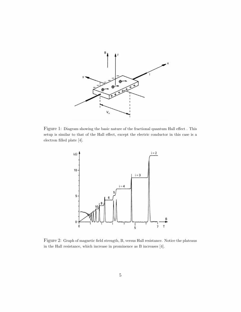
Figure 1: Diagram showing the basic nature of the fractional quantum Hall effect . This

setup is similar to that of the Hall effect, except the electric conductor in this case is a

electron filled plate [4].

Figure 2: Graph of magnetic field strength, B, versus Hall resistance. Notice the plateaus

in the Hall resistance, which increase in prominence as B increases [4].

5

field). Alternatively, the filling fraction essentially denotes the electron den-sity, with values between 0 and 1 representing a partially filled electron field.For the integer quantum Hall effect, this filling fraction is always an integer,therefore, the individual Landau energy levels are always filled completely.In the fractional Quantum Hall effect, the filling fractions can be any pos-itive rational number, and the anyon behavior cannot be solely describedthrough Landau quantization, and we run into multi-particle interactions.For this reason, fractional quantum Hall states are modeled by symmetric oranti-symmetric polynomials of infinite variables, which make up the wave-functions that characterize the electrons’ behavior.

For certain ideal interaction potentials, the Schroedinger equation canbe solved exactly, e.g. the Laughlin state and the Pfaffian state (whereinelectrons only interact in groups, not repelling each other directly). Theseexact solutions come in the form of

Ψ = e−14

∑Ni=1 |zi|2P (z1, z2, ..., zn),

where P is both a symmetric polynomial (because any two electrons can befreely exchanged) as well as translation invariant (because the entire systemcan experience a shift in any direction, without experiencing a change otherthan contributed by the Gaussian term).

The most fundamental family of fractional quantum Hall state polyno-mials is the Laughlin family of wavefunctions, of the form

P =∏i<j

(zi − zj)n. (3.1)

Discovered by Robert Laughlin, in response to experimental observation ofthe Hall conductivity plateau, these polynomials are the most fundamental ofsymmetric (or anti-symmetric if n is odd) translation invariant polynomials.All other known fraction quantum Hall state polynomials are based upon aform of the Laughlin.

The Laughlin states can take any value for ν = 1/n for some odd integern, where the phase–and thus n–can be varied by controlling the strength ofthe magnetic field. As another example the Wigner crystal can have thefilling fraction going to zero, effectively ν = 0. The Laughlin states allow theelectrons to flow much like an incompressible fluid, while the Wigner crystaltries to maintain a (triangular) lattice.

6

A fractional quantum Hall polynomial which has gained attention overrecent years is the Moore-Read Pfaffian, of the form

Ppf = A(1

z1 − z21

z3 − z4· · · 1

zN−1 − zN)∏i<j

(zi − zj). (3.2)

There is general speculation that the Pfaffian ν = 5/2 state entails the non-abelian statistics that has been long sought after in topological quantumcomputing.

4 Pattern of Zeros

In order to better study the properties and behavior of these infinite variablesymmetric polynomials, our mentor along with a few colleagues developed thepattern of zeroes approach. This approach allows for a constructive analysisof polynomials of infinite variables, which would otherwise be a very difficulttask. The pattern of zeroes approach is very useful, studied in [5].

As in [5] we denote Sa as the order of zero of the polynomial when any avariables are fused together, and refer the sequence Sa, a ∈ N as the patternof zeros. For example, if we take the Laughlin (3.1) for ν = 1/2 state, wehave

Example 4.1

S1 = 0

S2 = 2

S3 = 6

Sa = 2

(a

2

)= a(a− 1)

Let la = Sa−Sa−1 (with convention S0 = 0), and the encoder nl =∞∑i=1

δl,li ,

which counts the number of times l appears in the sequence la. Thus, in theabove example we have

Sa : 0, 2, 6, 12, 20, ...

la : 0, 2, 4, 6, 8, ...

nl : 1, 0, 1, 0, 1, ...

7

In [5] a symmetric polynomial is said to satisfy the n-cluster conditionwhen nl is periodic. The number of particles, n, equals the sum of theelements in each period of nl, and the number of orbitals, m, equals thenumber of elements in the period of nl. In the example, we have n = 0+1 = 1and m = 2. We notice that conveniently, n/m gives us the filling fraction, ν.In this case

Sa+nk = Sa + kSn +k(k − 1)nm

2+ kma. (4.1)

Sa+nk is quadratic in k and is completely determined by S2, · · · , Sn (S1 = 0)and n,m.

However, in [5], the polynomials studied are exclusively quadratic , i.e.,their pattern of zeroes grows quadratically.

5 Cubic Wavefuntions

Upon introduction to the infinite variable symmetric polynomials of theFQHE, we analyzed the patterns of zeroes of a few wavefuntions of ourown invention. These wavefunctions were based upon the same basic struc-ture of the Laughlin. We noticed a particular wavefunction, which yields aSa sequence similar to the Pfaffian state, but grows cubically rather thanquadratically. This wavefunction is described by the polynomial

P =∏

i<j<k

((zi − zj)n + (zj − zk)n + (zk − zi)n).

In our research, we study the n = 2 polynomial most extensively. Howev-er, adhering to the previous method of extracting the filling fraction ν fromSa, one finds that the sequence pl is not periodic, and thus does not satisfythe cluster condition. Furthermore, the filling fraction n/m approaches zeroas the number of particles remains constant while the number of orbitalsincreases. Approximating the Kronecker delta function as a second differ-ence of Sa, this property seems logical, and can be extended to all otherpolynomials of cubic growth.

Using the method of pattern of zeroes in [5], we attempt to reach a fillingfraction for this polynomial.

8

Sa : 0, 2, 8, 20, 40, 70, ..., 2

(a

3

)la : 0, 2, 6, 12, 20, 30, ...

nl : 1, 0, 1, 0, 0, 0, 1, 0, 0, 0, 0...

Notice that nl is not periodic, and therefore the polynomial does not satisfythe n-cluster condition. Moreover, as l approaches infinity, n/m→ 0.

We can ensure that the filling fraction does indeed converge to zero byusing the formal definition of ν = N/ deg(zi), where N is the number ofvariables. Thus we have

deg(zi) = 2

((n

3

)−(n− 1

3

))= 2

((n(n− 1)(n− 2)

3!− (n− 1)(n− 2)(n− 3)

3!

)= 3

((n− 1)(n− 2)

3

)= (n− 1)(n− 2)

Therefore, we have

ν = limn→∞

n

(n− 1)(n− 2)= 0

In fact, the filling fraction approaches zero for all cubically growing Sa.This can be seen by inversely relating the average second difference of Sa withthe filling fraction ν. This is because the kronecker delta function essentiallyacts as a modified difference. For example, the second difference da for theLaughlin n = 2 wavefunction is 2, while the filling fraction is 1/2.

Another explanation can be seen through examining the electron behaviorcharacterized by this polynomial on the complex plane. As sets of threeelectrons converge, each factor approaches zero with degree two. Thus if Nelectrons are converging, then the total degree of the zero will be

(n2

), which

grows as N3/6. Using the established pattern-of-zeroes method, the firstdifference of this function grows as N2/2, which has gaps of order N . Thusthe orbitals have filling fraction of order 1/N .

Because the previously defined pattern of zeroes always approaches zero,we analyzed cubic polynomials by further taking a second difference, then

9

applying the Kronecker delta function. Here, as before define Di = Si −

Si−1, di = Di −Di−1, and pd =∞∑k=1

δd,dk . Thus,

Sa =a∑

i=1

Di, (5.1)

Da =a∑

i=1

di. (5.2)

Taking the P =∏

i<j<k

((zi − zj)2 + (zj − zk)2 + (zk − zi)2) polynomial as

an example, we start of with

Sa : 0, 2, 8, 20, 40, ...

Da : 0, 2, 6, 12, 20, ...

da : 0, 2, 4, 6, 8, ...

pd : 1, 0, 1, 0, 1, 0, ...

Note that we had to take a second difference in order to yield a periodicpd. Additionally, the sequence pd for P polynomials matches the sequencenl for the Laughlin polynomials for equal exponent n, although n = 1 is notdefined for P polynomials.

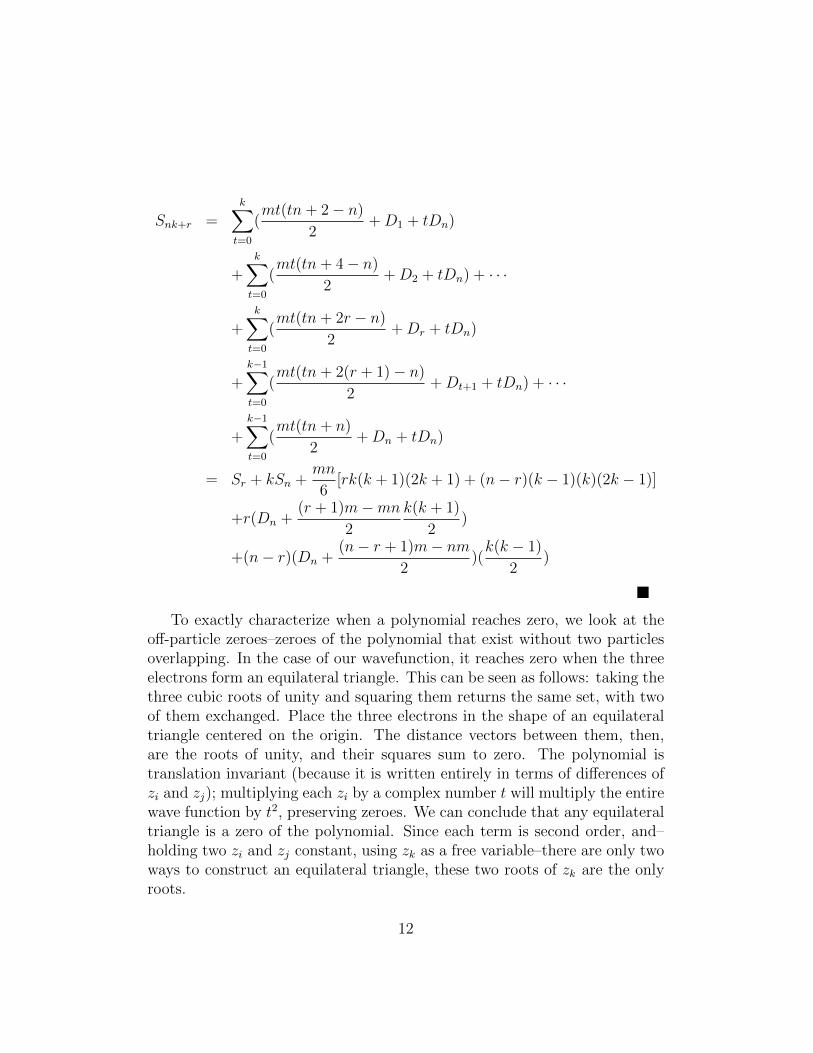
We derive a general recursive formula for the Sa patterns of zeroes for acubic polynomial when pd is periodic.

Proposition 5.1

Snk+r = Sr + kSn +mn

6[rk(k + 1)(2k + 1) + (n− r)(k − 1)(k)(2k − 1)]

+r(Dn +(r + 1)m−mn

2

k(k + 1)

2)

+(n− r)(Dn +(n− r + 1)m− nm

2)(k(k − 1)

2).

Proof: Starting with the definitions of n and m, we have

m = p0 + p1 + p2 + · · ·+ pn−1

10

From here, we can see that dnk+r = mk+dr. Now, we want to find a recursiveformula for Da. We have

Dnk+r = d1 + d2 + d3 + · · · +dnk+r

= d1 + dn+1 + d2n+1 + · · · +dnk+1

+d2 + dn+2 + d2n+2 + · · · +dnk+2...

......

...+dr + dn+r + d2n+r + · · · +dnk+r

+dr+1 + dn+r+1 + d2n+r+1 + · · · +dn(k−1)+r+1...

......

...+dn + d2n + d3n + · · · +dn(k−1)+n

(5.3)

=k∑

t=0

(mt+ d1) +k∑

t=0

(mt+ d2) + · · ·+k∑

t=0

(mt+ dr)

+k−1∑t=0

(mt+ dr+1) + · · ·+k−1∑t=0

(mt+ dn)

=mk(kn+ 2r − n)

2+Dr + kDn. (5.4)

Note that (5.4) is (4.1) applied to Da and pd. Now we have

Snk+r = D1 +D2 +D3 + · · ·+Dnk+r

Arraying the summation as in (5.3) and using (5.4) yields

11

Snk+r =k∑

t=0

(mt(tn+ 2− n)

2+D1 + tDn)

+k∑

t=0

(mt(tn+ 4− n)

2+D2 + tDn) + · · ·

+k∑

t=0

(mt(tn+ 2r − n)

2+Dr + tDn)

+k−1∑t=0

(mt(tn+ 2(r + 1)− n)

2+Dt+1 + tDn) + · · ·

+k−1∑t=0

(mt(tn+ n)

2+Dn + tDn)

= Sr + kSn +mn

6[rk(k + 1)(2k + 1) + (n− r)(k − 1)(k)(2k − 1)]

+r(Dn +(r + 1)m−mn

2

k(k + 1)

2)

+(n− r)(Dn +(n− r + 1)m− nm

2)(k(k − 1)

2)

To exactly characterize when a polynomial reaches zero, we look at theoff-particle zeroes–zeroes of the polynomial that exist without two particlesoverlapping. In the case of our wavefunction, it reaches zero when the threeelectrons form an equilateral triangle. This can be seen as follows: taking thethree cubic roots of unity and squaring them returns the same set, with twoof them exchanged. Place the three electrons in the shape of an equilateraltriangle centered on the origin. The distance vectors between them, then,are the roots of unity, and their squares sum to zero. The polynomial istranslation invariant (because it is written entirely in terms of differences ofzi and zj); multiplying each zi by a complex number t will multiply the entirewave function by t2, preserving zeroes. We can conclude that any equilateraltriangle is a zero of the polynomial. Since each term is second order, and–holding two zi and zj constant, using zk as a free variable–there are only twoways to construct an equilateral triangle, these two roots of zk are the onlyroots.

12

We would like to further show that any polynomial that has zeroes at anequilateral triangle has a filling fraction that approaches zero. Given thatour wavefunction has only these roots, it can be viewed as the fundamentalfactor of any equilateral triangle zeroes, just as each term in the Laughlinpolynomial is the fundamental factor for a zero that occurs when two elec-trons are directly coincident. Any polynomial, then, that also has off-particleequilateral triangle zeros for all numbers of electrons n must be a multipleof P . As a multiple, any zeroes ours has will have to be zeroes of this otherone as well, so the degrees of its zeroes will necessarily grow at least as fastas ours. As such, its filling fraction must go to zero at least as fast as 1/N .

6 Physical Nature of Cubic Wavefunctions

Numerical tests were carried out to discover what conditions maximized thewavefunction for many-electron systems. It was found that the wavefunctionreached a maximum when all electrons were collinear (Fig. 3). The spacingof electrons did influence the amplitude of the wavefunction, but there weremany many degrees of freedom in the movement, allowing the electrons tomove as long as they did so in certain pairs opposite to one another.

Figure 3: Plot of one configuration of 4 electrons that maximizes the wave function.

We can intuitively explain this phenomenon of collinearity as follows.Each pair of electrons is responsible for one pair of off-particle zeroes, one on

13

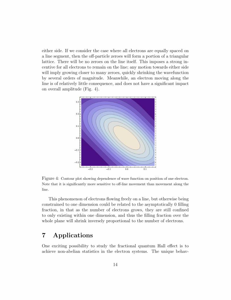
either side. If we consider the case where all electrons are equally spaced ona line segment, then the off-particle zeroes will form a portion of a triangularlattice. There will be no zeroes on the line itself. This imposes a strong in-centive for all electrons to remain on the line; any motion towards either sidewill imply growing closer to many zeroes, quickly shrinking the wavefunctionby several orders of magnitude. Meanwhile, an electron moving along theline is of relatively little consequence, and does not have a significant impacton overall amplitude (Fig. 4).

Figure 4: Contour plot showing dependence of wave function on position of one electron.

Note that it is significantly more sensitive to off-line movement than movement along the

line.

This phenomenon of electrons flowing freely on a line, but otherwise beingconstrained to one dimension could be related to the asymptotically 0 fillingfraction, in that as the number of electrons grows, they are still confinedto only existing within one dimension, and thus the filling fraction over thewhole plane will shrink inversely proportional to the number of electrons.

7 Applications

One exciting possibility to study the fractional quantum Hall effect is toachieve non-abelian statistics in the electron systems. The unique behav-

14

ior of these non-abelian anyons was first only seen as an intriguing naturalphenomenon, much like the integer quantum Hall effect. However, recent-ly, researchers have proposed that these particular anyons could be used toconstruct a topological quantum computer. This computer utilizes the worldlines of the anyons to form braids in 3D spacetime. These braids act asthe logic gates of the computer, each occupying individual quantum states.The reason why this topological configuration is preferred over a trappedquantum particle configuration is because the topological properties of thebraids resist quantum decoherence, which is a major problem with trappedquantum particles. However, further research is essential in the area of non-abelian anyons, as it has not yet been confirmed whether these statistics canbe realized in fractional quantum Hall systems. There is speculation thatthe ν = 5/2 FQH quantum state exhibits non-abelian statistics.

8 Conclusions and Future Work

Our family of new polynomials is only the start of our research. Mathemati-cally, we would like to pursue a theory for symmetric polynomials of infinitevariables for cubic growth rate analogous to the FQH wave functions. Severalof the properties that our polynomials exhibit have not been proved, so weare working on their proofs rigorously. Also we need to find more examplesof cubic growth polynomials and develop a theory for their structures.

As one potential application, our model polynomials Ψ potentially de-scribe gas or liquid states of quantum phases of matter. One future directionof research is to use them to explain the discovered Wigner solid at fillingfraction 1/3 [7]. Consider a linear combination of the Laughlin 1/3 Ψ1/3 withthe cubic polynomial Ψ0, for t=0, it is the FQH liquid, and at t=1, it is somegas/crystal. So possibly for some intermediate value tws, it will be a Wignersolid. There are other known model wave functions for Wigner crystals [1],we can numerically test their overlap with our wave functions.

Our preliminary numerical study revealed a phenomenon of collinearitythat our wave functions achieve maximum values when the electrons alignalong a certain direction in the plane. Further numerical simulation wouldprovide deeper intuition and guidance for how our model wave functions arerelated to quantum phases of matter in electron systems.

15

References

[1] Maki, Kazumi, and Xenophon Zotos. Static and dynamic properties ofa two-dimensional Wigner crystal in a strong magnetic field. PhysicalReview B 28.8 (1983): 4349.

[2] Simon, S., Rezayi, E. H., Cooper, N. Pseudopotentials for Multi-particleInteractions in the Quantum Hall Regime. Physical Review B 75, 195306(2007).

[3] Smits, O. Clustered states in the fractional quantum Hall effect. MasterThesis. Universiteit van Amsterdam. (2007)

[4] Stormer, H., Tsui, D. The Quantized Hall effect. Science Vol. 220 no.4603 pp. 1241-1246 (1983).

[5] Wen, X.G. and Wang, Z. Pattern-of-zeros approach to Fractional quan-tum Hall states and a classification of symmetric polynomial of infinitevariables. (2012).

[6] Wen, X.G. and Wang, Z. A Classification of symmetric polynomials ofinfinite variables - a construction of Abelian and non-Abelian quantumHall states. Physics Review B 77, 235108 (2008).

[7] Zhu, Han, et al. Observation of a Pinning Mode in a Wigner Solid withnu= 1/3 Fractional Quantum Hall Excitations. Physical Review Letters105.12 (2010): 126803.

16