Citation: Huppert, S.; Plé, T.;

Bonella, S.; Depondt, P.; Finocchi, F.

Simulation of Nuclear Quantum

Effects in Condensed Matter Systems

via Quantum Baths. Appl. Sci. 2022,

12, 4756. https://doi.org/10.3390/

app12094756

Academic Editors: Alessandro Sergi

and Gabriel Hanna

Received: 19 March 2022

Accepted: 27 April 2022

Published: 9 May 2022

Publisher’s Note: MDPI stays neutral

with regard to jurisdictional claims in

published maps and institutional affil-

iations.

Copyright: © 2022 by the authors.

Licensee MDPI, Basel, Switzerland.

This article is an open access article

distributed under the terms and

conditions of the Creative Commons

Attribution (CC BY) license (https://

creativecommons.org/licenses/by/

4.0/).

applied sciences

Article

Simulation of Nuclear Quantum Effects in Condensed MatterSystems via Quantum Baths

Simon Huppert 1 , Thomas Plé 1, Sara Bonella 2, Philippe Depondt 1 and Fabio Finocchi 1,*1 Institut des Nanosciences de Paris (INSP), CNRS UMR 7588, Sorbonne Université, 4 Place Jussieu,

75005 Paris, France; simon.huppert@sorbonne-universite.fr (S.H.); thomas.ple@sorbonne-universite.fr (T.P.);philippe.depondt@sorbonne-universite.fr (P.D.)

2 Centre Européen de Calcul Atomique et Moléculaire (CECAM), Ecole Polytechnique Fédérale de Lausanne,1015 Lausanne, Switzerland; sara.bonella@epfl.ch

* Correspondence: fabio.finocchi@sorbonne-universite.fr

Abstract: This paper reviews methods that aim at simulating nuclear quantum effects (NQEs) usinggeneralized thermal baths. Generalized (or quantum) baths simulate statistical quantum features, andin particular zero-point energy effects, through non-Markovian stochastic dynamics. They make useof generalized Langevin Equations (GLEs), in which the quantum Bose–Einstein energy distributionis enforced by tuning the random and friction forces, while the system degrees of freedom remainclassical. Although these baths have been formally justified only for harmonic oscillators, theyperform well for several systems, while keeping the cost of the simulations comparable to the classicalones. We review the formal properties and main characteristics of classical and quantum GLEs, inrelation with the fluctuation–dissipation theorems. Then, we describe the quantum thermostat andquantum thermal bath, the two generalized baths currently most used, providing several examplesof applications for condensed matter systems, including the calculation of vibrational spectra. Themost important drawback of these methods, zero-point energy leakage, is discussed in detail withthe help of model systems, and a recently proposed scheme to monitor and mitigate or eliminateit—the adaptive quantum thermal bath—is summarised. This approach considerably extends thedomain of application of generalized baths, leading, for instance, to the successful simulation ofliquid water, where a subtle interplay of NQEs is at play. The paper concludes by overviewing furtherdevelopment opportunities and open challenges of generalized baths.

Keywords: generalized Langevin equation; nuclear quantum effects; quasi-classical simulations;fluctuation–dissipation theorem

1. Introduction

This paper reviews methods that use generalized thermal baths, that we shall indicategenerically as quantum baths. Other expressions, such as generalized or quasiclassicalbaths, are used in the literature to designate a family of methods revolving around variousflavors of dynamics aiming at mimicking quantum properties via generalized Langevinequations. We adopt here the generic expression quantum bath, which is clear enough tospecify the field without entering into the technical details separating these schemes toapproximate nuclear quantum effects (NQEs) and, in particular, atomic zero-point energy(ZPE).

It is well-recognised that NQEs cannot be neglected for systems at low temperaturesor at high pressure, where they can have, for example, a strong influence on phase tran-sitions [1–3]. Nuclear quantum effects, however, also often come into play at ambientconditions, typically when the thermal energy of chemical bonds in molecules is compa-rable or smaller than the associated vibrational ZPE or when characteristic interatomicdistances in the system are comparable to the de Broglie wavelength of the nuclei. Theseconditions are met, in particular, in systems containing light atoms and most notably hydro-gen [4,5], which is a ubiquitous constituent of inorganic compounds and a basic element

Appl. Sci. 2022, 12, 4756. https://doi.org/10.3390/app12094756 https://www.mdpi.com/journal/applsci

Appl. Sci. 2022, 12, 4756 2 of 39

in biological systems. Thus, nuclear quantum effects influence, for example, the stabilityof crystal polymorphs of pharmaceutical interest, the spectroscopy of ice and water, orenzymatic reactions in living organisms [6–9]. NQEs are also required to reveal the effectof isotopic substitutions on equilibrium properties, as a classical description of the nucleipredicts identical statistical properties for all isotopes. The exact simulation of these effectsis, however, a challenging problem due to the large (sometimes unachievable) compu-tational cost of available methods. Time-independent statistical properties of quantumnuclei at thermal equilibrium can be obtained using the so-called classical isomorphism ofpath integrals (see Section 6), in which a quantum particle is represented as a collection ofbeads interacting via an effective classical-like potential. While this approach guaranteestheoretical convergence to the exact quantum result in the limit of an infinite numberof beads, it necessitates in practice to simulate a number of degrees of freedom that canbecome prohibitive, in particular when first-principles methods are used for the interatomicinteractions. The situation is even more problematic for time-dependent properties forwhich exact simulation methods scale exponentially with the number of degrees of freedom.Different approaches have been proposed, such as in [10,11], each with their own strengthsand weaknesses; but, in spite of several interesting results, no clear, practical and generalreference method has emerged.

In the following, we focus on the family of approximate methods for simulatingquantum nuclear effects that rely on the use of quantum baths. Although these methodscan substantially differ from one another in their practical implementation, they all aim atintroducing quantum statistical properties into classical trajectory-based dynamics. This isachieved via a stochastic evolution that takes the form of a generalized Langevin Equation(GLE), in which the quantum Bose–Einstein energy distribution is enforced instead ofequipartition, by means of an appropriate tuning of the random and friction forces. Themain advantage of these approaches is that the number of degrees of freedom in the systemand the deterministic part of the propagation remain classical, thus enabling them to mimicquantum properties at a numerical cost directly comparable to that of standard Langevindynamics. Contrary to standard Langevin, however, quantum baths exhibit a complexnon-Markovian dynamics whose formal properties are not obvious. In particular, whilethese methods deliver remarkable performances in a growing number of applications, theycannot be formally justified except for harmonic systems. This intriguing scenario motivatesour approach for this review. In Section 2, we start by stating some fundamental resultsin the statistical mechanics of classical and quantum systems, the fluctuation–dissipationtheorems (FDT). We then introduce the standard and generalized Langevin equations andset the stage for the following developments. This is done, in particular, by recalling how theGLE can be derived starting from the physical picture of a generic system (not necessarilyharmonic) bilinearly coupled to an environment modelled as a set of harmonic oscillators.We shall consider both classical and quantum versions of this system-bath model anddescribe how the quantum version can be used, via an appropriate quasiclassical limit,to motivate the quantum bath algorithms on which we focus in this review. While moregeneral models for the bath are possible (including, in particular, anharmonicity) these arenot particularly relevant for this work and will therefore not be discussed, nor includedin examples. Section 3 focuses on using the quantum FDT to build GLEs that combineclassical deterministic evolution with quantum stochastic behaviour to mimic NQEs. Inparticular, we introduce two approaches, the Quantum Thermal Bath [12] (QTB) andthe Quantum Thermostat [13,14] (QT) that have recently attracted considerable interest.Section 4 aims at understanding more in depth the capabilities of the quantum thermalbath via the detailed analysis of simple low-dimensional systems that enable a comparisonwith exact quantum results. In particular, the most important pathology of this type ofmethods, namely the ZPE leakage, is illustrated on an elementary example. Althoughthis section focuses on the QTB, which is formally simpler and has fewer parameters thanthe QT, the general observations apply to both frameworks. In Section 5, we reviewthe capabilities of quantum bath methods by summarizing some significant applications

Appl. Sci. 2022, 12, 4756 3 of 39

to realistic models of condensed matter systems. Remarkably, these techniques proveuseful not only in the simulation of static equilibrium properties of quantum nuclei, butalso in the calculation of vibrational spectra [15], including subtle anharmonic featuresthat elude other trajectory-based approximations to quantum dynamics [16]. In Section 6,we complete the overview of important applications of thermal baths by showing howthey can be used to improve the convergence of calculations based on the path integralformalism. We then introduce in Section 7 a recent development that, by exploiting thequantum fluctuation–dissipation theorem, enables to monitor and efficiently compensateZPE leakage. This approach, known as the adaptive quantum thermal bath [17] (adQTB)extends considerably the domain of application of the QTB, leading, for example, to thesuccessful simulation of liquid water [18]. The review ends with a discussion of remaininglimitations, open questions and possible future developments of quantum baths as effectiveand accurate tools for the simulation of condensed phase systems.

We conclude this Introduction by noting that GLEs have a long and rich history, withapplications in a very broad range of domains that we do not account for here. The literatureon quantum baths is also rapidly increasing. While we have tried to provide appropriatereferences throughout the text, we have chosen to present the material focusing on resultsand derivations that seemed more directly related to the methods at the core of this work,intended as a relatively self-contained introduction to a still-developing set of exciting newalgorithms for growing classes of quantum problems in physics and chemistry.

2. The Langevin Equation as a Thermal Bath

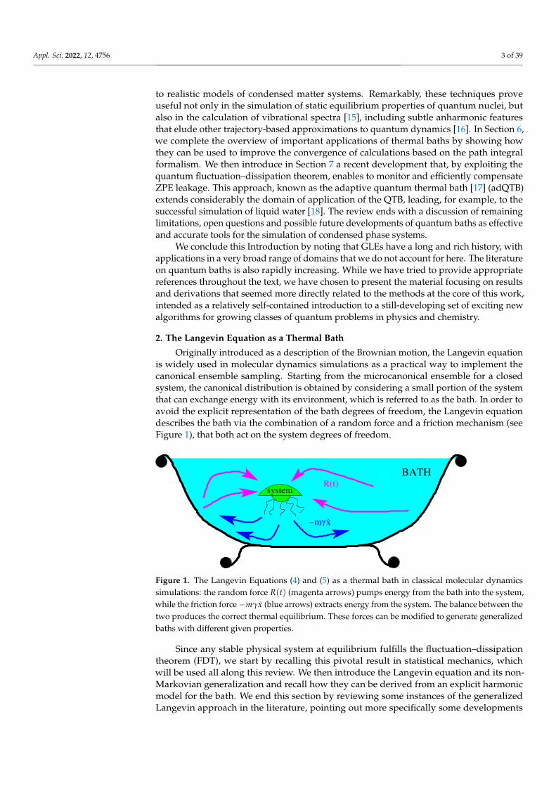
Originally introduced as a description of the Brownian motion, the Langevin equationis widely used in molecular dynamics simulations as a practical way to implement thecanonical ensemble sampling. Starting from the microcanonical ensemble for a closedsystem, the canonical distribution is obtained by considering a small portion of the systemthat can exchange energy with its environment, which is referred to as the bath. In order toavoid the explicit representation of the bath degrees of freedom, the Langevin equationdescribes the bath via the combination of a random force and a friction mechanism (seeFigure 1), that both act on the system degrees of freedom.

−m xγ.

systemR(t)

BATH

Figure 1. The Langevin Equations (4) and (5) as a thermal bath in classical molecular dynamicssimulations: the random force R(t) (magenta arrows) pumps energy from the bath into the system,while the friction force−mγx (blue arrows) extracts energy from the system. The balance between thetwo produces the correct thermal equilibrium. These forces can be modified to generate generalizedbaths with different given properties.

Since any stable physical system at equilibrium fulfills the fluctuation–dissipationtheorem (FDT), we start by recalling this pivotal result in statistical mechanics, whichwill be used all along this review. We then introduce the Langevin equation and its non-Markovian generalization and recall how they can be derived from an explicit harmonicmodel for the bath. We end this section by reviewing some instances of the generalizedLangevin approach in the literature, pointing out more specifically some developments

Appl. Sci. 2022, 12, 4756 4 of 39

that are relevant in the perspective of the implementation of quantum bath methods toapproximate NQEs, as presented in Section 3.

2.1. Linear Response and Fluctuation–Dissipation Theorems

Linear response theory provides useful relations characterizing dynamical propertiesunder external perturbations via averages over the equilibrium probability of the system,e.g., thermal probability density. We first introduce the complex admittance or susceptibilityχ(ω) that characterizes the linear response of a system subject to a perturbative forceF(t) = Re[F0 eiωt] along a given direction x. At first order in the perturbation, the changein the velocity along x induced by the perturbation (here and in the remainder of thesection, we use one-dimensional notations; the generalization to higher dimension isstraightforward) reads:

∆v(t) = Re[F0 χ(ω) eiωt]

This relation can be considered as a definition for χ(ω). For a classical system atthermal equilibrium at temperature T, it can be shown that the following fluctuation–dissipation theorem (FDT) holds [19,20]:

Cvv(ω) = 2kBT Re[χ(ω)] (1)

The FDT as derived by Kubo in [19] is actually more general than Equation (1) andcan be used to relate the cross-correlation spectrum CAB(ω) of two arbitrary observables Aand B to the corresponding linear response function. In our case, Equation (1) relates thereal part of the susceptibility (that is dissipative) to the equilibrium velocity autocorrelationspectrum (that characterizes fluctuations):

Cvv(ω) =∫ ∞

−∞dt 〈v(0)v(t)〉 e−iωt (2)

The FDT characterizes the frequency distribution of energy at equilibrium, in itsclassical Formulation (1), it expresses the equipartition of energy in the system. However, aslightly different FDT can be derived for quantum systems [19,21]:

Csvv(ω) = 2θ(ω, T) Re[χ(ω)] with θ(ω, T) =

hω

2coth

(hω

2kBT

)(3)

Here the classical thermal energy kBT has been replaced by the quantum Bose–Einsteindistribution θ(ω, T), and the autocorrelation spectrum that is used is now the Fouriertransform of the symmetrized correlation function:

Csvv(ω) =

∫ ∞

−∞dt Tr

[12

ρeq

v(0)v(t) + v(t)v(0)]

e−iωt

with ρeq the equilibrium density operator. v(t) now designates the time-dependent velocityoperator in the Heisenberg picture. The definition of the linear susceptibility is alsomodified in the quantum case and is related to the change induced by the perturbativeforce on the density operator ρ. The fluctuation–dissipation theorem plays a key role inthe generalized Langevin equations used to sample the classical canonical ensemble, as wewill develop in the following sections. More recently, the quantum version of this theoremhas also been employed to design the trajectory-based approximations for the simulationof NQEs at the core of this review.

2.2. The Langevin Equation in Classical Molecular Dynamics Simulations

In its basic form, the Langevin equation of motion writes:

mx = −dVdx−mγx + R(t) (4)

Appl. Sci. 2022, 12, 4756 5 of 39

where R(t) is a random force with zero mean (usually taken from a Gaussian distribution)and characterized by a white noise correlation function:

〈R(t)R(t + τ)〉 = 2γmkBTδ(τ) (5)

The random and friction forces model the effect of a thermal bath (see Figure 1)and ensure the canonical statistics, including the energy equipartition theorem and thefluctuation–dissipation theorem as stated in Section 2.1. The constant γ is the strength ofthe coupling of the thermal bath with the simulated system. Its inverse 1/γ provides anindication of the relaxation time of the system, that is, the time it takes for the random forceand the dissipation to equilibrate.

Used as a thermostat in molecular dynamics simulations, the Langevin Equation (4)provides, for any γ, an exact sampling of the canonical Boltzmann distribution. Moreprecisely, it can be proved that the probability distribution converges exponentially to theinvariant one starting from a wide range of different initial conditions [22], thus avoidingtemperature oscillations or other spurious effects that other thermostats, such as Nosé-Hoover, can generate. Dynamical properties, on the other hand, are affected by the couplingwith the bath and depend on the value of γ. In particular, the damping term generallybroadens the peaks corresponding to modes in the vibrational spectra over a typicalwidth γ.

2.3. Generalized Langevin Equation (GLE)

The standard (Markovian) Langevin Equation (4) can be generalized in the followingmanner:

mx = −dVdx−∫ t

−∞ds K(t− s) x(s) + R(t) (6)

This equation is non-Markovian since the friction force does not only depend on thevelocity x at time t, but is rather expressed as an integral over past values of x throughthe memory kernel K(τ), which determines the actual dependence. In order to enforce thecanonical ensemble statistics and the equipartition of energy, the random force should thenbe related to K(τ) by the following relation:

〈R(t)R(t + τ)〉 = kBT K(τ) (7)

which reduces to (5) in the Markovian limit K(τ) = 2mγδ(τ). As the bath is supposedto be at equilibrium, the time correlation function 〈R(t)R(t + τ)〉 does not depend on thearbitrary time origin t. Defining the Fourier transformed quantities (here, we modify thememory kernel, which is in principle defined for non-negative times, by symmetrization asK(−τ) = K(τ)):

K(ω) =∫ ∞

−∞dτ K(τ) e−iωτ

CRR(ω) =∫ ∞

−∞dτ 〈R(t)R(t + τ)〉 e−iωτ ,

yields the following relation:CRR(ω) = kBT K(ω). (8)

Equation (8)—or its time-domain version, (7)—follows from the equilibrium betweenthe system and the thermal bath, and it is generally referred to as a fluctuation–dissipationtheorem (FDT), similarly to Equation (1). The latter, however, is a general result of linearresponse theory that involves only intrinsic observables of the system (its velocity auto-correlation and its linear response function) whereas Equations (7) and (8), characterizethe system–bath interactions via the friction and random forces in the particular context ofthe generalized Langevin dynamics. As pointed out by Kubo, Toda and Hatsishume [20],

Appl. Sci. 2022, 12, 4756 6 of 39

Equation (1) can be regarded as more fundamental, and following these authors, we willrefer to it as the first-kind FDT, while Equations (7) and (8) (that can be derived from it as acorollary when the potential V(x) is harmonic) will be designated as second-kind FDT.

2.4. Coupling to a Harmonic Bath

The generalized Langevin equation (6) appears in a variety of contexts. In particular,a slightly different form of GLE can be derived under very general assumptions usingprojection operator techniques [20,23], an approach that has recently lead to interestingdevelopments [24,25]. However, the damping and random forces obtained in this formalismare generally not explicit. In this section, we focus on an alternative, more practical andexplicit approach: we derive the GLE from the description of a system bilinearly coupled toa bath of independent harmonic oscillators. In passing, we note that, in principle, the bathcan be constructed in different ways, for instance by including non-harmonic oscillators.However, the bath of harmonic oscillators is at the same time easy-to-treat analyticallyand can describe all features that are relevant for the physical system. The extendedHamiltonian for the bath and the physical system, which can be harmonic or not, (the lattercase being the most physically relevant one) is then:

H =p2

2m+ V(x) + ∑

j

[p2

j

2mj+

12

mjω2j (qj − x)2

](9)

where x and p are the system coordinate and momentum, while qj, pj are an ensemble ofharmonic oscillators that constitute the thermal bath. The coupling to the system arisesfrom the fact that the equilibrium position of the bath oscillators is taken at qj − x andtherefore changes in time with the variations of x. It is then easily shown that the equationof motion for the system coordinate can be recast into a GLE of the form of (6), where thememory kernel K(τ) is defined as:

K(τ) = ∑j mjω2j cos(ωjτ),

or equivalently, K(ω) = π ∑j mjω2j[δ(ω−ωj) + δ(ω + ωj)

] (10)

The damping force is therefore generally non-Markovian with a kernel that dependson the spectral density of the bath oscillators. In particular, in the limit of an infinitenumber of bath oscillators with a spectral density proportional to 1/ω2, K(ω) becomesconstant and the Markovian limit is recovered. The random force R(t) is related to theinitial configuration of the bath at an initial time t0:

R(t) = −K(t− t0)x(t0) + ∑j

[mjω

2j qj(t0) cos[ωj(t− t0)] + ωj pj(t0) sin[ωj(t− t0)]

](11)

If t0 is in a distant past, the first term vanishes. Moreover, if the bath oscillators areassumed to be initially (i.e., at t0) in thermal equilibrium, the random force autocorrelationfunction can be shown to obey the second-kind FDT of Equations (7) and (8).

Interestingly, if the system–bath Hamiltonian (9) is treated quantum-mechanically, aGLE formally identical to Equation (6) can be derived for the time-dependent operator x inthe Heisenberg picture. The expression of the memory kernel K(τ) and the random forceR(t) are the same as in the classical case (only R(t) is now an operator), but the second-kindFDT becomes (compare to (8)):

CsRR(ω) =

∫ ∞

−∞dt

12⟨

R(t)R(t + τ) + R(t + τ)R(t)⟩

e−iωτ = θ(ω, T)K(ω) (12)

where, similarly to what was reported for the first-kind FDT (3), the symmetrised correlationfunction is used and the classical average thermal energy kBT is replaced by its quantumcounterpart θ(ω, T).

Appl. Sci. 2022, 12, 4756 7 of 39

In the developments above, we followed mostly the work and formalism of Ford andcoworkers in [26,27]. In their studies, the authors point out that the quite simple harmonicbath model is more general than it appears. First, they show that, for the GLE (6) to bephysically meaningful, the memory kernel K(ω) should be positive for all frequencies.(Ford and coauthors actually consider more generally the Laplace transform:

µ(z) =∫ ∞

0dt e−izτK(τ),

that is related to the Fourier transform of the (symmetrized) memory kernel byK(ω) = 2Re[µ(ω + i0+)]. They show that µ(z) is analytical in the upper half-plane (zis a complex variable), and belongs to the class of the so-called positive real functionsthat possess several specific mathematical properties that the authors then use in theirargumentation on the generality of the harmonic bath model [27]). Now, according toEquation (10), with an appropriate choice of the frequencies ωj (potentially in infinitenumber), the harmonic bath can be tailored to produce any arbitrary positive memorykernel K(ω). Therefore, it can be regarded as a very generic prototype for the GLE (6) andthe authors proceed by pointing out the relation between the harmonic bath of Equation (9)and some of the pre-existing models. Interestingly, in a former work [28], Cortes et al.had shown that the simple and general second-kind FDT in (12) might not be valid whenconsidering forms of the system-bath coupling more complex than the bilinear interaction.In that case, and for a quantum mechanical treatment (in the classical case the FDT remainsof a simple form), the relation between the dissipation and the fluctuations depends on thedetails of the actual system–bath coupling. In particular, Cortes et al. derive an expressionfor the FDT in the case of a quadratic interaction.

2.5. Quasiclassical Limit of Harmonic Bath

The Hamiltonian (9) or closely related harmonic bath models are common startingpoints to derive GLE also when looking at quasiclassical approximations for quantum dy-namical properties. In general, these developments start from a fully quantum dynamicaldescription of a generic system coupled to the harmonic bath and then approximate thedynamics in some flavor of the classical limit. The specific form of the results dependsboth on the procedure enforced to impose the classical limit (e.g., high temperature, for-mal limit for h → 0, stationary phase approximation of the propagator. . . ), and on theadopted representation of quantum mechanics. For example, starting from the Wignerrepresentation of quantum averages, nuclear quantum effects can be approximated usinggeneralized Langevin equations where the friction and random forces are kept Markovianbut become position-dependent [29,30]. Furthermore, one can take the classical limit for alldegrees of freedom (semiclassical methods) or exploit knowledge of the exact solution ofthe harmonic part of the problem to derive a mixed quantum–classical scheme in whichthe bath is described quantum mechanically, while the dynamics of the system, includingthe coupling to the harmonic bath, is treated classically (quasiclassical or mixed quantum–classical limit). Mixed quantum–classical limits, however, are delicate. For instance, Baderand Berne [31] considered the—apparently simple—case of a harmonic system linearlycoupled to a harmonic bath to investigate the problem of vibrational energy relaxation.They recovered the well-known result that, for this kind of system, quantum and classicaldynamics lead to the same time-evolution for averages and showed that the quantumrelaxation time can be evaluated from a purely classical calculation. However, they alsoproved that—when a mixed quantum–classical dynamics is imposed on the system—theresult for the relaxation time is incorrect and different depending on whether the bath istreated quantum mechanically and the system classically or vice-versa.

A careful analysis of the mixed quantum–classical limit that nicely sets the stage forthe methods presented in the next chapter was performed by Schmid [32]. Schmid focusedon the time evolution of the density matrix of a generic quantum system linearly coupled toa bath of quantum harmonic oscillators (as in (9)) as written in the path integral formulation

Appl. Sci. 2022, 12, 4756 8 of 39

of quantum mechanics (see also Section 6). In the coordinate representation, the densitymatrix determines the probability to find the system at a given position at time t = 0 and atanother assigned position at time t. Within the path integral formalism, the density matrixcan be computed as a functional integral over the set of all possible paths connecting theinitial and final positions of the system and bath in the assigned time t. The harmonicnature of the bath enables an explicit expression for the marginal density matrix of thesystem to be obtained by integrating over the paths of the bath. This still leaves an integralover the system’s paths to perform. When the coupling with the bath is sufficiently strong,quantum coherence effects are strongly suppressed. The integral can then be approximatedto argue that the relevant paths for the system become stochastic trajectories of the form:

mx = −dVdx−mγx + R(t) (13)

where R(t) is a Gaussian stochastic process such that, in Fourier space,

CRR(ω) = 2mγθ(ω, T) (14)

The result above is obtained by introducing a non-trivial (and somewhat heuristic)probabilistic interpretation of the path integral representation of the density matrix andenforcing a quasiclassical approximation based on a truncation of an expansion of thepotential that is not always easy to justify. Although Equations (13) and (14) seem formallyidentical to the quantum generalized Langevin Equations (6) and (12) in the particularcase of a Markovian friction kernel K(τ) = 2mγδ(τ), a fundamental difference has beenintroduced with the quasiclassical approximation: whereas in Equation (6), x referred to thequantum position operator (time-dependent in the Heisenberg picture), in Equation (13), xis now the position of a classical-like system, following a stochastic trajectory. This resultthus combines a fully classical evolution of the system (given by the deterministic force−dV/dx) with a colored thermostat that injects quantum properties, and in particular zeropoint energy, in the dynamics. This early approach bears remarkable similarities with thetwo more recent methods detailed in the next section.

3. Enforcing Quantum Statistics via Generalized Bath

In this section, we focus on two approaches, the Quantum Thermal Bath (QTB) andthe Quantum Thermostat (QT) that were developed independently in 2009 by two differentgroups. Though these methods differ in their practical implementation, they both prescribea form of GLE that combines a classical evolution for the system and the coupling to aquantum bath designed to induce relevant quantum properties (e.g., zero-point energy) inthe otherwise classical evolution of the system.

3.1. The Quantum Thermal Bath

The quantum thermal bath was proposed by Dammak and coworkers [12] to ap-proximate NQEs in general molecular dynamics simulations via a generalized Langevinequation. They use a Markovian friction kernel and a colored random force R(t) with anautocorrelation spectrum which is tailored according to the energy distribution θ(ω, T) ofthe quantum harmonic oscillator. The equations of the resulting dynamics are identical tothose derived from the quasiclassical approximation by Schmid [32]. For one-dimensionalsystems, Equations (13) and (14) hold; their generalization to multiple atomic degrees offreedom is straightforward. However, contrary to Schmid, who aimed at modelling thedynamics of a system coupled to an actual physical bath, in the QTB, the Langevin equationis simply used as a thermostat in order to enforce the quantum statistical distribution ofenergy (including zero-point energy effects). The expression of the random force autocorre-lation, Equation (14), is universal, i.e., system-independent, so that the method does notrequire a priori knowledge of the system or of its detailed spectral density. Heuristically,this form of GLE tends to thermalize the vibration modes of the system with the average

Appl. Sci. 2022, 12, 4756 9 of 39

energy distribution of quantum harmonic oscillators in equilibrium at temperature T, hencethe lexical origin of the quantum thermal bath.

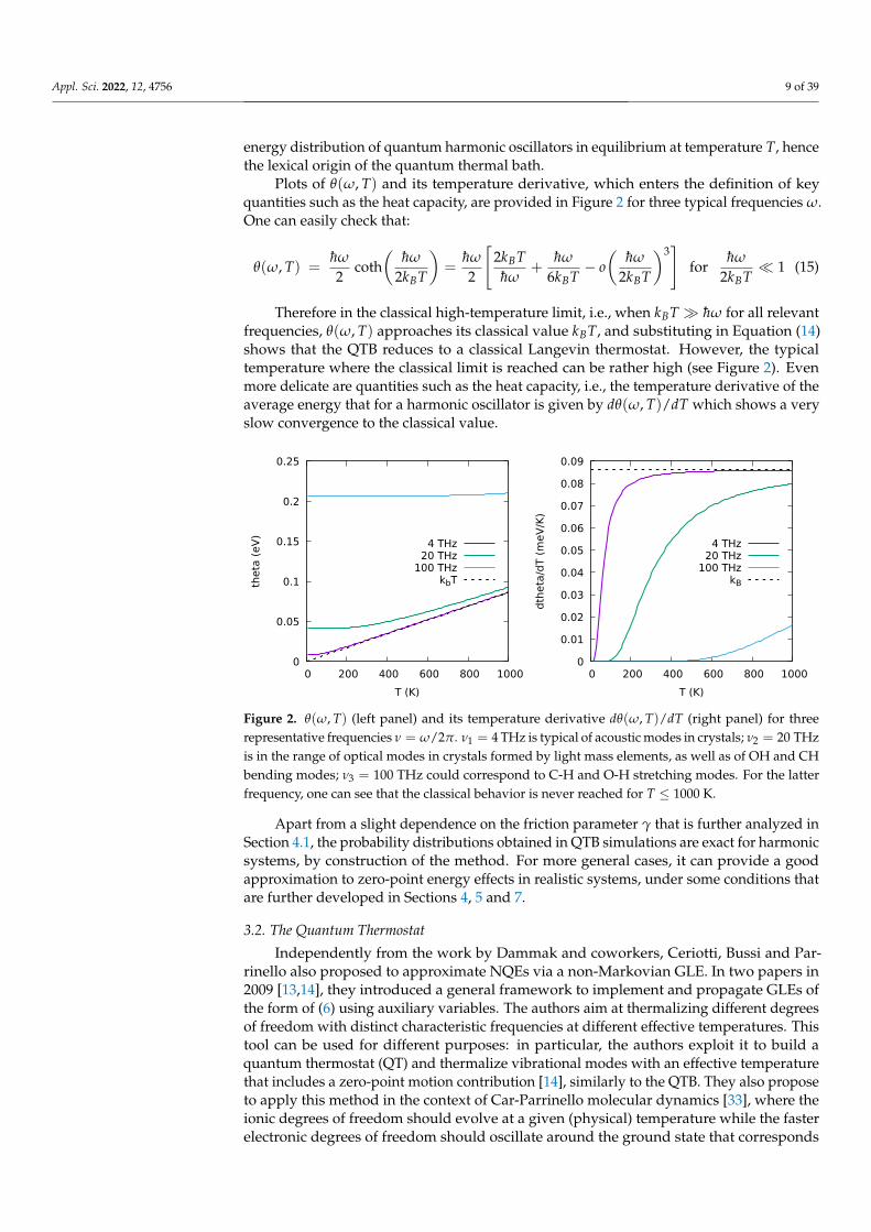
Plots of θ(ω, T) and its temperature derivative, which enters the definition of keyquantities such as the heat capacity, are provided in Figure 2 for three typical frequencies ω.One can easily check that:

θ(ω, T) =hω

2coth

(hω

2kBT

)=

hω

2

[2kBThω

+hω

6kBT− o(

hω

2kBT

)3]

forhω

2kBT 1 (15)

Therefore in the classical high-temperature limit, i.e., when kBT hω for all relevantfrequencies, θ(ω, T) approaches its classical value kBT, and substituting in Equation (14)shows that the QTB reduces to a classical Langevin thermostat. However, the typicaltemperature where the classical limit is reached can be rather high (see Figure 2). Evenmore delicate are quantities such as the heat capacity, i.e., the temperature derivative of theaverage energy that for a harmonic oscillator is given by dθ(ω, T)/dT which shows a veryslow convergence to the classical value.

0

0.05

0.1

0.15

0.2

0.25

0 200 400 600 800 1000

theta

(eV

)

T (K)

4 THz20 THz

100 THzkbT

0

0.01

0.02

0.03

0.04

0.05

0.06

0.07

0.08

0.09

0 200 400 600 800 1000

dth

eta

/dT (

meV

/K)

T (K)

4 THz20 THz

100 THzkB

Figure 2. θ(ω, T) (left panel) and its temperature derivative dθ(ω, T)/dT (right panel) for threerepresentative frequencies ν = ω/2π. ν1 = 4 THz is typical of acoustic modes in crystals; ν2 = 20 THzis in the range of optical modes in crystals formed by light mass elements, as well as of OH and CHbending modes; ν3 = 100 THz could correspond to C-H and O-H stretching modes. For the latterfrequency, one can see that the classical behavior is never reached for T ≤ 1000 K.

Apart from a slight dependence on the friction parameter γ that is further analyzed inSection 4.1, the probability distributions obtained in QTB simulations are exact for harmonicsystems, by construction of the method. For more general cases, it can provide a goodapproximation to zero-point energy effects in realistic systems, under some conditions thatare further developed in Sections 4, 5 and 7.

3.2. The Quantum Thermostat

Independently from the work by Dammak and coworkers, Ceriotti, Bussi and Par-rinello also proposed to approximate NQEs via a non-Markovian GLE. In two papers in2009 [13,14], they introduced a general framework to implement and propagate GLEs ofthe form of (6) using auxiliary variables. The authors aim at thermalizing different degreesof freedom with distinct characteristic frequencies at different effective temperatures. Thistool can be used for different purposes: in particular, the authors exploit it to build aquantum thermostat (QT) and thermalize vibrational modes with an effective temperaturethat includes a zero-point motion contribution [14], similarly to the QTB. They also proposeto apply this method in the context of Car-Parrinello molecular dynamics [33], where theionic degrees of freedom should evolve at a given (physical) temperature while the fasterelectronic degrees of freedom should oscillate around the ground state that corresponds

Appl. Sci. 2022, 12, 4756 10 of 39

to the instantaneous ionic configuration, at much smaller temperatures [13]. The authorssuccessfully applied the colored bath thermostat on a model polarizable system and verifiedthat the fast degrees of freedom (i.e., the motion of the centers of mass of the shells withrespect to their nuclei) are correctly thermalized. More generally, they showed that the col-ored bath thermostat can be adapted to specific cases once the density of vibrational statesis known and that it allows a faster thermalization than the Nosé–Hoover chains [13,22].

Starting from the Orstein–Uhlenbeck theory of stochastic processes, Ceriotti andcoworkers show how a non-Markovian GLE can be implemented via a Markovian Langevindynamics for an extended set of variables of which two are the physical position andmomentum (for a one-dimensional physical system) and N are additional auxiliary mo-menta [34]. In this way, the colored thermostat GLE can be efficiently applied by integratingthe Markovian dynamics in the (N + 2)-dimensional space via usual molecular dynamicstechniques. This dynamics is governed by the following equations:x

ps

= −

0 −1/m 0V′(x) app aT

p0 ap A

xps

+

0 0 00 bpp bT

p0 bp B

0rpr

(16)

where s and s are the N-component vectors of the auxiliary momenta and their timederivatives, A and B are (N × N) matrices of adjustable parameters that characterizerespectively the friction and the random force memory kernels, together with the N-component parameter vectors ap, ap and bp, bp. V′(x) is the spatial derivative of thepotential energy and the (N + 1)-component vector (rp, r) contains normalized white noisevariables: 〈ri(t)rj(t′)〉 = δijδ(t − t′). The dynamics in the extended (x, p, s)-space istherefore Markovian and it can be solved analytically for a harmonic potentialV(x) = mω2x2/2. In more general non-linear cases, a numerical algorithm based onthe symmetric Trotter decomposition of the Liouvillian can be used, where the linear driftand the random force terms in ( p, s) are integrated exactly according to the theory ofOrnstein–Uhlenbeck processes, whereas the evolution of x and the non-linear part of p areintegrated via a velocity Verlet scheme [34].

As described in detail in appendix in [34], by integrating away the auxiliary momentas, Equation (16) reduces to a GLE in the form of (6) for the physical degree of freedom x,with a memory kernel:

K(τ) = 2appδ(τ)− apTe−|τ|Aap

In Appendix B, we illustrate the method by examining two simple cases for N = 1 andN = 2, which correspond to an exponentially decaying memory kernel and to a dampedoscillatory kernel, respectively, and we explicitly write the associated A and B matrices.Generally, the kernels that can build via the extended variable formalism include (althoughnot exclusively) functions of the form K(τ) = Re

[cke−αk |τ|+iωkt

]with arbitrary parameters

ck, αk and ωk. Appendix A of ref. [34] provides a detailed mathematical formalism.The classical FDT (8) is enforced when

BpBTp = mkBT(Ap + AT

p ), (17)

where Bp is the (N + 1)× (N + 1) matrix that comprises bpp, bp, bp and B (and similarlyfor Ap). However, the noise matrix Bp can also be chosen not to fulfill the classical FDT, sothat the GLE can be arbitrarily tuned in order to thermalize the different frequencies of thesystem with well-chosen effective temperatures.

While in [13], the focus was on the thermalization of classical degrees of freedom atdifferent temperatures, in the following paper [14] the same authors applied the coloredbaths strategy in order to include quantum corrections to the classical dynamics of ionsin systems that are weakly anharmonic, such as diamond and ordinary ice Ih. In order todesign this quantum thermostat (QT), they considered the particular case of the harmonicoscillator V(x) = 1

2 mω2x2 for which the stochastic equations of motion (16) can be solved

Appl. Sci. 2022, 12, 4756 11 of 39

analytically and the exact kinetic and potential energies of the physical system explicitlycomputed. The parameters of the GLE are then tuned in order for the average position andmomentum distributions to be as close as possible to that of a quantum harmonic oscillatorthat is Gaussian, as in the classical case, but with a width that is a function of the oscillationperiod ω:

1m〈p2〉 = mω2 〈x2〉 = hω

2coth

(hω

2kBT

)= θ(ω, T) (18)

By properly adjusting K(τ) and the noise correlation function, one can tune the averagefluctuations in position and in momentum so as to reproduce the quantum–mechanicalbehavior in Equation (18) over a wide range of vibrational frequencies. In practice, thisis done via a fitting procedure of the Ap and Bp matrices that have been introduced inEquation (16). This method is general and versatile and offers a wide choice for the frictionand random force kernels; nonetheless, it requires a fine tuning of the characteristic matrices,which might depend on the system under consideration. The QT method has been madeavailable in the open-source i-PI suite [35], which has enabled its wider use [36–38].

4. Critical Analysis of Quantum Baths: Model Systems

In Sections 3.1 and 3.2, the generalized baths (QTB and QT) are introduced as toolsto impose the quantum statistics to a system that generally follows classical laws of mo-tion. However, the question of the trustworthiness of quantum baths methods should beaddressed. In this section, we provide a systematic analysis of the performances of the QTBon 1D and 2D model systems for which exact solutions are available analytically or canbe obtained for comparison from a direct numerical resolution of Schrödinger’s equation(another example with a 1D double well is given in Appendix C). Although we focus hereon the QTB formalism, similar results could be obtained with the quantum thermostatof [14].

4.1. Harmonic Systems

A pedagogical introduction to the QTB has been given by Barrat and Rodney, withseveral useful remarks, in particular, concerning the application of the QTB to a harmonicsystem, V(x) = 1

2 mω20x2 [39]. In that case, as the force is linear with position, an explicit

expression can be obtained for the Fourier transform of the position and the velocity andhence for their respective correlation spectra:

Cxx(ω) =2γ θ(ω, T)/m

(ω2 −ω20)

2 + ω2γ2and Cvv(ω) =

2γ ω2θ(ω, T)/m(ω2 −ω2

0)2 + ω2γ2

(19)

These spectra correspond to Lorentzian peaks centered at ω0, and with a width γ.They are good approximations to the quantum symmetrized correlation spectra Cs

xx(ω)and Cs

vv(ω) apart from a spectral broadening with respect to the Dirac δ—function expectedfor the 1D quantum system, which is only recovered in the γ → 0 limit. The integrals ofthese two spectra provide, respectively, the average potential and kinetic energies as:

〈Epot〉 =∫ dω

2π

γ ω20

(ω2 −ω20)

2 + ω2γ2θ(ω, T) (20)

〈Ekin〉 =∫ dω

2π

γ ω2

(ω2 −ω20)

2 + ω2γ2θ(ω, T) (21)

As the zero-point energy term in θ(ω, T) is linear for large ω, the integral in (21) di-verges logarithmically. Barrat and Rodney therefore suggested the introduction of a cutofffrequency ωmax in the random force spectrum, that should be larger than the highest fre-quency of the physical system. (Note that a finite integration time step δt implicitly imposesa maximal frequency δt−1/2. However, the use of a noise power spectrum without anexplicit high-frequency cutoff ωmax poses various numerical problems). In Appendix A, the

Appl. Sci. 2022, 12, 4756 12 of 39

practical noise generation as well as the choice of the algorithms to integrate the Langevinequation is briefly discussed. With this precaution, in the limit of small values of γ, theLorentzian factors in Equations (20) and (21) tend to Dirac δ—functions and both the kineticand the potential energy equal θ(ω0, T)/2 as expected for the quantum harmonic oscillator(for nonzero γ, the average energies are slightly different from θ(ω0, T)/2, although thisdifference can be corrected using spectral deconvolution techniques [18,40]). The positionand the momentum probability distributions obtained in QTB simulations of the harmonicoscillator are Gaussian, with widths fixed by Equations (20) and (21), therefore the methodprovides exact estimates (at least in the γ→ 0 limit) for the quantum average of any staticobservable depending only on position or momentum, including zero-point energy effects.As mentioned above, it also yields a good approximation to some dynamical propertiessuch as position and velocity autocorrelation spectra. This distinction is important in thecontext of nuclear quantum effects simulations as path-integral techniques can provide ex-act references for static properties (though at an elevated computational cost, see Section 6),but only approximate methods are available to simulate the quantum dynamical propertiesof complex systems with large numbers of atoms.

The paragraphs below examine the effect of anharmonicity on the accuracy of QTBsimulations. However, even at the harmonic level, a remark should be made about staticobservables with a joint position and momentum dependence such as the total energy fluc-tuations:

∆E2 = 〈E2〉 − 〈E〉2 = 〈(Ekin + Epot)2〉 − 〈Ekin + Epot〉2 =

[hω0

2sinh

(hω0

2kBT

)−1]2

= kBT2 dθ(ω0, T)dT

(22)

for the quantum harmonic oscillator at temperature T. In contrast, in QTB simulations,the energy fluctuations are equal to θ(ω0, T)2, as the method is equivalent in the harmoniccase to a classical Langevin dynamics at the effective temperature θ(ω0, T)/kB (at least inthe small γ limit). Indeed, even though the QTB describes correctly the fluctuations ofthe kinetic and potential energies separately, it cannot capture the intrinsically quantumcorrelation between the two observables, which leads to a systematic overestimation of∆E2, in particular at low temperatures hω0

2kBT 1. As a consequence, in QTB simulations,quantities such as the heat capacity should be evaluated by differentiation of the averageenergy with respect to temperature, as they cannot be directly related to energy fluctuationsas it is usual in classical MD. The overestimation of the energy fluctuations may also haveindirect consequences on the estimation of some dynamical observables in more complexsystems (in particular barrier crossing rates).

4.2. Morse Potential in One Dimension

The anharmonic Morse potential (Figure 3) can be written as:

V(x) = V0 e−x−x0

d

(e−

x−x0d − 2

)(23)

where V0 is the depth of the well, x0 the position of the minimum and d the ‘width’ of thewell which in practice controls the anharmonicity thereof.

Appl. Sci. 2022, 12, 4756 13 of 39

-3

-2.5

-2

-1.5

-1

-0.5

0

0.5

1

0.6 0.8 1 1.2 1.4 1.6 1.8 2 0

1

2

3

4

5

6

7

8

<x>Quantum = 1.02 Å<x>QTB = 1.02 Å<x>Classical = 1.002 Å

V(x

) [e

V]

Densi

ties

x [Å]

T=300K

V(x)Exact quantum distribution

QTB distributionClassical distribution (x0.5)

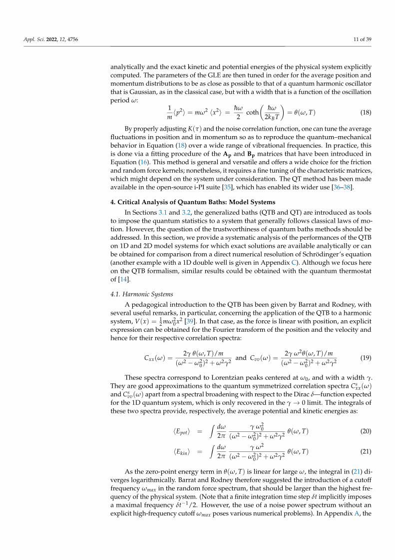
Figure 3. A ‘mildly’ anharmonic Morse potential (magenta, left-hand scale), with the positiondistributions (right-hand scale) for a classical simulation (yellow), a quantum solution throughSchrödinger’s equation (green) and the Quantum Thermal Bath (light blue).

4.2.1. A ‘Mildly’ Anharmonic Example

Simulations were carried out with the following parameters: V0 = 3.0 eV, x0 = 1.0 Å,d = 0.4 Å, T = 300 K, γ = 0.1 THz and cutoff frequency fmax = 500 THz. The mass of theparticle is that of a proton. These parameters yield a harmonic frequency of 3185 cm−1, ofthe same order of magnitude as that of OH stretching modes in various systems. The zero-point energy over V0 ratio is 0.065, so this example can be considered as mildly anharmonic,given that, at this low temperature, only the ground state is significantly populated.

The quantum analysis and the QTB both yield a mean postition 〈x〉 = 1.02 Å, whilethe classical simulation yields 1.00 Å. The quantum total energy (actually the zero-pointenergy at this temperature) turns out to be 194 meV while the QTB gives 197 meV (forthe small friction coefficient γ used in this case, the kinetic energy overestimation effectmentioned in Section 4.1 is minor and the dependence on the frequency cutoff is negligible)and the classical only 26 meV which, of course, does not take into account the large ZPE.The quantum distribution is shown in green in Figure 3 while the classical distribution(yellow) in much sharper. The distribution generated by the QTB (blue) is adequatelybroadened, however, its shape is slightly modified: the maximum is at the the classicalposition, while its tail reaches out further.

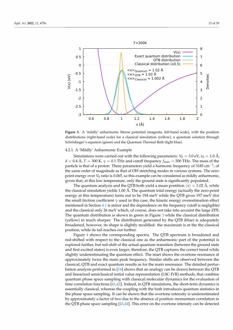
Figure 4 shows the corresponding spectra. The QTB spectrum is broadened andred-shifted with respect to the classical one as the anharmonic part of the potential isexplored further, but red-shift of the actual quantum transition (between the ground stateand first excited states) is even larger; therefore, the QTB captures the correct trend whileslightly underestimating the quantum effect. The inset shows the overtone resonance atapproximately twice the main peak frequency. Similar shifts are observed between theclassical, QTB and exact quantum results as for the main resonance. The detailed pertur-bation analysis performed in [16] shows that an analogy can be drawn between the QTBand linearized semiclassical initial value representation (LSC-IVR) methods, that combinequantum phase space sampling with classical molecular dynamics for the evaluation oftime correlation functions [41,42]. Indeed, in QTB simulations, the short-term dynamics isessentially classical, whereas the coupling with the bath introduces quantum statistics inthe phase space sampling. It can be shown that the overtone intensity is underestimatedby approximately a factor of two due to the absence of position–momentum correlation inthe QTB phase space sampling [43,44]. This error on the overtone intensity can be detected

Appl. Sci. 2022, 12, 4756 14 of 39

(and potentially corrected) using the first-kind fluctuation–dissipation theorem criteriondefined in Section 7, and it remains limited compared to that of path integral methods(see Section 6), which yield a much lower overtone intensity, similar to that of classicalsimulations [16].

0

0.02

0.04

0.06

0.08

0.1

0.12

0.14

1500 2000 2500 3000 3500

[arb

. unit

s]

ν [cm-1]

ClassicalQTB

Quantum transition

0 0.0002 0.0004 0.0006 0.0008

0.001 0.0012 0.0014

5000 6000

(x10)

ν [cm-1]

Figure 4. Cvv(ω) spectra for the ‘mildly’ anharmonic Morse potential, for the classical MD simulation(magenta), the QTB (blue) and the first quantum transition between the ground state and first excitedstate (green). The inset shows show the overtones (the classical spectrum is multiplied by a factorof 10).

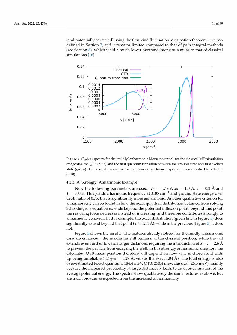
4.2.2. A ‘Strongly’ Anharmonic Example

Now the following parameters are used: V0 = 1.7 eV, x0 = 1.0 Å, d = 0.2 Å andT = 300 K. This yields a harmonic frequency at 3185 cm−1 and ground state energy overdepth ratio of 0.75, that is significantly more anharmonic. Another qualitative criterion foranharmonicity can be found in how the exact quantum distribution obtained from solvingSchrödinger’s equation extends beyond the potential inflexion point: beyond this point,the restoring force decreases instead of increasing, and therefore contributes strongly toanharmonic behavior. In this example, the exact distribution (green line in Figure 5) doessignificantly extend beyond that point (x ≈ 1.14 Å), while in the previous (Figure 3) it doesnot.

Figure 5 shows the results. The features already noticed for the mildly anharmoniccase are enhanced: the maximum still remains at the classical position, while the tailextends even further towards larger distances, requiring the introduction of xmax = 2.6 Åto prevent the particle from escaping the well: in this strongly anharmonic situation, thecalculated QTB mean position therefore will depend on how xmax is chosen and endsup being unreliable (〈x〉QTB = 1.27 Å, versus the exact 1.04 Å). The total energy is alsoover-estimated (exact quantum: 184.4 meV, QTB: 250.4 meV, classical: 26.3 meV), mainlybecause the increased probability at large distances x leads to an over-estimation of theaverage potential energy. The spectra show qualitatively the same features as above, butare much broader as expected from the increased anharmonicity.

Appl. Sci. 2022, 12, 4756 15 of 39

-0.8

-0.6

-0.4

-0.2

0

0.2

0.4

0.6

0.8

1

0.6 0.8 1 1.2 1.4 1.6 1.8 2 0

1

2

3

4

5

6

7

8

V(x

) [e

V]

Densi

ties

x [Å]

T=300K

V(x)Exact quantum distribution

QTB distributionClassical distribution (x0.5)

0

0.005

0.01

0.015

0.02

0.025

0.03

0.035

1500 2000 2500 3000 3500

[arb

. unit

s]

ν [cm-1]

ClassicalQTB

Quantum transition

0 0.0002 0.0004 0.0006 0.0008

0.001 0.0012 0.0014

4000 5000 6000

(x10)

Figure 5. Probability distributions (top) and Cvv(ω) spectra (bottom) for the strongly anharmonicMorse potential, for the classical MD simulation (magenta), the QTB (blue) and the first quantumtransition between the ground state and first excited state (green). The inset shows show the overtones.Note that the classical spectrum is multiplied by a factor of 10.

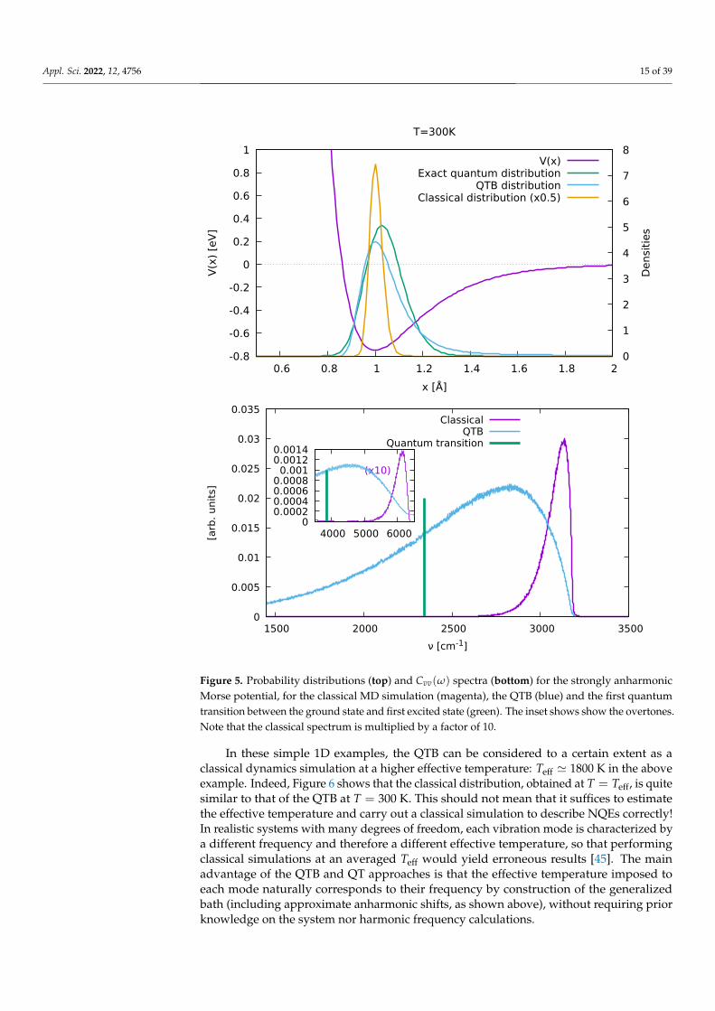
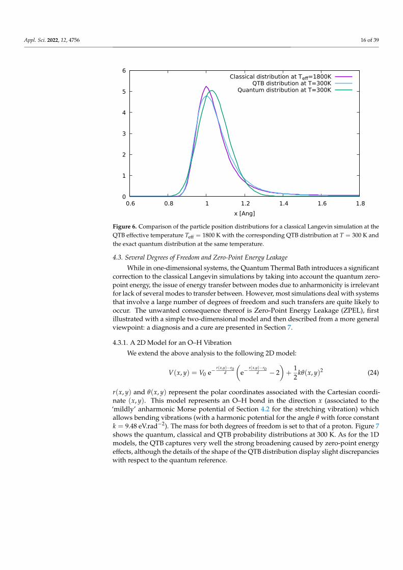
In these simple 1D examples, the QTB can be considered to a certain extent as aclassical dynamics simulation at a higher effective temperature: Teff ' 1800 K in the aboveexample. Indeed, Figure 6 shows that the classical distribution, obtained at T = Teff, is quitesimilar to that of the QTB at T = 300 K. This should not mean that it suffices to estimatethe effective temperature and carry out a classical simulation to describe NQEs correctly!In realistic systems with many degrees of freedom, each vibration mode is characterized bya different frequency and therefore a different effective temperature, so that performingclassical simulations at an averaged Teff would yield erroneous results [45]. The mainadvantage of the QTB and QT approaches is that the effective temperature imposed toeach mode naturally corresponds to their frequency by construction of the generalizedbath (including approximate anharmonic shifts, as shown above), without requiring priorknowledge on the system nor harmonic frequency calculations.

Appl. Sci. 2022, 12, 4756 16 of 39

0

1

2

3

4

5

6

0.6 0.8 1 1.2 1.4 1.6 1.8

x [Ang]

Classical distribution at Teff=1800KQTB distribution at T=300K

Quantum distribution at T=300K

Figure 6. Comparison of the particle position distributions for a classical Langevin simulation at theQTB effective temperature Teff = 1800 K with the corresponding QTB distribution at T = 300 K andthe exact quantum distribution at the same temperature.

4.3. Several Degrees of Freedom and Zero-Point Energy Leakage

While in one-dimensional systems, the Quantum Thermal Bath introduces a significantcorrection to the classical Langevin simulations by taking into account the quantum zero-point energy, the issue of energy transfer between modes due to anharmonicity is irrelevantfor lack of several modes to transfer between. However, most simulations deal with systemsthat involve a large number of degrees of freedom and such transfers are quite likely tooccur. The unwanted consequence thereof is Zero-Point Energy Leakage (ZPEL), firstillustrated with a simple two-dimensional model and then described from a more generalviewpoint: a diagnosis and a cure are presented in Section 7.

4.3.1. A 2D Model for an O–H Vibration

We extend the above analysis to the following 2D model:

V(x, y) = V0 e−r(x,y)−r0

d

(e−

r(x,y)−r0d − 2

)+

12

kθ(x, y)2 (24)

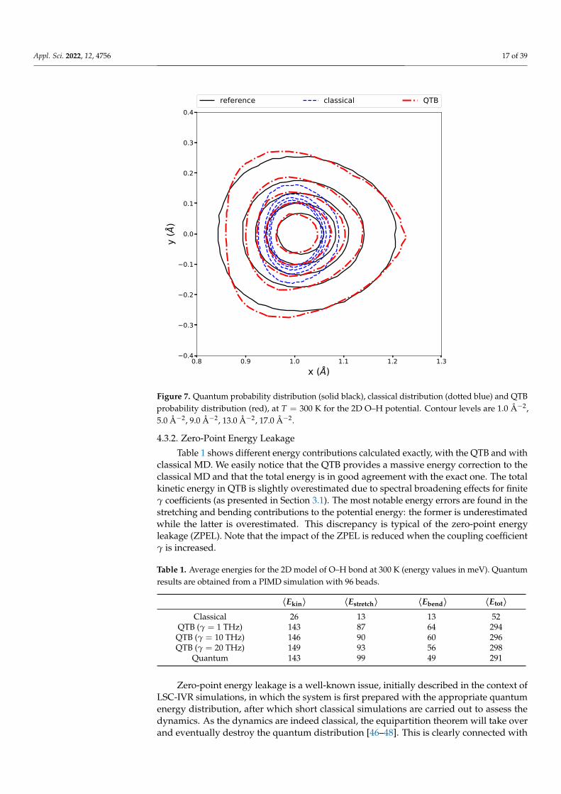
r(x, y) and θ(x, y) represent the polar coordinates associated with the Cartesian coordi-nate (x, y). This model represents an O–H bond in the direction x (associated to the‘mildly’ anharmonic Morse potential of Section 4.2 for the stretching vibration) whichallows bending vibrations (with a harmonic potential for the angle θ with force constantk = 9.48 eV.rad−2). The mass for both degrees of freedom is set to that of a proton. Figure 7shows the quantum, classical and QTB probability distributions at 300 K. As for the 1Dmodels, the QTB captures very well the strong broadening caused by zero-point energyeffects, although the details of the shape of the QTB distribution display slight discrepancieswith respect to the quantum reference.

Appl. Sci. 2022, 12, 4756 17 of 39

0.8 0.9 1.0 1.1 1.2 1.3x (Å)

0.4

0.3

0.2

0.1

0.0

0.1

0.2

0.3

0.4

y (Å

)

reference classical QTB

Figure 7. Quantum probability distribution (solid black), classical distribution (dotted blue) and QTBprobability distribution (red), at T = 300 K for the 2D O–H potential. Contour levels are 1.0 Å−2,5.0 Å−2, 9.0 Å−2, 13.0 Å−2, 17.0 Å−2.

4.3.2. Zero-Point Energy Leakage

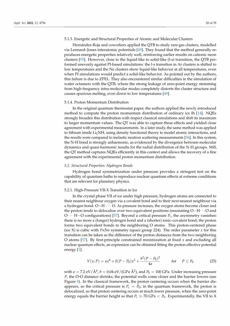
Table 1 shows different energy contributions calculated exactly, with the QTB and withclassical MD. We easily notice that the QTB provides a massive energy correction to theclassical MD and that the total energy is in good agreement with the exact one. The totalkinetic energy in QTB is slightly overestimated due to spectral broadening effects for finiteγ coefficients (as presented in Section 3.1). The most notable energy errors are found in thestretching and bending contributions to the potential energy: the former is underestimatedwhile the latter is overestimated. This discrepancy is typical of the zero-point energyleakage (ZPEL). Note that the impact of the ZPEL is reduced when the coupling coefficientγ is increased.

Table 1. Average energies for the 2D model of O–H bond at 300 K (energy values in meV). Quantumresults are obtained from a PIMD simulation with 96 beads.

〈Ekin〉 〈Estretch〉 〈Ebend〉 〈Etot〉Classical 26 13 13 52

QTB (γ = 1 THz) 143 87 64 294QTB (γ = 10 THz) 146 90 60 296QTB (γ = 20 THz) 149 93 56 298

Quantum 143 99 49 291

Zero-point energy leakage is a well-known issue, initially described in the context ofLSC-IVR simulations, in which the system is first prepared with the appropriate quantumenergy distribution, after which short classical simulations are carried out to assess thedynamics. As the dynamics are indeed classical, the equipartition theorem will take overand eventually destroy the quantum distribution [46–48]. This is clearly connected with

Appl. Sci. 2022, 12, 4756 18 of 39

anharmonicity that allows vibrational modes to exchange energy, resulting, in practice, ina flow of energy from high-frequency modes to low-frequency modes. As the effectivetemperature can be very high, the outcome might be dramatic, as the melting down of thesystem in solid-state simulations. In the case of LSC-IVR simulations, the problem can beaddressed by carrying out short enough classical dynamics, so that the leakage does notsignificantly alter the energy distribution and thus the dynamical results.

It is not so with the quantum baths methods [34,49] as the quantum energy distributionis generated on the fly through the colored Langevin thermostat. The result is therefore acompromise between how much energy is being pumped into the system by the colorednoise and how fast this energy is flowing to low frequency vibrational modes finally tobe dissipated by the friction forces. A systematic endeavour [50] to measure ZPEL inQTB simulations as a function of anharmonicity and the coupling coefficient γ in simplemodel systems such as non-linearly coupled harmonic oscillators showed that ZPEL indeedincreases with anharmonicity and that increasing the coupling coefficient γ significantlyreduces the effects of ZPEL. Similar observations were made regarding the QT in the earlypapers on this method [14,34] and strongly coupled generalized baths were designed inorder to mitigate the effect of ZPEL, an approach comparable to the increase of the couplingcoefficient γ of the QTB. However, the spectral broadening induced by large couplingcoefficients can hinder the use of quantum baths for the computation of vibration spectra.Even more importantly, large system–bath couplings do not completely suppress ZPEL,which can remain significant in strongly anharmonic systems such as liquid water whereit has massive consequences, as examined in Section 7.3. Some authors also proposed tomodify the colored noise memory kernel in the QTB method in order to compensate forthe ZPEL and restore the correct energy distribution between the different modes [49,51].However, without an appropriate criterion to detect and quantify the ZPEL in general cases,these attempts remained somewhat ad hoc and could not be generalized. Such a criterionwas finally derived in [17], and is the basis for the adaptive QTB method presented inSection 7.

5. Applications of Quantum Baths to Realistic Systems

Quantum baths have been used to introduce the quantum statistics in the simulationof several systems, and yield valuable results. In the following, we discuss some selectedapplications of these methods to simulate the properties of condensed matter systems, bysplitting the discussion between structural properties and time-dependent observables.These examples illustrate the usefulness of quantum bath approaches and highlight theirmost serious pathology, i.e., zero-point energy leakage, which motivates the detailedanalysis of ZPEL and the recent work to mitigate its effects presented in Section 7. Thestudies reviewed in this section include both QTB and QT simulations, though fewer innumber for the latter method. We note that the GLE framework developed in the context ofthe QT also found a wide application in its extension to path integral molecular dynamics(briefly presented in Section 6).

5.1. Structural and Thermodynamic Properties

An important quantity for crystals is the Debye temperature ΘD, below which thespecific heat and other thermodynamic properties diverge from their classical behavior [52].In particular, crystals with ΘD > 300 K can show significant nuclear quantum effects atroom temperature.

5.1.1. MgO

Dammak and coworkers [12] showed that the QTB reproduces the experimental trendsof the lattice parameter and the heat capacity of the MgO crystal as a function of temperature.While recovering the classical limit for temperatures close to or above the Debye temperature(ΘD ' 940 K in MgO), the specific heat follows the expected quantum behavior at lowtemperatures (CV → 0 as T → 0), in excellent agreement with experimental data.

Appl. Sci. 2022, 12, 4756 19 of 39

5.1.2. Diamond

Diamond has a particularly high Debye temperature ΘD ' 2000 K. Ceriotti andcoworkers [14] applied the quantum thermostat (QT) to model diamond crystals, whereinteratomic interactions were described with a semi-empirical potential, and comparedtheir results to existing path integral (PI) simulations. The internal energy Eint(T) andlattice parameter a(T) as provided by the QT follow the PI trends with temperature downto T ∼ 0.06ΘD. Below this temperature, the quantum thermostat failed to counterbalancethe strong phonon–phonon coupling, which results in zero-point energy leakage from highto low frequencies and a too-short phonon lifetime. Therefore, Eint(T) and a(T) sensitivelydiverge from the PI behavior at low temperatures.

Isotope Effects: LiH vs. LiD

Simulations that rely on classical statistical mechanics cannot account for isotope effectsstraightforwardly, because statistical averages are independent of the nuclear mass. Amarked isotope effect takes place in LiH/LiD crystals; the Debye temperatures, as obtainedby fitting the thermal conductivity of LiH and LiD crystals, are 851 K and 638 K, respectively(see [53] and references therein). One of the first QTB simulations in conjunction withthe first-principle description of interatomic forces via the density functional theory [53]explained why the lattice parameter of LiH is significantly larger than that of LiD fromvery low temperatures up to 600 K, as experimentally observed. The volume expansioncoefficient is also different in this T range between the two isotopes. The elastic properties ofLiH and LiD with increasing pressure are markedly distinct, which reflects in two differentequations of state for the two isotopes as measured by X-ray diffraction experiments inthe 0–94 GPa pressure range [54]. Remarkably, the quasi-harmonic approximation failsin reproducing the isotope shift in pressure ∆P, which is defined as the difference inpressure between LiH and LiD at fixed volume (see Figure 8). The QTB simulations followthe experimental trend in ∆P, while the quasi-harmonic approximation deviates from it,especially when P increases. This has been interpreted as a consequence of the importanceof anharmonic contributions to the thermal properties of those crystals.

0.01

0.02

0.03

0.04

0.00100 200 3000100 200 3000

Temperature (K)

Experimental Simulation

LiH

LiH

LiD LiD

a(T

) –

a LiD(T

=0

K)

(Å

)

Figure 8. Lattice parameter a of cubic LiH and LiD vs. temperature, with respect to the LiD latticeparameter at T = 0 K. Left—experimental; right—QTB simulations.

Appl. Sci. 2022, 12, 4756 20 of 39

5.1.3. Energetic and Structural Properties of Atomic and Molecular Clusters

Hernández-Roja and coworkers applied the QTB to study rare-gas clusters, modelledvia Lennard–Jones interatomic potentials [49]. They found that the method generally re-produces energetic properties relatively well, reinforcing earlier results on cationic neonclusters [55]. However, close to the liquid-like to solid-like (l-s) transition, the QTB per-formed unevenly against PI-based simulations: the l-s transition in Ar clusters is shifted tolow temperatures and the Ne clusters show liquid-like behavior at all temperatures, evenwhen PI simulations would predict a solid-like behavior. As pointed out by the authors,this failure is due to ZPEL. They also encountered similar difficulties in the simulation ofwater octamers with the QTB, where the strong leakage of zero-point energy stemmingfrom high-frequency intra-molecular modes completely distorts the cluster structure andcauses spurious melting, even down to low temperatures [49].

5.1.4. Proton Momentum Distribution

In the original quantum thermostat paper, the authors applied the newly introducedmethod to compute the proton momentum distribution of ordinary ice Ih [14]. NQEsstrongly broaden this distribution with respect classical simulations and shift its maximumto larger momentum values. The QT was able to capture these effects and yielded closeagreement with experimental measurements. In a later study, the same method was appliedto lithium imide Li2NH, using density functional theory to model atomic interactions, andthe results were compared to inelastic neutron scattering measurements [56]. In this system,the N-H bond is strongly anharmonic, as evidenced by the divergence between moleculardynamics and quasi-harmonic results for the radial distribution of the N-H groups. Still,the QT method captures NQEs efficiently in this context and allows the recovery of a fineagreement with the experimental proton momentum distribution.

5.2. Structural Properties: Hydrogen Bonds

Hydrogen bond symmetrization under pressure provides a stringent test on thecapability of quantum baths to reproduce nuclear quantum effects at extreme conditionsthat are relevant for planetary physics.

5.2.1. High-Pressure VII-X Transition in Ice

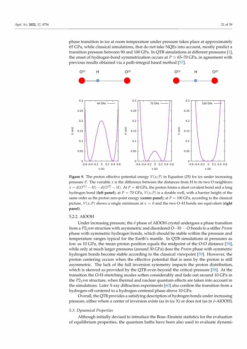
In the crystal phase VII of ice under high pressure, hydrogen atoms are connected totheir nearest neighbour oxygen via a covalent bond and to their next-nearest neighbour viaa hydrogen bond: O−H · · · O. As pressure increases, the oxygen atoms become closer andthe proton tends to delocalize over two equivalent positions (resonating O−H· · ·O andO· · · H−O configurations) [57]. Beyond a critical pressure Pc, the asymmetry vanishes:there is no more a (longer) hydrogen bond and a (shorter) ionic–covalent bond; the protonforms two equivalent bonds to the neighboring O atoms. This proton-centered phase(ice X) is cubic with Pn3m symmetry (space group 224). The order parameter x for thistransition can be taken as the difference of the proton distances from the two neighboringO atoms [57]. By first-principle constrained minimization at fixed x and excluding allnuclear quantum effects, an expression can be obtained fitting the proton effective potentialenergy [1]:

V(x; P) = ax4 + b(P− P0)x2 +b2(P− P0)

2

4afor P ≤ P0 (25)

with a = 7.2 eV/Å4, b = 0.04 eV/(GPa Å2), and P0 = 100 GPa. Under increasing pressureP, the O-O distance shrinks; the potential wells come closer and the barrier lowers (seeFigure 9). In the classical framework, the proton centering occurs when the barrier dis-appears, so the critical pressure is Pc = P0; in the quantum framework, the proton isdelocalized, so that proton centering occurs at much lower pressure, when the zero-pointenergy equals the barrier height so that Pc ' 70 GPa < P0. Experimentally, the VII to X

Appl. Sci. 2022, 12, 4756 21 of 39

phase transition in ice at room temperature under pressure takes place at approximately65 GPa, while classical simulations, that do not take NQEs into account, mostly predict atransition pressure between 90 and 100 GPa. In QTB simulations at different pressures [1],the onset of hydrogen-bond symmetrization occurs at P ' 65–70 GPa, in agreement withprevious results obtained via a path-integral based method [57].

0

0.05

0.1

0.15

0.2

0.25

0.3

-0.6 -0.4 -0.2 0 0.2 0.4 0.6

V (

eV

)

x (A)

40 GPa

0

0.05

0.1

0.15

0.2

0.25

0.3

-0.6 -0.4 -0.2 0 0.2 0.4 0.6

V (

eV

)

x (A)

70 GPa

0

0.05

0.1

0.15

0.2

0.25

0.3

-0.6 -0.4 -0.2 0 0.2 0.4 0.6

V (

eV

)

x (A)

100 GPa

O(1) O(2)H O(1) O(2)H

Figure 9. The proton effective potential energy V(x; P) in Equation (25) for ice under increasingpressure P. The variable x is the difference between the distances from H to its two O neighbors:x = d(O(1) − H)− d(O(2) − H). At P = 40 GPa, the proton forms a short covalent bond and a longhydrogen bond (left panel); at P = 70 GPa, V(x; P) is a double well, with a barrier height of thesame order as the proton zero-point energy (center panel); at P = 100 GPa, according to the classicalpicture, V(x; P) shows a single minimum at x = 0 and the two O–H bonds are equivalent (rightpanel).

5.2.2. AlOOH

Under increasing pressure, the δ phase of AlOOH crystal undergoes a phase transitionfrom a P21nm structure with asymmetric and disordered O−H· · ·O bonds to a stiffer Pnnmphase with symmetric hydrogen bonds, which should be stable within the pressure andtemperature ranges typical for the Earth’s mantle. In QTB simulations at pressures aslow as 10 GPa, the mean proton position equals the midpoint of the O-O distance [58],while only at much larger pressures (around 30 GPa) does the Pnnm phase with symmetrichydrogen bonds become stable according to the classical viewpoint [59]. However, theproton centering occurs when the effective potential that is seen by the proton is stillasymmetric. The lack of the full inversion symmetry impacts the proton distribution,which is skewed as provided by the QTB even beyond the critical pressure [58]. At thetransition the O-H stretching modes soften considerably and fade out around 10 GPa inthe P21nm structure, when thermal and nuclear quantum effects are taken into account inthe simulations. Later X-ray diffraction experiments [60] also confirm the transition from ahydrogen-off-centered to a hydrogen-centered phase above 10 GPa.

Overall, the QTB provides a satisfying description of hydrogen bonds under increasingpressure, either where a center of inversion exists (as in ice X) or does not (as in δ-AlOOH).

5.3. Dynamical Properties

Although initially devised to introduce the Bose–Einstein statistics for the evaluationof equilibrium properties, the quantum baths have been also used to evaluate dynami-

Appl. Sci. 2022, 12, 4756 22 of 39

cal properties. The following results show that the performances of quantum baths arerather system- and property-dependent, although in most cases the introduction of NQEsvia the quantum baths improves the description of vibrational properties, even in veryanharmonic systems. Although the coupling with the bath tends to distort vibrationalspectra, particularly in the context of the QT method, this effects can be efficiently correcteda posteriori using spectral deconvolution techniques [18,40]. Moreover, quantum bathshave been employed to study intrinsically nonequilibrium properties, such as thermalconductivity in crystals (see Section 5.3.3).

5.3.1. Phonon Spectra in Pure and Salty Ices under Pressure

As observed in Section 4, QTB simulations provide direct access to vibrational spectra,accounting consistently (though approximately) for anharmonic and quantum effects.This property has been exploited in different studies to confront QTB results with other,more established simulation methods [15,18], or with experimental data. In particular,the phonon spectrum of ice was extracted from QTB simulations at various pressures,computed from the Fourier transform of the velocity–velocity autocorrelation function [1].

These QTB results are shown in Figure 10, and compared with the infra-red absorptionand Raman scattering data. The QTB reproduces the experimental data well in the wholepressure range, including the softening of the O-H stretching mode close to the VII-Xtransition. This softening is an essential feature of the transition that can be related tothe response of the system: in the classical picture, the squared frequency of the softphonon mode is proportional to the inverse susceptibility χ−1 and, in the simple one-dimensional double-well model, χ is maximum at the transition pressure Pc. This relatesthe O-H stretching mode softening with the enhanced fluctuations of the dipole momentthat typically occurs at the transition. Interestingly, the O-H stretching mode softeningoccurs at larger pressures when a small quantity (∼1%) of LiCl or NaCl salt is incorporatedinto the ice crystal, an effect that is well captured by the QTB [61].

1000

2000

3000

0 20 40 60 80 100 120 140 160 180

Freq

uenc

y (c

m-1)

Pressure (GPa)

νT

νR

νR"

ν2

ν3,ν1

T2g

νD

0

5

10

15

20

25

0 500 1000 1500 2000 2500 3000 3500 4000

Arbi

trary

uni

ts

Frequency (cm )-1

20 GPa30 GPa46 GPa70 GPa

110 GPa140 GPa

Figure 10. (Left panel): ice spectra obtained through the Fourier transform of the velocity-velocityautocorrelation function from QTB simulations at several pressures [1]. (Right panel): the peaksextracted from the QTB ice spectra (lines) are compared to the experimental infrared and Ramanscattering data (triangles and circles).

Contrary to previous beliefs, this effect is not due to steric hindrance, but to the a-symmetrization of the OHO triplet because of the long-range dipolar field generated bythe dissociated Li+ Cl− or Na+ Cl− salts. Accordingly, the critical pressure for the VII-Xtransition in salty ice under pressure is upshifted and much closer to its classical value thanin pure ice. This counterintuitive phenomenon (salty ice is “more classical” than pure ice)shows the subtleties of nuclear quantum effects in hydrogen-bonded systems.

5.3.2. Highly-Excited Molecules

Calvo and coworkers [62] studied the response of naphtalene to a strong laser pulseat varying frequencies by using classical molecular dynamics or accounting for nuclearquantum effects via path-integral molecular dynamics or the QTB. First, they observed

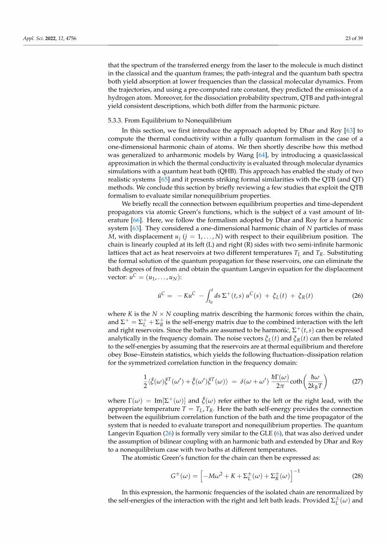
Appl. Sci. 2022, 12, 4756 23 of 39

that the spectrum of the transferred energy from the laser to the molecule is much distinctin the classical and the quantum frames; the path-integral and the quantum bath spectraboth yield absorption at lower frequencies than the classical molecular dynamics. Fromthe trajectories, and using a pre-computed rate constant, they predicted the emission of ahydrogen atom. Moreover, for the dissociation probability spectrum, QTB and path-integralyield consistent descriptions, which both differ from the harmonic picture.

5.3.3. From Equilibrium to Nonequilibrium

In this section, we first introduce the approach adopted by Dhar and Roy [63] tocompute the thermal conductivity within a fully quantum formalism in the case of aone-dimensional harmonic chain of atoms. We then shortly describe how this methodwas generalized to anharmonic models by Wang [64], by introducing a quasiclassicalapproximation in which the thermal conductivity is evaluated through molecular dynamicssimulations with a quantum heat bath (QHB). This approach has enabled the study of tworealistic systems [65] and it presents striking formal similarities with the QTB (and QT)methods. We conclude this section by briefly reviewing a few studies that exploit the QTBformalism to evaluate similar nonequilibrium properties.

We briefly recall the connection between equilibrium properties and time-dependentpropagators via atomic Green’s functions, which is the subject of a vast amount of lit-erature [66]. Here, we follow the formalism adopted by Dhar and Roy for a harmonicsystem [63]. They considered a one-dimensional harmonic chain of N particles of massM, with displacement uj (j = 1, . . . , N) with respect to their equilibrium position. Thechain is linearly coupled at its left (L) and right (R) sides with two semi-infinite harmoniclattices that act as heat reservoirs at two different temperatures TL and TR. Substitutingthe formal solution of the quantum propagation for these reservoirs, one can eliminate thebath degrees of freedom and obtain the quantum Langevin equation for the displacementvector: uC = (u1, . . . , uN):

uC = − KuC −∫ t

t0

ds Σ+(t, s) uC(s) + ξL(t) + ξR(t) (26)

where K is the N × N coupling matrix describing the harmonic forces within the chain,and Σ+ = Σ+

L + Σ+R is the self-energy matrix due to the combined interaction with the left

and right reservoirs. Since the baths are assumed to be harmonic, Σ+(t, s) can be expressedanalytically in the frequency domain. The noise vectors ξL(t) and ξR(t) can then be relatedto the self-energies by assuming that the reservoirs are at thermal equilibrium and thereforeobey Bose–Einstein statistics, which yields the following fluctuation–dissipation relationfor the symmetrized correlation function in the frequency domain:

12〈ξ(ω)ξT(ω′) + ξ(ω′)ξT(ω)〉 = δ(ω + ω′)

hΓ(ω)

2πcoth

(hω

2kBT

)(27)

where Γ(ω) = Im[Σ+(ω)] and ξ(ω) refer either to the left or the right lead, with theappropriate temperature T = TL, TR. Here the bath self-energy provides the connectionbetween the equilibrium correlation function of the bath and the time propagator of thesystem that is needed to evaluate transport and nonequilibrium properties. The quantumLangevin Equation (26) is formally very similar to the GLE (6), that was also derived underthe assumption of bilinear coupling with an harmonic bath and extended by Dhar and Royto a nonequilibrium case with two baths at different temperatures.

The atomistic Green’s function for the chain can then be expressed as:

G±(ω) =[−Mω2 + K + Σ±L (ω) + Σ±R (ω)

]−1(28)

In this expression, the harmonic frequencies of the isolated chain are renormalized bythe self-energies of the interaction with the right and left bath leads. Provided Σ±L (ω) and

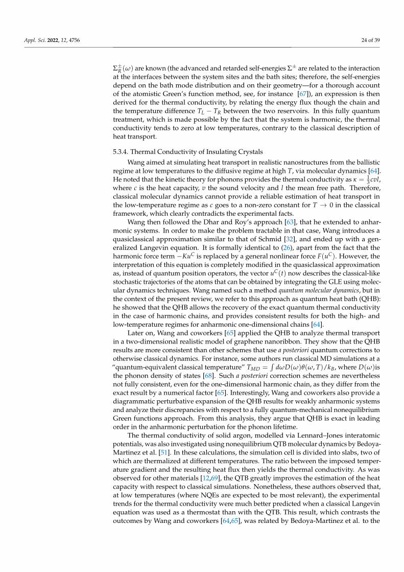
Appl. Sci. 2022, 12, 4756 24 of 39

Σ±R (ω) are known (the advanced and retarded self-energies Σ± are related to the interactionat the interfaces between the system sites and the bath sites; therefore, the self-energiesdepend on the bath mode distribution and on their geometry—for a thorough accountof the atomistic Green’s function method, see, for instance [67]), an expression is thenderived for the thermal conductivity, by relating the energy flux though the chain andthe temperature difference TL − TR between the two reservoirs. In this fully quantumtreatment, which is made possible by the fact that the system is harmonic, the thermalconductivity tends to zero at low temperatures, contrary to the classical description ofheat transport.

5.3.4. Thermal Conductivity of Insulating Crystals

Wang aimed at simulating heat transport in realistic nanostructures from the ballisticregime at low temperatures to the diffusive regime at high T, via molecular dynamics [64].He noted that the kinetic theory for phonons provides the thermal conductivity as κ = 1

3 cvl,where c is the heat capacity, v the sound velocity and l the mean free path. Therefore,classical molecular dynamics cannot provide a reliable estimation of heat transport inthe low-temperature regime as c goes to a non-zero constant for T → 0 in the classicalframework, which clearly contradicts the experimental facts.

Wang then followed the Dhar and Roy’s approach [63], that he extended to anhar-monic systems. In order to make the problem tractable in that case, Wang introduces aquasiclassical approximation similar to that of Schmid [32], and ended up with a gen-eralized Langevin equation. It is formally identical to (26), apart from the fact that theharmonic force term −KuC is replaced by a general nonlinear force F(uC). However, theinterpretation of this equation is completely modified in the quasiclassical approximationas, instead of quantum position operators, the vector uC(t) now describes the classical-likestochastic trajectories of the atoms that can be obtained by integrating the GLE using molec-ular dynamics techniques. Wang named such a method quantum molecular dynamics, but inthe context of the present review, we refer to this approach as quantum heat bath (QHB):he showed that the QHB allows the recovery of the exact quantum thermal conductivityin the case of harmonic chains, and provides consistent results for both the high- andlow-temperature regimes for anharmonic one-dimensional chains [64].

Later on, Wang and coworkers [65] applied the QHB to analyze thermal transportin a two-dimensional realistic model of graphene nanoribbon. They show that the QHBresults are more consistent than other schemes that use a posteriori quantum corrections tootherwise classical dynamics. For instance, some authors run classical MD simulations at a“quantum-equivalent classical temperature” TMD =

∫dωD(ω)θ(ω, T)/kB, where D(ω)is

the phonon density of states [68]. Such a posteriori correction schemes are neverthelessnot fully consistent, even for the one-dimensional harmonic chain, as they differ from theexact result by a numerical factor [65]. Interestingly, Wang and coworkers also provide adiagrammatic perturbative expansion of the QHB results for weakly anharmonic systemsand analyze their discrepancies with respect to a fully quantum-mechanical nonequilibriumGreen functions approach. From this analysis, they argue that QHB is exact in leadingorder in the anharmonic perturbation for the phonon lifetime.

The thermal conductivity of solid argon, modelled via Lennard–Jones interatomicpotentials, was also investigated using nonequilibrium QTB molecular dynamics by Bedoya-Martinez et al. [51]. In these calculations, the simulation cell is divided into slabs, two ofwhich are thermalized at different temperatures. The ratio between the imposed temper-ature gradient and the resulting heat flux then yields the thermal conductivity. As wasobserved for other materials [12,69], the QTB greatly improves the estimation of the heatcapacity with respect to classical simulations. Nonetheless, these authors observed that,at low temperatures (where NQEs are expected to be most relevant), the experimentaltrends for the thermal conductivity were much better predicted when a classical Langevinequation was used as a thermostat than with the QTB. This result, which contrasts theoutcomes by Wang and coworkers [64,65], was related by Bedoya-Martinez et al. to the

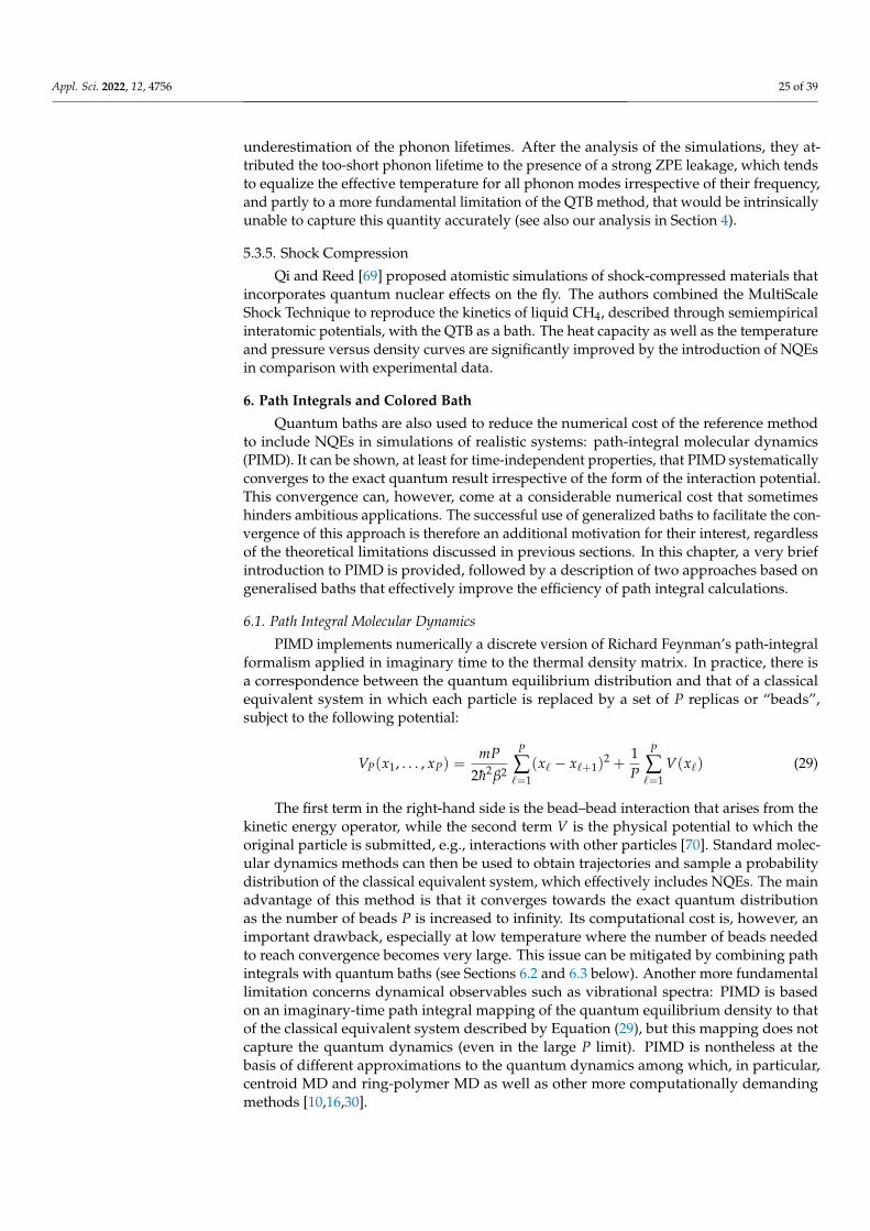
Appl. Sci. 2022, 12, 4756 25 of 39

underestimation of the phonon lifetimes. After the analysis of the simulations, they at-tributed the too-short phonon lifetime to the presence of a strong ZPE leakage, which tendsto equalize the effective temperature for all phonon modes irrespective of their frequency,and partly to a more fundamental limitation of the QTB method, that would be intrinsicallyunable to capture this quantity accurately (see also our analysis in Section 4).

5.3.5. Shock Compression

Qi and Reed [69] proposed atomistic simulations of shock-compressed materials thatincorporates quantum nuclear effects on the fly. The authors combined the MultiScaleShock Technique to reproduce the kinetics of liquid CH4, described through semiempiricalinteratomic potentials, with the QTB as a bath. The heat capacity as well as the temperatureand pressure versus density curves are significantly improved by the introduction of NQEsin comparison with experimental data.

6. Path Integrals and Colored Bath

Quantum baths are also used to reduce the numerical cost of the reference methodto include NQEs in simulations of realistic systems: path-integral molecular dynamics(PIMD). It can be shown, at least for time-independent properties, that PIMD systematicallyconverges to the exact quantum result irrespective of the form of the interaction potential.This convergence can, however, come at a considerable numerical cost that sometimeshinders ambitious applications. The successful use of generalized baths to facilitate the con-vergence of this approach is therefore an additional motivation for their interest, regardlessof the theoretical limitations discussed in previous sections. In this chapter, a very briefintroduction to PIMD is provided, followed by a description of two approaches based ongeneralised baths that effectively improve the efficiency of path integral calculations.

6.1. Path Integral Molecular Dynamics

PIMD implements numerically a discrete version of Richard Feynman’s path-integralformalism applied in imaginary time to the thermal density matrix. In practice, there isa correspondence between the quantum equilibrium distribution and that of a classicalequivalent system in which each particle is replaced by a set of P replicas or “beads”,subject to the following potential:

VP(x1, . . . , xP) =mP

2h2β2

P

∑`=1

(x` − x`+1)2 +

1P

P

∑`=1

V(x`) (29)

The first term in the right-hand side is the bead–bead interaction that arises from thekinetic energy operator, while the second term V is the physical potential to which theoriginal particle is submitted, e.g., interactions with other particles [70]. Standard molec-ular dynamics methods can then be used to obtain trajectories and sample a probabilitydistribution of the classical equivalent system, which effectively includes NQEs. The mainadvantage of this method is that it converges towards the exact quantum distributionas the number of beads P is increased to infinity. Its computational cost is, however, animportant drawback, especially at low temperature where the number of beads neededto reach convergence becomes very large. This issue can be mitigated by combining pathintegrals with quantum baths (see Sections 6.2 and 6.3 below). Another more fundamentallimitation concerns dynamical observables such as vibrational spectra: PIMD is basedon an imaginary-time path integral mapping of the quantum equilibrium density to thatof the classical equivalent system described by Equation (29), but this mapping does notcapture the quantum dynamics (even in the large P limit). PIMD is nontheless at thebasis of different approximations to the quantum dynamics among which, in particular,centroid MD and ring-polymer MD as well as other more computationally demandingmethods [10,16,30].

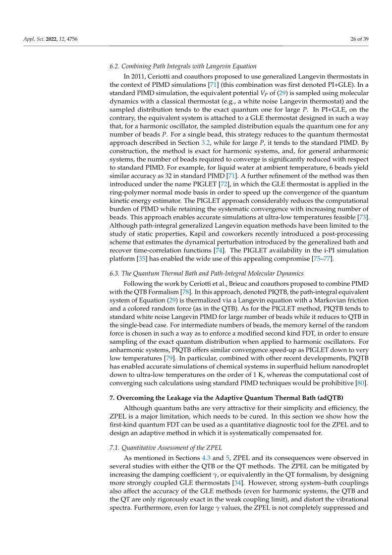
Appl. Sci. 2022, 12, 4756 26 of 39

6.2. Combining Path Integrals with Langevin Equation

In 2011, Ceriotti and coauthors proposed to use generalized Langevin thermostats inthe context of PIMD simulations [71] (this combination was first denoted PI+GLE). In astandard PIMD simulation, the equivalent potential VP of (29) is sampled using moleculardynamics with a classical thermostat (e.g., a white noise Langevin thermostat) and thesampled distribution tends to the exact quantum one for large P. In PI+GLE, on thecontrary, the equivalent system is attached to a GLE thermostat designed in such a waythat, for a harmonic oscillator, the sampled distribution equals the quantum one for anynumber of beads P. For a single bead, this strategy reduces to the quantum thermostatapproach described in Section 3.2, while for large P, it tends to the standard PIMD. Byconstruction, the method is exact for harmonic systems, and, for general anharmonicsystems, the number of beads required to converge is significantly reduced with respectto standard PIMD. For example, for liquid water at ambient temperature, 6 beads yieldsimilar accuracy as 32 in standard PIMD [71]. A further refinement of the method was thenintroduced under the name PIGLET [72], in which the GLE thermostat is applied in thering-polymer normal mode basis in order to speed up the convergence of the quantumkinetic energy estimator. The PIGLET approach considerably reduces the computationalburden of PIMD while retaining the systematic convergence with increasing number ofbeads. This approach enables accurate simulations at ultra-low temperatures feasible [73].Although path-integral generalized Langevin equation methods have been limited to thestudy of static properties, Kapil and coworkers recently introduced a post-processingscheme that estimates the dynamical perturbation introduced by the generalized bath andrecover time-correlation functions [74]. The PIGLET availability in the i-PI simulationplatform [35] has enabled the wide use of this appealing compromise [75–77].

6.3. The Quantum Thermal Bath and Path-Integral Molecular Dynamics

Following the work by Ceriotti et al., Brieuc and coauthors proposed to combine PIMDwith the QTB Formalism [78]. In this approach, denoted PIQTB, the path-integral equivalentsystem of Equation (29) is thermalized via a Langevin equation with a Markovian frictionand a colored random force (as in the QTB). As for the PIGLET method, PIQTB tends tostandard white noise Langevin PIMD for large number of beads while it reduces to QTB inthe single-bead case. For intermediate numbers of beads, the memory kernel of the randomforce is chosen in such a way as to enforce a modified second kind FDT, in order to ensuresampling of the exact quantum distribution when applied to harmonic oscillators. Foranharmonic systems, PIQTB offers similar convergence speed-up as PIGLET down to verylow temperatures [79]. In particular, combined with other recent developments, PIQTBhas enabled accurate simulations of chemical systems in superfluid helium nanodropletdown to ultra-low temperatures on the order of 1 K, whereas the computational cost ofconverging such calculations using standard PIMD techniques would be prohibitive [80].

7. Overcoming the Leakage via the Adaptive Quantum Thermal Bath (adQTB)

Although quantum baths are very attractive for their simplicity and efficiency, theZPEL is a major limitation, which needs to be cured. In this section we show how thefirst-kind quantum FDT can be used as a quantitative diagnostic tool for the ZPEL and todesign an adaptive method in which it is systematically compensated for.

7.1. Quantitative Assessment of the ZPEL

As mentioned in Sections 4.3 and 5, ZPEL and its consequences were observed inseveral studies with either the QTB or the QT methods. The ZPEL can be mitigated byincreasing the damping coefficient γ, or equivalently in the QT formalism, by designingmore strongly coupled GLE thermostats [34]. However, strong system–bath couplingsalso affect the accuracy of the GLE methods (even for harmonic systems, the QTB andthe QT are only rigorously exact in the weak coupling limit), and distort the vibrationalspectra. Furthermore, even for large γ values, the ZPEL is not completely suppressed and

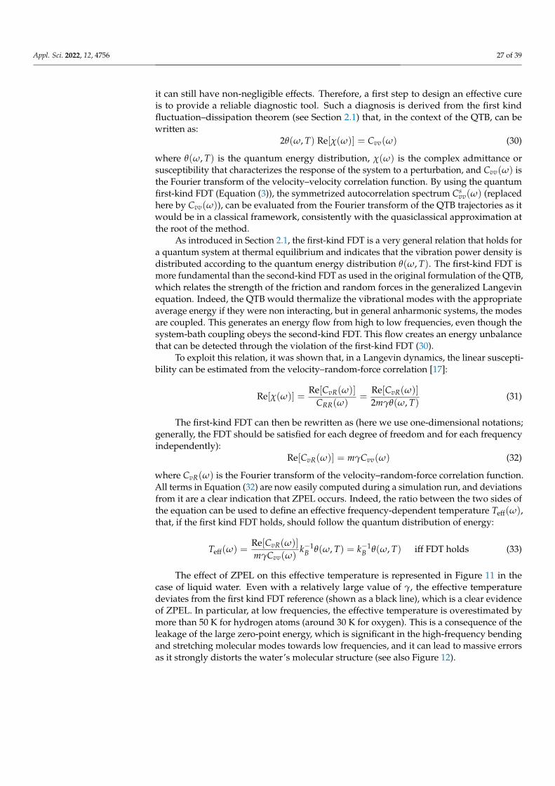
Appl. Sci. 2022, 12, 4756 27 of 39

it can still have non-negligible effects. Therefore, a first step to design an effective cureis to provide a reliable diagnostic tool. Such a diagnosis is derived from the first kindfluctuation–dissipation theorem (see Section 2.1) that, in the context of the QTB, can bewritten as:

2θ(ω, T) Re[χ(ω)] = Cvv(ω) (30)

where θ(ω, T) is the quantum energy distribution, χ(ω) is the complex admittance orsusceptibility that characterizes the response of the system to a perturbation, and Cvv(ω) isthe Fourier transform of the velocity–velocity correlation function. By using the quantumfirst-kind FDT (Equation (3)), the symmetrized autocorrelation spectrum Cs

vv(ω) (replacedhere by Cvv(ω)), can be evaluated from the Fourier transform of the QTB trajectories as itwould be in a classical framework, consistently with the quasiclassical approximation atthe root of the method.

As introduced in Section 2.1, the first-kind FDT is a very general relation that holds fora quantum system at thermal equilibrium and indicates that the vibration power density isdistributed according to the quantum energy distribution θ(ω, T). The first-kind FDT ismore fundamental than the second-kind FDT as used in the original formulation of the QTB,which relates the strength of the friction and random forces in the generalized Langevinequation. Indeed, the QTB would thermalize the vibrational modes with the appropriateaverage energy if they were non interacting, but in general anharmonic systems, the modesare coupled. This generates an energy flow from high to low frequencies, even though thesystem-bath coupling obeys the second-kind FDT. This flow creates an energy unbalancethat can be detected through the violation of the first-kind FDT (30).

To exploit this relation, it was shown that, in a Langevin dynamics, the linear suscepti-bility can be estimated from the velocity–random-force correlation [17]:

Re[χ(ω)] =Re[CvR(ω)]

CRR(ω)=

Re[CvR(ω)]

2mγθ(ω, T)(31)

The first-kind FDT can then be rewritten as (here we use one-dimensional notations;generally, the FDT should be satisfied for each degree of freedom and for each frequencyindependently):

Re[CvR(ω)] = mγCvv(ω) (32)

where CvR(ω) is the Fourier transform of the velocity–random-force correlation function.All terms in Equation (32) are now easily computed during a simulation run, and deviationsfrom it are a clear indication that ZPEL occurs. Indeed, the ratio between the two sides ofthe equation can be used to define an effective frequency-dependent temperature Teff(ω),that, if the first kind FDT holds, should follow the quantum distribution of energy:

Teff(ω) =Re[CvR(ω)]

mγCvv(ω)k−1

B θ(ω, T) = k−1B θ(ω, T) iff FDT holds (33)

The effect of ZPEL on this effective temperature is represented in Figure 11 in thecase of liquid water. Even with a relatively large value of γ, the effective temperaturedeviates from the first kind FDT reference (shown as a black line), which is a clear evidenceof ZPEL. In particular, at low frequencies, the effective temperature is overestimated bymore than 50 K for hydrogen atoms (around 30 K for oxygen). This is a consequence of theleakage of the large zero-point energy, which is significant in the high-frequency bendingand stretching molecular modes towards low frequencies, and it can lead to massive errorsas it strongly distorts the water’s molecular structure (see also Figure 12).

Appl. Sci. 2022, 12, 4756 28 of 39

Frequency (cm )-1

Eff

ect

ive t

em

pera

ture

(K

)

Figure 11. Effective temperature Teff versus frequency as defined by Equation (33) in liquid water at300 K described with the q-TIP4P/F model and simulated with the QTB method using γ = 20 ps−1.The blue dashed line corresponds to oxygen (it is average over all O atoms and over all threedirections x, y and z), the dotted orange line to hydrogen, and the black continuous line is thereference k−1

B θ(ω, T) that corresponds to the first-kind FDT. The simulations were performed usingTinker-HP software [81] and parameters similar to that in Ref. [18]. The inset represents a zoom onthe low-frequency region and the vibrational power spectrum mCvv(ω) is shown as a dashed-dottedgrey line.

distance (A)

classical MD

standard QTB

adaptive QTB

reference (PIMD)

O-O

RD

F

distance (A)

O-H

RD

F

x4

-1γ

coeffi

cien

t (p

s )

r

Frequency (cm )-1

Figure 12. Radial distribution functions (RDF) in liquid water at 300 K described with the q-TIP4P/Fmodel and simulated with different molecular dynamics methods (left, oxygen–oxygen; middle,oxygen–hydrogen). The friction coefficient used for QTB and adQTB methods is γ = 20 ps−1, theadapted random force coefficients γr(ω) are plotted on the right panel for oxygen (dashed blue) andhydrogen (dotted orange) atoms. The simulations were performed using Tinker-HP software [81]and parameters similar to that in Ref. [18].

7.2. A Cure through Strict Enforcement of the First Kind FDT

To design a cure for ZPEL, an adaptive procedure was proposed in order to compensatethe energy unbalance measured via the first-kind FDT [17]. To that end, the second-kindFDT is broken and two different frequency-dependent coupling coefficients are introduced:γr(ω), that replaces γ in the random force power spectrum, Equation (14), and γ f (ω) thatcharacterizes the memory kernel of the friction force that is rendered non-Markovian (itis related to the memory kernel in Equation (6), by K(ω) = 2mRe[γ f (ω)]). The first-kindFDT is then written as [17]:

Re[CvR(ω)] = mγr(ω)Cvv(ω) (34)

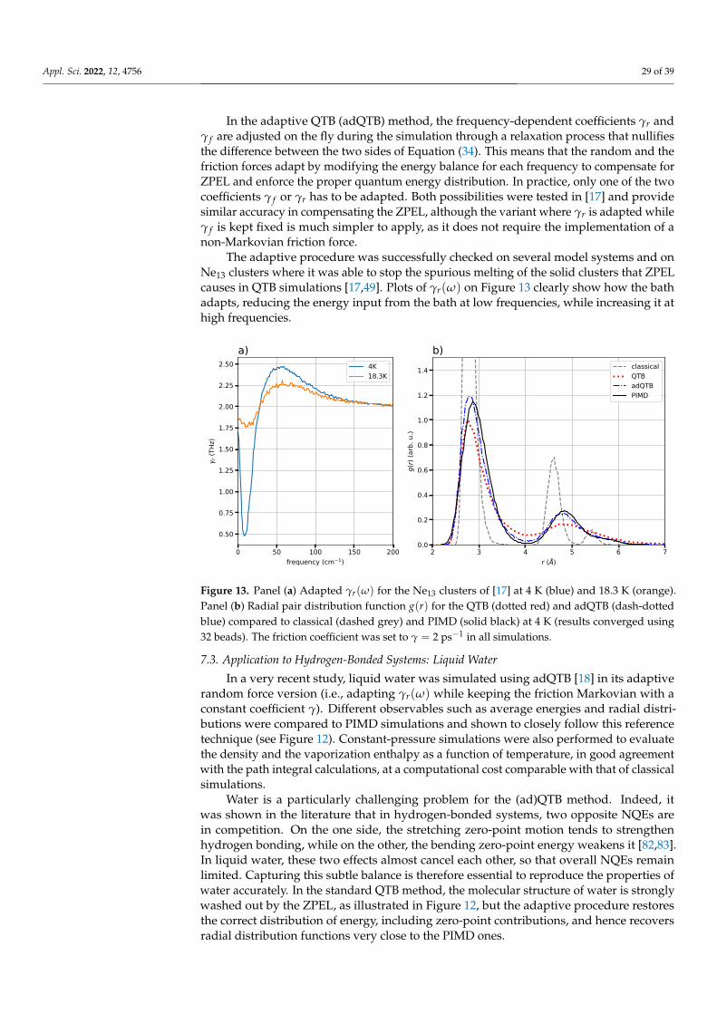
Appl. Sci. 2022, 12, 4756 29 of 39

In the adaptive QTB (adQTB) method, the frequency-dependent coefficients γr andγ f are adjusted on the fly during the simulation through a relaxation process that nullifiesthe difference between the two sides of Equation (34). This means that the random and thefriction forces adapt by modifying the energy balance for each frequency to compensate forZPEL and enforce the proper quantum energy distribution. In practice, only one of the twocoefficients γ f or γr has to be adapted. Both possibilities were tested in [17] and providesimilar accuracy in compensating the ZPEL, although the variant where γr is adapted whileγ f is kept fixed is much simpler to apply, as it does not require the implementation of anon-Markovian friction force.

The adaptive procedure was successfully checked on several model systems and onNe13 clusters where it was able to stop the spurious melting of the solid clusters that ZPELcauses in QTB simulations [17,49]. Plots of γr(ω) on Figure 13 clearly show how the bathadapts, reducing the energy input from the bath at low frequencies, while increasing it athigh frequencies.

0 50 100 150 200frequency (cm 1)

0.50

0.75

1.00

1.25

1.50

1.75

2.00

2.25

2.50

r (TH

z)

a)4K18.3K

2 3 4 5 6 7r (Å)

0.0

0.2

0.4

0.6

0.8

1.0

1.2

1.4

g(r)

(arb

. u.)

b)classicalQTBadQTBPIMD

Figure 13. Panel (a) Adapted γr(ω) for the Ne13 clusters of [17] at 4 K (blue) and 18.3 K (orange).Panel (b) Radial pair distribution function g(r) for the QTB (dotted red) and adQTB (dash-dottedblue) compared to classical (dashed grey) and PIMD (solid black) at 4 K (results converged using32 beads). The friction coefficient was set to γ = 2 ps−1 in all simulations.

7.3. Application to Hydrogen-Bonded Systems: Liquid Water

In a very recent study, liquid water was simulated using adQTB [18] in its adaptiverandom force version (i.e., adapting γr(ω) while keeping the friction Markovian with aconstant coefficient γ). Different observables such as average energies and radial distri-butions were compared to PIMD simulations and shown to closely follow this referencetechnique (see Figure 12). Constant-pressure simulations were also performed to evaluatethe density and the vaporization enthalpy as a function of temperature, in good agreementwith the path integral calculations, at a computational cost comparable with that of classicalsimulations.

Water is a particularly challenging problem for the (ad)QTB method. Indeed, itwas shown in the literature that in hydrogen-bonded systems, two opposite NQEs arein competition. On the one side, the stretching zero-point motion tends to strengthenhydrogen bonding, while on the other, the bending zero-point energy weakens it [82,83].In liquid water, these two effects almost cancel each other, so that overall NQEs remainlimited. Capturing this subtle balance is therefore essential to reproduce the properties ofwater accurately. In the standard QTB method, the molecular structure of water is stronglywashed out by the ZPEL, as illustrated in Figure 12, but the adaptive procedure restoresthe correct distribution of energy, including zero-point contributions, and hence recoversradial distribution functions very close to the PIMD ones.

Appl. Sci. 2022, 12, 4756 30 of 39

Interestingly, this study also confirms the potential interest of the adQTB for the inclu-sion of NQEs in the estimation of vibrational spectra: the infrared absorption spectrum ofwater was computed and compared to thermostated ring-polymer molecular dynamics(TRPMD), one of the most common approximations derived from the path-integral formal-ism for the calculation of time-dependent properties. The adQTB provides comparableaccuracy to TRPMD, and it even captures better the high-frequency part of the infraredspectrum, where overtone and combination bands appear, whose amplitude the TRPMDmethod is unable to reproduce [16,84,85].

8. Quantumness from Baths: State of the Art and Open Issues

Quantum baths rely on a kind of blend of classical and quantum features: the systemdegrees of freedom follow a classical dynamics in which quantum effects are introduced viaa generalized Langevin equation. Langevin dynamics turns out to be remarkably versatileand enables various choices for the bath characteristics and the strength of the coupling tothe system. In quantum baths methods, it is used to reproduce zero-point energy (ZPE)effects by thermalizing the modes of the system at a well-chosen frequency-dependenteffective temperature. These approaches are particularly suited for the simulation of thestatistical properties of systems that are at the borderline between the classical and thequantum worlds. This is typically the case of light nuclei in molecules and condensedmatter, such as H, He, or Li, or even heavier nuclei at low temperatures. In these cases,ZPEs can dramatically change the energetic landscape of the system, especially for highlyanharmonic systems and shallow potential energy profiles; at low temperatures (muchsmaller than the ZPE) some fluctuations can be frozen, which impacts the computedresponse functions, such as the heat capacity; when energy barriers are present betweenseveral distinct configurations, the quantum description can greatly differ from the classicalone, whenever the extension of the nuclear wavefunction is comparable to the width of theenergy barrier. Isotope effects are another important example of NQEs, as purely classicalaverages are mass-independent. Therefore, the variation under isotope substitution of thethermodynamical properties (geometric isotope effect) or the reaction rates (kinetic isotopeeffect) are often clear experimental markers of the importance of quantum mechanics.In addition, within the realm of condensed matter physics, simulations involve a largenumber of degrees of freedom subject to non trivial potentials that are often expensiveto calculate. When NQEs cannot be neglected—in many cases even at room temperatureand pressure—methods to account for them must therefore be adapted to these specificconstraints. Quantum baths attempt to use a classical formalism in which the energydistribution is altered to follow the Bose–Einstein distribution via a stochastic processincluded into a generalized Langevin equation. Apart from some technical subtleties thatcome along with the use of the generalized Langevin formalism, these methods do notinvolve increasing the computational load substantially, which make them highly desirablefor the simulation of condensed matter systems, with thousands of atoms and more, thatcould be unfeasible otherwise.

The idea of enforcing the correct quantum energy distribution in realistic moleculardynamics simulations through a generalized Langevin equation is rather recent. As formany other approaches [86], this quantum–classical blend is clearly an approximation,which must be assessed.

An important shortcoming of these approaches, which is common also to some othermixed quantum–classical methods, is the zero-point energy leakage, that is, the trend totransfer a significant part of the excess ZPE from high to low frequencies. In this respect, theuse of a generalized fluctuation–dissipation theorem (FDT) to monitor and regulate energyfluxes between the bath and the distinct degrees of freedom of the system has provided anelegant and easily implementable solution to this problem. The last-generation adaptiveQTBs enforce the first-kind FDT to every frequency separately rather than the second-kindFDT, as used in previous quantum baths methods, and, by keeping the ZPE leakage belowa certain threshold via an effective built-in feedback mechanism, is affirming as a quite

Appl. Sci. 2022, 12, 4756 31 of 39

safe mixed quantum–classical approximate scheme to appreciate NQEs in many systems.Moreover, this solution to the ZPE leakage made it possible to distinguish the intrinsicinaccuracies of the QTB method from those that are induced by the leakage, thus openingthe way to other possible improvements of quantum baths. We note that, although theadaptive procedure has so far only been explored in the context of the QTB, in principle itcould be extended to the QT formalism as well.

We stress that, at variance with their classical counterpart, the equilibrium distributionsobtained from quantum baths cannot be derived analytically apart from a few cases, suchas the harmonic oscillators. We illustrated through a few examples the performancesof quantum baths (focusing more particularly on the QTB) both on equilibrium, time-independent, averages, and time-dependent correlation functions. Quite a wide experiencehas thus been gained on various systems, differing by the kind of interatomic bondingand the thermodynamic conditions. Rather generally, the QTB yields the maxima of theparticle distributions at the minima of the potential energy surface, as do the classical ones.This is a minor shortcoming for mildly anharmonic cases, but might be a serious limitationwhen dealing with strongly anharmonic systems, characterized by double wells or whenshallow potential energy surfaces are combined with large ZPE contributions; in suchcases, a comparison with exact probability distributions as obtained via path-integral-basedsimulations could be helpful. However, in many realistic problems, and even close tophase transitions (for which the potential typically presents double well features), quantumbaths much improve the classical description, capturing the correct trends and yieldingquantitatively reliable results for a number of observables.

It turns out the quantum baths provide also encouraging results when dynamicalprocesses are under scrutiny. They combine approximate sampling of the quantum thermaldistribution with an essentially classical time propagation. The vibrational spectra, whichcan be easily obtained and analyzed as in the purely classical dynamics, can provide arelevant description of vibrational properties, including anharmonic properties, overtonesand resonances, although a built-in criterion for attaining the convergence with respectto fully quantum simulations has not emerged yet. Many questions remain open in thatrespect, and quantum transport phenomena represent an interesting challenge at the timeof writing.

Another recent use of quantum baths relies on their coupling to other methods. Inthis respect, the combination of quantum baths with the path-integral formalism oftenprovides a good compromise: while path-integral-based methods converge towards exactequilibrium states when the number of beads is increased, they are costly. When thebeads are thermalized or coupled to quantum baths, their number can be significantlyreduced. This enables the simulations of molecules and condensed matter systems at verylow temperatures, which are otherwise out of reach within pure path-integral moleculardynamics, by keeping the number of beads relatively small.

To conclude, quantum baths have known an increasing number of applications for thesimulation of material properties since their conception. In this review, we analyzed thedifficulties in their use as well as their shortcomings; at the same time, we prospected newsolutions for making them more reliable and physically sound. We anticipate that otherimprovements will be built, so as to make generalized (quantum) baths an increasinglyreliable simulation tool for nuclear quantum effects in material science.

Author Contributions: Writing—original draft, review & editing, S.H., T.P., S.B., P.D. and F.F. Allauthors have read and agreed to the published version of the manuscript.

Funding: This research received no external funding.

Data Availability Statement: The published data are available on request.

Conflicts of Interest: The authors declare no conflict of interest.

Appl. Sci. 2022, 12, 4756 32 of 39

Appendix A. Colored Noise Generation

While in the QT formalism, by Ceriotti et al., the GLE arises from a Markoviandynamics in an extended phas space, the Quantum Thermal Bath (QTB) explicitly relies on anon-Markovian random force, and requires the numerical generation of a colored noise, thatis a time-correlated noise, to mimic the quantum frequency-dependent energy distribution.

(i) A priori noise generation

In the original paper [12] as in the former work by Wang [64], the noise is generatedin the frequency domain: the real and imaginary parts of the discrete Fourier transformcomponents of R(ω) are drawn as Gaussian random numbers with an amplitude corre-sponding to Equation (14). Backward Fourier transform then provides the force in thetime domain R(t) that is stored in a large file before starting the actual simulation. Duringthe simulation, the numbers are then simply read as needed. This method is well suitedfor ab initio molecular dynamics [1,53], where electronic calculations are computationallyexpensive so that the number of atoms and the simulation length remain relatively small.However, when simulating long trajectories with quickly evaluated analytical interatomicforces fields, storage and access to very large random force fields can become problematic.Furthermore, this a priori generation method for the colored random force is not suited toadQTB simulations where the memory kernel is adapted on-the-fly during the moleculardynamics in order to compensate for ZPE leakage.

(ii) On-the-fly noise generation

An alternative, on-the-fly noise-generation method was proposed [39], based on theobservation that the QTB colored noise can be obtained by filtering a white noise [87] withthe filter defined by:

H(ω) =√

2mγθ(ω, T) (A1)

The random force R(t) can then be obtained on-the-fly in real time by convolution ofthe deterministic function H(t) (the inverse Fourier transform of H(ω)) with a Gaussiannormalized white noise r(t) (with a spectral density Crr(ω) = 1). Discretization yields:

Hk = H(k δω), k ∈ [−n, n− 1]

This, of course, introduces a cutoff frequency ωmax related to the discretization timestep: ωmax = nδω = π

δt . Since H(t) must be real,

H(` δt) = H` =1

2n

n−1

∑k=−n

Hk cosπk`

n(A2)

and,

R(` δt) = R` =n−1

∑m=−n

Hmr`−m (A3)

where rm is a random number with Gaussian distribution, zero mean and variance√

δt.In practice, the time step used for the noise generation does not have to be equal to thedynamical time step δt: Barrat and Rodney introduce the possibility to choose a larger timestep h = Mδt, by keeping the random force constant for M consecutive dynamical steps.The convolution formula then becomes:

H(`h) = H` =1

2n

n−1

∑k=−n

Hk cosπk`

nand R(`h) = R` =

n−1

∑m=−n

Hmr`−m

This has two advantages: firstly it allows updating the random force every M timesteps only, and dividing the number of convolution points 2n by M while keeping the sametime interval T = 2nMδt for the convolution. This considerably reduces the computation

Appl. Sci. 2022, 12, 4756 33 of 39

load. Secondly, it naturally decreases the cutoff frequency to ωmax = π/h = π/Mδt, whichcan be useful to avoid kinetic energy overestimation, as indicated in Section 4.1.

The increase of the random force step h modifies its effective correlation spectrum,which should be taken into account by replacing filter (A1) with

Hc(ω) =H(ω)

C(ω), C(ω) =

sin(h ω/2)h ω/2

(A4)

that is, correcting with the Fourier transform of the appropriate square function, since therandom force is kept constant on M consecutive timesteps.

(iii) Segmented noise generation

In the adQTB method, the spectra CvR(ω) and Cvv(ω) appearing in Equation (34) haveto be evaluated periodically during the course of the simulation, in order to adapt the bathcoefficients γr(ω) or γ f (ω). The adaptation also implies that the colored noise correlationspectrum is modified periodically. Generating the noise a priori for the whole duration ofthe simulation is thus not possible. It would in principle be possible to divide the trajectoryin segments of length Tseg = nδt and use the a priori method (i) to generate the colorednoise at the beginning of each segment for the duration Tseg only. However, this wouldimply a rupture of the noise memory kernel, since the random force at the beginning of anew segment would be entirely uncorrelated with the force at the end of the former one.The associated error is small if Tseg is much longer than the random force typical correlationtime, but this might not be the case, particularly when using short segments to acceleratethe adaptation process. On the other hand, the on-the-fly method (ii) is compatible with theadQTB—with a periodical adaptation of the filter H(ω)—but it requires the introduction ofa large random force time step h = Mδt in order to be computationally efficient.

A workaround can be found with the segmented noise generation, that combines ideasfrom both previous methods in order to alleviate their respective drawbacks. This methodrelies on the filtering Formula (A3), but the latter is applied at the beginning of eachsegment only, in order to generate the random force for the whole duration Tseg, takingadvantage of the computational efficiency of Fast Fourier Transform (FFT) algorithms inorder to avoid the introduction of a larger step than δt. In practice, one initializes theprocedure by generating the normal white noise ri for 3n steps and store it in an array r(t).The convolution with the filter is then performed in the frequency domain at the beginningof each segment and the colored random force R(t) is finally obtained by backward FFT.The whole procedure can be summed up in the expressions:

r(t)↔ [r1, . . . , r3n] with ri ∼ N (0, δt)

R(t)↔ FFT−1[

fωmax (ω)√

2mγr(ω)θ(ω, T)× FFT[r](ω)]

(A5)

for t = iδt, i = n + 1, . . . , 2n

where fωmax (ω) is a function implementing an explicit cutoff at frequency ωmax (for instancea Fermi function centered at a well-chosen ωmax < π/δt in order to avoid kinetic energyoverestimation, as indicated in Section 4.1). Note that R(ω) should retain Hermitiansymmetry in order for the resulting colored force in the time domain to be real. Therandom force used for the coming segment is then given by the middle part of R(t) (fromindex n + 1 to 2n), even though the white noise r(t) is considered also for the preceding(i = 1, . . . , n) and for the ulterior (i = 2n + 1, . . . , 3n) ones, which avoids any rupture of thememory kernel at the transition between segments. At the end of each simulation segment,after the adaptation of the coupling parameters γr(ω) the white noise array is shifted byn indices, a new white noise segment is generated for i = 2n + 1, . . . , 3n and the Fourierspace convolution procedure is repeated to provide the colored force R(t) for the comingsegment i = n + 1, . . . , 2n.

Appl. Sci. 2022, 12, 4756 34 of 39

Appendix B. Extended Variable Approach to the Generalized Langevin Equation: TwoSimple Cases

In this appendix, we illustrate the extended variable strategy of Ceriotti et al. forpractical implementation of the GLE with two simple examples where the number ofauxiliary momenta is N = 1 and N = 2, the matrix Ap and Bp are given explicitely as wellas the corresponding memory kernel.

In the N = 1 case, we consider following equations of motions for x, p (the physicalposition and momentum, respectively) and the auxiliary momentum s:

x = p/m

p = −∇V(x) +√

γτ−1F s (A6)

s = − τ−1F s −

√γτF−1 p +

√2mτ−1

F kBT R(t)

where m is the mass of the (physical) degrees of freedom and R a Gaussian white noise.According to the general expression given in Section 3.2, the memory kernel is then a finitetime-range decaying exponential: K(τ) = (γτ−1

F ) e−|τ|/τF , τF is the self-correlation time andγ the amplitude of the friction. Both are free parameters of the thermostat and the couplingbetween the physical momentum p and the auxiliary momentum s increases with γ, whilethe limit of white noise is recovered for τF → 0 (more precisely, for all relevant frequenciesω τ−1

F ). If the coupling terms are dropped (the second term on the right-hand side ofthe two last equations), the motion reduces to a markovian Brownian dynamics for s and aNewtonian conservative dynamics for p, both decoupled. The equations of motion (A6)obey to the classical FDT (17), and the equilibrium distribution for the extended system

can be shown to be P ∝ exp(− p2/2m+V(x)

kBT − s2

2mkBT

).

More versatile functional forms for the memory kernel can be obtained by increasingthe number of auxiliary momenta. In particular, for N = 2, the following choice of matrices:

Ap =

0

√γτ−1

F /2√

γτ−1F /2

−√

γτ−1F /2 0 −Ω

−√

γτ−1F /2 Ω 2τ−F 1

, Bp =

0 0 00 0 00 0 b

, with Ω =√

ω2 + τ−2F

yields the memory kernel K(τ) = γτF

e−|τ|/τF Re[eiωτ ]. The classical FDT is then simply

b2 = 4mkBTτ−1F . The corresponding equations of motion for the extended system describe

the coupling between the physical coordinates (x, p) and a damped harmonic oscillatorof frequency Ω, subject to a (Markovian) Langevin thermostat with a friction coefficient2τ−1

F . The coefficient γ controls the coupling between this harmonic oscillator and thephysical system. From this simple example, it is easy to understand how, by further in-creasing the number N of auxiliary momenta, one can obtain the generic memory kernelK(τ) = Re

[cke−αk |τ|+iωkτ

]that can be arbitrarily tuned via the coefficient ck, αk and ωk. Fur-

thermore, the classical FDT condition can be broken, for example by coupling the physicalsystem with damped harmonic oscillators thermalized at different effective temperatures.In the QT method, the classical FDT is broken in such a way as to thermalize the harmonicmodes of the physical system with the quantum equilibrium energy θ(ω, T), instead ofenforcing the classical equipartition of energy.

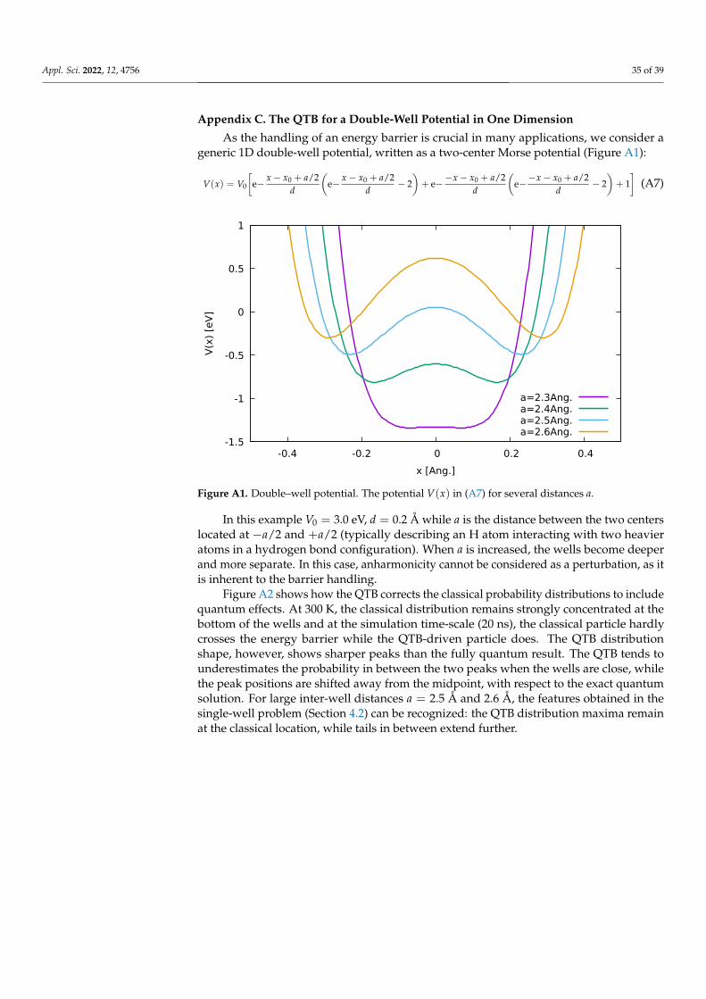
Appl. Sci. 2022, 12, 4756 35 of 39

Appendix C. The QTB for a Double-Well Potential in One Dimension

As the handling of an energy barrier is crucial in many applications, we consider ageneric 1D double-well potential, written as a two-center Morse potential (Figure A1):

V(x) = V0

[e− x− x0 + a/2

d

(e− x− x0 + a/2

d− 2)+ e−−x− x0 + a/2

d

(e−−x− x0 + a/2

d− 2)+ 1]

(A7)

-1.5

-1

-0.5

0

0.5

1

-0.4 -0.2 0 0.2 0.4

V(x

) [e

V]

x [Ang.]

a=2.3Ang.a=2.4Ang.a=2.5Ang.a=2.6Ang.

Figure A1. Double–well potential. The potential V(x) in (A7) for several distances a.

In this example V0 = 3.0 eV, d = 0.2 Å while a is the distance between the two centerslocated at −a/2 and +a/2 (typically describing an H atom interacting with two heavieratoms in a hydrogen bond configuration). When a is increased, the wells become deeperand more separate. In this case, anharmonicity cannot be considered as a perturbation, as itis inherent to the barrier handling.

Figure A2 shows how the QTB corrects the classical probability distributions to includequantum effects. At 300 K, the classical distribution remains strongly concentrated at thebottom of the wells and at the simulation time-scale (20 ns), the classical particle hardlycrosses the energy barrier while the QTB-driven particle does. The QTB distributionshape, however, shows sharper peaks than the fully quantum result. The QTB tends tounderestimates the probability in between the two peaks when the wells are close, whilethe peak positions are shifted away from the midpoint, with respect to the exact quantumsolution. For large inter-well distances a = 2.5 Å and 2.6 Å, the features obtained in thesingle-well problem (Section 4.2) can be recognized: the QTB distribution maxima remainat the classical location, while tails in between extend further.

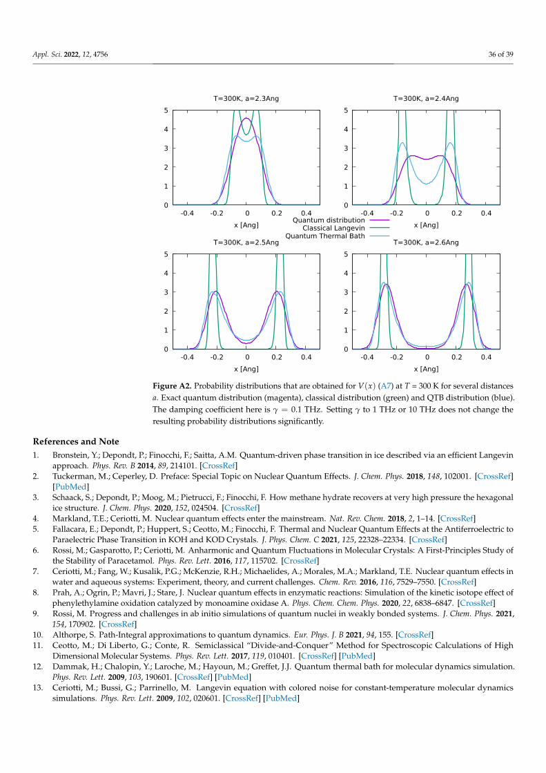
Appl. Sci. 2022, 12, 4756 36 of 39

0

1

2

3

4

5

-0.4 -0.2 0 0.2 0.4

x [Ang]

T=300K, a=2.3Ang

Quantum distributionClassical Langevin

Quantum Thermal Bath

0

1

2

3

4

5

-0.4 -0.2 0 0.2 0.4

x [Ang]

T=300K, a=2.4Ang

0

1

2

3

4

5

-0.4 -0.2 0 0.2 0.4

x [Ang]

T=300K, a=2.5Ang

0

1

2

3

4

5

-0.4 -0.2 0 0.2 0.4

x [Ang]

T=300K, a=2.6Ang

Figure A2. Probability distributions that are obtained for V(x) (A7) at T = 300 K for several distancesa. Exact quantum distribution (magenta), classical distribution (green) and QTB distribution (blue).The damping coefficient here is γ = 0.1 THz. Setting γ to 1 THz or 10 THz does not change theresulting probability distributions significantly.

References and Note1. Bronstein, Y.; Depondt, P.; Finocchi, F.; Saitta, A.M. Quantum-driven phase transition in ice described via an efficient Langevin

approach. Phys. Rev. B 2014, 89, 214101. [CrossRef]2. Tuckerman, M.; Ceperley, D. Preface: Special Topic on Nuclear Quantum Effects. J. Chem. Phys. 2018, 148, 102001. [CrossRef]

[PubMed]3. Schaack, S.; Depondt, P.; Moog, M.; Pietrucci, F.; Finocchi, F. How methane hydrate recovers at very high pressure the hexagonal

ice structure. J. Chem. Phys. 2020, 152, 024504. [CrossRef]4. Markland, T.E.; Ceriotti, M. Nuclear quantum effects enter the mainstream. Nat. Rev. Chem. 2018, 2, 1–14. [CrossRef]5. Fallacara, E.; Depondt, P.; Huppert, S.; Ceotto, M.; Finocchi, F. Thermal and Nuclear Quantum Effects at the Antiferroelectric to

Paraelectric Phase Transition in KOH and KOD Crystals. J. Phys. Chem. C 2021, 125, 22328–22334. [CrossRef]6. Rossi, M.; Gasparotto, P.; Ceriotti, M. Anharmonic and Quantum Fluctuations in Molecular Crystals: A First-Principles Study of

the Stability of Paracetamol. Phys. Rev. Lett. 2016, 117, 115702. [CrossRef]7. Ceriotti, M.; Fang, W.; Kusalik, P.G.; McKenzie, R.H.; Michaelides, A.; Morales, M.A.; Markland, T.E. Nuclear quantum effects in

water and aqueous systems: Experiment, theory, and current challenges. Chem. Rev. 2016, 116, 7529–7550. [CrossRef]8. Prah, A.; Ogrin, P.; Mavri, J.; Stare, J. Nuclear quantum effects in enzymatic reactions: Simulation of the kinetic isotope effect of

phenylethylamine oxidation catalyzed by monoamine oxidase A. Phys. Chem. Chem. Phys. 2020, 22, 6838–6847. [CrossRef]9. Rossi, M. Progress and challenges in ab initio simulations of quantum nuclei in weakly bonded systems. J. Chem. Phys. 2021,

154, 170902. [CrossRef]10. Althorpe, S. Path-Integral approximations to quantum dynamics. Eur. Phys. J. B 2021, 94, 155. [CrossRef]11. Ceotto, M.; Di Liberto, G.; Conte, R. Semiclassical “Divide-and-Conquer” Method for Spectroscopic Calculations of High

Dimensional Molecular Systems. Phys. Rev. Lett. 2017, 119, 010401. [CrossRef] [PubMed]12. Dammak, H.; Chalopin, Y.; Laroche, M.; Hayoun, M.; Greffet, J.J. Quantum thermal bath for molecular dynamics simulation.

Phys. Rev. Lett. 2009, 103, 190601. [CrossRef] [PubMed]13. Ceriotti, M.; Bussi, G.; Parrinello, M. Langevin equation with colored noise for constant-temperature molecular dynamics

simulations. Phys. Rev. Lett. 2009, 102, 020601. [CrossRef] [PubMed]

Appl. Sci. 2022, 12, 4756 37 of 39

14. Ceriotti, M.; Bussi, G.; Parrinello, M. Nuclear Quantum Effects in Solids Using a Colored-Noise Thermostat. Phys. Rev. Lett. 2009,103, 030603. [CrossRef] [PubMed]

15. Calvo, F.; Van-Oanh, N.T.; Parneix, P.; Falvo, C. Vibrational spectra of polyatomic molecules assisted by quantum thermal baths.Phys. Chem. Chem. Phys. 2012, 14, 10503–10506. [CrossRef]

16. Plé, T.; Huppert, S.; Finocchi, F.; Depondt, P.; Bonella, S. Anharmonic spectral features via trajectory-based quantum dynamics: Aperturbative analysis of the interplay between dynamics and sampling. J. Chem. Phys. 2021, 155, 104108. [CrossRef]

17. Mangaud, E.; Huppert, S.; Plé, T.; Depondt, P.; Bonella, S.; Finocchi, F. The Fluctuation–Dissipation Theorem as a Diagnosisand Cure for Zero-Point Energy Leakage in Quantum Thermal Bath Simulations. J. Chem. Theory Comput. 2019, 15, 2863–2880.[CrossRef]

18. Mauger, N.; Plé, T.; Lagardère, L.; Bonella, S.; Mangaud, E.; Piquemal, J.P.; Huppert, S. Nuclear Quantum Effects in liquid water atnear classical computational cost using the adaptive Quantum Thermal Bath. J. Phys. Chem. Lett. 2021, 12, 8285–8291. [CrossRef]

19. Kubo, R. The fluctuation–dissipation theorem. Rep. Prog. Phys. 1966, 29, 255. [CrossRef]20. Kubo, R.; Toda, M.; Hashitsume, N. Statistical Physics II: Nonequilibrium Statistical Mechanics; Springer Science & Business Media:

New York, NY, USA, 2012; Volume 31.21. Callen, H.; Welton, T. Irreversibility and Generalized Noise. Phys. Rev. 1951, 83, 34. [CrossRef]22. Herzog, D.P.; Mattingly, J.C. Ergodicity and Lyapunov Functions for Langevin Dynamics with Singular Potentials. Commun. Pure

Appl. Math. 2019, 72, 2231–2255. [CrossRef]23. Mori, H. Transport, collective motion, and Brownian motion. Prog. Theor. Phys. 1965, 33, 423–455. [CrossRef]24. Glatzel, F.; Schilling, T. The interplay between memory and potentials of mean force: A discussion on the structure of equations

of motion for coarse-grained observables. Europhys. Lett. 2022, 136, 36001. [CrossRef]25. Meyer, H.; Voigtmann, T.; Schilling, T. On the non-stationary generalized Langevin equation. J. Chem. Phys. 2017, 147, 214110.

[CrossRef] [PubMed]26. Ford, G.; Kac, M. On the quantum Langevin equation. J. Stat. Phys. 1987, 46, 803–810. [CrossRef]27. Ford, G.W.; Lewis, J.T.; O’Connell, R. Quantum langevin equation. Phys. Rev. A 1988, 37, 4419. [CrossRef]28. Cortes, E.; West, B.J.; Lindenberg, K. On the generalized Langevin equation: Classical and quantum mechanics. J. Chem. Phys.

1985, 82, 2708–2717. [CrossRef]29. Liu, J.; Zhang, Z. Path integral Liouville dynamics: Applications to infrared spectra of OH, water, ammonia, and methane. J.

Chem. Phys. 2016, 144, 034307. [CrossRef]30. Plé, T.; Huppert, S.; Finocchi, F.; Depondt, P.; Bonella, S. Sampling the thermal Wigner density via a generalized Langevin

dynamics. J. Chem. Phys. 2019, 151, 114114. [CrossRef]31. Bader, J.S.; Berne, B. Quantum and classical relaxation rates from classical simulations. J. Chem. Phys. 1994, 100, 8359–8366.

[CrossRef]32. Schmid, A. On a quasiclassical Langevin equation. J. Low Temp. Phys. 1982, 49, 609–626. [CrossRef]33. Hutter, J. Car–Parrinello molecular dynamics. WIREs Comput. Mol. Sci. 2012, 2, 604–612. [CrossRef]34. Ceriotti, M.; Bussi, G.; Parrinello, M. Colored-noise thermostats à la carte. J. Chem. Theory Comput. 2010, 6, 1170–1180. [CrossRef]35. Kapil, V.; Rossi, M.; Marsalek, O.; Petraglia, R.; Litman, Y.; Spura, T.; Cheng, B.; Cuzzocrea, A.; Meißner, R.H.; Wilkins, D.M.; et al.

i-PI 2.0: A universal force engine for advanced molecular simulations. Comput. Phys. Commun. 2019, 236, 214–223. [CrossRef]36. Druzbicki, K.; Krzystyniak, M.; Hollas, D.; Kapil, V.; Slavícek, P.; Romanelli, G.; Fernandez-Alonso, F. Hydrogen dynamics in

solid formic acid: Insights from simulations with quantum colored-noise thermostats. J. Phys. Conf. Ser. 2018, 1055, 012003.[CrossRef]

37. Prlj, A.; Marsili, E.; Hutton, L.; Hollas, D.; Shchepanovska, D.; Glowacki, D.R.; Slavícek, P.; Curchod, B.F. Calculating Photoab-sorption Cross-Sections for Atmospheric Volatile Organic Compounds. ACS Earth Space Chem. 2022, 6, 207–217. [CrossRef]

38. Kundu, A.; Govoni, M.; Yang, H.; Ceriotti, M.; Gygi, F.; Galli, G. Quantum vibronic effects on the electronic properties of solidand molecular carbon. Phys. Rev. Mat. 2021, 5, L070801. [CrossRef]

39. Barrat, J.L.; Rodney, D. Portable Implementation of a Quantum Thermal Bath for Molecular Dynamics Simulations. J. Stat. Phys.2011, 144, 679–689. [CrossRef]

40. Rossi, M.; Kapil, V.; Ceriotti, M. Fine tuning classical and quantum molecular dynamics using a generalized Langevin equation. J.Chem. Phys. 2018, 148, 102301. [CrossRef]

41. Miller, W.H. The semiclassical initial value representation: A potentially practical way for adding quantum effects to classicalmolecular dynamics simulations. J. Phys. Chem. A 2001, 105, 2942–2955. [CrossRef]

42. Liu, J. Recent advances in the linearized semiclassical initial value representation/classical W igner model for the thermalcorrelation function. Int. J. Quantum Chem. 2015, 115, 657–670. [CrossRef]

43. Basire, M.; Borgis, D.; Vuilleumier, R. Computing Wigner distributions and time correlation functions using the quantum thermalbath method: Application to proton transfer spectroscopy. Phys. Chem. Chem. Phys. 2013, 15, 12591. [CrossRef] [PubMed]

44. Beutier, J.; Borgis, D.; Vuilleumier, R.; Bonella, S. Computing thermal Wigner densities with the phase integration method. J.Chem. Phys. 2014, 141, 084102. [CrossRef] [PubMed]

45. Li, C.; Paesani, F.; Voth, G.A. Static and Dynamic Statistical Correlations in Water: Comparison of Classical Ab Initio MolecularDynamics at Elevated Temperature with Path Integral Simulations at Ambient Temperature. 2022. Available online: https://chemrxiv.org/engage/chemrxiv/article-details/61d77876db142e078eb6257f (accessed on 4 March 2022).

Appl. Sci. 2022, 12, 4756 38 of 39

46. Ben-Nun, M.; Levine, R.D. Conservation of zero-point energy in classical trajectory computations by a simple semiclassicalcorrespondence. J. Chem. Phys. 1994, 101, 8768–8783. [CrossRef]

47. Habershon, S.; Manolopoulos, D.E. Zero point energy leakage in condensed phase dynamics: An assessment of quantumsimulation methods for liquid water. J. Chem. Phys. 2009, 131, 244518. [CrossRef] [PubMed]

48. Althorpe, S.C.; Alvertis, A.; Barford, W.; Benson, R.L.; Burghardt, I.; Giannini, S.; Habershon, S.; Hammes-Schiffer, S.; Hay, S.;Iyengar, S.; et al. Zero-point energy and tunnelling: General discussion. Faraday Discuss. 2020, 221, 478–500. [CrossRef]

49. Hernández-Rojas, J.; Calvo, F.; Noya, E.G. Applicability of quantum thermal baths to complex many-body systems with variousdegrees of anharmonicity. J. Chem. Theory Comput. 2015, 11, 861–870. [CrossRef]

50. Brieuc, F.; Bronstein, Y.; Dammak, H.; Depondt, P.; Finocchi, F.; Hayoun, M. Zero-point energy leakage in Quantum Thermal Bathmolecular dynamics simulations. J. Chem. Theory Comput. 2016, 12, 5688–5697. [CrossRef]

51. Bedoya-Martinez, O.N.; Barrat, J.L.; Rodney, D. Computation of the thermal conductivity using methods based on classical andquantum molecular dynamics. Phys. Rev. B 2014, 89, 014303. [CrossRef]

52. Deacon, C.; de Bruyn, J.; Whitehead, J. A simple method of determining Debye temperatures. Ame. J. Phys. 1992, 60, 422.[CrossRef]

53. Dammak, H.; Antoshchenkova, E.; Hayoun, M.; Finocchi, F. Isotope effects in lithium hydride and lithium deuteride crystals bymolecular dynamics simulations. J. Phys. Condens. Matter 2012, 24, 435402. [CrossRef]

54. Loubeyre, P.; Le Toullec, R.; Hanfland, M.; Ulivi, L.; Datchi, F.; Hausermann, D. Equation of state of 7LiH and 7LiD from x-raydiffraction to 94 GPa. Phys. Rev. B 1998, 57, 10403. [CrossRef]

55. Calvo, F.; Naumkin, F.; Wales, D. Nuclear quantum effects on the stability of cationic neon clusters. Chem. Phys. Lett. 2012,551, 38–41. [CrossRef]

56. Ceriotti, M.; Miceli, G.; Pietropaolo, A.; Colognesi, D.; Nale, A.; Catti, M.; Bernasconi, M.; Parrinello, M. Nuclear quantum effectsin ab initio dynamics: Theory and experiments for lithium imide. Phys. Rev. B 2010, 82, 174306. [CrossRef]

57. Benoit, M.; Marx, D.; Parrinello, M. Tunnelling and zero-point motion in high-pressure ice. Nature 1998, 392, 258–261. [CrossRef]58. Bronstein, Y.; Depondt, P.; Finocchi, F. Thermal and nuclear quantum effects in the hydrogen bond dynamical symmetrization

phase transition of δ-AlOOH. Eur. J. Mineral. 2017, 29, 385–395. [CrossRef]59. Tsuchiya, J.; Tsuchiya, T. Elastic properties of δ-AlOOH under pressure: First principles investigation. Phys. Earth Planet. Inter.

2009, 174, 122–127. [CrossRef]60. Simonova, D.; Bykova, E.; Bykov, M.; Kawazoe, T.; Simonov, A.; Dubrovinskaia, N.; Dubrovinsky, L. Structural Study of δ-AlOOH

Up to 29 GPa. Minerals 2020, 10, 1055. [CrossRef]61. Bronstein, Y.; Depondt, P.; Bove, L.E.; Gaal, R.; Saitta, A.M.; Finocchi, F. Quantum versus classical protons in pure and salty ice

under pressure. Phys. Rev. B 2016, 93, 024104. [CrossRef]62. Calvo, F.; Falvo, C.; Parneix, P. Atomistic modeling of vibrational action spectra in polyatomic molecules: Nuclear quantum

effects. J. Phys. Chem. A 2014, 118, 5427. [CrossRef]63. Dhar, A.; Roy, D. Heat Transport in Harmonic Lattices. J. Stat. Phys. 2006, 125, 801–820. [CrossRef]64. Wang, J.S. Quantum thermal transport from classical molecular dynamics. Phys. Rev. Lett. 2007, 99, 160601. [CrossRef]65. Wang, J.S.; Ni, X.; Jiang, J.W. Molecular dynamics with quantum heat baths: Applications to nanoribbons and nanotubes. Phys.

Rev. B 2009, 80, 224302. [CrossRef]66. Zhang, W.; Fisher, T.S.; Mingo, N. The Atomistic Green’s Function Method: An Efficient Simulation Approach for Nanoscale

Phonon Transport. Numer. Heat Transf. Part B Fundam. 2007, 51, 333–349. [CrossRef]67. Sadasivam, S.; Che, Y.; Huang, Z.; Chen, L.; Kumar, S.; Fisher, T. The atomistic Green’s function method for interfacial phonon

transport. Ann. Rev. Heat Transf. 2014, 17, 89–145. [CrossRef]68. Wang, C.Z.; Chan, C.T.; Ho, K.M. Tight-binding molecular-dynamics study of phonon anharmonic effects in silicon and diamond.

Phys. Rev. B 1990, 42, 11276. [CrossRef]69. Qi, T.; Reed, E.J. Simulations of Shocked Methane Including Self-Consistent Semiclassical Quantum Nuclear Effects. J. Phys.

Chem. A 2012, 116, 10451–10459. [CrossRef]70. Parrinello, M.; Rahman, A. Study of an F center in molten KCl. J. Chem. Phys. 1984, 80, 860–867. [CrossRef]71. Ceriotti, M.; Manolopoulos, D.E.; Parrinello, M. Accelerating the convergence of path integral dynamics with a generalized

Langevin equation. J. Chem. Phys. 2011, 134, 084104. [CrossRef]72. Ceriotti, M.; Manolopoulos, D.E. Efficient First-Principles Calculation of the Quantum Kinetic Energy and Momentum Distribution

of Nuclei. Phys. Rev. Lett. 2012, 109, 100604. [CrossRef]73. Uhl, F.; Marx, D.; Ceriotti, M. Accelerated path integral methods for atomistic simulations at ultra-low temperatures. J. Chem.

Phys. 2016, 145, 054101. [CrossRef]74. Kapil, V.; Wilkins, D.; Lan, J.; Ceriotti, M. Inexpensive modeling of quantum dynamics using path integral generalized Langevin

equation thermostats. J. Chem. Phys. 2020, 152, 124104. [CrossRef]75. Giberti, F.; Hassanali, A.A.; Ceriotti, M.; Parrinello, M. The role of quantum effects on structural and electronic fluctuations in

neat and charged water. J. Phys. Chem. B 2014, 118, 13226–13235. [CrossRef]76. Fang, W.; Chen, J.; Rossi, M.; Feng, Y.; Li, X.Z.; Michaelides, A. Inverse temperature dependence of nuclear quantum effects in

dna base pairs. J. Phys. Chem. Lett. 2016, 7, 2125–2131. [CrossRef]

Appl. Sci. 2022, 12, 4756 39 of 39

77. Lamaire, A.; Wieme, J.; Rogge, S.M.J.; Waroquier, M.; Van Speybroeck, V. On the importance of anharmonicities and nuclearquantum effects in modelling the structural properties and thermal expansion of MOF-5. J. Chem. Phys. 2019, 150, 094503.[CrossRef]

78. Brieuc, F.; Dammak, H.; Hayoun, M. Quantum thermal bath for path integral molecular dynamics simulation. J. Chem. TheoryComput. 2016, 12, 1351–1359. [CrossRef]

79. Schran, C.; Brieuc, F.; Marx, D. Converged colored noise path integral molecular dynamics study of the zundel cation down toultralow temperatures at coupled cluster accuracy. J. Chem. Theory Comput. 2018, 14, 5068–5078. [CrossRef]

80. Brieuc, F.; Schran, C.; Uhl, F.; Forbert, H.; Marx, D. Converged quantum simulations of reactive solutes in superfluid helium: TheBochum perspective. J. Chem. Phys. 2020, 152, 210901. [CrossRef]

81. Lagardère, L.; Jolly, L.H.; Lipparini, F.; Aviat, F.; Stamm, B.; Jing, Z.F.; Harger, M.; Torabifard, H.; Cisneros, G.A.; Schnieders, M.J.;et al. Tinker-HP: A massively parallel molecular dynamics package for multiscale simulations of large complex systems withadvanced point dipole polarizable force fields. Chem. Sci. 2018, 9, 956–972. [CrossRef]

82. Habershon, S.; Markland, T.E.; Manolopoulos, D.E. Competing quantum effects in the dynamics of a flexible water model. J.Chem. Phys. 2009, 131, 024501. [CrossRef]

83. Li, X.Z.; Walker, B.; Michaelides, A. Quantum nature of the hydrogen bond. Proc. Natl. Acad. Sci. USA 2011, 108, 6369–6373.[CrossRef]

84. Benson, R.L.; Trenins, G.; Althorpe, S.C. Which quantum statistics–classical dynamics method is best for water? Faraday Discuss.2019, 221, 350–366. [CrossRef] [PubMed]

85. Benson, R.L.; Althorpe, S.C. On the ‘Matsubara heating’ of overtone intensities and Fermi splittings. J. Chem. Phys. 2021,155, 104107. [CrossRef] [PubMed]

86. A paradigmatic case is the Density Functional Theory, which has a longstanding record of controversial approximations beforebecoming the most popular scheme for solving the many-electron problem, at least for the ground state; see, e.g.,: Kohn, W.“Electronic Structure of Matter—Wave Functions and Density Functionals”, Nobel Lecture. Rev. Mod. Phys. 1999, 71, 1253.[CrossRef]

87. Oppenheim, A.V.; Schafer, R.W.; Buck, J.R. Discrete-Time Signal Processing; Prentice Hall: Englewood Cliffs, NJ, USA, 1999.