The Addison-Wesley Series in Finance

Copeland/Weston

Financial Themy

and Cmporate Policy

Dufey/Giddy Cases in International Finance

Eakins, Finance: Investments,

Institutions, and Management

Eiteman!Stonehill!Moffett

- Multinational Business Finance

Gitman

Principles of Managerial Finance

Gitman

Principles of Managerial Finance

-Brief Edition

Gitman/J oehnk

Fundamentals of Investing

Gitman!Madura

Introduction to Finance

Hughes/MacDonald

International Banking:

Text and Cases

Madura

Personal Finance

Marthinsen

Risk Takers: Uses and Abuses

of Financial Derivatives

McDonald

Derivatives Markets

Megginson

Cmporate Finance Themy

Melvin

International Money and Finance

Mishkin/Eakins

Financial Markets and Institutions

Moffett

Cases in International Finance

Moffett/Stonehill!Eiteman

Fundamentals of

Multinational Finance

Rejda

Principles of Risk Management

and Insurance

Solnik!McLeavey

International Investments

Derivatives Markets Second Edition

R 0 B E R T L. M c D 0 N A L D Northwestern University

Kellogg School of Management

Boston San Francisco New York

London Toronto Sydney Tokyo Singapore Madrid

Mexico City Munich Paris Cape Town Hong Kong Montreal

Editor-in-Chief: Denise Clinton Senior Sponsoring Editor: Donna Battista Senior Project Manager: Mary Clare McEwing Development Editor: Marjorie Singer Anderson Senior Production Supervisor: Nancy Fenton Executive Marketing Manager: Stephen Frail Design Manager: Regina Hagen Kolenda Text Designer: Regina Hagen.Kolenda Cover Designer: Rebecca Light Co�er and Interior Image: Private Collection/Art for After Hours/SuperStock Senior Manufacturing Btt')'er: Carol Melville Supplements Editor: Marianne Groth Project Management: Elm Street Publishing Services, Inc.

Copyright ©2006 Pearson Education, Inc.

All rights reserved. No part of this publication may be reproduced, stored in a retrieval system, or transmitted, in any form or by any means, electronic, mechanical, photocopying, recording, or otherwise, without the prior written permission of the publisher.

For information on obtaining permission for the use of material from this work, please submit a written request to Pearson Education, Inc., Rights and Contracts Department, 75 Arlington Street, Suite 300, Boston, MA 02116 or fax your request to (617) 848-7047 . Printed in the United States of America .

Library of Congress Cataloging-in-Publication Data McDonald, Robert L. (Robert Lynch), 1954-

Derivatives markets, 2e I Robert L. McDonald. p.cm.

Includes index. ISBN 0-321-28030-X 1. Derivative securities. I. Title.

HG6024.A3 M3946 2006 332.64'5-dc21 ISBN 0-321-28030-X 12345678910-HT-09 08 07 06 05

Fo1· Irene, Claire, David, and Hemy

Preface XX1

Chapter 1 Introduction to Derivatives

1.1 What Is a Derivative? 1 Uses of Derivatives 2 Perspectives on Derivatives 3 Financial Engineering and Security

Design 3

1.2 The Role of Financial Markets 4 Financial Markets and the Averages 4 Risk-Sharing 5

1.3 Derivatives in Practice 6 Growth in Derivatives Trading 7 How Are Derivatives Used? 10

1.4 Buying and Short-Selling Financial Assets 11 Buying an Asset 11 Short-Selling 12 The Lease Rate of an Asset 14 Risk and Scarcity in Short-Selling 15 Chapter Sumn!al)' 16

Further Reading 16

Problems 17

PART ONE INSURANCE,

HEDGING, AND SIMPLE STRATEGIES

19

Chapter 2 An Introduction to Forwards and Options 21 2.1 Forward Contracts 21

The Payoff on a Forward Contract 23 Graphing the Payoff on a Forward

Contract 25

Comparing a Forward and Outright Purchase 26

Zero-Coupon Bonds in Payoff and Profit Diagrams 28

Cash Settlement Versus D� livery 3 0 Credit Risk 3 0

2.2 Call Options 31 Option Terminology 3 2 Payoff and Profit for a Purchased Call

Option 3 3 Payoff and Profit for a Written Call

Option 3 7

2.3 Put Options 38 Payoff and Profit for a Purchased Put

Option 3 9 Payoff and Profit for a Written Put

Option 40 The "Moneyness" of an Option 4 3

2.4 Summary of Forward and Option Positions 43 Long Positions 44

Short Positions 44

2.5 Options Are Insurance 45 Homeowner's Insurance Is a Put Option 45 But I Thought Insurance Is Prudent and Put

Options Are Risky... 47 Call Options Are Also Insurance 4 7

2.6 Example: Equity-Linked CDs 48 Graphing the Payoff on the CD 49 Economics of the CD 50 Why Equity-Linked COs? 5 1 Chapter Sumn!al)' 52

Further Reading 53

Problems 54

Appendix 2.A: More on Buying a Stock Option 56

Dividends 5 6

vii

Viii � C O N T ENTS

Exercise 57

Margins for Written Options 57

Taxes 58

Chapter 3 Insurance, Collars, and Other Strategies 59 3.1 Basic Insurance Strategies 59

Insuring a Long Position: Floors' 59

Insuring a Short Position: Caps 6 2 Selling Insurance 6 3

3.2 Synthetic Forwards 66 Put-Call Parity 6 8

3.3- Spreads and Collars 70 Bull and Bear Spread s 7 1 Box Spread s 7 2 Ratio Spread s 7 3 Collars 7 3

3.4 Speculating on Volatility 78 Strad d les 78 Butterfly Spread s 8 1 Asymmetric Butterfly Spread s 82

3.5 Example: Another Equity-Linked Note 83 Chapter Summary 85

Further Reading 86

Problems 87

Chapter 4 Introduction to Risk Management 91 4.1 Basic Risk Management: The

Producer's Perspective 91 Hed ging with a Forward Contract 9 2 Insurance: Guaranteeing a Minimum Price

with a Put Option 9 3 Insuring by Selling a Call 95 Ad justing the Amount of Insurance 96

4.2 Basic Risk Management: The Buyer's Perspective 98 Hed ging with a Forward Contract 9 8

Insurance: Guaranteeing a Maximum Price with a Call Option 9 9

4.3 Why Do Firms Manage Risk? 100 An Example Where Hed ging Ad d s

Value 10 1 Reasons to Hed ge 10 3 Reasons Not to Hed ge 106

Empirical Evidence on Hed ging 106

4.4 Golddiggers Revisited 108 Selling the Gain: Collars 10 8 Other Collar Strategies 1 12 Paylater Strategies 1 13

4.5 Selecting the Hedge Ratio 113 Cross-Hed ging 114

Quantity Uncertainty 116 Chapter Stmti11G1)' 119

Further Reading 120

Problems 120

PART 1WO FORWARDS,

FUTURES, AND SWAPS 125

Chapter 5 Financial Forwards and Futures 127 5.1 Alternative Ways to Buy a Stock 12 7 5.2 Prepaid Forward Contracts on

Stock 128 Pricing the Prepaid Forward by

Analogy 128 Pricing the Prepaid Forward by Discounted

Present Value 129 Pricing the Prepaid Forward by

Arbitrage 129

Pricing Prepaid Forward s with Divid end s 13 1

5.3 Forward Contracts on Stock 133 Creating a Synthetic Forward

Contract 135 Synthetic Forward s in Market-Making and

Arbitrage 136 ·

No-Arbitrage Bounds with Transaction Costs 13 8

Quasi-Arbitrage 13 9 Does the Forward Price Predict the Future

Price? 140 An Interpretation of the Forward Pricing

Formula 14 1

5.4 Futures Contracts 142 The S&P 500 Futures Contract 14 3 Margins and Marking to Market 144 Comparing Futures and Forward

Prices 14 6 Arbitrage in Practice: S&P 500 Index

Arbitrage 14 7 Quanta Index Contracts 149

5.5 Uses of Index Futures 150 Asset Allocation 150 Cross-hedging with Index Futures 15 1

5.6 Currency Contracts 154 Currency Prepaid Forward 155 Currency Forward 15 6 Covered Interest Arbitrage 15 6

5.7 Eurodollar Futures 160 Chapter SumnWI)' 160

Further Reading 162

Problems 162

Appendix 5.A: Taxes and the Forward Price 166

Appendix S.B: Equating Forwards and Futures 166

Chapter 6 Commodity Forwards and Futures 169

6.1 Introduction to Commodity Forwards 169

6.2 Equilibrium Pricing of Commodity Forwards 171

· 6.3 Nonstorability: Electricity 172 6.4 Pricing Commodity Forwards by

Arbitrage: An Example 17 4

C O N T ENTS � ix

An Apparent Arbitrage and Resolution 175

Pencils Have a Positive Lease Rate 17 6

6.5 The Commodity Lease Rate 178 The Lease Market for a Commodity 178 Forward Prices and the Lease Rate 17 9

6.6 Carry Markets 181 Storage Costs and Forward Prices 18 1 Storage Costs and the Lease Rate 18 2 The Convenience Yield 18 2

6.7 Gold Futures 184 Gold Investments 18 7 Evaluation of Gold Production 18 7

6.8 Seasonality: The Corn Forward Market 188

6.9 Natural Gas 191 6.10 Oil 194 6.11 Commodity Spreads 195 6.12 Hedging Strategies 196

Basis Risk 197 Hedging Jet Fuel with Crude Oil 19 9 Weather Derivatives 19 9 Chapter SummGI)' 200

Further Reading 201

Problems 201

Chapter 7 Interest Rate Forwards and Futures 205

7.1 Bond Basics 205 Zero-Coupon Bonds 20 6 Implied Forward Rates 20 8 Coupon Bonds 210

Zeros from Coupons · 2 11 Interpreting the Coupon Rate 2 12 Continuously Compounded Yields 2 13

7.2 Forward Rate Agreements, Eurodollars, and Hedging 214 Forward Rate Agreements 214

Synthetic FRAs 216 Eurodollar Futures 218 Interest Rate Strips and Stacks 223

X � C O NTENTS

7.3 Duration and Convexity 223 Duration 224 Duration Matching 227 Convexity 228

7.4 Treasury-Bond and Treasury-Note Futures 230

7.5 Repurchase Agreements 233 Chapter Summary 235

Further Reading 23 7

Problems 237

Appendix 7.A: Interest Rate and Bond Price Conventions 241

Bonds 242 Bills 244

Chapter 8 Swaps 247 8.1 An Example of a Commodity

Swap 247 Physical Versus Financial Settlement 248

Why Is the Swap Price Not $20 .50 ? 250

The Swap Counterpart}' 250 The Market Value of a Swap 25 3

8.2 Interest Rate Swaps 254 A Simple Interest Rate Swap 254 Pricing and the Swap Counterpart}' 255 Computing the Swap Rate in General 257

The Swap Curve 258 The Swap's Implicit Loan Balance 260 Deferred Swap s 26 1

Why Swap Interest Rates? 26 2 Am ortizing and Accreting Swaps 26 3

8.3 Currency Swaps 264 Currency Swap Formulas 267

Other Currency Swaps 267

8.4 Commodity Swaps 268 The Commodity Swap Price 26 8 Swaps with Variable Quantity and

Price 26 9

8.5 Swaptions 271 8.6 Total Return Swaps 272

Chapter Sumnzal)' 274

Further Reading 275

Problems 275

PART THREE OPTIONS 279

Chapter 9 Parity and Other Option Relationships 281 9.1 Put-Call Parity 281

Options on Stocks 28 3 Options on Currencies 28 6 Options on Bonds 28 6

9.2 Generalized Parity and Exchange Options 287 Options to Exchange Stock 28 8 What Are Calls and Puts? 28 9 Currency Options 29 0

9.3 Comparing Options with Respect to Style, Maturity, and Strike 292 European Versus American Options 29 3 Maximum and Minimum Option

Prices 29 3 Early Exercise for American Options 29 4 Time to Expiration 297 Different Strike Prices 29 9

Exercise and Moneyness 3 0 4 Chapter Szmmzary• 305

Further Reading 306

Problems 306

Appendix 9.A: Parity Bounds for American Options 310

Appendix 9.B: Algebraic Proofs of Strike-Price Relations 311

Chapter 10 Binomial Option Pricing: I 313 10.1 A One-Period Binomial Tree 313

Computing the Option Price 3 14 The Binomial Solution 3 15 Arbitraging a Mispriced Option 3 18

10.2

10.3 10.4 10.5

A Graphical Interpretation of the Binomial Formula 3 19

Risk-Neutral Pricing 3 20 Constructing a Binomial Tree 3 21 Another One-Period Example 3 22 Summary 3 22

Two or More Binomial Periods 323 A Two-Period European Call 3 2 3 Many Binomial Periods 3 26

Put Options 328 American Options 329 Options on Other Assets 330 Option on a Srock Index 3 3 0 Options on Currencies 3 3 2 Options on Futures Contracts 3 3 2 Options on Commodities 3 3 4 Options on Bonds 3 3 5 Summary 3 3 6 Chapter Summary 33 7

Further Reading 337

Problems 338

Appendix 1 O.A: Taxes and Option Prices 341

Chapter 11 Binomial Option Pricing: II 343 11.1 Understanding Early Exercise 343 11.2 Understanding Risk-Neutral

Pricing 346 The Risk-Neutral Probability 3 4 6 Pricing an Option Using Real

Probabilities 3 47

11.3 The Binomial Tree and Lognormality 351 The Random Walk Model 3 5 1 Modeling Stock Prices as a Random

Walk 3 5 2 Continuously Compounded Returns 353 The Standard Deviation of Returns 3 54 The Binomial Model 3 55 Lognormality and the Binomial

Model 3 55

11.4 11.5

CO NTENTS � xi

Alternative Binomial Trees 3 5 8 Is the Binomial Model Realistic? 3 59

Estimating Volatility 360 Stocks Paying Discrete Dividends 361 Modeling Discrete Dividends 3 6 1 Problems with the Discrete Dividend

Tree 3 6 2 A Binomial Tree Using the Prepaid

Forward 3 6 3 Chapter Summary 365

Further Reading 366

Problems 366

Appendix ll.A: Pricing Options with True Probabilities 369

Appendix 11.B: Why Does Risk-Neutral Pricing Work? 369

Utility-Based Valuation 3 6 9 Standard Discounted Cash Flow 3 7 1

Risk-Neutral Pricing 3 7 1 Example 3 7 2 Why Risk-Neutral Pricing Works 3 73

Chapter 12 The Black-Scholes Formula 375 12.1 Introduction to the Black-Scholes

Formula 375 Call Options 3 7 5 Put Options 378 When Is the Black-Scholes Formula

Valid? 3 7 9

12.2 Applying the Formula to Other Assets 379 Options on Srocks with Discrete

Dividends 3 8 0 Options on Currencies 3 8 1 Options on Futures 3 8 1

12.3 Option Greeks 382 Definition of the Greeks 3 8 2 Greek Measures for Portfolios 3 88

Option Elasticity 3 8 9

Xii � C O NT E NTS

12.4 Profit Diagrams Before Maturity 395 Purchased Call Option 3 96 Calendar Spreads 3 97

12.5 Implied Volatility 400 Computing Implied Volatility 400

Using Implied Volatility 40 2

12.6 Perpetual American Options 403 Barrier Present Values 403 Perpetual Calls 404 Perpetual Puts 404 Chapter Summary 405

Further Readilzg 405

Problems 406

Appendix 12.A: The Staizdard Normal Distribution 409

Appendix 12.B: Formulas for Option Greeks 410

. Delta 410 Gamma 410 Theta 410 Vega 411 Rho 411 Psi 411

Chapter 13 Market-Making and Delta-Hedging 41 3 13.1 What Do Market-Makers Do? 413 13.2 Market-Maker Risk 414

Option Risk in the Absence of Hedging 414

Delta and Gamma as Measures of Exposure 41 6

13.3 Delta-Hedging 417 An Example of Delta-Hedging for 2

Days 417 Interpreting the Profit Calculation 418 Delta-Hedging for Several Days 4 20

A Self-Financing Portfolio: The Stock .Moves One a 4 22

13.4 The Mathematics of Delta-Hedging 422 Using Gamma to Better Approximate the

Change in the Option Price 4 23

Delta-Gamma Approximations 4 24 Theta: Accounting for Time 4 25 Understanding the Market-Maker's

Profit 4 27

13.5 The Black-Scholes Analysis 429 The Black-Scholes Argument 4 29 Delta-Hedging of American Options 430

What Is the Advantage to Frequent Re-Hedging? 43 1

Delta-Hedging in Practice 432

Gamma-Neutrality 433

13.6 Market-Making as Insurance 436 Insurance 436 Market-Makers 437 Chapter Swnmmy 438

Further Reading 438

Problems 438

Appendix 13.A: Taylor Series Approximations 441

Appendix 13.B: Greeks in the Binomial Model 441

Chapter 14 Exotic Options: I 443 14.1 Introduction 443 14.2 Asian Options 444

XYZ's Hedging Problem 445 Options on the Average 446 Comparing Asian Options 447

An Asian Solution for XYZ 448

14.3 Barrier Options 449 Types of Barrier Options 450 Currency Hedging 451

14.4 Compound Options 453 Compound Option Parity 454

14.5 14.6

Options on Dividend-Paying Stocks 455 Currency Hedging with Compound

Options 456

Gap Options 457 Exchange Options 459 European Exchange Options 459 Chapter Summary 461

Further Reading 462

Problems 462

Appendix 14.A: Pricing Formulas for Exotic Options 466

Asian Options Based on the Geometric Average 466

Compound Options 467 Infinitely Lived Exchange Option 46 8

PART FOUR FINANCIAL

ENGINEERING AND APPLICATIONS

471

Chapter 15 Financial Engineering and Security Design 473 15.1 The Modigliani-Miller Theorem 473 15.2 Pricing and Designing Structured

Notes 474 Zero-Coupon Bonds 474 Coupon Bonds 475

Equity-Linked Bonds 476 Commodity-Linked Bonds 478 Currency-Linked Bonds 48 1

15.3 Bonds with Embedded Options 482 Options in Coupon Bonds 482 Options in Equity-Linked Notes 483 Valuing and Structuring an Equity-Linked

CD 483 Alternative Structures 48 5

15.4 Engineered Solutions for Golddiggers 486 Gold-Linked Notes 486 Notes with Embedded Options 48 8

15.5 Strategies Motivated by Tax and Regulatory Considerations 490 Capital Gains Deferral· 490

Tax-Deductible Equity 495 Chapter Summary 498

Further Reading 498

Problems 498

CO NTE NTS � xiii

Chapter 16 Corporate Applications 503 16.1 Equity, Debt, and Warrants 503

Debt and Equity as Options 503 Multiple Debt Issues 51 1 Warrants 512 Convertible Bonds 513 Callable Bonds 516

Bond Valuation Based on the Stock Price 520

Other Bond Features S20 Put Warrants 522

16.2 Compensation Options 523 Whose Valuation? 525 Valuation Inputs 527

An Alternative Approach to Expensing Option Grants 52 8

Repricing of Compensation Options 53 1 Reload Options 532

Level3 Communications 534

16.3 The Use of Collars in Acquisitions 538 The Northrop Grumman-TRY Merger

53 8 Chapter Summary 542

Further Reading 542

Problems 543

Chapter 17 Real Options 547 17.1 Investment and the NPV Rule 548

Static NPV 548 The Correct Use of NPV 549 The Project as an Option 550

17.2 Investment under Uncertainty 551 A Simple DCF Problem 551 Valuing Derivatives on the Cash Flow

552 Evaluating a Project with a 2 -Year

Investment Horizon 554 Evaluating the Project with an Infinite

Investment Horizon 558

XiV � C O NTENTS

17.3 Real Options in Practice 55 8 Peak-Load Electricity Generation 559 Research and Development 563

17.4 Commodity Extraction as an Option 565 Single-Barrel Extraction under

Certainty 565 Single-Barrel Extraction under

Uncertainty 569 Valuing an Infinite Oil Reserve 570

17.5 Commodity Extraction with Shut-Down and Restart Options 572 Permanent Shutting Down 574

Investment When Shutdown Is Possible 576

Restarting Production 57 8 Additional Options 57 8 Chapter Swnmal)' 579

Further Reading 580

Problems 580

Appendix 17.A: Calculation of Optimal Time to Drill an Oil Well 583

Appendix 17.B: The Solution with Shutting Down and Restarting 583

PART FIVE ADVANCED PRICING

THEORY 5 85

Chapter 1 8 The Lognormal Distribution 587 18.1 The Normal Distribution 587

Converting a-Normal Random Variable to Standard Normal 590

Sums of Normal Random Variables 591

18.2 The Lognormal Distribution 593 18.3 A Lognormal Model of Stock

Prices 595 18.4 Lognormal Probability

Calculations 598 Probabilities 599

Lognormal Confidence Intervals 6 0 0 The Conditional Expected Price 6 0 2 The Black-Scholes Formula 6 04

18.5 Estimating the Parameters of a Lognormal Distribution 605

18.6 How Are Asset Prices Distributed? 608 Histograms 6 0 8 Normal Probability Plots 6 09 Chapter Summary 613

Further Reading 613

Problems 614

Appendix 18.A: The Expectation of a Lognomzal Variable 615

Appendix 18.B: Constructing a Normal Probability Plot 616

Chapter 19 Monte Carlo Valuation 61 7 19.1 Computing the Option Price as a

Discounted Expected Value 617 Valuation with Risk-Neutral

Probabilities 61 8 Valuation with True Probabilities 6 19

19.2 Computing Random Numbers 621 Using Sums of Uniformly Distributed

Random Variables 6 22 Using the Inverse Cumulative Normal

Distribution 6 22

19.3 Simulating Lognormal Stock Prices 623 Simulating a Sequence of Stock

Prices 623

19.4 Monte Carlo Valuation 624 Monte Carlo Valuation of a European

Call 6 25 Accuracy of Monte Carlo 6 26 Arithmetic Asian Option 6 27

19.5 Efficient Monte Carlo Valuation 630 Control Variate Method 63 0

Other Monte Carlo Methods 63 2

19.6 Valuation of American Options 633

19.7 The Poisson Distribution 636 19.8 Simulating Jumps with the Poisson

Distribution 639 Multiple Jumps 6 4 3

19.9 Simulating Correlated Stock Prices 643 Generating 11 Correlated Lognormal

Random Variables 644 Chapter Summary 645

Further Reading 645

Problems 646

Appendix 19.A: Formulas for Geometric Average Options 648

Chapter 20 Brownian Motion and Ito's Lemma 649 20.1 The Black-Scholes Assumption about

Stock Prices 649 20.2 Brownian Motion 650

Definition of Brownian Motion 6 50 Properties of Brownian Motion 6 5 2 Arithmetic Brownian Motion 6 5 3 The Ornstein-Uhlenbeck Process 6 54

20.3 Geometric Brownian Motion 655 Lognormality 6 55 Relative Importance of the Drift and Noise Terms 656

Correlated Ito Processes 6 57 Multiplication Rules 6 58

20.4 The Sharpe Ratio 659 20.5 The Risk-Neutral Process 660

20.6 Ito's Lemma 663 Functions of an Ito Process 66 3 Multivariate Ito's Lemma 665

20.7 Valuing a Claim on sa 666 The Process Followed by S" 66 7 Proving the Proposition 66 8 Specific Examples 669 Valuing a Claim on S" Q" 670

20.8 Jumps in the Stock Price 672 Chapter Sumntal)' 674

C O N T E NTS � XV

Further Reading 674

Problems 675

Chapter 2 1 The Black-Scholes Equation 679 21.1 Differential Equations and Valuation

under Certainty 679 The Valuation Equation 6 8 0 Bonds 6 8 0 Dividend-Paying Stocks.

6 8 1

The General Structure 6 8 1

21.2 The Black-Scholes Equation 681 Verif ying the Formula f or a

Derivative 6 8 3 The Black-Scholes Equation and

Equilibrium Returns 686 What If the Underlying Asset Is Not an

Investment Asset? 6 8 8

21.3 Risk-Neutral Pricing 690 Interpreting the Black-Scholes

Equation 690 The Backward Equation 691 Derivative Prices as Discounted Expected

Cash Flows 69 2

21.4 Changing the Numeraire 693 21.5 Option Pricing When the Stock Price

CanJump 696 Merton's Solution f or Diversifiable Jumps

697 Chapter Summa/)' 698

Further Reading 698

Problems 699

Appendix 21.A: Multivariate Black-Scholes Analysis 700

Appendix 21.B: Proof of Proposition 21.1 701

Chapter 22 Exotic Options: II 703 22.1 Ali-or-Nothing Options 703

Terminology 70 3 Cash-or-Nothing Options 704

Asset-or-Nothing Options 706

XVi � C O NT E NTS

22.2

22.4

Ordinary Options and Gap Options 706

Delta-Hedging Ali-or-Nothing Options 707

Ali-or-Nothing Barrier Options 710 Cash-or-Nothing Barrier Options 710

Asset-or-Nothing Barrier Options 715 Rebate Options 716

Barrier Options 717 Quanto� 718 The Yen Perspective 7 20 The Dollar Perspective 7 21 A Binomial Model for the

Dollar-Denominated Investor 7 24

22.5- Currency-Linked Options 727 Foreign Equity Call Struck in Foreign

Currency 7 28 Foreign Equity Call Struck in Domestic

Currency 7 29 Fixed Exchange Rare Foreign Equity

Call 730 Equity-Linked Foreign Exchange

Call 73 1

22.6 Other Multivariate Options 732 Exchange Options 73 2 Options on the Best of Two Assets 733

Basket Options 735 Chapter Swnnial)' 73 6

Further Reading 736

Problems 737

Chapter 23 Volatility 741

23.1 Implied Volatility 741 23.2 Measurement and Behavior of

Volatility 7 44 Historical Volatility 744 Exponentially Weighted Moving Average

746 Time-Varying Volatility: ARCH 747 The GARCH Model 751 Realized Quadratic Variation 755

23.3 Hedging and Pricing Volatility 757 Variance and Volatility Swaps 758 Pricing Volatility 759

23.4 Extending the Black-Scholes Model 763 Jump Risk and Implied Volatility 764 Constant Elasticity of Variance 766

The Heston Model 76 8 Evidence 771 Chapter Summa/)' 773

Further Reading 773

Problems 774

Appendix 23.A 777

Chapter 24 Interest Rate Models 779

24.1 Market-Making and Bond Pricing 779 The Behavior of Bonds and Interest

Rates 7 8 0 An Impossible Bond Pricing Model 7 8 0 A n Equilibrium Equation for Bonds 7 8 1 Delta-Gamma Approximations for

Bonds 7 8 4

24.2 Equilibrium Short-Rate Bond Price Models 785 The Rendelman-Bartter Model 7 8 5 The Vasicek Model 7 8 6 The Cox-Ingersoll-Ross Model 7 8 7 Comparing Vasicek and CIR 7 8 8

24.3 Bond Options, Caps, and the Black Model 790

24.4 A Binomial Interest Rate Model 793 Zero-Coupon Bond Prices 794 Yields and Expected Interest Rates 796

Option Pricing 79 7

24.5 The Black-Derman-Toy Model 798 Verifying Yields 8 0 2 Verifying Volatilities 8 03 Constructing a Black-Derman-Toy

Tree 8 04 Pricing Examples 8 0 5

Chapter Szmzmary 808

Further Reading 808

Problems 809

Appendix 24.A: The Heath­farrow-Morton Model 811

Chapter 25 Value at Risk 81 3 25.1 Value at Risk 813

Value at Risk f or One Stock 815 VaR f or Two or More Stocks 817 VaR f or Nonlinear Portf olios 81 9 VaR f or Bonds 8 26

Estimating Volatility 830 Bootstrapping Return Distributions 83 1

25.2 Issues with VaR 832 Alternative Risk Measures 83 2 VaR and the Risk-Neutral Distribution 835

Subadditive Risk Measures 837 Chapter Szmnnmy 83 8

Further Reading 839

Problems 839

Chapter 26 Credit Risk 841 26.1 Default Concepts and Terminology

841 26.2 The Merton Default Model 843

Def ault at Maturity 843 Related Mod els 845

26.3 Bond Ratings and Default Experience 847 Using Ratings to Assess Bankruptcy

Probability 84 7 Recovery Rates 850 Reduced Form Bankruptcy Models 8 5 2

26.4 Credit Instruments 853 Collateralized Debt Obligations 853 Credit Def ault Swaps and Related

Structures 858 Pricing a Def ault Swap 86 2 CDS Indices 864

C O NTE NTS � xvii

Chapter SumnWI)' 866

Further Reading 867

Problems 867

PART SIX APPENDIXES 871

Appendix A The Greek Alphabet 873

Appendix B Continuous Compounding 875 B.1 The Language of Interest Rates 875 B.2 The Logarithmic and Exponential

Functions 876 Changing Interest Rates 877

Symm etry f or Increases and Decreases 8 78

Problems 878

Appendix C jensen's Inequality 881 · C.1 Example: The Exponential Function

881 C.2 Example: The Price of a Call 882 C.3 Proof of Jensen's Inequality 884

Problems 884

Appendix D An Introduction to Visual Basic for Applications 885 D.1 Calculations without VBA 885 D.2 How to Learn VBA 886 D.3 Calculations with VBA 886

Creating a Simple Function 886 A Simple Example of a Subroutine 888 Creating a Button to Invoke a Subroutine

888 Functions Can Call Functions 88 9

Illegal Function Names 88 9 Dif f erences between Functions and

Subroutines 8 9 0

XViii � C O N T E NTS

D.4 Storing and Retrieving Variables in a Worksheet 890 Using a Named Range to Read and Write

Numbers f rom a Spreadsheet 8 91 Reading and Writing to Cells That Are Not Named 8 9 2

Using the Cells Functions to Read and Write to Cells 8 9 2

Reading f rom within a Function 8 93

D.S Using Excel Functions from within VBA 893 Using VBA to Compute the Black-Scholes

Formula 8 94 The Object Browser 8 95

D.6 -Checking f!Jr Conditions 896 D.7 Arrays 897

Defining Arrays 8 97

D.8 Iter!:ltion 899 A Simple for Loop 8 9 9

Creating a Binomial Tree 900 Other Kind s o f Loops 9 01

D.9 Reading and Writing Arrays 901 Arrays as Outputs 901 Arrays as Inputs 903

D.lO Miscellany 904 Getting Excel to Generate Macros f or You

904 Using Multiple Modules 905 Recalculation Speed 905 Debugging 9 06 Creating an Add-In 906

Glossary 907 Bibliography 921 Index 935

Deriva6v;, have moved to the cent« of modem coq>nmte finance, ;nve"men", and the management of financial institutions . They have also had a profound impact on other management functions such as business strategy, operations management, and marketing. A major drawback, however, to making the power of derivatives accessible to students and practitioners alike has been the relatively high degree of mathematical sophistication required for understanding the underlying concepts and tools.

With Robert McDonald' s Derivatives Markets, we finally have a derivatives text that is a wonderful blend of the economics and mathematics of derivatives pricing and easily accessible to MBA students and advanced undergraduates. It is a special pleasure for me to introduce this new edition, since I have long had the highest regard for the author's professional achievements and personal qualities.

The book' s orientation is neither overly sophisticated nor watered down, but rather a mix of intuition and rigor that creates an inherent flexibility for the structuring of a derivatives course. The author begins with an introduction to forwards and futures and motivates the presentation with a discussion of their use in insurance and risk manage- · ment. He looks in detail at forwards and futures on stocks, stock indices, currencies, interest rates, and swaps. His treatment of options then follows logically from con­cepts developed in the earlier chapters. The heart of the text-an extensive treatment of the binomial.option model and the Black-Scholes equation-showcases the author' s crystal-clear writing and logical development of concepts. Excellent chapters on finan­cial engineering, security design, corporate applications, and real options follow and shed light on how the concepts can be applied to actual problems.

The last third of the text provides an advanced treatment of the most important concepts of derivatives discussed earlier. This part can be used by itself in an advanced derivatives course, or as a useful reference in introductory courses. A rigorous de­velopment of the Black-Scholes equation, exotic options, and interest rate models are presented using Brownian Motion and Ito's Lemma. Monte Carlo simulation methods are also discussed in detail. New chapters on volatility and credit risk provide a clear discussion of these fast-developing areas.

Derivatives concepts are now required for every advanced finance topic. There­fore, it is essential to introduce these concepts at an early stage of MBA and under­graduate business or economics programs, and in a fashion that most students can un­derstand. This text achieves this goal in such an appealing, inviting way that students will actually enjoy their journey toward an understanding of derivatives .

EDUARDO 5. SCHWARTZ

xix

ThiTiy yea.-' ago the Blaok-Scho!o' focmula wa, new, and derivative< wa, an e<oteric and specialized subject. Today, a basic knowledge of derivatives is necessar}r to understand modern finance. For example, corporations routinely hedge and insure using deriva­tives, finance activities with structured products, and use derivatives models in capital budgeting. This book will help you to understand the derivative instruments that exist, how they are used, who sells them, how they are priced, and how the tools and concepts are useful more broadly in finance.

Derivatives is necessarily an analytical subject, but I have tried throughout to emphasize intuition and to provide a common sense way to think about the formulas. I do assume that a reader of this book already understands basic financial concepts such as present value, and elementary statistical concepts such as mean and standard deviation. Most of the book should thus be accessible to anyone who has studied elementary finance. For those who want to understand the subject at a deeper level, the last part of the book. develops the Black-Scholes approach to pricing derivatives and presents some of the standard mathematical tools used in option pricing, such as Ito's Lemma. There are also chapters dealing with applications: corporate applications, financial engineering, and real options.

In order to make the book accessible to readers with widely varying backgrounds and experiences, I use a "tiered" approach to the mathematics. Chapters 1-9 emphasize present value calculations, and there is almost no calculus until Chapter 18 .

Most of the calculations in this book can be replicated using Excel spreadsheets on the CD-ROM that comes with the book. These allow you to experiment with the pricing models and build your own spreadsheets. The spreadsheets on the CD-ROM contain option pricing functions written in Visual Basic for Applications, the macro language in Excel. You can easily incorporate these functions into your own spreadsheets. You can also examine and modify the Visual Basic code for the functions . Appendix D explains how to write such functions in Excel and documentation on the CD-ROM lists the option pricing functions that come with the book. Relevant built-in Excel functions are also mentioned throughout the book.

PLAN OF THE BOOK

This book grew from my teaching notes for two MBA derivatives courses at Northwest­ern University's Kellogg School of Management. The two courses roughly correspond

xxi

xxii � P R E FA C E

to the first two-thirds and last third of the book. The first course i s a general introduction to derivative products (principally futures, options, swaps, and structured products), the markets in which they trade, and applications. The second course is for those wanting a deeper understanding of the pricing models and the ability to perform their own analysis. The advanced course assumes that students know basic statistics and have seen calculus, and from that point develops the Black-Scholes option-pricing framework as fully as possible. No one expects that a 1 0-week MBA-level course will produce rocket scien­tists, but mathematics is the language of derivatives and it would be cheating students to pretend otherwise.

You may want to cover the material in a different order than it occurs in the book, so I wrote chapters to allow flexible use of the material. I indicate several possible paths through the material below. In many cases it is possible to hop around. For example, I wrote the book expecting that the chapters on lognormality and Monte Carlo simulation might be used in a first derivatives course.

The book has five parts plus appendixes. Part 1 introduces the basic building blocks o{ derivatives : forward contracts and call and put options . Chapters 2 and 3 examine these basic instruments and some common hedging and investment strategies. Chapter 4 illustrates the use of derivatives as risk management tools and discusses why firms might care about risk management. These chapters focus on understanding the contracts and strategies, but not on pricing.

Part 2 considers the pricing of forward, futures, and swaps contracts . In these contracts, you are obligated to buy an asset at a pre-specified price, at a future date. The main question is: What is the pre-specified price, and how is it determined? Chapter 5 examines forwards and futures on financial assets, Chapter 6 discusses commodities, and Chapter 7 looks at bond and interest rate forward contracts. Chapter 8 shows how swap prices can be deduced from forward prices.

Part 3 studies option pricing. Chapter 9 develops intuition about options prior to delving into the mechanics of option pricing. Chapters 10 and 1 1 cover binomial option pricing and Chapter 12, the Black-Scholes formula and option Greeks. Chapter 13 explains delta-hedging, which i s the technique used by market-makers when managing the risk of an option position, and how hedging relates to pricing. Chapter 14 looks at a few important exotic options, including Asian options, barrier options, compound options, and exchange options.

The techniques and formulas in earlier chapters are applied in Part 4. Chapter 15 covers financial engineering, which is the creation of new financial products from the derivatives building blocks in earlier chapters. Debt and equity pricing, compensation options, and mergers are covered in Chapter 16. Chapter 17 studies real options-the application of derivatives models to the valuation and management of physical invest­ments .

Finally, Part 5 explores pricing and hedging in depth. The material in this part explains in more detail the structure and assumptions underlying the standard derivatives models. Chapter 1 8 covers the lognormal model and shows how the Black-Scholes formula is an expected value. Chapter 19 discusses Monte Carlo valuation, a powerful and commonly used pricing technique. Chapter 20 explains what it means to say that

W H AT Is N EW I N T H E S ECO N D E D I T I O N � xxiii

stock prices follow a diffusion process, and also covers Ito's Lemma, which is a key result in the study of derivatives. (At this point you will discover that Ito's Lemma has

already been developed intuitively in Chapter 13, using a simple numerical example.)

Chapter 21 derives the Black-Scholes partial differential equation (PDE). Although the Black-Scholes formula is famous, the Black-Scholes equation, discussed in this chapter, is the more profound result. Chapter 22 covers exotic options in more detail

than Chapter 14, including digital barrier options and quantos. Chapter 23 discusses

volatility_ estimation and stochastic volatility pricing models. Chapter 24 shows how

the Black-Scholes and binomial analysis apply to bonds and interest rate derivatives. Chapter 25 covers value-at-risk, and Chapter 26 discusses the burgeoning market in

credit products.

WHAT IS NEW IN THE SECOND EDITION

There are two new chapters in this edition, covering volatility and credit risk:

• Chapter 23 covers empirical volatility models, such as GARCH and realized

volatility; financial instruments that can be used to hedge volatility, such as vari­ance swaps; and pricing models that incorporate jumps and stochastic volatility,

such as the Heston model.

• Chapter 26 covers structural models of bankruptcy risk (the Merton model);

tranched structures such as collateralized debt obligations; credit default swaps and credit indexes.

There are numerous changes and new examples throughout the book. Among the

more important changes are the following:

o An expanded discussion of bond convexity

o An expanded treatment of computing hedge ratios

o An expanded treatment of convertible and callable bonds

• Discussion of the new option expensing rules in FAS 123R and the Bulow-Shoven

expensing proposal

• Discussion of a variable prepaid forward on Disney stock issued by Roy Disney

• In-depth discussion of a mandatorily convertible bond issued by Marshall & Ilsley,

including pricing and structuring

• The use of simulation to price American options

• Additional discussion of implied volatility

• Enhanced discussion of the link between discounted cash flow valuation and risk­

neutral valuation

:xxiv � P R E FA C E

• An expanded discussion of value-at-risk

• New spreadsheet functions for pricing options with fixed dividends, CEV option

pricing, the Merton jump model, and others

NAVIGATING THE MATERIAL

There are potentially many ways to cover the material in this book. The material is

generally presented in order of increasing mathematical difficulty, which means that

related material is sometimes split across distant chapters. For example, fixed income is

covered in Chapters 7 and 24, and exotic options in Chapters 14 and 22. Each of these chapters is at the level of the neighboring chapters. As an illustration of one way to use

the book, here is the material I cover in the courses I teach (within the chapters I skip

some specific topics due to time constraints):

o Introductory course: 1-6, 7 . 1 , 8-10, 1 1 . 1-1 1 .2, 12, 13 . 1-13 .3 , 14, 15 .4--15.5, 16, 17 .

o Advanced course: 13 , 1 8-22, 7, 8, 15 . 1-15.3, 23 , 24, 25 , 26.

The table on page xxv outlines some possible sets of chapters to use in courses that

have different emphases. There are a few sections of the book that provide background

on topics every reader should understand. These include short-sales (Section 1 .4), con­tinuous compounding (Appendix B), prep�d forward contracts (Sections 5 . 1 and 5 .2), and zero-coupon bonds and implied forward rates (Section 7.1).

A NOTE ON EXAMPLES

Many of the numerical examples in this book display intermediate steps to assist you

in following the calculations. In most cases it will also be possible for you to cre­ate a spreadsheet and compute the same answers starting from the basic assumptions.

However, numbers displayed in the text are generally rounded to three or four decimal

points, while spreadsheet calculations have many more significant digits. This creates a

dilemma: Should results in the book match those you would obtain using a spreadsheet,

or those you would obtain by computing the displayed equations?

As a general rule, the numerical examples in the book will provide the results

you would obtain by entering the equations directly in a spreadsheet. The displayed

calculations will help you follow the logic of a calculation, but a spreadsheet will be helpful in reproducing the final result.

SUPPLEMENTS

A robust package of ancillary materials for both instructors and students accompanies the text.

S U P P L E M E NTS � XXV

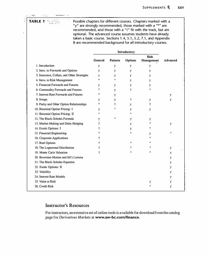
Possible chapters for different courses. Chapters marked with a "y" are strongly recommended, those marked with a "*" are recommended, and those with a "t" fit with the track, but are optional. The advanced course assumes students have a lready taken a basic course. Sections 1.4, 5.1, 5.2, 7 .1, and Appendix B are recommended backgroundfor all introductory courses.

Introductory Risk

General Futures Options Manageme?t Advanced I. Introduction y y y y

2. Intra. to Forwards and Options y y y y

3. Insurance, Collars, and Other Strategies y y y y

4. Intra. to Risk Management * ::: y y

5. Financial Forwards and Futures y y y y

6. Commodity Forwards and Futures * y t *

7. Interest Rate Forwards and Futures * y y

8. Swaps y y t y y

9. Parity and Other Option Relationships * t y t 1 0. Binomial Option Pricing: I y * y y

II. Binomial Option Pricing: II * :::

1 2. The Black-Scholes Formula y * y y

1 3. Market-Making and Delta-Hedging t y * y

14. Exotic Options: I t y *

1 5 . Financial Engineering * * y *

I 6. Corporate Applications t *

1 7. Real Options t * *

1 8 . The Lognormal Distribution t * * y

1 9. Monte Carlo Valuation t * * y

20. Brownian Motion and Ito's Lemma y

2 I. The Black-Scholes Equation y

22. Exotic Options: II y

23. Volatility y

24. Interest Rate Models y

25. Value at Risk y y

26. Credit Risk * y

Instructor's Resources

For instructors, an extensive set of online tools is available for download from the catalog

page for Derivatives Markets at www.aw-bc.com/finance.

XXVi � P R EFAC E

An online Instructor's Solutions Manual by Mark Cassano, University of Cal­

gary, and Rudiger Fahlenbrach, Ohio State University, contains complete solutions to all end-of-chapter problems in the text and spreadsheet solutions to selected problems.

The online Test Bank by Matthew W. Will, University of Indianapolis, features

approximately ten to fifteen multiple-choice questions, five short-answer questions, and one longer essay question for each chapter of the book.

The Test Bank is available in both print and electronic formats, including Windows

or Macintosh TestGen files and Microsoft Word files. The TestGen and Test Bank are

available online at http://www.aw-bc.com/irc.

Online PowerPoint slides, developed by Charles Cao, Pennsylvania State Uni­versity; Ufuk Ince, University of Washington; and Ekaterina Emm, Georgia State Uni­

versity, provide lecture outlines and selected art from the book. Copies of the slides can

be downsized and distributed to students to facilitate note taking during class.

The Instructors Resource Disk contains the computerized Test Bank files (Test­Gen), the Instructor Manual files (Word), the Test Bank files (Word) and PowerPoint

files.

Student Resources

A printed Solutions Manual by Mark Cassano, University of Calgary and Rudiger Fahlenbrach, Ohio State University, provides answers to all the even-numbered problems

in the textbook.

New to this edition, Practice Problems and Solutions, by Rudiger Fahlenbrach, Ohio State University, contains additional problems and worked-out solutions for each

chapter of the textbook.

Spreadsheets with user-defined option pricing functions in Excel are included on

a CD-ROM packaged with the book. These Excel functions are written in VBA, with the code accessible and modifiable via the Visual Basic editor built into Excel. These

spreadsheets and any updates are also posted on the book's Web site.

ACKNOWLEDGMENTS

Kellogg student Tejinder Singh catalyzed the book in 1994 by asking that the Kellogg

Finance Department offer an advanced derivatives course. Kathleen Hagerty and I

initially co-taught that course and my part of the course notes (developed with Kathleen's

help and feedback) evolved into the last third of this book. In preparing the second edition, I received invaluable assistance from Rudiger

Fahlenbrach, Ohio State University, who read much of the new material with a critical eye, and who both caught mistakes and offered valuable suggestions. Numerous other

students, colleagues, and readers provided comments on the first edition. Colleagues in

the Kellogg finance department who were generous with their time include Torben An­

dersen, Kathleen Hagerty, Ravi Jagannathan, Deborah Lucas, Mitchell Petersen, Ernst Schaumburg, Costis Skiadas, and David Stowell. Many Kellogg MBA and Ph.D. stu­

dents helped, but I want to especially thank Arne Staal, Caroline Sasseville, and Alex

AC K N O W LE D G M E NTS � XXVU

Wolf. Others who reviewed new material include David Bates, University of Iowa;

Luca Benzoni, University of Minnesota; Mikhail Chernov, Columbia University ; and Darrell Duffie, Stanford University. Mark Schroder, Michigan State University, kindly

provided code to calculate the non-central chi-squared distribution, and Kellogg student

Scott Freemon implemented this code in VBA.

A special note of thanks goes to David Hait, president of OptionMetrics, for per­mission to include options data on the CD-ROM.

I also received help and comments from George Allayanis, University of Vir­ginia; Jeremy Bulow, Stanford University ; Raul Guerrero, Dynamic Decisions; Darrell

Karolyi, Compensation Strategies, Inc.; C. F. Lee, Rutgers University ; David Nachman,

University of Georgia; Ani! Shivdasani, University of North Carolina;- and Nicholas

Wonder, Western Washington University. I would like to particularly thank those who provided valuable feedback for the

second edition, including Turan Bali, Baruch College, City University of New York;

Philip Bond, Wharton School, University of Pennsylvania; Michael Brandt, Duke Uni­

versity; Charles Cao, Pennsylvania State University ; Bruce Grundy, Melbourne Business School, Australia; Shantaram Hegde, University of Connecticut; Frank Leiber, Bell At­

lantic ; Ehud Ronn, University of Texas, Austin; Nejat Seyhun, University of Michigan;

John Stansfield, University of Missouri, Columbia; Christopher Stivers, University of Georgia; Joel Vanden, Dartmouth College; and Guofu Zhou, Washington University, St.

Louis. I would be remiss not to acknowledge those who assisted with the first edition,

including Tom Arnold, Louisiana State University; David Bates, University of Iowa; Luca Benzoni, University of Minnesota; Mark Broadie, Columbia University; Mark A.

Cassano, University of Calgary; George M. Constantinides, University of Chicago; Kent

Daniel, Northwestern University ; Jan Eberly, Northwestern University ; Virginia France, University of Illinois; Steven Freund, Suffolk University ; Rob Gertner, University of

Chicago; Kathleen Hagerty, Northwestern University; David Haushalter, University of

Oregon; James E. Hodder, University of Wisconsin-Madison; Ravi Jagannathan, North­

western University ; Avraham Kamara, University of Washington; Kenneth Kavajecz,

Whartori School, University of Pennsylvania; Arvind Krishnamurthy, Northwestern Uni­

versity; Dennis Lasser, State University of New York at B inghamton; Camelis A. Los, Kent State University; Deborah Lucas, Northwestern University; Alan Marcus, Boston

College; Mitchell Petersen, Northwestern University ; Todd Pulvino, Northwestern Uni­

versity ; Ernst Schaumburg, Northwestern University ; Eduardo Schwartz, University of California-Los Angeles ; David Shimko, Risk Capital Management Partners, Inc.; Ani! Shivdasani, University of North Carolina-Chapel Hill ; Costis Skiadas, Northwestern

University; Donald Smith, Boston University; David Stowell, Northwestern University ;

Alex Triantis, University of Maryland; and Zhenyu Wang, Yale University. The follow­

ing served as software reviewers: James Bennett, University of Massachusetts-Boston;

Gordon H. Dash, University of Rhode Island; Adam Schwartz, University of Mississippi ; and Robert E. Whaley, Duke University.

Special thanks are due to George Constantinides, Jennie France, Kathleen Hagerty,

Ken Kavajecz, Alan Marcus, Costis Skiadas, and Alex Triantis for their willingness to

XXViii � P R E FA C E

read and comment upon some of the material multiple times and for class-testing. Mark Broadie generously provided his pricing software, which I used both to compute the Heston model and to double-check my own calculations.

I thank Rudiger Fahlenbrach, Mark Cassano, Matt Will, and Charles Cao for their excellent work on the ancillary materials for this book. In addition, Rudiger Fahlenbrach, Paskalis Glabadanidis, Jeremy Graveline, Dmitry Novikov, and Krish­namurthy Subramanian served as accuracy checkers for the book and Andy Kaplin provided programming assistance.

Among practitioners who helped, I thank Galen Burghardt of Carr Futures, Andy Moore of El Paso Corporation, Brice Hill of Intel, Alex Jacobson of the International Securities Exchange, and Blair Wellensiek of Tradelink, L.L.C.

With any book, there are many long-term intellectual debts. From the many, I want to single out two. I had the good fortune to take several classes from Robert Merton at MIT while I was a graduate student. Every derivatives book is deeply in his debt, and this one is no exception. His classic papers from the 1970s are as essential today as they were 3o" years ago. I also learned an enormous amount working with Dan Siegel, with whom I wrote several papers on real options. Dan's death in 199 1 at the age of 35 was a great loss to the profession, as well as to me personally.

The editorial and production team at Addison-Wesley made it clear from the outset that their goal was to produce a high-quality book. I was lucky to have the project over­seen by Addison Wesley's talented and tireless Finance Editor, Donna Battista. Project Manager Mary Clare McEwing expertly kept track of myriad details and offered ex-

. cellent advice when I needed a sounding· board. Development Editor Mmjorie Singer Anderson offered innumerable suggestions, improving the manuscript significantly. Pro­duction Supervisor, Nancy Fenton marshalled forces to tum manuscript into a physical book. Among those forces were the excellent teams at Elm Street Publishing Services and Techsetters. I received numerous compliments on the design of the first edition, which has been carried through ably into the second. Kudos are due to Gina Kolenda and Rebecca Light for their creativity in text and cover design.

The Addison-Wesley team and I have tried hard to minimize errors, including the use of the accuracy checkers noted above. Nevertheless, of course, I alone bear responsibility for remaining errors. Errata and software updates will be available at www.aw-bc.com/mcdonald. Please let us know if you do find errors so we can update the list.

I produced the original manuscript and revision using Gnu Emacs and MikTeX, extraordinarily powerful and robust tools for authors. I am deeply grateful to the world­wide community that produces and supports this software.

My deepest and most heartfelt thanks go to my family. Through both editions I have relied heavily on their understanding, love, support, and tolerance. This book is dedicated to my wife, Irene Freeman, and children Claire, David, and Henry.

RLM

AC K N OWL E D G M E NTS � xxix

Robert L. McDonald is E1win P. Nemmers Distinguished Professor of Finance at North­western University 's Kellogg School of Management, where he has taught since 1984. He is co-Editor of the Review of Financial Studies and has been Associate Editor of the Journal of Finance, Journal of Financial and Quantitative Analysis, Management Science, and other journals. He has a BA in Economics from the University of North Carolina at Chapel Hill and a Ph.D. in Economics from MIT.

CHAPTER r - - - -- --- - - ·---------- - -----�------- - - · - - - - -----------·

Introduction to Derivatives

Risk is the central element that influences financial behavio1:

-Robert C. Merton ( 1999)

1' . 1 he world of finance and capital markets has undergone a stunning transformation in the

last 30 years . Simple stocks and bonds now seem almost quaint alongside the dazzling,

fast-paced, and seemingly arcane world of futures, options, swaps, and other "new"

financial products. (The word "new" is in quotes because it turns out that some of these

products have been around for hundreds of years . )

Frequently this world pops up in the popular press : Procter & Gamble lost

$ 1 50 million in 1994, B arings bank lost $ 1 .3 billion in 1 995 , Long-Term Capital Man­

agement lost $3 .5 billion in 1 998 and (according to some press accounts) almost brought

the world financial system to its knees. 1 What is not in the headlines is that, most of the

time, for most companies and most users, these financial products are an everyday part

of business. Just as companies routinely issue debt and equity, they also routinely use

swaps to fix the cost of production inputs, futures contracts to hedge foreign exchange

risk, and options to compensate employees, to mention j ust a few examples.

1 . 1 WHAT IS A D ERIVATIVE ? Options, futures, and swaps are examples of derivatives. A derivative is a financial

instrument (or more simply, an agreement between two people) that has a value deter­

mined by the price of something else. For example, a bushel of com is not a derivative;

it is a commodity with a value determined by the price of corn. However, you could

enter into an agreement with a friend that says: If the price of a bushel of com in one

year is greater than $3, you will pay the friend $ 1 . If the price of com is less than $3, the friend will pay you $ 1 . This is a derivative in the sense that you have an agreement

with a value depending on the price of something else (com, in this case) .

You might think: "That's not a derivative; that's just a bet on the price of com."

So it is: Derivatives can be thought of as bets on the price of something. But don ' t

1 A readable summary o f these and other infamous derivatives-related losses i s in Jorion (200 1 ) .

1

� I NT R O D U CT I O N TO D E R I VAT I V ES

automatically think the term "bet" is pejorative. Suppose your family grows corn and your friend's family buys corn to mill into cornmeal. The bet provides insurance: You earn $ 1 if your family's corn sells for a low price; this supplements your income. Your friend earns $ 1 if the corn his family buys is expensive; this offsets the high cost of corn. Viewed in this light, the bet hedges you both against unfavorable outcomes. The contract has reduced risk for both of you.

Investors could also use this kind of contract simply to speculate on the price of corn. In this case the contract is not insurance. And that is a key point: It is not the contrac._r itself, but how it is used, and who uses it, that determines whether or not it is risk-reducing. Context is everything.

Although we' ve just defined a derivative, if you are new to the subject the impli­cations of the definition will probably not be· obvious right away. You will come to a deeper understanding of derivatives as we progress through the book, studying different products and their underlying economics.

Uses of Derivatives

What are reasons someone might use derivatives? Here are some motives :

Risk management Derivatives are a tool for companies and other users to reduce risks. The corn example above illustrates this in a simple way: The farmer-a seller of com-enters into a contract which makes a payment when -the price of corn is low. This contract reduces the risk of loss for the farmer, who we therefore say is hedging.

It is common to think of derivatives· as forbiddingly complex, but many derivatives are simple and familiar. Every form of insurance is a derivative, for example. Automobile insurance is a bet on whether you will have an accident. If you wrap your car around a tree, your insurance is valuable; if the car remains intact, it is not.

Speculation Derivatives can serve as investment vehicles . As you will see later in the book, derivatives can provide a way to make bets that are highly leveraged (that is, the potential gain or loss on the bet can be large relative to the initial cost of making the bet) and tailored to a specific view. For example, if you want to bet that the S&P 500 stock index will be between 1 300 and 1400 one year from today, derivatives can be constructed to let you do that.

Reduced transaction costs Sometimes derivatives provide a lower-cost way to effect a particular financial transaction. For example, the manager of a mutual fund may wish to sell stocks and buy bonds. Doing this entails paying fees to brokers and paying other trading costs, such as the bid-ask spread, which we will discuss later. It is possible to trade derivatives instead and achieve the same economic effect as if stocks had actually been sold and replaced by bonds. Using the derivative might result in lower transaction costs than actually selling stocks and buying bonds.

Regulatory arbitrage It is sometimes possible to circumvent regulatory restrictions, taxes, and accounting rules by trading derivatives. Derivatives are often used, for exam­ple, to achieve the economic sale of stock (receive cash and eliminate the risk of holding

W H AT I S A D E R I VAT I V E? � 3

the stock) while still maintaining physical possession of the stock. This transaction may allow the owner to defer taxes on the sale of the stock, or retain voting rights, without the risk of holding the stock.

These are common reasons for using derivatives. The general point is that deriva­tives provide an alternative to a simple sale or purchase, and thus increase the range of possibilities for an investor or manager seeking to accomplish some goal.

Perspectives on Derivatives

How you think about derivatives depends on who you are. In this book we will think about three distinct perspectives on derivatives:

The end-user perspective End-users are the corporations, investment managers, and investors who enter into derivative contracts for the reasons listed in the previous section: to manage risk, speculate, reduce costs, or avoid a rule or regulation. End-users have a goal (for example, risk reduction) and care about how a derivative helps to meet that goal.

The market-maker perspective Market-makers are intermediaries, traders who will buy derivatives from customers who wish to sell, and sell derivatives to customers who wish to buy. In order to make money, market-makers charge a spread: They buy at a low price and sell at a high price. In this respect market-makers are like grocers who buy at the low wholesale price and sell at the higher retail price. Market­makers are also like grocers in that their inventory reflects customer demands rather than their own preferences: As long as shoppers buy paper towels, the grocer doesn't care whether they buy the decorative or super-absorbent style. After dealing with customers, market-makers are left with whatever position results from accommodating customer demands. Market-makers typically hedge this risk and thus are deeply concerned about the mathematical details of pricing and hedging.

The economic observer Finally, we can look at the use of derivatives, the activities of the market-makers, the organization of the markets, the logic of the pricing models, and try to make sense of everything. This is the activity of the economic observer. Regulators must often don their economic observer hats when deciding whether and how to regulate a certain activity or market participant.

These three perspectives are intertwined throughout the book, but as a general point, in the early chapters the book emphasizes the end-user perspective. In the late chapters, the book emphasizes the market-maker perspective. At all times, however, the economic observer is interested in making sense of everything.

Financial Engineering and Security Design

One of the major ideas in derivatives-perhaps the major idea-is that it is generally possible to create a given payoff in multiple ways. The construction of a given financial product from other products is sometimes called financial engineering. The fact that

� I NTRO D U CT I O N TO D E R I VAT I V ES

this is possible has several implications. First, since market-makers need to hedge their positions, this idea is central in understanding how market-making works. The market­maker sells a contract to an end-user, and then creates an offsetting position that pays him if it is necessary to pay the customer. This creates a hedged position.

Second, the idea that a given contract can be replicated often suggests how it can be customized. The market-maker can, in effect, turn dials to change the risk, initial premium, and payment characteristics of a derivative. These changes permit the creation of a product that is more appropriate for a given situation.

Third, it is often possible to improve intuition about a given derivative by realizing that it is equivalent to something we already understand.

Finally, because there are multiple ways to create a payoff, the regulatory arbitrage discussed above can be difficult to stop. Distinctions existing in the tax code, or in regulations, may not be enforceable, since a particular security or derivative that is regulated or taxed may be easily replaced by one that is treated differently but has the same economic profile.

A theme running throughout the book is that derivative products can generally be constructed from other products.

1 .2 THE ROLE OF FINANCIAL MARKETS

We take for granted headlines saying that the Dow Jones Industrial Average has gone up 100 points, the dollar has fallen against the yen, and interest rates have risen. But why do we care about these things? Is the rise and fall of a particular financial index (such as the Dow Jones Industrial Average) simply a way to keep score, to track winners and losers in the economy? Is watching the stock market like watching sports, where we root for certain players and teams-a tale told by journalists, full of sound and fury, but signifying nothing?

Financial markets in fact have an enormous, often underappreciated, impact on everyday life. To help us understand the role of financial markets we will consider the Average family, living in Anytown. Joe and Sarah Average have 2.3 children and both work for the XYZ Co., the dominant employer in Anytown. Their income pays for their mortgage, transportation, food, clothing, and medical care. What is left over goes toward savings earmarked for their children's college tuition and their own retirement.

What role do global financial markets and derivatives play in the lives of the Averages?

Financial Markets and the Averages

The Averages are largely unaware of the ways in which financial markets affect their lives. Here are a few:

• The Average's employer, XYZ Co. , has an ongoing rieed for money to finance operations and investments. It is not dependent on the local bank for funds because it can raise the money it needs by issuing stocks and bonds in global markets.

TH E RO LE O F F I N A N C I A L M A R K ETS � 5

• XYZ Co. insures itself against certain risks. In addition to having property and casualty insurance for its buildings, it uses global derivatives markets to protect itself against adverse currency, interest rate, and commodity price changes. By being able to manage these risks, XYZ is less likely to go into bankruptcy, and less likely to throw the Averages into unemployment.

• The Averages invest in mutual funds. As a result they pay lower transaction costs than if they tried to achieve comparable diversification by buying individual stocks.

• Since both Averages work at XYZ, they run the risk that if XYZ does fall on hard times they will lose their jobs. The mutual funds in which they invest own stocks in a broad array of companies, ensuring that the failure of any one company will not wipe out their savings .

• The Averages live in an area susceptible to tornadoes and insure their home. If their insurance company were completely local, it could not offer tornado insurance because one disaster would leave it unable to pay claims. By selling tornado risk in global markets, the insurance company can in effect pool Anytown tornado risk with Japan earthquake risk and Florida hurricane risk. This pooling makes insurance available at lower rates.

• The Averages borrowed money from Anytown bank to buy their house. The bank sold the mortgage to other investors, freeing itself from interest rate and default risk associated with the mortgage, leaving that to others. Because the risk of their mortgage is borne by those willing to pay the highest price for it, the Averages get the lowest possible mortgage rate.

In all of these examples, particular financial functions and risks have been split up and parceled out to others. A bank that sells a mortgage does not have to bear the risk of the mortgage. An insurance company does not bear all the risk of a disaster. Risk-sharing is one of the most important functions of financial markets.

Risk -Sharing

Risk is an inevitable part of our lives and all economic activity. As we've seen in the example of the Averages, financial markets enable the financial losses from at least some of these risks to be shared. Risk arises from natural events, such as earthquakes, floods, and hurricanes, and from unnatural events such as wars and political conflicts . Drought and pestilence destroy agriculture every year in some part of the world. Some economies boom as others falter. On a more personal scale, people are born, die, retire, find jobs, lose jobs, marry, divorce, and become ill.

In the face of this risk, it seems natural to have arrangements where the lucky share with the unlucky. Risk-sharing occurs informally in families and communities. The insurance market makes formal risk-sharing possible. Buyers pay a premium to obtain various kinds of insurance, such as homeowner's insurance. Total collected premiums are then available to help those whose houses bum down. The lucky, meanwhile, did not need insurance and have lost their premium. The market makes it possible for the lucky to help the unlucky.

6 � I NTRO D U CT I O N TO D E R I VAT I V ES

In the business world, changes in commodity prices, exchange rates, and interest rates can be the financial equivalent of a house burning down. If the dollar becomes expensive relative to the yen, some companies are helped and others are hurt. It makes sense for there to be a mechanism enabling companies to exchange this risk, so that the lucky can, in effect, help the unlucky.

Even insurers need to share risk. Consider an insurance company that provides earthquake insurance for California residents. A large earthquake could generate claims sufficient to bankrupt a stand-alone insurance company. Thus, insurance companies often use the reinsurance market to buy, from reinsurers, insurance against large claims. Reinsurers pool different kinds of risks, thereby enabling insurance risks to become more widely held.

In some cases, reinsurers further share risks by issuing catastrophe bonds-bonds that the issuer need not repay if there is a specified event, such as a large earthquake, causing large insu(ance claims. Bondholders willing to accept earthquake risk can buy these bonds, in exchange for greater interest payments on the bond if there is no earthquake. An earthquake bond allows earthquake risk to be borne by exactly those investors who wish to bear it.

Although there are mechanisms for sharing many kinds of risks, some have argued that significantly more risk-sharing is possible and desirable. The economist Robert Shiller (Shiller, 2003) envisions the creation of entirely new markets for risk-sharing, including home equity insurance (to trade risks associated with house prices), income­linked loans (personal loans that need not be fully repaid if wages decline in a particular occupation), and macro insurance (contracts with payments linked to national incomes) . While these markets do not yet exist, there is a trend toward more inclusive markets for risk transfer. For example, Goldman Sachs and Deutsche Bank have recently created an "economic derivatives" market in which it is possible to buy claims with payouts based on economic statistics. The box on page 7 discusses this market.

You might be wondering what this discussion has to do with the notions of diver­sifiable and nondiversifiable risk familiar from portfolio theory. Risk is diversifiable risk if H is unrelated to other risks. The risk that a lightning strike will cause a factory to burn down, for example, .is idiosyncratic and hence diversifiable. If many investors share a small piece of this risk, it has no significant effect on anyone. Risk that does not vanish when spread across many investors is nondiversifiable risk. The risk of a stock market crash, for example, is nondiversifiable.

Financial markets in theory serve two purposes. Markets permit diversifiable risk to be widely shared. This is efficient: By definition, diversifiable risk vanishes when it is widely shared. At the same time, financial markets permit nondiversifiable risk, which does not vanish when shared, to be held by those most willing to hold it. Thus, the fundamental economic idea underlying the concepts and mm*ets discussed in this book is that the existence of risk-sharing mechanisms benefits evei)'Oile.

1 .3 DERIVATIVES IN PRACTICE

Derivatives use and the variety of derivatives have grown over the last 30 years.

Eco n o m i c Derivatives

Government agencies in most countries periodically announce economic statistics, such as the number of jobs in the economy, production in different sectors, and the level of sales. These statistics provide information about the performance of the economy and-since policy makers rely upon them--can provide clues to future government policy. Consequently, money managers, dealers, and other market participants pay close attention to these statistics; their release often results in a flurry of trading activity and changes in stock and bond prices .

Because of the importance of these statistics for financial markets, Goldman Sachs and Deutsche Bank created a market in economic derivatives, in which it is possible to trade claims with payoffs based on these statistics. Specifically, beginning in late 2002, it became possible to trade claims based on employment (U.S . nonfarm payrolls), industrial production (the Purchasing

Growth in Derivatives Trading

D E R I VAT I V ES I N P RACTI C E � 7

Manager's Index), and U.S . retail sales. A European consumer price index was added in 2003 . Participants can, in effect, bet on whether the statistics will be higher or lower than expected.

Whereas it is possible to trade stocks and bonds on any business day, the market for most economic derivatives is open only briefly before the government releases the statistic . Specifically, if the nonfarm payroll number is to be released on a Friday, on the day before there will be one hour during which participants can submit orders to buy or sell various derivatives based on the nonfarm payroll number. At the end of the hour, buyers are matched against sellers and prices are determined using a procedure known as a Dutch auction.2 This market permits the trading of many different kinds of claims that we will discuss in later chapters, including forwards, calls, puts, spreads, straddles, strangles, and digital options.

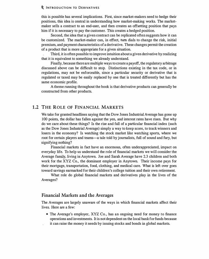
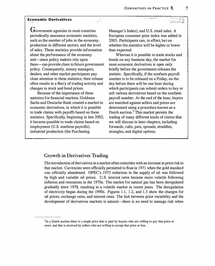
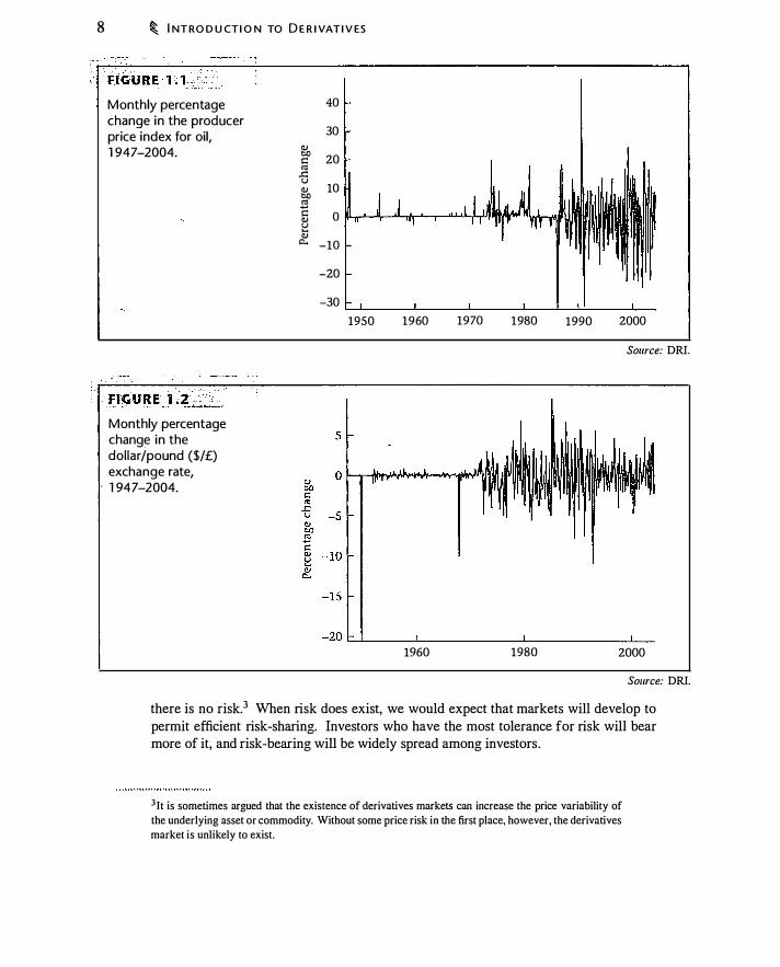
The introduction of derivatives in a market often coincides with an increase in price risk in that market. Currencies were officially permitted to float in 1 97 1 when the gold standard was officially abandoned. OPEC's 1 973 reduction in the supply of oil was followed by high and variable oil prices . U.S. interest rates became more volatile following inflation and recessions in the 1 970s. The market for natural gas has been deregulated gradually since I 978, resulting in a volatile market in recent years. The deregulation of electricity began during the 1990s. Figures 1 . 1 , 1 .2, and 1 .3 show the changes for oil prices, exchange rates, and interest rates. The link between price variability and the development of derivatives markets is natural-there is no need to manage risk when

2 In a Dutch auction there is a single price that is paid by buyers who are wil l ing to pay that price or

more, and that is received by sellers who are wi l ling to accept that price or less.

8 � I NT RO D U CT I O N TO D E R I VAT I V ES

Monthly percentage change in the producer price index for oil, 1947-2004.

Monthly percentage change in the dol lar/pound ($/£) exchange rate,

. 1 947-2 004.

Ill co I: "'

..c:: u Ill co "' ..... I: Ill u ..... Ill "'"'

40

30

20

10

0

-10

-20

-30

1950 1960 1970 1980

1960 1980

1990 2000

Source: DRI.

2000

Source: DRI.

there is no risk.3 When risk does exist, we would expect that markets will develop to permit efficient risk-sharing. Investors who have the most tolerance for risk will bear more of it, and risk-bearing will be widely spread among investors .

3It is sometimes argued that the existence of derivatives markets can increase the price variability of

the underlying asset or commodity. Without some price risk in the first place, however, the derivatives market is unlikely to exist.

FIGU R E 1 . 3

Monthly change in 3-month Treasury b i l l rate, 1947-2004.

; F IGURE 1.4

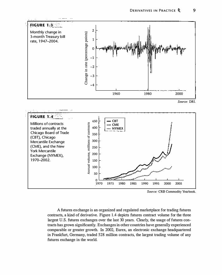
Mil l ions of contracts traded annual ly at the Chicago Board of Trade (CBT), Chicago Mercanti le Exchange (CME), and the New York Mercantile Exchange (NYMEX), 1970-2002.

� � :::: ·a 0.. QJ � "' c QJ u .... QJ .3-B "' ..... . 5 QJ � :::: "'

..::: u

"' ti e t:: 0 u .... 0 t: � E .,; E ::l 0 > "' g �

2

1

0

-1

-2

-3

-4

450

400

350

300

250

200

150

100

so 0 1970

D E R I VATI V ES I N P RACTI C E � 9

1960 1980 2000

Source: DR!.

- CBT I = CME · • · NYMEX � I 0 ' € � ;,

) . I

� 'I � •"'" · · �·· � .. /'" , ....... · • · s: -·

�-- -· --- - I · · · · • • 1975 1980 1985 1990 1995 2000 2005

Source: CRB Commodity Yearbook.

A futures exchange is an organized and regulated marketplace for trading futures contracts, a kind of derivative. Figure 1 .4 depicts futures contract volume for the three largest U.S. futures exchanges over the last 30 years. Clearly, the usage of futures con­tracts has grown significantly. Exchanges in other countries have generally experienced comparable or greater growth. In 2002, Eurex, an electronic exchange headquartered in Frankfurt, Germany, traded 528 million contracts, the largest trading volume of any futures exchange in the world.

10 � I NTRO D U CT I O N TO D E R I VAT I V ES

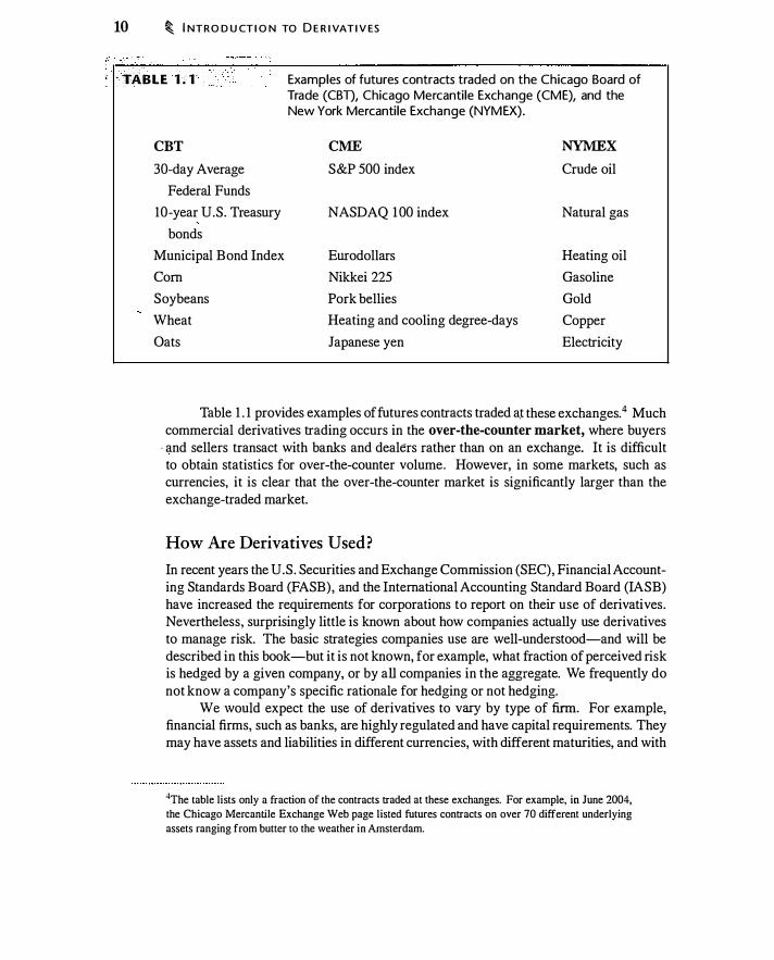
TABLE 1 . 1

CBT

30-day Average

Federal Funds

10-year U.S. Treasury

bonds

Municipal Bond Index

Com

Soybeans

Wheat

Oats

Examples of futures contracts traded on the Chicago Board of Trade (CBD, Chicago Mercanti le Exchange (CME), and the New York Mercanti le Exchange (NYM EX).

CME NYMEX S&P 500 index Crude oil

NASDAQ 1 00 index Natural gas

Eurodollars Heating oil

Nikkei 225 Gasoline

Pork bellies Gold

Heating and cooling degree-days Copper

Japanese yen Electricity

Table 1 . 1 provides examples of futures contracts traded at these exchanges.4 Much commercial derivatives trading occurs in the over-the-counter market, where buyers

· and sellers transact with banks and dealers rather than on an exchange. It is difficult to obtain statistics for over-the-counter volume. However, in some markets, such as currencies, it is clear that the over-the-counter market is significantly larger than the exchange-traded market.

How Are Derivatives Used?

In recent years the U.S. Securities and Exchange Commission (SEC), Financial Account­ing Standards Board (FASB), and the International Accounting Standard Board (IASB) have increased the requirements for corporations to report on their use of derivatives. Nevertheless, surprisingly little is known about how companies actually use derivatives to manage risk. The basic strategies companies use are well-understood-and will be described in this book-but it is not known, for example, what fraction of perceived risk is hedged by a given company, or by all companies in the aggregate. We frequently do not know a company's specific rationale for hedging or not hedging.

We would expect the use of derivatives to vary by type of firm. For example, financial firms, such as banks, are highly regulated and have capital requirements. They may have assets and liabilities in different currencies, with different maturities, and with

4The table lisiS only a fraction of !he contraciS traded at lhese exchanges. For example, in June 2004,

!he Chicago Mercantile Exchange Web page listed futures contraciS on over 70 different underlying

assets ranging from butter to !he weather in Amsterdam.

B U Y I N G A N D S H O RT-S E L L I N G F I N A N C I A L ASS ETS � 11

different credit risks. Hence banks could be expected to use interest rate derivatives, currency derivatives, and credit derivatives to manage risks in those areas. Manufac­turing firms that buy raw materials and sell in global markets might use commodity and currency derivatives, but their incentives to manage risk are less clear-cut because they are not regulated in the same ways as financial firms.

1 .4 B UYING AND SHORT-SELLING FINANCIAL ASSETS

Throughout this book we will talk about buying and selling-and short-selling-assets such as stocks. These basic transactions are so important that it is worth describing the details. First, it is important to understand the costs associated with buying and selling. Second, a very important idea used throughout the book is that of short-sales. The concept of short-selling should be intuitive-a short-sale is just the opposite of a purchase-but for almost everyone it is hard to grasp at first. Even if you are familiar with short sales, you should spend a few minutes reading this section.

Buying an Asset

Suppose you want to buy 1 00 shares of XYZ stock. This seems simple: If the stock price is $50, 100 shares will cost $50 x 1 00 = $5000. However, this calculation ignores transaction costs.

First, there is a commission, which is a transaction fee you pay your broker. A commission for the above order could be $ 15 , or 0.3% of the purchase price.

Second, the term "stock price" is, surprisingly, imprecise. There are in fact two prices, a price at which you can buy, and a price at which you can sell. The price at which you can buy is called the offer price or ask price, and the price at which you can sell is called the bid price. Where do these terms come from?

To buy stock, you can pick up the phone and call a broker. If the stock is not too , obscure and your order is not too large, your purchase will probably be completed in a matter of seconds. Have you ever wondered where the stock comes from that you have just bought? It is possible that at the exact same moment, another customer called the broker and put in an order to sell. More likely, however, a market-maker sold you the stock. Market-makers do what their name implies: They make markets. If you want to buy, they sell, and if you want to sell, they buy. In order to earn a living, market-makers sell for a high price and buy for a low price. If you deal with a market-maker, therefore, you buy for a high price and sell for a low price. This difference between the price at which you can buy and the price at which you can sell is called the bid-ask spread.5

In practice the bid�ask spread on the stock you are buying may be $49.75 to $50. This means that you can buy for $50/share and sell for $49.75/share. If you were to buy

5If you think a bid-ask spread is unreasonable, ask what a world without dealers would be like. Every buyer would have to find a seller, and vice versa. The search would be costly and take time. Dealers,

because they maintain inventory, offer an immediate transaction, a service called immediacy.

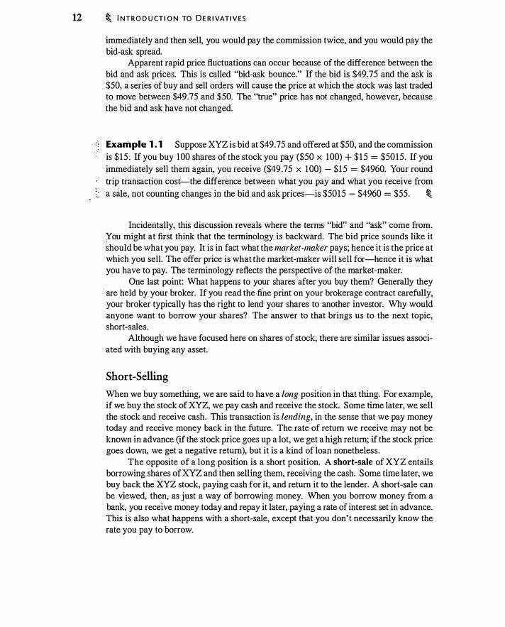
12 � I NTRO D U CT I O N TO D E R I VATI V ES

immediately and then sell, you would pay the commission twice, and you would pay the bid-ask spread.

Apparent rapid price fluctuations can occur because of the difference between the bid and ask prices. This is called "bid-ask bounce." If the bid is $49.75 and the ask is $50, a series of buy and sell orders will cause the price at which the stock was last traded to move between $49.75 and $50. The "true" price has not changed, however, because the bid and ask have not changed.

Example 1 . 1 Suppose XYZ is bid at $49.75 and offered at $50, and the commission is $ 15 . If you buy 100 shares of the stock you pay ($50 x 100) + $ 1 5 = $50 15 . If you immediately sell them again, you receive ($49 .75 x 100) - $15 = $4960. Your round trip transaction cost-the difference between what you pay and what you receive from a sitle, not counting changes in the bid and ask prices-is $5015 - $4960 = $55. �

Incidentally, this discussion reveals where the terms "bid" and "ask" come from. You might at first think that the terminology is backward. The bid price sounds like it should be what you pay. It is in fact what the market-maker pays; hence it is the price at which you sell. The offer price is what the market-maker will sell for-hence it is what you have to pay. The terminology reflects the perspective of the market-maker.

One last point: What happens to your shares after you buy them? Generally they · are held by your broker. If you read the fi

-ne print on your brokerage contract carefully,

your broker typically has the right to lend your shares to another investor. Why would anyone want to borrow your shares? The answer to that brings us to the next topic, short-sales.

Although we have focused here on shares of stock, there are similar issues associ­ated with buying any asset.

Short -Selling

When we buy something, we are said to have a long position in that thing. For example, if we buy the stock of XYZ, we pay cash and receive the stock. Some time later, we sell the stock and receive cash. This transaction is lending, in the sense that we pay money today and receive money back in the future. The rate of return we receive may not be known in advance (if the stock price goes up a lot, we get a high return; if the stock price goes down, we get a negative return), but it is a kind of loan nonetheless.

The opposite of a long position is a short position. A short-sale of XYZ entails borrowing shares of XYZ and then selling them, receiving the cash. Some time later, we buy back the XYZ stock, paying cash for it, and return it to the lender. A short-sale can be viewed, then, as just a way of borrowing money. When you borrow money from a bank, you receive money today and repay it later, paying a rate of interest set in advance. This is also what happens with a short-sale, except that you don' t necessarily know the rate you pay to borrow.

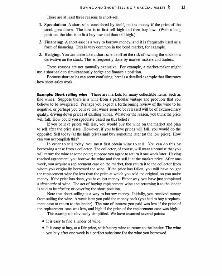
B U Y I N G A N D S H O RT-S E L L I N G F I N A N C I A L ASS ETS � 13

There are at least three reasons to short-sell :

1. Speculation: A short-sale, considered by itself, makes money if the price of the stock goes down. The idea is to first sell high and then buy low. (With a long position, the idea is to first buy low and then sell high.)

2. Financing: A short-sale is a way to borrow money, and it is frequently used as a form of financing. This is very common in the bond market, for example.

3. Hedging: You can undertake a short-sale to offset the risk of owning the stock or a derivative on the stock. This is frequently done by market-makers and traders.

These reasons are not mutually exclusive. For example, a market-maker might use a short-sale to simultaneously hedge and finance a position.

Because short-sales can seem confusing, here is a detailed example that illustrates how short-sales work.

Example: Short-selling wine There are markets for many collectible items, such as fine wines . Suppose there is a wine from a particular vintage and producer that you believe to be overpriced. Perhaps you expect a forthcoming review of the wine to be negative, or perhaps you believe that wines soon to be released will be of extraordinary quality, driving down prices of existing wines . Whatever the reason, you think the price will fall. How could you speculate based on this belief?

If you believe prices will rise, you would buy the wine on the market and plan to sell after the price rises. However, if you believe prices will fall, you would do the opposite: Sell today (at the high price) and buy sometime later (at the low price) . How can you accomplish this?

In order to sell today, you must first obtain wine to sell. You can do this by borrowing a case from a collector. The collector, of course, will want a promise that you will return the wine at some point; suppose you agree to return it one week later. Having reached agreement, you borrow the wine and then sell it at the market price. After one . week, you acquire a replacement case on the market, then return it to the collector from whom you originally borrowed the wine. If the price has fallen, you will have bought the replacement wine for less than the price at which you sold the original, so you make money. If the price has risen, you have lost money. Either way, you have just completed a short-sale of wine. The act of buying replacement wine and returning it to the lender is said to be closing or covering the short position.

Note that short-selling is a way to borrow money. Initially, you received money from selling the wine. A week later you paid the money back (you had to buy a replace­ment case to return to the lender) . The rate of interest you paid was low if the price of the replacement case was low, and high if the price of the replacement case was high.

This example is obviously simplified. We have assumed several points :

• It is easy to find a lender of wine.

• It is easy to buy, at a fair price, satisfactory wine to return to the lender: The wine you buy after one week is a perfect substitute for the wine you borrowed.

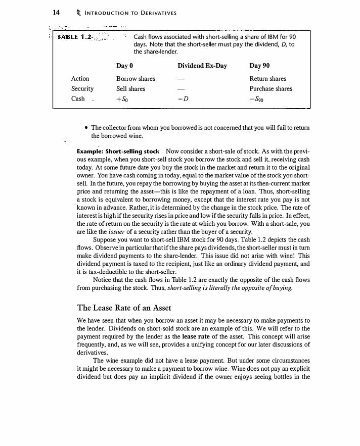
14 � I NTRO D U CT I O N TO D E R I VAT I V ES

� .. ·. .

Action

Security

Cash

Cash flows associated with short-sel l ing a share of IBM for 90

days. Note that the short-sel ler must pay the dividend, D, to the share-lender.

Day O

Borrow shares

Sell shares

+So

Dividend Ex-Day

-D

Day 90

Return shares

Purchase shares

-Sgo

• The collector from whom you borrowed is not concerned that you will fail to return the borrowed wine.

Example: Short-selling stock Now consider a short-sale of stock. As with the previ­ous example, when you short-sell stock you borrow the stock and sell it, receiving cash today. At some future date you buy the stock in the market and return it to the original owner. You have cash coming in today, equal to the market value of the stock you short­sell. In the future, you repay the borrowing by buying the asset at its then-current market price and returning the asset-this is like the repayment of a. loan. Thus, short-selling a stock is equivalent to borrowing money, except that the interest rate you pay is not

· known in advance. Rather, it is determined by the change in the stock price. The rate of interest is high if the security rises in price and low if the security falls in price. In effect, the rate of return on the security is the rate at which you borrow. With a short-sale, you are like the issuer of a security rather than the buyer of a security.

Suppose you want to short-sell IBM stock for 90 days. Table 1 .2 depicts the cash flows . Observe in particular that if the share pays dividends, the short-seller must in tum make dividend payments to the share-lender. This issue did not arise with wine ! This dividend payment is taxed to the recipient, just like an ordinary dividend payment, and it is tax-deductible to the short-seller.

Notice that the cash flows in Table 1 .2 are exactly the opposite of the cash flows from purchasing the stock. Thus, short-selling is literally the opposite of buying.

The Lease Rate of an Asset

We have seen that when you borrow an asset it may be necessary to make payments to the lender. Dividends on short-sold stock are an example of this. We will refer to the payment required by the lender as the lease rate of the asset. This concept will arise frequently, and, as we will see, provides a unifying concept for our later discussions of derivatives .

The wine example did not have a lease payment. But under some circumstances it might be necessary to make a payment to borrow wine. Wine does not pay an explicit dividend but does pay an implicit dividend if the owner enjoys seeing bottles in the

B U Y I N G A N D S H O RT-S E L L I N G F I N A N C I A L ASS ETS � 15

cellar. The owner might thus require a payment in order to lend a bottle. This would be a lease rate for wine.

Risk and Scarcity in Short-Selling

The preceding examples were simple illustrations of the mechanics and economics of short -selling, and they demonstrate the ideas you will need to understand our discussions of deriyatives. It turns out, however, that some of the complexities we skipped over are easy to understand and are important in practice. In this section we use the wine example to illustrate some of these practical issues.

Credit risk As the short-seller, you have an obligation to the lender to return the wine. The lender fears that you will renege on this obligation. This concern can be addressed with collateral: After you sell the wine, the lender can hold the money you received from selling the wine. You have an obligation to return the wine; the lender keeps the money in the event that you don't.

Holding on to the money will help the lender feel more secure, but after thinking the matter over, the lender will likely want more from you than just the current value of the wine. Suppose you borrow $5000 worth of wine. What happens, the lender will think, if the price of that particular wine rises to $6000 one week later? This is a $ 1000 loss on your short-sale. In order to return the wine, you will have to pay $6000 for wine you just sold for $5000. Perhaps you cannot afford the extra $ 1000 and you will fail to return the borrowed wine. The lender, thinking ahead, will be worried at the outset abou·t this possibility and will ask you to provide more than the $5000 the wine is worth, say an extra $ 1000. This extra amount is called a haircut, and serves to protect the lender against your failure to return the wine when the price rises.6 In practice, short-sellers must have funds-called capital-to be able to pay haircuts. The amount of capital places a limit on their ability to short-sell.

Scarci.ty As the short-seller, do you need to worry about the short-sale proceeds? The·

lender is going to have $6000 of your money. Most of this, however, simply reflects your obligation, and we could ask a trustworthy third party, such as a bank, to hold the money so the lender cannot abscond with it. However, when you return the wine, you are going to want your money back, plus interest. This raises the question: What rate of interest will the lender pay you? Over the course of the short-sale, the lender can invest your money, eaining, say, 6%. The lender could offer to pay you 4% on the funds, thinking to keep as a fee the 2% difference between the 6% earned on the money and the 4% paid to you. What happens if the lender and borrower negotiate?

Here is the �nteresting point: The rate of interest the lender pays on the collateral is going to depend on how many people want to borrow wine from the particular vintage

6Note that the lender is not concerned about your failure to perform when the price goes down because

the lender has the money !

16 � I NT RO D U CT I O N TO D E R I VATI V ES

and producer, and how many are willing to lend it! As a practical matter, it may not be easy to find a lender. If there is high demand for borrowed wine, the lender will offer a low rate of interest, essentially earning a fee for being willing to lend something that is scarce. However, if no one else wants to borrow the wine, the lender might conclude that a small fee is better than nothing and offer you a rate of interest close to the market rate.

The rate paid on collateral is called different things in different markets, the repo rate in bond markets and the short rebate in the stock market. Whatever it is called, the difference between this rate and the market rate of interest is another cost to your short-sale.

CHAPTER SUMMARY Derivatives are financial instruments with a payoff determined by the price of something else. They can be used as a tool for risk management and speculation, and to reduce transaction costs or avoid taxes and regulation.

One important function of financial markets is to facilitate optimal risk-sharing. The growth of derivatives markets over the last 50 years has coincided with an increase in the risks evident in various markets. Events such as the 1973 oil shock, the abandonment of fixed exchange rates, and the deregulation of energy markets have created a new role

. for derivatives. A short-sale entails borrowing a security, selling it, making dividend (or other cash)

payments to the security lender, and then returning it. A short-sale is conceptually the opposite of a purchase. Short-sales can be used for speculation, as a form of financing, or as a way to hedge. Many of the details of short-selling in practice can be understood as a response to credit risk of the short-seller and scarcity of shares that can be borrowed. Short-sellers typically leave the short-sale proceeds on deposit with lenders, along with additional capital called a haircut. The rate paid on this collateral is called the short rebate, and is less than the interest rate.

FURTHER READING The rest of this book provides an elaboration of themes discussed in this chapter. How­ever, certain chapters are directly related to the discussion. Chapters 2, 3, and 4 introduce forward and option contracts, which are the basic contracts in derivatives, and show how they are used in risk management. Chapter 13 discusses in detail how derivatives market­makers manage their risk, and Chapter 15 explains how derivatives can be combined with instruments such as bonds to create customized risk-management products.

The derivatives exchanges have Web sites that list their contracts. The Web sites for the exchanges in Figure 1 .4 are www.cbot.com (Chicago Board ofTrade), www.cme. com (Chicago Mercantile Exchange), and www.nymex.com (New York Mercantile Exchange). Economic derivatives are discussed at www.gs.com/econderivs.

P RO B L E M S � 17

Jorion ( 1995) examines in detail one famous "derivatives disaster": Orange County in California. Bernstein ( 1992) presents a history of the development of fi­nancial markets, and Bernstein ( 1 996) discusses the concept of risk measurement and how it evolved over the last 800 years. Miller ( 1_986) discusses origins of past financial innovation, while Merton ( 1 999) and Shiller (2003) provide a stimulating look at pos­siblefitture developments in financial markets. Froot and O'Connell ( 1 999) and Froot (2001 ) examine the market for catastrophe reinsurance. D'Avolio (2001 ) explains the economics and practices associated with short-sales . Finally, Lewis ( 1 989) is a classic, funny, insider's account of investment banking, offering a different (to say the least) perspective on the mechanics of global risk-sharing.

PROBLEMS

1 .1 . Heating degree-day and cooling degree-day futures contracts make payments based on whether the temperature is abnormally hot or cold. Explain why the following businesses might be interested in such a contract:

a. Soft-drink manufacturers.

b. Ski-resort operators.

c. Electric utilities.

d. Amusement park operators.

1.2. Suppose the businesses in the previous problem use futures contracts to hedge their temperature-related risk. Who do you think might accept the opposite risk?

1.3. ABC stock has a bid price of $40.95 and an ask price of $41 .05 . Assume there is a $20 brokerage commission.

a. What amount will you pay to buy 100 shares?

b. What amount will you receive for selling 100 shares?

c. Suppose you buy 100 shares, then immediately sell 100 shares with the bid and ask prices being the same in both cases. What is your round-trip transaction cost?

1.4. Repeat the previous problem supposing that the brokerage fee is quoted as 0.3% of the bid or ask price.

·

1.5. Suppose a security has a bid price of $ 100 and an ask price of $ 100. 12. At what price can the market-maker purchase a security? At what price can a market­maker sell a security? What is the spread in dollar terms when 100 shares are traded?

1.6. Suppose you short-sell 300 shares of XYZ stock at $30. 1 9 with a commission charge of 0.5%. Supposing you pay commission charges for purchasing the se­curity to cover the short-sale, how much profit have you made if you close the short-sale at a price of $29.87?

18 � I NT R O D U CT I O N TO D E R I VATI V ES

1.7. Suppose you desire to short-sell 400 shares of JKI stock, which has a bid price of $25 . 1 2 and an ask price of $25 .3 1 . You cover the short position 1 80 days later when the bid price is $22.87 and the ask price is $23.06.

a. Taking into account only the bid and ask prices (ignoring commissions and interest), what profit did you earn?

b. Suppose that there is a 0.3% commission to engage in the short-sale (this is the commission to sell the stock) and a 0.3% commission to close the short-sale (this is the commission to buy the stock back). How do these commissions change the profit in the previous answer?

c. Suppose the 6-month interest rate is 3% and that you are paid nothing on the short-sale proceeds. How much interest do you lose during the 6 months in which you have the short position?

1.8. When you open a brokerage account, you typically sign an agreement giving the l;>roker the right to lend your shares without notifying or compensating you. Why do brokers want you to sign this agreement?

1.9. Suppose a stock pays a quarterly dividend of $3. You plan to hold a short position in the stock across the dividend ex-date. What is your obligation on that date? If you are a taxable investor, what would you guess is the tax consequence of the payment? (In particular, would you expect the dividend to be tax deductible?) Suppose the company announces instead that the dividend is $5. Should you care that the dividend is different from-what you expected?

1.10. Short interest is a measure of the aggregate short positions on a stock. Check an online brokerage or other financial service for the short interest on several stocks of your choice. Can you guess which stocks have high short interest and which have low? Is it theoretically possible for short interest to exceed 100% of shares outstanding?

1.11. Suppose that you go to a bank and borrow $ 100. You promise to repay the loan in 90 days for $ 102. Explain this transaction using the terminology of short-sales.

1.12. Suppose your bank's loan officer tells you that if you take out a mortgage (i.e., you borrow money to buy a house) you will be permitted to borrow no more than 80% of the value of the house. Describe this transaction using the terminology of short-sales .

PA.R T O N E

L this part oftlze book, Chapters 2-4, we examine the basic derivatives

contracts: forward contracts, futures contracts, call options, and put

options. All of these are contracts between two parties, with a payoff at

some future date based on the price of an underlying asset (this is why

they are called derivatives).

There are a number oft/zings we want to understand about these in­

struments. What are they? How do theywork and what do they cost? If

you enter into a forward contract, futures contract, or option, what obli­

gations or rights have you acquired? Payoff and profit diagrams provide

an important graphical tool to summarize the risk of these contracts.

Once we understand what the basic deJivatil•es contracts are, what

can we do with them? We will see that, among other things, they can

be used to provide insurance, to convert a stock investment into a risk­

free investment and vice versa, and to speculate in a variety of ways.

Derivatives can often be customized for a particular purpose. We will see

how corporate risk managers can use derivatives, and some reasons for

doing so.

·In this part of the book we take the prices of derivatives as given;

the underlying pricing models will be covered in much of the rest of the

19

book. The main mathematical tool is present and future value calcu­

lations. We do, however, develop one key pricing idea: put-call parity.

Put-call parity is important because it demonstrates a link among the dif­

ferent contracts we exainine in these chapters, telling us how the prices of

fonvard contracts, call options, and put options are related to one another.

�

C�ER_:2 "·-----.-�---------

An Introduction to Forwards and Options

Tru, ohapte; introduce' the b"io derivatives oontraots o focwrucd oootrnCts, oall options, and put options. These fundamental contracts are widely used, and serve as building blocks for more complicated derivatives that we discuss in later chapters. We explain here how the contracts work and how to think about their risk. We also introduce an extremely important tool for analyzing derivatives positions-namely, payoff and profit diagrams. The terminology and concepts introduced in this chapter are fundamental and will be used throughout this book.

2.1 FORWARD CONTRACTS

Suppose you wish to buy a share of stock. Doing so entails at least three separate steps: ( l ) setting the price to be paid, (2) transferring cash from the buyer to the seller, and (3) transferring the share from the seller to the buyer. With an outright purchase of stock, all three occur simultaneously. However, as a logical matter, a price could be set today and the transfer of shares and cash would occur at a specified date in the future.

This is in fact the definition of a forward contract: It sets today the terms at which you buy or sell an asset or commodity at a specific time in the future. A forward contract does the following:

• Specifies the quantity and exact type of the asset or commodity the seller musr deliver.

• Specifies delivery logistics, such as time, date, and place.

• Specifies the price the buyer will pay at the time of delivery.

• Obligates the seller to sell and the buyer to buy, subject to the above specifications.

The time at which the contract settles is called the expiration date. The asset or com­modity on which the forward contract is based is called the underlying asset. Apart from commissions and bid-ask spreads (see Section 1 .4), a forward contract requires no initial payment or: premium. The contractual forward price simply represents the price at which consenting adults agree today to transact in the future, at which time the buyer pays the seller the forward price and the seller delivers the asset.

Futures contracts are similar to forward contracts in that they create an obligation to buy or sell at a predetermined price at a future date. We will discuss the institutional and pricing differences between forwards and futures in Chapter 5. For the time being, think of them as interchangeable.

21

22 � AN I NT R O D U CT I O N TO F O RWA R D S A N D O PT I O N S

I ndex futures price l istings.

Index Futures UFETIME OPEN OPEN HIGH LOW SffiLE CHG HIGH LOW lilT

OJ Industrial Average (CBl)·$10 x Index Sept 9953 10085 9950 10062 113 10557 9835 40�20 De< 10072 10080 10005 10059 116 10575 11440 349 Est vol 7,149; vol Mon 8,914; open lnt 40,969, •132. ldx prl: Hi 1010313; lD 996354; Oose 1008514, •123.22.

Mini OJ Industrial Average (CBT)·$5 x Index Sept 9956 10087 9949 10062 113 10629 9840 48,695 Vol Tue 105,733; open int 48,789, •1,159.

OJ-AIG Commodity Index <CBT>·$100 x Index Aug _ •. ·- 455.9 .• 485.0 449.4 2,886 Est val 0; val Mon 0; open int 2,886, unch. ldx p�: Hi 144.743; lD 144.024; Oose 144341, -.019.

S&P 500 Index (CME)·$250 x index Sept 108310 109600 108300 109250 960 1160BO 78100 575,947 Dec 109350 109550 109300 109290 970 116010 78100 12,717 Est val 39,263; val Mon 37,876; open int 589,488, -1,470, idx p�: Hi 1096.65; lD 1084.07; Oose 1094.83, •10.76.

Mini S&P 500 ((lolEl·$50 x Index Sept 108300 109600 108275 109250 950 114850 107500 596,759 Vol Tue 729,906; open int 642,116, •334.

S&P Midcap 400 (<t.!El·$500 x index Sept 567.00 575.00 567.00 573.40 715 61650 508.70 13,640 Est voi 496; vol Mon 700; open int 13,640, <49. ldx prl: HI 574.85; lo 56631; Qose 574.02, •7.63.

Nasdaq :1.00 (CME)·$100 x index Sept 137300 139800 137250 139050 1750 156500 136000 70,024 Est vol 12,432; vol Mon 12,422; open int 72,319, -20. ldx prl: Hi 1395.95; lD 137U6; Oose 139150, •2310.

Source: Wall Street Joumal, July 28, 2004, p. C- 16.

Figure 2. 1 shows futures price listings from the Wall Street Joumal for futures contracts on several stock indices, including the Dow Jones Industrial Average (DJ 30) and the Standard and Poor's 500 (S&P 500). The indices are the underlying assets for . the contracts. (A stock index is the average price of a group of stocks . In these examples we work with this group price rather than the price of just one stock.) The first column of the listing gives the expiration month. The columns that follow show the price at the beginning of the day (the open), the high and low during the day, and the settlement price, which reflects the last transactions of the day.

The listing also gives the price change from the previous day, the high and low during the life of the futures contract, and open interest, which measures the number of contracts outstanding. (Since each trade of a contract has both a buyer and a seller, a buyer-seller pair counts as one contract.) Finally, the head of the listing tells us where the contracts trade (the Chicago Board of Trade [CBT] and Chicago Mercantile Exchange [CME]), and the size of the contract, which for the S&P 500 is $250 times the index value. We will discuss such futures contracts in more detail in Chapter 5. There are many more exchange-traded stock index futures contracts than those in Figure 2. 1 , both in the United States and around the world.

The price quotes in Figure 2. 1 are from July. The September and December prices for the two contracts are therefore prices set in July for purchase of the index in later months. For example, the September S&P 500 futures price is $ 1 092.50 and

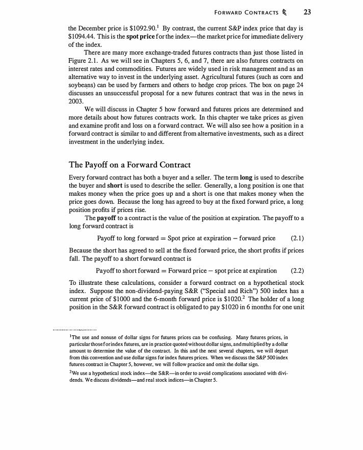
FO RWA R D CO NTR ACTS � 23

the December price is $ 1092.90. 1 By contrast, the current S&P index price that day is $ 1094.44. This is the spot price for the index-the market price for immediate delivery of the index.

There are many more exchange-traded futures contracts than just those listed in Figure 2. 1 . As we will see in Chapters 5 , 6, and 7, there are also futures contracts on interest rates and commodities. Futures are widely used in risk management and as an alternative way to invest in the underlying asset. Agricultural futures (such as corn and soybeans) can be used by farmers and others to hedge crop prices. The box on page 24 discusses an unsuccessful proposal for a new futures contract that was in the news in 2003 .

We will discuss in Chapter 5 how forward and futures prices are determined and more details about how futures contracts work. In this chapter we take prices as given and examine profit and loss on a forward contract. We will also see how a position in a forward contract is similar to and different from alternative investments, such as a direct investment in the underlying index.

The Payoff on a Forward Contract

Every forward contract has both a buyer and a seller. The term long is used to describe the buyer and short is used to describe the seller. Generally, a long position is one that makes money when the price goes up and a short is one that makes money when the price goes down. Because the long has agreed to buy at the fixed forward price, a long position profits if prices rise.

The payoff to a contract is the value of the position at expiration. The payoff to a long forward contract is

Payoff to long forward = Spot price at expiration - forward price (2. 1 )

Because the short has agreed to sell at the fixed forward price, the short profits if prices fall . The payoff to a short forward contract is

Payoff to short forward = Forward price - spot price at expiration (2.2)

To illustrate these calculations, consider a forward contract on a hypothetical stock index. Suppose the non-dividend-paying S&R ("Special and Rich") 500 index has a current price of $ 1000 and the 6-month forward price is $ 1020.2 The holder of a long position in the S&R forward contract is obligated to pay $ 1020 in 6 inonths for one unit

1 The use and nonuse of dollar signs for futures prices can be confusing. Many futures prices, in

particular those for index futures, are in practice quoted without dollar signs, and multiplied by a dollar amount to determine the value of the contract. In this and the next several chapters, we will depart

from this convention and use dollar signs for index futures prices. When we discuss the S&P 500 index

futures contract in Chapter 5, however, we will follow practice and omit the dollar sign.

2We use a hypothetical stock index-the S&R-in order to avoid complications associated with divi­

dends. We discuss dividends-and real stock indices-in Chapter 5.

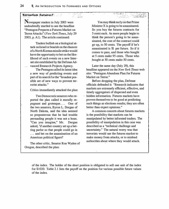
24 � AN I NTRO D U CT I O N TO FO RWA R D S A N D O PT I O N S

- · . Jerrorism . Futures? .·

Newspaper readers in July 2003 were undoubtedly startled to see the headline "Pentagon Prepares a Futures Market on Terror Attacks" (New York Times, July 29 2003, p. AI ) . The article continued:

Traders bullish on a biological at­tack on-Israel or bearish on the chances of a N orth Korean missile strike would have the opportunity to bet on the like­lihood of such events on a new Inter­net site established by the Defense Ad­vanced Research Projects Agency.

The Pentagon called its latest idea a new way of predicting events and part of its search for the "broadest pos­sible set of new ways to prevent ter­rorist attacks." Critics immediately attacked the plan:

Two Democratic senators who re­ported the plan called it morally re­pugnant and grotesque. . . . One of the two senators, Byron L. Dorgan of North Dakota, said the idea seemed so preposterous that he had trouble persuading people it was not a hoax. "Can you imagine," Mr. Dorgan asked, 'if another country set up .a bet­ting parlor so that people could go in . . . and bet on the assassination of an American political figure?

The other critic, Senator Ron Wyden of Oregon, described the plan:

You may think early on that Prime Minister X is going to be assassinated. So you buy the futures contracts for 5 cents each. As more people begin to think the person's going to be assas� sin a ted, the cost of the contract could go up, to 50 cents. The payoff if he's assassinated is $1 per future. So if it comes to pass, and those who bought at 5 cents make 95 cents. Those who bought at 50 cents make 50 cents .

Later the same day (July 29), this headline appeared on the New York Times web site: "Pentagon Abandons Plan for Futures Market on Terror."

Before dropping the plan, Defense officials defended it: "Research indicates that markets are extremely efficient, effective, and timely aggregators of dispersed and even hidden information. Futures markets have proven themselves to be good at predicting such things as elections results; they are often better than expert opinions."

A common concern about futures markets is the possibility that markets can be manipulated by better informed traders. The possibility of manipulation in this case was described as a "technical challenge and uncertainty." The natural worry was that terrorists would use the futures market to make money from attacks, or to mislead authorities about where they would attack.

of the index. The holder of the short position is obligated to sell one unit of the index for $ 1 020. Table 2 . 1 lists the payoff on the position for various possible future values of the index.

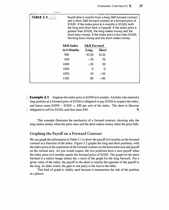
F O RWA R D C O N TRACTS � 25

Payoff after 6 months from a long S&R forward contract and a short S&R forward contract at a forward price of $1020. If the index price in 6 months is $1020, both the long and short have a 0 payoff. If the index price is greater than $1020, the long makes money and the short loses money. If the index price is less than $1020,

the long loses money and the short makes money.

S&R index S&R Forward

in 6 Months Long Short

900 -$ 1 20 $ 1 20

950 -70 70

1 000 -20 20

1 020 0 0

1 050 30 -30

1 100 80 -80

- Example 2.1 Suppose the index price is $ 1 050 in 6 months. A holder who entered a long position at a forward price of $ 1 020 is obligated to pay $ 1 020 to acquire the index, and hence earns $ 1050 - $ 1 020 = $30 per unit of the index. The short is likewise obligated to sell for $ 1 020, and thus loses $30. �

This example illustrates the mechanics of a forward contract, showing why the long IJ!.akes money when the price rises and the short makes money when the price falls. ·

Graphing the Payoff on a Forward Contract

We can graph the information in Table 2. 1 to show the payoff in 6 months on the forward contract as a function of the index. Figure 2.2 graphs the long and short positions, with the index price at the expiration of the forward contract on the horizontal axis and payoff on the vertical axis. As you would expect, the two positions have a zero payoff when the index price in 6 months equals the forward price of $ 1 020. The graph for the short forward is a mirror image (about the x-axis) of the graph for the long forward. For a given value of the index, the payoff to the short is exactly the opposite of the payoff to the long. In other words, the gain to one party is the loss to the other.

This kind of graph is widely used because it summarizes the risk of the position at a glance.

26 � AN I NTRO D U CT I O N TO F O RWA R D S AN D O PT I O N S

Long and short forward positions on the S&R 500 index.

Payoff ($)

200

150

100

50

0 1----------:*-----i + Long forward -+- Short forward

-50

-100

-150

-200

-250 L--L---L--L---���--�--�--� 800 850 900 950 1000 1050 1 100 1 150 1200

S&R Index Price ($)

Comparing a Forward and Outright Purchase

The S&R forward contract is a way to acquire the index by paying $ 1 020 after 6 months. An alternative way to acquire the index is to purchase it outright at time 0, paying $ 1 000. Is there any advantage to using the forward contract to buy the index, as opposed to purchasing it outright?

If we buy the S&R index today, it costs us $ 1000. The value of the position in 6 months is the value of the S&R index. The payoff to a long position in the physical S&R index is graphed in Figure 2.3 . For comparison, the payoff to the long forward position, is graphed as well. Note that the axes have different scales in Figures 2.3 and 2.2.

To see how Figure 2.3 i.s constructed, suppose the S&R index price is $0 after 6 months. (This is just a thought experiment for the purpose of constructing the graph, but if you would like to be concrete, imagine that the S&R index contained Internet firms in the year 2000 which would be bankrupt in 200 1 .) If the index price is $0, the physical index will be worth $0; hence we plot a 0 on the y-axis against 0 on the x-axis. For all other prices of the S&R index, the payoff equals the value of the S&R index. For example, if we own the index and the price in 6 months is $750, the value of the position is $750.

If the index price in 6 months is $0, the payoff to the forward contract, using equation (2 . 1 ) , is

Payoff to long forward = 0 - $ 1 020 = -$ 1 020

If instead the index price is $ 1 020, the long index position will be worth $ 1 020 and the forward contract will be worth $0.

·

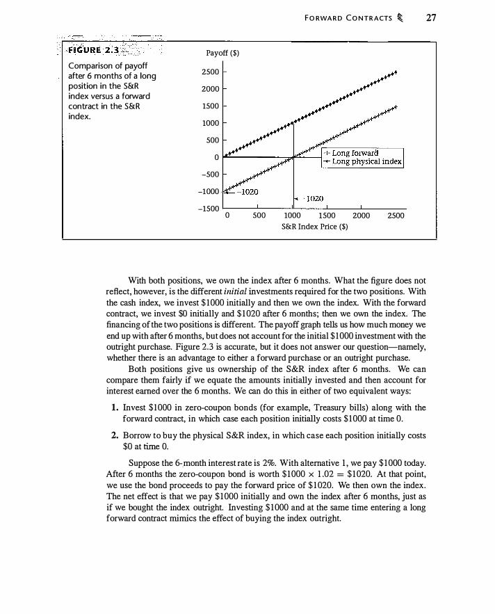
Comparison of payoff after 6 months of a long position in the S&R index versus a forward contract in the S&R index.

Payoff ($)

2500

2000

1500

1000

500

0

-500

-1000

-1500 0 500 1000

F O RWA R D CO NTR ACTS � 27

1500 2000 2500

S&R Index Price ($)

With both positions, we own the index after 6 months. What the figure does not reflect, however, is the different initial investments required for the two positions. With the cash index, we invest $ 1000 initially and then we own the index. With the forward contract, we invest $0 initially and $ 1 020 after 6 months; then we own the index. The financing of the two positions is different. The payoff graph tells us how much money we end up with after 6 months, but does not account for the initial $ 1 000 investment with the outright purchase. Figure 2.3 is accurate, but it does not answer our question-namely, whether there is an advantage to either a forward purchase or an outright purchase.

Both positions give us ownership of the S&R index after 6 months. We can compare them fairly if we equate the amounts initially invested and then account for interest earned over the 6 months. We can do this in either of two equivalent ways:

1. Invest $ 1 000 in zero-coupon bonds (for example, Treasury bills) along with the forward contract, in which case each position initially costs $ 1 000 at time 0.

2. Borrow to buy the physical S&R index, in which case each position initially costs $0 at time 0.

Suppose the 6-.month interest rate is 2%. With alternative 1 , we pay $ 1 000 today. After 6 months the zero-coupon bond is worth $ 1 000 x 1 .02 = $ 1 020. At that point, we use the bond proceeds to pay the forward price of $ 1 020. We then own the index. The net effect is that we pay $ 1 000 initially and own the index after 6 months, just as if we bought the index outright. Investing $ 1 000 and at the same time entering a long forward contract mimics the effect of buying the index outright.

28 � A N I NTRO D U CT I O N TO F O RWA R D S A N D O PT I O N S

With alternative 2 , we borrow $ 1000 to buy the index, which costs $ 1 000. Hence we make no net cash payment at time 0. After 6 months we owe $ 1 000 plus interest. At that time we repay $ 1 000 x 1 .02 = $ 1 020 for the borrowed money. The net effect is that we invest nothing initially, and after six months pay $ 1 020. We also own the index. Borrowing to buy the stock therefore mimics the effect of entering into a long forward contract.3

We conclude that when the index pays no dividends, the only difference between the forward contract and the cash index investment is the timing of a payment that will be made for certain. Therefore, we can compare the two positions by using the interest rate-to shift the timing of payments. In the above example, we conclude that the forward contract and the cash index are equivalent investments, differing only in the timing of the cash flows. Neither form of investing has an advantage over the other.

This analysis suggests a way to systematically compare positions that require different initial investments. We can assume that we borrow any required initial payment. At expiration, we receive the payoff from the contract, and repay any borrowed amounts . We will call this the net payoff or profit. Because this calculation accounts for differing initial investments in a simple fashion, we will primarily use profit rather than payoff diagrams throughout the book.4 Note that the payoff and profit diagrams are the same for a forward contract because it requires no initial investment.

To summarize, a payoff diagram graphs the cash value of a position at a point in time. A profit diagram subtracts from the payoff the future value of the investment in the position.

· This discussion raises a question: Given our assumptions, should we really expect

the forward price to equal $ 1 020, which is the future value of the index? The answer in this case is yes, but we defer a detailed explanation until Chapter 5 .

Zero-Coupon Bonds in Payoff and Profit Diagrams

The preceding discussion showed that the long forward contract and outright purchase of the physical S&R index are essentially the same once we take time value of money into account. Buying the physical index is like entering into the forward contract and simultaneously investing $ 1 000 in a zero-coupon bond. We can see this same point graphically by using a payoff diagram where we include a zero-coupon bond.

Suppose we enter into a long S&R index forward position, and at the same time purchase a $ 1 000 zero-coupon bond, which will pay $ 1 020 after 6 months. (This was

3 If the index paid a dividend in this example, then we would receive the dividend by holding the physical index, but not when we entered into the forward contract. We will see in Chapter 5 how to

take dividends into account in this comparison.

4The term "profit" is defined variously by accountants and economists. All of our profit calculations

are for the purpose of comparing one position with another, not computing profit in any absolute sense.

;;a:JG'u R �·.� ��!:�1�;�. · Payoff d iagram for a long S&R forward contract, together with a zero-coupon bond that pays $1 020 at maturity. Summing the value of the long forward plus the bond at each S&R Index price g ives the line labeled "Forward + Bond."

Payoff ($)

2500

2000

1500 $1020

500

F O RWA R D C O N T RACTS � 29

o +='-------::Il'tr----; + Long forward +- $ 1000 bond

-500 ...._ Forward + bond

0 500 1000 1500 2000 2500

S&R Index Price ($)

alternative 1 in the previous section.) Algebraically, the payoff to the forward plus the bond is

Forward + bond = Spot price at expiration - $ 1 020 + $ 1 020 ._,.._.,

Forward payoff Bond payoff

= Spot price at expiration

This is the same as the payoff to investing in the physical index. The payoff diagram for this position is an easy modification of Figure 2.3. We

simply add a line representing the value of the bond after 6 months ($ 1000 x 1 .02 = $ 1 020), and then add the bond payoff to the forward payoff. This is graphed in Figure 2.4. The forward plus bond looks exactly like the physical index in Figure 2.3.

What is the profit diagram corresponding to this payoff diagram? For the forward contract, profit is the same as the payoff because there is no initial investment. Profit for the forward plus bond is obtained by subtracting the future value of the initial investment. The initial investment was the cost of the bond, $ 1 000. Its future value is, by definition, $ 1 020, the value of the bond after 6 months. Thus, the profit diagram for a forward contract plus a bond is obtained by ignoring the bond! Put differently, adding a bond to a position leaves a profit diagram unaffected.

Depending on the context, it can be helpful to draw either payoff or profit diagrams. Bonds can be used to shift payoff diagrams vertically, but do not change the profit calculation.

30 � A N I NT RO D U CT I O N TO F O RWA R D S A N D O PT I O N S

Cash Settlement Versus Delivery

The foregoing discussion assumed that at expiration of the forward contract, the contract called for the seller (the party short the forward contract) to deliver the cash S&R index to the buyer (the party long the forward contract) . However, a physical transaction in a broad stock index will likely have significant transaction costs. An alternative settlement procedure that is widely used is cash settlement. Instead of requiring delivery of the actual index, the forward contract settles financially. The two parties make a net cash payment, which yields the same cash flow as if delivery had occurred, and both parties had

, then closed out their positions. We can illustrate this with an example.

Example 2.2 Suppose that the S&R index at expiration is $ 1040. Because the forward price is $ 1020, the long position has a payoff of $20. Similarly, the short positi�n loses $20. With cash settlement, the short simply pays $20 to the long, with no transfer of the physical asset, and hence no transaction costs. It is as if the long paid $ 1 020, acquired the index worth $ 1040, and then immediately sold it with no transaction costs.

If the S&R index price at expiration had instead been $960, the long position would [ : have a payoff of -$60 and the short would have a payoff of $60. Cash settlement in this U case entails the long paying $60 to the short. �

Cash settlement is feasible only when there is an accepted reference price upon which the settlement can be based. Cash settlement is not limited to forward contracts­virtually any financial contract can be settled using cash rather than delivery.

Credit Risk

Any forward or futures contract-indeed, any derivatives contract-has credit risk, which means there is a possibility that the counterparty who owes money fails to make a payment. If you agree to sell the index in one year at a fixed price and the spot price turns out to be lower than the forward price, the counterparty is obligated to buy the index for more than it is worth. You face the risk that the counterparty will for some reason fail to pay the forward price for the index. Similarly the counterparty faces the risk that you will not fulfill the contract if the spot price in one year turns out to be higher than the forward price.

With exchange-traded contracts, the exchange goes to great lengths to minimize this risk by requiring collateral of all participants and being the ultimate counterparty in all transactions. We will discuss credit risk and collateral in more detail when we discuss futures contracts in Chapter 5. With over-the-counter contracts, the fact that the

CALL O PT I O N S � 3 1

contracts are transacted directly between two parties means that each counterparty bears the credit risk of the other. 5

Credit risk is an important problem with all derivatives, but it is also quite com­plicated. Credit checks of counterparties and credit protections such as collateral and bank letters of credit are commonly employed to guard against losses from counterparty default.

2.2 CALL OPTIONS

We have seen that a forward contract obligates the buyer (the holder of �e long position) to pay the forward price at expiration, even if the value of the underlying asset at expira­tion is less than the forward price. Because losses are possible with a forward contract, it is natural to wonder: Could there be a contract where the buyer has the right to walk away from the deal?

The answer is yes; a call option is a contract where the buyer has the right to buy, but not the obligation to buy. Here is an example illustrating how a call option works at expiration.

Example 2.3 Suppose that the call buyer agrees to pay $ 1020 for the S&R index in 6 months but is not obligated to do so. (The buyer has purchased a call option.) If in 6 months the S&R price is $ 1 1 00, the buyer will pay $ 1020 and receive the index. This is

3 a payoff of $80 per unit of the index. If the S&R price is $900, the buyer walks away. �

Now think about this transaction from the seller's point of view. The buyer is in control of the option, deciding when to buy the index by paying $ 1 020. Thus, the rights , of the option buyer are obligations for the option seller.

Example 2.4 If in 6 months the S&R price is $ 1 100, the seller will receive $ 1020 and give up an index worth more, for a loss of $80 per unit of the index. If the S&R price is less than $ 1020, the buyer will not buy, so the seller has no obligation. Thus, at expiration, the seller will have a payoff which is zero (if the S&R price is less than

t $ 1 020) or negative (if the S&R price is greater than $ 1 020). �

5 0f course, credit risk also exists in exchange-traded contracts. The specific details of how exchanges

are structured to minimize credit risk is a complicated and fascinating subject (see Edwards and Ma

( 1992), ch. 3, for details). In practice, exchanges are regarded by participants as good credit risks.

32 � A N I NT R O D U CT I O N TO F O RWA R D S A N D O PT I O N S

Does it seem as if something i s wrong here? Because the buyer can decide whether to buy, the seller cannot make money at expiration. This situation suggests that the seller must, in effect, be "bribed" to enter into the contract in the first place. At the time the buyer and seller agree to the contract, the buyer must pay the seller an initial price, or premium. This initial payment compensates the seller for being at a disadvantage at expiration. Contrast this with a forward contract, for which the initial premium is zero.

Option Terminology

Her:e are some key terms used to describe options:

Strike price: The strike price, or exercise price, of a call option is what the buyer pays for the asset. In the example above, the strike price was $ 1 020. The strike price can be set at any value.

Exercise: The exercise of a call option is the act of paying the strike price to receive the asset. In Example 2.3, the buyer decided after 6 months whether to exercise the option-that is, whether to pay $ 1 020 (the strike price) to receive the S&R index.

Expiration: The expiration of the option is the date by which the option must either be exercised or it becomes worthless. The option in Example 2.3 had an expiration of 6 months.

Exercise style: The exercise style of the option governs the time at which exercise can occur. In the above example, exercise could occur only at expiration. Such an option is said to be a European-style option. If the buyer has the right to exercise at any time during the life of the option, it is an American-style option. If the buyer can only exercise during specified periods, but not for the entire life of the option, the option is a Bermudan-style option. (The terms "European" and "American," by the way, have nothing to do with geography. European, American, and Bermudan options are bought and sold worldwide.)

To summarize, a European call option gives the owner of the call the right, but not the obligation, to buy the underlying asset on the expiration date by paying the strike price. The option described in Examples 2.3 and 2.4 is a 6-month European-style S&R call with a strike price of $1020. The buyer of the call can also be described as having a long position in the call.

Figure 2.5 presents a small portion of the option price listings for the S&P 500 Index option traded at the Chicago Board Options Exchange. Each row represents a different option, with the expiration month, strike price, a "c" or a "p" to denote call or put, the number of contracts traded that day, the premium at the last trade of the day, the change from the previous day, and open interest. As with futures, every option trade requires a buyer and a seller, so open interest measures the number of buyer-seller pairs. The box below discusses some of the mechanics of buying an option.

For the time being, we will discuss European-style options exclusively. We do this because European options are the simplest to discuss and are also quite common in

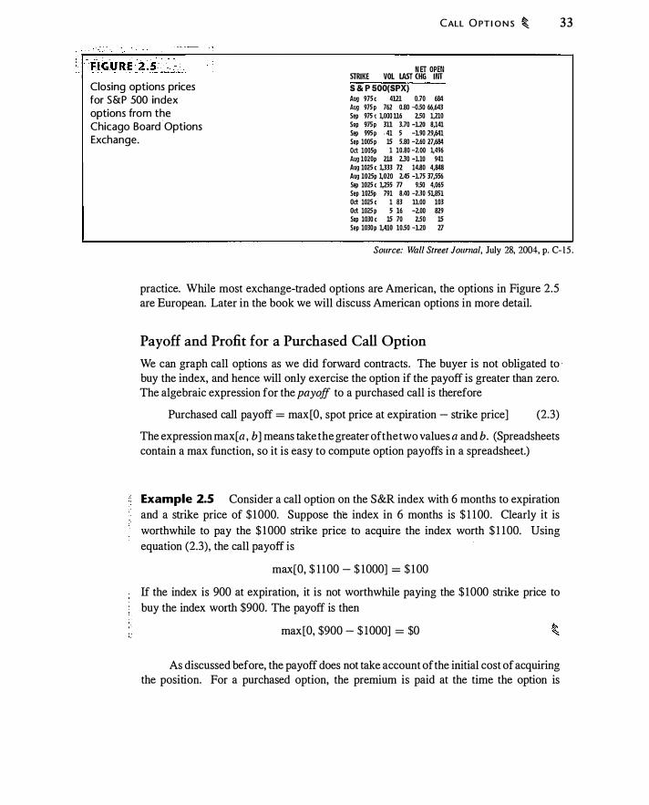
Closing options prices for S&P 500 index options from the Chicago Board

· Options

Exchange.

CALL O PT I O N S � 33

N ET OPEN STRIKE VOL lAST CHG INT S & P 500(SPX) Aug 975 c 412l 0.70 684

Aug 975 p 762 0.80 -{)50 66,643

Sep 975 c LDDD ll6 250 1,210

Sep 975 p 3ll 3.70 -UO 8,141

Sep 995 p · 41 5 -L90 7.9,641

Sep 1005 p l5 5.80 -2.60 27,684

Oct 1005p 1 10.80 -z.oo L496

Aug 1020 p 2l8 2.30 -uo 941

Aug 1025 c L333 n 14.80 4,848

Aug 1025p L020 2.45 -L75 37,556

Sep 1025 c L255 77 950 4,065

Sep 1025p 791 8.40 -2.30 5L85l

Oct 1025 c 1 83 llDD 103

Oct 1025 p 5 16 -2.00 829 Sep 1030 c l5 70 250 l5 Sep 1030 p L41D 1050 -UD 27

Source: Wall Street Jouma/, July 28, 2004, p. C-15 .

practice. While most exchange-traded options are American, the options in Figure 2.5 are European. Later in the book we will discuss American options in more detail.

Payoff and Profit for a Purchased Call Option

We can graph call options as we did forward contracts. The buyer is not obligated to · buy the index, and hence will only exercise the option if the payoff is greater than zero. The algebraic expression for the payoff to a purchased call is therefore

Purchased call payoff = max[O, spot price at expiration - strike price] (2.3)

The expression max[ a , b] means take the greater of the two values a and b. (Spreadsheets contain a max function, so it is easy to compute option payoffs in a spreadsheet.)

Example 2.5 Consider a call option on the S&R index with 6 months to expiration and a strike price of $ 1000. Suppose the index in 6 months is $ 1 100. Clearly it is worthwhile to pay the $ 1000 strike price to acquire the index worth $ 1 100. Using equation (2.3), the call payoff is

max[O, $ 1 1 00 - $ 1000] = $ 100

If the index is 900 at expiration, it is not worthwhile paying the $ 1000 strike price to buy the index worth $900. The payoff is then

max[O, $900 - $ 1000] = $0

As discussed before, the payoff does not take account of the initial cost of acquiring the position. For a purchased option, the premium is paid at the time the option is

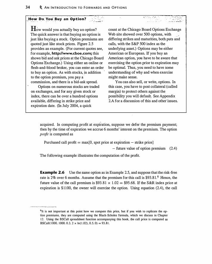
34 � A N I NTRO D U CT I O N TO F O RWA R D S A N D O PT I O N S

. Ho�

_Do You Buy an Option?

How would you actually buy an option? The quick answer is that buying an option is just like buying a stock. Option premiums are quoted just like stock prices. Figure 2.5 provides an example. (For current quotes see, for example, http://www.cboe.com; this shows bid and ask prices at the Chicago Board Options Exchange.) Using either an online or flesh-and-blood broker, you can enter an order to buy an option. As with stocks, in addition to the option premium, you pay a commission, and there is a bid-ask spread.

Optio!ls on numerous stocks are traded on exchanges, and for any given stock or index, there can be over a hundred options available, differing in strike price and expiration date. (In July 2004, a quick

count at the Chicago Board Options Exchange Web site showed over 500 options, with differing strikes and maturities, both puts and calls, with the S&P 500 index as the underlying asset.) Options may be either American or European. If you buy an American option, you have to be aware that exercising the option prior to expiration may be optimal. Thus, you need to have some understanding of why and when exercise might make sense.

You can also sell, or write, options . In this case, you have to post collateral (called margin) to protect others against the possibility you will default. See Appendix 2.A for a discussion of this and other issues.

acquired. In computing profit at expiration, suppose we defer the premium payment; then by the time of expiration we accrue 6 months' interest on the premium. The option profit is computed as

Purchased call profit = max[O, spot price at expiration - strike price]

- future value of option premium (2.4)

The following example illustrates the computation of the profit.

Example 2.6 Use the same option as in Example 2.5, and suppose that the risk-free rate is 2% over 6 months . Assume that the premium for this call is $93 .8 1 .6 Hence, the future value of the call premium is $93 .8 1 x 1 .02 = $95 .68. If the S&R index price at expiration is $ 1 1 00, the owner will exercise the option. Using equation (2.4), the call

6It is not important at this point how we compute this price, but if you wish to replicate the op­tion premiums, they are computed using the Black-Scholes formula, which we discuss in Chapter 1 2. Using the BSCall spreadsheet function accompanying this book, the call price is computed as BSCall ( I OOO, 1 000. 0.3, 2 x ln ( 1 .02) , 0.5. 0) = 93 .8 1 .

profit is

CALL O PT I O N S � 35

max[O, $ 1 100 - $ 1000] - $95 .68 = $4.32

If the index is 900 at expiration, the owner does not exercise the option. It is not worthwhile paying the $ 1000 strike price to buy the index worth $900. Profit is then

max[O, $900 - $1000] - $95 :68 = -$95 .68,

reflecting the loss of the premium.

We graph the call payoff by computing, for any index price at expiration, the payoff on the option position as a function of the price. We graph the call profit by subtracting from this the future value of the option premium. Table 2.2 computes the payoff and profit at different index values, computed as in Examples 2.5 and 2.6. Note that because the strike price is fixed, a higher market price at expiration of the S&R index benefits the call buyer.

Figure 2.6 graphs the call payoff that is computed in Table 2.2. The graph clearly shows the "optionality" of the option: Below the strike price of $ 1000, the payoff is zero, while it is positive and increasing above $ 1000.

1� ���BLI:: _�;.��c-�2_4ii .. . . . i Payoff a n d profit after 6 months from a purchased 1 .000-strike S&R cal l option with a future value of premium of $95.68. The option premium is assumed to be $93 .81 and the effective interest rate is 2% over 6 months. The payoff is computed using equation (2.3) and the profit us ing equation (2.4).

S&R index Call Future Value Call in 6 months Payoff of Premium Profit

800 $0 -$95.68 -$95.68

850 0 -95.68 -95.68

900 0 -95.68 -95.68

950 0 -95.68 -95.68

1000 0 -95.68 -95.68

1050 50 -95.68 -45 .68

1 100 100 -95.68 4.32

1 150 150 -95.68 54.32

1200 200 -95.68 104.32

36 � AN I NT RO D U CTI O N TO FO RWA R D S A N D O PT I O N S

� .. FI G U R E 2 ; 6 �· · � The payoff at expiration of a purchased S&R cal l with a $ 1 000 strike price.

Profit at expiration for purchase of 6-month S&R index cal l with strike price of $ 1 000 versus profit on long S&R index forward position.

Payoff ($)

200

1SO

100

1 -+- Purchased call i

so

0 +---+---+---+---�---------------

-so

-100

-1SO

-200

-2SO t___'---'---'---.I----.1.-._.L..__.L..__� 800 8SO 900 9SO 1000 10SO 1 100 1 1SO 1200

Profit ($)

200

1SO

S&R Index Price ($)

100

/

Index price = $ 1020 so

o r----------------7�--��--------so

-10o �-+--+-�+--�-

-1SO

-200

+ Purchased call -+- Long forward

-2SQ L--..__-�-�-�-�-�-�-�� 800 8SO 900 9SO 1000 10SO 1 100 1 1SO 1200

S&R Index Price ($)

The last column in Table 2.2 computes the call profit at different index values. Because a purchased call and a forward contract are both ways to buy the index, it is interesting to contrast the two. Thus, Figure 2.7 plots the profit OJ) both a purchased call and a long forward contract. Note that profit and payoff diagrams for an option differ by the future value of the premium, whereas for a forward contract they are the same.

CA L L O PT I O N S � 37

If the index rises, the forward contract is more profitable than the option because it does not entail paying a premium. If the index falls sufficiently, however, the option is more profitable because the most the option buyer loses is the future value of the premium. This difference suggests that we can think of the call option as an insured position in the index. Insurance protects against losses, and the call option does the same. Carrying the analogy a bit further, we can think of the option premium as, in part, reflecting the cost of that insurance. The forward, which is free, has no such insurance, and potentially has losses larger than those on the call.

This discussion highlights the important point that there are always trade-offs in selecting a position. The forward contract outperforms the call if the index rises and underperforms the call if the index falls sufficiently. When all contracts are fairly priced, you will not find a contract that has higher profits for all possible index market prices.

Payoff and Profit for a Written Call Option

Now let's look at the option from the point of view of the seller. The seller is said to be the option writer, or to have a short position in a call option. The option writer is the counterparty to the option buyer. The writer receives the premium for the option and then has an obligation to sell the underlying security in exchange for the strike price if the option buyer exercises the option.

The payoff and profit to a written call are just the opposite of those for a purchased call:

Written call payoff = - max[O, spot price at expiration - strike price] (2.5)

Written call profit = - max[O, spot price at expiration - strike price]

+ future value of option premium (2.6)

This example illustrates the option writer's payoff and profit. Just as a call buyer is long in the call, the call seller has a short position in the call .

Example 2.7 Consider a 1000-stri.ke call option on the S&R index with 6 months to expiration. At the time the option is written, the option seller receives the premium of $93 .8 1 .

Suppose the index i n 6 months i s $ 1 1 00. It i s worthwhile for the option buyer to pay the $ 1000 strike price to acquire the index worth $ 1 100. Thus, the option writer will have to sell the index, worth $ 1 100, for the strike price of $ 1000. Using equation (2.5), the written call payoff is

- max[O, $ 1 1 00 - $1000] = -$ 100.

The premium has earned 2% interest for 6 months and is now worth $95.68. Profit for the written call is

-$100 + $95 .68 = -$4.32.

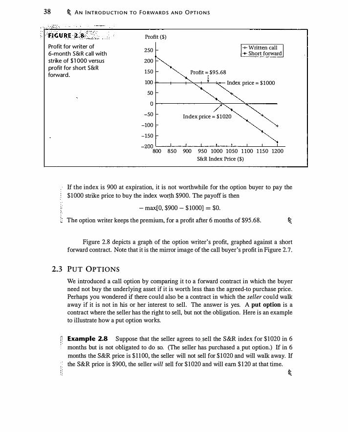
38 � A N I NTRO D U CT I O N TO FO RWA R D S A N D O PT I O N S

Profit for writer of 6-month S&R cal l with strike of $1 000 versus profit for short S&R forward.

Profit ($)

250

200

150 Profit = $95.68

+ Written call + Short forward

100 -1=---t---t-""-:--+-....__�- Index price = $ 1000

so o �--------------��--��-------

-50 Index price = $1020 � -100 "" ·� -150

-200 L---L--L---L--L--�--�-�--� 800 850 900 950 1000 1050 1 100 1 150 1200

S&R Index Price ($)

If the index is 900 at expiration, it is not worthwhile for the option buyer to pay the $ 1000 strike price to buy the index worth $900. The payoff is then

- max[O, $900 - $ 1000] = $0.

The option writer keeps the premium, for a profit after 6 months of $95 .68.

Figure 2.8 depicts a graph of the option writer's profit, graphed against a short forward contract. Note that it is the mirror image of the call buyer's profit in Figure 2. 7.

2.3 PUT OPTIONS

We introduced a call option by comparing it to a forward contract in which the buyer need not buy the underlying asset if it is worth less than the agreed-to purchase price. Perhaps you wondered if there could also be a contract in which the seller could walk away if it is not in his or her interest to sell . The answer is yes. A put option is a contract where the seller has the right to sell, but not the obligation. Here is an example to illustrate how a put option works.

Example 2.8 Suppose that the seller agrees to sell the S&R index for $ 1020 in 6 months but is not obligated to do so. (The seller has purchased a put option.) If in 6 months the S&R price is $ 1 1 00, the seller will not sell for $ 1 020 ;md will walk away. If

the S&R price is $900, the seller will sell for $ 1 020 and will earn $ 1 20 at that time.

P UT O PT I O N S � 39

A put must have a premium for the same reason a call has a premium. The buyer of the put controls exercise; hence the seller of the put will never have a positive payoff at expiration. A premium paid by the put buyer at the time the option is purchased compensates the put seller for this no-win position.

It is important to be crystal clear about the use of the terms "buyer" and "seller" in the above example, because there is potential for confusion. The buyer of the put owns a contract giving the right to sell the index at a set price. Thus, the buyer of the put is a seller of the index! Similarly, the seller of the put is obligated to buy the index, should the put buyer decide to sell. Thus, the buyer of the put is potentially a seller of the index, and the seller of the put is potentially a buyer of the index. (If thinking through these transactions isn't automatic for you now, don' t worry. It will become second nature as you continue to think about options.)

Other terminology for a put option is the same as for a call option, with the obvious change that "buy" becomes "sell ." In particular, the strike price is the agreed-upon selling price ($ 1 020 in Example 2.8), exercising the option means selling the underlying asset in exchange for the strike price, and the expiration date is that on which you must exercise the option or it is valueless. As with call options, there are European, American, and Bermudan put options.

Payoff and Profit for a Purchased Put Option

We now see how to compute payoff and profit for a purchased put option. The put option · gives the put buyer the right to sell the underlying asset for the strike price. The buyer does this only if the asset is less valuable than the strike price. Thus, the payoff on the put option is

Put option payoff = max[O, strike price - spot price at expiration] (2.7)

The put buyer has a long position in the put. Here is an example.

Example 2.9 Consider a put option on the S&R index with 6 months to expiration and a strike price of $ 1000.

Suppose the index in 6 months is $ 1 100. It is not worthwhile to sell the index worth $ 1 100 for the $ 1000 strike price. Using equation (2.7), the put payoff is

max[O, $ 1000 - $ 1 100] = $0

If the index were 900 at expiration, it is worthwhile selling the index for $ 1000. The payoff is then

max[O, $ 1 000 - $900] = $ 100

As with the call, the payoff does not take account of the initial cost of acquiring the position. At the time the option is acquired, the put buyer pays the option premium to the put seller; we need to account for this in computing profit. If we borrow the premium

40 � AN I NTR O D U CT I O N TO F O RWA R D S A N D O PT I O N S

amount, we must pay 6 months' interest. The option profit is computed as

Purchased put profit = max[O, strike price - spot price at expiration]

- future value of option premium (2.8)

The following example illustrates the computation of profit on the put.

Example 2. 1 0 Use the same option as in Example 2.9, and suppose that the risk-free rate is 2% over 6 months. Assume that the premium for this put is $74.20.7 The future value of the put premium is $74.20 x 1 .02 = $75 .68.

If the S&R index price at expiration is $ l l00, the put buyer will not exercise the option. Using equation (2.8), profit is

· max[O, $ 1000 - $ l l00] - $75 .68 = -$75 .68

reflecting the loss of the premium. If the index is $900 at expiration, the put buyer exercises the put, selling the index

for $ 1000. Profit is then

max[O, $ 1000 - $900] - $75 .68 = $24.32

reflecting the payment of premium.

Table 2.3 computes the payoff and profit on a purchased put for a range of index values at expiration. Whereas call profit increases as the value of the underlying asset increases, put profit increases as the value of the underlying asset decreases.

Because a put is a way to sell an asset, we can compare it to a short forward position, which is a mandatory sale. Figure 2.9 graphs profit from the purchased put described in Table 2.3 against the profit on a short forward.

We can see from the graph that if the S&R index goes down, the short forward, which has no premium, has a higher profit than the purchased put. If the index goes up sufficiently, the put outperforms the short forward. As with the call, the put is like an insured forward contract. With the put, losses are limited should the index go up. With the short forward, losses are potentially unlimited.

Payoff and Profit for a Written Put Option

Now we examine the put from the perspective of the put writer. The put writer is the counterparty to the buyer. Thus, when the contract is written, the put writer receives the

7This price is computed using the Black-Scholes formula for the price of a put: BSPut ( J OOO. 1 000, 0 .3 , 2 x ln ( J .02) . 0.5, 0) = 74.20. We will discuss this formula in Chapter 1 2.

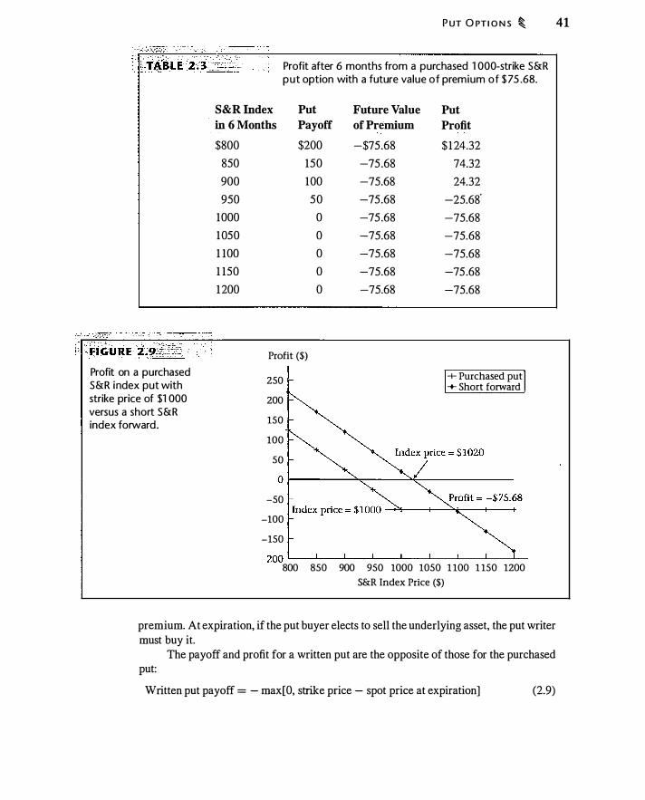
Profit on a purchased S&R index put with strike price of $1 000 versus a short S&R index forward.

P UT O PT I O N S � 41

Profit after 6 months from a purchased 1 000-strike S&R put option with a future value of premium of $ 75 .68.

S&R index Put Future Value Put

in 6 Months Payoff of Premium Profit

$800

850

900

950

1000

1050

1 100

1 150

1 200

$200

150

100

50

0

0

0

0

0

Profit ($)

250

200

150

100

-$75.68 $ 124.32

-75 .68 74.32

-75.68 24.32

-75.68 -25.68.

-75 .68 -75.68

-75.68 -75.68

-75.68 -75.68

-75.68 -75 .68

-75.68 -75.68

-1- Purchased put -+- Short forward

so o r-------��----��-------------

-50

-100

-150

-200 �--�--�--�--�--�--�--�--� 800 850 900 950 1000 1050 1 100 1 150 1200

S&R Index Price ($)

premium. At expiration, if the put buyer elects to sell the underlying asset, the put writer must buy it.

The payoff and profit for a written put are the opposite of those for the purchased put:

Written put payoff = - max[O, strike price - spot price at expiration] (2.9)

42 � AN I NTRO D U CT I O N TO FO RWA R D S AN D O PT I O N S

Written put profit = - max[O, strike price - spot price at expiration]

+ future value of option premium (2. 1 0)

The put seller has a short position in the put.

Example 2.1 1 Consider a 1000-strike put option on the S&R index with 6 months to expiration. At the time the option is written, the put writer receives the premium of $74.20.

Suppose the index in 6 months is $ 1 1 00. The put buyer will not exercise the put. Thus, the put writer keeps the premium, plus 6 months' interest, for a payoff of 0 and profit of $75 .68.

If the index is $900 in 6 months, the put owner will exercise, selling the index for $ 1000. Thus, the option writer will have to pay $ 1000 for an index worth $900. Using equation (2.9), the written put payoff is

- max[O, $ 1000 - $900] = -$100

The premium has earned 2% interest for 6 months, and is now worth $75.68. Profit for the written put is therefore

-$ 100 + $75 .68 = -$24.32

Figure 2. 1 0 graphs the profit diagram for a written put. As you would expect, it is the mirror image of the purchased put.

Written S&R index put option with strike of $ 1 000 versus a long S&R index forward contract.

Profit ($)

200

150

100

50

0 �------��----�t--------------

-50

-100

-150

-200

Index price = $ 1020

+ Written put + Long forward

-2SQ L---L---�--�---L---L--�--�----L-800 850 900 950 1000 1050 1 100 1 150 1200

S&R Index Price ($)

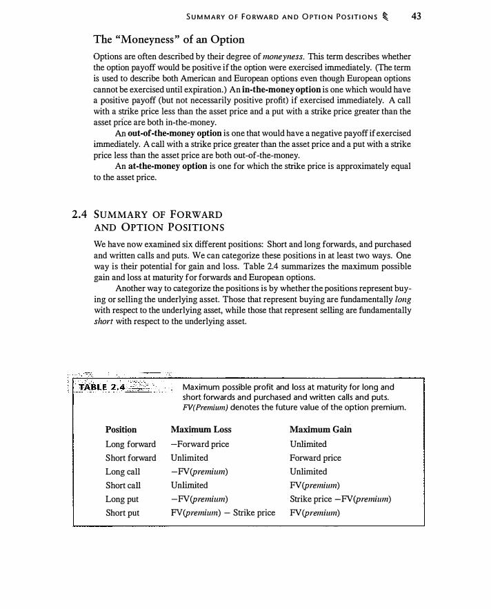
S U M M A RY O F FO RWA R D A N D O PTI O N P O S I T I O N S � 43

The "Moneyness" of an Option

Options are often described by their degree of moneyness. This term describes whether the option payoff would be positive if the option were exercised immediately. (The term is used to describe both American and European options even though European options cannot be exercised until expiration.) An in-the-money option is one which would have a positive payoff (but not necessarily positive profit) if exercised immediately. A call with a strike price less than the asset price and a put with a strike price greater than the asset pri"ce are both in-the-money.

An out-of-the-money option is one that would have a negative payoff if exercised immediately. A call with a strike price greater than the asset price and a put with a strike price less than the asset price are both out-of-the-money.

An at-the-money option is one for which the strike price is approximately equal to the asset price.

2.4 SUMMARY OF FORWARD AND OPTION POSITIONS

We have now examined six different positions: Short and long forwards, and purchased and written calls and puts. We can categorize these positions in at least two ways. One way is their potential for gain and loss. Table 2.4 summarizes the maximum possible gain and loss at maturity for forwards and European options.

Another way to categorize the positions is by whether the positions represent buy­ing or selling the underlying asset. Those that represent buying are fundamentally long with respect to the underlying asset, while those that represent selling are fundamentally short with respect to the underlying asset.

Position

Long forward

Short forward

Long call

Short call

Long put

Short put

Maximum possible profit and loss at maturity for long and short forwards and purchased and written cal ls and puts. FV(Premium) denotes the future value of the option premium.

Maximum Loss

-Forward price

Unlimited

-FV(premium)

Unlimited

-FV(premium)

FV(premium) - Strike price

Maximum Gain Unlimited

Forward price

Unlimited

FV(premium)

Strike price -FV(premium)

FV (premium)

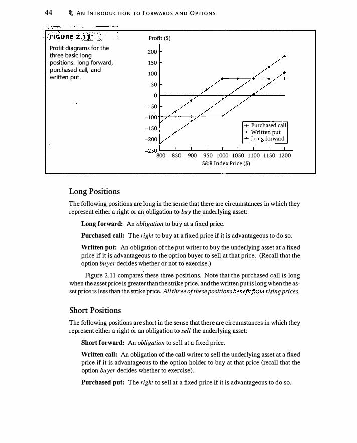
44 � A N I NT R O D U CT I O N TO F O RWA R D S AN D O PT I O N S

Profit diagrams for the three basic long positions: long forward, purchased call, and written put.

Long Positions

Profit ($)

200

150

100

50

0 �------��----�'---��-------

-50

-100 -1=-�+----t-:.,£--+---l" -150

-200

+ Purchased call -+- Written put ..,._ Long forward

-250 �-L---L---�-�-�--�-�--� 800 850 900 950 1000 1050 1 100 1 150 1200

S&R Index Price ($)

The following positions are long in the. sense that there are circumstances in which they represent either a right or an obligation to buy the underlying asset:

Long forward: An obligation to buy at a fixed price.

Purchased call: The right to buy at a fixed price if it is advantageous to do so.

Written put: An obligation of the put writer to buy the underlying asset at a fixed price if it is advantageous to the option buyer to sell at that price. (Recall that the option buyer decides whether or not to exercise.)

Figure 2. 1 1 compares these three positions. Note that the purchased call is long when the asset price is greater than the strike price, and the written put is long when the as­set price is less than the strike price. All three of these positions benefit from rising prices.

Short Positions

The following positions are short in the sense that there are circumstances in which they represent either a right or an obligation to sell the underlying asset:

Short forward: An obligation to sell at a fixed price.

Written call: An obligation of the call writer to sell the underlying asset at a fixed price if it is advantageous to the option holder to buy at that price (recall that the option buyer decides whether to exercise).

Purchased put: The right to sell at a fixed price if it is advantageous to do so.

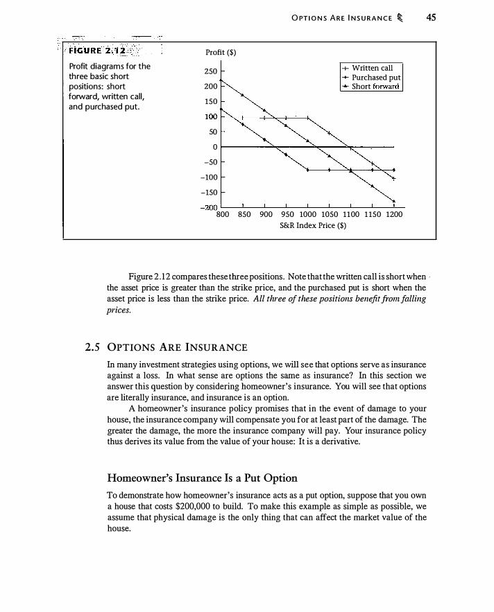
Profit diagrams for the three basic short positions: short forward, written call, and purchased put.

Profit ($)

2SO

200

O PT I O N S A R E I N S U R A N C E � 45

+ Written call -+- Purchased put ....._ Short forward

1SO

100 ��+---����-*

so 0 �--------�------��--��--�----

-SO

-100

-1SO

-200 L-__ L_ __ L_ __ L_ __ L_ __ L_ __ L_ __ �--� 800 8SO 900 9SO 1000 10SO 1100 1 1SO 1200

S&R Index Price ($)

Figure 2 . 1 2 compares these three positions. Note that the written call is short when · the asset price is greater than the strike price, and the purchased put is short when the asset price is less than the strike price. All three of these positions benefit from falling prices.

2.5 OPTIONS ARE INSURANCE

In many investment strategies using options, we will see that options serve as insurance against a loss. In what sense are options the same as insurance? In this section we answer this question by considering homeowner's insurance. You will see that options are literally insurance, and insurance is an option.

A homeowner's insurance policy promises that in the event of damage to your house, the insurance company will compensate you for at least part of the damage. The greater the damage, the more the insurance company will pay. Your insurance policy thus derives its value from the value of your house: It is a derivative.

Homeowner's Insurance Is a Put Option

To demonstrate how homeowner's insurance acts as a put option, suppose that you own a house that costs $200,000 to build. To make this example as simple as possible, we assume that physical damage is the only thing that can affect the market value of the house.

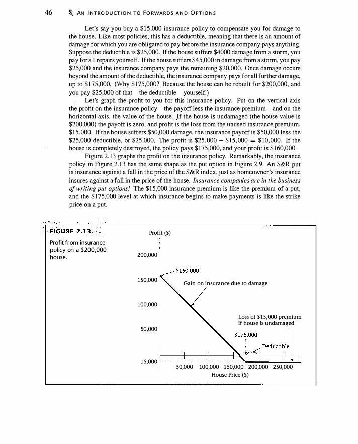
46 � AN I N TRO D U CTI O N TO FO RWA R D S A N D O PT I O N S

Let's say you buy a $ 1 5 ,000 insurance policy to compensate you for damage to the house. Like most policies, this has a deductible, meaning that there is an amount of

damage for which you are obligated to pay before the insurance company pays anything. Suppose the deductible is $25,000. If the house suffers $4000 damage from a storm, you

pay for all repairs yourself. If the house suffers $45,000 in damage from a storm, you pay

$25,000 and the insurance company pays the remaining $20,000. Once damage occurs beyond the amount of the deductible, the insurance company pays for all further damage,

up to $ 1 75 ,000. (Why $ 1 75,000? Because the house can be rebuilt for $200,000, and

you pay $25,000 of that-the deductible-yourself.)

, Let's graph the profit to you for this insurance policy. Put on the vertical axis

the profit on the insurance policy-the payoff less the insurance premium-and on the

horizontal axis, the value of the house. If the house is undamaged (the house value is $200,000) the payoff is zero, and profit is the loss from the unused insurance premium,

$ 1 5 ,000. If the house suffers $50,000 damage, the insurance payoff is $50,000 less the

$25,000 deductible, or $25,000. The profit is $25 , 000 - $ 15 , 000 = $ 10 ,000. If the house is completely destroyed, the policy pays $ 175,000, and your profit is $ 160,000.

Figure 2. 1 3 graphs the profit on the insurance policy. Remarkably, the insurance

policy in Figure 2. 1 3 has the same shape as the put option in Figure 2.9. An S&R put is insurance against a fall in the price of the S&R index, just as homeowner's insurance

insures against a fall in the price of the house. Insurance companies are in the business of writing put options! The $ 1 5,000 insurance premium is like the premium of a put, and the $ 1 75,000 level at which insurance begins to make payments is like the strike

price on a put.

Profit from insurance pol icy on a $200,000 house.

Profit ($)

200,000

150,000

100,000

50,000

15,000

Gain on insurance due to damage

Loss of $ 15,000 premium if house is undamaged

50,000 100,000 1 50,000 200,000 250,000

House Price ($)

O PT I O N S A R E I N S U R A N C E � 47

The idea that a put option is insurance also helps us understand what makes a put option cheap or expensive. Two important factors are the riskiness of the underlying asset and the amount of the deductible. Just as with insurance, options will be more expensive when the underlying asset is riskier. Also, the option, like insurance, will be less expensive as the deductible gets larger (for the put option, this means lowering the strike price).

You have probably recognized that there are some practical differences between a financial put option and homeowner's insurance. One important difference is that the S&R put pays off no matter why the index price declines. Homeowner's insurance, on the other hand, pays off only if the house declines in value for specified reasons. In particular, a simple decline in real estate prices is not covered by typical homeowner's insurance policies. We avoided this complication by assuming at the outset that only damage could affect the value of the house.

But I Thought Insurance Is Prudent and Put Options Are Risky . . .

If we accept that insurance and put options are the same thing, how do we reconcile this with the common idea that buying insurance is prudent and buying put options is risky?

The risk of a derivative or any other asset or security can only be evaluated in context. Figure 2. 1 3 depicts the risk of an insurance contract without considering the risk of the insured asset. This would be like owning insurance on your neighbor's house . . It would be "risky" because you would buy the insurance policy, and you would lose your entire investment if there were no insurance claim. 8 We do not normally think of insurance like this, but it illustrates the point that an insurance policy is a put option on the insured asset.

In the same way, Figure 2.9 depicts the risk of a put option without considering the risk of any other positions an investor might be holding. In contrast to homeowner's insurance, many investors do own put options without owning the underlying asset This , is why options have a reputation for being risky while homeowner's insurance does not. With stock options it is possible to own the insurance without the asset Of course, many investors who own put options also own the stock. For these investors, the risk is like that of insurance, which we normally think of as risk-reducing rather than risk-increasing.

Call Options Are Also Insurance

Call options can also be insurance. Whereas a put option is insurance for an asset we already own, a call option is insurance for an asset we plan to own in the future. Put differently, a put option is insurance for a long position while a call option is insurance for a short position.

80f course, in real life no insurance company will sell you insurance on your neighbor's house. The

reason is that you will then be tempted to cause damage in order to make your policy valuable. Insurance

companies call this "moral hazard."

48 � AN I NT R O D U CT I O N TO F O RWA R D S AN D O PT I O N S

Return to the earlier example of the S&R index. Suppose that the current price of the S&R index is $ 1000 and that we plan to buy the index in the future. If we buy an S&R call option with a strike price of $ 1000, this gives us the right to buy S&R for a maximum cost of $ 1000/share. By buying a call, we have bought insurance against an increase in the price.

2.6 EXAMPLE: EQUITY-LINKED CDS

Although options and forwards are important in and of themselves, they are also com­mollly used as building blocks in the construction of new financial instruments. For example, banks and insurance companies offer investment products that allow investors to benefit from a rise in a stock index and.that provide a guaranteed return if the market declines. We can "reverse-engineer" such equity-linked CDs and notes using the tools we have developed thus far.9

Ji�!fc:_r:_E!!�!�:i_Linked Products

The equity-linked CD described in the text provides a zero return (a refund of the initial investment) if the index declines, and a return linked to the index if the index rises. In general, a combination of a bond and one or more equity options is called an equity-linked note. It is possible to specify the linkage to the index in different ways, leading to many variants on the basic structure.

MITTS (Market Index Target Term Securities), issued by Merrill Lynch, resemble the equity-linked note described in the text, except that they are traded on the American Stock Exchange. (CDs are issued by a bank and are generally not tradeable.) For example, l\1ITIS issued in 2002 and maturing in 2009 provide a return linked to the Dow Jones Industrial Average. Specifically, the note promises approximately 86% of the simple appreciation of the Dow Jones average over the 7-year life of the note.

A common alternative is to compute the maturity payment of the note based on the average level of the index over the life of the CD. For example, State Farm Bank has offered to investors a Market Rate Certificate of Deposit. These have 5 years to maturity and have a payoff based on the arithmetic average of the quarter-end S&P index level for the 12 quarters prior to maturity. Instead · of receiving 70% of the simple return, this particular CD pays 90% of the return based on the 1 2-quarter average. (The specific terms of the CD will vary with market conditions.) An option based on an average of prices over time, rather than a single price at maturity, is called an Asian option. We discuss Asian options in Chapter 14 and equity-linked notes in Chapter 15 .

9 A CD (certificate o f deposit) is a kind o f interest-bearing bank account. You can think of a C D as

being the same as a note or a bond.

EXA M P LE : EQU ITY- L I N K E D COS � 49

A simple 5 112 year CD with a return linked to the S&P 500 might have the following structure: At maturity, the CD is guaranteed to repay the invested amount, plus 70% of the simple appreciation in the S&P 500 over that time. 1 0

We can ask several questions about the CD:

• Is the CD fairly priced? • How can we decompose the product in terms of options and bonds? • How does the issuing bank hedge the risk associated with issuing the product? • How does the issuing bank make a profit?

To understand this product, suppose the S&P index is 1 300 initially and an investor invests $ 10,000. If the index is below 1 300 after 5.5 years, the CD returns to the investor the original $ 10,000 investment. If the index is above 1 300 after 5.5 years, the investor receives $ 10,000 plus 70% of the percentage gain on the index. For example, if the index is 2200, the investor receives

$10 ,000 X (1 + (2200/ 1300 - 1) X 70%] = $14, 846

At first glance this product appears to permit gains but no losses. However, by now you are probably skeptical of a phrase like "gains but no losses"; the investor must pay something for an investment like this.

Graphing the Payoff on the CD

As a first step in analyzing the CD, we will draw a payoff diagram. If we invest $ 10,000, we receive at least $ 10,000. If the index rises to Sfinal > 1 300, we also receive on our investment 70% of the rate of return

Thus, �e CD pays

Sfinal _ I 1300

$ 10,000 x ( 1 + 0.7 x max [ 0, :;�� - 1]) Figure 2 . 14 graphs the payoff at expiration to this investment in the CD.

(2. 1 1 )

Recall the discussion in Section 2. 1 of incorporating a zero-coupon bond into a payoff diagram. Per unit of the index (there are 10 ,000/ 1300 = 7.69 units of the index in a $ 10,000 investment), the CD buyer receives 0.7 of an index call option, plus a zero-coupon bond paying $ 1300 at expiration.

Table 2.5 computes the payoff to the equity-linked CD for different values of the index.

1 0This is the structure of a CD issued in 1 999 by First Union National Bank.

50 � AN I NTRO D U CT I O N TO F O RWA R D S A N D O PT I O N S

Payoff (thousands of $) Payoff at expiration to $1 0,000 investment in an equity-l inked CD that repays the in itial investment at expiration plus 70% of the rate of appreciation of the mq_rket above 1 300.

Economics of the CD

1-+--- Payoff of CD I 13

12

1 1

9

I I I :- $1300 I I I . 8L---�--�--��L-�--�--�----� 600 800 1000 1200 1400 1600 1800 2000

S&P 500 at Expiration

Payoff of equity-l inked CD at expiration.

S&P index CD

After 5.5 Years Payoff

500 $ 10,000.00 1000 10,000.00 1500 1 1 ,076.92 2000 13 ,769.23 2500 16,461 .54 3000 19 , 153.85

Now we are in a position to understand the economics of this product. Think about what happens if the index is below 1300 at expiration. We pay $ 10,000 and we receive $ 10,000 back, plus an option. Thus, we have forgone interest on $ 10,000 in exchange for the possibility of receiving 70% of the gains on the S&P. Suppose that the effective

EXA M P L E : EQU I TY- L I N K E D CDS � 5 1

annual interest rate i s 6%; after 5 112 years, the buyer has lost interest of

$ 10 ,000 X ( 1 .06)-5 ·5 - $10,000 = -$2,742

Essentially, the buyer forgoes interest in exchange for a call option on the index. With this description we have reverse-engineered the CD, decomposing it in terms

of an option and a bond. The question of whether the CD is fairly priced turns on whether the $2742 is a fair price for the index option implicit in the CD. Given information about the interest rate, the volatility of the index, and the dividend yield on the index, it is possible to price the option to determine whether the CD is fairly priced. We perform that analysis for this example in Chapter 15 .

Why Equity-Linked CDs?

With reverse-engineering, we see that an investor could create the equivalent of an equity-linked CD by buying a zero-coupon bond and 0.7 call options. Why, then, do products like this exist?

Consider what must be done to replicate the payoff. If a retail investor were to insure an index investment using options, the investor would have to learn about options, decide what maturity, strike price, and quantity to buy, and pay transaction costs. Exchange-traded options have at most 3 years to maturity, so obtaining longer­term protection requires rolling over the position at some point.

An equity-linked CD provides a prepackaged solution. It may provide a pattern of . market exposure that many investors could not otherwise obtain at such low transaction costs.

The idea that a prepackaged deal may be attractive should be familiar to you. Supermarkets sell whole heads of lettuce-salad building blocks, as it were-and they also sell, at a premium price, lettuce already washed, torn into bite-sized pieces, and mixed as a salad. The transaction cost of salad preparation leads some consumers to prefer the prepackaged salads.

What does the financial institution get out of this? Just as the supermarket earns profit on prepackaged salads, the issuing bank wants to earn a transaction fee on the CD. When it sells a CD, the issuing bank borrows money (the zero-coupon bond portion of the CD) and receives the premium for writing a call option. The cost of the CD to the bank is the cost of the zero-coupon bond plus the cost of the call option. Obviously the bank would not issue the equity-linked CD in the first place unless it was less expensive than alternative ways to attract deposits, such as standard CDs. The equity-linked CD is risky because the bank has written a call, but the bank can manage this risk in several ways, one of which is to purchase call options from a dealer to offset the risk of having written calls. Using data from the early 1990s, Baubonis et al. ( 1 993) estimated that issuers of equity-linked CDs earned about 3 .5% of the value of the CD as a fee, with about 1 % as the transaction cost of hedging the written call . 1 1

1 1 A back-of-the-envelope calculation in Chapter 15 suggests the issuer fees for this product are in the neighborhood of 4% to 5%.

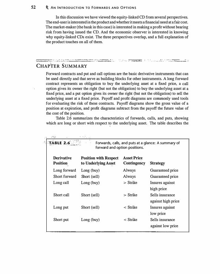
52 � A N I NT R O D U CT I O N TO FO RWA R D S A N D O PT I O N S

In this discussion we have viewed the equity-linked CD from several perspectives. The end-user is interested in the product and whether it meets a financial need at a fair cost. The market-maker (the bank in this case) is interested in making a profit without bearing risk from having issued the CD. And the economic observer is interested in knowing why equity-linked CDs exist. The three perspectives overlap, and a full explanation of the product touches on all of them.

CHAPTER S UMMARY

Forward contracts and put and call options are the basic derivative instruments that can be used directly and that serve as building blocks for other instruments. A long forward contract represents an obligation to buy the underlying asset at a fixed price, a call option gives its owner the right (but not the obligation) to buy the underlying asset at a fixed· price, and a put option gives its owner the right (but not the obligation) to sell the underlying asset at a fixed price. Payoff and profit diagrams are commonly used tools for evaluating the risk of these contracts. Payoff diagrams show the gross value of a position at expiration, and profit diagrams subtract from the payoff the future value of the cost of the position.

Table 2.6 summarizes the characteristics of forwards, calls, and puts, showing which are long or short with respect to the underlying asset. The table describes the

TABLE 2 . 6 . . ' . Forwards, cal ls, and puts at a glance: A summary of forward and option positions.

Derivative Position with Respect Asset Price

Position to Underlying Asset Contingency Strategy

Long forward Long (buy) Always Guaranteed price

Short forward Short (sell) Always Guaranteed price

Long call Long (buy) > Strike Insures against

high price

Short call Short (sell) > Strike Sells insurance

against high price

Long put Short (sell) < Strike Insures against

low price

Short put Long (buy) < Strike Sells insurance

against low price

The basic profit diagrams: long and short forward, long and short call, and long and short put.

Profit

Profit

Profit

Long forward

Stock Price

Long call

Stock Price

Long put

Stock Price

F U RTH E R R EA D I N G � 53

Profit Short forward

Stock Price

Profit Short call

Stock Price

Profit Short put

Stock Price

strategy associated with each: Forward contracts guarantee a price, purchased options are insurance, and written options are selling insurance. Figure 2. 1 5 provides a graphical summary of these positions.

Options can also be viewed as insurance. A put option gives the owner the right to sell if the price declines, just as insurance gives the insured the right to sell (put) a . damaged asset to the insurance company.

FURTHER READING We use the concepts introduced in this chapter throughout the rest of this book. Chapter 3 presents a number of basic option strategies which are widely used in practice, including caps, collars, and floors. Chapter 4 presents the use of options in risk management.

A more general question raised implicitly in this chapter is how the prices of forwards and options are determined. Chapter 5 covers financial forwards and futures in detail, and Chapter 1 0 introduces the basic ideas underlying option pricing.

Brokerages routinely supply options customers with an introductory pamphlet about options entitled Characteristics and Risks of Standardized Options. This is avail­able online from http://www.cboe.com. You can also obtain current option prices from Web sites such as the CBOE's and various brokerage sites.

54 � AN I NTRO D U CT I O N TO F O RWA R D S A N D O PT I O N S

The notion that options are insurance has been applied in practice. Sharpe ( 1 976), for example, analyzed optimal pension funding policy taking into account pension insur­ance provided by the Pension Benefit Guaranty Corporation. Merton ( 1977a) observed that bank deposit insurance and in fact any loan guarantee can be modeled as a put option. Baubonis et al . ( 1 993) discuss equity-linked CDs.

PROBLEMS

In the following problems, if the "effective annual interest rate" i s r, a $ 1 investment yields 1 + r after one year.

2.1. Suppose XYZ stock has a price of $50 and pays no dividends. The effective annual interest rate is 1 0%. Draw payoff and profit diagrams for a long position in the stock. Verify that profit is 0 at a price in one year of $55.

2.2. Using the same information as the previous question, draw payoff and profit diagrams for a short position in the stock. Verify that profit is 0 at a price in one year of $55 .

2.3. What position is the opposite of a purchased call? The opposite of a purchased put?

2.4. a. Suppose you enter into a long 6-month forward position at a forward price of $50. What is the payoff in 6 months for prices of $40, $45, $50, $55, and $60?

b. Suppose you buy a 6-month call option with a strike price of $50. What is the payoff in 6 months at the same prices for the underlying asset?

c. Comparing the payoffs of parts (a) and (b), which contract should be more expensive (i .e., the long call or long forward)? Why?

2.5. a. Suppose you enter into a short 6-month forward position at a forward price of $50. What is the payoff in 6 months for prices of $40, $45, $50, $55, and $60?

b. Suppose you buy a 6-month put option with a strike price of $50. What is the payoff in 6 months at the same prices for the underlying asset?

c. Comparing the payoffs of parts (a) and (b), which contract should be more expensive (i.e., the long put or short forward)? Why?

2.6. A default-free zero-coupon bond costs $9 1 and will pay $ 100 at maturity in 1 year. What is the effective annual interest rate? What is the payoff diagram for the bond? The profit diagram?

2.7. Suppose XYZ stock pays no dividends and has a current price of$50. The forward price for delivery in 1 year is $55. Suppose the 1 -year effective annual interest rate is 10%.

a. Graph the payoff and profit diagrams for a forward contract on XYZ stock with a forward price of $55.

P R O B L E M S � 55

b. Is there any advantage to investing in the stock or the forward contract? Why?

c. Suppose XYZ paid a dividend of $2 per year and everything else stayed the same. Now is there any advantage to investing in the stock or the forward contract? Why?

2.8. Suppose XYZ stock pays no dividends and has a current price of $50. The forward price for delivery in one year is $53 . If there is no advantage to buying either the stock or the forward contract, what is the 1 -year effective interest rate?

2.9. An off-market forward contract is a forward where either you have to pay a pre­mium or you receive a premium for entering into the contract. (With a standard forward contract, the premium is zero.) Suppose the effective annual interest rate is 10% and the S&R index is 1000. Consider 1 -year forward contracts.

a. Verify that if the forward price is $ 1 100, the profit diagrams for the index and the 1 -year forward are the same.

b. Suppose you are offered a long forward contract at a forward price of $ 1 200. How much would you need to be paid to enter into this contract?

c. Suppose you are offered a long forward contract at $ 1000. What would you be willing to pay to enter into this forward contract?

2.10. For Figure 2.7, verify the following:

a. The S&R index price at which the call option diagram intersects the x -axis is $ 1 095.68.

b. The S&R index price at which the call option and forward contract have the same profit is $924.32.

2.11. For Figure 2.9, verify the following:

a. The S&R index price at which the put option diagram intersects the x-axis is $924.32.

b. The S&R index price at which the put option and forward contract have the same profit is $ 1095.68.

2.12. For each entry in Table 2.4, explain the circumstances in which the maximum gain or loss occurs .

2.13. Suppose the stock price is $40 and the effective annual interest rate is 8%.

a. Draw on a single graph payoff and profit diagrams for the following options:

(i) 35-strike call with a premium of $9. 1 2.

(ii) 40-strike call with a premium of $6.22.

(iii) 45-strike call with a premium of $4.08.

56 � AN I NTRO D U CT I O N TO F O RWA R D S A N D O PT I O N S

b . Consider your payoff diagram with all three options graphed together. Intuitively, why should the option premium decrease with the strike price?

2.14. Suppose the stock price is $40 and the effective annual interest rate is 8%. Draw payoff and profit diagrams for the following options:

a. 35-strike put with a premium of $ 1 .53.

b. 40-strike put with a premium of $3 .26.

c. 45-strike put with a premium of $5.75 .

Consider your payoff diagram with all three options graphed together. Intuitively, why should the option premium increase with the strike price?

2.15. The profit calculation in the chapter assumes that you borrow at a fixed interest rate to finance investments. An alternative way to borrow is to short-sell ·stock. What complications would arise in calculating profit if you financed a $ 1000 S&R index investment by shorting IBM stock, rather than by borrowing $ 1 000?

2.16. Construct a spreadsheet that permits you to compute payoff and profit for a short and long stock, a short and long forward, and purchased and written puts and calls. The spreadsheet should let you specify the stock price, forward price, interest rate, option strikes, and option premiums. Use the spreadsheet's max function to compute option payoffs.

APPENDIX 2 .A: MORE ON BUYING A STOCK OPTION

The box on page 34 discusses buying options. There are at least four practical issues that an option buyer should be aware of: Dividends, exercise, margins, and taxes. In this section we will focus on retail investors and exchange-traded stock options. Be aware that specific rules regarding margins and taxes change frequently. This section is intended to help you identify issues and is not intended as a substitute for professional brokerage, accounting, or legal advice.

Dividends

The owner of a standard call option has the right to buy a fixed number of shares of stock at a fixed price, but has no right to receive dividends paid on the underlying stock over the life of the option. When a stock pays a dividend, the stock price declines by approximately the amount of the dividend. This decline in the price lowers the return to the owner of a call option.

For exchange-traded options in the United States, there is typically no adjustment in the terms of the option if the stock pays an "ordinary" dividend (one that is typical for the stock). However, if the stock pays an unusual dividend, then officials at the Options Clearing Corporation (OCC) decide whether or not to make an adjustment.

A P P E N D I X 2 .A : M O R E O N B U Y I N G A STO C K O PT I O N � 57

In June 2003, Iomega Corporation declared a $5 dividend, payable on October 1 . At the time of the declaration, Iomega's share price was $ 1 I .40. Since the dividend was 44% of the share price, the OCC reduced all Iomega option strike prices by $5, effective October 2. 1 2

When we discuss option pricing, we will see that it is necessary to take dividends into account when pricing an option.

Exercise

Some options, for example those that are cash-settled, are automatically exercised at maturity; the option owner need not take any action. Suppose you own a traded op­tion that is not cash-settled and not automatically exercised. In this case you must provide exercise instructions prior to the broker's deadline. If you fail to do so, the option will expire worthless. When you exercise the option, you generally pay a com­mission. If you do not wish to own the stock, exercising the option would require that you pay a commission to exercise and then a commission to sell the shares. It might be preferable to sell the option instead of exercising it. If you do wish to own the underlying asset, you can exercise the option. The option writer who is ob­ligated to fulfill the option exercise (delivering the shares for a call or buying the shares for a put) is said to have been assigned. Assignment can involve paying a commis­siOn.

American-style options can be exercised prior to expiration. If you own an option and fail to exercise when you should, you will lose money relative to following the optimal exercise strategy. If you write the option, and it is exercised (you are assigned), you will be required to sell the stock (if you sold a call) or buy the stock (if you sold a put) . Therefore, if you buy or sell an American option, you need to understand the circumstances under which exercise might be optimal. Dividends are one factor that can affect the exercise decision. We discuss early exercise in Chapters 9 and 1 1 .

Margins for Written Options

Purchased options for which you fully pay require no margin, as there is no counterparty risk. With written option positions, however, you can incur a large loss if the stock moves against you. When you write an option, therefore, you are required to post collateral to insure against the possibility that you will default. This collateral is called margin.

Margin rules are beyond the scope of this book and change over time. Moreover, different option positions have different margin rules. Both brokers and exchanges can provide information about current margin requirements.

1 2Reducing the strike price by the amount of the dividend leaves call holders worse off, albeit better off than if no adjustment had been made. If S is the cum-dividend stock price and S - D the ex-dividend stock price, Merton ( 1 973b, p. ! 52) shows that to leave the value of a call position unchanged, it is necessary to reduce the strike price by the factor (S - D)fS, and give the option holder Sf(S - D) - I additional options. An option with a value protected against dividends is said to be payout-protected.

58 � A N I NTRO D U CT I O N T O F O RWA R D S A N D O PT I O N S

Taxes

Tax rules for derivatives in general can be complicated, and they change frequently as the tax law changes. The taxation of simple option transactions is straightforward.

If you purchase a call option or stock and then sell it, gain or loss on the position is treated like gain or loss on a stock, and accorded long-term or short-term capital gains treatment depending on the length of time for which the position has been held. If you purchase a call option and then exercise it, the cost basis of the resulting stock position is the exercise price plus the option premium plus commissions. The holding period for the resulting stock position begins the day after the option is exercised. The time the option is held does not contribute to the holding period.

The rules become more intricate when forwards and options are held in tandem with the underlying asset. The reasons for this complexity are not hard to understand. Tax laws in the United States accord different tax treatment to different kinds of income. The tax code views interest income, dividend income, and capital gains income as distinct and subject to different tax rules. Futures also have special rules. However, using derivatives, one kind of income can be turned into another. We saw in this chapter, for example, that buying zero-coupon bonds and a forward contract mimics a stock investment.

One category of special rules governs a constructive sale. If you own a stock, entering into certain option or forward positions can trigger a constructive sale, meaning that even if you continue to own the stock, for tax purposes you are deemed to have sold it at the time you enter into the forward or option positions. By shorting a forward against the stock, for example, the stock position is transformed into a bond position. When you have no risk stemming from stock ownership, tax law deems you to no longer be an owner.

The so-called straddle rules are tax rules intended to control the recognition of losses for tax purposes when there are offsetting risks as with constructive sales. Such positions often arise when investors are undertaking tax arbitrage, which is why the positions are accorded special treatment. A stock owned together with a put is a tax straddle. 1 3 Generally, the straddle rules prevent loss recognition on only a part of the entire position. A straddle for tax purposes is not the same thing as an option straddle, discussed in Chapter 3 .

I t i s probably obvious to you that if you are taxable and transact in options, and especially if you have both stock and offsetting option positions, you should be prepared to seek professional tax advice.

13 For an il lustration of the complexity, in this particular case, an exception to the straddle rules occurs if the stock and put are a "married put," meaning that the two are purchased together and the stock is deli vered to settle the put.

C�E�,3··· .. Insurance] Collars] and Other

Strategies I n the Ia" chaptcr we intmduced fmwanl< , cal1<, ""d put<; <howed that option' rnce

insurance; and looked at an example of how options can be building blocks. In this chapter we continue these themes, showing how the use of options can be interpreted as buying or selling insurance. We also continue the building block approach, examining the link between forward prices and option prices, and looking at some common option strategies, including spreads, straddles, and collars . Among your goals in this chapter should be to understand the reasons for using one strategy instead of another and to become facile with drawing and interpreting profit and loss diagrams.

3 . 1 BASIC INSURANCE STRATEGIES

There are infinite ways to combine options to create different payoffs. In this section we examine two important kinds of strategies in which the option is combined with a position in the underlying asset. First, options can be used to insure long or short asset positions. Second, options can be written against an asset position, in which case the option writer is selling insurance. In this section we consider four positions : Being long the asset coupled with a purchased put or written call, and being short the asset coupled with a purchased call or written put.

J? this section we continue to use the S&R index examples presented in Sections 2.2 and 2.3. We assumed a 2% effective 6-month interest rate, and premiums of $93 .809 for the 1000-strike 6-month call and $74.201 for the 1 000-strike 6-month put.

Insuring a Long Position: Floors

The analysis in Section 2.5 demonstrated that put options are insurance against a fall in the price of an asset. Thus, if we own the S&R index, we can insure the position by buying an S&R put option. The purchase of a put option is also called a floor, because we are guaranteeing a minimum sale price for the value of the index.

To examine this strategy, we want to look at the combined payoff of the index position and put. In the last chapter we graphed them separately; now we add them together to see the net effect of holding both positions at the same time.

Table 3 . 1 summarizes the result of buying a 1 000-strike put with 6 months to expiration, in conjunction with holding an index position with a current value of $ 1000. The table computes the payoff for each position and sums them to obtain the total payoff.

59

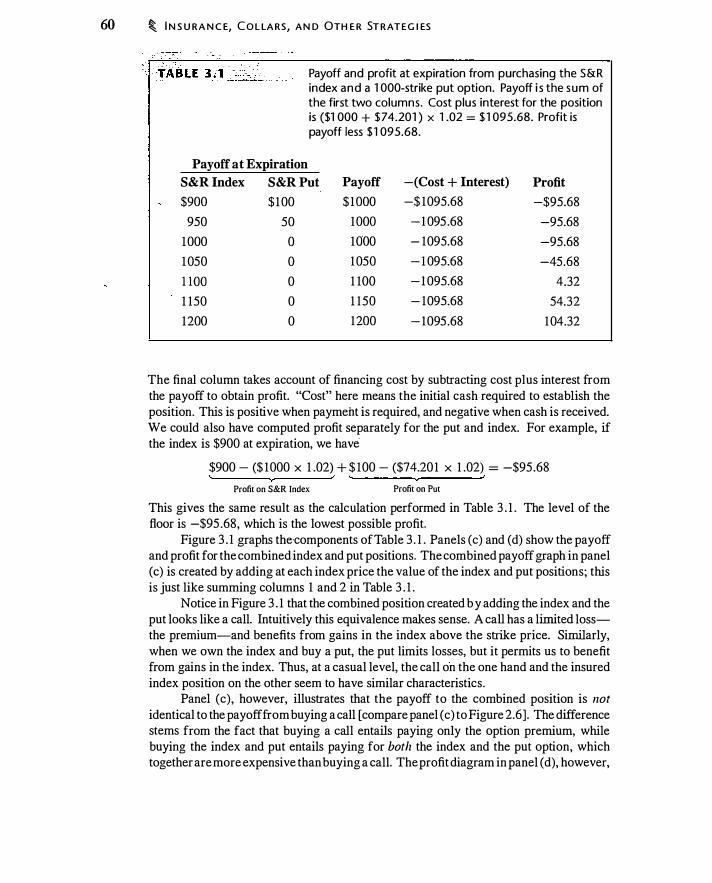
60 � I N S U RA N C E, C O L LA RS, A N D OTH E R ST RATEG I ES

Payoff and profit at expiration from purchasing the S&R index and a 1 000-strike put option. Payoff i s the sum of the first two columns. Cost plus interest for the position is ($1 000 + $ 74.201 ) x 1 .02 = $ 1 095.68. Profit is payoff less $ 1 095.68.

Payoff at Expiration

S&R index S&R Put Payoff -(Cost + Interest) Profit

$900 $ 100 $ 1000 -$ 1095.68 -$95.68

950 50 1000 - 1 095 .68 -95.68

1000 0 1000 - 1095.68 -95.68

1 050 0 1050 - 1 095.68 -45.68

l lOO 0 1 100 - 1 095.68 4.32

1 150 0 l l50 - 1095.68 54.32

1200 0 1200 - 1095 .68 104.32

The final column takes account of financing cost by subtracting cost plus interest from the payoff to obtain profit. "Cost" here means the initial cash required to establish the position. This is positive when payment is required, and negative when cash is received. We could also have computed profit separately for the put and index. For example, if the index is $900 at expiration, we have

$900 - ($ 1000 X 1 .02) + $ 100 - ($74.20 1 X 1 .02) = -$95 .68

Profit on S&R Index Profit on Put This gives the same result as the calculation performed in Table 3 . 1 . The level of the floor is -$95 .68, which is the lowest possible profit.

Figure 3 . 1 graphs the·components of Table 3 . 1 . Panels (c) and (d) show the payoff and profit for the combined index and put positions. The combined payoff graph in panel (c) is created by adding at each index price the value of the index and put positions; this is just like summing columns 1 and 2 in Table 3 . 1 .

Notice in Figure 3 . 1 that the combined position created b y adding the index and the put looks like a call. Intuitively this equivalence makes sense. A call has a limited loss­the premium-and benefits from gains in the index above the strike price. Similarly, when we own the index and buy a put, the put limits losses, but it permits us to benefit from gains in the index. Thus, at a casual level, the call on the one hand and the insured index position on the other seem to have similar characteristics.

Panel (c), however, illustrates that the payoff to the combined position is not identical to the payoff from buying a call [compare panel (c) to Figure 2.6]. The difference stems from the fact that buying a call entails paying only the option premium, while buying the index and put entails paying for both the index and the put option, which together are more expensive than buying a call. The profit diagram in panel (d), however,

Panel (a) shows the payoff diagram for a long position in the index (column 1 in Table 3 . 1 ) . Panel (b) shows the payoff . diagram for a purchased index put with a strike price of $1 000 (column 2 in Table 3 . 1 ) . Panel (c) shows the combined payoff diagram for the index and put (column 3 in Table 3.1 ) . Panel (d) shows the combined profit diagram for the index and put, obtained by subtracting $ 1 095.68 from the payoff diagram in panel (c) (column 5 in Table 3 . 1 ) .

BAS I C I N S U RA N C E STRATE G I ES � 61

Payoff ($) Payoff ($) Long S&R Index Long S&R Put

2000 2000

1000 1000

0 · · · · · · · · · · · · · · · · · · · · · · · · · · · · · · · · · · · · · 0

-1000 -1000

-2000 -2000 0 500 1000 1500 2000 0 500 . 1000 1500 2000

S&R Index at Expiration S&R Index at Expiration (a) (b)

Payoff ($) Profit ($) Combined payoff Combined profit

2000 2000

1000 ' 1000

0 $1000

· · - · · · · · · · · · · · · · · · · · · · · · · · · · · · 0 f -1000 -1000 -$95.68

-2000 -2000 0 500 1000 1500 2000 0 500 1000 1500 2000

S&R Index at Expiration S&R Index at Expiration (c) (d)

does look like a call. We discussed in Section 2. 1 that adding a bond to a payoff diagram , shifts it vertically but leaves a profit diagram unaffected. The combined position of index plus put in panel (c) is actually equivalent to buying a 1000-strike call and buying a zero-coupon bond that pays $ 1000 at expiration of the option.

The profit diagram in panel (d) of Figure 3 . 1 does not merely resemble the profit diagram for buying an S&R index call with a strike price of $ 1000, graphed in Figure 2. 7; it is identical. We can see this by comparing Table 2.2 with Table 3 . 1 . The profit of -$95 .68 for prices below $ 1000 is exactly the future value of the 1000-strike 6-month to expiration call premium above.

The zero-coupon bond thus affects the payoff in panel (c), but leaves profit in panel (d) unaffected. The cash flows in purchasing a call are different from the cash flows in buying an asset and insuring it, but the profit for the two positions is the same. If we had explicitly borrowed the present value of $ 1000 ($ 1000/1 .02 = $980.39) to offset the cost of the index and put, then the payoff and profit diagrams, panels (c) and (d) in Figure 3 . 1 , would be identical.

The point that buying an asset and a put generates a position that looks like a call can also be seen using the homeowner's insurance example from Section 2.5. There,

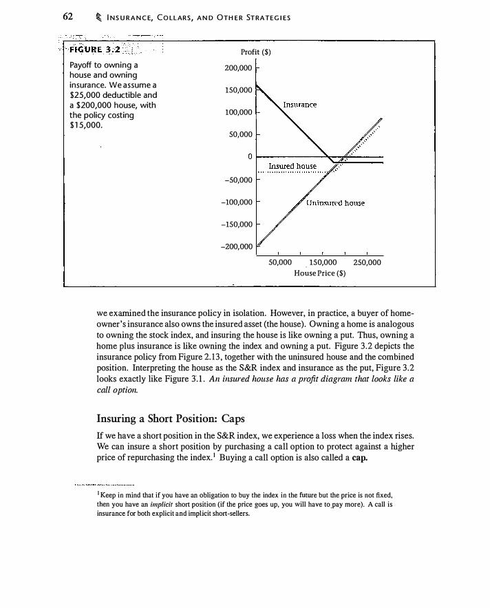
62 � I N S U RA N C E, C O LLARS, A N D OTH E R STRATEG I ES

Payoff to owning a house and owning insurance. We assume a $25,000 deductible and a $200,000 house, with the policy costing $ 1 5,000.

Profit ($)

200,000

150,000

100,000

50,000

-50,000

-100,000

-150,000

-200,000

50,000 . 150,000 250,000 House Price ($)

we examined the insurance policy in isolation. However, in practice, a buyer of home­owner's insurance also owns the insured asset (the house). Owning a home is analogous to owning the stock index, and insuring the house is like owning a put. Thus, owning a home plus insurance is like owning the index and owning a put. Figure 3 .2 depicts the insurance policy from Figure 2. 13 , together with the uninsured house and the combined position. Interpreting the house as the S&R index and insurance as the put, Figure 3 .2 looks exactly like Figure 3". 1 . An insured house has a p!Vfit diagram that looks like a call option.

Insuring a Short Position: Caps

If we have a short position in the S&R index, we experience a loss when the index rises. We can insure a short position by purchasing a call option to protect against a higher price of repurchasing the index. 1 Buying a call option is also called a cap.

1 Keep in mind that if you have an obligation to buy the index in the future but the price is not fixed, then you have an implicit short position (if the price goes up, you will have to pay more). A call is insurance for both explicit and implicit short-sellers.

BAS I C I N S U R A N C E STRAT EG I ES � 63

Payoff and profit at expiration from short-sel l ing the S&R index and buying a 1 000 strike ca l l option at a premium of $93.809. The payoff is the sum of the first two columns. Cost plus interest for the position is ( -$1 000 + $93 .809) x 1 .02 = -$924.32. Profit is payoff p lus $924.32.

Payoff at Expiration

Short S&R Index S&R Call Payoff -(Cost + Interest) Profit

-$900 $0 -$900 $924.32 $24.32

-950 0 -950 924.32 -25.68

- 1 000 0 - 1000 924.32 -75.68

- 1050 50 - 1 000 924.32 -75 .68

- 1 100 100 - 1 000 924.32 -75.68

- 1 1 50 150 - 1 000 924.32 -75.68

- 1200 200 - 1000 924.32 -75 .68

Table 3.2 presents the payoff and profit for a short position in the index coupled with a purchased call option. Because we short the index, we earn interest on the short proceeds less the cost of the call option, giving -$924.32 as the future value of the cost.

Figure 3 .3 graphs the columns of Table 3.2. The payoff and profit diagrams resemble those of a purchased put. As with the insured index position in Figure 3 . 1 , we have to be careful in dealing with cash flows. The payoff in panel (c) of Figure 3 .3 is like that of a purchased put coupled with borrowing. In this case, the payoff diagram for shorting the index and buying a call is equivalent to that from buying a put and borrowing the present value of $ 1 000 ($980.39). Since profit diagrams are unaffected by bm;rowing, however, the profit diagram in panel (d) is exactly the same as that for a

·

purchased S&R index put. You can see this by comparing panel (d) with Figure 2.9. Not only does the insured short position look like a put, it has the same loss as a purchased put if the price is above $ 1000: $75 .68, which is the future value of the $74.20 1 put premium.

Selling Insurance

We can expect that some investors want to purchase insurance. However, for every insurance buyer there must be an insurance seller. In this section we examine strategies in which investors sell insurance.

It is possible, of course, for an investor to simply sell calls and puts. Often, however, investors also have a position in the asset when they sell insurance. Writing an option when there is a corresponding long position in the underlying asset is called covered writing, option overwriting, or selling a covered call. All three terms mean

64 � I N S U R A N C E, C O LLA RS, A N D OTH E R STRAT EG I ES

FIGURE 3.3: . ..

Panel (a) shows the payoff diagram for a short position in the index (column 1 in Table 3 .2). Panel (b) shows the payoff diagram for a purchased index call with a strike price of $ 1 000 (column 2 in Table 3 .2). Panel (c) shows the combined payoff diagram for the

yhort index and long cal l (column 3 in Table 3 .2). Panel (d) shows the combined profit diagram for the short index and long call, obtained by adding $924.32 to the payoff diagram in panel (c) (column 5 in Table 3.2).

Payoff ($)

2000

1000

0

-1000

Short S&R Index

0 500 1000 1500 2000

S&R Index at Expiration

{a)

Payoff ($)

Combined Payoff 2000

1000 -$ 1000

0 · · · · · · · · · · · · · · · · · · · · · · ·f · · · · · · · · ·

-1000

-2000 '---'---J.___.L___.l.__ 0 500 1000 1500 2000

S&R Index at Expiration

(c)

Payoff ($)

Long S&R Call 2000

-1000

-2000 L...-_J.___.L___.l.__..L__ 0 500 1000 1500 2000

S&R Index at Expiration

(b)

Profit ($)

2000

1000

0

-1000

Combined Profit

t -$75 .68

-2000 .____...____ _ _,__ _ __._ _ __,__ 0 500 1000 1500 2000

S&R Index at Expiration

(d)

essentially the same thing.2 In contrast, naked writing occurs when the writer of an

option does not have a position in the asset. In addition to the covered writing strategies we will discuss here, there are other

insurance-selling strategies,.such as delta-hedging, which are less risky than naked writ­

ing and are used in practice by market-makers. We will discuss these other strategies later in the book, particularly in Chapter 13 .

Covered call writing If we own the S&R index and simultaneously sell a call option, we have written a covered call. A covered call will have limited profitability if the index increases, because an option writer is obligated to sell the index for the strike price. Should the index decrease, the loss on the index is offset by the premium earned from

2Technically, "option overwriting" refers to selling a call on stock you already own, while a "covered write" entails simultaneously buying the stock and selling a call. The distinction is irrelevant for our purposes.

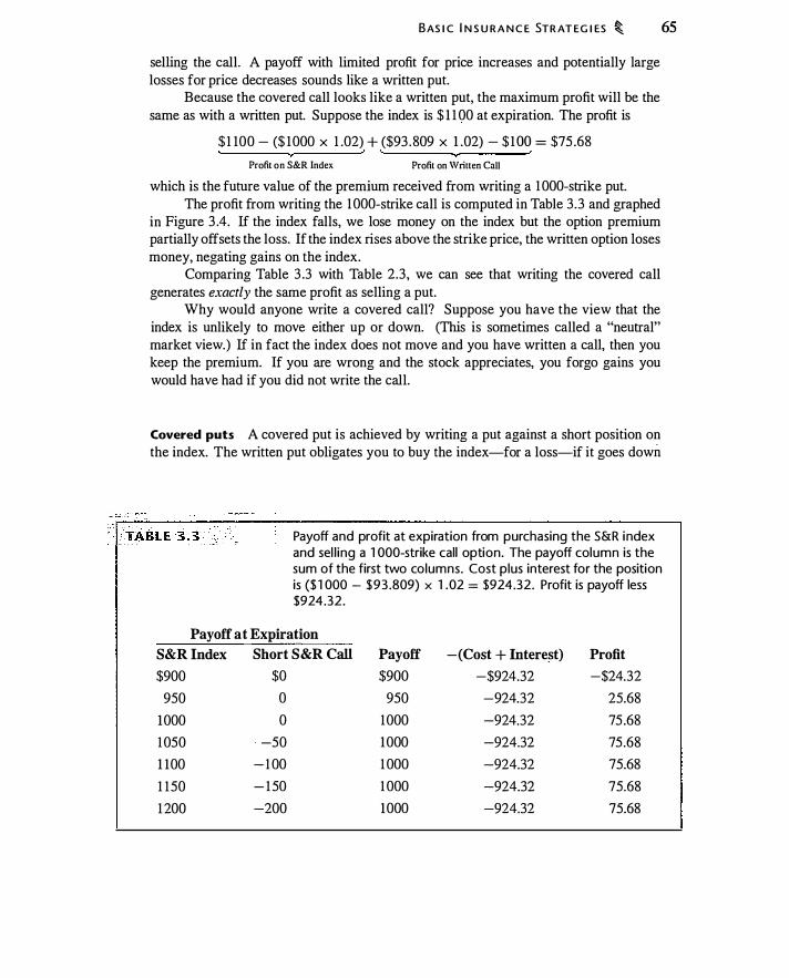
BAS I C I N S U RA N C E STR AT EG I ES � 65

selling the call. A payoff with limited profit for price increases and potentially large losses for price decreases sounds like a written put.

Because the covered call looks like a written put, the maximum profit will be the same as with a written put. Suppose the index is $ 1 1 00 at expiration. The profit is

$ 1 100 - ($ 1000 X 1 .02) + ($93 . 809 X 1 .02) - $ 1QQ = $75 .68

Profit on S&R Index Profit on Written Call

which is the future value of the premium received from writing a 1 000-strike put. The profit from writing the 1000-strike call is computed in Table 3.3 and graphed

in Figure 3 .4. If the index falls, we lose money on the index but the option premium partially offsets the loss. If the index rises above the strike price, the written option loses money, negating gains on the index.

Comparing Table 3 .3 with Table 2.3, we can see that writing the covered call generates exactly the same profit as selling a put.

Why would anyone write a covered call? Suppose you have the view that the index is unlikely to move either up or down. (This is sometimes called a "neutral" market view.) If in fact the index does not move and you have written a call, then you keep the premium. If you are wrong and the stock appreciates, you forgo gains you would have had if you did not write the call.

Covered puts A covered put is achieved by writing a put against a short position on the index. The written put obligates you to buy the index-for a loss-if it goes down

Payoff and profit at expiration from purchasing the S&R index and sel l ing a 1 000-strike call option. The payoff column is the sum of the first two columns. Cost plus interest for the position is ($ 1 000 - $93 .809) x 1 .02 = $924.32. Profit is payoff less $924.32.

Payoff at Expiration

S&R index Short S&R Call Payoff -(Cost + Interest) Profit

$900 $0 $900 -$924.32 -$24.32

950 0 950 -924.32 25.68

1000 0 1000 -924.32 75 .68

1050 . -50 1000 -924.32 75.68

1 100 - 1 00 1 000 -924.32 75.68

1 150 - 1 50 1 000 -924.32 75.68

1 200 -200 1000 -924.32 75.68

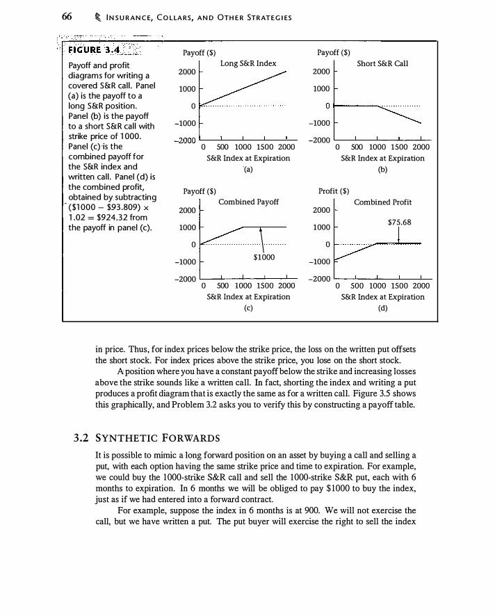
66 � I N S U R A N C E, C O L LA RS, A N D OTH E R STRAT E G I ES

Payoff and profit diagrams for writing a covered S&R cal l . Panel (a) is the payoff to a long S&R position . Panel (b) is the payoff to a short S&R cal l with strike price of 1 000. Panel (c) -is the combined payoff for the S&R index and written cal l . Panel (d) is the combined profit, obtained by subtracting

- ($1 000 - $93 .809) X 1 .02 = $924.32 from the payoff in panel (c).

Payoff ($)

Long S&R Index 2000

1000

0

-1000

-2000 .___._____..___ _ _.___...__ 0 500 1000 1500 2000

S&R Index at Expiration '(a)

Payoff ($)

Combined Payoff 2000

1000

0 · · · · · · · · · · · · · · · · · · - - - - - -\ · · · · · - - · ·

-1000 $1000

-2000 '-----'----'----'----'---0 500 1000 1500 2000

S&R Index at Expiration

(c)

Payoff ($)

Short S&R Call 2000

1000

O t------·..:..:·· · · · · · - · · · · · · · · ·

-1000

-2000 '-----'----'----'----'--0 500 1000 1500 2000

S&R Index at Expiration

(b)

Profit ($)

Combined Profit 2000

1000 $75.68

0

-1000

-2000 '----'----'----'---..1...-0 500 1000 1500 2000

S&R Index at Expiration

(d)

in price. Thus, for index prices below the strike price, the loss on the written put offsets the short stock. For index prices above the strike price, you lose on the short stock.

A position where you have a constant payoff below the strike and increasing losses above the strike sounds like a written call. In fact, shorting the index and writing a put produces a profit diagram that is exactly the same as for a written call. Figure 3.5 shows this graphically, and Problem 3.2 asks you to verify this by constructing a payoff table.

3 .2 SYNTHETIC FORWARDS

It is possible to mimic along forward position on an asset by buying a call and selling a put, with each option having the same strike price and time to expiration. For example, we could buy the 1000-strike S&R call and sell the 1000-strike S&R put, each with 6 months to expiration. In 6 months we will be obliged to pay $ 1000 to buy the index, just as if we had entered into a forward contract.

For example, suppose the index in 6 months is at 900. We will not exercise the call, but we have written a put. The put buyer will exercise the right to sell the index

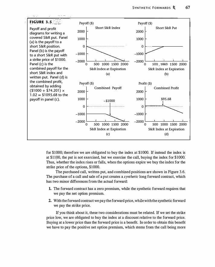
, F I G U R E 3 . 5 - '

Payoff and profit diagrams for writing a covered S&R put. Panel (a) is the payoff to a short S&R position. Panel (b) is the p�yoff to a short S&R put with a strike price of $1 000. Panel (c) is the combined payoff for the short S&R index and written put. Panel (d) is the combined profit, obtained by adding ($1 000 + $ 74.201 ) X 1 .02 = $1 095.68 to the payoff in panel (c).

Payoff ($)

Short S&R Index 2000

1000

0 · · · - · · · · · · · · · · · · · · · · · · · · · · · · · · · · · · · ·

-1000

-2000 0 500 1000 1500 2000

S&R Index at Expiration

(a)

Payoff ($)

Combined Payoff 2000

1000 -$1000

0 " " " " " " " " " " " " " . . . . . . . . . . . . . .

-1000 1--------

SYNTH ETI C F O RWA R D S � 67

Payoff ($)

Short S&R Put 2000

1000

0

-1000

-2000 0 500 , 1000 1500 2000

S&R Index at Expiration

(b)

Profit ($)

Combined Profit 2000

1000 $95 .68

l 0 · · · · · · · · · · · · · · · - · - " " " " " " " " " " " "

-1000

-2000 -2000 .___,___J.___J._____.L.,.-0 500 1000 1500 2000 0 500 1000 1500 2000

S&R Index at Expiration

(c)

S&R Index at Expiration

(d)

for $1000; therefore we are obligated to buy the index at $1000. If instead the index is at $1 100, the put is not exercised, but we exercise the call, buying the index for $ 1000.· Thus, whether the index rises or falls, when the options expire we buy the index for the strike price of the options, $1000.

The purchased call, written put, and combined positions are shown in Figure 3.6. The purchase of a call and sale of a put creates a synthetic long forward contract, which has two minor differences from the actual forward:

1. The forward contract has a zero premium, while the synthetic forward requires that we pay the net option premium.

2. With the forward contract we pay the forward price, while with the synthetic forward we pay the strike price.

If you think about it, these two considerations must be related. If we set the strike price low, we are obligated to buy the index at a discount relative to the forward price. Buying at a lower price than the forward price is a benefit. In order to obtain this benefit we have to pay the positive net option premium, which stems from the call being more

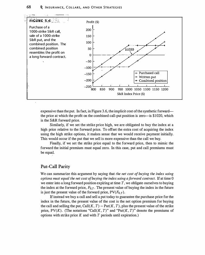
68 � I N S U R A N C E, C O L LA RS, A N D OTH E R STRATEG I ES

Purchase of a 1 000-strike S&R call, sale of a 1 000-strike S&R put, and the combined position. The combined position resembles the profit on a long forward contract.

Profit ($)

200

150

100

so o r-------��------�----�--------

-so -100 -1=--.,.L..+---+-:.,-L--+----¥ -150

-200

+ Purchased call + Written put ...... Combined position

-2SQ L---L---�--�--�--L---L---L---� 800 850 900 950 1000 1050 1 100 1 150 1200

S&R Index Price ($)

expensive than the put. In fact, in Figure 3 .6, the implicit cost of the synthetic forward­the price at which the profit on the combined call-put position is zero-is $ 1 020, which is the S&R forward price.

Similarly, if we set the strike price high, we are obligated to buy the index at a high price relative to the forward price. To offset the extra cost of acquiring the index using the high strike options, it makes sense that we would receive payment initially. This would occur if the put that we sell is more expensive than the call we buy.

Finally, if we set the strike price equal to the forward price, then to mimic the forward the initial premium must equal zero. In this case, put and call premiums must be equal.

Put -Call Parity

We can summarize this argument by saying that the net cost of buying the index using options must equal the net cost of buying the index using a forward colltract. If at time 0 we enter into a long forward position expiring at time T, we obligate ourselves to buying the index at the forward price, Fo,T · The present value of buying the index in the future is just the present value of the forward price, PV(Fo,T ) .

If instead we buy a call and sell a put today to guarantee the purchase price for the index in the future, the present value of the cost is the net option premium for buying the call and selling the put, Call(K, T) - Put(K, T) , plus the present value of the strike price, PV(K) . (The notations "Call(K, T)" and "Put(K, T)" denote the premiums of options with strike price K and with T periods until expiration.) ·

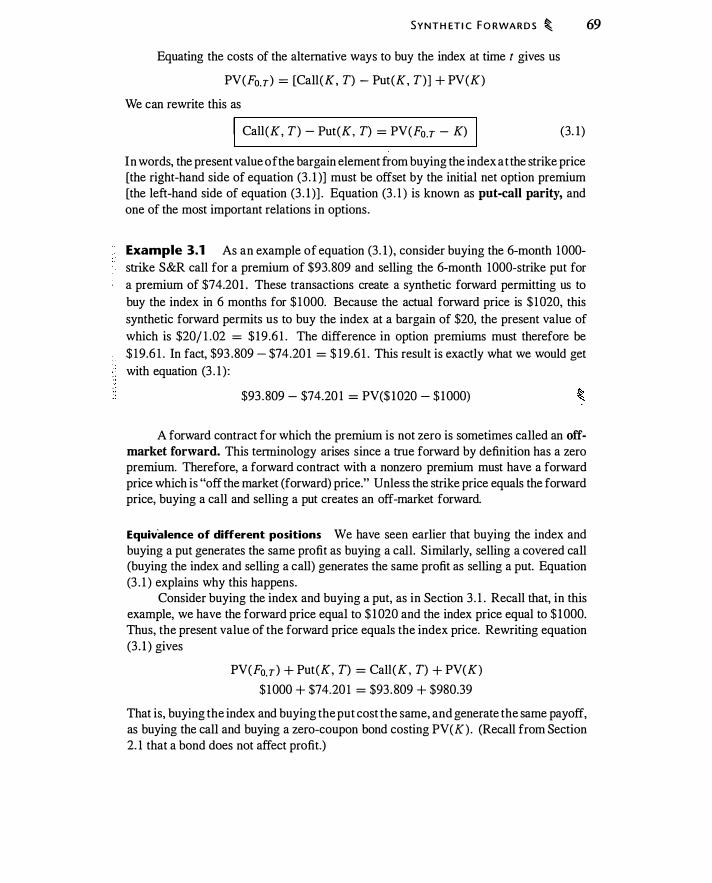
SYNTH ET I C F O RWA R D S � 69

Equating the costs of the alternative ways to buy the index at time t gives us

PV(Fo.T) = [Call(K, T) - Put(K, T) ] + PV(K)

We can rewrite this as

I Call(K, T) - Put(K, T) = PV(Fo.T - K) I (3. 1 )

In words, the present value of the bargain element from buying the index at the strike price [the right-hand side of equation (3 . 1 )] must be offset by the initial net option premium [the left-hand side of equation (3 . 1 )] . Equation (3 . 1 ) is known as put-call parity, and one of the most important relations in options.

Example 3.1 As an example of equation (3 . 1 ) , consider buying the 6-month 1000-strike S&R call for a premium of $93.809 and selling the 6-month 1000-strike put for a premium of $74.201 . These transactions create a synthetic forward permitting us to buy the index in 6 months for $ 1000. Because the actual forward price is $ 1020, this synthetic forward permits us to buy the index at a bargain of $20, the present value of which is $20/ 1 .02 = $ 19 .6 1 . The difference in option premiums must therefore be $ 19.6 1 . In fact, $93 .809 - $74.20 1 = $ 19 .6 1 . This result is exactly what we would get with equation (3 . 1 ) :

$93 . 809 - $74.20 1 = PV($ 1020 - $1000)

A forward contract for which the premium is not zero is sometimes called an off­market forward. This terminology arises since a true forward by definition has a zero premium. Therefore, a forward contract with a nonzero premium must have a forward price which is "off the market (forward) price." Unless the strike price equals the forward price, buying a call and selling a put creates an off-market forward.

Equivalence of different positions We have seen earlier that buying the index and buying a put generates the same profit as buying a call. Similarly, selling a covered call (buying the index and selling a call) generates the same profit as selling a put. Equation (3 . 1 ) explains why this happens.

Consider buying the index and buying a put, as in Section 3 . 1 . Recall that, in this example, we have the forward price equal to $ 1 020 and the index price equal to $ 1000. Thus, the present value of the forward price equals the index price. Rewriting equation (3 . 1 ) gives

PV(Fo, T) + Put(K, T) = Call(K, T) + PV(K)

$ 1000 + $74.20 1 = $93 . 809 + $980.39

That is, buying the index and buying the put cost the same, and generate the same payoff, as buying the call and buying a zero-coupon bond costing PV(K) . (Recall from Section 2. 1 that a bond does not affect profit.)

70 � I N S U RAN C E, CO LLA RS, A N D OTH E R ST RATEG I ES

Similarly, in the case of writing a covered call, we have

PV(Fo,T) - Call(K, T) = PV(K) - Put(K, T)

That is , writing a covered call has the same profit as lending PV(K) and selling a put. Equation (3 . 1 ) provides a tool for constructing equivalent positions.

No arbitrage In deriving equation (3 . 1 ), and in some earlier discussions, we relied on the idea that if two different investments generate the same payoff, they must have the same cost. This commonsensical idea is one of the most important in the book. If eq).lation (3 . 1 ) did not hold, there would be both low-cost and high-cost ways to acquire the index at time T. We could simultaneously buy the index at low cost and sell the index at high cost. This transaction has no risk (since we both buy and sell the index) and generates a positive cash flow (because of the difference in costs). Taking advantage of such an opportunity is called arbitrage, and the idea that prices should not permit arbitrage is called "no-arbitrage pricing." We implicitly illustrated this idea earlier in showing how owning the index and buying a put has the same profit as a call, etc . No-arbitrage pricing will be a major theme in Chapter 5 and beyond.3

3 .3 SPREADS AND COLLARS

There are many well-known, commonly used strategies that combine two or more op­tions. In this section we discuss some 9f these strategies and explain the motivation for using them. The underlying theme in this section is that there are always trade-offs in designing a position: It is always possible to lower the cost of a position by reducing its payoff. Thus there are many variations on each particular strategy.

All the examples in this section will use the set of option prices in Table 3 .4. We will assume the continuously compounded interest rate is 8% .

. . . • TABLE 3 A · .. Black-Scholes option prices assuming stock price = $40,

volati l ity = 30%, effective annual risk-free rate = 8.33% (8%, continuously compounded), d ividend yield = $0, and 91 days to expiration.

Strike Call Put

35 6. 1 3 0.44

40 2.78 1 .99

45 .97 5 .08

3 Another way to express the principle of no arbitrage is using profit diagrams. Given two profit diagrams, there is an arbitrage opportunity if one diagram is everywhere above the other.

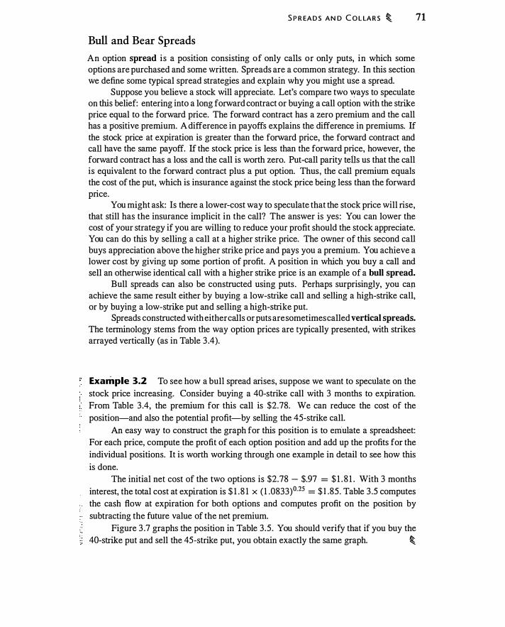
Bull and Bear Spreads

S P R EA D S AN D C O L LA R S � 71

An option spread is a position consisting of only calls or only puts, in which some options are purchased and some written. Spreads are a common strategy. In this section we define some typical spread strategies and explain why you might use a spread.

Suppose you believe a stock will appreciate. Let's compare two ways to speculate on this belief: entering into a long forward contract or buying a call option with the strike price equal to the forward price. The forward contract has a zero premium and the call has a positive premium. A difference in payoffs explains the difference in premiums. If

the stock price at expiration is greater than the forward price, the forward contract and call have the same payoff. If the stock price is less than the forward price, however, the forward contract has a loss and the call is worth zero. Put-call parity tells us that the call is equivalent to the forward contract plus a put option. Thus, the call premium equals the cost of the put, which is insurance against the stock price being less than the forward price.

You might ask: Is there a lower-cost way to speculate that the stock price will rise, that still has the insurance implicit in the call? The answer is yes : You can lower the cost of your strategy if you are willing to reduce your profit should the stock appreciate. You can do this by selling a call at a higher strike price. The owner of this second call buys appreciation above the higher strike price and pays you a premium. You achieve a lower cost by giving up some portion of profit. A position in which you buy a call and sell an otherwise identical call with a higher strike price is an example of a bull spread.

Bull spreads can also be constructed using puts . Perhaps surprisingly, you cap achieve the same result either by buying a low-strike call and selling a high-strike call, or by buying a low-strike put and selling a high-strike put.

Spreads constructed with either calls or puts are sometimes called vertical spreads. The terminology stems from the way option prices are typically presented, with strikes arrayed vertically (as in Table 3 .4).

Example 3.2 To see how a bull spread arises, suppose we want to speculate on the stock price increasing. Consider buying a 40-strike call with 3 months to expiration. From Table 3 .4, the premium for this call is $2.78. We can reduce the cost of the position-and also the potential profit-by selling the 45-strike call.

An easy way to construct the graph for this position is to emulate a spreadsheet: For each price, compute the profit of each option position and add up the profits for the individual positions. It is worth working through one example in detail to see how this is done.

The initial net cost of the two options is $2.78 - $.97 = $ 1 . 8 1 . With 3 months interest, the total cost at expiration is $ 1 . 8 1 x ( 1 .0833)0·25 = $ 1 .85 . Table 3 .5 computes the cash flow at expiration for both options and computes profit on the position by subtracting the future value of the net premium.

Figure 3 .7 graphs the position in Table 3 .5 . You should verify that if you buy the 40-strike put and sell the 45-strike put, you obtain exactly the same graph. �

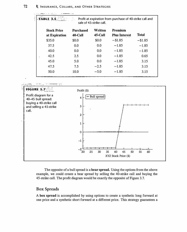
72 � I N S U R A N C E, C O LLARS , A N D OTH E R STRATEG I ES

· . . . · . -'::..' ' TABLE 3 . 5 . . . . . -:.:.-'-"'�-="""-'--

Stock Price

at Expiration

$35.0

37.5

40.0

42.5

45 .0

47.5

50.0

Profit diagram for a 40-45 bul l spread: buying a 40-strike cal l and sel l ing a 45-strike calL

Profit at expiration from purchase of 40-strike cal l and sale of 45-strike cal l .

Purchased Written Premium

40-Call 45-Call Plus Interest Total

$0.0 $0.0 -$1 .85 -$ 1 .85

0.0 0.0 - 1 .85 - 1 .85

0.0 0.0 - 1 .85 - 1 .85

2.5 0.0 - 1 .85 0.65

5.0 0.0 - 1 .85 3 . 1 5

7.5 -2.5 - 1 .85 3 . 1 5

10.0 -5.0 - 1 .85 3 . 1 5

Profit ($)

4 I+ Bull spread I

3

2

1

o r---------------�---------------

-1

-2 �=±��=±�±_�---��---� 20 25 30 35 40 45 50 55 60 XYZ Stock Price ($)

The opposite of a bull spread is a bear spread. Using the options from the above example, we could create a bear spread by selling the 40-strike call and buying the 45-strike call. The profit diagram would be exactly the opposite· of Figure 3.7.

Box Spreads

A box spread is accomplished by using options to create a synthetic long forward at one price and a synthetic short forward at a different price. This strategy guarantees a

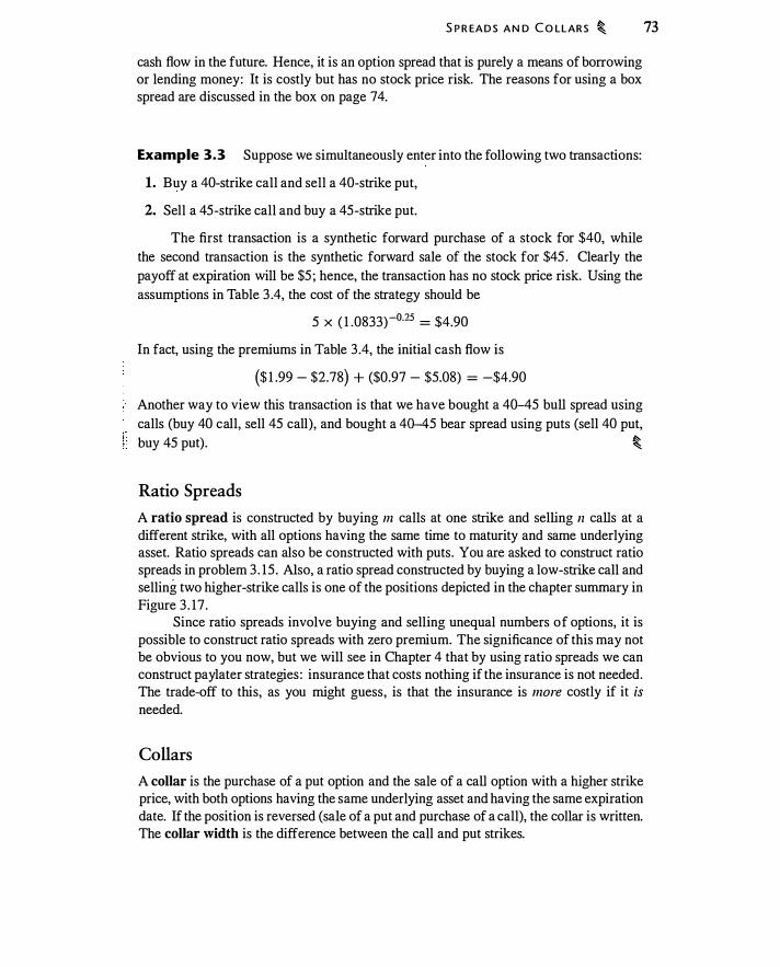
S P R EA D S A N D C O LLARS � 73

cash flow in the future. Hence, it is an option spread that is purely a means of borrowing or lending money: It is costly but has no stock price risk. The reasons for using a box spread are discussed in the box on page 74.

Example 3.3 Suppose we simultaneously enter into the following two transactions:

1. Buy a 40-strike call and sell a 40-strike put,

2. Sell a 45-strike call and buy a 45-strike put.

The first transaction is a synthetic forward purchase of a stock for $40, while the second transaction is the synthetic forward sale of the stock for $45 . Clearly the payoff at expiration will be $5 ; hence, the transaction has no stock price risk. Using the assumptions in Table 3 .4, the cost of the strategy should be

5 X ( 1 .0833)-0·25 = $4.90

In fact, using the premiums in Table 3 .4, the initial cash flow is

($ 1 .99 - $2.78) + ($0.97 - $5.08) = -$4.90

Another way to view this transaction is that we have bought a 40-45 bull spread using calls (buy 40 call, sell 45 call), and bought a 40-45 bear spread using puts (sell 40 put,

� � �- �

Ratio Spreads

A ratio spread is constructed by buying m calls at one strike and selling n calls at a different strike, with all options having the same time to maturity and same underlying asset. Ratio spreads can also be constructed with puts. You are asked to construct ratio spreads in problem 3 . 15 . Also, a ratio spread constructed by buying a low-strike call and selling two higher-strike calls is one of the positions depicted in the chapter summary in Figure 3 . 17 .

Since ratio spreads involve buying and selling unequal numbers of options, it is possible to construct ratio spreads with zero premium. The significance of this may not be obvious to you now, but we will see in Chapter 4 that by using ratio spreads we can construct pay later strategies : insurance that costs nothing if the insurance is not needed. The trade-off to this, as you might guess, is that the insurance is more costly if it is needed.

Collars

A collar is the purchase of a put option and the sale of a call option with a higher strike price, with both options having the same underlying asset and having the same expiration date. If the position is reversed (sale of a put and purchase of a call), the collar is written. The collar width is the difference between the call and put strikes.

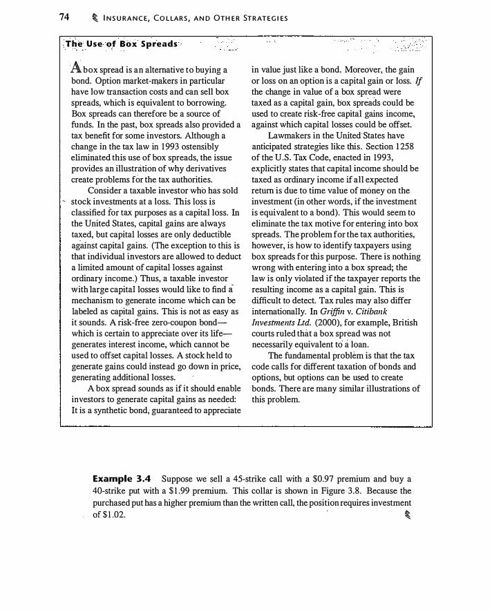
74 � I N S U RA N C E, CO L LARS , A N D OTH E R STR ATEG I ES

The U s e of Box S p reads

A box spread is an alternative to buying a bond. Option market-makers in particular have low transaction costs and can sell box spreads, which is equivalent to borrowing, Box spreads can therefore be a source of funds. In the past, box spreads also provided a tax benefit for some investors. Although a change in the tax law in 1 993 ostensibly eliminated this use of box spreads, the issue provides an illustration of why derivatives create problems for the tax authorities.

Consider a taxable investor who has sold - stock investments at a loss. This loss is

classified for tax purposes as a capital loss. In the United States, capital gains are always taxed, but capital losses are only deductible agrunst capital gains. (The exception to this is that individual investors are allowed to deduct a limited amount of capital losses against . ordinary income.) Thus, a taxable investor with large capital losses would like to find a mechanism to generate income which can be labeled as capital gains. This is not as easy as it sounds. A risk-free zero-coupon bond­which is certain to appreciate over its life­generates interest income, which cannot be used to offset capital losses. A stock held to generate gains could instead go down in price, generating additional losses.

A box spread sounds as if it should enable investors to generate capital gains as needed: It is a synthetic bond, guaranteed to appreciate

......

in value just like a bond. Moreover, the gain or loss on an option is a capital gain or loss. If the change in value of a box spread were taxed as a capital gain, box spreads could be used to create risk-free capital gains income, against which capital losses could be offset.

Lawmakers in the United States have anticipated strategies like this . Section 1 258 of the U.S. Tax Code, enacted in 1993, explicitly states that capital income should be taxed as ordinary income if all expected return is due to time value of money on the investment (in other words, if the investment is equivalent to a bond). This would seem to eliminate the tax motive for entering into box spreads. The problem for the tax authorities, however, is how to identify taxpayers using box spreads for this purpose. There is nothing wrong with entering into a box spread; the law is only violated if the taxpayer reports the resulting income as a capital gain. This is difficult to detect. Tax rules may also differ internationally. In Griffin v. Citibank Investments Ltd. (2000), for example, British courts ruled that a box spread was not necessarily equivalent to a loan.

The fundamental problem is that the tax code calls for different taxation of bonds and options, but options can be used to create bonds. There are many similar illustrations of this problem.

Example 3.4 Suppose we sell a 45-strike call with a $0.97 premium and buy a 40-strike put with a $ 1 .99 premium. This collar is shown in Figure 3 .8 . Because the purchased put has a higher premium than the written call, the position requires investment of $ 1 .02. �

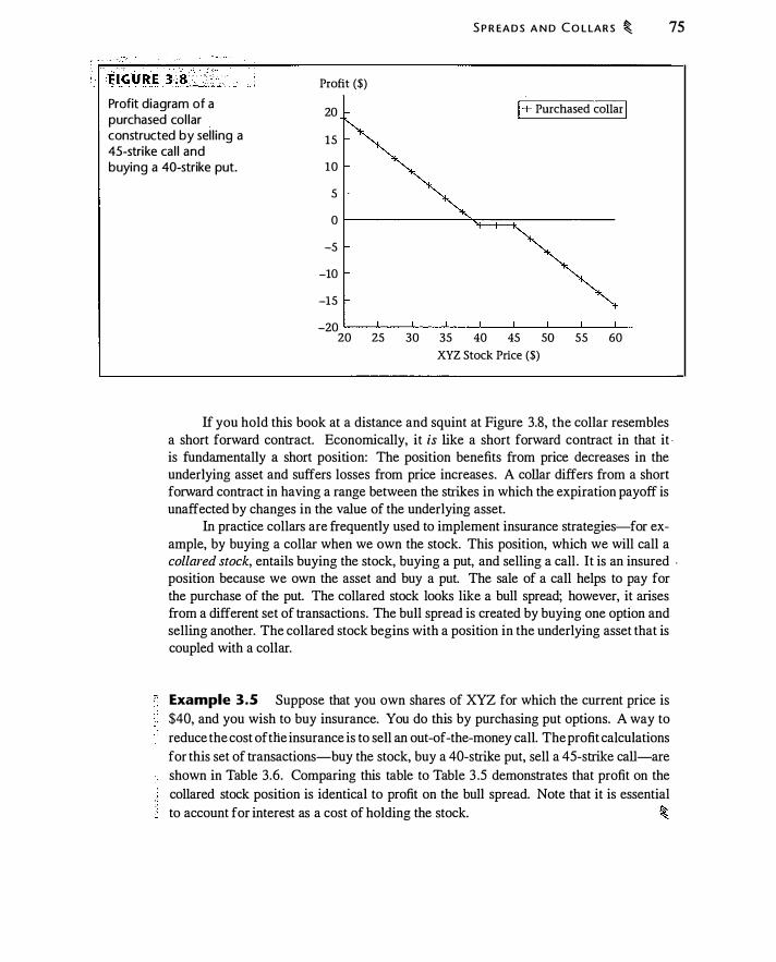
Profit ($)

Profit diagram of a 20 purchased col lar

constructed by sel l ing a 15 45-strike cal l and buying a 40-strike put. 10

5

0

-5

-10

-15

-20 20 25 30

S P R EA D S A N D C O L LA R S � 75

I+ Purchased collar I

35 40 45 so 55 60

XYZ Stock Price ($)

If you hold this book at a distance and squint at Figure 3.8, the collar resembles a short forward contract. Economically, it is like a short forward contract in that it · is fundamentally a short position: The position benefits from price decreases in the underlying asset and suffers losses from price increases. A collar differs from a short forward contract in having a range between the strikes in which the expiration payoff is unaffected by changes in the value of the underlying asset.

In practice collars are frequently used to implement insurance strategies-for ex­ample, by buying a collar when we own the stock. This position, which we will call a collared stock, entails buying the stock, buying a put, and selling a call . It is an insured . position because we own the asset and buy a put. The sale of a call helps to pay for the purchase of the put. The collared stock looks like a bull spread; however, it arises from a different set of transactions. The bull spread is created by buying one option and selling another. The collared stock begins with a position in the underlying asset that is coupled with a collar.

Example 3.5 Suppose that you own shares of XYZ for which the current price is $40, and you wish to buy insurance. You do this by purchasing put options. A way to reduce the cost of the insurance is to sell an out-of-the-money call. The profit calculations for this set of transactions-buy the stock, buy a 40-strike put, sell a 45-strike call-are shown in Table 3.6. Comparing this table to Table 3 .5 demonstrates that profit on the collared stock position is identical to profit on the bull spread. Note that it is essential to account for interest as a cost of holding the stock.

76 � I N S U R A N C E, CO LLA RS, A N D OTH E R STR AT EG I ES

Profit at expiration from purchase of 40-strike put and sale of 45-strike cal l .

Stock Price Purchased Written Premium Profit

at Expiration 40-Put 45-Call Plus Interest on Stock Total

$35.00 $5.00 $0.00 -$1 .04 -$5.8 1 -$ 1 .85

37.50 2.50 0.00 - 1 .04 -3.3 1 - 1 . 85

40.00 0.00 0.00 - 1 .04 -0.8 1 - 1 .85

42.50 0.00 0.00 - 1 .04 1 .69 0.65

45 .00 0.00 0.00 - 1 .04 4. 1 9 3 . 1 5

47 .50 0.00 -2.50 - 1 .04 6.69 3 . 1 5

50.00 0.00 -5.00 - 1 .04 9. 19 3 . 1 5

If you have a short position in the stock, you can collar the position by buying a call for insurance and selling an out-of-the-money put to partially fund the call purchase. The result looks like a bear spread.

Zero-cost collars The collar depicted in Table 3 .6 entails paying a net premium of $ 1 .02: $ 1 .99 for the purchased put, ·against $0.97 for the written call. It is possible to find strike prices for the put and call such that the two premiums exactly offset one another. This position is called a zero-cost collar.

To illustrate a zero-cost collar, suppose you buy the stock and buy the 40-strike put that has a premium of $ 1 .99. Trial and error reveals that a call with a strike of $41 .72 also has a premium of $ 1 .99. Thus, you can buy a 40-strike put and sell a 4 1 .72-strike call without paying any premium. The result is depicted in Figure 3.9. At expiration, the collar exposes you to stock price movements between $40 and $41 .72, coupled with downside protection below $40. You pay for this protection by giving up gains should the stock move above $41 .72.

For any given stock there is an infinite number of zero-cost collars. One way to see this is to first pick the desired put strike below the forward price. It is then possible to find a strike above the forward price such that a call has the same premium.

Understanding collars One aspect of the zero-cost collar that may seem puzzling is that you can finance the purchase of an at-the-money put by selling an out-of-the-money call. In the above example, with the stock at $40, you were able to costlessly buy a 40-strike put by also selling a 4 1 . 72-strike call. This makes it seem as if you have free insurance with some possibility of gain. Even if you are puzzled by this, you probably realize that "free" insurance is not possible, and something must be wrong with this way of thinking about the position.

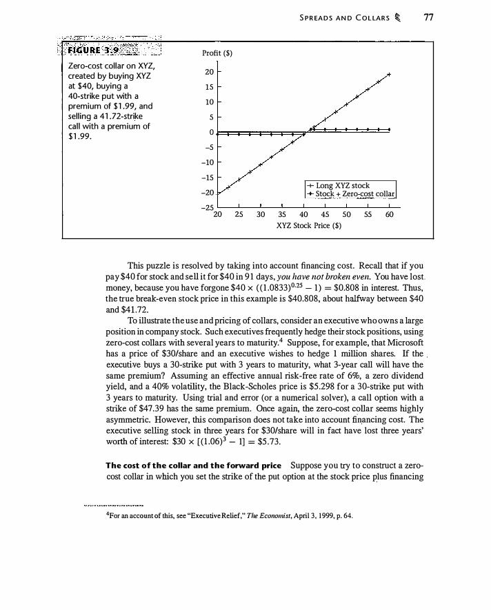
Zero-cost col lar on XYZ, created by buying XYZ at $40, buying a 40-strike put with a premium of $ 1 .99, and sel l ing a 41 .72-strike cal l with a premium of $ 1 .99.

Profit ($)

20

15

10

5

0

-5

-10

-15

-20

-25 20 25

S P R EA D S A N D C O L LA R S � 77

-+- Long XYZ stock -+- Stock + Zero-cost collar

30 35 40 45 so 55 60

XYZ Stock Price ($)

This puzzle is resolved by taking into account financing cost. Recall that if you pay $40 for stock and sell it for $40 in 9 1 days, you have not broken even. You have lost. money, because you have forgone $40 x ( ( 1 .0833)0·25 - 1 ) = $0.808 in interest. Thus, the true break-even stock price in this example is $40.808, about halfway between $40 and $41 .72.

To illustrate the use and pricing of collars, consider an executive who owns a large position in company stock. Such executives frequently hedge their stock positions, using zero-cost collars with several years to maturity.4 Suppose, for example, that Microsoft has a price of $30/share and an executive wishes to hedge 1 million shares. If the . executive buys a 30-strike put with 3 years to maturity, what 3-year call will have the same premium? Assuming an effective annual risk-free rate of 6%, a zero dividend yield, and a 40% volatility, the Black-Scholes price is $5 .298 for a 30-strike put with 3 years to maturity. Using trial and error (or a numerical solver), a call option with a strike of $47.39 has the same premium. Once again, the zero-cost collar seems highly asymmetric. However, this comparison does not take into account fi

-nancing cost. The

executive selling stock in three years for $30/share will in fact have lost three years' worth of interest: $30 x [ ( 1 .06)3 - 1] = $5 .73.

The cost of the collar and the forward price Suppose you try to construct a zero­cost collar in which you set the strike of the put option at the stock price plus financing

4For an account of this, see "Executive Relief," The Economist, April 3, 1 999, p. 64.

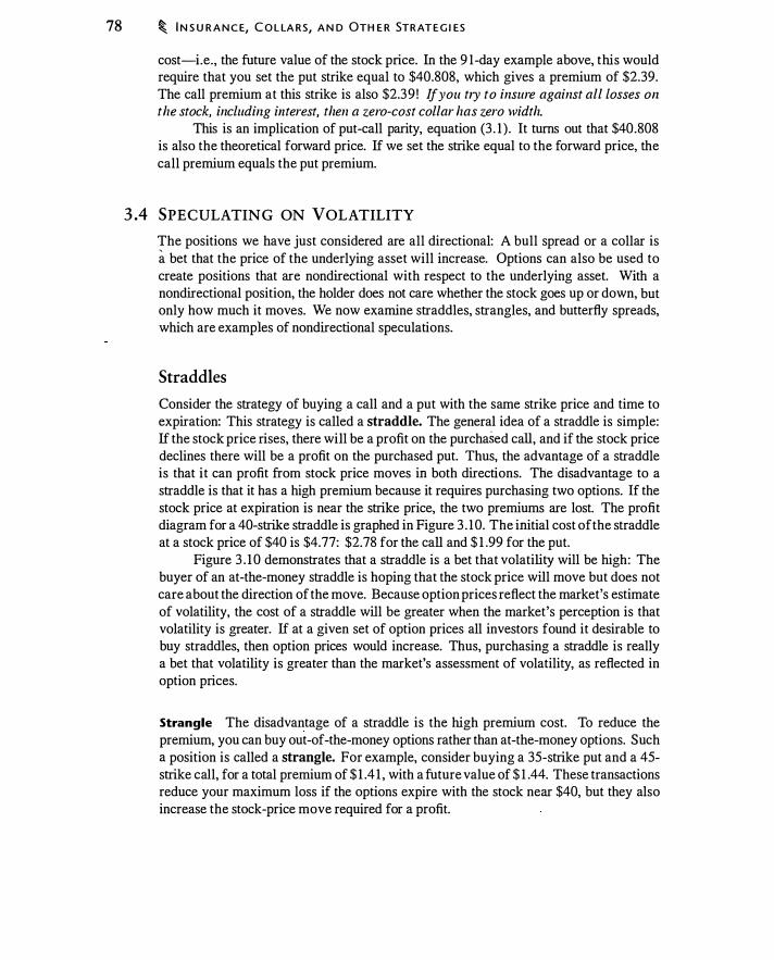
78 � I N S U R A N C E, C O L LA RS, A N D OTH E R STRAT E G I ES

cost-i.e., the future value of the stock price. In the 9 1-day example above, this would require that you set the put strike equal to $40.808, which gives a premium of $2.39. The call premium at this strike is also $2.39 ! If you tl}' to insure against all Losses on the stock, including illterest, then a zero-cost collar has zero width.

This is an implication of put-call parity, equation (3 . 1 ) . It turns out that $40.808 is also the theoretical forward price. If we set the strike equal to the forward price, the call premium equals the put premium.

3 .4 SPECULATING ON VOLATILITY

The positions we have just considered are all directional: A bull spread or a collar is a bet that the price of the underlying asset will increase. Options can also be used to create positions that are nondirectional with respect to the underlying asset. With a nondirectional position, the holder does not care whether the stock goes up or down, but only how much it moves. We now examine straddles, strangles, and butterfly spreads, which are examples of nondirectional speculations.

Straddles

Consider the strategy of buying a call and a put with the same strike price and time to expiration: This strategy is called a straddle. The general idea of a straddle is simple: If the stock price rises, there will be a profit on the purchased call, and if the stock price declines there will be a profit on the purchased put. Thus, the advantage of a straddle is that it can profit from stock price moves in both directions. The disadvantage to a straddle is that it has a high premium because it requires purchasing two options. If the stock price at expiration is near the strike price, the two premiums are lost. The profit diagram for a 40-strike straddle is graphed in Figure 3 . 1 0. The initial cost of the straddle at a stock price of $40 is $4.77: $2.78 for the call and $ 1 .99 for the put.

Figure 3 . 1 0 demonstrates that a straddle is a bet that volatility will be high: The buyer of an at-the-money straddle is hoping that the stock price will move but does not care about the direction of the move. Because option prices reflect the market's estimate of volatility, the cost of a straddle will be greater when the market's perception is that volatility is greater. If at a given set of option prices all investors found it desirable to buy straddles, then option prices would increase. Thus, purchasing a straddle is really a bet that volatility is greater than the market's assessment of volatility, as reflected in option prices.

Strangle The disadvantage of a straddle is the high premium cost. To reduce the premium, you can buy out-of-the-money options rather than at-the-money options. Such a position is called a strangle. For example, consider buying a 35-strike put and a 45-strike call, for a total premium of $ 1 .4 1 , with a future value of $ 1 .44. These transactions reduce your maximum loss if the options expire with the stock near $40, but they also increase the stock-price move required for a profit.

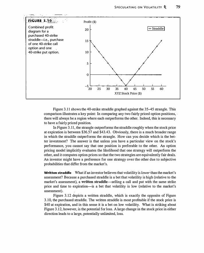
Combined profit diagram for a purchased 40-strike straddle-i.e., purchase of one 40-strike ca l l option and one 40-strike put option.

Profit {$)

20

15

10

5

S P E C U LAT I N G O N VO LAT I L I TY � 79

I+ Straddle I

-5 �--�--�--�--��--L---�---L--�--20 25 30 35 40 45 so 55 60

XYZ Stock Price ($)

Figure 3 . 1 1 shows the 40-strike straddle graphed against the 35-45 strangle. This comparison illustrates a key point: In comparing any two fairly priced option positions, . there will always be a region where each outperforms the other. Indeed, this is necessary to have a fairly priced position.

In Figure 3 . 1 1 , the strangle outperforms the straddle roughly when the stock price at expiration is between $36.57 and $43 .43 . Obviously, there is a much broader range in which the straddle outperforms the strangle. How can you decide which is the bet­ter investment? The answer is that unless you have a particular view on the stock's performance, you cannot say that one position is preferable to the other. An option pricing model implicitly evaluates the likelihood that one strategy will outperform the other, and it computes option prices so that the two strategies are equivalently fair deals. An investor might have a preference for one strategy over the other due to subjective probabilities that differ from the market's .

Written straddle What if an investor believes that volatility is lower. than the market's

assessment? Because a purchased straddle is a bet that volatility is high (relative to the market's assessment), a written straddle--selling a call and put with the same strike price and time to expiration--is a bet that volatility is low (relative to the market's assessment) .

Figure 3 . 12 depicts a written straddle, which is exactly the opposite of Figure 3 . 1 0, the purchased straddle. The written straddle is most profitable if the stock price is $40 at expiration, and in this sense it is a bet on low volatility. What is striking about Figure 3 . 1 2, however, is the potential for loss. A large change in the stock price in either direction leads to a large, potentially unlimited, loss.

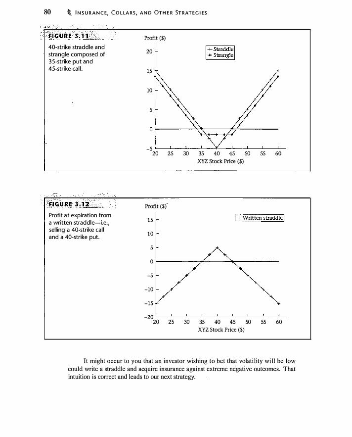
80 � I N S U R A N C E, C O LLA RS, A N D OTH E R STRATE G I ES

40-strike straddle and strangle composed of 35-strike put and 45-strike cal l .

Profit at expiration from a written straddle-i.e., selling a 40-strike cal l and a 40-strike put.

Profit ($)

20

15

10

5

-5 L---�--�--�--�--�--�--�--�� 20 25 30 35 40 45 so 55 60

Profit ($)

15

10

5

0

-5

-10

-15

-20 20 25

XYZ Stock Price {$)

I+ Written straddle !

30 35 40 45 50 55 60

XYZ Stock Price ($)

It might occur to you that an investor wishing to bet that volatility will be low could write a straddle and acquire insurance against extreme negative outcomes. That intuition is correct and leads to our next strategy.

Butterfly Spreads

S P E C U LAT I N G O N VO LAT I L I TY � 81

The straddle writer can insure against large losses on the straddle by buying options to protect against losses on both the upside and downside. Buying an out-of-the-money put provides insurance on the downside, protecting against losses on the at-the-money writ­ten put. Buying an out-of-the-money call provides insurance on the upside, protecting against losses on the written at-the-money calL

Figure 3 . 1 3 displays the straddle written at a strike price of $40, along with the options to safeguard the position: A 35-strike put and a 45-strike calL The net result of combining these three strategies is an insured written straddle, which is called a butterfly spread, graphed in Figure 3 . 14. It can be thought of as a written stradd,le for the timid (or for the prudent!) .

Comparing the butterfly spread to the written straddle (Figure 3 . 14), we see that the butterfly spread has a lower maximum profit (due to the cost of insurance) if the stock at expiration is close to $40, and a higher profit if there is a large move in the stock price, in which case the insurance becomes valuable.

We will see in Chapter 9 that by understanding the butterfly spread we gain im­portant insights into option prices. Also, the butterfly spread can be created in a variety of ways: solely with calls, solely with puts, or by using the stock and a combination of calls and puts. 5 You are asked to verify this in Problem 3 . 1 8. The spread in Figure 3 . 14

Written 40-strike straddle, purchased 45-strike call, and purchased 35-strike put. These positions combined generate the butterfly spread . g raphed in Figure 3 . 1 4.

Profit ($)

15

10

5

-5

-10

-15

+ Written straddle -+- Purchased call _... Purchased put

-20 �--L---�--�---L---L--�---J--�� 20 25 30 35 40 45 so 55 60

XYZ Stock Price ($)

5Technically, a true butterfly spread is created solely with calls or solely with puts. A butterfly spread

created by selling a straddle and buying a strangle is called an "iron butterfly."

82 � I N S U RA N C E, C O L LARS , A N D OT H E R STRATE G I ES

Profit ($)

Comparison of the 15 35-40-45 butterfly

spread-obtained by 10 adding the profit

diagrams in Figure 5

3 . 1 3-with the written 40-strike straddle.

0

-5

-10

-15

-20

+ Written straddle -+- Butterfly

20 25 30 35 40 45 50 55 60

XYZ Stock Price ($)

can also be created by simultaneously buying a 35--40 bull spread and a 40--45 bear spread.

Asymmetric Butterfly Spreads

Examine Figure 3 . 15 . It looks like a butterfly spread except that it is asymmetric: The peak is closer to the high strike than to the low strike. This picture was created by buying two 35-strike calls, selling ten 43-strike calls (with a premium of $ 1 .525, using the assumptions in Table � .4), and buying eight 45-strike calls. The position is like a butterfly in that it earns a profit if the stock stays within a small range, and the loss is the same for high and low stock prices. However, the profit diagram is now tilted to the right, rather than being symmetric.

Suppose you knew that you wanted a position that looks like Figure 3 . 1 5 . How would you know how many options to buy and sell to construct this position? In order to obtain this position, the strikes clearly have to be at 35, 43, and 45 . The total distance between 35 and 45 is 10 . The number 43 is 80% (= 431035 ) of the way from 35 to 45 . In fact, we can write 43 as

43 = (0.2 X 35) + (0.8 X 45)

This way of writing 43 tells us our call position: For every written 43-strike call, we want to buy 0.2 35 calls and 0.8 45 calls . Thus if we sell ten 43-strike calls, we buy two 35 calls and eight 45-strike calls.

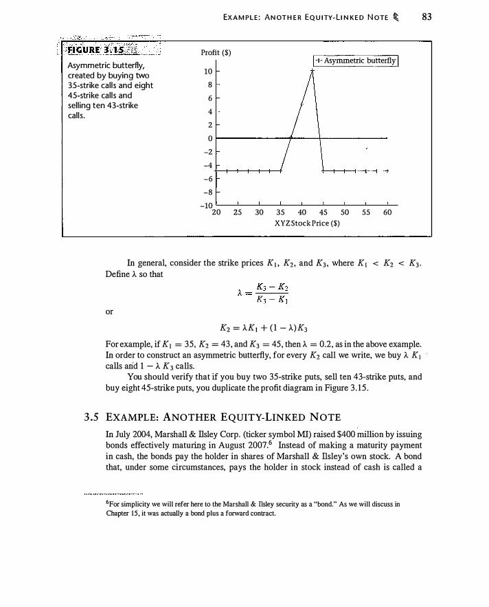
Asymmetric butterfly, created by buying two 35-strike cal ls and eight 45-strike cal ls and sel l ing ten 43-strike cal ls .

EX A M P L E : AN OT H E R EQ U I TY- L I N K E D N OTE � 83

Profit ($) I+ Asymmetric butterfly I

10

8

6

4

2

0

-2

-4

-6

-8

-10 20 25 30 35 40 45 50 55 60

XYZ Stock Price ($)

In general, consider the strike prices Kr . K2 , and K3, where K1 < K2 < K3 . Define A so that

or

Kz = AKt + ( 1 - A)K3

For example, if K1 = 35 , K2 = 43, and K3 = 45, then A = 0.2, as in the above example. In order to construct an asymmetric butterfly, for every K2 call we write, we buy A K1 calls arid 1 - A K3 calls.

You should verify that if you buy two 35-strike puts, sell ten 43-strike puts, and buy eight 45-strike puts, you duplicate the profit diagram in Figure 3 . 15 .

3 .5 EXAMPLE: ANOTHER EQUITY-LINKED NOTE

In July 2004, Marshall & llsley Corp. (ticker symbol Ml) raised $400 million by issuing bonds effectively maturing in August 2007.6 Instead of making a maturity payment in cash, the bonds pay the holder in shares of Marshall & llsley's own stock. A bond that, under some circumstances, pays the holder in stock instead of cash is called a

6For simplicity we will refer here to the Marshall & llsley security as a "bond." As we will discuss in

Chapter 15 , it was actually a bond plus a forward contract.

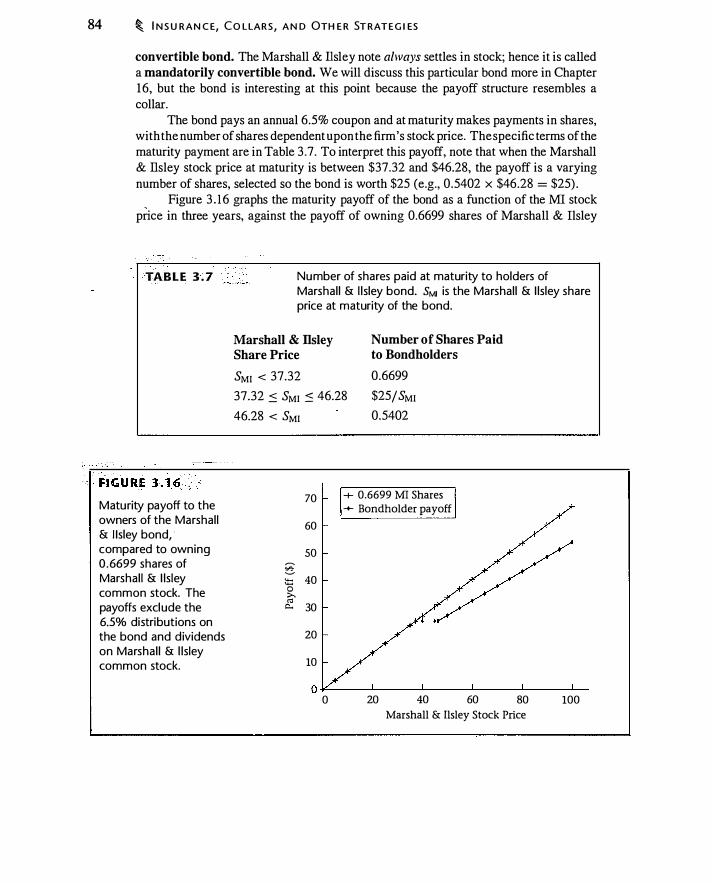
84 � I N S U RAN C E, CO LLARS , A N D OTH E R ST RATEG I ES

convertible bond. The Marshall & lis ley note always settles in stock; hence it is called a mandatorily convertible bond. We will discuss this particular bond more in Chapter 16, but the bond is interesting at this point because the payoff structure resembles a collar.

The bond pays an annual 6.5% coupon and at maturity makes payments in shares, with the number of shares dependent upon the firm's stock price. The specific terms of the maturity payment are in Table 3 .7. To interpret this payoff, note that when the Marshall & llsley stock price at maturity is between $37.32 and $46.28, the payoff is a varying number of shares, selected so the bond is worth $25 (e.g., 0.5402 x $46.28 = $25) .

Figure 3 . 1 6 graphs the maturity payoff of the bond as a function of the Ml stock price in three years, against the payoff of owning 0.6699 shares of Marshall & llsley

TAB L E 3 . 7

Maturity payoff to the owners of the Marshal l & I Isley bond, · compared to owning 0 .6699 shares of Marshal l & l ls ley common stock. The payoffs exclude the 6.5% distributions on the bond and dividends on Marshal l & l lsley common stock.

. ·. • Number of shares paid at maturity to holders of Marshal l & l lsley bond. SM1 is the Marshal l & l lsley share price at maturity of the bond.

Marshall & Dsley Share Price

SMI < 37.32

Number of Shares Paid to Bondholders

0.6699

37.32 ::::: SMI ::::: 46.28

46.28 < SMI

$25/SMI

0.5402

70

60

so

§: tt:: 40 0 >-. "'

� 30

20

10

+ 0.6699 MI Shares -+- Bondholder payoff

0 �-----L------L-----�----�------� 0 20 40 60 80 100

Marshall & Ilsley Stock Price

C H A PT E R S U M M A RY � 85

stock. Both graphs ignore dividends and other distributions . Based solely on comparing the maturity payoffs, investing in the bond is inferior to investing in the common stock. However, distributions on the bond (6.5% annually) are greater than on the stock (an annual dividend of about 2%); so without performing a valuation analysis it is impossible to say whether investors should prefer one or the other, or be indifferent. Accounting for the distributions would shift the payoff lines upward and would lead the bond to outperform 0.6699 shares of stock at low prices, with the stock outperforming the bond at high ppces.

The Marshall & Ilsley share price was $37.32 on the day the bond was issued. The bond was designed so that, at issue, it would sell for $25, which is the same price as 0.6699 shares.

The bond was also designed so that bondholders would forgo 24% of the appre­ciation on the stock above $37.32. We have $37.32 x 1 .24 = $46.28, and 25/46.28 = 0.5402. This accounts for the flat range in the payoff and the number of shares exchanged above a share price of $46.28.

Finally, in order for the bond to underperform the stock above $37.32, yet to sell at the share price, it is necessary to compensate bondholders with additional payments. The 6.5% coupon accomplishes this .

How would we price the bond? The graph in Figure 3 . 1 6 should remind you of a written collar. One way to construct the same graph is by ( 1 ) owning 0.6699 shares of stock (ignoring dividends), (2) selling 0.6699 calls with a strike price of $37.32, and (3) buying 0.5402 calls with a strike price of $46.28. The algebraic expression for the payoff is

Payoff = 0.6699 x [sMr - max(O, SMr - 37.32) + -1- x max(O, SMr - 46.28)]

1 .24 (3.2)

Note that the bond holder is implicitly selling a low strike call and buying 1 1 1 .24 high strike calls, and is therefore owed option premium. The bondholder also forgoes divi­dends on the stock. These two factors explain the 6.5% distribution, which is effectively the dividend plus the amortized option premium. By pricing these options and valuing the 6.5% distribution, we can arrive at a fair price for the bond.

This discussion leaves unanswered the question of why Marshall & Ilsley would issue such a bond. We have also not discussed all the details of the bond's structure. We return to these issues in Chapter 15 .

CHAPTER SUMMARY Puts are insurance against a price decline and calls are insurance against a price increase. Combining a long or short position in the asset with an offsetting position in options (for example, a long position in the asset is coupled either with a purchased put or written call) leads to the various possible positions and their equivalents in Table 3 .8 .

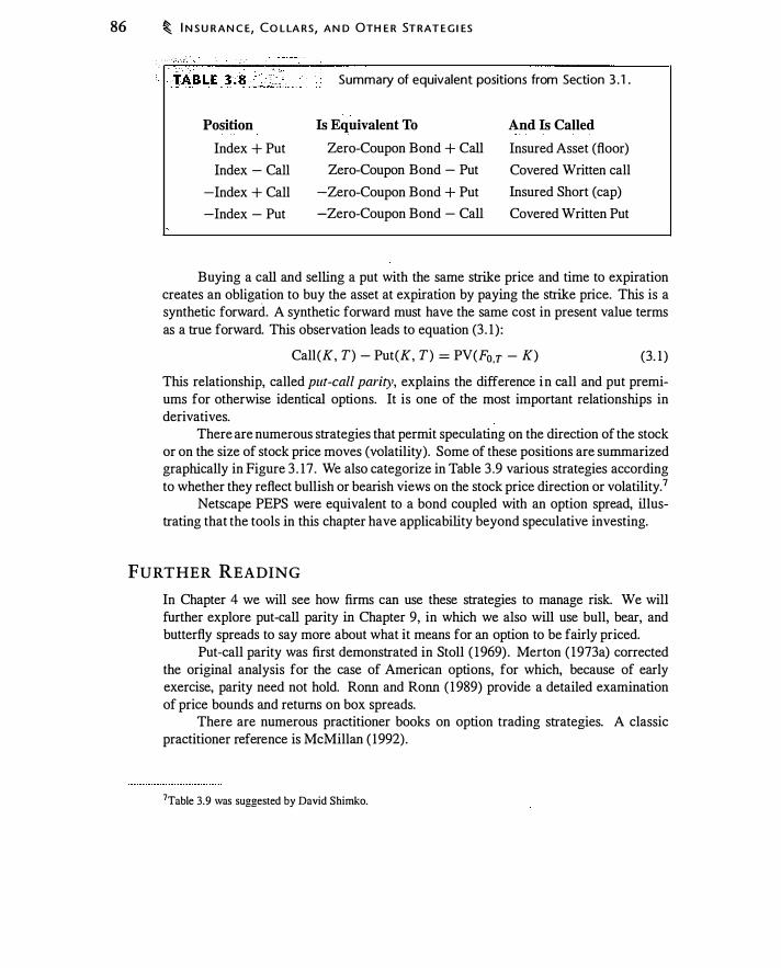
86 � I N S U R A N C E, CO L LA RS, A N D OTH E R ST RAT E G I ES

. - - - . . ' - �

Summary of equivalent positions from Section 3 . 1 .

Position Is Equivalent To And Is Called

Index + Put Zero-Coupon Bond + Call Insured Asset (floor)

Index - Call Zero-Coupon Bond - Put Covered Written call

-Index + Call -Zero-Coupon Bond + Put Insured Short (cap)

-Index - Put -Zero-Coupon Bond - Call Covered Written Put

Buying a call and selling a put with the same strike price and time to expiration creates an obligation to buy the asset at expiration by paying the strike price. This is a synthetic forward. A synthetic forward must have the same cost in present value terms as a true forward. This observation leads to equation (3 . 1 ) :

Call(K, T) - Put(K, T) = PV(Fo.r - K) (3. 1 )

This relationship, called put-call parity, explains the difference in call and put premi­ums for otherwise identical options. It is one of the most important relationships in derivatives.

There are numerous strategies that permit speculating on the direction of the stock or on the size of stock price moves (volatility). Some of these positions are summarized graphically in Figure 3 . 17 . We also categorize in Table 3 .9 various strategies according to whether they reflect bullish or bearish views on the stock price direction or volatility. 7

Netscape PEPS were equivalent to a bond coupled with an option spread, illus­trating that the tools in this chapter have applicability beyond speculative investing.

FURTHER READING

In Chapter 4 we will see how firms can use these strategies to manage risk. We will further explore put-call parity in Chapter 9, in which we also will use bull, bear, and butterfly spreads to say more about what it means for an option to be fairly priced.

Put-call parity was first demonstrated in Stoll ( 1969) . Merton ( 1973a) corrected the original analysis for the case of American options, for which, because of early exercise, parity need not hold. Ronn and Ronn ( 1 989) provide a detailed examination of price bounds and returns on box spreads.

There are numerous practitioner books on option trading strategies. A classic practitioner reference is McMillan ( 1992) .

7Table 3.9 was suggested by David Shimko.

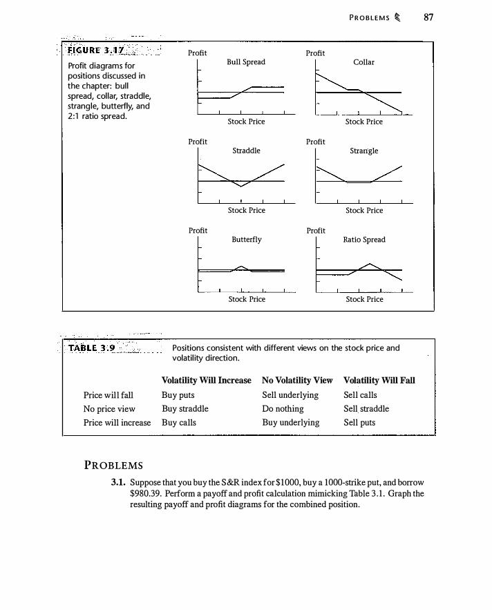
Profit diagrams for positions discussed in the chapter: bul l spread, col lar, straddle, strang le, butterfly, and 2:1 ratio spread.

Price will fall

No price view

Price will increase

PROBLEMS

Profit Bull Spread

Stock Price

Profit Straddle

Stock Price

Profit Butterfly

Stock Price

Profit

Profit

Profit

P R O B LE M S � 87

Collar

Stock Price

Strangle

Stock Price

Ratio Spread

Stock Price

' Positions consistent with different views on the stock price and volati l ity direction.

Volatility Will Increase No Volatility View Volatility Will Fall

Buy puts Sell underlying Sell calls

Buy straddle Do nothing Sell. straddle

Buy calls Buy underlying Sell puts

3.1. Suppose that you buy the S&R index for $ 1000, buy a 1000-strike put, and borrow $980.39. Perform a payoff and profit calculation mimicking Table 3 . 1 . Graph the resulting payoff and profit diagrams for the combined position.

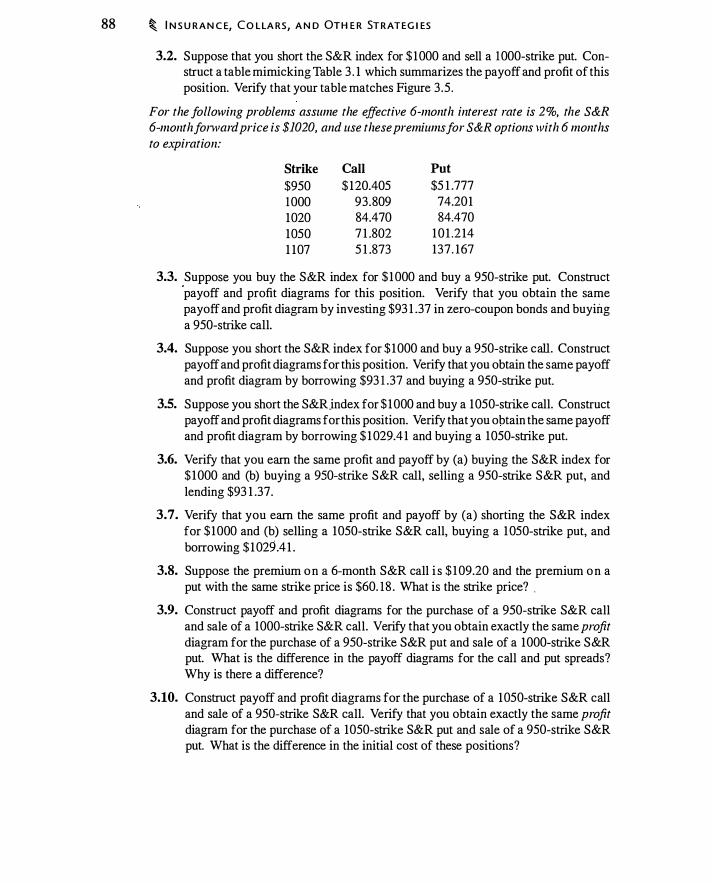
88 � I N S U R A N C E, C O LLA RS, A N D OTH E R STRATEG I ES

3.2. Suppose that you short the S&R index for $ 1000 and sell a 1000-strike put. Con­struct a table mimicking Table 3 . 1 which summarizes the payoff and profit of this position. Verify that your table matches Figure 3 .5 .

For the following problems assume the effective 6-month interest rate is 2%, the S&R 6-monthforward price is $1020, and use these premiums for S&R options with 6 months to expiration:

Strike

$950 1000 1020 1050 1 107

Call

$ 120.405 93.809 84.470 7 1 .802 5 1 .873

Put

$5 1 .777 74.201 84.470

10 1 .2 14 137. 167

3.3. Suppose you buy the S&R index for $ 1000 and buy a 950-strike put. Construct "payoff and profit diagrams for this position. Verify that you obtain the same payoff and profit diagram by investing $93 1 .37 in zero-coupon bonds and buying a 950-strike call.

3.4. Suppose you short the S&R index for $ 1000 and buy a 950-strike call. Construct payoff and profit diagrams for this position. Verify that you obtain the same payoff and profit diagram by borrowing $93 1 .37 and buying a 950-strike put.

3.5. Suppose you short the S&R_index for $ 1000 and buy a 1050-strike call. Construct payoff and profit diagrams for this position. Verify that you obtain the same payoff and profit diagram by borrowing $ 1 029.4 1 and buying a 1050-strike put.

3.6. Verify that you earn the same profit and payoff by (a) buying the S&R index for $ 1000 and (b) buying a 950-strike S&R call, selling a 950-strike S&R put, and lending $93 1 .37.

3.7. Verify that you earn the same profit and payoff by (a) shorting the S&R index for $ 1000 and (b) selling a 1050-strike S&R call, buying a 1050-strike put, and borrowing $ 1029.4 1 .

3.8. Suppose the premium o n a 6-month S&R call i s $ 109.20 and the premium o n a put with the same strike price is $60. 18 . What is the strike price? _

3.9. Construct payoff and profit diagrams for the purchase of a 950-strike S&R call and sale of a 1000-strike S&R call. Verify that you obtain exactly the same profit diagram for the purchase of a 950-strike S&R put and sale of a 1000-strike S&R put. What is the difference in the payoff diagrams for the call and put spreads? Why is there a difference?

3.10. Construct payoff and profit diagrams for the purchase of a 1050-strike S&R call and sale of a 950-strike S&R call. Verify that you obtain exactly the same profit diagram for the purchase of a 1 050-strike S&R put and sale of a 950-strike S&R put. What is the difference in the initial cost of these positions?

P RO B L E M S \ 89

3.11. Suppose you invest in the S&R index for $ 1 000, buy a 950-strike put, and sell a 1 050-strike call. Draw a profit diagram for this position. What is the net option premium? If you wanted to construct a zero-cost collar keeping the put strike equal to $950, in what direction would you have to change the call strike?

3.12. Suppose you invest in the S&R index for $ 1000, buy a 950-strike put, and sell a 1 107-strike call. Draw a profit diagram for this position. How close is this to a zero-cost collar?

3.13. Draw profit diagrams for the following positions :

a . 1 050-strike S&R straddle.

b. Written 950-strike S&R straddle.

c. Simultaneous purchase of a 1 050-strike straddle and sale of a 950-strike S&R straddle.

3.14. Suppose you buy a 950-strike S&R call, sell a 1 000-strike S&R call, sell a 950-strike S&R put, and buy a 1000-strike S&R put.

a. Verify that there is no S&R price risk in this transaction.

b. What is the initial cost of the position?

c. What is the value of the position after 6 months?

d. Verify that the implicit interest rate in these cash flows is 2% over 6 months.

3.15. Compute profit diagrams for the following ratio spreads:

a. Buy 950-strike call, sell two 1050-strike calls.

b. Buy two 950-strike calls, sell three 1050-strike calls.

c. Consider buying n 950-strike calls and selling m 1 050-strike calls so that the premium of the position is zero. Considering your analysis in (a) and · (b), what can you say about nfm? What exact ratio gives you a zero premium?

3.16. In the previous problem we saw that a ratio spread can have zero initial premium. Can a bull spread or bear spread have zero initial premium? A butterfly spread? Why or why not?

3.17. Construct an asymmetric butterfly using the 950-, 1 020-, and 1050-strike options . How many of each option do you hold? Draw a profit diagram for the position.

3.18. Verify that the butterfly spread in Figure 3 . 14 can be duplicated by following transactions (use the option prices in Table 3 .4):

a. Buy 35 call, sell two 40 calls, buy 45 call.

b. Buy 35 put, sell two 40 puts, buy 45 put.

c. Buy stock, buy 35 put, sell two 40 calls, buy 45 call.

90 � I N S U RAN C E, C O L LARS , A N D OTH E R STRATE G I ES

3.19. Here is a quote from an investment Web site about an investment strategy using options:

One strategy investors are applying to the XYZ options is using "syn­thetic stock." A synthetic stock is created when an investor simultane­ously purchases a call option and sells a put option on the same stock. The end result is that the synthetic stock has the same value, in terms of capital gain potential, as the underlying stock itself. Provided the premiums on the options are the same, they cancel each other out so the transaction fees are a wash.

Suppose, to be concrete, that the premium on the call you buy is the same as the premium on the put you sell, and both have the same strikes and times to expiration.

a. What can you say about the strike price?

b. What term best describes the position you have created?

c. Suppose the options have a bid-ask spread. If you are creating a synthetic purchased stock and the net premium is zero inclusive of the bid-ask spread, where will the strike price be relative to the forward price?

d. If you create a synthetic short stock with zero premium inclusive of the bid-ask spread, where will the strike price be relative to the forward price?

e. Do you consider the "transaction fees" to really be "a wash"? Why or why not?

-

3.20. Construct a spreadsheet for which you can input up to five strike prices and quanti­ties of put and call options bought or sold at those strikes, and which will automat­ically construct the total expiration payoff diagram for that position. Modify the spreadsheet to permit you to choose whether to graph a payoff or profit function.

' :Business, like life, is inherently risky. Finns convert inputs such "' !aboc,. mw m"erials, and machines into goods and services. A firm is profitable if the cost of what it produces exceeds the cost of the inputs. Prices can change, however, and what appears to be a profitable activity today may not be profitable tomorrow. Many instruments are avail­able that permit firms to hedge various risks, ranging from commodity prices to weather. A firm that actively uses derivatives and other techniques to alter its risk and protect its profitability is engaging in risk management. In this chapter we take a look at how derivatives-such as forwards, calls, and puts-are used in practice to manage risk.

We begin by examining two hypothetical firms-Golddiggers, a gold-mining firm, and Auric Enterprises, a manufacturer using gold as an input-to see what risks they face and to demonstrate the use of derivatives strategies to manage those risks. After looking at these examples we will explore some reasons firms seek to manage risk in the first place.

4.1 BASIC RISK MANAGEMENT: THE PRODUCER'S PERSPECTIVE

Golddiggers is a gold-mining firm planning to mine and sell 100,000 ounces of gold over the next year. For simplicity, we will assume that they sell all of the next year's production precisely 1 year from today, receiving whatever the gold price is that day. The price of gold today is $405/oz. We will ignore production beyond the next year.

Obviously Golddiggers-like any producer-hopes that the gold price will rise over the next year. However, Golddiggers 's management computes estimated net income for a range of possible prices of gold in 1 year (Table 4. 1 ). The net income calculation shows that Golddiggers's profit is affected by gold prices.

Should Golddiggers simply shut the mine if gold prices fall enough to make net income negative? The answer depends on the extent to which costs are fixed. The firm incurs the fixed cost whether or not it produces gold. Variable costs are incurred only if the mine operates. Thus, for any gold price above the variable cost of $50/oz., it will make sense to produce gold. 1

1 Suppose the gold price is $350/oz. If Golddiggers produces no gold, the finn loses its fixed cost, $330/oz. If Golddiggers produces gold, the finn has fixed cost of $330/oz. and variable cost of $50/oz.,

and so loses $350 - ($330+ $50) = -$30/oz. It is better to lose only $30, so Golddiggers will produce

even when they have negative net income. If the gold price were to fall below the variable cost of $50, then it would make sense to stop producing.

9 1

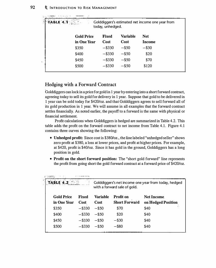
92 � I NTRO D U CT I O N TO R I S K M A N A G E M E N T

-:---, - ---- -" ·· - --- -::· > - - - - . , · - • • iA'BLE 4.t -:L ,� · ·. ·· Golddiggers's estimated net income one year from

today, unhedged.

Gold Price Fixed Variable Net

in One Year Cost Cost Income

$350 -$330 -$50 -$30

$400 -$330 -$50 $20

$450 -$330 -$50 $70

$500 -$330 -$50 $ 120

Hedging with a Forward Contract

Golddiggers can lock in a price for gold in 1 year by entering into a short forward contract, agreeing today to sell its gold for delivery in 1 year. Suppose that gold to be delivered in 1 year can be sold today for $420/oz. and that Golddiggers agrees to sell forward all of its gold production in 1 year. We will assume in all examples that the forward contract settles financially. As noted earlier, the payoff to a forward is the same with physical or financial settlement.

Profit calculations when Golddiggers is hedged are summarized in Table 4.2. This table adds the profit on the forward contract to net income from Table 4. 1 . Figure 4. 1 contains three curves showing the following:

• Unhedged profit: Since cost is $380/oz., the line labeled "unhedged seller" shows zero profit at $380, a loss at lower prices, and profit at higher prices. For example, at $420, profit is $40/oz. Since it has gold in the ground, Golddiggers has a long position in gold.

• Profit on the short forward position: The "short gold forward" line represents the profit from going short the gold forward contract at a forward price of $420/oz.

Gold Price Fixed

in One Year Cost

$350 -$330

$400 -$330

$450 -$330

$500 -$330

Golddiggers's net income one year from today, hedged with a forward sale of gold.

Variable Profit on Net Income

Cost Short Forward on Hedged Position

-$50 $70 $40

-$50 $20 $40

-$50 -$30 $40

-$50 -$80 $40

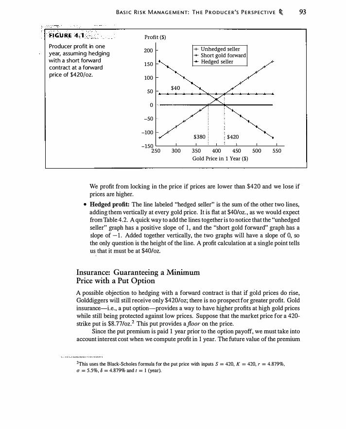
BAS I C R I S K M ANAG E M E NT: TH E P R O D U C E R 'S P E R S P ECT I V E � 93

Producer profit in one year, assuming hedging with a short forward contract at a forward price of $420/oz.

Profit ($)

200

150

100

50

0

-50

-100

-150 250

$40

300

+ Unhedged seller -+- Short gold forward � Hedged seller

$380 : $420

350 400 450

Gold Price in 1 Year ($)

500 550

We profit from locking in the price if prices are lower than $420 and we lose if prices are higher.

• Hedged profit: The line labeled "hedged seller" is the sum of the other two lines, adding them vertically at every gold price. It is flat at $40/oz. , as we would expect from Table 4.2. A quick way to add the lines together is to notice that the "unhedged seller" graph has a positive slope of I , and the "short gold forward" graph bas a slope of - 1 . Added together vertically, the two graphs will have a slope of 0, so the only question is the height of the line. A profit calculation at a single point tells us that it must be at $40/oz.

Insurance: Guaranteeing a Minimum Price with a Put Option

A possible objection to hedging with a forward contract is that if gold prices do rise, Golddiggers will still receive only $420/oz; there is no prospect for greater profit. Gold insurance-i.e., a put option-provides a way to have higher profits at high gold prices while still being protected against low prices. Suppose that the market price for a 420-strike put is $8.77/oz.2 This put provides afioor on the price.

Since the put premium is paid 1 year prior to the option payoff, we must take into account interest cost when we compute profit in 1 year. The future value of the premium

2This uses the Black-Scholes formula for the put price with inputs S = 420, K = 420, r = 4.879%,

a = 5.5%, a = 4.879% and t = I (year).

94 � I NTRO D U CTI O N TO R I S K MA N A G E M E N T

i s $8.77 x 1 .05 = $9.2 1 . As with the forward contract, we assume financial settlement, although physical settlement would yield the same net income.

Table 4.3 shows the result of buying this put. If the price is less than $420, the put is exercised and Golddiggers sells gold for $420/oz. less the cost of the put. This gives net income of $30.79. If the price is greater than $420, Golddiggers sells gold at the market price.

The insurance strategy-buying the put-performs better than shorting the for­ward if the price of gold in 1 year is more than $429.2 1 . Otherwise the short forward outperforms insurance. Figure 4.2 shows the unhedged position, profit from the put by itself, and the result of hedging with the put.

- : : ,-cc- : ' - :· :.� TABLE 4 . 3

Gold Price

in One Year

$350

$400

$450

$500

Comparison of unhedged position, 420-strike put option, and unhedged position plus 420-strike put.

Golddiggers's net income 1 year from today, hedged with a 420-strike put option.

Fixed Variable

Cost Cost

-$330 -$50

-$330 -$50

-$330 -$50

-$330 -$50

Profit ($)

200

1SO

100

so $30.79

0

-SO

-100

Profit on

Put Option

$60.79

$ 1 0.79

-$9.2 1

-$9.2 1

+ Unhedged seller -+- Purchased put _.... Hedged seller

$420

Net

Income

$30.79

$30.79

$60.79

$ 1 10.79

-1SO L-----1-----'----:.__.L.__.:__----l. __ __r_ __ ..L__ 2SO 300 3SO 400 4SO soo sso

Gold Price in I . Year ($)

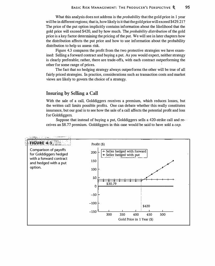
BAS I C R I S K M A N AG E M E NT: TH E P RO D U C E R 'S P E R S P ECT I V E � 95

What this analysis does not address is the probability that the gold price in 1 year will be in different regions; that is, how likely is it that the gold price will exceed $429.2 1 ? The price of the put option implicitly contains information about the likelihood that the gold price will exceed $420, and by how much. The probability distribution of the gold price is a key factor determining the pricing of the put. We will see in later chapters how the distribution affects the put price and how to use information about the probability distribution to help us assess risk.

Figure 4.3 compares the profit from the two protective strategies we have exam­ined: Selling a forward contract and buying a put. As you would expect, neither strategy is clearly preferable; rather, there are trade-offs, with each contract outperforming the other for some range of prices.

The fact that no hedging strategy always outperforms the other will be true of all fairly priced strategies. In practice, considerations such as transaction costs and market views are likely to govern the choice of a strategy.

Insuring by Selling a Call

With the sale of a call, Golddiggers receives a premium, which reduces losses, but the written call limits possible profits. One can debate whether this really constitutes insurance, but our goal is to see how the sale of a call affects the potential profit and loss for Golddiggers.

Suppose that instead of buying a put, Golddiggers sells a 420-strike call and re- -ceives an $8.77 premium. Golddiggers in this case would be said to have sold a cap.

r_ �,-�Qfy�€ �;4�5;�---· Comparison of payoffs for Golddiggers hedged with a forward contract and hedged with a put option.

Profit ($)

200 I + Seller hedged with forward I + Seller hedged with put J

150

/ 100

50 �--1-t----1--1-+ $30.79 o r---------_._ _____ _

-SO

-100 $420

-150 '----'----'----'----'---'-----'----300 350 400 450 500

Gold Price in 1 Year ($)

96 � I NTRO D U CTI O N TO R I S K MA N A G E M E N T

Comparison of Golddiggers hedging with sale of 420-strike cal l versus unhedged.

Profit ($)

200 + Unhedged seller -+- Written call

1so ..._ Seller hedged with written call

100

so

0

-SO

-100

$49.21

-1SO ...._ _ __,_ __ _,_ __ .J..._...:..._--L __ _._ __ _,____ 2SO 300 3SO 400 4SO

Gold Price in 1 Year ($)

sao sso

Figure 4.4 shows the payoff to this strategy. If we compute the actual profit 1 year from today, we see that if the gale! price in 1 year exceeds $420, Golddiggers will show profits of

$420 + $9.21 - $380 = $49.21

That is , Golddiggers sells gold for $420 (since the written call is exercised by the holder), receives the future value of the premium, and has a cost of $380. If the price of gold is less than $420, Golddiggers will make

Pgold + $9.2 1 - $380

On the downside, Golddiggers has exposure to gold but keeps the option premium. By writing the call, Golddiggers keeps the $8.77 call premium and 1 year later

makes $9.2 1 more than an unhedged gold seller. On the other hand, if the gold price exceeds $420, the call is exercised and the price Golddiggers receives is thus capped at $420. Thus, for gold prices above $429.2 1 , an unhedged strategy has a higher payoff than that of writing a 420-strike call. Also, for prices below $410.79, being fully hedged is preferable to having sold the call.

Adjusting the Amount of Insurance

Consider again Golddiggers's strategy of obtaining insurance against a price decline by purchasing a put option. A common objection to the purchase of insurance is that it is expensive. Insurance has a premium because it eliminates the risk of a large loss, while allowing a profit if prices increase. The cost of insurance reflects this asymmetry.

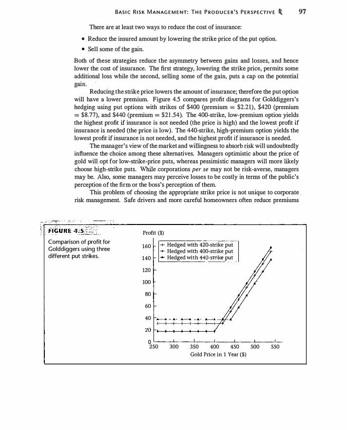
BAS I C R I S K M A N AG E M E NT: TH E P R O D U C E R 'S P E R S P E CTI V E � 97

There are at least two ways to reduce the cost of insurance:

o Reduce the insured amount by lowering the strike price of the put option.

o Sell some of the gain.

Both of these strategies reduce the asymmetry between gains and losses, and hence lower the cost of insurance. The first strategy, lowering the strike price, permits some additional loss while the second, selling some of the gain, puts a cap on the potential gain.

Reducing the strike price lowers the amount of insurance; therefore the put option will have a lower premium. Figure 4.5 compares profit diagrams for Golddiggers 's hedging using put options with strikes of $400 (premium = $2.2 1) , $420 (premium = $8.77), and $440 (premium = $21 .54). The 400-strike, low-premium option yields the highest profit if insurance is not needed (the price is high) and the lowest profit if insurance is needed (the price is low). The 440-strike, high-premium option yields the lowest profit if insurance is not needed, and the highest profit if insurance is needed.

The manager's view of the market and willingness to absorb risk will undoubtedly influence the choice among these alternatives. Managers optimistic about the price of gold will opt for low-strike-price puts, whereas pessimistic managers will more likely choose high-strike puts. While corporations per se may not be risk-averse, managers may be. Also, some managers may perceive losses to be costly in terms of the public's perception of the firm or the boss's perception of them.

This problem of choosing the appropriate strike price is not unique to corporate . risk management. Safe drivers and more careful homeowners often reduce premiums

Comparison of profit for Golddiggers using three different put strikes.

Profit {$)

160 + Hedged with 420-strike put -+- Hedged with 400-strike put

140 _... Hedged with 440-strike put

120

100

80

60

40

o �----�--��--��--�----�----�--250 300 350 400 450 500 550

Gold Price in 1 Year {$)

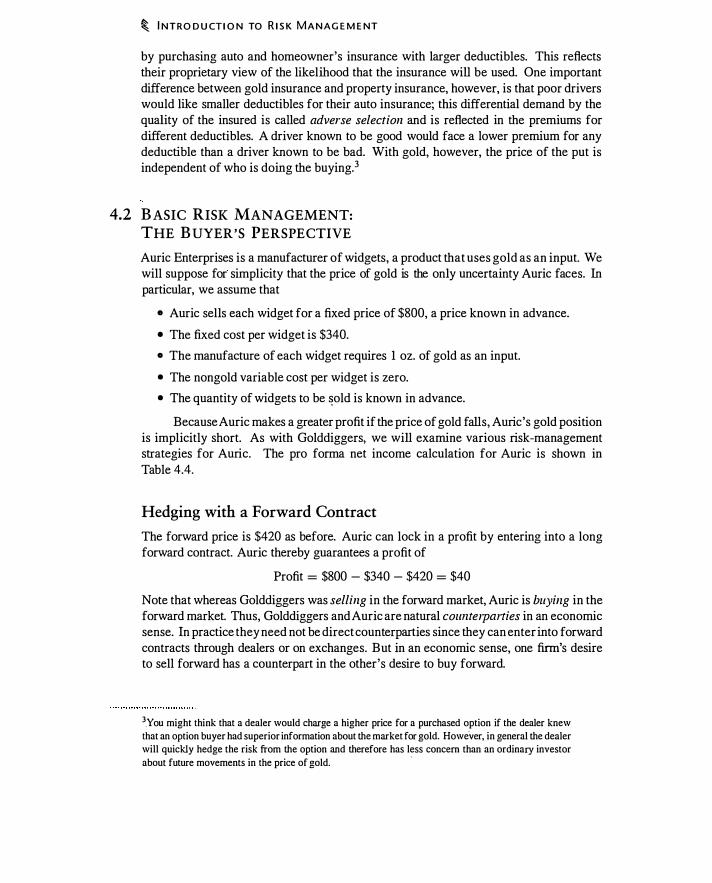
� I NTRO D U CT I O N TO R I S K M A N AG E M E NT

by purchasing auto and homeowner's insurance with larger deductibles. This reflects their proprietary view of the likelihood that the insurance will be used. One important difference between gold insurance and property insurance, however, is that poor drivers would like smaller deductibles for their auto insurance; this differential demand by the quality of the insured is called adverse selection and is reflected in the premiums for different deductibles. A driver known to be good would face a lower premium for any deductible than a driver known to be bad. With gold, however, the price of the put is independent of who is doing the buying.3

4.2 B ASIC RISK MANAGEMENT: THE B UYER'S PERSPECTIVE

Auric Enterprises is a manufacturer of widgets, a product that uses gold as an input. We will suppose for simplicity that the price of gold is the only uncertainty Auric faces. In particular, we assume that

• Auric sells each widget for a fixed price of $800, a price known in advance.

• The fixed cost per widget is $340.

• The manufacture of each widget requires 1 oz. of gold as an input.

• The nongold variable cost per widget is zero.

• The quantity of widgets to be �old is known in advance.

Because Auric makes a greater profit if the price of gold falls, Auric's gold position is implicitly short. As with Golddiggers, we will examine various risk-management strategies for Auric. The pro forma net income calculation for Auric is shown in Table 4.4.

Hedging with a Forward Contract

The forward price is $420 as before. Auric can lock in a profit by entering into a long forward contract. Auric thereby guarantees a profit of

Profit = $800 - $340 - $420 = $40

Note that whereas Golddiggers was selling in the forward market, Auric is buying in the forward market. Thus, Golddiggers and Auric are natural cozmterpm1ies in an economic sense. In practice they need not be direct counterparties since they can enter into forward contracts through dealers or on exchanges. But in an economic sense, one firm's desire to sell forward has a counterpart in the other's desire to buy forward.

3You might think that a dealer would charge a higher price for a purchased option if the dealer knew

that an option buyer had superior information about the market for gold. However, in general the dealer will quickly hedge the risk from the option and therefore has less concern than an ordinary investor

about future movements in the price of gold. ·

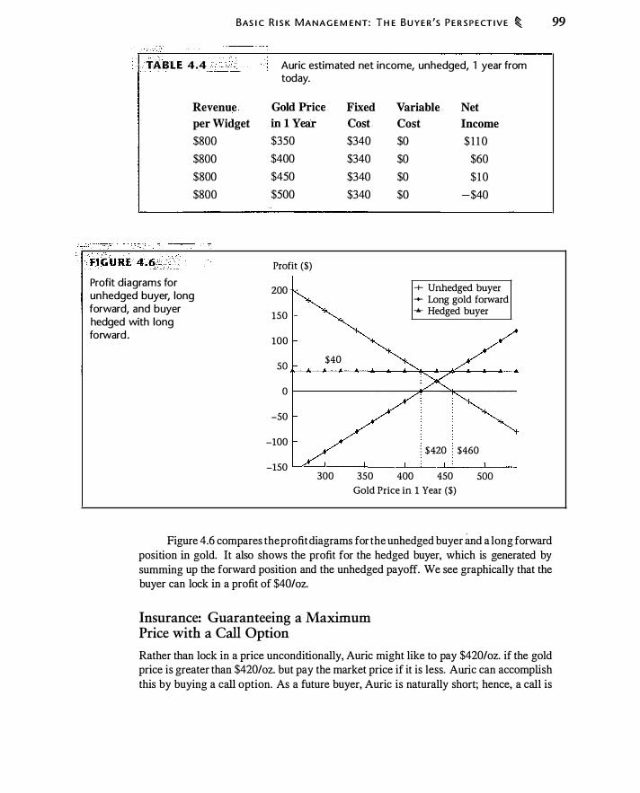
BAS I C R I S K M A N A G E M E NT: T H E B U Y E R 'S P E R S P ECT I V E � 99

TABLE 4.4 · " Auric estimated net income, unhedged, 1 year from

Revenue

per Widget

$800

$800

$800

$800

Profit diagrams for unhedged buyer, long forward, and buyer hedged with long forward .

today.

Gold Price

in 1 Year

$350

$400

$450

$500

Profit ($)

200

1SO

100

so $40

0

-SO

-100

-1SO 300

Fixed

Cost

$340

$340

$340

$340

3SO

Variable . Net

Cost Income

$0

$0

$0

$0

400

$ 1 1 0

$60

$ 1 0

-$40

-+- Unhedged buyer -+- Long gold forward _.. Hedged buyer

: $420 : $460

4SO soo

Gold Price in 1 Year ($)

Figure 4.6 compares the profit diagrams for the unhedged buyer and a long forward position in gold. It also shows the profit for the hedged buyer, which is generated by summing up the forward position and the unhedged payoff. We see graphically that the buyer can lock in a profit of $40/oz.

Insurance: Guaranteeing a Maximum Price with a Call Option

Rather than lock in a price unconditionally, Auric might like to pay $420/oz. if the gold price is greater than $420/oz. but pay the market price if it is less. Auric can accomplish this by buying a call option. As a future buyer, Auric is naturally short; hence, a call is

100 � I NTRO D U CT I O N TO R I S K M ANAG E M E NT

..• _· • TABLE 4 . 5 __;� - Auric net income 1 year from today, hedged with 420-strike ca l l option.

Gold Price

in 1 Year

$350

$400

$450

$500

Unhedged Net Income

from Table 4.4

$ 1 1 0

$60

$ 10

-$40

Profit on Net

Call Option Income

-$9.2 1 $ 100.79

-$9.2 1 $50.79

$20.79 $30.79

$70.79 $30.79

insurance. Suppose the call has a premium of $8.77/oz. (recall that this is the same as the premium on the put with the same strike price) . The future value of the premium is $8.77 X 1 .05 = $9.2 1 .

If Auric buys the insurance contract, net income on the hedged position will b e as shown in Table 4.5 . If the price is less than $420, the call is worthless at expiration and Auric buys gold at the market price. If the price is greater than $420, the call is exercised and Auric buys gold for $420/oz., less the cost of the call. This gives a profit of $30.79.

If the price of gold in 1 year is less than $410.79, insuring the price by buying the call performs better than locking in a price of $420. At low prices, the option permits us to take advantage of lower gold prices. If the price of gold in 1 year is greater than $410.79, insuring the price by buying the call performs worse than locking in a price of $420 since we have paid the call premium.

Figure 4. 7 shows the profit from the call by itself, along with the results of hedging with the call. As before, the graph does not show the probability that the gold price in 1 year will be in different regions ; hence, we cannot evaluate the likelihood of different outcomes.

4.3 WHY D o FIRMS MANAGE RISK?

The Golddiggers and Auric examples illustrate how the two companies can use forwards, calls, and puts to reduce losses in case of an adverse gold price move, essentially insuring their future cash flows. Why would a firm use these strategies?

In Chapter 1 we listed four reasons that firms might use derivatives: to hedge, to speculate, to reduce transaction costs, and to effect regulatory arbirage. In practice, more than one of these considerations may be important. We have already discussed the fact that market views-for example, opinions about the future price of gold--can affect the choice of a hedging strategy. Thus, the choice of a hedging strategy can have a speculative component. Managers often cite the accounting treatment of a transaction as important, and transaction costs are obviously a consideration.

In this section we discuss why firms might hedge, ignoring speculation, transac­tions costs, and regulation (but we do consider taxes). It seems obvious that managers would want to reduce risk. However, in a world with fairly priced derivatives, no trans-

Comparison of profit for unhedged gold buyer, gold buyer hedged with call, and stand-alone cal l .

Profit ($)

200

1SO

100

so

0

-SO

W H Y Do F1 R M S M A N A G E R I S K? � 101

-$9.21

+ Unhedged seller -+- Purchased call ...,_ Buyer hedged with call

$30.79

: $420 � $460

-100 L---�----�----L-���---L----� 2SO 300 3SO 400 4SO soo sso

Gold Price in 1 Year ($)

action costs, and no other market imperfections such as taxes, derivatives change the distribution of cash flows but do not increase the value of cash flows. Moreover, large . publicly held firms are owned by diverse shareholders. These shareholders can, in theory, configure their own portfolios to bear risk optimally, suiting their own taste. In order to hedge, the firm must pay commissions and bid-ask spreads, and bear counterparty credit risk. Why incur these costs?

There are several reasons that firms might seek to manage risk. Before discussing them, let's think about what derivatives accomplish. To be concrete, suppose that Gold­diggers sells gold forward at $420/oz. As we saw, this guarantees a net i.J!come of $40/oz . .

When hedged with the forward, Golddiggers will have a profit of $40 whatever the price in 1 year. In effect, the value of the reduced profits, should the gold price rise, subsidizes the payment to Golddiggers should the gold price fall. If we use the term "state" to denote a particular gold price in 1 year, we can describe the hedging strategy as shifting dollars from more profitable states (when gold prices are high) to less profitable states (when gold prices are low) .

This shifting of dollars from high gold price states to low gold price states will have value for the firm if the finn values the dollar more in a low gold price state than in a high gold price state. Why might a firm value a dollar differently in different states?

An Example Where Hedging Adds Value

Consider a firm that produces one unit per year of a good costing $10. Immediately after production, the firm receives a payment of either $ 1 1 .20 or $9, with 50% probability. Thus, the firm has either a $ 1 .20 profit or a $ I loss. On a pre-tax basis, the firm has an

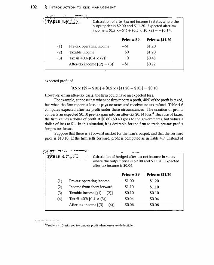
102 � I NTRO D U CTI O N TO R I S K M A N A G E M E N T

( 1 ) (2) (3)

Calculation of after-tax net income in states where the output price is $9.00 and $ 1 1 .20. Expected after-tax income is (0.5 x - $ 1 ) + (0.5 x $0.72) = -$0. 1 4.

Price = $9 Price = $11.20 Pre-tax operating income -$1 $ 1 .20 Taxable income $0 $ 1 .20 Tax @ 40% [0.4 X (2)] 0 $0.48 After-tax income [(2) - (3)] -$ 1 $0.72

expected profit of

(0.5 X ($9 - $ 10)] + (0.5 X ($ 1 1 .20 - $ 1 0)] = $0. 1 0

However, on an after-tax basis, the firm could have an expected loss . For example, suppose that when the firm reports a profit, 40% of the profit is taxed,

but when the firm reports a loss, it pays no taxes and receives no tax refund. Table 4.6 computes expected after-tax profit under these circumstances. The taxation of profits converts an expected $0. 1 0 pre-tax gain into an after-tax $0. 14 loss.4 Because of taxes, the firm values a dollar of profit at $0.60 ($0.40 goes to the government), but values a dollar of loss at $ 1 . In this situation, it is desirable for the firm to trade pre-tax profits for pre-tax losses .

Suppose that there is a forward market for the firm's output, and that the forward price is $ 10. 10. If the firm sells forward, profit is computed as in Table 4. 7. Instead of

( 1 ) (2) (3) (4)

Calculation of hedged after-tax net income in states where the output price is $9.00 and $ 1 1 .20. Expected after-tax income is $0.06.

Price = $9 Price = $11.20 Pre-tax operating income -$1 .00 $ 1 .20 Income from short forward $ 1 . 10 -$ 1 . 1 0 Taxable income [ ( 1 ) + (2)] $0. 10 $0. 10 Tax @ 40% [0.4 x (3)] $0.04 $0.04 After-tax income [(3) - (4) ] $0.06 $0.06

4Problem 4. 1 5 asks you to compute profit when losses are deductible.

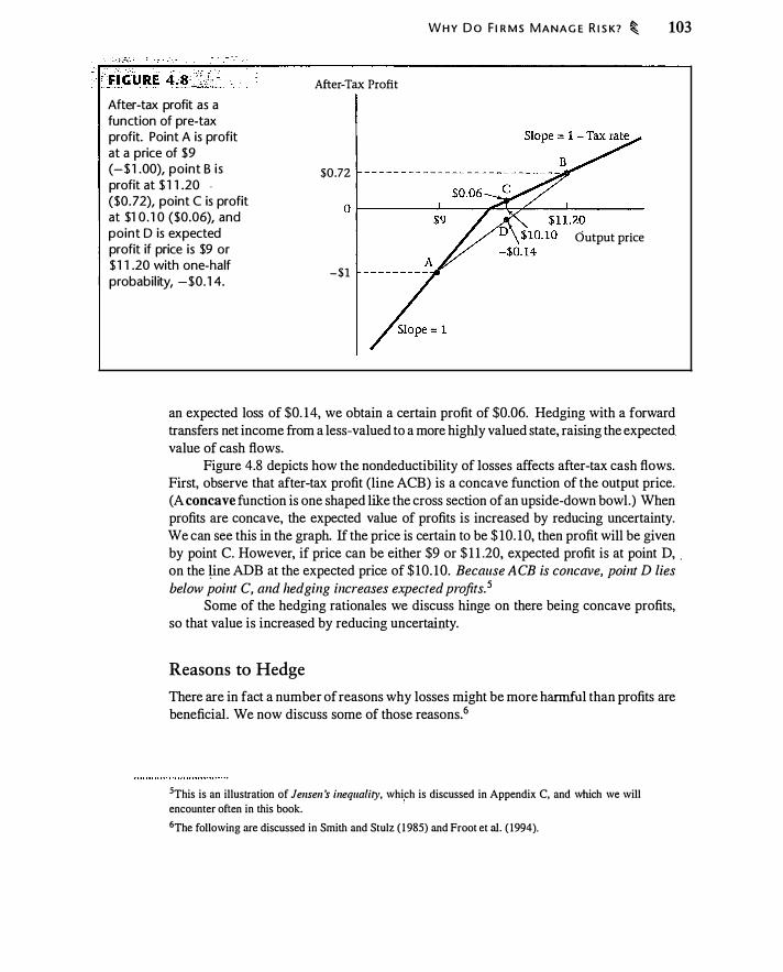
After-tax profit as a function of pre-tax profit. Point A is profit at a price of $9 (- $ 1 .00), point B is profit at $ 1 1 .20 . ($0.72), point C is profit at $1 0 . 1 0 ($0.06), and point D is expected profit if price is $9 or $ 1 1 .20 with one-half probabil ity, -$0. 1 4.

After-Tax Profit

$0.72

-$1

W H Y D o F I R M S M A N A G E R I S K? � 103

Output price

an expected loss of $0. 14, we obtain a certain profit of $0.06. Hedging with a forward transfers net income from a less-valued to a more highly valued state, raising the expected value of cash flows.

Figure 4.8 depicts how the nondeductibility of losses affects after-tax cash flows. First, observe that after-tax profit (line ACB) is a concave function of the output price. (A concave function is one shaped like the cross section of an upside-down bowl.) When profits are concave, the expected value of profits is increased by reducing uncertainty. We can see this in the graph. If the price is certain to be $ 10. 10, then profit will be given by point C. However, if price can be either $9 or $ 1 1 .20, expected profit is at point D, . on the �ne ADB at the expected price of $ 10. 10. Because ACB is concave, point D lies below point C, and hedging increases expected profits. 5

Some of the hedging rationales we discuss hinge on there being concave profits, so that value is increased by reducing uncertainty.

Reasons to Hedge

There are in fact a number of reasons why losses might be more harmful than profits are beneficial. We now discuss some of those reasons.6

5This is an illustration of Jensen 's inequality, which is discussed in Appendix C, and which we will

encounter often in this book.

6The following are discussed in Smith and Stulz ( 1 985) and Froot et al. ( 1994).

104 � I NTRO D U CTI O N TO R I S K MA N AG E M ENT

Taxes The previous example illustrating the effect of taxes was oversimplified in as­surning that losses are completely untaxed, but it is typically the case that governments tax profits but do not give full credits for losses. Tax systems usually permit a loss to be offset against a profit from a different year. However, in present value terms, the loss will have a lower effective tax rate than that applied to profits, which still generates a motive to hedge.

There are other aspects of the tax code that can encourage firms to shift income using derivatives; such uses may or may not appear to be hedging and may or may not be approved of by tax authorities. Tax rules that may entice firms to use derivatives

)nclude the separate taxation of capital and ordinary income (derivatives can be used to convert one form of income to another), capital gains taxation (derivatives can be used to defer taxation of capital gains incorp.e as with collars), and differential taxation across countries (derivatives can be used to shift income from one country to another).

Bankruptcy and distress costs An unusually large loss can threaten the survival of a firm. The most obvious reason is that a money-losing firm may be unable to meet fixed obligations, such as debt payments and wages. If a firm appears to be in distress, customers may be less willing to purchase its goods. (Would you buy a car or computer­both of which come with long-term warranties-from a company that appears likely to go out of business and would then be unable to honor its warranties?)

Actual or threatened bankruptcy can be costly; a dollar ofloss can cost the company more than a dollar. As with taxes, this is a reason for firms to enter derivatives contracts that transfer income from profit states to loss states, thereby reducing the probability of bankruptcy or distress.

Costly external financing Even if a loss is not large enough to threaten the survival of a firm, the firm must pay for the loss, either by using cash reserves or by raising funds externally (for example, by borrowing or issuing new securities).

Raising funds externally can be costly. There are explicit costs, such as bank and underwriting fees. There can also be implicit costs. If you borrow money, the lender may worry that you need to borrow because you are in decline, which increases the probability that you will not repay the loan. The lender's thinking this way raises the interest rate on the loan. The same problem arises even more severely with equity issues.

At the same time, cash reserves are valuable because they reduce a firm's need to raise funds externally in the future. So if the firm uses cash to pay for a loss, the reduction in cash increases the probability that the firm will need costly external financing in the future.

The fact that external financing is costly can even lead the firm to forgo investment projects it would have taken had cash been available to use for financing.

Thus, however the firm pays for the loss, a dollar of loss may actually cost the firm more than a dollar. Hedging can safeguard cash reserves and reduce the probability of costly external financing.

W H Y D o F I R M S M A N A G E R I S K? � 105

Increase debt capacity Because of the deductibility of interest expense for tax pur­poses, firms may find debt to be a tax-advantaged way to raise funds.7 However, lenders, fearful of bankruptcy, may be unwilling to lend to firms with risky cash flows. The amount that a firm can borrow is its debt capacity.

A firm that credibly reduces the riskiness of its cash flows should be able to borrow more, since for any given level of debt, bankruptcy is less likely. Such a firm is said to have raised its debt capacity. To the extent debt has a tax advantage, such a firm will also be more valuable.

Managerial risk aversion While large, public firms are owned by · well-diversified investors, firm managers are typically not well-diversified. Salary, bonus, and compen­sation options are all tied to the performance of the firm.

An individual who is unwilling to take a fair bet (i .e. , one with an expected payoff equal to the money at stake) is said to be risk-averse. Risk-averse persons are harmed by a dollar of loss more than they are helped by a dollar of gain. Thus, they benefit from reducing uncertainty. The effect is analogous to that shown in Figure 4.8.

If managers are risk-averse and have wealth that is tied to the company, we might expect that they will try to reduce uncertainty. However, matters are not this simple: Managers are often compensated in ways that encourage them to take more risk. For example, options given to managers as compensation, which we discuss in Chapter 16, are more valuable, other things equal, when the firm's stock price is riskier. Thus, a manager's risk aversion may be offset by compensation that is more valuable if the firffi is riskier.

Nonfinancial risk management Firms make risk-management decisions when they organize and design a business. For example, suppose you plan to sell widgets in Europe. You can construct a plant in the United States and export to Europe, or you can construct the plant in Europe, in which case costs of construction, labor, interest rates, and other ' inputs ·will be denominated in the same currency as the widgets you sell. Exchange rate hedging, to take one example, would be unnecessary.

Of course, if you build in a foreign country, you will encounter the costs of doing business abroad, including dealing with different tax codes and regulatory regimes.

Risk can also be affected by such decisions as leasing versus buying equipment, which determines the extent to which costs are fixed. Firms can choose flexible produc­tion technologies that may be more expensive at the outset, but which can be reconfigured at low cost. Risk is also affected by the decision to enter a particular line of business in the first place. Firms making computer mice and keyboards, for example, have to consider the possibility of lawsuits for repetitive stress injuries.

7For a discussion of this issue, see Brealey and Myers (2003, ch. 1 7).

106 � I NTR O D U CT I O N TO R I S K MANAG E M E N T

The point i s that risk management i s not a simple matter of hedging or not hedging using financial derivatives, but rather a series of decisions that start when the business is first conceived.

Reasons Not to Hedge

There are also reasons why firms might elect not to hedge:

• Transacting in derivatives entails paying transaction costs, such as commissions and the bid-ask spread.

• The firm must assess costs and benefits of a given strategy; this can require costly expertise.

• The firm must monitor transactions and have managerial controls in place to prevent unauthorized trading.

• The firm must be prepared for tax and accounting consequences of their transac­tions. In particular, this may complicate reporting.

Thus, while there are reasons to hedge, there are also costs. When thinking about costs and benefits, keep in mind that some of what firms do could be called risk manage­ment but may not obviously involve derivatives. For example, suppose Auric enters into a 2-year agreement with a supplier to buy gold at a fixed price. Will management think of this as a derivative? In fact this is a derivative under current accounting standards (it is a swap, which we discuss in Chapter 8), but it is exempt from derivatives accounting. 8 Finally, firms can face collateral requirements (the need to post extra cash with their counterparty) if their derivatives position loses money.

The box on page 108 illustrates an attempt to manage risk that backfired.

Empirical Evidence on Hedging

We know surprisingly little about the risk-management practice and derivatives use of firms in real life. It is difficult to tell, from publicly available information, the extent to which firms use derivatives. Beginning in 2000, Statement of Financial Accounting Standards (SFAS) 133 required firms to recognize derivatives as assets or liabilities on the balance sheet, to measure them at fair value, and to report changes in their market value.9 This reporting does not necessarily reveal a firm's hedging position (forward contracts have zero value, for example). Prior to 2000, firms had to report notional exposure; hence much existing evidence relies on data from the 1990s.

Research tries to address two questions: How much do firms use derivatives and why? Financial firms--commercial banks, investment banks, broker-dealers, and other

8Current derivatives accounting rules contain a "normal purchases and sales" exemption. Firms need not use derivatives accounting for forward contracts with physical delivery, for quantities likely to be

used or sold over a reasonable period in the normal course of business.

9 See Gastineau et a!. (200 I) for a discussion of SFAS 133 and previous accounting rules.

W H Y D o F I R M S M A N A G E R I S K? � 107

financial institutions-transact in derivatives frequently. Risks are identifiable, and regulators encourage risk management. The more open question is the extent to which nonfinancial firms use derivatives. We can summarize research findings as follows:

o Roughly half of nonfinancial firms report using derivatives, with usage greater among large firms (Bodnar et al. , 1998; Bartram et al. , 2004).

o Among firms that do use derivatives, less than 25% of perceived risk is hedged, with firms likelier to hedge short-term risks (Bodnar et al . , 1 998).

o Firms with more investment opportunities are likelier to hedge (Geczy et al. , 1997). o Firms that use derivatives have a higher market value (AllayanQis and Weston,

200 1 ; Allayannis et al., 2004; Bartram et al. , 2004) and more leverage (Graham and Rogers, 2002; Haushalter, 2000). 1 0

Guay and Kothari (2003) verify many of these findings but conclude that for most firms, derivatives use is of minor economic significance. In their sample of large firms, slightly more than half report derivatives usage. Among derivatives users, the authors estimate that the median firm hedges only about 3% to 6% of exposure to interest rates and exchange rates.

Because data are hard to obtain, some studies have focused on particular industries and even firms. Tufano ( 1996), Petersen and Thiagarajan (2000), and Brown et al. (2003) have examined hedging behavior by gold-mining firms. Using a uniquely detailed data set, Tufano found that most gold firms use some derivatives, with the median firm in his sample (North American firms) selling forward about 25% of 3-year production. Fifteen

percent of firms used no derivatives. Brown et al. found substantial variation over time in the amount hedging by gold firms. Firms tended to increase hedging as the price rose, and managers reported that they adjusted hedges based on their views about gold prices.

The currency-hedging operations of a U.S.-based manufacturing firm are examined in detail by Brown (2001) , who finds that foreign exchange hedging is an integral part of firm operations, but the company has no clear rationale for hedging. For example, Brown reports one manager saying, "We do not take speculative positions, but the extent we are

.hedged depends on our views." Faulkender (2005) finds consistent evidence for

interest-rate hedging in the chemical industry. These firms increase exposure to short­term interest rates as the yield curve becomes more upward-sloping, 1 1 but correlations between cash flows and interest rates do not affect behavior.

The varied evidence suggests that some use of derivatives is common, especially at large firms, but the evidence is weak that economic theories explain hedging.

10Graham and Smith ( 1 999) find that after-tax profits are concave for a majority of firms, as in Figure 4.8. However, Graham and Rogers (2002) are unable to find a link between hedging and tax-induced

concavity.

1 1 An upward-sloping yield curve means that long-term bond yields are greater than short-term bond yields. This appears to make short-term financing Jess expensive. However, we will see in Chapters 7 and 8 that if a company hedges all of its future short-term financing costs, long-term and short-term

financing will cost the same.

108 � I NTRO D U CTI O N TO R I S K M A N A G E M ENT

Ford Motor Co. stunned investors in January 2002 when it announced a $ 1 billion write-off on stockpiles of palladium, a precious metal Ford used in catalytic converters (devices that reduce polluting emissions from cars and trucks) . Ironically, Ford sustained the loss while attempting to actively manage palladium risk.

According to the Wall Street Jounzal (see Gregory L. White, "A Mismanaged Palladium Stockpile Was Catalyst for Ford's Write-Off," February 6, 2002, p. Al), Ford in the late 1 980s h.ad begun to use palladium as a replacement for platinum. Palladium prices were steady unti1 1997, when Russia, a major

_supplier with a large stockpile of palladium, withheld supply from the market. Prices more than doubled to $350/oz. at a time when Ford was planning to increase its use of the metal. By early 2000, prices had doubled again, �o

· $700. While GM had begun work several years earlier to reduce reliance on palladium, Ford continued to rely heavily on the metal.

In 2000, Ford management agreed to allow the purchasing staff to stockpile

4.4 GOLDDIGGERS REVISITED

palladium. The purchasing staff evidently did not communicate with Ford's treasury department, which had hedging experience. Thus, for example, Ford did not buy puts to protect against a drop in palladium prices. The purchasing staff also did not communicate with Ford's research department, which was working to reduce reliance on palladium. Ford continued to buy palladium in 2001 as prices exceeded $ 1000. However, by the middle of the year, palladium prices had fallen to $350.

By the end of 2001 , Ford had developed technology that would eventually reduce the need for palladium by 50%. The year-end price of palladium was $440/oz.

As a result of this experience, "Ford has instituted new procedures to ensure that treasury-department staffers with experience in hedging are involved in any major commodities purchases in the future, [Ford Chief Financial Officer Martin] Inglis says."

We have looked at simple hedging and insurance strategies for buyers and sellers. We now examine some additional strategies that permit tailoring the amount and cost of insurance. For simplicity we will focus primarily on Golddiggers; however, in every case there are analogous strategies for Auric.

Table 4.8 lists premiums for three calls and puts on gold with 1 year to expiration and three different strikes. The examples use these values.

Selling the Gain: Collars

As discussed earlier, we can reduce the cost of insurance by reducing potential profit, i .e., by selling our right to profit from high gold prices. We can do this by selling a call. If the gold price is above the strike on the call, we are contractually obligated to sell at the strike. This caps our profits, in exchange for an initial premium payment.

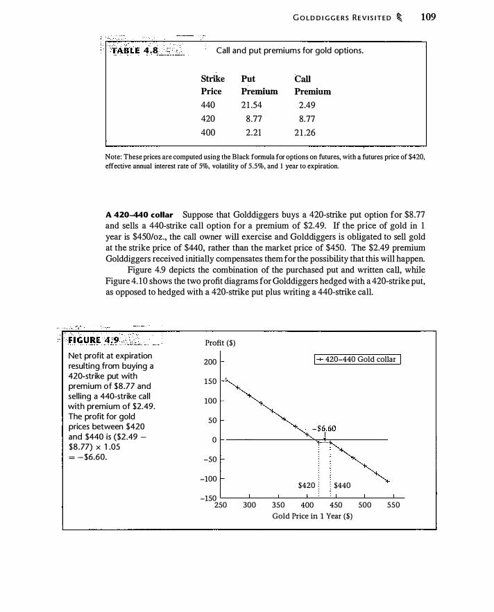
G O LD D I G G E RS R E V I S I T E D � 109

, , ''> '- ' ' · . . · ' . ' > ' : ,, ' 'TABLE · 4.8 = , Cal l and put premiums for gold options.

Strike Put Call

Price Premium Premium

440 2 1 .54 2.49 420 8 .77 8.77 400 2.21 2 1 .26

Note: These prices are computed using the Black fonnula for options on futures, with a futures price of $420,

effective annual interest rate of 5%, volatility of 5.5%, and I year to expiration.

A 420440 collar Suppose that Golddiggers buys a 420-strike put option for $8 .77 and sells a 440-strike call option for a premium of $2.49. If the price of gold in 1 year is $450/oz., the call owner will exercise and Golddiggers is obligated to sell gold at the strike price of $440, rather than the market price of $450. The $2.49 premium Golddiggers received initially compensates them for the possibility that this will happen.

Figure 4.9 depicts the combination of the purchased put and written call, while Figure 4. 10 shows the two profit diagrams for Golddiggers hedged with a 420-strike put, as opposed to hedged with a 420-strike put plus writing a 440-strike call.

Profit ($)

Net profit at expiration 200 resultingfrom buying a

420-strike put with 150 premium of $8.77 and

sel l ing a 440-strike cal l 100

with premium of $2.49. The profit for gold prices between $420

50

and $440 is ($2.49 - 0 $8. 77) X 1 .05 = - $6.60. -50

-100

-150 250 300

I+ 420-440 Gold collar I

350

$420 : $440

400 450

Gold Price in 1 Year ($)

500 550

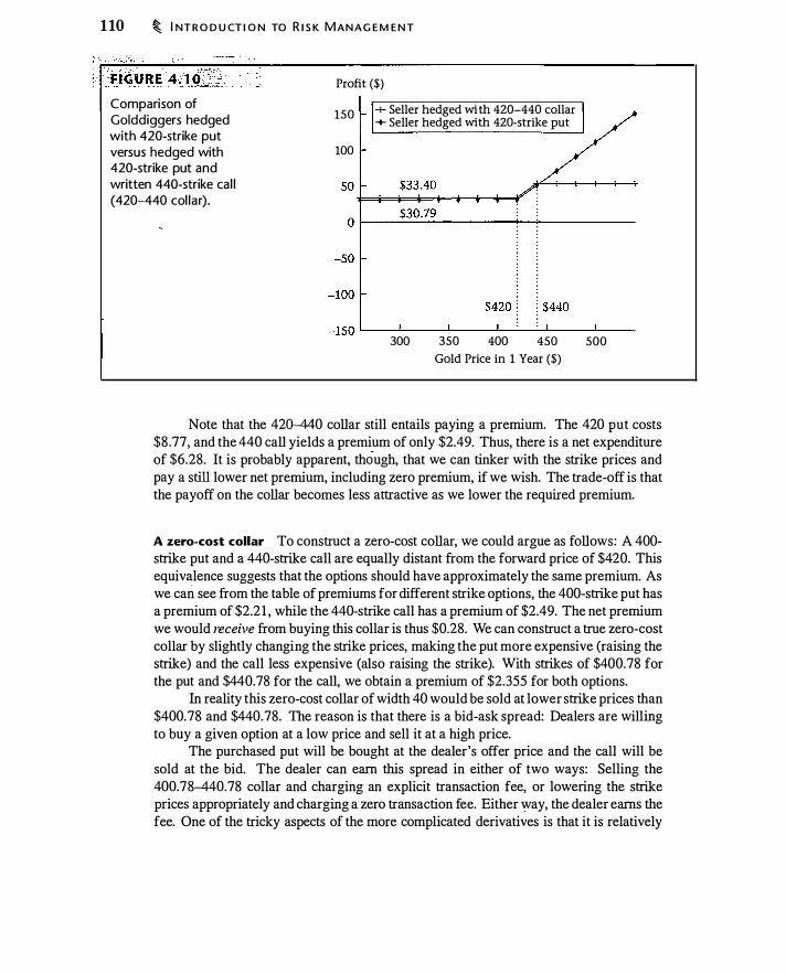
110 � I NT R O D U CT I O N TO R I S K MANAG E M E N T

Profit ($)

Comparison of Golddiggers hedged with 420-strike put versus hedged with 420-strike put and written 440-strike cal l (420-440 col lar).

150 + Seller hedged with 420-440 collar + Seller hedged with 420-strike put

100

300 350 400 450

Gold Price in 1 Year ($)

500

Note that the 42�0 collar still entails paying a premium. The 420 put costs $8 .77, and the 440 call yields a premium of only $2.49. Thus, there is a net expenditure of $6.28. It is probably apparent, though, that we can tinker with the strike prices and pay a still lower net premium, including zero premium, if we wish. The trade-off is that the payoff on the collar becomes less attractive as we lower the required premium.

A zero-cost collar To construct a zero-cost collar, we could argue as follows: A 400-strike put and a 440-strike call are equally distant from the forward price of $420. This equivalence suggests that the options should have approximately the same premium. As we cari see from the table of premiums for different strike options, the 400-strike put has a premium of $2.2 1 , while the 440-strike call has a premium of $2.49. The net premium we would receive from buying this collar is thus $0.28. We can construct a true zero-cost collar by slightly changing the strike prices, making the put more expensive (raising the strike) and the call less expensive (also raising the strike). With strikes of $400.78 for the put and $440.78 for the call, we obtain a premium of $2.355 for both options.

In reality this zero-cost collar of width 40 would be sold at lower strike prices than $400.78 and $440.78. The reason is that there is a bid-ask spread: Dealers are willing to buy a given option at a low price and sell it at a high price.

The purchased put will be bought at the dealer's offer price and the call will be sold at the bid. The dealer can earn this spread in either of two ways: Selling the 400.78-440.78 collar and charging an explicit transaction fee, or lowering the strike prices appropriately and charging a zero transaction fee. Either way, the dealer earns the fee. One of the tricky aspects of the more complicated derivatives is that it is relatively

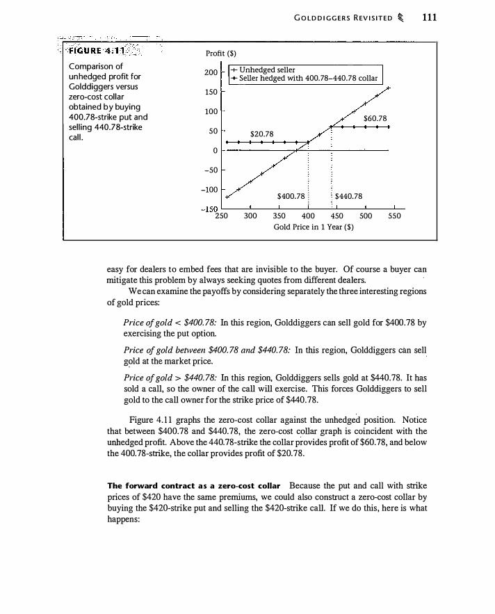
Comparison of unhedged profit for Golddiggers versus zero-cost col lar obtained by buying 400.78-strike put and sel l ing 440.78-strike cal l .

G O LD D I G G ERS R EV I S IT E D � 111

Profit ($)

200 + Unhedged seller + Seller hedged with 400.78-440.78 collar

150

100 $60.78

50 $20.78

0

-50

-100 $400.78 � $440.78

-150 L..._ _ __,_ __ _,_ __ ..___....:......L __ -L. __ ..,L_ 250 300 350 400 450 500 550

Gold Price in 1 Year ($)

easy for dealers to embed fees that are invisible to the buyer. Of course a buyer can mitigate this problem by always seeking quotes from different dealers.

We can examine the payoffs by considering separately the three interesting regions of gold prices:

Price of gold < $400. 78: In this region, Golddiggers can sell gold for $400.78 by exercising the put option.

Price of gold between $400. 78 and $440. 78: In this region, Golddiggers can sell g�ld at the market price.

·

Price of gold > $440. 78: In this region, Golddiggers sells gold at $440.78. It has sold a call, so the owner of the call will exercise. This forces Golddiggers to sell gold to the call owner for the strike price of $440.78.

Figure 4. 1 1 graphs the zero-cost collar against the unhedged position. Notice that between $400.78 and $440.78, the zero-cost collar graph is coincident with the unhedged profit. Above the 440. 78-strike the collar provides profit of $60.78, and below the 400. 78-strike, the collar provides profit of $20.78 .

The forward contract a s a zero-cost collar Because the put and call with strike prices of $420 have the same premiums, we could also construct a zero-cost collar by buying the $420-strike put and selling the $420-strike call. If we do this, here is what happens:

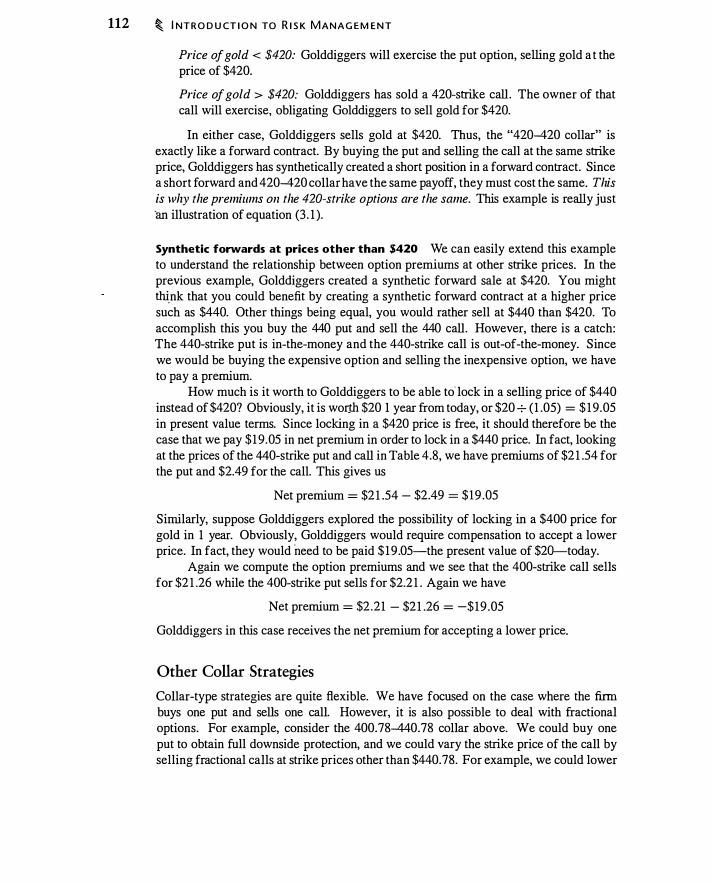
112 � I NTRO D U CT I O N TO R I S K M A N A G E M E N T

Price of gold < $420: Golddiggers will exercise the put option, selling gold a t the price of $420.

Price of gold > $420: Golddiggers has sold a 420-strike call. The owner of that call will exercise, obligating Golddiggers to sell gold for $420.

In either case, Golddiggers sells gold at $420. Thus, the "420-420 collar" is exactly like a forward contract. By buying the put and selling the call at the same strike price, Golddiggers has synthetically created a short position in a forward contract. Since a short forward and 420-420 collar have the same payoff, they must cost the same. This is why the premiums on the 420-strike options are the same. This example is really just an illustration of equation (3 . 1 ).

Synthetic forwards at prices other than $420 We can easily extend this example to understand the relationship between option premiums at other strike prices. In the previous example, Golddiggers created a synthetic forward sale at $420. You might �nk that you could benefit by creating a synthetic forward contract at a higher price such as $440. Other things being equal, you would rather sell at $440 than $420. To accomplish this you buy the 440 put and sell the 440 call. However, there is a catch: The 440-strike put is in-the-money and the 440-strike call is out-of-the-money. Since we would be buying the expensive option and selling the inexpensive option, we have to pay a premium.

How much is it worth to Golddiggers to be able to. lock in a selling price of $440 instead of $420? Obviously, it is wor.ili $20 1 year from today, or $20 -;- (1 .05) = $ 19.05 in present value terms. Since locking in a $420 price is free, it should therefore be the case that we pay $19.05 in net premium in order to lock in a $440 price. In fact, looking at the prices of the 440-strike put and call in Table 4.8, we have premiums of $2 1 .54 for the put and $2.49 for the call. This gives us

Net premium = $2 1 .54 - $2.49 = $19 .05

Similarly, suppose Golddiggers explored the possibility of locking in a $400 price for gold in 1 year. Obviously, Golddiggers would require compensation to accept a lower price. In fact, they would need to be paid $ 19 .05-the present value of $2�today.

Again we compute the option premiums and we see that the 400-strike call sells for $2 1 .26 while the 400-strike put sells for $2.2 1 . Again we have

Net premium = $2.21 - $21 .26 = -$19 .05

Golddiggers in this case receives the net premium for accepting a lower price.

Other Collar Strategies

Collar-type strategies are quite flexible. We have focused on the case where the firm buys one put and sells one call. However, it is also possible to deal with fractional options. For example, consider the 400.78-440.78 collar above. We could buy one put to obtain full downside protection, and we could vary the strike price of the call by selling fractional calls at strike prices other than $440.78. For example, we could lower

S E L ECTI N G TH E H E D G E R AT I O � 113

the call strike price below $440.78, in which case we would obtain a higher premium per call. To offset the higher premium, we could buy less than one call. The trade-off is that we cap the gold price on part of production at a lower level, but we maintain some participation at any price above the strike.

Alternatively we could raise the cap level (the strike price on the call) and sell more than one call. This would increase participation in gold price increases up to the cap level, but also have the effect of generating a riet short position in gold if prices rose above the cap.

Paylater Strategies

A disadvantage to buying a put option is that Golddiggers pays the premium even when the gold price is high and insurance was, after the fact, unnecessary. One strategy to avoid this problem is a pay later strategy, where the premium is paid only when the insurance is needed. While it is possible to construct exotic options in which the premium is paid only at expiration and only if the option is in the money, the strategy we discuss here is a ratio spread using ordinary put options . The goal is to find a strategy where if the gold price is high, there is no net option premium. If the gold price is low, there is insurance, but the effective premium is greater than with an ordinary insurance strategy.

If there is no premium when the gold price is high, we must have no initial premium. This means that we must sell at least one option. Consider the following strategy for Golddiggers: Sell a 434.6-strike put and buy two 420-strike puts. Using our assumptions; the premium on the 434.6-strike put is $ 17.55, while the premium on the 420-strike put is $8.77. Thus, the net option premium from this strategy is $17 .55 - (2 x $8.775) = 0.

Figure 4. 12 depicts the result of Golddiggers 's hedging with a paylater strategy. When the price of gold is greater than $434.60, neither put is exercised, and Golddiggers 's profit is the same as if it were unhedged. When the price of gold is between $420 and $434.60, because of the written $434.60 put, the firm loses $2 of profit for every $ 1 decline i n the price of gold. Below $420 the purchased 420-strike puts are exercised, · and profit becomes constant. The net result is an insurance policy that is not paid for unless it is needed.

Also depicted in Figure 4. 12 is the familiar result from a conventional insurance strategy of hedging by purchasing a single 420-strike put. When the gold price is high, the paylater strategy with a zero premium outperforms the single put. When the gold price is low, the paylater strategy does worse because it offers less insurance. Thus, the premium is paid later, if insurance is needed.

4.5 SELECTING THE HED GE RATIO

In the Golddiggers and Auric examples, we performed all calculations in terms of one unit of gold, and made two important assumptions. First, we assumed perfect correlation between the price of gold and the price of what each company wants to hedge. Second, we assumed that the companies knew for certain the quantity of gold they would sell and buy. As a result of these assumptions, we effectively assumed that the hedge ratio is one,

114 � I NTRO D U CT I O N TO R I S K M A N AG E M E N T

Depiction of "paylater" strategy, in which Golddiggers sells a 434.6-strike put and buys two 420-strike puts, compared to the conventional insurance strategy of buying a 420-strike put.

Profit ($)

200

150

100

so

0

-50

-100

-+- Unhedged seller -+- Seller hedged with 420-strike put ......_ Paylater • Seller hedged with paylater

$420 � � $434.60

-1SO L---�-----L-----L���----L---�L-250 300 350 400 450

Gold Price in 1 Year ($)

500 550

where the hedge ratio is defined as the ratio of the forward position to the underlying asset.

In practice, neither assumption-may be valid. We first examine the effect of widget price uncertainty on hedging, and discuss cross-hedging. We then examine quantity unce11ainty using an agricultural example.

Cross-Hedging

In the Auric example we assumed that widget prices are fixed. However, since gold is used to produce widgets, widget prices might vary with gold prices. If widget and gold prices vary one-for-one, Auric's profits would be independent of the price of gold and Auric would have no need to hedge. 1 2

More realistically, the price of widgets could change with the price of gold, but not one-for-one; other factors could affect widget prices as well. In this case, Auric might find it helpful to use gold derivatives to hedge the price of the widgets it sells as well as the price of the gold it buys. Using gold to hedge widgets would be an example of cross­

hedging: the use of a derivative on one asset to hedge another asset. Cross-hedging arises in many different contexts.

12"0ne-for-one" in this context means that if the price of gold rises by $ 1 , the. price of a widget rises

by $1 times the amount of gold used to make the widget.

S E L E CT I N G T H E H E D G E RAT I O � 115

The hedging problem for Auric is to hedge the difference in the price of widgets and gold. Conceptually, we can think of hedging widgets and gold separately, and then combining those separate hedges into one net hedge.

To generalize the Auric example, suppose that buying Ng ounces of gold enables us to produce Nw widgets. Profit per ounce of gold, without hedging, is

(4. 1 )

where_Pw is the widget price. Suppose that we go long H gold futures contracts, each covering 1 oz. of gold. If

F is the gold forward price, the return on the hedged position is

Hedged profit = Nw Pw - Ng Pgold + H ( Pgold - F)

The variance of the return on the hedged position is given by ? ? ? ? ? uhedged = N;;p� + (H - Ng)-u-g + 2(H - Ng)Nwpu wu g (4.2)

where u w is the standard deviation of the widget price, u g is the standard deviation of the gold price, and p is the price correlation between widgets and gold. Note that pu wCJ g is the covariance between widget and gold prices.

The variance-minimizing hedge position, H*, is 13

H* = Ng - Nw pu w

CJg (4.3)

Equation (4.3) has a straightforward interpretation. The first term hedges costs-i.e., we enter into a long position on the amount of gold we use in production, Ng . The second term hedges revenue, providing the quantity of gold forwards we use to hedge widgets . The term pu w I u g is the coefficient from regressing the widget price on the gold price. 14 This regression coefficient times the number of widgets, Nw, gives us the number of gold contracts to use in hedging widget price risk. The result is that the hedge quantity,

1 3This can be derived by differentiating equation (4.2) with respect to H*. 14The tenn pa w!a g measures the comovement of gold and widget prices, which is typically measured

using a linear regression. A common approach is to regress price changes on price changes:

Pw.r - Pw,t- 1 = a + {J(Pg.r - Pg,r- r > + llr

where the subscript t denotes the value at time t . Other specifications, including the use of percentage

changes, or regressing levels on levels, are possible. The correct regression to use depends on context. In general, regressions using changes are more likely to give a correct hedge coefficient since the

goal of the hedge is to have changes in the price of the asset matched by changes in futures price.

In Chapters 5 and 6, we will present examples of hedging stocks and jet fuel, and the appropriate

regressions will be returns on returns (stocks) and changes on changes Get fuel). Regressions of level

on level are problematic in many contexts. For example, in the case of stocks, asset pricing models tell

us that stock retrtms are related, but we would not expect a stable relationship between two prices. The

appropriate regression is returns on returns. A comprehensive discussion is Siegel and Siegel ( 1 990,

pp. 1 14-135).

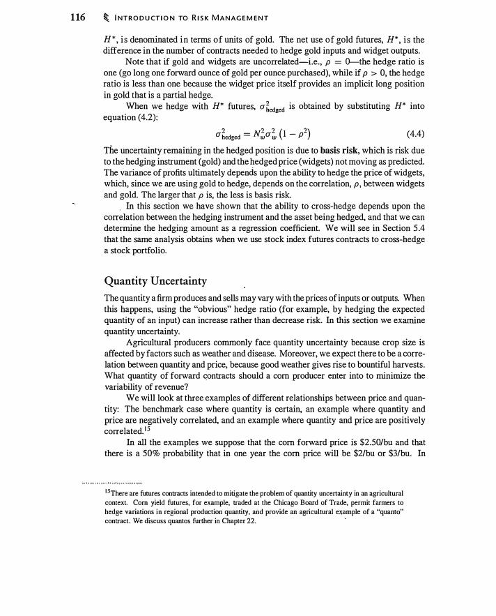
116 � I NT R O D U CT I O N TO R I S K M A N AG E M E N T

H * , i s denominated in terms of units of gold. The net use of gold futures, H*, i s the difference in the number of contracts needed to hedge gold inputs and widget outputs.

Note that if gold and widgets are uncorrelated-i.e., p = 0---the hedge ratio is one (go long one forward ounce of gold per ounce purchased), while if p > 0, the hedge ratio is less than one because the widget price itself provides an implicit long position in gold that is a partial hedge.

When we hedge with H* futures, o-�edoed is obtained by substituting H* into equation (4.2):

e

') ') ') ( ") a-hedged = N;;p� l - p- (4.4)

The uncertainty remaining in the hedged position is due to basis risk, which is risk due to the hedging instrument (gold) and the hedged price (widgets) not moving as predicted. The variance of profits ultimately depends upon the ability to hedge the price of widgets, which, since we are using gold to hedge, depends on the correlation, p, between widgets and gold. The larger that p is, the less is basis risk.

. In this section we have shown that the ability to cross-hedge depends upon the correlation between the hedging instrument and the asset being hedged, and that we can determine the hedging amount as a regression coefficient. We will see in Section 5 .4 that the same analysis obtains when we use stock index futures contracts to cross-hedge a stock portfolio.

Quantity Uncertainty

The quantity a firm produces and sells may vary with the prices of inputs or outputs. When this happens, using the "obvious" hedge ratio (for example, by hedging the expected quantity of an input) can increase rather than decrease risk. In this section we examine quantity uncertainty.

Agricultural producers commonly face quantity uncertainty because crop size is affected by factors such as weather and disease. Moreover, we expect there to be a corre­lation between quantity and price, because good weather gives rise to bountiful harvests. What quantity of forward GOntracts should a corn producer enter into to minimize the variability of revenue?

We will look at three examples of different relationships between price and quan­tity: The benchmark case where quantity is certain, an example where quantity and price are negatively correlated, and an example where quantity and price are positively correlated. 1 5

In all the examples we suppose that the corn forward price is $2.50/bu and that there is a 50% probability that in one year the corn price will be $2/bu or $3/bu. In

1 5There are futures contracts intended to mitigate the problem of quantity uncertainty in an agricultural

context. Corn yield futures, for example, traded at the Chicago Board of Trade, permit farmers to hedge variations in regional production quantity, and provide an agricultural e)lample of a "quanta" contract. We discuss quantos further in Chapter 22.

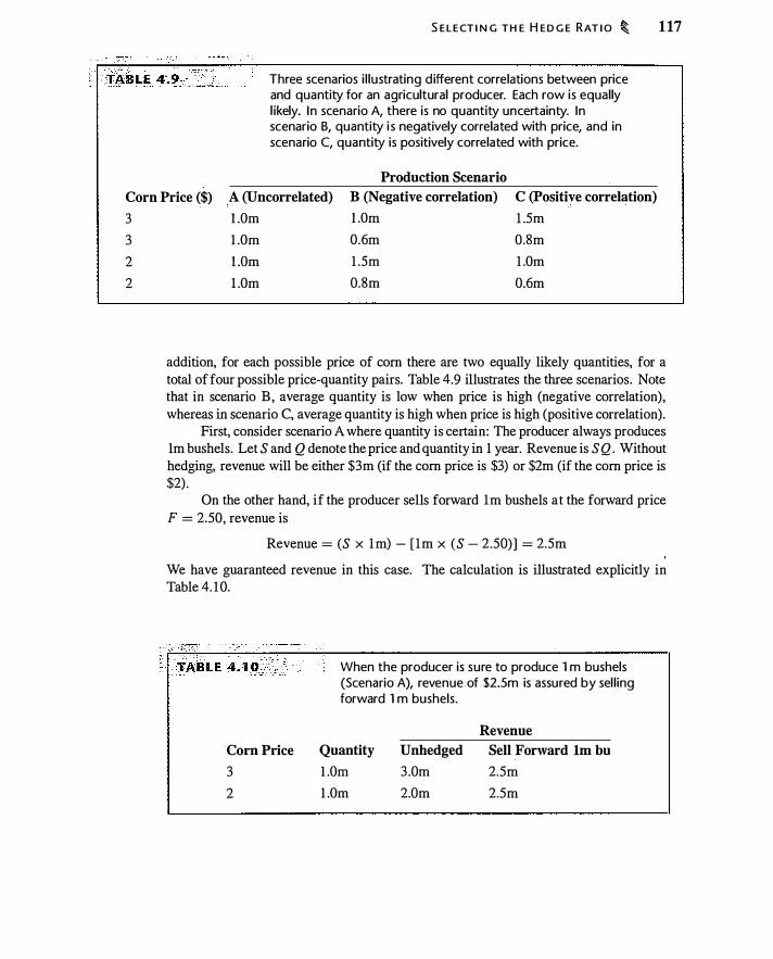
S E L E CT I N G TH E H E D G E RAT I O � 117

Three scenarios i l lustrating different correlations between price and quantity for an agricultural producer. Each row is equal ly l ikely. I n scenario A, there is no quantity uncertainty. In scenario B, quantity i s negatively correlated with price, and in scenario C, quantity is positively correlated with price.

Production Scenario

Corn Price ($) A (Uncorrelated) B (Negative correlation) C (Positive correlation)

3 3 2 2

LOrn LOrn 1 .5m LOrn 0.6m 0.8m LOrn L5m LOrn LOrn 0.8m 0.6m

addition, for each possible price of com there are two equally likely quantities, for a total of four possible price-quantity pairs. Table 4.9 illustrates the three scenarios. Note that in scenario B , average quantity is low when price is high (negative correlation), whereas in scenario C, average quantity is high when price is high (positive correlation).

First, consider scenario A where quantity is certain: The producer always produces 1m bushels. Let S and Q denote the price and quantity in 1 year. Revenue is SQ . Without hedging, revenue will be either $3m (if the com price is $3) or $2m (if the com price is $2) .

On the other hand, if the producer sells forward 1m bushels at the forward price F = 2.50, revenue is

Revenue = (S x 1 m) - [ 1 m x (S - 2.50)] = 2.5m

We have guaranteed revenue in this case. The calculation is illustrated explicitly in Table 4. 1 0.

Com Price

3 2

When the producer is sure to produce 1 m bushels (Scenario A), revenue .of $2.5m is assured by sel l ing forward 1 m bushels.

Quantity

LOrn LOrn

Unhedged

3 .0m 2.0m

Revenue

Sell Forward lm bu

2.5m 2.5m

118 � I NTRO D U CTI O N TO R I S K MANA G E M ENT

In general, i f the producer enters into forward contracts on H units, hedged rev­enue, R(H) , will be

Hedged revenue = R (H) = (S x Q) + [H x (S - F)] (4.5)

Using equation ( 4 .5) , when there is uncertainty, the variability of hedged revenue, u�(HJ ' is

u� <HJ = uiQ + H2ui + 2HPsQ,sO"sQus (4.6)

The standard deviation of total revenue, S Q, is u SQ • and the correlation of total rev­el_!.ue with price is p SQ,S · As in the preceding discussion of cross-hedging, the H that minimizes the variance of hedged revenue will be

H = . PsQ,sO" sQ us

(4.7)

This is the same as the second term in equation (4.3) . The formula for the variance­minimizing hedge ratio in equation ( 4. 7) is the negative of the coefficient from a regres­siori of unhedged revenue on price. We can therefore determine the variance-minimizing hedge ratios for the negative- and positive-correlation scenarios (scenarios B and C) in Table 4.9 either by using equation (4.7) directly, or else we can run a regression of revenue on price.

First, consider what happens in Scenario B if we hedge by shorting the expected quantity of production. As a benchmark, column 3 of Table 4. 1 1 shows that unhedged revenue has variability of $0.654m. From Table 4.9, expected production in the negative

Results in Scenario B (negative correlation between the price of corn and the quantity of production) from shorting 975,000 corn forwards (columns 4 and 5) and from sel l ing forward 1 00,000 bushels (columns 6 and 7). Each price-quantity combination is equa l ly l ikely, with a probabi l ity of 0 .25 . Standard deviations are computed using the population estimate of standard deviation.

Urihedged Sell Forward 0.975m bu Sell Forward O.lOOm bu

Price Quantity Revenue Futures Gain Total Futures Gain Total

$3 LOrn $3 .0m -$0.488m $2.5 1 2m -$0.050m $2.95m $3 0.6m $ 1 .8m -$0.488m $ 1 .3 1 2m -$0.050m $ 1 .75m $2 1 .5m $3.0m $0.488m $3 .488m $0.050m $3 .05m $2 0.8m $ 1 .6m $0.488m $2.088m $0.050m $ 1 .65m

0" total revenue $0.654m $0.8 14m $0.652m

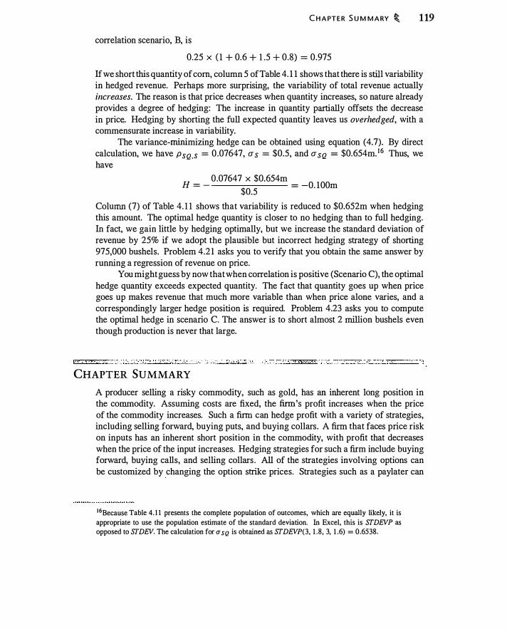
correlation scenario, B, is

C H A PTER S U M M A RY � 119

0.25 X ( 1 + 0.6 + 1 .5 + 0.8) = 0.975

If we short this quantity of corn, column 5 of Table 4. 1 1 shows that there is still variability in hedged revenue. Perhaps more surprising, the variability of total revenue actually increases. The reason is that price decreases when quantity increases, so nature already provides a degree of hedging: The increase in quantity partially offsets the decrease in price. Hedging by shorting the full expected quantity leaves us overhedged, with a commensurate increase in variability.

The variance-minimizing hedge can be obtained using equation (4.7). By direct calculation, we have PsQ.s = 0.07647, us = $0.5, and usQ = $0.654m. 1 6 Thus, we have

0 .07647 x $0.654m H = - = -0. 100m

$0.5 Column (7) of Table 4. 1 1 shows that variability is reduced to $0.652m when hedging this amount. The optimal hedge quantity is closer to no hedging than to full hedging. In fact, we gain little by hedging optimally, but we increase the standard deviation of revenue by 25% if we adopt the plausible but incorrect hedging strategy of shorting 975,000 bushels. Problem 4.2 1 asks you to verify that you obtain the same answer by running a regression of revenue on price.

You might guess by now that when correlation is positive (Scenario C), the optimal hedge quantity exceeds expected quantity. The fact that quantity goes up when price goes up makes revenue that much more variable than when price alone varies, and a correspondingly larger hedge position is required. Problem 4.23 asks you to compute the optimal hedge in scenario C. The answer is to short almost 2 million bushels even though production is never that large.

CHAPTER SUMMARY A producer selling a risky commodity, such as gold, has an inherent long position in the commodity. Assuming costs are fixed, the firm's profit increases when the price of the commodity increases. Such a firm can hedge profit with a variety of strategies, including selling forward, buying puts, and buying collars. A firm that faces price risk on inputs has an inherent short position in the commodity, with profit that decreases when the price of the input increases. Hedging strategies for such a firm include buying forward, buying calls, and selling collars. All of the strategies involving options can be customized by changing the option strike prices. Strategies such as a pay later can

16Because Table 4. I 1 presents the complete population of outcomes, which are equally likely, it is

appropriate to use the population estimate of the standard deviation. In Excel, this is STDEVP as opposed to STDEV. The calculation for u sQ is obtained as STDEVP(3, 1 .8 , 3, 1 .6) = 0.6538.

120 � I NTRO D U CT I O N TO R I S K MANAG E M E N T

provide insurance with no initial premium, but on which the company has greater losses should the insurance be needed.

Hedging can be optimal for a company when an extra dollar of income received in times of high profits is worth less than an extra dollar of income received in times of low profits. Profits for such a firm are concave, in which case hedging can increase expected cash flow. Concave profits can arise from taxes, bankruptcy costs, costly external finance, preservation of debt capacity, and managerial risk aversion. Such a firm can increase expected cash flow by hedging. Nevertheless, firms may elect not to hedge for reasons including transaction costs of dealing in derivatives, the requirement for expertise, the need to monitor and control the hedging process, and complications from tax and accounting considerations.

FURTHER READING

In this and earlier chapters we have examined uses of forwards and options, taking for granted the pricing of those contracts. Two big unanswered questions are: How are those prices determined? How does the market for them work?

In Chapters 5 through 8, we will explore forward and futures contracts discussing pricing as well as how market-makers function. In Chapters 1 0 through 13 , we will answer the same questions for options. Chapter 14 will discuss how exotic options can be used in risk-management strategies in place of the ordinary puts and calls discussed in this chapter.

Wharton and erne regularly survey nonfinancial firms to assess their hedging. A recent survey is summarized in Bodnar et al. ( 1 998). Bartram et al. (2004) examine hedging behavior in an international sample of over 7000 firms . Tufano ( 1996, 1998), Petersen and Thiagarajan (2000), and Brown et al. (2003) have studied hedging practices in the gold-mining industry. Other papers examining hedging include Geczy et al. ( 1 997), Allayannis and Weston (2001) , Allayannis et al. (2003), and Allayannis et al. (2004). Guay and Kothari (2003) attempt to quantify_ derivatives usage using information in firm annual reports from 1997. Brown (2001 ) provides an interesting and detailed description of the hedging .decisions by one (anonymous) firm and Faulkender (2005) examines interest rate hedging in the chemical industry.

Gastineau et al. (2001 ) discuss Statement of Financial Accounting Standards 133, which currently governs accounting for derivatives.

Finally, Fleming ( 1997) relates some of the history of (the fictitous) Auric Enterprises.

PROBLEMS

For the following problems consider the following three firms :

• XYZ mines copper, with fixed costs of $0.50/lb and variable cost of $0.40/lb. • Wirco produces wire. It buys copper and manufactures wire. One pound of copper

can be used to produce one unit of wire, which sells for the price of copper plus $5. Fixed cost per unit is $3 and noncopper variable cost is $ 1 .50.

P RO B LE M S � 121

• Telco installs telecommunications equipment and uses copper wire from Wirco as an input. For planning purposes, Telco assigns a fixed revenue of $6.20 for each unit of wire it uses.

The 1 -year forward price of copper is $ 1/lb. The 1 -year continuously compounded interest rate is 6%. One-year option prices for copper are shown in the table below. 1 7

Strike Call Put

0.9500 $0.0649 $0.0178 0.9750 0.0500 0.0265 1 .0000 0.0376 0.0376 1 .0250 0.0274 0.0509 1 .0340 0.0243 0.0563 1 .0500 0.0194 0.0665

In your answers, at a minimum consider copper prices in 1 year of $0.80, $0.90, $ 1 .00, $ 1 . 10, and $ 1 .20.

4.1. If XYZ does nothing to manage copper price risk, what is its profit 1 year from now, per pound of copper? If on the other hand XYZ sells forward its expected copper production, what is its estimated profit 1 year from now? Construct graphs illustrating both unhedged and hedged profit.

4.2. Suppose the 1 -year copper forward price were $0.80 instead of $ 1 . If XYZ were to sell forward its expected copper production, what is its estimated profit one year from now? Should XYZ produce copper? What if the forward copper price is $0.45?

4.3. Compute estimated profit in 1 year if XYZ buys a put option with a strike of $0.95, $ 1 .00, or $ 1 .05. Draw a graph of profit in each case.

4.4. Compute estimated profit in 1 year ifXYZ sells a call option with a strike of $0.95, $ 1 .00, or $ 1 .05. Draw a graph of profit in each case. ·

4.5. Compute estimated profit in 1 year if XYZ buys collars with the following strikes:

a. $0.95 for the put and $ 1 .00 for the call. b. $0.975 for the put and $ 1 .025 for the call. c. $ 1 .05 for the put and $ 1 .05 for the call.

Draw a graph of profit in each case.

4.6. Compute estimated profit in 1 year if XYZ buys pay later puts as follows (the net premium may not be exactly zero):

a. Sell one 1 .025-strike put and buy two 0.975-strike puts.

1 7These are option prices from the Black formula assuming that the risk-free rate is 0.06, volatility is

0. 1 , and time to expiration is one year.

122 � I NTRO D U CT I O N TO R I S K M A N AG E M E N T

b . Sell two 1 .034-strike puts and buy three 1 .00-strike puts.

Draw a graph of profit in each case.

4.7. If Telco does nothing to manage copper price risk, what is its profit 1 year from now, per pound of copper that it buys? If it hedges the price of wire by buying copper forward, what is its estimated profit 1 year from now? Construct graphs illustrating both unhedged and hedged profit.

4.8. Compute estimated profit in 1 year if Telco buys a call option with a strike of $0.95 , $ 1 .00, or $ 1 .05 . Draw a graph of profit in each case.

4.9. Compute estimated profit in 1 year if Telco sells a put option with a strike of $0.95, $ 1 .00, or $ 1 .05 . Draw a graph ofprofit in each case.

4.10. Compute estimated profit in 1 year if Telco sells collars with the following strikes:

a. $0.95 for the put and $ 1 .00 for the call. b. $0.975 for the put and $ 1 .025 for the call. c. $0.95 for the put and $0.95 for the call.

Draw a graph of profit in each case.

4.11. Compute estimated profit in 1 year if Telco buys pay later calls as follows (the net premium may not be exactly zero) :

a. Sell one 0.975-strike call and buy two 1 .034-strike calls. b. Sell two 1 .00-strike calls and buy three 1 .034-strike calls.

Draw a graph of profit in each case.

4.12. Suppose that Wirco does nothing to manage the risk of copper price changes. What is its profit 1 year from now, per pound of copper? Suppose that Wirco buys copper forward at $ 1 . What is its profit 1 year: from now?

4.13. What happens to the variability ofWirco's profit ifWirco undertakes any strategy (buying calls, selling puts, collars, etc.) to lock in the price of copper next year? You can use your answer to the previous question to illustrate your response.

4.14. Golddiggers has zero net income if it sells gold for a price of $380. However, by shorting a forward contract it is possible to guarantee a profit of $40/oz. Suppose a manager decides not to hedge and the gold price in 1 year is $390/oz. Did the firm earn $10 in profit (relative to accounting break-even) or lose $30 in profit (relative to the profit that could be obtained by hedging)? Would your answer be different if the manager did hedge and the gold price had been $450?

4.15. Consider the example in Table 4.6. Suppose that losses are fully tax-deductible. What is the expected after-tax profit in this case?

4.16. Suppose that firms face a 40% income tax rate on all profits. In particular, losses receive full credit. Firm A has a 50% probability of a $ 1000 profit and a 50%

P R O B LE M S � 123

probability of a $600 loss each year. Firm B has a 50% probability of a $300 profit and a 50% probability of a $ 100 profit each year.

a. What is the expected pre-tax profit next year for firms A and B? b. What is the expected after-tax profit next year for firms A and B?

4.17. Suppose that firms face a 40% income tax rate on positive profits and that net losses receive no credit. (Thus, if profits are positive, after-tax income is (1 - 0.4) x profit, while if there is a loss, after-tax income is the amount lost.) Firms A and B have the same cash flow distribution as in the previous problem. Suppose the appropriate effective annual discount rate for both firms is 10%.

a. What is the expected pre-tax profit for A and B? b. What i s the expected after-tax profit for A and B? c . What would Firms A and B pay today to receive next year's expected

cash flow for sure, instead of the variable cash flows described above?

For the following problems use the BSCall option pricing function with a stock price of $420 (the forward price), volatility of 5.5%, continuously compounded interest rate of 4.879%, dividend yield of 4.879%, and time to expiration of 1 year. The problems require you to vary the strike prices.

4.18. Consider the example of Auric.

a. Suppose that Auric insures against a price increase by purchasing a 440- · strike call. Verify by drawing a profit diagram that simultaneously selling a 400-strike put will generate a collar. What is the cost of this collar to Auric?

b. Find the strike prices for a zero-cost collar (buy high-strike call, sell low-strike put) for which the strikes differ by $30.

4.19. Suppose that LMN Investment Bank wishes to sell Auric a zero-cost collar of · width 30 without explicit premium (i.e., there will be no cash payment from Auric to LMN). Also suppose that on every option the bid price is $0.25 below the Black-Scholes price and the offer price is $0.25 above the Black-Scholes price. LMN wishes to earn their spread ($0.25 per option) without any explicit charge to Auric. What should the strike prices on the collar be? (Note : Since the collar involves two options, LMN is looking to make $0.50 on the deal. You need to find strike prices that differ by 30 such that LMN makes $0.50.)

4.20. Use the same assumptions as in the preceding problem, without the bid-ask spread. Suppose tha� we want to construct a pay later strategy using a ratio spread. Instead of buying a 440-strike call, Auric will sell one 440-strike call, and use the premium to buy two higher-strike calls, such that the net option premium is zero.

a. What higher strike for the purchased calls will generate a zero net option premium?

b. Graph the profit for Auric resulting from this strategy.

124 � I NT R O D U CT I O N TO R I S K MANAG E M E N T

4.21. Using the information in Table 4. 1 1 , verify that a regression of revenue on price gives a regression slope coefficient of about 100,000.

4.22. Using the information in Table 4.9 about Scenario C:

a. Compute a total revenue when correlation between price and quantity is positive.

b. What is the correlation between price and revenue?

4.23. Using the information in Table 4.9 about Scenario C:

a. Using your answer to the previous question, use equation ( 4. 7) to compute the variance-minimizing hedge ratio.

b. Run a regression of revenue on price to compute the variance-minimizing hedge ratio.

c. What is the variability of optimally hedged revenue?

4;24. Using the information in Table 4.9 about Scenario C:

a. What is the expected quantity of production? b. Suppose you short the expected quantity of corn. What is the standard

deviation of hedged revenue?

4.25. Suppose that price and quantity are positively correlated as in this table:

Price

$2 $3

Quantity

0.6m bu 0.934m bu

Revenue

$ 1 .2m $2.8m

There is a 50% chance of either price. The futures price is $2.50. Demonstrate the effect of hedging if we do the following:

a. Short the expected quantity. b. Short the minimum quantity. c. Short the maximum quantity. d. What is the hedge position that eliminates variability in revenue? Why?

PA R T T W O For CA.JtL-r M1 Futur e-r1 � SWPJU

Torward contracts permit the purchase of an asset in the future at

terms that are set today. In earlier chapters we took fonvard prices as

given. In this part-Chapters 5-8-we explore in detail the pricing of

forward and futures contracts on a wide variety of underlying assets:

financial assets (such as stocks, currencies, and bonds) and commodities

(such as gold, com, and natural gas). We also examine swaps, which

have multiple future settlement dates, as opposed to forward contracts,

which settle on a single date. Swaps are in effect a bundle of fonvard

contracts combined with borrowing and lending. As such, swaps are a

natural generalization of fonvard contracts.

Forward contracts involve deferring receipt of, and payment for,

the underlying asset. Thus, computing the fonvard price requires you to

determine the costs and benefits of this deferral. As in Part 1, present

and future value calculations are the primary pricing tool.

125

Financial Forwards and Futures

E.Wrucd oonrraols-whioh pennit finn' and inve.to" to gurucantee a price fm a future purchase or sale-are a basic financial risk management tool. In this chapter we continue to explore these contracts and study in detail forward and futures contracts on financial instruments, such as stocks, indexes, currencies, and interest rates. Our objectives are to understand more about the use of these contracts, how they are priced, and how market-makers hedge them.

Questions to keep in mind throughout the chapter include: Who might buy or sell specific contracts? What kinds of firms might use the contract for risk management? Why is the contract designed as it is?

5 .1 ALTERNATIVE WAYS TO B UY A STOCK

The purchase of a share of XYZ stock has three components : ( 1 ) fixing the price, (2) the buyer making payment to the seller, and (3) the seller transferring share ownership to the buyer. If we allow for the possibility that payment and physical receipt can occur at different times, say time 0 and time T, then once the price is fixed there are four logically possible purchasing arrangements : Payment can occur at time 0 or T, and physical receipt can occur at time 0 or T. Table 5 . 1 depicts these four possibilities, along with their customary names. Let's discuss these different arrangements. 1

Outright purchase: The typical way to think about buying stock. You simulta­neously pay the stock price in cash and receive ownership of the stock.

Fully leveraged purchase: A purchase in which you borrow the entire purchase price of the security. Suppose you borrow the share price, S0, and agree to repay the borrowed amount at time T. If the continuous! y compounded interest rate is r, at time T you would owe erT per dollar borrowed, or S0erT .

Prepaid forward contract: An arrangement in which you pay for the stock today and receive the stock at an agreed-upon future date.2 The difference between a

1 All of these arrangements can be reversed in the case of the seller. Problem 5. 1 asks you to describe

them from that perspective.

2The term prepaid fonvard contract, or prepay, is widely used in practice and such contracts are

common. The Enron transaction discussed in Chapter 8 and a hedging transaction by Roy Disney, discussed in Chapter 15, used prepaid swaps and forwards.

127

128 � F I N A N C I A L F O RWA R D S A N D FUTU R ES

Four different ways to buy a share of stock that has price 50 at time 0 . At time 0 you agree to a price, which is paid either today or at time T. The shares are received either at 0 or T. The interest rate is r.

Description

Outright purchase Fully leveraged purchase Prepaid forward contract Forward contract

Pay at

Time

0 T

0 T

Receive Security

at Time Payment

0 So at time 0 0 Soe'T at time T

T ? T ? X erT

prepaid forward contract and an outright purchase is that with the former, you receive the stock at time T. We will see that the price you pay is not necessarily the stock price.

Forward contract: An arrangement in which you both pay for the stock and receive it at time T, with the time T price specified at time 0.

From Table 5 . 1 it is clear that you pay interest when you defer payment. The interesting question is how deferring the physical receipt of the stock affects the price; this deferral occurs with both the forward and prepaid forward contracts. What should you pay for the stock in those cases?3

5 .2 PREPAID FORWARD CONTRACTS ON STOCK

A prepaid forward contract entails paying today to receive something-stocks, a foreign currency, bonds-in the future. The sale of a prepaid forward contracts permits the owner to sell an asset while retaining physical possession for a period of time.

We will derive the prepaid forward price using three different methods: pricing by analogy, pricing by present value, and pricing by arbitrage.

Pricing the Prepaid Forward by Analogy

Suppose you buy a prepaid forward contract on XYZ. By delaying physical possession of the stock, you do not receive dividends and have no voting or control rights. (We ignore here the value of voting and control.)

3The arrangements also differ with respect to credit risk, which arises from the possibilility that the

person on the other side of the transaction will not fulfill his or her end of the deal. (And of course the

person on the other side of the deal may be worried about you fulfilling your obligation.)

P R E PA I D F O RWA R D C O N TRACTS O N STO C K � 129

In the absence of dividends, whether you receive physical possession today or at time T is irrelevant: In either case you own the stock, and at time T it will be exactly as if you had owned the stock the whole time.4 Therefore, when there are no dividends, the price of the prepaidfonvard colltract is the stock price today. Denoting the prepaid forward price for an asset bought at time 0 and delivered at time T as F,JT , the prepaid forward price for delivery at time T is

·

Fci,T = So (5 . 1 )

Pricing the Prepaid Forward by Discounted Present Value

We can also derive the price of the prepaid forward using present value: We calculate the expected value of the stock at time T and then discount that value at an appropriate rate of return. The stock price at time T, ST, is uncertain. Thus in computing the present value of the stock price, we need to use an appropriate risk-adjusted rate.

If the expected stock price at time T based on information we have at time 0 is Eo(ST ) , then the prepaid forward price is given by

Fci,T = Eo (ST )e-aT (5 .2)

where a , the expected return on the stock, is determined using the CAPM or some other model of expected returns.

How do we compute the expected stock price? By definition of the expected return, we expect that in T years the stock will be worth

Eo(ST) = SoeaT

Thus, equation (5 .2) gives

F.p E (S ) -aT S, aT -aT S, o,T = o T e = oe e = o

For a nondividend-paying stock, the prepaid forward price is the stock price.

Pricing the Prepaid Forward by Arbitrage

Classical arbitrage describes a situation in which we can generate a positive cash flow either today or in the future by simultaneously buying and selling related assets, with no net investment of funds and with no risk. Arbitrage, in other words, is free money. An extremely important pricing principle, which we will use often, is that the price of a derivative should be such that no arbitrage is possible.

Here is an example of arbitrage. Suppose that the prepaid forward price exceeds the stock price-i.e:, Fci,T > S0• The arbitrageur will buy low and sell high by buying

4Suppose that someone secretly removed shares of stock from your safe and returned them 1 year later.

From a purely financial point of view you would never notice the stock to be missing.

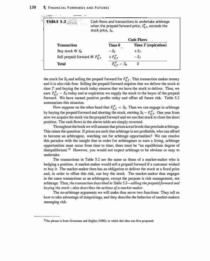
130 � F I N A N C I A L F O RWAR D S A N D FUTU R ES

Transaction

Buy stock @ So

Cash flows and transactions to undertake arbitrage when the prepaid forward price, Ft,p exceeds the stock price, 50 •

Cash Flows

Time 0 Time T (expiration)

-So +ST Sell prepaid forward @ F ri, T +F{,T -ST Total

the stock for So and selling the prepaid forward for F ,J T . This transaction makes money and it is also risk-free: Selling the prepaid forward requires that we deliver the stock at time T and buying the stock today ensures that we have the stock to deliver. Thus, we earn Fri,T - So today and at expiration we supply the stock to the buyer of the prepaid forward. We have earned positive profits today and offset all future risk. Table 5.2 summarizes this situation.

Now suppose on the other hand that Fri,T < So . Then we can engage in arbitrage by buying the prepaid forward and shorting the stock, earning So - F ri, T . One year from now we acquire the stock via the prepaid forward and we use that stock to close the short position. The cash flows in the above table are simply reversed.

Throughout the book we will assume that prices are at levels that preclude arbitrage. This raises the question: If prices are such that arbitrage is not profitable, who can afford to become an arbitrageur, watching out for arbitrage opportunities? We can resolve this paradox with the insight that in order for arbitrageurs to earn a living, arbitrage opportunities must occur from time to time; there must be "an equilibrium degree of disequilibrium."5 However, you would not expect arbitrage to be obvious or easy to undertake.

The transactions in Table 5.2 are the same as those of a market-maker who is hedging a position. A market-maker would sell a prepaid forward if a customer wished to buy it. The market-maker then has an obligation to deliver the stock at a fixed price and, in order to offset this risk, can buy the stock. The market-maker thus engages in the same transactions as an arbitrageur, except the purpose is risk management, not arbitrage. Thus, tlze transaction described in Table 5.2-selling the prepaid forward and buying the stock---also describes the actions of a market-make�:

The no-arbitrage arguments we will make thus serve two functions: They tell us how to take advantage of mispricings, and they describe the behavior of market-makers managing risk.

5The phrase is from Grossman and Stiglitz ( 1980), in which this idea was first proposed.

P R E PA I D F O RWA R D C O NTRA CTS O N STO C K � 13 1

Pricing Prepaid Forwards with Dividends

When a stock pays a dividend, the prepaid forward price is less than the stock price. The owner of stock receives dividends, but the owner of a prepaid forward contract does not. This difference creates a financial distinction between owning the stock and holding the prepaid forward. It is necessary to adjust the prepaid forward price to reflect dividends that are received by the shareholder, but not by the holder of the prepaid forward contract.

Discrete dividends To understand the effects of dividends, we will compare prepaid forwards on two stocks: Stock A pays no dividend, and otherwise identical stock B pays a $5 dividend 364 days from today, just before the expiration of the prepaid forwards. We know that the prepaid forward price for stock A is the current stock price. What is the prepaid forward price for stock B?

Since the $5 dividend is paid just before the delivery date for the stock 1 year from today, on the delivery date stock B will be priced $5 less than stock A. Thus, the price we pay today for stock B should be lower than that for stock A by the present value of $5.

In general, the price for a prepaid forward contract will be the stock price less the present value of dividends to be paid over the life of the contract. Suppose there are multiple dividend payments made throughout the life of the forward contract: A stock is expected to make dividend payments of D,, at times ti , i = 1 , . . . , n . A prepaid forward contract will entitle you to receive the stock at time T but without receiving the interim dividends. Thus, the prepaid forward price is

II

Fri,T = So - LPVo,r, (D,, ) (5 .3) i= l

where PVo.r, denotes the time 0 present value of a time ti payment.

Example 5.1 Suppose XYZ stock costs $ 1 00 today and is expected to pay a $ 1 .25 quarterly dividend, with the first coming 3 months from today and the last just prior to the delivery of the stock. Suppose the annual continuously compounded risk-free rate is 10%. The quarterly continuously compounded rate is therefore 2.5%. A 1 -year prepaid forward contract for the stock would cost

4

Fri,1 = $ 1 00 - L $ 1 .25e-0·025i = $95 .30 i= l

The calculation in this example implicitly assumes that the dividends are certain. Over a short horizon this might be reasonable. Over a long horizon we would expect dividend risk to be greater, and we would need to account for this in computing the present value of dividends.

132 � F I N A N C I A L F O RWA R D S A N D FUTU R E S

Continuous dividends For stock indexes containing many stocks, i t i s common to model the dividend as being paid continuously at a rate that is proportional to the level of the index; i.e., the dividend yield (the annualized dividend payment divided by the stock price) is constant. This is an approximation, but in a large stock index there can be dividend payments on a large proportion of days.6 The dividend yield is not likely to be fixed in the short run: When stock prices rise, the dividend yield falls, at least temporarily. Nevertheless, we will assume a constant proportional dividend yield for purposes of this discussion.

To model a continuous dividend, suppose that the index price is So and the an­nualized daily compounded dividend yield is 8. Then the dollar dividend over one day is

' 8 Daily dividend = 365 x So

Now suppose that we reinvest dividends in the index. Because of reinvestment, after T years we will have more shares than we started with. Using continuous compounding to approximate daily compounding, we get

Number of shares = ( 1 +

3:

5 r6SxT �

e"T

At the end of T years we have approximately eliT more shares than initially. Now suppose we wish to invest today in order to have one share at time T . We can

buy e-F.T shares today. Because of dividend reinvestment, at time T, we will have e"T more shares than we started with, -so we end up with exactly one share. Adjusting the initial quantity in this way in order to offset the effect of income from the asset is called tailing the position. Tailing enables us to offset the effect of continuous dividends. We will encounter the concept of tailing frequently.

Since an investment of e-F.T So gives us one share at time T, this is the time 0 prepaid forward price for delivery at time T :

I Fc{T = Soe-liT I (5 .4)

where 8 is the dividend yield and T the time to maturity of the prepaid forward contract.

Example 5.2 Suppose that the index is $ 125 and the annualized daily compounded dividend yield is 3%. The daily dollar dividend is

Dividend = (0.03 + 365) x $125 = $0.0 1027

6There is significant seasonality in dividend payments, which can be important in practice. A large number of U.S. firms pay quarterly dividends in February, May, August, and November. German firms,

by contrast, pay annual dividends concentrated in May, June, and July.

\).�1/lr Exe_r!=!s� PI'ice Options

· • Jri,�oine countries, including Australia and Switzerland, it is possible to buy stock options with very low strike prices-so low that it is virtually certain the option will expire in-the-money. For example, in Australia, the strike price is a penny. Such an option is called a low exercise price option (LEPO) . These often exist in order to avoid taxes or transaction fees associated with directly trading the stock. LEPOs do not pay dividends and do not carry voting rights. As with any call option, a LEPO is purchased outright, and entitles the option holder to acquire the stock at expiration by paying the (low) strike price. The payoff of a LEPO

F O RWA R D C O NTR ACTS O N STO C K � 133

expiring at !}me T is

max(O, ST - K) However, if the strike price, K, is so low

that the option is certain to be exercised, this is just

ST - K This option has a value at time 0 of

FciT - PV(K)

Since the strike price of the option is close to zero, a LEPO is essentially a prepaid forward contract.

or a little more than one penny per unit of the index. If we start by holding one unit of the index, at the end of 1 year we will have

e0·03 = 1 .030455

shares. Thus, if we wish to end the year holding one share, we must invest in

e-0-03 = 0.970446

shares. The prepaid forward price is

$ 1 25e-0·03 = $ 1 2 1 .306

5 .3 FORWARD CONTRACTS ON STOCK

Now that we have analyzed prepaid forward contracts, it is easy to derive forward prices. The only difference between the prepaid forward and the forward is the timing of the payment for the stock. Thus, the forward price is just the future value of the prepaid forward.

Here are forward prices for the cases we have considered:

No dividends: Taking the future value of equation (5 . 1 ) , for the time 0 forward price of a stock that is delivered at time T, we have

Fo, T = FV(Fci,T) = SoerT (5.5)

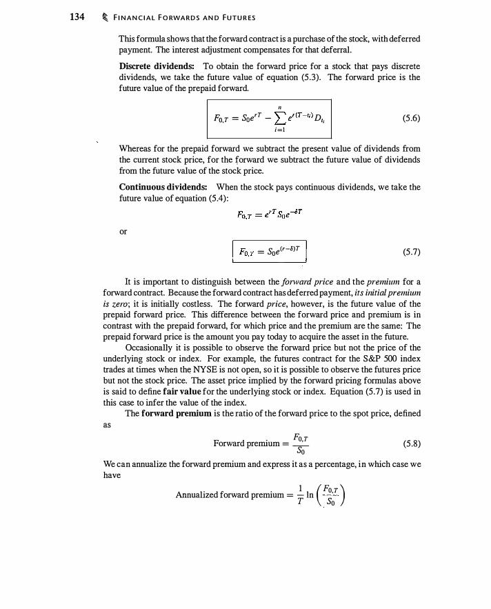
134 � F I N A N C I A L F O RWA R D S A N D FUTU R ES

This formula shows that the forward contract is a purchase of the stock, with deferred payment. The interest adjustment compensates for that deferral.

Discrete dividends: To obtain the forward price for a stock that pays discrete dividends, we take the future value of equation (5 .3) . The forward price is the future value of the prepaid forward.

II F. = s, erT - "'"" er (T-r, ) D . �T 0 � �

i = l (5 .6)

Whereas for the prepaid forward we subtract the present value of dividends from the current stock price, for the forward we subtract the future value of dividends from the future value of the stock price.

Continuous dividends: When the stock pays continuous dividends, we take the future value of equation (5 .4) :

or

D S e<r-8)T ro, T = 0 (5 .7)

It is important to distinguish between the fonvard price and the premium for a forward contract. Because the forward contract has deferred payment, its initial premium is zero; it is initially costless. The forward price, however, is the future value of the prepaid forward price. This difference between the forward price and premium is in contrast with the prepaid forward, for which price and the premium are the same: The prepaid forward price is the amount you pay today to acquire the asset in the future.

Occasionally it is possible to observe the forward price but not the price of the underlying stock or index. For example, the futures contract for the S&P 500 index trades at times when the NYSE is not open, so it is possible to observe the futures price but not the stock price. The asset price implied by the forward pricing formulas above is said to define fair value for the underlying stock or index. Equation (5 .7) is used in this case to infer the value of the index.

as The forward premium is the ratio of the forward price to the spot price, defined

. Fo,T Forward prelillum = -­So

(5 .8)

We can annualize the forward premium and express it as a percentage, in which case we have

Annualized forward premium = � In ( Fo,T ) T So

F O RWA R D CO N T RACTS O N STO C K � 135

For the case of continuous dividends, equation (5 .7), the annualized forward premium is simply the difference between the risk-free rate and the dividend yield.

Creating a Synthetic Forward Contract

A market-maker or arbitrageur must be able to offset the risk of a forward contract. It is possible to do this by creating a syllthetic forward contract to offset a position in the actual forward contract.

In this discussion we will assume that dividends are continuous and paid at the rate 8, and hence that equation (5 .7) is the appropriate forward price. We can then create a synthetic long forward contract by buying the stock and borrowing to fund the position. To see how the synthetic position works, recall that the payoff at expiration for a long forward position on the index is

Payoff at expiration = ST - Fo,T

In order to obtain this same payoff, we buy a tailed position in the stock, investing S0e-aT . This gives us one share at time T. We borrow this amount so that we are not required to pay anything additional at time 0. At time T we must repay S0e<r-li)T and we sell the stock for ST . Table 5 .3 demonstrates that borrowing to buy the stock replicates the expiration payoff to a forward contract.

Just as we can use the stock and borrowing to synthetically create a forward, we can also use the forward to create synthetic stocks and bonds . Table 5 .4 demonstrates that we can go long a forward contract and lend the present value of the forward price to · synthetically create the stock. The expiration payoff in this table assumes that equation (5 .7) holds. Table 5.5 demonstrates that if we buy the stock and short the forward, we create cash flows like those of a risk-free bond. The rate of return on this synthetic bond-the construction of which is summarized in Table 5.5-is called the implied

repo rate. To summarize, we have shown that

Transaction

Forward = Stock - zero-coupon bond (5 .9)

Demonstration that borrowing S0 e-H to buy e-sr shares of the index replicates the payoff to a forward contract, Sr - Fo,T·

Cash Flows

Buy e-aT units of the index Borrow Soe-liT

Time O

-So e-aT

+So e-aT

Time T (expiration)

+ST -Soe<r-li)T

Total 0

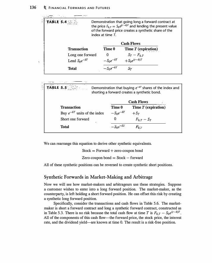
136 � F I N A N C I A L F O RWA R D S A N D F UTU R ES

Demonstration that going long a forward contract at the price Fo. r = S0ff.r -o)T and lending the present va lue of the forward price creates a synthetic share of the index at time T.

Cash Flows

Transaction

Long one forward Lend S0e-87

Time O

0 -Sae-8T

Time T (expiration)

Sy - Fa.T +Sae(r-8)T

Total

TAB L E 5 . 5 �- .

Transaction

Demonstration that buying e-H shares of the index and shorting a forward creates a synthetic bond.

Cash Flows

Time 0 Time T (expiration)

Buy e-8T units of the index Short one forward

-Sae-87 +ST 0 Fo,T - Sy

Total

We can rearrange this equation to derive other synthetic equivalents.

Stock = Forward + zero-coupon bond

Zero-coupon bond = Stock - forward

All of these synthetic positions can be reversed to create synthetic short positions.

Synthetic Forwards in Market-Making and Arbitrage

Now we will see how market-makers and arbitrageurs use these strategies. Suppose a customer wishes to enter into a long forward position. The market-maker, as the counterparty, is left holding a short forward position. He can offset this risk by creating a synthetic long forward position.

Specifically, consider the transactions and cash flows in Table 5.6. The market­maker is short a forward contract and long a synthetic forward contract, constructed as in Table 5.3 . There is no risk because the total cash flow at time T is Fa,T - S0e(r-8>7 . All of the components of this cash flow-the forward price, the stock price, the interest rate, and the dividend yield-are known at time 0. The result is a risk-free position.

Transaction

F O RWA R D C O NTRACTS O N STO C K � 137

Transactions and cash flows for a cash-and-carry: A market-maker is short a forward contract and long a synthetic forward contract.

Cash Flows

Buy tailed position in stock, paying S0e-8T

Borrow Soe-liT

Time O

-Soe-liT

+Soe-liT

Time T (expiration)

+Sr -Soe<r-li)T

Short forward

Total

Transaction

0 Fo.T - Sr

0 Fo,T - Soe<r-li)T

Transactions and cash flows for a reverse cash-and-carry: A market-maker is long a forward contract and short a synthetic forward contract.

Cash Flows

Time 0 Time T (expiration)

Short tailed position in stock, receiving S0e-liT

Lend S0e-liT +Soe-liT -Sy -Soe-liT +Soe<r-li)T

Long forward

Total

0 Sr - Fo,T

0 Soe<r-li)T - Fo,T

Similarly, suppose the market-maker wishes to hedge a long forward position. Then it is possible to reverse the positions in Table 5.6. The result is in Table 5.7.

A transaction in which you buy the underlying asset and short the offsetting forward contract is called a cash-and-carry. A cash-and-carry has no risk: You have an obligation to deliver the asset but also own the asset The market-maker offsets the short forward position with a cash-and-carry. An arbitrage that involves buying the underlying asset and selling it forward is called a cash-and-carry arbitrage. As you might guess, a reverse cash-and-carry entails short-selling the index and entering into a long forward position.

If the forward contract is priced according to equation (5 .7), then profits on a cash­and-carry are zero. We motivated the cash-and-carry in Table 5.6 as risk management by a market-maker. However, an arbitrageur might also engage in a cash-and-carry. If the forward price is too high relative to the stock price-i.e. , if Fo.T > S0e<r-li)T -then an arbitrageur or market-maker can use the strategy in Table 5 .6 to make a risk-free profit

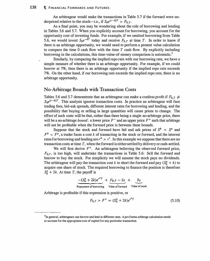
138 � F I N A N C I A L F O RWA R D S A N D FUTU R ES

An arbitrageur would make the transactions in Table 5 .7 if the forward were un­derpriced relative to the stock-i.e., if Soe(r-�)T > Fo, T ·

As a final point, you may be wondering about the role of borrowing and lending in Tables 5.6 and 5.7. When you explicitly account for borrowing, you account for the opportunity cost of investing funds. For example, if we omitted borrowing from Table 5 .6, we would invest S0e-�T today and receive Fo.T at time T. In order to know if there is an arbitrage opportunity, we would need to perform a present value calculation to compare the time 0 cash flow with the time T cash flow. By explicitly including borrowing in the calculations, this time-value-of-money comparison is automatic.?

Similarly, by comparing the implied repo rate with our borrowing rate, we have a simple measure of whether there is an arbitrage opportunity. For example, if we could borrow at 7%, then there is an arbjtrage opportunity if the implied repo rate exceeds 7%. On the other hand, if our borrowing rate exceeds the implied repo rate, there is no arbitrage opportunity.

·No-Arbitrage Bounds with Transaction Costs

Tables 5.6 and 5.7 demonstrate that an arbitrageur can make a costless profit if Fo, T :f. Soe(r-�)T . This analysis ignores transaction costs. In practice an arbitrageur will face trading fees, bid-ask spreads, different interest rates for borrowing and lending, and the possibility that buying or selling in large quantities will cause prices to change. The effect of such costs will be that, rather than there being a single no-arbitrage price, there will be a no-arbitrage bound : a lower price p- and an upper price p+ such that arbitrage will not be profitable when the forward price is between these bounds.

Suppose that the stock and forward have bid and ask prices of sb < sa and pb < pa , a trader faces a cost k of transacting in the stock or forward, and the interest rates for borrowing and lending are rb > r1 . In this example we suppose that there are no transaction costs at time T, when the forward is either settled by delivery or cash-settled.

We will first derive F+. An arbitrageur believing the observed forward price, Fo.T . is too high, will undertake the transactions in Table 5.6 : Sell the forward and borrow to buy the stock. For simplicity we will assume the stock pays no dividends. The arbitrageur will pay the transaction cost k to short the forward and pay (S0 + k) to acquire one share of stock. The required borrowing to finance the position is therefore S0 + 2k. At time T, the payoff is

Repayment of borrowing Value of forward Value of stock

Arbitrage is profitable if this expression is positive, or

Fo.r > p+ = (S0 + 2k)erbr

7In general, arbitrageurs can borrow and lend at different rates. A pro forma arbitrage calculation needs

to account for the appropriate cost of capital for any particular transaction.

(5 . 1 0)

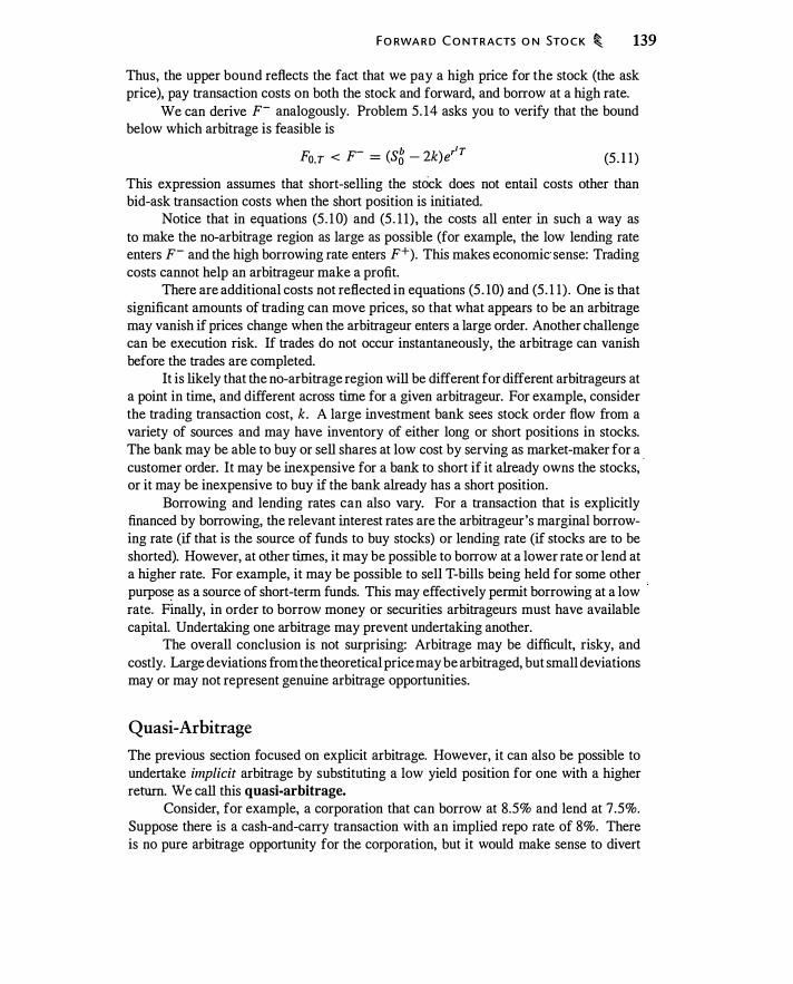
F O RWA R D C O NTRACTS O N STO C K � 139

Thus, the upper bound reflects the fact that we pay a high price for the stock (the ask price), pay transaction costs on both the stock and forward, and borrow at a high rate.

We can derive p- analogously. Problem 5. 14 asks you to verify that the bound below which arbitrage is feasible is

Fo,T < p- = cs8 - 2k)er'T (5 . 1 1 )

This expression assumes that short-selling the stock does not entail costs other than bid-ask transaction costs when the short position is initiated.

Notice that in equations (5 . 1 0) and (5 . 1 1) , the costs all enter in such a way as to make the no-arbitrage region as large as possible (for example, the low lending rate enters p- and the high borrowing rate enters F+). This makes economic sense: Trading costs cannot help an arbitrageur make a profit.

There are additional costs not reflected in equations (5 . 10) and (5 . 1 1 ) . One is that significant amounts of trading can move prices, so that what appears to be an arbitrage may vanish if prices change when the arbitrageur enters a large order. Another challenge can be execution risk. If trades do not occur instantaneously, the arbitrage can vanish before the trades are completed.

It is likely that the no-arbitrage region will be different for different arbitrageurs at a point in time, and different across time for a given arbitrageur. For example, consider the trading transaction cost, k. A large investment bank sees stock order flow from a variety of sources and may have inventory of either long or short positions in stocks. The bank may be able to buy or sell shares at low cost by serving as market-maker for a . customer order. It may be inexpensive for a bank to short if it already owns the stocks, or it may be inexpensive to buy if the bank already has a short position.

Borrowing and lending rates can also vary. For a transaction that is explicitly financed by borrowing, the relevant interest rates are the arbitrageur's marginal borrow­ing rate (if that is the source of funds to buy stocks) or lending rate (if stocks are to be shorted). However, at other times, it may be possible to borrow at a lower rate or lend at a higher rate. For example, it may be possible to sell T-bills being held for some other purpos� as a source of short-term funds. This may effectively permit borrowing at a low rate. Finally, in order to borrow money or securities arbitrageurs must have available capital. Undertaking one arbitrage may prevent undertaking another.

The overall conclusion is not surprising: Arbitrage may be difficult, risky, and costly. Large deviations from the theoretical price may be arbitraged, but small deviations may or may not represent genuine arbitrage opportunities.

Quasi-Arbitrage

The previous section focused on explicit arbitrage. However, it can also be possible to undertake implicit arbitrage by substituting a low yield position for one with a higher return. We call this quasi-arbitrage.

Consider, for example, a corporation that can borrow at 8.5% and lend at 7.5%. Suppose there is a cash-and-carry transaction with an implied repo rate of 8%. There is no pure arbitrage opportunity for the corporation, but it would make sense to divert

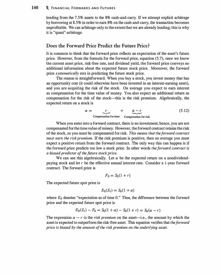
140 � F I N A N C I A L FO RWA R D S AN D F UTU R ES

lending from the 7.5% assets to the 8% cash-and-carry. If we attempt explicit arbitrage by borrowing at 8.5% in order to earn 8% on the cash-and-carry, the transaction becomes unprofitable. We can arbitrage only to the extent that we are already lending; this is why it is "quasi" -arbitrage.

Does the Forward Price Predict the Future Price?

It is common to think that the forward price reflects an expectation of the asset's future price. However, from the formula for the forward price, equation (5 .7), once we know the current asset price, risk-free rate, and dividend yield, the forward price conveys no additional information about the expected future stock price. Moreover, the forward price systematically errs in predicting the future stock price.

The reason is straightforward. When you buy a stock, you invest money that has an opportunity cost (it could otherwise have been invested in an interest-earning asset), and you are acquiring the risk of the stock. On average you expect to earn interest as ·compensation for the time value of money. You also expect an additional return as compensation for the risk of the stock-this is the risk premium. Algebraically, the expected return on a stock is

ct. = + ct. - r '-....-' Compensation for time Compensation for risk

(5 . 12)

When you enter into a forward contract, there is no investment; hence, you are not compensated for the time value of money. However, the forward contract retains the risk of the stock, so you must be compensated for risk. This means that the forward contract must eam the risk premium. If the risk premium is positive, then on average you must expect a positive return from the forward contract. The only way this can happen is if

the forward price predicts too low a stock price. In other words the forward contract is a biased predictor of the future stock price.

We can see this algebraically. Let a be the expected return on a nondividend­paying stock and let r be the effective annual interest rate. Consider a 1 -year forward contract. The forward price is

Fo = So ( l + r)

The expected future spot price is

Eo (S! ) = So ( l + ct.)

where Eo denotes "expectation as of time 0." Thus, the difference between the forward price and the expected future spot price is

Eo (SI ) - Fo = So ( 1 + a) - So ( 1 + r) = So (ct. - r)

The expression ct. - r is the risk premium on the asset-i.e., the amount by which the asset is expected to outperform the risk-free asset. This equation verifies that the f01ward price is biased by the amount of the risk premium on the underlying asset.

FO RWA R D C O NTRACTS O N STO C K � 141

For example, suppose that a stock index has an expected return of 15%, while the risk-free rate is 5%. If the current index price is 100, then on average we expect that the index will be 1 15 in 1 year. The forward price for delivery in 1 year will be only 1 05, however. This means that a holder of the forward contract will on average earn positive profits, albeit at the cost of bearing the risk of the index. 8

This bias does not imply that a forward contract is a good investment. Rather, it tells us that the risk premium on an asset can be created at zero cost and hence has a zero value. Though this seems surprising, it is a result from elementary finance that if we buy any asset and borrow the full amount of its cost-a transaction that requires no investment-then we earn the risk premium on the asset. Since a forward contract has the risk of a fully leveraged investment in the asset, it earns the risk premium. This proposition is true in general, not just for the example of a forward on a nondividend­paying stock.

An Interpretation of the Forward Pricing Formula

The forward pricing formula for a stock index, equation (5 .7), depends on r - 8, the difference between the risk-free rate and the dividend yield. This difference is called the cost of carry.

Suppose you buy a unit of the index that costs S and fund the position by borrowing at the risk-free rate. You will pay rS on the borrowed amount, but the dividend yield will provide offsetting income of 8S. You will have to pay the difference, (r - 8)S, on an ongoing basis. This difference is the net cost of carrying a long position in the asset;

.

hence, it is called the "cost of carry." Now suppose you were to short the index and invest the proceeds at the risk-free

rate. You would receive S for shorting the asset and earn r S on the invested proceeds, but you would have to pay 8S to the index lender. We will call 8 the lease rate of the index; it is what you would have to pay to a lender of the asset. The lease rate of an asset is the annualized cash payment that the borrower must make to the lender. For a nondiv�dend-paying stock, the lease rate is zero while for a dividend-paying stock, the lease rate is the dividend.

Here is an interpretation of the forward pricing formula:

Forward price = Spot price + futerest to carry the asset - Asset lease rate (5 . 1 3) Cost of carry

The forward contract, unlike the stock, requires no investment and makes no payouts and therefore has a zero cost of carry. One way to interpret the forward pricing formula is that, to the extent the forward contract saves our having to pay the cost of carry, we are willing to pay a higher price. This is what equation (5 . 13) says.

8 Accounting for dividends in this example would not change the magnitude of the bias since dividends

would lower the expected future price of the index and the forward price by equal amounts.

142 � F I N A N C I A L F O RWA R D S A N D FUTU R ES

5 .4 FUTURES CONTRACTS

Futures contracts are essentially exchange-traded forward contracts. As with forwards, futures contracts represent a commitment to buy or sell an underlying asset at some future date. Because futures are exchange-traded, they are standardized and have specified delivery dates, locations, and procedures. Futures may be traded either electronically or in trading pits, with buyers and sellers shouting orders to one another (this is called open outcry). Each exchange has an associated clearinghouse. The role of the clearinghouse is to match the buys and sells that take place during the day, and to keep track of !he obligations and payments required of the members of the clearinghouse, who are called clearing members. After matching trades, the clearinghouse typically becomes the counterparty for each clearing member.

Although forwards and futures are similar in many respects, there are differences.

• Whereas forward contracts are settled at expiration, futures contracts are settled daily. The determination of who owes what to whom is called marking-to-market. Frequent marking-to-market and settlement of a futures contract can lead to pricing differences between the futures and an otherwise identical forward.

• As a result of daily settlement, futures contracts are liquid-it is possible to offset an obligation on a given date by entering into the opposite position. For example, if you are long the September S&P 500 futures contract, you can cancel your obligation to buy by entering into an offsetting obligation to sell the September S&P 500 contract. If you use the same broker to buy and to sell, your obligation is officially cancelled.9

-

• Over-the-counter forward contracts can be customized to suit the buyer or seller, whereas futures contracts are standardized. For example, available futures con­tracts may permit delivery of 250 units of a particular index in March or June. A forward contract could specify April delivery of 300 units of the index.

• Because of daily settlement, the nature of credit risk is different with the futures contract. In fact, futures contracts are structured so as to minimize the effects of credit risk.

• There are typically daily price limits in futures markets (and on some stock ex­changes as well). A price limit is a move in the futures price that triggers a temporary halt in trading. For example, there is an initial S% limit on down moves in the S&P 500 futures contract. An offer to sell exceeding this limit can trigger a temporary trading halt, after which time a 10% price limit is in effect. If that is exceeded, there are subsequent 15% and 20% limits. The rules can be complicated, but it is important to be aware that such rules exist.

9 Although forward contracts may not be explicitly marketable, it is generally possible to enter into an offsetting position to cancel the obligation to buy or sell.

S i n g l e Stock Futu re s

Futures contracts on individual stocks in the United States began trading in November 2002 on OneChicago, an electronic exchange owned jointly by the Chicago Board Options Exchange, the Chicago Board of Trade, and the Chicago Mercantile Exchange. Earlier, the trading of single stock futures had been stalled by disagreements among exchanges and by a regulatory turf battle between the Securities and Exchange Commission, which regulates stocks and stock options, and the Commodity Futures Trading Commission, which regulates commodity and equity index futures.

Single stock futures were controversial even before trading began, with d�sagreement

F UTU R ES C O NTRACTS � 143

about how successful the product would be. What need would single stock futures serve? There was already a well-established market for buying and short -selling stocks, and we saw in Chapter 3 that investors could create synthetic stock forwards using options. Would differences in margin requirements, transaction costs, or contract characteristics make the new product successful?

Since 2002, one competitor to OneChicago (NQLX) has entered and then exited the market for single stock futures in the United States. Trading volume has proved disappointing for some advocates (see Zwick and Collins, 2004) .

We will illustrate futures contracts with the S&P 500 index futures contract as a specific example.

The S&P 500 Futures Contract

The S&P 500 futures contract has the S&P 500 stock index as the underlying asset. Futures on individual stocks have recently begun trading in the United States. See the box above. Figure 2. 1 shows a newspaper quotation for the S&P 500 index futures contract along "Yith other stock index futures contracts, and Figure 5. 1 shows its specifications. · The notional value, or size, of the contra�t is the dollar value of the assets underlying one contract. In this case it is by definition $250 X 1 300 = $325, 000. 10

The S&P 500 is an example of a cash-settled contract: Instead of settling by actual delivery of the underlying stocks, the contract calls for a cash payment that equals the profit or loss as if the contract were settled by delivery of the underlying asset. On the expiration day, the S&P 500 futures contract is marked-to-market against the actual cash index. This final settlement against the cash index guarantees that the futures price equals the index value at contract expiration.

1 0 Because the S&P 500 index is a fabricated number-a value-weighted average of individual stock prices-the S&P 500 index is treated as a pure number rather than a price and the contract is defined at maturity to have a size of $250 x S&P 500 index.

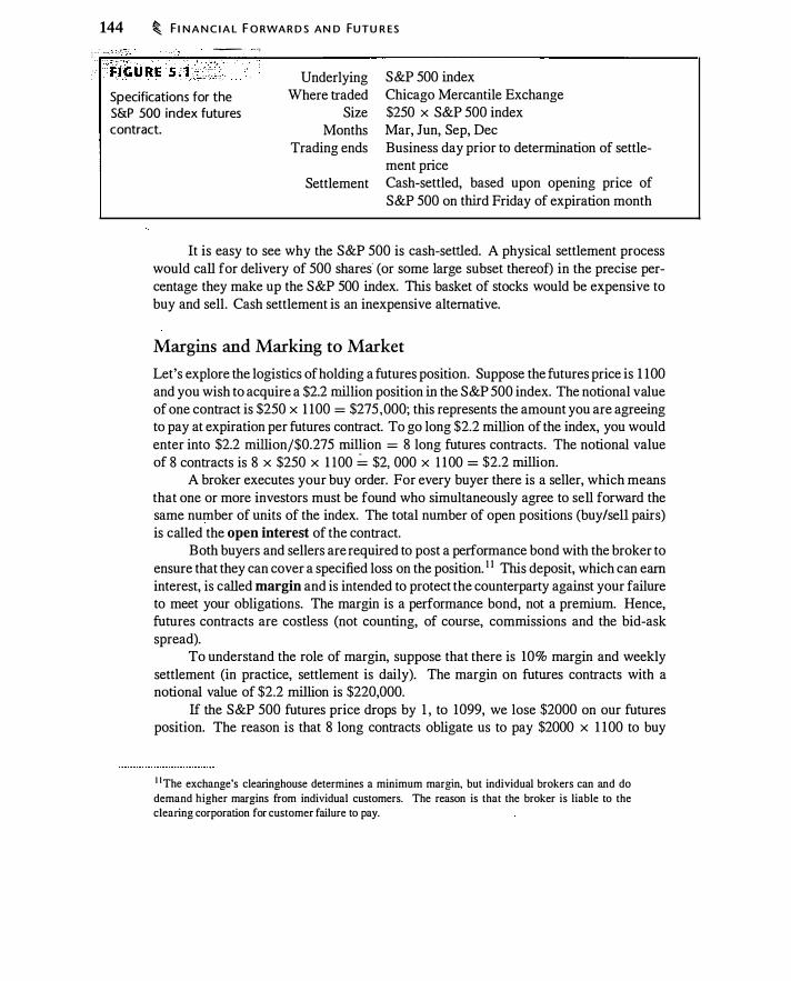
144 � F I N A N C I A L F O RWA R D S AN D FUTU R ES

c < c�· . . -- · ' "

Specifications for the S&P 500 index futures contract.

Underlying Where traded

Size Months

Trading ends

S&P 500 index Chicago Mercantile Exchange $250 x S&P 500 index Mar, Jun, Sep, Dec Business day prior to determination of settle-ment price

Settlement Cash-settled, based upon opening price of S&P 500 on third Friday of expiration month

It is easy to see why the S&P 500 is cash-settled. A physical settlement process would call for delivery of 500 shares- (or some large subset thereof) in the precise per­centage they make up the S&P 500 index. This basket of stocks would be expensive to buy and sell. Cash settlement is an inexpensive alternative.

Margins and Marking to Market

Let's explore the logistics of holding a futures position. Suppose the futures price is 1 100 and you wish to acquire a $2.2 million position in the S&P 500 index. The notional value of one contract is $250 x 1 100 = $275 ,000; this represents the amount you are agreeing to pay at expiration per futures contract. To go long $2.2 million of the index, you would enter into $2.2 millionj$0.275 million = 8 long futures contracts. The notional value of 8 contracts is 8 x $250 x 1 100 � $2, 000 x 1 100 = $2.2 million.

A broker executes your buy order. For every buyer there is a seller, which means that one or more investors must be found who simultaneously agree to sell forward the same number of units of the index. The total number of open positions (buy/sell pairs) is called the open interest of the contract.

Both buyers and sellers are required to post a performance bond with the broker to ensure that they can cover a specified loss on the position. 1 1 This deposit, which can earn interest, is called margin and is intended to protect the counterparty against your failure to meet your obligations. The margin is a performance bond, not a premium. Hence, futures contracts are costless (not counting, of course, commissions and the bid-ask spread).

To understand the role of margin, suppose that there is 10% margin and weekly settlement (in practice, settlement is daily). The margin on futures contracts with a notional value of $2.2 million is $220,000.

If the S&P 500 futures price drops by 1 , to 1099, we lose $2000 on our futures position. The reason is that 8 long contracts obligate us to pay $2000 x 1 100 to buy

1 1 The exchange's clearinghouse determines a minimum margin, but individual brokers can and do

demand higher margins from individual customers. The reason is that the broker is liable to the clearing corporation for customer failure to pay.

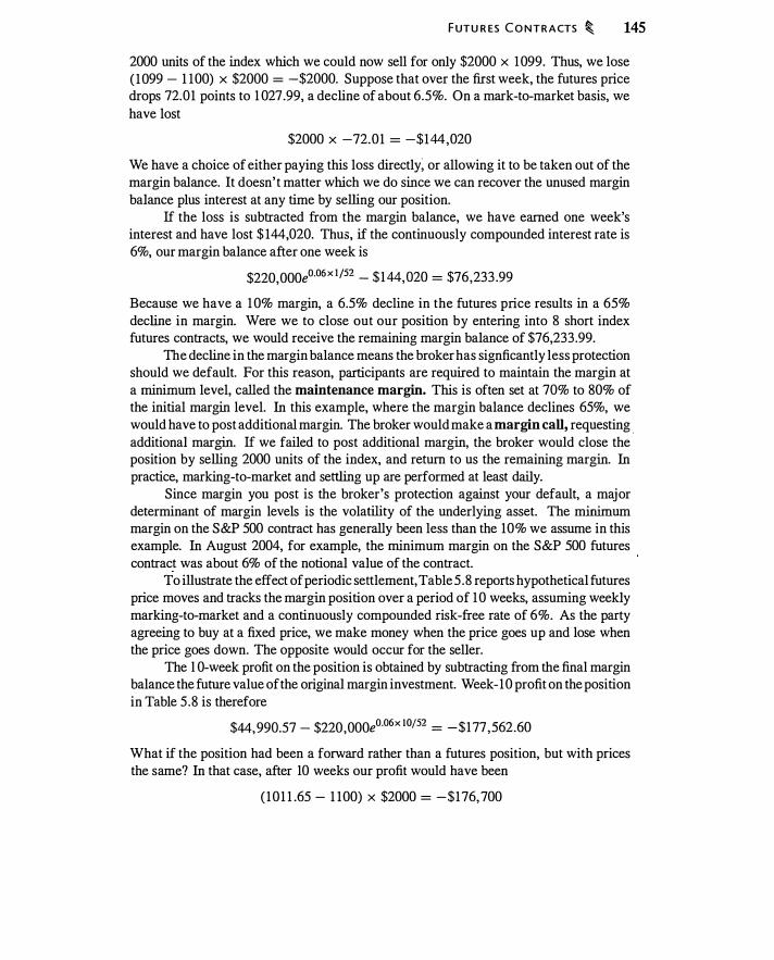
F UTU R ES C O NTRACTS � 145

2000 units of the index which we could now sell for only $2000 x 1099. Thus, we lose ( 1099 - 1 100) x $2000 = -$2000. Suppose that over the first week, the futures price drops 72.01 points to 1 027.99, a decline of about 6.5%. On a mark-to-market basis, we have lost

$2000 X -72.01 = -$144,020

We have a choice of either paying this loss directly; or allowing it to be taken out of the margin balance. It doesn' t matter which we do since we can recover the unused margin balance plus interest at any time by selling our position.

If the loss is subtracted from the margin balance, we have earned one week's interest and have lost $ 144,020. Thus, if the continuously compounded interest rate is 6%, our margin balance after one week is

$220,000e0·06x lfSZ - $144,020 = $76,233 .99

Because we have a 1 0% margin, a 6.5% decline in the futures price results in a 65% decline in margin. Were we to close out our position by entering into 8 short index futures contracts, we would receive the remaining margin balance of $76,233.99.

The decline in the margin balance means the broker has signficantly less protection should we default. For this reason, participants are required to maintain the margin at a minimum level, called the maintenance margin. This is often set at 70% to 80% of the initial margin level. In this example, where the margin balance declines 65%, we would have to post additional margin. The broker would make a margin call, requesting . additional margin. If we failed to post additional margin, the broker would close the position by selling 2000 units of the index, and return to us the remaining margin. In practice, marking-to-market and settling up are performed at least daily.

Since margin you post is the broker's protection against your default, a major determinant of margin levels is the volatility of the underlying asset. The minimum margin on the S&P 500 contract has generally been less than the 10% we assume in this example. In August 2004, for example, the minimum margin on the S&P 500 futures contract was about 6% of the notional value of the contract.

To illustrate the effect of periodic settlement, Table 5 .8 reports hypothetical futures price moves and tracks the margin position over a period of 10 weeks, assuming weekly marking-to-market and a continuously compounded risk-free rate of 6%. As the party agreeing to buy at a fixed price, we make money when the price goes up and lose when the price goes down. The opposite would occur for the seller.

The l 0-week profit on the position is obtained by subtracting from the final margin balance the future value of the original margin investment. Week-1 0 profit on the position in Table 5 .8 is therefore

$44,990.57 - $220,000e0·06x iOJSZ = -$177 ,562.60

What if the position had been a forward rather than a futures position, but with prices the same? In that case, after 10 weeks our profit would have been

( 10 1 1 .65 - 1 100) X $2000 = -$176, 700

146 � F I N A N C I A L F O RWAR D S A N D FUTU R ES

Week

0

2 3 4 5 6 7 8 9

10

Mark-to-market proceeds a n d margin balance over 1 0 weeks from long position in 8 S&P 500 futures contracts. The last column does not include additional margin payments. The final row represents expiration of the contract.

Futures Price Margin

Multiplier ($) Price Change Balance($)

2000.00 1 100.00 220,000.00 2000.00 1027.99 -72.0 1 76,233 .99 2000.00 1037.88 9 .89 96, 102.01 2000.00 1073.23 35.35 166,9 12 .96 2000.00 1048.78 -24.45 1 1 8,205.66 2000.00 1090.32 41 .54 201 ,422. 13 2000.00 1 106.94 16.62 234,894.67 2000.00 1 1 10.98 4.04 243,245.86 2000.00 1024.74 -86.24 7 1 ,046.69 2000.00 1007.30 -l7.44 36,248.72 2000.00 101 1 .65 4.35 44,990.57

Why do the futures and forward profits differ? The reason is that with the futures contract, interest is earned on the mark-to-market proceeds. Given the prices in Table 5.8, the loss is larger for futures than forwards because prices on average are below the initial price and we have to fund losses as they occur. With a forward, by contrast, losses are not funded until expiration. Earning interest on the daily settlement magnifies the gain or loss compared to that on a forward contract. Had there been consistent gains on the position in this example, the futures profit would have exceeded the forward profit. Appendix 5.B demonstrates that the ultimate payoff to a forward and futures contract can be equated in this example by adjusting the number of futures contracts so as to undo the magnifying effect of interest.

Comparing Futures and Forward Prices

An implication of Appendix 5 .B is that if the interest rate were not random, then forward and futures prices would be the same. However, what if the interest rate varies randomly? Suppose, for example, that on average the interest rate increases unexpectedly when the futures price increases; i.e., the two are positively correlated. Then the margin balance would grow (due to an increased futures price) just as the interest rate was higher. The margin balance would shrink as the interest rate was lower. · On average in this case, a long futures position would outperform a long forward contract.

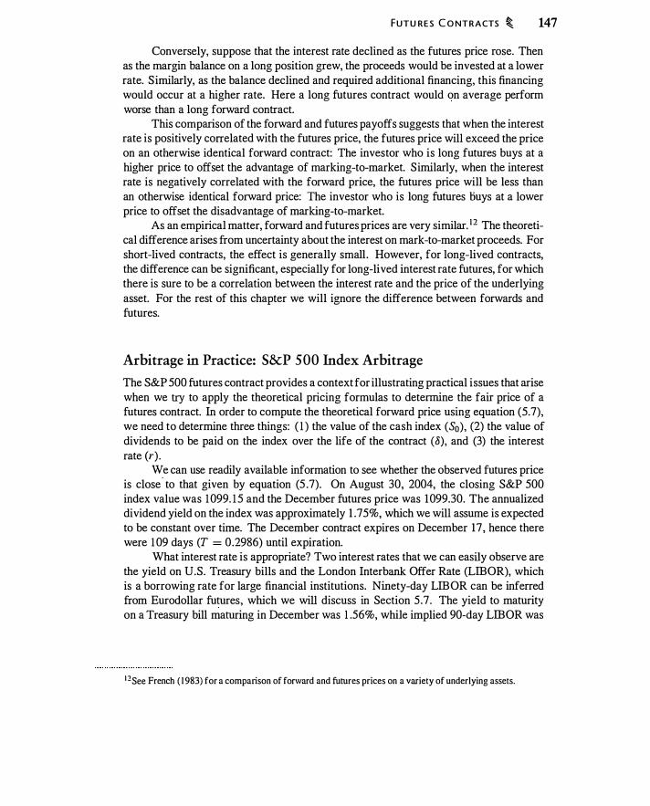
FUTU RES C O NTRACTS � 147

Conversely, suppose that the interest rate declined as the futures price rose. Then as the margin balance on a long position grew, the proceeds would be invested at a lower rate. S imilarly, as the balance declined and required additional financing, this financing would occur at a higher rate. Here a long futures contract would on average perform worse than a long forward contract.

This comparison of the forward and futures payoffs suggests that when the interest rate is positively correlated with the futures price, the futures price will exceed the price on an otherwise identical forward contract: The investor who is long futures buys at a higher price to offset the advantage of marking-to-market. Similarly, when the interest rate is negatively correlated with the forward price, the futures price will be less than an otherwise identical forward price: The investor who is long futures tiuys at a lower price to offset the disadvantage of marking-to-market.

As an empirical matter, forward and futures prices are very similar. 1 2 The theoreti­cal difference arises from uncertainty about the interest on mark-to-market proceeds. For short-lived contracts, the effect is generally small . However, for long-lived contracts, the difference can be significant, especially for long-lived interest rate futures, for which there is sure to be a correlation between the interest rate and the price of the underlying asset. For the rest of this chapter we will ignore the difference between forwards and futures.

Arbitrage in Practice: S&P 500 Index Arbitrage

The S&P 500 futures contract provides a context for illustrating practical issues that arise when we try to apply the theoretical pricing formulas to determine the fair price of a futures contract. In order to compute the theoretical forward price using equation (5.7), we need to determine three things: ( 1 ) the value of the cash index (S0), (2) the value of dividends to be paid on the index over the life of the contract (8), and (3) the interest rate (r) .

We can use readily available information to see whether the observed futures price is close

. to that given by equation (5 .7). On August 30, 2004, the closing S&P 500

index value was 1 099. 1 5 and the December futures price was 1099.30. The annualized dividend yield on the index was approximately 1 .75%, which we will assume is expected to be constant over time. The December contract expires on December 17, hence there were 1 09 days (T = 0.2986) until expiration.

What interest rate is appropriate? Two interest rates that we can easily observe are the yield on U.S. Treasury bills and the London Interbank Offer Rate (LIBOR), which is a borrowing rate for large financial institutions. Ninety-day LIBOR can be inferred from Eurodollar futures, which we will discuss in Section 5.7. The yield to maturity on a Treasury bill maturing in December was 1 .56%, while implied 90-day LIB OR was

1 2See French ( 1 983) for a comparison of forward and futures prices on a variety of underlying assets.

148 � F I N A N C I A L F O RWA R D S A N D F UT U R E S

1 .86% from September to December. Using the T-hill rate, 1 3 the theoretical futures price is

Soe<r-o)T = 1099 _ 1 5e(O.O I 56-0.0 I 75) x l 09/365 = 1098 _53

The theoretical price using LIB OR instead of the T-hill rate is Soe<r-o)T = 1099 . 1 5e(O.OI 86-0.0 I 75) x l 09/365 = 1 099_5 1

There are two theoretical prices, depending upon which interest rate we use; the actual December futures price, 1 099.30, is between these two prices. Does this mean that there is an arbitrage opportunity?

There are a number of considerations in interepreting these differences in prices :

• Future dividends on the S&P ·500 stocks are uncertain. For pricing a 3-month futures contract, one could use equation (5 .6), with actual recent cash dividends on the underlying stocks for D1, as proxies for forthcoming dividends. There is still a risk that dividends will change over the next 3 months. The risk is greater for longer-dated futures contracts.

• There are transaction costs of arbitrage. As illustrated by equations (5 . 1 0) and (5 . 1 1 ), transaction costs create no-arbitrage regions, rather than no-arbitrage prices. In practice, a representative bid-ask spread on the index futures contract might be 20 to 30 basis points (a basis point on the S&P futures contract is 0.0 1 ) and 0.25% to 0.5% on the stocks in the index when traded in significant quantities.

• Different interest rates will reflect differences in issuer credit risk. With margin requirements, daily settling up, and clearinghouse guarantees, the credit risk of a futures contract is not the same as that of either Treasury bills or LIBOR. In practice, LIBOR is frequently used to compute forward prices.

• Because of transaction costs, an arbitrageur will usually buy not the entire 500-stock index, but instead a subset of it. 14 The futures contract and the offsetting position in stocks may thus not move exactly together. When buying a large number of stocks, there is also execution risk-the possibility that prices move during the time between the order being placed and the stock being actually purchased.

1 3This example uses yields as if they were quoted as continuously compounded, which they are not. However, for short periods and low interest rates, there is almost no difference between effective annual

and continuously compounded rates. For example, if the effective annual rate is 2%, the continuously

compounded equivalent is ln ( l .02) = 0.0 1 98, or 1 .98%. In practice, interest rates are quoted using a

variety of arcane conventions for annualizing the rate.

14Another way to trade the cash index is with the use of Standard and Poor's Depository Receipts (SPDRs). These are unit investment trusts that are backed by a portfolio intended to mimic the S&P 500. Investors can convert units of 50,000 SPDR shares into the actual stock and can convert stock

into SPDRs. This keeps SPDRs close to the S&P 500 index, but in practice SPDRs may be mispriced relative to the cash S&P 500 just as futures are.

F UTU R ES C O NTRACTS � 149

Arbitrageurs will need to take into account these considerations. Ultimately, the only way to know if arbitrage is profitable is to assess specific prices, trading costs, and borrowing and lending rates.

Quanto Index Contracts

At first glance the Chicago Mercantile Exchange's Nikkei 225 futures contract-see a newspaper quotation in Figure 5 .2 and the details summarized in Figure 5 .3-is a stock index contract like the S&P 500 contract. However, there is one very important difference: Settlement of the contract is in a different currency (dollars) than the currency of denomination for the index (yen). 1 5

To see why this is important, consider a dollar-based investor wishing to invest in the Nikkei 225 cash index. This investor must undertake two transactions : changing dollars to yen and using yen to buy the index. When the position is sold, the investor reverses these transactions, selling the index and converting yen back to dollars. There are two sources of risk in this transaction: the risk of the index, denominated in yen, and the risk that the yen/dollar exchange rate will change. From Figure 5.3, the Nikkei 225

Listing for the Nikkei 225 futures contract from the Wall Street journal, ju ly 21 , 2004.

.. ' ' ·· FIGU RE 5 :_3 �:

Specifications for "the Nikkei 225 index futures contract.

UFETIME OPEN OPEPl HIGH LOW SETTLE CHG HIGH LOW INT

Nikkei 225 Stock Average (CME)·$5 x Index Sept llilO. ll370. 11220. 11365. 55 ll210. 9710. 31,205 Est vol 2,597; vol Mon 2,663; open lnt 31,302, -134. Index: Hl ll31814; Lo ill9l76; Close lll5837, -117.63.

Underlying Where traded

Size Months

Trading ends

Nikkei 225 Stock Index Chicago Mercantile Exchange $5 x Nikkei 225 Index Mar, Jun, Sep, Dec Business day prior to determination of settle-ment price

Settlement Cash-settled, based upon opening Osaka quo­tation of the Nikkei 225 index on the second Friday of expiration month

1 5There is also a yen-denominated Nikkei 225 futures contract that trades at the Osaka exchange. Since

it is purely yen-denominated, this contract is priced according to equation (5.7).

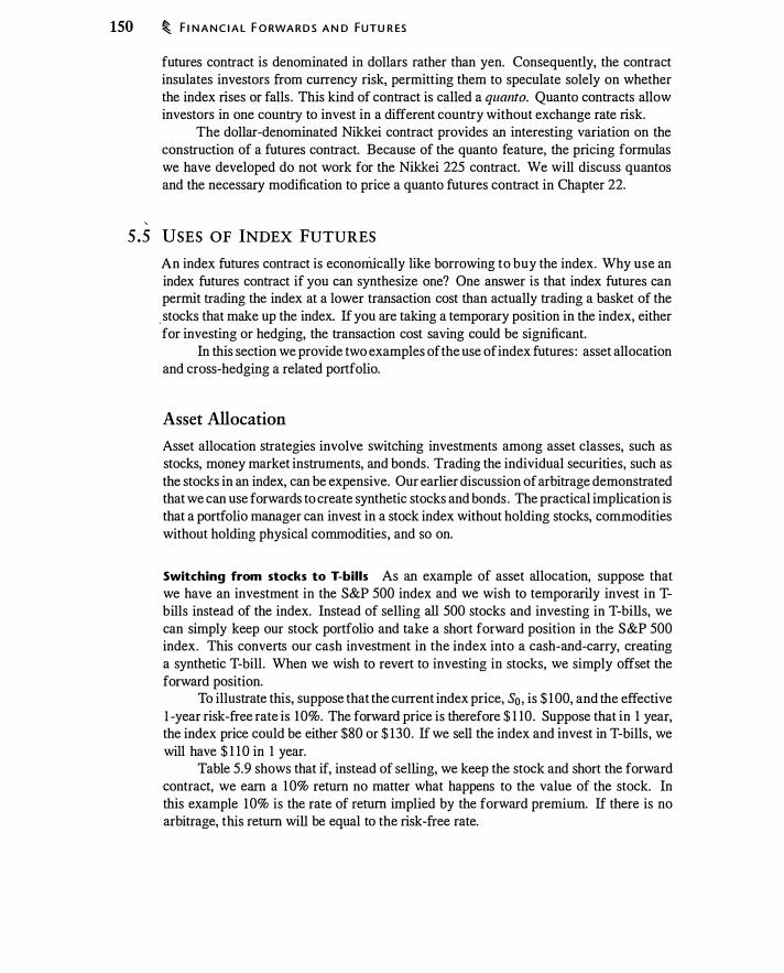
150 � F I N A N C I A L F O RWA R D S A N D FUTU R ES

futures contract is denominated in dollars rather than yen. Consequently, the contract insulates investors from currency risk, permitting them to speculate solely on whether the index rises or falls . This kind of contract is called a quanta. Quanta contracts allow investors in one country to invest in a different country without exchange rate risk.

The dollar-denominated Nikkei contract provides an interesting variation on the construction of a futures contract. Because of the quanta feature, the pricing formulas we have developed do not work for the Nikkei 225 contract. We will discuss quantos and the necessary modification to price a quanta futures contract in Chapter 22.

5.5 USES OF INDEX FUTURES

An index futures contract is econorriically like borrowing to buy the index. Why use an index futures contract if you can synthesize one? One answer is that index futures can permit trading the index at a lower transaction cost than actually trading a basket of the . stocks that make up the index. If you are taking a temporary position in the index, either for investing or hedging, the transaction cost saving could be significant.

In this section we provide two examples of the use of index futures : asset allocation and cross-hedging a related portfolio.

Asset Allocation

Asset allocation strategies involve switching investments among asset classes, such as stocks, money market instruments, and bonds. Trading the individual securities, such as the stocks in an index, can be expensive. Our earlier discussion of arbitrage demonstrated that we can use forwards to create synthetic stocks and bonds . The practical implication is that a portfolio manager can invest in a stock index without holding stocks, commodities without holding physical commodities, and so on.

Switching from stocks to T-bills As an example of asset allocation, suppose that we have an investment in the S&P 500 index and we wish to temporarily invest in T­bills instead of the index. Instead of selling all 500 stocks and investing in T-bills, we can simply keep our stock portfolio and take a short forward position in the S&P 500 index. This converts our cash investment in the index into a cash-and-carry, creating a synthetic T-hill. When we wish to revert to investing in stocks, we simply offset the forward position.

To illustrate this, suppose that the current index price, S0 , is $ 1 00, and the effective 1 -year risk-free rate is 10%. The forward price is therefore $ 1 10. Suppose that in 1 year, the index price could be either $80 or $ 130. If we sell the index and invest in T-bills , we will have $ 1 1 0 in 1 year.

Table 5.9 shows that if, instead of selling, we keep the stock and short the forward contract, we earn a 10% return no matter what happens to the value of the stock. In this example 10% is the rate of return implied by the forward premium. If there is no arbitrage, this return will be equal to the risk-free rate.

Transaction

Own stock @ $ 1 00

U S ES O F I N D EX FUTU R ES � 151

Effect of owning the stock and sel l ing forward, assuming that 50 = $1 00 and F0,1 = $1 1 0.

Cash Flows

Today 1 year, St = $80 1 year, S1 = $130 -$ 1 00 $80 $ 1 30

Short forward @ $ 1 1 0 0 $ 1 10 - $80 $ 1 10 - $ 1 30

Total -$ 100 $ 1 1 0 $ 1 1 0

General asset allocation We can use forwards and futures to perform even more sophisticated asset allocation. Suppose we wish to invest our portfolio in Treasury bonds (long-term Treasury obligations) instead of stocks . We can accomplish this reallocation with two forward positions: Shorting the forward S&P 500 index and going long the forward T-bond. The first transaction converts our portfolio from an index investment to a T-hill investment. The second transaction converts the portfolio from a T-hill investment to a T-bond investment. This use of futures to convert a position from one asset category (stocks) to another (bonds) is called a futures overlay.

Futures overlays can have benefits beyond reducing transaction costs. Suppose . an investment management company has portfolio managers who successfully invest in stocks they believe to be mispriced. The managers are judged on their performance relative to the S&P 500 stock index and consistently outperform the index by 2% per year (in the language of portfolio theory, their "alpha" is 2%). Now suppose that new clients of the company like the performance record, but want to invest in bonds rather than stocks. The investment management company could fire its stock managers and hire bond managers, but its existing investment managers are the reason for the company's success. The company can use a futures overlay to continue to invest in stocks, but to provide a bond return instead of a stock return to investors. By investing in stocks, shorting index futures, and going long bond futures, the managers continue to invest in stocks, but the client receives a bond return plus 2% rather than a stock return plus 2%. This use of futures to transform an outperforming portfolio on one asset class into an outperforming portfolio on a different asset class is called alpha-porting.

Cross-hedging with Index Futures

Index futures are often used to hedge portfolios that are not exactly the index. As discussed in Section 4.5, this is called cross-hedging.

Cross-hedging with perfect correlation Suppose that we have a portfolio that is not the S&P 500, and we wish to shift the portfolio into T-bills. Can we use the S&P 500 futures contract to do this? The answer depends on the correlation of the portfolio with

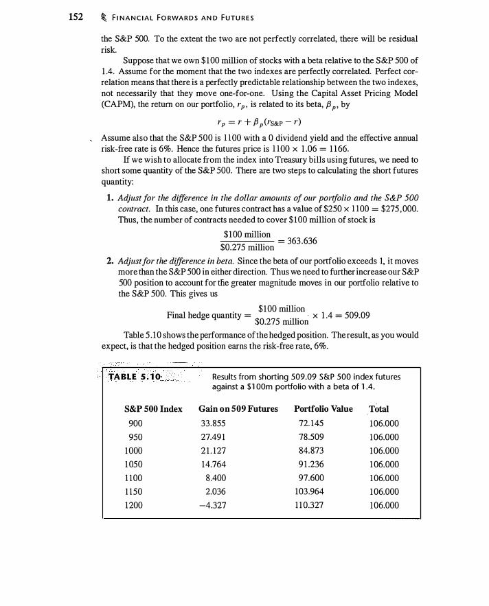
152 � F I N A N C I A L FO RWA R D S A N D F UTU R E S

. ··

the S&P 500. To the extent the two are not perfectly correlated, there will be residual risk.

Suppose that we own $ 100 million of stocks with a beta relative to the S&P 500 of 1 .4. Assume for the moment that the two indexes are perfectly correlated. Perfect cor­relation means that there is a perfectly predictable relationship between the two indexes, not necessarily that they move one-for-one. Using the Capital Asset Pricing Model (CAPM), the return on our portfolio, rp , is related to its beta, f3 P ' by

rp = r + f3 p (rs&P - r)

Assume also that the S&P 500 is l l OO with a 0 dividend yield and the effective annual risk-free rate is 6%. Hence the futures price is l l OO x 1 .06 = 1 1 66.

If we wish to allocate from the index into Treasury bills using futures, we need to short some quantity of the S&P 500. There are two steps to calculating the short futures quantity:

1. Adjust for the difference in the dollar amounts of our portfolio and the S&P 500 contract. In this case, one futures contract has a value of $250 x l l OO = $275 ,000. Thus, the number of contracts needed to cover $ 100 million of stock is

$ 100 million = 363 _636

$0.275 million 2. Adjust for the difference in beta. Since the beta of our portfolio exceeds I, it moves

more than the S&P 500 in either direction. Thus we need to further increase our S&P 500 position to account for tlie greater magnitude moves in our portfolio relative to the S&P 500. This gives us

$ 100 million Final hedge quantity =

$O mill" x 1 .4 = 509.09

.275 IOn Table 5 . 1 0 shows the performance of the hedged position. The result, as you would

expect, is that the hedged position earns the risk-free rate, 6%.

. . . .. . , . . . TABLE 5 : 1 0 ··• .. ·.

S&P 500 Index

900 950

1000 1 050 1 100 1 150 1200

Results from shorting 509.09 S&P 500 index futures against a $ 1 OOm portfolio with a beta of 1 .4 .

Gain on 509 Futures Portfolio Value Total

33.855 72. 145 106.000 27.49 1 78 .509 106.000 2 1 . 127 84.873 106.000 14.764 9 1 .236 1 06.000 8 .400 97.600 106.000 2.036 103 .964 106.000

-4.327 1 1 0.327 106.000

U S ES O F I N D EX F UTU R ES � 153

Cross-hedging with imperfect correlation The preceding example assumes that the portfolio and the S&P 500 index are perfectly correlated. In practice, correlations be­tween two portfolios can be substantially less than one. Using the S&P 500 to hedge such a portfolio would introduce basis risk, creating a hedge with residual risk. 1 6

Denote the return and invested dollars on the portfolio as rp and lp . Assume that we short H futures contracts, each with a notional value N. The futures position earns the risk premium, rs&P - r . Thus, the return on the hedged position is

Hedged return = rplp + H x N x (rs&P - r)

Repeating the analysis in Section 4.5 [in particular, see equation 4.2.J , the variance­minimizing hedge position, H*, is

H* =

=

_ lp Cov(rp , rs&P) N a�&P lp

- N f3p

(5 . 14)

The hedge quantity is denominated in terms of a quantity of futures contracts. The second equality follows because Cov(rp , rs&p)fa�&P is the slope coefficient when we regress the portfolio return on the S&P 500 return; i .e. , it is the portfolio beta with respect to the S&P 500 index. Equation (5 . 14) is also the formula we used in concluding that, with perfect correlation, we should short 509.09 contracts.

Notice that the hedge ratio in equation (5 . 14) depends on the ratio of the market value of the portfolio, I P • to the notional value of the S&P 500 contract, N. Thus, as the portfolio changes value relative to the S&P 500 index, it is necessary to change the hedge ratio. This rebalancing is necessary when we calculate hedge ratios using a relationship based on returns, which are percentage changes.

When we add H* futures to the portfolio, the variance of the hedged portfolio, ,

. ahedged • IS

, , , ( ' ) ahedged = a-pi-p 1 - p- (5 . 1 5)

where p is the correlation coefficient between the portfolio and the S&P 500 index. This is the same as equation (4.4) . The correlation coefficient, p, can be computed directly from rp and rs&P. but it is also the square root of the regression r-squared (R2) when we regress rp on rs&P in order to estimate {3 .

Example 5 .3 Suppose we are optimistic about the performance of the NASDAQ index relative to the S&P 500 index. We can go long the NASDAQ index and short

1 6There is additional basis risk in such a hedge because, for reasons discussed in Section 5.4, the S&P 500 futures contract and the cash price of the S&P 500 index may not move perfectly together.

154 � F I N A N C I A L F O RWA R D S A N D FUTU R ES

the S&P 500 futures. We obtain the variance-minimizing position in the S&P 500 by using equation (5 . 14) . A 5-year regression (from June 1 999 to June 2004) of the daily NASDAQ return on the S&P 500 return gives

I"NASD = -0.000 1 + 1 .4784 X (rs&P - r) (0.0003) (0.0262)

R2 = 0.7 1 88

The regression beta tells us to short a dollar value of the S&P that is 1 .4 784 times greater than the NASDAQ position we hold. The correlation coefficient between the two returns, p, is J0.7 1 88 = 0.8478. 1 7 The daily standard deviation of the return on the NASDAQ over this period is 2.24%. Hence, using equation (5 . 15), for a $ 1 million investment, the variance of the hedged position is

CJ�ASD/; ( 1 - p2) = 0.02242 X- ($ 1m)2 X ( 1 - 0.7 1 88) = ($ 1 1 , 878)2

Thus, the daily standard deviation of the hedged return is $ 1 1 ,878.

Risk management for stock-pickers An asset manager who picks stocks is often making a bet about the relative, but not the absolute, performance of a stock. For example, XYZ might be expected to outperform a broad range of stocks on a risk­adjusted basis. If the economy suffers a recession, however, XYZ will decline in value even if it outperforms other stocks. Index futures can be used in this case to help isolate the relative performance of XYZ.

Suppose the return of XYZ i_s given by the CAPM:

rxyz = axvz + r + fJxyz(r,. - r) (5 . 1 6)

The term axyz in this context represents the expected abnormal return on XYZ. If we use the S&P 500 as a proxy for the market, then we can select H according to equation (5 . 14). The result for the hedged position will be that, on average, we earn axvz + r . The risk of the position will be given by equation (5 . 1 5) . Since the correlation of an individual stock and the index will not be close to 1 , there will be considerable remaining risk. However, the portfolio will not have market risk.

5.6 CURRENCY CONTRACTS

Currency futures and forwards are widely used to hedge against changes in exchange rates. The pricing of currency contracts is a straightforward application of the principles we have already discussed. Newspaper listings for exchange-traded currency contracts are shown in Figure 5 .4.

Many corporations use currency futures and forwards for short-term hedging. An importer of consumer electronics, for example, may have an obligation to pay the manufacturer ¥150 million 90 days in the future. The dollar revenues from selling these

1 7You can, of course, also compute the correlation coefficient directly from the time series of returns.

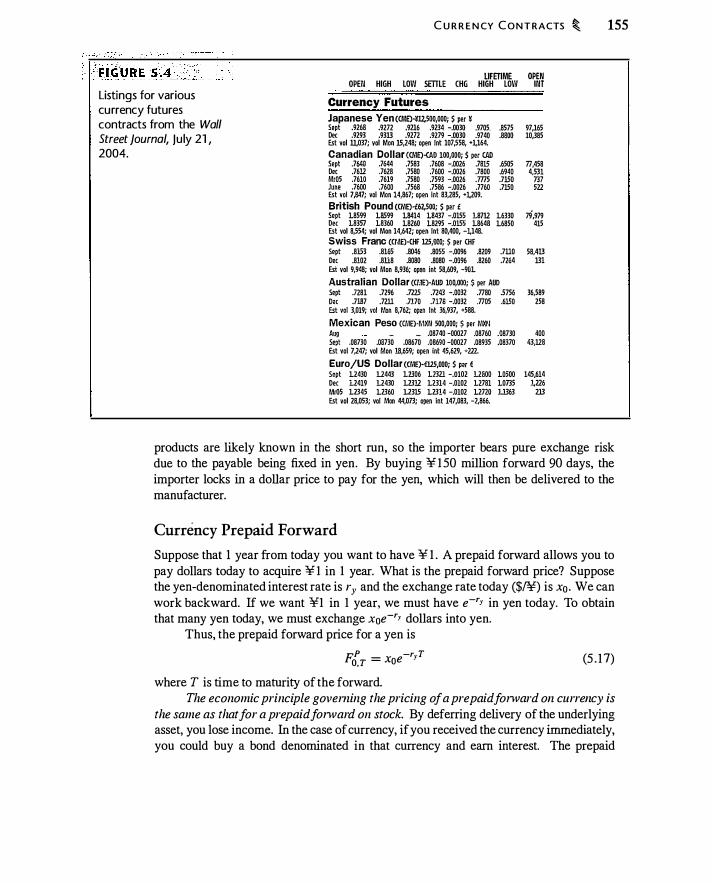
C U R R E N CY C O N T RACTS � 155

Listings for various currency futures contracts from the Wall Street journal, ju ly 21 ,

2004.

LIFETIME OPEN OPEN HIGH LOW SffiLE CHG HIGH LOW INT

Currency Futures Japanese Yen CCMEH12,50o,ooo; $ per ¥ Sept .9268 .9272 .9216 .9234 -.DOlO .9705. .8575 97,165 Dec .929l .9lll .9272 .9279 -.DOlO .9740 .8800 10,385 Est vol 11,037; vol Moo 15,248; open lot 107,558, •!,164.

Canadian Dollar ccMEHAD 1oo,ooo; $ per CAD Sept .7640 .7644 .758l .7608 -.0026 .7815 .6505 77.458 De< .76U .7628 .7580 .7600 -.0016 .7800 .6940 4,531 Mr05 .7610 .7619 .7580 .7593 -.0016 .m5 .7150 7J7 June .7600 .7600 .7568 .7586 -.0016 .7760 .7150 522 Est vol 7,847; vol Mon 14,867; open int 83,185, •!,109.

British Pound CCME>-£62,500; $ per t 79,979 Sept 18599 18599 18414 18437 -.0155 187l1 16330

Dec 18J57 18l60 18160 18295 -.0155 18648 16850 415 Est vol 8,554; vol Mon 14,641; open lnt 80,400, -!,148. Swiss Franc (ctdEHHF m,ooo; $ per CHF Sept .815J .8165 .8046 .8055 -.0096 .8209 .7110 58.413 Dec .8102 .8118 .8080 .8080 -.0096 .8160 .7164 lll Est vol 9,948; vol Mon 8,936; open int 58,609, -901

Australian Dollar (C/•1E>·AUD 1oo,ooo; $ per AUD Sept .7281 .7196 .7115 .7143 -.0031 .7780 5756 36,589 Dec .7187 .71ll .7170 .7178 -.0031 .7705 .6150 258 Est vol 3,019; vol Mon 8,761; open lnt 36,937, •588.

Mexican Peso (C/.IEH1XN soo,ooo; $ per MXtl Aug ·- - .08740 -00027 .08760 .08730 400 Se�t .08730 .08730 .08670 .08690 -00027 .08935 .08370 43,128 Est vol 7,247; vol Mon 18,659; opoo int 45,619, +222.

Euro/US Dollar <CME)-€!2S,OOO; $ P" € Sept 12430 1244l 12306 12321 -.0102 12800 10500 145,614 Dec 12419 12430 12312 12314 -.0102 12781 10735 1,226 Mr05 12345 12360 12315 12314 -.0102 1Z7ZO 11363 2ll Est vol 28.053; vol Moo 44,073; o�eo iot 147,083, -2,866.

products are likely known in the short run, so the importer bears pure exchange risk due to the payable being fixed in yen. By buying ¥ 1 50 million forward 90 days, the importer locks in a dollar price to pay for the yen, which will then be delivered to the manufacturer.

Currency Prepaid Forward

Suppose that 1 year from today you want to have ¥ 1 . A prepaid forward allows you to pay dollars today to acquire ¥ 1 in 1 year. What is the prepaid forward price? Suppose the yen-denominated interest rate is ry and the exchange rate today ($/¥) is x0 . We can work backward. If we want ¥1 in 1 year, we must have e-r,. in yen today. To obtain that many yen today, we must exchange x0e-r,. dollars into yen.

Thus, the prepaid forward price for a yen is F.P - X e-r,. T

O, T - 0 . (5 . 1 7)

where T is time to maturity of the forward. The economic principle governing the pricing of a prepaid forward on currency is

the same as that for a prepaid forward on stock. By deferring delivery of the underlying asset, you lose income. In the case of currency, if you received the currency immediately, you could buy a bond denominated in that currency and earn interest. The prepaid

156 � F I N A N C I A L F O RWA R D S A N D FUTU R ES

forward price reflects the loss of interest from deferring delivery, just as the prepaid forward price for stock reflects the loss of dividend income. This is why equation (5 . 17) is the same as that for a stock paying a continuous dividend, equation (5.4).

- Example 5.4 Suppose that the yen-denominated interest rate is 2% and that the current exchange rate is 0.009 dollars per yen. Then in order to have 1 yen in 1 year, we would invest today

Currency Forward

0.009$j¥ X ¥ 1 X e-0·01 = $.008822

The prepaid forward price is the dollar cost of obtaining 1 yen in the future. Thus, to obtain the forward price, compute the future value using the dollar-denominated interest rate, r :

Fo. T = xoe<r-r_.. )T (5 . 1 8)

The forward currency rate will exceed the current exchange rate when the domestic risk-free rate is higher than the foreign risk-free rate. 1 8

Example 5.5 Suppose that the yen-denominated interest rate is 2% and the dollar­denominated rate is 6%. The current exchange rate is 0.009 dollars per yen. The 1 -year forward rate is

0.009e0·06-0·02 = 0.009367

Notice that equation (5 . 1 8) is just like equation (5.7), for stock index futures, with the foreign interest rate equal to the dividend yield. The interest rate difference r - ry is the cost of carry for a foreign currency (we borrow at the domestic rate r and invest the proceeds in a foreign money-market instrument, earning the foreign rate ry as an offset to our cost) . If we wish to borrow foreign currency, ry is the lease rate.

Covered Interest Arbitrage

We can synthetically create a forward contract by borrowing in one currency and lending in the other. If we want to have 1 yen in the future, with the dollar price fixed today, we

1 80f course if you think about it , every currency transaction can be expressed in terms of either currency, for example as yen/dollar or dollar/yen. If the forward price exceeds the current exchange rate viewed

from the perspective of one currency, i t must be less from the perspective of the other.

C U R R E N CY C O N T RACTS � 157

can pay today for the yen, and borrow in dollars to do so. To have 1 yen in 1 year, we need to invest

xoe-r_.. T

in dollars, and we obtain this amount by borrowing. The required dollar repayment is

Xoe(r-r_.. )T

which is the forward exchange rate.

Example 5.6 Suppose that xo = 0.009, ry = 2%, and r = 6%. The dollar cost of buying 1 yen today is 0.009 x e-0·02 = 0.008822. We defer the dollar payment by borrowing at 6%, for a cost 1 year from today of 0 .008822e0·06 = 0.009367. This transaction is summarized in Table 5 . 1 1 . �

The example shows that borrowing in one currency and lending in another creates the same cash flow as a forward contract. If we offset this borrowing and lending position with an actual forward contract, the resulting transaction is called covered

interest arbitrage. To summarize, a forward exchange rate reflects the difference in interest rates

denominated in different currencies. Imagine that you want to invest $ 1 for 1 year. You can do so by buying a dollar-denominated bond, or you can exchange the dollar into another currency and buy a bond denominated in that other currency. You can then use currency forwards to guarantee the exchange rate at which you will convert the foreign currency back into dollars. The principle behind the pricing of currency forwards is that a position in foreign risk-free bonds, with the currency risk hedged, pays the same return as domestic risk-free bonds.

Synthetical ly creating a yen forward contract by borrowing in dol lars and lending in yen. The payoff at t ime 1 is ¥1 - $0.009 367.

Cash Flows

Year O Year l

Transaction $ ¥ $ ¥ Borrow x0e-r_.. dollar at 6% ($) +0.008822 -0.009367 Convert to yen @ 0.009 $/¥ -0.008822 +0.9802 Invest in yen-denominated bill (¥) -0.9802

Total 0 0 -0.009367

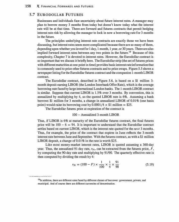
158 � F I N A N C I A L FO RWA R D S A N D FUTU R ES

5 .7 EURODOLLAR FUTURES

Businesses and individuals face uncertainty about future interest rates. A manager may plan to borrow money 3 months from today but doesn' t know today what the interest rate will be at that time. There are forward and futures contracts that permit hedging interest rate risk by allowing the manager to lock in now a borrowing rate for 3 months in the future.

The principles underlying interest rate contracts are exactly those we have been discussing, but interest rates seem more complicated because there are so many of them, depending upon whether you invest for 1 day, 1 month, 1 year, or 30 years. There are also ' implied forward interest rates between any two points in the future. 1 9 Because of this complexity, Chapter 7 is devoted to interest rates. However, the Eurodollar contract is so important that we discuss it briefly here. The Eurodollar strip (the set of futures prices with different maturities at one point in time) provides basic interest rate information that is commonly used to price other futures contracts and to price swaps. Figure 5 .5 shows a newspaper listing for the Eurodollar futures contract and the companion 1 -month LlliOR contract.

The Eurodollar contract, described in Figure 5 .6, is based on a $1 million 3-month deposit earning LlliOR (the London Interbank Offer Rate), which is the average borrowing rate faced by large international London banks. The 1 -month LlliOR contract is similar. Suppose that current LlliOR is 1 .5% over 3 months. By convention, this is annualized by multiplying by 4, so the quoted LlliOR rate is 6%. Assuming a bank borrows $1 million for 3 months, a change in annualized LlliOR of 0.0 1% (one basis point) would raise its borrowing cost by 0.000 1 /4 x $ 1 million = $25 .

The Eurodollar futures price at expiration of the contract is

100 - Annualized 3-month LlliOR

Thus, if LlliOR is 6% at maturity of the Eurodollar futures contract, the final futures price will be 1 00 - 6 = 94. It is important to understand that the Eurodollar contract settles based on current LlliOR, which is the interest rate quoted for the next 3 months. Thus, for example, the price of the contract that expires in June reflects the 3-month interest rate between June and September. With the futures contract, as with a $ 1 million LlliOR deposit, a change of 0.0 1 % in the rate is worth $25.

Like most money-market interest rates, LlliOR is quoted assuming a 360-day year. Thus, the annualized 9 1 -day rate, 1"9 1 . can be extracted from the futures price, F, by computing the 90-day rate and multiplying by 9 1/90. The quarterly effective rate is then computed by dividing the result by 4:

1 1 9 1 1"9 1 = ( 100 - F ) X - X - X -

100 4 90

1 9In addition, there are different rates faced by different classes of borrower: government, private, and municipal. And of course there are different currencies of denomination.

(5 . 19)

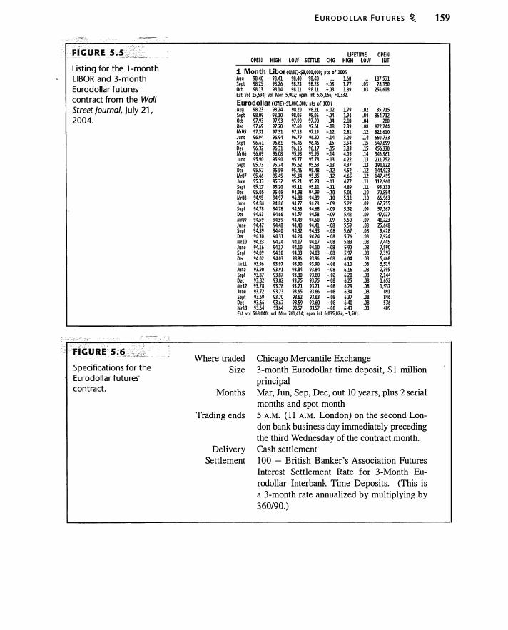
Listing for the 1 -month LIBOR and 3-month Eurodollar futures contract from the Wall Street journal, ju ly 21 , 2004.

FltuRI:• ·s .€- •- _: ___ _ Specifications for the Eurodollar futures· contract.

OPHJ HIGH LOW

E U R O D O LLA R FUTU R ES � 159

LIFETIME OPEN SETTLE CHG HIGH LOW INT 1. Month libor (CME)·$3,000,000; pts of IDO� Aug 98.40 98.41 98.40 98.40 -.o3 160 .o3 187,551 Sept 98.25 98.26 98.23 98.23 1n 28,150 Oct 98.13 98.14 95.11 98.11 -.03 189 .03 256,603 Est vol 15,694; vol Mon 5,902; open int 635,166, •1.332.

Eurodollar CCME)·$l.Ooo,ooo; pts of roo:. Aug 98.23 9814 9810 9811 -.02 179 .02 35,715 Sept 98.09 98.10 98.05 98.06 -.04 194 .04 864,7U Oct 97.93 97.93 97.90 97.90 -.04 Z.lO .04 280 Dec 97.69 97.70 97.60 97.61 -.08 2.39 .08 877,744 Mr05 9731 9731 97.18 97.19 -.12 2.81 .12 8Z2,610 June 96.94 96.94 96.79 96.80 -.14 310 .14 660,733 Sept 96.61 96.61· 96.46 96.46 -.15 3.54 .15 549,699 Dec 96.32 9631 96.16 96.17 -.15 3.83 .15 456,330 Mr06 96.09 96.08 95.93 95.95 -.14 4.05 .14 346,961 June 95.90 95.90 95.n 95.78 -.13 412 .13 Zl1,752 Sept 95.73 95.74 95.62 95.63 -.13 437 .13 191,822 Dec 9557 9559 95.46 95.48 -.12 452 .1Z 144,923 Mr07 95.46 95.45 9534 9535 -.12 4.65 .1Z 147,495 June 9533 9532 9511 95.23 -.11 4.n .11 :UZ.960 Sept 95.17 9510 95.11 95.11 -.11 4.89 .11 93,133 Dec 95.05 95.08 94.98 94.99 -.10 5.01 .10 70,854 Mr08 94.95 94.97 94.88 94.89 -.10 5.11 .10 66,963 June 94.84 94.86 94.n 94.78 -.09 512 .09 67,755 Sept 94.78 94.78 94.68 94.68 -.09 5.32 .09 57,367 D2C 94.63 94.66 94.57 9458 -.09 5.42 .09 47,027 Mr09 9459 9459 94.49 94.50 -.09 5.50 .09 41,223 June 94.47 94.48 94.40 94.41 -.08 559 .08 25,648 Sept 94.39 94.40 9432 9433 -.08 5.67 .08 9,428 Dec 9430 9431 9414 94.24 -.08 5.76 .08 7,924 MrlO 94.23 94.24 9411 94.17 -.08 5.83 .OS 7,445 June 94.16 94.17 94.10 94.10 -.08 5.90 .08 7,590 Sept 94.09 94.10 94.03 94.03 -.08 5.97 .08 7,397 Dec 94.02 94.03 93.96 93.96 -.08 6.04 .08 5,468 Mrll 93.96 93.97 93.90 93.90 -.08 6.10 .08 5,519 Jun• 93.90 93.91 93.84 93.84 -.08 6.16 .08 2.395 Sept 93.87 93.87 93.80 93.80 -.08 610 .08 2,144 Doc 93.82 93.82 93.75 93.75 -.08 615 .08 1,652 Mr12 93.78 93.78 93.71 93.71 -.08 619 .08 1,537 June 93.n 93.i3 93.65 93.66 -.08 634 .03 891 Sept 93.69 93.70 93.62 93.63 -.08 637 .OS 846 Dec 93.66 93.67 9359 93.60 -.08 6.40 .08 536 Mr13 93.64 93.64 93.57 93.57 -.08 6.43 .08 409 Est vol 568,040; vol t�on 761,414; open int 6,035,024, -1,501

Where traded Size

Months

Trading ends

Delivery Settlement

Chicago Mercantile Exchange 3-month Eurodollar time deposit, $ 1 million principal Mar, Jun, Sep, Dec, out 10 years, plus 2 serial months and spot month 5 A.M. ( 1 1 A.M. London) on the second Lon­don bank business day immediately preceding the third Wednesday of the contract month. Cash settlement 1 00 - British Banker's Association Futures Interest Settlement Rate for 3-Month Eu­rodollar Interbank Time Deposits. (This is a 3-month rate annualized by multiplying by 360/90.)

160 � F I N A N C I A L F O RWA R D S A N D F UTU R E S

Three-month Eurodollar contracts have maturities out to 1 0 years, which means that it is possible to use the contract to lock in a 3-month rate as far as 10 years in the future. The September 2007 futures price in Figure 5.5, for example, is 95. 1 1 . A position in this contract can be used to lock in an annualized rate of 4.89% from September 2007 to December 2007.

The Eurodollar contract can be used to hedge interest rate risk. For a borrower, for example, a short position in the contract is a hedge since it pays when the interest rate rises and requires payment when the interest rate falls. To see this, suppose that 7 months from today we plan to borrow $ 1 million for 90 days, and that our borrowing r:ate is the same as LIB OR. The Eurodollar futures price for 7 months from today is 94; this implies a 90-day rate of ( 100 - 94) x 90/360 x 1 / 1 00 = 1 .5%. Now suppose that 7 months hence, 3-month LIB OR is 8%, which implies a Eurodollar futures price of 92. The implied 90-day rate is 2%. Our extra borrowing expense over 90 days on $1 million will therefore be (0.02 - 0.0 1 5) x $ 1m = $5 ,000.

This extra borrowing expense is offset by gains on the short Eurodollar contract. The Eurodollar futures price has gone down, giving us a gain of $25 per basis point, or $25 x 100 x (94 - 92) = $5 ,000. The short position in the futures contract compensates us for the increase in our borrowing cost.20 In the same way, a long position can be used to lock in a lending rate.

The Eurodollar futures price is a construct, not the price of an asset. In this sense Eurodollar futures are different from the futures contracts we have already discussed. Although Eurodollar LIBOR is closely related to a number of other interest rates, there is no one specific identifiable asset that underlies the Eurodollar futures contract.

LIB OR is quoted in currencies other than dollars, and comparable rates are quoted in different locations. In addition to LIBOR, there are PIBOR (Paris), TIBOR (Tokyo), and Euribor (the European Banking Federation).

Finally, you might be wondering why we are discussing LIB OR rather than rates on Treasury bills. Business and bank borrowing rates move more in tandem with LIB OR than with the government's borrowing rate. Thus, these borrowers use the Eurodollar futures contract to hedge. LIBOR is also a better measure of the cost of funds for a market-maker, so LIB OR. is typically used to price forward contracts. We will further discuss Eurodollar futures in Chapter 7.

CHAPTER SUMMARY The purchase of a stock or other asset entails agreeing to a price, making payment, and taking delivery of the asset. A forward contract fixes the price today, but payment and

20It might occur to you that the Eurodollar contract pays us at the time we borrow, but we do not pay

interest until the loan matures, 9 1 days hence. Since we have time to earn interest on the change in the value of the contract, the hedge ratio should be less than I contract per $1 million borrowing. We discuss this complication in Chapter 7.

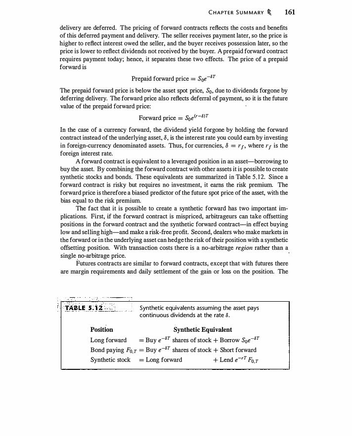
C H A PT E R S U M M A RY � 161

delivery are deferred. The pricing of forward contracts reflects the costs and benefits of this deferred payment and delivery. The seller receives payment later, so the price is higher to reflect interest owed the seller, and the buyer receives possession later, so the price is lower to reflect dividends not received by the buyer. A prepaid forward contract requires payment today; hence, it separates these two effects. The price of a prepaid forward is

Prepaid forward price = S0e -liT

The prepaid forward price is below the asset spot price, S0, due to dividends forgone by deferring delivery. The forward price also reflects deferral of payment, so it is the future value of the prepaid forward price:

Forward price = Soe<r-li)T

In the case of a currency forward, the dividend yield forgone by holding the forward contract instead of the underlying asset, 8 , is the interest rate you could earn by investing in foreign-currency denominated assets. Thus, for currencies, 8 = r1 , where r1 is the foreign interest rate.

A forward contract is equivalent to a leveraged position in an asset-borrowing to buy the asset. By combining the forward contract with other assets it is possible to create synthetic stocks and bonds. These equivalents are summarized in Table 5 . 1 2. Since a forward contract is risky but requires no investment, it earns the risk premium. The forward price is therefore a biased predictor of the future spot price of the asset, with the bias equal to the risk premium.

The fact that it is possible to create a synthetic forward has two important im­plications. First, if the forward contract is mispriced, arbitrageurs can take offsetting positions in the forward contract and the synthetic forward contract-in effect buying low and selling high-and make a risk-free profit. Second, dealers who make markets in the forward or in the underlying asset can hedge the risk of their position with a synthetic offsetting position. With transaction costs there is a no-arbitrage region rather than a single _no-arbitrage price.

Futures contracts are similar to forward contracts, except that with futures there are margin requirements and daily settlement of the gain or loss on the position. The

•· · · · · · · --· · ··· -

Position

Synthetic equivalents assuming the asset pays continuous dividends at the rate 8 .

Synthetic Equivalent

Long forward = Buy e-liT shares of stock + Borrow S0e-liT

Bond paying Fo,T = Buy e-liT shares of stock + Short forward Synthetic stock = Long forward + Lend e-rT Fo,T

162 � F I N A N C I A L F O RWA R D S AN D F UTU R E S

contractual differences between forwards and futures can lead to pricing differences, but in most cases forward prices and futures prices are very close.

In addition to hedging, forward and futures contracts can be used to synthetically switch a portfolio invested in stocks into bonds. A portfolio invested in Asset A can remain invested in Asset A but earn the returns associated with Asset B, as long as there are forward or futures contracts on A and B . This is called a futures overlay.

The Eurodollar futures contract, based on LIBOR (London Interbank Offer Rate) is widely used for hedging interest rate risk. Because the Eurodollar futures contract does not represent the price of an asset (at settlement it is 100 - LIBOR), it cannot be ,priced using the formulas in this chapter.

FURTHER READING Chapter 6 continues our exploration of forward markets by considering commodity forwards, which are different from financial forwards in important ways. Chapter 7 then examines interest rate forwards. Whereas forward contracts provide a price for delivery at one point in time, swaps, discussed in Chapter 8, provide a price for a series of deliveries over time. Swaps are a natural generalization of forward contracts.

The pricing principles discussed in this chapter will also play important roles when we discuss option pricing in Chapters 10, 1 1 , and 12 and financial engineering in Chap- . ter 15 .

To get a sense of the range of traded contracts, look at the futures page of the Wall Street Joumal, and also explore the-Web sites of futures exchanges: the Chicago Board of Trade (www.cbot.com), the Chicago Mercantile Exchange (www.cme.com), the New York Mercantile Exchange (www.nymex.com), and the London International Financial Futures Exchange (www.liffe.com), among others. These sites typically provide current prices, along with information about the contracts: What the underlying asset is, how the contracts are settled, and so forth. The site for One Chicago (www.

onechicago.com) provides information about single stock futures in the United States . . It is well accepted that forward prices are determined by the models and consider­

ations in this chapter. Siegel and Siegel ( 1990) is a standard reference book on futures. Early papers that examined futures pricing include Modest and Sundaresan ( 1983), Cor­nell and French ( 1983), which emphasized tax effects in futures pricing (see Appendix 5.A), and French ( 1 983), which compares forwards and futures when both exist on the same underlying asset. Brennan and Schwartz ( 1990) explore optimal arbitrage when there are transaction costs and Reinganum ( 1986) explores the arbitrage possibilities inherent in time travel. There is a more technical academic literature focusing on the difference between forward and futures contracts, including Black ( 1976a), Cox et al. ( 1 98 1 ) , Richard and Sundaresan ( 198 1 ), and Jarrow and Oldfield ( 1981 ) .

PROBLEMS 5.1. Construct Table 5.1 from the perspective of a seller, providing a descriptive name

for each of the transactions.

P R O B LE M S � 163

5.2. A $50 stock pays a $1 dividend every 3 months, with the first dividend coming 3 months from today. The continuously compounded risk-free rate is 6%.

a. What is the price of a prepaid forward contract that expires 1 year from today, immediately after the fourth-quarter dividend?

b. What is the price of a forward contract that expires at the same time?

5.3. A $50 stock pays an 8% continuous dividend. The continuously compounded risk-free rate is 6%.

a. What is the price of a prepaid forward contract that expires 1 year from today?

b. What is the price of a forward contract that expires at the same time?

5.4. Suppose the stock price is $35 and the continuously compounded interest rate is 5%.

a. What is the 6-month forward price, assuming dividends are zero? b. If the 6-month forward price is $35.50, what is the annualized forward

premium? c. If the forward price is $35 .50, what is the annualized continuous dividend

yield?

5.5. Suppose you are a market-maker in S&R index forward contracts. The S&R in� dex spot price is 1 100, the risk-free rate is 5%, and the dividend yield on the index is 0.

a. What is the no-arbitrage forward price for delivery in 9 months? b. Suppose a customer wishes to enter a short index futures position. If

you take the opposite position, demonstrate how you would hedge your resulting long position using the index and borrowing or lending.

c. Suppose a customer wishes to enter a long index futures position. If

you take the· opposite position, demonstrate how you would hedge your resulting short position using the index and borrowing or lending.

5.6. Repeat the previous problem, assuming that the dividend yield is 1 .5%.

5.7. The S&R index spot price is 1 100, the risk-free rate is 5%, and the dividend yield on the index is 0.

a. Suppose you observe a 6-month forward price of 1 1 35 . What arbitrage would you undertake?

b. Suppose you observe a 6-month forward price of 1 1 15 . What arbitrage would you undertake?

5.8. The S&R index spot price is 1 1 00, the risk-free rate is 5%, and the continuous dividend yield on the index is 2%.

164 � F I N A N C I A L F O RWA R D S A N D FUTU R ES

a. Suppose you observe a 6-month forward price of 1 120. What arbitrage would you undertake?

b. Suppose you observe a 6-month forward price of 1 1 10 . What arbitrage would you undertake?

5.9. Suppose that 1 0 years from now it becomes possible for money managers to engage in time travel. In particular, suppose that a money manager could travel to January 1 98 1 , when the 1 -year Treasury bill rate was 12.5%.

a. If time travel were costless, what riskless arbitrage strategy could a money manager undertake by traveling back and forth between January 198 1 and January 1982?

b. If many money managers undertook this strategy, what would you expect to happen to interest rates in 1 98 1 ?

c . Since interest rates were 12 .5% i n January 1 98 1 , what can you conclude about whether costless time travel will ever be possible?

5.10. The S&R index spot price is 1 100 and the continuously compounded risk-free rate is 5%. You observe a 9-month forward price of 1 129.257.

a. What dividend yield is implied by this forward price? b. Suppose you believe the dividend yield over the next 9 months will be

only 0.5%. What arbitrage would you undertake? c. Suppose you believe the dividend yield will be 3 % over the next 9 months.

What arbitrage would you undertake?

5.11. Suppose the S&P 500 index futures price is currently 1200. You wish to purchase four futures contracts on margin.

a. What is the notional value of your position? b. Assuming a 1 0% initial margin, what is the value of the initial margin?

5.12. Suppose the S&P 500 index is currently 950 and the initial margin is 1 0%. You wish to enter into 10 S&P 500 futures contracts.

a. What is the notional value of your position? What is the margin? b. Suppose you earn a continuously compounded rate of 6% on your margin

balance, your position is marked to market weekly, and the maintenance margin is 80% of the initial margin. What is the greatest S&P 500 index futures price 1 week from today at which will you receive a margin call?

5.13. Verify that going long a forward contract and lending the present value of the forward price creates a payoff of one share of stock when

a. The stock pays no dividends. b. The stock pays discrete dividends. c. The stock pays continuous dividends.

P RO B LE M S � 165

5.14. Verify that when there are transaction costs, the lower no-arbitrage bound is given by equation (5 . 1 1 ) .

5.15. Suppose the S&R index is 800, and that the dividend yield is 0. You are an arbitrageur with a continuously compounded borrowing rate of 5 .5% and a con­tinuously compounded lending rate of 5%.

a. Supposing that there are no transaction fees, show that a cash-and-carry arbitrage is not profitable if the forward price is less than 845.23, and that a reverse cash-and-carry arbitrage is not profitable if the forward price is greater than 841 .02.

b. Now suppose that there is a $1 transaction fee, paid at time 0, for going either long or short the forward contract. Show that the upper and lower no-arbitrage bounds now become 846.29 and 839.97.

c. Now suppose that in addition to the fee for the forward contract, there is also a $2.40 fee for buying or selling the index. Suppose the contract is settled by delivery of the index, so that this fee is paid only at time 0. What are the new upper and lower no-arbitrage bounds?

d. Make the same assumptions as in the previous part, except assume that the contract is cash-settled. This means that it is necessary to pay the stock index transaction fee (but not the forward fee) at both times 0 and 1 . What are the new no-arbitrage bounds?

e. Now suppose that transactions in the index have a fee of0.3% of the value of the index (this is for both purchases and sales) . Transactions in the forward contract still have a fixed fee of $ 1 per unit of the index at time 0. Suppose the contract is cash-settled so that when you do a cash-and­carry or reverse cash-and-carry you pay the index transaction fee both at time I and time 0. What are the new upper and lower no-arbitrage bounds? Compare your answer to that in the previous part. (Hint: To . handle the time I transaction fee, you may want to consider tailing the stock position.)

5.16. Suppose the S&P 500 currently has a level of 875. The continuously compounded return on a 1 -year T-bill is 4.75%. You wish to hedge an $800,000 portfolio that has a beta of 1 . 1 and a correlation of 1 .0 with the S&P 500.

a. What is the 1 -year futures price for the S&P 500 assuming no dividends? b. How many S&P 500 futures contracts should you short to hedge your

portfolio? What return do you expect on the hedged portfolio?

5.17. Suppose you are selecting a futures contract with which to hedge a portfolio. You have a choice of six contracts, each of which has the same variability, but with correlations of -0.95, -0. 75, -0.50, 0, 0.25 , and 0.85. Rank the futures contracts with respect to basis risk, from highest to lowest basis risk.

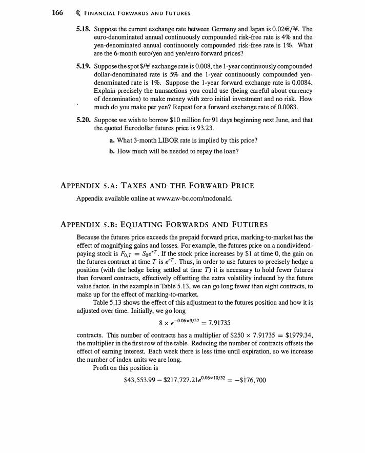
166 � F I N A N C I A L F O RWA R D S A N D FUTU R ES

5.18. Suppose the current exchange rate between Germany and Japan is 0.02€/¥. The euro-denominated annual continuously compounded risk-free rate is 4% and the yen-denominated annual continuously compounded risk-free rate is I %. What are the 6-month euro/yen and yen!euro forward prices?

5.19. Suppose the spot $/¥ exchange rate is 0.008, the I -year continuously compounded dollar-denominated rate is 5% and the I -year continuously compounded yen­denominated rate is I %. Suppose the 1 -year forward exchange rate is 0.0084. Explain precisely the transactions you could use (being careful about currency of denomination) to make money with zero initial investment and no risk. How much do you make per yen? Repeat for a forward exchange rate of 0.0083 .

5.20. Suppose we wish to borrow $ I O million for 9 I days beginning next June, and that the quoted Eurodollar futures price is 93.23.

a. What 3-month LIBOR rate is implied by this price?

b. How much will be needed to repay the loan?

APPENDIX S .A: TAXES AND THE FORWARD PRICE

Appendix available online at www.aw-bc.com/mcdonald.

APPENDIX S . B : EQUATING FORWARDS AND FUTURES

Because the futures price exceeds the prepaid forward price, marking-to-market has the effect of magnifying gains and losses. For example, the futures price on a nondividend­paying stock is Fo. T = S0e'T . If the stock price increases by $ I at time 0, the gain on the futures contract at time T is e'T . Thus, in order to use futures to precisely hedge a position (with the hedge being settled at time T) it is necessary to hold fewer futures than forward contracts, effectively offsetting the extra volatility induced by the future value factor. In the example in Table 5 . 1 3 , we can go long fewer than eight contracts, to make up for the effect of marking-to-market.

Table 5 . 1 3 shows the effect of this adjustment to the futures position and how it is adjusted over time. Initially, we go long

8 X e-0.06x9f52 = 7 . 9 1735

contracts. This number of contracts has a multiplier of $250 x 7 .9 I735 = $ 1979.34, the multiplier in the first row of the table. Reducing the number of contracts offsets the effect of earning interest. Each week there is less time until expiration, so we increase the number of index units we are long.

Profit on this position is

$43, 553.99 - $2 1 7,727 .2I e0·06x i Of52 = -$ i76 , 700

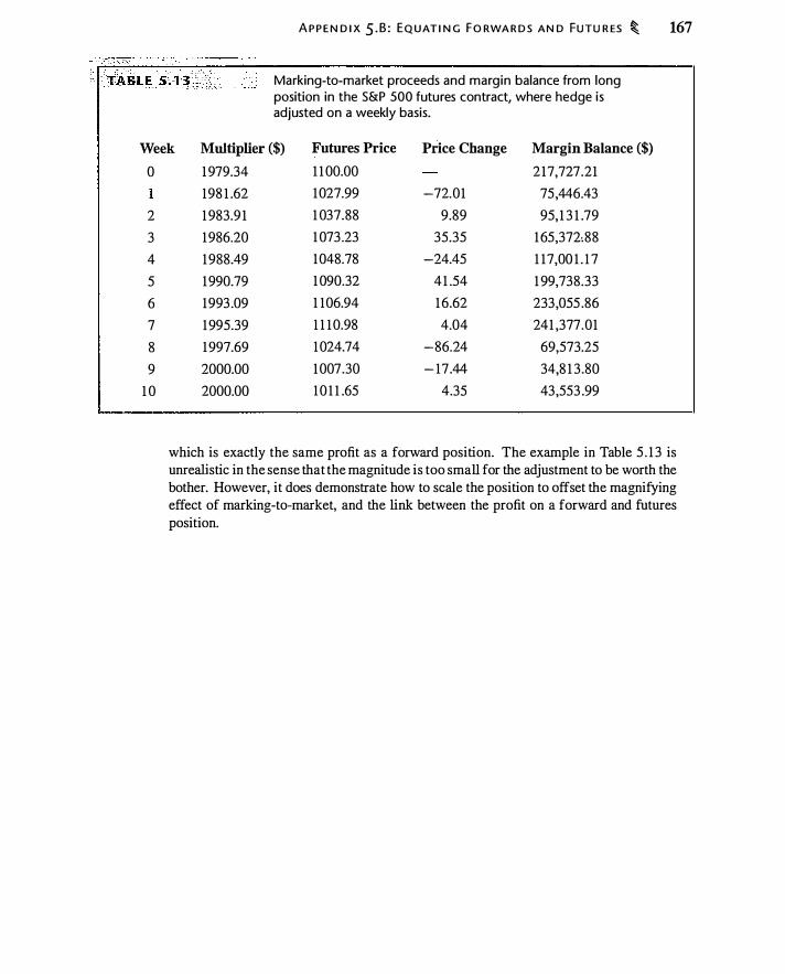
A P P E N D I X 5 . B : EQUAT I N G F O RWA R D S AN D FUTU R ES � 167

Marking-to-market proceeds and margin balance from long position in the S&P 500 futures contract, where hedge is adjusted on a weekly basis.

Week Multiplier ($) Futures Price Price Change Margin Balance ($) 0

2

3

4

5

6

7

8

9

1 0

1 979.34 1 1 00.00 2 17,727.21

198 1 .62 1027.99 -72.01 75,446.43

1 983.9 1 1 037.88 9.89 95, 1 3 1 .79

1986.20 1 073 .23 35.35 1 65,372:88

1988.49 1048.78 -24.45 1 17,00 1 . 1 7

1 990.79 1 090.32 41 .54 1 99,738.33

1993 .09 1 106.94 1 6.62 233,055 .86

1995.39 1 1 1 0.98 4.04 241 ,377 .01

1 997.69 1 024.74 -86.24 69,573.25

2000.00 1 007.30 - 17 .44 34,8 1 3 .80

2000.00 1 0 1 1 .65 4.35 43,553 .99

which is exactly the same profit as a forward position. The example in Table 5 . 1 3 is unrealistic in the sense that the magnitude is too small for the adjustment to be worth the bother. However, it does demonstrate how to scale the position to offset the magnifying effect of marking-to-market, and the link between the profit on a forward and futures position.

C�ER 6 -, ,·- - - -•- --.0c c(_ , •. >;," - - o -- . - -. • • o";:J;;,; - .,:,_.�_:_ · - . - ' " " · - c - - - -,."/"'""

Commodity Forwards and Futures

'IIMoy ob=ved that all happy families are all alike; each unhappy family ;, unhappy in its own way. An analogous idea in financial markets might be: Financial forwards are all alike; each commodity forward, however, has some unique economic characteristic that must be understood in order to appreciate forward pricing in that market. In this chapter we will see how commodity forwards and futures differ from, and are similar to, financial forwards and futures.

In our discussion of forward pricing for financial assets we relied heavily on the fact that for financial assets, the price of the asset today is the present value of the asset at time T, less the value of dividends to be received between now and time T. We will explore the extent to which this relationship also is true for commodities.

6.1 INTRODUCTION TO COMMODITY FORWARDS

Chapter 5 introduced the formula for a forward price on a financial asset:

Fo,T = Soe<r-o)T (6. 1 )

where So i s the spot price of the asset, r i s the continuously compounded interest rate, and o i.s the continuous dividend yield on the asset. The difference between the forward ·

price and spot price reflects the cost and benefits of delaying payment for, and receipt of, the asset. In Chapter 5 we treated forward and futures prices as the same; we continue to ignore the pricing differences in this chapter.

On any given day, for many commodities there are futures contracts available that expire in a number of different months. The set of prices for different expiration dates for a given commodity is called the forward curve or the forward strip for that date. Table 6. 1 displays futures prices with up to 6 months to maturity for several commodities. Let's consider these prices and try to interpret them using equation (6. 1 ) . To provide a reference interest rate, 3-month LIBOR on May 5, 2004, was 1 .22%, or about 0.3% for 3 months. From May to July, the forward price of corn rose from 3 14.25 to 3 19.75. This is a 2-month increase of 3 19 .75/3 14.25 - 1 = 1 .75%, an annual rate of approximately 1 1 %, far in excess of the 1 .22% annual interest rate. In the context of the formula for pricing financial forwards, equation (6. 1 ), we would need to have a continuous dividend yield, o, of -9. 19% in order to explain this rise in the forward price over time.

169

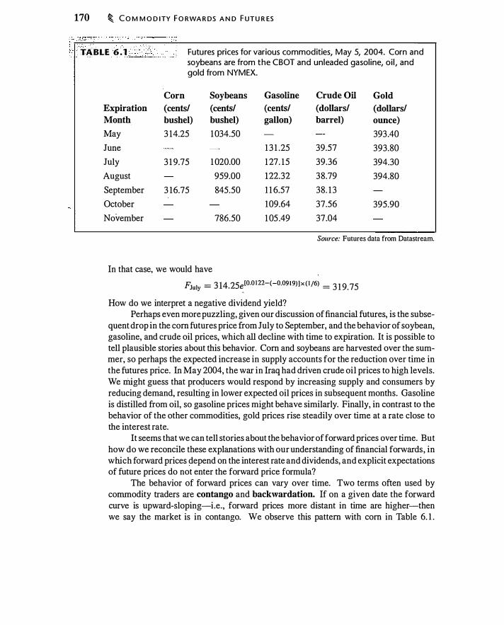
170 � CO M M O D ITY F O RWA R DS A N D F UTU R ES

1 T;(BLE 6 . 1 > , Futures prices for various commodities, May 5, 2004. Corn and soybeans are from the CBOT and unleaded gasoline, o i l , and gold from NYMEX.

Corn Soybeans Gasoline Crude Oil Gold

Expiration (cents/ (cents/ (cents/ (dollars/ (dollars/

Month bushel) bushel) gallon) barrel) ounce)

May 3 14.25 1 034.50 393 .40

June 1 3 1 .25 39.57 393.80

July 3 1 9.75 1 020.00 1 27. 15 39.36 394.30

August 959.00 122.32 38.79 394.80

September 3 16.75 845.50 1 1 6.57 38 . 1 3

October 109.64 37.56 395.90

November 786.50 1 05 .49 37.04

Source: Futures data from Datastream.

In that case, we would have

FJuly = 3 14.25�[0.0 122-(-0.09 1 9) ]x ( l /6) = 3 1 9.75

How do we interpret a negative dividend yield? Perhaps even more puzzling, given our discussion of financial futures, is the subse­

quent drop in the corn futures price from July to September, and the behavior of soybean, gasoline, and crude oil prices, which all decline with time to expiration. It is possible to tell plausible stories about this behavior. Corn and soybeans are harvested over the sum­mer, so perhaps the expected increase in supply accounts for the reduction over time in the futures price. In May 2004, the war in Iraq had driven crude oil prices to high levels. We might guess that producers would respond by increasing supply and consumers by reducing demand, resulting in lower expected oil prices in subsequent months. Gasoline is distilled from oil, so gasoline prices might behave similarly. Finally, in contrast to the behavior of the other commodities, gold prices rise steadily over time at a rate close to the interest rate.

It seems that we can tell stories about the behavior offorward prices over time. But how do we reconcile these explanations with our understanding of financial forwards, in which forward prices depend on the interest rate and dividends, and explicit expectations of future prices do not enter the forward price formula?

The behavior of forward prices can vary over time. Two terms often used by commodity traders are contango and backwardation. If on a given date the forward curve is upward-sloping-i.e., forward prices more distant in time are higher-then we say the market is in contango. We observe this pattern with corn in Table 6. 1 .

EQU I L I B R I U M P R I C I N G O F C O M M O D ITY F O RWA R D S � 171

If the forward curve is downward sloping, as with gasoline, we say the market is in backwardation. Forward curves can have portions in backwardation and portions in contango, as does that for crude oil.

It would take an entire book to cover commodities in depth. Our goal here is to understand the logic of forward pricing for commodities and where it differs from the logic of financial forward pricing. What is the forward curve telling us about the market for the commodity?

6.2 EQUILIBRIUM PRICING OF COMMODITY FORWARDS

As with forward prices on financial assets, commodity forward prices are the result of a present value calculation. To understand this, it is helpful to consider synthetic commodities.

Just as we could create a synthetic stock with a stock forward contract and a zero­coupon bond, we can also create a synthetic commodity by combining a forward contract with a zero-coupon bond. Consider the following investment strategy: Enter into a long commodity forward contract at the price Fo,T and buy a zero-coupon bond that pays Fo,T at time T. Since the forward contract is costless, the cost of this investment strategy at time 0 is just the cost of the bond, or

Time 0 cash flow = -e-rT F0 T At time T, the strategy pays

Sr - Fo,T '-...---' + Fo r ._;.....,

Forward contract payoff Bond payoff

= Sr

(6.2)

where Sr is the time T price of the commodity. This investment strategy creates a synthetic commodity, in that it has the same value as a unit of the commodity at time T. Note that, from equation (6.2), the cost of the synthetic commodity is the prepaid . forward price, e-rT Fo,T ·

Valuing a synthetic commodity is easy if we can see the forward price. Suppose, however, that we do not know the forward price. Computing the time 0 value of a unit of the commodity received at time T is a standard problem: You discount the expected commodity price to determine its value today. Let E0 (Sr) denote the expected time-T price as of time 0, and let a denote the appropriate discount rate for a time-T cash flow of Sr . Then the present value is

(6.3)

The important point is that expressions (6.2) and (6.3) represent the same value. Both reflect what you would pay today to receive one unit of the commodity at time T. Equating the two expressions, we have

e-rT Fo,T = Eo(Sr ) e-aT (6.4)

172 � C O M M O D ITY FO RWA R D S AN D F UTU R ES

Rearranging this equation, we can write the forward price as

Fo,T =e'T Eo (ST )e-aT

=Eo(ST )e(r-a)T (6.5)

Equation (6.5) demonstrates the link between the expected commodity price, E0(ST ) , and the forward price. As with financial forwards (see Chapter 5), the forward price i s a biased estimate of the expected spot price, Eo(ST ) , with the bias due to the risk premium on the commodity, a - r. 1

Equation 6.4 deserves emphasis: The time-T forward price discounted at the risk-, free rate back to time 0 is the present value of a unit of commodity received at time T .

This calculation i s useful when performing NPV calculations involving commodities for which forward prices are available. Thus, for example, an industrial producer who buys oil can calculate the present value of future oil costs by discounting oil forward prices at the risk-free rate. The present value of future oil costs is not dependent upon whether or not the producer hedges. We will see an example of this calculation later in the chapter.

If a commodity cannot be physically stored, the no-arbitrage pricing principles discussed in Section 5.2 cannot be used to obtain a forward price. Without storage, equation (6.5) determines the forward price. However, it is difficult to implement this formula, which requires forecasting the expected future spot price and estimating a . Moreover, even when physically possible, storage may be costly. Given the difficulties of pricing commodity forwards, our goal will be to _interpret forward prices and to understand the economics of different commodity markets.

In the rest of the chapter, we will further explore similarities and differences between forward prices for commodities and financial assets . Some of the most important differences have to do with storage: whether the commodity can be stored and, if so, how costly it is to store. The next section provides an example of forward prices when a commodity cannot be stored.

6.3 NONSTORABILITY: ELECTRICITY

The forward market for electricity illustrates forward pricing when storage is not possible. Electricity is produced in different ways: from fuels such as coal and natural gas, or from nuclear power, hydroelectric power, wind power, or solar power. Once it is produced, electricity is transmitted over the power grid to end-users. Electricity has characteristics

1 Historical commodity and futures data, necessary to estimate expected commodity returns, are rel­atively hard to obtain. Bodie and Rosansh.-y ( 1 980) examine quarterly futures returns from 1950 to

1 976, while Gorton and Rouwenhorst (2004) examine monthly futures returns from 1959 to 2004.

Both studies construct portfolios of synthetic commodities-T-bills plus commodity futures-and find that these portfolios earn the same average return as stocks, are on average negatively correlated with

stocks, and are positively correlated with inflation. These findings imply that a portfolio of stocks

and synthetic commodities would have the same expected return and less risk than a diversified stock

portfolio alone.

N O N STO R A B I L I TY : E l E CT R I C ITY � 173

·� � � �··· . TABLE 6.2 �--�-..c·----" Day-ahead price, by hour, for 1 megawatt-hour of electricity in New York City, September 7, 2004.

Time Price Time Price Time Price Time Price

0000 $35.68 0600 $40.03 1200 $6 1 .46 1 800 $57.8 1

0 100 $3 1 .59 0700 $49.64 1300 $6 1 .47 1900 $62. 18

0200 $29.85 0800 $53.48 1400 $6 1 .74 2000 $60. 12

0300 $28.37 0900 $57. 15 1500 $62.7 1 2 100 $54.25

0400 $28.75 1000 $59.04 1600 $62.68 2200 $52.89

0500 $33 .57 1 1 00 $6 1 .45 1700 $60.28 2300 $45 .56

Source: Bloomberg.

that distinguish it not only from financial assets, but from other commodities as well. What is special about electricity?

First, electricity is difficult to store, hence it must be consumed when it is produced or else it is wasted.2 Second, at any point in time the maximum supply of electricity is fixed. You can produce less but not more. Third, demand for electricity varies substantially by season, by day of week, and by time of day.

To illustrate the effects of nonstorability, Table 6.2 displays 1 -day ahead hourly prices for 1 megawatt-hour of electricity in New York City. The 1 -day ahead forward price is $28.37 at 3 A.M., and $62.7 1 at 3 P.M. Since you have learned about arbitrage, you are possibly thinking that you would like to buy electricity at the 3 A.M. price and sell it at the 3 P.M. price. However, there is no way to do so. Because electricity cannot be stored, its price is set by demand and supply at a point in time. There is also no way to buy winter electricity and sell it in the summer, so there are seasonal variations as well as intraday variations . Because of peak-load plants that operate only when prices are high, power suppliers are able to temporarily increase the supply of electricity. However, expectations about supply are already reflected in the forward price.

Given these characteristics of electricity, what does the electricity forward price represent? The prices in Table 6.2 are best interpreted using equation (6.5) . The large price swings over the day primarily reflect changes in the expected spot price, which in tum reflects changes in demand over the day.

Notice two things. First, the swings in Table 6.2 could not occur with financial assets, which are stored. (It is so obvious that financial assets are stored that we usually don't mention it.) As a consequence, the 3 A.M. and 3 P.M. forward prices for a stock . '

2There are ways to store electricity. For example, it is possible to use excess electricity to pump water uphill and then, at a later time, release it to generate electricity. Storage is uncommon, expensive, and

entails losses, however.

174 � C O M M O D ITY F O RWA R D S A N D FUTU R ES

will be almost identical . If they were not, it would be possible to engage in arbitrage, buying low at 3 A.M. and selling high at 3 P.M. Second, whereas the forward price for a stock is largely redundant in the sense that it reflects information about the current stock price, interest, and the dividend yield, the forward prices in Table 6.2 provide information we could not otherwise obtain, revealing information about the future price of the commodity. This illustrates the forward market providing price discovery, with forward prices revealing information, not otherwise obtainable, about the future price of the commodity.

6.4 PRICING COMMODITY FORWARDS BY ARBITRAGE: . AN EXAMPLE

Electricity repre�>ents the extreme of nonstorability. However, many commodities are storable. To see the effects of storage, we now consider the very simple, hypothetical example of a forward contract for pencils. We use pencils as an example because they are familiar and you will have no preconceptions about how such a forward should work, because it does not exist.

Suppose that pencils cost $0.20 today and for certain will cost $0.20 in 1 year. The economics of this assumption are simple. Pencil manufacturers produce pencils from wood and other inputs. If the price of a pencil is greater than the cost of production, more pencils are produced, driving down the market price. If the price falls, fewer pencils are produced and the price rises. The market price of pencils thus reflects the cost of production. An economist would say that the supply of pencils is pelfectly elastic.

There is nothing inherently inconsistent about assuming that the pencil price is expected to stay the same. However, before we proceed, note that a constant price would not be a reasonable assumption about the price of a nondividend-paying stock. A nondividend-paying stock must be expected to appreciate, or else no one would own it. At the outset, there is an obvious difference between this commodity and a financial asset.

One way to describe this difference between the pencil and the stock is to say that, in equilibrium, stocks and other financial assets must be held by investors, or stored. This is why the stock price appreciates on average; appreciation is necessary for investors to willingly store the stock.

The pencil, by contrast, need not be stored. The equilibrium condition for pencils requires that price equals marginal production cost. This distinction between a storage and production equilibrium is a central concept in our discussion of comrnmodities.3

3You may be thinking that you have pencils in your desk and therefore you do, in fact, store pencils.

However, you are storing them to save yourself the inconvenience of going to the store each time you need a new one, not because you expect pencils to be a good financial investment akin to stock. When storing pencils for convenience, you will store only a few at a time. Thus, for the moment, suppose

that no one stores pencils. We return to the concept of storing for convenience in Section 6.6.

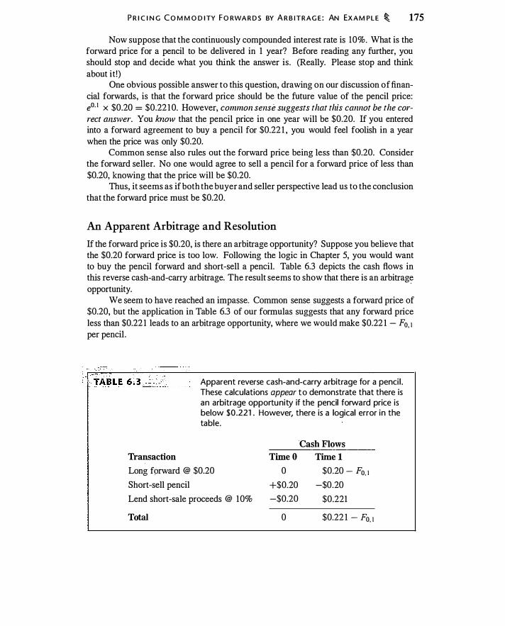
P R I C I N G C O M M O D I TY F O RWA R D S BY A R B ITRAG E : AN EXA M P L E � 175

Now suppose that the continuously compounded interest rate is 10%. What is the forward price for a pencil to be delivered in 1 year? Before reading any further, you should stop and decide what you think the answer is. (Really. Please stop and think about it ! )

One obvious possible answer to this question, drawing on our discussion of finan­cial forwards, is that the forward price should be the future value of the pencil price: e0· 1 x $0.20 = $0.22 10. However, common sense suggests that this cannot be the cor­rect answer. You know that the pencil price in one year will be $0.20. If you entered into a forward agreement to buy a pencil for $0.22 1 , you would feel foolish in a year when the price was only $0.20.

Common sense also rules out the forward price being less than ·$0.20. Consider the forward seller. No one would agree to sell a pencil for a forward price of less than $0.20, knowing that the price will be $0.20.

Thus, it seems as if both the buyer and seller perspective lead us to the conclusion that the forward price must be $0.20.

An Apparent Arbitrage and Resolution

If the forward price is $0.20, is there an arbitrage opportunity? Suppose you believe that the $0.20 forward price is too low. Following the logic in Chapter 5, you would want to buy the pencil forward and short-sell a pencil. Table 6.3 depicts the cash flows in this reverse cash-and-carry arbitrage. The result seems to show that there is an arbitrage opportunity.

We seem to have reached an impasse. Common sense suggests a forward price of $0.20, but the application in Table 6.3 of our formulas suggests that any forward price less than $0.22 1 leads to an arbitrage opportunity, where we would make $0.22 1 - F0, 1 per pencil .

Transaction

Apparent reverse cash-and-carry arbitrage for a penci l . These calculations appear to demonstrate that there is an arbitrage opportunity if the pencil forward price is below $0 .221 . However, there is a logical error in the table.

Cash Flows

Time O Time l

Long forward @ $0.20

Short-sell pencil

0 $0.20 - Fo. 1 +$0.20 -$0.20

Lend short-sale proceeds @ 10%

Total

-$0.20 $0.221

0 $0.22 1 - Fo, 1

176 � C O M M O D ITY F O RWA R D S A N D FUTU R ES

Once again it is time to stop and think before proceeding. Examine Table 6.3 closely; there is a problem.

The arbitrage assumes that you can short-sell a pencil by borrowing it today and returning it in a year. However, recall that pencils cost $0.20 today and will cost $0.20 in a year. Borrowing one pencil and returning one pencil in a year is an interest-free loan of $0.20. No one will /end you the pencil without charging you an additional fee.

If you are to short-sell, there must be someone who is both holding the asset and willing to give up physical possession for the period of the short-sale. Unlike stock, nobody holds pencils in a brokerage account. It is straightforward to borrow a financial asset and return it later, in the interim paying dividends to the owner. However, if you borrow an unused pencil and return an unused pencil at some later date, the owner of the pencil loses interest for the duration of the pencil loan since the pencil price does not change.

Thus, the apparent arbitrage in the above table has nothing at all to do with forward contracts on pencils. If you find someone willing to lend you pencils for a year, you should borrow as many as you can and invest the proceeds in T-bills. You will earn the interest rate and pay nothing to borrow the money.

You might object that pencils do provide a flow of services-namely, making marks on paper. However, this service flow requires having physical possession of the pencil and it also uses up the pencil. A stock loaned to a short-seller continues to earn its return; the pencil loaned to the short-seller earns no return for the lender. Consequently, the pencil borrower must make a payment to the lender to compensate the lender for lost time value of money.

Pencils Have a Positive Lease Rate

How do we correct the arbitrage analysis in Table 6.3? We have to recognize that the lender of the pencil has invested $0.20 in the pencil. In order to be kept financially whole, the lender of a pencil will require us to pay interest. The pencil therefore has a lease rate of 10%, since that is the interest rate. With this change, the corrected reverse cash-and-carry arbitrage is in Table 6.4.

When we correctly account for the lease payment, this transaction no longer earns profits when the forward price is $0.20 or greater. If we turn the arbitrage around, buying the pencil and shorting the forward, the cash-and-carry arbitrage is depicted in Table 6.5. These calculations show that any forward price greater than $0.22 1 generates arbitrage profits.

Using no-arbitrage arguments, we have ruled out arbitrage for forward prices less than $0.20 (go long the forward and short-sell the pencil) and greater than $0.22 1 (go short the forward and long the pencil). However, what if the forward price is between $0.20 and $0.22 1 ?

If there is an active lending market for pencils, we can narrow the no-arbitrage price even further: We can demonstrate that the forward price must be $0.20. The lease rate of a pencil is 10%. Therefore a pencil lender can earn 10% by buying the pencil and lending it. The lease payment for a short seller is a dividend for the lender. Imagine that

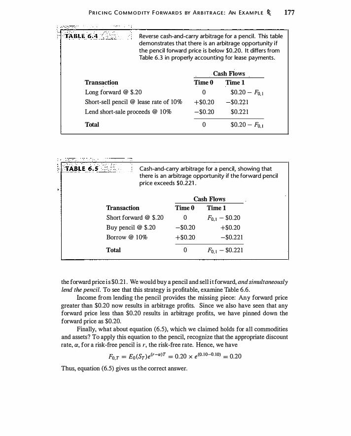
P R I C I N G CO M M O D ITY F O RWAR D S BY A R B ITRAG E : AN EXA M P L E � 177

Reverse cash-and-carry arbitrage for a penci l . This table demonstrates that there is an arbitrage opportunity if the pencil forward price is below $0.20. It differs from Table 6 .3 in properly accounting for lease payments.

Cash Flows

Transaction Time O Time l

Long forward @ $.20 0 $0.20 - Fa, t Short-sell pencil @ lease rate of 10%

Lend short-sale proceeds @ 10%

+$0.20 -$0.2?1

-$0.20 $0.221

Total 0 $0.20 - Fa, I

Cash-and-carry arbitrage for a pencil, showing that there is an arbitrage opportun ity if the forward pencil price exceeds $0.221 .

Transaction

Short forward @ $.20

Buy pencil @ $.20

Borrow @ 10%

Total

Cash Flows

Time O Time l

0 Fa, 1 - $0.20

-$0.20 +$0.20

+$0.20 -$0.221

0 Fa, I - $0.22 1

the forward price i s $0.21 . We would buy a pencil and sell i t forward, and simultaneously lend the pencil. To see that this strategy is profitable, examine Table 6.6.

Income from lending the pencil provides the missing piece: Any forward price greater than $0.20 now results in arbitrage profits. Since we also have seen that any forward price less than $0.20 results in arbitrage profits, we have pinned down the forward price as $0.20.

Finally, what about equation (6.5), which we claimed holds for all commodities and assets? To apply this equation to the pencil, recognize that the appropriate discount rate, a, for a risk-free pencil is r, the risk-free rate. Hence, we have

Fo,T = Eo (ST )e<r-a)T = 0.20 X e<O. I O-O. IO) = 0.20

Thus, equation (6.5) gives us the correct answer.

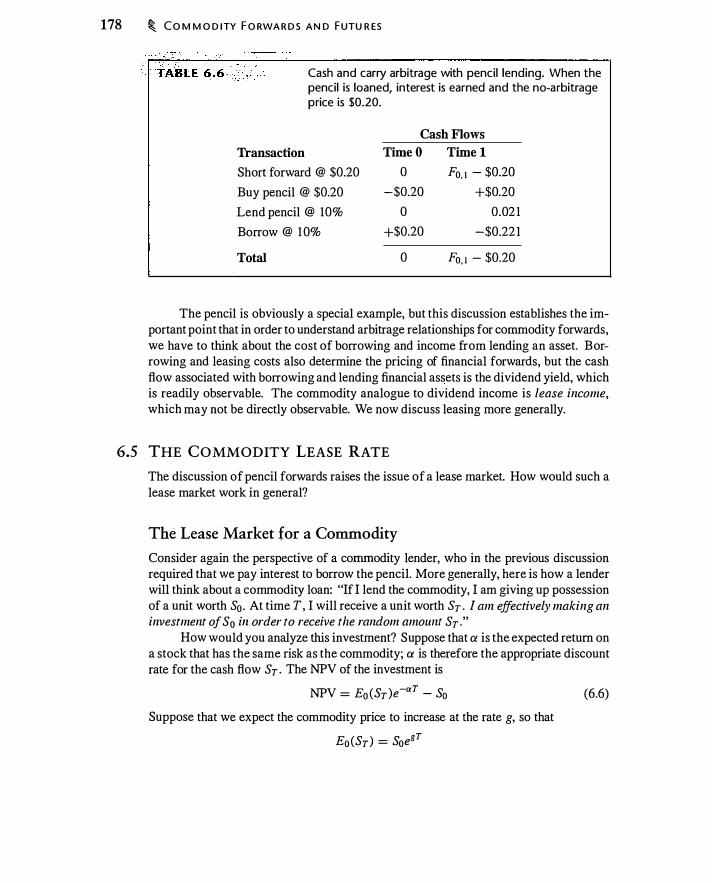
178 � CO M M O D ITY F O RWA R D S AN D F UTU R ES

Cash and carry arbitrage with pencil lending. When the pencil is loaned, interest is earned and the no-arbitrage price is $0.20.

Cash Flows

Transaction Time O Time t

Short forward @ $0.20 0 Fo. I - $0.20

Buy pencil @ $0.20 -$0.20 +$0.20

Lend pencil @ 10% 0 0.02 1

Borrow @ 10% +$0.20 -$0.22 1

Total 0 Fo, I - $0.20

The pencil is obviously a special example, but this discussion establishes the im­portant point that in order to understand arbitrage relationships for commodity forwards, we have to think about the cost of borrowing and income from lending an asset. Bor­rowing and leasing costs also determine the pricing of financial forwards, but the cash flow associated with borrowing and lending financial assets is the dividend yield, which is readily observable. The commodity analogue to dividend income is lease income, which may not be directly observable. We now discuss leasing more generally.

6.5 THE COMMODITY LEASE RATE

The discussion of pencil forwards raises the issue of a lease market. How would such a lease market work in general?

The Lease Market for a Commodity

Consider again the perspective of a commodity lender, who in the previous discussion required that we pay interest to borrow the pencil. More generally, here is how a lender will think about a commodity loan: "If I lend the commodity, I am giving up possession of a unit worth S0 . At time T, I will receive a unit worth ST . I am effectively making an investment of S0 in order to receive the random amount ST ."

How would you analyze this investment? Suppose that a is the expected return on a stock that has the same risk as the commodity; a is therefore the appropriate discount rate for the cash flow ST . The NPV of the investment is

NPV = Eo (ST )e-aT - So

Suppose that we expect the commodity price to increase at the rate g, so that

Eo (ST) = SoegT

(6.6)

TH E C O M M O D ITY L EAS E RATE � 179

Then from equation (6.6), the NPV of the commodity loan, without payments, is

NPV = Soe<g-a)T - S0 (6.7)

If g < a, the commodity loan has a negative NPV. However, suppose the lender demands that the borrower return e<a-g)T units of the commodity for each unit borrowed. If one unit is loaned, e<a-g)T units will be returned. This is like a continuous proportional lease payment of a - g to the lender. Thus, the lease rate is the difference between the commodity discount rate and the expected growth rate of the commodity price, or

81 = a - g

With this payment, the NPV of a conunodity loan is

NPV = Soe(a-g)T e(g-a)T - So = 0

(6.8)

(6.9)

Now the commodity loan is a fair deal for the lender. The commodity lender must be compensated by the borrower for the opportunity cost associated with lending. When the future pencil price was certain to be $0.20, the opportunity cost was the risk-free interest rate, 10%.

Note that if Sr were the price of a nondividend-paying stock, its expected rate of appreciation would equal its expected return, so g = a and no payment would be r�quired for the stock loan to be a fair deal.4 Commodities, however, are produced; as with the pencil, their expected price appreciation need not equal a .

Forward Prices and the Lease Rate

Suppose we have a commodity where there is an active lease market, with the lease rate given by equation (6.8). What is the forward price?

The key insight, as in the pencil example, is that the lease payment is a dividend. If we borrow the asset, we have to pay the lease rate to the lender, just as with a dividend­paying stock. If we buy the asset and lend it out, we receive the lease payment. Thus, . the fonnula for the forward price with a lease market is

(6. 1 0)

Tables 6.7 and 6.8 verify that this formula is the no-arbitrage price by performing the cash-and-carry and reverse cash-and-carry arbitrages. In both tables we tail the position in order to offset the lease income.

The striking thing about Tables 6.7 and 6.8 is that on the surface they are exactly like Tables 5.6 and 5.7, which depict arbitrage transactions for a dividend-paying stock. In an important sense, however, the two sets of tables are quite different. With the stock, the dividend yield, 8, is an observable characteristic of the stock, reflecting payment received by the owner of the stock wlzetlzer or not tlze stock is loaned.

4As we saw in Chapter 5, for a nondividend-paying stock, the present value of the future stock price is

the current stock price.

180 � C O M M O D ITY F O RWA R D S A N D FUTU R ES

Cash-and-carry arbitrage with a commodity for which the lease rate is Of. The impl ied no-arbitrage restriction is Fo,r :'S 50 eCr -lif)T_

Transaction

Short forward @ Fo,r Buy e-8rT commodity units and lend @ Df Borrow @ r

Total

Time O

0

-Soe-8rT

+Soe-8rT

0

Cash Flows

Time T

Fo,r - Sr +Sr -'-Soe<r-8r)T

Reverse cash-and-carry arbitrage with a commodity for which the lease rate is Of. The implied no-arbitrage restriction is Fo,r 2: Soe<r -lif)T_

Transaction

Long forward @ Fo, r

Short e-8rT commodity units with leas� rate 81 Lend @ r

Total

Cash Flows

Time O Time T

0 Sr - Fo,r +Soe-81T -Sr -Soe-8rT +Soe<r-81 )T

0 . Soe<r-8r )T - Fo,T

. With pencils, by contrast, the lease rate, 81 = a - g, is income earned only if the pencil is loaned. In fact, . notice in Tables 6. 7 and 6.8 that the arbitrageur never stores the commodity ! Thus, equation (6. 1 0) holds whether or not the commodity can be, or is, stored.

One of the implications of Tables 6.7 and 6.8 is that the lease rate has to be consistent with the forward price. Thus, when we observe the forward price, we can infer what the lease rate would have to be if a lease market existed. Specifically, if the forward price is Fo, r , the annualized lease rate is

(6. 1 1 )

If instead we use an effective annual interest rate, r, the effective annual lease rate is

8 = ( 1 + r)

- l I (Fo,rfS) I fT

The denominator in this expression annualizes the forward premium.

(6. 1 2)

CAR RY M A R K ETS � 181

In some markets, consistent and reliable quotes for the spot price are not available, or are not comparable to forward prices. In such cases, the near-term forward price can be used as a proxy for the spot price, S.

By definition, contango-an upward-sloping forward curve--occurs when the lease rate is less than the risk-free rate. Backwardation-a downward-sloping forward curve--occurs when the lease rate exceeds the risk-free rate.

6.6 CARRY MARKETS

Sometimes it makes sense for a commodity to be stored, at least temporarily. Storage is also called carry, and a commodity that is stored is said to be in a carry market.

One reason for storage is seasonal variation in either supply or demand, which causes a mismatch between the time at which a commodity is produced and the time at which it is consumed. With some agricultural products, for example, supply is seasonal (there is a harvest season) but demand is constant over the year. In this case, storage permits consumption to occur throughout the year.

With natural gas, by contrast, there is high demand in the winter and low demand il} the summer, but relatively constant production over the year. This pattern of use and production suggests that there will be times when natural gas is stored.

Storage Costs and Forward Prices

Storage is not always feasible (for example, fresh strawberries are perishable) and when technically feasible, storage is almost always costly. When storage is feasible, how do storage costs affect forward pricing? Put yourself in the position of a commodity merchant who owns one unit of the commodity and ask whether you would be willing to store this unit until time T. You face the choice of selling it today, receiving So, or selling it at time T. If you elect to sell at time T, you can sell forward (to guarantee the price you will receive), and you will receive Fo,T - This is a cash-and-carry.

The cash-and-carry logic with storage costs suggests that you will store only if the present value of selling at time T is at least as great as that of selling today. Denote the future value of storage costs for one unit of the commodity from time 0 to T as A.(O, T) . Indifference between selling today and a t time T requires

[Fo, T - A.(O, T)] Revenue from selling today Net revenue from selling at time T

This relationship in tum implies that if storage is to occur, the forward price is at least

Fo,T � Soe'T + A.(O, T) (6. 13 )

In the special case where storage costs are paid continuously and are proportional to the value of the commodity, storage cost is like a continuous negative dividend of A., and we can write the forward price as

(6. 14)

182 � CO M M O D I TY F O RWA R D S A N D FUTU R ES

When there are no storage costs (A. = 0), equations (6. 13 ) and (6. 14) reduce to our familiar forward pricing formula from Chapter 5 .

When there are storage costs, the forward price is higher. Why? The selling price must compensate the commodity merchant for both the financial cost of storage (interest) and the physical cost of storage. With storage costs, the forward curve can rise faster than the interest rate. We can view storage costs as a negative dividend in that, instead of receiving cash flow for holding the asset, you have to pay to hold the asset.

Example 6.1 Suppose that the November price of corn is $2.50/bushel, the effective 'monthly interest rate is 1 %, and storage costs per bushel are $0.05/month. Assuming that corn is stored from November to Febn,Iary, the February forward price must compensate owners for interest and storage. The future value of storage costs is

$0.05 + ($0.05 x 1 .0 1 ) + ($0.05 x 1 .0 12) = ($0.05/.0 1 ) x [( 1 + 0.01 )3 - 1] = $0. 1 5 1 5

Thus, the February forward price will be

2.50 X ( 1 .0 1 )3 + 0. 15 15 = 2.7273

Problem 6.9 asks you to verify that this is a no-arbitrage price.

Keep in mind that just becau�e a commodity can be stored does not mean that it should (or will) be stored. Pencils were not stored because storage was not economically necessary: A constant new supply of pencils was available to meet pencil demand. Thus, equation (6. 1 3) describes the forward price when storage occurs. Whether and when a commodity is stored are peculiar to each commodity.

Storage Costs and the Lease Rate

Suppose that there is a carry market for a commodity, so that its forward price is given by equation (6. 1 3) . What is the lease rate in this case?

Again put yourself in the shoes of the commodity lender. If you lend the commod­ity, you are saved from having to pay storage cost. Thus, the lease rate should equal the negative of the storage cost. In other words, the lender will pay the borrower! In effect, the commodity borrower is providing "virtual storage" for the commodity lender, who receives back the commodity at a point in the future. The lender making a payment to the borrower generates a negative dividend.

The Convenience Yield

The discussion of commodities to this point has ignored business reasons for holding commodities. For example, suppose you are a food manufacturer for whom corn is an essential input. You will hold an inventory of corn. If you end up holding too much

CA R RY M A R K ETS � 183

com, you can sell the excess. However, if you hold too little and run out of com, you must stop producing, idling workers and machines. Your physical inventory of com in this case has value-it provides insurance that you can keep producing in case there is a disruption in the supply of com.

In this situation, com holdings provide an extra nonmonetary return that is some­times referred to as the convenience yield.5 You will be willing to store com with a lower rate of return than if you did not earn the convenience yield. What are the implications of the convenience yield for the forward price?

Suppose that someone approached you to borrow a commodity from which you derived a convenience yield. You would think as follows: "If I lend the commodity, I am bearing interest cost, saving storage cost, and losing the value I denve from having a physical inventory. I was willing to bear the interest cost already; thus, I will pay a commodity borrower storage cost less the convenience yield."

Suppose the continuously compounded convenience yield is c, proportional to the value of the commodity. The commodity lender saves A - c by not physically storing the commodity; hence, the commodity borrower pays 8 = c - A, compensating the lender for convenience yield less storage cost. Using an argument identical to that in Table 6.8, �e conclude that the forward price must be no less than

Fo,T 2:: Soe<r-8)T = Soe<r+}..-c)T

This is the restriction imposed by a reverse cash-and-carry, in which the arbitrageur borrows the commodity and goes long the forward.

Now consider what happens if you perform a cash-and-carry, buying the com­modity and selling it forward. If you are an average investor, you will not earn the con­venience yield (it is earned only by those with a business reason to hold the commodity). You could try to lend the commodity, reasoning that the borrower could be a commercial user to whom you would pay storage cost less the convenience yield. But those who earn the convenience yield likely already hold the optimal amount of the commodity. There may be no way for you to eam the convenience yield when pelforming a cash-and-can}'· . Those )Vho do not earn the convenience yield will not own the commodity.

Thus,for an average investor, the cash-and-carry has the cash flows6

Fo,T - ST + ST - Soe<r+A)T = Fo,T - Soe<r+A)T

This expression implies that the forward price must be below S0e<r+A)T if there is to be no cash-and-carry arbitrage.

5The tenn convenience yield is defined differently by different authors. Convenience yield generally

means a return to physical ownership of the commodity. In practice it is sometimes used to mean the

lease rate. In this book, the lease rate of a commodity can be inferred from the forward price using

equation (6. I 1 ).

6In this expression, we assume we tail the holding of the commodity by buying e>.T units at time 0,

and selling off units of the commodity over time to pay storage costs.

184 � CO M M O D ITY F O RWA R D S A N D F UTU R ES

In summary, from the perspective of an arbitrageur, the price range within which there is no arbitrage is

(6. 15)

The convenience yield produces a no-arbitrage region rather than a no-arbitrage price. The observed lease rate will depend upon both storage costs and convenience. Also, as in Section 5.3, bid-ask spreads and trading costs will further expand the no-arbitrage region in equation (6. 15) .

As another illustration of convenience yield, consider again the pencil example ,of Section 6.4. In reality, everyone stores a few pencils in order to be sure to have one available. You can think of this benefit from storage as the convenience yield of a pencil. However, because the supply of pencils is perfectly elastic, the price of pencils is fixed at $0.20. Convenience yield in this case does not affect the forward price, but it does explain the decision to store pencils.

The difficulty with the convenience yield in practice is that convenience is hard to observe. The concept of the convenience yield serves two purposes. First, it explains patterns in storage-for example, why a commercial user might store a commodity when the average investor will not. Second, it provides an additional parameter to better explain the forward curve. You might object that we can invoke the convenience yield to explain any forward curve, and therefore the concept of the convenience yield is vacuous. While convenience yield can be tautological, it is a meaningful economic concept and it would be just as arbitrary to assume that there is never convenience. Moreover, the upper bound in equation (6. 15) depends on storage costs but not the convenience yield. Thus, the convenience yield only explains anomalously low forward prices, and only when there is storage.

We will now examine particular commodities to illustrate the concepts from the previous sections .

6.7 GOLD FUTURES

Gold is durable, relatively inexpensive to store (compared to its value), widely held, and actively produced through gold mining. Because of transportation costs and purity concerns, gold often trades in certificate form, as a claim to physical gold at a specific location. There are exchange-traded gold futures, specifications for which are in Figure 6. 1 .7

Figure 6.2 is a newspaper listing for the NYMEX gold futures contract. Figure 6.3 graphs the futures prices for all available gold futures contracts-the forward curve­for the first Wednesday in June, from 2001 to 2004. (Newspaper listings for most futures contracts do not show the full set of available expiration dates, so Figure 6.3

7Gold is usually denominated in troy ounces (480 grains), which are approximately 9.7% heavier than the more familiar avoirdupois ounce (437.5 grains). Twelve troy ounces make I troy pound, which

weighs approximately 0.37 kg.

·· F I G U R E 6 � 1 <

Specifications for the NYMEX gold futures contract.

Listing for the NYMEX gold futures contract from the Wall Street journal, ju ly 21 , 2004.

The forward curve for gold on four dates, from NYMEX gold futures prices.

G O L D FUTU R ES � 185

Underlying Where traded

Size Months

Refined gold bearing approved refiner stamp New York Mercantile Exchange 100 troy ounces Feb, Apr, Aug, Oct, out two years. Jun, Dec, out 5 years

Trading ends Delivery

Third-to-last business day of maturity month Any business day of the delivery month

460

440

420 'N 0 400 --� Q) 380 u

·;::: � 360 "' Q) ....

340 .2 ::: """

320

300

280

260 0

LIFETIME OPH! HIGH LOW SETTLE CHG HIGH LOW

Gold (WX)·lOO troy oL; $ par troy oL July 40190 -3.70 40010 38050 Aug 406.00 40710 399.70 402.10 -3.70 433.00 324.70 Oct 407.50 408.00 40120 403.40 -3.70 432.00 332.00 D" 408.50 409.90 402.00 404.80 -3.70 436.50 290.00 Fb05 408.50 408.50 405.00 406.40 -3.70 435.00 33150 Aug 411.00 411.00 411.00 41180 -3.70 416.50 379.00 Dec 420.00 420.00 420.00 415.90 -3.70 44150 298.40 Est vol 51,000; vol l,lon 3!,225; open lnt 262,052, -!,522.

OPEN INT

4 139,287

11.310 62,036 6,614 2,290 6,387

06-jun-2001

••••••••••••• 05-jun-2002

=== 04-jun-2003

02-jun-2004 ,... ....

.... ... .... ....

.... ....

- -- -- - -- -

.... *' ... .... .... ....

-··

-··

·-···

-·····-····-·····

-·····-····-

··

·

···

·

··

10 20 30 40 so

Months to Maturity

60

Source: Futures data from Datastream.

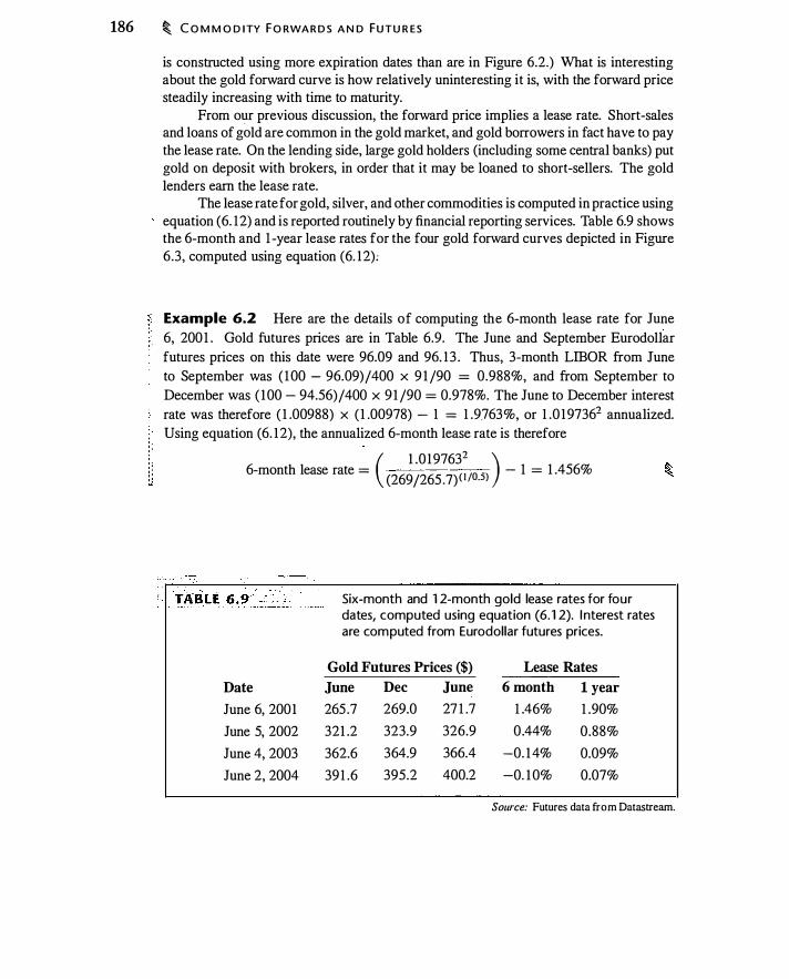
186 � C O M M O D ITY F O RWA R D S A N D FUTU R ES

is constructed using more expiration dates than are in Figure 6.2.) What is interesting about the gold forward curve is how relatively uninteresting it is, with the forward price steadily increasing with time to maturity.

From our previous discussion, the forward price implies a lease rate. Short-sales and loans of gold are common in the gold market, and gold borrowers in fact have to pay the lease rate. On the lending side, large gold holders (including some central banks) put gold on deposit with brokers, in order that it may be loaned to short-sellers. The gold lenders earn the lease rate.

The lease rate for gold, silver, and other commodities is computed in practice using equation (6. 12) and is reported routinely by financial reporting services. Table 6.9 shows the 6-month and 1 -year lease rates for the four gold forward curves depicted in Figure 6.3, computed using equation (6. 1 2) :

Example 6.2 Here are the details of computing the 6-month lease rate for June 6, 200 1 . Gold futures prices are in Table 6.9. The June and September Eurodollar futures prices on this date were 96.09 and 96. 1 3 . Thus, 3-month LIBOR from June to September was ( 1 00 - 96.09)/400 x 9 1 /90 = 0.988%, and from September to December was ( 100 - 94.56)/400 x 9 1 /90 = 0.978%. The June to December interest rate was therefore ( 1 .00988) x ( 1 .00978) - 1 = 1 .9763%, or 1 .0 197362 annualized. Using equation (6. 1 2), the annualized 6-month lease rate is therefore ( 1 .0 197632 )

6-month lease rate = (2691265 _7)0 /0.5) - 1 = 1 .456%

Date

June 6, 2001

June 5, 2002

June 4, 2003

June 2, 2004

Six-month and 1 2-month gold lease rates for four dates, computed using equation (6. 1 2). I nterest rates are computed from Eurodollar futures prices.

Gold Futures Prices ($) Lease Rates

June Dec June 6 month I year

265 .7 269.0 27 1 .7 1 .46% 1 .90%

321 .2 323.9 326.9 0 .44% 0.88%

362.6 364.9 366.4 -0. 14% 0.09%

39 1 .6 395.2 400.2 -0. 1 0% 0.07%

Source: Futures data from Datastream.

G O LD FUTU R ES � 187

Gold Investments

If you wish to hold gold as part of an investment portfolio, you can do so by holding physical gold or synthetic gold-i.e., holding T-bills and going long gold futures. Which should you do? If you hold physical gold without lending it, and if the lease rate is positive, you forgo the lease rate. You also bear storage costs . With synthetic gold, on the other hand, you have a counterparty who may fail to pay so there is credit risk. Ignoring credit risk, however, synthetic gold is generally the preferable way to obtain gold price exposure.

Table 6.9 shows that the 6-month annualized gold lease rate is 1 .46% in June 200 1 . Thus, by holding physical gold instead of synthetic gold, an investor would lose this 1 .46% return. 8 In June 2003 and 2004, however, the lease rate was about -0. 10%. If storage costs are about 0. 1 0%, an investor would be indifferent between holding physical and synthetic gold. The futures market on those dates was compensating investors for storing physical gold.

Some nonfinancial holders of gold will obtain a convenience yield from gold. Consider an electronics manufacturer who uses gold in producing components. Suppose that running out of gold would halt production. It would be natural in this case to hold a buffer stock of gold in order to avoid a stock-out of gold, i.e., running out of gold. For this manufacturer, there is a return to holding gold-namely, a lower probability of stocking out and halting production. Stocking out would have a real financial cost, and the manufacturer is willing to pay a price-the lease rate-to avoid that cost.

Evaluation of Gold Production

Suppose we have an operating gold mine and we wish to compute the present value of future production. As discussed in Section 6.2, the present value of the commodity received in the future is simply the present value--computed at the risk-free rate--of the forward price. We can use the forward curve for gold to compute the value of an operating gold mine.

Suppose that at times t; , i = 1 , . . . , n, we expect to extract n1, ounces of gold by paying an extraction cost x(t; ) . We have a set of n forward prices, Fo,1, . If the continuously compounded annual risk-free rate from time 0 to t; is r (O, t; ) , the value of the gold mine is

II PV gold production = L n11 [ Fo,r, - x (t; )] e -r(O,r, )r,

i = l (6. 1 6)

This equation assumes that the gold mine is certain to operate the entire time and that the quantity of production is known. Only price is uncertain. (We will see in Chapter 1 7

8The cost o f I ounce o f physical gold i s So. However, from equation (6. 1 0), the cost o f I ounce o f gold

bought as a prepaid forward is Soe-�rT . Synthetic gold is proportionally cheaper by the lease rate, lh .

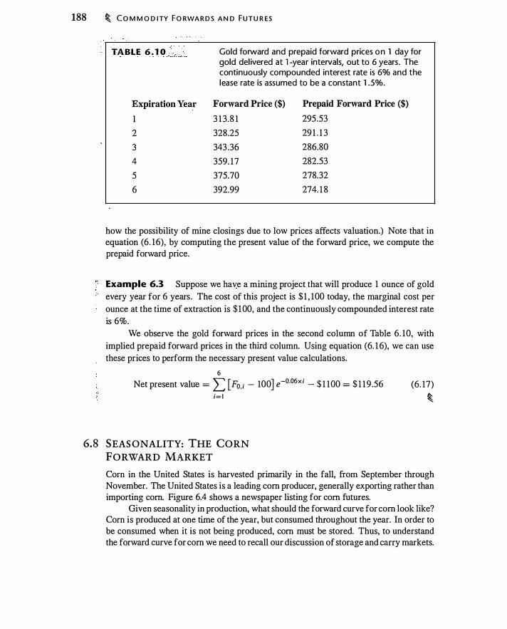
188 � CO M M O D ITY FO RWA R D S A N D FUTU R ES

TABLE 6 . 1 0 : , Gold forward and prepaid forward prices o n 1 day for gold del ivered at 1 -year intervals, out to 6 years. The continuously compounded interest rate is 6% and the lease rate is assumed to be a constant 1 .5%.

Expiration Year Forward Price ($) Prepaid Forward Price ($)

1 3 1 3.8 1 295 .53

2 328.25 29 1 . 1 3 .., 343 .36 286.80 .J

4 359. 17 282.53

5 375.70 278.32

6 392.99 274. 1 8

how the possibility of mine closings due to low prices affects valuation.) Note that in equation (6. 16), by computing the present value of the forward price, we compute the prepaid forward price.

Example 6.3 Suppose we have a mining project that will produce 1 ounce of gold every year for 6 years . The cost of this project is $ 1 , 100 today, the marginal cost per ounce at the time of extraction is $ 1 00, and the continuously compounded interest rate is 6%.

We observe the gold forward prices in the second column of Table 6. 1 0, with implied prepaid forward prices in the third column. Using equation (6. 1 6), we can use these prices to perform the necessary present value calculations.

6 Net present value = L [ Fo.; - 100 J e -o.o6xi - $ 1 100 = $ 1 1 9 .56

i= l

6.8 SEAS ONALITY: THE CORN FORWARD MARKET

(6. 17)

�

Corn in the United States is harvested primarily in the fall, from September through November. The United States is a leading corn producer, generally exporting rather than importing corn. Figure 6.4 shows a newspaper listing for corn futures.

Given seasonality in production, what should the forward curve for corn look like? Corn is produced at one time of the year, but consumed throughout the year. In order to be consumed when it is not being produced, corn must be stored. Thus, to understand the forward curve for corn we need to recall our discussion of storage and carry markets.

--�--� Listing for the CBOT corn futures contract from the Wall Street journal, ju ly 21 , 2004_

S EAS O NA L ITY: TH E C O R N F O RWA R D M A R K ET � 189

LIFETIME OPHJ OPEfl HIGH LOW SETTLE CHG HIGH LOW liU

Corn (CBD-5,000 ;u; «nts per bu. Sept 236.50 237.50 232.75 2311.00 -3.00 34100 ll.9.75 162,000 Dec 244.75 246.00 240.75 242.00 -3.00 341.50 232.50 307,442 Mr05 252.25 254.00 248.75 25015 -2.50 342.00 239.00 52,447 May 258.00 259.75 255.00 256.00 -3.00 344.00 243.50 16,608 July 262.00 263.25 259.00 2t0.00 -2.50 342.00 246.50 13,7!7 Sept 262.75 263.00 2w.oo· 26015 -2.75 299.03 260.00 3,058 Dec 262.50 262.75 260.00 26050 -2.75 28850 235.00 10,707 Est vol 74,710; vol Mon 7L892; open lnt 566,t64, + L488.

As discussed in Section 6_6, storage is an economic decision in which there is a trade-off between selling today and selling tomorrow_ If we can sell com today for $2/bu and in 2 months for $2_25/bu, the storage decision entails comparing the price we can get today with the present value of the price we can get in 2 months_ In addition to interest, we need to include storage costs in our analysis_

An equilibrium with some current selling and some storage requires that com prices be expected to rise at the interest rate plus storage costs, which implies that there will be an upward trend in the price between harvests_ While com is being stored, the forward price should behave as in equation (6_ 14), rising at interest plus storage costs_

Once the harvest begins, storage is no longer necessary; if supply and demand remain constant from year to year, the harvest price will be the same every year_ The com price will fall to that level at harvest, only to begin rising again after the harvest

The market conditions we have described are graphed in Figure 6_5, which depicts a hypothetical forward curve as seen from time o_ Between harvests, the forward price

A hypothetical fo!Ward curve for corn, assuming the harvest occurs at years 0, 1 , 2, etc

Forward Price {$/bu)

5_o

4_5

4_0

3_5

3_0

2-5

2_0

L5

LO

o_5

O L---�----�----L---�-----L----� 0 0.5 LO L5

Year

2_0 2 _5 3.0

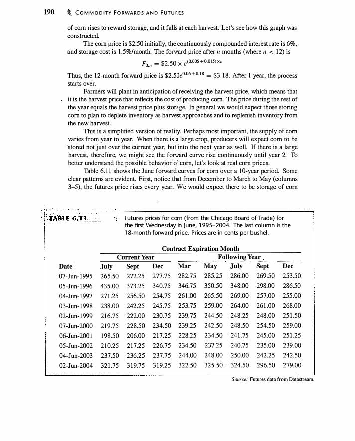
190 � C O M M O D ITY F O RWA R D S A N D F UTU R ES

of com rises to reward storage, and it falls at each harvest. Let's see how this graph was constructed.

The com price is $2.50 initially, the continuously compounded interest rate is 6%, and storage cost is 1 .5%/month. The forward price after n months (where n < 1 2) is

Fo n = $2.50 X e(0.005 + 0.0 1 5) xn

Thus, the 1 2-month forward price is $2.50e0·06+ 0· 1 8 = $3 . 1 8 . After 1 year, the process starts over.

Farmers will plant in anticipation of receiving the harvest price, which means that it is the harvest price that reflects the cost of producing com. The price during the rest of the year equals the harvest price plus storage. In general we would expect those storing com to plan to deplete inventory as harvest approaches and to replenish inventory from the new harvest.

This is a simplified version of reality. Perhaps most important, the supply of com varies from year to year. When there is a large crop, producers will expect com to be ·stored not just over the current year, but into the next year as well. If there is a large harvest, therefore, we might see the forward curve rise continuously until year 2. To better understand the possible behavior of com, let's look at real com prices.

Table 6. 1 1 shows the June forward curves for com over a 1 0-year period. Some clear patterns are evident. First, notice that from December to March to May (columns 3-5), the futures price rises every year. We would expect there to be storage of com

•' -···-·' ·"·'-�---·--· Futures prices for corn (from the Chicago Board of Trade) for the first Wednesday in june, 1 995-2004. The last column is the 1 8-month forward price. Prices are in cents per bushel .

Contract Expiration Month

Current Year Following Year

Date July Sept Dec Mar May July Sept Dec

07-Jun- 1995 265.50 272.25 277.75 282.75 285.25 286.00 269.50 253.50

05-Jun- 1996 435 .00 373 .25 340.75 346.75 350.50 348.00 298.00 286.50

04-Jun- 1997 27 1 .25 256.50 254.75 26 1 .00 265 .50 269.00 257.00 255 .00

03-Jun- 1998 238.00 242.25 245 .75 253.75 259.00 264.00 26 1 .00 268.00

02-Jun- 1999 2 16.75 222.00 230.75 239.75 244.50 248.25 248 .00 25 1 .50

07-Jun-2000 2 19.75 228.50 234.50 239.25 242.50 248 .50 254.50 259.00

06-Jun-200 1 1 98.50 206.00 2 17.25 228.25 234.50 241 .75 245 .00 25 1 .25

05-Jun-2002 2 1 0.25 2 17.25 226.75 234.50 237.25 240.75 235.00 239 .00

04-Jun-2003 237.50 236.25 237.75 244.00 248.00 250.00 242.25 242.50

02-Jun-2004 32 1 .75 3 1 9.75 3 19.25 322.50 325 .50 . 324.50 296.50 279.00

Source: Futures data from Datastream.

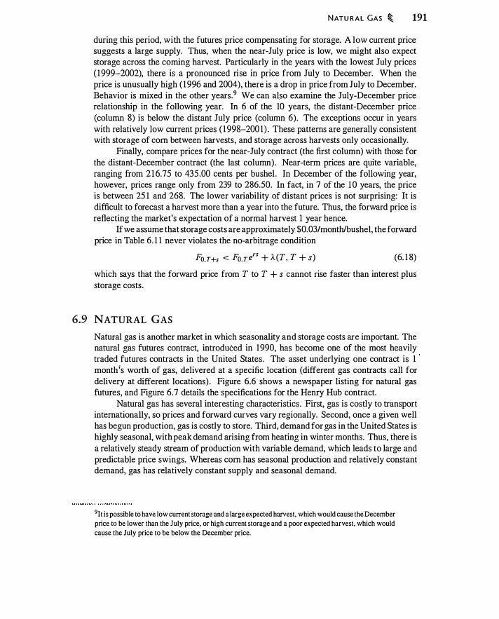
NATU R A L GAS � 191

during this period, with the futures price compensating for storage. A low current price suggests a large supply. Thus, when the near-July price is low, we might also expect storage across the coming harvest. Particularly in the years with the lowest July prices ( 1 999-2002), there is a pronounced rise in price from July to December. When the price is unusually high ( 1 996 and 2004), there is a drop in price from July to December. Behavior is mixed in the other years.9 We can also examine the July-December price relationship in the following year. In 6 of the lO years, the distant-December price (column 8) is below the distant July price (column 6). The exceptions occur in years with relatively low current prices ( 1 998-200 1) . These patterns are generally consistent with storage of com between harvests, and storage across harvests only occasionally.

Finally, compare prices for the near-July contract (the first column) with those for the distant-December contract (the last column). Near-term prices are quite variable, ranging from 2 1 6.75 to 435 .00 cents per bushel . In December of the following year, however, prices range only from 239 to 286.50. In fact, in 7 of the l O years, the price is between 25 1 and 268. The lower variability of distant prices is not surprising: It is difficult to forecast a harvest more than a year into the future. Thus, the forward price is reflecting the market's expectation of a normal harvest 1 year hence.

If we assume that storage costs are approximately $0.03/month/bushel, the forward price in Table 6. 1 1 never violates the no-arbitrage condition

Fo,T+s < Fo.Ters + J.. (T, T + s) (6. 1 8)

which says that the forward price from T to T + s cannot rise faster than interest plus storage costs.

6.9 NATURAL GAS

Natural gas is another market in which seasonality and storage costs are important. The natural gas futures contract, introduced in 1990, has become one of the most heavily traded futures contracts in the United States. The asset underlying one contract is 1 month;s worth of gas, delivered at a specific location (different gas contracts call for delivery at different locations) . Figure 6.6 shows a newspaper listing for natural gas futures, and Figure 6.7 details the specifications for the Henry Hub contract.

Natural gas has several interesting characteristics . First, gas is costly to transport internationally, so prices and forward curves vary regionally. Second; once a given well has begun production, gas is costly to store. Third, demand for gas in the United States is highly seasonal, with peak demand arising from heating in winter months. Thus, there is a relatively steady stream of production with variable demand, which leads to large and predictable price swings. Whereas com has seasonal production and relatively constant demand, gas has relatively constant supply and seasonal demand.

9It is possible to have low current storage and a large expected harvest, which would cause the December

price to be lower than the July price, or high current storage and a poor expected harvest, which would

cause the 1 uly price to be below the December price.

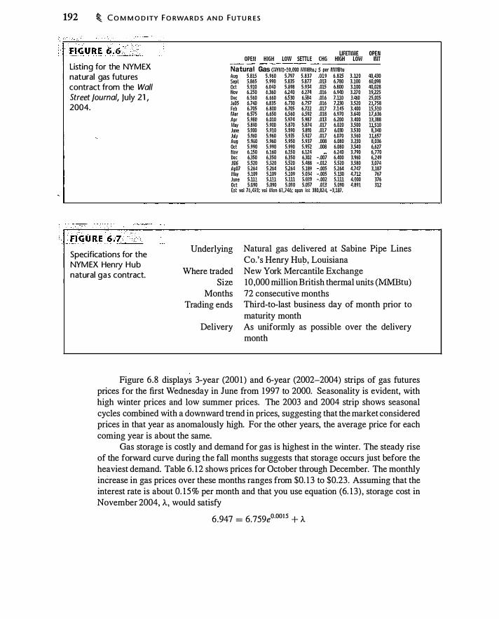
192 � C O M M O D ITY F O RWA R D S A N D FUTU R ES

Listing for the NYMEX natural gas futures contract from the Wall Street journal, ju ly 21 , 2004.

Specifications for the NYM EX Henry Hub natural gas contract.

UFETIME OPEN OPEN HIGH LOW SffiLE CHG HIGH LOW INT

Natural Gas GlYMHO,OOO iliMBtu; $ per MMBtu Aug 5.815 5.960 5.797 5.837 .019 6.825 3.110 40,430 Sept i865 5.990 5.835 5.877 .013 6.780 3.100 60,098 Oct 5.910 6.1MO 5.li98 5.934 .015 6.800 3100 40,028 Nov 6.250 �360 6240 6.274 .016 6.940 3.210 19,225 D" 6.560 6.660 6.530 6584 .016 7.110 3.460 25,005 J;05 6.740 6.835 6.730 6.7)/ .016 7.230 3.520 21,758 FEb 6.705 6.800 6.705 6.722 .017 7.145 3.400 15,510 Mar 6.575 6.650 6.560 6.592 .018 6.970 3.640 17,636 Apr 5.980 6.010 5.974 5.987 .013 6200 3.400 13,388 May 5.890 5.900 5.870 5.874 .017 6.020 3500 11,510 June 5.900 5.910 5.890 5.890 .017 6.030 3530 8,340 July 5.960 5.960 5.935 5.9ll .017 6.070 3560 11,657 Aug 5.960 5.960 5.950 5.937 .008 6.080 3.230 8,036 Oct 5.990 5.990 5.990 5.952 .008 6.080 3540 6,627 Nov 6.150 6.160 6.150 6.124 6.240 3.790 6,770 De< 6350 6350 6350 6302 -.007 6.400 3.960 6,249 JIU6 5.520 5520 5520 5.488 -.012 5.520 3580 3,074 Ap07 5.264 5.264 5264 5.189 -.005 5.264 4.747 3,187 May 5.109 5.109 5.109 5.034 -.005 5.130 4.7U 767 Juno 5.lll 5.lll 5.lll 5.039 -.002 5.lll 4.000 376 Oct 5.090 5.090 5.090 5.057 .013 5,090 4.891 3U E!t vol 76,493; vol Mon 61,746; open ir.t 380,824, •3,187.

Underlying

Where traded Size

Months Trading ends

Delivery

Natural gas delivered at Sabine Pipe Lines Co.'s Henry Hub, Louisiana New York Mercantile Exchange 10,000 million British thermal units (MMBtu) 72 consecutive months Third-to-last business day of month prior to maturity month As uniformly as possible over the delivery month

Figure 6.8 displays 3-year (200 1 ) and 6-year (2002-2004) strips of gas futures prices for the first Wednesday in June from 1997 to 2000. Seasonality is evident, with high winter prices and low summer prices. The 2003 and 2004 strip shows seasonal cycles combined with a downward trend in prices, suggesting that the market considered prices in that year as anomalously high. For the other years, the average price for each coming year is about the same.

Gas storage is costly and demand for gas is highest in the winter. The steady rise of the forward curve during the fall months suggests that storage occurs just before the heaviest demand. Table 6. 12 shows prices for October through December. The monthly increase in gas prices over these months ranges from $0. 1 3 to $0.23 . Assuming that the interest rate is about 0. 15% per month and that you use equation (6. 1 3) , storage cost in November 2004, A, would satisfy

6.947 = 6.759e0·00 1 5 + A

Forward curves for natural gas for the first Wednesday in june from 2001 to 2004. Prices are dol lars per M MBtu, from NYM EX.

. . . . .

7.5

NATU R A L GAS � 193

06-Jun-2001

=== 05-Jun-2002

••••••••••••• 04--Jun-2003

1\ - - - - 02-Jun-2004

I.-. I ;.l �I "' � I \ �-J I

"' � s ;:J .... & 4.5

4

3.5

l I f\ \ i\\ .. .1 \ 1\ ... .- ; .:-. .... _, . \ ,, :_ f \ /\, �N A

···-� :. ••• .J �.�.. \::.::7 \.

1 0 20 30 40 so 60 70 80

Months to Maturity

Source: Futures data from Datastream .

june natural gas futures prices for October, November, and December in the same year, for 2001 to 2004.

Date Oct Nov Dec

06-Jun-2001 2 . 1 73 2.305 2.435

05-Jun-2002 3 .352 3 .6 17 3 .850

04-Jun-2003 6.428 6.528 6.658

02-Jun-2004 6.58 1 6.759 6.947

Source: Futures data from Datastream.

implying an estimated storage cost of A. = $0. 178 in November 2004. You will find different imputed marginal storage costs in each year, but this is to be expected if marginal storage costs vary with the quantity stored.

Because of the expense in transporting gas internationally, the seasonal behavior of the forward curve can vary in different parts of the world. In tropical areas where gas is used for cooking and electricity generation, the forward curve is relatively flat because demand is relatively flat. In the Southern hemisphere, where seasons are reversed from the Northern hemisphere, the forward curve will peak in June and July rather than December and January.

194 � C O M M O D I TY F O RWA R D S A N D FUTU R ES

Recent developments in energy markets could alter the behavior of the natural gas forward curve in the United States. Power producers have made greater use of gas-fired peak-load electricity plants. These plants have increased summer demand for natural gas and may permanently alter seasonality.

6.10 OIL

Both oil and natural gas produce energy and are extracted from wells, but the different physical characteristics and uses of oil lead to a very different forward curve than that for gas. Oil is easier to transport than gas. Transportation of oil takes time, but oil has a global market. Oil is also easier to store than gas . Thus, seasonals in the price of crude oil are relatively unimportant. Specifications for the NYMEX light oil contract are shown in Figure 6.9. Figure 6. 10 shows a newspaper listing for oil futures. The NYMEX forwar4 curve on four dates is plotted in Figure 6. 1 1 .

·. ··· · . : � FIGURE 6 .� :� � }0D

Specifications for the NYMEX l ight, sweet crude oi l contract.

FIGU RE 6 . 10

Listing for the NYMEX crude oi l futures contract from the Wall Street journal, Ju ly 21 , 2004.

Underlying

Where traded Size

Months

Trading ends

Delivery

Specific domestic crudes delivered at Cush­ing, Oklahoma New York Mercantile Exchange 1000 U.S. barrels (42,000 gallons) 30 consecutive months plus long-dated fu­tures out 7 years Third-to-last business day preceding the 25th calendar day of month prior to maturity month As uniformly as possible over the delivery month

UFETIME OPEN HIGH LOW SETTLE CHG HIGH LOW

OPEN INT

Crude Oil , Light Sweet WYMH,ooo bbls.; $ per bbl. Aug 41.63 4230 '0.51 40.86 -0.78 42.30 20.84 29,478 Sept 4141 4175 4031 40.44 -100 4190 20.82 236,034 Oct 40.85 4105 39.80 39.88 -100 4130 23.75 68,7M flov 4038 40.45 39.52 39.45 -0.93 40.70 24.75 35,763 Dac 39.85 40.10 39.00 39.04 -0.89 40.30 16.35 60,6n Ja05 39.34 39.50 39.20 38.55 -0.86 39.50 23.25 23,149 F<b 38.89 39.05 38.65 38.13 -0.83 39.15 23.85 13,656 i\lar 38.49 38.53 38.20 37.74 -!I.SO 38.65 23.05 14,312 Apr 38.05 38.20 37.s; 37 37 -0.78 38.50 23.25 10,589 June 37 30 37.45 36.60 36.68 -0.73 37.55 2240 22,138 Sept 36.65 36.65 36.65 35.96 -!1.67 36.85 24.00 8,357 Dec 36.00 36.05 35.90 35.44 -0.61 3630 17.00 47,n4 Dc06 34.15 34.15 34.15 33.58 -0.58 34.15 19.10 34,365 Dc07 32.75 32.75 32.75 32.19 -055 32.75 19.50 12,536 Dc08 3175 3180 3170 3122 -055 32.00 19.75 U967 Dc09 3UO 3UO 3120 30.48 -!155 3120 2250 10,916 DclO 30.85 30.95 3D.63 30.18 -055 3100 27.15 15,928 Est vol 204,514, vol l.lon 248,398; opon int 708,255, -1,567.

Seven-year strip of NYM EX crude oil futures prices, $/barrel, for four different dates. � OJ .... ... "' co -...

� ClJ u

·;:::: � "' ClJ .... .2 ;::: I':.

40

38 \ 36 \

' ' 34

..... ..... .... .... 32

30

28

26

.... ... ... ....

C O M M O D ITY S P R EA D S � 195

06-}un-2001

=== 05-Jun-2002

···•··••····· 04-J un-2003

- - - - 02-}un-2004

... _ _ _ - ..... _ _ _ _ _

: � ............. _

·· ··· · - · ·· · -· ·· - · · - ·· · - · ··· - ·· - · ··· ··-20�--�--�--�--�--�----�--�--�---

0 10 20 30 40 50 60 70 80

Months to Maturity

Source: Futures data from Datastream.

On the four dates in the figure, near-term oil prices range from $25 to $40, while · the 7-year forward price in each case is between $22 and $30. The long-run forward price is less volatile than the short-run forward price, which makes economic sense. In the short run, an increase in demand will cause a price increase since supply is fixed. A supply shock (such as production restrictions by the Organization of Petroleum Exporting Countries [OPEC]) will cause the price to increase. In the long run, however, both supply and demand have time to adjust to price changes with the result that price movements are atteJ).Uated. The forward curve suggests that market participants in June 2004 did not expect the price to remain at $40/barrel.

6.1 1 COMMODITY SPREADS

Some commodities are inputs in the creation of other commodities, which gives rise to commodity spreads. Soybeans, for example, can be crushed to produce soybean meal and soybean oil (and a small amount of waste) . A trader with a position in soybeans and an opposite position in equivalent quantities of soybean meal and soybean oil has a crush spread and is said to be "trading the crush."

Similarly, crude oil is refined to make petroleum products, in particular heating oil and gasoline. The refining process entails distillation, which separates crude oil into different components, including gasoline, kerosene, and heating oil. The split of oil into these different components can be complemented by a process known as "cracking";

196 � C O M M O D ITY F O RWA R D S A N D FUTU R E S

hence, the difference i n price between crude oil and equivalent amounts of heating oil and gasoline is called the crack spread.

Oil can be processed in different ways, producing different mixes of outputs. The spread terminology identifies the number of gallons of oil as input, and the number of gallons of gasoline and heating oil as outputs. Traders will speak of "5-3-2," "3-2- 1 ," and "2- 1 - 1 " crack spreads. The 5-3-2 spread, for example, reflects the profit from taking 5 gallons of oil as input, and producing 3 gallons of gasoline and 2 gallons of heating oil. A petroleum refiner producing gasoline and heating oil could use a futures crack spread to lock in both the cost of oil and output prices. This strategy would entail going long oil futures and short the appropriate quantities of gasoline and heating oil futures. Of course there are other inputs to production and it is possible to produce other outputs, such as jet fuel, so the crack spread is not a perfect hedge.

E�ample 6.4 Suppose we consider buying oil in July and selling gasoline and heat­ing oil in August. On June 2, 2004, the July futures price for oil was $39.96/barrel, or $0.95 14/gallon (there are 42 gallons per barrel) . The August futures prices for un­leaded gasoline and heating oil were $ 1 .2427/gallon and $ 1 .0 17 1/gallon. The 3-2- 1 crack spread tells us the gross margin we can lock in by buying 3 gallons of oil and producing 2 gallons of gasoline and 1 of heating oil. Using these prices, the spread is

(2 X $ 1 .2427) + $ 1 .0 1 7 1 - (3 X $0.95 14) = $0.6482

or $0.6482/3 = $0.2 1 6 1 /gallon. In this calculation we made no interest adjustment for the different expiration months of the futures contract. �

There are crack spread options trading on NYMEX. Two of these options pay based on the difference between the price of heating oil and crude oil, and the price of gasoline and heating oil, both in a 1 : 1 ratio.

6.12 HEDGING STRATEGIES

In this section we discuss some of the complications that can arise when using commodity futures and forwards to hedge commodity price exposure. In Section 3 .3 we discussed one such complication: the problem of quantity uncertainty, where, for example, a farmer growing corn does not know the ultimate yield at the time of planting. Other issues can arise. Since commodities are heterogeneous and often costly to transport and store, it is common to hedge a risk with a commodity contract that is imperfectly correlated with the risk being hedged. This gives rise to basis risk : The price of the commodity underlying the futures contract may move differently than the price of the commodity you are hedging. For example, because of transportation cost and time, the price of natural gas in California may differ from that in Louisiana, which is the

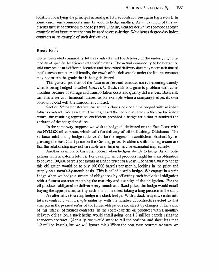
H E D G I N G ST RAT EG I ES � 197

location underlying the principal natural gas futures contract (see again Figure 6.7). In some cases, one commodity may be used to hedge another. As an example of this we discuss the use of crude oil to hedge jet fuel. Finally, weather derivatives provide another example of an instrument that can be used to cross-hedge. We discuss degree-day index contracts as an example of such derivatives.

Basis Risk

Exchange-traded commodity futures contracts call for delivery of the underlying com­modity at specific locations and specific dates. The actual commodity to be bought or sold may reside at a different location and the desired delivery date may riot match that of the futures contract. Additionally, the grade of the deliverable under the futures contract may not match the grade that is being delivered.

This general problem of the futures or forward contract not representing exactly what is being hedged is called basis risk. Basis risk is a generic problem with com­modities because of storage and transportation costs and quality differences . Basis risk can also arise with financial futures, as for example when a company hedges its own borrowing cost with the Eurodollar contract.

Section 5.5 demonstrated how an individual stock could be hedged with an index futures contract. We saw that if we regressed the individual stock return on the index return, the resulting regression coefficient provided a hedge ratio that minimized the variance of the hedged position.

In the same way, suppose we wish to hedge oil delivered on the East Coast with the NYMEX oil contract, which calls for delivery of oil in Cushing, Oklahoma. The variance-minimizing hedge ratio would be the regression coefficient obtained by re­gressing the East Coast price on the Cushing price. Problems with this regression are that the relationship may not be stable over time or may be estimated imprecisely.

Another example of basis risk occurs when hedgers decide to hedge distant obli­gations with near-term futures. For example, an oil producer might have an obligation to deli�er 100,000 barrels per month at a fixed price for a year. The natural way to hedge this obligation would be to buy 1 00,000 barrels per month, locking in the price and supply on a month-by-month basis. This is called a strip hedge. We engage in a strip hedge when we hedge a stream of obligations by offsetting each individual obligation with a futures contract matching the maturity and quantity of the obligation. For the oil producer obligated to deliver every month at a fixed price, the hedge would entail buying the appropriate quantity each month, in effect taking a long position in the strip.

An alternative to a strip hedge is a stack hedge. With a stack hedge, we enter into futures contracts with a single maturity, with the number of contracts selected so that changes in the present value of the future obligations are offset by changes in the value of this "stack" of futures contracts. In the context of the oil producer with a monthly delivery obligation, a stack hedge would entail going long 1 .2 million barrels using the near-term contract. (Actually, we would want to tail the position and short less than 1 .2 million barrels, but we will ignore this.) When the near-term contract matures, we

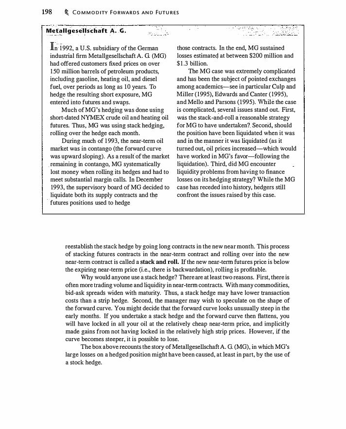
198 � C O M M O D ITY FO RWA R D S AN D FUTU R ES

Meta l l g e s e l l s c h aft A. G .

In 1 992, a U.S. subsidiary of the German industrial firm Metallgesellschaft A. G (MG) had offered customers fixed prices on over 1 50 million barrels of petro1eum products, including gasoline, heating oil, and diesel fuel, over periods as long as 1 0 years. To hedge the resulting short exposure, MG entered into futures and swaps.

Much of MG's hedging was done using short-dated NYMEX crude oil and heating oil futures. Thus, MG was using stack hedging, rolling over the hedge each month.

During much of 1 993, the near-term oil market was in contango (the forward curve was upward sloping). As a result of the market

. remaining in contango, MG systematically lost money when rolling its hedges and had to meet substantial margin calls. In December 1993, the supervisory board of MG decided to liquidate both its supply contracts and thf'! futures positions used to hedge

those contracts. In the end, MG sustained losses estimated at between $200 million and $ 1 .3 billion.

The MG case was extremely complicated and has been the subject of pointed exchanges among academics-see in particular Culp and Miller ( 1995), Edwards and Canter ( 1995), and Mello and Parsons ( 1995). While the case is complicated, several issues stand out. First, was the stack-and-roll a reasonable strategy for MG to have undertaken? Second, should the position have been liquidated when it was and in the manner it was liquidated (as it turned out, oil prices increased-which would have worked in MG's favor-following the liquidation) . Third, did MG encounter liquidity problems from having to finance losses on its hedging strategy? While the MG case has receded into history, hedgers still confront the issues raised by this case.

reestablish the stack hedge by going long contracts in the new near month. This process of stacking futures contracts in the near-term contract and rolling over into the new near-term contract is called a stack and roll. If the new near-term futures price is below the expiring near-term price (i .e., there is backwardation), rolling is profitable.

Why would anyone use a stack hedge? There are at least two reasons. First, there is often more trading volume and liquidity in near-term contracts. With many commodities, bid-ask spreads widen with maturity. Thus, a stack hedge may have lower transaction costs than a strip hedge. Second, the manager may wish to speculate on the shape of the forward curve. You might decide that the forward curve looks unusually steep in the early months . If you undertake a stack hedge and the forward curve then flattens, you will have locked in all your oil at the relatively cheap near-term price, and implicitly made gains from not having locked in the relatively high strip prices. However, if the curve becomes steeper, it is possible to lose.

The box above recounts the story ofMetallgesellschaftA. G. (MG), in which MG's large losses on a hedged position might have been caused, atleast in part, by the use of a stock hedge.

Hedging Jet Fuel with Crude Oil

H E D G I N G STRAT E G I ES � 199

Jet fuel futures do not exist in the United States, but firms sometimes hedge jet fuel with crude oil futures along with futures for related petroleum products. 1 0 In order to perform this hedge, it is necessary to understand the relationship between crude oil and jet fuel prices. If we own a quantity of jet fuel and hedge by holding H crude oil futures contracts, our mark-to-market profit depends on the change in the jet fuel price and the change in the futures price:

(6. 19)

where P1 is the price of jet fuel and F1 the crude oil futures price. We �an estimate H by regressing the change in the jet fuel price (denominated in cents per gallon) on the change in the crude futures price (denominated in dollar per barrel) . Doing so using daily data for January 2000-June 2004 gives (standard errors are in parentheses)

P1 - Pr- 1 = 0.009 + 2.037(� - F1_ ! ) R2 = 0.287 (6.20) (0.069) (0.094)

The futures price used in this regression is the price of the current near-term contract. The coefficient on the futures price change tells us that, on average, when the crude futures price increases by $ 1 , a gallon of jet fuel increases by $0.02. Suppose that as part of a particular crack spread, 1 gallon of crude oil is used to produce 1 gallon of jet fuel. Then, other things equal, since there are 42 gallons in a barrel, a $1 increase in the price of a barrel of oil will generate a $ 1142 = $0.0238 increase in the price of jet fuel. This is approximately the regression coefficient. "

The R2 in equation (6. 19) is 0.287, which implies a correlation coefficient of about 0.50. The hedge would therefore have considerable residual risk.

Weather Derivatives

Weather derivatives provide another illustration of cross-hedging. Weather as a business risk cal_l be difficult to hedge. For example, weather can affect both the prices of energy '

products and the amount of energy consumed. If a winter is colder than average, home­owners and businesses will consume extra electricity, heating oil, and natural gas, and the prices of these products will tend to be high as well. Conversely, during a warm winter, energy prices and quantities will be low. While it is possible to use futures markets to hedge prices of commodities such as natural gas, hedging the quantity is more difficult.

1°For example, Southwest Airlines reportedly used a combination of crude oil and heating oil futures

to hedge jet fueL See Melanie Trottman, "Southwest Airline's Big Fuel-Hedging Call Is Paying Off," H�/1 Street Joumal, January 1 6, 2004, p. 84. 1 1 Recall that in Section 5.5 we estimated a hedge ratio for stocks using a regression based on percentage

changes. In that case, we had an economic reason (an asset pricing model) to believe that there was a stable relationship based upon rates of return. With crude and jet fuel, crude is used to produce jet

fuel, so it makes sense that dollar changes in the price of crude would be related to dollar changes in

the price of jet fueL

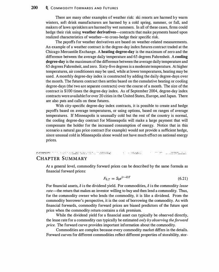
200 � C O M M O D ITY FO RWA R D S A N D FUTU R E S

There are many other examples of weather risk: ski resorts are harmed by warm winters, soft drink manufacturers are harmed by a cold spring, summer, or fall, and makers of lawn sprinklers are harmed by wet summers. In all of these cases, firms could hedge their risk using weather derivatives-contracts that make payments based upon realized characteristics of weather-to cross-hedge their specific risk.

The payoffs for weather derivatives are based on weather-related measurements. An example of a weather contract is the degree-day index futures contract traded at the Chicago Mercantile Exchange. A heating degree-day is the maximum of zero and the difference between the average daily temperature and 65 degrees Fahrenheit. A cooling �egree-day is the maximum of the difference between the average daily temperature and 65 degrees Fahrenheit, and zero. Sixty-five degrees is a moderate temperature. At higher temperatures, air conditioners may be �sed, while at lower temperatures, heating may be used. A monthly degree-day index is constructed by adding the daily degree-days over the month. The futures contract then settles based on the cumulative heating or cooling degree-days (the two are separate contracts) over the course of a month. The size of the contract is $ 1 00 times the degree-day index. As of September 2004, degree-day index contracts were available for over 20 cities in the United States, Europe, and Japan. There are also puts and calls on these futures.

With city-specific degree-day index contracts, it is possible to create and hedge payoffs based on average temperatures, or using options, based on ranges of average temperatures. If Minneapolis is unusually cold but the rest of the country is normal, the cooling degree-day contract for Minneapolis will make a large payment that will compensate the holder for the increased consumption of energy. Notice that in this scenario a natural gas price contract (for example) would not provide a sufficient hedge, since unusual cold in Minneapolis alone would not have much effect on national energy prices.

CHAPTER SUMMARY

At a general level, commodity forward prices can be described by the same formula as financial forward prices:

Fo.T = Soe(r-o)T (6.2 1 )

For financial assets, 8 i s the dividend yield. For commodities, 8 i s the commodity lease rate-the return that makes an investor willing to buy and then lend a commodity. Thus, for the commodity owner who lends the commodity, it is like a dividend. From the commodity borrower's perspective, it is the cost of borrowing the commodity. As with financial forwards, commodity forward prices are biased predictors of the future spot price when the commodity return contains a risk premium.

While the dividend yield for a financial asset can typically be observed directly, the lease rate for a commodity can typically be estimated only by obsen,ing tlzefonvard price. The forward curve provides important information abo1,1t the commodity.

Commodities are complex because every commodity market differs in the details. Forward curves for different commodities reflect different properties of storability, stor-

P R O B LE M S � 201

age costs, production, and demand. Electricity, gold, com, natural gas, and oil all have distinct forward curves, reflecting the different characteristics of their physical markets. These idiosyncracies will be reflected in the commodity lease rate. When there are seasonalities in either the demand or supply of a commodity, the commodity will be stored (assuming this is physically feasible), and the forward curve for the commodity will reflect storage costs. Some holders of a commodity receive benefits from physical ownership. This benefit is called the commodity's convenience yield. The convenience yield creates different returns to ownership for different investors, and may or may not be reflected in the forward price. The convenience yield can lead to no-arbitrage regions rather than a no-arbitrage price. It can also be costly to short-sell commodities with a significant convenience yield.

FURTHER READING We will see in later chapters that the concept of a lease rate-which is a generalization of a dividend yield-helps to unify the pricing of swaps (Chapter 8), options (Chapter 1 0), and commodity-linked notes (Chapter 15) . One particularly interesting application of the lease rate arises in the discussion of real options in Chapter 17 . We will see there that if an extractable commodity (such as oil or gold) has a zero lease rate, it will never be extracted. Thus, the lease rate is linked in an important way with production decisions.

A useful resource for learning more about commodities is the Chicago Board of Trade ( 1998). The Web sites of the various exchanges (e.g., NYMEX and the CBOT) are also useful resources, with information about particular commodities and trading and hedging strategies.

Siegel and Siegel ( 1990) provide a detailed discussion of many commodity fu­tures. There are numerous papers on commodities. Bodie and Rosansky ( 1980) and Gorton and Rouwenhorst (2004) examine the risk and return of commodities as an in­vestme[lt. Brennan ( 199 1 ), Pindyck ( 1 993b), and Pindyck ( 1994) examine the behavior · of commodity prices. Schwartz ( 1997) compares the performance of different models of commodity price behavior. Jarrow and Oldfield ( 1 98 1 ) discuss the effect of storage costs on pricing, and Routledge et al. (2000) present a theoretical model of commodity forward curves .

Finally, Metallgesellschaft engendered a spirited debate. Papers written about that episode include Culp and Miller ( 1995), Edwards and Canter ( 1995), and Mello and Parsons ( 1995).

PROBLEMS 6.1. The spot price of a widget is $70.00 per unit. Forward prices for 3 , 6, 9, and 12

months are $70.70, $7 1 .4 1 , $72. 13 , and $72.86. Assuming a 5% continuously compounded annual risk-free rate, what are the annualized lease rates for each maturity? Is this an example of contango or backwardation?

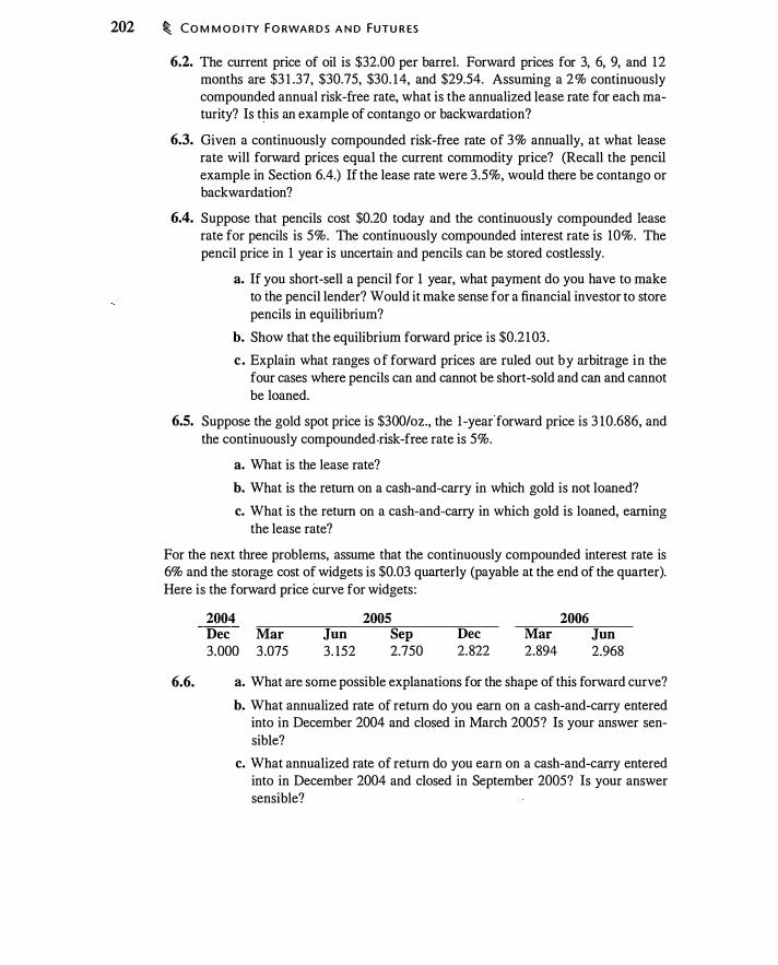
202 � CO M M O D I TY F O RWA R D S A N D FUTU R ES

6.2. The current price of oil is $32.00 per barrel. Forward prices for 3, 6, 9, and 12 months are $3 1 .37, $30.75, $30. 14, and $29.54. Assuming a 2% continuously compounded annual risk-free rate, what is the annualized lease rate for each ma­turity? Is this an example of contango or backwardation?

6.3. Given a continuously compounded risk-free rate of 3% annually, at what lease rate will forward prices equal the current commodity price? (Recall the pencil example in Section 6.4.) If the lease rate were 3.5%, would there be contango or backwardation?

6.4. Suppose that pencils cost $0.20 today and the continuously compounded lease rate for pencils is 5%. The continuously compounded interest rate is 10%. The pencil price in 1 year is uncertain and pencils can be stored costlessly.

a. If you short-sell a pencil for 1 year, what payment do you have to make to the pencil lender? Would it make sense for a financial investor to store pencils in equilibrium?

b. Show that the equilibrium forward price is $0.2 1 03 .

c . Explain what ranges of forward prices are ruled out by arbitrage in the four cases where pencils can and cannot be short-sold and can and cannot be loaned.

6.5. Suppose the gold spot price is $300/oz., the ! -year forward price is 3 10.686, and the continuously compounded-risk-free rate is 5%.

a. What is the lease rate?

b. What is the return on a cash-and-carry in which gold is not loaned?

c. What is the return on a cash-and-carry in which gold is loaned, earning the lease rate?

For the next three problems, assume that the continuously compounded interest rate is 6% and the storage cost of widgets is $0.03 quarterly (payable at the end of the quarter). Here is the forward price curve for widgets:

2004 Dec 3.000

Mar 3 .075

Jun 3. 152

2005 Sep 2.750

Dec 2.822

Mar 2.894

2006 Jun 2.968

6.6. a. What are some possible explanations for the shape of this forward curve?

b. What annualized rate of return do you earn on a cash-and-carry entered into in December 2004 and closed in March 2005? Is your answer sen­sible?

c. What annualized rate of return do you earn on a cash-and-carry entered into in December 2004 and closed in September 2005? Is your answer sensible?

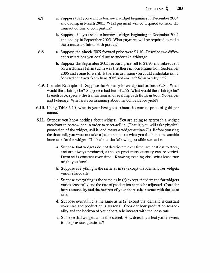
P R O B L E M S � 203

6.7. a. Suppose that you want to borrow a widget beginning in December 2004 and ending in March 2005 . What payment will be required to make the transaction fair to both parties?

b. Suppose that you want to borrow a widget beginning in December 2004 and ending in September 2005 . What payment will be required to make the transaction fair to both parties?

6.8. a. Suppose the March 2005 forward price were $3 . 10. Describe two differ-ent transactions you could use to undertake arbitrage.

b. Suppose the September 2005 forward price fell to $2.70 and subsequent forward prices fell in such a way that there is no arbitrage from September 2005 and going forward. Is there an arbitrage you could undertake using forward contracts from June 2005 and earlier? Why or why not?

6.9. Consider Example 6. 1 . Suppose the February forward price had been $2.80. What would the arbitrage be? Suppose it had been $2.65. What would the arbitrage be? In each case, specify the transactions and resulting cash flows in both November and February. What are you assuming about the convenience yield?

6.10. Using Table 6. 1 0, what is your best guess about the current price of gold per ounce?

6.11. Suppose you know nothing about widgets. You are going to approach a widget merchant to borrow one in order to short-sell it. (That is, you will take physical­possession of the widget, sell it, and return a widget at time T.) Before you ring the doorbell, you want to make a judgment about what you think is a reasonable lease rate for the widget. Think about the following possible scenarios.

a. Suppose that widgets do not deteriorate over time, are costless to store, and are always produced, although production quantity can be varied. Demand is constant over time. Knowing nothing else, what lease rate might you face?

b. Suppose everything is the same as in (a) except that demand for widgets varies seasonally.

c. Suppose everything is the same as in (a) except that demand for widgets varies seasonally and the rate of production cannot be adjusted. Consider how seasonality and the horizon of your short-sale interact with the lease rate.

d. Suppose everything is the same as in (a) except that demand is constant over time and production is seasonal. Consider how production season­ality and the horizon of your short-sale interact with the lease rate.

e. Suppose that widgets cannot be stored. How does this affect your answers to the previous questions?

Suppo'e you have the opportunity to 'pend $ 1 one yem from today to <eceive $2 two Y""'' from today. What is the value of this opportunity? To answer this question, you need to know the appropriate interest rates for discounting the two cash flows. This comparison is an example of the most basic concept in finance: using interest rates to compute present values. Once we find a present value for one or more assets, we can compare the values of cash flows from those assets even if the cash inflows and cash outflows occur at different times. In order to perform these calculations, we need information about the set of interest rates prevailing between different points in time.

We begin the chapter by reviewing basic bond concepts--coupon bonds, yields to maturity, and implied forward rates. Any reader of this book should understand these basic concepts . We then look at interest rate forwards and forward rate agreements, which permit hedging interest rate risk. Finally, we look at bond futures and the repo market.

7.1 B OND BASICS

Table 7. 1 presents information about current interest rates for bonds maturing in from 1 to 3 years. ldelltical information is presented in five different ways in tlze table. Although the information appears differently across columns, it is possible to take the information in any ·one column of Table 7. 1 and reproduce the other four columns. '

illustrating how similar information is presented in practice, Figure 7. 1 reproduces a newspaper listing of information about outstanding U.S . government bonds . The listing reports a price per $ 100 of maturity value and a yield to maturity for each bond. A wide range of maturities exists at any point in time, but the U.S . government issues Treasury securities only at specific maturities-typically 3 months, 6 months, and 1 , 2, 5, 10, and 30 years. 2 Government securities that are issued with less than 1 year to maturity and that make only a single payment, at maturity, are called Treasury bills. Notes and bonds pay

1 Depending upon how you do the computation, you may anive at numbers slightly different from

those in Table 7 . I . The reason is that all of the entries except those in column I are rounded in the last digit, and there are multiple ways to compute the number in any given column. Rounding error will therefore generate small differences among computations performed in different ways.

2Treasury securities are issued using an auction. In the past the government also issued bonds with maturities of 3 and 7. Between 2002 and 2005 the government issued no 30-year bonds.

205

206 � I NT E R EST RAT E F O RWA R D S A N D F UTU R ES

Five ways to present equiva lent information about default-free interest rates. All rates but those in the the last column are effective annual rates.

(1) (2) (3) (4) (5)

Continuously

Years to Zero-Coupon Zero-Coupon One-Year Implied Par Compounded

Maturity Bond Yield Bond Price Forward Rate Coupon Zero Yield

1

2

3

6.00% 0.943396 6.00000% 6.00000% 5 .82689%

6.50 0.88 1 659 7.00236 6.48423 6.29748

7.00 0.8 16298 8.00705 6.95485 6.76586

coupons and are issued at a price close to their maturity value (i .e. , they are issued at par). Notes have 1 0 or fewer years to maturity and bonds have more than I 0 years to maturity. The distinctions between bills, notes, and bonds are not important for our purposes; we will refer to all three as bonds. You will also see Treasury inflation protected securities (TIPS) in Figure 7 . 1 . These are bonds for which payments are adjusted for inflation. Finally, the most recently issued government bonds are called on-the-run; other bonds are called off-the-run. These terms are used frequently in talking about government bonds since on-the-run bonds generally have lower yields and greater trading volume than off-the-run bonds. Appendix 7.A discusses some of the conventions used in bond price and yield quotations.

In addition to government bond information, there is also a listing for STRIPS. A STRIPS-Separate Trading of Registered Interest and Principal of Securities-is a claim to a single interest payment or the principal portion of a government bond. These claims trade separately from the bond. STRIPS are zero-coupon bonds since they make only a single payment at maturity. "STRIPS" should not be confused with the forward strip, which is the set of forward prices available at a point in time.

We need a way to represent bond prices and interest rates. Interest rate notation is, unfortunately and inevitably, cumbersome, because for any rate we must keep track of three dates: the date on which the rate is quoted, and the period of time (this has beginning and ending dates) over which the rate prevails. We will let r1 (t1 , t2) represent the interest rate from time t1 to time t2 , prevailing on date t. If the interest rate is current-i.e., if t = t1 -and if there is no risk of confusion, we will drop the subscript.

Zero-Coupon Bonds

We begin by showing that the zero-coupon bond yield and zero-coupon bond price, columns ( 1 ) and (2) in Table 7. 1 , provide the same information. A zero-coupon bond is a bond that makes only a single payment at its maturity date. Our notation for zero­coupon bond prices will mimic that for interest rates. The price of a bond quoted at time

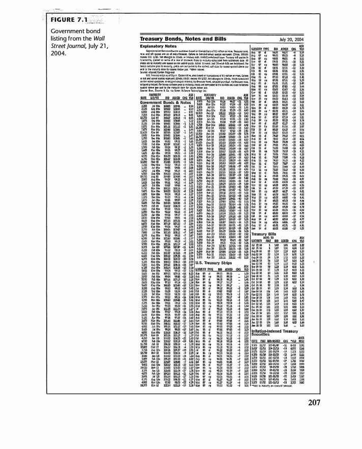
Government bond l isting from the Wall Street journal, ju ly 2 1 ,

2004.

Treasury Bonds, Notes and Bills Explanatory Notes

July 20 2004 f,UJIJFJTY TYPE BID ASKED ASk Q!G YlD ... lll ... 1.ll ... lll .,. ill -]] llol -11 13!1 -11 J.n -11 JE -11 J.U -11 J.n -u 1.u -u u1 -11 1.36 -lJ l.:;"l ·ll J.5.l -u 151 -n 1.u -11 1!1 -14 1.1""5 -H 1.!! -14 U9 -1� lSl -14 ua -li l!O -lS l.'f/ -1� l'i6 -H U.? -g Ul -ll U9 ·15 4.01 -15 4JD ·ll w -15 Ul -15 Ul -1s m ·ll '-'2 -11 .Ul -u u� -IS 4.30 -15 ... � -u .u1 ·15 Ul -u rn -1� us -15 4.57 -� .ut. -u uz -1!. .Ul ·15 ...,. _,. .50 _,. 10 -ll .... -15 "-.B -11 �,5; -u m -11 U7 -15 .Ul -v '-"

207

208 � I NT E R EST RATE FO RWA R D S A N D F UTU R ES

t0, with the bond to be purchased at t1 and maturing at t2 , is P,0 Ct1 , t2) . As with interest rates, we will drop the subscript when to = tJ .

The 1 -year zero-coupon bond price of P (O, 1 ) = 0.943396 means that you would pay $0.943396 today to receive $ 1 in 1 year. You could also pay P (O, 2) = 0.88 1 659 today to receive $1 in 2 years and P (O, 3) = 0.8 1 6298 to receive $1 in 3 years.

The yield to maturity (or illfernal rate of return) on a zero-coupon bond is simply the percentage increase in dollars earned from the bond. For the 1 -year bond, we end up with 1 /0.943396 - 1 = 0.06 more dollars per $ 1 invested. If we are quoting interest rates as effective annual rates, this is a 6% yield.

For the zero-coupon 2-year bond, we end up with 1 /0.88 1 659 - 1 = 0. 1 34225 more dollars per $ 1 invested. We could call this a 2-year effective interest rate of 1 3 .4225%, but it is conventional to quote rates on an annual basis. If we want this yield to be comparable to the 6% yield on the 1 -year bond, we could assume annual compounding and get ( 1 + r (O, 2))2 = 1 . 1 34225, which implies that r (O, 2) = 0.065. In general,

1 P (O, n ) = ----­

[ 1 + r (O, n)]" (7. 1 )

Note from equation (7. 1 ) that a zero-coupon bond price is a discount factor: A zero-coupon bond price is what you would pay today to receive $ 1 in the future. If you have a future cash flow at time t, C. you can multiply it by the price of a zero-coupon bond, P (0, t), to obtain the present value of the cash flow. Because of equation (7 . 1 ) , multiplying by P (O, t) is the same as discounting at the rate r (O, t ) , i .e . ,

C, C, x P (O, t) =

[ I + r (O, t)] '

The inverse of the zero-coupon bond price, 1/ P (O, t) , provides a future value factor. In contrast to zero-coupon bond prices, interest rates such as those in Figure 7 . 1

are subject to quoting conventions that can make their interpretation difficult (if you doubt this, see Appendix 7.A) . Because of their simple interpretation, we can consider zero-coupon bond prices as the building block for all of fixed income.

A graph of annualized zero-coupon yields to maturity against time to maturity is called the zero-coupon yield curve. A yield curve shows us how yields to maturity vary with time to maturity. In practice, it is common to present the yield curve based on coupon bonds, not zero-coupon bonds.

Implied Forward Rates

We now see how column (3) in Table 7 . 1 can be computed from either column ( l ) or (2). The 1 -year and 2-year zero-coupon yields are the rates you can earn from year 0 to year 1 and from year 0 to year 2. There is also an implicit rate that can be earned from year 1 to year 2 that must be consistent with the other two rates. This rate is called the implied forward rate.

Suppose we could today guarantee a rate we could earn from year 1 to year 2. We know that $ 1 invested for 1 year earns [ 1 + r0 (0 , l)] and $ 1 invested for 2 years earns

FlG;URE 7 . 2

A n investor investing for 2 years has a choice of buying a 2-year zero-coupon bond paying [1 + r0(0, 2)]2 or buying a 1 -year bond paying 1 + r0(0, 1) for 1 year, and reinvesting the proceeds at the impl ied foiWard rate, r0(1 ,2) between years 1 and 2. The implied foiWard rate makes the investor indifferent between these alternatives.

Earn r(O, 1 )

B O N D BAS I CS � 209

[1 + r(O, 1 )] x [1 + r(1, 2)]

Earn implied forward rate, r(1 , 2)

Earn r(O, 2) per year [1 + r(O, 2)j2

[ 1 + r0 (0, 2)f . Thus, the time 0 forward rate from year 1 to year 2, r0 ( 1 , 2) , should satisfy

or

[ 1 + ro (O, 1 ) ] [ 1 + roO , 2)] = [ 1 + ro (O, 2)f

1 + ro O , 2) = [1 + ro (O, 2)f

1 + ro (O, 1 ) (7.2)

Figure 7.2 shows graphically how the implied forward rate is related to 1- and 2-year, yields, If ro O . 2) did not satisfy equation (7.2), then there would be an arbitrage oppor­tunity. Problem 7 . 1 5 asks you to work through the arbitrage. In general, we have

(7.3)

Corresponding to 1 -year and 2-year interest rates, ro (O, 1 ) and ro (O, 2) , we have prices of 1 -year and 2-year zero-coupon bonds, P0(0, 1) and P0 (0, 2) . Just as the interest rates imply a forward 1 -year interest rate, the bond prices imply a 1 -year forward zero-coupon bond price. The implied forward zero-coupon bond price must be consistent with the implied forward interest rate. Rewriting equation (7.3), we have

(7.4)

The implied forward zero-coupon bond price from t1 to t2 is simply the ratio of the zero-coupon bond prices maturing at t2 and t1 •

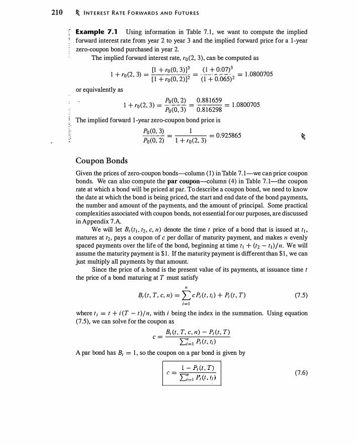
210 � I NT E R EST RATE F O RWA R D S A N D FUTU R ES

Example 7.1 Using information in Table 7 . I , we want to compute the implied forward interest rate from year 2 to year 3 and the implied forward price for a 1 -year zero-coupon bond purchased in year 2.

The implied forward interest rate, ro (2, 3) , can be computed as

[l + r (0 3)]3 ( l + 0 07)3 l + r (2 3) =

0 ' = ·

= 1 .0800705 0 ' [ I + r0 (0 , 2)]2 ( I + 0.065)2

or equivalently as

P0(0, 2) 0 .88 I659 l + ro (2, 3) =

Po(O, 3) =

0_8 16298 = 1 .0800705

The implied forward 1 -year zero-coupon bond price is

Coupon Bonds

Po (O, 3) =

1 = 0.925865

Po(O, 2) 1 + ro (2, 3)

Given the prices of zero-coupon bonds-column ( I ) in Table 7. 1-we can price coupon bonds. We can also compute the par coupon-column (4) in Table 7 . 1-the coupon rate at which a bond will be priced at par. To describe a coupon bond, we need to know the date at which the bond is being priced, the start and end date of the bond payments, the number and amount of the payments, and the amount of principal. Some practical complexities associated with coupon bonds, not essential for our purposes, are discussed in Appendix 7 .A

We will let B, (t1 , t2 , c, n ) denote the time t price of a bond that is issued at t1 , matures at t2 , pays a coupon of c per dollar of maturity payment, and makes n evenly spaced payments over the life of the bond, beginning at time t1 + (t2 - t1 ) jn . We will assume the maturity payment is $ 1 . If the maturity payment is different than $ 1 , we can just multiply all payments by that amount.

Since the price of a. bond is the present value of its payments, at issuance time t the price of a bond maturing at T must satisfy

· II

B, (t, T, c, n ) = L cP, (t, t; ) + P, (t , T) i= l

(7 .5)

where t; = t + i (T - t)/n , with i being the index in the summation. Using equation (7.5), we can solve for the coupon as

B, (t , T, c, 11 ) - P, (t, T) c =

2::;'= 1 P, (t, t; )

A par bond has B, = I , so the coupon on a par bond is given by

(7.6)

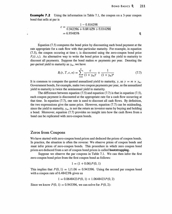
B O N D BAS I CS � 211

Example 7.2 Using the information in Table 7. 1 , the coupon on a 3-year coupon bond that sells at par is

1 - 0 .8 16298 c = ��������--����

0.943396 + 0.88 1 659 + 0.8 1 6298 = 6.95485%

Equation (7 .5) computes the bond price by discounting each bond payment at the rate appropriate for a cash flow with that particular maturity. For example, in equation (7 .5), the coupon occuring at time t; is discounted using the zero-coupon bond price P1 (t , t; ). An alternative way to write the bond price is using the yield to maturity to discount all payments. Suppose the bond makes m payments per year. Denoting the per-period yield to maturity as )'111 , we have

II C 1

B1 (t , T, c, n ) = L . + . i= l

( 1 + Ym )' ( 1 + Ym )" (7.7)

It is common to compute the quoted annualized yield to maturity, y, as y = m x )'111 • Government bonds, for example, make two coupon payments per year, so the annualized yield to maturity is twice the semiannual yield to maturity.

The difference between equation (7.5) and equation (7.7) is that in equation (7.5), each coupon payment is discounted at the appropriate rate for a cash flow occurring at that time. In equation (7.7), one rate is used to discount all cash flows. By definition, the two expresssions give the same price. However, equation (7 .7) can be misleading, since the yield to maturity, )'111 , is not the return an investor earns by buying and holding a bond. Moreover, equation (7. 7) provides no insight into how the cash flows from a bond can be replicated with zero-coupon bonds.

Zeros from Coupons

We have started with zero-coupon bond prices and deduced the prices of coupon bonds . In practice, the situation is often the reverse: We observe prices of coupon bonds and must infer prices of zero-coupon bonds. This procedure in which · zero coupon bond prices are deduced from a set of coupon bond prices is called bootstrapping.

Suppose we observe the par coupons in Table 7 . 1 . We can then infer the first zero-coupon bond price from the first coupon bond as follows :

1 = ( 1 + 0.06) P (O , 1 )

This implies that P (O, 1 ) = 1 / 1 .06 = 0.943396. Using the second par coupon bond with a coupon rate of 6.48423% gives us

1 = 0.0648423 ? (0, 1) + 1 .0648423 ? (0, 2)

Since we know P (O, 1) = 0.943396, we can solve for P (O, 2) :

212 � I NT E R EST RATE F O RWA R D S A N D FUTU R ES

1 - 0.0648423 X 0.943396 P (O, 2) = ---

1 .-06

-4-84_

2_3 __ _

= 0.88 1659

Finally, knowing P (O, 1 ) and P (O, 2) , we can solve for P (O, 3) using the 3-year par coupon bond with a coupon of 6.95485%:

1 = (0.0695485 X P (O, 1 ) ) + (0.0695485 X P (O, 2) ) + ( 1 .0695485 X P (O, 3) )

which gives us

1 - (0.0695485 X 0.943396) - (0.0695485 X 0.88 1659) P (O, 3) =

1 .0695485 = 0.8 16298

There is nothing about the procedure that requires the bonds to trade at par. In fact, we do not even need the bonds to all have different maturities. For example, if we had a 1 -year bond and two different 3-year bonds, we could still solve for the three zero-coupon bond pnces by solving simultaneous equations.

Interpreting the Coupon Rate

A coupon rate-for example the 6.95485% coupon on the 3-year bond-determines the cash flows the bondholder receives. However, except in special cases, it does not correspond to the rate of return thatan investor actually earns by holding the bond.

Suppose for a moment that interest rates are certain; i .e. , the implied forward rates in Table 7 . 1 are the rates that will actually occur in years 1 and 2. Imagine that we buy the 3-year bond and hold it to maturity, reinvesting all coupons as they are paid. What rate of return do we earn? Before going through the calculations, let's stop and discuss the intuition. We are going to invest an amount at time 0 and to reinvest all coupons by buying more bonds, and we will not withdraw any cash until time 3. In effect, we are constructing a 3-year zero-coupon bond. Thus, we should earn the same return as on a 3-year zero: 7%. This buy-and-hold return is different than the yield to maturity of 6.95485%. The coupon payment is set to make a par bond fairly priced, but it is not actually the return we earn on the bond except in the special case when the interest rate is constant over time.

Consider first what would happen if interest rates were certain, we bought the 3-year bond with a $ 100 principal and a coupon of 6.95485%, and we held it for 1 year. The price at the end of the year would be

6.95485 106.95485

B, =

1 .0700237 + ( 1 .0700237) ( 1 + 0.0800705) = 99.045 15

The ! -period return is thus

6.95485 + 99.045 15 ! -period return =

100 - 1

= 0.06

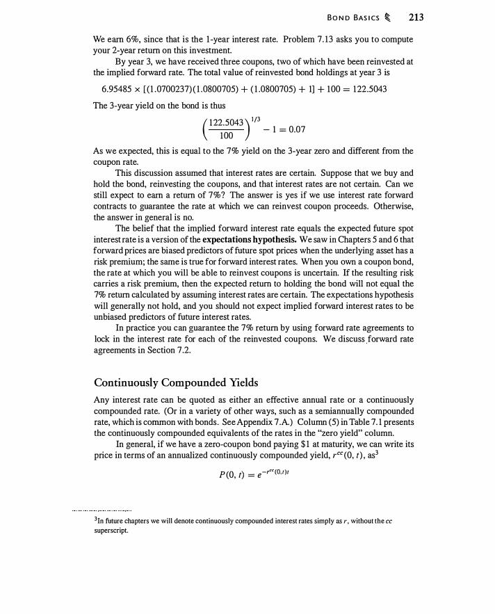
B O N D BAS I CS � 213

We earn 6%, since that is the 1 -year interest rate. Problem 7. 13 asks you to compute your 2-year return on this investment.

By year 3, we have received three coupons, two of which have been reinvested at the implied forward rate. The total value of reinvested bond holdings at year 3 is

6.95485 X ( ( 1 .0700237) ( 1 .0800705) + ( 1 .0800705) + 1) + 100 = 122.5043

The 3-year yield on the bond is thus ( 1 22.5043 ) I /J 100

- 1 = 0.07

As we expected, this is equal to the 7% yield on the 3-year zero and different from the coupon rate.

This discussion assumed that interest rates are certain. Suppose that we buy and hold the bond, reinvesting the coupons, and that interest rates are not certain. Can we still expect to earn a return of 7%? The answer is yes if we use interest rate forward contracts to guarantee the rate at which we can reinvest coupon proceeds. Otherwise, the answer in general is no.

The belief that the implied forward interest rate equals the expected future spot interest rate is a version of the expectations hypothesis. We saw in Chapters 5 and 6 that forward prices are biased predictors of future spot prices when the underlying asset has a risk premium; the same is true for forward interest rates. When you own a coupon bond, the rate at which you will be able to reinvest coupons is uncertain. If the resulting risk carries a risk premium, then the expected return to holding the bond will not equal the 7% return calculated by assuming interest rates are certain. The expectations hypothesis will generally not hold, and you should not expect implied forward interest rates to be unbiased predictors of future interest rates.

In practice you can guarantee the 7% return by using forward rate agreements to lock in the interest rate for each of the reinvested coupons. We discuss forward rate agreements in Section 7 .2.

Continuously Compounded Yields

Any interest rate can be quoted as either an effective annual rate or a continuously compounded rate. (Or in a variety of other ways, such as a semiannually compounded rate, which is common with bonds. See Appendix 7 .A.) Column (5) in Table 7. 1 presents the continuously compounded equivalents of the rates in the "zero yield" column.

In general, if we have a zero-coupon bond paying $ 1 at maturity, we can write its price in terms of an annualized continuously compounded yield, rcc (O, t) , as3

P (O, t) = e-rcc <o. r)r

3In future chapters we will denote continuously compounded interest rates simply as r, without the cc superscript.

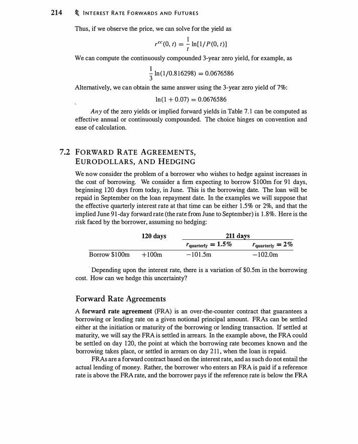
214 � I NT E R EST RATE F O RWA R D S A N D FUTU R ES

Thus, if we observe the price, we can solve for the yield as

rcc (O, t) = � ln [ l / P (O, t)] t

We can compute the continuously compounded 3-year zero yield, for example, as

� ln ( l /0.8 1 6298) = 0.0676586

Alternatively, we can obtain the same answer using the 3-year zero yield of 7%:

ln ( l + 0.07) = 0.0676586

Any of the zero yields or implied forward yields in Table 7 . I can be computed as effective annual or continuously compounded. The choice hinges on convention and ease of calculation.

7.2 FORWARD RATE AGREEMENTS, EURODOLLARS, AND HEDGING

We now consider the problem of a borrower who wishes to hedge against increases in the cost of borrowing. We consider a firm expecting to borrow $ 1OOm for 9 1 days, beginning 120 days from today, in June. This is the borrowing date. The loan will be repaid in September on the loan repayment date. In the examples we will suppose that the effective quarterly interest rate at that time can be either 1 .5% or 2%, and that the implied June 9 1 -day forward rate (the rate from June to September) is 1 .8%. Here is the risk faced by the borrower, assuming no hedging:

120 days 211 days

r quarterly = 1.5 % r quarterly = 2 % Borrow $ 1 OOm + l OOm - 1 0 1 .5m - 1 02.0m

· Depending upon th.e interest rate, there is a variation of $0.5m in the borrowing cost. How can we hedge this uncertainty?

Forward Rate Agreements

A forward rate agreement (FRA) is an over-the-counter contract that guarantees a borrowing or lending rate on a given notional principal amount. FRAs can be settled either at the initiation or maturity of the borrowing or lending transaction. If settled at maturity, we will say the FRA is settled in arrears. In the example above, the FRA could be settled on day 120, the point at which the borrowing rate becomes known and the borrowing takes place, or settled in arrears on day 2 1 1 , when the loan is repaid.

FRAs are a forward contract based on the interest rate, and as such do not entail the actual lending of money. Rather, the borrower who enters an FRA is paid if a reference rate is above the FRA rate, and the borrower pays if the reference rate is below the FRA

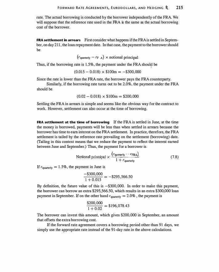
FO RWA R D RATE AG R E E M E NTS, E U RO D O L LA RS, AN D H E D G I N G � 215

rate. The actual borrowing is conducted by the borrower independently of the FRA. We will suppose that the reference rate used in the FRA is the same as the actual borrowing cost of the borrower.

FRA settlement in arrears First consider what happens if the FRA is settled in Septem­ber, on day 2 1 1 , the loan repayment date. In that case, the payment to the borrower should be

(rquanerly - �"FRA) X notional principal

Thus, if the borrowing rate is 1 .5%, the payment under the FRA shoul� be

(0.0 15 - 0.0 1 8) x $100m = -$300, 000

Since the rate is lower than the FRA rate, the borrower pays the FRA counterparty. Similarly, if the borrowing rate turns out to be 2.0%, the payment under the FRA

should be

(0.02 - 0.0 1 8) x $ 1 00m = $200,000

Settling the FRA in arrears is simple and seems like the obvious way for the contract to work. However, settlement can also occur at the time of borrowing.

FRA settlement at the time of borrowing If the FRA is settled in June, at the time the money is borrowed, payments will be less than when settled in arrears because the borrower has time to earn interest on the FRA settlement. In practice, therefore, the FRA settlement is tailed by the reference rate prevailing on the settlement (borrowing) date. (Tailing in this context means that we reduce the payment to reflect the interest earned between June and September.) Thus, the payment for a borrower is

(rquarterly - �"FRA) Notional principal x __:___::.______::. __ ____:_

1 + �"quarterly

If �"quarterly = 1 .5%, the payment in June is

-$300'000 = -$295 566.50

1 + 0.015 '

(7.8)

By definition, the future value of this is -$300, 000. In order to inake this payment, the borrower can borrow an extra $295,566.50, which results in an extra $300,000 loan payment in September. If on the other hand �"quarterly = 2.0% , the payment is

$200,000

0 0? = $ 196, 078 .43

1 + . -

The borrower can invest this amount, which gives $200,000 in September, an amount that offsets the extra borrowing cost.

If the forward rate agreement covers a borrowing period other than 9 1 days, we simply use the appropriate rate instead of the 9 1 -day rate in the above calculations.

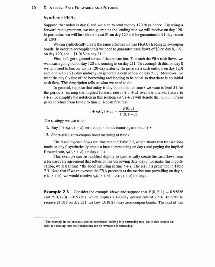
16 � I NT E R EST RATE FO RWA R D S A N D FUTU R ES

Synthetic FRAs

Suppose that today is day 0 and we plan to lend money 120 days hence. By using a forward rate agreement, we can guarantee the lending rate we will receive on day 1 20. In particular, we will be able to invest $1 on day 120 and be guaranteed a 9 1 -day return of 1 .8%.

We can synthetically create the same effect as with an FRA by trading zero-coupon bonds. In order to accomplish this we need to guarantee cash flows of $0 on day 0, -$1 on day 120, and +$ 1 . 0 1 8 on day 2 1 1 .4

First, let's get a general sense of the transaction. To match the FRA cash flows, we , want cash going out on day 120 and coming in on day 2 1 1 . To accomplish this, on day 0 we will need to borrow with a 120-day maturity (to generate a cash outflow on day 1 20) and lend with a 2 1 1 day maturity (to generate a cash inflow on day 2 1 1 ) . Moreover, we want the day 0 value of the borrowing and lending to be equal so that there is no initial cash flow. This description tells us what we need to do.

In general, suppose that today is day 0, and that at time t we want to lend $ 1 for the period s , earning the implied forward rate ro (t , t + s) over the interval from t to t + s . To simplify the notation in this section, r0 (t , t + s) will denote the nonamzua!ized percent return from time t to time s. Recall first that

The strategy we use is to

P (O, t) 1 + ro (t , t + s) = ---­

P (O, t + s)

1. Buy 1 + r0 (t , t + s) zero-coupon bonds maturing at time t + s.

2. Short-sell 1 zero-coupon bond maturing at time t .

The resulting cash flows are illustrated in Table 7 .2 , which shows that transactions made on day 0 synthetically create a loan commencing on day t and paying the implied forward rate, r0 (t, t + s) , on day t + s .

This example can be modified slightly to synthetically create the cash flows from a forward rate agreement that settles on the borrowing date, day t. To make this modifi­cation, we sell at time t the bond maturing at time t + s. The result is presented in Table 7 .3 . Note that if we reinvested the FRA proceeds at the market rate prevailing on day t , r1 (t , t + s ) , we would receive r0 (t , t + s) - r1 (t , t + s) on day t .

Example 7.3 Consider the example above and suppose that P (O, 2 1 1 ) = 0.95836 and P (O, 120) = 0.9756 1 , which implies a 120-day interest rate of 2.5%. In order to receive $ 1 .0 1 8 on day 2 1 1 , we buy 1 . 0 1 8 2 1 1 -day zero-coupon bonds. The cost of this

4The example in the previous section considered locking in a borrowing rate, but in this section we

lock in a lending rate; the transactions can be reversed for borrowing.

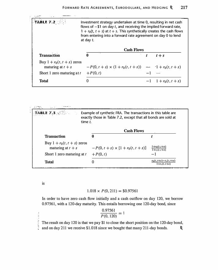
F O RWA R D RATE AG R E E M E NTS, E U RO D O L LA RS, A N D H E D G I N G � 217

I nvestment strategy undertaken at time 0, resu lting in net cash flows of - $ 1 on day t, and receiving the implied forward rate, 1 + r0(t, t + s) at t + s. This synthetical ly creates the cash flows from entering into a forward rate agreement on day 0 to lend at day t.

Cash Flows

Transaction 0 t t + s Buy 1 + ro (t , t + s) zeros

maturing at t + s - P (O, t + s) x ( 1 + ro (t , t + s)) · 1 + ro (t, t + s)

Short 1 zero maturing at t +P (O, t) - 1

Total 0 - 1 l + ro (t , t + s)

Example of synthetic FRA. The transactions in this table are exactly those in Table 7.2, except that a l l bonds are sold at time t.

is

Transaction

Buy 1 + ro (t , t + s) zeros maturing at t + s

Short 1 zero maturing at t

Total

Cash Flows

0

- P (O, t + s) x [ 1 + r0 (t , t + s)]

+ P (O, t)

0

1 . 0 1 8 X P (O, 2 1 1 ) = $0.97561

t

l +ro(t , t+s) l +r1 (t , t+s) - 1

ro(l , t+s)-r, (I , t+s) I +r, (1 , /+sl

In order to have zero cash flow initially and a cash outflow on day 120, we borrow 0.9756 1 , with a 120-day maturity. This entails borrowing one 120-day bond, since

0.9756 1 --- = 1 P (O, 120)

The result on day 120 is that we pay $1 to close the short position on the 120-day bond, and on day 2 l l we receive $ 1 .0 1 8 since we bought that many 2 l l -day bonds. �

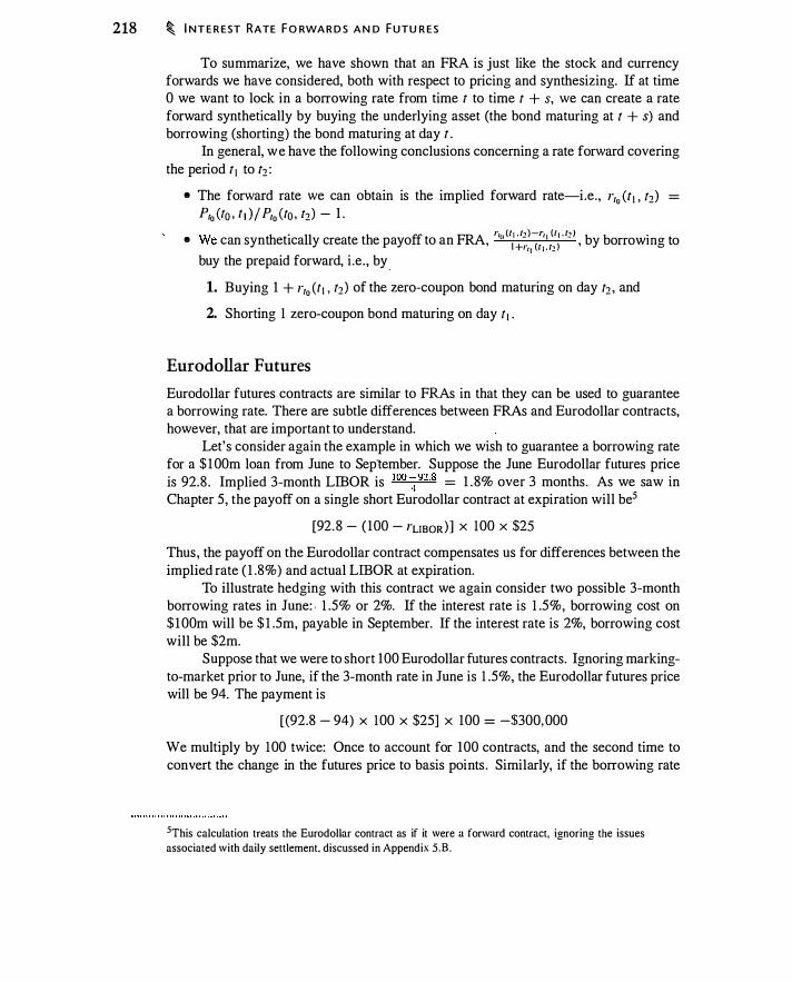
218 � I NT E R EST RATE F O RWA R D S A N D F UTU R ES

To summarize, we have shown that an FRA is just like the stock and currency forwards we have considered, both with respect to pricing and synthesizing. If at time 0 we want to lock in a borrowing rate from time t to time t + s, we can create a rate forward synthetically by buying the underlying asset (the bond maturing at t + s) and borrowing (shorting) the bond maturing at day t .

In general, we have the following conclusions concerning a rate forward covering the period t 1 to t2 :

• The forward rate we can obtain is the implied forward rate-i.e. , r10 (t 1 , t2) = Pr0 (to , t ! ) / P10 (to , t2 ) - 1 .

nr h · ll h ff FRA r," (l , .h )-rq (l , . h )

b b ·

• vve can synt et1ca y create t e payo to an , I +-· ( l - , y orrowmg to , , , l t . l! buy the prepaid forward, i .e. , by

. 1. Buying 1 + r10 Ct1 , t2 ) of the zero-coupon bond maturing on day t2 , and

2. Shorting 1 zero-coupon bond maturing on day t 1 •

Eurodollar Futures

Eurodollar futures contracts are similar to FRAs in that they can be used to guarantee a borrowing rate. There are subtle differences between FRAs and Eurodollar contracts, however, that are important to understand.

Let's consider again the example in which we wish to guarantee a borrowing rate for a $ 1 00m loan from June to Seplember. Suppose the June Eurodollar futures price is 92.8 . Implied 3-month LIBOR is

1 00-:;92·8 = 1 . 8% over 3 months. As we saw in Chapter 5, the payoff on a single short Eurodollar contract at expiration will be5

[92. 8 - ( 100 - I"LJBOR)] X 100 X $25

Thus, the payoff on the Eurodollar contract compensates us for differences between the implied rate ( 1 .8%) and actual LIBOR at expiration.

To illustrate hedging with this contract we again consider two possible 3-month borrowing rates in June: . 1 .5% or 2%. If the interest rate is 1 .5%, borrowing cost on $ 1 00m will be $ 1 .5m, payable in September. If the interest rate is 2%, borrowing cost will be $2m.

Suppose that we were to short 100 Eurodollar futures contracts. Ignoring marking­to-market prior to June, if the 3-month rate in June is 1 .5%, the Eurodollar futures price will be 94. The payment is

[ (92.8 - 94) X 100 X $25] X 100 = -$300, 000

We multiply by 100 twice: Once to account for 100 contracts, and the second time to convert the change in the futures price to basis points . Similarly, if the borrowing rate

5This calculation treats the Eurodollar contract as if it were a forward contract, ignoring the issues associated with daily settlement. discussed in Appendix 5.B.

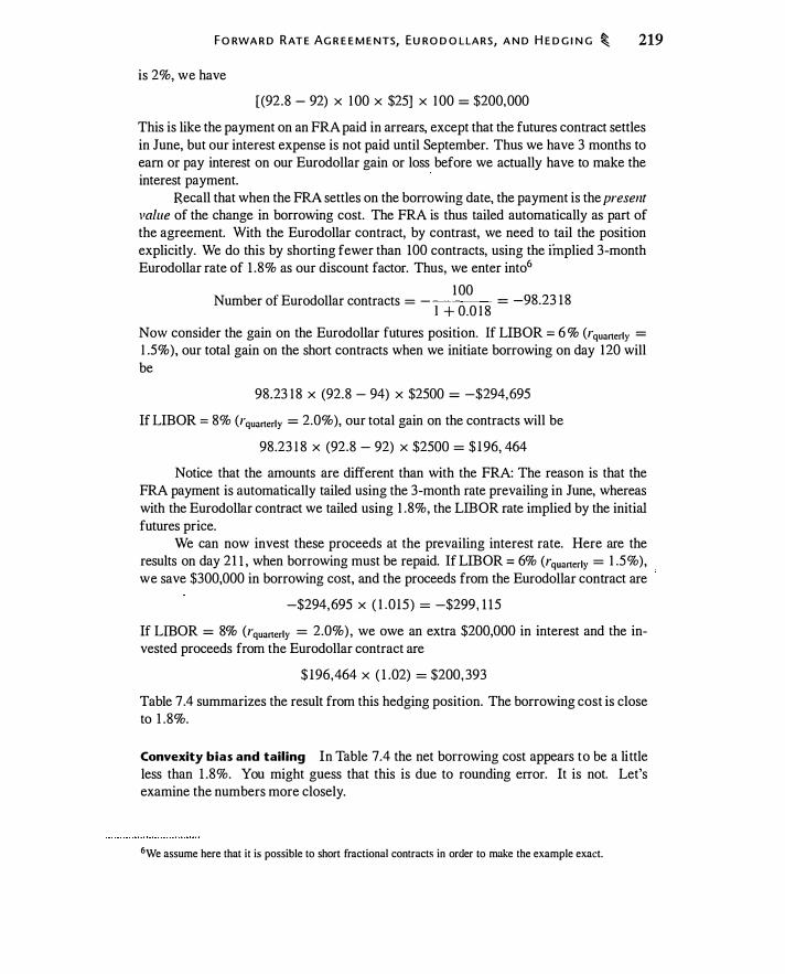
F O RWA R D RAT E AG R E E M E NTS, EU RO D O LLA RS, A N D H E D G I N G � 219

is 2%, we have

((92 .8 - 92) X 1 00 X $25) X 1 00 = $200,000

This is like the payment on an FRA paid in arrears, except that the futures contract settles in June, but our interest expense is not paid until September. Thus we have 3 months to earn or pay interest on our Eurodollar gain or loss before we actually have to make the interest payment.

Recall that when the FRA settles on the borrowing date, the payment is the present value of the change in borrowing cost. The FRA is thus tailed automatically as part of the agreement. With the Eurodollar contract, by contrast, we need to tail the position explicitly. We do this by shorting fewer than 100 contracts, using the implied 3-month Eurodollar rate of 1 .8% as our discount factor. Thus, we enter into6

. 1 00 Number of Eurodollar contracts = - = -98.23 18

1 + 0.0 1 8

Now consider the gain on the Eurodollar futures position. If LID OR = 6 % (rquanerly = 1 .5%), our total gain on the short contracts when we initiate borrowing on day 120 will be

98.23 1 8 X (92.8 - 94) X $2500 = -$294,695

If LIB OR = 8% (rquanerly = 2.0% ), our total gain on the contracts will be

98.23 1 8 X (92 .8 - 92) X $2500 = $ 1 96, 464

Notice that the amounts are different than with the FRA: The reason is that the FRA payment is automatically tailed using the 3-month rate prevailing in June, whereas with the Eurodollar contract we tailed using 1 .8%, the LID OR rate implied by the initial futures price.

We can now invest these proceeds at the prevailing interest rate. Here are the results on day 2 1 1 , when borrowing must be repaid. If LIB OR = 6% (rquanerly = 1 .5% ) , we save $300,000 in borrowing cost, and the proceeds from the Eurodollar contract are

-$294, 695 X ( 1 .015) = -$299 , 1 15

If LIBOR = 8% (rquanerly = 2.0%) , we owe an extra $200,000 in interest and the in­vested proceeds from the Eurodollar contract are

$ 196,464 X ( 1 .02) = $200, 393

Table 7.4 summarizes the result from this hedging position. The borrowing cost is close to 1 .8%.

Convexity bias and tailing In Table 7.4 the net borrowing cost appears to be a little less than 1 .8%. You might guess that this is due to rounding error. It is not. Let's examine the numbers more closely.

6We assume here that it is possible to short fractional contracts in order to make the example exact.

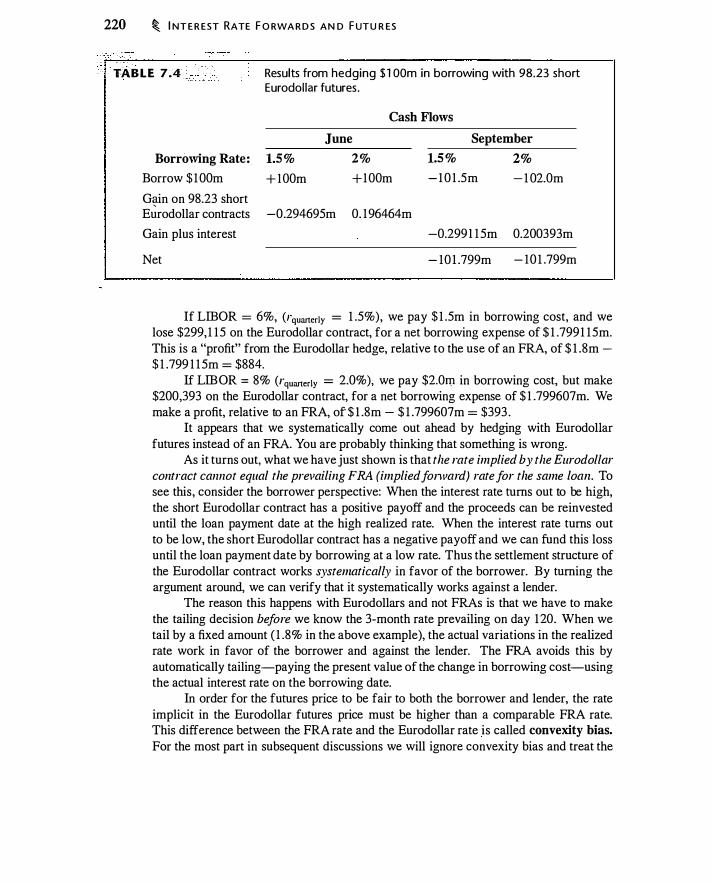
220 � I NT E R EST RATE F O RWA R D S AN D F UTU R ES

TABLE 7A Results from hedging $ 1 OOm in borrowing with 98.23 short Eurodollar futures .

Cash Flows

Borrowing Rate : .

Borrow $ 1OOm

G{lin on 98.23 short

1.5%

+ lOOm

June

2%

+lOOm

Eurodollar contracts -0.294695m 0. 196464m

Gain plus interest

Net

September

1.5 %

- 1 0 1 .5m

2%

- 1 02.0m

-0.299 1 1 5m 0.200393m

- 10 1 .799m - 10 1 .799m

If LIBOR = 6%, (rquarterly = 1 .5%), we pay $ 1 .5m in borrowing cost, and we lose $299, 1 15 on the Eurodollar contract, for a net borrowing expense of $ 1 .799 1 15m. This is a "profit" from the Eurodollar hedge, relative to the use of an FRA, of $ 1 .8m ­$ 1 .799 1 1 5m = $884.

If LIBOR = 8% (rquarterly = 2.0%), we pay $2.0q� in borrowing cost, but make $200,393 on the Eurodollar contract, for a net borrowing expense of $ 1 .799607m. We make a profit, relative to an FRA, of$ 1 .8m - $ 1 .799607m = $393 .

It appears that we systematically come out ahead by hedging with Eurodollar futures instead of an FRA. You are probably thinking that something is wrong.

As it turns out, what we have just shown is that the rate implied by the Eurodollar contract cannot equal the prevailing FRA (implied fonvard) rate for the same loan. To see this, consider the borrower perspective: When the interest rate turns out to be high, the short Eurodollar contract has a positive payoff and the proceeds can be reinvested until the loan payment date at the high realized rate. When the interest rate turns out to be low, the short Eurodollar contract has a negative payoff and we can fund this loss until the loan payment date by borrowing at a low rate. Thus the settlement structure of the Eurodollar contract works systematically in favor of the borrower. By turning the argument around, we can verify that it systematically works against a lender.

The reason this happens with Eurodollars and not FRAs is that we have to make the tailing decision before we know the 3-month rate prevailing on day 120. When we tail by a fixed amount ( 1 .8% in the above example), the actual variations in the realized rate work in favor of the borrower and against the lender. The FRA avoids this by automatically tailing-paying the present value of the change in borrowing cost-using the actual interest rate on the borrowing date.

In order for the futures price to be fair to both the borrower and lender, the rate implicit in the Eurodollar futures price must be higher than a comparable FRA rate. This difference between the FRA rate and the Eurodollar rate is called convexity bias.

For the most part in subsequent discussions we will ignore convexity bias and treat the

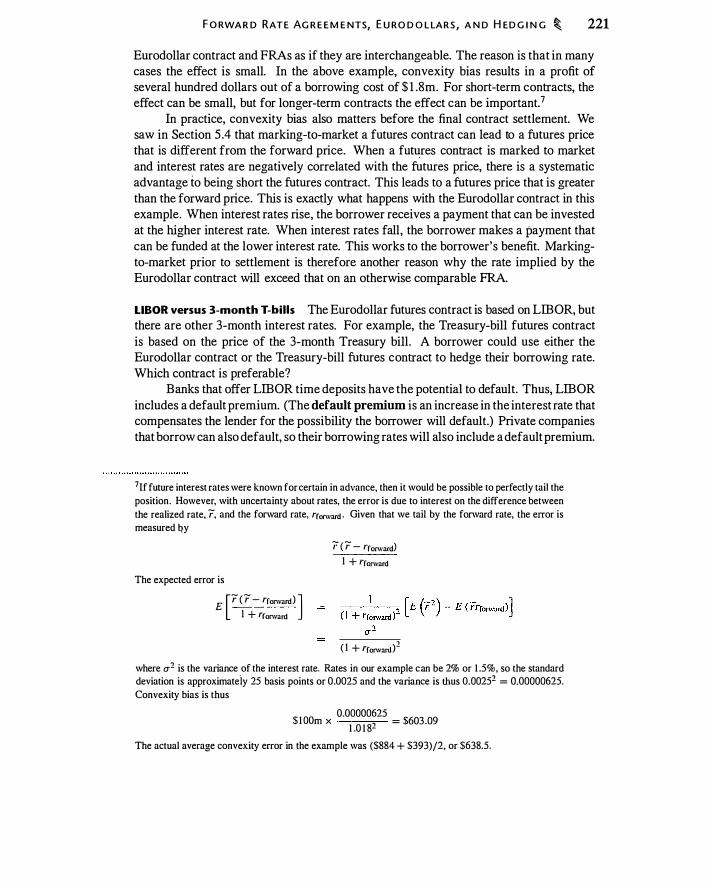
F O RWA R D RATE AG R E E M E NTS, E U RO D O L LARS , A N D H ED G I N G � 221

Eurodollar contract and FRAs as if they are interchangeable. The reason is that in many cases the effect is small. In the above example, convexity bias results in a profit of several hundred dollars out of a borrowing cost of $ 1 .8m. For short-term contracts, the effect can be small, but for longer-term contracts the effect can be important.7

In practice, convexity bias also matters before the final contract settlement. We saw in Section 5 .4 that marking-to-market a futures contract can lead to a futures price that is different from the forward price. When a futures contract is marked to market and interest rates are negatively correlated with the futures price, there is a systematic advantage to being short the futures contract. This leads to a futures price that is greater than the forward price. This is exactly what happens with the Eurodollar contract in this example. When interest rates rise, the borrower receives a payment that can be invested at the higher interest rate. When interest rates fall, the borrower makes a payment that can be funded at the lower interest rate. This works to the borrower's benefit. Marking­to-market prior to settlement is therefore another reason why the rate implied by the Eurodollar contract will exceed that on an otherwise comparable FRA.

LIBOR versus 3-month T-bills The Eurodollar futures contract is based on LIB OR, but there are other 3-month interest rates. For example, the Treasury-bill futures contract is based on the price of the 3-month Treasury bill. A borrower could use either the Eurodollar contract or the Treasury-bill futures contract to hedge their borrowing rate. Which contract is preferable?

Banks that offer LIB OR time deposits have the potential to default. Thus, LIB OR includes a default premium. (The default premium is an increase in the interest rate that compensates the lender for the possibility the borrower will default.) Private companies that borrow can also default, so their borrowing rates will also include a default premium.

7If future interest rates were known for certain in advance, then it would be possible to perfectly tail the position . However, with uncertainty about rates, the error is due to interest on the difference between the realized rate, r, and the forward rate, Tforward · Given that we tail by the forward rate, the error is measured by

The expected error is

r ( r- I" forward) I + /"forward

E [r (r- Tforward) J I + /"forward

( I + Tforward)2

where a1 is the variance of the interest rate. Rates in our example can be 2% or 1 .5%, so the standard deviation is approximateiy 25 basis points or 0.0025 and the variance is thus 0.00252 = 0.00000625. Convexity bias is thus

$ 1 00 0.00000625

= $603 09 m x 1 .0 1 82

.

The actual average convexity error in the example was ($884 + $393)/2, or $638.5.

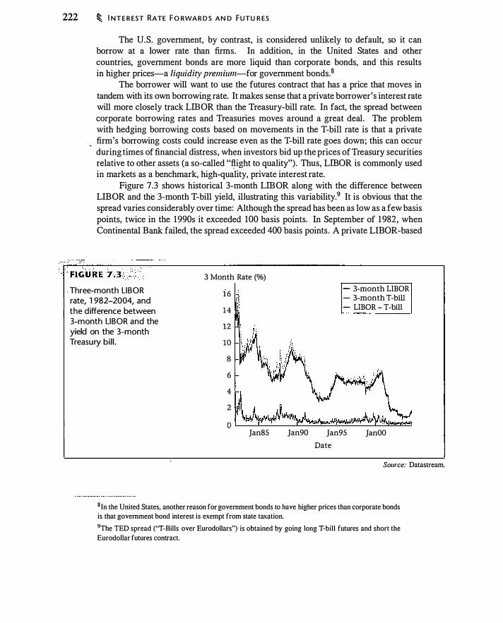
222 � I NT E R EST RATE F O RWA R D S AN D FUTU R ES

The U.S. government, by contrast, is considered unlikely to default, so it can borrow at a lower rate than firms. In addition, in the United States and other countries, government bonds are more liquid than corporate bonds, and this results in higher prices-a liquidity premium-for government bonds.8

The borrower will want to use the futures contract that has a price that moves in tandem with its own borrowing rate. It makes sense that a private borrower's interest rate will more closely track LIB OR than the Treasury-bill rate. In fact, the spread between corporate borrowing rates and Treasuries moves around a great deal. The problem with hedging borrowing costs based on movements in the T-bill rate is that a private firm's borrowing costs could increase even as the T-bill rate goes down; this can occur during times of financial distress, when investors bid up the prices of Treasury securities relative to other assets (a so-called "�ight to quality"). Thus, LIBOR is commonly used in markets as a benchmark, high-quality, private interest rate.

Figure 7.3 shows historical 3-month LIBOR along with the difference between LIBOR and the 3-month T-bill yield, illustrating this variability.9 It is obvious that the spread varies considerably over time: Although the spread has been as low as a few basis points, twice in the 1990s it exceeded 100 basis points. In September of 1 982, when Continental Bank failed, the spread exceeded 400 basis points. A private LIBOR-based

. Three-month UBOR rate, 1 982-2004, and the difference between 3-month UBOR and the yield on the 3-month Treasury bi l l .

3 Month Rate (o/o)

i6 14

12

10

8

6 4

2

Jan85 Jan90

- 3-month LIBOR - 3-month T-bill - LIBOR - T-bill

Jan95

Date

JanOO

Source: Datastream.

8 In the United States, another reason for government bonds to have higher prices than corporate bonds

is that government bond interest is exempt from state taxation. 9The TED spread ("T-Bills over Eurodollars") is obtained by going long T-bill futures and short the

Eurodollar futures contract.

D U RAT I O N A N D C O N V EX ITY � 223

borrower who had hedged its borrowing rate by shorting T-hill futures in August of 1 982 would by September have lost money on the T-hill contract as Treasury rates declined, while the actual cost of borrowing (LID OR) would have remained close to unchanged. This example illustrates the value of using a hedging contract that reflects the actual cost of borrowing.

The Eurodollar futures contract is far more popular than the T-hill futures contract. Trading volume and open interest on the two contracts were about equal in the early 1980s. }Iowever, in August 2004, open interest on the Eurodollar contract exceeded 6 million contracts, while the T-hill contract had zero open interest. This is consistent with LffiOR being a better measure of private sector interest rates than the T-hill yield.

Interest Rate Strips and Stacks

Suppose a borrower plans to borrow $ 1OOm by rolling over 3-month debt for a period of 2 years, beginning in 6 months. Thus, the borrowing will take place in month 6, month 9, month 12, etc. The borrower in this situation faces eight unknown quarterly borrowing rates. We saw in Section 6. 12 that an oil hedger could hedge each commitment individually (a strip) or could hedge the entire commitment using one near-dated contract (a stack) . The same alternatives are available with interest rates.

One way to hedge is to enter into separate $ 100m FRAs for each future 3-month period. Thus, we would enter into one FRA for months 6-9, another for months 9-12, etc. This strip hedge should provide a perfect hedge for future borrowing costs.

Depending on market conditions, using a strip is not a! ways feasible. For example,·

forward prices may not be available with distant maturities, or liquidity may be poor at distant maturities. Rather than individually hedging the borrowing cost of each quarter, an alternative in the context of this example is to use a "stack" of short-term FRAs or Eurodollar contracts to hedge the present value of future borrowing costs.

In the above example, we will be borrowing $ 1 00 million per quarter for eight quarters. To effect a stack, we would enter into forward agreements on the 3-month rate, maturing in 6 months, for slightly less than $800 million. (We enter into less than $800 · million

. of forward rate agreements due to tailing for quarters 2 through 8 .)

As with the oil example in Section 6. 12, the obvious problem with a stacking strat­egy is basis risk: Quarterly borrowing costs in distant quarters may not move perfectly with borrowing costs in near quarters.

Once we reach the first quarter of borrowing, all of the forward agreements mature and we need to renew our hedge. We now face seven quarters with unknown borrowing costs and therefore we enter into forward agreements for slightly less than $700 million. The constant renewal of the hedging position necessary to effect a stack and roll is exactly like that in the oil example.

7.3 DURATION AND CONVEXITY

An important characteristic of a bond is the sensitivity of its price to interest rate changes, which we measure using duration. Duration tells us approximately how much the bond's price will change for a given change in the bond's yield. Duration is thus a summary

224 � I NT E R EST RATE F O RWA R D S AN D FUTU R ES

measure of the risk of a bond, permitting a comparison of bonds with different coupons, times to maturity, and discounts or premiums relative to principal. In this section we also discuss convexity, which is another measure related to bond price risk.

Duration

Suppose a bond makes m coupon payments per year for T years in the amount C 1m , and pays M at maturity. Let y 1m be the per-period yield to maturity (by convention, y is the annualized yield to maturity) and n = m x T the number of periods until maturity. The price of the bond, B (y), is given by

L" Clm M B (y) = . . + ----. ( l + ylm)' ( 1 + ylm)" l = l

The change in the bond price for a unit change in the yield, y, is 10

Change in bond price � i C I m n M Unit change in yield

= - {=; m ( 1 + ylm)i+ 1 - m ( 1 + ylm)"+l

1 [� i c I m n M ] = -1 + ylm {=; m ( 1 + ylm)i

+ m ( 1 + ylm)"

<7·9)

Equation (7 .9) tells us the dollar change in the bond price for a change of 1 .0 in y. It is natural to scale this either to reflect a change per percentage point [in which case we divide equation (7.9) by 100] or per basis point [divide equation (7.9) by 10,000] . Equation (7.9) divided by 10,000 is also known as the price value of a basis point (PVBP). To interpret PVBP for a bond, we need to know the par value of the bond.

Example 7.4 Consider the 3-year zero-coupon bond in Table 7 . 1 with a yield to maturity of 7%. The bond price per $ 100 of maturity value is $ 1 001 1 .073 = $81 .62979. At a yield of7.01 %, one basis point higher, the bond price is $ 1001 1 .070 1 3 = $8 1 .6069 1 , a change of -$0.02288 per $ 100 of maturity value.

As an alternative way to derive the price change, we can compute equation (7.9) with C = 0, M = $ 100, n = 3, and m = 1 to obtain

I $ 100 - - X 3 X -- = -$228.87

1 .07 1 .073

In order for this to reflect a change of I basis point, we divide by I 0,000 to obtain

-$228 .871 10 ,000 = -$0.02289, almost equal to the actual bond price change. This illustrates the importance of scaling equation (7.9) appropriately. �

1 0This is obtained by computing the derivative of the bond price with respect to the yield, dB(y)jdy.

D U RATI O N A N D C O N V EX I TY � 225

When comparing bonds with different prices and par values, it is helpful to have a measure of price sensitivity expressed per dollar of bond price. We obtain this by dividing equation (7.9) by the bond price, B(y) and multiplying by - 1 . This gives us a measure known as modified duration, which is the percentage change in the bond price for a unit change in the yield:

Change in bond price I Modified duration = - �

x -· -Unit change in yield B(y)

1 1 [� i c I m n M ]

B(y) I + ylm {;;;: 7;; ( I + ylm)i +

m ( I + ylm)" (7. 1 0)

We obtain another measure of bond price risk-Macaulay duration-by multi­plying equation (7. 1 0) by 1 + ylmY This puts both bond price and yield changes in percentage terms and gives us an expression with a clear interpretation:

Change in bond price Macaulay duration = - x

Unit change in yield

1 + ylm B(y)

1 [t i C I m n M ]

B(y) i= l m ( l + ylm ) i + m ( 1 + ylm)"

(7. 1 1 )

To interpret this expression, note that ( C I m) I ( 1 + y I m ) ; is the present value of the i th bond payment, which occurs in i I m years. The quantity C I ml [( l + y I m ); B(y)] is therefore the fraction of the bond value that is due to the i th payment. Macaulay duration is a weighted average of the time (number of periods) until the bond payments occur, with the weights being the percentage of the bond price accounted for by each payment. This interpretation of Macaulay duration as a time-to-payment measure explains why these measures of bond price sensitivity are called "duration." 1 2 For a zero-coupon bond, equation (7. l l ) implies that Macaulay duration equals time to maturity.

Macaulay duration illustrates why maturity alone is not a satisfactory risk measure for a coupon bond. A coupon bond makes a series of payments, each with a different maturity. Macaulay duration summarizes bond price risk as a weighted average of these different maturities.

1 1 This measure of duration is named after Frederick Macaulay, who wrote a classic history of interest rates (Macaulay, 1 938). 1 2The Excel duration functions are Duration for Macaulay duration and MDuration for modified duration.

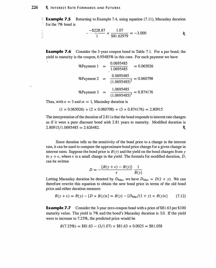
226 � I NT E R EST RATE F O RWA R D S A N D FUTU R ES

,. Example 7 .S Returning to Example 7 .4, using equation (7 . I I ), Macaulay duration for the 7% bond is

-$228.87 1 .07 0 0 ---- X = -3. 0

I $81 .62979

Example 7.6 Consider the 3-year coupon bond in Table 7. 1 . For a par bond, the yield to maturity is the coupon, 6.95485% in this case. For each payment we have

%Payment I =

%Payment 2

%Payment 3 =

0.0695485

1 .0695485 = 0.065026

0.0695485 = 0.060798 ( I .0695485)2

1 .0695485 0 8 6 ----""73 = . 74I 7

( 1 .0695485)

Thus, with n = 3 and m = 1, Macaulay duration is

( 1 X 0.065026) + (2 X 0.060798) + (3 X 0.874176) = 2.809 15

The interpretation of the duration of2.8 I i s that the bond responds to interest rate changes as if it were a pure discount bond with 2.8 1 years to maturity. Modified duration is 2 .809 15/ 1 .0695485 = 2.626482. �

Since duration tells us the sensitivity of the bond price to a change in the interest rate, it can be used to compute the approximate bond price change for a given change in interest rates. Suppose the bond price is B (y) and the yield on the bond changes from y to y + E , where E is a small change in the yield. The formula for modified duration, D, can be written

D = [B (y + E) - B (y)] I

E B (y)

Letting Macaulay duration be denoted by DMac , we have DMac = D(l + y). We can therefore rewrite this equation to obtain the new bond price in terms of the old bond price and either duration measure:

B (y + E) = B(y) - [D X B (y)E] = B (y) - (DMac/0 + y) X B(y)E] (7 . 1 2)

Example 7.7 Consider the 3-year zero-coupon bond with a price of $8 I .63 per $ 100 maturity value. The yield is 7% and the bond's Macaulay duration is 3.0. If the yield were to increase to 7.25%, the predicted price would be

B (7 .25%) = $81 .63 - (3/ 1 .07) X $8 1 .63 X 0.0025 = $8 1 .058

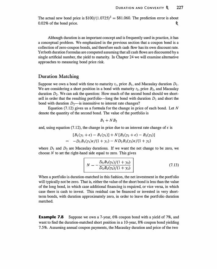
D U R AT I O N A N D C O N V E X I TY � 227

The actual new bond price is $ 100/ ( 1 .0725)3 = $8 1 .060. The prediction error is about 0.02% of the bond price. �

Although duration is an important concept and is frequently used in practice, it has a conceptual problem. We emphasized in the previous section that a coupon bond is a collection of zero-coupon bonds, and therefore each cash flow has its own discount rate. Yet both duration formulas are computed assuming that all cash flows are discounted by a single artificial number, the yield to maturity. In Chapter 24 we will examine alternative approaches to measuring bond price risk.

Duration Matching

Suppose we own a bond with time to maturity t1 , price B 1 , and Macaulay duration D1 • We are considering a short position in a bond with maturity t2 , price B2 , and Macaulay duration D2 . We can ask the question: How much of the second bond should we short­sell in order that the resulting portfolio-long the bond with duration D 1 and short the bond with duration D2-is insensitive to interest rate changes?

Equation (7 . 12) gives us a formula for the change in price of each bond. Let N denote the quantity of the second bond. The value of the portfolio is

B 1 + NB2

and, using equation (7 . 1 2) , the change in price due to an interest rate change of E is

[B I ()' I + E) - Bl (yl )] + N [B2 (Y2 + E) - B2 ()'2)]

-DI BI ()' J )E/ ( 1 + )' J ) - ND2B2 CY2)E/ ( l + )'2)

where D 1 and D2 are Macaulay durations. If we want the net change to be zero, we choose N to set the right-hand side equal to zero. This gives

(7. 13)

When a portfolio is duration-matched in this fashion, the net investment in the portfolio will typically not be zero. That is, either the value of the short bond is less than the value of the long bond, in which case additional financing is required, or vice versa, in which case there is cash to invest. This residual can be financed or invested in very short­term bonds, with duration approximately zero, in order to leave the portfolio duration matched.

Example 7.8 Suppose we own a 7-year, 6% coupon bond with a yield of 7%, and want to find the duration-matched short position in a 1 0-year, 8% coupon bond yielding 7.5%. Assuming annual coupon payments, the Macaulay duration and price of the two

228 � I NT E R EST RAT E FO RWA R D S A N D FUTU R ES

bonds is 5.882 years and $94.6 l l , and 7.297 years and $ 1 03 .432, respectively. Thus, if we own one of the 7-year bonds, we must hold

_ 5 .882 X 94.6 1 1 /( 1 .07) = _0_7408

7.297 X 1 03 .432/ ( 1 .075)

units of the 1 0-year bond. The short position in the 10-year bond is not enough to pay for the 7-year bond; hence, investment in the portfolio is 1 x 94.6 1 1 - 0.7408 x 1 03 .432 = 17 .99. If the yield on both bonds increases 25 basis points, the price change of the portfolio is

- 1 .289 + (-0.7408) X - 1 .735 = -0.004

Convexity ·

The hedge in example 7.8 is not perfect because duration changes as the interest rate changes. 1 3 Convexity measures the extent to which duration changes as the bond's yield changes. The formula for convexity is 14

. 1 [L" i (i + 1 ) Cfm n (n + 1 ) M ] Convexity = -- . + --'----=---'-- --------=-

B (y) i = l m2 ( l + y/m)'+2 m2 ( l + y/m)"+2

(7. 14)

We can use convexity in addition to duration to obtain a more accurate prediction of the new bond price. When we include convexity, the price prediction formula, equation (7. 1 2), becomes 1 5

B(y + E) = B(y) - [D x B (y) x E] + 0.5 x Convexity x B(y) x E2 (7. 15)

where D i s modified duration. Here is an example of computing a bond price at a new yield using both duration and convexity.

Example 7.9 Consider again example 7.7. We want to predict the new price of a 3-year zero-coupon bond when the interest rate changes from 7% to 7.25%. Using

1 3At the original yields, we computed a hedge ratio of 0.7408. Problem 7. 1 9 asks you to compute

the hedge ratio that would have exactly hedged the portfolio had both interest rates increased 25 basis points and decreased 25 basis points. The two hedge ratios are different, which means that one hedge

ratio would not have worked perfectly.

14Th is is obtained by taking the second derivative of the bond price with respect to the yield to maturity, d2 B (y)fdy2 , and normalizing the result by dividing by the bond price. 15If you recall calculus, you may recognize equation (7 . 1 2) as a Taylor series expansion of the bond

price. See Appendix 1 3.A

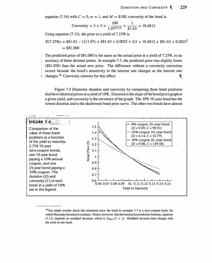
D U R AT I O N AN D C O N V EX ITY � 229

equation (7 . 14) with C = 0, m = 1 , and M = $ 1 00, convexity of the bond is

. 100 1 ConveXIty = 3 X 4 X

l .Q7(3+2l X 8 1 .63

= 10.48 12

Using equation (7 . 15), the price a t a yield of 7.25% is

B(7.25%) = $8 1 .63 - (3/ 1 .07) X $8 1 .63 X 0.0025 + 0.5 X 10 .48 12 X $8 1 .63 X 0.00252

= $8 1 .060

The predicted price of $8 1 .060 is the same as the actual price at a yield of 7.25%, to an accuracy of three decimal points . In example 7.7, the predicted price was slightly lower ($8 1 .058) than the actual new price. The difference without a conv�xity correction occurs because the bond's sensitivity to the interest rate changes as the interest rate changes. 16 Convexity corrects for this effect. �

Figure 7.4 illustrates duration and convexity by comparing three bond positions that have identical prices at a yield of 10%. Duration is the slope of the bond price graph at a given yield, and convexity is the curvature of the graph. The 10% 1 0-year bond has the lowest duration and is the shallowest bond price curve. The other two bonds have almost

Comparison of the value of three bond positions as a function of the yield to maturity: 2 .71 8 1 0-year zero-coupon bonds, one 1 0-year bond paying a 1 0% annual coupon, and one 25-year bond paying a 1 0% coupon. The duration (D) and convexity (C) of each bond at a yield of 1 0% are in the legend.

1.5

1 .4

0 .9

0 .8

0.7

- 0% coupon 10-year bond (D = 9 .09, C = 90.91)

- 10% coupon 10-year bond (D = 6.14, C = 52.79)

- 10% coupon 25-year bond (D = 9.08, C = 139.58)

0.6 �--L--'---L..___l._.J..__J___l. _ __t__.l__ 0.06 0.07 0.08 0.09 01 0 . 1 1 0.12 0.13 0 .14 0.15

Yield to Maturity

1 6You might wonder about this statement since the bond in example 7.7 is a zero-coupon bond, for

which Macaulay duration is constant. Notice, however, that the bond price prediction formula, equation

(7. 1 2), depends on modified duration, which is DMaciO + y). Modified duration does change with

the yield on the bond.

230 � I NT E R EST RATE F O RWA R D S A N D F UTU R ES

equal durations at a yield of 10% and their slopes are equal in the figure. However, the 25-year bond exhibits greater curvature: Its price is above the 10-year bond at both lower and higher yields. This greater curvature is what it means for the 25-year bond to have greater convexity.

The idea that using both duration and convexity provides a more accurate model of bond price changes is not particular to bonds, but it pertains to options as well . This is our first glimpse of a crucial idea in derivatives that will appear again in Chapter 13 when we discuss delta-gamma approximations, as well as throughout the book.

7.4 TREASURY-B OND AND TREASURY-NOTE FUTURES

The Treasury-note and Treasury-bond futures contracts are important instruments for hedging interestrate risk. 1 7 Figure 7.5 shows newspaper listings for these futures, and the specifications for the T-note contract are listed in Figure 7 .6 . The bond contract is sirrular except that the deliverable bond has a maturity of at least 15 years, or if the bond is callable, has 15 years to first call . The two contracts are similar; we will focus here on the T-note contract. In this discussion we will use the terms "bond" and "note" interchangeably.

The basic idea of the T-note contract is that a long position is an obligation to buy a 6% bond with between 6.5 and 10 years to maturity. To a first approximation we can think of the underlying as being like a stock with a dividend yield of 6%. The futures price would then be computed as with a stock index: The future value of the current bond price, less the future value of coupons payable over the life of the futures contract.

F I G U R E 7 . 5 .-

Treasury-bond and Treasury-note futures l istings from the Wall Street journal, Ju ly 2 1 ,

2004.

Interest Rate Futures Treasury Bonds (CBT)·$IOO,ooo; pis 32nds of 100I Sopt 109·13 109-14 108-ll7 108-ll -32 ll4-30 101·24 504,m D" 107-28 108-liO 107-ll1 107-04 -32 113-07 1011-24 18,209 Est vol 220,782; vol Mon 136,287; open lnt 522,624, -1L075.

Treasury Notes (CBTl·$100.000; pis 32nds of 100� Sept ll·ll5 ll-125 lllf-16 111-185 -24.0 15.095 106·13 1,333,368 DO< 109·30 UO-liO 09·095 109·10 -Z4.0 13-ll45 105-14 35,374 Est vol 723,n9; vol Mon 388,611; opon int 1,368,752. -11,572. 5 Yr. Treasury Notes (CBT)-$100,000; pis 32nds of 100� Sopt lllf-01 lllf-01 109-13 109-15 -17.0 UZ-15 106-29 1,162,334 Est vol 408,DZ4; vol Mon 164,023; opi!n int 1,235,146, •3,661

2 Yr. Treasury Notes (Cim-$2oo,ooo; pis 3Znds of 100� Sopt 05-235 105-24 05-162 105·17 -f>.7 106-01 04·187 187,818 Est vol ZO,JZZ; vol Mon 14,354; open lnt 187,818, -1,093.

1 7The interest rate on the I 0-year Treasury note is a commonly used benchmark interest rate, hence the I 0-year note futures are important.

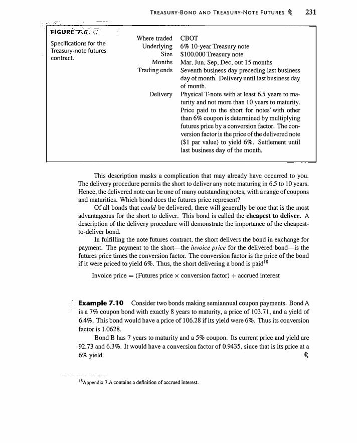
Specifications for the Treasury-note futures contract.

TREASURY-BOND AND TREASURY-NOTE FUTURES � 231

Where traded CBOT Underlying

Size Months

Trading ends

6% 10-year Treasury note $100,000 Treasury note Mar, Jun, Sep, Dec, out 15 months Seventh business day preceding last business day of month. Delivery until last business day of month.

Delivery Physical T-note with at least 6.5 years to ma­turity and not more than 10 years to maturity. Price paid to the short for notes· with other than 6% coupon is determined by multiplying futures price by a conversion factor. The con­version factor is the price of the delivered note ($1 par value) to yield 6%. Settlement until last business day of the month.

This description masks a complication that may already have occurred to you. The delivery procedure permits the short to deliver any note maturing in 6.5 to 10 years. Hence, the delivered note can be one of many outstanding notes, with a range of coupons and maturities. Which bond does the futures price represent?

Of all bonds that could be delivered, there will generally be one that is the most advantageous for the short to deliver. This bond is called the cheapest to deliver. A description of the delivery procedure will demonstrate the importance of the cheapest­to-deliver bond.

In fulfilling the note futures contract, the short delivers the bond in exchange for payment. The payment to the short-the invoice price for the delivered bond-is the futures price times the conversion factor. The conversion factor is the price of the bond if it were priced to yield 6%. Thus, the short delivering a bond is paid 18

Invoice price = (Futures price x conversion factor) + accrued interest

Example 7.10 Consider two bonds making semiannual coupon payments. Bond A is a 7% coupon bond with exactly 8 years to maturity, a price of 103.71, and a yield of 6.4%. This bond would have a price of 106.28 if its yield were 6%. Thus its conversion factor is 1.0628.

Bond B has 7 years to maturity and a 5% coupon. Its current price and yield are 92.73 and 6.3%. It would have a conversion factor of 0.9435, since that is its price at a 6% yield. �

18 Appendix 7 .A contains a definition of accrued interest.

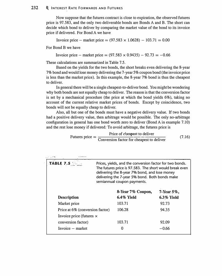
232 � INTEREST RATE FORWARDS AND FUTURES

Now suppose that the futures contract is close to expiration, the observed futures price is 97.583, and the only two deliverable bonds are Bonds A and B. The short can decide which bond to deliver by comparing the market value of the bond to its invoice price if delivered. For Bond A we have

Invoice price- market price= (97.583 x 1.0628) - 103.71 = 0.00

For Bond B we have

Invoice price- market price= (97.583 x 0.9435)- 92.73 = -0.66

These calculations are summarized in Table 7.5. Based on the yields for the two bonds, the short breaks even delivering the 8-year

7% bond and would lose money delivering the 7-year 5% coupon bond (the invoice price is less than the market price). In this example, the 8-year 7% bond is thus the cheapest to deliver.

In general there will be a single cheapest-to-deliver bond. You might be wondering why both bonds are not equally cheap to deliver. The reason is that the conversion factor is set by a mechanical procedure (the price at which the bond yields 6%), taking no account of the current relative market prices of bonds. Except by coincidence, two bonds will not be equally cheap to deliver.

Also, all but one of the bonds must have a negative delivery value. If two bonds had a positive delivery value, then arbitrage would be possible. The only no-arbitrage configuration in general has one bond worth zero to deliver (Bond A in example 7.10) and the rest lose money if delivered: To avoid arbitrage, the futures price is

Price of cheapest to deliver Futures price = --------=-------­

Conversion factor for cheapest to deliver (7.16)

TABLE 7.5 .· .... . . . . .

Description

Market price

Prices, yields, and the conversion factor for two bonds. The futures price is 97.583. The short would break even delivering the 8-year 7% bond, and lose money delivering the 7-year 5% bond. Both bonds make semiannual coupon payments.

8-Year7% Coupon, 7-YearS%,

6.4% Yield 6.3% Yield

103.71 92.73 Price at 6% (conversion factor) 106.28 94.35 Invoice price (futures x

conversion factor) 103.71 92.09 Invoice - market 0 -0.66

REPURCHASE AGREEMENTS � 233

This discussion glosses over subtleties involving transaction costs (whether you already own a bond may affect your delivery profit calculation) and uncertainty before the delivery period about which bond will be cheapest to deliver. Also the T-note is deliverable at any time during the expiration month, but trading ceases with 7 business days remaining. Consequently, if there are any remaining open contracts during the last week of the month, the short has the option to deliver any bond at a price that might be a week out of date. This provides a delivery option for the short that is also priced into the contract. There are other complications, but suffice it to say that the T-bond and T-note contracts are complex.

The T-bond and T-note futures contracts have been extremely successfuL The contracts illustrate some important design considerations for a futures contract. Consider first how the contract is settled. If the contract designated a particular T-bond as the underlying asset, that T-bond could be in short supply, and in fact it might be possible for someone to corner the available supply. (A market corner occurs when someone buys most or all of the deliverable asset or commodity.) A short would then be unable to obtain the bond to deliver. In addition, the deliverable T-bond would change from year to year and the contract would become more complicated, since traders would have to price the futures differently to reflect different underlying bonds for different maturity dates.

An alternative scheme could have had the contract cash-settle against a T-bond index, much like the S&P 500. This arrangement, however, introduces basis risk, as the T-bond futures contract might then track the index but fail to track any particular bond.

In the end, settlement procedures for the T-bond and T-note contracts permitted a range of bonds and notes to be delivered. Since a high-coupon bond is worth more than an otherwise identical low-coupon bond, there had to be a conversion factor, in order that the short is paid more for delivering the high-coupon bond.

The idea that there is a cheapest to deliver is not exclusive to Treasury bonds. The same issue arises with commodities, where a futures contract may permit delivery of commodities at different locations or of different qualities.

7.5 REPURCHASE AGREEMENTS

An extremely important kind of forward contract is a repurchase agreement, or repo.19 A repo entails selling a security with an agreement to buy it back at a fixed price. It is effectively a reverse cash-and-carry-a sale coupled with a long forward contract. Like any reverse cash-and-carry, it is equivalent to borrowing. The particular twist with a repo is that the underlying security is held as collateral by the counterparty, who has bought the security and agreed to sell it at a fixed price. Thus, a repo is collateralized borrowing. Repos are common in bond markets, but in principle a repurchase agreement can be used for any asset.

19For a detailed treatment of repurchase agreements, see Steiner ( 1997).

234 � INTEREST RATE FORWARDS AND FUTURES

Example 7.11 Suppose you enter into a 1-week repurchase agreement for a 9-month $1m Treasury bill. The current price of the T-bill is $956,938, and you agree to repurchase it in I week for $958,042. You have borrowed money at a 1-week rate of 958,042/956,938- 1 = 0.115%, receiving cash today and promising to repay cash plus interest in a week. The security provides collateral for the loan. �

The party who initiates the repo owns the asset when the transaction is completed and is therefore the financial owner of the security. During the repo, however, the coun­terparty owns the bond. Most repos are overnight. A longer-term repurchase agreement is called a term repo.

The counterparty is said to have entered into a reverse repurchase agreement, or reverse repo, and is short the forward contract. This is a loan of cash for the duration of the agre.ement with a security held as collateral. It can also be described as a cash­and-carry.

If the borrower does not repay the loan, the lender keeps the security. Thus, the counterparty's view of the risk of the transaction differs according to the quality of the collateral. Collateral with a more variable price and a less liquid market is lower quality from the perspective of the lender. Because collateral quality varies, every security can have its own market-determined repo rate.

Repurchase agreements are most common for government securities, and can be negotiated to require a specific security as collateral--called a special collateral

repurchase agreement--or with any of a variety of government securities as collateral­called a general collateral repurchase agreement. General collateral repos have greater flexibility and hence lower transaction costs.

The repo rate on special collateral repos will generally be below that on general collateral repos. Suppose that there is demand for a specific bond as a speculative investment. The owner of such a bond can engage in a repurchase agreement, and high demand for the bond will drive the repo rate down. A low repo rate means that the

. original bondholder can earn interest on the cash received for the bond that exceeds the repo rate, thereby profiting from the specialness of the bond.

In addition to a repo rate that reflects collateral quality, dealers can also charge a haircut, which is the amount by which the value of the collateral exceeds the amount of the loan. The haircut reflects the credit risk of the borrower. A 2% haircut would mean that the borrower receives only 98% of the market value of the security, providing an additional margin of protection for the counterparty.

Repurchase agreements are frequently used by dealers to finance inventory. In the ordinary course of business a dealer buys and sells securities. The purchase of a security requires funds. A dealer can buy a bond from a customer and then repo it overnight. The money raised with the repo provides the cash needed to pay the seller. The dealer then has a cost of carrying the bond equal to the repo rate. 20 The counterparty on this

20The repurchase agreement in this example provides financing. The dealer still is the ultimate owner of the bond and thus has price risk that could be hedged with futures contracts.

CHAPTER SUMMARY � 235

transaction is an investor with cash to invest short-term, such as a corporation. The investor buys the bond, promising to sell it back. This is lending.

The same techniques can be used to finance speculative positions. Hedge funds, for example, use repurchase agreements. A hedge fund speculating on the price difference between two Treasury bonds can finance the transaction with repos. An example of this is discussed in the Long-Term Capital Management box on page 236.

How do we engage in a transaction like this-long bond A and short bond B-in practice? The answer is that we undertake the following two transactions simultaneously:

The long position: Buy bond A and repo it. Use the cash raised in the repo to pay for the bond (recall that dealers finance inventory in this fashion). When it is time to reverse the repo, sell the bond and use the cash raised from the sale to buy the bond back and close the repo position (think of the sale and close of the repo as happening simultaneously). Note that a low repo rate for this bond works to the arbitrageur's advantage, since it means that the repurchase price of the bond is low. The arbitrageur also benefits from a price increase on the bond.

The short position: Borrow bond B by entering into a reverse repurchase agree­ment. We receive the bond (collateral for the loan) via the reverse repo, sell it, and use the proceeds to pay the counterparty. At the termination of the agreement, buy the bond back in the open market and return it, being paid the repo rate. Since we receive interest in this transaction, a high repo rate works to our advantage as does a price decrease on the bond.

Since the investor is betting that there will be a reduction in the price difference between the two bonds, it is necessary to enter into both legs of the transaction. The arbitrageur would like a low repo rate on the purchased bond and a high repo rate on the sold bond, as well as a price increase of the purchased bond relative to the short-sold bond.

In practice, haircuts on both bond positions are a transaction cost. Haircuts are a capital requirement imposed by the counterparty, which means that an arbitrageur must have capital to undertake an otherwise self-financing arbitrage transaction. Differences in repo rates on the assets can be an additional transaction cost. Even if the price gap between the two bonds does not close, the arbitrage can be prohibitively costly if the difference in repo rates on the two bonds is sufficiently great. Cornell and Shapiro ( 1989) document that in one well-known episode of on-the-run/off-the-run arbitrage (see the box on page 236), the repo rate on an on-the-run (short-sold) bond went to zero, making arbitrage costly even though the price gap remained when the on-the-run bond became off-the-run.

- - -· ·-- ----- ----·---�---·-·:.:.:._.�.:,.-.........:..... , __ .-;_,:..,;_�_, . -=--·: ·_,.:.._ ·---·. - o.>n·;"�.--;�-:·

CHAPTER SUMMARY

The price of a zero-coupon bond with T years to maturity tells us the value today of $1 to be received at time T. The set of these bond prices for different maturities is the zero-coupon yield curve and is the basic input for present value calculations. There are

236 � INTEREST RATE FORWARDS AND FUTURES

Long-Term Capital Management ..

Repurchase agreements are a common financing strategy, but they achieved particular notoriety during the Long-Term Capital Management (LTCM) crisis in 1998. LTCM was a hedge fund with a luminous roster of partners, including star bond trader John Meriwether, former Federal Reserve Vice'Chairman David Mullins, and academics Robert Merton and Myron Scholes, who won the Nobel Prize in Economics while associated with LTCM.

Many of LTCM's strategies involved so-called convergence trades, meaning that they were a bet that the prices of two assets would grow closer together. One well-known convergence trade involved newly issued on-the-run 30-year Treasury bonds, which typically sold at a lower yield than the almost identical off-the-run 29 �-year Treasury bond. One might bet that the yields of the 30-year and 29 1-year bonds would converge as the 30-year bond aged and became off-the-run. Traders made this bet by short -selling the on-the-run bond and buying the off-the-run bond. When the on-the-run bond became off-the-run, its yield should (in theory) have equaled that of the other off-the-run bond, and

the price of the two bonds should have converged. The trader would profit from the convergence in price, buying back the former on-the-run bond at its new, cheaper price.

In his book about LTCM, Lowenstein (2000, p. 45) described the trade like this: "No sooner did Long-Term buy the off-the-run bonds than it loaned them to some other Wall Street firm, which then wired cash to Long-Term as collateral. Then Long-Term turned around and used this cash as collateral on the bonds that it borrowed. The collateral it paid equaled the collateral it collected. In other words, Long-Term pulled off the entire $2 billion trade without using a dime of its own cash." (Emphasis in original.) Many forward contracts, of course, are entered into without a party "using a dime of its own cash." LTCM also reportedly paid small or no haircuts.

When LTCM failed in the fall of 1998, it had many such transactions and thus potentially many creditors. The difficulty of unwinding all of these intertwined positions was one of the reasons the Fed brokered a buyout of LTCM by other banks, rather than have LTCM explicitly declare bankruptcy.

equivalent ways to express the same information about interest rates, including the par coupon rate and implied forward rates.

Forward rate agreements (FRAs) permit borrowers and lenders to hedge the interest rate by locking in the implied forward rate. If the interest rate changes, FRAs require a payment reflecting the change in the value of the interest rate as of the loan's maturity day. Eurodollar contracts are an alternative to FRAs as a hedging mechanism. However, Eurodollar contracts make payment on the initiation date for the loan rather than the maturity date, so there is a timing mismatch between the Eurodollar payment and the interest payment date. This gives rise to convexity bias, which causes the rate implied by the Eurodollar contract to be greater than that for an otherwise equivalent FRA. Treasury bill contracts are yet another possible hedging vehicle, but suffer from basis risk since

PROBLEMS � 237

the change in the government's borrowing rate may be different from the change in the borrowing rate for a firm or individual.

Duration is a measure of a bond's risk. Modified duration is the percentage change in the bond price for a unit change in the interest rate. Macaulay duration is the percentage change in the bond price for a percentage change in the discount factor. Duration is not a perfect measure of bond price risk. A portfolio is said to be duration-matched if it consists of short and long bond positions with equal value-weighted durations. Convexity is a measure of the change in duration as the bond's yield to maturity changes.

Treasury-note and Treasury-bond futures contracts have Treasury notes and bonds as underlying assets. A complication with these contracts is that a rflnge of bonds are deliverable, and there is a cheapest to deliver. The futures price will reflect expectations about which bond is cheapest to deliver.

Repurchase agreements and reverse repurchase agreements are synthetic short­term borrowing and lending, the equivalent of reverse cash-and-carry and cash-and-carry transactions.

FURTHER READING

Basic interest rate concepts are fundamental in finance and are used throughout this book. Some of the formulas in this chapter will appear again as swap rate calculations in Chapter 8. Chapter 15 shows how to price bonds that make payments denominated in foreign currencies or commodities, and how to price bonds containing options. While the bond price calculations in this chapter are useful in practice, concepts such as duration have conceptual problems. In Chapter 24, we will see how to build a coherent, internally consistent model of interest rates and bond prices.

Useful references for bond and money market calculations are Stigum ( 1990) and Stigum and Robinson (1996). Sundaresan (2002) and Tuckman (1995) are fixed-income texts that go into topics in this chapter in more depth. Convexity bias is studied by Burghardt and Hoskins (1995) and Gupta and Subrahmanyam (2000). Grinblatt and Longstaff (2000) discuss the market for STRIPS and study the pricing relationships between Treasury bonds and STRIPS. The repo market is discussed in Fleming and Garbade (2002, 2003, 2004).

PROBLEMS

7.1. Suppose you observe the following zero-coupon bond prices per $1 of maturity payment: 0.96154 (1-year), 0.91573 (2-year), 0.87630 (3-year), 0.82270 (4-year), 0.77611 (5�year). For each maturity year compute the zero-coupon bond yields (effective annual and continuously compounded), the par coupon rate, and the 1-year implied forward rate.

7.2. Using the information in the previous problem, find the price of a 5-year coupon bond that has a par payment of $1,000.00 and annual coupon payments of $60.00.

� INTEREST RATE FORWARDS AND FUTURES

7.3. Suppose you observe the following effective annual zero-coupon bond yields: 0.030 ( 1-year), 0.035 (2-year), 0.040 (3-year), 0.045 (4-year), 0.050 (5-year). For each maturity year compute the zero-coupon bond prices, continuously com­pounded zero-coupon bond yields, the par coupon rate, and the 1-year implied forward rate.

7.4. Suppose you observe the following 1-year implied forward rates: 0.050000 ( 1-year), 0.034061 (2-year), 0.036012 (3-year), 0.024092 (4-year), 0.001470 (5-year). For each maturity year compute the zero-coupon bond prices, effective an­nual and continuously compounded zero-coupon bond yields, and the par coupon rate.

7.5. Suppose you observe the following continuously compounded zero-coupon bond yields: 0.06766 ( 1-year), 0.05827 (2-year), 0.04879 (3-year), 0.04402 (4-year), 0.03922 (5-year). For each maturity year compute the zero-coupon bond prices, effective annual zero-coupon bond yields, the par coupon rate, and the 1-year implied forward rate.

7.6. Suppose you observe the following par coupon bond yields: 0.03000 ( 1-year), 0.0349 1 (2-year), 0.03974 (3-year), 0.04629 ( 4-year), 0.05174 (5-year). For each maturity year compute the zero-coupon bond prices, effective annual and con­tinuously compounded zero-coupon bond yields; and the 1-year implied forward rate.

7.7. Using the information in Table 7. 1,

a. Compute the implied forward rate from time 1 to time 3.

b. Compute the implied forward price of a par 2-year coupon bond that will be issued at time 1.

7.8. Suppose that in order to hedge interest rate risk on your borrowing, you enter into an FRA that will guarantee a 6% effective annual interest rate for 1 year on $500,000.00. On the date you borrow the $500,000.00, the actual interest rate is 5%. Determine the dollar settlement of the FRA assuming

a. Settlement occurs on the date the loan is initiated.

b. Settlement occurs on the date the loan is repaid.

7.9. Using the same information as the previous problem, suppose the interest rate on the borrowing date is 7 .5%. Determine the dollar settlement of the FRA assuming

a. Settlement occurs on the date the loan is initiated.

b. Settlement occurs on the date the loan is repaid.

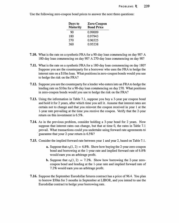
PROBLEMS � 239

Use the following zero-coupon bond prices to answer the next three questions:

Days to Maturity

90 180 270 360

Zero-Coupon Bond Price

0.99009 0.97943 0.96525 0.95238

7.10. What is the rate on a synthetic FRA for a 90-day loan commenCing on day 90? A 180-day loan commencing on day 90? A 270-day loan commencing on day 90?

7.11. What is the rate on a synthetic FRA for a 180-day loan commencing on day 180? Suppose you are the counterparty for a borrower who uses the FRA to hedge the interest rate on a $10m loan. What positions in zero-coupon bonds would you use to hedge the risk on the FRA?

7.12. Suppose you are the counterparty for a lender who enters into an FRA to hedge the lending rate on $1Om for a 90-day loan commencing on day 270. What positions in zero-coupon bonds would you use to hedge the risk on the FRA?

7.13. Using the information in Table 7.1, suppose you buy a 3-year par coupon bond and hold it for 2 years, after which time you sell it. Assume that interest rates are certain not to change and that you reinvest the coupon received in year 1 at the 1-year rate prevailing at the time you receive the coupon. Verify that the 2-year return on this investment is 6.5%.

7.14. As in the previous problem, consider holding a 3-year bond for 2 years. Now suppose that interest rates can change, but that at time 0, the rates in Table 7 .I

prevail. What transactions could you undertake using forward rate agreements tci ·guarantee that your 2-year return is 6.5%?

7 .15. Consider the implied forward rate between year 1 and year 2, based on Table 7 .1.

a. Suppose that ro(l, 2) = 6.8%. Show how buying the 2-year zero-coupon bond and borrowing at the 1-year rate and implied forward rate of 6.8% would earn you an arbitrage profit.

b. Suppose that roO, 2) = 7 .2%. Show how borrowing the 2-year zero­coupon bond and lending at the 1-year rate and implied forward rate of 7.2% would earn you an arbitrage profit.

7.16. Suppose the September Eurodollar futures contract has a price of 96.4. You plan to borrow $50m for 3 months in September at LIB OR, and you intend to use the Eurodollar contract to hedge your borrowing rate.

240 � INTEREST RATE FORWARDS AND FUTURES

a. What rate can you secure?

b. Will you be long or short the Eurodollar contract?

c. How many contracts will you enter into?

d. Assuming the true 3-month LIB OR is 1% in September, what is the settlement in dollars at expiration of the futures contract? (For purposes of this question, ignore daily marking-to-market on the futures contract.)

7.17. A lender plans to invest $100m for 150 days, 60 days from today. (That is, if today is day 0, the loan will be initiated on day 60 and will mature on day 210.) The implied forward rate over 150 days, and hence the rate on a 150-day FRA, is 2.5%. The actual interest rate over that period could be either 2.2% or 2.8%.

a. If the interest rate on day 60 is 2.8%, how much will the lender have to . pay if the FRA is settled on day 60? How much if it is settled on day

210?

b. If the interest rate on day 60 is 2.2%, how much will the lender have to pay if the FRA is settled on day 60? How much if it is settled on day 210?

7.18. Consider the same facts as the previous problem, only now consider hedging with the 3-month Eurodollar futures. Suppose the Eurodollar futures contract that matures 60 days from today has a price on day 0 of 94.

a. What issues arise in using the 3-month Eurodollar contract to hedge a 150-day loan?

b. If you wish to hedge a lending position, should you go long or short the contract?

c. What 3-month LIBOR is implied by the Eurodollar futures price? Ap­proximately what lending rate should you be able to lock in?

d. What position in Eurodollar futures would you use to lock in a lending rate? In· doing this, what assumptions are you making about the relation­ship between 90-day LIBOR and the 150-day lending rate?

7 .19. Consider the bonds in Example 7 .8. What hedge ratio would have exactly hedged the portfolio if interest rates had decreased by 25 basis points? Increased by 25 basis points? Repeat assuming a 50-basis-point change.

7.20. Compute Macaulay and modified durations for the following bonds:

a. A 5-year bond paying annual coupons of 4.432% and selling at par.

b. An 8-year bond paying semiannual coupons with a coupon rate of 8% and a yield of 7%.

c. A 10-year bond paying annual coupons of 6% with a price of $92 and maturity value of $100.

A P P E N D I X 7.A: I NT E R EST R AT E A N D B O N D P R I C E C O N V E N T I O N S � 241

7.21. Consider the following two bonds which make semiannual coupon payments : a 20-year bond with a 6% coupon and 20% yield, and a 30-year bond with a 6% coupon and a 20% yield.

a. For each bond, compute the price value of a basis point.

b. For each bond, compute Macaulay duration.

c. "For otherwise identical bonds, Macaulay duration is increasing in time to maturity." Is this statement always true? Discuss.

7.22. An 8-year bond with 6% annual coupons and a 5 .004% yield sells for $106.44 with a Macaulay duration of 6.63 1 864. A 9-year bond has ?%·annual coupons with a 5 .252% yield and sells for $ 1 1 2.29 with a Macaulay duration of 7.098302. You wish to duration-hedge the 8-year bond using a 9-year bond. How many 9-year bonds must we short for every 8-year bond?

7.23. A 6-year bond with a 4% coupon sells for $ 102.46 with a 3.5384% yield. The conversion factor for the bond is 0.90046. An 8-year bond with 5.5% coupons sells for $ 1 13.564 with a conversion factor of 0.9686. (All coupon payments are semiannual.) Which bond is cheaper to deliver given a T-note futures price of 1 1 3 .8 1 ?

7.24. a. Compute the convexity of a 3-year bond paying annual coupons of 4.5% and selling at par.

b. Compute the convexity of a 3-year 4.5% coupon bond that makes semi­annual coupon payments and that currently sells at par.

c. Is the convexity different in the two cases? Why?

7.25. Suppose a 1 0-year zero coupon bond with a face value of $ 1 00 trades at $69.20205 .

a. What is the yield to maturity and modified duration of the zero-coupon bond?

b. Calculate the approximate bond price change for a 50 basis point increase in the yield, based on the modified duration you calculated in part a). Also calculate the exact new bond price based on the new yield to maturity.

c. Calculate the convexity of the 1 0-year zero-coupon bond.

d. Now use the formula (equation 7 . 1 5) that takes into account both duration and convexity to approximate the new bond price. Compare your result to that in part b).

APPENDIX 7.A: INTEREST RATE AND B OND PRICE CONVENTIONS

This appendix will focus on conventions for computing yields to maturity for different kinds of bonds, and the conventions for quoting bond prices. When discussing yields to maturity, it is necessary to distinguish on the one hand between notes and bonds, which

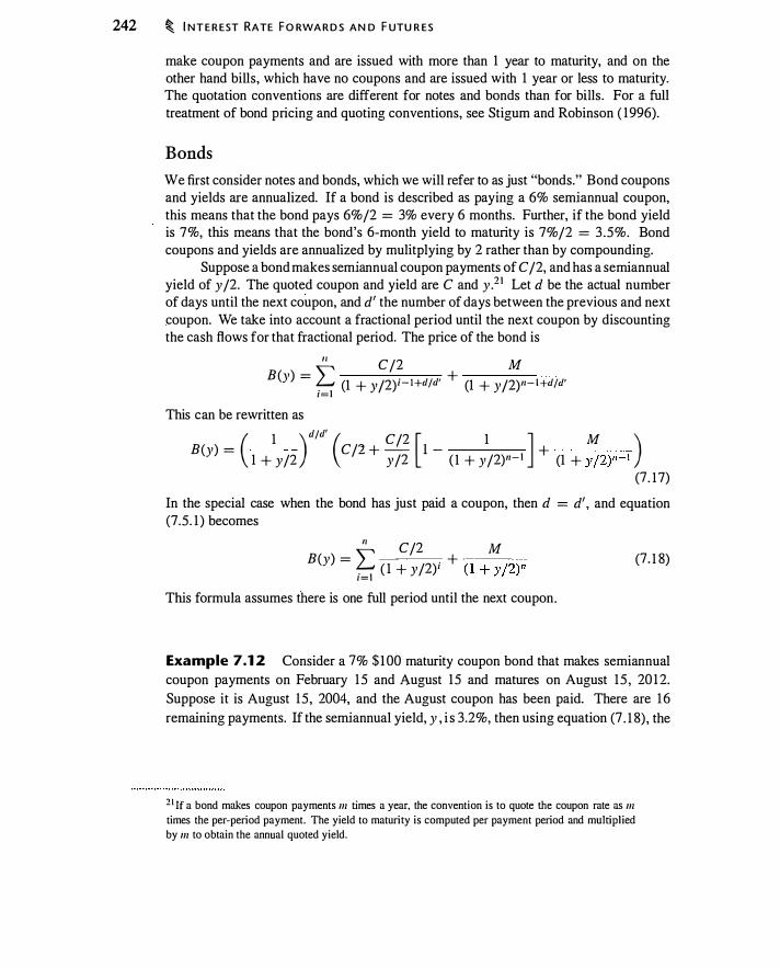
242 � I NT E R EST RATE FO RWA R D S A N D FUTU R ES

make coupon payments and are issued with more than 1 year to maturity, and on the other hand bills, which have no coupons and are issued with 1 year or less to maturity. The quotation conventions are different for notes and bonds than for bills . For a full treatment of bond pricing and quoting conventions, see Stigum and Robinson ( 1996).

Bonds

We first consider notes and bonds, which we will refer to as just "bonds." Bond coupons and yields are annualized. If a bond is described as paying a 6% semiannual coupon, this means that the bond pays 6%/2 = 3% every 6 months. Further, if the bond yield is 7%, this means that the bond's 6-month yield to maturity is 7%/2 = 3 .5%. Bond coupons and yields are annualized by mulitplying by 2 rather than by compounding.

Suppose a bond makes semiannual coupon payments of C /2, and has a semiannual yield of y/2. The quoted coupon and yield are C and y.2 1 Let d be the actual number of days until the next coupon, and d' the number of days between the previous and next .coupon. We take into account a fractional period until the next coupon by discounting the cash flows for that fractional period. The price of the bond is

II C/2 M B(y) = � (1 + yf2)i-l+dfd' + (1 + yf2)11-1+d/d' z=1

This can be rewritten as ( 1 ) dfd' ( C/2 [ 1 J M ) B(y) = C/2+- 1- + -----.,. 1 + y/2 y/2 ( 1 + y/2)11-1 (1 + y/2)11-1 (7. 17)

In the special case when the bond has just paid a coupon, then d = d', and equation (7.5 . 1 ) becomes

II C/2 M B(y) = � ( 1 + y/2); + -( 1_+_)_'/-2)-11 z=1 This formula assumes there is one full period until the next coupon.

(7. 1 8)

Example 7.1 2 Consider a 7% $ 100 maturity coupon bond that makes semiannual coupon payments on February 1 5 and August 15 and matures on August 15 , 201 2. Suppose it is August 15, 2004, and the August coupon has been paid. There are 1 6 remaining payments. If the semiannual yield, y , i s 3.2%, then using equation (7 . 1 8) , the

2 1 If a bond makes coupon payments m times a year, the convention is to quote the coupon rate as m times the per-period payment. The yield to maturity is computed per payment period and multiplied

by m to obtain the annual quoted yield.

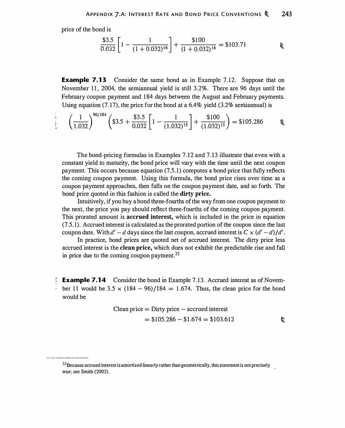
A P P E N D IX 7.A : I NT E R EST RATE A N D B O N D P R I C E C O N V E N T I O N S � 243

price of the bond is

$3.5 [ 1 J $ 1 00 0.032

1 -( 1 + 0.032)16 +

(1 + 0.032)16 = $ 103 ·7 1

Example 7. 1 3 Consider the same bond as in Example 7. 1 2. Suppose that on November 1 1 , 2004, the semiannual yield is still 3 .2%. There are 96 days until the February coupon payment and 1 84 days between the August and February payments. Using equation (7 . 1 7), the price for the bond at a 6.4% yield (3.2% senliannual) is ( 1 ) 96/184 ( $3 .5 [ 1 J $ 100 )

1 .032 $3.5 +

0.032 1 -

( 1 .032)15 + ( 1 .032)15 = $ 1 05·286

The bond-pricing formulas in Examples 7 . 1 2 and 7 . 1 3 illustrate that even with a constant yield to maturity, the bond price will vary with the time until the next coupon payment. This occurs because equation (7.5 . 1 ) computes a bond price that fully reflects the coming coupon payment. Using this formula, the bond price rises over time as a coupon payment approaches, then falls on the coupon payment date, and so forth. The bond price quoted in this fashion is called the dirty price.

Intuitively, if you buy a bond three-fourths of the way from one coupon payment to the next, the price you pay should reflect three-fourths of the coming coupon payment. This prorated amount is accrued interest, which is included in the price in equation (7.5 . 1 ) . Accrued interest is calculated as the prorated portion of the coupon since the last coupon date. With d' - d days since the last coupon, accrued interest is C x (d' - d) j d'.

In practice, bond prices are quoted net of accrued interest. The dirty price less accrued interest is the clean price, which does not exhibit the predictable rise and fall •

in price due to the coming coupon payment.22

r Example 7.1 4 Consider the bond in Example 7 . 1 3 . Accrued interest as of N ovem­ber 1 1 would be 3 .5 x ( 1 84 - 96) / 1 84 = 1 .674. Thus, the clean price for the bond would be

Clean price = Dirty price - accrued interest

= $ 1 05 .286 - $ 1 .674 = $ 103.6 1 2

22Because accrued interest is amortized linearly rather than geometrically, this statement is not precisely

true; see Smith (2002) .

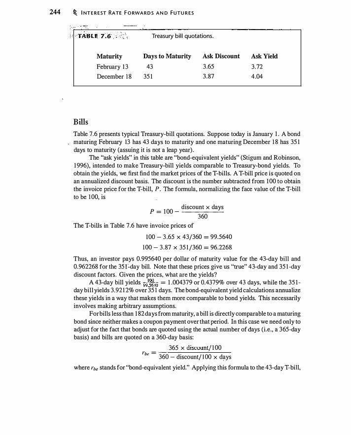
244 � I NT E R EST RATE F O RWA R D S A N D FUTU R ES

•· TABLE 7.6 ·.···· Treasury bill quotations.

Bills

Maturity

February 1 3

December 1 8

Days to Maturity

43

35 1

Ask Discount

3 .65

3 .87

Ask Yield

3 .72

4.04

Table 7.6 presents typical Treasury-bill quotations. Suppose today is January l . A bond maturing February 13 has 43 days to maturity and one maturing December 1 8 has 35 1 days to maturity (assuing it is not a leap year) .

The "ask yields" in this table are "bond-equivalent yields" (Stigum and Robinson, 1 996), intended to make Treasury-bill yields comparable to Treasury-bond yields. To obtain the yields, we first find the market prices of the T-bills. A T-bill price is quoted on an annualized discount basis . The discount is the number subtracted from 100 to obtain the invoice price for the T-bill, P. The formula, normalizing the face value of the T-bill to be 100, is

discount x days p = 100 -360

The T-bills in Table 7.6 have invoice prices of

100 - 3 .65 X 43/360 = 99.5640

100 - 3.87 X 35 1 /360 = 96.2268

Thus, an investor pays 0.995640 per dollar of maturity value for the 43-day bill and 0.962268 for the 35f-day bill. Note that these prices give us "true" 43-day and 35 1 -day discount factors. Given the prices, what are the yields?

A 43-day bill yields 99���0 = 1 .004379 or 0.4379% over 43 days, while the 35 1-day bill yields 3.92 1 2% over 35 1 days. The bond-equivalent yield calculations annualize these yields in a way that makes them more comparable to bond yields. This necessarily involves making arbitrary assumptions.

For bills less than 1 82 days from maturity, a bill is directly comparable to a maturing bond since neither makes a coupon payment over that period. In this case we need only to adjust for the fact that bonds are quoted using the actual number of days (i .e. , a 365-day basis) and bills are quoted on a 360-day basis:

365 x discount/ 100 l"be = --------'---

360 - discount/ I 00 x days

where r11e stands for "bond-equivalent yield." Applying this formula to the 43-day T-bill,

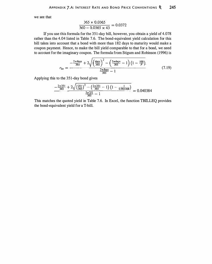
A P P E N D I X 7.A: I NT E R EST RAT E AN D B O N D P R I C E C O N V E N T I O N S � 245

we see that

36�� ;0�·�:�

43 = 0•0372

If you use this formula for the 35 1 -day bill, however, you obtain a yield of 4.078 rather than the 4.04 listed in Table 7 .6. The bond-equivalent yield calculation for this bill takes into account that a bond with more than 1 82 days to maturity would make a coupon payment. Hence, to make the bill yield comparable to that for a bond, we need to account for the imaginary coupon. The formula from Stigum and Robinson ( 1 996) is

_ 2xdays + 2 365 ( day�) 2 _ ( 2xd�ys _ 1) ( 1 _ 100 ) 36) 36) p .

rbe = ---------'---;:--:,----------2xdays _ 1 365 Applying this to the 35 1 -day bond gives

2x351 +? / ( 351 ) 2 ( 2x351 1 ) ( 1 I ) - 365 -v 365 365 o.962268 ____ _:__----:2=-x-=3)""'-1-_-1------- = 0.040384

365

(7. 1 9)

This matches the quoted yield in Table 7.6. In Excel, the function TBILLEQ provides the bond-equivalent yield for a T-bill.

C�ER.8 Swaps

Lus fM we have talked about derivatives oontraots that settle on a single date. A fonvMd contract, for example, fixes a price for a transaction that will occur on a specific date in the future. However, many transactions occur repeatedly. Firms that issue bonds make periodic coupon payments. Multinational firms frequently exchange currencies. Firms that buy commodities as production inputs or that sell them make payments or receive income linked to commodity prices on an ongoing basis.

These situations raise the question: If a manager seeking to reduce risk confronts a risky payment stream-as opposed to a single risky payment-what is the easiest way to hedge this risk? One obvious answer to this question is that we can enter into a separate forward contract for each payment we wish to hedge. However, it might be more convenient, and entail lower transaction costs, if there were a single transaction· that we could use to hedge a stream of payments.

A swap is a contract calling for an exchange of payments over time. One party makes a payment to the other depending upon whether a price turns out to be greater or less than a reference price that is specified in the swap contract. A swap thus provides a means to hedge a stream of risky payments. By entering into an oil swap, for example, an oil buyer confronting a stream of uncertain oil payments can lock in a fixed price for oil over a period of time. The swap payments would be based on the difference between ·

a fixed price for oil and a market price that varies over time. From this description, you can see that there is a relationship between swaps and

forward contracts. In fact, a forward contract is a single-payment swap. It is possible to price a multi-date swa�eterrnine the fixed price for oil in the above example-by using information from the set of forward prices with different maturities (i.e., the strip). We will see that swaps are nothing more than forward contracts coupled with borrowing and lending money.

8.1 AN EXAMPLE OF A COMMODITY SWAP

We begin our study of swaps by presenting an example of a simple commodity swap. Our purpose here is to understand the economics of swaps. In particular we wish to understand how a swap is related to forwards, why someone might use a swap, and how market-makers hedge the risk of swaps. In later sections we present swap-price formulas

247

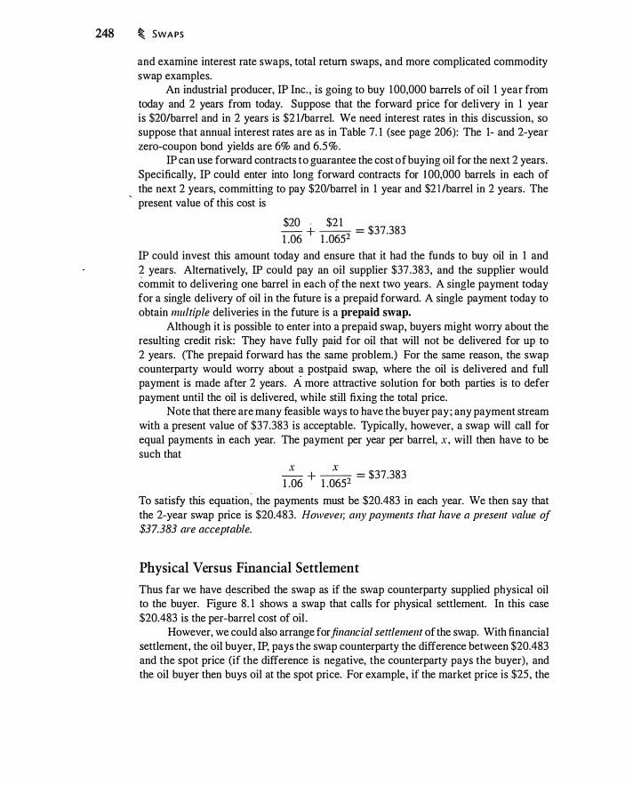
248 � SWA PS

and examine interest rate swaps, total return swaps, and more complicated commodity swap examples.

An industrial producer, IP Inc. , is going to buy 100,000 barrels of oil 1 year from today and 2 years from today. Suppose that the forward price for delivery in 1 year is $20/barrel and in 2 years is $2 1/barrel. We need interest rates in this discussion, so suppose that annual interest rates are as in Table 7. 1 (see page 206) : The 1- and 2-year zero-coupon bond yields are 6% and 6.5 %.

IP can use forward contracts to guarantee the cost of buying oil for the next 2 years. Specifically, IP could enter into long forward contracts for I 00,000 barrels in each of the next 2 years, committing to pay $20/barrel in 1 year and $21/barrel in 2 years. The present value of this cost is

$20 - $2 1 - + -- = $37.383 1 .06 1 .0652

IP could invest this amount today and ensure that it had the funds to buy oil in 1 and 2 years. Alternatively, IP could pay an oil supplier $37.383, and the supplier would commit to delivering one barrel in each of the next two years . A single payment today for a single delivery of oil in the future is a prepaid forward. A single payment today to obtain multiple deliveries in the future is a prepaid swap.

Although it is possible to enter into a prepaid swap, buyers might worry about the resulting credit risk: They have fully paid for oil that will not be delivered for up to 2 years. (The prepaid forward has the same problem.) For the same reason, the swap counterparty would worry about � postpaid swap, where the oil is delivered and full payment is made after 2 years . A more attractive solution for both parties is to defer payment until the oil is delivered, while still fixing the total price.

Note that there are many feasible ways to have the buyer pay; any payment stream with a present value of $37.383 is acceptable. Typically, however, a swap will call for equal payments in each year. The payment per year per barrel, x, will then have to be such that

X X - + -- = $37.383 1 .06 1 .0652

To satisfy this equation : the payments must be $20.483 in each year. We then say that the 2-year swap price is $20.483. Howeve1; any payments that have a present value of $37.383 are acceptable.

Physical Versus Financial Settlement

Thus far we have described the swap as if the swap counterparty supplied physical oil to the buyer. Figure 8. 1 shows a swap that calls for physical settlement. In this case $20.483 is the per-barrel cost of oil .

However, we could also arrange for financial settlement of the swap. With financial settlement, the oil buyer, IP, pays the swap counterparty the difference between $20.483 and the spot price (if the difference is negative, the counterparty pays the buyer), and the oil buyer then buys oil at the spot price. For example, if the market price is $25 , the

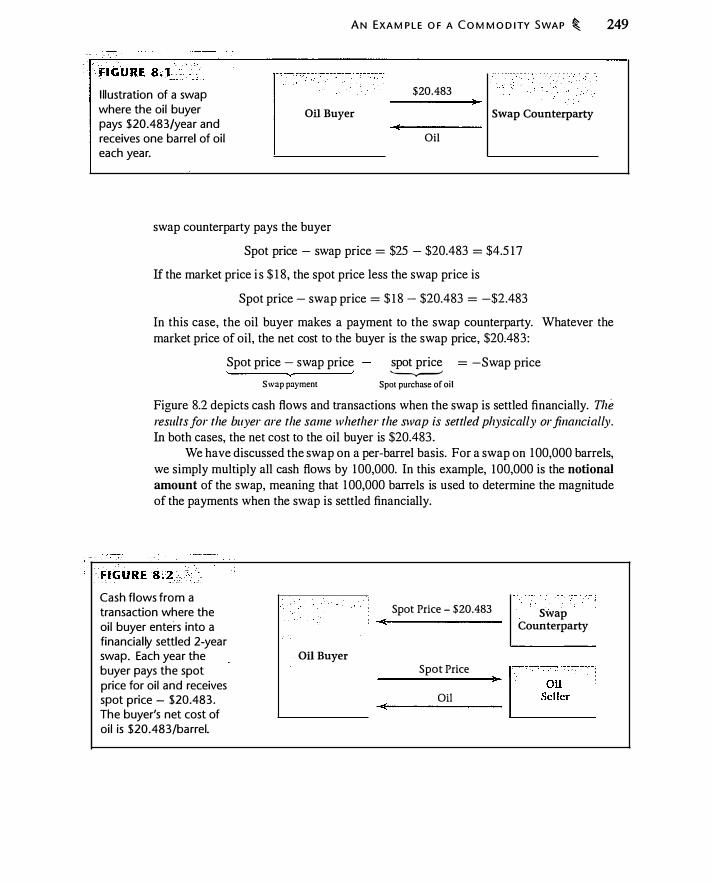
Illustration of a swap where the oil buyer pays $20.483/year and receives one barrel of oil each year.

A N EXAMP L E O F A COMMO D I TY SWA P � 249

$20.483

Oil Buyer Swap Counterparty

Oil

swap counterparty pays the buyer

--- - -_

Spot price - swap price = $25 - $20.483 = $4.5 1 7

If the market price i s $ 1 8, the spot price less the swap price is

Spot price - swap price= $ 1 8 - $20.483 = -$2.483

In this case, the oil buyer makes a payment to the swap counterparty. Whatever the market price of oil, the net cost to the buyer is the swap price, $20.483:

Spot price - swap price

Swap payment spot price = -Swap price '-,.-'

Spot purchase of oil

Figure 8.2 depicts cash flows and transactions when the swap is settled financially. The results for the buyer are the same whether the swap is settled physically or financially. In both cases, the net cost to the oil buyer is $20.483.

We have discussed the swap on a per-barrel basis. For a swap on 1 00,000 barrels, we simply multiply all cash flows by 1 00,000. In this example, 1 00,000 is the notional

amount of the swap, meaning that 1 00,000 barrels is used to determine the magnitude of the payments when the swap is settled financially.

Cash flows from a transaction where the oil buyer enters into a financially settled 2-year swap. Each year the buyer pays the spot price for oil and receives spot price - $20.483. The buyer's net cost of oil is $20.483/barrel.

Oil Buyer

Spot Price - $20.483

Spot Price

Oil

Swap Counterparty

250 � SWA PS

Why Is the Swap Price Not $20.50?

The swap price, $20.483, is close to the average of the two oil forward prices, $20.50. However, it is not exactly the same. Why?

Suppose that the swap price were $20.50. The oil buyer would then be committing to pay $0.50 more than the forward price the first year and would pay $0.50 less than the forward price the second year. Thus, relative to the forward curve, the buyer would have made an interest-free loan to the counte1party. There is implicit lending in the swap.

Now consider the actual swap price of $20.483/barrel. Relative to the forward curve prices of $20 in 1 year and $2 1 in 2 years, we are overpaying by $0.483 in the first year and we are underpaying by $0.5 1 7 in the second year. Therefore, the swap is equivalent to being long the two forward contracts, coupled with an agreement to lend $0.483 to the swap counterparty in I year, and receive $0.5 1 7 in 2 years. This loan has the effect of equalizing the net cash flow on the two dates.

The interest rate on this loan is 0.5 1 7/0.483 - l = 7%. Where does 7% come from? We assumed that 6% is the 1 -year zero yield and 6.5% is the 2-year yield. Given these interest rates, 7% is the 1 -year implied forward yield from year l to year 2. (See Table 7 . 1 . ) By entering into the swap, we are lending the counterparty money for l year beginning in 1 year. If the deal is priced fairly, the interest rate on this loan should be the implied forward interest rate.

The Swap Counterparty:

The swap counterparty is a dealer, who hedges the oil price risk resulting from the swap. The dealer can hedge in several ways. First, imagine that an oil seller would like to Jock in a fixed selling price of oil . In this case, the dealer locates the oil buyer and seller and serves as a go-between for the swap, receiving payments from one party and passing them on to the other. In practice the fixed price paid by the buyer exceeds the fixed price received by the seller. This price difference is a bid-ask spread and is the dealer's fee.

Figure 8.3 illustrates how this transaction would work with financial settlement. The oil seller receives the spot price for oil and receives the swap price less the spot price, on net receiving the swap price. The oil buyer pays the spot price and receives the spot price less the swap price. The situation where the dealer matches the buyer and seller is called a back-to-hack transaction or "matched book" transaction. The dealer bears the credit risk of both parties but is not exposed to price risk.

A more interesting situation occurs when the dealer serves as counterparty and hedges the transaction using forward markets. Let's see how this would work.

After entering the swap with the oil buyer, the dealer has the obligation to pay the spot price and receive the swap price. If the spot price rises, the dealer can lose money. The dealer has a short position in 1 - and 2-year oil.

The natural hedge for the dealer is to enter into long forward or futures contracts to offset this short exposure. Table 8. 1 illustrates how this strategy works. As we discussed earlier, there is an implicit loan in the swap and this is apparent in Table 8 . 1 . The net

F IGU RE 8.3'-:

Spot Price - $20.483

Oil Buyer

Spot Price

Oil

AN EXAMPLE OF A COMMODITY SWAP � 251

Swap Counterparty

Spot Price - $20.483

Spot Price

Oil

Oil Seller

Cash flows from a transaction where an oil buyer and seller each enters into a financially settled 2-year swap. The buyer pays the spot price for oil and receives spot price -$20.483 each year as a swap payment. The oil seller receives the spot price for oil and receives $20.483 -spot price as a swap payment.

·- .

Positions and cash flows for a dealer who has an obligation to receive the fixed price in an oil swap and who hedges the exposure by going long year 1 and year 2 oil forwards.

Year Payment from Oil Buyer

$20.483 - Year 1 spot price

2 $20.483 - Year 2 spot price

Long Forward

Year 1 spot price - $20

Year 2 spot price - $2 1

Net

$0.483

-$0.5 1 7

cash flow for the hedged dealer i s a loan, where the dealer receives cash i n year I and repays it in year 2.

This example shows that hedging the oil price risk in the swap does not fully hedge the position. The dealer also has interest rate exposure. If interest rates fall, the dealer will not be able to earn a sufficient return from investing $0.483 in year 1 to repay $0.5 1 7 i n year 2 . Thus, In addition to entering oil forwards, i t would make sense for the dealer to use Eurodollar contracts or forward rate agreements to hedge the resulting interest rate exposure.

The box on p. 252 shows an extreme example of a hedged transaction-allegedly used to hide debt and manipulate earnings-involving Enron and J. P. Morgan Chase.

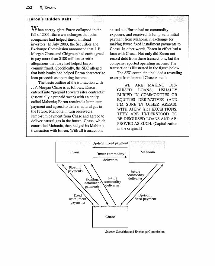
252 � SWAPS

. Enron's Hidden Debt

When energy giant Enron collapsed in the fall of 200 1, there were charges that other companies had helped Enron mislead investors. In July 2003, the Securities and Exchange Commission announced that J. P. Morgan Chase and Citigroup had each agreed to pay more than $ 100 million to settle allegations that they had helped Enron commit fraud. Specifically, the SEC alleged that both banks had helped Enron characterize loan proceeds as operating income.

The basic outline of the transaction with J. P. Morgan Chase is as follows. Enron entered· into "prepaid forward sales contracts" (essentially a prepaid swap) with an entity called Mahonia; Enron received a lump-sum

·payment and agreed to deliver natural gas in the future. Mahonia in turn received a lump-sum payment from Chase and agreed to deliver natural gas in the future. Chase, which

· controlled Mahonia, then hedged its Mahonia transaction with Enron. With all transactions

netted out, Enron had no commodity exposure, and received its lump-sum initial payment from Mahonia in exchange for making future fixed installment payments to Chase. In other words, Enron in effect had a loan with Chase. Not only did Enron not record debt from these transactions, but the company reported operating income. The transaction is illustrated in the figure below.

The SEC complaint included a revealing excerpt from internal Chase e-mail:

WE ARE MAKING DIS­GUISED LOANS, USUALLY BURIED IN COMMODITIES OR EQUITIES DERIVATIVES (AND I'M SURE IN OTHER AREAS). WITH AFEW [sic] EXCEPTIONS, THEY ARE UNDERSTOOD TO BE DISGUISED LOANS AND AP­PROVED AS SUCH. (Capitalization in the original. )

·····• Up-front fixed payment ---·-·c-·--.----·---..,---·:·;

Enron Future commodity deliveries

Chase

Mahonia

Source: Securities and Exchange Commission.

The Market Value of a Swap

AN EXAMPLE OF A COMMODITY SWAP � 253

When the buyer first enters the swap, its market value is zero, meaning that either party could enter or exit the swap without having to pay anything to the other party (apart from commissions and bid-ask spreads) . From the oil buyer's perspective, the swap consists of two forward contracts plus an agreement to lend money at the implied forward rate of 7%. The forward contracts and forward rate agreement have zero value, so the swap does as well.

Once the swap is struck, however, its market value will generally no longer be zero, for two reasons. First, the forward prices for oil and interest rates will change over time. New swaps would no longer have a fixed price of $20.483; bene�, one party will owe money to the other should one party wish to exit or unwind the swap.

Second, even if oil and interest rate forward prices do not change, the value of the swap will remain zero only until the first swap payment is made. Once the first swap payment is made, the buyer has overpaid by $0.483 relative to the forward curve, and hence, in order to exit the swap, the counterparty would have to pay the oil buyer $0.483 . Thus, even if prices do not change, the market value o f swaps can change over time due to the implicit borrowing and lending.

A buyer wishing to exit the swap could negotiate terms with the original counter­party to eliminate the swap obligation. An alternative is to leave the original swap in place and enter into an offsetting swap with whoever offers the best price. The original swap called for the oil buyer to pay the fixed price and receive the floating price; the offsetting swap has the buyer receive the fixed price and pay floating. The original obligation would be cancelled except to the extent that the fixed prices are different. However, the difference is known, so oil price risk is eliminated. (There is still credit risk when the original swap counterparty and the counterparty to the offsetting swap are different. This could be a reason for the buyer to prefer offsetting the swap with the original counterparty.)

To see how a swap can change in value, suppose that immediately after the buyer enters the swap, the forward curve for oil rises by $2 in years I and 2. Thus, the year- 1 forward price becomes $22 and the year-2 forward price becomes $23. The original swap will no longer have a zero market value.

Assuming interest rates are unchanged, the new swap price is $22.483 . (Problem 8 . 1 asks you to verify this .) The buyer could unwind the swap at this point by agreeing to sell oil at $22.483 , while the original swap still calls for buying oil at $20.483. Thus, the net swap payments in each year are

(Spot price - $20.483) + ($22.483 - spot price) = $2

Original swap New swap

The present value 6f this difference is

$2 $2 = $3 .650

1 .06 + ( 1 .065)2

The buyer can receive a stream of payments worth $3.65 by offsetting the original swap with a new swap. Thus, $3.65 is the market value of the swap.

254 � SWAPS

If interest rates had changed, we would have used the new interest rates in com­puting the new swap price.

The examples we have analyzed in this section illustrate the fundamental charac­teristics of swaps and their cash flows. In the rest of the chapter, we will compute more realistic swap prices for interest rates, currencies, and commodities and see some of the ways in which we can modify the terms of a swap.

8.2 INTEREST RATE SWAPS

C<;Jmpanies use interest rate swaps to modify their interest rate exposure. In this section we will begin with a simple example of an interest rate swap, similar to the preceding oil swap example. We will then present general pricing formulas and discuss ways in which the basic swap structure can be altered.

A Simple Interest Rate Swap

Suppose that XYZ Corp. has $200m of floating-rate debt at LIB OR-meaning that every year XYZ pays that year's current LIBOR-but would prefer to have fixed-rate debt with 3 years to maturity. There are several ways XYZ could effect this change.

First, XYZ could change their interest rate exposure by retiring the floating-rate debt and issuing fixed-rate debt in its place. However, an actual purchase and sale of debt has transaction costs.

Second, they could enter into a strip of forward rate agreements (FRAs) in order to guarantee the borrowing rate for the remaining life of the debt. Since the FRA for each year will typically carry a different interest rate, the company will lock in a different rate each year and, hence, the company's borrowing cost will vary over time, even though it will be fixed in advance.

A third alternative is to obtain interest rate exposure equivalent to that of fixed rate debt by entering into a swap. XYZ is already paying a floating interest rate. They therefore want to enter a swap in which they receive a floating rate and pay the fixed rate, which we will suppose is 6.9548%. This swap is illustrated in Figure 8 .4. Notice the similarity to the oil swap.

In a year when the fixed 6.9548% swap rate exceeds 1 -year LIBOR, XYZ pays 6.9548% - LIBOR to the swap counterparty. Conversely, when the 6.9548% swap rate is less than LIBOR, the swap counterparty pays LIBOR - 6.9548% to XYZ. On net, XYZ pays 6.9548%. Algebraically, the net interest payment made by XYZ is

XYZ net payment = - LIBOR + LIBOR - 6.9548% = -6.9548% �

Floating payment Swap payment

The notional principal of the swap is $200m: It is the amount on which the interest payments-and, hence, the net swap payment-is based. The life of the swap is the swap term or swap tenor.

There are timing conventions with a swap similar to those for a forward rate agreement. At the beginning of a year, the borrowing rate for that year is known.

... . .

FIGURE 8.4� _ _;_

Illustration of cash flows for a company that borrows at LIBOR and swaps to fixed-rate exposure at 6.9548%.

Borrower (XYZ)

.···

INTEREST RATE SWAPS � 255

Pay LIBOR (floating)

Pay 6.9548% ·(fixed)

Receive LIBOR (floating)

,��=�--� �

Swap Counterparty

However, the interest payment on the loan is due at the end of the year. The interest rate determination date for the floating interest payment would therefore occur at the beginning of the period. As with an FRA we can think of the swap payment being made at the end of the period (when interest is due).

With the financially settled oil swap, only net swap payments-in this case the difference between LIBOR and 6 .9548%-are actually made between XYZ and the counterparty. If one party defaults, they owe to the other party at most the present value of net swap payments they are obligated to make at current market prices. This means that a swap generally has less credit risk than a bond: Whereas principal is at risk with · a bond, only net swap payments are at risk in a swap.

The swap in this example is a construct, making payments as if there were an exchange of payments between a fixed-rate and floating-rate bond. In practice, a fund manager might own fixed-rate bonds and wish to have floating-rate exposure while continuing to own the bonds. A swap in which a fund manager receives a floating rate in exchange for the payments on bonds the fund continues to hold is called an asset swap.

Pricing and the Swap Counterparty

To understand the pricing of the swap, we will examine it from the perspective of both the counterparty and the firm. We first consider the perspective of the counterparty, who we assume is a market-maker.

The market-maker is a counterparty to the swap in order to earn fees, not to take on interest rate risk. Therefore, the market-maker will hedge the transaction. The market­maker receives the fixed rate from the company and pays the floating rate; the danger for the market-maker is that the floating rate will rise. The risk in this transaction can be hedged by entering into forward rate agreements. We express the time 0 implied forward rate between time t ; and fj as r0(t;, fj) and the realized 1 -year rate as fr;· The current 1 -year rate, 6%, is known. With the swap rate denoted R, Table 8.2 depicts the risk-free (but time-varying) cash flows faced by the hedged market-maker.

How is R determined? Obviously a market-maker receiving the fixed rate would like to set a high swap rate, but the swap market is competitive. We expect R to be bid

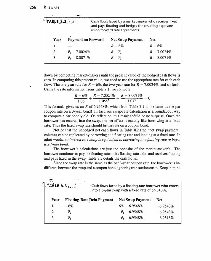
256 � SWAPS

· .

•.. · TABLE 8.2 Cash flows faced by a market-maker who receives fixed and pays floating and hedges the resulting exposure using forward rate agreements.

Year Payment on Forward Net Swap Payment Net

R - 6% R - 6%

2 r-2 - 7.0024% R - r1 R - 7.0024%

3 r3 - 8.oo11% R - r3 R - 8.0071%

down by competing market-makers until the present value of the hedged cash flows is zero. In computing this present value, we need to use the appropriate rate for each cash flow: The one-year rate for R - 6%, the two-year rate for R - 7.0024%, and so forth. Using the rate information from Table 7 . 1 , we compute

R - 6% R - 7.0024% R - 8 .007 1 % 1.06 + 1 .0652 + 1.073 = 0

This formula gives us an R of 6.9548%, which from Table 7. 1 is the same as the par coupon rate on a 3-year bond! In fact, our swap-rate calculation is a roundabout way to compute a par bond yield. On reflection, this result should be no surprise. Once the borrower has entered into the swap, the net effect is exactly like borrowing at a fixed rate. Thus the fixed swap rate should be the rate on a coupon bond.

Notice that the unhedged net cash flows in Table 8.2 (the "net swap payment" column) can be replicated by borrowing at a floating rate and lending at a fixed rate. In other words, an interest rate swap is equivalent to borrowing at a floating rate to buy a fixed-rate bond.

The borrower's calculations are just the opposite of the market-maker's. The borrower continues to pay the floating rate on its floating-rate debt, and receives floating and pays fixed in the swap. Table 8 .3 details the cash flows.

Since the swap rate is the same as the par 3-year coupon rate, the borrower is in­different between the swap and a coupon bond, ignoring transaction costs. Keep in mind

Year

2

3

Cash flows faced by a floating-rate borrower who enters into a 3-year swap with a fixed rate of 6.9548%.

Floating-Rate Debt Payment Net Swap Payment Net

-6% 6% - 6.9548% -6.9548%

-r1 r-2 - 6.9548% -6.9548%

-r3 r3 - 6.9548% . -6.9548%

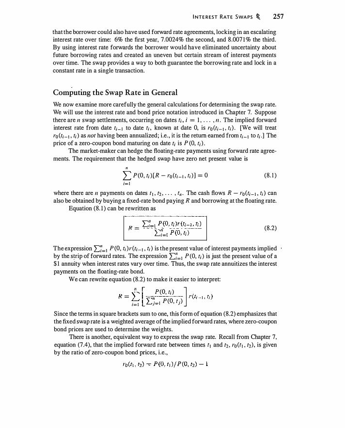
INTEREST RATE SWAPS � 257

that the borrower could also have used forward rate agreements, locking in an escalating interest rate over time: 6% the first year, 7.0024% the second, and 8 .007 1 % the third. By using interest rate forwards the borrower would have eliminated uncertainty about future borrowing rates and created an uneven but certain stream of interest payments over time. The swap provides a way to both guarantee the borrowing rate and lock in a constant rate in a single transaction.

Computing the Swap Rate in General

We now examine more carefully the general calculations for determining the swap rate. We will use the interest rate and bond price notation introduced in Chapter 7. Suppose there are n swap settlements, occurring on dates t;, i = I, . . . , 11. The implied forward interest rate from date t;-l to date t;, known at date 0, is r0 (t;_1 , t; ). [We will treat r0 (t;_1 , t; ) as not having been annualized; i.e., it is the return earned from t;-1 to t; .] The price of a zero-coupon bond maturing on date t; is P (0, t; ) .

The market-maker can hedge the floating-rate payments using forward rate agree­ments. The requirement that the hedged swap have zero net present value is

II L P (O , t; )[R - roCt;-J, t; ) ] = 0 (8. 1 ) i=l

where there are n payments on dates t1 , t2 , . .. , t11• The cash flows R - ro (t; -I , t; ) can also be obtained by buying a fixed-rate bond paying R and borrowing at the floating rate.

Equation (8. 1 ) can be rewritten as

(8.2)

The expression L,;'=1 P (O, t; )r(t;-1 , t; ) is the present value of interest payments implied by the s�rip of forward rates. The expression I:,;'= I P (0, t; ) is just the present value of a $ 1 annuity when interest rates vary over time. Thus, the swap rate annuitizes the interest payments on the floating-rate bond.

We can rewrite equation (8.2) to make it easier to interpret: �[ P (O,t; ) ] R = L..... "" r(t;_1 , t; )

i=l L.... j=l P (O , tj)

Since the terms in square brackets sum to one, this form of equation (8.2) emphasizes that the fixed swap rate is a weighted average of the implied forward rates, where zero-coupon bond prices are used to determine the weights.

There is another, equivalent way to express the swap rate. Recall from Chapter 7, equation (7.4), that the implied forward rate between times t1 and t2, ro (t1, t2), is given by the ratio of zero-coupon bond prices, i .e. ,

258 � SWAPS

Therefore equation (8 . 1 ) can be rewritten

� � [ P (O , t;-t) ] � P (O , t; ) [R - r(t;_ 1 , t; ) ] = � P (O , t;) R - P (O t·) + 1 i=( i=( ' I

Setting this equation equal to zero and solving for R gives us

1 - P0(0, t,) R = "" L..,;=t Po(O, t; )

(8.3)

You may recognize this as the formula for the coupon on a par coupon bond, equation (7,.6), from Chapter 7. This in tum can be rewritten as

, R L P (O, t; ) + P (O, t,) = 1

i=l This is the valuation equation for a bond priced at par with a coupon rate of R.

The conclusion i s that the swap rate is the coupon rate on a par coupon bond. This· result is intuitive since a firm that swaps from floating-rate to fixed-rate exposure ends up with the economic equivalent of a fixed-rate bond.

The Swap Curve

As discussed in Chapter 5, the Eurodollar futures contract provides a set of 3-month forward LIB OR rates extending out 1 .0 years. It is possible to use this set of forward interest rates to compute equation (8.2) or (8.3). As discussed in Chapter7, zero-coupon bond prices can be constructed from implied forward rates.

The set of swap rates at different maturities implied by LIB OR is called the swap curve. There is an over-the-counter market in interest rate swaps, which is widely quoted. The swap curve should be consistent with the interest rate curve implied by the Eurodollar futures contract, which is used to hedge swaps. 1

Here is how we construct the swap curve using the set of Eurodollar prices.2 Column 2 of Table 8 .4 lists 2 years of Eurodollar futures prices from June 2004. The next column shows the implied 9 1 -day interest rate, beginning in the month in column 1 . For example, using equation (5. 1 9), the June price of 98.5558 implies a June to

1 The Eurodollar contract is a futures contract, while a swap is a set of forward rate agreements. Because

of convexity bias, discussed in Chapter 7, the swap curve constructed from Eurodollar futures contracts

following the procedure described in this section will be somewhat greater than the observed swap

curve. This is discussed by Burghardt and Hoskins (1995) and Gupta and Subrahmanyam (2000). 2Collin-Dufresne and Solnik (200 1 ) point out that the credit risk implicit in the LffiOR rate underlying the Eurodollar futures contract is different than the credit risk of an interest rate swap. LffiOR is

computed as an average 3-month borrowing rate for international banks with good credit. Banks that experience credit problems are dropped from the sample. Thus, by construction, the pool of banks represented in the Eurodollar contract never experience a credit downgrade. A firm with a swap, by

contrast, could be downgraded.

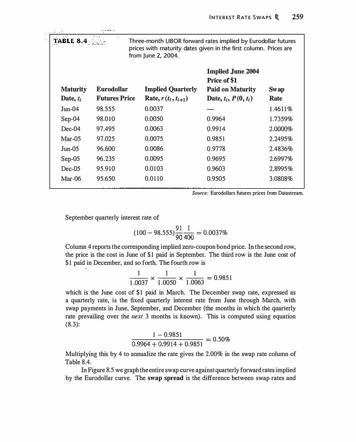
Maturity Date, t; Jun-04

Sep-04

Dec-04

Mar-05

Jun-05

Sep-05

Dec-05

Mar-06

Eurodollar

INTEREST RATE SWAPS � 259

Three-month LIBOR forward rates implied by Eurodollar futures prices with maturity dates given in the first column. Prices are from June 2, 2004.

Implied June 2004 Price of $1

Implied Quarterly Paid on Maturity Swap Futures Price Rate, r(t;, t;+l) Date, t;, P(O, t;) Rate

98.555 0.0037 1 .46 1 1 %

98.0 1 0 0.0050 0 .9964 1 .7359%

97.495 0.0063 0.99 1 4 2.0000%

97.025 0.0075 0.985 1 2.2495%

96.600 0.0086 0.9778 2.4836%

96.235 0.0095 0 .9695 2.6997%

95.9 1 0 0.0 1 03 0.9603 2.8995 %

95.650 0.0 1 1 0 0.9505 3 .0808%

Source: Eurodollars futures prices from Datastream.

September quarterly interest rate of

( 1 00 - 98.555) �� 4�

0 = 0.0037%

Column 4 reports the corresponding implied zero-coupon bond price. In the second row, the price is the cost in June of $ 1 paid in September. The third row is the June cost of $ 1 paid in December, and so forth. The fourth row is

1 1 l -- X -- X -- = 0.985 1 1 .0037 1 .0050 1 .0063

which is the June cost of $ 1 paid in March. The December swap rate, expressed as a quarterly rate, is the fixed quarterly interest rate from June through March, with swap payments in June, September, and December (the months in which the quarterly rate prevailing over the next 3 months is known) . This is computed using equation (8.3) :

1 - 0.985 1 0 0 --��------------= .5 %

0.9964 + 0.99 14 + 0.985 1

Multiplying this by 4 to annualize the rate gives the 2.00% in the swap rate column of Table 8 .4.

In Figure 8.5 we graph the entire swap curve against quarterly forward rates implied by the Eurodollar curve. The swap spread is the difference between swap rates and

260 � SWAPS

Forward 3-month interest rate curve implied by the Eurodol lar strip, swap rates, and constant maturity Treasury yields for june 2, 2004.

8

7

6

[ 5

3

2

- Forward Curve · - · Swap Curve - t-- Treasury Curve

./ � ....................... ·""' ......... / .,.-"

,·.,.-. / // · If 'II I 1 '

-·-· __ ..

___ .... -----

Jan04 ]an06 JanOS JanlO Janl2 Janl4 Janl6

Maturity

Source: Datastream.

Treasury-bond yields for comparable maturities. Thus, Figure 8.5 also displays yields on government bonds .

The Swap's Implicit Loan Balance

An interest rate swap behaves much like the oil swap in Section 8 . 1 . At inception, the swap has zero value to both parties. If interest rates change, the present value of the fixed payments and, hence, the swap rate will change. The market value of the swap is the difference in the present value of payments between the old swap rate and the new swap rate. For example, consider the 3-year swap in Table 8 .3 (see page 256). If interest rates rise after the swap is entered into, the value of the existing 6 .9548% swap will fall for the party receiving the fixed payment.

Even in the absence of interest rate changes, however, the swap in Table 8 .3 changes value over time. Once the first swap payment is made, the swap acquires negative value for the market-maker (relative to the use of forwards) because in the second year the market-maker will make a net cash payment. Similarly, the swap will have positive value for the borrower (again relative to the use of forwards) after the first payment is made. In order to smooth payments, the borrower pays "too much" (relative to the forward curve) in the first year and receives a refund in the second year. The swap is equivalem to entering imo forward contracts and undertaking some additional borrowing and lending.

The 1 0-year swap rate in Figure 8.5 is 5 .3986%. We can use this value to illustrate the implicit borrowing and lending in the swap. Consider an investor who pays fixed and

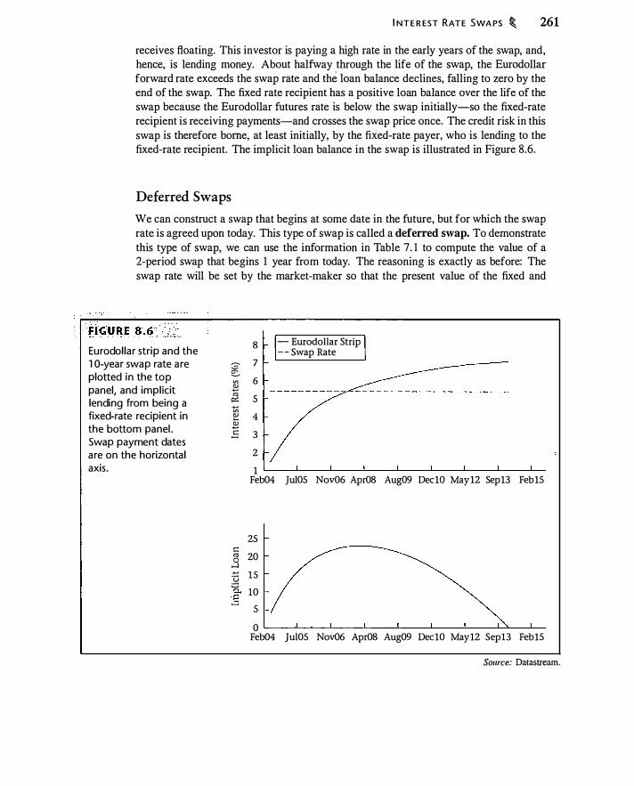
INTEREST RATE SWAPS � 261

receives floating. This investor is paying a high rate in the early years of the swap, and, hence, is lending money. About halfway through the life of the swap, the Eurodollar forward rate exceeds the swap rate and the loan balance declines, falling to zero by the end of the swap. The fixed rate recipient has a positive loan balance over the life of the swap because the Eurodollar futures rate is below the swap initially-so the fixed-rate recipient is receiving payments-and crosses the swap price once. The credit risk in this swap is therefore borne, at least initially, by the fixed-rate payer, who is lending to the fixed-rate recipient. The implicit loan balance in the swap is illustrated in Figure 8.6.

Deferred Swaps

We can construct a swap that begins at some date in the future, but for which the swap rate is agreed upon today. This type of swap is called a deferred swap. To demonstrate this type of swap, we can use the information in Table 7 . 1 to compute the value of a 2-period swap that begins 1 year from today. The reasoning is exactly as before: The swap rate will be set by the market-maker so that the present value of the fixed and

Eurodollar strip and the 1 0-year swap rate are plotted in the top panel, and implicit lending from being a fixed-rate recipient in the bottom panel. Swap payment dates are on the horizontal axis.

�

� "' � "' � ..... "' I!J iii .5

1:: "' 0 ...:I ..... :g 0.. .§

8 - Eurodollar Strip -- Swap Rate

7

6

5

4

3

2

1 �--�----�---�--�----�----�--�----�-Feb04 Jul05 Nov06 Apr08 Aug09 DeclO Mayl2 Sepl3 Febl5

25

20

15

10

5

0 L----L--��--�--�----�--�----�---L-Feb04 ]ul05 Nov06 Apr08 Aug09 DeclO Mayl2 Sep13 Febl5

Source: Datastream.

262 � SWAPS

floating payments is the same. This gives us

R - 0.070024 R - 0.08007 1 ----,------- + = 0

1 .0652 1 .073

Solving for R, the deferred swap rate is 7.4854%. In general, the fixed rate on a deferred swap beginning in k periods is computed as

This can also be written as

R _ L:T=k Po(O, t;)ro(t;_,, t;) - '\'T L...i=k P(O, t;)

P(O, tk-1) - P(O, t11) R = "'"

L...i=k P(O, t;)

Equation (8.4) is equal to equation (8.2) when k = 1.

Why Swap Interest Rates ?

(8.4)

(8 .5)

Managers sometimes say that they would like to borrow short-term because short-term interest rates are on average lower than long-term interest rates. Leaving aside the question of whether this view makes sense theoretically, let's take for granted the desire to borrow at short-term interest rates. The problem facing the manager is that the firm may be unable to borrow significant amounts by issuing short-term debt.

When a firm borrows by issuing long-term debt, bondholders bear both interest rate risk and the credit risk of the firm. If the firm borrows short-term (for example, by issuing commercial paper), lenders primarily bear credit risk.

In practice, short-term lenders appear unwilling to absorb large issues from a single borrower because of �redit risk. For example, money-market mutual funds that hold commercial paper will not hold large amounts of any one firm's commercial paper, preferring instead to diversify across firms. This diversification minimizes the chance that a single bankruptcy will significantly reduce the fund's rate of return.

Because short-term lenders are sensitive in this way to credit risk, a firm cannot borrow a large amount of money short-term without lenders demanding a higher interest rate. By contrast, long-term lenders to corporations-for example, pension funds and insurance companies-willingly assume both interest rate and credit risk. Thus there are borrowers who wish to issue short-term debt and lenders who are unwilling to buy it. Swaps provide a way around this problem, permitting the firm to separate credit risk and interest rate risk.

Suppose, for example, that a firm borrows long-term and then swaps into short-rate exposure. The firm receives the fixed rate, pays the fixed rate to bondholders, and pays the floating rate on the swap. The net payment is the short-term rate, which is the rate the firm wanted to pay.

INTEREST RATE SWAPS � 263

Credit risk does not vanish; it is still mostly held by the long-term bondholders. The swap counterparty faces credit risk since the firm could go bankrupt when the value of the swap is positive to the counterparty (this would occur if interest rates had risen). The notional principal of the loan is not at risk for the swap counterparty, however, so the credit risk in the swap is less than for a short-term loan. Thus, by swapping its interest rate exposure, the firm pays the short-term interest rate, but the long-tenn bondholders colltinue to bear most of the credit risk.

If it seems odd to you that the firm can use a swap to convert a high fixed rate into a low floating rate, recognize that any time there is an upward-sloping yield curve, the short-term interest rate is below the long-term interest rate. If you reduce the period for which your borrowing rate is fixed (which happens when you swap fixed for floating), you borrow at the lower short-term interest rate instead of the higher long-term interest rate.

Swaps thus permit separation of two aspects of borrowing: credit risk and interest rate risk. To the extent these risks are acquired by those most willing to hold them, swaps increase efficiency.

Amortizing and Accreting Swaps

We have assumed that the notional value of the swap remains fixed over the life of the swap. However, it is also possible to engage in a swap where the notional value is changing over time. For example, consider a floating-rate mortgage, for which everj payment contains an interest and principal component. Since the outstanding principal is declining over time, a swap involving a mortgage would need to account for this . Such a swap is called an amortizing swap because the notional value is declining over time. It is also possible for the principal in a swap to grow over time. This is called an accreting swap.

Let Q1 be the relative notional amount at time t. Then the basic idea in pricing a swap with a time-varying notional amount is the same as with a fixed notional amount: ·

The present value of the fixed payments should equal the present value of the floating payments:

II L Q,, P (O, t; ) [R - r (t;_ 1 , t; ) ] = 0 (8.6) i= l

where, as before, there are 11 payments on dates r� . t2 , • • . , t11 • Equation (8.6) can be rewritten as

R = :L;'= 1 Q,, P (O, t; )r (t;- l , t; )

:L;'= 1 Q,, P (O, t; ) (8.7)

The fixed swap rate is still a weighted average of implied forward rates, only now the weights also involve changing notional principal.

Many other structures are possible for swaps based on interest rates or other prices. One infamous swap structure is described in the box on page 264, which recounts the 1 993 swap between Procter & Gamble and Bankers Trust.

264 � SWAPS

The Procter & G a m b l e Swap

In November 1 993, consumer products company Procter & Gamble (P&G) entered into a 5-year $200m notional value swap with Bankers Trust. The contract called for P&G to receive a 5 .3% fixed rate from Bankers Trust and pay the 30-day commercial paper rate less 75 basis points, plus a spread. Settlements were to be semiannual. The spread would be zero for the first settlement, and thereafter be fixed at the spread as of May 4, 1994.

The spread was determined by the difference between the 5-year constant

_maturity treasury (CMT) rate (the yield on a 5-year Treasury bond, but a constructed rate since there is not always a Treasury bond with exactly 5 years to expiration) and the price per $ 1 00 of maturity value of the 6.25% 30-year Treasury bond. The formula for the spread was

Spread = max

o.os1s x .:J - pnce o -year on •

( ·S-yc:1r CMT% 98 - . f 30 b d ) 1 00

• 0

At inception in November 1 993, the 5-year CMT rate was 5 .02% and the 30-year Treasury price was 1 02.578 1 1 . The expression in the max function evaluated to - . 1 7 (- 1 7 basis points), so the spread was zero.

If the spread were 0 on May 4,. 1 994, P&G would save 75 basis points per year on

8.3 CURRENCY SWAPS

$200m for 4.5 years, an interest rate reduction worth approximately $7m. However, notice something important: If interest rates rise before the spread determination date, then the 5-year CMT goes up and the price of the

30-year bond goes down. Thus, the swap is really a bet on the direction of interest rates, not the difference in rates !

The swap is recounted in Smith ( 1 997) · and Srivastava ( 1 998). Interest rates rose after

P&G entered the swap. P&G and B ankers Trust renegotiated the swap in January 1 994, and P&G liquidated the swap in March, with a loss of about $ 1 00m. P&G sued Bankers Trust, complaining in part that the risks of the swap had not been adequately disclosed by B ankers Trust.

In the end P&G and Bankers Trust settled, with P&G paying B ankers Trust about $35m. [Forster ( 1 996) and Horwitz ( 1996) debate the implications of the trial and settlement.] The notion that Procter & Gamble might have been uninformed about the risk of the swap, and if so, whether this should have mattered, was controversial. U.S. securities laws are often said to protect "widows and orphans." Nobel-prize-winning economist Merton Miller wryly said of the case, "Procter is the widow and Gamble is the orphan."

Firms sometimes issue debt denominated in a foreign currency. A firm may do this as a hedge against revenues received in that currency, or because perceived borrowing costs in that currency are lower. Whatever the reason, if the firm later wants to change the cun·ency to which they have exposure, there are a variety of ways to do so. The firm can use forward contracts to hedge exchange rate risk, or it can use a currency swap, in which payments are based on the difference in debt payments denominated in different currencies.

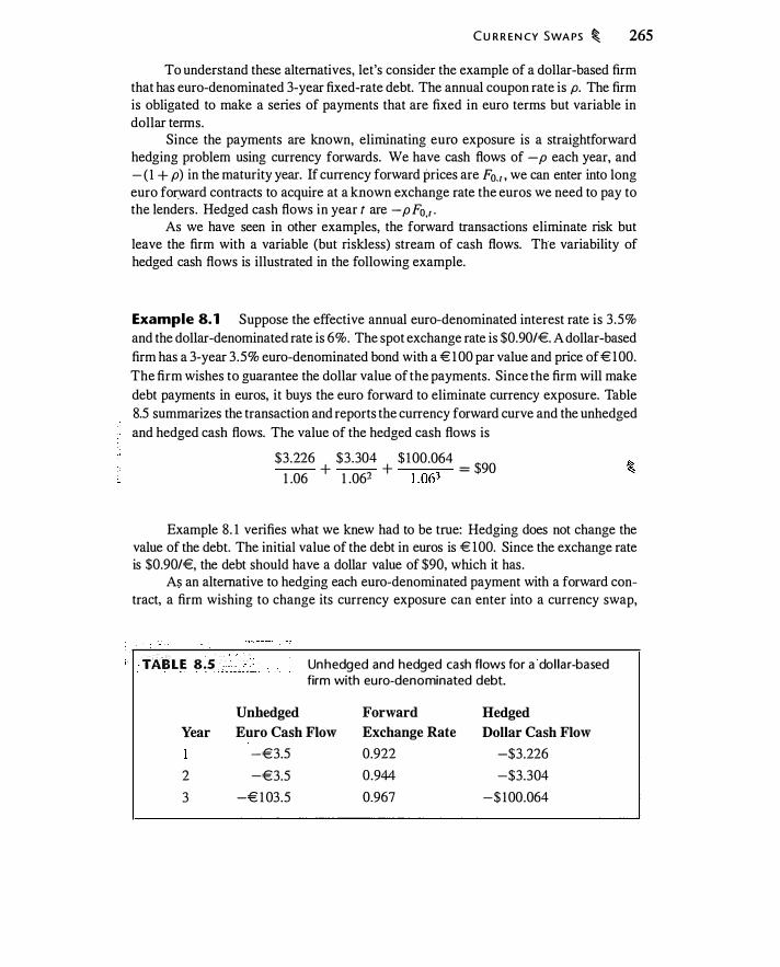
CU RRENCY SWAPS � 265

To understand these alternatives, let's consider the example of a dollar-based firm that has euro-denominated 3-year fixed-rate debt. The annual coupon rate is p. The firm is obligated to make a series of payments that are fixed in euro terms but variable in dollar terms.

Since the payments are known, eliminating euro exposure is a straightforward hedging problem using currency forwards. We have cash flows of -p each year, and - ( 1 + p) in the maturity year. If currency forward prices are Fo.r , we can enter into long euro for:ward contracts to acquire at a known exchange rate the euros we need to pay to the lenders. Hedged cash flows in year t are -p F0,

1•

As we have seen in other examples, the forward transactions eliminate risk but leave the firm with a variable (but riskless) stream of cash flows. The variability of hedged cash flows is illustrated in the following example.

Example 8. 1 Suppose the effective annual euro-denominated interest rate is 3 .5% and the dollar-denominated rate is 6%. The spot exchange rate is $0.90/€. A dollar-based firm has a 3-year 3 .5% euro-denominated bond with a € 1 00 par value and price of€ 1 00. The firm wishes to guarantee the dollar value of the payments. Since the firm will make debt payments in euros, it buys the euro forward to eliminate currency exposure. Table 8.5 summarizes the transaction and reports the currency forward curve and the unhedged and hedged cash flows. The value of the hedged cash flows is

$3.226 $3 .304 $ 1 00.064 - $ 0

1 .06 + 1 .062 + 1 .063 - 9

Example 8 . 1 verifies what we knew had to be true: Hedging does not change the value of the debt. The initial value of the debt in euros is € 100. Since the exchange rate is $0.90/€, the debt should have a dollar value of $90, which it has.

As an alternative to hedging each euro-denominated payment with a forward con­tract, a firm wishing to change its currency exposure can enter into a currency swap,

TABLE 8.5 ·.· . . . ··�··· ·

Unhedged

Unhedged and hedged cash flows for a dollar-based firm with euro-denominated debt.

Forward Hedged Year Euro Cash Flow Exchange Rate Dollar Cash Flow

-€3.5 0.922 -$3.226

2 -€3.5 0.944 -$3.304

3 -€ 1 03.5 0.967 -$ 1 00.064

266 � SWAPS

which entails making debt payments in one currency and receiving debt payments in a different currency. There is typically an exchange of principal at both the start and end of the swap. Compared with hedging the cash flows individually, the cmTency swap generates a different cash flow stream, but with equivalent value. We can examine a currency swap by supposing that the firm in Example 8 . 1 uses a swap rather than forward contracts to hedge its euro exposure.

Example 8.2 Make the same assumptions as in Example 8 . 1 . The dollar-based firm en,ters into a swap where it pays dollars (6% on a $90 bond) and receives euros (3.5% on a € 1 00 bond). The firm's euro exposure is eliminated. The market-maker receives dollars and pays euros. The position of the market-maker is summarized in Table 8 .6 . The present value of the market-maker's net cash flow is

$2. 1 74 $2.096 $4.664 � + 1 .062 -

! .063 = 0

The mark�t-maker's net exposure in this transaction is long a dollar-denominated bond and short a euro-denominated bond. Table 8 .6 shows that after hedging there is a series of net cash flows with zero present value. As in all the previous examples, the effect of the swap is equivalent t9 entering into forward contracts, coupled with borrowing or lending. In this case, the firm is lending to the market-maker in the first 2 years, with the implicit loan repaid at maturity.

The fact that a currency swap is equivalent to borrowing in one currency and lending in the other is familiar from our discussion of currency forwards in Chapter 5 . There w e saw the same i s true o f currency forwards.

TABLE 8.6 . · · ·.· . .

Unhedged and hedged cash flows for a dollar-based firm with euro-denominated debt. The effective annual dollar­denominated interest rate is 6% and the effective annual euro-denominated interest rate is 3 .5%.

Forward Exchange Receive Dollar Pay Hec:)ged Net Cash Year Rate ($/€) Interest Euro Interest Flow

0.92 17 $5 .40 -€3.5 X 0.92 1 7 $2. ! 74

2 0.9440 $5 .40 -€3 .5 X 0.9440 $2.096

3 0.9668 $95 .40 -€ ! 03.5 X 0.9668 -$4.664

C U R R E N CY SWAPS � 267

Currency Swap Formulas

Currency swap calculations are the same as those for the other swaps we have discussed. To see this, consider a swap in which a dollar annuity, R, is exchanged for an annuity in another currency, R* . Given the foreign annuity, R*, what is R?

We start with the observation that the present value of the two annuities must be the same. There are n payments and the time-0 forward price for a unit of foreign currency delivered at time ti is Fo.1, . This gives

II L [ R Po.,, - R* Fo.,, Po. ,, ] = 0 i= l

I n calculating the present value o f the payment R* , w e first convert t o dollars b y mul­tiplying by F0.1, . We can then compute the present value using the dollar-denominated zero-coupon bond price, Po.1, . Solving for R gives

'\;'�I p, R* F. R = L-J= I 0,1; 0,/j

L:7=1 Po.,, (8.8)

This expression is exactly like equation (8 .2), with the implied forward rate, roUi- l , ti ) , replaced by the foreign-currency-denominated annuity payment translated into dollars, R*Fo.,, .

When coupon bonds are swapped, we have to account for the difference in maturity value as well as the coupon payment, which is an annuity. If the dollar bond has a par value of $ 1 , the foreign bond will have a par value of l lxo , where x0 is the current exchange rate expressed as dollars per unit of the foreign currency. If R* is the coupon rate on the foreign bond and R is the coupon rate on the dollar bond, the present value of the difference in payments on the two bonds is

II L [ R Po.,, - R* Fo.t, Po,,, I xo] + Po.t,. ( 1 - Fo,,,. I xo) = 0 i= l

The division by x0 accounts for the fact that a $ 1 bond i s equivalent to 1 I x0 bonds with a par value of I unit of the foreign currency. The dollar coupon in this case is

R = L:;'= 1 Po,,, R* Fo.,)xo + Po,, .. (Fo.1,, /xo - 1 ) '\;'II p, L-i=l 0,/;

(8.9)

The fixed payment, R, is the dollar equivalent of the foreign coupon plus the amortized value of the difference in the maturity payments of the two bonds. Problem 8. 1 6 asks you to verify that equation (8.9) gives 6% using the assumptions in Tables 8.5 and 8.6 .

Other Currency Swaps

There are other kinds of currency swaps. The preceding examples assumed that all bor­rowing was fixed rate. Suppose the dollar-based borrower issues a euro-denorninated

268 � SWAPS

loan with a jloating interest rate. In this case there are two future unknowns: the ex­change rate at which interest payments are converted, and-because the bond is floating rate-the amount of the interest payment. Swapping this loan to a dollar loan is still straightforward, however; we just require one extra hedging transaction.

We first convert the floating interest rate into a fixed interest rate with a euro interest rate swap. The resulting fixed-rate euro-denominated exposure can then be hedged with currency forwards and converted into dollar interest rate exposure. Given the assumptions in Table 8.6, the euro-denominated loan would swap to a 3.5% floating­rate loan. From that point on, we are in the same position as in the previous example.

In general, we can swap fixed-to-fixed, fixed-to-floating, floating-to-fixed, and floating-to-floating. The analysis is similar in all cases.

One kind of swap that might on its face seem s imilar is a diff swap, short for differential swap. In this kind of swap; payments are made based on the difference in floating interest rates in two different currencies, with the notional amount in a single currency. For example, we might have a swap with a $ 1 Om notional amount, but the swap would pay in dollars, based on the difference in a euro-denominated interest rate and a dollar-denominated interest rate. If the short-term euro interest rate rises from 3.5% to 3.8% with the dollar rate unchanged, the annual swap payment would be 30 basis points on $ 1 0m, or $30,000. This is like a standard interest rate swap, only for a diff swap, the reference interest rates are denominated in different currencies.

Standard currency forward contracts cannot be used to hedge a diff swap. The problem is that we can hedge the change in the foreign interest rate, but doing so requires a transaction denominated in the forejgn currency. We can ' t easily hedge the exchange rate at which the value of the interest rate change is converted because we don 't know in advance how much currency will need to be converted. In effect there is quantity uncertainty regarding the foreign currency to be converted. We have seen this kind of problem before, in our discussion of crop yields in Chapter 4 and in our discussion of dollar-denominated Nikkei index futures in Chapter 5. The diff swap is an example of a quanto swap. We will discuss quantos in Chapter 22.

8.4 COMMODITY SWAPS

At the beginning of this chapter we looked at a simple two-date commodity swap. Now we will look at commodity swaps more generally, present the general formula for a commodity swap--showing that the formula is exactly the same as for an interest rate swap--and look at some ways the swap structure can be modified.

The Commodity Swap Price

The idea of a commodity swap, as discussed in Section 8. 1 , is that we use information in the commodity forward curve to fix a commodity price over a period of time. We can derive the swap price following the same logic as before.

C O M M O D I TY SWAPS � 269

Think about the position of the market-maker, who we suppose receives the fixed payment, F, makes the floating payment, and hedges the risk of the floating payment. If there are n swap payments, the resulting hedged cash flow is

Hedged cash flow for payment i = F - Fo.r,

With competitive market-makers, the present value of the net hedged swap payments will be zero (ignoring bid-ask spreads) :

·

II L P (O, t; ) ( F - F0,,, ) i= l

(8. 1 0)

As before, P (0, t; ) is the price of a zero-coupon bond paying $ 1 at time t; . Equation (8. 1 0) implies that the present value of the swap payments equals the present value of the forward curve:

II II

i= l i= l Solving for the swap price, we obtain

F = L::;'= t P (O, t; ) Fo,r,

L::;'= 1 P (O, t; ) (8. 1 1 )

Compare equation (8. 1 1 ) with equation (8.2) for an interest rate swap. They are the ·

samefomwla, except that the imerest swap rate is a weighted average ofimpliedfonvard interest rates and the commodity swap price is a weighted average ofcommodityfonvard prices.

Because of seasonality in both price and quantity, natural gas provides an interest­ing context for examining commodity swaps. The swap curves for June 2002 and June 2004, computed using equation (8. 1 1 ) , are plotted in Figure 8.7.

Swaps with Variable Quantity and Price

It might make sense for a gas buyer with seasonally varying demand (for example, someone buying gas for heating) to enter into a swap in which quantities vary over time. For example, a buyer might want three times the quantity in the w�ter months as in the summer months. A buyer also might be willing to fix different prices in different seasons-for example, if there is seasonal variation in the price of the output produced using gas as an input. How do we determine the swap price with seasonally varying quantities?

Let Q,, denote the quantity of gas purchased at time t; . Once again, we can think about this from the perspective of the competitive market-maker. The market-maker who hedges the swap will enter into varying quantities of forward contracts in different months to match the variable quantity called for in the swap. The zero-profit condition is still that the fixed and floating payments have zero present value, only in this case they

270 � SWAPS

Six-year swap curves for june 5, 2002, and june 2, 2004, based on Henry Hub Natural Gas Futures and interest rates from Eurodollar futures. Each point on the swap curve represents the fixed price for a swap terminating in that month.

7.5

7

6.5

4.5

4

3.5

- 06/05/02 Forward Curve -+- 06/05/02 Swap Curve -- 06/02/04 Forward Curve -+ 06/02/04 Swap Curve

/ .J I

3 '-------'---�--....._ __ ...._ _ ___.c___-.L __ _.___ Jan Jan Jan Jan Jan

Swap Maturity

Jan Jan Jan

Source: Futures prices from Datastream.

must be weighted by the appropria!e quantities. Thus, we have

II L P (O, t; ) Q,, ( ft - Fa.,, ) i= l

The swap price is thus

F = L::;'= 1 Q,, P (O, t; ) Fo,t1

L::;'= 1 Q,, P (O, t; ) (8 . 1 2)

This equation makes perfect sense: If we are going to buy more gas when the forward price is high, we have to weight more heavily the forward price in those months. When Q, = 1 , the formula is the same as equation (8. 1 1 ), when the quantity is not varying.

We can also permit prices to be time-varying. If we let the summer swap price be denoted by ft., and the winter price by Fw, then the summer and winter swap prices can be any prices that satisfy the market-maker's zero present value condition:

i e summer i E winter

L P (O, t; ) Q,, Fo. t1 + L P(O, t; ) Q1, Fo. 11 i e summer i e winter

The notations i E summer and i E winter mean to sum over only the months in those seasons. This gives us one equation and two unknowns, Fw and ft., . Once we fix one of the two prices, the equation will give us the other.

8.5 SWAPTIONS

SWAPT I O N S � 271

An option to enter into a swap is called a swaption. We can see how a swaption works by returning to the two-date oil swap example in Section 8 . 1 . The 2-year oil swap price was $20.483. Suppose we are willing to buy oil at $20.483/barrel, but we would like to speculate on the swap price being even lower over the next 3 months .

Consider the following contract: If in 3 months the fixed price for a swap com­mencing in 9 months ( I year from today) is $20.483 or above, we enter into the swap, agreeing to pay $20.483 and receive the floating price for 2 years. If, on the other hand, the market swap price is below $20.483 , we have no obligation . If the swap price in 3 months is $ 1 9.50, for example, we could enter into a swap at that time at the $ 1 9.50 price, or we could elect not to enter any swap.

With this contract we are entering into the swap with $20.483 as the swap price only when the market swap price is greater; hence, this contract will have a premium. In this example, we would have purchased a payer swaption, since we have the right, but not the obligation, to pay a fixed price of $20.483 for 2 years of oil. The counterparty has sold this swaption.

When exercised, the swaption commits us to transact at multiple times in the future. It is possible to exercise the option and then offset the swap with another swap, converting the stream of swap payments into a certain stream with a fixed present value. Thus, the swaption is analogous to an ordinary option, with the present value of the swap obligations (the price of the prepaid swap) as the underlying asset.

The strike price in this example is $20.483, so we have an at-the-money swaption. We could make the strike price different from $20.483 . For example, we could reduce the swaption premium by setting the strike above $20.483.

Swaptions can be American or European, and the terms of the underlying swap­fixed price, floating index, settlement frequency, and tenor-will be precisely specified.

Example 8.3 Suppose we enter into a European payer oil swaption with a strike price of $2 1 . The underlying swap commences in 1 year and has two annual settlements. After 3 months, the fixed price on the underlying swap is $2 1 .50. We exercise the option, obligating us to pay $2 1/barrel for 2 years. If we wish to offset the swap, we can enter into a swap to receive the $2 1 .50 fixed price. In year 1 and year 2 we will then receive $2 1 .50 and pay $2 1 , for a certain net cash flow each year of $0.50. The floating payments cancel. �

A receiver swaption gives you the right to pay the floating price and receive the fixed strike price. Thus, the holder of a receiver swaption would exercise when the fixed swap price is below the strike.

Although we have used a commodity swaption in this example, an interest rate or currency swaption would be analogous, with payer and receiver swaptions giving the right to pay or receive the fixed interest rate.

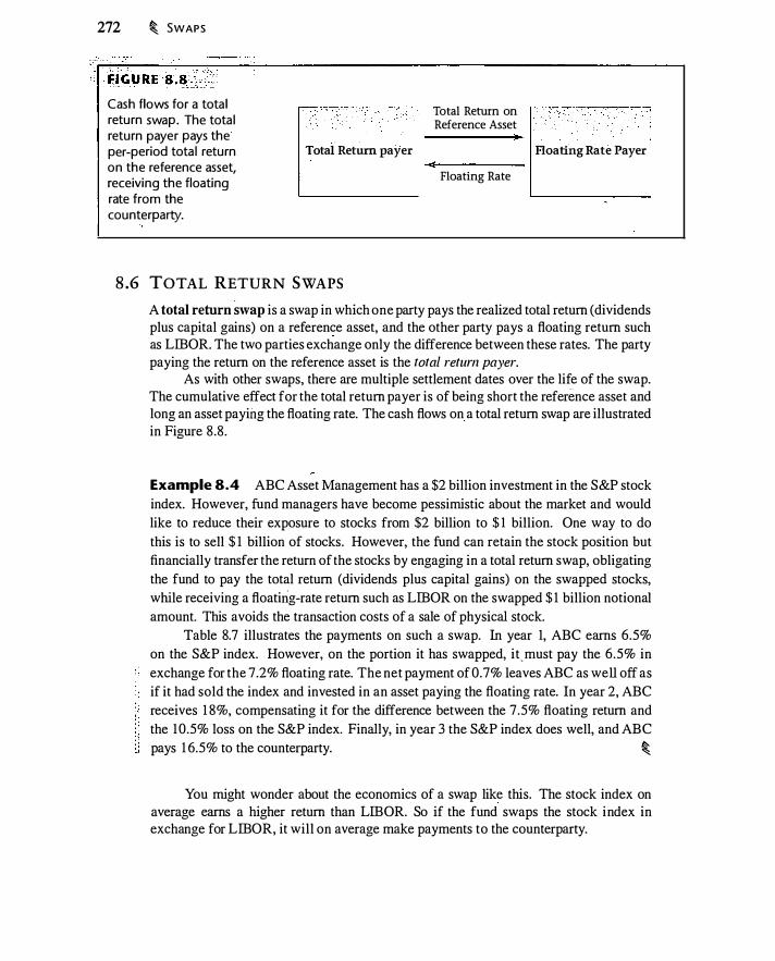
272 � SWAPS

Cash flows for a total return swap. The total return payer pays the per-period total return on the reference asset, receiving the floating rate from the counterparty.

Total Return on Reference Asset

Total Retum payer Floating Rate Payer

Floating Rate

8.6 TOTAL RETURN SWAPS

A total return swap is a swap in which one party pays the realized total return (dividends plus capital gains) on a reference asset, and the other party pays a floating return such as LIBOR. The two parties exchange only the difference between these rates. The party paying the return on the reference asset is the total return payer.

As with other swaps, there are multiple settlement dates over the life of the swap. The cumulative effect for the total return payer is of being short the reference asset and long an asset paying the floating rate. The cash flows on a total return swap are illustrated in Figure 8 .8 .

Example 8.4 ABC Asset Management has a $2 billion investment in the S&P stock index. However, fund managers have become pessimistic about the market and would like to reduce their exposure to stocks from $2 billion to $ 1 billion. One way to do this is to sell $ 1 billion of stocks. However, the fund can retain the stock position but financially transfer the return of the stocks by engaging in a total return swap, obligating the fund to pay the total return (dividends plus capital gains) on the swapped stocks, while receiving a floating-rate return such as LIBOR on the swapped $ 1 billion notional amount. This avoids the transaction costs of a sale of physical stock.

Table 8.7 illustrates the payments on such a swap. In year 1, ABC earns 6.5% on the S&P index. However, on the portion it has swapped, it _ must pay the 6 .5% in exchange for the 7.2% floating rate. The net payment of 0.7% leaves ABC as well off as if it had sold the index and invested in an asset paying the floating rate. In year 2, ABC receives 1 8%, compensating it for the difference between the 7.5% floating return and the 1 0.5% loss on the S&P index. Finally, in year 3 the S&P index does well, and ABC pays 1 6.5% to the counterparty. �

You might wonder about the economics of a swap like this. The stock index on average earns a higher return than LIBOR. So if the fund swaps the stock index in exchange for LIB OR, it will on average make payments to the counterparty.

- ..

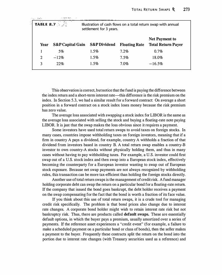
TOTA L R ETU R N SWAPS � 273

Illustration of cash flows on a total return swap with annual settlement for 3 years.

Net Payment to Year S&P Capital Gain S&P Dividend Floating Rate Total Return Payer

I 5% 1 .5 % 7.2% 0.7%

2 -.:. 1 2% 1 .5 % 7.5% 1 8 .0%

3 22% 1 .5% 7 .0% - 1 6.5%

This observation is correct, but notice that the fund is paying the difference between the index return and a short -term interest rate-this difference is the risk premium on the index. In Section 5 .3 , we had a similar result for a forward contract: On average a short position in a forward contract on a stock index loses money because the risk premium has zero value.

The average loss associated with swapping a stock index for LIB OR is the same as the average loss associated with selling the stock and buying a floating-rate note paying LIB OR. It is just that the swap makes the loss obvious since it requires a payment.

Some investors have used total return swaps to avoid taxes on foreign stocks. In many cases, countries impose withholding taxes on foreign investors, meaning that if a firm in country A pays a dividend, for example, country A withholds a fraction of that dividend from investors based in country B. A total return swap enables a country-B investor to own country-A stocks without physically holding them, and thus in many cases without having to pay withholding taxes . For example, a U.S. investor could first swap out of a U.S. stock index and then swap into a European stock index, effectively becoming the counterparty for a European investor wanting to swap out of European stock exposure. Because net swap payments are not always recognized by withholding rules, tlus transaction can be more tax-efficient than holding the foreign stocks directly.

Another use of total return swaps is the management of credit risk. A fund manager holding corporate debt can swap the return on a particular bond for a floating-rate return. If the company that issued the bond goes bankrupt, the debt holder receives a payment on the swap compensating for the fact that the bond is worth a fraction of its face value.

If you think about this use of total return swaps, it is a crude tool for managing credit risk specifically. The problem is that bond prices also change due to interest rate changes. A corporate bond holder might wish to retain interest rate risk but not bankruptcy risk. Thus, there are products called default swaps. These are essentially default options, in which the buyer pays a premium, usually amortized over a series of payments. If the reference asset experiences a "credit event" (for example, a failure to make a scheduled payment on a particular bond or class of bonds), then the seller makes a payment to the buyer. Frequently these contracts split the return on the bond into the portion due to interest rate changes (with Treasury securities used as a reference) and

274 � SWAPS

the portion due to credit quality changes, with the swap making payments based only on the latter. We discuss these swaps in Chapter 26.

CHAPTER S UMMARY

A swap is a contract calling for an exchange of payments, on one or more dates, deter­mined by the difference in two prices. A single-payment swap is the same thing as a cash-settled forward contract. In the simplest swaps, a fixed payment is periodically ex­changed for a floating payment. A firm can use a swap to lock in a long-term commodity price, a fixed interest rate, or a fixed exchange rate. Considering only the present value of cash flows, the same result is obtained using a strip of forward contracts and swaps. The difference is that hedging with a strip of forward contracts results in net payments that are time-varying. In contrast, hedging with a swap results in net payments that are constant over time. The value of a swap is zero at inception, though as swap payments ·are made over time, the value of the swap can change in a predictable way.

The fixed price in a swap is a weighted average of the corresponding forward prices. The swap formulas in different cases all take the same general form. Let fo (t; ) denote the forward price for the floating payment in the swap. Then the fixed swap payment is

R _ .z=;'= 1 P (O, t; )fo (t; ) -- .z=;'= 1 P (O, t; )

(8. 1 3)

Table 8 .8 summarizes the substitutions to make in equation (8. 13 ) to get the various swap formulas shown in the chapter. This formula can be generalized to permit time variation in the notional amount and the swap price, and the swap can start on a deferred basis.

An important characteristic of swaps is that they require only the exchange of net payments, and not the payment of principal . So if a firm enters an interest rate swap, for example, it is required only to make payments based on the difference in interest rates, not on the underlying principal . As a result, swaps have less credit risk than bonds.

Total return swaps involve exchanging the return on an asset for a floating rate such as LIBOR. The term swap is also used to describe agreements like the Procter &

: . . TABLE 8.8 ·.· . ... ·.

To Obtain Formula for

Interest rate swap

Currency swap (annuity)

Commodity swap

Equivalent forms of the swap-rate calculation. For the currency swap, F0.,1 is the forward price for the foreign currency. For the commodity swap, F0.,1 is the forward price for the commodity.

Substitute in Equation (8.13)

fo(t; ) = roUi- 1 , t; ) fo (t; ) = R* Fo.,, fo (t; ) = Fo.t,

Equation in Chapter

Equation (8.2)

Equation (8.8)

Equation (8. 1 1 )

F U RTH E R READING � 275

Gamble swap (page 264), which required payments based on the difference in interest rates and bond prices, as well as default swaps .

FURTHER READING

The same formulas used to price swaps will appear again in the context of structured notes, which we will encounter in Chapter 1 5 . We will discuss default swaps in Chapter 25.

Litzenberger ( 1992) provides an overview of the swap market. Turnbull ( 1987) discusses arguments purporting to show that the use of swaps can have .a positive net present value. Default swaps are discussed by Tavakoli ( 1 998). Because of convexity bias (Chapter 7), the market interest rate swap curve is not exactly the same as the swap curve constructed from Eurodollar futures. This is discussed in Burghardt and Hoskins ( 1 995) and Gupta and Subrahmanyam (2000). The SEC complaint against J. P. Morgan Chase is at http://www.sec.gov/litigation/complaints/comp 1 8252.htm.

PROBLEMS

Quarter

Some of the problems that follow use Table 8.9. Assume that the current exchange rate is $0.90/€.

8.1. Consider the oil swap example in Section 8 . 1 with the 1- and 2-year forward prices of $22/barrel and $23/barrel. The 1 - and 2-year interest rates are 6% and 6.5%. Verify that the new 2-year swap price is $22.483 .

8.2. Suppose that oil forward prices for 1 year, 2 years, and 3 years are $20, $2 1 , and $22. The 1 -year effective annual interest rate is 6.0%, the 2-year interest rate is 6.5%, and the 3-year interest rate is 7 .0%.

a. What is the 3-year swap price?

b. What is the price of a 2-year swap beginning in one year? (That is, the first swap settlement will be in 2 years and the second in 3 years.)

8.3. Consider the same 3-year oil swap. Suppose a dealer is paying the fixed price and receiving floating. What position in oil forward contracts will hedge oil price risk

1 2 3 4 5 6 7 8 Oil forward price 2 1 2 1 . 1 20.8 20.5 20.2 20 1 9.9 1 9.8 Gas swap price 2.2500 2.4236 2.3503 2.2404 2.2326 2.2753 2.2583 2.2044 Zero-coupon bond price 0.9852 0.970 1 0.9546 0.9388 0.923 1 0.9075 0.89 1 9 0.8763 Euro-denominated zero-coupon bond price 0.99 1 3 0.9825 0.9735 0.9643 0.955 1 0.9459 0.9367 0.9274 Euro forward price ($/€) 0.9056 0.9 1 1 5 0.9 1 78 0.9244 0.93 1 2 0.938 1 0.9452 0.9524

276 � SWAPS

in this position? Verify that the present value of the locked-in net cash flows is zero.

8.4. Consider the 3-year swap in the previous example. Suppose you are the fixed-rate payer in the swap. How much have you overpaid relative to the forward price after the first swap settlement? What is the cumulative overpayment after the second swap settlement? Verify that the cumulative overpayment is zero after the third payment. (Be sure to account for interest.)

8.5. Consider the same 3-year swap. Suppose you are a dealer who is paying the fixed oil price and receiving the floating price. Suppose that you enter into the swap and immediately thereafter all interest rates rise 50 basis points (oil forward prices are unchanged). What happens to the value of your swap position? What if interest rates fall 50 basis points? What hedging instrument would have protected you against interest rate risk in this position?

8.6. Supposing the effective quarterly interest rate is 1 .5%, what are the per-barrel swap prices for 4-quarter and 8-quarter oil swaps? (Use oil forward prices in Table 8.9.) What is the total cost of prepaid 4- and 8-quarter swaps?

8.7. Using the information about zero-coupon bond prices and oil forward prices in Table 8.9, construct the set of swap prices for oil for 1 through 8 quarters.

8.8. Using the information in Table 8.9, what is the swap price of a 4-quarter oil swap with the first settlement occurring in the third quarter?

8.9. Given an 8-quarter oil swap price of $20.43 , construct the implicit loan balance for each quarter over the life of the swap.

8.10. Using the zero-coupon bond prices and oil forward prices in Table 8.9, what is the price of an 8-period swap for which two barrels of oil are delivered in even­numbered quarters and one barrel of oil in odd-numbered quarters?

8.11. Using the zero-coupon bond prices and natural gas swap prices in Table 8.9, what are gas forward prices for each of the 8 quarters?

8.12. Using the zero-coupon bond prices and natural gas swap prices in Table 8.9, what is the implicit loan amount in each quarter in an 8-quarter natural gas swap?

8.13. What is the fixed rate in a 5-quarter interest rate swap with the first settlement in quarter 2?

8.14. Using the zero-coupon bond yields in Table 8.9, what is the fixed rate in a 4-quarter interest rate swap? What is the fixed rate in an 8-quarter interest rate swap?

8.15. What 8-quarter dollar annuity is equivalent to an 8-quarter annuity of € 1 ?

8.16. Using the assumptions in Tables 8 .5 and 8.6, verify that equation (8.9) equals 6%.

P R O B LE M S � 277

8.17. Using the information in Table 8.9, what are the euro-denominated fixed rates for 4- and 8-quarter swaps?

8.18. Using the information in Table 8 .9, verify that it is possible to derive the 8-quarter dollar interest swap rate from the 8-quarter euro interest swap rate by using equation (8.9).

PA R T T H R E E

· z earlier chapters we have seen how options work, and introduced some

of the terminology related to options. In this part of the book we return

to options, with the goal of understanding how they are priced.

Forward contracts (and futures and swaps) represent a binding com­

mitment to buy or sell the underlying asset in the future. Because the

commitment is binding, but deferred, time value of money is the main

economic idea used in determining forward prices.

Options, on the other hand, need not be exercised. Intuitively, you

would expect the probability distribution of the stock to affect the op­

tion price. Consequently, in discussing option pricing we will use some

concepts from basic probability. However, it turns out that there is much

to say about options without needing to think about the probability dis­

tribution of the stock. bi Chapter 9 we explore concepts such as parity

in more depth, and discuss some basic intuition about option prices that

can be gleaned using only time value of money arguments.

Chapters 10 and 11 introduce the binomial option pricing model.

This model assumes that the stock can move only in a very simple way,

but provides the intuition underlying more complicated option pricing

279

calculations. Chapter 12 presents the Black-Scholes option pricing for­

mula, which is one of the most important formulas in finance.

As with forwards, futures, and swaps, option contracts are bought

and sold by market-makers who hedge the risk associated with market­

making. Chapter 13 looks at how market-makers hedge their option risk,

and shows the precisesensein which the price of an option reflects the cost

of synthetically creating it . . Finally, Chapter 14 discusses exotic options,

which are variants of the standard options we have been .discussing. �

Parity and Other Option Relationships

< wth this ohaptcr we begin to study option pricing. Up to tllli; point we have primru-­ily studied contracts entailing.firm commitmellfs, such as forwards, futures, and swaps. These contracts do not permit either party to back away from the agreement. Optionality occurs when it is possible to avoid engaging in unprofitable transactions. The prin­cipal question in option pricing is: How do you value the right to back away from a commitment?

Before we delve into pricing models, we devote this chapter to refining our common sense about options. For example, Table 9 . I contains call and put prices for IBM for four different strikes and two different expiration dates. These are American-style options. Here are some observations and questions about these prices :

• What determines the difference between put and call prices at a given strike?

• How would the premiums change if these options were European rather than Amer­ican?

• It appears that, for a given strike, the January options are more expensive than the November options. Is this necessarily true?

• Do call premiums always decrease as the strike price increases? Do put premiums always increase as the strike price increases?

• Both call and put premiums change by less than the change in the strike price. Does this always happen?

These questions, and others, will be answered in this chapter, but you should take a minute and think about the answers now, drawing on what you have learned in previous chapters. While doing so, pay attention to lzow you are trying to come up with the answers. What constitutes a persuasive argument? Along with finding the answers, we want to understand how to think about questions like these.

9.1 PUT-CALL PARITY

Put-call parity is perhaps the single most important relationship among option prices. In Chapter 2 we argued that synthetic forwards (created by buying the call and selling the put) must be priced consistently with actual forwards. The basic parity relationship for

281

282 � PA R I TY A N D OTH E R O PT I O N R E LAT I O N S H I PS

IBM option prices, dollars per share, October 1 5, 2004. The closing price of IBM on that day was $84.85.

Calls Puts Strike Expiration Bid ($) Ask ($) Bid ($) Ask ($)

75 November 9 .90 1 0.30 0.20 0.25

80 November 5 .30 5 .60 0.60 0.70

85 November 1 .90 2. 1 0 2. 1 0 2.30

90 November 0.35 0.45 5 .50 5 .80

75 January 10.50 10.90 0.70 0.80

80 January 6.50 6.70 1 .45 1 .60

85 January 3 .20 3 .40 3 . 1 0 3.30

90 January 1 .20 1 .35 6. 1 0 6.30

Source: Chicago Board Options Exchange (www.cboe.com).

European options with the same strik� price and time to expiration is

Call - put = PV(forward price - strike price)

Equation (3. 1 ) from Chapter 3 expresses this more precisely:

C(K, T) - P (K, T) = PVo. T ( Fo. T - K) = e-rT (Fo, T - K)

(9. 1 )

where C ( K, T) is the price of a European call with strike price K and time to expiration T, P(K, T) is the price of. a European put, Fo, T is the forward price for the underlying asset, K is the strike price, T is the time to expiration of the options, and PVo, T denotes the present value over the life of the options. Note that e-rT Fo. T is the prepaid forward price for the asset and e-rT K is the prepaid forward price for the strike, so we can also think of parity in terms of prepaid forward prices.

The intuition for equation (9 . 1 ) is that buying a call and selling a put with the strike equal to the forward price (Fa. T = K) creates a synthetic forward contract and hence must have a zero price. If we create a synthetic long forward position at a price lower than the forward price, we have to pay PVo.T ( Fo. T - K) since this is the benefit of buying the asset at the strike price rather than the forward price.

Parity generally fails for American-style options, which may be exercised prior to maturity. Appendix 9.A discusses a version of parity for American options.

We now consider the parity relationship in more detail for different underlying assets .

P UT-CA LL PA R I TY � 283

Options on Stocks

If the underlying asset is a stock and Div is the stream of dividends paid on the stock, then from Chapter 5, e-rT Fo.T = So - PVo. r (Div) . Thus, from equation (9. 1 ), the parity relationship for European options on stocks is

C(K, T) = P (K, T) + [So - PVo. r (Div)] - e-rT K (9.2)

where So is the current stock price and PVo.r (Div) is the present value of dividends payable over the life of the stock. For index options, we know that So - PVo.r (Div) = S0e-liT . Hence, we can write

C(K, T) = P (K, T) + Soe-1iT - PVo. r (K)

- Example 9.1 Suppose that the price of a nondividend-paying stock is $40, the continuously compounded interest rate is 8%, and options have 3 months to expiration. A 40-strike European call sells for $2.78 and a 40-strike European put sells for $ 1 .99. This is consistent with equation (9.2) since

$2.78 = $ 1 .99 + $40 - $40e-O.OS x 0 .2S

Why does the price of an at-the-money call exceed the price of an at-the-money put by $0.79? We can answer this question by recognizing that buying a call and selling a put is a synthetic alternative to buying the stock, with different cash flows than an outright purchase.

Figure 9 . 1 represents the cash flows for a synthetic and outright purchase. Note that the synthetic purchase of the stock entails a cash outflow of $0.79 today and $40 at expiration, compared with an outright purchase that entails spending $40 today.

Also, both positions result in the ownership of the stock 3 months from today. With the outright purchase of stock, we still own the stock in 3 months. With the synthetic purchase: we will own the stock if the price is above $40 because we will exercise the call . We will also own the stock if the price is below $40, because we sold a put that

Cash flows for outright purchase of stock and for synthetic stock created by buying a 40-strike cal l and sel l ing a 40-strike put.

Outright Purchase of Stock Day O Day 9 1

1-------------------1 Own 1 share -$40

Buy Call, Sell Put

1-------------------i Own 1 share -$0. 79 -$40

284 � PA R I TY AN D OTH E R O PT I O N R E LAT I O N S H I PS

will be exercised; as the put-writer we have to buy the stock. In either case, in 3 months we pay $40 and acquire the stock.

Finally, the dollar risk of the positions is the same. In both cases, a $ 1 change in the stock price at 3 months will lead to a $ 1 change in the value of the position. In other words, both positions entail economic ownership of the stock. You can verify that the risk is the same by drawing a profit and loss diagram for the two positions.

Thus, by buying the call and selling the put we own the stock, but we have deferred the payment of $40 until expiration. To obtain this deferral we must pay 3 months of interest on the $40, the present value of which is $0 .79. The option premiums differ by interest on the deferral of payment for the stock. Interest is the reason that at-the-money European calls on nondividend-paying stock always sell for more than at-the-money European puts with the same expiration.

Note that if we reverse the position by selling the call and buying the put, then we are synthetically short-selling the stock. In 3 months, the options will be exercised and we will receive $40. In this case, the $0.79 compensates us for deferring receipt of the stock price.

There are differences between the outright and synthetic positions. First, the stock pays dividends and the synthetic does not. This example assumed that the stock paid no dividends . If it did, the cost of the actual stock would exceed that of the synthetic by the present value of dividends paid over the life of the options. Second, the actual stock has voting rights, unlike the synthetic position.

Example 9.2 Make the same -assumptions as in Example 9. 1 , except suppose that the stock pays a $5 dividend just before expiration. The price of the European call is $0.74 and the price of the European put is $4.85 . These prices satisfy parity with dividends, equation (9.2):

$0.74 _ $4.85 = ($40 _ $5e-0.08x0.25 ) _ $40e-0.08x0.25

The call price is higher than the put price by interest on the strike ($0.79) and lower by the present value of the dividend ($4.90), for a net difference of $4. 1 1 . �

In this example, the at-the-money call sells for less than an at-the-money put since dividends on the stock exceed the value of interest on the strike price.

It is worth mentioning a common but erroneous explanation for the higher pre­mium of an at-the-money call compared to an at-the-money put. The profit on a call is potentially unlimited since the stock price can go to infinity, while the profit on a put can be no greater than the strike price. This explanation seems to suggest that the call should be more expensive than the put. 1 However, parity shows that the true reason for the call being more expensive (as in Example 9. 1 ) is time value of money.

1 In fact, the argument also seems to suggest that every stock is worth more than its price!

P UT-CA L L PA R I TY � 285

Synthetic stock Parity provides a cookbook for the synthetic creation of options, stocks, and T-bills.

The example above shows that buying a call and selling a put is like buying the stock except that the timing of the payment for the stock differs in the two cases . Rewriting equation (9.2) gives us

So = C(K, T) - P (K , T) + PVo.T (Div) + e-rT K (9.3)

To match the cash flows for an outright purchase of the stock, in addition to buying the call and selling the put, we have to lend the present value of the strike and dividends to be paid over the life of the option. We then receive the stock in 9 1 days .

.

· Example 9.3 In Example 9 . 1 , PV0,0_25 (K) = $40e-o.osxo.25 = $39.2 1 . Hence, by buying the call for $2.78, selling the put for $ 1 .99, and lending $39.2 1 , we invest a total of $40 today. In 9 1 days, we have the two options and a T-bill worth $40. We acquire the stock via one of the exercised options, using the $40 T-bill to pay the strike price.

� Synthetic T-bills If we buy the stock, sell the call, and buy the put, we have purchased the stock and short-sold the synthetic stock. This transaction gives us a hedged position that has no risk but requires investment. Parity shows us that

So + P (K , T) - C ( K , T) = PVo, T ( K ) + PVo. T (Div)

We have thus created a position that costs PV(K) + PVo. T CDiv) and that pays K + F Vo, T (Div) at expiration. This is a synthetic Treasury bill.

Example 9.4 In Example 9 . 1 , PV0,0_25 (K) = $39.2 1 . Hence, by buying the stock, buying a put, and selling the call, we can create a T-bill that costs $39.2 1 and pays $40 in 9 1 days. �

Since T-bills are taxed differently than stocks, the ability to create a synthetic Trea­sury bill with the stock and options creates problems for tax and accounting authorities . How should the return on this transaction be taxed-as a stock transaction or as interest income? Tax rules call for this position to be taxed as interest, but you can imagine taxpayers trying to skirt these rules.

The creation of a synthetic T-hill by buying the stock, buying a put, and selling a call is called a conversion. If we short the stock, buy a call, and sell a put, we have created a synthetic short T-bill position and this is called a reverse conversion.

Synthetic options Parity tells us that

C(K, T) = So - PVo.T (Div) - PVD.T ( K) + P(K, T)

286 � PA R I TY A N D OTH E R O PT I O N R E LAT I O N S H I PS

and that

P(K, T) = C(K, T) - So + PVo,r (K) + PVo , r (Div)

The first relation says that a call is equivalent to a leveraged position on the un­derlying asset [So - PVo. r (Div) - PV(K)] , which is insured by the purchase of a put. The second relation says that a put is equivalent to a short position on the stock, insured by the purchase of a call.

Options on Currencies

Suppose we have options to buy euros by paying dollars. From our discussion of currency forward contracts in Chapter 5, we know that the dollar forward price for a euro is Fo, T = xoe<r-r€)T ' where Xo is the current exchange rate denominated as $/€, 1"€ is the euro-denominated interest rate, and r is the dollar-denominated interest rate. The parity relationship for options to buy one euro by paying xo is then

C(K, T) - P (K, T) = xoe-r€T - Ke-rT (9 .4)

Buying a euro call and selling a euro put is equivalent to lending euros and borrowing dollars. Equation (9.4) tells us that the difference in the call and put premiums simply reflects the difference in the amount borrowed and loaned, in the currency of the country in which the options are denominated.

Example 9.5 Suppose the current $/€ exchange rate is 0.9, the dollar-denominated interest rate is 6%, and the euro-denominated interest rate is 4%. By buying a dollar­denominated euro call with a strike of $0.92 and selling a dollar-denominated euro put with the same strike, we construct a position where in 1 year we will buy € 1 by paying $0.92. We can accomplish the same thing by lending the present value of€ 1 today (with a dollar cost of $0.9e-0·04 = $0. 8647) and paying for this by borrowing the present value of $0,92 ($0.92e-0·06 = $0.8664). The proceeds from borrowing exceed the amount we need to lend by $0.00 1 7 . · Equation (9.4) performs exactly this calculation, giving us a difference between the call premium and put premium of

xoe-r€T - Ke-rT = 0.9$/€ X €e-0.04x l - $0.92 X e-0.06x l

= $0. 8647 - $0.8664 = -$0.00 1 7

Options on Bonds

Finally, we can construct the parity relationship for options on bonds . The prepaid forward for a bond differs from the bond price due to coupon payments (which are like dividends) . Thus if the bond price is Bo we have

C(K, T) = P (K, T) + [Bo - PVo, r (Coupons) ] ...:... PVo. r (K) (9.5)

G E N E R A L I Z E D PA R ITY A N D EXC H A N G E O PT I O N S � 287

Note that for a pure-discount bond, the parity relationship is exactly like that for a nondividend-paying stock.

9.2 GENERALIZED PARITY AND EXCHANGE OPTIONS

The preceding section showed how the parity relationship works for different underlying assets. Now we will generalize parity to apply to the case where the strike asset is not necessarily cash but could be any other asset. This version of parity includes all previous versions as special cases.

Suppose we have an option to exchange one asset for another. Let the underlying asset, asset A, have price S, , and the strike asset (the asset which, at our discretion, we surrender in exchange for the underlying asset), asset B, have the price Q1 • Let F/:T (S) denote the time t price of a prepaid forward on the underlying asset, paying ST at time T, and let F/T (Q) denote the time t price of a prepaid forward on asset B, paying QT at time T. We use the notation C(S, , Q, , T - t) to denote the time t price of an option with T - t periods to expiration, which gives us the right to give up asset B in exchange for asset A. P (S, , Q, , T - t) is defined similarly as the right to give up asset A in exchange for asset B. Now suppose that the call payoff at time T is

C(ST , QT , 0) = max(O, ST - QT)

and the put payoff is

P (ST , QT , 0) = max(O, QT - ST)

Then for European options w e have this form o f the parity equation:

The use of prepaid forward prices in the parity relationship completely takes into ac­count the dividend and time value of money considerations. This version of parity tells us that there is nothing special about an option having the strike amount designated as cash. In general, options can be designed to exchange any asset for any other asset, and the relative put and call premiums are determined by prices of prepaid forwards on the underlying and strike assets.

To prove equation (9.6) we can use a payoff table in which we buy a call, sell a put, sell a prepaid forward on A, and buy a prepaid forward on B . This transaction is illustrated in Table 9.2.

If the strategy in Table 9.2 does not pay zero at expiration, there is an arbitrage opportunity. Thus, we expect equation (9 .6) to hold. All European options satisfy this formula, whatever the underlying asset.

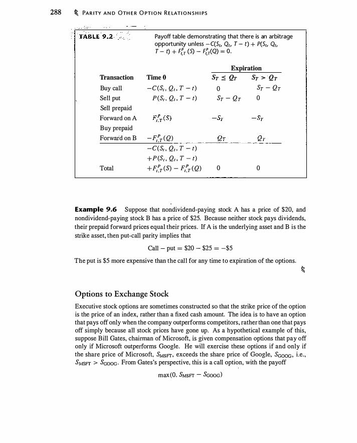
288 � PA R ITY A N D OTH E R O PT I O N R E LAT I O N S H I PS

Transaction

Buy call

Sell put

Sell prepaid

Forward on A

Buy prepaid

Forward on B

Total

Payoff table demonstrating that there is an arbitrage opportunity unless -C(St, Ot, T - t) + P(St, Ot, T - t) + Fi,r (S) - Fi,7(Q) = 0.

Time O

-C(S� > Q1 , T - t)

P(Sr , Q1 , T - t)

F/T (S)

-F/:T (Q) -C(S� > Q1 , T - t) +P (S� > Q1 , T - t) +F/:T (S) - F/:T (Q)

Expiration

Sr � Qr Sr > QT 0 ST - QT ST - QT 0

0 0

Example 9.6 Suppose that nondividend-paying stock A has a price of $20, and nondividend-paying stock B has a price of $25. Because neither stock pays dividends, their prepaid forward prices equal their prices . If A is the underlying asset and B is the strike asset, then put-call parity implies that

Call - put = $20 - $25 = -$5

The put is $5 more expensive than the cal l for any time to expiration of the options.

Options to Exchange Stock

Executive stock options are sometimes constructed so that the strike price of the option is the price of an index, rather than a fixed cash amount. The idea is to have an option that pays off only when the company outperforms competitors, rather than one that pays off simply because all stock prices have gone up. As a hypothetical example of this, suppose Bill Gates, chairman of Microsoft, is given compensation options that pay off only if Microsoft outperforms Google. He will exercise these options if and only if the share price of Microsoft, S�v�sFT, exceeds the share price of Google, Sa000 , i .e. , S�v�sFT > Saooa - From Gates's perspective, this is a call option, with the payoff

max(O, S�v�sFT - Saooa)

G E N E R A L I Z E D PA R I TY A N D EXC H A N G E O PT I O N S � 289

Now consider the compensation option for Eric Schmidt, CEO of Google. He will receive a compensation option that pays off only if Google outperforms Microsoft, i .e. ,

max(O, Saooa - S�v�sFr) This is a call from Schmidt's perspective.

Here is the interesting twist: Schmidt's Google call looks to Gates like a Microsoft put ! And Gates's Microsoft call looks to Schmidt like a Google put. Either option can be viewed as a put or call ; it is simply a matter of perspective. The distinction between a put and a call in this example depends upon what we label the underlying asset and what we label as the strike asset.

What Are Calls and Puts ?

The preceding discussion suggests that labeling an option as a call or put is always a matter of convention. It is an important convention because we use it all the time in talking about options. Nevertheless, in general we can interpret calls as being puts, and vice versa. We can see why by using an analogy.

When you go to the grocery store to obtain bananas, you typically say that you are buying bananas. The actual transaction involves handing cash to the grocer and receiving a banana. This is an exchange of one asset (cash) for another (a banana) . We could also describe the transaction by saying that we are selling cash (in exchange for bananas). The point is that an exchange occurs, and we can describe it either as buying the thing we receive, or selling the thing we surrender.

Any transaction is an exchange of one thing for another. Whether we say we are buying or selling is a matter of convention. This insight may not impress your grocer, but it is important for options since it suggests that the labeling we commonly use to distinguish calls and puts is a matter of convention.

To see how a call could be considered a put, consider a call option on a stock. This is the right to exchange a given number of dollars, the strike price K, for stock worth S, if the stock is worth more than the dollars. For example, suppose that if S > K, we earn S - K. We can view this as either of two transactions:

• Buying one share of stock by paying K. In this case we exercise when S > K . This i s a call option o n stock.

• Selling K dollars in exchange for one share of stock. Again we exercise when S > K-i.e., when the dollars we sell are worth less than the stock. This is a put option on dollars, with a share of stock as the strike asset.

Under either interpretation, if S < K we do not exercise the option. If the dollars are worth more than the stock, we would not sell them for the stock.

Now consider a put option on a stock. The put option confers the right to exchange one share of stock for a given number of dollars. Suppose S < K; we earn K - S. We can view this in either of two ways:

• Selling one share of stock at the price K .

290 � PA R I TY A N D OTH E R O PT I O N R E LATI O N S H I PS

• Buying K dollars by paying one share of stock. This is a call where we have the right to give up stock to obtain dollars.

If S > K we do not exercise under either interpretation. If the dollars are worth less than the stock, we would not pay the stock to obtain the dollars.

Currency Options

The idea that calls can be relabeled as puts is not just academic; it is used frequently by currency traders. A currency transaction involves the exchange of one kind of currency for another. In this context, it is obvious to market participants that referring to a particular currency as having been _bought or sold is a matter of convention. Labeling a particular option a call or a put depends upon which currency you regard as your home currency.

In the following example we will show that a dollar-denominated call option on · euros, which gives you the right to pay dollars to receive euros, is equivalent to a euro-denominated put option on dollars, which gives the right to sell a dollar for euros. Obviously, the strike prices and option quantities must be chosen appropriately for there to be an equivalence.

We will say that an option is "dollar-denominated" if the strike price and premium are denominated in dollars. An option is "euro-denominated" if the strike price and premium are in euros.

Suppose the current exchange rate is xo = 0.90$/€, and consider the following two options :2

1. A 1-year dollar-denominated call option on euros with a strike price of $0.92 and premium of $0.0337. In 1 year, the owner of the option has the right to buy € 1 for $0.92. The payoff on this option, in dollars, is therefore

max(O, x1 - 0.92)

2. A 1 -year euro-denominated put option on dollars with a strike of 0_�2 = € 1 .0870. The premium of this option is €0.0407. In 1 year the owner of this put has the right to give up $ 1 and receive € 1 .0870; the owner will exercise the put when $ 1 is worth less than € 1 .0870. The euro value of $ 1 in 1 year will be l jx 1 • Hence, the payoff of this option is

max (o, -1 - 2_) 0.92 X (

Since x 1 > 0.92 exactly when 0_�2 > * ' the euro-denominated dollar put will be exercised when, and only when, the dollar-denominated euro call is exercised.

2These are Black-Scholes prices with a current exchange rate of0.90 $/€, a dollar-denominated interest

rate of 6%, a euro-denominated interest rate of 4%, and exchange rate volatility of I 0%.

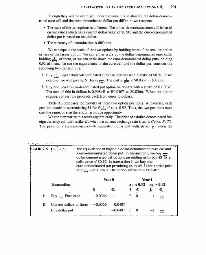
G EN E R A L I Z E D PA R I TY A N D EXC H A N G E O PT I O N S � 291

Though they will be exercised under the same circumstances, the dollar-denomi­nated euro call and the euro-denominated dollar put differ in two respects:

• The scale of the two options is different. The dollar-denominated euro call is based on one euro (which has a current dollar value of $0.90) and the euro-denominated dollar put is based on one dollar.

• The currency of denomination is different.

We can equate the scale of the two options by holding more of the smaller option or less of the larger option: We can either scale up the dollar-denominated euro calls, holding 0_�2 of them, or we can scale down the euro-denominated doll<\[ puts, holding 0.92 of them. To see the equivalence of the euro call and the dollar put, consider the following two transactions:

1. Buy 0_�2 1 -year dollar-denominated euro call options with a strike of $0.92. If we exercise, we will give up $ 1 for €0_�2 • The cost is o.�2 x $0.0337 = $0.0366.

2. Buy one 1 -year euro-denominated put option on dollars with a strike of € 1 .0870. The cost of this in dollars is 0.90$/€ x €0.0407 = $0.0366. When the option expires, convert the proceeds back from euros to dollars.

Table 9.3 compares the payoffs of these two option positions . At exercise, each position results in surrendering $ 1 for € 0_�2 if x1 > 0.92. Thus, the two positions must cost the same, or else there is an arbitrage opportunity.

We can summarize this result algebraically. The price of a dollar-denominated for­eign currency call with strike K, when the current exchange rate is x0 , is Cs (x0 , K, T) . The price of a foreign-currency-denominated dollar put with strike 1z , when the

I :

II:

Transaction

The equivalence of buying a dol lar-denominated euro call and a euro-denominated dol lar put. In transaction I, we buy o.�2 dol lar-denominated call options permitting us to buy €1 for a strike price of $0.92. In transaction I I , we buy one euro-denominated put permitting us to sel l $1 for a strike price of € 0_�2 = € 1 .0870. The option premium is €0.0407.

Year O Year l X1 < 0.92 X1 � 0.92

$ € $ € $ € Buy o.�2 Euro calls -0.0366 0 0 - 1 I 0.92

Convert dollars to Euros -0.0366 0.0407

Buy dollar put -0.0407 0 0 - 1 I 0.92

292 � PA R I TY A N D OTH E R O PT I O N R E LATI O N S H I PS

exchange rate is _!_ , is P1 ( _!_ , -K1 , T) . Adjusting for currency and scale differences, xo .\a the prices are related by

Cs (xo. K, T) = xo K P1 (__!__ , __!__ , T) xo K

(9.7)

This insight-that calls in one currency are the same as puts in the other-is common­place among currency traders. While this observation is interesting in and of itself, its generalization to all options provides a fresh perspective for thinking about what calls and puts actually are.

9.3 COMPARING OPTIONS WITH RESPECT TO STYLE, MATURITY, AND STRIKE

We now examine how option prices change when there are changes in option charac­teristics, such as exercise style (American or European), the strike price, and time to expiration. Remarkably, we can say a great deal without a pricing model and without making any assumptions about the distribution of the underlying asset.3 Thus, whatever the particular option model or stock price distribution used for valuing a given option, we can still expect option prices to behave in certain ways.

Here is an example of the kind of questions we will address in this section. Suppose you have three call options, wit!l strikes of $40, $45, and $50. How do the premiums on these options differ? Common sense suggests that, with a call option on any underlying asset, the premium will go down as you raise the strike price; it is less valuable to be able to buy at a higher price.4 Moreover, the decline in the premium cannot be greater than $5 . (The right to buy for a $5 cheaper price cannot be worth more than $5.)

Following this logic, the premium will drop as we increase the strike from $40 to $45, and drop again when we increase the strike further from $45 to $50. Here is a more subtle question: In which case will the premium drop more? It turns out that the decline in the premium from $40 to $45 must be greater than the decline from $45 to $50, or else there is an arbitrage opportunity.

In this section we will explore the following issues for stock options (some of the properties may be different for options on other underlying assets):

• How prices of otherwise identical American and European options compare.

3The so-called "theory of rational option pricing," on which this section is based, was first presented

in 1 973 by Robert Merton in an astonishing paper (Merton ( 1 973b)). This material is also superbly

exposited in Cox and Rubinstein ( 1 985). 4If you are being fastidious, you will say the option premium cannot increase as the strike goes up.

Saying that the option premium will decrease as the strike increases does not account for the possibility

that all the premiums are zero, and hence the premium will not go down, but will remain unchanged,

as the strike price increases.

C O M PA R I N G O PT I O N S W I T H R ES P E CT TO STY LE, M ATU R I TY, A N D STR I K E � 293

• How option prices change as the time to expiration changes.

• How option prices change as the strike price changes.

A word of warning before we begin this discussion: If you examine option price listings in the newspaper, you can often find option prices that seemingly give rise to arbitrage opportunities. There are several reasons for this. One is that some reported op­tion price quotes are stale, meaning that the comparison is among option prices recorded at diffe�:ent times of the day. Moreover, an apparent arbitrage opportunity only becomes genuine when bid-ask spreads (see Table 9. 1 ), commissions, costs of short-selling, and market impact are taken into account. Caveat arbitrageur!

European Versus American Options

Since an American option can be exercised at any time, it must always be at least as valuable as an otherwise identical European option. (By "otherwise identical" we mean that the two options have the same underlying asset, strike price, and time to expiration.) Any exercise strategy appropriate to a European option can always be duplicated with an American option: The American option cannot be less valuable. Thus we have

CAmer (S, K, T) 2: CEur (S, K, T) PAmer (S, K, T) 2: PEur (S, K , T)

(9.8a)

(9.8b)

We will see that there are times when the right to early-exercise is worthless, and, hence, American and European options have the same value.

Maximum and Minimum Option Prices

It is often useful to understand just how expensive or inexpensive an option can be. Here are some basic limits.

Calls The price of a European call option

• Cannot be negative, because the call need not be exercised.

• Cannot exceed the stock price, because the best that can happen with a call is that you end up owning the stock.

• Must be at least as great as the price implied by parity with a zero put value.

Combining these statements, together with the result about American options never being worth less than European options, gives us

S 2:: CAmer(S, K , T) 2:: CEur (S, K , T) 2:: max[O, PVo.T (Fo.T ) - PVo,T (K)] (9.9)

where present values are taken over the life of the option.

294 � PA R I TY A N D OTH E R O PT I O N R E LATI O N S H I PS

Puts Similarly, a put

• Cannot be worth more than the undiscounted strike price, since that is the most it can ever be worth (if the stock price drops to zero, the put pays K at some point).

• Must be at least as great as the price implied by parity with a zero call value.

Also, an American put is worth at least as much as a European put. This gives us

K 2: PAmer (S, K , T) ::: PEur (S, K, T) 2: max[O, PV(K) - PV(Fo,T ) ] (9. 10)

Early Exercise for American Options

When might we want to exercise an option prior to expiration? An important result is that an American call option on a nondividend-paying stock should never be exercised prior to expiration. You may, however, rationally exercise an American-style put option prior to expiration.

Calls on a nondividend-paying stock We can demonstrate in two ways that an American-style call option on a nondividend-paying stock should never be exercised prior to expiration. Early exercise is not optimal if the price of an American call prior to expiration satisfies

CAmer (Sr . K, T - t) > S1 - K .

If this inequality holds, you would lose money by early-exercising (receiving S1 - K) as opposed to selling the option (receiving CAmer (S1 , K, T - t) > S1 - K).

We will use put -call parity to demonstrate that early exercise is not rational . If the option expires at T, parity implies that

CEur CSI , K , T) = S1 - K + PEur CS1 , K , T - t) '--v--'

Exercise value Insurance against ST < K

+ K ( l - e-r(T-I) ) > S1 - K (9. 1 1 )

Time value of money on K

Since the put price, PEur CSr . K, T - t ) , and the time value of money on the strike, K (1 - e-r(T -ll ) , are both positive, this equation establishes that the European call option premium on a nondividend paying stock always is at least as great as S1 - K . From equation (9.8), w e also know that CArner 2: CEur · Thus w e have

CArner 2: CEur > S, - K

Since CArner• the American option premium, always exceeds S - K , we would lose money exercising an American call prior to expiration, as opposed to selling the option.

Equation (9. 1 1 ) is useful because it shows us precisely why we would never early­exercise. Early-exercising has two effects. First, we throw away the implicit put pro­tection should the stock later move below the strike price. · Second, we accelerate the payment of the strike price.

C O M PA R I N G O PT I O N S W I T H R ES P E CT TO STY LE , M ATU R I TY, A N D STR I K E � 295

A third effect is the possible loss from deferring receipt of the stock. However, when there are no dividends, we lose nothing by waiting to take physical possession of the stock.

We have demonstrated that if a stock pays no dividends, you should never see an option selling for less than S1 - K. In fact, equation (9. 1 1 ), like equation (9.9), actually implies the stronger result that you should never see a call on a nondividend-paying stock sell for less than S1 - K e-r<T -t l . What happens if you do observe an option selling for too low a price? If C < S1 - K and the option is American, you can buy the option, exercise it, and earn S1 - K - CAmer (S1 , K, T - t) > 0. However, what if the option is European and therefore cannot be exercised early? In this case the arbitrage is: Buy the option, short the stock, and lend the present value of the strike price. Table 9.4 demonstrates the arbitrage in this case. The sources of profit from the arbitrage are the same as those identified in equation (9 . 1 1 ) .

It is important to realize that this proposition does not say that you must hold the option until expiration. It says that if you no longer wish to hold the call, you should sell it rather than early-exercising it.5

Exercising calls just prior to a dividend If the stock pays dividends, the parity rela­tionship is

C(S� > K, T - t) = P (S� > K , T - t) + S1 - PV1 , T (Div) - PV1 . T (K)

Using this expression, we cannot always rule out early exercise as we did above. Early exercise is not optimal at any time where

Transaction

Buy call

Short stock

Lend K e-r(T -1 )

Total

K - PV1 , T (K) > PV1, T (Div) (9. 1 2)

Demonstration of arbitrage if a call option with price C sel ls for less than St - Ke-rcr - t) . Every entry in the row labeled "total" is nonnegative.

Time t

-C

Sr

- Ke-r(T-1)

Sr - Ke-r<T-r ) - C

Expiration or Exercise, Time T ST < K ST > K

0 ST - K

0

5 Some options, such as compensation options, cannot be sold. In practice it is common to see executives

exercise options prior to expiration and then sell the stock. The discussion in this section demonstrates

that such exercise would be irrational if the option could be sold, or if the stock could be sold short.

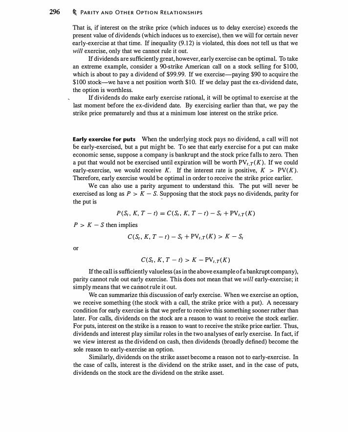
296 � PA R ITY A N D OTH E R O PT I O N R E LATI O N S H I PS

That is, if interest on the strike price (which induces us to delay exercise) exceeds the present value of dividends (which induces us to exercise), then we will for certain never early-exercise at that time. If inequality (9. 1 2) is violated, this does not tell us that we will exercise, only that we cannot rule it out.

If dividends are sufficiently great, however, early exercise can be optimal. To take an extreme example, consider a 90-s trike American call on a stock selling for $ 1 00, which is about to pay a dividend of $99.99. If we exercise-paying $90 to acquire the $ 1 00 stock-we have a net position worth $ 1 0. If we delay past the ex-dividend date, the option is worthless.

If dividends do make early exercise rational, it will be optimal to exercise at the last moment before the ex-dividend date. By exercising earlier than that, we pay the strike price prematurely and thus at a minimum lose interest on the strike price.

Early exercise for puts When the underlying stock pays no dividend, a call will not be early-exercised, but a put might be. To see that early exercise for a put can make economic sense, suppose a company is bankrupt and the stock price falls to zero. Then a put that would not be exercised until expiration will be worth PV1 .T (K) . If we could early-exercise, we would receive K. If the interest rate is positive, K > PV(K) . Therefore, early exercise would be optimal in order to receive the strike price earlier.

We can also use a parity argument to understand this. The put will never be exercised as long as P > K - S. Supposing that the stock pays no dividends, parity for the put is

·

P (S1 , K, T - t) = C(S1 , K, T - t) - Sr + PV1.T (K)

P > K - S then implies

C(S1 , K, T - t) - S1 + PVr .T (K) > K - Sr

or

C(S1 , K , T - t) > K - PVr.T (K)

If the call is sufficiently valueless (as in the above example of a bankrupt company), parity cannot rule out early exercise. This does not mean that we will early-exercise; it simply means that we caimot rule it out.

We can summarize this discussion of early exercise. When we exercise an option, we receive something (the stock with a call, the strike price with a put) . A necessary condition for early exercise is that we prefer to receive this something sooner rather than later. For calls, dividends on the stock are a reason to want to receive the stock earlier. For puts, interest on the strike is a reason to want to receive the strike price earlier. Thus, dividends and interest play similar roles in the two analyses of early exercise. In fact, if we view interest as the dividend on cash, then dividends (broadly defined) become the sole reason to early-exercise an option.

Similarly, dividends on the strike asset become a reason not to early-exercise. In the case of calls, interest is the dividend on the strike asset, and in the case of puts, dividends on the stock are the dividend on the strike asset.

CO M PA R I N G O PT I O N S W I T H R ES P E CT TO STY L E, M ATU R I TY, A N D STR I K E � 297

The point of this section has been to make some general statements about when early exercise will not occur, or under what conditions it might occur. Early exercise is a trade-off involving time value of money on the strike price, dividends on the underlying asset, and the value of insurance on the position. In general, figuring out when to exercise requires an option pricing model. We will discuss early exercise further in Chapters 1 0 and 1 1 .

Time to Expiration

How does an option price change as we increase time to expiration? If the options are American, the option price can never decline with an increase in time to expiration. If

the options are European, the price can go either up or down as we increase time to expiration.

American options An American call with more time to expiration is at least as valuable as an otherwise identical call with less time to expiration. An American call with 2 years to expiration, for example, can always be turned into an American option with 1 year to expiration by voluntarily exercising it after 1 year. Therefore, the 2-year call is at least as valuable as the 1 -year call.

The same is true for puts: A longer-lived American put is always worth at least as much as an otherwise equivalent European put.

European options A European call on a nondividend-paying stock will be at least as valuable as an otherwise identical call with a shorter time to expiration. This occurs · because, with no dividends, a European call has the same price as an otherwise identical American call . With dividends, however, longer-lived European options may be less valuable than shorter-lived European options. Economic forces that make it optimal to exercise an option early can make a short-lived European option worth more than a long-lived European option.

To see this for calls, imagine a stock that will pay a liquidating dividend 2 weeks from today.6 A European call with I week to expiration will have value since it is exercisable prior to the dividend. A European call with 3 weeks to expiration will have no value since the stock will have no value at expiration. This is an example of a longer­lived option being less valuable than a shorter-lived option. Note that if the options were American, we would simply exercise the 3-week option prior to the dividend.

Longer-lived European puts can also be less valuable than shorter-lived European puts. A good example of this is a bankrupt company. The put will be worth the present value of the strike price, with present value calculated until time to expiration. Longer­lived puts will be worth less than shorter-lived puts. If the options were American, they would all be exercised immediately and hence would be worth the strike price.

6 A liquidating dividend occurs when a firm pays its entire value to shareholders. A firm is worthless after paying a liquidating dividend.

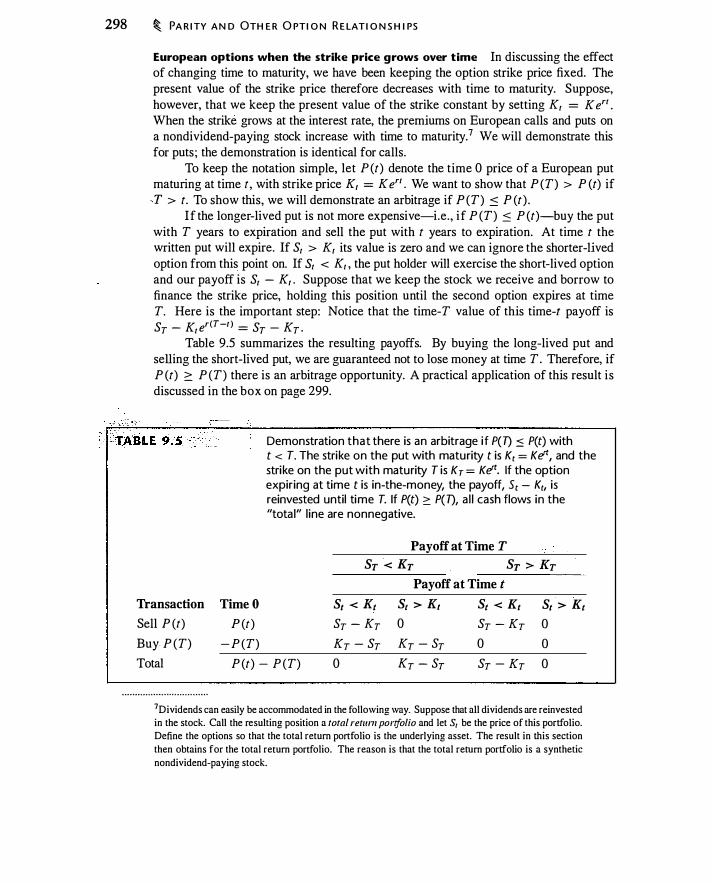
298 � PA R I TY AN D OTH E R O PTI O N R E LAT I O N S H I PS

European options when the strike price grows over time In discussing the effect of changing time to maturity, we have been keeping the option strike price fixed. The present value of the strike price therefore decreases with time to maturity. Suppose, however, that we keep the present value of the strike constant by setting Kr = Kerr . When the strike grows at the interest rate, the premiums on European calls and puts on a nondividend-paying stock increase with time to maturity.7 We will demonstrate this for puts ; the demonstration is identical for calls.

To keep the notation simple, let P (t) denote the time 0 price of a European put maturing at time t, with strike price Kr = Kerr . We want to show that P (T) > P (t) if

,y > t. To show this, we will demonstrate an arbitrage if P (T) ::=: P (t) . If the longer-lived put is not more expensive-i.e. , if P (T) ::=: P (t)-buy the put

with T years to expiration and sell the put with t years to expiration. At time t the written put will expire. If Sr > Kr its value is zero and we can ignore the shorter-lived option from this point on. If Sr < Kr , the put holder will exercise the short-lived option and our payoff is Sr - Kr . Suppose that we keep the stock we receive and borrow to finance the strike price, holding this position until the second option expires at time T. Here is the important step: Notice that the time-T value of this time-t payoff is ST - Kr er<T-r ) = ST - KT .

Table 9.5 summarizes the resulting payoffs. By buying the long-lived put and selling the short-lived put, we are guaranteed not to lose money at time T . Therefore, if P (t) � P (T) there is an arbitrage opportunity. A practical application of this result is discussed in the box on page 299.

Transaction

Sell P (t)

Buy P (T)

Total

· · · · · · · · · · · • • h • • • • • · · · · · · · · · . . · ·

Time O

P (t)

- P (T)

Demonstration that there is an arbitrage if P(7) :::: P(t) with t < T. The strike on the put with maturity t is K1 = Ket, and the strike on the put with maturity T is KT = Ket. If the option expiring at time t is in-the-money, the payoff, 51 - K1, is reinvested until time T. If P(t) :::: P(7), a l l cash flows in the "total" l ine are nonnegative.

Payoff at Time T ST < Kr Sr > Kr

Payoff at Time t St < Kt St > Kt St < Kt St > Kt

ST - KT 0 ST - KT 0

KT - ST KT - ST 0 0

P (t) - P (T) 0 KT - ST ST - KT 0

7Dividends can easily be accommodated in the following way. Suppose that all dividends are reinvested in the stock. Call the resulting position a total retum portfolio and let S, be the price of this portfolio. Define the options so that the total return portfolio is the underlying asset. The result in this section

then obtains for the total return portfolio. The reason is that the total return portfolio is a synthetic

nondividend-paying stock.

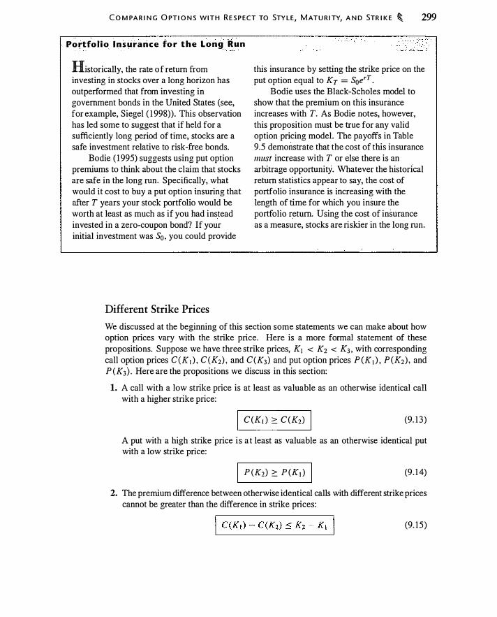
C O M PA R I N G O PT I O N S W I T H R E S P ECT TO STY LE, M ATU R I TY, A N D STR I K E � 299

Po rtfo l i o Insurance for the Long Run

Historically, the rate of return from investing in stocks over a long horizon has outperformed that from investing in government bonds in the United States (see, for example, Si�gel ( 1 998)). This observation has led some to suggest that if held for a sufficiently long period of time, stocks are a safe investment relative to risk-free bonds.

Bodie ( 1 995) suggests using put option premiums to think about the claim that stocks are safe in the long run. Specifically, what would it cost to buy a put option insuring that after T years your stock portfolio would be worth at least as much as if you had instead invested in a zero-coupon bond? If your initial investment was S0 , you could provide

Different Strike Prices

this insurance by setting the strike price on the put option equal to K r = S0erT .

Bodie uses the Black-Scholes model to show that the premium on this insurance increases with T. As Bodie notes, however, this proposition must be true for any valid option pricing model. The payoffs in Table 9.5 demonstrate that the cost of this insurance must increase with T or else there is an arbitrage opportunity. Whatever the historical return statistics appear to say, the cost of portfolio insurance is increasing with the length of time for which you insure the portfolio return. Using the cost of insurance as a measure, stocks are riskier in the long run.

We discussed at the beginning of this section some statements we can make about how option prices vary with the strike price. Here is a more formal statement of these propositions. Suppose we have three strike prices, K1 < K2 < K3 , with corresponding call option prices C(K1 ) , C (Kz) , and C(K3) and put option prices P (K 1 ) , P (Kz) , and P (K3) . Here are the propositions we discuss in this section:

1. A call with a low strike price is at least as valuable as an otherwise identical call with a higher strike price:

I C(KI ) ::: C (Kz) I (9. 1 3 )

A put with a high strike price i s a t least as valuable as an otherwise identical put with a low strike price:

I P (Kz) ::: P (KJ ) I (9 . 1 4)

2. The premium difference between otherwise identical calls with different strike prices cannot be greater than the difference in strike prices:

(9. 15 )

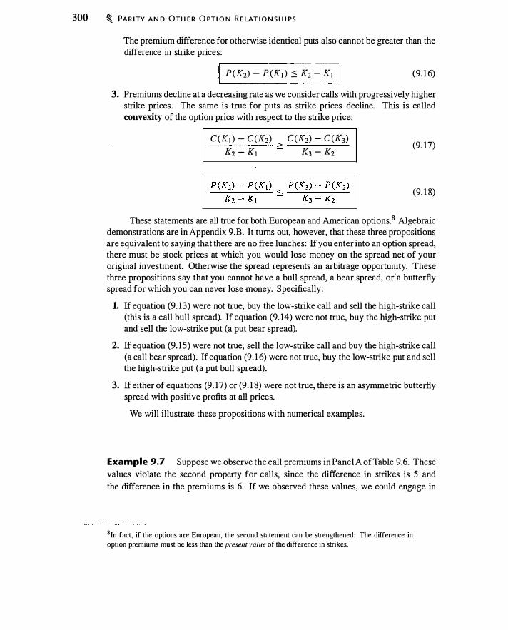
300 � PA R I TY AN D OTH E R O PT I O N R E LAT I O N S H I PS

The premium difference for otherwise identical puts also cannot be greater than the difference in strike prices:

I P(K2) - P (KI ) .::; K2 - Kl I (9. 1 6)

3. Premiums decline at a decreasing rate as we consider calls with progressively higher strike prices. The same is true for puts as strike prices decline. This is called convexity of the option price with respect to the strike price:

C(K! ) - C(K2) > C(K2) - C(K3) K2 - K1 K3 - K2

(9 . 17)

(9. 1 8)

These statements are all true for both European and American options. 8 Algebraic demonstrations are in Appendix 9 .B. It turns out, however, that these three propositions are equivalent to saying that there are no free lunches: If you enter into an option spread, there must be stock prices at which you would lose money on the spread net of your original investment. Otherwise the spread represents an arbitrage opportunity. These three propositions say that you cannot have a bull spread, a bear spread, or'a butterfly spread for which you can never lose money. Specifically:

1. If equation (9. 13) were not true, buy the low-strike call and sell the high-strike call (this is a call bull spread). If equation (9. 14) were not true, buy the high-strike put and sell the low-strike put (a put bear spread).

2. If equation (9. 15 ) were not true, sell the low-strike call and buy the high-strike call (a call bear spread) . If equation (9 . 1 6) were not true, buy the low-strike put and sell the high-strike put (a put bull spread).

3. If either of equations (9 . 1 7) or (9 . 1 8) were not true, there is an asymmetric butterfly spread with positive profits at all prices.

We will illustrate these propositions with numerical examples.

Example 9.7 Suppose we observe the call premiums in Panel A of Table 9.6. These values violate the second property for calls, since the difference in strikes is 5 and the difference in the premiums is 6. If we observed these values, we could engage in

8In fact, if the options are European, the second statement can be strengthened: The difference in option premiums must be less than the presem value of the difference in strikes.

C O M PA R I N G O PT I O N S W ITH R ES P E CT TO STY L E, M ATU R I TY, A N D STR I K E � 301

Panel A shows ca l l option premiums for which the change in the option premium ($6) exceeds the change in the strike price ($5). Panel B shows how a bear spread can be used to arbitrage these prices. By lending the bear spread proceeds, we have a zero cash flow at time 0; the cash outflow at time T is always greater than $ 1 .

Panel A

Strike

Premium 1 8 1 2

Transaction Time 0

Buy 55-strike call - 12

Sell 50-strike call 1 8

Total 6

Panel B

Expiration or Exercise

Sr < SO SO � Sr � 55 Sr ::: 55 0 0 Sr - 55

0

0 -5

arbitrage by buying the 55-strike call and selling the 50-strike call, which is a bear spread. Note that we receive $6 initially and never have to pay more than $5 in the future. This

:! is an arbitrage, whatever the interest rate. �

Now consider the third proposition, strike price convexity. There is a different way to write the convexity inequality, equation (9. 17) . Since K2 is between K1 and K3 , we can write it as a weighted average of the other two strikes, that is

where

A = K3 - K2 K3 - KI

With this expression for A, it is possible to rewrite equation (9. 17) as

Here is an example illustrating convexity.

Example 9.8 If K1 = 50, K2 = 59, and K3 = 65, A = �;:::�� = 0.4; hence,

59 = 0.4 X 50 + 0.6 X 65

(9. 1 9)

(9.20)

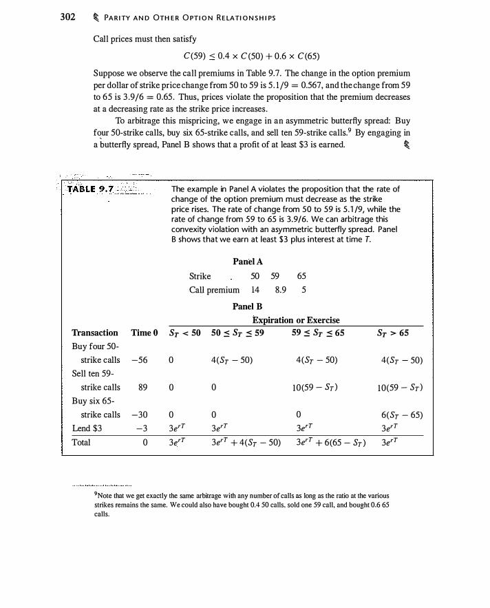
302 � PA R I TY A N D OTH E R O PTI O N R E LATI O N S H I PS

Call prices must then satisfy

C (59) s 0.4 X C (50) + 0.6 X C (65)

Suppose we observe the call premiums in Table 9.7. The change in the option premium per dollar of strike price change from 50 to 59 is 5 . 1 /9 = 0.567, and the change from 59 to 65 is 3 .9/6 = 0.65 . Thus, prices violate the proposition that the premium decreases at a decreasing rate as the strike price increases .

To arbitrage this mispricing, we engage in an asymmetric butterfly spread: Buy four 50-strike calls, buy six 65-strike calls, and sell ten 59-strike calls.9 By engaging in a butterfly spread, Panel B shows that a profit of at least $3 is earned. �

The example in Panel A violates the proposition that the rate of change of the option premium must decrease as the strike price rises. The rate of change from 50 to 59 is 5 . 1 /9, while the rate of change from 59 to 65 is 3 .9/6. We can arbitrage this convexity violation with an asymmetric butterfly spread. Panel B shows that we earn at least $3 plus interest at time T.

Panel A

Strike 50 59 65

Call premium 14 8.9 5

Panel B

Expiration or Exercise Transaction Time O Sr < 50 50 ::: Sr ::: 59 59 ::: Sr ::: 65 Sr > 65

Buy four 50-

strike calls -56 0

Sell ten 59-

strike calls 89 0

Buy six 65-

strike calls -30 0

Lend $3 -3 3erT

Total 0 3erT

4(Sr - 50)

0

0 3erT

3erT + 4(Sr - 50)

4(Sr - 50)

10 (59 - Sr )

0 3erT

3erT + 6(65 - Sr )

4(Sr - 50)

1 0(59 - Sr)

6(Sr - 65) 3erT

3erT

9Note that we get exactly the same arbitrage with any number of calls as long as the ratio at the various

strikes remains the same. We could also have bought 0.4 50 calls, sold one 59 call, and bought 0.6 65

calls.

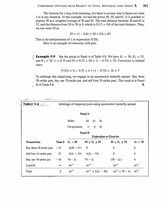
CO M PA R I N G O PT I O N S W I T H R ES P ECT TO STY LE, M ATU R I TY, A N D ST R I K E � 303

The formula for A may look imposing, but there is an easy way to figure out what A is in any situation. In this example, we had the prices 50, 59, and 65 . It is possible to express 59 as a weighted average of 50 and 65. The total distance between 50 and 65 is 15 , and the distance from 50 to 59 is 9, which is 9/ 1 5 = 0.6 of the total distance. Thus, we can write 59 as

59 = ( 1 - 0.6) X 50 + 0.6 X 65

This is tpe interpretation of A in expression (9.20). Here is an example of convexity with puts.

Example 9.9 See the prices in Panel A of Table 9.8 . We have K1 = 50, K1 = 55, and K3 = 70. A = 0.75 and 55 = 0.75 x 50 + (1 - 0.75) x 70. Convexity is violated since

P (55) = 8 > 0.75 X 4 + ( 1 - 0.75) X 16 = 7

To arbitrage this mispricing, we engage in an asymmetric butterfly spread: Buy three 50-strike puts, buy one 70-strike put, and sell four 55-strike puts . The result is in Panel B of Table 9.8 . �

Arbitrage of mispriced puts using asymmetric butterfly spread.

Panel A

Strike 50 55 70

Put premium 4 8 1 6 Panei B

Expiration or Exercise

Transaction Time O Sr < 50 50 :::: Sr :::: 55 55 :::; Sr � 70 Sr > 70 Buy three 50-strike puts - 12 3 (50 - Sr) 0 0 0

Sell four 55-strike puts 32 4(Sr - 55) 4(Sr - 55) 0 0

Buy one 70-strike put - 16 70 - Sr 70 - Sr (70 - Sr) 0

Lend $4 -4 4e'T 4e'T 4e'T 4e'T

Total 0 4e'T 4e'T + 3 (Sr - 50) 4e'T + 70 - Sr 4e'T

304 � PA R ITY A N D OTH E R O PT I O N R E LATI O N S H I PS

In this case, we always make at least 4. Figure 9.2 illustrates the necessary shape of curves for both calls and puts relating the option premium to the strike price.

Exercise and Moneyness

If it is optimal to exercise an option, it is also optimal to exercise an otherwise identical option that is more in-the-money. Consider what would have to happen in order for this not to be true.

Suppose a call option on a dividend-paying stock has a strike price of $50, and the stock price is $70. Also suppose that it is optimal to exercise the option. This means that the option must sell for $70 - $50 = $20.

Now what can we say about the premium of a 40-strike option? We know from the discussion above that the change in the premium is no more than the change in the strike price, or else there is an arbitrage opportunity. This means that

c (40) s $20 + ($50 - $40) = $30

Since the 40-strike call is worth $30 if exercised, it must be optimal to exercise it. Following the same logic, this is also true for puts.

�"

FIGURE 9.2 " Option Premium

I l l ustration of convexity and other strike price 50

properties for calls and 45 puts. For cal ls the premium is decreasing 40 in the strike, with a

35 slope less than one in absolute va lue. For puts 30 the premium is increasing in the strike, 25

with a slope less than 20

one. For both, the graph is convex, i.e., 15 shaped l ike the cross

10 section of a bowl .

5

0 0 20 40 60 80 100

Strike Price

-- ---

�.:.:_ .. 0._;::.-.:;�:z:-·,

CHAPTER SUMMARY

C H A PT E R S U M M A RY � 305

Put-call parity is one of the most important relations in option pricing. Parity is the observation that buying a European call and selling a European put with the same strike price and time to expiration is equivalent to making a leveraged investment in the un­derlying asset, less the value of cash payments to the underlying asset over the life of the option. Different versions of parity for different underlying assets appear in Table 9.9. In every case the value on the left-hand side of the parity equation is the price of the underlying asset less its cash flows over the life of the option. The parity relationship can be algebraically rearranged so that options and the underlying asset create a synthetic bond, options and a bond create a synthetic stock, and one kind of option together with the stock and bond synthetically create the other kind of option.

The idea of an option can be generalized to permit an asset other than cash to be the strike asset. This insight blurs the distinction between a put and a call. The idea that puts and calls are different ways of looking at the same contract is commonplace in currency markets.

Option prices must obey certain restrictions when we vary the strike price, time to maturity, or option exercise style. American options are at least as valuable as European options. American calls and puts become more expensive as time to expiration increases, but European options need not. European options on a nondividend-paying stock do become more expensive with increasing time to maturity if the strike price grows at the interest rate. Dividends are the reason to exercise an American call early, while interest is the reason to exercise an American put early. A call option on a nondividend-paying stock will always have a price greater than its value if exercised; hence, it should never be exercised early.

There are a number of pricing relationships related to changing strike prices. In particular, as the strike price increases, calls become less expensive with their price

' - TABLE 9 . 9 --_ - . _---·_-_

Underlying Asset

Futures contract

Stock, no-dividend

Versions of put-cal l parity. Notation in the table includes the spot currency exchange rate, x0; the risk-free interest rate in the foreign currency, r1; and the current bond price, 80 •

Parity Relationship

Stock, discrete dividend

Stock, continuous dividend

Currency

e-rT Fo. T = C(K, T) - P (K, T) + e-rT K

So = C ( K , T) - P ( K , T) + e-rT K

So - PVo.T (Div) = C(K, T) - P (K , T) + e-rT K e-8T So = C(K, T) - P (K, T) + e-rT K

e-r,Txo = C(K, T) - P (K, T) + e-rT K

Bo - PVo.T (Coupons) = C(K, T) - P (K , T) + e-rT K Bond

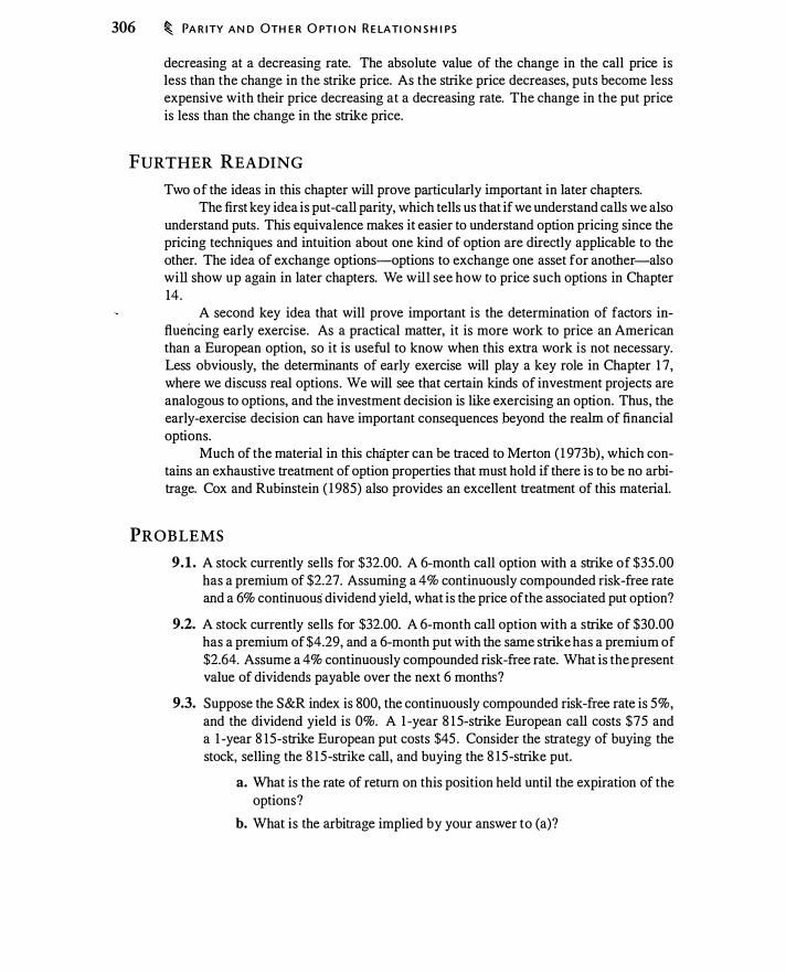
306 � PA R ITY A N D OTH E R O PT I O N R E LATI O N S H I PS

decreasing at a decreasing rate. The absolute value of the change in the call price is less than the change in the strike price. As the strike price decreases, puts become less expensive with their price decreasing at a decreasing rate. The change in the put price is less than the change in the strike price.

FURTHER READING

Two of the ideas in this chapter will prove particularly important in later chapters. The first key idea is put-call parity, which tells us that if we understand calls we also

understand puts. This equivalence makes it easier to understand option pricing since the pricing techniques and intuition about one kind of option are directly applicable to the other. The idea of exchange options--options to exchange one asset for another-also will show up again in later chapters. We will see how to price such options in Chapter 14.

A second key idea that will prove important is the determination of factors in­fluencing early exercise. As a practical matter, it is more work to price an American than a European option, so it is useful to know when this extra work is not necessary. Less obviously, the determinants of early exercise will play a key role in Chapter 1 7, where we discuss real options. We will see that certain kinds of investment projects are analogous to options, and the investment decision is like exercising an option. Thus, the early-exercise decision can have important consequences beyond the realm of financial options.

Much of the material in this chapter can be traced to Merton ( 1 973b ) , which con­tains an exhaustive treatment of option properties that must hold if there is to be no arbi­trage. Cox and Rubinstein ( 1 985) also provides an excellent treatment of this material.

PROB LEMS

9.1. A stock currently sells for $32.00. A 6-month call option with a strike of $35.00 has a premium of $2.27. Assuming a 4% continuously compounded risk-free rate and a 6% continuous dividend yield, what is the price of the associated put option?

9.2. A stock currently sells for $32.00. A 6-month call option with a strike of $30.00 has a premium of $4.29, and a 6-month put with the same strike has a premium of $2.64. Assume a 4% continuously compounded risk-free rate. What is the present value of dividends payable over the next 6 months?

9.3. Suppose the S&R index is 800, the continuously compounded risk-free rate is 5%, and the dividend yield is 0%. A 1 -year 8 15-strike European call costs $75 and a 1 -year 8 15-strike European put costs $45 . Consider the strategy of buying the stock, selling the 8 15-strike call, and buying the 8 15-strike put.

a. What is the rate of return on this position held until the expiration of the options?

b. What is the arbitrage implied by your answer to (a)?

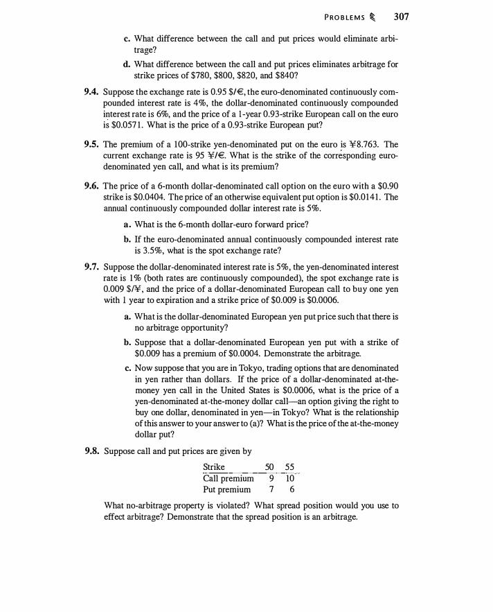
P RO B LE M S � 307

c. What difference between the call and put prices would eliminate arbi­trage?

d. What difference between the call and put prices eliminates arbitrage for strike prices of $780, $800, $820, and $840?

9.4. Suppose the exchange rate is 0.95 $/€, the euro-denominated continuously com­pounded interest rate is 4%, the dollar-denominated continuously compounded interest rate is 6%, and the price of a 1 -year 0.93-strike European call on the euro is $0.057 1 . What is the price of a 0.93-strike European put?

9.5. The premium of a 100-strike yen-denominated put on the euro is ¥8.763. The current exchange rate is 95 ¥/€. What is the strike of the corresponding euro­denominated yen call, and what is its premium?

9.6. The price of a 6-month dollar-denominated call option on the euro with a $0.90 strike is $0.0404. The price of an otherwise equivalent put option is $0.0 14 1 . The annual continuously compounded dollar interest rate is 5%.

a. What is the 6-month dollar-euro forward price?

b. If the euro-denominated annual continuously compounded interest rate is 3.5%, what is the spot exchange rate?

9.7. Suppose the dollar-denominated interest rate is 5%, the yen-denominated interest rate is 1 % (both rates are continuously compounded), the spot exchange rate is 0.009 $/¥, and the price of a dollar-denominated European call to buy one yen with 1 year to expiration and a strike price of $0.009 is $0.0006.

a. What is the dollar-denominated European yen put price such that there is no arbitrage opportunity?

b. Suppose that a dollar-denominated European yen put with a strike of $0.009 has a premium of $0.0004. Demonstrate the arbitrage.

c. Now suppose that you are in Tokyo, trading options that are denominated in yen rather than dollars . If the price of a dollar-denominated at-the­money yen call in the United States is $0.0006, what is the price of a yen-denominated at-the-money dollar call-an option giving the right to buy one dollar, denominated in yen-in Tokyo? What is the relationship of this answer to your answer to (a)? What is the price of the at -the-money dollar put?

9.8. Suppose call and put prices are given by

Strike 50 55 Call premium 9 10 Put premium 7 6

What no-arbitrage property is violated? What spread position would you use to effect arbitrage? Demonstrate that the spread position is an arbitrage.

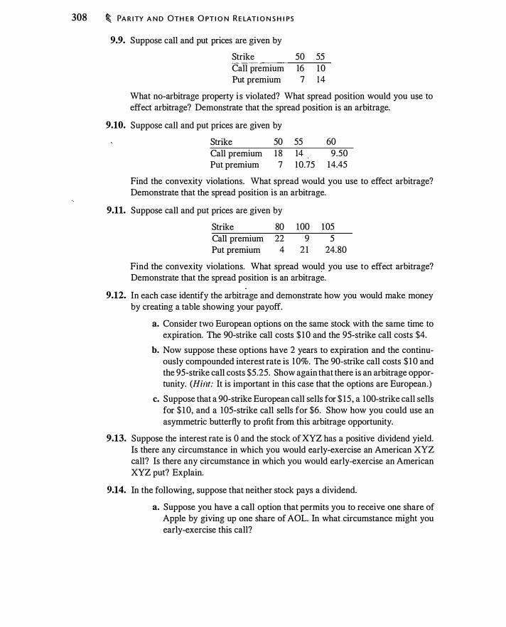
308 � PA R ITY A N D OTH E R O PT I O N R E LAT I O N S H I PS

9.9. Suppose call and put prices are given by

Strike 50 55 Call premium 16 I 0 Put premium 7 14

What no-arbitrage property i s violated? What spread position would you use to effect arbitrage? Demonstrate that the spread position is an arbitrage.

9.10. Suppose call and put prices are given by

9.11.

Strike Call premium Put premium

50 55 1 8 14 7 10.75

60 9.50

14.45

Find the convexity violations. What spread would you use to effect arbitrage? Demonstrate that the spread position is an arbitrage.

Suppose call and put prices are given by

Strike 80 100 1 05 Call premium 22 9 5 Put premium 4 2 1 24.80

Find the convexity violations. What spread would you use to effect arbitrage? Demonstrate that the spread position is an arbitrage.

9.12. In each case identify the arbitrage and demonstrate how you would make money by creating a table showing your payoff.

a. Consider two European options on the same stock with the same time to expiration. The 90-strike call costs $ 1 0 and the 95-strike call costs $4.

b. Now suppose these options have 2 years to expiration and the continu­ously compounded interest rate is l O%. The 90-strike call costs $ 1 0 and the 95-strike call costs $5.25. Show again that there is an arbitrage oppor­tunity. (Hilit: It is important in this case that the options are European.)

c. Suppose that a 90-strike European call sells for $ 15 , a 100-strike call sells for $ 1 0, and a 1 05-strike call sells for $6. Show how you could use an asymmetric butterfly to profit from this arbitrage opportunity.

9.13. Suppose the interest rate is 0 and the stock of XYZ has a positive dividend yield. Is there any circumstance in which you would early-exercise an American XYZ call? Is there any circumstance in which you would early-exercise an American XYZ put? Explain.

9.14. In the following, suppose that neither stock pays a dividend.

a. Suppose you have a call option that permits you to receive one share of Apple by giving up one share of AOL. In what .circumstance might you early-exercise this call?

P R O B LE M S � 309

b. Suppose you have a put option that permits you to give up one share of Apple, receiving one share of AOL. In what circumstance might you early-exercise this put? Would there be a loss from not early-exercising if Apple had a zero stock price?

c. Now suppose that Apple is expected to pay a dividend. Which of the above answers will change? Why?

9.15. The price of a nondividend-paying stock is $ 1 00 and the continuously compounded nsk-free rate is 5%. A 1 -year European call option with a strike price of $ 100 x e0·05x 1 = $ 1 05 . 127 has a premium of $ 1 1 .924. A H year European call option with a strike price of $ 1 00 x e0·05x 1 .S = $ 1 07 .788

-has a premium of $ 1 1 .50.

Demonstrate an arbitrage.

9.16. Suppose that to buy either a call or a put option you pay the quoted ask price, de­noted C0 (K , T) and Pa (K, T), and to sell an option you receive the bid, Cb (K, T) and Pb (K, T) . Similarly, the ask and bid prices for the stock are Sa and Sb . Finally, suppose you can borrow at the rate rH and lend at the rate �"L · The stock pays no dividend. Find the bounds between which you cannot profitably perform a parity arbitrage.

9.17. In this problem we consider whether parity is violated by any of the option prices in Table 9. 1 . Suppose that you buy at the ask and sell at the bid, and that your continuously compounded lending rate is 2% and your borrowing rate is 4%. Ignore transaction costs on the stock, for which the price is $ 106.79. Assume that IBM is expected to pay a $0. 14 dividend in early May. For each strike and expiration, what is the cost if you

a. Buy the call, sell the put, short the stock, and lend the present value of the strike price?

b. Sell the call, buy the put, buy the stock, and borrow the present .value of the strike price?

9.18. Consider the April 95 , 100, and 105 call option prices in Table 9 . 1 .

a. Does convexity hold if you buy a butterfly spread, buying at the ask price and selling at the bid?

b. Does convexity hold if you sell a butterfly spread, buying at the ask price and selling at the bid?

c. Does convexity hold if you are a market-maker either buying or selling a butterfly, paying the bid and receiving the ask?

d. Suppose the ask price for the 100-strike call had been $9.20 instead of $9.00. Is there a convexity violation? For whom?

310 � PA R I TY A N D OTH E R O PT I O N R E LAT I O N S H I PS

APPENDIX 9 .A : PARITY B OUNDS FOR AMERICAN OPTIONS

The exact parity relationship discussed in Chapter 9 only holds for European options. However, American options often come close to obeying put-call parity, especially when options have short times to expiration.

With a nondividend-paying stock, the call will not be exercised early, but the put might be. The effect of early exercise for the put is to accelerate the receipt of the strike price. Since interest on the strike price is small for short times to maturity, parity will come close to holding for short-lived American options on nondividend-paying stocks.

We now let P and C refer to prices of American options. The American put can be more valuable than the European put, and we have

P � C + PV(K) - S However, suppose that the put were exercised early. Then it would be worth K - S. For example, if we think of synthetically creating the stock by buying the call and selling the put, there is a chance that we will pay K before expiration, in the event the stock price plummets and the put is early-exercised. Consequently, if we replace the present value of the strike with the undiscounted strike, we have a valid upper bound for the value of the put. It will be true (and you can verify with a no-arbitrage argument) that

When there are no dividends, we have C + K - S as an upper bound on the put, and European parity as a lower bound (since an American put is always worth at least as much as a European put). The parity relationship can be written as a restriction on the put price or on the call price:

C + K - S � P � C + PV(K) - S P + S - PV(K) � C � P + S - K

Thus, when there are no dividends, European parity can be violated to the extent of interest on the strike price. Since this will be small for options that are not long-lived, European parity can remain a good approximation for American options.

Dividends add the complication that the call as well as the put may be exercised early. There exists the possibility of a large parity violation because of the following "whipsaw" scenario: The call is exercised early to capture a large dividend payment, the stock price drops, and the put is then exercised early to capture interest on the strike price. The possibility that this can happen leads to a wider no-arbitrage band. With dividends, the parity relationship becomes (Cox and Rubinstein, 1 985, p. 1 52)

C + K + PV(D) - S � P � C + PV(K) - S P + S - PV(K) � C � P + S - PV(D) - K

The upper bound for the call is the same as in European parity, except without dividends. The intuition for the upper bound on the call option (the left-hand side) is that we can avoid the loss of dividends by early-exercising the call; hence, it is the same

A P P E N D I X g . B : ALG E B R A I C P R O O FS O F STR I K E-P R I C E R E LAT I O N S � 311

bound as in the European case with n o dividends . The lower bound exists because it may not be optimal to exercise the call to avoid dividends, and it may be optimal to early-exercise the put.

Consider the worst case for the call . Suppose K = $ 100 and S = $ 100, and the stock is about to pay a liquidating dividend (i.e., D = $ 1 00). We will not exercise the call, s ince doing so gives us nothing. The put will be exercised after the dividend is paid, once the stock is worthless. So P = $ 1 00. The relationship then states

C :::: P + S - D - K = 100 + 100 - 100 - 100 = 0

And indeed, the call will be worthless in this case.

APPENDIX 9 .B : ALGEBRAIC PROOFS OF STRIKE-PRICE RELATIONS

Appendix available online at www.aw-bc.cornlmcdonald.

CHABTER1o Binomial Option Pricing: I

I" e;,u" ohapt= wo di""'"d how tho prioo of ono option ;, re!atod to tho prioo of another, but we did not explain how to determine the price of an option relative to the price of the underlying asset. In this chapter we discuss the binomial option pricing model, with which we can compute the price of an option, given the characteristics of the stock or other underlying asset.

The binomial option pricing model assumes that, over a period of time, the price of the underlying asset can move only up or down by a specified amount-that is, the asset price follows a binomial distribution. Given this assumption, it is possible to determine a no-arbitrage price for the option. Surprisingly, this approach, which appears at first glance to be overly simplistic, can be used to price options, and it conveys much of the intuition underlying more complex (and seemingly more realistic) option pricing models that we will encounter in later chapters. It is hard to overstate the value of thoroughly understanding the binomial approach to pricing options .

Because of its usefulness, we devote this and the next chapter to binomial option pricing. In this chapter, we will see how the binomial model works and use it to price both European and American call and put options on stocks, currencies, and futures contracts. As part of the pricing analysis, we will also see how market-makers can create options synthetically using the underlying asset and risk-free bonds. In the next chapter, we will explore the assumptions underlying the model.

10.1 A ONE-PERIOD BINOMIAL TREE

Binomial pricing achieves its simplicity by making a very strong assumption about the stock price: At any point in time, the stock price can change to either an up value or a down value. In-between, greater, or lesser values are not permitted. The restriction to two possible prices is why the method is called "binomial ." The appeal of binomial pricing is that it &?plays the logic of option pricing in a simple setting, using only algebra to price options.

The binomial approach to pricing was first used by Sharpe ( 1978) as an intuitive way to explain option pricing. Binomial pricing was developed more formally by Cox et al. ( 1979) and Rendleman and Bartter ( 1 979), who showed how to implement the model, demonstrated the link between the binomial model and the Black-Scholes model,

3 13

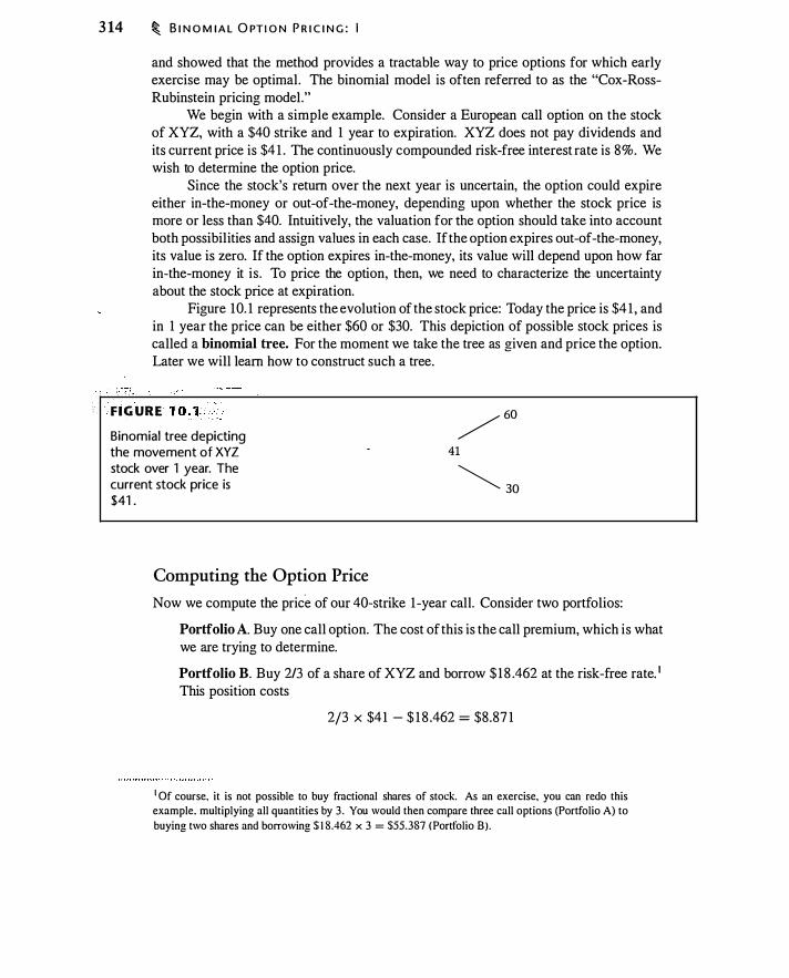
3 14 � B I N O M I A L O PTI O N P R I C I N G : I

and showed that the method provides a tractable way to price options for which early exercise may be optimal. The binomial model is often referred to as the "Cox-Ross­Rubinstein pricing model."

We begin with a simple example. Consider a European call option on the stock of XYZ, with a $40 strike and 1 year to expiration. XYZ does not pay dividends and its current price is $4 1 . The continuously compounded risk-free interest rate is 8%. We wish to determine the option price.

Since the stock's return over the next year is uncertain, the option could expire either in-the-money or out-of-the-money, depending upon whether the stock price is more or less than $40. Intuitively, the valuation for the option should take into account both possibilities and assign values in each case. If the option expires out-of-the-money, its value is zero. If the option expires in-the-money, its value will depend upon how far in-the-money it is . To price the option, then, we need to characterize the uncertainty about the stock price at expiration.

Figure 10. 1 represents the evolution of the stock price: Today the price is $4 1 , and in 1 year the price can be either $60 or $30. This depiction of possible stock prices is called a binomial tree. For the moment we take the tree as given and price the option. Later we will learn how to construct such a tree .

•· • F I G U R E 1 0 . 1 Binomial tree depicting the movement of XYZ stock over 1 year. The current stock price is $41 .

. .

Computing the Option Price

/ 60 41

� 30

Now we compute the price of our 40-strike 1 -year call . Consider two portfolios:

Portfolio A. Buy one call option. The cost of this is the call premium, which is what we are trying to determine.

Portfolio B. Buy 2/3 of a share of XYZ and borrow $ 1 8 .462 at the risk-free rate. 1

This position costs

2/3 X $41 - $ 1 8 .462 = $8.87 1

1 Of course, it is not possible to buy fractional shares of stock. As an exercise, you can redo this example. multiplying all quantities by 3 . You would then compare three call options (Portfolio A) to

buying two shares and borrowing $ 1 8.462 x 3 = $55.387 (Portfolio 8).

A O N E- P E R I O D B I N O M I A L TR E E � 3 15

Now we compare the payoffs to the two portfolios l year from now. Since the stock can take on only two values, we can easily compute the value of each portfolio at each possible stock price.

For Portfolio A, the time 1 payoff is max[O, S1 - $40] :

Payoff

Stock Price in 1 Year (S1) $30 $60

0 $20

In computing the payoff for Portfolio B, we assume that we sell the shares at the market price and that we repay the borrowed amount, plus interest ($ 1 8 .462 x e·08 = $20) . Thus we have

2/3 purchased shares Repay loan of $ 1 8 .462

Total payoff

Stock Price in 1 Year (S1) $30 $60 $20 $40

-$20 -$20 0 $20

Note that Portfolios A and B have the same payoff: Zero if the stock price goes down, in which case the option is out-of-the-money, and $20 if the stock price goes up . . Therefore, both portfolios should have the same cost. Since Portfolio B costs $8.87 1 , then given our assumptions, the price of one option must be $8. 871 . Portfolio B is a synthetic call, mimicking the payoff to a call by buying shares and borrowing.

The idea that positions that have the same payoff should have the same cost is called the law of one price. This example uses the law of one price to determine the option price. We will see shortly that there is an arbitrage opportunity if the law of one price is violated.

J:he call option in the example is replicated by holding 2/3 shares, which implies that one option has the risk of 2/3 shares. The value 2/3 is the delta (.6.) of the option: the number of shares that replicates the option payoff. Delta is a key concept, and we will say much more about it later.

Finally, we can say something about the expected return on the option. Suppose XYZ has a positive risk premium (i.e., the expected return on XYZ is greater than the risk-free rate). Since we create the synthetic call by borrowing to buy the stock, the call is equivalent to a leveraged position in the stock, and therefore the call will have an expected return greater than that on the stock. The option elasticity, which we will discuss in Chapter 12, measures the amount of leverage implicit in the option.

The Binomial Solution

In the preceding example, how did we know that buying 2/3 of a share of stock and borrowing $ 1 8.462 would replicate a call option?

3 16 � B I N O M I A L O PT I O N P R I C I N G : I

We have two instruments to use in replicating a call option: shares of stock and a position in bonds (i.e., borrowing or lending). To find the replicating portfolio, we need to find a combination of stock and bonds such that the portfolio mimics the option.

To be specific, we wish to find a portfolio consisting of !1 shares of stock and a dollar amount B in lending, such that the portfolio imitates the option whether the stock rises or falls. We will suppose that the stock has a continuous dividend yield of o, which we reinvest in the stock. Thus, as in Section 5 .2, if you buy one share at time t , at time t + lz you will have elih shares. The up and down movements of the stock price reflect the ex-dividend price.

We can write the stock price as u So when the stock goes up and as d So when the price goes down. We can represent the stock price tree as follows:

/ uS s

�dS In this tree u is interpreted as one plus the rate of capital gain on the stock if it goes up, and d is one plus the rate of capital loss if it goes down. (If there are dividends, the total return is the capital gain or loss, plus the dividend.)

Let C, and Cd represent the value of the option when the stock goes up or down, respectively. The tree for the stock implies a corresponding tree for the value of the option:

/ c" Co

If the length of a period is h , the interest factor per period is erh . The problem is to solve for !1 and B such that our portfolio of !1 shares and B in lending duplicates the option payoff. The value of the replicating portfolio at time lz, with stock price s, , is

!1 S, + er" B

At the prices s, = d S and s, = u S, a successful replicating portfolio will satisfy2

(!1 X dS X e8" ) + (B X erh ) = Cd (11 x u S X e"" ) + (B X er" ) = C,

2The term es" arises in the following equations because the owner of the stock receives a proportional

dividend that we assume is reinvested in shares.

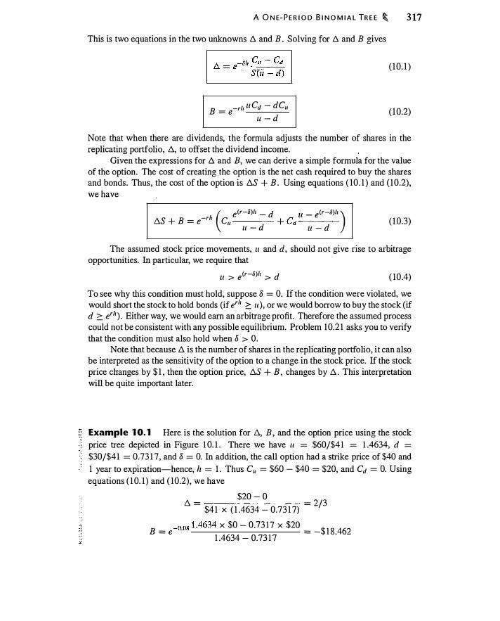
A O N E- P E R I O D B I N O M I A L TR E E � 3 17 This is two equations in the two unknowns 1:3. and B . Solving for 1:3. and B gives

B -ril uCd - dCu = e u - d

( 1 0. 1 )

( 1 0.2)

Note that when there are dividends, the formula adjusts the number of shares in the replicating portfolio, /:3., to offset the dividend income.

Given the expressions for 1:3. and B, we can derive a simple formula for the value of the option. The cost of creating the option is the net cash required to buy the shares and bonds. Thus, the cost of the option is 1:3.S + B . Using equations ( 10 . 1 ) and ( 1 0.2), we have

/:3.S + B = e-ril C11 + Cd----( e<r-8)11 _ d u _ e<r-a)h ) u - d u - d

( 1 0.3)

The assumed stock price movements, u and d, should not give rise to arbitrage opportunities. In particular, we require that

ll > e<r-a)h > d ( 10 .4)

To see why this condition must hold, suppose 8 = 0. If the condition were violated, we would short the stock to hold bonds (if er11 ::::, u ) , or we would borrow to buy the stock (if d ::::, .er1' ) . Either way, we would earn an arbitrage profit. Therefore the assumed process could not be consistent with any possible equilibrium. Problem I 0.2 1 asks you to verify that the condition must also hold when 8 > 0.

Note that because 1:3. is the number of shares in the replicating portfolio, it can also be interpreted as the sensitivity of the option to a change in the stock price. If the stock price changes by $ 1 , then the option price, /:3.S + B , changes by /:3. . This interpretation will be quite important later.

Example 1 0. 1 Here is the solution for /:3., B, and the option price using the stock price tree depicted in Figure 1 0. 1 . There we have u = $60/$4 1 = 1 .4634, d = $30/$41 = 0.73 1 7, and 8 = 0. In addition, the call option had a strike price of $40 and 1 year to expiration-hence, lz = 1 . Thus C11 = $60 - $40 = $20, and Cd = 0. Using equations ( 1 0. 1 ) and ( 10.2), we have

$20 - 0 /:3. =

$4 1 X ( 1 .4634 - 0.73 1 7) = 213

B = e-0.08 1 .4634 X $0 - 0.73 1 7 X $20 = -$ 1 8 .462

1 .4634 - 0.73 1 7

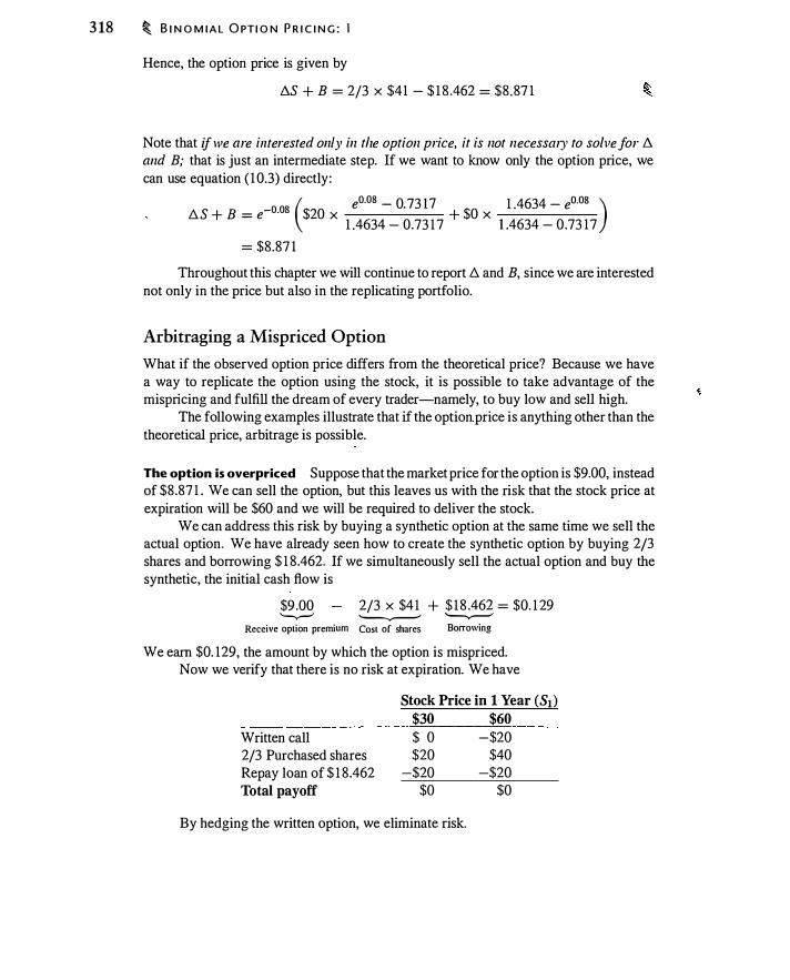
3 18 � B I N O M I A L O PT I O N P R I C I N G : I

Hence, the option price is given by

!:lS + B = 2/3 X $41 - $ 1 8 .462 = $8.87 1

Note that if we are illferested only in tlze option price, it is not necessmy to solve for !:l and B; that is just an intermediate step. If we want to know only the option price, we can use equation ( 1 0.3) directly :

!:l S + B = e-o.os $20 x + $ X -----( e0·08 - 0. 73 17 0

1 .4634 - e0·08 ) 1 .4634 - 0.73 1 7 1 .4634 - 0.73 17

= $8.87 1

Throughout this chapter we will continue to report !:l and B, since we are interested not only in the price but also in the replicating portfolio.

Arbitraging a Mispriced Option

What if the observed option price differs from the theoretical price? Because we have a way to replicate the option using the stock, it is possible to take advantage of the mispricing and fulfill the dream of every trader-namely, to buy low and sell high.

The following examples illustrate that if the option price is anything other than the theoretical price, arbitrage is possible.

The option is overpriced Suppose that the market price for the option is $9.00, instead of $8.87 1 . We can sell the option, but this leaves us with the risk that the stock price at expiration will be $60 and we will be required to deliver the stock.

We can address this risk by buying a synthetic option at the same time we sell the actual option. We have already seen how to create the synthetic option by buying 2/3 shares and borrowing $ 1 8.462. If we simultaneously sell the actual option and buy the synthetic, the initial cash flow is

$9 .00 '-v-'

2/3 X $41 + $ 1 8 .462 = $0. 1 29 '--v-"' '-.,..-'

Receive option premium Cost of shares Borrowing

We earn $0. 129, the amount by which the option is mispriced. Now we verify that there is no risk at expiration. We have

Written call 2/3 Purchased shares Repay loan of $ 1 8 .462 Total payoff

Stock Price in 1 Year (S1) $30 $60 $ 0 -$20 $20 $40

-$20 -$20 $0 $0

By hedging the written option, we eliminate risk.

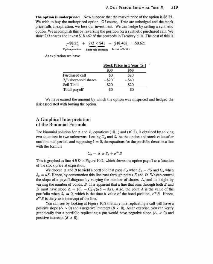
A O N E- P E R I O D B I N O M I A L TR E E � 3 19

The option is underpriced Now suppose that the market price of the option is $8.25 .

We wish to buy the underpriced option. Of course, i f we are unhedged and the stock price falls at expiration, we lose our investment. We can hedge by selling a synthetic option. We accomplish this by reversing the position for a synthetic purchased call : We short 2/3 shares and invest $ 1 8 .462 of the proceeds in Treasury bills. The cost of this is

-$8 .25 + 2/3 X $4 1 - $ 1 8 .462 = $0. 62 1 '-v--' '-v---' ...__,_..,

Option premium Short-sale proceeds Invest in T-bills

At expiration we have

Purchased call 2/3 short-sold shares Sell T-hill Total payoff

Stock Price in 1 Year (S1) $30 $60

$0 $20

-$20 -$40

$20 $20

$0 $0

We have earned the amount by which the option was mispriced and hedged the risk associated with buying the option.

A Graphical Interpretation of the Binomial Formula

The binomial solution for 11 and B, equations ( 10. 1 ) and ( 10.2), is obtained by solving two equations in two unknowns. Letting c, and s, be the option and stock value after one binomial period, and supposing o = 0, the equations for the portfolio describe a line with the formula

C, = 11 x s, + e'" B

This is graphed as line AE D in Figure 1 0.2, which shows the option payoff as a function of the stock price at expiration.

We choose 11 and B to yield a portfolio that pays Cd when S, = d S and C11 when s, = u S . Hence, by construction this line runs through points E and D. We can control the slope of a payoff diagram by varying the number of shares, /1, · and its height by varying the number of bonds, B. It is apparent that a line that runs through both E and D must have slope 11 = (C11 - Cd) / (u S - dS) . Also, the point A is the value of the portfolio when s, = 0, which is the time-lz value of the bond position, e'" B. Hence, e'" B is the y-axis i)ltercept of the line.

You can see by looking at Figure 1 0.2 that any line replicating a call will have a positive slope (b. > 0) and a negative intercept (B < 0). As an exercise, you can verify graphically that a portfolio replicating a put would have negative slope (/1 < 0) and positive intercept (B > 0) .

320 � B I N O M I A L O PTI O N P R I C I N G :

The payoff to an expiring cal l option is the dark heavy l ine. The payoff to the option at the points dS and uS are Cd and Cu (at point D). The portfolio consisting of t:;. shares and 8 bonds has intercept e'hB and slope t:;., and by construction goes through both points E and D. The slope of the l ine is calcu lated as :�� between points E and D, which g ives the formula for /:;..

Option Payoff

C, = uS - K

Intercept = eriiB A

Risk-Neutral Pricing

Run = uS - dS

S1, (Stock price after one period)

So far we have not specified the probabilities of the stock going up or down. In fact, probabilities were not used anywhere in the option price calculations. Since the strategy of holding t. shares and B bonds replicates the option whichever way the stock moves, the probability of an up or down movement in the stock is irrelevant for pricing the option.

Although probabilities are not needed for pricing the option, there is a probabilistic interpretation of equation ( 10.3) . Notice that in equation ( 10.3) the terms (e<r-li)h -d)j(u - d) and (u - e<r-lilh )/ (ll - d) sum to 1 and are both positive (this follows from inequality 1 0.4) . Thus, we can interpret these terms as probabilities. Let

e<r-li)h _ d p* = ---­

u - d

Equation ( 1 0.3) can then be written as

I C = e-rh [p*C, + ( 1 - p*)Cd]

( 10.5)

( 1 0.6)

This expression has the appearance of a discounted expected value. It is peculiar, though, because we are discounting at the risk-free rate, even though the risk of the option is at least as great as the risk of the stock (a call option is a leveraged position in the stock since B < 0). In addition, there is no reason to think that p* is the true probability that the stock will go up; in general it is not.

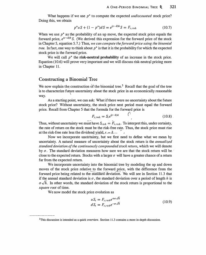
A O N E- P E R I O D B I N O M I A L TR E E � 321

What happens if we use p* to compute the expected wzdiscowzted stock price? Doing this, we obtain

p*uS + ( 1 - p*)dS = e<r-li)h S = F1.1+h ( 10.7)

When w� use p* as the probability of an up move, the expected stock price equals the forward price, e<r-li)h S. (We derived this expression for the forward price of the stock in Chapter 5, equation 5 .7.) Thus, we can compute tlzefonvard price using the binomial tree. In filet, one way to think about p* is that it is the probability for which the expected stock price is the forward price.

We will call p* the risk-neutral probability of an increase in the stock price. Equation ( 1 0.6) will prove very important and we will discuss risk-neutr<}.l pricing more in Chapter 1 1 .

Constructing a Binomial Tree

We now explain th� construction of the binomial tree.3 Recall that the goal of the tree is to characterize fut�re uncertainty about the stock price in an economically reasonable way.

As a starting point, we can ask: What if there were no uncertainty about the future stock price? Without uncertainty, the stock price next period must equal the forward price. Recall from Chapter 5 that the formula for the forward price is

(' ( 1 0.8) .

Thus, without uncertainty we must have Sr+h = F, . 1+" . To interpret this, under certainty, the rate of return on the stock must be the risk-free rate. Thus, the stock price must rise at the risk-free rate less the divideng_ yJdd,.l"-=-D .- "

Now we incorporate uncertainty, but we first need to define what we mean by uncertainty. A natural measure of uncertainty about the stock return is the annualized standard deviation of the continuously compounded stock return, which we will denote by a . J'he standard deviation measures how sure we are that the stock return will be ·

close to the expected return. Stocks with a larger a will have a greater chance of a return far from the expected return.

We incorporate uncertainty into the binomial tree by modeling the up and down moves of the stock price relative to the forward price, with the difference from the forward price being related to thestandaid deviatic1n� We will see in Section 1 1 .3 that if the annual standard deviation is a , the standard deviation over a period of length lz is a .Jli. In other words, the standard deviation of the stock return is proportional to the square root of time.

We now model the stock price evolution as

S - F. +u./Ti u 1 - 1. 1+/Je ds - F. -u ./Ti 1 - 1 , 1+he

3This discussion is intended as a quick overview. Section 1 1 .3 contains a more in-depth discussion.

( 1 0.9)

322 � B I N O M I A L O PT I O N P R I C I N G : I

Using equation ( 10.8), we can rewrite this as

ll = e(r-8)h+CJ"./1i d = e(r-8)h-CJ"./1i ( 1 0. 10)

This is the formula we will use to construct binomial trees. Note that if we set volatility equal to zero (i.e., a = 0) , we will have li S, = dS, = Fr.r+h · Thus, with zero volatility, the price will still rise over time, just as with a Treasury bill. Zero volatility does not mean that prices are fixed; it means that prices are known in advance.

We will refer to a tree constructed using equation ( 10. 1 0) as a "forward tree." In Section 1 1 .3 we will discuss alternative ways to construct a tree, including the Cox­Ross-Rubinstein tree.

Another One:-Period Example

We_ began this section by assuming that the stock price followed the binomial tree in Figure 1 0. 1 . The up and down stock prices of $30 and $60 were selected to make the example easy to follow. Now we present an exctmple where everything is the same except that we use equation ( 10. 1 0) to construct the up and down moves.

Suppose volatility is 30%. Since the period is 1 year, we have h = 1, so that a .Jh = 0.30. We also have So = $41 , r = 0.08, and 8 = 0. Using equation ( 10 . 1 0), we get

li S = $41 e(O.OS-O) x l+0.3 x../T = $59.954 dS = $41 e(0.08-0) x 1 -0.3 x ../T = $32.903 ( 10. 1 1 )

Because the binomial tree is different than i n Figure 10. 1 , the option price will be different as well .

Using the stock prices given in equation ( 10. 1 1 ), we have u = $59.954/$41 = 1 .4623 and d = $32.903/$4 1 = 0.8025 . With K = $40, we have C11 = $59.954 -$40 = $ 19 .954, and Cd = 0. Using equations ( 10. 1 ) and ( 1 0.2), we obtain

/::;.. = $19 .954 - 0 = 0.7376 $41 X ( 1 .4623 - 0.8025)

0 08 1 .4623 X $0 - 0.8025 X $ 19 .954 $ B = e- · = - 22.405

1 .4623 - 0.8025 Hence, the option price is given by

/::;.. S + B = 0.7376 X $41 - $22.405 = $7 . 839

This example is summarized in Figure 10.3 .

Summary

We have covered a great deal of ground in this section, so we pause for a moment to . review the main points:

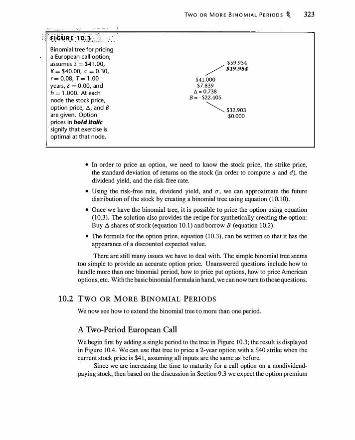
: : t=lciuRE't�E�L �� . . Binomial tree for pricing a European cal l option; assumes S = $41 .00, K = $40.00, a = 0.30, r = 0.08, T = 1 .00 years, 8 = 0.00, and h = 1 .000. At each node the stock price, option price, t., and B are given. Option prices in bold italic signify that exercise is optimal at that node.

TWO O R M O R E B I N O M I A L P E R I O D S � 323

$59.954 /$19.954 $41 .000 $ 7.839

f. = 0.738 B = -$22.405

� $32.903 $0.000

• In order to price an option, we need to know the stock price, the strike price, the standard deviation of returns on the stock (in order to compute u and d), the dividend yield, and the risk-free rate.

• Using the risk-free rate, dividend yield, and u , we can approximate the future distribution of the stock by creating a binomial tree using equation ( 1 0. 1 0) .

• Once we have the binomial tree, i t i s possible to price the option using equation ( 10.3). The solution also provides the recipe for synthetically creating the option: Buy l:l shares of stock (equation 1 0. 1 ) and borrow B (equation 1 0.2).

• The formula for the option price, equation ( 1 0.3), can be written so that it has the appearance of a discounted expected value.

There are still many issues we have to deal with. The simple binomial tree seems too simple to provide an accurate option price. Unanswered questions include how to handle more than one binomial period, how to price put options, how to price American options, etc. With the basic binomial formula in hand, we can now turn to those questions.

10.2 TWO OR MORE BINOMIAL PERIODS

We now see how to extend the binomial tree to more than one period.

A Two-Period European Call

We begin first by adding a single period to the tree in Figure 10.3 ; the result is displayed in Figure 1 0.4. We can use that tree to price a 2-year option with a $40 strike when the current stock price is $41 , assuming all inputs are the same as before.

Since we are increasing the time to maturity for a call option on a nondividend­paying stock, then based on the discussion in Section 9.3 we expect the option premium

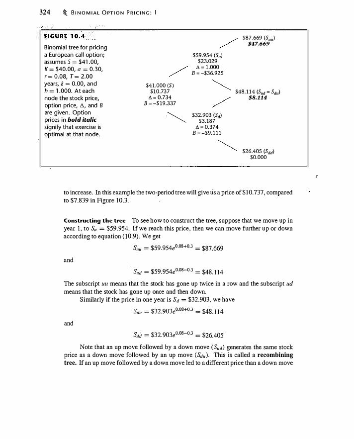
324 � B I N O M I A L O PT I O N P R I C I N G :

Binomial tree for pricing a European cal l option; assumes 5 = $41 .00, K = $40.00, a = 0.30, r = 0.08, T = 2.00 years, 8 = 0.00, and h = 1 .000. At each node the stock price, option price, l::i, and B are given. Option prices in bold italic signify that exercise is optimal at that node.

$41 .000 (S ) $10.737

L'1 = 0.734 B = -$ 19.337

-�

$59.954 (Su) $23.029 D. = 1 .000

B = -$36.925

$32.903 (Sc�) $3.187

L'1 = 0.374 B = -$9. 1 1 1

$87.669 (Suul $47.669

$48. 114 (Sud = Sdu) $8.114

$26.405 (Sdd) $0.000

to increase. In this example the two-period tree will give tis a price of $ 1 0.737, compared to $7.839 in Figure 10.3.

Constructing the tree To see how to construct the tree, suppose that we move up in year 1 , to Su = $59.954. If we reach this price, then we can move further up or down according to equation ( 10.9). We get

Suu = $59.954e0.08+0.3 = $87.669

and

Sud = $59.954eO.OS-0.3 = $48. 1 14 The subscript uu means that the stock has gone up twice in a row and the subscript ud means that the stock has gone up once and then down.

Similarly if the price in one year is Sd = $32.903, we have

Sdu = $32.903e0·08+0·3 = $48. 1 14

and

Sttd = $32.903e0·08-0·3 = $26.405

Note that an up move followed by a down move (S11d) generates the same stock price as a down move followed by an up move (Stt11 ). This is called a recombining tree. If an up move followed by a down move led to a different price than a down move

Tw o O R M O R E B I N O M I A L P E R I O D S � 325

followed by an up move, we would have a nonrecombining tree.4 A recombining tree has fewer nodes, which means less computation is required to compute an option price. We will see examples of nonrecombining trees in Sections 1 1 .5 and 24.4.

We also could have used equation ( 10. 10) directly to compute the year-2 stock prices. Recall that u = e0·08+0-3 = 1 .462 and d = e0·08-03 = 0.803. We have

Suu = u2 X $41 = e2x (O.OS+0.3) X $4 1 = $87.669

Sud = Sdu = !I X d X $41 = e<O.OS+0.3) X e<O.OS-0.3) X $41 = $48. 1 14

Sdd = d2 X $41 = e2x (O.OS-0.3) X $41 = $26.405

Pricing the call option How do we price the option when we have two binomial periods? The key insight is that we work bachvard through the binomial tree. In order to use equation ( 10.3), we need to know the option prices resulting from up and down moves in the subsequent period. At the outset, the only period where we know the option price is at expiration.

Knowing the price at expiration, we can determine the price in period 1. Having determined that price, we can work back to period 0.

Figure 1 0.4 exhibits the option price at each node as well as the details of the replicating portfolio at each node. Remember, however, when we use equation ( 1 0.3), it is not necessary to compute f".. and B in order to derive the option price.5 Here are details of the solution:

Year 2, Stock Price = $87.669 Since we are at expiration, the option value is max(O, S - K) = $47 .669.

Year 2, Stock Price = $48.114 Again we are at expiration, so the option value is $8. 1 14.

Year 2, Stock Price = $26.405 Since the option is out of the money, the value is 0.

Year 1, Stock Price = $59.954 At this node we use equation ( 10.3) to compute the option value. (Note that once we are a! this node, the "up" stock price, u S, is $87.669, and the "down" stock price, dS, is $48. 1 14.)

e-O.O& $47 .669 X + $8. 1 14 X = $23 .029 ( e0·08 - 0.803 1 .462 - e0·08 ) 1 .462 - 0.803 1 .462 - 0.803

4In cases where the tree recombines, the representation of stock price movements is also (and, some argue, more properly) called a lattice. The term tree would then be reserved for nonrecombining stock

movements.

5 As an exercise, you can verify the !'J. and B at each node.

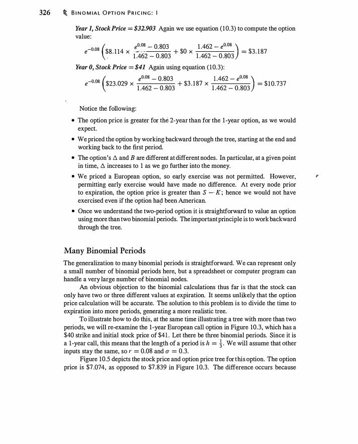
326 � B I N O M I A L O PT I O N P R I C I N G : I

Year 1, Stock Price = $32.903 Again we use equation ( 10.3) to compute the option value:

( e0·08 - 0.803 1 .462 - e0·08 ) e-0.08 $8 . 1 14 X 1 .462 - 0.803 + $0 X 1 .462 - 0.803 = $3 . 1 87

Year 0, Stock Price = $41 Again using equation ( 10.3) :

( e0·08 - 0.803 1 .462 - e0·08 ) e-0.08 $23 .029 X 1 .462 - 0.803 + $3 . 1 87 X 1 .462 - 0.803 = $ 10.737

Notice the following: • The option price is greater for the 2-year than for the 1 -year option, as we would

expect. • We priced the option by working backward through the tree, starting at the end and

working back to the first period. • The option's D. and B are different at different nodes. In particular, at a given point

in time, D. increases to 1 as we go further into the money. • We priced a European option, so early exercise was not permitted. However, r:

permitting early exercise would have made no difference. At every node prior to expiration, the option price is greater than S -

- K ; hence we would not have exercised even if the option ha� been American.

• Once we understand the two-period option it is straightforward to value an option using more than two binomial periods. The important principle is to work backward through the tree.

Many Binomial Periods

The generalization to many binomial periods is straightforward. We can represent only a small number of binomial periods here, but a spreadsheet or computer program can handle a very large number of binomial nodes.

An obvious objection to the binomial calculations thus far is that the stock can only have two or three different values at expiration. It seems unlikely that the option price calculation will be accurate. The solution to this problem is to divide the time to expiration into more periods, generating a more realistic tree.

To illustrate how to do this, at the same time illustrating a tree with more than two periods, we will re-examine the 1 -year European call option in Figure 10.3, which has a $40 strike and initial stock price of $41 . Let there be three binomial periods. Since it is a 1-year call, this means that the length of a period is h = 1 · We will assume that other inputs stay the same, so r = 0.08 and u = 0.3.

Figure 10.5 depicts the stock price and option price tree for this option. The option price is $7 .074, as opposed to $7.839 in Figure 10.3. The difference occurs because

Binomial tree for pricing a European call option; assumes S = $41 .00, K = $40.00, u = 0.30, r = 0.08, T = 1 .00 years, 8 = 0.00, and h = 0.333 . At each node the stock price, option price, b.., and B are given. Option prices in bold italic signify that exercise is optimal at that node.

$41.000 $7.074

/',. = 0.706 B = -$21 .885

TWO O R M O R E B I N O M I A L P E R I O D S � 327

$61 . 149 $22.202

$74.678 /$34.678 / !'> = 1 .000

/ B = -$38.947

$50.071 $ 12.889 !1 = 0.922

B = -$33.264

$35.41 1 $2.535

/',. = 0.450 B = -$ 13.405

$52.814 $12.814 $43.246 / $5 .700

!1 = 0.829 � B = -$30. 139 �

$30.585 $0.000

l'> = 0.000 B = $0.000

$37.35 1 $0.000

� $26.416 $0.000

the nu�erical approximation is different; it is quite common to see large changes in a binomial price when the number of periods, n, is changed, particularly when n is small.

Since the length of the binomial period is shorter, u and d are smaller than before ( 1 .22 12 and 0.8637 as opposed to 1 .462 and 0.803 with 1z = 1 ) . Just to be clear about the procedure, here is how the second-period nodes are computed:

Su = $41 e0.08x l f3+0.3./T73 = $50.07 1 sd = $41 e0.08x 1 /3-0.3./T/3 = $35 .4 1 1

The remaining nodes are computed similarly. The option price is computed by working backward. The risk-neutral probability

of the stock price going up in a period is eo.os x 1 /3 - 0.8637 1 .22 1 2 - 0.8637

= 0.4568

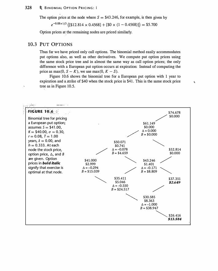
328 � B I N O M I A L O PT I O N P R I C I N G : I

The option price at the node where S = $43 .246, for example, is then given by

e-O.OSx l /3 ([$ 1 2. 8 14 x 0.4568] + [$0 X ( 1 - 0.4568)]) = $5 .700

Option prices at the remaining nodes are priced similarly.

10.3 PUT OPTIONS

Thus far we have priced only call options. The binomial method easily accommodates put options also, as well as other derivatives. We compute put option prices using the same stock price tree and in almost the same way as call option prices ; the only difference with a European put option occurs at expiration: Instead of computing the price as max(O, S - K) , we use max(O, K - S).

Figure 10.6 shows the binomial tree for a European put option with 1 year to expiration and a strike of $40 when the stock price is $41 . This is the same stock price � tree as in Figure 10.5.

F I G U RE 1 0 . 6 Binomial tree for pricing a European put option; assumes 5 = $41 .00, K = $40.00, u = 0.30, r = 0.08, T = 1 .00 years, 8 = 0.00, and h = 0.333 . At each node the stock price, option price, �' and 8 are given. Option prices in bold italic signify that exercise is optimal at that node.

/ $41 .000 $2.999

!J. = -0.294 B = $ 15 .039

�

$50.071 $0.741

!J. = -0.078 B = $4.659

� /

$35.411 $5 .046

!J,. = -0.550 B = $24.51 7

$74.678 / $0.000

$61 . 149 $0.000

!J. = 0.000 B = $0.000

� $52.814 $0.000

$43.246 / $1 .401

!J. = -0.171 � B = $8.809

$37.351 $2.649 /

$30.585 $8.363

!J,. = -1 .000 B = $38.947

� $26.416 $13.584

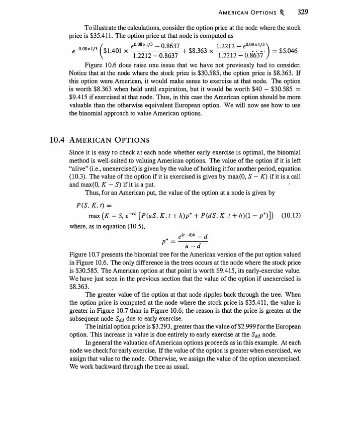
A M E R I CA N O PT I O N S � 329

To illustrate the calculations, consider the option price at the node where the stock price is $35.4 1 1 . The option price at that node is computed as

e-O.OSx l/3 $ 1 .401 X + $8.363 X = $5.046 ( eO.OS x 1/3 _ 0.8637 1 .22 1 2 _ eO.OSx 1 /3 ) 1 .22 1 2 - 0.8637 1 .22 12 - 0.8637

Figure 1 0.6 does raise one issue that we have not previously had to consider. Notice that at the node where the stock price is $30.585, the option price is $8.363. If

this option were American, it would make sense to exercise at that node. The option is worth ·$8.363 when held until expiration, but it would be worth $40 - $30.585 =

$9.415 if exercised at that node. Thus, in this case the American option should be more valuable than the otherwise equivalent European option. We will now see how to use the binomial approach to value American options.

10.4 AMERICAN OPTIONS

Since it is easy to check at each node whether early exercise is optimal, the binomial method is well-suited to valuing American options. The value of the option if it is left "alive" (i .e., unexercised) is given by the value of holding it for another period, equation ( 1 0.3). The value of the option if it is exercised is given by max(O, S - K) if it is a call and max(O, K - S) if it is a put.

Thus, for an American put, the value of the option at a node is given by

P (S, K, t) =

max (K - S, e-rh [P (uS, K , t + lz)p* + P (dS, K , t + lz) ( 1 - p*)] ) ( 10. 1 2)

where, as in equation ( 10.5),

e<r-o)h _ d p* = ------,,--

lt - d Figure 1 0.7 presents the binomial tree for the American version of the put option valued in Figure 10.6. The only difference in the trees occurs at the node where the stock price is $30.585. The American option at that point is worth $9.4 15, its early-exercise value. We have just seen in the previous section that the value of the option if unexercised is $8.363 .

The greater value of the option at that node ripples back through the tree. When the option price is computed at the node where the stock price is $35.4 1 1 , the value is greater in Figure 1 0.7 than in Figure 10.6; the reason is that the price is greater at the subsequent node Sdd due to early exercise.

The initial option price is $3.293, greater than the value of $2.999 for the European option. This increase in value is due entirely to early exercise at the Sdd node.

In general the valuation of American options proceeds as in this example. At each node we check for early exercise. If the value of the option is greater when exercised, we assign that value to the node. Otherwise, we assign the value of the option unexercised. We work backward through the tree as usual.

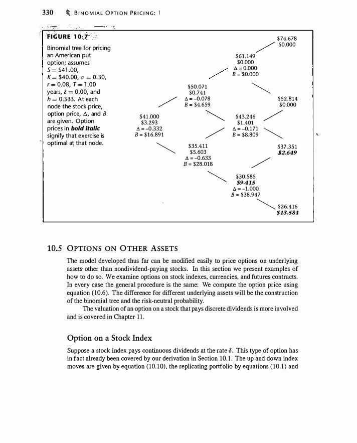
330 � B I N O M I A L O PT I O N P R I C I N G :

.· ··· . .

·.

.. .··

.

•· ·· FIGURE 1 0 . 7. <

Binomial tree for pricing an American put option; assumes s = $41 .00, K = $40.00, rr = 0. 30, r = 0.08, T = 1 .00 years, 8 = 0.00, and h = 0.333. At each node the stock price, option price, !:!., and B are given. Option prices in bold italic signify that exercise is

- optimal a� that node.

/

$41.000 $3 .293

/:,. = -0.332 B = $16.89 1

�

10.5 OPTIONS ON OTHER ASSETS

$50.071 $0.741

t:. = -0.078 B = $4.659

� /

$35.411 $5.603

/:,. =-0.633 B = $28.018

$74.678 / $0.000

$61 . 149 $0.000

1:. = 0.000 B = $0.000

� $52.814 $0.000

$43 .246 / $1 .401

/:,. = -0. 171 � B = $8.809

$37.35 1 $2.649 /

$30.585 $9.415 /:,. = -1 .000 B = $38.947

� $26.416 $13.584

The model developed thus far can be modified easily to price options on underlying assets- other than nondividend-paying stocks. In this section we present examples of how to do so. We examine options on stock indexes, currencies, and futures contracts. In every case the general procedure is the same: We compute the option price using equation ( 10.6). The difference for different underlying assets will be the construction of the binomial tree and the risk -neutral probability.

The valuation of an option on a stock that pays discrete dividends is more involved and is covered in Chapter 1 1 .

Option on a Stock Index

Suppose a stock index pays continuous dividends at the rate o . This type of option has in fact already been covered by our derivation in Section 1 0. 1 . The up and down index moves are given by equation ( 10. 1 0), the replicating portfolio by equations ( 1 0. 1 ) and

O PTI O N S O N OTH E R ASS ETS � 331

( 10.2), and the option price b y equation ( 1 0.3). The risk-neutral probability i s given by equation ( 1 0.5).6

Figure 10 .8 displays a binomial tree for an American call option on a stock index. Note that because of dividends, early exercise is optimal at the node where the stock price is $ 1 57 . 1 0 1 . Given these parameters, we have p* = 0.457; hence, when S = $ 157. 1 0 1 , the value of the option unexercised is

e�O.OS x i /3 [0.457 X $87 .747 + ( 1 - 0.457) X $32.779] = $56.942

Since 57. 1 0 1 > 56.942, we exercise the option at that node.

.. . · .·-

FiGURE . 1 o��f"cL . .

Binomial tree for pricing an American call option on a stock index; assumes S = $ 1 1 0.00, K = $1 00.00, u = 0.30, r = 0.05, T = 1 .00 years, 8 = 0.035, and h = 0.333 . At each node the stock price, option price, !:::.., and B are given. Option prices in bold italic signify that exercise is optimal at that node.

$ 1 10.000 $18.593 IJ. = 0.691

B = -$57.408

$187.747 /$87.747 $157. 101 $57.101

/ IJ. = 0.988 / B = -$98.347

$131 .458 $33 .520 IJ. = 0.911

B = -$86.185

$92.970 $6.616

IJ. = 0.447 B = -$34.984

$132.779 $32.779 $1 1 1 . 106 / $14.726 IJ. = 0.833 �

B = -$77.871 �

$78.576 $0.000

l:l = O.OOO B = $0.000

$93.904 $0.000

� $66.41 1 $0.000

6Intuitively, dividends can be taken into account either by ( 1 ) appropriately lowering the nodes on the

tree and leaving risk-neutral probabilities unchanged, or (2) by reducing the risk-neutral probability and leaving the tree unchanged. The forward tree adopts the first approach.

332 � B I N O M I A L O PT I O N P R I C I N G :

Options on Currencies

With a currency with spot price x0, the forward price is Fo,h = x0e<r-rtlh , where r1 is the foreign interest rate. Thus, we construct the binomial tree using

ux = xe<r-rf)h+u../Ji dx = xe<r-rt)h-u../Ji

There is one subtlety in creating the replicating portfolio: Investing in a "currency" means investing in a money-market fund or fixed income obligation denominated in tbat currency. (We encountered this idea previously in Chapter 5 .) Taking into account interest on the foreign-currency-denominated obligation, the two equations are

/::,. X dxerfh + erh X B = cd

/::,. X uxerth + er" X B = ell The risk-neutral probability of an up move in this case is given by

e<r-rt)h - d p* = ----­u - d ( 10. 13)

Notice that if we think of r1 as the dividend yield on the foreign currency, these two equations look exactly like those for an index option. In fact the solution is the same as for an option on an index: Set the dividend yield equal to the foreign risk-free rate and the current value of the index equal to the spot exchange. rate.

Figure 10.9 prices a dollar-denominated American put option on the euro. The current exchange rate is assumed to be $ 1 .05/€ and the strike is $ 1 . 10/€. The euro­denominated interest rate is 3 . 1 %, and the dollar-denominated rate is 5.5%.

Because volatility is low and the option is in-the-money, early exercise is optimal at three nodes prior to expiration.

Options on Futures Contracts

We now consider options on futures contracts. We assume the forward price is the same as the futures price. Since we build the tree based on the forward price, we simply add up and down movements around the current price. Thus, the nodes are constructed as

II = eu../Ji d = e-u../Ji

Note that this solution for u and d is exactly what we would get for an option on a stock index if 8, the dividend yield, were equal to the risk-free rate.

In constructing the replicating portfolio, recall that in each period a futures contract pays the change in the futures price, and there is no investment required to enter a futures contract. The problem is to find the number of futures contracts, t:,., and the lending, B ,

that replicates the option. We have

/::,. X (d F - F) + er" X B = cd

/::,. X (u F - F) + erh X B = C,

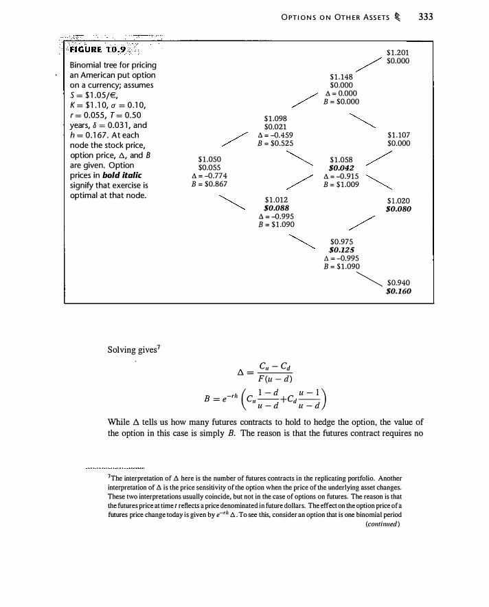
. . · . · >FIGURE lO��·i�; ;

Binomial tree for pricing an American put option on a currency; assumes s = $ 1 .05/€, K = $ 1 . 1 0, a = 0.1 0, r = 0.055, T = 0.50 years, 8 = 0.03 1 , and h = 0. 1 67. At each node the stock price, option price, !!:., and 8 are given. Option prices in bold italic signify that exercise is optimal at that node.

Solving gives7

O PTI O N S O N OT H E R ASS ETS � 333

$ 1 .050 $0.055

!:J. = -0.774 B = $0.867

$ 1 .098 $0.021

;:,. = -0.459 B = $0.525

$ 1 .012 $0.088 ;:,. = -0.995 B = $1 .090

l::i = C, - Cd F(u - d)

$1 . 148 $0.000

!:J. = 0.000 B = $0.000

$ 1 .058 $0.042 !:J. = -0.915 B = $1 .009

$0.975 $0.125 !:J. = -0.995 B = $1 .090

$1 .201 $0.000

$1 . 107 $0.000

$ 1 .020 $0.080

� $0.940 $0.160

B = e C,--+Cd ---rh ( I - d u - I ) u - d u - d

While l::i tells us how many futures contracts to hold to hedge the option, the value of the option in this case is simply B. The reason is that the futures contract requires no

7The interpretation of I'> here is the number of futures contracts in the replicating portfolio. Another

interpretation of I'> is the price sensitivity of the option when the price of the underlying asset changes.

These two interpretations usually coincide, but not in the case of options on futures. The reason is that

the futures price at time 1 reflects a price denominated in future dollars. The effect on the option price of a futures price change today is given by e-rh !:J. . To see this, consider an option that is one binomial period

(continued)

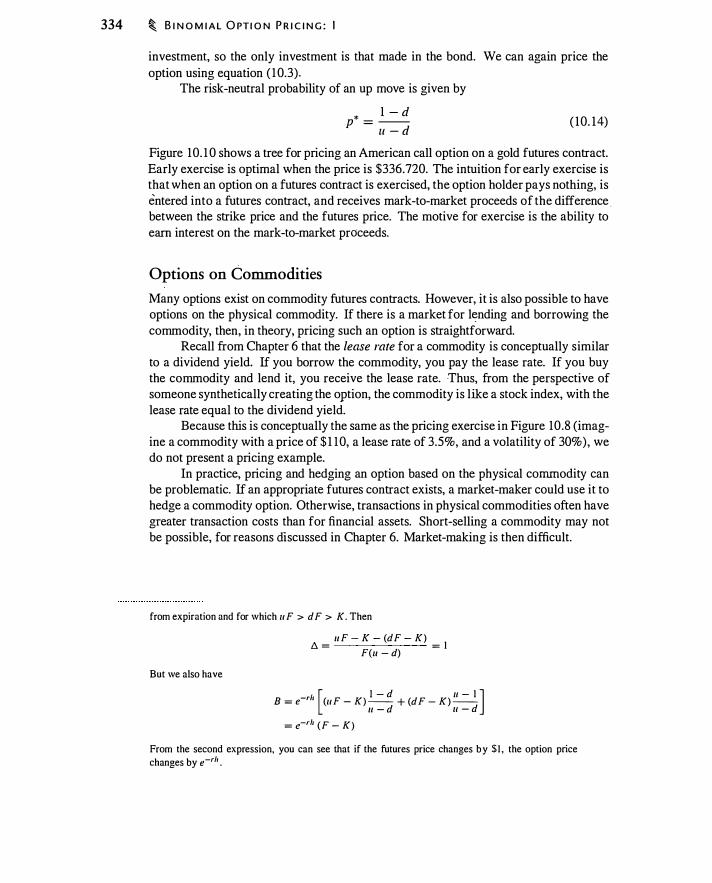
334 � B I N O M I A L O PT I O N P R I C I N G : I

investment, so the only investment is that made in the bond. We can again price the option using equation ( 1 0.3) .

The risk-neutral probability of an up move is given by

1 - d p* = -- ( 10. 14)

u - d

Figure 10. 1 0 shows a tree for pricing an American call option on a gold futures contract. Early exercise is optimal when the price is $336.720. The intuition for early exercise is that when an option on a futures contract is exercised, the option holder pays nothing, is entered into a futures contract, and receives mark-to-market proceeds of the difference . between the strike price and the futures price. The motive for exercise is the ability to earn interest on the mark-to-market proceeds.

Options on Commodities

Many options exist on commodity futures contracts. However, it is also possible to have options on the physical commodity. If there is a market for l�nding and borrowing the commodity, then, in theory, pricing such an option is straightforward.

Recall from Chapter 6 that the lease rate for a commodity is conceptually similar to a dividend yield. If you borrow the commodity, you pay the lease rate. If you buy the commodity and lend it, you receive the lease rate. Thus, from the perspective of someone synthetically creating the option, the commodity is like a stock index, with the lease rate equal to the dividend yield.

Because this is conceptually the same as the pricing exercise in Figure 10 .8 (imag­ine a commodity with a price of $ 1 10, a lease rate of 3.5%, and a volatility of 30% ), we do not present a pricing example.

In practice, pricing and hedging an option based on the physical commodity can be problematic. If an appropriate futures contract exists, a market-maker could use it to hedge a commodity option. Otherwise, transactions in physical commodities often have greater transaction costs than for financial assets. Short-selling a commodity may not be possible, for reasons discussed in Chapter 6. Market-making is then difficult.

from expiration and for which 11 F > d F > K. Then

But we also have

II F - K - (d F - K ) D. = = I

F(u - d)

B = e-rll (11 F - K ) -- + (d F - K ) --

[ 1 - d 11 - I J 11 - d 11 - d

= e-rll ( F - K )

From the second expression, you can see that if the futures price changes by $ I , the option price

changes by e -rll .

; F .• tuaE 1 o;_io!!f _

- .

Binomial tree for pricing an American call option on a futures contract; assumes S = $ 300.00, K = $300.00, a = 0.1 0, r = 0.05, T = 1 .00 years, 8 = 0.05, and h = 0.333 . At each node the stock price, option price, !'!.., and 8 are given. Option prices in bold italic signify that exercise is optimal at that node.

$300.000 $ 12.488 Ll = 0.513

B = $12.488

Options on Bonds

O PTI O N S O N OTH E R ASS ETS � 335

$356.733 /$56.733 $336.720 $36.720

/ Ll = 1 .000 / B = $36.720

$317.830 $21 .843 Ll = 0.768

B = $21.843

$283 . 170 $4.066

Ll = 0.260 B = $4.066

$317.830 $17.830 $300.000 / $8.515

Ll = 0.514 '-......._ B = $8.515 '-......._

$267.284 $0.000

Ll = 0.000 B = $0.000

$283 .170 $0.000

�$252.290 $0.000

Finally, we will briefly discuss options on bonds. We devote a separate chapter later to , discussing fixed-income derivatives, but it is useful to understand at this point some of the issues in pricing options on bonds. As a first approximation we could just say that bonds are like stocks that pay a discrete dividend (a coupon), and price bond options using the binomial model.

However, bonds differ from the assets we have been discussing in two important respects.

1. The volatility of a bond decreases over time as the bond approaches maturity. The prices of 30-day Treasury bills, for example, are much less volatile than the prices of 30-year Treasury bonds. The reason is that a given change in the interest rate, other things equal, changes the price of a shorter-lived bond by less.

2. We have been assuming in all our calculations that interest rates are the same for all maturities, do not change over time and are not random. While these assumptions may be good enough for pricing options on stocks, they are logically inconsistent for pricing options on bonds: If interest rates do not change unexpectedly, neither do bond prices.

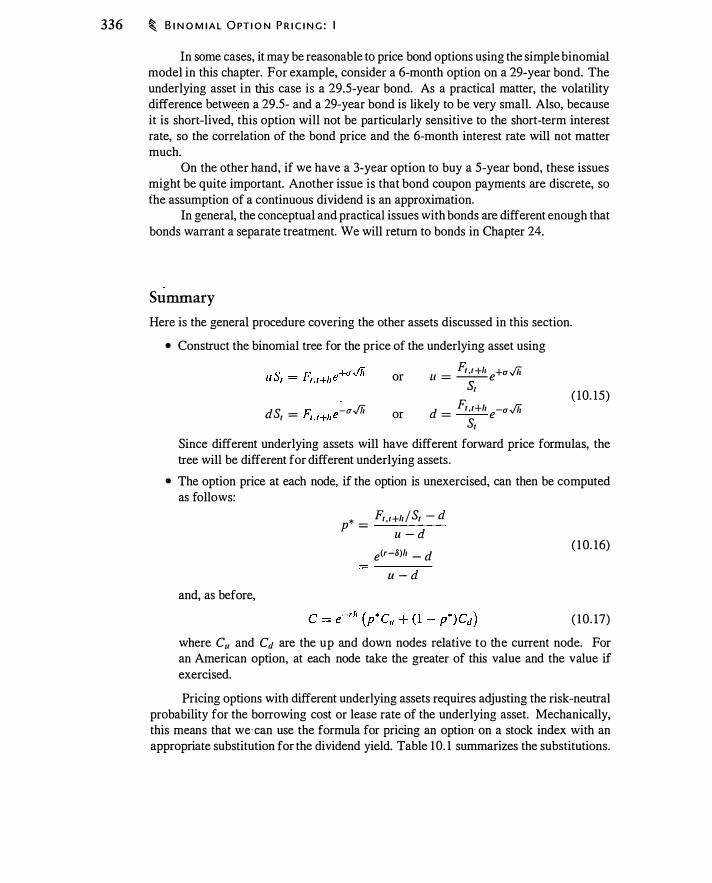
336 � B I N O M I A L O PT I O N P R I C I N G : I

In some cases, it may be reasonable to price bond options using the simple binomial model in this chapter. For example, consider a 6-month option on a 29-year bond. The underlying asset in this case is a 29.5-year bond. As a practical matter, the volatility difference between a 29.5- and a 29-year bond is likely to be very small. Also, because it is short-lived, this option will not be particularly sensitive to the short-term interest rate, so the correlation of the bond price and the 6-month interest rate will not matter much.

On the other hand, if we have a 3-year option to buy a 5-year bond, these issues might be quite important. Another issue is that bond coupon payments are discrete, so the assumption of a continuous dividend is an approximation.

In general, the conceptual and practical issues with bonds are different enough that bonds warrant a separate treatment. We will return to bonds in Chapter 24.

Summary

Here is the general procedure covering the other assets discussed in this section.

• Construct the binomial tree for the price of the underlying asset using

or

ds - L' -u../h 1 - r1 ,1+h e or

FI .I+h +u..fh u = -- e sf

d = FI , I+h e-u../h sf

( 10. 15)

Since different underlying assets will have different forward price formulas, the tree will be different for different underlying assets.

• The option price at each node, if the option is unexercised, can then be computed as follows:

"' FI, I+/J /SI - d p · =

u - d

e<r-o)h _ d ( 1 0. 16)

= ----

u - d and, as before,

( 10. 17)

where C11 and Cd are the up and down nodes relative to the current node. For an American option, at each node take the greater of this value and the value if exercised.

Pricing options with different underlying assets requires adjusting the risk-neutral probability for the borrowing cost or lease rate of the underlying asset. Mechanically, this means that we-can use the formula for pricing an option on a stock index with an appropriate substitution for the dividend yield. Table I 0. 1 summarizes the substitutions.

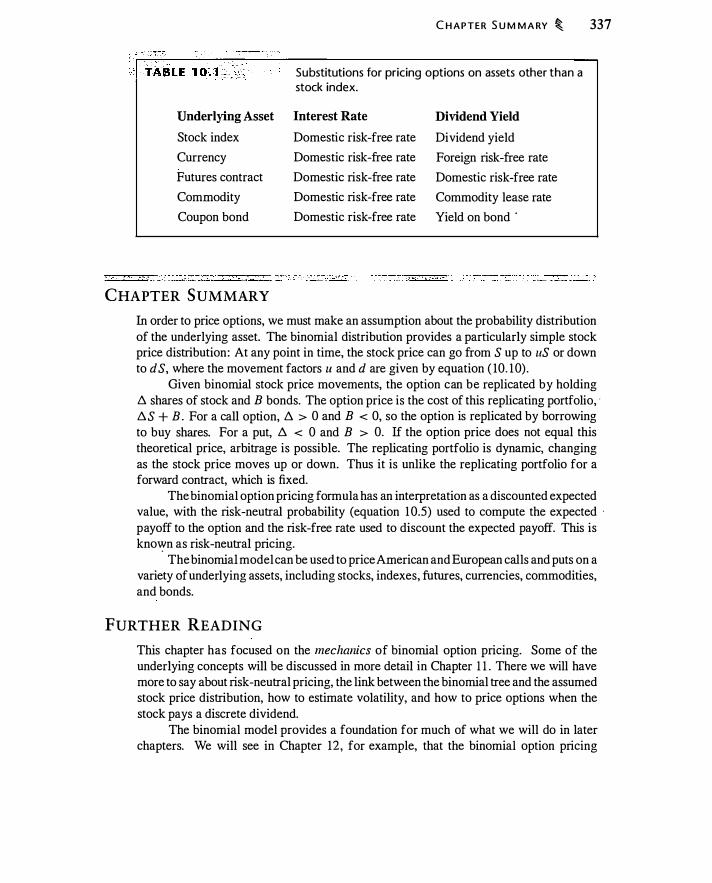
Underlying Asset

Stock index

Currency

Futures contract

Commodity

Coupon bond

CHAPTER SUMMARY

C H APTER S U M M A RY � 337

Substitutions for pricing options on assets other than a stock index.

Interest Rate Dividend Yield

Domestic risk-free rate Dividend yield

Domestic risk-free rate Foreign risk-free rate

Domestic risk-free rate Domestic risk-free rate

Domestic risk-free rate Commodity lease rate

Domestic risk-free rate Yield on bond ·

In order to price options, we must make an assumption about the probability distribution of the underlying asset. The binomial distribution provides a particularly simple stock price distribution: At any point in time, the stock price can go from S up to uS or down to dS, where the movement factors u and d are given by equation ( 10. 1 0) .

Given binomial stock price movements, the option can be replicated by holding b. shares of stock and B bonds. The option price is the cost of this replicating portfolio, · b.S + B . For a call option, b. > 0 and B < 0, so the option is replicated by borrowing to buy shares. For a put, b. < 0 and B > 0. If the option price does not equal this theoretical price, arbitrage is possible. The replicating portfolio is dynamic, changing as the stock price moves up or down. Thus it is unlike the replicating portfolio for a forward contract, which is fixed.

The binomial option pricing formula has an interpretation as a discounted expected value, with the risk-neutral probability (equation 1 0.5) used to compute the expected ·

payoff to the option and the risk-free rate used to discount the expected payoff. This is knmyn as risk-neutral pricing.

The binomial model can be used to price American and European calls and puts on a variety of underlying assets, including stocks, indexes, futures, currencies, commodities, and bonds.

FURTHER READING

This chapter has focused on the mechanics of binomial option pricing. Some of the underlying concepts will be discussed in more detail in Chapter l l . There we will have more to say about risk-neutral pricing, the link between the binomial tree and the assumed stock price distribution, how to estimate volatility, and how to price options when the stock pays a discrete dividend.

The binomial model provides a foundation for much of what we will do in later chapters. We will see in Chapter 12 , for example, that the binomial option pricing

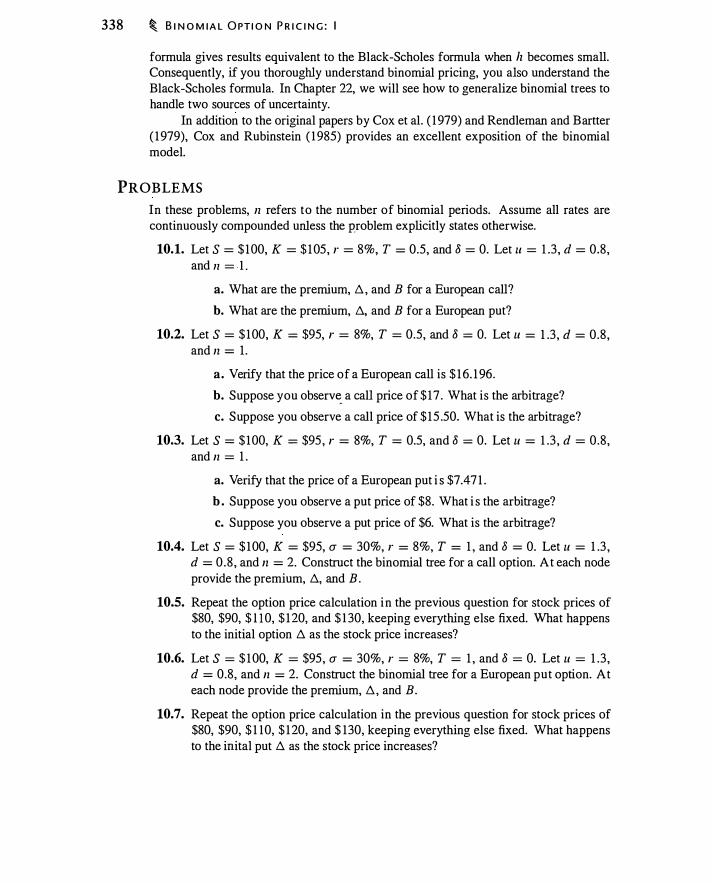
338 � B I N O M I A L O PT I O N P R I C I N G : I

formula gives results equivalent to the Black-Scholes formula when lz becomes small. Consequently, if you thoroughly understand binomial pricing, you also understand the Black-Scholes formula. In Chapter 22, we will see how to generalize binomial trees to handle two sources of uncertainty.

In addition to the original papers by Cox et al. ( 1 979) and Rendleman and Bartter ( 1 979), Cox and Rubinstein ( 1 985) provides an excellent exposition of the binomial model.

PROB LEMS

In these problems, n refers to the number of binomial periods. Assume all rates are continuously compounded unless the problem explicitly states otherwise.

10.1. Let S = $ 100, K = $ 1 05, r = 8%, T = 0.5, and 8 = 0. Let u = 1 .3 , d = 0.8, and n = - 1 .

a. What are the premium, D. , and B for a European call?

b. What are the premium, D., and B for a European put?

10.2. Let S = $ 100, K = $95, r = 8%, T = 0.5, and 8 = 0. Let u = 1 .3 , d = 0.8, and n = 1 .

a. Verify that the price of a European call is $ 1 6. 1 96.

b. Suppose you observ� a call price of $ 17 . What is the arbitrage?

c. Suppose you observe a call price of $ 15 .50. What is the arbitrage?

10.3. Let S = $ 100, K = $95 , r = 8%, T = 0.5, and 8 = 0. Let u = 1 .3 , d = 0.8, and n = 1 .

a. Verify that the price of a European put i s $7.4 7 1 .

b . Suppose you observe a put price of $8. What i s the arbitrage?

c. Suppose you observe a put price of $6. What is the arbitrage?

10.4. Let S = $ 100, K = $95, a = 30%, r = 8%, T = 1 , and 8 = 0. Let u = 1 .3 , d = 0 .8 , and n = 2. Construct the binomial tree for a call option. At each node provide the premium, D., and B .

10.5. Repeat the option price calculation in the previous question for stock prices of $80, $90, $ l l 0, $ 1 20, and $ 1 30, keeping everything else fixed. What happens to the initial option D. as the stock price increases?

10.6. Let S = $ 1 00, K = $95, a = 30%, r = 8%, T = 1 , and 8 = 0. Let u = 1 .3 , d = 0.8, and n = 2. Construct the binomial tree for a European put option. At each node provide the premium, D. , and B.

10.7. Repeat the option price calculation in the previous question for stock prices of $80, $90, $ 1 10, $ 1 20, and $ 130, keeping everything else fixed. What happens to the inital put D. as the stock price increases?

P R O B LE M S � 339

10.8. Let S = $ 100, K = $95, u = 30%, r = 8%, T = 1 , and 8 = 0. Let u = 1 .3 , d = 0.8, and n = 2. Construct the binomial tree for an American put option. At each node provide the premium, /J., and B .

10.9. Suppose So = $ 1 00, K = $50, r = 7 .696% (continuously compounded), 8 = 0, and T = 1 .

a. Suppose that for h = 1 , we have u = 1 .2 and d = 1 .05. What is the binomial option price for a call option that lives one period? Is there any problem with having d > 1 ?

b . Suppose now that u = 1 .4 and d = 0.6. Before comp�ting the option price, what is your guess about how it will change from your previous answer? Does it change? How do you account for the result? Interpret your answer using put-call parity.

c. Now let u = 1 .4 and d = 0.4. How do you think the call option price will change from (a)? How does it change? How do you account for this? Use put-call parity to explain your answer.

10.10. Let S = $ 100, K = $95, r = 8% (continuously compounded), u = 30%, 8 = 0, T = 1 year, and n = 3.

a. Verify that the binomial option price for an American call option is $ 1 8 .283 . Verify that there is never early exercise; hence, a European call would have the same price.

b. Show that the binomial option price for a European put option is $5.979. Verify that put-call parity is satisfied.

c. Verify that the price of an American put is $6.678.

10.11. Repeat the previous problem assuming that the stock pays a continuous dividend of 8% per year (continuous! y compounded) . Calculate the prices of the American . and European puts and calls. Which options are early-exercised?

10.U. Let S = $40, K = $40, r = 8% (continuously compounded), u = 30%, 8 = 0, T = 0.5 year, and n = 2.

a. Construct the binomial tree for the stock. What are u and d?

b. Show that the call price is $4. 1 10.

c. Compute the prices of American and European puts.

10.13. Use the same data as in the previous problem, only suppose that the call price is $5 instead of $4. 1 10.

a. At time 0, assume you write the option and form the replicating portfolio to offset the written option. What is the replicating portfolio and what are the net cash flows from selling the overpriced call and buying the synthetic equivalent?

340 � B I N O M I A L O PT I O N P R I C I N G : I

b. What are the cash flows in the next binomial period (3 months later) if the call at that time is fairly priced and you liquidate the position? What would you do if the option continues to be overpriced the next period?

c. What would you do if the option is underpriced the next period?

10.14. Suppose that the exchange rate is $0.92/€. Let rs = 4%, and 1"€ = 3%, u = 1 .2, d = 0.9, T = 0.75, n = 3, and K = $0.85.

a. What is the price of a 9-month European call?

b. What is the price of a 9-month American call?

10.15. Use the same inputs as in the previous problem, except that K = $ 1 .00.

a. What is the price of a 9�month European put?

b. What is the price of a 9-month American put?

10.16. Suppose that the exchange rate is 1 dollar for 1 20 yen. The dollar interest rate is 5% (continuously compounded) and the yen rate is 1 % (continuously compounded). Consider an at-the-money American dollar call that is yen­denominated (i.e., the call permits you to buy 1 dollar for 1 20 yen). The option has 1 year to expiration and the exchange rate volatility is 10%. Let n = 3 .

a. What is the price of a European call? An American call?

b. What is the price of a European put? An American put?

c. How do you account for the pattern of early exercise across the two options?

10.17. An option has a gold futures contract as the underlying asset. The current 1 -year gold futures price i s $300/oz., the strike price i s $290, the risk-free rate is 6%, volatility is 1 0%, and time to expiration is 1 year. Suppose n = 1 . What is the price of a call option on gold? What is the replicating portfolio for the call option? Evaluate the statement: "Replicating a call option always entails borrowing to buy .the underlying asset."

10.18. Suppose the S&P 500 futures price is 1000, a = 30%, r = 5%, 8 = 5%, T = 1 , and n = 3 .

a. What are the prices of European calls and puts for K = $ 1 000? Why do you find the prices to be equal?

b. What are the prices of American calls and puts for K = $ 1 000?

c. What are the time-0 replicating portfolios for the European call and put?

10.19. For a stock index, S = $ 1 00, a = 30%, r = 5%, 8 = 3%, and T = 3. Let ll = 3 .

a . What i s the price of a European call option with a strike of $95 ?

b. What is the price of a European put option with a strike of $95?

A P P E N D I X 1 0.A: TAX ES A N D O PTI O N P R I C ES � 341

c. Now let S = $95, K = $ 100, a = 30%, r = 3%, and 8 = 5%. (You have exchanged values for the stock price and strike price and for the interest rate and dividend yield.) Value both options again. What do you notice?

10.20. Repeat the previous problem calculating prices for American options instead of European. What happens?

10.21. Suppose that u < e<r-li)h . Show that there is an arbitrage opportunity. Now suppose that d > e<r-li)h . Show again that there is an arbitrage opportunity.

APPENDIX l O .A : TAXES AND OPTION PRICES

It is possible to solve for a binomial price when there are taxes. Suppose that each form of income is taxed at a different rate: interest at the rate r; , capital gains on a stock at the rate r 8 , capital gains on options at the rate r 0 , and dividends at the rate rd. We assume that taxes on all forms of income are paid on an accrual basis, and that there is no limit on the ability to deduct losses or to offset losses on one form of income against gains on another form of income.

We then choose /::,.1 and B1 by requiring that the after-tax return on the stock/bond portfolio equal the after-tax return on the option in both the up and down states. Thus we require that

[SI+h - r8 (S1+h - S1 ) + 8S1 ( l - id)] /::,.1 + [1 + rh ( l - r)] B1 = </Jt+h (St+h ) - r 0 [<P1+h (S1+h ) - ¢1 (SI ) ]

The solutions for /::,. and B are then

/::,. = 1 - r o ¢ 1 (S{) - ¢ 1 (Si) 1 - r8 st - Si

( 10. 1 8) .

B = 1 (u¢ 1 (S!) - d¢ 1 (S{) _ _ t:,._So [ r8 - ro

+ 80 _ rd)]) 1 - r; u - d 1 - r0 1 - r J + r��--- g

1 - r o

This gives an option price of 1

¢1 = 1 _ r; [p*¢1+h (S�h ) + ( 1 - p*)¢1+h (S;+h)] 1 + r��---

1 - ro where

1 - r; 1 - id 1 + r11-- - 8--- - d p* = ___

1_-_r,_8_--:-

1_-_

r_o __ u - d

( 10. 19)

( 10.20)

In practice, dealers are marked-to-market for tax purposes and face the same tax rate on all forms of income. In this case taxes drop out of all the option-pricing expressions. When dealers are the effective price-setters in a market, taxes should not affect prices.

Binomial Option Pricing: II

Chapte; !0 introduced binomial option pricing, focu,ing on how the model can be ""'" to compute European and American option prices for a variety of underlying assets. In this chapter we continue the discussion of binomial pricing, delving more deeply into the economics of the model and its underlying assumptions.

First, the binomial model can value options that may be early-exercised. We will examine early exercise in more detail, and see that the option pricing calculation reflects the economic determinants of early exercise discussed in Chapter 9.

Second, the binomial option pricing formula can be interpreted as the expected option payoff one period hence, discounted at the risk-free rate. In Chapter 10 we referred to this calculation as risk-neutral pricing. This calculation appears to be inconsistent with standard discounted cash flow valuation, in which expected cash flows are discounted at a risk-adjusted rate, not the risk-free rate. We show that, in fact, the binomial pricing · formula (and, hence, risk-neutral valuation) is consistent with option valuation using standard discounted cash flow techniques.

Third, we modeled the stock price by using volatility (cr ) to determine the mag­nitude of the up and down stock price movements. In this chapter we explain this calculation in more detail. What is the economic meaning of this assumption? In con­structing the binomial tree, why is volatility multiplied by the square root of time ( cr ..Jii)? How should we estimate volatility?

Finally, we saw how to price options on stock indices where the dividend is con­tinu<?US. In this chapter we adapt the binomial model to price options on stocks that pay discrete dividends.

11 . 1 UNDERSTANDING EARLY EXERCISE

In deciding whether to early-exercise an option, the option holder compares the value of exercising immediately with the value of continuing to hold the option, and exercises if immediate exercise is more valuable. This is the comparison we performed at each binomial node when we valued American options in Chapter 10.

We obtain an economic perspective on the early-exercise decision by considering the costs and benefits of early exercise. As discussed in Section 9.3, there are three economic considerations governing the decision to exercise early. By exercising, the option holder

343

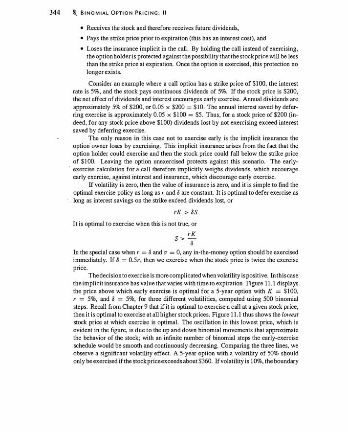
344 � B I N O M I A L O PT I O N P R I C I N G : I I

• Receives the stock and therefore receives future dividends,

• Pays the strike price prior to expiration (this has an interest cost), and

• Loses the insurance implicit in the call . By holding the call instead of exercising, the option holder is protected against the possibility that the stock price will be less than the strike price at expiration. Once the option is exercised, this protection no longer exists.

Consider an example where a call option has a strike price of $ 1 00, the interest rate is 5%, and the stock pays continuous dividends of 5%. If the stock price is $200, the net effect of dividends and interest encourages early exercise. Annual dividends are approximately 5% of $200, or 0.05 x $200 = $ 10. The annual interest saved by defer­ring exercise is approximately 0.05 x $ 1 00 = $5 . Thus, for a stock price of $200 (in­deed, for any stock price above $ 1 00) dividends lost by not exercising exceed interest saved by deferring exercise.

The only reason in this case not to exercise early is the implicit insurance the option· owner loses by exercising. This implicit insurance arises from the fact that the option holder could exercise and then the stock price could fall below the strike price of $ 1 00. Leaving the option unexercised protects against this scenario. The early­exercise calculation for a call therefore implicitly weighs dividends, which encourage early exercise, against interest and insurance, which discourage early exercise.

If volatility is zero, then the value of insurance is zero, and it is simple to find the optimal exercise policy as long as r and 8 are constant. It is optimal to defer exercise as

. long as interest savings on the strike exceed dividends lost, or

rK > 8S

I t is optimal to exercise when this i s not true, or

r K S > -

8 In the special case when r = 8 and a = 0, any in-the-money option should be exercised immediately. If 8 = 0.5r, th.en we exercise when the stock price is twice the exercise price.

The decision to exercise is more complicated when volatility is positive. In this case the implicit insurance has value that varies with time to expiration. Figure 1 1 . 1 displays the price above which early exercise is optimal for a 5-year option with K = $ 1 00, r = 5%, and 8 = 5%, for three different volatilities, computed using 500 binomial steps. Recall from Chapter 9 that if it is optimal to exercise a call at a given stock price, then it is optimal to exercise at all higher stock prices. Figure 1 1 . 1 thus shows the lowest stock price at which exercise is optimal. The oscillation in this lowest price, which is evident in the figure, is due to the up and down binomial movements that approximate the behavior of the stock; with an infinite number of binomial steps the early-exercise schedule would be smooth and continuously decreasing. Comparing the three lines, we observe a significant volatility effect. A 5-year option with a volatility of 50% should only be exercised if the stock price exceeds about $360. If volatilitY is I 0%, the boundary

Early-exercise boundaries for volatil ities of 1 0%, 30%, and 50% for a 5-year American cal l option. In a l l cases . K = $ 1 00, r = 5%, and 8 = 5%.

U N D E R STA N D I N G EA R LY EX E R C I S E � 345

Exercise Boundary 400

300

250

0.5 1.0 1.5 2.0 2.5 3.0 3.5 4.0 4.5 5.0 Time in Years

drops to $ 1 30. This volatility effect stems from the fact that the insurance value lost by early-exercising is greater when volatility is greater.

Figure 1 1 .2 performs the same experiment for put options with the same inputs. The picture is similar, as is the logic: The advantage of early exercise is receiving the

f strike price sooner rather than later. The disadvantages are the dividends lost by giving up the stock, and the loss of insurance against the stock price exceeding the strike price.

Early-exercise boundaries for volatil ities of 1 0%, 30%, and 50% for a 5-year American put option. In all cases K = $ 1 00, r = 5%, and 8 = 5%.

Exercise Boundary 100

90

80

70 60 1 ���

��������u��=.�0;.3�0��*������.��

so �

40 �-��NI���u�=�O�.s�o�����""'

30 Iii 20��--�--��--�--�--L-�--�--J

0 0.5 1.0 1.5 2.0 2.5 3.0 3.5 4.0 4.5 5.0 Time in Years

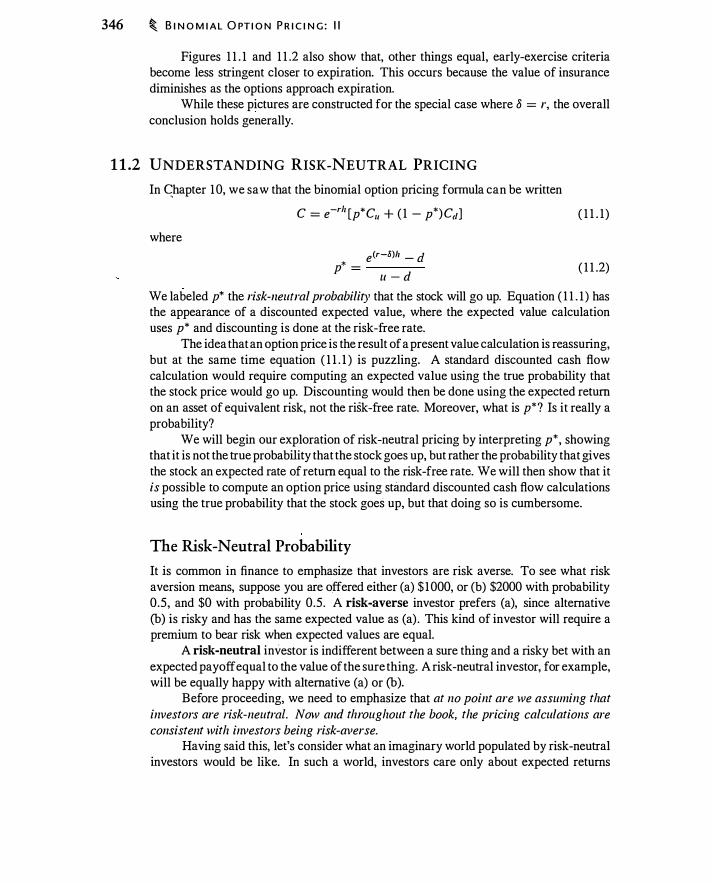
346 � B I N O M I A L O PT I O N P R I C I N G : I I

Figures 1 1 . 1 and 1 1 .2 also show that, other things equal, early-exercise criteria become less stringent closer to expiration. This occurs because the value of insurance diminishes as the options approach expiration.

While these pictures are constructed for the special case where 8 = r, the overall conclusion holds generally.

1 1 .2 UNDERSTANDING RISK-NEUTRAL PRICING

In C,hapter 1 0, we saw that the binomial option pricing formula can be written

where

C = e-rh [p*C11 + ( 1 - p*)Cc�] ( 1 1 . 1 )

e<r-8)11 _ d p* = ( 1 1 .2)

u - d We labeled p* the risk-neutral probability that the stock will go up. Equation ( 1 1 . 1 ) has the appearance of a discounted expected value, where the expected value calculation uses p* and discounting is done at the risk-free rate.

The idea that an option price is the result of a present value calculation is reassuring, but at the same time equation ( 1 1 . 1 ) is puzzling. A standard discounted cash flow calculation would require computing an expected value using the true probability that the stock price would go up. Discounting would then be done using the expected return on an asset of equivalent risk, not the risk-free rate. Moreover, what is p*? Is it really a probability?

We will begin our exploration of risk-neutral pricing by interpreting p*, showing that it is not the true probability that the stock goes up, but rather the probability that gives the stock an expected rate of return equal to the risk-free rate. We will then show that it is possible to compute an option price using standard discounted cash flow calculations using the true probability that the stock goes up, but that doing so is cumbersome.

The Risk-Neutral Probability

It is common in finance to emphasize that investors are risk averse. To see what risk aversion means, suppose you are offered either (a) $ 1000, or (b) $2000 with probability 0.5, and $0 with probability 0.5. A risk-averse investor prefers (a), since alternative (b) is risky and has the same expected value as (a) . This kind of investor will require a premium to bear risk when expected values are equal.

A risk-neutral investor is indifferent between a sure thing and a risky bet with an expected payoff equal to the value of the sure thing. A risk-neutral investor, for example, will be equally happy with alternative (a) or (b).

Before proceeding, we need to emphasize that at no point are we assuming that investors are risk-neutral. Now and throughout the book, the pricing calculations are consistent with investors being risk-averse.

Having said this, let's consider what an imaginary world populated by risk-neutral investors would be like. In such a world, investors care only about expected returns

U N D E R STA N D I N G R I S K- N E UT R A L P R I C I N G � 347

and not about riskiness. Assets would have no risk premium since investors would be willing to hold assets with an expected return equal to the risk-free rate.

In this hypothetical risk-neutral world, we can solve for the probability of the stock going up, p*, such that the stock is expected to earn the risk-free rate. In the binomial model we assume that the stock can go up to uS or down to d S. If the stock is to earn the risk-free return on average, then the probability that the stock will go up, p*, must satisfy

Solving for p* gives

p*uSe8" + (1 - p*)dSi1' = erh S

e<r-8)h - d p*

u - d

This is exactly the definition of p* in equation ( 1 1 .2). This is why we refer to p* as the risk-neutral probability that the stock price will go up. It is the probability that the stock price would increase in a risk-neutral world.

Not only would the risk-neutral probability, equation ( 1 1 .2), be used in a risk­neutral world, but also all discounting would take place at the risk-free rate. Thus, the option pricing formula, equation ( 1 1 . 1 ) , can be said to price options as if investors are risk-neutral. At the risk of being repetitious, we are not assuming that investors are actually risk-neutral, and we are not assuming that risky assets are actually expected to earn the risk-free rate of return. Rather, risk-neutral pricing is an interpretation of the

fonnulas above. Those formulas in turn arise from finding the cost of the portfolio that replicates the option payoff.

Interestingly, this interpretation of the option-pricing procedure has great practical importance; risk -neutral pricing can sometimes be used where other pricing methods are too difficult. We will see in Chapter 1 9 that risk-neutral pricing is the basis for Monte Carlo valuation, in which asset prices are simulated under the assumption that assets earn the risk-free rate, and these simulated prices are used to value the option.

Pricing an Option Using Real Probabilities

We are left with the question: Is option pricing consistent with standard discounted cash flow calculations? The answer is yes. We can use the true distribution for the future stock price in computing the expected payoff to the option. This expected payoff can then be discounted with a rate based on the stock's required return.

Discounted cash flow is not used in practice to price options because there is no reason to do so: It is necessary to compute the option price in order to compute the correct discount rate. However, we present two examples of valuing an option using real probabilities to see the difficulty in using real probabilities, and also to understand how to determine the risk of an option.

Suppose that the continuously compounded expected return on the stock is a and that the stock does not pay dividends . Then if p is the true probability of the stock going up, p must be consistent with u, d, and a :

puS + ( 1 - p)dS = ea" s ( 1 1 .3)

348 � B I N O M I A L O PT I O N P R I C I N G : II

Solving for p gives us

eah - d p =

u - d ( 1 1 .4)

For probabilities to be between 0 and 1 , we must have u > eah > d. Using p, the actual expected payoff to the option one period hence is

ealr - d ll - eah pC11 + ( 1 - p)Cd =

d Cu +

d Cd

u - ll -( 1 1 .5)

Now we face the problem with using real as opposed to risk-neutral probabilities : At what rate do we discount this expected payoff? It is not correct to discount the option at the expected return on the stock, a, because the option is equivalent to a leveraged investment in the stock and, hence, is riskier than the stock.

Denote the appropriate per-period discount rate for the option as y . To compute y , w e can use the fact that the required return o n any portfolio i s the weighted average of the return!'; on the assets in the portfolio. 1 In Chapter 1 0, we saw that an option is equivalent to holding a portfolio consisting of /1 shares of stock and B bonds. The expected return on this portfolio is

eyh __

S/1 ail

B rh ------ e + e Sb. + B Sb. + B

( 1 1 .6)

We can now compute the option price as the expected opti<,m payoff, equation ( 1 1 .5), discounted at the appropriate discount rate, given by equation ( 1 1 .6). This gives

e-yil Cu + Cd [ eah - d u - eah J u - d u - d

( 1 1 .7)

I t turns out that this gives us the same option price as pelfomzing the risk-neutral calcu­

lation. Appendix 1 l .A demonstrates algebraically that equation ( 1 1 . 7) is equivalent to the risk -neutral calculation, equation ( 1 1 . 1 ) .

The calculations leading to equation ( 1 1 .7) started with the assumption that the expected return on the stock is a. We then derived a consistent probability, p, and discount rate for the option, y. You may be wondering if it matters whether we have the "correct" value of a to start with. The answer is that it does not matter: Any consistent pair of a and y will give the same option price. Risk-neutral pricing is valuable because setting a = r results in the simplest pricing procedure.

A one-period example To see how to value an option using true probabilities, we will compute two examples. First, consider the one-period binomial example in Figure 1 1 .3 . Suppose that the continuously compounded expected return on XY Z i s a = 1 5 % . Then the true probability of the stock going up, from equation ( 1 1 .4 ), is

e0· 1 5 - 0.8025 p = = 0.5446

1 .4623 - 0.8025

1 See, for example, Brealey and Myers (2003, ch. 9).

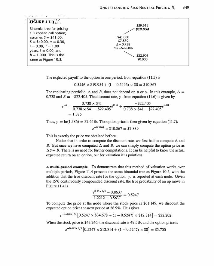
F.IGURE H ��if_'_ Binomial tree for pricing a European call option; assumes S = $41 .00, K = $40.00, u = 0.30, r = 0.08, T = 1 .00 years, 8 = 0.00, and . h = 1 .000. This is the same as Figure 1 0 .3 .

U N D E R STA N D I N G R I S K- N E UT R A L P R I C I N G � 349

$59.954 /$19.954 $41 .000 $7.839

!J. = 0.738 B = -$22.405

� $32.903 $0.000

The expected payoff to the option in one period, from equation ( 1 1 .5) is

0.5446 X $ 19.954 + (1 - 0.5446) X $0 = $ 10.867

The replicating portfolio, l:l and B, does not depend on p or ex. In this example, l:l =

0. 738 and B = -$22.405 . The discount rate, y , from equation ( 1 1 .6) is given by

ylz 0.738 X $41 o 15 -$22.405 O OS e = 0.738 x $4 1 - $22.405

e . + 0.738 x $41 - $22.405

e .

= 1 .386

Thus, y = ln ( 1 .386) = 32.64%. The option price is then given by equation ( 1 1 .7) :

e-0·3264 x $ 1 0.867 = $7 .839

This is exactly the price we obtained before. Notice that in order to compute the discount rate, we first had to compute l:l and

B . But once we have computed l:l and B , we can simply compute the option price as l:l S + B. There is no need for further computations. It can be helpful to know the actual expected return on an option, but for valuation it is pointless .

A multi-period example To demonstrate that this method of valuation works over multiple periods, Figure 1 1 .4 presents the same binomial tree as Figure 1 0.5, with the addition that the true discount rate for the option, y, is reported at each node. Given the 15% continuously compounded discount rate, the true probability cif an up move in Figure 1 1 .4 is

e0. 15 x l f3 - 0.8637 ------,---- = 0.5247 1 .22 1 2 - 0.8637

To compute the price at the node where the stock price is $6 1 . 149, we discount the expected option price the next period at 26.9%. This gives

e-0·269x l f3 [0.5247 x $34.678 + ( 1 - 0.5247) X $ 1 2. 8 1 4] = $22.202

When the stock price is $43.246, the discount rate is 49.5%, and the option price is

e-0.49Sx l /3 [0.5247 x $ 1 2. 8 1 4 + { 1 - 0.5247) X $0] = $5 .700

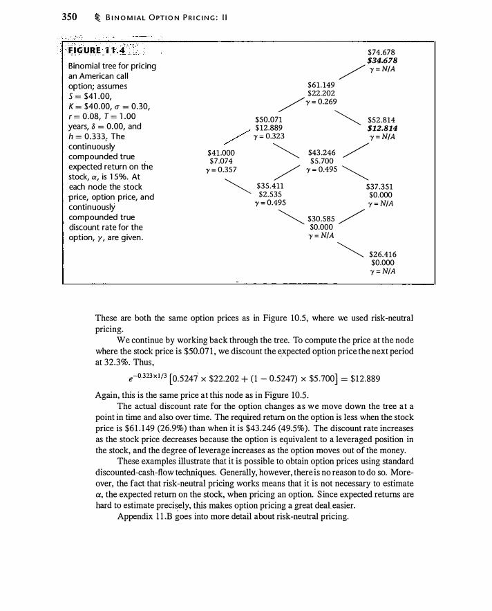
350 � B I N O M I A L O PT I O N P R I C I N G : I I

... F iGURE 1 l.4_L,c. Binomial tree for pricing an American ca l l option; assumes 5 = $41 .00, K = $40.00, a = 0 .30, r = 0.08, T = 1 .00 years, 8 = 0.00, and h = 0.333< The continuously compounded true expected return on the stock, a, is 1 5%. At each node the stock -price, option price, and continuously compounded true discount rate for the option, y, are g iven .

$61 . 149 $22.202

/y = 0.269

$74.678 $34.678 / y = N/A

$50.071 �

$52.814 / $ 12.889 $12.814

/ y = 0.323 y = N/A

$41 .000 �

$43.246 / $7.074 $5.700 y = 0.357 / y = 0.495 �

� $35.411 $37.351 $2.535 $0.000 y = 0.495 y = N/A

� $30.585 / $0.000 y = NIA �

$26.416 $0.000 y = NIA

These are both the same option prices as in Figure 10.5, where we used risk-neutral pricing.

We continue by working back through the tree. To compute the price at the node where the stock price is $50.07 1 , we discount the expected option price the next period at 32.3%. Thus,

e-0.3ZJx l fJ [0.5247 x $22.202 + ( 1 - 0.5247) X $5 .700] = $12.889

Again, this is the same price at this node as in Figure 10.5 . The actual discount rate for the option changes as we move down the tree at a

point in time and also over time. The required return on the option is less when the stock price is $6 1 . 149 (26.9%) than when it is $43 .246 (49.5%). The discount rate increases as the stock price decreases because the option is equivalent to a leveraged position in the stock, and the degree of leverage increases as the option moves out of the money.

These examples illustrate that it is possible to obtain option prices using standard discounted-cash-flow techniques. Generally, however, there is no reason to do so. More­over, the fact that risk-neutral pricing works means that it is not necessary to estimate a, the expected return on the stock, when pricing an option. S ince expected returns are hard to estimate preci�ely, this makes option pricing a great deaL easier.

Appendix 1 1 .B goes into more detail about risk-neutral pricing.

T H E B I N O M I A L TR E E A N D LOG N O R M A L ITY � 35 1

11 .3 THE BINOMIAL TREE AND LOGNORMALITY

The usefulness of the binomial pricing model hinges on the binomial tree providing a reasonable representation of the stock price distribution. In this section we discuss the motivation for and plausibility of the binomial tree. We will define a lognormal distribution and see that the binomial tree approximates this distribution.

The Random Walk Model

It is often said that stock prices follow a random walk. In this section we will explain what a random walk is. In the next section we will apply the random walk model to stock prices.

To understand a random walk, imagine that we flip a coin repeatedly. Let the random variable Y denote the outcome of the flip. If the coin lands displaying a head, Y = 1 . If the coin lands displaying a tail, Y = - 1 . If the probability of a head is 50%, we say the coin is fair. After n flips, with the i th flip denoted Y; , the cumulative total, Z, , is

II

Z11 = L Y; ( 1 1 .8) i=l

It turns out that the more times we flip, on average, the farther we will move from where we start. We can understand intuitively why with more flips the average distance from the starting point increases. Think about the first flip and imagine you get a head. You move to + 1 , and as far as the remaining flips are concerned, this is your new starting point. After the second flip, you will either be at 0 or +2. If you are at zero, it is as if you started over; however if you are at +2 you are starting at +2. Continuing in this way your average distance from the starting point increases with the number of flips.2

Another way to represent the process followed by Z, is in terms of the change in

We �an rewrite this more explicitly as

Heads: Z11 - Z11- l = + 1 Tails : Z11 - Z11- I = - 1

( 1 1 .9) (1 1 . 10)

2 After n flips, the average squared distance from the starting point will be n. Conditional on the first flip being a head, your average squared distance is 0.5 x 0 + 0.5 x 22 = 2. If your first flip had been a tail, your average squared distance after two moves would also be 2. Thus, the unconditional average

squared distance is 2 after 2 flips. If D� represents your squared distance from the starting point, then

D� = 0.5 X (D,_, + 1 )2 + 0.5 X (D,_, - 1 )2 = D�-1 + I Since D� = 0, this implies that D� = n . This idea that with a random walk you drift increasingly

farther from the starting point is an important concept later in the book.

352 � B I N O M I A L O PT I O N P R I C I N G : I I

With heads, the change in Z is 1 , and with tails, the change in Z is - 1 . This random walk is illustrated in Figure 1 1 .5 .

The idea that asset prices should follow a random walk was articulated in Samuel­son ( 1 965). In efficient markets, an asset price should reflect all available information. By definition, new information is a surprise. In response to new information the price is equally likely to move up or down, as with the coin flip. The price after a period of time is the initial price plus the cumulative up and down movements due to informational surprises.

Modeling Stock Prices as a Random Walk

The idea that stock prices move up or down randomly makes sense; however, the de­scription of a random walk in the previous

· section is not a satisfactory description of

stock price movements. Suppose we take the random walk model in Figure 1 1 .5 literally. Assume the beginning stock price is $ 100, and the stock price will move up or down $ 1 each tiq1e we flip the coin. There are at least three problems with this model:

1. If by chance we get enough cumulative down movements, the stock price will become negative. Because stockholders have limited liability (they can walk away from a bankrupt firm), a stock price will never be negative.

2. The magnitude of the move ($ 1 ) should depend upon how quickly the coin flips occur and the level of the stock price. If we flip coins once a second, $ 1 moves

I l l ustration of a random walk, where the counter, Z, increases by one when a fai r coin fl ip comes up heads, and decreases by one with tai ls.

Cumulative Counter, Z 5

0

-5

-10

-15

-20

-25

-30 L-�L-�--�--�--�--�--�---L---L--� 0 so 100 150 200 250 300 350 400 450 500

Number of Coin Flips, 11

T H E B I N O M I A L TR E E A N D LO G N O R M A L I TY � 353

are excessive; in real life, a $ 1 00 stock will not typically have 60 $1 up or down movements in 1 minute. Also, if a $ 1 move is appropriate for a $ 1 00 stock, it likely isn't appropriate for a $5 stock.

3. The stock on average should have a positive return. The random walk model taken literally does not permit this.

It turns out that the binomial model is a variant of the random walk model that solves all .of these problems at once. The binomial model assumes that continuously compounded returns are a random walk. Thus, before proceeding, we first review some properties of continuously compounded returns.

Continuously Compounded Returns

Here is a summary of the important properties of continuously compounded returns. (See also Appendix B at the end of this book.)

The logarithmic function computes returns from prices Let S1 and Sr+lr be stock prices at times t and t + lz. The continuously compounded return between t and t + lz , rr ,r+lr is then

( 1 1 . 1 1 )

The exponential function computes prices from returns If we know the con­tinuously compounded return, we can obtain Sr+h by exponentiating both sides of equation ( 1 1 . 1 1 ) . This gives

( 1 1 . 1 2)

Continuously compounded returns are additive Suppose we have continuously compounded returns over a number of periods-for example, r1 ,r+h • rr+h .r+2fr , etc. The continuously compounded return over a long period is the sum of continuously compounded returns over the shorter periods, i.e.,

II rr , t+llh = L rr+(i- l )h , t+ih

i= l ( 1 1 . 13)

Continuously compounded returns can be less than -100% A continuously compounded return that is a large negative number still gives a positive stock price. The reason is that er is positive for any r. Thus, if the log of the stock price follows a random walk, the stock price cannot become negative.

Here are some examples illustrating these statements.

" Example 1 1 . 1 Suppose the stock price on four consecutive days is $ 1 00, $ 1 03, $97, and $98 . The daily continuously compounded returns are

ln ( 103/ 100) = 0.02956; ln(97 / 1 03) = -0.06002; ln (98/97) = 0.0 1 026

354 � B I N O M I A L O PT I O N P R I C I N G : I I

The continuously compounded return from day 1 to day 4 is ln(98j 100) = -0.0202. This is also the sum of the daily continuously compounded returns :

1" 1 ,2 + 1"2,3 + 1"3,4 = 0.02956 + ( -0.06002) + 0.0 1 026 = -0.0202 �

' Example 1 1 .2 Suppose that the stock price today is $ 1 00 and that 1 year from today it is $ 10. The percentage return is ( 1 0 - 1 00) / 100 = -0.9 = -90%. However, the continuously compounded return is ln(10/ 100) = -2.30, a continuously compounded

D return-of -230%. �

, , Example 1 1 .3 Suppose that the stock price today is $100 and that over 1 year the continuously compounded return is -500%. Using equation ( 1 1 . 1 2) , the end-of-year

: price wip be small but positive: S1 = 1 00e-5·00 = $0.6738. The percentage return is L 0.6738/ 1 00 - 1 = -99.326%. �

The Standard Deviation of Returns

Suppose the continuously compounded return over month i is l"monthly,i . From equation ( 1 1 . 1 3), we can sum continuously compounded returns. Thus; the annual return is

- 12

!"annual = L l"monthly,i i=l

The variance of the annual return is therefore ( 12 ) Var(rannual) = Var � l"nionthly ,i

1=1 ( 1 1 . 1 4)

Now suppose that returns are uncorrelated over time; that is, the realization of the return in one period does not affect ·the expected returns in subsequent periods. With this assumption, the variance of a sum is the sum of the variances. Also suppose that each month has the same variance of returns. If we let a2 denote the annual variance, then from equation ( 1 1 . 14) we have

? ? a- = 1 2 X a�onthly

Taking the square root of both sides and rearranging, we can express the monthly standard deviation in terms of the annual standard deviation:

a a monthly = .JI2

If we split the year into n periods of length 1z (so that lz = 1 / n) , the standard deviation over the period of length /z, a11 , is

a, = a ./h. ( 1 1 . 15)

T H E B I N O M I A L TR E E A N D LO G N O R M A L I TY � 355

The standard deviation therefore scales with the square root of time. This is why a ,Jh appears in the binomial pricing model.

The Binomial Model

We are now in a position to better understand the binomial model, which is

S - s e<r-8)/r±u.fli t+lr - t

Taking logs, we obtain

( 1 1 . 1 6)

Since ln(Sr+lr l S1 ) is the continuously compounded return from t to t + h , rr , r+lr • the binomial model is simply a particular way to model the continuously compounded return. That return has two parts, one of which is certain [(r - 8)h], and the other of which is uncertain and generates the up and down stock price moves (±a ,Jli).

Let's see how equation ( 1 1 . 1 6) solves the three problems in the random walk discussed earlier:

1. The stock price cannot become negative. Even if we move down the binomial tree many times in a row, the resulting large, negative, continuously compounded return will give us a positive price.

2. As stock price moves occur more frequently, h gets smaller, therefore up and down moves get smaller. By construction, annual volatility is the same no matter how many binomial periods there are. S ince returns follow a random walk, the percentage price change is the same whether the stock price is $ 1 00 or $5.

3. There is a (r - 8)/z term, and we can choose the probability of an up move, so we can guarantee that the expected change in the stock price is positive.

To illustrate that the binomial tree can be thought of as a random walk, Figure 1 1 .6 illustrates the stock price that results when the continuously compounded return follows a random walk. The figure is one particular path through a 500-step binomial tree, with the particular path generated by the same sequence of coin flips as in Figure 1 1 .5 .

Lognormality and the Binomial Model

The binomial tree approximates a lognormal distribution, which is commonly used to model stock prices.

First, what is the lognormal distribution? The lognormal distribution is the proba­bility distribution that arises from the assumption that continuously compounded retums on the stock are normally distributed. When we traverse the binomial tree, we are implicitly adding up binomial random return components of (r - 8)/z ± a ,Jh. In the limit (as n -+ oo or, the same thing, lz -+ 0), the sum of binomial random variables is normally distributed. Thus, continuously compounded returns in a binomial tree are

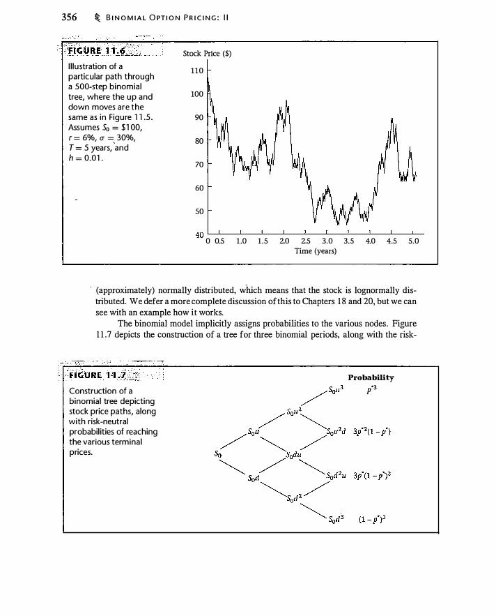
356 � B I N O M I A L O PT I O N P R I C I N G : I I

I l lustration of a particular path through a 500-step binomial tree, where the u p and down moves are the same as in Figure 1 1 .5 . Assumes 50 = $ 1 00, f = 6%, (]" = 30%, T = 5 years,

'and

h = 0.01 .

Stock Price ($)

110

100

90

80

70

60

50

40 L-L_ __ L_ __ L_ __ L_ __ L_ __ L_ __ L_ __ L_ __ L_ __ � 0 0.5 1 .0 1 .5 2.0 2.5 3.0 3.5 4.0 4.5 5.0

Time (years)

(approximately) normally distributed, which means that the stock is lognormally dis­tributed. We defer a more complete discussion of this to Chapters 1 8 and 20, but we can see with an example how it works.

The binomial model implicitly assigns probabilities to the various nodes. Figure 1 1 .7 depicts the construction of a tree for three binomial periods, along with the risk-

··· .. · · FIGURE ·H2Z.�r:. Construction of a binomial tree depicting stock price paths, along with risk-neutral probabil ities of reaching the various terminal prices.

Probability p*3

T H E B I N O M I A L TR E E A N D LO G N O R M A L I TY � 357

neutral probability of reaching each final period node. There is only one path-sequence of up and down moves-reaching the top or bottom node (mw or ddd), but there are three paths reaching each intermediate node. For example, the first node below the top (S0u

2d) can be reached by the sequences uud, udu, or duu . Thus, there are more paths that reach the intermediate nodes than the extreme nodes.

We can take the probabilities and outcomes from the binomial tree and plot them against a lognormal distribution with the same parameters. Figure l l .8 compares a three-period binomial approximation with a lognormal distribution assuming that the initial stock price is $ 1 00, volatility is 30%, the expected return on the stock is 10%, and the time horizon is 1 year. Because we need different scales for the discrete and continuous distributions, lognormal probabilities are graphed on the left vertical axis and binomial probabilities on the right vertical axis.

Suppose that a binomial tree has n periods and the risk-neutral probability of an up move is p* . To reach the top node, we must go up n times in a row, which occurs with a probability of (p*)" . The price at the top node is Su" . There is only one path through the tree by which we can reach the top node. To reach the first node below the top node, we must go up n - 1 times and down once, for a probability of (p*)"- 1 x (1 - p*) . The price at that node is Su"- 1 d. Since the single down move can occur in any of the n periods, there are n ways this can happen. The probability of reaching the i th node below the top is (p*)"-i x ( 1 - p*); . The price at this node is Su"-i d; . The number of ways to reach this node is

Number of ways to reach i th node = = n ! (ll)

(11 - i ) ! i ! i

where n ! = n x (n - 1 ) x . . . x 1 .3

Comparison of lognormal distribution with three-period · binomial approximation.

Lognormal Probablity Binomial Probability

0.014 1---------------l 0.45 0.012 0.40

0.35 0.010 1----tp----;,....----------j

0.30 0.008 0.25 0.006 0.20

0.004 1----+----T----------� 0.15 0.10

0.002 J---+-------->,.....---------1 0.05

0 0 0 50 100 150 200 250 300 350 400

1- Lognormal II Binomial !

3The expression G) can be computed in Excel using the combinatorial function, Combin(n , i ) .

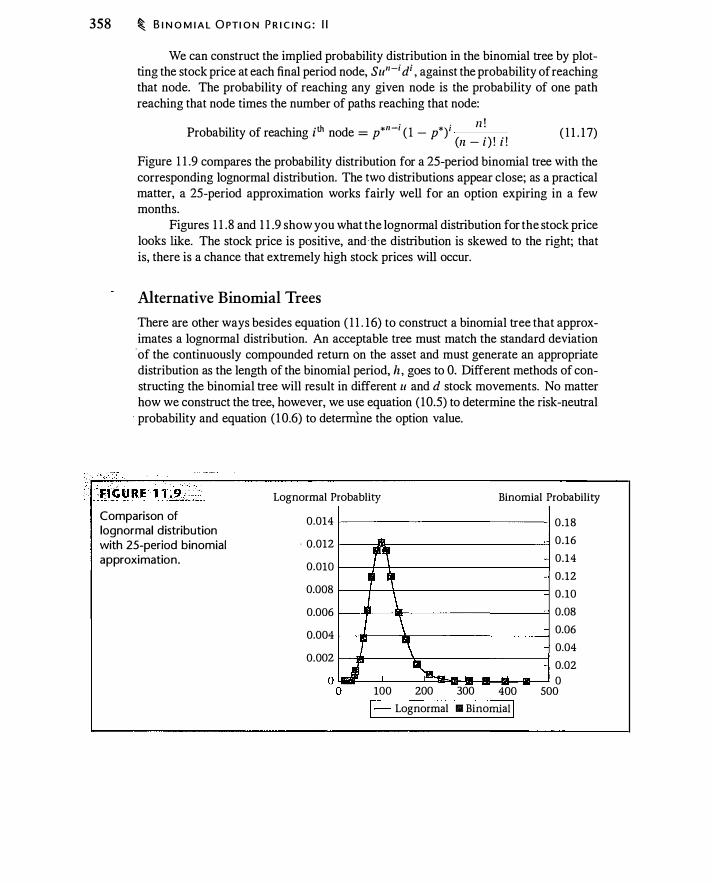
358 � B I N O M I A L O PTI O N P R I C I N G : I I

We can construct the implied probability distribution in the binomial tree by plot­ting the stock price at each final period node, S u" -i di , against the probability of reaching that node. The probability of reaching any given node is the probability of one path reaching that node times the number of paths reaching that node:

. . ll ! Probability of reaching ith node = p*"-' ( 1 - p*)' . . ( 1 1 . 1 7) (ll - l ) ! t !

Figure 1 1 .9 compares the probability distribution for a 25-period binomial tree with the corresponding lognormal distribution. The two distributions appear close; as a practical matter, a 25-period approximation works fairly well for an option expiring in a few months.

Figures 1 1 . 8 and 1 1 .9 show you what the lognormal distribution for the stock price looks like. The stock price is positive, and· the distribution is skewed to the right; that is, there is a chance that extremely high stock prices will occur.

Alternative Binomial Trees

There are other ways besides equation ( 1 1 . 1 6) to construct a binomial tree that approx­imates a lognormal distribution. An acceptable tree must match the standard deviation ·of the continuously compounded return on the asset and must generate an appropriate distribution as the length of the binomial period, h , goes to 0. Different methods of con­structing the binomial tree will result in different u and d stoc;k movements. No matter how we construct the tree, however, we use equation ( 10.5) to determine the risk-neutral

· probability and equation ( 1 0.6) to detei1lline the option value.

Comparison of lognormal distribution with 25-period binomial approximation.

Lognormal Probablity Binomial Probability

0.014 f--------------1 . 0.012 f----;ll!c------------=1

0.010 f--+-+-----------1 0.008 f--+---+-----------::::1 0.006 f----'1"---___,111----------=1 0.004 1---tdl---.1.---------� 0.002 f---111-----'c----------l

0.18 0.16 0.14 0.12 0.10 0.08 0.06 0.04 0.02 0

100 200 300 400 500 1- Lognormal II Binomial I

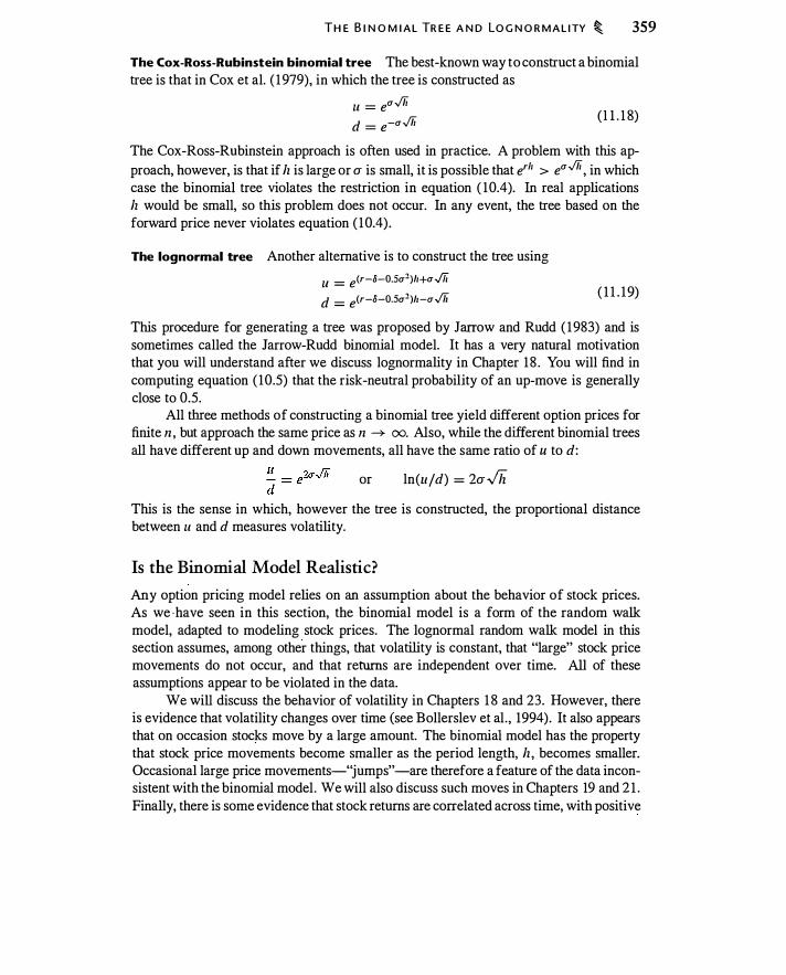
T H E B I N O M I A L TR E E A N D LO G N O R M A L I TY � 359

The Cox-Ross-Rubinstein binomial tree The best-known way to construct a binomial tree is that in Cox et al. ( 1 979), in which the tree is constructed as

u = ea./ii d = e-a./ii

( 1 1 . 1 8)

The Cox-Ross-Rubinstein approach is often used in practice. A problem with this ap­proach, however, is that if h is large or a is small, it is possible that e'" > ea./ii, in which case the binomial tree violates the restriction in equation ( 10.4). In real applications h would be small, so this problem does not occur. In any event, the tree based on the forward price never violates equation ( 10.4) .

The lognormal tree Another alternative is to construct the tree using Ll = e(r-/i-0.5a2)h+a.Jii d = e(r-/i-0.5a2)h-a./ii ( 1 1 . 1 9)

This procedure for generating a tree was proposed by Jarrow and Rudd ( 1983) and is sometimes called the Jarrow-Rudd binomial model. It has a very natural motivation that you will understand after we discuss lognormality in Chapter 18 . You will find in computing equation ( 10.5) that the risk-neutral probability of an up-move is generally close to 0.5.

All three methods of constructing a binomial tree yield different option prices for finite n , but approach the same price as n -+ oo. Also, while the different binomial trees all have different up and down movements, all have the same ratio of u to d:

or ln(ujd) = 2a,Jh

This is the sense in which, however the tree is constructed, the proportional distance between u and d measures volatility.

Is the Binomial Model Realistic?

Any option pricing model relies on an assumption about the behavior of stock prices. As we · have seen in this section, the binomial model is a form of the random walk model, adapted to modeling stock prices. The lognormal random walk model in this section assumes, among other things, that volatility is constant, that "large" stock price movements do not occur, and that returns are independent over time. All of these assumptions appear to be violated in the data.

We will discuss the behavior of volatility in Chapters 1 8 and 23. However, there is evidence that volatility changes over time (see Bollerslev et al. , 1994). It also appears that on occasion stocks move by a large amount. The binomial model has the property that stock price movements become smaller as the period length, h , becomes smaller. Occasional large price movements-"jumps"-are therefore a feature of the data incon­sistent with the binomial model. We will also discuss such moves in Chapters 19 and 2 1 . Finally, there is some evidence that stock returns are correlated across time, with positive

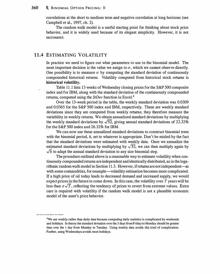
360 � B I N O M I A L O PT I O N P R I C I N G : I I

correlations at the short to medium term and negative correlation at long horizons (see Campbell et al., 1997, ch. 2).

The random walk model is a useful starting point for thinking about stock price behavior, and it is widely used because of its elegant simplicity. However, it is not sacrosanct.

11 .4 ESTIMATING VOLATILITY

In practice we need to figure out what parameters to use in the binomial model. The most important decision is the value we assign to a , which we cannot observe directly. One possibility is to measure a by computing the standard deviation of continuously compounded historical returns. Volatility computed from historical stock returns is historical volatility.

Table l l . l lists i 3 weeks of Wednesday closing prices for the S&P 500 composite index and for IBM, along with the standard deviation of the continuously compounded returns, computed using the StDev function in Excel.4

Over the 13-week period in the table, the weekly standard deviation was 0.0309 and 0.0365 for the S&P 500 index and IBM, respectively. These are weekly standard deviations since they are computed from weekly returns; they therefore measure the variability in weekly returns. We obtain annualized standard deviations by multiplying the weekly standard deviations by .)52, giving annual standard deviations of 22.32% .for the S&P 500 index and 26.32% for IBM.

We can now use these annualized standard deviations to construct binomial trees with the binomial period, h, set to whatever is appropriate. Don't be misled by the fact that the standard deviations were estimated with weekly data. Once we annualize the estimated standard deviations by multiplying by .)52, we can then multiply again by .fh to adapt the annual standard deviation to any size binomial step.

The procedure outlined above is a reasonable way to estimate volatility when con­tinuously compounded returns are independent and identically distributed, as in the loga­rithmic random walk model in Section 1 1 .3 . However, if returns are not independent-as with some commodities, for example-volatility estimation becomes more complicated. If a high price of oil today leads to decreased demand and increased supply, we would expect prices in the future to come down. In this case, the volatility over T years will be less than a .JT, reflecting the tendency of prices to revert from extreme values. Extra care is required with volatility if the random walk model is not a plausible economic model of the asset's price behavior.

4We use weekly rather than daily data because computing daily statistics is complicated by weekends

and holidays. In theory the standard deviation over the 3 days from Friday to Monday should be greater

than over the I day from Monday to Tuesday. Using weekly data avoids this kind of complication.

Further, using Wednesdays avoids most holidays.

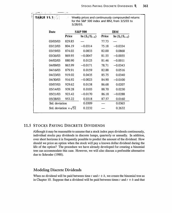
STO C K S PAY I N G D I S C R ET E D I V I D EN DS � 361

- - ·

··· TABLE 1 1. 1 Weekly prices and continuously compounded returns for the S&P 500 index and IBM, from 3/5/03 to 5/28/03 .

Date S&P SOO IBM Price In (Stf St-t) - Price In (St f St-t)

03/05/03 829.85 77.73 03/1 2/03 804. 1 9 -0.03 14 75 . 1 8 -0.0334 03/19/03 874.02 0.0833 82.00 0.0868 03/26/03 869.95 -0.0047 8 1 .55 -0.0055 04/02/03 880.90 0.0 125 8 1 .46 -0.00 1 1 04/09/03 865.99 -0.0 17 1 78.7 1 -0.0343 0411 6/03 879.9 1 0 .0159 82.88 0.05 16 04/23/03 9 19.02 0.0435 85 .75 0.0340 04/30/03 9 16.92 -0.0023 84.90 -0.0 100 05/07/03 929.62 0.0 138 86.68 0.0207 05114/03 939.28 0 .0103 88 .70 0.0230 05/2 1 103 923 .42 -0.0 170 86. 1 8 -0.0288 05/28/03 953 .22 0.03 1 8 87.57 0.0 160 Std. deviation 0.0309 0.0365 Std. deviation x -J52 0.2232 0.2632

11 .5 STOCKS PAYING DISCRETE DIVIDENDS

Although it may be reasonable to assume that a stock index pays dividends continuously, individual stocks pay dividends in discrete lumps, quarterly or annually. In addition, over short horizons it is frequently possible to predict the amount of the dividend. How should we price an option when the stock will pay a known dollar dividend during the life of the option? The procedure we have already developed for creating a binomial tree can accommodate this case. However, we will also discuss a preferable alternative due to Schroder ( 1 988) .

Modeling Discrete Dividends

When no dividend will be paid between time t and t + h , we create the binomial tree as in Chapter 10 . Suppose that a dividend will be paid between times t and t + h and that

362 � B I N O M I A L O PT I O N P R I C I N G : I I

its future value at time t + h is D. The time t forward price for delivery at t + lz i s then Fr , r+lr = S, erlr - D

Since the stock price at time t + h will be ex-dividend, we create the up and down moves based on the ex-dividend stock price: s:' = (S, e'lr - D) ea../Ti

Sf = (S, e'lr - D) e-a./ii ( 1 1 .20)

How does option replication work when a dividend is imminent? When a dividend is paid, we have to account for the fact that the stock earns the dividend. Thus, we have

The solution is

( s:' + D) D. + e'lr B = C11

(S1 + D) D. + e'lr B = Cd

Cu - Cd D. = ----,-s:' - sf

B = e-rlr [ s:' cd - SfCu ] - t:..De-rlr s:' - sf Because the dividend is known, we decrease the bond position by the present value of the certain dividend. (When the dividend is proportional to the stock price, as with a stock index, we reduce the stock position, equation ( 10. 1).) The expression for the option price is given by equation ( 10 . 17) .

Problems with the Discrete Dividend Tree

The practical problem with this procedure is that the tree does not completely recombine after a discrete dividend. In all previous cases we have examined, we reached the same price after a given number of up and down movements, regardless of the order of the movements.

Figure 1 1 . 1 0, in which a - dividend with a period-2 value of $5 is paid between periods 1 and 2, demonstrates that with a discrete dividend, the order of up and down movements affects the price. In the third binomial period there are six rather than four possible stock prices.

To see how the tree is constructed, period-1 prices are $41 eo.os x I /3+0.3 x ./173 = $50.07 1 $41eo.OSx l /3-0.3x./173 = $35 .41 1

The period-2 prices from the $50.07 1 node are

($50.07 l e0·08x 1 13 - 5) X e0·3 x.,!T73 = $55 .203

($50.07 1e0·08 x l /3 - 5) X e-0.3 x./173 = $39.041

Repeating this procedure for the node S = $35.4 1 1 gives prices of $37 .300 and $26.380. You can see that there are now four prices instead of three after two binomial steps: The

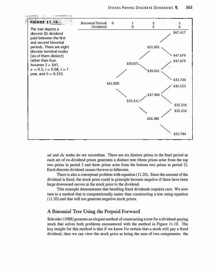
The tree depicts a .discrete $5 dividend paid between the first and second binomial periods. There are eight discrete terminal nodes (six of them distinct) rather than four. Assumes S = $41 , a = 0.3, r = 0.08, t = 1 year, and h = 0.333 .

Binomial Period: Dividend:

STO C K S PAY I N G D I S C R ET E D I V I D E N D S � 363

0 1 0

2 5

/

3 0

$67 .417

$55.203 ""'-

/ ""'-$47.679

$50.071� / $47.679 / $39.041 ""'-""'-

$33.720 $41 .000 / $45.553

� /$37.300 ""'-$35.411

""'-

$32.216 � / $32.216

$26.380

� $22.784

ud and du nodes do not recombine. There are six distinct prices in the final period as each set of ex-dividend prices generates a distinct tree (three prices arise from the top two prices ·in period 2 and three prices arise from the bottom two prices in period 2). Each discrete dividend causes the tree to bifurcate.

There is also a conceptual problem with equation ( 1 1 .20). Since the amount of the dividend is fixed, the stock price could in principle become negative if there have been large downward moves in the stock prior to the dividend.

This example demonstrates that handling fixed dividends requires care. We now turn to a method that is computationally easier than constructing a tree using equation ( 1 1 .20) and that will not generate negative stock prices.

A Binomial Tree Using the Prepaid Forward

Schroder ( 1988) presents an elegant method of constructing a tree for a dividend-paying stock that solves both problems encountered with the method in Figure 1 1 . 1 0. The key insight for this method is that if we know for certain that a stock will pay a fixed dividend, then we can view the stock price as being the sum of two components : the

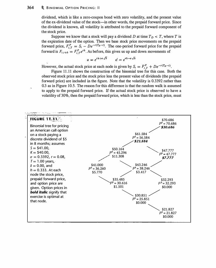
364 � B I N O M I A L O PT I O N P R I C I N G : I I

dividend, which is like a zero-coupon bond with zero volatility, and the present value of the ex-dividend value of the stock-in other words, the prepaid forward price. Since the dividend is known, all volatility is attributed to the prepaid forward component of the stock price.

Suppose we know that a stock will pay a dividend D at time To < T, where T is the expiration date of the option. Then we base stock price movements on the prepaid forward price, F/:r = S1 - De-r(To-l) . The one-period forward price for the prepaid forward is F1 •1+11 = F/:rer" . As before, this gives us up and down movements of

However, the actual stock price at each node is given by S1 = F/r + De-r(To-l) . Figure 1 1 . 1 1 shows the construction of the binomial tree for this case. Both the

observed stock price and the stock price less the present value of dividends (the prepaid forward price) are included in the figure. Note that the volatility is 0.3392 rather than 0.3 as in Figure 10.5. The reason for this difference is that the random walk is assumed to apply to the prepaid forward price. If the actual stock price is observed to have a volatility of 30%, then the prepaid forward price, which is less than the stock price, must

Binomial tree for pricing an American ca l l option on a stock paying a d iscrete dividend of $5 in 8 months; assumes s = $41 .00, K = $40.00, rr = 0.3392, r = 0.08, T = 1 .00 years, · li = 0.00, and h = 0.333 . At each node the stock price, prepaid forward price, and option price are g iven. Option prices in bold italic signify that exercise is optimal at that node.

$61 .584

$70.686 FP = 70.686 /$30.686

FP = 56.584 /$21.584 $50. 164 �

FP = 45.296 � p$�7·777

/ $ 1 l 308 F - 47.777 /

. $7.777 $41 .000

FP = 36.260 $5.770

� $43.246 / FP = 38.246 / $3.417 �

� $35 .485 $32.293 FP = 30.616 pP = 32.293 $1 .501 $0.000

� $30.851 /

FP = 25.85 1 $0.000 �

$21 .827 FP = 21 .827 $0.000

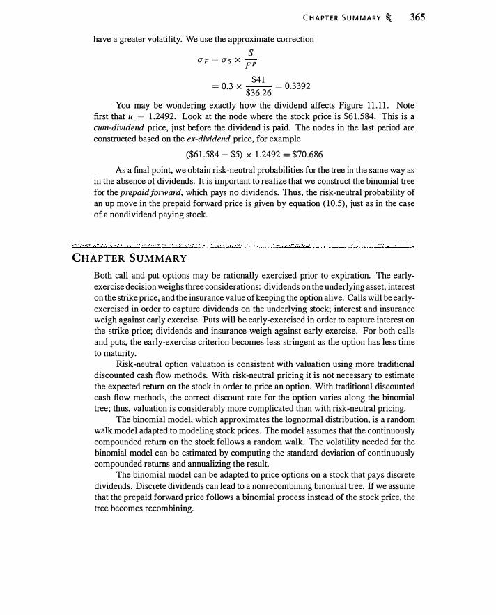
C H A PT E R S U M M A RY � 365

have a greater volatility. We use the approximate correction

s (J" F = (J" s X FP

$41 = 0.3 X $36_26 = 0.3392

You may be wondering exactly how the dividend affects Figure 1 1 . 1 1 . Note first that u . = 1 .2492. Look at the node where the stock price is $6 1 .584. This is a cum-dividend price, just before the dividend is paid. The nodes in the last period are constructed based on the ex-dividend price, for example

($6 1 .584 - $5) X 1 .2492 = $70.686 As a final point, we obtain risk-neutral probabilities for the tree in the same way as

in the absence of dividends. It is important to realize that we construct the binomial tree for the prepaidj01ward, which pays no dividends. Thus, the risk-neutral probability of an up move in the prepaid forward price is given by equation ( 1 0.5), just as in the case of a nondividend paying stock.

CHAPTER SUMMARY Both call and put options may be rationally exercised prior to expiration. The early­exercise decision weighs three considerations: dividends on the underlying asset, interest on the strike price, and the insurance value of keeping the option alive. Calls will be early­exercised in order to capture dividends on the underlying stock; interest and insurance weigh against early exercise. Puts will be early-exercised in order to capture interest on the strike price; dividends and insurance weigh against early exercise. For both calls and puts, the early-exercise criterion becomes less stringent as the option has less time to maturity.

Ris}\-neutral option valuation is consistent with valuation using more traditional discounted cash flow methods. With risk-neutral pricing it is not necessary to estimate the expected return on the stock in order to price an option. With traditional discounted cash flow methods, the correct discount rate for the option varies along the binomial tree; thus, valuation is considerably more complicated than with risk-neutral pricing.

The binomial model, which approximates the lognormal distribution, is a random walk model adapted to modeling stock prices. The model assumes that the continuously compounded return on the stock follows a random walk. The volatility needed for the binomial model can be estimated by computing the standard deviation of continuously compounded returns a,nd annualizing the result.

The binomial model can be adapted to price options on a stock that pays discrete dividends. Discrete dividends can lead to a nonrecombining binomial tree. If we assume that the prepaid forward price follows a binomial process instead of the stock price, the tree becomes recombining.

366 � B I N O M I A L O PT I O N P R I C I N G : I I

FURTHER READING

The binomial model can be used to derive the Black-Scholes model, which we discuss in Chapter 12 . The practical importance of risk-neutral pricing will become evident in Chapter 19 , when we see that Monte Carlo valuation hinges upon risk-neutral pricing. In that chapter we will also reexamine Figure 1 1 .4 and show how the option price may be computed as an expected value using only stock prices in the final period.

The issue of how the stock price is distributed will also arise frequently in later chapters . Chapter 1 8 discusses lognorrnality in more detail and presents evidence that stock prices are not exactly lognormally distributed. Chapter 20 will examine in more detml the question of how the stock price moves, in particular what happens when lz gets very small in the binomial model.

We will return to the determinants of early exercise in Chapter 17, when we discuss real options.

The literature on risk-neutral pricing is fairly technical. Cox and Ross ( 1 976) was the first paper to use risk-neutral pricing and Harrison and Kreps ( 1 979) studied the economic underpinnings. Two good treatments of this topic are Huang and Litzenberger ( 1 988, ch. 8)-their treatment inspired Appendix 1 l .B-and Baxter and Rennie ( 1996).

Campbell et al. ( 1 997) and Cochrane (200 1 ) summarize evidence on the distribu­tion of stock prices. The original Samuelson work on asset prices following a random walk (Samuelson, 1 965) remains a classic, modern empirical evidence notwithstanding.

Broadie and Detemple ( 1996) discuss the computation of American option prices, and also discuss alternative binomial aEproaches and their relative numerical efficiency.

PROB LEMS

Many (but not all) of these questions can be answered with the help of the BinomCall and BinomPut functions available on the spreadsheets accompanying this book.

11.1. Consider a one-period binomial model with h = 1 , where S = $ 1 00, r = 0, CJ = 30%, and 8 = 0.08. Compute American call option prices for K = $70, $80, $90, and $ 100.

a. At which strike(s) does early exercise occur? b. Use put-call parity to explain why early exercise does not occur at the

higher strikes. c. Use put-call parity to explain why early exercise is sure to occur for all

lower strikes than that in your answer to (a).

11.2. Repeat Problem 1 1 . 1 , only assume that r = 0.08. What is the greatest strike price at which early exercise will occur? What condition related to put-call parity is satisfied at this strike price?

11.3. Repeat Problem 1 1 . 1 , only assume that r = 0.08 and 8 = 0. Will early exercise ever occur? Why?

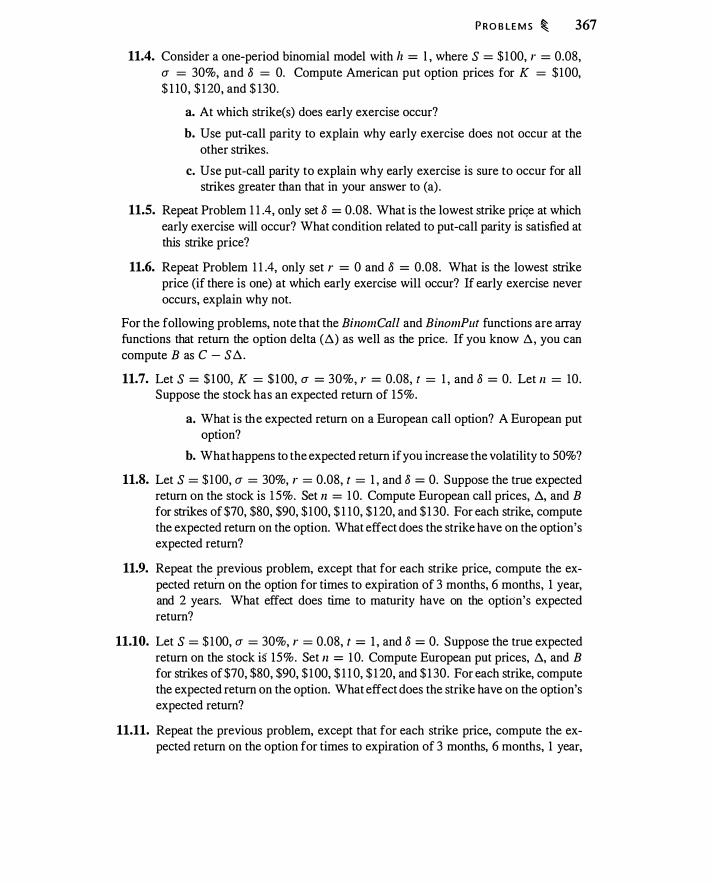
P RO B LE M S � 367

11.4. Consider a one-period binomial model with lz = l , where S = $ 1 00, r = 0.08, u = 30%, and 8 = 0. Compute American put option prices for K = $100, $ 1 10, $ 1 20, and $ 130.

a. At which strike(s) does early exercise occur?

b. Use put-call parity to explain why early exercise does not occur at the other strikes.

c. Use put-call parity to explain why early exercise is sure to occur for all strikes greater than that in your answer to (a) .

11.5. Repeat Problem 1 1 .4, only set 8 = 0.08. What is the lowest strike pri<;e at which early exercise will occur? What condition related to put-call parity is satisfied at this strike price?

11.6. Repeat Problem 1 1 .4, only set r = 0 and 8 = 0.08. What is the lowest strike price (if there is one) at which early exercise will occur? If early exercise never occurs, explain why not.

For the following problems, note that the BinomCall and BinomPut functions are array functions that return the option delta (.6.) as well as the price. If you know .6., you can compute B as C - S .6..

11.7. Let S = $ 1 00, K = $ 1 00, u = 30%, r = 0.08, t = 1 , and 8 = 0. Let n = 10. Suppose the stock has an expected return of 15%.

a. What is the expected return on a European call option? A European put option?

b. What happens to the expected return if you increase the volatility to 50%?

11.8. Let S = $ 1 00, u = 30%, r = 0.08, t = 1 , and 8 = 0. Suppose the true expected return on the stock is 1 5%. Set n = 1 0. Compute European call prices, .6., and B for strikes of $70, $80, $90, $ 100, $ 1 10, $ 1 20, and $ 1 30. For each strike, compute the expected return on the option. What effect does the strike have on the option's expected return?

11.9. Repeat the previous problem, except that for each strike price, compute the ex­pected return on the option for times to expiration of 3 months, 6 months, 1 year, and 2 years. What effect does time to maturity have on the option's expected return?

11.10. Let S = $ 1 00, u = 30%, r = 0.08, t = I , and 8 = 0. Suppose the true expected return on the stock is 15%. Set n = 1 0. Compute European put prices, .6., and B for strikes of $70, $80, $90, $ 1 00, $ 1 1 0, $ 1 20, and $ 1 30. For each strike, compute the expected return on the option. What effect does the strike have on the option's expected return?

11.11. Repeat the previous problem, except that for each strike price, compute the ex­pected return on the option for times to expiration of 3 months, 6 months, 1 year,

368 � B I N O M I A L O PT I O N P R I C I N G : I I

and 2 years. What effect does time to maturity have on the option's expected return?

11.12. Let S = $ 1 00, a = 0.30, r = 0.08, t = 1, and 8 = 0. Using equation ( 1 1 . 1 7) to compute the probability of reaching a terminal node and Sz/ d"-i to compute the price at that node, plot the risk-neutral distribution of year-1 stock prices as in Figures 1 1 .8 and 1 1 .9 for II = 3 and II = 10 .

11.13. Repeat the previous problem for n = 50. What is the risk-neutral probability that sl < $80? sl > $ 1 20?

11.14. We saw in Section 10. 1 that the undiscounted risk-neutral expected stock price equals the forward price. We will verify this using the binomial tree in Fig­ure 1 1 .4.

a. Using S = $ 1 00, r = 0.08, and 8 = 0, what are the 4-month, 8-month, and 1 -year forward prices?

b. Verify your answers in (a) by computing the risk-neutral expected stock price in the first, second, and third binomial period. Use equation ( 1 1 . 1 7) to determine the probability of reaching each node.

11.15. Compute the 1 -year forward price using the 50-step binomial tree in Prob­lem 1 1 . 1 3 .

11.16. Suppose S = $ 1 00, K = $95, r = 8% (continuously compounded), t = 1 , a = 30%, and 8 = 5 % . Explicitly construct an 8-period binomial tree using the Cox-Ross-Rubinstein expressions for u and d:

Compute the prices of European and American calls and puts.

11.17. Suppose S = $1 00, K = $95, r = 8% (continuously compounded), t = 1 , a = 30%, and 8 = 5%. Explicitly construct an 8-period binomial tree using the lognormal expressions for u and d:

Compute the prices of European and American calls and puts.

11.18. Obtain at least 5 years' worth of daily or weekly stock price data for a stock of your choice.

a. Compute annual volatility using all the data.

b. Compute annual volatility for each calendar year in your data. How does volatility vary over time?

c. Compute annual volatility for the first and second half of each year in your data. How much variation is there in your estimate?

11.19. Obtain at least 5 ·years of daily data for at least three stocks and, if you can, one currency. Estimate annual volatility for each year for each asset in your data.

A P P E N D I X 1 1 . 8 : W H Y D O ES R I S K- N E U T R A L P R I C I N G WO R K? � 369

What do you observe about the pattern of historical volatility over time? Does historical volatility move in tandem for different assets?

11.20. Suppose that S = $50, K = $45, a = 0.30, r = 0.08, and t = 1 . The stock will pay a $4 dividend in exactly 3 months. Compute the price of European and American call options using a four-step binomial tree.

APPENDIX 1 1 .A: PRICING OPTIONS WITH TRUE PROBABILITIES

In this appendix we demonstrate algebraically that computing the option price in a consistent way using a as the expected return on the stock gives the correct option price. Using the definition of y , equation ( 1 1 .6), we can rewrite equation ( 1 1 .7) as ( 1 [ erh _ d u - erh eah _ erh ])

(L�.S + B) eah /.),S + erh B u - d Cu + u - d Cd + u - d (Cu - Cd)

Since /.)..S + B is the call price, we need only show that the expression in large parenthe­ses is equal to one. From the definitions of /.), and B we have

erh - d u - erh --- Cu+---Cd=er11 (/.).S + B) u - d u - d

We can rewrite ( 1 1 .4) as

(/.),S + B) ( I [ er11 (/.),S + B) + (eah - erh )/.),SJ) =/.).S + B eah /.),S + erh B

This follows since the expression in large parentheses equals one.

APPENDIX 1 1 .B : WHY DOES RISK-NEUTRAL PRICING WORK ?

There is a large and highly technical literature on risk-neutral pricing. The underlying economic idea is fairly easy to understand, however.

Utility-Based Valuation

The starting point is that the well-being of investors is not measured in dollars, but in utility. Utility is a. measure of satisfaction. Economists say that investors exhibit declining marginal utility: Starting from a given level of wealth, the utility gained from adding $1 to wealth is less than the utility lost from taking $ 1 away from wealth. Thus, we expect that more dollars will make an investor happier, but that if we keep adding dollars, each additional dollar will make the investor less happy than the previous dollars.

Declining marginal utility implies that investors are risk-averse, which means that an investor will prefer a safer investment to a riskier investment that has the same

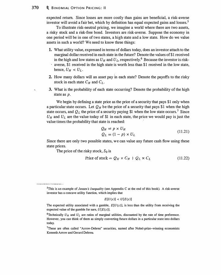
370 � B I N O M I AL O PTI O N P R I C I N G : I I

expected return. Since losses are more costly than gains are beneficial, a risk-averse investor will avoid a fair bet, which by definition has equal expected gains and losses.5

To illustrate risk-neutral pricing, we imagine a world where there are two assets, a risky stock and a risk-free bond. Investors are risk-averse. Suppose the economy in one period will be in one of two states, a high state and a low state. How do we value assets in such a world? We need to know three things:

1. What utility value, expressed in terms of dollars today, does an investor attach to the marginal dollar received in each state in the future? Denote the values of $ 1 received in the high and low states as U H and U L, respectively. 6 Because the investor is risk­averse, $ 1 received in the high state is worth less than $ 1 received in the low state, hence, UH < UL .

2. How many dollars will an asset pay in each state? Denote the payoffs to the risky stock in each state CH and CL .

3. What is the probability of each state occurring? Denote the probability of the high state as p.

We begin by defining a state price as the price of a security that pays $ 1 only when a particular state occurs. Let Q H b e the price of a security that pays $ 1 when the high state occurs, and Q L the price of a security paying $1 when the low state occurs. 7 Since U H and U L are the value today of $1 in each state, the price we would pay is just the value times the probability that state is reached:

QH == p X UH QL = ( 1 - p) X UL

( 1 1 .2 1 )

Since there are only two possible states, w e can value any future cash flow using these state prices.

The price of the risky stock, So is

( 1 1 .22)

5This is an example of Jensen 's Inequality (see Appendix C at the end of this book). A risk-averse investor has a concave utility function, which implies that

E[U (x)] < U[E(x)] The expected utility associated with a gamble, E[U (x)], is less than the utility from receiving the

expected value of the gamble for sure, U [E(x)] . 6Technically U H and U L are ratios of marginal utilities, discounted by the rate of time preference.

However, you can think of them as simply converting future dollars in a particular state into dollars today.

7These are often called "Arrow-Debreu" securities, named after Nobel-prize-winning economists

Kenneth Arrow and Gerard bebreu.

A P P E N D I X 1 1 . B : W H Y D O ES R I S K- N E U T R A L P R I C I N G WO R K? � 371

Since the risk-free bond pays $1 in each state, we have

Price of bond = QH x 1 + QL x 1 ( 1 1 .23)

We can calculate rates of return by dividing expected cash flows by the price. Thus, the risk-free rate is

1 1 + r = =--:----:--­

Price of bond 1

The expected return on the stock is

p X CH + ( 1 - p) CL 1 + a = "---::--,------,----=--­

Price of stock

= p X CH + ( 1 - p) CL Q H X CH + QL X CL

Standard Discounted Cash Flow

( 1 1 .24)

( 1 1 .25)

The standard discounted cash flow calculation entails computing the security price by discounting the expected cash flow at the expected rate of return. In the case of the stock, this gives us

p X CH + ( 1 - p) CL . .::...._ _____ ::____ = Pnce of stock

1 + a This is simply a rewriting of equation ( 1 1 .25); hence, it is obviously correct. Similarly, the bond price is

Risk-Neutral Pricing

1 . -- = Pnce of bond 1 + r

The point of risk-neutral pricing is to sidestep the utility calculations above. We are looking for probabilities such that when we use those probabilities to compute expected cash flows without explicit utility adjustments, and discount that expectation at the risk­free rate, then we will get the correct answer.

The trick is the following: Instead of utility-weighting the cash flows and comput­ing expectations, we utility-weight the probabilities, creating new "risk-neutral" proba­bilities. Now we will see how to perform risk-neutral pricing in this context. Use the state prices in equation ( 1 1 .2 1 ) to define the risk-neutral probability of the high state, p*, as

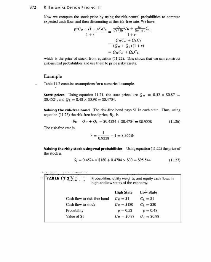
372 � B I N O M I A L O PT I O N P R I C I N G : I I

Now we compute the stock price by using the risk-neutral probabilities to compute expected cash flow, and then discounting at the risk-free rate. We have

*C ( 1 *)C _Sl.it_ c + .......Q.b_c p H + -

p L QH+QL H QH+QL L ��--���� = ���--���--

1 + r 1 + r

QHCH + QLCL (QH + QL) ( 1 + r)

= QHCH + QLCL whic\1 is the price of stock, from equation ( 1 1 .22). This shows that we can construct risk-neutral probabilities and use them to price risky assets.

Example

Table 1 1 .2 contains assumptions for a numerical example.

State prices Using equation 1 1 .2 1 , the state prices are QH $0.4524, and QL = 0.48 x $0.98 = $0.4704.

0.52 X $0.87

Valuing the risk-free bond The risk-free bond pays $1 in each state. Thus, using equation ( 1 1 .23) the risk-free bond price, Bo , is

Bo = QH + QL = $0:4524 + $0.4704 = $0.9228

The risk-free rate is 1

r = -- - 1 = 8 .366% 0.9228

( 1 1 .26)

Valuing the risky stock using real probabilities Using equation ( 1 1 .22) the price of the stock is

So = 0.4524 x $ 1 80 + 0.4704 x $30 = $95 .544 ( 1 1 .27)

Probabil ities, utility weights, and equity cash flows in high and low states of the economy.

Cash flow to risk-free bond

Cash flow to stock

Probability

Value of $ 1

High State

CH = $ 1

CH = $ 1 80

p = 0.52

UH = $0.87

Low State

CL = $ 1

CL = $30

p = 0.48

UL = $0.98

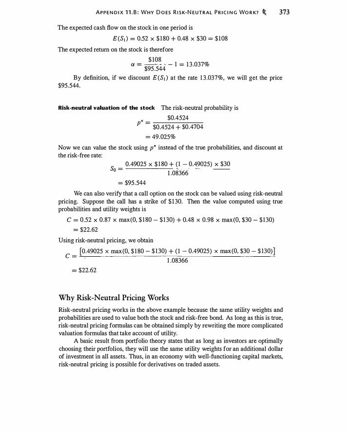
A P P E N D I X 1 1 . B : W H Y D O ES R I S K- N EUTRAL P R I C I N G WO R K? � 373

The expected cash flow on the stock in one period is

E(SI ) = 0.52 X $ 1 80 + 0.48 X $30 = $ 108 The expected return on the stock is therefore

$ 108 a = $95 .544 - 1 = 1 3 .037%

By definition, if we discount E(SI ) at the rate 1 3 .037%, we will get the price $95.544.

Risk-neutral valuation of the stock The risk-neutral probability is

* $0.4524 p =

$0.4524 + $0.4704 = 49.025%

Now we can value the stock using p* instead of the true probabilities, and discount at the risk-free rate:

0.49025 X $ 1 80 + ( 1 - 0.49025) X $30 So = 1 .08366

= $95.544 We can also verify that a call option on the stock can be valued using risk-neutral

pricing. Suppose the call has a strike of $ 130. Then the value computed using true probabilities and utility weights is

C = 0.52 X 0.87 X max(O, $ 1 80 - $ 130) + 0.48 x 0.98 X max(O, $30 - $ 130) = $22.62

Using risk-neutral pricing, we obtain

[0.49025 x max(O, $ 1 80 - $ 130) + ( 1 - 0.49025) x max(O, $30 - $ 130)] c = . 1 .08366

= $22.62

Why Risk-Neutral Pricing Works

Risk-neutral pricing works in the above example because the same utility weights and probabilities are used to value both the stock and risk-free bond. As long as this is true, risk-neutral pricing formulas can be obtained simply by rewriting the more complicated valuation formulas that take account of utility.

A basic result from portfolio theory states that as long as investors are optimally choosing their portfolios, they will use the same utility weights for an additional dollar of investment in all assets. Thus, in an economy with well-functioning capital markets, risk-neutral pricing is possible for derivatives on traded assets.

374 � B I N O M I A L O PT I O N P R I C I N G : I I

When would risk-neutral pricing not work? Suppose you have an asset you cannot trade or hedge, or you have a non tradable asset with cash flows that cannot be replicated by the cash flows of traded assets. If you cannot trade or offset the risk of the asset, then there is no guarantee that the marginal utility you use to value payoffs from this asset in a given state will be the same as for other assets. In other words, U H and U L will differ across assets. If the same U H and U L are not used to value the stock and bond, the calculations in this appendix fail. Valuing the non tradable stream of cash flows then requires computing the utility value of the payoffs. The point of risk-neutral pricing is to avoid having to do this.

The Black-Scholes Formula

.I.� ��73 Fi"he< Black '"d Mymn Schol"' (Black and Schol.,, 1973) published a formula-the Black-Scholes formula-for computing the theoretical price of a Euro­pean call option on a stock. Their paper, coupled with closely related work by Robert Merton, revolutionized both the theory and practice of finance. The history of the Black­Scholes formula is discussed in the box on page 376.

In this chapter we present the Black-Scholes formula for pricing European options, explain how it is used for different underlying assets, and discuss the so-called option Greeks--delta, gamma, theta, vega, rho, and psi-which measure the behavior of the option price when inputs to the formula change. We also show how observed option prices can be used to infer the market's estimate of volatility. Finally, while there is in general no simple formula comparable to Black-Scholes for valuing options that may be exercised early, perpetual options are an exception. We present the pricing formulas for perpetual American calls and puts.

12.1 INTRODUCTION TO THE B LACK-S CHOLES FORMULA

To introduce the Black-Scholes formula, we first return to the binomial model, discussed in Chapters 10 and 1 1 . When computing a binomial option price, we can vary the number of binomial steps, holding fixed the time to expiration. Table 12. 1 computes binomial call option prices, using the same inputs as in Figure 10.3 , and increases the number of steps, n. Changing the number of steps changes the option price, but once the number of steps becomes great enough we appear to approach a limiting value for the price. The last row reports the call option price if we were to use an infinite number of steps. We can't literally have an infinity of steps in a binomial tree, but it is possible to show that as the number of steps approaches infinity, the option price is given by the Black-Scholes formula. Thus, the Black-Scholes formula is a limiting case of the binomial formula for the price of a European option.

Call Options

The Black-Scholes formula for a European call option on a stock that pays dividends at the continuous rate 8 is

375

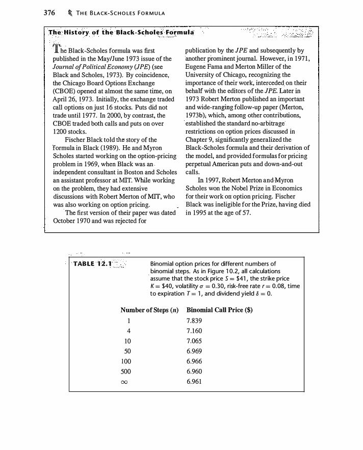
376 � TH E B LA C K-S C H O LES F O R M U LA

The History of the Black-Schoi�� I�rmula

Th� Black-Scholes formula was first published in the May/June 1 973 issue of the Joumal of Political Economy (JPE) (see Black and Scholes, 1973). By coincidence, the Chicago Board Options Exchange (CBOE) opened at almost the same time, on April 26, 1 973 . Initially, the exchange traded call options on just 1 6 stocks. Puts did not trade until 1 977. In 2000, by contrast, the CBOE traded both calls and puts on over 1 200 stocks.

Fischer Black told the story of the formula in B_lack ( 1989). He and Myron Scholes started working on the option-pricing problem in 1969, when Black was an independent consultant in Boston and Scholes an assistant professor at MIT. While working on the problem, they had extensive discussions with Robert Merton of MIT, who was also working on option pricing.

· The first version of their paper was dated October 1 970 and was rejected for

publication by the JPE and subsequently by another prominent journal. However, in 1 97 1 , Eugene Fama and Merton Miller of the University of Chicago, recognizing the importance of their work, interceded on their behalf with the editors of the JPE. Later in 1 973 Robert Merton published an important and wide-ranging follow-up paper (Merton, 1973b), which, among other contributions, established the standard no-arbitrage restrictions on option prices discussed in Chapter 9, significantly generalized the Black-Scholes formula and their derivation of the model, and provided formulas for pricing perpetualAmerican puts and down-and-out calls.

In 1997, Robert Merton and Myron Scholes won the Nobel Prize in Economics for their work on option pricing. Fischer Black was ineligible for the Prize, having died in 1995 at the age of 57.

TAB LE 1 2 . 1 . . ·. · . · · Binomial option prices for different numbers of . binomial steps. As in Figure 1 0.21 a l l calculations assume that the stock price S = $41 1 the strike price K = $401 volati l ity u = 0.301 risk-free rate r = 0.081 time to expiration T = 1 1 and dividend yield 8 = 0.

Number of Steps (n) Binomial Call Price ($) 1 7.839 4 7 . 160

10 7.065 50 6.969

100 6.966 500 6.960 00 6.96 1

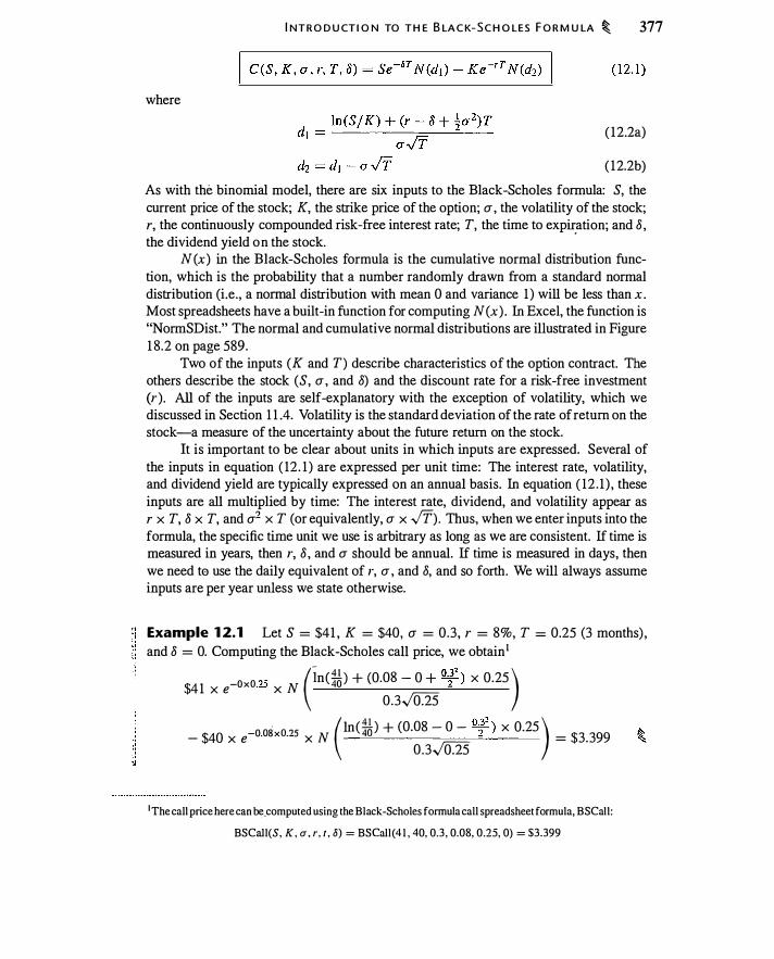
where

I NT R O D U CT I O N TO T H E B LA C K- S C H O LES F O R M U LA � 377

( 12.2a)

( 12.2b) As with the binomial model, there are six inputs to the Black-Scholes formula: S, the current price of the stock; K, the strike price of the option; a , the volatility of the stock; r, the continuously compounded risk-free interest rate; T, the time to expU:ation; and 8 , the dividend yield on the stock.

N (x) in the Black-Scholes formula is the cumulative normal distribution func­tion, which is the probability that a number randomly drawn from a standard normal distribution (i.e., a normal distribution with mean 0 and variance 1 ) will be less than x . Most spreadsheets have a built-in function for computing N(x) . In Excel, the function is "NormSDist." The normal and cumulative normal distributions are illustrated in Figure 1 8.2 on page 589.

Two of the inputs (K and T) describe characteristics of the option contract. The others describe the stock (S, a , and 8) and the discount rate for a risk-free investment (r) . All of the inputs are self-explanatory with the exception of volatility, which we discussed in Section 1 1 .4. Volatility is the standard deviation of the rate of return on the stock-a measure of the uncertainty about the future return on the stock.

It is important to be clear about units in which inputs are expressed. Several of the inputs in equation ( 12. 1 ) are expressed per unit time: The interest rate, volatility, and dividend yield are typically expressed on an annual basis. In equation ( 12 . 1 ) , these inputs are all multiplied by time: The interest rate, dividend, and volatility appear as r x T, 8 x T, and a2 x T (or equivalently, a x ,JT). Thus, when we enter inputs into the formula, the specific time unit we use is arbitrary as long as we are consistent. If time is measured in years, then r, 8 , and a should be annual. If time is measured in days, then we need to use the daily equivalent of r, a , and 8, and so forth. We will always assume inputs are per year unless we state otherwise.

Example 1 2.1 Let S = $41 , K = $40, a = 0.3, r = 8%, T = 0.25 (3 months) , and 8 = 0. Computing the Black-Scholes call price, we obtain1

$41 x e x -� x N -_0 0 ?-< (In( -4401 ) + (0.08 - 0 + 0�2

) x 0.25 ) 0.3.)[25

- $40 x e · x -- x N = $3.399 _0 08· O ?S ( ln(;M- ) + (0.08 - 0 - 0�2

) x 0.25 ) 0.3.)[25

1The call price here can be_ computed using the Black-Scholes formula call spreadsheet formula, BSCall:

BSCall(S, K, a , r, t , 8) = BSCall (4 1 , 40, 0.3 , 0.08, 0.25, 0) = $3.399

378 � T H E B LA C K-S C H O LES FO R M U LA

There is one input which does not appear in the Black-Scholes formula, namely the expected return on the stock. You might guess that stocks with a high beta would have a higher expected return; hence, options on these stocks would have a higher probability of settlement in-the-money. The higher expected return would seem to imply a higher option price. However, as we saw in Section 1 1 .2, a high stock beta implies a high option beta, so the discount rate for the expected payoff to such an option is correspondingly greater. The net result-one of the key insights from the Black-Scholes analysis-is that beta is irrelevant: The larger average payoff to options on high beta stocks is exactly offset by the larger discount rate.

Put Options

The Black-Scholes formula for a European put option is

I P (S, K , a , r, T, 8) = Ke-rT N(-dz) - se-ST N(-dd ( 1 2.3)

where d1 and d2 are given by equations ( 12.2a) and ( 1 2.2b). Since the Black-Scholes call and put prices, equations ( 1 2. 1 ) and ( 1 2.3), are for

European options, put-call parity must hold: P (S, K, a, r, T, 8) = C(S, K, a, r, T, 8) + Ke-rT - Se-8T ( 12.4)

This version of the formula follows from equations ( 1 2. 1 ) and ( 12.3), together with the fact that for any x, 1 - N(x) = N(�x) . (This equation says that the probability of a random draw from the standard normal distribution being above x, 1 - N (x) , equals the probability of a draw being below -x, N(-x) .)

Example 1 2.2 Using the same inputs as in Example 12. 1 , the put price is $ 1 .607. We can compute the put price in two ways. First, computing it using equation ( 12.3), we obtain2

$40e · x ·-·N -_0 08 o �� ( ln( 40:U) + (0.08 - 0 - 0�2 )0.25 )

0.3.JQ.E

- $41e- x ·- N - - = $ 1 .607 0 0 �5 ( ln( 4±..01 ) + (0.08 - 0 + 0�2 )0.25) 0.3.JQ.E

Computing the price using put-call parity, equation ( 12.4), we have

P (41 , 40, 0 .3 , 0.08, 0.25 , 0) = 3 .339 + 40e-O.OS xO.ZS - 4 1 = $ 1 .607

2The put price here can be computed using the Black-Scholes put spreadsheet .formula, BSPut:

BSPut(S, K, a, r, t , 8) = BSPut(4 1 , 40, 0.3, 0.08, 0.25 , 0) = $ 1 .607

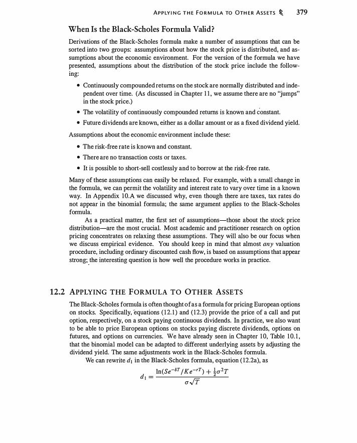
A P P LY I N G T H E F O R M U LA TO OTH E R ASS ETS � 379

When Is the Black-Scholes Formula Valid?

Derivations of the Black-Scholes formula make a number of assumptions that can be sorted into two groups: assumptions about how the stock price is distributed, and as­sumptions about the economic environment. For the version of the formula we have presented, assumptions about the distribution of the stock price include the follow­ing:

• Continuously compounded returns on the stock are normally distributed and inde­pendent over time. (As discussed in Chapter 1 1 , we assume there are no "jumps" in the stock price.)

• The volatility of continuously compounded returns is known and constant. • Future dividends are known, either as a dollar amount or as a fixed dividend yield.

Assumptions about the economic environment include these:

• The risk-free rate is known and constant. • There are no transaction costs or taxes. • It is possible to short-sell costlessly and to borrow at the risk-free rate.

Many of these assumptions can easily be relaxed. For example, with a small change in the formula, we can permit the volatility and interest rate to vary over time in a known way. In Appendix lO.A we discussed why, even though there are taxes, tax rates do not appear in the binomial formula; the same argument applies to the Black-Scholes formula.

As a practical matter, the first set of assumptions-those about the stock price distribution-are the most crucial. Most academic and practitioner research on option pricing concentrates on relaxing these assumptions . They will also be our focus when we discuss empirical evidence. You should keep in mind that almost any valuation procedure, including ordinary discounted cash flow, is based on assumptions that appear strong; the interesting question is how well the procedure works in practice.

12.2 APPLYING THE FORMULA TO OTHER ASSETS

The Black-Scholes formula is often thought of as a formula for pricing European options on stocks. Specifically, -equations ( 1 2. 1 ) and ( 1 2.3) provide the price of a call and put option, respectively, on a stock paying continuous dividends. In practice, we also want to be able to price European options on stocks paying discrete dividends, options on futures, and options on currencies. We have already seen in Chapter 1 0, Table 1 0. 1 , that the binomial model can be adapted to different underlying assets by adjusting the dividend yield. The same adjustments work in the Black-Scholes formula.

We can rewrite d1 in the Black-Scholes formula, equation ( 12.2a), as ln(Se-oT I K e-rT) + -}u2T

d , = -

u.,JT

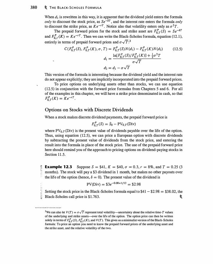
380 � TH E B LA C K- S C H O LES F O R M U LA

When d1 is rewritten in this way, it is apparent that the dividend yield enters the formula only to discount the stock price, as se-•r , and the interest rate enters the formula only to discount the strike price, as K e-rT . Notice also that volatility enters only as u2T.

The prepaid forward prices for the stock and strike asset are F{r (S) = se-•r

and F{r (K) = K e-rT . Then we can write the Black-Scholes formula, �quation ( 12 . 1 ), entirely in terms of prepaid forward prices and u.Jf:3

C(Fci,r (S) , Fci,r (K) , u , T) = Fci,r (S)N(di ) - Fci,r (K)N (d2) ( 12.5) ln[F{r (S)/F{r (K)] + �u2T

dl = ' ' -u.JT d2 = d1 - uvT

This version of the formula is interesting because the dividend yield and the interest rate do not appear explicitly; they are implicitly incorporated into the prepaid forward prices.

To price options on underlying assets other than stocks, we can use equation ( 12.5) in conjunction with the forward price formulas from Chapters 5 and 6. For all of the examples in this chapter, we will have a strike price denominated in cash, so that Fci,r (K) = Ke-rr .

Options on Stocks with Discrete Dividends

When a stock makes discrete dividend payments, the prepaid forward price is p -

F0,r (S) = So - PVo,r(Div) where PVo,r CDiv) is the present value of dividends payable over the life of the option. Thus, using equation ( 12.5), we can price a European option with discrete dividends by subtracting the present value of dividends from the stock price, and entering the result into the formula in place of the stock price. The use of the prepaid forward price here should remind you of the approach to pricing options on dividend-paying stocks in Section 1 1 .5 .

Example 1 2.3 Suppose S = $41 , K = $40, u = 0 .3 , r = 8%, and T = 0.25 (3 months). The stock will pay a $3 dividend in 1 month, but makes no other payouts over the life of the option (hence, 8 = 0). The present value of the dividend is

PV(Div) = $3e-0.08x l f 12 = $2.98

Setting the stock price in the Black-Scholes formula equal to $41 - $2.98 = $38 .02, the Black-Scholes call price is $ 1 .763 . �

3We can also let V (T) = a -IT represent total volatility-uncertainty about the relative time-T values

of the underlying and strike assets--over the life of the option. The option price can then be written solely in terms of Fci,T (S), Fci,T (K), and V(T) . This gives us a minimalist version of the Black-Scholes

formula: To price an option you need to know the prepaid forward prices of the underlying asset and

the strike asset, and the relative volatility of the two.

A P P LY I N G T H E F O R M U LA TO OTH E R ASS ETS � 381

Compared to the $3.399 price computed in Example 1 2. 1 , the dividend reduces the option price by about $ 1 .64, or over half the amount of the dividend. Note that this is the price of a European option. An American option might be exercised just prior to the dividend, and hence would have a greater price.

Options on Currencies

We can price an option on a currency by replacing the dividend yield with the foreign interest rate. If the spot exchange rate is x (expressed as domestic currency per unit of foreign currency), and the foreign currency interest rate is r1 , the prepaid for.ward price for the currency is

Fci7 (x) = xoe-rtT

Using equation ( 12.5), the Black-Scholes formula becomes

C(x , K, u , r, T, rf) = xe-r1T N(dt ) - Ke-rT N(d2) In(x/K) + (r - r1 + .,}u2)T

dt = -u.Jf

( 1 2.6)

This formula for the price of a European call on currencies is called the Garman­Kohlhagen model, after Garman and Kohlhagen ( 1983).

The price of a European currency put is obtained using parity:

P (x, K, u, r, T, rf) = C(x , K, u , r, T, r1) + Ke-rT - xe-rtT

n Example 1 2.4 Suppose the spot exchange rate is x = $0.92/€, K = $0.9, u = 0. 10, r = 6% (the dollar interest rate), T = 1 , and I"J = 3 .2% (the euro-denominated interest rate). The price of a dollar-denominated euro call is $0.0606, and the price of a

� dollar-denominated euro put is $0.0172. �

Options on Futures

The prepaid forward prise for a futures contract is just the present value of the futures price. Thus, we price a European option on a futures contract by using the futures price as the stock price and setting the dividend yield equal to the risk-free rate. The resulting formula is also known as the Black formula:

C(F, K, u , r, T, r) = Fe-rT N(dt ) - Ke-rT N(d2) ln(F / K) + .,}u2T

dt = -u.Jf

d2 = dt - u-!f

( 12.7)

382 � TH E B LA C K-S C H O LES F O R M U LA

The put price is obtained using the parity relationship for options on futures : P (F, K, a , r, T, r) = C(F, K, a , r, T, r) + Ke-rT - Fe-rT

' Example 1 2.5 Suppose the 1 -year futures price for natural gas is $2. 1 O/Ml\.1Btu and the volatility is 0.25. We have F = $2. 1 0, K = $2. 10, a = 0.25, r = 0.055, T = 1 , and 8 = 0.055 (the dividend yield is set to equal the interest rate). The Black-Scholes

t call price and put price are both $0. 1 9772 1 . �

12.3 OPTION GREEKS

Option Greeks are formulas that express the change in the option price when an input to the formula changes, taking as fixed all the other inputs.4 One important use of Greek measures is to assess risk exposure. For example, a market-making bank with a portfolio of options would want to understand its exposure to stock price changes, interest rates, volatility, etc. A portfolio manager wants to know what happens to the value of a portfolio of stock index options if there is a change in the level of the stock index. An options investor would like to know how interest rate changes and volatility changes affect profit and loss.

Keep in mind that the Greek measures by assumption change only one input at a time. In real life, we would expect interest rates and stock prices, for example, to change together. The Greeks answer the question, what happens when one and only one input changes?

The actual formulas for the Greeks appear in Appendix 1 2.B. Greek measures can be computed for options on any kind of underlying asset, but we will fC?cus here on stock options.

Definition of the Greeks

The units in which changes ·are measured are a matter of convention. Thus, when we define a Greek measure, we will also provide the assumed unit of change.

Delta (�) measures the option price change when the stock price increases by $ 1 .

Gamma (r) measures the change in delta when the stock price increases by $ 1 .

Vega measures the change in the option price when there i s an increase in volatility of one percentage point.5

4Specifically, the Greeks are mathematical derivatives of the option price formula with respect to the inputs.

5"Vega" is not a Greek letter . . "Kappa" and "lambda" are also sometimes used to mean the same thing

as vega.

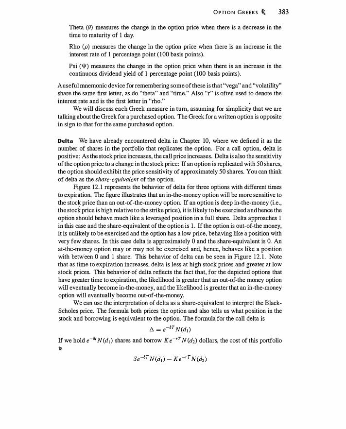
O PTI O N G R E E K S � 383

Theta (B) measures the change in the option price when there is a decrease in the time to maturity of 1 day.

Rho (p) measures the change in the option price when there is an increase in the interest rate of 1 percentage point ( 100 basis points).

Psi (W) measures the change in the option price when there is an increase in the continuous dividend yield of 1 percentage point (100 basis points).

A useful mll.emonic device for remembering some of these is that "vega" and "volatility" share the same first letter, as do "theta" and "time." Also "r" is often used to denote the interest rate and is the first letter in "rho."

We will discuss each Greek measure in tum, assuming for simplicity that we are talking about the Greek for a purchased option. The Greek for a written option is opposite in sign to that for the same purchased option.

Delta We have already encountered delta in Chapter 10, where we defined it as the number of shares in the portfolio that replicates the option. For a call option, delta is positive: As the stock price increases, the call price increases. Delta is also the sensitivity of the option price to a change in the stock price: If an option is replicated with 50 shares, the option should exhibit the price sensitivity of approximately 50 shares. You can think of delta as the share-equivalent of the option.

·

Figure 12. 1 represents the behavior of delta for three options with different times to expiration. The figure illustrates that an in-the-money option will be more sensitive to the stock price than an out-of-the-money option. If an option is deep in-the-money (i.e., the stock price is high relative to the strike price), it is likely to be exercised and hence the option should behave much like a leveraged position in a full share. Delta approaches 1 in this case and the share-equivalent of the option is 1 . If the option is out-of-the money, it is unlikely to be exercised and the option has a low price, behaving like a position with very few shares. In this case delta is approximately 0 and the share-equivalent is 0. An at-the-money option may or may not be exercised and, hence, behaves like a position with betw·een 0 and 1 share. This behavior of delta can be seen in Figure 12. 1 . Note that as time to expiration increases, delta is less at high stock prices and greater at low stock prices. This behavior-of delta reflects the fact that, for the depicted options that have greater time to expiration, the likelihood is greater that an out-of-the money option will eventually become in-the-money, and the likelihood is greater that an in-the-money option will eventually become out-of-the-money.

We can use the interpretation of delta as a share-equivalent to interpret the Black­Scholes price. The formula both prices the option and also tells us what position in the stock and borrowing is equivalent to the option. The formula for the call delta is

/::;. = e-�T N(dJ ) If we hold e-�t N (d1 ) shares and borrow K e-rT N (d2) dollars, the cost of this portfolio lS

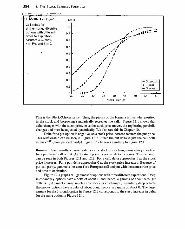
384 � T H E B LA C K-S C H O LES F O R M U LA

Call deltas for at-the-money 40-strike options with d ifferent times to expiration. Assumes a = 30%, r = 8%, and 8 = 0.

Delta

1.0

0.9

0.8

0.7

0.6

0.5

0.4

0.3

0.2

0.1

0 20 25 30 35 40 45

Stock Price ($)

so

-+- 3 months + 1 year ..... 3 years

55 60

This is the Black-Scholes price. Thus, the pieces of the formula tell us what position in the stock and borrowing synthetically recreates the call . Figure 12 . 1 shows that delta changes with the stock price, so as the stock price moves, the replicating portfolio changes and must be adjusted dynamically. We also saw this in Chapter 10 .

Delta for a put option is negative, so a stock price increase reduces the put price. This relationship can be seeq in Figure 1 2.2. Since the put delta is just the call delta minus e-oT (from put-call parity), Figure 1 2.2 behaves similarly to Figure 1 2. 1 .

Gamma Gamma-the change i n delta as the stock price changes-is always positive for a purchased call or put. As the stock price increases, delta increases. This behavior can be seen in both Figures 12. 1 and 1 2.2. For a call, delta approaches 1 as the stock price increases. For a put, delta approaches 0 as the stock price increases. Because of put-call parity, gamma is the same for a European call and put with the same strike price and time to expiration.

Figure 1 2.3 graphs call gammas for options with three different expirations. Deep in-the-money options have a delta of about 1 , and, hence, a gamma of about zero. (If delta is 1 , it cannot change much as the stock price changes.) Similarly deep out-of­the-money options have a delta of about 0 and, hence, a gamma of about 0. The large gamma for the 3-month option in Figure 1 2.3 corresponds to the steep increase in delta for the same option in Figure 1 2. 1 .

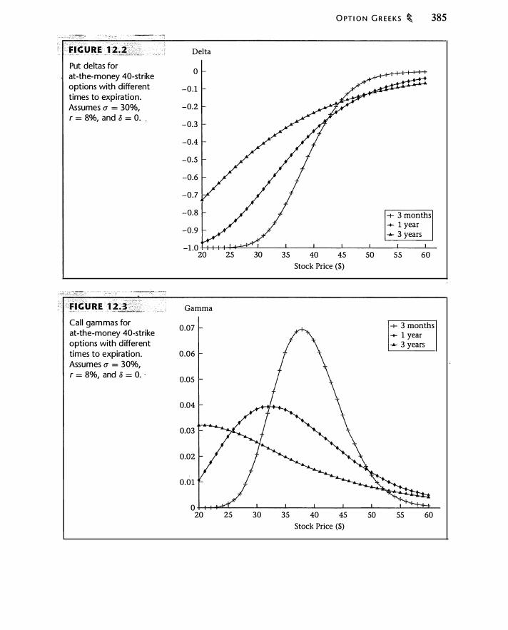
Put deltas for at-the-money 40-strike options with different times to expiration. Assumes u = 30%, r = 8%, and 8 = 0.

Cal l gammas for at-the-money 40-strike options with d ifferent times to expiration. Assumes u = 30%, r = 8%, and 8 = 0. ·

Delta

0

-0.1

-0.2

-0.3

-0.4

-0.5

-0.6

-0.7

-0.8

-0.9

-1 .0 20

Gamma

0.07

0.06

0.05

0.04

0.03

0.02

0.01

0 20

25 30

25 30

35

35

O PT I O N G R E E K S � 385

-+- 3 months -+- 1 year "*- 3 years

40 45 50 55 60 Stock Price ($)

-+- 3 months -+- 1 year "*- 3 years

40 45 50 55 60 Stock Price ($)

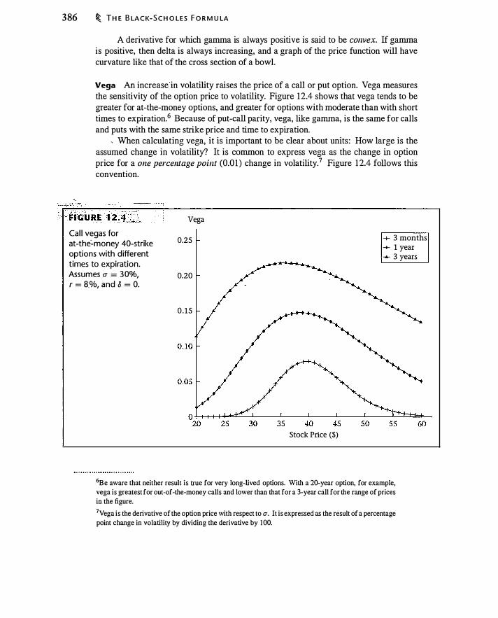
386 � T H E B LA C K-S C H O LES F O R M U LA

A derivative for which gamma is always positive is said to be convex. If gamma is positive, then delta is always increasing, and a graph of the price function will have curvature like that of the cross section of a bowl.

Vega An increase in volatility raises the price of a call or put option. Vega measures the sensitivity of the option price to volatility. Figure 1 2.4 shows that vega tends to be greater for at-the-money options, and greater for options with moderate than with short times to expiration.6 Because of put-call parity, vega, like gamma, is the same for calls and puts with the same strike price and time to expiration.

, When calculating vega, it is important to be clear about units : How large is the assumed change in volatility? It is common to express vega as the change in option price for a one percelltage point (0.01 ) change in volatility.7 Figure 1 2.4 follows this convention.

Cal l vegas for at-the�money 40-strike options with different times to expiration. Assumes u = 30%, r = B.o/o, and 8 = 0.

Vega

0.25

0.20

0.15

Stock Price ($)

+ 3 months -+ 1 year ..,.._ 3 years

6B e aware that neither result is true for very long-lived options. With a 20-year option, for example,

vega is greatest for out-of-the-money calls and lower than that for a 3-year call for the range of prices

in the figure.

7Vega is the derivative of the option price with respect to cr. It is expressed as the result of a percentage

point change in volatility by dividing the derivative by I 00.

O PT I O N G R E E K S � 387

Theta Options generally-but not always-become less valuable as time to expiration decreases. Figure 1 2.5 depicts the call price for out-of-the-money, at-the-money, and in­the-money options as a function of the time to expiration. For the at-the-money (strike = $40) option, time decay is most rapid at expiration. For the others, time decay is more steady. Figure 1 2.6 graphs theta explicitly for three different times to expiration, showing that time decay is greatest for the at-the-money short-term option.

Time decay can be positive for European options in some special cases. Deep-in­the-money .call options on an asset with a high dividend yield and deep-in-the-money puts are two examples. In both cases we would want to exercise the options early if possible. Since we cannot, the option effectively becomes a T-bill, appreciating as it gets close to expiration. This effect is evident in Figure 1 2.7, in which the in-the-money (50-strike) put becomes more valuable, other things equal, as expiration approaches. Figure 12 .8 on page 390 graphs the put theta explicitly, illustrating the positive theta.

When interpreting theta we need to know how long is the assumed change in time. Figures 12.6 and 1 2.8 are computed assuming a 1 -day change in time to expiration. It is also common in practice to compute theta over longer periods, such as 10 days.

Rho Rho is positive for an ordinary stock call option. Exercising a call entails paying the fixed strike price to receive the stock; a higher interest rate reduces the present value of the strike. Similarly, for a put, rho is negative, since the put entitles the owner to

FIGURE 1 2. 5 . Cal l prices for options with d ifferent strikes at d ifferent times to expiration. Assumes s = $40, u = 30%, r = 8%, and 8 = 0. .

Option Premium ($)

18

16

14

12

10

8

6

4

2

0.5

-+- Strike = $30 -+- Strike = $40 ..._ Strike = $50

1.0 1 .5 2.0 2.5 3.0 Time to Expiration (years)

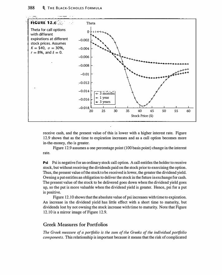
388 � T H E B LA C K-S C H O LES F O R M U LA

Theta for cal l options with different expirations at d ifferent stock prices. Assumes K = $40, a = 30%, r = 8%, and 8 = 0.

Theta

-0.002

-0.004

-0.006

-0.008

-0.01

.-0.012

-0.014

-0.016 + 3 months -+- 1 year ..._ 3 years

-0.018 c__ _ _._ __ ...._ _ __._ __ ..J.....:.. _ __,_ __ _.__--l. __ _L__ 20 25 30 35 40 45 so 55

Stock Price ($)

receive cash, and the present value of this is lower with a higher interest rate. Figure 12.9 shows that as the time to expiration increases and as a call option becomes more in-the-money, rho is greater.

Figure 1 2.9 assumes a one percentage point ( 100 basis point) change in the interest rate.

Psi Psi is negative for an ordinary stock call option. A call entitles the holder to receive stock, but without receiving the dividends paid on the stock prior to exercising the option. Thus, the present value of the stock to be received is lower, the greater the dividend yield. Owning a put entitles an obligation to deliver the stock in the future in exchange for cash. The present value of the stock to be delivered goes down when the dividend yield goes up, so the put is more valuable when the dividend yield is greater. Hence, psi for a put is positive.

Figure 12 . 10 shows that the absolute value of psi increases with time to expiration. An increase in the dividend yield has little effect with a short time to maturity, but dividends lost by not owning the stock increase with time to maturity. Note that Figure 12 . 1 0 is a mirror image of Figure 1 2.9.

Greek Measures for Portfolios

The Greek measure of a portfolio is the sum of tlze Greeks of the individual portfolio components. This relationship is important because it means that the risk of complicated

60

Put prices for options with d ifferent strikes at different times to expiration. Assumes s = $40, (I = 30%, r = 8%, and 8 =0 . .

Option Premium ($)

10

9

8

7

6

5

4

3

O PT I O N G R E E K S � 389

+ Strike = 30 -+ Strike = 40 ..._ Strike = 50

Time to Expiration (years)

option positions is easy to evaluate. For a portfolio containing n options with a single underlying stock, where the quantity of each option is given by w; , we have

II

llportfolio = L W; ll; i= l

The same relation holds true for the other Greeks as well.

- Example 1 2.6 Table 1 2.2 on page 392 lists Greek measures for a 40-45 bull spread. Greeks for the spread are Greeks for the 40-strike call less those for the 45-strike call.

�

Option Elasticity

An option is an alternative to investing in the stock. Delta tells us the dollar risk of the option relative to the stock: If the stock price changes by $ 1 , by how much does the option price change? The option elasticity, by comparison, tells us the risk of the option relative to the stock in percentage terms: If the stock price changes by 1%, what is the percentage change in the value of the option?

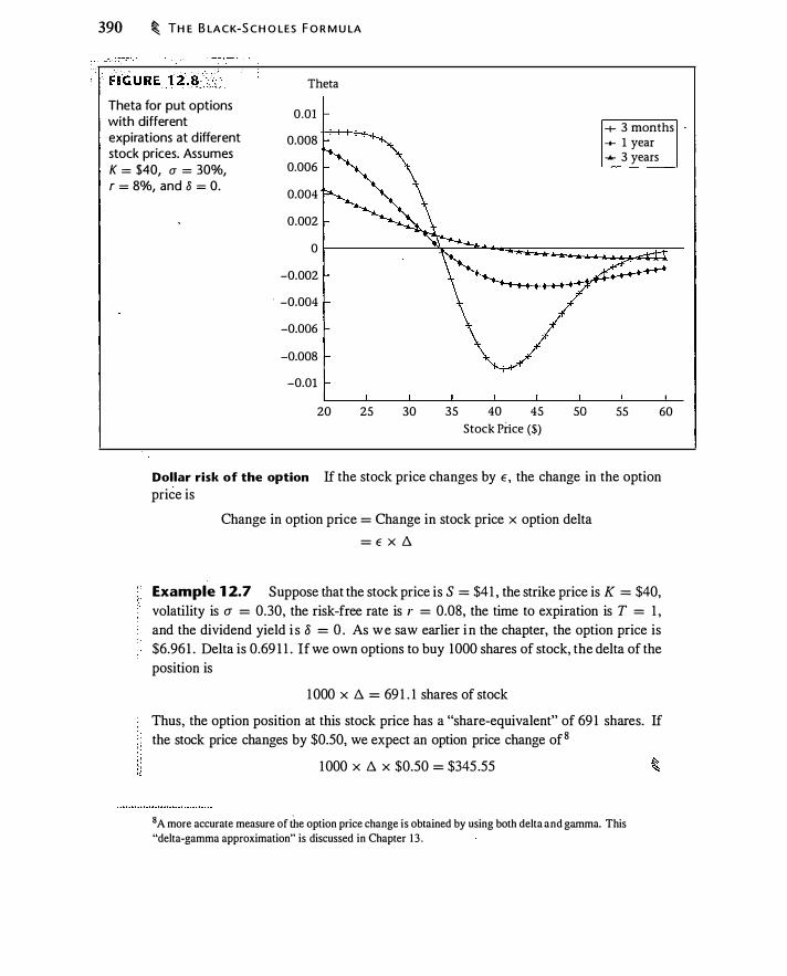
390 � TH E B LA C K-S C H O LES f O R M U LA

Theta

0.01 Theta for put options with different expirations at d ifferent stock prices. Assumes K = $40, a = 30%,

-+- 3 months 0.008 -+- 1 year

0.006 ..... 3 years

r = 8%, and 8 = 0. 0.004

0.002

0

-0.002

. -0.004

-0.006

-0.008

-0.01

20 25 30 35 40 45 so 55 60 Stock Price (S)

Dollar risk of the option If the stock price changes by E, the change in the option price is

Change in option price = Change in stock price x option delta = E X /:,.

Example 1 2.7 Suppose that the stock price is S = $41 , the strike price is K = $40, volatility is u = 0.30, the risk-free rate is r = 0.08, the time to expiration is T = 1 , and the dividend yield i s 8 = 0 . As we saw earlier i n the chapter, the option price is $6.961 . Delta is 0.69 1 1 . If we own options to buy 1000 shares of stock, the delta of the position is

1 000 x /:,. = 69 1 . 1 shares of stock

Thus, the option position at this stock price has a "share-equivalent" of 69 1 shares. If the stock price changes by $0.50, we expect an option price change of8

1000 X /:,. X $0.50 = $345 .55

8 A more accurate measure of the option price change is obtained by using both delta and gamma. This

"delta-gamma approximation" is discussed in Chapter 1 3 .

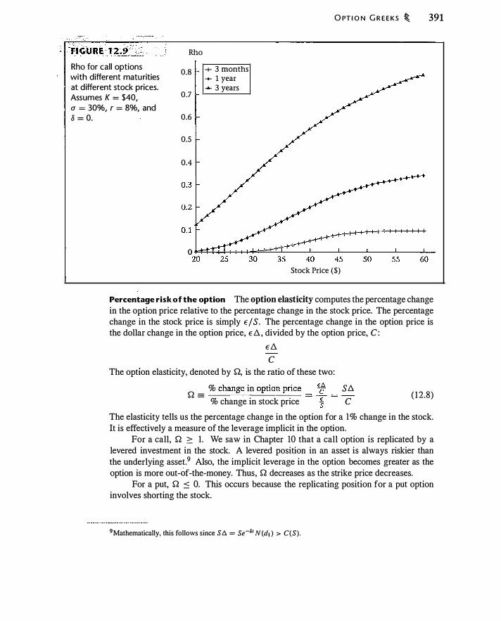
Rho for cal l options with different maturities at different stock prices. Assumes K = $40, CJ = 30%, r = 8%, and 8 = 0.

Rho

0.8

0.7

0.6

0.5

0.4

+ 3 months -+- 1 year � 3 years

O PT I O N G R E E K S � 391

Stock Price ($)

Percentage risk of the option The option elasticity computes the percentage change in the option price relative to the percentage change in the stock price. The percentage change in the stock price is simply E IS. The percentage change in the option price is the dollar change in the option price, E /::;. , divided by the option price, C:

E /::;. c

The option elasticity, denoted by Q, is the ratio of these two:

% change in option price Q = ------"--=------'=---­

% change in stock price Sf:;. c

( 1 2.8)

The elasticity tells us the percentage change in the option for a 1% change in the stock. It is effectively a measure of the leverage implicit in the option.

For a call, Q :::::: 1. We saw in Chapter 10 that a call option is replicated by a levered investment in the stock. A levered position in an asset is always riskier than the underlying asset.9 Also, the implicit leverage in the option becomes greater as the option is more out-of-the-money. Thus, Q decreases as the strike price decreases.

For a put, Q ::": 0. This occurs because the replicating position for a put option involves shorting the stock.

9Mathematically, this follows since Sll. = Se-M N (di l > C(S).

392 � T H E B LA C K-S C H O LES F O R M U LA

Psi for cal l options with different maturities at d ifferent stock prices. Assumes K = $40, u = 30%, r = 8%, and 8 = 0.

Psi

-0.8

-1

-1 .2

-1 .4

-1.6 + 3 months ..... 1 year � 3 years

-1 .8 '------'----'---'-----'----'----''-----'----'--20

W;

Price

Delta

Gamma

Vega

Theta

Rho

25 30 35 40 45 so 55 Stock Price ($)

Greeks for the bull spread examined in Chapter 3, where S = $40, u = 0.3, r = 0.08, and T = 91 days, with a purchased 40-strike call and a written 45-strike cal l . The column titled "combined" is the d ifference between column 1 and column 2.

Option 1 Option 2 Combined

1 - 1 2.7804 0.97 10 1 .8094 0.5824 0.28 15 0.3009 0.0652 0.0563 0.0088 0.0780 0.0674 0.0 106

-0.0 1 73 -0.0 134 -0.0040 0.05 1 1 0.0257 0.0255

60

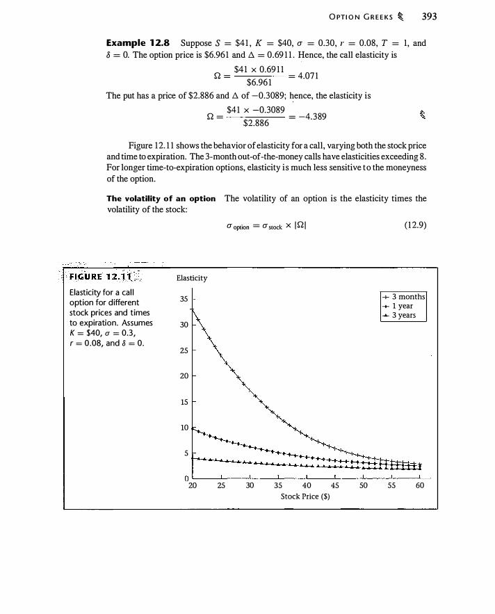
O PTI O N G R E E KS � 393

Example 1 2.8 Suppose S = $41 , K = $40, u = 0.30, r = 0.08, T = 1, and o = 0. The option price is $6.96 1 and /'<;.. = 0.69 1 1 . Hence, the call elasticity is

$41 X 0.69 1 1 Q = = 4.07 1 $6.96 1

The put has a price of $2.886 and /'<;.. of -0.3089; hence, the elasticity is

$41 X -0.3089 Q = = -4.389

$2.886

Figure 12. 1 1 shows the behavior of elasticity for a call, varying both the stock price and time to expiration. The 3-month out -of-the-money calls have elasticities exceeding 8 . For longer time-to-expiration options, elasticity i s much less sensitive to the moneyness of the option.

The volatility of an option The volatility of an option is the elasticity times the volatility of the stock:

Elasticity for a cal l option for d ifferent stock prices and times to expiration. Assumes K = $40, a = 0.3, r = 0.08, and 8 = 0.

Elasticity

35

30

25

20

15

10

5

U option = U stock X I Q I ( 1 2.9)

+ 3 months --+-- 1 year � 3 years

0�--�----�----�----�----L---�----�----� 20 25 30 35 40 45 so 55 60

Stock Price ($)

394 � TH E B LA C K-S C H O LES F O R M U LA

where I Q I is the absolute value of Q . Since elasticity is a measure of leverage, this calculation is analogous to the computation of the standard deviation of levered equity by multiplying the unlevered beta by the ratio of firm value to equity. Based on Figure 1 2. 1 1 , for a stock with a 30% volatility, an at-the-money option could easily have a volatility of 120% or more.

The risk premium of an option Since elasticity measures the percentage sensitivity of the option relative to the stock, it tells us how the risk premium of the option compares to that of the stock. In Section 1 1 .2, we computed the discount rate for an option. We were implicitly using option elasticity to do this.

At a point in time, the option is equivalent to a position in the stock and in bonds; hence, the return on the option is a weighted average of the return on the stock and the risk-free rate. Let a denote the expected rate of return on the stock, y the expected return on the option, and r the risk-free rate. We have

!l S ( !l S ) y =

C(S) a + 1 -

C (S) r

Since !l S / C ( S) is elasticity, this can also be written

y = Qa + ( 1 - Q)r

or

( 12 . 1 0)

Thus, the risk premium on the option equals the risk premium on the stock times Q . Using our earlier facts about elasticity, we conclude that if the stock has a positive

risk premium, then a call always has an expected return at least as great as the stock and that, other things equal, the expected return on an option goes down as the stock price goes up. In terms of the capital asset pricing model, we would say that the option beta goes down as the option becomes more in-the-money. For puts, we conclude that the put always has an expected return less than that of the stock.

The Sharpe ratio of an option The Sharpe ratio for any asset is the ratio of the risk premium to volatility:

a - r Sharpe ratio = -­

u Using equations ( 12.9) and (12 . 1 0), the Sharpe ratio for a call is

Q (a - r) a - r Sharpe ratio for call = = --

Qu u

( 12. 1 1)

( 12 . 1 2)

Thus, the Sharpe ratio for a call equals the Sharpe ratio for the underlying stock. This equivalence of the Sharpe ratios is obvious once we realize that the option is always

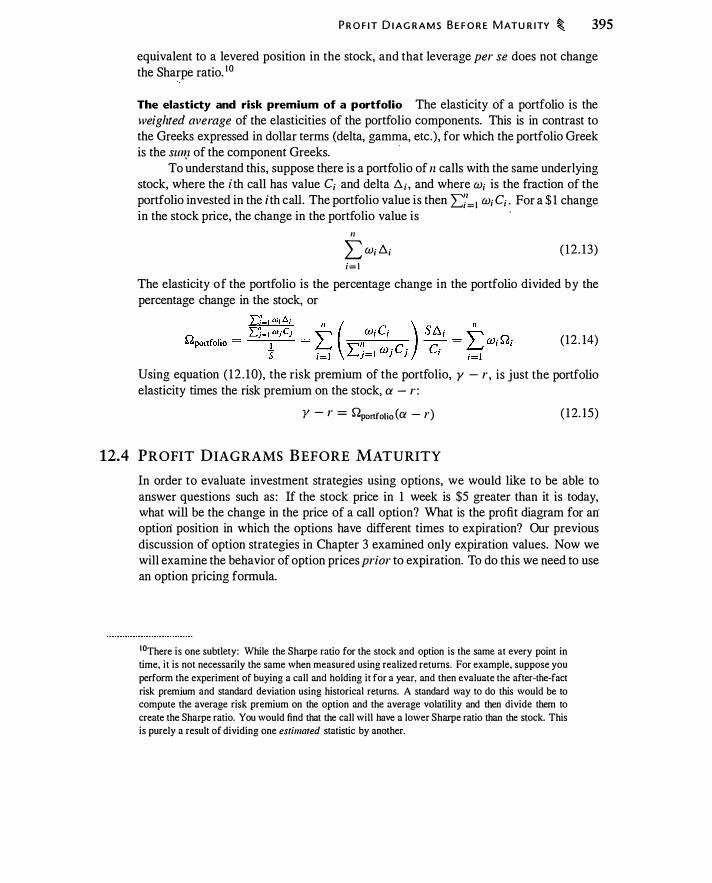
P R O F IT D I AG R A M S B E F O R E M ATU R ITY � 395

equivalent to a levered position in the stock, and that leverage per se does not change the Sharpe ratio. 1 0

The elasticty and risk premium of a portfolio The elasticity of a portfolio is the weighted average of the elasticities of the portfolio components. This is in contrast to the Greeks expressed in dollar terms (delta, gamma, etc.) , for which the portfolio Greek is the sw�z of the component Greeks.

-

To understand this, suppose there is a portfolio of n calls with the same underlying stock, where the i th call has value C; and delta D. ; , and where w; is the fraction of the portfolio invested in the i th call. The portfolio value is then I:;'= I w; C; . For a $ 1 change in the stock price, the change in the portfolio value is ·

II � W; b.; i=l

( 12. 13)

The elasticity of the portfolio is the percentage change in the portfolio divided by the percentage change in the stock, or

( 12 . 14)

Using equation ( 1 2 . 1 0), the risk premium of the portfolio, y - r , is just the portfolio elasticity times the risk premium on the stock, a - r :

Y - r = S1portfolio (a - r) ( 1 2. 15)

12.4 PROFIT DIAGRAMS BEFORE MATURITY

In order to evaluate investment strategies using options, we would like to be able to answer questions such as : If the stock price in 1 week is $5 greater than it is today, what will be the change in the price of a call option? What is the profit diagram for an option position in which the options have different times to expiration? Our previous discussion of option strategies in Chapter 3 examined only expiration values. Now we will examine the behavior of option prices prior to expiration. To do this we need to use an option pricing formula.

1 0There is one subtlety: While the Sharpe ratio for the stock and option is the same at every point in

time, it is not necessarily the same when measured using realized returns. For example, suppose you

perform the experiment of buying a call and holding it for a year, and then evaluate the after-the-fact

risk premium and standard deviation using historical returns. A standard way to do this would be to compute the average risk premium on the option and the average volatility and then divide them to

create the Sharpe ratio. You would find that the call will have a lower Sharpe ratio than the stock. This

is purely a result of dividing one estimated statistic by another.

396 � T H E B LA C K-S C H O LES F O R M U LA

Purchased Call Option

Consider the purchase of a call option. Just as with expiring options, we can ask what the value of the option is at a particular point in time and for a particular stock price. Table 1 2.3 shows the Black-Scholes value of a call option for five different stock prices at four different times to expiration. By varying the stock price for a given time to expiration, keeping everything else the same, we are able to graph the value of the call.

Figure 1 2. 1 2 plots Black-Scholes call option prices for stock prices ranging from $20 to $60, including the values in Table 1 2.3 . Notice that the value of the option prior to expiration is a smoothed version of the value of the option at expiration.

The payoff diagram depicted in Figure 1 2 . 1 2 does not show us how the value of the option compares to its original cost. In order to do that, we can subtract the cost of the option, plus interest. 1 1

In order to determine profitability, we need to answer two questions that were unnecessary for the payoff diagram: What is the initial cost of the option position, and what is- the holding period? To compute the profit, we take the value of the position and subtract the cost of the position, including interest.

Example 1 2.9 The 1-year option in Table 1 2.3 costs $6.285 at a stock price of $40. If after I day the stock price is still $40, the value of the option will have fallen to $6.274, and the 1 -day holding period profit is $6.274 - $6.285 x e 0-081365 = -$0.0 12 . This loss reflects the theta of the option. If the stock price were to increase to $42, the option premium would increase to $7.655 , and the 1 -day holding period profit would be $7.655 - $6.285 x e0·081365 = $ 1 .369.

Stock Price ($)

36

38

40

42

44

Value of 40-strike cal l option at d ifferent stock prices and times to expiration. Assumes r = 8%, u = 30%,

" 8 = 0.

Time to Expiration 12 Montbs 6 Montbs 3 Montbs 0 (Expiration)

3 .90 2.08 1 .00 0

5 .02 3 .02 1 .75 0

6.28 4. 1 6 2.78 0

7.67 5 .47 4.07 2

9. 15 6.95 5.58 4

1 1 As we discussed in Chapter 2, this is like assuming the option is financed by borrowing.

P R O F I T D I AG RA M S B E F O R E MATU R ITY � 397

Option Premium ($)

Payoff diagram for a cal l option for different stock prices and times to expiration. Assumes K = $40, r = 8%, 8 = 0, and a = 30%.

25

20

15

10

5

-1- 12 months -+- 6 months ..... 3 months -e- Expiration

o ��������HH�--�----L_--� __ _L_ 20 25 30 35 40 45 50 55 60

Stock Price ($}

After 6 months, the holding period profit at a price of $40 would be $4. 155 -$6.285 x e o.osxo.s = -$2.386. Even if the stock price had risen to $42, the holding period return would still be a negative -$ 1 .068. These profit calculations are illustrated in Figure 1 2. 1 3 . �

•

The option premium graphs in Figures 1 2. 1 2 and 1 2. 1 3 can help us understand the behavior of delta and gamma discussed in Section 1 2.3 . In all cases the slope of the call option graph is positive. This corresponds to a positive delta. In addition, the slope becomes greater as the stock price increases. Delta increasing with the stock price corresponds to a positive gamma. The fact that gamma is always positive implies that the graphs will be curved like the cross section of a bowl, i.e., the option price is convex. A positive gamma implies convex curvature. A negative gamma implies the opposite (concave) curvature.

Calendar Spreads

We saw in Chapter 3 that there are a number of option spreads that permit you to speculate on the volatility of a stock, including straddle, strangle, and butterfly spreads. These

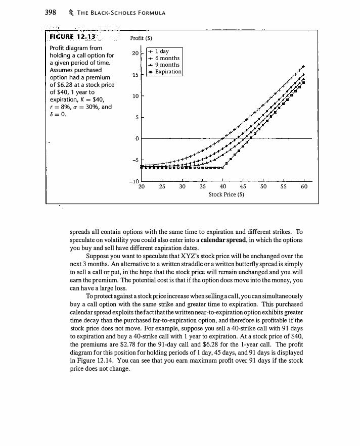
398 � T H E B LA C K-S C H O LES F O R M U LA

Profit diagram from holding a cal l option for a given period of time. Assumes purchased option had a premium of $6.28 at a stock price of $40, 1 year to expiration, K = $40, r = 8%, CY = 30%, and 8 = 0.

Profit ($)

20

15

10

5

-5

-+- 1 day -+- 6 months .... 9 months ... Expiration

-1QL---�----�--��--�----�--�----�----L-

20 25 30 35 40 45 so 55 60

Stock Price ($)

spreads all contain options with the same time to expiration and different strikes. To speculate on volatility you could also enter into a calendar spread, in which the options you buy and sell have different expiration dates.

Suppose you want to speculate that XYZ's stock price will be unchanged over the next 3 months. An alternative to a written straddle or a written butterfly spread is simply to sell a call or put, in.the hope that the stock price will remain unchanged and you will earn the premium. The potential cost is that if the option does move into the money, you can have a large loss.

To protect against a stock price increase when selling a call, you can simultaneously buy a call option with the same strike and greater time to expiration. This purchased calendar spread exploits the fact that the written near-to-expiration option exhibits greater time decay than the purchased far-to-expiration option, and therefore is profitable if the stock price does not move. For example, suppose you sell a 40-strike call with 9 1 days to expiration and buy a 40-strike call with 1 year to expiration. At a stock price of $40, the premiums are $2.78 for the 9 1-day call and $6.28 for the 1 -year call . The profit diagram for this position for holding periods of 1 day, 45 days, and 9 1 days is displayed in Figure 12 . 14. You can see that you earn maximum profit over 9 1 days if the stock price does not change.

Profit diagram for a calendar spread. Assumes we sel l a 9 1 -day 40-strike call with premium of $2.78, and buy a 365-day 40-strike cal l with premium of $6 .28. Assumes S = $40, rr = 30%, r = 8o/o, and 8 = 0.

Profit ($)

2

1

-1

-2

-3

P R O F I T D I AG R A M S B E F O R E M ATU R ITY � 399

-+- 1 day -+- 45 days ..._ 91 days

-4�--�----�----L---�----�----L---�----�-20 25 30 35 40 45 so 55 60

Stock Price ($)

We can understand the behavior of profit for this position by considering the theta of the two options. Figure 1 2.6 shows that theta is more negative for the 9 1-day call ( -0.0 1 73) than for the 1 -year call ( -0.0 104). Thus, if the stock price does not change over the course of 1 day, the position will make money since the written option loses more value than the purchased option. Over 9 1 days, the written 9 1 -day option will lose its full _value (its price declines from $2.78 to 0), while the 1 -year option will lose only

·

about $ 1 (its price declines from $6.28 to $5.28) if the stock price does not change. The difference in the rates of time decay generates profit of approximately $ 1 . 78 .

The profit diagram also illustrates that at a stock price of $40, delta for the position is initially positive. Over 1 day, the maximum profit occurs if the stock price rises by a small amount. This reflects the fact that the delta of the written 9 1-day call is 0.5825 and that of the purchased 1 -year call is 0.66 15 , for a net positive delta of 0.0790. With the 9 1-day holding period, the portion of the graph below 40 reflects the purchased 1 -year option, which becomes increasingly unprofitable as the stock price falls. Above 40, the gain on the purchased 1 -year option is offset by the loss on the expiring 9 1 -day call. Since it is expiring, the delta of the 9 1-day call is - 1 for stock prices above 40, which results in the graph turning back down to a negative slope above 40. As the stock price continues to increase, however, the delta of the purchased 1 -year call increases toward 1 , so the slope of the net position approaches zero.

400 � TH E B LA C K-S C H O LES F O R M U LA

12.5 IMPLIED VOLATILITY

Volatility is unobservable, and Figure 1 2.4 shows that option prices, particularly for near-the-money options, can be quite sensitive to volatility. Thus, choosing a volatility to use in pricing an option is difficult but also quite important. 1 2

One approach to obtaining a volatility is to use the history of returns to compute historical volatility (see Section 1 1 .4). A problem with historical volatility is that history is not a reliable guide to the future: Markets have quiet and turbulent periods and predictable events such as Federal Reserve Board Open Market Committee meetings can create periods of greater than normal uncertainty. There are sophisticated statistical models designed to improve upon simple volatility estimates, but no matter what you do, you cannot count on history to provide you with a reliable estimate of future volatility.

In many cases we can observe option prices for an asset. We can then invert the question: Instead of asking what volatility we should use to price an option, we can compute an option's implied volatility, which is the volatility that would explain the observed option price. Assuming that we observe the stock price S, strike price K, interest rate r , dividend yield 8, and time to expiration T, the implied call volatility i s the u that solves

Market option price = C(S, K, u , r, T, 8) ( 1 2. 16)

By definition, if we use implied volatility to price an option, we obtain the market price of the option. Thus, we cannot use implied volatility to l:).Ssess whether an option price is correct, but implied volatility does tell us the market's assessment of volatility.

Computing Implied Volatility

Computing an implied volatility requires that we ( 1 ) observe a market price for an option and (2) have an option pricing model with which to infer volatility. Equation ( 1 2. 16) cannot be solved directly for the implied volatility, u , so it is necessary to use an iterative procedure to solve the equation. Any pricing model can be used to calculate an implied volatility, but Black-Scholes implied volatilities are frequently used as benchmarks.

Example 1 2. 1 0 Suppose we observe a 45-strike 6-month European call option with a premium of $8 .07. The stock price is $50, the interest rate is 8%, and the dividend yield is zero. We can compute the option price as

$8.07 = BSCall(50, 45 , u, 0.08, 0.5, 0) .

1 10f the five other inputs to the Black-Scholes formula, we also cannot observe dividends. Over short

horizons, however, dividends are typically stable, so past dividends can be used to forecast future

dividends.

I M P L I E D VO LATI L I TY � 401

By trial and error (or by using a tool such as Excel's Goalseek), we find that setting a = 28.7% gives us a call price of $8.07 . 1 3 �

Table 12.4 lists ask prices of calls and puts on the S&P 500 index, along with implied volatilities computed using the Black-Scholes formula. These S&P options are European style, so the Black-Scholes model is appropriate. Notice that, although the implied volatilities in the table are not all equal, they are all in a range between 13% and 16%. We could describe the general level of S&P option prices by saying that the options are trading at about a 15% volatility level. There are typically numerous options on a given asset; implied volatility can be used to succinctly describe �the general level of option prices for a given underlying asset.

There is one clear pattern in the implied volatilities in Table 12.4. For a given expiration month, volatilities decline as the strike price increases. This occurs with both the calls and puts . For example, the volatility for the November calls declines from 16.3% to 1 2.84% as the strike rises from 1 1 00 to 1 1 50. The decline is evident but smaller for the later expiration months. This systematic change in implied volatility across strike

-- · . . .. -"' . · .• :� TABLE 1 2 .4�'

Strike

($) Expiration

1 1 00 1 1120/2004

1 125 1 1120/2004

1 150 1 1/20/2004

1 100 12/1 8/2004

1 125 1 2/1 8/2004

1 150 1 2/1 8/2004

1 100 1122/2005

1 1 25 1122/2005

1 150 1122/2005

Implied volatil ities for S&P 500 options, 1 0/28/2004. Option prices (ask) from www.cboe.com; assumes 5 = $ 1 1 27.44, 8 = 1 .85%, r = 2%.

Call Price hnplied Put Price hnplied

($) Volatility ($) Volatility

34.80 0. 1 630 6.80 0. 1575

17 . 10 0. 1434 14.70 0. 1447

5.80 0 . 1 284 29.20 0. 1389

41 .70 0. 1 559 13 .80 0. 1539

24.50 0. 1 396 22.50 0. 1436

13 .00 0. 1 336 35 .50 0. 1 35 1

49. 10 0. 1567 20.40 0. 1 5 1 8

33 .00 0. 1 463 29.40 0. 1427

20.00 0. 1363 41 .50 0. 1 337

1 3 An implied volatility function is available with the spreadsheets accompanying this book.

402 � T H E B LAC K-S C H O LES FO R M U LA

prices occurs generally for different underlying assets and is called volatility skew. 14 When you graph implied volatility against the strike price, the resulting line can take different shapes, often described as "smiles," "frowns," and "smirks." Explaining these patterns and modifying pricing models to account for them is a challenge for option pricing theory. We will discuss this important issue further in Chapter 23 .

When examining implied volatilities, it is helpful to keep put-call parity in mind. If options are European, then puts and calls with the same strike and time to expiration must have the same implied volatility. This is true because prices of European puts and calls must satisfy the parity relationship or else there is an arbitrage opportunity. Thus, skew is not related to whether an option is a put or a call, but rather to differences in the strike price and time to expiration. Although call and put volatilities are not exactly equal in Table 1 2.4, they are close enough that parity arbitrage would not be profitable after transaction costs are taken into account. For example, for the in-the-money options in Table 12 .4, bid-ask spreads are as wide as $2, a difference that can account for more than <l: percentage point of implied volatility on one option alone.

Using Implied Volatility

Implied volatility is important for a number of reasons. First, if you need to price an option for which you cannot observe a market price, you can use implied volatility to generate a price consistent with the prices of traded options. Market-makers, for example, will price options consistently with prices of similar options. Second, as we previously discussed, implied volatility -is often used as a quick way to describe the level of option prices on a given underlying asset. Option prices are sometimes quoted in terms of volatility, rather than as a dollar price. Third, volatility skew provides a measure of how well option pricing models work. Because volatility is unobservable, a standard approach to testing the validity of the Black-Scholes model is to see whether, for a given underlying asset, implied volatilities are the same at all strike prices. The existence of volatility skew suggests that the Black-Scholes model and assumptions are not a perfect description of the world. We will discuss alternative pricing models in Chapter 23.

To better understand the importance of implied volatility, recognize that informa­tion about future volatility is uniquely provided by options markets. You can think of option markets as providing information about volatility that is not available elsewhere. In fact, there is now an exchange-traded futures contracts based on an index of implied volatility for the S&P 500. Just as stock markets provide information about stock prices and permit trading stocks, option markets provide information about volatility, and, in effect, permit the trading of volatility. Viewed from this perspective, we should expect information about volatility to be one of the most important things we can learn from option prices. We will discuss volatility in more depth in Chapter 23.

14The Black-Scholes formula is derived assuming that volatility is constant across strikes. Thus,

it is internal ly inconsistent to use the Black-Scholes model to track changes in implied volatility.

Nevertheless, it is a widely used benchmark.

P E R P ET U A L AM E R I CA N O PT I O N S � 403

12.6 PERPETUAL AMERICAN OPTIONS

The Black-Scholes for:nula prices options that are only exercised at expiration. In this section we present formulas, based on Merton ( 1 973b), for the prices of calls and puts that never expire. We will call such options perpetual options. They are also known as expirationless options.

American options are harder to price than European options because it is difficult to characterize the optimal exercise strategy. Using the binomial model, we saw in Section 1 1 . 1 that for a finitely lived call option on a dividend-paying stock, the stock price at which it is optimal to exercise the option declines as the option approaches expiration. It is this changing optimal exercise price that makes it hard to derive a v�luation formula.

With perpetual American options it is possible to derive a valuation formula be­cause such an option always has the same time to expiration: infinity. S ince time to expiration is constant, the option exercise problem will look the same today, tomorrow, and forever. Thus, the price at which it is optimal to exercise the option is constant. The optimal exercise strategy entails picking the right exercise barrier and exercising the option the first time the stock price reaches that barrier.

Barrier Present Values

As a prelude to valuing a perpetual option, consider computing the present value of $ 1 payable when the stock price reaches a level, H . We call H the barrier level and call the value today of $ 1 paid when the stock price reaches H the "barrier present value." It turns out there is a simple formula for this, which differs depending upon whether H is above or below the current stock value, S.

If H is above S (i.e., S has to rise to reach H), the value today of $ 1 received when S reaches H -the barrier present value-is ( s ) h ) yalue of $ 1 received when S first reaches H from below =

H

where 1 r - 8 /z l = - - -- + 2 u 2 (r - 8 1 ) 2 2r -- - - + ­u 2 2 u2

( 1 2. 1 7)

If H is below S (i .e . , S has to fall to reach H), the value of $1 received when S reaches H is ( s ) 112

Value of $ 1 received when S first reaches H from above = H

where 1 r - 8 !z? = - - -- -- 2 u 2

(r - 8 1 ) 2 2r -- - - + -u 2 2 u2

( 1 2. 1 8)

404 � TH E B LA C K-S C H O LES F O R M U LA

Perpetual Calls

Suppose we have a perpetual American call with strike K. If we decide to exercise the option whenever S reaches the barrier H, then at exercise we receive H - K. From equation ( 12 . 17) , the value of receiving H - K when S reaches H is ( s ) " '

(H - K) H

In order to finish computing the value of the call we need to specify H, the price at which the call should be exercised. We simply need to pick a value for H that makes the value of lhe call as great as possible. If we make H too small, then we prematurely throw away option value (i.e., protection against a subsequent price decline). If we make H too large, then we forgo dividends for too long while waiting to exercise. It is possible to show that the exercise level H* that maximizes the value of the call is 1 5

H · - K --"' ( /z l ) lz l - 1

Since /z 1 > 1 , we have H* > K. Making this substitution, the value of the perpetual call is

K (lz 1 - 1 s ) " ' Price of perpetual call = -- -- -

/z 1 - l h 1 K ( 1 2. 19)

If 8 = 0, then H* = oo; i .e. , it is never optimal to exercise a call option on a nondividend­paying stock.

Perpetual Puts

For a perpetual put, using equation ( 1 2. 1 8) , the value if we exercise when S = H is given by

where

( s ) "' (K - H)

H

1 r - 8 h? = - - -- -

- 2 a2 (r - 8 1 ) 2 2r -- - - + ­a2 2 a2

15This is accomplished by differentiating the expression with respect to H, setting the derivative equal to zero, and solving for H .

FU RTH E R R EA D I N G � 405

Again selecting the exercise level H* to maximize the value of the put, we get

H* = K � /z2 - 1

which implies that the price of the perpetual put is

K (h" - 1 S )"2 Price of perpetual put = --· ---- -

1 - lz2 h2 K

------.----��-. :.._ - --�: .::s.l.:· � j ,-'C_' : -�_- ,_ -. _ -

CHAPTER S UMMARY

( 1 2.20)

Under certain assumptions, the Black-Scholes formula provides an exact formula­approximated by the binomial formula-for pricing European options. The inputs to the Black-Scholes formula are the same as for the binomial formula: the stock price, strike price, volatility, interest rate, time to expiration, and dividend yield. As with the binomial formula, the Black-Scholes formula accommodates different underlying assets by changing the dividend yield (see Table 10 . 1 for a summary).

Option Greeks measure the change in the option price (or other option charac­teristic) for a change in an option input. Delta, gamma, vega, theta, rho, and psi are widely used in practice to assess the risk of an option position. The option elasticity is the percentage change in the option's price for a 1 % change in the stock price. The volatility and beta of an option are the volatility and beta of the stock times the option elasticity. Thus, an option and the underlying stock have the same Sharpe ratio.

Of the inputs to the Black-Scholes formula, volatility is hardest to estimate. In practice it is common to use the formula in backward fashion to infer the market's estimate of volatility from the option price. This implied volatility is computed by finding the volatility for which the formula matches observed market prices for options. In theory, all options of a given maturity should have the same implied volatility. In practice, they · do not: a phenomenon known as volatility skew.

Although there is no simple formula for valuing a finitely lived American option, there are simple formulas in the special case of perpetual puts and calls.

FURTHER READING

Chapter 13 will explore in more detail the market-maker's perspective on options, in­cluding how a market-maker uses delta to hedge option positions and the circumstances under which market-makers earn profits or make losses. Chapter 14 extends the discus­sion in this chapter to include exotic options .

In Chapters 15 , 16, and 1 7, we will use option pricing to explore applications of option pricing, including the creation of structured products, issues in compensation options, capital structure, tax management with options, and real options.

406 � T H E B LA C K-S C H O LES F O R M U LA

Chapters 1 8 through 2 1 delve more into the mathematical underpinnings of the Black-Scholes model. The barrier present value calculations will be discussed again in Chapter 22. We will discuss volatility in much more detail in Chapter 23 .

The classic early papers on option pricing are Black and Scholes ( 1 973) and Merton ( 1 973b ). The details of how the binomial model converges to the Black-Scholes model are in Cox et al. ( 1 979). The perpetual put formula is derived in Merton ( 1 973b ). The link between the perpetual call and put formulas is discussed by McDonald and Siegel ( 1 986).

PROBLEMS

In answering many of these problems you can use the functions BSCall, BSPut, CallPer­petual, and PutPe1petual and the accompanying functions for the Greeks (see the spread­sheets on the CD-ROM accompanying this book) .

12.1. Use a spreadsheet to verify the option prices in Examples 1 2. 1 and 1 2.2.

12.2. Using the BinomCall and BinomPut functions, compute the binomial approxi­mations for the options in Examples 1 2. 1 and 1 2.2. Be sure to compute prices for n = 8, 9, 1 0, 1 1 , and 1 2. What do you observe about the behavior of the binomial approximation?

12.3. Let S = $ 1 00, K = $ 1 20, u = 30%, r = 0.08, and 8 = 0.

a. Compute the Black-Scholes call price for 1 year to maturity and for a variety of very long times to maturity. What happens to the option price as T -7 oo?

b. Set 8 = 0.00 1 . Repeat (a) . Now what happens to the option price? What accounts for the difference?

12.4. Let S = $ 1 20, K = $ 1 00, u = 30%, r = 0, and 8 = 0.08.

a. Compute the Black-Scholes call price for 1 year to maturity and for a variety of very long times to maturity. What happens to the price as T -7 oo?

b. Set r = 0.00 1 . Repeat (a) . Now what happens? What accounts for the difference?

12.5. The exchange rate is ¥95/€, the yen-denominated interest rate is 1 .5%, the euro-denominated interest rate is 3 .5%, and the exchange rate volatility is 10%.

a. What is the price of a 90-strike yen-denominated euro put with 6 months to expiration?

b. What is the price of a 1190-strike euro-denominated yen call with 6 months to expiration?

c. What is the link between your answer to (a) and your answer to (b), converted to yen?

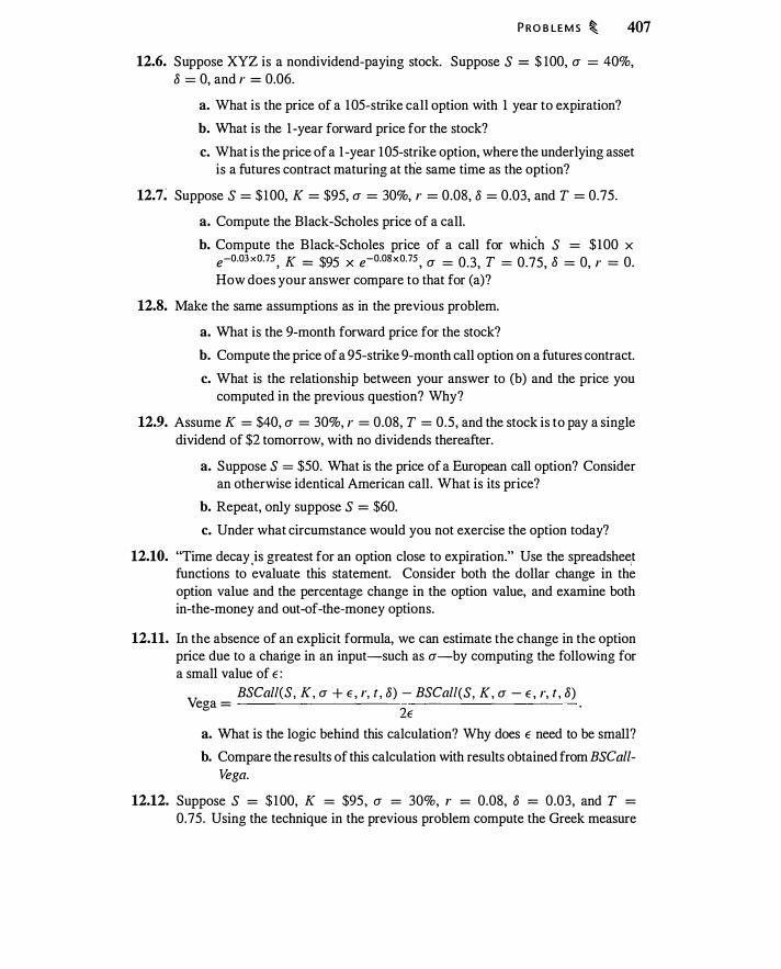
P RO B LE M S � 407

12.6. Suppose XYZ is a nondividend-paying stock. Suppose S = $ 100, a = 40%, 8 = 0, and r = 0.06.

a. What is the price of a 1 05-strike call option with 1 year to expiration?

b. What is the 1 -year forward price for the stock?

c. What is the price of a 1 -year 1 05-strike option, where the underlying asset is a futures contract maturing at the same time as the option?

12.7; Suppose S = $ 1 00, K = $95, a = 30%, r = 0.08, 8 = 0.03, and T = 0.75.

a. Compute the Black-Scholes price of a call.

b. Compute the Black-Scholes price of a call for which S = $100 x e-0.03 x0.75

, K = $95 X e-0.08 x0.75 , a = 0.3, T = 0.75, 8 = 0, r = 0. How does your answer compare to that for (a)?

12.8. Make the same assumptions as in the previous problem.

a. What is the 9-month forward price for the stock?

b. Compute the price of a 95-strike 9-month call option on a futures contract.

c. What is the relationship between your answer to (b) and the price you computed in the previous question? Why?

12.9. Assume K = $40, a = 30%, r = 0.08, T = 0.5, and the stock is to pay a single dividend of $2 tomorrow, with no dividends thereafter.

a. Suppose S = $50. What is the price of a European call option? Consider an otherwise identical American call. What is its price?

b. Repeat, only suppose S = $60.

c. Under what circumstance would you not exercise the option today?

12.10. "Time decay _is greatest for an option close to expiration." Use the spreadshee,t functions to evaluate this statement. Consider both the dollar change in the option value and the percentage change in the option value, and examine both in-the-money and out-of-the-money options.

12.11. In the absence of an explicit formula, we can estimate the change in the option price due to a change in an input-such as a-by computing the following for a small value of E :

BSCall(S, K, a + E , r, t , 8) - BSCall(S, K, a - E , r, t , 8) Vega = .

2E a. What is the logic behind this calculation? Why does E need to be small?

b. Compare the results of this calculation with results obtained from BSCall­Vega.

12.12. Suppose S = $ 1 00, K = $95 , a = 30%, r = 0.08, 8 = 0.03, and T = 0.75. Using the technique in the previous problem compute the Greek measure

408 � T H E B LA C K-S C H O LES F O R M U LA

corresponding to a change in the dividend yield. What is the predicted effect of a change of 1 percentage point in the dividend yield?

12.13. Consider a bull spread where you buy a 40-strike call and sell a 45-strike call. Suppose S = $40, CJ = 0.30, r = 0.08, 8 = 0, and T = 0.5 . Draw a graph with stock prices ranging from $20 to $60 depicting the profit on the bull spread after 1 day, 3 months, and 6 months.

12.14. Consider a bull spread where you buy a 40-strike call and sell a 45-strike call . Suppose CJ = 0.30, r = 0.08, 8 = 0, and T = 0.5.

a. Suppose S = $40. What are delta, gamma, vega, theta, and rho?

b. Suppose S = $45 . What are delta, gamma, vega, theta, and rho?

c. Are any of your answers to (a) and (b) different? If so, why?

12.15. Consider a bull spread where you buy a 40-strike put and sell a 45-strike put. Suppose CJ = 0.30, r = 0.08, 8 = 0, and T = 0.5.

a. Suppose S = $40. What are delta, gamma, vega, theta, and rho?

b. Suppose S = $45 . What are delta, gamma, vega, theta, and rho?

c. Are any of your answers to (a) and (b) different? If so, why?

d. Are any of your answers different in this problem from those in Problem 12 . 14? If so, why?

12.16. Assume r = 8%, CJ = 30%, 8 = 0. In doing the following calculations, use a stock price range of $60-$ 140, stock price increments of $5, and two different times to expiration: 1 year and 1 day. Consider purchasing a 100-strike straddle, i .e. , buying one 100-strike put and one 100-strike call.

a. Compute delta, vega, theta, and rho of the call and put separately, for the different stock prices and times to expiration.

b. Compute delt�, vega, theta, and rho of the purchased straddle (do this by adding the Greeks of the individual options) . As best you can, explain intuitively the signs of the straddle Greeks.

c. Graph delta vega, theta, and rho of the straddle with 1 year to expiration as a function of the stock price. In each case explain why the graph looks as it does.

12.17. Assume r = 8%, CJ = 30%, 8 = 0. Using ! -year-to-expiration European options, construct a position where you sell two 80-strike puts, buy one 95-strike put, buy one 1 05-strike call, and sell two 120-strike calls. For a range of stock prices from $60 to $ 140, compute delta, vega, theta, and rho of this position. As best you can, explain intuitively the signs of the Greeks.

12.18. Consider a perpetual call option with S = $50, K = $60, r = 0.06, CJ = 0 .40, and 8 = 0.03 .

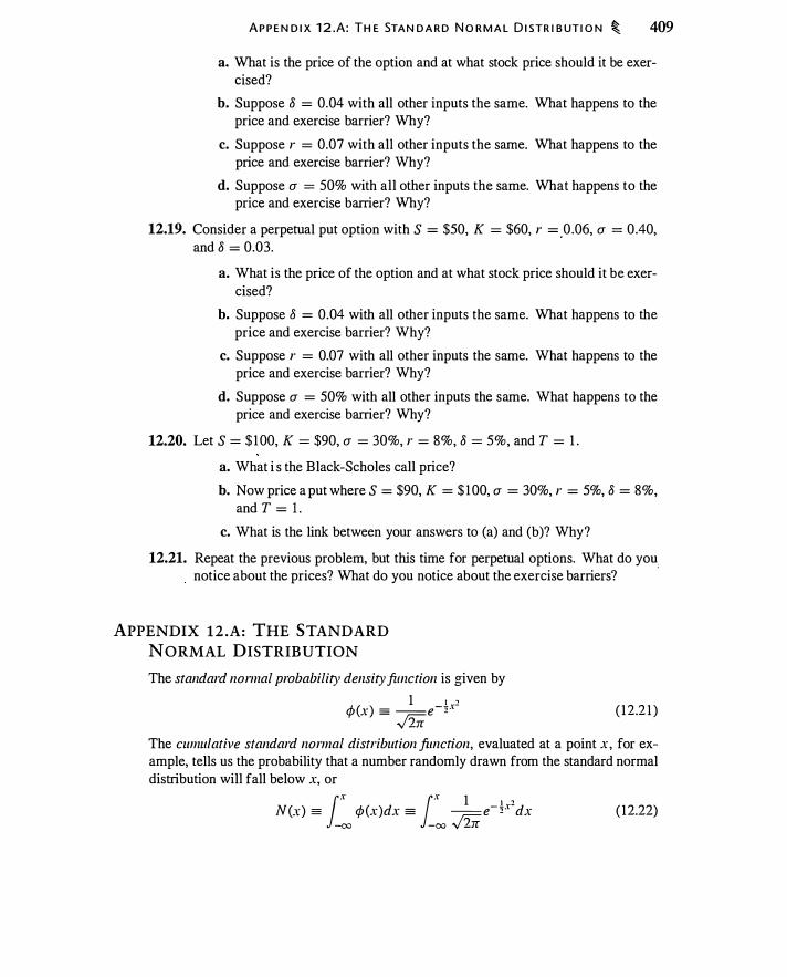
A P P E N D I X 1 2 .A: TH E STAN D A R D N O R M A L D I STR I B UT I O N � 409

a. What is the price of the option and at what stock price should it be exer­cised?

b. Suppose 8 = 0.04 with all other inputs the same. What happens to the price and exercise barrier? Why?

c. Suppose r = 0.07 with all other inputs the same. What happens to the price and exercise barrier? Why?

d. Suppose a = 50% with all other inputs the same. What happens to the price and exercise barrier? Why?

12.19. Consider a perpetual put option with S = $50, K = $60, r = .0.06, a = 0.40, and 8 = 0.03.

a. What is the price of the option and at what stock price should it be exer­cised?

b. Suppose 8 = 0.04 with all other inputs the same. What happens to the price and exercise barrier? Why?

c. Suppose r = 0.07 with all other inputs the same. What happens to the price and exercise barrier? Why?

d. Suppose a = 50% with all other inputs the same. What happens to the price and exercise barrier? Why?

12.20. Let S = $ 1 00, K = $90, a = 30%, r = 8%, 8 = 5%, and T = 1 .

a. What i s the Black-Scholes call price?

b. Now price a put where S = $90, K = $ 1 00, a = 30%, r = 5%, 8 = 8%, and T = I .

c. What is the link between your answers to (a) and (b)? Why?

12.21. Repeat the previous problem, but this time for perpetual options. What do you notice about the prices? What do you notice about the exercise barriers?

·

APPENDIX 12 .A: THE STANDARD NORMAL DISTRIBUTION

The standard normal probability density function is given by

1 I .2 ¢(x) = --e->-'

.j2ii ( 1 2.2 1 )

The cumulative standard normal distribution fimction, evaluated at a point x, for ex­ample, tells us the probability that a number randomly drawn from the standard normal distribution will fall below x, or

N(x) = ¢(x)dx = -- e-!x' dx lx �x 1

-CXJ -(X) .j2ii ( 12.22)

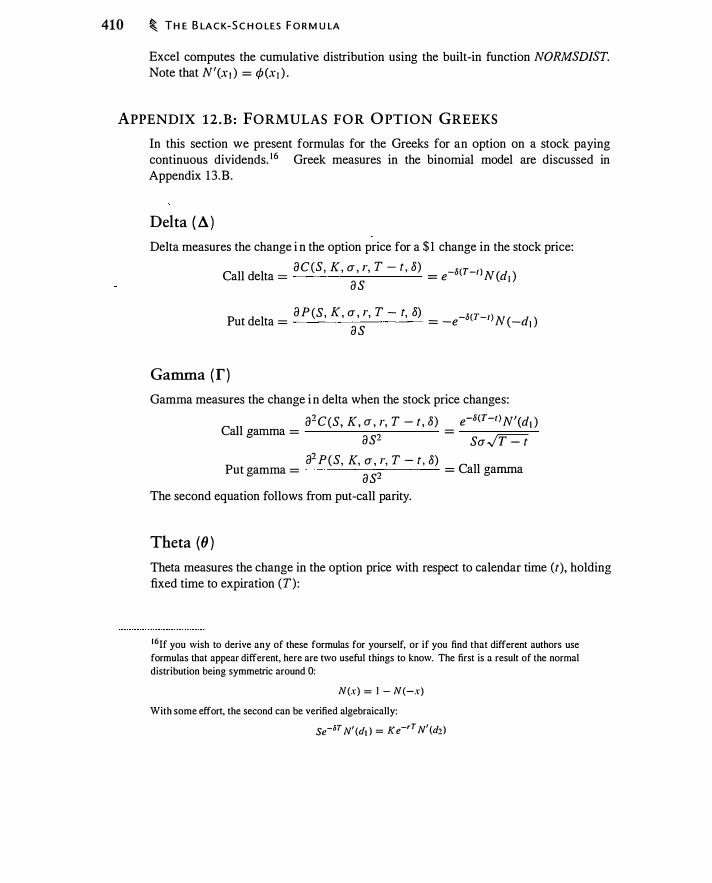
410 � T H E B LA C K-S C H O LES F O R M U LA

Excel computes the cumulative distribution using the built-in function NORMSDIST. Note that N'(x1 ) = ¢ (xJ ) .

APPENDIX 1 2 . B : FORMULAS FOR OPTION GREEKS

In this section we present formulas for the Greeks for an option on a stock paying continuous dividends. 1 6 Greek measures in the binomial model are discussed in Appendix l3 .B.

Delta ( A )

Delta measures the change i n the option price for a $ 1 change in the stock price:

Call delta = aC(S, K, u , r, T - t , 8)

= e-S<T-r l N (d1 ) a s

Put delta = a P (S, K , u ' r, T - t, 8)

= -e-s<T-r) N ( -di ) a s

Gamma ( f ) Gamma measures the change i n delta when the stock price changes:

a2C(S K u r T - t 8) e-S(T-r) N'(d ) Call cramma = ' ' ' ' ' = I

'=' as2 su,JT=f a2 P (S, K, u , r, T - t , 8)

Put gamma = ? = Call gamma a s-

The second equation follows from put-call parity.

Theta (fJ ) Theta measures the change in the option price with respect to calendar time (t), holding fixed time to expiration (T) :

1 6If you wish to derive any of these formulas for yourself, or if you find that different authors use

formulas that appear different, here are two useful things to know. The first is a result of the normal

distribution being symmetric around 0:

N(x) = I - N (-x)

With some effort, the second can be verified algebraically:

Se-1iT N' (d! ) = K e-rT N' (d1 )

A P P E N D I X 1 2 . B : F O R M U LAS F O R O PTI O N G R E E KS � 411

aces, K, a, r , T - t , o) Call theta = --------­

a t

a P eS, K, a , r, T - t , o) Put theta = ----.,-----­

at = Call theta + r K e-r(T -I ) - ose-o(T -I )

If time to expiration is measured in years, theta will be the annualized change in the option value. To obtain a per-day theta, divide by 365.

Vega

Vega measures the change in the option price when volatility changes. Some writers also use the terms lambda or kappa to refer to this measure:

C II aces, K , a , r, T - t , o)

S -o(T-t )N'ed ) �T a vega = = e 1 v 1 - t a a

a P es, K , a , r, T - t , o) Put vega = = Call vega

a a It is common to report vega as the change in the option price per percentage poillf change in the volatility. This requires dividing the vega formula above by 100.

Rho (p ) Rh o i s the partial derivative of the option price with respect to the interest rate:

Call rho = aces, K, a , r, T - t , o)

= eT - t)Ke-r<T-I ) Ned2) ar

P h aP (S, K, a , r, T - t , o)

(T )K -r<T-t >N ( d ) ut r o = = - - t e - , ar -

These expressions for rho assume a change in r of 1 .0. We are typically interested in evaluating the effect of a change of 0.0 1 ( 100 basis points) or 0.000 1 (1 basis point) . To report rho as a change per percentage point in the interest rate, divide this measure by 100. To interpret it as a change per basis point, divide by 10,000.

Psi ( 1fr ) Psi is the partial derivative of the option price with respect to the continuous dividend yield:

412 � T H E B LA C K-S C H O LES F O R M U LA

Call psi = a C (S, K, a ' r, T - t , o)

= -(T - t) Se-a<T-rJ N (di ) ao

Put psi = a P (S , K, a , r, T - t , 8)

= (T - t) Se-a <T-r J N (-di ) . ao

To interpret psi as a price change per percentage point change in the dividend yield, divide by 100.

Market-Making and Delta-Hedging

, A; Je"t " llnportant "' the Block -Schole' fonnnla is the Block-S;hole' technique for deriving the formula. In this chapter we explore the Black-Scholes technique by considering the market-maker perspective on options. What issues confront the market professionals who supply the options that customers want to buy? The insights we gain from studying this question apply not only to pricing call and put options but also to derivatives pricing and risk management in general.

The Black-Scholes approach to deriving the option pricing formula assumes that market-makers are profit-maximizers in a competitive market who want to hedge the risk of their option positions. As in Chapter 1 0, market -makers can hedge by taking a stock position that offsets the option's delta. Because option deltas change as the stock price changes, market-makers must continually review and modify their hedging decisions.

We will see that the costs of carrying a hedged option position can be expressed in terms of delta, gamma, and theta, option Greeks that were introduced in Chapter 1 2. On average, competitive market-makers should expect to break even by hedging. Under certain assumptions about the behavior of the stock price, the market -maker's break-even price is the Black-Scholes option price. Thus, as with any other good in a competitive market, the price of an option should equal the market-maker's cost of producing it.

13 .1 WHAT DO MARKET-MAKERS D O ?

A market-maker stands ready to sell to buyers and to buy from sellers . The owner of an appliance store, for example, is a market-maker. The store owner buys televisions at a low price (the wholesale price) and sells them at cost plus a markup (the retail price), earning the difference. The markup must at a minimum cover the cost of doing business-rent, salaries, utilities, and advertising-so that the retail price covers the cost of acquiring televisions plus all other costs of doing business. In the language-of securities markets, we would say that the appliance dealer has both a bid price and an ask price. The bid price is the price at which the dealer buys the television, also known as the wholesale price. The ask price is the price at which the dealer will sell the television, also known as the retail price.

An appliance seller does not select which models to sell based on personal pref­erence and does not expect to profit by speculating on the price of a television. Rather, the appliance dealer selects inventory based on expected customer demand and earns

413

414 � M A R K ET- M A K I N G A N D D E LTA-H E D G I N G

profit based on the markup. The store maintains an inventory, and the owner is able to satisfy customers who walk in and want to buy a television immediately. Market-makers supply immediacy, permitting customers to trade whenever they wish.

Proprietary trading, which is conceptually distinct from market-making, is trad­ing to express an investment strategy. Customers and proprietary traders typically expect their positions to be profitable depending upon whether the market goes up or down. In contrast, market-makers profit by buying at the bid and selling at the ask. The position of a market-maker is the result of whatever order flow arrives from customers .

A difference between appliance sellers and financial market-makers is that an appliance store must possess a physical television in order to sell one. A financial market­maker, by contrast, can supply an asset by short-selling, thereby generating inventory as needed.

In some cases market-makers may trade as customers, but then the market-maker is paying the bid-ask spread and therefore not serving as a market-maker.

13 .2 MARKET-MAKER RISK

Without hedging, an active market-maker will have an arbitrary position generated by fulfilling customer orders. An arbitrary portfolio has uncontrolled risk. An adverse price move has the potential to bankrupt the market-maker. Consequently, market-makers attempt to hedge the risk of their positions.

Market-makers can control risk by delta-hedging. As in Chapter 10, the market­maker computes the option delta and-takes an offsetting position in shares. We say that such a position is delta-hedged. In general a delta-hedged position is not a zero­value position: The cost of the shares required to hedge is not the same as the cost of the options . Because of the cost difference, the market-maker must invest capital to maintain a delta-hedged position.

A key idea in derivatives is that such a hedged position should earn the risk-free rate: You have money tied up so you should earn a return on it, and you have no risk so you should earn the risk-free rate. We used this argument explicitly in our discussion of forward pricing in Chapter 5, and implicitly in binomial pricing in Chapter 10. The notion that a hedged position earns the risk-free rate is a linchpin of almost all derivative pricing models. It was the fundamental idea exploited by Black and Scholes in their derivation of the option pricing model.

With the help of a simple numerical example, we can understand not only the intuition of the Black-Scholes model, but the mathematics as well. Delta-hedging is key to pricing because it is the technique for offsetting the risk of an option position. If we think of option producers as selling options at cost, then delta-hedging provides us with an understanding of what the cost of the option is when it is replicated. Delta-hedging is thus both a technique widely used in practice, and a key to understanding option pricing.

Option Risk in the Absence of Hedging

If a customer wishes to buy a 9 1 -day call option, the market-maker fills this order by selling a call option. To be specific, suppose that S = $40, K = $40, u = 0.30,

M A R K ET- M A K E R R I S K � 415

r = 0.08 (continuously compounded), and 8 = 0. We will let T denote the expiration time of the option and t the present, so time to expiration is T - t. Let T - t = 9 1 /365. The price, delta, gamma, and theta for this call are listed in Table 1 3 . 1 .

Because the market-maker has written the option, the sign of the Greek measures for the position is opposite those of a purchased option. In particular, the written option is like shorting shares of stock (negative delta) and the option gains in value over time (positive theta). Because delta is negative, the risk for the market-maker who has written a call is that the stock price will rise.

Suppose that the market-maker does not hedge the written option and the stock price rises to $40.75. We can measure the profit of the market-maker by marking-to­market the position. Marking-to-market answers the question: If we liquidated the position today, what would be the gain or loss? In the case of an option price increase, the market-maker would need to buy the option back at a higher price than that at which it was sold, and therefore would lose money. At a stock price of $40.75, the call price would increase to $3.2352, so the market-maker profit on a per-share basis would be $2.7804 - $3.2352 = -$0.4548. 1

Figure 1 3 . 1 graphs the overnight profit of the unhedged written call option as a function qf the stock price, against the profit of the option at expiration. In computing overnight profit, we are varying the stock price holding fixed all other inputs to the Black­Scholes formula except for time to expiration, which decreases by 1 day. It is apparent from the graph that the risk for the market-maker is a rise in the stock price. Although it is not obvious from the graph, if the stock price does not change, the market-maker will profit because of time decay: It would be possible to liquidate the option position by buying options at a lower price the next day than the price at which they were sold originally.

·.··

.

Price and Greek information for a call option with S = $40, K = $40, u = 0. 30, r = 0.08 (continuously compounded), T - t = 91 /365, and 8 = 0.

Purchased Written

Call price 2.7804 -2.7804 Delta 0.5824 -0.5824

Gamma 0.0652 -0.0652

Theta -0.0 173 0.0 173

1 For simplicity, this calculation ignores the overnight interest that the market-maker can earn on the

proceeds from selling the option. In this case, interest per share is (exp(.OS/365) - 1) x $2.7804 =

$0.0006. Later examples will account for interest.

416 � M A R K ET- M A K I N G A N D D E LTA- H E D G I N G

Depiction of overnight and expiration profit from writing a cal l option on one share of stock, if the market-maker is unhedged.

Profit ($)

5

-5

-10

-15

-20

20 25 30 35 45

Stock Price {$)

Delta and Gamma as Measures of Exposure

-a- Expiration - After 1 day

so 55

Since delta tells us the price sensitivity of the option, it also measures the market-maker's exposure. The delta of the call at a stock price of $40 is 0.5824, which suggests that a $ 1 increase in the stock price should increase the value of the option by approximately $0.5824. A $0.75 increase in the stock price would therefore increase the option price by $0.75 x 0.5824 = $0.4368. However, the actual increase in the option's value is $0.4548, greater by $0.0 1 80.

This discrepancy occurs because delta varies with the stock price: As the stock price increases and the option moves more into the money, delta also increases. At a stock price of $40.75, delta is 0.6301 . Thus, the delta at $40 will understate the actual change in the value of the option due to a price increase.

Similarly, delta will overstate the decline in the value of the option due to a stock price decrease. If the stock price had fallen $0.75 to $39.25, the option price would have declined to $2.3622, which would result in a gain of $0.4 1 82 to the market-maker. Using delta, we would have predicted a price decline of -$0.75 x 0.5824 = -$0.4368, which is greater than the actual decline. This occurs because the option delta decreases as the stock price declines. The delta at this new price is 0.5326,

Gamma measures the change in delta when the stock price changes. In the example above, the gamma of 0.0652 means that delta will change by approximately 0.0652 if

60

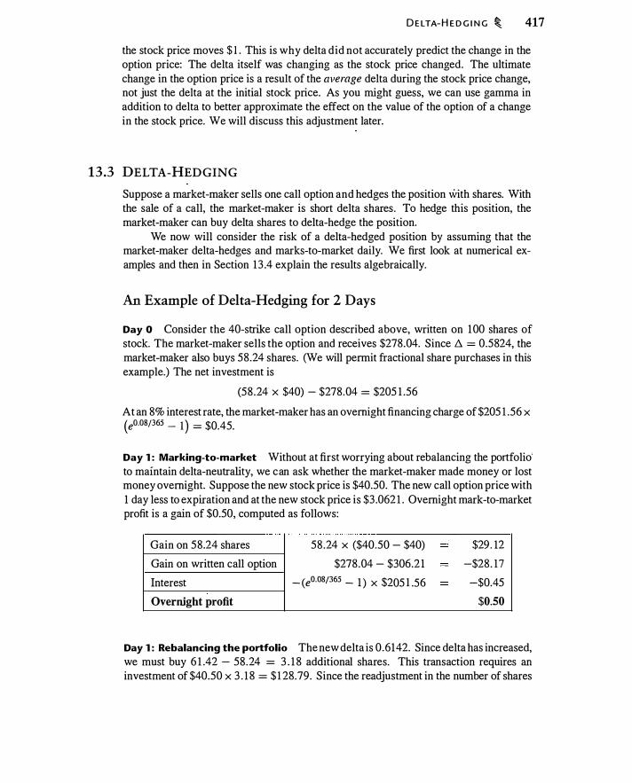
D E LTA- H E D G I N G � 417

the stock price moves $ 1 . This is why delta did not accurately predict the change in the option price: The delta itself was changing as the stock price changed. The ultimate change in the option price is a result of the average delta during the stock price change, not just the delta at the initial stock price. As you might guess, we can use gamma in addition to delta to better approximate the effect on the value of the option of a change in the stock price. We will discuss this adjustment later.

13 .3 DELTA-HEDGING

Suppose a market-maker sells one call option and hedges the position with shares. With the sale of a call, the market-maker is short delta shares. To hedge this position, the market-maker can buy delta shares to delta-hedge the position.

We now will consider the risk of a delta-hedged position by assuming that the market-maker delta-hedges and marks-to-market daily. We first look at numerical ex­amples and then in Section 13 .4 explain the results algebraically.

An Example of Delta-Hedging for 2 Days

Day 0 Consider the 40-strike call option described above, written on 1 00 shares of stock. The market-maker sells the option and receives $278.04. Since /::;. = 0.5824, the market-maker also buys 58.24 shares. (We will permit fractional share purchases in this example.) The net investment is

(58 .24 X $40) - $278.04 = $205 1 .56

At an 8% interest rate, the market-maker has an overnight financing charge of $205 1 .56 x (eO.OB/365 - I ) = $0.45.

Day 1 : Marking-to-market Without at first worrying about rebalancing the portfolio' to maintain delta-neutrality, we can ask whether the market-maker made money or lost money overnight. Suppose the new stock price is $40.50. The new call option price with 1 day less to expiration and at the new stock price is $3 .062 1 . Overnight mark-to-market profit is a gain of $0.50, computed as follows:

Gain on 58.24 shares

Gain on written call option

Interest

Overnight profit

58 .24 X ($40.50 - $40)

$278.04 - $306.2 1 - (e0·081365 - 1 ) x $205 1 .56

$29 . 12

-$28. 17

-$0.45

$0.50

Day 1 : Rebalancing the portfolio The new delta is 0 .6142. Since delta has increased, we must buy 6 1 .42 - 58.24 = 3 . 1 8 additional shares. This transaction requires an investment of $40.50 x 3 . 1 8 = $ 1 28.79. Since the readjustment in the number of shares

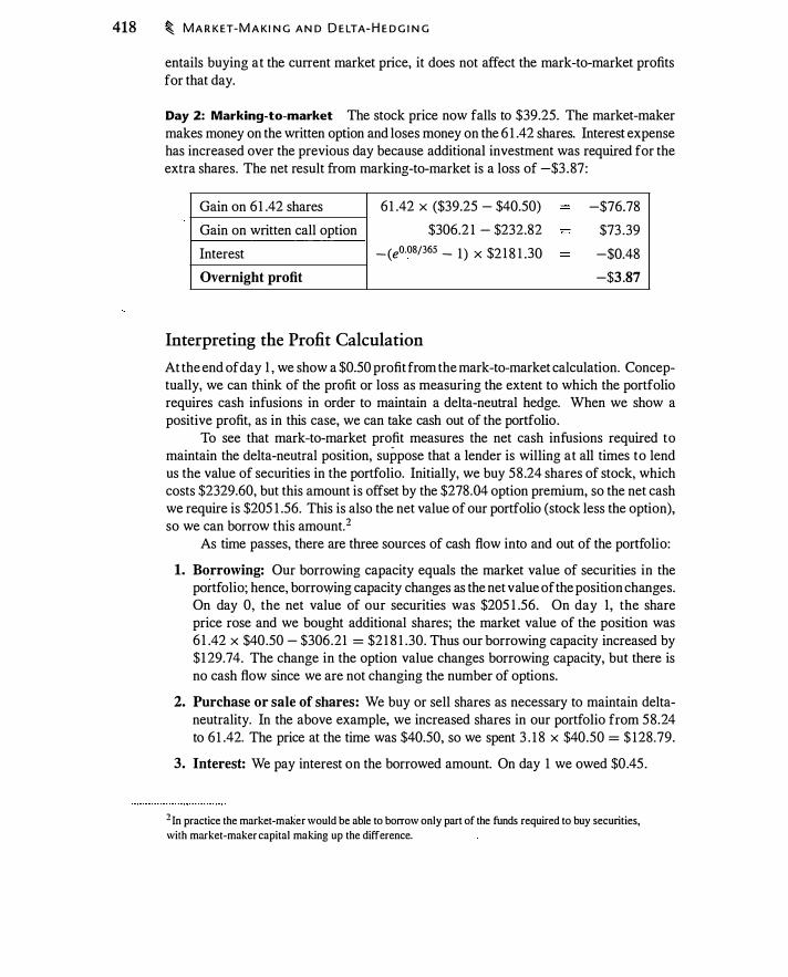
418 � MARKET-MAK ING AND DELTA-HEDG ING

entails buying at the current market price, it does not affect the mark-to-market profits for that day.

Day 2: Marking-to-market The stock price now falls to $39.25. The market-maker makes money on the written option and loses money on the 6 1 .42 shares. Interest expense has increased over the previous day because additional investment was required for the extra shares. The net result from marking-to-market is a loss of -$3 .87 :

Gain on 6 1 .42 shares

Gain on written call option

Interest

Overnight profit

6 1 .42 X ($39.25 - $40.50)

$306.2 1 - $232.82 - (e0·081365 - 1 ) X $2 1 8 1 .30

Interpreting the Profit Calculation

-$76.78

$73 .39

-$0.48

-$3 .87

At the end of day I , we show a $0.50 profit from the mark-to-market calculation. Concep­tually, we can think of the profit or loss as measuring the extent to which the portfolio requires cash infusions in order to maintain a delta-neutral hedge. When we show a positive profit, as in this case, we can take cash out of the portfolio.

To see that mark-to-market profit measures the net cash infusions required to maintain the delta-neutral position, suppose that a lender is willing at all times to lend us the value of securities in the portfolio. Initially, we buy 58.24 shares of stock, which costs $2329.60, but this amount is offset by the $278.04 option premium, so the net cash we require is $205 1 .56. This is also the net value of our portfolio (stock Jess the option), so we can borrow this amount. 2

As time passes, there are three sources of cash flow into and out of the portfolio:

1. Borrowing: Our borrowing capacity equals the market value of securities in the portfolio; hence, borrowing capacity changes as the net value of the position changes. On day 0, the net value of our securities was $205 1 .56. On day 1, the share price rose and we bought additional shares; the market value of the position was 6 1 .42 x $40.50 - $306.21 = $2 1 8 1 .30. Thus our borrowing capacity increased by $1 29.74. The change in the option value changes borrowing capacity, but there is no cash flow since we are not changing the number of options.

2. Purchase or sale of shares: We buy or sell shares as necessary to maintain delta­neutrality. In the above example, we increased shares in our portfolio from 58.24 to 6 1 .42. The price at the time was $40.50, so we spent 3 . 1 8 x $40.50 = $ 128.79.

3. Interest: We pay interest on the borrowed amount. On day 1 we owed $0.45 .

2 In practice the market-maker would be able to borrow only part of the funds required to buy securities,

with market-maker capital making up the difference.

D E LTA- H E D G I N G � 419

Thus, we need $ 1 28 .79 to buy more shares and $0.45 to pay interest expense. The change in our borrowing capacity-the extra amount the bank will lend us-is $ 1 29.7 4. The difference between what the bank will lend us on the one hand and the cost of additional shares plus interest on the other is

$ 1 29 .74 - $ 1 28.79 - $0.45 = $0.50

Since the bank is willing to lend us the value of our securities, we are free to pocket the $0.50 that is left over.

This example demonstrates that the mark-to-market profit equals the net cash flow generated by always borrowing to fully fund the position. Another way to see the equality of mark-to-market profit and net cash flow is by examining the sources and uses of funds, and the extent to which it is necessary to inject additional cash into the position in order to maintain the delta-neutral hedge. We can calculate the net cash flow from the portfolio as

Net cash flow = Change in borrowing capacity - cash used to purchase additional shares - interest

Let D.; denote the option delta on day i , S; the stock price, C; the option price, and M V; the market'value of the portfolio. Borrowing capacity on day i is M V; = D.; S; - C; ; hence, the change in borrowing capacity is

MV; - MV;- 1 = D.; S; - C; - (/i;_ , S;- 1 - C;_ ! )

The cost of purchasing additional shares is S; (D.; - D.; _ 1 ) , and interest owed on day i depends on the previous day's borrowing, rMV;_ 1 . Thus, on day i we have

Net cash flow = MV; - MV;_ 1 - S; (D.; - D.;_ ! ) - rMV;_ 1 = D.; S; - C; - (D.;- J S;- 1 - C;_ ! ) - S; (D.; - D.;_ ! ) - rMV;- 1 = fi;- 1 (S; - S;_ ! ) - (C; - C;- 1 ) - rMV;_ 1

The last expression is the overnight gain on shares, less the overnight gain on the option, ' less interest; this result i s identical to the profit calculation we performed above. In the numerical example, we have

MV, - MVo - S1 (D. I - D.o) - rMVo = $2 1 8 1 .30 - $205 1 .56 - $ 1 28.79 - $0.45 = $0.50

This value is equal to the overnight profit we calculated between day 0 and day 1 . Thus, w e can interpret the daily mark-to-market profit or loss a s the amount of

cash that we can pocket (if there is a profit) or that we must pay (if there is a loss) in order to fund required purchases of new shares and to continue borrowing exactly the amount of our securities. When we have a positive profit, as on day 1, we can take money out of the portfolio, and when we have a negative profit, as on day 2, we must put money into the portfolio.

A hedged portfolio that never requires additional cash investments to remain hedged is self-financing. One of the questions we will answer is under what condi­tions ·a delta-hedged portfolio is self-financing.

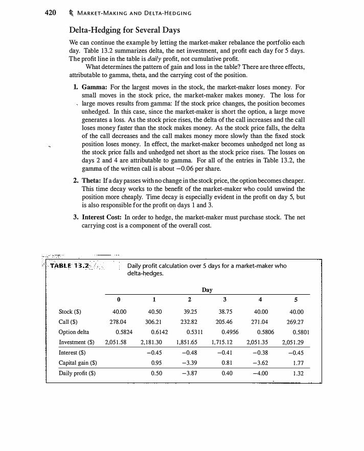
420 � M A R K ET- M A K I N G A N D D E LTA- H E D G I N G

Delta-Hedging for Several Days

We can continue the example by letting the market-maker rebalance the portfolio each day. Table 13 .2 summarizes delta, the net investment, and profit each day for 5 days. The profit line in the table is daily profit, not cumulative profit.

What determines the pattern of gain and loss in the table? There are three effects, attributable to gamma, theta, and the carrying cost of the position.

1. Gamma: For the largest moves in the stock, the market-maker loses money. For small moves in the stock price, the market-maker makes money. The loss for large moves results from gamma: If the stock price changes, the position becomes unhedged. In this case, since the market-maker is short the option, a large move generates a loss. As the stock price rises, the delta of the call increases and the call loses money faster than the stock makes money. As the stock price falls, the delta of the call decreases and the call makes money more slowly than the fixed stock position loses money. In effect, the market-maker becomes unhedged net long as the stock price falls and unhedged net short as the stock price rises. The losses on days 2 and 4 are attributable to gamma. For all of the entries in Table 13 .2, the gamma of the written call is about -0.06 per share.

2. Theta: If a day passes with no change in the stock price, the option becomes cheaper. This time decay works to the benefit of the market-maker who could unwind the position more cheaply. Time decay is especially evident in the profit on day 5, but is also responsible for the profit o� days 1 and 3 .

3. Interest Cost: In order to hedge, the market-maker must purchase stock. The net carrying cost is a component of the overall cost.

Stock ($)

Call ($)

Option delta

Investment ($) Interest ($)

Capital gain ($)

Daily profit ($)

0

40.00

278.04

Daily profit calculation over 5 days for a market-maker who delta-hedges.

Day 1 2 3 4

40.50 39.25 38.75 40.00

306.2 1 232.82 205 .46 27 1 .04

0.5824 0.6 1 42 0.53 1 1 0.4956 0.5806

5

40.00

269.27

0.580 1

2,05 1 .58 2, 1 8 1 .30 1 ,85 1 .65 1 , 7 1 5 . 1 2 2,05 1 .35 2,05 1 .29

-0.45 -0.48 -0.4 1 -0.38 -0.45

0.95 -3.39 0.8 1 -3 .62 1 .77

0.50 -3.87 0.40 -4.00 1 .32

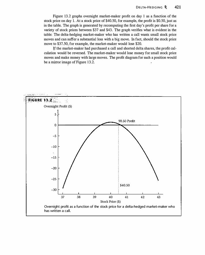
D E LTA-H E D G I N G � 421

Figure 13 .2 graphs overnight market-maker profit on day 1 as a function of the stock price on day 1 . At a stock price of $40.50, for example, the profit is $0.50, just as in the table. The graph is generated by recomputing the first day's profit per share for a variety of stock prices between $37 and $43 . The graph verifies what is evident in the table: The delta-hedging market-maker who has written a call wants small stock price moves and can suffer a substantial loss with a big move. In fact, should the stock price move to $37 .50, for example, the market-maker would lose $20.

If the market-maker had purchased a call and shorted delta shares, the profit cal­culation would be reversed. The market-maker would lose money for small stock price moves and make money with large moves. The profit diagram for such a position would be a mirror image of Figure 1 3 .2.

Overnight Profit ($)

5

-5

-10

-15

-20

-25

-30

37 38 39

: $40.50

40

Stock Price ($)

41 42 43

Overnight profit as a function of the stock price for a delta-hedged market-maker who has written a cal l .

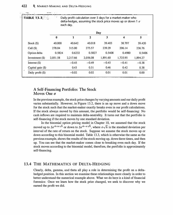
422 � M A R K ET-M A K I N G A N D D E LTA-H E D G I N G

TABLE 133 < ' Daily profit calculation over 5 days for a market-maker who delta-hedges, assuming the stock price moves up or down 1 u each day.

Day 0 1 2

Stock ($) 40.000 40.642 40.0 1 8

Call ($) 278.04 3 1 5 .00 275.57

Option delta 0.5824 0.6232 0.5827

Investment ($) 2,05 1 .58 2,2 1 7.66 2,056.08

Interest ($) -0.45 -0.49

Capital gain ($) 0.43 0.5 1

Daily profit ($) -0.02 0.02

A Self-Financing Portfolio: The Stock Moves One u

3

39.403

239.29

0.5408

1 ,89 1 .60

-0.45

0.46

0.0 1

4 5

38.797 39.420

206. 1 4 236.76

0.4980 0.5406

1 ,725.95 1 ,894.27

-0.4 1 -0.38

0.42 0.38

O.D I 0.00

In the previous example, the stock price changes by varying amounts and our daily profit varies substantially. However, in Figure 13 .2, there is an up move and a down move for the stock such that the market-maker exactly breaks even in our profit calculations. If the stock always moved by this amount, the portfolio would be self-financing: No cash inflows are required to maintain delta-neutrality. It turns out that the portfolio is self-financing if the stock moves by one standard deviation.

In the binomial option pricing model in Chapter 1 0, we assumed that the stock moved up to serh+a../ii or down to serh-a../ii, where a,Jh is the standard deviation per interval of the rate of return on the stock. Suppose we assume the stock moves up or down according to this binomial model. Table 13 .3 , which is otherwise the same as the previous example, shows the results of the stock moving up, down three times, and then up. You can see that the market-maker comes close to breaking even each day. If the stock moves according to the binomial model, therefore, the portfolio is approximately self-financing.

13 .4 THE MATHEMATICS OF DELTA-HEDGING

Clearly, delta, gamma, and theta all play a role in determining the profit on a delta­hedged position. In this section we examine these relationships more closely in order to better understand the numerical example above. What we do here is a kind of financial forensics : Once we learn how the stock price changed, we seek to discover why we earned the profit we did.

TH E M AT H E M AT I CS O F D E LTA-H E D G I N G � 423

Using Gamma to Better Approximate the Change in the Option Price

Delta alone is an inaccurate predictor of the change in the option price because delta changes with the stock price. When delta is very sensitive to the stock price (gamma is large), the inaccuracy will be relatively great. When delta is not sensitive to the stock price (gamma is small) , the inaccuracy will be relatively small . Since gamma measures the cha,nge in delta, Wf? can use gamma to develop a better approximation for the change in the option price.

If the stock price were $40.75 instead of $40, the option price would be $3 .2352 instead of $2.7804. For the purpose of computing the change in the option price, we want to know the average rate of price increase between $40 and $40.75, which we can approximate by averaging the deltas at $40 and $40.75 :

�40 + �40.75 �Averaoe = -----= 2

We could then approximate the option price at $40.75 by computing

C ($40.75) = C($40) + 0.75 X �Average ( 1 3 . 1 )

When w e average the deltas at $40 and $40.75, we have to compute deltas at two different stock prices. A different approach is to approximate the average delta by using only the delta evaluated at $40 together with gamma. Since gamma measures the change in delta, we can approximate the delta at $40.75 by adding 0.75 x r to �40 :

�40.75 = �4o + o.75 x r Using this relationship, the average delta is

�4o + c�4o + o.75 x n �Average =

2 l

= �40 + 2 X 0.75 X r Using·equation ( 1 3 . 1 ) , we can then approximate the call price as

C ($40.75) = C($40) + 0.75 X �Average

= C($40) + 0.75 X ( �40 + � X 0.75 X r) l ? = C($40) + 0.75 x �4o + - x 0.75- x r 2

( 13 .2)

The use of delta and gamma to approximate the new option price is called a delta-gamma approximation.3

3You may recognize that we have already encountered the idea of a delta-gamma approximation in Chapter 7, when we used duration {delta) and convexity {gamma) to approximate the price change of

a bond.

424 � M A R K ET- M A K I N G A N D D E lTA- H E D G I N G

Example 1 3. 1 If the stock price rises from $40 to $40.75, the option price in­creases from $2.7804 to $3.2352. Using a delta approximation alone, we would estimate C ($40.75) as

C ($40.75) = C ($40) + 0.75 X 0.5824 = $3 .2172

Using a delta-gamma approximation, we obtain

I C ($40.75) = C($40) + 0.75 X 0.5824 + 2 X 0.752 X 0.0652 = $3 .2355

The delta-gamma approximation is significantly closer to the true option price at $40.75 than is the delta approximation.

Similarly, for a stock price decline to $39.25, the true option price is $2.3622. The delta approximation gives

C($39.25) = C ($40) - 0.75 X 0.5824 = $2.3436

The delta-gamma approximation gives

C ($39.25) = C($40) - 0.75 X 0.5824 + � X 0.752 X 0.0652 = $2.36 1 9

Again, the delta-gamma approximation i s more accurate . .

Delta-Gamma Approximations

We now repeat the previous arguments using algebra. For a "small" move in the stock price, we know that the rate at which delta changes is given by gamma. Thus, if over a time interval of length h the stock price change is

E = Sr+h - Sr

then gamma is the change in delta per dollar of stock price change, or

f(Sr ) = b.. (S,+, ) - b.. (S, )

E

Rewriting this expression, delta will change by approximately the magnitude of the price change, E, times gamma, E f :

( 1 3.3)

If the rate at which delta changes is constant (meaning that gamma is constant), this calculation is exact.

How does equation ( 1 3.3) help us compute the option price change? If the stock price changes by E, we can compute the option price change if we know the average delta over the range ·st+lr to S, . If r is approximately constant, the average delta is

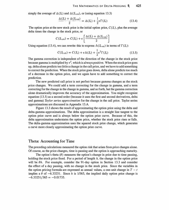
TH E M ATH E M AT I CS O F D E LTA- H E D G I N G � 425

simply the average of !;;. (S1 ) and !;;. (Sr+h ) , or (using equation 13 .3)

!;;. (Sr ) + !;;. (Sr+h ) = !;;. (Sr ) + �Ef' (Sr ) 2 2 ( 1 3 .4)

The option price at the new stock price is the initial option price, C(S1 ) , plus the average delta times the change in the stock price, or

C(Sr+h ) = C(S1 ) + E [ /;;. (Sr ) +2!;;. (Sr+h ) ]

Using equation ( 1 3 .4), we can rewrite this to express /;;. (Sr+h ) in terms of f(S1 ) : I , C(Sr+h ) = C(S1 ) + E/;;. (Sr ) + 2E-f (S1 ) ( 1 3.5)

The gamma correction is independent of the direction of the change in the stock price because gamma is multiplied by E2, which is always positive. When the stock price goes up, delta alone predicts too little a change in the call price, and we have to add something to correct the prediction. When the stock price goes down, delta alone predicts too much of a decrease in the option price, and we again have to add something to correct the prediction.

The new predicted call price is not perfect because gamma changes as the stock price changes. We could add a term correcting for the change in gamma, and a term correcting for the change in the change in gamma, and so forth, but the gamma correction alone dramatically improves the accuracy of the approximation. You might recognize equation ( 13 .5) as a second order (because it uses the first and second derivatives, delta and gamma) Taylor series approximation for the change in the call price. Taylor series approximations are discussed in Appendix B.A.

Figure 1 3 .3 shows the result of approximating the option price using the delta and delta-gamma approximations. The delta approximation is a straight line tangent to the option price curve and is always below the option price curve. Because of this, the delta approximation understates the option price, whether the stock price rises or falls . The d�lta-gamma approximation uses the squared stock price change, which generates ·

a curve more closely approximating the option price curve.

Theta: Accounting for Time

The preceding calculations measured the option risk that arises from price changes alone. Of course, as the price changes, time is passing and the option is approaching maturity.

The option's theta (0 ) measures the option's change in price due to time passing, holding the stock price fixed. For a period of length lz, the change in the option price will be 0/z. For example, consider the 9 1 -day option in Section 1 3 .3 and consider the effect of a day passing, with no change in the stock price. Since the variables in the option pricing formula are expressed as annual values, a one-unit change in T - t implies a e of -6.3325 1 . Since h is 11365, the implied daily option price change is -6.3325 1 /365 = -0.01735.

426 � M A R K ET-M A K I N G A N D D E LTA- H E D G I N G

Delta- and delta-gamma approximations of option price. The true option price is represented by the bold l ine, and approximations by dashed l ines.

Option Price ($)

Delta-gamma approximation

So Stock Price ($)

Delta approximation

Adding theta to our previous option price prediction equation, we have

C (Sr+lz , T - t - h) 1 ?

= C (S1 , T - t) + E fi (S1 , T - t) + 2E-f (Sr . T - t) + !ze (S1 , T - t) ( 1 3 .6)

The experiment reflected in this equation is this: Starting with an option with T - t periods until expiration and a stock price of S1 , we want to express the new option price as a function of the old price and the delta, gamma, and theta evaluated at the original price and time to expiration. This formula is quite accurate for relatively small changes in time and in the stock price.

" Example 1 3.2 Table 1 3 .4 shows the results from using equation ( 1 3 .6) to predict the option price change when prices move by $0.75 (E = ±0.75). In this example, fi = 0.5824, r = 0.0652, and lz(} = -0.0 173 . Note that in each case the formula

t, slightly overstates the change, but the predicted price is close to the actual price. �

Sr+lz = $40.75

Sr+lz = $39.25

TH E M ATH E M AT I CS O F D E LTA- H E D G I N G � 427

Predicted option price over a period of 1 day, assuming stock price move of $0.75, using equation (1 3 .6) . Assumes that u = 0 . 3, r = 0.08, T - t = 91 days, and 8 = 0, and the initial stock price is $40.

Option Price 1 Day Later (h = 1 day)

Starting Price E A !E2r 2 ()lz Predicted Actual

$2.7804 0.4368 0.0 1 83 -0.0 1 73 $3.2 1 82 $3.2 176

$2.7804 -0.4368 0.0 1 83 -0.0 173 $2.3446 $2.3452

Understanding the Market-Maker's Profit

The calculations in Tables 13 .2 and 13 .3 use actual option price changes over 1 day, not approximations. However, by using equation ( 13 .6) to approximate the change in the option price we can better understand the profit results in those tables.

The value of the market -maker's investment-long delta shares and short a call-is the value of delta shares of stock less the value of the call, or

[).r Sr - C (Sr )

Suppose that over the time interval /z, the stock price changes from S1 to Sr+lz · The change in the value of the portfolio is the change in the value of the stock and option positions, less interest expense:

[).r (Sr+lz - Sr) - [C (Sr+lz ) - C (Sr )] ..._,_.,

Change in value of stock Change in value of option Interest expense Now recall equation ( 1 3 .6), in which we characterized the change in the option price. Substituting equation ( 1 3 .6) for C (Sr+lz ) - C(S1 ) in this expression tells us

1 ? [).r (Sr+h - Sr ) - [[).r (Sr+h - Sr ) + 2 (Sr+lz - Sr )-rr + 8/z] - rh[[).r Sr - C(Sr ) ]

= - (�E2f1 + 81/z + rlz [[).1 S1 - C (S1 )]) ( 13 .7)

This expression gives us the profit of the market-maker when the stock price changes by E over an interval of length lz. It is quite important and variants of it will appear later in the book.

On the right-hand side of equation ( 13 .7) we see the effects of gamma, theta, and interest:

428 � M A R K ET- M A K I N G A N D D E LTA- H E D G I N G

1. Gamma: The effect of gamma is measured by -1E2r1 • Since the gamma of the call is positive, by writing the call the market-maker will lose money in proportion to the square of the stock price change. The larger the stock move, the greater is the loss.

2. Theta: The effect of theta is measured by -e1 1z . Since theta for the call is negative, the option writer benefits from theta.

3. Interest cost: Interest is measured by -rlz [t:.1 S1 - C(S1 ) ] . The option writer has a net investment because t:.1 shares are more expensive than one option. Hence, interest is a net cost.

Since e is negative, time decay benefits the market-maker, whereas interest and gamma work against the market-maker.

Let's examine how E , the change in the stock price, enters equation ( 1 3 .7). Note first that because we have delta-hedged, E itself does not affect market-maker profit. However, profit does depend on the squared change in the stock price, E2 . Consequently, as we saw in Table 1 3 .2, it is the magnitude-not the direction of the stock price move­that determines profit.

Table 13 .5 calculates equation ( 1 3 . 7) for various moves in the stock price. Because equation ( 13 .7) depends only on the squared stock price move, the calculation is the same for moves up and down.

If the stock price moves $0.628 1 , equation ( 13 .7) is exactly zero. We have already seen in Table 13 .3 that the market-maker approximately breaks even for a one-standard­deviation move in the stock. Here we arrive at the same result. Let's explore this idea further.

TAB LE 1 3 . S . c Predicted effect, using equation (1 3 .7), of different-sized stock price moves on the profit of a delta-hedged market -maker.

Absolute Value of Price Move, IE I - �E2r - (Jh - rh[ASt - C (St)]

0.0000 1 .283

0.2500 1 .080

0.5000 0.470

0.628 1 0.000

0.7500 -0.546

1 .0000 - 1 .970

1 .5000 -6.036

T H E B LA C K-S C H O LES A N A LYS I S � 429

If cr is measured annually, then a one-standard-deviation move over a period of length lz is cr S1 -J/i. Therefore a squared one-standard-deviation move is

E2 - CT2 S21z - I ( 1 3 .8)

Substituting this expression for E2 , we can rewrite equation ( 1 3.7) as ( 1 1 1 ) Market-maker profit = - zcr-S�f1 + 81 + r [.6.1 S1 - C(S1 )] lz ( 1 3 .9)

This expression gives us market-maker profit when the stock moves one standard devia­tion. As an example, let lz = 1 /365 and cr = 0.3. Then cr S -J/i = $0.628 1 . From Table 13 .5 , with this stock price move equation ( 1 3 .9) is exactly zero ! (Problem 1 3 . 1 3 asks you to verify this.) It is not an accident that equation ( 1 3 .9) is zero for this price move. We explain this result in Section 1 3 .5 .

In Table 1 3 .5, the loss from a $ 1 move i s substantially larger in absolute value than the gain from no move. However, small moves are more probable than big moves. If we think of returns as being approximately normally distributed, then stock price moves greater than one standard deviation occur about one-third of the time. The market-maker thus expects to make small profits about two-thirds of the time and larger losses about one-third of the time. On average, th� market-maker will break even.

13.5 THE BLACK-S CHOLES ANALYSIS

We have discussed how a market-maker can measure and manage the risk of a portfolio containing options. What is the link to pricing an option?

The Black-Scholes Argument

If a stock moves one standard deviation, then a delta-hedged position will exactly break even, taking into account the cost of funding the position. This finding is not a coin­cidence; it reflects the arguments Black and Scholes used to derive the option pricing • formula.

Imagine, for example, that the stock always moves exactly one standard deviation every minute.4 A market-maker hedging every minute will be hedged over an hour or over any period of time. Black and Scholes argued that the money invested in this hedged position should earn the risk-free rate since the resulting income stream is risk-free.

Equation ( 1 3 .9) gives us an expression for market-maker profit when the stock moves one standard deviation. Setting this expression to zero gives

4There are 365 x 24 x 60 = 525, 600 minutes in a year. Thus, if the stock's annual standard deviation is 30%, the per-minute standard deviation is 0.3/ .J525,600 = 0.04%, or $0.0 1 6 for a $40 stock.

430 � M A R K ET- M A K I N G A N D D E LTA-H E D G I N G

If we divide by h and rearrange terms, we get

( 1 3 . 1 0)

This is the equation Black and Scholes used to characterize the behavior of an option. The Greeks r, D., and 8 are partial derivatives of the option price. Equation ( 1 3 . 10) is the well-known Black-Scholes partial differential equation, or just Black-Scholes equation (as opposed to the Black-Scholes formula for the price of a European call). We will see in' later chapters that this relationship among the Greeks is as fundamental in valuing risky cash flows as is e-rT when valuing risk-free cash flows.

Equation ( 1 3 . 1 0) embodies numerous assumptions, among them that the underly­ing asset does not pay a dividend, the option itself does not pay a dividend, the interest rate and volatility are constant, and the stock moves one standard deviation over a small time intervaL With these assumptions, equation ( 13 . 10) holds for calls, puts, American options, European options, and most of the exotic variants we will consider in Chapter 14. With simple modifications, an equation like ( 1 3 . 10) will also hold for options on dividend-paying stocks, currencies, futures, bonds, etc. The link between delta-hedging and pricing is one of the most important ideas in finance.

Delta-Hedging of American Qptions

Equation ( 1 3 . 10) holds for American options as well as for European options, but it does not hold at times when it is optimal to early-exercise the option. Consider a deep-in­the-money American put option and suppose the option should be exercised early. Since early exercise is optimal, the option price is K - S; hence, D. = - 1 , r = 0, and 8 = 0. In this case, equation ( 1 3 . 1 0) becomes

[r X ( - 1 ) X sf ] + ( � X 0) + 0 = r X ( K - St ) Note that -r S1 appears on both sides of the equation. Thus, we can rewrite the equation as

O = rK

Since this equation is false, something is wrong. We began by assuming that the put was so far in-the-money that it should be early-exercised. From the discussion of early exercise in Chapter 1 0, this means that interest received on the strike exceeds the loss of the implicit call option. Thus, if the option should be exercised but you own it, delta-hedge it, and do not exercise it, then you lose interest on the strike you are not receiving. Similarly, if you have written the option and delta-hedged, and the owner does not exercise, then you are earning arbitrage profit of r K .

Thus, equation ( 1 3 . 1 0 ) i s only valid i n a region where early exercise i s not optimal. If an option should b� exercised but is not exercised, then behavior is irrational and there is no reason why a delta-hedged position should earn the risk-free rate and thus no reason that equation ( 1 3 . 1 0) should hold.

TH E B LA C K-S C H O LES A N A LYS I S � 43 1

What Is the Advantage to Frequent Re-Hedging?

In practice, because of transaction costs, it is expensive for a market-maker to trade shares for every change in an option delta. Instead, a delta-hedger will wait for the position to become somewhat unhedged before trading to reestablish delta-neutrality. In the binomial model in Chapter 10, and in the preceding discussion, we assumed that market-makers maintain their hedged position and that stock prices move exactly one standard deviation. In real life the stock price will rarely move exactly one standard deviation over the course of a day. What does the market-maker lose by hedging less frequently?

Boyle and Emanuel ( 1980) considered a market-maker who delta-hedges at set intervals, rather than every time the stock price changes. Let x; denote the number of standard deviations the stock price moves-we can think of x; as being drawn randomly from the standard normal distribution. Also let R,.; denote the period-i return to a delta­hedged market-maker who, as in our earlier example, has written a call. Boyle and Emanuel show that this return can be written as5

( 1 3 . 1 1 )

where r is the option's gamma and.lz is the time interval between hedge readjustments. From Boyle and Emanuel, the variance of xf - 1 is 2; hence,

1 ( , , )2 Var(R, , ; ) = 2 s-a-rJz ( 1 3 . 1 2)

We assume-as in the binomial model-that the stock return is uncorrelated across time, so that x; is uncorrelated across time.

Now let's compare hedging once a day against hedging hourly (suppose trading occurs around the clock) . The daily variance of the return earned by the market-maker who hedges once a day is given by

1 ( , , ) 2 Var(R I/365. 1 ) = 2 S-a-r /365

The daily return of the market-maker who hedges hourly is the sum of the hourly returns. Assuming for the sake of simplicity that S and r do not change much, that variance is

Var (t R,.) = t � [S2a2f/ (24 x 365)]2

1 = - x Var(R 1 1365 1 ) 24 ,

Thus, by hedging hourly instead of daily the market-maker's total return variance is reduced by a factor of 24.

5This expression can be derived by assuming that the stock price move, E, is normally distributed with

variance Su.J/i, and subtracting equation ( 1 3.9) from ( 1 3.7).

432 � M A R K ET-M A K I N G A N D D E LTA- H E D G I N G

Here is the intuition for this result. Whatever the hedging interval, about two-thirds of the price moves will be less than a single standard deviation, whereas one-third will be greater. Frequent re-hedging does not avoid these large or small moves, since they can occur over any interval. However, frequent hedging does permit better averaging of the effects of these moves. Whether you hedge once a day or once an hour, the typical stock price move you encounter will likely not be close to one standard deviation. However, if you hedge every hour, over the course of a day you will have 24 moves and 24 opportunities to re-hedge. The average move over this period is likelier to be close to one standard deviation. The gains from small moves and losses from large moves will te;nd to average over the course of a day. In effect, the more frequent hedger benefits from diversification over time.6

Example 1 3.3 . Using Boyle and Emanuel's formulas to study the market-maker problem in Section 1 3 .3 , the standard deviation of profit is about $0.075 for a market­maker who hedges hourly. Since hedging errors are independent from hour to hour, the daily standard deviation for an hourly hedger would be $0.075 x ffi = $0.37. If the market-maker were to hedge only daily as in our example, the daily standard deviation would be about $ 1 .82 . �

As you would expect, the mean return on a delta-hedged position is zero, even if the hedge is not frequently readjusted.

Delta-Hedging in Practice

The Black -Scholes analysis outlined here is the linchpin of modem option pricing theory and practice. Market-makers use equation ( 1 3 . 10) to price options, subject to qualifica­tions mentioned above.

We have seen, however, that delta-hedging does not eliminate risk. One problem, which we emphasized above, is that a delta-hedged portfolio with negative gamma can sustain losses due to large moves in the price of the underlying asset. Consequently, a delta-hedging market-maker needs to worry about gamma. Another problem, discussed in the box on page 434, is that firms can unexpectedly change their dividend payments .

There are at least four ways a market-maker can try to reduce the risk of extreme price moves. Note that some of these strategies require the market-maker to acquire

6This resembles the problem faced by an insurance company. If the company insures one large asset,

the standard deviation of the loss is .jii greater than if it insures n small assets, with the same total

insured value in each case. Similarly, we can view the return over each hedging interval as being an

independent draw from a probability distribution.

TH E B LAC K-S C H O L ES A N A LYS I S � 433

specific option positions, which means that the market-maker may have to pay the bid­ask spread. Since the bid-ask spread is revenue for the market-maker, paying the spread is undesirable.

First, just as market-makers can adopt a delta-neutral position, they can also adopt a gamma-neutral position. This position cannot be achieved with the stock alone, since the gamma of the stock is zero. Thus, to be gamma-neutral the market-maker must buy or sell options so as to offset the gamma of the existing position. 7 We provide an example of gamma-neutrality below.

Second, in a related strategy, market-makers can use static option replication, a strategy in which options are used to hedge options. In our delta-hedging example, the market-maker might not be able to buy an exactly offsetting call option to hedge the written call, but by selectively setting the bid and ask prices for related options, might be able to acquire an option position requiring only infrequent rebalancing. To take a simple example, if the market-maker were able to buy a put with the same strike price and maturity as the written call (e.g., by setting the bid price to attract any seller of that option), then by buying 100 shares to offset the risk of the position, the market-maker would have used put-call parity to create a hedge that is both gamma- and delta-neutral for the life of the options .

Third, a market-maker can buy out-of-the-money options as insurance. In our example of delta-neutral hedging of a written option, the market-maker could buy a deep-out-of-the-money put and a deep-out-of-the-money call. The two options would be relatively inexpensive and would protect against large moves in the stock. One problem with this solution is that, since option positions in the aggregate sum to zero, the market-making community as a whole can buy protective options only if investors in the aggregate are willing to sell them. Investors, however, are usually thought to be insurance buyers rather than insurance sellers.

Fourth, a market -maker can create a financial product by selling the hedging error, as discussed by Carr and Madan ( 1 998). For example, to hedge a negative-gamma, delta-neutral position, the market-maker would make a payment to a counterparty if the stock makes a small move in either direction, and receive payment from the counterparty' if the stock makes a large move in either direction. This is effectively a variance swap, which we will discuss in more detail in Chapter 23. The point is that the market-maker can potentially solve the delta-hedging problem by creating a new product.

Gamma-Neutrality

Let's explore gamma-hedging in more depth. Suppose we wish to both delta-hedge and gamma-hedge the written option described in Table 1 3 . 1 . We cannot do this using just

7Market-makers sometimes buy and hold over-the-counter options issued by a firm. For example, in

the late 1990s some firms sold put options on their own stock. These options were reportedly held by

dealers and delta-hedged. One possible motivation for dealers to undertake such a transaction would be to acquire positive gamma. See McDonald (2004) for a discussion.

434 � M A R K ET-M A K I N G A N D D E LTA- H E D G I N G

[)iVidend Risk

Market-makers price options taking into account the dividends they expect a stock to pay. If a firm announces a significant change in dividend policy, delta-hedgers can make or lose money depending on their position and depending on whether the derivatives they hold an:; protected against dividend changes.

In 1998, Daimler-Benz surprised option market-makers by announcing a special . one-time dividend, creating a dividend payout of about 14%, or 1 0 times the usual dividend

_ yield. The Deutsche Teiminbi:irse (DTB), the exchange-where Daimler options were traded, decided not to adust the terms of exchange-traded options to account for the dividend. The DTB was criticized for this, and some dealers were said to have sustained significant losses.

The stated policy of the Options Clearing Corporation ( 1994, 2003 supplement) in the United States is that typically there is adjustment only for "extraordinary" cash dividends or distributions, i.e., those exceeding " 10% of the market value of the underlying security outstanding. Determinations . . . are made on a case-by-case basis."

In July 2004 Mocrosoft announced that it would make a special one-time payment of $3/share, a dividend yield in excess of 10% based on Microsoft's price at the time of the announcement. The Options Clearing Corporation in the United States responded by declaring that it would reduce strike prices on Microsoft options by $3 when the dividend was paid.

the stock, because the gamma of stock is zero. Hence, we must acquire another option in an amount that offsets the gamma of the written call . Table 1 3 .6 presents information for the 3-month 40-strike call , and also for a 4-month 45-strike call . We will use the latter to gamma-hedge the former.

The ratio of the gamma of the two options is8

fK=40.r=0.25 _ 0.065 1 _

1 ?408 . fK=45.r=0.33 - 0.0524 -

·-( 1 3 . 13 )

Thus, we need to buy 1 .2408 of the 45-strike 4-month options for every 40-strike 3-month option we have sold. The Greeks resulting from the position are in the last column of Table 13 .6. Since delta is -0. 1749, we need to buy 17 .49 shares of stock to be both delta- and gamma-hedged.

Figure 1 3 .4 compares this delta- and gamma-hedged position to the delta-hedged position, discussed earlier, in which the same call was written. The delta-hedged position has the problem that large moves always cause losses. The gamma-hedged position loses less if there is a large move down, and can make money if the stock price increases. Moreover, as Table 13.6 shows, the gamma-hedged position has a positive vega. Why would anyone not gamma-hedge?

8The gammas in equation ( 1 3 . 1 3 ) are rounded. The actual gammas are 0.065063 and 0.052438, the

ratio of which is 1 .2408.

Price ($)

Delta

Gamma

Vega

Theta

Rho

T H E B LA C K- S C H O LES A N A LYS I S � 435

Prices and Greeks for 40-strike call, 45-strike ca l l, and the (gamma-neutral) portfolio resulting from sell ing the 40-strike cal l for which T - t = 0.25 and buying 1 .2408 45-strike cal ls for which T - t = 0.33 . By buying 1 7.49 shares, the market-maker can be both delta- and gamma-neutra l . Assumes S = $40, u = 0.3, r = 0.08, and 8 = 0.

40-Strike 45•Strike Sell 40-Strike Call, Buy Call Call 1.2408 45-Strike Calls

2.7847 1 .3584 - 1 .0993

0.5825 0.3285 -0. 1749

0.065 1 0.0524 0.0000

0.078 1 0.083 1 0.0250

-0.0 173 -0.0 1 29 0.00 1 3

0.05 13 0.0389 -0.003 1

· F I GU R E 1 3 .4�.' , Overnight

Comparison of 1 -day Profit ($)

holding period profit 100 - Delta-hedged written call

for delta-hedged - - Delta- and gamma-hedged written call /

/

position described in /

50 / / Table 1 3 .2 and delta-

� ---

and gamma-hedged 0 position described in

� �

� ---

Table 1 3 .6. -50 _... _... / /

-100

-150

-200

-250

-300

-350

30 32 34 36 38 40 42 44 46 48 50 Stock Price ($)

436 � M A R K ET-M A K I N G AN D D E LTA- H E D G I N G

There are two reasons. First, as noted already, gamma-hedging requires the use of additional options. The market-maker will have to obtain the required option position from another market -maker, paying the bid-ask spread. In this example, all profits earned from writing the 40-strike call will go to pay the market-maker who sells the 45-strike call used in gamma-hedging. In a large portfolio, however, with many options bought and sold, naturally offsetting one another, gamma-hedging the net exposure would not require many option transactions.

The second reason is that if end-users on average buy puts and calls, then in the aggregate they have positive gamma (the end-users "buy gamma," to use market­making parlance). By definition, market -makers in the aggregate must then have negative gamma. Thus, while in principle any one market-maker could gamma-hedge, not all market-makers could be gamma-neutral. If investors want to buy insurance, they will not be gamma-neutral, and, hence, market-makers cannot in the aggregate be gamma-neutral.

In addition to gamma, other risks, such as vega and rho, can be hedged in the same fashion as delta.

13 .6 MARKET-MAKING AS INSURANCE

The preceding discussion suggests that market-makers who write options can sustain large losses, even if they delta-hedge. This conclusion suggests that option market­making (and derivatives market-making more generally) has more in common with insurance than you might at first think.

Insurance

Insurance companies attempt to pool diversifiable risks . All insured individuals pay an insurance premium. The premiums are then used to compensate those who suffer losses, while those without losses lose the premium. Insurance thereby spreads the pain rather than forcing a few unlucky individuals to bear the brunt of inevitable losses.

In the classic model of an insurance company, risks are independent. Suppose an insurance company provides insurance for a large number of identical households, each of which has an independent I % chance in any year of losing $ 100,000 in a fire. The expected loss for each house is 1 % x $ 1 00, 000 = $ 1 , 000. This is the "actuarially fair" insurance premium, in the sense that if the insurance company collects this amount from each household, it will on average be able to pay annual insurance claims. In general insurance will be priced to cover the expected loss, plus costs of doing business, less interest earned on the premium.

However, even with diversification, there is a chance that actual insurance claims in a particular year will exceed $ 1 000 per insured household, in which case the insurance company will not be able to fulfill its promises unless it has access to additional funds. Thus, the seller of a risk-management product-the insurance company-has a risk­management problem of its own-namely to be sure that it can meet its obligations to customers . Meeting such obligations is not just a matter of eonscience for management;

M A R K ET-M A K I N G AS I N S U R A N C E � 437

if there is a significant chance that the insurance company will be bankrupted by claims, there will be no customers in the first place !

Insurance companies have two primary ways to ensure that they meet claims:

1. Capital: Insurance companies hold capital, i .e. , a buffer fund in case there is an un­usually large number of claims. Because of diversification, for any given bankruptcy probability insurers can use a smaller reserve fund per insured house as the number of insured houses grows. Capital in the form of reserves has traditionally been an important buffer for insurance companies against unexpectedly large claims.

2. Reinsurance: There is always the possibility of a loss that can exceed any fixed amount of capital. An insurance company can in turn buy insurance against large losses, in order to be able to make large payouts if necessary. Insurance for in­surance companies is called reinsurance. Insurance companies buy insurance from reinsurance firms to cover the event that claims exceed a certain amount. Reinsur­ance is a put option: The reinsurance claim gives the insurance company the right to sell to the reinsurers claims that have lost money. Reinsurance does not change the aggregate need for capital, but it does permit further diversification.

Market-Makers

Now consider again the role of market-makers. Suppose that investors, fearful of a market crash, wish to buy out-of-the-money puts . Out-of-the-money put writers are selling insurance against large market moves. It is precisely when large market moves occur that delta-hedging breaks down. Just like an insurance company, a market-maker requires capital as a cushion against losses. Since capital has a cost, market-makers may also raise the cost of written options that require a disproportionately large commitment of capital per dollar of premium.

Reinsurance for a market-maker would entail buying out-of-the-money put options to move some risk to another market-maker, but ultimately if the financial industry is a. net writer of insurance, there must be capital in the event of losses .

The importance of capital and the analogy to insurance becomes more obvious when we consider new derivatives markets. For example, think about weather deriva­tives. Financial institutions have hedged ski-resort operators against warm winters, soft­drink manufacturers against cold summers, and lawn sprinkler manufacturers against wet summers . Ultimately, the bank must find a counterparty willing to absorb the risk. If you think about the risks in weather insurance, on a global basis they are like tradi­tional insurance. Weather contracts in the United States can be diversified with weather contracts in Asia, and ultimately the global capital committed to insurance absorbs the reinsurance risk. Global capital markets broadly defined are thus the natural party to absorb these risks.

Some risk, however, is not globally diversifiable. Consider writing puts on the S&P 500. If the U.S. stock market suffers a large decline, other markets around the world are likely to follow. Ultimately, it is capital that safeguards the financial industry.

438 � M A R K ET-M A K I N G A N D D E LTA- H E D G I N G

Delta-hedging plays a key role, but in the end there is always risk that must be absorbed by capital.

- �.----·- - - -----··

• ....:. •.• ...o.::.- · ... , _ _-. ,.· . . - . -.:;;.__.

CHAPTER SUMMARY

Market-makers buy and sell to satisfy customer demand. A derivatives market-maker can use the underlying stock to delta-hedge the resulting position. By definition, the r:etum on a delta-hedged position does not depend on the direction in which the stock price moves, but it does depend on the magnitude of the stock price move. A position with zero delta and negative gamma makes money for small stock price moves and loses money for large stock price moves. If the gamma of the position is positive, it makes money for large moves and loses money for small moves. Either way, the delta-hedged position breaks e·ven if the stock moves one standard deviation.

Using a delta-gamma-theta approximation to characterize the change in the value of the delta-hedged portfolio, we can demonstrate that there are three factors that explain the profitability of the portfolio. First, gamma measures the tendency of the portfolio to become unhedged as the stock price moves. Second, theta measures the gain or loss on the portfolio due to the passage of time alone. Third, the market-maker will have interest income or expense on the portfolio.

If we assume that the stock price moves one standard deviation and impose the condition that the market-maker earns zero profit, then a fair option price satisfies a par­ticular relationship among delta, gamma, and theta. This relationship, equation ( 1 3 . 10), is the foundation of the Black-Scholes option pricing analysis and applies to derivatives in general, not just to calls and puts.

Ultimately, market-making is risky and requires capital. If customers on average buy puts and calls, and if we think of options as insurance, then market-makers are in the same business as insurance companies. This requires capital, since if an extreme ev�nt occurs, delta-hedging will fail.

FURTHER READING

The main example in this chapter assumed that the Black-Scholes formula provided the correct option price and illustrated the behavior of the formula, viewed from the perspective of a delta-hedging market-maker. In Chapters 20 and 2 1 we will start by building a model of how stock prices behave, and see how the Black-Scholes formula is derived. As in this chapter, we will conclude that equation ( 1 3 . 10) is key to understanding option pricing.

PROB LEMS

In the following problems assume, unless otherwise stated, that S = $40, a = 30%, r = 8%, and 8 = 0.

P RO B LE M S � 439

13.1. Suppose you sell a 45-strike call with 91 days to expiration. What is delta? If the option is on 100 shares, what investment is required for a delta-hedged portfolio? What is your overnight profit if the stock tomorrow is $39? What if the stock price is $40.50?

13.2. Suppose you sell a 40-strike put with 91 days to expiration. What is delta? If the option is on 100 shares, what investment is required for a delta-hedged portfolio? What is your overnight profit if the stock price tomorrow is $39? What if it is $40.50?

13.3. Suppose you buy a 40-45 bull spread with 91 days to expiration. If you delta­hedge this position, what investment is required? What is your overnight profit if the stock tomorrow is $39? What if the stock is $40.50?

13.4. Suppose you enter into a put ratio spread where you buy a 45-strike put and sell two 40-strike puts. If you delta-hedge this position, what investment is required? What is your overnight profit if the stock tomorrow is $39? What if the stock is $40.50?

13.5. Reproduce the analysis in Table 1 3 .2, assuming that instead of selling a call you sell a 40-strike put.

13.6. Reproduce the analysis in Table 1 3 .3 , assuming that instead of selling a call you sell a 40-strike put.

13.7. Consider a 40-strike 1 80-day call with S = $40. Compute a delta-gamma-theta approximation for the value of the call after 1 , 5, and 25 days. For each day, consider stock prices of $36 to $44.00 in $0.25 increments and compare the actual option premium at each stock price with the predicted premium. Where are the two the same?

13.8. Repeat the previous problem for a 40-strike 1 80-day put.

13.9 . . Consider a 40-strike call with 9 1 days days to expiration. Graph the results from the following calculations.

a. Compute the actual price with 90 days to expiration at $ 1 intervals from $30 to $50.

b. Compute the estimated price with 90 days to expiration using a delta approximation.

c. Compute the estimated price with 90 days to expiration using a delta­gamma approximation.

d. Compute the estimated price with 90 days to expiration using a delta­gamma-theta approximation.

13.10. Consider a 40-strike call with 365 days to expiration. Graph the results from the following calculations.

a. Compute the actual price with 360 days to expiration at $ 1 intervals from $30 to $50.

440 � M A R K ET- M A K I N G A N D D E LTA-H E D G I N G

b. Compute the estimated price with 360 days to expiration using a delta approximation.

c. Compute the estimated price with 360 days to expiration using a delta­gamma approximation.

d. Compute the estimated price with 360 days to expiration using a delta­gamma-theta approximation.

13.11. Repeat Problem 13 .9 for a 9 1 -day 40-strike put.

13.12. Repeat Problem 13 . 10 for a 365-day 40-strike put.

13.13. Using the parameters in Table p. l , verify that equation ( 1 3 .9) is zero.

13.14. Consider a put for which T = 0.5 and K = $45 . Compute the Greeks and verify that equation ( 1 3 .9) is zero.

13".15. You own one 45-strike call with 1 80 days to expiration. Compute and graph the 1 -day holding period profit if you delta- and gamma-hedge this position using a 40-strike call with 1 80 days to expiration.

13.16. You have sold one 45-strike put with 1 80 days to expiration. Compute and graph the 1 -day holding period profit if you delta- and gamma-hedge this position using the stock and a 40-strike call with 1 80 days to expiration.

-

13.17. You have written a 35-40-45 butterfly spread with 9 1 days to expiration. Com-pute and graph the 1 -day holding period profit if you delta- and gamma-hedge· this position using the stock and a 40-strike call with 1 80 days to expiration.

13.18. Suppose you enter into a put ratio spread where you buy a 45-strike put and sell two 40-strike puts, both with 91 days to expiration. Compute and graph the 1 -day holding period profit if you delta- and gamma-hedge this position using the stock and a 40-strike call with 1 80 days to expiration.

13.19. You have purchased a 40-strike call with 9 1 days to expiration. You wish to delta-hedge, but you are also concerned about changes in volatility ; thus, you want to vega-hedge your position as well.

a. Compute and graph the 1 -day holding period profit if you delta- and vega­hedge this position using the stock and a 40-strike call with 1 80 days to expiration.

b. Compute and graph the 1 -day holding period profit if you delta-, gamma-, and vega-hedge this position using the stock, a 40-strike call with 1 80 days to expiration, and a 45-strike put with 365 days to expiration.

13.20. Repeat the previous problem, except that instead of hedging volatility risk, you wish to hedge interest rate risk, i.e., to rho-hedge. In addition to delta-, gamma-, and rho-hedging, can you delta-gamma-rho-vega hedge?

A P P E N D I X 1 3 . 8 : G R E E K S I N TH E B I N O M I A L M O D E L � 441

APPENDIX 1 3 .A: TAYLOR SERIES APPROXIMATIONS

We have seen that the change in the option price can be expressed in terms of delta, gamma, and theta. The resulting expression is really just a particular approximation to the option price, called a Taylor series approximation.

Let G (x , y) be a function of two variables . Taylor's theorem says that the value of the function at the point G (x + Ex , y + Ey) may be approximated using derivatives of the function, as follows :

G (x + Ex , Y + Ey) =

G (x , y) + Ex Gx Cx , y) + Ey Gy (X , y)

1 [ ' ') ] + 2 E; Gxx (x , y) + E): Gyy (x , y) + 2ExEy Gx,y (x , y)

+ � [E�G.ux (x , y) + 3E;Ey G.uy (X , y) + 3ExE�Gxyy (X , y) + E;. Gyyy G (x , y)]

+ · · · ( 1 3 . 14)

The approximation may be extended indefinitely, using successively higher-order deriva­tives. The nth term in the expansion is

11 ( ) 1 II i 11-i - ""' . E XE \' Gxi , yn-i (X , y) n! !---- 1 • • •

t=O where the notation Gx• ,y"-' (x , y) means take the i th derivative with respect to x and the (11 - i ) th derivative with respect to y . The Taylor series is useful when the approximation is reasonably accurate with few terms.

For our purposes, it is enough to note that the delta-gamma approximation, equation ( 1 3 .6), looks like a Taylor series approximation that stops with the second derivative. You may wonder, however, why there is no second derivative with respect to time. ' You may also wonder why the approximation stops with the second derivative. These questions will arise again and be answered in Chapter 20.

APPENDIX 1 3 .B : GREEKS IN THE BINOMIAL MODEL

The Black-Scholes Greeks are obtained by differentiating the option price. However, the general binomial option price calculation is not a formula but an algorithm. How can option Greeks be computed using the binomial tree? We can use some of the relations between delta, gamma, and theta discussed in this chapter to compute the binomial Greeks.

From Chapter 10 , the option price and stock price for first two time steps in the binomial model can be represented as in Figure 1 3 .5 . We saw in Chapter 1 0 that delta

442 � M A R K ET-MA K I N G A N D D E LTA- H E D G I N G

. . .

· • F IGURE 1 3 . 5 Time 0 Time h Time 2h Time O Time h Time 2h Option price and stock price trees, assuming that the stock can move up or down u or d each period.

Co �

�

c,

cd

� c,,

� � Cud

� cdd

at the initial node is computed using the fonnula C - Cd

/';,(S, 0) = e-8" -"-­u S - dS

II liS � 11S � > 11dS So � dS

� ddS

( 1 3 . 15)

Gamma is the change in delta. We cannot compute the change in delta for the time-0 delta, since only one delta at a single stock price is defined at that point. But we can compute the change in delta at time lz using the two deltas that are defined there. Thus, � h�

-

fl (uS , lz) - fl (dS, lz) f (S, , lz ) = u S - dS ( 1 3 . 1 6)

This is an approximation since we wish to know gamma at time 0, not at time h , and at the price S0 . However, even with a -small number of binomial steps, the approximation works reasonably well.

With theta we are interested in the pure effect on the option price of changing time. We can calculate this using delta and gamma. Define

E = udS - S Using the delta-gamma-theta approximation, equation ( 1 3 .6), we can write the option price at time 2/r and node u d S as

. 1 ? C (udS, 2h) = C(S, 0) + E fl (S, 0) + 2E-f (S, 0) + 2h8 (S, 0)

Solving for 8 (S, 0) gives

C (uds, 2/z) - E fl (S, O) - h2 r cs, O) - c cs, O) 8 (S, 0) = ?I

-_ j

( 1 3 . 17)

Exotic Options : I

T:

u, fruc we have di,cu"ed """dan! option,, futu=, ond 'wap, . By altering the tenru of standard contracts like these, you obtain a "nonstandard" or "exotic" option. Exotic options can provide precise tailoring of risk exposures, and they permit investment strategies difficult or costly to realize with standard options and securities. In this chapter we discuss some basic kinds of exotic options, including Asian, barrier, compound, gap, and exchange options. In Chapter 22 we will consider other exotic options.

14.1 INTRODUCTION

Imagine that you are discussing currency hedging with Sally Smith, the risk manager of XYZ Corp., a dollar-based multinational corporation with sizable European operations . XYZ has a large annual inflow of euros that are eventually converted to dollars. XYZ is considering the purchase of 1 -year put options as insurance against a fall in the euro but is also interested in exploring alternatives. You have already discussed with Smith the hedging variants from Chapters 2 and 3, including different strike prices, a collar, and a pay later strategy.

Suppose that Smith offhandedly mentions that XYZ receives large euro payments on a monthly basis, amounting to hundreds of millions of dollars per quarter. In thinking about how to hedge this position, you might reason as follows: "A standard 1 -year put option would hedge the firm against the level of the euro on the one day the option expires. This hedge would have significant basis risk since the price at expiration could be quite different from the average price over the year. Buying a strip of put options in which one option expires every month would have little basis risk but might be expensive. Over the course of the year what really matters is the average exchange nite over this period; the ups and downs around the average rate cancel out by definition. I wonder if there is any way to base an option on the average of the euro/dollar exchange rate?"

This train of thought leads you to construct a new kind of option-based on the average price, rather than the price at a point in time-that addresses a particular business concern: It provides a more precise hedge against the risk that matters, namely the average exchange rate. This example demonstrates that exotic options can solve a particular business problem in a way that standard options do not. Generally, an exotic option (or nonstandard option) is simply an option with some contractual difference from standard options. Although we will focus on hedging examples, these products can also be used to speculate.

443

444 � EXOTI C O PT I O N S : I

It is not hard to invent new kinds of options. The challenge is to invent new options that are potentially attractive to buyers (which we did in the preceding example) and that can be priced and hedged without too much difficulty. In Chapters 1 0 and 13 , we saw how a market-maker can delta-hedge an option position. That analysis led us to see how the price of an option is equivalent to the cost of synthetically manufacturing the option. In particular, an option is fairly priced when there is a certain relationship among the Greeks of the option.

Options with exotic features can generally be priced and delta-hedged in the same way as ordinary options. 1 As a consequence, exotic derivative products are quite com­mon in practice and the technology for pricing and hedging them is well understood. In fact, since many such options are in common use, the term "exotic" is an anachronism. We will continue to use it, however.

The goal in this chapter is not to master the mathematical details of particular products, but rather to gain an intuitive understanding of the trade-offs in design and pric;ing. Consequently, most of the formulas appear in the chapter appendix.

Since exotic options are often constructed by tweaking ordinary options in minor ways, ordinary options are useful as benchmarks for exotics. To understand exotic options you should ask questions like these:

• How does the payoff of the exotic compare to that of a standard option?

• Can the exotic option be approximated by some portfolio of other options?

• Is the exotic option cheap or exp�nsive relative to standard options? Understanding the economics of the option is a critical step in understanding its pricing and use.

• What is the rationale for the use of the exotic option?

• How easily can the exotic option be hedged? An option may be desirable to a customer, but it will not be sold unless the risk arising from market-making can be controlled.

14.2 ASIAN OPTIONS

An Asian option has a payoff that is based on the average price over some period of time. An Asian option is an example of a path-dependent option, which means that the value of the option at expiration depends upon the path by which the stock arrived at its final price.2 Such an option has the potential to solve XYZ's hedging problem.

1 However, as we will see in Chapter 22, there are options that are quite difficult to hedge even though

they are easy to price.

2You can think of path dependence in the context of a binomial pricing modeL In the binomial model of Chapter 1 0, udu and duu are a series of up and down stock price moves-paths-<lccurring in a

different order but which lead to the same final stock price. Thus, both yield the same payoff for a

European option. However, with a path-dependent option, these two paths would yield different final

option payoffs because the intermediate stock prices were different.

AS I A N O PT I O N S � 445

There are many practical applications in which we average prices. In addition to cases where the firm cares about the average exchange rate (as with XYZ), averaging is also used when a single price at a point in time might be subject to manipulation or price swings induced by thin markets. Bonds convertible into stock, for example, often base the terms of conversion on the average stock price over a 20-day period at the end of the bond's life. Settlement based on the average is called an Asian tail, since the averaging occurs only at the termination of the contract.

·

As we will see, Asian options are worth less at issuance than otherwise equivalent ordinary options. The reason is that the averaged price of the underlying asset is less volatile than the asset price itself, and an option on a lower volatility asset is worth less.

XYZ's Hedging Problem

Let's think more about XYZ's currency hedging problem. Suppose that XYZ has a monthly euro inflow of €100m, reflecting revenue from selling products in Europe. Its costs, however, are primarily fixed in dollars. Let x; denote the dollar price of a euro in month i . At the end of the year, the converted amount in dollars is 1 2

€ 1 00m x LX;er( l 2-i)f l 2 ( 14. 1 ) i= l We have numerous strategies available for hedging the end-of-year cash flow. Here are a few obvious ones :

• Strip of forward contracts: Sell euro forward contracts maturing each month over the year. The premium of this strategy is zero.

• Euro swap: Swap euros for dollars. We saw in Chapter 8 that, except for the timing of cash flows, a swap produces the same result as hedging with the strip of forwards. A swap also has a zero premium.

• Strip of puts: Buy 12 put options on € 1OOm, each maturing at the end of a different month. The cost is the 12 option premiums.

As we saw in Chapter 2, the difference between the forward and option strategies is the ability to profit from a euro appreciation, but we pay a premium for the possibility of earning that profit. You can probably think of other strategies as well.

The idea of an Asian option stems from expression ( 14. 1 ) : What we really care about is the future value of the sum of the converted cash flows. This in tum depends on the sum of the month-end exchange rates. If for simplicity we ignore interest, what we are trying to hedge is

�Xi = 12 X Li�d X; 12 ( 1 2 ) 1= 1 ( 14.2)

The expression in parentheses is the month-end arithmetic average exchange rate, which motivates the idea of an option on the average.

446 � EXOT I C O PTI O N S : I

Options on the Average

As a logical matter there are eight basic kinds of Asian options, depending upon whether the option is a put or a call, whether the average is computed as a geometric or arithmetic average, and whether the average asset price is used in place of the price of the underlying asset or the strike price. Here are details about some of these alternatives.

The definition of the average It is most common in practice to define the average as an arithmetic average. Suppose we record the stock price every h periods from time 0 to T ; there are then N = T / h periods. The arithmetic average is defined as

1 N A (T) =

N f; Su, ( 14.3)

While arithmetic averages are typically used, they are mathematically inconvenient.3 It is �omputationally easier, but less common in practice, to use the geometric average stock price, which is defined as

( 14.4)

There are easy pricing formulas for options based on the geometric average (see the chapter appendix).

Whether the average is used as the asset price or the strike The payoff at maturity can be computed using the average stock price either as the price of the underlying asset or as the strike price. When the average is used as the asset price, the option is called an average price option. When the average is used as the strike price, the option is called an average strike option. Here are the four variants of options based on the geometric average:

Geometric average price call = max[O, G (T) - K] ( 1 4.5)

Geometric average price put = max[O, K - G (T)] ( 1 4.6)

Geometric average strike call = max[O, ST - G (T)] ( 14.7)

Geometric average strike put = max[O, G (T) - ST] ( 1 4.8)

The terms "average price" and "average strike" refer to whether the average is used in place of the asset price or the strike price. In each case the average could also be computed as an arithmetic average, giving us our eight basic kinds of Asian options.

The following example illustrates the difference between an arithmetic and geo­metric average.

3Because the sum of lognormal variables is not lognormally distributed, there are no simple pricing

formulas for options based on the arithmetic average.

AS I A N O PT I O N S � 447

Example 1 4. 1 Suppose that we compute the average based on quarterly stock prices over 1 year. We observe stock prices of $55, $72, $6 1 , and $85 . The arithmetic average is

$55 + $72 : $6 1 + $85 = $68.250

The geometric average is

($55 X $72 x $6 1 X $85)0.25 = $67.3 1 5

The chapter appendix has (relatively simple) formulas for pricing European options based on the geometric average. We further discuss options based on the arithmetic average in Chapter 19 .

Comparing Asian Options

Table 14. 1 shows values of geometric average price calls and puts. If the number of averages, N, is one, then the average is the final stock price. In that case the average price call is an ordinary call.

Intuitively, averaging reduces the volatility of G (T) relative to the volatility of the stock price at expiration, Sr , and thus we should expect the value of an average price

N

2 3 5 1 0 · 50 1000 00

Premiums of at-the-money geometric average price and geometric average strike cal ls and puts, for different numbers of prices averaged, N. The case N = 1 for the average price options is equivalent to Black-Scholes values. Assumes 5 = $40, K = $40, r = 0.08, a = 0.3, 8 = 0, and t = 1 .

Average Price ($) Average Strike ($) Call Put Call Put

6.285 3 .209 0 .000 0.000 4.708 2.645 2.225 1 .2 13 4.209 2.445 2.748 1 .436 3 . 8 19 2.28 1 3 . 148 1 .6 1 0 3 .530 2 . 155 3 .440 1 .740 3 .302 2.052 3 .668 1 . 843 3 .248 2.027 3 .722 1 .868 3.246 2.026 3 .725 1 .869

448 � EXOT I C O PT I O N S : I

option to decrease with the number of stock prices used to compute the average. This is evident in Table 14. 1 , which shows the decline in value of the average price option as the frequency of averaging increases.

Table 1 4. 1 also shows that, in contrast to average price calls, the price of an average strike call increases with the number of averaging periods. The average of stock prices between times 0 and T is positively correlated with the stock price at time T, Sr . If G (T) is high, Sr is likely to be high as well. More frequent averaging makes the average strike option more valuable because it reduces the correlation between Sr and G (T) . To see this pattern, consider what happens if the average is computed only using the final stock price. The value of the call is

max[O, Sr - G (T)]

If only one stock price observation is used, G (T) = Sr , and the value of the option is zero for sure. With more frequent averaging the correlation is reduced and the value of the average strike option increases .

When would an average strike option make sense? Such an option pays off when there is a difference between the average asset price over the life of the option and the asset price at expiration. Such an option could be used for insurance in a situation where we accumulated an asset over a period of time and then sold the entire accumulated position at one price.

An Asian Solution for XYZ

If XYZ receives euros and its costs are fixed in dollars, profits are reduced if the euro depreciates-that is, if the number of dollars received for a euro is lower. We could construct an Asian put option that puts a floor, K, on the average exchange rate received. The per euro payoff of this option would be

max 0 K - - '"" x· ( 1

1 2 ) ' 1 2 L..., I i=l

( 14.9)

For example, if we wanted to guarantee an average exchange rate of $0.90 per euro, we would set k = $0.9. If the average exchange rate was less than that, we would be paid the difference between $0.9 and the average. Since we repatriate € 1 .2b over the course of a year, we would buy contracts covering € 1 .2b.

Do you recognize the kind of option described by equation ( 14.9)? The average is arithmetic, the average is used in place of the asset price, and it is a put. Hence, it is an arithmetic average price Asian put.

There are other hedging strategies XYZ could use. Table 14.2 lists premiums for several alternatives. The single put expiring at year-end is the most expensive option. As discussed earlier, it has basis risk because the year-end exchange rate could be quite different from the average. Two other strategies have signficantly less basis risk: the strip of European puts expiring monthly and the arithmetic Asian put. The strip of puts protects against low exc�ange rates month-by-month, whereas the Asian option protects

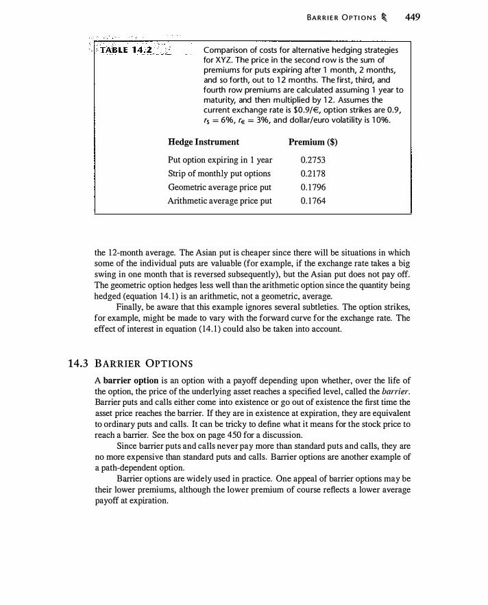
BA R R I E R O PTI O N S � 449

Comparison of costs for alternative hedging strategies for XYZ. The price in the second row is the sum of premiums for puts expiring after 1 month, 2 months, and so forth, out to 1 2 months. The first, third, and fourth row premiums are calculated assuming 1 year to maturity, and then m ultiplied by 1 2 . Assumes the current exchange rate is $0 .9/€, option strikes are 0.9, rs = 6%, r€ = 3%, and dol lar/euro volati l ity is 1 Oo/o.

Hedge Instrument Premium ($)

0.2753

0.2 178

0. 1 796

0. 1 764

Put option expiring in I year

Strip of monthly put options

Geometric average price put

Arithmetic average price put

the 12-month average. The Asian put is cheaper since there will be situations in which some of the individual puts are valuable (for example, if the exchange rate takes a big swing in one month that is reversed subsequently), but the Asian put does not pay off. The geometric option hedges less well than the arithmetic option since the quantity being hedged (equation 14. 1 ) is an arithmetic, not a geometric, average.

Finally, be aware that this example ignores several subtleties. The option strikes, for example, might be made to vary with the forward curve for the exchange rate. The effect of interest in equation ( 14. 1 ) could also be taken into account.

14.3 BARRIER OPTIONS

A barrier option is an option with a payoff depending upon whether, over the life of the option, the price of the underlying asset reaches a specified level, called the barrier. Barrier puts and calls either come into existence or go out of existence the first time the asset price reaches the barrier. If they are in existence at expiration, they are equivalent to ordinary puts and calls. It can be tricky to define what it means for the stock price to reach a barrier. See the box on page 450 for a discussion.

Since barrier puts and calls never pay more than standard puts and calls, they are no more expensive than standard puts and calls. Barrier options are another example of a path-dependent option.

Barrier options are widely used in practice. One appeal of barrier options may be their lower premiums, although the lower premium of course reflects a lower average payoff at expiration.

450 � EXOT I C O PT I O N S : I

Are Al l Barrier Options Createc f Ect�al?

One difficulty in designing a barrier option is defining the barrier. What does it mean for the S&P 500 index, for example, to "hit" the level 1500? Does it mean that the closing price exceeds 1 500? Does it mean that, at some point during the day, the reported index exce�ds that level? If so, whose report of the price is to be used?

What about manipulation of the index? Suppose the index reaches 1499.99 and then there is a large trade in a single stock, pushing the index to 1500.0 1 ." Is it possible that someone entered a buy order with the intention of manipulating the index? Since either the buyer or seller could try to

. manipulate the price, it is common to define

Types of Barrier Options

. •

a barrier using a price average computed over some period of time. An average of this type is less easily manipulated; (Concern about manipulation is one reason for the use of Asian tails, often used in securities convertible into stock.)

Barrier options sold by different firms may use different definitions of the barrier. Thus, a company might find that the barrier option it bought from Bank A to offset the option it sold to Bank B is not really an offset, because the definition of the barrier for the two options is slightly different. Hsu ( 1 997) discusses many of the practical problems that arise with barrier options.

There are three basic kinds of barrier options:

1. Knock-out options: These go out of existence (are "knocked-out") if the asset price reaches the barrier. If the price of the underlying asset has to fall to reach the barrier, the option is a down-and-out. If the price of the underlying asset has to rise to reach the barrier, the option is an up-and-out.

2. Knock-in options: These come into existence (are "knocked-in") if the barrier is touched. If the price of the underlying asset has to fall to reach the barrier, the option is a down-and-in. If the asset price has to rise to reach the barrier, it is an up-and-in.

3. Rebate options: These make a fixed payment if the asset price reaches the barrier. The payment can occur either at the time the barrier is reached, or at the time the option expires, in which case it is a deferred rebate. Rebate options can be either "up rebates" or "down rebates," depending on whether the barrier is above or below the current price.

Figure 1 4. 1 illustrates how a barrier option works. The stock price starts at around $ 1 00, ends at $80, and hits the barrier of$75 about halfway through the year. If the option were a 95-strike down-and-in put, the option would knock in and pay $ 1 5 ($95 - $80) at expiration. If the option were a down-and-out put, it would be worthless at expiration. If the option were a down-and-in call, it would knock-in at $75 but still be worthless at expiration because the stock price is below the strike price.

BA R R I E R O PT I O N S � 451

I l lustration of a barrier option where the initial stock price is $1 00 and the barrier is $ 75 . At t = 0.5 the stock hits the barrier.

Stock Price ($)

105

100

95

90

85

80

75 Barrier

Stock hits barrier

70

65

0 0.1 0.2 0.3 0.4 0.5 0.6 0 .7 0.8 0.9 1 .0

Time (years)

The formulas for the various kinds of barrier options are discussed in Chapter 22. While we mention rebate options here for completeness, we will discuss them in more detail in Chapter 22 .

. The important parity relation for barrier options is

"Knock-in" option + "Knock-out" option = Ordinary option ( 14. 1 0)

For example, for otherwise equivalent options, we have

Down-and-in call + Down-and-out call = Standard call

Since these option ·premiums cannot be negative, this equation demonstrates directly that barrier options have lower premiums than standard options.

Currency Hedging

Consider once again XYZ. Here we will focus on hedging only the cash flow occurring in 6 months to see how barrier puts compare to standard puts.

What kinds of barrier puts make sense in the context of XYZ's hedging problem? We are hedging against a decline in the exchange rate, which makes certain possibilities less attractive. A down-and-out put would be worthless when we needed it. Similarly, an

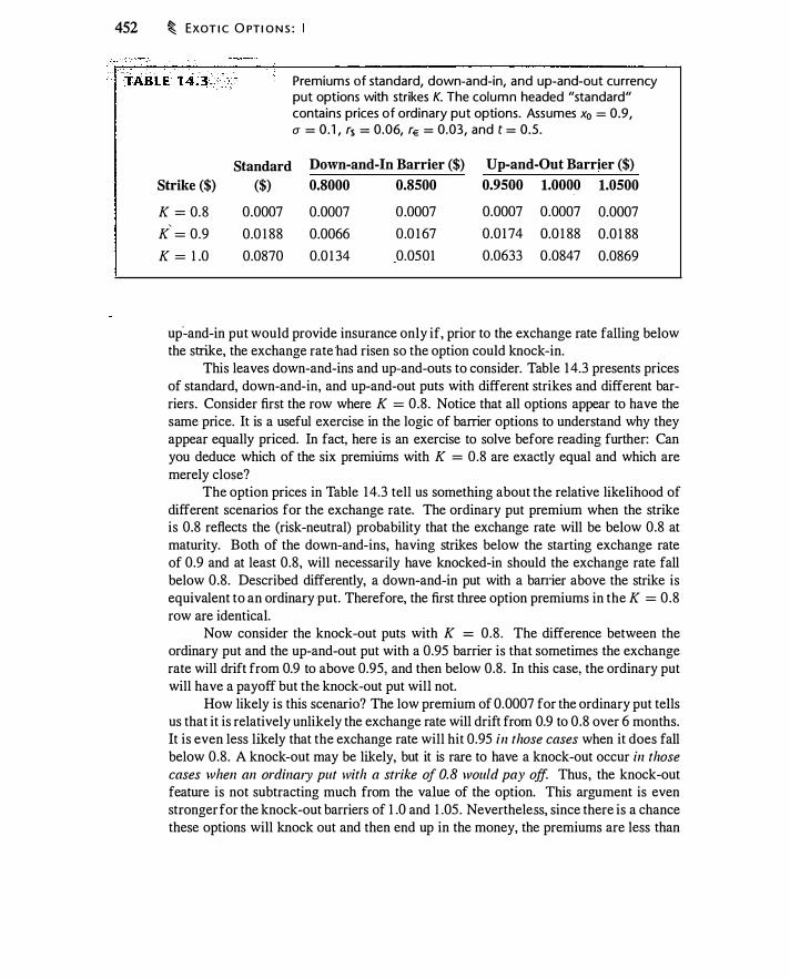
452 � EXOT I C O PT I O N S :

Standard Strike ($) ($)

K = 0.8 0.0007

K'

= 0.9 0.0 1 88

K = 1 .0 0.0870

Premiums of standard, down-and-in, and up-and-out currency put options with strikes K. The column headed "standard" contains prices of ordinary put options. Assumes x0 = 0.9, a = 0.1 , rs = 0.06, r€ = 0.03, and t = 0.5.

Do·wn-and-In Barrier ($) Up-and-Out Barrier ($)

0.8000 0.8500 0.9500 1.0000 1.0500

0.0007 0.0007 0.0007 0.0007 0.0007

0.0066 0.0 1 67 0.0 1 74 0.0 1 88 0.0 1 88

0.0 1 34 0.0501 0.0633 0.0847 0.0869

up--and-in put would provide insurance only if, prior to the exchange rate falling below the strike, the exchange rate had risen so the option could knock-in.

This leaves down-and-ins and up-and-outs to consider. Table 1 4.3 presents prices of standard, down-and-in, and up-and-out puts with different strikes and different bar­riers. Consider first the row where K = 0.8 . Notice that all options appear to have the same price. It is a useful exercise in the logic of barrier options to understand why they appear equally priced. In fact, here is an exercise to solve before reading further: Can you deduce which of the six premiums with K = 0.8 are exactly equal and which are merely close?

The option prices in Table 14.3 tell us something about the relative likelihood of different scenarios for the exchange rate. The ordinary put premium when the strike is 0.8 reflects the (risk-neutral) probability that the exchange rate will be below 0.8 at maturity. Both of the down-and-ins, having strikes below the starting exchange rate of 0.9 and at least 0.8, will necessarily have knocked-in should the exchange rate fall below 0.8. Described differently, a down-and-in put with a ban·ier above the strike is equivalent to an ordinary put. Therefore, the first three option premiums in the K = 0 .8 row are identical.

Now consider the knock-out puts with K = 0.8 . The difference between the ordinary put and the up-and-out put with a 0.95 barrier is that sometimes the exchange rate will drift from 0.9 to above 0.95, and then below 0.8. In this case, the ordinary put will have a payoff but the knock-out put will not.

How likely is this scenario? The low premium of 0.0007 for the ordinary put tells us that it is relatively unlikely the exchange rate will drift from 0.9 to 0.8 over 6 months. It is even less likely that the exchange rate will hit 0.95 in those cases when it does fall below 0.8. A knock-out may be likely, but it is rare to have a knock-out occur in those cases when an ordinGJ)' put with a strike of 0.8 would pay off. Thus, the knock-out feature is not subtracting much from the value of the option. This argument is even stronger for the knock-out barriers of 1 .0 and 1 .05 . Nevertheless, since there is a chance these options will knock out and then end up in the money, the premiums are less than

C O M PO U N D O PT I O N S � 453

for the knock-in puts and are increasing with the barrier. Thus, the up-and-out prices in the K = 0.8 row are slightly less than the price of an ordinary put.

When the strike price is 1 .0, the up-and-outs with barriers of 1 .0 and 1 .05 have substantially all the value of the ordinary put with the same strike. The interpretation is that most of the value of the puts comes from scenarios in which the option remains in-the-money; in those scenarios in which the option knocks out, the exchange rate on average does not fall enough for the option to be valuable.

14.4 COMPOUND OPTIONS

A compound option is an option to buy an option. If you think of an-ordinary option as an asset-analogous to a stock-then a compound option is similar to an ordinary option.

Compound options are a little more complicated than ordinary options because there are two strikes and two expirations, one each for the underlying option and for the compound option. Suppose that the current time is to and that we have a compound option which at time t1 will give us the right to pay x to buy a European call option with strike K. This underlying call will expire at time T > t 1 • Figure 14.2 compares the timing of the exercise decisions for this compound option with the exercise decision for an ordinary call expiring at time T .

If we exercise the compound call at time t1 , then the price of the option we receive is C (S, K, T - t1 ) . A t time T, this option will have the value max (O, Sr - K ) , the same as an ordinary call with strike K . At time ft , when the compound option expires, the value of the compound option is

The timing of exercise decisions for a

.compound cal l option on a cal l compared with an ordinary call option.

max[C (Sr1 , K, T - f t ) - x , 0]

Ordinary call

T

Buy option Option expiration

Call to buy call (compound option)

to tl

Buy compound option Decision to exercise compound option

T

Expiration of underlying option (if compound option was exercised)

454 � EXOT I C O PT I O N S : I

We only exercise the compound option if the stock price at time t1 is sufficiently grea.t that the value of the call exceeds the compound option strike price, x . Let S* be the critical stock price above which the compound option is exercised. By definition, S* satisfies

C(S* , K, T - t1 ) = x ( 1 4. 1 1 )

The compound option is exercised for S,1 > S* . Thus, in order for the compound call to ultimately be valuable, there are two events

that must take place. First, at time t1 we must have S, 1 > S* ; that is, it must be worthwhile to exercise the compound call. Second, at time T we must have ST > K ; that is, it must be profitable to exercise the underlying call. Because two events must occur, the formula for a compound call contains a bivariate cumulative normal distribution, as opposed to the univariate distribution in the Black-Scholes formula.

Formulas for the four compound options-an option to buy a call (CallOnCall), an option to sell a call (PutOnCall), an option to buy a put (Cal!OnPut, and an option to .sell a put (PutOnPut)-are in the chapter appendix. Valuing a compound option is different from valuing an ordinary option in part for mathematical rather than for con­ceptual reasons. The Black-Scholes formula assumes that the stock price is lognormally distributed. However, the price of an option-because there is a significant probability that it will be worthless--cannot be lognormally distributed. Thus, while an option on an option is conceptually similar to an option on a stock, it is mathematically different.4

The trick in deriving a formula for the price of a compound option is to value the option based on the value of the stock, w�ch is lognormally distributed, rather than the price of the underlying option, which is not lognormally distributed.

Compound Option Parity

As you might guess, there are parity relationships among the compound option prices . Suppose we buy a call on a call, and sell a put on a call, where both have the same strike, underlying option, and time to maturity. When the compound options expire, we will acquire the underlying option by paying the strike price x. If the stock price is high, we will exercise the compound call, and if the stock price is low, the compound put will be exercised and we will be forced to buy the call . Thus, the difference between the call on call and put on call premiums, plus the present value of x , must equal the premium to acquire the underlying option outright. That is,

CallOnCall(S, K, x, CJ , r, t1 , t2 , 8) - PutOnCall (S, K, x, CJ , r, t 1 , t2 , 8) + x e-r11 = BSCall (S, K, CJ , r, t2 , 8) ( 14. 1 2)

An analogous relationship holds for puts.

4Geske ( 1 979) was the first to derive the formula for a compound option.

C O M PO U N D O PTI O N S � 455

Options on Dividend-Paying Stocks

We saw in Chapter 1 1 that it is possible to price American options on dividend-paying stocks using the binomial model. It turns out that the compound option model also permits us to price an option on a stock that will pay a single discrete dividend prior to expiration.

Suppose that at time t1 the stock will pay a dividend, D. We have a choice of exercising the option at the cum-dividend price,5 S,, + D, or holding the call, which will have a: value reflecting the ex-dividend price, S, , . Thus, at t1 , the value of the call option is the greater of its exercise value, S,, + D - K, and the option valued at the ex-dividend price, C(S,, , T - lt ) :

( 1 4. 1 3)

By put-call parity, at time t1 we can write the value of the ex-dividend unexercised call as

C(S,. , T - lt ) = P (S1. , T - lt ) + S1 , - Ke-r<T-t. J

Making this substitution in equation ( 14. 1 3) and rewriting the result, w e obtain

S,, + D - K + max (P [S1. , T - t t ] - [D - K (1 - e-r(T-t • > )] , 0) ( 14. 1 4)

The value of the option is the present value of this expression. Equation ( 14. 1 4) tells us that we can value a call option on a dividend-paying stock

as the sum of the following:

1. The stock, with present value S0. (So is the present value of S,, + D.)

2. Less the present value of the strike price, K e-rt , .

3. Plus the value of a compound option-a call option on a put option-with strike price D - K ( 1 - e-r(T _,, > ) and maturity date t 1 , permitting the owner to buy a put option with strike price K and maturity date T .

I n this interpretation, exercising the compound option corresponds to keeping the option on the stock unexercised. To see this, notice that if we exercise the compound option in equation ( 14. 1 4), we give up the dividend and gain interest on the strike in order to acquire the put. The total is

S,, + P (S,, , T - ft ) - Ke-r<T-t, )

If we do not exercise the compound option, we receive the stock plus dividend, less the strike:

S,, + D - K This valuation exercise provides a way to understand early exercise. We can view exercising an American call as not exercising the compound option to buy a put in

5The stock is Cltm-di••idend if a purchaser of the stock will receive the dividend. Once the stock goes ex-di1•ideml. the purchaser will not receive the dividend.

456 � EXOT I C O PT I O N S : I

equation ( 14. 14). The cost of not exercising is that we lose the dividend, less interest on the strike. This is exactly the intuition governing early exercise that we developed in Chapters 9 and 1 1 .

Example 1 4.2 Suppose a stock with a price of$ 1 00 will pay a $5 dividend in 9 1 days (t1 = 0.249) . An option with a strike price of $90 will expire in 152 days (T = 0 .4 1 6) . Assume u = 0.3 and r = 0.08. The value of a European call on the stock is

BSCall ($ 100 - $5e-<o.osxo.249> , $90, 0 .3 , 0.08, 0.4 16, 0) = $ 1 1 .678

The value of an American call is computed as the present value of equation ( 14. 14 ), with the exercise price for the compound option equal to 5 - 90( 1 - e-o.os x (0.4 I 6-0·249) ) = 3 . 805, and time to maturity 0.249 for the compound option and 0.4 16 for the underlying option. The price of the compound option is

CallOnPut (S, K, x , u , r, t1 , T, 8) = CallOnPut ( 100, 90, 3 . 805 , 0.30, 0.08, 0.249, 0.4 16, 0) = $0.999

Thus, the value of the American option is

$ 100 - $90e-0·249xo.os + $0.999 = $ 12.774.

Moreover, the option should be exercised if the stock price cum-dividend is above $89.988. �

Currency Hedging with Compound Options

Compound options provide yet another variation on possible currency-hedging strate­gies. Instead of buying a 6-month put option on the euro, we could buy a call option on a put option. In effect, this compound option is giving us the opportunity to wait and see what happens.

Suppose that after 3 months we will decide whether to buy the put option. Here is one way to structure such a transaction. We could figure out what premium a 3-month put with a strike of $0.9 would have, if the exchange rate were still at 0.9. The Black­Scholes formula tells us that a 3-month at-the-money option with a strike of $0.9 would have a premium of $0.0146. (This value compares with the premium of $0.0 1 88 for the 6-month option from Table 14.3 .)

Now we can use the compound pricing formula to price a call on a put, setting the strike to equal $0.0 146. The price of this compound call is $0.0093 . So by paying less than two-thirds the premium of the 6-month at-the-money option, we can buy an option that permits us to pay $0.0 146 for a 3-month option. By selecting this strike, we have constructed the option so that we will exercise it if the exchange rate is below 0.9. If the exchange rate goes up, we will not exercise the option and save the premium. If the exchange rate goes down, we will acquire an in-the-money option for the price of an at-the-money option. Marty other structures are possible.

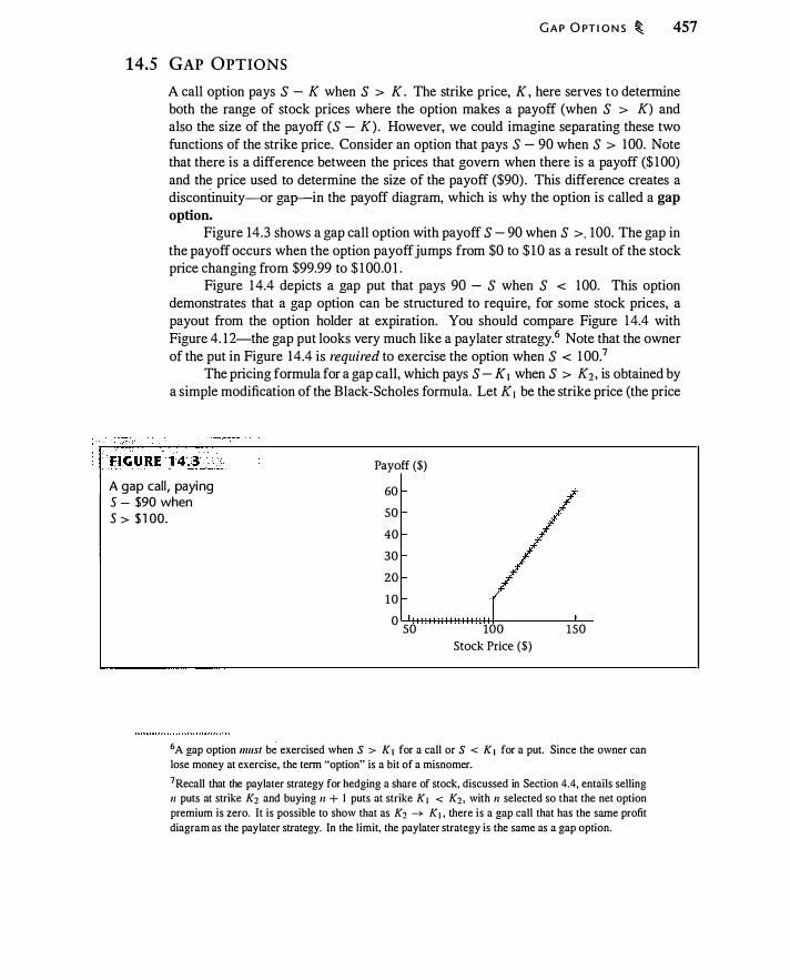
G A P O PT I O N S � 457

14.5 GAP OPTIONS

A call option pays S - K when S > K . The strike price, K , here serves to detennine both the range of stock prices where the option makes a payoff (when S > K) and also the size of the payoff (S - K). However, we could imagine separating these two functions of the strike price. Consider an option that pays S - 90 when S > 100. Note that there is a difference between the prices that govern when there is a payoff ($ 1 00) and the price used to determine the size of the payoff ($90) . This difference creates a discontinuity-or gap-in the payoff diagram, which is why the option is called a gap option.

Figure 14.3 shows a gap call option with payoff S - 90 when S >. 100. The gap in the payoff occurs when the option payoff jumps from $0 to $ 1 0 as a result of the stock price changing from $99.99 to $ 1 00.0 1 .

Figure 14.4 depicts a gap put that pays 90 - S when S < 100. This option demonstrates that a gap option can be structured to require, for some stock prices, a payout from the option holder at expiration. You should compare Figure 14.4 with Figure 4. 12-the gap put looks very much like a pay later strategy.6 Note that the owner of the put in Figure 14.4 is required to exercise the option when S < 1 00.1

The pricing formula for a gap call, which pays S - K 1 when S > K2, is obtained by a simple modification of the Black-Scholes formula. Let K 1 be the strike price (the price

A gap call, paying S - $90 when

Payoff ($)

60

s > $ 1 00. 50

40

30

20

10

0 50 100

Stock Price ($) 150

6 A gap option must b� exercised when S > K 1 for a call or S < K 1 for a put. Since the owner can

lose money at exercise, the tenn "option" is a bit of a misnomer.

7Recall that the pay later strategy for hedging a share of stock, discussed in Section 4.4, entails selling 11 puts at strike K2 and buying 11 + 1 puts at strike K1 < K2, with 11 selected so that the net option

premium is zero. It is possible to show that as K2 -->- K1 , there is a gap call that has the same profit

diagram as the pay later strategy. In the limit, the pay later strategy is the same as a gap option.

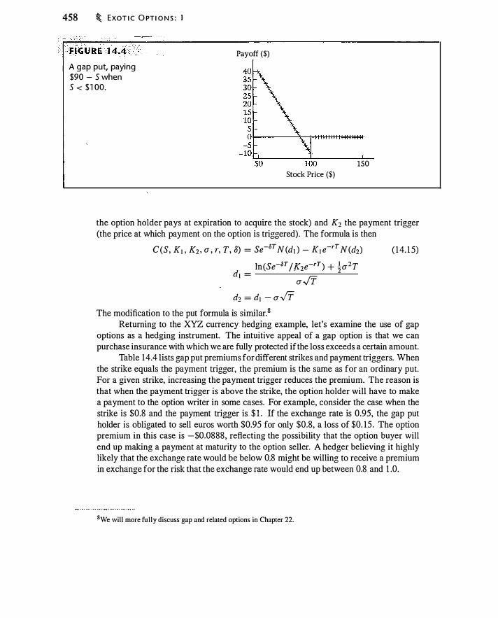
458 � EXOT I C O PT I O N S :

A gap put, paying $90 - S when s < $ 1 00.

Payoff ($)

150 Stock Price ($)

the option holder pays at expiration to acquire the stock) and K2 the payment trigger (the price at which payment on the option is triggered). The formula is then

C (S, K1 , K2 , a , r, T, 8) = Se-aT N (d! ) - K1 e-rT N (d2) ( 1 4. 1 5)

d _ ln (Se-aT I K2e-rT) + ta2T

I - a.JT d2 = d1 - a-If

The modification to the put formula is similar.8

Returning to the XYZ currency hedging example, let's examine the use of gap options as a hedging instrument. The intuitive appeal of a gap option is that we can purchase insurance with which we are fully protected if the loss exceeds a certain amount.

Table 14.4 lists gap put premiums for different strikes and payment triggers. When the strike equals the payment trigger, the premium is the same as for an ordinary put. For a given strike, increasing the payment trigger reduces the premium. The reason is that when the payment trigger is above the strike, the option holder will have to make a payment to the option writer in some cases. For example, consider the case when the strike is $0.8 and the payment trigger is $ 1 . If the exchange rate is 0.95, the gap put holder is obligated to sell euros worth $0.95 for only $0.8, a loss of $0. 15 . The option premium in this case is -$0.0888, reflecting the possibility that the option buyer will end up making a payment at maturity to the option seller. A hedger believing it highly likely that the exchange rate would be below 0.8 might be willing to receive a premium in exchange for the risk that the exchange rate would end up between 0.8 and 1 .0.

8We will more ful ly discuss· gap and related options in Chapter 22.

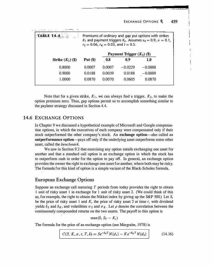
TABLE 1 4 .4 �

Strike (K1) ($)

0.8000

0.9000

1 .0000

EXC H A N G E O PT I O N S � 459

Premiums of ordinary and gap put options with strikes K1 and payment triggers K2 • Assumes x0 = 0.9, a = 0.1 , rs = 0.06, r€ = 0.03, and t = 0.5 .

Payment Trigger (K2) ($) Put ($) 0.8 0.9 1 .0

0.0007 0.0007 -0.0229 -0.0888

0.0 1 88 0.0039 0.0 1 88 -0.0009

0.0870 0.0070 0.0605 0.0870

Note that for a given strike, K1 , we can always find a trigger, K2, to make the option premium zero. Thus, gap options permit us to accomplish something similar to the paylater strategy discussed in Section 4.4.

14.6 EXCHANGE OPTIONS

In Chapter 9 we discussed a hypothetical example of Microsoft and Google compensa­tion options, in which the executives of each company were compensated only if their stock outperformed the other company's stock. An exchange option-also called an outperformance option-pays off only if the underlying asset outperforms some other asset, called the benchmark.

We saw in Section 9.2 that exercising any option entails exchanging one asset for another and that a standard call option is an exchange option in which the stock has to outperform cash in order for the option to pay off. In general, an exchange option provides the owner the right to exchange one asset for another, where both may be risky. The formula for this kind of option is a simple variant of the Black-Scholes formula.

European Exchange Options

Suppose an exchange call maturing T periods from today provides the right to obtain 1 unit of risky asset 1 in exchange for 1 unit of risky asset 2. (We could think of this as, for example, the right to obtain the Nikkei index by giving up the S&P 500.) Let S1 be the price of risky asset 1 and K1 the price of risky asset 2 at time t, with dividend yields 8 s and 8 K , and volatilities a s and a K . Let p denote the correlation between the continuously compounded returns on the two assets. The payoff to this option is

max(O, ST - Kt ) The formula for the price of an exchange option (see Margrabe, 1 978) is

( 14. 16)

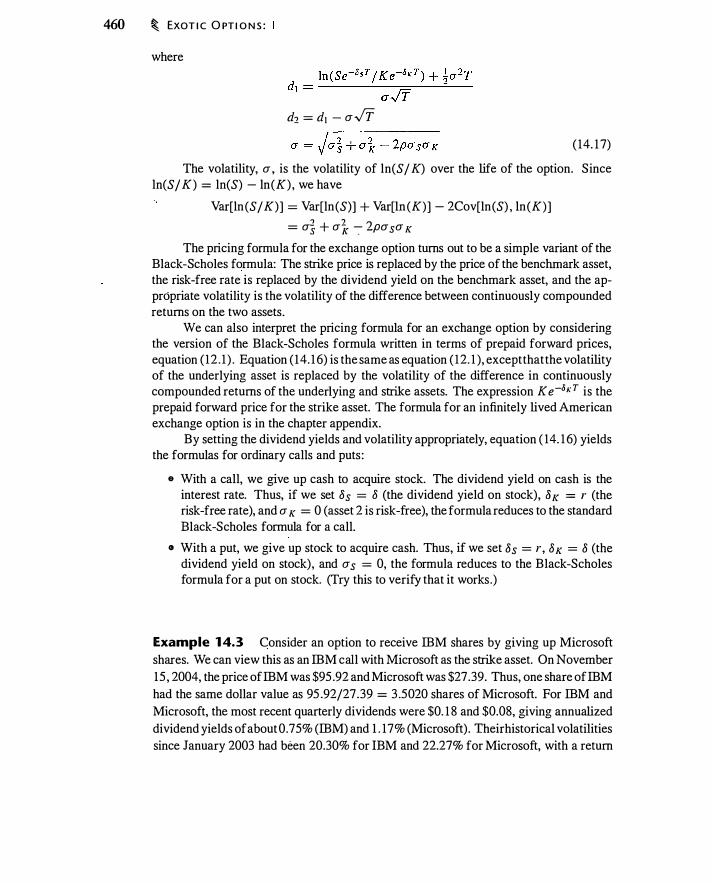
460 � EXOT I C O PT I O N S :

where

d1 = d1 - a-IT

a = Ja} + a� - 2pasaK ( 14. 1 7)

The volatility, a, is the volatility of ln(S / K) over the life of the option. Since ln(S/ K) = ln(S) - ln(K) , we have

Var[ln (S/ K)] = Var[ln(S)] + Var[ln (K)] - 2Cov[ln(S) , ln(K)] , ? ? = a5 + ak -:- _pasa K

The pricing formula for the exchange option turns out to be a simple variant of the Black-Scholes formula: The strike price is replaced by the price of the benchmark asset, the risk-free rate is replaced by the dividend yield on the benchmark asset, and the ap­propriate volatility is the volatility of the difference between continuously compounded returns on the two assets.

We can also interpret the pricing formula for an exchange option by considering the version of the Black-Scholes formula written in terms of prepaid forward prices, equation ( 12 . 1 ) . Equation ( 14. 1 6) is the same as equation ( 1 2. 1 ), except that the volatility of the underlying asset is replaced by the volatility of the difference in continuously compounded returns of the underlying and strike assets. The expression K e-"K T is the prepaid forward price for the strike asset. The formula for an infinitely lived American exchange option is in the chapter appendix.

By setting the dividend yields and volatility appropriately, equation ( 14. 1 6) yields the formulas for ordinary calls and puts :

e With a call, we give up cash to acquire stock. The dividend yield on cash is the interest rate. Thus, if we set os = o (the dividend yield on stock), OK = r (the risk-free rate), and a K = 0 (asset 2 is risk-free), the formula reduces to the standard Black-Scholes formula for a call.

e With a put, we give up stock to acquire cash. Thus, if we set os = r , oK = o (the dividend yield on stock), and as = 0, the formula reduces to the Black-Scholes formula for a put on stock. (Try this to verify that it works .)

Example 1 4.3 Consider an option to receive IBM shares by giving up Microsoft shares. We can view this as an IBM call with Microsoft as the strike asset. On November 15 , 2004, the price of IBM was $95 .92 and Microsoft was $27.39. Thus, one share of IBM had the same dollar value as 95 .92/27.39 = 3 .5020 shares of Microsoft. For IBM and Microsoft, the most recent quarterly dividends were $0. 1 8 and $0.08, giving annualized dividend yields of about 0.75% (IBM) and 1 . 17% (Microsoft). Their historical volatilities since January 2003 had been 20.30% for IBM and 22.27% for Microsoft, with a return

C H A PT E R S U M M A RY � 461

correlation of 0.6869. The volatility of the relative prices, (J, is therefore

(J = J0.20302 + 0.22272 - 2 X . 6869 X .2030 X .2227

= 0. 1 694

Suppose the option permits exchanging equal values of Microsoft for IBM, based on the November 15 prices. We could then exchange 3.5020 shares of Microsoft for 1 share of IBM. The price of a 1 -year "at-the-money" exchange call would be

BSCall ($95 .92, 3 .5020 x $27.39, 0. 1 694, 0.0 1 17 , 1 , 0.0075) = $6.6 133

Because Microsoft is the strike asset, we replace the risk-free rate 'Yith Microsoft's dividend yield. Assuming a risk-free rate of 2%, a plain 1 -year at-the-money call on IBM would be worth

BSCall ($95 .92, $95 .92, 0 .2030, 0.02, 1 , 0.007) = $8.2545

Problem 14. 1 9 asks you to think about the circumstances under which XYZ might hedge currency risk using exchange options.

CHAPTER SUMMARY

An exotic option is created by altering the contractual terms of a standard option. Exotic options permit hedging solutions tailored to specific problems and speculation tailored to particular views. Examples of exotic options include the following:

• Asian options have payoffs that are based on the average price of the underlying asset over the life of the option. The average price can be used in place of either the underlying asset (an average price option) or in place of the strike price (an , average strike option) . Averages can be arithmetic or geometric.

• Barrier options have payoffs that depend upon whether the price of the underlying asset has reached a barrier over the life of the option. These options can come into existence (knock-in options) or go out of existence (knock-out options) when the barrier is reached.

• Compound options are options on options : Put or call options with put or call options as the underlying asset.

• Gap options are options where the option payoff jumps at the price where the option comes into the money.

• Exchange options are options that have risky assets as both the underlying asset and the strike asset.

It is helpful in analyzing exotic options to compare them to standard options: In what ways does an exotic option resemble a standard option? How will its price compare

462 � EXOT I C O PT I O N S : I

to that of an ordinary option? When might someone use the exotic option instead of a standard option?

FURTHER READING

In Chapter 16 we will see some more applications of exotic options. In Chapter 21 we will discuss the underlying logic of pricing exotic options and in Chapter 22 we will discuss additional exotic options.

General books covering exotic options include Briys and Bellala ( 1998), Haug , ( 1 998), Wilmott ( 1 998), and Zhang ( 1 998). Rubinstein ( 199 1 b) discusses exchange options, Rubinstein ( 199 1 a) discusses compound options, and Rubinstein and Reiner ( 199 1 a) discuss barrier options.

PROB LEMS

To answer many of these questions you can use the exotic option functions in the spread­sheet accompanying this book.

14.1. Obtain monthly stock prices for 5 years for three stocks. Compute the arithmetic and geometric average month-end price for each stock. Which is greater?

14.2. Suppose you observe the prices {5 , 4, 5, 6, 5 } . What are the arithmetic and geo­metric averages? Now you-observe {3 , 4, 5, 6, 7 } . What are the two averages? What happens to the difference between the two measures of the average as the standard deviation of the observations increases?

14.3. Suppose that S = $100, K = $ 100, r = 0.08, a = 0.30, 8 = 0, and T = 1 . Construct a standard two-period binomial stock price tree using the method in Chapter 10.

a. Consider stock price averages computed by averaging the 6-month and 1 -year prices. What are the possible arithmetic and geometric averages after 1 year?

b. Construct a binomial tree for the average. How many nodes does it have after 1 year? (Hint: While the moves ud and du give the same year- 1 price, they do not give the same average in year 1 .)

c. What is the price of an Asian arithmetic average price call?

d. What is the price of an Asian geometric average price call?

14.4. Using the information in the previous problem, compute the prices of

a. An Asian arithmetic average strike call.

b. An Asian geometric average strike call.

14.5. Repeat Problem 14.3, except construct a three-period binomial tree. Assume that Asian options are based on averaging the prices every 4 months.

P RO B LE M S � 463

a. What are the possible geometric and arithmetic averages after 1 year?

b. What is the price of an Asian arithmetic average price call?

c. What is the price of an Asian geometric average price call?

14.6. Let S = $40, K = $45, a = 0.30, r = 0.08, T = 1, and 8 = 0.

a. What is the price of a standard call?

b. What is the price of a knock-in call with a barrier of $44. Why?

c. What is the price of a knock-out call with a barrier of $44? Why?

14.7. Let S = $40, K = $45, a = 0.30, r = 0.08, 8 = 0, and T = {0.25 , 0.5, 1 , 2, 3 , 4, 5 , 1 00} .

.

a. Compute the prices of knock-out calls with a barrier of $38.

b. Compute the ratio of the knock-out call prices to the prices of standard calls. Explain the pattern you see.

14.8. Repeat the previous problem for up-and-out puts assuming a barrier of $44.

14.9. Let S = $40, K = $45, a = 0.30, r = 0.08, and 8 = 0. Compute the value of knock-out calls with a barrier of $60 and times to expiration of 1 month, 2 months, and so on, up to 1 year. As you increase time to expiration, what happens to the price of the knock-out call? What happens to the price of the knock-out call relative to the price of an otherwise identical standard call?

14.10. Examine the prices of up-and-out puts with strikes of $0.9 and $ 1 .0 in Table 14.3. With barriers of $ 1 and $ 1 .05, the .90-strike up-and-outs appear to have the same premium as the ordinary put. However, with a strike of 1 .0 and the same barriers, the up-and-outs have lower premiums than the ordinary put. Explain why. What would happen to this pattern if we increased the time to expiration?

14.11. Suppose S = $40, K = $40, a = 0.30, r = 0.08, and 8 = 0.

a. What is the price of a standard European call with 2 years to expiration?

b. Suppose you have a compound call giving you the right to pay $2 1 year from today to buy the option in part (a). For what stock prices in 1 year will you exercise this option?

c. What is the price of this compound call?

d. What is the price of a compound option giving you the right to sell the option in part (a) in 1 year for $2?

14.12. Make the same assumptions as in the previous problem.

a. What is the price of a standard European put with 2 years to expiration?

b. Suppose you have a compound call giving you the right to pay $2 1 year from today to buy the option in (a) . For what stock prices in 1 year will you exercise this option?

c. What is the price of this compound call?

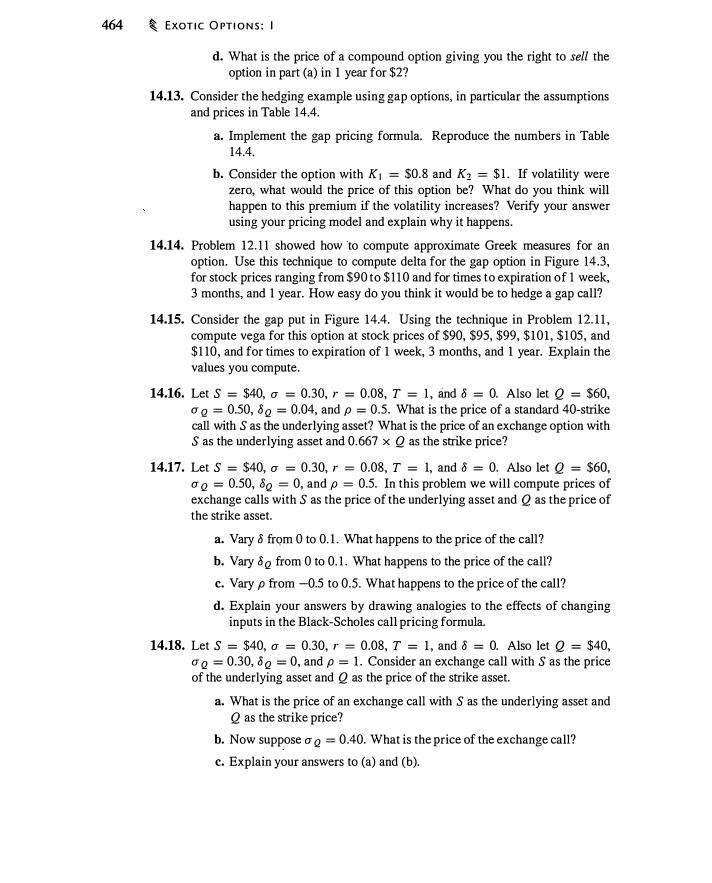
464 � EXOT I C O PT I O N S : I

d. What is the price of a compound option giving you the right to sell the option in part (a) in 1 year for $2?

14.13. Consider the hedging example using gap options, in particular the assumptions and prices in Table 14.4.

a. Implement the gap pricing formula. Reproduce the numbers in Table 14.4.

b. Consider the option with K1 = $0.8 and K2 = $ 1 . If volatility were zero, what would the price of this option be? What do you think will happen to this premium if the volatility increases? Verify your answer using your pricing model and explain why it happens.

14.14. Problem 12. 1 1 showed how to compute approximate Greek measures for an option. Use this technique to compute delta for the gap option in Figure 14.3, for stock prices ranging from $90 to $ 1 1 0 and for times to expiration of 1 week, 3 months, and 1 year. How easy do you think it would be to hedge a gap call?

14.15. Consider the gap put in Figure 14.4. Using the technique in Problem 1 2. 1 1 , compute vega for this option at stock prices of $90, $95, $99, $ 1 0 1 , $ 1 05 , and $ 1 10 , and for times to expiration of 1 week, 3 months, and 1 year. Explain the values you compute.

14.16. Let S = $40, u = 0.30, r = 0.08, T = 1 , and 8 = 0. Also let Q = $60, u Q = 0.50, 8 Q = 0.04, and p = 0.5. What is the price of a standard 40-strike call with S as the underlying asset? What is the price of an exchange option with S as the underlying asset and 0.667 x Q as the strike price?

14.17. Let S = $40, u = 0.30, r = 0.08, T = 1, and 8 = 0. Also let Q = $60, u Q = 0.50, 8Q = 0, and p = 0.5. In this problem we will compute prices of exchange calls with S as the price of the underlying asset and Q as the price of the strike asset.

a. Vary 8 frqm 0 to 0. 1 . What happens to the price of the call?

b. Vary 8 Q from 0 to 0. 1 . What happens to the price of the call?

c. Vary p from -0.5 to 0.5. What happens to the price of the call?

d. Explain your answers by drawing analogies to the effects of changing inputs in the Black-Scholes call pricing formula.

14.18. Let S = $40, u = 0.30, r = 0.08, T = 1 , and 8 = 0. Also let Q = $40, u Q = 0.30, 8 Q = 0, and p = 1 . Consider an exchange call with S as the price of the underlying asset and Q as the price of the strike asset.

a. What is the price of an exchange call with S as the underlying asset and Q as the strike price?

b. Now suppose u Q = 0.40. What is the price of the exchange call?

c. Explain your answers to (a) and (b).

P RO B LE M S � 465

14.19. XYZ wants to hedge against depreciations of the euro and is also concerned about the price of oil, which is a significant component of XYZ's costs. However, there is a positive correlation between the euro and the price of oil : The euro appreciates when the price of oil rises. Explain how an exchange option based on oil and the euro might be used to hedge in this case.

14.20. A chooser option (also known as an as"you-like-it option) becomes a put or call at the discretion of the owner. For example, consider a chooser on the S&R index for which both the call, with value C ( S1 , K, T - t) , and the put, with value P (S1 , K, T - t) , have a strike price of K. The index pays no dividends. At the choice date, t 1 , the payoff of the chooser is

max[C (S1" K, T - t1 ) , P (S1" K, T - ti ) ]

a. If the chooser option and the underlying options expire simultaneously, what ordinary option position is this equivalent to?

b. Suppose that the chooser must be exercised at t1 and that the underlying options expire at T. Show that the chooser is equivalent to a call option with strike price K and maturity T plus e-li(T -to > put options with strike price K e-(r-li) (T -to > and expiration t1 .

14.21. Suppose that S = $ 1 00, u = 30%, r = 8%, and 8 = 0. Today you buy a contract which, 6 months from today, will give you one 3-month to expiration at-the-money call option. (This is called a forward start option.) Assume that r, u , and 8 are certain not to change in the next 6 months.

a. Six months from today, what will be the value of the option if the stock price is $ 1 00? $50? $200? (Use the Black-Scholes formula to compute the answer.) In each case, what fraction of the stock price does the option cost?

b. What investment today would guarantee that you had the money in 6 months to buy an at-the-money option?

c. What would you pay today for the forward start option in this example?

d. How would your answer change if the option were to have a strike price that was 1 05% of the stock price?

14.22. You wish to insure a portfolio for 1 year. Suppose that S = $ 100, u = 30%, r = 8%, and 8 = 0. You are considering two strategies. The simple insurance strategy entails buying one put option with a 1 -year maturity at a strike price that is 95% of the stock price. The rolling insurance strategy entails buying one 1 -month put option each month, with the strike in each case being 95% of the then-current stock price.

a. What is the cost of the simple insurance strategy?

b. What is the cost of the rolling insurance strategy? (Hint: See the previous problem.)

c. Intuitively, what accounts for the cost difference?

466 � EXOT I C O PT I O N S : I

APPENDIX 14 .A: PRICING FORMULAS FOR EXOTIC OPTIONS

In this appendix we present formulas for some of the options discussed in this chapter.

Asian Options Based on the Geometric Average

The average can be used in place of either the asset price (an average price option) or the strike price (an average strike option).

Average price options Suppose the risk-free rate is r and the stock has a dividend yield 8 and volatility u. We compute the average using N equally spaced prices from 0 to T , with the first observation at time T / N. A European geometric average price option can then be valued using the Black-Scholes formula for a call by setting the dividend yield and volatility equal to

and

* 1 [ N - 1 � N + 1 u2 (N + 1 ) (2N + 1 ) J o = 2 r -N- + (o + O.Su-) -

N- - -

N-2 ___

6 __ _

u*

= :!._ j (N + 1 ) (2N + 1 ) N V 6

With continuous sampling, i .e . , N = oo, the formulas reduce to

and

"' 1 ( 1 �) o · = 2 r + o + 6u-

. {1 u" = U v 3

( 1 4. 1 8)

( 1 4. 1 9)

Deriving these results is easier than you might guess, but requires some background covered in Chapters 18 and 19 . The derivation is in Appendix 19 .A.

Average strike options In order to value the geometric average strike option, we need to know the correlation between the average, G(T) , and the terminal stock price, ST . We also need to recognize that the strike asset is the average; hence, we value the option like an exchange option (see Section 14.6), in which we exchange the time-T stock price for its average.

In Appendix 19 .A, we show that the average strike option can be valued using the Black-Scholes forrimla, with the following substitutions:

a Replace the risk-free rate with the "dividend yield," equation ( 14. 1 8).

e Replace the volatility with

** _

r;:;; (N + l ) (2N + 1 ) _ ? J (N + 1 ) (2N + 1 ) u - u v T 1 +

6N2 -P 6N2

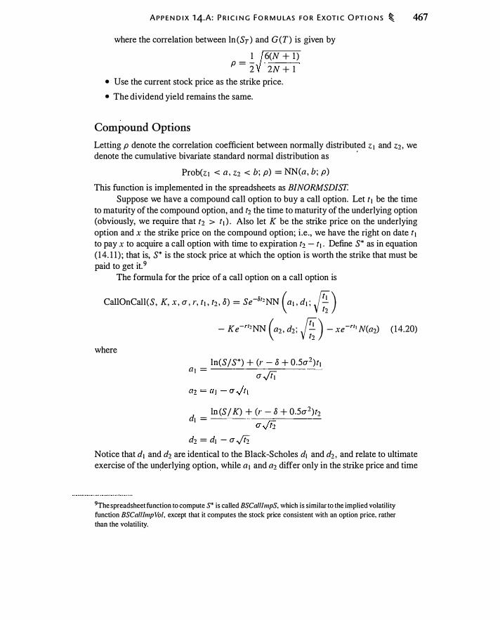
A P P E N D I X 1 4.A: P R I C I N G F O R M U LAS FO R EXOT I C O PT I O N S � 467

where the correlation between ln (ST ) and G (T) is given by

I 6(N + I ) p = -

2 2N + I • Use the current stock price as the strike price.

• The dividend yield remains the same.

Compound Options

Letting p denote the correlation coefficient between normally distributed z 1 and z2 , we denote the cumulative bivariate standard normal distribution as

'

Prob(z , < a , zz < b; p) = NN(a, b; p)

This function is implemented in the spreadsheets as BINORMSDIST. Suppose we have a compound call option to buy a call option. Let t1 be the time

to maturity of the compound option, and t2 the time to maturity of the underlying option (obviously, we require that tz > t1 ) . Also let K be the strike price on the underlying option and x the strike price on the compound option; i .e. , we have the right on date t 1 to pay x to acquire a call option with time to expiration t2 - t1 • Define S* as in equation ( 14. 1 1 ) ; that is, S* is the stock price at which the option is worth the strike that must be paid to get it. 9

The formula for the price of a call option on a call option is

CallOnCall(S, K, X , CJ , r, r, , tz , o) = se-012NN (a , , d, ; /f;)

where

a , =

- K e-r12NN ( a2 , dz ; /f;) - xe-n' N(az) ( 14.20)

ln(S IS*) + (r - o + 0.5CJ2)t1 CJ ,Jtj

In (S I K) + (r - o + 0.5CJ2)tz d, = ----------��--------

CJ .ji2 dz = d, - CJ .ji2

Notice that d1 and d2 are identical to the Black-Scholes d1 and d2 , and relate to ultimate exercise of the underlying option, while a 1 and a2 differ only in the strike price and time

9The spreadsheet function to compute S* is called BSCalllmpS, which is similar to the implied volatility

function BSCalllmpVo/, except that it computes the stock price consistent with an option price, rather

than the volatility.

468 � EXOT I C O PT I O N S : I

to expiration and relate to exercise of the compound option. The last term in equation ( 14.20) reflects payment of the compound option strike price and the condition under which it is paid. The sign on the correlation term, ..fi1Ti2, reflects whether exercise of the compound option is associated with an increase or decrease in the likelihood of exercising the underlying option. (The correlation is positive for a call on a call. For a call on a put, an increase in the stock price reduces the value of the put and also reduces the value of the option to buy the put; hence, the correlation is again positive.)

This discussion suggests that we can guess how the remaining compound option formulas will look. We would like to value puts on calls, calls on puts, and puts on puts.

The put on the call requires a positive sign on Ke-rr and a negative sign on se-81 , since the option if ultimately exercised will require the owner to be a call writer. The underlying option is in-the-money if S > K; hence, we want positive d1 and d2 • The compound option will be exercised and the strike X received if s < S* , which requires negative a 1 and a2 and a positive sign on x. Finally, if the stock price goes up, this increases the value of the call and decreases the value of the put on the call ; hence, the correlation must be negatively signed. Thus, the formula is

PutOnCall(S, K, x , CJ , r, tJ , t2 , 8) = -se-811NN ( -a1 , d1 ; -If;)

+ K e-r11NN ( -a2 , d2 ; -If;) + xe-rr, N( -a2) ( 14.2 1 )

Similar arguments give us the following formulas:

CallOnPut(S, K, x , CJ , r, t 1 , t2 , 8) = -se-811NN ( -a J , -d1 ; If;)

+ K e-r11NN ( -a2 , -d2 ; /f;) - xe-rt ' N ( -a2) ( 14.22)

PutOnPut(S, K, X, (J, r, f] , t2 , 8) = se-812NN (a ] , -dl ; -If;)

- Ke-r12NN (a2 , -d2 ; -If;) + xe-rt' N (a2) ( 14.23)

As an exercise, we can check that as t 1 approaches 0, the compound option formula simplifies to the greater of the value of the underlying option or zero.

Infinitely Lived Exchange Option

The logic of exchange options extends directly to the case of an infinitely lived American option. A key insight is that the optimal exercise level H really depends on the ratio of the values of the asset being received to the asset being given up; the absolute level is unimportant. Thus, if it is optimal to exchange stock A for stock B when the price of A is 100 and the price of B is 200, then it will be optimal to exchange A for B when their prices are 1 and 2. We therefore just need to find the ratio of prices at which exercise is optimal.

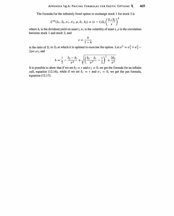
A P P E N D I X 1 4.A : P R I C I N G F O R M U LAS F O R EXOT I C O PT I O N S � 469

The formula for the infinitely lived option to exchange stock 1 for stock 2 is

oo ( S1 /Sz ) " C (S1 , Sz , cr 1 , cr2 , p , 8 1 , 82) = (s - 1 ) Sz -s-

where 8; is the dividend yield on asset i, cr; is the volatility of asset i, p is the correlation between stock 1 and stock 2, and

h S = --

1 - h is the ratio of S1 to S2 at which it is optimal to exercise the option. Let cr2 = crf + cr� -2pcr 1 cr2 and

It is possible to show that if we set 82 = r and cr 2 = 0, we get the formula for an infinite call, equation ( 1 2. 1 6), while if we set 8 1 = r and cr 1 = 0, we get the put formula, equation ( 12. 1 7) .

PART FOUR

Z the preceding chapters we have focused on fon�·ards, swaps, and op­

tions (including exotic options) as stand-alone financial claims. In the

next three chapters we will see that these claims can be used as finan­

cial building blocks to create new claims, and also see that derivatives

pricing theory can help us understand corporate financial policy and the

valuation of investment projects;

Specifically, in Chapter 15 we see how it is possible to construct and

price bonds that make payments that, instead of being denominated in

cash, are denominated in stocks, commodities, and different currencies.

Such bonds can be structured to contain embedded options. We also

see how such claims can be used for risk management and how tlzeit

issuance can be motivated by tax and regulatory considerations. Chapter

16 examines some corporate contexts in which derivatives are important,

including corporate financial policy, compensation options, and mergers.

Chapter 17 examines rea/options, in which the insights from derivatives

pricing are used to value investment projects.

471

Financial Engineering and Securi� Design

E.-ward,, c,ll,, P""· ""d common exotic option' can be •dded to bond' o< othe<wi'e combined to create new securities. For example, many traded securities are effectively bonds with embedded options. Individual derivatives thus become building blocks­ingredients used to construct new kinds of financial products. In this chapter we will see how to assemble the ingredients to create new products. The process of constructing new instruments from these building blocks is called financial engineering.

15 .1 THE MODIGLIANI-MILLER THEOREM

The starting point for any discussion of modern financial engineering is the analysis of Franco Modigliani and Merton Miller (Modigliani and Miller, 1 958) . Before their work, financial analysts would puzzle over how to compare the values of firms with similar operating characteristics but different .financial characteristics. Modigliani and Miller realized that different financing decisions (for example, the choice of the firm's debt-to-equity ratio) may carve up the firm's cash flows in different ways, but if the total cash flows paid to all claimants is unchanged, the total value of all claims would remain the same. They showed that if firms differing only in financial policy differed in market value, profitable arbitrage would exist. Using their famous analogy, the price of whole milk should equal the total prices of the skim milk and butterfat that can be derived from that milk.1

The Modigliani-Miller analysis requires numerous assumptions : For example, there are no taxes, no transaction costs, no bankruptcy costs, and no private information. Nevertheless, the basic Modigliani-Miller result provided clarity for a confusing issue, and it created a starting point for thinking about the effects of taxes, transaction costs, and the like, revolutionizing finance.

All of the no-arbitrage pricing arguments we have been using embody the Modigliani-Miller spirit. For example, we saw in Chapter 2 that we could syntheti­cally create a forward contract using options, a call option using a forward contract,

1 Standard corporate finance texts offer a more detailed discussion of the Modigliani-Miller results.

The original paper (Modigliani and Miller, 1 958) is a classic.

473

474 � F I N A N C I A L E N G I N E E R I N G A N D S E C U R ITY D ES I G N

bonds, and a put, and so forth. In Chapter 10 we saw that an option could also be synthetically created from a position in the stock and borrowing or lending. If prices of actual claims differ from their synthetic equivalents, arbitrage is possible.

Financial engineering is an application of the Modigliani-Miller idea. We can combine claims such as stocks, bonds, forwards, and options and assemble them to create new claims. The price for this new security is the sum of the pieces combined to create it. When we create a new instrument in this fashion, as in the Modigliani­Miller analysis, value is neither created nor destroyed. Thus, financial engineering has no value in a pure Modigliani-Miller world. However, in real life, the new instrument

, may have different tax, regulatory, or accounting characteristics, or may provide a way for the issuer or buyer to obtain a particular payoff at lower transaction costs than the alternatives. Financial engineering !hus provides a way to create instruments that meet specific needs of investors and issuers .

As a starting point, you can ask the following questions when you confront new financial instruments :

• What is the payoff of the instrument?

• Is it possible to synthetically create the same payoffs using some combination of assets, bonds, and options?

• Who might issue or buy such an instrument?

• What problem does the instrument solve?

15 .2 PRICING AND DESIGNING STRUCTURED NOTES

We begin by examining structured notes. An ordinary note (or bond) has interest and maturity payments that are fixed at the time of issue. A structured note has interest or maturity payments that are not fixed in dollars but are contingent in some way. Structured notes can make payments based on stock prices, interest rates, commodities, or curren­cies, and they can have options embedded in them. The equity-linked CD discussed in Chapter 2 is an example of a structured note, as it has a maturity payment based upon the performance of the S&P 500 index. In this section we discuss structured notes without options. In the next section we will introduce notes with options .

Zero-Coupon Bonds

The most basic financial instrument is a zero-coupon bond. As in Chapter 7, let r5 (t0 , t1 ) represent the annual continuously compounded interest rate prevailing at time s ::::: t0 , for a loan from time to to time t1 • Similarly, the price of a zero-coupon bond purchased at time t0, maturing at time t1 , and quoted at time s is P5(t0 , tJ ). Thus, we have

Ps(to , t!) = e-rs(lo.t.J(to-to>

When there is no risk· of misunderstanding, we will assume that the interest rate is quoted at time t0 = 0, and the bond is also purchased then. We will denote the rate

P R I C I N G A N D D ES I G N I N G STR U CTU R E D N OTES � 475

r0 (0, t) = r(t), and the corresponding bond price P1• So we will write

Pr = e-r(t )t

P1 is the current price of a t-period zero-coupon bond. There are two important, equivalent interpretations of P1• First, P1 is a discount

factor, since it is the price today for $1 delivered at time t. Second, P1 is the prepaid forward price for $1 delivered at time t . These are different ways of saying the same thing:_

Zero-coupon bond price = Discount factor for $1 = Prepaid forward price for $ 1

Financial valuation entails discounting, which i s why zero-coupon bonds are a basic building block. The notion that prepaid forward prices are discount factors will play an important role in this chapter.

Coupon Bonds

Once we have a set of zero-coupon bonds, we can analyze other fixed payment instru­ments, such as ordinary coupon bonds. Consider a bond that pays the coupon c, 11 times over the life of the bond, makes the maturity payment M, and matures at time T . We will denote the price of this bond as B(O, T, c, 11, M). The time between coupon payments is T 111, and the ith coupon payment occurs at time t; = i x T I 11.

We can value this bond by discounting its payments at the interest rate appropriate for each payment. This bond has the price

II B(O, T, c, II, M) = L ce-r(t; )t; + M e-r(T)T

i=l II

= L cP11 + MPr i=l

( 1 5 . 1 )

This valuation equation shows us how to price the bond and also how to replicate the bond using zero-coupon bonds. Suppose we buy c zero-coupon bonds maturing in 1 year, c maturing in 2 years, and so on, and c + M zero-coupon bonds maturing in T years. This set of zero-coupon bonds will pay c in 1 year, c in 2 years, and c + M in T years. We can say that the coupon bond is engineered from a set of zero-coupon bonds with the same maturities as the cash flows from the bond.

In practice, bonds are usually issued at par, meaning that the bond sells today for its maturity value, M. We can structure the bond to make this happen by setting the coupon so that the price of the bond is M. Using equation (15 . 1 ), B (O, T, c, 11, M) = M if the coupon is set so that

( 1 - Pr) c = M �11 Li=l Pr;

( 15 .2)

We have seen this formula before. It appeared in Chapter 7 and it was also the formula for the swap rate, equation (8.3) in Chapter 8 .

476 � F I N A N C I A L E N G I N E E R I N G A N D S EC U R ITY D ES I G N

Equity-Linked Bonds

In this section we discuss pricing of various types of equity-linked bonds. Specifically, we consider a bond that, instead of paying M in cash at maturity, pays one share of XYZ stock at maturity. With this change in terms, the bond has an uncertain maturity value. Moreover, this change raises questions. What does it mean for such a bond to sell at par? If there are coupon payments, should they be paid in cash or in shares of XYZ? For regulatory and tax purposes, is this instrument a stock or a bond?

Zero-coupon equity-linked bond Suppose an equity-linked bond pays the bond­, holder one share of stock at time T. There are no interim payments. What is a fair price for this bond?

Although the language is now ·different, this valuation problem is the same as that of valuing a prepaid forward contract, which we analyzed in Chapter 5. In both cases the investor pays today to receive a share of stock at time T. In the context of this chapter, we could also call this instrument a zero-coupon equity-linked bond. Recall from Chapter 5 that the prepaid forward price is the present value of the forward price, Fcfr = PrFo.T· This relationship implies that for a nondividend-paying stock, Fri,T = e-rT S0e<r-8)T = So since 8 = 0. The prepaid forward price is the stock price.

Example 1 5. 1 Suppose that XYZ stock has a price of $100 and pays no dividends, and that the annual continuously compounded interest rate is 6%. In tlze absence of dividends, the prepaidfonvard price equals tlze stock price. Thus, we would pay $100

L to receive the stock in 5 years. �

This example shows that if we issue a bond promising to pay one share of a nondividend-paying stock at maturity, and the bond pays no coupon, then the bond will sell for the current stock price. In general, a bond is at par if the bond price equals the maturity payment of the bond. The bond in Example 15 .1 is at par since the bond pays one share of stock at maturity and the price of the note equals the price of one share of stock today.

Suppose the stock makes discrete dividend payments of Dr,. Then we saw in Chapter 5 that the prepaid forward price is

II Fri,T = So - L Pr, Dr,

i=l (15 .3)

If the stock pays dividends and the bond makes no coupon payments, the bond will sell at less than par.

Example 1 5.2 Suppose the price of XYZ stock is $100, the quarterly dividend is $1.20, and the annual continuously compounded interest rate is 6% (the quarterly interest

P R I C I N G A N D D ES I G N I N G STR U CTU R E D N OTES � 477

rate is therefore 1 .5%). From equation ( 15 .3) , the 5-year prepaid forward price for XYZ IS

20 $100- L$1.20e-O.OI5xi = $79.42

i=l

Thus, a zero-coupon equity-linked bond promising to pay one share of XYZ in 5 years would _have a price of $79.42. � Cash coupon payments We now add cash coupon payments to the bond. Represent the price of a bond paying n coupons of c each and a share at maturity as B(O, T, c, n , Sr ) . The valuation equation for such a note-the analog of equation ( 1 5 . 1 )-is

II B(O, T, c, n , Sr) = c L P1; + Fcf.7

i=l ( 1 5 .4)

The value today of the maturity payment, which is one share of stock, is the prepaid forward price, Fcf.7.

If the stock pays dividends, then in order for the bond to sell at par-the current price of the stock-it must make coupon payments. In particular, the note must pay coupons with a present value equal to the presellf value of dividends over the life of the note. To see this, use equation ( 15 .3) to rewrite equation ( 1 5 .4):

I I I I B(O, T, c, n, Sr) = c L P1; +So-L P1;DI;

i=l i=l

In words: The price of the bond, B , will equal the stock price, S0, as long as the present value of the bond's coupons (the first term on the right-hand side) equals the present value of the stock dividends (the third term on the right-hand side) .

In general, if we wish to price an equity-linked note at par, from equation ( 1 5 .4), the bond price B will equal the stock price, S0, if the coupon, c, is set so that

So- F{7 c = ��� ,

L...i=l PI; ( 1 5 .5)

That is, the coupon must amortize the difference between the stock price and the prepaid forward price.

7 Example 1 5.3 Consider XYZ stock as in Example 15 .2. If the note promised to pay $ 1 .20 quarterly-a coupon equal to the stock dividend-the note would sell for $100. �

Notice that equation ( 1 5.5) is the same as the equation for a par coupon on a cash bond, equation ( 1 5 .2). Instead of 1 - Pr in the numerator, we have So- F{7. The former is the difference between the price of $1 and the prepaid forward pric� for $ 1

478 � F I N A N C I A L E N G I N E E R I N G A N D S EC U R I TY D ES I G N

delivered at time T. The latter is the difference between the price of one share and the prepaid forward price for one share delivered at time T.

In practice, dividends may change unexpectedly over the life of the note. The note issuer must decide: Should the dividend on the note change to match the dividend paid by the stock, or should the dividend on the note be fixed at the outset using equation ( 1 5 .5)? The price should be the same in either case, but a different party bears dividend risk.

Interest in-kind An alternative to paying interest in cash is to pay interest in fractional shares. For example, the coupon could be the value of 2% of a share at the time of payment, rather than a fixed $2. To price such a bond, we represent the number of fractional shares received at each coupon payment as c*. The value at time 0 of a share received at time t is Fcf.1• Thus, the formula for the value of the note at time t0, V0 is

II

Vo = c* L Fci,1, + Fcf.T i=l

The number of fractional shares that must be paid each year for the note to be initially priced at par, i .e. , for V0 = S0, is

So- FrJT c* = n � Li=l Fo,r1

( 15 .6)

When we pay coupons as shares rather than cash, the coupons have variable value. Thus, it is appropriate to use the prepaid forward for the stock as a discount factor rather than the prepaid forward for cash.

In the special case of a constant expected continuous dividend yield, 8, this equation becomes

. 1 - e-8T c"' = =::------=-'\'11 -81; L..,i=l e

( 1 5 .7)

We can compare this expression for c* with that for the coupon on an ordinary cash bond. In the special case of a constant interest rate and assuming a $1 par value, equation (15.2) becomes

c = =::----­'\'11 -n L..,i=l e ' ( 1 5 .8)

Comparing the equations for c and c* makes it apparent that the appropriate discount factor for a coupon is determined from the lease rate on the underlying asset. In the case of a bond denominated in cash, the lease rate is the interest rate, while in the case of a bond completely denominated in shares, the lease rate is the dividend yield.

Commodity-Linked Bonds

Now we repeat the analysis of the previous section, except that instead of paying a share of stock at maturity, we suppose the note pays one unit of a commodity. We ask the same questions about how to structure this note. We will see that the commodity lease rate

P R I C I N G A N D D ES I G N I N G STR U CTU R E D N OTES � 479

replaces the dividend yield. A commodity-linked note will pay a coupon if the lease rate is positive, and the present value of coupon payments on the note must equal the present value of the lease payments on the commodity.

Zero-coupon commodity-linked bonds Suppose we have a note that pays one unit of a commodity in the future, with no interim cash flows. What is the price of the note? Once again, the answer is, by definition, the present value of the forward price, or the prepaid· forward price. As we saw in Chapter 6, the difference between the spot price and the prepaid forward price is summarized by the lease rate. Thus, the discount from the spot price on a zero-coupon note reflects the lease rate.

Example 1 5.4 Suppose the spot price of gold is $400/oz. , the 3-year forward price is $455/oz., and the 3-year continuously compounded interest rate is 6.25%. Then a zero-coupon note paying 1 ounce of gold in 3 years would sell for

Fci,r = $455e-0·0625 x3 = $377.208

This amount is less than the spot price of $400 because the lease rate is positive. � Cash interest Suppose we have a commodity with a current price of S0 and a forward price of Fo.r. and we have a commodity-linked note paying a cash coupon. For the note to sell at par, we need to set the coupon so that

II So= c L P,, + PrFo.T

i=l

Since by definition of the prepaid forward price, Pr Fo.T = FrJ T• we have

So- Fci,r c = "'" L-i=l P,,

exactly as with a dividend-paying stock. The coupon serves to amortize the lease rate. Thus, the lease rate plays the role of a dividend yield in pricing a commodity-linked note. The present value calculation treats the lease rate exactly as if it were a dividend yield; what matters is that there is a difference between the prepaid forward price and the current spot price.2

8 Example 1 5.5 Suppose the spot price of gold is $400/oz. , the 3-year forward price is $455/oz., the 1 -year continuously compounded interest rate is 5 .5%, the 2-year rate is

2 As we saw in Chapter 6, a lease rate can be negative if there are storage costs. In this case, the holder

of a commodity-linked note benefits by not having to pay storage costs associated with the physical

commodity and will therefore pay a price above maturity value (in the case of a zero-coupon note) or

else the note must carry a negative dividend, meaning that the holder must make coupon payments to

the issuer.

480 � F I N A N C I A L EN G I N E E R I N G A N D S EC U R ITY D ES I G N

6%, and the 3-year rate i s 6.25%. The annual coupon i s then determined as

c = __ $400 - $3

?77 .208

?- = $8.56 1

e-O.O:l:l + e-0.06x_ + e-0.06_Jx3

The annual coupon on a 3-year gold-linked note is therefore about 2% of the spot price. �

A 2% yield in this example might seem like cheap financing, but this is illusory and stems from denominating the note in terms of gold. When the yield on gold (the lease rate) is less than the yield on cash (the interest rate), the yield on a gold-denominated note is less than the yield on a dollar-denominated note. This effect is reversed in cases where the interest rate in a particular currency is below the lease rate of gold. In Japan during the late 1 990s, the yen-denominated interest rate was close to zero, so the coupon rate on a gold note would have been greater than the interest rate on a yen-denominated note.

Interest in-kind As with stocks, we can pay fractional units of the commodity as a periodic interest payment. The present value of the payment at time t is computed using the prepaid forward price, Fcfr Thus the value of a commodity-linked note at par is exactly the same as for an equity-linked note paying interest in-kind:

II -* "\' p p

So = c L...., Fo,t, + Fo. r

i = l The formula for c* is given by equation ( 1 5 .6).

Perpetuities A perpetuity is an infinitely lived coupon bond. We can use equations ( 15.7) and ( 1 5 .8) to consider two perpetuities: one that makes annual payments in dollars and another that pays in units of a commodity. Suppose we want the dollar perpetuity to have a price of M and the commodity perpetuity to have a price of S0. Using standard perpetuity calculations, if we let T -+ oo in equation ( 15.8) (this also means that n -+ oo ), the coupon rate on the dollar bond is

1 r �

c = M---;=r = M (e - 1 ) = rM

1-e-' where r is the effective annual interest rate. Similarly, for a perpetuity paying a unit of a commodity, equation ( 15.7) becomes

1 8 �

c* = So�

= So(e - 1 ) = 8So

1-e-•

where 8 is the effective annual lease rate. Thus, in order for a commodity perpetuity to be worth one unit of the commodity, it must pay the lease rate in units of the commodity. (For example, if the lease rate is 2%, the bond pays 0.02 units. of the commodity per year.)

P R I C I N G A N D D ES I G N I N G STR U CTU R E D N OTES � 481

What if a bond pays one unit of the commodity per year, forever? We know that if it pays 8 S, in perpetuity it is worth S0. Thus, if it pays S, it is worth

So 8 ( 15 .9)

This is the commodity equivalent of a perpetuity. The conclusion of this section is simple: Commodity-linked notes are formally

like equity-linked notes, with the lease rate taking the place of the dividend yield.

Currency-Linked Bonds

What happens if we change the currency of denomination of the bond? As you can probably guess by now, the foreign interest rate, being the lease rate on the foreign currency, takes the place of the dividend yield on the stock.

Suppose that we want to compare issuing a par-coupon bond denominated entirely in dollars and a par-coupon bond denominated entirely in another currency. We will let BF denote zero-coupon bond prices denominated in the foreign currency, rF(t) the foreign interest rate, and P/ the price of a zero-coupon bond denominated in the foreign currency.

As you would expect, a bond completely denominated in a foreign currency will have a coupon given by the formula

F 1 - P{ c = M II F Li=l P,, In other words, foreign interest rates are used to compute the coupon.

What happens when the principal, M, is in the domestic currency and the interest payments are in the foreign currency? Once again we just solve for the coupon payment that makes the bond sell at par. There are two ways to do this.

First, we can discount the foreign currency coupon payments using the foreign interest rate, and then translate their value into dollars using the current exchange rate; x0 (denominated as $/unit of foreign currency). The value of the ith coupon is x0P/ c, and the value of the bond is

II B(O, T, cF, II, M) = x0cF L P/: + M Pr

i=l Alternatively, we can translate the future coupon payment into dollars using the forward currency rate, F0,, and then discount back at the dollar-denominated interest rate, P1• The value of the bond in this case is

II B(O, T, cF, II, M) = cF L Fo,r1P1, + MPr i=l

The two calculations give the same result since the currency forward rate, from equation (5 . 1 8) is given by

pF r;o _X er(t)t e-rF(t)t _X _I_ ro,r - o -

o P,

482 � F I N A N C I A L E N G I N E ER I N G A N D S EC U R ITY D ES I G N

The fonvard price forforeign exchange is set so that it makes n o difference whether we convert the currency and then discoullf, or discoullf and then convert the currency.

The coupon on a par bond with foreign interest and dollar principal is given by

(15.10)

The currency formula is the same as that for equities and commodities . If we think of the foreign interest rate as a dividend yield on the foreign currency, equation (15.10) is the same as our previous coupon expressions.

15 .3 B ONDS WITH EMBEDDED OPTIONS

We now consider the pricing of bonds with embedded options. Such bonds are common. 3 Any option or combination of options can be added to a bond. The option premium (if a purchased option is added to the bond) is amortized and subtracted from the coupon. If the option is written, the amortized premium is added to the coupon.

Options in Coupon Bonds

One common kind of equity-linked note has a structure where, at maturity, the holder can receive some fraction of the return on the stock but does not suffer a loss of principal if the stock declines. We obtain thi� structure by embedding call options in the note.

Let y denote the extent to which the note participates in the appreciation of the underlying stock; we will call y the price participation of the note. In general, the value V0 of a note with fixed maturity payment M, coupon c, maturity T, strike price K, and price participation y can be written

II Vo = M Pr + c L P1; + yBSCall(So , K, CJ , r, T, 8) (15.11)

i=l

Equation (15.11) assum�s that the principal payment is cash. It could just as well be shares. Equation (15.11) also assumes that the note has a single embedded call option.

Given equation (15.11), we could arbitrarily select M, T, c, K, andy and then value the note, but it is common to structure notes in particular ways. To take one example, suppose that the initial design goals are as follows:

1. The note's initial price should equal the price of a share, i.e., V0 = S0 .

2. The note should guarantee a return of at least zero, i.e., M = V0•

3In addition to convertible bonds offered by firms, there are bonds offered under many names for

different kinds of equity-linked notes-for example, DECS (Debt Exchangeable for Common Stock),

PEPS (Premium Equity Participating Shares), and PERCS (Preferred Equity Redeemable for Common

Stock), all of which are effectively bonds plus some options position.

B O N D S W ITH E M B E D D E D O PT I O N S � 483

3. The note should pay some fraction of stock appreciation above the initial price, i .e. , K = Vo .

These conditions imply that Vo = So = M = K, and thus the price of the note satisfies the equation

II So = c L Pr, + SoPr + yBSCall(So, So , u, r, T, 8) ( 15 . 1 2)

i=l

Given these constraints, equation ( 1 5 . 1 2) implies a relationship between the coupon, c, and price participation, y. Given a coupon, c, we can solve for y, and vice versa.

Options in Equity-Linked Notes·

With an equity-linked note, the maturity value is shares rather than a fixed number of dollars. The price of a note at par paying one unit of a share at expiration is

II So = c L Pr, + Fri,r + yBSCall(S, K, u, r, T, 8) ( 1 5.1 3)

i=l

Compare equations ( 1 5 . 12) and ( 1 5 . 1 3) . Instead of paying So dollars at expiration, the equity-linked note pays one share. If the share pays no dividends, then (assuming y � 0) the equity-linked note can sell at par only if c = y = 0. To the extent the share pays dividends, it is necessary for the note to offer either coupons or options.

Valuing and Structuring an Equity-Linked CD

We have already described in Section 2.6 an example of an equity-linked CD, but we did not analyze the pricing. The CD we discussed has a 5 .5-year maturity and a return linked to the S&P 500 index.

Pricing the CD Suppose the S&P index at issue is So and is S5.5 at maturity. The CD pays no coupons (c = 0), and it gives the investor 0.7 at-the-money calls (y = 0.7 and K = S0) . After 5.5 years the CD pays

So + 0.7 x max (S5.5 - So , 0)

Using equation ( 15 . 1 1 ), the value of this payoff at time 0 is

So x P5.5 + 0.7 x BSCall(So , So , u, r, 5 .5 , 8)

where P5.5 = e-rx5·5.

( 1 5 . 14)

( 15 . 1 5)

To perform this valuation, we need to make assumptions about the interest rate, the volatility, and the dividend yield on the S&P 500 index. Suppose the 5.5-year interest rate is 6%, the 5-year index volatility is 30%, the S&P index is 1 300, and the dividend yield is 1 .5%. We have two pieces to value. The zero-coupon bond paying $ 1 300 is worth

$ 1 300e-0·06x5.5 = $934.60

484 � F I N A N C I A L E N G I N E E R I N G A N D S E C U R ITY D ES I G N

The 0.7 call options have a value of

0.7 x BSCall ($ 1 300, $ 1 300, 0 .3 , 0.06, 5 .5 , 0.0 1 5) = $309 .Ql

The two pieces together, assuming they could be purchased without fees or spreads in the open market, would cost

$934.60 + $309.Ql = $ 1 243 .6 1

This is $56.39 less than the $ 1 300 initial investment. This difference suggests that the sellers earn a 4.3% commission (56.391 1 300) for selling the CD. This analysis makes it clear why the CD does not provide 100% of market appreciation. At 1 00%, the value of the CD would exceed $ 1 300, and the bank would lose money by offering it.

The bank is a retailer, offering _the CD to the public in order to make a profit from it. The bank's position is that it has borrowed $934.60 and written 0.7 call options . You can think of equation ( 1 5 . 1 5) as the wholesale cost of the CD-it is the theoretical cost to the bank of this payoff. As a retailer, an issuing bank typically does not accept the market risk of issuing the CD. Banks offering products like this often hedge the option exposure by buying call options from an investment bank or dealer. The bank itself need not have option expertise in order to offer this kind of product.

The CD is offered by a bank that wants to earn commissions. The originating bank will hedge the CD, and must either bear the cost and risks of delta-hedging, or else buy the underlying option from another source. Retail customers may have trouble comparing subtly different products offered by different banks. Customers who have not read this book might not understand option pricing, and hence will be unable to calculate the theoretical value of the CD. On balance, it seems reasonable that we would find the value of the CD to be less than its retail cost by at least several percent. Here are some other considerations:

• It would have been costly for retail customers to duplicate this payoff, particularly since 5-year options were not readily available to public investors at the time of issue.

• Investors buying this product are spared the need to learn as much about options and, for example, taxes on options, as they would were they to replicate this payoff for themselves.4

• The price we have just computed is a ballpark approximation: It is not obvious what the appropriate volatility and dividend inputs are for a 5 .5-year horizon.

Any specific valuation conclusion obviously depends entirely on the interest rate, volatility, and dividend assumptions . However, Baubonis et al. ( 1 993) suggest that fees in this range are common for equity-linked CD products.

4Jt turns out that the tax treatment in the United States of an equity-linked CD such as this one is fairly

complicated. A bond with a payment linked to a stock index is considered to be "contingent interest

debt." The bondholder must pay tax annually on imputed interest, and there is a settling up procedure

at maturity. Issuers of such bonds frequently recommend that they be held in tax-exempt accounts.

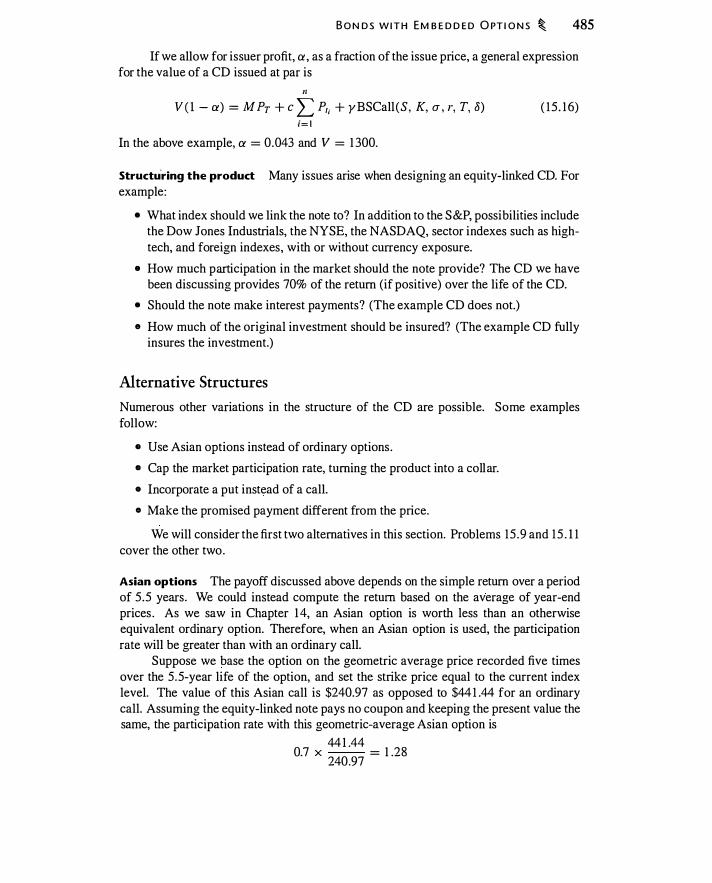
B O N D S W ITH EM B E D D E D O PT I O N S � 485

If we allow for issuer profit, a, as a fraction of the issue price, a general expression for the value of a CD issued at par is

11 V(l- a) = M PT + c L P11 + yBSCall (S, K, u, r, T, 8) ( 1 5 . 1 6)

i=l In the above example, a = 0.043 and V = 1 300.

Structu-ring the product Many issues arise when designing an equity-linked CD. For

example:

• What index should we link the note to? In addition to the S&P, possibilities include the Dow Jones Industrials, the NYSE, the NASDAQ, sector indexes such as high­tech, and foreign indexes, with or without currency exposure.

• How much participation in the market should the note provide? The CD we have been discussing provides 70% of the return (if positive) over the life of the CD.

• Should the note make interest payments? (The example CD does not.)

e How much of the original investment should be insured? (The example CD fully insures the investment.)

Alternative Structures

Numerous other variations in the structure of the CD are possible. Some examples follow:

e Use Asian options instead of ordinary options .

• Cap the market participation rate, turning the product into a collar.

• Incorporate a put instead of a call.

• Make the promised payment different from the price.

We will consider the first two alternatives in this section. Problems 15 .9 and 15 . 1 1 cover the other two.

Asian options The payoff discussed above depends on the simple return over a period of 5 .5 years. We could instead compute the return based on the average of year-end prices . As we saw in Chapter 14, an Asian option is worth less than an otherwise equivalent ordinary option. Therefore, when an Asian option is used, the participation rate will be greater than with an ordinary call.

Suppose we base the option on the geometric average price recorded five times over the 5.5-year life of the option, and set the strike price equal to the current index level. The value of this Asian call is $240.97 as opposed to $441 .44 for an ordinary call. Assuming the equity-linked note pays no coupon and keeping the present value the same, the participation rate with this geometric-average Asian option is

441 .44 0.7 X

240.97 = 1 .28

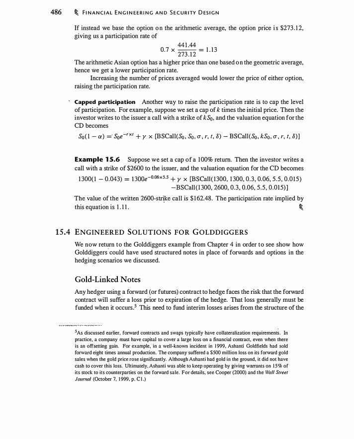
486 � F I N A N C I A L E N G I N E E R I N G A N D S E C U R I TY D ES I G N

If instead we base the option o n the arithmetic average, the option price i s $273 . 1 2, giving us a participation rate of

44 1 .44 0.7 X -- = 1 . 1 3

273 . 1 2 The arithmetic Asian option has a higher price than one based o n the geometric average, hence we get a lower participation rate.

Increasing the number of prices averaged would lower the price of either option, raising the participation rate.

' Capped participation Another way to raise the participation rate is to cap the level of participation. For example, suppose we set a cap of k times the initial price. Then the investor writes to the issuer a call with a strike of kS0, and the valuation equation for the CD becomes

So ( 1 - a) = S0e-rxr + y x [BSCall(So , So , a, r, t, 8) - BSCall(So , kSo , a, r, t, 8) ]

Example 1 5.6 Suppose we set a cap of a 1 00% return. Then the investor writes a call with a strike of $2600 to the issuer, and the valuation equation for the CD becomes

1 300( 1 - 0.043) = 1300e-0·06x5·5 + y x [BSCall( 1300, 1 300, 0 .3 , 0.06, 5 .5 , 0.0 15 ) -BSCall ( l 300, 2600, 0.3 , 0.06, 5 .5 , 0 .015)]

The value of the written 2600-strike call is $ 1 62.48 . The participation rate implied by this equation is 1 . 1 1 . �

15 .4 ENGINEERED SOLUTIONS FOR GOLDDIGGERS

We now return to the Golddiggers example from Chapter 4 in order to see show how Golddiggers

·could have used structured notes in place of forwards and options in the

hedging scenarios we discussed.

Gold-Linked Notes

Any hedger using a forward (or futures) contract to hedge faces the risk that the forward contract will suffer a loss prior to expiration of the hedge. That loss generally must be funded when it occurs. 5 This need to fund interim losses arises from the structure of the

5 As discussed earlier, forward contracts and swaps typically have collateralization requirements . In practice, a company must have capital to cover a large loss on a financial contract, even when there is an offsetting gain. For example, in a well-known incident in 1 999, Ashanti Goldfields had sold forward eight times annual production. The company suffered a $500 million loss on its forward gold sales when the gold price rose significantly. Although Ashanti had gold in the ground, it did not have cash to cover this loss. Ultimately, Ashanti was able to keep operating by giving warrants on 1 5 % of its stock to its counterparties on the forward sale. For details, see Cooper (2000) and the Wall Street Joumal (October 7, 1 999, p. C l.)

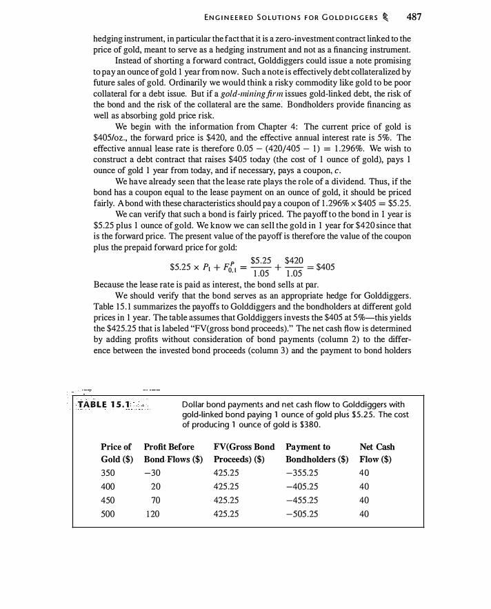
EN G I N E E R E D S O LUT I O N S F O R G O LD D I G G E R S � 487

hedging instrument, in particular the fact that it is a zero-investment contract linked to the price of gold, meant to serve as a hedging instrument and not as a financing instrument.

Instead of shorting a forward contract, Golddiggers could issue a note promising to pay an ounce of gold 1 year from now. Such a note is effectively debt collateralized by future sales of gold. Ordinarily we would think a risky commodity like gold to be poor collateral for a debt issue. But if a gold-mining firm issues gold-linked debt, the risk of the bond and the risk of the collateral are the same: Bondholders provide financing as well as absorbing gold price risk.

We begin with the information from Chapter 4: The current price of gold is $405/oz., the forward price is $420, and the effective annual interest rate is 5%. The effective annual lease rate is therefore 0.05 - (420/405 - 1 ) = 1 .296%. We wish to construct a debt contract that raises $405 today (the cost of 1 ounce of gold), pays I ounce of gold I year from today, and if necessary, pays a coupon, c.

We have already seen that the lease rate plays the role of a dividend. Thus, if the bond has a coupon equal to the lease payment on an ounce of gold, it should be priced fairly. A bond with these characteristics should pay a coupon of 1 .296% x $405 = $5 .25.

We can verify that such a bond is fairly priced. The payoff to the bond in I year is $5 .25 plus 1 ounce of gold. We know we can sell the gold in 1 year for $420 since that is the forward price. The present value of the payoff is therefore the value of the coupon plus the prepaid forward price for gold:

p $5 .25 $420 $5.25 x P1 + F0 1 = -- + -- = $405 ' 1 .05 1 .05

Because the lease rate is paid as interest, the bond sells at par. We should verify that the bond serves as an appropriate hedge for Golddiggers .

Table I 5 . 1 summarizes the payoffs to Golddiggers and the bondholders at different gold prices in I year. The table assumes that Golddiggers invests the $405 at 5%-this yields the $425.25 that is labeled "FV(gross bond proceeds)." The net cash flow is determined by adding profits without consideration of bond payments (column 2) to the differ­ence between the invested bond proceeds (column 3) and the payment to bond holders

TABLE 15.1

Price of Gold ($)

350

400

450

500

Dollar bond payments and net cash flow to Golddiggers with gold-linked bond paying 1 ounce of gold plus $5.25. The cost of producing 1 ounce of gold is $380.

Profit Before FV(Gross Bond Payment to Net Cash Bond. Flows ($) Proceeds) ($) Bondholders ($) Flow ($)

-30 425.25 -355.25 40

20 425 .25 -405 .25 40

70 425 .25 -455 .25 40

1 20 425 .25 -505 .25 40

488 � F I N A N C I A L E N G I N E E R I N G A N D S E C U R I TY D ES I G N

(column 4). In this case, issuing the bond achieves the same result as selling a forward contract (compare Table 15 . 1 and Table 4.2), so Golddiggers is completely hedged.

The chief difference between the gold-linked note and the forward contract is that the former provides financing, the latter doesn't . If Golddiggers seeks financing (in order to construct the mine, for example), the issuance of a gold-linked note might be preferable to borrowing and hedging separately.

Notes with Embedded Options

A gold-linked bond leaves bondholders with the risk of a loss should the gold price drop. Golddiggers could instead offer a bond that promises bondholders that they will receive interest plus appreciation of gold above $420.

Such a bond implicitly gives holders a call option on gold with a strike price of $420. From Chapter 2, the cost of this option today is $8.77, with a future value of $8.77 x 1 .05 = $9.2 1 . Let the promised payment on the bond be the $405 issue price ·plus the coupon, c. In 1 year, the bond is worth

$405 + c + max(O, S1 - $420)

The valuation equation for the bond is

$405 + c $8.77 = $405

1 .05 + Solving for c gives c = $ 1 1 .04, which is a yield of 2. 726%. Golddiggers thus issues a bond for $405 , with a 2.726% coupon, with additional payments to bondholders if the price of gold exceeds $420. The difference between the 2.726% coupon and 5% is due to the value of the embedded call option.

What is the result for Golddiggers from having issued this bond? If Golddiggers invests at 5% the $405 bond proceeds, then it will have $425.25 cash in 1 year. Recall that costs are $380/oz. If the gold price in 1 year exceeds $420, Golddiggers will show profits of

$420 + $9.2 1 - $380 = $49.2 1

whereas if gold is less than $420, Golddiggers will make

s1 + $9.2 1 - $380

Table 15.2 summarizes the cash flows to bondholders and to Golddiggers from the issuance of this bond. You can verify that this is exactly the same payoff as obtained when Golddiggers hedges by writing a call. The commodity-linked bond achieves the same effect.

Instead of having a low coupon and protection against low gold prices, bondholders might be willing to bear the risk of a decline in the price of gold in exchange for a higher coupon. For example, Golddiggers could issue a bond in which bondholders sell a 420-strike put to Golddiggers. Golddiggers in turn would have to pay greater interest to compensate bondholders for selling the put. The bond would be structured as follows:

.···. ' ...

E N G I N E E R E D S O LUTI O N S F O R G O L D D I G G E R S � 489

. · . · . . ·, TABLE 1 5.2 "· .• Dolla r bond payments and net cash flow to Golddiggers with

gold-linked bond providing gold appreciation to bondholders.

Price of Profit Before FV (Gross Bond Payment to Net Cash Gold ($) Bond Flows ($) Proceeds) ($) Bondholders ($) Flow ($)

350 -30 425 .25 -416.04 -20.79

400 20 425 .25 -416.04 29.21

450 70 425 .25 -446.04 49.21

500 120 425 .25 -496.04 49.2 1

• The initial bond price is $405 .

• The promised payment on the bond is $434.46, a 7.274% rate of interest.

• If gold sells for less than $420, the payment is reduced by $420 - S1•

The bondholders have written a put option to Golddiggers and hence in 1 year receive the future value of the premium. If the price of gold is above $420, Golddiggers makes

$425 .25 - $434.46 + (S1 - $380) = S1 - $380 - $9.2 1

If gold is below $420, Golddiggers makes

$425 .25 - $434.46 + ($420 - S1 ) + (S1 - $380) = $30.79

With this bond, Golddiggers in effect buys a 420-strike put. Table 15 .3 depicts the net cash flow to Golddiggers from issuing this bond. The cash flows are identical to Table 4.3, where Golddiggers purchased a 420-strike put option as insurance against low gold prices ..

" . ".·· .: .

·· · TABLE 15.3 <c., .

Dollar bond payments and net cash flow to Golddiggers with gold-linked bond in which bondholders sell put option to Golddiggers.

Price of Profit Before FV(Gross Bond Payment to Net Cash Gold ($) Bond Flows ($) Proceeds) ($) Bondholders ($) Flow ($)

350 -30 425.25 -364.46 30.79

400 20 425.25 -414.46 30.79

450 70 425 .25 -434.46 60.79

500 120 425 .25 -434.46 1 1 0.79

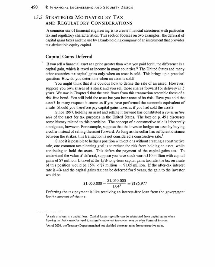
490 � F I N A N C I A L EN G I N E E R I N G AN D S EC U R I TY D ES I G N

15 .5 STRATEGIES MOTIVATED BY TAX AND REGULATORY CONSIDERATIONS

A common use of financial engineering is to create financial structures with particular tax and regulatory characteristics . This section focuses on two examples : the deferral of capital gains taxes and the use by a bank-holding company of an instrument that provides tax-deductible equity capital .

Capital Gains Deferral

If you sell a financial asset at a price greater than what you paid for it, the difference is a capital gain, which is taxed as income in many countries.6 The United States and many other countries tax capital gains only when an asset is sold. This brings up a practical question: How do you determine when an asset is sold?

You might think that it is obvious how to define the sale of an asset. However, suppose you own shares of a stock and you sell those shares forward for delivery in 5 years. We saw in Chapter 5 that the cash flows from this transaction resemble those of a risk-free bond. You still hold the asset but you bear none of its risk. Have you sold the asset? In many respects it seems as if you have performed the economic equivalent of a sale. Should you therefore pay capital gains taxes as if you had sold the asset?

Since 1997, holding an asset and selling it forward has constituted a constructive sale of the asset for tax purposes in the United States. The box on p. 49 1 discusses some history related to this provisjon. The concept of a constructive sale is inherently ambiguous, however. For example, suppose that the investor hedges an asset by buying a collar instead of selling the asset forward. As long as the collar has sufficient distance between the strikes, this transaction is not considered a constructive sale.7

Since it is possible to hedge a position with options without creating a constructive sale, one common tax-planning goal is to reduce the risk from holding an asset, while continuing to hold the asset. This defers the payment of the capital gains tax. To understand the value of deferral, suppose you have stock worth $ 1 0 million with capital gains of $7 million . If taxed at the 15% long-term capital gains tax rate, the tax on a sale of this position would be 15% x $7 million = $ 1 .05 million. If the after-tax interest rate is 4% and the capital gains tax can be deferred for 5 years, the gain to the investor would be

$ 1 , 050, 000 $ 1 ,050, 000 -

1 .045 = $ 1 86, 977

Deferring the tax payment is like receiving an interest-free loan from the government for the amount of the tax.

6 A sale at a loss is a capital loss. Capital losses typically can be subtracted from capital gains when figuring tax. but cannot be used to a significant extent to reduce taxes on other forms of income. 7 As of 2004, the Treasury Department had not clarified the exact rules for constructive sales.

ST RATEGIES M OT IVATE D BY TAX A N D R E G U LATO RY C O N SID E RATI O N S � 491

Constructive Sales

In late 1995, Estee Lauder and Ronald Lauder sold 1 3 . 8 million shares of Revlon (see Henriques, 1 997). The capital gains tax owed on a direct sale of these shares was estimated at $95 million. The Lauders did not directly sell the ·shares they owned, however. Instead they borrowed 1 3 . 8 million shares from family members, and sold those borrowed shares. Technically they still owned their original shares and owed shares to relatives, but they had received money from selling the borrowed shares. This maneuver is known as "shorting-against-the-box." Clearly shorting-against-the-box has the earmarks of a sale, in that the shareholder has no remaining risk of ownership and has received cash for the stock.

Astounding as it may seem, shorting-against-the-box was for years a well-known and legal strategy for deferring the payment of capital gains taxes. Taxes on the position were not owed until the short position was closed by returning the borrowed shares. Unfortunately for the Lauders, their

transaction received publicity and was widely criticized.

Congress in 1 997 passed a tax bill that made a short-against-the-box equivalent to a sale of the stock. The Lauder transaction was believed to be one reason for this tax rule. The idea was that a transaction that was the economic equivalent of a sale would be called a constructive sale and taxed like a sale. Facing IRS action, the Lauders in 1 997 sold their shares and paid a large tax bill.

A short-against-the-box is a constructive sale because the shareholder has no remaining risk from the shares. What if a hedging transaction leaves some risk? When does a hedge become a constructive sale? The 1 997 bill permits shareholders to defer realization if they entered into hedges with sufficient residual risk, such as collars with a large enough difference between the call and put strikes. The bill left it to the Treasury Department to specify the regulations that would codify permissible tax deferral strategies.

Tax deferral for individuals Stockholders with large appreciated stock positions can use a collar to reduce the risk of their holdings. Data on such transactions can be hard to obtain, but Bettis et a! . (200 I) studied the use by executives of zero-cost collars from 1 996 to I 998. They found that those who used zero-cost collars on average collared one-third of their stock. Almost no executive used equity swaps, which would likely have resulted in a constructive sale.8 In one widely reported example, Paul Allen, a cofounder of Microsoft, entered into collars on 76 million Microsoft shares during October and November of 2000 (McMurray, 200 l).

Entering into a zero-cost collar reduces the risk of holding an asset, but it does not generate the cash that would be obtained from having sold the asset. However, once a

8Even before the tax law formally changed in 1 997. the IRS was threatening to challenge forward sales

of stock as constructive sales.

492 � F I N A N C I A L E N G I N E E R I N G A N D S E C U R I TY D ES I G N

stock position has been collared, the collared stock can serve as collateral for a loan. For example, suppose an executive owns stock and enters into a zero-cost collar where the put strike is $90. With this position, the executive is guaranteed to receive at least $90 at maturity. Thus, a bank can lend the present value of $90 using the stock plus put as collateral.

It is also possible to engineer a single instrument that hedges a stock position and pays cash to the owner. In August 2003 , Walt Disney Co vice-chairman Roy Disney sold a 5-year variable prepaid forward (VPF) contract covering a large percentage of his Disney stock holdings . The contract called for Roy Disney to deliver to Credit Suisse First Boston a variable number of shares in 5 years . To quote from the Form 4 filed with the SEC:

The VPF Agreement provides that on August 1 8 , 2008 ("Settlement Date"), [Roy Disney] will deliver a number of shares of Common Stock to CSFB LLC (or . . . the cash equivalent of such shares) as follows: (a) if the average VWAP ["Value Weighted Average Price"] of the Common Stock for the 20 trading days preceding and including the Settlement Date ("Settle­ment Price") is less than $2 1 .75 1 , a delivery of 7,500,000 shares; (b) if the Settlement Price is equal to or greater than $2 1 .75 1 per share ("Downside Threshold") but less than or equal to $32.6265 per share ("Upside Thresh­old"), a delivery of shares equal to the Downside Threshold/Settlement Price x 7,500,000; and (c) if the Settlement Price is greater than the Upside Threshold, a delivery of shares equal to ( 1 - ( 1 0.8755/Settlement Price)) x 7, 500, 000.

Figure 1 5 . 1 graphs the dollar value of the payoff of the prepaid forward, along with the net payoff for owning a share and selling the prepaid forward. The net payoff is the same as that for a collared stock. This transaction permitted Roy Disney to retain the voting rights in the shares, receive substantial cash, and presumably defer any capital gains he had on the position. According to a Wall Street Journal article about the transaction,9 similar transactions hll.d been undertaken by more than 40 corporate directors in the United States.

Tax deferral for corporations Corporations may also wish to sell an asset without creating a constructive sale. A corporation has an alternative not open to most investors­namely, the issuance of a note with a payoff linked to the price of the appreciated stock. A well-known example of this is the 1996 issuance by Times-Mirror Co of an equity-linked note, where the note was linked to the stock price of Netscape.

In April 1 995, Times Mirror had purchased 1 . 8 million shares of Netscape in a private placement. The price (adjusted for subsequent share splits) was $2/share. The

9 Randall Smith and Bruce Orwall. "Roy Disney Reaps S 1 25 Million in a Novel Stock-Sale Package," Wall Street Joumal. p. e 1. August 2 1 . 2003 .

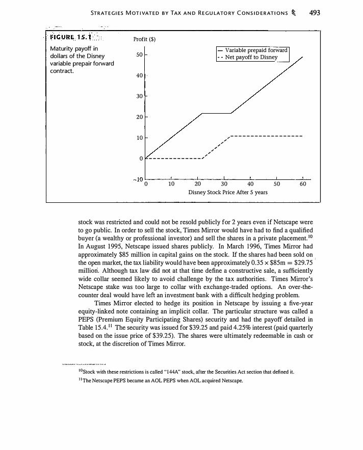
STR AT E G I ES M OTIVATE D B Y TAX A N D R E G U LATO RY C O N S I D E R AT I O N S � 493

Maturity payoff in dollars of the Disney variable prepair forward contract.

Profit ($)

50

40

30

20

- Variable prepaid forward - - Net payoff to Disney

10 - - - - - - - - - - - - - - - - - -

.... .... 0 _ _ _ _ _ _ _ _ _ _ _ _ _ ., ....

.... .... "' "'

....

-1QL-----J-----�------L------L----�------�

0 10 20 30 40 50 60

Disney Stock Price After 5 years

stock was restricted and could not be resold publicly for 2 years even if Netscape were to go public. In order to sell the stock, Times Mirror would have had to find a qualified buyer (a wealthy or professional investor) and sell the shares in a private placement. 10

In August 1 995, Netscape issued shares publicly. In March 1 996, Times Mirror had approximately $85 million in capital gains on the stock. If the shares had been sold on . the open market, the tax liability would have been approximately 0.35 x $85m = $29.75 ·

milliori. Although tax law did not at that time define a constructive sale, a sufficiently wide collar seemed likely to avoid challenge by the tax authorities . Times Mirror's Netscape stake was too large to collar with exchange-traded options. An over-the­counter deal would have left an investment bank with a difficult hedging problem.

Times Mirror elected to hedge its position in Netscape by issuing a five-year equity-linked note containing an implicit collar. The particular structure was called a PEPS (Premium Equity Participating Shares) security and had the payoff detailed in Table 15 .4. 1 1 The security was issued for $39.25 and paid 4.25% interest (paid quarterly based on the issue price of $39.25). The shares were ultimately redeemable in cash or stock, at the discretion of Times Mirror.

1 0 Stock with these restrictions is called " 144A" stock, after the Securities Act section that defined it. 1 1 The Netscape PEPS became an AOL PEPS when AOL acquired Netscape.

494 � F I N A N C I A L E N G I N E E R I N G A N D S E C U R I TY D ES I G N

, ,

TABLE l SA

Netscape Share Price

SNetscape < 39.25

Payment at maturity on Times Mirror PEPS, showing the dependence of the maturity payment on the future price of Netscape stock.

Payment to Times Mirror PEPS-Holders

SNetscape

39 .25 :S SNetscape :S 45 . 1 4 45 . 1 4 < SNetscape

39.25 39.25 + 0.8696 X (SNetscape - 45 . 14)

The effect of issuing the PEPS was like that of Roy Disney selling the variable prepaid forward. Times Mirror received cash at issuance and could deliver shares. The PEPS structure is graphed in Figure 1 5 .2, along with the payoff of the hedged position. In order to avoid challenge as a constructive sale, the issuance left Times MiiTOr imperfectly hedged. If at maturity the Netscape stock piice was less than $39.25, Times Mirror would lose the interest payments ; hence the net payoff line is below zero. Above $45 . 1 4, Times Mirror has the risk of holding 1 3% of the shares . Note that $39.25 x 1 . 1 5 = $45 . 14,

Payoff to owners of PEPS and to Times Mirror, including interest. The PEPS-holder payoff includes the present value of the 4.25% interest payment; hence, the payoff is greater than $0 at a stock price of $0.

Payoff ($)

100

80

60

40

20

0

-20 0 20 40 60

+ Netscape stock -+- PEPS-holder payoff .._ Net to Times-Mirror

80 100

Netscape Stock Price ($)

STR ATEG I ES M OT I VATE D BY TAX A N D R EG U LATO RY C O N S I D E R ATI O N S � 495

and for the slope, 0.8696 = 1 /1 .15. Thus the collar width and slope above $45.14 are both determined using 15%.

Tax-Deductible Equity

Under U.S . tax law, interest payments on corporate debt are tax-deductible, while divi­dend payments on equity are not. The distinction between debt and equity may at first seerri clear-cut, but with financial engineering it is easy to blur the distinction. For ex­ample, suppose a firm issues equity-linked notes that promise coupon payments (like debt) but have a payment at maturity contingent on the firm's stock price (like equity) . Is such a financial claim debt or equity for tax purposes?

In practice it is possible to design financing vehicles that have a significant equity component, yet for which the payments are at least partially tax-deductible for the firm. In this section we will examine in more detail the Marshall & llsley Corp. (M&I) convertible bond discussed in Chapter 3, with the payoff depicted in Figure 3 . 1 6. As we discussed, the bond payoff resembles a stock coupled with written and purchased calls . Nevertheless, payments on the bond are partially tax-deductible for the issuer. Moreover, M&I is a bank holding company, and the bond provided capital for regulatory purposes. 1 2

With a structure like the M&I convertible, myriad details hinge on complex tax, accounting, and regulatory considerations. Our purpose in discussing the bond is to understand at a general level the kinds of issues that financial engineering can address. We ignore specific details that aren' t needed in conveying a sense of the transaction.

The M&I convertible bond actually consisted of two components : an ownership stake in a trust containing M&I bonds, and a stock purchase contract requiring that the convertible bondholder make a future payment in exchange for shares . These two components are separable, in that an investor could in theory hold one without the other. Here are some of the details on these two pieces:

e Interest in the trust: M&I issued $400 million of subordinated debt (debt with very low priority in the event of bankruptcy) maturing in 2038, paying a 3 .9% coupon. These bonds were placed into a trust. 1 3 Each unit of the convertible bond contains an interest in the trust for $25 par value worth of these subordinated bonds. After 3 years, the bond coupon will be reset so that the bond trades at par. The bonds are subordinated so they can count as regulatory capital .

• Stock purchase contract: Each stock purchase contract pays a 2.6% coupon and requires the investor, after 3 years, to pay $25 for between 0.5402 and 0.6699

12Banks worldwide are required to have capital to cover potential losses on loans and investments. The specific rules are in flux, but generally speaking, "tier one" capital is equity, retained earnings, and preferred stock, while "tier two" capital is subordinated debt. Limited amounts of preferred trust securities, such as the M&I convertible, can be counted as tier one capital. See Mishkin and Eakins (2003, ch. 1 8) for an overview of bank regulation.

1 3 A trust is an entity holding an asset for the benefit of another party. A trust is controlled by a trustee.

496 � F I N A N C I A L E N G I N E E R I N G A N D S E CU R ITY D ES I G N

shares. (At the time of the offering, the M&I share price was $37.32. The value of 0.6699 shares was $25 .) The number of shares that the investor receives after 3 years depends on the M&I stock price at that time, Srv11 :

0.6699 shares $25 I Srvu shares 0.5402 shares

if if if

Srvu :S $37.32 $37.32 < Srvn < $46.28 Srvn � $46.28

The bonds held in trust serve as collateral to ensure that the investor can pay the $25 to buy shares in 3 years, eliminating credit risk for M&I.

How can we understand the pricing of the convertible? Think of the investor as having paid $25 for the 3 .9% bonds and nothing for the stock purchase contract. If you compare the stock purchase contract with 0.6699 shares of M&I, there are both costs and benefits of the stock purchase contract relative to the stock: The investor is obligated in 3 years to pay the offering day price for 0.6699 shares ($25) but could in three years receive as few as 0.5402 shares. The investor also does not receive the dividend on the underlying shares (M&I had a 2% dividend yield) . However, the investor can acquire future shares for the offering day price. Taking all three considerations into account, the investor receives a 2.6% dividend in return for entering into the stock purchase contract at a zero initial cost. 14

The structure is diagrammed in Figure 15 .3 . To summarize: M&I issues a bond and a stock purchase contract that together comprise a con.vertible bond. Investors receive a 6.5% coupon: 3.9% from the bonds and 2.6% from the stock purchase contract. For M&I, the 3.9% coupon is tax-deductible because it is interest on the subordinated debt. The 2.6% payment on the stock purchase contract is not debt interest and hence is not deductible. At maturity of the stock purchase contract, the par value of the bond can be used to pay for the stock.

At this point, it may be helpful to answer some questions that may occur to you:

• Why didn 't M &/ simply issue a single instrument, conveJtible into stock, with the same payoff? As we noted earlier, the bond payoff resembles stock plus options. The payoff is unlike that for an ordinary bond or even an ordinary-convertible bond, both of which proinise to pay at least par value at maturity. A single instrument with the structure of the M&l convertible-with no minimum promised payment­would have been deemed too equity-like and the payment would not have been tax-deductible.

• The bond/wider bought the trust unit (containing subordinated bonds) plus a stock purchase contract. If you have to hold these as a unit, isn 't this the same thing as holding a single instrument? The key to allowing tax-deductibility of the interest is that the bonds and stock purchase contract do not have to be held as a unit. The subordinated bonds expire 30 years after the stock purchase contract matures. They are documented as distinct entities . Moreover, the convertible-holder has the right

14Problem 1 5 .23 asks you to analyze the pricing of the contract

ST RATEG I ES M OT I VAT E D BY TAX A N D R E G U LATO RY C O N S I D E R AT I O N S � 497

l nital cash flows and periodic payments to investors on the M&l convertible bond. The dotted lines are cash flows at maturity.

M & I

Subordinated Trust stake

-3-.-9°-v.

d

-, :-:-:-er-e-st.-r -rru,: -3

-.-

9°_v._>�_n_t_er

-

e

-

st .. 1

$25 . $25 : Trust as

2.6% Dividend

; collateral ; for future � stock purchase

. Stock 2.6% Dividend

-<· · · · · · · · · · · · · · · · · · · purchase -<· · · · · · · · · · · · · · · · · · ·

$25 contract $25 · · · · · · · · · · · · · · · · · · ·)- · · · · · · · · · · · · · · · · · · ·>

Variable Variable number of number of

shares shares

Investors

to hold the stock purchase contract but to substitute Treasury securities as collateral in place of the stake in the trust.

• What if interest rates in 3 years have risen and the value of the subordinated bond has fallen below $25? The bonds are issued subject to a remarketing agreement. This means that in 3 years the interest rate on the bonds will be reset so that the bonds sell at par ($25). Thus, the bonds will be worth $25 at exactly the time when the shareholders need to pay $25 for the variable number of shares. 1 5

• Why did the stock purchase contract have a kink, instead of just being a simple fonvard contract? The dividend on the forward purchase contract compensates the investor for the possibility of receiving fewer than 0.6699 shares at maturity and the loss of the dividend on the underlying shares, less the gain from deferring the $25 share cost. In exchange for giving up more appreciation, the investor receives a greater dividend. The kink is determined by the willingness of seller and buyers to trade appreciation for current income.

Many financial institutions have used a trust structure like that in the M&I trans­action. Related structures under different names (for example, "Upper DECS") are used by companies wishing to obtain partially tax-deductible equity-like financing.

1 5We have not discussed the possibility that remarketing would fail or what would happen if M&I

enters bankruptcy. The publicly available prospectus for the bond discusses these detai ls.

498 � F I N A N C I A L E N G I N E E R I N G A N D S EC U R I TY D ES I G N

Finally, note that the M&I convertible and the Netscape PEPS both have payoffs incorporating a collarlike structure, but the motivations are different. The Netscape PEPS was intended to avoid a constructive sale of stock, while the M&I convertible incorporates a collar as a way for investors (and the company) to express a view.

----�-L..::..:...:...:.....::.;..:---.:...:.:.... ;·�-�- - - �:�-,�:.- ·_

CHAPTER SUMMARY

Zero-coupon bonds, forwards, calls, and puts serve as building blocks that can be used to engineer new financial products. Fair pricing of a product will depend upon volatility, the dividend or lease rate, and the currency of denomination. Ordinary bonds that are simply denominated in something other than cash follow a simple pricing principle: The lease rate of the underlying asset becomes the coupon rate on the bond.

The specific characteristics of a financial product can be varied, though when one characteristic is changed, another must be changed to keep the value the same. The dials that we can tum include the participation in the underlying asset (via embedded calls and puts), the guaranteed minimum, and the coupon. Pricing theory tells us how to make these tradeoffs.

Instruments can be designed specifically to take advantage of tax rules and reg­ulations. The Disney prepaid forward, Netscape PEPS, and M&I convertible bond are examples of this.

FURTHER READING

In this chapter we focused on the creation of engineered instruments using basic building blocks such as assets, bonds, forward contracts, and options. However, using the Black­Scholes technology based on delta-hedging (discussed in Chapter 1 3), it is possible to engineer more complicated instruments. We will cover the more general approach in Chapter 21 and see some applications in Chapter 22.

Readings about structured products (including some not discussed in this chap­ter) include Baubonis et a! . ( 1 993), McConnell and Schwartz ( 1 992), Arzac ( 1 997), and Crabbe and Argilagos ( 1 994 ) . For more information about Western-Southern, a deal sim­ilar to Times-Mirror Netscape PEPS, see http://www.kel logg.northwestern.edu/

faculty/petersen/html.

PROBLEMS

Some of the problems that follow use Table 1 5 .5 and the following assumptions: The spot price of oil is $20.90. Let S1 denote the time price of the S&P 500 index, and assume that the price of the S&P 500 index is S0 = $ 1200 and the continuous annual dividend yield on the S&P 500 index is 1 .5%.

1 2 3 4 Quarter

5 6

P R O B LE M S � 499

7 8 Oil forward price ($) 2 1 .0 2 J . l 20.8 20.5 20.2 20.0 1 9.9 1 9.8

Zero-coupon bond price (S) 0.9852 0.970 1 0.9546 0.9388 0.923 1 0.9075 0.89 1 9 0.8763

15.1. Consider a 5-year equity-linked note that pays one share of XYZ at maturity. The price of XYZ today is $ 1 00, and XYZ is expected to pay its annual dividend of $ 1 at the end of this year, increasing by $0.50 each year. The fifth dividend will be paid the day before the note matures. The appropriate discount rate for dividends is a continuously compounded risk-free rate of 6%.

Suppose that the day after the note is issued, XYZ announces a permanent dividend increase of $0.25 . What happens to the price of the equity-linked note?

15.2. Suppose the effective semiannual interest rate is 3%.

a . What is the price of a bond that pays one unit of the S&P index in 3 years?

b. What semiannual dollar coupon is required if the bond is to sell at par?

c. What semiannual payment of fractional units of the S&P index is required if the bond is to sell at par?

15.3. Use information from Table 1 5 .5 .

a. What is the price of a bond that pays one unit of the S&P index in 2 years?

b. What quarterly dollar coupon is required if the bond is to sell at par?

c. What quarterly payment of fractional units of the S&P index is required if the bond is to sell at par?

15.4. Assume that the volatility of the S&P index is 30%.

a. What is the price of a bond that after 2 years pays S2 + max(O, S2 - So) ?

b . Suppose the bond pays s2 + [A. X max(O, s2 - So) ] . For what A will the bond sell at par?

15.5. Assume that the volatility of the S&P index is 30%.

a. What is the price of a bond that after 2 years pays So + max(O, S2 - So) ?

b . Suppose the bond pays So + [A. X max(O, s2 - So)] i n year 2 . For what A. will the bond sell at par?

500 � F I N A N C I A L E N G I N E E R I N G A N D S EC U R I TY D ES I G N

15.6. Assume that the volatility of the S&P index is 30% and consider a bond with the payoff s2 + ), X [max (O, s1 - So) - max(O, s2 - K)] .

a . If A = 1 and K = $ 1 500, what i s the price of the bond?

b. Suppose K = $ 1 500. For what A will the bond sell at par?

c. If A = I , for what K will the bond sell at par?

The next six problems will deal with the equity-linked CD in Section 1 5 .3 .4. If necessary, use the assumptions in that section.

15.7. Explain how to synthetically create the equity-linked CD in Section 1 5 .3 by using a forward contract on the S&P index and a put option instead of a call option. (Him: Use put-call parity. Remember that the S&P index pays dividends. )

15.8. Consider the equity-linked CD in Section 15 .3 . Assuming that profit for the issuing bank is zero, draw a graph showing how the participation rate, y , varies with the coupon, c. Repeat assuming the issuing bank earns profit of 5%.

15.9. Compute the required semiannual cash dividend if the expiration payoff to the CD is $ 1 300 - max(O, 1 300 - S5.5) and the initial price is to be $ 1 300.

15.10. Compute A if the dividend on the CD is O and the payoff is $ 1 300-max(O, 1 300-S5.5) + A x max(O, S5.5 - 2600) and the initial price is to be $ 1 300.

15.11. Compute )... if the dividend on the CD is 0, the initial price is $ 1 300, and the payoff is $ 1200 + A x max(O, S55 - 1 300) .

15.12. Consider the equity-linked CD example in Section 1 5 .3 .

a . What happens to the value of the CD as the interest rate, volatility, and dividend yield change? In particular, consider alternative volatilities of 20% and 40%, interest rates of0.5% and 7%, and dividend yields of 0.5% and 2.5%.

b. For each parameter change above, suppose that we want the product to continue to earn a 4.3% commission . What price participation, y , would the CD need to have in each case to keep the same market value?

15.13. Use the information in Table 1 5 .5 .

a . What i s the price of a bond that pays one barrel of oil 2 years from now?

b. What annual cash payment would the bond have to make in order to sell for $20.90?

15.14. Using the information in Table 1 5 .5 , suppose we have a bond that pays one barrel of oil in 2 years.

a. Suppose the bond pays a fractional barrel of oil as an interest payment after 1 year and after 2 years, in addition to the one barrel after 2 years.

P R O B LE M S � SOl

What payment would the bond have to make in order to sell for par ($20.90)?

b. Suppose that the oil payments are quarterly instead of annual . How large would they need to be for the bond to sell at par?

15.15. Using the information in Table 15 .5 , suppose we have a bond that after 2 years pays one barrel of oil plus ).. X max(O, s2 - 20.90) , where s2 is the year-2 spot price of oil. If the bond is to sell for $20.90 and oil volatility is 15%, what is ).. ?

15.16. Using the information in Table 15 .5 , assume that the volatility of oil is 15%.

a. Show that a bond that pays one barrel of oil in 1 year sells today for $ 1 9 .2454.

b. Consider a bond that in 1 year has the payoff SI + max(O, KI - SI ) -max(O, SI -K2) . Find the strike prices K I and K2 such that K2-KI = $2, and the price of the bond is $ 1 9.2454. How would you describe this payoff?

c. Now consider a claim that in 1 year pays SI - $20.50 + max(O, KI -SI ) - max(O, SI - K2) , where KI and K2 are from the previous answer. What is the value of this claim? What have you constructed?

15.17. Swaps often contain caps or floors. In this problem, you are to construct an oil contract that has the following characteristics: The initial cost is zero. Then in each period, the buyer pays the market price of oil if it is between KI and K2 ; otherwise, if S < KI , the buyer pays KI , and if S > K1, the buyer pays K2 (there is a floor and a cap). Assume that K2 - KI = $2 and that oil volatility is 15%.

a . If there is a single settlement date in 1 year, what are K I and K 2?

b. If the swap settles quarterly for eight quarters, what are K I and K2?

15.18 .. You have been asked to construct an oil contract that has the following charac­teristics: The initial cost is zero. Then in each period, the buyer pays S - F, with a cap of $2 1 .90 - F and a floor of $ 1 9.90 - F. Assume oil volatility is 15%. What is F?

15.19. Using Figure 3 . 1 6 on page 84 as the basis for a discussion, explain under what circumstances an investor might prefer a PEPS to the stock or vice versa.

15.20. Consider again the Netscape PEPS discussed in this chapter and assume the following: the price of Netscape is $39.25 ; Netscape is not expected to pay dividends; the interest rate is 7%; and the 5-year volatility of Netscape is 40%. What is the theoretical value of the PEPS?

15.21. A DECS contract pays two shares if Sr < 27 . 875, 1 .667 shares if the price is above Sr > 33 .45, and $27.875 and $55.75 otherwise. The quarterly dividend is $0.87. Value this DECS assuming that S = $26.70, u = 35%, r = 9%, and T = 3 .3 and that the underlying stock pays a quarterly dividend of $0. 10.

502 � F I N A N C I A L EN G I N E E R I N G AN D S E C U R ITY D ES I G N

The next two problems are based o n the M&I stock purchase contract.

15.22. A stock purchase contract with a zero initial premium calls for you to pay for one share of stock in 3 years. The stock price is $ 100 and the 3-year interest rate is 3%.

• If you expect the stock to have a zero dividend yield, what price in 3 years would you agree to pay for the stock?

• If the stock has a 2% dividend yield, what price in 3 years would you agree to pay for the stock?

• Now suppose that the stock purchase contract calls for you to pay $ 100 in 3 years for one share of stock. What annual payment on the stock purchase contract would be fair if the dividend yield on the stock is zero? What if it is 4%?

15.23. Value the M&I stock purchase contract assuming that the 3-year interest rate is 3% and the M&I volatility is 1 5%. How does your answer change if volatility is 35%?

C.· . . ·:r. ·· .. ·__:r· .... ···.• . . •· ·. A "· .. ·.· .. \"ra:,;y<.·.••:·.(r . · · .. E·.· . •R· ·· .. ·· . .. r .. c_ ' l.: :��:i:.t �- 0 v - -_; ' --- -- - ' - - - - - - - - - �0 - ___ ,

Corporate Applications

I n thh ohaptec we look at .orne oontex" in whieh fi'm' i"ue derivatives: eithec explidtly or implicitly. First, Black and Scholes ( 1 973) observed that common debt and equity can be viewed as options, with the firm's assets as the underlying asset. We show how this insight can be used to price debt subject to default, as well as the implications for determining how leverage affects the expected return on equity. We also examine warrants, convertible debt, and callable debt as examples of securities that explicitly contain options .

Second, many firms grant options as compensation to employees. These options typically cannot be exercised for some period of time and cannot be sold, so they raise interesting valuation issues. In addition, compensation options often have nonstandard features.

Third, merger deals in which firm A offers their own stock to buy firm B sometimes offer price protection to firm B shareholders. This protection can take the form of a collar. We examine one merger-Northrop Grumman-TRW-that used a collar for this purpose.

16 .1 EQUITY, DEBT, AND WARRANTS

Firms often issue securities that have derivative components. For example, firms issue options to employees for financing, and convertible debt is a bond coupled with a call' option. However, even simple securities, such as ordinary debt and equity, can be viewed as derivatives. In this section we examine both implicit and explicit options issued by firms.

Debt and Equity as Options

Consider a firm with the following very simple capital structure. The firm has nondivi­dend-paying equity outstanding, along with a single zero-coupon debt issue. Represent the time t values of the assets of the firm, the debt, and the equity as A, , B, , and £, . The debt matures at time T and has maturity value B.

We assume throughout this section that there are no taxes, bankruptcy costs, trans­action costs, or other market imperfections.

The value of the debt and equity at time T will depend upon the value of the firm's assets. Equity-holders are the legal owners of the firm; in order for them to have

503

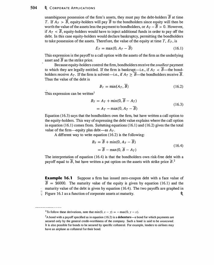
504 � C O R PO RATE A P P L I CATI O N S

unambiguous possession of the firm's assets, they must pay the debt-holders B at time T. If AT > B, equity-holders will pay B to the bondholders since equity will then be worth the value of the assets less the payment to bondholders, or AT - B > 0. However, if AT < B, equity-holders would have to inject additional funds in order to pay off the debt. In this case equity-holders would declare bankruptcy, permitting the bondholders to take possession of the assets. Therefore, the value of the equity at time T, ET , is

ET = max(O, AT - B) ( 1 6. 1 )

This expression is the payoff to a call option with the assets of the firm as the underlying asset and B as the strike price.

Because equity-holders control the firm, bondholders receive the small est payment to which they are legally entitled. If the firm is bankrupt-i.e., if AT < B-the bond­holders receive AT . If the firm is solvent-i.e. , if AT :::0: B-the bondholders receive B . Thus the value of the debt is

( 1 6.2)

This expression can be written 1

BT = AT + min(O, B - AT) ( 1 6.3)

= AT - max(O, AT - B)

Equation ( 1 6.3) says that the bondholders own the firm, but have written a call option to the equity-holders. This way of expressing the debt value explains where the call option in equation ( 1 6. 1 ) comes from. Suiruning equations ( 1 6. 1 ) and ( 1 6.2) gives the the total value of the firm-equity plus debt-as AT ·

A different way to write equation ( 1 6.2) is the following:

BT = B + min(O, AT - B)

= B - max(O, B - AT) ( 1 6.4)

The interpretation of equation ( 16.4) is that the bondholders own risk-free debt with a payoff equal to B , but have written a put option on the assets with strike price B . 2

Example 1 6. 1 Suppose a firm has issued zero-coupon debt with a face value of B = $6000. The maturity value of the equity is given by equation ( 1 6. 1 ) and the maturity value of the debt is given by equation ( 16.4). The two payoffs are graphed in Figure 1 6. I as a function of corporate assets a t maturity. �

1 To follow these derivations, note that min (O, x - y) = - max{O, y - x).

2 A bond with a payoff specified as in equation ( 1 6.2) is a debenture-a bond for which payments are secured only by the general credit-worthiness of the company. Such a bond is said to be unsecured. It is also possible for bonds to be secured by specific collateral. For example, lenders to airlines may have an airplane as collateral for their bond.

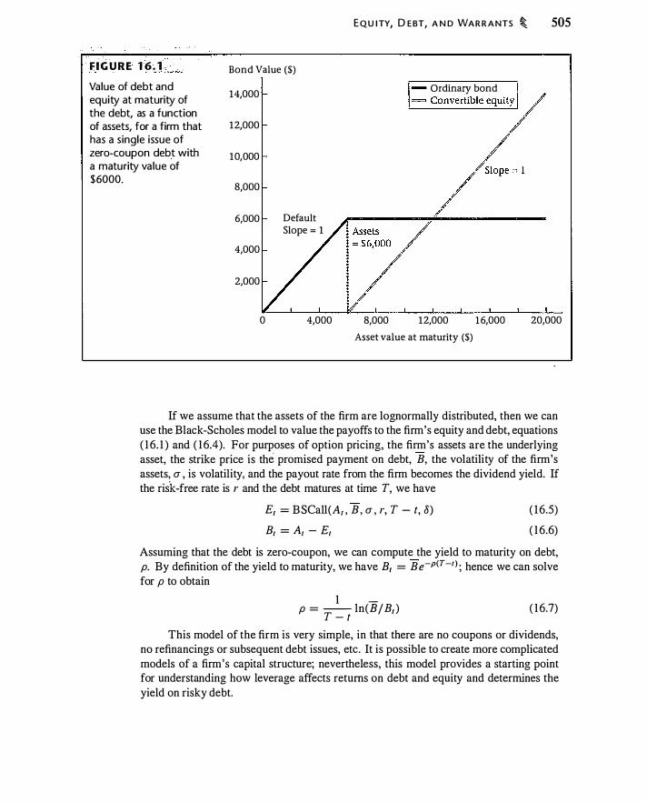
F I G U R E 1 6 . 1 - . Value of debt and equity at maturity of the debt, as a function of assets, for a firm that has a single issue of zero-coupon debt with a maturity va lue of $6000.

Bond Value ($)

14,000

12,000

10,000

8,000

6,000 Default Slope = 1

4,000

2,000

0 4,000

EQU ITY, D E BT, A N D WA R R A NTS � 505

- Ordinary bond � Convertible'/

1/ 8,000 12,000 1 6,000 20,000

Asset value at maturity ($)

If we assume that the assets of the firm are lognormally distributed, then we can use the Black-Scholes model to value the payoffs to the firm's equity and debt, equations ( 1 6. 1 ) and ( 16.4). For purposes of option pricing, the firm's assets are the underlying asset, the strike price is the promised payment on debt, B, the volatility of the firm's assets, a , is volatility, and the payout rate from the firm becomes the dividend yield. If the risk-free rate is r and the debt matures at time T, we have

E1 = BSCall(A1 , B , a, r, T - t, 8) Bt = At - Et

( 1 6.5)

( 1 6.6)

Assuming that the debt is zero-coupon, we can compute the yield to maturity on debt, p. By definition of the yield to maturity, we have B1 = Be-p(T-t) ; hence we can solve for p to obtain

1 -p = -- ln(B/ B1 ) T - t

( 1 6.7)

This model of the firm is very simple, in that there are no coupons or dividends, no refinancings or subsequent debt issues, etc. It is possible to create more complicated models of a firm's capital structure; nevertheless, this model provides a starting point for understanding how leverage affects returns on debt and equity and determines the yield on risky debt.

506 � C O R PO RATE A P P L I CAT I O N S

Viewing debt and equity as options also provides a framework for thinking about credit risk. Equation ( 1 6.4) shows that defaultable debt is equivalent to owning default­free debt plus a put option on the assets of the firm. An investor owning a corporate bond could buy such a put; the result would be economically equivalent to owning a default­free bond. Thus, the value of the put is the value of insurance to protect bondholders against default. We will examine credit risk more in Chapter 26.

Example 1 6.2 Suppose that B = $ 1 00, A0 = $90, r = 6%, a = 25%, 8 = 0 (the ,firm makes no payouts), and T = 5 years. We have

Eo = BSCall($90, $ 1 00, 0.25 , 0.06, 5, 0)

= $27.07

The value of the debt is

Bo = $90 - $27.07

= $62.93

The debt-to-value ratio of this firm is therefore $62.93/$90 maturity on debt is

I p = :S ln ( I 00/62.93)

= 0.0926

0.699. The yield to

The debt yield of 9.26% is 326 basis points greater than the risk-free rate.

Leverage and the Expected Return on Debt and Equity

Example 1 6.2 shows that, because of the possibility of bankruptcy, the yield to maturity on debt exceeds the risk-free rate. However, an investor in the bond earns the yield to maturity only if the firm does not go bankrupt. Accounting for the possibility of bankruptcy, the investor on average will earn a return less than the yield to maturity and greater than the risk-free rate. In effect, debt that can default bears some of the risk of the assets, sharing this risk with the equity-holders.

We can compute the expected return on both debt and equity using the concept of option elasticity, which we discussed in Chapter 1 2. Recall that the elasticity of an option tells us the relationship between the expected return on the underlying asset and that on the option. Using equation ( 1 2 . 1 0), we can compute the expected return on equity as

( 1 6.8)

EQU ITY, D E BT, A N D WA R RA NTS � 507

where rA is the expected return on assets, r is the risk-free rate, and QE is the elasticity of the equity. Using equation ( 1 6.5), elasticity is

Ar f".. E QE = -- ( 1 6.9) Er

where 8. £ is the option delta. We can compute the expected return on debt using the debt elasticty, Q 8 :

ra = r + (rA - r) x rl a ( 1 6. 1 0)

The elasticity calculation is slightly more involved for debt than for equity. Since we compute debt value as B1 = A1 - Er . the elasticity of debt is a weightt;d average of the asset and equity elasticities:

A1 E1 QB = QA - QE Ar - Er Ar - Er

The elasticity of any asset with respect to itself is one, so we have QA = 1 .

( 1 6. 1 1 )

Using equations ( 16 .8)-( 1 6. 1 1 ), you can verify that if you owned a proportional interest in the debt and equity of the firm, the expected return on your portfolio would be the expected return on the assets of the firm:

(%Equity x r£ ) + (%Debt x ra ) = rA ( 1 6. 1 2)

It bears emphasizing that this relationship requires that r8 represent the expected return on debt, not the yield to maturity.

Using the option model, we can also see how the dollar values of debt and equity change when there is a change in the value of the assets . In other words, we can ask what the deltas of debt and equity are. From equation ( 16.5), if assets increase in value by $ 1 , equity will increase by the delta of the call option. From equation ( 1 6.6), debt will increase by one less the equity delta.

It is instructive to compare the expected return calculation for equity in equation ( 1 6.8) with a common alternative calculation. If we assume the debt is risk-free, the, expected return on equity is3

� 1 1"£ = r + (rA - r) . %Eqmty

( 1 6. 1 3)

This is the familiar Modigliani-Miller expression for the expected return on levered equity. Equation ( 1 6. 1 3) can be obtained from equation ( 1 6.8) by assuming that the delta of the equity is one, which implies that the delta of the debt is zero. Viewing debt and equity as options, by contrast, allows us take into the account the effects of possible bankruptcy. Equation ( 1 6.8) assumes that debt- and equity-holders share the risk of the assets, so equation ( 1 6.3) will give a higher I"£ than equation ( 1 6.8) .

3This expression is also sometimes written as I"£ = r,\ + (rA - r ) x D/ E.

508 � C O R P O RATE A P P L I CATI O N S

Example 1 6.3 Use the same assumptions as i n Example 16.2, and suppose that the expected return on assets, r11 , is 10%. The equity delta is

BSCallDelta(90, 100, 0.25 , 0.06, 5, 0) = 0.735

The debt delta is 1 - 0. 735 = 0.265 . Thus, if the asset value increases by $ 1 , the value of the debt increases by $0.735 and the value of the debt increases by $0.265 .

Using equation ( 1 6.9), the equity elasticity is

90 X 0.735 ---- = 2.443

27.07 The expected return on equity is therefore

f£ = 0.0·6 + (0. 1 - 0.06) X 2.443

= 0. 1577

. Using equation ( 1 6. 1 1 ) , the debt elasticity is

90 27.07 ---- X 1 - X 2.443 = 0.3793 90 - 27.07 90 - 27.07

The expected return on debt is therefore

rs = 0.06 + (0. 1 - 0.06) x 0 .3793

= 0.0752

Note that the 7.52% expected return on debt is greater than the risk-free rate (6%) and less than the yield to maturity on debt (9.26%).

If we owned equity and debt in the same proportion in which they were issued by the firm, we would have a return of

27.07 90 - 27.07 90 X 0. 1577 + 90

X 0.0752 = 0. 1000

Since 1 0% is the expected return on assets, this illustrates equation ( 1 6 . 1 2) . Finally, if we were to (erroneously) assume that debt i s risk-free and use equation

( 1 6. 1 3) to compute the expected return on equity, we would obtain

A 1 rE = 0.06 + 27_07 190

(0. 1 - 0.06)

= 0. 1929

This calculation gives an expected return on equity substantially greater than 15 .77%. �

This example computes expected returns for a particular leverage ratio. As the firm becomes more levered, equity-holders bear more asset risk per dollar of equity. If assets have a positive beta, the expected return on equity will increase with leverage.

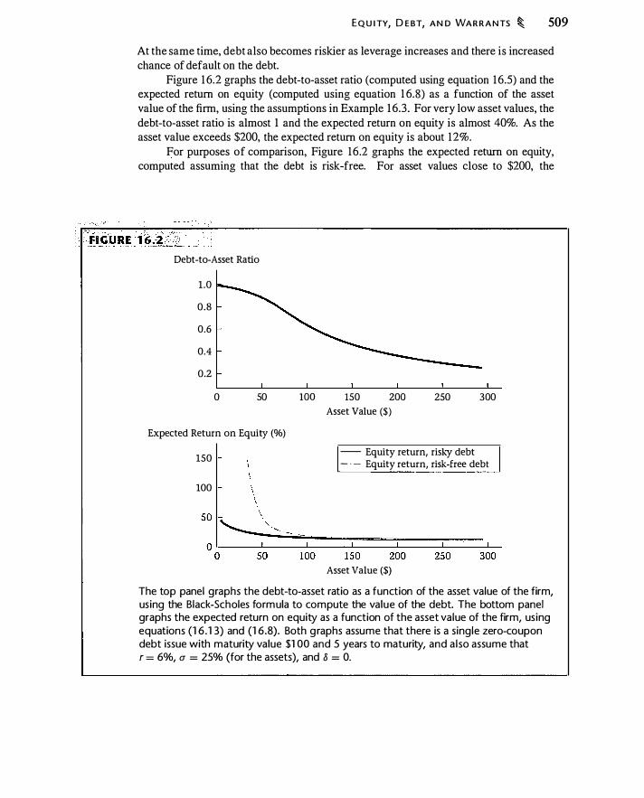
EQU I TY, D E BT, AN D WA R R A NTS � 509

At the same time, debt also becomes riskier as leverage increases and there is increased chance of default on the debt.

Figure 1 6.2 graphs the debt-to-asset ratio (computed using equation 1 6.5) and the expected return on equity (computed using equation 1 6.8 ) as a function of the asset value of the firm, using the assumptions in Example 1 6.3. For very low asset values, the debt-to-asset ratio is almost 1 and the expected return on equity is almost 40%. As the asset value exceeds $200, the expected return on equity is about 1 2%.

For purposes of comparison, Figure 16.2 graphs the expected return on equity, computed assuming that the debt is risk-free. For asset values close to $200, the

Debt-to-Asset Ratio

1 .0

0.8

0.6

0.4

0.2

0 50 100 150 200 250 300 Asset Value ($)

Expected Return on Equity (o/o)

150 -- Equity return, risk-y debt - · - Equity return, risk-free debt

100

Asset Value ($)

The top panel graphs the debt-to-asset ratio as a function of the asset value of the firm, using the Black-Scholes formula to compute the value of the debt. The bottom panel graphs the expected return on equity as a function of the asset value of the firm, using equations (1 6 . 1 3) and (1 6 .8). Both graphs assume that there is a single zero-coupon debt issue with maturity value $1 00 and 5 years to maturity, and also assume that r = 6%, a = 25% (for the assets), and 8 = 0.

5 10 � C O R PO RATE A P P L I CAT I O N S

difference i s less than 20 basis points. For a very highly levered (low asset value) firm, however, the difference in Figure 16 .2 is dramatic.

Conflicts between debt and equity The idea that equity is a call option on the firm and that corporate bonds are risky provides insights into relations between debt- and equity-holders . Since equity-holders control the firm, bondholders may be concerned that equity-holders will take actions that would harm them, or may fail to take actions that would help them.

There are two decisions equity-holders make that affect the relative value of debt and equity. First, equity-holders can affect the volatility of assets. Equity-holders can increase asset volatility either by increasing the operating risk of existing assets, or by "asset substitution," replacing existing assets with riskier assets . An increase in volatility, other things equal, increases the vaiue of the equity-holder's call option and therefore reduces the value of debt. In Example I 6.2, the vega of the equity is 0.66, so an increase in asset volatility of 0.0 I leads to an increase in the market value of equity of $0.66, which is 0.66/27 .07 = 2.4% of equity value. Debt value would decline by $0.66.

A second decision that equity-holders can make is the size of payouts to share­holders, such as dividends and share repurchases. To see why payouts are a potential problem for bondholders, suppose that the firm makes an unexpected one-time $ 1 payout to shareholders. This payout reduces assets by $ 1 . The delta of the equity with respect to assets is less than one, so the value of equity declines by less than $ 1 . Since the value of debt plus equity equals assets, the value of the debt inust decline by one less the delta of the equity. Unanticipated payoJJtS to equity-holders therefore can hurt bondholders .

Bondholders are well aware of the potentially harmful effects of asset substitution and dividends. Bond covenants (legal restrictions on the firm) often limit the ability of the firm to change assets or pay dividends. Viewing debt and equity as options makes it clear why such restrictions exist.

Bondholders also encounter problems from actions that shareholders fail to take. Suppose the firm has a project worth $2 that requires shareholders to make a $ 1 invest­ment. If shareholders make the investment, they pay $ 1 , the value of the assets increases by $2 and the value of the shares rises by 2 x b.. The gain to shareholders is less than the increase in the value of assets. The difference of 2 - 2 x b. goes to the bondholders. In making a positive NPV investment, shareholders help bondholders .

The shareholders in this example only will make the investment if the value of shares goes up by more than the $ 1 they invest, which will only occur if b. > 0.5 . In order for shareholders to be willing to invest, the NPV must be great enough that shareholders gain after allowing for the value increase that is lost to debt-holders.4 Thus, because of debt, the shareholders may fail to make positive NPV investments . A related problem is asset substitution: Shareholders might make negative NPV investments that increase asset risk, thereby transferring value from bondholders to stockholders.

4The idea that the debt may harm investment incentives is developed in Myers ( 1 977) .

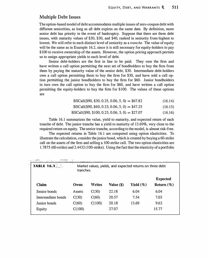
EQU I TY, D E BT, A N D WA R R A NTS � 5 1 1

Multiple Debt Issues

The option-based model of debt accommodates multiple issues of zero-coupon debt with different seniorities, as long as all debt expires on the same date. By definition, more senior debt has priority in the event of bankruptcy. Suppose that there are three debt issues, with maturity values of $30, $30, and $40, ranked in seniority from highest to lowest. We will refer to each distinct level of seniority as a tranche. The value of equity will be the same as in Example 1 6.2, since it is still necessary for equity-holders to pay $ 100 to receive ownership of the assets. However, the option pricing approach permits us to assign appropriate yields to each level of debt.

Senior debt-holders are the first in line to be paid. They own the firm and have written a call option permitting the next set of bondholders to buy the firm from them by paying the maturity value of the senior debt, $30. Intermediate debt-holders own a call option permitting them to buy the firm for $30, and have sold a call op­tion permitting the junior bondholders to buy the firm for $60. Junior bondholders in turn own the call option to buy the firm for $60, and have written a call option permitting the equity-holders to buy the firm for $ 100. The values of these options are

BSCall($90, $30, 0.25 , 0.06, 5 , 0) = $67.82

BSCall($90, $60, 0.25, 0.06, 5 , 0) = $47.25

BSCall($90, $ 1 00, 0.25, 0.06, 5, 0) = $27.07

( 16 . 14)

( 1 6. 1 5)

( 1 6. 1 6)

Table 1 6. 1 summarizes the value, yield to maturity, and expected return of each tranche of debt. The junior tranche has a yield to maturity of 1 3 .69%, very close to the required return on equity. The senior tranche, according to the model, is almost risk-free.

The expected returns in Table 1 6. 1 are computed using option elasticities . To illustrate the calculation, consider the junior bond, which is created by buying a 60-s trike call on the assets of the firm and selling a I 00-strike call. The two option elasticities are 1 .7875 (60-s trike) and 2.4432 ( 100-strike). Using the fact that the elasticity of a portfolio

Claim

Senior bonds

Intermediate bonds ·

Junior bonds

Equity

Market values, yields, and expected returns on three debt tranches.

Expected

Owns Writes V alue ($) Yield (%) Return (%)

Assets C(30) 22. 1 8 6.04 6.04

C(30) C(60) 20.57 7 .54 7.03

C(60) C( 1 00) 20. 1 8 1 3 .69 9.63

C( lOO) 27.07 15 .77

5 12 � C O R PO R ATE A P P L I CATI O N S

i s a weighted average of the elasticities of the portfolio components, the elasticity of the junior bond is

47 .25 27 .07 ----- X 1 .7875 - X 2 .4432 = 0.9077 47.25 - 27.07 47 .25 - 27.07

The expected return on the junior debt is therefore

ljunior = 0.06 + (0. 10 - 0.06) X 0.9077 = 0.0963

Table 16 . 1 makes it clear why debt cannot be treated as a single homogeneous class when firms with complex capital structures enter bankruptcy. The interests of the most junior debt-holders may well resemble the interests of equity-holders more than those of senior debt-holders.

Warrants

Firms sometimes issue options explicitly. If a firm issues a call option on its own stock, it is known as a warrant. (The term "warrant" is used here to denote options on a firm issued by the firm itself, though in practice the term includes traded options issued in fixed supply.) When a warrant is exercised, the warrant-holder pays the firm the strike price, K, and receives a share worth more than K (or else the holder would not have exercised the warrant). Thus, the act of exercise is dilutive to other shareholders in the sense that the firm has sold a share for less than it is worth. Of course, existing shareholders are aware of warrants outstanding and can anticipate this potential exercise. The problem is how to value the warrant, and how to value the equity given the existence of warrants. This valuation problem does not arise with ordinary options, because they are traded by third parties and their exercise has no effect on the firm.

To see how to value a warrant, suppose the firm has 11 shares outstanding, and that the outstanding warrants are European, on m shares, with strike price K. The asset value is A .

A t expiration, if warrant-holders exercise the warrants, they pay K per share and rec;eive m shares. After the warrants are exercised, the firm has assets worth A + m K, hence exercised warrants are worth

_A_+_n

_z K _

_ K _ _ 1_z _ (!!..

_ K)

n + m n + m n ( 1 6. 17 )

The expression Ajn is the value of a share of equity in the absence of warrants. Thus, equation ( 1 6. 1 7) suggests that we can value a warrant in two steps. First, we compute an option price with A j n as the under! ying asset and K as the strike price, ignoring dilution. Second, we multiply the result by a dilution correction factor, nj(n + m) . This second step accounts for the fact that warrant exercise changes the number of shares outstanding, with the new shares issued at a "below-market" price of K. The warrant can be valued by using the Black-Scholes formula:

_n_BSCall

(!!.. , K, a , r, t, o) n + m n ·

( 1 6. 1 8)

Convertible Bonds

EQU ITY, D E BT, A N D WA R R A NTS � 5 13

In addition to issuing warrants directly, firms can issue warrants embedded in bonds. A convertible bond is a bond that, at the option of the bondholder, can be exchanged for shares in the issuing company. A simple convertible bond resembles the equity-linked notes we studied in Chapter 15 , except that the bond is convertible into the company's own shares rather than the shares of a third party . . The call option in the bond gives the bondholder the right to surrender the bond's maturity payment, M, in exchange for q shares: The valuation of a convertible bond entails valuing both debt subject to default and a warrant.

Suppose there are m bonds with maturity payment M, each of whtch is convertible into q shares. The value of the firm at time T is AT . If there are n original shares outstanding, then there will be n + mq shares if the bond is converted. At expiration, the bondholders will convert if the value of per share of the assets after conversion, AT/ (11 + mq ), exceeds the value per share of the maturity payment that bondholders would forgo:

or ll

AT M --- > -11 + mq q

--- -- - - > 0 (AT M n + mq )

n + mq n q n ( 1 6. 1 9)

This expression i s different from equation ( 1 6. 1 2) for warrants, because rather than injecting new cash into the firm when they convert, the bondholders instead avoid taking cash out of the firm.

Conversion occurs if the assets increase sufficiently in value. If the assets decrease, the firm could default on the promised maturity payment. Assuming the convertible i s the only debt issue, bankruptcy occurs if assets are worth less the promised payment to all convertible holders, or AT < m M. The payoff of the convertible at maturity, time T, is

mM- max (0, m M - AT) + mq x x max 0, - - - ( 1 6.20) ll ( AT M n + mq )

n + mq n q n '-v-' Bond Writ!en put mq Purchased warranL'

Thus, owning m convertibles can be valued as owning a risk-free bond with maturity payment mM, selling a put on the firm's assets, and buying mq warrants with strike Mfq x (n + mq)jn .

Equation ( 1 6.20) can be rewritten as

max [min (m M , AT) , mq AT] n + mq ( 1 6.2 1 )

This version of the convertible payoff can be interpreted as follows: Shareholders give bondholders the least they can (min[M, AT/m]) ; if it i s optimal to do so, convertible

5 14 � C O R P O RATE A P P L I CAT I O N S

holders can then exchange this amount for the conversion value, which i s their propor­tionate share of the assets (mq j[n + mq] x AT) .

Example 1 6.4 Suppose a firm has issued m = 6 convertible bonds, each with maturity value M = $ 1 000 and convertible into q = 50 shares. The firm has n = 400 common shares outstanding. Figure 1 6.3 shows the maturity payoff for the aggregate value of the convertible bonds, comparing it with the maturity payoff of otherwise identical nonconvertible bonds issued by the same firm. The six bonds have a total promised maturity value of $6000, so default occurs when assets are below that level. Equation ( 1 6. 1 9) implies that conversion occurs when assets exceed $ 1 000 x 700/50 = $ 14,000. The slope of the convertible payoff above $ 14,000 is mq j(n + mq) = 3/7, less than the slope in default, because convertible investors share gains with existing shareholders, but once in default, convertible bondholders bear additional losses alone (in default, shares are already worthless) . �

Just as we valued ordinary zero-coupon bonds with the Black-Scholes formula, we can also use the Black-Scholes formula to value a bond convertible at maturity.

F I GU R E 1 6 . 3 Maturity payoffs for the aggregate value of an ordinary bond and a convertible bond, using the parameters in Example (1 6.5) .

Bond Value ($)

18,000

1 6,000

14,000

. 12,000

10,000

8,000

1- Ordinary bond I = Convertible equity 1/

/ �ersion /,x (Slope = 3/7)

./ / /' /

::::: � ffuult !·:=:.

A�et> = $ 1 4,000 2,000 v �:�·

pe = 1)

0 5,000 10,000 15,000 20,000 25,000 30,000 35,000 40,000

Asset value at maturity ($)

. .

EQU I TY, D E BT, A N D WA R RA NTS � 5 15

Example 1 6.5 Suppose a firm has assets of $ 1 0,000 with a single debt issue con­sisting of six zero-coupon bonds, each with a maturity value of $ 1 000 and with T = 5 years to maturity. The asset volatility is u = 30% and the risk-free rate is r = 6%. The firm makes no payouts.

If the single debt issue is not convertible, the price is

- ($ 1 0 000 ) $ 1000 x e-0·06x:> - BSPut � , $ 1 000, 0.30, 0.06, 5 , 0 = $70 1 .27

The yield on the nonconvertible bond is ln ( l 000j70 1 .27)/5 = 0.07 10, greater than the risk-free rate because of the risk of bankruptcy.

Suppose the debt issue is instead the convertible bond described in Example ( 1 6.4 ) . Using equation ( 1 6.20), the value of all convertible bonds is

6 x $ 1 000 x e-0·06x5 - BSPut ($ 10 ,000, 6 x $ 1 000, 0.30, 0.06, 5, 0) 6 50

400 BSC ll

( $ 10,000 $ 1 000 400 + 6 x 50 ) + X X 400 + 6 X 50

X a 400 ' -so 400 ' 0·30• 0·06• 5 • O

= $5276.35

Each bond has a price of $879.39. The yield on a bond is ln ($ 1000/$879.39)/5 = 0.0257. This is below the yield on an otherwise equivalent nonconvertible bond because of the conversion option: The bondholders have a call option for which they pay by accepting a lower yield on the debt. The value of a share is ($ 1 0,000 -$5276.35) /400 = $ 1 1 .809. Bondholders will convert if at maturity the assets are worth more than

M X (11 + mq)jq = $ 1000 X (400 + 6 X 50)/50 = $ 14,000

Convertible bonds are typically issued at terms such that a significant increase in the stock price is required for conversion to be worthwhile. In Example 1 6.5, each bond

.

gives the holder the right to convert into 50 shares, so the strike price is $ 1000150 = $20. Since the stock price is $ 1 1 .809, the ratio of the strike price to the stock price, which is called the conversion premium, is $20/$ 1 1 . 809 - 1 = 69.4%. In practice, conversion premiums are most commonly between 20% and 40%.

Why do firms issue convertible bonds? One explanation is that convertible bonds resolve one of the conflicts between equity- and debt-holders. Shareholders can take value from holders of ordinary bonds by increasing volatility, even if this action has no beneficial effect from the perspective of the firm as a whole. However, convert­ibles are harmed less than ordinary debt by an increase in volatility, and may even be helped. Financing with convertibles instead of ordinary debt thus reduces the incentive of shareholders to raise volatility.

In practice, valuation of convertible bonds is more complicated than in this ex­ample. First, convertible bonds are typically American options, convertible for much of the life of the bond. Second, convertible bonds typically are not zero-coupon. The

5 16 � C O R PO RATE A P P L I CAT I O N S

payment of coupons complicates the analysis because bankruptcy becomes possible at times other than expiration and the reduction in assets stemming from the payment of the coupon (or any other cash payment to the firm's security-holders). This coupon reduces assets but is also paid to the bondholders. Third, many companies pay dividends . If the dividends that can be earned by converting the bond into stock exceed the bond coupon, there can be a reason for bondholders to convert before maturity. Finally, interest rates and volatility can change, and the circumstances of default may be more complicated than we have assumed (for example, when there are other debt issues, default could occur prior to maturity) . The value of the bond can then change for reasons other than stock price changes.

It is possible to value convertible bonds incorporating early exercise, dividends, and callability.5 It is also possible to incorporate interest rate risk using techniques described later in the book.

·

Callable Bonds

Many bonds are callable, meaning that, prior to maturity, the company has the right to give bondholders a predetermined payment in exchange for the bonds . The idea underlying a callable bond is that the bond issuer can buy the bond back at a relatively cheap price if it becomes expensive. A bond can become expensive because interest rates have fallen, in which case the issuer would like to exchange the existing bonds for new bonds carrying a lower coupon rate. A bond can also become expensive if the market perceives that the company is- less likely to default. Again, in this case the company would like to exchange the existing bond for a newly issued bond with a lower default premium. A firm can always buy bonds back at a market price, but there is generally no advantage to doing so. Callability permits the company to buy bonds back at a relatively low price. Of course the company pays for this right by receiving a lower price when it issues the bond.

The predetermined price at which a company can call a bond is specified by a call schedule. Bonds are typically noncallable for several years after issuance, a period dming which the bond is said to have call protection. Callability is, in effect, an option that investors sell to the bond issuer. In return, the company issuing the bonds pays a higher yield on the bonds.

Convertible bonds are typically callable. When the issuer calls a convertible bond, the holder of the bond has the choice of surrendering the bond in exchange for the call price or converting. Callability is a way for issuers to shorten the life of the bond, potentially forcing holders to convert prior to maturity. The issuer-acting in the interests of shareholders-follows a call strategy that minimizes the value of the bond. Bondholders, by contrast, follow a conversion strategy that maximizes the value of the bond.

5Ingersoll ( 1 977) and Brennan and Schwartz ( 1 977) discuss the valuation of convertible bonds.

EQU ITY, D E BT, AN D WA R R A NTS � 5 17

Since bonds can be called prior to expiration, we cannot value the call provision using Black-Scholes. However, we can value a callable bond binomially. The call strategy for an issuer is like the exercise of an American option: The issuer calls if it is more valuable to do so than to leave the bond outstanding for another period.

Figure 1 6.4 presents binomial valuation examples for four bonds : an ordinary bond, a convertible bond, a callable bond, and a callable convertible bond. We examine noncallable bonds as benchmarks in order to better understand the effect of callability. We value these bonds using the binomial pricing model outlined in Chapters 10 and 1 1 . In each case, the assets of the firm are the underlying asset, and the value of the bonds is determined by the value of the assets . To perform the valuation, we move backward through the tree, as in Chapter 10. The assumptions in Figure 1 6.4 are the same as those in Example 1 6.5, so the results in the example and figure are comparable for the ordinary and convertible bonds.

Callable nonconvertible bonds We first consider the binomial valuation of an ordi­nary, noncallable bond (Panel B in Figure 1 6.4) and its callable counterpart (Panel D in Figure 1 6.4). The yield on the callable bond (7.57%) exceeds that on the noncallable bond (7.29%) because of the option that bondholders have written to the firm.

How are bond prices in Figure 1 6.4 computed? For the ordinary bond, the value in year 5 is

Bs = min(m M, As) = min ($6000, As)

There are s ix $ 1 000 bonds outstanding, and shareholders wil l pay to these bondholders the value of the firm or $6000, whichever is less. Note that default occurs at the bottom node in year 5 since the value of assets is less than the required bond payment, $6000. Prior to maturity, the value at each node is calculated as in a typical binomial valuation, with

B1 = e-rh [p B�11 + ( 1 - p) B;�_,.J

For a given node at time t , B�11 is the bond value if assets move up from that node, and B1�11 is the bond value if assets move down from that node.

The binomial valuation of the callable bond is straightforward. Let K1can denote the call schedule. The call price in this example is set to equal the price of a bond yielding 6.75%. At time 1 .67, for example, the company could call by paying the bondholders $479 1 . 1 0, which, for a bond maturing in 3 .33 years, is a yield of 6.75%. We assume that the risk-free rate is fixed; thus the only reason for the company to call the bond is if the company could issue replacement bonds at a lower coupon due to a decrease in default risk.

Shareholders wish to minimize the value of the bonds, hence their value is

B1 = min [ Leave the bond outstanding, call ] . [ -rl! ( B+ + ( 1 ) B- ) Kcall] = mm e p t+II - p t+II , t ( 1 6.22)

If you compare the binomial trees in Panels B and D, it is apparent why the callable bond has a lower price at issue than the ordinary bond. At the top node in year 1 .67,

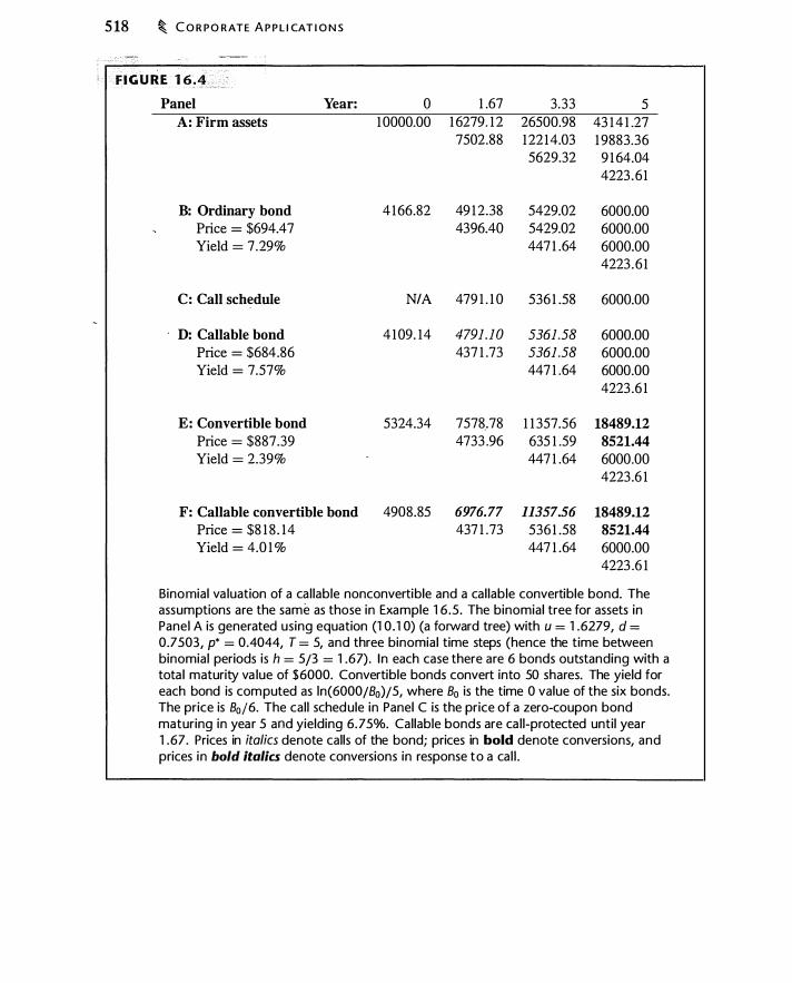
5 18 � C O R P O RATE A P P L I CAT I O N S

Panel Year: A: Firm assets

B: Ordinary bond Price = $694.47 Yield = 7 .29%

C: Call schedule

· D: Callable bond Price = $684.86 Yield = 7.57%

E: Convertible bond Price = $887.39 Yield = 2.39%

F: Callable convertible bond Price = $8 1 8 . 14 Yield = 4.0 1 %

0 1 0000.00

4 166.82

N/A

4 109. 14

5324.34

4908.85

1 .67 3 .33 5 1 6279. 1 2 26500.98 43 14 1 .27 7502.88 1 22 14.03 1 9883.36

5629.32 9 1 64.04 4223 .6 1

49 1 2.38 5429.02 6000.00 4396.40 5429.02 6000.00

447 1 .64 6000.00 4223 .6 1

479 1 . 1 0 536 1 .58 6000.00

4791 .10 5361 .58 6000.00 437 1 .73 5361.58 6000.00

447 1 .64 6000.00 4223 .6 1

7578 .. 78 1 1 357.56 18489.12 4733 .96 635 1 .59 8521.44

447 1 .64 6000.00 4223 .6 1

6976. 77 11357.56 18489.12 437 1 .73 536 1 .58 8521.44

447 1 .64 6000.00 4223 .6 1

Binomial va luation of a cal lable nonconvertible and a cal lable convertible bond. The assumptions are the same as those in Example 1 6 .5 . The binomial tree for assets in Panel A is generated using equation (1 0 . 1 0) (a forward tree) with u = 1 .6279, d = 0.7503, p* = 0.4044, T = 5, and three binomial time steps (hence the time between binomial periods is h = 5/3 = 1 .67) . I n each case there are 6 bonds outstanding with a tota l maturity va lue of $6000. Convertible bonds convert into 50 shares. The yield for each bond is computed as ln(6000/Bo)/5, where 80 is the time 0 value of the six bonds. The price is 80j6. The cal l schedule in Panel C is the price of a zero-coupon bond maturing in year 5 and yielding 6. 75%. Cal lable bonds are ca l l-protected until year 1 .67 . Prices in italics denote calls of the bond; prices in bold denote conversions, and prices in bold italics denote conversions in response to a cal l .

EQU I TY, D E BT, A N D WA R RA NTS � 5 19

the noncallable bonds are worth $49 1 2.38, for a yield of 6%. (If assets reach that node, default will not occur.) The firm calls the callable bond at that node since it is now possible to issue default-free debt. The prospect of this call prevents the bondholders from receiving a capital gain. This in turn lowers the initial price of the bond. Problem 16. 15 asks you to compute share prices at each node so that you can see the effect on shareholders of the different bonds.

Callable convertible bonds We now consider noncallable and callable convertible bonds, Panels E and F in Figure 16 .4. Note first thar, as in Example 1 6.5, the yield on the convertible noncallable bond (2.39%) is lower than that on the ordinary bond (7.29%) because convertible bondholders receive a call option and pay for this with a lower yield.

Using equation ( 1 6.2 1 ), the year 5 value for the convertible bond is . n 1 q

max [mm (m M, A5) , As ] 11 + mq In Panel E in Figure 1 6.3, bondholders convert at the top two nodes in year 5, receive the maturity payment in cash at the next node, and the firm defaults at the bottom node.

Prior to maturity, the convertible investor values the bond as the greater of its conversion value and the value of letting the bond live one more period:

B1 = max [ Continue to hold, convert ]

= max [e-r" (pB1�h + ( 1 - p) B1�, ) , m

q A1] 11 + m q ( 1 6.23)

B1 is the total value of the bonds . You may recognize this expression as almost identical to equation ( 1 0. 1 0) for valuing an American call option on a stock. The difference is that the payoff is the conversion value instead of S1 - K .

When the bond is both convertible and callable, there is a tug-of-war between the firm and the bond investors. We can imagine the bond value being determined as follows: The bondholders decide whether to hold or convert (maximizing the bond, value).. Given this decision, the firm decides whether to call (minimizing the bond value) . If the firm calls, bondholders revisit their decision about whether or not to convert (again maximizing the bond value, conditional upon the behavior of the firm). This chain of reasoning implies the following valuation equation:

B1 = max {min [max( Continue to Hold, Convert) , Call ] , Convert }

= max {min [max (e -rh [p B1�h + (1 - p) B1�1J , 111 q A. 1 ) , K1can] , 11 + mq

�--------�--------� � �

----"-- AI mq }

11 + m q �

Com•en

Hold Conven Cal l

( 1 6.24)

As you would expect, the ability to call a convertible bond lowers its price, raising its yield from 2.39% to 4.0 1 %. By comparing Panels E and F in Figure 1 6.4, you can see

520 � C O R PO RATE A P P L I CATI O N S

why this happens. I n year 1 .67 at the top node, it i s optimal to wait to convert if the bond is noncallable. This gives a bond value in Panel E of $7578.78. However, if the bond is callable using the call schedule in Panel C, the firm will call at the top node in year 1 .67. In response, the bondholders convert, giving them 50 shares worth $6976.66. The bond is worth less because shareholders cannot delay the conversion. The firm does not call at the lower node in year 1 .67 because the credit quality of the bond deteriorates at that node.

Bond Valuation Based on the Stock Price

The binomial examples in Figure 1 6.4 assume that the assets of the firm follow a binomial process and use the resulting tree to- value a convertible bond. This approach becomes complicated when the firm's capital structure contains multiple bonds and convertible securities.

An altemati ve approach, often used in practice, is to base valuation of a convertible bond on a binomial tree for the stock, rather than on assets. A standard binomial tree for the stock, however, will never reach a zero stock price, and thus a convertible bond valued on this tree will be priced as if it were default-free. This raises the question: How can we incorporate bond default risk into the pricing procedure?

Tsiveriotis and Fernandes ( 1 998) suggest valuing separately the bond income and the stock income from an optimally managed convertible bond. Their procedure accounts for default by discounting bond i_ncome at a rate greater than the risk-free rate, while the component of the bond income related to conversion into stock is discounted at the risk-free rate.

Other Bond Features

It is possible to issue bonds that are considerably more complex than those we have considered. Conversion and call schedules can vary with time in complicated ways . Bonds can be puttable, meaning that the investor can sell them back to the firm at a predetermined price. Bonds can pay contingellt interest, meaning that if a particular event occurs, the interest rate on the bond changes.

As we saw in Chapter 15 , particular structures are often a response to tax and accounting considerations. Another example is the use of colltingellt convertible bonds, also known as "co-co's."

Firms report earnings on a per-share basis. For a firm that has issued only shares and ordinary debt, computing earnings per share (EPS) is straightforward since there is no ambiguity about the number of shares outstanding. However, if a firm has issued convertible debt or warrants, how many shares should the firm use in computing EPS? Under financial accounting rules in the United States, the firm must compute the worst­case fully diluted earnings per share. When the firm has issued a convertible security, this generally means adding back to earnings after-tax interest on the convertible, and adding the number of convertible shares to shares outstanding.

(.o-Co Puffery?

GM was taken by surprise in July 2004 when the FASB proposed new rules governing the accounting treatment of contingent convertibles :6

The earnings of General Motors will be reduced by $ 1 per share, or 15 percent of the carmaker's target for the year, by new accounting rules for an increasingly popular type of bond expected to come into force this win­ter.

John Devine, chief financial offi­cer, said the change to the treatment of contingently convertible bonds would confuse investors, and GM would not have issued them if it had known it was coming. GM is thought to be the largest issuer of the "co-co" bonds, with over $8 billion outstanding . . . .

"To say the least, this is very dis­ruptive to us," Mr. Devine said. "It has significant ramifications for how investors look at our business. It con­fuses investors." . . .

Mr. Devine expects the new rules to come into force towards the end of the year, and GM would then have to restate its eps figures. Net income would be unaffected.

EQU ITY, D E BT, A N D WA R R A NTS � 521

Co-co secuntres were first in­troduced in 2000 and have become popular because of their accounting advantages. They make up the bulk of new issuance in the convertible mar­ket, but will be far less attractive under the new rules.

"It will substantially decrease the number of co-cos," one convertible securities analyst said.

Two weeks later, GM had found a solution to its dilemrna:7

Devine . . . said GM had found a solution to the problem that would meet the requirements of the Financial Accounting Standards Board, which oversees US accounting.

"GM would waive its right to is­sue stock to settle at least the princi­pal amount of debt," Mr. Devine told the Management Briefing Seminars, an annual automotive conference in Michigan.

"This means we would use cash rather than stock and significantly limit the dilutive effect." . . .

Accounting for instruments like co-cos remains a confusing and contentious issue.

In recent years firms have issued contingent convertible bonds, which are secu­rities that for a time received different accounting treatment than ordinary convertibles. Holders of such bonds can convert only when a contingency-such as the stock price

6"New Bond Rules to Dent GM Earnings.'' by James Mackintosh and Jenny Wiggins, Financial Times, London ed., July 22, 2004, p. 26. 7"GM acts on New Co-Co Bond Rules" by Jeremy Grant, Financial Times, London ed., August 6, 2004, p. 24.

522 � C O R P O R ATE A P P L I CAT I O N S

being sufficiently high-has occurred. Prior to 2005 , firms were permitted to ignore such bonds in computing fully diluted EPS . However, the FASB ruled that such bonds had to be treated as convertibles, and a number of firms that had issued such bonds were forced to change the way they accounted for them.

The box on page 52 1 discusses the reaction of one company to the FASB 's new rule, and makes it clear that the accounting treatment of a security is important for issuers .

Put Warrants

When shares are used to pay employees (as for example with compensation options), there is an increase in the number of shares outstanding. Companies making heavy use of share compensation frequently buy shares back from other shareholders (a share repurchase) so there is no nefincrease in the number of shares outstanding.8

Many companies that repurchased shares during the 1 990s also sold put options on their own stock; a commonly stated rationale for issuing such put warrants (see, for example, Thatcher et al . , 1 994) is that the put sales are a hedge against the cost of repurchasing shares. Intel, Microsoft, and Dell, for example, all sold significant numbers of puts, with Microsoft alone earning well over $ 1 billion in put premiums during the 1 990s. Here is a quote from Microsoft's 1999 1 0-K describing the put program:

Microsoft enhances its repurchase program by selling put warrants . . . . On June 30, 1 999, 1 63 million warrants were outstanding with strike prices ranging from $59 to $65 per share. The put warrants expire between Septem­ber 1 999 and March 1002. The outstanding put warrants permit a net-share settlement at the Company's option and do not result in a put warrant liability on the balance sheet.

How do we think about this transaction? If Microsoft repurchases shares, via a written put or by any other means, nonselling shareholders are in effect buying shares from selling shareholders. It is common to say that managers should maximize share­holder value, but which set of shareholders do they care about? Despite this theoretical ambiguity, we will examine the transaction using a standard profit and loss calculation.

Figure 16.5 is a profit diagram for various alternatives. Suppose that the share price today is $ 1 00 and the firm will for certain buy one share back in 3 years. The firm has 3 years to earn interest on the $ 1 00 it could have spent today. The profit diagram shows that if the price is still $ 1 00 in 3 years, the firm has profited by the amount of this interest. The sale of a put expiring in 3 years generates the curve labeled "Written Put."

The third curve in Figure I 6.5 shows the combined profit and loss for a short share and written put. (By put-call parity, this position looks like a written call . ) Should the share price rise, the firm repurchases shares at a higher price but keeps the put premium. If the share price falls, the firm is obligated to pay the strike price to repurchase shares. This transaction is the mirror image of covered call writing, discussed in Chapter 3.

8Corporate finance theory offers no justification for this practice, but firms seem to believe that it is

imponant.

Profit diagram for being short a share of stock, writing a put, and the combination of the two.

Profit ($)

1SO

100

so

0 #"

- // -SO / -100

-1SO

-200

0 so 100

C O M P E N SATI O N O PT I O N S � 523

- Short stock = Written put ••••• Short stock + written put

··· .

.. .. •···

··· ... .. ···

···•···

· .

.. .

. ······

·····

····

•·· ...

1SO 200 2SO 300 Stock Price at Expiration ($)

In practice, dealers have purchased the puts written by firms such as Microsoft, Intel, and Dell. The dealers reportedly hold the puts and delta-hedge the position, as in Chapter 1 3 , thus reducing their risk. Moreover, the transactions, including the dealer's hedging trades, occur without any public announcement. In effect, put-selling firms transact with shareholders using the dealer as a conduit. When the share price rises, the d�lta of the dealer's purchased put, which is negative, increases toward zero and the dealer sells the shares it had purchased to hedge the put. When the share price falls, delta increases to negative one and the dealer buys additional shares to hedge its position. The dealer, acting on behalf of the firm, buys as the share price declines and sells as the share price rises.

Problem 1 6. 1 9 asks you to examine a binomial example of this transaction, show­ing first that the firm could accomplish the same end as put-writing by transacting directly in its shares. Second, the problem asks you to show how the counterparty dealer delta­hedges the transaction.

16.2 COMPENSATION OPTIONS

Many firms compensate executives and other employees with call options on the com­pany's own stock. The use of such compensation options is common and significant in many companies, but has declined since 2002.

524 � C O R P O RATE A P P L I CATI O N S

Microsoft, for example, estimated i n its 1 999 annual report ( 10-K) that its grants that year of 78 million options were worth about $ 1 .6 billion. This is approximately $52,000 per employee (Microsoft had 3 1 ,000 employees). Elsewhere in its 1 0-K, Mi­crosoft reported that total outstanding options on 766 million shares (against 5 billion shares outstanding) had a market value on June 30, 1 999, of $69 billion, or $2 million per employee.

Many other companies made significant use of compensation options. Eberhart (2005) found in a sample of 1 800 firms using compensation options in 1 999 that options were on average 1 2% of shares outstanding. Moreover, the use of options has not been restricted to executives : Core and Guay (200 1 ) found in a sample of 750 companies that two-thirds of option grants were to nonexecutive employees.

The use of compensation options has declined in recent years. Several develop­ments seem to be responsible for this change. First, the market decline in 2000 left many employees with deep out-of-the-money options and created morale problems for companies heavily dependent upon options. The box on page 526 discusses Microsoft's response to its overhang of out-of-the-money options.

Second, both the Financial Accounting Standards Board (FASB) in the United States and the International Accounting Standards Board (IASB) announced that they would require companies to recognize employee option grants as a compensation ex­pense. Throughout the 1 990s most companies had treated compensation options as worthless when computing earnings.9 An attempt by the FASB to require option ex­pensing in the early 1 990s was defeated by companies opposed to expensing. Many of these companies were concerned about the decline in reported earnings that would result from expensing.

The logic behind requiring companies to expense option grants is straightforward. If a company pays cash to an employee, the company deducts the payment as an expense. If an otherwise identical company replaces some of the cash with an option grant, that company will report systematically higher earnings than the first unless the value of the option grant is also deducted as an expense.

To think about expensing, you can perform the following thought experiment: Imagine that a firm that issues options to employees were to hedge its obligations by buying a contract from a third party. Under the terms of this contract, the third party would pay the firm the value of the option when the employee exercises it. The firm could grant an option and buy the hedging contract, thereby insulating shareholders from the effect of the grant. The cost of this hedging contract is the cost to the firm of the option grant.

If a firm does not buy such a contract, it self-insures, meaning that shareholders bear the cost of the option grant. Either way, the cost of the insurance is the cost to shareholders of the compensation option. The problem of valuing a compensation option amounts to asking how much it would cost the firm to hedge its compensation commitments .

9SFAS 1 23 did require companies to report the value of options in a footnote. This value-frequently

computed using the Black-Scholes formula-did not affect reported earnings.

C O M P E N SATI O N O PT I O N S � 525

In December 2004, the FASB issued Statement of Financial Accounting Standards (SFAS) 123R, which contained the final rules, effective in June 2005, for companies to follow in expensing options. The statement

requires a public entity to measure the cost of employee services received in exchange for an award of equity instruments based on the grant-date fair value of the award (with limited exceptions) . That cost will be recognized over the period during which an employee is required to provide service in exchange for the award-the requisite service period (usually the vesting period). 1 0

A company might grant options that vest after three years and expire after seven years. Under SFAS 1 23R, the company could value these options using the Black-Scholes or the binomial formula, and then expense 1 /3 of their value over each year of the vesting period.

The valuation of compensation options is complicated by the fact that there are many special considerations in valuing them:

• Compensation options cannot be sold and typically are not fully vested (i.e., the employee does not own them) for several years.

• The executive may resign, be fired, die, or become disabled, or the company may be acquired. Any of these may affect the value of the option grant, either by forcing early exercise (as may happen with a death) or requiring that the options be forfeited (in the event the executive is fired) .

• The term of the options can be 10 years or more, which makes volatility and dividend estimates difficult.

• The company may not have a publicly traded stock, in which case the stock price must be estimated.

• There may be unusual contractual features of the compensation option contract For example, the strike price may be an industry stock price index.

Such considerations make it harder to value compensation options than short-lived exchange-traded options. We will now discuss some of the issues that arise in option expensing.

Whose Valuation?

Compensation options cannot be traded. An employee who cannot sell options will typically discount their value. As a result, you can expect that firms and employees will value compensation options differently. Such a difference in valuation can occur for any compensation other than immediate cash.

10Statement of Financial Accounting Standards No. 1 23R. p. ii.

526 � C O R P O R ATE A P P L I CATI O N S

The E n d o f Com pensation O pt ions?

In July 2003, the Wall Street Journal proclaimed: 'The golden age of stock options is over." (See "Microsoft Ushers Out The Era of Options," by Robert A. Guth and Joann S . Lublin, Wall Street Journal, July 14, 2003.) Microsoft stock had fallen recently and many employees had out-of-the-money options. Employees expressed what CEO Steve Ballmer called "angst" about the low stock price, and the effect on option values.

Microsoft's CFO was quoted in the article as saying that employees could no longer expe<?t to become wealthy from stock options:

"If you think what happened in the nineties is going to happen again­it's not," said Microsoft Chief Finan­cial Officer John Connors. In a recent interview he described the PC market boom as a "phenomenon" that "no­body will ever likely repeat."

Microsoft announced that it would eliminate the use of options as compensation, issuing restricted stock instead. (Restricted stock is stock that cannot be sold for a period of time.)

In addition, Microsoft entered into an agreement with JP Morgan Chase whereby the

bank would, on a one-time basis, offer to buy ·

employee options. The bank bought the options at modified terms; for example, maturities were reduced to a maximum of three years. As a result employees sold their options for a price that in many cases was significantly less than the unrestricted price for an otherwise equivalent traded option. JP Morgan Chase, which would hold the options it acquired, informed Microsoft employees that it would be short-selling shares in order to delta-hedge the option position. Slightly more than half of employee options were sold in this fashion.

Microsoft's avoidance of options appeared to be part of a general trend. One survey found a 50% reduction in the value of option grants between 2001 and 2003 . ("Stock Option Awards Sharply Cut," by Ruth Simon, Wall Street Journal, December 14, 2004, p. D3.)

In 2005, Microsoft chairman Bill Gates even told a group of business writers, "I regret that we ever used stock options." (Reuters, "Gates Regrets Paying with Stock Options," www.cnn.com, May 3, 2005)

Accounting standards require that companies deduct the cost to the company. The goal is to measure cost to nonemployee shareholders , not value to employees. For example, suppose a company grants employees non tradable membership in a golf club costing $ 1 5 ,000 per year. No one would value the membership at more than $ 1 5 ,000, because it can be purchased for that amount. However, someone who does not play golf might value the membership at zero. Thus, while for one executive the membership might displace $ 1 5,000 of salary, for another, it might not displace any salary. However, in either case, shareholders bear the $ 1 5,000 cost. The fact that the employee discounts the membership s value does not reduce the cost to the firm. For shareholders, the key question is the cost to the company: How should shareholders value option grants, given the behavior of employees .

Valuation Inputs

C O M P E N SATI O N O PT I O N S � 527

SFAS 1 23R calls for the valuation to measure fair market value of the option. This requires that companies estimate the likely behavior of employees with respect to exercise and forfeiture of options, and also that the company estimate prospective volatility and dividends. 1 1 To illustrate several practical issues in measuring cost to the company, we again consider Microsoft as an example. In accord with SFAS 1 23, Microsoft in 1 999 valued its options using Black-Scholes and disclosed this value in a footnote. The options vested in 4 1 /2 years and expired after 7 years. Here is the discussion from Microsoft's 1 999 1 0-K:

[Option] value was estimated using an expected life of 5 years, no div­idends, volatility of 0.32 in 1 999 and 1998 and 0.30 in 1997, and risk-free interest rates of 6.5%, 5.7%, and 4.9% in 1 997, 1 998, and 1 999.

Microsoft does not document how it chose volatilities, but these are close to historical volatilities in each year. Using weekly data, historical volatilities for Microsoft for July to June were 32% for 1 996-1997, 30% for 1997-1 998, and 39% for 1 998-1999.

Why did Microsoft use a 5-year expiration to value options expiring in 7 years? We learned in Chapter 9 that it is never optimal to early-exercise a publicly traded call option on a nondividend-paying stock since it can be sold for more than its intrinsic value. However, compensation options cannot be sold. Thus, the value of the options to the holder may be less than intrinsic value. In this case, employees may exercise the options before expiration. 1 2 This is in fact how employees behave: In practice, execu­tives frequently exercise a large fraction of their in-the-money options as soon as they vest. 1 3 In addition to exercise by continuing employees, options are often canceled due to death, termination, or retirement of the employee. Taxes can also potentially affect the exercise decision, although a common tax-motivated argument for early exercise is incorrect. 14 Finally, compensation options cannot be exercised until they vest. A realistic

1 1 Since dividends reduce the value of an option, it is possible that widespread use qf compensation

options has resulted in a reduction in corporate dividends.

12See Kulatilaka and Marcus ( 1 994) for a discussion of the employee's valuation of options.

13Huddart ( 1 998) shows that options are disproportionately exercised on the first through fourth an­

niversaries of the grant, in blocks of 25% of the grant. Since i t is common for grants to vest 25% annually, this finding S!Jggests that many options are being exercised as soon as possible.

14An employee is taxed at ordinary income rates on the exercise of a nonqualified option, with subse­

quent gains on the stock being taxed at capital gains rate. Some have argued that employees optimistic

about the share price should exercise compensation options early in order to maximize the percentage

of income taxed at the favorable capital gains rate. This argument is incorrect. However, if the ordinary

income rate is expected to increase, early exercise can be optimal. For a discussion see McDonald

(2003).

528 � C O R P O RATE A P P L I CAT I O N S

valuation would account for the likelihood of these various factors. The assumed 5-year life is intended to account for the expected life of an option. 1 5

It is possible to modify both the Black-Scholes and binomial models to account for complications due to early exercise. For example, suppose that 4-year options vest after 3 years. The company examines historical data and estimates that 5% of outstanding options will be forfeited each year during the vesting period. Furthermore, the company believes that half of the remaining options will be exercised at vesting, with the other half exercised at expiration. One could then value the option grant as being partially a 3-year option and partially a 4-year option:

(1 - 0.05)3 [0.5 x 3-year option + (1 - 0.05) x 0.5 x 4-year option] ( 16.25)

In this expression, each option pri�e is weighted by the fraction of employees who historically exercised at that time. A problem with this approach is that it does not recognize that employee behavior depends on the stock price. If the option is deeply in the money in ·the early years, fewer employees are likely to resign before the options .vest. If the option is out of the money in year 3, all employees who do not resign will wait before deciding whether to exercise, which lengthens option maturity. Thus, the assumptions about exercise behavior will generally be incorrect. Bodie et al. (2003) point out that for these reasons, equation ( 16.25) will undervalue the option. A binomial model or Monte Carlo valuation (which we will discuss in Chapter 1 9) permits a more flexible and realistic treatment of early exercise.

An Alternative Approach to Expensing Option Grants

There are alternative ways to account for option expense. For example, companies could fully deduct the market value of the option at exercise; this is the approach taken in taxing option grants. A deduction at exercise gives an expense with the correct present value. However, by waiting to deduct the expense, the firm's reported income in earlier years will not reflect the economic value of compensation in those years .

Another alternative is suggested by Bulow and Shaven (2004). They propose an option expense calculation that records an expense for each period that the option remains unexercised. Their approach neatly sidesteps many valuation difficulties and provides a correct present value of option deductions. Moreover, the method provides insight into why a long-term option grant is costly. We will illustrate the proposal in the specific context of compensation options, but the methodology is generally applicable to long-term contracts and contingent liabilities.

1 5 Jf a company alters its assumption about the exercise behavior of employees, the estimated value of

newly issued options will change. Cisco. for example. changed its assumed option life from 5.6 to 3 .3

years. reducing the estimated value of its option grants by 23%. from $ 1 .3 to $ 1 .0 billion. See "Cisco

May Profit on New Option Assumptions.'' by Scott Thurm, Wall Street Jouma/, December 7, 2004, p. C I .

C O M P E N SATI O N O PT I O N S � 529

Bulow and Shoven make the observation that most option contracts are exercisable after a vesting period, and that employees or heirs are typically required to exercise their options within 90 days of resignation or death. Thus, in practice, a 1 0-year option can be viewed as a renewable 90-day option, extendible (by the employee's continuing to work) for 39 additional 90-day periods. Bulow and Shoven propose taking the value of this extension as the deduction in each quarter. 1 6 The value of the extension is the market value of a 90-day option, less intrinsic value. The present value of expected option expense computed in this fashion is the fair market value for an option with the same time to expiration.

Figure 16.6 provides a binomial example illustrating how the Bulow-Shoven pro­posal works for a 3-year option that vests immediately, and for which recipients can exercise the option in year 1 , 2, or 3, or one year after resignation. The binomal value of the three-year 1 00-strike option is $28 . 1 5 ; you can verify this by applying the binomial pricing method to the stock price tree in Panel A.

Panel D of Figure 1 6.6 shows the annual expense reported under the Bulow-Shoven scheme. To see how the entries in Panel D are calculated, consider the $4.88 expense in year 1 when the stock price is $ 1 34.99. From Panel C, the price of a one-year option at that node is $39.86. Option expense in that year is therefore fair market value less intrinsic value, or $39.86 - 34.99 = $4.88. Why do we deduct intrinsic value? The reason is that the deduction for the year 2 intrinsic value was, in effect, already taken the previous yew; when we deducted the value of a one-year option. The price of a one-year option is the present value of the next year's intrinsic value. Therefore, the only new value to deduct in a given year is the value of a one-year option over and above that year's intrinsic value, which is the present value of next year's intrinsic value. In effect, the Bulow-Shoven scheme amortizes the value of the three-year option, where the amortization amount varies with the stock price.

You can compute the present value of all deductions in Panel D by using the binomial pricing method with the same parameters used to generate Panel A. As an exercise, you can verify that the present value of deductions in Panel D is $28. 15 , which is also_the the binomial value of a 3-year option.

·

There are several points to make about this example. First, the full deductions with a present value of $28 . 1 5 are reported by the company only if the option is held unexercised until year 3. Thus, the proposal solves the problem of early exercise and the employee leaving the company. Second, the actual deductions are substantially less than the maximum possible value of the option at exercise. Third, expenses behave in what might appear to be a counterintuitive fashion, with reported option expense greatest when the option is at-the-money. In year 2, for example, expense is greatest when the stock price is $ 1 00. The reason is that the value of delaying exercise on a deep-in-the-money option is primarily the value of delaying the payment of the strike price. Thus, in Panel D, $4.88 is the one-year present value of interest on $ 1 00. When

1 6Consider the analogy with wages. An employee may have a long-term employment contract speci­

fying wages for 10 years, but the firm on the income statement only deducts wages paid each quarter.

The goal of the Bulow-Shoven proposal is to afford similar treatment to options.

530 � C O R PO RATE A P P L I CATI O N S

Panel A: Stock price process

B: Intrinsic value (max[O, S1 - K])

C: One period option value

Year:

D: Reported expense (Panel C less Panel B)

0 1 1 00.00 1 34.99

74.08

0.00 34.99 0.00

1 6.96 39.86 0.00

1 6.96 4.88 0.00

2 3 1 82.2 1 245 .96 100.00 1 34.99 54.88 74.08

40.66

82.2 1 1 45 .96 0.00 34.99 0.00 0.00

0.00

87.09 0.00 16.96 0.00 0.00 0.00

0.00

4.88 0.00 1 6.96 0.00 0.00 0.00

0.00

Option expense calcu lation under the Bulow-Shoven proposa l . Assumes K = $ 1 00, u = 0 .30, r = 0 .05, 8 = 0, and T = 3 years. The risk-neutral probabil ity of an up move is p = 0.5097. The CRR binomial stock price process is in Panel A. Panel B reports the option intrinsic value, max[O, 51- K]. Panel C reports the one-period option value. Panel D reports the annual option expense.

the option is at-the-money, however, put-call parity tells us that the value of the implicit put option is also important, and this is why the at-the-money expense is greater. To say this differently, an employee who prematurely exercises an option that is near the money loses more economic value than an employee who prematurely exercises an option that is deep in the money. The option expense calculation in Figure 1 6.6 reflects this .

Suppose a firm must compute annual option expense and separated employees have two years to exercise their options. How does this change the calculation? In this case, by working one more year, the employee obtains a new two-year option and gives up the remaining one year on the previous year's two-year option. It is straightforward to calculate expense in this situation. Using the assumptions in Figure 1 6.6, Problem 1 6.24 asks you to verify that the present value of option expense in this case again equals the fair market value of $28. 15 .

Note that i f we were to apply this methodology to a grant of stock, we would expense the entire grant initially. A share of stock is like a zero-exercise price option,

C O M P E N SATI O N O PT I O N S � 531

and with no dividends, such an option i s worth the share price. Price would therefore equal intrinsic value in every period, resulting in zero expense every period after the first.

Finally, note that this expensing method is generally applicable to contingent lia­bilities, and it thus has broad applicability beyond compensation options. In general, in order to record a current expense, it is necessary to value the liability only over a short horizon, and then to do so repeatedly.

Repricing of Compensation Options

Between July and December of 1 997, the price of Oracle stock fell from a (split-adjusted) high ofalmost $ 14 in August to $7.25 on December 1 1 . On December 12 , Oracle's Board of Directors lowered the strike price on a number of Oracle's compensation options. This excerpt is from Oracle's 1 0-Q issued in January 1998 :

In December 1 997, the Company reduced the exercise price of approx­imately 20% of the outstanding common stock options held by the Com­pany's employees to the fair market value per share as of the date of the reduction in price. The Company repriced these employee stock options in an effort to retain employees at a time when a significant percentage of employee stock options had exercise prices that were above fair market value. The Company believes that stock options are a valuable tool in com­pensating and retaining employees. Executive officers and directors were excluded from this repricing.

Reducing the exercise price of compensation options in response to a decline in the stock price is called option repricing. The delta of a deep-out-of-the-money option is low, so that subsequent stock price changes will not have much effect on the value of employee options. Companies in this case often reprice options. 1 7

If you expect that options will be repriced if the price falls, how valuable is the op­tion grant in the first place? We can answer this question using barrier options, discussed in Chapter 14. An option that is going to be repriced if the stock price reaches a certain level can be modeled as a knock-out option (the originally granted option vanishes), plus a knock-in option (a new option replaces it) with the same barrier. Specifically, suppose that the option strike is K, and that at the barrier, H, a new at-the-money option will be issued in place of the original option. A repriceable option is then worth

CallDownOut(S, K, a, r, T, 8, H) + CallDownln(S, H, a, r, T, 8, H) ( 16.26)

The second term reflects the knock-in call being at-the-money when it knocks in.

1 7Morgenson ( 1 998) reported that in addition to Oracle, option repricing occurred at Netscape Com­

munications, Apple Computer, Bay Networks, Best Buy, and Oxford Health Plans, among others.

532 � C O R P O RATE A P P L I CATI O N S

Example 1 6.6 Suppose S = $ 1 00, a = 0.4, r = 0.06, t = 10, 8 = 0.0 1 , and that options will be repriced if the stock price hits $60. The value of an option that will not

be repriced is

BSCall ($ 1 00, $ 1 00, 0.4, 0.06, 1 0, 0.0 1 ) = $54.43

The value of an otherwise equivalent option that will be repriced at $60 is

CallDownOut($ 1 00, $ 1 00, 0.4, 0.06, 10 . 0.0 l , 60)

+ CallDownln ($ 1 00, $60, 0.4, 0.06, 10 , 0.0 1 , 60) = $4 1 . 1 1 + $20.30 = $6 1 .4 1

Thus, the possibility of repricing increases the value of the option by 1 3%.

Reload Options

A reload option gives the option-holder new call options when existing call options are exercised. The idea is that the option-holder uses shares to pay for exercise, and­new at-the-money options are granted for each share given up in this fashion. This type of option is best explained with an example. Assume that a 1 0-year option grant for 1 000 shares with a strike price of $ 1 00 permits a single reload. Suppose the employee exercises the option when the stock price is $250, with 4 ye<:u-s of option life remaining. The exercise price requires a payment of $ 100 x 1 000 = $ 100,000. This amount can be paid in cash or by surrendering $ 1 00,000/$250 = 400 shares. An executive paying the strike price by surrendering shares receives 400 new at-the-money options with 4 years to expiration.

Amason and Jagannathan ( 1 994) pointed out that there are two important charac­teristics of reload options. First, the reload feature is valuable: A reload option can be worth 30% more than an otherwise equivalent option without the reload feature. Second, reload options cannot be valued using the Black-Scholes formula because reload options may be early-exercised. However, they can be valued using the binomial option pricing model .

Reload options might seem esoteric, but Saly et al. ( 1 999) show that l l 35 reload options were granted, in 1 997, out of a total of 9673 grants reported in the S&P Execu­comp database. SFAS 1 23R accounts for reloads by ignoring the extra value of the reload feature when the option is granted, and accounting for the additional expense when the option is exercised and reloaded. 1 8 This treatment is in the spirit of the Bulow-Shoven expensing proposal, discussed above.

Reload options can be valued binomially. This is accomplished by replacing the exercise amount at the time of exercise, S - K, with the value of a new reload option. We will illustrate this in the simplest possible fashion, with a two-period binomial example.

1 8Saly et al. ( 1 999) suggest that reload options may be a way to give management undisclosed com­

pensation.

C O M P E N SATI O N O PT I O N S � 533

Figure 1 6.7 shows the binomial valuation of an ordinary option and a reload option with a single reload. The binomial price for an option without a reload provision is $38.28. (The Black-Scholes price for this option is $36.76.) The reload price, by contrast, is $42.25, and a reload optimally occurs in the second binomial period. Let's examine how this works.

First, consider the valuation without a reload. When S = $ 1 79.37 in period I , the value of the option left al ive is $94. 1 53, while the value exercised is $79 .37. As we would expect since there are no dividends, the option is not exercised early; the value in period 0 is $38.28.

When a reload is permitted, the one candidate node for a reload is when S =

$ 1 79 .3 7. (A reload would have no value at S = $ 1 00 or in the final period.) If a reload occurs, the option-holder receives $79.37 for exercising the option, and 100/ 1 79.37 options are issued with a strike price of $ 1 79.37 and 2 years to maturity. Thus, we calculate the value of the option at this node as

$79 .37 + l ;�-�7

e-o.os x2 (0.395 X $ 142.36 + 0.605 x $0) = $ 1 06.09 ( 1 6.27)

From Figure 1 6.7. the value of the reload option is $42.25, 1 0.5% greater than in the absence of the reload.

In general, we can compute the value of the reload at every node by solving another binomial pricing problem valuing the appropriate number of newly issued options. The

$321 . 73 $321 . 73 $221 . 73 $142.36

� � $ 1 79 .37 l $ 1 79.37 1 $94. 153 $106.09 �

� � $ 137 .71

$ 100 �

$ 137 .71 $ 100 $0

$38.28 $37 .71 $42.25 � � �

$ 137 .71 $76.78 $ 76.78 � $37.71 $ 12.69 $ 12.69 � �

$58.95 $58.95 $0 $0

Binomial valuation of ordinary option (binomial tree on the left) and reload option (binomial tree on the right) . The calculations assume that S = $1 00, K = $1 00, a = 0 .3, r = 0.08, 8 = 0, T = 4, h = 2, and that there is a s ingle reload . Stock prices and option prices are shown at each node, with the reload value in ital ics . A reload occurs at the boxed stock price. In this example, we have u = 1 .794, d = 0. 768, and p = 0.395.

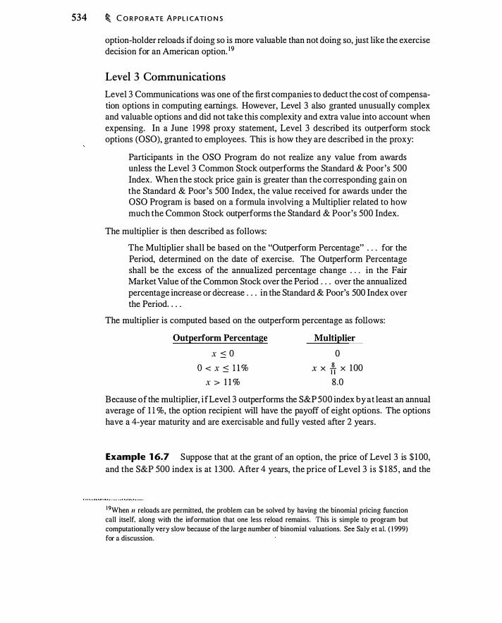
534 � C O R PO RATE A P P L I CATI O N S

option-holder reloads if doing so is more valuable than not doing so, just like the exercise decision for an American option. 1 9

Level 3 Communications

Level 3 Communications was one of the first companies to deduct the cost of compensa­tion options in computing earnings. However, Level 3 also granted unusually complex and valuable options and did not take this complexity and extra value into account when expensing. In a June 1 998 proxy statement, Level 3 described its outperform stock options (OSO), granted to employees. This is how they are described in the proxy:

Participants in the OSO Program do not realize any value from awards unless the Level 3 Common Stock outperforms the Standard & Poor's 500 Index. When the stock price gain is greater than the corresponding gain on the Standard & Poor's 500 Index, the value received for awards under the OSO Program is based on a formula involving a Multiplier related to how much the Common Stock outperforms the Standard & Poor's 500 Index.

The multiplier is then described as follows:

The Multiplier shall be based on the "Outperform Percentage" . . . for the Period, determined on the date of exercise. The Outperform Percentage shall be the excess of the annualized percentage change . . . in the Fair Market Value of the Common Stock over the Period . . . over the annualized percentage increase or decrease . . . in the Standard & Poor's 500 Index over the Period . . . .

The multiplier is computed based on the outperform percentage as follows:

Outperform Percentage

X :'S O O < x :'S l l %

X > 1 1 %

Multiplier

0

X X * X 1 00

8 .0

Because of the multiplier, if Level 3 outperforms the S&P 500 index by at least an annual average of 1 1 %, the option recipient will have the payoff of eight options. The options have a 4-year maturity and are exercisable and fully vested after 2 years .

Example 1 6.7 Suppose that at the grant of an option, the price of Level 3 is $ 1 00, and the S&P 500 index is at 1 300. After 4 years, the price of Level 3 is $ 1 85 , and the

1 9When 11 reloads are permitted, the problem can be solved by having the binomial pricing function

call itself, along with the information that one less reload remains. This is simple to program but

computationally very slow because of the large number of binomial valuations. See Saly et al. ( 1 999)

for a discussion.

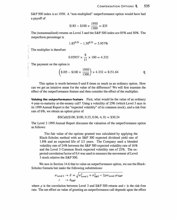
C O M P E N SAT I O N O PT I O N S � 535

S&P 500 index i s a t 1 950. A "non-multiplied" outperformance option would have had a payoff of

1 950 $ 1 85 - $ 100 X - = $35

1 300 The (nonannualized) returns on Level 3 and the S&P 500 index are 85% and 50%. The outperform percentage is

The multiplier is therefore

1 .850.25 - 1 .500.25 = 5.957%

- 8 0.0.)957 X U X 100 = 4.332

The payment on the option is

( 1 950) $ 1 85 - $ 1 00 X

1 300 X 4.332 = $ 15 1 .64

This option is worth between 0 and 8 times as much as an ordinary option. How can we get an intuitive sense for the value of the difference? We will first examine the effect of the outperformance feature and then consider the effect of the multiplier.

Valuing the outperformance feature First, what would be the value of an ordinary 4-year-to-maturity at-the-money call? Using a volatility of 25% (which Level 3 says in its 1 999 Annual Report is the "expected volatility" of its common stock) , and a risk-free rate of 6%, we obtain an option price of

BSCall($ 1 00, $ 1 00, 0.25, 0.06, 4, 0) = $30.24

The Level 3 1 999 Annual Report discusses the valuation of the outperformance option as follows:

The fair value of the options granted was calculated by applying the Black-Scholes method with an S&P 500 expected dividend yield rate of 1 .8% and an expected life of 2.5 years. The Company used a blended volatility rate of 24% between the S&P 500 expected volatility rate of 16% and the Level 3 Common Stock expected volatility rate of 25o/o. The ex­pected correlation factor of 0.4 was used to measure the movement of Level 3 stock relative the S&P 500.

We saw in Section 14.6 that to value an outperformance option, we use the Black­Scholes formula but make the following substitutions :

aLevel 3 -+ U = J a�evel 3 + a�&P - 2paLevel 3aS&P

r -+ os&P

where p is the correlation between Level 3 and S&P 500 returns and r is the risk-free rate. The net effect on value of granting an outperformance call depends upon the effect

536 � C O R PO RATE A P P L I CAT I O N S

of these substitutions. The "blended" volatility, B , can be greater or less than a Leve1 3 • In recent years, 8s&P has been less than r. The calculation Level 3 makes for the blended volatility is

B = J0.252 + 0. 1 62 - 2 X 0.4 X 0.25 X 0. 1 6

= 0.2368

which is rounded to 24%. The price of the outperformance option is therefore

BSCall($ 1 00, $ 100, 0.2368 , O.Q 1 8 , 4, 0) = $2 1 .75

This is about � of the value of the ordinary option. This reduction in value is primarily due to replacing the 6% interest rate with a 1 .8% dividend yield. The volatility reduction by itself lowers the option price only to $29.44.

Adding the multiplier Now consider the effect of the multiplier. We can approximate the value of the multiplied option using gap options (described in Section 1 4.5) . The multiplier in effect provides additional options as outperformance increases. For every Jt = I �% per year by which Level 3 outperforms the S&P 500, the multiplier increases by 1 . Thus, we can approximate the effect of the multiplier by valuing a strip of gap outperformance options.

For example, the multiplier is 2 if over 4 years, Level 3 outperforms the S&P 500 by a factor of 1 .02754 = 1 . 1 146, nonannualized. To approximate the value of the option, we can assume that if outperformance is between 0 and 1 .375% per year, the option-holder receives nothing. Between 1 .375% and 2.75%, the option-holder receives one option. At 2.75% per year, the option-holder receives a second option, etc. Above 1 1 % per year, the option holder receives eight options. Each additional option can be valued as a gap option. For example, the option received if perfor­mance is above 2.75% per year would pay SLevd3 - Ss&P if Suvel3 > 1 .02754 x Ss&P·

Figure 1 6.8 shows the payoff of a single nonmultiplied option, plotted against the exact payoff and the payoff approximated by gap options. Note that the exact and gap approximation are not identical, but they are quite close.

Table 1 6.2 shows that, using the gap option approximation, the value of the com­pensation option is about seven times the value of a single option. A more precise binomial valuation using I 00 binomial steps gives a value for the option of $ 1 56.25, so the gap approximation of $ 1 53 is quite close. Monte Carlo valuation, which we will discuss in Chapter 1 9. provides an alternative way to value the Level 3 option.

Finally, it is interesting to note that it may be rational to exercise the Level 3 option early even in the absence of dividends. Suppose the option is close to expiration and the outperformance percentage is slightly above 1 1 %. If the holder exercises, the multiplier is 8. If the share price rises further, the multiplier remains 8. However, if the share price falls, the multiplier may fall to 7; by waiting to exercise, the option-holder can lose options. This extra loss from a share price decline can provide an incentive to exercise early. For very high prices, there is no incentive to exercise early since the multiplier remains constant. For low prices, the potential increase in the multiplier offsets the

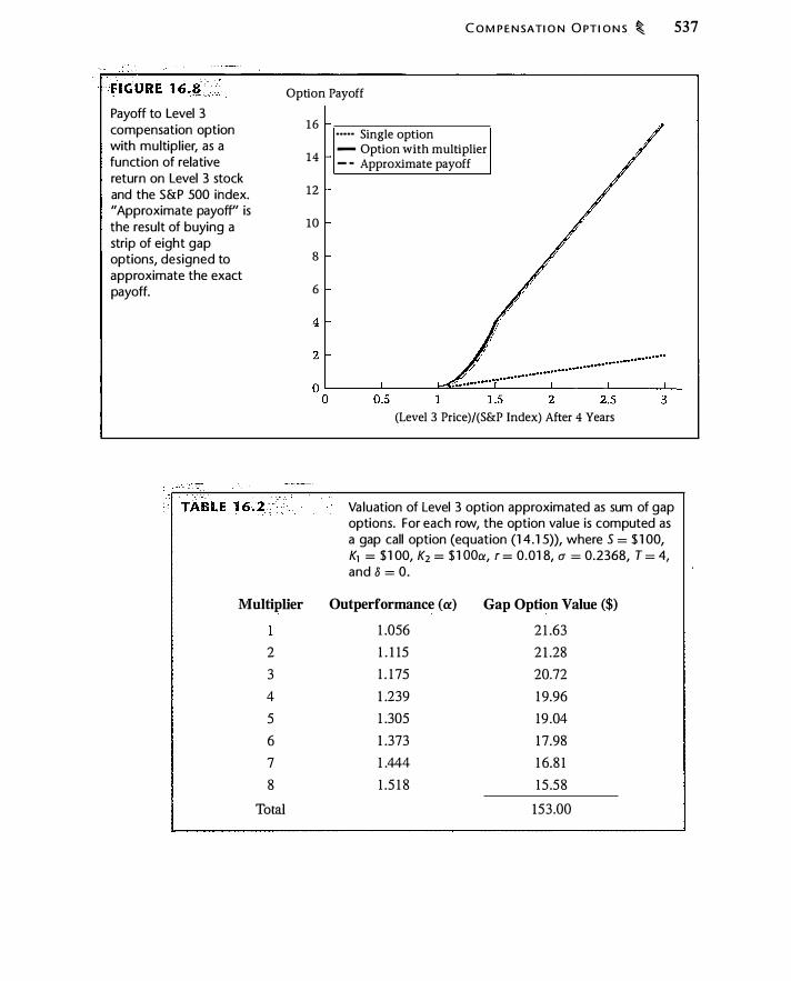
C O M P E N SATI O N O PT I O N S � 537

Option Payoff Payoff to Level 3 compensation option with multipl ier, as a function of relative return on Level 3 stock and the S&P 500 index. "Approximate payoff' is the result of buying a strip of eight gap options, designed to approximate the exact payoff.

Multiplier

2

3

4

5

6

7

8

Total

1 6

14

12

10

8

6

• • • • • Single option - Option with multiplier - - Approximate payoff

(Level 3 Price)/(S&P Index) After 4 Years

Valuation of Level 3 option approximated as sum of gap options. For each row, the option value is computed as a gap call option (equation (1 4 . 1 5)), where S = $ 1 00, K1 = $ 1 00, K2 = $ 1 OOa, r = 0.01 8, u = 0.2368, T = 4, and 8 = 0.

Outperformance (Ci) Gap Option Value ($)

1 .056 2 1 .63

1 . 1 15 2 1 .28

1 . 1 75 20.72

1 .239 1 9.96

1 .305 19 .04

1 .373 1 7.98

1 .444 1 6.8 1

1 .5 1 8 15 .58

153 .00

538 � C O R P O RATE A P P L I CAT I O N S

potential reduction in the multiplier. Thus, early exercise i s potentially optimal only for intermediate prices and close to expiration.

16.3 THE USE OF COLLARS IN ACQUISITIONS

A common financial transaction is for one firm (the acquirer) to buy another (the target) by buying its common stock. The acquirer can pay for these shares with cash or by exchanging its own shares for target firm shares. Collarl ike structures are frequently used in these transactions.

Suppose that under the purchase agreement, each target share will be exchanged for x shares of the acquirer (x is the exchange ratio) . Once the target agrees to the purchase, the acquisition will general ly take �ime to complete, often six months or more.20 Target shareholders will be concerned that the acquirer's stock will drop before the merger is completed, in which case the dollar value of x acquirer shares will be lower. To protect against a price drop, it is possible to exchange whatever number of shares have a fixed dollar value. (For example, if the acquirer price is $ 100, exchange 1 share for each target share. If the acquirer price is $50, exchange 2 shares for each target share.) However, target shareholders may also wish to participate in share price gains that the acquirer experiences; this suggests fixing the exchange ratio rather than the dollar value. There are four common offer structures that address considerations such as these:2 1

a Fixed stock offer: A offers to pay B a fixed number of A shares per B share.

• Floating stock offer: A offers to pay B however many shares have a given dollar value, based on A's share price just before the merger is completed.

a Fixed collar offer: There is a range for A's share price within which the offer is a fixed stock offer. Outside this range the deal can become a floating stock offer or may be subject to cancellation.

• Floating collar offer: There is a range for A's share price within which the offer is a floating stock offer. Outside this range the deal can become a fixed stock offer or may be subject to cancellation.

Figure 16.9 illustrates these four types of acquisition offers. As this l ist shows, it is possible to modify the extent to which the target bears the risk of a change in the stock price of the acquirer. More complicated structures are also possible.

The Northrop Grumman-TRW merger

Northrop Grumman's 2002 bid for TRW is an example of a merger offer with a collar. In July 2002, Northrop Grumman and TRW agreed that Northrop would pay $7.8 billion for TRW. News headlines stated that Northrop offered "$60 per share," but the offer actually resembled a collar. The number of Northrop Grumman shares to be exchanged for each

10 In many cases. for example. regu l atory agencies exam ine the acquis i tion to see i f i t i s anticompetitive.

2 1 Fuller (2003 ) discusses the kinds of offers and the moti ves for usi ng al lernati ve kinds of col lars.

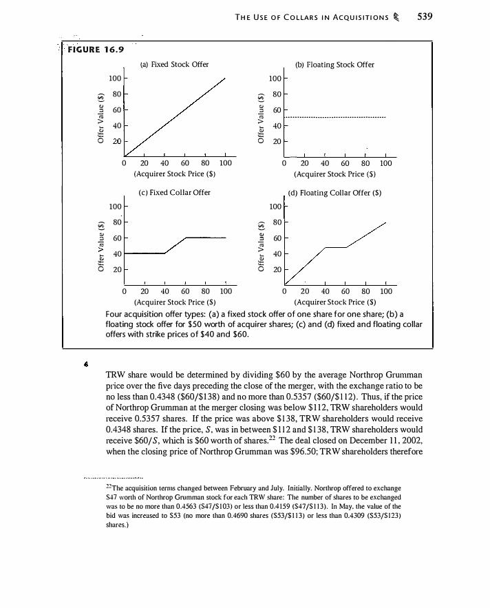
TH E U S E O F C O L LA R S I N ACQU I S IT I O N S � 539

F IGURE 1 6 .9

§ g rw > -� ·�

0

� 2 > � 0

100

80

60

40

0

100

80

60

40

20

0

(a) Fixed Stock Offer (b) Floating Stock Offer

100

� 80 � CJ

60 :::: rw . ....... . . . . . .. . . . - - - . ......... ...... ..... ............... ..

> 40 .� ....

0 20

20 40 60 80 100 0 20 40 60 80 100

(Acquirer Stock Price ($) (Acquirer Stock Price ($)

(c) Fixed Collar Offer (d) Floating Collar Offer ($)

100

g 80

CJ 60 ::::

� > 40 � 0 20

20 40 60 80 100 0 20 40 60 80 100

(Acquirer Stock Price ($) (Acquirer Stock Price ($)

Four acquisition offer types: (a) a fixed stock offer of one share for one share; (b) a floating stock offer for $50 worth of acquirer shares; (c) and (d) fixed and floating col lar offers with strike prices of $40 and $60.

TRW share would be determined by dividing $60 by the average Northrop Grumman p1ice over the five days preceding the close of the merger, with the exchange ratio to be no less than 0.4348 ($60/$ 1 38) and no more than 0.5357 ($60/$ 1 1 2) . Thus, if the price of Northrop Grumman at the merger closing was below $ 1 1 2, TRW shareholders would receive 0.5357 shares. If the price was above $ 1 38, TRW shareholders would receive 0.4348 shares . If the price, S, was in between $ 1 1 2 and $ 1 38, TRW shareholders would receive $60/ S, which is $60 worth of shares.22 The deal closed on December 1 1 , 2002, when the closing price of Northrop Grumman was $96.50; TRW shareholders therefore

22The acquisition tem1s changed between February and July. Initial ly. Northrop offered to exchange

$47 worth of Northrop Grumman stock for each TRW share: The number of shares to be exchanged

was to be no more than 0 .4563 (S47j$ 1 03) or less than 0 .4 159 ($47j$ 1 1 3) . In May, the value of the

bid was increased to $53 (no more than 0.4690 shares ($53/$ 1 1 3) or less than 0.4309 ($53/$ 1 23)

shares. )

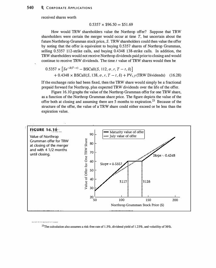
540 � C O R P O RATE A P P L I CATI O N S

received shares worth

0.5357 X $96.50 = $5 1 .69

How would TRW shareholders value the Northrop offer? Suppose that TRW shareholders were certain the merger would occur at time T, but uncertain about the future Norththrop Grumman stock price, S. TRW shareholders could then value the offer by noting that the offer is equivalent to buying 0.5357 shares of Northrop Grumman, selling 0.5357 1 1 2-strike calls, and buying 0.4348 1 38-strike calls. In addition, the TRW shareholders would not receive Northrop dividends paid prior to closing and would continue to receive TRW dividends . The time t value of TRW shares would then be

0 .5357 x [se-o(T-t l - BSCall (S, 1 1 2 , u , r, T - t , 8)] + 0.4348 x BSCall (S, 1 38 , u , r, T - t, 8) + PV1,T (TRW Dividends) ( 1 6.28)

If the exchange ratio had been fixed, then the TRW share would simply be a fractional prepaid forward for Northrop, plus expected TRW dividends over the life of the offer.

Figure 1 6. 1 0 graphs the value of the Northrop Grumman offer for one TRW share, as a function of the Northrop Grumman share price. The figure depicts the value of the offer both at closing and assuming there are 5 months to expiration.23 Because of the structure of the offer, the value of a TRW share could either exceed or be less than the expiration value.

F I G U R E 1 6 . 1 0

Value of Northrop 90

<lJ Grumman offer for TRW � at closing of the merger ..<::; 80 V"l and with 4 1 /2 months 3: � 70 until closing. r

<lJ

- Maturity value of offer = july value of offer

c 0 60

2 .

� 50 u...

0 0 40 � � 30 >

20 1 $ 13'

50 100 150 200

Northrop Grumman Stock Price (S)

23The calculation also assumes a risk-free rate of 1 .5'7o, dividend yield of 1 .25%, and volati l i ty of 36'7o.

TH E U S E O F C O LLA R S I N ACQU I S I T I O N S � 541

Figure 1 6. 1 1 depicts equation ( 1 6.28) using the historical Northrop Grumman stock price from July to December 2002, assuming that the offer would close on December 1 1 .24 The theoretical value of a TRW share under the terms of the offer is consistently greater than the market price of a TRW share. This is what we would expect to see, since in order to induce the target company to accept an offer, the acquirer generally has to offer a price greater than the perceived value of the target as a stand-alone company. Since there is some chance the merger might not occur, the target share price is below the value of the offer. The difference between the value of a TRW share and the theoretical value of the offer declined toward zero as December approached. Had the merger been cancelled for some reason, the value of a TRW share would have diverged from the value under the terms of the offer.

Risk arbitrageurs take positions in the two stocks in order to speculate on the success or failure of the merger. 25 Equation ( 16 .27) tells us that the offer is equivalent to a portfolio of Northrop shares and options. Thus, using the option replication technique of Chapter41 0, we can hold Northrop shares and borrowing or lending to synthetically create a position equivalent to the offer. Because the price of TRW is less than the offer value, an arbitrageur speculating that the merger would succeed could then take a long position in TRW shares and a short position in the offer, short-selling delta shares of

F I G U R E 1 6 . 1 1 -- TRW price Panel A graphs equation

65 - - Value of offer (1 6 .27) and the TRW 60

stock price from ju ly to 55

December. Panel B graphs the absolute 50

difference between the 45

two l ines in Panel A. (a) 07/01/02 10/01/02 01/01/03

2.5 2

1 .5

1 0.5

0 -0.5

(b) 07/01/02 10/01/02 01/01/03

24It was necessary for Northrop Grumman and TRW to receive regulatory approval from European

authorities, the U. S . Department of Defense and the U. S . Department of Justice. Final approval from

the Department of Justice was on December 1 0 and the merger was completed on December I I .

25Mitchell and Pulvino (200 1 ) examine the historical returns earned by risk arbitrageurs.

542 � C O R P O RATE A P P L I CATI O N S

Northrop. If the offer succeeds, the position earns the difference i n ptice depicted in Figure 1 6 . 1 1 : if the offer fails, the difference should diverge and the arbitrageur would lose money.

CHAPTER SUMMARY

Three corporate contexts in which options appear, either explicitly or implicitly, are capital structure (debt, equity. and wmrants), compensation. and acquisitions.

If we view the assets of the firm as being like a stock, then debt and equity can be valued as options with the assets of the firm as the underlying asset. Viewing corporate securities as options provides a natural way to measure bankruptcy risk, and illuminates conflicts between bondholders and stockholders .

Compensation options m·e an explicit use of options by corporations. They exhibit a variety of complications. some naturally occun·ing (early exercise decisions by risk­

. averse employees) and some created by the issuer (repricing, reloads, outperformance, and multipliers) . For this reason they provide an interesting context in which to use the exotic pricing fonnulas from Chapter 1 4.

Offers by one firm to purchase another sometimes have embedded collars. The Grumman offer to buy TRW was an example of this.

FURTHER READING

The idea that debt and equity are options was first pointed out by Black and Scholes ( 1 973). Merton ( 1 974) and Metton ( 1 977) analyzed the pricing of perpetual debt and demonstrated that the Modigliani-Miller theorem holds even with (costless) bankruptcy. Two principal applications of this idea m·e the determination of the fair yield on risky debt and the assessment of bankruptcy probabilities. Galai and Masulis ( 1 976) derived the link between the return on assets and the return on the firn1's stock.

The discussion of wmrants and convertible bonds in this chapter assumes that the options are European . . With American warrants the optimal exercise strategy can be more complicated than with European options. The reason is that exercise alters the assets of the firm. The problem of optimal American warrant exercise is studied by Emanuel ( 1 983 ) , Constantinides ( 1 984). and Spatt and Sterbenz ( 1 988) . McDonald (2004) exam­ines the tax implications of wan-ant issues, including put warrants. Complications also arise with convertible bonds, which in practice m·e almost always callable. Thus, valu­ing a convertible bond requires understanding the call strategy. Classic papers studying the pricing of convertibles include Brennan m1d Schwartz ( 1977) and Ingersoll ( 1 977). Hmris and Raviv ( 1 985) discuss how asymmetric information affects the decision to call the bond, and Stein ( 1 992) discusses the decision to issue convertibles in the first place. Finally, there is a lm·ge empirical literature on the convertible call decision; for example, see Asquith ( 1 995) . Gi.intay et al . (2004) examine the decision to issue callable bonds.

Papers on compensation options include Saly et al . ( 1 999), Johnson and Tian (2000a), and Johnson and Tian (2000b). Repricing is studied by Chance et al. (2000) and Acharya et al . (2000). Petrie (2000) examines the use of collars in acquisitions .

PROB LEMS

P R O B L E M S � 543

For all problems, unless otherwise stated assume that the firm has assets worth A = $ 1 00, and that O" = 30%, r = 8%, and the firm makes no payouts prior to the maturity date of the debt.

16.1. There is a single debt issue with a maturity value of $ 1 20. Compute the yield on this deb�assuming that it matures in 1 year, 2 years, 5 years, or 1 0 years. What . debt-to-equity ratio do you observe in each case?

16.2. There is a single debt issue. Compute the yield on this debt assuming that it matures in 1 year and has a maturity value of $ 1 27 .42, 2 years . with a maturity value of $ 135.30, 5 years with a maturity value of $ 1 6 1 .98, or 1 0 years with a maturity value of $2 1 8.65. (The maturity value increases with maturity at a 6% rate. ) What debt-to-equity ratio do you observe in each case?

16.3. There are four debt issues with different priorities, each promising $30 at matu­rity.

a. Compute the yield on each debt issue assuming that all four mature in 1 year, 2 years, 5 years, or 1 0 years.

b. Assuming that each debt issue matures in 5 years, what happens to the yield on each when you vary O" ? When you vary r?

16.4. Suppose there is a single 5-year zero-coupon debt issue with a maturity value of $ 1 20. The expected return on assets is 12%. What is the expected return on equity? The volatility of equity? What happens to the expected return on equity as you vary A, O" , and r?

16.5. Repeat the previous problem for debt instead of equity.

16.6. In this problem we examine the effect of changing the assumptions in Example 1 6. 1 .

a. Compute the yield on debt for asset values of $50, $ 1 00, $ 1 50, $200, and $500. How does the yield on debt change with the value of assets?

b. Compute the yield on debt for asset volatilities of 1 0% through 1 00%, in increments of 5%.

For the next three problems, assume that a firm has assets of $ 1 00 and 5-year-to-maturity zero-coupon debt with a face value of $ 1 50. Assume that investment projects have the same volatility as existing assets.

16.7. The firm is considering an investment project costing $ 1 . What is the amount by which the project's value must exceed its cost in order for shareholders to be willing to pay for it? Repeat for project values of $ 1 0 and $25 .

16.8. Now suppose the firm finances the project by issuing debt that has lower priority than existing debt. How much must a $ 1 , $ 10, or $25 project be worth if the shareholders are willing to fund it?

544 � C O R PO RATE A P P L I CATI O N S

16.9. Now suppose the finn finances the project by issuing debt that has higher pri­ority than existing debt. How much must a $ 1 0 or $25 project be worth if the shareholders are willing to fund it?

16.10. Assume there are 20 shares outstanding. Compute the value of the warrant and the share price for each of the following si tuations.

a. Warrants for 2 shares expire in 5 years and have a strike price of $ 1 5 .

b . Wan·ants for 1 5 shares expire i n I 0 years and have a strike of $20.

16.11. A finn has outstanding a bond with a 5-year maturity and maturity value of $50, convertible into 10 shares. There are also 20 shares outstanding. What is the price of the warrant? The share price? Suppose you were to compute the value of the convertible as a risk-free bond plus an option, valued using the Black-Scholes formula and the share price you computed. How accurate is this?

16.12. Suppose a firm has 20 shares of equity. a l 0-year zero-coupon debt with a maturity value of $200, and wan-ants for 8 shares with a strike price of $25 . What is the value of the debt, the share price, and the price of the warTant?

16.13. Suppose a firm has 20 shares of equity and a I 0-year zero-coupon convertible bond with a maturi ty value of $200, convertible into 8 shares . What is the value of the debt. the shar·e price, and the price of the warrant?

16.14. Using the assumptions of Example 16.3, suppose you were to perform a "naive" valuation of the convertible as a risk-free bond plus 50 call options on the stock. How does the price you compute compare with that computed in the example?

16.15. Consider Panels B and D in Figure 1 6.4. Using the information in each panel, compute the share price at each node for each bond issue.

16.16. As discussed in the text, compensation options are prematurely exercised or canceled for a variety of reasons. Suppose that compensation options both vest and expire in 3 years and that the probability is 10% that the executive will die in year I and I 0% in year 2. Thus, the probability that the executive lives to expiration is 80%. Suppose that the stock price is $ 1 00, the interest rate is 8%, the volatility is 30%, and the dividend yield is 0.

a. Value the option by computing the expected time to exercise and plug­ging this into the Black-Scholes formula as time to maturity.

b. Compute the expected value of the option given the different possible times until exercise.

c. Why are the answers for the two calculations different?

16.17. XYZ Corp. compensates executives with 10-year· European call options, granted at the money. If there is a significant drop in the share price, the company 's board will reset the strike price of the options to equal the new share price. The maturity of the repriced option will equal the remaining maturity of the original option. Suppose that u = 30%, r = 6%, 8 = 0, and that the original share price is $ I 00.

P RO B LE M S � 545

a. What is the value at grant of an option that will not be repriced?

b. What is the value at grant of an option that is repriced when the share price reaches $60?

c. What repricing trigger maximizes the initial value of the option?

16.18. Suppose that top executives of XYZ are told they will receive at-the-money call options on l 0,000 shares each year for the next 3 years. When granted, the

. options have 5 _xears to maturity. XYZ's stock price is $ 1 00, volatility is 30%, and r = 8%. EStimate the value of this promise. (Hint: See Problem 14.2 1 . )

16.19. Suppose that S = $ 1 00, a = 30%, r = 6%, t = I . and 8 = 0. XYZ writes a European put option on one share with strike price K = $90.

a. Construct a two-period binomial tree for the stock and price the put. Compute the replicating portfolio at each node.

b. If the firm were synthetical ly creati ng the put (i .e. , trading to obtain the same cash flows as if it issued the put), what transactions would it undertake?

c. Consider the bank that buys the put. What transactions does it undertake to hedge the transaction?

d. Why might a firm prefer to issue the put warrant instead of boiTowing and repurchasing shares?

16.20. Firm A has a stock price of $40 and has made an offer for firm B where A promises to pay $60/share for B , as long as A's stock price remains between $35 and $45 . If the price of A is below $35, A will pay 1 . 7 I 4 shares, and if the price of A is above $45 , A wiii pay 1 .333 shares. The deal is expected to close in 9 months. Assume a = 40%, r = 6%. and 8 = 0.

a. How are the values 1 .7 14 and 1 .333 an·ived at?

b. What is the value of the offer?

c. How sensitive is the value of the offer to the volatility of A's stock?

16.21. Firm A has a stock price of $40, and has made an offer for finn B where A promises to pay 1 .5 shares for each share of B, as long as A's stock price remains between $35 and $45 . If the p1ice of A is below $35, A will pay $52.50/share, and if the price of A is above $45 , A will pay $67 .50/share. The deal is expected to close in 9 months. Assume a = 40%, r = 6%, and 8 = 0.

a. How are the values $52.50 and $67.50 arrived at?

b. What is the value of the offer?

c. How does the value of this offer compare with that in Problem 1 6.20?

16.22. The strike price of a compensation option is general ly set on the day the option is issued. On November l 0, 2000, the CEO of Analog Devices, Jerald Fishman. received 600.000 options. The stock price was $44.50. Four days later. the price

546 � C O R P O RATE A P P L I CAT I O N S

rose to $63 .25 after an earnings release:

Maria Tagliaferro of Analog said the timing of the two events [option grant and earnings release] is irrelevant because company policy is that no option vests until at least three years from its granting date. "What happens to the stock price in the day, the hour, the year the option is granted is not relevant to that option," she said. "The stock price only becomes relevant after that option has vested."26

In its annual report for 2000, Analog Devices reported that the expected life of its options granted that year was 4.9 years, with a 56.6% volatility and 6% risk-free rate. The company paid no dividends until 2003 .

a. Using the inputs from the annual report, and assuming no dividends, estimate the value to the CEO of an at-the-money option grant at a stock price of $44.50.

b. Estimate the value of an at-the-money grant at a price of $63 .25.

c. Estimate the value of a newly granted option at a strike of $44.50 when the stock price is $63 .25.

d. Do you agree with Maria Tagliaferro? Why or why not?

16.23. Four years after the option grant, the stock price for Analog Devices was about $40. Using the same input as in the previous problem, compute the market value of the options granted in 2000, assuming that they were issued at strikes of $44.50 and $63 .25 .

16.24. Suppose that a firm offers a 3-year compensation option that vests immediately. An employee who resigns has two years to decide whether to exercise the option. Compute annual compensation option expense using the stock price tree in Figure 1 6.6. Verify that the present value of the option deductions is $28. 1 5 .

26See "SEC Probes Analog Devices· Options," Wall Street lou mal, Dece�ber 2, 2004, p. 86.

CHA_1JTER17 Real Options

'I., r., we have primarily discu"ed fimmcial "'sets, but many of the most importont decisions that firms make concern real assets, a term that broadly encompasses factories, mines, office buildings, research and development, and other nonfinancial firm assets. In this chapter we will see that it is possible to analyze investment and operating decisions for real assets using pricing models we have developed for financial options.

To illustrate how it can be possible to evaluate an investment decision as an option, consider a firm that is deciding whether or not to build a factory. Compare the following two descriptions:

• A call option is the right to pay a strike price to receive the present value of a stream of future cash flows (represented by the price of the underlying asset) .

• An investment project is the right to pay an investment cost to receive the present value of a stream of future cash flows (represented by the present value of the project) .

Do you notice the similarities in these two statements? We have

Investment Project Call Option

Investment cost Strike price

Present value of project = Price of underlying asset

This comparison suggests that we can view any investment project as a call option, with the investment cost equal to the strike price and the present value of cash flows equal to the asset price. The exploitation of this and other analogies between real investment projects and financial options has come to be called real options, which we define as the application of derivatives theory to the operation and valuation of real investment projects. Note the phrase "operation and valuation." We will see in this chapter that you cannot value a real asset without also understanding how you will operate it. We have encountered this link before: You cannot value any option without understanding when you will exercise it.

547

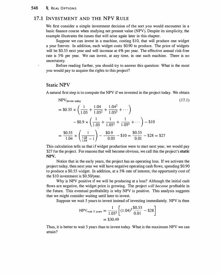
548 � REAL O PT I O N S

17.1 INVESTMENT AND THE NPV RULE

We first consider a simple investment decision of the sort you would encounter in a basic finance course when studying net present value (NPV). Despite its simplicity, the example illustrates the issues that will arise again later in this chapter.

Suppose we can invest in a machine, costing $ 1 0, that will produce one widget a year forever. In addi tion, each widget costs $0.90 to produce. The price of widgets will be $0.55 next year and will increase at 4% per year. The effective annual risk-free rate is 5% per year. We can invest, at any time, in one such machine. There is no uncertainty.

Before reading further, you should try to answer thi s question: What is the most you would pay to acquire the rights to this project?

Static NPV

A natural first step is to compute the NPV if we invested in the project today. We obtain

NPV Im·cst today

_ _ ( I 1 .04 1 .042 ) = $O . .).) X

1 .05 +

] .052 +

1 .053 + . . .

( I I 1 . ) - $0.9 X -- + --� + ---;:-:;- + · · · - $ 1 0

I .0.) 1 .05- l .OY

- -- X - -- - 1 - -- - - 27 - $0.55 ( . I ) $0.9 $ O _ $0.55

$·? 8

_

$ 1 .04 : :g; - I 0.05 0 .01 -

( 1 7. 1 )

This calculation tells us that i f widget production were to start next year, we would pay $27 for the project. For reasons that will become obvious, we call this the project's static NPV.

Notice that in the early years, the project has an operating loss. If we activate the project today, then next year we will have negative operating cash flows, spending $0.90 to produce a $0.55 widget. In addition, at a 5% rate of interest, the opportunity cost of the $ 1 0 investment is $0.50/year.

Why is NPV positive if we will be producing at a loss? Although the initial cash flows are negative, the widget price is growing. The project will become profitable in the future. This eventual profitability is why NPV is positive. This analysis suggests that we might consider waiting until later to invest.

Suppose we wait 5 years to invest instead of investing immediately. NPV is then

1 [ 5 $0.55 J NPYwait 5 years = J .055 ( 1 .04) O.O l - $28

= $30.49

Thus, it is better to wait 5 years than to invest today. What is the maximum NPV we can attain?

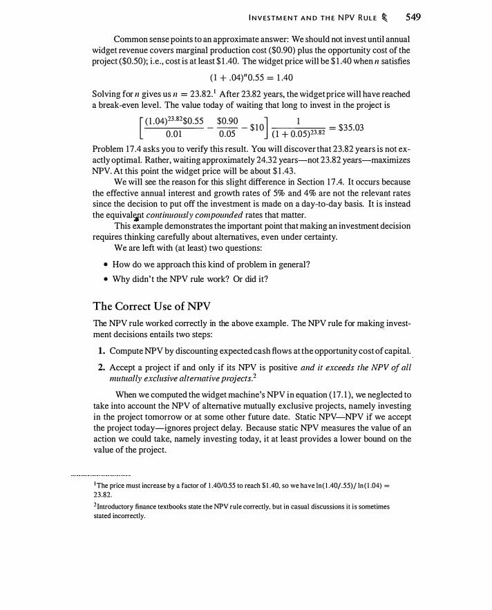
I N V ESTM E N T A N D TH E N PV R U L E � 549

Common sense points to an approximate answer: We should not invest until annual widget revenue covers marginal production cost ($0.90) plus the opportunity cost of the project ($0.50); i .e . , cost is at least $ 1 .40. The widget price will be $ 1 .40 when n satisfies

( 1 + . 04)"0.55 = 1 .40

Solving for n gives us n = 23.82. 1 After 23.82 years, the widget price will have reached a break-even level. The value today of waiting that long to invest in the project is

----- - -- - $ 1 0 = $35.03 [ ( 1 .04)23·82$0.55 $0.90 J 1

0 .0 1 0 .05 ( l + 0.05)23.82

Problem 17 .4 asks you to verify this result. You will discover that 23.82 years is not ex­actly optimal. Rather, waiting approximately 24.32 years-not 23.82 years-maximizes NPV. At this point the widget price will be about $ 1 .43 .

We will see the reason for this slight difference in Section 1 7 .4. It occurs because the effective annual interest and growth rates of 5% and 4% are not the relevant rates since the decision to put off the investment is made on a day-to-day basis. It is instead the equival�t continuously compounded rates that matter.

This example demonstrates the important point that making an investment decision requires thinking carefully about alternatives, even under certainty.

We are left with (at least) two questions:

• How do we approach this kind of problem in general?

• Why didn' t the NPV rule work? Or did it?

The Correct Use of NPV

The NPV rule worked correctly in the above example . The NPV rule for making invest­ment decisions entails two steps:

1. Compute NPV by discounting expected cash flows at the opportunity cost of capital.

2. Accept a project if and only if its NPV is positive and it exceeds the NPV of all mutually exclusive alternative pmjects.2

When we computed the widget machine's NPV in equation ( 17 . 1 ), we neglected to take into account the NPV of alternative mutually exclusive projects, namely investing in the project tomorrow or at some other future date. Static NPV----'-NPV if we accept the project today-ignores project delay. Because static NPV measures the value of an action we could take, namely investing today, it at least provides a lower bound on the value of the project.

1 The price must increase by a factor of 1 .40/0.55 to reach $ 1 .40, so we have ln ( I .40j.55)/ ln ( 1 .04) = 23.82. 2Introductory finance textbooks state the NPV rule correctly, but in casual discussions it is sometimes

stated incorrectly.

550 � REAL O PT I O N S

I n this example it would be correct to invest in the project today if not activating the project today meant that we would lose it forel'e/: Under this assumption, the mutually exclusive alternative (never taking the project) has a value of 0, so taking it today would be correct.

To decide whether and when to invest in an arbitrary project, we need to be able to compute the value of delaying that investment. As suggested at the start of the chapter, option pricing theory can help us to value delay.

The Project as an Option

The decision to invest in the project involves a comparison of net present values. In what sense is this an option?

We can interpret equation ( 1 7 . 1 ) so as to make the option analogy more apparent. When we take the project, we pay $ 1 0 and we commit to paying $0.90/year forever. The present value of this stream of costs is

$0.90 Present value of costs = $ 1 0 + -- = $28

0 .05 As we discussed earlier, we can view this present value as analogous to the exercise price in an option valuation . In return for paying $28, we receive a cash flow with a present value of

. s+ , Present -value of widget revenue = O.O 1

where S+ 1 is the widget price the year after we make the investment. When S+ 1 = $0.55, the present value of cash flow is $55 . This present value of widget revenue is the price the revenue stream would have if it were traded separately. It is analogous to the stock price in an option valuation, and therefore it is sometimes called the the twin security or the traded present value of the project.

Now recall the discussion in Sections 9.3 and 1 1 . 1 about the three factors governing early exercise of a call option: the dividends forgone by not acquiring the asset today; the interest saved by deferring the payment of the strike price; and the value of the insurance that is lost by exercising the option. It turns out that the same three considerations govern the decision to invest in the widget project.

First, by delaying investment. we lose the cash flow from selling widgets . The cash flow we do not receive is analogous to stock dividends we do not receive by holding an option rather than the underlying stock. The first period cash flow is $0.55 . The present value of future cash flows is $0.55/0.0 1 = $55 . Thus, the dividend yield is approximately 1 %. (We can also think of the dividend yield as the difference between the discount rate [5%] and the growth rate of the cash flows [4%] .)

Second, once we begin widget production, we are committed to spending the present value of the marginal widget cost. $ 1 8. along with the $ 1 0 initial investment. The annual value of delaying investment is interest on the total investment cost, or 0 .05 x $28 = $ 1 .40 per year.

I N V ESTM E N T U N D E R U N C E RTA I NTY � 551

Third and finally, in the widget project, there i s no uncertainty and therefore no insurance value to delaying investment.

We can compute the value of the widget project option using the perpetual call calculation discussed in Section 1 2.6. The formula assumes continuously compounded rates, so for the interest rate we use In ( I .05) = 4.879%, and for the dividend yield we use the difference between the continuously compounded interest rate and growth rate, or ln ( l .05) - ln ( l .04) = 0.9569%.

With S = $55 (the present value of revenue), K = $28 (the present value of costs) , r = 0.04879,.- = 0,3 and 8 = 0.009569, equation ( 1 2. 1 9) gives an option plice of $35 .03 and investment when the widget plice equals $ 1 .4276. We will call this price the investment trigger price. We reach this ptice after about 24.32 years, which velifies the answer we discussed earlier.

The example in this section illustrates the importance of thinking dynamically about a project and shows how this specific problem can be modeled as an option.

17.2 INVESTMENT UNDER UNCERTAINTY

In this section we discuss the valuation of real investment projects when cash flows are uncertain. With the widget project in the previous section, waiting to invest was optimal because project dividends were initially less than the interest gained from defeiTing the project. If we add uncertainty about project cash flows, the value of insurance (the implicit put option) also influences the decision to delay the project. In such a case, waiting to invest provides information about the value of the project. In this section we will use a binomial tree to value a project with uncertain cash flows.

As before, the decision to invest in such a project is like exercising an Ame1ican option: We pay the investment cost (strike price) to receive the asset (present value of future cash flows).

A Si�ple DCF Problem

We first examine a particularly simple valuation problem in order to better understand the link between discounted cash flow (DCF), real options, and financial options .

Suppose an analyst is evaluating a project that will generate a single cash flow, X , occurring at time T. As with many investment projects, it is not possible to observe market characteristics of the project. There is no way to directly estimate project returns, project volatility, or the co variances of the project with the stock market. Instead, suppose the analyst considers the economic fundamentals of the project and makes educated inferences about these charactelistics. The analyst might also look for public firms with a business resembling the project. The analyst could then use information about these public firms to infer characteristics (such as beta) of the project.

3 lt is necessary to set a to a smal l positive number such as 0.0000 1 to avoid a zero·d ivide error.

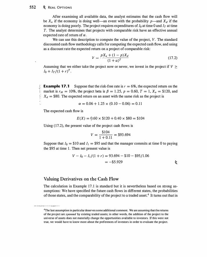
552 � R EA L O PTI O N S

After examining all available data, the analyst estimates that the cash flow will be Xu if the economy is doing well-an event with the probability p-and Xd if the economy is doing poorly. The project requires expenditures of /0 at time 0 and h at time T. The analyst determines that projects with comparable risk have an effective annual expected rate of return of a .

We can use this description to compute the value of the project, V . The standard discounted cash flow methodology calls for computing the expected cash flow, and using as a discount rate the expected return on a project of comparable risk:

pXu + ( 1 - p)Xcl V = --------�---

( 1 + a)T ( 17 .2)

Assuming that we either take the project now or never, we invest in the project if V :::: lo + h/( 1 + r)T .

Example 1 7. 1 Suppose that the risk-free rate is r = 6%, the expected return on the market is rM = 10%, the project beta is fJ = 1 .25, p = 0.60, T = 1 , Xu = $ 1 20, and Xc1 = $80. The expected return on an asset with the same risk as the project is

a = 0.06 + 1 .25 x (0. 10 - 0.06) = 0. 1 1

The expected cash flow is

E(X) = g.60 X $ 1 20 + 0.40 X $80 = $ 1 04

Using ( 17 .2), the present value of the project cash flows is

v = $ 1 04 = $93 .694

1 + 0. 1 1

Suppose that /0 = $ 1 0 and /1 = $95 and that the manager commits at time 0 to paying the $95 at time 1 . Then net present value is

V - lo - h /( 1 + r) = 93.694 - $ 10 - $95/ 1 .06

= -$5 .929

Valuing Derivatives on the Cash Flow

The calculation in Example 17 . 1 is standard but it is nevertheless based on strong as­sumptions : We have specified the future cash flows in different states, the probabilities of those states, and the comparability of the project to a traded asset.4 It turns out that in

4The last assumption in particular deserves some additional comment. We are assuming that the returns

of the project are spanned by existing traded assets; in other words, the addition of the project to the

universe of assets does not materially change the opportunities available to investors. If this were not

true, we would have to know more about the preferences of investors in order to evaluate the project.

I N V ESTM E N T U N D E R U N C ERTA I NTY � 553

valuing the project we have already made all the assumptions we need to make in order to value derivatives related to the project.

To see how to perform capital budgeting calculations involving options, suppose that if we invest /0 to start the project, the subsequent investment of /1 is optional : We make this further investment only if the project at time 1 has sufficient value. S ince the project has a good and bad outcome, it is natural to think about using binomial option valuation. In order to do so, we need to know the risk-neutral probability of the high outcome.5

Fortunately, we can easily compute risk-neutral probabilities for this project. Re­call from Chapter 1 0 that the expected risk-neutral price is the forward price. We have computed V, which is the price of an asset paying a single cash flow at time T. The forward price is

Fo.T = V ( l + r )T

The risk-neutral probability must therefore satisfy

p* Xu + ( 1 - p*)Xd = Fo.T Thus, we have

"' Fo T - xd p . = ---'-' --Xu - Xd This gives us the binomial tree (Xu and Xd) and the risk-neutral probability of a high outcome (p*). Notice that if we value the project using the risk-neutral distribution, then by construction we will obtain the original project value, V .

Example 1 7.2 Consider the same parameters a s i n Example 1 7 . 1 . The forward price for the project is

Fo. r = $93 .694 x ( 1 .06) = $99.3 1 5

The risk-neutral probability of the good outcome is

* 99.3 1 5 - 80 p = = 0.4829

1 20 - 80

If we value the project using the risk-neutral probability, we obtain

0 .4829 X $ 1 20 + ( 1 - 0.4829) X $80 $ ----------- = 93.694

1 .06 Now make the same assumptions as in Example 1 7. 1 , except that we decide at

time 1 whether to incur the $95 cost. We will choose to produce output in time 1 only

5In general we also need to know volatility to value an option. As we discussed in Chapter I 0, volati l i ty

determines the vertical distance between binomial nodes. Thus, in specifying the tree, we implicitly

specified volati lity.

554 � REAL O PT I O N S

when the cash flow is $ 1 20, since we would lose $ 1 5 by paying $95 to produce when the output sells for $80. The value of the project is

p* max[O, X11 - /J ] + ( 1 - p*) max[O, XL - h ] 1 - 0 1 + r

= 0.4829 X $25 + ( �- 0.4829) X 0

_ $ lO = $ 1 .389 � 1 .0

Given the risk-neutral probability and the cash flow distribution, we can value projects with options or other nonlinear cash flows.6

You may be thinking that there appears to be little difference between standard discounted cash flow valuation and real options valuation. Recognize that any financial valuation entails assigning a dollar value today to a (possibly uncertain) cash flow that occurs in the future. This description applies to the valuation of a project, as well as to valuing a bond, a stock, or an option.

When we value an option on a stock, we rely on the market to have already pe1formed part of the valuation-namely, valuing the stock. When we value an option on a project, we have to estimate the value of the project since we cannot observe it. This is true whether or not the project coma ins options.

This discussion illustrates the point we made before in Section 1 1 .2, that risk­neutral pricing and discounted cash flow are alternative means of valuing a future cash flow. If done using the same assumptions, the two methods give the same answer. In practice, of course, it is co-mmon to make simplifying assumptions for tractability. Answers may differ because the simplifying assumptions for different valuation methods are inconsistent.

Evaluating a Project with a 2-Year Investment Horizon

We now consider the problem of when to invest in a risky project. As before, the decision to invest in such a project is like exercising an American option: We pay the investment cost (strike price) to receive the asset (present value of future cash flows) . The widget project in the previous section had cash flows that were certain.

Suppose a project costs $ 100 and begins producing an infinite stream of cash flows 1 year after investment. Expected annual cash flows for the first year are $ 1 8 , and are expected to grow annually at a rate of 3%. Suppose further that the risk-free rate is 7%, the risk premium on the market i s 6%, and the beta of the project i s 1 .33 . Using the Capital Asset Pricing Model (CAPM). we compute the discount rate for the project in

6 Problem 1 7 .9 asks you to value a project paying the squared cash flow.

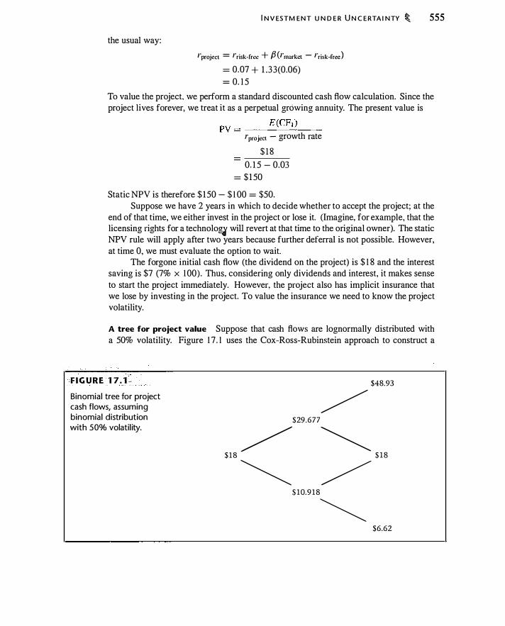
the usual way:

I N V ESTM E N T U N D E R U N C E RTA I NTY � 555

I" project = �"risk-free + ,8 Crmarket - I" risk-free ) = 0.07 + 1 .33(0.06) = 0. 1 5

To value the project. we perform a standard discounted cash flow calculation. Since the project lives forever. we treat it as a perpetual growing annuity. The present value is

PV = __ E_(C_F_1 ) __

�"project - growth rate

$ 1 8 0. 1 5 - 0.03

= $ 150

Static NPV is therefore $ 150 - $ 1 00 = $50. Suppose we have 2 years in which to decide whether to accept the project; at the

end of that time, we either invest in the project or lose it. (Imagine, for example, that the licensing rights for a technolo� will revert at that time to the original owner). The static NPV rule will apply after two years because further deferral is not possible. However, at time 0, we must evaluate the option to wait.

The forgone initial cash flow (the dividend on the project) is $ 1 8 and the interest saving is $7 (7% x 1 00) . Thus, considering only dividends and interest, it makes sense to start the project immediately. However, the project also has implicit insurance that we lose by investing in the project. To value the insurance we need to know the project volatility.

A tree for project value Suppose that cash flows are lognormally distributed with a 50% volatility. Figure 1 7 . 1 uses the Cox-Ross-Rubinstein approach to construct a

F I G U R E 1 7 . 1

Binomial tree for project cash flows, assuming binomial distribution with 50% volatil ity.

$ 1 8 � �

$48.93

/ $29 .677

� $ 1 8

/ $ 10.9 1 8

� $6.62

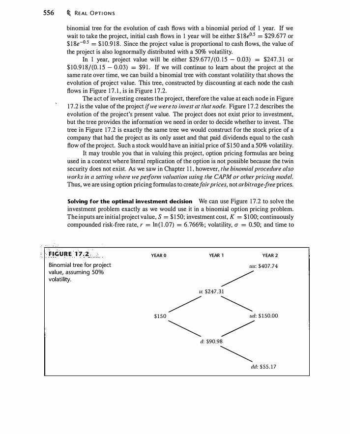
556 � REAL O PT I O N S

binomial tree for the evolution of cash flows with a binomial period of 1 year. If we wait to take the project, initial cash flows in 1 year will be either $ 1 8e0·5 = $29.677 or $ 1 8e-0·5 = $ 10.9 1 8 . Since the project value is proportional to cash flows, the value of the project is also lognormally distributed with a 50% volatility.

In l year, project value will be either $29 .677/(0. 1 5 - 0.03) = $247.3 1 or $ 10.9 1 8/(0. 1 5 - 0.03) = $9 1 . If we will continue to learn about the project at the same rate over time, we can build a binomial tree with constant volatility that shows the evolution of project value. This tree, constructed by discounting at each node the cash flows in Figure 1 7 . 1 , is in Figure 1 7 .2.

The act of investing creates the project, therefore the value at each node in Figure 1 7 .2 is the value of the project if we were to invest at that node. Figure 1 7 .2 describes the evolution of the project's present value. The project does not exist prior to investment, but the tree provides the informatfon we need in order to decide whether to invest. The tree in Figure 1 7 .2 is exactly the same tree we would construct for the stock price of a company that had the project as its only asset and that paid dividends equal to the cash flow of the project. Such a stock would have an initial price of $ 1 50 and a 50% volatility.

It may trouble you that in valuing this project, option pricing formulas are being used in a context where literal replication of the option is not possible because the twin security does not exist. As we saw in Chapter 1 1 , however, the binomial procedure also works in a setting where we pe1jorm valuation using the CAPM or other pricing model. Thus, we are using option pricing formulas to create fair prices, not arbitrage-free prices.

Solving for the optimal investment decision We can use Figure 1 7 .2 to solve the investment problem exactly as we would use it in a binomial option pricing problem. The inputs are initial project value, S = $ 1 50; investment cost, K = $ 1 00; continuously compounded risk-free rate, r = ln ( l .07) = 6.766%; volatility, a = 0.50; and time to

• . F I G U R E 1 7 . 2 Binomial tree for project value, assuming 50% volati l ity.

YEAR O YEAR 1 YEAR l

llll: $407.74

/ u: $247 .31

/ � $ 1 5 0 ud: $ 1 50.00

� / d: $90.98

� dd: $55 . 1 7

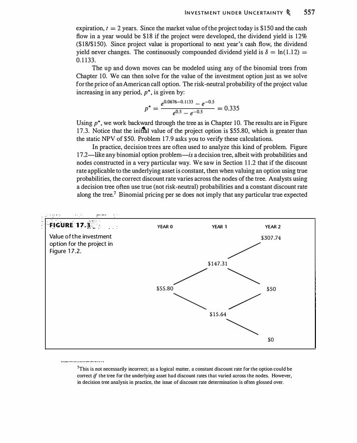
I N V ESTM E N T U N D E R U N C E RTA I NTY � 557

expiration, t = 2 years. Since the market value of the project today is $ 150 and the cash flow in a year would be $ 1 8 if the project were developed, the dividend yield is 1 2% ($ 1 8/$ 150). Since project value is proportional to next year's cash flow, the dividend yield never changes. The continuously compounded dividend yield is 8 = ln ( l . l 2) = 0. 1 1 33 .

The up and down moves can be modeled using any of the binomial trees from Chapter 1 0. We can then solve for the value of the investment option just as we solve for the price of an American call option. The risk-neutral probability of the project value increasing in any period, p* , is given by:

e0.0676-0. I I 33 _ e-0.5 p* = = 0.335

eD.5 _ e-0.5

Using p* , we work backward through the tree as in Chapter 10. The results are in Figure 1 7 .3 . Notice that the init�l value of the project option is $55 .80, which is greater than the static NPV of $50. Problem 1 7.9 asks you to verify these calculations.

In practice, decision trees are often used to analyze this kind of problem. Figure 1 7 .2-like any binomial option problem-is a decision tree, albeit with probabilities and nodes constructed in a very particular way. We saw in Section 1 1 .2 that if the discount rate applicable to the underlying asset is constant, then when valuing an option using true probabilities, the correct discount rate varies across the nodes of the tree. Analysts using a decision tree often use true (not risk-neutral) probabilities and a constant discount rate along the tree.7 Binomial pricing per se does not imply that any particular true expected

···.· . F I G U RE ]7 . . 3 : Value of the investment option for the project in Figure 1 7 .2 .

YEAR O

/ $55 .80

�

YEAR 1 YEAR 2

$307.74

/ $ 147.3 1

� $50

/ $ 15 .64

� $0

7This is not necessarily incorrect; as a logical matter, a constant discount rate for the option could be

correct if the tree for the underlying asset had discount rates that varied across the nodes. However,

in decision tree analysis in practice, the issue of discount rate determination is often glossed over.

558 � R EA L O PTI O N S

return i s constant; instead i t tel l s u s how to perform valuation s o that the assumptions about the project and the assumptions about the tree are consistent with each other.

Evaluating the Proj ect with an Infinite Investment Horizon

The above example assumes that we must start the project by year 2 and that we eval­uate it annually. Suppose instead that the project can be started at any time and then will l ive forever. The project is then a perpetual call option that we can evaluate us­ing the perpetual option pricing formula. Using continuously compounded inputs, we compute

CallPerpetual ($ 1 50, $ 1 00, 0.50. 0 .0676, 0. 1 1 33) = ( $63 .396, $245 . 7 1 }

When the project value is $ 1 50, the option value is $63 .396 and the optimal investment trigger is $245 .7 1 . In other words, we invest when the project is worth $245 .7 1 , more

· than twice the investment cost. If we invest immediately, the project is worth $50. The abil i ty to wait increases that value by $ 1 3 .396.

17.3 REAL OPTIONS IN PRACTICE

Real investment decisions often have optionlike features. Consider the following:

1. The decision about whether -and when to invest in investment projects .

2. The abil i ty to shut down, restart, and permanently abandon projects .

3. The ability to invest in projects that may give rise to future options.

4. The abi l ity to be flexible in the future about the choice of inputs, outputs, or pro­duction technologies.

We have already discussed the first-an investment project is a call option. We can view the abi l i ty to shut down a money-losing project (item 2 in the l ist above) as having the project plus a put option-an insurance policy to protect against even greater losses. The abi l i ty to invest in a way that gives ri se to future investment options ( item 3 , sometimes called "strategic options'') should remind you of a compound option (an option to buy an option). So-called ''flexibi l i ty options·· (item 4) are analogous to a type of exotic option cal led a rainbow option, which we will discuss in Chapter 22.

Despite the many s imi larities between real options and financial options, there is usually no simple and straightforward way to make real-l ife investment problems fit an option pricing formula. As with any valuation problem, it is necessary to analyze the specific problem. In this section. we look at two examples that use option analysis to value assets: peak-load electricity generation and pharmaceutical research and develop­ment. The box on page 559 describes an investment problem at Intel which was similar to a peak-load problem .

Peak-Load Manufacturing at I ntel

Manufacturers investing in production capacity and facing uncertain demand experience the same peak-load production problem as electricity producws. Consider a manufacturer investing in production capacity and facing uncertain demand. How should the manufacturer choose plant capacity? Consider choosing the plant's capacity to meet expected demand. If demand turns out to be less than forecast, the firm will either produce at a loss or have an idle plant. If demand is greater, the firm will forgo revenue. If it is necessary to produce whether demand is high or low, then extra capacity has no option value. However, if it is possible to idle an unused plant when demand is low, then extra production capacity is like a peak-load facility. The extra capacity gives the firm a call option.

Intel in 1 997 had to decide upon the capaci ty of a new plant. Semiconductor fabrication facilities ("fabs") cost about

REAL O PT I O N S I N P R A CT I C E � 559

$2 billion and take 2 years to construct, 1 year for the shell-the building-and l year for the equipment. The shell cost was about $350 million, with the rest reflecting equipment cost.

Intel analysts proposed building a shell 1 year ahead of schedule. If demand were high, the firm would be able to inst�ll equipment a year early and earn an extra year of revenue. If demand were low, the fim1 would maintain the building until needed, which was relatively inexpensive.

The planners sought to persuade senior management that early construction of a shel l provided benefits. Intel analysts developed a si mple binomial model that illustrated the costs and benefits of early construction. They verified that the Black-Scholes formula gave approximately the same option value. Intel then built the shell l year early.

Peak-Load Electricity Generations

In Chapter 6 we explai ned that electricity forward prices can vary over the course of a day. They also vary seasonally : In the United States. electricity forward prices are high in the summer and low in the winter. In addition to this predictable variation, electricity prices can be volatile. On extremely hot days, for example, prices can spike to l 00 times their average price .

A peak-load plant. as the name suggests. produces only when it is profitable to do so. exploiting spikes in the price of electricity. Such plants are designed so that they can be idled when the price of electricity is less than the cost of fueL but they can be quickly brought onl ine to produce power when the price of electric i ty i s high or when the price of fuel decl ines. Because it is turned on only when profitable, owning a peak-load plant is

sl t l 1ank David Moore of El Paso Corporat ion for helpfu l discussions and for providing representative data.

like owning a strip of call options, with options maturing daily.9 The underlying asset is electricity. The strike price is the cost of inputs required to produce a unit of electricity, including the cost of the fuel-typically natural gas-and other variable costs associated with operating the plant. 1 0 The heat rate, H, of a plant is the efficiency with which it turns gas into electricity (the number of :MJv!Btus required to produce a megawatt hour (MWh)) . t t

For the moment, let's consider only electricity and gas prices, and assume that we can ignore distribution costs and marginal operating, maintenance, and other costs. Then the profit of the plant is

Profit = max(Setec - H X Sgas . 0) This is the payoff to a European exchange option (see Section 14.6). The difference between the price of electricity and the cost of generation, Selec - H x Sgas , is called the spark spread. There are operating costs besides gas, but the spark spread is the variable component of marginal profit.

In order to value the option we need forward prices and volatilities for electricity and gas and the correlation between the two. The top panel in Figure 17 .4 shows representative forward curves for electricity and gas. The price curve for gas has a shape familiar from Section 6.9, exhibiting seasonal winter peaks. The electricity curve, by contrast, exhibits summer peaks. The ·bottom panel shows the spark spread implied by the prices in the first panel.

The value of a plant is the sum of the operating options it provides. Let F E.r; and Fa,t; represent the time 0 forward prices for electricity and gas delivered at time ti . If we ignore other marginal operating costs, then the value of the operating plant is 1 2

II Value of Plant = L BSCall(FE.t; > H x Fa.ri ' rr1i ' r, ti , r)

i=l ( 1 7.3)

where &� = a� . t; + H2 x a� . t; - 2p H a E.t; a G.t; . Because volatility changes with the time horizon in Figure 1 7 .4, volatility in expression 1 7 .3 has a time subscript. Equation ( 1 7.3) provides the value of the plant taking account of optionality. We could also value the plant assuming operation at all times; this would be a static NPV calculation. We can see how the static value relates to the true value by using put-call parity to rewrite

90perators will think not only about day-to-day operations, but hour-to-hour as well, since a plant may

be operated during the day and not at night.

1 0In practice, the term "strike price" is sometimes used to refer only to nongas variable costs.

1 1 The definition of heat rate is the number of BTUs required to produce one kilowatt/hour of electricity.

The heat rate times 1 000 is the number of British Thermal Units (BTUs) to produce one MWh.

For example, if the heat rate is 9000, then 9000 x 1 000 = 9m BTUs is required to produce one

megawatt/hour of electricity. If the price of natural gas is $3/MMBtu, then the gas cost of producing

one MWh of electricity is $27.

1 2Because the underlying asset is a forward price, the risk-free rate, r, is used as the dividend yield. This is the Black formula, equation ( 1 2.7) .

REAL O PT I O N S I N P R ACTI C E � 561

F I G U R E 1 7 .4

Elec Forward ($/MWh)

Gas Forward ($/:tvfMBtu)

80 3 .6 m 3A 60 3 .2 � 3� 40 2.8 30 2.6 20 '---------'------'-------'------'--------' 2.4 Year 0 Year 1 Year 2 Year 3 Year 4 Ye'ar 5

Date

Volatility

1 - Forward Electricity Volatility - · · Forward Gas Volatility

0.5

-

- - - - - - - - .... - - - · - - - - -

- . . . - . . - - - . . . . . - - - - - . -.

- . - . . . . - - - . - - -

o�---�----�--------�--------�--------� Year 0

Spark Spread ($)

40

20

0

Year 1 Year 2 Year 3 Year 4 Year 5

Date

-20L-------�--------�--------�--------J---------� Year O Year 1 Year 2 Year 3 Year 4 Year 5

Date

Forward price (top panel) and volati l ity (middle panel) curves for electricity and natural gas. The bottom panel depicts the spark spread implied by the forward price curves, assuming a heat rate of 9000.

equation ( 1 7.3) : II L [e-n' (FE. t, - H x Fc.1) + BSPut( F£.1, . H x Fc.1" u1" r, t; , r)]

i=l II II

i=l i=l

Static NPV Option not to operate

( 1 7 .4)

562 � R EA L O PT I O N S

This way of writing the plant's value makes apparent the difference between a static NPV calculation and the real options valuation. The static calculation assumes operation at aU times; we can value the plant by simply discounting the spark spread computed using forward prices. Equation ( 1 7.3) also makes it clear that the value of a peak-load plant does not stemfivm operating when prices are high-all plallts operate wizen prices are high-but ratlzerfimn shutting down when prices are low.

In reality, equation ( 1 7 .4) is overly simplified. There are marginal distribution, operation, and maintenance costs associated with an operating plant. Represent these costs as c. When we take these into account, marginal profit is

Profit = max[Selec - (H X Sgas + c) , 0]

This payoff is that of a spread option, since the payoff is positive if the spread Setec -H x Sgas exceeds c. An option with this payoff cannot be valued using the Black-Scholes formula because neither Selec - H x Sgas nor H x Sgas + c is lognormaUy distributed. Equation ( 17 .3) is therefore an approximation once nonfuel costs are added to the strike price. 1 3

When we include other costs, the static NPV of a peak-load plant is typically neg­ative. Adding the shutdown option, however, makes NPV positive. One implication is that, in equilibrium, after the optimal number of peak-load plants have been constructed, electricity prices will continue to be variable. Otherwise, the marginal peak-load plant would have negative NPV. Thus, the existence of peak-load technology will not eliminate equilibrium variability in electricity prices.

As a final point, note that the volatility curves in Figure 17 .4 are declining over time. From the standpoint of Year 0, a 2-year volatility is less than a 1 -year volatility. This is in contrast with stocks, for which we typically assume volatility is constant over time.

To understand the behavior of volatility for electricity, recall the discussion of stock prices in Section 1 1 .3 . The assumption that a stock price follows a random walk implies that volatility increases with the square root of time. Thus, volatility enters the Black-Scholes model as u .JT=(; this expression measures the volatility of the stock price over the horiz�n from t to T. By contrast, we do not expect electricity prices to foUow a random walk. When the electricity price is high, users consume less electricity and producers increase production. When prices are low, users consume more and producers produce less. Thus, the price of electricity reverts to a level reflecting the cost of production. When prices revert in this fashion, volatility grows with T at a rate less than .JT=t.

To consider a specific example, suppose it is January. From this perspective, the July price this year and the July price next year have similar distributions ; we won' t learn much about the July price this year or next until we approach July. (This is not strictly true because economic activity and even weather can follow long-term cycles, but suppose that it is a good approximation.) To compute an option price, we require annualized volatility, u, which the option pricing formula transforms into volatility over

1 3Haug ( 1 998, p. 59) discusses approximations that can be used to value spread options.

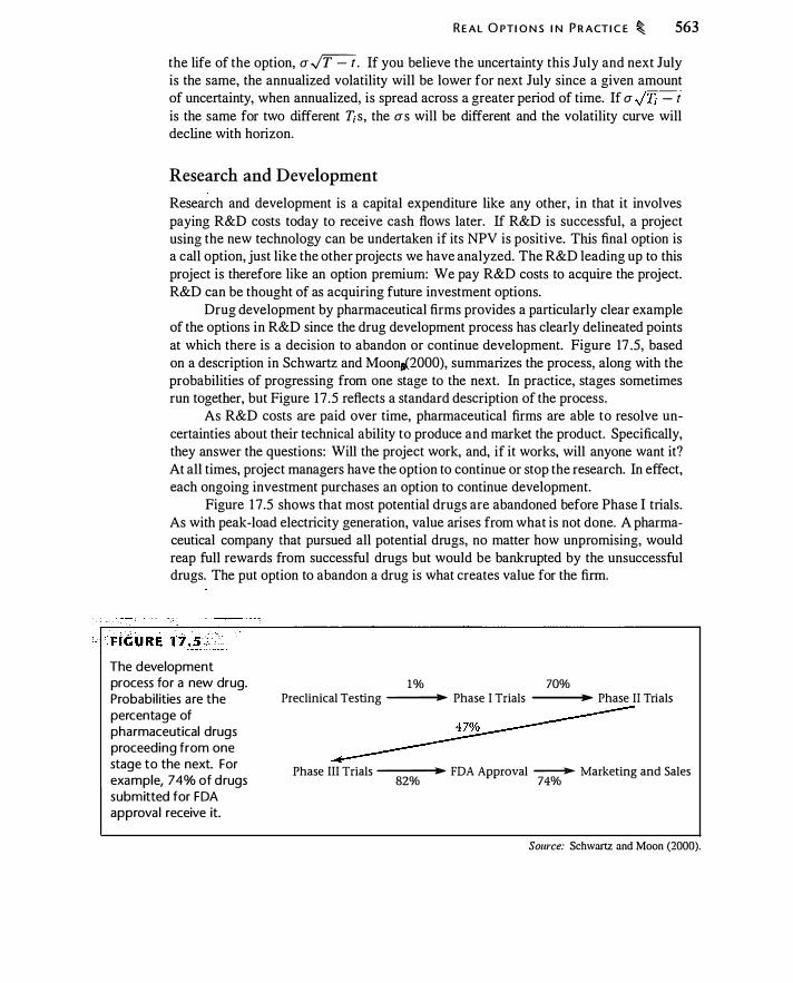
R E A L O PTI O N S I N P R ACT I C E � 563

the life of the option, a �. If you believe the uncertainty this July and next July is the same, the annualized volatility will be lower for next July since a given amount of uncertainty, when annualized, is spread across a greater period of time. If a ,JT; - t is the same for two different T;s, the as will be different and the volatility curve will decline with horizon.

Research and Development

Research and development is a capital expenditure like any other, in that it involves paying R&D costs today to receive cash flows later. If R&D is successful, a project using the new technology can be undertaken if its NPV is positive. This final option is a call option, just like the other projects we have analyzed. The R&D leading up to this project is therefore like an option premium: We pay R&D costs to acquire the project. R&D can be thought of as acquiring future investment options.

Drug development by pharmaceutical firms provides a particularly clear example of the options in R&D since the drug development process has clearly delineated points at which there is a decision to abandon or continue development. Figure 17 .5, based on a description in Schwartz and Moona(2000), summarizes the process, along with the probabilities of progressing from one stage to the next. In practice, stages sometimes run together, but Figure 17 .5 reflects a standard description of the process.

As R&D costs are paid over time, pharmaceutical firms are able to resolve un­certainties about their technical ability to produce and market the product. Specifically, they answer the questions: Will the project work, and, if it works, will anyone want it? At all times, project managers have the option to continue or stop the research. In effect, each ongoing investment purchases an option to continue development.

Figure 17.5 shows that most potential drugs are abandoned before Phase I trials. As with peak-load electricity generation, value arises from what is not done. A pharma­ceutical company that pursued all potential drugs, no matter how unpromising, would reap full rewards from successful drugs but would be bankrupted by the unsuccessful drugs. The put option to abandon a drug is what creates value for the firm.

The development process for a new drug. Probabi l ities are the percentage of pharmaceutical drugs proceeding from one stage to the next. For example, 74% of drugs submitted for FDA approval receive it.

1% 70% Preclinical Testing ----;� Phase I Trials ----;� Phase II Trials

Phase III Trials ---� FDA Approval ---.. Marketing and Sales 82% 74%

Source: Schwartz and Moon (2000).

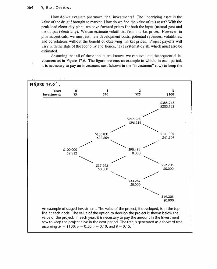
564 � R EA L O PT I O N S

How d o w e evaluate pharmaceutical investments? The underlying asset i s the value of the drug if brought to market. How do we find the value of this asset? With the peak-load electricity plant, we have forward prices for both the input (natural gas) and the output (electricity). We can estimate volati lities from market prices. However, in pharmaceuticals, we must estimate development costs, potential revenues, volatilities, and correlations without the benefit of observing market prices. Project payoffs will vary with the state of the economy and, hence, have systematic risk, which must also be estimated.

Assuming that all of these inputs are known, we can evaluate the sequential in­vestment as in Figure 17 .6. The figure presents an example in which, in each period, it is necessary to pay an investment cost (shown in the "investment" row) to keep the

F IGURE 1 7 . 6 • ·

Year: Investment:

0 $5

$ 1 00.000 $2.8 1 2

�

1 $ 1 0

$ 1 56.83 1 $22.869

$57 .695 $0.000

/ �

2 $25

$245 .960 $96.216

$90.484 0.000

/ �

/ � $33.287

$0.000

3 $ 1 00

$385 . 743 $285. 743

$ 1 4 1 .907 $41 .907

$ 52.205 $0.000

$ 1 9.205 $0.000

An example of staged investment. The va lue of the project, if developed, is in the top line at each node. The va lue of the option to develop the project is shown below the va lue of the project. In each year, it is necessary to pay the amount in the I nvestment row to keep the project a l ive in the next period . The tree is generated as a forward tree assuming 50 = $ 1 00, a = 0.50, r = 0 . 1 0, and 8 = 0 . 1 5 . ·

C O M M O D I TY EXTRACT I O N AS AN O PTI O N � 565

project alive for another period. The static NPV of the project is negative, since the initial value of the developed investment is $ 100, but the present value of the investment costs at a 1 0% rate of interest is $ 1 08 .60. This static calculation ignores the staging of the investment, which pem1its making later-year investment costs only if the project shows promise. With staging, the value of the development option is $2.8 1 2. Schwartz and Moon (2000), building on work by Pindyck ( 1 993a), developed a general valuation model, with staging, which is applicable to pharniaceutical R&D.

Peak-load pricing and research and development are examples of how option techniques are used in making investment decisions. In the next two sections we develop an extended example of commodity extraction, which is yet another area in which real option considerations are essential.

17.4 COMMODITY EXTRACTION AS AN OPTION

Natural resources investments are an important appl ication of option techniques to in­vestment decisions. 1 � The extraction of a resource from the ground exhibits many similarities to the exercise of a financial option. The resource has a value that can be re­alized by paying an extraction cost. The market'ror the resource is typically competitive so that the behavior of one producer does not affect the price.

In this section we will consider the problem of extracting oil from the ground. There is an initial cost to sink a well to commence production, after which we assume we keep producing forever. In Section 1 7 .5 we introduce the possibility of shutting down production when it is unprofitable.

Our goal in studying the oil extraction problem will be to understand the economics of this problem. The analysis is an example illustrating the costs and benefits of deferring investment and stopping and starting production. The specific formulas do not apply in every situation.

Single-Barrel Extraction under Certainty

Suppose there is a plot of land that contains one ban·el of oi l . The current price of a barrel of oil is $ 1 5 , the oil forward curve is such that the effective annual lease rate, 8, is 4% (constant over t ime and across matmities at a point in t ime), and the effective annual risk-free rate, r , is 5% (also constant over time) . There is no uncertainty about the future price of oil . The baiTel can be extracted at any time by paying $ 1 3 .60, which we denote X . Finally, to make matters simple, suppose that the land is completely worthless once the oil is extracted.

14 See in par[icular Brennan and Schwartz ( 1 985). McDonald and Siegel ( 1 986). and Paddock e[ al. ( 1 988) .

566 � R EA L O PT I O N S

If the price of oil at time 0 i s S1 , the time 0 forward price for deli very at time T is given by ( l + r ) T

Fo. T = So I + 0 ( 1 7 .5)

S ince prices are certain, the future spot price will equal the forward price; hence, the spot price of oil will grow forever at the rate (1 + r)/ ( 1 + 8) - 1 = 1 .05/ 1 .04 - 1 = 0.96 1 5% per year.

How much would you pay for this plot of land? The obvious answer-a bid of $ 1 .40 (= $ 1 5 - $ 13 .60)-ignores the possibility of delaying investment. As with the widget project, you camwtvalue the land witlwutfirst deciding under what circumstances you will extract oil from the ground. A bid of $ 1 .40 is too low. The correct answer is to select T to maximize the present value of net extraction revenue,

ST - x

( 1 + r)T ( 17 .6)

Using equation ( 1 7 .3) to model the change in the oil price over time, we can mechanically find the T that maximizes expression ( 1 7 .6). However, we want to discuss the reasons for delaying investment.

Optimal extraction The costs and benefits of extraction are probably familiar by now. If we delay extraction, the barrel of oil in the ground appreciates at 0.96 15% per year, less than the risk-free rate. we- lose 4% per year-the lease rate-on the value of the barrel . However, extracting the barrel costs $ 1 3 .60. By delaying extraction I year we earn another year's interest on this amount.

Thinking about costs and benefits in this way suggests a simple decision rule, familiar from the widget project: Delay extraction as long as the cost exceeds the benefit. The benefit in this case is constant from year to year since the extraction cost is constant, but the cost of delaying extraction-the forgone dollar lease payment-grows with the oil price.

This line of thinking leads to a back-of-the-envelope extraction rule. S ince the interest rate (5%) is 25% greater than the dividend yield (4%), the dividend yield lost by not investing will equal the interest saved when S = 1 .25 x $ 1 3 .60 = $ 17 . Thus, we should expect it to be optimal to extract the oil when S � $ 17 .

A more precise calculation i s to compare the NPV of investing today with that of investing tomorrow. At a minimum, if we are to invest, we must decide that the NPV of investing today exceeds that of waiting until tomorrow to invest. If we let rd and ad represent the daily interest rate and lease rate, then we defer investing as long as the present value of producing tomorrow exceeds the value of producing today. S ince tomorrow's oil price is today's oil price times (1 + rd)/ ( l + ad) , we delay investing as long as

-- S -- - X > S - X 1 ( l + rd )

I + rd I + ad .

C O M M O D ITY EXTRACT I O N AS A N O PT I O N � 567

This expression shows that we defer investment as long as

( 1 7.7)

In this case we have rd = 1 .05 1 1365 - I = 0.0 1 3368%, with the daily lease rate otl = 0.0 1 0746%. The trigger price, at which S = X t,7 ( \!;� ) , is $ 1 6.9 1 8 .

Note that, since daily rates are essentially the same as continuously compounded rates, we get the same answer by using continuous compounding. We invest when

ln ( l .05) St =

I 4 X $ 1 3 .60 = $ 1 6 .9 1 8

n ( l .O' )

This shows why our back-of-the-envelope answer of $ 1 7 is not exactly right. Instead of computing the ratio of effective annual rates (5%/4%), we want to compute the ratio of continuously compounded rates (In ( 1 .05) f ln ( 1 .04) ) .

Value and appreciation of the land We know that w e will extract when oil reaches a price of $ 1 6.9 1 8/baiTel. How long will this take? The annual growth rate of the price of oil is 1 .05/ 1 .04 - 1 = 0.96 1 5%. We have to find the t such that $ 1 5 x ( 1 .0096 15Y = $ 1 6 .9 1 8 . Solving gives us t = 1 2 .575 years. At that point the value of extraction will be $ 1 6.9 1 8 - $ 1 3 .60. Hence, NPV today is

-$ 1_6_.9_1 8_-=-::::

$:71 3_.6

_0 - $ I � -7- - 1 .796

1 .05 -·:> :>

This is what we would pay for the land today. This substantially exceeds the value of $ 1 .40 were we to extract the oil immediately.

At what rate does the land appreciate? The oil in the land is appreciating at 0.96 15% per year; nevertheless, the land itself appreciates at 5%. If the land appreciated a t less than 5%, no one would be willing to own it since bonds would earn a higher return. In fact, our valuation procedure ensures that the land earns 5% since that is the rate at which we di�count the future payoff. The properly operated oil reseJlle, whether producing or' not, must at all times pay the owner a fair return ( in this case, 5% ) .

Using t h e option pricing formula This problem is equivalent to deciding when to exercise a call option. By paying the extraction cost (the strike price), we can receive oil (the stock) . As with a financial call, early exercise is a trade-off between interest saved by delaying exercise and dividends forgone. OnGe we have possession of the oil, we can lease it; hence, oil 's lease rate is the dividend yield. We can verify our answers by using the formula for a perpetual call option, CallPerpetual , discussed in Chapter 1 2 . Set S = $ 1 5, K = $ 1 3 .60, CJ = 0.000 1 , r = ln ( 1 .05) , and 8 = 1n ( l .04) . 1 5 We get

Cal!Perpetual ($ 1 5 , $ 1 3 .60, 0.000 1 , ln ( I .05 ) , l n ( l .04) ) = { $ 1 .796, $ 1 6 .9 1 8 }

1 5To use equation ( 1 2. 1 9 ), we must convert the interest rate and dividend yield to continuously com­pounded rates.

568 � R E A L O PT I O N S

The option price i s $ 1 .796 and the optimal decision i s to exercise when the oil price reaches $ 16.9 1 8, exactly the answer we just obtained. The option formula implicitly makes the same calculations.

Like the widget example, this situation illustrates the similarity between the exer­cise of a financial and a real option.

Changing extraction costs What if the cost of extraction, X, changes over time? Inflation might cause X to grow, while technological progress might cause X to decline. Intuitively, real growth in the extraction cost will accelerate investment. The reason is that the benefit from delaying investment is less: We earn interest on money set aside to fund extraction, but some of that money has to be reinvested to fund the growth in extraction cost. Thus, if g is the growth rate of the extraction cost, our benefit from delay is r - g instead of r .

If we view the option to extract oil as a general option to exchange one asset (cash) for another (oil), our willingness to make the exchange depends on the relative

. dividend yields of the two assets. The option is equivalent to being long the underlying asset without receiving its dividend, and short the strike asset without having to pay its dividend. A high dividend yield on the asset we are giving up (the strike asset) makes us less willing to make the exchange, other things equal. Positive growth in the extraction cost reduces the dividend yield on the asset we are giving up, making us more anxious to give it up; hence, there is a lower trigger price.

In the example, if the growth rate of the extraction cost is 0.5% per annum (effective annual), then we would invest when, using continuously compounded rates,

_ r - g _ 0.04879 - 0.00498 $ _ $ S - -- X - 13 .60 - 15 . 1 9 8 0.03922 It will take 1 .32 years to reach this price, and the land would therefore be worth

($ 1 5 . 19 - $ 13 .60 X ( 1 .005) 1 .32) / 1 .05 1 .32 = $ 1 .407.

Growth in the extraction cost hastens extraction and lowers the value of the property. ·

Gold extraction revisited In Section 6.7 we saw that the lease rate of gold is positive. We can now see that if the lease rate of gold were zero, it would never be optimal to mine gold. 1 6 If a commodity has a zero lease rate, then the cost of delaying extraction is zero: It is always preferable to wait to extract.

To see why a zero lease rate implies that we would never extract gold, think about the comparison we just made between extracting oil today or tomorrow. If oil had a zero lease rate, then by definition the forward curve would be growing at the risk-free rate. The present value of oil tomorrow would be the value of oil today; nothing is lost by leaving it in the ground. The gain to deferral, however, would be interest saved on the extraction cost. Thus there would have been no reason ever to extract the oil. In effect,

1 6This also assumes that extraction cost grows less than the risk-free rate.

C O M M O D ITY EXTRACT I O N AS A N O PT I O N � 569

oil in the ground is worth as much as oil out of the ground, so why pay the extraction cost? Equation ( 17.7) and the option pricing formula give the same answer, with the extraction barrier approaching infinity as the lease rate approaches zero. Thus, gold, or Gil)' extractive resource, will never be extracted if the lease rate is zero.

This discussion provides an answer to the question of why gold has a positive lease rate. Investors hold a large stock of gold above ground despite the positive lease rate. The lease rate must therefore reflect a convenience yield earned by gold investors. This convenience yield is reflected in the forward curve as a positive lease rate. The positive lease rate in tum makes producers willing to extract new gold.

Single-Barrel Extraction under Uncertainty

Now we consider the effects of uncertainty on the oil extraction decision. Before pro­ceeding, try to answer this question: If we keep all variables unchanged (the lease rate, extraction cost, and so forth), except that the oil price is uncertain, how do the extraction trigger price and the value of the undeveloped land change?

Option reasoning gives unambiguous answers to this question: The extraction trigger price goes up and the land becomes more valuable. The comparison of dividends (the lease rate) to interest savings in the previous example captures two of the three reasons for early exercise. The third is insurance that results from the ability to delay taking the project. With uncertainty the insurance has value, which increases the value of delay. The forgone dividend has to be greater before it is worth giving up the implicit insurance. Another way to think about the investment decision is that by deferring extraction of the oil, we have more time to see if the oil price will decline or rise further. This effect induces additional delay, in the sense that we will optimally invest at a higher price.

If we decide to extract the oil when the price is S, we will receive S - X when S reaches S. From our discussion of barrier present values in Chapter 1 2, we know how to value a payoff of S - X when the price S is reached. Using the contingent present' value formula defined by equation ( 1 2 . 1 7), the value of the extraction option is

where

( s ) " l (S - $ 1 3 .60) s

I r - 8 lz l = - - -- + 2 a2

r - 8 1 ) 2 2r -- - - + -a2 2 a2

This is the present value of our investment strategy. By varying S, we can see how the present value of the project is affected by

different extraction trigger prices. Figure 1 7.7 compares the value of the land under different rules about when to pay $ 1 3.60 and extract the oil. When oil price volatility is 15%, the trigger price is higher and the land is more valuable. The trigger price that maximizes the value of the land is S = 25 .3388. At this price, we have a project value

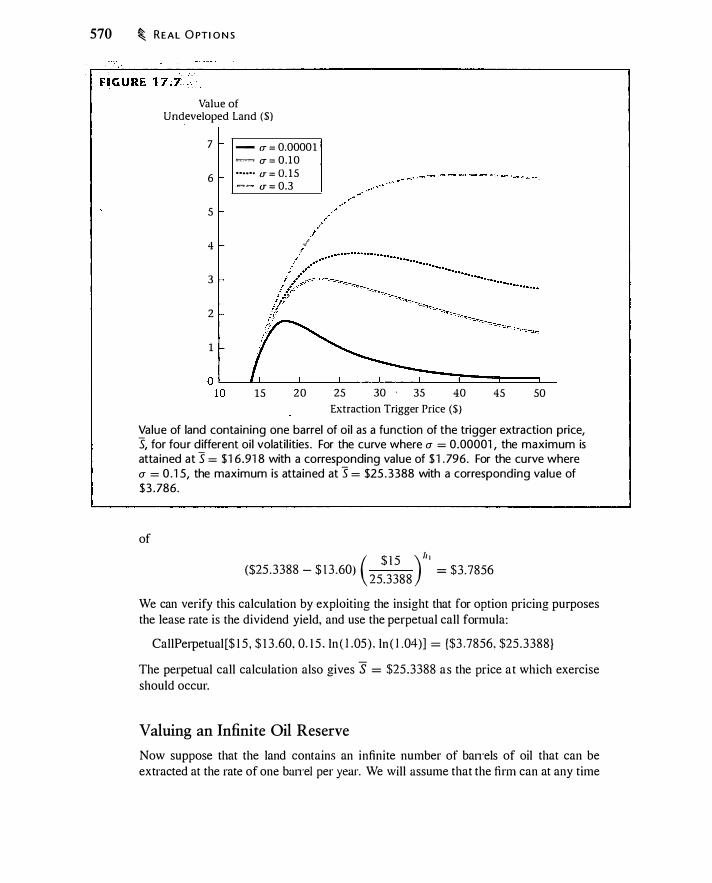
570 � R E A L O PT I O N S

Value of Undeveloped Land ($)

7 - CT = Q.QQQQ1 = cr = 0 . 10 •••••• CT = 0. 15 � - u = 0.3

6

5

4 -!

3

2

1

15 20 25 30 . 35 40

Extraction Trigger Price ($)

45 50

Value of land containing one barrel of oi l as a function of the trigger extraction price, S, for four d ifferent oi l volatil ities . For the curve where a = 0.00001 , the maximum is atta ined at S = $ 1 6.91 8 with a corresponding value of $ 1 . 796. For the curve where a = 0 . 1 5, the maximum is attained at S = $25 . 3388 with a corresponding value of $3 .786.

of

($25 .3388 - $ 1 3 .60) ( $ l 5

8 ) " ' = $3.7856

25.33 8

We can verify this calculation by exploiting the insight that for option pricing purposes the lease rate is the dividend yield, and use the perpetual call formula:

CallPerpetual [$ 1 5 , $ 1 3 .60, 0. 1 5 . ln ( l .05 ) , ln ( l .04)] = {$3 .7856, $25 .3388}

The perpetual call calculation also gives S = $25 .3388 as the price a t which exercise should occur.

Valuing an Infinite Oil Reserve

Now suppose that the land contains an infinite number of ban·els of oil that can be extracted at the rate of one ban·el per year. We will assume that the finn can at any time

C O M M O D I TY EXTRACT I O N AS A N O PTI O N � 571

invest I in order to turn the undeveloped reserve into a developed reserve. Exactly I year after that, the reserve will begin to produce one ban-e! of oil a year forever at a cost c per barrel . We solve this problem by working backward. We first compute the value of the firm supposing that i t i s already producing, and we then study the decision about when to invest.

Valuing the producing firm Once the firm has invested, i t will continue producing forever since the price of oil is always tising. Recall from our discussion of commodity forwards in Chapter 6 that the lease rate is the discount rate l inking the future commodity price with the current commodity price. Thus, the time t value of a barrel received at time T is PV, (F1 , T ) = F1 . r / 0 + r)T-1 = S, j ( l + 8) T-1 • The value of the producing firm at time 0 is therefore

� Fo.i - c � ( So c ) � ( l + r)i

= � ( l + 8)i-

( I + r)i t = l t = l

So c 8 r

( I 7 .8)

You might wonder why the present value of a ba!Tel of oi l a year forever is S0j8. We know that a perpetual-coupon bond paying c/year is worth c j r (the second term on the right in equation ( 1 7 .8)) . We saw in Chapter I 5 that the lease rate on a commodity bond is analogous to the interest rate on a cash bond. The operating well is l ike a bond paying one unit of the commodity forever, so the lease rate 8 is the appropriate discount rate for a bond denominated in a commodity, and So/ 8 is the value of the wel l .

Valuing t h e option t o invest If the firm invests at the price Sr , the value of the land at that time is the value of the producing well less the investment cost, I , or Sr j 8 - cj r - I . The value of the land today is

1 ( Sr c l I 1 ( [ c ]) ( I + r) T 8 - -;: - I J =

( 1 + r) T 8 Sr - 8 -;: + I ( 1 7 .9)

This is the value of the undeveloped oil reserve. Note the similarity with equation ( 17 .6) . If in equation ( 1 7 .6) we replace Sr with the present value of oil extracted, Sr j 8, and replace the extraction cost, X, with the present value of all extraction costs, c j r + I , then w e have a problem that appears the same as in the s ingle-ban·el case. We want to select T to maximize equation ( 1 7.9) . The right-hand side of equation ( 1 7 .9) expresses the value on a per-balTel basis, times I j8 . Having multiple barrels in the ground does not change anything fundamental about the problem if there is certainty and the oil price grows indefinitely.

Example 1 7.3 Suppose So = $ 1 5 , r = 5%, 8 = 4%, c = $8, and the value of the producing well is $ 1 5/0.04 - $8/0.05 = $2 1 5 . If the investment cost, I , is $ 1 80, then the per-barrel extraction cost is 8 (cj r + I ) = 0.04 x ($8/0.05 + $ 1 80) = $ 1 3 .60. The problem is the same as having 1 j 8 options to extract at a cost of $ 1 3 .60; hence, the

572 � R EA L O PT I O N S

solution is exactly the same as i n the single-barrel case. To appreciate the similarity, use the option pricing formula: [ $ 1 5 $8 J CallPerpetual - , - + 1 80, 0.00000 1 , ln ( l .05) , ln ( l .04)

0.04 0 .05

= {$44.9 14, $422.956}

The value of the well at which extraction occurs is $422.956. Thus, extraction occurs when S = 0.04 x $422 .956 = $ 16.9 1 8 . �

With uncertainty, we could have the ability to shut a producing well . We will assume for the moment that production continues forever. In that case, the problem is the same as in the single-barrel case.

Example 1 7.4 Make the same assumptions as in Example 17 .3, except suppose that the price of oil is lognormally distributed with a constant lease rate and volatility is CJ = 0. 15 . The land value and optimal extraction decision is given by [ $ 1 5 $8 J CallPerpetual - , - + $ 1 80, 0. 1 5 , ln ( l .05) , ln ( l .04) = {$94.639, $633 .469}

0 .04 0.05

The well is worth $94.639 and we invest when it is worth S /0.04 = $633 .469, or when S = $25 .3388. On a per-barrel basis, the well is worth 0.04 x $94.639 = $3 .7856.

l With these assumptions, the solution is the same as in the single-barrel case. �

In the absence of any shutdown options, the single- and infinite-barrel cases differ only in scale. The interesting difference arises when it is possible to avoid operating losses by shutting down, which matters only in the multiple-barrel case.

17.5 COMMODITY EXTRACTION WITH SHUT-DOWN AND RESTART OPTIONS

With production occurring over time and uncertainty about the price of oil, we face two new operating decisions: Whether to keep the well operating, or, if it has been shut down, whether to reopen it. There are thus three stages of production:

Initial investment in the well: We begin with an empty field containing oil. This is an undeveloped well. At what point do we drill the well and begin extraction? We answered this question in Section 1 7 .4, assuming that the well operates until the resource is exhausted.

C O M M O D ITY EXTRACT I O N W I T H S H UT- D O W N A N D R ESTA RT O PT I O N S � 573

Continuing to produce: Once we have made the investment in an oil well, we say that the property is developed. However, a developed well may or may not be producing. If we are extracting oil from the ground, we have a developed and producing well . However, if the oil price drops below extraction cost, it may make sense to pay a cost in order to shut down the well and avoid future operating losses. Then it is a shutdown well.

Restarting an operating well: Having shut down the well, if the oil price rises again, it may be possible to pay a cost and restart the well, turning it back into a producing well .

Thus, the well can be in one of three states: Undeveloped, producing, and shutdown (developed but not producing). Figure 1 7.8 shows a hypothetical price path of oil over time and possible operating rules. Investment occurs the first time the oil price reaches the investment trigger price, S. Production is shut down at the shutdown trigger price, S,, and restarted at the restart trigger price, S*. Thus, before point A the well is undeveloped. Between points A and B, and after C, the well is producing. Between B and C the well is shutdown. Key questions are: How do we determine the investment, shutdown, and restart triggers, S, S* , and S* , and what is the value of the land on which the oil is located?

Once again, we have to work backward, as in the binomial valuation of a stock option. Before we can decide the rule for investing (determining S), we have to determine the value of a producing well (this is the present value of future cash flows at the point we

F I G U R E 1 7 . 8 I nvestment and operating decisions for an oi l wel l . In itial investment occurs when the oi l price crosses the investment trigger price, S, at point A. Shutdown of production occurs when the price fa lls to the shutdown trigger, S* (point B). Production is restarted at the restart trigger, S*, at point C.

Oil Price (4)

5*

Time

- Oil Price = Investment Trigger ••••·· Restart Trigger - - Shutdown Trigger

574 � R EA L O PT I O N S

invest). In order to value a producing well, we need to understand operating decisions, specifically how S* , and S* are determined.

It is helpful to analyze shutting down and restarting by considering three separate cases:

1. Production can be shut down once permanently. After the well has been shut, the land has no additional value.

2. Production can be shut down once, then restarted once, this time permanently.

3. Production can be shut down and restarted an infinite number of times. 1 7

Each case layers a new option on the previous case. In addition to allowing additional shutting down and restarting, we can impose costs of doing so. We focus in this section on the case where the well can be shut down never or once after the initial investment. Appendix 1 7.B adds restarting to the analysis .

Permanent Shutting Down

Suppose that we are operating the well. If the current price is S and we ignore shutting down, the value of the operating well is simply

s c Voperating. no shutdown = -;- - -- u r ( 1 7 . 1 0)

Suppose that we can at any time pay a cost of k5 , abandon the well, and never produce again. s* is the price at which we shut down.

What is the value of shutting down? There are three considerations:

1. Once we shut down, we no longer sell oil . Thus, we give up the revenue stream with present value S/8.

2. We no longer pay the extraction cost, so we gain the present value c / r.

3. We give up ks , the shutdown cost.

Thus, the value of shutting down at price S* at a cost of ks is

S,. c (c ) S,. -__:_ + - - ks = - - ks - __:_

8 r r 8 ( 1 7. 1 1 )

This is the payoff to a put option with strike price cjr - ks and asset price S*/8. If we are operating and the price is S, we can value this put to determine the value of the option to shut down, as well as the trigger price, S* , for shutting down.

1 7The model with infinite shutdown and restart was first analyzed in Brennan and Schwartz ( 1 985) and

subsequently by Dixit ( 1 989).

C O M M O D ITY EXTRACT I O N W ITH S H UT- D O W N A N D RESTA RT O PTI O N S � 575

Example 1 7.5 Suppose the oil well is operating and the oil price is s = $ 10. We also have c = $8, a = 0. 15 , and effective annual r and 8 are 5% and 4%, respectively. If ks = $0, the value of the option to shut down is

PutPerpetual [$ 1 0/0.04, $8/0.05 , 0 . 1 5 , ln ( l .05) , ln ( l .04) ] = {$9.633, $ 1 06.830}

Thus, we shut down production when S/8 = $ 1 06.83 or when S = 0.04 x $ 1 06.83 =

$4.2n. At this point, the present value of continuing to produce is $4.273

-$8 .00

= -$53 . 1 7 0.04 0.05

By shutting down production, we avoid losses of $53 . 1 7. When ks = $25, the shutdown solution is

PutPerpetual($ 1 0/0.04, $8/0.05 - 25 , 0. 1 5 , 0.04879, 0.03922) = {$5.778, $90. 1 37 }

The shutdown trigger i s then S = 0.04 x $90. 1 37 = $3 .605. We pay $25 to avoid losses with a present value of -$69.863 . �

To interpret the shutdown results, there are two natural benchmark prices to con­sider. The first is the price at which the NPV of the operating will become zero, which occurs when S = 8 x cfr = $6.40. The second is the price equal to the marginal cost of production, c = $8. If S > $8, then we are making money by operating and we will not shut down. If $8 > S > $6.40, then we are losing money on an operating basis but the NPV of operating the well is positive. In this case we would consider shutting down if we could later restart production, but, because the NPV of operation is positive, we would not shut the well if the shutdown were petmanent. Finally, if S < $6.40, it may make sense to shut the well even if the shutdown were permanent. Note that in all cases, the initial investment is sunk and therefore irrelevant.

In Example 1 7.5, shutdown is permanent so the zero NPV price (S = $6.40) is the natural benchmark. The usual option exercise logic applies: We won ' t shut down as soon as present value is negative, because the decision is irreversible. In fact, we wait until the price is below $5. The price might subsequently increase; by shutting down we are unable to benefit from this reversal . This is the counterpart to not investing as soon as NPV is positive.

The value of the producing well Given that shutdown is possible, what is the value of a producing well? The answer is that the value of the well is the value of the perpetually producing well plus the value of the shutdown option:

Vopernting ( S) = Vno shutdown ( S) + Vshutdown option ( S) ( 1 7 . 1 2) s c [ s c J = - - - + PutPerpetual - , - - ks , a , ln ( l + r) , ln ( l + 8)

8 r 8 r

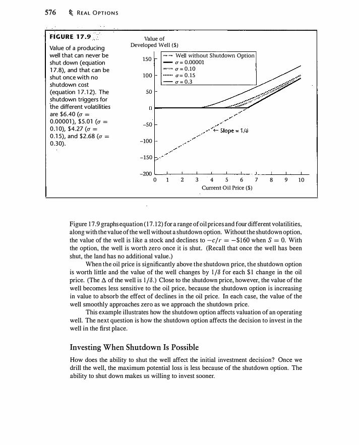
576 � R EA L O PT I O N S

F I G U R E 1 7 . 9 . Value of a producing wel l that can never be shut down (equation 1 7.8), and that can be shut once with no shutdown cost (equation 1 7. 1 2). The shutdown triggers for the different volati l ities are $6 .40 (u = 0.00001 ), $5 .01 (a = 0 . 1 0), $4.27 (a = 0 . 1 5), and $2.68 (a = 0.30) .

Value of Developed Well ($)

1SO

100

so

-SO

-100

-1SO

.-------------------------, - - Well without Shutdown Option - (T = 0.00001 = u = O.lO •••••• u= 0 . 1S - u = 0.3

-200 ��--�--�--�--�--�--�--�--�--�--0 1 2 3 . 4 s 6 7 8 9 10

Current Oil Price ($)

Figure 1 7 .9 graphs equation ( 1 7 . 1 2) for a range of oil prices and four different volatilities, along with the value of the well without a shutdown option. Without the shutdown option, the value of the well is l ike a stock and declines to -c / r = -$160 when S = 0. With the option, the well is worth zero once it is shut. (Recall that once the well has been shut, the land has no additional value.)

When the oil price is significantly above the shutdown price, the shutdown option is worth little and the value of the well changes by l /8 for each $ 1 change in the oil price. (The l'l of the well is 1 /8 . ) Close to the shutdown price, however, the value of the well becomes less sensitive to the oil price, because the shutdown option is increasing in value to absorb the effect of declines in the oil price. In each case, the value of the well smoothly approaches zero as we approach the shutdown price.

This example illustrates how the shutdown option affects valuation of an operating well. The next question is how the shutdown option affects the decision to invest in the well in the first place.

Investing When Shutdown Is Possible

How does the ability to shut the well affect the initial investment decision? Once we drill the well, the maximum potential loss is less becal)se of the shutdown option. The ability to shut down makes us willing to invest sooner.

CO M M O D ITY EXTRACTI O N W ITH S H UT- D O W N A N D R ESTA RT O PT I O N S � 577

To account for the value of the shutdown option we work backward. Equation ( 1 7. 1 2) gives the value of a producing well. Call this Vp (S) . If we invest at the price S, paying an investment cost of I , then the value at the time we invest is

Value of well at time of investment = Vp (S) - I

s c [s c · J = - - - + PutPerpetual - , - - ks , u , ln ( l + r) , ln( l + 8) - I 8 r 8 r ( 1 7 . 13 )

To solve for S, we need to find the present value of equation ( 1 7. 1 3 ), and then choose S to maximize this present value. For a given S, equation ( 1 7. 1 3) tells us the value of investing when S = S. If the oil price today is S < S, we can compute the present value of equation ( 1 7 . 1 3 ) using equation ( 1 7 . 14) . The value will depend upon the current oil price (the lower the price, the longer it will take to hit S), so we denote it as V1nves1 (S; S) . This present value is

Vlnvest (S ; S) = (1)"' X (� - :. + PutPerpetual [� . :. - ks , (J , ln( l + r) , In( 1 + o)] - I) 8 r 8 r

( 17 . 1 4)

Equation ( 17 . 1 4) can be maximized with respect to S using a spreadsheet or other nu­merical program.

Example 1 7.6 Suppose 8 = 0.04, r = 0.05, u = OJ5, c = $8, k_. = $0, and I = $ 1 80. If the current oil price, S, is $ 1 5, then the value ot"S that maximizes equation ( 1 7 . 1 4) is $25 . 1 2, and the value of the undeveloped well is Vlnves1 ($ 15 , $25 . 1 2) = $95 . 1 3 . If k5 = $25, then S = $25 .2 1 and the value of the undeveloped well is $94.93 .

if we increase the current oil price to S = $20, then the value of the undeveloped well increases to $ 1 77.0 I when ks = $0 and $ 1 76.64 when ks = $25 . S is the same as when S = $ 15 . �

This example illustrates some key points . First, as discussed earlier, the ability to shut down reduces the investment trigger, from $25.34 with no shutting down, to $25. 1 2 with shutting down. Second, if there is a cost of shutting down, shutting down occurs at a lower price and provides less protection. This mitigates the benefit of shutting down, raising the shutdown trigger to $25 .2 1 . Finally, a point that may be obvious but is important to understand: The investment trigger implied by maximizing equation ( 17 . 14) is independent of S, the current oil price. To see why, suppose that S = $25 . If S = $ 1 5, it must pass $20 before reaching $25 . Thus, if we evaluate the option when S = $20, we must obtain the same S as when S = $ 1 5 . Thus, S is independent of S.

578 � REAL O PT I O N S

Restarting Production

The preceding example assumed that the firm could never restart once it had shut down. In this section we examine the restart strategy if the firm could restart after it permanently had shut down.

Suppose the firm can pay kr to restart production. The ability to restart is a call option in which the firm receives S/8 by paying cfr + kr , future production costs plus the restart cost.

Example 1 7.7 The value of a shutdown well i s

CallPerpetual - , - + kr , a , log ( l + r) , log ( l + 8) [-S c J 8 r Assuming that S = $ 1 0, 8 = 0.04, r = 0.05, a = 0 . 15 , c = $8, and kr = $0, the option pricing formula gives us the value of the well as $94.46 and $ 1 1 .92 as the price at which m �� t

The ability to restart affects the decision to shut down. When we shut down, we not only cut off future losses but we also acquire a call option to restart. In equation ( 1 7 . 14) we acquired a put option when we invested, so in this case we acquire a call option when we exercise the put option ! And when we invest in the first place, we acquire the put option to shut down, but the value of that put now implicitly contains the call option to restart. The solution for this problem appears in Appendix 17 .B .

Additional Options

The firm might be able to restart and shut down production many times. We can determine triggers and solve for the value of the well by following the strategy in the previous sections. Details of the solution are in Appendix 17 .B.

Table 17 . 1 summarizes the price triggers for several different cases. The qualitative results are intuitive. As with any American option, we require that the oil well have positive NPV before we invest-we are reluctant to kill the put option implicit in the option to take the project. If shutting down in the future is possible, there is an additional put option available besides that from deferring investment, and we are willing to invest at a lower price. The addition of an option to restart once we have shut down makes us more willing to shut down, and, hence, more willing to invest. Adding costs to restarting and shutting down makes us more reluctant to restart, to shutdown, and, hence, to invest initially. More options generally mean more value and investment at a lower price; greater costs mean lower value and investment at a higher price.

The results in Table 17 . 1 illustrate a phenomenon called hysteresis, which Dixit ( 1 989, p. 622) defines as "the failure of an effect to reverse itself as the underlying cause

C H A PT E R S U M MARY � 579

Comparison of investment (5), shutdown (S*), and restart (S*) triggers under d ifferent assumptions. ks is the cost of shutting down the wel l and k, is the cost of restarting once it is shut. I n a l l cases, r = 5% and the lease rate is 8 = 4%.

Parameters Number of Times Triggers (} ks kr Shutdown Restart s s* S*

0.0 0 0 1 6.92

0 . 1 5 0 0 25.34

0. 1 5 0 0 25. 1 2 4.27

0 . 1 5 25 0 25. 14 3 .60

0. 1 5 0 0 25.00 6.03 1 1 .92

0. 1 5 25 25 25. 1 7 4.33 1 3 .79

0. 1 5 25 25 00 00 25. 1 7 4.37 1 3 . 1 8

i s reversed." Suppose that all oil producers have a marginal extraction cost of $8. The current oil price is $7, following a period in which it was $30, and there is a shutdown cost. Oil production is currently unprofitable, and we would not invest in new capacity at this price, but production from existing wells is not unprofitable enough to shut down production. We are in a situation where the cause (the oil price) reversed itself, but the effect (the creation of an oil well) did not. Oil producers lose money on an operating basis, but are not losing enough to shut down production .

Real-life investment decisions exhibit hysteresis. To illustrate hysteresis in a dif­ferent context, Dixit ( 1989) considers investment decisions of a manufacturer with op- ·

erations in a foreign country. liKchange rate fluctuations will change the profitability of the foreign investment. Ho4ever, since investing and disinvesting are costly, it will be optimal to wait until the investment is suffciently profitable before investing, and sufficiently unprofitable before disinvesting. What appear to be sluggish investment decisions may s imply result from costs of undoing what has been done.

- � ' --�---···--------·· ---- _ _: _ ____ . ___ o' __ .,.:.. __ �-� .·. :. - -- -·---· -

CHAPTER SUMMARY

Real options is the analysis of investment decisions taking into account the ability to revise future operating decisions. Examples of real options include timing options (the ability to choose when to make an investment), shutdown options (the ability to stop production in order to avoid losses), sequential investments where the decision to make later investments depends on the outcome of earlier investments (common in R&D), and

580 � R EA L O PTI O N S

natural resource extraction. Investment decisions i n which such options are present can be analyzed using pricing tools from earlier chapters, such as the Black-Scholes model, perpetual options, binomial trees, and barrier present value calculations. In some cases the optimal decision is equivalent to the problem of when to exercise an American option. In general, however, as illustrated by the oil extraction problem, a simple option formulation is just a starting point for analysis.

.

Even when standard option pricing models are not directly applicable, understand­ing the economics of derivatives is helpful in understanding the economics of investment and operation decisions.

FURTHER READING

In later chapters we will encounter more general pricing techniques that expand our ability to solve real options problems. Early papers that used techniques from financial options to analyze real assets include Brennan and Schwartz ( 1985), McDonald and Siegel ( 1 985, 1 986). These papers study investment timing and the option to shut down and restart. Brennan (2000) insightfully summarizes the literature since then. There are several valuable books on real options, including Dixit and Pindyck ( 1994) and Trigeorgis ( 1 996).

A number of papers have applied real options to understanding the real estate market. These include Titman ( 1985), Grenadier ( 1996), and Grenadier ( 1999) .

Many firms use capital budgeting techniques more sophisticated than simple dis­counted cash flow. Triantis and Borison (200 1 ) survey managers on their use of real options, identifying three categories of real options usage: As an analytical tool, as a language and framing device for investment problems, and as an organizational process. McDonald (2000) argues that the use of high hurdle rates in capital budgeting could be an approximate way to account for real options.

PROBLEMS

17.1. Suppose you have a project that will produce a single widget. Widgets today cost $ 1 and the project costs $0.90. The risk-free rate is 5%. Under what circumstances would you invest immediately in the project? What conditions would lead you to delay the project?

17.2. You have a project costing $ 1 .50 that will produce two widgets, one each the first and second years after project completion. Widgets today cost $0.80 each, with the price growing at 2% per year. The effective annual interest rate is 5%. When will you invest? What is the value today of the project?

17.3. Consider again the project in Problem 1 7 .2, only suppose that the widget price is unchanging and the cost of investment is declining at 2% per year. When will you invest? What is the value today of the project?

P RO B LE M S � 58 1

17 .4. Consider the widget investment problem outlined in Section 1 7 . 1 . Show the following in a spreadsheet.

a. Compute annual widget prices for the next 50 years.

b. For each year, compute the net present value of investing in that year.

c. Discount the net present value for each year back to the present. Verify that investing when the widget price reaches $ 1 .43 is optimal.

17 .5. Again consider the widget investment problem in Section 1 7 . 1 . Verify that with S = $50, K = $30, r = 0.04879, u = 0, and 8 = 0.009569, the perpetual call price is $30.597 and exercise optimally occurs when the present value of cash flows is $ 152.957. What happens to the value of the project and the investment trigger when you change S? Why? What happens to the value of the project and the investment trigger when you increase volatility? Why?

17.6. The stock price of XYZ is $ 1 00. One million shares of XYZ (a negligible fraction of the shares outstanding) are buried on a tiny, otherwise worthless plot of land in a vault that would cost $50 million to excavate. If XYZ pays a dividend, you will have to dig up the shares to collect the dividend.

a. If you believe that XYZ will never pay a dividend, what would you pay for the land?

b. If you believe that XYZ will pay a liquidating dividend in 10 years, and the continuously compounded risk-free rate is 5%, what would you pay for the land?

c. Suppose that XYZ has a 1 % dividend yield and a volatility of 0.3 . At what price would you excavate and what would you pay for the land?

17.7. Repeat Problem 17 .6, only assume that after the stock is excavated, the land has an alternative use and can be sold for $30m.

17 .8. Consider the widget investment problem of Section 17 . 1 with the following modification. The expected growth 4ate of the widget price is zero. (This means there is no reason to consider projeat delay.) Each period, the widget price will be $0.25 with probability 0.5 or $2.25 with probability 0.5. Each widget costs $ 1 to produce.

a. What is the expected widget price?

b. If the firm produces a widget each period, regardless of the price, what is the NPV of the widget project?

c. If the firm can choose to produce widgets only when the widget price is greater than $ 1 , what is the NPV?

d. What happens to the NPV if widgets can cost $0. 1 0 or $2.40 with equal probability?

582 � R EA L O PT I O N S

17 .9. To answer this question, use the assumptions of Example 17 . 1 and the risk-neutral valuation method (and risk-neutral probability) described in Example 1 7 .2.

a. Compute the value of a claim that pays the square root of the cash flow in period 1 .

b. Compute the value of a claim that pays the square of the cash flow in period 1 .

c. Given your answers above computed using risk-neutral valuation, back out the tnte discount rate that would give you the same value for each claim. In each case is this rate bigger or smaller than the 1 1 % discount rate for the cash flow itself. Why?

17.10. Consider a project thafin one year pays $50 if the economy performs well (the stock market goes up) and that pays $ 100 if the economy performs badly (the stock market goes down). The probability of the economy performing well is 60%, the effective annual risk-free rate is 6%, the expected return on the market is 1 0%, and and the beta of the project is -0.50.

a. Compute the present value of the project's cash flows using the true probabilities and expected return on the project.

b. Compute the risk-neutral probability of the economy performing well, then repeat the valuation of the project using risk-neutral valuation.

17 .11. Verify the binomial calculations in Figure 17 .3 .

17.12. A project costing $ 1 00 will produce perpetual net cash flows that have an annual volatility of 35% with no expected growth. If the project existed, net cash flows today would be $8. The project beta is 0.5, the effective annual risk-free rate is 5%, and the effective annual risk premium on the market is 8%. What is the static NPV of the project? What would you pay to acquire the rights to this project if investment rights lasted only 3 years? What would you pay to acquire perpetual investment rights?

17.13. A project has certain cash flows today of $ 1 , growing at 5% per year for 1 0 years, after which the cash flow is constant. The risk-free rate is 5%. The project costs $20 and cash flows begin 1 year after the project is started. When should you invest and what is the value of the option to invest?

17.14. Consider the oil project with a single barrel, in which S = $ 15, r = 5%, 8 = 4%, and X = $ 1 3 .60. Suppose that, in addition, the land can be sold for the residual value of R = $ 1 after the barrel of oil is extracted. What is the value of the land?

17.15. Verify in Figure 1 7 .2 that if volatility were 30% instead of 50%, immediate exercise would be optimal .

17.16. Consider the last row of Table 1 7 . 1 . What is the solution for S* and S* when k,. = kr = 0? (This answer does not require calculation.)

A P P E N D I X 1 7. B : TH E S O LUT I O N W ITH S H UTT I N G D O W N AN D R ESTA RT I N G � 583

In the following five problems, assume that the spot price of gold is $300/oz, the effective annual lease rate is 3%, and the effective annual risk-free rate is 5%.

17.17. A mine costing $275 will produce 1 ounce of gold on the day the cost is paid. Gold volatility is zero. What is the value of the mine?

17 .18. A mine costing $ 1 000 will produce 1 ounce of gold per year forever at a marginal extraction cost of $250, with production commencing 1 year after the mine opens .

. Gold volatility is zero. What is the value of the mine?

17.19. Repeat Problems 17 . 17 and 17 . 1 8 assuming that the annual volatility of gold is 20%.

17 .20. Repeat Problem 17 . 1 8 assuming that the volatility of gold is 20% and that once opened, the mine can be costlessly shut down forever. What is the value of the mine? What is the price at which the mine will be shut down?

17.21. Repeat Problem 1 7. 1 8 assuming that the volatility of gold is 20% and that once opened, the mine can be costlessly shut down once, and then costlessly reopened once. What is the value of the mine? What are the prices at which the mine will be shut down and reopened?

APPENDIX 1 7 .A: CALCULATION OF OPTIMAL TIME TO DRILL AN OIL WELL

Appendix available online at www.aw-bc.com/mcdonald.

APPENDIX 1 7 . B : THE SOLUTION WITH SHUTTING D OWN AND RESTARTING

Appendix available online at www.aw-bc.com/mcdonald.

PA R T F I VE A� Pr� Tiwory aJUi Aptfica;tioiU

Xts part of the book provides a n introduction t o the mathematical

underpinnings of the Black-Scholes approach to pricing derivatives. The

standard derivation of the Black-Scholes model has tlVo components: an

assumption about how the stock price behaves, and the idea that prices

are determined by competitive delta-hedging market-makers.

Chapter 18 discusses the meaning of lognormality and illustrates

how the form of the Black-Scholes model arises from straightfonvard

lognormal probability calculations. Chapter 19 covers the Monte Carlo

pricing method, which is a powerful and flexible technique widely used to

price derivatives.

Black and Scholes assumed that stocks follow geometric Brownian

motion and used a mathematical tool called Ito's Lemma to solve the

problem they posed. These are discussed in Chapters 20 and 21. Chapter

21 in particular explains the derivation of tlze option formula and the

sense in which the Black-Scholes approach applies to more than ordinary

puts and calls. Chapter 22 continues the discussion of exotic options

begun in Chapter 14. Chapter 23 discusses volatility and Chapter 24 explains how the

Black-Scholes option pricing methodology can be applied to analyze the

pricing of bonds. Finally, Chapters 25 and 26 cover the assessment of

market risk, including valut� at risk, and credit risk.

585

CHA1ITER r8 . c '-'-'-'-·"-""-""'·' . ·--�---�--------' .. � . , ""-'--�-· ·-· -· . . ... c.c . ·.::=c:. : . . e·:c ..... �.c-" c :�:_ . .

The Lognormal Distribution

W have <een that it i< common in option pricing to M<ume the lognormality of a«et prices. The purpose of this chapter is to explain the meaning of this assumption. We first review the normal distribution, which gives rise to the lognormal distribution. We then define lognormality and illustrate some common calculations based on lognormality. These calculations result in terms that look much like the parts of the Black-Scholes formula. Finally, we examine stock returns to see whether stock price data seem consistent with lognormality.

We will find that stock prices are not exactly lognormal. Nevertheless, the lognor­mal assumption is the basis for many frequently used pricing formulas . Moreover, it is difficult to understand more realistic models used in practice without first understanding models based on the lognormal distribution.

18 .1 THE NORMAL DISTRIBUTION

A random variable, .\' , obeys the normal distribution-or is normally distributed-if the probability that .i takes on a particular value is described by the normal density function, which we represent by ¢ . The formula for the normal density function is 1

I I ( -' -•' ) 2 ¢(x ; f.L , a ) = �e- � -n

a v 2n ( 1 8 . 1 )

Notice i n equation ( 1 8 . 1 ) that i n order to calculate a value for ¢, in addition to x , you need to supply two numbers: a mean, f.L, and a standard deviation, a . For this reason, the normal distributio!1"is said to be a two-parameter distribution ; it is completely described by the mean and the standard deviation.

Figure 1 8 . 1 graphs equation ( 1 8. 1 ) for two different standard deviations (1 and 1 .5) , and for the same mean (0) . The normal density with J.L = 0 and a = 1 is called the standard normal density. When working with the standard normal density, we will write ¢ (x) , without a mean and standard deviation.

1 You can calculate the normal density in Excel using NonnDist(x./i.a.Fa/se).

587

588 � T H E LOG N O R M A L D I STR I B UT I O N

Two normal densities 0.40

with mean 0, one with 0.35 u = 1 (the standard

normal), the other with u = 1 .5 . 0.30

0.25

0.20

0. 15

0.10 </>(:-:; 0, 1 .5)

0.05

0 -6 -4 -2 0 2 4 6

Compared to the standard normal density, the normal density with u = 1 .5 assigns lower probabilities to values of x close to 0, and greater probabilities for x farther from 0. Increasing the variance spreads out the distribution. The mean locates the center of the distribution, and the standard deviation tells you how spread out it is. The normal density is symmetric about the mean, f.L, meaning that

¢ (J.L + a ; f.L, u) = ¢(J.L - a ; f.L, u)

If a random variable x i s normally distributed with mean f.L and standard deviation a , w e write this as

We will use z to represent a random variable that has the standard normal distribution:

z � N(O, 1)

We can use the normal distribution to compute the probability of different events, but we have to be careful about what we mean by an event. S ince the distribution is continuous, there are an infinite number of events that can occur when we randomly draw a number from the distribution. (This is unlike the binomial distribution, in which an event can have only one of two values.) The probability of any particular number being drawn from the normal distribution is zero. Thus, we use the normal distribution to describe the probability that a number randomly selected from the normal distribution will be in a particular range.

We could ask, for example, what is the probability that if we draw a number from the standard normal distribution, it will be less than some number a? The area under

TH E N O R M A L D I ST R I B UTI O N � 589

the curve to the left of a , denoted N(a) , equals this probability, Prob(z < a) . We call N(a) the cumulative normal distribution function. The integral from -oo to a is the area under the density over that range; it is cumulative in that it sums the probabilities from -oo to a . Mathematically, this is accomplished by integrating the standard normal density, equation ( 1 8 . 1 ) with f.L = 0 and u = 1 , from -oo to a :

N (a) = --e- 2·' dx 1{1 1 1 .2

-00 .Jiii ( 1 8.2)

As an example, N(0.3) is shown in Figure 1 8 .2. In the top panel, N(O.�) is the area under the normal density curve between -oo and 0.3 . In the bottom panel, N (0.3) is a point on the cumulative distribution. The range -oo to +oo covers all possible outcomes for a single draw from a normal distribution. The probability that a randomly drawn number will be less than oo is 1 ; hence, N(oo) = I . As you may already have surmised, the N (a) defined above is the same N ( ) used in computing the Black-Scholes formula.

There is no simple formula for the cumulative normal distribution function, equa­tion ( 1 8.2), but as we mentioned in Chapter 1 2, it is a frequent-enough calculation that modem spreadsheets have it as a built-in function. (In Excel the function is called

F I GU R E 18 . 2 Top panel: Area under the normal curve to the left of 0.3. Bottom panel: Cumulative normal d istribution . The height at x = 0 .3, g iven by N(0. 3), is 0 .61 79.

Standard Normal Density, cp(z)

0.4

0.3

0.2

0.1

o�--���L----L--��---L--����--�---4 -3

., Standard Normal Distribution, N(z)

1 .0 0.8

-2 -1 0 z

0.6 . . . . . . ti_ei_?.�t . . �.J\T(�_._3_) _�-� ... ��?.9.. . . . . . 0.4 0.2

1 2 3 4

o�--�----�---L--�L----L--��--�--�---4 -3 -2 -1 0 1 2 3 4

z

590 � TH E LOG N O R M A L D I STR I B UTI O N

NormSDist.) The area under the normal density from -oo to 0.3 is 0.6 1 79. Thus, if you draw a number from the standard normal distribution, 6 1 .79% of the time the number you draw will be less than 0.3.

Suppose that we wish to know the probability that a number drawn from the standard normal distribution will be between a and -a. We have

These relationships imply that

Prob(z < -a) = N(-a) Prob(z < a) = N(a)

Prob(-a < z < a) = N(a) - N(-a)

The area under the curve between -a and a equals the difference between the area below a and the area below -a. Since the standard normal distribution is symmetric about 0, the area under the curve above a equals the area under the curve below -a . Thus,

N(-a) = I - N(a) ( 1 8.3)

Example 1 8. 1 The probability that a number drawn from the standard normal dis­tribution will be between -0.3 and +0.3 is

Prob(-0.3 < z < 0.3) = N(0.3) - N(-0.3) = N(0.3) - [ 1 - N(0.3)] = 2 X 0.6 1 79 - 1 = 0.2358

Finally, if a variable obeys the standard normal distribution, it is extremely unlikely to take on large positive or negative values. The probability that a single draw will be below -3 or above 3 is only 0.0027 . If you drew from a standard normal distribution every day, you would draw above 3 or below -3 only about once a year. The probability of being below -4 or above 4 is 0.000063, which, with daily draws, would occur on average about once every 43.25 years.

Converting a Normal Random Variable to Standard Normal

If we have an arbitrary normal random variable, it is easy to convert it to standard normal. Suppose

Then we can create a standard normal random variable, z, by subtracting the mean and dividing by the standard deviation:

X - f.l z = --

(J ( 1 8 .4)

TH E N O R M A L D I ST R I B UT I O N � 591

Using this fact, we can compute the probability that x is less than some number b: (X - fL b - tL) Prob(x < b) = Prob -a- < -a-

Using equation ( 1 8.3), the complementary probability is

Prob(x > b) = 1 - Prob(x < b) (b - fL ) = 1 - N -a-

= N (fL � b) This result will be helpful in interpreting the Black-Scholes formula.

( 1 8 .5)

( 1 8.6)

If we have a standard normal random variable z, we can generate a variable x ,.....,

N(fL, a2) , using the following:

X = fL + az

Example 1 8.2 Suppose that x ,....., N(3, 25) and z ,....., N(O, 1 ) . Then

x - 3 T '"'-' N(O, 1 ) ,

and

3 + 5 X z ,....., N(3 , 25) t

Sums of Normal Random Variables

( 1 8.7)

Suppose we have n random variables x; , i = 1, . . . , n, with mean and variance E (x; ) = fL; , Var(x; ) = al, and covariance Cov(x; , x j ) = a ij . (The covariance between two random variables measures their tendency to move together. We can also write the covariance in terms of Pij • the correlation between x; and xj : aij = pija;a j.) Then the weighted sum of the n random variables has mean

and variance

( II ) II E i; WjXj = i; W;fL;

( II ) II II Var l:: w;x; = L L W;Wjaij

i= l i= l j= l

( 1 8 .8)

( 1 8.9)

592 � TH E LO G N O R M A L D I STR I B UT I O N

where w; and w j represent arbitrary weights. These formulas for the mean and variance are true for any distribution of the x; .

In general, the distribution of a sum of random variables is different from the distribution of the individual random variables. However, the normal distribution is an example of a stable distribution. A distribution is stable if sums of random variables have the same distribution as the original random variables. In this case, the sum of normally distributed random variables is normal . Thus, for normally distributed x; ,

A familiar special case of this occurs with the sum of two random variables:

ax1 + bx1 � N (aJ.L 1 + bJ.L1 , a1uf + b1u� + 2abpu 1 cr1)

( 1 8 . 1 0)

The central limit theorem Why does the normal distribution appear in option pric­ing (and frequently in other contexts)? The normal distribution is important because it arises naturally when random variables are added. The normal distribution was origi­nally discovered by mathematicians studying series of random events, such as gambling outcomes and observational errors.2 Suppose, for example, that a surveyor is making observations to draft a map. The measurements will always have some error, and the error will differ from measurement to measurement Errors can arise from observational error, imprecise use of the instruments, or simply from recording the wrong number. Whatever the reason, the errors will in general be accidental and, hence, uncorrelated. If you were using such error-prone data, you would like to know the statistical distri­bution of these errors in order to assess the reliability of your conclusions for a given number of observations, and also to decide how many observations to make to achieve a given degree of reliability. It would seem that the nature of the errors would differ depending on who made them, the kind of equipment used, and so forth. The remarkable result is that sums of such errors are approximately normal.

The normal distribution is therefqre not just a convenient, aesthetically pleasing distribution, but it iui.ses in nature when outcomes can be characterized as sums of independent random variables with a finite variance. The distribution of such a sum approaches normality. This result is known as the central limit theorem.3

In the context of asset returns, the continuously compounded stock return over a year is the sum of the daily continuously compounded returns. If news and other factors are the shocks that cause asset prices to change, and if these changes are independent, then it is natural to think that longer-period continuously compounded returns are normally

2The history of statistics-including the story of the normal distribution-is entertainingly related in

Bernstein ( 1 996). 3Most statistics books discuss one or more versions of the central limit theorem. See, for example,

DeGroot ( 1 975, pp. 227-23 1 ) or Mood et al. ( 1 974, pp. 233-236).

TH E LO G N O R M A L D I STR I B UT I O N � 593

distributed. Since the central limit theorem is a theorem about what happens in the limit, sums of just a few random variables may not appear normal. But the normality of continuously compounded returns is a reasonable starting point for thinking about stock returns.

18 .2 THE LOGNORMAL DISTRIBUTION

A random variable, y, is said to be lognormally distributed if ln(y) is normally dis­tributed. Put another way, if x is normally distributed, y is lognormal if it can be written in either of two equivalent ways: ·

ln (y) = x or

This last equation is the link between normally distributed continuously compounded returns and lognormality of the stock price.

By definition, the continuously compounded return from 0 to t is

R (O, t ) = ln(St fSo ) ( 1 8 . 1 1 )

Suppose R (O, t ) i s normally distributed. By exponentiating both sides, we obtain

( 1 8 . 1 2)

Equation ( 1 8 . 1 2) shows that if continuously compounded returns are normally dis­tributed, then the stock price is lognormally distributed. Exponentiation converts the continuously compounded return, R (O, t ) , into one plus the effective total return from 0 to t , eR(O, t ) . Notice that because S1 is created by exponentiation of R (O , t ) , a lognormal stock price cannot be negative.

We saw that the sum of normal variables is normal . For this reason, the product of lognormal random variables is lognormal . If x 1 and x2 are normal, then y1 = ex1 and y2 = ex2 are lognormal . The product of Y 1 and Y2 is

Since x1 + x1 is normal , ex1 +x2 is lognormal. Thus, because normality is preserved by addition, lognormality is preserved by multiplication. However, just as the product of normal random variables is not normal, the sum of lognormal random variables is not lognormal.

We saw in S.ection 1 1 .3 that the binomial model generates a stock price distribution that appears lognormal ; this was an example of the central limit theorem. In the bino­mial model, the continuously compounded stock return is binomially distributed. Sums of binomial random variables approach normality. Thus, in the binomial model, the contilluously compounded return approaches normality and the stock price distribution approaches lognormality.

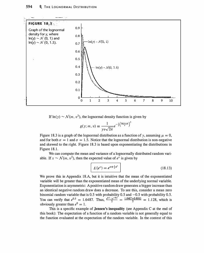
594 � TH E LOG N O R M A L D I ST R I B UT I O N

, _ - ' _' - '",

F I G U R E 1 8 .3

Graph of the lognormal density for y, where ln(y) � N (0, 1 ) and ln(y) � N (0, 1 .5) .

0.9

0.7

0 .6

0 .5

0 .4

0.3

0.2

0 .1

0 0 1

--�

2 3 4 5 6 7

If ln (y) � N(m , v1) , the lognormal density function is given by

1 - ! ( !!!!.±!!!. ) 2 g(y; m , v) = e 2 ,.

yv../2if

8 9 10

Figure 1 8 .3 is a graph of the lognormal distribution as a function of y, assuming J-L = 0, and for both u = 1 and u = 1 .5 . Notice that the lognormal distribution is non-negative and skewed to the right. Figure 1 8 .3 is based upon exponentiating the distributions in Figure 1 8 . 1 .

We can compute the mean and variance of a lognormally distributed random vari­able. If x � N(m , v2) , then the expected value of ex is given by

( 1 8 . 1 3)

We prove this in Appendix 1 8 .A, but it is intuitive that the mean of the exponentiated variable will be greater than the exponentiated mean of the underlying normal variable. Exponentiation is asymmetric: A positive random draw generates a bigger increase than an identical negative random draw does a decrease. To see this, consider a mean zero binomial random variable that is 0.5 with probability 0.5 and -0.5 with probability 0.5 . You can verify that e0·5 = 1 .6487. Thus, e"-'-+:,e-o.s = ' -6487�0-6065 = 1 . 1 28, which is obviously greater than e0 = l .

- -

This is a specific example of Jensen's inequality (see Appendix C at the end of this book) : The expectation of a function of a random variable is not generally equal to the function evaluated at the expectation of the random variable. In the context of this

A LO G N O R M A L M O D E L O F STO C K P R I C ES � 595

example, E (e-') f= eE(x) . Since the exponential function is convex, Jensen's inequality implies that E (e"') > eE<xl . Derivatives theory is replete with examples of Jensen's inequality.

The variance of a lognormal random variable is

( 1 8 . 14)

While we can compute the variance of a lognormal variable, it is much more convenient to use -only the variance of ln(y) , which is normal. We will not use equation ( 1 8 . 14) in the rest of this book.

18 .3 A LOGNORMAL MODEL OF STOCK PRICES

How do we implement lognormality as a model for the stock price? If the stock price S1 is lognormal, we can write

•·

Sr < - = e-

So where x, · the continously compounded return from 0 to t , is normally distributed. We want to find a specification for x that provides a useful way to think about stock prices.

Let the continuously compounded return from time t to some later time s be R (t , s ) . Suppose we have times to < t 1 < t2 . By the definition of the continuously compounded return, we have

The stock price at t2 Cffi\ therefore be expressed as

S = S eR(r , ,r,) 1! / 1 = s10eR(to . r , ) eR(t"r, )

= Sr0eR(r0 , r 1 )+R(r 1 , r2)

Thus, the continuously compounded return from to to t1, R (to , t2) , is the sum of the continuously compounded returns over the shorter periods :

( 1 8 . 15)

Example 1 8. 3 Suppose the stock price is initially $ 1 00 and the continuously com­pounded return ori a stock is 1 5% one year and 3% the next year. The price after I year is $ 1 00e0- 1 5 = $ 1 1 6. 1 834, and after 2 years is $ 1 1 6 . 1 834e0·03 = $ 1 1 9 .722. This equals l OOe0- 1 5+0.03 = lOOeO. I S . �

As we saw in Section 1 1 .3 , equation ( 1 8. 15), together with the assumption that returns are independent and identically distributed over time, implies that the mean and

596 � TH E LO G N O R M A L D I STR I B UT I O N

variance of returns over different horizons are proportional to the length of the horizon. Take the period of time from 0 to T and carve it up into 11 intervals of length lz , where lz = T I 11 . We can then write the continuously compounded return from 0 to T as the sum of the n returns over the shorter periods:

R (O, T) =R(O, lz) + R (lz , 2/z ) + · · · + R[(n - 1 ) /z , T] II

= L R [(i - 1 )/z , i lz ] i=l

Let E(R [(i - 1 ) /z , ilz ] ) = a11 and Var(R [(i - 1 ) /z , ilz ] ) = af, . Then over the entire period, the mean and variance are

-E[R(O, T)] = na11

Var[R (O, T) ] = naf, ( 1 8 . 1 6)

( 1 8 . 17)

Thus, if returns are independent and identically distributed, tlze mean and variance of tlze continuously compounded returns are proportional to time. This result corresponds with the intuition that both the mean and variance of the return should be greater over long horizons than over short horizons.

Now we have enough background to present an explicit lognormal model of the stock price. Generally we will let t be denominated in years and a and a be the annual mean and standard deviation, with 8 the annual dividend yield on the stock. We will assume that the continuously compounded capital gain from 0 to t , ln(S1 I S0) , is normally distributed with mean (a - 8 - 0.5a2)t and variance a2t :

l ln (S1 1So) � N[(a - 8 - 0.5a2) t , a1t] I ( 1 8 . 1 8)

This gives us two equivalent ways to write an expression for the stock price. First, recall from equation ( 1 8 . 7) that we can convert a standard normal random

variable, z, into one with an arbitrary mean or variance by multiplying by the standard deviation and adding the mean. We can write

1 � .ji ln(S1 ISo) = (a - 8 - 2a-)t + a tz ( 1 8 . 1 9)

Second, we can exponentiate equation ( 1 8. 1 9) to obtain an expression for the stock price:

S _ S (a-8- {cr� )t+cr Jiz 1 - oe -

We will use equation ( 1 8 .20) often in what follows.

( 1 8.20)

You may be wondering how to interpret equations ( 1 8 . 1 8), ( 1 8. 1 9) , and ( 1 8 .20) . The subtraction of the dividend yield, 8, is necessary since, other things equal, a higher dividend yield means a lower future stock price. But why do we subtract 1rr1 in the mean?

To understand equation ( 1 8 .20) it helps to compute the expected stock price. We can do this by breaking up the right-hand side of equation ( 1 8 .20) into two terms, one

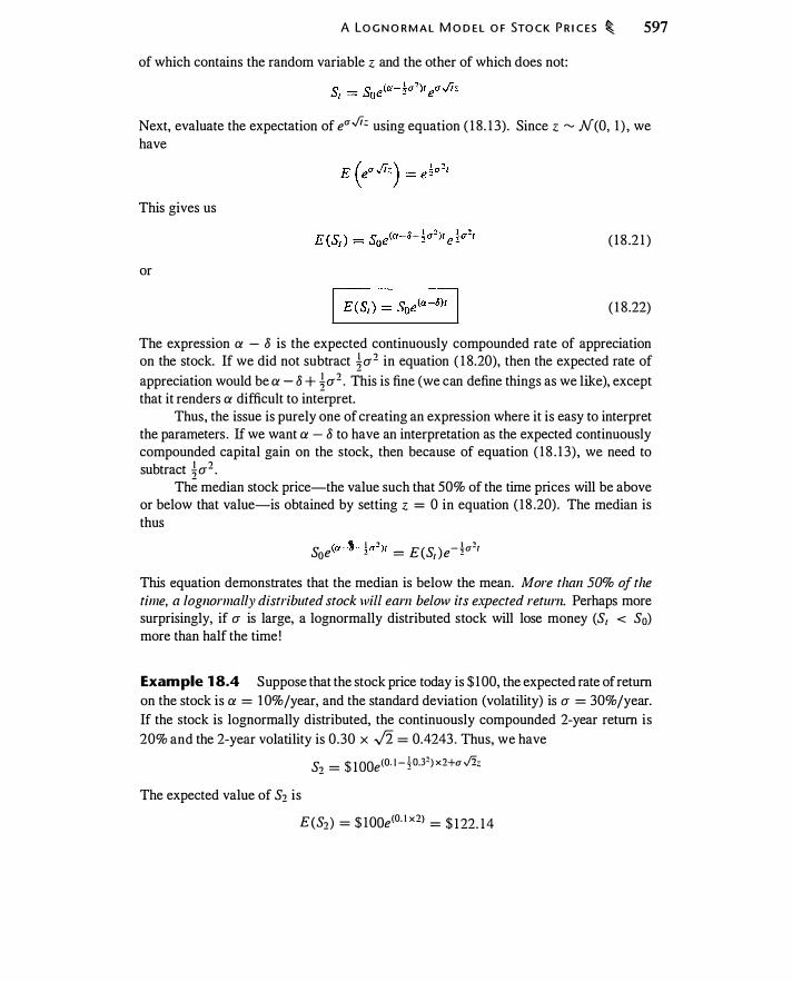
A LO G N O R M A L M O D E L O F STO C K P R I C ES � 597

of which contains the random variable z and the other of which does not:

Next, evaluate the expectation of e".../i� using equation ( 1 8 . 1 3) . Since z � N(O, 1 ) , we have

This gives us

( 1 8 .2 1 )

or

( 1 8 .22)

The expression a - 8 is the expected continuously compounded rate of appreciation on the stock. If we did not subtract :}a2 in equation ( 1 8.20), then the expected rate of appreciation would be a - 8 + !a2 . This is fine (we can define things as we like), except that it renders a difficult to interpret.

Thus, the issue is purely one of creating an expression where it is easy to interpret the parameters . If we want a - 8 to have an interpretation as the expected continuously compounded capital gain on the stock, then because of equation ( 1 8 . 1 3) , we need to subtract !a2 .

The median stock price-the value such that 50% of the time prices will be above or below that value-is obtained by setting z = 0 in equation ( 1 8 .20) . The median is thus

'8. I .., 1 .., s: (a-<J- ,a-)t _ E(S ) - ,a-t oe - - t e -

This equation demonstrates that the median is below the mean. More than 50% of the time, a lognormally distributed stock will earn below its expected return. Perhaps more surprisingly, if a is large, a lognormally distributed stock will lose money (S1 < So) more than half the time !

Example 1 8.4 Suppose that the stock price today is $ 1 00, the expected rate of return on the stock is a = 1 0%jyear, and the standard deviation (volatility) is a = 30%jyear. If the stock is lognormally distributed, the continuously compounded 2-year return is 20% and the 2-year volatility is 0 .30 x ../2 = 0.4243 . Thus, we have

s2 = $ 10Qe(O. I - !0.32 ) x2+aJ2z

The expected value of S2 is

E(S2) = $ 10Qe (O. I x2l = $ 1 22. 14

598 � TH E LO G N O R M A L D I STR I B UTI O N

The median stock price is

$ lOOe(O. I -0.5 x0.31 ) x 2 = $ 1 l l .63

If the volatility were 60%, the expected value would still be $ 1 22. 14, but the median would be

$ 100e(O. I -0.5 x0.61 ) x2 = $85 .2 1

Half the time, after 2 years the stock price would be below this value.

We can also define a "one standard deviation move" in the stock price. Since z has the standard normal distribution, then if z = 1 , the continuously compounded stock return is the mean plus one standard deviation, and if z = - 1 , the continuously compounded stock return is the mean minus one standard deviation.

Example 1 8.5 Using the same assumptions as in Example 1 8.4, a one standard deviation move up over 2 years is given by

S2 = $ 100e(O. I - �0.31 ) x 2+a./2x l = $ 1 70 . 62

A one standard deviation move down is given by

S2 = $ 100e (O. I - �0.31 ) x 2-a./2x l = $73 .03

We can think of these prices as logarithmically centered around the mean price of$ 122. 14. �

This discussion also shows us where the binomial models in Chapter 1 1 come from. In Section 1 1 .3 , we presented three different ways to construct a binomial model. All had up and down ·stock price moves of the form

S _ Seah+a.fii . u - '

where ct differed for the three models. In all cases, we generated up and down moves by setting z = ± 1 . As h -* 0 the three models converge; the effects of the different ct 's in the three cases are offset by the different risk-neutral probabilities.

18 .4 LOGNORMAL PROBABILITY CALCULATIONS

If S1 is lognormally distributed, we can use this fact to compute a number of probabilities and expectations . For example, we can compute the probability that an option will expire in the money, and, given that it expires in the money, the expected stock price. In this section we will present formulas for these calculations.

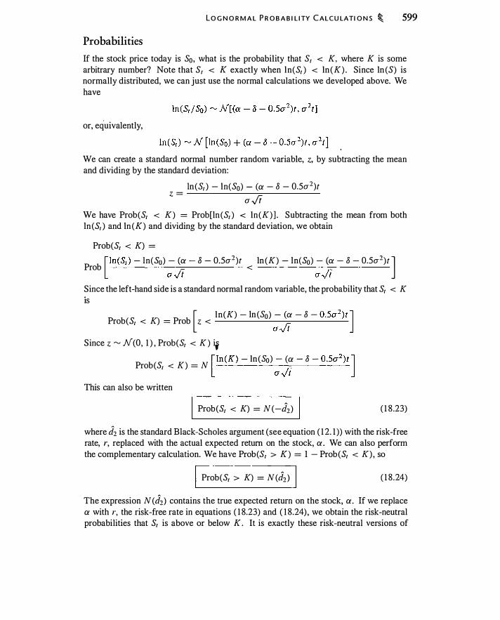
LO G N O R M A L P R O B A B I L I TY CALCU LATI O N S � 599

Probabilities

If the stock price today is S0, what is the probability that S1 < K, where K is some arbitrary number? Note that S1 < K exactly when ln(S1 ) < ln (K) . Since ln (S) is normally distributed, we can just use the normal calculations we developed above. We have

or, equivalently,

We can create a standard normal number random variable, z, by subtracting the mean and dividing by the standard deviation:

ln (S1 ) - ln(S0) - (a - 8 - 0.5u2)t z =

u0

We have Prob(S1 < K) = Prob[ln (S1 ) < ln (K) ] . Subtracting the mean from both ln (S1 ) and ln (K) and dividing by the standard deviation, we obtain

Prob(S1 < K) = [ ln(S1 ) - ln(So) - (a - 8 - 0.5u1)t ln (K) - ln(So) - (a - 8 - 0.5u1)t J Prob r. < r. CT.y ( CT.y t Since the left-hand side is a standard normal random variable, the probability that S1 < K IS

[ ln(K) - ln (S0) - (a - 8 - 0.5u2) t ] Prob(S1 < K) = Prob z < r. CT.y t

Since z � N(O, 1 ) , Prob(S1 < K ) iy [ ln (K) - ln (So) - (a - 8 - 0.5u2) t ]

Prob(S1 < K) = N r. CT.y ( This can also be written

I Prob(S1 < K) = N ( -J2) I ( 1 8 .23)

where J2 is the standard Biack-Scholes argument (see equation ( 1 2. 1 )) with the risk-free

rate, r, replaced with the actual expected return on the stock, a . We can also perform the complementary calculation. We have Prob(S1 > K) = I - Prob(S1 < K), so

I Prob(S1 > K) = N(d2) I ( 1 8 .24)

The expression N (d2) contains the true expected return on the stock, a. If we replace a with r, the risk-free rate in equations ( 1 8.23) and ( 1 8.24) , we obtain the risk-neutral probabilities that S1 is above or below K . It is exactly these risk-neutral versions of

600 � TH E LO G N O R M A L D I STR I B UTI O N

equations ( 1 8.23) and ( 1 8 .24) that appear i n the Black-Scholes call and put option pricing formulas.

Lognormal Confidence Intervals

We can now answer questions about future prices, such as "what is the range of prices such that there is a 95% probability that the stock price will be in that range l year from today?" To answer this question, we compute the 95% confidence intervals for a number of different time horizons.

Suppose we would like to know the prices StL and SF such that Prob(StL < St ) = p /2 and Prob(Stu > St ) = p /2. If the stock price is So, we can generate StL and Stu as follows. We know from equation ( 1 8 .23) that

Prob(S < StL ) = N (-d2)

where

lf2 = [ln (SofStL ) + (a - 8 - 0.5u2 )t]/u..Ji

Thus, we want to find the stL such that the probability that St is less than stL is p /2, or

p/2 = N(-d2)

In order to do this, we need to invert the cumulative standard normal distribution function-i.e., ask what number d� corresponds to · a given probability. We can write this inverse cumulative normal_ probability function as N- 1 (p) . Then by definition, N- 1 [N (x )] = x. Fortunately, this is a standard calculation, and Excel and other spread­sheets contain a built-in function that does this . (In Excel it is NormS!nv.) We have

N- 1 (p/2) = -d2

Solving explicity for stL gives us

stL = Soe(a-o- ia1 )t+a./iN- l (p/2)

Similiarly, we solve for the stu such that

N- 1 ( l - p/2) = lh_

This gives us

s? = Soe(a-o- ia1)t+a./iN-1 ( 1 -pj2)

Thus, to generate a confidence interval for a lognormal price, we need only find the values of z corresponding to the same confidence interval for a N(O, l ) variable, and then substitute those values into the expression for the lognormal price.

Example 1 8.6 If p = 5%, N- 1 (0 .025) = - 1 .96 and N- 1 (0.975) = 1 .96. That is, there is a 5% probability that a standard normal random variable will be outside the range (- 1 .96, 1 .96) . Thus, if So = $ 1 00, t = 2, a = 0. 1 0, 8 = 0, and u = 0.30, we

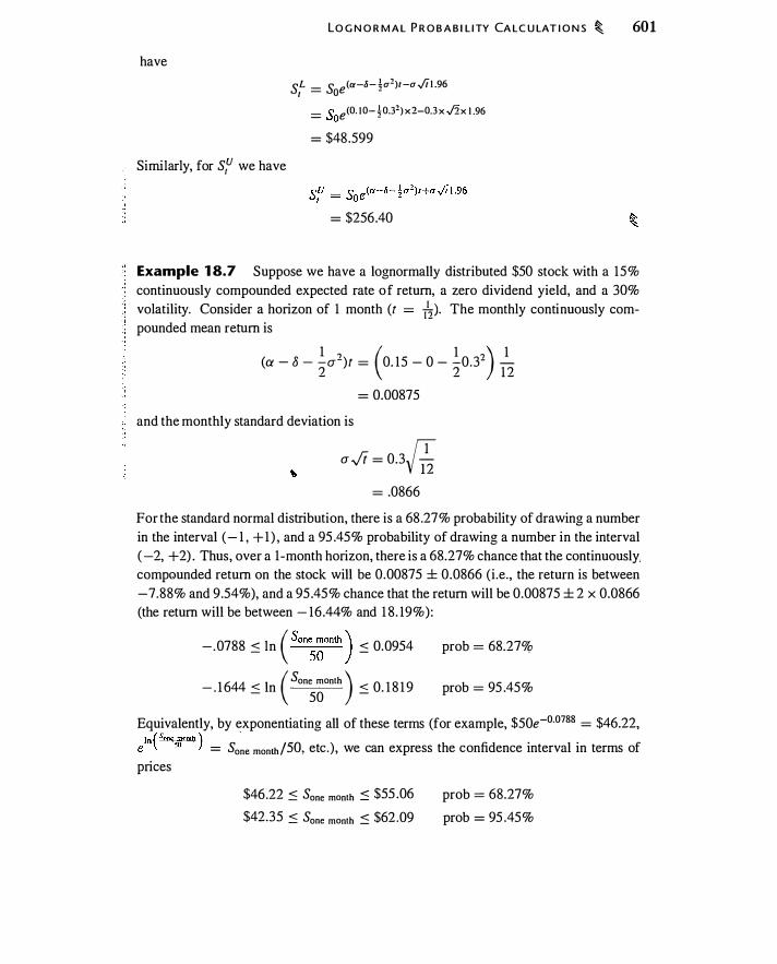
have

LO G N O R M A L P R O B A B I L I TY CA LC U LAT I O N S � 601

SL _ S (a-8- �a2)r-aJ11 .96 1 - ae -

_ <' e(O. I 0- �0.32) x2-0.3 xv'2x 1 .96 - ..JQ -

= $48 .599

Similarly, for S1u we have

= $256.40

Example 1 8.7 Suppose we have a lognormally distributed $50 stock with a 15% continuously compounded expected rate of return, a zero dividend yield, and a 30% volatility. Consider a horizon of 1 month (t = ii:). The monthly continuously com­pounded mean return is

(a - 8 - -cr)t = 0. 15 - 0 - -0.3- -

1 � ( 1 ") 1 2 2 1 2

= 0.00875

and the monthly standard deviation is

(J -Jt = 0.3rr; = .0866

For the standard normal distribution, there is a 68 .27% probability of drawing a number in the interval ( - 1 , + 1 ) , and a 95 .45% probability of drawing a number in the interval ( -2, +2) . Thus, over a 1-month horizon, there is a 68.27% chance that the continuously compounded return on the stock will be 0.00875 ± 0.0866 (i .e. , the return is between -7.88% and 9.54%), and a 95 .45% chance that the return will be 0.00875 ± 2 x 0.0866 (the return will be between - 16.44% and 1 8 . 19%) :

- .0788 .:S ln ( Son��onth ) .:S 0.0954 prob = 68.27%

- . 1 644 < ln ( Sane month ) < 0. 1 8 1 9 prob = 95 .45% - 50 -

Equivalently, by exponentiating all of these terms (for example, $50e-0·0788 = $46.22,

eln( s""sW""'h ) . = Sane month /50, etc.) , we can express the confidence interval in terms of

prices

$46.22 .:S Sane month .:S $55 .06

$42.35 .:S Sane month .:S $62 .09

prob = 68.27%

prob = 95 .45%

602 � T H E LOG N O R M A L D I STR I B UT I O N

" � �

TAB L E 1 8 . 1 Stock prices ($) corresponding to -2, -1 , 1 , and 2 standard deviations from the in ita l stock price of 50 .

Horizon Fraction of a Year -2u - liT +lu +2u

1 Day 0.0027 48.47 49.24 50.8 1 5 1 .6 1

1 Month 0.0849 42.35 46.22 55.06 60.09

1 Year 30.48 4 1 . 1 4 74.97 1 0 1 . 1 9

2 Years 2 26.40 40.36 94.28 144. 1 1

5 Years 5 22. 10 43.22 165.3 1 323.33

Using this same logic, we can compute one standard deviation and two standard devia­tion intervals over different horizons. This will give us 68.27% and 95.45% confidence intervals over those horizons, which are displayed in Table 1 8. 1 . For example, there is a 95 .45% chance over a 1 -day horizon that a $50 stock will be between $48 .47 and $5 1 .6 1 . Over a 5-year horizon, there is a 95 .45% chance that the stock price will be between $22. 10 and $323 .33. �

The calculation in Example 1 8 .7 is often used to compute loss probabilities and risk exposure. We will see in Chapter 25 that this is how value at risk (VaR) is calculated. The idea behind VaR is to assess the magnitude of a possible loss on a position that can occur with a given probability over a given horizon. So, for example, if we examine the 1 -day horizon in Table 1 8 . 1 , there is a 2.275% probability that over a 1 -day hmizon the stock price will drop below $48 .47 .4 In practice, it is common to evaluate the magnitude of moves of 1 .96u since this corresponds to a 5% ("once in 20 days") probability of occurrence.

The box on page 603 illustrates how the probability calculations in this section can be used to analyze the cost of portfolio insurance over time, previously discussed in Chapter 9.

The Conditional Expected Price

Given that an option expires in the money, what is the expected stock price? The answer to this question is the conditional expected stock price. For a put with strike price K , we want to calculate E(S1 I S1 < K) , the expected stock price conditional on S1 < K . To compute this expectation, we need to take into account only the portion of the probability density representing stock prices below K .

4You can verify the 2.275% probability b y computi ng N ( -2).

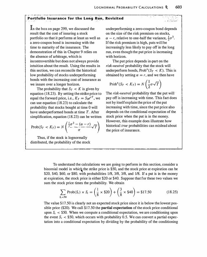
LO G N O R M A L P R O B A B I L ITY CALCU LAT I O N S � 603

Portfol io I nsurance for the Long Run, Revis ited

In the box on page 299, we discussed the result that the cost of insuring a stock portfolio so that it performs at least as well as a zero-coupon bond is increasing with the time to maturity of the insurance. The demonstration of this in Chapter 9 relies on the absence of arbitrage, which is incontrovertible but does not always provide intuition about the result. Using the results in this section, we can reconcile the historical low probability of stocks underperforming bonds with the increasing cost of insurance as we insure over a longer horizon.

The probability that ST < K is given by equation ( 1 8.23). By setting the strike price to equal the forward price, i .e. , K T = SoerT , we can use equation ( 1 8.23) to calculate the probability that stocks bought at time 0 will have underperformed bonds at time T. After s implification, equation ( 1 8 .23) can be written ( .!.a-2 - (a - r) ) Prob(ST < KT) = N 2 a .JT

Thus, if the stock is lognormally distributed, the probability of the stock

underperforming a zero-coupon bond depends on the size of the risk premium on stocks, a - r, relative to one-half the variance, �o-2• If the risk premium is high, puts wil l be -

increasingly less likely to pay off in the long run, even though the put price is increasing with horizon.

The put price depends in ·part on the risk-neutral probability that the stock will underperform bonds, Prob* (ST < K) . This is obtained by setting a = r , and we then have

Prob" (ST < KT) = N (�a.JT) The risk-neutral probability that the put will pay off is increasing with time. This fact does not by itself explain the price of the put increasing with time, since the put price also depends on the conditional expectation of the stock price when the put is in the money. However, this example does illustrate how historical tme probabilities can mislead about the price of insurance.

To understand the calculations we are going to perform in this section, consider a binomial model in whic� the strike price is $50, and the stock price at expiration can be $20, $40, $60, or $80, with probabilities 1 /8, 3/8 , 3/8 , and 1/8 . If a put is in the money at expiration, the stock price is either $20 or $40. Suppose that for these two values we sum the stock price times the probability. We obtain

� Prob(S1 ) X S1 = (� X $20) + (� X $40) = $ 1 7.50 S, <�O

( 1 8 .25)

The value $ 1 7.50 is clearly not an expected stock price since it is below the lowest pos­sible price ($20). We call $ 1 7.50 the partial expectation of the stock price conditional upon S1 < $50. When we compute a conditional expectation, we are conditioning upon the event S1 < $50, which occurs with probability 0.5 . We can convert a partial expec­tation into a conditional expectation by dividing by the probability of the conditioning

604 � T H E LO G N O R M A L D I STR I B UT I O N

event (S1 < $50). Thus, the conditional expectation is

1 � Prob(S1 ) x S1 = -1 [(� x $20) + (� x $4o)J

Prob(S1 < 50) £....: 0.5 8 8 S, <JO

= $35 ( 1 8.26)

The calculations for a lognormally distributed price are analogous, using integrals rather than summations.

The partial expectation of S1 , conditional on S1 < K, is K ? 1 (a-8)1 ( ln (K) - [ln (So) + (a - 8 + 0.5a-) t] ) S1 g (S1 ; So)dS1 = Soe N r. o · a-..; t

= Soe(a-ii)l N ( -JI )

( 1 8.27)

where g (S1 ; S0) is the probability density of S1 conditional on S0, and d1 is the Black­

·scholes d1 (equation ( 1 2. 1 )) with a replacing r . The probability that S1 < K is N ( -d

2) . Thus, the expectation of S1 conditional on S1 < K is

( 1 8.28)

For a call, we are interested in the expected price conditional on S > K. The partial expectation of S1 conditional on S1 > K is

100 (a-ii)l ( ln (So) - ln (K) + (a - 8 + 0.5a2)t ) S1 g (S1 ; So)dS1 = Se N r. K a -..; t = Soe(a-8)1 N(dt )

( 1 8 .29)

As before, except for the fact that it contains the expected rate of return on the stock, a, instead of the risk-free rate, the second term is just the Black-Scholes expression, N (dt ) . The conditional expectation is

( 1 8.30)

The Black-Scholes Formula

Using equations ( 1 8.23), ( 1 8.24), ( 1 8.28), and ( 1 8 .30), we can now heuristically derive the Black-Scholes formula. Recall that the Black-Scholes formula can be derived by assuming risk-neutrality. In this case, the expected return on stocks, a, will equal r , the risk-free rate. If we let g* denote the risk-neutral lognormal probability density, E* denote the expectation taken with respect to risk-neutral probabilities, and Prob* denote

EST I M AT I N G TH E PA R A M ET ERS O F A LO G N O R M A L D I STR I B UT I O N � 605

those probabilities, the price of a European call option on a nondividend-paying stock will be

C (S, K , a, r, t , 8) = e-rr rxo (S1 - K)g*(S1 ; So)dS1 JK = e-rr E*(S - K I S > K) x Prob* (S > K)

We can rewrite this as

C (S, K, a , r, t, 8) = e-rr E* (S I S > K) x Prob* (S > K)

- e-rr E*(K I S > K) X Prob* (S > K)

Using ( 1 8.23) and ( 1 8 .30), with a = r , this becomes

C (S, K, a, r, t, 8) = e-lir SN(d1 ) - Ke-rr N (d2)

which is the Black-Scholes formula. S imilarly, the formula for a European put option on a nondividend-paying stock

is derived by computing

P (S, K, a , r, t, 8) = e-rr E*(K - S I K > S) x Prob* (K > S)

We can rewrite this as

P (S, K, a, r, t, 8) = e-rr E*(K I K > S) x Prob* (K > S)

- e-rr E* (S I K > S) x Prob* (K > S)

and using ( 1 8 .24) and ( 1 8.28), with a = r , this becomes

P (S, K, a, r, t, 8) = Ke-'1 N (-dz) - e-or SN (-d1 )

18 .5 ESTIMATING THE PARAMETERS OF A LOGNORMAL DISTRIBUTION

In this· section we will see how to estimate the mean and variance of lognormally dis­tributed price data.

When stocks are lognormally distributed, a price S1 evolves from the previous price observed at time t - lz , according to

S _ S e<a-IS-a2j2)h+a.Jh� t - t-h

Suppose we have daily observat�ons. How would we estimate the mean and standard deviation? We have

Thus

In(S1 ) = ln (Sr-h ) + (a - 8 - a2 /2)/z + a .,Jhz

E [In (Sr / Sr-h )] = (a - 8 - a2 /2)/z

Var [ln (Sr /Sr-h ) ] = a2lz

606 � TH E LO G N O R M A L D I STR I B UTI O N

B y using the log ratio of prices at adjacent points in time, we can compute the continu­ously compounded mean and variance. Note that to estimate a, we have to add one-half the estimate of the variance to the estimate of the mean.

Example 1 8.8 Table 1 8.2 contains seven weekly stock price observations along with continuously compounded returns computed from those observations. You can compute the mean and standard deviation of the values in the third column (for example, using the Average and Stdev functions in Excel). Since these are weekly observations, we are estimating the weekly mean of the log price ratio and the weekly standard deviation.

The mean of the second column in Table 1 8 .2 is 0.006745 and the standard devi­ation is 0.038208. The annualized standard deviation is

Annualized standard deviation = 0.038208 x .J52 = 0.2755

Two adjustments are needed to interpret the mean. First, we have to annualize it. Second, since we computed the mean of the log returns, we have to add back one-half the variance. Thus, we obtain

Annualized expected return = 0.006745 x 52 + 0.5 x 0.27552 = 0.3887

The prices were generated randomly assuming using a standard deviation of 30% and a mean of 1 0%. Despite having only six observations, the standard deviation estimate is quite close to the true value of 30%. The estimated mean, however, is quite far off. �

We used hypothetical data in this example in order to compare the estimates to the true underlying parameters, something we cannot do with real data. As this example

TABLE 1 8 . 2 Hypothetical weekly stock price observations and corresponding weekly continuously compounded returns, ln(Stf 51 - 1 ) .

Week Price ($) ln(St I St-I )

1 00

2 1 05 .04 0.0492 'l 105 .76 0.0068 .)

4 1 08.93 0.0295

5 102.50 -0.0608

6 1 04.80 0.0222

7 104. 1 3 -0.0064

ESTI M AT I N G TH E PA R A M ETE R S O F A LO G N O R M A L D I STR I B UT I O N � 607

illustrates, mean returns are hard to estimate precisely because the mean is determined by the difference between where you start and where you end. If you start at a price of $ 100 and end at a price of $ 104, the in-between prices are irrelevant: If you had a big negative weekly return (say -20%), it must have been offset by a big positive return (on the order of +20%), or you would not have ended up at 104 ! Having many frequent observations is not helpful in estimating mean returns. What is helpful is having a long time interval, and seven weeks is not long.

Statistical theory tells us the precision of our estimate of the mean. With a normally distributed random variable, the standard deviation of the estimated mean is the standard deviation of the variable divided by the square root of the number of observations. The data in this example were generated using an actual weekly a of 0.3/-/52 = 0.04 16. Divide this by -/6 (since there are six return observations) to get 0.0 17 . Thus, one standard deviation for our estimate of the mean is 1 .7% on a weekly basis, or 12.25% annualized. There is a 68% probability that the annualized continuously compounded mean falls in the range 38% ± 1 2.25% ! A 95% confidence interval is 38% ± 24.5%. This is a wide range. Even with 10 years of weekly data, one standard deviation for our estimated annualized mean would be 30%/.J.SW = 1 .3%.

When we estimate a standard deviation, we are interested in the movement of the price. The more observations we have, the more precisely we can estimate move­ment. With six observations, an approximate 95% confidence interval for the standard deviation is approximately ± 1 8 percentage points .5 With only 26 weekly observations, the 95% confidence interval shrinks to ±8 percentage points. Moreover, unlike the mean, we can increase the precision of our estimate of the standard deviation by making more frequent observations. In general, standard deviations are easier to estimate than means.

In this discussion we have assumed that the variance is not changing over time. There is good evidence, however, that the variance does change over time, and sophis­ticated statistical methods can be used to estimate changing variances.

You should also be aware that, in practice, using data from very tiny intervals (e.g., �ourly prices) may not increase precision. Over short time periods, factors such as bid-ask bounce-the movement of the price between the bid and ask spreads due to some orders being sells and others being buys-can introduce into prices noise that is not related to the values we are trying to measure.

5The variability of the variance estimate is described by the chi-squared distribution. (The chi-squared

distribution is the distribution of sums of squared independent standard nonnal variables; hence, it

describes the distribution of the estimated variance when observations are independent.) Suppose we

wish to test the null hypothesis that our variance estimate s2 = a5 and that we have 11 observations.

The variable (11 - l )s2fa� has the chi-squared distribution with 11 - I degrees of freedom. If we wish

to perform a two-tailed test when we have six observations, the critical values for 0.975 and 0.025 confidence are 0.83 1 and 1 2.832. If our null hypothesis is that a� = 0.09, then the 95% confidence

interval is 0.0 1 496 - 0.23097. This corresponds to a range of standard deviations of 1 2.23% - 48.06%, or approximately 30% ± 1 8%. The calculation for 26 observations is similar.

�

608 � TH E LO G N O R M A L D I ST R I B UT I O N

1 8 .6 HOW ARE ASSET PRICES DISTRIBUTED ?

The lognormal model assumes that stock returns are independent over time (today's return does not affect future returns), that mean and volatility are constant over time, and that the distribution of continuously compounded returns is normal. However, we saw in Chapter 12 that implied volatilities differ for options with different strikes . One possible explanation is that stock prices are not lognormally distributed. How can we tell whether lognormality (or some other particular distribution) is a reasonable approximation for actual stock prices?

Histograms

One way to assess lognormality is si'mply to plot the continuously compounded returns as a histogram and see whether the resulting distribution appears normal. The top row of Figure 18 .4 presents histograms for daily returns over a 10-year period for the S&P

S&P DAILY RETURN

500

400

300

200

100

0 -0. 1 -0.05 0 0.05 0 .1

S&P WEEKLY RETURN

100

80

60

40

20

500

400

300

200

100

0 -0.2

1 20

1 00

80

60

40

20

I BM DAILY RETURN

-0. 1 0 0 .1 0.2

IBM WEEKLY RETURN

0 o L=��=---�-----L�---L---0. 1 -0.05 0 0.05 0.1 -0.2 -0. 1 0 0. 1 0.2

Histograms for dai ly and weekly returns on the S&P 500 index and I BM, from january 2, 1 991 , to October 24, 2001 .

H OW A R E ASS ET P R I C ES D I STR I B UT E D ? � 609

500 index and for IBM. The bottom row is histograms for weekly returns. Also plotted on each graph is a normal distribution, computed using the historical mean and standard deviation for each return series.6 Several observations are pertinent.

None of the histograms appears exactly normal. All of the histograms exhibit a peak around zero; the presence or absence of this peakedness is referred to as kurtosis (a measure of how "sharp" the peak of the distribution is), and the graph displays lep­tokurtosis (lepto meaning "small, thin, delicate")J For a normally distributed random variabk, kurtosis is 3. For the data plotted in Figure 1 8 .4, kurtosis for the S&P and IBM are 8.03 and 9.54 for daily returns, and 4.68 and 5.2 1 for weekly returns. Accompanying the peaks are fat tails, large returns that occur more often than would be predicted by the lognormal model . These shapes are typical for stock returns.

There are several possible explanations for returns appearing nonnormal . One is that stock prices can jump discretely from time to time. We will discuss jumps in subsequent chapters. Another explanation is that returns are normally distributed, but with a variance that changes over time. If actual daily returns are drawn from a distribution that has a 1 % volatility half the time and a 2% volatility half the time, the stock price histogram will appear fat -tailed. This blend of two distributions is commonly referred to as a mixture of normals model . Long-horizon returns, which result from summing short-horizon returns, will still appear normal.

Normal Probability Plots

Figure 1 8 .5 presents normal probability plots for the same data as Figure 1 8 .4. These plots are an alternative to histograms for assessing normality. We will examine normal probability plots as a tool for assessing normality and also to introduce a technique that we will encounter again in discussing Monte Carlo s imulation.

The interpretation of these plots is straightforward: If the data points (plotted with a "+") lie along the straight line in the graph, the data are consistent with a normal distribution. If the data plot is curved, the data are less likely to have come from a normaJ distribution. In both cases it appears the data are not normal. There are too many points to the left of the line for low values and to the right of the line for high values. The interpretation of the plots is that extreme low and high returns occur more often than with a normal distribution.

For both the S&P index and IBM, the weekly returns appear more normal than daily returns, in that the observations more closely resemble the straight line. This is the relationship we would expect from the central limit theorem. Weekly returns are the sum of daily returns. If daily returns are independent and identically distributed, the summed daily returns will tend toward normality.

6 An equivalent approach would be to normalize returns by subtracting the estimated mean and dividing

by the estimated standard deviation. The resulting series should then be standard normal i f returns are

truly lognormal. 7The kurtosis of a distribution is the fourth centfal moment (i.e., E[(x - tL)4], where fL is the mean)

divided by o.4.

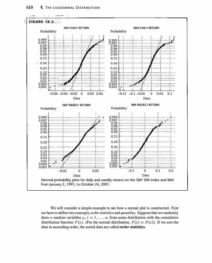
610 � TH E LO G N O R M A L D I STR I B UT I O N

S&P DAILY RETURN Probability

0.999 0.997

0.99 0.98 0.95 0.90 0.75 0.50

0.25 0 .10 0.05 0.02 0.01

0.003 0.001

: : : : : / : J : : : : i: : : : : : : : : t : : : : : : : : :� : : : : : : : : :� : : : : : : :;t: :�b:: : . . . . -:· . . . . . . . . ·:· . . . . . . . . ·:· . . . . . . . . ·:- . . . . . . , . . . . . . . . - � . . . . .

. . . . -�- . . . . . . . . -�- . . . . . . . . -�- . . . . . . . . -�· . . . . i.l � • . . . . . . . -� . . . . . • • • · ·:· • • • • • • • · ·:· • • . • • • . • • : . • • • . • . . · ·:· . • • • • -� - • • • • • • • ·# • • • • • . . . . . . . . . : . . . . . . . . . . : . . . . . . . . . . : . . . . . . . . . . :. . . . . . . -� . . . . . . . 0 -: . . . 0 . . . . . . . . .

. . . . . . . . · · · · -:· · · · · · · · · -:· · · · · · · · · ·:- · · · · · · · · · · · · · · · · ·::- · · · · · · · · · ::- · · · · · . . . . . . . . . . · · · - �· - · · · · · · · -=- · · · · · · · · ·=- · · · · · · ·=- · · · · · · · · ·= · · · · · · · · - � · - · · · . . . . . . . .

-0.06 -0.04 -0.02 0 0.02 0.04 Data

S&P WEEKLY RETURN Probability

0.999 0.997

0.99 0.98 0.95 0.90 0.75

0.50

0.25 0 .10 0.05 0.02 0.01

0.003 0.001

� :� � � �� � �� � J � �: � �: � � � � � : � � � T � : � : : � � : : � : . ;)�!: � :� . . . . . . . . . . . . . . . . ·:· . . . . . . . . . . . . . . . . -� · - . . . . . . . . . . . . �- . . . . . . . . . . . · · · · · · · · · · · · · ·:· · · · · · · · · · · · · · · · · · i · · · · · · · . . . . . . . ;: . . . . . . . . . . . . . . . . : : : · · · · · · · · · · · · · :· · · · · · · · · · · · · · · · · · : · · · · · · · · · · · · · · : · · · · · · · · · · . . .

. . . . · · · · · · · · · · · · · :· · · · · · · · · · · · · · · · · · · · · · · · · · · · · · · · · : · · · · · · · · · ·

. . . . . . . . . . . . . . . . . . . . . . . . . , . . . . . . . . . . • '7 : : · · · · · · · · · · · · · ·=· · · · ·/· · · · · · · · - : · - · · · · · · · · · · · · · · · � · · · · · · · · · ·

. . . . . . . . . . . . . : . . . ... � . . . . . . . . . - � . . . . . . . . . . . . . . . . . � - - . . . . . . . .

� � ;� � � � � � y�; � � � � � � � � � � � �-r � � � � � � � � � � � � � � � c � � � � � � � -0.05 0 0.05

IBM DAILY RETURN Probability

: : l: : : : : : : : : : I : : : : : : : : :± : : : : : : : : :! : : : : : : :J : : :·:�4;t� 0.999

0.997 0.99 0.98 0.95 0.90 0.75 0.50

0.25 0.10 0.05 0.02 0.01

0.003 0.001

. . .: . . . . . . . . . . ; . . . . . . . . . . : . . . . . . . . . . • . . . . . . . 1 . . . . . . . . . :. . . . . . . . .: . . . . . . . . . . ; . . . . . . . . . . : . . . . . . . . . . ; . . . . . . , . . . . . . . . . . ;. . . . . . · · + · · · · · · · · · ; • • • • • • • • • + · · · · · · · · · � · · · · I · �· · · · · · · · · · � · · · · · . . T . . . . . . . . . � . . . . . . . . . ·=· . . . . . . . . - � . . . . . . �- . . . . . . . · ·; . . . . .

-0. 1 5 -0. 1 -0.05 0 0.05 0 . 1 Data

IBM WEEKLY RETURN Probability

0.999 0.997

0.99 0.98 0.95 0.90 0.75

0.50

0.25 0 .10 0.05 0.02 0.01

0.003 0.001

. . . . . : . . . . . . = . . . . . . . . . . . . . . , . . . . . . . . . . . . . . i . . . . . . . . . . . . . .j. . . . . � � � � � � � � � � � t � � � � � � � � � � � � � !: � � � � � � � � � � � � l��� � � �� � �� : : : : . . . . . . . . . . . ·:· . . . . . . . . . . . . . ·:· . . . . . . . . . . � . . . . . . . . . . . . . ·:· . . . .

· · · · · · · · · · · t · · · · · · · · · · · · ·.

· · · · · · · · · · · · · � · · · · · · · · · · · · · t · · · · · · · · · · · · · · ·

T· · · · · · · · · · · i· · · · · · · · · · · · · - � · · · · · · · · · · · · · t · · · ·

· · · · · · · · · · · -=- · · · · · · · · · · · � · · · · · · · · · · · · · - � · · · · · · · · · · · · · -� · - · ·

: :�:i:i: : : : : : : : : : : : : t : : : : : : : : : : : : : i : : : : : : : : : : : : : :l : : : : . . . . . . . . . . . . · . . . . . . . . . . . . . . · . . . . . . . . . . . . . . · . . . . . . . . . . . . . . · . . . . .

-0. 1 0 0 .1 0.2 D� D�

Normal probabi l ity plots for dai ly and weekly returns on the S&P 500 index and I BM from january 2 , 1 991 , to October 24, 2001 .

We will consider a simple example to see how a normal plot is constructed. First we have to define two concepts, order statistics and quantiles. Suppose that we randomly draw n random variables x; , i = 1 , . . . , n, from some distribution with the cumulative distribution function F(x) . (For the normal distribution, F(x) = N (x)) . If we sort the data in ascending order, the sorted data are called order statistics.

H ow A R E ASS ET P R I C ES D I STR I B UT E D ? � 611

" Example 1 8.9 Suppose we draw from a distribution five times and obtain the values u { 7, 3, 1 1 , 5, 4 } . The order statistics are {3 , 4, 5, 7, 1 1 } . �

The qlh quantile of the distribution F is the smallest value x such that F (x) :::: q . In words, the qlh quantile is the x such that there is at least probability q of drawing a value from the distribution less than or equal to x.

" Example 1 8. 1 0 Suppose z is standard normal. The 1 0% quantile is the value such that there is a 10% chance that a draw from the standard normal distribution is less than that number. Using the inverse cumulative distribution, N- 1 (0. 10) = - 1 .282. Thus,

li the 1 0% quantile is - 1 .28 1 . The 30% quantile is N- 1 (0.3) = -0.524. � The idea of the normal probability plot (which can be done for any distribution,

not just normal) is to compare the distance between the quantiles of the data with the distance between the quantiles of the normal distribution. If they are the same, the normal probability plot is a straight line.

To see how this works, suppose we have the five values in Example 1 8.9. We want to assign quantiles to the data points, so with five data points we need five quantiles. Divide the range 0 - 100% into 0 - 20%, 20% - 40%, and so forth. Assign the order statistics (the ordered data points) to the midpoints of these ranges, so that 3 is assigned a quantile value of 1 0%, 4 a quantile value of 30%, 5 to 50%, 7 to 70%, and 1 1 to 90%.8 The normal probability plot then graphs these points against the points from the corresponding quantiles of the standard normal distribution.

The top left panel of Figure 1 8.6 presents the normal plot for the data in Exam­ple 1 8 .9 with the data points plotted against the corresponding z-values of the standard normal distribution. Appendix 1 8 .B explains the construction of this plot. The top right panel is exactly the same, except that the y-axis is labeled with probabilities correspond­ing to the z-values. The data do not appear normal, though with only five points there is a large possibility for error.

The bottom row of Figure 1 8 .6 presents normal probability plots with two different y-axes for 1000 randomly generated points from a N(O, 1 ) distribution. In this case the data lie along the line and, hence, appear normal. In all of the normal probability plots, the straight line is drawn connecting the 25% and 75% quantiles of the data.9 In essence, the normal probability plot changes the scale on the y-axis so the cumulative normal distribution is a straight line rather than an S-shaped cun1e.

8With six data points, we would have assigned quantile ranges of O - 16 .67, 1 6.67 - 33.33, etc., and

the order statistics would then be assigned to the quanti les 8.333, 25, 4 1 .67, etc.

9The straight line can be fitted in numerous ways. For example, Matlab connects the quarti les. In the

case of the sample data, the 1 0% and 30% quantiles are 3 and 4, so by interpolation the 25% quantile

is 3. 75. Similarly, the 70% and 90% quantiles are 7 and I I , so by interpolation the 75% quantile is 8.

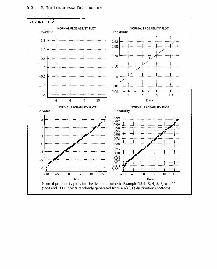
612 � TH E LO G N O R M A L D I ST R I B UT I O N

NORMAL PROBABILITY PLOT z-value

1 .5

1 .0

0.5

0

-0.5

-1.0

-1.5

. . . . . . - � . . . . . . . . . . . . . . ·:· . . . . . . . . . . . . . · :- . . . . . . . . . . . . . . � - . . . . . . . . . . . . . . . . : : : : + . . . . . . . . . .

. . . . . . ·: . . . . . . . . . . . . . · ·:· . . . . . . . . . . . . . -:- . . . . . . . . . . . . . . �- . . . . . . . . . . . . . . . . . . . . . . . . . . . . . . . i . . . . . . . . . . . . . . -�· . . . . . .+. . . . . . . ; . . . . . . . . . . . . . . �- . . . . . . . .

. . .

. . .

. . . . . .

. .

· · · · · · · � · · · · · + · · · · ·+ · · · · · · · · · · · · · · i · · · · · · · · · · · · · · ] · · · · · · · · ·

. . . .

. . . .

. . .

. . .

. . . . .

. . . · · · · · · 't· · · · · · · · · · · · · · ·:· · · · · · · · · · · · · · ·: · · · · · · · · · · · · · · :· · · · · · · · ·

. . . .

. . . .

. . .

. . .

. . .

. . . . . . · · · · · · · : · · · · · · · · · · · · · · ·:· · · · · · · · · · · · · · ·:· · · · · · · · · · · · · · · :· · · · · · · · · . . . .

. . . .

. . . .

. . . .

. . . .

. . .

. . . . . . . . . · : . . . . . . . . . . . . . . ·:· . . . . . . . . . . . . . ·:· . . . . . . . . . . . . . . �- . . . . . . . .

4 6 8 10

NORMAL PROBABILITY PLOT z-value

. . . . + 3 � - · · · · · · · · · · ·�· · · · · · · · · · · ·�· · · · · · · · · · · · � · · · · · · · · · · · � · · · · · · · · · · · ·

:· ·,t

2

1

0

-1

-2

-3

. . .

. .

. .

. . . . . . . . . . . . . ·:· . . . . . . . . . . ·:- . . . . . . . . . . . � . . . . . . . . . . . � - . . . . . . . ·:· . . . .

. . . . . . . . . . . . . .

. . . .

. . . .

. . . .

. . . . . · · · · · · · · · · · -:· · · · · · · · · · · ·:- · · · · · · · · · · · : · · · · · • • • ! • • · · · · · · · · · ·:: · · · ·

. . . .

. . . .

. . .

. . .

. . .

. . . . . . . · · · · · · · · · · · :· · · · · · · · · · · ·� · · · · · · · · : · · · · · · · · · · · !_ · · · · · · · · · · · :· · . . .

-10

. . . .

. . . .

. . . .

. . . . . . . .

. . . .

-5 0 5 10 15

NORMAL PROBABILITY PLOT Probability

0.95 0.90

0.75

0.50

0.25

0 .10

· · · · · · ·=· · · · · · · · · · · · · · · i · · · · · · · · · · · · · · · l- · · · · · · · · · · · · · · <\.· · ·�·"= · · ·

: : : ;. " . . . . . . . ( . . . . . . . . . . . . . � . . . . . . . . . . . . . . . � . . . . . . .

:·�-,;�

�- - . . . . +

� � � ... ... ... · · · · · · �· · · · · · · · · · · · · · - � · · · · · · · · · · · · ;·�-":' . . . . . . . . . . . . . .: . . . . . . . . .

� � ;... ... � �

� ... ... ... � � · · · · · · + · · · · · + · · · ;.""r-· - · · · · · · · · · · · · � · · · · · · · · · · · · · - �· · · · · · · · ·

� ... ... ... � � : : ... : + ... ' :

. . ·;. .... � . . . . . . . . . . . . . . � . . . . . . . . . . . . . . -�·- . . . . . . . . . . . . . �- . . . . . . . .

... ... : : : : . . . . . . . . . . .

. . . . · · · · · · - · · · · · · · · · · · · · · · · · · · · · · · · · · · · · · - · · · · · · · · · · · · · · - · · · · · · · · ·

. . .

. . . : : : 0.05 L----L-----L-----L----.1--

4 6 8 10

Data

NORMAL PROBABILITY PLOT Probability

0.999 0.997

0.99 0.98 0.95 0.90 0.75

. . + � : : : : : : : : : : t : : : : : : : : : :�: : : : : : : : : : : ; : : : : : : : : : : i : : : : : : : : : : :�: "/.: . . . . . . . . . . . . . . . . . . . !' . . . . . . . . . ·:- . . . . . . . . . · : . . . . • . . . . . � - · . • • . . -:· . . . .

. . . . . . . . . . . -:- . . . . . . . . . ·=· . . . . . . . . . - : . . . . . . . . . . �- . . . . . . . . . . .

· · · · · · · · · · !_· · · · · · · · · · ·:- · · · · · · · · · · : · · · · · · · · · · · · · · · · · · :· · · · · . . .

� - - . . . . . . . . ... . . . .

· · · · · · · · · · ·=· · · · · · . . · · ·=· · · · · · · · · · · ; . . . . . . . ; . . . . . . . . . . . ; . . . . . . . . . . . . . . . . . . . .

. . . . . . . . . . -:- . . . . . . . . . ·=· . . . . . . · l . . . . . . . . . . � - . . . . . . . . . ·=· . . . . . . . . . . . . . . .

. . . . . . . . . . .. . . . . . . . . ; . . . . . . . . . . ; . . . . . . . . . . .. . . . . . . . . . . . : . . . . . . . . .

0.50

0.25 0.10 0.05 0.02 O.Ql

0.003 . . . . . . . . . , . . . . . . . . . . . : . . . . . . . . . . . , . . . . . . . . . . , . . . . . . . . . . . : . . . . .

. · . . . • . . . • . . : • . . • . . . . . . . : . • . . . . . . . . - ? • . . . . . . . . . � - . . • . • . . . . . : • . . . .

0.001 l..L.---'-----'--__JL......_.L.__..J__ -10 -5 0 5 10 15

Data Data

Normal probabi l ity plots for the five data points in Example 1 8.9: 3, 4, 5, 7, and 1 1 (top) and 1 000 points randomly generated from a N(O, 1 ) distribution (bottom).

- -- -.

-- · -

--

- - -- - ---

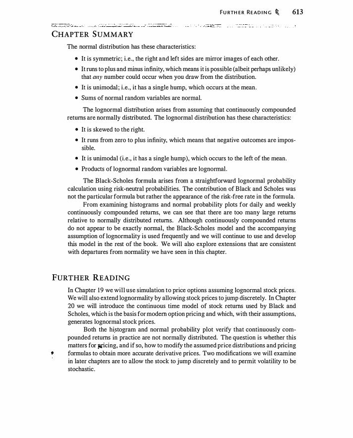
- · --··---�� .. �-�·-- · -· -- - . . . "-·-· �- ·- --�L-- _;_.·-- -��-'""' ;· - - '--, -··

CHAPTER SUMMARY

The normal distribution has these characteristics:

FU RTH E R READ I N G � 613

• It is symmetric; i .e . , the right and left sides are mirror images of each other.

• It runs to plus and minus infinity, which means it is possible (albeit perhaps unlikely) that any number could occur when you draw from the distribution.

• It is unimodal; i .e. , it has a single hump, which occurs at the mean.

• Sums of normal random variables are normal.

The lognormal distribution arises from assuming that continuously compounded returns are normally distributed. The lognormal distribution has these characteristics:

• It is skewed to the right.

• It runs from zero to plus infinity, which means that negative outcomes are impos­sible.

• It is unimodal (i .e., it has a single hump), which occurs to the left of the mean.

• Products of lognormal random variables are lognormal.

The Black-Scholes formula arises from a straightforward lognormal probability calculation using risk-neutral probabilities. The contribution of Black and Scholes was not the particular formula but rather the appearance of the risk-free rate in the formula.

From examining histograms and normal probability plots for daily and weekly continuously compounded returns, we can see that there are too many large returns relative to normally distributed returns. Although continuously compounded returns do not appear to be exactly normal, the Black-Scholes model and the accompanying assumption of lognormality is used frequently and we will continue to use and develop this model in the rest of the book. We will also explore extensions that are consistent with departures from normality we have seen in this chapter.

FURTHER READ ING

In Chapter 19 we will use simulation to price options assuming lognormal stock prices. We will also extend lognormality by allowing stock prices to jump discretely. In Chapter 20 we will introduce the continuous time model of stock returns used by B lack and Scholes, which is the basis for modern option pricing and which, with their assumptions, generates lognormal stock prices.

Both the histogram and normal probability plot verify that continuously com­pounded returns in practice are not normally distributed. The question is whether this matters for {alicing, and if so, how to modify the assumed price distributions and pricing

• formulas to obtain more accurate derivative prices. Two modifications we will examine in later chapters are to allow the stock to jump discretely and to permit volatility to be stochastic.

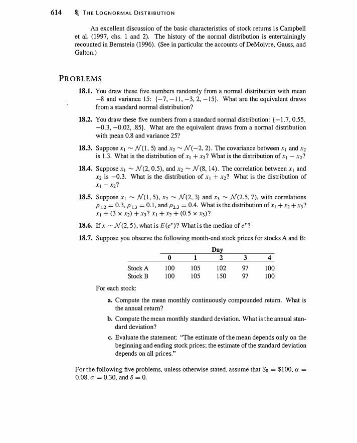
614 � TH E LO G N O R M A L D I ST R I B UT I O N

An excellent discussion of the basic characteristics of stock returns i s Campbell et al . ( 1 997, chs . 1 and 2). The history of the normal distribution is entertainingly recounted in Bernstein ( 1 996) . (See in particular the accounts of DeMoivre, Gauss, and Galton.)

PROBLEMS

18.1. You draw these five numbers randomly from a normal distribution with mean -8 and variance 1 5 : {-7, - 1 1 , -3, 2, - 15 } . What are the equivalent draws from a standard normal distribution?

18.2. You draw these five numbers from a standard normal distribution: { - 1 .7 , 0.55 , -0.3 , -0.02, . 85 } . What are the equivalent draws from a normal distribution with mean 0.8 and variance 25?

18.3. Suppose x 1 � N(l , 5) and x2 � N( -2, 2) . The covariance between x 1 and x2 is 1 .3 . What is the distribution of x1 + X2? What is the distribution of x 1 - x2?

18.4. Suppose x 1 � N(2, 0 .5) , and x2 � N(8, 14) . The correlation between x 1 and x2 is -0.3. What is the distribution of x 1 + x2? What is the distribution of X t - X2?

18.5. Suppose x 1 � N( 1 , 5 ) , x2 � N(2, 3) and x3 � N(2.5, 7) , with correlations p 1 ,2 = 0.3, p 1 ,3 = 0. 1 , and p2,3 = 0.4. What is the distribution ofx1 + x2 + x3 ? X i + (3 X X2) + x3 ? X t + x2 + (0.5 X X3) ?

18.6. If x � N(2, 5 ) , what i s E (ex ) ? What i s the median of ex ?

18.7. Suppose you observe the following month-end stock prices for stocks A and B :

Stock A Stock B

For each stock:

0 100 100

1 105 1 05

Day 2

102 1 50

3 97 97

4 100 100

a. Compute the mean monthly continuously compounded return. What is the annual return?

b. Compute the mean monthly standard deviation. What is the annual stan­dard deviation?

c. Evaluate the statement: "The estimate of the mean depends only on the beginning and ending stock prices ; the estimate of the standard deviation depends on all prices."

For the following five problems, unless otherwise stated, assume that So = $ 1 00, a = 0.08, u = 0.30, and 8 = 0.

A P P E N D I X 1 8.A: T H E EX P E CTAT I O N O F A LO G N O R M A L VA R I A B LE � 615

18.8. What is Prob(S, > $ 1 05) for t = 1? How does this probability change when you change t? How does it change when you change cr ?

18.9. What i s E(S, I S, > $ 1 05) for t = 1 ? How does this expectation change when you change t, cr, and r?

18.10. What is Prob(S, < $98) for t = 1? How does this probability change when you change t?

18.11. Let t = L What is E(S, I S, < $98)? What is E(S, I S, < $ 1 20)? How do both expectations change when you vary t from 0.05 to 5? Let cr = 0. L Does either answer change? How?

18.12. Let K T = SoerT . Compute Prob(ST < K T) and Prob(ST > K T) for a variety of Ts from 0.25 to 25 years. How do the probabilities behave? How do you reconcile your answer with the fact that both call and put prices increase with time?

18.13. Consider Prob(S, < K) , equation ( 1 8.23) , and E (S, I S, < K) , equation ( 1 8.28). Verify that it is possible to pick parameters such that changes in t can have ambiguous effects on Prob(S1 < K) (experiment with very short and long times to maturity, and set a > 0.5cr2) . Is the effect of t on E (S, I S, < K) ambiguous?

18.14. Select a stock or index and obtain at least 5 years of daily or weekly data. Estimate the annualized mean and volatility, using all data and 1 year at a time. Compare the behavior of your estimates of the mean with those of the standard deviation.

18.15. Select a stock that has at least 5 years of daily data. Create data sets consisting of daily data and weekly data, Wednesday to Wednesday. (The weekday function in Excel will tell you the day of the week corresponding to a date. Wednesday is 4.) For both data sets, create a histogram of returns and a normal plot Are the stock prices lognormal?

APPENDIX 1 8 .A: THE EXPECTATION OF A LOGNORMAL VARIABLE

In this appendix we verify equation ( 1 8 . 13) . Suppose that y � N(f-L, cr2) ; hence, e-'" i s lognormally distributed. The normal distribution is given by

� 1 I ( -'-1' )' ¢(x ; f-L, cr-) = --e-� " "" cr .Jiii

Hence, we can directly compute the expectation:

E(eY) = ex __ e-� " dx fOO 1 I ( -'-1' )'

-oo cr.Jiii

616 � TH E LO G N O R M A L D I ST R I B UT I O N

Collect the exponentiated terms under the integral. This gives us

E( '" ) �00 1 - __!, [ (x -td -2a�x ]d . e- = -- e 1n-- x

-oo u,J2lr Now focus on the exponentiated term in the square brackets. We have

(x - JL)2 - 2u2x x2 + JL2 - 2x (JL + u2)

( 1 8.3 1 )

= x2 + (JL + u2)2 _ 2X (JL + u2) + /L2 _ (/L + u2)2 [x - (JL + u2)f - u4 - 2JLu2

We can now substitute this expression into ( 1 8.3 1 ), obtaining

The last equality follows because the integral expression is one: It is the total area under -

a normal density with mean JL+rr2 and variance u2 . Thus we obtain equation ( 1 8. 13 ) .

APPENDIX 1 8 .B : CONSTRUCTING A NORMAL PROBABILITY PLOT

Appendix available online at www.aw-bc.com/mcdonald.

Monte Carlo V aiuation

So fa,. we have primarily discu,ed derivatives fo; which there is a (;�latively 'imple) valuation formula, or which can be valued binomially. For many common derivatives, however, a different approach is necessary. For example, consider arithmetic Asian options (see Section 1 4.2). There is no simple valuation formula for such options, and the binomial pricing approach is difficult because the final payoff depends on the specific path the stock price takes through the tree-i.e., the payoff is path-dependent. A pricing method that can be used in such cases is Monte Carlo valuation. In Monte Carlo valuation we simulate future stock prices and then use these simulated prices to compute the discounted expected payoff of the option. The idea that an option price is a discounted expected value is familiar from our discussion of the binomial model in Chapter 1 1 and the Black-Scholes formula in Chapter 1 8 .

Monte Carlo valuation is performed using the risk-neutral distribution, where we assume that assets earn the risk-free rate on average, and we then discount the expected payoff using the risk-free rate. We will see in this chapter that risk-neutral pricing is a cornerstone of Monte Carlo valuation; using the actual distribution instead would create a complicated discounting problem.

S ince with Monte Carlo you simulate the possible future values of the security, as a byproduct you generate the distribution of payoffs. The distribution can be extremely useful when you want to compare two investment strategies that have different distri­butions of outcomes. Computing value-at-risk for complicated portfolios is a common use of Monte Carlo.

In this chapter we will see why risk-neutral valuation is important for Monte Carlo, see how to produ�e normal random numbers, discuss the efficiency of Monte Carlo, introduce the Poisson distribution to help account for nonlognormal patterns in the data, and see how to create correlated random stock prices.

19.1 COMPUTING THE. OPTION PRICE AS A DISCOUNTED EXPECTED VALUE ... The concept of risk-neutral valuation is familiar from earlier Chapters 15 . We saw that option valuation can be performed as if all assets earned the risk-free rate of return and investors performed all discounting at this rate. Monte Carlo valuation exploits this insight. We assume that assets earn the risk-free rate of return and simulate their returns.

617

618 � M O NTE CA RLO VA LUAT I O N

For example, for any given stock price 3 months from now, we can compute the payoff on a call. We perform the simulation many times and average the outcomes. Since we use risk-neutral valuation, we then discount the average payoff at the risk-free rate in order to arrive at the price.

As a practical matter, Monte Carlo valuation depends critically on risk-neutral valuation. In order to see why this is so, we will compute an option price as an expected value with both risk-neutral and true probabilities, using an example we discussed in Chapters 1 0 and I I .

Valuation with Risk-Neutral Probabilities

We saw in equation ( 1 0.6) that we can interpret the one-period binomial option pricing calculation as an expected value, in which the expectation is computed using the risk­neutral probability p* , and discounting is at the risk-free rate.

In a multiperiod tree, we repeat this process at each node. For a European option, · the result obtained by working backward through the tree is equivalent to computing the expected option price in the final period, and discounting at the risk-free rate.

If there are 11 binomial periods, equation ( 1 I . I 7) gives the probability of reaching any given stock price at expiration. Let 11 represent the number of binomial steps and i the number of stock price down moves. We can value a European call option by computing the expected option payoff at the final node of the bin9mial tree and then discounting at the risk-free rate. For example, for a European call,

European call price =

To illustrate this calculation, Figure 1 9 . 1 shows the stock price tree from Figure 1 0.5, with the addition of the total risk-neutral probabilities of reaching each of the terminal nodes . Figure 19 . 1 demonstrates that the option can be priced by computing the expected payoff at expiration using the probability of reaching each final node, and then discounting at the risk-free rate. You can verify that the option price in Figure 19 . I is the same as that in Figure I 0.5 .

We can also use the tree in Figure I 9 . 1 to illustrate Monte Carlo valuation. Imagine a gambling wheel divided into four unequal sections, where each section has a proba­bility corresponding to one of the option payoffs in Figure 1 9. I : 9.5% ($34.678), 34% ($ 12.8 14) , 40.4% (0), and I 6% (0) . Each spin of the wheel therefore selects one of the final stock price nodes and option payoffs in Figure 19 . 1 . If we spin the wheel nu­merous times and then average the resulting option values, we will have an estimate of the expected payoff. Discounting this expected payoff at the risk-free rate provides an estimate of the option value.

It is easy to compute the actual expected payoff for the option in Figure 1 9. 1 without using a gambling wheel. However, the example illustrates how random trials can be used to perform valuation.

$41 .000

C O M PUT I N G TH E O PT I O N P R I C E AS A D I S C O U NT E D EX P E CT E D VA LU E � 619

$61 . 149

/ $50.071

/ $43.246

Price and Payoff

�:;!���] �"'=�"--"·�==""'

1 $52.8 14 � /L�-�=���J � / �

$35.41 1

� $30.585

$37 .351 $0.000

$26.416 $0.000

Total e-o.os x Total

Prob. x Probability Payoff

p·3 = 0.095

3p.2(1 - p·) = 0.340

3p.(1 - p•)Z = 0.404

(1 - p·)3 = 0. 1 60

1 .000

$3 .306

$4.357

$0.000

$0.000

$7.663 $7.074

Binomia l tree (the same as in Figure 1 0.5) showing stock price paths, along with risk-neutral probabi l ities of reaching the various terminal prices. Assumes S = $41 .00, K = $40.00, cr ""'0.30, r = 0.08, t = 1 .00 years, 8 = 0 .00, and h = 0 .333 . The risk-neutral probabi l ity of going up is p* = 0.4568. At the final node the stock price and terminal option payoff (beneath the price) are g iven .

Valuation with True Probabilities

The simple procedure we used to discount payoffs for the risk-neutral tree in Figure 19 . 1 does not work when we use actual probabilities. We analyzed the pricing of this option using true probabilities in Chapter 1 1 , in Figure 1 1 .4. We saw there that when using true probabilities to evaluate the option, the discount rate is different at different nodes on the tree. In fact, if we are to compute an option price as an expected value

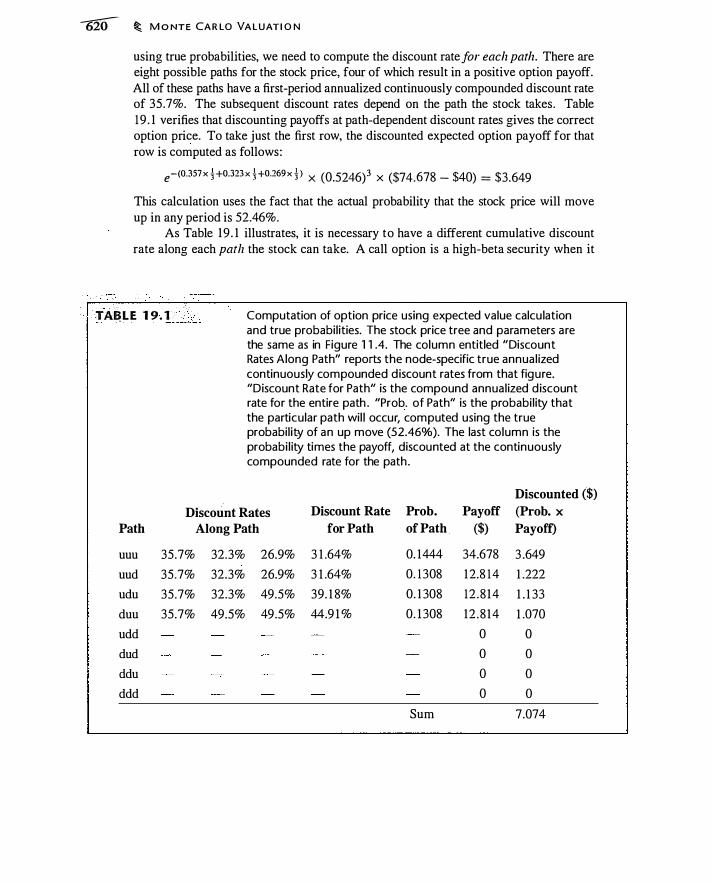
� � M o NTE CA R LO VA LUATI O N

using true probabilities, we need to compute the discount rate for each path. There are eight possible paths for the stock price, four of which result in a positive option payoff. All of these paths have a first-period annualized continuously compounded discount rate of 35.7%. The subsequent discount rates depend on the path the stock takes. Table 19 . 1 verifies that discounting payoffs at path-dependent discount rates gives the correct option price. To take just the first row, the discounted expected option payoff for that row is computed as follows:

e-(0.357x !+0.323 x t+0.:!69x ! > x (0.5246)3 X ($74.678 - $40) = $3.649

This calculation uses the fact that the actual probability that the stock price will move up in any period is 52.46%.

As Table 19 . 1 illustrates, it is necessary to have a different cumulative discount rate along each path the stock can take. A call option is a high-beta security when it

TA�LE 19 . 1 . . · . . Computation of option price using expected value calcu lation and true probabi l ities. The stock price tree and parameters are the same as in F igure 1 1 .4. The column entitled "Discount Rates Along Path" reports the node-specific true annual ized continuously compounded d iscount rates from that figure. "Discount Rate for Path" is the compound annual ized d iscount rate for the entire path . "Prob. of Path" is the probabi l ity that the particular path wil l occur, computed using the true probabil ity of an up move (52.46%). The last column is the probabi l ity times the payoff, discounted at the continuously compounded rate for the path .

Discounted ($)

Discount Rates Discount Rate Pro b. Payoff (Prob. x Path Along Path for Path of Path ($) Payoff)

uuu 35.7% 32.3% 26.9% 3 1 .64% 0. 1444 34.678 3 .649

uud 35.7% 32.3% 26.9% 3 1 .64% 0. 1 308 1 2.8 14 1 .222

udu 35.7% 32.3% 49.5% 39. 1 8% 0. 1 308 12 . 8 14 1 . 1 33

duu 35.7% 49.5% 49.5% 44.9 1 % 0. 1 308 12 . 8 14 1 .070

udd 0 0

dud 0 0

ddu 0 0

ddd 0 0

Sum 7.074

C O M PUT I N G RAN D O M N U M B E RS � 621

is out-of-the-money and it has a lower beta (but still higher than the stock) when it is in-the-money. This variation in the discount rate complicates discounting if we are using the true distribution of stock prices . 1

Risk-neutral valuation neatly sidesteps the hardest problem about using discounted cash flow valuation techniques with an option. While it is easy to compute the expected payoff of an option if the stock is lognormally distributed, it is hard to compute the discount rate. If we value options as if the world were risk-neutral, this complication is avoided.

·

19.2 COMPUTING RANDOM NUMBERS

In this section we discuss how to compute the normally distributed random numbers required for Monte Carlo valuation. We will take for granted that you can compute a uniformly distributed random number between 0 and I . The uniform distribution is de­fined on a specified range, over which the probability is I , and assigns equal probabilities to every interval of equal length on that range. A random variable, u, that is uniformly distributed on the interval (a , b), has the distribution U(a , b) . The uniform probability density, f(x ; a, b) , is defined as

1 f (x · a b) = -- · a < x < b ' ' b - a ' - -( 1 9.2)

and is 0 otherwise. When a = 0 and b = I, the uniform distribution is a flat line at a · height of 1 over the range 0 to 1 .

Drawing uniformly distributed random variables i s very common; virtually all programming languages and spreadsheets have a way to do this .2 The Rand built­in function in Excel does this, for example. It turns out that once we have a way to compute uniformly distributed random variables, there are two common ways to compute a normally distributed random variable. Many programs also have functions to compute normal random numbers directly, in which case it is not necessary to use these methods. However, the second method we will discuss can be used to compute random numbers drawn from any distrfbution.

'

1 Here is why a single discount rate does not work. Suppose we represent the terminal option price

associated with a particular pattern of stock price up and down movements by Ci (T) and the compound

discount factor for that path by fJi · S ince both the payoff and the discount rates are uncertain, we need

to compute£[Ci (T)/ ( 1 + {Ji )]. However, if we average the payoff and then separately average the

discount factors, we are computing the ratio of the averages, E[Ci ( T)]f £[( 1 + {Ji )], rather than the

average of the ratios. Jensen's inequality tells us that these are not the same calculation.

2Since computers are ultimately deterministic devices, it is virtually impossible to compute "true"

random numbers. See Judd ( 1 998, pp. 285-287) for a discussion and additional references.

622 � M O NTE CARLO VA LUAT I O N

Using Sums of Uniformly Distributed Random Variables

One standard technique to compute normally distributed random variables is to sum 1 2 uniform (0, 1 ) random variables and subtract 6 . Thus, we compute the N(O, 1 ) random variable Z as

1 2 Z = L..: u; - 6

i=l

, where the u; are distributed uniformly on (0, 1 ) . This technique works because the variance of a variable that i s uniformly dis­

tributed between 0 and 1 is 1 / 12 and the mean is 1 12 . Thus, if you sum 12 uniformly distributed random variables and subtract 6, you get a random variable with a variance of 1 and a mean of O. The sum of 1 2 uniform variables is not precisely normal, but it is close. This technique is an application of the central limit theorem.

Using the Inverse Cumulative Normal Distribution

It is also possible to draw a single uniformly distributed random number and convert it to a normally distributed random number. Suppose that u � U(O, 1 ) and z � N(O, 1 ) . As we saw i n Chapter 1 8, the cumulative distribution function, denoted U ( w ) for the uniform and N(y) for the normal, !s the probability that u < w or z < y, i .e.,

U (w) = Prob(u :::; w)

N(y) = Prob(z :::; y)

As discussed in Chapter 1 8, w is the U ( w) quantile and y is the N (y) quantile of the two distributions. If we randomly draw a uniform number u, how can we use u to construct a corresponding normal random number, z?

I t turns out that the same idea we used to construct normal plots in Section 1 8 .6 perffiits us to generate a I_J.ormal random number from a uniform random number. Instead of interpreting a random draw from the uniform distribution as a number, we interpret it as a quantile. So, for example, if we draw 0.7 from a U(O, 1) distribution, we interpret this as a draw corresponding to the 70% quantile. We then use the inverse distribution function, N- 1 (u) , to find the value from the normal distribution corresponding to that quantile.3 This technique works because, for any distribution, quantiles are uniformly

3The Excel function NormS!nl' computes the inverse cumulative normal distribution. Unfortunately,

there is a serious bug in this function in Office 97 and Office 2000. In both versions of Excel,

N01mSlnl'(0.9999996) = 5.066, and NonnS/n\'(0.9999991) = 5,000,000. Because of this, Excel

will on occasion produce a randomly drawn normal value of 5,000,000, which ruins a Monte Carlo

valuation. I thank Mark Broadie for pointing out this problem with using Excel to produce random

normal numbers.

S I M U LATI N G LO G N O R M A L STO C K P R I C ES � 623

distributed: If you draw from a distribution, by definition any quantile is equally likely to be drawn.

The algorithm is therefore as follows:

1. Generate a unifonnly distributed random number between 0 and 1 . Say this is 0.7.

2. Ask: What is the value of z such that N (z) = 0.7? The answer to this question is computed using the inverse cwnulative distribution function. In this case we have N- 1 (0. 7) = 0.5244. This value is a single draw of a standard normal random variable (0.5244) .

3. Repeat.

This procedure simulates draws from a normal distribution. To simulate a log-normal random variable, simulate a normal random variable and exponentiate the draws.

This procedure of using the inverse cumulative probability distribution is valuable because it works for any distribution for which you can compute the inverse cumulative distribution.

19.3 S IMULATING LOGNORMAL STOCK PRICES

Recall from Chapter 18 that if Z � N(O, 1 ) , a lognormal stock price can be written

( 19 .3) Suppose we wish to draw random stock prices for 2 years from today. From equation ( 19.3); the stock price is driven by the normally distributed random variable Z. Set T = 2, et = 0. 10 , 8 = 0, and u = 0.30. If we then randomly draw a set of standard normal Z's and substitut� the results into equation ( 19.3) , the result is a random set of lognormally distributed S2 's. The continuously compounded mean return will be 20% ( 10% per year) and the continuously compounded standard deviation of ln(S2) will be 0.3 X .j2 = 42.43%.

.

Simulating a Sequence of Stock Prices

There is another way to create a random set of prices 2 years from .now. We can also generate annual random prices and compound these to get a 2-year price. This will give us exactly the same distribution for 2-year prices. Here is how to do it:

• Compute the 1 -year price, S1 as

S _ S, e<O. I - �0.32) x l+o-.JlZ( l ) I - 0 -

• Using this S1 as the starting price, compute S2 :

S _ S e<O. l - �0.32) x 1+0.3.JlZ(2) 2 - I -

In these expressions, Z ( 1 ) and Z (2) are two draws from the standard normal distribution.

624 � M O NT E (AR LO VA LUAT I O N

If we substititute the expression for S 1 into Sz , we get

S _ S e(O. I - � 0.3') x 2+0.3 Ji[Z( I )+Z(2)] 2 - 0 - ( 1 9.4)

The difference between this expression and equation ( 19.3) is that instead of the term .J'iz, we have [Z ( 1 ) + Z(2)] . Note that

Var( .J'iZ) = 2

and

Var[Z ( l ) + Z(2)] = 2

Therefore, equations ( 1 9.3) and ( 1 9 .4) generate S2 's with the same distribution. If we really want to simulate a random stock price after 2 years, there is no reason

to draw two random variables instead of one. But if we want to simulate the patlz of the stock price over 2 years (for example, to price a path-dependent option), then we can do so by splitting up the 2 years into multiple periods.

In general, if we wish to split up a period of length T into intervals of length /z , the number of such intervals will b e n = T / lz . We have

and so on, up to

S _ S e<a-a- ! u' Jh+uJhZ( l ) , - 0

S _ S e<a-8- ..\u')h+uJhZ(2) 211 - , -

S _ S e<a-!i- �u2 )h+u JhZ(11 ) "" - (11 - l )h -

These n stock prices can be intepreted as equally spaced points on the stock price path between times 0 and T. Note that if we substitute s, into the expression for S211 , the expression for S211 into that for S3, , and so on, we get

S _ <' e<a-8- �u2)T +uJh[I:7=1 Z(il] T - o.JO -

S (a-/i- �u2)T+u ft[-Je I:;'= 1 Z(i l] = oe - " "

( 1 9.5)

Since )n I:;'=• Z(i) �N(O, 1 ) , we get the same distribution at time T with equation ( 19.5) as if we had drawn a single N(O, 1) random variable, as in equation ( 19.3) . The important difference is that by splitting up the problem into n draws, we simulate the path taken by S. The simulation of a path is useful in computing the value of path-dependent derivatives, such as Asian and barrier options, the value of which depend on the path by which the price arrives at Sr .

19.4 MONTE CARLO VALUATION

In Monte Carlo valuation, we perform a calculation similar to that in equation ( 1 9 . 1 ) . The option payoff at time T is a function of the stock price, Sr . Represent this payoff

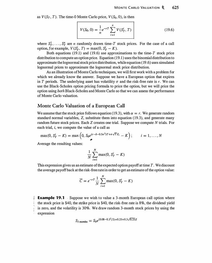
M O NT E C A R LO VA LUAT I O N � 625

as V (ST , T) . The time-0 Monte Carlo price, V (S0 , 0) , is then

1 II V (So , 0) = -e-rT L V (S� , T) 1l i= l

( 19.6)

where S} , . . . , S!f are n randomly drawn time-T stock prices. For the case of a call option, for example, V (S� , T) = max(O, S� - K) .

Both equations ( 19 . 1 ) and ( 19 .6) use approximations to the time-T stock price distribution to compute an option price. Equation ( 1 9 . 1 ) uses the binomial distribution to approximate the lognormal stock price distribution, while equation ( 19 .6) uses simulated lognormal prices to approximate the lognormal stock price distribution.

As an illustration of Monte Carlo techniques, we will first work with a problem for which we already know the answer. Suppose we have a European option that expires in T periods. The underlying asset has volatility a and the risk-free rate is r. We can use the Black-Scholes option pricing formula to price the option, but we will price the option using both Black-Scholes and Monte Carlo so that we can assess the performance of Monte Carlo valuation.

Monte Carlo Valuation of a European Call

We assume that the stock price follows equation ( 1 9 .3) , with a = r. We generate random standard normal variables, Z, substitute them into equation ( 19.3) , and generate many random future stock prices. Each Z creates one trial . Suppose we compute N trials. For each trial, i, we compute the value of a call as

max (O, s� - K) = max ( 0, Soe(r-8-0.5u2)T+u..ffZ; - K) ; ,. Average the resulting values :

1 N N t1 max(O, S� - K)

i = 1 , . . . , N

This expression gives us an estimate of the expected option payoff at time T . We discount the average payoff back at the risk-free rate in order to get an estimate of the option value:

- 1 N . c = e-rT

N L max(O, s� - K) i = l

Example 1 9.1 . Suppose we wish to value a 3-month European call option where the stock price is $40, the strike price is $40, the risk-free rate is 8%, the dividend yield is zero, and the volatility is 30%. We draw random 3-month stock prices by using the expression

S _ S e <0.08-0.32/2) x0.25+0.3 J0:EZ 3 months - 0

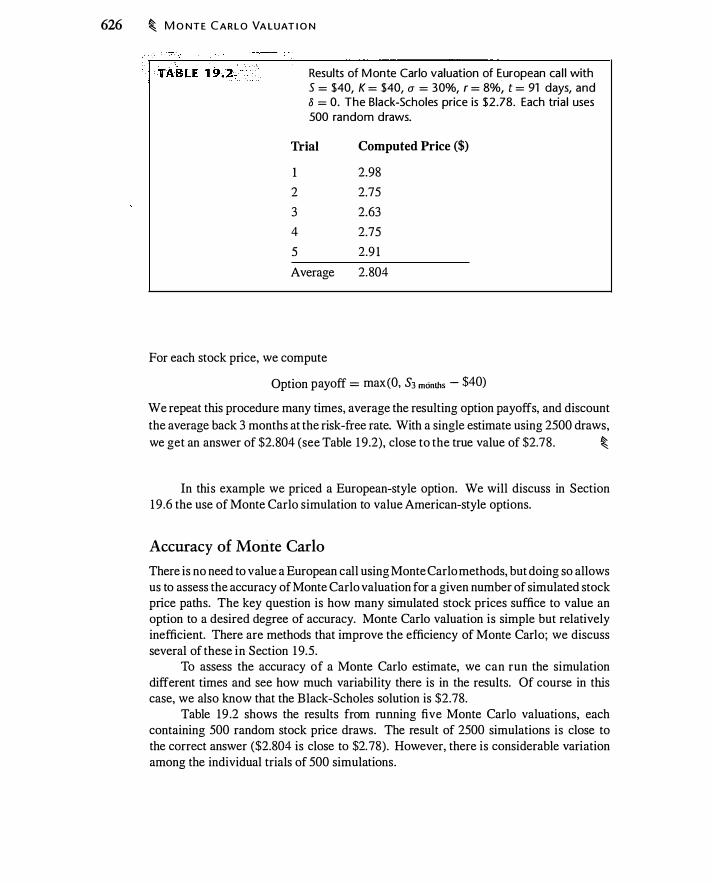
626 � M O NT E CARLO VA LUAT I O N

Results of M onte Carlo valuation of European ca l l with S = $40, K = $40, cr = 30%, r = 8%, t = 91 days, and 8 = 0. The Black-Scholes price is $2.78. Each tria l uses 500 random draws.

Trial Computed Price ($)

1 2.98

2 2.75

3 2.63

4 2.75

5 2.9 1

Average 2.804

For each stock price, we compute

Option payoff = max(O, S3 months - $40)

We repeat this procedure many times, average the resulting option payoffs, and discount the average back 3 months at the risk-free rate. With a single estimate using 2500 draws, we get an answer of $2.804 (see Table 1 9.2), close to the true value of $2.78 . �

In this example we priced a European-style option. We will discuss in Section 1 9.6 the use of Monte Carlo simulation to value American-style options.

Accuracy of Morite Carlo

There is no need to value a European call using Monte Carlo methods, but doing so allows us to assess the accuracy of Monte Carlo valuation for a given number of simulated stock price paths. The key question is how many simulated stock prices suffice to value an option to a desired degree of accuracy. Monte Carlo valuation is simple but relatively inefficient. There are methods that improve the efficiency of Monte Carlo; we discuss several of these in Section 1 9.5.

To assess the accuracy of a Monte Carlo estimate, we can run the simulation different times and see how much variability there is in the results. Of course in this case, we also know that the Black-Scholes solution is $2.78.

Table 19 .2 shows the results from running five Monte Carlo valuations, each containing 500 random stock price draws. The result of 2500 simulations is close to the correct answer ($2.804 is close to $2. 78) . However, there is considerable variation among the individual trials of 500 simulations.

M O NT E CA R LO VA L U AT I O N � 627

To assess accuracy, we need to know the standard deviation of the estimate. Let C (S; ) be the call price generated from the randomly drawn S; . If there are n trials, the Monte Carlo estimate is

- I II -c" = - .L: ccs; ) ll i= l

Let u c denote the standard deviation of one draw and u" the standard deviation of n

draws. The variance of a mean, given independent and identically distributed S; 's, is

or

? I ? u;, = -ue: ll

(J " = r.; CJ C y ll Thus, the standard deviation of the Monte Carlo estimate is inversely proportional to the square root of the number of draws.

In the Monte Carlo results reported in Table I 9.2, the standard deviation of a draw is about $4.05 . (This value is computed by taking the standard deviation of the 2500 price estimates used to compute the average.) For 500 draws, the standard deviation is

.,

$4.05 = $0. I 8 v'sOO

Given that the correct price is $2. 78, a $0. I 8 standard deviation is a substantial percentage of the option price (6.5% ) . With 2500 observations, the standard deviation is cut to $0.08, suggesting that the $2.80 estimate from averaging the five answers was only accidentally close to the correct answer. In order to have a I % ($0.028) standard deviation, we would need to have 2 1 ,000 trials.

Arithmetic Asian Option

In the previous example of Monte Carlo valuation we valued an option that we already could value with the Black-Scholes formula. In practice, Monte Carlo valuation is useful under these conditions:

• Where the number of random elements in the option valuation problem is too great to permit direct numerical solution.

• Where underlying variables are distributed in such a way that direct solutions are difficult.

• Where options are path-dependent, i .e. , the payoff at expiration depends upon the path of the underlying asset price.

For the case of a path-dependent option, the use of Monte Carlo estimation is straightforward. As discussed above, we can simulate the path of the stock as well as its terminal value. For example, consider the valuation of a security that at the end of 3 months makes a payment based on the arithmetic average of the stock price at the

628 � M o NTE CA R LO VA LUAT I O N

end of months 1 , 2 , and 3 . As discussed in Chapter 14, this i s an arithmetic average price Asian option: "Asian" because the payoff is based on an average, and "arithmetic average price" because the arithmetic average stock price replaces the actual stock price at expiration.

How will the value of an option on the average compare with an option that settles based on the actual expiration-day stock price? Intuitively, averaging should reduce the likelihood of large gains and losses. Any time the stock ends up high (in which case the call will have a high value at expiration), it will have traversed intermediate stock prices in the process of reaching a high value. The payoff to the Asian option will reflect these lower intermediate prices, and, hence, large payoffs will be much less likely.

We compute the 1-month, 2-month, and 3-month stock prices as follows:

S I = 40e<r-�-a2 /2)T f3+a Jf/3Z( l )

Sz = Sl e<r-�-a2j2)Tj3+aJf/3Z('1)

s3 = S'1e(r-�-a2j'1)Tf3+aJf73Z(3)

where Z ( l ) , Z(2), and Z(3) are independent draws from a standard normal distribution. We repeat the trial many times and draw many Z, 's. The value of the security is then computed as

( 1 9.7)

Example 1 9.2 Let r = 8%, u = 0.3, and suppose that the initial stock price is $40. Figure 1 9.2 compares histograms for the actual risk-neutral stock price distri-

12000 Histograms for 10000 risk-neutral stock price 8000 distribution after 3 6000 months (top panel) and 4000 risk-neutral d istribution 2000 for the average stock 0 price created by 20 25 30 35 40 45 so 55 60

averaging the three month-end stock prices 12000 during the same period 10000 (bottom panel). 8000 Assumes 50 = $40, r = 6000 8%, cr = 30%, and o = 4000 0. These histograms 2000 were generated using 0 1 00,000 trials. 20 25 30 35 40 45 so 55 60

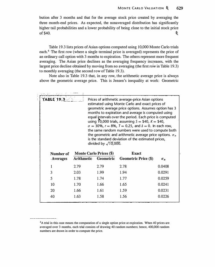
M O NTE CA R LO VA L U AT I O N � 629

bution after 3 months and that for the average stock price created by averaging the three month-end prices . As expected, the nonaveraged distribution has significantly higher tail probabilities and a lower probability of being close to the initial stock price � � �

Table 1 9.3 lists prices of Asian options computed using 10,000 Monte Carlo trials each.4 The first row (where a single terminal price is averaged) represents the price of an ordinary call option with 3 months to expiration. The others represent more frequent averaging. The Asian price declines as the averaging frequency increases, with the largest price decline obtained by moving from no averaging (the first row in Table 1 9.3) to monthly averaging (the second row of Table 1 9 .3) .

Note also in Table 1 9.3 that, in any row, the arithmetic average price is always above the geometric average price. This is Jensen's inequality at work: Geometric

Number of - Averages

1

3

5

10

20

40

Prices of arithmetic average-price Asian options estimated using Monte Carlo and exact prices of geometric average price options. Assumes option has 3 months to expiration and average is computed using equal intervals over the period . Each price is computed using ;'-o,ooo trials, assuming S = $40, K = $40, u = 30%, r = 8%, T = 0.25, and 8 = 0. In each row, the same random numbers were used to compute both the geometric and arithmetic average price options. u n is the standard deviation of the estimated prices, d ivided by .}1 0,000.

Monte Carlo Prices ($) Exact Arithmetic Geometric Geometric Price ($) CTn

2.79 2.79 2.78 0.0408

2.03 1 .99 1 .94 0.029 1

1 .78 1 .74 1 .77 0.0259

1 .70 1 .66 1 .65 0.0241

1 .66 1 .6 1 1 .59 0.023 1

1 .63 1 .58 1 .56 0.0226

4A trial in this case means the computation of a single option price at expiration. When 40 prices are

averaged over 3 months, each trial consists of drawing 40 random numbers; hence, 400,000 random

numbers are drawn in order to compute the price.

630 � M O NTE CA R LO VA LUAT I O N

averaging produces a lower average stock price than arithmetic averaging, and hence a lower option price.

19.5 EFFICIENT MONTE CARLO VALUATION

We have been describing what might be called "naive" Monte Carlo, making no attempt to reduce the variance of the simulated answer for a given number of trials . There are a number of methods to achieve faster Monte Carlo valuations.5

Control Variate Method

We have seen that naive Monte Carlo estimation of an arithmetic Asian option requires many simulations. In Table 19 .3 , even with 10,000 simulations, there is still a standard deviation of several percent in the option price.

In each row of Table 1 9.3 , the same random numbers are used to estimate the option price. As a result, the errors in the estimated arithmetic and geometric prices are correlated: When the estimated price for the geometric option is high, this occurs because we have had high returns in the stock price simulation. This should result in a high arithmetic price as well.

This observation suggests the control variate . method to increase Monte Carlo accuracy. The idea underlying this method is to estimate the error on each trial by using the price of a related option that does have a pricing formula. The error estimate obtained from this control price can be used to improve the accuracy of the Monte Carlo price on each trial.

Asian options provide an effective illustration of this idea.6 Because we have a formula for the price of a geometric Asian option (see Section 14.2), we know whether the geometric price from a Monte Carlo valuation is too high or too low. For a given set of random stock prices, the arithmetic and geometric prices will typically be too high or too low in tandem, so we can use information on the error in the geometric price to adjust our estimate of the arithmetic price, for which there is no formula.

To be specific, we use simulation to estimate the arithmetic price, A, and the geometric price, G. Let G and A represent the true geometric and arithmetic prices. The error for the Monte Carlo estimate of the geometric price is (G - G) . We want to use this error to improve our estimate of the arithmetic price.

Consider calculating

5Excellent overviews are Boyle et a!. ( 1 997) and Glasserman (2004). See also Judd ( 1 998, ch. 8), which in tum contains other references, and Campbell et a!. ( 1 997, ch. 9) .. 6This example follows Kemna and Vorst ( 1 990), who used the control variate method to price arithmetic

Asian options.

( 1 9 . 8)

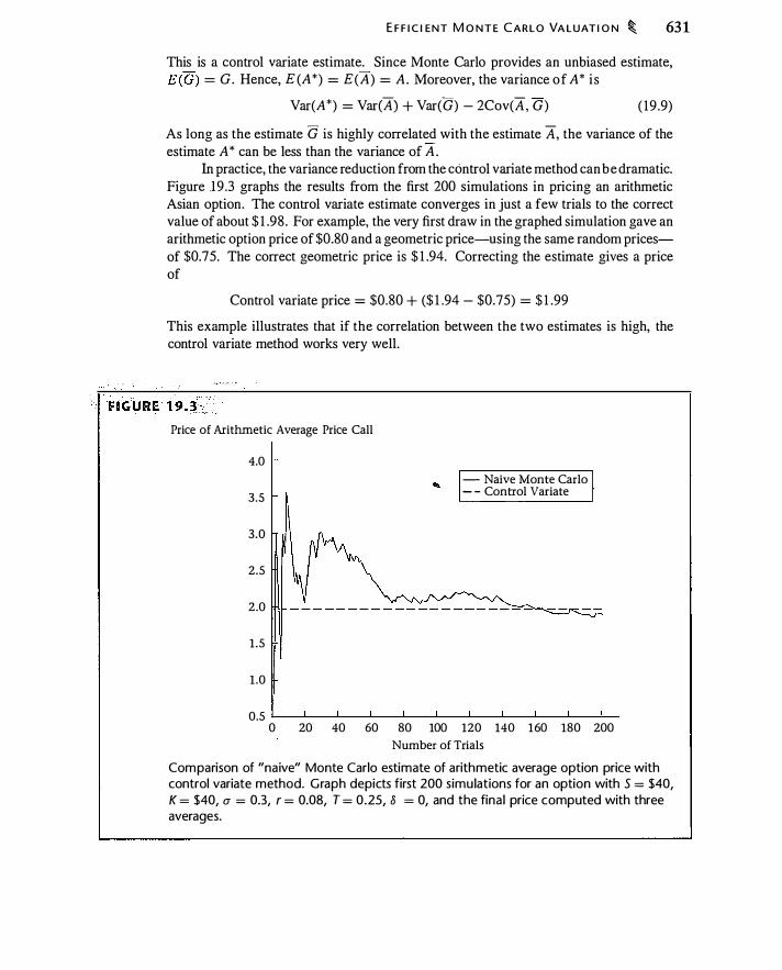
E F F I C I ENT M O N T E CARLO VA LUAT I O N � 63 1

This is a control variate estimate. Since Monte Carlo provides an unbiased estimate, E(G) = G. Hence, E (A*) = E(A) = A. Moreover, the variance of A* i s

Var(A*) = Var(A) + Var(G) - 2Cov(A, G) ( 19 .9)

As long as the estimate G is highly correlated with the estimate A, the variance of the estimate A* can be less than the variance of A .

In practice, the variance reduction from the control variate method can be dramatic. Figure .1 9 .3 graphs the results from the first 200 simulations in pricing an arithmetic Asian option. The control variate estimate converges in just a few trials to the correct value of about $ 1 .98 . For example, the very first draw in the graphed simulation gave an arithmetic option price of $0.80 and a geometric price-using the same random prices­of $0.75. The correct geometric price is $ 1 .94. Correcting the estimate gives a price of

Control variate price = $0.80 + ($ 1 .94 - $0.75) = $ 1 .99

This example illustrates that if the correlation between the two estimates is high, the control variate method works very well .

Price of Aritlunetic Average Price Call

4.0 - Naive Monte Carlo

3.5 - - Control Variate

3.0

2.5

2.0

1 .5

1 .0

0.5 L-�-�--�---L--�--�--�--����-0 20 40 60 80 100 120 140 160 180 200

Number of Trials

Comparison of "naive" Monte Carlo estimate of arithmetic average option price with control variate method. Graph depicts first 200 s imulations for an option with S = $40, K = $40, a = 0.3, r = 0.08, T = 0.25, 8 = 0, and the fina l price computed with three averages.

632 � M O NT E (AR LO VA LUATI O N

Boyle et al . ( 1 997) point out that equation ( 1 9.8) does not i n general provide the minimum variance Monte Carlo estimate, and in some cases can even increase the variance of the estimate. They suggest that instead of estimating equation ( 1 9.8), you estimate

A* = A + .B (G - G) ( 1 9 . 1 0)

The variance of this estimate is

Var(A*) = Var(A) + .B2Var(G) - 2.BCov(A, G) ( 1 9. 1 1 )

The variance Var(A*) is minimized by setting .B = Cov(A, G)/Var(G) . One way to obtain .B is to perform a small number of Monte Carlo trials, run a regression of equation ( 19 . 1 0) to obtain [3, and then use [3 for the remaining trials. The optimal value of .B will vary depending on the application.

Other Monte Carlo Methods

The control variate example is just one method for improving the efficiency of Monte Carlo valuation. The antithetic variate method uses the insight that for every simulated realization, there is an opposite and equally likely realization. For example, if we draw a random normal number of 0.5, we could just as well have drawn -0.5. By using the opposite of each normal draw we can get two simulated outcomes for each random path we draw. This seems as if it would help, since it doubles the number of draws. But drawing a random number -is often not the time-consuming part of a Monte Carlo calculation.

There can be an efficiency gain because the two estimates are negatively correlated; adding them reduces the variance of the estimate. In practical terms, this means that if you draw an extreme estimate from one tail of the distribution, you will also draw an extreme estimate from the other tail, balancing the effect of the first draw. Boyle et al. ( 1997) find modest benefits from using the antithetic variate method.

Another important class of methods controls the region in which random numbers are generated. Stratified sampling is an example of this kind of method. Suppose you have 100 uniform random numbers, u; , i = 1 , . . . , 100. With naive Monte Carlo you would compute z; = N- 1 (u;) . This calculation treats each random number as representing a random draw from the cumulative distribution. However, because of random variation, 100 uniform random numbers will not be exactly uniformly distributed and therefore the z; will not be exactly normal. We can improve the distribution of the u ; , and therefore of the z; , i f we treat each number as a random draw from each percentile of the uniform distribution. Thus, take the first draw, u 1 , and divide it by 1 00. The resulting £1 1 is now uniformly distribtuted over [0,0.0 1 ] . Take the second draw, divide it by 1 00, and add 0.0 1 . The resulting li2 is uniformly distributed over (0.01 ,0.02). For the i th draw, compute it; = (i - 1 + u; )/ 100. This value is uniformly distributed over the i th percentile. Proceeding in this way we are guaranteed to generate a random number for each percentile of the normal distribution. You can select a number of intervals

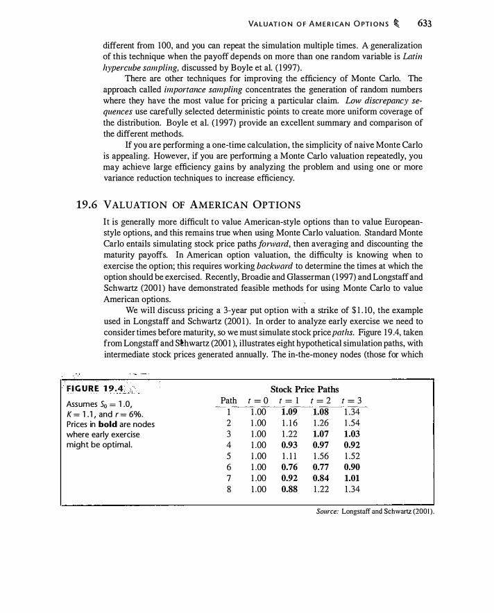
VA LUAT I O N O F A M E R I CA N O PT I O N S � 633

different from 100, and you can repeat the simulation multiple times. A generalization of this technique when the payoff depends on more than one random variable is Latin hypercube sampling, discussed by Boyle et al. ( 1 997).

There are other techniques for improving the efficiency of Monte Carlo. The approach called importance sampling concentrates the generation of random numbers where they have the most value for pricing a particular claim. Low discrepancy se­quences use carefully selected deterministic points to create more uniform coverage of the distribution. Boyle et al. ( 1 997) provide an excellent summary and comparison of the different methods.

If you are performing a one-time calculation, the simplicity of naive Monte Carlo is appealing. However, if you are performing a Monte Carlo valuation repeatedly, you may achieve large efficiency gains by analyzing the problem and using one or more variance reduction techniques to increase efficiency.

19.6 VALUATION OF AMERICAN OPTIONS

It is generally more difficult to value American-style options than to value European­style options, and this remains true when using Monte Carlo valuation. Standard Monte Carlo entails simulating stock price pathsfonvard, then averaging and discounting the maturity payoffs. In American option valuation, the difficulty is knowing when to exercise the option; this requires working bachvard to determine the times at which the option should be exercised. Recently, Broadie and Glasserman ( 1 997) and Longstaff and Schwartz (200 1 ) have demonstrated feasible methods for using Monte Carlo to value American options.

We will discuss pricing a 3-year put option with a strike of $ 1 . 10, the example used in Longstaff and Schwartz (200 1 ) . In order to analyze early exercise we need to consider times before maturity, so we must simulate stock price paths. Figure 19 .4, taken from Longstaff and S�hwartz (200 1 ), illustrates eight hypothetical simulation paths, with intermediate stock prices generated annually. The in-the-money nodes (those for which

FI G U R E 1 9 .4 -, ___ Stock Price Paths

Assumes 50 = 1 .0, Path t = O t = I t = 2 t = 3 K = 1 . 1 , and r = 6%. 1 1 .00 1.09 1.08 1 .34 Prices in bold are nodes 2 1 .00 1 . 1 6 1 .26 1 .54 where early exercise 3 1 .00 1 .22 1.07 1.03 might be optimal . 4 1 .00 0.93 0.97 0.92

5 1 .00 1 . 1 1 1 .56 1 .52 6 1 .00 0.76 0.77 0.90 7 1 .00 0.92 0.84 1.01 8 1 .00 0.88 1 .22 1 .34

Source: Longstaff and Schwartz (200 I ) .

634 � M O N TE CARLO VA LUAT I O N

S < $ 1 . 1 0) are candidate nodes for exercise of the option; in Figure 19 .4 they are in bold (this ignores exercise at time 0). How do we determine at which of these nodes early exercise is optimal?

The idea underlying any method of American option valuation is to compare the value of immediate exercise to the continuation value of the option-i.e., the value of keeping the option alive.7 The problem is therefore to estimate the continuation value at each point in time.

It is worth noting one potential problem in estimating continuation value, which stems from the use of future stock prices on a given path to decide whether to exercise on that path. Consider path 1 in Figure 19 .4. The option is out-of-the-money, and therefore worthless, at t = 3 . Therefore, on this path we would be better off at t = 2 exercising rather than waiting. However, in deciding to exercise by looking ahead on the path, we are using knowledge of the future stock price, which is information we will not have in real life. Valuing the option assuming we know the future price will give us too high a value. The way to mitigate such "lookahead bias" is to base an exercise decision on average outcomes from a given point forward. There are at least two ways to characterize the average outcome from a given point. One is to use a regression to characterize the continuation value based on analysis of multiple paths. This is the method proposed by Longstaff and Schwartz (200 1) . Another is create additional branches from each node, providing multiple outcomes that we can average to characterize continuation value at that node. This is the basis for the Broadie and Glasserman ( 1 997) procedure.

To price the option using regression analysis, we work backward through the columns of Figure 19 .4, running a regression at each time to estimate continuation value as a function of the stock price. We work backward because the continuation value at t = 1 will depend upon whether exercise is optimal on a given path at t = 2. At t = 2, there are five paths ( 1 , 3 , 4, 6, and 7) where the option i s in-the-money and exercise could be optimal. For each of these paths, we know the value of exercising immediately and the value of waiting. Longstaff and Schwartz run a regression of the present value of waiting to exercise (i .e. , the continuation value) against the stock price and stock price squared. At time 2, we obtain the following result:

Continuation value at time 2 = - 1 .07 + 2.98 X s - 1 . 8 1 X S2

where S is the time 2 stock price. Now for each node where exercise could be optimal, we insert the stock price at that node into the regression equation and obtain an estimate of continuation value. By comparing this to intrinsic value, we decide whether to exercise at that node. For example, when S = 1 .08 in row 1, the esimated value of waiting to exercise is

- 1 .07 + 2.98 X 1 .08 - 1 . 8 1 X 1 . 1 66 = 0.037 ( 1 9. 1 2)

7For example, this is the comparison in the binomial valuation in equation ( 1 0. 1 0).

VA LUAT I O N O F A M E R I CA N O PTI O N S � 635

Since the immediate exercise value is 1 . 1 0 - 1 .08 = 0.02, which is less the 0.037, we wait at that node. Table 1 9.4 summarizes the results.

We then repeat the analysis at t = 1, using the results at t = 2. The final decision about where to exercise the option is summarized in Figure 1 9.5. We can value the option by computing the present value of cash flows based on exercising at the nodes where doing so is optimal. The final American put value is $0. 1 144, compared with $0.0564 for a European value computed using the same simulated paths.

A problem with the regression approach is that it is not obvious how to select an appropriate functional form for the continuation regression. Longstaff and Schwartz (200 1 ) report obtaining similar results for a variety of functional forms, but for each new problem it will be desirable to experiment with different functions.

Broadie and Glasserman ( 1997) adopt a different approach, pointing out that Amer­ican option valuations are subject to different kinds of biases. As we discussed above, an estimator will give too high a valuation to the extent it uses information about the future to decide whether to exercise at a given time. Estimators will be biased low to the extent that early exercise is suboptimal (since optimal exercise maximizes the value

TABLE 1 9A Exercise analysis at t = 2 for those nodes in F igure 1 9 .4 where 5 < $ 1 . 1 0 at t = 2.

Path PV(Wait) s 82 Exercise Continuation Result

0.000 1 .08 1 . 1 66 0.02 0.037 Wait 3 0.066 1 .07 1 . 145 0.03 0.046 Wait 4 0. 1 70 0.97 0.941 0. 1 3 0. 1 1 8 Exercise 6 0. 1 88 0.7� 0.593 0.33 0. 152 Exercise 7 0.085 0.84 0.706 0.26 0. 156 Exercise

Stock Price Paths

Summary of results Path t = O t = I t = 2 t = 3 showing the nodes at 1 .00 1 .09 1 .08 1 .34 which exercise is 2 1 .00 1 . 1 6 1 .26 1 .54 optimal (in bold) for 3 1 .00 1 .22 1 .07 1.03 the paths in F igure 4 1 .00 0.93 0.97 0.92 1 9.4. 5 1 .00 1 . 1 1 1 .56 1 .52

6 1 .00 0.76 0.77 0.90 7 1 .00 0.92 0.84 1 .0 1 8 1 .00 0.88 1 .22 1 .34

636 � M O NTE CA R LO VA LUAT I O N

of the option). To address the two errors, Broadie and Glasserman use two estimators, one with high bias and one with low bias. In constructing these estimators, they create sample paths in which there are multiple branches from each node. The resulting set of paths resembles a nonrecombining binomial tree with more than two branches from each node.

The high bias estimator assesses the continuation value by averaging the discounted values on branches emanating from a point and exercising if the value of doing so is greater than the value of continuing. Because the subsequent branches are constructed by simulation, there will be sampling error. To see the effects of such error, suppose exercise is optimal at a node. If the subsequent branches are too high due to sampling error, we will not exercise and assign an even higher value to the node than would be obtained by (optimally) exercising. Now suppose that exercise is not optimal at a node but subsequent branches are too low due to sampling error. We will then exercise and again assign a higher value to the node than we should, given the subsequent branch values.8

The low bias estimator is obtained by splitting the branches from each node into two sets. Using the first set, we estimate the value of continuation and decide whether to exercise. If it is optimal to continue, we use the second set of nodes to estimate the continuation value. By using separate sets of nodes to make the exercise decision and to estimate continuation value, this estimator avoids the "high bias" discussed above. But to the extent the exercise decision is suboptimal, the inferred option value will be too low. Both estimators are biased, but both also converge to the true option value as the number of paths increases.

The Broadie and Glasserman approach is computationally involved, but provides a general method for accomodating early exercise in a simulation model .

19.7 THE POISSON DISTRIBUTION

We have seen that the lognormal distribution assigns a low probability to large stock price moves. One approach to generating a more realistic stock price distribution is to permit large stock price moves to occur randomly. Occasional large price moves can generate the fat tails observed in the data in Section 1 8 .6.

The Poisson distribution is a discrete probability distribution that counts the number of events-such as large stock price moves-that occur over a period of time. The Poisson distribution is summarized by the parameter A., where A.lz is the probability that one event occurs over the short interval lz . A Poisson-distributed event is very

8 Note that the other two kinds of sampling errors do not matter for assessing the value of early exercise. If i t is not optimal to exercise and subsequent branches are too high, we wil l not exercise and therefore not erroneously attribute value to exercising. Similarly, if it is optimal to exercise and subsequent values are too low, we will exercise, giving the correct value to early exercise.

TH E P O I S S O N D I STR I B UTI O N � 637

unlikely to occur more than once over a sufficiently short interval . Thus, A is like an annualized probability of the event occurring over a short interval.9

Over a longer period of time, t , the probability that the event occurs exactly m times is given by

e-J.t (At )111 p(m , At) = ---'--­

m ! The cumulative Poisson distribution i s then the probability that there are m or fewer events .from 0 to t . 1 0

111 e-J.t (At); P(m , At) = Prob(x S m ; At) = L . 1 i=O I .

Given an expected number of events, the Poisson distribution tells us the probability that we will see a particular number of the events over a given period of time. 1 1 The mean of the Poisson distribution is At.

Example 1 9. 3 Suppose the probability of a market crash is A = 2% per year. Then the probability of seeing no market crashes in any given year can be computed as p (O, 0.02 x 1 ) = 0.9802. The probability of seeing no crashes over a 10-year period would be p (O, 0.02 x 10) = 0.8 1 87 . The probability of seeing exactly two crashes over a 1 0-year period would be p (2, 0.02 x 10) = 0.0 1 64. �

Figure 1 9.6 graphs the Poisson distribution for three values of the Poisson param­eter, At. Suppose we are interested in the number of times an event will occur over a

9By definition, the number of occurrences of an event is Poisson-distributed if four assumptions are

satisfied: '

I. The probability that one event will occur in a small interval h is proportional to the length of the interval .

2. The probability that more than one event will occur in a small interval h is substantially smaller than the

probability that a single event will occur.

3. The number of events in nonoverlapping time intervals is independent.

4. The expected number of events between time t and time t + s is independent of t .

The Poisson distribution can be derived from these four assumptions. See Casella and Berger (2002). 10In Excel, you can compute p(m , At) as Poisson(m , At ,false) , and the cumulative distribution,

P(m , At) , as Poisson(m , At, true) . 1 1The probability that no event occurs between time 0 and time t is p (O, ),t) = e-j·' . The probability

that one or more events occurs between 0 and t is therefore I - e-j.r . This expression is also the

cumulative distribution of the exponential distribution, which models the time until the first event.

The density function of the exponential distribution is f(t . A) = Ae-j·' .

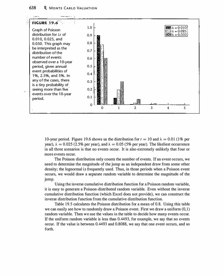
638 � M O NT E CA R LO VA LUAT I O N

Graph of Poisson 1 .0

distribution for /..t of 0.9 0.01 0, 0.025, and 0.050. This graph may 0.8

be interpreted as the 0.7

distribution of the number of events 0.6 observed over a 1 0-year period, g iven annual 0.5 event probabil ities of

0.4 1 %, 2.5%, and 5%. I n any o f the cases, there 0.3 is a tiny probabi l ity of seeing more than five 0.2 events over the 1 0-year

0.1 period.

0 0 1 2 3 4 5

1 0-year period. Figure 1 9.6 shows us the distribution for t = 1 0 and A = 0.0 1 ( 1% per year), A = 0.025 (2.5% per year), and A = 0.05 (5% per year). The likeliest occurrence in all three scenarios is that no events occur. It is also extremely unlikely that four or more events occur.

The Poisson distribution only counts the number of events. If an event occurs, we need to determine the magnitude of the jump as an independent draw from some other density ; the lognormal i.s frequently used. Thus, in those periods when a Poisson event occurs, we would draw a separate random variable to determine the magnitude of the jump.

Using the inverse cumulative distribution function for a Poisson random variable, it is easy to generate a Poisson-distributed random variable. Even without the inverse cumulative distribution function (which Excel does not provide), we can construct the inverse distribution function from the cumulative distribution function.

Table 1 9 .5 calculates the Poisson distribution for a mean of 0.8. Using this table we can easily see how to randomly draw a Poisson event. First we draw a uniform (0, 1 ) random variable. Then we use the values in the table to decide how many events occur. If the uniform random variable is less than 0.4493, for example, we say that no events occur. If the value is between 0.4493 and 0.8088, we say that one event occurs, and so forth.

· . ..

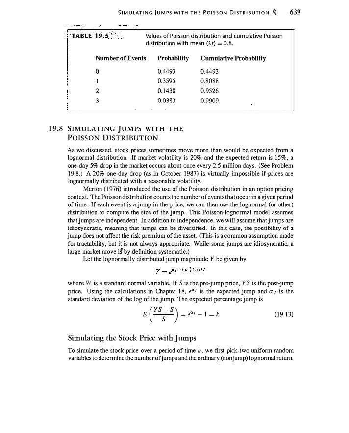
TABLE 1 9S

S I M U LAT I N G j U M PS W ITH T H E P O I S S O N D I STR I B UT I O N � 639

Values of Poisson d istribution and cumulative Poisson distribution with mean (At) = 0.8 .

Number of Events Probability Cumulative Probability

0 0.4493 0.4493 0.3595 0.8088

2 0. 1438 0.9526 3 0.0383 0.9909

19.8 SIMULATING JUMPS WITH THE POISS ON DISTRIBUTION

As we discussed, stock prices sometimes move more than would be expected from a lognormal distribution. If market volatility is 20% and the expected return is 1 5%, a one-day 5% drop in the market occurs about once every 2.5 million days. (See Problem 19.8.) A 20% one-day drop (as in October 1987) is virtually impossible if prices are lognormally distributed with a reasonable volatility.

Merton ( 1 976) introduced the use of the Poisson distribution in an option pricing context. The Poisson distribution counts the number of events that occur in a given period of time. If each event is a jump in the price, we can then use the lognormal (or other) distribution to compute the size of the jump. This Poisson-lognormal model assumes that jumps are independent. In addition to independence, we will assume that jumps are idiosyncratic, meaning that jumps can be diversified. In this case, the possibility of a jump does not affect the risk premium of the asset. (This is a common assumption made for tractability, but it is not always appropriate. While some jumps are idiosyncratic, a large market move ig by definition systematic.)

Let the lognormally distributed jump magnitude Y be given by

where W is a standard normal variable. If S is the pre-jump price, Y S is the post-jump price. Using the calculations in Chapter 1 8, ea1 is the expected jump and a 1 is the standard deviation of the log of the jump. The expected percentage jump is ( YS - S) E S = ea1 - 1 = k

Simulating the Stock Price with Jumps

( 1 9. 1 3)

To simulate the stock price over a period of time h , we first pick two uniform random variables to determine the number of jumps and the ordinary (nonjump) lognormal return.

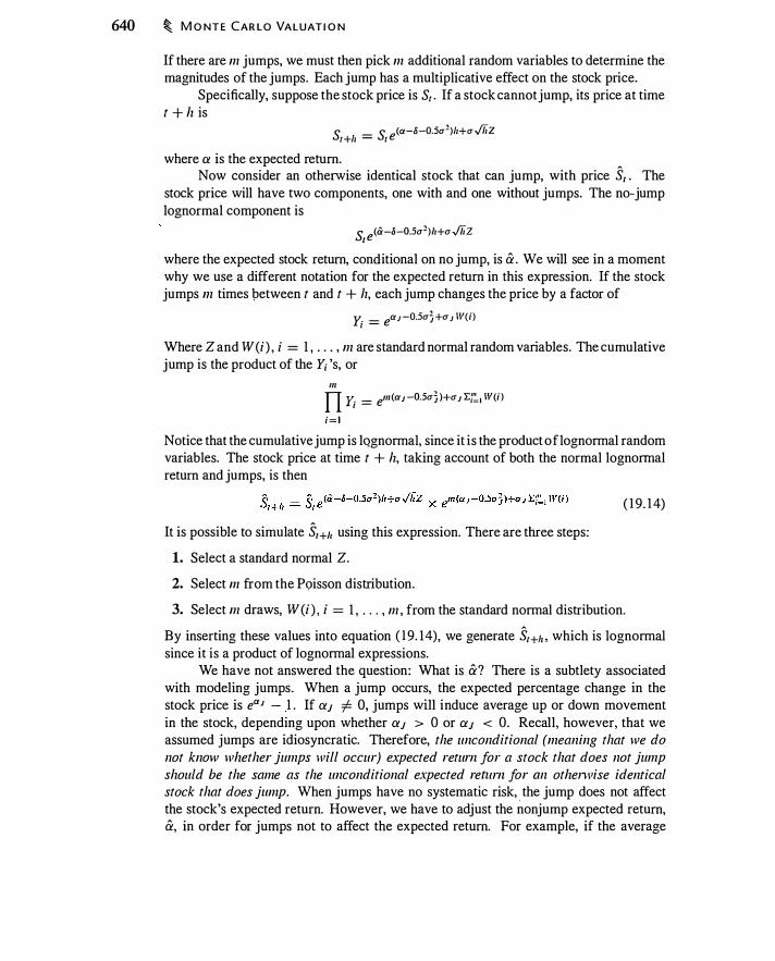
640 � M O NT E CAR LO VA LUAT I O N

If there are m jumps, we must then pick m additional random variables to determine the magnitudes of the jumps. Each jump has a multiplicative effect on the stock price.

Specifically, suppose the stock price is S, . If a stock cannot jump, its price at time t + h is

S _ S e<a-d-0.5u1)1z+u./fiZ t+!J - t

where a is the expected return. Now consider an otherwise identical stock that can jump, with price S1• The

stock price will have two components, one with and one without jumps. The no-jump lognormal component is

S, e<a-d-0.5u1 )lz+u ./ii z

where the expected stock return, conditional on no jump, is & . We will see in a moment why we use a different notation for the expected return in this expression. If the stock jumps m times between t and t + h, each jump changes the price by a factor of

Y; = ea1 -0.5u} +u 1 ll'(i)

Where Z and W(i ) , i = 1 , . . . , m are standard normal random variables. The cumulative jump is the product of the Y; 's, or

Ill n Y; = em<aJ -o.su} J+uJ E;: , w<i J

i= l

Notice that the cumulative jump is lqgnormal, since it is the product of lognormal random variables. The stock price at time t + h, taking account of both the normal lognormal return and jumps, is then

It is possible to simulate Sr+lz using this expression. There are three steps:

1. Select a standard normal Z.

2. Select m from the P9isson distribution.

( 1 9. 14)

3. Select m draws, W(i ) , i = 1 , . . . , m , from the standard normal distribution.

By inserting these values into equation ( 1 9. 14), we generate Sr+lz , which is lognormal since it is a product of lognormal expressions.

We have not answered the question: What is &? There is a subtlety associated with modeling jumps. When a jump occurs, the expected percentage change in the stock price is ea1 - 1 . If a1 =/= 0, jumps will induce average up or down movement in the stock, depending upon whether a1 > 0 or a1 < 0. Recall, however, that we assumed jumps are idiosyncratic. Therefore, the unconditional (meaning that we do not know whether jumps will occur) expected return for a stock that does not jump should be the same as the unconditional expected return for mz othenvise identical stock that does jump. When jumps have no systematic risk, . the jump does not affect the stock's expected return. However, we have to adjust the nonjump expected return, &, in order for jumps not to affect the expected return. For example, if the average

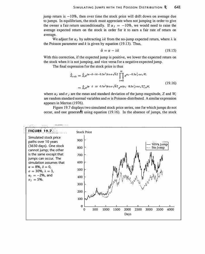
S I M U LAT I N G j U M PS W ITH TH E P O I S S O N D I ST R I B UT I O N � 641

jump return is - 1 0%, then over time the stock price will drift down on average due to jumps. In equilibrium, the stock must appreciate when not jumping in order to give the owner a fair return unconditionally. If a 1 = -10%, we would need to raise the average expected return on the stock in order for it to earn a fair rate of return on average.

We adjust for a1 by subtracting Ak from the no-jump expected return, where ).. is the Poisson parameter and k is given by equation ( 1 9. 1 3) . Thus,

& = a - Ak ( 1 9. 1 5)

With this correction, if the expected jump is positive, we lower the expected return on the stock when it is not jumping, and vice versa for a negative expected jump.

The final expression for the stock price is thus 111

S� - SA e<a-8-}.k-0.5a2 )!J+a.fiiZ U eaJ -0.5a�+aJ IVi t+!J - I i=O ( 1 9 . 1 6)

where a1 and a 1 are the mean and standard deviation of the jump magnitude, Z and W; are random standard normal variables and m is Poisson-distributed. A similar expression appears in Merton ( 1 976).

Figure 1 9 .7 displays two simulated stock price series, one for which jumps do not occur, and one generatt!l using equation ( 1 9 . 1 6) . In the absence of jumps, the stock

Stock Price

Simu lated stock price paths over 1 0 years (3650 days) . One stock cannot jump; th� other is the same except that jumps can occur. The s imulation assumes that a = 8%, 8 = 0,

900

800

700

600

500 (}' = 30%, J... = 3, a1 = -2%, and 400 Uj = 5%.

300

200

100

OL---�--�----�--�----L----L----L---�-0 500 1000 1500 2000 2500 3000 3500 4000

Days

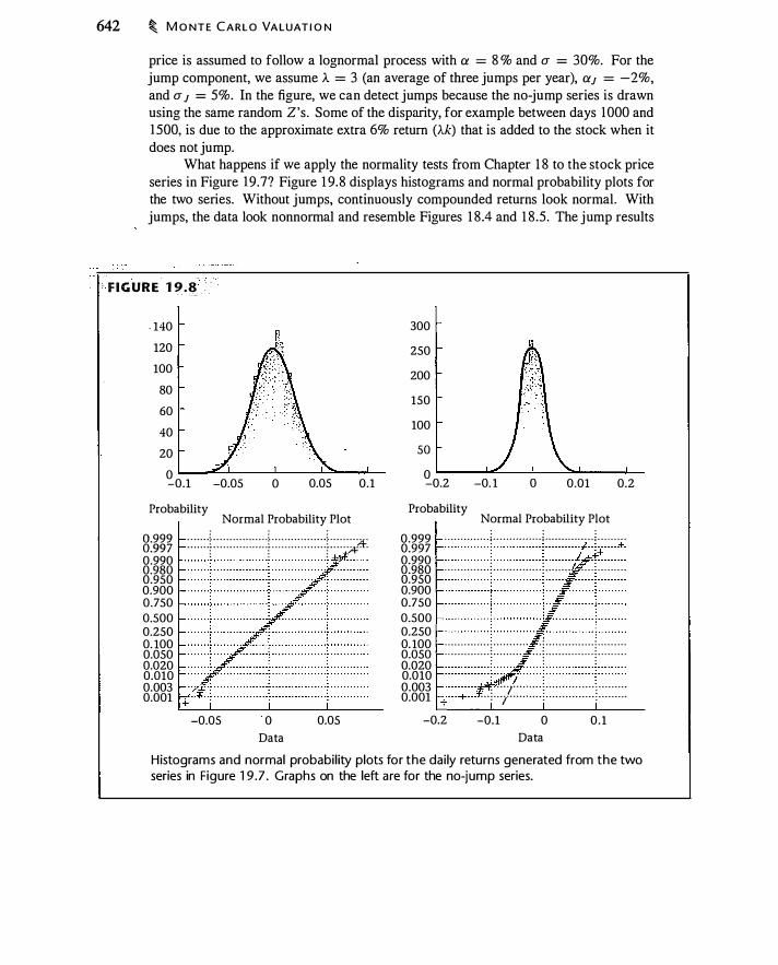
642 � M O NT E CARLO VA LUAT I O N

price is assumed to follow a lognormal process with a = 8 % and a = 30%. For the jump component, we assume A = 3 (an average of three jumps per year), a1 = -2%, and a 1 = 5%. In the figure, we can detect jumps because the no-jump series is drawn using the same random Z's . Some of the disparity, for example between days 1000 and 1 500, is due to the approximate extra 6% return (Ak) that is added to the stock when it does not jump.

What happens if we apply the normality tests from Chapter 1 8 to the stock price series in Figure 19.7? Figure 1 9.8 displays histograms and normal probability plots for the two series. Without jumps, continuously compounded returns look normal. With jumps, the data look nonnormal and resemble Figures 1 8 .4 and 1 8 .5 . The jump results

F IGURE 1 9 . 8_

- 140

120

100

80

60

40

20

0 -0.1

Probability

-0.05 0 0.05

Normal Probability Plot . . .

0.1

8:§§? : : : : : : :i : : : : : : : : : : : : : : : : :i : : : : : : : : : : : : : : : : :i : : : : ::�:<�-: 0.990 . . 0.980 0.950 0.900 0.750 0.500 0.250 0. 100 0.050 0.020 0.010 0.003 0.001

-0.05 0 Data

0.05

300

250

200

150

100

so

0 L...---�----L-----""'-1..--....L---0.2 -0. 1 0

Probability

0.01

Normal Probability Plot . . .

0.2

0.999 . . . . . . . . . . . . . . ; . . . . . . . . . . . . . . . i . . . . . . . . . . . . . . . i . . . . . . . . . 0.997 : : : : : : : : : : : : : : : : : : : : : : : : : : : : : : : : : : : : : : : :/-+�:: : :�: 0.990 . . . 0.980 · · · · · · · · · · · · · · = · · · · · · · · · · · · · · · = · · · · · · · · . . . . : . . . . . . . . . 0.950 0.900 0.750 0.500 0.250 0. 100 · · · · · · · · · · · · · · : · · · · · · · · · · · · = · · · · · · · · · · · · · · · = · · · · · · · · ·

0.050 · · · · · · · · · · · · · · = · · · · · · · · · · · · = · · · · · · · · · · · · · · · = · · · · · · · · ·

0.020 . . .

0.010 0.003 I . . 0.001 �: : ::; : : : . . . � . : :;c::: : : : : j : : : : : : : : : : : : : : : � : : : : : : : : :

-0.2 -0.1 0 Data

0.1

Histograms and normal probabi l ity plots for the dai ly returns generated from the two series in Figure 1 9 .7 . Graphs on the left are for the no-jump series.

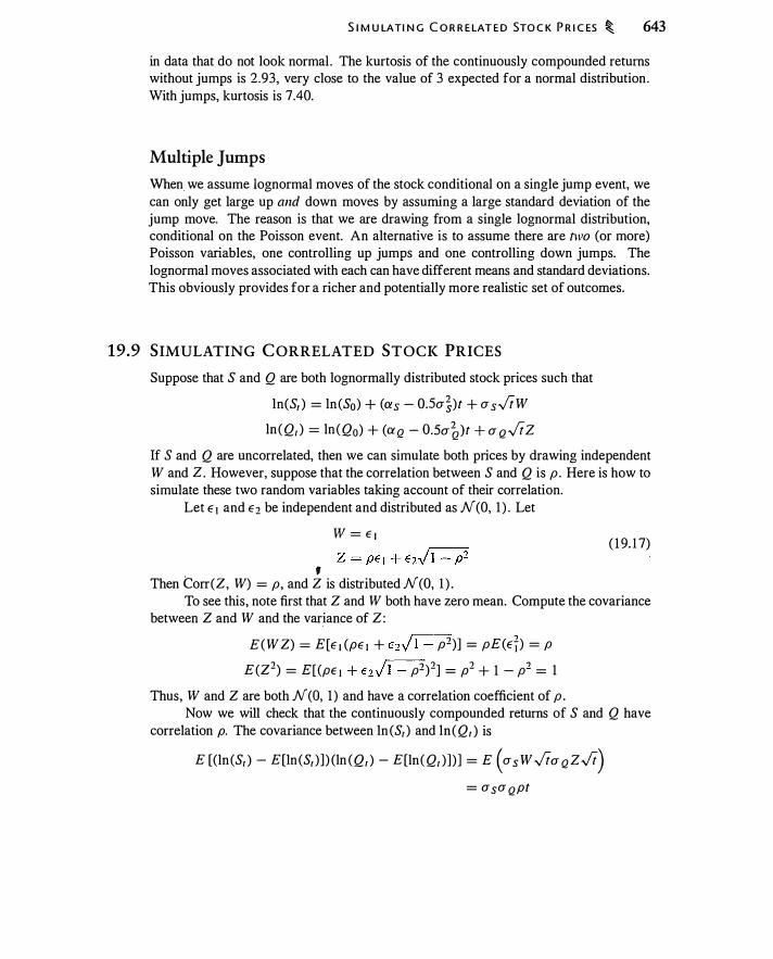
S I M U LATI N G C O R R E LAT E D STO C K P R I C ES � 643

in data that do not look normal . The kurtosis of the continuously compounded returns without jumps is 2.93, very close to the value of 3 expected for a normal distribution. With jumps, kurtosis is 7.40.

Multiple Jumps

When we assume lognormal moves of the stock conditional on a single jump event, we can only get large up and down moves by assuming a large standard deviation of the jump move. The reason is that we are drawing from a single lognormal distribution, conditional on the Poisson event. An alternative is to assume there are two (or more) Poisson variables, one controlling up jumps and one controlling down jumps. The lognormal moves associated with each can have different means and standard deviations. This obviously provides for a richer and potentially more realistic set of outcomes.

19.9 SIMULATING CORRELATED STOCK PRICES

Suppose that S and Q are both lognormally distributed stock prices such that

ln(S1 ) = ln (So) + (as - O .Sa�)t + asJ!W ln (Q1 ) = ln (Qo) + (aQ - O.Sa�)t + a QJ!z

If S and Q are uncorrelated, then we can simulate both prices by drawing independent W and z. However, suppose that the correlation between S and Q is p . Here is how to simulate these two random variables taking account of their correlation.

Let E 1 and E2 be independent and distributed as N(O, 1 ) . Let

W = E ) ( 1 9. 1 7)

f Then Corr(Z, W) = p, and Z is distributed N(O, 1 ) .

To see this, note first that Z and W both have zero mean. Compute the covariance between Z and W and the variance of Z :

E (WZ) = E[E J (PE l + E2J 1 - p2)] = pE(ET) = p

E(Z2) = E[(PE l + E2J1 - p2)2] = p2 + 1 - p2 = 1

Thus, W and Z are both N(O, 1 ) and have a correlation coefficient of p . Now we will check that the continuously compounded returns of S and Q have

correlation p. The covariance between ln (S1 ) and ln (Q1 ) is

E [(ln (S1 ) - E[ln (S1 ) ] ) (ln (Q1 ) - E[ln( Q1 ) ] ) ] = E (asWJ!aQzJt) = asaQpt

644 � M O NT E CARLO VA LUAT I O N

The correlation coefficient is . a sa Q Pf

Correlatron = r; r; = p a sv ta Q v t

Thus, if W and Z have correlation p, so will the continuously compounded returns of S and Q.

Generating n Correlated Lognormal Random Variables

Suppose we have n correlated lognormal variables. The question we address here is how to generalize the previous analysis. The first of the n random variables will have n - 1 pairwise correlations with the others. The second will have n - 2 (not counting its correlation with the first, which we have already counted) . Continuing in this way, we will have

1 n - 1 + n - 2 + · · · + 1 = 2n (n - I )

pairwise correlations we have to take into account. We will denote the correlation between variables i and j as Pi,j ·

We denote the original uncorrelated random N(O, 1 ) variables as E 1 , E 2 , . . . , E 11 • The correlated random variables are Z ( 1 ) , Z (2) , . . . , Z(n) , with

We can generate the Z(i ) as

E[Z(i )Z (j) ] = Pi,j

Z(i ) = L a;,j Ej j= l

where the a;,j are coefficients selected to make sure the pairwise correlations are correct. Creating the coefficients a;,j has a recursive solution. That is, we construct Z ( l ) ,

then Z(2) using the soh.rtion to Z ( l ) , and so on. The formula for the a;,j is

a;,j = � Pi,j - L aj,kai,k

[ j- 1 ] j . j k= l

i - 1

a;,; = 1 - L: a1,k k= l

i > j

For the case of two random variables, this reduces to equation ( 1 9 . 1 7) .

( 1 9 . 1 8)

The matrix of a;,j 's is called the Cholesky decomposition of the original cor­relation matrix. In order for equation ( 1 9. 1 8) to give correct coefficients, the set of correlations must be positive-definite, which means that the correlations must be such thanhere is no way to sum random variables and compute a negative variance. This is

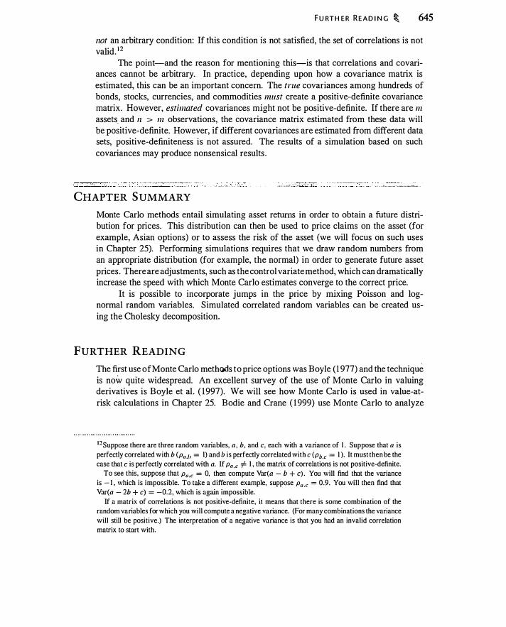
F U RT H E R READ I N G � 645

not an arbitrary condition: If this condition is not satisfied, the set of correlations is not valid. 1 2

The point-and the reason for mentioning this-is that correlations and covari­ances cannot be arbitrary. In practice, depending upon how a covariance matrix is estimated, this can be an important concern. The true covariances among hundreds of bonds, stocks, currencies, and commodities must create a positive-definite covariance matrix. However, estimated covariances might not be positive-definite. If there are m assets and n > m observations, the covariance matrix estimated from these data will be positive-definite. However, if different covariances are estimated from different data sets, positive-definiteness is not assured. The results of a simulation based on such covariances may produce nonsensical results.

·-·--·-··· -·- --·-····----------·--··-----··· _._ . __ :_· -· · -·· = · -- - - �---· :.. - ---·- -----� --� ---·-- ---'---:..-._o. _________ ---· ---· .

CHAPTER S UMMARY

- - ·-·-···----·····--·

___ : __ ; =<- -·- .,-.. ; ,; - . - . ' . • . . -- . .. - ---�--- -----

Monte Carlo methods entail simulating asset returns in order to obtain a future distri­bution for prices. This distribution can then be used to price claims on the asset (for example, Asian options) or to assess the risk of the asset (we will focus on such uses in Chapter 25). Performing simulations requires that we draw random numbers from an appropriate distribution (for example, the normal) in order to generate future asset prices. There are adjustments, such as the control variate method, which can dramatically increase the speed with which Monte Carlo estimates converge to the correct price.

It is possible to incorporate jumps in the price by mixing Poisson and log­normal random variables. Simulated correlated random variables can be created us­ing the Cholesky decomposition.

FURTHER READING

The first use of Monte Carlo methoos to price options was Boyle ( I 977) and the technique is now quite widespread. An excellent survey of the use of Monte Carlo in valuing derivatives is Boyle et al . ( 1 997). We will see how Monte Carlo is used in value-at­risk calculations in Chapter 25. Bodie and Crane ( 1 999) use Monte Carlo to analyze

1 2Suppose there are three random variables, a, b, and c, each with a variance of I . Suppose that a is

perfectly correlated with b (Pa.l> = I) and b is perfectly correlated with c (pb.c = 1 ). It must then be the

case that c is perfectly correlated with a. If Pa.c of. I , the matrix of correlations is not positive-definite.

To see this, suppose that Pa.c = 0, then compute Var(a - b + c) . You will find that the variance

is - I , which is impossible. To take a different example, suppose Pa.c = 0.9. You will then find that

Var(a - 2b + c) = -0.2, which is again impossible.

If a matrix of correlations is not positive-definite, it means that there is some combination of the

random variables for which you will compute a negative variance. (For many combinations the variance

will still be positive.) The interpretation of a negative variance is that you had an invalid correlation

matrix to start with.

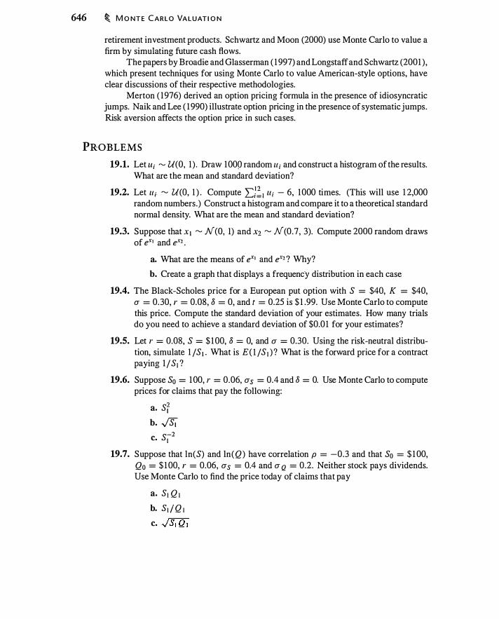
646 � M O NT E CARLO VA LUAT I O N

retirement investment products. Schwartz and Moon (2000) use Monte Carlo to value a firm by simulating future cash flows.

The papers by Broadie and Glasserman ( 1 997) and Longstaff and Schwartz (200 1 ) , which present techniques for using Monte Carlo to value American-style options, have clear discussions of their respective methodologies.

Merton ( 1976) derived an option pricing formula in the presence of idiosyncratic jumps. Naik and Lee ( 1 990) illustrate option pricing in the presence of systematic jumps. Risk aversion affects the option price in such cases.

PROBLEMS

19.1. Let u; � U(O, 1 ) . Draw 1009 random u; and construct a histogram of the results. What are the mean and standard deviation?

19.2. Let u ; � U(O, 1 ) . Compute 'LJ: , u ; - 6, 1000 times. (This will use 1 2,000 random numbers.) Construct a histogram and compare it to a theoretical standard normal density. What are the mean and standard deviation?

19.3. Suppose that x 1 � N(O, 1) and x2 � N(0.7, 3). Compute 2000 random draws of ext and ex1 .

a. What are the means of ext and ex1 ? Why?

b. Create a graph that displays a frequency distribution in each case

19.4. The Black-Scholes price for a European put option with S = $40, K = $40, u = 0.30, r = 0.08, o = 0, and t = 0.25 is $ 1 .99. Use Monte Carlo to compute this price. Compute the standard deviation of your estimates. How many trials do you need to achieve a standard deviation of $0.0 1 for your estimates?

19.5. Let r = 0.08, S = $ 1 00, o = 0, and u = 0.30. Using the risk-neutral distribu­tion, simulate 1 IS 1 • What is E ( I IS t ) ? What is the forward price for a contract paying 1 ISr ?

19.6. Suppose So = 1 00, r = 0.06, us = 0.4 and o = 0. Use Monte Carlo to compute prices for claims that pay the following:

a. Sf b. �

S-? c. l -

19.7. Suppose that ln(S) and ln(Q ) have correlation p = -0.3 and that So = $ 1 00, Qo = $ 1 00, r = 0.06, us = 0.4 and u Q = 0.2. Neither stock pays dividends. Use Monte Carlo to find the price today of claims that pay

a. St Q t

b. St i Q r

c. JSt Q t

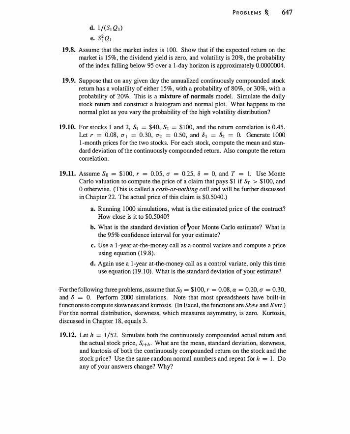
d. 1 /(S1 Q t )

e. Sf Q I

P R O B L E M S � 647

19.8. Assume that the market index is 1 00. Show that if the expected return on the market is 15%, the dividend yield is zero, and volatility is 20%, the probability of the index falling below 95 over a 1 -day horizon is approximately 0.0000004.

19.9. Suppose that on any given day the annualized continuously compounded stock · return has a volatility of either 15%, with a probability of 80%, or 30%, with a

probability of 20%. This is a mixture of normals model. Simulate the daily stock return and construct a histogram and normal plot. What happens to the normal plot as you vary the probability of the high volatility distribution?

19.10. For stocks 1 and 2, S1 = $40, S2 = $ 100, and the return correlation is 0.45 . Let r = 0.08, u 1 = 0.30, u1 = 0.50, and o 1 = o2 = 0. Generate 1 000 1 -month prices for the two stocks. For each stock, compute the mean and stan­dard deviation of the continuously compounded return. Also compute the return correlation.

19.11. Assume So = $ 1 00, r = 0.05, u = 0.25, o = 0, and T = 1. Use Monte Carlo valuation to compute the price of a claim that pays $ 1 if ST > $ 100, and 0 otherwise. (This is called a cash-or-nothing call and will be further discussed in Chapter 22. The actual price of this claim is $0.5040.)

a. Running 1 000 simulations, what is the estimated price of the contract? How close is it to $0.5040?

b. What is the standard deviation of�our Monte Carlo estimate? What is the 95% confidence interval for your estimate?

c. Use a 1 -year at-the-money call as a control variate and compute a price using equation ( 1 9.8) .

d. Again use a 1 -year at-the-money call as a control variate, only this time use equation ( 19 . 1 0) . What is the standard deviation of your estimate?

For the following three problems, assume that So = $ 100, r = 0 .08, a = 0.20, u = 0.30, and o = 0. Perform 2000 simulations . Note that most spreadsheets have built-in functions to compute skewness and kurtosis. (In Excel, the functions are Skew and Kurt.) For the normal distribution, skewness, which measures asymmetry, is zero. Kurtosis, discussed in Chapter 1 8, equals 3 .

19.12. Let h = 1 /52. Simulate both the continuously compounded actual return and the actual stock price, Sr+ll . What are the mean, standard deviation, skewness, and kurtosis of both the continuously compounded return on the stock and the stock price? Use the same random normal numbers and repeat for h = I . Do any of your answers change? Why?

648 � M O NT E CARLO VA LUAT I O N

19.13. An options trader purchases 1000 1 -year at-the-money calls o n a nondividend­paying stock with So = $ 100, a = 0.20, and a = 0.25 . Assume the options are priced according to the Black-Scholes formula and r = 0.05.

a. Use Monte Carlo (with 1000 simulations) to estimate the expected return, standard deviation, skewness, and kurtosis of the return on the call when it is held until expiration. Interpret your answers .

b. Repeat for an at-the-money put.

19.14. Repeat the previous problem, only assume that the options trader purchases 1000 1 -year at-the-money straddles.

19.15. Refer to Table 1 9. 1 .

a. Verify the regression coefficients i n equation ( 19 . 1 2) .

b. Perform the analysis for t = 1 , verifying that exercise is optimal on paths 4, 6, 7, and 8, and not on path 1 .

19.16. Refer to Figure 1 9.2.

a. Verify that the price of a European put option is $0.0564.

b. Verify that the price of an American put option is $0. 1 144. Be sure to allow for the possibility of exercise at time 0.

19.17. Assume S0 = $50, r = 0.05, a = 0.50, and 8 = 0. The Black-Scholes price for a 2-year at-the�money put is $ 1 0.906. Suppose that the stock price is lognormal but can also jump, with the number of jumps Poisson-distributed. Assume a = 0.05 (the expected return to the stock is equal to the risk-free rate), a = 0.50, A = 2, a1 = -0.04, a 1 = 0.08.

a. Using 2000 simulations incorporating jumps, simulate the 2-year price and draw a histogram of continuously compounded returns.

b. Using Monte Carlo incorporating jumps, value a 2-year at-the-money put. Is this value significantly different from the Black-Scholes value?

APPENDIX 1 9 .A : FORMULAS FOR GEOMETRIC AVERAGE OPTIONS

Appendix available online at www.aw-bc.com/mcdonald.

CHAPTER 2.o Brownian Motion and Ito's Lemma

Thl, chapte< addre"e' two ;mportant topk,. H"t, ;n the 'tudy of derivative,, "ock and other asset prices are commonly assumed to follow a stochastic process called geometric Brownian motion. This chapter explains what this means and develops the notation and assumptions underlying the Black-Scholes model.

Second, given that a stock price follows geometric Brownian motion, we want to characterize the behavior of a claim-such as an option-that has a payoff dependent upon the stock price. For this purpose we need Ito's Lemma, which tells us the process followed by a claim that is a function of the stock price.

This material is mathematically more challenging than the material in earlier chap­ters, but it provides the foundation for everything that comes later, as well as much of what has come before. Both academic researchers on options and practitioners rely on the concepts and techniques discussed in this chapter.

20.1 THE BLACK-SCHOLES ASSUMPTION ABOUT STOCK PRICES

The yast majority of technical option pricing discussions, including the original paper by Black and Scholes, begin by assuming that the price of the underlying asset follows a process like the following:

dS(t) -- = adt + O"dZ(t) S (t)

(20. 1 )

In this expression, S(t) is the stock price, d S(t) i s the instantaneous change in the stock price, a is the continuously compounded expected return on the stock, O" is the contin­uously compounded standard deviation (volatility), and Z(t) is a normally distributed random variable that follows a process called Brownian motion. The variable dZ(t) represents the change in Z(t) over a short period of time. A stock obeying equation (20. 1 ) is said to follow a process called geometric Brownian motion. Expressions like equation (20. 1 ) are called stochastic differential equations.

One purpose of this chapter is to understand the meaning of equations like (20. 1 ) . For our purposes, there are two important implications of this equation:

649

650 � B RO W N I A N M OT I O N A N D ITO 'S LE M M A

1. If the stock price follows equation (20. 1 ) , the distribution of S(T) , given the current price S (O) , is lognormal, i .e.

ln[S(T)] � N(ln[S(O)] + [a - 0.5a2] T, a2T) The assumption that the stock follows geometric Brownian motion thus provides a foundation for our assumption that the stock price is lognormally distributed.

2. Lognormality tells us about the distribution of the stock price at a point in time. For many purposes, however, we are interested not just in the distribution at a terminal point but also the path the stock price takes in getting to that terminal point. With barrier options, for example, the price of the option depends upon the probability that the asset price reaches the barrier. Geometric Brownian motion allows us to describe this path.

Our goal is to provide a heuristic, rather than technical, understanding of equations like (20. 1 ).

20.2 B ROWNIAN MOTION

A stochastic process is a random process that is a function of time. Brownian motion is a stochastic process that is a random walk occurring in continuous time, with move­ments that are continuous rather than discrete. It is a basic building block for standard derivatives pricing models. A random walk can be generated by flipping a coin each period and moving one step, with the direction determined by whether the coin is heads or tails. To generate Brownian motion, we would flip the coins infinitely fast and take infinitesimally small steps at each point. Since all steps are infinitely small, movements are continuous. As you might guess, a careful mathematical formulation of this concept requires mathematics beyond the scope and purpose of this book. 1

Definition of Brownian Motion

Let Z(t) represent the value of a Brownian motion at time t . Brownian motion is a continuous stochastic process, Z (t) , with the following characteristics:

o Z(O) = 0.

e Z(t + s) - Z(t) is normally distributed with mean 0 and variance s .

o Z(t + s J ) - Z(t) i s independent of Z(t) - Z(t - s2) , where s 1 , s2 > 0. In other words, nonoverlapping increments are independently distributed.

e Z(t) is continuous (you can draw a picture of Brownian motion without lifting your pencil) .

1The development in this section draws heavily on Cox and Miller ( 1 965, ch. 5) and Merton ( 1 990).

For a more abstract approach to this material, see Duffie ( 1 996) and Karatzas and Shreve ( 1 99 1 ).

B ROWN I A N M OT I O N � 651

These properties imply that Z(t) is a martingale: a stochastic process for which E [Z(t + s) IZ (t)] = Z(t) . The process Z(t) is also called a diffusion process.

To represent this process mathematically, we can focus on the change in Z(t) , which we model as binomial, times a scale factor that makes the change in Z(t) small over a small period of time. Brownian motion is then the limit of a sum of infinitesimal increments over a period of time. Denote the short period of time as h , and let Y(t) be a random draw from a binomial distribution, where Y (t) is ± I with probability 0.5. Note that E �Y (t)] = 0 and Var[Y (t)] = 1 . We can write

Z(t + h) - Z(t) = Y(t + h).Jh (20.2)

Over any period of time longer than /z, Z will be the sum of the binomial increments specified in equation (20.2). Let n = T I h be the number of intervals of length h between 0 and T. We have

II II Z(T) - Z(O) = :l)Z[ih] - Z[(i - 1 )/z ] ) = L Y(ih )

.Jh

i = l i= l Since h = T 1 n , we can also write this as

[ I 11 ] Z(T) - Z(O) = ..rr -Jii E Y(ih ) (20.3)

To understand the properties of Z(T) , we must first understand the properties of the term in square brackets in equation (20.3). Since E[Y (ih )] = 0, we have [ I 11 ]

E -Jii E Y(ih ) = 0

Also, since Var[Y (i lz ) ] = I , and the Y 's are independent, we have [ I 11 ] 1 11 Var � L Y (i lz ) = - L I = 1

.y 1l 1l i = l i= l Thus, the term in square brackets has mean 0 and variance 1 , since it is the sum of n

independent random variables with mean 0 and variance I , divided by -Jii. By the Central Limit Theorem, the distribution of the sum of independent binomial

random variables approaches normality. We have 1 II

lim � " Y (i lz ) � N(O, 1 ) 11---7 00 y ll � i= l

The division by -Jli in this expression prevents the variance from going to infinity as n goes to infinity. ·

Returning to equation (20.3), the multiplication by ../T on the right-hand side multiplies the variance by T. Thus, in the limit we have

Z(T) - Z(O) -+ N(O, T)

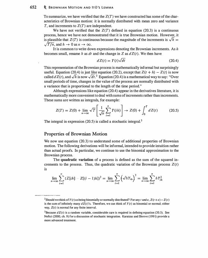
652 � B R OW N I A N M OT I O N A N D ITO 'S LE M M A

To summarize, we have verified that the Z (T) we have constructed has some of the char­acteristics of Brownian motion: it is normally distributed with mean zero and variance T, and increments to Z (T) are independent.

We have not verified that the Z(T) defined in equation (20.3) is a continuous process, hence we have not demonstrated that it is true Brownian motion. However, it is plausible that Z (T) is continuous because the magnitude of the increments is .Jli = -JT!ii, and h ---+ 0 as n ---+ oo.

I t is common to write down expressions denoting the Brownian increments . As h becomes small, rename h as dt and the change in Z as dZ(t ) . We then have

dZ(t) = Y (t).Jdi (20.4) This representation of the Brownian process is mathematically informal but surprisingly useful. Equation (20.4) is just like ·equation (20.2), except that Z (t + h) - Z (t) is now called dZ(t) , and .J1i is now

-Jdi.2 Equation (20.4) is a mathematical way to say: "Over small periods of time, changes in the value of the process are normally distributed with a variance that is proportional to the length of the time period."

Although expressions like equation (20.4) appear in the derivatives literature, it is mathematically more convenient to deal with sums of increments rather than increments. These sums are written as integrals, for example:

Z(T) = Z(O) + lim .JT r.; L Y(ih) ---+ Z(O) + dZ(t) [ 1 11 ] 1T

11-->00 y ll i= l 0

The integral in expression (20.5} is called a stochastic integral.3

Properties of Brownian Motion

(20.5)

We now use equation (20.3) to understand some of additional properties of Brownian motion. The following derivations will be informal, intended to provide intuition rather than actual proofs. In particular, we continue to use the binomial approximation to the Brownian process.

The quadratic .variation of a process is defined as the sum of the squared in­crements to the process . Thus, the quadratic variation of the Brownian process Z (t) IS

11 11 ., n lim

"'(Z[ih] - Z[(i - l )h ] )2 = lim "' (..fhru,) - = lim "' hY;�, IJ-'1-00 � ll� OO � IJ-+00 �

i= l i= l i= l

2Should we think of Y (t) as being binomially or normally distributed? For any t and E, Z (t +E) - Z(t ) is the sum of infinitely many dZ(t)'s . Therefore, we can think of Y (t) as binomial or normal; either

way, Z(t) is normal for any finite interval.

3 Because d Z (t) is a random variable, considerable care is required in defining equation (20.5). See

Neftci (2000, ch. 9) for a discussion of stochastic integration. Karatzas and Shreve ( 1 99 I) provide a

more advanced treatment.

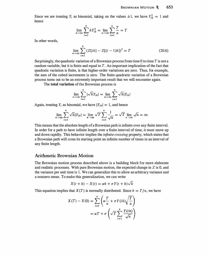
B ROWN I A N M OTI O N � 653

Since we are treating Y; as binomial, taking on the values ± 1 , we have Y;�, = 1 and hence

In other words,

n n T lim � h Y;�, = lim � - = T

ll-HXJ � 11-7-00 L....t Jl

n

i= l i= l

lim � (Z[ilz] - Z[(i - l )/z])2 = T IJ�OO L....t i= l

(20.6)

Surprisingly, the quadratic variation of a Brownian process from time 0 to time T is not a random variable, but it is finite and equal to T . An important implication of the fact that quadratic variation is finite, is that higher-order variations are zero. Thus, for example, the sum of the cubed increments is zero. The finite quadratic variation of a Brownian process turns out to be an extremely important result that we will encounter again.

The total variation of the Brownian process is ll II

lim L I.Jh Yu, l = lim � .Jh I Yu, l 1J--+ 00 ll--+ 00 L....t i= l i= l Again, treating Y; as binomial, we have I Yu, l = 1 , and hence

n n l lim � .Jh1 Yu, l = lim -JT � r.; = -JT lim .Jii = oo

ll---+ 00 L....t 11--+00 L....t v 1l IJ--7-00 i= l i= l This means that the absolute length of a Brownian path is infinite over any finite interval . In order for a path to have infinite length over a finite interval of time, it must move up and down rapidly. This behavior implies the infinite crossing property, which states that a Brownian path will cross its starting point an infinite number of times in an interval of any finite length.

Arithmetic Brownian Motion

The Brownian motion process described above is a building block for more elaborate and realistic processes. With pure Brownian motion, the expected change in Z is 0, and the variance per unit time is 1 . We can generalize this to allow an arbitrary variance and a nonzero mean. To make this generalization, we can write

.

X(t + h) - X (t) = ah + aY(t + h).Jh

This equation implies that X(T) is normally distributed. Since lz = T jn , we have n ( T /r;) X (T) - X (O) = L a- + aY (ilz) -

1l /l i= l

= ctT + a (nt Y(i::) ) i= l .jii

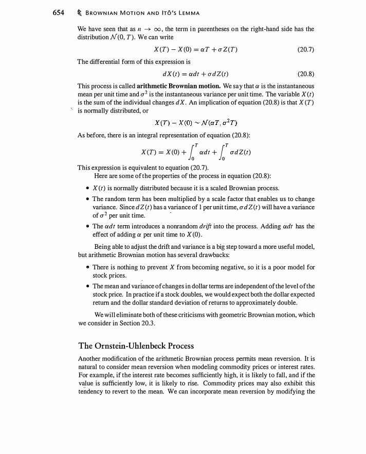
654 � B RO W N I A N M OT I O N A N D ITO 'S L E M M A

We have seen that as n --+ oo , the term i n parentheses on the right-hand side has the distribution N(O, T) . We can write

X (T) - X (O) = ctT + lT Z(T) (20.7)

The differential form of this expression is

dX (t) = ctdt + O"dZ(t) (20.8) This process is called arithmetic Brownian motion. We say that a is the instantaneous mean per unit time and 0"2 is the instantaneous variance per unit time. The variable X (t) is the sum of the individual changes d X. An implication of equation (20.8) is that X (T) is normally distributed, or

As before, there is an integral representation of equation (20.8) :

X (T) = X (O) + 1T ctdt + 1T O"dZ (t)

This expression is equivalent to equation (20.7). Here are some of the properties of the process in equation (20.8) :

• X (t) is normally distributed because it is a scaled Brownian process.

• The random term has been multiplied by a scale factor that enables us to change variance. Since d Z(t) has a variance of 1 per unit time, lTd Z(t) will have a variance of 0"2 per unit time. -

• The adt term introduces a nonrandom drift into the process. Adding ctdt has the effect of adding a per unit time to X (O) .

Being able to adjust the drift and variance is a big step toward a more useful model, but arithmetic Brownian motion has several drawbacks:

• There is nothing to prevent X from becoming negative, so it is a poor model for stock prices .

• The mean and variance of changes in dollar terms are independent of the level of the stock price. In practice if a stock doubles, we would expect both the dollar expected return and the dollar standard deviation of returns to approximately double.

We will eliminate both of these criticisms with geometric Brownian motion, which we consider in Section 20.3 .

The Ornstein-Uhlenbeck Process

Another modification of the arithmetic Brownian process permits mean reversion. It is natural to consider mean reversion when modeling commodity prices or interest rates. For example, if the interest rate becomes sufficiently high, it is likely to fall , and if the vaJue is sufficiently low, it is likely to rise. Commodity piices may also exhibit this tendency to revert to the mean. We can incorporate mean reversion by modifying the

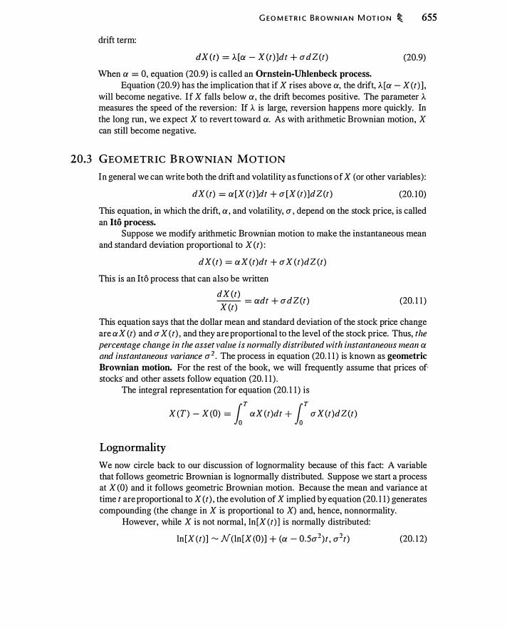
G EO M ETR I C B R O W N I A N M OT I O N � 655

drift term:

dX (t) = A.[a - X (t)]dt + udZ(t) (20.9) When a = 0, equation (20.9) is called an Ornstein-Uhlenbeck process.

Equation (20.9) has the implication that if X rises above a, the drift, A.[a - X (t ) ] , will become negative. If X falls below a, the drift becomes positive. The parameter A measures the speed of the reversion: If A is large; reversion happens more quickly. In the long run, we expect X to revert toward a. As with arithmetic Brownian motion, X can still become negative.

20.3 GEOMETRIC B ROWNIAN MOTION

In general we can write both the drift and volatility as functions of X (or other variables) :

dX(t) = a[X (t)]dt + u [X (t)]dZ(t) (20. 1 0) This equation, in which the drift, a, and volatility, u , depend on the stock price, is called an Ito process.

Suppose we modify arithmetic Brownian motion to make the instantaneous mean and standard deviation proportional to X (t) :

dX(t) = aX (t)dt + u X (t)dZ (t) This is an Ito process that can also be written

dX (t) -- = adt + udZ(t) X (t) (20. 1 1 )

This equation says that the dollar mean and standard deviation of the stock price change are a X (t) and u X (t) , and they are proportional to the level of the stock price. Thus, the percellfage change in the asset value is normally distributed with instantaneous mean a and instantaneous variance u2 • The process in equation (20. 1 1 ) is known as geometric Brownian motion. For the rest of the book, we will frequently assume that prices of• stocks· and other assets follow equation (20. 1 1 ) .

The integral representation for equation (20. 1 1 ) is

X (T) - X (O) = faT aX (t)dt + faT u X(t)dZ(t)

Lognormality

We now circle back to our discussion of lognormality because of this fact: A variable that follows geometric Brownian is lognormally distributed. Suppose we start a process at X (0) and it follows geometric Brownian motion. Because the mean and variance at time t are proportional to X (t) , the evolution of X implied by equation (20. 1 1 ) generates compounding (the change in X is proportional to X) and, hence, nonnormality.

However, while X is not normal, ln [X (t) ] is normally distributed:

ln [X (t)] � N(ln[X (O)] + (a - 0.5u2)t , u2t) (20. 1 2)

656 � B RO W N I A N M OTI O N A N D ITO 'S L E M M A

As a result, we can write

X(t) = X(O)e(a-0.5cr0) r+crv'iZ (20. 1 3) where Z � N(O, 1 ) . This is the link between Brownian motion and lognormality. If a variable is distributed in such a way that instantaneous percentage changes follow geo­metric Brownian motion, then over discrete periods of time, the variable is lognormally distributed.

Given that X follows (20. 1 1 ), we can compute the expected value of X at a point in the future. It follows from the discussion in Section 1 8 .2 that

E[X (t) ] = X (O)e(a-o.scr')r Eo (ecrv'iZ) = X (0)e(a-O.Scr0)r eD.5cr0r

� X (O)e"1 (20. 14)

Thus, a in equation (20. 1 1 ) is the expected, continuously compounded return on X.

Relative Importance of the Drift and Noise Terms

Consider the discrete counterpart for geometric Brownian motion :

X (t + h) - X (t) = aX (t)h + CJ X (t) Y (t).Jh

Over a short interval of time, there are two components to the change in X: a deterministic component, aX(t)h , and a randoiJl component, CJ X(t) Y (t).Jh. An important fact is that over short periods of time, the character of the Brownian process is determined almost entirely by the random component. The drift can be undetectable amid all the up and down movement generated by the random term.

To understand why the random term is important over short horizons, consider the ratio of the standard deviation to the drift:

CJ X (t) -IJi CJ =

aX(t)h a-lii This ratio becomes infinite as 1z approaches dt .

A numerical example shows this more concretely. Suppose a = 10% and CJ = 10%. Over a year, the mean and standard deviations are the same. Table 20. 1 shows that the ratio increases as the time interval becomes smaller. Over a period of 1 day, the standard deviation is 19 times larger than the mean. This is important in practice since it means that when you look at daily returns, you are primarily seeing the movement of a random variable following pure Brownian motion.4 The deterministic drift (the expected return) is virtually undetectable.

4There are other considerations when you look at prices over short periods of time, including the

bouncing of prices between the bid and the ask, and the effects of trades such as large blocks that may

temporarily depress prices. Brownian motion implies that even in the absence of these effects; prices

would still bounce around significantly.

. . . ·

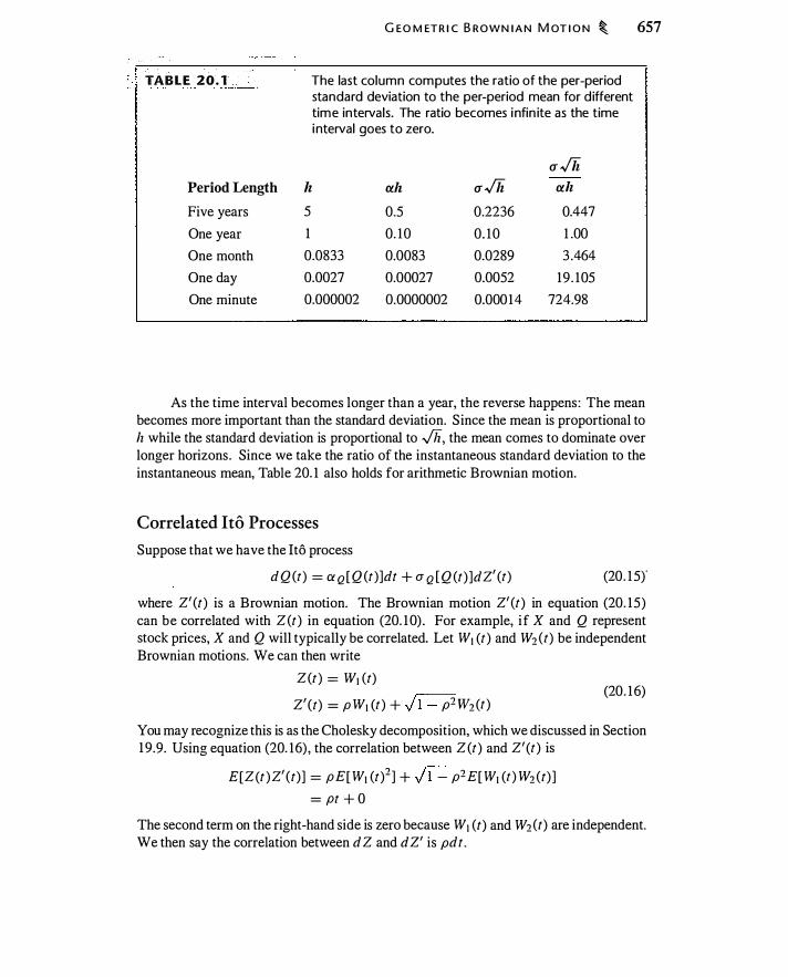
TABLE 20. 1

Period Length

Five years

One year

One month

One day

One minute

G EO M ETR I C B ROWN I A N M OT I O N � 657

The last column computes the ratio of the per-period standard deviation to the per-period mean for d ifferent time intervals. The ratio becomes infin ite as the time interval goes to zero.

CT -/li 1z a.h CT-/li a.h 5 0.5 0.2236 0.447 1 0. 10 0. 10 1 .00 0.0833 0.0083 0.0289 3 .464 0.0027 0.00027 0.0052 19 . 105 0.000002 0.0000002 0.00014 724.98

As the time interval becomes longer than a year, the reverse happens : The mean becomes more important than the standard deviation. S ince the mean is proportional to h while the standard deviation is proportional to .Jh, the mean comes to dominate over longer horizons . Since we take the ratio of the instantaneous standard deviation to the instantaneous mean, Table 20. 1 also holds for arithmetic Brownian motion.

Correlated Ito Processes

Suppose that we have the Ito process

d Q (t) = a Q [Q (t)]dt + a Q [Q (t)]dZ' (t) (20. 15)' where Z' (t) is a Brownian motion. The Brownian motion Z' (t) in equation (20. 15) can be correlated with Z(t) in equation (20. 10) . For example, if X and Q represent stock prices, X and Q will typically be correlated. Let W1 (t ) and W2 (t) be independent Brownian motions. We can then write

Z(t) = W1 (t)

Z' (t) = pW1 (t ) + )1 - p2Wz (t) (20. 16)

You may recognize this is as the Cholesky decomposition, which we discussed in Section 1 9.9. Using equation (20. 16) , the correlation between Z(t) and Z'(t ) is

E[Z(t )Z' (t)] = pE[W1 (t)2 ] + .)1 - p2 E[W1 (t ) W2 (t) ] = pt + O

The second term on the right-hand side is zero because W1 (t) and W2(t) are independent. We then say the correlation between d Z and d Z' is pdt.

658 � B R OW N I A N M OT I O N A N D ITO 'S L E M M A

Multiplication Rules

The dominance of the noise term over short intervals has another implication. Since the behavior of dX is dominated by the noise term, the squared return, (dX)2 , reflects primarily the noise term. We have

[X (t + lz) - X (t)f = [ aX(t)lz + cr X (t) Y(t).Jhr

Expanding this expression and simplifying, we have

[X (t + lz) - X (t)f = a2 X (t)2/z2 + 2acr X (t) 2Y (t)lz 1 .s + cr2 X (t)2 Y (t)21z

Suppose that h is 1 day. Then lz = 0.00274, !z l .5 = 0.000 143, and lz2 = 0.0000075 . If lz is 1 hour, then h = 0.000 1 14, !z l .5 = 0.00000 12, and /z2 = 0.0000000 1 . Clearly, the relative magnitude of the term multiplied by h is much greater than the other terms as lz becomes very small. In addition, if we think of Y as binomial, then Y (t )2 = 1 . This leads us to write

or

essentially ignoring all terms that are higher powers of lz . This equation tells us that if we look at the squared stock price change over a small interval, all we are seeing is the effect of the variance.

We can also consider terms like

[X (t + /z) - X(t)]lz

Rewriting this expression gives us [ aX (t)lz + cr X (t) Y (t).Jh] lz = aX (t) lz2 + cr X (t) Y (t)Jz l .5

Since the smallest power of 1z is 1 .5 , this entire term vanishes relative to 1z as lz goes to zero.

Suppose we have two different Ito processes such as equations (20. 1 0) and (20. 15)._ We can write dZ' (t) = Y'.Jdt where E[Y (t) Y' (t) ] = p. Thus, p is the correlation between Y (t) and Y'(t) . We have

E ([X (t + lz) - X(t)] [Q (t + h) - Q (t)l)

= E ([aX(t)h + crX(t) Y (t + lz)Jh] [a Q Q (t)lz + CTQ Q(t)Y' (t + h )Jh]) = CTCT QPX (t) Q (t)h + (terms with power 2: !) One way to make these calculations mechanical is to use the following so-called

"multiplication rules" for terms containing dt and d Z:

dt x dZ = 0

(dt)2 = 0

(20. 1 7a)

(20. 1 7b)

(dZ)2 = dt dZ x dZ' = pdt

TH E S H A R P E R AT I O � 659

(20. 1 7c) (20. 1 7d)

The reasoning behind these multiplication rules is that the multiplications resulting in powers of dt greater than 1 vanish in the limit.

20.4 THE- SHARPE RATIO

If asset i has expected return a; , the risk premium is defined as

Risk premium; = a; - r

where r is the risk-free rate. A basic idea in finance is that the return on an asset is linked to its risk, where risk is measured as the covariance between the return on the asset and investor utility.5 In the Capital Asset Pricing Model (CAPM), the risk that matters is the covariance between a stock and the market return since investor utility depends on the market return. There are other models of risk, but for our purposes we need not take a stand on a particular model.

The Sharpe ratio for asset i is the risk premium, a; - r, per unit of volatility, a; : a · - r

Sharpe ratio; = -' -. -a;

(20. 1 8)

The Sharpe ratio is commonly used to compare well-diversified portfolios and is not intended to compare individual assets. In particular, if diversifi.able risk is different, two assets with the same a can have different risk premiums (and hence different Sharpe ratios) if they have different covariances with the market. However, we can use the Sharpe ratio to compare two perfectly correlated claims, such as a derivative and its underlying asset. The main point of this section is that two assets that are perfectly correlated will have the same Sharpe ratio.

To see that two perfectly correlated assets must have the same Sharpe ratio, consider the processes for two nondividend paying stocks :

dS1 = a 1 S1 dt + a 1 S1 dZ dS2 = a2S2dt + a2S2dZ

(20. 19) (20.20)

Because the two stock prices are driven by the same dZ, it must be the case that (a 1 - r)ja 1 = (a2 - r)ja2 , or else there will be an arbitrage opportunity.

Before we examine the arbitrage, let's explore the intuition. For example, in the CAPM, the risk premium of asset i , a; - r, is

a; - r = /3; (aM - r) (20.2 1 )

5 See Appendix l l .B .

660 � B R O W N I A N M OT I O N A N D ITO 'S L E M M A

where CiM i s the expected return on the market portfolio. The beta of asset i i s

P;.Ma; /3; = -- (20.22) aM

where Pi.M is the correlation of asset i with the market, a; is the volatility of the asset, and aM is the market volatility. Using equation (20.22), we can rewrite equation (20.2 1 ) as

Ci; - r CiM - r --- = Pi,M __ _ a; aM (20.23)

Thus, if two assets have the same correlation with the market (P;.M ), they will have the same Sharpe ratios. In equations (20. 1 9) and (20.20), the fundamental uncertainty driving the processes for both S 1 an� S2 is d Z. Thus, both assets have the same correlation with the market, and in the CAPM would have equal Sharpe ratios.

We will now demonstrate an arbitrage if the Sharpe ratios in equations (20. 1 9) and (20.20) are different. Suppose that the Sharpe ratio for asset I is greater than that for asset 2. We then buy 1 / (a 1 S1 ) shares of asset l and short l / (a2S2) shares of asset 2. These two positions will generally have different costs, so we invest (or borrow) the cost difference, l fa 1 - l /a2, by buying (or borrowing) the risk-free bond, which has the rate of return rdt . The return on the two assets and the risk-free bond is

--dS1 - --dSz + - - - rdt = -- - -- dt 1 1 ( I I ) (Ci l - r Ciz - r ) a 1 S1 a2S2 az a 1 . a 1 az (20.24)

This demonstrates that if the Sh�e ratio of asset 1 is greater than that of asset 2, we can construct a zero-investment portfolio with a positive risk-free return. Therefore, to preclude arbitrage, assets 1 and 2 must have the same Sharpe ratio.6

This link between volatility and risk premiums for perfectly con·elated assets arose in Chapter 1 2 when we discussed option elasticity. There we saw that the Sharpe ratio for a stock and an option on the stock are the same. The reason is that the stock and option have the same underlying source of risk-the same d Z. They do not have the same volatility-the volatility of a call option is greater than that of the stock-and, hence, they do not have the same risk premium. Nevertheless, they do have the same Sharpe ratio.

20.5 THE RISK-NEUTRAL PROCESS

We saw in Chapters 1 0 and 1 1 that we can interpret the binomial model either as repre­senting a risk-neutral stock price process, in which case we set probabilities so that assets earn the risk-free rate and we discount cash flows at the risk-free rate, or as representing the true stock price process, in which case we use true probabilities and discount at an appropriate (not risk-free) interest rate. In valuing options using Monte Carlo simulation in Chapter 19 , we again used the risk-neutral approach, assuming that stocks on average

6Problem 20. 1 2 asks you to consider the case where two assets are perfectly negatively correlated.

TH E R I S K- N E UT R A L P R O C ESS � 661

earn the risk -free rate and discounting expected payoffs at that rate. The risk -neutral pric­ing method arises from no-arbitrage pricing, but there is underlying economic intuition that we discuss in this section.

The notion of a risk-neutral process for the stock arises with Ito processes, just as in the binomial tree. We saw in Section 20.2 that Brownian motion is a process for which E[Z(t + s)] = Z(t) . In other words, Brownian motion is a martingale. In order to make such a statement, we must specify a probability distribution, or measure, for Z(t + s) , conditional on Z(t) . This point requires emphasis: in order to say whether a stochastic process is a martingale, we need to specify a probability distribution for the process.

Suppose the true price process is

dS(t) -- = (a - 8)dt + crdZ(t) S(t) (20.25)

where 8 is the dividend yield on the stock. This process represents the stock price we observe in the world, with dZ(t) the unexpected portion of the stock return. On average we expect the stock to appreciate at the rate a - 8, and the deviations from this return should have mean zero. In other words, Z(t) should be a martingale under the true probability distribution.

Now let's consider how a risk-averse investor assesses the stock price process. In utility terms, a risk-averse investor by definition values $ 1 of gain less than $ 1 of loss. When such an investor receives the return on an asset, the portion of the return that is a martingale will have negative expected value in utility terms: The gain from an increase in Z (t + h) will be worth less than the loss from an equal decrease in Z (t + lz ) .

In equilibrium, this lower expected utility is offset by the asset paying a risk premium, a - r.

This description suggests that there might be another way to write the return on the asset. Suppose we create a new process

Z(t), such that Z(t) does generate a martingale

in utility terms for a risk-averse investor. (Note that this implies that Z(t) is not a

martingale with respect to the true probability distribution.) In order to offset risk · aversion, we must modify the distribution for Z(t + /z) so that positive outcomes are more likely than negative outcomes. However, if we want to substitute dZ(t) for dZ(t) in equation (20.25), the transformed process will not give us the correct stock price unless we reduce the drift term to compensate for the greater expected value of dZ(t) . It turns out that if

Z(t) is a martingale when evaluated in terms of the investor's utility, the appropriate offsetting change in the drift is to remove the risk premium. This gives us the risk-neutral price process

dS(t) --- = (r - 8)dt + crdZ(t) S(t)

(20.26)

In this equation, we subtract the risk premium, a - r, from the drift a - 8, and we replace dZ(t) with dZ(t) . As in the binomial model, when we replace a with r, we must also modify the probabilities associated with stock price movements. Also here and in the binomial model, when we switch to the risk-neutral process, the volatility remains the same.

662 � B R O W N I A N M OT I O N A N D ITO 'S L E M M A

The probability distribution associated with the risk-neutral process, dZ(t) , is said to be the risk-neutral measure. When we perform risk-neutral pricing, we will implicitly assume that we are using the risk-neutral measure. With this revised price process, we can perform valuation as if the investor were risk-neutral, because we have transformed Z (t) to Z (t) in order to make the investor behave risk-neutrally with respect to the revised process. Thus, using equation (20.26), we can perform valuation as if Z{t) were a martingale, because a risk-averse investor will treat it as such in valuation.

It is important to emphasize that in the applications we have discussed to this point, we need not do any extra work in order to use equation (20.26) for pricing.7 In particular, we do not need to worry about how to construct Z (t) from Z (t) . For example, when we perform Monte Carlo valuation of a derivative with a stock as the underlying asset, we draw mean zero random variables to simulate Z (t) and we use those random variables for pricing-discounting expected payoffs at the risk-free rate-without any further adjustment.

The technical result underlying the transformation from equation (20.25) to equa­tion (20.26) is called Girsanov's theorem.8 Girsanov's t�eorem states that a Brownian process, Z(t) , can be transformed into a new process, dZ(t) = dZ(t) + l}dt, that is a martingale under a transformed probability distribution.9 Girsanov's theorem explains how to create the transformed probability distribution. In the case we are discussing, the transformation is based on the Sharpe ratio: set 17 = (a - r) / u . Thus, we have ( a r ) (a - 8)dt + udZ(t) = (r - o)dt + u dZ(t) + -

u-dt

= (r - 8)dt + udZ(t)

The economic intuition behind the change of measure is that investors in equilib­rium are indifferent to a small change in the allocation of their portfolio between risky

7We will see in later chapters, particularly when discussing fixed income, that in some contexts we

need to take account of the risk premium on the underlying asset when moving from equation (20.25)

to equation (20.26).

8References on Girsanov's theorem include Karatzas and Shreve ( 1 99 1 , sec. 3.5), Baxter and Rennie

( 1 996) and Neftci (2000, ch. 1 4).

9 A simplified version ofGirsanov's theorem states that if Z (I) is a Brownian motion under the probabil­

ity density f(t), then Z(t) = Z(l) + 171 , is a Brownian motion under the probability density 1; (1 )/(1 ) ,

where � (1 ) = exp(-qZ(I ) - 0.5q21 ) . The probability density function for a normal variable with

variance 1 is [ I "] I f(t) = exp - - z- --

21 .J21[i You can see how the Girsanov transformation works by examining � (t )f(l) . Writing out � (I) and

combining terms, we obtain [ I ,] I [ I "] I � (I ) exp - - Z(t)- = = exp - - (Z + 171 )- = � � � � � � � �

The last expression i s the probability density for a normally distributed variable with mean -171.

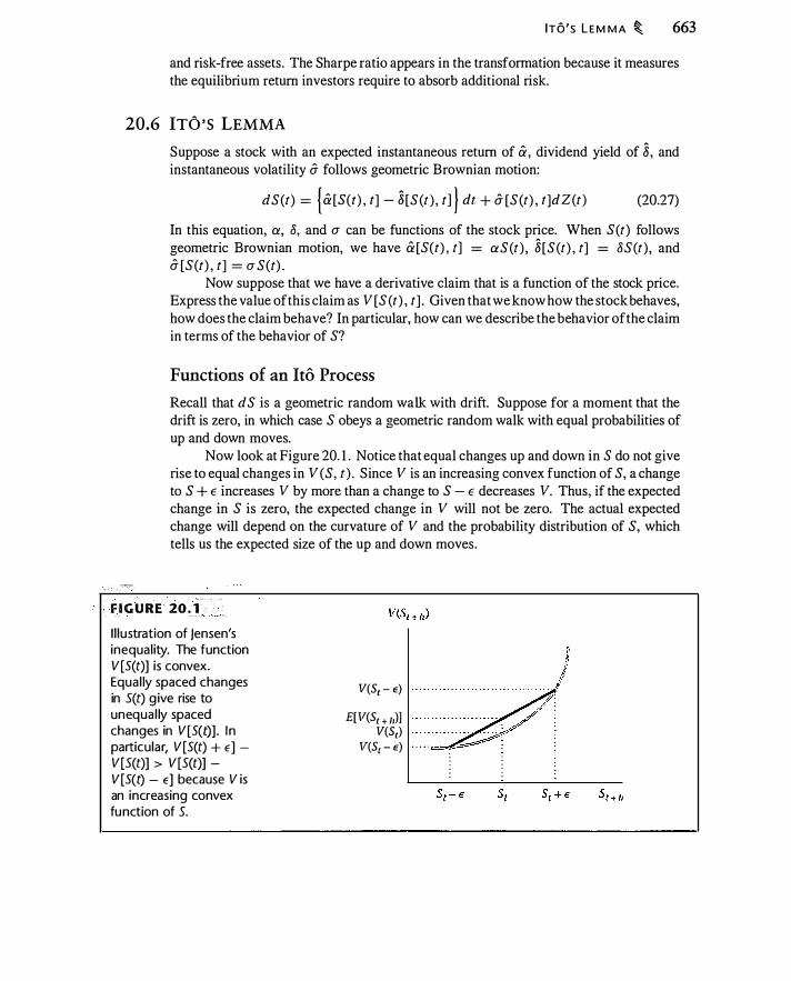
ITO's L E M M A � 663

and risk-free assets. The Sharpe ratio appears in the transformation because it measures the equilibrium return investors require to absorb additional risk.

20.6 ITO'S LEMMA

. · . c-.�

Suppose a stock with an expected instantaneous return of &, dividend yield of 8, and

instantaneous volatility u follows geometric Brownian motion:

dS(t) = {a[S(t) , t] -8[S(t ) , t] } dt + u [S(t) , t]dZ(t) (20.27)

In this equation, a, 8, and a can be functions of the stock price. When S{t) follows geometric Brownian motion, we have &[S(t) , t] = aS(t) , 8 [S(t) , t] = 8S(t) , and u [S(t) , t] = aS(t) .

Now suppose that we have a derivative claim that is a function of the stock price. Express the value of this claim as V[S (t) , t] . Given that we know how the stock behaves, how does the claim behave? In particular, how can we describe the behavior of the claim in terms of the behavior of S?

Functions of an Ito Process

Recall that d S is a geometric random walk with drift. Suppose for a moment that the drift is zero, in which case S obeys a geometric random walk with equal probabilities of up and down moves.

Now look at Figure 20. 1 . Notice that equal changes up and down in S do not give rise to equal changes in V(S, t ) . Since V is an increasing convex function of S, a change to S + E increases V by more than a change to S - E decreases V. Thus, if the expected change in S is zero, the expected change in V will not be zero. The actual expected change will depend on the curvature of V and the probability distribution of S, which tells us the expected size of the up and down moves .

, ... . . . . . · .•.

F I G U RE 20. 1 .... ·· . . ···· ·

I l lustration of jensen's inequal ity. The function V[S(t)] is convex. Equal ly spaced changes in S(t) g ive rise to unequal ly spaced changes in V [S(�] . I n particular, V [S(t) + E] -V[S(t)] > V[S(t)] -V[S(t) - E] because V is an increasing convex function of 5.

V(St - E)

E[ \!(St + 1,)] V(St)

V(St - E)

) �� . . . . . . . . . . . .

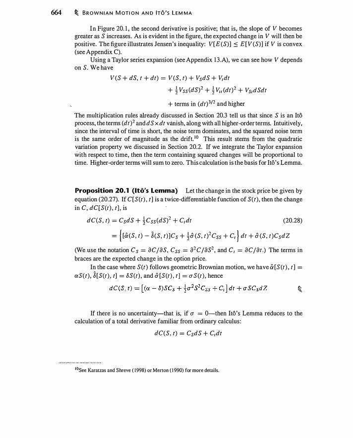
664 � B R O W N I A N M OTI O N A N D ITO 'S L E M M A

In Figure 20. 1 , the second derivative i s positive; that is, the slope of V becomes greater as S increases . As is evident in the figure, the expected change in V will then be positive. The figure illustrates Jensen's inequality: V[E (S)] ::=:: E[V (S)] if V is convex (see Appendix C).

Using a Taylor series expansion (see Appendix 13 .A), we can see how V depends on S. We have

V (S + dS, t + dt) = V (S , t) + VsdS + V,dt

+ t Vss (dS)2 + t Vu (dt)2 + Vs,dSdt

+ terms in (dt)312 and higher

The multiplication rules already discussed in Section 20.3 tell us that since S is an Ito process, the terms (dt )2 and d S x dt vanish, along with all higher-order terms. Intuitively, since the interval of time is short, the noise term dominates, and the squared noise term is the same order of magnitude as the drift. 1 0 This result sterns from the quadratic variation property we discussed in Section 20.2. If we integrate the Taylor expansion with respect to time, then the term containing squared changes will be proportional to time. Higher-order terms will sum to zero. This calculation is the basis for Ito's Lemma.

Proposition 20.1 (Ito's Lemma) Let the change in the stock price be given by equation (20.27). If C[S(t) , t] is a twice-differentiable function of S(t) , then the change in C, dC[S(t) , t] , is

dC(S, t) = CsdS + iCss (dS)2 + C,dt (20.28)

= { [& (S, t ) - 8 (S, t ) ]Cs + iu (S, t )2Css + C, } dt + u (S, t )CsdZ

(We use the notation Cs = acjaS, Css = a2CjaS2 , and C, = acjat .) The terms in braces are the expected change in the option price.

In the case where S(t) follows geometric Brownian motion, we have & [S (t) , t ] = aS(t) , 8 [S(t ) , t] = 8S(t) , and B [S(t) , t] = aS(t) , hence

If there is no uncertainty-that is, if a = 0-then Ito's Lemma reduces to the calculation of a total derivative familiar from ordinary calculus :

dC(S, t) = CsdS + C,dt

1 0See Karatzas and Shreve ( 1 998) or Merton ( 1 990) for more details.

ITO 's L E M M A � 665

The extra term involving the variance arises from (dS)2 and is the Jensen's inequality correction due to the uncertainty of the stochastic process.

We encountered Ito's Lemma-without naming it-when we discussed delta­gamma approximations in Chapter 13 . Equation ( 1 3 .6) stated

C[S(t + lz) , t + h] - C[S(t) , t] � [S(t + h) - S (t)] t.. [S(t) , t] + Hser + h) - sct)fnscr) , r] + e [s(r) , r]h

Make the substitutions h ---+ dt and S(t + h) - S(t) ---+ dS, and recall that r, .0.. , and e are just partial derivatives of the option price:

.0.. = Cs ; r = Css ; e = C, The delta-gamma approximation over a very short period of time is Ito's Lemma.

We can use Ito's Lemma to verify that the expression for a lognormal stock price satisfies the equation for geometric Brownian motion, equation (20.27).

Example 20. 1 The expression for a lognormal stock price is

S(t) = S(O)e<a-8- �a1)t+aZ(t ) (20.29)

The stock price is a function of the Brownian process Z(t) . We can use Ito's Lemma to characterize the behavior of the stock as a function of Z (t) . We have

as(t) -- = CJS(t ) · BZ (t) '

Ito 's Lemma states that dS(t) is given as

dS(t) = BS (t) dt + BS(t) dZ(t) + � a2S(t�

[dZ(t)f at BZ(t) 2 BZ (t)-

( 1 ") 1 0 = a - 8 - l(J- S(t)dt + CJ S(t)dZ(t) + l(J-S(t)dt

= (a - o)S(t)dt + CJS (t)dZ(t)

In going from the second line to the third we have used the fact that dZ(t)2 = dt. This calculation demonstrates that by using Ito's Lemma to differentiate equation (20.29), we recover equation (20.27). �

Multivariate Ito's Lemma

So far we have considered the case where the value of an option depends on a single Ito process. A derivative may have a value depending on more than one price, in which case we can use a multivariate generalization of Ito's Lemma.

666 � B R O W N I A N M OT I O N A N D ITO 'S LEM MA

Proposition 20.2 (Multivariate Ito's Lemma) Suppose we have n correlated Ito processes :

i = l , . . . , ll

Denote the pairwise correlations as E(dz; x dzj ) = P;.jdt . If C(S1 , • • • , S, , t) is a twice-differentiable function of the S; 's, we have

,

i= l

11 /J

i= l j = l The expected change in C per unit time is

1 , - , ,

dt E [dC (S, , . . . , Sn , t ) ] = :L>�; S; Cs, + t L L CJ;CJ jPij S; SjCs,si + C, � i= l i= l j=l

Example 20.2 Suppose C(S1 , S1) = S1 S1 . Then by Ito's Lemma we have

d(St S:J.) = S1dS, + S,dS1 + dS, dS1 This implies that

1 dt E (dC} = (a , + a2 + PCJ tCJ 1)S1 S1

Note that since C(S1 , S2) does not depend explicitly on time, C, = 0.

Example 20.2 is interesting because we know that the product of lognormal vari­ables is lognormal . Hence, we might expect that the drift for the product of two lognormal variables would just be the sum of the drifts. However, Example 20.2 shows that the drift has an extra term, stemming from the term dS1 dS1, due to the covariation between the two variables. The intuition for this result will be explored further in the discussion of quantos in Chapter 22.

20.7 VALUING A CLAIM ON Sa

Suppose we have a claim with a payoff depending on S raised to some power. For example, we may have a claim that pays S(T)2 at time T . In this section we examine this claim with two goals. First, we want to compute the price of such a claim. Second, we want to understand the different ways to approach the problem of valuing the claim.

The following proposition gives us the forward and prepaid forward prices for this claim.

VA LU I N G A C LA I M O N 5° � 667

Proposition 20.3 Suppose S follows the process given by equation (20.27). The value at time 0 of a claim paying S(T)11-the prepaid forward price-is

Fcf.T [S(T)a ] = e-rT S(O)a e [a (r-8)+ !a (a- l )a2]T

The forward price for S(T)0 is

Fo,T [S(T)a ] = S(O)a e[a (r-8l+!a (a- l )a2] T

The lease rate for a claim paying sa is 8* = r - a (r - 8) - ta(a - 1 )u2 •

(20.30)

(20.3 1 )

�

To prove this proposition, we will first use Ito's Lemma to determine the process followed by sa . We will then use three different arguments to obtain the pricing formula, equation (20.30).

The Process Followed by sa Consider a claim maturing at time T that pays C [S(T) , T] = S(T)D . If S follows equation (20.27), then we can use Ito's Lemma to determine the process followed by sa . We obtain

Dividing by sa , we get

dS11 - = [a (a - 8) + �a(a - l )u2] dt + audZ sa - (20.32)

Thus, sa follows geometric Brownian motion with drift a (a - 8) + �a (a - 1 )u2 and risk ai:J-dZ. Hence, if a is the expected return for S, the expected return of a claim with price sa will be

a (a - r) + r (20.33)

Thus, the risk premium is a (a - r) . There is another way to obtain the drift term in equation (20.32) that does not

require the use of Ito's Lemma. We can write

S(T)a = S (O)a ea (a-8-0.5a2)T +aaZ(T)

Using equation ( 1 8 . 13 ) to compute the expectation of a lognormal variable, we have

E [S (T)a ] = S (Ot ea<a-8-0.5a2)T +D.5a2a2T

= S (O)a e!a (a-8)+0.5a(a- l )a2JT

668 � B R OW N I A N M OTI O N A N D ITO'S L EM M A

Thus, the expected continuously compounded return on sa is a (a - 8) + 0.5a (a - l )a2, as in equation (20.32).

Proving the Proposition

Given equations (20.32) and (20.33), there are three arguments we can use to compute the time-0 value of a claim that pays S(T)a at time T. All three methods will confirm Proposition 20.3 .

Risk-neutral pricing First we use risk-neutral pricing. Subtract the risk premium, ' a (a - r) , from the drift, a (a - 8), to obtain the following as the risk-neutral process

for dS0 :

- = a (r - 8) + -a(a - 1 )a- dt + aadZ · dSa [ 1 �J ,. sa 2

(20.34)

Using the drift term in equation (20.34 ), the expected value of the claim at time T under · the risk-neutral measure, which we denote E*, is

E� [S(T)" ] = S(O)a e[a (r-8l+ia (a- l )u']T (20.35)

We saw in Section 10 . 1 that the expected price under the risk-neutral measure is the for­ward price. Thus, equation (20.35) gives the forward price. Discounting this expression at the risk-free rate gives us the prepaid forward price, equation (20.30).

Discounted cash flow We can· also value the claim on S" by discounting the true (nonrisk-neutral) expected value. To do this we must compute the expected value of the claim and discount the expected payoff appropriately. From equation (20. 1 4) , the expected value of S(T)" is

Eo [S (T)a ] = S(O)a e[a (a-o)+ Ha- l )u']T

The discount rate is expression (20.33) . The price at time 0 of a claim paying S(T)a at time T is the prepaid forward price, which we will denote F{T (S0 ) :

F{T (S" ) = e-[r+a<a-r)JT E (S(T)a )

= e-[r+a (a-r) ]T S(O)" e[a(a-8>+ia (ll- l >u' ]T

= S(O)a e-rT e[a (r-8>+ill (a- l )u2]T

Note that the risk premium on the stock, a - r , drops out. The forward price for S" , which we will denote Fo.T (S0 ) , is just the future value of the prepaid forward:

Fo. T (Sa ) = erT F{T (S")

= S (O)" e [" <r-8>+4a<ll- l )u'] T

The use of a single discount rate works i n this case because the payoff to the claim is simple. In general, computing a price as a nonrisk-neutral discounted expected value is more difficult than this.

·

VA LU I N G A C LA I M O N sa � 669

Finding the lease rate Finally, we value the claim by finding its lease rate. We ask what cash payment the claim would have to make in order for us to willingly hold it, or equivalently, what payment we would have to make to short-sell it. We can then treat the lease rate as the dividend yield and compute the forward price.

From equation (20.32), the claim has risk a adZ and so must be expected to earn a rate of return of a (o: - r) + r. Equation (20.32) also tells us that the actual expected capital gain on this security is a (o: - 8) + �a (a - 1 )a2 •

In order to hold the security, we would need to earn the difference between the expected return and expected capital gain as a cash payment. Thus, the payment would have to be

8* = a (o: - r) + r - [a (o: - 8) + �a (a - l )a2]

= r - a (r - 8) - �a(a - 1 )a2

The value 8* is the lease rate of the claim paying sa . The prepaid forward price is then

FcfT (Sa ) = S(O)ae-.S*T

= S(O)a e[-r+a(r-o>+ 1a <a- l )u2]T

This is the same as equation (20.30).

Specific Examples

We now examine four special cases of equations (20.30) and (20.3 1 ) : a = - 1 , 0, 1 , and 2.

Claims on S First, suppose a = 1 . Equation (20.30) then gives us

V (O) = S(O)e-.sT

This equation is just the prepaid forward price on a stock.

Claims on S0 If a = 0, the claim does not depend on the stock price; rather since S0 = 1 , it is a bond. Setting a = 0 gives us

V (O) = e-rT

which is the price of a T -period pure discount bond.

Claims on S2 When a = 2 the claim pays S(T )2 . From equation (20.3 1 ), the forward price is

Fo.T (S2) = e'T S(0)2e- [-r+2.S-u2JT

= S(0)2e2(r-cS)T eu2T

= [Fo. T (S)]2 eu2T (20.36)

670 � B ROWN IAN M OTI O N AN D ITO'S L EM M A

Thus, the forward price on the squared stock price i s the squared forward price times a variance term. The squared forward price is intuitive, but the variance term requires some discussion.

One way to think about equation (20.36) is to perform the following thought experiment. Suppose that we have an ordinary stock with a price denominated in dollars . Now imagine that we have a second stock that is identical to the first except that instead of receiving dollars when we sell the stock, we receive one share of ordinary stock for each dollar in the quoted price of the second stock. This conversion from dollars to shares is what it means to have a squared security.

With the squared stock, when the stock price goes up, we not only receive the extra ' dollars a share of stock is worth, but we also receive the appreciated value of each share

we receive in lieu of dollars. We therefore receive an extra gain when the stock price goes up.

The effect works in reverse when the price goes down. In that case, we receive fewer dollars per share, and each share received in lieu of dollars is worth less as well. However, the lower price per share hurts us less because we receive fewer shares ! Thus, on average, the extra we receive when the price goes up exceeds the loss when the price goes down. This effect becomes more important as the variance is greater, since large losses and large gains become more likely.

The result is that we will pay extra for the security, and the extra amount we pay is positively related to the variance. This example provides another illustration of Jensen's inequality.

Claims on 1 /S Finally, let a = - 1 , so the claim pays 1 /S. Using equation (20.3 1 ) with a = -1 , we get

Fo,T ( l /S) = [ 1 /S(O) ] e<o-r)T eu'T

_ F. - I eu'T - O. T

As with the squared security, the forward price is increasing in volatility. The payoffs for both the S2 and 1 / S securities are convex; hence, Jensen's inequal­

ity tells us that the price is higher when the asset price is risky than when it is certain. In both cases the forward price contains a volatility term, and in both cases the price is increasing in volatility. If we considered a concave claim, for example .JS, the effect of increased volatility would be to lower the value of the claim. End-of-chapter problems 20.5-20.8 provide examples.

Valuing a Claim on saQb

Now we generalize the previous example by having two prices . Consider a claim paying S(Tt Q(T)b where S follows

dS S = (as - os)dt + usdZs (20.37)

VALU I N G A C LA I M O N 5° � 671

and Q follows

(20.38)

where

Proposition 20.4 Suppose that S and Q follow the processes given by equations (20.37) and (20.38) . The forward ptices for sa and Qb are given by Proposition 20.3 . The forward price for sa Qb is the product of those two forward prices times a covariance correction factor:

The variance of sa Qb is given by

a2u� + b2u� + 2abpu seT Q

Note that the squared security, S2 , is a special case of Proposition 20.4. When S = Q, a = b = 1 , and p = 1 (since a variable is perfectly correlated with itself), the covariance term becomes

� abpusu Q = u5

This gives us the same result as equation (20.36) for the forward price for a squared stock.

Using multivariate Ito's Lemma, the process for sa Qb is

d (sa Qb) [ 1 � I � --'-�-,-b -'- = a (as - 8s) + b (aQ - 8Q) + ?a (a - l )cr5 + ?b (b - 1 )u-Q � Q - -

+ abpu seT Q J dt + au sdZs + bu QdZQ (20.39)

The expected return on this claim depends on the risk premiums for both S and Q: 1 1

r + a (as - r) + b(a Q - r)

As before, there are three ways to find the price of a prepaid forward on this claim. Here we use risk-neutral pricing. Problem 20. 1 3 asks you to use the discounting and lease-rate methods to find the answer.

1 1 Problem 20. 1 1 asks you to verify that this expression gives the expected return.

672 � B ROWN I A N MOTI O N AN D ITO'S L EM MA

The risk -neutral process for d S" Qb i s obtained by subtracting the risk premium, a (as - r ) + b(a Q - r), from the drift in equation (20.39). This gives

d (sa ob ) ---'----=-b -'- = [a (r - 8s) + b(r - 8Q) + �a (a - l )cr� + �b(b - l )cr2Q sa Q . - -

+ abpcr scr Q J dt + acr sdZ� + bcr QdZ'Q

The expected time-T value of sa Qb under the risk-neutral measure is

E* [ S (Tt Q (T)b ] = S (O)a Q (O)b e[a (r-8s )+b(r-oQ )+ta <a- 1 )cr�+th<b- 1 )crt+abpcr 5cr Q JT

Using Proposition 20.3, in particular equation (20.3 1 ) , this expression can be rewritten as

p, (S" Ob) = p, (S" ) P, ( Ob) eabpcrscr Q T O, T - O,T O, T - (20.40) The expression on the right is the product of the forward prices times a factor that accounts for the covariance between the two assets .

This is an important result: The price that results when we multiply two prices together requires a correction for the covariance. We will see this result again in Chapters 2 1 and 22.

Proposition 20.4 can be generalized. Suppose there are n stocks, each of which follows the process

dS; -- = (a · - 8 · )dt + cr ·d7 · S;

I I I -1

where dz;dZj = pijdt. Let

II V (t) = n S�'

The forward price for V is then

20.8 jUMPS IN THE STOCK PRICE 1 2

i= l

(20.4 1 )

(20.42)

(20.43)

A practical objection to the Brownian process as a model of the stock price is that Brow­nian paths are continuous-there are no discrete jumps in the stock price. In practice, asset prices occasionally do seem to jump; a famous example is October 1 9, 1 987, when the Dow Jones index fell 22% in one day. A move of this size is exceedingly unlikely

1 1This section follows Merton ( 1 976).

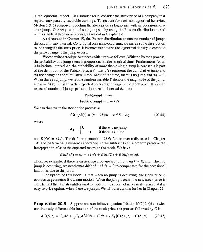
j U M PS I N TH E STO C K P R I C E � 673

in the lognormal model . On a smaller scale, consider the stock price of a company that reports unexpectedly favorable earnings. To account for such nonlognormal behavior, Merton ( 1 976) proposed modeling the stock price as lognormal with an occasional dis­crete jump. One way to model such jumps is by using the Poisson distribution mixed with a standard Brownian process, as we did in Chapter 1 9 .

As discussed in Chapter 1 9, the Poisson distribution counts the number of jumps that occur in any interval. Conditional on a jump occurring, we assign some distribution to the change in the stock price. It is convenient to use the lognormal density to compute the price change if the jump occurs.

We can write a stock price process with jumps as follows. With the Poisson process, the probability of a jump event is proportional to the length of time. Furthermore, for an infinitesimal interval dt, the probability of more than a single jump is zero (this is part of the definition of the Poisson process). Let q (t) represent the cumulative jump and dq the change in the cumulative jump. Most of the time, there is no jump and dq = 0. When there is a jump, we let the random variable Y denote the magnitude of the jump, and k = E(Y) - 1 is then the expected percentage change in the stock price. If A. is the expected number of jumps per unit time over an interval dt, then

ProbGump) = A.dt Prob(no jump) = 1 - A.dt

We can then write the stock price process as

where

dS(t)jS(t) = (a - Ak)dt + adZ + dq

if there is no jump if there is a jump

(20.44)

and E(dq) = Akdt . The drift term contains -Akdt for the reason discussed in Chapter 19 : The dq term has a nonzero expectation, so we subtract A.kdt in order to preserve the . interpr!'!tation of a as the expected return on the stock. We have

E(dSjS) = (a - Ak)dt + E(crdZ) + E (dq) = adt

Thus, for example, if there is on average a downward jump, then k < 0, and, when no jump is occurring, we need extra drift of -A.kdt > 0 to compensate for the occasional bad times due to the jump.

The upshot of this model is that when no jump is occurring, the stock price S evolves as geometric Brownian motion. When the jump occurs, the new stock price is YS. The fact that it is straightforward to model jumps does not necessarily mean that it is easy to price options when there are jumps. We will discuss this further in Chapter 2 1 .

Proposition 20.5 Suppose an asset follows equation (20.44). If C(S, t ) i s a twice continuously differentiable function of the stock price, the process followed by C is

1 1 1 dC(S, t) = CsdS + 2Csscr-S-dt + C,dt + A.Ey [C (SY, t) - C(S, t) ] (20.45)

674 � B ROWN IAN M OT I O N AN D ITO 'S L EM M A

The last term i n equation (20.45) i s the expected change i n the option price conditional on the jump times the probability of the jump. �

The last term in equation (20.45) accounts for the jump. That term is not present in the version of lto's Lemma for a stock that cannot jump, equation (20.28).

- - - - - - -�---------------- _____ , · - - - - - - ----- -----· . -· -··. _. _ --�...;,-·. ·_· _;___':;:.._.:_ . . . ; --·-· --·--- - ·-· . .

CHAPTER S UMMARY

A stochastic process Z(t) is a Brownian motion if it is normally distributed, changes independently over time, has variance proportional to time, and is continuous. The _change in Brownian motion is denoted dZ(t) . The process Z(t) and its change dZ(t) provide the foundation for modem derivatives pricing models. The Brownian process Z(t) by itself would be a poor model of an asset price, but its change, dZ(t) , provides a model for asset risk. By multiplying dZ(t) by a scale factor and adding a drift term, we can control the variance and mean, and thereby construct more realistic processes. Such processes are called Ito processes or diffusion processes. Black and Scholes used just such a process in their original derivation of the o'ption pricing model.

Given that a stock follows . a particular Ito process, Ito's Lemma permits us to compute the process followed by an option or other claim on the stock. The pricing of claims with payoffs sa and sa Qb , where S and Q follow geometric Brownian motion, illustrates the use of Ito's Lemma.

An important objection to Brownian motion as a driving process for a stock is the continuity of its path. It is possible to add jumps to a Brownian process, and there is a version of ItO's Lemma for such cases.

FURTHER READING

We will use the concepts in this chapter throughout the rest of the book. In the next chapter we will directly apply the concepts of this chapter, in particular Ito's Lemma, showing that prices of derivatives must satisfy a particular partial differential equation. In later chapters we will use these concepts to discuss the pricing of exotic options (Chapter 22), options based on interest rates (Chapter 24), and risk assessment (Chap­ter 25).

Many books cover the material in this chapter at a more advanced level. Merton ( 1 990) in particular is an outstanding introduction . Other good sources include Neftci (2000), Duffie ( 1 996), Wilmott ( 1 998), Karatzas and Shreve ( 1 99 1 ), and Baxter and Rennie ( 1 996).

PROB LEMS

P R O B LEMS � 675

For the following four problems, use Ito's Lemma to determine the process followed by the specified equation, assuming that S(t) follows (a) arithmetic Brownian motion, equa­tion (20.8); (b) a mean reverting process, equation (20.9) ; and (c) geometric Brownian motion, equation (20.27).

20.1. Use Ito's Lemma to evaluate d[ln(S)] .

20.2. Use Ito's Lemma to evaluate dS2 .

20.3. Use Ito's Lemma to evaluate ds- 1 •

20.4. Use Ito 's Lemma to evaluate d(.)S) .

20.5. Suppose that S follows equation (20.37) and Q follows equation (20.38). Use Ito's Lemma to find the process followed by S2 Q0·5 .

20.6. Suppose that S follows equation (20.37) and Q follows equation (20.38) . Use Ito's Lemma to find the process followed by ln(S Q) .

20.7. Suppose S(O) = $ 100, r = 0.06, as = 0 .4 and 8 = 0 . Use equation (20.30) to compute prices for claims that pay the following:

a. S2

b. -JS c. s-2

Compare your answers to the answers you obtained to Problem 1 9.6.

20.8. Suppose that ln (S) and ln ( Q) have correlation p = -0.3 and that S(O) = $ 100, Q (0) = $ 1 00, r = 0.06, as = 0.4 and a Q = 0.2. Neither stock pays dividends. Use equation (20.40) to find the price today of claims that pay

a. S Q

b . S/ Q

c . ..[SQ d. 1 / (SQ)

e . S2 Q

Compare your answers to the answers you obtained to Problem 1 9 .7.

20.9. Suppose that X(t) follows equation (20.9). Use Ito's Lemma to verify that a solution to this differential equation is

Xr = X (O)e-).r + a ( 1 - e-).r ) + a 11 e!.(s-r )dZs

(Hint: Note that when t increases by a small amount, the integral term changes by dZ(t) . )

676 � B RO W N I A N M OT I O N AN D ITO 'S LEM M A

20.10. The formula for an infinitely lived call is given i n equation ( 1 2. 1 9) . Suppose that S follows equation (20.27), with a replaced by r and that E* (dV) = r V dt. Use Ito's Lemma to verify that the value of the call, V (S) , satisfies this equation:

tcr 2S2 Vss + (r - 8)SVs - r V = 0 20.11. Suppose that the processes for S1 and S2 are given by these two equations:

dS[ = a [ S[ dt + CT [ S[dZ [ d s2 = a2S2dt + CT2S2d z2

Note that the diffusions d Z 1 and d Z2 are different. In this problem we want to find the expected return on Q , aQ , where Q follows the process

dQ = aQ Qdt + Q ( 17 1 dZ 1 + 1]2dZ1) Show that, to avoid arbitrage,

1) 1 IJ2 aQ - r = -(a l - r) + -(a2 - r) CT [ 0"2

(Hint: Consider the strategy of buying one unit of Q and shorting Q17 1 IS 1 cr 1 units of S1 and Q 172/ S2cr2 units of S2 • Finance any net cost using risk-free bonds.)

20.12. Suppose that S follows equation (20.27) with 8 = 0. Consider an asset that follows the process

. d Q / Q = aQdt - 1]dZ What is aQ , expressed in terms of a? (Hint: Find a zero-investment position in S and Q that eliminates risk.)

20.13. Suppose that S and Q follow equations (20.37) and (20.38) . Derive the value of a claim paying S(T)a Q (T)b by each of the following methods :

a. Computing the expected value of the claim and discounting at an appro­priate rate. (Hint: The expected return on the claim can be derived using the result of Problem 20. 1 1 . )

b. Computing the lease rate and substituting this into the formula for the forward price.

20.14. Assume that one stock follows the process

dS/ S = adt + udZ (20.46)

Another stock follows the process

dQjQ = aQdt + udZ + dq 1 + dqz (20.47) (Note that the ud Z terms for S and Q are identical .) Neither stock pays dividends. dq 1 and dq2 are both Poisson jump processes with Poisson parameters .A 1 and .A2 • Conditional on either jump occurring the percentage change in the stock price is Y1 - 1 or Yz - 1 .

P RO B LE M S � 677

Consider the two stock price processes, equations (20.46) and (20.47).

a. If there were no jump terms (i.e., }q = )..2 = 0), what would be the relation between a and a Q?

b. Suppose there is just one jump term ()..2 = 0) and that Y1 > 1 . In words, what does it mean to have Y1 > 1 ? What can you say about the relation between a and a Q ?

c. Write an expression for a Q when both jump terms are nonzero. Explain intuitively why aQ might be greater or less than a.

CHAPTER 2r -�·----- ----- ��-"·-'------------------

The Black -Scholes Equation

I n deriving the option pricing formula, Black and Schol"' "udied the p�blem faced by a delta-hedging market-maker. As we saw in Chapter 13 , the market-maker who sells a call option buys shares to offset the risk of the written call. To analyze this situation it is necessary to characterize the risk of the position as a function of the share price. Ito's Lemma, discussed in Chapter 20, provides a tool that permits us to see how the option price changes in response to the stock price.

Black and Scholes assumed that the stock follows geometric Brownian motion and used Ito's Lemma to describe the behavior of the option price. Their analysis yields a partial differential equation, which the correct option pricing formula must satisfy.

In this chapter we study the Black-Scholes approach to pricing options. ' This methodology is important not only for pricing European call options; it provides the intellectual foundation for pricing virtually all derivatives, and also underpins the risk-· management practices of modern financial institutions.

21 .1 DIFFERENTIAL EQUATIONS AND VALUATION UNDER CERTAINTY

The e�d result of the Black-Scholes derivation is a partial differential equation that describes the price of an option. At first glance the idea of using a differential equation to perform valuation may seem perplexing and special to options. However, differential equations can also be used to motivate even very simple calculations that appear in an elementary finance course. The valuation of stocks and bonds when payouts are known provides simple examples . We will demonstrate this in order to provide some context for the discussion of the Black-Scholes model.

1 Robert Merton also contributed fundamental ly to understanding the option pricing problem. As a

result, the analysis in this chapter can also appropriately be referred to as the '"Black-Scholes-Merton"'

methodology.

679

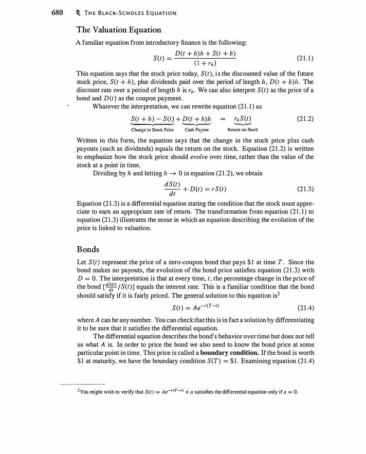
680 � TH E B LA C K-S C H O LES EQUAT I O N

The Valuation Equation

A familiar equation from introductory finance is the following:

D(t + h)lz + S(t + h ) S(t) = -------

( 1 + I"!J ) (2 1 . 1 )

This equation says that the stock price today, S(t) , i s the discounted value of the future stock price, S(t + lz ) , plus dividends paid over the period of length /z , D(t + h)lz . The discount rate over a period of length lz is I"!J . We can also interpret S (t) as the price ·of a bond and D(t) as the coupon payment.

Whatever the interpretation, we can rewrite equation (2 1 . 1 ) as

S(t + lz ) - S(t) + D(t + h)h = I), S (t) Change in Stock Price

'-,--' '--.,.-' Cash Payout Return on Stock

(2 1 .2)

Written in this form, the equation says that the change in the stock price plus cash . payouts (such as dividends) equals the return on the stock. Equation (2 1 .2) is written to emphasize how the stock price should evolve over time, rather than the value of the stock at a point in time.

Dividing by lz and letting lz --7 0 in equation (2 1 .2), we obtain

dS(t) ----;If + D(t) = rS(t) (2 1 .3)

Equation (2 1 .3) is a differential equation stating the condition that the stock must appre­ciate to earn an appropriate rate ·of return. The transformation from equation (2 1 . 1 ) to equation (2 1 .3) illustrates the sense in which an equation describing the evolution of the price is linked to valuation.

Bonds

Let S(t) represent the price of a zero-coupon bond that pays $ 1 at time T . Since the bond makes no payouts, the evolution of the bond price satisfies equation (2 1 .3) with D = 0. The interpretation is that at every time, t , the percentage change in the price of the bond [ d��t l j S(t) ] equals the interest rate. This is a familiar condition that the bond should satisfy if it is fairly priced. The general solution to this equation is2

S(t) = Ae-r<T-r ) (2 1 .4) where A can be any number. You can check that this is in fact a solution by differentiating it to be sure that it satisfies the differential equation.

The differential equation describes the bond's behavior over time but does not tell us what A is. In order to price the bond we also need to know the bond price at some particular point in time. This price is called a boundary condition. If the bond is worth $ 1 at maturity, we have the boundary condition S(T) = $ 1 . Examining equation (2 1 .4)

2You might wish to verify that S(t ) = Ae-r(T -n + a satisifies the differential equation only if a = 0.

TH E B LA C K-S C H O LES EQUATI O N � 681

shows that S(T) can equal $1 only if A = $ 1 . Thus, the bond price is

S(t) = $1 x e-r(T-r )

The condition S(T) = $ 1 is called a terminal boundary condition because it sets the bond price at its maturity date. If instead we knew the bond price today, S(O) , we could set A so that the equation gave the correct value for S(O) . That value would be an initial boundary condition.

The solution confirms what you already know: The price of the bond is the present value of $ 1 .

Dividend-Paying Stocks

We can interpret S(t) as the price of a risk-free stock that pays a continuous fixed dividend of D and has a price of S at time T . Equation (2 1 .3) then says that at every time, t, dividends plus capital gains on the stock provide the risk-free rate of return.

Since we know the value at time T will be S, we also have the boundary condition

S(T) = S Equation (2 1 .3) with this boundary condition has the solution

S(t) = ! T De-r(s-r )ds + se-r(T-r)

The stock price today is the discounted value of dividends to be paid between now and time T , plus the present value of the stock at time T . Again, the discrete time version of this equation is the standard present value formula taught in every introductory finance class.

The General Structure

Under certainty, a bond or stock will be priced so that the owner receives a risk -free return. The differential equation in these examples describes how the security changes from a given point. The boundary condition describes the price at some point in the security's life (such as at a bond's maturity date) . By combining the differential equation and the boundary condition, we can determine the price of the bond at any point in time.

By analogy, if at every point you know an automobile's speed and direction, and if you know where it stops, you can work backward to figure out where it started. Essentially the same idea is used to price options: We know the price of the option at maturity (for a call it is max [O, S - K]), and we then need to know how the option price changes over time.

21 .2 THE BLACK-S CHOLES EQUATION

Consider the problem of owning an option and buying or selling enough shares to create a riskless position. Assume that the stock price follows geometric Brownian motion:

dS s = (a - o)dt + udZ (2 1 .5)

682 � TH E B LACK-S C H O LES EQUAT I O N

where a i s the expected return on the stock, u is the stock's volatility, and 8 i s the continuous dividend yield on the stock. The option value depends on the stock price, S(t) , and time, t, so we write it as V [S(t) , t] . Also suppose there are risk-free bonds that pay the return r. If we invest W in these bonds, the change in the value of the bond position is

dW = rWdt (2 1 .6) Let I denote the total investment in the option, stocks, and the risk-free bond.

Suppose that we buy N shares of stock to hedge the option and invest W in risk-free bonds so that our total investment is zero. Then we have

I = V(S, t) + NS + W = 0 (2 1 .7) The zero-investment condition ensures that we keep track of financing costs. It imposes the requirement that in order to buy more of one asset we have to sell something else. To buy stock, for example, we can short-sell bonds.

Applying Ito's Lemma to equation (2 1 .7), we have

di = dV + N(dS + 8Sdt) + dW = V1dt + VsdS + 1u2S2 Vssdt + N(dS + 8Sdt) + rWdt (2 1 .8)

If we own the physical stock, we receive dividends ; this accounts for the N8Sdt term.3 As in Chapter 1 3 , we delta-hedge the position to eliminate risk. The option's delta

(.6.) is V5 . We delta-hedge by setting

N = -Vs Holding this number of shares has two results. First, the d S and, hence, d Z terms in equation (2 1 .8) vanish, so the portfolio is no longer affected by changes in the stock price-the portfolio is risk-free. Second, because we are also maintaining zero invest­ment (equation 2 1 .7) our holding of bonds is whatever is necessary to finance the net purchase or sale of the option and the hedging position in stock:

W = VsS - V

Substituting N = -Vs and this expression for W into equation (2 1 .8) gives

di = V1dt + 1u2 S2 Vssdt - Vs8Sdt + r (VsS - V)dt

(2 1 .9)

(2 1 . 1 0) With a zero-investment, zero-risk portfolio, we should expect to earn a zero return or else there is arbitrage, so that d I = 0. Imposing this condition in equation (2 1 . 1 0) and dividing by dt gives

1 1 1 � + 2u-s- Vss + (r - 8)SVs - r V = 0 (2 1 . 1 1 )

3 Similarly, if we short the stock we have to pay the dividends.

TH E B LA C K-S C H O LES E Q U AT I O N � 683

This is the famous Black-Scholes partial differential equation (PDE), which we will call the Black-Scholes equation.4 (We will refer to the formula giving us the price of a European call as the Black-Scholesformu/a .) Appendix 2 l .A derives the generalization of equation (2 1 . 1 1 ) when the value of V depends on more than one underlying asset.

The significance of equation (2 1 . 1 1 ) is that the price of an option must satisfy this equation, or else there is an arbitrage opportunity. In fact you may recall this equation from Chapter 1 3 . There we examined delta-hedging and saw that the delta, gamma, and theta of. a fairly priced option had to be related in a certain way. Since Vss is the option's gamma, Vs the option's delta, and V, the option's theta, equation (2 l . l l ) describes the same relationship among the Greeks.

We started this discussion by supposing that we owned an option that we wished to delta-hedge. Nothing in the derivation uses the fact that V is the price of a call option or indeed any particular kind of option at all. Thus, equation (2 1 . 1 1 ) describes the change in value of any contingent claim for which the underlying assumptions are met.5 To be sure, we have assumed a great deal : That (a) the underlying asset follows geometric Brownian motion with constant volatility, (b) the underlying asset pays a continuous proportional dividend at the rate o (this can be zero), (c) the contingent claim itself pays no dividend and has a payoff depending on S, (d) the interest rate is fixed, with equal borrowing and lending rates, and (e) there are no transaction costs.

These assumptions are unquestionably violated in practice. There are transaction costs, volatility and interest rates change over time, asset prices can jump, etc. However, our goal is to have a thorough understanding of how derivatives pricing and hedging works in this basic setting. This is a starting point for developing more realistic models .

Verifying the Formula for a Derivative

We can now answer the main question of option pricing: Given that asset prices follow geometric Brownian motion (equation 2 1 .5) what is the correct formula for the price of an option? As discussed in Section 2 1 . 1 , there are two conditions. The pricing formula . must satisfy the Black-Scholes equation, (2 1 . 1 1 ), and it must also satisfy the appropriate boundary conditions for the option. If we satisfy both conditions, we have the correct option price.

Almost all of the nonstandard option formulas we looked at in Chapter 14 solve the Black-Scholes equation.6 The pricing formulas seem different, but they differ only

4When the derivative claim makes a payout, D (t)dt, then equation (2 1 . 1 1 ) becomes

1'1 + !a2 S2 \'ss + (r - 8)S l's + D(t) - r \1 = 0

5Equation (2 1 . 1 1 ) holds for unexercised American options as well as for European options.

6The exception is Asian options. Since the Asian option payoff is based on the average stock price,

prices of those options solve a different partial differential equation, in which there is a term reflecting

the evolution of the average.

684 � TH E B LA C K-S C H O LES EQUAT I O N

i n the boundary conditions. Appendix 2 l .C discusses a general set of solutions. Here, we discuss several particular solutions in order to convey the basic idea of how the Black-Scholes equation works .

Simple present value calculations Let's begin by considering two familiar calcula­tions: the price of a zero-coupon bond and the prepaid forward contract for a stock.

Suppose the bond matures at time T and pays $ 1 . The boundary condition is that it must be worth $ 1 at time T. In addition it must satisfy the Black-Scholes equation, equation (2 1 . 1 1 ) . Consider this formula for the price of the bond:

V 1 (t , T) = e-r<T-rJ (2 1 . 1 2) First, this satisfies the boundary condition since v I (T' T) = $ 1 . Second, the price of the bond does not depend on the price of a stock. Thus, Vs = 0 and Vss = 0. Equation (2 1 . 1 1 ) then becomes

V 1 - rV 1 / -

Equation (2 1 . 1 2) satisfies this equation, with the boundary condition V 1 (T, T) = $ 1 . Now consider the prepaid forward contract for a share of stock. We know the

value is

V2 [S(t ) , t] = S(t)e-8<T-r J (2 1 . 1 3) Since this contract pays a share at maturity, the boundary condition is that it is worth a share at maturity:

V2 [S(T) , T] = S(T) We will verify that equation (2 1 . 1 3) solves the Black-Scholes equation. We have

V2 _ -8(T-t ) s - e Vffs = 0 "V;2 = 8S(t)e-8(T-r)

Substituting these into the Black-Scholes equation gives

4a1S(t) 2 x 0 + (r - 8) S(t) x e-8 (T-r ) + 8S(t)e-8(T-r ) - rS(t)e-o(T-r ) = 0

Equation (2 1 . 1 3) thus satisfies the Black-Scholes equation and the boundary condition. Notice that for both claims, Vss = 0; their gamma is zero. We already saw in

Chapter 5 that we can replicate a prepaid forward by buying a tailed position in the stock. No further trading is necessary. This static hedging strategy works because gamma is zero.

Call option A European call option has the boundary condition

V [S(T) , T] = max[O, S(T) - K] (2 1 . 14)

T H E B LA C K-S C H O LES EQUAT I O N � 685

Let's verify that the Black-Scholes formula does satisfy the boundary condition. We can examine the behavior of the formula as t approaches T, the option expiration date. From equation ( 1 2. 1 ) , the value of the call is

se-8(T-r ) N (di ) - Ke-r(T-r ) N(d2)

For an option at expiration, since t = T, the terms e-8(T -n and e-r(T -r ) are both equal to l . What happens to N(d1 ) and N(d2) ?

We will rewrite slightly the definitions o f d1 and d2 :

ln(SIK) ( 1 ' ) �

d1 = �+ r - 8 + -;;a-a....; T - t - a

d2 = d1 - a � As t approaches T, the difference between d1 and d2 goes to zero, since the term -a� goes to zero. Moreover, the term (r - 8 + �a2)� also goes to zero. Thus, both d 1 and d2 are governed by the term In ( S I K) j a�-

If S > K, then the option is in-the-money and ln(S I K) > 0. If S < K, the option is out-of-the-money and 1n(SI K) < 0. Thus, as t --7 T, we have

S > K ln(SI K) > 0 ln (SI K) N (d1 ) = N (d2) = 1 =} =} --7 +oo =}

a�

S < K =} 1n (SI K) < 0 =} 1n(SI K)

a� --7 - 00 =} N(di ) = N(d2) = 0

Thus, at expiration the Black-Scholes formula for a call evaluates to S - K if S > K, and 0 i f S < K , so i t satisfies the boundary condition, equation (2 1 . 14 ) . The call formula also satisfies equation (2 1 . 1 1 ), but we will not verify that here.

Puts can be analyzed just like calls. European puts have the boundary condition

V[S(T) , T] = max[O, K - S(T)] The put formula contains N(-d1 ) and N (-d2) ; as a result, the N ( ) expressions at maturity equal 1 when S < K, and 0 when S > K .

AU-or-nothing options It turns out that both terms in the Black-Scho1es formula indi­vidually satisfy the Black-Scholes equation. Consequently, each of the two expressions

3 _8(T-r l ( ln (S(t)l K] + [r - 8 + 0.5a2] [T - t] ) V [S(t ) , t] = e S x N r;;;---; a....; T - t

4 -r(T-r ) ( ln [S(t)l K] + [r - 8 - 0.5a2] [T - t] ) V [S{t ) , t] = e x N r;;;---; a....; T - t

on its own is a legitimate price of a derivative. What are they the prices of?

(2 1 . 15 )

(2 1 . 1 6)

686 � T H E B LA C K-S C H O LES EQUAT I O N

An asset-or-nothing option pays one share of stock if S(T) > K, and noth­ing otherwise.7 Examine V3 closely. We have V3 [S(T ) , T] = 0 if S(T) < K, and V3 [S(T) , T] = S(T) if S(T) > K. Thus, at time T, V3 has the same value as an asset­or-nothing option. Moreover, because V3 satisfies the Black-Scholes equation, it gives the correct value at time t for this payoff. Thus, V3 is the value of an asset-or-nothing option.

A cash or nothing option pays $1 at time T if S(T) > K, and nothing otherwise.8 Equation (2 1 . 1 6) has the same value at maturity as a cash-or-nothing option and satisifies the Black-Scholes equation. Thus, equation (2 1 . 1 6) gives us the time-t value of a cash­or-nothing option. Both asset-or-nothing and cash-or-nothing options are examples of ali-or-nothing options, which pay a discrete amount or nothing.

A European call option is equivalent to buying one asset-or-nothing option and selling K cash-or-nothing options, both maturing at time T. The price of a European call is the cost of this strategy:

V3 [S(t ) , t] - K x V4[S(t ) , t]

You should verify that this is in fact the Black-Scholes formula. (See Problem 2 1 .7 .) The fact that V3 and V4 solve the Black-Scholes equation gives us pricing formulas

for two new derivatives, asset-or-nothing and cash-or-nothing options. Also, however, because V4 by itself solves the Black-Scholes equation, we could have sold any number of cash-or-nothing options and still had a valid price for a derivative claim. In order to create a standard call, we buy one asset-or-nothing. option and sell K cash-or-nothing options. However, suppose we had instead sold O.S K cash-or-nothing options. The resulting claim would have paid S(T) - O.SK if S(T) > K and 0 otherwise. This is a gap option, discussed in Chapter 1 4. This analysis verifies that equation ( 14. 15) gives the correct price for a European gap call.9

The boundary conditions we have considered thus far are all terminal boundary conditions, meaning that they are satisfied by an option at expiration. American options and some nonstandard options have a boundary condition that must be satisfied prior to expiration. For example, barrier options have boundary conditions prior to expiration related to knocking in or out. Nevertheless, their price still solves equation (2 1 . 1 1 ).

The Black-Scholes Equation and Equilibrium Returns

In the foregoing derivation of the option pricing formula we required that a delta-hedged position earn the risk-free rate of return. A different approach to pricing an option is to impose the condition that the actual expected return on the option must equal the

7This claim is also called a digital share. 8This claim is also called digital cash. 9In practice, ali-or-nothing and gap options are difficult to delta-hedge. We will discuss this further in

Chapter 22.

T H E B LA C K-S C H O LES E QU AT I O N � 687

equilibrium expected return. 1 0 As we saw in Section 1 1 .2 in the context of the binomial model, the expected return on the option changes as the option moves into or out of the money.

We can decompose the return on the option into expected and unexpected compo­nents . Using Ito's Lemma, we have

SVsadZ

Expected return Unexpected return Thus, the instantaneous expected return on the option is

1 E(d V) dt v

__!__ [ta2S2 Vss + (ex - o )SVs + V, ] dt dt v

= aoption

The unexpected portion of the return is

E(dV) _ dV = SVs adZ

v v v = aoptiondZ

(2 1 . 1 7)

(2 1 . 1 8)

(2 1 . 1 9)

In interpreting this expression, recall that SV5j V is the option's elasticity, Q. Thus, we have

a option = Qa (2 1 .20)

This is a result we presented in Chapter 12 . We know from Chapter 20 that two assets with returns generated by the same d Z

must have the same Sharpe ratio. Thus, we have ex - r aoption - r

= a aoption

Using equation (2 1 .20), we can rewrite equation (2 1 .2 1 ) to give

SVs aoption - r = -- (a - r)

v

(2 1 .2 1 )

(2 1 .22)

In words, the risk premium on the option is the risk premium on the stock times the option elasticity. We can interpret equation (2 1 .22) as stating an equilibrium condition that the option must obey. In other words, if we view the option as just another asset, it must be priced so that its expected return is related to the expected return on the stock in a particular way.

1 0Btack and Scholes also used this method to solve for the option price in their original paper.

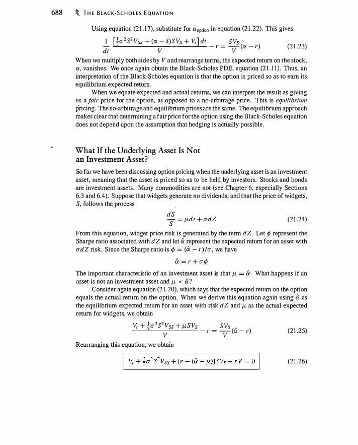
688 � T H E B LAC K-S C H O LES EQUAT I O N

Using equation (2 1 . 1 7), substitute for a option in equation (2 1 .22). This gives

1 [ �a2 S2 Vss + (a - 8)SVs + V, J dt SVs - - - r = -(a - r) dt v v (2 1 .23)

When we multiply both sides by V and rearrange terms, the expected return on the stock, a, vanishes : We once again obtain the Black-Scholes PDE, equation (2 1 . 1 1 ) . Thus, an interpretation of the Black-Scholes equation is that the option is priced so as to earn its equilibrium expected return.

When we equate expected and actual returns, we can interpret the result as giving us a fair price for the option, as opposed to a no-arbitrage price. This is equilibrium pricing. The no-arbitrage and equilibrium prices are the same. The equilibrium approach makes clear that determining a fair price for the option using the Black-Scholes equation does not depend upon the assumption that hedging is actually possible.

What H the Underlying Asset Is Not an Investment Asset?

So far we have been discussing option pricing when the under! ying asset is an investment asset, meaning that the asset is priced so as to be held by investors. Stocks and bonds are investment assets. Many commodities are not (see Chapter 6, especially Sections 6.3 and 6.4). Suppose that widgets generate no dividends; and that the price of widgets, S, follows the process

dS S = f.Ldt + adZ (2 1 .24)

From this equation, widget price risk is generated by the term dZ. Let 4> represent the Sharpe ratio associated with d Z and let & represent the expected return for an asset with adZ risk. Since the Sharpe ratio is 4> = (a - r)/a , we have

& = r + a¢ The important characteristic of an investment asset is that fL = & . What happens if an asset is not an investment asset and fL < &?

Consider again equation (2 1 .20), which says that the expected return on the option equals the actual return on the option. When we derive this equation again using & as the equilibrium expected return for an asset with risk d Z and fL as the actual expected return for widgets, we obtain

V, + �a2S2 Vss + tLSVs SVs � - - r = -(a - r) v v

Rearranging this equation, we obtain

(2 1 .25)

(2 1 .26)

TH E B LA C K- S C H O LES EQUAT I O N � 689

If you compare equation (2 1 .26) with (2 l . l l ), the dividend yield, 8, has been replaced with a - f.L, the difference between the equilibrium expected return and the actual expected return on noninvestment widgets. 1 1

Let 8 = a - J.L. We can interpret 8 as follows: J.L is the return you get from holding a widget and a is the return you must expect if you are to voluntmily hold a widget. Thus, in order for you to hold a widget you would need an additional return of 8 = a - J.L. Given the expected widget price change, f.L, the only way to receive the extra return is through . a dividend. This is the reason that a - J.L replaces the dividend yield in the Black-Scholes equation.

We have encountered this concept before: 8 is the lease rate for the widget, or more generally the lease rate for an asset with expected capital gain /.l· and risk CJdZ. When you lend a commodity, you receive its capital gains. The lease rate is the extra income you need to make you willing to buy and lend the asset. In the same way, 8 is the extra income you need to make you willing to hold a widget as an investment asset.

In practice, a widget-linked bond could be used to hedge the risk of a widget option. If the widget bond were constructed so that its price equalled the widget price today and at maturity, we saw in Chapter 15 that the bond would pay the widget lease rate as a coupon. This coupon, being a cash payment on the underlying asset, would play the role in the option pricing formula of a dividend on the underlying asset. This idea of a hypothetical lease-rate-paying, widget-linked security is also like the nvin security

mentioned in Chapter 17 . It provides an investment vehicle for owning the risk dZ. If such a twin security existed, we could use i t to hedge the risk of the option, and its dividend yield, 8, would appear in the option price.

An equivalent way to write equation (2 1 .26) is to replace a with r + fjJCJ. We then obtain I V, + tCJ2S2 Vss + (J.L - ¢CJ )SVs - rV = 0 I (2 1 .27)

In this version, the coefficient on the SVs term is the drift on the widget less the risk premium appropriate for widgets.

Note that when the asset is an investment asset, a = a and f.l = a - 8 = r + fjJCJ - 8. Both equations (21 .26) and (2 1 .27) reduce to equation (2 1 . 1 1 ) .

To summarize, the Black-Scholes PDE, equation (2 1 . 1 1 ) , also characterizes deriva­tive prices for assets that are not investment assets . In the case of an asset that is not an investment asset, the dividend yield, 8, is replaced with the lease rate of the asset, 8 .

Example 21 .1 To see how to use equation (2 1 .26), suppose we have an option for which the maturity payoff is based upon the stock price raised to a power, sa . This type

1 1 This modi fication to the Black-Scholes equation is discussed in Constantinides ( 1 978) and McDonald

and Siegel ( 1 984).

690 � TH E B LA C K-S C H O LES EQUAT I O N

of option is called a power option. For example, we could have a call option with a payoff of

max(S" - K" , 0)

We have already seen in Proposition 20.3 that the lease rate on an asset paying S" is 8* = r - a (r - 8) - 4a (a - l )a2 . From Ito's Lemma the volatility is aa. Thus, using equation (2 1 .26), we can price the option by using S" as the stock price, Ka as the strike price, 8* as the dividend yield, and aa as the volatility. �

21 .3 RISK-NEUTRAL PRICING

The expected return on the stock, a, does not appear in the Black-Scholes equation, equation (2 1 . 1 1 ) . Thus, when pricing derivatives on investment assets, only the risk­free rate matters; the actual expected return on a stock is irrelevant for pricing an option on the stock. The binomial pricing formula (see Chapter 10) also depends only on the risk-free rate.

This observation led Cox and Ross ( 1 976) to the following important observation: Since only the tisk-free rate appears in the Black-Scholes PDE, it must be consistent with any possible world in which there is no arbitrage. If we are trying to value an option, we can assume that we are in the world in which it is easiest to value the option. Valuation will be easiest in a risk-neutral world, in which (if it actually existed) all assets would earn the risk-free rate of return an� we would discount expected future cash flows at the risk-free rate. Thus, we can value options and other derivative claims by assuming that the stock earns the risk-free rate of return and calculate values based on that premise. We assume that the stock in this world follows the process

dS -

- = (r - 8)dt + adZ s

(2 1 .28)

As we keep emphasizing, the risk-neutral distribution is not an assumption about investor risk preferences. It is a device that can be used when pricing by arbitrage is possible (see Appendix 1 1 .B for a discussion).

Interpreting the Black-Scholes Equation

The actual expected change in the option price is given by

I I � � -E(dV) = V1 + .,.u-S- \Iss + (a - 8) SVs dt - (2 1 .29)

Let £* represent the expectation with respect to the risk-neutral distribution. Under the risk-neutral distribution, the expected change in the stock price is E* (d S) = (r - 8)dt. The drift in the option price can thus be written

_!_E*(dV) = Vr + �a1S1 Vss + (r - 8)SVs dt � (2 1 .30)

R I S K- N EUTRAL P R I C I N G � 691

The Black-Scholes equation, (2 1 . 1 1 ), can therefore be rewritten as

1 "' -E · (dV) = r V dt (2 1 .3 1 )

Under the risk-neutral process, the option appreciates on average at the risk-free rate.

The Backward Equation

Closely related to equation (2 1 .3 1 ) are the following equations, which characterize both the actual and risk-neutral probability distributions:

�E (dV) = O dt �E* (d \1) = 0 dt

For the risk-neutral process, equation (2 1 .33) is

I I

? ? v; + 1u-S- Vss + (r - 8) SV5 = 0

(2 1 .32)

(2 1 .33)

(2 1 .34)

Equation (2 1 .34) is called the Kolmogorov backward equation for the geometric Brownian motion process given by equation (2 1 .28). Whereas the Black-Scholes PDE characterizes prices, the backward equation characterizes probabilities. The backward equation is just like the Black-Scholes PDE except that there is no r V term. 1 2

The Black-Scholes equation can be interpreted as saying that the expected return on the option must equal the risk-free rate. The backward equation pertains to probabilities of events, such as the probability that an option will expire in-the-money. To understand how such probabilities should behave, suppose we decide that the probability is 0.65 that the stock price 1 year from today will be greater than $100. We know today that if the stock price goes up tomorrow, we will then assign a greater probability to this event. If the stock price goes down tomorrow, our estimate of the probability will go · down. · However, we should not expect our estimate of the probability to change on average: Our expectation today, of tomorrow's probability, must also be 0.65 . If today's estimate of tomorrow's probability were not 0.65, then 0.65 could not have been the correct probability today.

Thus, whereas the price of a financial asset is expected to change over time, the expected change in the probability of an event is zero. This is why the backward equation does not have the r V term.

If f(ST ; St ) is the probability density for ST given that the price today is sh both of these expressions would satisfy the backward equation:

1 2The backward equation is covered in delail in standard texts (see. for example, Cox and Miller ( 1 965).

and Karlin and Taylor ( 1 98 1 )) . Wilmott ( 1 998, ch. I 0) contains a particularly clear heuristic derivation

of equation (2 1 .34 ).

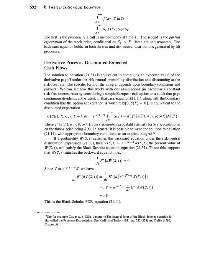
692 � T H E B LA C K-S C H O LES EQUAT I O N

r"' j (ST ; St )dST JK fcc ST f (ST ; St )llST JK

The first is the probability a call is in-the-money at time T . The second is the partial expectation of the stock price, conditional on ST > K . Both are undiscounted. The backward equation holds for both the true and risk-neutral distributions generated by Ito processes.

' Derivative Prices as Discounted Expected Cash Flows

The solution to equation (2 1 .3 1 ) is equivalent to computing an expected value of the derivative payoff under the risk-neutral probability distribution and discounting at the risk-free rate. The specific form of the integral depends upon boundary conditions and payouts. We can see how this works with our assumptions (in particular a constant risk-free interest rate) by considering a simple European call option on a stock that pays continuous dividends at the rate 8. In that case, equation (2 1 . 1 1 ) , along with the boundary condition that the option at expiration is worth max[O, S(T) - K] , is equivalent to the discounted expectation

C[S(t) , K, a, r, T - t , 8] = e-r�T-n lee [S(T) - K.] j* [S(T) , a, r, 8 ; S(t)]dS(T)

where f* [S(T) , a, r, 8 ; S(t) ] is the risk-neutral probability density for S(T) , conditional on the time-t price being S(t) . In general it is possible to write the solution to equation (2 1 . 1 1 ) , with appropriate boundary conditions, as an explicit integral. 1 3

If a probability W (S, t) satisifies the backward equation under the risk-neutral distribution, expression (2 1 .33), then V (S , t) = e-r(T-I ) W (S, t ) , the present value of W (S, t ) , will satisfy the Black-Scholes equation, equation (2 1 .3 1 ) . To see this, suppose that W (S, t) satisfies the backward equation, i .e. ,

Since V = e-r(T -I ) W, we have

:t

E* [d W (S , t ) ] = 0

1 1 dt E* [dV (S, t) ] = dt E* {d [e-r <T-n W (S, t)] }

= r V + e -r <T-t J _!_ E* [d W(S, t ) ]

dt = r V

This is the Black-Scholes PDE, equation (2 1 . 1 1 ) .

1 3 See for example Cox et al. ( 1 985a, Lemma 4).The integral form of the Black-Scholes equation is

also called the Feynman-Kac solution. See Karlin and Taylor ( 1 98 1 , pp. 222-224) and Duffie ( 1 996,

Chapter 5) .

C H A N G I N G TH E N U M E R A I R E � 693

This result means that discounted risk-neutral probabilities and partial expecta­tions are prices of derivatives. Thus, any risk-neutral probability or partial expectation also has a corresponding derivative price. As an example of this, we saw in Chapter 1 8 that the Black-Scholes term N (d2) is the risk-neutral probability that an option is in-the-money at expiration. The discounted probability, e-r(T -t) N (d2) , is therefore the price of a derivative that pays $ 1 if the option is in-the-money at expiration.

21 .4 CHANGING THE NUMERAIRE

Now we consider what happens when the number of options (or other derivative con­tracts) that we receive at expiration is random, determined by some asset price. This odd-sounding payoff is common. Consider the following example.

Example 21 .2 The price today of a nondividend-paying stock is $ 100, and the forward price is $ 106. 1 84. Joe bets Sarah that in 1 year the stock price will be greater than $ 106. 1 84. Joe wants the loser to pay one share to the winner. Sarah wants the loser to pay $106. 1 84 to the winner.

The share received by Joe would be worth more than $106. 1 84 if he wins. Sim­ilarly, Sarah's desired payoff of $ 106. 1 84 is worth more than one share if she wins. Are either of these fair bets? If not, who has the more valuable side of the bet if it is denominated in shares? Who has the more valuable side of the bet if it is denominated in cash?

If Sarah wins (i.e., the share price is below $ 106. 1 84), a payment of $ 1 06. 1 84 will exceed the value of one share. If Joe wins (i .e. , the share price is greater than $ 106. 1 84 ), a payment of one share will be worth more than $ 106. 1 84. However, it is not obvious which bet has a greater fair value given a current stock price of $ 100. Assuming no inside information about the stock, would an investor pay a greater price for Joe's desired bet or Sarah's desired bet?

We can describe the two forms of the bet as each having a different numeraire or unit of denomination. Joe's desired bet is denominated in shares, whereas Sarah's desired bet is denominated in dollars. You can interpret the share-denominated bet as paying either a fixed number of shares (one) or a variable number of dollars (the dollar price of one share). The dollar-denominated bet pays a fixed number of dollars ($ 106. 1 84) or a variable number of shares (the number of shares with the value $ 1 06. 1 84). The general question we want to answer is how a change in the numeraire (unit of denomination) for a derivative changes the price of the derivative.

Here are some other examples where a change of denomination is relevant:

e Currency translation: A cash flow originating in yen (for example) can be valued in yen, or in some other currency. We will discuss this example in depth in Chap­ter 22.

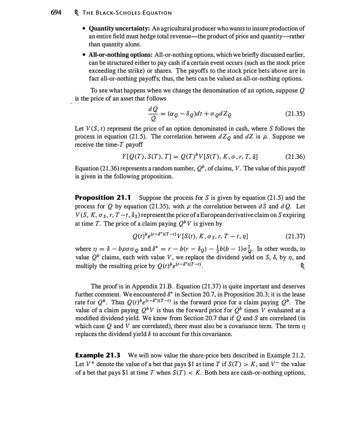
694 � T H E B LA C K-S C H O LES EQUAT I O N

• Quantity uncertainty: An agricultural producer who wants to insure production of an entire field must hedge total revenue-the product of price and quantity-rather than quantity alone.

• Ali-or-nothing options: Ali-or-nothing options, which we briefly discussed earlier, can be structured either to pay cash if a certain event occurs (such as the stock price exceeding the strike) or shares. The payoffs to the stock price bets above are in fact ali-or-nothing payoffs; thus, the bets can be valued as aU-or-nothing options.

To see what happens when we change the denomination of an option, suppose Q is the price of an asset that follows

d O Q = (a Q - 8Q )dt + u QdZQ (2 1 .35)

Let V (S, t) represent the price of an option denominated in cash, where S follows the process in equation (2 1 .5). The correlation between dZQ and dZ is p. Suppose we receive the time-T payoff

Y[Q (T) , S(T) , T] = Q (T)b V [S(T) , K , u , r, T, 8] (2 1 .36) Equation (2 1 .36) represents a random number, Qb , of claims, V. The value of this payoff is given in the following proposition.

Proposition 21 . 1 Suppose the process for S is given by equation (2 1 .5) and the process for Q by equation (2 1 .35), with p the correlation between d S and d Q. Let V (S, K, us . r, T - t, 8s) represent the price of a European derivative claim on S expiring at time T. The price of a claim paying Qb V is given by

Q(t)be(r-o" )(T-I) V [S (t) , K , us , r, T - t , 17 ] (2 1 .37)

where 17 = 8 - bpuu Q and 8* = r - b(r - 8Q) - ib(b - l )u� . In other words, to value Qb claims, each with value V, we replace the dividend yield on S, 8, by 17 , and multiply the resulting price by Q (tle(r-o") (T-1) . �

The proof is in Appendix 2 l .B . Equation (2 1 .37) is quite important and deserves further comment. We encountered 8* in Section 20.7, in Proposition 20.3 ; it is the lease rate for Qb. Thus Q (t)be(r-8" )(T-r) is the forward price for a claim paying Qb. The value of a claim paying Qb V is thus the forward price for Qb times V evaluated at a modified dividend yield. We know from Section 20.7 that if Q and S are correlated (in which case Q and V are correlated), there must also be a covariance term. The term 17 replaces the dividend yield 8 to account for this covariance.

Example 21 .3 We will now value the share-price bets described in Example 2 1 .2 . Let v+ denote the value of a bet that pays $ 1 at time T if S(T) > K, and v - the value of a bet that pays $ 1 at time T when S(T) < K. Both bets are cash-or-nothing options,

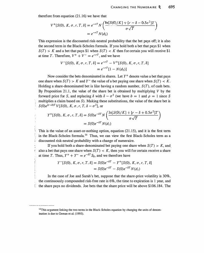
therefore from equation (2 1 . 1 6) we have that

C H A N G I N G TH E N U M E R A I R E � 695

v+ [S(O) , K, a , r, T, o] = e-rT N cn[S(O)/ K] +}:;. o - 0.5a2] T ) = e-rT N(d2)

This expression is the discounted risk-neutral probability that the bet pays off; it is also the second term in the Black-Scholes formula. If you hold both a bet that pays $ 1 when S(T) :> K and a bet that pays $ 1 when S(T) < K then for certain you will receive $ 1 at time T. Therefore, v+ + v- = e-rT , and we have

v- [S(O) , K, a , r, T, o] = e-rT - v+ [S(O) , K, a , r, T, 8] = e-rT [ l - N(d2)]

Now consider the bets denominated in shares. Let y+ denote value a bet that pays one share when S(T) > K and y- the value of a bet paying one share when S(T) < K. Holding a share-denominated bet is like having a random number, S(T) , of cash bets. By Proposition 2 1 . 1 , the value of the share bet is obtained by multiplying V by the forward price for S, and replacing o with 8 - a2 (we have b = I and p = 1 since S multiplies a claim based on S). Making these substitutions, the value of the share bet is S(O)e<r-.l>T V [S(O) , K, a , r, T, 8 - a2] , or

y+ [S(O) , K, a , r, T, 8] = S(O)e-8T N cn [S(O)/ K ] +au; 8 + 0.5a2]T ) = S(O)e-8T N(d1 )

This is the value of an asset-or-nothing option, equation (2 1 . 1 5) , and it is the first term in the Black-Scholes formula. 14 Thus, we can view the first Black-Scholes term as a discounted risk-neutral probability with a change of numeraire.

If you hold both a share-denominated bet paying one share when S(T) > K, and also a bet that pays one share when S(T) < K, then you will for certain receive a share at time T. Thus, y+ + y- = e-oT S0 , and we therefore have

r- [S(O) , K, a , r, T, 8] = S(O)e-8T - y+ [S(O) , K, a , r, T, o] = S(O)e-8T - S(O)e-8T N (di )

In the case of Joe and Sarah's bet, suppose that the share-price volatility is 30%, the continuously compounded risk-free rate is 6%, the time to expiration is 1 year, and the share pays no dividends . Joe bets that the share price will be above $ 1 06. 1 84. The

14This argument linking the two terms in the Black-Scholes equation by changing the units of denom­

ination is due to Geman et al. ( 1 995).

696 � T H E B LA C K-S C H O LES EQUAT I O N

value of this bet is

Value of Joe's Bet = y+[ lOO, 1 06. 1 84, 0.30, 0.08, l , 0] = $55 .962

The opposite side of Joe's bet-receiving one share when S(T) < $ 1 06. 1 84--has the value $ 1 00 - $55 .962 = $44.038.

Sarah's bet pays $ 1 06. 1 84 if the price is below $ 1 06. 1 84; this bet has the value

Value of Sarah's Bet = e-O.OS x I - v+ooo, 1 06. 1 84, 0.30, 0.08, l , 0] = $55 .962

The opposite side of Sarah's bet pays e-.os x $ 1 06. 1 84 - $55 .962 = $44.038 . Thus, both Sarah and Joe wish to denominate the bet in their favor. Moreover, Sarah and Joe's desired bets have the same value ! �

Problem 2 1 .8 asks you to find the strike prices such that the cash and share­denominated bets have equal value. We will return to changes in the unit of denomination in Chapter 22 when we discuss more nonstandard options.

21 :5 OPTION PRICING WHEN THE STOCK PRICE CAN JUMP

We discussed jumps in the stock price in Chapters 1 9 and 20. Jumps pose a problem for the Black-Scholes option pricing methodology. When the stock price can jump discretely as well as move continuously, a position that hedges against small moves will not also hedge against big moves. As we saw in Chapter 13 , large moves in the stock typically cannot be hedged.

The fact that jumps cannot be hedged does not mean that option pricing is impossi­ble; rather, it means that risk-neutral option pricing may be impossible. When moves in the option price cannot be hedged, we can still price the option by computing discounted expected payoffs using the actual probability density rather than the risk-neutral proba­bility density. The problem- is that the option has the risk of a leveraged position in the stock, and we do not know what discount rate is appropriate. Some assumption about appropriate discount rates (which is really an assumption about investor preferences) will then be necessary to price an option. 1 5

Merton ( 1 976) derived an option pricing formula when the stock price can jump by assuming that the jump risk is diversifi.able. This assumption neatly sidesteps the discounting issue since diversifi.able risk does not affect expected returns. While jump risk for a broad index is not diversifi.able, arguably many of the discrete moves for individual stocks are. In that case, by holding a portfolio of delta-hedged positions, the market-maker can diversify the effects of jump risk.

15See Naik and Lee ( 1 990) for an example of equil ibrium option pricing when there are jumps that cannot be hedged.

O PT I O N P R I C I N G W H E N T H E STO C K P R I C E CA N j U M P � 697

Ultimately, the importance of jumps and their systematic component is an empirical issue. Nevertheless, Merton's formulas provide useful insights into the effects of jumps.

Merton's Solution for Diversifiable Jumps ·

Suppose that the stock follows the process

dS(t) /S(t) = (a - Ak)dt + udZ + dq (2 1 .38) where, over an interval dt, a jump occurs with probability A.dt, and dq = 0 if there is no jump and Y - 1 if there is a jump. The jump magnitude, Y, is lognormally distributed such that

(2 1 .39) Thus, if the stock price is S before a jump, it is Y S following the jump, where Y - 1 is the percentage change in the stock price due to the jump, and k = E(Y - 1 ) is the expected percentage jump. Asume that the occurrence and magnitude of the jump are uncorrelated with the stock return.

Merton ( 1 976) shows that with the stock following equation (2 1 .38), and with jumps diversifiable, the Black-Scholes PDE becomes

V1 + t Vssu2 S2 + Vs (r - 8 - Ak)S + A.Ey [V (SY, t) - V (S, t) ] = r V (2 1 .40) When jumps are lognormal, as in equation (2 1 .39), Merton shows that the price

of a European call is 1 6

oo e-).' T (A.'T/ ( ) � i ! BSCall S, K, Ju1 + iu� j T , r - Ak + ia1 j T, T, 8 z =O

where A.' = A.e"1 . The price of a call is obtained by put-call parity.

(2 1 .4 1 )

Equation (2 1 .4 1 ) provides the option value as a n expectation o f European option prices with respect to the probability of a given number of jumps occurring. Conditional on i jumps, we replace the variance, u2 T, with u2T + iu� , a quantity that reflects • the added variance from having i discrete lognormal price moves. We also replace the risk-free rate, r , with (r - Ak)T + ia1 . The instantaneous drift, r - A.k, is increased by the cumulative mean of i jumps, ia1 . 1 1

An interesting special case occurs when the only possible jump that can occur is a jump of the stock price to zero. If the stock jumps to zero, a call option becomes worthless : V (SY, t) = 0, and A.k = -A. . Hence, with a jump to zero, the PDE for a call

1 6When jumps need not be lognormal, Merton ( 1 976) shows that the solution for cal ls is obtained as

an expected value of the Black-Scholes formula:

oo e-i.T (ii.T/ -i.kT . L . , E; [BSCall (SY11 e , K , a , J , T, o)] i=O I .

where £; denotes the expectation conditional on i jumps.

1 7We discussed in Chapter 19 the reason for subtracting U.

698 � TH E B LACK-S C H O LES EQUAT I O N

becomes

V1 + i Vsscr2 S2 + Vs (r + A. - 8) S = (r + A.) V Every occurrence of r is replaced by r + A.; hence, when the stock can jump to zero with instantaneous probability A.dt, the value of a European call, BSCall;. is

BSCall;_ (S, K, cr, r, T - t , 8) = BSCali(S, K, cr , r + A., T - t, 8)

The formula for a put, BSPut;._ , is then obtained by put-call parity : 1 8

BSPut;. (S, K, u , r, T - t , 8 )

(2 1 .42)

= BSCali(S, K, cr , r + A., T - t, 8, A.) - Se-o<T -t l + K e-r<T -r l

We will discuss the Merton jump formula further in Chapter 23 .

----· :__::.,.__· . -· --" · -.....c

CHAPTER SUMMARY

The Black-Scholes equation, equation (2 1 . 1 1 ), characterizes the behavior of a derivative as a function of the price of one or more underlying assets . (The B 1ack-Scholes equation also appeared in Chapter 1 3 as a break-even condition for delta-hedging market-makers.) We can interpret the B1ack-Scho1es equation as requiring that a derivative earn an ap­propriate rate of return, which occurs when the delta, gamma, and theta of an asset satisfy a particular relationship. The B1ack-Scholes equation is thus a generalization of the idea, familiar from introductory finance, that zero-coupon bonds appreciate at the risk-free rate. Probabilities and partial expectations satisfy a related condition known as the backward equation. Along with the Black-Scholes equation, a derivative must satisfy an appropriate boundary condition.

A change of the units of an option payoff is called a change of numeraire. Propo­sition 2 1 . 1 shows that the price effect of a change of numeraire is accounted for with a simple transformation of the pricing formula.

FURTHER READING

In Chapter 22, we extend the Black-Scholes analysis to exotic options and in Chapter 24 to studying interest rates.

Two classic papers on option pricing are Black and Scholes ( 1 973) and Merton ( 1 973b). Merton ( 1 976) extends the Black-Scholes model to allow diversifiable jumps in the stock price, and Naik and Lee ( 1 990) develop a model to price options when

1 8For a put option, the solution does not entail replacing every occurrence of r with r + )�. The reason

is that the POE for the put option is different from the POE for the call option in the case of a jump.

There is a different boundary condition when the stock jumps to zero:

P (O, t ) = Ke-rT rather than 0 in the case of a cal l.

P R O B LE M S � 699

jumps are systematic . The Heston model is described in Heston ( 1 993). In addition to Bakshi et al. ( 1 997) and Bates (2000), recent empirical studies of volatility skew include Benzoni (200 1 ), Andersen et al. (2002), Eraker (200 1 ), and Pan (2002).

Cox and Miller ( 1 965) and Wilmott ( 1 998, ch. 1 0) discuss the backward equation and its counterpart, the forward equation, which characterizes the probability density for S1 , conditional on Sr . Geman et al . ( 1 995) studied the role of changing the numeraire as a pricing technique. Schroder ( 1 999) extends their results, including examples with stochastic volatility and jump-diffusion models. Ingersoll (2000) provides some addi­tional examples of the use of this technique. Marcus and Modest ( 1984, 1 986) examine quantity uncertainty in agricultural production.

PROB LEMS

21.1. Verify that equation (2 1 . 1 2) satisfies the Black-Scholes equation. What is the boundary condition for which this is a solution?

21.2. Verify that ASaeyr satisfies the Black-Scholes PDE for ( 1 r - 8 ) a = 2 - a2 ±

( r - 8 1 ) 2 2(r - y) -- - - + ---'--a2 2 a2

21.3. Use the Black-Scholes equation to verify the solution in Chapter 20, given by Proposition 20.3, for the value of a claim paying sa .

21.4. Assuming that the stock price satisfies equation (20.27), verify that K e-r(T -rl + S(t)e-&(T -1 ) satisfies the Black-Scholes equation, where K is a constant. What is the boundary condition for which this is a solution?

21.5. Verify that S(t)e-o(T -r) N (d1 ) satisfies the Black-Scholes equation.

21.6. Verify that e-r(T -1 ) N (d2) satisfies the Black-Scholes equation.

21.7 . . Use the answers to the previous two problems to verify that the Black-Scholes formula, equation ( 1 2. 1 ) , satisfies the Black-Scholes equation. Verify that the boundary condition V [S(T) , T] = max[O, S(T) - K] is satisfied.

21.8. Consider Joe and Sarah's bet in Examples 2 1 .2 and 2 1 .3 .

a . In this bet, note that $ 1 06. 1 84 i s the forward price. A bet paying $ 1 i f the share price is above the forward price is worth less than a bet paying $ 1 if the share price i s below the forward price. Why?

b. Suppose the bet were to be denominated in cash. If we want the bet to pay x if S > x, what would x have to be in order to make the bet fair?

c. Now suppose that we pay one share if S > x. What would x have to be in this case to make the bet fair?

21.9. Consider again the bet in Example 2 1 .3 . Suppose the bet is S - $ 1 06. 1 84 if the price is above $ 1 06. 1 84, and $ 1 06. 1 84 - S if the price is below $ 106. 1 84. What is the value of this bet to each party? Why?

700 � T H E B LACK-S C H O LES EQUAT I O N

21.10. Suppose that a derivative claim makes continuous payments at the rate r . Show that the Black-Scholes equation becomes

1 � � Vr + la-S- Vss + (r - 8)SVs + r - rV = 0

For the following four problems assume that S follows equation (2 1 .5) and Q follows equation (2 1 .35). Suppose So = $50, Qo = $90, T = 2, r = 0.06, 8 = 0.02, 8Q = 0.0 1 , a = 0.3, O" Q = 0.5, and p = -0.2. Use Proposition 2 1 . 1 to find solutions to the problems . Optional: For each problem, verify the solution using Monte Carlo.

2'1.11. What is the value of a claim paying Q(T)2S(T)? Check your answer using Proposition 20.4.

21.12. What is the value of a claim paying Q (T)- 1 S(T)? Check your answer using Proposition 20.4.

21.13. You are offered the opportunity to receive for free the payoff

[Q (T) - Fo. T (Q)] x max[O, S(T) - K] (Note that this payoff can be negative.) Should you accept the offer?

21.14. An agricultural producer wishes to insure the value of a crop. Let Q represent the quantity of production in bushels and S the price of a bushel. The insurance payoff is therefore Q(T) x V [S(T) , T] , where V is the price of a put with K = $50. What is the cost of insurance'?

APPENDIX 2 1 .A : MULTIVARIATE BLACK-SCHOLES ANALYSIS

Consider a claim for which the payoff depends on the 1 1 asset prices, s I , s2 , . . . , sll ' where

dSi S. = (ai - oi )dt + aidZi I

(2 1 .43)

The pairwise correlation between Si and Sj is Pij · Let V (S1 , S2 , . . . , S11 , t , T) be the value of this claim. Consider a portfolio consisting of the claim, the n assets, and bonds, W, such that

II

i= l Using the multivariate version of Ito's Lemma (Proposition 20.2, Multivariate Ito's Lemma), the change in the value of the portfolio is

II l II II II dl = Frdt + L Vs,dSi + ?

L L dSidSj Vs, sidt + L NidSi + dW i= l - i= l j= l i= l

In order to delta-hedge V, set Ni = -Vs, . Hold bonds to finance the residual such that I = 0. The same analysis used to derive equation (2 1 . 1 1 ) leads to the following PDE

A P P E N D I X 21 . B : P R O O F O F P R O P O S I T I O N 21 .1 � 701

for V : II 1 II II

v; + 'L)r - 8; )S; Vs, + ? L L a;ajP;.j S; Sj Vs,sj = r V i= l - i= l j= l

APPENDIX 2 1 .B : PROOF OF PROPOSITION 2 1 . 1

(2 1 .44)

In this section we will verify the solution in Proposition 2 1 . 1 . We begin by assuming that we have a derivative price V ( S, a , r, T - t, 8) , that satisfies

V1 + (r - 8)SVs + �a2S2 Vss = rV (2 1 .45) By the multivariate Black-Scholes equation described in Appendix 2 l .A, the claim Y (S, Q, t) must satisfy

Y1 + (r - 8)SYs + (r - 8Q ) QY Q + � (a2 S2Yss + a� Q2Y QQ + 2paa QSQYsQ) = rY Guess the solution Y = Ae-<r-o")r Qb W, where A is determined by boundary conditions, 8* is to be determined, and W satisfies the same boundary condition as V . Compute the derivatives of this guess and substitute them into equation (2 1 .44). After simplification (in particular, the Y multiplying every term divides out), this yields

8* - r + b(r - 8Q ) + �atb(b - 1 )

+ � { W1 + [r - (8 - bpaa Q) ]SWs + �a2 S2 Wss } = r (2 1 .46)

The term in braces is the same as equation (2 1 .45), except that 8 is replaced with 17 =

8 - bpaa Q · Thus , W is the same as V except that 8 is replaced by 17 . With this replacement, from equation (2 1 .45), the term in parentheses equals r W. Equation (2 1 .46) becomes

rW 8* - r + b(r - 8Q ) + �a2Qb (b - 1 ) + - = r - w This equation is satisfied if 8* = r - b(r - 8Q ) - �a�b (b - 1 ) . Thus, with the 17 and 8* in Proposition 2 1 . 1 , the candidate solution solves

-equation (2 1 .44). The parameter A

is set so, at the point the option is exercised, A = e<r-nr . For a European option, set A = e<r-o•)T to solve the terminal boundary condition.

APPENDIX 2 1 .C : SOLUTIONS FOR PRICES AND PROBABILITIES

Appendix available online at www.aw-bc.com/mcdonald.

,,, -./0- - _-"C._. i -'----�"-----�· -- -----

Exotic Options : II

C h•ptO< 14 introduoed exotio ( o< non"'"'druU) option,, induding barriO<: g•p, '"'d outpO<­formance options. In this chapter, we continue our study of exotic options. There are two main themes in this chapter. First, we introduce a variety of simple options such as aU-or-nothing options that can be used as components for building more complex options. Second, we will examine options that depend on prices of more than one asset, such as quantos and rainbow options. The discussion in this chapter relies on material in Chapters 20 and 2 1 .

Throughout this chapter, w e will assume that there are two assets that follow the processes

dS s = (a - o)dt + adZ

dO Q = (aQ - OQ)dt + a QdZQ

The correlation between dZ and dZQ is pdt .

22. 1 ALL-OR-NOTHING OPTIONS

(22. 1 )

(22.2)

We b�gin with a discussion of simple ali-or-nothing options, which pay the holder a discrete amount of cash or a share if some particular event occurs. These are described as ali-or-nothing (also called binmy or digital options) because the payoff can be thought of as 0 or 1 : Either you receive the cash or share, or you do not.

Terminology

There are many different kinds of ali-or-nothing options ; payoffs can be contingent on the stock price at expiration, as well as on whether the stock price has hit a barrier over the life of the option. We are interested in these options in and of themselves, and also because they are building blocks, useful for constructing variants of ordinary puts and calls as well as barrier options.

Naming all of these options can be a complex task. Table 22. 1 describes the naming scheme we will use. The terminology will make sense as we introduce the various claims.

703

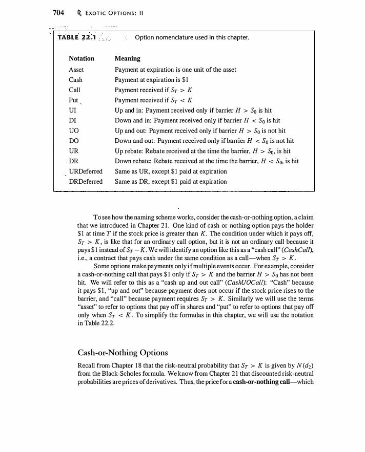
704 � EXOT I C O PT I O N S : I I

TABLE 2 2 � 1 Option nomenclature used in this chapter.

Notation

Asset

Meaning

Payment at expiration is one unit of the asset

Payment at expiration is $ 1 Cash

Call Payment received if Sr > K

Put Payment received if Sr < K

UI Up and in: Payment received only if barrier H > So is hit

DI Down and in: Payment received only if barrier H < So is hit

uo Up and out: Payment received only if barrier H > So is not hit Down and out: Payment received only if barrier H < S0 is not hit

Up rebate: Rebate received at the time the barrier, H > S0, is hit Down rebate: Rebate received at the time the barrier, H < S0, is hit

Same as UR, except $ 1 paid at expiration

DO

UR

DR

URDeferred

DRDeferred Same as DR, except $ 1 paid at expiration

To see how the naming scheme works, consider the cash-or-nothing option, a claim that we introduced in Chapter 2 1 . One kind of cash-or-nothing option pays the holder $ 1 at time T if the stock price is greater than K. The condition under which it pays off, Sr > K, is like that for an ordinary call option, but it is not an ordinary call because it pays $ 1 instead of Sr - K. We will identify an option like this as a "cash call" ( CashCall),

i .e . , a contract that pays cash under the same condition as a call-when Sr > K. Some options make payments only i f multiple events occur. For example, consider

a cash-or-nothing call that.pays $ 1 only if Sr > K and the barrier H > So has not been hit. We will refer to this as a "cash up and out call" (CashUOCall): "Cash" because it pays $ 1 , "up and out" because payment does not occur if the stock price rises to the barrier, and "call" because payment requires Sr > K. Similarly we will use the terms "asset" to refer to options that pay off in shares and "put" to refer to options that pay off only when Sr < K. To simplify the formulas in this chapter, we will use the notation in Table 22.2.

Cash-or-Nothing Options

Recall from Chapter 1 8 that the risk-neutral probability that Sr > K is given by N (d1) from the Black-Scholes formula. We know from Chapter 2 1 that discounted risk-neutral probabilities are prices of derivatives. Thus, the price for a cash-or-nothing call-which

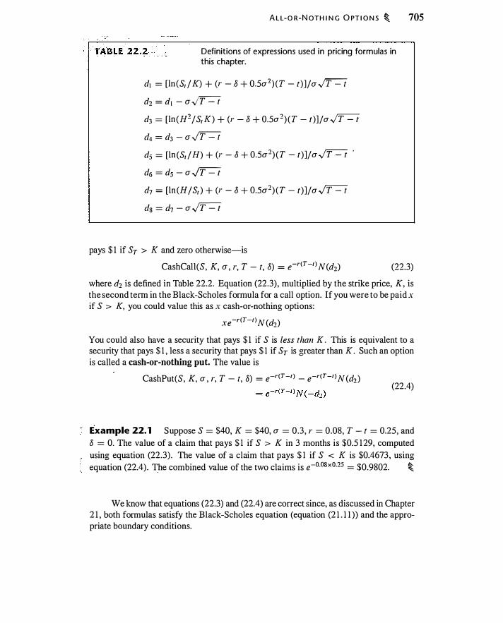
A L L-O R-N OTH I N G O PT I O N S � 705

Definitions of expressions used in pricing formulas in this chapter.

d1 = [ln (S1 / K) + (r - 8 + 0.5a2) (T - t) ]/a�

d2 = d1 - a�

d3 = [ln (H2/S1 K) + (r - 8 + 0.5a2) (T - t)]/a�

d4 = d3 - a�

d5 = [ln (S1 / H) + (r - 8 + 0.5a2) (T - t)]/a� ·

d6 = d5 - a�

d1 = [ln (H/S1 ) + (r - 8 + 0.5a2) (T - t)]/a�

ds = d1 - a�

pays $ 1 if Sr > K and zero otherwise-is

CashCall(S, K, a , r, T - t, 8) = e-r(T-I) N(d2) (22.3) where d2 is defined in Table 22.2. Equation (22.3), multiplied by the strike price, K, is the second term in the Black-Scholes formula for a call option. If you were to be paid x if S > K, you could value this as x cash-or-nothing options:

xe-r(T -1 ) N (d2)

You could also have a security that pays $ 1 if S is less than K . This is equivalent to a security that pays $ 1 , less a security that pays $ 1 if Sr is greater than K. Such an option is called a cash-or-nothing put. The value is

CashPut(S, K, a , r, T - t, 8) = e-r(T -I ) - e-r(T -I) N (d2 ) (22.4)

·- Example 22. 1 Suppose S = $40, K = $40, a = 0.3, r = 0.08, T - t = 0.25, and 8 = 0. The value of a claim that pays $ 1 if S > K in 3 months is $0.5 1 29, computed using equation (22.3) . The value of a claim that pays $ 1 if S < K is $0.4673 , using equation (22.4). The combined value of the two claims is e-o.osxo.25 = $0.9802. �

We know that equations (22.3) and (22.4) are correct since, as discussed in Chapter 2 1 , both formulas satisfy the Black-Scholes equation (equation (2 1 . 1 1 )) and the appro­priate boundary conditions.

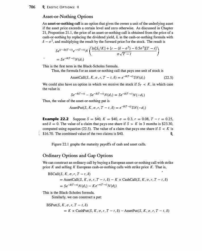
706 � EXOT I C O PT I O N S : I I

Asset -or-Nothing Options

An asset-or-nothing call is an option that gives the owner a unit of the underlying asset if the asset price exceeds a certain level and zero otherwise. As discussed in Chapter 2 1 , Propostion 21 . 1 , the price of an asset-or-nothing call is obtained from the price of a cash-or-nothing by replacing the dividend yield, 8, in the cash-or-nothing formula with 8 - cr 1 , and multiplying the result by the forward price for the stock. The result is

se<r-8) (T-1 ) e-r(T-1) N ( ln [S1 / K] + [r - (8 - cr2) - 0.5cr1] [T - t] ) CT�

= se-o(T-I ) N (d, )

This is the first term in the Black-Scholes formula. Thus, the formula for an asset-or-nothing call that pays one unit of stock is

AssetCall (S, K, cr , r, T - t, 8) = e-8(T-l ) SN (di ) (22.5) We could also have an option in which we receive the stock if ST < K , in which case the value is

se-o(T-1) - se-o(T-1 ) N (d, ) = se-o(T-1 ) N (-di )

Thus, the value of the asset-or-nothing put is

AssetPut(S, K, cr, r, T - t , 8) = e-o<T-l) SN (-d1 )

Example 22.2 Suppose S = $40, K = $40, cr = 0.3 , r = 0.08, T - t = 0.25, and 8 = 0. The value of a claim that pays one share if S > K in 3 months is $23.30, computed using equation (22.5). The value of a claim that pays one share if S < K is

L $ 16.70. The combined value of the two claims is $40. �

Figure 22. 1 graphs the maturity payoffs of cash and asset calls.

Ordinary Options and Gap Options

We can construct an ordinary call by buying a European asset-or-nothing call with strike price K and selling K European cash-or-nothing calls with strike price K. That is ,

BSCall(S, K, cr, r, T - t , 8) = AssetCall (S, K, cr, r, T - t , 8) - K x CashCall(S, K, cr, r, T - t , 8)

= se-o(T-r) N (di ) - Ke-r(T-I) N (d1)

This is the Black-Scholes formula. Similarly, we can construct a put:

BSPut(S, K, cr , r, T - t, 8)

= K x CashPut(S, K, cr, r, T - t , 8) - AssetPut(S, K , cr , r, T - t, 8)

Payoff at maturity to one asset cal l and 40 cash cal ls . Assumes K = $40, u = 0.30, r = 0 .08, and 8 = 0. The payoff to both is zero for S < $40.

-

Option Value ($)

50

45

40

35

30

25

20

15

10

5

- Asset Call •••••• Cash Call

A L L-O R-N OT H I N G O PT I O N S � 707

0��--_.--�--�--��L-�---L--�--� 30 32 34 36 38 40 42 44 46 48 50

Stock Price at Expiration ($)

Finally, we can construct a gap option using asset-or-nothing options. Consider a call option that pays S - K 1 if S > K 1 . The value of this is

AssetCall(S, K1 , a , T - t , r, 8) - K1 x CashCall (S, K1 , a , T - t , r, 8)

We buy an asset call and sell K1 cash calls, both with the strike price K1.

Example 22.3 Suppose S = $40, K = $40, a = 0.3, r = 0.08, T - t = 0.25 , and 8 = 0. The price of an ordinary call is an asset call less 40 cash calls. Using results in Examples 22. 1 and 22.2, the price of the ordinary call is $23 .30 - 40 x $0.5 129 =

$2.7848. The price of a gap call in which the owner pays $20 (K! ) if the stock is greater

than $40 (K1) at expiration is $23 .20 - 20 x $0.5 1 29 = $ 1 3 .0427. �

Delta-Hedging Ali-or-Nothing Options

Ali-or-nothing options appear frequently in writings about options, but they are rela­tively rare in practice. The reason is that they are easy to price but hard to hedge. To understand why, think about the position of a market-maker when such an option is close to expiration. The nightmare scenario for a market-maker is that the option is close to

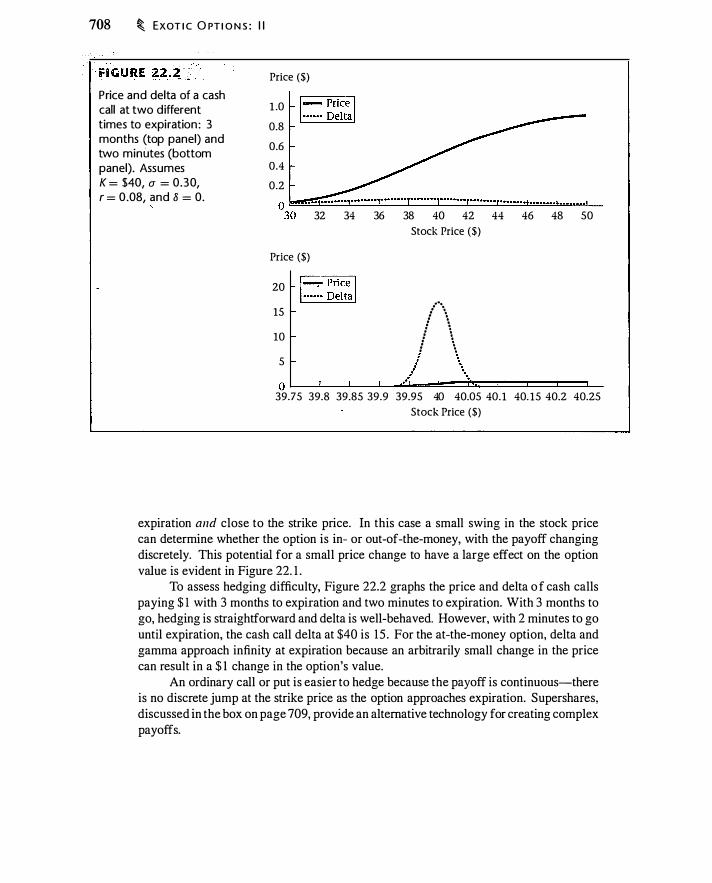
708 � EXOT I C O PT I O N S : I I

Price and delta of a cash call at two different times to expiration : 3 months (top panel) and two minutes (bottom panel). Assumes K = $40, a = 0.30, r = 0.08, and 8 = 0.

Price ($)

1 .0

0.8

0.6

0.4

0.2

Price ($)

20

15

10

5

32 34 36 38 40 42 44 46 48 50 Stock Price ($)

... / \ i \ . .

. . . . . . . .

.. li \ ... O L_��--J-������=r==��

39.75 39.8 39.85 39.9 39.95 40 40.05 40.1 40. 15 40.2 40.25 Stock Price ($)

expiration and close to the strike price. In this case a small swing in the stock price can determine whether the option is in- or out-of-the-money, with the payoff changing discretely. This potential for a small price change to have a large effect on the option value is evident in Figure 22. 1 .

To assess hedging difficulty, Figure 22.2 graphs the price and delta o f cash calls paying $ 1 with 3 months to expiration and two minutes to expiration. With 3 months to go, hedging is straightforward and delta is well-behaved. However, with 2 minutes to go until expiration, the cash call delta at $40 is 15 . For the at-the-money option, delta and gamma approach infinity at expiration because an arbitrarily small change in the price can result in a $ 1 change in the option's value.

An ordinary call or put is easier to hedge because the payoff is continuous-there is no discrete jump at the strike price as the option approaches expiration. Supershares, discussed in the box on page 709, provide an alternative technology for creating complex payoffs.

sue.c:!rshares

Hakannson ( 1 976) proposed a concept known as supershares, which could be used to create exotic option-like payoffs without the need for delta-hedging by a dealer. The idea of a supers hare is to create shares that pay $1 in particular circumstances, and to use these as building blocks for more complicated instruments. Supershares can be illustrated with a s imple example.

Suppose that the risk-free rate is 10%, the market index is 100, and over the next year there are three possible values of the market index: $60, $ 1 1 0, and $ 1 60. (The use of three possible prices is just for simplicity.) Define three supershares that pay $1 if the market in I year is $60, $1 if the market i s $ 1 1 0, and $ 1 i f the market i s $ 1 60. Call these shares "down," "middle," and "up."

We can create a fund with a $ 100 million investment in the index, and finance it by selling 60 million down shares, 1 10 million middle shares, and 1 60 million up shares. 1 If the market is $60 in 1 year, the entire $60 million is paid to the holders of the down shares. If the market is $ 1 60, the entire amount is paid to the holders of the up shares. Note that if you were to buy all of these shares, you would earn a return equivalent to a $ 100 million investment in the index. (You could also buy 6 down shares, 1 1 middle shares, and 1 6 up shares for a small position in the index.) If you bought 100 each of the

A L L- O R-N OTH I N G O PTI O N S � 709

down, middle; and up shares, you would have a risk-free zero-coupon bond paying $ 100. By buying just the down shares, you could replicate the payoff to a cash-or-nothing put, and so forth.

Although the supershare payoffs resemble the payoffs of cash-or-nothing options, the elegant simplicity of the supershare idea is that the shares are created as fully-collateralized contingent claims on a fund. No delta-hedging is required. Relative pricing of the components is determined by the willingness of investors to hold them, but the portfolios replicating a bond and the index must be priced correctly or else there would be arbitrage.

Supershares were actually brought to market in November 1992 by Leland, O'Brien, and Rubinstein (the first and third named principals are finance professors). The product consisted of exchange-traded money market and index funds, which could be decomposed into four supershares that could be traded individually at the Chicago Board Options Exchange. There were significant regulatory hurdles to introducing supershares, described in Lux ( 1 992). Trading volume was weak and after several years the product was abandoned. The exchange-traded index fund, however, was the precursor to current popular products such as exchange-traded funds and SPDRs.

1 In the examples in Hakannson ( 1 976), shares are created paying returns every percentage point

between -50% and +60%.

710 � EXOT I C O PT I O N S : I I

22.2 ALL-OR-NOTHING BARRIER OPTIONS

Barrier options, introduced in Chapter 14, are options in which the option comes into or goes out of existence if the price of the underlying asset hits a barrier.2 There are down-and-out options, which become worthless if the stock price hits a barrier price below the initial stock price, as well as up-and-out, down-and-in, and up-and-in options. We can construct options such as these using all-or-notlzing barrier options.

Suppose we take a cash-or-nothing call paying $ 1 if ST > K, but modify it by adding the additional requirement that it will only pay $ 1 at expiration if the stock has also hit the barrier H sometime during the life of the option. If H < S(O) , this is a

' down-and-in cash call. Using the notation in Table 22. 1 , this would be a CaslzDICall. Just as we were able to construct ordinary options from digital options, we will also be able to construct barrier options from· digital barrier options.

We will examine three different kinds of barrier options:

e A contract that pays $1 contingent on either a barrier having or not having been reached (cash-or-nothing barrier options).

o A contract that pays a share of stock worth S contingent on either a barrier having or not having been reached (asset-or-nothing barrier options) .

• A contract that pays $ 1 at the time a barrier is reached (rebate options) or that pays $ 1 at expiration as long as the barrier has been reached during the life of the option (deferred rebate options) . By valuing these pieces and adding them together we can price any standard barrier

option. The assumption that the stock follows geometric Brownian motion makes it possible to derive relatively simple formulas for these options.

There are 16 basic kinds of ali-or-nothing barrier options. First, consider cash-or­nothing barrier options that pay $ 1 at expiration. Such options can knock -in or knock -out; they can be calls (pay cash if ST > K) or puts (pay cash if ST < K); and the barrier event can occur if the barrier is above the price (up-and-ins or up-and-outs) or below the price (down-and-ins or down-and-outs) . This gives us 23 = 8 basic cash-or-nothing barrier options to value . . By the same reasoning there are also 8 basic asset-or-nothing barrier options, for a total of 1 6 ali-or-nothing barrier options.

Cash-or-Nothing Barrier Options

We first consider the valuation of barrier cash-or-nothing options. To anticipate the results in this section, we will first see how to value one particular barrier cash-or­nothing option, a down-and-in cash call. From this one formula we will be able to value the remaining seven cash-or-nothing options and deferred rebate options.

2Three comprehensive discussions of barrier options are Rubinstein and Reiner ( 1 99 1 a), Rubinstein

and Reiner ( 1 99 1 b), and Derman and Kani ( 1 993).

A L L-O R -N OT H I N G B A R R I E R O PT I O N S � 711

Assume that the option i s issued at time 0 and expires at time T. Let S1 denote the greatest stock price between times 0 and t (where t _.::: T) and let S.1 denote the lowest stock price between times 0 and t . Suppose the barrier is below the initial stock price, i .e. , H < S0. A cash down-and-in call (CashD!Call) is an option that pays $ 1 if two conditions are satisfied. First, at some point prior to maturity, the stock price drops to reach H, i.e., S.r _.::: H. Second, at expiration, the stock price is greater than the strike price, K.

We can analyze this option by first examining the risk-neutral probability that this joint event CS.r _.::: H and Sr 2: K) occurs. This probability should satisfy three conditions :

1. Once the barrier has been hit (Jr _.::: H) the probability equals the probability that Sr 2: K (the barrier at this point is irrelevant) .

2. If at time T, S.r _.::: H and Sr 2: K, the probability equals 1 .

3 . If at time T , S.r > H or Sr < K, the probability equals 0.

Assume that H _.::: K, and consider this expression:

') r-/J I ProbCS.r _.::: H and Sr > K) = ( �) - "' - N(d4) (22.6)

The terms d1 through ds are defined in Table 22.2. In Appendix 2 l .C, which is found on the book's Web site (www.aw-bc.com/mcdonald), we saw that an expression of this form solves the backward equation. We also want to verify that it satisfies the three boundary conditions described above.

First, at the point where S1 = H, equation (22.6) collapses to N (d2 ) , which is the risk-neutral probability that Sr > K. (This occurs because when H = S1 , d1 = d3 • You should examine equation (22.6) to verify that this happens.) Thus, once we hit the barrier, the barrier value H drops out of the expression because it is irrelevant. Second, if at expiration S.r _.::: H and Sr > K, then equation (22.6) equals l . The reason is that the probability equals N (d2) once the barrier is hit, and if Sr > K, N (d2) = 1 . Finally, if S.r > H, i .e. , S1 never reaches H, then at expiration H2 < Sr K (recall that H _.::: K) and equation (22.6) collapses to 0. Thus, equation (22.6) both satisfies the backward equation and obeys the appropriate boundary conditions.

Equation (22.6) assumes that H _.::: K. Why is this important? The answer is that if H > K, the boundary conditions may be violated. Consider the case where at expiration Sr = $55, K = $45, and H = $54 (thus violating the condition H _.::: K), and the boundary has not been hit. In this case a correct expression for the probability will evaluate to zero at expiration. However, ln (H2 I Sr K) = ln (542 145 x 55) = 0. 1 64, so equation (22.6). at maturity will equal l when the event has not occurred.

As a final comment on equation (22.6), you might ask why it is necessary to multiply N (d4) by the term (HI S)2<r-a)fa'- 1 • The answer is simply that N(d4) by itself does not solve the backward equation, whereas equation (22.6) does solve the backward equation.

712 � EXOTI C O PT I O N S : I I

To handle the case where H > K we need a more complicated version of equation (22.6). When H > K, we have

") r-0 I Prob(�r :S . H and Sr > K) = N (d2) - N (d6) + ( �) - "

'-

N (ds) (22.7)

Problem 22.3 asks you to verify that this equation satisfies the boundary conditions. Note that when S = H, N (d6) = N (d8 ) ; the formula again reduces to N (d2) .

Down-and-in cash call Equations (22.6) and (22.7) give us expressions for the prob­ability that the barrier is hit and Sr > K. What is the value of a claim that pays $ 1 when this event occurs? To answer this question we can use the result from Chapter 2 1 that discounted risk-neutral probabilities are prices of derivative claims. Discounting equations (22.6) and (22.7), we have

CashDICall(S, K, a , r, T - t, 8, H) = � r-! I e-rCT-rl ( q.t " 2 -

N (d4) H :S K

e-r(T-r l [ N (d2) - N (d6) + ( q.(·-,'- l N (ds)] H > K

(22.8)

Equation (22.8) gives us the value for a cash down-and-in call when So > H. There are three closely related options we can now price: Cash down-and-out calls (CaslzDO­Call), cash down-and-in puts (CaslzD!Put), and cash down-and-out puts (CashDOPut) . We can value each of these using only the formula for the cash down-and-in call, equation (22.8). In addition, we can value a deferred down rebate option.

Deferred down rebate option We first value a deferred down rebate, which is a claim that pays $ 1 at time T as long as the barrier has been hit over the life of the option. The payoff to this claim does not depend on a strike price: It pays $ 1 as long as the barrier has been hit. We will call this claim a deferred down rebate. It is a "down rebate" becaus� it pays $ 1 if we reach the barrier, and it is "deferred" because the payment is at expiration rather than at the time we reach the barrier. We obtain the value of this claim by setting K = $0 in equation (22.8). Since we always have Sr > 0, the result is a claim that pays $ 1 at T as long as Sr :S H. Thus, we have3

DRDeferred(S, a , r, T - t , 8 , H) = CashDICall (S, 0, a , r, T - t , 8, H) (22.9)

Note that since we set K = 0, the value of the deferred down rebate does not depend on the strike price.

Now we can compute the value of the remaining three options.

Down-and-out cash call We can create a synthetic cash call by buying down-and-in and down-and-out cash calls with the same barrier; this combination is guaranteed to

3 In pefonning this calculation, to avoid a zero-divide error it is necessary to set K to be small, such as

K = $0.00000 I . rather than exactly SO.

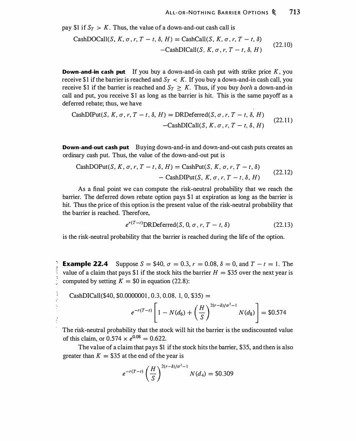
A L L- O R - N OT H I N G BA R R I E R O PT I O N S � 713

pay $1 if ST > K. Thus, the value of a down-and-out cash call is

CashDOCall(S, K, a , r, T - t, 8, H) = CashCall (S, K, a , r, T - t, 8) -CashDICall (S , K, a , r, T - t, 8, H)

(22. 1 0)

Down-and-in cash put If you buy a down-and-in cash put with strike price K, you receive $ 1 if the barrier is reached and ST < K. If you buy a down-and-in cash call, you receive $ 1 if the barrier is reached and ST � K. Thus, if you buy both a down-and-in call and put, you receive $ 1 as long as the barrier is hit. This is the same payoff as a deferred rebate; thus, we have

CashDIPut(S, K, a , r, T - t , 8, H) = DRDeferred(S, a , r, T - t, 8, H) -CashDICall(S, K, a , r, T - t, 8 , H)

(22. 1 1 )

Down-and-out cash put Buying down-and-in and down-and-out cash puts creates an ordinary cash put. Thus, the value of the down-and-out put is

CashDOPut(S, K, a, r, T - t , 8 , H) = CashPut(S, K, a, r, T - t , 8) (22. 1 2)

- CashDIPut(S, K, a , r, T - t , 8 , H) As a final point we can compute the risk-neutral probability that we reach the

barrier. The deferred down rebate option pays $ 1 at expiration as long as the barrier is hit. Thus the price of this option is the present value of the risk-neutral probability that the barrier is reached. Therefore,

er<T -r )DRDeferred(S, 0, a , r, T - t, 8) (22. 1 3)

is the risk-neutral probability that the barrier is reached during the life of the option.

Example 22.4 Suppose S = $40, a = 0.3, r = 0.08, 8 = 0, and T - t = 1 . The value of a claim that pays $ 1 if the stock hits the barrier H = $35 over the next year is computed by setting K = $0 in equation (22.8) :

CashDICall($40, $0.0000001 , 0 .3 , 0 .08, I , 0, $35) = [ (H ) 2(r-8)/<r1- l ]

e-r(T-1) l - N(d6) + S N(ds) = $0.574

The risk-neutral probability that the stock will hit the barrier is the undiscounted value of this claim, or 0.574 x e0·08 = 0.622.

The value of a claim that pays $1 if the stock hits the barrier, $35, and then is also greater than K = $35 at the end of the year is

( H) 1(r-8)ja1- l e-r(T-r) S N(d4) = $0.309

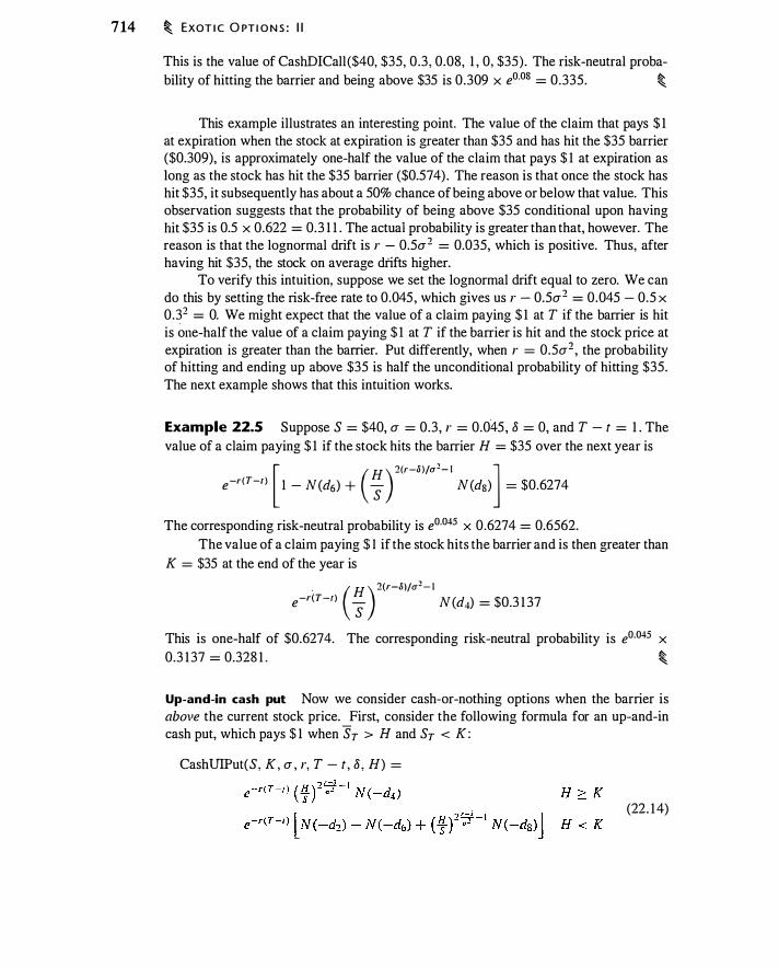
714 � EXOT I C O PT I O N S : I I

This is the value of CashDICall ($40, $35, 0 ,3 , 0.08, 1 , 0, $35) . The risk-neutral proba­bility of hitting the barrier and being above $35 is 0 .309 x e

0·08 = 0.335. �

This example illustrates an interesting point. The value of the claim that pays $ 1 at expiration when the stock at expiration is greater than $35 and has hit the $35 barrier ($0.309), is approximately one-half the value of the claim that pays $ 1 at expiration as long as the stock has hit the $35 barrier ($0.574) . The reason is that once the stock has hit $35, it subsequently has about a 50% chance of being above or below that value. This observation suggests that the probability of being above $35 conditional upon having hit $35 is 0.5 x 0.622 = 0.3 1 1 . The actual probability is greater than that, however. The reason is that the lognormal drift is r - 0.5a2 = 0.035, which is positive. Thus, after having hit $35, the stock on average drifts higher.

To verify this intuition, suppose we set the lognormal drift equal to zero. We can do this by setting the risk-free rate to 0.045 , which gives us r - 0.5a2 = 0.045 - 0.5 x 0.32 = 0. We might expect that the value of a claim paying $ 1 at T if the barrier is hit is one-half the value of a claim paying $ 1 at T if the barrier is hit and the stock price at expiration is greater than the barrier. Put differently, when r = 0.5a2 , the probability of hitting and ending up above $35 is half the unconditional probability of hitting $35. The next example shows that this intuition works.

Example 22.5 Suppose S = $40, a = 0.3 , r = 0.045 , 8 = 0, and T - t = 1 . The value of a claim paying $ 1 if the stock hits the barrier H = $35 over the next year is

[ ( H) 2(r-8)/a1- l ] e-r(T-

t) 1 - N(d6) + S N (ds) = $0.6274

The corresponding risk-neutral probability is e0·045

x 0.6274 = 0.6562. The value of a claim paying $ 1 if the stock hits the barrier and is then greater than

K = $35 at the end of the year is

. ( H ) 2(r-.l)/a2- l e-r(T-t) S N (d4) = $0.3 1 37

This is one-half of $0.6274. The corresponding risk-neutral probability is e0·045

x 0.3 1 37 = 0.328 1 . �

Up-and-in cash put Now we consider cash-or-nothing options when the barrier is above the current stOck price. First, consider the following formula for an up-and-in cash put, which pays $ 1 when ST > H and ST < K:

CashUIPut(S, K, a , r, T - t , 8 , H) =

(22. 1 4)

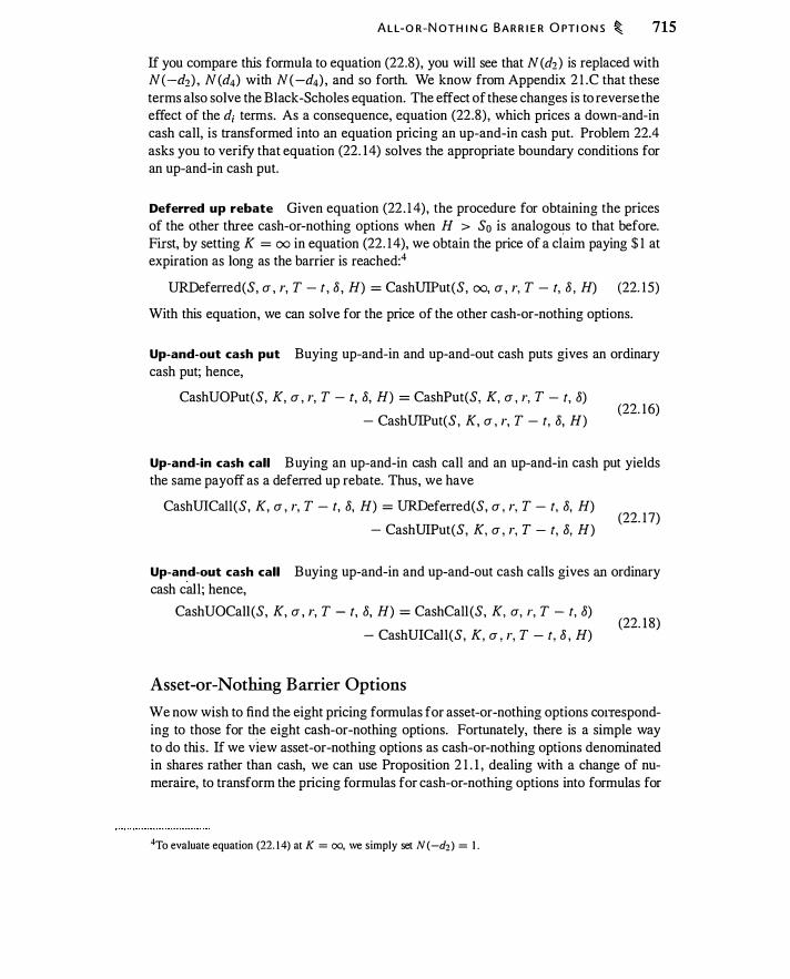
A L L-O R-N OTH I N G BAR R I E R O PT I O N S � 715

If you compare this formula to equation (22.8), you will see that N (d2 ) is replaced with N ( -d2) , N (d4) with N ( -d4) , and so forth. We know from Appendix 2 l .C that these terms also solve the Black-Scholes equation. The effect of these changes is to reverse the effect of the d; terms. As a consequence, equation (22.8), which prices a down-and-in cash call, is transformed into an equation pricing an up-and-in cash put. Problem 22.4 asks you to verify that equation (22. 14) solves the appropriate boundary conditions for an up-and-in cash put.

Deferred up rebate Given equation (22 . 1 4), the procedure for obtaining the prices of the other three cash-or-nothing options when H > So is analogolls to that before. First, by setting K = oo in equation (22. 14), we obtain the price of a claim paying $ 1 at expiration as long as the barrier is reached:4

URDeferred(S, a , r, T - t , 8 , H) = CashUIPut(S, oo, a , r, T - t, 8 , H) (22. 1 5)

With this equation, we can solve for the price of the other cash-or-nothing options.

Up-and-out cash put Buying up-and-in and up-and-out cash puts gives an ordinary cash put; hence,

CashUOPut(S, K, a , r, T - t, 8, H) = CashPut(S, K, a , r, T - t, 8) - CashUIPut(S , K, a , r, T - t, 8, H)

(22. 1 6)

Up-and-in cash call Buying an up-and-in cash call and an up-and-in cash put yields the same payoff as a deferred up rebate. Thus, we have

CashUICall(S, K, a , r, T - t, 8, H) = URDeferred(S, a , r, T - t, 8, H) - CashUIPut(S, K, a , r, T - t, 8, H)

(22. 1 7)

Up-and-out cash call Buying up-and-in and up-and-out cash calls gives an ordinary cash call ; hence,

CashUOCall (S, K, a , r, T - t, 8, H) = CashCall (S, K, a, r, T - t, 8) - CashUICall(S, K, a , r, T - t, 8 , H)

(22. 1 8)

Asset-or-Nothing Barrier Options

We now wish to find the eight pricing formulas for asset-or-nothing options cmTespond­ing to those for the eight cash-or-nothing options. Fortunately, there is a simple way to do this . If we view asset-or-nothing options as cash-or-nothing options denominated in shares rather than cash, we can use Proposition 2 1 . 1 , dealing with a change of nu­meraire, to transform the pricing formulas for cash-or-nothing options into formulas for

4To evaluate equation (22. 1 4) at K = oo, we simply set N ( -d2) = I .

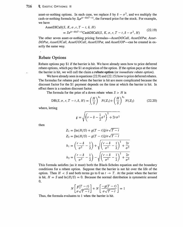
716 � EXOT I C O PT I O N S : I I

asset-or-nothing options . In each case, we replace 8 by 8 - a2, and w e multiply the cash-or-nothing formula by S0e <r-IJ ) (T -t ) , the forward price for the stock. For example, we have

AssetDICall(S, K, a , r, T - t, 8, H) (22. 1 9)

= se<r-ll) (T-I)CashDICall(S, K, a , r, T - t , 8 - a2 , H) The other seven asset-or-nothing pricing formulas-AssetDOCall, AssetD/Put, Asset­DOPut, AssetU/Call, AssetUOCall, AssetU/Put, and AssetUOP--can be created in ex-actly the same way.

Rebate Options

Rebate options pay $ 1 if the barrier is hit. We have already seen how to price deferred rebate options, which pay the $ 1 at expiration of the option. If the option pays at the time the barrier is hit, we will call the claim a rebate option (or immediate rebate option) .

We have already seen in equations (22.9) and (22. 1 5) how to price deferred rebates. The formulas for rebates paid when the barrier is hit are more complicated because the discount factor for the $ 1 payment depends on the time at which the barrier is hit. In effect there is a random discount factor.

The formula for the price of a down rebate when S > H is

(H ) Il 1 (H ) !J, DR(S, a , r, T - t , 8 , H) =

_ S N(ZI )+ S N(Z2)

where, letting

then

Z 1 = [ln (H/S) + g(T - t) ]/a� Z2 = (ln (H/S) - g(T - t) ]/a �

( r - 8 1 ) Jz , = -- - - +

a2 2

!z , = -- - - -( ,. - 8 1 ) - a2 2

( r - 8 1 ) 2 2r -- - - + ­a2 2 a2

( r - 8 1 ) 2 2r -- - - + ­a2 2 a2

(22.20)

This formula satisfies (as it must) both the B lack-Scholes equation and the boundary conditions for a rebate option. Suppose that the barrier is not hit over the life of the option. Then H < S and both terms go to 0 as t � T. At the point when the barrier is hit, H = S and ln (H / S) = 0. Because the normal distribution is symmetric around 0,

N [ g(T - t) ] + N [-g(T - t) ] =

l a ..j"T-=t a ..j"T-=t

Thus, the formula evaluates to 1 when the barrier is hit.

B A R R I E R O PT I O N S � 717

The up-rebate formula is symmetric: (H ) " ' (H ) "" UR(S, a , r, T - t , 8 , H) = S N (-Z 1 ) + S N (-Zz) (22.2 1 )

where all variables are defined as above for the down rebate. If we Jet T ---+ oo, the formulas for up and down rebates become the barrier present

value formulas, equations ( 1 2. 17) and ( 1 2. 1 8}, discussed in Chapter 12. (Problem 22.5 asks yo.u to verify this.) The rebate formulas provide the value of $1 when the stock price hits a barrier, and this is exactly the calculation performed by barrier present value calculations, only for the case of infinitely Jived claims.

22.3 BARRIER OPTIONS

At this point it is easy to construct the barrier option formulas from Chapter 14 using the preceding formulas. A down-and-out call, for example, can be valued as

CallDownOut(S, K, a , r, T - t, 8, H) = AssetDOCall(S, K, a , r, T - t, 8, H) - K x CashDOCall(S, K, a , r, T - t , 8 , H)

Up-and-outs, down-and-ins, and so forth are all constructed analogously. See Table 22.3 for a listing of formulas for barrier calls and puts.

As another example of the use of aU-or-nothing options as building blocks, capped options are single options that have the payoff of bull spreads, except that the option is exercised the first time the stock price reaches the upper strike price. An example of an American capped option is an option with a strike price of $ 100 and a cap of $ 1 20. When the stock hits $ 120, the option pays $20. If the option expires without the stock having hit $ 120, then the payoff is max (ST - 100, 0) . This option can be priced as the sum of the following two options:

• A rebate call, which pays the $20 when the stock hits $ 1 20 prior to expiration.

• A knock-out call with a strike of $ 100, which knocks out at $ 1 20.

If the stock reaches $ 1 20 prior to expiration, the rebate is triggered and the call knocks out. If the stock has not hit $ 120 prior to expiration but is above $100, the

Up-and-In

Up-and-Out

Down-and-In

Down-and-Out

Formulas for barrier puts and cal ls. In each case, the arguments for the functions are (S, K, a, r, T - t, 8, H).

Call

AssetUICall - K x CashUICall

AssetUOCall - K x CashUOCall

AssetDICall - K x CashDICall

AssetDOCall - K x CashDOCall

Put

K x CashUIPut - AssetUIPut

K x CashUOPut - AssetUOPut

K x CashDIPut - AssetDIPut

K x CashDOPut - AssetDOPut

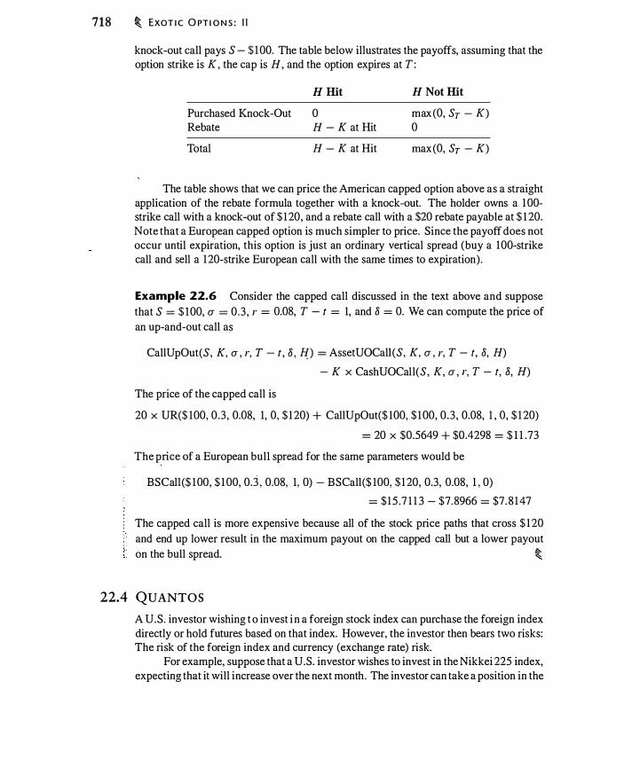
718 � EXOT I C O PT I O N S : I I

knock-out call pays S - $ 100. The table below illustrates the payoffs, assuming that the option strike is K , the cap is H, and the option expires at T:

Purchased Knock-Out Rebate

Total

H Hit

0 H - K at Hit

H - K at Hit

H Not Hit

max(O, ST - K) 0

max(O, ST - K)

The table shows that we can price the American capped option above as a straight application of the rebate formula together with a knock-out. The holder owns a 1 00-strike call with a knock-out of $ 120, and a rebate call with a $20 rebate payable at $ 1 20. Note that a European capped option is much simpler to price. Since the payoff does not occur until expiration, this option is just an ordinary vertical spread (buy a 100-strike call and sell a 120-strike European call with the same times to expiration).

Example 22.6 Consider the capped call discussed in the text above and suppose that S = $ 100, CJ = 0.3 , r = 0.08, T - t = 1, and 8 = 0. We can compute the price of an up-and-out call as

CallUpOut(S, K, u , r, T - t, 8 , H_) = AssetUOCali (S, K, u , r, T - t, 8, H)

- K x CashUOCall(S, K, u , r, T - t, 8, H)

The price of the capped call is

20 x UR($ 100, 0 .3 , 0.08, 1, 0, $ 1 20) + CallUpOut($ 100, $ 1 00, 0 .3 , 0.08, 1 , 0, $ 1 20)

= 20 X $0.5649 + $0.4298 = $ 1 1 .73

The price of a European bull spread for the same parameters would be

BSCall ($ 100, $ 1 00, 0.3 , 0.08, 1, 0) - BSCall($ 100, $ 1 20, 0.3, 0.08, 1 , 0)

= $15 .7 1 1 3 - $7.8966 = $7. 8 147

The capped call is more expensive because all of the stock price paths that cross $ 1 20 and end up lower result in the maximum payout on the capped call but a lower payout on the bull spread. �

22.4 QUANTOS

A U.S. investor wishing t o invest i n a foreign stock index can purchase the foreign index directly or hold futures based on that index. However, the investor then bears two risks: The risk of the foreign index and currency (exchange rate) risk.

For example, suppose that a U.S. investor wishes to invest in the Nikkei 225 index, expecting that it will increase over the next month. The investor can take a position in the

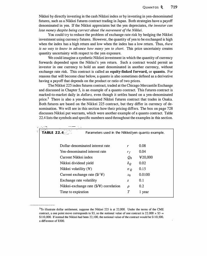
QUA NTOS � 7 19

Nikkei by directly investing in the cash Nikkei index or by investing in yen-denominated futures, such as a Nikkei futures contract trading in Japan. Both strategies have a payoff denominated in yen. If the Nikkei appreciates but the yen depreciates, the investor can lose money despite being correct about the movement of the Nikkei.

You could try to reduce the problem of exchange rate risk by hedging the Nikkei investment using currency futures. However, the quantity of yen to be exchanged is high when the index has a high return and low when the index has a low return. Thus, there is no way to know in advance how many yen to short. This price uncertainty creates quantity uncertainty with respect to the yen exposure.

We could imagine a synthetic Nikkei investment in which the quantity of currency forwards depended upon the Nikkei's yen return. Such a contract Would permit an investor in one currency to hold an asset denominated in another currency, without exchange rate risk. This contract is called an equity-linked forward, or quanto. For reasons that will become clear below, a quanta is also sometimes defined as a derivative having a payoff that depends on the product or ratio of two prices.

The Nikkei 225 index futures contract, traded at the Chicago Mercantile Exchange and discussed in Chapter 5, is an example of a quanta contract. This futures contract is marked-to-market daily in dollars, even though it settles based on a yen-denominated price.5 There is also a yen-denominated Nikkei futures contract that trades in Osaka. Both futures are based on the Nikkei 225 contract, but they differ in currency of de­nomination. We will see in this section how their pricing differs. The box on page 728 discusses Nikkei put warrants, which were another example of a quanta contract. Table 22.4 lists the symbols and specific numbers used throughout the examples in this section.

TAIUE 2 2 .4. , Parameters used in the Nikkei/yen quanta example.

Dollar-denominated interest rate r 0.08

Yen-denominated interest rate I"J 0.04

Current Nikkei index Qo ¥20,000

Nikkei dividend yield 8Q 0.02

Nikkei volatility (¥) O" Q 0. 1 5

Current exchange rate ($/ ¥) xo 0.0 100

Exchange rate volatility s 0. 1

Nikkei-exchange rate ($/¥) correlation p 0.2

Time to expiration T 1 year

5To i l lustrate dollar settlement, suppose the Nikkei 225 is at 22,000. Under the terms of the CME

contract, a one point move corresponds to £5, so the notional value of one contract is 22,000 x $5 = $ 1 1 0,000. If instead the Nikkei had been 22, 1 00, the notional value of the contract would be S 1 1 0,500,

a difference of $500.

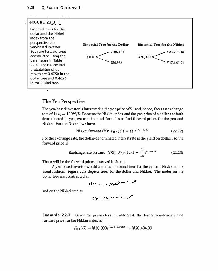
720 � EXOT I C O PT I O N S : I I

F I G U RE 22. � Binomial trees for the dol lar and the Nikkei index from the perspective of a yen-based investor. Both are forward trees constructed using the parameters in Table 22.4. The risk-neutral probabi l ities of up moves are 0.4750 in the dol lar tree and 0.4626 i n the Nikkei tree.

Binomial Tree for the Dollar < $ 106. 184

$ 100

$86.936

The Yen Perspective

Binomial Tree for the Nikkei < ¥23, 706. 10

¥20,000

¥ 1 7,561 .91

The yen-based investor is interested in the yen price of $ 1 and, hence, faces an exchange rate of 1 j x0 = 1 00¥ j$. Because the Nikkei index and the yen price of a dollar are both denominated in yen, we use the usual formulas to find forward prices for the yen and Nikkei. For the Nikkei, we have

Nikkei forward (¥) : Fo.T CQ) = Q0e(rJ-oQ lT (22.22)

For the exchange rate, the dollar-denominated interest rate is the yield on dollars, so the forward price is

1 Exchange rate forward (¥/$): Fo.T ( l fx) = -e<'J-r)T (22.23)

xo These will be the forward prices observed in Japan.

A yen-based investor would construct binomial trees for the yen and Nikkei in the usual fashion. Figure 22.3 depicts trees for the dollar and Nikkei. The nodes on the dollar tree are constructed as

and on the Nikkei tree as

Example 22.7 Given the parameters in Table 22.4, the 1 -year yen-denominated forward price for the Nikkei index is

Fo, l ( Q) = ¥20, 000e<0·04-0.02) x 1 = ¥20,404.03

QUANTOS � 721

and that for the exchange rate is

Fo, t ( 1 /x) = ¥100e(0.04-0.0S) x l = ¥96.079

We can also compute the forward prices on both trees as expected values . For the dollar tree we have

Fo, 1 ( l jx) = 0.4750 x $ 106. 1 84 + ( 1 - 0.4750) x $86.936 = $96.079

For the. Nikkei tree we have6

F0, 1 (Q ) = ¥0.4626 x ¥23 , 706. 10 + ( 1 - 0.4626) x ¥17 ,56 1 .9 1 = ¥20,404.03

The Dollar Perspective

Now we consider yen and Nikkei investments from the perspective of a dollar-based investor. The yen forward price is given by

Exchange rate forward ($/¥): Fo.T (x) = x0e(r-rJ )T (22.24) However, from the dollar perspective, the forward price of the Nikkei is not so straight­forward.

As discussed above, any Nikkei investment entails a combination of currency and index risk. To see why, suppose a dollar-based investor buys e-SQT units of the Nikkei and holds it for T years. The actual steps in this transaction are as follows:

1. Exchange Q0x0e-SQT dollars into yen (this is enough dollars to buy e-SQT units of the index).

2. Buy e-SQT units of the Nikkei index and hold for T periods.

3. Dividends are paid continuously over time and reinvested in the index; after T years we have an additional e8QT shares.

4. After T years sell the index and convert back into dollars.

The time-T value of the investment, denominated in dollars, is

The payoff is a combination of yen and Nikkei risk; we will call this investment the currency-translated index. Here is a point that is crucial for understanding what fol­lows: From the perspective of a dollar-based investm; the dollar-translated price of a yen-denominated asset, YT, is just like any other dollar-denominated asset. However, QT is not the price of an asset for a dollar-based investor, because there is no simple way to obtain the risk of Q without also bearing currency risk.

6The calculation shown here uses rounded numbers and therefore does not exactly equal ¥20,404.03.

722 � EXOT I C O PT I O N S : I I

If you are not convinced that YT really is like any other dollar-denominated asset, consider the following thought experiment. Suppose you learn of a new stock, traded on a U.S. exchange, called "As American as Apple Pie, Inc." (AAAPI). The price is in dollars, just like any other domestic stock. You decide to investigate the stock and, to your surprise, you learn that the company is actually an American Depositary Receipt (ADR) for the Nikkei index.7 The sole asset of this company is shares of the Nikkei, translated into dollars at the current exchange rate, and held in trust. The value at any time is Y1 = x1 Q1 and it has a dividend yield of OQ . This ADR trades just like a dollar-denominated stock, because it is a dollar-denominated stock. Had you not investigated, you would never have known that you were holding a currency-translated yen-denominated stock.

This thought experiment is important, because it tells us that, for a dollar-based investor, the forward price for Y is given by8

Fo,T (Y) = Yoe(r-oQ )T (22.25)

Since we can trade shares of AAAPI, we can undertake arbitrage if the forward price is anything other than equation (22.25). Similarly, the prepaid forward price on the currency-translated index is

(22.26)

In order to obtain Nikkei risk without currency risk, we need to combine the dollar­translated Nikkei with a position in forward yen contracts . Intuitively, we want to invest in Y and use currency contracts to hedge exchange rate risk. Let Vr .T (Y1 , x1 ; T) represent the price of a claim that, at maturity, pays the dollar value of the Nikkei. The boundary condition for this security is

- YT VT.T (YT , xT ; T) = x - (22.27) XT

where j' is an arbitrary exchange rate determined in advance. The boundary condition says that we will receive Y T , the dollar-translated Nikkei, convert it to yen by multiplying by l j:(T , and then convert back to dollars at the rate i. (Since the only purpose of i is to convert yen to dollars, the value is arbitrary and we can set it to 1 . In practice the contract can call for any fixed exchange rate. ) Prior to time T, the market-maker

7 In simplest terms, an ADR is a claim to a trust containing a foreign stock. ADRs are a common means

for investors in one country to buy a stock trading in another country.

8We saw in Chapter 20 that if S and Q are asset prices, then the forward price for S Q contained a

covariance term. You may be wondering why there is no such covariance term in equation (22.26) .

In general, if an asset with price So is traded and can be held by investors, then its forward price is

Soe(r-SlT . This is a no-arbitrage result. In the discussion in Chapter 20, we assume that S and Q are

both prices of assets that can be held directly by investors. In that case S Q does not represent the price

of an asset. In the discussion here, x Q is the price of an asset that can be held directly by investors, but

Q cannot be held directly. In general, S, Q, and S Q cannot all simultaneously be the prices of traded

assets.

QUANTOS � 723

hedges the value of the security using both the dollar-translated Nikkei and exchange rate contracts. Equation (22.27) makes it clear why quantos are said to be derivatives that depend on the ratio or product of two assets.9

We can price this contract by using Proposition 2 1 . 1 . That proposition implies that we obtain the forward price for Y T j XT by multiplying the forward price for Y by the forward price for l jx, and adjusting the dividend yield to take account of the covariance between x and Y .

To apply Proposition 2 1 . 1 we need to know the forward price of 1 jx for dollar­denominated investors. We can obtain the forward price for 1 jx using Proposition 20.3 . This gives10

F,.T ( 1 jx) = ..!...e<rrr+s2) (T-t) xo

We also need to know the covariance between x and Y. Using Ito's Lemma, that covariance is

1 ry -[dx - E(dx)] [dY - E (dY)] = psa Q + s­dt (22.28)

In applying Proposition 2 1 . 1 , we have b = - 1 ; hence, when we compute the forward price for Q we replace O Q with O Q - ( - l ) (psa Q + s2) .

Putting this all together, using Proposition 2 1 . 1 and with i = 1 we have

(22.29)

The dollar-denominated forward price for the Nikkei index is the same as the yen­denominated forward price, with a covariance correction. The prepaid quanta index forward price is thus

(22.30)

The role of the covariance term in equation (22.29) is intuitive. Consider an investor who buys the cash Nikkei index and ultimately converts yen back to dol­lars. Suppose the index and the exchange rate (measured in dollars/yen) are positively

9If the market-maker hedges a claim with value V using x and Y, the claim value must satisfy the

mulitvariate Black-Scholes equation. In this case, the equation is

0.5s2x2 llr.r + 0.5(s2 + a2 + 2psa) Y2 Vrr + (s2 + psa) Yx Vr.t

+ \l, (r - rf)X + Vy (r - 8)Y + V, - r V = 0

10In this calculation we start with the forward price for x from the dollar perspective and convert it to

the forward price for l fx. As a result, the forward price for l fx given here is different from that given

by equation (22.23), which is the appropriate forward price given a yen perspective.

724 � EXOT I C O PT I O N S : I I

correlated. When the index does well, there are many yen to exchange. If p is positive, on average the exchange rate is favorable when there are many yen to exchange. When the index does poorly, there are fewer yen to exchange so the decline in the exchange rate does not matter as much. Thus, other things equal, the positive correlation system­atically benefits the unhedged investment in the Nikkei relative to a contract with a fixed exchange rate. Consequently, if the exchange rate is fixed, as in a quanta contract, the price for the index settling in dollars will be lower in order to compensate the buyer for the loss of beneficial correlation between the index and exchange rate.

Example 22.8 Using equation (22.29) and the information in Table 22.4, the yen forward price is

Fo. I = xoe<r-rJ)I = O.O l $j¥e<O.OS-0.04) = 0.0 1 0408$/¥

The forward price for the currency-translated Nikkei is

Fo. I = .to Qoe<'-8Q )I = 0.0 1 $/¥ X ¥20 , oooe<O.OS-0.01) = $2 12 .367

Finally, using equation (22.29), the quanta forward price is

Vo, I ($200, 0 .0 1 $/¥) = ¥20, oooe<0.04-0.02-0.2xO. I x 0. 1 5)

= ¥20 , 342.9 1

This is lower than the yen-denomina!ed Nikkei forward price of ¥20,404 in Example 22.7. �

A Binonlial �odel for the Dollar-Denominated Investor

As another way to understand quanta pricing, we can construct a binomial tree that simultaneously models the currency-translated index and the exchange rate. In addition to this particular application of two-variable binomial trees, some options have prices that depend on two state variables.

In Figure 22.3 we constructed separate binomial trees for the yen-based investor. For the dollar-based investor we need to construct a tree that takes account of the corre­lation between the Nikkei and the yen. We can do so by first modeling the behavior of the yen in the usual way, and then, conditional upon the yen, model the movement in the Nikkei. 1 1 Since for each yen move there are two Nikkei moves, the tree will have four binomial nodes. We will denote these as {ull , ud, du , dd} , with the first letter denoting the yen move and the second the Nikkei move. We have a choice of constructing a joint tree for the yen and Nikkei or the yen and dollar-translated Nikkei, but we obtain the

1 1 This is similar to the two-variable binomial model in Rubinstein ( 1 994). See also Boyle et al. ( 1 989) for a procedure to generate n-asset binomial trees.

QUA NTOS � 725

same answer either way. Here we will model the yen and Nikkei. Problem 22. 1 7 asks you to jointly model the yen and dollar-translated Nikkei.

The basic idea underlying the joint binomial model for x and Q is as follows . If x and Q are lognormal, they evolve like this :

(22.3 1 a)

(22.3 1 b)

In the standard binomial model, we simply approximate Z 1 and Z2 binomially, so that Z; = ± 1 . However, we want to induce correlation between Z1 and Z2 • We can create correlation by using the Cholesky decomposition discussed in Chapter 19 . Begin by rewriting equation (22.3 1 ) using equation ( 1 9. 17) :

(22.32a)

(22.32b)

Thus, zl = E i and z2 = PEl + J 1 - p2E2 . By construction, this zl and z2 have correlation p. Now we construct the binomial tree by setting E 1 = ± I (the exchange rate moves up or down) and E2 = ± I (the index moves up or down) . There are four possible outcomes, which we will label A (E 1 = 1 ; E2 = 1 ), B (E 1 = 1 ; E2 = - 1 ) , C

(E J = - 1 ; E2 = 1 ), and D (E J = - 1 ; E2 = - 1 ) . For a dollar-based investor, the possible yen moves are

X - x - ,. e<r-rr)h+s../ii - ,. ll • A - • B - •'0 - •'0

Xc = Xo = xoe<r-rr lh-s../ii = xod

For each yen move, there are two Nikkei moves :

0 = 0 e<rr-8o )lr+aQ ../ii(p+F-i;'il = OoA - A _o _

0 = 0 e<rr-oQ)h+aQ../ii(p-F-i;'iJ = OoB _ n _o _

0 = 0 e<rr-8Q )h+aQ ../ii(-p+F-i;'il = 0 C _ c _o _o 0 = 0 e <rr-oQ )h+ao../ii(-p-F-i;'il = 0 D _ o _o _o

(22.33a)

(22.33b)

(22.34a)

(22.34b)

(22.34c)

(22.34d)

Finally, we have to determine the risk-neutral probabilities associated with the nodes. As in Chapter 10, the risk-neutral probability for an up move of the currency is

e<r-rr)h - d p = ---­u - d

(22.35)

where u and d are implied by equation (22.33a) and (22.33b ) . The risk-neutral probability for an up move in the currency is 0.4750.

Recall that the risk-neutral probability arises from the requirement that an invest­ment in the asset earn the risk-free rate. Specifically, for the currency, we consider an investment in the yen-denominated risk-free asset, hedged to remove currency risk when the investment is turned back into dollars . This investment earns the dollar-denominated risk-free return if the probability of an up move is given by equation (22.35).

726 � EXOT I C O PT I O N S : I I

Time 1 Yen, x 1 Nikkei, Q1 < ¥23,706.10

0.01 1503 $/¥

Q0 = ¥20,000 < ¥18,647.88 x0 = 0.01$/¥ < ¥22,325 .56

0.009418$/¥ ¥ 1 7,561 .91

Risk-Neutral X1Q1 Probability

$ 272.68 0.2194

$214.50 0.2556 $ 210.25 0.2425

$ 165.39 0.2825

The binomial process for the dol lar/yen exchange rate (x) and the Nikkei (Q). The last two columns contain the value of the currency-translated Nikkei and the risk-neutral probabi l ity of each node, computed using equations (22.35) and (22 .37).

We need a similar argument for the Nikkei. Since we cannot own the Nikkei index

without bearing currency risk, we model an investment in the dollar-translated Nikkei.

Let p* denote the probability of an up move in the Nikkei, conditional on the move in the

yen. We require that the dollar-translated Nikkei investment earn the dollar-denominated

risk-free rate. This gives us ·

x,. QApp* + x,. QBp ( l - p*) + xd Qc ( 1 - p)p*

Solving for p* gives

* xoQoe<r-•Q lh - x,. QBP - xdQo ( 1 - p) p = px,. (QA - QB) + ( 1 - p)xd (Qc - Qo) e<r-8Q )h - uBp - dD( l - p)

= ----------�--------�-·pu (A - B) + ( 1 - p)d(C - D)

(22.36)

(22.37)

This expression is a generalization of the one-variable formula for a risk-neutral proba­

bility, taking account of the two up and two down states for Q. Figure 22.4 depicts the binomial tree constructed using equations (22.33) and

(22.34), and probabilties of each node constructed using equations (22.35) and (22.37). The quanto forward price can be constructed as the expectation E(YI /xi ) .

� Example 22.9 Using Figure 22.4 we can compute forward prices for the yen, the M dollar-translated Nikkei, and the quanta Nikkei. The risk-neutral probability of an up

move in the yen is 0.4750. The yen forward price is

Fo. t (x) = 0.4750 X 0.0 1 1503$/¥ + ( 1 - 0.4750) X 0.00941 8$/¥ = 0.0 10408$/¥

f� � �j fj tl i1 !i

C U R R E N CY-LI N K E D O PT I O N S � 727

The forward price for the currency-translated Nikkei is

Fo, l (x Q) = 0.2 194 X $272.68 + 0.2556 X $2 14.50 + 0.2425 X $210.25 + 0 .2825 X $ 165 .39 = $212.367

Finally, the quanto forward price is

F. = 0.2 1 94 X $272"68 0.2556 X

$214·50 0: 1 (Q) 0.0 1 1503$/¥ + 0.01 1503$/¥

$210.25 $ 165.39 +0.2425 X 0.00941 8$j¥ + 0.2825 X

0.00941 8$j¥ = ¥20,342.9 1

� All of the prices computed from the tree match those in Example 22.8 .

The tree in Figure 22.4 can be extended to multiple periods. Rubinstein ( 1994) shows that in general, with n steps, there are (n + 1 )2 nodes; for example, with two

steps there are nine nodes. To see why, if we add another binomial period to the tree, there are 42 = 1 6 combinations of the up-down moves (AA, AB , . . . , DD). The order

of the moves is irrelevant, so, for example, AB = BA . This equivalence eliminates

n x (n - 1 ) = 6 nodes, leaving 10. Further, from equation (22.34 ) , A B = CD. Because

n = 2, this leaves (n + 1)2 = 9 unique nodes.

22.5 CURRENCY-LINKED OPTIONS

There are several common ways to construct options on foreign assets, for which the

return has an exchange rate component. 12 The different variants permit investors to

assume different amounts of currency and equity risk. In this section we examine four variants and their pricing formulas. We will continue to use the notation and numbers

from Table 22.4 . . Before we discuss particular currency-linked options, recall the result from Chapter

12, equation ( 1 2.5), and Chapter 14, equation ( 14. 1 6) , that an option can be priced using

only the prepaid forward prices for the underlying asset and strike asset, and the relative

volatility of the two. 13 The intuition for this result is that a market-maker could hedge an

option position using the two prepaid forwards, neither of which, by definition, makes

any payouts. In the discussions to follow we will use this result to simplify the valuation

of seemingly complex options.

12This section draws heavily from Reiner ( 1992), in particular adopting Reiner's tenninology for the

different kinds of options.

13To convince yourself of this, note that

BSCall(S, K, a , r, T, 8) = BSCall(Se-&T , K e-rT , a , 0, T, 0)

This equality will hold for any inputs you try.

728 � EXOT I C O PT I O N S : I I

Nikkei Put Warrants

An example of quanta options is the Nikkei 225 put warrants that traded on the American Stock Exchange beginning in 1 990. Ryan and Granovsky (2000) provide an interesting account of the history of these options, in which Nikkei risk was repackaged and transfon:ped several times by various global financial players.

Japanese institutional investors in the late 1 980s bought Nikkei bull notes. These were bonds that carried a high coupon and contained an embedded written put spread: The note principal was not paid in full if the Nikkei fell below ¥32,000. The issuer of the notes was a European bank that sold the embedded put spread to an investment bank and entered into a currency swap to achieve dollar-denominated financing without any Nikkei risk. Japanese buyers were willing to pay a price that made it profitable for the European bank to issue the notes and hedge the resulting exposure.

The investment bank, having bought the put spread, had short exposure to the Nikkei. It sold dollar-denominated Nikkei puts to a European sovereign, which in turn sold dollar-denominated Nikkei puts to investors who wanted dollar-denominated Nikkei exposure in the form of SEC-registered securities without investment bank credit risk. (The sovereign issuer bore the investment bank credit risk and the notes carried sovereign risk.)

The net result of this chain of transactions was that Japanese institutional investors were betting-via the bull notes-that the Nikkei would rise. Buyers of the dollar-denominated Nikkei put warrants were betting that the Nikkei would falL In the end, the Nikkei index suffered a long decline and the put warrant buyers ·won the bet.

Foreign Equity Call Struck in Foreign Currency

If we want to speculate on a foreign index, one possibility is to buy an option completely denominated in a foreign currency. The value of this option at expiration is

where K r denotes the strike denominated in the foreign currency. As an example, we might have a I -year call option to buy the Nikkei index by

paying ¥ 19 ,500. An investor based in the foreign currency would use this kind of option ; thus, i t can be priced using the Black-Scholes formula from the perspective of the foreign currency. Only yen inputs-the yen-denominated interest rate and the Nikkei volatility and dividend yield-enter the pricing formula. The dollar price can be obtained by converting the option price at the current exchange rate.

C U R R E N CY- L I N K E D O PT I O N S � 729

C¥ = Qoe-.sQr N(d1 ) - Kfe-r1t N(d2)

d1 = ln ( Qoe-.SQt / K fe-r11 ) + 1cr�t

CT Q.jt

d2 = d1 - CTQ.jt

(22.38)

Thus, we price this option by using the Black-Scholes formula with inputs appropriate for the asset being denominated in a different currency.

Example 22. 1 0 Using the parameters in Table 22.4 and assuming a: strike price of ¥19,500, we price the call by using the Black-Scholes formula and setting S = ¥20,000 (the current Nikkei index price), K = ¥19,500, cr Q = 0.15 (the Nikkei volatility in yen), r1 = 0.04, T - t = 1 , and oQ = 0.02 (the dividend yie1d on the Nikkei) . We obtain a call price ofBSCall(¥20,000; ¥19 ,500; 0 . 15 ; 0.04; 1 ; 0 .02) = ¥1632. 16. The dollar price is $ 16.32. �

Foreign Equity Call Struck in Domestic Currency

Suppose we have a call option to buy the Nikkei but we denominate the strike, K, in dollars. If we exercise the option, we pay K dollars to acquire the Nikkei, which is worth xr Q r . Thus, at expiration, the option is worth

V (xr Q r , T) = max(O, xr Qr - K)

In order to price this option, recognize that Y (T) = xr Qr, the currency-translated index, is priced like any domestic asset. The prepaid forward price for the currency-translated index is, from equation (22.26), x0 Q0e-&Q T . The prepaid forward price for the strike is K e-rT . The value of the option will depend upon the distribution of xr Q y ; thus, the volatility that enters the option pricing formula is that of the currency-translated index. The volatility of x, Q, is

v = J cr� + s2 + 2pcr QS

Using this volatility and the prepaid forward prices we have

C = xo Qoe-liT N(dt ) - e-rr KN(d2)

d, = ln (xo Qoe-.sr ;e-rr K) + 1 v2t

v.Ji d2 = dt - v.Ji

(22.39)

You can interpret this formula in terms of prepaid forward prices or as the Black-Scho1es formula with x0 Q0 as the stock price, 8 Q as the dividend yield, v as the volatility, the domestic interest rate r as the risk-free rate, and K as the strike price.

730 � EXOT I C O PTI O N S : I I

" Example 22. 1 1 Using the parameters in Table 22.4, the volatility is

v = J0 . 1 52 + 0. J 2 + (2 X 0.2 X 0. 1 5 X 0. 1 ) = 0. 1 962

and assuming a strike price of $ 1 95, we price the call using prepaid forwards as

BSCall (xo Qoe-8r, Ke-rr , v , 0, T, 0)

= BSCall (0.0 1 $/¥ x ¥20,000e-0·02 , $ 1 95 x e-0-08 , 0. 1 962, 0, 1 , 0) = $24.07 1 9

Fixed Exchange Rate Foreign Equity Call . .

�

Suppose we have a foreign equity call denominated in the foreign currency, but with the option proceeds to be repatriated at a predetermined exchange rate. This is a quanta option, analogous to the quanta forward, with the value of the option translated into dollars at a fixed exchange rate. Let i represent this rate. The payoff to this option with strike price K 1 (denominated in the foreign currency) is

V ( Q r , T) = i x max(O, Qr - KJ)

= max(O, i Qr - i KJ)

Once again we can construct the pricing formula by thinking in terms of forward prices for the underlying and strike asse!s. From a dollar perspective, the underlying asset, i Qr , is a quanta index investment. The strike asset is simply a fixed number of dollars, translated at the rate -� . Since -� is just a scale factor, we can set .� = 1 .

Because the exchange rate is fixed, the volatility that affects the value of the option is that of the foreign-currency-denominated foreign index, u Q . We can obtain the pricing formula by using the prepaid forwards for the underlying and strike asset:

C = Fci,r ( Q) N(d! ) - e-rr K1N(d2)

d _ ln [Ft_1 (Q )/e-rT KJ] + 1utT

. I -U Q .Jf

d2 = d1 - U Q -J{

(22.40)

The formula for Fci.r C Q) is given in equation (22.30). Note that all values are dollar­denominated since -� implicitly multiplies all prices. By substituting for Fci,1 , equation (22.40) is the Black-Scholes formula with Q0 as the stock price, O Q + psu Q + r - r1 as the dividend yield, the domestic interest rate r as the risk-free rate, K 1 as the strike, and u Q as the volatility.

Example 22. 1 2 Using the parameters in Table 22.4 and assuming a strike price of ¥ 1 9,500 with a fixed exchange rate of i = 0.0 1$/¥, we price the call by using the

C U R R E N CY- L I N K E D O PTI O N S � 73 1

Black-Scholes formula. We obtain

BSCall(Fci.T (Q ) , Kte-rT , CJ Q , 0, T, 0) =

BSCall(0 .0 1$/¥ x ¥20, 000 x e-<o.o2+o.2x0· 1 xo. t s+o.os-0.04l , 0.0 1 $/¥ x ¥19, 500e-0·08 , 0. 15 , 0, 1 , 0) = $ 15 .3 1 87

Problem 22.6 asks you to verify that you obtain the same answer with x0 Q0 as the underlying asset and an appropriate choice of the dividend yield. �

Equity-Linked Foreign Exchange Call

If we invest in a foreign asset, we might like to insure against low exchange rates when we convert back to the domestic currency, while still having the ability to profit from favorable exchange rates. Buying an exchange rate put is insufficient because the quantity of currency to be exchanged is uncertain. What we want is an option that guarantees a minimum exchange rate wizen we convert tlze asset value back to the domestic currency. Such an option must therefore protect a variable quantity of currency. This is an equity-linked foreign exchange option, which is another example of a quanta option.

Let K be the minimum exchange rate. Then the payoff to such an insured position would be

QTXT + QT max(O, K - XT) = QT K + QT max(O, XT - K) = QT K + max(O, QTXT - QT K)

(22.41 )

The expression to the left of the equal sign in equation (22.41 ) is the unprotected currency­translated Nikkei investment plus QT exchange rate puts with strike K . The equivalent expression on the right is a quanta investment with the fixed exchange rate equal to K, plus QT exchange rate calls. Either way, the protection entails receiving the payoff to a random number of options. All cash flows are denominated in the home currency.

There are at least two ways to value the payoff in equation (22.4 1 ) : ( I ) By using Proposition 2 1 . 1 and (2) by using the prepaid forward approach. Using Proposition 2 1 . 1 , we value QT x max(O, XT - K) as a currency call with a change of numeraire. We will pursue that approach; Problem 22.7 asks you to derive the same formula using prepaid forward prices .

The forward price for QT is the quanta forward price, equation (22.29). The put is a standard currency call denominated in the home currency. Since it is a currency option, the dividend yield is the foreign interest rate. To change the numeraire we subtract pus, the covariance between Q and x , from the dividend yield, r1 . Thus, we price the payoff QT x max(O, XT :- K) by multiplying Qoe<rJ-aQ-pas)T , the quanta forward price, times the Black-Scholes currency call formula with r1 replaced by r1 - pus. This gives

c = Qoe<rJ-OQ-pas)T [xoe-(rf-pas)T N(dt ) - e-rT K N (d2 )] = xo Qoe-8QT N(dt ) - K Qoe-(r+8Q+pas-rf )T N(d2)

(22.42)

732 � EXOT I C O PT I O N S : I I

ln (xo/ K ) + (r - r1 + pas + 0.5s2) T dl = --�--��--���------� s../T d2 = d1 - s../T

This is the price of a call option with x0 Qo as the stock price, K Qo as the strike price, r + 8 Q + pas - r1 as the risk- free rate, 8 Q as the dividend yield, and s as the volatility. It is perhaps surprising that only the volatility of the exchange rate matters. This occurs because the underlying option is a currency option and the change of numeraire does not affect the volatility.

ft Example 22. 1 3 Using the parameters in Table 22.4 and assuming a strike price U of 0.00975$/¥, we price the call by -using the Black-Scholes formula. The price of

the underlying asset is x0 Q0 = 0.01 $/¥ x ¥20,000 = $200, the strike price is 0.00975$/¥ x ¥20,000 = $ 1 95, the risk-free rate is replaced by r + 8Q + pas - r1 =

0.08 + 0.02 + 0.2 x 0. 1 5 x 0. 1 - 0.04 = 0.063, and the dividend yield is 8 Q = 0.02. The value of the option in equation (22.42) is

BSCall($200, $ 1 95 , 0. 1 0, 0.063, l , 0.02) = $ 1 5 .7287

22.6 OTHER MULTIVARIATE OPTIONS

Quantos are a particular kind of claim with a payoff dependent on the price of two assets. There are many other options for which the payoff depends on two or more assets. In this section we examine several kinds of multivariate options that can be priced either by modifying the Black-Scholes formula or by using the bivariate normal distribution. We will also see how to price some of these options binomially. Throughout this section, we assume that the assets S and Q follow the processes given by equations (22. 1 ) and (22.2) .

Exchange Options

We saw in Section 14.6 that exchange options, in which the strike price is the price of a risky asset, can be priced with a simple modification of the Black-Scholes formula. Here we will use a change of numeraire to see why this is so.

At maturity, an exchange option with price V (S� > Q1 , t) pays

V (ST , QT , T) = max(ST - QT , 0)

= QT X max(ST/ QT - 1 , 0) (22.43)

This payoff is like receiving a random number, QT, of options in which the underly­ing asset is ST / QT and the strike price is $ 1 . We can price this option by applying Propositions 20.4 and 2 1 . 1 .

OTH E R M U LT IVA R I ATE O PT I O N S � 733

First, consider the price of an option with S I Q as the underlying asset. We can price this option using the Black-Scholes formula with the lease rate for S 1 Q in place of the dividend yield and the variance of ln(S I Q) as the variance. Propositions 20.3 and 20.4 imply that the lease rate for S I Q is

8* = r + 8 - 8 Q - a� + paa Q

and the variance is

&2 = a2 + a� - 2paa Q

Denote the value of this option by W(SI Q, t ) . Its price is

W(SI Q, t) = SI Qe-�·<T-1>N(dJ ) - e-'1 N(d2)

a) = ln(S I Q) + (r - 8* + 0.5u2) (T - t)

&�

d2 = d1 - u�

(22.44)

(22.45)

(22.46)

(22.47)

(22.48)

Now we want to value the option with payoff Q x W(SI Q, t) . To do this we apply Proposition 2 1 . 1 . The covariance between Q and S I Q is paa Q - a� . Thus, applying Proposition 2 1 . 1 , we replace 8* with

8* - (paa Q - a� ) = r + 8 - 8 Q

Finally, multiplying W by Qe<r-�.> <T-I) gives

V(S, Q, t) = Se-�<T-I) N(dJ ) - Qe-�Q (T-I) N(d2)

d1 = ln (SI Q) + (8 Q - 8 + 0.5&2) (T - t)

&� d2 = d1 - u �

(22.49)

This is the formula for an exchange option from Section 14.6. The risk-free rate is replaced by 8 Q and the volatility by u .

American exchange options can b e valued using a two-state variable binomial tree, as in Section 22.4. However, it is also possible to value an American exchange option using a one-variable binomial tree. Rubinstein ( 1991b) shows that a standard binomial tree can be constructed setting the volatility equal to u , the dividend yield equal to 8, and the risk-free rate equal to 8 Q . This result can also be demonstrated by using arguments based on Propositions 20.4 and 2 1 . 1 .

Options on the Best of Two Assets Suppose an investor allocates a portfolio to both the S&P index and the currency­translated Nikkei. Allocating the portfolio to the index that the investor believes will obtain the highest return is called market-timing. A perfect market-timer would invest in the S&P when it outperformed the Nikkei and the Nikkei when it outperformed the

734 � EXOT I C O PT I O N S : I I

S&P. What is the value of being able to infallibly select the portfolio with the superior performance?

We can answer this question by valuing an option giving us the greater of the two returns. This option would have the payoff max(Sr , Qr ), where S is the S&P index and the Q the Nikkei index. Note that

max(Sr , Qr) = Qr + max(Sr - Qr , 0) Thus, an option on the best of two assets is the same as owning one asset plus an option to exchange that asset for the other asset. As discussed in Chapter 9, max(Sr - Qr , 0) can be viewed either as a call on S with strike asset Q, or as a put on Q, with strike asset S. '

An investor allocating funds between the S&P index and the Nikkei index might also want to include cash in the comparison, so that there is a guaranteed minimum return. If K represents this minimum return, the payoff for a perfect market-timer is then

max(K, Sr , Qr)

This option, called a rainbow option, has no simple one-variable solution. Instead, valuing this option requires the use of the bivariate normal distribution. 14 The bivariate normal distribution is defined as

Prob(z 1 < a , Z2 < b; p) = NN (a , b; p) (22.50) where z 1 and z2 are standard normal random variables With correlation coefficient p . You may recall that we used the biv<!riate normal distribution in Chapter 14 to value compound options.

The formula for a rainbow option is

RainbowCall(S, Q, K, a, s , p , 8 , 8 Q , T - t)

where

= Se-a<T-rJ { N(dsQ) - NN[ -d1 (S) , dsQ , (pa Q - a)fUJ }

+ Qe-8Q <T-1} { N(dQs) - NN[-d1 ( Q) , dQs , (pa - a Q)/a] } + Ke-r(T-I) NN[-d2 (S) , -d2 ( Q) , p]

ln (S/ K) + (r - 8 + 0.5a2) (T - t) dt (S) = � a.y T - t

ln (Q/ K) + (r - 8 Q + 0.5a�) (T - t) di (Q) = � a Q v T - t

d2 (S) = d1 (S) - a� d2 ( Q) = d1 (Q) - a Q �

14Stulz ( 1 982) first valued a rainbow option. See also Rubinstein ( l 99 l c) for a discussion.

(22.5 1 )

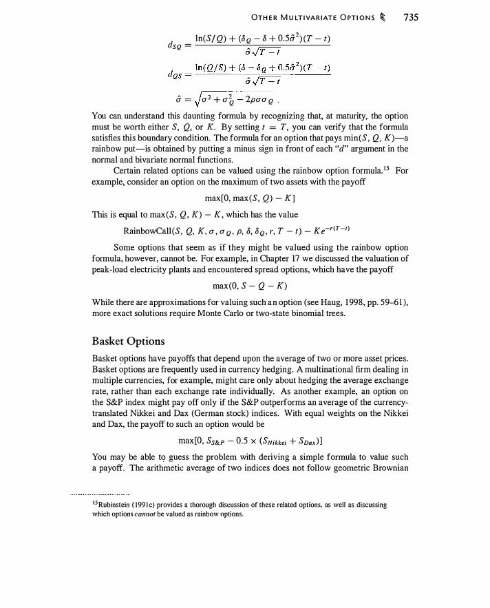
OTH E R M U LT I VA R I AT E O PT I O N S � 735

d _ ln(Sf Q) + (o Q - o + 0.5&2) (T - t) SQ - A ry-: C5 y 1 - t

ln (Q/ S) + (o - oQ + 0.5&2) (T - t) dQs - ���-----====---�--� -

A ry-: CJ '\{ 1 - t

& = J rr2 + rrt - 2prrrr Q

You can. understand this daunting formula by recognizing that, at maturity, the option must be worth either S, Q, or K. By setting t = T, you can verify that the formula satisfies this boundary condition. The formula for an option that pays min(S , Q , K)-a rainbow put-is obtained by putting a minus sign in front of each "d" argument in the normal and bivariate normal functions.

Certain related options can be valued using the rainbow option formula. 1 5 For example, consider an option on the maximum of two assets with the payoff

max[O, max(S, Q) - K]

This is equal to max(S, Q , K) - K, which has the value

RainbowCall (S, Q, K, rr , rr Q • p, o, o Q , r, T - t ) - K e-r<T -/)

Some options that seem as if they might be valued using the rainbow option formula, however, cannot be. For example, in Chapter 17 we discussed the valuation of peak-load electricity plants and encountered spread options, which have the payoff

max(O, S - Q - K)

While there are approximations for valuing such an option (see Haug, 1 998, pp. 59-6 1 ), more exact solutions require Monte Carlo or two-state binomial trees.

Basket Options

Basket ?Ptions have payoffs that depend upon the average of two or more asset prices. Basket options are frequently used in currency hedging. A multinational firm dealing in multiple currencies, for example, might care only about hedging the average exchange rate, rather than each exchange rate individually. As another example, an option on the S&P index might pay off only if the S&P outperforms an average of the currency­translated Nikkei and Dax (German stock) indices . With equal weights on the Nikkei and Dax, the payoff to such an option would be

max[O, Ss&P - 0.5 X (SNikkei + Soax) ]

You may be able to guess the problem with deriving a simple formula to value such a payoff. The arithmetic average of two indices does not follow geometric Brownian

1 5 Rubinstein ( 1 99 l c) provides a thorough discussion of these related options, as well as discussing which options cannot be valued as rainbow options.

736 � EXOT I C O PT I O N S : I I

motion. (In fact, if an index is an arithmetic average of stocks, the index itself does not

follow geometric Brownian motion. We have been making the common, yet inconsis­

tent, assumption that both stocks and indices containing those stocks follow geometric

Brownian motion.)

Because the payoff can depend on many random variables and there is no easy

formula, Monte Carlo is a natural technique for valuing basket options. Moreover,

basket options provide a natural application for the control variate method to speed up

Monte Carlo. A basket option based on the geometric average can be valued using

Black-Scholes with appropriate adjustments to the volatility and dividend yield. This

pqce can then serve as a control variate for the more conventional basket option based

on an arithmetic average.

CHAPTER SUMMARY

It is possible to build new derivative claims by using simpler claims as building blocks.

Important building blocks include ali-or-nothing options, which pay either cash or an as­

set under certain conditions. Assuming that prices are lognormal with constant volatility,

it is straightforward to value cash-or-nothing and asset-or-nothing options both with and

without barriers. Cash-or-nothing claims can be priced as discounted risk-neutral prob­

abilities, and a change of numeraire can then be used to price asset-or-nothing options. These claims can be used to create, among other things, ordinary options, gap options,

and barrier options. While these options are straightforward to price, they may be quite

difficult to hedge because of discontinuities in the payoff created by the ali-or-nothing

characteristic.

Quantos are claims for which the payoff depends on the product or quotient of two

prices. They can be priced using arguments developed in Chapters 20 and 2 1 . Quantos

can be used to remove the currency risk from an investment in a foreign stock index

and thus are used in international investing. It is possible to construct bivariate binomial

trees to price quantos. International investors can also use currency-linked options to

tailor their exposure to currency. The standard currency options can be priced using

prepaid forwards and change of numeraire.

Other options, such as rainbow and basket options, have payoffs depending on

two or more asset prices. Some of these options have simple pricing formulas; others

must be valued binomially, using Monte Carlo, or in some other way.

FURTHER READING

Mark Rubinstein and Eric Reiner published a series of papers on exotic options in Risk magazine in the early 1990s. These provide a comprehensive discussion of pricing for­

mulas on a wide variety of options. Some of the material in this chapter is based directly

on those papers, which can be hard to obtain but are available on Mark Rubinstein's

website (http://www.in-the-money.com). Ingersoll (2000) also provides examples

P R O B L E M S � 737

of the use of all-or-nothing options as building blocks. An alternative approach to two­state binomial pricing is detailed in Boyle et al. ( 1 989).

If you are interested in more pricing formulas, Haug ( 1 998) presents numerous formulas and discusses approximations when those simple formulas are not available. Wilmott ( 1 998) also has a comprehensive discussion emphasizing the use of partial differential equations (which, as we have seen, underlie all derivatives pricing). Zhang ( 1 998) and Briys and Bellala ( 1 998) discuss exotic options, including many not discussed in this chapter. In practice, the hitting of a barrier is often determined on a daily or other periodic basis. Broadie et al. ( 1 997) provide a simple correction term that makes the barrier pricing formulas more accurate when monitoring of the barrier is not continuous . One class of options we have not discussed is lookback options, which pay out based on the highest (or lowest) price over the life of the option. These are discussed in Goldman et al. ( 1979a) and Goldman et al. ( 1 979b) and are covered in Problems 22. 1 3 and 22. 14.

PROBLEMS -.____

22.1. A collect-on-delivery call (COD) costs zero initially, with the payoff at expi­ration being 0 if S < K, and S - K - P if S ::: K. The problem in valuing the option is to determine P, the amount the option-holder pays if the option is in-the-money at expiration. The premium P i s determined once and for all when the option is created. Let S = $ 100, K = $ 1 00, r = 5%, a = 20%, T - t = 1 year, and o = 0.

a. Value a European COD call option with the above inputs . (Hint: Rec­ognize that you can construct the COD payoff by combining an ordinary call option and a cash-or-nothing call. )

b. Compute delta and gamma for a COD option. (You may do this by com­puting the value of the option at slightly different prices and calculating delta and gamma directly, rather than by using a formula.) Consider dif­ferent stock prices and times to expiration, in particular setting t close to T .

c . How hard i s i t to hedge a COD option?

22.2. A barrier COD option is like a COD except that payment for the option occurs whenever a barrier is struck. Price a barrier COD put for the same values as in the previous problem, with a barrier of $95 and a strike of $90. Compute the delta and gamma for the pay later put. Compare the behavior of delta and gamma with that for a COD. Explain the differences, if any.

22.3. Verify that equation (22. 7) satisfies the appropriate boundary conditions for Prob�T ::::: H and ST > K) .

22.4. Verify that equation (22. 14) (for both cases K > H and K < H) solves the boundary conditions for an up-and-in cash put.

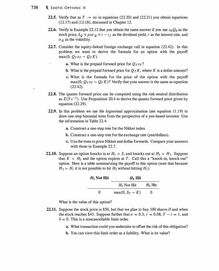
738 � EXOT I C O PT I O N S : I I

22.5. Verify that as T ---+ oo in equations (22.20) and (22.2 1 ) you obtain equations ( 1 2. 1 7) and ( 1 2. 1 8), discussed in Chapter 12.

22.6. Verify in Example 22. 1 2 that you obtain the same answer if you use x0 Q0 as the stock price, 8 Q + psa Q + r - r1 as the dividend yield, r as the interest rate, and a Q as the volatility.

22.7. Consider the equity-linked foreign exchange call in equation (22.42). In this problem we want to derive the formula for an option with the payoff max(O, QTXT - Q T K) .

a. What is the prepaid forward price for Q TxT ?

b. What is the prepaid forward price for Q T K, where K is a dollar amount?

c. What is the formula for the price of the option with the payoff max(O, Q TxT - QT K)? Verify that your answer is the same as equation (2i42) .

22.8. The quanta forward price can be computed using the risk-neutral distribution as E(Yx - 1 ) . Use Proposition 20.4 to derive the quanta forward price given by equation (22.29) .

22.9. In this problem we use the lognormal approximation (see equation 1 1 . 1 9) to draw one-step binomial trees from the perspective of a yen-based investor. Use the information in Table 22.4.

a. Construct a one-step tree for the Nikkei index.

b. Construct a one-step tree for the exchange rate (yen/dollars) .

c. Use the trees to price Nikkei and dollar forwards . Compare your answers with those in Example 22.7.

22.10. Suppose an option knocks in at H1 > S, and knocks out at H2 > H 1 • Suppose that K < H2 and the option expires at T. Call this a "knock-in, knock-out" option. Here is a table summarizing the payoff to this option (note that because H2 > H1 it is not possible to hit H2 without hitting H1 ) :

H1 Not Hit

H2 Not Hit

0 max(O, ST - K) 0

What is the value of this option?

22.11. Suppose the stock price is $50, but that we plan to buy 100 shares if and when the stock reaches $45 . Suppose further that a = 0.3, r = 0.08, T - t = 1 , and 8 = 0. This is a noncancellable limit order.

a. What transaction could you undertake to offset the risk of this obligation?

b. You can view this limit order as a liability. What is its value?

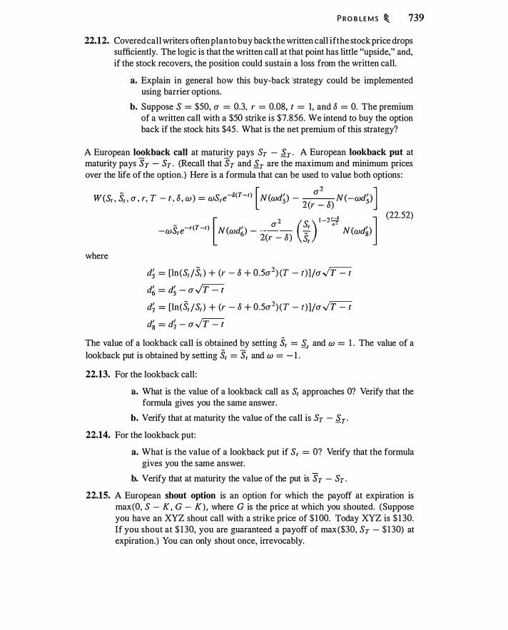
P RO B LE M S � 739

22.12. Covered call writers often plan to buy back the written call if the stock price drops sufficiently. The logic is that the written call at that point has little "upside," and, if the stock recovers, the position could sustain a loss from the written call.

a. Explain in general how this buy-back strategy could be implemented using barrier options.

b. Suppose S = $50, CJ = 0.3, r = 0.08, t = 1, and 8 = 0. The premium of a written call with a $50 strike is $7.856. We intend to buy the option back if the stock hits $45 . What is the net premium of this strategy?

A European lookback call at maturity pays Sr - s_T . A European lookback put at maturity pays S T - Sr . (Recall that S T and s_T are the maximum and minimum prices over the life of the option.) Here is a formula that can be used to value both options :

W(Sr . S1 , CJ , r, T - f. , 8 , w) = wS1e-li(T-r> [N(wd�) - CJ2 N(-wd�)J · 2(r - 8)

where [ ? s 1 -2'-� ] (22.52)

-wSre-r(T-r> N(wd�) - CJ- (.;._) a2 N(wd�) 2(r - 8) S1

d� = [ln (Sr /S1 ) + (r - 8 + 0.5CJ2) (T - t)] /CJ�

d� = d� - (J� d� = [ln (Sr /S1 ) + (r - 8 + 0.5CJ2) (T - t)]/CJ�

d� = d� - (J� The value of a lookback call is obtained by setting Sr = Jr and w = 1 . The value of a lookback put is obtained by setting S1 = Sr and w = - 1 .

22.13. For the lookback call :

a. What is the value of a lookback call as S1 approaches 0? Verify that the formula gives you the same answer.

b. Verify that at maturity the value of the call is Sr - s_T .

22.14. For the lookback put:

a. What is the value of a lookback put if S1 = 0? Verify that the formula gives you the same answer.

b. Verify that at maturity the value of the put is S T - Sr . 22.15. A European shout option is an option for which the payoff at expiration is

max(O, S - K, G - K), where G is the price at which you shouted. (Suppose you have an XYZ shout call with a strike price of $ 1 00. Today XYZ is $ 1 30. If you shout at $ 1 30, you are guaranteed a payoff of max($30, Sr - $ 1 30) at expiration.) You can only shout once, irrevocably.

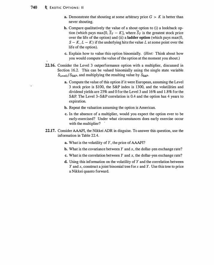
740 � EXOT I C O PT I O N S : I I

a. Demonstrate that shouting at some arbitrary price G > K is better than never shouting.

b. Compare qualitatively the value of a shout option to (i) a lookback op­tion (which pays max[O, S7 - K], where S7 is the greatest stock price over the life of the option) and (ii) a ladder option (which pays max(O, S - K, L - K) if the underlying hits the value L at some point over the life of the option).

c. Explain how to value this option binomially. (Hint: Think about how you would compute the value of the option at the moment you shout.)

22.16. Consider the Level 3 outperformance option with a multiplier, discussed in Section 1 6.2. This can be valued binomially using the single state variable SLevel3 / Ss&p, and multiplying the resulting value by Ss&P ·

a. Compute the value of this option if it were European, assuming the Level 3 stock price is $ 100, the S&P index is 1300, and the volatilities and dividend yields are 25% and 0 for the Level 3 and 16% and 1 .8% for the S&P. The Level 3-S&P correlation is 0.4 and the option has 4 years to expiration.

b. Repeat the valuation assuming the option is American.

c. In the absence of a multiplier, would you expect the option ever to be early-exercised? Under what circumstances does early exercise occur with the multiplier? -

22.17. Consider AAAPI, the Nikkei ADR in disguise. To answer this question, use the information in Table 22.4.

a. What is the volatility of Y, the price of AAAPI?

b. What is the covariance between Y and x , the dollar-yen exchange rate?

c. What is the correlation between Y and x, the dollar-yen exchange rate?

d. Using this information on the volatility of Y and the correlation between Y and x, construct a joint binomial tree for x and Y. Use this tree to price a Nikkei quanto forward.

Volatility

�:lity i' a critical input nc<oe""'l' foe pdcing option,, but it ;, not dire;tly ob<cmblc and it is not constant over time. Consequently, both theorists and practitioners are concerned with the behavior of volatility and the construction of option pricing models in which volatility can change. Hedging volatility risk is also an important issue for market-makers.

In this chapter we will discuss specific techniques for measuring stock price volatil­ity and also demonstrate how volatility models can be incorporated into the Black­Scholes pricing framework. The pricing models have the potential to explain observed prices better than the Black-Scholes formula, but the models are derived using the same pricing principles that we discussed in Chapter 2 1 .

The chapter i s divided into four general topics:

• Implied volatility : What information do option prices provide about volatility, both at a point in time and over time?

• Volatility estimation: Given the past history of stock returns, what can you say about volatility?

• Volatility hedging: What instruments are available to hedge volatility risk?

• Option pricing: How can we price options when volatility is stochastic?

You should keep in mind when reading this chapter that the distribution of asset prices remains an area in which there is significant ongoing research. Statistical tech­niques for measuring volatility continue to evolve, and there is ongoing research into the question of which pricing models best explain observed option prices .

23 .1 IMPLIED V 0 LATILITY

To provide a context for the discussion in this chapter, we begin by revisiting implied volatility, a concept. we discussed in Section 12.5. Figure 23 . 1 depicts implied volatil­ities for exchange-traded IBM options on January 1 8, 200 1 , an arbitrarily chosen date. The patterns are typical for equity options, with in-the-money (low strike) calls having higher implied volatilities than at-the-money and out-of-the-money calls. In addition, the implied volatility curve is flatter for options with longer time to maturity. You may

741

742 � VO LAT I L I TY

Impl ied volatilties for I BM cal l options, january 1 8, 2001 . The top panel shows impl ied volatil ities for options with 1 , 3, and 6 months to expiration, while the bottom panel shows impl ied volatil ities for options with 1 and 2 years to expiration . The I BM closing price on january 1 8 was $ 1 08.31 .

Implied Volatility

- 1 month = 3 months

0.8 • • • 6 months

0.6

0.4

o.2L-�--�--�--�--�--�--L-�--�--�--70 80 90 100 1 10 120 130 140 150 160 1 70

Implied Volatility

1

0.8

0.6

0.4 r-----------0.2L-�---L--�--����--�--�--L-�--

70 80 90 100 1 10 120 130 140 150 160 170

Source: Optionmetrics

see volatilities plotted in a three-dimensional graph, with time to maturity on one axis and strike prices on a different axis. Such a plot is called a volatility surface.

The pattern of implied volatilities generally is referred to as the volatility skew. However, specific patterns are frequently observed. If you use your imagination, the implied volatility plot in Figure 23 . 1 resembles a lopsided grin or a smirk. The pattern in the figure is sometimes called a volatility smirk. When the plot of implied volatility against strike prices looks like a smile, it is called a volatility smile. Volatility frowns may also be observed.

Implied volatility may seem like a natural way to measure the volatility that is expected to prevail over a future period of time. However, the fact that implied volatilities are not constant across strike prices and over time raises at least two issues. First, it is common to measure implied volatility using the Black-Scholes model, which assumes that volatility is constant. The volatility skew may reflect pricing or specification error in the Black-Scholes model, which raises the question of what implied volatility actually measures. Second, since there is no single measure of implied volatility (for the same asset, implied volatilities differ across strikes and across option maturities) , how should we interpret the implied volatility numbers? Should we look at volatility at a particular "moneyness"? Is there some way to average the different volatilities? We will see later in this chapter that some theoretical pricing models are able to account for implied volatility patterns such as those in Figure 23. 1 .

The top panel depicts the old VIX from 1 986 to 2004. The bottom panel compares the new and old VIX indices during 2004.

Implied Volatility (%)

100

80

60

40

20

I M P L I E D VO LAT I L ITY � 743

0�-L----�--�-----L----L----L----� 1987 1990 1993 1995 1998 200J 2004

Date

Implied Volatility (%)

20

18

14

12 � __ _L ____ L_ __ _L ____ L_ __ _L ____ L_ __ _oc_ 02/23 04/13 06/02 07/22 09/10 10/30 12/19

Date

Source: ci'IOE

In addition to examining the pattern of implied volatilities at a point in time, it is also possible to track implied volatilities over time. Since 1 993 the Chicago Board Options Exchange (CBOE) has reported an index of implied volatility for near-term S&P 100 index options. This index is called the "VIX, " after its ticker symbol. Using this measure, we can track changes over time in implied volatility. Originally, the CBOE computed implied-volatility by extracting implied volatility from near-the-money options, much as we discussed in Section 12.5 . This index is called the "Old VIX, " with ticker symbol VXO. However, beginning in 2003, the CBOE began computing implied volatility based on a new formula that we will describe later in this chapter.

Figure 23.2 plots the old VIX index from 1986 to 2004, and compares the new and old VIX for one year. The spike in the VIX in 1 987 occurs on four days, October 1 9, 20, 22, and 26, when the VIX exceeded 1 00%. This period corresponds to the October 1 9, 1 987, market crash, in which the Dow Jones index declined over 20% on one day. 1

The bottom panel in Figure 23.2 compares the new and old VIX during one year, showing that while the two measures are not identical, they are generally quite close. At

1 Plotting implied volatility over time raises the question of whether implied volatility is an accurate

forecast of actual future volatility. Generally, implied volatility is a biased forecast of future volatility

(e.g., see Bates, 2003).

744 � VO LAT I L ITY

the scale in the top panel, it would be difficult to detect any difference at all in the two series.

We will see in Section 23.3 below that the new VIX measure neatly finesses the problem of which particular option implied volatility to use by considering prices of all out-of-the-money options with a given time to maturity.

23 .2 MEASUREMENT AND BEHAVIOR OF VOLATILITY

In this section we examine different ways to characterize and measure the behavior of volatility using only historical information about the asset price. In our examples we will concentrate on stock price volatility.

We take as a starting point the lognormal model of stock prices. Suppose the stock price follows this process:

dSrfS, = (a - o)dt + a (S, , X, , t)dZ (23 . 1 ) where a i s the continuously compounded expected return o n the stock, 8 i s the con­tinuously compounded dividend yield, and a (S, , X, , t) is the instantaneous volatility. This familiar looking equation is subtly different than the process we assumed in earlier chapters. In equation (23 . 1 ), volatility at a point in time can depend on the level of the stock price S, other variables, X, and time. By comparisqn, the standard Black-Scholes assumption is that a (S, , X, , t) = a0, a constant. Equation (23. 1 ) is an example of a stock price process with stochastic volatility, in which instantaneous volatility can change randomly.2

Given a series of stock prices that we observe every lz periods, we can compute continuously compounded returns, E :

Et+h = ln (S,+h l S, ) We will assume throughout this section that lz is small, and therefore that we can ignore the mean return.

Historical Volatility

The natural starting point for examining volatility is historical volatility, which we com­pute using past stock returns. Suppose that we observe n continuously compounded stock returns over a period of length T, so that h = T jn . Under the assumption that volatility is constant, we can estimate the historical annual variance of returns, a2, as

A 2 1 1 2 [ Tl ] a - - --- E H - lz (n - 1 ) � i

2Note that there are no jumps in equation (23. 1 ) , and we will assume that the volatil ity, u (S, X, t) , also does not jump. I t is possible to permit jumps for both; for example, see Duffie et al . (2000).

(23.2)

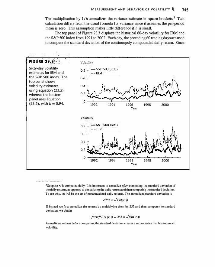
M EAS U R E M ENT A N D B E H AV I O R O F VO LATI L ITY � 745 The multiplication by 1 / lz annualizes the variance estimate in square brackets.3 This calculation differs from the usual formula for variance since it assumes the per-period mean is zero. This assumption makes little difference if lz is small.

The top panel of Figure 23.3 displays the historical 60-day volatility for IBM and the S&P 500 index from 199 1 to 2002. Each day, the preceding 60 trading days are used to compute the standard deviation of the continuously compounded daily return. Since

Sixty-day volati l ity estimates for I BM and the S&P 500 index. The top panel shows volati l ity estimates using equation (23.2), whereas the bottom panel uses equation (23 .5), with b = 0.94.

Volatility

1992

Volatility

1992

1994

1994

1996 Year

1996 Year

1998

1998

2000

2000

3 Suppose r; is computed daily. It is important to annualize after computing the standard deviation of the daily returns, as opposed to annualizing the daily returns and then computing the standard deviation. To see why, let {r; } be the set of nonannualized daily returns. The annualized standard deviation is

.Jill x Jvar( {r; } ) If instead we first annualize the returns by multiplying them by 252 and then compute the standard deviation, we obtain

Jvar(252 x {r; } ) = 252 x Jvar( {r; } ) Annualizing returns before computing the standard deviation creates a return series that has too much volatil i ty.

746 � VO LAT I L ITY

there are approximately 252 trading days in a year, the resulting standard deviation is multiplied by .J252 to produce an annualized standard deviation.

The use of overlapping 60-day intervals induces smoothness in the series, since each day's return affects the next 60 days of volatility calculations. Even so, there is a great deal of variability in the standard deviation. For both series, volatility appears to have risen toward the end of the 1 990s.

It is natural to estimate volatility using daily returns for all trading days. It is important to recognize, however, that not all calendar days, and not even all trading days, exhibit the same volatility. For example, if all days were the same, return volatility ,over a weekend (from Friday's close of trading to Monday's close of trading) should be ../3 times the weekday volatility. However, French and Roll ( 1986) showed that returns from Friday to Monday were significantly less volatile than returns over three consecutive weekdays. More recently, Dubinsky and Johannes (2004) showed that individual stock price volatilities are greater on the days when firms make earnings announcements than on other days. Thus, while equation (23 .2) provides an estimate of annualized volatility, the volatilities on individual days can vary.

Exponentially Weighted Moving Average

Because volatility in Figure 23.3 appears to be changing over time, it is natural to try to take this variation into account ..yhen estimating volatility. We might reason that if volatility is changing, we want to emphasize more recent observations at the expense of more distant observations. One way to do this is to compute an exponentially weighted moving average (EWMA) of the squared stock returns.

The EWMA formula computes volatility at time t as a weighted average of the time t - 1 EWMA estimate, 8-�WMA ,_ 1 , and the time t - 1 squared stock price change, E�_ 1 • Thus, we have

·

(23 .3)

where b is the weight applied to the previous EWMA estimate. We can lag equation (23 .3) and substitute the resulting expression for 8-�WMA,r- l into the right-hand side of equation (23 .3). Continuing in this way, we obtain the EWMA estimator as a weighted average of past squared returns:

00 o-�\VMA,t = L [( I - b)bi- 1 ] E�-i (23 .4)

i=l The term in square brackets in equation (23 .5) is the weight applied to historical returns. The weights decline at the rate b, with the most recent return receiving the greatest weight. Because 2:::�1 ( 1 - b)bi- l = I , the weights on past squared returns sum to one.

It is also possible to use a moving window when estimating EWMA volatility. For example, we might use only the previous n days of data. In this case, equation (23 .5)

M EAS U R E M ENT A N D B E H AV I O R O F VO LAT I L I TY � 747

becomes II [ (1 - b)bi- 1

] cT�WMA.r = � L'�- ( 1 _ b)bj- 1

E�-i

1 = 1 J- 1

= II [ ( l - b)bi- I JE2· L.:: 1 - b�� . 1 -1

i= l

Because z:=;1= 1 ( 1 - b)bi- l = 1 - h11 , the weights again sum to one.

(23 .5)

There is also a simple updating formula, analogous to equation (23 .3), in the case of a moving window estimate. Each period we add the latest observation and drop the oldest observation. Equation (23 .5) is equivalent to

(23 .6)

Example 23. 1 Suppose b = 0.94 and ll = 60. We have 1 - b11 = 0.9756. The first term in equation (23 .6) is then

( 1 - 0"94) = 0.06 1 5

0.9756 This compares with a weight of 1 /60 = 0.0 1 67 for each observation in the equal­weighted estimator in equation 23.2. Subsequent (earlier) observations have weights of 0.0578, 0.0543, 0.05 1 1 , etc.

The bottom panel in Figure 23.3 displays the EWMA estimate for b = 0.94 and n = 60 days. Note that the EWMA estimator is considerably more variable than the standard historical volatility estimate. This additional variability occurs because the most recent observation has four times the weight in the EWMA estimator as in the standard estimator. Thus a particularly large return will create a large effect on the estimate. This effect will then decay at the rate b. �

There are two problems with the EWMA estimator, one practical and one concep­tual. First, if we use the EWMA estimator in equation (23 .3) to forecast future volatility, we obtain a constant expected volatility at any horizon. The reason is that the forecast of E� is G-�_ 1 , so that all forecasts of future volatility would equal G-�_ 1 • Thus, the EWMA estimator does not forecast patterns in future volatility. Second, the EWMA estimator is not derived from a formal statistical model in which volatility can vary over time. ARCH and GARCH, which we discuss next, address both problems.

Time-Varying Volatility: ARCH

A casual examination of data, such as looking at historical volatilities (Figure 23.3), or looking at the behavior over time of implied volatilities (Figure 23.2), suggests that

748 � VO LAT I L I TY

volatilities are not constant.4 What do we do once we formally accept that volatilities change over time? Ideally we would have a statistical model that permits volatility changes to occur. Such a model could serve both to provide better estimates of volatility and also to provide a building block for better pricing models.

Research on the behavior of volatility shows that for many assets, there are periods of turbulence and periods of calm: high volatility tends to be followed by high volatility and low volatility by low volatility. Put differently, during a period when measured volatility is high, the typical day tends to exhibit high volatility. (High volatility could in principle also arise from an increased chance of large but infrequent price moves. ) Figure 23.4 displays squared daily returns for the S&P 500 index and IBM. At a casual level, this figure exhibits this effect, with periods in which many of the daily squared returns are large, and periods when many are small. This is called volatility clustering.

If volatility is persistent, a volatility measure should weight recent returns more heavily than more distant returns. This difference in weighting is exactly how an EWMA volatility estimate differs from the ordinary equally weighted volatility measure. ARCH and GARCH models also give more weight to recent returns.

The ARCH model The autoregressive conditional heteroskedasticity (ARCH) model of Engle ( 1 982) and the subsequent GARCH (Generalized ARCH) model of Bollerslev ( 1 986) are important and widely used volatility models that attempt to capture statistically the ebb and flow of volatility.5 Engle in fact won the 2003 Nobel Prize in economics for his work in this area (see the box on page 750) . The basic idea motivating ARCH is that if volatility is high today it is likelier than average to be high tomorrow. Engle ( 1 982) provided a statistical framework for modeling this effect.

A statistical model for asset prices could take the form

ln(S1 /S1_, ) = (a - 8 - 0.5a2)lz + E1 (23.7)

In this specification, the error term would have variance

var(E1 ) = a2h (23 .8)

4We can perfonn a back-of-the-envelope calculation by assuming that continuously compounded re­turns are nonnally distributed. In that case, the ratio of variances drawn from independent time periods has the the F distribution. If we estimate two annual volatil ities using 252 observations, the ratio of the two estimated variances is distributed F(a , 25 1 , 25 1 ) . The 99.5% and 0.005% confidence levels are obtained from F- 1 (p, 25 1 , 25 1 ) , where p = 0.995 or p = 0.005. At a I % significance level, the two bounds for the ratio of estimated variances are 1 .386 and 0.722, corresponding to volati l ity ratios of l . l 77 and 0.849. Thus, if volatil ity in one year is 15%, a subsequent measured volati lity outside the range 1 2.74%- I 7.66% rejects the hypothesis of constant variance at a I % significance level. 5Bollerslev et al. ( ! 994) surveys the literature on ARCH and its variants. Two recent accessible in­troductions were written as a result of the 2003 Nobel prize: Diebold (2004) and Royal Swedish Academy of Sciences (2003). Nelson (I 99 I ) proposed exponential GARCH. which models the behav­ior of l n (a2 ) .

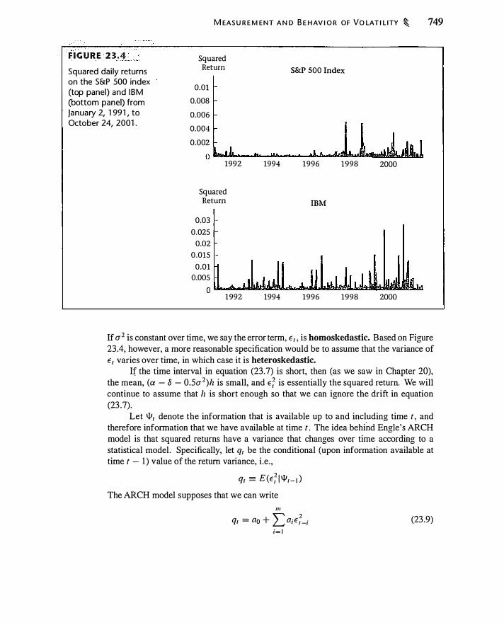
F IGU R E 2 3 . 4 Squared dai ly returns on the S&P 500 index (top panel) and I BM (bottom panel) from january 2, 1 991 , to October 24, 2001.

M EAS U R E M ENT A N D B E H AV I O R OF VO LAT I L I TY � 749

Squared Return

O.Ql

0.008

0.006

0.004

0.002

S&P 500 Index

0 �w---&-�----�����muaw�� 1992

Squared Return

0.03

0.025 0.02

0.015

0.01

1994 1996 1998 2000

IBM

0.005

0 YM���Yd������������ 1992 1994 1996 1998 2000

If u2 is constant over time, we say the error term, E 1 , is homoskedastic. Based on Figure 23.4, however, a more reasonable specification would be to assume that the variance of E1 varies over time, in which case it is heteroskedastic.

If the time interval in equation (23 .7) is short, then (as we saw in Chapter 20), the mean, (a - 8 - 0.5u2)h is small, and E; is essentially the squared return. We will continue to assume that h is short enough so that we can ignore the drift in equation (23 .7).

Let Ill, denote the information that is available up to and including time t , and therefore information that we have available at time t . The idea behind Engle's ARCH model is that squared returns have a variance that changes over time according to a statistical model. Specifically, let q, be the conditional (upon information available at time t - I ) value of the return variance, i .e. ,

q, = E(E� I Illr- � )

The ARCH model supposes that we can write Ill

q, = ao + L a;E�-i i= l

(23 .9)

750 � VO LAT I L I TY

A Nobe l Prize fo r Volati l ity

The 2003 Nobel Prize in economics was awarded to Robert F. Engle and Clive Granger for their work in statistical methods in economics. Engle was cited for his work in studying the behavior of volatility. This quote, from the Royal Swedish Academy of Science press release announcing the award of the 2003 economics prize, describes Engle's contribution:

Random fluctuations over time­volatility-are particularly significant because the value of shares, options and other financial instruments de­pends on their risk. Fluctuations can vary considerably over time; turbu­lent periods with large fluctuations are followed by calmer periods with small fluctuations. Despite such time­varying volatility, in want of a better alternative, researchers used to work -

with statistical methods that pre­suppose constant volatility. Robert Engle's discovery was therefore a major breakthrough. He found that the concept of autoregressive condi­tional heteroskedasticity (ARCH) ac­curately captures the properties of many time series and developed meth­ods for statistical modeling of time­varying volatility. His ARCH models have become indispensable tools not only for researchers, but also for an­alysts on financial markets, who use them in asset pricing and in evaluat­ing portfolio risk.

Granger was cited for his work in cointegration, a statistical method important for studying .the long-run behavior of economic time series.

where a0 > 0. a; ::::: 0, i = 1 , . . . , m. Equation (23 .9) is an ARCH(m) model, signifying that there are m lagged terms. In order for volatility to be well-behaved, we must have L:,;'= 1 a; < I . This model states that volatility at a point in time depends upon recent observed volatility.

At this point we can understand the meaning of "autoregressive conditional het­eroskedasticty." Autoregressive means that the value at a point in time depends on past values. Heteroskedasticity means that variances are not equal. The unconditional vari­ance is the variance estimated over a long period of time. The conditional variance is the variance estimated at a point in time, taking into account ("conditional upon") recent volatility. Thus, autoregressive conditional lzeteroskedasticity essentially means that the level of variance depends on recent past levels of variance. This is the behavior captured by equation (23 .9).

ARCH volatility forecasts An important practical question is how many lags we need in order to estimate equation (23.9). To better understand the behavior of an ARCH model , let's consider a single lag, where we set a 1 > 0 and a; = 0, i > 1 . The volatility

M EAS U R E M E N T A N D B E H AV I O R O F VO LAT I L ITY � 751

equation is then

(23 . 1 0)

where ao > 0 and a 1 < l . Equation (23 . 1 0) is an ARCH( ! ) model. Suppose we forecast volatility at time t + 1 , t + 2, etc. , using only the information

we have at time t . Equation (23 . 1 0) implies that for a one-period ahead forecast of q1 we have

E(E�+ 1 IIlir- 1 ) = ao + a 1 E (E� IIllr - 1 )

= ao + a 1 (ao + a 1 E�_ 1 )

Similarly, for a two-period ahead forecast,

E(E;d 'llr-d = ao + a 1 E(E;+ 1 I Ilir- 1 )

= ao + a 1 [ao + a 1 (ao + a 1 E;_ 1 ) ]

Continuing in this way, for an n-period-ahead forecast, we have

E(E;+n l 'llr- 1 ) = ao ( 1 + t a ; ) + a;' E�- 1 r= 1

(23 . 1 1 )

This predicted pattern of volatility persistence i s very specific and inflexible. A large squared return today implies larger squared returns at all future dates, but the effect decays per period by the factor a 1 • Shocks to volatility are expected to die off at a constant rate.

Equation (23 . I 1 ) implies that unconditional volatility (the value we would estimate as a long-run average) is

_ , , ao a- = ao ( l + a 1 + a( + . . . ) = --

1 - a 1 Thus, with estimates of a0 and a 1 we can compute the unconditional volatility.

(23 . 12)

In practice, if markets become more turbulent, they may remain more turbulent for a period of time. Equation (23 .9) with a single lag cannot account for a period of sustained high volatility. As you might guess, more than one lag-generally many lags-are necessary for ARCH to fit the data.

The GARCH Model

The GARCH model, due to Bollerslev ( 1 986), is a variant of ARCH that allows for infinite lags yet can be estimated with a small number of parameters. The GARCH model has the form

Ill II q1 = ao + L a; E;_i + L b;qr-i

i= 1 j= 1 (23 . 1 3)

h 0 · 0 · - 1 b · > O · - 1 d '\'111 · + '\'" b· 1 w ere a0 > , a, 2: , 1 - , • • • , n z , , _ , 1 - , • • • , n , an L..., ; = 1 a, L...,;= 1 , < .

752 � VO LAT I L ITY

This model states that volatility at a point in time depends upon recent volatility as well as recent squared returns. Equation (23 . 1 3) is a GARCH(m,n) model.

GARCH( l , l ) is frequently used in practice. The GARCH( l , l ) model is

(23 . 14)

It is instructive to compare the GARCH( l , l ) model to the ARCH( 1 ) model , equation (23 . 1 0) . To do this, we can rewrite equation (23 . 14) to eliminate q1_ 1 on the right-hand side. Lagging equation (23 . 14) and substituting the result for q1_ 1 on the right-hand side of equation (23 . 1 4) , we obtain

q, = Go + G ! E;_ I + b1 (ao + G ! E;_2 + b t qt-2)

Continuing in this way, we obtain 00 00

q, = ao L ); + a 1 I ); E;_ 1 _; i=O i=O

(23 . 1 5)

A GARCH( l , l ) model is therefore equivalent to an ARCH(oo) model in which the lag coefficients decline at the rate b 1 • Notice that the last term in equation (23 . 1 5) can be rewritten in terms of an EWMA volatility estimator (23 .5):

ao a 1 A ? q, = 1 - b l

+ 1 - b l

uEWMA (23 . 1 6)

It is important to note that the parameter b 1 in the EWMA expression in equation (23 . 1 6) is not arbitrarily chosen, as in equation (23 .3), but is estimated as part of the GARCH estimation procedure.

Maximum likelihood estimation of a GARCH model Given the assumption that continuously compounded returns have a distribution that is conditionally normal, with variance q1 and mean zero, we can estimate a GARCH model using maximum likeli­hood.6 The probability density for E1 , conditional on q1 , is

1 0 - "! j(E1 ; q1 ) = J

? e- .�E, q, (23 . 1 7) _rrq,

Since the E1 are conditionally independent, the probability of observing the particular set of II returns is the product of the probabilities, which gives us the likelihood function:

I I II 1 - 1 IT j(E; Iq; ) = IT --- e-O.�eJq;

i= l i= l ..j2iUji

6 Alexander (200 I ) discusses the estimation of GARCH models and is replete with examples.

M EAS U R E M ENT A N D B E H AV I O R O F VO LATI L ITY � 753

For a GARCH( l , l ), qi is a function of ao, a 1 , and b 1 • The maximum likelihood estimate is the set of parameters-Go, a 1 , and b 1-that maximizes the probability of observing the returns we actually observed. Typically it is easiest to maximize the log of the likelihood function, in which case maximizing the likelihood is the same as maximizing

II L [ -0.5 ln (qi ) - 0.5Ef /qi ] (23 . 1 8) i= l

We omit the term -0.5 ln(2n) since it does not affect the solution. The maximization of equation (23 . 1 8) can be performed in statistical packages or even using Solver in Excel (see the chapter appendix) .

Volatility forecasts We can forecast volatility in the GARCH( l , 1 ) model as we did in the ARCH( l ) model. To understand the calculation, recognize that since q1 =

E(E� I W1_ J ) , we then have E(q1 jW1-j ) = E(E� I W1-j ) for j 2: 1 . Thus, using equa­tion (23. 14) , we have

E(q,+ I I Wt-d = ao + a1 E(E� jW,_ J ) + b J E(q, j W,_ t ) = ao + (a J + b t )E (qt ! Wt- J )

= ao + (a 1 + b J ) (ao + a 1 E�_ 1 + b 1 qt- 1 )

The goal in this calculation is to express the forecasted value of q1+ 1 in terms of what we can observe at time t-namely, E1_ 1 and q1_ 1 • Following the same procedure, we obtain

E(q1+2 I W,_ J ) = ao + ao (a J + b J ) + (a 1 + b J )2 (ao + G J E�- I + b 1 qt- 1 )

For a k step-ahead forecast, we have

k E(qt+k i Wt- 1 ) = ao + ao L (a J + bd + Ca 1 + bd (a J E�_ 1 + b l q,_ J )

i= l As we let k go to infinity, we obtain an estimate of unconditional volatility in the GARCH( l , l ) model :

(23 . 1 9)

Using equations (23. 1 6) and (23 . 1 9), we can express the GARCH( l , l ) equation in terms of the EWMA estimate of volatility:

(23.20)

where a = ( 1 - a 1 - b 1 ) / ( l - b J ) . Thus, the GARCH( l , l ) expected volatility at a point in time is a weighted average of the unconditional variance, iJ2, and the current estimated EWMA volatility, D-�WMA"

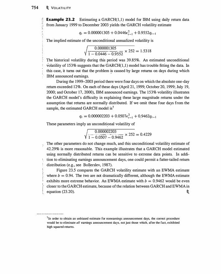
754 � VO LAT I L ITY

Example 23.2 Estimating a GARCH( l , l ) model for IBM using daily return data from January 1999 to December 2003 yields the GARCH volatility estimate

q1 = 0.00000 1 305 + 0.0446E�- I + 0.9552q1- i

The implied estimate of the unconditional annualized volatility is

0 .000001 305 1 - 0.0446 - 0.9552

X 252 = 1 "53 1 8

The historical volatility during this period was 39.85%. An estimated unconditional volatility of 153% suggests that the GARCH( l , l ) model has trouble fitting the data. In this case, it turns out that the problem is caused by large returns on days during which IBM announced earnings.

During the 1999-2003 period there were four days on which the absolute one-day return exceeded 12%. On each of these days (April 2 1 , 1 999; October 20, 1999; July 1 9, 2000; and October 17 , 2000), IBM announced earnings. The 153% volatility illustrates the GARCH model 's difficulty in explaining these large magnitude returns under the assumption that returns are normally distributed. If we omit these four days from the sample, the estimated GARCH model is 7

q1 = 0.000002203 + 0.0507E�- I + 0.9462q1- i

These parameters imply an unconditi_onal volatility of

0.000002203 X 252 = 0.4229 1 - 0.0507 - 0.9462

The other parameters do not change much, and this unconditional volatility estimate of 42.29% is more reasonable. This example illustrates that a GARCH model estimated using normally distributed returns can be sensitive to extreme data points. In addi­tion to eliminating earnings announcement days, one could permit a fatter-tailed return distribution (e.g., see Bollerslev, 1 987).

Figure 23.5 compares the GARCH volatility estimate with an EWMA estimate where b = 0.94. The two are not dramatically different, although the EWMA estimate exhibits more extreme behavior. An EWMA estimate with b = 0.9462 would be even closer to the GARCH estimate, because of the relation between GARCH and EWMA in equation (23 .20). �

7 In order to obtain an unbiased estimate for noneamings announcement days, the correct procedure would be to eliminate all earnings announcement days, not just those which, after the fact, exhibited high squared returns.

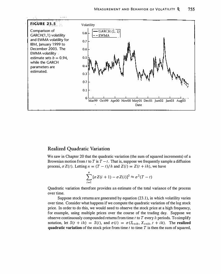
F IGU R E 23 .5 Comparison of GARCH(1 , 1 ) volati l ity and EWMA volati l ity for I BM, january 1 999 to December 2003. The EWMA volatil ity . estimate sets b = 0.94, while the GARCH parameters are estimated.

M EAS U R E M ENT A N D B E H AV I O R O F VO LAT I L I TY � 755

Volatility

o.s ·�--G=-A-=R-=c=H=-(-1 ,-1-,) I - - EWMA . 0.7

0.6

0.5

0.3

0.1

O L-�---L--�----�--�----L----L--�L_ __ J__ Mar99 Oct99 AprOO NovOO MayOI DecOl Jun02 jan03 Aug03

Date

Realized Quadratic Variation

We saw in Chapter 20 that the quadratic variation (the sum of squared increments) of a Brownian motion from t to T is T - t . That is, suppose we frequently sample a diffusion process, a Z(t) . Letting n = (T - t)/ 1z and Z(i ) = Z(t + i lz ) , we have

II :L)a Z (i + 1 ) - a Z(i)f � a 2 (T - t) i = l

Quadratic variation therefore provides an estimate of the total variance of the process over time.

Suppose stock returns are generated by equation (23 . 1 ) , in which volatility varies over time. Consider what happens if we compute the quadratic variation of the log stock price. In order to do this, we would need to observe the stock price at a high frequency, for example, using multiple prices over the course of the trading day. Suppose we observe continuously compounded returns from time t to T every II periods. To simplify notation, let S (t + ih) = S (i ) , and a (i ) = a (Sr+ift , Xr+ift , t + i lz ) . The realized quadratic variation of the stock price from time t to time T is then the sum of squared,

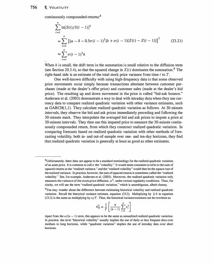
756 � VO LAT I L I TY

continuously compounded returns:8

II

L )n [S(i )/S(i - l )f i = l

II

= L { [a - 8 - 0.5u (i - 1 )2]/z + u (i - l ) [Z (i ) - Z(i - 1 ) 1 } 2 i= l

II

� 'L rr(i - 1 )2/z i = l

(23 .2 1 )

When lz i s small, the drift term i n the summation i s small relative to the diffusion term (see Section 20.3 .4), so that the squared change in Z (t) dominates the summation .9 The right-hand side is an estimate of the total stock price variance from time t to T .

One well-known difficulty with using high-frequency data i s that some observed price movements occur simply because transactions alternate between customer pur­chases (made at the dealer's offer price) and customer sales (made at the dealer's bid price). The resulting up and down movement in the price is called "bid-ask bounce." Andersen et al . (2003) demonstrate a way to deal with intraday data when they use cur­rency data to compare realized quadratic variation with other variance estimates, such as GARCH( l , l ) . They calculate realized quadratic variation as follows. At 30-minute intervals, they observe the bid and ask prices immediately preceding and following the 30-minute mark. They interpolate the averaged bid and ask prices to impute a price at 30-minute intervals. They then use this imputed price to measure the 30-minute contin­uously compounded return, from which they construct realized quadratic variation. In comparing forecasts based on realized quadratic variation with other methods of fore­casting volatility, both in- and out-of-sample over one- and ten-day horizons, they find that realized quadratic variation is generally at least as good as other estimates.

8Unfo�unately. there does not appear to be a standard terminology for the realized quadratic variation of an asset price. It is common to call a the "volati l ity." It would seem consistent to refer to the sum of squared returns as the "realized variance," and the "realized volatility" would then be the square root of the realized variance. In practice, however, the sum of squared returns is sometimes called the "realized volati lity." See, for example, Andersen et al. (2003). Moreover, the realized quadratic variation only measures the variance of the stock price diffusion, a2, under certain regularity conditions. Thus, for clarity, we will use the term "realized quadratic variation," which is unambiguous, albeit clumsy. 9You may wonder about the difference between estimating historical volatil i ty and realized quadratic variation. Recall the historical variance estimate, equation (23.2). Multiplying by 1/ h in equation (23.2) is the same as multiplying by 11 I T. Thus, the historical variance estimate can be rewritten as

Apart from the 11 /(11 - I ) term, this appears to be the same as annualized realized quadratic variation. In practice, the term "historical volatil ity" usually implies the use of daily or· less frequent data over medium to long horizons, while "quadratic variation" implies the use of intraday data over short horizons.

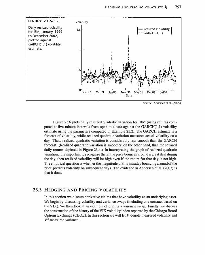
Dai ly rea l ized volati l ity for IBM, January, 1 999 to December 2002, plotted against GARCH(1 , 1 ) volati l ity estimate.

Volatility

1 .5

1

0.5

H E D G I N G A N D P R I C I N G VO LAT I L ITY � 757

- Realized violatility - - GARCH ( 1 , 1)

o ���--�--��--�----�----�-----L-----

Mar99 Oct99 AprOO NovOO MayOl DecOl jul02 Date

Source: Andersen et al. (2005).

Figure 23.6 plots daily realized quadratic variation for IBM (using returns com­puted at five-minute intervals from open to close) against the GARCH( l , l ) volatility estimate using the parameters computed in Example 23.2. The GARCH estimate is a forecast of volatility, while realized quadratic variation measures actual volatility on a day. Thus, realized quadratic variation is considerably less smooth than the GARCH forecast. (Realized quadratic variation is smoother, on the other hand, than the squared daily returns depicted in Figure 23 .4.) In interepreting the graph of realized quadratic variation, it is important to recognize that if the price bounces around a great deal during the day, then realized volatility will be high even if the return for that day is not high. The empirical question is whether the magnitude of this intraday bouncing around of the price predicts volatility on subsequent days. The evidence in Andersen et al . (2003) is that it does.

23.3 HEDGING AND PRICING VOLATILITY

In this section we discuss derivative claims that have volatility as an underlying asset. We begin by discussing volatility and variance swaps (including one contract based on the VIX). We then look at an example of pricing a variance swap. Finally, we discuss the construction of the history of the VIX volatility index reported by the Chicago Board Options Exchange (CBOE). In this section we will let V denote measured volatility and V2 measured variance.

758 � VO LAT I L I TY

Variance and Volatility Swaps

A variance swap is a forward contract that pays the difference between a forward price, Fo.T ( V2) , and some measure of the realized stock price variance, V2 , over a period of time multiplied by a notional amount. The payoff to a variance swap is

[V2 - Fo.T (V2) ] x N

where N is the notional amount of the contract. There are numerous measurement details that we have to specify in order to write the contract for a variance swap:

, • How frequently the return is measured

• Whether returns are continuously compounded or arithmetic

• Whether the variance is measured by subtracting the mean or by simply squaring the returns

• The period of time over which variance is measured

• · How to handle days on which, unexpectedly, trading does not occur

Most of these design issues are straightforward, but the last deserves some com­ment. Most futures contracts settle based upon a final observable price. A variance contract, by contrast, settles based upon a series of prices . Therefore, failing to observe a price (for example, because the market is unexpectedly closed) creates a problem for measuring the realized variance. If the market is unexpectedly closed on day t , then the next measured return will be a two-day return, which will have a greater expected variance than a one-day return. The following example shows how one contract deals with this issue.

Example 23.3 Three-month S&P 500 variance futures traded on the Chicago Fu­tures exchange are an example of a variance swap. The payoff is based on the annualized sum of squared, continuously compounded daily returns over a three-month period, V2 • The measured price is quot�d as V2 x 10 ,000, and by definition a one-unit change in this number (called a variance point) is worth $50.

For simplicity, we treat the payoff as if it were a forward contract, settling on one day. Let E; be the continuously compounded return on day i. The payoff at expiration is

[ n., - 1 7 ] $50 x 1 0, 000 x 252 x L _5__ - Fo,T (V2 ) l le - l

i = l

In this formula, l l a is the actual number of S&P prices used in constructing V2 (hence there are l la - 1 returns), and ne is the number of expected trading days at the outset of the contract. Thus, in the event of an unexpected trading halt, the sum of squared returns will be divided by a number larger than the number of squared returns. The reason for this is that the trading halt will not necessarily change the total variance over the period (if the trading halt is on a Tuesday, for example, the Monday to Wednesday return will

H E D G I N G A N D P R I C I N G VO LAT I L ITY � 759

typically reflect two days of volatility). Dividing the sum of squared returns by II a would mechanically increase the measured variance when there is a trading halt. Dividing by l ie prevents this. �

A volatility swap is like a variance swap except that it pays based on volatility rather than variance. The payoff is

(V - Fo. r (V)) x N

where Fo. r (V ) is the forward price for volatility.

Example 23.4 The Chicago Board Options Exchange volatility index, the VIX, is the basis for a volatility futures contract that trades on the Chicago Futures Exchange. Unlike the variance futures contract, the volatility futures contract settles based upon the VIX index. The payoff is

1000 x [VIXr - Fo. r (V) ]

In comparing the volatility futures contract (Example 23.4) with the variance futures contract (Example 23.3), note that the two contracts are based on volatility measured over different periods of time. The variance contract settles based on realized quadratic variation over the period from 0 to T, and thus the futures price reflects volatility expectations from time 0 to time T. The VIX contract, since it is based on the VIX index, measures volatility expectations from time T to time T + 30 days. Thus, the volatility contract measures volatility going forward from the settlement date, while the variance contract looks backward from the settlement date.

There are at least two reasons that the variance contract is in some sense more ·

"natural" than a volatility contract. First, we will see below that it is possible to price and hedge a variance forward contract (given some assumptions) using option prices. The pricing of a volatility forward contract is more complicated due to Jensen's inequality. Because the volatility is the square root of the variance, Jensen's inequality implies that the volatility forward price will be less than the square root of the variance forward price of the variance.

Second, variance swaps arise naturally from dealers hedging their option positions. Recall from Chapter 13, in particular equation ( 1 3 . 1 1 ) , that the profit of a delta-hedging dealer depends on the squared stock price change. Dealers can hedge this risk in realized variance by using variance swaps. For example a dealer with a negative gamma position could enter a swap that pays the dealer when the stock has a large price change.

Pricing Volatility

We will see in this section one way to determine the fair price for a forward contract on variance.

760 � VO LAT I L ITY

Consider a variance contract that pays the sum of squared price changes from time 0 to time T. If price changes are measured over an interval of length lz = T j n, the contract would have the payoff

Payoff = L s(i+l )/z. - sill -11 ( ) ' i= l S,�z

(23 .22)

Note that, since arithmetic and continuously compounded returns are close over small intervals, this is the same as the realized quadratic variation measure discussed in the previous section. As lz gets small, this equation (23.22) becomes

Payoff = ( (J (S1 , X1 , t)2dt (23.23) Jo where (J (S, X, t) is the diffusion coefficient in equation (23 . 1 ) . We want to answer two closely related questions. First, how is it possible to replicate the payoff to such a contract? Second, how should the contract be priced? As you might suspect, replicating the contract yields a way to price it.

In principle, the price of a forward contract on variance will be the expectation of equation (23 .23) under the risk-neutral measure. In practice, how do we compute such an expectation? The following section will provide one answer.

The log contract Neuberger ( 1994) pointed out that a· forward contract that pays

(23 .24)

could be used to hedge and speculate on variance. A claim with the payoff in equation (23 .24) is a log contract. As of early 2005, there is no exchange-traded log contract in existence, but for the moment, suppose such a contract does exist.

Assuming the stock price follows equation (23 . 1 ), we can use Ito's Lemma to characterize the process followed by the log of the stock price. (Note that we assume that the stock price does not jump.) Equation (23. 1 ) permits a wide range of processes for the volatility, but the prospective volatility over the next instant is known. Applying Ito's Lemma, we have

Thus,

1 I , d[In(S, ) ] = -dS - 0 .5 ----:jds-

s s-

I 0.5(J (t)2dt = SdS - d[ln(S1 )]

Integrating this equation, we have

0.5 (T (J2 (t)dt = (T !_dS - ( d[ln (S1 ) ]dt Jo Jo S Jo

The integral on the left-hand side is quadratic variation over 0 to T. Let G-2 denote

H E D G I N G A N D P R I C I N G VO LAT I L ITY � 761

annualized realized volatility from time 0 to time T. We can then rewrite this as

A � 1 T I 0.5Ta- = -dS - ln (ST/So)

0 s (23 .25)

The right-hand side of equation (23 .25) is the cumulative return to an investment in I IS shares, less the return on a contract paying the realized continuously compounded return on the stock price from time 0 to time T . The left-hand side is annualized realized quadra.tic variation, which from equation (23 .23) is also the payoff on a variance contract. Equation (23 .25) demonstrates the connection between the payoff to the log contract and volatility.

Take expectations of both sides of equation (23.25) with respect to the risk-neutral stock price distribution. The expectation of d SIS under the risk-neutral distribution is rdt . Hence we obtain

0.5T E* [a2] = E* [1T �dS - ln(SriSo)] = rT - E* [In (SriSo) ] (23 .26)

This expression seems to be of little help in pricing volatility. There is a trick, however, for pricing the log contract using other instruments .

Valuing the log contract Demeterfi et al. ( 1 999) and CmT and Madan ( 1 998) inde­pendently showed that it is possible to use a portfolio of options to replicate the payoff on the log contract. Note first that ib

1 [

Sr ] b Sr Sr -� (K - Sr)dK = ln(K) + - = ln (b) - ln (a) + - - -

a K- K a b a

Use this to obtain the following identity, for any Sr (see Demeterfi et a! . , 1 999): 1 0

( Sr ) Sr - S* is. 1 100 1 - In - = - + -� max(K - Sr , O)dK + -� max (Sr - K, O)dK

s* . s* o K- s. K-

Notice that if we take expectations of both sides with respect to the risk-neutral distri­bution for Sr , the integrals on the right-hand side become undiscounted option prices, and the expected stock price is the forward price. We can add and subtract ln (So) to the

10To interpret the expression on the right-hand side, notice that for any given ST, the value of the first integral is zero for K below ST , and the value of the second integral is zero for K above ST . Thus. the effective integration bounds are not 0 and oo, but they instead depend upon ST . For example, if Sr = S < K. s. , the equation becomes ( S ) S - S. (5• I -

- In S, = - � + Js K1 max (K - S, O)d K + O

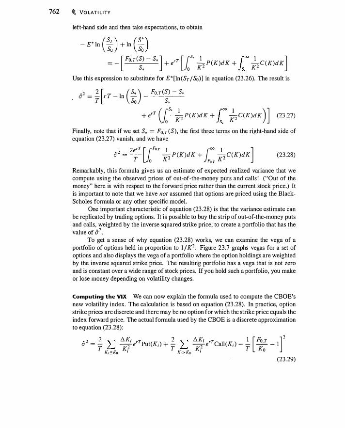
762 � VO LAT I L I TY

left-hand side and then take expectations, to obtain

- E* In ( �:) + In ( �:) = - [

Fo.r (S) - S* ] + err [1s. �P(K)dK + roo �C(K)dK] s* o K is. K

Use this expression to substitute for E* [ln (Sr/So)] in equation (23 .26). The result is

�2 2 [ ( S* ) Fo.r (S) - S* a = - rT - In - - -----T So S*

+ erT (1s. �P(K)dK + roo �C(K)dK)] (23 .27) o K- is. K-

Finally, note that if we set S* = Fo,r (S) , the first three terms on the right-hand side of equation (23.27) vanish, and we have

?erT [1Fo.T 1 100 1 J 52 = -- - 2P(K)dK + 2C(K)dK T 0 K �J K (23.28)

Remarkably, this formula gives us an estimate of expected realized variance that we compute using the observed prices of out-of-the-money puts and calls ! ("Out of the money" here is with respect to the forward price rather than the current stock price.) It is important to note that we have not assumed that options are priced using the Black­Scholes formula or any other specific model.

One important characteristic of equation (23 .28) is that the variance estimate can be replicated by trading options. It is possible to buy the strip of out-of-the-money puts and calls, weighted by the inverse squared strike price, to create a portfolio that has the value of 52.

To get a sense of why equation (23 .28) works, we can examine the vega of a portfolio of options held in proportion to 1 / K2 • Figure 23.7 graphs vegas for a set of options and also displays the vega of a portfolio where the option holdings are Weighted by the inverse squared strike price. The resulting portfolio has a vega that is not zero and is constant over a wide range of stock prices. If you hold such a portfolio, you make or lose money depending on volatili ty changes.

Computing the VIX We can now explain the formula used to compute the CBOE's new volatility index. The calculation is based on equation (23 .28). In practice, option strike prices are discrete and there may be no option for which the strike price equals the index forward price. The actual formula used by the CBOE is a discrete approximation to equation (23 .28):

? � 2 2 "" l::iK; rT 2 "" l::iK; rT 1 [ Fo.r ] -a = T � ---'] e Put(K; ) + - � ---']e Call(K; ) - - -- - 1

K; :".Ko K; T K; > Ko K; T Ko (23 .29)

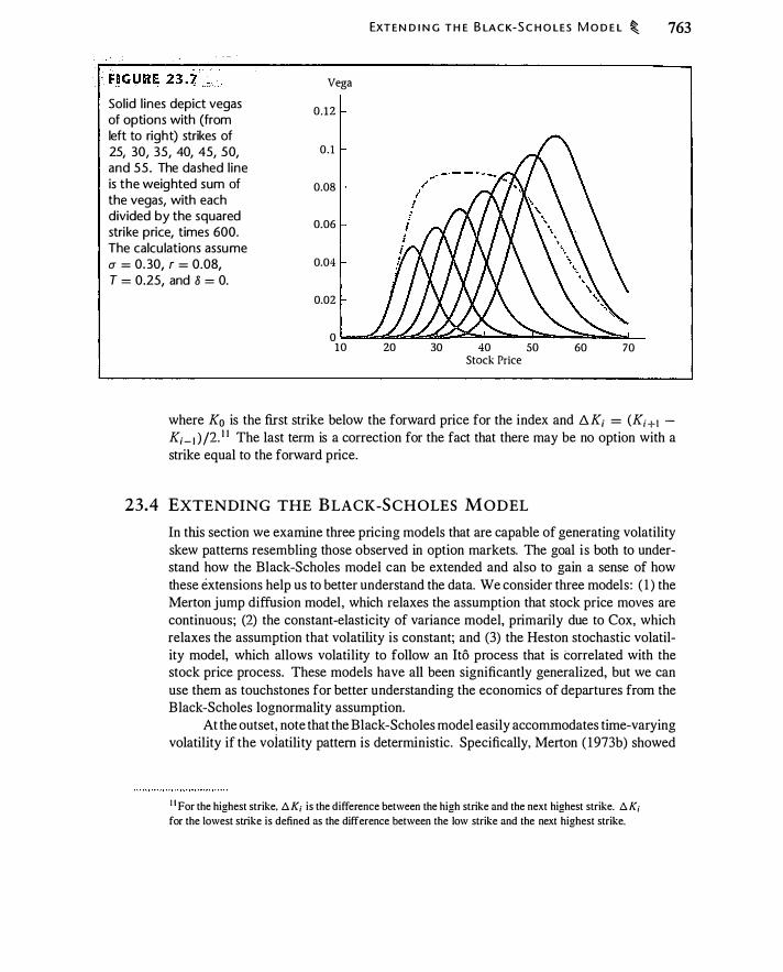
Solid l ines depict vegas of options with (from left to right) strikes of 25, 30, 35, 40, 45, 50, and 55. The dashed l ine is the weighted sum of the vegas, with each divided by the squared strike price, times 600. The calcu lations assume IJ = 0. 30, r = 0.08, T = 0.25, and 8 = 0.

Vega

0 .12

0 .1

0.08

0.06

0.04

0.02

0 10

EXT E N D I N G T H E B LA C K-S C H O LES M O D E L � 763

20 30 40 so 60 70 Stock Price

where K0 is the first strike below the forward price for the index and f!.. K; = (K;+ I -K;- d /2. 1 1 The last term is a correction for the fact that there may be no option with a strike equal to the forward price.

23.4 EXTENDING THE BLACK-SCHOLES MODEL

In this section we examine three pricing models that are capable of generating volatility skew patterns resembling those observed in option markets. The goal i s both to under­stand how the Black-Scholes model can be extended and also to gain a sense of how these extensions help us to better understand the data. We consider three models: ( 1 ) the Merton jump diffusion model, which relaxes the assumption that stock price moves are continuous; (2) the constant-elasticity of variance model, primarily due to Cox, which relaxes the assumption that volatility is constant; and (3) the Heston stochastic volatil­ity model, which allows volatility to follow an Ito process that is correlated with the stock price process. These models have all been significantly generalized, but we can use them as touchstones for better understanding the economics of departures from the Black-Scholes lognormality assumption.

At the outset, note that the Black-Scholes model easily accommodates time-varying volatility if the voiatili ty pattern is deterministic . Specifically, Merton ( 1 973b) showed

1 1 For the highest strike, !J. K; is the difference between the high strike and the next highest strike. !J. K; for the lowest strike is defined as the difference between the low strike and the next highest strike.

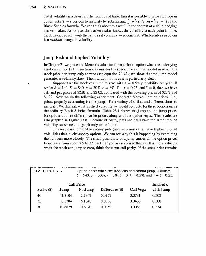
764 � VO LAT I L ITY

that if volatility is a deterministic function of time, then it is possible to price a European option with T - t periods to maturity by substituting .{ a2 (s)ds for a2 (T - t) in the Black-Scholes formula. We can think about this result in the context of a delta-hedging market-maker. As long as the market-maker knows the volatility at each point in time, the delta-hedge will work the same as if volatility were constant. What creates a problem is a random change in volatility.

Jump Risk and Implied Volatility

In Chapter 2 1 we presented Merton's valuation formula for an option when the underlying asset can jump. In this section we consider the special case of that model in which the stock price can jump only to zero (see equation 2 1 .42); we show that the jump model generates a volatility skew. The intuition in this case is particularly clear.

Suppose that the stock can jump to zero with ),. = 0.5% probability per year. If we let S = $40, K = $40, a = 30%, r = 8%, T - t = 0.25, and 8 = 0, then we have call and put prices of $2.8 1 and $2.02, compared with the no-jump prices of $2.78 and $ 1 .99. Now we do the following experiment: Generate "correct" option prices-i.e. , prices properly accounting for the jump-for a variety of strikes and different times to maturity. We then ask what implied volatility we would compute for these options using the ordinary Black-Scholes formula. Table 23 . 1 shows the jump and no-jump prices for options at three different strike prices, along with the option vegas . The results are also graphed in Figure 23 .8 . Because of parity, puts and calls have the same implied volatility, so we need to graph only one of them.

In every case, out-of-the money puts (in-the-money calls) have higher implied volatilities than at-the-money options. We can see why this is happening by examining the numbers more closely. The small possibility of a jump causes all the option prices to increase from about 2.5 to 3.5 cents. If you are surprised that a call is more valuable when the stock can jump to zero, think about put-call parity. If the stock price remains

. 1TAI8LE 2 3 . 1 Option prices when the stock can and cannot jump. Assumes S = $40, u = 30%, r = 8%, 8 = 0, A = 0.5%, and T - t = 0.25.

Call Price Implied a

Strike ($) Jump No Jump Difference ($) Call Vega with Jump

40 2.8 104 2.7847 0.0257 0.078 1 0.303

35 6. 1 704 6. 1 348 0.0356 0.0436 0.308

30 10.6679 1 0.6320 0.0359 0.0083 0.334

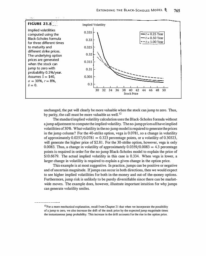
EXTEN D I N G TH E B LA C K-SC H O LES M O D E L � 765

F I G U R E 2 3 . 8 Implied Volatility

Impl ied volatil ities computed using the Black-Scholes formula for three d ifferent times to maturity and different strike prices. The underlying option prices are generated when the stock can jump to zero with probabi l ity 0.5%/year. Assumes S = $40,

0.335

0.33

0.325

0.32

0.3 15

0.31

0.305

.... .... .... ....

- t = 0.25 Year - t = O.SO Year - - t = l .OO Year

... _ - --=- ..... .... _

- - - - - ·

a = 30%, r = 8%, 8 = 0. 0.3

30 32 34 36 38 40 42 44 46 48 50 Stock Price

unchanged, the put will clearly be more valuable when the stock can jump to zero. Thus, by parity, the call must be more valuable as well. 1 2

The standard implied volatility calculation uses the Black-Scholes formula without a jump adjustment to compute the implied volatility. The no-jump prices all have implied volatilities of 30%. What volatility in the no-jump model is required to generate the prices in the jump column? For the 40-strike option, vega is 0.078 1 , so a change in volatility of approximately 0.0257/0.078 1 = 0.323 percentage points, or a volatility of 0.30323 , will generate the higher price of $2.8 1 . For the 30-strike option, however, vega is only 0.0083. Thus, a change in volatility of approximately 0 .0359/0.0083 = 4.3 percentage points is required in order for the no-jump Black-Scholes model to explain the price of $ 10.6679. The actual implied volatility in this case is 0.334. When vega is lower, a larger change in volatility is required to explain a given change in the option price.

This example is at most suggestive. In practice, jumps can be positive or negative and of uncertain magnitude. If jumps can occur in both directions, then we would expect to see higher implied volatilities for both in-the-money and out-of�the-rponey options. Furthermore, jump risk is unlikely to be purely diversifiable since there can be market­wide moves. The example does, however, illustrate important intuition for why jumps can generate volatility smiles.

12 For a more mechanical explanation, recall from Chapter 2 1 that when we incorporate the possibility of a jump to zero, we also increase the drift of the stock price by the expected jump magnitude times the instantaneous jump probability. This increase in the drift accounts for the rise in the option price.

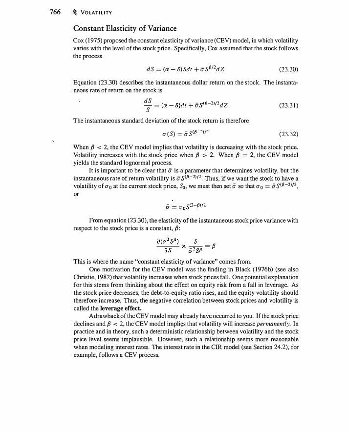
766 � VO LAT I L ITY

Constant Elasticity of Variance

Cox ( 1 975) proposed the constant elasticity of variance (CEV) model, in which volatility varies with the level of the stock price. Specifically, Cox assumed that the stock follows the process

dS = (a - 8)Sdt + a sPI2dZ (23 .30)

Equation (23 .30) describes the instantaneous dollar return on the stock. The instanta­neous rate of return on the stock is

dS _ < " �JJ? - = (a - 8)dt + aS "-- -dZ s

The instantaneous standard deviation of the stock return is therefore

a (S) = a s<P-2J/2

(23 .3 1 )

(23 .32)

When {3 < 2, the CEV model implies that volatility is decreasing with the stock price. Volatility increases with the stock price when {3 > 2. When {3 = 2, the CEV model yields the standard lognormal process.

It is important to be clear that a is a parameter that determines volatility, but the instantaneous rate of return volatility is a s<P-2ll2 . Thus, if we want the stock to have a volatility of a0 at the current stock price, S0, we must then �>et a so that a0 = a s<P-2ll2 , or

From equation (23 .30), the elasticity of the instantaneous stock price variance with respect to the stock price is a constant, {3 :

This is ·where the name "constant elasticity of variance" comes from. One motivation for the CEV model was the finding in Black ( 1 976b) (see also

Christie, 1982) that volatility increases when stock prices fall. One potential explanation for this stems from thinking about the effect on equity risk from a fall in leverage. As the stock price decreases, the debt-to-equity ratio rises, and the equity volatility should therefore increase. Thus, the negative correlation between stock prices and volatility is called the leverage effect.

A drawback of the CEV model may already have occurred to you. If the stock price declines and {3 < 2, the CEV model implit;!S that volatility will increase permanently. In practice and in theory, such a deterministic relationship between volatility and the stock price level seems implausible. However, such a relationship seems more reasonable when modeling interest rates. The interest rate in the CIR model (see Section 24.2), for example, follows a CEV process.

EXTE N D I N G TH E B LA C K-S C H O LES M O D E L � 767

The CEV pricing formula There is a relatively simple pricing formula for a European call when the stock price follows the CEV process. 1 3 Following Schroder ( 1 989), define

2(r - 8) K = �------�----------� 0'2(2 _ {3) (e<r-8) (1-,BJT _ 1 ) X = K s1-,8 e<r-8) (1-,B)T

y = K K1-.B

The CEV pricing formula for a European call is different for the cases f3 < 2 and f3 > 2. Let Q (a , b , c) denote the noncentral chi-squared distribution function with b degrees of freedom and noncentrality parameter c, evaluted at a . 14 The CEV call price is given by

Se-oT [ I - Q(2y , 2 + 2/(2 - {3) , 2x)] - Ke-rT Q(2x , 2/ (2 - {3) , 2y)

se-liT [ I - Q(2x , 2/({3 - 2) , 2y)] - Ke-rT Q(2y , 2 + 2/ ({3 - 2) , 2x)

{3 < 2 (23.33)

{3 > 2

Implied volatility in the CEV model When f3 < 2, the CEV model generates a Black­Scholes implied volatility skew curve resembling that in Figure 23. 1 : Implied volatility decreases with the option strike price. To understand why the CEV model generates this volatility skew, note from equation (23.3 1 ) that when f3 < 2 and the stock price falls, volatility increases. Thus compared with the case of a constant volatility, an out­of-the-money put option has a greater chance of exercise and is likely to be deeper in the money when it is exercised. The only way for the Black-Scholes model to account for this higher price is with a higher volatility. As the strike price increases, less of the option value is due to the stock price behavior at low prices, and volatility therefore need not increase as much.

Figure 23.9 plots implied volatility curves generated by using the Black-Scholes formula to compute implied volatility for prices generated by the CEV model. The top panel shows that, for the given parameters, the implied volatility curve is unaffected by · changi·ng time to maturity.

1 3Cox ( 1 996) originally derived a pricing formula in terms of infinite series for the case fJ < 2. Emanuel and MacBeth ( 1 982) generalized Cox's analysis to the case where fJ > 2. Schroder ( 1 989) showed that both cases could be expressed more compactly in terms of the noncentral chi-squared cumulative distribution function. Davydov and Linetsky (200 1 ) derive 'pricing formulas barrier and lookback options under a CEV process. 14The pricing formula is sometimes written in terms of the complementary noncentral chi-squared distribution, which is I - Q(a. b, c). The noncentral chi-squared distribution, unlike the chi-squared distribution, is not typically a standard function built into spreadsheets. However, it is available in software programs such as Matlab and Mathematica.

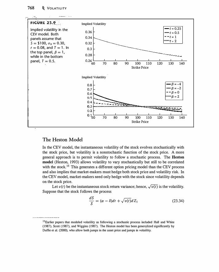
768 � VO LAT I L ITY

Implied volati l ity in the CEV model. Both panels assume that S = $ 1 00, a 0 = 0. 30,

Implied Volatility

0.36

0.34

0.32

0.3

0.28

- t = 0.25

- t = O.S - - t = 1

r = 0.08, and T = 1 . In the top panel, f3 = 1 , while in the bottom panel, T = 0.5 . 0.26 L----L----''-----'-----'---.J...._ _ __J_ __ .J.._ _ _L_

60 70

Implied Volatility

The Heston Model

0.8

0.7

0.6

70

80 90

80 90

100 1 10 120 130 140

Strike Price

- {3 = -4

- {3 = -2 - - {3 = 0

. . . . {3 = 2

100 1 10 120 130 140

Strike Price

In the CEV model, the instantaneous volatility of the stock evolves stochastically with the stock price, but volatility is a nonstochastic function of the stock price. A more general approach is to permit volatility to follow a stochastic process. The Heston model (Heston, 1 993) allows volatility to vary stochastically but still to be correlated with the stock. 1 5 This generates a different option pricing model than the CEV process and also implies that market-makers must hedge both stock price and volatility risk. In the CEV model, market-makers need only hedge with the stock since volatility depends on the stock price.

Let v (t) be the instantaneous stock return variance; hence, .JV(t) is the volatility. Suppose that the stock follows the process

dS S = (a - o)dt + .;;;ci)dZ1 (23 .34)

1 5Earlier papers that modeled volati lity as following a stochastic process included Hull and White ( 1 987), Scott ( 1 987), and Wiggins ( 1 987). The Heston model has been generalized significantly by Duffie et al. (2000), who allow both jumps in the asset price and jumps in volati l ity.

EXTE N D I N G TH E B LA C K-S C H O LES M O D E L � 769

Assume that the variance, u(t) , follows the mean-reverting process

dv(t ) = K [v - v(t) ]dt + a vfv(i)dZJ.

We assume that E(dZ 1dZ2) = pdt . (23 .35)

The interpretation of equations (23 .34) and (23 .35) is familiar. Equation (23 .34) for the stock is the same as equation (2 1 .5) except that the volatility, �' is random. The equation for volatility, equation (23 .35), has two noteworthy characteristics. First, the instantaneous variance, v (t ) , is mean-reverting, tending toward the value ii, with a speed of adjustment given by K . Second, the volatility of variance, a v ,JV(i), depends on the square root of v (t ) , and variance is therefore said to follow a square root process.

Suppose that the risk premium for the risk a v,JV(i)dZ2 can be written as v (t)f3 v , where we assume f3v is constant. This assumption that the risk premium is proportional to the level of the variance is analytically convenient. Given this assumption about the risk premium, the risk-neutral volatility process is

dv(t) = {K [v - v (t) ] - v (t)f3v } dt + a vfv(i)dz; = K* [v* - v (t)] dt + a vfv(i)dz;

(23 .36)

where K* = K + f3v and ii* = VKj (K + f3v) . This model of stochastic volatility is the Heston model .

Let V[S(t ) , v (t ) , t] represent the price of a derivative on the stock when the stock price and volatility are given by equations (23.34) and (23 .35). Suppose we proceed with the Black-Scholes derivation, in which we hold the option and try to hedge the resulting risk. We immediately encounter the problem that there are two sources of risk, d Z 1 and d Z1 . A position in the stock will hedge d Z 1 , but what can we use to hedge risk resulting from stochastic volatility? Apart from other options, there will typically be no asset that is a perfect hedge for volatility. 16 In that case, we rely on the equilibrium approach to pricing the option. The PDE for the derivative V [S(t) , v (t ) , t] is then:

4 v (t )S1 Vss + 4a�v (t) Vvv + pv (t)a vSVsv (23 .37)

+ (r - o) SVs + { K [v - v (t) ] - v(t)f3 v } Vv + V, = r V This equation i s the multivariate Black-Scholes equation, described i n Appendix 2 l .A The third term is due to the covariance between the stock return and volatility. Since there is no asset to hedge volatility, the coefficient on the Vv term has a correction for the risk premium associated with volatility.

Heston ( 1 993) shows that equation (23 .37) has an integral solution that can be evaluated numerically. Given this solution, we can see how implied volatility behaves when volatility is stochastic. S imilar to the analysis of jumps in Section 2 1 .5, we price options for different strikes and expirations under the stochastic volatility model and

1 6 It might be possible to use other options on the same stock to hedge volati lity, but the option would then be priced relative to the price of the option used as a hedge.

770 � VO LAT I L ITY

F I G U R E 23 .1.0 Black-Scholes Implied Volatility

0.36

0.34

0.32

0.3

'0.28

0.26

u,. = 0.10; p = 0

- t = 0.2S Year - t = O.S Year - - t = 1 Year

30 3S 40 4S Strike Price ($)

so

Black-Scholes Implied Volatility

0.36

0.34

0.32

0.3

0.28

0.26

a;. = O.SO; p = 0

- t = 0.2S Year - t = O.S Year - - t = 1 Year � � .. ... -.. ..

.... .. _ _ _ .,. _ _ _ _

30 3S 40 4S Strike Price ($)

so

Biack-Scholes Implied Volatility

0.36

0.34

0.32

0.3

0.28

0.26

u,, = 0.10; p = -0.30

- t = 0.2S Year - t = O.S Year - - t = 1 Year

--

-=------==------------ - - - - - .... .,.. _ _ _ _ _ _ _

30 3S 40 4S Strike Price ($)

so

Black-Scholes Implied Volatility

0.36

0.34

0.32

0.3

0.28

0.26

u,, = O.SO; p = -0.30

- t = 0.2S Year � t = O.S Year

30 3S 40 4S Strike Price ($)

so

Impl ied volati l ities computed using the Black-Scholes formula when prices are computed using the Heston model for three d ifferent times to maturity, d ifferent strike prices, and two d ifferent volatil ities of volatil ity, u v· The top panel assumes that a v = 0 . 1 0, while the bottom panel assumes that a v = 0 .5 . In both panels, K* = 2.0, v(t) = 0. 32, V = 0.25, r = 8%, and 8 = 0.

then use Black-Scholes to compute implied volatilities. We assume that the stock price is $40 and compute implied volatilities for options with strike prices ranging from $30 to $50 and with maturities from 3 months to I year.

Figure 23 . 10 shows the result of this experiment for two different values of a v and p. In the figure the long-run volatility, i!*, is 25%, less than the current volatility, 32%. Because volatility reverts to the mean, implied volatility decreases with time to maturity in every case. In the panel where a v = 0. 10 and p = 0, there is almost no skew, although the mean reversion in volatility is apparent. When a v .= 50% and p = 0, the figure exhibits both symmetric skew and mean reversion. The asymmetric skew in both

EXTE N D I N G TH E B LACK-S C H O LES M O D E L � 771

right-hand panels of Figure 23. 1 0 arises from assuming a negative correlation between volatility and the stock price.

Evidence

The main challenge for an option pricing model is to match the observed volatility skew. 1 7 The literature investigating ways to do this is too large to adequately summarize here. Instead, we will sketch the nature of findings in the literature and highlight issues that arise when trying to match models to data.

The pricing models in this section illustrate ways in which modifying the Black­Scholes assumptions can enable a pricing model to better fit observed option prices. For example, all the pricing models we have discussed are capable of generating higher implied volatities for in-the-money (low-strike) calls. The Merton jump model and the CEV model in the examples above both generate implied volatility curves that are flatter as time to maturity increases. 1 8 Combinations of the models, such as a Heston model that also allows jumps, seem able to reproduce qualitative features of Figure 23. 1 . However, matching models to data is a more involved exercise than just a visual comparison of implied volatility curves.

To illustrate the issues, suppose you want to match the Heston stochastic volatility model to data. There are a number of ways you might proceed. First, on a given day, you could find a set of model inputs that best matches the volatility curves for that day. This entails finding a return variance (v (t) ) , a volatility of volatility (a v ) , a mean reversion rate (K*) , a long-run risk-neutral variance (ii*), and a correlation between volatility and the stock return (p ) , that match the data for a particular day.

Matching implied volatilities across a set of options on a given day is a cross­sectional test of the model. Once you admit multiple days of data, the model has time-series implications as well. Equations (23 .35) and (23 .36) imply that volatility evolves over time in a specific way. If you look at the evolution of volatility over time, does it match equation (23 .35)? Are the parameters that enable the model to fit the cross- ' section consistent with those implied by the volatility time series? When there is a risk premium in the equilibrium pricing model (as in the Heston model), it is potentially easier

1 7The true model should give equal implied volatil ities for options at different strikes and maturities. For example, if the Heston stochastic volati l i ty model were true and option prices were consistent with equation (23.37), then Black-Scholes implied volatilities would exhibit skew, but if the Heston model were used to compute implied volatil ity, then the options in Figure 23. 1 0 would all have implied volatil ities of 32%.

1 8 1t is not obvious how to interpret the change with respect to maturity in implied volati l i ty curves such as those in Figures 23. 1 , 23.8, 23.9, and 23. 1 0. The issue is that the economic distinction between a $50

strike and a $55 strike is greater with one week to expiration than with one year to expiration; therefore. other things equal, we might expect to see flatter volatil ity curves as time to expiration increases. Bates (2000) corrects for this effect by scaling strike prices by a .Ji, effectively measuring distance between strikes in "standard deviation units."

772 � VO LAT I L ITY

to reconcile the behavior of the stock with option prices because there is an additional parameter. However, as Bates (2003) emphasizes, a risk premium must be plausible.

Bakshi et al . ( 1 997) and Bates (2000) both asked whether option pricing models incorporating jumps and stochastic volatility can generate realistic volatility skew for options based on the S&P 500. 1 9 Both studies find greater volatility skew at short maturities than at long maturities. If you compare Figures 23 .8 and 23 . 10, you can see that this pattern is generated by the jump model but not as obviously by the Heston model. This explains why, although Bakshi et al . ( 1997) found that the stochastic volatility model provided the best overall explanation of prices, they added jumps to account for skew at short maturities.20 They also found that permitting stochastic interest rates (which can be added in the same fashion as stochastic volatility) helped explain prices at longer maturities.

Bates (2000) found that jump models (as in Figure 23.8) fit near-term option prices better but found the jump parameters implausible: the stock price does not appear to jump as often as implied by the estimates necessary to explain implied volatility. Bates also concluded that in order for the stochastic volatility model to explain skew, the volatility of volatility had to be implausibly large. However, Duffie et al. (2000) developed a pricing procedure that permitted jumps in both the asset price and the volatility, and noted that allowing jumps in volatility potentially addressed the problem of an implausibly large volatility of volatility.

Broadie et al . (2004) conclude that "models with jumps in returns drastically improve overall pricing performance . . . [and] jumps in volatility offer a significant pricing improvement in the cross-section unless a model with jumps in returns is allowed to have a volatility-of-jump risk premium." In other words, jumps in at least some dimensions are important, and risk premia can be important as well .2 1

To add one more layer of complication, casual observation suggests that in some cases volatility changes deterministically over time. When a firm announces earnings, for example, volatility will be higher than on ordinary days. You can show that this is true by comparing the volatility of returns on earnings announcement days against that on other days. Dubinsky and Johannes (2004) show that this effect is also appar­ent in option prices, which imply a higher volatility before an earnings announcement than after.22 This finding suggests that in addition to the use of increasingly sophisti-

1 9Bakshi et al. ( 1 997) examined European options on the S&P 500 index while Bates (2000) examined options on the S&P 500 futures contract. 2°Carr and Wu (2003) formalize the intuition that jumps matter more if there is a short time to expiration. 2 1 It is possible to measure volatil ity risk premia directly by looking at the returns on portfolios that are hedged against stock price risk. For example, Coval and Shumway (200 1 ) find negative returns on zero-delta written straddles on the S&P I 00 and S&P 500 indexes. Since the written straddle loses money when volatility increases, this finding may be at least in part attributable to a volatility risk premium. Bakshi and Kapadia (2003) find smaller risk premia associated with delta-hedged individual stocks than with index options. 22In fact, we saw the effect of earnings announcements in Example 23.2 when we estimated a GARCH( l , l ) model for IBM and found the estimates sensitive to the inclusion of four earnings an­nouncement days.

F U RT H E R R E A D I N G � 773

cated mathematical pricing models, careful option pricing requires data sets that identify anticipated days of unusual volatility.23

' . . . .. . ,�.---·--------- -�--.-t,··- c ' , , v-, < _ . --·-.,;;.,,.;., - -� ------'-"··'---. . ---· --· · ______ _:._.,_

CHAPTER SUMMARY

For options on a given underlying asset on a given day, implied volatility generally varies across option strikes and maturities. Implied volatility also varies over time. As a result there is great interest in measuring volatilities and in pricing options when volatility can vary.

Methods of measuring volatility using past data include historical volatility, expo­nentially weighted moving average volatility, ARCH, GARCH, and realized quadratic variation. ARCH and GARCH estimates are based upon a formal statistical model in which volatility is random. Realized quadratic variation exploits high frequency data to obtain a reliable volatility estimate using data from a short time horizon.

Both variance and volatility swaps permit hedging and speculation on volatility. The variance forward price can be obtained as a weighted sum of the prices of traded European options, a calculation that is the basis for the VIX measure of implied volatility.

The Black-Scholes model does not perfectly explain observed option prices; there is volatility skew, which means that implied volatility varies with the strike price and time to expiration. Two modifications to the model are to permit jumps in the stock price and to allow volatility to be stochastic. Both changes generate option prices that exhibit volatility skew and that better fit the data than the unmodified Black-Scholes model.

Attempts to explain prices of traded options suggest that it is important to account for jumps in both the asset price and volatility, and that risk premiums on one or both jumps may be important.

FURTHER READING

Early studies of stock returns (e.g. , Fama, 1 965) found that continuously compounded returns exhibit too many large returns to be consistent with normality. In recent years, research has focused on specifying stock price processes that give theoretical option prices consistent with observed prices. Introductions to GARCH models include Royal Swedish Academy of Sciences (2003), and Bollerslev et al. ( 1994). Alexander (200 1 ) is a readable text for less technical readers. Realized quadratic variation as a measure of volatility is presented and applied in Andersen et al . (2003) .

Demeterfi et al. ( 1 999) present a clear and well-written discussion of volatility hedging, and the paper also develops the volatility measure used now to construct the VIX. See also Chicago Board Options Exchange (2003) .

23This is no t just an issue for individual firms. Governments make economic announcements on prespecified days a t set times, and these announcements sometimes generate large moves in prices. For example, Han week ( 1 994) shows that implied volatil ity in Eurodollar futures options is greater on days when the government announces aggregate employment.

774 � VO LAT I L ITY

The first papers to suggest alternative assumptions about the stock price for option pricing were Cox and Ross ( 1 976), Cox ( 1 996), and Merton ( 1 976). Merton noted in his paper that the jump model had the potential to explain volatility skew patterns noted by practitioners at the time. The first stochastic volatility models were proposed by Hull and White ( 1 987), Scott ( 1 987), and Wiggins ( 1987). The Heston ( 1 993) model has been generalized by Duffie et a!. (2000), who develop a pricing framework that can accomodate jumps in volatility as well as in the stock price.

The empirical literature examining the ability of option pricing models to fit ob­served prices is rapidly evolving. Well-known papers include Bakshi et a!. ( 1 997), Bates (2900), and Pan (2002). Current research (which include citations to numerous other papers) include Andersen et a!. (2005) and Broadie et a! . (2004) . Dubinsky and Jo­hannes (2004) examine deterministic volatility changes, such as those due to earnings announcements.

PROB LEMS

For many of the first fifteen problems you will need to use data on the CD accompanying this book. The CD contains stock prices, option prices, and interest rates for a variety of maturities. If an interest rate you need is missing, use the rate for the nearest available maturity.

23.1. Using weekly price data (constructed Wednesday to Wednesday), compute his­torical annual volatilities for .IBM, Xerox, and the S&P 500 index for 1 99 1 through 2004. Annualize your answer by multiplying by -J52. Also compute volatility for each for the entire period.

23.2. Compute daily volatilities for 199 1 through 2004 for IBM, Xerox, and the S&P 500 index. Annualize by multiplying by ,Jili. How do your answers compare to those in Problem 1 ?

23.3. For the period 1 999-2004, using daily data, compute the following:

a. An EWMA estimate, with b = 0.95, of IBM's volatility using all data.

b. An EWMA estimate, with b = 0.95, of IBM's volatility, at each date using only the previous 60 days of data.

Plot both estimates. How different are they?

23.4. Estimate a GARCH( l , 1 ) for the S&P 500 index, using data from January 1 999 to December 2003 .

23.5. Replicate the GARCH( 1 , 1 ) estimation in Example 23.2, using daily returns from on IBM from January 1999 to December 2003 . Compare your estimates with and without the four largest returns.

23.6. Use the following inputs to compute the price of a European call option: S = $ 1 00, K = $50, r = 0.06, u = 0.30, T = 0.0 1 , 8 = 0.

P RO B LE M S � 775

a. Verify that the Black-Scholes price is $50.0299.

b. Verify that the vega for this option is almost zero. Why is this so?

c. Verify that if you compute the option price with volatilities ranging from 0.05 to 1 .00, you get essentially the same option price and vega remains about zero. Why is this so? What happens if you set a = 5 .00 (i.e. , 500%)?

d. What can you conclude about difficulties in computing implied volatility for very short-term, deep in-the-money options?

23.7. Use the same inputs as in the previous problem. Suppose that you observe a bid option price of $50 and an ask price of $50. 10 .

a . Explain why you cannot compute an implied volatility for the bid price.

b. Compute an implied volatility for the ask price, but be sure to set the initial volatility at 200% or greater. Explain why the implied volatility for the ask price is extremely large.

c. (Optional) Examine the code for the BSCalllmp Vol function. Explain why changing the starting volatilty can affect whether or not you obtain an answer.

d. What can you conclude about difficulties in computing and interpreting implied volatilities for deep in-the-money options?

23.8. Use the following inputs to compute the price of a European call option: S = $50, K = $ 1 00, r = 0.06, a = 0.30, T = 0.0 1 , 8 = 0.

a. Verify that the Black-Scholes price is zero.

b. Verify that the vega for this option is zero. Why is this so?

c. Suppose you observe a bid price of zero and an ask price of $0.05. What answers do you obtain when you compute implied volatility for these prices. Why?

d. Why would market-makers set such prices?

e. What can you conclude about difficulties in computing and interpreting implied volatility for very short-term, deep out-of-the-money options?

23.9. Compute January 12 bid and ask volatilities (using the Black-Scholes implied volatility function) for IBM options expiring January 17 . For which options are you unable to compute a plausible implied volatility? Why?

23.10. Compute January 12 bid and ask volatilties (using the Black-Scholes implied volatility function) for IBM options expiring February 2 1 .

a . D o you observe a volatility smile?

b. For which options are you unable to compute a plausible implied volatil­ity? Why?

776 � VO LAT I L I TY

23.11. Compute January 1 2 implied volatilities using the average of the bid and ask prices for ffiM options expiring February 2 1 (use the Black-Scholes implied volatility function). Compare your answers to those in the previous problem. Why might someone prefer to use implied volatilities based on the average of the bid and ask prices, rather than the bid and ask volatilities individually?

23.12. In this problem you will compute January 12 bid and ask volatilties (using the Black-Scholes implied volatility function) for one-year ffiM options expiring the following January. Note that ffiM pays a dividend in March, June, September, and December.

a. Compute implied volatilities ignoring the dividend.

b. Take dividends into account using the discrete dividend correction to the Black Scholes formula, presented in Chapter 12 . For simplicity, discount all observed future dividends at a 2% continuously compounded rate. How much difference does this correction make in implied volatility?

c. Take dividends into account by computing a dividend yield for ffiM based on its annualized dividend rate as of January 1 2. Use this dividend yield in the Black-Scholes model. How different are the implied volatilties from those you obtain in the previous part?

d. Do you observe a volatility smile?

23.13. For this problem, use the implied volatilities for the options expiring in January 2005, computed in the precedl.ng problem. Compare the implied volatilties for calls and puts. Where is the difference largest? Why does this occur?

23.14. Suppose S = $ 100, r = 8%, a = 30%, T = I , and 8 = 0. Use the Black­Scholes formula to generate call and put prices with the strikes ranging from $40 to $250, with increments of $5. Compute the implied volatility from these prices by using the formula for the VIX (equation 23.29). What happens to your estimate if you use strikes that differ by $ 1 or $ 1 0, or strikes that range only from $60 to $200?

23.15. Explain why the VIX formula in equation (23.29) overestimates implied volatil­ity if options are American.

The following three problems use the Merton jump formula. As a base case, assume S = $ 100, r = 8%, a = 30%, T = I, and 8 = 0. Also assume that A = 0 .02, a1 = -0.20 and a 1 = 0.30.

23.16. Using the Merton jump formula, generate an implied volatility plot for K = 50, 55 , 0 0 0 1 50.

a. How is the implied volatility plot affected by changing ct1 to -0.40 or -0. 1 0?

b. How is the implied volatility plot affected by cha_nging A to 0.0 1 or 0.05?

A P P E N D I X 23 .A � 777

c. How is the implied volatility plot affected by changing a 1 to 0. 1 0 or 0.50?

23.17. Using the base case parameters, plot the implied volatility curve you obtain for the base case against that for the case where there is a jump to zero, with the same 'A.

23.18. Repeat problem 23. 1 6, except let a 1 = 0�20, and in part (b) consider expected . alternate jump magnitudes of 0. 1 0 and 0.50.

The following two problems both use the CEV option pricing formula. Assume in both that S = $ 1 00, r = 8%, a0 = 30%, T = 1 , and 8 = 0.

23.19. Using the CEV option pricing model, set f3 = 1 and generate option prices for strikes from 60 to 140, in increments of 5, for times to maturity of 0.25, 0.5, 1 .0, and 2.0. Plot the resulting implied volatilties. (This should reproduce Figure 23.9.)

23.20. Using the CEV option pricing model, set f3 = 3 and generate option prices for strikes from 60 to 140, in increments of 5, for times to maturity of 0.25, 0.5, 1 .0, and 2.0. Plot the resulting implied volatilties.

APPENDIX 23 .A

Here i s one way to set up a spreadsheet in order to estimate a GARCH model by maximum likelihood using Excel.

1. Enter daily prices in column B , beginning in B 1 0.

2. Compute continuously compounded returns for a 5-year period in column C, begin­ning in row 1 1 . Leave cells A 1 :C7 empty.

3. In column D compute the squared continuously compounded return. This will be E2 .

4. In cell E l l , enter the variance of the continuously compounded returns. This will be your starting value for q .

5 . In cell E 12, enter the formula =$B$ 1 +$B$2*D l 2+$B$3*E 1 1 . B e sure to pay attention to which cells are absolute and which are relative references. Copy this formula down the length of your data.

6. In cell F l 3 , enter the formula = - ln (£ 13) - Dl3/ £ 13 . Copy this formula down. This is your log-likelihood function for each observation.

7. Suppose that your last return is in row 1200. In cell B4, enter the formula = SUM(Fl3 :F l200) . This is the log-likelihood function for your data.

8. In Solver, set up the following constraints: B 1 � 0 .000000 1 , B2 � 0.0000000 1 , B 3 > 0, B 2 .:::; 0.99999999 - B3.

778 � VO LAT I L ITY

9. In cell B5, enter the formula B l/( l -B2-B3) . This is your unconditional variance estimate.

10. In cell B6, enter the formula SQRT(B5*252). This is your unconditional annualized standard deviation.

11. Set up Solver to maximize cell B4 (the likelihood) by varying cells B 1 :B3 (the parameters) .

12. Solve !

Your solution will likely be quite sensitive to several factors : to starting values, to the Solver options, and to unusually large squared returns. You should change the tolerance (in Solver options) to 1 % or less. You should also experiment with different starting values for the parameters.

Interest Rate Mode Is

Ou: go.J in this chapte< is to unde<StMd how to price derivotives th;t have bonds and interest rates, rather than stocks, as the underlying asset. We begin by seeing how the Black-Scholes approach to option pricing, discussed in Chapter 2 1 , applies to bonds. As with stocks, there is a partial differential equation that characterizes the behavior of bond prices and other functions of interest rates. The Vasicek and Cox-Ingersoll­Ross models illustrate the procedure for deriving bond prices from an assumed model of the short-term interest rate. Next we examine the pricing of bond and interest rate options using the Black model (the name for the version of the Black-Scholes model for which the underlying asset is a futures contract) . The Black model assumes that forward interest rates are lognormally distributed and can be used to price interest rate caps as well as bonds. Finally we examine binomial interest rate models, in particular the Black-Derman-Toy model.

24.1 MARKET-MAKING AND B OND PRICING

In this section we examine market-making in bonds in order to better understand how the Black-Scholes option pricing framework applies to bonds. We begin by examining the hedging of one bond with another.

The Black-Scholes derivation of the option pricing model characterizes the fair op­tion price for a delta-hedging market-maker. Vasicek ( 1 977) used the same approach for pricing bonds. Consider a delta-hedging bond portfolio manager, like the market-maker who delta-hedged options in Chapters 1 3 and 2 1 . Specifically, suppose the manager owns one bond with maturity Tz and hedges this bond by buying N bonds with maturity T1 (N can be negative) . The position is financed using short-term bonds paying r. Hedg­ing one bond with another is often called duration-hedging rather than delta-hedging. The intent of duration- and delta-hedging is the same, but as we will see, the two are generally not the same if we use the standard definition of duration from Section 7 . 8 .

The logic of the Vasicek approach to pricing bonds i s identical to the Black-Scholes approach to analyzing options : We think about the problem faced by a market-maker and see what it tells us about bond price behavior. We will focus on pricing zero-coupon bonds since, as discussed in Chapter 7, they are a building block for all fixed-income products.

779

780 � I NT E R EST RATE M O D E LS

The Behavior of Bonds and Interest Rates

Before discussing how a bond market-maker would delta-hedge, we first need to specify how bonds behave. Suppose we try to model a zero-coupon bond the same way we model a stock, by assuming that the bond price, P (t , T) follows an Ito process:

dP p = a(r, t )dt + q (r, t)dZ (24. 1 )

In this equation, the coefficients a and q cannot be constants and i n fact must be modeled rather carefully to ensure that the bond satisfies its boundary conditions. For example, th,e bond must be worth $1 at maturity. Also, the volatility of the bond price should decrease as the bond approaches maturity-a given change in interest rates affects the price of a long-lived bond more than the price of a short-Jived bond. Neither of these restrictions is automatically reflected in equation (24. 1 ) . In order to accommodate such behavior a and q must be carefully specified functions of the interest rate and time.

An alternative to beginning with equation (24. 1 ) is to model the behavior of the interest rate and solve for the bond price. If we follow this approach, the bond price will automatically behave in an appropriate way, as long as the interest rate process is reasonable.

Suppose we assume that the short-term interest rate foJlows the Ito process

dr = a (r)dt + rr (r)dZ (24.2)

This equation for the behavior of the interest rate is general, in that the drift and standard deviation are functions of r. Given eq!Jation (24.2), what is the bond price? We will see that different bond price models arise from different versions of this interest rate process.

An Impossible Bond Pricing Model

We will first look at a bond pricing model that is intuitive, appealing in its simplicity, and widely used informally as a way to think about bonds. We will assume that the yield curve is flat; that is, at any point in time, zero-coupon bonds at ail maturities have the same yield to maturity. If the interest rate changes, yields for all bonds change uniformly so that the yield curve remains flat. Unfortunately, this model of the yield curve gives rise to arbitrage opportunities. It can be instructive, however, to see what doesn't work in order to better appreciate what does.

To analyze the flat-yield curve assumption, we assume that the interest rate follows equation (24.2). The price of zero-coupon bonds is given by

P (t , T) = e-r<T-1 ) (24.3)

In this specification, every bond has yield to maturity r. We now analyze the delta-hedging problem. If we buy one bond maturing at time

T2, hedge by buying N bonds maturing at time T1 , and finance the difference at the short-term interest rate, the bond portfolio has value

I = N P (t , T, ) + P(t , T2) + W = 0

Since W is invested in short-term bonds, we have

dW = rWdt

(24.4)

(24.5)

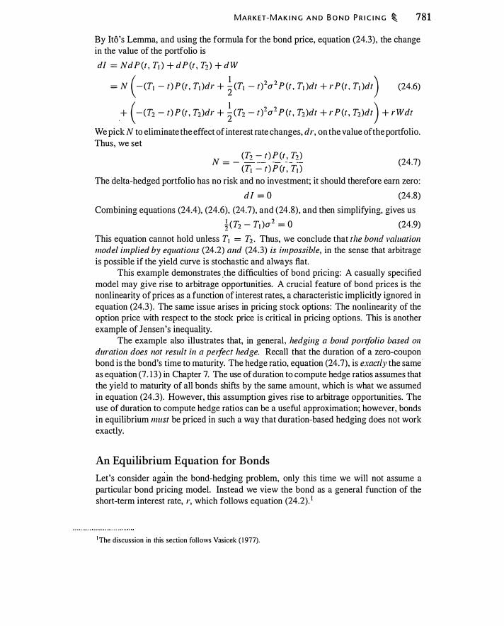
M A R K ET- M A K I N G A N D B O N D P R I C I N G � 781

By Ito's Lemma, and using the formula for the bond price, equation (24.3), the change in the value of the portfolio is

dl = NdP (t , Tr ) + dP (t , T2) + dW

( 1 ? ? ) = N -(T1 - t) P (t , T1 )dr + 2: (T1 - t)-a-P (t , T1 )dt + rP (t , T1 )dt (24.6)

( I ? ? ) + -(Tz - t) P (t , Tz)dr + 2 (Tz - t)-a- P (t , Tz)dt + rP (t , T2)dt + rWdt

We pick N to eliminate the effect of interest rate changes, dr, on the value of the portfolio. Thus, we set

N = _ (Tz - t) P (t , Tz) (T1 - t) P (t , Tr ) (24.7)

The delta-hedged portfolio has no risk and no investment; it should therefore earn zero:

dl = 0 (24.8)

Combining equations (24.4), (24.6), (24.7), and (24.8), and then simplifying, gives us

� (Tz - Tr )a2 = 0 (24.9)

This equation cannot hold unless T1 = T2 . Thus, we conclude that the bond valuation model implied by equations (24.2) and (24.3) is impossible, in the sense that arbitrage is possible if the yield curve is stochastic and always flat.

This example demonstrates ,the difficulties of bond pricing: A casually specified model may give rise to arbitrage opportunities. A crucial feature of bond prices is the nonlinearity of prices as a function of interest rates, a characteristic implicitly ignored in equation (24.3) . The same issue arises in pricing stock options: The nonlinearity of the option price with respect to the stock price is critical in pricing options. This is another example of Jensen's inequality.

The example also illustrates that, in general, hedging a bond portfolio based Oil duration does not result in a pe1ject hedge. Recall that the duration of a zero-coupon bond is the bond's time to maturity. The hedge ratio, equation (24.7), is exactly the same · as equation (7 . 1 3 ) in Chapter 7. The use of duration to compute hedge ratios assumes that the yield to maturity of all bonds shifts by the same amount, which is what we assumed in equation (24.3). However, this assumption gives rise to arbitrage opportunities. The use of duration to compute hedge ratios can be a useful approximation; however, bonds in equilibrium must be priced in such a way that duration-based hedging does not work exactly.

An Equilibrium Equation for Bonds

Let's consider again the bond-hedging problem, only this time we will not assume a particular bond pricing model. Instead we view the bond as a general function of the short-term interest rate, r, which follows equation (24.2). 1

1 The discussion in this section follows Vasicek ( 1 977).

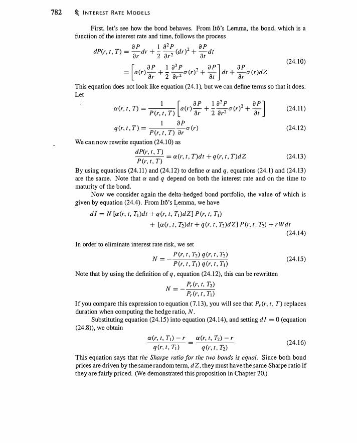
782 � I NT E R EST RATE M O D E LS

First, let's see how the bond behaves. From Ito's Lemma, the bond, which is a function of the interest rate and time, follows the process

a P 1 a2P ? a P dP(r, t , T) = -dr + - -? (dr)- + -dt ar 2 ar- at [ a P 1 a2 P ? a P J a P

= a (r)- + - -? u (r)- + - dt + -u(r)dZ ar 2 ar- at ar

(24. 1 0)

This equation does not look like equation (24. 1 ), but we can define terms so that it does. Let

1 [ a P 1 a2 P ? a P J a (r, t , T) = a (r)- + --? u (r)- + -P(r, t , T) ar 2 ar- at

1 aP q (r, t , T ) = u (r) P (r, t , T) ar

We can now rewrite equation (24. 1 0) as dP(r, t, T) ----'- = a (r, t , T)dt + q (r, t , T)dZ P (r, t , T)

(24. 1 1 )

(24. 1 2)

(24. 13 )

By using equations (24. 1 1 ) and (24. 1 2) to define a and q , equations (24. 1 ) and (24. 13 ) are the same. Note that a and q depend on both the interest rate and on the time to maturity of the bond.

Now we consider again the delta-hedged bond portfolio, the value of which is given by equation (24.4) . From Ito's �emma, we have

d I = N [a (r, t, T1 )dt + q (r, t, TJ )dZ] P (r, t, TJ ) + [a (r, t , T2)dt + q (r, t , T2)dZ] P (r, t , T2) + rWdt

(24. 1 4)

In order to eliminate interest rate risk, we set

N = P (r, t , T2) q (r, t , T2) P (r, t , T1 ) q (r, t , TJ )

Note that by using the definition of q , equation (24. 1 2), this can be rewritten

N = _ Pr (r, t, T2) Pr (r, t , T1 )

(24. 15 )

If you compare this expression to equation (7 . 1 3), you will see that Pr (r, t , T) replaces duration when computing the hedge ratio, N.

Substituting equation (24. 15 ) into equation (24. 14 ), and setting d I = 0 (equation (24.8)), we obtain

a (r, t, T1 ) - r a (r, t, T2) - r = q (r, t , TJ ) q (r, t , T2)

(24. 1 6)

This equation says that the Shmpe ratio for the two bonds is equal. Since both bond prices are driven by the same random term, d Z, they must have the same Sharpe ratio if they are fairly priced. (We demonstrated this proposition in Chapter 20.)

M A R K ET- M A K I N G A N D B O N D P R I C I N G � 783

Denote the Sharpe ratio for dZ as ¢(r, t). For any bond we then have

a (r, t, T) - r ---- = ¢(r, t)

q (r, t , T) Substituting equations (24. 1 1 ) and (24. 1 2) for a and q then gives us

1 � a2 P a P a P -cr (r)--� + [a (r) - cr (r)¢(r, t) ]- + - - r P = 0 2 ar- ar at

(24. 17)

(24. 1 8)

When the short-term interest rate is the only source of uncertainty, this partial differential equation must be satisfied by any zero-coupon bond. Different bonds will have different maturity dates and therefore different boundary conditions. All bonds solve the same PDE, however. The B1ack-Scholes equation, equation (2 1 . 1 1 ), characterizes claims that are a function of the stock price. Equation (24. 1 8) is the analogous equation for derivative claims that are a function of the interest rate.

A difference between equation (24. 1 8) and equation (2 1 . 1 1 ) is the explicit appear­ance of the risk premium, cr (r, t)¢ (r, t ) , in the bond equation. Let's talk about why that happens.

In the context of stock options, the Black-Scholes problem entails hedging an option with a stock, which is an investment asset. The stock is expected to earn its risk premium, which we will call ¢'cr . Thus, for the stock, the drift term, which is analogous to a (r) , equals r + ¢'cr . The Black-Scholes delta-hedging procedure eliminates the risk premium on the stock. By subtracting the risk premium, we are left with the risk-free rate, r, as a coefficient on the a v 1 as term in equation (2 1 . 1 1 ) .

The interest rate, by contrast, is not the price of an investment asset. The interest rate is a characteristic of an asset, not an asset by itself. The risk-neutral process for the interest rate is obtained by subtracting the risk premium from the drift. The risk-neutral process for the interest rate is therefore

I dr = [a (r) - cr (r)¢ (r, t) ]dt + cr (r)dZ I (24. 1 9) '

The drift in this equation is what appears in equation (24. 1 8) . You can also confirm that equation (24. 1 8) is the same as equation (24. 1 7) .

Given a zero-coupon bond (which has a terminal boundary condition that the bond is worth $ 1 at maturity), Cox et a!. ( 1 985b) show that the solution to equation (24. 1 8) is

P [t , T, r (t) ] = E; [e-R(t . Tl] (24.20)

where E* represents the expectation taken with respect to risk-neutral probabilities and R(t , T) is the random variable representing the cumulative interest rate over time:

R (t , T) = !T r(s)ds (24.2 1 )

Thus, to value a zero-coupon bond, we take the expectation over all the discount factors implied by these paths. We will see the discrete time analogue of this equation when we examine binomial models.

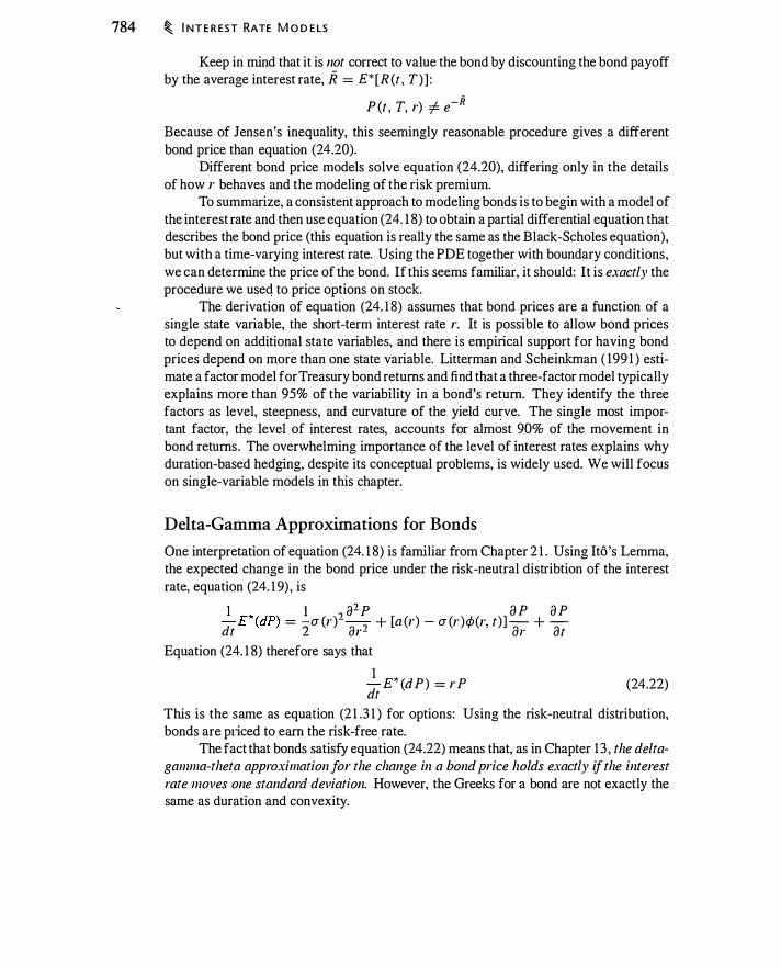
784 � I NT E R EST RATE M O D E LS

Keep in mind that it is not correct to value the bond by discounting the bond payoff by the average interest rate, R = E* [R (t , T)] :

P (t , T, r) =/= e-i?

Because of Jensen's inequality, this seemingly reasonable procedure gives a different bond price than equation (24.20).

Different bond price models solve equation (24.20), differing only in the details of how r behaves and the modeling of the risk premium.

To summarize, a consistent approach to modeling bonds is to begin with a model of the interest rate and then use equation (24. 1 8) to obtain a partial differential equation that describes the bond price (this equation is really the same as the Black-Scholes equation), but with a time-varying interest rate. Using the PDE together with boundary conditions, we can determine the price of the bond. If this seems familiar, it should: It is exactly the procedure we used to price options on stock.

The derivation of equation (24. 1 8) assumes that bond prices are a function of a single state variable, the short -term interest rate r. It is possible to allow bond prices to depend on additional state variables, and there is empirical support for having bond prices depend on more than one state variable. Litterman and Scheinkman ( 199 1 ) esti­mate a factor model for Treasury bond returns and find that a three-factor model typically explains more than 95% of the variability in a bond's return. They identify the three factors as level, steepness, and curvature of the yield curve. The single most impor­tant factor, the level of interest rates, accounts for almost 90% of the movement in bond returns. The overwhelming importance of the level of interest rates explains why duration-based hedging, despite its conceptual problems, is widely used. We will focus on single-variable models in this chapter.

Delta-Gamma Approximations for Bonds

One interpretation of equation (24. 1 8) is familiar from Chapter 2 1 . Using Ito's Lemma, the expected change in the bond price under the risk-neutral distribtion of the interest rate, equation (24. 1 9) , is

1 . r � a2 P a P a P dt E'" (dP) = la (r)- ar1 + [a (r) - a (r)¢(r, t)]/h- + at

Equation (24. 1 8) therefore says that

1 *

dt E · (d P) = r P (24.22)

This is the same as equation (2 1 .3 1 ) for options: Using the risk-neutral distribution, bonds are priced to earn the risk-free rate.

The fact that bonds satisfy equation (24.22) means that, as in Chapter 1 3 , the delta­gamma-theta approximation for the change in a bond price holds exactly if the interest rate moves one standard deviation. However, the Greeks for a bond are not exactly the same as duration and convexity.

EQU I L I B R I U M S H O RT-RATE B O N D P R I C E M O D E LS � 785

We discussed bond duration and convexity in Chapter 7 . For a zero-coupon bond, duration is time to maturity and convexity is squared time to maturity. Conceptually it seems as if duration should be the delta of a bond and convexity should be gamma. However, this is true only in the "impossible" bond pricing model of equation (24.3) . For any correct bond pricing model, duration and convexity will be different than Pr/ P and Prr / P . We will see examples of this in the next section.

24.2 EQUILIBRIUM SHORT-RATE BOND PRICE MODELS

In this section we discuss several bond pricing models based on equation (24. 1 8), in which all bond prices are driven by the short-term interest rate, r . The three pricing models we discuss-Rendleman-Bartter, Vasicek, and Cox-Ingersoll-Ross--differ in their specification of a (r) , u (r) , and </J(r) . These differences can result in very different pricing implications.

The Rendelm�m-Bartter Model

The simplest models of the short-term interest rate are those in which the interest rate follows arithmetic or geometric Brownian motion. For example, we could write

dr = adt + udZ (24.23)

In this specification, the short-rate is normally distributed with mean r0 + at and vari­ance u2t . There are several objections to this model :

• The short-rate can be negative. It is not reasonable to think the nominal short­rate can be negative, since if it were, investors would prefer holding cash under a mattress to holding bonds.

• The drift in the short-rate is constant. If a > 0, for example, the short-rate will drift up over time forever. In practice if the short-rate rises, we expect it to fall; i .e. , it is mean-reverting.

• The volatility of the short-rate is the same whether the rate is high or low. In practice, we expect the short-rate to be more volatile if rates are high.

The Rendleman and Bartter ( 1980) model, by contrast, assumes that the short-rate follows geometric Brownian motion :

dr = ardt + urdz (24.24)

While interest rates can never be negative in this model, one objection to equation (24.24) is that interest rates can be arbitrarily high. In practice we would expect rates to exhibit mean reversion; if rates are high, we expect them on average to decrease. The Rendleman-Bartter model, on the other hand, says that the probability of rates going up or down is the same whether rates are 100% or 1 %.

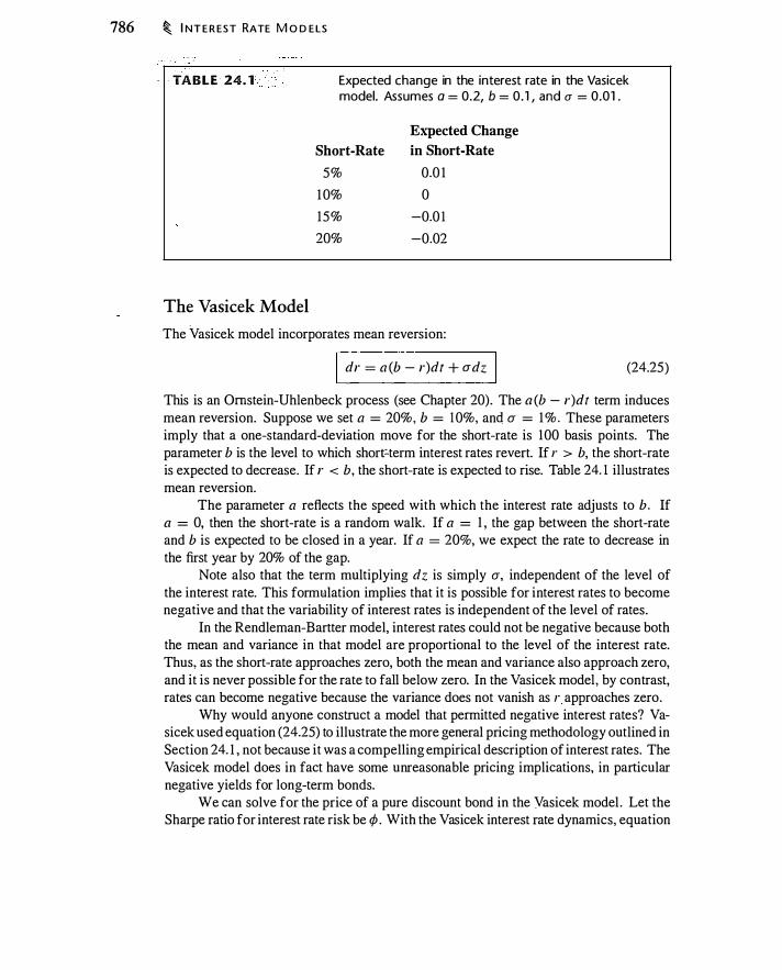
786 � I NT E R EST RATE M O D E LS

· .. · · . · · :

TAB L E 24. 1 Expected change in the interest rate in the Vasicek model. Assumes a = 0.2, b = 0.1 , and a = 0.01 .

The Vasicek Model

Short-Rate

5% 10% 15% 20%

E:\:pected Change in Short-Rate

0.0 1 0

-0.0 1 -0.02

The Vasicek model incorporates mean reversion:

I dr = a (b - r)dt + adz (24.25)

This is an Omstein-Uhlenbeck process (see Chapter 20). The a (b - r)dt term induces mean reversion. Suppose we set a = 20%, b = I 0%, and u = 1% . These parameters imply that a one-standard-deviation move for the short-rate is 100 basis points. The parameter b is the level to which short:term interest rates revert. If r > b, the short-rate is expected to decrease. If r < b, the short-rate is expected to rise. Table 24. 1 illustrates mean reversion.

The parameter a reflects the speed with which the interest rate adjusts to b. If a = 0, then the short-rate is a random walk. If a = I , the gap between the short-rate and b is expected to be closed in a year. If a = 20%, we expect the rate to decrease in the first year by 20% of the gap.

Note also that the term multiplying d z is simply u, independent of the level of the interest rate. This formulation implies that it is possible for interest rates to become negative and that the variability of interest rates is independent of the level of rates.

In the Rendleman-Bartter model, interest rates could not be negative because both the mean and variance in that model are proportional to the level of the interest rate. Thus, as the short-rate approaches zero, both the mean and variance also approach zero, and it is never possible for the rate to fall below zero. In the Vasicek model, by contrast, rates can become negative because the variance does not vanish as r approaches zero.

Why would anyone construct a model that permitted negative interest rates? Va­sicek used equation (24.25) to illustrate the more general pricing methodology outlined in Section 24. 1 , not because it was a compelling empirical description of interest rates. The Vasicek model does in fact have some unreasonable pricing implications, in particular negative yields for long-term bonds.

We can solve for the price of a pure discount bond in the Vasicek model . Let the Sharpe ratio for interest rate risk be ¢ . With the Vasicek interest rate dynamics, equation

EQ U I L I B R I U M S H O RT-RATE B O N D P R I C E M O D E LS � 787

(24.25), equation (24. 1 8) becomes

1 , a2 P a P a P - c r - + [a (b - r) - a¢]- + - - rP = 0 2 ar1 ar at

The bond price formula that solves this equation subject to the boundary condition P (T, T, r) = 1 , and assuming a =/= 0, is2

P [t , T, r (t) ] = A (t , T)e-B(r , T)r(l ) (24.26)

where

A(t , T) = ei'(B(r . T )+t-T)- B'u'f4a

B(t , T) = ( 1 - e-a(T-r ) )/a r = b + a ¢Ia - 0.5a1 ja1

with r being the yield to maturity on an infinitely lived bond.

The Cox-Ingersoll-Ross Model

The Cox-Ingersoll-Ross (CIR) model (Cox et al. , 1 985b) assumes a short-term interest rate model of the form

I dr = a (b - r)dt + a.)Tdz I (24.27)

The variance of the interest rate is proportional to the square root of the interest rate, instead of being constant as in the Vasicek model. Because of this subtle difference, the CIR model satisfies all the objections to the earlier models:

• It is impossible for interest rates to be negative. If r = 0, the drift in the rate is positive and the variance is zero, so the rate will become positive.

• As the short-rate rises, the volatility of the short-rate also rises.

• The short-rate exhibits mean reversion.

The assumption that the variance is proportional to .jr also turns out to be con­venient analytically-Cox, Ingersoll, and Ross (CIR) derive bond and option pricing formulas using this model. The risk premium in the CIR model takes the form

¢ (r, t) = ¢.JT!a (24.28)

2When a = 0, the solution is equation (24.26), with

B = T - t

When a = 0 the interest rate follows a random walk; therefore, i' is undefined.

788 � I NT E R EST RATE M O D E LS

With this specification for the risk premium and equation (24.27), the CIR interest rate dynamics, the partial differential equation for the bond price is

1 � a2 P - a P a P -u-r - + [a (b - r) - r¢] - + - - r P = 0

. 2 ar2 ar at The CIR bond price looks similar to that for the Vasicek dynamics, equation (24.26), but with A (t , T) and B(t , T) defined differently:

where

P [t , T, r (t) ] = A (t , T)e-B<r . T>r<r >

[ 2ye<a+¢+y) (T-t )/2 ] 2abfa1

A (t . T) = ·

(a + ¢ + y) (eY<T-t) - 1 ) + 2y

. 2(eY (T -t ) - 1 ) B(t , T) = ---=--------=,---,---­

(a + ¢ + y) (eY<T-t) - 1 ) + 2y

y = J(a + fP)2 + 2u2

(24.29)

With the CIR process, the yield on a long-term bond approaches the value r = 2abj(a + ¢ + y) as time to maturity goes to infinity.

Comparing Vasicek and CIR

How different are the prices generated by the CIR and Vasicek models? What is the role of the different variance specifications in the two models?

Figure 24. 1 illustrates the yield curves generated by the Vasicek and by the CIR models, assuming that the current short-term rate, r , is 5%, a = 0.2 and b = 10%. Volatility in the Vasicek model is 2% in the top panel and 10% in the bottom panel . The volatility, u , has a different interpretation in each model. In the Vasicek model, volatility is absolute, whereas in the CIR model, volatility is scaled by the square root of the current interest rate: To make the CIR volatility comparable at the initial interest rate, it is set so that uciR.fi = uvasiceb or 0.0894 in the top panel and 0.447 in the bottom panel. The interest rate risk premium is assumed to be zero.

The two models can exhibit very different behavior. The bottom panel has a relatively high volatility. For short-term bonds-with a maturity extending to about 2.5 years-the yield curves look similar. This is a result of setting the CIR volatility to match the Vasicek volatility. Beyond that point the two diverge, with Vasicek yields below CIR yields. The long-run interest rate in the Vasicek model is -0.025, whereas that in the CIR model is 0.0463 . This difference is evident in Figure 24. 1 as the Vasicek yields approach zero (in the long run approaching -0.025).

What accounts for the difference in medium to long-term bonds? As discussed earlier, the pricing formulas are based on averages of interest rate paths, as in equation (24.20) . Some of the interest paths in the Vasicek model will be negative. Although

Yield curves impl ied by the Vasicek and CIR models, assuming that r = 0.05, a = 0.2, b = 0. 1 . In the top panel, u = 0.02 in the Vasicek model and u = 0.02/.JO.OS = 0.0894 in the CIR model . In the bottom panel, u = 0 . 1 0 in the Vasicek model and u = 0 . 1 0/v'<f.55 = 0.447 in the C IR model . In a l l cases, ¢ = 0.

EQU I L I B R I U M S H O RT- RATE B O N D P R I C E M O D E LS � 789

Yield to Maturity

0.09

0.08

0.07

0.06

Yield to Maturity

10 1 5

Maturity (years)

20 25

0.06 t 0.05 �- --":l':- ·:0:::0· • • ::: •• :::

. :------- -----.

. . . . 0.04

0.03

0.02

O.Dl

. . .... . .,

"' • ., .. ., ,.. .. . .. ... ... . . . .. . . .. .. . " • • • • a ,. .. .,

�

.. . " "' • .. .. ,

.. .. .. .. .. .o; ., O L-L-------�--------�--------�------�� 0 5 10 15

Maturity (years)

0 25

the typical path will be positive because of mean reversion-rates will be pulled toward 10%-there will be paths on which rates are negative. Because of Jensen's inequality, these paths will be disproportionately important. Over sufficiently long horizons, large ·

negative interest rates become more likely and this leads to negative yields. In the CIR model, this effect results in the long-run yield decreasing with volatility. Negative yields are impossible in the CIR model, however, since the short-term interest rate can never become negative.

In the top panel, with relatively low volatility, both yield curves are upward sloping. The effect of mean reversion outweighs that of volatility. In the long run, the Vasicek yield exceeds the CIR yield because volatility increases with the level of the interest rate in the CIR model. Consequently, the Jensen's inequality effect is more pronounced in the CIR model than in the Vasicek model.

We mentioned earlier that hedging in the context of this kind of interest rate model is different from duration hedging. In the CIR and Vasicek models, delta and gamma for a zero-coupon bond are based on the change in the short-term rate. The following example illustrates that the resulting hedge ratios can differ from duration and convexity as traditionally measured.

790 � I N T E R EST RATE M O D E LS

Example 24. 1 Consider a 5-year zero-coupon bond priced using the CIR model, and suppose that a = 0.2, b = 0. 1 , r = 0.08, ¢ = 0, and a = 0.2. The bond price is $0.667 . Because it is a 5-year zero-coupon bond, duration is 5 and convexity is 25. However, in the CIR model with these parameters, Pr = - 1 .9 1 8 and Prr = 5 .5 1 8 . The implied sensitivities to the short-term rate are - Pr I P = 2.876 (instead of 5) and Prr I P = 8 .273 (instead of 25). �

24.3 B OND OPTIONS, CAPS, AND THE B LACK MODEL

We encountered the Black formula for pricing options on futures in Chapter 12 . In this section we see how to use the Black model to price interest rate and bond options. The idea behind using the Black model in this context is that the forward price for a bond is the underlying asset, and we assume that this forward price is lognormally distributed.

We will begin by seeing how the Black model can be used to price an option on a zero-coupon bond. As in Chapter 7, let P1 (T, T + s) denote the time-t price of a zero­coupon bond purchased at T and paying $ 1 at time T + s . If t = T, then Pr (T, T + s) is the spot price of the bond and we will write P (T, T + s) without a subscript. If t < T, then P, (T, T + s) is a forward price, which we will also represent as F1 , r [P (T, T + s) ] .

Consider a call option with strike price K , expiring at time T, on a zero-coupon bond paying $ 1 at time T + s. The payoff of this option at time T is

Call option payoff = max[O, P (T, T + s) - K] (24.30)

We can price this option as an exchange option (see Sections 14.6 and 22.6). Recall that the time-t forward price of the bond deliverable at T is

Ft ,T [P (T, T + s)] = P (t , T + s)l P (t , T) (24.3 1 )

The prepaid forward price of this bond at time t i s F1 ,r [P (T, T + s ) ] x P (t , T) = P (t , T + s) , which is just the time-t price of the T + s maturity bond. The time-t prepaid forward for the strike price is K P (t, T ) .

The appropriate volatility for pricing this exchange option i s the volatility of the ratio of the prepaid forward prices for the underlying asset and strike asset:

Var(ln[P (t ,T + s)l K P (t , T) ] ) = Var(ln[P (t, T + s)l P (t , T)]

= Var(ln (F1 , r [P (T, T + s) ] ) )

That is , the volatility that enters the pricing formula is the volatility of the forward price for the bond, where the forward contract calls for time-T delivery of the bond maturing at T + s .

B O N D O PT I O NS , CAPS , A N D TH E B LACK M O D E L � 791

If we assume that the bond forward price is lognormally distributed with constant volatility u, we obtain the Black formula for a bond option:3

C [F, P (O, T) , u , T] = P (O, T) [FN(d1 ) - KN(d1) ] (24.32)

where

ln (F I K) + O.Su1T d, = --�--��---u v'T

d1 = d1 - u .JT

and where F is an abbreviation for the bond forward price F0,T [P (T, T + s)] . Since P (O, T )F = P (O, T + s) , this formula simply uses the price of the T + s bond as the underlying asset. The formula for a put can be obtained by put-call parity.

This use of the Black formula to price bond options is intuitively reasonable. The price of any particular bond varies over time. However, the value of a bond option depends upon the volatility of the ratio in the prices of bonds with different maturities. If today is time t and the option expires at time T, the interest rate from time t to time T affects the discounting of both the underlying asset (the bond maturing at time T + s) and the strike price (from time t to time T) . Since the option price depends on ln[P (t , T + s) I P (t, T)] , only the volatility of the bond forward price affects the price of the option.

The Black formula can be extended to price options on interest rates. Imagine that a floating rate borrower wishes to hedge the interest rate at time T for a loan with time to maturity s (therefore maturing at time T + s) . We saw in Chapter 7 that the forward interest rate from time T to time T + s, Ro(T, T + s ) , is

P (O. T) Ro (T, T + s) =

. - 1 P (O, T + s)

(24.33)

Notice that in equation (24.33), R is not annualized. If you invest $1 at time T at the forward rate, after s periods you will have 1 + Ro (T, T + s ) .

One way for the borrower to hedge interest rate risk is by entering into a forward rate agreement (FRA), receiving at time T + s the difference between the spot s-period rate, Rr (T, T + s) , and the forward rate, R0 (T, T + s) :

Payoff to FRA = Rr (T, T + s) - R0(T, T + s)

As an alternative to hedging with an FRA, the borrower could enter into a call option on an FRA, with strike price KR . Thls option, which is also called a caplet, at time T + s

3Note that we can write the option in terms of the bond prices as P (O, T +s)N(dt ) - K P (O. T)N(ch) . where d1 = ( ln[P (O, T +s)f K P(O, T)] +0.5a2T)ja./T. Writing the formula as in equation (24.32) emphasizes that the relevant volatility is that of the forward bond price.

792 � I NT E R EST RATE M O D E LS

pays

Payoff to caplet = max[O, Rr (T, T + s) - K R ] (24.34)

The caplet permits the borrower to pay the time-T market interest rate if it is below K R , but receive a payment for the difference i n rates if the rate i s above K R . If settled at time T, the option would pay

1 ------ max[O, Rr(T, T + s) - KR] l + Rr (T, T + s)

E.et Rr be shorthand for Rr (T, T + s ) . We can rewrite equation (24.35) as

(24.35)

Note that 1 j (1 + Rr) is the time-T price of a bond paying $1 at time T + s . The expression on the right-hand side of equation (24.36) is therefore the expiration payoff to 1 + KR bond put options with strike price 1 / ( 1 + KR) . The bond option model, equation (24.32), can therefore be used to price caplets.

An interest rate cap is a collection of caplets. Suppose a borrower has a floating rate loan with interest payments at times t; , i = 1 , . . . , n. A cap would make the series of payments

-

Cap payment at time t;+ t = max[O, R,, (t; , t;+ t ) - KR]

The value of the cap is the summed value of the individual caplets.

(24.37)

' Example 24.2 One-year and 2-year zero-coupon bonds with a $1 maturity value have prices of $0.909 1 and $0.8 1 16. The 1 -year implied forward 1 -year bond price is therefore $0.8 1 1 6/$0.909 1 = $0.8928, with an implied forward rate of 12 .0 1 %. Sup­pose the volatility of the forward bond price is 10%. The price of a 1 -year put option to sell the 1 -year bond for a price of $0.88 is

BSPut($0. 8 1 16 , $0.909 1 x $0.88, 0. 1 , 0, 1 , 0) = $0.0267

In practice, the implied volatility from the Black formula is convenient for quoting prices of caps and caplets . For example, the statement that caps are priced at about a 10% volatility (using the Black formula) gives a general sense of prices, even though there is likely to be a volatility skew across strikes.

- - -

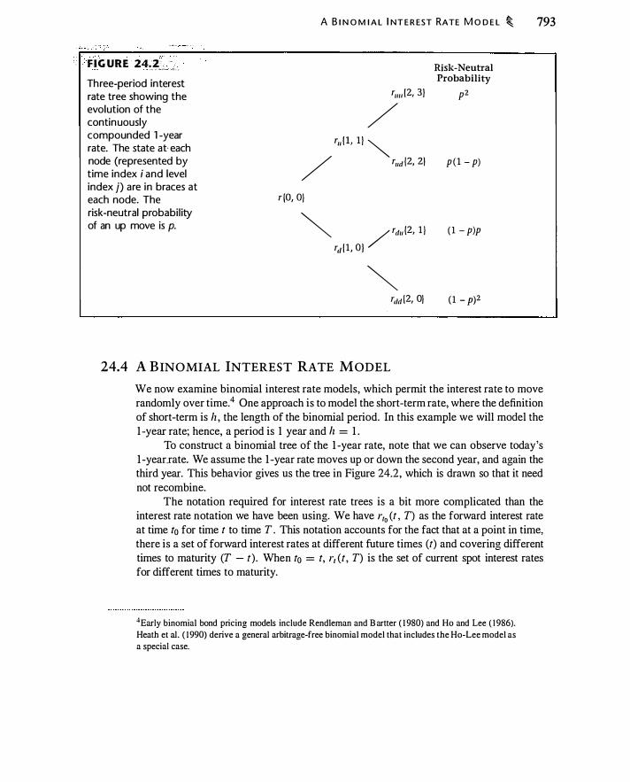
FIGURE 244�" "c . .

Three-period interest rate tree showing the evolution of the continuously compounded 1 -year rate. The state at each node (represented by time index i and level index j) are in braces at each node. The risk-neutral probabi l ity of an up move is p.

A B I N O M I A L I NT E R EST RATE M O D E L �

r1111 (2, 3 }

/ T11 ( 1, 1 } �

/ r11d (2, 2}

r {O, 0}

� / rd11 (2, 1 }

r,t f 1 , 0 }

� rt/d (2, 0}

Risk-Neutral Probability

p1

p (1 - p)

( 1 - p)p

( 1 - p)1

24.4 A BINOMIAL INTEREST RATE MODEL

793

We now examine binomial interest rate models, which permit the interest rate to move randomly over time.4 One approach is to model the short-term rate, where the definition of short-term is h , the length of the binomial period. In this example we will model the 1 -year rate; hence, a period is 1 year and lz = 1 .

To construct a binomial tree of the 1 -year rate, note that we can observe today's 1 -year.rate. We assume the 1 -year rate moves up or down the second year, and again the third year. This behavior gives us the tree in Figure 24.2, which is drawn so that it need not recombine.

The notation required for interest rate trees is a bit more complicated than the interest rate notation we have been using. We have r10 (t , T) as the forward interest rate at time to for time t to time T . This notation accounts for the fact that at a point in time, there is a set of forward interest rates at different future times (t) and covering different times to maturity (T - t). When to = t, r1 (t, T) is the set of current spot interest rates for different times to maturity.

4Early binomial bond pricing models include Rendleman and B artter ( 1 980) and Ho and Lee ( 1 986).

Heath et al. ( 1 990) derive a general arbitrage-free binomial model that includes the Ho-Lee model as a special case.

794 � I NT E R EST RATE M O D E LS

When we have a binomial tree as in Figure 24.2, at each node we have a large set of spot interest rates for different maturities, as well as forward rates. Thus, we need to expand the notation to identify the node under discussion. We will let r10 (t , T; j ) represent the interest rate prevailing from t to T , where the rate i s quoted a t time to < t and the state is j . Since to tells us the binomial period at which the rate is quoted, you can think of j as telling us the height along the tree at time to . Similarly, at any point in time t0 , there is a set of both spot and implied forward zero-coupon bond prices, P10 (t , T ; j ) .

Using this notation, the one-period rate at the i th time and level j i s ri (i , i + 1 ; j ) .5

In Figure 24.2 the initial one-period rate is r0 (0, 1 ; 0) and the rate rd11 , for example, is r2 (2, 3 ; 1 ) . The timing is such that the final nodes represent one-period rates observed two periods from today. Thus, the tree in Figure 24.2 can price bonds up to 3 years in maturity. Let p denote the risk-neutral probability of an up move. We will assume that rates are continuously compounded in this example.

Zero-Coupon Bond Prices

At time 0 we can determine a bond price on the binomial tree in much the same way we determined option prices in a binomial stock-price tree. The one-period bond price at any time is determined by discounting at the current one-period rate, which is given at each node:

Pi (i , i + 1 ; j) = e-r, U. i+ J ; j)lz (24.38)

We can value a two-period bond by discounting the expected one-period bond price, one period hence. At any node we can value an n-period zero-coupon bond by proceeding in this way recursively. Beginning in period i + n, we value one-period bonds, then in period i + n - 1 we have two-period bond values, and so forth.

Because the tree can be used at any node to value zero-coupon bonds of any maturity (up to the remaining size of the tree), the tree also generates implied forward interest rates of all maturities and volatilities of implied forward rates. Thus, we can equivalently specify a binomial interest rate tree in terms of interest rates, zero-coupon bond prices, or volatilities of implied forward interest rates.6

5 Any interest rate is reached by one (or more, if the tree is recombining) combination of up and down movements. One convenient way to characterize a node is by numbering the nodes at a given point in time, beginning with 0 at the bottom node. If we are at node j in period i , then we can move to either node 2 x j or 2 x j + I in period i + I. For example, if we are at node I in period I, then we can move to node 2 (2 x I) or 3 (2 x I + I ) in period 2. It is also possible to use this scheme to assign to each node the number 2; + j. Thus, the [0, 0} node is numbered I (2° + 0), the [ I , 0} node is numbered 2 (2 1 + 0), and so on. In effect this uses a binary representation to number the nodes. This scheme is suggested in Rendleman (2002). 6The central role of volatility in a term structure model is emphasized by Heath et al. ( 1 990) and Heath et al. ( 1 992). Their model is discussed in Appendix 24.A.

·

A B I N O M I A L I NT E R EST RAT E M O D E L � 795

Using the tree in Figure 24.2, we obtain the following valuation equations. For the one-period bond we have

Po (O, l ; 0) = e-rh (24.39)

The two-year bond is priced by working backward along the tree. In the second period, the price of the bond is $ 1 . One year from today, the bond will have the price e-r .. with probability p or e-r,, with probability I - p. The price of the bond is therefore

Po (O, 2; 0) = e-rh [pe-r"" + ( I - p)e-r"" ] = e-rh [p P1 ( 1 , 2; 1 ) + ( I - p) P1 ( 1 , 2; 0)] .

(24.40)

(24.4 1 )

Thus, we can price the 2-year bond using either the interest rate tree o r the implied bond prices.

Finally, the 3-year bond is again priced by traversing the entire tree. The price is $ 1 after 3 years. After 2 years, the price will be $ 1 discounted at r11 11 , r11d , rd1, or rdd · Continuing in this way, the price is

Po(O, 3 ; 0) = e-r [pe-r" (pe-r"" + ( 1 - p)e-r"" )

+ ( 1 _ p)e-r" (pe-r"" + ( I _ p)e-r"" ) ] (24.42)

The 3-year bond calculation can be written differently. By collecting terms in equation (24.42), we can rewrite it as

Po (O, 3 ; 0) = p2e-(r+r.,+r.,., ) + p ( l _ p)e-<r+r.,+ruJl

+ (1 _ p)pe-<r+rJ+rJ,. ) + ( 1 _ p)2e-<r+rJ+TJJ) (24.43)

This version of equation (24.42) makes clear that we can value the bond by considering separately each path the interest rate can take. Each path implies a realized discount factor. We then compute the expected discount factor, using risk-neutral probabilities. Denoting this expectation as E* , the value of the zero-coupon bond is

More generally, letting ri represent the time-i rate, we have

(24.44)

All bond valuation models implicitly calculate equation (24.44) .

Example 24. 3 Figure 24.2 constructs an interest rate tree assuming that the current 1 -year rate is 1 0% and that each year the 1 -year rate moves up or down 4%, with prob­ability p = 0.5 . We can use this tree to price 1 -, 2-, and 3-year zero-coupon default-free bonds.

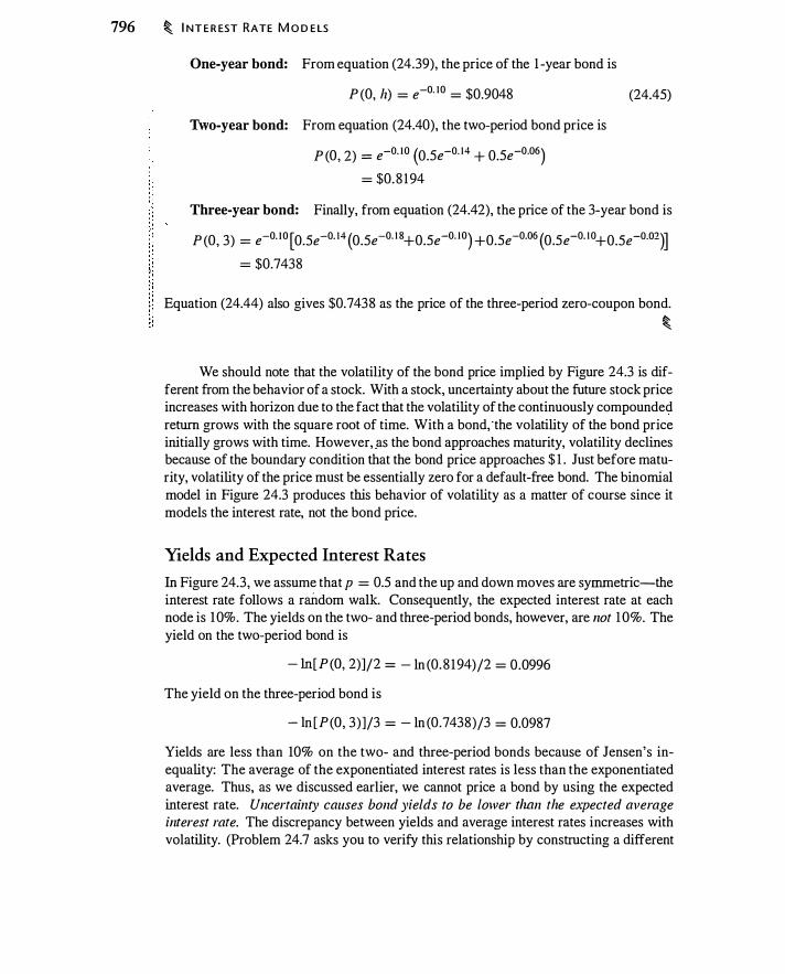
796 � I NT E R EST RATE M O D E LS

One-year bond: From equation (24.39), the price of the 1 -year bond is

P (O, h) = e-0· 1 0 = $0.9048

1\vo-year bond: From equation (24.40), the two-period bond price is

P (O, 2) = e-o.w (0.5e-0· 14 + 0.5e-0·06) = $0. 8 1 94

(24.45)

Three-year bond: Finally, from equation (24.42), the price of the 3-year bond is

P (O, 3) = e-0. 1 0 [0.5e-0. 14 (0.5e-0. 1 8+0.5e-O. IO) +0.5e-0.06 (0.5e-0. 1 0+0.5e-0.02)] = $0.7438

Equation (24.44) also gives $0.7438 as the price of the three-period zero-coupon bond. �

We should note that the volatility of the bond price implied by Figure 24.3 is dif­ferent from the behavior of a stock. With a stock, uncertainty about the future stock price increases with horizon due to the fact that the volatility of the continuously compounded return grows with the square root of time. With a bond, the volatility of the bond price initially grows with time. However, _as the bond approaches maturity, volatility declines because of the boundary condition that the bond price approaches $ 1 . Just before matu­rity, volatility of the price must be essentially zero for a default-free bond. The binomial model in Figure 24.3 produces this behavior of volatility as a matter of course since it models the interest rate, not the bond price.

Yields and Expected Interest Rates

In Figure 24.3, we assume that p = 0.5 and the up and down moves are symmetric-the interest rate follows a random walk. Consequently, the expected interest rate at each node is 10%. The yields on the two- and three-period bonds, however, are not 10% . The yield on the two-period bond is

- ln[ P (O, 2)]/2 = - ln (0. 8 1 94)/2 = 0.0996

The yield on the three-period bond is

- ln [P (O, 3) ]/3 = - ln (0.7438)/3 = 0.0987

Yields are less than 10% on the two- and three-period bonds because of Jensen's in­equality: The average of the exponentiated interest rates is less than the exponentiated average. Thus, as we discussed earlier, we cannot price a bond by using the expected interest rate. Uncertainty causes bond yields to be lower than the expected average interest rate. The discrepancy between yields and average interest rates increases with volatility. (Problem 24.7 asks you to verify this relationship by constructing a different

. •. .. . .

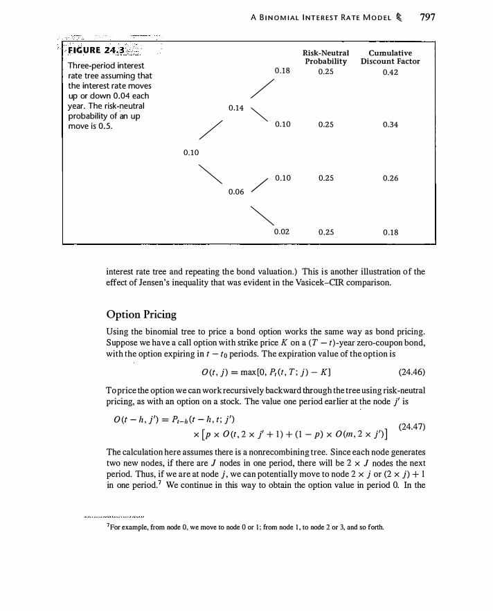
I=IGU RE 24�l:Lc.:

Three-period interest rate tree assuming that the interest rate moves up or down 0.04 each year. The risk-neutra l probabil ity of im up move is 0.5 .

0.14

/ 0.10

� 0.06

A B I N O M I A L I NT E R EST RATE M O D E L � 797

0 .18

/ �

0. 1 0

/ 0 . 1 0

� 0.02

Risk-Neutral Cumulative Probability Discount Factor

0.25 0.42

0.25 0.34

0.25 0.26

0 .25 0 . 1 8

interest rate tree and repeating the bond valuation.) This i s another illustration of the effect of Jensen's inequality that was evident in the Vasicek-CIR comparison.

Option Pricing

Using the binomial tree to price a bond option works the same way as bond pricing. Suppose we have a call option with strike price K on a (T - t) -year zero-coupon bond, with the option expiring in t - to periods. The expiration value of the option is

O (t , j) = max [O, P1 (t , T ; j ) - K] (24.46)

To price the option we can work recursively backward through the tree using risk-neutral pricing, as with an option on a stock. The value one period earlier at the node j' is

O (t - h , j') = P1-�z (t - lz , t ; j') x [P x O (t , 2 x j' + 1 ) + ( 1 - p) x O (m, 2 x j')]

(24.47)

The calculation here assumes there is a nonrecombining tree. Since each node generates two new nodes, if there are J nodes in one period, there will be 2 x J nodes the next period. Thus, if we are at node j , we can potentially move to node 2 x j or (2 x j) + 1 in one period.7 We continue in this way to obtain the option value in period 0. In the

7 For example, from node 0, we move to node 0 or I ; from node I , to node 2 or 3, and so forth.

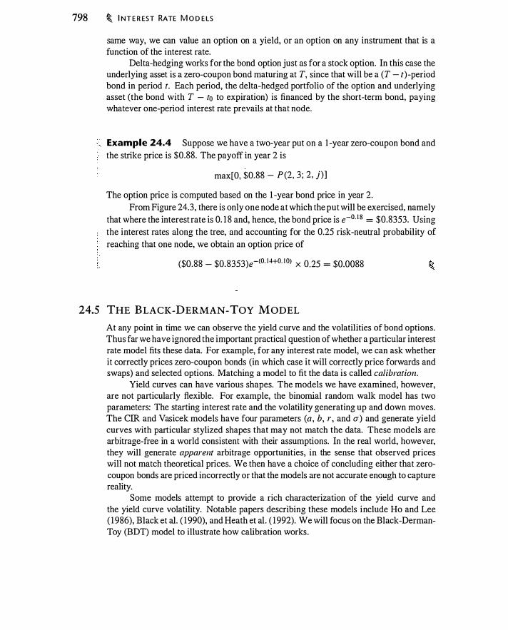
798 � I NT E R EST RATE M O D E LS

same way, we can value an option on a yield, or an option on any instrument that is a function of the interest rate.

Delta-hedging works for the bond option just as for a stock option. In this case the underlying asset is a zero-coupon bond maturing at T, since that will be a (T - f)-period bond in period t. Each period, the delta-hedged portfolio of the option and underlying asset (the bond with T - to to expiration) is financed by the short-term bond, paying whatever one-period interest rate prevails at that node.

Example 24.4 Suppose we have a two-year put on a 1 -year zero-coupon bond and the strike price is $0.88. The payoff in year 2 is

max[O, $0.88 - P (2, 3 ; 2, j)]

The option price is computed based on the 1 -year bond price in year 2. From Figure 24.3, there is only one node at which the put will be exercised, namely

that where the interest rate is 0. 1 8 and, hence, the bond price is e-0• 1 8 = $0.8353. Using the interest rates along the tree, and accounting for the 0.25 risk-neutral probability of reaching that one node, we obtain an option price of

($0.88 - $0.8353)e-<0· 14+0. IO) x 0.25 = $0.0088

24.5 THE BLACK-DERMAN-TOY MODEL

At any point in time we can observe the yield curve and the volatilities of bond options. Thus far we have ignored the important practical question of whether a particular interest rate model fits these data. For example, for any interest rate model, we can ask whether it correctly prices zero-coupon bonds (in which case it will correctly price forwards and swaps) and selected options. Matching a model to fit the data is called calibration.

Yield curves can have various shapes. The models we have examined, however, are not particularly flexible. For example, the binomial random walk model has two parameters: The starting interest rate and the volatility generating up and down moves. The CIR and Vasicek models have four parameters (a , b, r , and cr) and generate yield curves with particular stylized shapes that may not match the data. These models are arbitrage-free in a world consistent with their assumptions. In the real world, however, they will generate apparent arbitrage opportunities, in the sense that observed prices will not match theoretical prices. We then have a choice of concluding either that zero­coupon bonds are priced incorrectly or that the models are not accurate enough to capture reality.

Some models attempt to provide a rich characterization of the yield curve and the yield curve volatility. Notable papers describing these models include Ho and Lee ( 1 986), Black et al. ( 1 990), and Heath et al . ( 1 992). We will focus on the Black-Derman­Toy (BDT) model to illustrate how calibration works.

TABLE 24:2 - - --

Maturity (years)

1

2

3

4

T H E B LA C K- D E R M A N -TOY M O D E L � 799

Hypothetical bond-market data. Bond prices and yields are the observed prices and effective annual yields for zero-coupon bonds with the indicated maturity. Volatil ity refers to the volati l ity of the bond price 1 year from today.

Yield to Bond Volatility in Maturity Price ($) Year l

1 0% 0.909 1 N/A

1 1 % 0.8 1 1 6 1 0%

12% 0.7 1 1 8 15%

1 2.5% 0.6243 14%

The basic idea of the Black-Derman-Toy model is to compute a binomial tree of short-term interest rates, with a flexible enough structure to match the data. We will begin with sample data and demonstrate that a particular tree matches these data. We will then explain how to construct the tree. We assume in this discussion that the length of a binomial period is 1 year, although that is arbitrary.

Table 24.2 lists market information about bonds that we would like to match. We follow the Black-Derman-Toy paper in using effective annual yields rather than continuously compounded yields. Since the table contains prices of zero-coupon bonds, we can infer the term structure of implied forward interest rates. There is also information about the volatility of interest rates. The column headed "Volatility in Year 1 " is the standard deviation of the natural log of the yield for that bond 1 year hence. (We could, if we wished, convert this into a standard deviation of the bond price in a year.) The volatility for the n-year bond tells us the uncertainty about the year- 1 yield on an (11 - I ) ­year bond. The volatility in year 1 of the 2-year bond i s 1 0% ; this tells us that the 1 -year yield in year 1 will have a 10% volatility. Similarly, the volatility in year 1 of the 4-year bond (which will be a 3-year bond in year 1 ) is 14%. While the tree matches observed yields and volatilities, it makes no attempt to capture the evolution of the yield curve over time. The yield curve evolution is of course implicit in the tree, but the tree is not calibrated with this in mind.

The BDT approach provides enough flexibility to match this data. Black, Derman, and Toy describe their tree as driven by the short-term rate, which they assume is log­normally distributed. The general structure of the resulting tree is illustrated in Figure 24.4. We assume that the risk-neutral probability of an up move in the interest rate is 50%.

For each period in the tree there are two parameters. Ri/, can be thought of as a rate level parameter at a given time and a ; as a volatility parameter. These parameters can be used to match the tree with the data. In an ordinary lognormal stock-price tree,

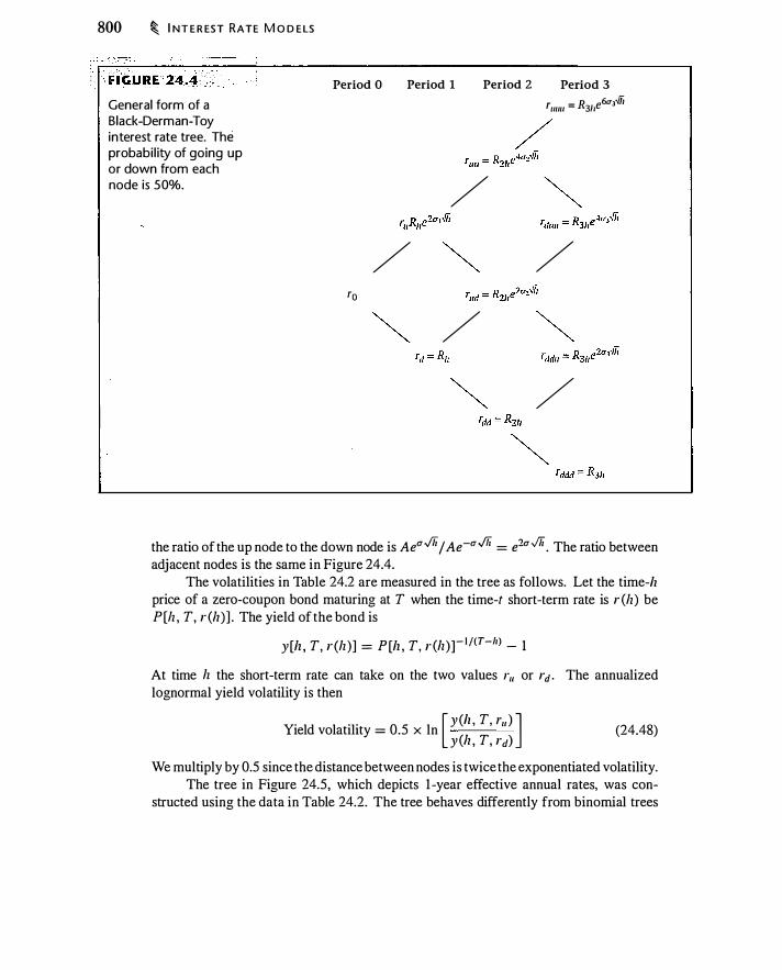
800 � I NT E R EST RATE M O D E LS

: _ FlGURE 24�.1-b.�: -� General form of a Black-Derman-Toy interest rate tree. The

probabi l ity of going up or down from each node is 50%.

Period 0 Period 1 Period 2

/ /

ro

/

Period 3 r""" = R311e6u,,n,

/

/

the ratio of the up node to the down node is Aea..fii j Ae-a..fii = e2a../ii. The ratio between adjacent nodes is the same in Figure 24.4.

The volatilities in Table 24.2 are measured in the tree as follows. Let the time-/z price of a zero-coupon bond maturing at T when the time-t short-term rate is r (h) be P [h , T, r (h)] . The yield of the bond is

y[h , T, r(lz)] = P [h , T, r (h)r l/(T-h) - 1

At time lz the short-term rate can take on the two values r11 or rd . The annualized lognormal yield volatility is then

[ y(/z , T, 1"11 ) ] Yield volatility = 0.5 x ln y(h , T, rd)

(24.48)

We multiply by 0.5 since the distance between nodes is twice the exponentiated volatility. The tree in Figure 24.5, which depicts 1 -year effective annual rates, was con­

structed using the data in Table 24.2. The tree behaves differently from binomial trees

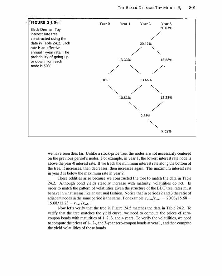
F IGURE 24. 5 .. · .. · ··•

Black-Derman-Toy interest rate tree constructed using the data in Table 24.2. Each rate is an effective annual 1 -year rate. The probabil ity of going up or down from each node is 50%.

Year 0

10%

TH E B LA C K- D E R M A N -TOY M O D E L � 801

Year 1

13 .22%

10.82%

Year 2 Year 3 20.03%

/ 20. 1 7%

/ 1 5 . 68%

13 .66%

/ 12.28%

/ 9.25%

9 . 62%

we have seen thus far. Unlike a stock-price tree, the nodes are not necessarily centered on the previous period's nodes. For example, in year 1 , the lowest interest rate node is above the year-0 interest rate. If we track the minimum interest rate along the bottom of the tree, it increases, then decreases, then increases again. The maximum interest rate in year 3 is below the maximum rate in year 2.

These oddities arise because we constructed the tree to match the data in Table 24.2. Although bond yields steadily increase with maturity, volatilities do not. In order to match the pattern of volatilities given the structure of the BDT tree, rates must behave in what seems like an unusual fashion. Notice that in periods 2 and 3 the ratio of adjacent nodes in the same period is the same. For example, 1"111111 I rd1111 = 20.03 I 15 .68 =

15 .681 1 2.28 = l"duu l �"ddu ·

Now let's verify that the tree in Figure 24.5 matches the data in Table 24.2. To verify that the tree matches the yield curve, we need to compute the prices of zero­coupon bonds with maturities of 1 , 2, 3, and 4 years . To verify the volatilities, we need to compute the prices of 1 -, 2-, and 3-year zero-coupon bonds at year 1 , and then compute the yield volatilities of those bonds.

802 � I NT E R EST RATE M O D E LS

' �2C . · . · .. ·.·. · · · · · ·· ·· • · •· FIGU RE 24,�� ::.2::::..

Tree of 1 -year bond prices impl ied by the tree in Figure 24.5 . The price at each node is 1 /(1 + r), where r is the rate at the corresponding node in that figure.

Verifying Yields

Year O Year 1

$0.8832

/ $0.909 1

$0.9023

Year 2 Year 3 $0.83 3 1

/ $0.8321

/ � $0.8644

/ $0.8798

/ $0.8906

/ $0.9153

$0.9 123

The rate at the first node is 10%, which corresponds to the current 1 -year yield. We can compute the price (and thus yield) of the 2-year zero-coupon bond by

starting in year 2 and working backward. It is slightly more convenient to use the tree of 1 -year bond prices in Figure 24.6. In year 1, the 2-year bond will be worth either $0.8832 (a yield of 13 .22%) or $0.9023 (a yield of 10.82%). Thus, the discounted expected price at time 0 is

$0.909 1 X (0.5 X $0.8832 + 0.5 X $0.9023) = $0.8 1 16

Figure 24.7 illustrates the tree corresponding to this calculation. The price of the 3-year zero is computed in a similar way. Working backwards

from the year-3 nodes we have

$0.909 1 X [0.5 X $0.8832 X (0.5 X $0.832 1 + 0.5 X $0.8798)

+ 0.5 X $0.9023 X (0.5 X $0.8798 + 0.5 x . $0.9 1 53)] = $0.7 1 1 8

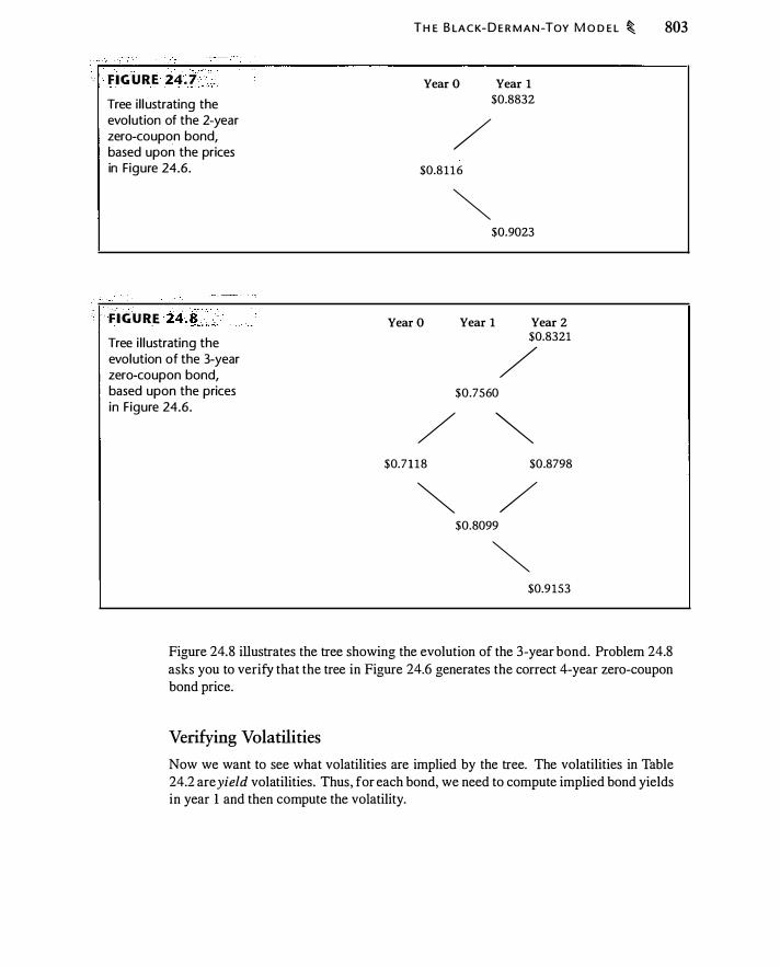
... F IGURE 24 . 7 Tree i l l ustrating the evolution of the 2-year zero-coupon bond, based upon the prices in F igure 24.6 .

·.· . . FIGU RE 24JE;=-­Tree i l lustrating the evolution of the 3-year zero-coupon bond, based upon the prices in F igure 24.6 .

T H E B LA C K- D E R M A N -TOY M O D E L � 803

Year O Year 1 $0.8832

/ $0.8116

� $0.9023

Year O Year 1 Year 2 $0.8321

/ $0.7560

/ � $0.7118 $0.8798

� / $0.8099

� $0.9 153

Figure 24.8 illustrates the tree showing the evolution of the 3-year bond. Problem 24.8 asks you to verify that the tree in Figure 24.6 generates the correct 4-year zero-coupon bond price.

Verifying Volatilities

Now we want to see what volatilities are implied by the tree. The volatilities in Table 24.2 are yield volatilities. Thus, for each bond, we need to compute implied bond yields in year l and then compute the volatility.

804 � I NT E R EST RATE M O D E LS

For the 2-year bond ( 1 -year bond in year 1 ) , the yield volatility using equation (24.48) is ( 0.8832- 1 - 1 )

0.5 x ln 0_9023_ 1 _ 1

= 0. 1

From Figure 24.8, the 3-year bond in year 1 (which will be a 2-year bond) will be worth either $0.7560, with a yield of 0.7560- 1 12 - 1 = 0. 1501 or 0.8099- 1 12 - 1 = 0. 1 1 1 2. The yield volatility is then

0.5 x ln -- = 0. 15 (0 . 1 5 0 1 )

0. 1 1 1 2

Both yields match the inputs in Table· 24.2. Problem 24.9 asks you to verify that the tree generates the correct 4-year yield

volatility.

Constructing a Black-Derman-Toy Tree

We have verified that the tree in Figure 24.5 is consistent with the data in Table 24.2. Now we turn the question around: Given the data, how did we generate the tree in the first place? The answer is that we started at early nodes and worked to the later nodes, building the tree outward.

The first node is given by the prevailing 1 -year rate. Therefore the 1 -year bond price is

Thus, Ro = 0. 10.

$0.909 1 = -1

-1 + Ro

(24.49)

For the second node, the year- 1 price of a 1 -year bond is P ( 1 , 2, r11 ) or P ( 1 , 2, rd) .

We require that two conditions be satisfied:

1 $0.8 1 1 6 = [0.5 x P ( l , 2, r11 ) + 0.5 X P ( 1 , 2, rd ) ]

1 + 0. 1 0

= 0.5 X + 0.5 X --1 ( 1 1 )

1 + 0. 1 0 1 + R 1 e2a 1 1 + R t

0. 1 0 = 0.5 X ln ( [P ( 1 , 2, r11 )- 1 - 1 ]/ [P ( 1 , 2, rd) - 1- 1 ])

= 0.5 X ln (R , e2a / R J )

(24 .50)

(24.5 1 )

The second equation gives u s a = 0. 1 and this value enables u s to solve the first equation to obtain R 1 = 0 . 1082 .

It is a bit messier to solve for the next set of conditions, but conceptually we are still fitting two parameters (R2 and a2) to match two inputs (the 3-year yield and the 2-year yield volatility 1 year hence) . The possible prices of a 2-year bond at the two

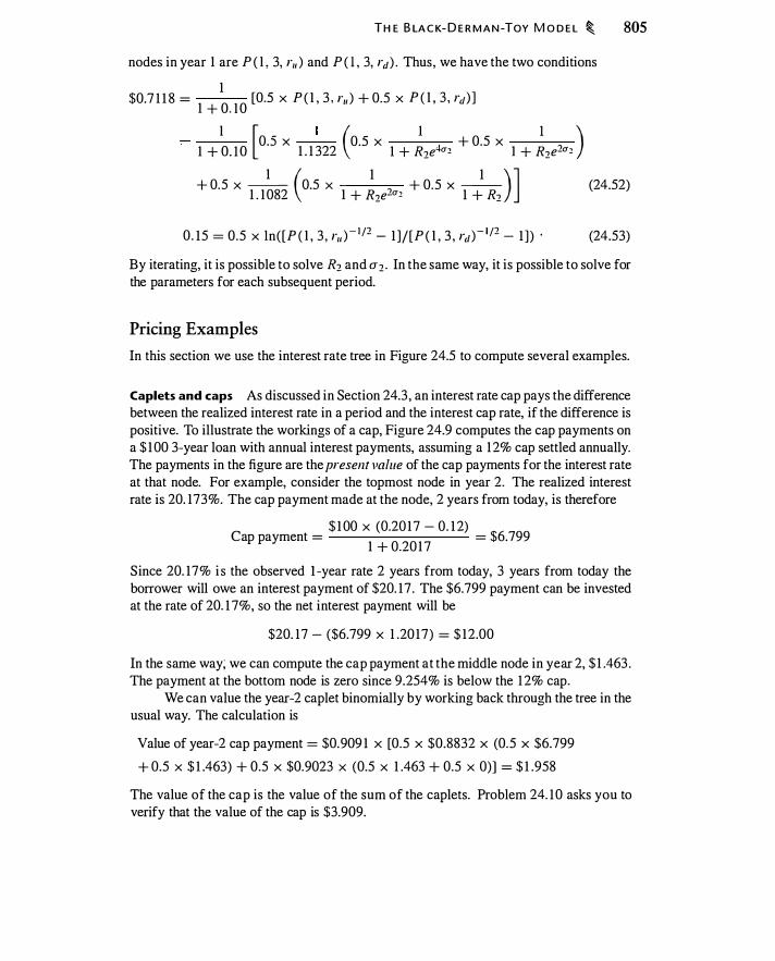
TH E B LA C K- D E R M A N -TOY M O D E L � 805

nodes in year 1 are P ( l , 3, r11 ) and P ( l , 3, rd) . Thus, we have the two conditions

1 $0.7 1 1 8 =

1 + O. l O [0.5 X P ( l , 3 , r11 ) + 0.5 X P ( l , 3 , rd) ]

l [0.5 X _I_ (0.5 x I 4 + 0.5 X l )

1 + O. I O 1 . 1 322 1 + R2e u, I + R2e2u,

+ 0.5 X -- 0.5 X + 0.5 X --

1 ( 1 1 ) ] 1 . 1 082 1 + R2e2u, 1 + R2

0 . 15 = 0 .5 X ln( [P ( l , 3 , r11 ) - 1 12 - 1 ] / [P ( l , 3 , rtl)- ! 12 - 1 ] ) ·

(24.52)

(24.53)

By iterating, it is possible to solve R2 and u2 • In the same way, it is possible to solve for the parameters for each subsequent period.

Pricing Examples

In this section we use the interest rate tree in Figure 24.5 to compute several examples.

Caplets and caps As discussed in Section 24.3 , an interest rate cap pays the difference between the realized interest rate in a period and the interest cap rate, if the difference is positive. To illustrate the workings of a cap, Figure 24.9 computes the cap payments on a $ 1 00 3-year loan with annual interest payments, assuming a 1 2% cap settled annually. The payments in the figure are the present value of the cap payments for the interest rate at that node. For example, consider the topmost node in year 2. The realized interest rate is 20. 173%. The cap payment made at the node, 2 years from today, is therefore

$ 1 00 X (0.20 17 - 0. 1 2) Cap payment = = $6.799

1 + 0.20 17

Since 20. 17% i s the observed ! -year rate 2 years from today, 3 years from today the borrower will owe an interest payment of $20. 17 . The $6.799 payment can be invested at the rate of 20. 1 7%, so the net interest payment will be

$20. 17 - ($6.799 X 1 .20 17) = $ 12.00

In the same way; we can compute the cap payment at the middle node in year 2, $ 1 .463 . The payment at the bottom node is zero since 9.254% is below the I 2% cap.

We can value the year-2 caplet binomially by working back through the tree in the usual way. The calculation is

Value of year-2 cap payment = $0.909 1 x [0.5 x $0.8832 x (0.5 x $6.799

+ 0.5 X $ 1 .463) + 0.5 X $0.9023 X (0.5 X 1 .463 + 0.5 X 0)) = $ 1 .958

The value of the cap is the value of the sum of the caplets. Problem 24. I 0 asks you to verify that the value of the cap is $3.909.

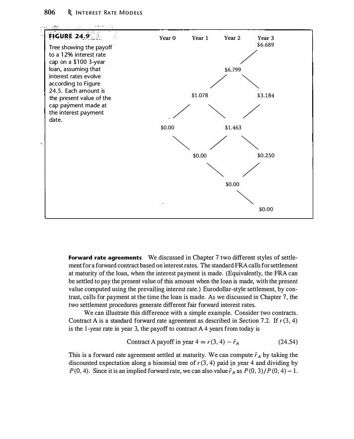
806 � I NT E R EST RATE M O D E LS

F I G U R E 24. 9

Tree showing the payoff to a 1 2% interest rate cap on a $ 1 00 3-year loan, assuming that interest rates evolve according to Figure 24.5 . Each amount is the present value of the cap payment made at the interest payment date.

Year O

/ $0.00

�

Year 1 Year 2 Year 3 $ 6 .689

/ $6.799

/ � $ 1 .078 $ 3 . 1 84

� / $ 1 .463

/ � $0.00 $0.250

� / $0.00

� $0.00

Forward rate agreements We discussed in Chapter 7 two different styles of settle­ment for a forward contract based on interest rates. The standard FRA calls for settlement at maturity of the loan, when the interest payment is made. (Equivalently, the FRA can be settled to pay the present value of this amount when the loan is made, with the present value computed using the prevailing interest rate.) Eurodollar-style settlement, by con­trast, calls for payment at the time the loan is made. As we discussed in Chapter 7, the two settlement procedures generate different fair forward interest rates.

We can illustrate this difference with a simple example. Consider two contracts . Contract A is a standard forward rate agreement as described in Section 7.2. If r (3 , 4) is the 1 -year rate in year 3, the payoff to contract A 4 years from today is

Contract A payoff in year 4 = r (3 , 4) - rA (24.54)

This is a forward rate agreement settled at maturity. We can compute rA by taking the discounted expectation along a binomial tree of r (3 , 4) paid in year 4 and dividing by P (O, 4) . Since it is an implied forward rate, we can also value TA as P (O, 3)/ P (O, 4) - 1 .

TH E B LA C K- D E R M A N -TOY M O D E L � 807

Contract B is a forward agreement that settles on the borrowing date in year 3 :

Contract B payoff in year 3 = r (3 , 4 ) - i'8 (24.55)

This second contract resembles a Eurodollar futures contract. There is no marking­to-market prior to settlement, which would occur with a real futures contract, but the timing of settlement is mismatched with the timing of interest payments . The correlation between the contract payment and the interest rate discussed above and in Section 7.2 is therefore present in contract B . We can compute i'8 by taking the discounted expectation along a binomial tree of r (3 , 4) paid in year 3, and dividing by P (O, 3) .

Example 24.5 We can value both contracts A and B using the interest rate tree in Figure 24.5. The rate on contractA is i'A = P (0, 3)/ P (0, 4) - 1 = 0.7 1 1 8/0.6243 - 1 = 0. 140 1 34.

Contract B can be valued as follows. Suppose the forward rate on B is r8 . In year 3, B makes the payment r (3 , 4) - i'8 . We can value on the tree the payment r (3 , 4) ; the time = 0 value of i'8 is simply i'8 x P (O, 3 ) . Figure 24. 10 depicts the payment for

.. F IGURE . 24. 1 Q; , Tree depicting value of a contract that pays the prevai l ing 1 -year interest rate 3 years from today. I nterest rates are from Figure 24.5 . If the contract value at any node is V(r), the amount at each node is [0.5

. x V(ru) + 0.5 x V(rd)]/(1 + r).

Year O

/ $ 10.03

�

Year 1 Year 2 Year 3 $20.03

/ $ 14.86

/ � $ 1 1 .99 $ 1 5 .68

� / $ 12.30

/ � $ 10.07 $ 1 2.28

� / $10.02

� $9 .62

808 � I NT E R EST RATE M O D E LS

a $ 1 00 notional amount. In the final period, we receive the prevailing 1 -year rate times $ 1 00. We then discount this payment back through the tree. The time-0 value is $ 1 0.03 . The implied rate is $ 10.03/ P (O, 3) = $ 10.03/$7 1 . 1 8 = 0. 1409.

Thus, Eurodollar-style settlement in year 3 raises the forward rate from 14.0 1 % to 1 1 ! i 14.09%. Problem 24. 1 1 asks you to verify using the binomial tree that rA = 14.0 1 34%. u �

CHAPTER SUMMARY

----- -- ··-"--· �"''� . o·c'·- '-:=;{

Derivatives that are functions of interest rates can be priced and hedged in the same way as options . . As with derivatives on stocks, prices of interest rate derivatives are characterized by a partial differential equation that is essentially the same as the Black­Scholes equation. The Vasicek and Cox-Ingersoll-Ross interest rate models are derived using this equation by assuming that the short-term interest rate follows particular means­reverting processes. These models generate theoretical yield curves but are too restrictive to match observed yield curves .

Under the assumption that the forward price for a bond is lognormally distributed, the Black model can be used to price bond and interest rate options, and therefore interest rate caps.

The Black-Derman-Toy tree is a binomial interest rate tree calibrated to match zero-coupon yields and a particular set of volatilities. This calibration ensures that it matches a set of observed market prices (for example the swap curve) but not necessarily the evolution of the yield curve. Valution of interest rate claims on a binomial interest rate tree is much like that on a stock-price tree.

FURTHER READING

Classic treatments of bond pricing with interest rate uncertainty are Vasicek ( 1 977) and Cox et al. ( 1985b). These are examples of so-called "affine" term structure models, discussed more generally in Duffie and Kan ( 1996) and Dai and Singleton (2000).

Binomial treatments include Rendleman and Bartter ( 1980), Ho and Lee ( 1986), and Black et al . ( 1 990). Heath et al. ( 1992) have been extremely influential insofar as they provide an equilibrium characterization of the evolution of forward rates. See also Brace et al. ( 1997) and Miltersen et al. ( 1 997). More in-depth treatments of interest rate derivatives can be found in Hull (2000, chs. 20-22), Rebonato ( 1 996), Jarrow ( 1996), and James and Webber (200 1) .

Litterman and Scheinkman ( 1 99 1 ) is a classic study of factors affecting bond returns. Bliss ( 1997) surveys this literature.

PROBLEMS

P RO B LE M S � 809

For the first three problems, use the following information :

Bond maturity (years)

Bond price

1-Year forward price volatility

0 .9259

2

0.8495

0. 1000

3

0.7722

0. 1 050

24.1. a. What is the 1 -year bond forward price in year 1 ?

4

0.7020

0. 1 100

b. What is the price of a call option that expires in 1 year; giving you the right to pay $0.9009 to buy a bond expiring in 1 year?

c. What is the price of an otherwise identical put?

d. What is the price of an interest rate caplet that provides an 1 1 % (effective annual rate) cap on 1 -year borrowing I year from now?

24.2. a. What is the 2-year forward price for a 1 -year bond?

b. What is the price of a call option that expires in 2 years, giving you the right to pay $0.90 to buy a bond expiring in 1 year?

c. What is the price of an otherwise identical put?

d. What is the price of a interest rate caplet that provides an 1 1 % (effective annual rate) cap on 1 -year borrowing 2 years from now?

24.3. What is the price of a 3-year interest rate cap with an 1 1 .5% (effective annual) cap rate?

24.4. Suppose the yield curve is flat at 8%. Consider 3- and 6-year zero-coupon bonds. You buy one 3-year bond and sell an appropriate quantity of the 6-year bond to duration-hedge the position. Any additional investment is in short-term

· (zero-duration) bonds. Suppose the yield curve can move up to 8.25% or down to 7.75% over the course of 1 day. Do you make or lose money on the hedge? What does the result tell you about the (impossible) flat-yield curve model discussed in Section 24. 1 ?

24.5. Suppose the yield curve is flat at 6%. Consider a 4-year 5%�coupon bond and an 8-year 7%-coupon bond. All coupons are annual.

a. What are the prices and durations of both bonds?

b. Consider buying one 4-year bond and duration-hedging by selling an appropriate quantity of the 8-year bond. Any residual is financed with short-term (zero-duration) bonds. Suppose the yield curve can move up to 6.25% or down to 5 .75% over the course of 1 day. What are the results from the hedge?

810 � I NT E R EST RATE M O D E LS

24.6. Consider two zero-coupon bonds with 2 years and 10 years to maturity. Let a = 0.2, b = 0. 1 , r = 0.05, u \'asicek = 10%, and U cf R = 44.72 1 %. The interest rate risk premium is zero in each case. We will consider a position consisting of one $ 1 00 par value 2-year bond, which we will hedge with a position in the 10-year bond.

a. Compute the prices, deltas, and gammas of the bonds using the CIR and Vasicek models. How do delta and gamma compare to duration and convexity?

b. Suppose the Vasicek model is true. You wish to hedge the 2-year bond using the 1 0-year bond. Consider a 1 -day holding period and suppose the interest rate moves one standard deviation up or down. What is the return on the duration-hedged position? What is the return on the Vasicek delta-hedged position?

c. Repeat the previous part, only use the CIR model in place of the Vasicek model.

24.7. Construct a 4-period, 3-step (8 terminal node) binomial interest rate tree where the initial interest rate is 1 0% and rates can move up or down by 2%; model your tree after that in Figure 24.3 . Compute prices and yields for 1- , 2-, 3-, and 4-year bonds. Do yields decline with maturity? Why?

24.8. Verify that the 4-year zero-coupon bond price generated by the tree in Figure 24.6 is $0.6243 .

24.9. Verify that the 1 -year yield volatility of the 4-year zero-coupon bond price gen­erated by the tree in Figure 24.6 is 0. 14.

24.10. Verify that the price of the 12% interest rate cap in Figure 24.9 is $3.909.

24.11. Using a binomial tree like that in Figure 24. 1 0, verify that the 1 -year forward rate 3 years hence in Figure 24.5 is 14.0 1 34%.

For the next four problems, here are two BDT interest rate trees with effective annual interest rates at each node.

0.08000 0.07676 0. 1 0362

Tree #1 0.08 170 0. 1 0635 0. 1 3843

0.07943 0.09953 0. 1 2473 0. 1 5630

0.07552 0.09084 0. 1 0927 0. 1 3 143 0. 15809

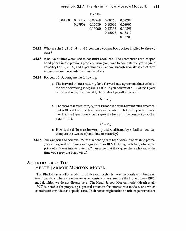
A P P E N D I X 24.A : TH E H EATH -j A R ROW-M O RTO N M O D E L � 811

Tree #2

0.08000 0.08 1 1 2 0.08749 0.08261 0.07284 0.09908 0 . 1 0689 0 . 1 0096 0.08907

0 . 1 3060 0. 1 2338 0. 1 089 1 0 . 1 5078 0. 133 1 7

0. 1 6283

24.12. What are the 1 -, 2-, 3-, 4-, and 5-year zero-coupon bond prices implied by the two trees?

24.13. What volatilities were used to construct each tree? (You computed zero-coupon bond prices in the previous problem; now you have to compute the year- 1 yield volatility for 1 -, 2-, 3-, and 4-year bonds.) Can you unambiguously say that rates in one tree are more volatile than the other?

24.14. For years 2-5, compute the following:

a. The forward interest rate, r1, for a forward rate agreement that settles at the time bmmwing is repaid. That is, if you borrow at t - 1 at the 1 -year rate r, and repay the loan at t , the contract payoff in year t is

b. The forward interest rate, re , for a Eurodollar-style forward rate agreement that settles at the time borrowing is initiated. That is, if you borrow at t - I at the 1 -year rate r, and repay the loan at t, the contract payoff in year t - 1 is

(r - re) c. How is the difference between r1 and re affected by volatility (you can

compare the two trees) and time to maturity?

24.15. You are going to borrow $250m at a floating rate for 5 years. You wish to protect yourself against borrowing rates greater than 10 .5%. Using each tree, what is the price of a 5-year interest rate cap? (Assume that the cap settle-s each year at the time you repay the borrowing.)

APPENDIX 24 .A : THE HEATH-}ARROW-MORTON MODEL

The Black-Derman-Toy model illustrates one particular way to construct a binomial tree from data. There are other ways to construct trees, such as the Ho and Lee ( 1 986) model, which we do not discuss here. The Heath-Jarrow-Morton model (Heath et al . , 1 992) is notable for proposing a general structure for interest rate models, one which contains other models as a special case. Their basic insight is that no-arbitrage restrictions

812 � I NT E R EST RAT E M O D E LS

require that the evolution of forward rates (or equivalently, forward bond prices) hinges in a specific way on bond price volatilities. When you adopt a specific volatility model, you implicitly adopt a specific model for the evolution of forward interest rates.

To understand the link between volatilities and forward rates, suppose the single­state variable is the short-term interest rate, r, and we have two zero-coupon bonds with prices P (t , T1 , r) and P (t , T2 , r) with T2 > T1 • The implied forward zero-coupon bond price between T1 and T2 is

F( T T ) _ _ P

_(t_, T:-

2_, ,_. ) t , ( , 2 - P (t , Tt , r) (24.56)

Under the risk-neutral distribution, all zero-coupon bond prices follow the equation

dP -p = rdt + q (t , T, r)dZ (24.57)

Using Ito's Lemma, this equation implies that the forward bond price follows the process

dF ? F = [q (t , Tt , r) - - q (t , Tt , r)q (t , T2 , r)]dt + [q (t , h r) - q (t , T1 , r)]dZ

We can do this same calculation for every possible forward bond price. In every case, only bond price volatilities affect the evolution of the fonvard cun1e.

We can use equation (24.57) to derive the process that must be followed by forward interest rates. If the forward bond price is F(t , T1 , T2) , then the implied forward interest rate is

Using Ito's Lemma to compute df, we obtain

df = _ 1 (dF _ � (dF)2 )

T2 - Tt F 2 F2 Hq (t , h r)2 - q (t , Tt , r)2] dt + q (t , Tt , r) - q (t , h r) dZ

T2 - Tt T2 - Tt

(24.58)

The intuition for the result that the forward rate process depends on volatilities is straight­forward. For all bonds, the risk-neutral expected return is the risk-free rate, and in a one-factor world, the prices of all bonds are perfectly correlated. The forward bond price, P (t, T2) j P (t, Tt ) , varies only because of the volatility differences for the two bonds . Thus, the process for the forward bond price, and, hence, the forward interest rate, depends only on volatilities. This approach is more general than Black-Derman­Toy since a model of the volatility process can potentially be calibrated to the evolution of the yield curve as well as a snapshot at a point in time.

J arrow ( 1996), Rebonato ( 1996), and James and Webber (200 1) discuss empirical implementation of the model, which entails assuming and calibrating a model for bond volatilities.

IJ

��� ' �-'---"�:Oc-_i:cc_cd:.�:t:2:= - --- - ---��----��- ---

v aiue at Risk

A sland>rrd way to "'""" risk is to evalute the distribution of pos�ble outcomes, with a focus on the worst that might happen. Insurance companies, for example, are in the business of assessing the likelihood of insured events, and the resulting possible losses for the insurer. Financial institutions must understand their portfolio risks in order to determine the capital needed to suppport their business .

In this chapter we use the framework and tools developed earlier in this book to understand this kind of risk assessment. Specifically, we discuss value at risk, which is a method frequently used to measure the possible losses on a portfolio of financial assets. Chapter 26 discusses the related problem of assessing credit risks.

25 . 1 VALUE AT RISK

A financial institution might have a complex portfolio containing stocks, bonds with different maturities and with various embedded options, and instruments denominated in different currencies. The form of these instruments could be simple notes or complex options. Value at risk (VaR) is one way to perform risk assessment for such a portfolio. The idea of value at risk is to estimate the losses on a portfolio that occur with a given probability.

With an estimate of the distribution of outcomes we can either ask about the probability of losing a given sum (e.g., what is the chance our loss exceeds $5m?) or ask, for a given probability, how much might we lose (what level of loss do we exceed with a I % probability)? For example, a derivatives market-maker could estimate that for a given portfolio there is a I % chance of losses in excess of $500,000. The amount $500,000 is then the 1 -day value at risk with a 99% level of confidence. 1 In general, computing value at risk means finding the value of a portfolio such that there is a specified probability that the portfolio will be worth at least this much over a given horizon. The choice of horizon and probability will depend on how VaR is to be used. Regulators have

1 In this example, the market-maker loses $500,000 with a I% probability and performs better 99% of the time. It is common to speak of 99% as the "confidence level." S ince VaR is always based upon tail probabilities, in practice it will be obvious that a "99% VaR" and a " I % VaR" refer to the same quantity.

813

814 � VA LU E AT R I S K

proposed assessing capital using the 99% 1 0-day VaR (see the box o n page 8 15 for more details). "Riskrnetrics" (see J. P. Morgan/Reuters ( 1 996)), developed by J. P. Morgan in the mid- 1990s, is one comprehensive proposal for a value at risk methodology. Much o� the discussion in this section, especially for bonds, follows the Riskrnetrics methodology.

Before we discuss how to compute value at risk, recognize that the ideas underlying risk assessment matter in contexts other than measuring the riskiness of bank portfolios. For example, suppose a firm has $ 1 Om in capital and can pursue one of two investment opportunities, each costing $ 1 0 million. One year, investment A returns $ 1 2 million for sure, whereas investment B returns $24 million with probability one-half and $0 with

,probability one-half. Suppose the risk of investment B is idiosyncratic and the risk-free rate is 1 0%. Standard investment theory will assess both projects as having the same positive NPV. However, with investment B, half of the time the firm will lose its entire investment and therefore all of its capital. In order to make additional investments, the firm must raise additional capital, a costly process. Once we account for the costs associated with losing all capital, A and B may no longer seem equally attractive. More generally, managers will want to know how much of a firm's capital is at risk with a given project. Risk assessment can therefore affect project selection.2

Distributions of outcomes matter at the personal level as well. Suppose you are planning for retirement. You will need to decide both how much to save and how to allocate your savings among stocks, bonds, and other assets . For any strategy, a key question is : What is the probability that by following this strategy you will fail to achieve a desired minimum level of retirement savings by the time you retire?3 This is not the only question to ask, but a strategy. with a high probability of leaving you penniless­no matter how desirable on other grounds-should call for careful consideration. We will not discuss personal financial planning in this chapter, but the ideas underlying risk assessment can be used in making personal decisions as well as corporate decisions.

There are at least three uses of value at risk. First, as mentioned, regulators can use VaR to compute capital requirements for financial institutions. Second, managers can use VaR as an input in making risk-taking and risk-management decisions. Third, managers can also use VaR to assess the quality of the bank's models. For example, if the models say that there is a 5% chance that a particular trading operation will lose $ 1 m over a 1 -day horizon, then on average once every 20 days (5% of the time) the trading operation should lose $ 1 m. If losses of this size occur more frequently, the models are assigning too little risk to the bank's activities. If such losses occur less frequently, the models are assigning too much risk.

Most of the examples in this section use lognormally distributed stocks and linear normal approximations to illustrate VaR calculations. Currencies and commodities can be modeled in this way as well. Although for long horizons it might not be reasonable

2See Stutz ( 1 996) for a detailed discussion of the link between investment decisions and risk assessment. 3Bodie and Crane ( 1 999) for example use Monte Carlo simulation to examine return distributions to assess the suitability of financial products for retirement savings.

VaR a n d Reg u l atory C a p i t a l

Regulators in most countries require that financial institutions maintain minimum levels of capital . The Basel Committee on Banking Supervision in 1996 outlined a framework for capital standards proposing that financial institutions use VaR in determining capital for market risks, defined as risk arising from stocks, commodities, interest rates, and foreign exchange. (Other categories of risk are credit risk and operational risk.) The proposal (Basel Committee on Banking Supervision, 1 996) stated the following:

Banks will have flexibility in de­vising the precise nature of their mod­els, but the following minimum stan­dards will apply for the purpose of calculating their capital charge. Indi­vidual banks or their supervisory au­thorities will have discretion to apply stricter standards.

(a) "Value-at-risk" must be com­puted on a daily basis .

(b) In calculating the value-at­risk, a 99th percentile, one-tailed con­fidence interval is to be used.

VA LU E AT R I S K � 815

(c) In calculating value-at -risk, an instantaneous price shock equivalent to a 1 0 day movement in prices is to be used, i .e. , the minimum "holding period" will be ten trading days . . . .

(d) The choice of historical ob­servation period (sample period) for calculating value-at-risk will be con­strained to a minimum length of one year . . . .

(f) No particular type of model is prescribed. So long as each model used captures all the material risks run by the bank, . . . banks will be free to use models based, for example, on variance-covariance matrices, histori­cal simulations, or Monte Carlo sim­ulations.

This approach to determining capital for market risks was reaffirmed in the 2004 revision of the Basel capital guidelines, known as Basel II.

to treat commodities as lognormally distributed, for short horizons this is generally a reasonable assumption. We ignore the possibility of jumps. We discuss bonds separately.

Value at Risk for One Stock

Suppose .1:11 is the dollar return on a portfolio over the horizon h , and f (x , h) is the distribution of returns. Define the value at risk of the portfolio as the return, x11 (c) , such that Prob(i11 ::::: x11 (c) ) = c. In other words, x11 (c) is the c quantile of the return distribution over the horizon h .

Value a t risk measures the loss that will occur with a given probability over a specified period of time. Notice that the definition of value at risk requires that we specify both a horizon, lz , and a probability, c.

Suppose a portfolio consists of a single stock and we wish to compute value at risk over the horizon lz. If the distribution of the stock price after lz periods, S11 , is lognormal,

816 � VA LU E AT R I S K

we have

(25 . 1 ) 11

As we saw in Chapter 1 8, if we pick a stock price S, , then the probability that the stock price will be below s, is

- ( ln (S, ) - ln(S0) - (a - 8 - 0.5a2)/z ) Prob(S, < S, ) = N IL a v iz

(25.2)

The complementary calculation is to compute the S, (c) corresponding to the prob­(lbility c. By the definition of S, (c) , we have

_ ( ln (S, (c) ) - ln (S0) - (a - 8 - 0.5a2)h ) e - N _ IL a v h (25 .3)

We can solve for s, (c) by using the inverse cumulative probability distribution, N- 1 • Applying this function to both sides of equation (25 .3), we have

_ 1 ln (S, (c) ) - ln(So) - (a - 8 - 0.5a2)h N (c) = JL (25 .4) a v iz

Solving for s, (c) gives

(25.5)

This expression should look familiar from Chapter 1 8 . In equation (25 .5), N- 1 (c) takes the place of a standard normal random variable.

Example 25.1 Suppose we own $3m worth of stock A, which has an expected return of 15% and a 30% volatility, and pays no dividend. Moreover, assume A is lognormally distributed. The value of the position in 1 week, V, is

V = $3m x e<O. l 5-0.5 x0.32 ) �+0.3�Z (25 .6)

where Z � N(O, 1 ) . Given this assumed stock price distribution, a 5% loss will occur i f Z satisfies

or

We have

$3m x e<0. 1 5-0.5 x0.32 )�+0.3�Z = 0.95 x $3m

ln (0.95) - (0. 15 - 0.5 x 0.32) b z = - = - 1 .28 15

0 . 3 X r;; y 52

NormSDist( - 1 .28 1 5) = 0. 1000

Thus, we expect that 1 0% of the time there will be a weekly loss in excess of 5%.

VA L U E AT R I S K � 817

With 95% probability, the value of the portfolio over a 1 -week horizon will exceed

$3m x e<O. I 5-0.5 x0.32 l f, +0.3�x (- L645) = $2.8072m

wher� N- 1 (0.05) = - 1 .645. In this case, we would say the 95% value at risk is $2.8072m - $3m = -$0. 1 928m. �

If the assumption of lognormality is valid and if the inputs are correct, a 1 -week loss of this magnitude occurs on average once every 20 weeks.

In practice it is common to simplify the VaR calculation by assuming a normal return rather than a lognormal return. Recall from Chapter 20 that the standard lognor­mal model is generated by assuming normal returns over very short horizons. We can therefore approximate the exact lognormal result with a normal approximation:

s, = So ( 1 + ah + zrr..fh) We could also further simplify by ignoring the mean:

s, = So ( I + zrr..fh) Both equations (25 .7) and (25 .8) become less reasonable as h grows.

(25 .7)

(25 .8)

Example 25.2 Using the same assumptions as in Example 25. 1 , equation (25 .7) gives

[ 0. 1 5 ( 0.3 )] $3m X 1 + S

l + .j52 X ( - 1 .645) = $2.8033m

VaR is therefore $2. 8033m - $3m = -$0. 1 966m. Ignoring the mean, equation (25 .8) gives ( 0.3 ) $3m x 1 + .J52 x (- 1 .645) = $2.7947m

VaR is $2.7947m - $3m = -$0.2053m.

Figure 25 . 1 compares the three models-lognormal, normal with mean, and nor­mal without mean--over horizons of one day to one year. As you would expect, the approximation ignoring the mean (equation 25.8) is less accurate over longer horizons. In practice the mean is often ignored for two reasons. First, as we saw in Chapter 1 8, means are hard to estimate precisely. Second, as we saw in Chapter 20, for short horizons the mean is less important than the diffusion term in an Ito process .

VaR for Two or More Stocks

When we consider a portfolio having two or more stocks, the distribution of the future portfolio value is the sum of lognormally distributed random variables and is therefore

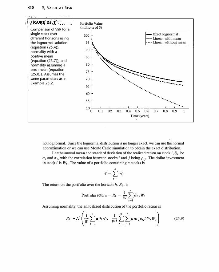
818 � VA LU E AT R I S K

Comparison of VaR for a s ingle stock over d ifferent horizons using the lognormal solution (equation (25 .4)), normality with a positive mean (equation (25 .7)), and normality assuming a zero mean (equation (25 .8)). Assumes the same parameters as in Example 25 .2.

Portfolio Value (millions of $)

100 - Exact lognormal = Linear, with mean

95 • • • • Linear, without mean

90

85

80

75

70

65

60

55

' '

��; \ .....

...... � ...

.......

.. ..

··. . . .

. . . . .

. . . .

· · . . .

.. . .

.. . . . .

. . . .

. . . .

"" -'� · ... .. "' . .

. . ..

.. ... ... . .

. .

5 0 �--�--�--�--�--�--�----�--�--�--�-0 0 . 1 0.2 0.3 0.4 0.5 0.6 0.7 0.8 0.9

Time (years)

1

not lognormal . Since the lognormal distribution is no longer exact, we can use the normal approximation or we can use Monte Carlo simulation to obtain the exact distribution.

Let the annual mean and standard deviation of the realized return on stock i, &; , be a; and u ; , with the correlation between stocks i and j being Pij · The dollar investment in stock i is W; . The value of a portfolio containing n stocks is

II

The return on the portfolio over the horizon h, R11 , is

l II Portfolio return = R11 =

W L ii;,!J W; i= l

Assuming normality, the annualized distribution of the portfolio return is

(25 .9)

VA LU E AT R I S K � 819

Example 25. 3 Suppose we have a1 = 0. 15 , a 1 = 0.3, W1 = $3m, a2 = 0. 1 8, a2 = 0.45, W2 = $5m, and p 1 ,2 = 0.4. The annual mean of the portfolio return is

w,a , + W2a2 $3m X 0. 1 5 + $5m X 0. 1 8 Clp = =

$ 3 $ = 0. 1 6875

W, + W2 m + 5m

The annual standard deviation of the portfolio return, a P ' i s

ap = Jw?ai + Wfa� + 2W, W2a r a2P 1 .2

Wr + W2

J($3m X 0 .3)2 + ($5m X 0.45)2 + (2 X $3m X $5m X 0.3 X 0.45 X 0.4) $3m + $5m

= 0.342 1 6

Using equation (25 .7), there i s a 95% probability that i n I week, the value o f the porfolio will exceed

$8m X [( 1 + (0 . 1 6875 X 5�) + (0.342 16 X .[[;_ X (- 1 .645)) ] = $7 .40 1 54m

The 1 -week 95% VaR is therefore $7.40 154m - $8m = -$0.5985m. Using equation (25 .8) , which ignores the mean, we have a 95% chance that the value of the portfolio will exceed

$8m X ( 1 + 0.342 1 6 X .[[;_ X ( - 1 .645)) = $7 .3756m

The 1 -week VaR ignoring the mean is therefore $7.3756m - $8m = -$0.6244m. �

This example illustrates the effects of diversification. Although stock 2, which constitutes more than half of the portfolio, has a standard deviation of 45%, the portfolio standard deviation is only about 34%. Problem 25.5 asks you to consider the effects of different correlations.

If there are n assets, the VaR calculation requires that we specify at least the standard deviation (and possibly the mean) for each stock, along with all pairwise cor­relations.

VaR for Nonlinear Portfolios

If a portfolio contains options as well as stocks, it is more complicated to compute the distribution of returns. Specifically, suppose the portfolio consists of 11 different stocks with w; shares of stock i worth w; S; = W; . There are also N; options worth C(S; ) for each stock i . The portfolio value is therefore W = :L:�'= 1 [w; S; + N;C; (S; ) ] . We cannot easily compute the exact distribution of this portfolio; not only is the sum of the

820 � VA LU E AT R I S K

lognormally distributed stock prices not lognormal, but the option price distribution is complicated.

We will explore two different approaches to handling nonlinearity. First, we can create a linear approximation to the option price by using the option delta. Second, we can value the option using an appropriate option pricing formula and then perform Monte Carlo simulation to obtain the return distribution.4

Delta approximation If the return on stock i is a; , we can approximate the return ,on the option as f::..;a; , where f::.. ; is the option delta. The expected annual return on the stock and option portfolio is then

l - II Rp =

W �a;S; (w; + N; f::.. ; ) (25 . 1 0)

The term w; + N; f::.. ; measures the exposure to stock i . The variance of the return is

� l II II

U(, = W1 L L S; Sj (W; + N; f::.. ; ) (Wj + Nj f::..j )U;U j Pij

i= l j=l (25. 1 1 )

With this mean and variance, we can mimic the n-stock analysis. First, however, we will compute an example with a single stock for which we know the exact solution.

Example 25.4 Suppose we own 30,000 shares of a nondividend-paying stock and have sold 105-strike call options, with I year to expiration, on 25,000 shares. The stock price is $ 1 00, the stock volatility is 30%, the expected return on the stock is 1 5%, and the risk-free rate is 8%. The Black-Scholes option price is $ 1 3 .3397 and the value of the portfolio is

W = 30,000 X $ 100 - 25,000 X $ 1 3 .3397 = $2, 666,507

(Since the written options are a liability, we subtract their value in computing the value of the portfolio.) The delta of the option is 0 .6003 . Using equations (25 . 1 0) and (25 . 1 1 ) , we obtain Rp = 0.084343 and u P = 0. 1 6869. The written options reduce the mean and volatility of the portfolio. Therefore, there is a 95% chance that the value of the portfolio

4A third alternative is to use a delta-gamma approximation, which-as we saw in Chapter 1 3-is more accurate than a delta approximation. However, because the gamma term depends on the squared change in the stock price, the approximation is harder to implement than the delta approximation. The Riskmetrics Tee/mica/ Documelll (Morgan/Reuters 1 996, pp. 1 29- 1 33) discusses an approach for implementing the delta-gamma approximation.

in 1 week will exceed

VA LU E AT R I S K � 821

$2, 666,507 X ( 1 + 0.084343 X 512

+ 0. 1 6869 X ![;_ X ( - 1 .645)) = $2,568,220 (25 . 1 2)

Value at risk using the delta approximation is therefore $2,568,220 - $2, 666,507 =

-$98,287. We can compute the exact value at risk by first determining the stock price that

we will exceed with a 95% chance, and then computing the exact portfolio value at that price. With 95% probability, we will exceed the stock price

$ 1 00 X e(0. 1 5-0.5x0.32) -h+0.3�x (- 1 .645) = $93 .574

If this is the stock price 1 week later, the option price will be $9.59 13 , and the value of the portfolio will be

($93 .574 X 30,000) - ($9 .59 1 3 X 25,000) = $2, 576,438

The exact 95% value a t risk i s therefore $2,576,438 - $2,666,507 = -$99,069. �

Figure 25.2 compares the exact value of the portfolio as a function of the stock price 7 days later, compared to the value implied by the delta approximation. The delta approximation is close, but the VaR derived using delta is slightly low. The delta approximation also fails to account for theta-the time decay in the option position. Because the option is written, time decay over the 1 -week horizon increases the return of the portfolio. This increased return is barely perceptible in Figure 25.2 as the exact portfolio value exceeds the delta approximation when the stock price is close to $ 1 00.

Example 25.5 Suppose we have two stocks along with written call options on those stocks. Information for the stocks and options is in Table 25 . 1 . Using this information, we obtain a portfolio value of

W = (30,000 X $ 1 00) - (25 , 000 X $ 1 3 .3397)

+ (50,000 X $ 100) - (60,000 X 10 .35 1 1 ) = $7,045 ,440

Using equations (25 . 1 0) and (25 . 1 1 ) , the annual mean and standard deviation are 8.392% and 1 6.6 1 7%. There is a 95% chance that the portfolio value will exceed

W X [ 1 + (Rp X lz) + (up X -Jh X z)] = $7,045 ,440 x [ 1 + 0.08392 X _..!.._ + 0. 1 66 17 X {T X (- 1 .645)] = $6,789, 740

s2 V 52

822 � VA L U E AT R I S K

Comparison of exact portfolio value after 1 week with a delta approximation. Assumes the position is long 30,000 shares of stock at $ 1 00 and short 25,000 cal l options with a strike price of $ 1 05 . Value at risk is the difference between the original portfolio value and that at the 5% stock price.

Portfolio Value ($)

X 106 3

2.9

2.8

- Exact • - • Delta approximation

/,.. .-:

A

2.7 Original portfolio value

2 6 :: : : : : :r�:�����:���::· ·:···· · · ! / 2.5

2.4

80 90

. . . . . . . : 95o/d Probability stock ! - pric� exceeds this level . . . . : . .

95 100 105 110 115 120 Stock Price ($)

I nformation about two stocks and cal l options on those stocks. Assumes the risk-free rate is 8% and that neither stock pays a dividend. The correlation between the stocks is 0 .4.

Stock Information Option Information

Stock S # Shares cx O" C(S) Strike A Expiration # Shares

# I

# 2

$ 100 30,000

$ 100 50,000

0. 1 5 0.30 $ 13 .3397 $ 1 05

0. 1 8 0.45 $ 10.35 1 1 $ 1 10

The 95% value at risk .over a 1 -week horizon is therefore

0.6003 1 .0

0.4941 0.5

VaR = $6,789 ,740 - $7,045 ,440 = -$255 ,700

-25,000

-60,000

Monte Carlo simulation The delta approximation can work poorly for nonlinear port­folios. For example, consider an at-the-money written straddle (a written call and written put, both with the same strike price) . The straddle suffers a loss if the stock price in-

VA LU E AT R I S K � 823

creases or decreases, which is not a situation suited to a linear approximation. Because of losses from stock moves in either direction, we need a two-tailed approach to VaR. Monte Carlo simulation works well in this situation since the simulation produces the distribution of portfolio values.

To use Monte Carlo simulation in the case of a single stock, we randomly draw a set of stock prices as discussed in Chapter 19 . For multiple stocks, we can use the appropriate parameters for each stock and use the Cholesky decomposition (see Section 19.8) to ensure . the appropriate correlation among stock prices. Once we have the portfolio values corresponding to each draw of random prices, we sort the resulting portfolio values in ascending order. The 5% lower tail of portfolio values, for example, is used to compute the 95% value at risk.

We will look at two examples in which we compute VaR for a position using Monte Carlo simulation. First we will examine a straddle on a single stock, and then a straddle-like position that contains a written call on one stock and a written put on the other.

Example 25.6 Consider the 1 -week 95% value at risk of an at-the-money written straddle on 1 00,000 shares of a single stock. Assuming that S = $ 1 00, K = $ 1 00, u = 30%, r = 8%, T = 30 days, and 8 = 0, the initial value of the straddle is -$685 ,776. Because the underlying asset is a single stock, we can compute the VaR of the position directly without Monte Carlo simulation. Figure 25 .3 graphs the exact value of the straddle after 1 week, compared with its initial value.5 The expected return on the stock is 1 5% in this calculation.

Table 25.2 shows a subset of the values plotted in Figure 25.3. Examine the boxed entries in Table 25.2. If the stock price declines, there is a 0.9% probability that the value of the position will be less than -$942,266. If the stock price rises, there is a 4% chance that the position value will be less than -$942,639. Thus, in total, there is a 4.9% probability of a loss in excess of about $942,452, which is the average of the bo.xed numbers. The 1 -week 95% VaR is therefore approximately -$942,452 -(-$685 ,776) = -$256, 676. Even in this one-stock example, calculating the VaR for this two-tailed position is not as simple as computing the stock prices that are exceeded with 2.5% probability.

Monte Carlo simulation simplifies the analysis. To use Monte Carlo we randomly draw a set of z � N(O, 1 ) , and construct the stock price as

S - s e<a-8-0.5rr1)1z+rr.Jhz " - 0 (25 . 1 3)

We compute the Black-Scholes call and put prices using each stock price, which gives us a distribution of straddle values. We then sort the resulting straddle values in ascending order. The 5% value is used to compute the 95% value at risk.

5The increase in value of the straddle if the stock price does not change is due to theta.

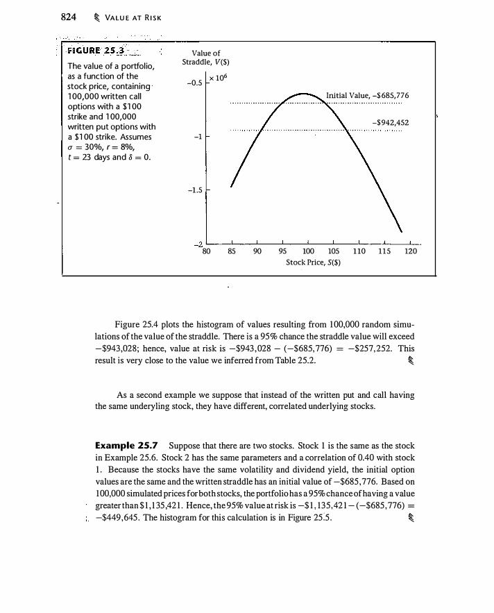
824 � VA LU E AT R I S K

The va lue of a portfol io, as a function of the stock price, containing 1 00,000 written cal l options with a $ 1 00

strike and 1 00,000

written put options with a $ 1 00 strike. Assumes a = 30%, r = 8%,

t = 23 days and 8 = 0.

Value of Straddle, V(S)

-0.5 X 106

-1

-1 .5

Initial Value, -$ 685, 776

-$ 942,452

-2L---�--�----�---L----L---�--�----� 80 85 90 95 100 105 1 10 1 1 5 120

Stock Price, S(S)

Figure 25.4 plots the histogram of values resulting from 1 00,000 random simu­lations of the value of the straddle. There is a 95% chance the straddle value will exceed -$943,028; hence, value at risk is -$943 ,028 - (-$685, 776) = -$257, 252. This result is very close to the value we inferred from Table 25.2. �

As a second example we suppose that instead of the written put and call having the same underyling stock, they have different, correlated underlying stocks.

Example 25.7 Suppose that there are two stocks. Stock 1 is the same as the stock in Example 25.6. Stock 2 has the same parameters and a correlation of 0.40 with stock 1 . Because the stocks have the same volatility and dividend yield, the initial option values are the same and the written straddle has an initial value of -$685 ,776. Based on 100,000 simulated prices for both stocks, the portfolio has a 95% chance of having a value greater than $ 1 , 1 35 ,42 1 . Hence, the 95% value at risk is -$ 1 , 135 ,42 1 - ( -$685 , 776) =

-$449,645 . The histogram for this calculation is in Figure 25 :5 . �

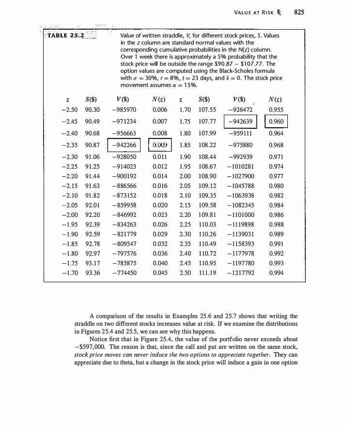
VA LU E AT R I S K � 825

TAB LE 2 5 . 2 � . . Value of written straddle, V, for different stock prices, 5 . Values in the z column a re standard normal values with the corresponding cumulative probabi l ities in the N(z) column. Over 1 week there is approximately a 5% probabi l ity that the stock price will be outside the range $90.87 - $1 07 .77 . The option va lues are computed using the Black-Scholes formula with a = 30%, r = 8%, t = 23 days, and 8 = 0. The stock price movement assumes a = 1 5%.

z S($) V($) N(z) z S($) V($) N(z) -2.50 90.30 -985970 0.006 1 .70 1 07.55 -926472 0.955

-2.45 90.49 -97 1234 0.007 1 .75 1 07 .77 -942639 1 0.960 1 -2.40 90.68 -956663 0.008 1 .80 1 07 .99 -959 1 1 1 0.964

-2.35 90.87 -942266 1 o.oo9 1 1 .85 1 08 .22 -975880 0.968

-2.30 9 1 .06 -928050 0.0 1 1 1 .90 1 08.44 -992939 0.97 1

-2.25 9 1 .25 -9 14023 0.0 1 2 1 .95 1 08 .67 - 10 1 028 1 0 .974

-2.20 9 1 .44 -900 1 92 0.0 14 2.00 1 08.90 - 1027900 0.977

-2. 15 9 1 .63 -886566 0.0 16 2.05 1 09. 1 2 - 1045788 0.980

-2. 10 9 1 .82 -873 152 0.0 1 8 2. 1 0 109.35 - 1063938 0.982

-2.05 92.0 1 -859958 0.020 2. 15 1 09.58 - 1082345 0.984

-2.00 92.20 -846992 0.023 2.20 1 09.8 1 - 1 1 0 1 000 0.986

- 1 .95 92.39 -834263 0.026 2.25 1 1 0 .03 - 1 1 19898 0.988

- 1 .90 92.59 -82 1 779 0.029 2.30 1 10 .26 - 1 13903 1 0.989

- 1 .85 92.78 -809547 0.032 2.35 1 1 0.49 - 1 158393 0.99 1

- 1 .80 9(-.97 -797576 0.036 2 .40 1 10.72 - 1 177978 0.992

- 1 .75 93 . 1 7 -785875 0.040 2.45 1 10.95 - 1 1 97780 0 .993

- 1 .70 93.36 -774450 0.045 2.50 1 1 1 . 1 9 - 1 2 1 7792 0.994

A comparison of the results in Examples 25 .6 and 25.7 shows that writing the straddle on two different stocks increases value at risk. If we examine the distributions in Figures 25.4 and 25.5, we can see why this happens.

Notice first that in Figure 25 .4, the value of the portfolio never exceeds about -$597,000. The reason is that, since the call and put are written on the same stock, stock price moves can never induce the two options to appreciate together. They can appreciate due to theta, but a change in the stock price will induce a gain in one option

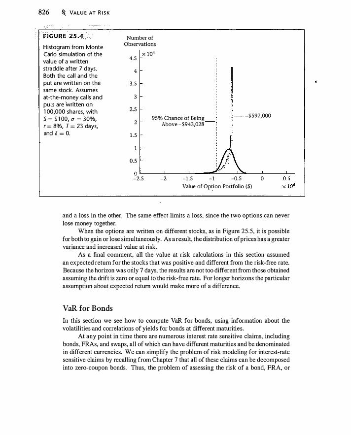
826 � VA LU E AT R I S K

H istogram from Monte Carlo s imulation of the value of a written straddle after 7 days. Both the cal l and the put are written on the same stock. Assumes at-the-money ca l ls and pu:..s are written on 1 00,000 shares, with S = $ 1 00, a = 30%, r = 8%, T = 23 days, and 8 = 0.

Number of Observations

X 104 4.5

4

3.5

3

2.5

2

1 .5

1

0.5

95% Chance of Being Above -$943,028

- -$597,000

O L-----�-----L----��--���--�----�--2.5 -2 -1 .5 -1 --0.5 0

Value of Option Portfolio ($)

and a loss in the other. The same effect limits a loss, since the two options can never lose money together.

When the options are written on different stocks, as in Figure 25 .5, it is possible for both to gain or lose simultaneously. As a result, the distribution of prices has a greater variance and increased value at risk.

As a final comment, all the value at risk calculations in this section assumed an expected return for the stocks that was positive and different from the risk-free rate. Because the horizon was orily 7 days, the results are not too different from those obtained assuming the drift is zero or equal to the risk-free rate. For longer horizons the particular assumption about expected return would make more of a difference.

VaR for Bonds

In this section we see how to compute VaR for bonds, using information about the volatilities and correlations of yields for bonds at different maturities.

At any point in time there are numerous interest rate sensitive claims, including bonds, FRAs, and swaps, all of which can have different maturities and be denominated in different currencies. We can simplify the problem of risk modeling for interest-rate sensitive claims by recalling from Chapter 7 that all of these claims can be decomposed into zero-coupon bonds. Thus, the problem of assessing the risk of a bond, FRA, or

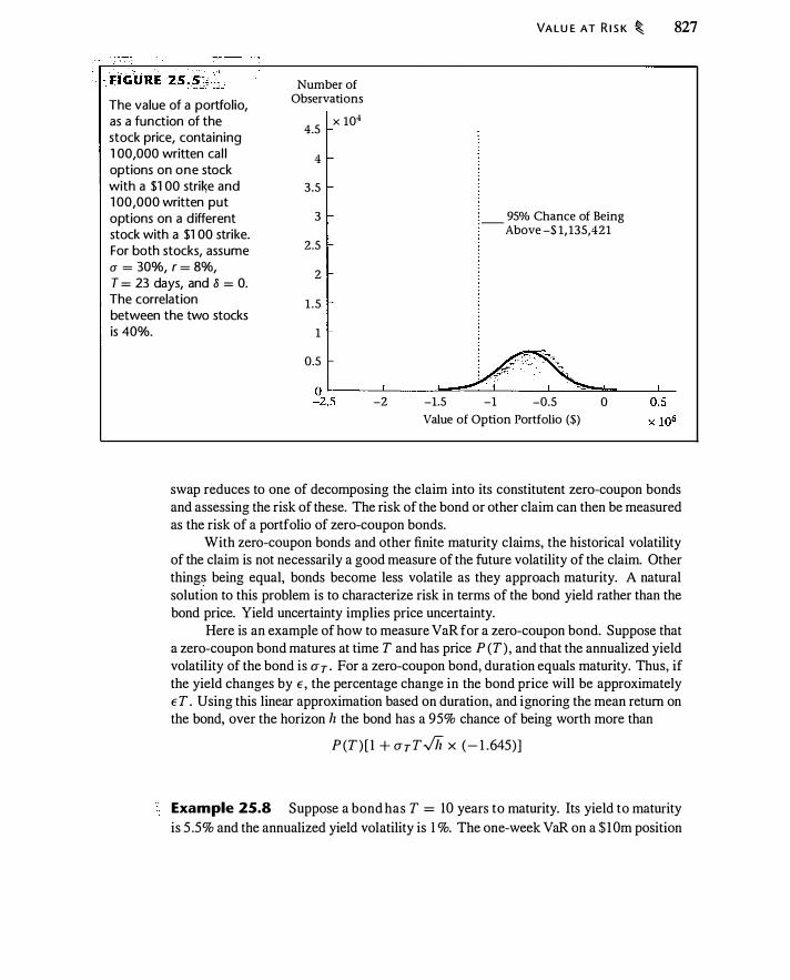
The value of a portfolio, as a function of the stock price, containing 1 00,000 written cal l options on one stock with a $1 00 strike and 1 00,000 written put options on a d ifferent stock with a $1 00 strike. For both stocks, assume rr = 30%, r = 8%, T = 23 days, and 8 = 0. The correlation between the two stocks is 40%.

Number of Observations

X 104 4.5

4

3.5

3

2.5

2

1 . 5

1

0.5

-2 -1.5

VA LU E AT R I S K � 827

_ 95% Chance of Being Above -S 1 , 135,421

-1 -0.5 0

Value of Option Portfolio (S)

swap reduces to one of decomposing the claim into its constitutent zero-coupon bonds and assessing the risk of these. The risk of the bond or other claim can then be measured as the risk of a portfolio of zero-coupon bonds.

With zero-coupon bonds and other finite maturity claims, the historical volatility of the claim is not necessarily a good measure of the future volatility of the claim. Other thing� being equal, bonds become less volatile as they approach maturity. A natural solution to this problem is to characterize risk in terms of the bond yield rather than the bond price. Yield uncertainty implies price uncertainty.

Here is an example of how to measure VaR for a zero-coupon bond. Suppose that a zero-coupon bond matures at time T and has price P (T) , and that the annualized yield volatility of the bond is cr T . For a zero-coupon bond, duration equals maturity. Thus, if the yield changes by E , the percentage change in the bond price will be approximately ET . Using this linear approximation based on duration, and ignoring the mean return on the bond, over the horizon lz the bond has a 95% chance of being worth more than

P (T ) [ l + O" T T .Jh X ( - 1 .645)]

Example 25.8 Suppose a bond has T = lO years to maturity. Its yield to maturity is 5 .5% and the annualized yield volatility is l %. The one-week VaR on a $ 1 Om position

828 � VA LU E AT R I S K

i n these bonds is

$ 10m X [ 1 + 0.01 X 10 X fJ;, X ( - 1 .645)] - $1 0m = -$228, 1 20

Now suppose that instead of a single bond we have a portfolio of zero-coupon bonds . In particular, suppose we own W1 of a bond maturing at Tr with annualized yield volatility CJ T1 and W2 of a bond maturing at T2 with annualized yield volatility CJ T2 • Let p represent the correlation between the yields on the two bonds. (This yield volatility i!lformation could be estimated using historical data or using implied volatilities.) As with a portfolio of stocks, we can use the delta approximation, only here instead of two correlated stock returns we have two correlated bond yields.

Example 25.9 Let T1 = 1 0, T2 = 15, u T1 = 0.0 1 , II T2 = 0.01 2 p = 0.985, W1 . = $6m and W2 = $4m. Since the portfolio is 60% invested in the 1 0-year bond and 40% invested in the 15-year bond, the variance of the bond portfolio is

(0.6 X 0.0 1 X 1 0)2 + (0.4 X 0.0 1 2 X 15)2

+ (2 X 0.985 X 0.6 X 0.4 X 0.0 1 X 1 0 X 0.0 1 2 X 15 ) = 0 .01729

The volatility is .J0 .01729 = 0. 1 3 15 . The 95% one-week VaR for this portfolio is therefore

$ 1 0m x [ 1 + 0. 1 3 1 5ji752 x (- 1 .645)] - $ 10m = -$301 , 638 �

We discussed in Chapter 24 the shortcomings of duration as a measure of bond price risk, so you might be wondering about the use of duration in these examples. Duration here is used mechanically to compute the price change for a bond for a given change in the bond's own yield. This is a delta approximation to the actual bond price change. The conceptual problem with duration becomes problematic when we use duration to compute a hedge ratio for two bonds. The hedge ratio calculation assumes that the yield to maturity for the two bonds changes by the same amount. By contrast, in Example 25.9 each bond has a different yield volatility and there is an imperfect correlation between the two yields; thus, we do not assume that all yields to maturity change by the same amount-i.e., that there is a parallel yield curve shift. (For a parallel yield curve shift we would need each bond to have the same annualized yield volatility and p = 1 .)

In general, if we are analyzing the risk of an instrument with multiple cash flows, the first step is to find the equivalent portfolio of zero-coupon bonds. A 1 0-year bond with semiannual coupons is equivalent to a portfolio of 20 zero-coupon bonds. Every interest rate claim is decomposed in this way into interest rate "buckets" containing the claim's constituent zero-coupon bonds. A set of bonds and swaps reduces to a portfolio of long and short positions in zero-coupon bonds. We need volatilities and correlations for all these bonds.

VA LU E AT R I S K � 829

As an empirical matter, the movement of a zero-coupon bond at an 8-year maturity, for example, is highly correlated with that of a zero-coupon bond at an 8 1/2-year maturity. Thus, for tractability, volatility and yields are tracked only at certain benchmark maturities: In Riskmetrics, these are 1 , 3 , 6, and 1 2 months, and 2, 3 , 4, 5 , 7, 9 , 10, 15 , 20, and 30 years. If we have a zero-coupon bond in the portfolio that does not exactly match a benchmark maturity, we want to determine the portfolio of the benchmark zero­coupon bonds that matches the characteristic of the nonbenchmark zero-coupon bond. The goal is to find an interpolation procedure to express any hypothetical zero-coupon bond in terms of the benchmark zero-coupon bonds. This procedure in which cash flows are allocated to benchmark claims (in this case zero-coupon bonds) is called cash flow mapping.

Suppose, for example, that we wish to assess the risk of a 12-year zero-coupon bond, given information on the 1 0-year and 15-year zero-coupon bonds . It is reasonable to use simple linear interpolation to obtain the yield and yield volatility for the 12-year bond from those of the 1 0-year and 15-year bonds. For example, if the yield and volatility of the t-year bond are y, and u 1 , linear interpolation gives us

)' J 2 = (0.6 X )' JO) + (0.4 X )' J5)

U 1 2 = (0.6 X U J O) + (0.4 X U J5 )

(25 . 14)

(25 . 15)

These interpolations enable us to determine the price and volatility of $1 paid in year 1 2. In particular, the price is e-y,1 x 1 2 • However, we are not finished because these interpola­tions do not provide correlations between the 1 2-year zero and the adjacent benchmark bonds. We need these correlations because we could have a portfolio containing 1 0-, 1 2-, and 15-year bonds.

The next step is to ask what combination of the 1 0- and 1 5-year zero-coupon bonds would have the same volatility as the hypothetical 1 2-year bond. If we let w equal the fraction allocated to the 1 0-year bond, we must solve

uf2 = (a

luf

0) + [( 1 - w)2uf0] + [2p 10, 1 5w ( l - w)uwu 15 ] (25 . 1 6)

Since this is a quadratic equation, there are two solutions for w. Typically, as in the following example, one of the two solutions will be economically appealing and the other will seem unreasonable.

Example 25. 1 0 Suppose we have a $1 cash flow occurring in year 12 and that we wish to map to the 1 0- and 1 5-year zero-coupon bonds. Suppose that y 10 = 5.5%, y15 = 5 .75%, u 10 = 1 %, u 15 = 1 .2%, and p = 0.985. The yield and volatility of the hypothetical 1 2-year zero-coupon bond are

)'12 = (0.6 X 0.055) + (0.4 X 0 .0575) = 0.056

() 1 2 = (0.6 X 0.01 ) + (0.4 X 0.0 1 2) = O.Q 108

We next need to find the cash flow mapping that matches the volatility. Solving equation (25 . 1 6) gives the two solutions w = 6.2097 and w = 0.5797. The first solution maps

830 � VA LU E AT R I S K

the cash flow by going long 62 1 % of the 10-year bond and short 520% of the 15-year bond. The second, more economically reasonable solution, entails going long 57.97% of the 1 0-year bond and 42.03% of the 15-year bond. �

Notice that the solution w = 0.5797 is close to the 60%-40% split you might have guessed at the outset. Given these weights, value at risk for the 1 2-year bond can be computed in the same way as VaR for the bond portfolio in Example 25 .9.

If you find this procedure confusing, recognize that if we had mapped the 1 2-year �ond by assigning 60% of it to the 1 0-year bond and 40% to the 15-year bond, then we would not have mate/zed the yield and volatility given by equations (25 . 14) and (25 . 1 5) . Because of the nonlinear relationship between prices and yields, an interpolation based on the yield will give a different cash flow map than an interpolation based on prices.

Although we have discussed cash flow mapping in the context of bonds, mapping can be applied to any claim with multiple cash flows.

Estimating Volatility

Volatility is the key input in any VaR calculation. In most of the examples in this chapter, return volatility over the horizon h is a ,Jh, with a constant. This calculation assumes both that the volatility, a, does not change, and that returns are independent over time. In practice, both assumptions may be violated.

It is straightforward to estimate historical volatilties given a time series of returns. However, volatility is typically not constant over time. As a consequence, it is necessary to update volatility estimates when VaR is computed. In Chapter 23 we discussed a num­ber of ways to estimate volatility : simple historical volatility, exponentially weighted moving average, GARCH, realized volatility, and implied volatility. Keep in mind, however, that when volatility is stochastic, there can be a risk premium for volatility that will affect the option price. Inferring the volatility from option prices when volatility is stochastic requires careful modeling, since it is necessary to disentangle the true implied volatility and the risk premium. This is an area of ongoing research.

Depending on the asset, returns may be correlated over time. To a first approxi­mation, stock returns are independent over time. However, over horizons as short as a day, returns may be negatively correlated due to factors such as bid-ask bounce. There is some evidence of negative correlation at longer horizons, though the effect is more subtle.

When returns are correlated, volatility does not scale with ,Jh. If returns are negatively correlated over time, then high returns are followed by low returns. Thus, negative return correlation dampens volatility relative to the independent returns case. If returns are positively correlated, high returns follow high returns, which results in a higher volatility than in the independent returns case.

With commodities, return independence may depend on the horizon. For example, high copper prices lead to increased supply and reduced demand, which eventually induces the price to fall . So return independence is not reasonable for long horizons .

VA LU E AT R I S K � 83 1

However, independence may be reasonable over shorter horizons, where supply and demand responses do not have time to occur.

Finally, we also require correlation estimates in order to compute volatilities of portfolios. Correlations can be estimated using historical data the same way as volatil­ities. However, it is important to be aware that, just as volatilities will change in times of financial stress, correlations will change as well . When there is a stock market crash, for example, by definition all stocks move together, exhibiting a temporarily high posi­tive correlation. It is important, therefore, to test correlation assumptions. One way to do this is by evaluating scenarios in which asset prices undergo large moves and asset correlations become extreme.

Bootstrapping Return Distributions

It is possible to use observed past returns to create an empirical probability distribu­tion of returns that can then be used for simulation. This procedure is called boot­strapping. The idea of bootstrapping is to sample, with replacement, from observed historical returns under the assumption that future returns will be drawn from the same distribution. For example, if the stock price over a 5-day period has returns of {-0.02, 0.0 15 , -0.0 1 , 0 . 10 , 0.03 } , then this distribution can be bootstrapped by ran­domly selecting one of these returns each time a new 1 -day return is needed. In effect, bootstrapping randomly shuffles past returns to create hypothetical future returns.

We have seen how the lognormal model has trouble accounting for events like the 1 987 market crash . The advantage of bootstrapping is that, since it is not based on a particular assumed distribution, it is consistent with any distribution of returns. For example, if an event like a significant market crash occurs once every 10 years historically, it will occur on average once every 1 0 years in the bootstrapped distribution.

A disadvantage of simple bootstrapping is that key features of the data might be lost when the data are reshuffled. For example, if historical returns exhibit persistence in volatility, randomly reshuffled historical returns will not exhibit such persistence. It is possible to bootstrap a distribution while preserving correlation; this is called a dependent bootstrap.6 First, it is possible to bootstrap by randomly selecting blocks of data at a time. The use of blocks preserves correlation across time within the blocks . Second, given a specification for the correlated series, we can estimate the correlated process and use this to bootstrap. For example, suppose we believe that a commodity price is generated by the process

(25 . 17)

If we fit this process to the data, we obtain an estimate of p and a time series of errors, Er+h · These errors should be uncorrelated if equation (25. 1 7) is correctly specified. We can then simulate the process in equation (25 . 1 7) by randomly drawing from the

6Two general discussions of bootstrapping that also discuss bootstrapping of dependent data are Shao and Tu ( 1 995, Chap. 9) and Horowitz (200 I ).

832 � VA LU E AT R I S K

estimated errors . This will generate a series with the observed correlation and with errors drawn from the data.

25 .2 ISSUES WITH VAR

VaR provides a single number that is easy to interpret and communicate. However, VaR is not the only way to assess risk, and it has conceptual shortcomings. In this section we discuss some alternatives to simple VaR and introduce the concept of subadditive risk measures. In the course of comparing risk measures, we will also discuss the use of the tr�e price distribution in computing VaR as compared to the risk-neutral distribution, which we use in pricing derivatives .

Alternative Risk Measures

Consider again the VaR for a single stock. Suppose the current stock price is So and we wish to assess the risk of this investment at time T. As before, if the confidence level is c, define S(c) as the stock price such that there is a c probability that the stock price at time T will be worth less than S(c) . In addition to VaR, we can compute two additional risk measures based_ on the VaR: the tail VaR, which we define below, and the cost of insurance against outcomes below the VaR level.

Tail VaR A shortcoming of VaR is that it specifies the ininimum loss that will occur with a given probability. In practice we would like to know the expected magnitude of the loss should a loss occur. This is called the tail VaR or the expected tail loss. For the simple case where the portfolio consists of one stock, we can assess the severity of the loss by computing the average loss conditional upon the stock price being less than S(c) . Whereas VaR specifies the level, S(c) , that will be breached with probability c, tail VaR measures the average severity of the breach. For the single stock case, tail VaR is defined as

(25 . 1 8)

In Section 1 8 .4 we discussed calculating the conditional expected stock price. For a lognom1ally distributed stock, we can use equation ( 1 8.28) to compute the conditional expectation.

Example 25. 1 1 Assume that we own stock with a current price of $ 1 00, a volatility of 30%, an expected return of 1 5%, and a dividend yield of 0. Also assume that the risk-free rate is 8%. Let T = 0 .5 .

Figure 25 .6 depicts the probability density for ST , the stock price at the 5% quantile, and the conditional expected stock price. To compute the VaR, we first need to compute S(0.05 ) :

S(0 .05) = $ 1 00e(0. 1 5-0.5 x0.32 ) x0.5- 1 .645 x0.30x..;'i).5

= $74.347

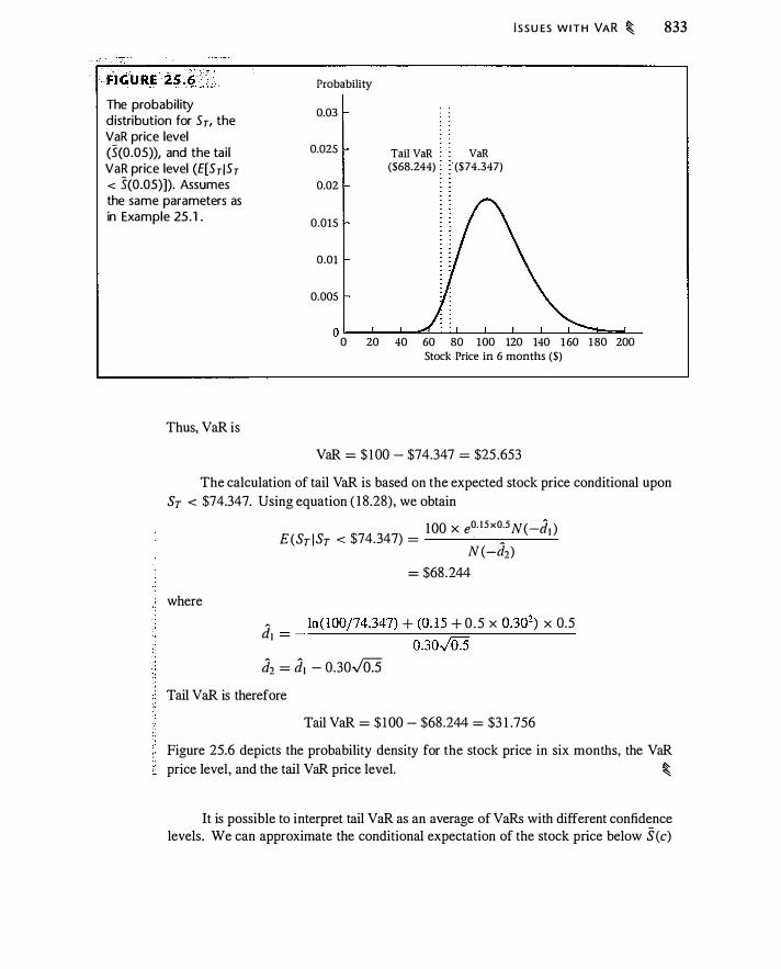
The probabi l ity d istribution for Sr, the VaR price level (.5(0.05)), and the tai l VaR price level (E[Sr iSr < .5(0.05)]). Assumes the same parameters as in Example 25 . 1 .

Thus, VaR is

Probability

0.03

0.025

0.02

0.015

0.01

0.005

Tail VaR VaR ($68.244) ($ 74.347)

I S S U ES W I T H VAR � 833

o �_.--��L-�--�--L-�--����-­o 20 40 60 80 100 120 140 1 60 1 80 200

Stock Price in 6 months ($)

VaR = $ 1 00 - $74.347 = $25 .653

The calculation of tail VaR is based on the expected stock price conditional upon ST < $74.347. Using equation ( 1 8.28), we obtain

where

100 X e0. 1 5 x0.5N(-dt ) E(ST I ST < $74.347) =

·

�

N (-d2) = $68 .244

� 1n ( l00j74.347) + (0. 1 5 + 0 . 5 X 0.302) X 0.5 dt = - ���----��---=�------�----

0.30J03 J2 =

dt - 0.30.Jo.5

Tail VaR is therefore

Tail VaR = $ 1 00 - $68 .244 = $3 1 .756

Figure 25.6 depicts the probability density for the stock price in six months, the VaR price level, and the tail VaR price level. �

It is possible to interpret tail VaR as an average of VaRs with different confidence levels. We can approximate the conditional expectation of the stock price below S(c)

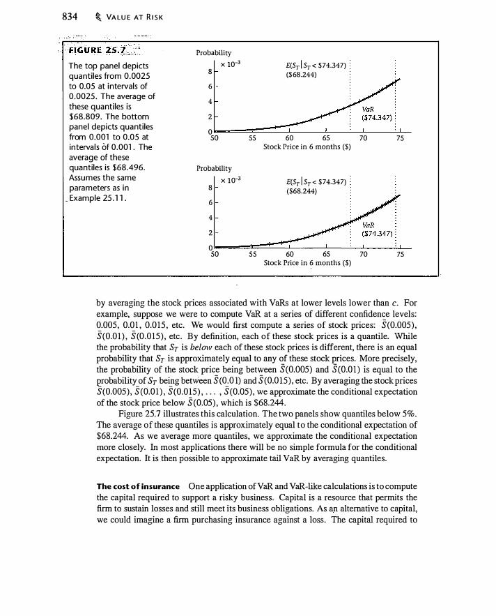
834 � VA LU E AT R I S K

The top panel depicts quantiles from 0.0025 to 0.05 at intervals of 0 .0025 . The average of these quanti les is $68.809. The bottom panel depicts quantiles from 0.001 to 0.05 at intervals of 0.001 . The average of these quantiles is $68.496. Assumes the same parameters as in

_ Example 25 . 1 1 .

Probability

X 10-3

8

6

4

2

0 so

Probability

X 10-3

8

6

4

2

0 so

E(Sy ! Sy < $ 74.347) ($ 68.244)

55 60 65 70 75 Stock Price in 6 months ($)

E(Sy ! Sy < $ 74.347) � ($68.244)

55 60 65 70 75 Stock Price in 6 months ($)

by averaging the stock prices associated with VaRs at lower levels lower than c. For example, suppose we were to compute VaR at a series of different confidence levels: 0.005, 0.0 1 , 0.0 15 , etc. We would first compute a series of stock prices: S(0.005) , S(0.0 1 ) , S (0 .0 15) , etc . By definition, each of these stock prices is a quantile. While the probability that ST is below each of these stock prices is different, there is an equal probability that ST is approximately equal to any of these stock prices. More precisely, the probability of the stock price being between S(0.005) and S(0.0 1 ) is equal to the probability of ST being between S(O.O 1) and S(O.O l5) , etc. By averaging the stock prices S(0.005) , S(0.0 1 ) , S(0.0 15) , . . . , S(0.05) , we approximate the conditional expectation of the stock price below S(0.05) , which is $68.244.

Figure 25.7 illustrates this calculation. The two panels show quantiles below 5%. The average of these quantiles is approximately equal to the conditional expectation of $68.244. As we average more quantiles, we approximate the conditional expectation more closely. In most applications there will be no simple formula for the conditional expectation. It is then possible to approximate tail VaR by averaging quantiles.

The cost of insurance One application ofVaR and VaR-like calculations is to compute the capital required to support a risky business. Capital is a resource that permits the firm to sustain losses and still meet its business obligations. As an alternative to capital, we could imagine a firm purchasing insurance against a loss . The capital required to

I S S U ES W I T H VAR � 835

undertake the business would then be the price of this insurance. The market price of this insurance provides another way to measure risk.

Returning to our exll!_llple of a single stock portfolio, if we insure against losses due to a stock price below S(c) , then the time T payoff on such an insurance policy will be

max[O, S(c) - ST]

Thus, the insurance premium is the value of a put option with strike price S(c) and time to expiration T. We can obtain the value of the put by computing

e-rT E* [S(c) - ST ! ST < S(c)] x Prob* [ST < S(c)]

= e-rT {S (c) x -E* [ST ! ST < S(c) ] } x Prob* [ST < S(c)] (25 . 19)

where E* and Prob* represent the expectation and probability computed with respect to the risk-neutral distribution. The put price calculation appears similar to the conditional price calculation used in computing taii VaR, but the two calculations are not identical. One obvious difference is that tail VaR is computed using the conditional expectation of the stock price under the true distributio!l, while the option price

_uses the risk-neutral

distribution. Note that while Prob[ST < S(c)] = c, Prob* [ST < S(c)] I= c unless the risk premium on the asset is zero (a = r) . Also, the put price is discounted, while the tail VaR is not.

VaR horizons are often short, so that discounting may not be an important issue. Also, with a short horizon the difference between the risk-neutral and true distribution may not be large.7

- Example 25. 1 2 Assume the same parameters as in Example 25. 1 1 , and also that the risk-free rate is 8%. The price of a put with 6 months to expiration and a strike of $74.347 is

BSPut(IOO, 74.347, 0.30, 0.08, 0.50, 0) = $0.4289

VaR and the Risk-Neutral Distribution

It might seem odd to you that we have mostly used the risk-neutral distribution in this book, but in discussing VaR we have concentrated on the true distribution. Using the foregoing examples, we can explore this difference.

7When prices move continuously and the hedging of risks is possible, the difference between the true and risk-neutral distributions depends upon the risk premium, (a - r)lz . When h is small, the risk premium will be small. When jumps are possible, the risk premium associated with the jump could create a significant difference between the risk-neutral and true distributions even over short horizons.

836 � VA LU E AT R I S K

Let's try to interpret VaR and tail VaR i n terms of insurance. If we are willing to accept losses less than the VaR level, then we can think of VaR as a deductible: It is the loss we willingly sustain before insurance pays anything. The difference between tail VaR and VaR is then the average payout from insurance; this payout occurs with true probability c. Since we are using the true distribution, the appropriate discount rate for a conditional expectation is unclear. (This is another manifestation of the problem of obtaining a "true" discount rate for an option.) Let y denote the discount rate. A back-of­the-envelope calculation for the value of the average insurance payoff, assuming y = r , is8

e-yT [Tail VaR - VaR] x Prob[ST < S(c) ] T - -

= e-y {So - E[ST I ST < S(c)] - [So - S(c) ] } x c

= e-O.OSxO.SO X (74.347 - $68 .244) X 0.05

= 0.2932

(25 .20)

The value of insurance inferred from the VaR calculations is substantially less than that computed using the Black-Scholes formula. There are two reasons why this calculation gives the wrong answer.

First, 5% is the VaR probability under the true distribution, not under the risk­neutral distribution. The risk-neutral probability that ST < 74.347 is 6.945%. The risk-neutral probability is greater than the true probability because the 8% risk-free rate is less than the 1 5% expected return on the stock (i.e. , a > r) .

Second, the conditional expected stock price under the risk-neutral distribution is less than that under the true distribution:

E* (ST I ST < $74.347) = $67.9 1 9

Again, th e true conditional expectation exceeds the risk-neutral conditional expectation because a > r .

We can change the probability and conditional expectation to their risk-neutral values and repeat the calculation in equation 25 .20. We then obtain

e-O.OSxO.SO X ($74.347 - $67 .9 1 9) X 0 .06945 = $0.4289

This is the same as the put premium in Example 25 . 1 1 . As a final comment, note that the 5 % VaR will also be different depending upon

whether we use the true or risk-neutral distribution. In this discussion we continued to use $74.347---{;omputed under the true distribution-as the VaR stock price.

The conclusion of this discussion is that we need to be cautious when interpreting VaR and tail VaR calculations. Economically, when a > r, VaR-style calculations computed using the true stock price distribution understate the insurance cost because they fail to properly account for the risk premium as a component of the drift on the asset.

8If there is no risk premium on the stock-i.e., a = r-this calculation produces the Black-Scholes put price.

I S S U ES W I T H VA R � 837

The risk premium is compensation for the fact that when the stock earns a low return, investors generally have suffered losses on their investments (their marginal utility of consumption is high). Insurance hedges against this outcome and is therefore valuable to investors. The Black-Scholes calculation properly accounts for the role of the risk premium, while the back-of-the-envelope calculation using VaR does not.

Subadditive Risk Measures

Artzner et al . ( 1 999) point out a conceptual problem with VaR. As we have discussed, a common use of a risk measure is to decide how much capital is required to support an activity. Artzner et al. argue that a reasonable risk measure (or measure of required capital) should have certain properties, among them subadditivity.9 If p(X) is the risk measure associated with activity X (the capital required to support activity X), then p

. is subadditive if for two activities X and Y

p (X + Y) S p(X) + p (Y) (25.2 1 )

This simply says that the risk measure for the two activities combined should b e less than that for the two activities separately. Because combining activities creates diversification, the capital required to support two activities together should be no greater than that required to support the two separately. If capital requirements are imposed using a rule that is not subadditive, then firms can reduce required capital by splitting up activities.

VaR is not subadditive. To show this, Artzner et al. provide an example using European out-of-the-money cash-or-nothing options having the same time to expiration and written on a single stock. Option A, a cash-or-nothing call, pays $ 1 if ST > H, while option B , a cash-or-nothing put, pays $1 if ST < L . Represent the premiums of the two options as PA and Pn and suppose that either option has a 0.8% probability of paying off. The probability that either option expires out-of-the-money is 99.2%, and the probability that both options expire out-of-the-money is 98.4%.

Consider a financial institution that writes such options. For either option consid­ered alone, the bank is confident at a 99% level that the option will not be exercised, in which case the bank keeps the premium. Thus, VaR at a 99% confidence level is - PA (for option A) or - Pn (for option B) . VaR is negative because with 99% confidence, the option writer will keep the premium without the option being exercised.

Now suppose the institution sells both options. Because the two written options have the same underlying stock, they are perfectly negatively correlated. Therefore, the probability that one of the two options wiii be exercised is 0.8% + 0.8% = 1 .6%. In the lowest 1 % of the return distribution, one of the two options will be exercised. The VaR

9 Artzner et al. ( 1 999) define coherent risk measures as those satisifying four properties: ( I ) subaddi­

til•ity; (2) monotonicity: if X :::; Y, p(X) 2:: p(Y) (if the loss is greater, the risk measure is greater); (3) translation invariance: p(X + a) = p(X) - a (if you add S l to the cash flow, the risk measure is reduced by S l ); and (4) positive homogeneity p(),X) = ),p(X) for ), > 0 (if you multiply the risk by 10, the risk measure i ncreases by I 0).

838 � VA LU E AT R I S K

at the 99% level for the writer of the two options i s therefore $ 1 - PA - P8 . We have

VaR(-A - B) = $ 1 - PA - Pn > - PA - P8 = VaR(-A) + VaR(- B)

This expression has the opposite inequality as equation (25 .2 1 ), so VaR is not subadditive in this example. In words, the institution can eliminate risk, as measured by 99% VaR, by undertaking the two activities in separate entities.

As a different example that illustrates this point, suppose you are comparing activity C, which generates a $ 1 loss with a 1 . 1 % probability, with activity D, which generates a $ 1 m loss with a 0.9% probability. Any reasonable rule should assign greater risk (and {equire more capital) for activity D, but a 1 % VaR would be greater for C than for D .

These examples highlight an intuitively undesirable property of VaR as a risk measure: a small change in the VaR probability can cause VaR to change by a large amount. For the written cash-or-nothing call in this example, a 0 .8 1 % VaR is - P A , while the 0.79% VaR i s $ 1 - PA .

In contrast with VaR, tail VaR and the cost of insurance are both subadditive. Intuitively, tail VaR takes into account the distribution of losses beyond the VaR level, so it does not change abruptly when we change the VaR probability. To see that it is subadditive in our examples, the tail VaRs at the 99% level for A and B are

p (A) = 0 .8 X ( 1 - Ptl ) + 0.2 X (-PA) = 0 .8 - PA

p (b) = 0 .8 x ( 1 - Pn) + 0.2 x (- Pn) = 0.8 - Pn

With the same confidence level, tail VaR at the 99% level for A and B together is

p (A + B) = 1 - P;1 - Pn

We then have

p (A + B) = 1 - P;� - Pn < p(A) + p (B) = 1 .6 - P;� - P8

Thus, tail VaR in this example is subadditive. As for the subadditivity of insurance premiums, Merton ( 1973b) demonstrated that

options on portfolios are no more expensive than a portfolio of options on the portfolio constituents. Insurance premiums are therefore subadditive.

CHAPTER SUMMARY

Value at risk (VaR) is used to measure and manage risk-for example, in computing capital requirements. VaR deals primarily with so-called "market risks": price changes of stocks, currencies, interest rates, and commodities. The value at risk of a portfolio is the level of loss that will be exceeded a given percentage of the time over a specified horizon. Computing value at risk requires approximating the return distribution of the portfolio, which in tum requires information on the variance and covariance of assets in the portfolio. When portfolios are simple-for example, containing only stocks­standard portfolio risk calculations can be used to compute VaR. When portfolios contain options and other nonlinear assets, Monte Carlo simulation is commonly used to assess

P RO B LE M S � 839

the return distribution of the portfolio. It is possible to construct examples in which VaR is an ill-behaved risk measure. Tail VaR, whlch takes into account the distribution of losses beyond the VaR level, and the cost of insurance against losses exceeding the VaR level, may provide better alternatives.

FURTHER READING

The Riskmetrics Technical Document (1. P. Morgan/Reuters, 1996) is available from www.riskmetrics.com. It was distributed by J. P. Morgan-and now by Riskmetrics­to explain VaR, illustrate some of the calculations behlnd VaR, and review some of the judgments behlnd the particular set of calculations. The document was influential and remains worth reading.

Pearson (2002) provides an excellent overview ofVaR," with very clear discussions

of relevant mathematical techniques. Jorion (2001 ) provides a broad overview of the regulatory, practical, and analytical issues in computing VaR. Hendricks ( 1 996) compares the results from computing VaR in a variety of different ways. Artzner et al. ( 1 999) is an influential paper offering some important warnings about the use of VaR as a decision­making tool. Further explorations along these lines include Acerbi (2002) and Acerbi and Tasche (2002), and other papers in the July 2002 special issue of the Journal of Banking and Finance.

PROB LEMS

In the following problems, assume that the risk-free rate is 0.08 and that there are three stocks with a price of $ 1 00 and the following characteristics:

Stock A Stock B Stock·C

Ci

0. 1 5 0. 1 8 0. 1 6

0.30 0.45 0.50

0.00 0.02 0.00

Correlation with B

0.25 1 .00 0.30

Correlation with C

0.20 0.30 1 .00

25.1. Consider the expression in equation (25.6). What is the exact probability that, over a 1 -day horizon, stock A will have a loss?

25.2. Assuming a $ 1 0m investment in one stock, compute the 95% and 99% VaR for stocks A and B over 1 -day, 1 0-day, and 20-day horizons.

25.3. Assuming a $ 1 0m investment that is 40% stock A and 60% stock B, compute the 95% and 99% VaR for the position over 1 -day, 1 0-day, and 20-day horizons.

25.4. What are 95% and 99% 1 -, 1 0- and 20-day VaRs for a portfolio that has $4m invested in stock A, $3.5m in stock B, and $2.5m in stock C?

25.5. Using the same assumptions as in Example 25.3, compute VaR with and without the mean assuming correlations of - 1 , -0.5, 0, 0.5, and 1 . Is risk eliminated with a correlation of - 1 ? If not, why not?

� VAL U E AT R I S K

25.6. Using the delta-approximation method and assuming a $ 1Om investment i n stock A, compute the 95% and 99% 1- , 1 0-, and 20-day VaRs for a position consisting of stock A plus one 1 05-strike put option for each share. Use the same assumptions as in Example 25.4.

25.7. Repeat the previous problem, only use Monte Carlo simulation.

25.8. Compute the 95% 1 0-day VaR for a written strangle (sell an out-of-the-money call and an out-of-the-money put) on 1 00,000 shares of stock A. Assume the options have strikes of $90 and $ 1 10 and have 1 year to expiration. Use the delta-approximation method and Monte Carlo simulation. What accounts for the difference in your answers?

25.9. Using Monte Carlo, computet,he 95% and 99% 1- , 1 0-, and 20-day tail VaRs for the position in Problem 25.2.

25.10. Compute the 95% 1 0-day tail VaR for the position in Problem 25.8 .

25.11. Suppose you write a 1 -year cash-or-nothing put with a strike of $50 and a 1 -year cash-or-nothing call with a strike of $2 15 , both on stock A.

a. What is the 1 -year 99% VaR for each option separately?

b. What is the 1 -year 99% VaR for the two written options together?

c. What is the 1 -year 99% tail VaR for each option separately and the two together?

25.12. Suppose the 7-year zero-coupon bond has a yield of 6% and yield volatility of 1 0% and the 10-year zero-coupon bond has a yield of 6.5% and yield volatility of 9 .5%. The correlation between the 7-year and 1 0-year yields is 0.96. What are 95% and 99% 10-day VaRs for an 8-year zero-coupon bond that pays $ 1 0m at maturity?

25.13. Using the same assumptions as in Problem 25. 12, compute the 1 0-day 95% VaR for a claim that pays $3m each year in years 7-10.

CHA:IITER �6 --- ---- -· · ·-- · ... �v-"•"--· -'-=�-���-:'=:·;,_: :;-�-���� . .

Credit Risk

Le ri'k that a counte<parly will fiDI to meet a contractual payment obli�ation ;, known as credit risk. Such risk exists anytime one party promises to make a future payment to another. Credit risk arises with loans, corporate bonds, and derivative contracts, and market-making activities generally leave dealers exposed to credit risk. We will refer to the failure to make a promised payment as default. The term credit event is often used in contracts to refer to occurrences that suggest that a default is likely. Examples of credit events are declaration of bankruptcy, failure to make a bond payment, repudiation of an obligation, or a credit downgrade. 1

In this chapter we present a framework for analyzing credit risk and we see how credit risk affects the prices of claims. We also discuss concepts and terminology that are essential for understanding credit risk. Finally, we look at the instruments used to modify, hedge, and trade credit risk, such as credit default swaps.

26.1 DEFAULT CONCEPTS AND TERMINOLOGY

In this section we introduce basic concepts and terminology related to default in the context of pricing a zero-coupon bond. Suppose that a firm with asset value A0 issues a zero-coupon bond maturing at time T, with a promised payment of B . Let BT denote the market value of the bond at time T. At time T, there are two possible outcomes:

• AT > B . Since assets are worth more than the repayment owed bondholders, shareholders will repay bondholders in full, so BT = B .

• AT < B . Shareholders will walk away from the firm, surrendering it to bondhold­ers . The value of the bonds at time T is then BT = AT .

Let g*(AT ; Ao) denote the risk-neutral probability density for the time T asset value, conditional upon the time 0 asset value, A0. Then we can write the initial debt value,

1 A company that fails to make a promised payment may seek court protection-or a quick resolution of its dilemma-by declaring bankruptcy. Specific bankruptcy rules vary by country. We will use the terms "default" and "bankruptcy" interchangably and without regard to their precise legal meaning.

84 1

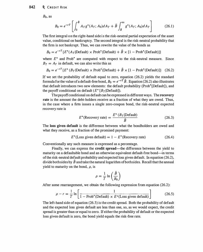
842 � C R E D I T R I S K

Bo, as

Bo = e-rY [foB Ayg* (Ay ; Ao)dAy + B hoo g* (Ay ; Ao)dAy J (26. 1 )

The first integral o n the right-hand side i s the risk-neutral partial expectation of the asset value, conditional on bankruptcy. The second integral is the risk-neutral probability that the firm is not bankrupt. Thus, we can rewrite the value of the bonds as

Bo = e-rY {E* (Ay !Default) x Prob* (Default) + B x [ 1 - Prob* (Default)] }

where E* and Prob* are computed with respect to the risk-neutral measure. Since By = Ay in default, we can also write this as

Bo = e-rY {E* (By iDefault) x Prob*.(Default) + i3 x [ 1 - Prob* (Default) ] } (26.2)

If we set the probability of default equal to zero, equation (26.2) yields the standard formula for the value of a default-free bond, B0 = e-rY i3. Equation (26.2) also illustrates that default introduces two new elements : the default probability (Prob*[Default] ), and the payoff conditional on default (E* [By iDefault]).

The payoff conditional on default can be expressed in different ways. The recovery rate is the amount the debt-holders receive as a fraction of what they are owed. Thus, in the case where a firm issues a single zero-coupon bond, the risk-neutral expected recovery rate is

,. E* (By !Default) E · (Recovery rate) = -----,=---­

B (26.3)

The loss given default is the difference between what the bondholders are owed and what they receive, as a fraction of the promised payment:

£* (Loss given default) = 1 - £* (Recovery rate) (26.4)

Conventionally any such measure is expressed as a percentage. Finally, we can express the credit spread-the difference between the yield to

maturity on a defaultable bond and an otherwise equivalent default-free bond-in terms of the risk-neutral default probability and expected loss given default. In equation (26.2), divide both sides by i3 and take the natural logarithm of both sides. Recall that the annual yield to maturity on the bond, p, is

p = _!_ ln ( B ) T Bo

After some rearrangement, we obtain the following expression from equation (26.2):

p - r = 2_ In [ 1 J T 1 - Prob* (Default) x £* (Loss given default)

(26.5)

The left-hand side of equation (26.5) is the credit spread. Both the probability of default and the expected loss given default are less than one, so, as we would expect, the credit spread is greater than or equal to zero. If either the probability of default or the expected loss given default is zero, the bond yield equals the risk-free rate.

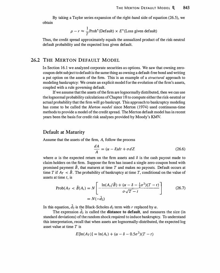
T H E M E RTO N D E FAU LT M O D E L � 843

By taking a Taylor series expansion of the right-hand side of equation (26.5), we obtain

p - r � _!_Prob* (Default) x £* (Loss given default) T

Thus, the credit spread approximately equals the annualized product of the risk-neutral default probability and the expected loss given default.

26.2 THE MERTON DEFAULT MODEL

In Section 1 6. 1 we analyzed corporate securities as options. We saw that owning zero­coupon debt subject to default is the same thing as owning a default-free bond and writing a put option on the assets of the firm. This is an example of a structural approach to modeling bankruptcy: We create an explicit model for the evolution of the firm's assets, coupled with a rule governing default

If we assume that the assets of the firm are lognormally distributed, then we can use the lognormal probability calculations of Chapter 1 8 to compute either the risk -neutral or actual probability that the firm will go bankrupt. This approach to bankruptcy modeling has come to be called the Me11on model since Merton ( 1 974) used continuous-time methods to provide a model of the credit spread. The Merton default model has in recent years been the basis for credit risk analyses provided by Moody's KMV.

Default at Maturity

Assume that the assets of the firm, A, follow the process

dA - = (ct - o)dt + crdZ A

(26.6)

where ct is the expected return on the firm assets and 8 is the cash payout made to claim holders on the firm. Suppose the firm has issued a single zero-coupon bond with promised payment B , that matures at time T and makes no payouts. Default occurs at time T if Ar < B . The probability of bankruptcy at time T, conditional on the value of assets at time t, is - [ ln(A1 /B) + (ct - 8 - �cr2) (T - t ) ]

Prob(Ar < B I A, ) = N �-cr...; T - t

= N(-d2) In this equation, J2 is the Black-Scholes d2 term with r replaced by ct .

(26.7)

The expression J2 is called the distance to default, and measures the size (in standard deviations) of the random shock required to induce bankruptcy. To understand this interpretation, recall that when assets are lognormally-distributed, the expected log asset value at time T is

E [ln (Ar) ] = ln(A1 ) + (ct - 8 - 0.5cr2) (T - t )

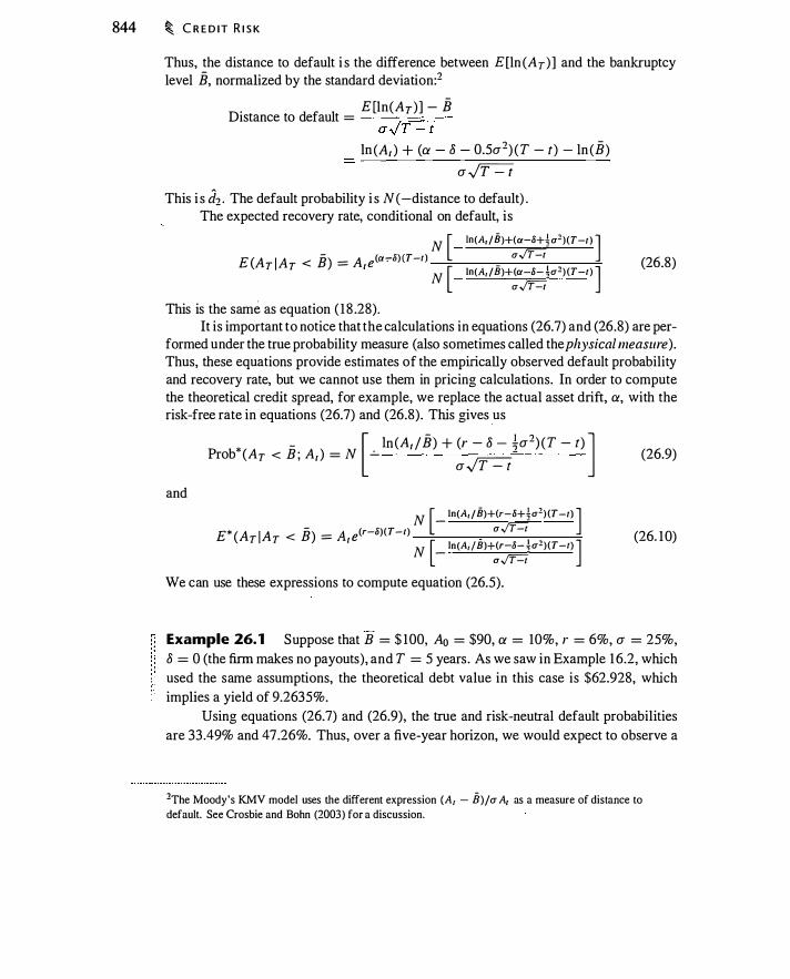
844 � C R E D IT R I S K

Thus, the distance to default i s the difference between E[ln (Ar) ] and the bankruptcy level B, normalized by the standard deviation:2

. E [ln (Ar) ] - B Distance to default = � av T - t

ln (A1 ) + (a - o - 0.5a2) (T - t) - ln (B)

a�

This i s d2 • The default probability i s N (-distance to default) . The expected recovery rate, conditional on default, is

N [ ln(fi, /B)+(a-H� cr2) (T-1) ] E (Ar iAr < B) = A le (ao-a) (T-I )

-" �

, N [ ln(fi, /B)+(a-8- �cr-) (T-1) ]

CT �

This is the same as equation ( 1 8 .28).

(26.8)

It is important to notice that the calculations in equations (26.7) and (26.8) are per­formed under the true probability measure (also sometimes called the physical measure). Thus, these equations provide estimates of the empirically observed default probability and recovery rate, but we cannot use them in pricing calculations. In order to compute the theoretical credit spread, for example, we replace the actual asset drift, a, with the risk-free rate in equations (26.7) and (26.8) . This gives us

and

- [ ln (Ar /B) + (r - o - ta2) (T - t) ] Prob* (Ar < B ; A1 ) = N -=- �-a T - t

N [- ln(ilr / B)+(r-H�u2) (T -I) J E* (Ar iAr < B) = A1 e(r-a)(T-I) " �

N [- ln(fl, I B)+(r-8- tcr2) (T -I) J CT �

We can use these expressions to compute equation (26.5).

(26.9)

(26. 10)

Example 26. 1 Suppose that B = $ 100, Ao = $90, a = 10%, r = 6%, a = 25%, o = 0 (the firm makes no payouts), and T = 5 years . As we saw in Example 16.2, which used the same assumptions, the theoretical debt value in this case is $62.928, which implies a yield of 9.2635%.

Using equations (26.7) and (26.9), the true and risk-neutral default probabilities are 33 .49% and 47.26%. Thus, over a five-year horizon, we would expect to observe a

2The Moody's KMV model uses the different expression (A1 - B)ja A1 as a measure of distance to default. See Crosbie and Bohn (2003) for a discussion.

T H E M E RT O N D E FA U LT M O D E L � 845

default one-third of the time. Under the risk-neutral measure, however, defaults occur almost half the time. The greater risk-neutral default probability is due to the assets growing more slowly under the risk-neutral measure.

Using equations (26.8) and (26. 1 0), the expected asset value conditional on default is $7 1 .867 under the true measure, and $68 . 1 44 under the risk -neutral measure. Expected recovery rates are therefore

7 1 .867 £ (Recovery rate) = -- = 0.7 1 867

100

under the true measure, and

. 68 . 144 £"'(Recovery rate) = -- = 0.68 144

1 00

under the risk-neutral measure. Note that the risk-neutral expected loss given default is

E* (Loss given default) = 1 - 0.68 144 = 0.3 1 866

Using the risk-neutral default probability and loss given default, we can compute the theoretical debt yield. From equation (26.5), the credit spread is

� ln [ 1 - 0.4726

1

x 0.3 1 866 ] = 0·032635

This implies a debt yield to maturity of 0.060 + 0.032635 = 0.092635, which is the same answer as that using the Black-Scholes formula to compute the theoretical debt value. �

As the preceding example shows, historical data on defaults provides different information than historical data on prices. Historical default frequencies and recovery rates, which are observed under the true measure, correspond to equations (26.7) and (26.8) .. If we examine credit spreads, by contrast, we can infer the risk-neutral ex­pected default frequency and recovery rate, which correspond to equations (26.9) and (26. 1 0) . Notice, however, that we would infer the same asset volatility from both sets of calculations.

Related Models

Suppose that the value of assets can jump to zero according to a Poisson process. Specifi­cally, suppose that over an interval dt, the probability of a jump to zero is Adt, and that the occurrence of this jump is independent of the market and of other defaults . We saw in Sec­tion 23.4 that when a stock can independently jump to zero, the value of a European call is obtained by replacing the risk-free rate, r , with r +A. As before, equity is a call option on the assets. If the firm makes no payouts, the value, B1 , of a single issue of zero-coupon

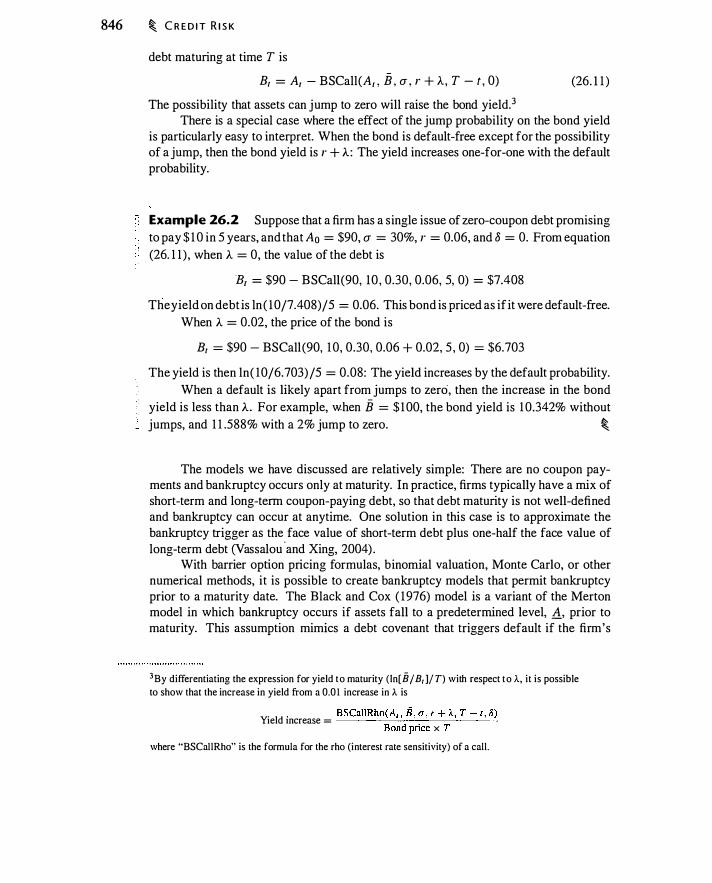
846 � C R E D I T R I S K

debt maturing at time T is

B, = A, - BSCall(A, , B , CJ , r + A, T - t , 0) (26. 1 1 )

The possibility that assets can jump to zero will raise the bond yield.3 There is a special case where the effect of the jump probability on the bond yield

is particularly easy to interpret. When the bond is default-free except for the possibility of a jump, then the bond yield is r + A: The yield increases one-for-one with the default probability.

Example 26.2 Suppose that a firm has a s ingle issue of zero-coupon debt promising to pay $ 1 0 in 5 years, and that Ao = $90, a = 30%, r = 0.06, and 8 = 0. From equation (26. 1 1 ) , when A = 0, the value of the debt is

B, = $90 - BSCall(90, 10 , 0.30, 0.06, 5, 0) = $7.408

The yield on debt is ln ( l 0/7.408)/5 = 0.06. This bond is priced as if it were default-free. When A = 0.02, the price of the bond is

B, = $90 - BSCall (90, 1 0, 0.30, 0.06 + 0.02, 5 , 0) = $6.703

The yield is then ln( l0/6.703) /5 = 0.08: The yield increases by the default probability. When a default is likely apart from jumps to zero, then the increase in the bond

yield is less than A. For example, when B = $ 100, the bond yield is 1 0.342% without jumps, and 1 1 .588% with a 2% jump to zero. �

The models we have discussed are relatively simple: There are no coupon pay­ments and bankruptcy occurs only at maturity. In practice, firms typically have a mix of short-term and long-term coupon-paying debt, so that debt maturity is not well-defined and bankruptcy can occur at anytime. One solution in this case is to approximate the bankruptcy trigger as the face value of short-term debt plus one-half the face value of long-term debt (Vassalou 'and Xing, 2004) .

With barrier option pricing formulas, binomial valuation, Monte Carlo, or other numerical methods, it is possible to create bankruptcy models that permit bankruptcy prior to a maturity date. The Black and Cox ( 1 976) model is a variant of the Merton model in which bankruptcy occurs if assets fall to a predetermined level, A_, prior to maturity. This assumption mimics a debt covenant that triggers default if the firm's

3By differentiating the expression for yield to maturity (ln[B I B, ]f T) with respect to A, i t is possible to show that the increase in yield from a 0.0 I increase in A is

. BSCallRho(A, , B, a, r + A, T - t, 8) Yield mcrease = ----::-.:...:..,.....:...,...:.._-=.:....__.:..._:_ Bond price x T

where "BSCallRho" is the formula for the rho (interest rate sensitivity) of a call .

B O N D RAT I N G S A N D D E FAU LT EX P E R I E N C E � 847

finanical condition worsens sufficiently. Equity in this model is a call option that knocks out if A1 :S .:1_.

26.3 B OND RATINGS AND DEFAULT EXPERIENCE

Bond ratings provide a measure of the credit risk for specific bonds . Such ratings, which are provided by third parties, attempt to measure the likelihood that a company will default on a bond.4 In the United States, the Securities and Exchange Commission (SEC) identifies specific credit-rating firms as Nationally Recognized Statistical Rating Organizations (NRSROs ). The history and significance of this designation was explained by the chairman of the SEC in congressional testimony:5

The Commission originally used the term "Nationally Recognized Sta­tistical Rating Organization," or NRSRO, with respect to credit rating agen­cies in 1 975 solely to differentiate between grades of debt securities held by broker-dealers as capital to meet Commission capital requirements. Since that time, ratings by NRSROs have become benchmarks in federal and state legislation, domestic and foreign financial regulations and privately negotiated financial contracts .

Moody's rates bonds using the designations Aaa, Aa, A, Baa, Ba, B , Caa, Ca, and C. Within each ratings category, bonds may be further rated as a 1 , 2, or 3, with 1 denoting the highest quality within a category. Standard and Poor's and Fitch have a similar rating system, using the designations AAA, AA, A, BBB, BB, B , CCC, CC, C.

The market distinguishes between "investment grade" (a rating of Baa!BBB or above) and "below-investment grade" or "speculative grade" (a rating below Baa!BBB) bond. Some investors are permitted to hold only investment grade bonds, and some contracts have triggers based upon whether a company's bond rating is investment grade. For example, prior to Enron's bankruptcy, some of the company's deals contained clauses requiring that Enron make payments if Enron lost its investment grade status. Enron 's financial difficulties were worsened when its rating fell below investment grade.

Using Ratings to Assess Bankruptcy Probability

A company that goes bankrupt will typically have had ratings downgrades prior to bankruptcy. By looking at the frequency with which bonds experience a ratings change,

4Companies pay ratings agencies to have their bonds rated. Some have criticized this practice, arguing that payment for ratings creates a conflict of interest. 5 "Testimony Concerning The State of the Securities Industry," by William H. Donaldson Chairman, U.S. SEC, U.S. Senate Committee on Banking, Housing, and Urban Affairs, March 9, 2005. As of mid-2005, five firms were recognized as NRSROs: Moody's Investor Services, Standard and Poor's, Fitch Ratings, Dominion Bond Rating Service, and A.M. Best.

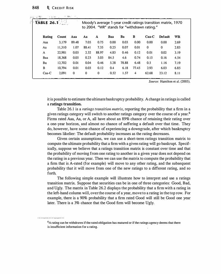
848 � C R E D IT R I S K

' TABLE 26 . 1 '

Moody's average 1 -year credit ratings transition matrix, 1 970 to 2004. "WR" stands for "withdrawn rating."

Rating Count Aaa A a A Baa Ba B Caa-C Default WR Aaa 3, 1 79 89.48 7.05 0.75 0.00 0.03 0.00 0.00 0.00 2.69

A a 1 1 ,3 1 0 1 .07 88.4 1 7.35 0.25 0.07 0.0 1 0 0 2.83

A 22,98 1 0.05 2.32 88.97 4.85 0.46 0. 1 2 0.0 1 0.02 3. 1 9

Baa 1 8,368 0.05 0.23 5 .03 84.5 4.6 0.74 0. 1 5 0. 1 6 4.54

B!! 1 2,702 0.0 1 0.04 0.46 5.28 78.88 6.48 0.5 1 . 1 6 7. 1 9

B 1 0,794 0.0 1 0.03 0. 1 2 0.4 6. 1 8 77.45 2.93 6.03 6.85

Caa-C 2,09 1 0 0 0 - 0.52 1 .57 4 62.68 23. 1 2 8 . 1 1

Source: Hamilton et al. (2005).

it is possible to estimate the ultimate bankruptcy probability. A change in ratings is called a ratings transition.

Table 26. 1 is a ratings transition matrix, reporting the probability that a firm in a given ratings category will switch to another ratings category over the course of a year.6 Firms rated Aaa, Aa, or A, all have about an 89% chance of retaining their rating over a one-year horizon, and almost no chance of suffering a default over that time. They do, however, have s'ome chance of experiencing a downgrade, after which bankruptcy becomes likelier: The default probability increases as the rating decreases.

Given certain assumptions, we can use a short-term ratings transition matrix to compute the ultimate probability that a firm with a given rating will go bankrupt. Specif­ically, suppose we believe that a ratings transition matrix is constant over time and that the probability of moving from one rating to another in a given year does not depend on the rating in a previous year. Then we can use the matrix to compute the probability that a firm that is A-rated (for example) will move to any other rating, and the subsequent probability that it will move from one of the new ratings to a different rating, and so forth.

The following simple example will illustrate how to interpret and use a ratings transition matrix. Suppose that securities can be in one of three categories: Good, Bad, and Ugly. The matrix in Table 26.2 displays the probability that a firm with a rating in the left-hand column will, over the course of a year, move to a rating in the top row. For example, there is a 90% probability that a firm rated Good will still be Good one year later. There is a 3% chance that the Good firm will become Ugly.

6 A rating can be withdrawn if the rated obligation has matured or if the ratings agency deems that there

is insufficient information for a rating.

From:

B O N D RATI N GS AN D D E FA U LT EX PE R I E N C E � 849

Ratings transition matrix. The entry in the ith row and jth column is the probabi l ity that a firm wil l , over one year, move from type i to type j.

To: Good Bad Ugly

Good 0.90 0.07 0.03 Bad 0. 1 5 0.75 0. 1 0

Ugly 0.06 0. 14 0.80

Notice that each row sums to one. This means that after one year each firm must be in one of the three categories. By contrast, in Table 26. 1 , there is a "Withdrawn Rating" category, indicating that a firm has for some reason dropped out of the Moody's rating universe.

We can use the transition matrix to compute the probability that a firm rated Good will still be Good two years from now. To perform this calculation, recognize that there are three different paths by which a firm that is now Good can still be Good in two years.

o There is a 90% chance that a Good firm remains Good over one year. There is therefore an 8 1 % (0.9 x 0.9) probability that the firm will be Good for both years.

o There is a 7% probability that the firm will be Bad next year, in which case there is a 15% chance the firm will be come Good the subsequent year. There is therefore a 1 .05% (0.07 x 0. 1 5) probability that the firm will go from Good to Bad and then back to Good.

• Finally, there is a 3% probability that the firm will become Ugly, and then a 6% probability that it will become Good again. There is therefore a 0. 1 8% (0.03 x 0.06) probability that the firm become Ugly and then Good.

The total probablity that a Good firm will still be Good in two years is therefore 82.23% :

(0.90 X 0.90) + (0.07 X 0 . 15 ) + (0.03 X 0.06) = 0.8223

In order to perform this calculation, it may at first seem necessary to enumerate the pos­sible transitions. Notice, however, that the calculation entails multiplying each element of the the first row of the transition matrix by the corresponding element of the first column, and then summing the results. It turns out that if we wish to know all possible transitions over a two-year period, we can construct a new matrix from the one-year transition matrix, where the element in the i th row and j th column of the new matrix is created by multiplying the i th row of the original matrix by the j th column of the original matrix and summing the results. Table 26.3 shows the result.

850 � C R E D IT R I S K

Ratings transition probabil ities after two years.

To: Good Bad Ugly

Good 0.8223 0. 1 1 97 0.0580 From: Bad 0.2535 0.5870 0. 1595

Ugly 0. 1 230 0.22 1 2 0.6558

In order to compute the ratings distribution after three years, we can duplicate the procedure, only taking the two-year matrix and multiplying it by the one-year matrix. This is the same as multiplying the one-year matrix by itself twice.

In general, let p (i, t; j, t + s) denote the probability that, over an s-year horizon, a firm will move from the rating in row i to that in column j. The entries in Table 26. 1 give us p (i, t; j, t + 1 ) . Suppose there are n ratings. Over 2 years, the probability of moving from rating i to rating j is

II p(i , t ; j, t + 2) =

L p(i , t ; k, t + I ) X p(k, t + 1 ; j, t + 2)

k=t

From the 2-year transitions we can go to 3 years, and then 4, and so on. Given the s - 1 -year transition probabilities, the s-year transition probability is

II p(i , t ; j, t + s) =

L p(i, t ; k, t + s - 1 ) x p(k, t + s - 1 ; j, t + s) (26. 1 2) k=l

Thus, a transition probability matrix can be used to tell us the probability that a firm will go bankrupt after a given period of time.

The long-term experience of bonds with a given rating is reported in Table 26.4. Note that if a bond has a Aaa rating, even after 20 years there is only a 1 .54% chance it will have gone bankrupt. However, if a bond is below-investment grade, there is a 47% chance of bankrutpcy over a 20-year horizon.

Recovery Rates

There is also historical information about recovery rates. Table 26.5 displays historical average recovery rates for different kinds of bonds. As you would expect, bonds desig­nated as more senior have higher recovery rates. When we modeled debt with different priorities in Section 1 6. 1 , we assumed that junior debt was not paid at all if senior debt was not completely repaid. This rule for assigning payments is called absolute priority.

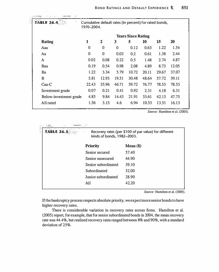
Rating

Aaa

A a

A

Baa

Ba

B

Caa-C

Investment grade

B O N D RATI N GS A N D D E FA U LT EX P E R I E N C E � 851

Cumulative default rates (in percent) for rated bonds, 1 970-2004.

Years Since Rating 1 2 3 5 10 15

0 0 0 0. 1 2 0.63 1 .22

0 0 0.03 0.2 0.6 1 1 .38

0.02 0.08 0.22 0.5 1 .48 2.74

0. 1 9 0.54 0.98 2.08 4.89 8.73 1 .22 3 .34 5 .79 1 0.72 20. 1 1 29.67 5 .8 1 1 2.93 19.5 1 30.48 48.64 57.72

22.43 35.96 46.7 1 59.72 76.77 78.53 0.07 0.2 1 0.4 1 0.92 2.3 1 4. 1 8

20

1 .54

2.44

4.87

1 2.05

37.07

59. 1 1

78.53

6.3 1

Below-investment grade 4.85 9.84 14.43 2 1 .9 1 33.6 1 42. 1 3 47.75

All rated

. · ' , . . . , :· ... _· · · · · TAB L E 26.5 ::- . .

1 .56 3 . 15 4.6 6.94 1 0.53 1 3 .5 1 1 6. 1 3

Source: Hamilton et al. (2005) .

Recovery rates (per $ 1 00 of par value) for d ifferent kinds of bonds, 1 982-2003 .

Priority Mean ($)

Senior secured 57.40

Senior unsecured 44.90

Senior subordinated 39. 10

Subordinated 32.00

Junior subordinated 28.90

All 42.20

Source: Hamilton et a! . (2005).

If the bankruptcy process respects absolute priority, we expect more senior bonds to have higher recovery rates.

There is considerable variation in recovery rates across firms. Hamilton et al . (2005) report, for example, that for senior subordinated bonds in 2004, the mean recovery rate was 44.4%, but realized recovery rates ranged between 8% and 90%, with a standard deviation of 25%.

852 � C R E D IT R I S K

Reduced Form Bankruptcy Models

The existence of data on corporate bond ratings, ratings changes, and defaults, suggests that we could construct statistical pricing models designed to match the behavior of bond prices. Such models are called reducedform models.1 In order to price bonds we require risk-neutral probabilities, so we cannot directly use historical data.

To understand how reduced form models work, consider the simplest version of such a model. Suppose a T -year bond promises to pay B at maturity and there is a zero recovery rate in the event of default. The risk-free rate is r and constant over time. If default follows a Poisson process with the risk-neutral intensity A, then the bond price depends only on time and on the occurrence of the jump. From Section 2 1 .5 , the partial differential equation for pricing the bond is

a B (t)- AB(t) = r B (t)

ar

With the boundary condition that B(T) = B , the bond price is8

B (t) = Be-(r+}.) (T-t) (26. 1 3 )

Given our strong assumptions that recovery rate is zero and interest rates are nonstochas­tic, it would seem a simple matter to price this bond by observing r and inferring A from data on defaults. The problem, however, is that equation (26. 1 3) presumes that A is a risk-neutral jump probability. Thus, we can infer A from bond prices but not from historical default data.

To understand the issue, suppose that bond defaults are idiosyncratic. In this case an investor can diversify default risk. We then expect A in equation (26. 13 ) to equal the historically observed A.

If defaults are correlated, however, then even a portfolio containing numerous bonds will encounter systematic losses from correlated defaults. Defaults occur when firms perform poorly-i.e. , when equity returns are low. Investors require a positive risk premium to hold such bonds, and therefore the risk-neutral default probability in equation (26. 1 3) will exceed the historical default probability.

A more general approach than that in equation (26. 1 3) uses ratings transitions. Equation (26. 1 3) does not take into account that default becomes more likely as ratings decline. With risk-neutral ratings transitions , it is possible to price bonds taking into account the various paths by which default can occur. Jarrow et al . ( 1 997) show how to use observed bond prices and historical ratings transitions to infer risk-neutral ratings transition probabilities .

7The reduced form approach was first used in Jarrow and Turnbull ( 1 995). See Duffie and S ingleton (2003) for a survey. 8Note that this is the same bond price solution we obtain in equation (26. 1 1 ) when B < A, and a = 0.

26.4 CREDIT INSTRUMENTS

C R E D IT I N STRU M ENTS � 853

The buyer of a corporate bond acquires both interest rate risk and the credit risk of a specific firm. A particular investor may wish to hold a different combination of these risks . There are ways to alter the mix: Investors can buy Treasury bonds instead of corporate bonds, thereby minimizing credit risk, or use interest rate derivatives to reduce or increase exposure to interest rate risk. More recently, it has become possible to use credit derivatives to trade the credit risk of a specific firm. In this section, we explain these instruments.

Collateralized Debt Obligations

A collateralized debt obligation (CDO) is a financial structure that repackages the cash flows from a set of assets. You create a CDO by pooling the returns from a set of assets and issuing financial claims to this pool. The CDO claims reapportion the returns on the asset pool. Typically, CDO claims are tranclzed, meaning that the different CDO claims have differing priorities with respect to the cash flows generated by the collateral. With a CDO, it is possible to take a group of risky bonds, for example, and create new claims, some of which are less risky than the original bonds, and others which are riskier.

Given this general description, there are many different ways a CDO can be struc­tured. First, the asset pool can be a fixed set of assets, in which case the CDO is static. If instead a manager buys and sells assets, the CDO is managed. Second, the CDO claims can directly receive the cash flows generated by the pool assets ; this is a cash flow CDO. Alternatively, the CDO claims can receive payments based on cash flows and the gain or loss from asset sales; this is a market value CDO.

There are at least two reasons for creating CDOs. First, financial institutions will sometimes want to securitize assets, effectively removing them from the institution's balance sheet by selling them to other investors. A CDO can be used to accomplish this, in which case it is a balance sheet CDO. Second, a CDO can be created in response to institutional frictions. For example, some investors are permitted to hold only investment grade b(;mds. As we will see below, CDOs can potentially be used to create investment grade bonds from a pool of noninvestment grade bonds. This is called an arbitrage CDO.

CDOs are relatively complex financial structures. The box included here provides an example of the legal arguments that sometimes result.

A CDO with independent defaults A simple example can illustrate how CDOs work. Suppose that there are three risky, speculative-grade bonds that each promise to pay $ 1 00 in one year. Defaults are independent and occur only at maturity of the bond. Each bond has a 10% risk-neutral probability of default and a 40% recovery rate, and the risk-free rate is 6%. The price of each bond is

e-0·06 [ ( 1 - 0. 1 ) X $ 1 00 + 0. 1 X $40] = $88.526

The yield on each bond is ln ( I 00/88.526) = 0. 1 2 1 9.

854 � C R E D IT R I S K

"Russ ian Dol l" CDOs

Considering its giant size, the decade-old credit-derivatives market is remarkably free of public squabbles . . . . [However] a battle in public would be of great interest to outsiders who would like to understand the market better. Such a fight is looming.

. . . Some CDOs, known as "Russian dolls,"· contain investments in other CDOs, making their monitoring extremely complicated. To make matters more difficult ­still, some CDOs are actively managed-i.e., the composition of the underlying portfolio can be changed by the asset manager.

In December 2000 Barclays, a big British bank, launched a Russian-doll CDO called Corvus (the Latin for "crow"), with a face value of $950m in tranches rated from AAA to B. Corvus performed badly, particularly after September 1 1 th 200 I . Fitch began to downgrade it in December 2002, and in early 2003 took the unprecedented step of -

publishing details of the Corvus portfolio on its web site. It included some unexpected stuff-for instance, exposure to airline leases

. . . ... ... · . . · ·

and loans for prefabricated-housing in America. It also had exposure to other CDOs, all constmcted by Barclays, some of which were never sold externally. By September 2003 the top three tranches of the CDO had fallen below a BBB rating (to ''junk" status) [see Table 26.6] . The other four tranches were rated CCC or lower. A similar Barclays CDO, called Nerva, fared even worse. Investors were not amused: AAA ratings are not meant to deteriorate so rapidly . . . .

If the case [a suit by HSH Nordbank, a German bank] does come to court, others will get to see how these complex financial instruments are put together and managed. One question for the court is whether Barclays correctly managed the potential conflict of interest when selecting credit risks from its own exposures for the CDO portfolio. Investors were not given details of each credit; Barclays argues that such disclosure was not required by the terms of the CDO. "The allegations in the suit are without merit," says a spokesman for the bank.9

So11rce: "Russian Doll,"' The Economist, September 23, 2004, p. 87.

Now suppose that there are investors wishing to invest in bonds, but some investors are happy to hold a speculative grade bond, while others seek safer bonds. We can create a CDO to rearrange the cash flows from a pool of bonds, in order to accomodate the different kinds of investors. The structure of the CDO is illustrated in Figure 26. 1 . The total promised payoff on the three bonds is $300; the CDO apportions this payoff among three tranches of unequal size. The senior tranche ($ 140) receives first claim to the bond payments, the mezzanine tranche ($90) has the next claim, and the subordinated tranche ($70) receives whatever is left. For the bond which is i th in line, with a promised

9The suit was settled out of court in February 2005.

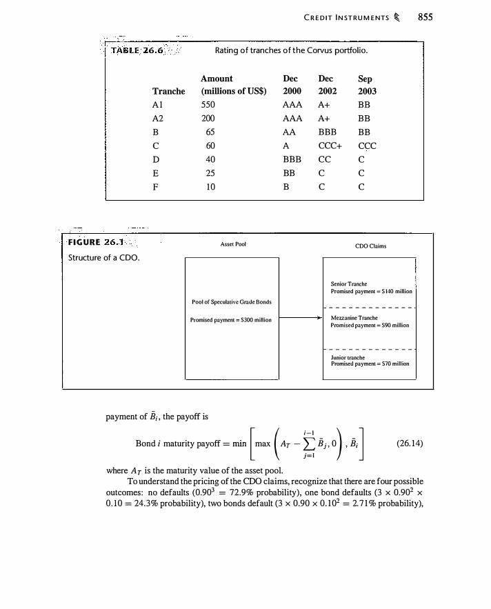
C R E D IT I N STRU M ENTS � 855

Rating of tranches of the Corvus portfolio.

Amount Dec Dec Sep Tranche (millions of US$) 2000 2002 2003 A I 550 AAA A+ BB

A2 200 AAA A+ BB

B 65 AA BBB BB

c 60 A CCC+ CCC

D 40 BBB cc c

E 25 BB c c

F 10 B c c

F I G U R E 26.1 Asset Pool COO Claims

Structure of a CDO.

Senior Tranche

Promised payment ; S 140 million

Pool of Speculative Grade Bonds - - - - - - - - - - - - -Mezzanine Tmnche Promised payment ; $300 million Promised payment ; S90 million - - - - - - - - - - - - -Junior tranche Promised payment ; S70 mill ion

payment of B; , the payoff is

Bond i maturity payoff � min [ mrut ( Ar -� B i , 0) , B,] where Ar is the maturity value of the asset pool.

(26. 14)

To understand the pricing of the CDO claims, recognize that there are four possible outcomes: no defaults (0.903 = 72.9% probability), one bond defaults (3 x 0.902 x 0. 10 = 24.3% probability), two bonds default (3 x 0.90 x 0. 1 02 = 2. 7 1 % probability),

856 � C R E D IT R I S K

Pricing of COO i n Figure 26. 1 , assuming that bond defaults are uncorrelated. Promised payoffs to the bonds are $ 1 40 (senior), $90 (mezzanine), and $ 70 (subordinated).

Number of Total Bond Payoff Defaults Probability Payoff Senior Mezzanine Subordinated

0 0.729 300 140 90 70

1 0.243 240 140 90 10

2 ' 0.027 1 80 140 40 0

3 0.00 1 1 20 120 0 0

Price 1 3 1 . 828 83 .403 50.347

Yield 0.0601 0.076 13 0.3296

Default probability 0.00 10 0.0280 0.27 1 0

Average recovery rate 0.857 1 0.4286 0. 1 28 1

and three bonds default (0. 1 03 = 0. 1 % probability). To compute the price of a CDO tranche, we can compute the expected_payoff of the tranche using the risk-neutral default probabilities.

The CDO pricing is illustrated in Table 26.7. Note that the senior tranche is almost risk-free. The only time the senior tranche is not fully paid is in the unlikely (0. 1 % probability) event that all three bonds default. In that case, the senior tranche receives $ 1 20, a recovery rate of85.7%. S ince i t is almost paid in full, investors will pay $ 1 3 1 .828 for the senior tranche, which is a yield of 6.02%.

The mezzanine tranche is fully paid if there is one default, but it is not fully paid if there are two or three defaults. The yield is 7 .6 1 % and the average recovery rate is 40/90 x 0.027/0.028 = 0.4285. Finally, the subordinated tranche receives less than full payment if there are any defaults. Consequently, it is priced to yield 32.96%. Note that the sum of the prices of the three tranches is $265 .58. As you would expect, this is the same as the price of the three bonds put into the asset pool .

This example might remind you of the discussion of tranched debt in Chapter 1 6, especially Table 16. 1 . The idea is exactly the same, except that instead of valuing claims on corporate assets (the bonds in Chapter 1 6) , we are valuing claims on a pool of corporate bonds.

A CDO with correlated defaults In the preceding example we assumed that the bonds were uncorrelated. As you might have guessed, this is an important assumption. Table 26.8 shows how the CDO tranches are priced if the bonds are perfectly correlated-i.e. ,

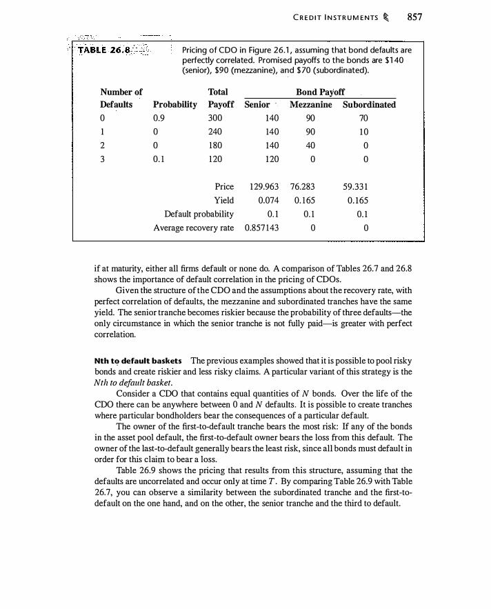
Number of Defaults

0

1

2

3

C R E D IT I N STR U M ENTS � 857

Pricing of COO in Figure 26.1 , assuming that bond defaults are perfectly correlated. Promised payoffs to the bonds are $1 40 (senior), $90 (mezzanine), and $ 70 (subordinated).

Total Bond Payoff Probability Payoff Senior · Mezzanine Subordinated

0.9 300 140 90 70

0 240 140 90 1 0 0 1 80 140 40 0 0. 1 1 20 1 20 0 0

Price 1 29.963 76.283 59.33 1

Yield 0.074 0. 1 65 0. 1 65 Default probability 0. 1 0. 1 0. 1

Average recovery rate 0.857 143 0 0

if at maturity, either all firms default or none do. A comparison of Tables 26.7 and 26.8 shows the importance of default correlation in the pricing of CDOs.

Given the structure of the CDO and the assumptions about the recovery rate, with perfect correlation of defaults, the mezzanine and subordinated tranches have the same yield. The senior tranche becomes riskier because the probability of three defaults-the only circumstance in which the senior tranche is not fully paid-is greater with perfect correlation.

Nth t� default baskets The previous examples showed that it is possible to pool risky bonds and create riskier and less risky claims. A particular variant of this strategy is the Nth to default basket.

Consider a CDO that contains equal quantities of N bonds. Over the life of the CDO there can be anywhere between 0 and N defaults . It is possible to create tranches where particular bondholders bear the consequences of a particular default.

The owner of the first-to-default tranche bears the most risk: If any of the bonds in the asset pool default, the first-to-default owner bears the loss from this default. The owner of the last-to-default generally bears the least risk, since all bonds must default in order for this claii:Jl to bear a loss.

Table 26.9 shows the pricing that results from this structure, assuming that the defaults are uncorrelated and occur only at time T . By comparing Table 26.9 with Table 26.7, you can observe a similarity between the subordinated tranche and the first-to­default on the one hand, and on the other, the senior tranche and the third to default.

858 � C R E D IT R I S K

.· . . . . . •

. TABLE 26 � 9 i Pricing o f Nth to default bonds. Assumes the bonds owned as assets have uncorrelated defau lts .

Probability Payoffs Expected Default Probability N or More Default No Default Payoff Price Yield

First 0.243 0.27 1 40 100 83 .74 78.863 0.237

Second 0.027 0.028 40 100 98.32 92.594 0.077

Third 0.00 1 0.00 1 40 100 99.94 94. 1 20 0.06 1

Figure 26.2 illustrates the pricing of Nth to default bonds for a 10-bond pool assuming default correlations of 0, 0.25, and 1 . 10 Again, we assume defaults occur only at time T. The result for a default correlation of 1 is like that in Table 26. 10 : When one bond defaults, all bonds default, so all claims have the same yield. The graphs for correlations of 0 and 0.25 show significant differences for yields for low numbers of defaults. The first-to-default tranche, for example, has a yield of 16.02% when defaults are uncorrelated and 1 3 .5 1 % when the default correlation is 0.25. This again illustrates that Nth to default baskets are a way to speculate on default correlations.

Credit Default Swaps and Related Structures

Credit derivatives, which have existed since the early 1990s, are contracts that permit the trading and hedging of credit risk. Credit derivatives permit institutions to hedge credit risk, in much the same way that, for example, gold futures permit the hedging of gold price risk. Table 26. 1 1 shows that the outstanding notional principal covered by credit default swaps, an important kind of credit derivative, has grown significantly over the

1 0How do we generate a default correlation of0.25 among ten bonds? We can generate ten independent

normally distributed random variables and create correlated normal random variables, z; , using the

Cholesky decomposition (equation 1 9 . 1 8). Following this procedure, each painvise correlation is 0.25.

Assuming a 1 0% unconditional default probability, a firm defaults if z; < - 1 .28 1 6. Note that once

we use this method, we can also let z; determine when in time the default occurs; we simply interpret

a smaller z; to mean that default occurs earlier. It is then necessary to specify a distribution for default

times. For example, suppose default occurs with a constant Poisson intensity. Then the time to default

is exponentially distributed, so that

Pr(default < t) = I - e-ht

Given this assumption, the default time is then r = - ln[N (z; ) ]/ /z . See Duffie and Yurday (2004a),

Li ( 1 999), and Watkinson and Roosevelt (2004) for a discussion of pricing credit tranches with default

correlations modeled in this fashion.

-

Number of Defaults

C R E D IT I N STR U M E NTS � 859

N

� o: 1 1::::: • • p�25 l f o:� I ;: p=0

:

2

s l 0 0 1 2 3 4 5 6 7 8 9 1 0 ° o 2 4 6 8 1 0 Number of Defaults N

fo: l[ p=:oo I F�o� � • • • p=1 :00 I

0 0 1 2 3 4 5 6 7 8 9 1 0 0 2 4 6 8 1 0 Number of Defaults N

Pricing of an Nth to default basket containing equal quantities of 1 0 bonds, each with a 1 0% probabil ity of defau lt.

TABLE 26 . 1 0 Pricing of Nth to default bonds. Assumes the bonds owned as assets have perfectly correlated defaults.

Probability Payoffs Expected Default Probability N or More Default No Default Payoff Price Yield

First 0. 1 00 0: 1 00 40 1 00 94.000 88.526 0. 1 22

Second 0. 1 00 0 . 1 00 40 1 00 94.000 88.526 0. 1 22

Third 0. 1 00 0. 1 00 40 100 94.000 88 .526 0. 1 22

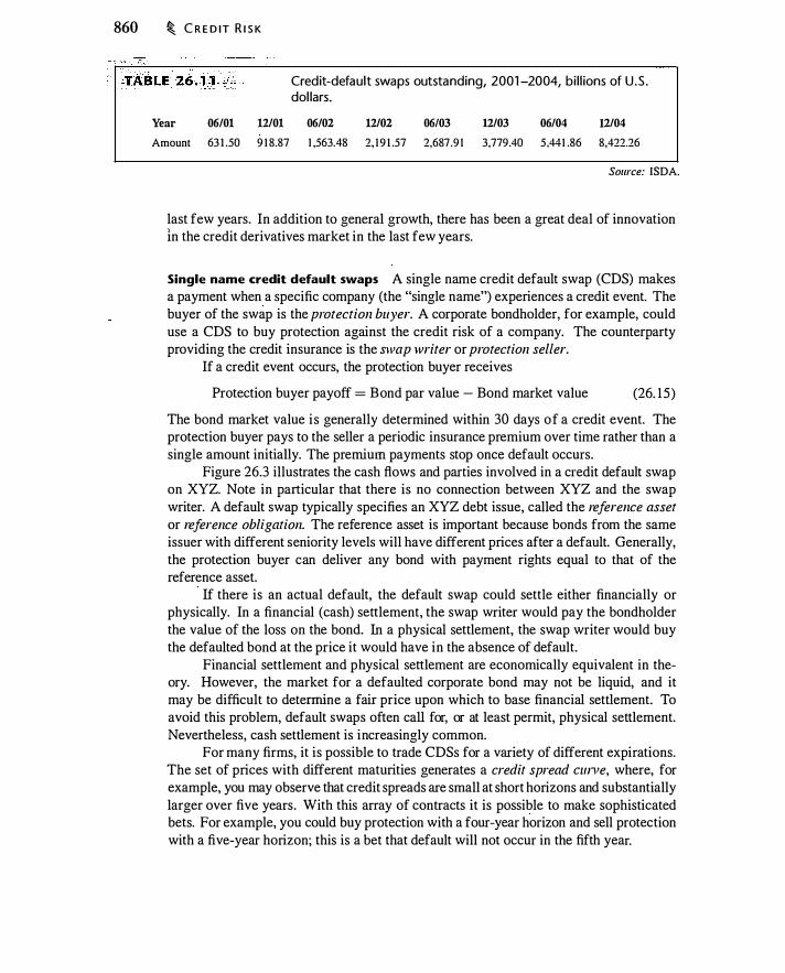
860 � C R E D IT R I S K

Credit-default swaps outstanding, 2001 -2004, bi l l ions of U.S . dol lars.

Year 06/01 12/01 06/02 12/02 06/03 12/03 06/04 12/04 Amount 63 1 .50 9 1 8.87 1 ,563.48 2, 1 9 1 .57 2,687.9 1 3,779.40 5 ,441 .86 8,422.26

Source: ISDA.

last few years. In addition to general growth, there has been a great deal of innovation in the credit derivatives market in the last few years.

Single name c:redit default swaps A single name credit default swap (CDS) makes a payment when a specific company (the "single name") experiences a credit event. The buyer of the swap is the protection buyer. A corporate bondholder, for example, could use a CDS to buy protection against the credit risk of a company. The counterparty providing the credit insurance is the swap writer or protection seller.

If a credit event occurs, the protection buyer receives

Protection buyer payoff = Bond par value - Bond market value (26. 15 )

The bond market value i s generally determined within 30 days of a credit event. The protection buyer pays to the seller a periodic insurance premium over time rather than a single amount initially. The premium payments stop once default occurs.

Figure 26.3 illustrates the cash flows and parties involved in a credit default swap on XYZ. Note in particular that there is no connection between XYZ and the swap writer. A default swap typically specifies an XYZ debt issue, called the reference asset or reference obligation. The reference asset is important because bonds from the same issuer with different seniority levels will have different prices after a default. Generally, the protection buyer can deliver any bond with payment rights equal to that of the reference asset.

If there is an actual default, the default swap could settle either financially or physically. In a financial (cash) settlement, the swap writer would pay the bondholder the value of the loss on the bond. In a physical settlement, the swap writer would buy the defaulted bond at the price it would have in the absence of default.

Financial settlement and physical settlement are economically equivalent in the­ory. However, the market for a defaulted corporate bond may not be liquid, and it may be difficult to determine a fair price upon which to base financial settlement. To avoid this problem, default swaps often call for, or at least permit, physical settlement. Nevertheless, cash settlement is increasingly common.

For many firms, it is possible to trade CDSs for a variety of different expirations. The set of prices with different maturities generates a credit spread Cllll'e, where, for example, you may observe that credit spreads are small at short horizons and substantially larger over five years. With this array of contracts it is possible to make sophisticated bets. For example, you could buy protection with a four-year horizon and sell protection with a five-year horizon; this is a bet that default will not occur in the fifth year.

. ·

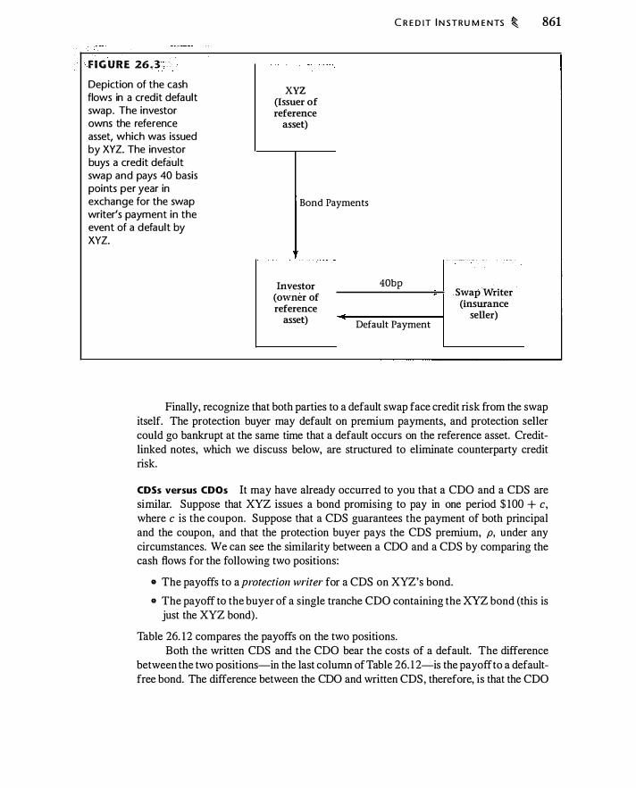
C R E D IT I N STRU M E NTS � 861

F IGURE 26 . 3 ··-·-- - · ·

Depiction of the cash XYZ

flows in a credit default (Issuer of swap. The investor reference owns the reference asset) asset, which was issued by XYZ. The investor buys a credit default swap and pays 40 basis points per year in exchange for the swap Bond Payments writer's payment in the event of a default by XYZ.

. . . . .. · · · · · · · · · ··-··

Investor 40bp Swap .Writer (owner of

reference (insurance

asset) seller) Default Payment

Finally, recognize that both parties to a default swap face credit risk from the swap itself. The protection buyer may default on premium payments, and protection seller could go bankrupt at the same time that a default occurs on the reference asset. Credit­linked notes, which we discuss below, are structured to eliminate counterparty credit risk.

CDSs versus CDOs It may have already occurred to you that a CDO and a CDS are similar. Suppose that XYZ issues a bond promising to pay in one period $ 100 + c, where c is the coupon. Suppose that a CDS guarantees the payment of both principal and the coupon, and that the protection buyer pays the CDS premium, p, under any circumstances. We can see the similarity between a CDO and a CDS by comparing the cash flows for the following two positions:

e The payoffs to a protection writer for a CDS on XYZ's bond.

e The payoff to the buyer of a single tranche CDO containing the XYZ bond (this is just the XYZ bond) .

Table 26. 12 compares the payoffs on the two positions. Both the written CDS and the CDO bear the costs of a default. The difference

between the two positions-in the last column of Table 26. 1 2-is the payoff to a default­free bond. The difference between the CDO and written CDS, therefore, is that the CDO

862 � C R E D I T R I S K

Comparison of a written CDS o n XYZ's bond, and a COO containing on ly an XYZ bond.

Event

No default

Default

CDO Buyer

$ I OO + c B l

Position Written CDS

p p - [C$ 100 + c) - Bl ]

Difference (CDO - CDS)

$ 100 + c - p $ 1 00 + c - p

is funded, meaning that the investor pays for it fully at the outset, while the CDS is unfunded, meaning that the investor pays nothing at the outset and can have payment obligations in the future. We can think of the CDO as analogous to a prepaid forward on the bond, while the written CDS is a forward contract on the bond.

Pricing a Default Swap

An investor who buys a bond and a default swap on the bond owns a synthetic default -free bond. This observation suggests that the default swap premium should approximately equal the default premium on the bond. To make this more precise, suppose we simul­taneously undertake the following set of transactions:

• Buy protection with a CDS on $ 1 00 worth of senior bonds issued by XYZ. The default swap premium is p.

• Short-sell a $ 100 default-free floating rate note paying r . Suppose that we can short-sell the bond costlessly.

• Buy XYZ senior floating-rate notes paying c = r + a, with par value $ 100. The premium a = c - r is constant over time.

The short -sale of the default -free note funds the purchase of the defaultable note. These transactions require no initial cash flow.

Each period prior to termination, the net cash flow on the position is c - (r + p) . XYZ either defaults o r does not default prior to maturity of the CDS, s o that the default swap terminates in either of two ways:

• If the CDS matures and XYZ has not defaulted, sell the XYZ floating rate bond and use the $ 100 proceeds to buy the default-free floating rate note in order to close the short sale. (By using floating rate notes, we ensure that both bonds are worth $ 100 if there is no default.)

• If XYZ defaults, under the terms of the CDS, surrender the defaulted floating rate notes in exchange for $ 1 00. Use the $ 100 proceeds to buy the default-free floating rate note in order to close the short sale.

In either case, there is no net cash flow.

C R E D IT I N STRU M E NTS � 863

Since we can enter and close the position with no net cash flow, the interim cash flows should also equal zero, which implies that c - (r + p) = 0, or

p = c - r (26. 16)

In other words, the default swap premium equals the credit spread. Notice that we made very strong assumptions to reach this conclusion, so we

should not expect equation (26. 1 6) to hold exactly. In practice, we would need to take into account a variety of complications, including time variation in the credit spread, bonds having fixed coupons instead of being floating rate, and transaction costs (such as costs of short-selling) . Duffie ( 1 999) discusses the effects of many such complications.

An important question implicitly raised by this discussion is the definition of an "otherwise equivalent default-free bond." It seems natural to use government bonds as a benchmark, but government bonds can be unique in certain respects. Prices of government bonds may include a liquidity premium and sometimes reflect special tax attributes (for example, in the United States, federal government bonds are exempt from state taxes) . Houweling and Vorst (2001 ) estimate a credit swap pricing model and find that, empirically, credit swap premiums are more related to the interest rate swap curve than to the government bond yield curve. This linkage between credit swaps and interest rate swaps suggests that the yield on an "equivalent default-free bond" is not the government bond curve, and in fact may not be directly observable. Rather the equivalent default-free yield may be inferred from the market for default swaps as the rate on the reference asset less the default swap premium.

Credit-linked notes A credit-linked note is a bond issued by one company with payments that depend upon the credit status (i.e., bankrupt or not) of a different company. For example, banks can issue credit-linked notes to hedge the credit risk of loans. To see how a credit-linked note works, suppose that bank ABC lends money to company XYZ. At the time of the loan, ABC creates a trust that issues notes: These are the credit­linked notes. The funds raised by the issuance of these notes are invested in bonds with a low probability of default (such as government bonds), which are held in the trust. lf XYZ remains solvent, ABC is obligated to pay the notes in fulL If XYZ goes bankrupt, the note-holders receive the XYZ loans and become creditors of XYZ. ABC takes possession of the securities in the trust. Thus, the credit-linked note is in effect a bond issued by ABC, which ABC does not need to repay in full if XYZ goes bankrupt. This structure eliminates a third-party insurance provider. Credit-linked notes can be rated and exchange-traded.

Because of the trust, the credit -linked notes can be paid in full even if ABC defaults. Thus, even though they are issued by ABC, the interest rate on the notes is determined by the credit risk of XYZ. An arrangement like this was used by Citigroup when it made loans to Enron in 2000 and 200 l . 1 1 When Enron went bankrupt in late 200 l, Citigroup

1 1 See Daniel Altman, "How Citigroup Hedged Bets on Enron," New York Times, February 8, 2002,

p. C I .

864 � C R E D IT R I S K

avoided losses o n over $ 1 billion i n loans because it had hedged the loans by issuing credit-linked notes.

Total rate of return swaps Total rate of return swaps, discussed in Chapter 8 , can also be used to hedge credit risk. These swaps are used less frequently than credit-default swaps. The difference between a total rate of return swap and the credit products we are discussing is that a total return swap for a bond makes payments based on changes in market value due to interest rate changes as well as due to credit changes. A CDS makes payments only if there is a credit event.

CDS Indices

A CDS index is an average of the premiums on a set of CDSs. Thus, a CDS index provides a way to track the overall market for credit. In this section we will discuss the kinds of structures and products that are traded.

To a first approximation, it is possible to replicate a CDS index by holding a pool of CDSs . 1 2 As with a single CDS, one party is a protection seller, receiving premium payments, and the other is a protection buyer, making the payments but receiving a payment from the seller if there is a credit event.

There are numerous ways in which a CDS index product can be structured and traded:

e A CDS index can be funded or unfunded. The unfunded version is like a credit default swap, except that the underlying asset is a basket of firms. The funded index is a note linked to the index with a collateral arrangement in case the note buyer had to make a payment.

e The claims are generally tranched in various ways, for example, simple priority or Nth to default.

e The underlying assets can represent different countries, currencies, maturities, or industries. · A 0-100% tranche on a CDS index can also be described as a synthetic CDO. The

returns on a CDS index reflect the performance of the bonds in the index, just as the returns on a CDO reflect the performance of the bonds in the asset pool.

Credit indices have had a relatively briefhistory. 1 3 There are a number of potential challenges in trading credit risk. Historically, the corporate bond market has been less liquid than the stock market. Trading volume for bonds is lower than for stocks, and bid-ask spreads have been higher. A large firm can have dozens of different bond issues outstanding.

1 2The replication may not be exact since a default index can define a credit event differently than a

single name CDS. For example, DJ TRAC-X, discussed below, specifies bankruptcy and failure to pay

as credit events. A single name CDS can have a broader definition.

1 3 See Duffie and Yurday (2004b) for an interesting account of the development of credit index products.

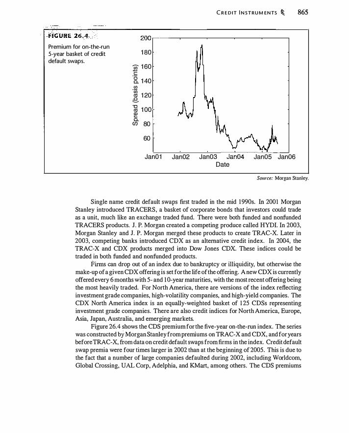
Premium for on-the-run 5-year basket of credit default swaps.

C R E D IT I N STRU M ENTS � 865

200 .-----�----�----�----�----�

1 80

(j) 1 60 -c ·g_ 1 40 en

-� 1 20 e. -g 1 00 Q) ....

0. (f) 80

60

Jan01 Jan02 Jan03 Date

Jan05 Jan06

Source: Morgan Stanley.

Single name credit default swaps first traded in the mid 1 990s. In 2001 Morgan Stanley introduced TRACERS, a basket of corporate bonds that investors could trade as a unit, much like an exchange traded fund. There were both funded and nonfunded TRACERS products. J. P. Morgan created a competing produce called HYDI. In 2003, Morgan Stanley and J. P. Morgan merged these products to create TRAC-X. Later in 2003, competing banks introduced CDX as an alternative credit index. In 2004, the TRAC-X and CDX products merged into Dow Jones CDX. These indices could be traded in both funded and nonfunded products.

Firms can drop out of an index due to bankruptcy or illiquidity, but otherwise the make-up of a given CDX offering is set for the life of the offering. A new CDX is currently offered every 6 months with 5- and 1 0-year maturities, with the most recent offering being the most heavily traded. For North America, there are versions of the index reflecting investment grade companies, high-volatility companies, and high-yield companies . The CDX North America index is an equally-weighted basket of 1 25 CDSs representing investment grade companies. There are also credit indices for North America, Europe, Asia, Japan, Australia, and emerging markets.

Figure 26.4 shows the CDS premium for the five-year on-the-run index. The series was constructed by Morgan Stanley from premiums on TRAC-X and CDX, and for years before TRAC-X, from data on credit default swaps from firms in the index. Credit default swap premia were four times larger in 2002 than at the beginning of 2005 . This is due to the fact that a number of large companies defaulted during 2002, including Worldcom, Global Crossing, UAL Corp, Adelphia, and KMart, among others . The CDS premiums

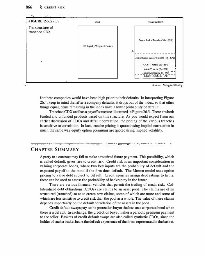
866 � C R E D IT R I S K

F IGURE 26.c.$l: _

The structure of tranched CDX.

cox

1 25 Equally Weighted Names

Tranched COX

Super Senior Tr•nche (30- 1 00%)

Junior Super Senior Tranche ( 1 5-30%)

AAA+ Tranche ( 1 0- 1 5�<)

A A A Tranche (6- IO%)

Junior Me>.zanine (3-6%) - - -Equily fmlicile (o.:-3%)- - -

Source: Morgan Stanley.

for these companies would have been high prior to their defaults. In interpreting Figure 26.4, keep in mind that after a company defaults, it drops out of the index, so that other things equal, firms remaining in the index have a lower probability of default.

Tranched CDX and has a payoff structure illustratecl in Figure 26.5 . There are both funded and unfunded products based on this structure. As you would expect from our earlier discussion of CDOs and default correlation, the pricing of the various tranches is sensitive to correlation. In fact, tranche pricing is quoted using implied correlation in much the same way equity option premiums are quoted using implied volatility.

- - ---�� --- ·-----�·--------� - -·· ___ _ .. ___ _ _

-'---':...c --�- �- - -�-- -- -��- --"�----.:...:.��:..;._ ----------- - ---

_ __ ·.:.'.·.::..'::.'"-"-' ' , , -_.,_-,>---�

CHAPTER S UMMARY

A party to a contract may fail to make a required future payment. This possibility, which is called default, gives rise to credit risk. Credit risk is an important consideration in valuing corporate bonds, where two key inputs are the probability of default and the expected payoff to the bond if the firm does default. The Merton model uses option pricing to value debt subject to default. Credit agencies assign debt ratings to firms; these can be used to assess the probability of bankruptcy in the future.

There are various financial vehicles that permit the trading of credit risk. Col­lateralized debt obligations (CDOs) are claims to an asset pool. The claims are often structured (tranched) so as to create new claims, some of which are more and some of which are less sensitive to credit risk than the pool as a whole. The value of these claims depends importantly on the default correlation of the assets in the pool.

Credit default swaps pay to the protection buyer the loss on a corporate bond when there is a default. In exchange, the protection buyer makes a periodic premium payment to the seller. Baskets of credit default swaps are also called synthetic CDOs, since the holder of such a basket bears the default experience of the firms represented in the basket,

P RO B LEMS ' 867

as with a CDO. A synthetic CDO can be funded (the investor pays fully at the outset) or nonfunded (there is no initial payment) .

The average premium on a basket of default swaps is effectively a credit index. These indices, such as Dow Jones CDX, serve as the basis for a variety of investment vehicles and investment strategies.

FURTHER READING

Both the actual traded credit contracts and pricing theory continue to evolve. Books with a practitioner perspective include Goodman and Fabozzi (2002) and Tavakoli (200 1 ) . Duffie ( 1 999) discusses the pricing of credit default swaps. Frameworks for analyz­ing_ credit risk are discussed in Credit Suisse Financial Products ( 1 997), J . P. Mor­gan ( 1 997), Kealhofer (2003a,b) and white papers on the Moody's KMV Web site, www.moodyskmv.com. A debate between advocates and critics of the KMV ap­proach is in the February 2002 issue of Risk (Kealhofer and Kurbat, 2002; Sobehart and Keenan, 2002).

Books with a more academic and theoretical perspective include Cossin and Pirotte (200 1 ) , Duffie and Singleton (2003) , Meissner (2005), and Schonbucher (2003). Duffie and Yurday (2004b,a) provide a blended discussion of the history of some of the prod­ucts, practical issues, and pricing models. Papers examining Merton-style models in­clude Jones et al . ( 1 984), Kim et al . ( 1 993), Leland ( 1994), Leland and Toft ( 1 996) and Longstaff and Schwartz ( 1 995). Empirical studies of Merton-style models include Anderson and Sundaresan (2000), Bharath and Shumway (2004), and Eom et al. (2004) . Shumway (200 1 ) estimates hazard models of bankruptcy. Johnson and Stulz ( 1 987), Hull and White ( 1 995), and Klein ( 1 996) consider how it affects prices of derivatives.

Data on bankruptcies are available from www.bankruptcydata.com. Simple summary data, such as the largest bankruptcies sorted by year, are available without charge.

PROB LEMS

For the first eight problems, assume that a firm has assets of $ 100, with u = 40%, ex = 15%, and 8 = 0. The risk-free rate is 8%.

26.1. The firm has a single outstanding debt issue with a promised maturity payment of $ 1 20 in 5 years. What is the probability of bankruptcy? What is the credit spread?

26.2. Suppose the firm issues a single zero-coupon bond with maturity value $ 1 00.

a. Compute the yield, probability of default, and expected loss given default for times to maturity of 1 , 2, 3, 4, 5, 1 0, and 20 years.

b. For each time to maturity compute the approximation for the yield:

p = r + _!_ x Prob Default x Expected loss given default T How accurate is the approximation?

868 � C R E D I T R I S K

26.3. Suppose the firm issues a single zero-coupon bond with time to maturity 3 years and maturity value $ 1 1 0.

a. Compute the price, yield to maturity, default probability, and expected recovery (E[BT I Default] ) .

b. Verify that equation (26.5) holds.

26.4. Suppose the firm issues a single zero-coupon bond.

a. Suppose the maturity value of the bond is $80. Compute the yield and default probability for times to maturity of 1, 2, 3, 4, 5, 1 0, and 20 years.

b. Repeat part (a), only supposing the maturity value is $ 1 20.

c. Does default probability increase or decrease with debt maturity? Ex­plain.

26.5. Repeat the ·previous problem, only compute the expected recovery value instead of the default probability. How does the expected recovery value change as time to maturity changes?

26.6. Suppose that there is a 3% per year chance that the firm's asset value can jump to zero. Assume that the firm issues 5-year zero coupon debt with a promised payment of $ 1 10. Using the Merton jump model, compute the debt price and yield, and compare to the results you obtain when the jump probability is zero.

26.7. Suppose the firm has a single �utstanding debt issue with a promised maturity payment of $ 1 20 in 5 years . Assume that bankruptcy is triggered by assets (which are observable) falling below $40 in value at any time over the life of the bond-in which case the bondholder receives $40 at that time-or by assets being worth less than $ 1 20 at maturity, in which case the the bondholder receives the asset value. What is the probability of bankruptcy over the life of the bond? What is the credit spread?

26.8. Repeat the previous problem, except that the time to maturity can be 1 , 2, 3, 4, 5, 1 0, or 20 years. How does the bond yield change with time to maturity?

For the next two problems, use this information on credit ratings . Suppose there are three credit ratings, F (first-rate), FF (future failure?), and FFF (fading, forlorn, and forsaken) . The transition matrix between ratings looks l ike this:

Rating From: F FF FFF

26.9. Consider a firm with an F rating.

F .9 . 1 5 . 1 0

Rating To:

FF FFF

.07 .03

.80 .05

.30 .6

a. What is the probability that after 4 years it will still have an F rating?

P RO B L E M S � 869

b. What is the probability that after 4 years it will have an FF or FFF rating?

c. From examining the transition matrix, are firms tending over time to become rated more or less highly? Why?

26.10. Consider two firms, one with an FF rating and one with an FFF rating. What is the probability that after 4 years each will have retained its rating? What is the probability that each will have moved to one of the other two ratings?

26.11. Suppose that in Figure 26.7 the tranches have promised payments of $ 160 (senior), $50 (mezzanine), and $90 (subordinated). Reproduce the table for this case, assuming zero default correlation.

26.12. Repeat the previous problem, only assuming that defaults are perfectly correlated.

26.13. Using Monte Carlo simulation, reproduce Tables 26.9 and 26. 10 . Produce a similar table assuming a default correlation of 25%.

26.14. Following Table 26.9, compute the prices of first, second, and Nth-to-default bonds assuming that defaults are uncorrelated and that there are 5, 1 0, 20, and 50 bonds in the portfolio. How are the Nth-to-default yields affected by the size of the portfolio?

26.15. Repeat the previous problem, assuming that default correlations are 0.25 .

PA R T S IX

APPENDIX A � '::.. : - - > ,· - �- _. -. - . - - - : --

The Greek Alphabet

'Ie u'e of Greek Jette<' i ' common i n writing about derivative' and mathematic' in general. Important concepts in this book are option characteristics that have the names of Greek letters such as "delta" and "gamma."

-

Table 1 . 1 presents the complete Greek alphabet, including both lowercase and uppercase forms. Some of the letters look like their Roman counterparts. Not all of these symbols will be used in the book.

- - - --- :

TABLE 1 . 1 The Greek alphabet.

alpha a A nu v N

beta f3 B xi � .::. gamma y r omicron 0 0 delta 8 ;:.,.. pi ][ TI epsilon E E rho p p zeta l; z sigma (J :E eta 1) H tau "[ T

theta e e upsilon v 1 iota I phi ¢ <I> kappa K K chi X X

lambda ).. A psi 1/f \II mu JL M omega w Q

873

ABPE�DIX B Continuous Compounding

I. thi' book we W<e both effective mmual intere" mte' and oontinuou;ly compounded interest rates. These are simply different conventions for expressing the same idea: If you invest $ 1 today, how much will you have after 1 year? One simple unambiguous way to answer this question is using zero-coupon bonds . If you invest $ 1 in zero-coupon bonds costing P (0, T) for a $ 1 maturity payoff at time T, then at time T you will have 1 / P (O, T) dollars . However, it is more common to answer the question using interest rates rather than zero-coupon bond prices.

Interest rates measure the rate of appreciation of an investment, but there are innu­merable ways of quoting interest rates. Continuous compounding turns out to provide a particularly s imple quoting convention, though it may not seem so simple at first. Since in practice option pricing formulas and other financial formulas make use of continuous compounding, it is important to be comfortable with it.

You might think that continuous compounding is not much used in the real world and, hence, there is no point in using it when studying derivatives . It is true that an auto dealer is likely to give you a blank stare if you inquire about the continuously compounded loan rate for your new car. However, continuous compounding does have advantages, and it is not often appreciated that almost all interest rate quoting conventions are complicated, some devilishly so. (If you doubt this, read Appendix 7 .A) .

B.l THE LANGUAGE OF INTEREST RATES

We begin with definitions. There are two terms that we will use often to refer to interest rates:

• Effective annual rate: If r is quoted as an effective annual rate, this means that if you invest $ 1 , n years later you will have ( 1 + r )" . If you invest x0 and earn X11 n years later, then the implied effective annual rate is (x11 jx0) 1 1" - I .

• Continously compounded rate: If r is quoted as an annualized continuously compounded rate, this means that if you invest $ 1 , n years later you will have er" . If you invest x0 and earn X11 n years later, then the implied annual continuously compounded rate is In (x11 fxo) / n .

Let's look at this definition i n more detail.

875

876 � C O NT I N U O U S C O M PO U N D I N G

B.2 THE LOGARITHMIC AND EXPONENTIAL FUNCTIONS

Interest rates are typically quoted as "r% per year, compounded n times per year." As every beginning finance student learns, this has the interpretation that you will earn an interest rate of rj n per period for n periods. Thus, if you invest $1 today, in 1 year you will have

In T years you will have

( I" ) " 1 + -II

( r )"T 1 + ­

- II (B . 1 )

What happens if we let n get very large, that is, i f interest i s compounded many times a year (even daily or hourly)? If, for example, the interest rate is 1 0%, after 3 years we will have

• ($ 1 + 0. 1 )3 = $ 1 .33 1 with annual compounding,

• ($ 1 + 0 . 1 / 1 2)36 = $ 1 .3482 with monthly compounding,

• ($ 1 + 0. 1 /365) 1 095 = $ 1 .34980 with daily compounding, and

• ($ 1 + 0 . 1 /8760)26280 = $ 1 .349856 with hourly compounding.

The exponential function is e-' , where e is a constant approximately equal to 2 . 7 1 828. If compounding is continuous-that is, if interest accrues every instant­then we can use the exponential function to compute future values. For example, with a 1 0% continuously compounded rate, after 3 years we will have a future value of

e0- 1 x3 = $ 1 .349859

Notice that assuming continuous compounding gives us a result very close to that assum­ing daily compounding. In Excel, we compute continuously compounded results using the built-in exponential function, exp. The above example is computed as exp(0. 1 x 3) .

Why does the exponential function work? The number e is defined as

( I" ) "T erT = lim 1 + -11---+ 00 II (B .2)

Thus, the expression defining e is the same expression used for interest compounding calculations, equation (B . I ) ! By using e, you can compute a future value.

If you know how much you have earned from a $ 1 investment, you can determine the continuously compounded rate of return by using the natural logarithm, ln. Ln is the inverse of the exponential function in that it takes a dollar amount and gives you a rate of return. In other words, if you apply the logarithmic function to the exponential function, you compute the original argument to the exponential function. Here is an example:

ln (er1 ) = rt

TH E LO G A R I T H M I C A N D EX P O N E N T I A L F U N CT I O N S � 877

Example 8.1 Suppose you have a zero-coupon bond that matures in 5 years. The price today is $62.092 for a bond that pays $ 1 00. The annually compounded rate of return is

($ 1 00/$62.092) 1 15 - l = 0. 10

The continuously compounded rate of return is

ln ($ 1 00/$62 .092) =

0.47655 = 0_0953 1

5 5 The continuously compounded rate of return of 9.53% corresponds to the annually com­pounded rate of return of l 0%. To verify this, observe that

e0.0953 = l . lO

Finally, note that

ln ( l . l O) = ln (e0·0953) = 0.0953

Changing Interest Rates

When we multiply exponentials, exponents add. So we have

Suppose you can invest for 4 years, earning a continouously compounded return of 5% the first 2 years and 6% the second 2 years . If you invest $1 today, after 4 years you will have

e2x0.05e2x0.06 = eO. I 0+0. 1 2 = $ 1 .246 1

We could of course do the same calculation using effective annual rates. For the first 2 years we earn e0·05 - 1 = 5 . 1 27%, and for the second 2 years, e0·06 = 6. 184%. The future value of $ 1 is

1 .05 1 272 1 .06 1 842 = $ 1 .246 1

This calculation gives us the same answer. What is the average annual rate earned over the 4 years? The average annual

continously compounded rate is

� ln ( l .24608) = 0.055

which is the average of 5% and 6%. However, if we express the answer in terms of effective annual rates, we get

1 .24608°·25 - l = 5 .654 1 %

This i s not the average of5 . 1 27% and 6. 1 84%, which i s 5 .6554. This makes calculations with continuous compounding easier.

878 � C O NT I N U O U S C O M P O U N D I N G

Symmetry for Increases and Decreases

On March 4, 1 999, the NASDAQ composite index closed at 2292.89. On March 1 0, 2000, the index closed at 5048.62. On January 2, 200 1 , the index closed at 229 1 .86, essentially the same level as in March 1 999. The percentage increase from March 1 999 to March 2000 was

5048 .62 --- - I = 120. 19% 2292.89

The subsequent decrease was

229 1 .86 --- - I - -54 60% 5048 .62

- .

When computing simple rates of return, a price can have an increase exceeding I OO%, but its decrease can never be greater than 100%.

We can do the same calculations using continuous compounding. The continuously compounded increase from March 1 999 to March 2000 was

ln (5048 .62/2292 .89) = 78.93%

while the subsequent decrease was

ln (229 1 .86/5048 .62) = -78.97%

When using continuous compounding, increases and det;:reases are symmetric. Moreover, if the index dropped to I 000, the continuously compounded return from

the peak would be

ln ( l 000/5048 .62) = - 16 1 .9 1 %

Continuously compounded returns can be less than - 100%.

PROBLEMS

B.l. a. A bond costs $67,032 today and pays $ 100,000 in 5 years. What is its continuou.sly compounded rate of return?

b. A bond costs $50 today, pays $ 1 00 at maturity, and has a continuously compounded annual return of 1 0%. In how many years does it mature?

c. An investment of $5 today pays a continuously compounded rate of 7.5%/year. How much money will you have after 7 years?

d. A stock selling for $ 1 00 is worth $5 1 year later. What is the continuously compounded return over the year? What if the stock price is $4? $3? $2? What would the stock price after 1 year have to be in order for the continuously compounded return to be -500%?

B.2. Suppose that over I year a stock price increases from $ 1 00 to $200. Over the subsequent year it falls back to $ 1 00.

a. What is the arithmetic return [i.e., (Sr+ l - S1 )/S1 ] over the first year? What is the continuously compounded return [i.e., ln (Sr+ l / S1 ) ] ?

P R O B LE M S ' 879

b. What is the arithmetic return over the second year? The continuously compounded return?

c. What do you notice when you compare the first- and second-year returns computed arithmetically and continuously?

B.3. Here are stock prices on 6 consecutive days: $ 1 00, $47, $88, $ 1 53, $2 1 2, $ 1 00. Note that the cumulative return over the 6 days is 0.

a. What are the arithmetic returns from the first to the second day, the second to the third, and so forth?

b. What are the continuously compounded returns from the. first to the second day, the second to the third, and so forth?

c. Suppose you want to compute the cumulative return over the 6 days. Suppose you don' t know the prices, but only your answers to parts (a) and (b). How would you compute the cumulative return (which is 0) using arithmetic returns and continuously compounded returns?

,' ,-;,- '-��:::!:'�-, ,.-_ - -- ---

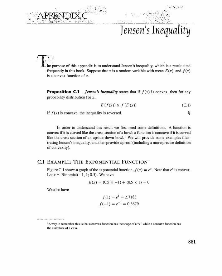
Jensen's Inequality

r I �e �"'PO'e of thi' appendix i' to undmtand Jen,en ., inequility, which ;, a re'ult cited frequently in this book. Suppose that x is a random variable with mean E(x) , and f(x) is a convex function of x .

Proposition C.l Jensen 's inequality states that if f(x) i s convex, then for any probability distribution for x,

E [f (x)] ::: f [E (x)]

If f(x) is concave, the inequality is reversed.

(C. 1 )

�

In order to understand this result we first need some definitions. A function is convex if it is curved like the cross-section of a bowl; a function is concave if it is curved like the cross section of an upside-down bowl. 1 We will provide some examples illus­trating Jensen's inequality, and then provide a proof (including a more precise definition of convexity).

C.l EXAMPLE: THE EXPONENTIAL FUNCTION

Figure C. l shows a graph of the exponential function, f(x) = ex . Note that ex is convex. Let x � Binomial ( - 1 , 1 ; 0.5) . We have

We also have

E(x) = (0.5 x - 1 ) + (0.5 x 1 ) = 0

f( l ) = e 1 = 2.7 1 83

f(- 1 ) = e- 1 = 0.3679

1 A way to remember this is that a convex function has the shape of a "v" while a concave function has

the curvature of a cave.

881

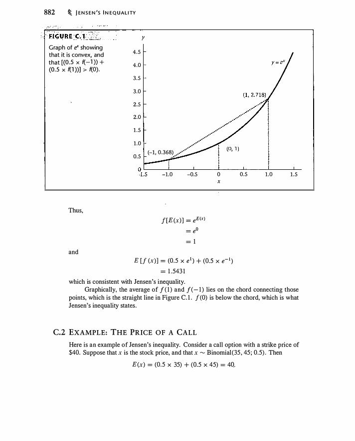
882 � j E N S E N 'S I N EQUAL I TY

Graph of e' showing that it is convex, and that [(0 .5 x f( -1 )) +

(0.5 x f(l ))) > f(O).

4.5

4 .0

3.5

3 .0

y

// ..•.

/ .. -·-··-

·'//·

··'

(-1, 0.368) ••

••

·•·••

2.5

2.0

1 .5

1 .0

Thus,

and

0.5 .... ••

-1.0 -0.5

f[E (x)] = eE(x)

= eo

= 1

0 X

E [f (x)] = (0.5 x e 1 ) + (0.5 x e- 1 ) = 1 .543 1

which is consistent with Jensen's inequality.

0.5 1 .0 1 .5

Graphically, the average of j ( l ) and j(- 1 ) lies on the chord connecting those points, which is the straight line in Figure C. l . f (0) is below the chord, which is what Jensen's inequality states .

C.2 EXAMPLE: THE PRICE OF A CALL

Here is an example of Jensen's inequality. Consider a call option with a strike price of $40. Suppose that x is the stock price, and that x � Binomial (35 , 45 ; 0.5) . Then

E(x) = (0.5 X 35) + (0.5 X 45) = 4Q.

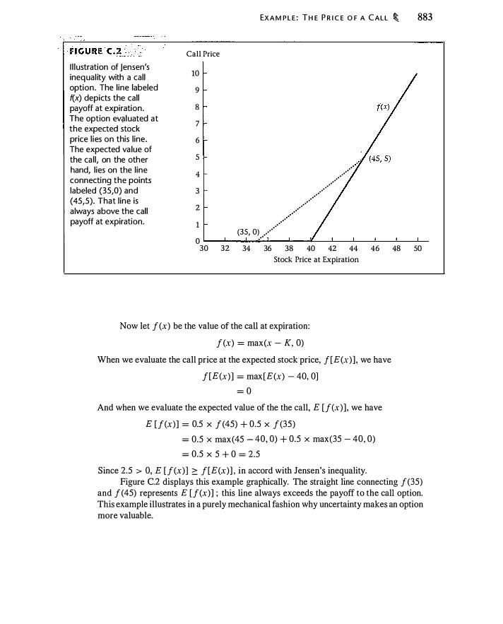
FIGURE. ·· c ;� "- :' . I l l ustration of jensen's inequal ity with a call option. The l ine labeled f(x) depicts the call payoff at expiration. The option ev?)luated at the expected stock price l ies on this l ine. The expected va lue of the ca l l , on the other hand, l ies on the l ine connecting the points labeled (35,0) and (45,5). That l ine is always above the call payoff at expiration.

Call Price

10

9

8

7

6

5

4

3

2

1

0 30 32

EXA M P L E : T H E P R I C E O F A CALL � 883

(35, 0) ....... ....

.. ··

..... ·····

.. ·

.. ... .. �···

..

.. , .. ····

.··

...

34 36 38 40 42 44 46 48 50 Stock Price at Expiration

Now let f (x) be the value of the call at expiration:

f (x) = max(x - K, 0)

When we evaluate the call price at the expected stock price, f[E(x)] , we have

f[E(x)] = max[E(x) - 40, 0]

= 0

And when we evaluate the expected value of the the call, E [f(x)] , we have

E [f(x)] = 0.5 X f(45) + 0.5 X f(35)

= 0.5 x max(45 - 40, 0) + 0.5 x max(35 - 40, 0)

= 0.5 X 5 + 0 = 2.5

Since 2.5 > 0, E [f(x)] :::: f[E(x)] , in accord with Jensen's inequality. Figure C.2 displays this example graphically. The straight line connecting f(35)

and f(45) represents E [f(x)] ; this line always exceeds the payoff to the call option. This example illustrates in a purely mechanical fashion why uncertainty makes an option more valuable.

884 � j EN S E N 'S I N E Q U A L I TY

C.3 PROOF OF jENSEN'S INEQUALITY2

A mathematical way to state the definition of convexity is that f (x) is convex if for any two points x and y, 0 :::::: A. :::::: 1 , and z = A.x + ( 1 - A.)y,

f(z) :::::: A.f (x) + ( 1 - A.) f (y) (C.2)

If f (x) is convex, then there is a line L (x) , running through the point [z , f (z)] such that L (z) = f (z) and for every x, f(x) 2:: L (x) . Because L (x) is a line, it can be written as a + bx, hence E[L(x)] = L[E(x) ] . Define L * (x) as the tangent line at the point { E (x) , f[E(x) ] } . (In Figure C. l , this line would be the tangent line at the point x = 0.)

Now because f(x) 2:: L* (x) , we have E [f (x)] 2:: E [L* (x)] = L* [E (x)] = f[E(x)] . (The last step is because we defined L* (x) to include the point { E (x) , f[E(x)] } .) This proves Jensen's inequality.

PROB LEMS

C.l. The logarithmic function is f(x) = ln(x ) .

a . Graph the logarithmic function in a spreadsheet. Observe that i t is con­cave.

b. Using whatever examples you wish, verify Jensen's inequality for the logarithmic function.

C.2. Do the following in a spreadsheet. Let u vary from 0.05 to 1 in increments of 0.05, and let h vary from 1 month to 1 year in increments of 1 month.

a. Compute 0.5 (ea../ii + e-a../ii)

b. Compute 0.5 (e-0·5a21z+a../ii + e-O.Sa21z-a../ii)

C.3. Let x � Binomial( -a , a ; 0.5) . Using a spreadsheet, evaluate E(ex-O.Sa\ for a 's

ranging from 0.025 to 1 , in increments of 0.025 .

C.4. Let x � Binomial(- 1 , 2; 0.67) . Verify Jensen's inequality for f (x) = ex .

C.S. For the example of the call option i n Section C.2, verify with a numerical example that the value of the call is increasing in the spread of the prices around the mean of $40.

C.6. Usi_ng the numerical example in Section C.2, verify Jensen's inequality fo�

optiOn. ---------------

2This proof is from Mood et al. ( 1 974).

ABBRhlDIX D An Introduction to Visual Basic

for Applications

"\[a! B""k foe AppHcation,, Excel'' powed'ul built-in pmgmmming l;.,guage, le" you incorporate user-written functions and subroutines into a spreadsheet. 1 You can easily calculate Black-Scholes and binomial option prices, for example. This appendix shows how to create user-written functions using VBA. You need not write complicated pro­grams using VBA in order for it to be useful. At the very least, knowing VBA can make it easier for you to analyze relatively complex problems, and to create better-documented, more reliable spreadsheets .

This appendix presumes that you have a basic knowledge of Excel, including the use of built-in functions and named ranges. It does not presume that you know anything about writing macros or programming. The examples here are mostly related to option pricing, but the principles apply generally to any situation in which you use Excel as a tool for numerical analysis.

All of the examples here are contained in the Excel workbook VBA_examples2.xls.

D.1 CALCULATIONS WITHOUT VBA

Suppose you wish to compute the Black-Scholes formula in a spreadsheet. Suppose also that you have named cells2 for the stock price (s), strike price (k), interest rate (r_), time to expiration (t), volatility (v), and dividend yield (d) . You could enter the following

· cell:

s * Exp ( - d* t ) *NormSDi s t ( ( Ln ( s / k ) + ( r_-d+v- 2 / 2 ) * t ) / ( v* t - 0 . 5 ) ) -k*Exp ( - r_* t ) *NormSDis t ( ( Ln ( s / k ) + ( r_-d-v- 2 I 2 ) * t ) / ( v* t - 0 . 5 ) )

Typing this formula is cumbersome, though of course you can copy the formula wherever you would like it to appear. It is possible to use Excel's data table feature to create a table of Black-Scholes prices, but this is cumbersome and inflexible. If you

1 This appendix is written for the versions of VBA in Office 2000 and Office XP. VBA changed dramat­

ically between Office 95 and Office 97 and will change in the future as VBA is replaced with VBA.Net.

When this happens, a guide will be available at the Web site for this book. There are numerous books

on VBA.

2 If you do not know what a named cell is. consult Excel's online help.

885

886 � AN I NTRO D U CT I O N TO V I S U A L BAS I C FO R A P P L I CATI O N S

want to calculate option Greeks (e.g., delta and gamma), you must again enter or copy the formulas into each cell where you want a calculation to appear. And if you decide to change some aspect of your formula, you have to hunt down ail occurrences and make the changes. When the same formula is copied throughout a worksheet, that worksheet potentially becomes harder to modify safely and reliably. When the worksheet is to be used by others, maintainability becomes even more of a concern.

Spreadsheet construction becomes even harder if you want to, for example, com­pute a price for a finite-lived American option. There is no way to do this in one cell, so you must compute the binomial tree in a range of cells and copy the appropriate formulas for the stock price and the option price. This is not so difficult with a three-step binomial calculation, but for I 00 steps you will spend quite a while setting up the spreadsheet. If you decide you want to set up a binomial tree for pricing put options, it can be time­consuming to edit your caii tree to price puts . If you plan ahead, you can make the formulas flexible and general with the use of "if' statements. But things would become much easier if you could create your own formulas within Excel . This is what Visual Basic for Applications permits you to do.

0.2 HOW TO LEARN VBA

Before delving into VBA, i t is helpful to appreciate what learning VBA will entail. First, you will never learn VBA by reading about it; you must try to use it. Part of the challenge is that if a macro language is so powerful that it enables you to do everything, it is going to be too complex for you to memorize all the commands. A book or tutorial (like this one) wiii enable you to use VBA to solve specific problems. However, once you want to do more, you will have to become comfortable figuring out VBA by trial and error.

To facilitate learning VBA, you should use the macro recorder in Excel . When you use the macro recorder, the results of your actions will be recorded in VBA. Try this: Select Tools !Macro !Record New Macro in Excel. Then create a simple graph using the graph wizard. Look at the VBA code that Excel creates. (This example is described in more detail on page 904.) The result is daunting when you first look at it , but if you want to use VBA to create graphs, the recorded macro gives you a starting point that you can modify; you need not create the basic code from scratch.

The main objective of this tutorial is to help you create your own functions. While the examples here relate to option pricing, there are many other uses of VBA.

D.3 CALCULATIONS WITH VBA

In this section we will discuss functions and subroutines, which are techniques in VBA for performing calculations or automating actions .

Creating a Simple Function

With VBA, it is a simple matter to create your own function, say BSCall, which will compute a Black-Scholes option price. To do this, you must first create and open a macro

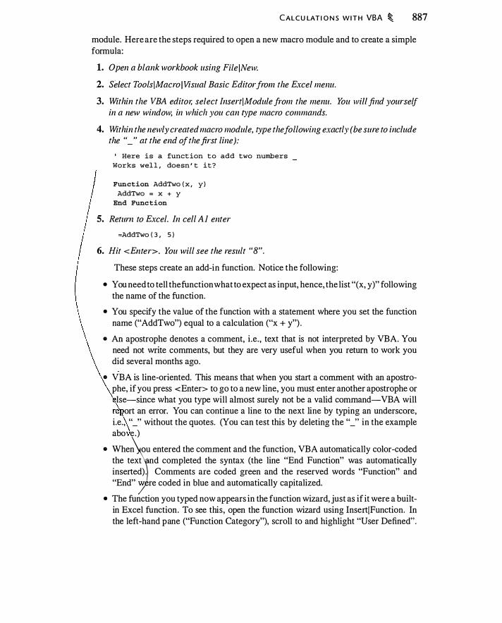
CALCU LAT I O N S W I T H VBA � 887

module. Here are the steps required to open a new macro module and to create a simple formula:

1. Open a blank workbook using File JNew.

2. Setect ToolsJMacro iVisual Basic Editor from the Excel menu.

3. Within the VBA editm; select InsertiModule from the menu. You will find yourself in a new window, in which you can type macro commands.

4. Within the newly created macro module, type the following exactly (be sure to include the "_" at the end of the first line):

' Here i s a funct ion to add two numbers Works wel l , doesn ' t i t ?

Function AddTwo ( x , y ) AddTwo = x + y

End Func tion

5. Return to Excel. In cell AI enter =AddTwo ( 3 , 5 )

6. Hit <Enter>. You will see the result "8".

These steps create an add-in function. Notice the following:

• You need to tell the function what to expect as input, hence, the list "(x, y)" following the name of the function.

• You specify the value of the function with a statement where you set the function name ("AddTwo") equal to a calculation ("x + y") .

• An apostrophe denotes a comment, i .e. , text that is not interpreted by VBA. You need not write comments, but they are very useful when you return to work you did several months ago.

• VBA is line-oriented. This means that when you start a comment with an apostro­phe, if you press <Enter> to go to a new line, you must enter another apostrophe or lse-since what you type will almost surely not be a valid command-VBA will

re ort an error. You can continue a line to the next line by typing an underscore, i.e., "_" without the quotes. (You can test this by deleting the "_" in the example abo e.)

• When�u entered the comment and the function, VBA automatically color-coded the text nd completed the syntax (the line "End Function" was automatically inserted) . Comments are coded green and the reserved words "Function" and "End" /re coded in blue and automatically capitalized.

• The function you typed now appears in the function wizard, just as if it were a built­in Excel function. To see this, open the function wizard using InsertJFunction. In the left-hand pane ("Function Category"), scroll to and highlight "User Defined".

888 � AN I NTRO D U CT I O N TO V I S U A L BAS I C F O R A P P L I CATI O N S

Note that "AddTwo" appears i n the right-side pane ("Function Name") . Click on it and Excel pops up a box where you are prompted to enter inputs for the function .

If you use a custom function in a spreadsheet, i t will automatically recalculate when the spreadsheet recalculates.

A Simple Example of a Subroutine

A function returns a result. A subroutine (called a "sub" by VBA) performs an action when invoked. In the above example we used a function, because we wanted to supply two numbers and have VBA add them for us and tell us the sum. While functions recalculate automatically, subroutines are a set of statements that execute when the subroutine is explicitly invoked. Here are the steps to create a subroutine:

1. Return to the Visual Basic Edit01:

2. Click on the "Module] " window.

3. At the bottom of the module (i.e. , below the function we just created) enter the following:

Sub DisplayBox ( ) Response = MsgBox ( " Greetings ! " )

End Sub

4. Return to Excel. 5. Run the subroutine by using ToolsiMacro iMacros, then double-clicking on "Dis­

playBox" out of the list.

We have just created and run a subroutine. It pops up a dialog box that displays a message. The MsgBox function can be very useful for giving information to the spreadsheet user.

Creating a Button· to Invoke a Subroutine

We ran the subroutine by clicking on Tools iMacro jMacros and then double-clicking on the subroutine name. If you are going to run the subroutine often, creating a button in the spreadsheet provides a shortcut to the subroutine. Here is how to create a button:

1. Move the mouse to the Excel too/bar and right-click once.

2. You will see a list oftoolbar names. Move the highlight bar down to "Forms " and left-click. A new too/bar will pop up.

3. The rectangular icon on this too/bar is the "Button " icon, which looks something like a button (of the software, not the clothing, variety). Click on it.

4. The cursor changes to a cmsshai1: Move the mouse to the spreadsheet, hold down the left mouse button, and drag to create a rectangle. When you lift yourfinger off the

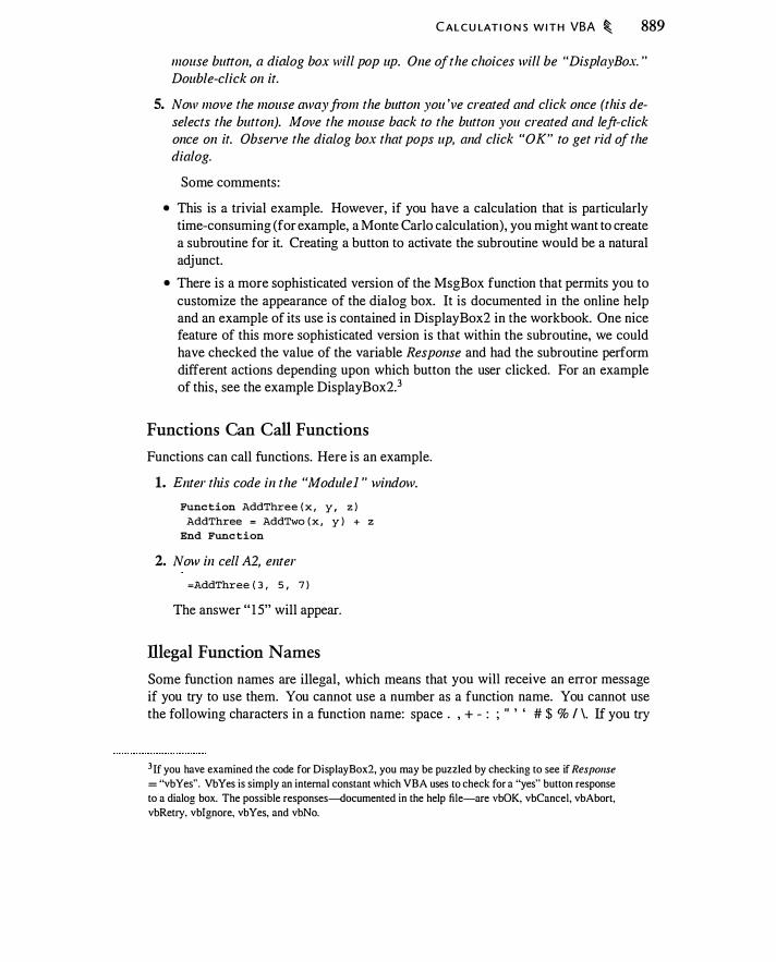
CALCU LAT I O N S W I T H VBA � 889

mouse button, a dialog box will pop up. One of the choices will be "DisplayBox. " Double-click on it.

5. Now move the mouse away from the button you 've created and click once (this de­selects the button). Move the mouse back to the button you created and /eft-click once on it. Obsen'e the dialog box that pops up, and click "OK" to get rid of the dialog.

Some comments:

• This is a trivial example. However, if you have a calculation that is particularly time-consuming (for example, a Monte Carlo calculation), you might want to create a subroutine for it. Creating a button to activate the subroutine would be a natural adjunct.

• There is a more sophisticated version of the MsgBox function that permits you to customize the appearance of the dialog box. It is documented in the online help and an example of its use is contained in DisplayBox2 in the workbook. One nice feature of this more sophisticated version is that within the subroutine, we could have checked the value of the variable Response and had the subroutine perform different actions depending upon which button the user clicked. For an example of this, see the example DisplayBox2.3

Functions Can Call Functions

Functions can call functions. Here is an example.

1. Enter this code in the "Module] " window. Func tion AddThree ( x , y , z )

AddThree = AddTwo ( x , y ) + z End Func tion

2. Now in cell A2, enter =AddThree ( 3 , 5 , 7 )

The answer " 1 5" will appear.

illegal Function Names

Some function names are illegal, which means that you will receive an error message if you try to use them. You cannot use a number as a function name. You cannot use the following characters in a function name: space . , + - : ; " ' ' # $ % I \. If you try

3 If you have examined the code for DisplayBox2, you may be puzzled by checking to see if Response = "vbYes''. VbYes is simply an internal constant which VB A uses to check for a "yes" button response

to a dialog box. The possible responses-documented in the help file-are vbOK, vbCancel, vbAbort,

vbRetry, vblgnore, vbYes, and vbNo.

890 � AN I NT RO D U CT I O N TO V I S U A L BAS I C F O R A P P L I CAT I O N S

to use any of these characters i n a name, Visual Basic lets you know immediately that something is wrong. Note that you can use an underscore where you would like to have a space for readability of the function name. So BS_2, for example, is a legal function name.

Here is a more subtle issue. There are function names that are legal but that you should not use. BS2 is an example. This would be fine as the name of a subroutine, which is not called directly from a cell. But think about what happens if you give this name to a user-defined function. You enter, for example, "BS2(3)", in a cell. How does Excel understand this? The problem is that "BS2" is also the name of a cell. So if you ,try to use it as a function in the spreadsheet, Excel will become confused and return an error. This is why, later in this tutorial, you will see functions named BS_2, BS_3, and so on.

Differences between Functions and Subroutines

Functions and subroutines are not interchangeable and do not have the same capabilities. Think of subroutines as code meant to be invoked by a button or otherwise explicitly called, while functions return results and are meant to be inserted into cells (although functions can also be called by subroutines). Because of their different purpose, some VBA capabilities will work in one but not the other.

In a subroutine, for example, you can write to cells of the workbook. With a subroutine you could perform a calculation and have the answer appear in cell A l . However, if you invoke a function from a worksheet b y entering it into a cell, you cannot write to cells from within that function. You cannot activate a worksheet or change anything about the display from within such a function. (On the other hand, if the function is invoked by a subroutine, but not invoked from a worksheet, it can do these things.) Subroutines, on the other hand, cannot be called from cells . These restrictions exist because functions and subroutines are intended for different purposes.

D.4 STORING AND RETRIEVING VARIABLES IN A WORKSHEET

Suppose that there is a value in the spreadsheet that you want to include as input to your function or subroutine. (For instance, you might have a variable that determines whether the option to be valued is American or European.) Or suppose you create a subroutine that performs computations. You may want to display the output in the spreadsheet. (For example, you might wish to create a subroutine to draw a binomial tree.) Using VBA, how do you read and write values to the spreadsheet?

If you are going to read and write numbers to specific locations in the spreadsheet, you must identify those locations . The easiest way to identify a location is to use a named range. The alternatives-which we will examine below-require that you "activate" a specific location or worksheet within the workbook, and then read and write within this activated region.

There are at least three ways to read and write to cells : ·

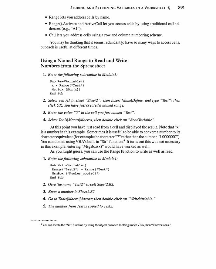
STO R I N G AN D R ET R I EV I N G VA R I A B LES I N A WO R KS H E ET � 891

• Range lets you address cells by name.

• Range().Activate and ActiveCell let you access cells by using traditional cell ad­dresses (e.g., "AI ") .

• Cell lets you address cells using a row and column numbering scheme.

You may be thinking that it seems redundant to have so many ways to access cells, but each is useful at different times.

Using a Named Range to Read and Write Numbers from the Spreadsheet

1. Enter the following subroutine in Module]: Sub ReadVariable ( )

x = Range ( " Tes t " ) MsgBox ( S t r ( x ) )

End Sub

2. Select cell AI in sheet "Sheet2 "; then bzsert!Name !Define, and type "Test"; then click OK. You have just created a named range.

3. Enter the value "5 " in the cell you just named "Test ".

4. Select Tools!Macro !Macros, then double-click on "ReadVariable ".

At this point you have just read from a cell and displayed the result. Note that "x" is a number in this example. Sometimes it is useful to be able to convert a number to its character equivalent (for example the character "7" rather than the number "7 .0000000") . You can do this using VB A's built-in "Str" function.4 It turns out this was not necessary in this example; entering "MsgBox(x)" would have worked as well.

As you might guess, you can use the Range function to write as well as read.

1. Emer the following subroutine in Module]: Sub Wri teVariable ( )

Range ( " Test2 " ) = Range ( " Tes t " ) MsgBox ( " Number_ copied ! " )

End Sub

2. Give the name "Test2 " to cell Sheet2.B2.

3. Enter a number in Sheet2.B2. 4. Go to Tools iMacro !Macros; then double-click on "Write Variable. "

5. The number from Test is copied to Test2.

4You can locate the "Str" function by using the object browser, looking under VB A, then "Conversions:"

892 � AN I NT RO D U CT I O N TO V I S U A L BAS I C F O R A P P L I CAT I O N S

Reading and Writing to Cells That Are Not Named

You can also access a specific cell directly. In order to do this, you first have to activate the worksheet containing the cell. Here is VBA code to read a variable:

Sub ReadVariable2 { ) Worksheets { " Sheet2 " ) . Activate Range ( " Al " ) . Act ivate x ; Act iveCel l . Value MsgBox ( S tr { x ) )

End Sub

In this subroutine we first activate the worksheet named "Sheet2." Next we activate the cell "Al" within Sheet2. You will see that when you have finished calling this function, the cursor has moved to cell A l in Sheet2. This is because the "active cell" is whatever cell the cursor happens to be on; the first two lines instruct the cursor to move to Sheet2.A l .

The active cell has properties, such as the font, color of the cell, and formatting. All of these properties may be accessed using the ActiveCell function. For fun, insert the line

Act iveCe l l . Font . Bold;True

after the MsgBox function. Then switch to Sheet2, ruri the subroutine, and watch the change in cell A I .

We can also assign a value to ActiveCell .Value; this i s a way to write to a cell . Here is a macro that does this:

Sub WriteVariable2 ( ) Worksheets ( " Sheet2 " ) . Activate Range ( " Al " ) . Act ivate x ; Act iveCe l l . Value Range ( " Bl " ) . Act ivate Act iveCe l l . Value ; x

End Sub

This subroutine reads the number from Sheet2.A 1 and copies it to Sheet2.B 1 .

Using the Cells Function to Read and Write to Cells

There is yet another way to read and write to cells . The Cells function lets you ad­dress cells using a numerical row and column numbering scheme. Here is an example illustrating how Cells works :

Sub Ce l l sExample ( ) ' Make " Sheet2 " the act ive sheet

Worksheet s ( " Sheet2 " ) . Ac t ivate ' The first ent ry i s the row , the s econd is the column

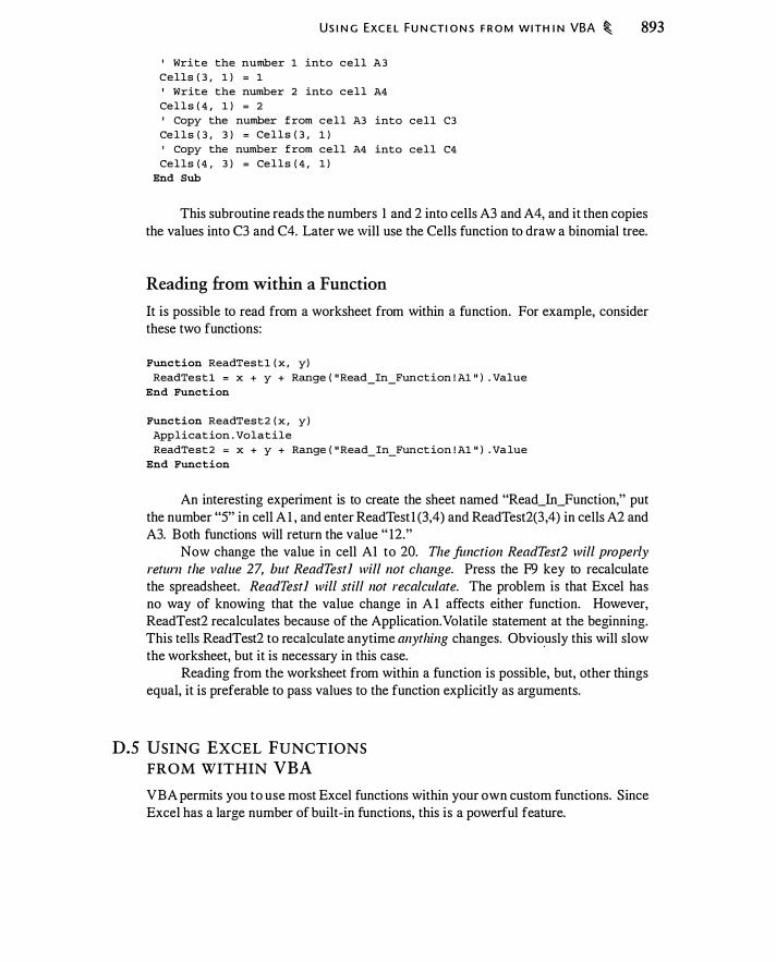
US I N G EXC E L FU N CTI O N S F R O M WITH I N VBA � 893

' Write the number 1 into cell A3 Cells ( 3 , 1 ) = 1

' Write the number 2 into c e l l A4 Cel l s ( 4 , 1 ) = 2

' Copy the number from cell A3 into cell C3 Ce l l s ( 3 , 3 ) = Cel l s ( 3 , 1 )

' Copy the number from cell A4 into cell C4 Ce lls ( 4 , 3 ) = Ce l l s ( 4 , 1 )

End Sub

This subroutine reads the numbers I and 2 into cells A3 and A4, and it then copies the values into C3 and C4. Later we will use the Cells function to draw a binomial tree.

Reading from within a Function

It is possible to read from a worksheet from within a function. For example, consider these two functions:

Func tion ReadTes t 1 ( x , y) ReadTes t l = x + y + Range ( " Read_In_Function ! A1 " ) . Value

End Func tion

Func tion ReadTes t2 ( x , y ) Applicat ion . Volatile ReadTest2 = x + y + Range ( " Read_In_Funct ion ! A1 " ) . Va lue

End Func tion

An interesting experiment is to create the sheet named "Read_In_Function," put the number "5" in cell A l , and enter ReadTest l (3,4) and ReadTest2(3,4) in cells A2 and A3. Both functions will return the value " 12."

Now change the value in cell AI to 20. The function ReadTest2 will properly return the value 27, but ReadTestl will not change. Press the F9 key to recalculate the spreadsheet. ReadTestl will still not recalculate. The problem is that Excel has no way of knowing that the value change in A I affects either function. However, ReadTest2 recalculates because of the Application. Volatile statement at the beginning. This tells ReadTest2 to recalculate anytime anything changes. Obviously this will slow the worksheet, but it is necessary in this case.

Reading from the worksheet from within a function is possible, but, other things equal, it is preferable to pass values to the function explicitly as arguments.

D.S USING EXCEL FUNCTIONS FROM WITHIN VBA

VBA permits you to use most Excel functions within your own custom functions. Since Excel has a large number of built-in functions, this is a powerful feature.

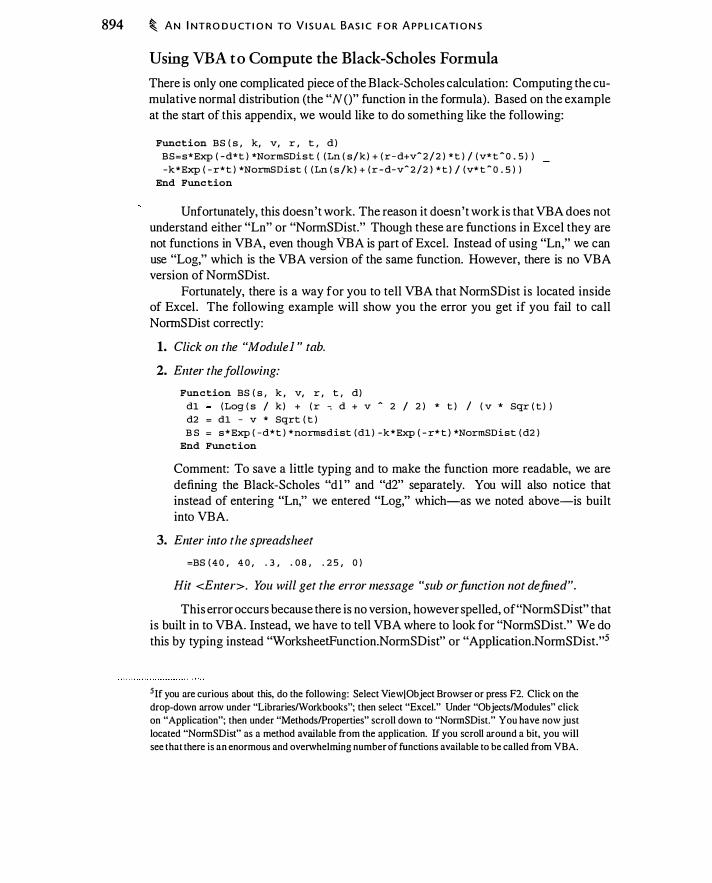
894 � AN I NTRO D U CT I O N TO V I S U A L BAS I C F O R A P P L I CATI O N S

Using VBA to Compute the Black-Scholes Formula

There is only one complicated piece of the Black -Scholes calculation: Computing the cu­mulative normal distribution (the "N ()" function in the formula) . Based on the example at the start of this appendix, we would like to do something like the following:

Function BS ( s , k, v, r , t , d ) BS=s*Exp ( - d* t ) *NormSDi s t ( ( Ln ( s l k ) + ( r - d+vA 2 1 2 ) * t ) l ( v* t A 0 . 5 ) ) -k*Exp ( - r* t ) *NormSDist ( ( Ln ( s lk l + ( r - d-vA 2 1 2 l * t l l (v* t A O . S ) )

End Func tion

Unfortunately, this doesn't work. The reason it doesn't work is that VBA does not understand either "Ln" or "NormSDist." Though these are functions in Excel they are not functions in VBA, even though YBA is part of Excel. Instead of using "Ln," we can use "Log," which is the VBA version of the same function. However, there is no VBA version of NormSDist.

Fortunately, there is a way for you to tell VBA that NormSDist is located inside of Excel. The following example will show you the error you get if you fail to call NormSDist correctly:

1. Click on the "Module] " tab.

2. Emer the following: Fun c tion BS ( s , k , v, r , t , d)

dl ( Log ( s I k ) + ( r � d + v A 2 I 2 ) * t ) I ( v * Sqr ( t ) ) d2 = dl - v * Sqrt ( t ) B S = s * Exp ( -d* t ) *normsdist ( dl ) -k*Exp ( - r* t ) *NormSDist ( d2 )

End Func tion

Comment: To save a little typing and to make the function more readable, we are defining the Black-Scholes "d l" and "d2" separately. You will also notice that instead of entering "Ln," we entered "Log," which-as we noted above-is built into VBA.

3. Enter illlo the spreadsheet =BS ( 4 0 , 4 0 , . 3 , . 0 8 , . 2 5 , 0 )

Hit <Enter>. You will get the error message "sub orfimction not defined".

This error occurs because there is no version, however spelled, of"NormSDrst" that is built in to VBA. Instead, we have to tell VBA where to look for "NormSDist." We do this by typing instead "WorksheetFunction.NormSDist" or "Application.NormSDist."5

;If you are curious about this, do the following: Select View(Object Browser or press F2. Click on the

drop-down arrow under "Libraries/Workbooks"; then select "Excel." Under "Objects/Modules" click

on "Application"; then under "Methods/Properties" scroll down to "NorrnSDist." You have now just

located "NormSDist" as a method available from the application. If you scroll around a bit, you will

see that there is an enormous and overwhelming number of functions available to be called from VBA.

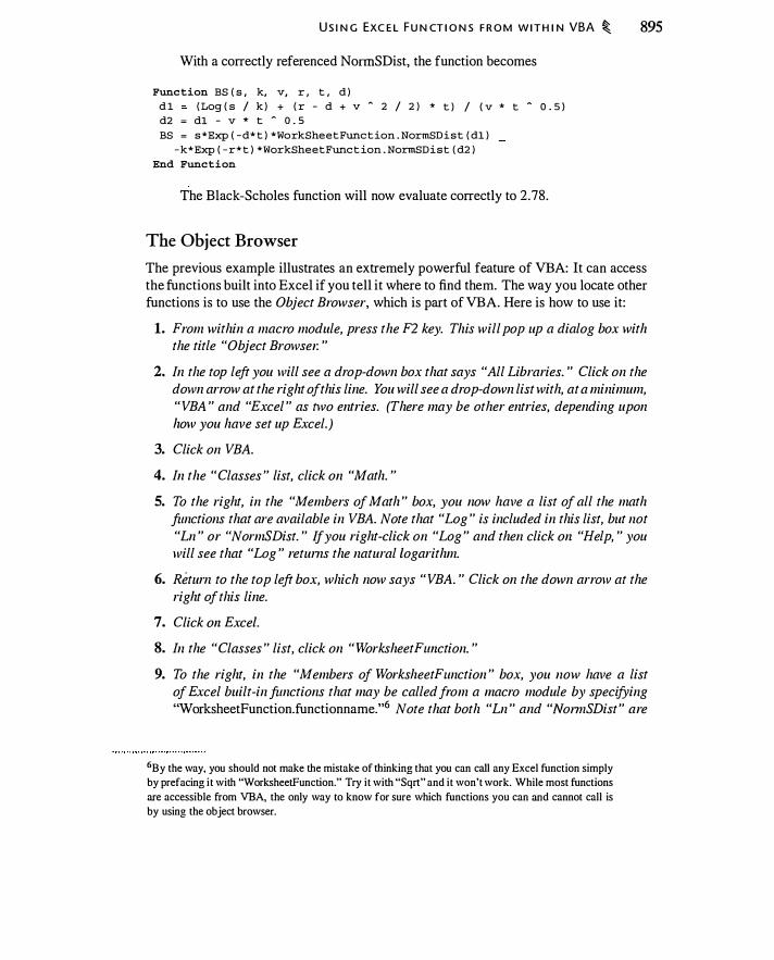
U S I N G EXC E L FU N CT I O N S F R O M W I T H I N VBA � 895

With a correctly referenced NorrnSDist, the function becomes

Func tion BS ( s , k, v, r , t , d ) d l ( Log ( s I k ) + ( r - d + v - 2 I 2 ) * t ) I ( v * t - 0 . 5 ) d2 ; dl - v * t - 0 . 5 BS ; s *Exp ( - d* t ) *WorkSheetFunc t ion . NormSD i s t ( dl )

- k*Exp ( - r* t ) *WorkSheetFunc t ion . NormSDist ( d2 ) End Func tion

The Black-Scholes function will now evaluate correctly to 2.78.

The Object Browser

The previous example illustrates an extremely powerful feature of VBA: It can access the functions built into Excel if you tell it where to find them. The way you locate other functions is to use the Object Browser, which is part of VBA. Here is how to use it:

1. From within a macro module, press the F2 key. This will pop up a dialog box with the title "Object Browse1: "

2. In the top left you will see a drop-down box that says "All Libraries. " Click on the down arrow at the right of this line. You will see a drop-down list with, at a minimum, "VBA " and "Excel " as two entries. (There may be other entries, depending upon how you have set up Excel. )

3. Click on VBA.

4. In the "Classes " list, click on "Math. "

5. To the right, in the "Members of Math " box, you now have a list of all the math functions that are available in VBA. Note that "Log " is included in this list, but not "Ln " or "NormSDist. " If you right-click on "Log " and then click 011 "Help, " you will see that "Log " retums the natural Logarithm.

6. Return to the top left box, which now says "VBA. " Click on the down arrow at the right of this line.

7. Click 011 Excel. 8. In the "Classes " list, click on "WorksheetFw1ction. "

9. To the right, in the "Members of Worksheet Function " box, you 1zow have a list of Excel built-in functions that may be called from a macro module by specifying "WorksheetFunction.functionname."6 Note that both "Ln " and "NomzSDist" are

6By the way, you should not make the mistake of thinking that you can call any Excel function simply

by prefacing i t with "WorksheetFunction." Try it with "Sqrt" and it won't work. While most functions

are accessible from VBA, the only way to know for sure which functions you can and cannot call is

by using the object browser.

896 � AN I NTRO D U CTI O N TO V I S U A L BAS I C F O R A P P L I CATI O N S

included in this list. Note also that "Log " is included in this list, but b e aware that Excel s "Log " function is base I 0 by default (you can specify a differellt base), whereas VBA s is base e.1

If you create any VBA functions that are even moderately ambitious, you will need to use the object browser. It is the heart and soul of VBA.

D.6 CHECKING FOR CONDITIONS

Frequently, you want to perform a calculation only if certain conditions are met. For example, you would not want to calculate an option price with a negative volatility. It makes sense to check to see if your inputs make sense before proceeding with the calculation and aborting-possibly with an error message-if they do not.

The easy way to check if a condition exists is to use the construct If . . . Then . . . Else.8 Here is an example of its use in checking for a negative volatility in the Black-Scholes formula:9

Func tion BS_2 ( s , k , v, r , t , d ) I f v > 0 Then

BS_2 = BS ( s , k, v, r , t , d ) E l s e

MsgBox ( " Negat ive_ volat i l i ty ! " ) BS 2 = CVErr ( xlErrValue )

End I f End Func tion

This function checks to see if volatility is greater than 0; if it is, the function com­putes the Black-Scholes formula using the BS function we created earlier. If volatility is not greater than zero, then two things happen: (i) a message box pops up to inform you of the mistake and (ii) the function returns a value indicating that there is an error.

In general you should be cautious about putting message boxes into a function (as opposed to a subroutine), since every time the spreadsheet is recalculated the message box will pop up.

Because error-checking is often critically important (you would not want to quote a client a price on a deal for which you had accidentally entered a negative volatility), it is worth expanding a bit on the use of the CVErr function.

7 Scroll down to the ":Log" entry and then click on the "?" button at the bottom left. If you use

"Log'' in a spreadsheet, or if you use "WorksheetFunction.log" in a function, you will get the base I 0

logarithm. However, if you use "Log" in a function, you will get the base e logarithm. Note also that,

as mentioned earlier, "Sqrt" is not included and, hence, is not available in VBA.

8There is also a Case . . . Select construct that we will not use but that is documented in VBA's help

file.

9You need to be aware that VBA will expect the "IfThen," "Else," and "End If' pieces to be on separate

lines. If you write "Else" on the same line as "If Then," for example, the code will fail .

A R RAYS � 897

If the user enters a negative volatility, you could just have Excel return a nonsense value for the option, such as -99. This would be a bad idea, however. Suppose you have a complicated worksheet with many option calculations. If you failed to notice the error, the -99 would be treated as a true option value and propagated throughout your calculations.

Alternatively, you could have the function return a string such as "Oops, you entered a negative volatility." Entering a string in a cell when you should have a number could have unpredictable effects on calculations that depend on the cell. It is obvious that an addition between a string and a number will fail. However, suppose you are performing a frequency count. Are you sure what will happen to the calculation if you introduce a string among the numbers in your data?

Excel has built-in error codes that are documented in VBA's online help. For example, xlErrNA returns "#N/A," xlErrRef returns "#REF! ," and xlErrValue returns "#VALUE!". By using CVErr along with one of the built-in error codes, you guarantee that your function will return a result that Excel recognizes as a numerical error. Excel programmers have already thought through the issues of how subsequent calculations should respond to a recognized error, and Excel usually does something reasonable in those circumstances.

D.7 ARRAYS

Often you will wish to use a single variable to store many numbers. For example, in a binomial option calculation, you have a stock price tree. After n periods, you have n + I possible stock prices. It can be useful to write the lowest stock price as S (O) , the next as S ( l ) , and the highest as S(n ) . The variable S is then called an array-it is a single variable that stores more than one number. Each item in the array is called an element. Think of an array as a table of numbers. You access a specific element of the array by specifying a row and column number. Figure D. l provides an example of an array.

Defining Arrays

When you create an array, it is necessary to tell VBA how big the array is going to be. You do this by using the Dim statement ("Dim" is short for "dimension"-the size of the array). Here are some examples of how to use Dim to create a one-dimensional array:

Dim P ( 2 ) As Doub l e

This creates an array of three double-precision real numbers, with the array index running from 0 to 2. (By default, the first subscript in an array in VBA is 0.) If you had written

Dim P ( 3 to 5 ) As Double

you would have created a three-element array with the index running from 3 to 5 . In this example we told Excel that the variable is type "Double." This was not necessary-we could have left the type unspecified and permitted Excel to determine the type automa­tically. It is faster and easier to detect mistakes, however, if we specify the type.

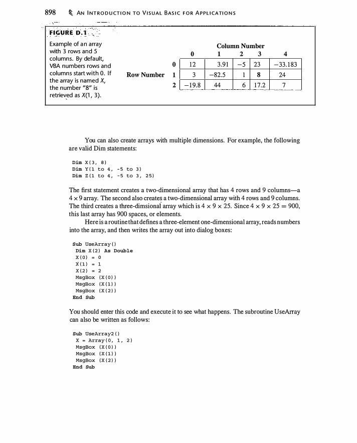
898 � AN I NT R O D U CT I O N TO V I S U A L BAS I C F O R A P P L I CATI O N S

F iGURE D . l Example of a n array with 3 rows and 5 columns. By default, VBA numbers rows and columns start with 0. If the array is named X, the number "8" is retriev

,ed as X(l , 3).

0 Row Number 1

2

0 1 2

3

- 1 9.8

Column Number 1 2 3 3.9 1 -5 23

-82.5 1 8 44 6 1 7 .2

4 -33 . 1 83

24

7

You can also create arrays with multiple dimensions. For example, the following are valid Dim statements:

Dim X ( 3 , 8 ) Dim Y ( l to 4 , - 5 to 3 ) Dim Z ( l to 4 , - 5 to 3 , 2 5 )

The first statement creates a two-dimensional array that has 4 rows and 9 columns-a 4 x 9 array. The second also create� a two-dimensional array with 4 rows and 9 columns. The third creates a three-dimsional array which is 4 x 9 x 25. Since 4 x 9 x 25 = 900, this last array has 900 spaces, or elements.

Here is a routine that defines a three-element one-dimensional array, reads numbers into the array, and then writes the array out into dialog boxes :

Sub UseArray ( ) Dim X ( 2 ) As Doub l e

X ( O ) = 0 X ( l ) = 1 X ( 2 ) = 2 MsgBox ( X ( O ) ) MsgBox ( X ( l ) ) MsgBox ( X ( 2 ) )

End Sub

You should enter this code and execute it to see what happens. The subroutine UseArray can also be written as follows:

Sub UseArray2 ( ) X = Array ( O , 1 , 2 ) MsgBox ( X ( O ) ) MsgBox ( X ( l ) ) MsgBox ( X ( 2 ) )

End Sub

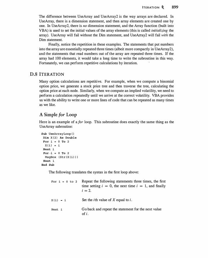
I T ERAT I O N � 899

The difference between UseArray and UseArray2 is the way arrays are declared. In UseArray, there is a dimension statement, and then array elements are created one by one. In UseArray2, there is no dimension statement, and the Array function (built into VBA) is used to set the initial values of the array elements (this is called initializing the array) . UseArray will fail without the Dim statement, and UseArray2 will fail with the Dim statement.

Finally, notice the repetition in these examples. The statements that put numbers into the array are essentially repeated three times (albeit more compactly in UseArray2), and the statements that read numbers out of the array are repeated three times. If the array had 100 elements, it would take a long time to write the subroutine in this way. Fortunately, we can perform repetitive calculations by iteration.

D.8 ITERATION Many option calculations are repetitive. For example, when we compute a binomial option price, we generate a stock price tree and then traverse the tree, calculating the option price at each node. Similarly, when we compute an implied volatility, we need to perform a calculation repeatedly until we arrive at the correct volatility. VBA provides us with the ability to write one or more lines of code that can be repeated as many times as we like.

A Simple for Loop

Here is an example of afor loop. This subroutine does exactly the same thing as the UseArray subroutine:

Sub UseArrayLoop ( ) Dim X ( 2 ) As Doub l e

F o r i = 0 To 2 X ( i ) = i

Next i

For - i = 0 To 2 MsgBox ( S tr ( X ( i ) ) )

Next i

End Sub

The following translates the syntax in the first loop above:

For i = o to 2 Repeat the following statements three times, the first time setting i = 0, the next time i = 1 , and finally i = 2.

X ( i ) i

Next i

Set the i th value of X equal to i .

Go back and repeat the statement for the next value of i .

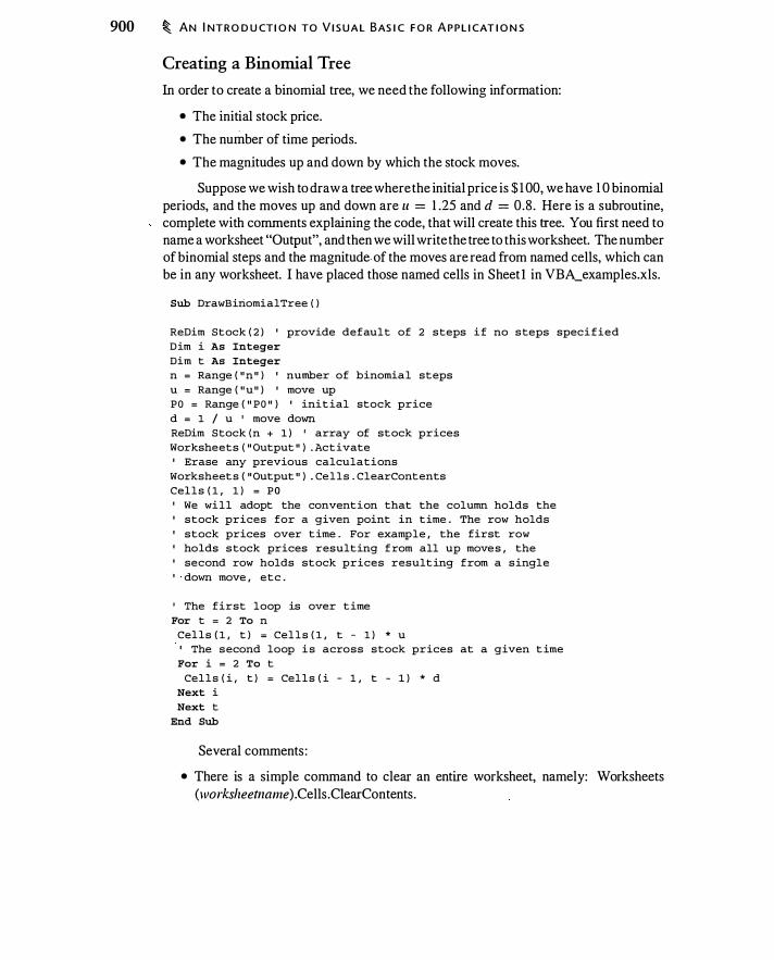
900 � AN I NTRO D U CT I O N TO V I S U A L BAS I C F O R APPL I CAT I O N S

Creating a Binomial Tree

In order to create a binomial tree, we need the following information:

• The initial stock price.

• The number of time periods.

• The magnitudes up and down by which the stock moves.

Suppose we wish to draw a tree where the initial price is $ 1 00, we have 1 0 binomial periods, and the moves up and down are u = 1 .25 and d = 0.8 . Here is a subroutine, complete with comments explaining the code, that will create this tree. You first need to name a worksheet "Output", and then we will write the tree to this worksheet. The number of binomial steps and the magnitude- of the moves are read from named cells, which can be in any worksheet. I have placed those named cells in Sheet ! in VBA_examples.xls.

Sub DrawBiriomialTree ( )

ReDim Stock ( 2 ) ' provide defaul t of 2 s teps i f no s teps speci fied D im i As Integer

Dim t As Integer

n = Range ( " n " ) ' number of binomial steps u = Range ( " u " ) ' move up P O = Range ( " P O " ) ' ini t ial stock price d = 1 I u ' move down ReDim Stock ( n + 1 ) ' array of stock prices Worksheets ( " Output " ) . Act ivate ' Erase any previous calculations

Worksheet s ( " Output " ) . Ce l l s . ClearContents Cel l s ( 1 , 1 ) = P O ' We wi l l adopt the convention that the column holds the ' s tock prices for a given point in time . The row holds ' s tock prices over t ime . For example , the first row ' holds s tock prices resulting f rom all up move s , the ' second row holds stock prices result ing from a s ingle ' down move , etc .

' The first loop is over t ime For t = 2 To n

Cel ls ( 1 , t ) = Cel l s ( 1 , t - 1 ) * u ' The s econd loop i s across s tock prices at a given t ime

For i = 2 To t Cel l s ( i , t ) = Cel l s ( i - 1 , t - 1 ) * d

Next i Next t

End Sub

Several comments :

• There is a simple command to clear an entire worksheet, namely: Worksheets ( wo rkslzeefllame) .Cells . ClearContents.

R EA D I N G AN D WR IT I N G A R R AYS � 901

• The use of the Cells function means that you can perform the calculation exactly as you would if you were writing it down, using subscripts to denote which price you are dealing with. Think about how much more complicated it would be to use traditional row and column notation (e.g., "A 1 ") to perform the same function.

• This subroutine does not price an option; it merely creates a binomial stock price tree.

Note that this subroutine uses the ReDim command to specify a flexible array size. Sometimes you do not know in advance how big your array is going to be. In this example you are unsure how many binomial periods the subroutine must handle. If you are going to use an array to store the full set of prices at each point in time, this presents a problem-how large do you make the array? You could specify the array to have a very large size, one larger than any user is ever likely to use, but this kind of practice could get you into trouble if memory is limited. Fortunately, with the ReDim statement VBA permits you to specify the size of an array using a variable.

Other Kinds of Loops

Although we will not discuss them, there are other looping constructs available in VBA. The following kinds of loops are available:

• Do Until . . . Loop and Do . . . Loop Until • Do While . . . Loop and Do . . . Loop While • While . . . Wend

If you ever think you need them, you can look these up in the online help. There is also a For Each . . . In . . . Next construct, which we discuss below.

D.9 READING AND WRITING ARRAYS

A powerful feature of VBA is the ability to read arrays as inputs to a function and also to write functions that return arrays as output.

Arrays as Output

Suppose you would like to create a single function that returns two numbers : The Black­Scholes price of a call option and the option delta. Let's call this function BS_3 and create it by modifying the function BS from Section D.5 . 1 .

Func tion BS_3 ( s , k , v , r , t , d ) dl = ( Log ( s I k ) + ( r - d + 0 . 5 * v � 2 ) * t ) I ( v * t � 0 . 5 ) d2 = dl - v * t � 0 . 5 ndl = WorksheetFunct ion . NormSD i s t ( dl ) nd2 = WorksheetFunct ion . NormSD i s t ( d2 ) de lta = Exp ( - d * t ) * ndl

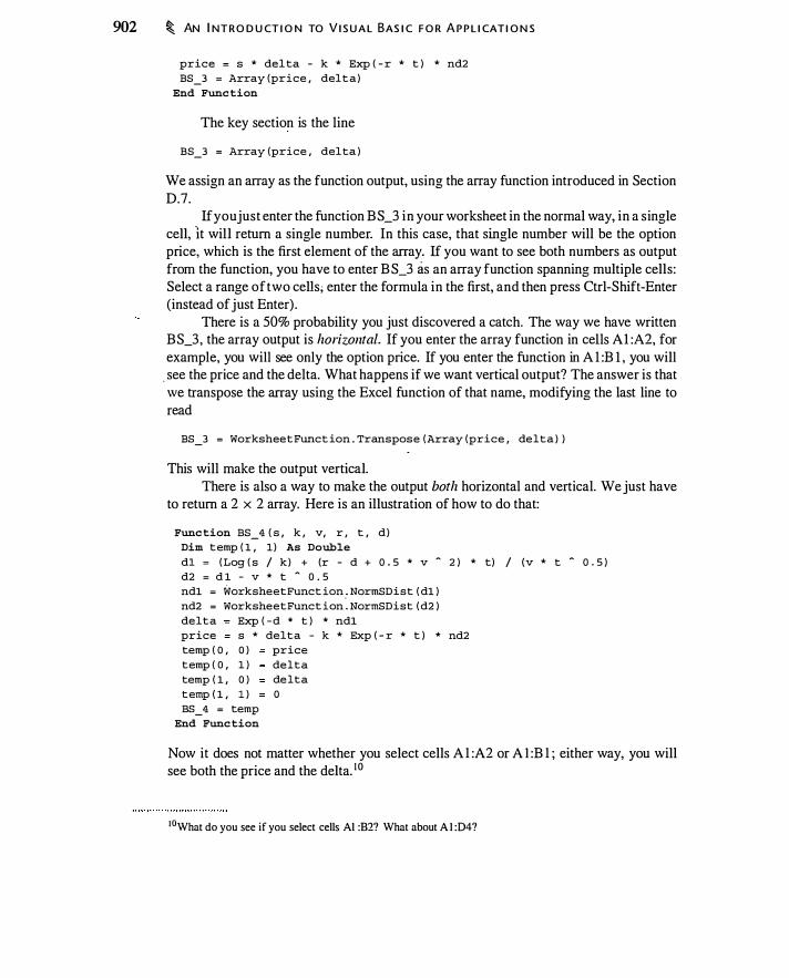
902 � AN I NTRO D U CT I O N TO V I S U A L BAS I C F O R A P P L I CAT I O N S

price = s * del ta - k * Exp ( - r * t ) * nd2 BS_3 = Array (price , del t a )

End Func tion

The key section is the line

BS_3 = Array (price , del ta )

We assign an array as the function output, using the array function introduced in Section D.7.

If you just enter the function BS_3 in your worksheet in the normal way, in a single cell, lt will return a single number. In this case, that single number will be the option price, which is the first element of the array. If you want to see both numbers as output from the function, you have to enter BS_3 as an array function spanning multiple cells: Select a range of two cells; enter the formula in the first, and then press Ctri-Shift-Enter (instead of just Enter).

There is a 50% probability you just discovered a catch. The way we have written BS_3, the array output is horizontal. If you enter the array function in cells A 1 :A2, for example, you will see only the option price. If you enter the function in A l :B 1 , you will

_ see the price and the delta. What happens if we want vertical output? The answer is that we transpose the array using the Excel function of that name, modifying the last line to read

BS_3 = Worksheet Funct ion . Transpos e (Array (price , delta ) )

This will make the output vertical. There is also a way to make the output both horizontal and vertical. We just have

to return a 2 x 2 array. Here is an illustration of how to do that:

Func tion BS_4 ( s , k , v, r , t , d ) Dim t emp ( l , 1 ) As Double

dl = ( Log ( s I k ) + (r - d + 0 . 5 * v � 2 ) * t) I (v * t � 0 . 5 ) d2 = d l - v * t � 0 . 5 ndl = WorksheetFunct ion : NormSDist ( dl ) nd2 = WorksheetFunct ion . NormSDist ( d2 ) delta Exp ( - d * t ) * ndl price s * delta - k * Exp ( - r * t ) * nd2 temp ( O , 0 ) price temp ( O , 1 ) delta temp ( l , 0 ) de lta temp ( l , 1 ) 0 BS_4 = temp

End Func tion

Now it does not matter whether you select cells A l :A2 or A l :B l ; either way, you will see both the price and the delta. 1 0

1 0What do you see if you select cells AI :B2? What about A I :04?

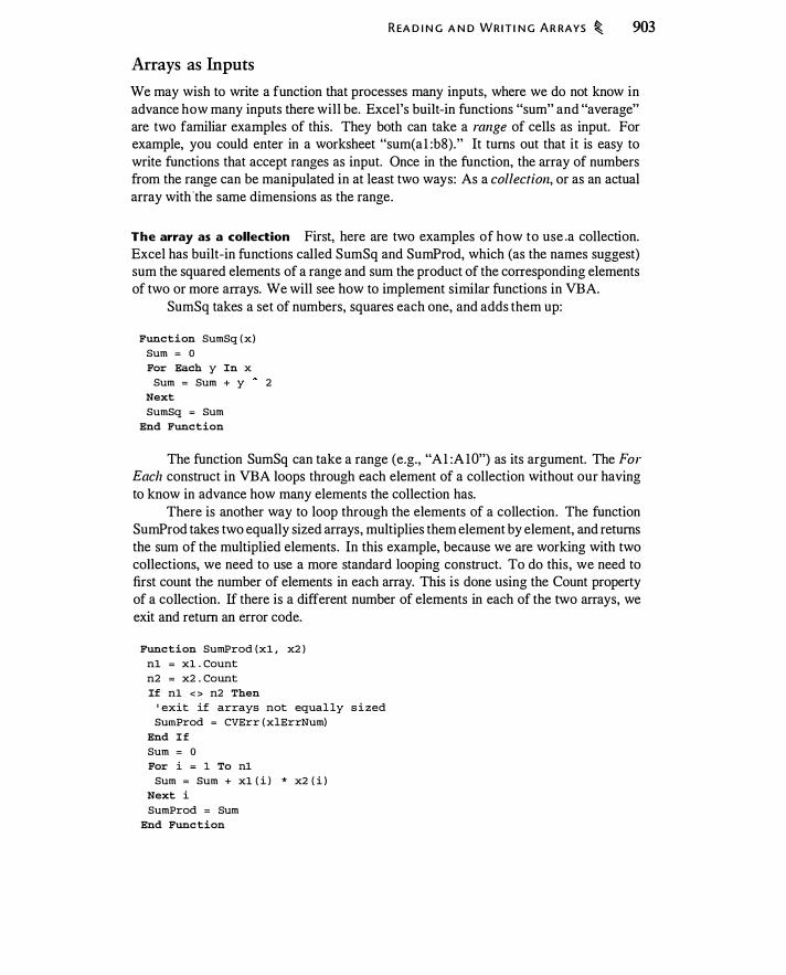
Arrays as Inputs

R EA D I N G A N D WR IT I N G A R RAYS � 903

We may wish to write a function that processes many inputs, where we do not know in advance how many inputs there will be. Excel's built-in functions "sum" and "average" are two familiar examples of this. They both can take a range of cells as input. For example, you could enter in a worksheet "sum(a l :b8)." It turns out that it is easy to write functions that accept ranges as input. Once in the function, the array of numbers from the range can be manipulated in at least two ways: As a collection, or as an actual array with .the same dimensions as the range.

The array as a collection First, here are two examples of how to use .a collection. Excel has built-in functions called SumSq and SumProd, which (as the names suggest) sum the squared elements of a range and sum the product of the corresponding elements of two or more arrays. We will see how to implement similar functions in VB A.

SumSq takes a set of numbers, squares each one, and adds them up:

Func tion SumSq ( x ) Sum ; 0 For Each y In x

Sum ; Sum + y 2 Next

SumSq ; Sum End Func tion

The function SumSq can take a range (e.g., "Al :A lO") as its argument. The For Each construct in VBA loops through each element of a collection without our having to know in advance how many elements the collection has.

There is another way to loop through the elements of a collection. The function SumProd takes two equally sized arrays, multiplies them element by element, and returns the sum of the multiplied elements. In this example, because we are working with two collections, we need to use a more standard looping construct. To do this, we need to first count the number of elements in each array. This is done using the Count property of a collection. If there is a different number of elements in each of the two arrays, we exit and return an error code.

Func tion SumProd (xl , x2 ) nl ; xl . Count n2 ; x2 . Count If nl < > n2 Then

• exit if arrays not equal ly s i zed SumProd ; CVErr ( xlErrNum)

End I f

Sum ; o For i ; 1 To nl

Sum ; Sum + xl ( i ) * x2 ( i ) Next i SumProd ; Sum

End Func tion

904 � AN I NTRO D U CT I O N TO V I S U A L BAS I C FO R A P P L I CATI O N S

The array a s a n array We can also treat the numbers i n the range as an array. The only trick to doing that is that we need to know the dimensions of the array, i .e . , how many rows and columns it has. The function RangeTest illustrates how to do this .

Func tion RangeTest (x) prod = 1 r = x . Rows . Count c = x . Columns . Count For i = 1 To r

For j = 1 To c prod = prod * x ( i , j )

Next j Next i RangeTe st WorksheetFunctio� . Transpose (Array ( prod , r , c ) )

End Func tion

This function again multiplies together the cells in the range. It returns not only the product, but also the number of rows and columns. .

When x is read into the function, it is considered by VBA to be an array. 1 1 Rows and Columns are properties of an array. The construct

x . Rows . Count

tells us the number of rows in the array. With this capability, we could multiply arrays, check to see whether two ranges have the same dimensions, and so on.

D.lO MIS CELLANY In this section we discuss miscellaneous topics.

Getting Excel to Generate Macros for You

Suppose you want to perform a task and you don't know how to program it in VBA. For example, suppose you want to create a subroutine to set up a graph. You can set up a graph manually and tell Excel to record the VBA commands that accomplish the same thing. You then examine the result and see how it works. To do this, select Tools !Macro !Record New Macro. Excel will record all your actions in a new module located at the end of your workbook, i .e . , following Sheet l6 . You stop the recording by clicking the Stop button that should have appeared on your spreadsheet when you started recording. Macro recording is an extremely useful tool for understanding how Excel and VBA work and interact.

1 1 You can verify this by using the VBA function Is Array. For example, you could write

y = I sArray ( x )

and y will have the value "true" if x is a range input t o the function.

M I S C E LLA N Y � 905

For example, here is the macro code Excel generates if you use the chart wizard to set up a chart using data in the range A2:C4. You can see, among other things, that the selected graph style was the fourth line graph in the graph gallery, and that the chart was titled "Here is the title." Also, each data series is in a column and the first column was used as the x-axis ("CategoryLabels:= l ") .

1 Macro1 Macro 1 Macro recorded 2 / 1 7 / 9 9 by Robert McDonald

Sub Macro1 ( ) Range ( "A2 : C4 " ) . Select ActiveSheet . ChartObj ects . Add ( 1 9 6 . 5 , 3 9 , 2 5 2 . 7 5 , 1 6 2 ) . Select Appl ication . CutCopyMode = Fal se Act iveChart . ChartWi zard Source : =Range ( "A2 : C4 " ) , Gal lery : =xlLine ,

Format : =4 , PlotBy : =xlColumns , CategoryLabe l s : = 1 , SeriesLabels _ : = 0 , HasLegend : = 1 , Title : = " Here is the Title " , CategoryTitle : = " X -Axi s " , ValueTit l e : = " Y-Axi s " , ExtraTitle : = " "

End Sub

Using Multiple Modules

You can split up your functions and subroutines among as many modules as you like­functions from one module can call another, for example. Using multiple modules is often convenient for clarity.

Recalculation Speed

One unfortunate drawback of VB A-and of most macro code in most applications-is that it is slow. When you are using built-in functions, Excel performs clever internal checking to know whether something requires recalculation (you should be aware that on occasion it appears that this clever checking goes awry and something that should be rec�lculated isn't) . When you write a custom function, however, Excel is not able to perform its checking on your functions, and it therefore tends to recalculate everything. This means that if you have a complicated spreadsheet, you may find vel}' slow recalcu­lation times. This is a problem with custom functions and not one you can do anything about.

If your calculation writes to the worksheet, you can significantly speed up your routine by turning off Excel 's screen updating. You do this by

Appl icat ion . ScreenUpdat ing=Fal s e

If you want to check the progress of your calculations, you can turn Screen Updating off at the beginning of your subroutine. Whenever you would like to see your calculation's progress (for example every IOOth iteration), you can turn it on and then immediately turn it off again. This will update the display.

Finally, the keystroke Ctrl-Break will (usually) stop a recalculation. Ctrl-Break is more reliable if your macro writes output to the screen or spreadsheet.

906 � AN I NTRO D U CT I O N TO V I S U A L BAS I C FO R A P P L I CATI O N S

Debugging

We will not go into details here, but VBA has sophisticated debugging capabilities. For example, you can set breakpoints (i.e., lines in your routine where Excel will stop calculating to give you a chance to see what is happening) and watches (which means that you can look at the values of variables at different points in the routine) . Look up "debugging" in the online help.

Creating an Add-In

Suppose you have written a useful set of option functions and wish to make them broadly available in your spreadsheets. You can make the functions automatically available in any spreadsheet you write by creating an add-in. To do this, you simply save the file as an add-in, by selecting File! Save As and then selecting the type of file to be "Microsoft Excel Add-in {*.xla)." Excel will create a file with the .xla extension that contains your functions. You can then make these functions automatically available by Tools iAdd-ins and browse to locate your own add-in module if it does not appear on the list. Any functions available through an add-in will automatically appear in the function list under the set of "User Defined" functions.

By default, a user of your add-in module will be able to see the VBA code by using the Visual Basic editor. You can password-protect the code from within the VBA editor by selecting Tools iVBAProject Properties . The protection tab gives you the option to "Lock Project for Viewing," which renders the code invisible.

GL©$�ARY o· • , · .. _ , _., ,

Absolute priority A procedure for a firm in bankruptcy in which junior creditors are not paid unless more senior creditors have been fully re­paid.

Accreting swap A swap where the notional amount increases over the life of the swap.

Accrued interest The pro-rated portion of a bond's coupon since the previous coupon date.

Alpha-porting Using a futures overlay to trans-fer a portfolio alpha (a measure of superior per­formance) from one asset class to another.

American option An option that may be exer-cised at any time during its life.

Amortizing swap A swap where the notional amount declines over the life of the swap.

Antithetic variate method A technique used in Monte Carlo valuation, in which each random draw is used to create two simulated prices from opposite tails of the asset price distribution.

Arbitrage A transaction generating a positive cash flow either today or in the future by simul­taneously buying and selling related assets, with no net inv\!stment of funds, and with no risk.

Arithmetic Brownian motion A continuous stochastic process, x (t) , in which the increments are given as dx(t) = ex dt + cr dZ, where dZ is the increment to a Brownian process.

Asian option An option in which the payoff at maturity depends upon an average of the asset prices over the life of the option.

Asian tail A reference price that is computed as an average of recent prices. For example, an equity-linked note may have a payoff based on the average daily stock price over the last 20 days (the Asian tail).

Ask price The price at which a dealer or market-maker offers to sell a security. Also called the offer price.

Asset swap A swap, typically involving a bond, in which fixed bond payments are swapped for payments based on a floating rate.

Asset-or-nothing call An option that pays a unit of the asset if the asset price exceeds the strike price at expiration or zero otherwise.

Asset-or-nothing option An option that pays a unit of the asset if the option is in-the-money or zero otherwise.

Asset-or-nothing put An option that pays a unit of the asset if the asset price is less than the strike price at expiration or zero otherwise.

Asymmetric butterfly spread A butterfly spread in which the distance between strike prices is not equal.

At-the-money An option for which the price of the underlying asset approximately equals the strike price.

Back-to-hack transaction A transaction where a dealer enters into offsetting transactions with different parties, effectively serving as a go­between.

Backward equation See Kolmogorov back-

ward equation.

Backwardation A forward curve in which the futures prices are falling with time to expiration.

Barrier option An option that has a payoff de-pending upon whether, at some point during the life of the option, the price of the underlying as­set has moved past a reference price (the barrier). Examples are knock-in and knock-out options.

Basis The difference between the cash price of the underlying asset and the futures price.

Basis point 1 I I OOlh of I %, i.e., one ten-thousandth (0.000 1 ).

Basis risk The possibility of unexpected changes in the difference between the price of

907

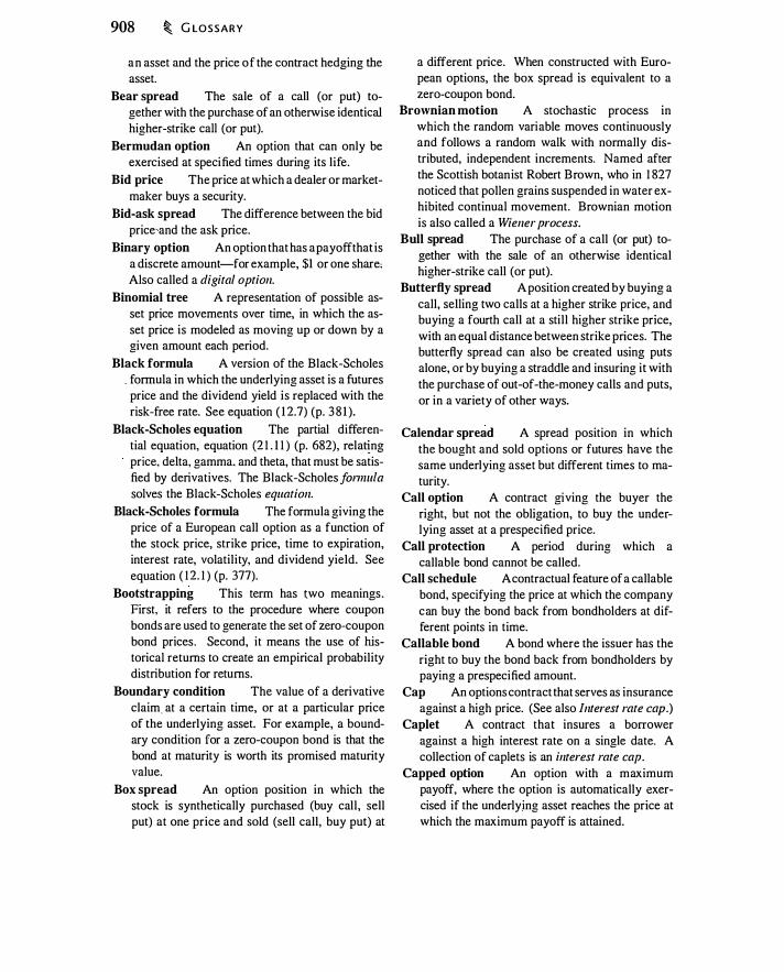
908 � G LOSSARY

an asset and the price of the contract hedging the asset.

Bear spread The sale of a call (or put) to-gether with the purchase of an otherwise identical higher-strike call (or put).

Bermudan option An option that can only be exercised at speci fied times during its l ife.

Bid price The price at which a dealer or market-maker buys a security.

Bid-ask spread The difference between the bid price,and the ask price.

Binary option An option that has a payoff that is a discrete amount-for example, $1 or one share, Also called a digital option.

Binomial tree A representation of possible as-set price movements over time, in which the as­set price is modeled as moving up or down by a given amount each period.

Black formula A version of the Black-Scholes . formula in which the underlying asset is a futures price and the dividend yield is replaced with the risk-free rate. See equation ( 1 2.7) (p. 3 8 1 ).

Black-Scholes equation The partial differen-tial equation, equation (2 1 . 1 1 ) (p. 682), rela�ng price, delta, gamma. and theta, that must be satis­fied by derivatives. The Black-Scholes fomw/a solves the Black-Scholes equation.

Black-Scholes formula The formula giving the price of a European call option as a function of the stock price, strike price, time to expiration, interest rate, volatility, and dividend yield. See equation ( 1 2. 1 ) (p. 377).

Bootstrapping This term has rwo meanings. First, it refers to the procedure where coupon bonds are used to generate the set of zero-coupon bond prices . Second, it means the use of his­torical returns to create an empirical probability distribution for returns.

Boundary condition The value of a derivative claim. at a certain time, or at a particular price of the underlying asset. For example, a bound­ary condition for a zero-coupon bond is that the bond at maturity is worth its promised maturity value.

Box spread An option position in which the stock is synthetically purchased (buy call, sell put) at one price and sold (sell call, buy put) at

a different price. When constructed with Euro­pean options, the box spread is equivalent to a zero-coupon bond.

Brownian motion A stochastic process in which the random variable moves continuously and follows a random walk with normally dis­tributed, independent increments. Named after the Scottish botanist Robert Brown, who in 1 827 noticed that pollen grains suspended in water ex­hibited continual movement. Brownian motion is also called a Wiener process.

Bull spread The purchase of a call (or put) to-gether with the sale of an otherwise identical higher-strike call (or put).

Butterfly spread A position created by buying a call, selling two calls at a higher strike price, and buying a fourth call at a sti l l higher strike price, with an equal distance between strike prices. The butterfly spread can also be created using puts alone, or by buying a straddle and insuring it with the purchase of out-of-the-money calls and puts, or in a variety of other ways.

Calendar spread A spread position in which the bought and sold options or futures have the same underlying asset but different times to ma­turity.

Call option A contract giving the buyer the right, but not the obligation, to buy the under­lying asset at a prespecified price.

Call protection A period during which a callable bond cannot be called.

Call schedule A contractual feature of a callable bond, specifying the price at which the company can buy the bond back from bondholders at dif­ferent points in time.

Callable bond A bond where the issuer has the right to buy the bond back from bondholders by paying a prespecified amount.

Cap An options contract that serves as insurance against a high price. (See also Interest rate cap.)

Caplet A contract that insures a borrower against a high interest rate on a single date. A collection of caplets is an interest rate cap.

Capped option An option with a maximum payoff, where the option is automatically exer­cised if the underlying asset reaches the price at which the maximum payoff is attained.

Carry Another term for owning an asset, typ-ically used to refer to commodities. (See also Carry market and Cost of carry).

Carry market A situation where the forward price is such that the return on a cash-and-carry is the risk-free rate.

Cash flow mapping A procedure in which the cash flows of a given claim are assigned--or mapped-to a set ofbenchmark claims. This pro­vides a way to approximate the claim in terms of the benchmark claims.

Cash settlement A procedure where settlement entails a cash payment from one party to the other, instead of delivery of an asset.

Cash-and-carry The simultaneous spot pur-chase and forward sale of an asset or commodity.

Cash-and-carry arbitrage The use of a cash-and-carry to effect an arbitrage.

Cash-or-nothing call An option that pays a fixed amount of cash if the asset price exceeds the strike price at expiration or zero otherwise.

Cash-or-nothing option An option that pays a fixed amount of cash if the option is in-the-money or zero otherwise.

Cash-or-nothing put An option that pays a fixed amount of cash if the asset price is less than the strike price at expiration or zero otherwise.

CDO See collateralized debt obligation.

Central limit theorem One of the most impor-tant results in statistics, which states that the sum of independent and identically distributed ran­dom variables has a limiting distribution that is normal.

Cheapest to deliver When a futures contract gives the seller a choice of asset to deliver to the buyer, the asset that is most profitable for the short to deliver.

Cholesky decomposition A formula used to construct a set of correlated random variables from a set of uncorrelated random variables.

Clean price The present value of a bond's fu-ture cash flows less accrued interest.

Clearinghouse A financial organization, typi-cally associated with one or more exchanges, that matches the buy and sell orders that take place during the day and keeps track of the obliga­tions and payments required of the members of the clearinghouse.

G LOSSARY � 909

Collar The purchase of a put and sale of a call at a higher strike price.

Collar width The difference between the strike prices of the two options in a collar.

Collateralized debt obligation a financial struc-ture that consists of a pool of assets, financed by issuing financial claims that reapportion the re­turn on the asset pool.

Collect-on-delivery option An option where the premium is paid only when the option is ex­ercised.

Commodity spread Offsetting long and short positions in closely related commodities. (See also Crack spread and Crush spread.)

Compound option An option that has an option as the underlying asset.

Concave Shaped like the cross section of an upside-down bowl.

Constructive sale A term in tax law describing the owner of an asset entering into an offsetting position that largely eliminates the risk of holding the asset.

Contango A forward curve in which futures prices are rising with time to expiration.

Contingent convertible bond A bond that be-comes convertible once a contingency (for ex­ample, the share price is greater than $ 1 00 for 30 days) has occurred.

Continuation value The value ofleaving an op-tion unexercised. You make an exercise decision by comparing the continuation value to the value of immediate exercise.

Continuously compounded interest rate A way of quoting an interest rate such that if $ 1 is in­vested at a continuously compounded rate of r,

the payoff in one year is er .

Control variate method A technique used in Monte Carlo valuation in which simulated asset prices are used to compute two derivatives prices: The price of the derivative that is being valued, and the price of a related derivative for which the value is known. The error in valuing the deriva­tive with a known price is used as a control for that with the unknown price.

Convenience yield A nonmonetary return to ownership of an asset or commodity.

Conversion A risk-free position consisting of an asset, a purchased put, and a written call.

910 � G LOSSARY

Convertible bond A bond which, at the option of the bondholder, can be surrendered for a spec­ified number of shares of stock.

Convex Shaped like the cross section of a bowl. Convexity The second derivative of a bond's

price with respect to a change in the interest rate, divided by the bond price.

Cooling degree day The greater of (i) 65 de-grees Farenheit minus the average daily temper­ature, and (ii) zero.

Cost of carry The interest cost of owning an as-set, less lease or dividend payments received as a result of ownership; the net cash flow resulting from borrowing to buy an asset.

Covered call A long position in an asset to-gether with a written call on the same asset.

Covered interest arbitrage A zero-investment strategy with simultaneous borrowing in one cur­rency, lending in another, and entering into a forward contract to guarantee the exchange rate when the loans mature.

Covered write A long position in an asset cou-pled with sale of a call option on the same asset.

Crack spread The difference between the price of crude oil futures and that of equivalent amounts of heating oil and gasoline.

Credit derivative A claim where the payoff de-. pends upon the credit rating or default status of a

firm. Credit risk Risk resulting from the possibility

that a counterparty will be financially unable to meet its contractual obligations.

Credit spread The difference between the yields on a bond that can default and on an oth­erwise equivalent default-free bond.

Credit-linked note A bond that has payments determined at least in part by credit events (e.g., default) at a different firm.

Cross-hedging The use of a derivative on one underlying asset to hedge the risk of another un­derlying asset.

Crush spread The difference between the price of a quantity of soybeans and that of the soybean meal and oil that can be produced by those soy­beans.

Cumulative distribution function A function giving the probability that a value drawn from a distribution will be less than or equal to some specified value.

Cumulative normal distribution function The cumulative distribution function for the nor­mal distribution; N(x) in the Black-Scholes equation.

Currency swap A swap in which the parties make payments based on the difference in debt payments in different currencies.

Currency-translated index An investment in an index denominated in a foreign currency, where the buyer bears both currency and asset risk.

Debenture A bond for which payments are se-cured only by the general credit of the issuer.

Debt capacity The maximum amount of debt that can be issued by a firm or secured by a spe­cific asset.

Default premium The difference between the yield on a bond and that on an otherwise equiva­lent default-free bond.

Default swap A contract in which the swap buyer pays a regular premium; in exchange, if a default in a specified bond occurs, the swap

· seller pays the buyer the loss due to the default.

Deferred down rebate option A deferred re-bate option for which the current stock price is above the rebate barrier.

Deferred rebate option A claim that pays $ 1 at expiration if the price of the underlying asset has reached a barrier prior to expiration.

Deferred swap A swap with terms specified to-day, but for which swap payments begin at a later date than for an ordinary swap.

Deferred up rebate option A deferred rebate option for which the current stock price is below the rebate barrier.

Delivery The act of the seller (e.g., of a forward contract) supplying the underlying asset to the buyer.

Delta The change in the price of a derivative due to a change in the price of the underlying asset.

Delta-gamma approximation A formula using the delta and gamma to approximate the change in the derivative price due tq a change in the price of the underlying asset.

Delta-gamma-theta approximation A for-mula using the delta, gamma, and theta to ap­proximate the change in the derivative price due to a change in the price of the underlying asset and the passage of time.

Delta-hedging Hedging a derivative position using the underlying asset, with the amount of the underlying asset determined by the derivative's sensitivity (delta} to the price of the underlying asset.

Derivative A financial instrument that has a value determined by the price of something else.

Diff swap A swap in which payments are based on the difference in floating interest rates on a given notional amount denominated in a single currency.

Differential equation An equation relating a variable to its derivatives and one or more in­dependent variables.

Diffusion process Generally, a continuous stochastic process in which uncertainty increases with time. Also used to describe the Brownian (random) part of an Ito process.

Digital option Another name for a binary op-tion.

Dirty price The present value of a bond's fu-ture cash flows (this implicitly includes accrued interest).

Distance to default The distance between the current firm asset value and the level at which default occurs, measured in standard deviations.

Diversifiable risk Risk that is, in the l imit, eliminated by combining a large number of as­sets in a portfolio.

Down-and-in A knock-in option for which the barrier is less than the current price of the under­) ying asset.

Down-and-out A knock-out option for which the barrier is less than the current price of the underlying asset.

Drift The expected change per unit time in an asset price.

Duration Generally, the weighted average life of the bond, which also provides a measure of the bond's sensitivity to interest rate changes. Two common duration measures are modified dura­

tion and Macaulay duration.

G LOSSARY � 911

Effective annual interest rate A way o f quot-ing an interest rate such that the quoted rate is the annual percentage increase in an amount invested at this rate. If $ 1 is invested at an effective annual rate of r, the payoff in one year is $ 1 + r.

Elasticity The percent change in an option price for a I % change in the price of the underlying as­set.

Equity-linked forward A forward contract (e.g., for currency) where the quantity to be bought or sold depends upon the performance of a stock or stock index.

European option An option that can only be ex-ercised at expiration.

Exchange option An option permitting the holder to obtain one asset by giving up another. Standard calls and puts are exchange options in which one of the two assets is cash.

Exercise The exchange of the strike price (or strike asset) for the underlying asset at the terms specified in the option contract.

Exercise price Under the terms of an option contract, the amount that can be exchanged for the underlying asset.

Exercise style The circumstances under which an option holder has the right to exercise an op­tion. "European" and "American" are exercise styles.

Exotic option A derivatives contract in which an ordinary derivative has been altered to change the characteristics of the derivative in a meaning­ful way. Also called a nonstandard option.

Expectations hypothesis A term with multiple meanings, one of which is that the expected fu­ture interest rate equals the implied forward rate.

Expected Tail Loss The expected loss condi-tional upon the VaR loss being exceeded. An­other name for Tail VaR.

Expiration The date beyond which an unexer-cised option is worthless.

Fair value Another name for the theoretical for-ward price: Spot price plus interest less the future value of dividends.

Financial engineering Creating new financial instruments by combining other derivatives, or more generally, by using derivatives pricing tech­niques.

912 � G LO SS A RY

Floor An option position that guarantees a min-imum price.

Forward contract An agreement that sets to-day the terms-including price and quantity-at which you buy or sell an asset or commodity at a specific time in the future.

Forward curve The set of forward or futures prices with different expiration dates on a given date for a given asset.

Forward premium The annualized percentage difference I:Jetween the forward price and the spot price.

Forward rate agreement A forward contract for an interest rate.

Forward strip Another name for the fonvard

curve.

Funded A position that is paid for in full at the outset. A prepaid forward, for example, is a funded position in a stock. See also unfunded.

Futures contract An agreement that is similar to a forward contract except that the buyer and seller post margin and the contract is marked­to-market periodically. Futures are typically exchange-traded.

Futures overlay Converting an investment in asset A into the economic equivalent of an invest­ment in asset B by entering into a short futures position on asset A and a long futures position on asset B.

Gamma The change in delta when the price of the underlying asset changes by one unit.

Gap option An. option where the option owner has the right to exercise the option at strike K 1

if the stock price exceeds (or, depending on the option, is less than) the price K2• For an ordinary option, Kt = K2.

Geometric Brownian motion A continuous stochastic process, x (t) , in which the increments are given as dx (t)/x (t) = adt + udZ , where d Z is the increment to a Brownian process.

Girsanov's theorem A result that permits a change in the drift of an Ito process accompa­nied by a change in the probability distribution of the Brownian motion driving the process.

Greeks A term generally referring to delta, gamma, vega, theta, and rho, all of which mea­sure the change in the price of a derivative when

there is a change in an input to the pricing for­mula.

Haircut The collateral, over and above the mar-ket value of the security, required by the lender when a security is borrowed.

Heat rate A measure of the efficiency with which heat can be used to produce electricity. Specifically, it is the number of British Thermal Units required to produce 1 kilowatt/hour of elec­tricity.

Heating degree day The greater of (i) the aver-age daily temperature minus 65 degree Farenheit, and (ii) zero.

Hedge ratio In a hedging transaction, the ratio of the quantity of the forward or futures position to the quantity of the underlying asset.

Hedging An action-such as entering into a derivatives position-that reduces the risk of loss.

Heston model An option pricing model in which the instantaneous variance of the stock re­turn follows a mean-reverting square root pro­cess .

. Heteroskedasticity Data that is characterized by variances that are not equal, either over time or across different observations at a point in time.

Historical volatility The standard deviation of the continuously compounded return on an asset, measured using historical prices.

Homoskedasticity Data that is characterized by variances that are equal over time or across dif­ferent observations at a point in time.

Hysteresis The failure of an effect to reverse i t-self as the underlying cause is reversed.

Implied forward rate The forward interest rate between time t1 and time t2 (t1 < t2) that makes an investor indifferent between, on the one hand, buying a bond maturing at t2, and, on the other hand, buying a bond maturing at t1 and reinvest­ing the proceeds at this forward interest rate.

Implied repo rate The rate of return on a cash-and-carry.

Implied volatility The volatility for which the theoretical option price (typically computed us­ing the Black-Scholes formula) equals the ob­served market price of the option.

Interest rate cap A contract that periodically pays the difference between the market interest rate and a guaranteed rate, if the difference is pos­itive.

In-the-money An option that would have value if exercised. For an in-the-money call, the stock price exceeds the strike price. For an in-the­money put, the stock price is less than the strike price.

Investment trigger price The price of an in-vestment project (or the price of the good to be produced) at which it is optimal to invest in the project.

Ito process A continuous stochastic process that can be written in the form dX (t) = a[X (t) , t] dt + u [X (t ) , t] dZ(t ) , where dZ(t) is the increment to a Brownian process.

Ito's Lemma If x follows an Ito process, Ito's Lemma describes the process followed by f(x) .

For example, if x is a stock price and f (x) an option price, Ito's Lemma characterizes the be­havior of the option price in terms of the process for the stock.

Jensen's inequality If x is a random variable and f(x) is convex, Jensen's inequality states that E[f(x)] � f[E(x)] . The inequality is reversed if f (x) is concave.

Jump-diffusion model A process for an asset price in which the asset most of the time follows an Ito process but can also jump discretely, with occurrence of the jump controlled by a Poisson process.

Kappa Another name for vega.

Knock-in option An option in which there can only be a final payoff if, during a specified pe­riod of time, the price of the underlying asset has reached a specified level.

Knock-out option An option in which there can only be a final payoff if, during a specified period of time, the price of the underlying asset has not

reached a specified level.

Kolmogorov backward equation A partial differential equation, (see equation (2 1 .32) (p. 69 1 ), that is related to the Black-Scholes equation and that is satisfied by probability distributions for the underlying asset.

G LO S SA RY � 913

Kurtosis A measure of the peakedness of a prob-ability distribution. For a random variable x with mean JL and standard deviation u , kurtosis is the fourth central moment divided by the squared variance, E (x - JL)4ju4 • For a normal random variable, kurtosis is 3 .

Ladder option If the barrier L > K i s reached over the life of the option, a ladder option at expi­ration pays max(O, L - K, ST - K) . If the barrier is not reached, the option pays max(O, ST - K).

Lambda Another name for vega.

Lattice A binomial tree in which an up move followed by a down move leads to the same price as a down move followed by an up move. Also called a recombining tree.

Law of one price The assertion that two portfo-lios generating exact! y the same return must have the same price.

Lease rate The annualized payment required to borrow an asset, or equivalently, the annualized payment received in exchange for lending an as­set.

Leverage effect A rise in the stock price volatil-ity when the stock price declines.

LffiiD London Interbank B id Rate. See Ll-BOR.

LffiOR London Interbank Offer Rate. A mea-sure of the borrowing rate for large international banks. The British Banker's Association deter­mines LIBOR daily for different currencies by surveying at least 8 banks, asking at what rate they could borrow, dropping the top and bot­tom quartiles of the responses, and computing an arithmetic average of the remaining quotes. Since LIBOR is an average, there may be no ac­tual transactions at that rate. Confusingly, LI­BOR is also sometimes referred to as a lending rate. This is because a bank serving as a market­maker in the interbank market will offer to lend money at a high interest rate (LIB OR) and borrow money at a low interest rate (LIBID). (The differ­ence between LIBOR and LIBID is the bid-ask spread in the interbank market.) A bank needing to borrow will thus pay LIB OR, and a bank with excess funds will receive LIBID.

Log contract A derivative contract that, at ma-turity, pays the natural log of an asset price.

914 � G LOSSARY

Lognormal distribution A probability distri-bution in which the natural logarithm of the ran­dom variable is normally distributed.

Long A position is long with respect to a price if the position profits from an increase in that price. An owner of a stock profits from an increase in the stock price and, hence, is long the stock. An owner of an option profits from an increase in volati lity and, hence, is long volatility.

Long forward The party to a forward contract who has an obligation to buy the underlying asset.

Lookback call See Lookback option.

Look back option An option that, at maturity, pays off based on the maximum (ST) or mini­mum (§_T) stock price over the life of the option. A /ookback call has the payoff ST - �T and a

- /ookback put has the payoff S T - ST . Lookback put See Lookback option.

Macaulay duration The percent change in a bond's price for a given percent change in one plus the bond's yield. This calculation can be interpreted as the weighted average life of the bond, with the weights being the percentage of the bond's value due to each payment.

Maintenance margin The level of margin at which the contract holder is required to add cash or securities to the margin account.

Mandatorily convertible bond A bond that makes payments in shares instead of cash, with the number of shares paid to the bondholder typ­ically dependent upon the share price.

Margin A deposit required for both buyers and sellers of a futures contract, which indemnifies the counterparty against the failure of the buyer or seller to meet the obligations of the contract.

Margin call The requirement that the owner of a margined position add funds to the margin ac­count. This can result from a loss on the position or an increase in the margin requirement.

Market corner Owning a large percentage of the available supply of an asset or commodity that is required for delivery under the terms of a derivatives contract.

Market-maker A trader in an asset, commodity, or derivative who simultaneously offers to buy at one price (the bid price) or to sell at a higher price (the offer price), thereby "making a market."

Market-timing The allocation of assets be-tween stocks and bonds in an attempt to invest in whichever asset is going to have a higher re­turn.

Mark-to-market The procedure of revaluing a portfolio or position to reflect current market prices.

Martingale A stochastic process for which E[X(t + s) J <P (t) ] = X (t) , where <P (t) is in­formation available at time t .

Modified duration The percent change i n a bond's price for a unit change in the yield. Mod­ified duration is also Macaulay duration divided by one plus the bond's yield per payment period.

Monte Carlo valuation A procedure for pric-ing derivative claims by discounting expected payoffs, where the expected payoff is computed using simulated prices for the underlying asset.

Naked writing Selling options without an off-setting position in the underlying asset.

Net payoff Another term for profit.

Non-traded asset A cash flow stream that can-not be purchased directly in financial market. Many corporate investment projects are non­traded because they can only be acquired by buy­ing the entire company.

Nondiversifiable risk Risk that remains after a large number of assets are combined in a portfo­lio.

Nonrecombining tree A binomial tree describ-ing asset price moves in which an up move fol­lowed by a down move yields a different price than a down move followed by an up move.

Nonstandard option See Exotic option.

Normal distribution A bell-shaped, symmet-ric, continuous probability distribution that as­signs positive probability to all values from -oo

to +oo. Sometimes called the "bell curve." (See also Cemral limit theorem.)

Notional amount The dollar amount used as a scale factor in calculating payments for a forward contract, futures contract, or swap.

Notional principal The notional amount for an interest rate swap.

Numeraire The units . in which a payoff is de-nominated.

Offer price The same as the ask price.

Off-market forward A forward contract in which the forward price is set so that the value of the contract is not zero.

Off-the-run A government bond that is not one of the recently issued bonds.

On-the-run The most recently auctioned gov-ernment bonds at the government's specific auc­tion maturities.

Open interest The quantity of a derivatives contract that is outstanding at a point in time. (One long and one short position count as one unit outstanding.)

Open outcry A system of trading in which buy-ers and sellers in one physical location convey offers to buy and sell by gesturing and shouting.

Option elasticity The percent change in an op-tion price for a I % change in the price of the underlying asset.

Option overwriting Selling a call option against a long position in the underlying asset.

Option writer The party with a short position in the option.

Order statistics The 11 draws of a random vari-able sorted in ascending order.

Out-of-the-money An option that would be ex-ercised at a loss. An out-of-the-money call has the stock price less than the strike price. An out­of-the-money put has the stock price greater than the strike price.

Outperformance option An option in which the payoff is determined by the extent to which one asset price is greater than another asset price.

Over-the-counter market A term used gener-ally to refer to transactions (e.g., purchases and sales of securities or derivatives contracts) that occur without the involvement of a regulated ex­change.

Par bond A bond for which the price at issue equals the maturity value.

Par coupon The coupon rate on a par bond. Partial expectation The sum (or integral) of a

set of outcomes times the probability of those outcomes.

Path-dependent A derivative where the final payoff depends upon the path taken by the stock price, instead of just the final stock price.

G LOSSARY ' 915

Payer swaption A swaption giving the holder the right to be the fixed-rate payer in a swap.

Pay later strategy Generally used to refer to op-tion strategies in which the position buyer makes no payments unless the option moves more into the money.

Payoff . The value of a position at a point in time. The term often implicitly refers to a payoff at ex­piration or maturity.

Payoff diagram A graph in which the value of a derivative or other claim at a point in time is plotted against the price of the underlying asset.

Payout protected A characteristic of a deriva-tive where a change in the dividend payout on the underlying asset does not change the value of the derivative.

Perpetual option An option that never expires. Poisson distribution A probability distribution

that counts the number of events occurring in an interval of time, assuming that the occurrence of events is independent.

Positive-definite An 11 x 11 matrix with elements a;.j is positive-definite if, for every w; =f. 0, i = I , . . . , 11 , I:;'= t I:�= t W; Wjai.j > 0. A covari­ance matrix is positive-definite.

Power option An option where the payoff is based on the price of an asset raised to a power.

Prepaid forward contract A contract calling for payment today and delivery of the asset or commodity at a time in the future.

Prepaid forward price The price the buyer pays today for a prepaid forward contract.

Prepaid swap A contract calling for payment today and delivery of the asset or commodity at multiple specified times in the future.

Price limit In futures markets, the size of a fu-tures price move such that trading is halted tem­porarily.

Price participation The extent to which an equity-linked note benefits from an increase in the price of the stock or index to which it is l inked.

Price value of a basis point The change in a bond price due to a ! -basis-point change in the yield of the bond. Frequently abbreviated PVBP.

Profit The payoff less the future value of the original cost to acquire the position.

Profit diagram A graph plotting the profit on a position against a range of prices for the under­lying asset.

916 � G LOSSARY

Proprietary trading Taking positions in an as-set or derivative to express a view-for example, that a stock price will rise or that implied volatil­ity will fall.

Psi The change in the price of a derivative due to a change in the dividend yield.

Purchased call A long position in a call. Purchased put A long position in a put. Put option A contract giving the buyer the right,

but not the obligation, to sell the underlying asset at a prespecified price.

Put-call parity'

A relationship stating that the difference between the premiums of a call and a put with the same strike price and time to expi­ration equals the difference between the present value of the forward price and _the present value of the strike price.

Puttable bond A bond that the investor can sell back to the issuer at a predetermined price sched­ule.

Quadratic variation The sum of squared incre-ments to a Brownian motion.

Quantile A data point is the xth quantile if x% of the data lies below that point.

Quanto A derivatives contract with a payoff in which foreign-currency-denominated quantities

. are treated as if they were denominated in the domestic currency.

Quasi-arbitrage The replacement of one asset or position with another that has equivalent risk and a higher expected rate of return.

Rainbow option An option that has a payoff based on the maximum or minimum of two (or more) risky assets and cash. For example, the payoff to a rainbow call is max (Sr , Q r , K), where Sr and Qr are risky asset prices.

Random walk A stochastic process, X (t), in which increments, E (t) , are independent and identically distributed: X (t) = X(t - h) + E (t) .

Ratings transition A change in the credit rating of a bond from one value to another.

Ratio spread Buying m of an option at one strike and selling n of an otherwise identical op­tion at a different strike.

Real options The applications of derivatives theory to the operation and valuation of real (physical) investment projects.

Realized quadratic variation The sum of squared continuously compounded asset returns, typically measured at a high frequency.

Realized volatility Another term for realized quadratic variation.

Rebate option A claim that pays $ 1 at the time the price of the underlying asset reaches a barrier.

Receiver swaption A swaption giving the holder the right to receive the fixed rate in a swap.

Recombining tree A binomial tree describing asset price moves in which an up move followed by a down move yields the same price as a down move followed by an up move. Also called a lattice.

Recovery rate The percentage of par value re-ceived by a bond holder in a bankruptcy.

Reference price A market price or rate used to determine the payoff on a derivatives contract.

Repo Another name for a repurchase agree-

ment.

Repo rate The annualized percentage differ-ence between the ori

_ginal sale price and final re­

purchase price in a repurchase agreement. Repricing The replacement of an out-of-the-

money compensation option with an at-the­money compensation option.

Repurchase agreement The sale of a security coupled with an agreement to buy it back at a later date.

Reverse cash-and-carry The simultaneous short-sale and forward purchase of an asset or commodity.

Reverse conversion A short position in an as-set coupled with a purchased call and written put, both with the same strike price and time to expi­ration. The position is equivalent to a short bond.

Reverse repo Another name for reverse repur-

chase agreement.

Reverse repurchase agreement The purchase of a security coupled with an agreement to sell it at a later date. The opposite of a repurchase agreement.

Rho The change in value of a derivative due to a change in the interest rate.

Risk averse A term describing an investor who prefers x to taking a risky bet with an expected value equal to x.

Risk management The active use of deriva-tives and other techniques to alter risk and protect profitability.

Risk neutral A term describing an investor who is indifferent between receiving x and taking a risky bet with an expected value equal to x .

Risk premium The difference between the ex-pected return on an asset and the risk-free rate; the expected return differential that compensates investors for risk.

Risk-neutral measure The probability distri-bution for an asset transformed so that the ex­pected return on the asset is the risk-free rate.

Risk-neutral probability In the binomial model, the probability of an up move in the asset price such that the expected return on the asset is the risk-free rate.

Self-financing portfolio A portfolio that re-tains specified characteristics (e.g., it is zero­investment and risk-free) without the need for additional investments in the portfolio.

Settlement The time in a transaction at which all obligations of both the buyer and the seller are fulfilled.

Share-equivalent The position in shares that has equivalent dollar risk to a derivative. (See also Delta.)

Sharpe ratio For an asset, the ratio of the risk premium to the return standard deviation.

Short A position is short with respect to a price if the position profits from a decrease in that price. A short-seller. of a stock profits from a decrease in the stock price and, hence, is short the stock. A seller of an option profits from a decrease in volatility and, hence, is short volatil ity.

Short call A call that has been sold. Short forward The party to a forward contract

who has an obligation to sell the underlying asset. Short put A put that has been sold. Short rebate The rate of return paid on collat-

eral when shares are borrowed. Short-against-the-box The short-sale of a

stock that the short-seller owns. The result of a short-against-the-box is that the short-seller has both a long and short position and, hence, bears no risk from the stock yet receives the value of the shares from the short sale.

G LOSSARY � 917

Short-sale A transaction in which an investor borrows a security, sells it, and then returns it at a later date to the lender. If the security makes payments, the short-seller must make the same payments to the lender.

Shout option A shout call option expiring at time T has the payoff max(O, S; - K, Sr - K), where i is the time and S; is the price at which the option holder "shouted," thereby guaranteeing an expiration payoff at least as great as S; - K.

Skewness A measure o f the symmetry of a prob-ability distribution. For a random variable x with mean J-L and standard deviation rr, skewness is the third central moment divided by the cubed standard deviation, E (x - J-L)3 frr3 • For a nor­mal variable, skewness is 0. (See also Volatility

skew.) Spark spread The difference between the price

of electricity and that of the quantity of natural gas required to produce the electricity.

Spot curve The set of zero-coupon bond prices with different maturities, usually inferred from government bond prices.

Spot price The current market price of an asset. Spread Simultaneously buying and selling

closely related derivatives. A spread in options is a position in which some options are bought and some are sold, and all options in the position are calls or all are puts. (See also Calendar spread

and Commodity spread.) Spread option An option with a payoff where a

spread (the difference between prices) takes the place the of the underlying asset.

Stable distribution A probability distribution for which sums of random variables have the same distribution as the original random vari­able. The normal distribution is stable because sums of normally distributed random variables are normally distributed.

Stack and roll A hedging strategy in which an existing stack hedge with maturing futures con­tracts is replaced by a new stack hedge with longer dated futures contracts.

Stack hedge Hedging a stream of obligations by entering futures contracts with a single ma­turity, with the number of contracts selected so that changes in the presellt value of the future obligations are offset by changes in the value of this "stack" of futures contracts.

918 � G LOSSARY

Static NPV The net present value of a project at a point in time, ignoring the possibility of post­poning adoption of the project.

Static option replication The use of options to hedge options, with the goal of creating a hedging portfolio that has a delta that naturally moves in tandem with the delta of the option being hedged.

Stochastic differential equation An equation characterizing the change in a variable in which one or more of the differential terms are incre­ments to a_stochastic process.

Stochastic process A mathematical model for a random process as a function of time

Stochastic volatility A process in which the in-stantaneous volatility can vary randomly, either as a function of the stock price or other variables.

Stock index An average of the prices of a group of stocks. A stock index can be a simple aver­age of stock prices, in which case it is equally

weighted, or it can be a weighted average, with the \veights proportional to market capitalization, in which case it is value-weighted.

Straddle The purchase of a call and a put with the same strike price and time to expiration.

Strad�le rules Tax regulations controlling the circumstances in which a loss on a claim can be realized when a taxpayer continues to own related securities or derivatives.

Strangle The purchase of a put and a higher-strike call with the same time to expiration.

Stratified sampling A technique used in Monte Carlo valuation in which random numbers are drawn from each percentile (or other regular in­terval ) of the distribution.

Strike price Another term for exercise price.

Strip hedge Hedging a stream of obligations by offsetting each individual obligation with a fu­tures contract matching the maturity and quantity of the obl igation.

STRIPS Acronym for Separate Trading of Reg-

istered Interest and Principal of Securities.

STRIPS are the interest and principal payments from Treasury bonds and notes traded as individ­ual securities.

Structured note A bond that makes payments that, at least in part, are contingent on some vari­able such as a stock price, interest rates, or ex­change rates.

Supershare A claim to a portfolio that pays the holder a portion of the portfolio only if a particu­lar event occurs. (An example of an event would be the asset losing between 25% and 26% of its value.)

Swap A contract calling for the exchange of pay-ments over time. Often one payment is fixed in advance and the other is floating, based upon the realization of a price or interest rate.

Swap spread The difference between the fixed rate on an interest rate swap and the yield on a Treasury bond with the same maturity.

Swap tenor The lifetime of a swap.

Swap term Another name for swap tenor.

Swaption An option to enter into a swap.

Tail VaR The expected loss conditional upon the VaR loss being exceeded.

Tailing A reduction in the quantity of an asset held in order to offset future income received by the asset.

Tenor Time to maturity or expiration of a con-tract, frequently used when referring to swaps.

Term repo A repurchase agreement lasting for a specified period of time longer than one day.

Theta The change in the value of a derivative due solely to the passage of time.

Time decay Another term for theta.

Total return swap A swap in which one party pays the total return (dividends plus capital gains) on a reference asset, and the other party pays a floating rate such as LIBOR.

Traded present value The value an investment project would have once the investment was made; also called twin security.

Twin security See Traded present value.

Underlying asset The asset whose price deter-mines the profitability of a derivative. For exam­ple, the underlying asset for a purchased call is the asset that the call owner can buy by paying the strike price.

Unfunded A position that is not paid for at the outset and for which cash inflows and outflows can later occur. A forward contract, for exam­ple, is an unfunded position in a stock. See also funded.

Up-and-in A knock-in option for which the bar-rier exceeds the current price of the underlying asset.

Up-and-out A knock-out option for which the barrier exceeds the current price of the underly­ing asset.

Value at risk The level of loss that will be ex-ceeded a given percentage of the time over a given horizon.

Vanilla A standard option or other derivative. For example, ordinary puts and calls are "vanilla" options.

Variance swap A forward contract that settles based on cumulative squared asset returns.

Vega The change in the price of a derivative due to a change in volatility. Also sometimes called kappa or lambda.

Vertical spread The sale of an option at one strike and purchase of an option of the same type (call or put) at a different strike, both having the same underlying asset and time to expiration.

Volatility The standard deviation of the contin-uously compounded return on an asset.

Volatility clustering The tendency of high volatility days to be followed by high volatility days.

Volatility skew Generally, implied volatility as a function of the strike price. Volatility skew refers to a difference in premiums as reflected in differences in implied volatility. Skew is some­times used more precisely to refer to a difference in implied volatilities between in-the-money and out-of-the-money options.

Volatility smile A volatility skew in which both in-the-money and out-of-the-money options have a higher volatility than at-the-money options (i.e., when you plot implied volatility against the strike price, the curve looks like a smile).

G LOSSARY ' 919

Volatility surface A three-dimensional graph in which volatility is plotted against strike price and time to maturity.

Volatility swap A forward contract that settles based on some measure of the standard deviation of returns on an asset.

Warrant An option issued by a firm with its own stock as the underlying asset. This term also refers more generally to an option issued in fixed supply.

Weather derivative A derivative contract with a payment based on a weather-related measure­ment, such as heating or cooling degree days.

Wiener process See Brownian motion.

Written call A call that has been sold; a short call .

Written put put.

A put that has been sold; a short

Written straddle The simultaneous sale of a call and sale of a put, with the same strike price and time to expiration.

Yield curve The set of yields to maturity for bonds with different times to maturity.

Yield to maturity The single discount factor for which the present value of a bond's payments is equal to the observed bond price.

Zero-cost collar The purchase of a put and sale of a call where the strikes are chosen so that the premiums of the two options are the same.

Zero-coupon bond A bond that makes only a single payment, at maturity.

Zero-coupon yield curve The set of yields to maturity for zero-coupon bonds with different times to maturity.

BIBLIQGRAPFfY: ··

Acerbi, C., 2002, "Spectral Measures of Risk: A Coherent Repreentation of Subjective Risk

Aversion," Journal of Banking and Finance, 26(7), 1 505- 1 5 1 8.

Acerbi, C. and Tasche. D., 2002, "On the Coherence of Expected Shortfall," Journal of Banking

and Finance, 26(7), 1487- 1 503.

Acharya, V. V., John, K., and Sundaram, R. K., 2000, "On the Optimality of Resetting Executive

Stock Options," Journal of Financial Economics, 57( 1 ) , 65- 1 O J .

Alexander, C., 200 1 , Market Models, Wiley, Chichester, England.

Allayannis, G, Brown, G, and Klapper, L. F., 2003, "Capital Structure and Financial Risk: Evi­

dence from Foreign Debt Use in East Asia," Journal of Finance, 58, 2667-2709.

Allayannis, G, Lei, U., and Miller, D., 2004, "Corporate Governance and the Hedging Premium

Around the World," Working Paper, Darden School, University of Virginia.

Allayannis, G and Weston, J., 200 1 , "The Use of Foreign Currency Derivatives and Firm Market

Value," Review of Financial Studies, 14( 1 ), 243-276.

Andersen, T., Benzoni, L., and Lund, J., 2002, '"An Empirical Investigation of Continuous-Time

Equity Return Models," Journal of Finance, 57(3), 1 239-1 284, forthcoming.

Andersen, T. G, Bollerslev, T., Diebold, F. X., , and Labysd, P., 2003, "Modeling and Forecasting

Realized Volatility," Econometrica, 7 1 (2) , 579-625 .

Andersen, T. G, Bollerslev, T., Frederiksen, P. H., and Nielsen, M., 2005, "Jumps in Financial

Markets," Unpublished, Kellogg School, Northwestern University.

Anderson, R. and Sundaresan, S. , 2000, "A Comparative Study of Structural Models of Corporate

Bond Yields: An Exploratory Investigation," Joumal of Banking and Finance, 24( 1 -2), 255-

269.

Amason, S . T. and Jagannathan, R., 1 994, "Evaluating Executive Stock Options Using the Bin.o­

miai Option Pricing Model," Working Paper, Carlson School of Management, University of Minnesota.

Artzner, P., Delbaen, F., Eber, J.-M., and Heath, D., 1 999, "Coherent Measures of Risk," Mathe­

matical Finance, 9(3), 203-228.

Arzac, E. R., 1 997, "PERCs, DECs, and Other Mandatory Convertibles,'' Journal of Applied

Corporate Finance, 1 0( 1 ), 54-63.

Asquith, P., 1 995, "Convertible Bonds Are Not Called Late,'' Journal of Finance, 50( 4 ) , 1 275-89.

Bakshi, G, Cao, C., and Chen, Z., 1 997, "Empirical Performance of Alternative Option Pricing

Models,'' Journal of Finance, 52(5), 2003-49.

Bakshi, G and Kapadia, N., 2003, "Volatility risk Premium Embedded in Individual Options: Some New Insights," Journal of Derivatives. pp. 45-54.

Bartram, S. M., Brown, G W., and Fehle, F. R., 2004. "International Evidence on Financial

Derivatives Use,'' Working Paper, University of North Carolina.

Basel Committee on Banking Supervision, 1 996, Amendmellf to the Capital Accord to Incorporate

Market Risks, Technical report, Bank for International Settlements.

921

922 � B I B L I O G RA P H Y

Bates, D . S . , 2000, "Post-'87 Crash Fears the S&P 500 Futures Option Market," Joumal of

Econometrics, 94, 1 8 1-238.

Bates, D. S., 2003, "Empirical Option Pricing: A Retrospection," Joumal of Econometrics, 1 1 6(1-2) , 387-404.

Baubonis, C., Gastineau, G, and Purcell, D. , 1 993, "The Banker's Guide to Equity-Linked Cer­tificates of Deposit," Joumal of Derivatives, 1 (2), 87-95.

Baxter, M. and Rennie, A., 1 996, Financial Calculus: An Introduction to Derivative Pricing,

Cambridge University Press, Cambridge, England.

Benzoni, L., 200 1 , "Pricing Options under Stochastic Volatility: An Empirical Investigation," Unpublished, University of Minnesota.

Bernstein, P. L., 1 992, Capita/ Ideas: The Improbable Origins of Modem Wall Street, Free Press, New York.

Bernstein, P. L., 1 996, Against the Gods: The Remarkable Story of Risk, John Wiley & Sons, New York.

Bettis, J. C., Bizjak, J. M., and Lemmon, M. L., 200 1 , "Managerial Ownership, Incentive Con­tracting, and the Use of Zero-Cost Collars and Equity Swaps by Corporate Insiders," lou mal

of Financial and Quantitative Analysis, 36(3), 345-370.

Bharath, S . T. and Shumway, T., 2004, "Forecasting Default with the KMV-Merton Model," Working Paper, University of Michigan.

Black, F., 1 976a, "The Pricing of Commodity Contracts," Joumal of Financial Economics, 3( 1 12), 167-179.

Black, F. , 1976b, "Studies of Stock Price Volatility Changes," Proceedings of the 1976 Meetings of

the American Statistical Association, Business and Economics Statistics Section, pp. 1 77-1 8 1 .

Black, F. , 1 989, "How We Came Up With �e Option Pricing Formula," Joumal of Portfolio

Management, 15 (2), 4-8.

Black, F. and Cox, J., 1 976, "Valuing Corporate Securities: Some Effects of Bond Indenture Provisions," lou mal of Finance, 3 1 , 35 1-367.

Black, F., Derman, E., and Toy, W., 1 990, "A One-Factor Model of Interest Rates and Its Appli­cation to Treasury Bond Options," Financial Analysts lou mal, 46( 1 ), 33-39.

Black, F. and Scholes, M., 1 973, "The Pricing of Options and Corporate Liabilities," Joumal of

Political Economy, 8 1 , 637-659.

Bliss, R. R., 1997, "Movements in the Term Structure of lnterest Rates," Federal Reserve Bank

of Atlama Economic Review, 82(4), 1 6-33.

Bodie, Z., 1995, "On the Risk of Stocks in the Long Run," Financial Analysts Joumal, 5 1 (3), 1 8-22.

Bodie, Z. and Crane, D. , 1 999, "The Design and Production ofNew Retirement Savings Products," Joumal of Portfolio Management, 25(2), 77-82.

Bodie, Z., Kaplan, R. S . , and Merton, R. C., 2003, "For the Last Time: Stock Options Are an

Expense," Harvard Business Review, pp. 3-1 1 .

Bodie, Z . and Rosansky, V. 1., 1 980, "Risk and Return i n Commodity Futures," Financial Analysts

Joumal, pp. 3-14.

Bodnar, G M., Hayt, G S. , and Marston, R. C., 1 998, " 1 998 Wharton S urvey of Financial Risk Management by US Non-Financial Firms," Financial Management, 27(4), 70-9 1 .

Bollerslev, T., 1 986, "Generalized Autoregressive Conditional Heteroskedasticity," Joumal of

Econometrics.

Bollerslev, T., 1 987, "A Conditional Heteroskedastic Time Series Model for Speculative Prices and Rates of Return," Review of Economics and Statistics, 69, 542-547.

B I B L I O G R A P H Y � 923

Bollerslev, T., Engle, R. F., and Nelson, D. B. , 1 994, "ARCH Models," in R. F. Engle and D. L. McFadden, (eds.) "Handbook of Econometrics," volume 4 of Handbooks in Economics,

chapter 49, pp. 2959-3038, Elsevier Science, B.V., Amsterdam.

Boyle, P. P., 1 977, "Options: A Monte Carlo Approach," Journal of Financial Economics, 4(3),

323-338. Boyle, P. P., Broadie, M., and Glasserman, P., 1 997, "Monte Carlo Methods for Security Pricing,"

Journal of Economic Dynamics and Control, 2 1 (8-9), 1267-1 322.

Boyle, P. P. and Emanuel, D., 1 980, "Discretely Adjusted Option Hedges," Joumal of Financial

Economics, 8(3), 259-282.

B oyle, P. P., Evnine, J. , and Gibbs, S. , 1 989, "Numerical Evaluation of Multivariate Contingent Claims," Review of Financial Studies, 2(2), 24 1-250.

Brace, A., Gatarek, D., and Musiela, M., 1 997, "The Market Model of lnterest Rate Dynamics," Mathematical Finance, 7, 1 27-1 54.

Brealey, R. and Myers, S., 2003, Principles of C01porate Finance, Irwin McGraw-Hill, Burr Ridge, IL, 6th edition.

Brennan, M. and Schwartz, E., 1 985, "Evaluating Natural Resource Investments," Joumal of

Business, 58, 1 35-1 57.

Brennan, M. J., 1 99 1 , "The Price of Convenience and the Evaluation of Commodity Contingent Claims," in D. Lund and B. 0ksendal , (eds.) "Stochastic Models and Option Values: Ap­

plications to Resources, Environment and Investment Problems," Contributions to Economic Analysis, pp. 33-7 1 , North-Holland, Amsterdam.

Brennan, M. J., 2000, "Real Options: Development and New Contributions," in Brennan and Trigeorgis (2000), chapter I , pp. 1 - 1 0.

Brennan, M. J. and Schwartz, E. S . , 1 977, "Convertible Bonds: Valuation and Optimal Strategies for Call and Conversion," Journal of Finance, 32(5), 1 699- 1 7 1 5 .

Brennan, M. J. and Schwartz, E . S . , 1 990, "Arbitrage in Stock Index Futures," Joumal of Business,

63( 1 ), S7-3 1 . Brennan, M . J . and Trigeorgis, L., (eds.) 2000, Project Flexibility, Agency, and Competition: New

Developments in the TheOI)' and Application of Real Options, Oxford University Press, London.

B riys, E. and Bellala, M., 1 998, Options, Futures and Exotic Derivatives: TheOI)', Application

and Practice, Wiley Frontiers in Finance, John Wiley & Sons, Chichester, England.

Broadie, M., Chernov, M., and Johannes, M., 2004, "Model Specification and Risk Premiums: the Evidence from the Futures Options," Working Paper, Columbia University.

Broadie, M. and Detemple, J. , 1 996, "American Option Valuation: New Bounds, Approximations,

and a Comparison of Existing Methods," Review of Financial Studies, 9(4), 1 2 1 1-1250.

Broadie, M. and Glasserman, P. , 1 997, "Pricing American Style Securities by S imulation," Joumal

of Economic Dynamics and Control, 2 1 , 1 323-1 352.

Broadie, M., Glasserman, P., and Kou, S . G, 1 997, "A Continuity Correction for D iscrete Barrier Options," Mathematical Finance, 7(4), 325-349.

Brown, G W., 200 1 , "Managing Foreign Exchange Risk With Derivatives," Joumal of Financial

Economics, 60(2-3), 40 1-448.

Brown, G W., Crabb, · P. R., and Haushalter, D., 2003, "Are Firms Successful at Selectively Hedging?" Working Paper, University of North Carolina.

Bulow, J. and Shaven, J. B., 2004, "Accounting for Options," Working Paper, Stanford University, March 2004.

Burghardt, G and Hoskins, W., 1 995, "The Convexity Bias in Eurodollar Futures," Risk, 8(3), 63-70.

924 � B I B L I O G RA P H Y

Campbell, J . Y., Lo, A . W., and MacKinlay, A . C . , 1 997, The Econometrics of Financial Markets,

Princeton University Press, Princeton, NJ.

Carr, P. and Madan, D., 1 998, "Towards a Theory of Volati lity Trading," in R. Jarrow, (ed.) "Volati l ity," pp. 4 1 7--427, Risk Publications.

Carr, P. and Wu, L., 2003, "What Type of Process Underl ies Options? A Simple Robust Test,"

Journal of Finance, 58(6), 258 1 -26 1 0.

Casella, G. and Berger, R. L., 2002, Statistical Inference, Duxbury, Pacific Grove, CA, 2nd edition.

Chance, D. M., Kumar, R., and Todd, R. B., 2000, "The 'Repricing' of Executive Stock Options," Journal of Financial Economics, 57( I ) , 1 29-1 54.

Chicago Board of Trade, 1 998, Commodity Trading Manual, Chicago Board of Trade.

Chicago Board Options Exchange, 2003, VIX: CBOE Volatility Index, Technical report, Chicago Board Options Exchange.

Christie, A. A., 1 982, "The Stochastic Behavior .of Common Stock Variances," Joumal of Financial

Economics, 1 0(4), 407--432.

Cochrane, J. H., 200 1 , Asset Pricing, Princeton University Press, Princeton, NJ .

CoBin-Dufresne, P. arid Solnik, B. , 200 I , "On the Term Structure of Default Premia in the Swap and LIB OR Markets," Journal of Finance, 56(3), I 095- 1 1 1 5 .

Constantinides, G. M . , 1 978, '"Market Risk Adjustment in Project Valuation," Journal of Finance,

. 33(2), 603-6 1 6.

Constantinides, G. M .• 1 984, "Warrant Exercise and Bond Conversion in Competitive Markets," Journal of Financial Economics, 1 3(3), 37 1 -397.

Cooper, L.. 2000, "Caution Reigns," Risk, 1 3(6), 1 2- 1 4, south Africa Special Report.

Core. J. E. and Guay, W. R . • 200 1 , "Stock Option Plans for Non-Executive Employees," Journal

of Financial Economics, 61 (2), 253-287.

Cornell, B . and French, K. R.. 1 983, "Taxes and the Pricing of Stock Index Futures," Journal of

Finance, 38(3), 675-694.

Cornell , B. and Shapiro, A. C., 1 989, "The Mispricing of US Treasury Bonds: A Case Study," Review of Financial Studies, 2(3 ). 297-3 1 0.

Cossin, D. and Pirotte, H., 200 I . Advanced Credit Risk Analysis, Wiley, Chichester, UK.

CovaL J. D. and Shumway, T . • 200 1 , "Expected Option Returns," Journal of Finance, 56(3).

983- 1 009. Cox, D. and Miller, H. D. , 1 965 , The Theory of Stochastic Processes, Chapman and Hall, London.

Cox, J. C., 1 975, "Notes on Option Pricing I : Constant Elasticity of Variance Diffusions," Working Paper, Stanford University (reprinted in Journal of Portfolio lv!anagemellf 1 996, 22, 1 5-1 7).

Cox, J. C., 1 996. "The Constant Elasticity of Variance Option Pricing Model," Joumal of Portfolio

Management, (22). 1 5- 1 7. Cox. J. C., Ingersoll, J. E., Jr., and Ross. S. A .• 1 98 1 , "The Relation Between Forward Prices and

Futures Prices," Journal of Financial Economics, 9(4), 32 1 -346.

Cox. J. C., Ingersoll, J. E., Jr. , and Ross, S. A., 1 985a, "An lntertemporal General Equilibrium Model of Asset Prices," Econometrica, 53(2), 363-384.

Cox, J. C., Ingersoll, J. E., Jr., and Ross, S . A., 1 985b, "A Theory of the Term Structure of Interest

Rates," Econometrica, 53(2), 385--408. Cox. J. C. and Ross, S. A . • 1 976, "The Valuation of Options for Alternative Stochastic Processes,"

Joumal of Fincmcial Economics. 3( 1 /2), 1 45- 1 66.

Cox. J. C., Ross, S . A., and Rubinstein, M . • 1 979, "Option Pricing: A Simplified Approach," Journal of Financial Economics, 7(3), 229-263 .

Cox, J. C. and Rubinstein, M .• 1 985, Options Markets, Prentice-Hall, Englewood Cliffs. NJ.

B l B L I O G R A P H Y � 925

Crabbe, L. E. and Argilagos, J. D., 1 994, "Anatomy of the Structured Note Market," Journal of

Applied Corporate Finance, 7(3), 85-98. Credit Suisse Financial Products, 1 997, CreditRisk+, Technical report, Credit Suisse First Boston,

London. Crosbie, P. and Bohn, J., 2003, Modeling Default Risk, white paper, Moody's KMV. Culp, C. L. and Miller, M. H., 1 995, "Metallgesellschaft and the Economics of Synthetic Storage,"

Joumal of Applied Co1porate Finance, 7(4), 62-76. Dai, Q. and S ingleton, K. J., 2000, "Specification Analysis of Affine Term Structure Models,"

Journal of Finance, 55(5), 1 943-1 978. D'Avolio, G., 200 1 , "The Market for Borrowing Stock," Graduate School of Business Adminis­

tration, Harvard University. Davydov, D. and Linetsh.-y, V., 200 1 , "Pricing and Hedging Path-Dependent Options Under the

CEV Process," Management Science, 47(7), 949-965. DeGroot, M. H., 1 975, Probability and Statistics, Addison-Wesley, Reading, MA. Demeterfi, K., Derman, E., Kamal, M., and Zou, J., 1 999, "A Guide to Volatility and Variance

Swaps," Joumal of Derivatives, 6(4), 9-32. Derman, E. and Kani, 1., 1 993, "The Ins and Outs of Barrier Options," Goldman Sachs Quantitative

Strategies Research Notes. Diebold, F. X., 2004, "The Nobel Memorial Prize for Robert F. Engle," NBER Working Paper

10423. Dixit, A., 1 989, "Entry and Exit Decisions Under Uncertainty," Journal of Political Economy, 97,

620-638. Dixit, A. K. and Pindyck, R. S. , 1 994, Investment Under Uncertainty, Princeton University Press,

Princeton, N.J. Dubinsky, A. and Johannes, M., 2004, "Earnings Announcements and Equity Options," Unpub­

lished, Columbia Graduate School of Business. Duffie, D., 1 996, Dynamic Asset Pricing TheOJ)', Princeton University Press, Princeton, NJ, 2nd

edition. Duffie, D., 1 999, "Credit Swap Valuation," Financial Analysts Journal, 55( I ), 73-87. Duffie, D. and Kan, R., 1 996, "A Yield-Factor Model of Interest Rates," Mathematical Finance,

6(4), 379-406. Duffie, D., Pan, J., and Singleton, K., 2000, "Transform Analysis and Asset Pricing for Affine

Jump-Diffusions," Econometrica, 68(6), 1 343- 1 376. Duffie, D. and Singleton, K. J., 2003, Credit Risk, Princton University Press, Princeton, NJ. Duffie, D. and Yurday, E. C., 2004a, TRAC-X Derivatives: Structured Credit Index Products and

Default Correlation, Case F-269, Stanford Graduate School of Business.

Duffie, D. and Yurday, E. C., 2004b, TRAC-X: Emergence of Default Swap Index Products, Case F-268, Stanford Graduate School of Business.

Eberhart, A. C., 2005, "Employee Stock Options as Warrants," Joumal of Banking and Finance,

29( 1 0), 2409-2433 . Edwards, F. R. and Canter, M. S . , 1 995, "The Collapse of Metallgesellschaft: Unhedgeable Risks,

Poor Hedging Strategy, or Just Bad Luck?" Journal of Applied C01porate Finance, 8( 1 ), 86-105 .

Edwards, F. R. and Ma, C. W., 1 992, Futures and Options, McGraw-Hill, New York. Emanuel, D. C., 1 983, "Warrant Valuation and Exercise Strategy," Journal of Financial Eco­

nomics, 1 2(2), 2 1 1 -235. Emanuel, D. C. and MacBeth, J. D., 1 982, "Further Results on the Constant Elasticity of Variance

Call Option Pricing Model," Journal of Financial and Quantitative Analysis, 1 7(4), 533-554.

926 � B I B L I O G RA P H Y

Engle, R . F. , 1 982, "Autoregressive Conditional Heterodskedasticity With Estimates of the Vari­ance of U.K. Inflation," Econometrica, 50, 987- 1 008.

Eom, Y. H., Helwege, J. , and Huang, J.-Z., 2004, "Structural Models of Corporate Bond Pricing:

An Empirical Analysis," Review of Financial Studies, 1 7(2), 499-544.

Eraker, B. , 200 1 , "Do Stock Prices and Volatility Jump? Reconciling Evidence from Spot and Option Prices," Unpublished, Duke University.

Fama, E. F., 1 965, "The Behavior of Stock Prices," Joumal of Business, 38( 1 ) , 34-- 1 05.

Faulkender, M., 2005, "Hedging or Market Timing? Selecting the Interest Rate Exposure of Corporate Debt," Joumal of Finance, 60(2), 93 1-962.

Flemipg, I . , 1 997, Goldfinger, Fine Communications, New York.

Fleming, M. J. and Garbade, K. D., 2002, "When the Back Office Moved to the Front B urner: Settlement Fails in the Treasury Market After 9/1 1 ," FRBNY Economic Policy Review, 8(2), 35-57.

Fleming, M. J. and Garbade, K. D., 2003, "The Repurchase Agreement Refined: GCF Repo," Current Issues in Economics and Finance, 9(6), 1-7.

Fleming, M. J. and Garbade, K. D. , 2004, "Repurchase Agreements with Negative Interest Rates," Current Issues in Economics and Finance, 1 0(5), 1-7.

Forster, D. M., 1 996, "The State of the Law After Procter & Gamble 1 ' Banker 's Trust," Derivatives

Quarterly, 3(2), 8- 17 .

· French, K. R . , 1 983, "A Comparison of Futures and Forward Prices," lou mal of Financial Eco­

nomics, 1 2(3), 3 1 1-342.

French, K. R. and Roll, R., 1 986, "Stock Return Variances: the Arrival of Information and the

Reaction of Traders," Joumal of Financial Economics, 1 7( 1 ), 5-26.

Froot, K., Scharfstein, D., and Stein, J., 1 994� "A Framework for Risk Management," lou mal of

Applied Corporate Finance, 7(3), 22-32.

Froot, K. A., 200 1 , "The Market for Catastrophe Risk: A Clinical Examination," Joumal of

Financial Economics, 60(2-3), 529-57 1 .

Froot, K . A . and O' Connell, P. G J. , 1 999, "The Pricing o f U.S. Catastrophe Reinsurance," in K. A. Froot, (ed.) "The Financing of Catastrophe Risk," pp. 1 95-23 1 , University of Chicago Press, Chicago.

Fuller, K. P., 2003, "Why Some Firms Use Collar Offers In Mergers," Financial Review, 38( 1 ), 1 27-1 50.

Galai, D. and Masulis, R. W., 1 976, 'The Option Pricing Model and the Risk Factor of Stock,"

Joumal of Financial Economics, 3( 112), 53-8 1 .

Garman, M . B . and Kohlhagen, S . W., 1 983, "Foreign Currency Option Values," Joumal of

Intemational Money and Finance, 2(3), 23 1-237.

Gastineau, G L., Smith, D. J., and Todd, R., 200 1 , Risk Management, Derivatives, and Financial

Analysis Under SFAS No. 133, The Research Foundation of AIMR and B lackwell Series in

Finance.

Geczy, C., Minton, B. A., and Schrand, C., 1 997, "Why Firms Use Currency Derivatives," lou mal

of Finance, 52(4), 1 323-1 354.

Gem an, H., Karoui, N. E., and Rochet, J .-C., 1 995, "Changes ofNumeraire, Changes of Probability Measure and Option Pricing," Joumal of Applied Probability, 32, 443-458.

Geske, R., 1 979, "The Valuation of Compound Options," Joumal of Financial Economics, 7 , 63-8 1 .

Glasserman, P., 2004, Monte Carlo Methods in Financial Engineering, number 5 3 i n Applications of Mathematics, Springer-Verlag, New York.

B I B L I O G RA P H Y � 927

Goldman, B. M., Sosin, H. B. , and Gatto, M. A. , 1 979a, "Path Dependent Options: Buy at the Low, Sell at the High," Journal of Finance, 34(5), 1 1 1 1 -1 1 27.

Goldman, B . M., Sosin, H. B . , and Shepp, L. A., 1 979b, "On Contingent Claims That Insure Ex-post Optimal Stock Market Timing," Journal of Finance, 34(2), 40 1-4 1 3 .

Goodman, L. S. and Fabozzi, F. 1., 2002, Collatera/iz.ed Debt Obligations: Structures and Analysis,

Wiley. Gorton, G. and Rouwenhorst, K. G., 2004, "Facts and Fantasies About Commodity Futures,"

NBER Working Paper 1 0595. Graham, J. R. and Rogers, D. A., 2002, "Do Firms Hedge in Response to Tax Incentives?" Joumal

of Finance, 57, 8 1 5-839. Graham, J. R. and Smith, C. W., Jr. , 1 999, "Tax Incentives to Hedge," Journal of Finance, 54(6),

224 1 -2262.

Grenadier, S. R., 1 996, 'The Strategic Exercise of Options: Development Cascades and Over­building in Real Estate Markets," Journal of Finance, 5 I (5), 1 653- 1 679.

Grenadier, S . R., 1 999, "Information Revelation through Option Exercise," Review of Financial

Studies, 1 2( 1 ), 95-1 29.

Grin blatt, M. and Longstaff, F. A., 2000, "Financial Innovation and the Role of Derivative Secu­rities: An Empirical Analysis of the Treasury STRIPS Program," Joumal of Finance, 55(3),

1 4 1 5-1436.

Grossman, S . J. and Stiglitz, J. E., 1 980, "On the Impossibil ity of lnformationally Efficient Mar­kets," American Economic Review, 70(3), 393-408.

Guay, W. and Kothari , S . P., 2003, "How Much Do Firms Hedge with Derivatives?" Joumal of

Financial Economics, 70, 423-462.

Gi.intay, L., Prabhala, N., and Una!, H., 2004, "Callable Bonds, Interest Rate Risk, and the Supply Side of Hedging," Working Paper, University of Maryland, Smith School of Business.

Gupta, A. and Subrahmanyam, M. G., 2000, "An Empirical Examination of the Convexity Bias in

the Pricing of lnterest Rate Swaps," Joumal of Financial Economics, 55(2), 239-279.

Hakannson, N. H., 1 976, "The Purchasing Power Fund: A New Kind of Financial Intermediary," Financial Analysts Joumal, 32(6), 49-59.

Hamilton, D. , Varma, P., Ou, S., and Cantor, R., 2005, Default and Recovery Rates of Corporate

Bond Issuers: A Statistical Review of Moody 's Ratings Pe1[ormance /920-2004, Technical report, Moody's Investor's Services.

Hanweck, G. A., 1 994, Essays on Interest-Rate Volatility and the Pricing of /merest-Rate Derivative

Assets, Ph.D. thesis, Department of Managerial Economics and Decision Sciences, Kellogg School, Northwestern University.

Harris, M. and Raviv, A., 1 985, "A Sequential Signalling Model of Convertible Debt Call Policy," Joumal of Finance, 40(5), 1 263- 1 28 1 .

Harrison, J. M. and Kreps, D. M., 1 979, "Martingales and Arbitrage i n Multiperiod Securities Markets," Joumal of Economic TheOJ)', 20, 38 1-408.

Haug, E. G., 1 998, The Complete Guide to Option Pricing Formulas, McGraw Hill, New York. Haushalter, G. D., 2000, "Financing Policy, Basis Risk, and Corporate Hedging: Evidence from

Oil and Gas Producers," Joumal of Finance, 55( 1 ), 1 07-1 52.

Heath, D. , Jarrow, R., and Morton, A., 1 990, "Bond Pricing and the Term Structure of Interest Rates: A Discrete Time Approximation," Journal of Financial and Quantitative Analysis, 25( 4 ), 4 1 9-440.

Heath, D., Jarrow, R. , and Morton, A., 1 992, "Bond Pricing and the Term Structure of Interest Rates: A New Methodology for Contingent Claims Valuation." Econometrica, 60( 1 ), 77- 1 05.

928 � B I B L I O G RA P H Y

Hendricks, D., 1 996, "Estimation of Value-at-Risk Models Using Historical Data," Federal Re­

sen'e Bank of New York Economic Policy Review, 2( 1 ) , 39-69. Henriques, D. B., 1 997, "The Wealthy Find New Ways to Escape Tax on Profits," The New York

Times, Dec. 1 , C ! . Heston, S . L., 1 993, "A Closed-Form Solution for Options with Stochastic Volatility with Appli­

cations to Bonds and Currency Options," Review of Financial Studies, 6(2), 327-343. Ho, T. S . Y. and Lee, S .-B . , 1 986, "Term Structure Movements and Pricing Interest Rate Contingent

Claims," Joumal of Finance, 4 1 (4), 1 0 1 1- 1 029. Horowitz, J., 200 1 , "The Bootstrap," in J. J . Heckman and E. Learner, (eds.) "Handbook of

Econometrics," volume 5, pp. 3 1 59-3228, Elsevier Science B. V., Amsterdam. Horwitz, D. L., 1996, "P&G v. Banker 's Trust : What's All the Fuss?" Derivatives Quarterly,

3(2), 1 8-23. Houweling, P. and Vorst, T., 200 1 , "An Empirical. Comparison of Default Swap Pricing Models,"

Erasmus University Working Paper. Hsu, H., 1 997, "Surprised Parties," Risk, 1 0(4), 27-29. Huang, C. and Litzenberger, R., 1 988, Fozmdations for Financial Economics, Elsevier Science

Publishing Co., New York. Huddart, S. , 1 998, "Patterns of Stock Option Exercise in the United States," in J. Carpenter and

D. Yermack, (eds.) "Executive Compensation and Shareholder Value," chapter 8, pp. 1 1 5- 1 42, Kluwer Academic Publishers, Norwell, MA.

Hull, J. C., 2000, Options, Futures, and Other Derivatives, Prentice-Hall, Upper Saddle River, NJ, 4th edition.

Hull, J. C. and White, A., 1 987, "The Pricing of Options on Assets with Stochastic Volatilities," Joumal of Finance, 42, 28 1 -300 .

. Hull, J. C. and White, A., 1995, "The Impact of Default Risk on the Prices of Options and Other Derivative Securities," Joumal of Banking and Finance, 19 , 299-322.

Ingersoll, J. E., Jr., 1 977, "A Contingent-Claims Valuation of Convertible Securities," Joumal of

Financial Economics, 4(3), 289-322. Ingersoll, J. E., Jr., 2000, "Digital Contracts: S imple Tools for Pricing Complex Derivatives,"

Joumal of Business, 73( 1 ), 67-88. J. P. Morgan, 1997, CreditMetrics-Teclmical Document, Technical report, J. P. Morgan & Co.,

New York. J. P. Morgan/Reuters, 1 996, RiskMetrics-Tec/mical Documelll, Technical report, J. P. Morgan &

Co., New York, 4th edn. James, J. and Webber, N., 200 1 , Interest Rate Modeling, Wiley, Chichester, England. Jarrow, R. A., 1 996, Modeling Fixed Income Securities and Illlerest Rate Options, McGraw-Hill,

New York. Jarrow, R. A., Lando, D., and Turnbull, S. M., 1 997, "A Markov Model for the Term Structure of

Credit Risk Spreads," Review of Financial Studies, 1 0(2), 48 1-523. Jarrow, R. A. and Oldfield, G S., 1 98 1 , "Forward Contracts and Futures Contracts," Joumal of

Financial Economics, 9(4), 373-382. Jarrow, R. A. and Rudd, A., 1 983, Option Pricing, Richard D. Irwin, Homewood, lllinois. Jarrow, R. A. and Turnbull, S . M., 1 995, "Pricing Derivatives on Financial Securities Subject to

Credit Risk," Joumal of Finance, 50( 1 ), 53-85. Johnson, H. and Stulz, R., 1 987, "The Pricing of Options With Default Risk," Joumal of Finance,

42(2), 267-280. Johnson, S . A. and Tian, Y. S., 2000a, "Indexed Executive Stock Options," .Joumal of Financial

Economics, 57( 1 ), 35-64.

B I B L I O G R A P H Y � 929

Johnson, S . A. and Tian, Y. S. , 200Gb, "The Value and Incentive Effects of Nontraditional Executive Stock Option Plans," Journal of Financial Economics, 57( 1 ) , 3-34.

Jones, E. P., Mason, S . P., and Rosenfeld, E., 1 984, "Contingent Claims Analysis of Corporate Capital Structures: An Empirical Investigation," Journal of Finance, 39(3), 6 1 1-25.

Jorion, P., 1 995, Big Bets Gone Bad: Derivatives and Bankruptcy in Orange County, Academic Press, San Diego, CA.

Jorion, P., 200 1 , Value at Risk, McGraw-Hill, New York, 2nd edition. Judd, K. L., 1 998, Numerical Methods in Economics, MIT Press, Cambridge, MA. Karatzas, r. · and Shreve, S . E., 1 99 1 , Brownian Motion and Stochastic Calculus, Springer-Verlag,

2nd edition. Karatzas, I. and Shreve, S. E., 1 998, Methods of Mathematical Finance, number 39 in Applications

of Mathematics: Stochastic Modelling and Applied Probability, Springer-Verlag, New York. Karlin, S . and Taylor, H. M., 1 98 1 , A Second Course in Stochastic Processes, Academic Press,

New York. Kealhofer, S . , 2003a, "Quantifying Credit Risk I: Default Prediction," Financial Analysts Joumal,

59( 1 ), 30-44. Kealhofer, S . , 2003b, "Quantifying Credit Risk II: Default Prediction," Financial Analysts Jour­

nal, 59(3), 78-92. Kealhofer, S . and Kurbat, M., 2002, "Predictive Merton Models," Risk, 1 5 (2), 67-7 1 . Kemna, A. G Z. and Vorst, A. C. F. , 1 990, "A Pricing Method for Options Based on Average Asset

Values," Journal of Banking and Finance, 1 4, 1 1 3- 1 29. Kim, I. J., Ramaswamy, K., and Sundaresan, S., 1 993, "Does Default Risk in Coupons Affect the

Valuation Of Corporate Bonds?: A Contingent Claims Model," Financial Management, 22(3), 1 1 7-3 1 .

Klein, P., 1 996, "Pricing B lack-Scholes Options With Correlated Credit Risk," Journal of Banking

and Finance, 20, 1 2 1 1 - 1 229. Kulatilaka, N. and Marcus, A. J., 1 994, "Valuing Employee Stock Options," Financial Analysts

Journal, 50, 46-56. Leland, H. E., 1 994, "Corporate Debt Value, Bond Covenants, and Optimal Capital Structure,"

Journal of Finance, 49(4), 1 2 1 3-52. Leland, H. E. and Toft, K. B., 1 996, "Optimal Capital Structure, Endogenous Bankruptcy, and the

Term Structure of Credit Spreads," Journal of Finance, 5 1 (3), 987- 1 0 19 . Lewis, M.,- 1 989, Liar 's Poker, Penguin, New York. Li, D. X., 1 999, "On Default Correlation: A Copula Function Approach," RiskMetrics Group. Litterrnan, R. and Scheinkman, J., 1 99 1 , "Common Factors Affecting Bond Returns," Journal of

Fixed Income, 1 ( 1 ) , 54-6 1 . Litzenberger, R . H., 1 992, "Swaps: Plain and Fanciful," Joumal of Finance, 47(3), 83 1-850. Longstaff, F. and Schwartz, E., 1 995, "A Simple "approach to Valuing Risky Fixed and Floating

Rate Debt," Journal of Finance, 50(3), 789-8 1 9. Longstaff, F. A. and Schwartz, E. S., 200 1 , "Valuing American Options by Simulation: A Least

Squares Approach," Review of Financial Studies, 14( 1 ), I 1 3-147 . Lowenstein, R . , 2000, When Genius Failed: The Rise and Fall of Long-Term Capital Management,

Random House, New York. Lux, H., 1 992, "LOR's Big Gamble on SuperShares," Investment Dealer 's Digest, 5 8(48), 1 2, 30. Macaulay, F. R., 1 938, The Movement of Interest Rates, Bond Yields and Stock Prices in the United

States Since 1856, National Bureau of Economic Research. Margrabe, W., 1 978, "The Value of an Option to Exchange One Asset for Another," Joumal of

Finance, 33( 1 ), 1 77- 1 86.

930 � B I B L I O G RA P H Y

McConnell , J . J . and Schwartz, E. S . , I 992. 'The Origin o f LYONs: A Case Study i n Financial Innovation," Journal of Applied C01porate Finance, 4(4), 40-47.

McDonald, R. L., 2000, "Real Options and Rules of Thumb in Capital Budgetiag," in Brennan and Trigeorgis (2000), chapter 2, pp. I 3-33.

McDonald, R. L., 2003 , "Is it Optimal to Accelerate the Payment of Income Tax on Share-Based Compensation?" Unpublished, Northwestern University.

McDonald, R. L., 2004, "The Tax (Dis)Advantage of a Firm Issuing Options on Its Own Stock," Journal of Public Economics, 88(5), 925-955 .

McDonald, R. L . and Siegel, D. , I 986, "The Value of Waiting to Invest," Quarterly Joumal of

Economics, 1 0 1 (4), 707-727. McDonald, R. L. and Siegel , D. R., I 984, "Option Pricing When the Underlying Asset Earns a

Below-Equilibrium Rate of Return: A Note," Journal of Finance, 39( 1 ), 26 1 -265. McDonald, R. L. and Siegel, D. R., 1 985, "Investment and the Valuation of Firms When There Is

an Option to Shut Down," Imemational Economic Review, 26(2), 33 1 -349. McMillan, L. G., I 992, Options as a Strategic lnvestmellf, New York Institute of Finance, New

York, 3rd edition. McMurray, S., 200 1 , "Ka-ching Around the Collar: "Costless collars" can cut execs' stock risk.

But are they good for shareholders?" http://www.business2.com/b2/web/articles/ 0, 1 7863 , 5 1 3 1 80,00.html .

. Meissner, G., 2005, Credit Derimtives, Blackwell Publ ishing, Malden, MA. Mello. A. S. and Parsons, J . E., I 995, "Maturity Structure of a Hedge Matters: Lessons from the

Metallgesellschaft Debacle," Journal of Applied Cmporate Finance, 8( 1 ), 1 06-1 20. Merton, R. C., I 973a, "The Relationship Between Put and Call Option Prices: Comment," Journal

of Finance, 28( 1 ), 1 83- 1 84. Merton, R. C., 1 973b, "Theory of Rationat Option Pricing," Bell Joumal of Economics and

Managemellf Science, 4( I ), 1 4 1 - I 83. Merton, R. C., I 974, "On the Pricing of Corporate Debt: The Risk Structure of Interest Rates,"

Journal of Finance, 29(2), 449-470. Merton, R. C., I 976, "Option Pricing When Underlying Stock Returns are Discontinuous," Joumal

of Financial Economics. 3( I ) , 1 25- 1 44. Merton, R. C., I 977, "On the Pricing of Contingent Claims and the Modigliani-Mil ler Theorem,"

Journal of Financial Economics, 5(2), 24 1 -249. Merton, R: C., 1 990, "On the Mathematics and Economics Assumptions of Continuous-Time

Models," in R. C. Merton, (ed.) "Continuous-Time Finance," chapter 3, pp. 57-93, Basil Blackwell, Cambridge, MA.

Merton, R. C., I 999, "Finance Theory and Future Trends: the Shift to Integration." Risk, 1 I (7), 48-5 1 .

Mil ler, M. H., I 986, "Financial Innovation: The Last Twenty Years and the Next," Journal of

Financial and Quantitative Analysis, 2 I ( 4 ) , 459-4 7 1 . Miltersen, K . R., Sandmann, K., and Sondermann, D., I 997, "Closed Form Solutions for Term

Structure Derivatives with Lognormal Interest Rates," Jouma/ of Finance, 52( 1 ), 409-430. Mishkin, F. S . and Eakins, S. G., 2003, Financial Markets + Institutions, Addison-Wesley, Boston,

MA. 4th edition. Mitchell, M. and Pulvino, T., 200 I , "Characteristics of Risk and Return in Risk Arbitrage," Journal

of Finance.

Modest. D. M. and Sundaresan. M., I 983, "The Relationship between Spot and Futures Prices in Stock Index Futures Markets: Some Preliminary Evidence," Journal ofFutures Markets, 3( 1 ) , 1 5-4 1 .

B I B L I O G R A P H Y � 93 1

Modigliani, F. and Miller, M., 1 958, 'The Cost of Capital , Corporation Finance, and the Theory of Investment," American Economic Review, 48(3), 26 1-297.

Mood, A. M., Graybill, F. A., and Boes, D. C., 1 974, llltroduction to the Theol)' of Statistics,

McGraw-HilL New York, 3rd edition. Morgenson, G, 1 998, "Trimming Stock Options' Sails: Accounting Proposal Would Lift the Cost

of Repricing," The New York Times, August 20, D I . Myers, S. C., 1 977, "Determinants of Corporate Borrowing," Journal of Financial Economics,

5(2), 1 47-75. Naik, V. and Lee, M., 1 990, "General Equilibrium Pricing of Options on the Market Portfolio with

Discontinuous Returns," Review of Financial Swdies, 3(4), 493-52 1 . Neftci, S . N., 2000, A n introduction to the Mathematics of Financial Derivatives, Academic Press,

San Diego, CA, 2nd edition. Nelson, D. B., I 99 I , "Conditional Heterskedasticity in Asset Returns: A New Approach," Econo­

metrica, 59, 347-370. Neuberger, A., I 994, "The Log Contract," Journal of Portfolio Managemellt, 20(2), 74-80. Paddock, J. L., Siegel, D. R., and Smith, J. L. , I 988, "Option Valuation of Claims on Real Assets :

The Case of Offshore Petroleum Leases," Quarterly Journal of Economics, 1 03(3), 479-508. Pan, J., 2002, "The Jump-Risk Premia Implicit in Options: Evidence from an Integrated Time­

Series Study," Journal of Financial Economics, 63( 1 ), 3-50. Pearson, N. D., 2002, Risk Budgeting: Portfolio Problem Solving with Value-at-Risk, John Wiley

& Sons, Inc. Petersen, M. A. and Thiagarajan, S. R., 2000, "Risk Measurement and Hedging: With and Without

Derivatives," Financial Management, 29(4), 5-29. Petrie, K. N., 2000, "Why Some Firms Use Collar Offers In Mergers," Working Paper, Terry

College of Business, University of Georgia. Pindyck, R. S., 1 993a, "Investments of Uncertain Cost," Joumal of Financial Economics, 34( 1 ),

53-76. Pindyck, R. S., I 993b, "The Present Value Model of Rational Commodity Pricing," The Economic

Journal, 1 03 (4 1 8), 5 1 1-530. Pindyck, R. S . , I 994, "Inventories and the Short-Run Dynamics of Commodity Prices," Rand

Journal of Economics, 25( I ), I 4 I-I59. Rebonato, R., I 996, !merest Rate Option Models, Wiley, Chichester, England, 2nd edition. Reiner, E., 1 992, "Quanto Mechanics," Risk, 5 (3), 59-63 . Reinganum, M. R., I986, "Is Time Travel Impossible? A Financial Proof," Journal of Portfolio

Managemellf, I 3 ( 1 ), 1 0-12. Rendleman, R. J., Jr., 2002, Applied Derivatives: Options, Futures, and Swaps, Blackwell,

Malden, MA. Rendleman, R. J., Jr. and Bartter, B. J., 1 979, "Two-State Option Pricing," Journal of Finance,

34(5), 1 093- I I 10 . Rendleman, R. J . , Jr. and Bartter, B . J . , I 980, "The Pricing of Options on Debt Securities," Journal

of Financial and Quantitative Analysis, XV( ! ) , 1 1-24. Richard, S. F. and Sundaresan, M., 1 98 I , "A Continuous Time Equilibrium Model of Forward

Prices and Futures Prices in a Multigood Economy," Journal of Financial Economics, 9(4), 347-37 1 .

Ronn, A . G and Ronn, E . I., 1 989, "The Box Spread Arbitrage Conditions: Theory, Tests, and Investment Strategies," Review of Financial Swdies, 2( I ), 9 I - 1 08.

Routledge, B . R., Seppi, D . J . , and Spatt, C. S. , 2000, "Equil ibrium Forward Curves for Com­modities," Journal of Finance, 55(3), I 297- I 338.

932 � B I B L I O G R A P H Y

Royal Swedish Academy of Sciences, 2003, Time-Series Econometrics: Cointegration and Au­

toregressive Conditional Heteroskedasticity, Technical report, Royal Swedish Academy of Sci­ences.

Rubinstein, M., 1 99 l a, "Double Trouble," Risk, 5( 1 ), 73. Rubinstein, M., 1 99 l b, "One for Another," Risk, 4(7), 30-32. Rubinstein, M., 1 99 1 c, "Somewhere Over the Rainbow," Risk, 4( 1 0), 63-66. Rubinstein, M., 1994, "Return to Oz," Risk, 7( 1 1 ), 67-7 1 . Rubinstein, M. and Reiner, E., 1 99 l a, "Breaking Down the Barrier," Risk, 4(8), 28-35. Rubinstein, M. and Reiner, E., 1 99 l b, "Unscrambling the B inary Code," Risk, 4(9), 75-83. Ryan, M. D. and Granovsky, R. J. , 2000, "Nikkei 225 Put Warrants," in J. C. Francis, W. W. Toy,

and J. G Whittaker, (eds.) "The Handbook of Equity Derivatives," chapter 1 7 , pp. 368-394, Wiley, New York, revised edition.

Saly, P. J., Jagannathan, R., and Huddart, S. J. , 1_999, "Valuing the Reload Features of Executive Stock Options," Accoullfing Horizons, 1 3(3), 2 1 9-240.

Samuelson, P. A., 1 965, "Proof that Properly Anticipated Prices Fluctuate Randomly," Industrial

Management Review; 6(2), 4 1-49. Schonbucher, P., 2003, Credit Derivatives Pricing Models, Wiley. Schroder, M., 1 988, "Adapting the B inomial Model to Value Options on Assets with Fixed-Cash

Payouts," Financial Analysts Joumal, 44(6), 54-62. Schroder, M., 1 989, "Computing the Constant Elasticity of Variance Option Pricing Formula,"

Joumal of Finance, 44( 1 ), 2 1 1-2 1 9. Schroder, M., 1999, "Changes of Numeraire for Pricing Futures, Forwards, and Options," Review

of Financial Studies, 1 2(5), 1 143-1 1 63. Schwartz, E. S. , 1 997, "The Stochastic Behavior of Commodity Prices: Implications for Valuation

and Hedging," Journal of Finance, 52(3), 923-973 . Schwartz, E. S. and Moon, M., 2000, "Rational Valuation of Internet Companies," Financial

Analysts Joumal, 56(3), 62-75. Scott, L. 0., 1 987, "Option Pricing when the Variance Changes Randomly: Theory, Estimation,

and an Application," Journal of Financial and Quallfitative Analysis, 22(4), 4 1 9-438. Shao, J. and Tu, D., 1 995, The Jackknife and Bootstrap, Springer-Verlag, New York. Sharpe, W. F., 1 976, "Corporate Pension Funding Policy," Joumal of Financial Economics, 3(3),

1 83-1 93 . Sharpe, W. F., 1 978, Investments, Prentice-Hall, Englewood Cliffs, NJ. Shiller, R. J., 2003, The New Financial Order: Risk in the 21st Century, Princeton University

Press, Princeton, New Jersey. Shumway, T., 200 I , "Forecasting Bankruptcy More Accurately: A Simple Hazard Model," Joumal

of Business, 74( 1 ), 1 0 1 - 1 24. Siegel, D. and Siegel, D., 1 990, Futures Markets, Dryden Press, Chicago. Siegel, J. J., 1 998, Stocks for the Long Run, McGraw-Hill, 2nd edition. Smith, C. W. and Stulz, R. M., 1 985, "The Determinants of Firms' Hedging Policies," Joumal of

Financial and Quantitative Analysis, 20(4), 39 1-405. Smith, D., 2002, "Two Common Textbook Misstatements About Bond Prices and Yields," Un­

published, Boston University School of Management. Smith, D. J., 1997, "Aggressive Corporate Finance: A Close Look at the Procter & Gamble­

Bankers Trust Leveraged Swap," Journal of Derivatives, 5(4), 67-79. Sobehart, J. and Keenan, S., 2002, "The Need for Hybrid Models," Risk, 15 (2), 73-77. Spatt, C. S. and Sterbenz, F. P., 1988, "Warrant Exercise, Dividends, and Reinvestment Policy,"

Joumal of Finance, 43(2), 493-506.

B I B L I O G RA P H Y � 933

Srivastava, S. , 1 998, "Value at Risk Analysis of a Leveraged Swap," Working Paper, Carnegie­

Mellon University. Stein, J. C., 1 992, "Convertible Bonds as Backdoor Equity Financing," Joumal of Financial

Economics, 32( 1 ), 3-2 1 . Steiner, R., 1 997, Mastering Repo Markets, FI' Market Editions, Pitman Publishing, London.

Stigum, M., 1 990, The Money Market, McGraw-Hill, New York, 3rd edition.

Stigum, M. and Robinson, F. L., 1 996, Money Market & Bond Calculations, Richard D. Irwin,

Inc., Chicago, IL. Stoll , H. R., 1 969, "The Relationship between Put and Call Option Prices," Journal of Finance,

24(5), 80 1-824.

Stoll , H. R., 1 973, "The Relationship Between Put and Call Option Prices: ReP.ly," Journal of

Finance, 28( 1 ), 1 85-1 87.

Stulz, R., 1 982, "Options on the Minimum or the Maximum of Two Risky Assets," Journal of

Financial Economics, 1 0(2), 1 6 1- 1 85.

Stulz, R., 1 996, "Rethinking Risk Management," Joumal of Applied C01porate Finance, 9(3), 8-24.

Sundaresan, S. , 2002, Fixed Income Markets and Their Derivatives, South-Western, Cincinnati,

OH. Tavakoli, J. M., 1 998, Credit Derivatil•es: A Guide to Instruments and Applications, Wiley, New

York. Tavakoli, J. M., 200 1 , Credit Derivatives & Synthetic Stmctures: A Guide to Instruments and

Applications, Wiley, New York, 2nd edition.

Thatcher, K. L., Flynn, T., Ehrlinger, J., and Reel, M., 1 994, Equity Put Warrants: Reducing the

Costs and Risks of a Stock Repurchase Program, Technical report, Salomon Brothers, New York.

Titman, S., 1 985, "Urban Land Prices under Uncertainty," American Economic Review, 75(3), 505-5 14.

Triantis, A. and Borison, A., 200 1 , "Real Options: State of the Practice," Journal of Applied

C01porate Finance, 14(2), 8-24. Trigeorgis, L. , 1 996, Real Options: Managerial Flexibility and Strategy in Resource Allocation,

MIT Press, Cambridge, MA.

Tsiveriotis, K. and Fernandes, C., 1 998, "Valuing Convertible Bonds with Credit Risk," Journal

afFixed Income, 8(2), 95- 1 02.

Tuckrnan, B. , 1 995, Fixed Income Securities, Wiley, New York. Tufano, P., 1 996, "Who Manages Risk? An Empirical Analysis of Risk Management Practices in

the Gold Mining Industry," Joumal of Finance, 51 (4), 1 097-1 1 38. Tufano, P., I 998, "The Determinants of Stock Price Exposure: Financial Engineering and the Gold

Mining Industry," Journal of Finance, 53(3), 1 0 1 5- 1 052.

Turnbull, S . M., 1 987, "Swaps: Zero Sum Game?" Financial Managemellt, 1 6( 1 ), 1 5-2 1 .

Vasicek, 0., 1 977, "An Equilibrium Characterization of the Term Structure," Journal of Financial

Economics, 5(2), 1 77-1 88.

Vassalou, M. and Xing, Y. , 2004, "Default Risk in Equity Returns," Joumal of Finance, 59(2), 83 1-868.

Watkinson, L. and Roosevelt, D., 2004, Correlation: The Layman s Guide to Implied Correlation,

Product note, Morgan Stanley Fixed Income, New York.

Wiggins, J. B . , 1 987, "Option Values Under Stochastic Volatilities," Journal of Financial Eco­

nomics, 1 9, 35 1-372.

934 � B I B L I O G RA P H Y

Wilmott, P., 1 998, Derivatives: The TheOI)' and Practice of Financial Engineering, John Wiley & Sons, Chichester, England.

Zhang, P. G, 1 998, Exotic Options: A Guide to Second Generation Options, World Scientific, Singapore, 2nd edition.

Zwick, S. and Collins, P. P., 2004, "One Year In and the Jury is Still Out," Futllres, 33( 1 ), 66.

Bold entries are defined in the glossary.

Absolute priority, 850-85 1 Accounting, for derivatives, 1 06-1 07 Accreting swap, 263 Accrued interest, 243 Acquisitions, collars in, 538-542 Adverse selection, 98 After-tax profit, as concave function of output

price, 1 03 Alexander, C., 752n Allayannis, G., 1 07 Allen, Paul, 49 1 AU-or-nothing options, 685-686, 694, 703-709

barrier options, 7 1 0-7 1 7 delta-hedging of, 707-708 terminology for, 703-704, 705

Alpha, of stocks, 1 5 1 Alphabet, Greek, 873 Alpha-porting, 1 5 1 Altman, Daniel, 863 American call option, binomial tree for pricincr 350 American-style option, 32, 293, 329, 330

''"

delta-hedging of, 430 exercise of, 57, 294-297 Monte Carl valuation of, 633-636 parity bounds for, 3 1 0-3 1 1 perpetual, 403-405 strike prices for, 300 time to expiration of, 297

Amortizing swap, 263 Andersen, T. G., 756 Antithetic variate method, 632 Appreciation, of land, 567 Arbitrage, 70, 129

asymmetric butterfly spread and, 302, 303

bear spread and, 301 cash-and-carry, 137-138 covered interest, 156-157 forward pricing and, 1 7 5-1 7 6 for mispriced option, 3 1 8-323 no-arbitrage bounds and, 1 3 8-139 on-the-run/off-the-run, 235, 236 pricing commodity forwards by, 1 74- 178 pricing prepaid forward by, 1 29-1 30 quasi-arbitrage, 1 39-140 regulatory, 2-3 S&P 500 index arbitrage, 1 47-149 synthetic forwards and, 1 36-138

Arbitrage CDO, 853 ARCH (autoregressive conditional

heteroskedasticity) model, 747-75 1 Arithmetic Asian option, Monte Carlo valuation

and, 627-630 Arithmetic average, 446-447 Arithmetic Brownian motion, 653-654

Ornstein-Uhlenbeck process and, 654-655 Amason, S. T., 532 Arrays, VBA and, 897-899, 90 1-904 Arrow, Kenneth, 370n Arrow-Debreu securities, 370n Artzner, P., 837 Asian option, 48, 444-449

on the average, 446-447 based on geometric average, 466-467 for CD structure, 485-486 comparing, 447-448 hedging strategies and, 445, 448-449 Monte Carlo valuation and, 627-630 payoff in, 683n

Asian tail, 445 Ask, origins of term, 1 2

935

936 � I N D EX

Ask price, 1 1 Asset

as investment asset, 688-690 lease rate of, 1 4- 1 5 Sharpe ratio and, 659-660 underlying, 2 1 valuation of, 558 volatility of, 5 1 0

Asset allocation general , 1 5 1 as index futures use, 1 50--1 5 1

Asset-or-nothing call, 706 Asset-or-nothing option, 686

barrier options, 7 1 5-7 1 6 Asset price

average as, 446-447 distribution of, 608-6 1 2

Asset swap, 255 Asymmetry

in insurance purchase, 96-97 of zero-cost collar, 77

As-you-like-it option, 465 At-the-money call, 284 At-the-money geometric average price, 447 At-the-money option, 43, 530 At-the-mm1ey put, 76, 284 At-the-money written straddle, 822-823 Autoregressive, 750 Average price options, 466 Average strike options, 466-467

Back-to-hack transaction, 250 Backwardation, 1 70 Backward equation, Ko1mogorov, 69 1-692 Bakshi, G, 772 Balance sheet COO, 853 Bankers Trust, Procter & Gamble swap with, 263,

264 Bankruptcy, 84 1 n . See also Default

bond ratings and probability of, 847.:...850 hedging and, 1 03 reduced form models, 852

Banks, capital to cover losses, 495n Barclays, Russian-doll COO from, 854 Barrier COD option, 737 Barrier option, 449-453, 7 1 7-7 1 8

ali-or-nothing, 7 1 0--7 1 7

asset-or-nothing, 7 1 5-7 1 6 cash-or-nothing, 7 1 0-7 15 defining barrier for, 450 types of, 450-45 1

Barrier present values, 403 Bartram, S. M., 1 07

Bartter, B. J., 3 1 3, 793n Basel Committee on Banking Supervision, value at

risk and, 8 1 5 Basis risk, 1 1 6, 1 96- 1 98

in hedge with residual risk, 1 53n in T-bond and T-note futures, 233

Basket options, 735-736

Bates, D. S. , 743n, 77 l n, 772 Baxter, M., 662n, 674 Bear spread, 72, 300, 30 1 Below-investment grade bonds, 847 Benchmark, 459 Bernstein, P. L., 592n Best, A. M., 847n Beta, index futures and, 1 52 Bettis, J. C., 49 1 Bias

convexity, 2 1 9-22 1 - futures price, by risk premium, 140-- 1 4 1

Bid, origins o f term, 1 2 Bid-ask bounce, 1 2, 756 Bid-ask spread, 1 1- 1 2 Bid price, 1 1 Bills. See Treasury bills B inomial formula, graphic interpretation of, 3 1 9,

320 Binomial interest rate model, 793-798 Binomial model, 355, 528

Black-Scholes formula and, 375 for dollar-denominated investor, 724-727 Greeks in, 44 1 -442 lognormality and, 355-358 origins of, 598 path dependence and, 444n for pricing reload options, 532-534

Binomial option pricing, 3 1 3. See also Binomial tree

American options and, 329, 330 early exercise of option, 343-346 one-period binomial tree and, 3 1 3-323 options on other assets, 330-336 put options and, 328-329 two or more binomial periods and, 323-328

Binomial pricing formula, 3 1 5-3 1 8 Binomial tree, 3 1 4, 553, 555-556

alternative, 358-359

for American call option, 364

Black-Derman-Toy model and, 798-808

constructing, 32 1 -322

Cox-Ross-Rubinstein approach, 359

for dollar and Nikkei index, 720

generalization to many periods, 326-328

lognormality and, 35 1 -360

nonrecombining tree, 324

option Greeks and, 441-442

path through, 356, 357

prepaid forward and, 363-365

for pricing of American call option, 33 1 , 335, 350

for pricing of American put option, 330, 333

for pricing of European call option, 323, 324, 327, 349

for pricing of European put option, 328 for project value, 555-556 recombining tree, 324 stock price paths on, 356 with two or more binomial periods, 323-328 valuation with risk-neutral probabilities, 6 1 8,

6 1 9 VBA for, 900-90 1

Binomial valuation, of callable noncovertible and convertible bonds, 5 1 8

Black, Fischer, 375, 376, 503, 798. See also

specific formulas and models Black-Cox mod!!!, 846 Black-Derman-Toy model, 779, 798-808

constructing tree, 804-805 Black formula, 38 1-3 82, 560n

bond options, caps, and, 790-792 Black-Scholes analysis

Delta-hedging in practice and, 432 multivariate, 700-70 1 option pricing and, 70, 290n, 429-436,

679-698 Black-Scholes equation, 679-698

equilibrium returns and, 686-688 interest rate derivatives, for, 783 jumps and, 696 market-maker hedging claim and, 723n for pricing options, 679, 68 1-690 risk-neutral pricing and, 690-69 1

I N D EX � 937

Black-Scholes formula, 375-405 . See also specific types of options

applying to other assets, 379-382 assumptions about, 379, 649-650 binomial model and, 3 1 3-3 1 4 for bonds, 779 call provision and, 5 1 7 for computing value of debt, 509 computing with Visual Basic for Applications,

894-895 derivation of, 585 heuristic derivation of, 604-605 history of, 376 implied volatility and, 400-402 inputs to, 377-378 lognormal distribution of stock price and, 453 market-makers and, 4 1 3 Monte Carlo valuation and, 625 option Greeks, 382-395 for option premiums, 34n for payoffs to equity and debt, 505 pricing formula for exchange option and, 460 profit diagrams before maturity, 395-399 value at risk and, 836 value of options and, 524n for valuing bond convertible at maturity,

5 14-5 1 6 volatility and, 763-773

Black-Scholes Greeks, 44 1-442 Black-Scholes-Merton methodology, 679n Black-Scholes partial differential equation (PDE).

See Black-Scholes equation Bodie, Z., 1 72n, 299, 528, 8 1 4n Bodnar, G. M., 1 07 Bohn, J., 844n Bollerslev, T., 748, 75 1 Bond(s). See also specific types

basics of, 205-2 1 4 Black-Scholes equation for, 779 boundary condition for, 680-68 1 box spread alternative to, 74 callable, 5 1 6-520 catastrophe, 6 cheapest to deliver, 23 1 commodity-linked, 478-48 1 contingent convertible, 520 convertible, 84, 5 1 3-5 1 6 coupon, 2 1 0-2 1 1 , 475 coupons and yields, 242-244

938 � I N D EX

currency-linked, 48 1 as debenture, 504n delta-gamma approximations for, 784-785 duration-hedging with, 779 with embedded options, 482-486 equilibrium equation for, 78 1-784 equity-linked, 476-478 features of, 520-522 high- and low-coupon, 233 interest rates and, 780 Marshall & Ilsley, 83-85 off-the-run, 206 on-the-run, 206 options on, 286-287, 335-336 par value of, 496 iJ! payoff diagram, 6 1 price conventions for, 24 1-245 prices, yields, and conversion factors for, 232 recovery rates for, 850-85 1 Treasury-bond futures, 230-233 value at risk for, 826-830 valuing bond convertible at maturity, 5 14-5 1 6 verifying volatility for, 803-804 verifying yields for, 802-803 volatility for, 828-830 Wall Street Journal government bond listing,

207 zero-coupon, 28-29, 6 1 , 206-208, 474-475,

794-796 Bond options

caps, Black model, and, 790-792 delta-hedging for, 798

Bond pricing, market-making and, 779-785 Bond ratings

bankruptcy probability and, 847-850

default and, 847-852

recovery rates for, 850-85 1

Bond valuation, based on stock price, 520

Bond volatility, 794-796, 8 1 2

Bootstrapping bonds, 2 1 1 probability distributions, 83 1-832

Borrowers, rates by class of, 1 58n Borrowing, 4 1 8

arbitrage and, 1 39 swaps and separation of, 263

Boundary condition, 680-68 1 of European call option, 680-68 1

for tenninal boundary conditions, 686 Box spread, 72-73, 74 Boyle, P. P., 43 1 , 630n, 632n, 633, 724n Brealey, R., 1 05n Brennan, M. J., 5 1 6n, 565n, 574n Broadie, Mark, 622n, 633, 635, 636, 772 Brown, G W., 1 07

Brownian motion, 649-674, 650 arithmetic, 653-654 continuous paths in, 672-674 geometric, 655-659 Girsanov's theorem and, 662-663 and Ito processes, 655-659 properties of, 652-653 quadriatic variation of, 652-653 risk-neutral process and, 660-663

BuJl spread, 7 1-72, 300

Greeks for, 392

profit diagram for, 87

Bulow, J., 528, 529

Bulow-Shoven expensing proposal, 528, 529, 532

Burghardt, G, 258n

Butterfly spread, 8 1-82, 300

asymrnetric, 82-83, 302, 303

profit diagram for, 87

Buyer

long as, 23

risk management by, 98-100

B uying of index and put, 69 vs. short-selling, 14

Calendar spread, 397-399 Callable bonds, 5 1 6-520

convertible, 5 1 9-520 nonconvertible, 5 17-5 1 9

Call option, 3 1-38, 547, 558, 684-685. See also

Purchased call option asset-or-nothing, 706 at-the-money, 284 binomial tree for pricing European, 323 Black-Scholes formula for, 375-378 as cap, 62-63 cash-or-nothing, 704-705 in CD structure, 485 collar and, 73

down-and-out cash call, 7 1 2-7 1 3 elasticity for, 393 equity-linked foreign exchange call , 73 1 -732 European call option, 293 exercising prior to dividend, 295-296 fixed exchange rate foreign equity call,

730-73 1 formula for, 460 formulas for barrier, 7 1 7 gamma for, 384, 385 as high-beta security, 620-62 1 as insurance, 47-48, 99-100 insuring by selling, 95-96 on nondividend-paying stock, 294-295 payoff for, 33-37, 320 perpetual, 404 premium of, 60 price and Greek information for, 4 1 5 pricing of, 325-326 profit diagram and, 60-6 1 profit diagram of insured house and, 62 psi for, 388, 392 put-call parity and, 68-70 as puts, 289-290 selling of, I 08-109 strike price properties for, 304 summary of, 52 up-and-in cash call, 7 1 5 up-and-out cash call, 7 1 5 written, 37-38

Call payoff, 35 Call profit, 35 Call protection, � 16 Call schedule, 5 1 6 Cap, 62-63, 792, 805

bond options, B lack model, and, 790-792 interest rate, 792 selling of, 95

Capital insurance against loss and, 834-835 insurance companies and, 437 regulatory, 8 1 5 short-seller needs for, 1 5 .

Capital Asset Pricing Model (CAPM), 659-660 Capital expenditure, research and development as,

563-565 Capital gains, deferring, 490-495 Capital income, taxation of, 74

Capital loss, 490n

I N D EX � 939

Capital management, long-term crisis in, 236 Caplets, 805 Cap level, collars and, 1 1 3 CAPM. See Capital Asset Pricing Model (CAPM) Capped options, 7 1 7 Capped participation, for CD structure, 485-486 Carr, P., 433, 772n Carry, 1 8 1 Carry market, 1 8 I -I 84 Cash-and-carry, 1 37

reverse, 1 37 transactions and cash flows for, 1 37

Cash-and-carry arbitrage, 1 37, 1 77 lease rate and, 1 80 with lending, I 78

Cash call down-and-out, 7 1 2-7 1 3 price and delta of, 708 up-and-in, 7 I 5 up-and-out, 7 1 5

Cash coupon payments, 477-478 Cash flow

for company that borrows at LIB OR and swaps to fixed-rate exposure, 255

in credit default swap, 86 1 distribution through derivatives, ! O J for floating-rate borrower using swap, 256 of market-makers hedging with forward rate

agreements, 256 portfolio and, 4 1 8-4 1 9 short-selling and, 1 4 standard discounted, 37 1 stocks, puts, and, 283 from swaps, 249 on total return swap, 272, 273 unhedged and hedged for dollar-based firm, 265 valuing derivatives on, 552-554

Cash flow CDO, 853 Cash flow mapping, 829 Cash index, S&P's Depository Receipts (SPDRs)

and, 1 48n Cash interest, 4 79-480 Cash-or-nothing call, 647, 704-705 Cash-or-nothing options

barrier options, 7 1 0-7 1 5 supershare payoffs and, 709

Cash-or-nothing put, 705

940 � I N D EX

Cash put down-and-in, 7 1 3 up-and-in, 7 1 4-7 1 5 up-and-out, 7 1 5

Cash-settled contract, S&P 500 as, 143 Cash settlement, 30 Catastrophe bonds, 6 CBT. See Chicago Board of Trade (CBT) COO. See Collateralized debt obligation (COO) COs

alternative structures for, 485-486 economics of, 50-5 1 equity-linked, 48-52, 483-485 payoff on, 49, 50

CDS COOs and, 86 1-862 index, 864-866

COX, 865 Central limit theorem, 592-593 Certainty

single-barrel extraction under, 565-569 valuation under, 679-68 1

CEV model. See Constant elasticity of variance (CEV) model

Cheapest to deliver bond, 23 1 Chicago Board of Trade (CBT)

contracts traded annually at, 9 futures contracts traded on, 1 0 OneChicago and, 1 43 quantity uncertainty contract and, 1 1 6n

Chicago Board Options Exchange (CBOE) index of implied volatility (VIX), 743, 757, 759 OneChicago and,. 1 43 supershares and, 709

Chicago Mercantile Exchange (CME) contracts traded annually at, 9 futures contracts traded on, I 0 OneChicago and, 1 43

Chi-squared distribution, 607n Cholesky decomposition, 644, 657 Chooser option, 465 Cisco, 528n Clean price, 243 Clearinghouse, 1 42, 144n Clearing members, 1 42 CME. See Chicago Mercantile Exchange (CME) Co-cos. See Contingent convertible bonds (co-cos) Coherent risk measures, 837n

Collar, 73-75 in acquisitions, 538-542 CD structure as, 485, 420-440, I 09 price protection as, 503 profit diagram for, 87 short forward contract vs., 75 strategies with, 1 1 2- 1 1 3 use and pricing and, 76-77 zero-cost, 7 6, I I 0- 1 1 2, 49 1-492

Collar width, 73 Collateral

credit risk and, 30 .repurchase agreements and, 234

Collateralized debt obligation (COO), 853 COO index and, 864-866 CDS and, 86 1-862 with correlated defaults, 856-857 with independent defaults, 853-856 Nth to default basket and, 857-858, 859 types of, 853, 854

Collect-on-delivery call (COD), 737 Collin-Dufresne, P., 258n Commodities

lease rate for, 1 86 options on, 334 synthetic, 1 7 1 value at risk calculations and, 8 14

Commodity extraction costs of, 568 optimal, 566-567 as option, 565-572 with shut-down and restart options, 572-579 single barrel under certainty, 565-569 single barrel under uncertainty, 569-570

Commodity forwards, 1 69-1 84 equilibrium pricing of, 1 7 1- 172 as hedging strategy, 1 96-200 pricing by arbitrage, 1 74-178

Commodity futures as hedging strategy, 1 96-200 as synthetic commodities, 1 72n

Commodity lease rate, 1 78-1 8 1 Commodity-linked bonds, 478-48 1 Commodity spreads, 1 95-1 96 Commodity swaps, 247-254, 268-270

commodity swap price, 268-269 with variable quantity and price, 269-270

Compensation options, 503, 523-538 end of?, 526 expensing option grants and, 528-53 1 at Level 3 Communications, 534-538 repricing of, 53 1-532 selling of, 295n valuation inputs for, 527-528 valuation of, 525-526

Compound call option, exercise decisions for, 453 Compounding, continuous, 875-879 Compound option parity, 454 Compound options, 453-456, 467-468

currency hedging with, 456 Concave function, 1 03 Conditional expected price, 603-604 Confidence intervals, lognormal, 600-602 Constant elasticity of variance (CEV) model, 763,

766-767 implied volatility in, 767 pricing formula for, 767

Constantinides, G. M., 689n Constant maturity treasury (CMT) rate, 264 Constructive sale, 58, 49 1 Contango, 1 70-1 7 1 , 298 Contingent convertible bonds (co-cos}, 520,

52 1-522 Contingent interest, bonds and, 520 Continuation value, 634-635 Continuous compounding, 875-879 Continuous dividends, 1 32-1 33 , 1 34 Continuously compounded rate, 148n, 875 Continuously compounded returns, 353-354 Continuously compounded yields, 2 1 3-2 14 Control variate method, 630-632 Convenience yield, 1 82-1 84, 1 83 Convergence trades, 236 Conversion, 285 Conversion premium, 5 15 Convertible bond, 84, 482n, 495-498, 5 1 3-5 1 6

callable, 5 1 9-520 contingent, 520

Convexity, 224, 228-230 delta-gamma approximation and, 423n strike price and, 304

Convexity bias, 2 1 9-22 1 Cooling degree-day, 200 Cooper, L., 486n

Core, J. E., 524 Corn, futures prices for, 1 90 Cornell, B ., 235

I N D EX � 941

Corn forward market, seasonality and, 1 88-1 9 1 Corporations

derivatives issued by, 503-542 tax deferral for, 492-495

Correlated Ito processes, 657 Correlated stock prices, simulating, 643-645 Correlation coefficient, computing, 154n Correlations. See also Volatility

historical, 83 1 value at risk and, 828, 838-839

Cost(s) of commodity extraction, 568 of hedging, 1 06 storage, 1 8 1-1 82

Cost of carry, 1 4 1 Coupon bond, 2 1 0-2 1 1 , 242-244, 475

options in, 482-483 as perpetuity, 480-48 1 duration of, 225 zero-coupon, 474-475

Coupon bond prices, zero coupon bond prices deduced from, 2 1 1-2 1 2

Covered call, 64-65 profit from, 69 selling, 63-64 written put and, 65

Covered interest arbitrage, 156- 1 57 Covered put, 65-66 Covered writing, 63-64 Cox, J. C., 292n, 3 1 3, 359, 650n, 690, 69 l n, 692n,

763, 767n, 846 Cox-Ingersoll-Ross (CIR) model, 787-788

Vasicek model and, 788-790 Cox-Ross-Rubinstein binomial tree, 359, 555-556 "Cracking" process, 195- 1 96 Crack spread, 1 96 Crane, D., 8 14n Credit default swaps, 858-862

cash flows in, 86 1 single name, 860-86 1

Credit event, 273, 841 Credit instruments, 853-866. See also specific

types Credit-linked notes, 863-864

942 � I N D EX

Credit risk, I I , 1 5 , 30-3 1 , 84 1-867. See also

Default of interest rate swap, 258n, 263 in LIBOR rate, 258n swaps and, 263 value at risk and, 8 1 5

Credit spread, 842 Credit spread curve, 860 Credit tranches, 858n Crosbie, P., 844n Cross-hedging,,J I 4- 1 1 6

with imperfect correlation, 1 53 with index futures, 1 5 1-1 54 weather derivatives and, 1 99-200

Crush spread, 1 95 Cumulative normal distribution "function, 589 Cumulative normal distribution, inverse, 622-623 Cumulative standard normal distribution function,

409-4 1 0 Currencies

LIBOR quotes in, 1 60 options on, 286, 332, 38 1 value at risk calculations and, 8 1 4

Currency contracts, 1 54- 1 57 Currency,hedging, 45 1-453

with compound options, 456 Currency-linked bonds, 48 1-482 Currency-linked options, 727-732 Currency options, 290-292 Currency prepaid forward, 155-156 Currency risk, in Nikkei index, 726 Currency swaps, 264-268

formulas for, 267 . types of, 267-268

Currency-translated index, 72 1 Currency translation, 693 Curves. See also specific types

implied volatility, 74 1 swap, 25 8-260, 270 yield, 208

Daimler-Benz, dividend risk and, 434 Davydov, D., 767n Dax index, 735 DCF. See Discounted cash flow (DCF) Debenture, 504n

Debreu, Gerard, 370n Debt

conflict with equity, 5 1 0 defaultable, 506 of Enron, 252 investment incentives harmed by, 5 1 On leverage and expected return on, 506-5 1 0 multiple debt issues and, 5 1 1-5 1 2 as options, 503-5 1 0 value a t maturity, 505

Debt capacity, 1 05 Debt-to-asset ratio, as function of asset value of

. firm, 509-5 1 0 Decision trees, 557. See also Binomial tree DECS (Debt Exchangeable for Common Stock),

482n, 497 Default, 84 1

bond ratings and, 847-852 COOs and, 853-856 concepts and terminology of, 84 1 -843 cumulative rates of, 85 1 by large companies in 2002, 865-866 Merton model of, 843-845 related models of, 845-847

Defaultable debt, 506 Default premium, 22 1 Default swaps, 273-274

credit, 858-862 pricing of, 862-864 XYZ debt issue and, 860

Deferred capital gains, 490-495 Deferred down rebate option, 7 1 2 Deferred swap, 26 1 -262 Deferred up rebate option, 7 1 5 DeGroot, M . H., 592n Delivery, cash settlement and, 30 Delivery value, Treasury bonds, 23 1 Delta, 382, 383-384, 441

formula for, 4 1 0 a s measure o f exposure, 4 1 6-4 1 7 put, 385

Delta approximation, of portfolio returns, 820-82 1 , 822

Delta-gamma approximation, 423, 424-425, 665 for bonds, 784-785 of portfolio returns, 820n

Delta-gamma-theta approximation, 442

Delta-hedged bond portfolio, 782 Delta-hedged positions, 435 Delta-hedging, 4 1 4, 4 1 7-422, 686n

of aU-or-nothing options, 707-708 of American options, 430 for bond option, 798 market making and, 4 1 3-438 mathematics of, 422-429 in practice, 432-433 profit calculation and, 4 1 8-4 1 9 selling error in, 433 for several days, 420-422 supershares and, 709 for two days, 4 1 7-4 1 8

Delta-neutral position, 433 Dependent bootstrap, 83 1 Derivative, I

construction from other products, 4 corporate applications of, 503-542 credit, 858-860 financial firm use of, I 06- 1 07 growth in trading of, 7-1 0 nonfinancial firm use of, 1 07 perspectives on, 3 uses of, 2-3, 1 0- 1 1 valuing on cash flow, 552-554 verifying formula for, 683-686 weather derivatives as cross-hedging, 1 99-200

Derivative prices, as discounted expected cash flows, 692-693

Derman, E., 7 1 On Deutsche Bank, economic derivatives and, 6, 7 Deutsche Terminborse (DTB) exchange, 434 Diagrams. See specific types Diebold, F. X., 748n Differential equations, and valuation under

certainty, 679-68 1 Diff swap, 268 Diffusion process, 65 1 Digital cash option, 686n Digital share option, 686n Dirty price, for bond, 243 Discounted cash flow (DCF);55 1-552

standard, 3 7 1 techniques for option prices, 350 for valuing claim on S", 668

Discounted expected cash flows, derivative prices as, 692-693

I N D EX � 943

Discounted expected value, option price as, 6 1 7-62 1

Discounted present value, 1 29 Discrete dividends, 1 3 1 , 1 34

stocks with, 36 1-365 Discrete dividend tree, 362-363 Discrete probability distribution, Poisson

distribution as, 636-638, 639 Disney, Roy, 492 Distance to default, 843 Distress costs, hedging and, 1 03 Distribution

of asset prices, 608-6 1 2 chi-squared, 607n exponential, 637n lognormal, 587-6 1 2 normal, 587 of payoffs, 6 1 7 Poisson, 636-638, 639 return, 83 1 -832 stable, 592 two-parameter, 587

Diversifiable jumps, in Merton jump model, 697-698

Diversifiable risk, 6 Diversification, in portfolio, 8 1 9 Dividend, 5 1 0

binomial model and, 3 6 1 -365 continuous and forward price, 1 32, 1 34 discrete and forward price, 1 3 1 , 1 34 on index, 28n l iquidating, 297 on options, 56-57 option value and, 527n pricing prepaid forwards with, 1 3 1- 1 33

Dividend-paying stocks, 68 1 compound option model and, 455-456

Dividend risk, 434 Dixit, A., 574n, 578-579 Dollar-based investor, 7 1 9, 720, 72 1 -724 Dollar-denominated call option, on euros, 290-29 1 Dollar-denominated investor, binomial model for,

724-727 Dominion Bond Rating Service, 847n Donaldson, William H., 847n Down-and-in cash call, 7 1 2 Down-and-in cash put, 7 1 3 Down-and-in options, 450, 452

944 � I N D EX

Down-and-out cash call, 7 1 2-7 1 3 Down-and-out option, 450 Down rebate option, deferred, 7 1 2 Drift

geometric Brownian motion and, 656-657 geometric random walk with, 663

Drugs, development process for, 563-565 Duffie, D., 650n, 674, 744n, 768n, 772, 852n, 858n,

863, 864n Duration, 223-228

delta-gamma approximation and, 423n hedging of bond portfolio and, 78 1 Macaulay, 225 as measure of bond price risk, 828 modified, 225

Duration-hedging, with bonds, 779 Duration matching, 227-228 Dutch auction, 7

Early exercise of option, 343-346 Eberhart, A. C., 524 Economic derivatives, 6, 7 Economic observer perspective, on derivatives, 3 Effective annual rate, 1 48n, 875 Efficient Monte Carlo valuation, 630-633 J;:lasticity

for call option, 393 of defaultable bond, 507 of equity, 507 option, 389-395 of portfolio, 395, S l l -5 1 2

Elasticity of variance; constant, 766-767 Electricity

nonstorability of, 1 72-1 74 peak-load generation of, 559-563

Emanuel, D. C., 43 1 , 767n Embedded options

bonds with, 482-486 notes with, 488-489

End-user perspective, on derivatives, 3 Energy markets

natural gas forward curve and, 1 94 oil and, 1 94--1 95

Engle, Robert F., 748, 749, 750 Enron, 847

hidden debt of, 252

Equilibrium equation, for bonds, 78 1-784 Equilibrium pricing, of commodity forwards,

1 7 1- 1 72 Equilibrium returns, Black-Scho1es equation and,

686-688 Equilibrium short-rate bond price models, 785-790

Cox-Ingersoll-Ross model, 787-788 Rendleman-Bartter model, 785-786 Vasicek compared with Cox-Ingersoll-Ross,

788-790 Vasicek modeL 786-787

Equity . conflict with debt, 5 1 0 elasticity of, 507 leverage and expected return on, 506-5 1 0 as options, 503-5 10 tax-deductible, 495-498

Equity call, foreign, 728-729 Equity-linked bonds, 476-478 Equity-linked COs, 48-52

reverse-engineering for, 5 1 valuing and structuring, 483-485

Equity-linked foreign exchange call, 73 1 -732 Equity-linked forward, 7 1 9 Equity-linked note, 48

options in, 483 Equity-linked products, 48 Eurex, 9 Euribor (European Banking Federation) Interbank

Offer Rate, 1 60 Euro-denominated put option on dollars,

equivalence to dollar denominated call option on Euros, 290-29 1

Eurodollar contract, interest on, 1 60n Eurodollar futures, 1 5 8-1 60, 2 1 8-223 Eurodollar prices, swap curve with, 258-259 Eurodollar strip, 158

forward interest rate curve implied by, 260 ten-year swap rate and, 26 1

Euro interest rate swap, 268 European call, Monte Carlo valuation of, 625-626 European call option, 684--685

binomial tree for pricing, 323, 349 Black-Scholes formula for, 375-378 two-period, 323-326

European exchange option, electricity generation and, 560

European put option binomial tree for, 328 Black-Scholes formula for, 378

European-style option, 32, 293. See also specific types

Black-Scholes formula applied to, 379-380 strike prices for, 298, 300 time to expiration and value of, 297

EWMA. See Exponentially weighted moving average (EWMA)

Excel Monte Carlo valuation and, 622n Visual Basic for Applications (VBA), 885-906

Exchange option, 459-46 1 , 732-733

generalized parity and, 287-292

infinitely lived, 468-469

Exchange rate

Asian options and, 452

history of changes in, 8

Exchange-traded contracts, credit risk and, 30, 3 1 n

Exchange-traded index fund, 709

Exercise, 32

moneyness and, 304

of options, 57

Exercise price, 32

Exercise style, of option, 32

Exotic options, 443-46 1 , 703-736

Expectations hypothesis, 2 1 3

Expected interest rates, yields and, 796-797

Expected return

Black-Scholes equation and, 690

on debt an<:! equity, 506-5 1 0

of lognormally distributed stock, 597

Expected return on equity, as function of asset value of firm, 509-5 1 0

Expected tail loss, 832

Expensing, of option grants, 524-525, 528-53 1

Expiration change in, effect on option price, 297-298

of option, 32

Expiration date, 2 1

of option, 32

Exponential distribution, 637n

Exponential function, 876-878

Exponentially weighted moving average (EWMA), 746-747

I N D EX � 945

Exposure, delta and gamma as measures of, 4 1 6-4 1 7

External financing, hedging and, I 03

Fair value, 1 34 Fama, Eugene, 376 FASB. See Financial Accounting Standards Board

(FASB ) Faulkender, M . , 1 07 Feynman-Kac solution, 692n Financial Accounting Standards Board (FASB)

on compensation options, 524 contingent convertibles (co-cos) and, 52 1 derivatives reporting requirements and, 1 0 Statement of Financial Accounting Standards

(SFAS) 1 23R, 525 Financial assets

buying, 1 1- 1 2 short-selling, 1 2-14

Financial engineering, 3-4, 47 1 , 473 Modigliani-Miller theorem and, 474 security design and, 473-498 for tax and regulatory considerations, 490-498

Financial firms, derivatives used by, 1 06-1 07 Financial forwards. See Forward contracts Financial markets

impacts of, 4-5 role of, 4-6

Financial options, real options and, 558 Financial policy, Modigliani-Miller theorem and,

473-474 Financial products, routine categories of. I Financing

hedging and, 1 03 short-selling and, l 3 of zero-cost collar, 76-77

Financing cost, 60 Fitch Ratings, 847n Fixed collar offer, 538 Fixed exchange rate foreign equity call, 730-73 1 Fixed-rate bonds, swaps and, 256 Fixed stock offer, 538 Floating collar offer, 538 Floating interest rates, currency swaps and, 268 Floating stock offer, 538 Floors, 59-62

946 � I N D EX

Ford Motor Co., hedging for risk management by, 1 08

Foreign assets. See also Nikkei 225 index options on, 727-732

Foreign equity call, in foreign currency, 728-729 Foreign exchange call

equity-linked, 73 1 -732 fixed exchange rate, 730-73 1

Foreign stock index. See also Nikkei 225 index foreign equity call and, 729-730 risk of, 7 1 8-7 1 9

Fommlas. See specific formulas Forward

commodity, 1 69- 1 84, 1 96-200 currency, 1 54-1 55, ! 56 equity-linked (quanta), 7 1 9 interest rate, 205-237 prepaid, 727 summary of, 52 synthetic, 66-70, 1 1 2, 1 35-1 38

Forward contracts, 2 1-3 1 , 1 25, 1 28, 279. See

also Futures contracts canceling obligation to buy o� sell, l 42n collateralization and, 4S6n

-

cover�d interest arbitrage for, 1 56- 157 currency prepaid forward, 1 55- 156 equating with futures, 1 66 futures prices and, 1 46- 1 47 futures profits and, 146 graphing payoff on, 25, 26 hedging with, 92-93, 98-99 long and short positions, 43 off-market forwar<i and, 69 vs. outright purchase, 26-28 over-the-counter, 1 42 payoff on, 23-26 as single-payment sw,ap, 247 on stock, 1 33-1 4 1 synthetic, 1 35- 1 36 as zero-cost collar, l l l- 1 1 2

Forward curve, 1 69 for natural gas, 1 93

Forward premium, 1 34- 1 35 Forward price, 56 1

for claim on S" , 666-667 cost of collar and, 77-78 future price predicted by, 140- 1 4 1 o f gold; 1 88 lease rate and, 1 79-1 8 1

premium for forward contract and, 1 34 risk-neutral price as, 553 for S" Q", 670-672 storage costs and, 1 8 1- 1 82

Forward pricing formula, interpretation of, 14 1 Fonvard rate, implied, 208-2 1 0 Forward rate agreement (FRA), 2 1 4-2 1 5,

806-808, 826 Eurodollar futures and, 2 1 9-22 1

hedging with, 256 settlement at time of borrowing, 2 1 5 settlement i n arrears, 2 1 5 swap as, 258n synthetic, 2 1 6-2 1 8

Fonvard sale, hedging with, 92 Forward strip, 1 69 420-440 collar, 1 09 FRA. See Fonvard rate agreement (FRA) French, K. R., l 47n Froot, K., l 03n Fuller, K. P., 538n Fully leveraged purchase, of stock, 1 27 Funded CDO, 862 Funds, exchange-traded, 709 Future contracts, fonvard profits and, 1 46 Future interest rates, 22 1 n Future price, predicted by fonvard price, 140-141 Futures

asset allocation use in, 1 5 0-1 5 1 commodity, 1 96-200 currency, 1 54- 1 55 Eurodollar, 2 1 8-223 gold, 1 84-1 88 index, 1 50-1 54 interest rate, 205-237 oil, 1 94 pptions on, 3 8 1 -382 quanta contract and, 7 19 stock-index, 22 on terrorism, 24 Treasury-bond, 230-233 Treasury-note, 230-233

Futures contracts, 1 25, 1 42- 1 50, 279. See also

Fonvard contracts on CBT, CME, and NYMEX, 1 0 equating with forward contracts, 1 66 Eurodollar contract as, 258n Eurodollar futures, 1 58-1 60 fonvard contracts and, 2 1

forward price and, 1 46- 1 47 hedge quantity and, 1 53 index, 22 on individual stocks, 1 43 margin, marking to market, and, 1 44- 1 46 mark-to-market proceeds and margin balance

in, 1 46 Nikkei 225, 1 49- 1 50 options on, 332-334 quantity uncertainty and, 1 1 6n quanto index contracts and, 1 49-150 S&P 500, 1 43-1 44 S&P index arbitrage and, 1 47-1 49 traded on CBT, CME, and NYMEX, 1 0

Futures exchange, 9

Futures overlay, 1 5 1

Future value

forward price as, 1 3 3

i n profit diagrams, 3 6 o f option premium, 43

Gamma, 382, 384-386, 428, 442

to approximate change in option price, 423-424

ca11, 385

formula for, 4 1 0

hedging and, 420

as measure of exposure, 4 1 6

Gamma-hedging, 436

Gamma-neutrality, 433-436

Gap option, 457-459, 536, 686n, 706-707

GARCH (Generalized ARCH) model, 75 1 -754, 755

comparison with EWMA volatility, 755

estimating using Excel, 777-778

exponential, 748

maximum likelihood estimation of, 752-753

volatility forecasts in, 753-754

Gastineau, G L., 106n

Gates, Bill, on compensation options, 526

Geczy, C., 1 07

General collateral repurchase agreement, 234

Generalized parity, exchange options and, 287-292 Geometric average, 446-447

formulas for Asian options based on, 466-467 strike calls and puts, 447

I N D EX � 947

Geometric Brownian motion, 649, 655-659 Black and Scholes and, 679, 68 1-682 Ito's Lemma and, 665

Geometric random walk, with drift, 663 Geman, H., 695n Girsanov's theorem, 662 Glasserman, P., 630n, 633, 635, 636 Gold

extraction of, 568-569 forward price of, 1 88 gold-linked notes and, 486-488 investments in, 1 87 notes with embedded options and, 488-489 prepaid forward price of, 1 88 producer's perspective on risk management

and, 9 1-98, 1 09-1 13 valuing future production of, 1 87- 1 88

Gold futures, 1 84- 1 88 Goldman Sachs, economic derivatives and, 6, 7 Gorton, G, 1 72n Government securities, repos for, 234 Graham, J. R., 1 07 Granger, Clive, 750 Granovsky, R. J ., 728 Graphical interpretation, of binomial formula, 3 1 9,

320 Greek alphabet, 873 Greeks

in binomial model, 44 1-442 for bull spread, 392 defined, 382-388 formulas for, 4 1 0-4 1 2 option, 382-395 as portfolio measures, 388-389

Griffin v. Citibank Invesnnellts Ltd., 74 Grossman, S. 1., 1 30n Guay, W. R., 524 Gupta, A., 258n Guth, Robert A., 526

Haircut, 15, 234 Hakannson, N. H. , 709 Hamilton, D., 85 1 Haug, E. G., 562n Haushalter, G. D., 1 07 Heath, D. , 793n, 794n, 798

948 � I N D EX

Heath-Jarrow-Morton model, 8 1 1-8 1 2 Heating degree-day, 200 Heat rate, 560 Hedge

basis risk in, !53 cross-hedging and, l I 4--I I 6 stack, 1 97, 198 strip, 1 97 in swaps, 250-25 l

Hedged position, 4 Hedged profit, 9;'1 Hedge funds, repos for, 235 Hedge ratio, ! ! 3-! ! 9, l 14, 228n

quantity uncertainty and, l l 6- l l 9 variance-minimizing, 1 I 8

Hedging, 2. See also Cross-hedging; Delta-hedging

Asian options and, 445, 448-449 barrier options and, 449 of bond portfolio based on duration, 78 1 commodity futures, using, 1 96-200 currency, 45 1 -453, 456 delta-hedging, 4 1 7-422 of diff swap, 268 empirical evidence on, 1 06-1 07 with Eurodollar contract, l 60 with forward contract, 92-93, 98-99 with forward rate agreements, 256 frequency of re-hedging and, 43 1-432 of jet fuel with crude oil, 1 99 by market-makers, 4 1 3 option risk i n absence of, 4 1 4-4 15 reasons for, 1 00-- 1 0 I , 1 03- I 06 reasons for not hedging, 1 06 short -selling and, 1 3 swaps and, 24 7 value added by, 1 0 1- 1 03 volatility and, 74 1 , 757-763, 769n zero-cost collar and, l l I

Heston, S. L. , 763 Heston model, 768-77 1 Heteroskedastic, 749, 750 High-beta security, call option as, 620--62 1 Histogram

for assessing Iognormality, 608-609 jumps and, 642 for risk-neutral stock price distribution, 628

Historical correlations, 83 I Historical returns, of risk arbitrageurs, 54 l n

Historical volatility, 360, 36 1 , 744--746, 756n Ho, T. S. Y., 793n, 798 Home equity insurance, 6 Homeowner's insurance

with house, 6 I --62 as put option, 45-47

Homoskedastic error term, 749 Horowitz, J. , 83 1 n Hoskins, W. , 258n Houweling, P., 863 Huddart, S., 527n Hull, J. C., 768n Hysteresis, 578-579

IASB . See International Accounting Standards Board (IASB)

IBM, volatilities for, 742, 745 Immediacy, as dealer service, l I n Implicit borrowing and lending, i n swap, 260-26 l Implicit short position, 62n Implied forward rate, 208-2 1 0

expectations hypothesis and, 2 1 3 Implied repo rate, 1 35 Implied volatility, 400-402, 741 -744

in CEV model, 768 computing, 400-402 for IBM call options, 742 jump risk and, 764--765 over time, 743 using, 402

Importance sampling, 633 Income-linked loans, 6 Index. See also Stock index; specific indexes

buying of, 69 currency-translated, 72 I for futures contracts, 22 payoff from short-selling, 63 profit from short-selling, 63 put and, 59-62

Index futures. See also Futures contracts cross-hedging with, 1 5 1 - 1 54 hedge rate determination, ! 52 shorting of, ! 52 uses of, l 50-- I 54

Individuals, tax deferral for, 49 1-492 Infinite investment horizon, evaluating project

with, 558

Infinitely lived exchange option, 468-469 Ingersoll, J. E., Jr., 5 1 6n, 787-788 Inglis, Martin, I 08 Insurance

adjusting by changing strike, 96---98 call option and, 47-48, 99-100 homeowner's as put option, 45-47 market-making as, 436-438 minimum price guaranteed with put option,

93-95 options as, 45-48 portfolio, for long run, 603 by selling a call, 95-96 selling of, 63-66 strategies for, 59-66 value at risk and, 834--835, 836---837

Intel, peak-load manufacturing at, 559 Interest, 4 1 8-4 1 9

accrued, 243 cash, 4 79-480 contingent, 520 on Eurodollar contract proceeds, 1 60n

Interest in-kind, 4 78, 480 Interest rate

Black-Derman-Toy model and, 798-808 Black formula to price options on, 79 1 continuous compounding and, 875-879 conventions for, 24 1-245 determining, 1 5- 1 6 equilibrium short-rate bond price models,

785-790 futures and forward prices and, 146---1 47 reasons fo� swapping, 262- 263 S&P index arbitrage and, 1 47-1 48 short-term, 783 yields and expected rates, 796---797

Interest rate cap, 792 Interest rate curve, forward curve, 260 Interest rate forwards and futures, 205-237 Interest rate models, 779-808

binomial, 793-798 Cox-Ingersoll-Ross, 787-788 Heath-Jarrow-Morton model for, 8 1 1-8 1 2 Rendleman-Hartter, 785-786 Vasicek, 786---787

Interest rate risk Eurodollar contract for hedging, 1 60 swaps and, 263

Interest-rate sensitive claims and VaR, 826---827

Interest rate stacks, 223 Interest rate strips, 223 Interest rate swaps, 254--263

euro swap, 268 simple, 254--255 swaps and, 256

I N D EX � 949

Interest rate tree Black-Derman-Toy, 800, 80 1 three-period, example, 793, 797

Internal rate of return, 208 International Accounting Standards Board ( !ASB)

on compensation options, 524 derivatives reporting requirements and. 1 0 hedge accounting, 1 06---1 07

In-the-money option, 43, 304 Inverse cumulative normal distribution. 622-623 Investment. See also Net present value (NPV)

in gold, 1 87 in Nikkei 225 index. 728 NPV rule and, 548-55 1 in oil well, 572-578 solving for optimal decision, 556-558 staged, 564 under uncertainty, 55 1-558 when well shutdown is possible, 576-577

Investment asset, as underlying asset, 688-690 Investment cost, as strike price, 547 Investment grade bonds, 847 Investment horizon, evaluating project with 2-year

horizon, 554--558 Investment project, 547

as call option, 558 Investment trigger price, 55 1 Iomega Corporation, dividend of, 57 Ito process, 655-659 Ito's Lemma, 663--666

Black and Scholes and, 679 bond pricing model and. 78 1 , 782 log contract and, 663-666 multivariate, 665-666 applied to S" , 667--668

Jagannathan, R., 532 James, J., 8 1 2 Jarrow, R., 8 1 2, 852 Jarrow-Rudd binomial tree, 359 Jensen's inequality, 1 03n, 370n, 594--595, 62 l n,

663, 664, 665, 88 1-884 bond pricing and, 784

950 � I N D EX

exponential function and, 88 1-882 price of a call and, 8 82-883 proof of, 884

Jet fuel , hedging with crude oil, 1 99 Jorion, P., 1 n J. P. Morgan, 8 1 4 J. P. Morgan Chase, 526 Judd, K. L. , 62 1 n, 630n Jump diffusion model, 763 Jump risk, implied volatility and, 764-765 Jumps

multiple, 643 option pricing with, 696-698, 772 simulating with Poisson distribution, 639-643 in stock price, 672-674

Junior bonds, 5 1 1 -5 1 2 Junior tranche, 5 1 1

Kani, L 7 1 0n · Kapadia, N., 772n

Karatzas, I., 650n, 652n, 662n, 664n, 674 Karl in, S., 69 1 n, 692n Kemna, A. G. Z., 630n KMV model (Moody's), 844n Knock-in' options, 450 Knock-out options, 450 Kolmogorov backward equation, 69 1-692 Kulatilaka, N., 527n Kurtosis of a distribution, 609, 643

Ladder option, 740 Land, as option, 567 Latin hypercube sampling, 633 Lattice, 325n Lauder, Estee and Ronald, 49 1 Law of one price, 3 1 5 Lease market, for commodity, 1 78- 1 79 Lease rate, 14, 479n

of asset, 1 4- 1 5 cash-and-carry arbitrage and, 1 80 commodity, 1 78-1 8 1 forward prices and, 1 79-1 8 1 for gold, silver, and other commodities, 1 86,

568-569 storability and. 1 76- 1 78 storage costs and, 1 82 for valuing claim on S" , 669

Lee, M., 646, 696n Lee, S .-B . , 793n, 798

Leland, H. E., 709

Lending, of security, 1 2

arbitrage and, 1 3 9

LEPO. See Low exercise price option (LEPO)

Leptokurtosis, 609

Level 3 Communications, compensation options at, 534-538

Leverage, and expected return on debt and equity, 506-5 1 0

Leverage effect, 766

Li, D. X., 858n

LffiOR. See London Interbank Offer Rate (LffiOR)

Linear regression, hedges and, l l 5n

Linetsky, V., 767n

Liquidating dividend, 297

Liquidity, of futures contracts, 142

Liquidity premium, 222

Loan balance, of swap, 260-26 1 Loans, income-linked, 6 Logarithmic function, 876-878 Log contract, 760-762 ·

Lognormal confidence intervals, 600-602 Lognormal distribution, 587-6 1 2

and the Black Scholes formula, 605 estimating parameters of, 605-607 probability calculations and, 598-605 for value at risk calculations, 8 14

Lognormality binomial model and, 355-358 binomial tree and, 35 1 -360 comparison with three-period binomial

approximation, 357 geometric Brownian motion and, 655-656 histograms for assessing, 608-609

Lognormally distributed variable, 593-595 Lognormal model, of stock prices, 595-598, 744 Lognormal random variables, generating n

correlated, 644-645 Lognormal stock prices, simulating, 623-624 Lognormal, binomial, tree, 359 London Interbank Offer Rate (LillOR)

computing, 258n Eurodollar futures and, 1 58- 1 60, 2 1 8-22 1 history 3-month LffiOR and 3-month T-hill

yield, 222-223 interest rate and, 1 47-148

three-month forward rates, 259 vs. three-month T-bills, 22 1-223

Long (buyer), 23 Long call , profit, 53 Long forward, profit, 53 Long forward contract, synthetic, 67 Long forward position, 44, 52 Long position, bonds, repos, and, 235 Long positions; 1 2, 44, 52

floors and, 59-62 profit diagrams for, 44

Long put profit, 53 Long run, portfolio insurance for, 603 Long Term Capital Management, 236 Longstaff, F., 633, 635 Lookback call, European, 739 Lookback put, European, 739 Loops, in (VBA), 90 1

for loop, 899 Losses

capital , 490n with put and short forward, 40

Loss given default, 842 Low-coupon bonds, 233 Low discrepancy sequences, 633 Low exercise price option (LEPO), 1 33 Lublin, Joann S. , 526 Lux, H., 709

Macaulay, Frederick, 225n Macaulay duration, 225

for zero-coupon bond, 229n MacBeth, J. D., 767n Madan, D., 433 Maintenance margin, 1 45 Managed CDO, 853 Mandatorily convertible bond, 84 Mapping, cash flow, 829 Marcus, A. J. , 527n Margin, 1 44

maintenance, 145 marking to market and, · 144-146 for written options, 57

Marginal utility, declining, 369-370 Margin balance, in futures contracts, 146 Margin call, 1 45 Market(s). See also specific types

in contango, 1 70- 1 7 1

economic derivatives, 6 over-the-counter, 10 for risk-sharing, 6

Market corner, 233 Market-maker, 4, 4 1 3-4 14

I N D E X � 95 1

bid price, offer price, and, 1 2 delta-hedging aU-or-nothing options and,

707-708 dividend risk and, 434 exposure in currency swaps, 266 insurance and, 437-438 overnight profit of, 42 1 over-the-counter options and, 433n profit of, 427-429 risk of, 4 1 4-4 1 7, 437-438 and risk of extreme price moves, 432-433 roles of, 4 1 3-4 1 4 selling prepaid forward and, 1 30

Market-maker perspective, on derivatives, 3 Market-making, 4 1 3-438

bond pricing and, 779-785 as insurance, 436-438 synthetic forwards in, 136-138

Market risks, value at risk and, 8 1 5 Market-timing, 733-734 Market value, of swaps, 253-254 Market value CDO, 853 Marking-to-market, 1 42, 4 1 5 , 4 1 8

margins and, 1 44-146 proceeds and margin balance, 1 67

Mark-to-market proceeds, in futures contracts, 146 Married put, 58n Marshall & Ilsley security, 83-85

tax-deductible equity and, 495-498 Martingale, 65 1 "Matched book" transaction, 250 Mathematics, of delta-hedging, 422-429 Maturity

default at, 843-844 effect on option price, 297-298 payoff for Marshall & Ilsley bond, 84-85 profit diagrams before, 395-399 yield to, 208

McDonald, R. L. , 433n, 527n, 565n, 689n McMurray, S., 49 1 Mean return, estimate of, 607 Mean reversion, in arithmetic Brownian process,

654-655 Measurement, of volatility, 744-757

952 � I N D EX

Merger Northrop Grumman-TRW, 53 8-542 options in agreements, 538-539 price protection in, 503

Merrill Lynch, MITTS from, 48 Merton, Robert C., I, 292n, 376, 403, 639, 64 1 ,

650n, 664n, 673, 674, 679n, 696, 697, 843 jump diffusion model , 763 jump pricing model, 697-698

Merton default model, 843-845, 846 Metallgesel lschf!ft A. G. (MG), 198 Mezzanine tranche, COOs and, 854, 856 Microsoft, compensation options and, 524, 526,

527-528 Miller, H. D., 650n, 69 1 n Miller, Merton, 376, 473 . See also

Modigliani-Miller theorem Mispriced option, arbitrage for, 3 1 8-323 Mitchell, M., 54 1 n MITTS (Market Index Target Term Securities), 48 Mixture of normals model, 609, 647 Modeling, of discrete dividends, 361-362 Modified duration, 225, 237 Modigliani , Franco, 473 Modigliani-Miller theorem, 473-474, 507 Moneyness, exercise and, 304 Monotonicity, 837n Monte Carlo valuation, 528, 6 1 7-645, 8 14n

accuracy of, 626-627 of American options, 633-636 antithetic variate method, 632 arithmetic Asian option and, 627-630 for basket options, 736 computing random numbers, 62 1-623 control variate method of, 630-632 efficient, 630-633 of European call, 625-626 importance sampling and, 633 Latin hypercube sampling and, 633 low discrepancy sequences and, 633 naive, 63 1 , 633 for nonlinear portfolios, 822-826 stratified sampling and, 632-633 for value at risk of two or more stocks, 8 1 8 o f written straddle after 7 days, 826

Mood, A. M., 592n, 884n Moody's

bond ratings, 847

Investor Services, 847n KMV model, 844n

Moon, M., 563n, 565 Moore, David, 559n Moral hazard, 47n Morgan Stanley, TRACERS and, 865 Morgenson, G., 53 1 n Moving average, exponentially weighted, 746-747 Multi-date swap, 247 Multiple debt issues, 5 1 1 -5 1 2 Multivariate Black-Scholes analysis, 700-70 1 Multivariate Ito's Lemma, 665-666 Multivariate options

basket options, 735-736 exchange options as, 732-733 options on best of two assets, 733-734

Myers, S., 1 05n Myers, S . C., 5 1 0n

Naik, V., 646, 696n Naive Monte Carlo valuation, 63 1 , 633 Naked writing, 64 Nationally Recognized Statistical Rating

Organizations (NRSROs), 847 Natural gas, seasonality, storage, and, 1 9 1- 1 95

futures contract, 1 9 1 - 1 94 Natural resources, commodity extraction and,

565-572 Neftci , S . N., 652n, 662n, 674 Nelson, D. B . , 748n Net payoff, 28 Net present value (NPV)

correct use of, 549-550 investment and, 548-55 1 static, 548-549

Netscape, 492-493, 498 Neuberger, A., 760 New York Mercantile Exchange (NYMEX)

contracts traded annually at, 9 futures contracts traded on, I 0 gold futures contracts on, 1 85 light oil contracts on, 1 94 natural gas futures on, 1 92

Nikkei 225 index, 735 currency risk and, 726 futures contracts and, 1 49-J 50, 268

investing in, 7 1 8-7 1 9, 720-724 put warrants and, 728

No-arbitrage bounds, with transaction costs, 1 38-1 39

No-arbitrage pricing, 70 Noise term, geometric Brownian motion and,

656-657, 658 Nonconvertible bonds, callable, 5 1 7-5 1 9 Nondiversifiable risk, 6 Nonfinancial firms, derivatives used by, 1 07 Nonfinancial risk management, 1 05-106 Nonlinear portfolios, value at risk for, 8 1 9-826 Nonmonetary return, convenience yield as, 1 83 Nonrecombining tree, 325 Nonstandard option formulas, Black-Scholes

equation and, 683-684 Nonstandard options, 443-46 1 , 703-736 Nonstorablity, of electricity, 1 72-1 74 Normal density, 587-588 Normal distribution, 587-593

cumulative function, 589 cumulative inverse, 622-623 standard, 409-4 1 0

Normal probability plots, 609-6 1 2, 6 1 0 jumps and, 642-643

Normal random variables conversion to standard normal, 590-5 9 1 sums of, 5 9 1 -593

Northrop Grumman-TRW merger, 538-542 Notes. See also specific types

with embedded options, 488-489 equity-linked, 48, 483 gold-link�d. 486-488 structured, 474 Treasury note futures, 230-233

Notional amount of swap, 249 NPV. See Net present value (NPV) NQLX. See OneChicago Numeraire, 693-696 NYMEX. See New York Mercantile Exchange

(NYMEX)

O'Brien, J., 709 OCC. See Options Clearing Corporation (OCC) Offer price, I I Offer structures, 538

Off-market forward, 69 Off-the-run bonds, 206, 236 Oil, 1 94--1 95

hedging jet fuel with, 1 99 Oil extraction, 565-572

I N D EX � 953

with shut-down and restart options, 572-573 valuing infinite oil reserve, 570-572

Oil futures, 1 94 Oil market, 1 98 Oil prices. See also Swap(s)

derivatives markets and, 7 producer price index for, 8

OneChicago, 1 43 One-period binomial tree, 3 1 3-323 On-the-run bonds, 206, 236 On-the-run/off-the-run arbitrage, 235, 236 Open interest, 144 Open outcry, 1 42 Operational risk, value at risk and, 8 1 5 Optimal investment decision, solving for, 556-558 Option(s). See also Investment; Parity; specific

types ali-or-nothing, 685-686, 703-709 American-style, 32, 329, 330, 403, 404 arbitrage for mispriced, 3 1 8-323 Asian, 48, 444--449 asset-or-nothing barrier options, 7 1 5-7 1 6 on the average, 446-447 barrie� 449-453, 7 1 7-7 1 8 barrier COD, 737 basket, 735-736 on best of two assets, 733-734 Black-Scholes analysis in pricing of, 429-436 Black-Scholes equation for pricing of, 679-698 on bonds, 286-287, 335-336 bonds with embedded, 482-486 Bulow-Shoven proposal and, 529 buying, 34, 56-58 call, 3 1-38 capped, 7 1 7 closing prices for S&P 500 Index from CBOT,

33 on commodities, 334 commodity extraction as, 565-572 common debt and equity as. 503 compensation, 503, 523-528 compound, 453-456, 467-468 in coupon bonds, 482-483

954 � I N D EX

currency, 286, 290-292, 332, 38 1 , 727-732 debt as, 503-5 1 0 distribution o f returns i n portfolio and, 8 1 9-820 on dividend-paying stocks, 455-456 enlbedded, 488-489 equity as, 503-5 1 0 equity-linked foreign exchange, 73 1-732 in equity-l inked notes, 483 European-style, 32 European vs. American, 293 exchange, 28�-289, 459-46 1 exercise of, 57, 279, 304 exotic, 443-46 1 , 703-736 financial and real, 558 on futures, 332-334, 38 1-382 gamma to approximate change in, 423-424 gap, 457-459, 706-707 infinitely lived exchange options, 468-469 as insurance, 45-48 in-the-money, 43 ladder, 740 long and short positions, 43 maximum and minimum prices of, 293-294 multi-period example, 349-350 multivariate, 732-736 one-period binomial example, 348-349 outperformance, 459

- overpriced arbitrage of, 3 1 8 path-dependent, 444 payoff and profit diagrams for, 33-43 perpetual, 403-405 power option, 690 pricing using real probabilities, 347-350 put, 38-43, 328-329 rainbow, 734-735 real, 547-580 rebate, 7 1 6-7 1 7 reload, 532-534 repricing of, 53 1-532 risk premium of, 394 Sharpe ratio of, 394-395 shout, 739 spreads of, 70-73 on stock index, 330-33 1 on stocks, 283-286 on stocks with discrete dividends, 380-38 1 style, maturity, and strike of, 292- 304 summary of, 52

synthetic, 285-286 terminology for, 32-33 underpriced, 3 1 9 volatility of, 393-394 warrant and, 5 1 2 written, 37-38, 40-42

Option-based model , of debt, 5 1 1 Option elasticity, 389-395, 3 9 1 Option grants, expensing of, 528-53 1 Option Greeks, 382-395

formulas for, 4 1 0-4 1 2 Option overwriting, 63-64 Option premium

gl-aphs for, 397, 398 Option price

computation with expected value and true probabilities, 347-350, 620 computing, in one-period binomial model,

3 1 4-3 1 5 delta- and delta-gamma approximations of, 426 as discounted expected value, 347-350,

6 1 7-62 1 jumps and, 696-698, 764 taxes and, 341

Option pricing formula, for commodity extraction, 567-568

Option pricing model. See also Black-Scholes formula; Binomial model

evidence of volatility skew in, 77 1-773 Option risk, in absence of delta hedging, 4 1 4-4 1 5 Options Clearing Corporation (OCC), 56-57, 434 Option writer, 37, 38 Order statistics, 6 1 0 Ordinary options, 706-707 Ornstein-Uhlenbeck process, 654-655

Vasicek model and, 786 Orwall, B ruce, 492n OTC. See Over-the-counter market Out-of-the-money options, 43 Outperformance feature, valuing, 535-536 Outperformance option, 459

stock option (OSO), 534 Outputs, arrays as in VBA, 90 1-902 Over-the-counter contracts

credit risk and, 30-3 1 forward contracts, 142

Over-the-counter market, 1 0 Over-the-counter options, market-makers and, 433n

Paddock, J. L., 565n Palladium, Ford risk management and, 1 08 Par coupon, 2 1 0 Parity, 28 1 . See also Option(s)

bounds for American options, 3 1 0-3 1 I of compound options, 454 generalized, and exchange options, 287-292 put-call, 28 1-287

Partial expectation, 603--604 Par value of bond, 496 Path-dependent option, 444

barrier options as, 449 Monte Carlo valuation and, 627-628

Payer swaption, 27 1 Paylater strategy, 1 1 3, I 1 4, 457n Payoff, 23

Asian option, 683n call, 35 on CD, 49, 50 combined index position and put, 59-62 comparison of long position vs. forward

contract, 27 distribution of, 6 1 7 a t expiration, 36, 63, 65 on forward contract, 23-25 for future values of index, 25 graphing on forward contract, 25, 26 net, 28 for purchased and written call option, 33-37 for purchased and written put option, 39-42 supershare, 709

Payoff diagram, 28 for covered call, 66 for covere

·d put, 67

for long forward contract, 29 for purchased and written call option, 33-37 for purchased and written put option, 39-40 zero-coupon bonds in, 28-29

Payoff table, for arbitrage opportunity, 288 Payout-protected option, 57n Peak-load electricity generation, 559-563 Peak-load manufacturing, at Intel , 559 PEPS (Premium Equity Participating Shares),

482n, 493-494 Percentage risk, of option, 391-393 PERCS (Preferred Equity Redeemable for

Common Stock), 482n Perpetual calls, 404

Perpetual options, 403 Perpetual puts, 404-405 Perpetuities, 480-48 1 Petersen, M. A., 1 07

I N D EX � 955

Pharmaceutical investments, 563-565 Physical measure, 844 PIBOR (Paris Interbank Offer Rate), 1 60 Pindyck, R. S. , 565 Poisson distribution, 636--638, 639

pricing options with, 694-696

simulating jumps with, 639-643

Poisson process, 845

Portfolio

elasticity of, 395, 5 1 1 -5 1 2

gold as asset in, 1 87

Greek measures for, 388-389

risk assessment for, 8 1 3

risk premium of, 395

value at risk for nonlinear, 8 1 9-826 Portfolio insurance, for long run, 299, 603 Positive-definite correlations, 644--645 Positive homogeneity, 837n Positive lease rate, storability and, 1 76-- I 78 Power option, 690 Premium, 32

for call and put options, 39 default, 22 1 forward, 1 34- 1 35 future value of option premium, 43 liquidity, 222 option, 284, 300n

Premium for forward contract, forward price and, 1 34

Prepaid forward, 727 binomial tree with, 363-365 currency prepaid, 1 55-156

Prepaid forward contract (prepay), 1 27, 684 pricing by analogy, 1 28-1 29 pricing by arbitrage, 1 29-1 30 pricing by discounted present value, 1 29 pricing with dividends, 1 3 1-133 on stock, 1 28-1 33

Prepaid forward price for claim on S" , 666--667 of gold, 1 88

Prepaid swap, 248, 27 1 Enron and, 252

956 � I N D EX

Present value. See also Net present value (NPV) barrier values, 403 calculations of, 684 of cap payments, 805 of future stock price, 1 79n pricing by discounted, 1 29 of project, 547 traded, 550

Price ask, 1 1 bid, 1 1 clean, 243 dirty, 243 futures and forward, 146- 1 47 guaranteeing with put option, 93-95 offer, 1 1 strike, 32, 97-98

Price bonds, denoniinated in stocks, commodities, and currencies, 47 1

Price limit, 1 42 · Price options, average, 466

Price risk. derivatives and, 7-8 Price vari�bility, derivatives markets and, 7-8 Probability

of bankruptcy, 84 7-850 distribution, to stock price, 593-603 in high and low states of economy, 372 log normal, 599-600 normal plots, 609-6 1 2 risk-neutral, 32 1 , 6 1 8 in value at risk assessment, 8 1 3

Probability calculations, for lognormal distribution, 598-605

Probability distribution

for VaR and tai l VaR, 833 Probability measure, 844 Procter & Gamble, swap with Bankers Trust, 263,

264 Producer, risk management by, 9 1 -98 Producer price index, for oi l ( 1 947-2004), 8 Production, seasonality in, 1 88- 1 9 1 Profit, 2 8

call , 35 daily calculation for market-maker, 422 of delta-hedged market-maker, 428 diagrams of, 53 at expiration, 36, 63, 65 for gold prices, I 09

hedged, 93 fro� insurance on house, 46 for long positions, 44 overnight market-maker, 42 1 for purchased call option, 33-37 put, 39 on short forward position, 92-93 spark spread and, 560 unhedged, 92 for written put option, 40-42 from written straddle, 80

Profit from delta hedging, interpreting, 4 1 8--4 1 9 Profit diagram, 28

for bull spread, 72, 87

for butterfly, 87

for calendar spread, 399

for collar, 87

for covered call , 66

for covered put, 67

from holding call option; 398, 399

of insured house, 62

before maturity, 395-399

for no arbitrage, 70n. for ratio spread (2: 1 ), 87 for straddle, 79, 87 for strangle, 87 for unhedged buyer, long forward, and buyer

hedged with long forward, 99 zero-coupon bonds in, 28-29

Pro forma arbitrage calculation, 1 38n Proprietary trading, 4 14 Psi, 383, 388, 4 l l--4 1 2

for call options, 392 Pulvino, T., 54 1 n Purchase, o f stock, 1 27 Purchased call , gamma for, 384 Purchased call option, 396

payoff and profit for, 33-37 profit diagram for, 44

Purchased option, Greek for, 383-388 Purchased put, gamma for, 384 Purchased put option, 44--45

payoff and profit for, 39--40 Purchase of shares, 4 1 8 Purchasing Manger's Index, 7 Put-call parity, 68-70, 7 1 , 28 1-287, 530

versions of, 305

Put option, 38--43, 328-329 adjusting insurance with, 96-98 Black-Scholes formula for, 376, 378 buying of, 69 calls as, 289-290 cash-or-nothing, 705 in CD structure, 485 collar and, 73 covered, 65-66 delta for, 385 down-and-in cash put, 7 1 3 early exercise and, 296-297, 345-346 gamma for, 384 homeowner's insurance as, 45--47 as insurance, 59 payoff and profit for purchased, 39--40 perpetual, 404--405 premium for, 39 risk of, 47 strike price properties for, 304 summary of, 52 theta for, 390 up-and-in cash put, 7 1 4-7 1 5 up-and-out cash put, 7 1 5

Put premium, for gold options, 1 09 Put sales, as hedge, for share repurchase, 522 Put strikes, profit using various, 97 Puttable bonds, 520 Put warrants, 522-523, 728

Quadratic variation, 652-653 realized, ?55-757

Quantile, 6 1 1 Quantity uncertainty, l l 6- l l 9, 694 Quanto, 1 1 6n, 1 49-1 50, 7 1 8-727, 7 1 9 Quanta option, equity-l inked foreign exchange call

as, 7 3 1 -732 Quasi-arbitrage, 1 39- 1 40

Rainbow option, 734-735 Random numbers, comput.ing, 62 1-623 Random walk model, 35 1 -352

stock prices and, 352-353 Rate of return, 1 2 Ratings transition, 848-850 Ratio, hedge, 1 1 3-1 1 4

I N D EX � 957

Rational option pricing theory, 292n Ratio spread, 73

profit diagram for, 87 Real assets, 54 7 Realized quadratic variation, 755-757 Realized returns, Sharpe ratio and, 395n Realized volatility, 756n

for IBM, 757 Real options, 547-580 Rebate

deferred up, 7 1 5 short. 1 6

Rebate option, 450, 7 1 6-7 1 7 Rebonato. R., 8 1 2 Receiver swaption, 27 1 Recombining tree, 324-325 Recovery rate, 842

for bonds, 850-85 1 Reduced form bankruptcy models, 852 Reference asset (obligation), 860 Regression(s), hedges and, 1 1 5n Regression beta, hedging and, 1 1 5n, ! 54 Regulation, financial engineering for, 490--498 Regulatory arbitrage, 2-3, 4 Regulatory capital, value at risk and, 8 1 5 Re-hedging, frequency of, 43 1--432 Reiner, E., 7 1 On, 727n Reinsurance, insurance companies and, 437 Reinvestment, dividend, 1 32 Reload option, 532-534 Rendleman, R. J ., Jr., 3 1 3 , 793n Rendleman-Hartter model, 785-786 Rennie, A., 662n, 674 Repo rate, 1 6

implied, 1 35 Repos (repurchase agreements), 233-235

haircuts and, 234 Long-Term Capital Management (LTCM) crisis

( 1 998) and, 236 Repricing, 53 1 -532 Repurchases, put sales as hedge against, 522 Research and development, as capital expenditure,

563-565 Restart options, for oil production, 572-578 Return(s)

continuously compounded, 353-354 standard deviation of, 354-355 variance of continuously compounded, 596

958 � I N D EX

Return distributions, bootstrapping of, 83 1-832 Reverse cash-and-carry, 1 37 Reverse cash-and-carry arbitrage, 1 77

apparent, 1 75-176 lease rate and, 1 80

Reverse conversion, 285 Reverse repo, 234 Revlon stock, constructive sale of, 49 1 Rho, 383, 387-388, 4 l l Risk, l . See also specific types

basis, 1 1 6, 1 9?-- 198 bond price, 828 of coupon bond, 225 credit, 1 1 , 15, 30-3 1 , 8 1 5 , 84 1-867 diversifiable, 6 dividend, 434 duration as measure of, 237 of extreme price moves, 432-433 in foreign stock index, 7 1 8-7 1 9 insurance purchases and, 97 jump, 764-765 market, 8 1 5 o f market-maker, 4 1 4-4 1 7 nondiversifiable, 6 operational, 8 1 5 pooling o f i n insurance, 436 of put options, 47

- in short -selling, 1 5 swaps and, 263 value at risk and, 8 1 3-839 volatility, 74 1

Risk arbitrageurs, 541 Risk-averse investor, 1 05 , 346

declining marginal utility and, 369-370 risk-neutral process and, 66 1

Risk-free bond, valuing, 372 Risk-free rate of return, Monte Carlo valuation and,

6 1 7-6 1 8 Risk management, 2 , 9 1- 1 1 9

buyer's perspective on, 98-100 cash-and-carry as, 1 37 nonfinancial, 1 05-1 06 producer's perspective on, 9 1-98 reasons for, 1 00-1 07 for stock-pickers, 1 54

Risk measures, subadditive, 837-838 Risk-neutral distribution, value at risk and,

835-837

Risk-neutral investor, 346-347 Risk-neutral measure, 662-663 Risk-neutral pricing, 320-32 1 , 343, 346-350,

369-374, 690-693 as forward price, 553 reasons for success of, 373-374 for valuing claim on S" , 668

Risk-neutral probability, 32 1 , 346, 347, 7 1 3 , 725, 726

Risk-neutral process, 660-663 for d S" Qb, 670-672

Risk-neutral valuation, of stock, 373 Risk premium

forward contract earning of, 140 forward price bias by, 140- 1 4 1 o f option, 394 of portfolio, 395 Sharpe ratio and, 659 value at risk and, 836-837

Risk-sharing, 5-6 Risky stock, valuing with real probabilities, 372 Rogers, D. A., 1 07 Roosevelt, D., 858n Rosansky, V. I. , 1 72n Ross, S . A., 359, 555, 690, 787-788 Rouwenhorst, K. G., 1 72n Rubinstein, M., 292n, 359, 555, 709, 7 1 0n, 724n,

727, 735n Russian doll CDOs, 854 Ryan, M. D. , 728

S ales, constructive, 49 1 Saly, P. J. , 532, 534n S&P 500 futures contract, 1 43-144 S&P 500 index

arbitrage and, 1 47-1 49 volatility estimates for, 745

S &P Depository Receipts (SPDRs), 148n Scarcity, in short-selling, 1 5- 1 6 Scholes, Myron, 375, 376, 503. See also

Black-Scholes formula Schwartz, E. S., 5 1 6n, 563n, 565, 565n, 574n, 633,

635 Scott, L. 0., 768n Seasonality

corn forward market and, 1 88- 1 9 1

in dividend payments, l 32n natural gas and, 1 9 1 - 1 95

SEC. See Securities and Exchange Commission (SEC)

Securities. See also specific types Treasury, 205n

Securities and Exchange Commission (SEC), 847 derivatives reporting requirements and, 1 0

Security design, 4 financial engineering and, 473-498

Self-financing, 4 1 9 portfolio and, 422

Seller, short as, 23 Seniorities, of debt-holders, 5 1 1 Senior tranche, 5 1 1

CDOs and, 854, 856 SFAS. See Statement of Financial Accounting

Standards (SFAS) Shao, J., 83 l n Shapiro, A . C., 235 Share(s), convertible bond exchanged for, 5 1 3 Share-equivalent of option, delta as , 383-384 Share repurchases, 5 1 0, 522 Sharpe, W. F., 3 13 Sharpe ratio, 395n, 659-660, 663, 688

bond pricing model and, 782-783 of option, 394-395

Shiller, Robert, 6 Shimko, David, 86n Short (seller), 23 Short call profit, 53 Short forward contract, collar and, 75 Short forward_position, 44-45 Short forward profit, 53 Short position, 1 2, 44-45, 52

bonds, repos, and, 235 insuring with cap, 62-63

Short put profit, 53 Short rebate, 1 6 Short-sale, 1 2- 1 4

cash flows and, 1 4 risk and scarcity i n , 1 5- 1 6 o f wine, 1 3-14

Short-term interest rate, 783 Shout option, European, 739 Shoven, J. B . , 528, 529 Shreve, S . E., 650n, 652n, 662n, 664n, 674 Shut-down, of oil production, 572-578

Siegel, D. R., 1 1 5 , 565n, 689n Siegel, J. J., 299

I N D EX � 959

Simulation, of lognormal stock prices, 623-624 Single-barrel extraction of oil

under certainty, 565-569 under uncertainty, 569-570

Single name credit default swaps, 860-86 1 , 865 Single-payment swap, 247 Single stock futures, 1 43 Singleton, K. J. , 852n Smith, C. W., 1 03n, 1 07n Smith, D., 243n Smith, Randall , 492n Solnik, B . , 258n Southwest Airlines, jet fuel hedging by, l 99n Spark spread, 560, 561 SPDRs. See S&P Depository Receipts (SPDRs) Special collateral repurchase agreement, 234 Speculation, 2

financing with repos, 235 on foreign index, 728-729 short-selling and, 1 3 o n volatility, using options, 78-85

Speculative grade bonds, 847 Spot price, 23 Spread, 70-73, 7 1

bear, 72 bid-ask, 1 1- 1 2 box, 72-73 bull, 7 1 commodity, 1 95- 1 96 crack, 1 96 crush, 1 95 ratio, 73 vertical, 7 1

Spread option, 562 Stable distribution, 592 Stack and roll, 198 Stack hedge, 1 97, 1 98 Staged investment, 564 Standard and Poor's, 847n. See also S&P 500

entries Standard deviation

estimate of, 607 of returns, 354-355

Standard normal density, 5 87-588 Standard normal distribution, 409-4 1 0 Standard normal probability density function, 409

960 � I N D EX

Standard normal variable, conversion of normal random variable to, 590-59 1

Statement of Financial Accounting Standards (SFAS) l 23R, 525, 527, 532, (SFAS) 1 33 , 1 06

Static NPV, 548-549, 555 Static option replication, 433 Steiner, R., 233n Stiglitz, J. E., 1 30n Stochastic differential equations, 649 Stochastic process, 650, 768n Stochastic volaf!lity, 744, 763, 772 Stock

alternative ways to buy, 1 27-1 2 8 calls o n nondividend-paying, 294-295 cash flows for, 283 with discrete dividends, 3 6 1 -365 forward contracts on, 1 33- 1 4 1 options t o exchange, 288-289 prepaid forward contract (prepay) on, 1 28-1 33 risk management for picking, 1 54 risk-neutral valuation of, 373 short-sel ling, 1 4 synthetic, 285 value at risk for, 8 1 5-8 1 9

Stock index, 22-23 forward contract vs. option and, 37 option on, 330-33 1

Stock index futures, 22 Stock options. See Compensation options;

Option(s) Stock prices

bond valuation based on, 520 conditional expected price, 603-604 current price as present value of future price,

1 29, 1 79n jumps in, 672-674 lognormal model of, 595-598 portfolio value as function of, 827 as random walk, 352-353 simulating correlated, 643-645 simulating jumps with Poisson distribution,

639-643 simulating sequence of, 623-624 standard deviation correspondence and, 602

Stock price trees, option price trees and, 442 Stock purchase contract, 495-496 Storage

as carry, 1 8 1

of com, 1 89- 1 90 costs, forward prices, and, 1 8 1-1 82 costs and lease rate, 1 82 of electricity, 1 72- 1 74 of natural gas, 1 9 1- 1 95 positive lease rate and, 1 76- 178

Straddle, 78-80 at-the-money written, risk of, 822-823 profit diagram for, 87 on s ingle stock, 823-824 strangle and, 78-79. 80 written, 79-80

Straddle rules, 58 Strangle, 78-79, 80, 87 Strategic options, 558

future investment options as, 558 Stratified sampling, 632 Strike

foreign equity call struck in domestic currency, 729-730

pricing options for, 769 Strike price, 32, 299-304, 547, 560

average as, 446-447 convexity and, 304

. effect on option price, 299-304 risk management and, 97-98

Strike price convexity, 30 1 Strip, Eurodollar, 158 Strip hedge, 1 97 Strip, interest rate, 223 STRIPS, 206 Structured note, 474-482 Stutz, R., 8 1 4n Style, of options effect on price, 293 Subadditivity, 837-838 Subordinated tranche, COOs and, 854, 856 Subrahmanyam, M. G., 258n Supershares, 709 Supply, of com, 1 90 Swap(s), 1 25, 247, 279, 826

accreting, 263 amortizing, 263 asset, 255 cash flows from, 249 collateralization and, 486n commodity, 247-254, 268-270 computing rate, 257-258 currency, 264-268

default, 273-274, 858-863 deferred, 26 1-262 financial settlement of, 248-249 as forward rate agreements, 258n implicit loan balance of, 260-26 1 interest rate, 254--263 market value of, 253-254 physical settlement of, 248 prepaid, 248 total rate of return, 864 total return, 272-274 with variable quantity and price, 269-270 variance, 758-759 volatility, 759, 828-830

Swap counterparty, 250-25 1 , 255-257 Swap curves, 258-260, 270 Swap price, 250 Swap-rate calculation, 274 Swap spread, 259-260 Swap tenor, 254 Swap term, 254 Swaptions, 27 1 Synthetic commodity, 1 7 1 , 1 72n Synthetic forwards, 66-70, 1 1 2, 1 35-1 36, 1 6 1

box spreads and, 72-73 in market-making and arbitrage, 1 36-1 38

Synthetic FRAs, 2 1 6-2 1 8 Synthetic Nikkei investment, 7 1 9 Synthetic options, 285-286 Synthetic stock, parity and, 285 Synthetic T-bills, 285

Tailing, 1 32 Tail VaR, 832, 836-837 Tax-deductible equity, 495--498 Taxes

box spreads and, 74 corporate deferral, 492--495 for derivatives, 58 on employee options, 527n on equity-linked CD, 484n financial engineering for, 490--498 hedging and, 1 04, 1 06 individual deferral, 49 1--492 option prices and, 34 1

Taylor, H. M., 69 1 n, 692n Taylor series expansion, of bond price, 228n

T-bills. See Treasury bills Term repo, 234 Terrorism, futures on, 24 Theta, 383, 387, 428, 442

I N D EX � 961

delta-hedging and, 425--426, 427 formula for, 4 1 0--41 1 hedging and, 420 for put options, 390

Thiagarajan, S. R., I 07 TIBOR (Tokyo Interbank Offer Rate), 1 60 Times Mirror, 492--495 Time-varying volatility (ARCH), 747-75 1 T-note. See Treasury-note futures Total rate of return swaps, 864 Total return payer, 272 Total return swap, 272-274 TRACERS, 865 TRAC-X, 865 Traded present value, 550 Trades, arbitrage and, 1 39 Trading

of derivatives, 7-1 0 proprietary, 4 1 4

Tranched CDO claims, 853 Tranched CDX, 866 Tranches, 5 1 1

ratings of, 854--856 Transaction costs, 2

in bonds, 233 future overlays and, 1 5 1 hedging and, 1 06 no-arbitrage bounds with, 1 38-139

Translation invariance, 837n Treasury bill rate, monthly change in ( 1 947-2004),

9 Treasury bills, 244--245

LIBOR vs. 3-month T-bills, 22 1-223 quotations for, 244 stocks and, 150 synthetic, 1 72n, 285 yield on, 1 47

Treasury bond(s). See Bonds; Treasury-bond futures

Treasury-bond futures, 230-233 Treasury-note futures, 230-233 Treasury securities. See also Treasury bills

issuance of, 205n Trottman, Melanie, 1 99n

962 � I N D EX

True probabilities pricing options with, 369 valuation with, 6 1 9-62 1

Trust, tax-deductible equity and, 495-498 TRW. See Northrop Grumman-TRW merger Tu, D., 83 l n Tufano, P., 1 07 Turnbull, S. M., 852n Twin security, 550 Two-parameter distribution, 587 Two-period EuroRean call, 323-326

Uncertainty discounted cash flow and, 55 1 -552 investment under, 55 1 -558 quantity, 1 1 6-1 1 9 single-barrel extraction under, 569-570

Underlying asset, 2 1 Unfunded CDs, 862 Uniformly distributed random variables, sums of,

622 U.S. Tax Code, on capital income, 74 Unit of denomination, numeraire as, 693 Up-and-in cash call, 7 1 5 Up-and-in cash put, 7 1 4-7 1 5 Up-and-in options, 450 up:and-out cash call, 7 1 5 Up-and-out cash put, 7 1 5 Up-and-out-currency put options, 452 Up-and-out option, 450, 452 Upper DECS, 497 Upward-sloping yield curve, 1 07n Utility-based valuation, 369-37 1 Utility weights, in high and low states of economy,

372

Valuation. See also Monte Carlo valuation of American options, 633-636

bond, 520 under certainty, 679-68 1 of claim on S" , 666-672 of claim on sa Q11' 670-672 of compensation options, 524-525, 525-526 of derivatives on cash flow, 552-554 equation of, 680

of infinite oil reserve, 570-572 of log contract, 76 1 -762 Monte Carlo, 6 1 7-645 of oil producing firm, 57 1 of option for electricity and gas production,

560-563 of option to invest in oil, 57 1 -572 of project with 2-year investment horizon,

554-558 of project with infinite investment horizon, 558 with risk-neutral probabilities, 6 1 8, 6 1 9 with true probabilities, 6 1 9-62 1 utility-based, 369-37 1

Value· at risk (VaR), 8 1 3-839

alternative risk measures and, 832-835 for bonds, 826-830 estimating volatility in, 830-83 1 Monte Carlo simulation for, 822-826 for nonlinear portfolios, 8 1 9-826 for one stock, 8 1 5-8 1 7 regulatory capital and, 8 1 5 risk-neutral distribution and, 835-837 subadditive risk measures and, 837-838 for two or more stocks, 8 1 7-8 1 9

_uses of, 8 14-8 1 5 VaR. See Value at risk (VaR) Variable prepaid forward (VPF) contract, 492 Variance, constant elasticity of, 763, 766-767 Variance estimate, variability of, 607n Variance swap, 758-759 Vasicek, 0., 779, 78 l n Vasicek model , 786-787

Cox-Ingersoll-Ross model and, 788-790 Vassalou, M. , 846 VBA. See Visual Basic for Applications (VBA) Vega, 382, 386, 4 1 1

for at-the-money 40-strike options, 386 Vertical spread, 7 1 Visual Basic for Applications (VBA), 885-906

arrays and, 897-899 Black-Scholes formula computation with,

894-895 checking for conditions and, 896-897 creating button to invoke subroutine, 888-889 differences between functions and subroutines,

890 functions can call functions, 889 illegal function names, 889-890

iteration and, 899-90 1 object browser and, 895-896 storing and retrieving variables in worksheet,

890-893 subroutine in, 888 using Excel functions from within, 893-896

VIX volatility index, 743, 757, 762-763 Volatility, 74 1 -773

asymmetric· butterfly spread and, 82-83 averaging and, 447-448 Black-Scholes model and, 763-773 in bond pricing, 794--796 for bonds and swaps, 828-830 butterfly spreads and, 8 1-82 detenninistic changes over time, 772-773 early exercise of option and, 343-346 for electricity and natural gas, 560-562 equity-holders and, 5 1 0 estimating, 360, 36 1 , 830-83 1 Health-Jarrow-Morton model and, 8 1 2 hedging and pricing, 757-763 historical, 744--746 for IBM and S&P 500 index, 745 implied, 400-402, 741 -744 measurement and behavior of, 744--757 of option, 393-394, 553n pricing of, 759-763 speculating on, 78-85 stochastic, 744 straddles and, 78-80 of various positions, 87 verifying for bonds, 803-804 zero, 322 .

Volatility clustering, 748 Volatility forecasts, in GARCH model, 753-754 Volatility frowns, 742 Volatility skew, 402

in option pricing model, 77 1 -773 Volatility smile, 742 Volatility smirk, 742 Volatility surface, 742 Volatility swap, 759 Vorst, A. C. F., 630n Vorst, T., 863

Warrant, 5 1 2 put, 522-523

Watkinson, L., 858n

I N D EX � 963

Weather derivatives, 1 99-200 Webber, N., 8 1 2 Weston, J. , 1 07 White, A., 768n White, Gregory L., 1 OS Wiggins, J. B. , 768n Wilmott, P., 674 Writing

of covered call, 64--65 selling insurance and, 63-64

Written call option, 44--45, 96 ·

payoff and profit for, 37-38 with different underlying stocks, 824--826

Written options. See also Written call option; Written put

Greek for, 3 83-388 margins for, 57

Written put covered call and, 65 with different underlying stocks, 824--826 payoff and profit for, 40-42 profit diagram for, 42, 44 with same underlying stock, 823-824

Written straddle, 79-80 at-the-money, 822-823 butterfly spread and, 8 1-82

Wu, L., 772n Wyden, Ron, 24

Xing, Y., 846 XYZ debt issue, default swap and, 860

Yen-based investor, 7 1 9, 720-72 1 Yen forward contract, synthetic creation of, 157 Yield

bond, 242-244 continuously compounded, 2 1 3-2 14 convenience, 1 82-1 84 dividend, 1 32 effective annual rate, continuously

compounded rate, and, 1 48n expected interest rates and, 796-797 verifying bond, 802-803

Yield curve, 208 Black-Derman-Toy model and, 798

964 � I N D EX

bond pricing model and, 780-78 1 upward-sloping, ! 07n Vasicek and CIR models and, 789

Yield to maturity, 208, 24 1-245 Yurday, E. C., 858n, 864n

Zero-cost collar, 76-78, I I 0- 1 1 1 , 49 1-492 financing of, 76-77 forward contract as, 1 1 1-1 1 2

Zero-coupon bord, 206-208, 474-475, 779 commodity-linked, 479 default and, 84 1-843

equity-l inked, 476 inferring price of, 2 1 1-2 1 2 Macaulay duration and, 229n movement of, 829 payoff. profit, and, 28-29, 6 1 price of, 684 STRIPS as, 206 valuation of, 783 value at risk for, 827-828

Zero-coupon bond prices, 794-796 Zero-coupon debt, 5 1 1 Zero premium, of forward contract, 69 Zero volatil ity, 322