University of Calgary

PRISM: University of Calgary's Digital Repository

Graduate Studies The Vault: Electronic Theses and Dissertations

2017-12-21

Pricing tranches of Collateralize Debt Obligation

(CDO) using the one factor Gaussian Copula model,

structural model and conditional survival model

Ofori, Elizabeth

Ofori, E. (2017). Pricing tranches of Collateralize Debt Obligation (CDO) using the one factor

Gaussian Copula model, structural model and conditional survival model (Unpublished master's

thesis). University of Calgary, Calgary, AB.

http://hdl.handle.net/1880/106239

master thesis

University of Calgary graduate students retain copyright ownership and moral rights for their

thesis. You may use this material in any way that is permitted by the Copyright Act or through

licensing that has been assigned to the document. For uses that are not allowable under

copyright legislation or licensing, you are required to seek permission.

Downloaded from PRISM: https://prism.ucalgary.ca

UNIVERSITY OF CALGARY

PRICING TRANCHES OF COLLATERALIZE DEBT OBLIGATION (CDO)

USING THE ONE FACTOR GAUSSIAN COPULA MODEL, STRUCTURAL MODEL AND

CONDITIONAL SURVIVAL MODEL.

by

ELIZABETH OFORI

A THESIS

SUBMITTED TO THE FACULTY OF GRADUATE STUDIES

IN PARTIAL FULFILLMENT OF THE REQUIREMENTS FOR THE

DEGREE OF MASTER OF SCIENCE

GRADUATE PROGRAM IN MATHEMATICS AND STATISTICS

CALGARY, ALBERTA

December, 2017

© ELIZABETH OFORI 2017

Abstract

In this thesis we focus on the pricing of tranches of a synthetic collateralized Debt Obligation

(synthetic CDO) which is a vehicle for trading portfolio of credit risk. Our purpose is not to

create any new concept but we explore three different models to price the tranches of a synthetic

CDO. These three models include the one factor Gaussian copula model, structural model and the

conditional survival model

To this end, we provide a step by step description of the one factor Gaussian Copula model as

proposed by Li, structural model as by Hull Predecu and White and conditional survival model by

Peng and Kou. This thesis implement all the three models using the pricing procedure discussed

in Peng and Kou paper[33]. For practical purpose, we use MATLAB to calculate a synthetic CDO

tranche price based on the computation of a non-homogeneous portfolio of three reference entities

under the one factor Gaussian copula model, structural model and conditional survival model. We

calibrate the structural model to three cooperate bonds data to generate marginal probability of

default key to all the three models.

The pricing result of the three models are very close for the risky tranches whiles that of the less

risky are a little different which is attribute to the fact that the three models are affected by other

parameters such as correlation parameter and loading factor. Comparisons are then made between

the one factor Gaussian Copula and the structural model and the result tally with the observation

Hull, Predescu and White made concerning Gaussian copula model and structural model.

Keywords : Synthetic CDO, Default Correlation,Copula, Structural model and Conditional

survival model

ii

Acknowledgements

This work would not have been possible without the support and encouragement of many people.

First of all, I am very thankful to the Almighty father in heaven for how far he has brought me.

I would want to express my profound gratitude to Dr. Deniz Ayser Sezer, for being a patient

supervisor and for supporting this thesis with ideas and criticism.

I have to thank Dr. Tony Ware for advising me on who to contact to help with data for this

work. I would also like to acknowledge Janet Appiah, Lovia Ofori and University of Calgary

writing center for managing to make useful corrections. I am very thankful to Mobolaji Ogunsolu

and Jonathan Chavez Casillas for their support, advise and guidance in this work. I do not forget all

my friends: David Wiredu, Zijia Wang, Su Min Leem and Joshua Novak for their encouragement

and creative influence.

I cannot end without thanking my family especially my husband Mr. Addai Mensah-Gyamfi.

Thank you so much Yaw for your love and absolute confidence in me . Another big thank you to

my mother Janet Ofori for supporting me with the kids so I could get this work done. I dedicate

this work to my father Mr. Oscar Ofori and my daughters, Valerie, Mikayla and Myrna.

iii

Table of Contents

Abstract . . . . . . . . . . . . . . . . . . . . . . . . . . . . . . . . . . . . . . . . . . . iiAcknowledgements . . . . . . . . . . . . . . . . . . . . . . . . . . . . . . . . . . . . iiiTable of Contents . . . . . . . . . . . . . . . . . . . . . . . . . . . . . . . . . . . . . . ivList of Tables . . . . . . . . . . . . . . . . . . . . . . . . . . . . . . . . . . . . . . . . viList of Figures . . . . . . . . . . . . . . . . . . . . . . . . . . . . . . . . . . . . . . . . viiList of Symbols . . . . . . . . . . . . . . . . . . . . . . . . . . . . . . . . . . . . . . . viii1 Introduction To Collateralize Debt Obligation . . . . . . . . . . . . . . . . . . . . 11.1 Assets . . . . . . . . . . . . . . . . . . . . . . . . . . . . . . . . . . . . . . . . . 2

1.1.1 Credit Default Swap . . . . . . . . . . . . . . . . . . . . . . . . . . . . . 41.1.2 Single-name swaps . . . . . . . . . . . . . . . . . . . . . . . . . . . . . . 51.1.3 Basket Default swaps . . . . . . . . . . . . . . . . . . . . . . . . . . . . . 5

1.2 Liability . . . . . . . . . . . . . . . . . . . . . . . . . . . . . . . . . . . . . . . . 61.3 Purposes . . . . . . . . . . . . . . . . . . . . . . . . . . . . . . . . . . . . . . . . 8

1.3.1 Tranche Spread . . . . . . . . . . . . . . . . . . . . . . . . . . . . . . . . 81.3.2 Types of Tranches . . . . . . . . . . . . . . . . . . . . . . . . . . . . . . 9

1.4 Example explaining the dynamics of the Synthetic CDO . . . . . . . . . . . . . . 92 Pricing Models of Collateralized Debt Obligation (CDO) . . . . . . . . . . . . . . 142.1 Bottom-up Models . . . . . . . . . . . . . . . . . . . . . . . . . . . . . . . . . . 14

2.1.1 Modelling the joint distribution of default times . . . . . . . . . . . . . . . 152.1.2 Reduced Form Model . . . . . . . . . . . . . . . . . . . . . . . . . . . . 15

2.2 Top-down Model . . . . . . . . . . . . . . . . . . . . . . . . . . . . . . . . . . . 162.3 Introduction to the Models . . . . . . . . . . . . . . . . . . . . . . . . . . . . . . 16

2.3.1 Introduction to Copula . . . . . . . . . . . . . . . . . . . . . . . . . . . . 172.4 The One Factor Gaussian Copula Model [8],[13] . . . . . . . . . . . . . . . . . . 19

2.4.1 Modelling the firm’s value: . . . . . . . . . . . . . . . . . . . . . . . . . . 192.4.2 Conditional Default Probability Distribution Function . . . . . . . . . . . 202.4.3 Implementation of the One factor Model . . . . . . . . . . . . . . . . . . . 22

2.5 Structural Model . . . . . . . . . . . . . . . . . . . . . . . . . . . . . . . . . . . 232.5.1 The Firm Model . . . . . . . . . . . . . . . . . . . . . . . . . . . . . . . 242.5.2 Asset Correlation . . . . . . . . . . . . . . . . . . . . . . . . . . . . . . . 252.5.3 Model Implementation : . . . . . . . . . . . . . . . . . . . . . . . . . . . 26

2.6 Conditional Survival (CS) Model . . . . . . . . . . . . . . . . . . . . . . . . . . 272.6.1 CS Firm modelling . . . . . . . . . . . . . . . . . . . . . . . . . . . . . . 28

2.7 Comparison of the three models . . . . . . . . . . . . . . . . . . . . . . . . . . . 323 CDO Pricing Method . . . . . . . . . . . . . . . . . . . . . . . . . . . . . . . . . 333.1 Synthetic CDO Tranche Spread Formula . . . . . . . . . . . . . . . . . . . . . . . 333.2 CDO Pricing Simulation . . . . . . . . . . . . . . . . . . . . . . . . . . . . . . . 36

3.2.1 Simulating Cumulative Loss for One factor Gaussian Copula Method . . . 363.3 Simulating Cumulative Loss for Structural Model . . . . . . . . . . . . . . . . . . 36

3.3.1 Simulating Cumulative Loss for Conditional Survival Model . . . . . . . . 374 Numerical Results . . . . . . . . . . . . . . . . . . . . . . . . . . . . . . . . . . . 394.1 Description of Data for extracting Probability of default (qi) and default barrier . . 40

iv

4.1.1 Estimating Probability of Default, Distance to Default, Mean and Volatility 414.1.2 Simulating Distance to default and Volatility . . . . . . . . . . . . . . . . 434.1.3 Implementation of the Method . . . . . . . . . . . . . . . . . . . . . . . . 44

4.2 Interpretation of Results . . . . . . . . . . . . . . . . . . . . . . . . . . . . . . . 484.2.1 Effect of Correlation on Valuation of CDO Tranches . . . . . . . . . . . . 484.2.2 Difference Between Structural Model and One Factor Gaussian Copula

Model . . . . . . . . . . . . . . . . . . . . . . . . . . . . . . . . . . . . 505 Conclusion and Recommendations . . . . . . . . . . . . . . . . . . . . . . . . . . 51Bibliography . . . . . . . . . . . . . . . . . . . . . . . . . . . . . . . . . . . . . . . . 53A First Appendix . . . . . . . . . . . . . . . . . . . . . . . . . . . . . . . . . . . . 57A.1 Appendix . . . . . . . . . . . . . . . . . . . . . . . . . . . . . . . . . . . . . . . 57

A.1.1 Appendix 1 Structural Model Matlab Code . . . . . . . . . . . . . . . . . 57A.1.2 Appendix 2 Conditional Survival Model Matlab Code . . . . . . . . . . . 66A.1.3 Appendix 3 Proof of Proposition . . . . . . . . . . . . . . . . . . . . . . 77A.1.4 Appendix 4 Laplace Transform of a Compound Polya Process . . . . . . . 77

v

List of Tables

1.1 Synthetic CDO table . . . . . . . . . . . . . . . . . . . . . . . . . . . . . . . . . 10

2.1 iTraxx Europe Series 8 5-years Index . . . . . . . . . . . . . . . . . . . . . . . . . 27

4.1 Portfolio Structure Table . . . . . . . . . . . . . . . . . . . . . . . . . . . . . . . 404.2 Estimated Parameters . . . . . . . . . . . . . . . . . . . . . . . . . . . . . . . . . 464.3 Tranche Prices . . . . . . . . . . . . . . . . . . . . . . . . . . . . . . . . . . . . . 474.4 Copula model verses structural model . . . . . . . . . . . . . . . . . . . . . . . . 494.5 Difference between Copula model and structural model . . . . . . . . . . . . . . . 50

vi

List of Figures and Illustrations

1.1 Synthetic CDO . . . . . . . . . . . . . . . . . . . . . . . . . . . . . . . . . . . . 41.2 Single Default Swap . . . . . . . . . . . . . . . . . . . . . . . . . . . . . . . . . 61.3 Basket Default Swap . . . . . . . . . . . . . . . . . . . . . . . . . . . . . . . . . 7

3.1 EQUITY TRANCHE . . . . . . . . . . . . . . . . . . . . . . . . . . . . . . . . . 34

4.1 Apple bond. . . . . . . . . . . . . . . . . . . . . . . . . . . . . . . . . . . . . . . 414.2 Apple Excel data. . . . . . . . . . . . . . . . . . . . . . . . . . . . . . . . . . . . 44

vii

List of Symbols, Abbreviations and Nomenclature

Symbol Definition

U of C University of Calgary

viii

Chapter 1

Introduction To Collateralize Debt Obligation

Credit risk is the risk that a debt instrument will decline in value as a result of the borrower’s

inability (real or perceived) to satisfy the contractual terms of his/her borrowing arrangement. In

the case of corporate debt obligations, credit risk includes default risk and credit spread, where we

define :

• Default risk as exposure to loss due to non-payment by a borrower of a financial

obligation when it becomes payable,

• Credit spread risk as the inability of a borrower to pay the additional interest for

having a lower than satisfactory credit rating.

The most obvious way for a financial institution to transfer the credit risk of a loan or bond is by

selling the loan/bond to another party. Another form of credit risk transfer is securitization, which

has been used since 1980s (Fabozzi and Kothari 2007). In securitization, a financial institution,

such as a bank, pulls together the loans it generates and sells them to a special purpose vehicle

(SPV). The SPV obtains funds to acquire the pool of loans by issuing securities popularly called

tranches. The SPV pays interest and principle to the tranche owners using the cash flow it receives

from the pool of loans. While the bank retains some risk ( that is, if the bank seeks a 60% protection

on the loans they issue to reference entity, the bank retains 40% of the risk), majority of the risk is

transferred to the investors of the tranches issued by the SPV.

The most recent developments for transferring credit risk are credit derivatives such as collater-

alized debt obligations (CDOs), credit default swap, total return swap etc. For financial institutions,

credit derivatives such as credit default swap allow the transfer of credit risk to another party with-

out the sale of the loan. An example of a CDO created without the sale of the loan is a synthetic

CDO which seeks to generate income from swap contracts and other non-cash derivatives rather

1

than straightforward debt instruments such as bonds, student loans, or mortgages. Here the SPV

generates its income from its assets which are the credit default swaps and the tranches they issue

for investors to invest. Holders of the tranche receive payments which are derived from the cash

flow associated with the comprised credit swaps in the form of insurance contract premiums.

In general a CDO is a structured financial product that pulls together cash flow generating assets

(mortgage, loans, bonds and credit default swaps) and repackage these assets into discrete tranches

that can be sold to investors. A CDO can be initiated by one or more of the following: banks and

non-bank financial institutions, also referred to as sponsor or SPV. The SPV distributes the cash

flow from its asset portfolio to the holders of its various tranches in prescribed ways that take into

account the relative seniority of the tranches. Any CDO can be well described by focusing on its

three important attributes:

• Assets

• Liabilities

• Purpose

1.1 Assets

Like any company, a CDO has assets and its assets can be described in two main types of CDO

market:

• Cash flow CDO

• Synthetic CDO

These types of CDO market only differ by their underlying portfolio.

Cash flow CDOs are structured vehicles that issue different tranches of liabilities and use the

income it generate from the tranches to purchase the pool of loans (CDO’s assets) in the reference

portfolio from a loan issuer(example bank). The cash flows generated by the assets (i.e the loan

2

payment by reference entities) are used to pay investors interest and notional principle when there is

default. Whenever there is a default event, payment of notional principles are made in a sequential

order from the senior investor to the equity investor who bears the first-loss risk.

A synthetic CDO on the other hand does not actually purchase or own the portfolio of assets

on which it bears credit risk. Instead, the creator of synthetic CDO gains credit exposure by selling

protection through CDS. In turn, the synthetic CDO buys protection from investors through the

tranches it issues. These tranches are responsible for credit loses in the reference portfolio that

rises above a particular open point. Also, each tranches liability ends at a particular close point or

exhaustion point.

This thesis is interested in CDOs created using credit derivatives such as credit default swaps

(CDS) which are referred to as synthetic CDOs. There are two standardized CDS portfolios which

are mostly used to create synthetic CDO in the market. They are the CDX NA IG and iTraxx

standard portfolio. The CDX NA IG portfolio is made of 125 most liquid North American entities

with investment grade credit rating as published by Markit from time to time. Its price is quoted in

basis points. The iTraxx portfolio contains companies from the rest of the world and managed by

the international index company also owned by Markit. It was formed by merger in 2004 and they

are owned, managed and compiled by Markit. The synthetic CDO technology is applied to these

portfolio into standardized tranches with different risk levels to satisfy investors with different risk

favourites. Both CDX NA IG and iTraxx Europe are sliced into five tranches: equity tranche, junior

mezzanine tranche, senior mezzanine tranche, junior senior tranche, and super senior tranche.The

standard tranche structure of CDX NA IG is 0-3%, 3-7%, 7-10%, 10-15%, and 15-30% while

that of iTraxx Europe is 0-3%, 3-6%, 6-9%, 9-12%, and 12-22%. For both portfolio, the swap

premium of the equity tranche is paid differently from the non-equity tranches. For example, if the

market quote of the equity is 20% then it means the SPV (the protection buyer) pays the equity

tranche holder(protection seller) 20% of the principal upfront. In addition to the upfront payment,

the SPV also pays the equity tranche holder a fixed 500 basis points (5%) premium per annual on

3

the outstanding principal.

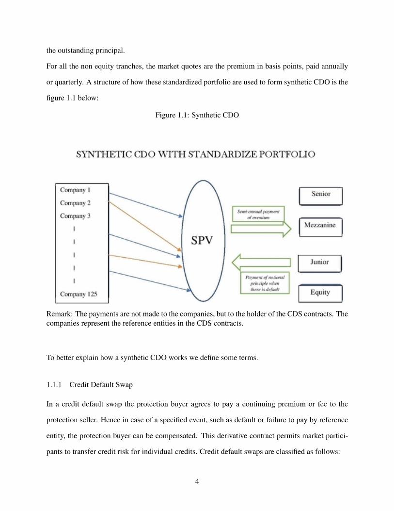
For all the non equity tranches, the market quotes are the premium in basis points, paid annually

or quarterly. A structure of how these standardized portfolio are used to form synthetic CDO is the

figure 1.1 below:

Figure 1.1: Synthetic CDO

Remark: The payments are not made to the companies, but to the holder of the CDS contracts. Thecompanies represent the reference entities in the CDS contracts.

To better explain how a synthetic CDO works we define some terms.

1.1.1 Credit Default Swap

In a credit default swap the protection buyer agrees to pay a continuing premium or fee to the

protection seller. Hence in case of a specified event, such as default or failure to pay by reference

entity, the protection buyer can be compensated. This derivative contract permits market partici-

pants to transfer credit risk for individual credits. Credit default swaps are classified as follows:

4

• Single-name swaps

• Basket swaps

1.1.2 Single-name swaps

Single-name default swap involves two parties: a protection seller and a protection buyer. The

protection buyer pays the protection seller a swap premium on a specified amount of the face

value on the bond (the principal) from an individual company. In return, when the reference entity

defaults, the protection seller pays the protection buyer who is the holder of the CDS contract its

notional principle.

In the documentation of a CDS contract, a credit event is defined. The list of credit events in

a CDS contract may include one or more of the following: bankruptcy, failure to pay an amount

above a specified threshold over a specified period, and debt restructuring of the reference entity.

The swap premium is paid on a series of dates, usually quarterly , based on the actual/360 date

count convention. In the absence of a credit event, the protection buyer makes a quarterly swap

premium payment until the expiration of a CDS contract. If a credit default occurs, two things

happen. First, the protection buyer pays whatever premium accrued between the last payment date

and the time of the credit default event (on a days fraction basis). After that payment, the protection

buyer pays no further premium. Second, the protection seller makes a payment to the protection

buyer. See figure 1.2 describing a single default swap.

1.1.3 Basket Default swaps

A basket default swap is a credit derivative on a portfolio of reference entities. The simplest

basket default swaps are first-to-default swaps, second-to-default swaps, and nth-to-default swaps.

With respect to a basket of reference entities (the number of people to whom the loan or bonds

has been issued), a first-to-default swap provides insurance for only the first default, a second-to-

default swap provides insurance for only the second default, and an nth-to-default swap provides

5

Figure 1.2: Single Default Swap

insurance for only the nth default. For example, in an nth-to-default swap, the protection seller

defines and makes a payment for the nth defaulted reference entity. Once a payment is made upon

the nth defaulted reference entity, the swap terminates. See figure 1.2.

1.2 Liability

Any company that has assets also has liabilities. In the case of a CDO, the liabilities of the SPV

are its tranches which have a detailed and strict ranking of seniority going up the CDO’s capital

structure as equity, junior tranche, mezzanine and senior. These tranches are commonly labelled

Class A, Class B, Class C and so forth going from top to bottom of the capital structure. They range

from the most secured AAA rated tranche with the greatest amount of subordination beneath it, to

the most riskier tranche called equity. In addition, the senior tranches are relatively safer because

they have first priority on the collateral in the event of default. As a result, the senior tranches of a

6

Figure 1.3: Basket Default Swap

CDO generally has a higher credit rating and offers a lower coupon rate than the junior tranches,

which offers a higher coupon rate to compensate for their higher risk level of default.

The rating of both the assets (reference entities) and liabilities (tranches) help investors to make

a decision on what CDO to invest. A high rating of reference entities generally implies a lower

risk for the investor investing in the tranches and therefore a lower premiums for the issuer(SPV).

Rating agencies such as Moody and S & P adopt different methodologies for rating tranches. They

can rate senior tranche of different CDOs differently and therefore one senior tranche may be a

safer investment than another senior tranche.

7

1.3 Purposes

CDOs are normally created for one of the following three purposes. Depending on any of these

purposes, CDOs can be created as a cash flow CDO or a synthetic CDO. The three purpose for

creating CDO’s are :

• To shrink a firm’s balance sheet and reduce its regulatory costs since most firms that

hold a large number of loans may have to pay high regulatory and funding costs.

• For asset managers to provide their management services to CDO investors.

• To increase the value of the firms asset by seeking protection.

A detailed purpose for creating CDO can be read in [26] by interested readers. We proceed with

an example explaining the cash flow of the synthetic CDO. We first define a few terms.

1.3.1 Tranche Spread

A tranche is simply a percentage of a structured debt product (CDO) that seeks to distribute the

interest rate risk across various credit rating securities. Examples of tranches in Collateralized

Debt Obligations are Senior, Mezzanine, Junior and equity. Tranche spread simply means the

price of the tranche (basically the percentage for calculating the premium) which the SPV pays to

the tranche holder.

Tranche loss window

Tranche loss window is the loss that each tranche structure can absorb. As the name indicates, it has

an open end and closing end. When the cumulative percentage loss of the portfolio of bonds reach

the open end, investors begins to make payment to SPV, and when the cumulative percentage loss

reaches the closing end, investors in the tranche make full payment of their notional principal and

no further loss can occur to them. The open end is also the level of subordination that a particular

tranche has beneath it. For example suppose the tranche structure is 0- 5% equity, 5%-15% junior,

8

15%-40% mezzanine and 40% - 100% senior debt. The equity has no subordination, the junior

tranche has 5% subordination and attaches at the 5% loss level. Similarly the mezzanine tranche

has 15% subordination and attaches at the 15% loss level and senior tranche has 40% subordination

and attaches at 40%.

1.3.2 Types of Tranches

• Senior Tranche : A senior tranche is the highest tranche of a security, that is one

deemed less risky. Any losses on the value of the security are only experienced in

the senior tranche once all other tranches have lost all their value. For this safety,

the senior tranche pays the lowest rate of interest. Investors who invest in senior

tranche always have a credit rate of AAA since they pay huge amount of notional

principle to the SPV to cover for its losses when there is a massive default event.

• Junior Tranche : A junior tranche is the lowest tranche of a security, i.e. the one

deemed most risky. Any losses on the value of the security are absorbed by the

junior tranche before any other tranche, but for accepting this risk the junior tranche

pays the highest rate of interest. The junior tranche can also be the equity tranche.

1.4 Example explaining the dynamics of the Synthetic CDO

Let’s assume there are 100 reference entities in the CDO pool with each entity given a bond with

face value $500 (hence the CDO pool has total of $50000 notional) at 5 years maturity with zero

recovery. Now suppose the issuer of these bonds seek protection on each of the bond from the SPV

via CDS contract. Then the SPV protect the loan issuer against a total loss of $50000. The SPV

then creates a CDO contract by pulling together the CDS contract with the following coupon rates

at the time of issuance as shown below in table 1.1

9

Tranches Tranche window Notional principle of Tranches Tranche spread (coupon)

Senior 40%-100% 30000 100 basis point

Mezzanine 15%-40% 12500 250 basis point

Junior 5%-15% 5000 400 basis point

Equity 0-5% 2500 60%

Total 50000

Table 1.1: Synthetic CDO table

From the table 1.1, the senior tranche is responsible for protecting the SPV against losses from

$20000 to $50000 (which is a total of 60% of $50000) whiles the SPV pays the senior tranche

holder $300 every three months. Likewise, the Mezzanine protects SPV against loss from 7500 to

20000 (which is total of 25% of $50000) and the SPV pays Mezzanine $312.5 (2.5% of $12500)

quarterly as well. The junior tranche too protects SPV against loss from $2500 to $7500 and SPV

pays junior tranche $200 every three months. However, the equity tranche holder protect the SPV

against loss from $0 to $2500 whiles the SPV has to pay 60% of $2500 ($1500) as upfront fee to the

equity tranche holder before the commence of the contract and an additional 500 basis points (5%)

of $2500 every year until the contract matures or until default. Note that the investors investing

in the synthetic CDO do not pay the notional principle at the initial stage of the contract and their

notional principles are determined by the total losses they protect.

Assuming 10 entities default in the CDO pool at the end of the 2nd year, then two things happen:

• Firstly, the CDO suffers a loss of $5000 and so the holder of the equity tranche

provides payment of $2500 to SPV. Similarly the junior tranche holder provides

$2500 payment to the SPV. The equity tranche holder receives total payment of

$1750($1500 fee plus $250 which is 2 years premium payment) and the junior

tranche holder receives $1600 (which is 4% of 5000 times 8 payments period) as

premiums from the SPV.

10

• Secondly, the equity tranche holder loses all his notional principle and does not

receive any premium again from the SPV. The junior tranche on the other hand loses

half of its notional principle and receives premium on just the half of its notional

principle ($2500) left.

This mechanism continues until the CDO matures. Now suppose the CDO does not incur any more

losses after the two years and matures, then

• The junior tranche holder makes a profit of $300 that is

( 40010000

∗2500)∗12+1600−2500 = $300

• Similarly the mezzanine and senior tranche holders make profit of $6250 and $6000

respectively without suffering any losses. The calculation of mezzanine profit is

( 25010000

∗12500)∗20 = $6250

Generally the issuer of CDO (SPV) retains the equity tranche since it is too risky for investors.

This means if there is no default at the end of the contract,the CDO issuer makes the most profit

since the equity tranche has the highest interest. The interest rate the tranches pay depends on the

risk of default of the firms in the reference portfolio. Because the risk of default of the firms are

affected by the default dependency of the firms, default dependency should be taken into account

in the pricing of tranches of the CDO. In particular, one needs to specify the joint distribution of

the default arrival time of firms given their marginal distributions. In this vein, the structural model

(developed by Merton (1974) and further extended by Zhou (2001)) and intensity-based models

(see Lando, 1998, Duffie and Singleton, 1999) have been developed to capture the spirit of default

correlation. However, the mostly used pricing model in the financial industry that captures default

correlation is the Normal Gaussian Copula model as discussed in Li (2000) and further developed

11

by others such as Gregory and Laurent (2003). Hull, Predescu and White (2005) incorporates

default correlation in a structural model. Some other models focus on capturing the cumulative

default intensities. For example, Kou and Peng in [33] propose modelling of CDO prices using the

idea of default clustering where they aim to capture the prices of CDOs under the 2008 financial

turmoil.

In this thesis, we examine three main models. These are :

• Gaussian Copula Model,

• Structural Model,

• Conditional Survival Model.

The Gaussian copula model is a type of a factor model developed by Li(2000). Its modelling can

be understood as a combination of the copula approach and the firm value approach of Merton

(1974). In the Gaussian Copula model framework, a firm defaults when its "asset value" modelled

as a certain stochastic process X, falls below a barrier. Joint distribution of the firms values are

defined in terms of the Gaussian copula. From this, one derive probability distribution of the

number of defaults by time T and the cumulative loss distribution, which are directly related to

the tranche interest rates when the companies have equal weight in the reference portfolio and

recovery rates are assumed to be constant.

Hull, Predescu and White (2005) proposed a different structural model to price the spread of

the tranches of a CDO. It models each firm value to has the common market risk and idiosyncratic

risk. To implement the model it uses Monte Carlo simulation. The simulation was carried out by

• Drawing a set of zero mean unit variance normally distributed random variables of

the common market risk and the idiosyncratic risk.

• These set of variables were then used to sample four sets of paths for the asset value

Xi.

12

• Company i was assumed to default at the time t if the value of Xi falls below the

barrier for the first time.

• The simulation was repeated 5,000 times generating 20,000 sets of paths. For each

set of paths the number of defaults, dk was determined and used to price CDO

spread with a specified formula.

Conditional Survival (CS) model is a cumulative default intensity model and it is an extension

to Duffie et al. (2001). This model was proposed by Peng and Kou in 2009. It models cumula-

tive default intensity as a sum of market factors and idiosyncratic factors. These market factors

are modelled using Polya processes and discrete integral CIR processes. The model was imple-

mented to price CDO using exact simulation and pricing without simulation. The exact simulation

was conducted by generating sample path from the market factors which are used to calculate the

conditional survival probabilities given the market factors, which are then used to generate condi-

tionally independent Bernoulli random variables which corresponds to default events. With these

random variables the cumulative loss distribution is generated, which is used in pricing the CDO

tranches.

This thesis intend to price the tranches of a synthetic CDO using these three models imple-

mented under the exact simulation method discussed in Peng and Kou (2009).

The remaining part of the thesis is structured as follows: the second chapter provides the key

formulations of the three methods. A detailed synthetic CDO tranche pricing process is described

in the third chapter. Chapter 4 presents the data used and calibration performed on each model.

Chapter 5 concludes this thesis with remarks, criticism of the models and recommendations for

future work.

13

Chapter 2

Pricing Models of Collateralized Debt Obligation (CDO)

In the rest of this thesis, we assume that there are n names in the CDO portfolio and use τ(i) to

denote the default time of the ith name, i = 1, ...,n. There are two types of credit risk modelling

approach used in the financial world. They are the bottom-up approach, which builds models for

the joint distribution of the default times of individual names in the portfolio, and the top-down

approach, which builds models for the cumulative loss of the whole portfolio without referring to

the underlying single names.

2.1 Bottom-up Models

In the bottom-up approach the default event of each reference entity is modelled. Then one com-

putes the expected loss incorporating the correlation structure from which the prices of tranche

spreads are obtained. Bottom up models specify the joint distribution of default times directly,

usually through copula structures. A popular bottom up model is the Gaussian copula model pro-

posed by Li (2000), which is the predominant model for the industry to price CDOs (see also Duffie

et al., 2003; Andersen et al., 2003). An important advantage of the bottom up model is its ability to

produce the joint distribution of default times which can cover a wider range of correlation product

such as the first-to-default swap, the nth-to-default swap etc than top down model. For example, if

we consider a CDO contract whose payoff depends on the underlying entity of the CDO ( example

vanilla bespoke CDO) then the reference entity is important and bottom up approach can be used

to price it. A known disadvantage of bottom up model is its inability to fit market data well since

it under prices CDO tranches. For example the one factor Gaussian copula does not appear to fit

market data well (see Hull and white (2004) and Kalemanova et. al. (2005)).

14

2.1.1 Modelling the joint distribution of default times

Default correlation measures the tendency of two companies to default at the same time. Two ways

for modelling the joint distribution of default times are

• Reduced form model

• Structural model

2.1.2 Reduced Form Model

Reduced form models, focuses on modelling the probability of default rather than trying to explain

default in terms of the firm’s asset value. Its main assumption is that default is always a surprise,

that is there is no sequence of events announcing its arrival. Reduced form model does not model

firm values but rather it models the instantaneous conditional probability of default. This model

was originally introduced by Jarrow and Turnbull (1992) and subsequently studied by Jarrow and

Turnbull (1995) and D. Duffie and K. Singleton (1999), among others. The key postulate empha-

sized in reduced form model is that the modeller observes the default indicator function as a Cox

process with an intensity parameter λ and a vector of state variable Xt . Some known examples of

the reduced model are Poisson processes and Cox processes .

Structural Models

The structural model was first introduced by Merton (1973) and it is based on the argument that a

default happens when a reference entity total asset fails to meet its own total liabilities. In another

words, the total asset value of the reference entity reaches a level that is below its total liability. In

the financial world, company or reference entity has two major ways of raising capital to support

their business. These include issuing bonds to people or issuing equity to investors. The bond

holders are mostly at risk, but they have the priority in collecting the remaining asset if the bond

issuer (reference entity) go bankrupt. Merton’s model is based on these basic principles. Let V be

the total asset of the reference entity and S the outstanding liability of the reference entity, both

15

time dependent. At maturity T,

• If V > S, the bond holders receive their promised amount S, while the equity holders

take away the rest which is V −S.

• If V ≤S, which is the case where the reference entity would fail their obligations,

the bond holders take everything that is left of the total asset, and the equity holder

(stock holder) get nothing.

2.2 Top-down Model

Top-down approach refers to modelling the cumulative portfolio loss distribution ignoring what

happens individually to the reference entities. This means that when using the top down approach,

the arrival times of the events (default) can be observed but the defaulted reference entity cannot be

recognised. One advantage of the top-down model is that it is easy to implement and calibrate. The

main disadvantage is that it cannot identify the defaulted entity in the reference pool. It therefore

cannot be used to price bespoke CDO’s since bespoke CDO’s are created specifically per the needs

of a group of investors and these investors might be interested in the reference entities that form

the credit portfolio which top down model cannot identify in the case of default. Some examples

of papers that present the top down model are Andersen (2006), Giesecke and Goldberg (2005)

and Arnsdorf and Halperin (2007).

2.3 Introduction to the Models

We investigate the following bottom up approach CDO pricing models:

• One factor Gaussian Copula Model

• Hull and White Structural Model

• Conditional Survival Model

16

These models are used to estimate the prices of tranches of a CDO. The main method common in

our analysis of these models is to generate samples from the joint distribution of the default times

of the reference entity and use the tranche spread formula discussed in [33] to price the tranches of

the CDO.

2.3.1 Introduction to Copula

To understand the one factor gaussian copula, we first need to give a brief introduction to how

copula function was form as explained in [7]. When modelling a credit derivative, it is intuitive to

think that default rate of a reference entity tends to be higher during recession and lower when the

economy is booming. That is each reference entity is subject to a common set of macroeconomic

influences in addition to idiosyncratic factors. The correlation structure should take into account

these common factors when evaluating the CDO. More precisely, we would like to link these

macroeconomic factors to the joint distribution of default times. Generally, knowing the joint

distribution of random variables allows one to derive the marginal distribution and their correlation

structure among the random variables but not vice versa. To specify the joint distribution, a copula

function can be used since copula function enables one to link univariate marginals to a multivariate

distribution. For instance, if we consider any uniform random variables U1,U2, ...,Un, the joint

distribution function C is defined as

C(u1,u2, ...,un) = P[U1 ≤ u1,U2 ≤ u2, ...,Un ≤ u].

This is called a copula function and for a given collection of univariate distribution functions

F1(x1),F2(x2), ...,Fn(xn), the function

C[F1(x1),F2(x2), ...,Fn(xn)] = F(x1,x2, ...,xn)

17

also defines a joint distribution with marginals given the Fi. This property can easily be shown as

follows:

C(F1(x1),F2(x2), ...,Fn(xn))

= P[U1 ≤ F1(x1),U2 ≤ F2(x2), ...,Un ≤ Fn(xn)]

= P[F−11 (U1)≤ x1,F−1

2 (U2)≤ x2, ...,F−1)(Un)≤ xn]

= P[X1 ≤ x1,X2 ≤ x2, ...,Xn ≤ xn]

= F(x1,x2, ...,xn).

The marginal distribution of Xi is

Fi(xi) = P(Ui ≤ Fi(xi)) =C(F1(+∞),F2(+∞), ...,Fi(xi), ...,Fn(+∞))

= P[X1 ≤+∞,X2 ≤+∞, ...,Xi ≤ xi, ...,Xn ≤+∞]

= P[Xi ≤ xi]

= Fi(Xi).

Some common Copula functions are

• Frank Copula : The Frank copula function is a symmetric Archimedean copula

which is defined as

C(u,v) =− 1α

ln[1+

(e−αu−1)(e−αv−1)e−α −1

], −∞≤ α ≤ ∞

.

• Bivariate or Gaussian Copula The Gaussian copula is define as

C(u,v) = Φ2

(Φ−1(u),Φ−1(v),ρ

)−1≤ ρ ≤ 2

where Φ2 is the bivariate normal distribution function with correlation coefficient

ρ , and Φ−1 is the inverse of a univariate normal distribution function.

18

The joint PDF of a standard bivariate normal distribution function with correlation coefficient ρ is

given as

fXY (x,y) =1

2π√

1−ρ2exp{− 1

2(1−ρ2)[x2−2ρxy+ y2]

}(2.1)

2.4 The One Factor Gaussian Copula Model [8],[13]

Li (1999, 2000) introduces the one-factor Gaussian copula model for the case of two reference

entities and Laurent and Gregory (2003) extend the model to the case of N companies. In this

model, the individual default times are assumed to be random and after a certain transformation

follow a normal distribution. Default times of each reference entity is linked to a single common

factor which is accordingly assumed to be normally distributed. From this linear dependence (that

is, the individual default times are linearly associated to a common factor after this transformation)

a correlation structure emerges between the pairwise random default times.

2.4.1 Modelling the firm’s value:

The one factor Gaussian copula model models the firm value Xi just as in CAPM (Capital Asset

Pricing Model) where a certain random variable ri (i.e. the return on an asset), can be explained

both by the level of a systematic risk M (i.e. the market risk) which is said to be a non-diversifiable

risk and a corresponding diversifiable one say Zi , which depends on the firm’s specific risk. From

this one can write a regression as follows:

ri = ρM+βZi.

Consider ρ as the sensitivity of the asset return r given the level of the systematic risk M and β its

corresponding sensitivity due to the diversifiable risk Z . Now, we replace the asset return by the

firm’s value Xi and interpret M as the common factor and Zi as the idiosyncratic risk (i.e. firm’s

specific risk). ρ and β are their respective weights, measuring the sensitivity of X towards each

19

source of risk. Note that all these variables are random and normally distributed. We can therefore

write the model for the individual firm value as follows:

Xi = ρM+βZi. (2.2)

It is assumed that the correlation between pairwise idiosyncratic risks Zi is zero. That is Corr(ZiZ j)=

0. Similarly, M is assumed to be independent of Zi. Without loss of generality, M,Zi and X are

assumed to have 0 mean and unit variance with the restriction that β =√

1−ρ2. We can then

write the firm’s value in terms of expectation as

E(Xi) = ρE(M)+βE(Zi) = 0

and

Var(Xi) = ρ2Var(M)+2ρβCov(M,Zi)+β

2Var(Zi)

Given that Corr(M,Zi) = 0 , Var(M) = 1 , Var(Zi) = 1, we can then write the variance as:

Var(Xi) = ρ2 + β 2 = 1 implying that β =√

1−ρ2. From this, we can rewrite the firm value

process as:

Xi = ρiM+√

1−ρ2i Zi, i = 1,2, ....,n (2.3)

This equation defines a correlation structure between the Xi dependent on a single common factor

M. The factor ρi satisfies −1≤ ρi ≤ 1 and corr(Xi,X j) = ρiρ j.

2.4.2 Conditional Default Probability Distribution Function

At this stage, we focus on an important input in pricing a pool of credit risks. In this section before

setting out the probability distribution of the default time conditional on the common factor, let us

first explain what we consider as default when dealing with a firm’s value. A default occurs when

a stock price of a firm drops below a certain level x. From this, we can say that a credit defaults

when the firm’s value is below the considered barrier x, that is Xi ≤ x. The probability of default

is then Pr(Xi ≤ x). Now let us assume a CDO includes n reference entities, i = 1,2, ...,n and the

20

default times τi of the ith reference entity follows a general continuous distribution Fi. Hence the

probability of a default occurring before the time t is

P(τi ≤ t) = Fi

In a one-factor copula model, it is assumed that the relationship between the default time τi of the

ith entity and the random variable Xi is

P(Xi < x) = P(τi < t) = Fi, i = 1,2, ...n.

This relationship is satisfied if

Xi = Φ−1[Fi(τi)], τi = F−1

i [Φ(Xi)]

and

t = F−1i (Φi(x)), x = Φ

−1i (Fi(t))

given Φi to be the cumulative distribution of Xi and Fi the cumulative distribution of τi. We now

have sufficient instruments to write down the conditional default probability function. Given the

common factors value, we can write the probability of default time of the individual reference

entity value as

P(τi < t |M) = P(

ρiM+√

1−ρ2i Zi < Φ

−1i (Fi(t)) |M

)= P

[Zi <

Φ−1i (Fi(t))−ρiM√

1−ρ2i

](2.4)

This intuitively tells us that given a value of the common factor M a default happens when the firm’s

idiosyncratic risk ( i.e. firms specific information) hits a certain level. The cumulative distribution

function of the conditional default probability that the individual firm will default at a certain time

t given the level of the common factor is:

P(τi < t |M) = H

{Φ−1i (Fi(t))−ρiM√

1−ρ2i

}(2.5)

where H is the standard normal cumulative distribution function. We refer to equation 2.4 as the

conditional default probability. We can simulate the default event of each firm using this model.

21

The advantage of the copula model is that it creates a tractable multivariate joint distribution for a

set of variables that is consistent with known marginal probability distributions for the variables.

It should be noted that any type of Copula functions can be used to model the default correlation

in valuation of CDOs.

2.4.3 Implementation of the One factor Model

The main quantity needed to price a CDO is the expected loss in the CDO credit portfolio which

is a function of the individual reference entity’s default risk within the credit portfolio and the

dependence between their default time. The copula method can be implemented to provide a direct

way to compute these quantities. The first step that has been used to compute the expected loss in

the CDO portfolio is to compute the conditional default probability for each of the reference entity.

Then given the common factor, these default probabilities are independent so one can compute

the unconditional default probability distribution at a time t. The unconditional default probability

distribution is then given as

P(τi < t) =ˆ

∞

−∞

P(τi < t |M)Φ(m)dm (2.6)

with Φ(m) being the density of the factor M. To compute this unconditional default probability

several approaches have been used. These include the Fourier transform, which was used by

Laurent and Gregory (2003), recursive algorithm used by Andersen, Sidenius and Basu (2003) and

the Binomial and Poisson approximation used by De Prisco, Iscoe and Kreinin (2005). Note that

Binomial and Poisson approximation approach for finding the unconditional distribution is best

when reference entities have equal weight in the portfolio with fixed recovery rate, same pairwise

correlation and same default intensity.

Now knowing the unconditional probability one can calculate the expected loss (portfolio loss

distribution) and continue to derive the tranche spread of the CDO. A formula to calculate the

tranche spread is derived in the next chapter. Other approaches have been used and interested

readers can read [13] to learn more on how the one factor Gaussian copula has been implemented.

22

However, in this thesis we implement the One factor Gaussian Copula in the way Kou and Peng

(2009) modelled their CDO structure, which will be discussed in detail when we talk about the

Conditional Survival model.

2.5 Structural Model

The first structural model of default for a single company was introduced by Merton (1974). In this

model a default occurs if the value of the assets of the company is below the face value of the bond

at a particular future time. Black and Cox (1976) provided an extension to the Merton model and

other extensions were provided by Ramaswamy and Sundaresan (1993), Leland (1994), Longstaff

and Schwartz (1995) and Zhou (2001a). However, all these papers looked at the default probability

of only one issuer. Zhou (2001b) and Hull and White (2001) were the first to incorporate default

correlation between different issuers into the Black and Cox first structural model. Zhou (2001b)

deduced a closed form formula for the joint default probability of two issuers, but his results cannot

easily be extended to more than two issuers. However Hull and White (2001) extented the model

to many issuers but their correlation model requires computationally time-consuming numerical

procedures [14].

Hull and White (2005) provides another way to model default correlation using the Black-

Cox structural model framework. Their approach can be used to price credit derivatives and was

computationally feasible when there are a large number of different companies. They assume that

the correlation between the asset values of different companies is driven by one or more common

factors. In their paper they consider first, a base case model, where the asset correlation and the

recovery rate are both constant and then extend the base case model in three ways. The first

allows the asset correlation to be stochastic and correlated with default rates. This is motivated by

empirical evidence that asset correlations are stochastic and increase when default rates are high

(using evidence from Servigny and Renault (2002), Das, Freed,Geng and Kapadia (2004)). They

secondly assume that the recovery rate are stochastic and correlated with default rates. This was

23

consistent with Altman et al (2005) who found that recovery rates are negatively dependent on

default rates. They thirdly assume a mixture of processes for asset prices that leads to both the

common factors and idiosyncratic factors having distributions with heavy tails.

2.5.1 The Firm Model

In the model, N different firms are assumed and we define Vi(t) as the value of the assets of

company i at time t (1≤ i≤ Ni). The value of each firm is assumed to follow a stochastic process

as shown below

dVi = µiVidt +σiVidXi

so that

dlnVi = (µi−σ2

i2)dt +σidXi (2.7)

where

• µi is the expected growth rate of the value of firm i

• σi is the volatility1 of the value of firm i

• Xi(t) is a Brownian motion2.

Firm i defaults whenever the value of its assets falls below a barrier Hi. This corresponds to the

Black and Cox (1976) extension of Merton (1974) model. µi and σi are assumed to be constant for

the barrier to be linear.

Corresponding to Hi there is a barrier H∗i (t) such that company i defaults when Xi falls below

H∗i (t) for the first time. Without loss of generality we assume that Xi(0) = 0. This means that

Xi(t) =lnVi(t)− lnVi(0)− (µi−

σ2i

2 )tσi

1volatility refers to the amount of uncertainty or risk about the size of changes in the asset value of each referenceentity

2A continuous stochastic process with stationary and independent increment with normal distribution mean 0 andstandard deviation

√t

24

and

H∗i (t) =lnHi− lnVi(0)− (µi−

σ2i

2 )tσi

where if Xi(t)< H∗i (t) firm i default. Similarly the value of each firm asset can be computed using

the formula

Vi(t) =Vi(0)exp(σXi +(µ− σ2i

2)t) (2.8)

and if Vi(t)< Hi the firm i default as well. Either of the two default procedure explained above can

generate the default event of each firm. Defining

βi =lnHi− lnVi(0)

σi

and

γi =−µi−σ2/2

σi

then the default barrier for Xi is given as

H∗i (t) = βi + γit

When µi and σi are constant, βi and γi are constant. For this case, [16] shows that the probability

of first hitting the barrier between times t and t+T is

P(t < τi ≤ t +T ) = N(

βi + γi(t +T )−Xi(t)√T

)+ exp[2(Xi(t)−βi− γit]N

(βi + γi(t−T )−Xi(t)√

T

)(2.9)

where N() denotes the standard normal cumulative distribution function

2.5.2 Asset Correlation

We assume that the process for modelling the state variable Xi is

dXi(t) = αi(t)dF(t)+√

1−αi(t)dUi(t) (2.10)

where F and Ui are Brownian motion with F(0) = Ui(0) = 0 and dUi(t)dF(t) = dUi(t)dU j(t) =

0, j 6= i The Brownian motion Xi therefore has a common component F and an idiosyncratic com-

ponent Ui. The variable αi, which may be a function of time or stochastic, defines the weighting

25

given to the two components. F can be thought of as a common factor affecting default probability.

When F(t) is low there is a tendency for the Xi to be low and it causes the rate at which defaults

will occur to be relatively high. Similarly, when F(t) is high there is also the tendency for the Xi to

be high and the rate at which default will occur is relatively low.

The parameter αi defines how sensitive the default probability of firm i is to the factor F . The

correlation between the processes followed by the assets of firms i1 and i2 is αi1αi2 . Note that

these Xi(t)s are used to simulate the asset value and can also be used to simulate default events.

2.5.3 Model Implementation :

Hull and White implemented using Monte Carlo simulation. They considered points in time

t0, t1, ..., tn (where t0 is the initial date of the contract and typically tk− tk−1 is three months) and

replaced the continuous barrier in the Black and Cox model with discrete barrier that was defined

only at those points. The barrier was chosen using the numerical procedure so that the default prob-

abilities in each interval (tk−1, tk) were the same as those for the continuous barrier. The simulation

was carried out by

• Drawing a set of zero mean unit variance normally distributed random variables ∆ fk

and ∆uik (1≤ k ≤ n,1≤ i≤ N)

• These set of variables were used to sample four sets of paths for the Xi.

f mk = f m

k−1 +(−1)mαik∆ fk

√∆t m = 0,1 f m

0 = 0

u jik = u j

i,k−1 +(−1) j√

1−α2ik∆ui,k

√∆t j = 0,1 u j

i,0 = 0

Xm jik = f m

k +u jik m, j = 0,1

where Xm jik is the value of Xi at time tk for a particular combination of m and j, and

αik is the value of αi between times tk−1 and tk.

The correlation parameters αi were assumed to be constant in each interval (tk−1, tk). Company i

was assumed to default at the mid point of time interval (tk−1, tk) if the value of Xi is below the

26

barrier for the first time at time tk. The simulation was repeated 5,000 times generating 20,000

sets of paths. For each set of paths the number of defaults, dk, that occur in each time interval,

(tk−1, tk), is determined. They then had a pricing formula which they used to estimate the prices of

the tranche spread. In this thesis we implement this method but use a different pricing method to

obtain the prices of the CDO tranches.

2.6 Conditional Survival (CS) Model

The main motivation behind the use of Conditional Survival model is the default clustering effect.

Default clustering effect means that one default event tends to trigger more default events both

across time and cross-sectionally. The most relevant empirical evidence of the default clustering

effect happened in 2008 where there was a massive financial turmoil. To capture default clustering

effect observed in this financial crisis was one of the motivation of the CS model ( Peng and Kou

2009).

In September 20, 2007 and March 14, 2008 there was a noticable default clustering effect

observed in the tranche spreads of the iTraxx Europe Series 8 5-years Index in the CDO Market

[33] as shown below.

Tranche 0-3% 3%-6% 6%-9% 9%-12% 12%-22% 22% -100%

09/20/2007 1812 84 37 23 15 7

03/14/2008 5150 649 401 255 143 70

Table 2.1: iTraxx Europe Series 8 5-years Index

From the table it can be observed that on March 14, 2008 the senior tranche had an extremely

high spread which was around 10 times as high as the previous year. Similarly, all the other

tranches from the table had high spread on March 14 ,2008 compared to September 20, 2007. This

showed that the default correlation was substantially high and the portfolio loss distribution had

significantly heavy tails at the peak of the financial crisis in 2008.

27

Default clustering can be captured by serial correlation(where serial correlation means the re-

lationship between a given variable and itself over various time and it is used to predict how well

the past price of a security predicts the future price) but some traditional stochastic processes such

as Brownian motions and Poisson processes have independent increments, which makes it hard for

them to generate serial correlation. To generate serial correlation, Polya process is used since it is a

counting process which has a fixed jump size 1 at each jump time. If one finds that the fixed jump

size might be restrictive, one could use a compound Polya process to incorporate random jump

sizes. A compound Polya process is easy to simulate, and its Laplace transform has a closed-form

formula, which is derived in the Appendix of this thesis. More precisely, a Polya process M(t) is a

Poisson process with a random rate ξ , where ξ is a Gamma random variable with shape parameter

α and scale parameter β . A gamma distribution is simply a two-parameter family of continuous

probability distributions and a random variable X is said to be gamma-distributed with shape α

and rate β if it is written as X ∼ Γ(α,β ).

In other words, conditional on ξ , M(t) is a Poisson process with rate ξ . The marginal distribu-

tion of a Polya process M(t) is given by

P(M(t) = i) =(

α + i−1i

)( 11+β t

)α( β t1+β t

)i, t > 0, i≥ 0

A Polya process has stationary but positively correlated increments since the covariance be-

tween their market factor at two point is greater than zero. Hence the arrival of one event tends

to trigger the arrival of more events, which makes Polya processes suitable for modelling defaults

that cluster in time. For more evidence of cross-sectional default clustering, one can read Peng and

Kou (2009), Azizpour and Giesecke (2008) and Longstaff and Rajan (2007).

2.6.1 CS Firm modelling

Peng and Kou (2009) extended the model proposed by Duffie et al. (2001) and proposed CS model

as

Λi =J

∑j=1

ai, jM j(t)+Xi(t), (2.11)

28

τi = in f{t ≥ 0 : Λi(t)≥ Ei}, i = 1, ...,n (2.12)

where Λi(t) is the cumulative default intensity of the ith name. Here M j(t) represents the jth market

factor (here the market factors could represent both observable and unobservable macroeconomic

variables that have market wide impact on the reference entity default probability) in the cumulative

default intensities, which is a non-negative, increasing, and right-continuous stochastic process

with M j(0) = 0, j = 1, ...,J. These market factors are all independent of Ei and Xi(t) but they can

be correlated with each other. Also unlike the intensity based model introduced by Jarrow and

Turnbull (1995), M j(t) is allowed to have jumps.

The coefficient ai, j ≥ 0 is the constant loading of the ith reference entity on the jth market factor,

for i = 1, ...,n; j = 1, ...,J. Xi(t) represents the idiosyncratic part of the cumulative default intensity

of the ith reference entity, which is a non-negative, right-continuous, and increasing process with

Xi(0) = 0, for i = 1, ...,n. Xi(t) are mutually independent, and also independent of the market

factors M j(t). Ei are independent exponential random variables with mean 1. Ei is independent of

the processes Xi(t) and M j(t).

Interestingly, there is no need to specify the dynamics of the idiosyncratic default risk factors

Xi(t). All that we need to specify in the CS model is the dynamics of the market factors M j(t),

j = 1, ...,J.

Conditional Survival Probabilities

We call the model conditional survival because conditional survival probabilities are the building

blocks for pricing tranches of the CDO as it will be shown in chapter 3. The conditional survival

probabilities in the CS model are very simple. Let M(t) = (M1(t), ...,MJ(t)) be the vector of

market factor processes and let

qci (t) = P(τi > t |M(t))

and

qi(t) = P(τi > t)

29

be the conditional survival probability and marginal survival probability of the ith reference entity,

respectively. Then we have this proposition as in [33]

Proposition 1 For the ith reference entity in the CS model, we have

qci (t) = E

[e−Xi(t)

]e−∑

Jj=1 ai, jM j(t) (2.13)

given

qi(t) = E[e−Xi(t)

]E[e−∑

Jj=1 ai, jM j(t)

](2.14)

And qci (t) can be represented by qi(t) and the market factors as

qci (t) = qi(t).

e−∑Jj=1 ai, jM j(t)

E[e−∑

Jj=1 ai, jM j(t)

] (2.15)

The proof of this proposition is in the appendix. This proposition shows that the conditional sur-

vival probability qci (t) can be computed analytically if the marginal survival probability qi(t) is

known and the Laplace transforms of the market factors M(t) have closed-form formulae. The

marginal survival probabilities qi(t), i = 1, ...,n. can usually be implied from market quotes of

single name derivatives or from relevant data analysis, since it seems unreasonable to include a

reference entity with unknown marginal default probability in the underlying portfolio of a CDO.

The conditional survival probabilities qci (t), i = 1, ...,n are useful because given the market fac-

tors M(t), the random variables 1(τi≤t), i = 1, ...,n are conditionally independent, and 1τi≤t has a

Bernoulli (1−qci (t)) distribution. This enables us to compute CDO tranche spreads. To be precise,

let Ni and Ri be the notional principal and recovery rate of the ith reference entity in the portfolio,

respectively. Then the cumulative loss process of the portfolio is given by

Lt =n

∑i=1

(1−Ri)Ni1(τi≤t), t ≥ 0 (2.16)

Therefore, conditioned on M(t), Lt is equal to the linear combination of independent Bernoulli

random variables, which further implies that the marginal distribution of Lt is only determined by

the dynamics of the market factors M(t). However, since CDO tranche spreads only depend on the

30

marginal distribution of Lt (as shown in next chapter), it follows that CDO tranche spreads also

depend only on the dynamics of the market factor M(t).

From equation 2.12, we clearly see that the CS model does not need the dynamics of idiosyn-

cratic cumulative intensities Xi(t). Hence no parameters for Xi(t) are needed and there is no need

to simulate Xi(t) for pricing CDOs. But instead we assume that the functions qi(t) are specified.

Specifying Market Factors in Model

According to the previous discussion, to price CDO tranches, we only need to specify the dynamics

of the market factors M(t). Peng and Kou (2009) uses Polya processes and discrete integral of CIR

processes as market factors but in our simulation we just considered Polya processes as the only

one market factor in the CS model.

Using a Polya process as the market factors has several advantages:

• A Polya process has stationary but positively correlated increments, which makes it

suitable for modelling defaults that cluster in time.

• The jumps of the market factor Polya process cause simultaneous jumps in the cu-

mulative intensities of all names, which produces strong cross-sectional correlation

among individual names.

• A Polya process is computationally tractable. The simulation of a Polya process,

which comprises the simulation of a Gamma random variable and a Poisson pro-

cess, is straightforward.

• In addition, the Laplace transform of a Polya process can be calculated in closed

form.

Properties of the CS Model

The CS model exhibits the following properties.

31

• The CS model can generate the simultaneous default of many reference entities

since when the market factor M j(t) jumps, all cumulative default intensity Λi(t)

jump together simultaneously, which can cause many Λi(t) to cross their respective

barriers Ei.

• The CS model allows fast CDO pricing based on simulation because one only needs

to simulate the value of market factors at coupon payment dates.

• The CS model provides automatic calibration to the underlying single-name CDS

in the portfolio since it uses marginal survival probability as an input.

The implementation of this model to price CDO is discussed in chapter 3. Also the other two

models, namely one factor Gaussian copula model and the structural model have been implemented

and the prices of the tranches are calculated using the same procedure as in [33].

2.7 Comparison of the three models

In contrast to the one factor Gaussian copula and the structural model, the CS model does not

specify the dynamics for idiosyncratic risk factors Xi(t)), thanks to the qci (t) equation that links

the conditional and unconditional survival probabilities without using Xi(t). To be able to compare

these models, the qi’s in the CS model are extracted from the market data since that is all we

need and we calibrate the parameters of the other two models to match that of the qis. A detailed

approach on how this is done is explained in chapter 4.

Now we proceed to chapter 3 and talk about the CDO pricing formula of this thesis.

32

Chapter 3

CDO Pricing Method

3.1 Synthetic CDO Tranche Spread Formula

Using the pricing theory explained in [33], let T0 = 0 be the effective date of the synthetic CDO

contract, T be the maturity date of the CDO, and 0< T1 < T2 < ... < Tm = T be the coupon payment

dates. Let Lt be the cumulative loss process as define in Eq. (2.15) and [a,b] be the CDO tranche

loss window. The tranche cumulative loss process is defined up to time t as

L[a,b]t = (Lt−a)+− (Lt−b)+, 0≤ t ≤ T. (3.1)

Pricing the CDO tranche involves a premium leg which is also called a fixed leg and a default or

floating leg. To find the present value of the default leg, we already know that the tranche holder

(protection seller) agrees to pay a certain amount of capital should a default occurs. Hence the

loss given default that the tranche holder faces is known to be the default leg at the time of default.

From an investors point of view, the payment that he could face should a default event occurs

depends on the difference between the tranche loss at dates Ti−1 and Ti which can be written as

dL[a,b]t . Also since we are trying to set an expected amount of capital in case of default which in

terms of expectation represents the tranche loss given default (default leg) we can expressed the

present value of the default leg as E[´ T

0 D(0, t)dL[a,b]t ]. The present value of default leg is just the

integral for a step function mean weighted sum of jumps and D(0, t) is the risk free discounter

factor from time t to time 0. For simplicity, it is usually assumed that defaults only occur in the

middle of coupon payment dates (see e.g. Mortensen, 2006; Andersen et al., 2003; Papageorgiou

33

Figure 3.1: EQUITY TRANCHE

et al.,2007). Under this simplification, the present value of the default leg is given by:

E[ˆ T

0D(0, t)dL[a,b]

t

]= E

[ m

∑i=1

ˆ Ti

Ti−1

D(0, t)dL[a,b]t

]= E

[ m

∑i=1

D(0,Ti−1 +Ti

2)(L[a,b]

Ti−L[a,b]

Ti−1)] (3.2)

Next, we compute the present value of the premium leg. The outstanding notional of the tranche

at time t is O[a,b]t = b−a−L[a,b]

t . Then the coupon payment at time Ti, i = 1, ...,m is specified

as

S[a,b] ∗ (Ti−Ti−1)

ˆ Ti

Ti−1

O[a,b]t

Ti−Ti−1dt = S[a,b]

ˆ Ti

Ti−1

O[a,b]t dt (3.3)

34

Assuming defaults only occur in the middle of premium periods, the present value of the premium

leg is given by

E[ m

∑i=1

D(0,Ti)S[a,b]ˆ Ti

Ti−1

O[a,b]t dt

]= E

[ m

∑i=1

D(0,Ti)S[a,b](Ti−Ti−1)12(O[a,b]

Ti−1+O[a,b]

Ti)]

= S[a,b]E[ m

∑i=1

D(0,Ti)(Ti−Ti−1)(

b−a−L[a,b]

Ti+L[a,b]

Ti−1

2

)].(3.4)

Note that only the Ti−1 and Ti with O[a,b]t non-zero are included in the sum, that’s because there

are no premium once the tranche loss reaches its end point b. By making the present value of the

premium leg and that of the default leg equal, we obtain the fair spread(price) of the tranche as

S[a,b] =E[

∑mi=1 D(0, Ti−1+Ti

2 )(L[a,b]Ti−L[a,b]

Ti−1)]

E[

∑mi=1 D(0,Ti)(Ti−Ti−1)

(b−a−

L[a,b]Ti

+L[a,b]Ti−1

2

)] , a > 0 (3.5)

The contractual specification of cash flows for the equity tranche is different from those of the

other tranches. The seller of the equity tranche pays an up-front fee at the beginning of the CDO

and pays coupons at a fixed running spread of 500 basis points per year to the buyer. For example

if we consider figure 3.1 at time τ1 the equity tranche holder receives $75 (5% of 1500) yearly

from the SPV if no default occurs. However after τ2 the equity investor receive $ 50 as premium

yearly. The equity tranche spread is defined as the ratio of the up-front fee to the notional of the

equity tranche, which is given by

S[0,b] =1b

{E[ m

∑i=1

D(0,Ti−1 +Ti

2)(L[0,b]

Ti−L[0,b]

Ti−1)]

−0.05E[ m

∑i=1

D(0,Ti)(Ti−Ti−1)(

b−L[0,b]

Ti+L[0,b]

Ti−1

2

)]} (3.6)

The formula for the spread of equity tranche follows as

b∗S[0,b]=E[ m

∑i=1

D(0,Ti−1 +Ti

2)(L[0,b]

Ti−L[0,b]

Ti−1)]−0.05E

[ m

∑i=1

D(0,Ti)(Ti−Ti−1)(

b−L[0,b]

Ti+L[0,b]

Ti−1

2

)].

35

3.2 CDO Pricing Simulation

It is clear from the above two equations that the CDO tranche spreads are determined by the

marginal distribution of the cumulative loss process Lt at coupon payment dates Tk,k = 1, ...,m.

Lt determines L[a,b]t for any tranche window hence, to price CDOs we only need to simulate LTk

exactly.

3.2.1 Simulating Cumulative Loss for One factor Gaussian Copula Method

As described under the one factor Gaussian copula, to simulate the cumulative loss we

• Simulate each Xi according to the model for the firms value which is the sum of

idiosyncratic component and a common component of the market as in equation

(2.2).

• Compare each generated Xi with default barrier generated from the market data

(explicit way of deriving the default barrier is explained under chapter 4). This

comparison generates the default event of each of the firm which together forms the

cumulative loss.

• We then proceed with finding the price of the tranches using equation (3.5).

3.3 Simulating Cumulative Loss for Structural Model

Under the structural model, there are two ways in which the cumulative loss can be simulated; the

first approach is

• Simulate Xi from equation (2.9) which is a Brownian motion following common

Weiner process M and idiosyncratic Weiner process Zi.

• As each firm is modelled to follow Xi and the firm defaults whenever Xi falls below

a default barrier H∗i as described under the structural model [13].

36

• Comparing each Xi with H∗i generates the cumulative loss of all firms and we can

then proceed in finding the CDO tranche prices using equation (3.5).

The second approach involves

• Simulating Xi from equation 2.9 and using it to calculate the asset value Vi.

• Comparing each reference entities asset value Vi with default barrier H to generate

the cumulative loss of all firms and then find the CDO tranche prices.

However we are interested in using the first approach.

3.3.1 Simulating Cumulative Loss for Conditional Survival Model

An advantage of using marginal survival probabilities as input to the CS model is that it renders the

simulation of idiosyncratic risk factors unnecessary. One only needs to simulate the market factor

M(t). Thus, it allows fast simulation for CDO pricing. The key observation is that conditional

on M(t), the random variables 1τi≤t , i = 1, ...,n. are conditionally independent, and 1τi≤t has a

Bernoulli (1−qci (t)) distribution, i = 1, ...,n. Suppose M(t) can be easily simulated and its Laplace

transform can be calculated in closed form, then we have the following algorithm to simulate the

cumulative loss LTk ,k = 1, ...,m :

1. Generate sample path of market factors M(Tk),k = 1, ...,m.

2. For each i= 1, ...,n, calculate the conditional survival probability qci (Tk),k= 1, ...,m,

according to Eq. (2.14), using the sample of market factor generated in Step 1.

3. Generate independent Bernoulli random variables Ii,k ∼ Bernoulli (1−qci (Tk)) dis-

tribution, i = 1, ...,n;k = 1, ...,m.

4. Calculate LTk = ∑ni=1(1−Ri)NiIi,k, k = 1, ...,m.

Using samples of LTk generated by the above algorithm, we can calculate the tranche spreads S[a,b]

given by equation (3.5).

37

We move to chapter 4 and discuss the data analysis and the numerical results.

38

Chapter 4

Numerical Results

In this section, we show the numerical results of pricing tranches of the CDO using the three meth-

ods we discussed in Chapter 2. For simplicity of computation purposes, we choose a hypothetical

non-homogeneous portfolio as reference entities for pricing of the synthetic CDO tranches. That

is:

• The correlation is assumed to be non-homogeneous for both Copula model and

Structural model

• The number of firms was assumed to be just 3 for easy simulation.

• The recovery rate for each firm is assumed to be non-homogeneous.

• A 5 years contract with quarterly coupon payments is assumed.

We want to make our comparisons using relevant values of the parameters used in each of the

models. To obtain the set of relevant values for the parameters, we use market data calibrated to

the structural model. This allows us to estimate the qi in CS model and find the barrier for both the

one factor Gaussian copula and the structural model. To establish these we pick three firms from

the market namely:

• Apple Corporate Bond

• American Credit Express Corporate Bond

• Pepsi Corporate Bond

These three bonds are used to estimate the volatility(σ ) and distance to default. To estimate µ

which is the risk-free interest rate we obtain it from the US treasury bill and it was 2% as of

07-02-2017

39

Reference Entity Notional principle of loan given Recovery rate

A 1113.57 40%

B 1114.22 50%

C 1000 30%

Total 3227.79

Table 4.1: Portfolio Structure Table

Table 4.1 above highlights the firm structure data used in pricing the tranches. This data is just

fictious it has nothing to do with the market data.

4.1 Description of Data for extracting Probability of default (qi) and default bar-

rier

We obtained Corporate coupon bond data from Bloomberg. Three bond firms were used as listed

above as Pepsi Company, Apple Company and American Credit Express corporate bond. All the

bonds had maturity of at most five years and these bonds were used since our simulation on pricing

the tranches of CDO was executed for firms with five year maturity and the current prices for each

bond was selected on 7-02-2017. A typical description of a particular coupon bond data is shown

in the figure below.

From figure 4.1 the apple bond is AAPL 2.5 02/09/22 corporate bond and it has a semi-

annual coupon payment of 2.5 and was Announced on 02-February-2017 with a maturity date

02-September-2022.

40

Figure 4.1: Apple bond.

4.1.1 Estimating Probability of Default, Distance to Default, Mean and Volatility

Using the idea explained under Bootstrap method in [27] the price of a coupon bond over a partic-

ular maturity is given as

C j,k = ∑i

C j,k,iZ j(0,Ti) (4.1)

where C j,k is the price of the kth bond in the jth category (for instance the first apple bond under

the apple company), C j,k,i is the coupon payment of this bond at date Ti and Z j(0,Ti) is the zero

coupon bonds of the firm. The pricing formula of a zero coupon bond is given by

Z(0,T ) = e−rT P(τm > T ) (4.2)

where τm is the first passage of the barrier m and m is a positive number. Using the idea of

maximum Brownian motion we know that τm > T if and only if the maximum of Brownian motion

on [0,T ] denoted by M(T ) satisfies M(T )≤m. Conversely M(T )≤m if and only if τm > T. Then

both τm > T and M(T )≤ m are identical so we have

P(τm > T ) = P(M(T )≤ m).

41

Hence the zero coupon bond can be written as

Z(0,T ) = e−rT P(M(T )≤ m). (4.3)

To deduce a formula for P(M(T ) ≤ m), we find the joint distribution between Brownian motion

with drift and the maximum of Brownian motion which is given as

fM(T ),X̃t(m,w) =

2(2m−w)T√

2πTeαw− 1

2 α2T− 12T (2m−w)2

, w≤ m, m≥ 0

and is zero for other values of m and w. Then integrating

ˆ m

0

ˆ u

−∞

fM(T ),X̃t(u,w)eαw−1/2α2T (2u−w)2

dwdu

gives

P(M(T )≤ m) = N(m−αT√

T)− e2αmN(

−m−αT√T

), m≥ 0. (4.4)

where α is the drift and m is the barrier of the Brownian motion X̃t . Looking at the structural

model, the asset value follows a geometric Brownian motion

Xt = rXtdt +σXtdX̃t (4.5)

and applying Ito’s formula[31] we obtain

lnXt

X0=(µ− σ2

2)t +σ X̃t (4.6)

and taking the exponential and multiplying both side by X0 gives the solution

Xt = X0 e((

r− 12 σ2)

t+σ X̃t

)= X0eσ X̂t

where

X̂t = α̂t + X̃t (4.7)

and

α =rσ− 1

2σ .

42

Then the first passage of distance to default (d) by Xt is the same as the first passage by X̂t of

1σ

log( d

X0

),

which is negative. Similarly the first passage of distance to default (d) is the same as the first

passage by −X̂t of

− 1σ

log( d

X0

),

which is positive. So the default time is τm, the first passage by−X̂t of the barrier m =− 1σ

log(

dX0

)given

X̂t = −̂αt− X̃t

with α = −α̂. Therefore using formula 4.4 we can rewrite the zero coupon bond pricing formula

as

Z(0,T ) = e−rT[N(−m+αT√

T

)− e2αmN

(m+αT√T

)]and r = risk-less rate which is the treasury bill rate obtained from Bloomberg. We then rewrite the

bond pricing formula as

C j,k = ∑i

C j,k,ie−rTi[N(−m+αTi√

Ti

)− e2αmN

(m+αT√T

)](4.8)

4.1.2 Simulating Distance to default and Volatility

Now using the new derived formula for the coupon bond price we can calibrate distance to default

and volatility using optimization by minimizing the error between our observed price and model

structural price by constructing the minimization equation as

Minimize∑J

(C j,k−∑C j,k,ie−rTi

[N(−m+αTi√

Ti

)− e2αmN

(m+αTi√Ti

)])2(4.9)

subject to the condition that α < 0, m > 0. This optimization problem can be solved using non-

linear least-squares solver in MATLAB which solves non-linear least-squares curve fitting prob-

lems of the form as discussed above.

43

4.1.3 Implementation of the Method

The optimization method is implemented as follows. We consider all bonds to have a maturity at

most five years. For example the Apple Firm data was compiled as shown below

Figure 4.2: Apple Excel data.

From the above data sheet we can construct the first bond summation for the optimization

problem as

100.08 = 1.55e−0.02∗0.5[N(m−α ∗0.5√

0.5

)− e2αmN

(−m−α ∗0.5√0.5

)]+1.55e−0.02∗1

[N(m−α ∗1√

1

)− e2αmN

(−m−α ∗1√1

)]+1.55e−0.02∗1.5

[N(m−α ∗1.5√

1.5

)− e2αmN

(−m−α ∗1.5√1.5

)]+101.55e−0.02∗2

[N(m−α ∗2√

2

)− e2αmN

(−m−α ∗2√2

)]Which is coded in Matlab as

44

% Coupon d a t a f o r t h e f i v e bond i s s u e d under a p p l e bond

x d a t a = [ 1 . 5 5 1 . 5 5 1 . 5 5 101 .55 0 0 0 0 0 0 ] ;

x 1 d a t a = [ 1 . 9 1 . 9 1 . 9 1 . 9 1 . 9 101 .9 0 0 0 0 ] ;

x 2 d a t a = [ 1 . 2 4 1 . 2 4 1 . 2 4 1 . 2 4 1 . 2 4 101 .24 0 0 0 0 ] ;

x 3 d a t a = [ 2 . 5 2 . 5 2 . 5 2 . 5 2 . 5 2 . 5 2 . 5 2 . 5 2 . 5 1 0 2 . 5 ] ;

x 4 d a t a = [ 1 . 5 4 1 . 5 4 1 . 5 4 1 . 5 4 1 . 5 4 1 . 5 4 1 . 5 4 1 . 5 4 1 . 5 4 1 0 1 . 5 4 ] ;

% Coupon i n t e r e s t payment t ime

t = [ 0 . 5 1 1 . 5 2 2 . 5 3 3 . 5 4 4 . 5 5 ] ;

%S i m u l a t i n g t h e Cummulat ive d i s t r i b u t i o n i n t h e e q u a t i o n

r = z e r o s ( 1 , 1 0 ) ; r1 = z e r o s ( 1 , 1 0 ) ; k = z e r o s ( 1 , 1 0 ) ; g= z e r o s ( 1 , 1 0 ) ; g1= z e r o s ( 1 , 1 0 ) ;w = z e r o s ( 1 , 1 0 ) ;

%x (1)=−2.2983

%x ( 2 ) = 0 .4922

f o r i =1:10

r ( i ) = (−x ( 1 ) + x ( 2 ) * t ( i ) ) / s q r t ( t ( i ) ) ;

end

f o r i =1:10

g ( i ) = c d f ( ’ Normal ’ , r ( i ) , 0 , 1 ) ;

end

f o r i =1:10

r1 ( i ) = ( x ( 1 ) + x ( 2 ) * t ( i ) ) / s q r t ( t ( i ) ) ;

end

f o r i = 1 :10

g1 ( i ) = c d f ( ’ Normal ’ , r1 ( i ) , 0 , 1 ) ;

end

f o r i =1:10

w( i ) = ( exp (−0.02* t ( i ) ) ) ;

45

end

% G e n e r a t i n g t h e f u n c t i o n under t h e L s q n o n l i n

fun = @( x ) ( ( ( ones ( 1 , 5 ) ) * [ ( t i m e s (w , ( g−exp (2* x ( 1 ) * x ( 2 ) ) * g1 ) ) * xda ta ’−100.084) ( t i m e s (w , ( g−exp (2* x ( 1 ) * x ( 2 ) ) * g1 ) ) * x1da ta ’−100.492) ( t i m e s (w , ( g−exp (2* x ( 1 ) * x ( 2 ) ) * g1 ) ) * x2da ta ’−100.067) ( t i m e s (w , ( g−exp (2* x ( 1 ) * x ( 2 ) ) * g1 ) ) * x3da ta ’−100.328) ( t i m e s (w , ( g−exp (2* x ( 1 ) * x ( 2 ) ) * g1 ) ) * x4da ta ’ −1 0 0 . 2 4 7 ) ] ’ ) ) ;

x0 = [ − 2 . 3 , 0 . 5 ] ;

o p t i o n s . MaxI t e r = 1000 ;

o p t i o n s . TolFun = 1e−38;

o p t i o n s . TolX = 1e−100;

o p t i o n s . A lgo r i t hm = ’ l e v e n b e r g−marquard t ’ ;

[ x , o u t p u t , e x i t f l a g ] = l s q n o n l i n ( fun , x0 , [ ] , [ ] , o p t i o n s )

Running this code with r = 0.02 gives the best α and m to be

α = 0.4922 m =−2.2983

solving for σ from this α gives

σ = 0.039082

and using this σ and m givesdX0

= 0.914094

which is very close to 1, it seems like default is imminent which does not sound realistic. Yet these

results are acceptable since we are marching market return with a structural model which is well

known to underestimate the rate of return of defaultable asset if σ is chosen to match historical

default rates. The results of volatility, m and α were estimated as shown in the table below for the

three firms.

Table 4.2: Estimated Parameters

46

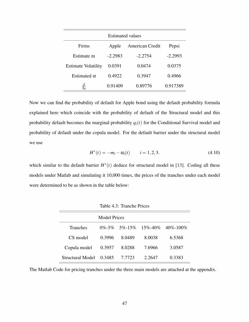
Estimated values

Firms Apple American Credit Pepsi

Estimate m -2.2983 -2.2754 -2.2993

Estimate Volatility 0.0391 0.0474 0.0375

Estimated α 0.4922 0.3947 0.4966

dX0

0.91409 0.89776 0.917389

Now we can find the probability of default for Apple bond using the default probability formula

explained here which coincide with the probability of default of the Structural model and this

probability default becomes the marginal probability qi(t) for the Conditional Survival model and

probability of default under the copula model. For the default barrier under the structural model

we use

H∗(t) =−mi−αi(t) i = 1,2,3. (4.10)

which similar to the default barrier H∗(t) deduce for structural model in [13]. Coding all these

models under Matlab and simulating it 10,000 times, the prices of the tranches under each model

were determined to be as shown in the table below:

Table 4.3: Tranche Prices

Model Prices

Tranches 0%-5% 5%-15% 15%-40% 40%-100%

CS model 0.3996 8.0489 8.0038 6.5368

Copula model 0.3957 8.0288 7.6966 3.0587

Structural Model 0.3485 7.7723 2.2647 0.3383

The Matlab Code for pricing tranches under the three main models are attached at the appendix.

47

4.2 Interpretation of Results

From the table 4.3 0% to 5% tranche (equity) is quoted as the percentage upfront payment required

on the assumption that subsequent payments will be 500 basis points per year. The other tranches

are also quoted as basis points per every three months. As observed from the prices table above,

it is clearly seen that all the three models give very close prices for the equity tranche. Similarly

the premium coupons of the junior tranche for all the three models are also very close. However

the Mezzanine tranche spread for the structural model is quite small as compared to the one factor

copula model and the CS model. For the senior tranche spread the prices differ for the three

models. The CS model gives a high price compared to the other two models. Also the one factor

copula has a higher senior tranche than the structural model which produced a small price for

the senior tranche. The equity tranche price simply determines the upfront fee to be paid to the

equity investors. For example in our pricing problem the CS model value the equity tranche as

39.96% which means the equity tranche holder receives $38.5 (39.96% of 96.2626) as an upfront

fee. The tranche prices of the other tranches are the fractions of the notional principle on each

tranche (premium) paid quarterly.

As shown from the table, the CS model and the one factor copula model are almost giving the

same value to the tranches which means they seem to be priced well under the cumulative loss

method explained above. Now we continue to experiment how changes in correlation factor for

the one factor Gaussian copula model and the structural model will affect each price.

4.2.1 Effect of Correlation on Valuation of CDO Tranches

From the description of each of the model, one factor Gaussian Copula model and the Structural

model are affected by the correlation factor. We then experiment how changes in the correlation

factor will affect the tranche prices. We experiment when the coefficient of the market factor for the

three firms increases from 0.1,0.2,0.3 to 0.4,0.5,0.6 and 0.7,0.8,0.9 respectively. This experiment

is the same as increasing correlation factor from 0.02,0.06,0.03 to 0.2,0.3,0.24 and 0.56,0.72,0.63

48

respectively. Noting that the correlation factor between reference entities X1,X2,X3 are define as

corr(X1X2) = 0.02, corr(X2X3) = 0.06 and corr(X1X3) = 0.03.

Table 4.4: Copula model verses structural model

Model Prices

Correlation 0.1,0.2,0.3

Tranches 0%-5% 5%-15% 15%-40% 40%-100%

Copula model 0.3957 8.0288 7.6966 3.0587

Structural Model 0.3485 7.7723 2.2647 0.3383

Correlation 0.4,0.5,0.6

Tranches 0%-5% 5%-15% 15%-40% 40%-100%

Copula model 0.3737 7.9327 7.4830 4.0507

Structural Model 0.3261 7.6533 2.1347 0.3252

Correlation 0.7,0.8,0.9

Tranches 0%-5% 5%-15% 15%-40% 40%-100%

Copula model 0.2252 7.6789 7.3704 5.6133

Structural Model 0.3124 7.5777 2.0910 0.3384

From table 4.4 it is observed that as we increase the correlation, the tranche prices for struc-

tural model decrease across all the tranches which means that the cost of protection decreases as

correlation increases.

Similarly, as correlation increases we observed that the tranche spread for the one factor Gaus-

sian copula model decreases for the equity tranche, junior tranche and mezzanine whiles the spread

of the senior tranche increases. This means that the lower tranches spread (premium of cost of

protection) is inversely proportional to correlation while the senior tranche premium is directly

proportional to correlation.

This results tally with the observation made by Hull and White in their paper [13]. They

49

observed that increasing correlation lowers the value for the junior tranches that bears the initial

losses and increases the value for the senior tranche that bears the later losses.

4.2.2 Difference Between Structural Model and One Factor Gaussian Copula Model

Table 4.5: Difference between Copula model and structural model

Difference:Structural - Gaussian Copula

Tranches

Correlation 0%-5% 5%-15% 15%-40% 40%-100%

0.1,0.2,0.3 -0.0472 -0.2565 -5.4319 -2.7204

0.4,0.5,0.6 -0.0476 -0.2794 -5.3483 -3.7255

0.7,0.8,0.9 0.028 -0.1012 -5.2794 -5.3049

Considering the table 4.2.2 above, it can be seen that the models produce quite similar results

for the equity and junior tranche but a wide difference for mezzanine and senior tranche. We mea-

sure the difference between the two models by calculating the spread difference across tranches.

We observe that the one factor Gaussian copula model has high spreads across tranches as com-

pared to the structural model. The results obtained are similar to that of Hull, Predescu and White

(2005) in [14] where they stated that the one factor Gaussian copula model is a good approxima-

tion to the basic structural model in a wide range of situations. Moreover considering all the three

model prices we can say with certainty that the CS model gives the best prices to the CDO structure

since default is imminent and investors need these high prices to be able to invest in the CDO.

50

Chapter 5

Conclusion and Recommendations

This thesis has been able to present the detailed pricing of synthetic CDO using one factor Gaus-

sian copula model, structural model and conditional survival model. To achieve these goals, vari-

ous correlation modelling approaches were used such as Li (2000), Hull and White (2004), Hull,

Predescu and White (2005) and Peng and Kou (2009). We found out that all these models, despite

the small differences tend to give comparable prices for the tranches of the portfolio of the three

sample reference entities.

Considering the tranche prices observed in chapter four, the three models give a very close

price for the equity tranche and junior tranche while the prices for mezzanine tranche and senior

tranche differ. However this thesis does not give any explicit reason why the tranche prices for the

less risky tranches are quite different since they can be attributed to several different features of

the modelling technique (structural verses copula, correlation structure, etc. Also from the prices

obtained from our simulation the CS model gives a higher prices for all four tranches compared to

the other two models and this high price favours investors because they receive a higher cash flow

from SPV. On the other hand the structural model gives the lowest tranche price in all the tranche

categories which favours SPV since it makes them spend less on premium payment.

In view of the experiment made on the one factor Gaussian copula model and the structural

model in chapter four, the experiment tends to give interesting results when the correlation pa-

rameter in both models are increased even for the small number of reference entities we used in

our simulation. Our conclusions coincide with the conclusions made by Hull, Predescu and White

(2005), in particular, we observed that as correlation increases the tranche price for the structural

model and that of the one factor Gaussian copula model decrease while the price of the senior

51

tranche increases. Moreover since we did not price these tranches under market data, we could not

determine which model is best fit for the market modelling so this thesis is silent on which model

is best for market pricing.

All these three models have their own advantages and drawbacks which can affect the price

of the tranches one way or the other. For instance Hull, Predescu and White (2005) revealed that

structural model was not a good fit to market data and also observed that the market standard model

does not appear to fit market data well [13]. Where the market standard model is the one factor

Gaussian copula model under the following assumptions:

• a fixed recovery rate of 40%,

• same CDS spreads for all of the underlying reference entities,

• same pairwise correlations,

• same default intensities for all the underlying reference entities.

Also the CS model is known to price tranches well when the economy is in recession as dis-

cussed by Peng and Kou (2009). Peng and Kou modelled the tranche prices based on three eco-

nomical factors where Polya process was used to simulate the financial crises state in the economy

and CIR model for the normal fluctuation in the economy. Their method gave a very close tranche

price compared to the market prices.

Lastly a common similarity between these three models is the fact that they all incorporate in

their model an economic factor or common factor and marginal default probability which makes

comparison possible.

52

Bibliography

[1] Andersen, L., Sidenius, J. and Basu, S. (2003),All Your Hedges in One Basket, RISK,

November, 67-72.

[2] Andersen, L. and Sidenius, J. (2005), Extensions to the Gaussian Copula: Random Recovery

and Random Factor Loadings, Journal of Credit Risk, 1.

[3] Arnsdorf, M., Halperin, I., 2007, Markovian bivariate spread-loss model for portfolio credit

derivatives. Working paper, Quantitative Research J.P. Morgan.

[4] Anna Kalemanova, Bernd Schmidy and Ralf Wernerz The Normal Inverse Gaussian Distri-

bution for Synthetic CDO Pricing, May 2005.

[5] Black, F. and J. Cox, 1976, Valuing Corporate Securities: Some Effects of Bond Indenture

Provisions, Journal of Finance, 31, 351-67.

[6] Christian Bluhm, On Copulas and their Application to CDO Pricing December 10, 2003.

[7] David X Li,(2000),On Default Correlation: A Copula Function Approach,Vice President of

Risk Management at AXA Financial in New York.

[8] Dezhong W, Svetlozar T., Frank J. Fabozzi (2006) Pricing Tranches of a CDO and CDS

Index: Recent Advances and Future Research.

[9] Darrell Duffie and Kenneth J. Singleton, Modelling Term Structures of Defaultable

Bonds,February 1998.

[10] Darrell Duffie, Lasse Heje Pedersen and Kenneth J. Singleton, Modeling Sovereign Yield

Spreads: A Case Study of Russian Debt, February 2003.

[11] Default risk : BusinessDictionary.com. Retrieved July 05, 2017, from BusinessDic-

tionary.com website: http://www.businessdictionary.com/definition/default-risk.html

53

[12] Frank J. and Kothari Vinod Securitization: The Tool of Financial Transformation. Yale ICF

Working Paper No. 07-07. Available at SSRN: https://ssrn.com/abstract=997079.

[13] Hull J. Predescu M, White A (2005) The valuation of correlation dependent credit deriva-

tives using a structural model Rotman School of Management.

[14] Hull J. and White A. (2001) Valuing Credit Default Swaps II: Modelling Default Correla-

tions Journal of Derivatives, Vol. 8, No. 3, 12-22 .

[15] Hull J. and White A. (2004) Valuation of a CDO and an nth to Default CDS Without Monte

Carlo Simulation The Journal of Derivatives Winter 2004, Vol. 12, No. 2: pp. 8-23.

[16] J. Michael Harrison (1990) Brownian Motion and Stochastic Flow SystemsGraduate School

of Business Stanford University.

[17] Jarrow, R., Turnbull, S., 1995, Pricing options on financial securities subject to credit risk.

Journal of Finance 50, 53-85.

[18] Jean-Paul Laurent and Jon Gregory Basket Default Swaps, CDOs and Factor Copulas,

September 2003.

[19] Joel Bessis (2010) Risk Management in Banking Wiley.

[20] Kay Giesecke, Portfolio Credit Risk : Top Down verses Bottom up Approaches,Stanford

University. Published in Frontiers in Quantitative Finance.

[21] Kay Giesecke and Lisa R. Goldberg, A Top-Down Approach to Multi-Name Credit, February

2005.

[22] Lando, D. (1998) On Cox Processes and Credit Risky Securities.

[23] Leland, H. E., 1994, Risky Debt, Bond Covenants and Optimal Capital Structure, Journal of

Finance, Vol. 49, 1213-1252.

54

[24] Longstaff, F. A. and Schwartz, E. S., 1995, A Simple Approach to Valuing Risky Fixed and

Floating Rate Debt, Journal of Finance, Vol. 50, No. 3, 789-819.

[25] Lucas D. ( March 1995),Default Correlation and Credit Analysis.,Journal of Finance, 29

(1974),pp,449-470.

[26] Lucas, Douglas J., Laurie S. Goodman, and Frank J. Fabozzi (2007) Collateralized debt

obligations and credit risk transfer.

[27] Petro Veronesi Fixed Income Securities, Valuation, Risk and Risk Management

[28] Robert A. Jarrow and Philip Protterb (2004) Structural versus reduced form models,Journal

of investment Management, Volume 2, No. 2, (2004), pp. 1-10.

[29] Robert C. Merton, On the pricing of Corporate Debt: The Risk Structure of Interest Rates,

May 1974.

[30] Sklar, A. (1973),A random Variables, Joint Distribution Functions and Copu-

las,Kybermetika,9 (1973), pp.449-460.

[31] Steven E Shreve Stochastic Calculus for Finance 11 Continuous-Time Models Springer Fi-

nance.

[32] Verschuere Benjamin , emphOn Copulas and their Application to CDO Pricing January

2006.

[33] X. Peng and S. Kou Default clustering and valuation of collateralized debt obligations

Working Paper, 2009.

[34] Zhou, Jian and Lobo, Gerald J., Disclosure Quality and Earnings Manage-

ment, May 1, 2001. Available at SSRN: https://ssrn.com/abstract=265550 or

http://dx.doi.org/10.2139/ssrn.265550.

55

[35] Zhou, C., 2001a, The Term Structure of Credit Spreads with Jump Risk, Journal of Banking

and Finance, Vol. 25, 2015-2040.

[36] Zhou, C., 2001b, An Analysis of Default Correlations and Multiple Defaults, Review of

Financial Studies, Vol. 14, No. 2, 555-576.

56

Appendix A

First Appendix

A.1 Appendix

A.1.1 Appendix 1 Structural Model Matlab Code

f u n c t i o n [ d e f a u l t ] = S t r u c t u r a l Model

T = 5 ;

mu = 0 . 0 1 ; s igma = 0 . 3 ; c o r = 0 . 1 ;

N = 2 0 ; n =20;

t = z e r o s (N , 1 ) ;

f o r i = 1 : 2 0 ;

t ( i ) = ( T /N)* i ;

t ;

end

% G e n e r a t i n g Brownian mot ions f o r Common r i s k

M = ( sigma * s q r t ( T /N) ) * ( t r i l ( ones (N ) ) * ( ( normrnd ( 0 , 1 , [N , 1 ] ) ) ) ) + mu* t ;

%p l o t ( t ,M, ’ b lue ’ )

%ho ld on ;

% For f i r m A

x = ( sigma * s q r t ( T /N) ) * ( t r i l ( ones (N ) ) * ( ( normrnd ( 0 , 1 , [N , 1 ] ) ) ) ) + mu* t ; % C o n s t r u c t e d brownian mot ion

%p l o t ( t , x , ’ red ’ )

%ho ld on ;

X = c o r *M + s q r t (1− c o r ^2)* x ; % Brownian mot ion o f f i r m A

57

v = 0 . 8 ; % i n i t i a l a s s e t v a l e o f f i r m A

V =( exp ( s igma *X + (mu−( s igma ^ 2 ) / 2 ) * ( t ) ) ) * v ;

% For f i r m B

y = ( sigma * s q r t ( T /N) ) * ( t r i l ( ones (N ) ) * ( ( normrnd ( 0 , 1 , [N , 1 ] ) ) ) ) + mu* t ;

%p l o t ( t ,M, ’ green ’ )

%ho ld on ;

Y = c o r *M + s q r t (1− c o r ^2)* y ;

s = 0 . 8 ;

S = ( exp ( s igma *Y + (mu−( s igma ^ 2 ) / 2 ) * ( t ) ) ) * s ;

%Firm C

z = ( sigma * s q r t ( T /N) ) * ( t r i l ( ones (N ) ) * ( ( normrnd ( 0 , 1 , [N , 1 ] ) ) ) ) + mu* t ;

%p l o t ( t ,M, ’ ye l low ’ )

%ho ld on ;

Z = c o r *M + s q r t (1− c o r ^2)* z ;

r = 0 . 8 ;

R = ( exp ( s igma *Z + (mu−( s igma ^ 2 ) / 2 ) * ( t ) ) ) * r ;

%Firm D

%p l o t ( t , w, ’ b lack ’ )

%ho ld on ;

%U =( exp ( s igma *W + (mu−( s igma ^ 2 ) / 2 ) * ( t ) ) ) * u;%

p l o t ( t , V, ’ red ’ )

ho ld on ;

p l o t ( t , R , ’ b lack ’ )

ho ld on ;

p l o t ( t , S , ’ ye l low ’ )

ho ld on ;

58

%p l o t ( t , U, ’ green ’ )

%ho ld on ;

V

S

R

%U

%P r o b a b i l i t y o f d e f a u l t b a r r i e r f o r Apple bond f o r f i r m A

a1= −2.2983 ; b1= 0 . 4 9 2 3 ; prob = z e r o s ( 2 0 , 1 ) ; c1= −2.2753; d1 = 0 . 3 9 4 5 ; e1= −2.2993; f1 = 0 . 4 9 6 6 ;

prob1 = z e r o s ( 2 0 , 1 ) ; prob2 = z e r o s ( 2 0 , 1 ) ;

f o r i = 1 :20

prob ( i ) = a1 + b1* t ( i ) ;

end

prob

f o r i = 1 :20

prob1 ( i ) = c1 + d1* t ( i ) ;

end

prob1

f o r i = 1 :20

prob2 ( i ) = e1 + f1 * t ( i ) ;

end

prob2

% C o n s t r u c t i n g b a r r i e r f o r a s s e t

a = z e r o s ( 2 0 , 1 ) ; e = z e r o s ( 2 0 , 1 ) ; f = z e r o s ( 2 0 , 1 ) ; h = z e r o s ( 2 0 , 1 ) ;

%d e f a u l t = z e r o s ( 1 , 4 ) ;

f o r i = 1 :20

i f ( X( i ) <= prob ( i ) )

59

a ( i ) = 1 ;

e l s e i f X( i ) > prob ( i )

a ( i ) = 0 ;

end

end

f o r i = 1 :20

i f Y( i ) <= prob1 ( i )

e ( i ) = 1 ;

e l s e i f Y( i ) > prob1 ( i )

e ( i ) = 0 ;

end

end

f o r i = 1 :20

i f Z ( i ) < prob2 ( i )

f ( i ) = 1 ;

e l s e i f Z ( i ) > prob2 ( i )

f ( i ) = 0 ;

end

end

%f o r i =1:20

%Aif U( i ) < D( i ) ;

%h ( i ) = 1

%e l s e i f U( i ) > D( i ) ;

% h ( i ) = 0

%end

d e f a u l t m a t r i x = [ a e f ]

60

% Loss on each f i r m

% Given t h a t f i r m 1 has a l o a n of 1113 .57 wi th a 40% r e c o v e r y ,

%Firm 2 l o a n 1114 .22 and 50% and

%Firm 3 has 1000 and 30% r e c o v e r y

%f i r m 1 l o s s

L1 = ( 1 −0 . 4 ) * 1 1 1 3 . 5 7 ;

%f i r m 2 l o s s

L2 = ( 1 −0 . 5 ) * 1 1 1 4 . 2 2 ;

%f i r m 3 l o s s

L3 = (1 −0 .3 )*1000 ;

Loss = [ L1 ; L2 ; L3 ] ;

%cummula t ive l o s s

CL = d e f a u l t m a t r i x * Loss

f o r i =1:20

t ( i )= ( 1 / 4 ) * i ;

end

%D i s c o u n t F a c t o r

d t = z e r o s ( 2 0 , 1 ) ;

Dt = z e r o s ( 2 0 , 1 ) ;

r = 0 . 0 5 ;

d t ( 1 ) = 1 / ( ( 1 + r ) ^ ( t ( 1 ) / 2 ) ) ;

f o r i = 2 :20

d t ( i ) = 1 / ( ( 1 + r ) ^ ( ( t ( i )+ t ( i − 1 ) ) / 2 ) ) ;

end

d t

Dt ( 1 ) = 1 / ( ( 1 + 0 . 0 5 ) ^ ( t ( 1 ) ) ) ; % second d i s c o u n t f a c t o r

61

f o r i = 2 : 20

Dt ( i ) = 1 / ( ( 1 + 0 . 0 5 ) ^ ( t ( i ) ) ) ;

end

Dt

d e l t a = z e r o s ( 2 0 , 1 ) ; % change i n t ime

d e l t a ( 1 ) = t (1)−0;

f o r i = 2 : l e n g t h ( t )

d e l t a ( i ) = t ( i )− t ( i −1);

end

% Tranche Cummulat ive l o s s e s

%E q u i t y 0−96.2626

%J u n i o r 96 .2626 − 288 .7878

%Mezzanine 288 .7878 − 770 .1008

%S e n i o r 770 .1008 − 1925 .252

LE = 96.2626;%* ones ( l e n g t h ( Mt ) , 1 ) ;

LJ = 192.5252;%* ones ( l e n g t h ( Mt ) , 1 ) ;

LM = 481.313;%* ones ( l e n g t h ( Mt ) , 1 ) ;

LS = 1155.1512;%* ones ( l e n g t h ( Mt ) , 1 ) ;

%%D e f a u l t

L e q u i t y = z e r o s ( n , 1 ) ;

L j u n i o r = z e r o s ( n , 1 ) ;

Lmezzanine = z e r o s ( n , 1 ) ;

L s e n i o r = z e r o s ( n , 1 ) ;

LKR = z e r o s ( n , 1 ) ;

LKT = z e r o s ( n , 1 ) ;

LKS = z e r o s ( n , 1 ) ;

62

f o r i = 1 : n ;

i f CL( i ) > LE

%i f LK > LE

L e q u i t y ( i ) = (CL( i )−0)−(CL( i )−96.2626) ;% cummulatve l o s s on e q u i t y

e l s e i f (0 < CL( i ))&&(CL( i ) < LE )

L e q u i t y ( i ) = CL( i ) ;

e l s e i f CL < 0

L e q u i t y ( i ) = 0 ;

end

end

LKR( i ) = CL( i )−LE ;

i f LKR( i ) > LJ

L j u n i o r ( i ) = ( ( LKR( i )−96.2626)−(LKR( i ) −2 8 8 . 7 8 7 8 ) ) ; % cummula t ive l o s s on j u n i o r

e l s e i f (0 < LKR( i ) ) && (LKR( i ) < LJ )

L j u n i o r ( i ) = max ( ( min (LKR( i ) , 2 8 8 . 7 8 7 8 ) −9 6 . 2 6 2 6 ) , 0 ) ;

e l s e i f LKR( i ) < 0

L j u n i o r ( i ) = 0 ;

end

end

LKT( i )= LKR( i )−LJ ;

i f LKT( i ) > LM

Lmezzanine ( i ) = ( ( LKT( i )−288.7878)−(LKT( i ) −7 7 0 . 1 0 0 8 ) ) ;

e l s e i f (0 < LKT( i ) ) && (LKT( i ) < LM)

Lmezzanine ( i )= LKT( i );%max ( ( min (LKT( i ) , 7 7 0 . 1 0 0 8 ) −2 8 8 . 7 8 7 8 ) , 0 ) ;

e l s e i f LKT( i ) < 0

63

Lmezzanine ( i ) = 0 ;

end

LKS( i ) = LKT( i )− LM;

i f LKS( i ) > LS

L s e n i o r ( i ) = ( ( LKS( i )−770.1008)−(LKS( i ) −1 9 2 5 . 2 5 2 ) ) ;

e l s e i f (0 < LKS( i ) ) && (LKS( i ) < LS )

L s e n i o r ( i ) = LKS( i );%max ( ( min (LKS( i ) , 1 9 2 5 . 2 5 2 ) −7 7 0 . 1 0 0 8 ) , 0 ) ;

e l s e i f LKS < 0

L s e n i o r ( i ) = 0 ;

end

end

L e q u i t y

L j u n i o r

Lmezzanine

L s e n i o r

% t r a n c h e p r i c e s

%E q u i t y s p r e a d

cumequi ty = z e r o s ( n , 1 ) ;

cumequ i ty ( 1 ) = L e q u i t y (1)−0;

f o r i = 2 : n ;

cumequ i ty ( i ) = L e q u i t y ( i )−L e q u i t y ( i −1);

end

cumesum = z e r o s ( n , 1 ) ;

cumesum ( 1 ) = ( L e q u i t y ( 1 ) + 0 ) / 2 ;

64

f o r i = 2 : n ;

cumesum ( i ) = ( L e q u i t y ( i )+ L e q u i t y ( i −1 ) ) / 2 ;

end

f = t i m e s ( Dt , d e l t a ) ;

R = LE − cumesum ;

SE = ( ( 1 / LE)* d o t ( dt , cumequ i ty ) ) −0 .05* ( d o t ( f , R ) ) ;

% J u n i o r Spread

c u m j u n i o r = z e r o s ( n , 1 ) ;

c u m j u n i o r ( 1 ) = L j u n i o r (1)−0;

f o r i = 2 : n ;

c u m j u n i o r ( i ) = L j u n i o r ( i )−L j u n i o r ( i −1);

end

s u m j u n i o r = z e r o s ( n , 1 ) ;

s u m j u n i o r ( 1 ) = ( L j u n i o r ( 1 ) + 0 ) / 2 ;

f o r i = 2 : n ;

s u m j u n i o r ( i ) = ( L j u n i o r ( i )+ L j u n i o r ( i −1 ) ) / 2 ;

end

U = (288.7878−96.2626)− ( s u m j u n i o r ) ;

SJ = ( d o t ( dt , c u m j u n i o r ) ) / ( d o t ( f ,U ) ) ;

% Mezzanine Spread

cummezz = z e r o s ( n , 1 ) ;

cummezz ( 1 ) = Lmezzanine (1)−0;

f o r i = 2 : n ;

cummezz ( i ) = Lmezzanine ( i )−Lmezzanine ( i −1);

end

summezz = z e r o s ( n , 1 ) ;

65

summezz ( 1 ) = ( Lmezzanine ( 1 ) + 0 ) / 2

f o r i = 2 : n ;

summezz ( i ) = ( Lmezzanine ( i )+ Lmezzanine ( i −1 ) ) / 2 ;

end

Z = ( 7 7 0 . 1 0 0 8 − 288.7878)− ( summezz ) ;

SM = ( d o t ( dt , cummezz ) ) / ( d o t ( f , Z ) ) ;

% S e n i o r t r a n c h e

cumsen io r = z e r o s ( n , 1 ) ;

cumsen io r ( 1 ) = L s e n i o r (1)−0;

f o r i = 2 : n ;

cumsen io r ( i ) = L s e n i o r ( i )−L s e n i o r ( i −1);

end

s u m s e n i o r = z e r o s ( n , 1 ) ;

s u m s e n i o r ( 1 ) = ( L s e n i o r ( 1 ) + 0 ) / 2 ;

f o r i = 2 : n ;

s u m s e n i o r ( i ) = ( L s e n i o r ( i )+ L s e n i o r ( i −1 ) ) / 2 ;

end

O = (1925.252−770.1008)− ( s u m s e n i o r ) ;

SS = ( d o t ( d t , cumsen io r ) ) / ( d o t ( f ,O ) ) ;

SE

SJ

SM

SS

d e f a u l t = [ SE SJ SM SS ]

end

A.1.2 Appendix 2 Conditional Survival Model Matlab Code

66

f u n c t i o n [ d e f a u l t ] = Nnewcsmodel

a l p h a = 3 ; b e t a = 2 ;

lambda = gamrnd ( a lpha , b e t a ) ;

%lambda = 0 . 5 ;

m a t u r i t y = 2 0 ;

t = 0

t a u = −l o g ( r and ) / lambda ;

T= t + t a u ;

k =0 ;

i n d e x = 1 ;

w h i l e ( T < m a t u r i t y )

k ( i n d e x ) = k ( end ) + 10* b e t a r n d ( 0 . 5 , 0 . 5 ) ;

T ( i n d e x ) = T ( end ) + t a u ;

i n d e x = i n d e x + 1 ;

end

k

T

s t a i r s ( T , k , ’ red ’ )

t = z e r o s ( 2 0 , 1 ) ; a t = z e r o s ( 2 0 , 1 ) ; Nt = z e r o s ( 2 0 , 1 ) ; Mt = z e r o s ( 2 0 , 1 ) ;

f o r i =1:20

t ( i )= ( 1 / 4 ) * i ;

a t ( i )= lambda * t ( i ) ;

Nt ( i ) = p o i s s r n d ( a t ( i ) ) ;

Mt ( i ) = sum ( rand ( Nt ( i ) , 1 ) ) ;

67

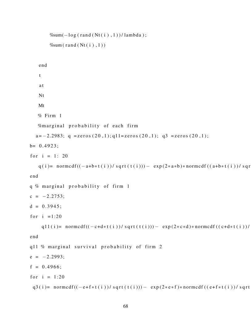
%sum(− l o g ( r and ( Nt ( i ) , 1 ) ) / lambda ) ;

%sum ( rand ( Nt ( i ) , 1 ) )

end

t

a t

Nt

Mt

% Firm 1

%m a r g i n a l p r o b a b i l i t y o f each f i r m

a =−2.2983; q = z e r o s ( 2 0 , 1 ) ; q11= z e r o s ( 2 0 , 1 ) ; q3 = z e r o s ( 2 0 , 1 ) ;

b= 0 . 4 9 2 3 ;

f o r i = 1 : 20

q ( i )= normcdf ((− a+b* t ( i ) ) / s q r t ( t ( i ) ) )− exp (2* a *b )* normcdf ( ( a+b* t ( i ) ) / s q r t ( t ( i ) ) ) ;

end

q % m a r g i n a l p r o b a b i l i t y o f f i r m 1

c = −2.2753;

d = 0 . 3 9 4 5 ;

f o r i =1:20

q11 ( i )= normcdf ((− c+d* t ( i ) ) / s q r t ( t ( i ) ) )− exp (2* c *d )* normcdf ( ( c+d* t ( i ) ) / s q r t ( t ( i ) ) ) ;

end

q11 % m a r g i n a l s u r v i v a l p r o b a b i l i t y o f f i r m 2

e = −2.2993;

f = 0 . 4 9 6 6 ;

f o r i = 1 :20

q3 ( i )= normcdf ((− e+ f * t ( i ) ) / s q r t ( t ( i ) ) )− exp (2* e * f )* normcdf ( ( e+ f * t ( i ) ) / s q r t ( t ( i ) ) ) ;

68

end

q3

%q = gampdf ( r and ( l e n g t h ( Mt ) , 1 ) , 1 , 1 ) ; % pdf from gamma f u n c t i o n

% g e n e r a t i n g t h e e x p e c t e d v a l u e i n q ( i ) e q u a t i o n

a1= 0 . 1 8 ;

g1=a1 *Mt ;

e1 = −g1 ;

k1 = exp ( 1 ) . ^ ( e1 ) ;

%e x p e c t a t i o n f o r p o i s s o n

p = 1 / ( 1 + b e t a * m a t u r i t y );% 20 i s t h e t ime frame i e T = 20

e x p e c t e d p o i s s o n 1 = ( ( p ) / (1− ( (1− p )* exp ( 1 ) ^ ( 0 . 5 * a1 ^ 2 ) ) ) ) ^ a l p h a ;% moment g e n e r a t i n g f u n c t i o n o f normal d i s t r b u t i o n

% f i n d i n g t h e c o n d i t i o n a l s u r v i v a l p r o b a b i l i t y f o r f i r m 1

w1= ones ( 1 , l e n g t h ( Mt ) ) * ( ( 1 / ( e x p e c t e d p o i s s o n 1 ) ) * k1 ) ;

qx = q*w1

% Firm 2

% g e n e r a t i n g t h e e x p e c t e d v a l u e i n q ( i ) e q u a t i o n

a2= 0 . 1 7 ;

g2=a2 *Mt ;

e2 = −g2 ;

k2 = exp ( 1 ) . ^ ( e2 ) ;

%e x p e c t a t i o n f o r p o i s s o n

p = 1 / ( 1 + b e t a * m a t u r i t y ) ;

e x p e c t e d p o i s s o n 1 1 = ( ( p ) / (1− ( (1− p )* exp ( 1 ) ^ ( 0 . 5 * a2 ^ 2 ) ) ) ) ^ a l p h a ;% r e v i s i t t h e moment g e n e r a t i n g f u n c t i o n

% f i n d i n g t h e c o n d i t i o n a l s u r v i v a l p r o b a b i l i t y f o r f i r m 1

w11= ones ( 1 , l e n g t h ( Mt ) ) * ( ( 1 / ( e x p e c t e d p o i s s o n 1 1 ) ) * k2 ) ;

69

qs = q11 *w11

%f i r m 3

% g e n e r a t i n g t h e e x p e c t e d v a l u e i n q ( i ) e q u a t i o n

a3= 0 . 1 6 ;

g3=a3 *Mt ;

e3 = −g3 ;

k3 = exp ( 1 ) . ^ ( e3 ) ;

%e x p e c t a t i o n f o r p o i s s o n

p = 1 / ( 1 + b e t a * m a t u r i t y ) ;

e x p e c t e d p o i s s o n 1 3 = ( ( p ) / (1− ( (1− p )* exp ( 1 ) ^ ( 0 . 5 * a3 ^ 2 ) ) ) ) ^ a l p h a ;% r e v i s i t t h e moment g e n e r a t i n g f u n c t i o n

% f i n d i n g t h e c o n d i t i o n a l s u r v i v a l p r o b a b i l i t y f o r f i r m 3

w13= ones ( 1 , l e n g t h ( t ) ) * ( 1 / ( e x p e c t e d p o i s s o n 1 3 )* k3 ) ;

qc = q3*w13

%B e r n o u l i random v a r i a b l e

h= z e r o s ( l e n g t h ( t ) , 1 ) ; h1 = z e r o s ( l e n g t h ( t ) , 1 ) ; h2 = z e r o s ( l e n g t h ( t ) , 1 ) ;

f o r i = 1 :20

i f r and (1) < qx ( i )

h ( i ) =1 ;

e l s e i f r and (1) > qx ( i )

h ( i ) = 0 ;

end

end

f o r i = 1 :20

i f r and (1) < qs ( i )

h1 ( i ) =1 ;

e l s e i f r and (1) > qs ( i )

70

h1 ( i ) = 0 ;

end

end

f o r i = 1 :20

i f r and (1) < qc ( i )

h2 ( i ) =1 ;

e l s e i f r and (1) > qc ( i )

h2 ( i ) = 0 ;

end

end

h

h1

h2

% Loss on each f i r m

% Given t h a t f i r m 1 has a l o a n of 1113 .57 wi th a 40% r e c o v e r y ,

%Firm 2 l o a n 1114 .22 and 50% and

%Firm 3 has 1000 and 30% r e c o v e r y

%f i r m 1 l o s s

L1 = ( 1 −0 . 4 ) * 1 1 1 3 . 5 7 ;

%f i r m 2 l o s s

L2 = ( 1 −0 . 5 ) * 1 1 1 4 . 2 2 ;

%f i r m 3 l o s s

L3 = (1 −0 .3 )*1000 ;

Loss = [ L1 ; L2 ; L3 ]

%cummula t ive l o s s

CL = [ h , h1 , h2 ]* Loss

71

%D i s c o u n t F a c t o r

d t = z e r o s ( l e n g t h ( t ) , 1 ) ;

Dt = z e r o s ( l e n g t h ( t ) , 1 ) ;

r = 0 . 0 5 ;

d t ( 1 ) = 1 / ( ( 1 + r ) ^ ( t ( 1 ) / 2 ) ) ;

f o r i = 2 : l e n g t h ( t )

d t ( i ) = 1 / ( ( 1 + r ) ^ ( ( t ( i )+ t ( i − 1 ) ) / 2 ) ) ;

end

d t

Dt ( 1 ) = 1 / ( ( 1 + 0 . 0 5 ) ^ ( t ( 1 ) ) ) ; % second d i s c o u n t f a c t o r

f o r i = 2 : l e n g t h ( t )

Dt ( i ) = 1 / ( ( 1 + 0 . 0 5 ) ^ ( t ( i ) ) ) ;

end

Dt

d e l t a = z e r o s ( l e n g t h ( t ) , 1 ) ; % change i n t ime

d e l t a ( 1 ) = t (1)−0;

f o r i = 2 : l e n g t h ( Mt )

d e l t a ( i ) = t ( i )− t ( i −1);

end

% Tranche Cummulat ive l o s s e s

%E q u i t y 0−96.2626

%J u n i o r 96 .2626 − 288 .7878

%Mezzanine 288 .7878 − 770 .1008

%S e n i o r 770 .1008 − 1925 .252

LE = 96.2626;%* ones ( l e n g t h ( Mt ) , 1 ) ;

LJ = 192.5252;%* ones ( l e n g t h ( Mt ) , 1 ) ;

72

LM = 481.313;%* ones ( l e n g t h ( Mt ) , 1 ) ;

LS = 1155.1512;%* ones ( l e n g t h ( Mt ) , 1 ) ;

%%D e f a u l t

L e q u i t y = z e r o s ( l e n g t h ( t ) , 1 ) ;

L j u n i o r = z e r o s ( l e n g t h ( t ) , 1 ) ;

Lmezzanine = z e r o s ( l e n g t h ( t ) , 1 ) ;

L s e n i o r = z e r o s ( l e n g t h ( t ) , 1 ) ;

LKR = z e r o s ( l e n g t h ( t ) , 1 ) ;

LKT = z e r o s ( l e n g t h ( t ) , 1 ) ;

LKS = z e r o s ( l e n g t h ( t ) , 1 ) ;

f o r i = 1 : l e n g t h ( t )

i f CL( i ) > LE

%i f LK > LE

L e q u i t y ( i ) = (CL( i )−0)−(CL( i )−96.2626) ;% cummulatve l o s s on e q u i t y

e l s e i f (0 < CL( i ))&&(CL( i ) < LE )

L e q u i t y ( i ) = CL( i ) ;

e l s e i f CL < 0

L e q u i t y ( i ) = 0 ;

end

end

LKR( i ) = CL( i )−LE ;

i f LKR( i ) > LJ

L j u n i o r ( i ) = ( ( LKR( i )−96.2626)−(LKR( i ) −2 8 8 . 7 8 7 8 ) ) ; % cummula t ive l o s s on j u n i o r

e l s e i f (0 < LKR( i ) ) && (LKR( i ) < LJ )

L j u n i o r ( i ) = max ( ( min (LKR( i ) , 2 8 8 . 7 8 7 8 ) −9 6 . 2 6 2 6 ) , 0 ) ;

73

e l s e i f LKR( i ) < 0

L j u n i o r ( i ) = 0 ;

end

end

LKT( i )= LKR( i )−LJ ;

i f LKT( i ) > LM

Lmezzanine ( i ) = ( ( LKT( i )−288.7878)−(LKT( i ) −7 7 0 . 1 0 0 8 ) ) ;

e l s e i f (0 < LKT( i ) ) && (LKT( i ) < LM)

Lmezzanine ( i )= LKT( i );%max ( ( min (LKT( i ) , 7 7 0 . 1 0 0 8 ) −2 8 8 . 7 8 7 8 ) , 0 ) ;

e l s e i f LKT < 0

Lmezzanine = 0 ;

end

LKS( i ) = LKT( i )− LM;

i f LKS( i ) > LS

L s e n i o r ( i ) = ( ( LKS( i )−770.1008)−(LKS( i ) −1 9 2 5 . 2 5 2 ) ) ;

e l s e i f (0 < LKS( i ) ) && (LKS( i ) < LS )

L s e n i o r ( i ) = LKS( i );%max ( ( min (LKS( i ) , 1 9 2 5 . 2 5 2 ) −7 7 0 . 1 0 0 8 ) , 0 ) ;

e l s e i f LKS < 0

L s e n i o r ( i ) = 0 ;

end

end

L e q u i t y

L j u n i o r

74

Lmezzanine

L s e n i o r

% t r a n c h e p r i c e s

%E q u i t y s p r e a d

cumequi ty = z e r o s ( l e n g t h ( t ) , 1 ) ;

cumequ i ty ( 1 ) = L e q u i t y (1)−0;

f o r i = 2 : l e n g t h ( t )

cumequ i ty ( i ) = L e q u i t y ( i )−L e q u i t y ( i −1);

end

cumesum = z e r o s ( l e n g t h ( t ) , 1 ) ;

cumesum ( 1 ) = ( L e q u i t y ( 1 ) + 0 ) / 2 ;

f o r i = 2 : l e n g t h ( t )

cumesum ( i ) = ( L e q u i t y ( i )+ L e q u i t y ( i −1 ) ) / 2 ;

end

f = t i m e s ( Dt , d e l t a ) ;

R = LE − cumesum ;

SE = ( ( 1 / LE)* d o t ( dt , cumequ i ty ) ) −0 .05* ( d o t ( f , R ) ) ;

% J u n i o r Spread

c u m j u n i o r = z e r o s ( l e n g t h ( t ) , 1 ) ;

c u m j u n i o r ( 1 ) = L j u n i o r (1)−0;

f o r i = 2 : l e n g t h ( t ) ;

c u m j u n i o r ( i ) = L j u n i o r ( i )−L j u n i o r ( i −1);

end

s u m j u n i o r = z e r o s ( l e n g t h ( t ) , 1 ) ;

s u m j u n i o r ( 1 ) = ( L j u n i o r ( 1 ) + 0 ) / 2 ;

f o r i = 2 : l e n g t h ( t )

75

s u m j u n i o r ( i ) = ( L j u n i o r ( i )+ L j u n i o r ( i −1 ) ) / 2 ;

end

U = (288.7878−96.2626)− ( s u m j u n i o r ) ;

SJ = ( d o t ( dt , c u m j u n i o r ) ) / ( d o t ( f ,U ) ) ;

% Mezzanine Spread

cummezz = z e r o s ( l e n g t h ( t ) , 1 ) ;

cummezz ( 1 ) = Lmezzanine (1)−0;

f o r i = 2 : l e n g t h ( t )

cummezz ( i ) = Lmezzanine ( i )−Lmezzanine ( i −1);

end

summezz = z e r o s ( l e n g t h ( t ) , 1 ) ;

summezz ( 1 ) = ( Lmezzanine ( 1 ) + 0 ) / 2 ;

f o r i = 2 : l e n g t h ( t )

summezz ( i ) = ( Lmezzanine ( i )+ Lmezzanine ( i −1 ) ) / 2 ;

end

Z = ( 7 7 0 . 1 0 0 8 − 288.7878)− ( summezz ) ;

SM = ( d o t ( dt , cummezz ) ) / ( d o t ( f , Z ) ) ;

% S e n i o r t r a n c h e

cumsen io r = z e r o s ( l e n g t h ( t ) , 1 ) ;

cumsen io r ( 1 ) = L s e n i o r (1)−0;

f o r i = 2 : l e n g t h ( t )

cumsen io r ( i ) = L s e n i o r ( i )−L s e n i o r ( i −1);

end

s u m s e n i o r = z e r o s ( l e n g t h ( t ) , 1 ) ;

s u m s e n i o r ( 1 ) = ( L s e n i o r ( 1 ) + 0 ) / 2 ;

f o r i = 2 : l e n g t h ( t )

76

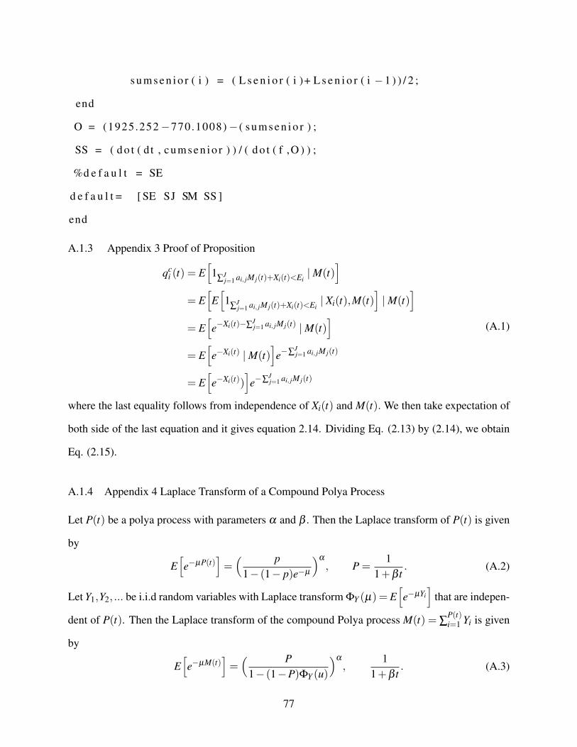
s u m s e n i o r ( i ) = ( L s e n i o r ( i )+ L s e n i o r ( i −1 ) ) / 2 ;

end

O = (1925.252−770.1008)− ( s u m s e n i o r ) ;

SS = ( d o t ( d t , cumsen io r ) ) / ( d o t ( f ,O ) ) ;

%d e f a u l t = SE

d e f a u l t = [ SE SJ SM SS ]

end

A.1.3 Appendix 3 Proof of Proposition

qci (t) = E

[1

∑Jj=1 ai, jM j(t)+Xi(t)<Ei

|M(t)]

= E[E[1

∑Jj=1 ai, jM j(t)+Xi(t)<Ei

| Xi(t),M(t)]|M(t)

]= E

[e−Xi(t)−∑

Jj=1 ai, jM j(t) |M(t)

]= E

[e−Xi(t) |M(t)

]e−∑

Jj=1 ai, jM j(t)

= E[e−Xi(t))

]e−∑

Jj=1 ai, jM j(t)

(A.1)

where the last equality follows from independence of Xi(t) and M(t). We then take expectation of

both side of the last equation and it gives equation 2.14. Dividing Eq. (2.13) by (2.14), we obtain

Eq. (2.15).

A.1.4 Appendix 4 Laplace Transform of a Compound Polya Process

Let P(t) be a polya process with parameters α and β . Then the Laplace transform of P(t) is given

by

E[e−µP(t)

]=( p

1− (1− p)e−µ

)α

, P =1

1+β t. (A.2)

Let Y1,Y2, ... be i.i.d random variables with Laplace transform ΦY (µ) = E[e−µYi

]that are indepen-

dent of P(t). Then the Laplace transform of the compound Polya process M(t) = ∑P(t)i=1 Yi is given

by

E[e−µM(t)

]=( P

1− (1−P)ΦY (u)

)α

,1

1+β t. (A.3)

77

Indeed, we can show this by noting that

E[e−uM(t)

]= E

[E[e−uM(t) | P(t)

]]= E

[(E[e−uYi]

)P(t)]= E

[e−log( 1

ΦY (u) )P(t)]

= E[e−vP(t)

]|v=log (

1ΦY (u)

)

= E[e−µP(t)

]=( p

1− (1− p)e−µ

)α

, P =1

1+β t

(A.4)

where the last equality follows from Eq. (A.2).

78