price formation in commodities markets
392
-
Upload
khangminh22 -
Category
Documents
-
view
0 -
download
0
Transcript of price formation in commodities markets


DRAFT VERSION
PRICE FORMATION IN
COMMODITIES MARKETS: FINANCIALISATION AND BEYOND
REPORT OF AN ECMI/CEPS TASK FORCE
JUNE 2013
CHAIR: ANN BERG RAPPORTEURS: DIEGO VALIANTE CHRISTIAN EGENHOFER
WITH CONTRIBUTION FROM: FEDERICO INFELISE
JONAS TEUSCH
CENTRE FOR EUROPEAN POLICY STUDIES BRUSSELS
This report is based on discussions during the CEPS-ECMI Task Force meetings on price formation in commodities markets, which were held on six occasions across 2011 and 2012.
Disclaimer. The findings of this Final Report do not necessarily reflect the views of all the members of the Task Force, or the views of their respective companies. Members contributed to the Task Force meetings and provided input to the discussions through presentations and relevant material for this Final Report. A set of principles has guided the drafting process to allow all of the interests represented in the Task Force to be heard and to comment on each chapter of the Final Report. Wherever fundamental disagreements arose, the rapporteurs have made sure that all views have been explained in a clear and fair manner. The Final Report was independently drafted by the author who is solely responsible for its content and any errors. Neither the Task Force members nor their respective companies necessarily endorse the conclusions of the Final Report.
Suggested citation. Valiante, D. (2013), “Commodities Price Formation: Financialisation and Beyond”,
CEPS-ECMI Task Force Report, Centre for European Policy Studies Paperback, Brussels.
ISBN 978-94-6138-183-5
© Copyright 2013, European Capital Markets Institute/Centre for European Policy Studies.
All rights reserved. No part of this publication may be reproduced, stored in a retrieval system or transmitted in any form or by any means – electronic, mechanical, photocopying, recording or otherwise – without the prior permission of the Centre for European Policy Studies.
Centre for European Policy Studies Place du Congrès 1, B-1000 Brussels
Tel: (32.2) 229.39.11 Fax: (32.2) 219.41.51 E-mail: [email protected]
Website: http://www.ceps.eu

CONTENTS
Acknowledgments ..................................................................................................................................... i
Preface......................................................................................................................................................... ii
Executive summary .................................................................................................................................. 1
Introduction ............................................................................................................................................... 1
1. Setting the scene: the structure of commodities markets ............................................................ 2
1.1 Defining ‘commodity’ and key product characteristics ...................................................... 2
1.2 Physical and futures markets ................................................................................................. 4
1.2.1 Physical markets: explaining their role in the value chain ...................................... 5
1.2.2 Futures markets ........................................................................................................... 20
1.2.3 Seaborne freight markets ........................................................................................... 32
1.2.4 Interaction between futures and physical markets price formation .................... 36
1.2.5 Why do market participants trade? .......................................................................... 41
1.3 Key futures market developments ....................................................................................... 45
1.3.1 What does financialisation mean? ............................................................................ 45
1.3.2 Shedding light on price trends and implications.................................................... 49
1.3.3 The growth and development of commodities index investing and other financial players .......................................................................................................................... 54
1.4 Interaction with financial assets: an empirical analysis of non-commercial positions . 62
2. Energy commodities ....................................................................................................................... 67
2.1 Crude oil markets ................................................................................................................... 67
2.1.1 Product and market characteristics: a market structurally subject to instability 69
2.1.2 Exogenous factors: measuring the impact of policy factors .................................. 83
2.1.3 Empirical analysis: the crucial link with the economic cycle ................................ 86
2.1.4 Market organisation: prospects and challenges for benchmark prices ............... 88
2.2 Natural gas markets ............................................................................................................... 99
2.2.1 Product and market characteristics: a promising future?.................................... 100
2.2.2 Exogenous factors: the key role of government actions ...................................... 113
2.2.3 Empirical analysis: weighing fundamentals ......................................................... 114
2.2.4 Market organisation: a European and a US model? ............................................. 115
3. Raw materials and industrial metals ......................................................................................... 121
3.1 Iron ore market ..................................................................................................................... 121
3.1.1 Product and market characteristics: the key industrial commodity .................. 122
3.1.2 Exogenous factors ..................................................................................................... 129
3.1.3 Market organisation: designing a new market structure .................................... 130
3.2 Aluminium market .............................................................................................................. 133
3.3 Copper market ...................................................................................................................... 153
4. Agricultural commodities ........................................................................................................... 167

4.1 Wheat market ........................................................................................................................ 167
4.1.1 Product and market characteristics: the key food commodity ........................... 168
4.1.2 Exogenous factors: assessing the role of government policies ........................... 179
4.1.3 Empirical analysis: dispelling myths and understanding the reality ................ 186
4.1.4 Market organisation: the essential role of futures markets ................................. 188
4.2 Corn market .......................................................................................................................... 190
4.2.1 Product and market characteristics: seeking long-term sustainability .............. 191
4.2.2 Exogenous factors: what role for government policies? ...................................... 207
4.2.3 Empirical analysis: growing link with energy commodities? ............................. 209
4.2.4 Market organisation: what future for international markets? ............................ 212
4.3 Soybean oil ............................................................................................................................ 213
4.3.1 Product and market characteristics: the key role of by-products ....................... 215
4.3.2 Exogenous factors: grasping the complex interaction ......................................... 226
4.3.3 Empirical analysis: what impact for biofuel policies? .......................................... 227
4.3.4 Market organisation .................................................................................................. 229
5. Soft commodities .......................................................................................................................... 231
5.1 Sugar market ......................................................................................................................... 231
5.1.1 Product and market characteristics: the rise of sugar cane ................................. 232
5.1.2 Exogenous factors: the effects of EU reforms ........................................................ 245
5.1.3 Market organisation: a fast developing international market ............................ 248
5.2 Cocoa market ........................................................................................................................ 249
5.2.1 Product and market characteristics: new prospects for alternative uses .......... 250
5.2.2 Exogenous factors: long-term effects of liberalisation ......................................... 260
5.2.3 Empirical analysis: the role of inventories ............................................................. 262
5.2.4 Market organisation: an immature market infrastructure .................................. 263
5.3 Coffee market ........................................................................................................................ 265
5.3.1 Product and market characteristics: the rise of Robusta coffee .......................... 267
5.3.2 Exogenous factors: the role of opportunity costs.................................................. 280
5.3.3 Empirical analysis: the effects of lower production costs.................................... 280
5.3.4 Market organisation: dealing with issues of market infrastructure ................... 281
6. Drivers of commodities price formation in physical and futures markets: concluding remarks ...................... 283
6.1 Market fundamentals........................................................................................................... 283
6.2 Evolving market organisation: a forward-looking perspective ..................................... 290
6.3 Matrix of weights for key drivers of price formation ...................................................... 293
Acronyms ............................................................................................................................................... 295
References .............................................................................................................................................. 297
Annex ...................................................................................................................................................... 305
Tables and Figures ........................................................................................................................ 305
Econometric analysis: Stata outputs .......................................................................................... 318
First chapter .......................................................................................................................... 318
Crude oil ................................................................................................................................ 331
Natural gas ............................................................................................................................ 338
Aluminium ............................................................................................................................ 340
Copper ................................................................................................................................... 344
Wheat ........................................................................................................................................... 347
Corn ..................................................................................................................................... 352
Soybean oil ............................................................................................................................ 357
Cocoa ..................................................................................................................................... 361
Coffee ........................................................................................................................................... 367
Task Force Participants ................................................................................................................ 372
List of boxes
Box 1. Key commodities market players ......................................................................................................... 12
Box 2. Unravelling the role of financial institutions in physical commodities markets ........................... 18
Box 3. The LME warehousing and warrants system ..................................................................................... 30
Box 4. Case study: corn storage hedge ............................................................................................................ 42
Box 5. Price reporting agencies (PRAs) in crude oil price formation mechanisms: the right of judgement............................................................................................................................................................ 92
Box 6. Liquefied natural gas (LNG): a long-term solution for gas transportation? ................................ 107
Box 7. China’s entry in the World Trade Organisation ............................................................................... 125
Box 8. The evolution of government intervention in agriculture in Europe and the United States ..... 181
Box 9. Current and future challenges for biofuels ....................................................................................... 201
Box 10. Causes and effects of market liberalisation: the case of cocoa ...................................................... 260
Box 11. The past, present and future of the ‘fair trade’ movement ........................................................... 277
Box 12. Key market failures in commodities markets and types of state intervention .......................... 289

| i
ACKNOWLEDGMENTS
The Centre for European Policy Studies and the European Capital Markets Institute gratefully acknowledge the financial support from the Task Force Members through the payment of a fee for their participation.
The author, Diego Valiante, wishes to thank Ann Berg (Chair of the Task Force) for her input during the Task Force meetings and constant support during the drafting process. He gratefully thanks his co-rapporteur Christian Egenhofer for his valuable support and guidance during the Task Force meetings and the drafting process, as well as for his direct inputs. He is also grateful to Federico Infelise for his constant and valuable research support, in particular for his assistance in handling a vast commodities dataset and his contributions to the empirical analyses. Jonas Teusch provided excellent research input to the chapter on energy commodities. The author also acknowledges comments and inputs from Willem Pieter de Groen, and direct input to the Task Force meetings from Christopher Gilbert, Philip Crowson, Bassam Fattouh, Howard Rogers and Ivan Diaz-Rianey.
The Final Report has greatly benefitted from the generous input of the Task Force members (see list in annex) through their presentations and, in particular, through the kind provision of datasets and raw data used throughout the report. In particular, the author wishes to thank Peter Blogg (LIFFE), Thomas Erickson (Bunge), Rachel Lees (LME), Anna Mac (LIFFE), Hartzell Mette (LKAB), Elizabeth Murphy (Platts), Saad Nizari (Goldman Sachs), Georgi Slavov (ICAP), Simon Smith (Argus Media), Francesca Stevens (Alcoa), and other experts CME Group.
Finally, the author has benefitted from the research support of Mirzha De Manuel and Francesco Grosso, the editing and review by Anne Harrington and Anil Shamdasani, and the help of the rest of the CEPS staff in finalising this report and in the organisation of the Task Force meetings.

| ii
PREFACE
Over the last decade, commodities markets have risen from relative obscurity to a subject of intense scrutiny by policy makers and financial supervisors. A dramatic rise in global productivity, markets liberalisation and increased access to international finance have fuelled commodity sector growth and trade. This growth in turn, along with market deregulation and swift technological advancement, including electronic trading, has engendered an unprecedented rise commodity linked financial transactions. Once considered an arcane field of business, commodities trading has drawn an entirely new sector - financial participants – into both physical and derivatives trading, raising concerns about the role of these participants in these markets. The food and financial crises between 2007 and 2009, which were accompanied by elevated levels of commodity price volatility, heightened these concerns and, together with other important market changes, led to the formation of this Task Force.
Supported by the input received in the Task Force meetings, this Final Report intends to demystify the commodities sphere by providing an in depth examination of the major commodity groups, focusing on product characteristics, supply chains, pricing, liquidity, financial intermediation, industry players and the interplay between derivatives markets and the underlying physical goods. In so doing, the Report contributes to the international debate with important information about the diverse market structures across commodities, including supply and demand elasticities, concentration of ownership, infrastructure organisation and layers of financial participation. While describing the endogenous factors, it also examines the increasing role of exogenous factors now impacting commodities. Finally, it assesses the drivers of the growth of derivatives markets and their impact on price formation.
Ideally, the paper will help those entrusted with commodity markets decision-making and supervision to gain a greater understanding of the various components of each market and how these markets operate within the global context. It should also heighten the debate surrounding the cross border regulatory harmonization process and jurisdictional issues as many commodity benchmarks allow multi-country delivery and settlement.
Markets evolve constantly. Prior to 2000, few analysts predicted the explosive growth of commodity markets, including derivatives markets. Although the principles of sound markets vary little overtime, the landscape beneath them is constantly shifting and increasing in complexity year after year. Today, the level of knowledge needed for proper supervision and rulemaking has never been higher. This Report is a timely contribution to the current state of commodities price formation.
Ann Berg
Chair of the Task Force
Independent Consultant to International Organisations Former Board Director, Chicago Board of Trade

DRAFT VERSION
| 1
EXECUTIVE SUMMARY
ommodities lie at the heart of the global economy. Access to and affordability of commodities are essential to the wellbeing, growth and competitiveness of our economies, which are highly dependent on commodity trade. Indeed, access to and affordability of essential food
commodities, such as staple foods, are important elements for the stability of many societies. Markets are seen as a guarantee to ensure this access and affordability, with the preconditions that they are transparent and competitive, and that market failures are properly addressed.
Volatile prices and actual or perceived government interference have raised questions over the efficient functioning of commodities price formation and sparked fears that instability could wreak havoc on global markets. Against this background, this CEPS-ECMI Task Force Report takes a fresh look at the structure of commodities markets and their price formation mechanisms, including their interaction with the international financial system.
The report surveys the functioning and market organisation of eleven different (storable) commodities markets to ascertain drivers of price formation and highlight potential market failures. These markets are: crude oil, natural gas, iron ore, aluminium, copper, wheat, corn, soybean oil, sugar, cocoa and coffee. The commodities can be grouped into four categories: energy, raw materials and base metals, agricultural, and soft commodities.
A complex marketplace
The way prices are formed in markets for physical commodities and futures contracts is the result of complex interactions between idiosyncratic factors, such as product characteristics (quality, storability or substitutability, etc.) and supply and demand factors (capital intensity, industry concentration, production facilities, average personal income level or technological developments, etc.), and exogenous factors, such as access to finance, public subsidies and interventions, and the weather.
Price formation relies on the efficient functioning of the market organisation for physical commodities and linked futures contracts. Market microstructure developments, such as market liberalisation, the development of futures market infrastructure and the expansion of international trade, have significantly altered the organisation of commodity markets over the last decade.
In general, supply factors (such as capital intensity) are more important drivers of price formation for energy commodities and industrial metals, while agricultural and soft commodities markets are more influenced by demand factors (such as income growth) and exogenous factors that can cause supply shocks (such as weather events or government policies). Energy commodities and industrial metals rely on a more complex market organisation with easier access to finance due to their ability to hold value (for carry trades), which may enhance pro-cyclicality with regards to shocks within the financial system (opportunity costs).
Market fundamentals
Volatile spot price levels across several commodities and a growing correlation between returns of financial and non-financial assets have raised concerns over the role of factors that are unrelated to market fundamentals in price formation. Exogenous factors, such as greater interaction with the financial system and supply constraints in the freight markets, have become increasingly important over the last decade. More detailed analysis is needed, however. The empirical analysis conducted in this report confirms that demand and supply fundamentals remain solid drivers of futures price formation across all the commodities markets covered by the report. By channelling information about supply and demand fundamentals to the physical and futures markets, together with ensuring smooth management and aggregate transparency of inventories, the functioning of commodities price formation mechanisms can be improved.
The growth of emerging economies (in particular, of Chinese industrial consumption) lies behind the structural shift in prices, which – through the astonishing growth of international markets – has contributed to greater interconnection between physical commodities markets and so to higher
C

2 | EXECUTIVE SUMMARY
responsiveness to pro-cyclical global demand factors. Despite the growth in demand slows down across commodities markets, demand levels are still reaching new historical peaks, thanks also to product and market characteristics. For instance, technological changes have promoted the widespread use of some commodities for alternative applications, such as corn for fuels or soybean oil for pharmaceutical products. New fundamental factors may therefore affect the use of a commodity and its price formation, which may ultimately increase the correlation with other factors that are not directly linked to the underlying physical commodity (the weight of crude oil prices in the price formation of corn, for example).
In fact, some commodities may be very responsive to crude oil prices. First, responsiveness is the result of the (exogenous) link to transport fuels or costs of fertilizers for agricultural commodities, for instance. Second, responsiveness to crude oil prices may be linked to direct government interventions to promote biofuels. This is the case for corn, for instance. However, the evidence points to only a weak (but strengthening) link between corn and crude oil, which rules out for the moment any transmission of the instability of energy policies to the market for corn.
In sum, demand has been constantly growing across all commodities markets for more than a decade. This has led to a general fall in stock-to-use ratios, in particular for agricultural and soft commodities. Without significant investments in new technologies, questions remain over the ability of current supply to satisfy growing demand in the long term.
In line with the historical trend, commodities are a volatile asset class and price volatility is on average within a stable range in the long term. However, the growing interconnection between financial and non-financial assets, and between regional physical markets, has amplified the reaction to market shocks, such as the recent financial crisis and the global economic downturn, and thus created volatility peaks in the short term. As a consequence, short-term volatility remains above pre-crisis levels, in particular for agricultural commodities.
International trade and the interaction with the financial system
The expansion of international trade across all commodities markets, supported by regional trade liberalisation and broader WTO commitments, has coincided with the economic expansion of emerging markets, such as China and Brazil, and their growing participation in these markets. The growth of domestic demand in the emerging economies has been an important driver of growth for commodities markets. Cross-border trade liberalisation has increased the effect of competition on commodities production costs and so made ‘traditional’ subsidy programmes ineffective and/or too costly. New developments on the supply side, such as new unconventional sources of natural gas or the new co-products of corn processing (e.g. biofuels), have also been stimulating cross-border trade in new markets.
Seaborne freight markets have become the backbone of international trade, but they can be subject to abrupt volatile trends when supply capacity has to adjust. In 2008, freight costs for iron ore shipped from Brazil went from roughly 200% to less than 20% of the commodity price in under six months.
Cross-border competition has come with the price of higher short-term volatility, though, which is coupled with the effects of government subsidy programmes that have supported artificial prices in several commodities and have increased incentives to invest in new more efficient technologies to reduce energy consumption in metal production or harvested areas for crops, for example. Growing links between commodities markets and international trade have intensified the effects of government actions such as export bans. Most notably, direct market interventions in an open market model with international trade are unable to create incentives to tackle underlying problems of market structure. When the fiscal capacity of a country is reduced, the market has to face sudden adjustments with highly volatile patterns. For instance, in agricultural and soft commodities markets, where the opportunity costs of the land use are high (e.g. US wheat farms) or too low (e.g. sugar plantations in Brazil), public investments in new technologies for innovative applications and infrastructures, respectively, might be a preferable alternative to subsidies. They might favour more efficient allocation of the land if the market itself is unable to rebalance due to such transaction costs.
The increasing interaction of commodities markets with the financial system over the last decade is commonly referred to as ‘financialisation’. Low costs of financing and lower opportunity costs (returns on alternative asset classes) have favoured storage of commodities (carry trades),

especially those with a good ‘store of value’ properties, such as metals. These circumstances have increased the opportunities for financial participants to enter these markets and the opportunities for commodity trading houses to use financial leverage to expand their physical interests. As a result, returns from commodities are increasingly pooled with returns from pure financial assets (a ‘pooling effect’). The process increases co-movements among asset classes that have historically been seen to be following opposite causal patterns. This situation is the result of the combined effects of multiple circumstances, including the growth of international trade and cross-border interaction among physical markets, reinforced by easier access to international finance and credit partly due to widespread expansionary monetary policies, a favourable regulatory framework with the deregulation in the US, and technological changes favouring electronic trading and promoting accessibility to futures markets from any remote location around the globe. In fact, empirical evidence suggests that a strong positive correlation between commodities prices and financial indices emerged in the early 2000s, when all of the factors mentioned above came together with renewed strength. Since then, the correlation has remained strongly positive across all commodities markets assessed by this CEPS-ECMI Task Force report. Overall, the financialisation process has increased pro-cyclicality, i.e. responsiveness to the economic cycle and vulnerability of commodities markets to short-term shocks also coming from the financial system. However, the latter has been instrumental to the growth of international commodities markets. Unless governments want to push back on international trade, financialisation is a natural outcome of the new environment we live in. Despite the growing interconnection, fundamentals remain key drivers of futures price formation.
Well before the financial crisis erupted in 2008, commercial participants (e.g. commodity producers and merchants) were responding to strong demand pressures by quickly expanding their physical business activities on a global level, so laying the path for the growth of futures markets and the entry of non-commercial participants (e.g. investment funds) who were attracted by high returns. Technological developments in trading (e.g. algorithmic trading), financial innovations (e.g. commodities indexes) and easy access to international finance, prompted by accommodating monetary policies, fuelled this expansion. The value of international trade in commodities futures has soared together with the size of commercial participants and their interests in futures markets, which have ultimately favoured the arrival of purely financial participants. The empirical analysis confirms that the expansion of commercial futures positions has been leading price formation in futures markets, through the steady increase in futures positions and OTC financial activities. Non-commercial futures positions have, in the meantime, become by far the biggest component of futures markets, though evidence still points to commercial participants leading price formation in futures markets.
Commodity trading houses with interests across different commodities markets and significant financial exposure have been boosted their physical holdings in international markets, and may become ‘too-physical-to-fail’. The use of financial leverage to increase physical holdings, through the easy access to international finance helped by accommodating monetary policies, may have systemic implications. Aggregate data on physical holdings, coupled with a minimum set of information confidentially disclosed to regulators, for example, may reduce risks of moral hazard for national governments that have to cope with the sheer size of these entities in case of trouble.
Technological developments have changed the infrastructure of commodities markets and prompted innovation and sophistication in risk management. While these changes provided tools for (some) trading practices by non-commercial participants, bundled in very high intra-day volumes, that can theoretically damage price formation in the short term through herding behaviours, the evidence in this report suggests that to date the role of non-commercial participants in commodities markets has been generally benign. The growth of index investments has not so far caused distortions in price formation. An indiscriminate ban of legitimate trading practices may result in liquidity losses at the expense of the efficiency of price formation, although this report does not perform an ex ante quantification. The actions of supervisors should target damaging trading practices, such as cornering attempts, rather than specific categories of traders. Proper surveillance mechanisms and supervision of exchanges policies are essential, in particular when it comes to dealing with complex algorithmic or pure high-frequency trading. More time and data (e.g. aggregate data on volumes by category of trader) are needed, however, to improve the analysis of trading practices in the short term and the long-term effects of financial participants on price formation.

4 | EXECUTIVE SUMMARY
Market organisation matters! The interaction between futures and spot markets
Futures markets are an essential infrastructure to support risk management in physical markets and, therefore, their price formation. Futures markets have supported the development of international trade and the consolidation of commercial participants fuelled by the opening up of international trade. Transparent and stable futures markets promote healthy interaction between the physical and financial spheres of commodities markets, which today are inextricably linked. As a result of greater interconnectedness, market infrastructure also allows faster circulation of information by increasing accessibility and so the resilience of price formation mechanisms. However, as market infrastructure adapts to a more global and interconnected environment after demutualisation, exposure to global risks requires a sophisticated surveillance mechanism and more coordination between supervisory authorities at international level.
As the industry pushes for consolidation at regional and global level, a minimum set of requirements to ensure accessibility and interaction with competitors while preserving rights on key intellectual properties may be beneficial for the innovation around new products and services to attract liquidity and, ultimately, serve the interests of commodity users. The implications of financial reforms on the market power of market infrastructures operators should be carefully assessed.
Warehousing and delivery systems linked to futures exchanges are an important element of efficient price formation, which help the convergence of futures to spot (physical) prices. Both loading out capacity and locations of warehouses depend on the nature of the commodity. For example, industrial metal warehouses are typically needed close to net consumption areas, while for agricultural commodities a location close to net production areas is often preferable, as the product requires immediate storage and delivery. Expanding points of delivery and/or increasing delivery capacity should depend on the characteristics of the underlying physical markets, in order to limit supply bottlenecks (i.e. delivery queues) and improve the functioning of international benchmarks. Internal management of positions by the exchange, linked to the actual delivery capacity of the infrastructure, may also be helpful to avoid artificial shortages if significant positions suddenly take delivery, as occurred in 2010 when the Armajaro fund took delivery of roughly 5% of global yearly production of cocoa in just a few days, creating a supply shortage among the exchange’s sponsored warehouses. This would require periodic assessment of the rules set by the infrastructure, whether they still fit structural developments in the underlying physical market.
Issues with the delivery system or liquidity problems with the underlying physical markets of the futures contracts that are recognised international benchmark prices can affect the functioning of commodities markets organisation and ultimately the convergence between futures (forward) and spot prices. Moreover, a well functioning delivery system provides an efficient tool to support supply adjustments when disequilibrium between physical demand and supply emerges. For instance, problems with the physical delivery of LME aluminium forwards are increasing the reliance on more opaque regional premia assessments (on average more than 15% of the nominal LME price in 2012), which are partially compensating for the fall in price of the official benchmark following a period of oversupply. Excess or shortage of supply in the physical market of the futures contract can also increase reliance on regional premia. The West Texas Intermediate and the Brent futures contracts, for crude oil, have been suffering from (regional) supply excess and shortage, respectively, in their underlying physical markets. Tackling the underlying supply balance and delivery issues is crucial for price formation. There is therefore a risk that by adding financial layers (e.g. the use of derivatives) and price assessments as a substitute for prices formed with arm’s length transactions or replacing transparent exchange-based price formation mechanisms with a pricing system reliant on assessed regional premia, the actual conditions of underlying physical markets may no longer be reflected. More broadly, a recognised international benchmark should i) have enough supply in the underlying reference physical market (supply security); ii) provide market access and an efficient price discovery system (demand security); and iii) promote competition in the upstream and downstream physical market, and where possible, develop secondary markets for underlying forward contracts. For markets such as crude oil, initiatives would need to be undertaken at the global level by the relevant forum to achieve these objectives.
Conflicts of interests in commodities markets can have harmful effects, with strong implications for physical flows and market competition. Therefore, rules for sponsored warehouses, for example,

should be set by the exchange only once the interest of its shareholders (often represented in the Board of the exchange) in the external market infrastructure, , e.g. ownership of sponsored warehouses, are properly disclosed and ultimately managed. Conflicts may arise, in particular, when financial and non-financial activities are combined in the same entity. Conflicts of interests between the ownership of market infrastructures and/or of physical/futures/other financial holdings of market participants therefore need to be appropriately identified, disclosed, and ultimately managed by the parties involved under the coordinated international supervision of competent authorities.
Finally, claims that the size of futures markets is many times larger than physical markets and thus may distort price formation based on underlying physical transactions cannot be proven, but also cannot be ruled out. Further data and analysis is required to substantiate such claims. When looking at liquidity curves in futures markets, the size of open interest is only a fraction of the corresponding physical markets size, with high peaks only for cocoa and coffee (respectively at around 80% and 210%). However, when looking at yearly volumes of contracts compared to yearly production, futures markets are many times larger than the corresponding physical production (up to nine times larger for the main corn futures contract). But the comparisons between volumes of transactions that are only carried out to exploit information about physical trades in the trading of different futures maturities (e.g. calendar spread) with the actual physical production (which is not a measure of the intensity of physical trade) may ultimately overestimate the weight of futures over physical markets. Physical production is an inaccurate and conservative proxy of underlying physical market transactions. Finally, this CEPS-ECMI Task Force Report estimates the total notional value of outstanding (open interest) over-the-counter and exchange-traded financial transactions in commodities (e.g. futures and options) at around $5.58 trillion in 2012. Over-the-counter transactions make up roughly 38% of the total outstanding value (open interest).
How can policy actions be improved?
Cross-border commodities trades involving rules set by a global market infrastructure operating in different jurisdictions with different legal entities and supervisory frameworks has created uncertainty for market participants that need to be addressed by supervisors. Greater coordination among competent national authorities in cross-border commodity transactions (e.g. supervision of rules governing the delivery system) would be highly beneficial for the functioning of key recognised benchmark futures contracts
More data on futures volumes aggregated by category of trader, as well as reliable aggregated information about underlying physical transactions, are needed for regulators and researchers to have a full understanding of short-term trading practices and their implications for commodities price formation. However, even if data is disclosed in aggregates, the transparency of underlying physical markets at the global level may be still unreliable if there is no effective private (based on reputation) or public enforcement mechanism. It can be even counterproductive to undertake policy actions on the basis of information that cannot be considered reliable and can therefore be used with strategic intent by producing countries in particular. For instance, data on crude oil storage within international initiatives such as the Joint Oil Data Initiative (JODI) may amplify the strategic behaviours of producing countries that often provide false or misleading information to the market.
Full transparency of methodologies and governance, and accessibility to underlying market data, is a crucial aspect for regulators to ensure the smooth functioning of price assessment services. A regulatory framework designed around public accountability will most likely preserve voluntary reporting by commodities firms and the right of judgement for price assessment entities in illiquid market conditions. The objective is to support the reputational market while at the same time avoiding the creation of a legally binding price assessment process that would only increase the systemic effects of market failures.

6 | EXECUTIVE SUMMARY
K E Y D R I V E R S O F C O M M O D I T I E S P R I C E F O R M A T I O N
P R O D U C T C H A R A C T E R I S T I C S
S U P P L Y F A C T O R S
◦ Quality
◦ Storability
◦ Renewability
◦ Recyclability
◦ Substitutability
◦ (Final) usability
◦ Production convertibility and capital intensity
◦ Horizontal and vertical integration
◦ Storability and transportability
◦ Industry concentration
◦ Geographical concentration (emerging markets)
◦ Technological developments
◦ Supply peaks and future trends
D E M A N D F A C T O R S E X O G E N O U S F A C T O R S
◦ Income growth and urbanisation
◦ Technological developments and alternative uses
◦ Long-term habits and demographics
◦ Economic cycle
◦ ‘Financialisation process’ and monetary policies
◦ Subsidies programmes
◦ General government interventions (e.g. export bans)
◦ The economic cycle and other macroeconomic events
◦ Technological developments
◦ Unpredictable events (e.g. weather)
M A R K E T O R G A N I S A T I O N
◦ Microstructural developments (e.g. competitive setting)
◦ Functioning of internationally recognised benchmark futures or physical prices
◦ International trade
◦ Expansion of commodities futures markets and ‘non-commercial’ investors
◦ Futures markets infrastructure

7 | EXECUTIVE SUMMARY
Key drivers of price formation matrices
Product, supply, and demand factors
Product Supply Demand
Storability Substitutability
Final usability
Freight costs
Alter-native uses
Production convertibility
Capital intensity
Value chain complexity
Industry concentration
Sunk costs
Geographical concentration
Stock-to-use ratio
Income growth
urbanisation
Price elasticity
Demand forecast
Energy commodities
Crude oil
Natural gas
Industrial metals/raw
material
Aluminium
Copper
Iron Ore
Agri-soft commodities
Wheat, Corn,
Soybean oil
Cocoa, Coffee,
White sugar
High Medium Low or none

Matrix of exogenous factors and market organisation
Exogenous factors Market organisation
Government intervention
Political instability
Weather Economic
cycle Crude oil
price Financial
layers Financialisation
Liquid futures
Physical price transparency
Delivery points - accessibility
Downstream concentration
Energy commodities
Crude oil -
Natural gas
Industrial metals/raw
material
Aluminium
Copper
Iron Ore
Agri-soft commodities
Wheat-Corn-Soybean oil
Cocoa-Coffee-White sugar
High Medium Low

INTRODUCTION
ommodities markets have attracted much attention during and after the financial crisis. Exceptionally volatile price patterns in 2008-2009 have created uncertainty and contributed to a polarised debate around the interaction between the financial and commodities markets. In
September 2011, the Centre for European Policy Studies and the European Capital Markets put together a Task Force comprising experts from commodities firms, market infrastructures operators, financial institutions, independent experts, academics, and policy-makers. After almost two years of data gathering and qualitative desk research, in addition to the information collected through presentations in Task Force meetings, the final report aims at dispelling myths and discussing realities about a complex and hotly debated issue. The study reviews price formation mechanisms in four groups of commodities markets, more specifically: crude oil, natural gas, iron ore, aluminium, copper, wheat, corn, soybean oil, sugar, cocoa, and coffee; grouped into four categories: energy, raw materials and base metals, agricultural, and soft. The report examines the key drivers of futures price formation, with particular focus on storable commodities and the interaction between futures and physical markets. Empirical and qualitative analyses adopt a long-term approach, leaving assessments of short-term trends to other research. A fundamental aspect of this analysis is the approach towards the complexity of commodities market structure. Commodities can be properly understood only by looking at the specific characteristics of the product and the organisation of the market. The report therefore describes the following:
1. The characteristics of supply and demand (fundamentals, product characteristics, freight markets, emerging markets demand, exogenous factors, etc.).
2. Market organisation (supply and distribution bottlenecks, anti-competitive practices, market infrastructure, exogenous shocks, etc.).
3. Trading practices and financialisation (fundamentals, interaction between futures and spot markets, trade transparency, benchmark prices, hedging practices, etc.).
4. Market surveillance (accountability of market participants, market transparency, access to information, conflicts of interest policies, market abuses, etc.).
The study is structured as follows:
Chapter 1 reviews the theoretical and empirical work on how commodities physical and futures markets work and interact, by also providing analyses on the interaction between commodities and financial assets.
Chapters 2 to 5 assess 11 different commodities markets by looking at product and market characteristics, exogenous factors, empirical analyses, and market organisation.
Chapter 6 recaps the key findings emerging in the report and gives a weight to each driver of price formation, taking into account the nature of the commodity.
C

1. SETTING THE SCENE: THE STRUCTURE OF
COMMODITIES MARKETS
ommodity markets are at the core of the global economy and influence people’s daily decisions about essential needs. Greater accessibility and control over commodities shape the actions of economies that are increasingly relying on the provision of resources mainly produced in emerging markets. Commodities markets rely on a complex interaction between
several factors, of which supply and demand factors are only some. Due to their importance, any market event would immediately attract a great deal of attention from policy-makers. In the wake of the recent financial crisis and its repercussions for commodities markets, regulators are eager to explore further market structure and practices of market participants and trading venues, to minimise the risk of market manipulations and to fully understand the link between physical and futures markets, as the latter grow in size and in their range of products.
This chapter illustrates the basic function and the nature of a commodity, and describes in particular the fundamental role of spot and futures markets. This section will also address the validity of some policy concerns, and shed new light on how commodity physical and futures markets have developed and will probably change.
1.1 Defining ‘commodity’ and key product characteristics
‘Search’ goods
A ‘commodity’ is a good with standard quality, verifiable ex ante, which can be traded on competitive and liquid global physical markets (Clark et al., 2001). More generally, goods and services can be classified into three categories: search goods, experience goods, and credence goods. A search good is a product or service for which it is possible to assess the quality before purchase. Search elements include those attributes of the relationship that are easily detected and understood by customers. An experience good, however, is a product or service for which the buyer can evaluate the quality only after its purchase and use. Finally, a credence good (Darby and Karni, 1973) is a product or service whose value and quality cannot be assessed even after its use, as its features cannot be easily compared with other products or services.
As Table 1 suggests, commodities are essentially search goods for which information on quality can be easily found before the purchase, with no need to experience the product (as it would be the case for experience goods such as ‘durables’; Nelson, 1970). This implies that demand for goods with similar supply and product characteristics will be intrinsically ‘less sticky’ to price changes (i.e. high price elasticity) for commodities than other goods (such as experience goods). These characteristics allow parties to ‘shop around’ more easily, especially for commodities with more standard quality (e.g. corn). Low costs to acquire information about product characteristics and other structural factors make these goods suitable for trade.
Table 1. Key characteristics
Types of goods Products
Quality assessment Use
Information costs
Ex ante Ex post
Search Commodities
(e.g. crude oil or rice) Yes Yes
Intermediate Low
Final
C

Experience Durable goods
(e.g. car) No Yes
Intermediate Medium
Final
Credence Financial services
(e.g. loan or investment advice)
No No Intermediate
High Final
Source: Author.
Each commodity has its own specific characteristics, such as product properties, availability in nature, transportability, production and storage processes, substitutability, concentration of producers/users, nature of the value chain, and so on. In addition, some commodities, such as agricultural commodities like wheat and corn, are renewable and therefore have seasonal price swings, mainly due to structural supply constraints. For instance, wheat can only be harvested once a year (from May for winter wheat to mid-August for spring wheat). Cocoa plants, in contrast, become commercially productive roughly five years after plantation and their economic life can last up to 40 years. Supply characteristics may therefore affect demand elasticity when, for instance, availability of substitute products is limited, as in the case of crude oil. Product characteristics, such as the ability to store the product over a long period, are also key elements. Notably, alternative uses, such as the production of ethanol from corn crops, and excessive dependence in the production process from energy costs, as in the smelting of alumina, allow commodities prices to influence each other’s price formation processes (again, as in the case of crude oil).
Endogenous factors, such as costs, production yields and end users’ reserve prices, are very specific factors influencing commodities prices in the short and long term. They are mainly linked to the way the commodity is produced (mining, extraction, plantation, etc.) and used. Particular demand and supply characteristics also expose commodities to a list of exogenous factors.
Table 2. Exposure to exogenous factors
Key product characteristics Exogenous factors Examples
Seasonality Weather and currency Drought
Transportability Freight market/mobility restrictions
Freight capacity
Alternative uses/substitutability
Other commodities markets
Biofuel policies
Storability Market/warehouse location
Pipeline disruption
Production yields External incentives for long-term investments or technological shock
Price subsidies
Source: Author.
Seasonality in the production of a commodity, such as wheat, exposes it to exogenous factors since production cannot be postponed to when conditions are more profitable. For instance, weather conditions may not allow the annual seasonal harvest, or currency devaluation may make it unprofitable to harvest wheat in that country on the basis of pre-agreed conditions. Transportability can be affected by costs of freight, which may be linked to the cost of other commodities or to the potential anti-competitive market structure of the sector. Restrictions to free mobility of specific commodities by governments (the Russian wheat export ban in 2008, for example) to promote national interests are another example of an exogenous factor. Accessibility to market infrastructure determines the possibility to develop liquid markets, where prices are readily available and less subject to temporary short-term supply and demand imbalances. Finally, the alternative use of a commodity (using corn to produce ethanol when crude oil prices soar, for instance) or lack of incentives for long-term investment in infrastructure and production (when price subsidies support

4 | SETTING THE SCENE: THE STRUCTURE OF COMMODITIES MARKETS
unsustainable market prices, for instance) are additional examples of how exogenous factors may drive price formation in these markets.
This wide set of characteristics affects the way commodities are traded and distributed. As a result, commodities markets are very diverse and supply and demand are influenced by several variables. Nevertheless, commodities are generally treated as being homogeneous products despite these differences. Their common use results in a wide range of users and the exogenous factors that may affect their demand. Both demand and supply instability, and the heavy dependence on exogenous variables, make commodities prices historically highly volatile (Cashin and McDermott, 2002). Prices are formed in many ways, and there are many variables that affect their patterns. As a result, long-term price trends are often predictable while short-term patterns are usually highly volatile, with big price swings that can reshape the ultimate allocation of resources in the market for long periods.
Commodities covered by this report can be grouped into three categories:
Energy (e.g. crude oil, natural gas).
Raw materials and industrial metals1 (e.g. iron ore, copper, aluminium).
Food and agriculture (e.g. wheat, rice).
Taken individually, commodities have a high level of homogeneity even though they may have different quality grades. As a result, the product characteristics of a commodity do not determine the competitive advantage of a business. Instead, success is achieved through the ability to integrate the value chain through an efficient vertical infrastructure that is able to link production to distribution at a low cost and to provide effective hedging tools to protect the whole value chain from volatile price patterns.
1.2 Physical and futures markets
The standard quality of the good makes commodities easy to sell to end users, whether consumers or industrial companies. With technological advances and the globalisation of trade, small regional markets have gradually become international or global market hubs, accessible directly through physical operations run by global freight companies and trading houses, or indirectly from any place in the world through the ‘pit’ (floor) or the electronic access to a venue running trading of physically deliverable (or offset) futures contracts globally. The creation of liquid and competitive international markets has reduced transaction costs and increased chances to meet individuals’ risk profiles. This section explores the general characteristics of commodities markets and their role in coping with commercial firms’ and individuals’ choice.
There are two types of commodities markets: physical and futures (derivatives) markets. The physical market is a general market (for which is hard to point to one specific place where the trade is
done) that accommodates the need to balance supply/demand disequilibria. Futures markets2,
instead, serve the intertemporal choice of end users by trading expectations on supply and demand patterns, which occur mainly through changes of inventory levels over a diverse time period. Particular market characteristics, such as seasonal production or demand, require the use of tools that can ensure sufficient time to plan business development and investments in production processes.
To accommodate demand and supply, these markets should be competitive and liquid (Clark et al., 2001), which means that they will be able to provide a market clearing price at all times, and for all quantities, within a reasonable time frame. The availability of market clearing prices for all orders sent by the buyer/seller implies a dynamic equilibrium between demand and supply. A competitive market structure would potentially increase efficiency and market liquidity over time. It is important
1 Metals can be grouped into precious (e.g. silver) and industrial (e.g. copper). Due to their scarcity and capacity to hold value, precious metals are mainly affected by the business cycle and exogenous factors (such as monetary policies) and only in a limited way by underlying physical market dynamics. For this reason, this report does not discuss for this set of commodities.
2 The report focuses only on futures markets. Other derivatives markets, such as option markets, are not part of this study.

that barriers to entry to and exit from the market are always kept fairly low, and competition authorities are able to enforce competition rules and fight monopolistic market behaviours. Particularly in commodities markets, structural supply or demand constraints may favour conditions for the development of monopolistic, oligopolistic or monopsonistic powers and, thus, for one or more counterparties to charge unfair mark-ups on final prices. Since commodities markets are central to the global economy, the efficiency of their market structure should be seen as a crucial area of coordination among national supervisory bodies.
1.2.1 Physical markets: explaining their role in the value chain
Physical markets bring together buying and selling interests in the physical commodity to level supply and demand imbalances, taking into account immediately available inventory levels. The spot price is the price of a commodity that is readily available to be delivered. The spot price at any time t (
) is mainly influenced by the equilibrium between supply and demand, which drives changes in
inventories (available stocks).
Net demand
Net demand (∆N) is the difference between supply X and demand Q, which are influenced by currently available market prices and demand/supply endogenous and exogenous factors (such as technological improvement in production and weather conditions). Changes in net demand affect levels of inventories, which ultimately determine the spot price. If there is more production than demand, inventories will increase so markets will get more supply and prices will go down, and vice versa if demand is higher than supply. Net demand represents a de facto indicator of inventory variations.
Figure 1 illustrates an example of the structural impact of inventories on spot prices (Pyndick, 2001). Let’s assume that there is a long period of drought in the United States, which reduces the
amount of corn crops that can be harvested.3 This would imply that to keep the current level of
demand, sellers of corn would need to reduce their available inventories to cope with lower-than-expected production.
Figure 1. Impact of inventories on spot prices
Source: Author.
3 The United States is one of the biggest producers in the world.
tP

6 | SETTING THE SCENE: THE STRUCTURE OF COMMODITIES MARKETS
With the gradual reduction of inventories, the line representing all demand/supply equilibria for different prices (but the same level of inventories) will shift upwards and prices will initially
increase to . Initially at , ∆N<0, i.e. demand is still higher than current supply. If the drought
continues and the supplier cannot produce more, the price will stabilise at a higher level ( ) with
lower levels of inventories but demand and supply in equilibrium (∆N=0). If the drought stops and production recovers in time, the production of corn crops will increase and the price will drop until
the net demand is equal to zero, again at .
1.2.1.1 The fundamental role of inventories
Inventories are the first real barrier against market prices fluctuations. Inventories minimise the costs of adjusting production due to foreseeable (e.g. demand volatility or increases in the marginal cost of production) and unforeseeable (e.g. weather shocks) market circumstances. Inventory levels keep demand and supply in equilibrium over time. In addition, they reduce marketing costs by facilitating production and delivery schedules (Pyndick, 1994; 2001). Inventories also reduce the impact of unpredictable disruptive events, working as a buffer against exogenous factors. As a consequence, the main drivers of inventory levels may vary depending on the type of commodity. For metal (and perhaps energy) commodities, inventory levels are primarily affected by the business cycle, mainly through GDP levels (Fama and French, 1988). When a peak in demand comes, inventory levels go down drastically to absorb the adjustment of production, and vice versa. For seasonal commodities such as food and agricultural commodities, however, weather changes may have important effects on inventory levels by affecting the productivity of the harvest season. In both cases, changes in the inventory levels have immediate effects on spot and futures prices, which react differently to the high or low level of inventories (Fama and French, 1988; Section 1.2.4 of this report).
Furthermore, inventories need to be properly managed because they have explicit and implicit costs of storage that will ultimately affect production costs. If released too quickly into the market, inventories can cause excessive supply and a drop in spot and futures prices. Management of inventories is a key risk management process for commodities firms.
Carrying a commodity (storage) over time has three main costs:
Costs of physical storage (and insurance).
Opportunity costs.
Costs from price risk.
Storage costs can be split into three subcategories: warehousing and handling costs (load in, load out, storage), insurance, and material degradation. Costs of storage essentially depend on the availability of warehouses, competition for them (if not owned by the commodity owner), and the nature of the commodity, which may need specific storage characteristics to limit material degradation. The storability of the commodity may be fairly limited – green coffee beans can only be stored for few months before losing their original properties, for instance. Another important cost of storage is the opportunity cost of carrying a commodity over time, which includes the interest foregone by not investing the capital in risk-free instruments instead of in the commodity. The central bank’s nominal interest rate is usually considered as point of reference to calculate foregone interest. Current and future rates of consumption, as well as price volatility, are elements that contribute to the cost of carry, but they may not be easily predicted. A third element is the potential cost (or benefit) if prices move against the commodity holder, in particular if the future spot price will be below expectations. In effect, expectations about spot prices are part of the storage costs internalised through futures prices. This cost can usually be efficiently hedged in the derivatives markets.
As already mentioned, storage levels change vis-à-vis changes in net demand levels (i.e. differences between supply and demand), N=X-Q. Net demand and thus storage levels are affected by the three costs mentioned above, which are main components of the marginal convenience yield (MCY), Ψ. The MCY represents the cost of carry for a commodity, i.e. the benefits of holding a commodity. The higher the MCY, the more negative the difference between futures and spot prices (‘backwardation’, i.e. spot prices are higher than futures prices), as the pressures to hold the commodity rather than buying a futures contract are higher.
2P 2P
3P
1P

Ψ=f(N, σ, r, p, ε)
The function Ψ, representing the marginal convenience yield, is affected by a key endogenous variable, i.e. the level of net demand N, the evolution of supply (production) and demand
(consumption).4 Other (exogenous) variables that directly impact levels of inventories, and so MCY,
are σ, r, p, ε, which cause a shift in the curve of the Ψ function. Price volatility σ has a positive relationship with inventory levels. The higher the volatility, the greater the protection requested, through higher inventory levels, by market participants. Inventories are the link between volatility
and spot prices in the future, through the impact of current spot prices on inventory levels.5 Risk-free
interest rates r affect the cost of carry of a commodity with a positive sign. The lower the interest rate, the smaller the cost opportunity to exploit potentially higher spot prices in the future. The expected spot price p affects the current and future rate of consumption, and so the inventory levels will shift accordingly. Other exogenous variables that may affect inventories, such as problems with the operational aspects of storage, can cause a shift of the MCY curve as well.
The MCY can be therefore represented (Pyndick, 2001) by,
Ψ = (1+ ) -[ ( ) + ] + (1)
where (1+ ) is the opportunity cost of investing money in other assets, [ ( )+
] is the future spot price at T (usually represented by the price of a future contract at time
T), which is composed of the expected future spot price at time t (now), plus the value added of
holding a commodity rather than an alternative investment. The , so called ‘risk-adjusted discount
rate’ (Pyndick, 2001), measures the excess return of a commodity over an alternative risk-free investment. It can be derived from equation (1), i.e.
= (2)
where is the price of a future contract with delivery date T. In addition, from equation (1)
we can derive the dividend yield of a commodity, which is
(3)
The dividend yield of a commodity is the return of carrying the commodity, minus the cost of physical storage, which unlike bonds or equities may be also negative. Further analysis of the interaction between spot and futures markets through inventories will be discussed in Section 1.2.4.
As shown above, inventories and supply/demand factors show strong links with spot prices. Empirical evidence confirms the significance of the link between prices and inventories over time and the sign of the relationship. Higher inventory levels put downward pressure on prices, and vice versa (see also the following chapters). As examples, let us consider two important commodities – corn and
copper. For corn, we take annual data in logarithms for beginning stocks6 and real prices7 from 1960 to
4 We refer to actual production and consumption, rather than expectations.
5 This finding is confirmed by the extensive empirical analyses run in the following chapters on the single markets and summarised in the last chapter.
6 We used beginning stocks (ending stock lagged of one period) rather than actual ending stocks because this data may feed better into price expectations. Estimations with ending stocks, however, are not significantly different from results with beginning stocks.
7 Real prices are calculated with 2005 GDP deflator based on data from 15 countries.
tr tP tE TPtTT Pr )( Tk
tr tP tE TP
tTT Pr )(
T
T
t
TttTTt
P
FPrPE ,
TtF ,
t
tTt
P
k
,

8 | SETTING THE SCENE: THE STRUCTURE OF COMMODITIES MARKETS
2011. The data confirm a strong negative correlation (ρ=-85%) between spot prices and inventory levels, even though the coefficient is low (i.e. the impact of the variable is somewhat limited). This is particularly the case for commodities that are subject to seasonal patterns and so to exogenous shocks,
such as weather-related events, which can materially affect the supply of the product.8
Figure 2. Link between real spot prices and inventories for corn, 1960-2011
Sources: Author’s estimates from US Department of Agriculture (USDA) and World Bank. Note: Natural logarithms.
The relationship with underlying spot prices is confirmed even when taking into consideration the size of global ending stocks over global consumption (stock-to-use ratio). Demand affects underlying prices by reducing the inventory levels, waiting for the production to adjust over time.
Figure 3. Stock-to-use ratio and real prices for corn, 1960-2011
Sources: Author’s calculation from USDA and World Bank. Note: Natural logarithms.
By adding consumption data, the relationship suggests a greater impact on prices but it explains less. As it is generally the case for agricultural commodities, demand does explain a great
8 For a more detailed analysis of fundamental drivers of supply and demand, see following chapters.
10
10.5
11
11.5
12
12.5
4.4 4.6 4.8 5 5.2 5.4 5.6 5.8
ln-b
egi
nn
ing
sto
cks
ln-real prices
R2= 0.727ρ= -0.852α= -0.4957
10%
15%
20%
25%
30%
35%
40%
45%
50%
4.4 4.6 4.8 5 5.2 5.4 5.6 5.8
Sto
ck-t
o-u
se r
atio
ln-real prices
R2= 0.2954ρ= -54.35%α= -2.2021

deal of price movements, but factors that constrain supply and ultimately impact on inventory levels, such as weather-related events, may often dominate price patterns.
Continuous interaction between inventories and production/demand determines general price trends. However, inventories are not always available if, for example, the product degrades quickly (or cannot be stored, as with electricity) or costs of production are high (due to fixed costs) and producers cannot increase capacity in the short term. For commodities that are not subject to seasonality, such as industrial metals, storage is less costly and consumption is fairly predictable. In this case, inventory levels generally play a more limited role and typically form a smaller fraction of total production, while external shocks to supply can have a strong impact. As production can only adjust slowly over time due to high fixed costs of increasing scale, however, consumption is also a key driver of price formation.
Annual data for LME copper (1992-2011) shows a weaker link between LME inventories9 and
LME real prices (Figure 4).
Figure 4. Link between inventories and real spot prices for copper, 1992-2011
Sources: LME, World Bank. Note: Natural logarithms.
As mentioned above, the complexity and costs of the production process for industrial metals, coupled with a fairly predictable demand, keep the absolute value of inventories very low in relation to total consumption (left-hand panel, Figure 5). Incentives to ‘produce and store’ may cause oversupply and so the supply side keeps a tight control over production and, thus, inventories. This limits the impact of inventory holdings on prices.
9 The study uses the words ‘inventories’ and ‘stocks’ as interchangeable.
3.80
4.10
4.40
4.70
5.00
5.30
5.60
5.90
6.20
6.50
6.80
7.10
7.2 7.4 7.6 7.8 8 8.2 8.4 8.6 8.8 9 9.2
Ln–
op
en
ing
sto
cks
ln – real prices
R2= 0.2339ρ= -0.4836α= -0.4236

10 | SETTING THE SCENE: THE STRUCTURE OF COMMODITIES MARKETS
Figure 5. Real prices link with copper inventories and consumption, 2000-2011
Sources: World Copper Association (WCA), World Bureau of Metal Statistics (WBMS), LME, World Bank.
When taking into account the impact of consumption on global ending stock (stock-to-use ratio), however, data show that consumption has a major impact on prices, which have a negative correlation (-74.64%) with stock-to-use ratio over the sample (as shown by the left-hand panel of Figure 5). This preliminary analysis confirms that commodities may have common drivers of price formation, but the impact of each driver on price patterns may be completely different depending on the type of commodity being analysed. A generalised approach across commodities, even with sophisticated statistical models, may be therefore unable to capture the significant divergences among commodities and their product characteristics. Following chapters present more detailed empirical analyses of drivers of price formation looking at each commodity market covered by this report.
For commodities that cannot be stored, such as electricity, there are no inventory levels that can smooth the impact of supply and demand imbalances on market prices. However, the use of derivative contracts (such as futures) can help to smooth volatility (see Section 1.2.2). With no inventories, it is typically difficult to build an open spot market because it requires high liquidity and a high number of participants. The inability to create such a market typically encourages long-term contracts between the supplier and the end user for quantities that may vary within a specific range agreed ex ante.
A second factor that has a strong impact on spot markets is ‘seasonality’. For agricultural commodities, seasonal factors affect volumes and timing of production and distribution of products. In effect, production can only take place at a specific time of the year. Therefore, if external factors – such as dry weather – emerge, the impact on prices can be devastating if demand remains stable. Wheat, for instance, can be harvested from May to September in all different quality grades. Anything that affects the plantation during the autumn or the harvest from May to September can have an immediate impact on prices, which can have long-term effects if this impact is prolonged and inventories are not large enough or cannot store wheat for long periods.
1.2.1.2 Physical markets organisation and reference prices
Physical markets can be mainly organised in two ways: as auction markets, or bilateral markets. Auctions bring together multiple buying and selling interests in a centralised and open platform, whereby interests interact through ex- ante transparent prices. The platform can be organised with a system of warehouses and depository receipts for each purchase, a standardised contract (ex ante information about quality and quantity of the commodity for each contract), and a clearinghouse that minimises counterparty risks in order to increase liquidity and attract key players at the global level. This platform is generally called ‘exchange’. Exchanges typically act as ‘riskless counterparties’, i.e. they do not use own capital to interpose itself and facilitate market transactions.
Exchanges differ from regional physical markets, which are small markets with limited size. Small physical market hubs have limited storage capacity and are able to serve only specific, small areas. They can be even pure auction mechanisms, which differ from a centralised exchange since no clearinghouse would interpose itself between the two parties and transactions may be customised
0
1,000
2,000
3,000
4,000
5,000
6,000
7,000
8,000
9,000
10,000
0%
2%
4%
6%
8%
10%
12%
14%
16%
2000 2001 2002 2003 2004 2005 2006 2007 2008 2009 2010 2011
Global ending stocks/consumption Real prices ($MT, rhs)
4%
6%
8%
10%
12%
14%
16%
7.2 7.4 7.6 7.8 8 8.2 8.4 8.6 8.8 9 9.2
sto
ck-t
o-u
se r
atio
ln-real prices
R2= 0.5572ρ= -0.7464α= -15.8

and/or occasional. These market hubs are close to pure bilateral markets, which are typically over-the-counter spot or forward contracts between a producer and an end user. Bilateral transactions can be also drafted as long-term contracts (LTCs), with agreement over long-term provision of a commodity (still frequently used in markets such as iron ore). These contracts are highly customised transactions to support hedging strategies, and are often complemented by transactions in open auction markets. Depending on the nature of transaction, whether it is to exchange cash flows or a physical commodity, an intermediary (respectively an investment bank or a commodity trading house) may also interpose between the two parties to facilitate the customisation of the transaction, even if this requires the direct holding of a commodity.
Spot physical markets can therefore have three different price settings:
1. Spot physical transactions (bilateral or through auctions).
2. Cash forward market with short-term delivery (bilateral or through auction if standardised).
3. Cash rolling front-month futures market (auction).
The pure spot physical markets are mainly regional hubs, bilateral transactions or any other market that provides the commodity on the spot, i.e. delivery is immediately after the transaction is concluded. These markets are typically not fully developed, since the immediate delivery of the product for large players cannot physically be done on the spot and requires a proper and efficient system of warehouses. These regional markets are decentralised and do not necessarily act as a riskless counterparty. They may, in fact, mix centralised transactions and over-the-counter bilateral negotiations, which may even involve risk capital of the market infrastructure.
The vast majority of international physical markets work as a cash physical forward market. A cash forward market is a cash physical market with physical delivery linked to the characteristic of the product. For some industrial metals, it may even go down to T+2 or T+3, while for agricultural commodities it would be closer to harvesting season. For instance, the London Metal Exchange offers this kind of forward market for metals, and in particular for aluminium and copper which are considered in this study, because of its widespread network of warehouses across key regional areas (742 sponsored warehouses in 14 countries10). The LME forward prices have thus become reference prices for several industrial metals in bilateral transactions.
Lastly, the rolling front-month futures contract is not strictly a physical market, but its price is very close to the underlying physical market because it is based on a futures contract that is deliverable at an imminent maturity (generally, up to three months). This means that market arbitrage pushes the price of the contract close to the underlying physical market price at maturity because it becomes a deliverable contract. It is typically the first futures contract available for delivery in the upcoming month, and is the futures contract with the shortest delivery date. It can be physically delivered or closed-out with an offsetting transaction before delivery. However, the front-month price would never have a perfect correspondence to a specific physical spot price, since differences in quality and location of delivery with the cash physical market need to be discounted in the final prices.
Reference prices
A benchmark (or reference) price is a price recognised by parties as fair for their bilateral transactions (Clark et al., 2001). The growth of multiple global liquid exchanges has increased the availability of liquid reference prices, which have promoted a more competitive environment, as markets that have been historically dominated by cartels or by a dominant producer are replaced by new and more competitive market settings. Even though the historical tensions in market structure between liquidity fragmentation and competition (market fragmentation) may emerge, ‘liquidity’ is the crucial aspect for a market price to become the reference for thousands of bilateral commodities transactions in the first place. Benchmark or reference prices usually differ by region. For instance, the West Texas Intermediate crude oil price used for North American production and distribution
10 LME is not the owner of the warehouses, but warehouses need to follow specific rules agreed with the exchange in advance. The exchange can also impose minimum loading amounts vis-à-vis the full capacity of the warehouse.

12 | SETTING THE SCENE: THE STRUCTURE OF COMMODITIES MARKETS
through pipelines (but also for bilateral contracts) is different from the Brent crude oil price, which is used more for European and Middle East benchmark prices, as well as for seaborne crude oil. The divergence between the two prices (spread or basis11) takes into account regional differences that the benchmarks represent, in terms of costs of transport, storage, delivery, and availability of the product. These aspects apply to all benchmark prices that have acquired a broader regional status over the years.
The rolling front-month futures price is often considered as a useful proxy for physical markets prices across commodities, even though cash forward auctions (e.g. for industrial metals) and benchmark regional spot market (assessed) prices (such as Dated Brent) are an important part of the market. Liquid reference prices are not available in every commodities market, however. For instance, even though spot regional prices have become available recently, iron ore has been until recently priced through LTCs between producers and users yearly revised in bilateral negotiations. The calculation of price in LCTs may also rely on external benchmarks, such oil-indexed prices for pipeline gas (see section 3.1). The reasons for the existence of less developed markets can be multiple. For instance, the high costs of production may induce the seller to link herself to a specific counterparty for a long period, as fixed costs would make the costs of a volatile production path unsustainable. Stability in the production plan through LCTs may be an essential element for these markets developing on a global scale. Finally, reference prices can also rely on figures assessed by specialised agencies that collect information about physical transactions from market participants or estimate the figure using market data if no eligible transactions are immediately available in some illiquid markets (see Box 5).
Market actors
The range of market players in physical markets has widened dramatically in recent years. Several players have acquired significant interest in commodities markets thanks to fast-developing international trade and easier access to credit, and their importance in modern economies has constantly grown. Risk management in the commodities business is a complex exercise that needs to be complemented by strong risk management tools. Commodities firms have gradually built their own risk management functions and trading desks to deal with risk in derivatives markets. Vertical integration of production, refining, and distribution, supported by a common risk management process, has been a successful model for big commodities firms and trading houses, such as Bunge and Glencore respectively.
However, not all commodities firms have deep enough pockets to build strong internal risk management functions, and so rely on the support of financial intermediaries for their commodities business. Over the years, investment banks and other financial intermediaries have gradually acquired important stakes in physical commodities, as part of the products they offer commodities firms (OTC hedging) or for the design of indexes to attract liquidity that could potentially enlarge their base offer. Acting directly in physical markets, however, has strong implications in terms of capital costs (fixed, variable, and for the opportunity cost to allocate resources to different uses). Physical commodities may also have high storage costs and, if interest rates are reasonably high, high opportunity costs. As a consequence, the involvement of non-commodity firms in physical markets is confined to few specialised financial players, and even less as financial institutions shrink in the aftermath to the financial crisis, while broader involvement of non-commodity firms is part of standardised futures markets and trading practices (see Section 1.2.2). In any case, both commodities and financial firms have increased their size and exposure to both physical and futures markets in the last decade.
Box 1. Key commodities market players
The galaxy of commodity firms is vast, with a diverse nature and size of underlying businesses, from small farmers to big international trading houses. Each commodity market has its own specificities,
11 This basis is different from the basis risk, which is the difference between spot and future prices.
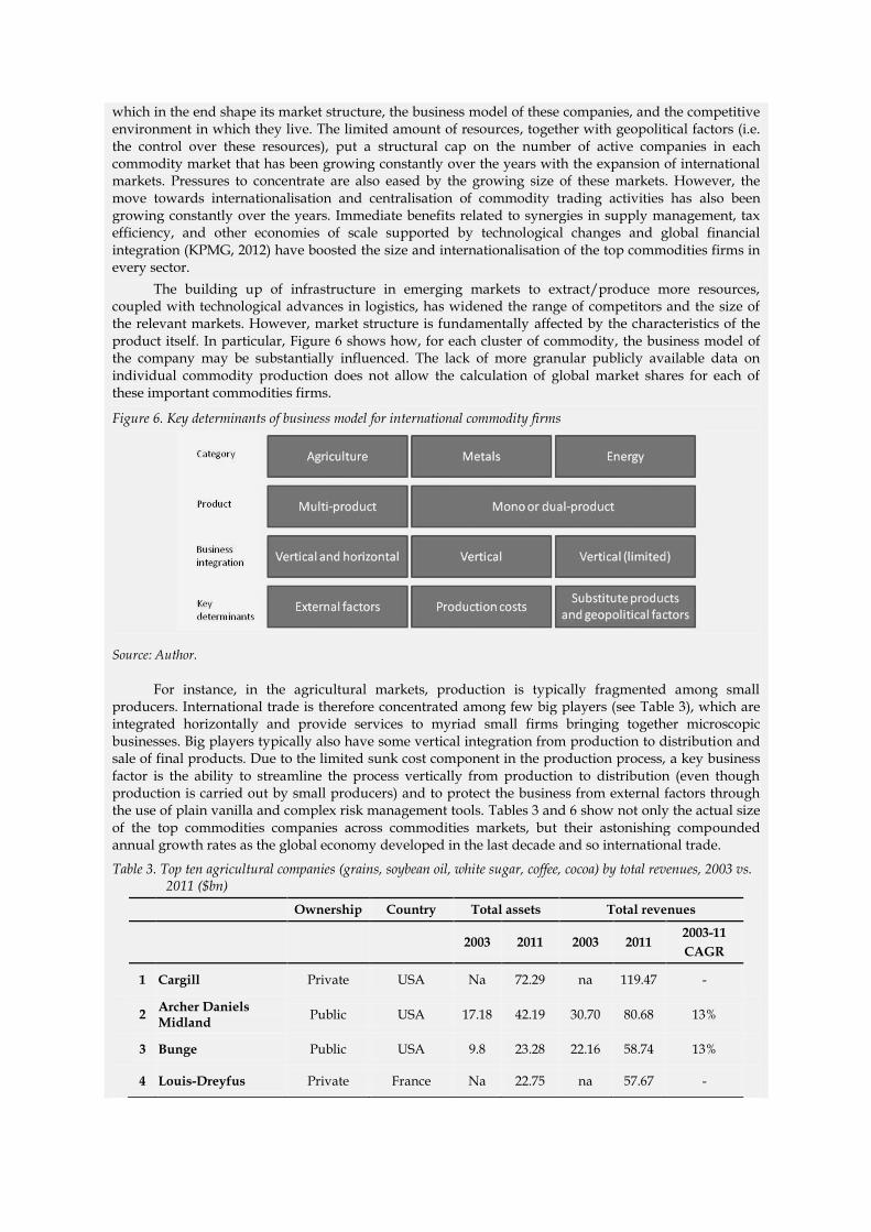
which in the end shape its market structure, the business model of these companies, and the competitive environment in which they live. The limited amount of resources, together with geopolitical factors (i.e. the control over these resources), put a structural cap on the number of active companies in each commodity market that has been growing constantly over the years with the expansion of international markets. Pressures to concentrate are also eased by the growing size of these markets. However, the move towards internationalisation and centralisation of commodity trading activities has also been growing constantly over the years. Immediate benefits related to synergies in supply management, tax efficiency, and other economies of scale supported by technological changes and global financial integration (KPMG, 2012) have boosted the size and internationalisation of the top commodities firms in every sector.
The building up of infrastructure in emerging markets to extract/produce more resources, coupled with technological advances in logistics, has widened the range of competitors and the size of the relevant markets. However, market structure is fundamentally affected by the characteristics of the product itself. In particular, Figure 6 shows how, for each cluster of commodity, the business model of the company may be substantially influenced. The lack of more granular publicly available data on individual commodity production does not allow the calculation of global market shares for each of these important commodities firms.
Figure 6. Key determinants of business model for international commodity firms
Source: Author.
For instance, in the agricultural markets, production is typically fragmented among small producers. International trade is therefore concentrated among few big players (see Table 3), which are integrated horizontally and provide services to myriad small firms bringing together microscopic businesses. Big players typically also have some vertical integration from production to distribution and sale of final products. Due to the limited sunk cost component in the production process, a key business factor is the ability to streamline the process vertically from production to distribution (even though production is carried out by small producers) and to protect the business from external factors through the use of plain vanilla and complex risk management tools. Tables 3 and 6 show not only the actual size of the top commodities companies across commodities markets, but their astonishing compounded annual growth rates as the global economy developed in the last decade and so international trade.
Table 3. Top ten agricultural companies (grains, soybean oil, white sugar, coffee, cocoa) by total revenues, 2003 vs. 2011 ($bn)
Ownership Country Total assets Total revenues
2003 2011 2003 2011
2003-11
CAGR
1 Cargill Private USA Na 72.29 na 119.47 -
2 Archer Daniels Midland
Public USA 17.18 42.19 30.70 80.68 13%
3 Bunge Public USA 9.8 23.28 22.16 58.74 13%
4 Louis-Dreyfus Private France Na 22.75 na 57.67 -

14 | SETTING THE SCENE: THE STRUCTURE OF COMMODITIES MARKETS
5 Kraft Public USA Na 98.84 na 54.37 -
6 Nestle Public Switzerland 66.83 129.05 66.53 46.53 -
7 Wilmar Public Singapore Na 39.64 na 44.71 -
8 Agrium Public Canada 2.27 13.14 2.4 15.47 26%
9 Conagra Public USA 15.0 11.41 16.9 12.30 -
10 Viterra Public Canada 0.78 7.01 2.7 11.79 20%
Source: Author calculations from websites, annual reports, and OANDA. *End of 2010. Note: Exchange rate with USD is yearly average.
In the market for metals and raw materials, the high fixed (and sunk) costs to start and keep production stable over time in order to reach a critical mass result in a fairly concentrated market, but still with some horizontal cross-product activities. A key business factor is the ability to integrate vertically production, refining, and smelting of metals to reach the end market with limited risk of squeezes along the value chain, or to specialise horizontally across the same stage of the value chain. However, both models require deep pockets and few firms have been able to develop such an integrated model. Not all industrial metal and raw materials companies have achieved high growth rates in the last decade, as Table 4 suggests, and those that have achieved high growth may have been specialising more in part of the value chain. Rising energy costs have been an important burden for companies involved in high energy-consuming refining activities, such as aluminium smelters.
Table 4. Top ten industrial metal and raw materials companies (aluminium, copper and iron ore) by total revenues, 2003 vs. 2011 ($bn)
Ownership Country Total assets Total revenues
2003 2011 2003 2011
2003-11
CAGR
1 ArcelorMittal Public Luxembourg 112.16* 121.88 80.17* 93.97 -
2 Bhp Billiton Public Australia-UK 28.87 102.89 16.54 71.74 20%
3 Rio Tinto Public Australia-UK na 119.55 58.1** 60.54 -
4 Vale Private Brazil 11.4 128.70 5.3 60.40 36%
5 Anglo American Public UK 34.4 87.28 24.9 51.12 9%
6 Alcoa Public USA 31.7 40.12 21.5 25.00 2%
7 Aluminumcorp of China
Public China na 21.87 na 18.72 -
8 Codelco State-owned Chile 8.9 20.83 3.7 17.52 22%
9 Mitsui Chemicals Public Japan 10.1 16.27 8.7 17.48 9%
10 Votorantim Private Brazil na 38.37 na 16.88 -
Source: Author’s selection from websites, annual reports, and OANDA. Note: A longer list is available in the Annex. Exchange rate with USD is yearly average. Note: *2006 data, **2008 data.
Geopolitical factors and the role of substitute products have pushed energy commodities firms to concentrate on the extraction and refining of oil, with limited horizontal integration across products (largely only to natural gas) and often limited vertical integration. Aside from a few global multi-product commodity firms that extract oil, refine it, and produce fuel products, the market is concentrated along national markets where oil can be extracted and exploited by the country concerned. The crucial role of energy markets in industrial economies has also prompted state intervention to keep control of access to a resource that can affect global economic and political equilibria. Geopolitical aspects have influenced the ownership of energy commodities firms. The number of state-owned companies in this sector is

noticeably higher than in other sectors (among emerging markets, in particular), and the nationalisation of the Argentine business of Repsol by the government has sparked fears among long-established privately and publicly owned international firms about the role of government policies in emerging countries.
Table 5. Key energy companies (crude oil and gas) by total revenues, 2003 vs. 2011 ($bn)
Ownership Country Total assets Total revenues
2003 2011 2003 2011
2003-11
CAGR
1 Royal Dutch Shell
Public Netherlands 219.51* 345.26 306.75* 470.17 -
2 Exxon Mobile Public USA 219.01** 331.05 370.68* 467.03 -
3 Sinopec Public China na 177.08 na 387.68 -
4 BP Public UK 112.82 293.07 178.72 375.52 10%
5 Petrochina Public China 50.12 296.69 21.27 310.04 40%
6 Total Public France 86.48 228.36 104.65 257.09 12%
7 Conoco Phillips Public USA 82.45 153.23 105.09 251.23 12%
8 Chevron Public USA 81.47 209.47 120.03 244.37 9%
9 Gazprom Public Russia 83.07 431.21 24.5 217.73 31%
10 Saudi Aramco State-owned Saudi Arabia na na na 210.00*** -
Source: Author’s selections from websites, annual reports and OANDA. Note: A longer list is available in the Annex. Exchange rate with USD is yearly average. *2005 data, **2006 data, ***2010 data.
As shown by Table 5, due to the relevant impact of the sector on the economy, total revenues of the energy commodity businesses are much higher than other sectors. The largest agricultural and metal firm would be a long way off the top ten in the list of largest energy firms by total revenues, at 18th and 19th, respectively (see Annex). The table also shows that the last decade has been a period of incredible growth for energy companies, as new oil-intensive emerging economies expanded beyond expectations.
Finally, there are a handful of global commodity trading companies that combine the offer of intermediary services for other commodity firms (for physical and financial services) and logistics in multiple commodities (typically oil, some metals and a few agricultural commodities). These firms, also due to the easy access to international finance, have increased their exposure to physical markets over the years through the ownership of firms dedicated to production, refining, and/or logistics. The nature of trading companies, which typically invest in the most profitable areas of commodities markets through sophisticated financial instruments and financial leverage, makes their offers more diversified across commodities markets, but also exposes them to fluctuations in futures markets and the financial system (due to their leveraged positions). Easier access to international finance and so to financial leverage, due to their nature of trading houses with strong financial expertise, has boosted revenues to levels close to those of big energy firms. The largest commodity trading company would be 6th in the list of the biggest oil and gas companies in the world, with much higher total revenues than those of the largest agricultural and metal businesses.
Table 6. Key trading companies by total revenues, 2003 vs. 2011 ($bn)
Ownership Country Total assets Total revenues
2003 2011 2003 2011 2003-11
CAGR

16 | SETTING THE SCENE: THE STRUCTURE OF COMMODITIES MARKETS
1 Vitol Private Netherlands na na 61* 297.00 22%*
2 Glencore Public Switzerland 59.90** 86.16 142.34** 186.15 -
3 Trafigura Private Netherlands na na na 121.50 -
4 Noble group Public Hong Kong 1.07 17.34 4.28 80.73 44%
5 Gunvor International
Private Cyprus na na na 80.00 -
6 Mercuria Private Switzerland na na na 75.00 -
7 Marubeni*** Public Japan 41 65 75.2 55.63 -
8 Xstrata Public Switzerland-
UK 10.00 74.83 3.47 33.88 33%
9 Marquard & Bahls AG
Private Germany 0.78 5.63 5.44 25.84 22%
10 System Capital Private Ukraine na 28.45 na 19.55 -
Source: Author’s selection from websites, annual reports and OANDA. Note: *2004 data; **2007 data; *Fiscal year ended in March 2012. Exchange rate with USD is yearly average.
These companies trade not only with their own proprietary capital, both in the physical and the financial marketplace, but also on behalf of other firms or as a direct counterparty of other commodity firms. Their involvement in physical market trading varies depending on the business model.
Table 6 shows ample divergence among total assets held by these firms. Companies exploit big investments in information and minimise costs for their cross-product activities. They run trading desks, like investment banks, and are usually headquartered in countries that provide some fiscal advantages or synergies with their assets holdings. Since the explosion of international trade at the beginning of the 2000s, the size of commodities trading houses in terms of total assets and revenues has increased exponentially. The recent merger between Glencore and Xstrata, which may create the biggest trading house worldwide with more than $160 billion in assets, is a sign that this market is gradually reaching a tipping point and more investments in direct physical holdings, rather than futures positions or intermediary services, may generate new synergies and increase profitability in a highly competitive environment. As these firms continue to grow, there might be an incentive for highly leveraged firms in the moment they begin to lose profitability to increase direct exposure to physical markets, as to become strategically ‘too-physical-to-fail’. This might increase the risk of moral hazard for national governments. Finally, qualitative and quantitative information on financial and physical activities for some of these global firms is limited (even in aggregate form and on a confidential basis to regulators), so an assessment by supervisors of financial stability and market structure implications is currently very hard to perform. Coordination at international level among public authorities might be needed to share and reconcile information about physical holdings of these companies.
Key risks
There are several endogenous risks for firms involved in trading physical commodities on the spot market. The most important is price risk, which is the risk for a commodity firm of being too exposed to future price trends by holding too much or too little inventory. As shown above, inventories play a crucial role in mitigating price volatility due to supply and demand imbalances. Another important risk is related to the shipment of commodities, in particular to volatile freight rates.
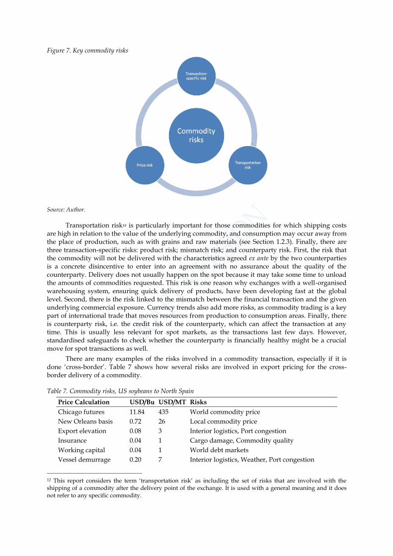
Figure 7. Key commodity risks
Source: Author.
Transportation risk12 is particularly important for those commodities for which shipping costs are high in relation to the value of the underlying commodity, and consumption may occur away from the place of production, such as with grains and raw materials (see Section 1.2.3). Finally, there are three transaction-specific risks: product risk; mismatch risk; and counterparty risk. First, the risk that the commodity will not be delivered with the characteristics agreed ex ante by the two counterparties is a concrete disincentive to enter into an agreement with no assurance about the quality of the counterparty. Delivery does not usually happen on the spot because it may take some time to unload the amounts of commodities requested. This risk is one reason why exchanges with a well-organised warehousing system, ensuring quick delivery of products, have been developing fast at the global level. Second, there is the risk linked to the mismatch between the financial transaction and the given underlying commercial exposure. Currency trends also add more risks, as commodity trading is a key part of international trade that moves resources from production to consumption areas. Finally, there is counterparty risk, i.e. the credit risk of the counterparty, which can affect the transaction at any time. This is usually less relevant for spot markets, as the transactions last few days. However, standardised safeguards to check whether the counterparty is financially healthy might be a crucial move for spot transactions as well.
There are many examples of the risks involved in a commodity transaction, especially if it is done ‘cross-border’. Table 7 shows how several risks are involved in export pricing for the cross-border delivery of a commodity.
Table 7. Commodity risks, US soybeans to North Spain
Price Calculation USD/Bu USD/MT Risks
Chicago futures 11.84 435 World commodity price
New Orleans basis 0.72 26 Local commodity price
Export elevation 0.08 3 Interior logistics, Port congestion
Insurance 0.04 1 Cargo damage, Commodity quality
Working capital 0.04 1 World debt markets
Vessel demurrage 0.20 7 Interior logistics, Weather, Port congestion
12 This report considers the term ‘transportation risk’ as including the set of risks that are involved with the shipping of a commodity after the delivery point of the exchange. It is used with a general meaning and it does not refer to any specific commodity.

18 | SETTING THE SCENE: THE STRUCTURE OF COMMODITIES MARKETS
Ocean freight 0.95 35 World commodity price, Weather, Port congestion
Discharge elevation 0.06 2 Interior logistics, Port congestion
Discharge storage 0.09 3 Interior logistics, World debt markets
Collection and fees 0.06 2 Political, Individual counterparty
Delivered in store in Bilbao
14.07 517 Sum of the foregoing
FX Rate 1.28 1.28 FX market
Euro/Bu Euro/MT
Dlvd in store Bilbao 11.04 406 Sum of the foregoing
Source: Bunge (2012).
Price risks, currency risks, freight and transportation risks, storage risks, and exogenous factors (such as weather and government decisions) are all among the factors that the international firm has to consider when deciding to trade ‘cross-border’.
Box 2. Unravelling the role of financial institutions in physical commodities markets
The business of financial institutions, and in particular banks, has developed in different directions in the last decade. The growing importance of finance for funding large and medium commodities businesses has led to diversification in the business model of investment banks, which have increased their investments in physical commodities trading. The growth of commodities firms and their global impact has led production and risk management functions to become more interconnected. This has become a profitable business for financial institutions, as commodities firms are not always able to handle all exposures through their own internal risk management systems. Table 8 shows the amounts at the stake in the commodities derivatives business for key financial institutions at the end of 2011. There are also myriad smaller banks that provide financing services to the commodities business.
Table 8. Top 12 most active financial institutions in commodities derivatives, by notional/total assets
€bn – End 2011 Notional value13
Gross value (fair value)*
Total assets
Revenues % Notional/ Total assets
% Gross/ Total assets
Ratio Gross/
Revenues
Morgan Stanley 607.07 61.60 579.00 25.02 104.85% 10 64% 2 46
Goldman Sachs 614.91 57.51 712.82 2 .25 86.26% .07% 2.59
JP Morgan 859.35 90.62 1,749.42 75.07 49.12% 5.18% 1.21
Barclays 857.09 26.89 1,876.86 38.76 45.67% 1.43% 0.69
Bank of America 639.22 29.65 1,643.84 72.91 38.89% 1.80% 0.41
Credit Suisse 281.62 n/a 862.41 21.56 32.65% n/a n/a
Société Générale 343.09 17.06 1,181.37 25.64 29.04% 1.44% 0.67
Deutsche Bank** 459.13 44.36 2,164.10 33.23 21.22% 2.05% 1.34
Citigroup 221.11 21.92 1,446.82 60.50 15.28% 1.52% 0.36
BNP Paribas** 156.29 13.75 1,965.28 42.38 7.95% 0.70% 0.32
Credit Agricole 69.79 8.50 1,860.00 35.13 3.75% 0.46% 0.24
HSBC 59.06 2.85 1,973.16 46.44 2.99% 0.14% 0.06
Tot. 5,167.72 374.71 18,015.09 498.88 49.71%^ 3.9%^ 1.15^
Global OTC 2,5714 405 - - - - -
Global ETD*** 3,585 - - - - - -
13 Balance sheets do not provide further granularity on how this notional value can be decomposed, i.e. what kind of commodities derivatives trades (OTC or it includes estimation of exchange-traded derivatives positions in commodities). It includes precious metals. For exchange-traded futures contracts, notional value in this analysis means value of open interest.
14 Including OTC derivatives on gold and other precious metals, at the end of 2012.

Source: 2011 Annual reports, SEC K10 files, BIS (2013 update), WFE/IOMA. *Before netting adjustments. ^Weighted average (notional). “Estimates. ***Conservative estimate of value of traded futures and options contracts. See section 1.2.2.3 for more details.15
The range of financial institutions is very broad and includes: brokers/dealers, private banks, commercial banks, merchant banks, insurance companies, investment managers, mutual funds, hedge funds, and private equity funds. To develop these activities, most of these institutions have invested significant resources in physical trading, such as supply and production firms, warehouses, and logistics/transportation companies.
As at today, for instance, Morgan Stanley owns:
Six power plants (three in Europe and three in the United States).
A fleet of roughly 100 vessels (through ownership control of Heidmar).
Several fuels and gas assets (through Transmontaigne Inc.16 and Heidmar).
These assets are marked in the balance sheet at a fair value of roughly $6 billion (end of 2011). The company is therefore positioned to provide production, distribution, and shipping services across several commodities. It provides bundles of services to main commodity producers through long-term contracts in which the bank commits to provide agreed amounts of a commodity, such as crude oil or gas, and related risk management services. This helps clients to manage risks with a single counterparty, as well as to expand in a market supporting investment decisions. However, the bank exposes itself to a wide array of exogenous factors.
“Commodity price and implied volatility risk as a result of market-making activities and maintaining positions in physical commodities (such as crude and refined oil products, natural gas, electricity, and precious and base metals) and related derivatives. [...]...changes can be caused by weather conditions; physical production, transportation and storage issues; or geopolitical and other events that affect the available supply and level of demand for these commodities.” (Morgan Stanley, 2011 SEC 10k file, p. 103).
The business is under threat from cyclical factors and upcoming regulatory tightening over systemically important financial institutions, which has already pushed some players to quit the commodity business (Royal Bank of Scotland and Nomura, for example) due to the higher costs of capital in the aftermath of the on-going financial crisis. But opportunities may also arise.
“We directly or indirectly own interests in, or otherwise become affiliated with the ownership and operation of public services, such as airports, toll roads and shipping ports, as well as power generation facilities, physical commodities and other commodities infrastructure components, both within and outside the United States. Recent market conditions may lead to an increase in opportunities to acquire distressed assets and we may determine opportunistically to increase our exposure to these types of assets. These activities expose us to new and enhanced risks, including risks associated with dealing with governmental entities, reputational concerns arising from dealing with less sophisticated counterparties and investors, greater regulatory scrutiny of these activities, increased credit-related, sovereign and operational risks, risks arising from accidents or acts of terrorism, and reputational concerns with the manner in which these assets are being operated or held.” (Goldman Sachs, 2011 SEC K10 file, p.28)
The fast development of the business also raises questions about the implications for competition, in particular whether the stake held in physical markets may exert dominant or oligopolistic pressure on price, as well as concentration risks for operations. Disclosure of physical holdings and ownership stakes, in aggregate fashion (following current initiatives in financial regulation), may become a key aspect for supervisors to properly oversee conflicts of interest between the different legitimate functions that these operators perform, to avoid anti-competitive behaviours, and to minimise the effects of non-financial risks on the stability of the financial system. Finally, more meaningful disclosure and breakdown of derivatives exposure can help to quantify the impact of such activities on the companies’ balance sheets. Current regulatory actions, both in Europe and the United States, are setting higher disclosure requirements for derivatives exposures, but the hard task will be to make this information meaningful.
15 These statistics do not include the turnover value of commodities futures and options of the London Metal Exchange, NYSE Euronext (US), Australian Securities Exchange SFE Derivatives Trading, Multi Commodity Exchange of India, Singapore Exchange, plus an undefined list of small commodities exchanges.
16 The Group has a storage capacity of over 22.35 million shell barrels.

20 | SETTING THE SCENE: THE STRUCTURE OF COMMODITIES MARKETS
Long-term price changes
In addition to exogenous factors affecting commodities prices, there are variables that do not directly affect supply and demand, but can create incentives that change long-term investment decisions and have a counteracting effect on price elasticity. These changes can happen on both the supply and the demand side. On the supply side, for instance, a prolonged peak in the level of prices may reduce the costs of capital, which may increase long-term investments in production, reducing production costs and thus prices in the long term (Geman, 2005; Figure 8a).
Figure 8. Supply shift and demand twist
(a) (b)
Source: Author.
However, it may also happen that high prices, subsidised by government policies, reduce the willingness of producers to invest in the long term as they feel protected by external support. This would ultimately result in an inability to compete in the market once these subsidies are lifted for any reason (such as a financial crisis), making it very hard to produce at the lower cost imposed by the market. Market prices may become unstable because it would time for production to adapt to the new environment. On the demand side, a prolonged increase in the price of crude oil may have a limited impact on requested quantities, but in the long term may push the economy to increasingly rely on alternative sources of energy, which would ultimately increase price elasticity and reduce the slope of the demand curve (see Figure 8b).
Underinvestment in supply has long been subject to discussion in the academic literature and policy-making. A combination of short-term and long-term aspects increases variables that affect price patterns. As a result, long-term price trends are often predictable, but the short-term pattern is highly volatile with big price swings that can reshape the ultimate allocation of resources in the market for long periods, and so change long-term price trends.17
1.2.2 Futures markets
Open markets are platforms matching buyers’ and sellers’ interests over one or multiple assets across space and time. Futures contracts (or ‘futures’) are agreements between two parties to buy or sell an agreed quantity of an asset (commodity) at a certain future date for an ex ante agreed price. This market accommodates the intertemporal choice of commodity producers, users and traders (so called ‘risk transfer’). It allows the management of demand and supply risks through the expectations for
17 To understand better the intensity of the link between supply and demand elasticity to market changes, please see markets descriptions in the following chapters.

inventory levels, which are the response function of physical demand/supply imbalances reflected by spot market prices.
Take, for example, a wheat producer that wants to protect its core business from a drop in prices during the next harvest period, perhaps resulting from oversupply due to very good weather conditions. The producer therefore decides to sell a quantity of futures contracts approximating the estimated production level with a contract expiration corresponding to the end of the harvest. In this way, the producer can almost fix the price of its harvest well before the harvest takes place. This gives the producer the ability to plan investments over the long term and to restrict potential losses to a predictable range. Before the expiration date of the futures contract, if the price of the original futures sale is higher than the prevailing market price, the producer would buy back the futures with an offsetting transaction at a lower price. This would hedge losses in the physical market incurred by selling at a lower market price than initially forecasted. However, if the market price is higher than the original futures sales price, the producer will sell the cash commodity in the marketplace and the higher cash price received would cover the losses caused by buying back the initial futures sale at a higher price. In the futures transaction, the difference between the initial futures price and the daily settlement price is marked-to-market by the exchange clearinghouse which maintains the financial integrity of the exchange by requiring initial margins for any new transaction and by collecting or remitting variation margins on a daily basis on all open positions. If the producer gains from the futures transaction, they would collect the value of the initial margin deposit plus the difference between the original and final price.
1.2.2.1 The development of futures markets: a brief history
The origins of modern futures markets date back to the 19th century, but physical commodities and archaic forms of futures markets have even more ancient origins going back to the beginning of the civilised world (Berg, 2011). Futures markets, as a market supporting the activities of physical commodities markets to reduce inefficiency and transaction costs, have been around for a little over a century and began operations with very simple contracts. The first futures contracts were effectively just delivery contracts, or ‘to arrive’ contracts (Gray and Rutledge, 1971), for producers in the surrounding areas of Chicago. The first exchange, the Chicago Board of Trade (CBOT), started operations in 1848 and soon became the point of reference for similar platforms across advanced economies. Over the years, these platforms have spread around market hubs to allow commodities actors to trade spot or transfer risk to those that could actually bear it close to large consumption areas. Dramatic price fluctuations and disputes among buyers (e.g. merchants) and sellers (e.g. farmers), especially in agricultural commodities where external factors such as the weather and means of transport had unforeseeable impacts, have made futures markets an indispensable tool to run a competitive commodities business.
Technological developments during the 1970s and 1980s made trading from remote locations possible. Following these important changes, a process of consolidation among exchanges to benefit from economies of scale began, first at the regional level and gradually now at the global level. The computerisation of trading has made competition among national exchanges possible. This process culminated in the 1990s with a general liberalisation of the sector. The vast majority of exchanges, at least all of them in Europe and the United States, have become for-profit entities that aim to expand business to find new opportunities and increase liquidity with higher volumes of transactions. Growing competition has also created an additional boost to technological innovation, thus increasing direct access to capital markets for end users. As a consequence of these market changes, commodities markets have expanded their volumes of transactions during the beginning of the 21st century, both on exchanges and over-the-counter bilateral markets. Key commodities exchanges are today the only place where the prices of specific commodities are formed and used as global benchmark prices for bilateral transactions. From small and niche market activities, exchanges today have become global actors with a diversified business that cuts across all services linked to trading of commodities derivatives and other financial instruments (e.g. clearing, settlement, data and technological services). Technological advances are pushing the boundaries of relevant markets at the global level, even though relevant legal and infrastructural issues at the national level impede the rapid development towards fully-fledged market competition among global exchanges.

22 | SETTING THE SCENE: THE STRUCTURE OF COMMODITIES MARKETS
Futures markets have historically been an essential part of commodities markets, helping commodities users and producers to hedge or transfer risk over their inventories due to seasonality issues (Irwin 1954). Working (1962) concluded that these markets have managed to facilitate contract holding, to build up different types of hedging strategies and to incorporate the convenience yield and thus price of storage in the intertemporal price spread. Futures prices represent the expected spot price on the basis of currently available information, especially for storable commodities (Carter, 2000). A lack of balance in the physical market pushes up futures prices, which ultimately results in additional price discovery when arbitrageurs absorb fairly quickly potential price abnormalities between futures and spot markets (Geman, 2005). Futures markets give a sense of where the spot price is heading, by signalling greater storage opportunities when futures prices are high and lower storage when futures prices drop close or below spot prices. However, this might not be the case for non-storable commodities, for which futures prices may be an unreliable forecast of cash market prices (Kamara, 1982) because no physical link with supply and demand can be established through the management of inventories. In this case, market liquidity is a key indicator of reliability.
1.2.2.2 Contractual characteristics
Despite the fact that futures contracts are a simple tool to transfer risk across time and space, the organisation of futures markets is rather complex, whether it is run through an exchange or bilaterally (over-the-counter) in a customised fashion. The ability to deal with transaction-specific risks is enhanced in a futures market setting, where contracts are standardised in terms of size and other factors. OTC markets are more costly and may require deep pockets that many commodities firms may not have. As Table 9 suggests, commodities transactions can be concluded through cash spot, cash forward, and futures contracts. Temporal and spatial risk transfer in commodities markets can be done through bilateral agreements mainly in the OTC space (forward contracts)18 or through standardised contracts listed on exchanges (futures contracts).
Forwards are customised contracts (volumes and quantities) and can be either Free-On-Board (FOB) priced or include cost of storage, insurance and freight (CIF) in the final price. Physical and (sometimes) cash settlement is done to maturity, so the holding period is typically to delivery. Customisation (plus limited exposure to interest rates and collateral requirements), however, comes at higher transaction costs and counterparty risk, which can make transactions less attractive for limited volumes. Futures contracts, on the other hand, are standardised contracts with delivery at a given location at a pre-defined set of dates during the year. The underlying commodity also has a common quality grade, which reduces delivery risks. Prices are typically FOB (or in warehouse; as for industrial metals) and contracts are typically offset with a reversal trade before maturity and marked-to-market on a daily basis through margin calls. By keeping a maintenance margin rather than disbursing the full value of the contract, buyers and sellers are leveraging to increase exposure with a limited amount of cash. These contracts should, in principle, serve commercial firms, which typically do not hold large amounts of cash. In contrast to OTC forwards, which are used for bigger volumes, these standardised contracts are highly liquid, due to the limited amount of cash needed. Small investors can also potentially invest in these markets. Through the system of margin calls, then, there is only a very limited exposure to counterparty risk (certainly less than in the case of forward contracts). However, standardised futures contracts may involve expose to other two types of risk: currency risk and interest rate risk. Since the contract is traded in the currency where the most liquid market is (historically) located, there is a currency risk for players acting in countries with a different currency. The currency for the vast majority of these products is the U.S. dollar. In addition, the open futures contract position requires the maintenance of a margin account where cash is kept away from alternative uses, so the opportunity cost is at least the risk-free interest rate.
18 That are not financial agreements (OTC swaps), which result in a pure exchange of cash flows rather than the delivery of a physical commodity. An OTC swap is a pure financial transaction.

Table 9. Key characteristics of transactions
Spot contract Forward contract Futures contract
Nature of transaction Bilateral (OTC)
Bilateral (OTC)
Multilateral (exchange)
Transaction terms
(delivery dates, contract size)
Customised Customised Standardised
Price FOB FOB/CIF FOB (or in warehouse)
Settlement Physical Cash/Physical
(to maturity/shipment)
Cash (daily) Offset/Physical
(to maturity, ‘physical’ if requested)
Typical holding period
To delivery To delivery Before delivery
Delivery Spot Customised Selected months
Storage costs No Yes Yes
Transaction costs Medium Medium/High Low
Leverage No No Yes
Counterparty risk Limited (spot)
High Limited
(daily mark-to-market)
Currency risk No Limited (choice)
Yes
Price risk No Yes Yes
Interest rate risk No No Yes
Regulation and supervision
Limited Limited High
Source: Author.
Both forward and futures contracts are exposed to price risk, which is affected by market-specific and/or exogenous factors that can make holding a commodity profitable and promote strategies to hedge commercial risks.
Two key elements have made futures contracts traded on exchange a successful tool to deal with commodity risks:
a. Margin calls. b. Physical delivery.
Margin calls (with a stable cash account) allow leverage and align open positions to market value, minimising counterparty risk. Profits and losses are thus realised before maturity, while as opposed to only at maturity for forwards. This key feature attracts liquidity and allows the contract to be closed out with an offset transaction at any time before delivery. The high standardisation of future contracts and daily collateralisation typically permit the closing out of contracts without running the risks of physical delivery (e.g. quality grade, delivery time, receipts, etc.). The transaction can be offset before delivery with an equal offsetting purchase or sale (essentially an exchange of cash; Lerner, 2000). Anecdotal evidence suggests that fewer than 2% of futures contracts are settled through physical delivery.
The physical delivery obligation, when the contract is brought to maturity, essentially aligns the futures contracts to the underlying spot market prices close to maturity (‘no arbitrage clause’, see below). For forwards, the contract is completed with actual delivery of the underlying commodity. In around 98% of futures, there is no actual delivery since traders enter into reversal trades (offsetting). Another way to terminate futures contracts, without an offsetting transaction or physical delivery, is the liquidation in cash of the difference between the agreed price to delivery and the spot price of the underlying commodity. Finally, parties can also agree a combination of compensation with an offsetting transaction and delivery of the commodity or the exchange of the futures position with a

24 | SETTING THE SCENE: THE STRUCTURE OF COMMODITIES MARKETS
corresponding physical market position of a market participant that wants to switch exposure to current prices with exposure to prices at a future date (exchange for physical).
Actual delivery of the commodity is set a few times a year for futures contracts on exchanges, depending on the type of futures contract that is traded on the exchange for that specific commodity. Typically, there are no more than four or five delivery dates per year (i.e. every three or four months).
1.2.2.3 Futures market structure
Financial transactions in commodities may take place on organised electronic multilateral platforms, such as exchanges, or in bilateral settings (over-the-counter). Due to lack of comparable data, the size of exchange-traded commodities futures and options markets versus the OTC markets at the end of 2012 can be only estimated. Roughly $1.36 trillion was the total notional value of outstanding global
OTC commodity forward and swaps in 2012.19 The notional value of outstanding contracts (open
interest) on futures commodities exchanges, estimated by taking the value of the turnover (as total value of traded contracts) of futures contracts and discounting it by a decompressing factor, is $3.17
trillion.20 As a result, outstanding value of exchange-traded futures contracts was at least 70% of total
OTC and ETD commodities futures markets ($4.53 trillion) at the end of 2012, up from 66% a year before, as OTC commodities derivatives have been shrinking more than $450 billion in one year, mainly due to regulatory pressures on collateral requirements, costs of capital and banks’ deleveraging (see Table 10).
Table 10. Notional value of outstanding commodities futures and options traded OTC and on exchange ($bn)
Exchange-traded Over-the-counter Total
2011 2012 2011 2012 2011 2012
Futures 21 3,226
(65%)
3,168
(70%)
1,745
(35%)
1,363
(30%) 4,971 4,531
Futures and options 3,585
(58%)
3,485
(62%)
2,570
(42%)
2,101
(38%) 6,155 5,584
Note: Exchange-traded data are conservative estimates derived from turnover value of futures and options contracts. 22 Value of over-the-counter positions is not daily marked-to-market.
Source: Author’s estimates from WFE/IOMA, BIS, CME, LIFFE, LME, ICE, other sources.
Due to its systemic size, the trading environment is also closely regulated and supervised by both exchanges and regulators. The interest of the platform operator is thus in ensuring that trades are done smoothly with no major dysfunctions, because only a stable and standardised trading environment can potentially attract the critical mass of liquidity needed to make the business of the neutral operator sustainable over time. As Figure 9 shows, commodity futures trading on exchanges has grown very fast in the last ten years, despite being already a significant part of commodities futures trading. OTC markets have also grown rapidly (at a slower pace, though), which suggests that more players have accessed these markets gradually over the last decade. After the crisis erupted in
19 Forward and swaps can be considered as the OTC market equivalent of futures exchanges contracts.
20 This ‘decompressing factor’, which is equal to 0.0338977, is a ratio between the weighted (by production in tonnes) average of the open interest ratio over physical production (in 2011) for selected liquid futures contracts (natural gas, crude oil, copper, aluminium, cocoa, coffee, corn, soybean oil, wheat, white sugar), and the weighted average (by production in tonnes) of the value of traded contracts ratio over value of physical production (in 2011 and average spot price from World Bank) for the same liquid contracts (except for copper, aluminium and white sugar; volumes of contracts traded during 2011 with maturity up to 12 months).
21 Forwards and swaps for OTC transactions.
22 The statistics published by the World Federation of Exchanges and the International Options Market Association do not include the turnover value of commodities futures (forwards) and options traded on the London Metal Exchange, NYSE Euronext (US), Australian Securities Exchange SFE Derivatives Trading, Multi Commodity Exchange of India, Singapore Exchange, plus an undefined list of very small commodities exchanges.

2007, however, OTC transactions have lost ground in favour of more open and transparent trading venues due to increasing cost of funding for bilateral transactions.
Figure 9. Growth of Exchange-traded and over-the-counter commodity derivatives (2002=100-2012)
Source: Author’s calculations from BIS, WFE, ECMI (2012). Note: Exchange-traded data on number of contracts
might be underestimated before 2008. Data include futures only for exchange-traded contracts.
The size of commodities futures exchanges has more than tripled since 2004, particularly as a result of the financial crisis, which has reduced dealers’ capital commitment in OTC transactions and increased the role of transparent venues as a cheaper source of liquidity for commodities users. The size of the global commodities futures exchange reached its peak in 2012, with almost 3 billion traded contracts and seven global market infrastructures of which no one is European and four of them are Chinese companies (see Figure 10).
Figure 10. Growth of commodity futures exchanges volumes by number of contracts, 2002-2012
Note: 2012 data for Multi Commodity Exchange of India is from 2011.23 Source: Author’s calculations from WFE and ECMI (2012).
23 ‘Others’ include: MICEX / RTS, NYSE Euronext (Europe), Bursa Malaysia Derivatives, ICE Futures Canada, Thailand Futures Exchange, Johannesburg SE, BM&FBOVESPA, ASX SFE Derivatives Trading, Korea Exchange, Buenos Aires SE, NYSE Euronext (US), Rofex, ASX Derivatives Trading, BSE India, Bursa Malaysia, Japan Exchange Group – Osaka, Tokyo Commodity Exchange (TOCOM), Tokyo Grain Exchange.

26 | SETTING THE SCENE: THE STRUCTURE OF COMMODITIES MARKETS
US and Chinese exchanges are the leading participants in commodities futures market infrastructure. As shown in Figure 10 and Figure 11, CME group is the biggest global exchange by value of open interest and number of traded contracts in its commodities markets, at least for the commodities covered in this report.
As suggested above, the growth of Chinese exchanges has been astonishing, and today they have a global market share of almost 50%, as China has de facto become the major commodities consumer in the world (Figure 11). Some Chinese exchanges have become points of reference in Asia but, partly due to governance issues and legal uncertainty for these emerging exchanges, most of benchmark futures prices are still formed in US and European venues.
Figure 11. Global commodity futures exchanges volumes by number of contracts, 2012
Note: Data for Multi Commodity Exchange of India is from end of 2011.
Source: Author’s calculations from WFE and ECMI (2012).
The trading landscape is still on the move, however, and global competition may lead to additional attempts at consolidation. The recent acquisition of NYSE LIFFE by ICE will certainly increase ICE’s global market share and will perhaps create the biggest European commodities exchange. Most importantly, the merger follows the path of consolidation between European and US exchanges striving to increase their market share and market power at the global level. Given the similar underlying macroeconomic conditions and financial systems of the two regions, cross-border merger and acquisition activities may find more solid ground for synergies and economies of scale to develop, as often seen in recent years. Finally, implications of current regulatory reforms on the market power of global infrastructures require further investigation. Commercial interest around new services that are generally considered not profitable (such as trade repositories) points at the market power generated by the economies of scale and scope that providing this service may offer, in combination with several trading, clearing and settlement services that vertically integrated market infrastructures already offer to clients.
1.2.2.4 Market organisation
The most common type of market setting for the trading of commodity futures is an auction system handled by ad hoc organisations (for-profit entities, after demutualisation) called ‘commodities futures exchanges’. This auction system, whether orders are submitted through an open outcry session (via a member of the exchange) or through an electronic trading platform (via a broker that is an exchange member and has pre-trade controls before the submission of the order), is open to anyone who meets the financial requirements needed to trade these standardised contracts (among which is a ‘margin account’). The nature of an auction requires the market to be fully transparent with regards to

membership rules, types of orders that users can introduce into the system, and prices of each lot of underlying contracts. Auction markets, in addition, have lower transaction costs and can ensure a more efficient flow of information into prices. However, these standardised markets may be unable to deal with block sizes, which can produce market impact if not properly managed. If price-sensitive information about market operations of a commodity firm is not properly managed by insiders, the market can also break down, ultimately causing a run on liquidity.
Electronic trading
The evolution and growth of commodity futures exchanges has followed the development of new legal and technological tools, which have made the trading process more standardised and suitable for electronic trading. On the legal side, future contracts traded on exchanges have at least four pre-determined aspects: quantity, delivery date, delivery point (among a list), and quality grade. On the technological side, the ‘electronification’ of trading has fit squarely into the modern developments of commodities markets and electronic trading has almost completely taken over the old open outcry (‘the pit’). For instance, as Figure 12 shows, almost all futures trading on CME for corn and wheat is done through an electronic platform, which increases the speed and volumes of transactions, reduces access costs, and provides a single access point from any location around the world.
Figure 12. Corn and wheat electronic futures (average daily volume)
Source: CME Group.
Obviously, the diffusion electronic may also carry costs, which are mainly linked to operational aspects, i.e. the ability to handle new technologies and computer algorithms smoothly and to supervise complex operations that could potentially become market manipulation (e.g. ‘cornering’ practices). However, technology also offers the ability to detect abusive practices through new, sophisticated tools and the astonishing growth of exchange trading in the last decade and greater choice for investors is strongly linked to the diffusion of technology in commodities trading.
Finally, electronic trading also means that new forms of trading and market-making activities take place with the use of complex technologies and algorithms, combined into the so-called ‘high-frequency’ trading practices. In commodities futures markets, high-frequency trading is a less prominent activity than for other asset classes (such as equities secondary markets) due to the different market microstructure. However, as for other asset classes, high-frequency trading in commodities futures markets may bridge price formation of futures contracts on the same commodity, but traded on different markets. High-frequency trading may be beneficial as long as it is properly supervised by the exchange. Practices or market orders that can distort price expectations should be

28 | SETTING THE SCENE: THE STRUCTURE OF COMMODITIES MARKETS
immediately identified and properly managed, or in some cases banned if the potential effects of such practices cannot be controlled by the infrastructure.
Clearing and margins
Clearing and settlement services are essential services for a commodity futures exchange, both for the financial settlement (in around 98% of the cases) and physical settlement. Clearing services, i.e. the definition of the net amount that a party will receive or will pay as a result of the futures contract position, are typically performed by a central counterparty (CCP). The CCP is often owned and run by the exchange, but there are many cases of commodities futures where the clearing services are outsourced to an external venue. The CCP, through an operation called ‘novation’, becomes the only counterparty of the transaction, so performing ‘netting’ (the calculation of one net claim if there are multiple open positions that refer to the same user). Typically, contracts are marked-to-market value on a daily basis. So at the end of the day, the CCP calculates the net claim or credit that the user has against its own margin account, and the user is finally asked to provide cash (or other assets on which a haircut is applied) if the margin account drops below the maintenance level in order to restore the initial level. Daily marked-to-market settlement of open positions, through the use of margin calls and other risk management service to minimise collateral use, allow better management of counterparty risk and the possibility to leverage high-value contracts with a minimum cash margin account (see Table 11).
Table 11. Margins and leverage
Main futures contract
Position Initial margin
Maintenance margin
Contract Value*
Initial Leverage*
Max Leverage*
CME
Corn
$2,363 $1,750 $37,750 16 22
Wheat
$3,038 $2,250 $43,300 14 19
Soybean Oil
$1,215 $900 $30,600 25 34
Copper
$5,400 $4,000 $93,145 17 23
WTI Crude
$6,548 $4,850 $87,040 13 18
Natural Gas
$2,565 $1,900 $34,790 13 18
ICE
Cocoa Hedge $1,250 $1,250 $24,750 20 20
Speculative $1,375 $1,250 $24,750 18 20
Coffee Hedge $4,050 $4,050 $60,375 15 15
Speculative $4,455 $4,050 $60,375 14 15
Sugar Hedge $2,050 $2,050 $21,280 10 10
Speculative $2,255 $2,050 $21,280 9 10
Soybean oil
Hedge $1,250 $1,250 $30,600 24 24
Speculative $1,375 $1,250 $30,600 22 24
Corn Hedge $2,100 $2,100 $37,600 18 18
Speculative $2,310 $2,100 $37,600 16 18
Brent Crude
$5,000 $4,200 $107,650 22 26
NYSE
Cocoa
£1,200.00 £1,062.00 £16,300 12 15
Coffee
$1,300.00 $1,040.00 $20,330 14 20
Sugar
$1,600.00 $1,408.00 $27,010 14 19
Wheat
£1,200.00 £900.00 £10,677 12 12

LME Aluminium
$3,252 $3,252 $49,063 15 15
Copper
$14,500 $14,500 $199,750 14 14
*Value at October 19th, 2012.
Source: Author’s calculations from exchanges and clearinghouses.
In addition, daily mark-to-market values and financial settlement of margin calls permit the contract to be closed out by an offsetting transaction at any time before the maturity of the contract. This makes commodity futures an easy-to-use tool for all type of commodities users and investors, which ultimately facilitates concentration of liquidity in the market (Geman, 2005).
Physical delivery and warehouses
A small proportion of futures contracts are settled through the physical delivery of the commodity at maturity. However, physical delivery plays an important role since it allows futures prices to converge to spot prices at maturity (taking into account a premium or discount that should be applied to the futures price at maturity). This ‘commitment to deliver’ the underlying physical commodity keeps futures markets tied to physical spot prices, even though most of the futures transactions are not physically delivered. Physical settlement promotes price discovery because it allows arbitrage between futures and spot markets in the first place. As for clearing services, the physical delivery of the commodity may be outsourced to external companies that manage warehouses in compliance with the rules set by the exchange (‘sponsored warehouses’). In addition to the general financial and conduct requirements to be eligible as a ‘sponsored warehouse’, rules typically deal with different aspects of commodities storage that may ultimately affect the correct execution of the physical delivery as promised in the future contract, and so distort market prices:
Physical storage of the commodity.
Delivery notes (promissory notes or warrants).
Location.
Warehouses (or grain elevators) have to comply with a minimum set of standards for the way they store commodities. For instance, bean commodities such as cocoa require storage in sealed bags, under a specific setting that allows sampling, along with several additional requirements for how the commodity should be handled and stored against external agents (see, for instance, LIFFE, 2012). All these measures should aim at minimising the degradability of the commodity.
Another important aspect is the issuance of warehouse receipts (or warrants) through which the user is entitled to receive the commodity from a specific warehouse in-store or free-on-board (FOB). In general, these receipts are a promise by the warehouse to deliver a good stored in their premises. They are not documents of ownership under English law, even though they can be negotiable instruments, so may not be accepted by financial institutions as a pledge. In some cases, therefore, these receipts may not ensure the delivery of the good in time, and the warehouse may not be held liable if the user cannot prove negligence. In addition, in the event of bankruptcy, the holder of a warehouse receipt will typically join the list of creditors of the warehouse company and would not be able to exercise its ownership right before a judge decide over the claim. A different regime has been implemented for LME warrants (see Box 3). Nevertheless, it is crucial that local laws do not add uncertainty to the legal value of the receipt, by adding additional taxes or other barriers to the smooth delivery of the commodity.
Finally, geographical location and capacity of the delivery system play a crucial role. The location of warehouses in key areas of net consumption (such as for metals) or net production (such as for agricultural products), logistical connections, effective systems of protection against corruption, and a sound legal system are the factors that contribute most to the attractiveness of commodity exchange for commodities users and to making the process of convergence of futures contract prices to the spot market price more efficient. The efficiency of futures markets is very much linked to that tiny 2% of physically settled trades. If the system of physical delivery is put in jeopardy by external factors (even government policies) or internal policies (of the exchange or the warehouse), the implications will affect the pricing of all futures contracts, whether in the end settled physically or offset. As a result of the inability to hedge on futures markets (because of the uncertainty in the final

30 | SETTING THE SCENE: THE STRUCTURE OF COMMODITIES MARKETS
price of futures contracts due to uncertainties in the physical delivery), spot prices will start to price the information of a badly functioning futures market, thus increasing volatility and pushing prices away from ‘pure’ supply and demand fundamentals. As stated by the IOSCO principle (2011) on “promotion of price convergence through settlement reliability”, “settlement and delivery procedures should reflect the underlying physical market”. Most notably, location of delivery points and/or delivery capacity shall meet characteristics of underlying physical markets, which would then limit supply bottlenecks (i.e., delivery queues) and promote the well-functioning of international benchmarks. Internal management of positions by the exchange, linked to the actual delivery capacity of the infrastructure, may be also helpful to avoid artificial shortages if significant positions take delivery in a short timeframe. Artificial supply cuts fuelled by delivery queues may increase reliance on less transparent price formation settings, such as price assessments based on submissions of physical transactions.
Box 3. The LME warehousing and warrants system
Most of the global exchange warehouse networks have a few delivery points in the continent where the exchange is located, or in another large area of net consumption/production. The London Metal Exchange, however, runs a different business model from the classic commodity exchange, due to its capillary system of warehouses. A network of 742 warehouses spread around the world (Table 12) ensures that the short-term futures contract (up to three months, usually) can be used as a cash price reference with delivery close to points of net consumption. No LME delivery is possible today in China.
Table 12. LME’s network of warehouses
Aluminium Copper Zinc Lead Tin Nickel Cobalt1 Cobalt2 Steel
All metals
Belgium 32 32 32 32 27 27 3 - 12 44
Germany 18 15 18 18 14 14 - - - 18
Italy 38 28 38 38 26 34 - - 2 40
Japan 6 - - - - - - - - 6
Korea (South)
58 58 - - 42 58 - - 5 63
Malaysia 52 52 52 52 24 49 - - 11 63
Netherlands 177 177 177 174 142 145 6 2 16 193
Singapore 54 54 54 54 50 50 3 3 - 54
Spain 20 20 20 20 20 20 - - 2 22
Sweden 8 7 7 7 - 2 - - - 8
Turkey - - - - - - - - 9 9
UAE - 8 8 8 - 8 - - 4 11
UK 37 31 37 37 33 33 - - - 37
USA 160 116 159 160 84 141 2 1 11 174
Grand Total 660 598 602 600 462 581 14 6 72 742
Source: LME.
As a result of this network, LME warehouses stored more than 11% of the global annual production of aluminium and less than 2% of copper, at the end of 2011. Due to the drop in demand following the crisis, high futures prices and low interest rates (see Section 1.3), the amount of aluminium in LME warehouses more than doubled from 2008 to 2009, becoming de facto the main global spot market for aluminium in the world.
Table 13. LME aluminium and copper stocks, 2003-2011
Year Global
Production Global
Consumption LME
stocks* % Global
production Global
Production Global
Consumption LME
stocks* % Global
production
Aluminium Copper
2003 28,002 27,608 1,423 5.08% 15,221 15,315 431 2.83%
2004 29,940 29,957 693 2.31% 15,832 16,671 49 0.31%
2005 31,889 31,689 644 2.02% 16,651 16,680 92 0.55%

2006 33,975 33,935 698 2.06% 17,353 17,007 191 1.1%
2007 38,186 37,411 929 2.43% 18,044 18,143 199 1.1%
2008 39,669 36,900 2,338 5.89% 18,501 18,138 341 1.84%
2009 37,198 34,765 4,624 12.43% 18,613 18,178 502 2.7%
2010 41,112 39,662 4,275 10.4% 19,190 19,365 378 1.97%
2011 43,652 42,027 4,979 11.41% 19,578 19,508 372 1.9%
2012 45,207 45,000 5,100 11.28% 19,951 20,376 300 1.5%
Source: LME, WMBS, International Aluminium Institute, CRU. Thousands of metric tonnes (MT). Note: see Annex for full data from 1992. Note: *end of the year, thousands tonnes. See also sections 3.2.1.4 and 3.3.1.4.
The delivery warrants issued by LME-sponsored warehouses is a special case in international banking finance. Even though they do not have legal value under English law, they are widely accepted as a fully negotiable receipt that can be pledged in financial transactions, such as loans to finance stocks rental costs. The reasons can be found in the requirements that LME asks of warehouses that want to be part of its network. There are three key requirements (LME, 2011):
1. The delivery warrant should identify the specific parcel of metal within the warehouse (plus the exact brand, weight and shape).24
2. In the event of bankruptcy, local laws must foresee that no restriction should be placed on owners of metals that want to take possession of the individually identified metal.
3. The warehouse should meet all other requirements that are requested by the international banking finance activities for the warrant to be accepted as a fully negotiable.
These three safeguards offer sufficient legal certainty for the claim. The first requirement establishes the claim of the user on a physically (individually) identifiable commodity within the premises of the warehouse. LME also decides which brands of aluminium are eligible to be traded and stored on the LME network. The second ensures that the local legal environment does not impede taking possession of that specific good, even under bankruptcy. The third requirement ensures that the warehouse is complaint with the additional requirements that the banking industry recognises as internationally acceptable market practices.
In addition to the legal aspects of the warrant, to be approved as a ‘good delivery point’:
The warehouse should be located in a area of net consumption and away from areas of production.
The area where the warehouse is located should be a key passage for international trading.
The location of the warehouse should be safe, politically and economically stable, and with an appropriate fiscal and legal system.
The first requirement above aims at protecting the location from volatile factors linked to short-term supply and demand trends by keeping the delivery point away from areas of production. The second ensures that the warehouse sits in the right place in terms of international trade of that commodity. The third requirement, in addition to those linked to the legal value of the warrant, ensures that the environment in which the warehouse operates is safe and sound. This minimises the impact of external factors on the price formation of future contracts and their convergence to spot prices.
No restrictions or transparency rules apply to the ownership of warehouses, which are usually owned by third parties to which LME outsources storage and final delivery of the commodity (see
Section 3.2.1.4).
The regulatory and supervisory environment
Due to their importance in strategic markets such as commodities, exchanges have received attention from regulators, especially in the United States, since the beginning of the last century (Pirrong, 1993; 1995). A specific authority in charge of supervising commodities futures markets, the Commodity Futures Trading Commission (CFTC), was established in the United States in 1974. The first comprehensive regulatory framework in the United States can be dated back to 1922 (the Grain
24 Each warrant is equivalent to one lot of the commodity.

32 | SETTING THE SCENE: THE STRUCTURE OF COMMODITIES MARKETS
Futures Act). Since then, US regulators have updated the text on several occasions, while in Europe and emerging markets is a different story. In Europe a limited set of regulations has been put in place over time at the national level, but harmonised European regulation is only being proposed now through the revision of the Markets in Financial Instruments Directive (Directive 2004/39) and the review of the Market Abuse Directive (Directive 2003/6) for commodities futures markets. The Regulation on Wholesale Energy Market Integrity and Transparency (REMIT), instead, mainly applies disclosure requirements to the physical market for energy. Supervision, however, is still fragmented at the national level and in many cases there is no clear understanding of which authority should be in charge of supervising the relevant infrastructures of the commodities exchange at the national and European level. Most of the supervision, at least until today, was done by the exchanges themselves through internal mechanisms to regulate and control trades. It is, in fact, in the interest of the trading venue that trades are run smoothly on the platform. However, since the transformation of exchanges into for-profit entities, regulators have gradually shifted their attention to new mechanisms of supervision that can best dedicate private and public (supervisors’) resources to enforcement and market surveillance. Recent market turmoil and the astonishing growth of commodities markets in the last decade have led regulators to consider a more comprehensive and integrated approach, which may ultimately benefit from a harmonised cross-border initiative.
1.2.3 Seaborne freight markets
Seaborne freight markets have become an essential part of constantly increasing commodity trades across the globe. The ability to ship commodities at a reasonable price may determine the success, or even the death, of a market. As market prices are mostly free-on-board (FOB)25, i.e. they do not include freight costs but only delivery at a pre-defined point, freight markets have developed an increasingly competitive environment, with cheaper freight rates that have made long-distance shipping sustainable and promoted a global network among operators and key trading venues.
There are two ways of classifying freight markets:
1. By type of commodity. 2. By capacity and means of transport.
The first splits commodities shipping into two further categories: wet and dry freight markets. Wet markets deal with seaborne transportation of oil and oil products. Dry markets are freight markets for dry bulk commodities, such as agricultural products like grains, and minerals/metals such as iron ore or aluminium. Almost 90% of all dry cargoes are metals and energy commodities. Only 10% of total dry cargo trades involve agricultural commodities, as these commodities tend to have limited storability over long periods, limited demand, or are usually produced close to consumption areas.
25 Alternative prices may include costs of freight and insurance (the cost, insurance and freight, or CIF, price), except costs of transport after unloading at the port of destination. This price is typically used for customised commodity derivatives traded ‘over-the-counter’. It is, in effect, efficient for low volumes, but it does not give control on the shipment.

Figure 13. Global dry cargo trade, 2011
Source: DVB Research.
The second way of classifying seaborne shipping is by capacity of the vessels, which may play a crucial role for low-price commodities that are consumed in high quantities. Here, there are three important categories: oil tankers, containers and dry bulk carriers. Although a larger vessel would allow more commodities to be shipped at a lower marginal cost, some destinations may limit the volume of ship possible due to the size of the port, for instance, or the need to pass through the Suez or Panama canals. Dry bulk cargoes can be either Capesize, Panamax, Suezmax or Handymax, while wet freights ships can be Aframax, Very Large Crude Carriers (VLCC), Ultra Large Crude Carriers (ULCC), Liquefied Natural Gas (LNG) carriers or other types of tankers (Table 14).
Table 14. Ship types and capacity
Dead Weight Tons (per ship) Commodities
Handymax 30,000 - 60,000 Dry bulk
Capesize 80,000 – 225,000 Dry bulk
VLOC Above 225,000 Dry bulk
Panamax 50,000 - 80,000 Dry bulk/Crude oil
Supramax 120,000 – 200,000 Dry bulk/Crude oil
Aframax 80,000 – 120,000 Crude oil
VLCC 200,000 – 350,000 Crude oil
ULCC 350,000+ Crude oil
LNG/LPG Carriers Up to 266,000 cubic meters Liquefied gas
Other tankers and general cargoes
Up to 45,000 (short range) Up to 100,000 (long range)
Containers, chemicals and other refined petroleum products
Sources: www.shipping-markets.com and various websites.
As the market develops, an increasing number of dry cargoes with a single deck are being built to carry massive numbers of containers. Containers allow better diversification and more flexible use for transport of multiple commodities.
The market shares of these various means of transport are more or less stable over time, due to the characteristics of the industry. Containers are increasingly competing with dry bulk carriers in the dry freight market, but most of the dry shipping is still done with bulk cargoes (Figure 14).

34 | SETTING THE SCENE: THE STRUCTURE OF COMMODITIES MARKETS
Figure 14. Dry fleet global capacity (dead weight millions tonnes)
Source: Author from UNCTADstat (United Nations Conference on Trade and Development).
The overall capacity of dry shipping has grown steadily over the last decade, as the production of metals and agricultural commodities has been increasing consistently despite the 2008 drop in global GDP and the economic slowdown due to the financial crisis. Shipping capacity has also increased for wet freight markets, as oil tankers are an important element of the growing international trade in natural gas and are needed to meet the high demand of emerging Asian countries, which have limited access to pipeline oil or gas.
The structure of freight markets presents many challenges. Inelastic demand and supply exposes the market to sudden price swings and prolonged periods of instability. Figure 15 describes supply and demand interaction. As demand for seaborne freight services grows, the curve gradually shifts to the right from point a to point b, i.e. more demand causes the equilibrium to move to a level with higher quantity to be supplied at a higher market-clearing price. The growth in demand for minerals and industrial metals for construction in emerging markets from 2001 to 2007 contributed to the gradual shift from point a to point c. Among the industrial metals, iron ore production went up 82.63%, aluminium by 56.27% and crude steel by 63.27%. Total global production of iron ore, steel, aluminium and copper soared by 72.8%, on average.
Figure 15. Supply and demand interaction
Source: Adapted from Nomikos (2012).
Eight years of steady growth in demand gradually raised prices and volatility to unsustainable levels, once the capacity of the system had reached the critical point c. Freight rates for Brazilian iron
0
200,000
400,000
600,000
800,000
1,000,000
1,200,000
1,400,000
1,600,000
1,800,000
1980
1981
1982
1983
1984
1985
1986
1987
1988
1989
1990
1991
1992
1993
1994
1995
1996
1997
1998
1999
2000
2001
2002
2003
2004
2005
2006
2007
2008
2009
2010
2011
2012
Other Oil tankers Bulk carriers Container ships
DWT
D1 D2 D3
S1
S2
d
c
b
aaP
bP
cP
dP
P

ore, for instance, reached up to 200% of the value of the underlying commodity in the autumn of 2007 (Figure 16).
Figure 16. Freight rates and total production/capacity (2006=100)
Sources: Author’s elaboration from ICAP, UNCTADstat, WBMS, World Steel Association (WSA), LKAB.26
As a consequence of this prolonged instability, investments flowed into the industry from financial firms to build sufficient capacity and keep up with growing volumes, shifting the supply curve (Figure 15) to the right (S2), i.e. the supply capacity experienced a sudden increase that pushed prices down over a short time frame. As a result of the growing supply of dry bulk cargoes (+33.62%) and the drop in demand in 2008, following the anaemic growth of global production due to the global financial crisis initially triggered by the burst of the housing market bubble in western economies, the cost of shipping tumbled by over 93% between June and December 2008 alone (Figure 17). Prices dropped to the equilibrium point d and may stay there for some time.
Figure 17. BDI index and dry freight capacity (mn Dead Weight Tonnes, DWT)
Sources: Author’s elaboration from ICAP and UNCTADstats.27
26 C3 freight rate is a dry bulk rate to ship iron ore from Brazil to China.
27 The Baltic Dry Index (BDI) represents a major dry freight cost index that collects rates on major global routes, widely used across the shipping industry.
0
20
40
60
80
100
120
140
160
180
200
0%
50%
100%
150%
200%
250%
Jan
06
Ap
r 0
6
Jul 0
6
Oct
06
Jan
07
Ap
r 0
7
Jul 0
7
Oct
07
Jan
08
Ap
r 0
8
Jul 0
8
Oct
08
Jan
09
Ap
r 0
9
Jul 0
9
Oct
09
Jan
10
Ap
r 1
0
Jul 1
0
Oct
10
Jan
11
Ap
r 1
1
Jul 1
1
Oct
11
Jan
12
C3 as % of Brazil Iron Ore FOB Total dry freight (mn DWT)
Aluminiun-Copper-Iron Ore-Steel production

36 | SETTING THE SCENE: THE STRUCTURE OF COMMODITIES MARKETS
Since December 2008, prices have been subject to significant swings but have never returned to the levels reached in 2008. Figure 18 shows the 750-trading-day annualised volatility28 for the BDI index (from April 2007 to April 2012). Volatility is higher than other major commodities and almost double the volatility of a major equity index.
Figure 18. 750-trading-day annualised volatility, 2007-2012
Sources: Author’s calculation from CME, ICAP and Yahoo Finance.
To hedge against these highly volatile trends and exogenous factors such as port congestion or geopolitical events, market participants are increasingly using forward contracts on underlying shipping routes, which are linked to indexes such as the BDI. These contracts are cash-settled, and OTC traded and cleared. They tend to have a high basis risk, i.e. the difference between the price of the forward and the underlying exposure, as they track an index and not the specific characteristics of the exposure. Liquidity in this market is usually concentrated in one-month to two-month contracts (Geman, 2005).
1.2.4 Interaction between futures and physical markets price formation
The interaction in price formation between futures and physical29 markets materialises in two phases: during the duration of the futures contract, and at maturity. During the duration of the futures contract, information about inventory levels and exogenous factors fuel increasing or decreasing divergence of futures prices with spot prices (Figure 19).
28 It is the annualised standard deviation of the natural logarithm of prices ratio.
29 The words ‘physical’ and ‘spot’ are used interchangeably in this report. ‘Spot price’ can be pure physical of rolling front month price.

Figure 19. Futures and spot prices interaction
Source: Author’s own.
When the futures price is above the spot price, i.e. the basis (difference between spot and futures price) is negative, the market is in ‘contango’. When the futures contract price is below the spot price (i.e. the basis is positive), the market is in ‘backwardation’. At maturity, the price of the futures should converge to the spot price due to the ‘commitment to deliver’ mentioned above, which does not allow arbitrage to become systematic. . Recent contributions, such as Hernandez and Torero (2010), claim that futures markets have been even leading price changes in spot markets.
The theory of storage
During the duration of the contract, futures prices (for different maturities) fluctuate and may diverge from spot prices. The difference between spot price, (at date t), and futures price,
(at date t and
maturity T) is typically called “basis”. The futures price can be written as follows:
(4)
Where r is the interest rate for risk-free alternative investments, k is the cost of warehousing and ρ is risk-adjusted discount rate for the commodity, i.e. the benefit from holding the physical commodity.
Then, following the MCY formula (1) above:
(5)
As a result, the basis is the marginal convenience yield (full cost of carry of a commodity), minus the sum of the interest forgone on alternative risk-free investments and the costs of warehousing the commodity. This means that the basis is positive (backwardation), so the spot price is higher than the futures price, when the futures price is insufficient to cover interest foregone and the cost of warehousing (exogenous factors). There is therefore an incentive to sell the commodity immediately, which results in a reduction in inventory levels. Besides the importance of warehousing systems and interest rates set through monetary policies, this suggests that several other factors put direct pressure on futures prices, but essentially through the increase or reduction of inventory levels that is a response function of demand and supply factors (Kaldor, 1939; Working, 1949; Telser, 1958; Brennan, 1958). Among these factors are monetary policies affecting interest rates (r), the costs and policies of the warehousing system (k), and the benefit from holding the commodity (ρ), which can be measured as follows:
(6)

38 | SETTING THE SCENE: THE STRUCTURE OF COMMODITIES MARKETS
This is the endogenous idiosyncratic factor that pushes anyone, whether a user or a producer, to hold a commodity. The first part of the equation is the reserve value that the holder gives to holding a commodity at date T, so the difference between expected spot price E(P) and current spot price. The second part is the net convenience yield, i.e. the dividend of the commodity, or the compounded value of current spot price at date T (using the risk-free interest rate) minus the current futures price, over the current spot price. As a consequence, both exogenous and endogenous factors (expectations) can affect inventories and, through them, the futures and spot price relationship (Figure 20).
Figure 20. Futures-spot price interaction through inventories
Source: Author’s own.
As inventories fall, the spot price gradually catches up with the futures price and the curve inverts into backwardation until, for one of the three reasons mentioned above, the inventory levels recover and futures prices begin to regain ground to converge at maturity. Following Section 1.2.1.1, Figure 21 illustrates the relationship between inventories and the marginal convenience yield, which ultimately affects the basis and so futures prices, creating a direct link between physical and futures markets.
Fama and French (1988) found evidence that inventory levels are positively related to the marginal convenience yield. This evidence has been also confirmed by the empirical analysis in the following chapters. The higher the level of inventory, the lower the MCY, so inventory levels are directly related to the three factors that ultimately affect future prices (r, k and ρ).
Figure 21. MCY-inventories relationship
Source: Fama and French (1988).

For metals, Fama and French (1988) found that when inventories are low, spot prices are more volatile than futures prices. The negative relationship between MCY and inventories has been also recognised by Routledge et al., (2000) and more recently by Gorton et al. (2008). This explains how futures prices are complementary tools to inventories in supporting the hedging strategies of commodities users and producers. For non-storable commodities, they are the only proper hedging tools available.
For storable commodities, as a consequence of the storage theory (i.e. the storage process, being a response function of supply and demand, drives futures and spot prices), when the futures curve is in contango a ‘cash and carry’ trade opportunity arises. More specifically, the commodity investor will have incentives to sell the forward contract and buy the commodity directly or through a loan, if the risk-free interest rate is sufficiently low. When the futures curve is in backwardation, though, the futures price is insufficient to cover cost of storage and interest foregone for alternative investments, so the commodities investor may enter in a ‘reverse cash and carry’ trade. He/she buys a future contract and sells the commodity immediately.
The theory of ‘normal backwardation’
In addition to the storage theory, there is an additional theory, generally attributed to Keynes (1923), which assigns to futures markets the role of a risk transfer mechanism where investors earn a risk premium for bearing the future spot price risk for classic hedgers. If hedging demand (net shorts) exceeds the supply of long investors (net long positions), the risk premium would be positive. As a result, futures markets should usually be backwarded (spot prices higher than futures prices), as the hedgers have to pay a risk premium to speculators. Futures prices are thus biased estimates of expected cash prices (Carter, 2000). The risk premium (π) can be defined as,
(7)
where E(PT
) is the expected spot price at date T and is the value of the future price with maturity
T. This theory, however, has found very weak evidence over the years (see, among others, Gray, 1961; Rockwell 1967; Gray and Routledge, 1971). As Table 15 shows, when looking at trading patterns for seven key commodities, for only a few of the past 23 years was the curve in backwardation for the majority of the trading days (using a differential between 3-months or second month and cash forward contracts or front-month).
Table 15. Contango and backwardation by commodity (years)
1990-2012*
Corn
Contango 21
Backwardation 2
(1996, 2012)
Wheat
Contango 20
Backwardation 3
(1992-93,1996)
Cocoa Contango 23
Backwardation 0
Aluminium Contango 23
Backwardation 0
Copper
Contango 13
Backwardation 10
(1990-91,1995-97,2004-2008)
White sugar Contango
7 (1992, 1998-2000, 2004, 2008-09)
Backwardation 15

40 | SETTING THE SCENE: THE STRUCTURE OF COMMODITIES MARKETS
Soybean oil
Contango 19
Backwardation 4
(1994-95, 2003-04)
Note: *Until 19/07/2012.
Source: Author’s calculation from CME Group, LME, LIFFE.
Cocoa and aluminium have not had prolonged periods in backwardation at all in the last 23 years. Only sugar still has a future-spot prices curve in backwardation today.
There are two problems with this theoretical framework. First, the hypothesis is that hedgers are all net shorts. As explained above, not all hedging positions are short (hedging may have very complex and diversified strategies). Second, as Gray and Routledge (1971) pointed out, Keynes may have been misinterpreted in his original idea. At his time, backwardation had several meanings and was also used to denote the risk premium paid by a seller to a buyer that allows postponing the delivery of a stock certificate. Following the two authors, Keynes may have just said that whether markets can reflect contango or backwardation, a risk premium is a “normal” component of the difference between spot and futures prices. In effect, if we disentangle the costs of storage and interest foregone from the basis, in the vast majority of cases the curve should offer a risk premium and so become backwardated. If this does not happen, there should be greater incentives to stock the commodity and benefit from contango later on. Keynes claimed that this was an exceptional situation vis-à-vis a ‘normal’ market activity.
Price convergence
A second important factor in the interaction among futures and spot markets is the convergence of futures contracts to the spot price. As mentioned above, this is mainly due to the ‘commitment to deliver’ embedded in the futures contract. When close to delivery, markets start to discount the fact that if the price of the future diverges at delivery, there is an opportunity of arbitrage among markets and so the market will adjust its value to the spot market. For instance, if at delivery day the futures price is lower than the spot price, the market will buy the futures contract until the two prices become equal (taking into account costs of delivery and differences due to different grades, etc.). Anticipating this behaviour, futures prices (front-month and other contracts with same maturity) will then adjust automatically to the spot price close to maturity (plus a differential). For corn futures contract traded on CBOT and spot price (US No.2, Yellow, U.S. Gulf, Friday, published by USDA), the differential around the last trade date (premium over futures price) was on average around 10% of the spot price in 2011.
As illustrated in Figure 22, the front-month begins to converge to the December month contract in August, at the end of the harvest, as both front and December month discount same information about supply and demand so the differential with spot prices (dashed line) is converging to the front-month one by arbitrages opportunities.

Figure 22. Futures price convergence in corn futures contracts
Source: Author’s elaboration from CBOT, FAO, USDA. Note: $cents/bushel; spot price is US No.2, Yellow, U.S.
Gulf (Friday).
The ‘commitment to deliver’ also ensures that futures market dynamics do not affect the spot market price directly. If prices do not catch up, arbitrage will produce convergence anyway. However, as suggested by Figure 22, futures and spot prices will in any case have some difference at maturity, as the futures prices embed delivery and interest foregone before you can actually hold the commodity.
Futures/spot price divergence can be determined by two sets of factors:
a. The underlying commodity and delivery. b. Problems with physical settlement.
First, there is divergence if the physical underlying asset to be hedged is different from the commodity underlying the futures contract (e.g. using a crude oil futures contract to hedge jet fuel costs), as well as delivery features of the contract that are embedded in the final price (f.o.b., in-store, etc). Second, divergence can be caused by any impediment that does not allow delivery of the physical commodity. These impediments can arise because of problems with the grade of the commodity (and its chemical attributes), or the location of the delivery. As discussed in the Chapter 2, a prolonged delay in delivering the commodity may cause a spike in order cancellations and a sudden increase in price of physical and futures because the supply of the commodity is constrained.
1.2.5 Why do market participants trade?
Investing in commodities has always been subject to greater scrutiny due to the implication that demand and supply patterns in these markets may have for the economy as a whole. The recent financial crisis has also increased the weight of investors shifting from purely financial asset classes to instruments with an underlying commodity or close proxy. Commodities are less subject to obsolescence (so they do not easily go out of market) and can be used as an inflation hedge. Among commodities, precious metals (like gold) have always played a larger role in the economy as a mean to protect value against inflation and have become an alternative to currency accumulation, especially in a world with low returns (IMF, 2012). Investing directly in commodities is, however, very costly due to the unpredictable factors that can change their price patterns and the amount of cash that is needed to cover daily margin calls for marked-to-market futures positions. Transferable securities, instead, can be held for long periods without any margin to be posted (unless they are purchased through leveraged operations).
The investment strategies in commodities are manifold. They can be clustered, however, in a few areas:
1. Hedging.

42 | SETTING THE SCENE: THE STRUCTURE OF COMMODITIES MARKETS
2. Funding. 3. Arbitraging. 4. Information trading.
Hedging
Hedging is, perhaps, the investment objective that has received most attention over the years. Futures markets were originally designed to accommodate the needs of commodities users and producers that wanted to hedge their business from the various risks linked to commodities. An example of a hedging strategy is the case of a trading firm that buys cash wheat and hedges the exposure to the physical commodity (to be delivered) in the period between the purchase and actual delivery to a buyer. Hedging can be short or long, as long as there is an immediate price risk to be protected, whether the commodity is physically held or not (e.g. electricity). Hedging activities can generate significant benefits (see among others, Heifner, 1972 and Peck, 1975), and there are several forms of commercial hedging (Working, 1962):
1. Arbitrage hedging. 2. Operational hedging. 3. Anticipatory hedging. 4. Selective hedging. 5. Pure risk-avoidance hedging.
Arbitrage hedging is not classical hedging but covers the commodities user or producer from the exposure caused by the divergence between the futures price and the spot price. The strategy predicts convergence between the two prices and positions the investor to benefit from predictable changes in the basis and to avoid any impact on the main hedging operation. Operational hedging is the classical hedging strategy, where the futures position facilitates commercial business by temporarily substituting a cash market transaction, so providing flexibility to the day-to-day operations as well as protection from price risk. Anticipatory hedging is the purchase or sale of a futures contract by a commercial firm in anticipation of a forthcoming cash market transaction. Selective hedging is done to avoid any risk on the transaction, so it should not provide any gain but simply protection over the completion of the operation. This hedging can certainly take various forms, either long or short positions. It is usually done to cover business operations from volatility risk. Finally, the pure ‘risk-avoidance’ hedge avoids unnecessary risk-taking by another position that is primarily based on information about future price trends rather than a specific physical exposure. This hedging is not usually done by the classic commodity firm, but by portfolio managers that want to diversify their portfolio. It often overlaps with ‘informed trading’ (see below).
Box 4. Case study: corn storage hedge
An example of a combined anticipatory and operational hedge is a corn storage hedge (Bunge, 2012). The user (or a producer collecting harvests from small regional farmers) in June wants to anticipate hedging the risk of storage from November (when he/she will buy the physical commodity) until March, which is the next available month for delivery. A large crop is expected (so large inventories and the spread between December and March is reasonably high).
The commodities firm buys the spread between December (the closest available date to the November harvest as in November the cash market is inactive) and the March futures contract, by selling the futures contract in March and buying the futures contract in December in case the crop is not large enough. For this transaction to be possible, the spread should be higher than the actual storage cost from November to March. Typically, the distance in time embeds this cost. When November comes, the commodity firm buys the corn from regional farmers and compares the spread with the March delivery. It should still realise a profit from the spread over the storage cost of keeping the commodity from November to delivery in March. Unwinding the futures position (spread) will produce additional costs, but the likely net gain of the hedge would remain positive (see below and Bunge, 2012).
Buy the spread:
Sell CH (corn futures with maturity in March) at 580
Buy CZ (corn futures with maturity in December) at 550

Gain put on spread: 30 (historically in June is 20; another reason to do the hedge)
If the harvest is disappointing and demand for storage space reverts to normal, the hedge will be beneficial.
The November outcome:
Sell physical corn for March delivery at 595
Buy physical corn in November spot market at 575
Revenue on physical transaction: 20
Storage cost November – March: -15
Profit on physical transaction: 5
Unwind futures spread:
Sell CZ at 575
Buy CH at 595
Loss unwinding spread: 20
Net gain on hedge: 30 - 20 =10
Net gain on physical transaction: 5
Final gain = 15
If the crop is larger the gain should be higher, but if there is a hedge you have the same net result. So hedging does not necessarily give unpredicted high returns, but allows the commodity firm to stabilise earnings over time and predict trends.
Other trading objectives
Another trading objective is generated from the need for liquidity/funding relief. Positions may be taken to meet specific regulatory requirements, or be due to increasing margin requirements that can no longer be met by the commodity firm. Both situations may cause some level of trading that is not justified by other investment strategies. Some new commodities indexes, structured as exchange-traded funds, are used by financial institution as liquidity relief (De Manuel and Lannoo, 2012), but their size is still small if precious metals and crude oil are not included (see Section 1.3). Spotting a divergence between futures and spot price at maturity is the classic example of arbitrage. If the futures price at maturity is lower than the spot price (beyond the spread between the two due to delivery costs), the commodity firm will exploit this situation by buying the futures rather than the spot. This type of trading is developed in all asset classes once an opportunity arises to generate returns without risk. The important aspect of this transaction is that this is a risk-free operation.
Informed trading, also known as ‘speculation’30, is a form of trading based on investments in private (non-inside) information, which the trader exploits to generate profits. Speculation is different from market manipulation, whereby the trader exploits inside information that is used illegally. It is important that the term ‘inside’ is properly defined to understand the distinction. Informed trading can be split into two main categories:
1. Trend spotters. 2. Index investing.
The first category includes several strategies aimed at anticipating the trend in future or spot prices. Among these, there are three important trading styles for commodities: a legal form of ‘scalping’; position trading; and ‘spread’ trading. Scalping is a different form of market making where the trader (through the use of advanced technologies, such as high-frequency trading) ‘makes’ the bid-ask spread by exploiting small changes in the bid-ask spread through trading tick sizes. This trading activity should provide liquidity and reduce the size of the bid-ask spread. Technological advances are making it more stable even in highly volatile market conditions, with limited liquidity withdrawal under volatility. Position trading is the classical ‘trend spotting’ strategy, using private information (e.g. research, whether from a newspaper article or a complex statistical model) to predict how the
30 This term is often used in a pejorative sense. However, the latin term speculare means ‘to look forward’, i.e. to use available information (legally acquired) to estimate where is the trend going and to benefit from it.

44 | SETTING THE SCENE: THE STRUCTURE OF COMMODITIES MARKETS
future curve will move and take a position accordingly. Finally, spread trading is an attempt to gain from the differences between future contracts with different maturities or commodities, by recognising specific price patterns. For instance, March contracts may be historically low in relation to those expiring in May, net of carrying costs and interest foregone. Other categories of spread trading deal with strategies to gain from transactions across similar commodities, by exploiting seasonality factors.
Index investing, whether for funding or informed trading, involves a significant new class of trader that has important differences with the classical informed trader, mainly taking long positions through indexes for long periods of time (see Section 1.3.3).
Informed trading can involve three types of analyses: fundamental analysis, which looks at the general fundamental aspects of the market (including political aspects); technical analysis, which follows patterns on complex charts; and quantitative analysis, which uses complex statistical models to identify trends and profit from them.
Table 16. Comparing investment objectives
PROs CONs
Hedging Risk protection and predictability Costly
Funding Liquidity relief Indirect costs on operations
Arbitrage Risk-free gain and price efficiency Occasional
Informed trading Investing in information, which flows into prices
Risky
Source: Author.
An important difference between informed trading (or speculation) and gambling is that speculation allows existing risk to be transferred to those that claim they can handle it, while gambling is new simply unnecessary risk. Informed trading allows new pieces of information
(whether low or high quality31) to be channelled into prices, thus increasing the efficiency of price
formation mechanism (Grossman, 1977; O’Hara, 1995). Publicly available information (or its interpretation) may be also wrong, but this noise increases the incentives for traders with good information to trade on the market and so bring in good information, which would not be the case for a market with fully-informed participants. This would be beneficial even though investors may bet on the continuation of the trend while the process of re-alignment to fundamentals goes on, and temporarily shift prices away from fundamentals (through herding), at a high risk of being caught in the re-adjustment process (De Long et al., 1990; Vansteenkiste, 2011). However, excessive information may also discourage investments in information if there is not sufficient return. It would deteriorate the quality of price formation. It seems highly unlikely, therefore, that informed trading would drive prices in liquid markets significantly away from fundamentals, as long as it is not the result of information that is not correctly priced by all market participants (such as the spillover effects of prolonged expansionary monetary policy operations) or it is an attempt at manipulation (see the next section for early empirical evidence). Even if trading activity were to drive prices away from fundamentals, it is not in the nature of such trading to hold long-term equilibrium based on low-quality information, unless for manipulation purposes (which is a different topic). This is particularly true for commodities futures markets, where positions are marked-to-market on a daily basis, so prolonged positions in futures markets without any link to fundamentals cannot be held for long without the involvement of significant amounts of cash to keep margins at maintenance level and so high risk.
31 It may be, in fact, incorrect to distinguish between informed and uninformed traders. All trading is done on the basis of information, whether it is a low quality or high quality, and whether it is based on a fundamental analysis, or a technical analysis, or just on a pure arbitrage among markets and products.

1.3 Key futures market developments
In recent years, as a result of the financial and economic crisis and the resulting slump in values of several asset classes, the rise in commodities prices volatility has led to questions over the organisation of futures and physical commodities markets. Spikes in food prices and volatility (and also in energy commodities) have called into question government policies and the role of the financial sector in supporting the development of physical markets (EU COM, 2011).
Food security, for instance, may have caused economic uncertainty and political instability in some emerging countries. Worries have thus mounted around the organisation of commodities markets, as the perception of the public opinion is easily deceived by the complexity of the interaction between futures and physical markets. In the meantime, all commodities markets in the last decade have rapidly grown in volume and have become, for some investors, a separated asset class because of their supposedly counter-cyclical nature (Gorton and Rouwenhorst, 2004; Geman, 2005). Investments have been diverted to commodities markets in a process known as ‘financialisation’, which some claim to be the cause of prolonged price spikes and volatility in certain commodities area.
1.3.1 What does financialisation mean?
‘Financialisation’ is the process of alignment of commodities returns with pure financial assets (‘pooling effect’), so increasing co-movements among asset classes that have been historically seen as following opposite causal pattern. This process began well before the financial crisis, but it has continued to develop in several ways over the years. There are at least three events that, combined together, have contributed to massive investments in commodities markets that have changed their structure and organisation, and which can be summarised in the word ‘financialisation’:
1. Access to credit post-deregulation. 2. International trade. 3. Technological developments.
Accommodating monetary policies, with easy access to cheap credit due to a prolonged period of low interest rates, have increased direct financing of commodities commercial operations. Frankel (2006) shows how the CRB commodity price index is strongly negatively related, both in the short and long-term, to real interest rates, which raises the question of how the transmission of any government policy (monetary or fiscal) results in new market developments for commodities (see Section 1.3.3). Accessibility to credit and transmission channels of monetary policies were also improved by a gradual removal of barriers for financial institutions that wanted to invest and provide support services to commodities markets. Regulatory changes throughout the 1990s in the United States culminated in 1999 with the US Gramm-Leach-Bliley Act (GLBA) or the Financial Services Modernization Act32, which repealed part of the Glass-Steagall Act (1933)33. The GLBA, in particular, allowed combination of different financial activities (commercial, investment and insurance), through the use of subsidiaries, within the same group. In addition, early evidence of a supposedly counter-cyclical nature of commodities markets and their role for diversification strategies (Gorton and Rouwenhorst, 2004, among others) has attracted liquidity from non-commercial players that has boosted the growth of futures markets.
The commitments to develop international trade through the gradual removal of subsidies programmes or other barriers to cross-border trade, which has led producers to look for risk management services to support production, have created enormous space for emerging countries that are large commodity producers or consumers. The entry of China, one of the biggest global trade partners and heavy industrial economies (e.g. in oil and raw materials; see Box 7), into the WTO has provoked a fundamental shift in the architecture of commodities markets and the size of financial flows supporting their activities. Lifting restrictions on capital flows over the years has increasingly promoted global trade, in particular across sectors and regions of the world that were not major commodities trading partners one or two decades ago.
32 Pub.L. 106–102, 113 Stat. 1338, enacted November 12, 1999.
33 Within the Banking Act, Pub.L. 73–66, 48 Stat. 162, enacted June 16, 1933.

46 | SETTING THE SCENE: THE STRUCTURE OF COMMODITIES MARKETS
Finally, technological developments and market liberalisation in the last decade have led exchanges and intermediaries to invest in infrastructure technology, which has promoted the ‘electronification’ of trading and the expansion of access points across the globe. Financial markets access for commodities producers, users and investors has strongly improved in the last decade. In effect, it is possible today to access exchanges remotely via the internet from any place in the world. This means that it is also easier for many small producers or users to access data on global benchmark prices and use them as reference prices for physical transactions. Exchanges therefore become an essential mechanism of price formation for both futures and physical commodities markets.
These developments altogether have pushed through new investments: direct purchases in the physical market, especially of those commodities with more counter-cyclical characteristics (e.g. gold) that can be stored with limited care; the purchase of stocks in commodities firms, both large and start-up companies with access to new resources (for oil companies, stock market capitalisation has more than doubled in less than ten years); the purchase of commodities futures and options to take indirect long or short positions in physical markets (Figure 23); or the purchase of commodity indexes units for passive long investments (see Section 1.3.3).
Figure 23. Commitment of traders (wheat CBOT futures contract)
Source: Author’s elaboration from CFTC database.
As a result, over the years, all types of traders have increased their position in the market more or less equally. ‘Commercial’ positions are prudential estimates, as many commercial companies may simply access OTC markets with non-commercial players that have to hedge the OTC position in open commodities futures markets. Large commodities firms have massively invested in own account trading desks to now compete with specialised financial institutions, and have become a point of reference for the hedging operations of many small-to-medium commodities firms. As Figure 23 suggests, commercial (with direct exposure or through dealers) and non-commercial positions have been growing exponentially since 2003, keeping the natural offsetting of long and short positions. Figure 24 illustrates more clearly the exponential growth of all key commodities futures markets, in particular between 2003 and 2005, which was the period of the official entry of China in the WTO and the beginning of aggressive expansionary monetary policies (see Section 1.4). Futures markets that have developed less have still at least doubled their original size (in open interest) in the last two decades.

Figure 24. Open interest by commodity (1 January 1995=100)
Source: Author’s elaboration from CME Group, LIFFE, LME. Note: monthly data.
As a result of these important changes, producers have gained better access to credit and are now able to obtain reward even for small, quality production, which ultimately increases the productivity of the land. Crops and other commodities can be stored longer because there is greater ability to control risk this causes.
The astonishing growth of futures markets is also reflected in very high volumes, which have become multiples of underlying physical markets. Table 17, for instance, shows the volumes of key futures benchmark contracts with maturity up to one year (in physical equivalent for the year 2011) and compares it with 2011 production. It is a conservative estimate, as the table does not include other key futures benchmark for some of these contracts. Since liquidity is mostly concentrated in the first year of the maturity (please, see liquidity curves of key futures contracts in Annex), only the rolling value of volumes with maturity up to 1 year have been considered to estimate the ratio.
Table 17. Benchmark futures contracts volumes and ratio over equivalent physical production
Futures volume
Futures contract (venue)
2011 global production
Ratio futures/physical
Unit
Corn 8,142,408,531 5k bushels (CBOT) 814,256,000 9.99 tonnes
Cocoa 39,072,420 10 tonnes (LIFFE) 3,899,657 10.02 tonnes
Soybean oil 289,710,107 60k pounds
(CBOT) 41,174,000 7.03 tonnes
Natural gas 746,722,190 10k mmBtu Henry Hub (NYMEX)
122,338,445 6.1 bn BTU
Crude oil 163,419,527,000 1k bbl
WTI (NYMEX) 32,266,000,000 5.06 bbl
Coffee 34,977,640 10 tonnes
Robusta (LIFFE) 8,063,160 4.34 tonnes
Wheat 1,630,041,328 5k bushels (CBOT) 653,000,000 2.5 tonnes
Source: Author’s calculations from various sources. Note: Volume of futures contracts for the year 2011 (number of contracts) with maturity up to 12 months. Data on volumes for crude oil, natural gas, cocoa, coffee may double if the other available liquid futures contract for each of these commodities (run by ICE) is included. Conservative estimates.

48 | SETTING THE SCENE: THE STRUCTURE OF COMMODITIES MARKETS
However, a totally different picture emerges by looking at open interest concentration across futures markets, and then comparing these volumes with the global production. Liquidity curves (see annex) suggest that liquidity is essentially concentrated on contracts with 9 to 12 months maturity. The table below suggests that most of the liquidity in futures markets is concentrated in the first 12 months, so the ratio over physical markets is measured accordingly.
Table 18. Benchmark futures contracts open interest and ratio over equivalent physical production
90th
percentile
Open Interest (in production
unit)
Futures contracts
Equivalent global
Production34
Ratio financial/physical
Natural Gas 8 months
(NYMEX) 12,954,71635
NYMEX - ICE
81,558,963
(bn BTU) 15.8%
Crude oil 25 months36
(NYMEX) 3,248,147,76037
WTI - Brent
67,220,833,333
(bbl) 4.8%
Copper 8 months (NYMEX)
6,339,000,00038 LME 23,516,000,000
(pounds) 26.96%
Aluminium n/a
(LME) 18,403,02539 LME
43,989,000* (tonnes)
41.84%
Cocoa 13 months
(LIFFE) 3,304,71140
LIFFE – ICE
4,223,917 (tonnes)
78.2%
Coffee 6 months (LIFFE)
2,921,64041 LIFFE -
ICE 1,343,860 (tonnes)
217.4%
Corn 11 months
(CBOT) 305,474,46642 CBOT
746,401,333 (tonnes)
40.09%
Soybean oil 6 months (CBOT)
2,897,56843 CBOT 20,587,000 (tonnes)
14%
Wheat 10 months
(CBOT) 115,932,65644 CBOT
544,166,667 (tonnes)
21.3%
White sugar 9 months (LIFFE)
3,443,95045 LIFFE 126,361,500
(tonnes) 2.73%
Note: conservative estimates. *12 months production.
Source: Author’s calculation from CME, LME, LIFFE, ICE, Goldman Sachs Research, BP, CRB Commodity Yearbook. Conservative estimates.
As shown above, despite a large increase, the actual size of open interest in futures markets vis-à-vis the global physical production is still in a range well below 100%. For commodities, such as
34 End 2011 equivalent global production is the physical production corresponding to the number of months estimated in the first column as corresponding liquidity. 35 31 May 2012. 36 Above 12 months we compare with cap global production to annual values to build the ratio. 37 31 May 2012. 38 28 September 2012. 39 28 September 2012. 40 28 September 2012. 41 31 August 2012. 42 19 July 2012. 43 19 July 2012. 44 19 July 2012. 45 30 March 2012.

coffee and cocoa, the market has been developing a lot, but physical is also fairly volatile, which has led several manufacturers to buy the commodity directly on the futures exchange.
To sum up, on the one hand, open interest positions are a fraction of the physical market, but on the other hand open interest positions do not capture the intra-day activities on futures markets. Futures markets volumes provide that information. Volumes in maturities within one year from trading day have now become multiples of the physical production, which shows signs of very intense activities. However, the analysis with volumes include types of transactions, from arbitrages between maturities to pure hedging, that help to improve the channelling of information about underlying physical markets into futures markets with no actual involvement of movements in underlying physical commodities (99% of these contracts, including pure hedging positions, are offset before maturity). Therefore, the comparison between transactions that are only done to exploit information about trades in underlying physical markets and actual physical production (which is not a measure
of physical trade) may overestimate the weight of futures over physical markets.46 Physical
production is a very conservative proxy of size and volumes of underlying physical market transactions.
1.3.2 Shedding light on price trends and implications
Commodities prices trends have historically been under the lens of regulators and the broader public due to their immediate implications for day-to-day life and the availability of cheap essential goods. There are three important factors that typically fall under scrutiny: price volatility; price correlation with non-supply/demand factors; and price spikes, which may have strong political implications for food commodities, for example (especially for low-income users).
Price volatility
From looking at historical price trends, volatility is nothing new in commodities markets (Reinhart and Wickham, 1994) and ‘boom-and-bust’ cycles are common in historical price patterns (Cashin, et al., 2002). Due to its regular frequency, the long-term impact of commodities prices volatility has often been overlooked. Volatility is harmful for the economy and affects economic growth, as it reduces incentives for physical capital accumulation (Tiago et al., 2011). Volatility may affect the price pattern of commodities in the short-term or become a more structural long-term issue. Evidence of structural long-term volatile patterns has not been confirmed by the academic literature. Gilbert and Morgan (2010) find that long-term structural volatility is still relatively low, but that new factors now form part of the equation, in particular biofuel production, index investing, and climate change. Figure 25 also confirms that volatility is still in line with the historical trend, but is on a rise in the short term. Whether more volatile patterns will be the norm in the years to come cannot be ascertained (Lee et al., 2012).
46 A measure of volume and aggregate size of physical trades during the reference year might have been a more accurate term of comparison, as often futures contracts lie behind a single physical transaction, which are certainly much higher than just the value of the annual production. There is currently no such publicly available information, not even in an aggregated fashion.

50 | SETTING THE SCENE: THE STRUCTURE OF COMMODITIES MARKETS
Figure 25. Historical real price volatility, 1925-2010*
Source: Author’s calculation from Bloomberg, IMF, Morgan Stanley Commodities. Note: *Ten-years annualised
rolling volatility.47 Annual data. 1915=100
A long list of endogenous and exogenous factors, assessed in this report, such as supply cuts or restrictions to trade that have also caused food crises, have pushed volatility up in the last 10-15 years. As Table 19 suggests, in recent years volatility has increased and remains stably above pre-crisis levels. The volatility peak was reached in 2008-2009 both for the food prices index and a general commodity return index (compiled by Thomson Reuters, Jefferies, Commodity Research Bureau).
Table 19. Volatility analysis and S&P 500 correlation48
Periods TRJ-CRB Total Return Index
volatility*
FAO Real Price Index volatility**
CRB-TR Index / S&P 500 Annualised correlation
2000-2007 0.16 0.25 0.01
2008-2012 0.22 0.53 0.42
2008-2009 0.26 0.65 0.37
2010-2012 0.18 0.45 0.55
Source: Author’s calculation from Thomson Reuters – Jefferies CRB index website, FAO Stats, IMF and Yahoo Finance. Note: Equally weighted averages of 1 year rolling volatility, as measured in footnote 47. *Daily data. **Monthly data.
Since inventories are more unpredictable factors for agricultural and soft commodities, low inventory levels and historically low stock-to-use ratios (especially for agricultural and soft commodities; see the following chapters) can drive volatile patterns, but there are also other key factors. Macroeconomic and money demand-driven factors are also leading drivers of price changes for all commodities (including agricultural ones; see Gilbert, 2012). However, the role of supply-driven issues, such as inventory levels and supply constraints due to delivery issues or government policies, should not be underestimated (see following chapters).
47 σ =
, where j is any individual annual observation.
48 See footnote 47.

Correlation is not causation
Another important element, which has come up in the aftermath of the collapse of major financial institutions, is the growing correlation between commodities prices and financial indexes (see Table 1 and Figure 26 for preliminary evidence).
Figure 26. CRB-TR & S&P 500 7 and 20 days volatilities and correlation, 1994-2012
Source: Author’s calculation from CRB-TR, Yahoo Finance.
Medium-term volatility spiked in 2009, but is now gradually going back to pre-crisis levels for both 7 and 20 days time range. Correlation with financial indexes, however, remains on average higher than over the past two decades. Unravelling the set of underlying causes that have caused this growing correlation is no easy task. Correlation does not mean causation (i.e. one is causing the other’s movement), but rather it may have been driven by a common underlying factor that pushes both variables in the same direction. The two variables, however, may still be moving in the same direction independently. Conclusions reached by some authors (among others, Schumann, 2011; Finance Watch, 2012; UNCTAD, 2012) that financial investors are causing prices to move erratically

52 | SETTING THE SCENE: THE STRUCTURE OF COMMODITIES MARKETS
because financial indexes are correlated to commodities indexes, may ultimately prove wrong (see Section 1.4). A light earthquake may cause two buildings to fall down, one over the other, but this does not mean that the first building caused the collapse of the other. Both buildings may have been built with similar, poor construction materials and so may have fallen at the same time when the light earthquake hit. How the collapse happened has established an apparent link between the two that may not exist. The following sections and chapters on the single commodities markets will look at the interplay between financial and non-financial variables to clarify this link and assess the long-term impact on commodities price formation.
Price spikes
Market prices are a zero-sum game, where one party gains and the other one loses. In principle, if the price formation mechanism is not affected by illegal practices or distorted incentives, price levels should not be a factor for distortion in the marketplace. However, not all commodities are the same (i.e. essential goods) and not all market participants can participate in the market with the same level of means. The initial allocation (distribution) of resources matters, especially when there is a minimum level of rights and standard of life to be preserved. The 2007-08 spike in food prices is a case in point. As confirmed above, highly volatile patterns and short-term price spikes in some food commodities in 2008 and 2009 generated anger and riots in many emerging markets, where income is barely enough to survive. These were also fuelled by other important political reasons that are not the subject of this report. Figure 27 confirms that prices of food commodities (in real and nominal terms) have reached a medium-term peak recently, due to important demand and supply factors that are discussed in the following sections.
Figure 27. FAO real and nominal Food Price Index, 1990-2013
Source: FAO Stats.
If we look at long-term real prices for the commodities in our report, there is a generalised growth of spot prices, but only five commodities markets have an annual average real price above historical levels (from 1975; see Figure 28). Common underlying factors that have boosted prices are discussed in following sections. Each commodity has its own market dynamics, however, so it may not be appropriate to bundle them in one analysis as price spikes may have been driven by significant trends in supply and demand fundamentals.

Figure 28. Long-term nominal and real spot prices for sample commodities, 1975-2012
Source: Author’s elaboration from World Bank. Note: World Bank Manufactures Unit Value Index deflator (representing 15 commodities countries with ad hoc weights, with base year=2005). Dashed line compares
2012 real price with historical trend. 49
49 For crude oil, average spot price of Brent, Dubai and West Texas Intermediate, equally weighted; for natural gas, average between natural gas (Europe) import border price, including UK (as of April 2010 includes a spot price component; between June 2000 - March 2010 excludes UK), and natural gas (U.S.), spot price at Henry Hub, Louisiana; for iron ore (Brazil), VALE (formerly CVRD) Carajas sinter feed, contract price, f.o.b. Ponta da Madeira 1% Fe-unit for mt, prior to year 2010 annual contract prices; for aluminium and copper, LME cash forwards; for wheat, no. 1, hard red winter, ordinary protein, export price delivered at the US Gulf port for prompt or 30 days shipment; for corn, no. 2, yellow, f.o.b. US Gulf ports; for soybean oil, crude, f.o.b. ex-mill Netherlands; for sugar,

54 | SETTING THE SCENE: THE STRUCTURE OF COMMODITIES MARKETS
More historical price trends (see Figure 29) confirm a recent heating up in price, but commodities have had noticeably higher spikes over the last century, both in price and volatility levels. In addition, before 2005, price patterns have been at a historical bottom for more than a decade and appear still below levels reached with the end of the Bretton Woods system and the oil crises during the 1970s. (next page)
Figure 29. Historical real prices (1915=100)
Source: Morgan Stanley Commodities from Bloomberg and IMF. Note: Front-month rolling futures annual prices,
CPI deflated.
Similar patterns in volatility and higher price levels can be traced back to the first oil crisis around 1973-74, which kept prices of agricultural at a higher level for some years (Radetzki, 2006; Wright, 2011), and for most of the 1980s. Oil prices, in particular, have reached almost the same historical peaks of the second oil crisis (1979-1980), which has raised some fundamental questions about the sustainability of its production. Finally, there are often some important misconceptions over price levels. While volatility, which manifests itself in sharp price jumps or drops, should to some extent worry policy-makers, high price levels are not necessarily bad per se. Prices provide incentives for producers to increase cultivation areas and productivity as the population grows and supply strives to keep up. Higher prices may increase local production and self-sufficiency. Very often in the past, prices have been subsidised by government actions that have reduced over time the incentives to invest in innovation to increase productivity. Policy actions should take a cost/benefit approach when dealing with measures that can affect the ‘regular’ market price formation and should rather focus on abating barriers that do not allow prices to efficiently reflect actual market circumstances.
1.3.3 The growth and development of commodities index investing and other financial players
New developments in financial markets during the last five to seven years have paved the way to a new form of investment that spans across asset classes. The rise of index investing in futures markets has touched upon all asset classes and grown very rapidly in commodities, reaching over $200 billion of net value (over $366 billion, as sum of long and short positions) in March 2013, following CFTC statistics (Table 20).
International Sugar Agreement (ISA) daily price, raw, f.o.b. and stowed at greater Caribbean ports; for cocoa, International Cocoa Organization daily price, average of the first three positions on the terminal markets of New York and London, nearest three future trading months; for coffee, equally weighted average between International Coffee Organization indicator prices, other mild Arabicas, average New York and Bremen/Hamburg markets, ex-dock, and Robustas, average New York and Le Havre/Marseilles markets, ex-dock.

Table 20. Total index investing in US commodities futures markets at March 2013
US Futures Market1
Notional Value
(US$bn)
(Notional Value > US$0.5bn)2 Long Short Net L (S)
Subtotal (>US$0.5 billion) 224.3 -65.6 158.7
Subtotal (<US$0.5 billion) 1.5 -0.4 1.1
Total Notional US Mkts 225.8 -66.1 159.8
Total Not'l Non-US Mkts 61 -14 46.9
Total All Markets 286.8 -80.1 206.7
Source: CFTC Index Investment data (28 March 2013).
The exchange-traded side of this business, in particular, has soared in the last three years, reaching more than $200 billion of assets invested in 2012. There are also a number of products tracking indexes that are offered in the OTC space, which are captured in vast amounts by the CFTC statistics (above). As Figure 30 suggests, most of the index investing in commodities (over 85%) is concentrated on precious metals, while a very small part is directed at agriculture and industrial metals.
Figure 30. Global commodity exchange-traded products (ETP) assets to March 2013 (quarterly, U$bn)
Source: ETF Securities (2013).
Markets for commodities exchange-traded products have been growing rapidly since the onset of the financial crisis and they were reinvigorated in 2012, reaching an historical peak since their initial diffusion back in the early 2000s. However, most of these activities are concentrated in precious metals (in particular, gold), which may explain the nature of this type of investing as a tool to diversify investment risk in complex portfolios.
Key characteristics
Index investing is an easy way to become exposed to a commodity without owning any underlying asset or without a commitment to deliver or buy any of them with daily margin calls (on futures markets). It can be considered one of the two main types of informed trading, with some particular

56 | SETTING THE SCENE: THE STRUCTURE OF COMMODITIES MARKETS
characteristics (Masters, 2008). A clear distinction must be made with other non-commercial trading. First, even though often fully collateralised transactions by clients, indexes offer a position across a range of commodities without using expensive margin positions in futures markets or directly owning the commodity (with their storage risks and opportunity costs). Second, investors typically take a
passive long position through these instruments on a basket of commodities. 50
Third, investors tend to hold these positions for a long period. This last aspect, in particular, differentiates them from classical informed traders, actively exploiting single pieces of information. There is no interest in trading the commodity, but rather in taking a position in these markets.
There are thousands of indexes available in the market, but roughly 80-90% of the assets are almost equally invested to track two big families of indexes: the Standard & Poor’s GSCI (Goldman
Sachs Commodity Index51; 24 commodities), whose main index gives a strong weight to energy
commodities; and the Dow Jones-UBS52 (20 commodities), whose main index has a more balanced
composition (Table 21). Both indexes were not been originally designed to be industry standard benchmarks for commodities investing, but were adapted later when markets started to spontaneously request these products.
Table 21. S&P GSCI and Dow Jones-UBS composition
Energy Agriculture
Industrial metals
Precious metals
Livestock
S&P GSCI 70.5% 14.7% 6.6% 3.5% 4.7%
UBS-Dow Jones 31.92% 32.26% 17.29% 12.99% 5.54%
Source: Standard & Poor’s Dow Jones Indices (2011, 2012b).
The index value is determined by a complex formula that takes into account futures markets prices and other reference prices (S&P, 2012). In addition, the futures contracts (‘designated contracts’) that are included in the formula are influenced by the level of investment support in the index family, which is currently set for the GSCI at $230 billion. Should investment estimates in the index family go above this threshold, this would trigger changes in the underlying combination of the basket of futures contracts that represents the liquidity in underlying futures markets. These futures contracts prices are then weighted by factors such as world production or volume of transactions. Finally, indexes are updated every year (typically in January). The rebalancing usually creates some market activity around the date, as these products tracking the indexes through the OTC swap shift a significant amount of money from a commodity to the other. However, as these indexes cover a basket of commodities, the actual amount involved may not produce important changes in specific markets. Nevertheless, as the products tracking single commodities are growing fast, the composition and rebalancing of these products may produce important market changes in individual markets once reached a significant size for that underlying market.
The design of the index and those companies involved in this process (i.e. updating the formula) are not those companies that design and sell the product that tracks the pattern of the index. The instruments through which investment are channelled are units of funds that track these indexes, which are marketed on exchanges or OTC. The most common way of trading these products are standardised funds units traded on exchange, which are easy to buy and sell. However, the range of ETPs is much broader and non-commodities ETPs are the biggest part of the market. Disregarding
50 As new indexes combining both long and short positions emerge (3rd generation indexes), the situation may move towards a more balanced combination of long and short positions.
51 Originally designed by Goldman Sachs and now acquired by Standard & Poor’s, which licenses them to those interested in tracking these widespread indexes, whether through funds units or index units.
52 In July 2012, Standard & Poor’s and CME Group have launched a joint venture called Standard & Poor’s Dow Jones Indices through which the two companies will produce investable indexes, bringing together the two biggest commodities index families.

ETPs assets with exposures on precious metals, the size of ETPs in the commodities treated in this report goes down to roughly $38 billion (Figure 31).
Figure 31. Breakdown of commodities ETPs per underlying exposure, Q3 2012 (US$ million)
Source: Blackrock ETP Landscape.
Since the fund may be unable (for costs and type of risks) to take a direct position in different futures or physical markets to replicate the return of the index (with minimal errors; so called “physical replication”), the funds can also signs an OTC swap agreement with an investment bank that ensures the perfect replication of the index in exchange of a constant flow of liquidity from investors (through the fund) to the bank (physical replication). The bank will then take exposure in the futures markets using most of the financial flows (and collateral) coming from the fund, and by rolling over their futures positions held to ensure that the index is tracked with precision over time.
Figure 32 shows the process through which investments in indexes are channelled through OTC and ETP products into futures markets, through the OTC swaps that funds sign with financial institutions.
Figure 32. Index investment flows in futures markets
Source: Author.

58 | SETTING THE SCENE: THE STRUCTURE OF COMMODITIES MARKETS
Index investments bring important benefits to markets by offering an easily marketable exposure to an asset class with lower transaction costs than those (direct and indirect costs) involved in investing directly in futures markets or in holding the physical commodity. New players can enter the markets and bring additional liquidity, increasing futures market access globally for all commodities market participants, whether physical or financial entities with an interest in physical assets. Their typically long and stable position favours those commodity firms (especially producers) that take short positions to hedge main business exposures. It also dilutes the dominant weight of the large physical players in the futures markets by also allowing small players to enter the market and take exposure.
Discussion about the impact that this market development is producing on futures markets and, indirectly, on physical trades is more controversial. Empirical analyses are typically based on CFTC positions of traders in US futures markets by type of entity (commercial and non-commercial) or purpose of investment (index investment, managed money, etc.)53. Across all US futures market, index investments have significantly increased their total position. For instance, in wheat futures contracts, index investments account for more than 20% of total positions in the market (Figure 33).
Figure 33. Wheat futures contract (% of open interest by category)
Source: CME Group from CFTC data (July 2012).
However, CFTC data may be controversial since the ‘commercial/non-commercial distinction’ underestimates commercial positions taken through dealers hedging OTC positions, while ‘index investing’ positions are available only for some futures contracts. In addition, by looking closely at the data, the series experience significant jumps until 2010-11, which may be signal of misreporting or new additions. From 2009, new Commitment of Traders (COT) data collected by CFTC shows instead a more granular overview of futures markets by type of trader going back to mid-2006. Type of trader, however, does not give a clear-cut distinction between pure commercial hedging and speculation (informed and uninformed trading). The CFTC reporting splits data into ‘managed money’, ‘swap dealers’, and ‘producers-users’. Managed money traders are investment funds (including hedge funds), i.e. participants engaging in futures trades on behalf of investment funds, but also investment trusts operated for the purpose of trading commodities (commodity pools). Commodity pools might also include non-financial players. Managed money traders are typically net long, but in some markets their net position might be short (as for natural gas in 2012; Figure 34). Swap dealers are largely financial institutions holding long positions, mainly to hedge (offset) derivatives contracts in OTC markets or to offer index funds products. Finally, producers-users are purely commercial players that usually have a net short position in futures markets in order to hedge price risk.
53 The methodology of collection does not ensure that statistics may include some level of double-counting.

Figure 34. Types of traders in futures markets, 2012 (% total open interest)
Source: Author’s elaboration from CFTC. Note: sum of long and short positions in 2012.
From the beginning of data collection (2006), however, the balance between categories of traders has not changed much. Managed money and swap dealers still represent over 50% of total open interest, while producers-users’ share is around 21%, as is that of ‘other reported’ and ‘non-reported’ positions (Figure 35). The entry of financial players in US commodities futures markets in the United States had been fuelled by deregulation in the early 2000s and was already a stable presence before the recent financial crisis.
Figure 35. Open interest by type of trader, 2007-2012
Source: Author’s calculation from CFTC. Note: weighted average (by total open interest of corresponding contract
each year) of 9 commodities futures contracts positions. Cocoa - ICE Futures US, Coffee C - ICE Futures US, Copper - Grade #1 - COMEX, Corn – CBOT, Crude oil – NYMEX, Natural gas – NYMEX, Soybean oil – CBOT, Sugar No. 11 - ICE Futures US, Wheat - (Chicago, Kansas, Minneapolis).
By looking at net positions (difference between short and long open positions) of futures participants a different picture emerges. As Figure 36 suggests, commodities users and producers in

60 | SETTING THE SCENE: THE STRUCTURE OF COMMODITIES MARKETS
2012 are on average net short and major counterparty to other trading intents (e.g. speculation) represented by financial counterparties.
Figure 36. Net positions by type of trader, 2012
Source: Author’s calculation from CFTC. Note: Difference between equally weighted average of long and short positions in 2012.
For crude oil and natural gas, instead, commodities producers and users hold a small net position (more balanced), while managed money and swap dealers are respectively net long and net short for crude, and respectively net short and net long for natural gas. Crude oil is the only futures contract where swap dealers are net short. Overall, net positions in crude oil and natural gas contracts are small in relation to the total size of the futures markets. Producers and users are more involved most likely in spread trading. In fact, another characteristic of trading futures is the possibility to take advantage of a change in price relationships (‘spread trading’, as defined by the CFTC glossary), which also includes the essential tool of risk-free arbitraging for the liquidity of futures markets. This category mainly includes the so called ‘calendar spread’, trading spreads between maturities of the same futures contract (i.e. March versus July for corn futures). Spread trading has also been more or less stable since the beginning of data collection, but with large shares of the total open interest in crude oil and natural gas, where regional differentials play an important role for commodities users and producers (Figure 37). Both commercial and non-commercial market participants are active (calendar) spread traders.

Figure 37. Spread trading, 2012 (% total open interest)
Source: Author’s elaboration from CFTC.
More microstructural analysis, with high-frequency data on open interests and volumes, is needed to assess the nature and the potential impact of spread trading. Unfortunately, the short data sample (from 2006) does not allow a long-term empirical analysis on market implications of such practices.
Evidence so far
Controversial evidence emerges around the impact of index investing and other financial positions on commodities futures markets, and thus on physical trades. No clear-cut evidence can currently point to commodities index investments as the cause of a bubble or more volatile trends in commodities markets, by inflating the value of futures contracts with continuous roll-over of long futures positions that exercise upward pressures on prices (see, among others, Irwin and Sanders, 2010). Büyüksahin and Harris (2011) do not find any evidence that financial positions drove crude oil price changes during the historical peak in July 2008. Gilbert (2010, 2012) shows that trend-following informed trading is generally benign, and that index investments may even reduce volatility, by bringing stable flows of investments to markets (see also Gilbert and Pfuderer, 2013). However, Gilbert (through Granger causality tests) and others (among them, Mayer, 2009 and Tang and Xiong, 2010) find that index investments and non-commercial trading have indeed pushed food prices upwards. Index investments appear to have been merely channelling information on macroeconomic factors into the price formation mechanism of futures contracts, however, which may not be necessarily a bad thing per se because it reduces probability of an unpredictable event when the information will be inevitably pushed into prices. Some temporary distortion in conjunction with the entry of non-commercial traders in the market and increased correlation with financial assets has been spotted too (Tang and Xiong, 2010; Silvennoinen and Thorp, 2010), but it appears only to be a temporary departure from fundamentals (see Vansteenkiste, 2011, assessing oil markets). As a result, this partial inflationary impact seems more driven by macroeconomic fundamentals and has been so far quantitatively negligible, also due to daily margin calls (if margin account drops below maintenance level due to a drop in prices), which put a cap on the potential expansion of the market into futures, and to the ultimate benefit that a passive long position across commodities can generate over time.
The assessment of the reasons behind the growth of financial positions, and in particular index investing following the recent 2008-09 financial crisis (Figure 30) is more interesting. Two important market developments in recent years may have led to these developments:

62 | SETTING THE SCENE: THE STRUCTURE OF COMMODITIES MARKETS
1. Growing funding needs of financial institutions and business diversification (sell-side). 2. Diversification of risk strategies (buy-side).
First, the implications of the financial crisis, such as soaring risk aversion (private sector deleveraging) and increasing capital and collateral needs to restore trust in the financial system, have
caused liquidity to dry up and balance sheets to shrink.54 Exchange-traded products in funds units,
backed by a basket of commodities or an OTC swap, can raise liquidity for financial institutions (Ramaswamy, 2011; De Manuel and Lannoo, 2012) in exchange for tracking an index, which also typically generates excess returns for the bank. The fund manager, if it is not the bank, gets the transaction fee, while the financial institution benefits from the liquidity flows and generates excess returns.
A second way monetary policies have influenced and led developments in this area is by pushing money into the system to support the deleveraging process and risk aversion. With a deleveraging process that fosters risk aversion and does not allow cash to enter in the credit market, capital markets play the role of allocating this hoard of liquidity that looks for risk diversification across asset class. The distinctive passive position of index investor reflects this underlying issue of asset diversification in a low-return and high-risk environment. To support this market behaviour, the academic literature (among others, Gorton and Rouwenhorst, 2004) has, until recently, strongly supported the view that commodities markets could have a counter-cyclical nature, so they could be considered an excellent tool to ensure diversification in portfolio management.
1.4 Interaction with financial assets: an empirical analysis of non-commercial positions
As mentioned earlier, several authors have established a link between non-commercial positions in commodities and financial assets, claiming that such positions have been driving the growth of futures markets, causing the transfer of volatile patterns from financial to non-financial assets. The empirical analysis starts from the conclusions of Frankel’s (2006) work, who found empirical support for the claim that low interest rates push real commodity prices up. Most notably, he confirms the findings of the economic theory (see section 1.2.4) on the negative impact of interest rates on the opportunity cost to carry on inventories of the commodity. This implies that monetary policies have a direct impact on commodities prices, at least through interest rates, thus establishing an intrinsic link between financial and non-financial assets. Moreover, the exchange rate is another transmission channel, representing the response function of the joint action of interest rates and changes in monetary aggregate, such as M2 also in the end influenced by real interest rates. Changes in the monetary aggregate would also capture unconventional central bank actions, which have become a tool frequently used to improve the transmission channel of monetary policies. Figure 38 shows how the dollar exchange rate has gradually devalued since 2002, as a result of bold cuts to nominal interest rates set by the central bank (and its effects on interbank rates) that started a new period of expansionary monetary policies.
54 Even if in a regional area such as the Eurozone the reduction of banks’ balance sheet has been contained by repeated ECB interventions, the reduction of collateral available in the system has anyway increased the funding needs of financial institutions.
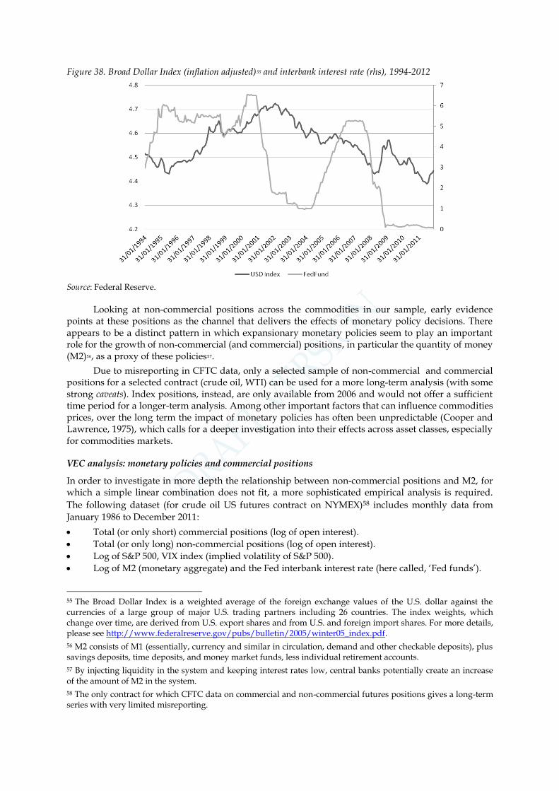
Figure 38. Broad Dollar Index (inflation adjusted)55 and interbank interest rate (rhs), 1994-2012
Source: Federal Reserve.
Looking at non-commercial positions across the commodities in our sample, early evidence points at these positions as the channel that delivers the effects of monetary policy decisions. There appears to be a distinct pattern in which expansionary monetary policies seem to play an important role for the growth of non-commercial (and commercial) positions, in particular the quantity of money (M2)56, as a proxy of these policies57.
Due to misreporting in CFTC data, only a selected sample of non-commercial and commercial positions for a selected contract (crude oil, WTI) can be used for a more long-term analysis (with some strong caveats). Index positions, instead, are only available from 2006 and would not offer a sufficient time period for a longer-term analysis. Among other important factors that can influence commodities prices, over the long term the impact of monetary policies has often been unpredictable (Cooper and Lawrence, 1975), which calls for a deeper investigation into their effects across asset classes, especially for commodities markets.
VEC analysis: monetary policies and commercial positions
In order to investigate in more depth the relationship between non-commercial positions and M2, for which a simple linear combination does not fit, a more sophisticated empirical analysis is required.
The following dataset (for crude oil US futures contract on NYMEX)58 includes monthly data from
January 1986 to December 2011:
Total (or only short) commercial positions (log of open interest).
Total (or only long) non-commercial positions (log of open interest).
Log of S&P 500, VIX index (implied volatility of S&P 500).
Log of M2 (monetary aggregate) and the Fed interbank interest rate (here called, ‘Fed funds’).
55 The Broad Dollar Index is a weighted average of the foreign exchange values of the U.S. dollar against the currencies of a large group of major U.S. trading partners including 26 countries. The index weights, which change over time, are derived from U.S. export shares and from U.S. and foreign import shares. For more details, please see http://www.federalreserve.gov/pubs/bulletin/2005/winter05_index.pdf.
56 M2 consists of M1 (essentially, currency and similar in circulation, demand and other checkable deposits), plus savings deposits, time deposits, and money market funds, less individual retirement accounts.
57 By injecting liquidity in the system and keeping interest rates low, central banks potentially create an increase of the amount of M2 in the system.
58 The only contract for which CFTC data on commercial and non-commercial futures positions gives a long-term series with very limited misreporting.

64 | SETTING THE SCENE: THE STRUCTURE OF COMMODITIES MARKETS
The dataset of futures positions for crude oil (commercial short and non-commercial long), despite changes to reporting criteria over the years, is the only CFTC legacy reports that shows no jumps in the series since the beginning of data collection from CFTC in 1986, which allows an assessment of long-term effects of monetary policies before and after the beginning of the expansionary era. Additional empirical analysis would be needed in the coming years, when the set of more granular data (available since 2006) will be sufficiently large to assess long-term effects, as this dataset may underestimate the impact of swap dealers on non-commercial long positions. Moreover, the analysis uses monthly data, which do not permit the assessment of more short-term patterns. The results of this analysis, therefore, should be interpreted as an assessment that is primarily valid over a sufficiently long time period.
Variables are stationary only in first difference (integrated of first order) and cointegrated (with stationary residuals), so linear regressions may be spurious and some Granger causality tests may give misleading results. Engel and Granger (1987) showed that the use of a simple linear regression with unit-root variables (even if de-trended) can generate numerous cases of spurious regression so, provided that a cointegration relation actually exists among the variables, the estimation of this relation is indeed quite powerful in avoiding misleading conclusions. The Vector Error Correction (VEC) model might be the best model to deal with variables subject to the same stochastic trend. VEC is an extension of a Vector Autoregressive Model (VAR) for variables that are non-stationary in levels,
but stationary in their first difference (first-order integration, I(1)).59 This model is particularly useful
as it can take into account any relation of cointegration among two variables, i.e. they share the same
stochastic trend.60
The first step checks cointegration among the variables (see Output #1 in the Annex). First, a linear regression between commercial positions and M2 appears spurious, as hinted at by very high t-statistics and R-squared. Second, a test for the existence of a relationship of cointegration is performed. The Dickey-Fuller test for unit root rejects the hypothesis (of unit root), so residuals of the cointegration equation (M2 regressed on commercial positions) are stationary and thus the two variables are cointegrated, as originally suspected. The two variables move with the same stochastic trend and adjust through a process of error correction that is described in the Annex (see Output #2).
The VEC analysis (described in Output #2) for the relation between the number of commercial positions in the crude oil futures market and M2 shows that the cointegration equations for both variables are statistically significant. Most notably, commercial positions react much faster to equilibrium shocks (8% rate) compared to M2, whose coefficient is negligible. This supports the thesis that commercial positions are affected by monetary policy actions much more than the other way around. The coefficient b1, which weights the impact of the cointegrated (lagged) variable on the dependent, is non-significant for M2, i.e. the lagged value of commercial position has no link with M2. The same is not true for commercial positions, as the lagged value of M2 is statistically significant. With this modified Granger, the conclusion is that M2 Granger-causes commercial positions and not vice-versa.
We apply the same approach to non-commercial positions and M2. As shown by Output #3, non-commercial positions adjust to equilibrium with M2 at an 18% rate. It therefore appears that are the non-commercial positions ‘to follow’ changes in M2. This is confirmed by the cointegrating coefficient of M2, which is not significant, hinting at the indifference of M2 towards the distance from equilibrium with non-commercial positions.
Finally, the same approach is used to assess the relationship between non-commercial long positions, which represent passive speculative investments that would supposedly divert futures markets from their fundamentals, and commercial short positions (a classic commodities hedge for
59 Testing hypotheses concerning the relationship between non-stationary variables is based on OLS regressions with data that had initially been differenced (Granger and Newbald, 1974). Although this method is correct in large samples, taking into account cointegration provides more a powerful analysis tool, as it doesn’t lose information on long run equilibrium and on levels.
60 While a deterministic trend is treatable by either regressing the variable on time (trend stationary) or eliminating the seasonality, to treat a stochastic trend and make the series stationary it is possible to just differentiate the variables.

final users). The initial test (Output #4) confirms that the regression is spurious and residuals are stationary, so variables can be considered cointegrated. The VEC analysis (Output #5) gives some interesting results. The cointegrating equation of a non-commercial long position has a statistically significant (at 1%) negative coefficient, which suggests that these positions react at deviations from equilibrium with commercial short positions. The opposite is not true. The cointegrating coefficient is significant at 5%, but with a very low positive coefficient. This points to an unstable equilibrium, so we could potentially ignore it. As a result, commercial short positions Granger-cause non-commercial long. Taking into account the findings in earlier sections, the growth of commercial players and the general interests in physical commodities markets in the last decade, with the quick and intense development of international trade, have proved fertile ground to promote the growth of non-commercial positions by providing liquidity, which could be accessed at very low costs due to accommodating monetary policies. This finding is in line with ample evidence showing, despite the potential to be harmful for price formation through herding behaviours, limited distortive effects of financial positions on commodities price formation.
Taking stock from the new CFTC disaggregated reporting
While the previous long-term price formation analysis with the legacy reports should be still valid over a long-term database (from 1986), the growth of passive investments together with other (typically long) swap dealers positions in recent years requires further analysis with the new CFTC reporting system that was launched in 2009 and goes back to 2006. The new reporting, therefore, disaggregates data on futures open positions in three main categories of traders, as discussed in previous sections. The analysis uses the new CFTC dataset, which includes weekly data on open positions for the three most liquid futures contracts in the US (crude oil, natural gas, and corn). The analysis in the previous section is replicated by running Granger causality tests. The Dickey-Fuller test suggests that variables are not cointegrated and Granger causality tests shall not thus lead to misleading results. Different lags for each futures contract have been considered, in line with lag-order selection statistics.
Table 22 confirms the results of the previous analysis but it qualifies it further. It confirms that M2 leads producers positions, which points at the potential impact of prolonged expansionary monetary policies on non-financial assets (through expansion of monetary base). However, from 2006, data for crude oil confirms an impact of the monetary base on the size of financial players’ positions in futures markets, while the impact of the monetary base only affects producers/users’ positions for natural gas and corn futures positions. Due to their constant growth in crude oil futures markets, non-commercial positions have become the main mean to transfer effects of policies and events that affect the monetary base.
Table 22. Granger causality tests
Variables Granger causality Reversed
IndependentDependent Crude
oil Natural
gas Corn
Crude oil
Natural gas
Corn
M2SD/MM long Yes* No No No No Yes***
M2Producers short No Yes* Yes* No Yes* No
Producers shortSD/MM long Yes** Yes** Yes** No No No
Note: *1%, **5%, ***10% significance. ‘SD/MM’ stands for ‘Swap dealers/Managed money’. See Output #10, Output #11, Output #12, in Annex.
Source: Author’s calculation.
Most notably, the analysis on the disaggregated futures positions confirms the results of the earlier vector error correction model by ascertaining the role of producers/users position in guiding swap dealers and managed money’s long positions (and not viceversa) for the top three futures contracts (by size of open interest). Financial futures positions still complement non-financial ones and are shaped by the latter. Therefore, the nature and the role of non-commercial players’ participation in commodities markets appears benign and essential for the development of commercial positions, and
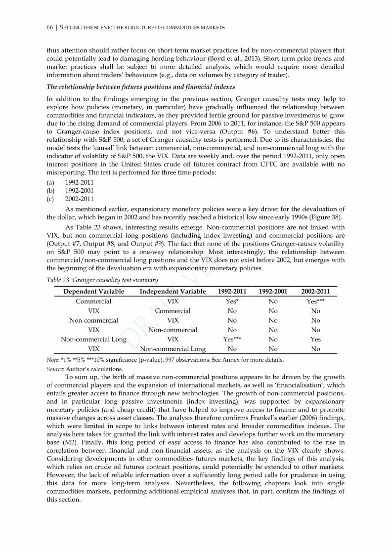
66 | SETTING THE SCENE: THE STRUCTURE OF COMMODITIES MARKETS
thus attention should rather focus on short-term market practices led by non-commercial players that could potentially lead to damaging herding behaviour (Boyd et al., 2013). Short-term price trends and market practices shall be subject to more detailed analysis, which would require more detailed information about traders’ behaviours (e.g., data on volumes by category of trader).
The relationship between futures positions and financial indexes
In addition to the findings emerging in the previous section, Granger causality tests may help to explore how policies (monetary, in particular) have gradually influenced the relationship between commodities and financial indicators, as they provided fertile ground for passive investments to grow due to the rising demand of commercial players. From 2006 to 2011, for instance, the S&P 500 appears to Granger-cause index positions, and not vice-versa (Output #6). To understand better this relationship with S&P 500, a set of Granger causality tests is performed. Due to its characteristics, the model tests the ‘causal’ link between commercial, non-commercial, and non-commercial long with the indicator of volatility of S&P 500, the VIX. Data are weekly and, over the period 1992-2011, only open interest positions in the United States crude oil futures contract from CFTC are available with no misreporting. The test is performed for three time periods:
(a) 1992-2011 (b) 1992-2001 (c) 2002-2011
As mentioned earlier, expansionary monetary policies were a key driver for the devaluation of the dollar, which began in 2002 and has recently reached a historical low since early 1990s (Figure 38).
As Table 23 shows, interesting results emerge. Non-commercial positions are not linked with VIX, but non-commercial long positions (including index investing) and commercial positions are (Output #7, Output #8, and Output #9). The fact that none of the positions Granger-causes volatility on S&P 500 may point to a one-way relationship. Most interestingly, the relationship between commercial/non-commercial long positions and the VIX does not exist before 2002, but emerges with the beginning of the devaluation era with expansionary monetary policies.
Table 23. Granger causality test summary
Dependent Variable Independent Variable 1992-2011 1992-2001 2002-2011
Commercial VIX Yes* No Yes***
VIX Commercial No No No
Non-commercial VIX No No No
VIX Non-commercial No No No
Non-commercial Long VIX Yes*** No Yes
VIX Non-commercial Long No No No
Note: *1% **5% ***10% significance (p-value). 997 observations. See Annex for more details.
Source: Author’s calculations.
To sum up, the birth of massive non-commercial positions appears to be driven by the growth of commercial players and the expansion of international markets, as well as ‘financialisation’, which entails greater access to finance through new technologies. The growth of non-commercial positions, and in particular long passive investments (index investing), was supported by expansionary monetary policies (and cheap credit) that have helped to improve access to finance and to promote massive changes across asset classes. The analysis therefore confirms Frankel’s earlier (2006) findings, which were limited in scope to links between interest rates and broader commodities indexes. The analysis here takes for granted the link with interest rates and develops further work on the monetary base (M2). Finally, this long period of easy access to finance has also contributed to the rise in correlation between financial and non-financial assets, as the analysis on the VIX clearly shows. Considering developments in other commodities futures markets, the key findings of this analysis, which relies on crude oil futures contract positions, could potentially be extended to other markets. However, the lack of reliable information over a sufficiently long period calls for prudence in using this data for more long-term analyses. Nevertheless, the following chapters look into single commodities markets, performing additional empirical analyses that, in part, confirm the findings of this section.

| 67
2. ENERGY COMMODITIES
2.1 Crude oil markets
Crude oil is by far the biggest commodity market in the world. Its production was valued at over $2.7
trillion at 2012 average prices.61. Its use in industrial applications was developed in the 19th century,
in particular after the discovery of a basic refining technique (boiling the product) to refine crude as kerosene. The invention of the combustion engine (originally designed for ethanol and biodiesel fuels) and the discovery of huge reservoirs (such as Spindletop in 1901) that made the United States the biggest producer in the world have radically changed the role of crude oil (Downey, 2009). While the basic refining technique today is still the core process to transform crude oil into fuels that can be used in combustion engines, the market has undergone significant changes in the last 150 years. At the end of the 19th century, several applications in which crude oil could be used were developed – for transport, in particular – and the long-term strategic importance of controlling this commodity became clear. Since John D. Rockfeller became a quasi-monopolist in oil extraction and fuel production around 1890 with his Standard Oil Company, which was eventually split, due to antitrust concerns, into several competing firms that are still important today (e.g. Exxon, Chevron, ConocoPhillips), the market has developed at an incredible pace. Due to its low production costs in relation to the yields in energy production, crude oil is the main source of fuel for transport and other industrial applications
(Figure 39).62 Crude oil is also a major source of energy supply (24%), with over 3 million tonnes used
in 2010 to meet increasing energy demand (IEA, 2012b).
Figure 39. Crude oil uses, 2010
Source: Author’s elaboration from EIA (2011). *Note: Agriculture, commercial and public services, residential, etc.
While the Middle East and South American regions, with their significant reservoirs, now drive production, the industry has also undergone several changes and, despite major oil companies holding only 14% of global crude production and 24% of global refinery capacity, international trade has developed at some pace as main oil producers have gradually nationalised their oil industries and pushed them to compete with global flows.
61 At 2012 average spot price of Brent, Dubai and West Texas Intermediate, equally weighed (World Bank). BP data on production.
62 For a historical perspective on oil markets, see Downey (2009).

68 | ENERGY COMMODITIES
Political instability and military conflicts over the years have put oil supply under severe strain, and historical prices illustrate these events rather well. In the short term, Figure 40 shows that, starting in the late 1990s, oil prices have risen dramatically until today, only interrupted by the 2008 financial crisis. The figure also shows that WTI and Brent prices, which have historically been very close to each other, have diverged significantly for regional components that will be discussed in following sections.
Figure 40. Real oil prices in the United States (WTI), Europe (Brent) and the Middle East (Dubai), 1982-2012
Source: World Bank Commodity Price Data. Notes: Crude oil, U.K. Brent 38` API, f.o.b. U.K ports, spot price;
Crude oil, Dubai Fateh 32` API, f.o.b. Dubai, spot price; Crude oil, West Texas Intermediate (WTI) 40` API, f.o.b. Midland Texas, spot price. Annual prices.
This short-term pattern, driven by demand from emerging markets and political instability in core oil countries, is also reflected in an unstable underlying long-term trend that started with the first oil crisis in 1973, after the Yom Kippur crisis (Figure 41).
Figure 41. Historical crude oil real spot prices, 1861–2012 ($2011/barrel)
Source: BP Stats. Note: 1861-1944 US Average, 1945-1983 Arabian Light posted at Ras Tanura, 1984-2011 Dated
Brent (Platts).

From 1973, and after the end of the fixed exchange rates regime of Bretton Woods, real prices saw only a few years of stable and low prices. The era of long-term stable prices ended then. With the war in Iraq in the early 2000s and greater Chinese participation in global trade (completed with its entry in the WTO), prices have begun to rally again, reaching another historical peak after the financial crisis. On top of supply cuts, this time demand played a greater role and the Organization of the Petroleum Exporting Countries (OPEC), which took over control of the supply chain from the United States in 1973, has been unable to offer price stability and to keep up with demand increases in an open global economy. Over the years, the difficulty of Saudi Arabia to cover other (even within OPEC) countries’ supply cuts shows the difficulty of controlling supply (if a tight control has been ever exercised) with strong demand pressures.
2.1.1 Product and market characteristics: a market structurally subject to instability
Petroleum, often simply denoted ‘oil’, is “a complex mixture of liquid hydrocarbons, chemical compounds containing hydrogen and carbon occurring naturally in underground reservoirs in sedimentary rock” (IEA et al., 2005). When discussing oil, one commonly distinguishes between the primary commodity (unrefined crude oil) and the secondary commodity (refined products, such as gasoline and lubricants). While crude oil is the most important primary oil commodity, other feedstock oils are also used to make oil products. The oil industry’s reference unit is barrels (abbreviated bbl, or simply b), but the volume of oil is sometimes also expressed in cubic metres or litres. The specific gravity or density of the liquid is needed to assess its energy content.
Qualities
The qualities of crude oil vary widely depending on the place of origin. A distinction is being made between heavy (e.g. Mexican Maya oil) and light crudes (e.g. Nigerian Bonny Light), depending on the density, i.e. the presence of more (heavy crude) or less (light crude) carbon atoms in hydrocarbon molecules. Light crude usually has a higher value because it can yield more high-value, lighter refined products, such as gasoline.
Crude oil generally finds its final use once it is refined, e.g. gasoline in transportation. Besides hydrocarbons, unprocessed crude oil sometimes contains impurities such as salts, metals (that may require desalting) or sulphur (that may require desulphurisation).63
Important properties for evaluating crude oil include (IEA et al., 2005):
Relative density (depends on light and heavy fractions in the crude)
Viscosity (i.e. the oil’s resistance to flowing)
Pour point (i.e. the lowest temperature at which a liquid still behaves as a fluid)
Water content
Sulphur content
Paraffin and asphaltene content (wax as percentage of mass)
Presence of contaminants and heavy metals
The pricing of crude oil depends largely on the above properties, as they will influence the processing and product output. The crude oil price is not only dependent on the energy content of the fuel, but is also influenced by the processing requirements. From an economic perspective, density (through a gravity indicator developed by the American Petroleum Institute (API) and sulphur content are the most important characteristics, given their impact on refined products properties. The API index ranges from 0⁰ to 100⁰. Most of the crude oil in the market is between 30⁰ and 39⁰ (referred to as ‘intermediate’). Above 39⁰, crude becomes more expensive; ‘lighter’ crude ideal for gasoline and for gas production has a very high API. Cheaper crude has an API below 25⁰, and can be used for construction materials or chemicals. The sulphur content can also lower the value of crude oil, because it affects the energy content, produces higher levels of pollution and corrodes metals (Downey, 2009).
63 IEA et al. (2005, p. 169): “The concentration of sulphur in crude oils varies from below 0.05% to more than 5% in some crudes – generally the higher the density of the crude oil, the greater the sulphur content. Low-sulphur crudes are often referred to as sweet crudes, while high-sulphur varieties are sour crude.”

70 | ENERGY COMMODITIES
Crude with lower sulphur content is denominated ‘sweet’ crude (below 1% of the total weight). The removal and disposal of sulphurs is expensive and is usually done at the end of the refining process.
Primary oil commodities also include other hydrocarbons such as natural gas liquids.64 Oil fulfils the characteristics of a search good. As the primary commodity is typically transformed into fuels or prepared for feedstock use through a refining process, it qualifies as a raw intermediate good (see the table in the Annex for a further distinction between primary and secondary oil products). Qualities can be easily assessed ex ante. Oil is a combustible fuel and cannot be recycled. However, in non-energy use, when oil is used as a feedstock to manufacture petrochemicals, these secondary commodities such as plastics may be recyclable. Production shows equivalent characteristics to mining and extraction of minerals and metals, but the costs involved might be lower in relative terms. Oil production (extraction) sites cannot be converted to extraction of other commodities. However, production companies may also be involved in extraction activities of other fossil fuels (such as natural gas). Also, refineries cannot be easily converted to production of other refined products from oil.
Storage
Crude oil can be easily stored for long periods. The high storability and cheap transportability, mainly through pipelines and ship carriers, make crude oil the ideal commodity for international trade. It is also generally believed that, with our oil-intensive economies, crude oil follows the economic cycle (see Section 2.2.3).
Oil stocks are important for the operation of the global oil supply system. Stocks balance supply and demand and ensure the security of supply by sending a clear signal to the market that the net importing countries will be able to fight back and cause losses by releasing these stocks. One can, therefore, distinguish between three kinds of stocks (adopted from IEA et al., 2005):
1. Primary stocks held in refinery tanks, bulk terminals, pipeline tankage, barges and tankers and ship bunkers for commercial purposes by the suppliers (e.g. producers, refiners, importers) or for strategic purposes by governments (e.g. US Strategic Petroleum Reserve) or by stockholding organisations (e.g. EBV in Germany);
2. Secondary stocks in small marketing facilities and retail establishments; and
3. Tertiary stocks held by end-consumers (e.g. power plants, industrial entities or consumers in the residential/commercial sector)
Production and consumption
In 2012, world oil production amounted to 89.9 million barrels a day, i.e. around 33 billion barrels a year (IEA, 2013). Apart from a significant drop during the second oil crisis (1979-1980) and despite supply cuts in some regions, global production has been steadily growing on average since 1965 to meet a soaring demand, in particular from emerging markets. The inability to keep up with this soaring demand in recent years, due to the rigidity of supply and lower yields from important production fields, has put the market in a constant deficit, which is reflected in highly volatile and upward-moving price patterns.
64 IEA et al. (2005, p. 170): “Natural gas liquids are liquid hydrocarbon mixtures, which are gaseous at reservoir temperatures and pressures, but are recoverable by condensation and absorption. Natural gas liquids can be classified according to their vapour pressure [...] A natural gas liquid with a low vapour pressure is a condensate; with an intermediate pressure, it is a natural gasoline, and with a high vapour pressure it is a liquid petroleum gas. [...] Natural gas liquids include propane, butane, pentane, hexane and heptane, but not methane and ethane, since these hydrocarbons need refrigeration to be liquefied. The term is commonly abbreviated as NGL.”

Figure 42. World (net) production and consumption, 1965-2012 (kbbl/day)
Source: Author’s elaboration from BP. Note: Net production is expressed as % of total production.
The share of the 12 OPEC member countries65 is considerable, amounting to 42% of world oil
production in 2011 (IEA, 2012b) and 43.4% in 2012 (BP Stats). OPEC produced 35.7 mb/d, 82% of which was ‘conventional’ crude oil. Among the non-OPEC producers (48.9 mb/d), the share of ‘conventional’ crude is two percentage points lower than the OPEC producers, largely due to the growth of unconventional supplies, particularly in North America (tight light oil and Canadian oil sands).
Saudi Arabia (13.43% of world production) and Russia (12.4%) are the largest oil producing countries, accounting for more than a quarter of the world oil production. As shown in Figure 43 below, other relevant producing countries include the United States (10.37%), China (4.84%), Canada (4.36%), and Iran (4.29%). Notably, China and Canada, for the first time since the 1980s, have produced more crude oil than Iran, which is the second producer in the Middle East.
65 Algeria, Angola, Ecuador, Islamic Republic of Iran, Iraq, Kuwait, Libya, Nigeria, Qatar, Saudi Arabia, United Arab Emirates and Venezuela.

72 | ENERGY COMMODITIES
Figure 43. Top fifteen producers, 2012 (%)
Source: Author’s elaboration from BP Stats.
Technically recoverable oil resources are still considerable – totalling 5,871 billion barrels (Figure 44). At 2011 levels of oil consumption, these resources would be sufficient to meet world oil demand for the next 185 years at the current consumption rate. This rough estimate, however, does not take into account expected demand growth and whether technically recoverable resources are economically and/or environmentally viable. Reserves estimates are in general not reliable, especially in non-OECD countries, because they may not account for upcoming developments in new technologies and exploration techniques (or other external factors) for extracting conventional or non-conventional oil. By only considering official proven reserves, at the 2011 rate of production, the world’s reserves would last for another 55 years (IEA, 2012b). This becomes 46 years if we discount current consumption rate (Figure 44).
Figure 44. Proven reserves, 1990-2011, and stock-to-use ratio, 2002-2011
Source: Author’s elaboration from EIA, OPEC.

New explorations and the increase in oil production in non-OPEC countries have been increasing forecasts of proven reserves over yearly consumption, despite higher demand, and storage accumulation to meet new demand. Among non-OPEC countries, production has been growing in recent years in both Asia and Africa to meet lower or steady production levels in key OPEC countries (e.g. Saudi Arabia).
Unconventional oil
IEA has estimated that 54% of technical oil resources come from unconventional oil (Table 24). While the Middle East holds the lion’s share of the remaining conventional oil resources (42%), most unconventional oil resources are located in the Americas (59%).
Table 24. Remaining technically recoverable oil resources by type and region, end 2011 (billion barrels)
Source: IEA (2012b, p. 101). Note: EHOB, extra-heavy oil and bitumen.
The ‘unconventional revolution’ in oil may have important geopolitical implications, resembling those that shale gas exerted on natural gas markets. However, an important obstacle to their development is the relatively low energy return on investment (EROI); the energy costs to produce the commodity is still very high, even though the gap with crude oil has been narrowing in the last decades due to technological advancements in production. There are three main types of unconventional oil (Downey, 2009): oil extracted from sands (e.g. bitumen); coal-based oil; and shale oil.
Oil from sands is heavy, with high asphaltene content and an API gravity below 15⁰. While its extraction is not very complex, sands need to be treated with a two-phase process requiring high amounts of water and energy. First, the heavy oil must be separated from sands and other impurities through a complex process that may involve the use of a solvent (such as propane) to reduce oil viscosity. Second, when the bituminous substance is extracted, a process involving high amounts of energy upgrades the oil to a higher API gravity, with fewer impurities, before being sent to a conventional refinery. The blending of this bituminous substance with light products is less expensive. Natural gas is generally used to produce energy for this heating process.

74 | ENERGY COMMODITIES
Oil can also be extracted from coal through a process that transforms the solid fuel into gas by heating it. Gas is then liquefied mainly through a process called ‘Fischer-Tropsch’, which uses catalysts (like cobalt) and heating. Alternatively, coal can be directly converted to a liquid through carbonisation (the Karrick process) or hydrogenation (Bergius process), which respectively use super-heating in the absence of air (in a retort) and a hot stream of pressed gases (dry process), together with catalysts and heavy oil/solvents (pumped into a reactor with hydrogen pressure), to convert the coal into liquids. These processes use a lot of energy, though they produce natural gases as by-products. As a result, if crude oil prices continue to increase and coal prices remain stable, oil sands may become an important source of unconventional oil, but at a high cost in terms of energy.
Finally, shale oil is oil extracted from sedimentary rock and has high kerogen content. Kerogen is rich in hydrocarbon molecules, but has insufficient hydrogen to be like crude oil. It is extracted through different processes that involve high temperatures and hydrogen is added after extraction. Hydrogen also requires an energy-intensive process to separate it from oxygen, available together in water.
International trade
Oil is the largest traded commodity worldwide, either through crude oil or through refined products. Crude oil is transported via pipelines or ships (e.g. on very large crude carriers).
Roughly 47% of the oil produced is traded interregionally (Figure 47; in IEA 2012b this figure is 48%), and large crude carriers (cargoes) dominate interregional trade. The Middle East is the biggest exporting region (20.7 mb/d), and its exports are expected to increase in the future. China is expected to become the world’s largest oil importer, overtaking the United States where demand is decreasing and indigenous production is on the rise (IEA, 2012b). As of today, however, China is still behind the United States (Figure 45).
Figure 45. Top ten exporters (left) and importers (right), 2011 (mt)
Source: IEA (2012).
When looking at net imports (the difference between exports and imports), however, the difference between the United States and China is smaller. Europe is the biggest net importer of oil in the world (Figure 46).
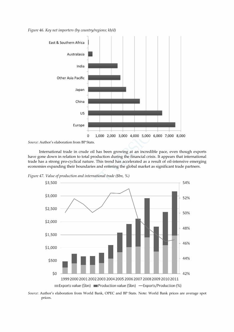
Figure 46. Key net importers (by country/regions; kb/d)
Source: Author’s elaboration from BP Stats.
International trade in crude oil has been growing at an incredible pace, even though exports have gone down in relation to total production during the financial crisis. It appears that international trade has a strong pro-cyclical nature. This trend has accelerated as a result of oil-intensive emerging economies expanding their boundaries and entering the global market as significant trade partners.
Figure 47. Value of production and international trade ($bn, %)
Source: Author’s elaboration from World Bank, OPEC and BP Stats. Note: World Bank prices are average spot
prices.

76 | ENERGY COMMODITIES
International trade is estimated at almost $1.5 trillion globally, and growing. The market is very volatile, however, and depends heavily on the economic cycle and the volatility of exchange rates.
2.1.1.1 Supply characteristics: ever-evolving market mechanisms
The nature of oil supply and its market structure finds its roots in over a century of political history, full of geopolitical events that have shaken the market equilibria several times. As a consequence, four important periods in the history of crude oil supply can be identified.
1870-1911 (the advanced world understands the importance of crude oil for economic development).
1931-1971 (the United States leads the expansion of international markets for crude oil).
1973-1986 (OPEC takes the lead in pricing in international markets, but with strong geopolitical pressures to limit supply cuts).
1986-today (markets-based oil pricing systems supported by price assessments).
From 1870 to 1911, the world discovered the importance of crude oil for daily life and its implications for global trade and geopolitical power. The period ended with the split of the quasi-monopolist Standard Oil into over 30 competing companies that immediately began geographical diversification. This situation led to a long period of international trade development, mainly through four former Standard Oil subsidiaries (Exxon, Mobil, Chevron, and Texaco) and three other international oil companies (Royal Dutch Shell, Anglo-Persian Oil Company, then renamed BP, and Gulf Oil), the so-called Seven Sisters. Other firms, such as Total, ConocoPhillips and ENI, soon arrived in the international markets. From 1931-1971, under the strong influence of production outputs set by the United States (through the Texas Railroad Commission; see Downey, 2009), major oil companies gained near total control of the international supply, becoming the main concessionaries of oil exploration and extraction in many countries around the world. Concessions were typically made on a 50/50 split of the revenues, as in the case of Saudi Arabia and Chevron. This period of stability for crude oil markets was helped by the oversupply of the United States and the currency stability granted by the gold standard. However, when the gold standard fell under the pressure of an unmanageable convertibility and the spare crude oil capacity of the United States (which was already stagnant in 1970) intended to control market prices resulted insufficient to manage the supply output, the system quickly collapsed. For the first time in history, US production started to decline and continued to do so during the 1970s, and also from mid-1980s until the commercialisation of non-conventional oil in recent years, which has brought production up to the 1992 level (Figure 48).
Figure 48. US crude oil production, 1965-2012 (kb/d)
Source: BP stats.

The main oil-producing countries (such as Iran), which took over from the United States as the top global producers and agreed to control supply through OPEC (established in 1960), decided to cut supply and show their power to exert sudden and deep economic pain in more advanced economies. Exploration and production concessions were renegotiated (e.g. ENI in Iran) and gradually withdrawn in several cases. Oil production was nationalised through local state companies in several countries. The regime of posted prices by the US supply (which helped multinational oil companies to consolidate their position) was gradually replaced by a system of administered prices run by OPEC (Fattouh, 2011). The gradual shift of control over supply officially began with the first oil crisis and the Yom Kippur war in 1973, and ended in 1979 with the Iranian Islamic revolution and the overthrow of the Shah. Since then, OPEC has managed to control supply and adjust production to meet soaring demand from advanced and emerging markets. A marker price (Arabian light) was used as a reference posted price to which a negotiated differential was applied. The system was held by common agreement between OPEC to manage supply together. Although it worked for a few years, the cartel often suffered from cheating by members that wanted to produce more and offer direct supply to third parties, rather than through a long-term contract with oil majors that could resell it, adding a price differential. As a result, a refinery netback pricing was introduced that limited the revenues accruable by the oil majors that were required to pay royalties in relation to the price that they were able to charge to final users. This system, which was introduced in 1984 also to guarantee stable revenues for the refining industry suffering capacity issues, was replaced in 1986 with the current system – a formula netback pricing. OPEC (and non-OPEC) crude producers sell their crude at a free-market crude oil benchmark price with differentials (see Section 2.1.4).
Following the 2008-09 crisis, which has signalled a shift in power towards emerging countries, a new period for the oil industry may emerge. As the spare capacity in OECD countries continues to decline, the gradual replacement from non-OPEC countries and non-conventional sources, which are more widespread across the world, may lead to further changes in the oil pricing systems and in the role of price differentials. Steadily growing Asian demand may speed up the process of reform of current sources of formula pricing provided by futures exchanges, which are already suffering from regional issues. Whether this reform would determine a more limited role for price differentials depends on how much of the market more liquid regional benchmarks are able to cover. The different grades and varieties of crude oil would always need to be based on differentials to take into account its heterogeneous nature.
Industry organisation
The exploration, extraction and production of crude oil are capital-intensive activities; oil producers must sustain significant initial sunk and fixed costs to run operations. Capital requirements are generally on the rise and, while accessible reservoirs continue to be extensively exploited, producers are now turning more to offshore or unconventional oil (e.g. oil sands). The amount of capital invested by the oil and gas industry is significant, especially in the upstream market, and continues to grow over the years (Table 25).
In recent years, the capital invested in exploration and production has been increasing substantially due to the need to improve new ways of extraction (e.g. deepwater drilling) and a general reduction in spare capacity of conventional oil. The five oil majors (BP, Chevron, ExxonMobil, Shell and Total) will invest over $120 billion in the upstream in 2013 (Argus Media, 2012), while the industry altogether is set to reach the historic threshold of $500 billion (Table 25).

78 | ENERGY COMMODITIES
Table 25. Oil and gas industry investment by company (nominal dollars)
Source: IEA (2012b).
Exploration and production (upstream) are subject to high uncertainty and need constant investment. Special contractors (e.g. drilling rig firms), who provide specialised expertise and equipment, typically support upstream activities (in particular, production). The need for capital has historically prompted consolidation in upstream markets, where multinational companies and nationalised oil companies can put more financial and political resources on the table. Concentration, however, might be more diluted when non-conventional oil is considered. Supply characteristics also push for vertical integration and partial horizontal integration with natural gas production. Costs of capital are also important for the downstream refining activities, with new refining activities costing roughly $1 billion per 100,000 barrels a day of capacity.
Figure 49. Upstream capital expenditure (CAPEX) estimates
Source: JP Morgan Commodities Research

As a result of these supply characteristics, supply elasticity is rather low in the short and medium term, as producers find it difficult to adjust production levels upwards at short notice (lengthy authorisation procedures or exploratory seismic work may be needed, for instance, for drilling and connecting wells to pipelines). Consequently, many large and complex non-OPEC projects can take between 5 and 15 years to go from approval to production, meaning the supply response is slow even if they receive immediate approval. Downward adjustment is sticky as well. Reservoir and wellbore characteristics may not allow simply restarting production later on. Strategic behaviour by producers, especially within the OPEC cartel, adds to the issue of supply-side inelasticity and the inability to face sudden production changes.
Demand and supply rigidity in the short term (‘bilateral price rigidity’) typically causes temporary price instability, not only for oil but also for other commodities such as raw materials. The reasons can be summarised as follows:
i) Production cannot be quickly modified, as capacity increases tend to take place in large increments – typical for heavy industries where scale considerations are important.
ii) Costs structure; if production requires large upfront investment, sunk costs will dominate direct costs, meaning that additional capacity that is created will tend to be used to spread the indirect cost on a larger production base.66
iii) Only some OPEC countries, notably Saudi Arabia and the other Arab Gulf producers, make large-scale investments to create capacity to be used for stand-by; this behaviour is essential to counteract the structural instability of prices, which is the spontaneous tendency of the market.67
Note also that investments in non-OPEC production were slow to respond to the oil price rise of 2000-07 because oil companies use conservative price assumptions in their investment planning. Also note that non-OPEC producers invariably maximise production, irrespective of price, because of the need to recoup the significant capital expenditure of oil exploration/production. Non-OPEC crude oil producers can thus be considered ‘price-takers’. OPEC producers, by contrast (and Saudi Arabia in particular), actively adjust production levels in response to prices. Investment by OPEC producers does not respond to higher demand quickly (if at all) because OPEC producers can better maximise revenue by producing less oil in a capacity-constrained market at a higher price than by meeting demand at a lower price.
On top of supply rigidities, demand is equally rigid as oil satisfies essential needs with considerable lead time (transport, heating with low price elasticity), taxation often isolates consumers from immediate impact, energy expenditure is often a small part of overall expenditure in OECD countries and is often subsidised in developing countries, and demand is often influenced by macro trends such as income and weather. As a result, given short-term supply and demand constraints, prices may be undetermined within a broad margin. Existing supply and demand will react seriously only if prices reach very high or very low levels. Given a prevailing price discovery mechanism (see below), the mechanism will generate a specific price; but the same balance or imbalance between demand and supply would prevail even with higher or lower prices. The so-called ‘marked fundamentals’, demand and supply, will normally validate whatever price has come to prevail. This price may be influenced by factors that are totally unrelated to oil fundamentals (for example, the value of the dollar relative to other currencies) and change accordingly; fundamentals will not be able to counteract this.
Freight costs are relevant, but due to the high outright price of crude in connection with sustained demand and the ability to easily store and ship the product, they are far less significant than for natural gas, for example. The relative share of transportation costs has declined significantly in recent years, due to high oil prices and decreasing transportation costs, inter alia due to excess tanker
66 Oil exploration and production activities are dominated by sunk costs. When a new field is discovered or new capacity is added, this will tend to be used to the maximum level that is compatible with the preservation of the long-term value of the field. A physical optimum exploitation rate typically applies to preserve the long-run value of the field.
67 Note also that the OPEC quota system may lead to lower prices but would rarely affect price stability.

80 | ENERGY COMMODITIES
tonnage. To give an example, shipping oil from Cushing in Oklahoma (a major trading hub for crude oil and the price settlement point for West Texas Intermediate on the New York Mercantile Exchange) to Europe costs around $13-14/bbl. This means that the current spread between the WTI crude oil price and Brent Crude (at time of writing, well above $14) may be unsustainable and driven by more fundamental issues (see Section 2.1.4).
Midstream (oil transportation) and downstream (refining and distribution) are typically less concentrated but competition also relies on government intervention, both at an infrastructural and a regulatory level. Lower concentration at these two levels is mainly due to still high oil reserves and limited costs of transportation. However, OPEC’s 42% market share in production is also able to exert some market power at lower levels of the value chain, especially in the case of Saudi Arabia.
2.1.1.2 Demand characteristics: will the world remain oil-dependent?
Crude oil was at the heart of the economic development of the last century. Economies still rely heavily on crude oil today as a main source of energy and chemicals used in day-to-day life. Even though the world (and in particular, more developed economies) is moving towards more reliance on more sustainable alternative sources, it may still be some decades before crude oil and derived products become secondary resources. The lack of substitutes, especially for transportation fuel, feeds a solid and steadily growing demand.
The share of oil in global total energy demand has been decreasing, from over 45% in 1973 to around 32% of primary world energy demand in 2010 (IEA, 2012b). It is generally believed that the relative share of oil in the energy mix of will decrease further to 25-27% by 2035. However, the demand for oil is still projected to rise in absolute terms, at a compound annual growth rate of 0.5%-0.8% between 2010 and 2035 in the IEA’s current and new policies scenarios. Only under the assumption of an ambitious global decarbonisation agenda (450ppm) would the annual growth rate be negative (-0.4%).
The demand side may experience some level of concentration in market structure, but the impact on competition and distribution bottlenecks is limited to regional or country-specific factors. Non-OECD countries mainly drive oil demand growth today, due to higher rates of economic growth and their oil-based manufacturing economies (especially for transport). Oil demand in the OECD countries, by contrast, is expected to decline at a compound annual rate of between -0.6% and -2.1% to 2035.
Figure 50. World oil demand by region; mn bbl/d

Source: IEA (2013).
In 2011, the world’s oil demand amounted to 88 million barrels per day (mb/d; BP stats). While oil is used all across the world, the top oil consuming countries in 2011 were the United States (23 mb/d, i.e. 25.3% of world oil demand), the EU-27 (15.9%), China (11.4%), Indonesia (5.0%), India (4.0%), Saudi Arabia (3.7%), Russia (3.4%), and Brazil (3.0%). The non-OECD world accounts for 43% of world oil demand (IEA, 2012b). In recent years, oil demand has grown rapidly in many emerging economies (especially in Asia) and this trend is expected to continue in the future. Despite a forecasted slowdown in consumption in 2013, China remains a leading driver of this growth, as its economy has expanded over the years in favour of an oil-intensive manufacturing economy and thus requires a relatively low-cost and constant energy supply (see Figure 51). Brazil and India have also shown important signs of growth, but at much lower rates.
Figure 51. China, Brazil and India Consumption, 1965-2013 (kbbl/d)
Source: Author’s elaboration from BP Stats and IEA (2013).
The share of oil in total primary energy demand varies across countries. In the OECD world, it is at a fairly high 36%. In the non-OECD world, it is on average ten percentage points lower. Accordingly, the share of oil in total primary energy demand in the BRICs is still below the OECD average (e.g. Russia 20%, India 24%, China 17%), with the exception of Brazil (40%). Numbers suggest that growth in oil consumption for emerging markets will continue in the coming years (Chatham House, 2012).
Oil use is complex and involves both energy and non-energy uses.68 By far the most important
global user is the transport sector, accounting for more than half of world oil demand, as shown in Figure 39). Both the construction and industrial sectors account for roughly 17%. Power generation, in steady decline over the last decade, is responsible for 7%. The share of the transport sector is projected to increase even more in the future to well above the current 50%, due to development in emerging economies.
68 IEA et al. (2005) distinguished between: (i) the transformation sector (e.g. electricity and heat production, oil used to produce gas in a gasification plant), (ii) energy industries in the energy sector, (iii) the transportation and distribution of oil (limited), (iv) the various sectors and branches of final consumption (industry, residential, etc.), including both energy and non-energy uses of oil.

82 | ENERGY COMMODITIES
Figure 52. World oil demand by sector in the IEA’s New Policies Scenario
Source: IEA (2012b). Notes: Other includes non-energy use, including feedstock for industry.
The demand for liquid fuels69 will grow exponentially in non-OECD countries (Figure 53),
while it will be more or less stable in advanced economies, though its composition may be subject to important changes as renewable fuel production is increases and becomes more widespread.
The availability of substitutes for oil varies widely across uses. In transport, substitutes exist in principle (biofuels, natural gas vehicles, biogas, hydrogen and electric power). These substitutes are, however, not readily available and would require huge investments (e.g. infrastructure needs of electric cars) or change in land use (for biofuels). Due to its high energy density, oil will probably remain cost-competitive compared to most alternatives, even if oil prices remain high. Fuel and feedstock switching is in principle possible in industry, using gas or biomass or making increased use of recycling, for example. Oil, which is mainly used for space heating in buildings, can be substituted by gas, electric power and renewables such as biomass or solar thermal. Numerous substitutes such as gas, nuclear, coal and renewables exist in power generation, where oil is generally not very competitive.
Figure 53. Liquid fuels consumption by region and sector, 2008-2035 (mb/d)
Source: Author’s elaboration from EIA (2011).
The demand elasticity to the price of oil depends on the sector. In the transportation sector, elasticity is quite low, at least in the short and medium term, given the lack of readily available
69 ‘Liquid fuels’ are all petroleum products, natural gas liquids, biofuels, and liquids derived from other hydrocarbon sources (coal to liquids and gas to liquids).

substitutes. In the industrial sector, long-term elasticity is moderate, but as some substitutes may require changes in the manufacturing process (e.g. new equipment, new chemical processes), this will often not be the case in the short and medium term. In the construction sector and power generation, elasticity is generally high as a number of substitutes are available. However, elasticity may be lower in the short term due to significant sunk costs for oil users (oil-fired power plants, heating systems, etc.) and long lead times with high capital costs for substitutes (especially nuclear power). Elasticity in the power sector is higher if spare capacity is high (e.g. in coal- or gas-fired power plants) or trade is possible (e.g. in the interconnected European electricity market).
2.1.1.3 Key product and market characteristics
The interesting combination of particular product characteristics and historically strong geopolitical factors has shaped market characteristics as described below:
Crude oil cannot be recycled, but petrochemicals products (plastics) are.
It has high substitutability, especially in some uses (such as transport fuel), and can be used in several areas, from energy to construction and chemicals.
Highly capital-intensive production, due to a lack of convertibility to alternative products (only natural gas is typically extracted jointly with oil), has prompted partial vertical (to refining) and horizontal (to natural gas) integration in the industry.
Long-term storability and low freight costs (compared to the underlying value) makes crude oil an ideal product for global trade, which exposes it less to the economic cycle as it becomes less dependent on consumption in single regional areas.
Supply and demand elasticities are very rigid in the short/medium term.
Demand elasticity is low and can only adjust to price in the long term (making oil security a strategic objective for all governments across the world).
Market concentration is medium-to-high in the upstream (exploration and production), mainly due to the high investments needed, while concentration is much lower in the downstream (transportation and distribution).
Demand still comes mostly from advanced economies, but the astonishing growth of emerging markets is the only current driver of growth and will be so for future consumption levels.
On the supply side, emerging markets have accrued an important share of conventional oil production, but future growth may mainly come from non-conventional sources (even though dependence from key oil producers is here to stay).
Driven by new developing economies, future demand will be still strong though production may not grow at the same speed, increasing the reliance on non-conventional sources of production.
Table 26. Product and market characteristics
Recycling/
Production convertibility
Substitutes/Horizontal integration
Alternative uses/ Vertical
integration
Capital intensity
Storabi-lity
Freight costs
incidence
Elasticity to price/ demand
Concen-tration
BRICs weight
Future Consumption/
Production
Demand side
None High High
High High Medium
Low
Medium
High High
Supply side
Low Medium High Low Mediu
m Medium
Note: ‘BRICs’ is used as an alternative term to define ‘emerging markets’.
Source: Author.
2.1.2 Exogenous factors: measuring the impact of policy factors
Government intervention in oil markets takes various forms and occurs both on the supply and demand side. Interventions differ significantly between the OECD, OPEC, and the rest of the world. A notable exception is aviation, where kerosene is exempt from taxation virtually everywhere.

84 | ENERGY COMMODITIES
In OECD countries, supply side royalties and taxes in different jurisdictions have a large impact on upstream investments. As part of its efforts to encourage governments to phase out environmentally harmful subsidies, the OECD and the IEA have put together a fossil fuel subsidy
inventory covering both the production and consumption of fossil fuels.70 The OECD inventory
measures the extent of favourable treatment with reference to national tax benchmarks. It provides some evidence that a favourable tax treatment for the oil industry is quite common in gas-producing OECD countries. As regards the demand side, OECD governments tend to impose very high taxes on the consumption of refined products (fuels) because of the collateral effects combined with the low demand elasticity (linked to transport means). This situation over time may have an (intentional) impact on consumption, prompting the search for alternative sources of fuel, and thus on crude production. Other incentive policies also have an important impact on demand. For example, the European industrial policy to promote diesel engine technology over gasoline has led to a significant misalignment between diesel and gasoline demand on the one hand, and European refinery production capacity for the two fuels on the other. Europe has accumulated a significant deficit of diesel production capacity and thus a surplus of gasoline capacity that has caused problems in the sector.
As a result, government intervention in upstream markets is channelled through agreement on royalties or with direct exploration and production through state-owned companies (less common). In OPEC and the non-OECD world in general, extraction and refining is often nationalised. Supply-side intervention also extends to the issue of ‘resource nationalism’, whereby countries with significant oil reserves limit or completely refuse access to those reserves by the private sector – in the Middle East including Saudi Arabia, Mexico, South America, and Africa. The lack of access to these low-cost reserves plays a major role in explaining why the marginal cost of oil production is at the current level. OPEC production agreements have a direct impact on supply, especially when Saudi Arabia alters production; royalties and taxes in different jurisdictions have a large impact on upstream investment; moratoria on drilling have a direct impact; licensing of acreage for upstream exploration and production is controlled by governments; and resource nationalism prevents exploration and production by private-sector companies in large areas of the world.
In the downstream market, taxation or subsidies for fuel products (e.g. gasoline) are the main means of intervention. In OECD countries, taxation is typically much higher than in other countries to stimulate changes in consumption habits (to more environment-oriented habits) and reduce the dependence on oil. As Figure 54 illustrates, taxation can increase spot gasoline prices by a factor of more than three, discouraging consumption in the long term and so indirectly affecting demand and supply of the physical commodity.
Figure 54. UK gasoline price with and without taxes
Source: JP Morgan (2011).
70 To access the database, please see http://www.oecd.org/site/tadffss/.

In oil-producing or emerging countries, however, taxation is often negative (i.e. prices are subsidised) and governments intervene to reduce prices at the pump or for industrial uses (in Saudi Arabia, for example, the intervention was estimated at around $45/bbl in 2011). Fuel subsidies have a major impact on demand, keeping it artificially high. This raises questions over the negative economic and environmental consequences.
Table 27. Key exogenous factors
Government intervention Other external factors
High Economic cycle, exchange rates and military conflicts
Source: Author.
Other political factors, which often lead to the formation or dissolution of governments, have been the source of important political instability and military conflicts in recent years (e.g. in Iraq, Libya and Nigeria). Other countries, such as Saudi Arabia, have repeatedly intervened to fill the supply gap, but often the magnitude of the intervention has been insufficient to prevent price and volatility spikes.
Finally, crude oil production and consumption is also affected by a long list of external factors, such as economic crises or policy decisions. The effects of the economic cycle and monetary policies are reflected in oil price trends mostly through the evolution of exchange rates and credit expansion (see the following section).
Figure 55. Five-year rolling Pearson correlation WTI front-month and S&P 500
Source: Author’s calculation. Note: daily data.
As Figure 55 shows, before 2002 the five-year rolling Pearson correlation between the natural logarithm of WTI front-month and the S&P 500 financial index has always been positive or negative at a more or less regular intervals. Since 2002, when expansionary monetary policies started to depress the strength of the dollar and expand credit, the correlation between prices and a financial index that should be only randomly correlated to another asset has become steadily positive (above 60%). As mentioned in Chapter 1, no conclusions can be drawn about causal relationships from correlation analyses, and certainly this cannot be interpreted as showing that the financial index leads prices in commodities. Rather, as mentioned above, it appears that an underlying common variable has

86 | ENERGY COMMODITIES
gradually prompted variables, only occasionally positively correlated, to move in the same direction for a prolonged period of time with a stable positive correlation. This analysis also finds support in the analyses carried out for other commodities markets.
2.1.3 Empirical analysis: the crucial link with the economic cycle
The empirical analysis of price formation in crude oil markets looks at relationships between front-month WTI price and key variables (such as inventories). The analysis is done on WTI front-month futures contract, which can be seen as a close approximation of spot prices of crude oil delivered at Cushing, Oklahoma. The Brent front-month futures price, representing the benchmark price for more than 60% of global trade, was also used. However, the futures contract (front-month) published by ICE may not necessarily be a close approximation of the Dated Brent final price (physical price) pricing actual deliveries at the Sullom Voe terminal in the North Sea. Financial layers with the support of price assessments to calculate differentials may cause wide divergences with the original Brent futures front-month contract.
The dataset has the following characteristics:
Monthly data from 01/01/1994 to 31/12/2011.
Natural logarithm (from now on simply ‘log’) of front-month WTI NYMEX price and Brent ICE (‘spot price’), differentiated to avoid spurious regressions. Prices are deflated using the US Producer Price Index (PPI) published by the Federal Reserve (‘the Fed’).
Log US ending stocks excluding SPR of crude oil (thousands barrels) provided by the US Energy Information Administration and EU-16 including Norway (provided by Argus Media).
Log Price-adjusted Broad Dollar Index published by the Fed.
Log of OECD leading composite indicator, as average of de-trended, smoothed and normalised
component series calculated for the United States (to capture the economic cycle).71
Log of the monetary aggregate M2, seasonally adjusted data published by the Fed.
Log of Standard and Poor’s (S&P) 500 index.
Log of the effective Fed funds rate (interbank interest rate), not seasonally adjusted.
The log of WTI front-month appears to be a unit root, as the Dickey-Fuller suggests, so variables in the model are differentiated. A simple linear model of differentiated variables seems to fit well the dataset. Main misspecification tests (normality, heteroskedasticity, and the Ramsey test for misspecification) on the linear regression model confirms the validity of the model. As described by Output #10 (for WTI) and Output #11 (for Brent), the regression provides straightforward and similar results for both WTI and Brent (Table 28).
71 The composite leading indicator is a times series, formed by aggregating a variety of component indicators which show a reasonably consistent relationship with a reference series (e.g. industrial production IIP up to March 2012 and since then the reference series is GDP) at turning points. The OECD CLI is designed to provide qualitative information on short-term economic movements, especially at the turning points, rather than quantitative measures. Therefore, the main message of CLI movements over time is the increase or decrease, rather than the amplitude of the changes. The OECD’s headline indicator is the amplitude adjusted CLI. The component series for each country are selected based on various criteria such as economic significance; cyclical behaviour; data quality; timeliness and availability. For the US indicator, the components are: dwellings started (number; Bureau of the Census); net new orders for durable goods (USD – million; Bureau of the Census); share prices, NYSE composite (2005=100; Bureau of the Census); consumer sentiment indicator (normal = 100; University of Michigan); weekly hours of work, manufacturing (hours; Bureau of Labor Statistics); purchasing managers index (BS) (% balance; Institute of Supply Management); spread of interest rates (% per annum; Federal Reserve). More information is available at http://www.oecd.org/std/clits/oecdcompositeleadingindicatorsreferenceturningpointsandcomponentseries.htm.

Table 28. WTI and Brent regressions output
Independent variable (WTI)
Coefficient (t-test)
Independent variable (Brent)
Coefficient (t-test)
US Inventories -0.53***
(-2.64) EU Inventories
-0.5**
(-2.41)
Broad Dollar Index -1.46***
(-2.9) Broad Dollar Index
-1.36***
(-2.84)
US OECD Demand 7.24***
(2.66) US OECD Demand
11.86***
(4.83)
China Demand 3.97**
(2.47) China Demand
4.13***
(3.10)
Note: ***1%, **5%, *10% significance.
Source: Author’s calculation.
The model is consistent with most of the theoretical background analysis in this section and in Chapter 1. First, the crude oil price shows a negative relationship with inventories, while exogenous factors, such as exchange rates and the economic cycle, are positively related. Chinese demand (estimated in a model without US demand) seems to influence oil price, but the US domestic demand effect prevails.
Futures contracts seem to provide a well-functioning driver of inventory levels. The basis (i.e. the difference between a spot or front-month contract and a purer futures contract) of both futures contracts with delivery in 4 and 12 months Granger-causes levels of inventories with a significant first lag (see Output #12). Results are robust and confirm the efficiency of the futures market in reflecting the underlying physical market.
The findings (in the Annex) also confirm a strong link with financial indexes, but the relationship with the S&P 500 needs further specification. Despite Output #13 suggesting that the S&P 500 Granger-causes the crude oil price (unilaterally) by regressing separately the S&P 500 on the crude
oil price (with a linear regression) and vice-versa (with an ARCH model),72 this relationship seems to
be significant both ways (see Output #14). A different approach can be used to confirm this analysis. A sample of monthly data from January 1983 to December 2001, when cuts to nominal interest rates started a period of expansionary monetary policies reflected on to the devaluation of the dollar, is tested to assess whether the relationship existed before 2002. Another test is run on monthly data from 2002 to 2011. As Output #15 shows, an ARCH autoregressive to model first-differentiated front-month prices as a dependent variable confirms that S&P 500 and oil prices were not statistically linked before the beginning of the credit-easing era (1983-2001), while they were in the following period (2002-2011). The results are confirmed by using a dataset based on Brent front-month futures prices (see Output #16). This result confirms the empirical analysis in Section 1.4, and in particular that the relationship with the financial index strengthened from the beginning of the dollar devaluation.
These results point to a significant impact of monetary policies on oil price formation, through interest rates and the expansion of the monetary base (with the effects on exchange rates), pushing oil prices and financial indexes in the same direction. These policies have also had an impact on the size
72 Due to unit root with differentiated levels, the ARCH model seems to fit the dataset better. The power of the ARCH model consists in the joint estimation of a mean equation and a separate variance equation, in which, by being able to model the behaviour through which past realizations of the error term influence the present one, the model allows for heteroskedasticity of the error term. In the simplest case of the ARCH (1) model used in this section, the variance equation is estimated in the following way ht=a+a1*e2t-1 where e is the error term of the mean equation. The GARCH (generalised autoregressive conditional heteroskedasticity) model, instead, introduces an autoregressive term of the variance equation. To test for the presence of ARCH effects in the series, a Lagrange Multiplier (LM) test (which tests the variance equation whether a and a1 are significant) can be used. As ARCH effects clearly emerge from the test in this dataset, an ARCH (1) model is used to understand the impact of key variables on soybean oil prices.

88 | ENERGY COMMODITIES
of futures markets and index positions (as discussed in previous sections; see in particular Section 1.4). This result confirms other findings on the broader impact of monetary policies through the exchange rate on the demand of oil (Schryder and Peersman, 2012).
2.1.4 Market organisation: prospects and challenges for benchmark prices
The development of market organisation in crude oil markets has undergone several changes over the years. Since the end of posted prices, at the end of the 1980s, market-based solutions have been developed but they are under continuous evolution. The pricing of physical crude oil today is a complex web of financial and physical transactions, which result in a combination of futures, forward, and spot prices traded on open platforms, OTC, or assessed by price reporting agencies (PRAs). This system relies on pricing formulas.
Crude oil prices (typically sold FOB) are formed through long-term contracts or spot transactions with delivery a few business days after the conclusion of the deal. In the latter, in effect, it is a ‘forward’ because spot cargoes for immediate delivery are rare due to logistical issues of making the commodity immediately available (especially if delivered seaborne). Often, the price of an oil cargo is linked to the time of loading. Crude oil can be traded at sea (by acquiring ownership of an entire vessel or lots of it) or at a terminal where the crude oil will be made available FOB through vessels or pipelines to the buyer (the typical physical delivery of futures contracts). There are two important factors that need to be taken into account in the pricing formula: location and crude quality (mainly density and sulphur content).
As mentioned above, crude oil is extracted in several different locations across the world and sold in a global market. Therefore, differentials are usually assessed (by PRAs) and applied to a benchmark price (an average) that reflects the standard quality of crude oil. Three futures contracts are widely adopted as benchmark price for crude oil:
1. Brent blend (traded on Intercontinental Exchange, ICE). 2. West Texas Intermediate (WTI; traded on NYMEX). 3. Dubai (is the Oman crude oil contract traded on Dubai Mercantile Exchange, DME).
Each is used to price physical transactions in a different location. WTI is used for oil shipments or local transactions in North America. Brent is used today for oil imported in the European Union, and for most seaborne oil cargoes as it is a benchmark based on cargo delivery in the North Sea. Finally, the Dubai benchmark is used for crude oil spot transactions in Asia and Africa (together with the Nigerian Bonny Light).
Published spot market prices, which rely on a combination of public prices and assessments, are also used in long-term supply contracts as a reference price. This system directly links prices under long-term supply contracts to prevailing spot market prices. Price reporting agencies also publish several official price differentials used in the pricing formulas of state-owned oil producers each month (Saudi Arabia, Iran, Iraq, Libya, Egypt, Nigeria, Mexico, etc.). The differentials applied to averages of benchmark crudes (so called ‘pricing formula’) are a central feature of the oil pricing system and are used by oil companies and traders to price cargoes under long-term contracts or in spot market transactions, by futures exchanges for the final settlement of their financial contracts, by banks and companies for the settlement of derivative instruments such as swap contracts, and by governments for taxation.
Formula pricing may have important advantages (Fattouh, 2011):
It takes into account the large variety in crude oils by adding a (positive or negative) premium to the reference price adjusted periodically to reflect differences in the quality of crudes, location and refinery demand, as well as other demand and supply factors of the various types of crudes.
It provides price flexibility to hedge from specific price risk, as it usually also accounts for time lags between the date of purchase of the cargo and the date of delivery at destination (e.g. Dated Brent).
It reduces the possibility to squeeze markets for less liquid benchmarks.
However, this system adds a level of discretion on how the price is assessed that increases the overall complexity of how the physical price is determined. In addition, benchmarks may rely on

markets with limited volumes of production, such as WTI, Brent (the biggest with less than 1.2 million barrels a day of production, out of over 89 million produced globally) and Dubai, thus setting prices for markets with higher volumes of production elsewhere in the world.
Table 29. Liquidity of underlying physical markets, Q1 2010
ASCI
WTI CMA + WTI P-Plus
Forties BFOE Dubai Oman
Production (mb/d) 736 300-400 562 1,220 70-80 710
Volume Spot Traded (mb/d) 579 939 514 635 86 246
Spot trades per month 260 330 18 98 3.5 10
Spot Trades Per Day 13 16 <1 5 <1 <1
Spot Buyers per Month 26 27 7 10 3 5
Number of Different Spot Sellers per Month
24 36 6 9 3 6
Largest 3 Buyers % of Total Spot Volume
43% 38% 63% 72% 100% 50%
Largest 3 Sellers % of Total Spot Volume
38% 51% 76% 56% 100% 80%
Source: Fattouh (2011, p. 28).
For instance, Brent blend prices help pricing for roughly 70% of the international trade in oil (a physical market worth around $1 trillion every year), but the value of the underlying market is $52.6 billion a year (around 5%), assuming an underlying production of 1.2 million barrels per day at a settlement price of $120 per barrel.
As underlying physical markets become thinner and thinner, the price discovery process becomes more difficult although methods to overcome this have been applied. It also opens space for squeezes in the physical market directly, rather than the futures market. PRAs, therefore, may be unable to observe enough genuine arms-length deals and would need to rely more on general information based on pure research. Furthermore, in thin markets, the danger of squeezes and distortions increases and, as a result, prices could then become less informative and more volatile, distorting consumption and production decisions.
Spot price formation: the case study of Brent crude oil pricing
While physical delivery of WTI is done at a price very close to the settlement price of the front-month futures contract traded on NYMEX (plus or less a differential), with delivery in different varieties and quantities at Cushing (Oklahoma) through pipelines, or through an index for sour crude published by
Argus (Argus Sour Crude Index, ASCI),73 the spot price of Brent blend (Dated Brent, published by
Platts) is a more complex assessment that is based on transaction data, forward contracts, and non-publicly available information linked together by several financial layers. Additionally, as Brent is mainly a seaborne crude oil, the standard delivery of a Brent shipment is 600,000 barrels so participation in the underlying market is limited to big players, even though other contracts are often made available separately for delivery in lower amounts. To ensure constant liquidity in the underlying physical market, the calculation of Brent price at delivery was expanded in 2002 to two other North Sea markets (Forties and Oseberg) and in 2007 to Ekofisk (with Oseberg, two Norwegian oil fields). Identifying the spot price of these different key regional crude oils is more complex and is typically done through financial layers comprising prices of forward contracts and related financial
73 In recent years, the Argus Sour Crude Index has emerged as a benchmark for US crude oil imports from Saudi Arabia, Kuwait and Iraq. It is a daily volume-weighted average price index of aggregate deals done for three component crude grades. The three crude oil grade components are: Mars, Poseidon and Southern Green Canyon.
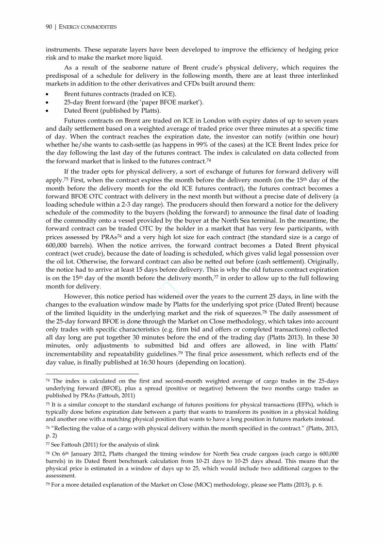
90 | ENERGY COMMODITIES
instruments. These separate layers have been developed to improve the efficiency of hedging price risk and to make the market more liquid.
As a result of the seaborne nature of Brent crude’s physical delivery, which requires the predisposal of a schedule for delivery in the following month, there are at least three interlinked markets in addition to the other derivatives and CFDs built around them:
Brent futures contracts (traded on ICE).
25-day Brent forward (the ‘paper BFOE market’).
Dated Brent (published by Platts).
Futures contracts on Brent are traded on ICE in London with expiry dates of up to seven years and daily settlement based on a weighted average of traded price over three minutes at a specific time of day. When the contract reaches the expiration date, the investor can notify (within one hour) whether he/she wants to cash-settle (as happens in 99% of the cases) at the ICE Brent Index price for the day following the last day of the futures contract. The index is calculated on data collected from
the forward market that is linked to the futures contract.74
If the trader opts for physical delivery, a sort of exchange of futures for forward delivery will
apply.75 First, when the contract expires the month before the delivery month (on the 15th day of the
month before the delivery month for the old ICE futures contract), the futures contract becomes a forward BFOE OTC contract with delivery in the next month but without a precise date of delivery (a loading schedule within a 2-3 day range). The producers should then forward a notice for the delivery schedule of the commodity to the buyers (holding the forward) to announce the final date of loading of the commodity onto a vessel provided by the buyer at the North Sea terminal. In the meantime, the forward contract can be traded OTC by the holder in a market that has very few participants, with
prices assessed by PRAs76 and a very high lot size for each contract (the standard size is a cargo of
600,000 barrels). When the notice arrives, the forward contract becomes a Dated Brent physical contract (wet crude), because the date of loading is scheduled, which gives valid legal possession over the oil lot. Otherwise, the forward contract can also be netted out before (cash settlement). Originally, the notice had to arrive at least 15 days before delivery. This is why the old futures contract expiration
is on the 15th day of the month before the delivery month,77 in order to allow up to the full following
month for delivery.
However, this notice period has widened over the years to the current 25 days, in line with the changes to the evaluation window made by Platts for the underlying spot price (Dated Brent) because
of the limited liquidity in the underlying market and the risk of squeezes.78 The daily assessment of
the 25-day forward BFOE is done through the Market on Close methodology, which takes into account only trades with specific characteristics (e.g. firm bid and offers or completed transactions) collected all day long are put together 30 minutes before the end of the trading day (Platts 2013). In these 30 minutes, only adjustments to submitted bid and offers are allowed, in line with Platts’
incrementability and repeatability guidelines.79 The final price assessment, which reflects end of the
day value, is finally published at 16:30 hours (depending on location).
74 The index is calculated on the first and second-month weighted average of cargo trades in the 25-days underlying forward (BFOE), plus a spread (positive or negative) between the two months cargo trades as published by PRAs (Fattouh, 2011)
75 It is a similar concept to the standard exchange of futures positions for physical transactions (EFPs), which is typically done before expiration date between a party that wants to transform its position in a physical holding and another one with a matching physical position that wants to have a long position in futures markets instead.
76 “Reflecting the value of a cargo with physical delivery within the month specified in the contract.” (Platts, 2013, p. 2)
77 See Fattouh (2011) for the analysis of slink
78 On 6th January 2012, Platts changed the timing window for North Sea crude cargoes (each cargo is 600,000 barrels) in its Dated Brent benchmark calculation from 10-21 days to 10-25 days ahead. This means that the physical price is estimated in a window of days up to 25, which would include two additional cargoes to the assessment.
79 For a more detailed explanation of the Market on Close (MOC) methodology, please see Platts (2013), p. 6.

To meet the change to 25 days in the assessment window and so to support the expansion of the notice period to at least 25 days before delivery, ICE has introduced a new futures contract (Brent NX), which expires on the 25th calendar day preceding the first day of the futures contract month to meet developments in underlying markets. However, the old contract (15th day) is still very liquid and it will take some time to replace it. The new assessment of the physical price (Dated Brent) is based over a 10- to 25-day window assessment of end-of-trading day prices of trades of BFOE cargoes collected by Platts with relevant criteria for liquidity purposes (average size, etc.), expands the set of physical transactions that are part of the assessment (about two cargoes of 600,000 barrels), and also changes the 25-day BFOE forward (as its secondary trading is based on the new Dated Brent price). The delivery time (with the new Dated Brent) in the following month for the old futures contract might be now less than 20 days.
Nevertheless, rather than a pure physical transaction, the Dated Brent should be more accurately seen as a forward contract with delivery between 10 and 25 days ahead (Downey, 2009). Dated Brent will be a floating price even during the delivery window. The divergence with the first month futures contract shows some seasonal patterns, since the delivery point is regularly under maintenance every year, but the spread has been widening in general in recent months, as liquidity of underlying physical remains a concern for the market (Figure 56).
Figure 56. Dated Brent vs Brent first-month futures contract intermonth spread (bbl), 2011-2012
Source: Platts.
On a particular date, the price of Dated Brent will reflect the price of oil delivery between 10 and 25 days ahead, and will roll over one day every day. For instance, on September 28th, the price will reflect delivery between October 7th and 21st. During the loading window (at least three days) and from 25 days before, the buyer will be exposed to the floating Dated Brent price with no possibility to fix the price by buying the corresponding BFOE forward for that month (already expired). The best way to hedge would be to buy the following forward month (fixed price, implied 25 days), but there would still be exposure to basis risk between the BFOE forward and Dated Brent.
In this case, another financial layer comes into play. Contracts for Difference (CFDs) allow the buyer to receive the price of the Dated Brent in exchange for the next-month forward price (a swap), so the total cost for the buyer will be the forward month at the day in which he/she wanted to hedge plus or minus the differential between the forward (held by the buyer) and the Dated Brent at the day of delivery. Whether a buyer is receiving physical delivery of a futures contract or is purchasing it himself, he would eventually need to get into a CFD to hedge basis risk at delivery date. The alternative can be a Dated to Front Line (DFL) contract, which is a swap between the Platts Dated Brent and the ICE Brent futures front-month prices. However, most of the transactions involve forwards, as they are seen as a closer approximation of the final Brent spot price (dated). Being based on an OTC market, with few traders and significant trade size, the transparency of such transactions is

92 | ENERGY COMMODITIES
low and trades are not linked to a system for the immediate delivery of the commodity or to inventories of BFOE oil.
Brent can be delivered in any of the four grades and the Forties quality is usually delivered, which is cheaper with a 44° API. PRAs publish the ‘de-escalator’, to discount the lower quality grade from the final price. Quality of delivered crude oil comes with the notice of the loading schedule.
Finally, there is another kind of price transformation that is regularly used for pricing of physical transactions. For instance, exports pricing of oil to Europe (and also sometimes to other regions) from Saudi Arabia relies on a Brent futures weighted average price of all trades (BWAVE), published on a daily basis.
Box 5. Price reporting agencies (PRAs) in crude oil price formation mechanisms: the right of judgement
Behind the complex interaction between futures and forward contracts lies the important role of price reporting agencies (PRAs) in assessing prices for key underlying physical markets. Over the years, PRAs have been an important tool for providing greater transparency in physical commodities markets where there are no legally binding transparency obligations for counterparties. Their price assessments have also helped price formation in adjacent futures markets when illiquid market conditions emerged. Recently, their role in some crude oil prices has been attracting considerable attention. At the November 2010 G20 summit in Korea, leaders called for a more detailed analysis on “how the oil spot market prices are assessed by oil price reporting agencies and how this affects the transparency and functioning of oil markets” (IEA et al., 2011, p. 6). In an earlier report in 2009, IOSCO recommended that “futures market regulators should encourage private organisations that collect relevant fundamental commodity information to adopt best practices and should evaluate what improvements are appropriate to enhance fundamental cash market data and develop recommendations for improvements” (IOSCO, 2009, p. 12). In particular, to address the core concern about price assessments using information that may not reflect cash markets, IOSCO (2012) has called for measures to enhance the transparency and integrity of such tools. Notwithstanding that methodologies to collect information and assess prices vary among markets to reflect differences in product characteristics and interaction between supply and demand, a set of common standards and best practices could be harmonised across the PRA industry.
Combining data reliability, transparency and enforcement in an environment in which there is no legal obligation, so information is instead disclosed by companies on a voluntary basis, requires sound policies. In illiquid market conditions, PRAs may need to exercise careful editorial judgement to avoid rumours or market expectations based on low-quality information feeding into their price assessment when an insufficient number of arm’s length transactions is available. “In the event of a wide bid/offer spread, Platts will not average the bid and offer. Platts will evaluate market conditions and establish an assessment that in its editorial judgment reflects the transactable level of Dubai and Oman. Unusually high or low price deals will be scrutinized by Platts to discern whether the deal is fit for assessment purposes.” (Platts 2013, Dubai-Oman price assessment methodology, p. 15). In effect, PRAs such as Argus only exercise judgement when limited information is available about confirmed transactions. Actionable bids and offers, and other market data such as spread trades to include spread values between grades, locations, etc. (see Argus, 2013), would feed price assessments. Editorial judgement using available market data relies on a strict application of a methodology that should protect the assessment from the improper influence of market rumours, even if it may rely on transactions carrying lower quality information (such as spread trades based on arbitrage or outlier transactions). To ensure that judgement is impartial and accurate and the information disclosed voluntarily by companies is true, tests are usually applied to confirm the details of the transactions and their alignment with normal trading behaviour. Tests would also make sure that participants and the justifications behind trading actions are credible. Conflicts of interest policies, in addition, are typically adopted to create an environment of sufficient impartiality.
Like credit rating agencies, PRAs work in reputational markets that already provide incentives to comply with high quality standards. However, internal enforcement of methodologies requirements and external enforcement on the quality of information voluntarily disclosed by commodities firms might be a complex task that requires a minimum set of legal obligations. All entities that produce an assessment of prices (based on judgment) to be used for actual transactions should comply with common standards. Full transparency of methodologies, governance, and access to underlying data become crucial aspects for regulators to ensure the smooth functioning of the market. A regulatory framework for the provision of price assessment services and for the reliability of the information that firms are voluntarily disclosed

(e.g. market manipulation rules in the case of false or deceiving information) might ensure effective supervision by reducing monitoring costs and creating ‘public accountability’ for the performance of price formation mechanisms. Harmonised standards, through a common set of guidelines that may be voluntarily adopted or become listing requirements for products based on price assessments (IOSCO, 2012), appear to be a viable compromise to ensure reliability of benchmarks administrators, calculators, and publishers for submitters that want to avoid liabilities in the use of their data. However, legal obligations should be appropriately weighted to avoid prices assessed by PRAs becoming legally binding mechanisms of price formation. The voluntary nature of the disclosure by commodities companies and the right of judgement by the PRA would preserve mechanisms of competition among price assessors and so benefit the provision of efficient price formation mechanisms, in line with IOSCO (2012, p. 34). Excessive administrative and liability costs may reduce incentives to provide information voluntarily, even though a liquid price formation mechanism is in the interest of commodities firms. The principles proposed by IOSCO (2012) recognise the importance of PRAs and some of the abovementioned concerns, and suggest so far80 the implementation of the following guidelines:
Full transparency of the methodologies criteria used for price assessments (including how and why judgement is used) and data collection to increase public accountability.
An open process of consultation when changes are proposed to the market.
Standardised and transparent procedures for data submission and reliability (bona fide).
Strict requirements for assessors and tight supervision of a direct supervisor.
Organisational requirements (such as audit trails, identification, management and disclosure of conflicts of interest rules).
Open procedures for complaints.
Detailed information readily available to financial markets authorities.
External auditing to check adherence to methodology.
Recent principles published by the European Securities and Markets Authority (ESMA) push this regulatory action even further (driven by recent scandals, such the potential LIBOR and Dated Brent manipulations), by proposing to regulate the users of benchmarks as well on top of administrators, publishers, calculators, and submitters (ESMA, 2013). Legal obligations such as running a due diligence on administrator and calculation agent may be unnecessarily burdensome and create strong extraterritorial impact, on top of the high cost to supervise millions of transactions that regularly use recognised benchmarks for their pricing (e.g. mortgage contracts or physical forward sales).
Finally, a deeper look into market mechanisms that impede the development of more liquidity benchmarks, causing overreliance on price assessments, is needed. In effect, the natural tendency of the market (due to the nature of the commodity) to trade crude oil differentials structurally reduces the liquidity of underlying physical markets. A less fragmented supply behind key liquid benchmarks, by aggregating supply of crude with similar characteristics, would reduce the reliance on paper markets rather than pure spot transactions. Increasing competition and accessibility to a common market infrastructure (with more physical hubs and delivery points, for instance) of underlying physical supply would favour the creation of sounder and more efficient price formation mechanisms. Regulatory reforms (both for OTC derivatives and other financial instruments), through the objective of ensuring greater transparency in commodity derivatives, may become a catalyst to prompt more accountable and efficient oil pricing systems, with a limited number of financial layers and greater competition among physical players. The recent initiative by PRAs to introduce a voluntary code to harmonise best practices for price reporting organisations (PROs) is certainly a signal that the market participants are ready to discuss how best markets can move to the next stage of development.
80 The IOSCO review and national regulatory reviews are still ongoing. “In the event that IOSCO's review concludes that implementation has been ineffective, or that further steps are required to achieve the principles’ overall objectives, IOSCO will consider other options, such as recommending direct governmental regulation of PRAs by an appropriate authority with expertise in energy markets and/or the creation of non-government statutory self-regulatory organizations (both alternatives may require careful evaluation of the risks and benefits of such regulation by authorities responsible for energy matters and legislative action.” (IOSCO, 2012, p. 9)

94 | ENERGY COMMODITIES
Benchmarks divergence: temporary syndrome or long-term market development
In recent years, as part of their continuous process of reorganisation, oil markets have experienced interesting developments around their most commonly used benchmarks. These changes have been reflected in a striking divergence between Brent spot (front-month futures) and WTI spot (and futures), as illustrated in Figure 57. It appears that both indexes have recently been reflecting regional problems with pipeline (WTI) and seaborne (Brent) delivery, whether oversupply or supply shortage.
Figure 57. Brent-WTI nominal prices divergence
Source: EIA, Thomson Reuters and World Bank.
The WTI benchmark has historically been an important benchmark for international oil markets, in particular when the capacity of its infrastructure (based on a complex web of pipelines in the United States) was high enough in relation to the available supply. Growing demand and greater supply converging at a point of delivery (Cushing, Oklahoma) that has limited capacity and flexibility to support the international trade has diminished the role of WTI to reflect global trade, and aligned the benchmark with the regional balance of supply and demand, which is in oversupply due to oil imported from Canada to meet high refinery demand in part of the country. Inventories have therefore been constantly growing, pushing prices downward vis-à-vis the Brent price and causing prices to ultimately diverge (Figure 58).

Figure 58. Weekly US ending stocks excluding SPR of crude oil, January 2010 – November 2012 (k/barrels)
Source: EIA.
However, as a futures contract, WTI is still very liquid with a high number of active investors trading the standard contract (1,000 barrels). Delivery allows the flexibility of different lots, thanks to the pipeline infrastructure, which diversifies the number of physical traders. WTI futures market liquidity reflects the maturity of the market compared to Brent futures contracts (Figure 59), but it may fail to reflect the infrastructural issues that have caused the two indexes to take different paths.
Figure 59. Brent-WTI Volumes and open interest (contracts)
Source: Author’s elaboration from ICE and CME Group.
While the United States continues not to solve its infrastructure bottleneck to redirect the oil glut towards the international markets, the WTI will hardly regain its status of global benchmark for crude oil.

96 | ENERGY COMMODITIES
Figure 60. BFOE Production Volumes (kb/d)
Source: Spencer (2012) from BP, RBA, Statistics Norway, UK Department of Energy and Climate Change.
Even though its seaborne nature attracts today over 70% of international trade, the Brent benchmark does not seem to be in much better shape. Despite the recent additions to the underlying physical market (the latest one with Ekofisk in 2007), production volumes behind the Brent have declined at a high rate, opening a discussion about the stability and vulnerability of its price formation.
For a market based on a web of forward transactions among a few big market participants (and split between four market locations) that are used to assess market prices, a constant liquidity of supply is essential to keep price formation mechanisms orderly. A market with delivery through interconnected pipelines, in contrast, may not require the same level of liquidity as it does not rely on multiple financial layers, with futures front-month that usually do the job well and drive prices, and thus liquidity, in the underlying physical market. It can be easily delivered to the trader that requires delivery. In addition to this structural difference between the two markets, there is a constant underlying reduction of oil supply from the North Sea that could continue to undermine the quality of the benchmark.
However, the Brent futures contract is the futures market with the biggest underlying physical market (BFOE market) currently available to support international benchmarks. North Sea crude loading, though in slight decline, continues to be around 2 mb/d (Figure 61).
Figure 61. North Sea (BFOE) crude loaded (kb/d)
Source: ICE (2013) from Bloomberg data.

To sum up, crude oil markets are once again looking at developments that, combined with new non-conventional oil discoveries, may produce structural changes that reshuffle the current market equilibrium. The infrastructure issues and the potentially more difficult issue of dropping spare production capacity suggest that future scenarios for crude oil markets are still susceptible to important changes, which may bring up another reshuffling of current benchmarks, and perhaps the emergence of new ones in fast-developing areas.
A way forward?
A smooth price formation mechanism is a crucial tool to contain volatility, an important threat in capital-intensive industries. In industries with long investment lead times, volatility may impede the formation of stable expectations over future prices in investment decisions. This can affect both large-scale corporate investment in, and individual consumer decisions on, energy-consuming equipment, producing lock-in effects that can last years. Volatility occurring around an identifiable trend line, however, would not be as much of a problem. Investors would still be able to form expectations concerning the future of prices and factor in the volatility as a random element of risk that can be addressed with the appropriate financial techniques (within the process of financialisation discussed in Chapter 1). The problem arises when the pattern of price changes is distorted by ‘natural’ developments and no stable trend is detectable.
Volume of production is a necessary condition for a benchmark’s success, but volumes are not the only factor that can affect the functioning of a benchmark price. Among these factors are:
physical supply fragmentation;
market accessibility for supply and an efficient delivery system (e.g. through pipelines or seaborne);
a liquid futures market and investors accessibility; and
competition among commercial oil users.
As illustrated by Figure 62, oil markets rely on three pillars: supply security, price discovery and competition.
Figure 62. Stable and efficient oil markets
Source: Author.
The natural tendency of crude oil markets to trade differentials, due to the nature of the commodity, may reduce the liquidity of underlying physical markets. Fragmentation of supply sources may affect physical supply security, and so the efficiency of price formation, if the supply is not properly channelled into the underlying physical market backing benchmark prices. A less fragmented supply behind key liquid benchmarks, by aggregating crude with similar characteristics, would reduce the reliance on paper markets rather than pure spot transactions. Increasing competition and accessibility to a common market infrastructure of underlying physical supply (with
Stable and efficient oil
markets
Price discovery
Supply security Competition

98 | ENERGY COMMODITIES
more physical hubs close to supply areas and delivery points, for instance; see Luciani, 2011) would help the creation of sounder and more efficient price formation mechanisms. Whether one or multiple suppliers, accessibility of supply to the underlying physical market and stability of production (also linked to political stability) are essential factors to secure oil supply. An appropriate delivery system, ideally supported by major pipeline infrastructures, is crucial. Forms of public-private partnership to revamp investments in market infrastructure and aggregate supply, which is not immediately in the interest of producing countries, would be beneficial to price formation. For instance, Brent developed as an international benchmark during the 1980s partly thanks to tax support provided by the UK Government to those companies trading in the spot market for Brent (Fattouh, 2011).
A better price discovery system that attracts and stabilises demand against volatility and price risk (demand security) through a liquid futures market contributes to the long-term development of global liquid benchmarks. However, massive investments would be needed to build a proper delivery system and the overall infrastructure (including significant storage capacity in the area and a fast delivery system) needed to run a global exchange. Finally, changes in the form of trading and its transparency may improve and secure price discovery. For instance, the introduction of take-or-pay contracts (as was done for natural gas) could increase demand security (Luciani, 2011). Transparency of underlying physical markets at global level may be unreliable if there is no effective mechanism of enforcement. It can be rather dangerous to undertake policy actions on the basis of information that cannot be considered reliable and can therefore be used with strategic intent by producing countries, in particular. For instance, data on crude oil storage is subject to strategic behaviours by producing countries that often provide false or misleading information.
With regards to increasing competition in supply and demand, the reduction of entry barriers for suppliers and greater competition on the demand side would produce beneficial effects in addressing incentives to provide the market with the required supply for its efficient functioning. In addition, market power (essentially due to entry barriers) at upstream and downstream levels typically produces an effect of double marginalisation, i.e. the imposition of a (monopolistic or oligopolistic) mark-up by both producers and retailers of oil and its finished products. Greater vertical integration would increase benefit end-users and minimise the distortion in distribution caused by double marginalisation in favour of end-users (Luciani, 2011).
Table 30. Market organisation
Physical market setting Pricing complexity Liquidity futures
market Delivery points
Oligopolistic (low liquidity)
High High High
(US, EU, Middle East)
Source: Author.
To conclude, the market for crude oil relies on an oligopolistic setting with a pricing system that is a complex web of forward and futures contracts, and low liquidity. Futures markets, in contrast, are liquid and provide delivery points in the main regional areas, but in different blends and often at additional cost.

2.2 Natural gas markets
Natural gas is a fundamental resource for the world’s energy supply in its lightest form (methane), and can also be found in other forms of hydrocarbons (mainly ethane, propane and butane). It is the
second biggest commodity market by value of production, with a value of $1.24 trillion in 2012.81 In its
conventional form, it is typically found on top of oil and water reservoirs underneath the earth, because natural gas is a hydrocarbon like crude oil but with a hydrocarbon molecule that has only four or fewer carbon atoms. Natural gas can be transformed into liquid only at very low temperatures (up to -161.6° Celsius, depending on the number of carbon atoms). Natural gas is also greener in terms of emissions production and damaging substances for the environment. In its most common form (methane), it is mainly used for electricity and heating systems, while in other forms is widely used for petrochemicals, plastics, and blending for gasoline fuel. Those extracting oil are also those involved in the extraction of natural gas. Once it is pulled out of the ground, it is cleaned of impurities (such as water and other gases) and then transported through a network of pipelines. However, it can also be transformed in liquid form (liquefied natural gas, or LNG) and sent to more distant locations where pipelines cannot reach.
Natural gas can be found in conventional formations, as described above, or in ‘unconventional’ ones, such as shale (a very soft rock that may contain high quantities of natural gas). After recent significant discoveries (especially in the United States), the term ‘unconventional’ may become obsolete. Other unconventional forms are deep rock formations or non-porous sands that require very deep drilling and more effort to bring the gas up to the field. Because of this supply unpredictability, natural gas price trends now follow regional differences rather than a common global trend (see Figure 63).
Figure 63. European and US natural gas real prices, 1960-2012 ($2005/mmbtu)
Note: Natural Gas (Europe), average import border price, including the UK. As of April 2010 includes a spot price
component. Between June 2000 - March 2010 excludes the UK. Natural Gas (US), spot price at Henry Hub, Louisiana.
Source: World Bank.
81 Price is the 2012 annual average ($10.26 mmbtu; equally weighted) of: Natural Gas (Europe), average import border price, including the UK (as of April 2010 includes a spot price component and between June 2000 - March 2010 excludes the UK); Natural Gas (US), spot price at Henry Hub (Louisiana); and Natural gas LNG (Japan), import price c.i.f. (recent two months' averages are estimates). Data on price collected from World Bank Commodities Database. Global production in 2012 estimated at 121,101 million Btu (BP Statistics).

100 | ENERGY COMMODITIES
After showing similar price movements, reflecting strong and uniform growth across the globe, natural gas prices in Europe and the United States have begun to discount the large discovery of shale gas in the United States. While prices in Europe have continued to climb, as energy supply security is scattered across the continent, US natural gas prices have fallen since 2009. After the commercial exploitation of enormous shale gas reservoirs, US and EU prices have diverged and are likely to stabilise at two different price levels in the short term. This new plateau may also stabilise in the long term, as US demand is gradually replaced by solid demand from Asia.
2.2.1 Product and market characteristics: a promising future?
The composition and quality of natural gas82 varies depending on the place of origin. 83 Before natural gas can be used commercially, it must undergo a process to remove undesirable components. After processing, natural gas fulfils the characteristics of a search good as the calorific value (i.e. the heating value) and other parameters affecting distribution and combustion can be readily measured at the delivery point (by using a gas chromatograph, for example), limiting transaction costs. Commercial contracts require that the gas be delivered within a certain specification range. The composition of natural gas (which determines its heating value) may be changed to fit transport purposes (to LNG) or end-use requirements.
Natural gas is a combustible fuel and cannot be recycled. However, following non-energy use, especially when gas is used as a feedstock for chemical products, the resultant products may be recyclable. Production is equivalent to mining and extraction firms, so gas production (extraction) sites cannot be converted to extraction of other commodities. Gas is sometimes a by-product of oil production (associated gas). Gas production companies are often also involved in oil extraction activities. Natural gas processing plants cannot be easily converted and, even if a much easier refining process than oil products is required, separation of natural gas from water and other hydrocarbons may require different treatments and ad hoc equipment.
LNG is natural gas cooled down to approximately -160° Celsius. Once liquefied, its volume is
about 0.17% that of gaseous natural gas, meaning its energy density is about 600 times higher.84
Furthermore, LNG weighs merely 45% of the equivalent volume of water (IEA, 2004). This gives LNG a volume and weight advantage, making it easier to store and transport. However, liquefaction is
highly capital intensive85 and storage facilities are required both after liquefaction at the exporting
terminal as well as before regasification at the importing terminal (discussed further below).
Compressed natural gas (CNG) is natural gas compressed to a higher pressure (usually 220 atmospheres) and stored in containers designed for that purpose. It is used as a fuel for road transport vehicles, especially in public transport. Its volume is approximately 0.4% that of natural gas at standard pressure (thus its energy density is around 250 times higher).
82 Natural gas “comprises gases, occurring in underground deposits, whether liquefied or gaseous, consisting mainly of methane. It includes both ‘non-associated’ gas originating from fields producing hydrocarbons only in gaseous form, and ‘associated’ gas produced in association with crude oil as well as methane recovered from coal mines (colliery gas)” (IEA, 2004).
83 Consequently the average calorific value of natural gas varies across countries (all in mJ/cm): Netherlands 35.40, Russia 37.83, Algeria 39.17 and Norway 42.51. For 2009, the IEA (Golden Rules, 2012) estimates the global average gross calorific value of natural gas at 38.4 mJ/cm (at 15°C at a pressure of 101.325 kilopascals).
84 Also, “the composition of LNG is usually richer in methane (typically 95%) than marketable natural gas which has not been liquefied. … Calorific values for re-gasified LNG range from 37.6 mJ/cm to 41.9 mJ/cm” (IEA, 2004).
85 Chevron’s Wheatstone LNG project in Australia is budgeted at A$29 billion. Construction began in late 2011; first LNG shipments are expected for 2016.

Storage
Storage is an essential element of the natural gas supply chain for three main reasons:
Demand variability: it would not make economic sense to build enough production and transmission capacity to meet peak demand.
Price volatility: storage can be an attractive instrument to hedge against the commercial risk of very high prices during peak demand and limit the market power of suppliers.
Risk of supply disruptions: as natural gas is often transported over long distances and across national borders, storage provides the possibility to reduce the risk of supply disruptions that may otherwise occur for technical, political or commercial reasons.
Gas storage facilities can be grouped into two categories: seasonal and peak. Seasonal storage facilities are built to store huge volumes of natural gas for peak demand. Peak storage sites are commonly smaller, but are able to react quickly to sudden changes in demand. Storage of natural gas in unliquefied and uncompressed form has huge space requirements, and storage costs are site-dependent. Commonly used sites are (1) depleted oil and gas fields (a cost effective option, especially used for seasonal storage), (2) acquifers, and (3) salt cavities (relatively small but very good withdrawal rates allow for peak shaving activities) (IEA, 2004). Storage above ground is relatively rare, with LNG storage facilities being a notable exception.
The key characteristics of storage are summarised in Table 31. Working capacity is the amount of gas can be injected, stored and delivered in a given storage site. Deliverability refers to the rate of injection and withdrawal per unit time, here expressed as million cubic metres per day.
Table 31. Key storage characteristics
Source: Le Fevre (2013).
LNG offers potential for storage, as gas in its liquefied form has a much better energy per unit of volume ratio. Liquefaction is costly, however, and gas would need to be permanently kept at around -160° Celsius. LNG storage is thus mainly used for peak shaving. Note that LNG import and

102 | ENERGY COMMODITIES
export terminals also contain storage, which may add to their business case as traders can exploit the storage.
Storage facilities require significant amounts of ‘cushion gas’ to maintain the required operating pressure, which adds to the capital costs of a storage project (Table 32).
Table 32. Typical capital and operating costs for storage facilities
Source: Le Fevre (2013).
Investments in storage are not necessarily market-driven. In response to the January 2009 gas crisis, for example, the European Union has adopted a gas supply security regulation, stipulating that EU member states have to be able to deliver gas for at least 30 days of average demand, as well as in the case of an infrastructure disruption under normal winter conditions. Gas storages were identified as a vital means to meet this target.
In addition, storage facilities are needed to ensure the safe operation of the gas transmission and distribution networks. They may also serve market developments by providing ‘wheeling, parking and loaning’ at major interconnections, for example. Storage is also for commerce, such as for the management of take-or-pay contracts (Le Fevre, 2013).
Production and international trade
Production of natural gas has more than tripled since 1970, and it continues to grow as new sources are explored and new technologies improve extraction practices. As with other standardised commodities with full control over supply, production and consumption have been growing without significant imbalances (no more than a 2% of global production per year in over 40 years).
Figure 64. Natural gas production and consumption balance, 1970-2012 (bcm, % rhs)
Source: Author’s elaboration from BP stats.

The most important gas producing countries in 2011 were the United States (651 bcm, roughly 20% of global production) and Russia (607 bcm, or roughly 19%), as illustrated by Figure 65. Other notable producing countries include Canada (4.64%), Qatar (3.5%), Iran (5.65%), Norway (3.03%), China (3.15%), Saudi Arabia (2.76%), Indonesia (2.38%) and the Netherlands (2.41%). Production in Brazil (0.5%) and India (1.4%) is rather low.
Figure 65. World gas supply by region, 2011 (bcm)
Source: Author’s elaboration from OPEC.
Exporting countries, however, are scattered across the world, with Eurasia, Norway and newcomers such as Qatar among the top exporters (Figure 66).
Figure 66. Exports by region (%)
Source: Author’s elaboration from OPEC.

104 | ENERGY COMMODITIES
On the import side, while Russian and US imports have declined in line with the growing internal production to achieve a more balanced position in the medium term, European and Asian demand has been increasing in the last five years (Figure 67) as a result of important decisions, such as the end of nuclear energy power in Japan and new Chinese policies to increase energy diversification.
Figure 67. Imports by region (bcm)
Source: Author’s elaboration from OPEC.
As natural gas becomes one of the key sources of energy production in the old continent, European dominance in natural gas imports grows, and so the continent’s dependence on international markets. The international market for natural gas has been growing steadily in the last decade, and in 2011 was worth almost $400 billion (Figure 68).
Figure 68. International trade for LNG, 1999-2011 ($bn)
Source: Author’s elaboration from World Bank, OPEC, and BP. Note: Price used in this chart is a simple average
of: Natural Gas (Europe), average import border price, including the UK (as of April 2010 includes a spot

price component and between June 2000 - March 2010 excludes the UK); Natural Gas (US), spot price at Henry Hub (Louisiana); and Natural gas LNG (Japan), import price c.i.f. (recent two months' averages are estimates). Data on price collected from World Bank Commodities Database.
The value of today exports is almost 35% of total production value, while in 1999 it was only around 20%. Also due to fast developments in technologies for LNG tankers and gas transportation, natural gas is the market that has experienced the fastest growth (in relative terms) of international trade in the last decade.
Gas reserves and stocks
Technically recoverable natural gas resources are still abundant – totalling 790,000 bcm (Table 33). At 2011 levels of gas consumption, these resources would be sufficient to meet world gas demand for the next 235 years.86 Eastern Europe/Eurasia (mainly Russia) and the Middle East together hold 58% of the remaining conventional gas resources, but only 17% of the remaining unconventional gas resources.
Table 33. Remaining technically recoverable natural gas resources by type and region, end 2011 (in tcm)
Total Unconventional
Conventional Unconventional
Tight Gas
Shale Gas
Coalbed methane
E. Europe/Eurasia 131 43 10 12 20
Middle East 125 12 8 4 -
Asia/Pacific 35 93 20 57 16
OECD Americas 45 77 12 56 9
Africa 37 37 7 30 0
Latin America 23 48 15 33 -
OECD Europe 24 21 3 16 2
World 421 331 76 208 47
Source: IEA WEO, 2012
While there are only limited conventional natural gas resources left in OECD countries, discoveries of unconventional resources (especially shale gas) have radically changed the picture. This holds particularly true for the United States (mainly shale gas), Canada and Australia (coalbed methane), but also potentially in the future for China (huge shale gas resources) and India. Europe
also has some shale gas resources (in Poland, the United Kingdom and Ukraine, for example).87
As a result of the abundant gas reserves, supply-side elasticity to demand is fairly high in the long term. However, for producers it may be difficult to adjust production levels upwards at short notice (a lengthy permitting process, exploratory seismic work may be needed, drilling and connecting wells to pipelines will take time, etc.). Downward adjustment is sticky as well (reservoir and wellbore characteristics would often not allow simply restarting production later; associated gas depends on combined oil and gas business case).
The impact of abundant supply in the United States, for instance, has caused a sharp increase in the stock-to-use ratio (Figure 69), which may be subject to a rebalance as the supply adjusts to new levels of demand and supply capacity.
86 This is, of course, a rather crude estimate, as demand is expected to rise in the future, technically recoverable does not mean economically and environmentally viable, and resource estimates are generally quite uncertain, especially in non-OECD countries.
87 See also Annex.

106 | ENERGY COMMODITIES
Figure 69. US stock-to-use ratio
Source: Author’s elaboration form BP stats.
Gas transportation
Freight costs are significant due to the low energy density and may, in some cases, exceed exploration and extraction costs. Gas trade is still dominated by pipelines, which are characterised by high fixed costs and long lead times. LNG is gaining market share, especially over long distances. Distribution networks require important upfront investments, but they may reduce total transportation costs once the network is up and running.
Pipelines account for 68% of total gas trade (IEA WEO, 2012), dominating gas trade especially over smaller distances. In long-distance high-pressure pipelines (made of steel, with diameters of 40 to
120 centimetres), gas moves at roughly 30 km/h.88 Construction costs vary widely both across
countries and time, depending inter alia on labour costs and the market price of steel. High fixed costs and long lead times are key, especially when pipelines span over a number of politically unstable countries, and so the transit dimension becomes important (Yafimava, 2011).
88 Source: Total website.

Box 6. Liquefied natural gas (LNG): a long-term solution for gas transportation?
As gas resources are distributed all around the world, and most continents cannot be connected to each other by pipelines, LNG infrastructure will play a central role in determining to what extent the globalisation of gas markets takes place. While pipelines generally remain the most common means of gas trade, LNG is already responsible for 42% of interregional gas trade (IEA WEO 2012). Global LNG trade volumes more than doubled between 2000 & 2010 (JRC 2012), clearly exceeding the increase in gas demand.
LNG regasification terminals are technologically more flexible than pipelines and therefore give less leverage to suppliers. Yet, at the same time, LNG liquefaction facilities are destination-flexible, meaning that producers can, in principle, export to any country with available LNG regasification capacity.
Planning and building an LNG liquefaction terminal takes 4-6 years, and they are expected to run for at least 20 years (with corresponding amortisation). Depending on the assumptions being made about amortisation and discount rates, liquefaction costs some $2-3 per mmbtu. Global regasification capacity represents roughly 2.5 times the global liquefaction capacity (JRC, 2012). There is therefore potential competition for LNG among consumers.
The total transportation capacity of the world’s LNG fleet (some 360 vessels in early 2013), with an average capacity of approximately 150,000 square metres, is around 54 mcm.89 Shipping via LNG vessels is relatively fast; while faster LNG vessels may reach some 50 km/h, LNG vessels commonly travel at an average of 35km/h. Shippers may adjust their speed based on their expectations about the development of the gas price. The number of shipping days and the associated time to conclude the transaction between trading partners of course vary widely depending on the distance. Some averages for common trading partners are reported below (transport and regasification costs in brackets; Argus Media):
1 day for shipments from Algeria to France and Spain (transport and regasification costs per mmbtu: ~$0.15).
7 days for shipments from Indonesia to South Korea and Japan (~$0.80).
8-9 days from Nigeria to France or Spain (~$0.90).
8-9 days from Australia to Japan and South Korea (~$0.90).
13-14 days from Oman and Quatar to South Korea and Japan (~$1.50).
20 days from from Algeria to South Korea (~$2.00).
Insurance costs are about 2% of total shipping and storage costs.
Henderson (2012) presents data on the hypothetical case of future large-scale LNG exports from the United States. He assumes liquefaction of natural gas to cost approximately $3/mmbtu. Transportation on an LNG vessel from the United States to Europe is around $1.3/mmbtu, from the United States to Asia (through the Panama Canal) would be approximately $3/mmbtu. Regasification costs are some $0.4/mmbtu.
Table 34. The delivered cost of US LNG exports to Europe and Asia ($/mmbtu)
Note: For the Asian figures Henderson assumes that the Panama Canal will be able to service LNG vessels as of 2014. Source: Henderson (2012, based on Cheniere Energy data).
Since LNG requires only limited connection to pipelines and, on average, lower investments in infrastructure than for crude oil, costs of transport are a key factor in LNG price. Due to this differential, LNG price has been significantly diverging from benchmark prices (Figure 70), though this difference may stabilise in the future.
89 More precise data on LNG can be found in Argus Media’s ‘Global LNG’ monthly, for instance.

108 | ENERGY COMMODITIES
Figure 70. LNG price versus US and EU benchmarks, 1960-2012 (nominal prices)
Source: World Bank. Note: Natural Gas (Europe), average import border price, including the UK. As of April 2010
includes a spot price component. Between June 2000 - March 2010 excludes the UK. Natural Gas (US), spot price at Henry Hub, Louisiana
Due to its easy transportability and flexibility to environment with no relevant pipelines infrastructures, LNG demand in areas such as China and Japan has been steadily increasing over the years and these areas have become the main source of demand for LNG global production (Figure 71).
Figure 71. Global LNG delivery (by region; mcm/day)
Source: Waterborne LNG from Rogers (2011).

The future of LNG is still uncertain. On the one hand, sustained demand from the East would keep demand solid for some time. On the other hand, new exploration and discovery of unconventional sources of natural gas may cast doubt on the sustainability of this continuous market expansion.
Natural gas can be also compressed to form CNG, which provides the advantage of fewer infrastructure requirements than for LNG and pipelines. The disadvantage is that is requires more space than LNG due to its lower energy density. Thus, while CNG could not compete with LNG at high volumes, it may be a promising transport option for small and remote gas fields (so called ‘stranded gas’). However, seaborne CNG transportation technology has not yet reached commercial
scale.90
2.2.1.1 Supply characteristics: a competitive international market
Natural gas is produced in all of the world’s regions. Exploration and extraction of natural gas are capital intensive, as gas producers must sustain initial sunk and subsequent fixed costs (generally somewhat higher for offshore and unconventional gas). For a more detailed discussion, see the section on crude oil.
The gas industry can be divided into three parts – upstream, midstream and downstream. Upstream activities refer to natural gas exploration and production. The midstream gas business includes the gathering system, processing, compressor stations, LNG terminals, underground storage facilities, as well as the gas transmission grid, hubs and market points. The downstream oil sector is a term commonly used to refer to the selling and distribution of natural gas to consumers. Note that midstream activities are often also grouped with downstream activities.
Upstream industry structures differ widely around the globe. While the United States is best
known for its so called ‘(super)majors’ – large ‘fully integrated’91 multinational oil and gas companies
(e.g. Chevron, ExxonMobil, ConocoPhilips, and Hess Corporation) – it is also home to a lot of ‘independents’ – small oil and gas companies focusing on the upstream business (e.g. Apache
Corporation, Devon Energy, and Pioneer Natural Resources).92 The US historically had regulated
wellhead prices which were completely abolished in 1989. Taken together, this creates a truly competitive upstream industry that is able to secure investments in high-risk projects, such as those that eventually resulted in the ‘quiet’ shale gas revolution that was originally driven by the independents. Producers are publicly listed or privately held companies (see 0).
In Europe, large integrated oil and gas companies dominate the upstream industry, with
smaller independent energy companies being a rather rare phenomenon.93 Apart from the United
States and Canadian companies who are often also active in Europe, important producers include BP, BG, DONG Energy, EBN, ENI, OMV, Shell, Statoil and Total. While European producers are generally publicly listed, in some countries governments still own a substantive share (67% of Statoil is owned by the Norwegian government and the Italian government holds a 30% ‘golden share’ in ENI). For most Europe-based producers, exploration and production activities in other parts of the world exceed those in Europe, given Europe’s limited endowment with natural gas.
In most other parts of the world, resource-rich countries usually control oil and gas producers, and they control the largest share of proven world natural gas reserves. Unlike the United States and European majors, their upstream activities are generally focused on their home country. Notable examples in the Middle East inlcude Saudi Aramco, the National Iranian Oil Company, Qatar Petroleum, Iraqi Oil Ministry, Kuwait Petroleum Corporation and Abu Dhabi National Oil Company. Russia’s most important gas producer is Gazprom, but Rosneft also has significant reserves. Major African gas companies include Sonatrach (Algeria) and Nigerian National Petroleum. Asia is inter alia
90 http://www.investmentu.com/2012/May/cng-natural-gas-transportation.html.
91 The major explore for and produce oil and gas around the world, own pipelines and tankers, and sell these products directly.
92 Canadian producers include Nexen and Vermilion Energy.
93 Of course, exceptions exist, e.g. UK-based Cuadrilla Resources.

110 | ENERGY COMMODITIES
home to Petronas (Malaysia), Pertamina (Indonesia) as well PetroChina (large shale gas reserves). In the non-US Americas, Pemex (Mexico) and Petroleos de Venezuela feature among the most prominent examples.
In most OECD countries and all of the European Union (as well as parts of the Energy Community), the organisation of the gas market has been affected by the liberalisation/deregulation agenda and especially the so-called ‘unbundling’ requirements. The main idea behind this is to separate the competitive part from the uncompetitive (natural monopoly) part of the industry. As a consequence, vertically integrated companies were (and are) required to sell their transmission assets (full-ownership unbundling) or at least create some form of independent transmission operator (legal, functional and accounting unbundling). Requirements for distribution systems go in a similar direction, but are generally less advanced. So far, the United States has been far more effective in ensuring third-party access to pipelines and storage facilities than the European Union, which is still struggling to provide “clear, non-discriminatory, timely and repeatable” market rules (JRC, 2012).
In the non-OECD world, things look considerably different and the gas industry is often in the hands of one or a few vertically integrated state companies. Yet, reforms are on the way, notably in China, where wellhead and transport prices are currently tightly regulated. More to the point, the Chinese government wants to implement a comprehensive pricing reform by 2015. Key components of the reform are a complete deregulation of wellhead prices and the setting of a maximum wholesale price linked to the price of imported fuels, including a 10% discount to encourage gas use. In the two provinces where the pricing reform has already taken effect on a trial basis, it has resulted in wholesale prices of $11-12/mmbtu. (IEA WEO 2012)
Liberalisation has had an impact across all of the gas supply chain. Upstream, regulated wellhead prices were only abolished completely in the United States in 1989. Midstream, third-party access to pipelines and storage makes a difference, allowing for the entry of new market participants. Downstream, unbundling requirements for distribution system operators may create more retail competition. The different levels influence each other. In particular, decisions taken in a number of major economies to prohibit long-term take-or-pay contracts for distribution system operators (e.g. in the United States in 1984 and Germany in 2010) heavily constrain companies that are active in the midstream business. In Germany, for example, midstream companies found themselves unable to pass the prices of their often oil-indexed LTC on to consumers, once spot prices were significantly lower.
If there were a global gas market, market concentration on the supply side (upstream) would be very low as gas resources are abundant and large numbers of companies are active in the upstream gas business. Yet, due to high transportation and storage costs, gas markets remain rather regional, and pipelines with high sunk costs and long lead times often bind buyers and sellers to each other. The LNG ‘revolution’ is currently changing the picture (increasing destination and origin flexibility). Regional differences remain significant, though. While the United States has a highly competitive upstream industry including the (super) majors as well as independents, in Europe the upstream industry is more concentrated (with strong historical incumbents complemented by the US majors). In the other parts of the world – which control the largest share of proven gas reserves – the market is commonly in the hands of one or few state-controlled companies.
The demand side (midstream and downstream) suffers from natural monopoly problems (gas networks and storage). Liberalisation efforts (unbundling and deregulation) have created some competition in OECD countries (especially the United States and the United Kingdom), but market concentration is still high in many markets. Vertical integration is still dominant in most other parts of the world, where market concentration is thus very high.
A list of the price formation factors for LTC, sales and wholesale gas markets on the supply side (Horstmann, 2011) follows:
Oil price (LTC). Coal price (substitute in power generation). Exploration and production costs. Transport and storage. Taxes.

2.2.1.2 Demand characteristics: dealing with high elasticity
Natural gas is a major energy source, representing 22% of world energy demand in 2010 (IEA WEO, 2012). The demand for gas is projected to rise in the future, at a compound annual growth rate of 0.7-1.9% between 2010 and 2035, depending on the scenario (IEA WEO, 2012). Most growth will come from non-OECD countries due to their higher rates of economic growth and currently underdeveloped gas markets.
In 2011, the world’s gas demand amounted to 3,361 bcm (IEA MTGMR, 2012).94 While natural
gas is used all across the world, the top natural gas consuming countries in 2011 were the United States (690 bcm, 20.5% of world gas demand), the EU-27 (489 bcm, 14.5%), Russia (483 bcm, 14.4%),
Iran (150 bcm, 4.5%), China (132 bcm, 3.9%), and Japan (121 bcm, 3.6%).95
Currently, the non-OECD world accounts for 52% of world gas demand (IEA WEO, 2012). In recent years, gas demand has grown rapidly in many emerging economies (especially in Asia) and this trend is expected to continue in the future (see below). However, the share of gas in total primary energy demand is still much lower in the BRICs, with the exception of Russia (Brazil 9%, Russia 55%, India 8%, China 4%).
Figure 72 demonstrates that, while sectorial gas use varies by region, power generation is generally the largest consumer of natural gas. Natural gas is also used in buildings (mainly for space and water heating), in industry (e.g. steel, glass, paper, fabrics, brick), in energy sectors other than power generation (oil and gas industry operations), for non-energy use as a raw material (e.g. paints, fertiliser, plastics) and in transport (natural gas vehicles).
Figure 72. 2011 World sectorial gas demand by region (in bcm)
Source: IEA Medium-Term Gas Market Outlook, 2012. Note: ‘Other’ includes energy industry own use, transport
and losses; ‘industry’ includes fertiliser.
Numerous substitutes for natural gas exist for most uses. The degree of substitutability of gas in power generation is, in principle, very high as a power system can be entirely based on other sources
such as nuclear, hydro or coal.96 However, investments in most forms of power-generation are rather
capital intensive (especially nuclear) and thus rather long-term (some 15 years for a combined cycle gas turbine, or around 50 years for nuclear). In addition, the construction of new generation capacity requires certain lead times; nuclear projects especially may take decades until they are finally built. In
94 Natural gas figures are reported in various units. This chapter gives volume data in billion cubic metres (bcm) and energy data in million British thermal units (mmbtu, sometimes also denoted MBtu). When volume data is given, it refers to natural gas at 15°C at a pressure of 101.325 kilopascals.
95 Data are from IEA Medium-Term Gas Market Outlook, 2012.
96 An example of a national power system that does not rely much on natural gas but rather coal is that of Poland.
0 100 200 300 400 500 600 700 800 900 1000
OECD Europe
OECD Americas
OECD Asia Oceania
Latin America
Africa
Middle East
FSU/Non-OECD Europe
Non-OECD Asia (excl. China)
China
Residential-commercial Industry Power generation Other

112 | ENERGY COMMODITIES
heating, the second largest user of natural gas in the OECD, gas can be substituted by oil, electric power, and biomass. In industry, substitutes for substitute natural gas can be produced from lignite or biofuels. As regards transport, oil, biogas, hydrogen and electric power are possible substitutes. Note, however, that transport is a globally irrelevant gas user at the moment.
Generally, the demand elasticity to price is relatively high due to the large number of substitutes available for natural gas. However, elasticity may become lower in the short term due to significant sunk costs for natural gas users (gas-fired power plants, heating systems, etc.) and long lead times and high capital costs for substitutes (especially nuclear power). Elasticity in the power sector is higher if spare capacity is high (e.g. with old coal-fired power plants in the United States) or trade is possible (e.g. in the interconnected European electricity market).
Natural gas demand is affected by a large number of variables at different time frames.97 On an
(intra)daily basis, gas demand varies according to temperature (e.g. more space heating if it is cold), time of the day (more water heating in the morning when people take a shower) as well as the workday/holiday schedule (less industrial demand during public holidays and weekends).
Gas demand is also influenced by seasonality (increased demand for heating in winter), geography/climate (more demand for heating in colder areas), as well as level of economic development (higher gas consumption in more prosperous regions).
Long-term drivers causing changes in gas demand are related to “policy, geopolitics, economics, technology and environmental concerns” (IEA ETP, 2012). The International Energy Agency has identified the following key drivers (IEA ETP, 2012):
Access to supply and infrastructure (availability of gas, fuel production from other sources, upstream and downstream infrastructure, distribution networks).
Economic development (increased gas consumption due to increased demand for heating, electricity, and industrial goods).
Competiveness of natural gas prices versus other sources (e.g. coal, nuclear, biogas, hydrogen).
Environmental impact of using other forms of energy (greenhouse gas emissions, which, if internalised, also affect the competiveness of natural gas vis-à-vis other sources).
Changes in technology (efficiency in power generation or combustion processes, electric heating, natural gas vehicles).
In the very long term, climate change may also affect gas demand through its impact on temperatures (‘global warming’) and weather patterns.
Factors that may affect the demand side are:98
Temperature (heating). Weather (seasonality). Timing affects of consumer behaviour (time of day, holidays). Long-term influencing factors are:
Product substitution. Economic changes. Political decisions and policies (e.g. environmental policies). Expansion and decommissioning of existing gas producing/transport capacity.
Consider this fragment from Horstmann’s presentation (2011):
Customers build up supply portfolios geared towards hub price levels and forward quotations. High availability of volumes decreases value of flexibility. Mix of different price elements requested but all based on forward price level: fixed prices for different maturities, gas price indexation, options, oil indexation (but oil indexed at much lower levels compared to LTC). Majority of customers request offers from multiple suppliers, unfortunately rather based on opaque tender processes rather than the market place (via exchanges or broker screens).
97 Effects may also vary depending on the level of analysis (individuals, households/ firms, countries and regions).
98 See also the previous section on product characteristics.

2.2.1.3 Key product and market characteristics
Product and market characteristics for natural gas provide a challenging array of key drivers of price formation:
The product is non-renewable or recyclable, and production cannot be converted to alternative commodities (only partially to crude oil extraction, but not refining).
Product substitutability is high, which increases the incentives for international firms to expand horizontally. This type of integration, however, is still infrequent and limited to crude oil.
Natural gas is mainly used for electricity production, but it can also be used for a few other purposes (production of plastics, etc.). Partial alternative uses and a capital-intensive production create incentives to integrate business vertically. Most natural gas firms are vertically integrated.
Storability is long but stocks are subject to seasonality and may be subject to unpredictable patterns in terms of new peaks during the consumption season.
Freight costs have an important impact on total costs, but they may be a valid substitute to long-term and large investments in infrastructures (such as new pipelines) for some regions.
Elasticity of demand is very high and adjusts quickly to developments in the fundamental interaction between supply and demand through market prices. Supply is slightly more rigid as it requires a capital-intensive producer to adjust quickly an expensive production process, but full control over supply greatly simplifies the implementation of this decision.
The international market for natural gas is fairly competitive, even though the nature of the commodity has naturally created small oligopolistic settings in regional markets.
Emerging markets are gradually shifting to natural gas, as infrastructures become ready in several areas, and energy strategies require these countries to focus on independence through source diversification.
Demand and supply of natural gas are projected to be higher in the future, in particular if new cheap sources of gas are discovered and can be exploited with limited impact on the environment.
Table 35. Product and market characteristics
Recycling/
Production convertibility
Substitutes/ Horizontal integration
Alternative uses/ Vertical
integration
Capital intensity
Stora-bility
Freight costs
Elasticity to price/ demand
Concen-tration
BRICs weight
Future Consumption/
Production
Demand side
None High Medium
High Medium Medium
High
Medium
High High
Supply side
Low Medium High Medium High High
Source: Author.
2.2.2 Exogenous factors: the key role of government actions
Government intervention on the supply side of natural gas is most pronounced in those countries where gas production is still nationalised. In OECD countries, governments sometimes provide significant tax breaks to the upstream gas industry, for example in the United States where this has arguably been important in laying the foundations for the shale gas revolution. Regulated wellhead prices may have a negative impact on production rates. In the United States, this practice was abolished as early as 1989; China has recently started the liberalisation process. (IEA WEO, 2012).
On the demand side, governments of gas-producing countries sometimes provide subsidies to keep the price of natural gas artificially low, stimulating demand. Regulated gas retail prices are still common even in OECD countries, which is potentially positive for demand, but negative for investments. A carbon price would increase the competitiveness of gas vis-à-vis coal, but in the long run might favour nuclear or renewables wherever these sources are substitutes. As carbon prices are either non-existent or relatively low (even in the European Union), the impact of this form of

114 | ENERGY COMMODITIES
government intervention has so far been limited. The OECD has recently published a comprehensive
fossil fuel subsidy report (OECD, 2012).99
Natural gas demand is affected by a large number of exogenous factors such as economic development (and crises) or policy decisions which particularly matter when they affect the competitiveness of natural gas vis-à-vis its substitutes, in the field of environmental policy (climate change, air pollution), for example, as well as industrial and innovation policy (promoting renewables or nuclear power, direct government spending toward innovative technologies).
Major disasters, such as Fukushima, may also play a role in influencing gas demand.
New rules, such as the Regulation on Energy Market Integrity and Transparency (REMIT), play an important role in improving levels of physical markets price transparency for regulatory purposes (i.e. market monitoring purposes), but also has an important role in improving transparency of fundamentals (e.g. gas production capacities, unplanned outages and planned maintenance, etc.). Transparency of fundamentals is different from price transparency but is also important for efficient and effective markets. The European Union’s 3rd Energy Package has already brought in new transparency of fundamentals requirements for natural gas (and power), and regulators, such as the Agency for the Cooperation of Energy Regulators (ACER) and its predecessor the European Regulators’ Group for Electricity and Gas (ERGEG), develop important regulatory technical guidelines on fundamental gas and electricity data.
Table 36. Exogenous factors in natural gas markets
Government intervention Main other external factors
High Oil prices, natural disasters
Source: Author.
2.2.3 Empirical analysis: weighing fundamentals
This section describes the results of the empirical analysis of natural gas markets. Data is monthly from 1st January 1994 to 31st December 2011. The dataset includes the settlement price of front-month contract traded on NYMEX. Prices are transformed in natural logarithms and deflated using the producer price index (PPI) published by the Federal Reserve. Data on US inventories are collected from the weekly working gas in underground storage provided by the Energy Information Administration (EIA) and also expressed in natural logarithms. The natural logarithm of the OECD
leading composite indicator100 for the United States (average of de-trended, smoothed, and
normalised component series) is used to capture the effect of demand and thus the economic cycle.
First, this section tests the fundamentals, i.e. the relationship between prices and key underlying factors, identified for natural gas as inventories and demand represented by the economic cycle (due to its fundamental use in electricity markets). To achieve meaningful results, an autoregressive integrated moving average (ARIMA) model was estimated, after having tested the Box-Jenkins methodology, which includes model identification and model selection through the analysis of autocorrelation and partial autocorrelation paths of the log real front-month price. Parameters are also estimated using the maximum log likelihood estimation, and the model has been checked through analysis of residuals.
As a result of this analysis, ARIMA (3,1,0), i.e. integrated of order 1 with 3 lags autoregressive and moving average equal to 0, appears to fit the dataset best.
The analysis finds that the front-month (‘spot price’) has a significant relationship with inventories and the economic cycle (see Output #17). The sign is negative for inventories and positive for demand factors, which confirms the important role of demand and supply fundamentals.
99 http://www.oecd.org/site/tadffss/ 100 For more info http://stats.oecd.org/Index.aspx?QueryId=6617.

Table 37. Regression output
Independent variable Coefficient (t-test)
US Inventories -5.1***
(-8.23)
US OECD 7.24***
(2.66)
Note: ***1%, **5%, *10% significance
Source: Author’s estimates.
The results confirm that underlying factors affecting supply and demand are drivers of price movements. Since gas prices are regional benchmarks, the impact of exchange rates has not been included.
The analysis also tests the impact of the futures curve on spot price.
A VAR Granger causality test was run between two variables and three lags taken in first difference to minimise risks of spurious regressions. This test (see Output #18) between spot price and futures contract with 4th delivery month maturity, i.e. the difference between the 4 delivery month futures contract negotiated on NYMEX and its front-month contract, suggests that the futures curve (contango or backwardation) may be driving spot prices, but the significance is at 10% and the coefficient is very low (below 0.1). However, this finding confirms the importance of the futures curve in price formation and its ability to absorb information about underlying physical markets and transfer this to inventory levels through the basis.
The same test was run against financial variables to measure the level of financialisation. Data in logarithms of the dollar monetary base (M2; seasonally adjusted stock value, published by the Federal Reserve System), interbank interest rate (Effective Federal Funds rate), and Standard & Poor’s 500 financial index (at close) are tested against the spot price. No statistically significant link emerged between any of these indicators and prices of natural gas (see Output #19).
2.2.4 Market organisation: a European and a US model?
There are various kinds of natural gas prices, whether wholesale prices (hub prices, border prices, city gate) or end-user prices (industrial, household). Components of natural gas prices include the cost of gas supplies, transmission, distribution and storage costs, retailer's margins and taxes. Both wholesale and retail prices vary widely across regions, and regulated prices are still common in the non-OECD world. Competing fuels include oil, electricity, coal (see Section 2.2.1), whose price development therefore impact on gas prices.
There are three price formation mechanisms:
1. Gas-to-gas competition based on offer and demand in wholesale and sales markets. 2. Oil-indexed LTCs for importing gas based on worldwide oil markets/FX. 3. Regulated prices.
There is no such thing as a global natural gas price,101 as shown in Figure 73. Until 2006, average natural gas prices in the United States, Europe and Asia were correlated with the oil price. This correlation ended for US gas prices as early as 2006. European gas prices have deviated significantly from oil price developments since 2010, and at the moment only Japanese LNG import prices follow oil prices.
101 As a consequence, each region has one or several price benchmarks that are only partly linked to one another. For North America, Henry Hub (a distribution hub located in Louisiana) prices are generally taken as a benchmark. When talking about European gas prices, one usually distinguishes at least between BAFA CFI (average German border import prices as reported by BAFA - Federal Office of Economics and Export Control) and NBP (National Balancing Point: The British virtual gas hub operated by TSO National Grid, covering all entry and exit points in mainland Britain. The British virtual gas hub operated by National Grid, covering all entry and exit points in Great Britain). For Asia, Platt’s JKM (Japan Korea Marker) may serve as a proxy.

116 | ENERGY COMMODITIES
Figure 73. Natural gas real prices in the United States, Europe and Japan, 1992-2012
Source: World Bank Commodity Price Data. Notes: Europe: average import border price and a spot price
component, beginning April 2010 including the UK; during June 2000 - March 2010 prices excludes the UK; US: spot price at Henry Hub, Louisiana; Japan: import price, CIF. Data in $2005/mmbtu and $2005/bbl. Annual prices.
Figure 74. Global gas price linkages
Source: Rogers (2012).
While the oil price is still highly relevant for wholesale price formation in continental Europe, through long-term contracts (indispensable tools to finance a costly network infrastructure), and the

OECD Pacific, one should not forget that most parts of the world, namely those that are not as dependent on imports, follow a different logic. Gas-to-gas (between gas supplies) competition on spot markets is prominent in North America, the United Kingdom and parts of continental Europe (e.g. the Netherlands), representing one third of global gas demand (Figure 74). Prices in many other parts of the world are regulated, however, and may even be set below supply costs to reach specific policy objectives.
In late 2012, world gas markets can be described as follows (adapted from Rogers, 2012):
North America is a largely self-sufficient gas market with Henry Hub prices of around $3.50/mmbtu.
Europe has a ‘hybrid’ gas market: o Hub spot prices range from $8/mmbtu to $14/mmbtu. o Oil-indexed contract prices are at $11-$13/mmbtu, meaning buyers will only satisfy their
take-or-pay commitments and purchase additional demand on sport markets, while trying to renegotiate their long-term contracts.
Asia has highly heterogeneous gas prices: o LNG contract prices range from $4/mmbtu to $18/mmbtu. o Spot cargoes arrive at around 15$/mmbtu (in Japan – at times linked to European hub
spot prices with a transport margin and premium).
While gas producers respond to price signals, it is difficult to adjust production levels at short notice. In case of increasing demand, production cannot be stepped up at short notice but needs longer lead times. The reason is that the process for granting permits, exploratory seismic work, and drilling and connecting wells to pipelines will take at least six months, usually longer. In addition, productivity rates of existing and planned wells are subject to uncertainty.
If demand declines and prices fall below the short-run marginal costs of production, an immediate halt to production may not be an option as reservoir and wellbore characteristics will often not allow simply restarting production once prices go up again. In addition, gas is sometimes a by-product (associated gas) of oil production, so even if low gas prices make production uneconomic, the combined oil and gas business case may look different. Also, companies may hedge their production at higher gas prices, one of the factors that explain why US gas production remained constant even when US gas prices fell below $2/mmbtu (IEA WEO, 2012). Furthermore, producers sometimes have to accept obligations to produce certain minimum volumes, perhaps as part of the licensing process.
The majority of internationally traded gas is traded under long-term contracts, usually 10-25 years (IEA WEO, 2012). Gas prices are often indexed to the oil price (oil products or crude oil),
limiting the possibility for arbitrage.102 While this was logical in the 1970s when burning gas was an
alternative to using oil in both power generation and heating, nowadays this logic has become obsolete in most parts of the world.
As with oil, traded market price transparency for natural gas is high because traded market prices (i.e. spot prices and forward delivery prices) are identified and published by a range of price reporting agencies, as well as by commodity futures exchanges to a limited extent. In addition to the traded markets, much natural gas is sold under long-term supply contracts, where transparency is mixed. Outside of the United States, many long-term gas contracts have historically been indexed to oil prices. But since the precise formulas are hardly ever made public, and since there is a wide range of ways that oil indexation is achieved in practice (e.g. indexed to various specific crudes, and/or to a combination of different oil products such as fuel oil and gasoil in bespoke proportions), levels of transparency for oil-indexed contracts is relatively low. In recent times, there has been a move toward greater use of indexation for spot gas prices in long-term contracts. While again the precise formulas used are confidential to the counterparties and not released, gas indexation arguably improves the
102 Excluding the possibility of renegotiation, there are two scenarios that limit arbitrage opportunities. First, if spot prices are higher than oil-indexed prices, the annual contract quantity level (ACQ) represents the maximum availability of oil-indexed imports. Second, if spot prices are lower, take-or-pay clauses represent the minimum level of oil-indexed imports.

118 | ENERGY COMMODITIES
degree of price transparency for long-term contracts because transparency in the spot gas markets is high and gas-on-gas indexation provides a high price correlation, unlike gas-to-oil indexation.
In traded natural gas markets, pricing is straightforward with contracts generally agreed on an absolute price (fixed price) basis. They can also sometimes be agreed in reference to a natural gas fixed price in a neighbouring market (a cross-border basis trade), or a fixed price for a different time period (e.g. a Q4-Q1 spread contract), but usually with a fixed price market at its centre. This type of contract takes into account regional differences, since its use is driven by the aim to maintain a stable relationship due to high sunk costs invested in pipelines and networks to link with the other party.
Financial instruments do not normally play a direct role in the pricing of a physical product. To the extent that financial contracts in natural gas are actively traded, their primary purpose is as tools for the management of price risk (e.g. swaps, options, etc.). While most LNG is traded under long-term contracts, just like internationally traded pipeline gas, there has been a shift to more flexible arrangements, partly as a result of very liquid markets (Figure 75). Besides North American projects, Rogers (2012) expects Australia, Qatar and Nigeria to become the most important players in global LNG supply.
Figure 75. World short-term LNG trade, 2000-2011
Source: IEA WEO (2012). Note: Short-term means trade under contracts of four-year duration or less, including
spot transactions.
Transportation and trade may be affected by government intervention both positively, through pipeline subsidies, and negatively, by failing to provide the regulatory incentives for network expansion or export restrictions (the United States is very reluctant to grant export licences for natural gas). (Trade) wars as well as resource nationalism come to mind. Also, long-term gas supply may increase as a result of government spending on innovations in drilling or exploration technologies. But governments may also enter into (free) trade agreements, facilitating the transportation of natural gas across national borders.
In Europe, gas pricing is undergoing major changes. The traditional oil product-linked gas is increasingly being questioned in the European Union, and the price for oil, as a competing source of energy, no longer plays a role in several major European wholesale markets. It is reasonable to expect that hub-based pricing will gradually take over. This poses challenges to existing long-term contracts, some of which may become untenable. The period up to 2014-15 is often considered a transitional one, which may eventually result in a new pricing and contractual gas framework. Yet, how this will look is still uncertain, partly because it does not only hinge upon economic fundamentals, but also has an important legal dimension. Here, the outcome of the antitrust case that the European Commission has brought forward against Gazprom may question the practice of oil-indexed gas pricing.

Figure 76. European trading hubs and connectivity
Source: Rogers, 2011.
Granted, the future is always uncertain, but with a view to gas pricing it nevertheless seems worth pointing to major market developments. Rogers (2011) singles out four of them:
Asian Natural Gas and LNG demand.
US Future Shale Gas Production Growth and potential scale of North American LNG exports.
Timing/slippage of new non-North American LNG projects.
Production versus pricing policy for European pipeline gas suppliers post oil-indexation.
As a consequence, drawing upon scenario analyses, Rogers (2012a) points to the key challenges for major players:
European pipeline suppliers will have to hope for high Asian demand, otherwise the availability of LNG will effectively push down European prices. Large-scale North American LNG exports could de facto imply a price ceiling for pipeline suppliers as well.
The commercial viability of North American LNG exports depends on high Asian demand and a European hub (NBP) ‘target price’, maintained at the expense of volume sold by European suppliers.
US upstream gas producers are vulnerable to low Asian demand when US production is high, even when European pipeline suppliers maintain a target supply floor. This does not make for “an attractive environment for upstream producers as it perpetuates the problems observed in 2011 of supply-driven inventory surpluses and low prices [...] an intensely competitive environment”.
For Asian LNG producers and buyers, low Asian demand would imply finding ‘new customers’ in the Atlantic Basin markets (or delaying projects in anticipation of such).
Finally, in order to handle important changes such as greater production flexibility and risk management of a more competitive environment (with liberalisation), futures markets are indispensable tools to deal with seasonality factors. As mentioned above, there is no global benchmark price for natural gas, but rather a futures index for Europe (NBP run by ICE) and a futures contract for the United States (Henry Hub natural gas traded and cleared on NYMEX). Futures markets, however, play a limited role for pricing of spot natural gas transactions through long-term contracts. The size of open interest over physical market is in a low range (see Section 1.3.1).

120 | ENERGY COMMODITIES
Table 38. Natural gas market organisation
Physical market setting Pricing complexity Liquidity futures market Delivery points
Competitive Medium Medium Limited (EU, US)
Source: Author.
Due to multiple sources of natural gas spread across different locations, the physical market setting is fairly competitive, and complexity is limited to pricing formulas for long-term contracts. Futures markets are liquid but benchmark for specific regional areas; no global benchmark has emerged. Delivery points for the futures contract are limited to a few regional locations set by the exchange, but this does not affect the efficiency of market structure since futures for this commodity reflect fundamental changes in their respective region.

121 |
3. RAW MATERIALS AND INDUSTRIAL METALS
3.1 Iron ore market
Iron ore is one of the biggest commodities market in the world (second only to crude oil), and its
yearly production is valued at around $300 billion.103 As with other mineral ores such as bauxite, iron
ore is an example of a commodity that has one main use – the production of steel. Up to 98% of the
iron ore produced worldwide is used for steel production (Yellishetty et al., 2010).104 It therefore plays
a crucial role in commodities markets as the principal source for steel production, which represents 95% of all metals production (Yellishetty et al., 2010). However, the commodity has particular product and market characteristics that other commodities do not have. Like few other raw materials, iron ore does not have a fully-fledged global liquid futures market that can ensure control over an ever-changing market environment, because it has been unable so far to develop a globally recognisable physical spot price. Market organisation is evolving, however, from a swap-based market to a futures-based market as new benchmark prices for physical markets develop (e.g. The Steel Index 62% for Chinese iron ore, or the IODEX 62% CFR-North China price run by Platts; Figure 77).
Figure 77. IODEX (62% CFR North China) Spot Price ($/tonne)
Figure 78. Iron ore nominal prices ($/tonne)
Source: Platts. Source: World Bank. Note: Iron ore (Brazil), VALE (formerly CVRD) Carajas sinter feed, contract price, f.o.b. Ponta da Madeira. Unit dry metric ton unit (dmtu) for mt 1% Fe-unit.105
103 At January 2013 value of TSI Iron ore CFR China 62% Fe ($147.5/tonne).
104 The remainder (typically, with magnetite content above 70%) is mainly used to wash coal form ashes (in heavy media process) and for cement manufacturing. In form of hematite, this ore can also be used for the preparation of electrodes.
105 Prior to year 2010, only annual contract prices.
0
50
100
150
200
250
20
09
-01
-05
2
00
9-0
2-2
6
20
09
-04
-23
2
00
9-0
6-1
8
20
09
-08
-11
2
00
9-1
0-0
2
20
09
-11
-25
2
01
0-0
1-2
1
20
10
-03
-17
2
01
0-0
5-1
1
20
10
-07
-06
2
01
0-0
8-3
0
20
10
-10
-25
2
01
0-1
2-2
0
20
11
-02
-16
2
01
1-0
4-1
1
20
11
-06
-06
2
01
1-0
7-2
8
20
11
-09
-20
2
01
1-1
1-1
1
20
12
-01
-09
2
01
2-0
3-0
6
20
12
-04
-30
2
01
2-0
6-2
5
20
12
-08
-17
2
01
2-1
0-1
1
20
12
-12
-07

122 | RAW MATERIALS AND INDUSTRIAL METALS
The old price setting based on long-term yearly-renewed contracts changed in 2010, after pressure from the market. It has led, on the one hand, to a reduction of the assessment period for many long-term (volume) contracts to even earlier than a month (Figure 78), while new spot prices (indexes) have emerged around key consumption areas and have also become references for several long-term (volume) contracts (Figure 77). Prices, in the meantime, have become more volatile and reached a historical peak, also in real terms (Figure 79).
Figure 79. Iron ore real price ($2005)
Note: Iron ore (Brazil), VALE (formerly CVRD) Carajas sinter feed, contract price, f.o.b. Ponta da Madeira. Unit dry metric ton unit (dmtu) for mt 1% Fe-unit. Prior to year 2010 annual contract prices.
Source: World Bank. Note: Source: World Bank.
The structural shift in real prices is so prominent that it may not only reflect the growth of emerging economies, but also the changes in the market microstructure and price formation mechanisms. The jump in price also factors in the growth of spot transactions versus long-term (volume-based) contracts. More flexible market solutions come at a cost to be charged by mining companies in the short term due to high fixed and sunk costs.
3.1.1 Product and market characteristics: the key industrial commodity
Iron ore is a ‘pure’ intermediate commodity that in general cannot be recycled (except for some uses, e.g. coal washeries), though its main derived product (steel) can be re-used for similar or alternative uses without losing its original properties as a metal. Steel scrap is the only viable alternative material used for steel production. Additionally, as with other mining operations, the production of iron ore (extraction and the first refining process) cannot be converted to other raw materials. It is highly dependent on steel demand.
There are at least six categories of ores (hematite and magnetite are rare ores with the highest iron content of 70%, on average) from which iron ore can be commercially extracted (the iron content should be at least above 25%). Alternative uses of these fines are very limited. Iron ore is mined in two forms: lump, and fines. However, it can also be sold in pellets, which increase productivity in steel production because the fire in the furnace can escape through the air flows created by the material.
Production
After a long period (1968-2002) below 1,000 megatonnes, world production of iron ore has more than doubled since then, as China entered the WTO in 2001 and implemented the removal of tariff restrictions by 1st January 2004. Production spiked in 2011 at over 2,000 megatonnes (2 billion tonnes).

Figure 80. Iron ore world production (megatonnes)
Source: Australian Bureau of Resources and Energy Economics (ABREE 2012).
Today, China is by far the biggest importer, and the second biggest producer, in the world (Figure 81). China is second only to Australia, which produces roughly 25% of global production, and ahead of Brazil (20% of global production).
Figure 81. Top four iron ore producing countries, 2004 and 2011
Source: Author’s elaboration from ABREE (2012).
Despite being one of the biggest producers on earth, China is still a net importer of iron ore due to its large manufacturing economy, as well as the low quality of its iron ore production (taking into account its low-quality ores, its real production should be halved to around 200 megatonnes; see Figure 83). This makes the country a price-taker at the global level. In 2011, China held a 60% global share of imports in iron ore, with 65% of net imports as a percentage of world imports (IMF, 2011), despite its position as second largest producer, and its consumption has not eased much since the collapse of financial markets in 2008 and resulting spillover effects on the global economy.

124 | RAW MATERIALS AND INDUSTRIAL METALS
Figure 82. Importers by countries and regions, 2011 (mn/t)
Figure 83. Chinese Iron ore demand, 2000-2017F
Source: Author’s elaboration from ABREE (2012). Source: CRU.
International trade
International trade and the emergence of new economies based on heavy industries have played a key role in market structure developments in iron ore and the new pricing mechanisms. Before the early 2000s, the size of iron ore production and cross-border trade was a small fraction of its peak in 2011.
Figure 84. International trade ($mn)
Source: Author’s calculation from World Bank and Australian Bureau of Resources and Energy Economics (ABREE, 2012).
The size of exports vis-à-vis production levels grew to around 50% towards the end of the 1990s. Due to its supply concentration, the growth of iron ore as a seaborne market has also contributed to the growth of its cross-border trade.
0 Mt
200 Mt
400 Mt
600 Mt
800 Mt
1000 Mt
1200 Mt
1400 Mt
Import Production Consumption

Box 7. China’s entry in the World Trade Organisation
China’s entry in the WTO is perhaps the most important event for international trade in the last two decades. After a 15-year process, China was admitted to the WTO on 11th November 2001 after requesting to resume as contracting party of the General Agreement on Tariffs and Trade (GATT) in 1986 and requesting to enter the WTO in 1995, when the institution was established. Commitments to remove tariffs and other restrictions, already started before the accession, were mostly met by the end of 2004 when China became a fully-fledged global trade partner in the WTO. The opening up of its economy began back in 1979 (Rumbaugh and Blancher, 2004) and had since gathered pace . Entry in the WTO has led China to reconsider, among other commitments, the following (WTO, 2001):
Discriminatory practices between Chinese and non-Chinese WTO members.
Dual-pricing practices for domestic and export products.
Price controls to protect domestic firms.
Updates to current regulatory framework to reach international standards.
Full right to export and import in the country.
Export subsidies for agricultural product.
Despite some exemptions from these commitments (cereals, tobacco and minerals, among others), the deadline for the implementation of these commitments was three years from accession (December 2004). Since 2001, China has been easing many of these restrictions, even though there are several areas where further improvements are needed. Agricultural policies, renewable energy technologies, electronic payments and insurance regulation are some of the key areas (USCBC, 2010).
China has become the third largest global exporter and is very close to overtaking the United States (Table 39). Despite losing ground, the European Union remains well ahead of China as global trade partner, however.
Table 39. Top global exporters and China (% of total exports)
2001 2003 2011
European Union 40.1% 42.0% 35.1%
United States 13.1% 10.9% 9.6%
Japan 5.8% 5.6% 4.2% (4th)
China 3.9% (5th) 5.2% (4th) 9.5% (3rd)
Source: Author’s elaboration from World Bank.
The gigantic growth of China is also clearly reflected in net imports. In particular, the explosion is visible for net imports in raw materials and metals, reaching around 14% and 30% of global imports, respectively.
Figure 85. Chinese net imports (% of world imports)
Source: IMF (2011, p. 4).

126 | RAW MATERIALS AND INDUSTRIAL METALS
Active global trade accounts are also reflected in consumption levels, with China becoming the top global consumer of iron ore, aluminium, copper, and soybean oil in 2011. It is among the top three global consumers for crude oil (2nd), wheat (2nd), corn (2nd), sugar (3rd), and natural gas (4th). No major levels of consumption emerge for cocoa and coffee, but the Chinese weight is constantly growing over time in these markets too.
Table 40. China’s ranking in key commodities markets, 2001-2011/2012
Production
(top 10; % tot)
Consumption
(top 10; % tot)
Exports
(top 10; % tot)
Imports
(top 10; % tot)
2001 2011/2012 2001 2011/2012 2001 2011/2012 2001 2011/2012
Crude oil 7th
(4.4%)
5th
(4.9%)
3rd
(6.3%)
2nd
(11.1%) no no n/a
2nd
(14.9%)
Natural Gas
n/a
(1.2%)
6th
(3.1%)
n/a
(1.1%)
4th
(4.1%) no no n/a
10th
(1.2%)
Iron ore n/a 2nd
(22.9%)
n/a
(13%)
1st
(50%) no no n/a
1st
(60.2%)
Aluminium 2nd
(13.5%)
1st
(41.8%) n/a
1st
(41.5%) no no 5th * 10th
Copper n/a 1st
(26.4%) n/a 1st no no n/a 1st
Wheata 2nd
(16%)
2nd
(7.7%)
2nd
(18.5%)
2nd
(17.9%) no no no no
Corna 2nd
(19%)
2nd
(15%)
2nd
(1.8%)
2nd
(22.4%) no no no no
Soybean oila
4th
(12.4%)
1st
(26.2%)
2nd
(14.7%)
1st
(28.9%) 3rd 1st no no
Sugara 5th
(5.2%)
4th
(7.2%)
5th
(6.7%)
3rd
(9%) no no 7th 4th
Cacao no no no no no no 9th 8th
Coffee no no no no no no no no
*In 2003. a2012 estimate. Source: Author’s calculation from IMF Database, BP, OPEC, ICSG, USDA and other governmental authorities.
For agricultural commodities, such as wheat and corn, not much has changed in the last decade in terms of consumption levels, as the population is gradually stagnating and alternative use of biofuels production is still in early development. Overall, however, China has become the top global commodities consumer. It is unquestionable that China, over time, will need to make more efficient use of current resources as the energy-intensive nature of its manufacturing economy and its ageing population will put additional unstable pressure on commodities prices if the country does not increase its independence from external provision of low-cost resources. The more China increases in size, the more its weight on commodities markets may become unsustainable (at least in the short term) if competing global players do not reduce consumption levels. This situation might be seen as an incentive to finally increase efficiency in the use of global resources, but it will take years before relevant changes may see the light.
3.1.1.1 Supply characteristics: a Cournot equilibrium?
Due to its remote location from areas of consumption, most of the iron ore used for international trade is seaborne, accounting for roughly 50% of global iron ore production. Fines make up most of this (67%), while lump ores (15%) and pellets (11%) play a smaller role. Global proven reserves are estimated at 170,000 megatonnes (USGS, 2012), which would last for roughly 80 years at the current production/consumption rate. However, iron can be found in several types of ores that are quite common on earth and which still need to be explored. Additionally, efficiency in the production of steel and its increasing substitution with other metals (e.g. aluminium) could potentially ease the pressure on increasing production. The substitutability of the product is limited to steel scrap on the demand side. Iron ore is mainly treated and used for steel production, and its final usability is limited. Despite its direct use for steel, vertical integration with steel producers is very limited. Production

requires a huge amount of capital and stable flows to cover high fixed costs (mainly energy costs), on top of the limited storability of these ores. The storability period for this commodity varies among the different types of iron ore produced. In general, though, iron ore is limited since the commodity is bulky and its properties require costly storage facilities and huge capacity (which may reduce commercial viability). The flexibility of production to demand is limited, which does not attract steel producers. As storage of iron ore is costly and storability is limited, supply becomes more rigid and freight costs become a key item of the total price charged to end-users.
On the supply side, iron ore mining companies are typically large companies also involved in the extraction of other important minerals and raw materials (e.g. BHP Billiton and Rio Tinto). A few producers are vertically integrated with steel producers to exploit economies of scale, while others rely on long-term contracts (3-5 years). Integration with the steel industry has historically been limited due to national interests in keeping supply national and therefore fragmented, thus limiting economies of scale. Iron ore production is instead fairly integrated horizontally with other mining activities of raw materials (e.g. copper). Integration is a key feature of capital-intensive production with high fixed costs. Barriers to entry are high, mainly due to:
Exploration costs (for good quality iron ore).
Extraction costs (licenses, transport, infrastructure).
The need for ‘deep pockets’ (acquisition of local mining companies).
A complex pricing system (periodic negotiations about reference/benchmark price for the different ores and regions).
Table 41. Top ten producers, 2011
Million tonnes
% World
Vale 309 17
Rio Tinto 181 10
BHP Billiton 159 8.2
Arcelor Mittal 50 2.7
Anglo American 46 2.6
Fortescue 39 2.1
Metalloinvest 38 2.1
Cliffs 37 2.1
System Capital 31 1.7
NMDC 30 1.7
Source: Storm (2011) from Raw Materials Group.
Figure 86. Market share of seaborne trade
Source: Crowson (2011) from Raw Materials Group.
Despite initial investment constraints, iron ore capacity and the marginal cost of production are reasonably predictable in the short term. In addition, low demand elasticity (Chang, 1994; Hellmer, 1997), concentration in seaborne iron ore (the top three control roughly 65% of the global seaborne market; Figure 86), the homogenous nature of the product, and the system of long-term contracts (meaning one or a few regional prices prevail in international trade), ensure that the market organisation of supply follows an oligopolistic model à la Cournot (Cournot, 1838; Farrell and Shapiro, 1990; Hellmer, 1997; Warell and Lundmark, 2008). Each firm knows and assumes as ‘fixed’ (in that period) the quantity of output the other firms will produce, and acts accordingly. Therefore, firms end up setting the quantity as a reaction function of other firms’ production, which can be estimated through data on mine capacity. Brazil is deemed to exploit a first-mover advantage in the European market (Hellmer, 1997) and Australia may have the same role in the Asian market. The ability to move the market by setting quantities is certainly more relevant for top companies that control most of the seaborne iron ore market. However, transaction costs (e.g., the need of high production volumes) may lead to deviations from equilibrium, and may ultimately reduce incentives to collude.

128 | RAW MATERIALS AND INDUSTRIAL METALS
The oligopolistic setting is often influenced by external factors, such as freight industry capacity and easier (cheaper) connectivity between regional areas. Freight costs are an important part of the seaborne iron ore price and can expose the market to unprecedented volatile patterns. For instance, freight costs (C3) in 2008 went down from 200% of FOB Brazil iron ore price to less than 10% in roughly six months (Figure 87). In other periods, it was more convenient to buy iron ore from Brazil and ship it to China instead of buying Chinese iron ore (Figure 88). However, recent changes with the increase in capacity of the freight industry have stabilised costs of freight for some time and ensure easy connectivity at the global level. This may increase the accessibility of new regional areas to the global market and reduce space for an oligopolistic setting as marginal costs become less predictable, so players can more easily defect to increase their profits. Small producers may even agree to non-profitable prices to win contracts, potentially creating a market imbalance that can move the market away from a Cournot equilibrium.
Figure 87. Freight cost (C3) as a % of FOB Brazil price
Source: ICAP.
Figure 88. Price differential China and Brazil ($/tonne)*
Source: ICAP. *Including C3 freight cost106
Globalisation also increases the likelihood that liquid spot prices may emerge and increase competition with other reference benchmark prices. These two factors can have a long-term impact on the supply setting. As a consequence, this static model would gradually become more dynamic (also on the basis of the lower profitability and stagnating demand) and induce big players to foster further industry consolidation to reduce the threat on seaborne trades of new regional markets. As today, production is geographically concentrated in a few countries, but things may change.
Finally, additional supply constraints are technological barriers to improving the production chain and making more efficient use of resources. Production also generates pollution, including CO2 emissions, while energy consumption requires access to cheap energy.
3.1.1.2 Demand characteristics: rigidity versus pro-cyclicality
In line with supply characteristics, demand is also inelastic and, despite the large vertically integrated steel producers, steel manufacturers are price-takers and fragmented among regional areas. Demand is clearly inelastic at least in the short run, however. Over longer periods, prolonged downward cycles could put the industry at risk of oversupply if market conditions do not stabilise in the medium term. For this reason, over the years the market has developed forms of long-term contracts to deal with supply and demand rigidity and to limit this instability. Contracts have been used to get credit from the banking system and develop production further. Emerging markets are also leading countries in the production process, and also through the constant growth of demand, which will drive future production and consumption (Figure 89).
106 C3 Freight cost is the benchmark cost of ship transport for bulk commodities from South America to Asia.

Figure 89. China and rest-of-the-world (ROW) iron ore consumption and seaborne demand
Source: BHP Billiton Iron Ore Growth and Outlook (2012).
Although the global economy has reduced its rate of growth, demand forecasts still remain solid, with seaborne iron ore demand growing at a faster pace as Chinese demand consolidates.
3.1.1.3 Key product and market characteristics
Key product and market characteristics of iron ore reflect a market for raw materials with:
High sunk costs.
Limited alternative uses and storability of the commodity.
Rigidity of supply.
Inelastic demand with limited cyclical patterns.
Moderate, but growing, industry concentration.
Emerging markets as important players on the supply and demand side.
Future consumption/production that is not going to slow down soon and that, together with the development of cross-border trade, has been driving significant changes to market structure.
Table 42. Key product and market characteristics
Recycling/ Production
convertibility
Substitutes/ Horizontal integration
Alternative uses/Vertical integration
Capital intensive
production
Stora-bility
Freight costs
incidence
Elasticity to price/ demand
Concen-tration
BRICs weight
Future
Consumption/ Production
Demand side
None Low Low
High Medium High
Low
Medium
High High
Supply side
Low Medium Medium Low High High
Source: Author.
3.1.2 Exogenous factors
Government intervention is mainly limited to countries where the government owns the mining companies (e.g. India) or to some countries where demand is far higher than production. Some restrictions to trade are applied in countries where demand is very high, such as China (10%) and India (10% on lump and 5% on fines). India may become a net importer now the Supreme Court has blocked mining activities that it claims are illegal. However, government intervention in other countries has also followed other directions. Most iron ore companies are private or have been privatised in the last two decades, so government interference is much lighter than in other raw materials markets. Additional government interventions are concentrated in supporting investments
130 | RAW MATERIALS AND INDUSTRIAL METALS
in infrastructure to increase capacity and distribution. Several projects have been financed, or have been proposed, to create iron ore pipelines in continental regions and production facilities typically need access to railways and commercial ports to ship materials promptly. However, the role of governments to ensure that the country can benefit from its own resources is still important. Governments (such as Brazil) have therefore sponsored privatisation of national companies to achieve greater economic efficiency (Schmitz, 2004). On the demand side, government intervention in iron ore is more occasional and not of a relevant size.
Table 43. Key exogenous factors
Government intervention Main other external factors
Demand side Low Economic cycle
Political instability Supply side Medium
Source: Author.
Global actors, such as the European Union, are increasingly looking for cooperation to promote discipline in international trade through dialogue and WTO dispute settlements (EU COM, 2011). Other initiatives to promote global standards, to reduce barriers to trade and to limit political instability may also result in a less volatile environment. Finally, as for other raw materials and base metal production, environmental standards are important to reduce pollution and make production sustainable in the long term. Anecdotal evidence shows the environmental impact of production can have long-term implications, not only for the local population through negative externalities (costs), but also for the profitability of the company. Efficiency in the use of resources and minimum environmental requirements could become global standards across commodities markets for international trade.
3.1.3 Market organisation: designing a new market structure
Pricing of iron ore in physical markets has historically been done through LTCs that are revised periodically. After the collapse of the annual pricing system in 2010, LTCs are still used for volumes (typically up to five years) but the price is revised periodically or is continuously linked to benchmark spot prices. LTCs with long-term volumes objectives are ‘bankable’, so they can be used to find financing and develop new mining and processing facilities that can improve capacity and efficiency in production and processing (Rogers and Robertson, 1987). LTC prices were originally revised every three to five years, then each year, but more recently even quarterly or monthly revisions have been introduced for contracts in Brazil. On the one hand, LTCs reduce fluctuations in price and move attention to the quality of the end product and long-term investments. There are many pricing models for LTCs and they can also rely on spot markets reviewed at a regular period. On the other hand, LTCs carry the costs of private negotiations if the difference in contractual power among the two sides and the information asymmetry are very high (the principal-agent model). Therefore, in a scarcely competitive environment, LTCs may help consolidation and rent creation, so ultimately increasing
costs for end-users. Spot prices contracts107, instead, allow parties to exploit short-term returns on
investments, and to reduce the dependency from contractual power and so the relative size of the counterparty negotiating the price. However, spot prices are exposed to bigger fluctuations as the market develops, and standardisations and other practices are required to make sure that the exchanged underlying product has standard qualities once the set of potential buyers and sellers widens. If not properly designed, market prices may paradoxically result in higher prices for end-users.
107 Anecdotal evidence estimates the number of spot transactions and LTCs based on a spot price to be roughly 50% of global transactions, with China being the leading actor.

Table 44. LTCs versus spot markets
LTCs Spot
Pros Cons Pros Cons
Lower volatility Information asymmetry Price efficiency Higher volatility
‘Bankable’ Deep pocket Market accessibility Fragmentation
Source: Author.
LTCs used to differ among regions (Warell and Lundmark, 2008). Iron ore LTCs for Japanese firms relied strongly on security of supply, stable prices, and a long-term relationship based on mutual cooperation, with infrequent revisions. European LTCs, however, have been more open to a market price with more frequent revisions (through a yearly spot contract, referred to as ‘evergreen’).
In regional areas where internal demand is constantly higher than supply, such as China, and industry concentration both on the demand (from the steel industry) and supply side is fairly low, spot prices have been emerging and are becoming a benchmark price for international trade. Pricing of iron ore LTCs is currently in constant motion to develop new pricing models. These prices are usually indexes, such as the Metal Bulletin Iron Ore (MBIO), which is based on a tonnage-weighted calculation of actual transactions normalised on iron ore content and freight of 62% iron (in Qingdao, China). Transactions from 58% to 66% are also eligible, and data is submitted by all segments of the industry – producers, consumers and other traders. Use of the index is limited to a small part of the market (mainly in China) and it has sometimes experienced difficulties in ensuring the quality of the iron ore delivered to users, but its diffusion worldwide will most likely continue. Other benchmark prices that may become global reference prices have been developed. For instance, The Steel Index (TSI) iron ore 62% Fe is used as a reference spot price for spot transactions on the Chinese mainland and for most swap transactions currently cleared on the Singapore Exchange (SGX). Platts IODEX is widely used as a basis for LTC pricing.
As physical market pricing develops, cash-settled swaps (over-the-counter bilateral transactions that are reported and centrally cleared on exchange) and futures markets (exchange-traded futures contracts) strive to emerge at global level. As today, the SGX is the top global exchange (followed by CME Group and Singapore Metal Exchange) in terms of iron ore swap trading (clearing) volumes. Despite losing market share to newcomers, SGX has increased the volume of OTC iron ore swap on its platform from 5,000 to 20,000 lots (over 10 megatonnes) in just over a year.
Figure 90. SGX Iron ore swap monthly volume (bars) and open interest (line)
Source: SGX.
While SGX and CME Group contracts track the TSI index, SMX refers to the MBIO index. All swap and futures contracts are cash-settled, as it is very premature to think about any warehouse system for iron ore. However, the market is still in evolution and – despite several initiatives that are gradually taking place – there is no global liquid futures market for iron ore yet. SGX, CME Group and SMX have launched futures contracts, but it may still be too early to draw any conclusion on their degree of development. It is unlikely that a single global price will prevail, as it would not reflect the diversity of the world steel market.

132 | RAW MATERIALS AND INDUSTRIAL METALS
Table 45. Key market organisation factors
Physical market setting
Pricing complexity
Liquidity swap/futures market
Delivery points
Oligopoly Low Low None
Source: Author.
Forward markets are estimated at 165 megatonnes per year (roughly 8.3% of total
production),108 which suggests growing activism to push markets to the next stage of development.
108 ICAP from undisclosed source.

3.2 Aluminium market
Aluminium has become a key commodity for sectors like construction, transport, aliments, new technologies and infrastructures over the years. It is one of the largest industrial metals markets, with
yearly production valued at around $107 billion in 2011.109 Its widespread use, in car manufacturing
or the beverages industry for instance, is due to special characteristics.
Figure 91. Aluminium usage by sector (% of total production)
Source: Alcoa.
The most important characteristics are low specific gravity (and low relative weight) at normal temperature, the ability to mix with other metals, resistance to corrosion, and high electrical and thermal conductivity. Its use continues to grow but at historically low real prices, due to greater industry capacity that has temporarily pushed markets in oversupply (Figure 92). Its diffusion is also led by its recyclability and high substitutability with steel or copper.
Figure 92. Aluminium LME cash real prices, 1960-2012 ($2005/tonne)
Source: World Bank.
109 Aluminium price from World Bank (2011 average price of LME 3-month cash) and data on production from ABREE (2012).

134 | RAW MATERIALS AND INDUSTRIAL METALS
The historical negative relationship between the cash price of aluminium and real interest rates (Frankel, 2006) also makes aluminium tightly related to the economic cycle, a sign of the key fundamental role that this metal has obtained in our economies, especially for transport and construction sectors.
3.2.1.1 Product and market characteristics: the key potentials of aluminium
Aluminium is produced from a raw material called bauxite, which is transformed into a refined material (alumina) and then into primary aluminium. The production of primary aluminium involves three stages. The first is the mining of bauxite, which is mainly located in South America, West Africa and Australia. The bauxite is mainly extracted with explosives and is then crushed and cleaned from impurities. After this first processing, bauxite is sent to alumina refineries that produce alumina through the Bayer process. This is typically done close to the mining area. The process involves several chemicals and results in alumina hydrate crystals that are then calcinated. Alternative processes (such as the Bayer-Sinter or Nepheline-based processes) typically require more energy and produce more residues, but they allow the use of a variety of aluminous materials with additional impurities, and residues can be used for some construction materials, such as cement. The final part of the process is the smelting of alumina into primary aluminium, which is the final product used across sectors in day-by-day life. Smelting takes place in several countries across the world, usually close to the area of consumption. Primary aluminium is produced mainly through the Hall-Hérroult process, which requires the electrolysis of alumina through carbon cathode, molten cryolite, and a carbon anode that allows the metal to split from other components. Finally, the liquid metal is mixed with alloy in large furnaces to complete the production of aluminium. The process produces different types of gases, mainly fluoride fumes and hydrocarbons, which require specific treatment for environmental protection (Luo and Soria, 2007).
Figure 93. Primary and secondary aluminium production chain
Source: Author.
As a consequence of a complex production process, the main costs are:
Alumina.
Energy.
Labour and administration (e.g. licences).
Carbon (e.g. cathodes and anodes).
Other (e.g. chemicals and spares).

As Figure 94 shows, in addition to the raw materials, additional variable costs now account for an average of 46% of production costs. As well as smelting inefficiencies that are a function of scale (on a small scale, inefficiencies are negligible), differences among countries (’location factor’) depend on the level and variability of input costs and the ability to combine them with flexible production processes over time (Blomberg and Jonsson, 2007). A peak of 30% in electricity costs has been reached in Europe, which is one of the reasons that production of primary aluminium has been gradually moving towards Asia and the Gulf countries, where energy and labour costs are lower and less viscous. Smelters in Europe are gradually moving from long-term contracts with energy providers to contracts in which prices are linked to a market price, which may increase flexibility in electricity provision, but also expose the producer to risks that were not necessarily hedged in derivatives markets before.
Figure 94. Main production costs
Source: Alcoa (2011) from CRU International.
Roughly 45% of the energy is lost during the production process, on top of the additional energy required (13kWh/Kg), in relation to the theoretical value required by the electrolytic process of 6.34 kWh/Kg (Luo and Soria, 2007). New technologies have so far been unable to offer a more efficient process, but the industry is constantly investing to improve the energy efficiency of the production phase.
Figure 95. Production of aluminium components, 2011 (kt)
Source: Author’s elaboration from ABREE (2012). Thousands of tonnes (kt).

136 | RAW MATERIALS AND INDUSTRIAL METALS
Production also requires a large amount of resources from the upstream (Figure 95). On average, four tonnes of bauxite are needed to produce two tonnes of alumina, from which in turn roughly one tonne of primary aluminium can be produced.
As mentioned above, aluminium can be sourced without losing its original properties (such as its light weight and conductivity) through indefinite recycling of old and new scrap. ‘Old scrap’ is the old finite product present with high aluminium content (from cars to drinks cans). Aluminium can be extracted from products with high or low aluminium content, whether alloys or pure high-grade aluminium. ‘New scrap’ is mainly residues of the primary aluminium production process that undergo a light refining process before they can be re-used. Recycling is a key element of the aluminium industry with great potential for savings of resources, reducing the need for space, and raising awareness of the environment (Blomberg and Soderholm, 2009). Recycling also allows for significant energy savings because it requires only 5% of the energy needed to produce one tonne of primary aluminium. The recent rise in prices has further increased the appetite for secondary aluminium, which also internalises the costs of extraction and of refining the raw materials. Aluminium can also substitute other metals, such as zinc, copper, HR steel and stainless. Aluminium has been gradually increasing the total share of the market and, indeed, replacing some of these metals in various applications.
Production
Global production and consumption have been gradually increasing over time, in particular since 2001 and around the period when emerging markets (led by Chinese demand) emerged as fast-growing global commodities traders. The compound annual growth rate (CAGR) between 2001 and 2012 reached 5.9%, perhaps a rate never seen before for the same time scale. 2012 production stood at over 45 megatonnes, and imbalances (production minus consumption) have historically never reached significant levels. Even recently, the constant surplus for the last four years is still low relative to global production. If the surplus continues, reinforced by unloading of accumulated reserves, it may have a bigger impact on the sustainability of the imbalance that cannot be quantified.
Figure 96. Aluminium historical production and consumption levels, 1968-2011 (kt)
Source: Author’s elaboration from ABREE (2012), Economist Intelligence Unit, Angel Research. Note: Thousands tonnes (kt).

Production of bauxite and alumina has also reached historical highs with astonishing rates of growth, especially for bauxite (Figure 97).
Figure 97. Historical production by production chain component, 1968-2011 (kt)
Note: Data on secondary aluminium until 2009.
Source: Author’s elaboration from ABREE (2012).
It is interesting to note that the production of secondary (recycled) aluminium has declined in the last two observations (2008-09), which points to specific conditions in the aluminium recycling industry that may not simply depend on demand factors.
Emerging markets, such as China, are active producers of primary aluminium at the global level. They produce over 75% of primary aluminium (with Chinese production at above 51%, mostly used for internal demand; Figure 98).
Figure 98. 2011 Top ten producers (by country)
Source: Author’s elaboration from USGS (2012b).

138 | RAW MATERIALS AND INDUSTRIAL METALS
The weight of emerging markets is even greater for the mining and refining of raw materials (bauxite and alumina), which is mainly located in these countries. However, anecdotal evidence shows that bauxite is a very common material that can potentially be extracted in several world regions, which may reduce potential bottlenecks in the mining sector in the future if these arise from one or more emerging markets.
International trade
The picture changes if we consider the global trade of aluminium, which is mainly concentrated in advanced economies, both in terms of exports and imports (Figure 99). China’s 50% share of world production is directly used to satisfy internal demand, mainly in the construction and transportation sectors. However, internal Chinese demand continues to grow at astonishing rates and China imported 35% of global production of bauxite in 2010, mainly from Indonesia (Moss, 2011). In 1970, China produced only 1% of global production; the figure was 4.4% in 1990, 11.5% in 2000, 20.2% in 2003, and 51% in 2011. This growth, which now shows signs of a gradual slowdown, may actually change China’s position from being almost independent to become a major net importer.
Figure 99. 2011 Top ten exporters (left) and importers (right)
Source: Author’s elaboration from ABREE (2012). kt
Major exporters are producers that have limited internal demand, such as Russia (with 35%
market share of total exports by the top ten).110 Imports, on the other hand, are mainly driven by the
manufacturing and construction industries. The biggest importers, with comparable shares of the import market, are the United States, Japan and Germany, where the biggest car manufacturing industries and construction companies also reside. Europe currently imports almost 50% of
aluminium consumption.111 With only a small amount of net imports, China has so far not been an
active partner in the global aluminium trade. Additionally, international trade for aluminium has increased in absolute terms, but in relative terms has dropped by 10% from 2004 (see Figure 100).
The drop also reflects the increase of domestic demand in emerging economies that have ultimately become producers of primary aluminium to reduce dependence from foreign production.
110 The Netherlands appears among the biggest exporters due to the biggest aluminium warehouse in Europe being located in Vlissingen.
111 Data from Alcoa, undisclosed source.

Figure 100. International trade ($bn)
Source: Author’s elaboration from ABREE (2012) and World Bank.
Storage
Primary aluminium can be safely stored almost indefinitely, which makes the costs of storage a key item for saving in the risk management of the commodity and does not strongly impact global trade.
Figure 101. Freight cost (Panamax voyage rate) as % of FOB bauxite price, 2006-2011
Source: ICAP.
As shown in Figure 101, at the highest peak of volatility the weight of freight costs were around 25% of the FOB price, but this only lasted for a short period (on average, the historical cost is around 10% of the FOB Bauxite price). As with all heavy materials requiring space, freight and transportation costs are an important part of the total shipping costs.

140 | RAW MATERIALS AND INDUSTRIAL METALS
Supply characteristics: the marginal costs dilemma
On the supply side, big producing companies are often horizontally integrated, so they are also involved in mining other important metals such as iron ore or copper (e.g. Rio Tinto). But most importantly, producers are vertically integrated to reap the benefits of economies of scale and scope. Production of primary aluminium is capital intensive because it requires a lot of energy to smelt the refined product, on top of high labour and chemicals costs. The cost of alumina is between 35% and 44% of total operating costs (CRU International, from Alcoa, 2011). As a consequence, producers need control over marginal costs and the best way to ensure some degree of independence is vertical integration with upstream markets. The ‘putty-clay’ technology used in aluminium production, or rather the inability to produce with alternative inputs, does not allow short-run flexibility in input prices, increasing the exposure to external factors. For instance, the significant exposure to electricity costs in the smelting industry has pushed producers over time to enter into long-term contracts with power operators. More market-based solutions have only recently been introduced into the European aluminium market, which may reduce costs on average (due to greater competition among power companies), but make it difficult to find enough capacity from a single power company and may increase the need for producers to access alternative markets (such as commodity derivatives) to manage more volatile prices via hedging instruments. Due to supply fragmentation and the lack of a European market for electricity, power companies are increasingly reluctant to engage in long-term contracts with energy-intensive industries. The situation may expose the aluminium supply to more volatile short-term contracts, which may increase costs if the liberalisation of the European energy market does not eventually deliver in terms of a single market and consolidation of the electricity industry.
Figure 102. Top ten aluminium companies by production output, 2011 (kt)
Source: Bloomberg, CRU.
Market concentration is high at the regional level, but very limited and fragmented across regions if we consider aluminium as a global market. However, primary aluminium is not a seaborne market (production of primary aluminium is often close to consumption areas), so regional divergences may be important to define the relevant market and to evaluate fragmentation.
As Figure 101 illustrates, the top ten companies produce around 50% of total global output. Despite high concentration at the regional level and a quasi-oligopoly at the global level, a Cournot model does not accurately describe the market setting (as it does for iron ore), where firms influence prices by setting the production quantity. Due to the less predictable input costs during the refining process, capacity and marginal costs are not as predictable as for raw materials (the bauxite market may have similar characteristics to that of iron ore and predictable capacity and marginal costs) and regional differences in smelting efficiencies ensure that players compete with each other to some extent on input costs (marginal costs).
More interestingly, despite the low amount of energy required and the current availability of scrap, the supply of recycled aluminium shows low own-price elasticity due to the high costs of

collecting scrap. This elasticity was estimated to 0.21 (Blomberg and Soderholm, 2009). The refining and re-smelting industries are at the core of this market, as the main parties involved in the recycling process. Low elasticity of supply would potentially affect any government policy aimed at providing financial support to aluminium production from scrap. Indirect support to reduce costs of collection might not be much more effective, as demand also lacks flexibility.
Demand characteristics: a role for product substitution?
As a consequence of the important components, short-term metal demand is typically inelastic (Geman, 2005), and demand for aluminium appears to follow this trend even though recycled products or other metals substitutes (e.g. steel or copper) can effectively substitute aluminium in most of its uses.
Figure 103. Global demand for primary aluminium, 2013 (megatonnes)
Source: Alcoa (2013).
Emerging markets are increasingly leading both demand and supply of aluminium, but Europe, the United States and Japan are maintaining their influence due to the size of their car manufacturing industries and leading positions in sectors such as defence and aerospace. The progressive extension of aluminium for additional uses, e.g. in innovative technologies, transport and green power solutions, will put strong pressure on future demand. Interesting qualities have made aluminium an indispensable metal for transport (e.g. aircrafts, trains, cars) and buildings (e.g. skyscrapers). 75% of all aluminium ever produced is still in use today, giving a strong indication of its crucial role in our
economies (Bertram et al., 2009; Bruggink and Marthchek, 2004). In 2004, over 2.4 million tonnes112
were consumed by car manufacturing in Europe, Japan and the United States (roughly 8% of global production), and this was only for one type of transport. A global estimate of total aluminium used in 2011 for car manufacturing, assuming that the global production of cars was around 60 million (not including commercial vehicles; data from the International Organization of Motor Vehicle Manufacturers, 2012) and that manufacturers use on average between 140 and 145 kg of aluminium per car, which applies to the United States and Europe (Ducker Automotive studies), would give a range of between 8.4 and 8.7 million tonnes per year (between 16.0% and 16.6% of global primary and
secondary aluminium production113).
112 Author’s elaboration from Luo and Soria (2007).
113 Data for secondary aluminium is from 2009 (BREE 2012).

142 | RAW MATERIALS AND INDUSTRIAL METALS
Figure 104. Stock-to-use ratio (%) and net production (kt)*
*Yearly average of LME closing stocks.
Source: author’s elaboration from WBMS and LME.
As Figure 104 suggests, net production has an impact on the stock-to-use ratio due to reduced or higher consumption adjustments. The low flexibility of supply to adapt to new demand creates short-term imbalances and spikes in stocks. Even though the stock-to-use ratio implicitly follows the economic cycle (through consumption), inventories of the main trading venue (representing up to 15% of global production) are still around 10% of consumption. In relation to future demand and production, it is reasonable to say that both will continue to grow (though perhaps at a lower pace).
Alcoa forecasts a surge in demand that will almost double its value by 2020 (Figure 105). New technologies and growing environmental constraints may increase the use of recycled products to support such strong demand. This will especially be the case in countries where consumption is high and recycling very low because of inefficient waste management (e.g. China). As long as this demand pressure does not materialise, high inventory levels in the medium term may affect the market when they are finally released into the system. Looking over a long time period (from the 1980s), real prices are still low, which may suggest that an upward price adjustment may be coming, despite the process of inventory accumulation. Operating costs, in particular for refining and smelting, are constantly growing due to high energy and labour costs. This could potentially produce a cut in available supply in some areas and so an additional impact on price.
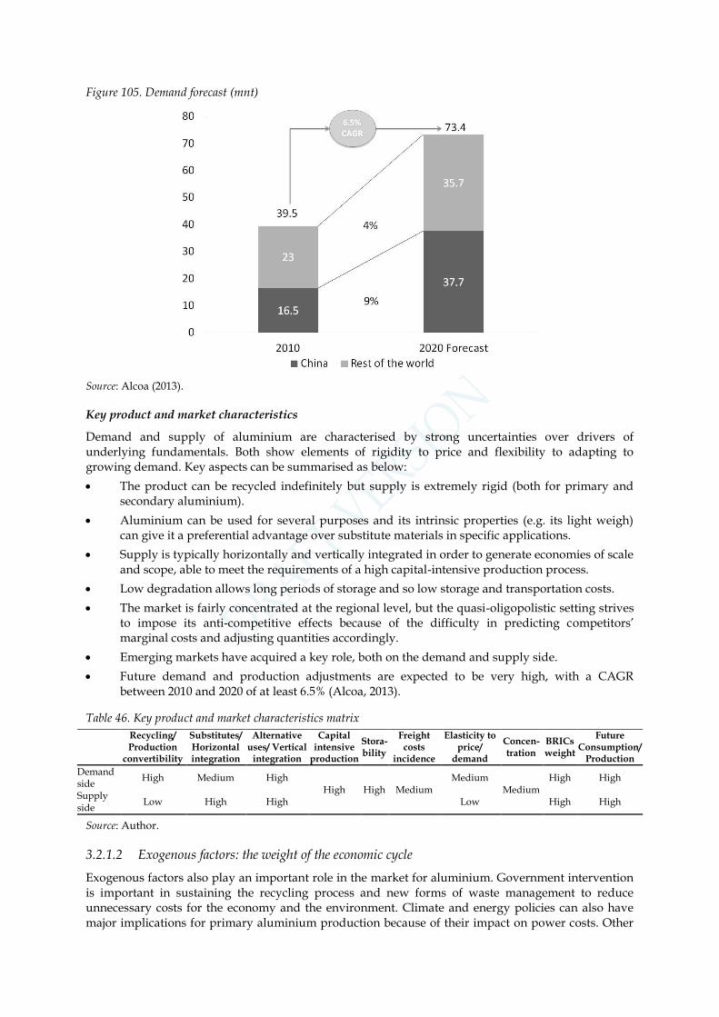
Figure 105. Demand forecast (mnt)
Source: Alcoa (2013).
Key product and market characteristics
Demand and supply of aluminium are characterised by strong uncertainties over drivers of underlying fundamentals. Both show elements of rigidity to price and flexibility to adapting to growing demand. Key aspects can be summarised as below:
The product can be recycled indefinitely but supply is extremely rigid (both for primary and secondary aluminium).
Aluminium can be used for several purposes and its intrinsic properties (e.g. its light weigh) can give it a preferential advantage over substitute materials in specific applications.
Supply is typically horizontally and vertically integrated in order to generate economies of scale and scope, able to meet the requirements of a high capital-intensive production process.
Low degradation allows long periods of storage and so low storage and transportation costs.
The market is fairly concentrated at the regional level, but the quasi-oligopolistic setting strives to impose its anti-competitive effects because of the difficulty in predicting competitors’ marginal costs and adjusting quantities accordingly.
Emerging markets have acquired a key role, both on the demand and supply side.
Future demand and production adjustments are expected to be very high, with a CAGR between 2010 and 2020 of at least 6.5% (Alcoa, 2013).
Table 46. Key product and market characteristics matrix
Recycling/ Production
convertibility
Substitutes/ Horizontal integration
Alternative uses/ Vertical
integration
Capital intensive
production
Stora-bility
Freight costs
incidence
Elasticity to price/
demand
Concen-tration
BRICs weight
Future Consumption/
Production
Demand side
High Medium High High High Medium
Medium Medium
High High
Supply side
Low High High Low High High
Source: Author.
3.2.1.2 Exogenous factors: the weight of the economic cycle
Exogenous factors also play an important role in the market for aluminium. Government intervention is important in sustaining the recycling process and new forms of waste management to reduce unnecessary costs for the economy and the environment. Climate and energy policies can also have major implications for primary aluminium production because of their impact on power costs. Other

144 | RAW MATERIALS AND INDUSTRIAL METALS
forms of intervention tend to limit the export of the commodity, especially in countries where internal production may not meet internal demand redirected to the domestic economy (e.g. India). Additionally, a great number of bauxite mines are state-owned (Ericsson, 2010). Overall, government intervention is currently limited. However, political instability remains a key risk factor for those materials (in particular, bauxite and alumina) that are produced in emerging markets.
Table 47. Exogenous factors
Government intervention Main other external factors
Medium Economic cycle (e.g. interest rates)
Political instability
Source: Author.
Another key fundamental aspect, particularly for metals due to their key role in our economies, is the adjustments caused by the economic cycle and its underlying drivers. As Figure 106 below suggests, aluminium prices have historically been strongly positively related to the economic cycle (represented by the OECD Composite Leading Indicator).
Figure 106. S&P 500 and VIX five-year rolling correlation with LME real cash price (monthly)
Source: Author’s calculation from OECD, Yahoo Finance, and Chicago Board Options Exchange (CBOE).
Price correlation with the volatility index (VIX), which is a measure of risk aversion and alternative measure of the cycle, has been consistently below zero since the middle of 1998, showing a stable link between metal prices and the economic cycle. As risk aversion grows, due to the negative economic cycle, prices appear to move in the opposite direction. The lag-one data is used for the VIX since the speed of adjustments to market shocks is certainly higher for a continuous market price than for a general indicator of market volatility.
Moreover, price correlations converged to zero when the financial crisis erupted with its disruptive effects for the financial system in September 2008. Aluminium prices, instead, have increasingly shown a strong positive correlation with the S&P500 but not with its implied volatility, which points to an underlying different driver influencing the economic cycle or the price directly that has caused two variables that have previously shown no correlation (or a negative one) to be positively correlated since 2002. This factor may be explained better by our earlier analysis on the impact of monetary policies on financial indexes and non-commercial positions in commodities markets. These policies may have led apparently unrelated variables to respond in a similar way to adjustments in the economic cycle (see Chapter 1). This also confirms the historical relationship between metal prices and interest rates (Frankel, 2006).
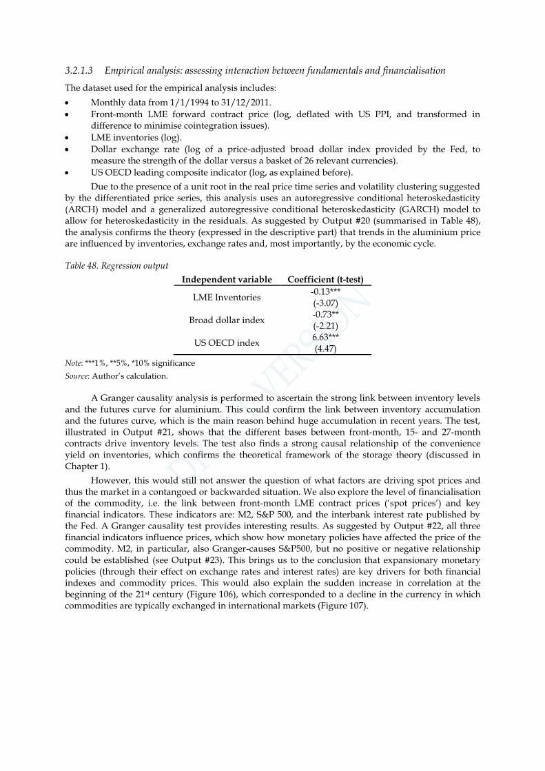
3.2.1.3 Empirical analysis: assessing interaction between fundamentals and financialisation
The dataset used for the empirical analysis includes:
Monthly data from 1/1/1994 to 31/12/2011.
Front-month LME forward contract price (log, deflated with US PPI, and transformed in difference to minimise cointegration issues).
LME inventories (log).
Dollar exchange rate (log of a price-adjusted broad dollar index provided by the Fed, to measure the strength of the dollar versus a basket of 26 relevant currencies).
US OECD leading composite indicator (log, as explained before).
Due to the presence of a unit root in the real price time series and volatility clustering suggested by the differentiated price series, this analysis uses an autoregressive conditional heteroskedasticity (ARCH) model and a generalized autoregressive conditional heteroskedasticity (GARCH) model to allow for heteroskedasticity in the residuals. As suggested by Output #20 (summarised in Table 48), the analysis confirms the theory (expressed in the descriptive part) that trends in the aluminium price are influenced by inventories, exchange rates and, most importantly, by the economic cycle.
Table 48. Regression output
Independent variable Coefficient (t-test)
LME Inventories -0.13*** (-3.07)
Broad dollar index -0.73** (-2.21)
US OECD index 6.63*** (4.47)
Note: ***1%, **5%, *10% significance
Source: Author’s calculation.
A Granger causality analysis is performed to ascertain the strong link between inventory levels and the futures curve for aluminium. This could confirm the link between inventory accumulation and the futures curve, which is the main reason behind huge accumulation in recent years. The test, illustrated in Output #21, shows that the different bases between front-month, 15- and 27-month contracts drive inventory levels. The test also finds a strong causal relationship of the convenience yield on inventories, which confirms the theoretical framework of the storage theory (discussed in Chapter 1).
However, this would still not answer the question of what factors are driving spot prices and thus the market in a contangoed or backwarded situation. We also explore the level of financialisation of the commodity, i.e. the link between front-month LME contract prices (‘spot prices’) and key financial indicators. These indicators are: M2, S&P 500, and the interbank interest rate published by the Fed. A Granger causality test provides interesting results. As suggested by Output #22, all three financial indicators influence prices, which show how monetary policies have affected the price of the commodity. M2, in particular, also Granger-causes S&P500, but no positive or negative relationship could be established (see Output #23). This brings us to the conclusion that expansionary monetary policies (through their effect on exchange rates and interest rates) are key drivers for both financial indexes and commodity prices. This would also explain the sudden increase in correlation at the beginning of the 21st century (Figure 106), which corresponded to a decline in the currency in which commodities are typically exchanged in international markets (Figure 107).

146 | RAW MATERIALS AND INDUSTRIAL METALS
Figure 107. Dollar Broad Index and interbank interest rates, 1994-2011 (rhs)
Source: Federal Reserve.
Exchange rates and interest rates as underlying factors linking commodity prices to financial assets is also made clear in Output #24. S&P 500 and aluminium prices appear to affect each other (see also Output #25), suggesting that there may be one or more common variables that make them move in the same direction. The results of regressing spot prices on S&P 500 before and after 2002 (see Output #26) confirm previous analyses, though. From 1994 to the end of 2001, no link emerges between S&P 500 and spot prices. From 2002 to 2011, however, the relationship changes and becomes statistically significant, with a positive sign. The more the financial index grows, the more the LME forward cash price moves in the same direction with a coefficient of 0.57.
3.2.1.4 Market organisation: the impact of financial deals and warehouse rules
The physical price can be formed through bilateral contracts, but is more frequently formed through cash forward contracts, traded on LME. The pricing complexity of the cash contract is fairly low and, most of the time, even bilateral transactions rely on the publicly available benchmark price. The futures (forward) market is fairly liquid and active, and accounts for over 15% of the value of global production (Table 18). The standardised product characteristics of metals permit the quick development of trading platforms with futures contracts trading these underlying commodities.

Figure 108. Basis and convenience yield (rhs), Q2 2003-Q1 2012 ($/tonne)
Source: Author’s calculation from LME and the Fed. Note: ‘Basis’ calculated as differential between cash forward
and the maturities mentioned above.
The low degradation of the metal, additionally, makes the ‘cheapest-to-deliver’ model the most successful (Geman, 2005). As a result, LME has built a system of warehouses over the years spread widely across the world (with roughly 740 licensed warehouses), making delivery very cheap. This model of delivery dramatically reduces the impact of freight and transportation costs for those using these contracts in pure physical transactions. However, recent issues linked to delivery of aluminium out of specific warehouses and the sudden growth of stocks have raised questions about the organisational rules set by the exchange and potential conflicts of interest with important financial institutions, which hold majority stakes in two of the largest warehouses in the United States and in Europe. Certainly, the underlying trend to accumulate aluminium comes from the drop in demand (and the negative economic cycle) and the strong net production surplus during the recent financial crisis, due to the inability in the short term to adjust production downwards (see above). A strong contango (spot prices much lower than forward prices) and the low interest rates, which keep the convenience yield (i.e. the total cost of holding a commodity) at a very low level and offer great opportunities for carry trades,114 lead this underlying trend. Figure 108 shows how the drop in the convenience yield, caused by a sudden halt in global demand and zero interest rates, has pushed the curve into a prolonged and strong contango, which is driving accumulation of inventories and in-store delivery and storage of aluminium. As a result, inventories behind LME aluminium contracts were worth more than 11% of the yearly global production in 2011.
While the absolute number may be still considered in a reasonable range (but not so common for industrial metals), the growth of cancelled warrants, i.e. metal that is requested for delivery, signals real problems in loading out aluminium from warehouses. In fact, the sheer increase in inventories, as showed in Figure 109, and the recent spike in cancelled warrants in at least two locations (Detroit for the United States and Vlissingen for the European Union) may also tell us an additional story.
114 Holding and carrying the commodity, benefitting from higher prices in the future.

148 | RAW MATERIALS AND INDUSTRIAL METALS
Figure 109. LME inventories and cancelled warrants (rhs)
Source: Author’s elaboration from Alcoa and LME Sword.
When interest rates reached almost zero across the advanced economies in 2007-08, the opportunity for a big carry trade emerged. Historically low aluminium prices, due to the financial crisis, have also made it easy to exploit a stable contango in the futures/forward curve. Accumulation has occurred due to inventories being maintained in LME warehouses, financed by financial institutions at very low interest rates, in order to resell when demand picks up again (with the end of the oversupply that increased with the economic crisis). This carry trade has allowed an unprecedented amount of aluminium stocks to flow into LME warehouses, especially in 2009 (Figure 110).
Figure 110. Aluminium flows in LME warehouses
Source: LME Sword.
Accumulating aluminium in LME warehouses was a rather smooth process, but the unloading process has caused several issues. Despite the recognised of the LME warrants system (see Box 3),

aluminium is currently stuck in long queues at delivery, specifically in the two locations mentioned
above. The delivery bottleneck is represented by cancelled warrants,115 which were almost none when
the accumulation of inventories began in 2008 (Figure 109). Delivery requests in specific consumption areas, such as Detroit in the United States and Vlissingen in the Netherlands, have waiting time of respectively 355 and 272 days on average (CRU, 2013) and there is no sign that this trend can be soon reversed, especially if demand will pick up again in the future months.
The reasons of this delivery cut are at least twofold. First, since users pay for the storage even if the metal is put in a queue to be loaded out, warehouses have incentives only to increase metal accumulation (load-in) and so to reduce their load-out rate to the minimum level set by the exchange. Second, the rules set by LME for sponsored warehouses allowed a very low daily delivery rate. Before April 2012, the delivery rate was based on the size of the warehouses, i.e. 1,500 tonnes for warehouses with space of 7,500 m2 or more (roughly all warehouses, Europe Economics 2011), 1,200 tonnes for 5,000 m2, and 800 tonnes for 2,500 m2. This system created the incentive to accumulate supply in one place, slowing down the delivery of the commodity (due to the low delivery out rate) and increasing the storage time for users. Specific warehouses located close to consumption areas have been stocked with massive quantities of aluminium over time. Detroit and Vlissingen, which also represent the closest points to the two of the biggest car manufacturing areas and general aluminium consumption areas in the world, stored over 1 million tonnes of aluminium each in September 2012, and also had the highest number of cancelled warrants. This problem in the system may have also contributed to keeping aluminium prices above the level that a four-year surplus in net production might have pushed them.
As a result of strong pressures from users and after the conclusions of a study commissioned by the LME itself (Europe Economics, 2011), the LME’s Board decided to increase the minimum delivery out rate. A new system, implemented in April 2012, calculates the minimum loading-out rate on the overall amount of metal stored in the warehouse rather than the size in m2 of the warehouse (as for the old system).
Table 49. Minimum delivery out of LME warehouses
Warehouse company’s tonnage stored per location Minimum delivery out
Up to 300,000 tonnes 1,500 tonnes
300,000 to 600,000 tonnes 2,000 tonnes
600,000 to 900,000 tonnes 2,500 tonnes
More than 900,000 tonnes 3,000 tonnes
Source: LME (2011).
Irrespective of whether the chosen level for the delivery out rate is sufficiently high, and notwithstanding the fact that these LME rules need to give incentives to warehouses to stay in the network, which is the core aspect of the LME business model, the system may still give incentives to warehouses to concentrate stocks in one place, because above a certain threshold of tonnage stored (900,000 tonnes) the minimum delivery out rate freezes. A system based on a minimum percentage of the total metal in storage (without thresholds) has been ruled out on the claim that it would increase operational costs for warehouses at an unsustainable level. Europe Economics estimated these costs at a minimum of $255 million for 2010 for a warehouse with 1 million tonnes and a minimum delivery rate of 50,000 tonnes. While it cannot be challenged that these extra operational costs are high, the solution applied by the exchange assumes that warehouses are unable to set their own capacity (in
115 Metal that is requested for delivery. In particular, holder that has metal on warrant decides to ship the metal out and notifies the warehouse holding warrant of the desire to cancel. The warehouse requires payment of out charges for loading before cancelling the warrant. It then gives the holder of cancelled warrant notice of when the shipment can be made. At this point, a book-keeping entry is made in LME stocks moving from ‘on warrant’ to ‘cancelled warrant’ but is still reported in total stocks. Rent continues to accrue on the cancelled warrant until it shipment date arrives. The holder of cancelled warrant must pay all accrued rent before metal is shipped. Once shipped, total cancelled warrants reported by LME are lowered by the amount shipped and total stock declines accordingly.

150 | RAW MATERIALS AND INDUSTRIAL METALS
competition) as a function of a minimum delivery rate calculated as a percentage of their total capacity. As rental fees are applied also on metal units waiting to be delivered, this model creates the incentive for the warehouses’ owners not to deliver no more units than the minimum quantity set by LME rules, which indirectly become a maximum delivery rate, in order to extract higher fees from aluminium users. Nonetheless, the rules of the exchange have to balance the right of the users to get delivery as soon as possible, and the incentives for the warehouses to be part of the LME network or otherwise compete freely among each other, which may not ensure the current capillarity of the LME warehousing network.
Additionally, the delivery rules set by the exchange will be now subject to periodic review (every six months) by a Committee that should fall under the UK Financial Conduct Authority’s supervision. However, the process shall be complemented by a conflicts of interest policy in relation to the final decision eventually approved by the Board. In fact, the owners of important warehouses in
main consumption areas (such as in Detroit and Vlissingen)116 are mainly important financial
institutions and commodities trading houses that also run a legitimate business of financing users to store aluminium in their warehouses, but most importantly had altogether a significant shareholding
in LME (but with no official majority within the Board)117 before the recent merger with the Hong
Kong Exchange, in which some of them keep an interest but diluted in its quasi-dispersed ownership.
Figure 111. Regional premia over LME cash, 2008-2012 ($/tonne)
Source: Alcoa from month-end pricing – Platts Metals Week and Metal Bulletin.
As a consequence of the delivery issue caused by the joint effect of cash-and-carry trades and LME delivery rules, regional premia over the LME aluminium cash price in the physical market, have soared to unprecedented levels, partially compensating the drop in the nominal price due to the period of oversupply (Figure 111). As premia are strongly influenced by the costs of the alternative way to source aluminium (LME cash forward), regional premia have partially followed the increase in cost of storage in main regional locations, which have soared due to the long queues to get metal out. Regional premia are now more than 15% of the nominal cash price.118
116 In particular, warehouses in Detroit are owned by Metro Group (owned by Goldman Sachs) and Henry Bath (owned by JP Morgan), while those in Vlissingen are owned by Pacorini (owned by Glencore) and Metro Group.
117 58 shareholders, including financial institutions, with single shareholdings below 11%.
118 The cost of storage for additional 355 days of storage is roughly $160/tonne ($45 cent per day; tariff in Vlissingen and Detroit in March 2013), which corresponds to an additional cost of roughly $160 million only in the US (with 1 million tonnes of cancelled warrant). Cost of storage is roughly 50% of the cost that is indirectly

Figure 112. US premium and cancelled warrant in North America, 1999-2012
Source: CRU (2013)
On top of the negative effects of a delivery system that does not reflect the characteristics of the underlying physical market, this situation could ultimately end up affecting the price formation of LME aluminium cash contract as a global benchmark price, so restricting users’ access to an important hedging tool and finally increasing the cost of the commodity for final users. 119 Moreover, a well functioning delivery system provides an efficient tool to support supply adjustments when disequilibrium in the physical market between demand and supply emerges.
More generally, when a system of physical delivery is put in jeopardy, either by external factors or internal policies, this situation may produce disruptive effects on the price formation of all cash and futures (forward) contracts in relation to their convergence with physical spot prices, even for those contracts that are typically cash-settled. Convergence is the only element of the non-arbitrage condition that has made futures contracts so important for commodities hedging. Therefore, some commodities firms may be unable to hedge on the futures market due to the uncertainty around the final price of the commodity caused by physical delivery problems. Spot prices, therefore, may have only started to price the information of a badly functioning cash and forward market, so increasing volatility and pushing premia away from a pure result of supply and demand interaction. In addition, the overreliance on the price formation of regional premia can deteriorate the value of the benchmark and so its liquidity, which may ultimately replace a transparent setting offered by the liquid cash forward market with a more opaque price formation mechanism based on assessed regional premia.
discounted into regional premia, on top of other loading out charges and indirect costs for not being able to get delivery when requested.
119 The London Metal Exchange has announced, on July 1st, 2013, the intention to change the minimum loading out rate for its warehouses under strong pressures from users. The consultation, available at http://www.lme.com/news-and-events/press-releases/press-releases/2013/07/lme-consults-on-changes-to-warehouse-policy-to-cut-queues/, proposes to increase the minimum loading out rate for warehouses with more than 100 days queues, by imposing an additional tonnage to the amount of metals loaded in (1,500 tonnes more than what has been loaded in for warehouses, that under 2012 rules, deliver out a minimum of 3,000 tonnes). If load-in rate is higher than minimum load-out rate, the warehouses are obliged to deliver out the excess. Rates will be calculated on a 3-months basis. Once implemented, the rules shall gradually reduce queues in main location, but it is not quantifiable the amount of time needed to bring queues below 100 days.

152 | RAW MATERIALS AND INDUSTRIAL METALS
Table 50. Key market organisation factors
Physical market setting Pricing complexity Liquidity futures market Delivery points
Oligopolistic Low High High
Source: Author.
The overall market organisation is based on an open oligopolistic setting in the physical market for supply with low complexity in the pricing system, which relies heavily on a cash forward market run by LME. Liquidity in futures markets is high and the exchange model allows delivery in several regions across the globe.

3.3 Copper market
Copper is a key commodity in several sectors of advanced and developing economies, from transport to new technologies (such as electronic devices) and monetary systems (see Figure 113). The yearly
production value can be estimated at around $ 161 billion.120 It is used in car manufacturing,
construction materials, plumbing, and many other sectors of the manufacturing industry. Copper improves energy efficiency, in particular in the distribution system. The production of copper from scrap does not affect its properties such that secondary copper typically cannot be distinguished from the primary one. Competition between materials also ensures that resources are depleted in a more efficient and sustainable way.
Figure 113. Refined copper usage by sector
Source: Raw Materials Group.
Over the years, copper has gained a more important role in ensuring high-energy efficient standards in the design of motors and devices for industrial use. Anecdotal evidence suggests that between 70-80% of the copper ever produced is still in circulation (similar to aluminium). In the last decade, despite its intrinsic cost, copper consumption has gone well beyond historical peaks as its use has become widespread. At the same time, however, this situation has exposed the commodity to the economic cycle. As a result, the copper price has swung significantly in the last decade, dropping to around $3,000/tonne in 2008 and then climbing up to more than $10,000 at the beginning of 2011. Copper is frequently analysed as an important measure of the state of the global economy.
Figure 114. LME copper real cash price (left) and 20-day rolling annualised volatility (right)
Source: Author’s calculation from LME and World Bank (MUVI).
120 Estimates from LME cash price (January 25th, $8,059,5/tonne) and 2011 production value taken from ICSG.

154 | RAW MATERIALS AND INDUSTRIAL METALS
The market has developed a more stable pattern recently as the economic cycle has stabilised, even though demand remains weak and is mainly reliant on Chinese growth. The demand trend has expanded by many times in the last decades, however, thanks to the development of new electronic mechanisms and new construction techniques.
3.3.1.1 Product and market characteristics: a quasi-precious metal?
Copper is in the same group of the periodic table as silver and gold (Group 11), typically produced as a semi-final product with unique characteristics. On the one hand, copper and its alloys (such as bronze, an alloy made mainly of copper and tin) are resistant to corrosion both in the open air and seawater. Its application in outdoor architectural components is widespread, as well as for plumbing supplies and seawater industrial plants. On the other hand, copper is a very malleable metal with the highest rate in nature of both electrical and thermal conductivity. Its easy formability, resistance, easily identifiable colour and intrinsic value, and its difficulty to counterfeit, make it a suitable material for the creation of money (i.e. coins). Its use is therefore widespread across monetary systems around the globe and in electricity networks. Finally, copper has a unique antimicrobial attribute that makes this metal a component of almost any organism on earth (Michels, 2006; CDA, 2010). Used in a balanced way and combined in alloys with other natural components, copper can be beneficial to human health. This use of copper is still developing, as scientific studies discover new important properties and combinations of the metal. All of these important properties have made copper a successful commodity since it was discovered more than 4,500 years ago, during the Bronze Age.
Production process
The production process is capital intensive and requires high-energy consumption. The main costs of production are energy, labour, administration (e.g. licenses), transportation from remote locations (ores have an average copper content of 1%), and solvents. Additionally, copper production depends on the price of copper itself and prices of closer substitutes, such as aluminium. The process to transform ores into refined products, ready to be used in multiple industrial sectors, involves four stages (Figure 115).
Figure 115. The copper production process
Source: Author.
First, copper ores are mined and crushed in open pits, often in very remote locations. Then, crushed ores are subject to a milling process typically done close to the mine by the same operator,

since crushed ores contain only 1% or less copper. The cost of transport for sale of non-milled copper ore with such a low copper content would be prohibitive. As a consequence, mining companies are typically integrated with milling activities. Once ores are extracted, there are two potential milling processes to transform them in products with a higher copper concentration. The most widely used is the flotation process for copper sulphides (e.g. chalcopyrite or chalcocite), which consists of a process of separation from most of the sulphides through flotation and the addition of anionic collectors such as xanthates. Flotation of copper oxides (such as azurite) is still under development and does not give good production results. Therefore, a second production process has been developed over the years – ‘leaching’. An alternative to the smelting process, this is a hydrometallurgical process that allows the extraction of copper from different types of ores (mainly oxidised due to exposure to air or to chemical substances, such as mines dumps) by immerging the product in sulphuric acid. The process, which increases the efficiency of copper production as it allows ores with high levels of impurities to be treated, is split into two types of treatment. First, the electrowinning process allows the extraction of copper through the immersion of an inert anode and a cathode in a solution with acid, so that copper is deposited on the cathode when electricity is channelled in the solution and the anode melts. This process can produce cathodes that do not need smelting and so can be sent directly to wire mills. A second leaching process is the precipitation of copper with special solutions, typically hydrogen sulphide. The copper cement is then sent to furnaces for smelting. Both leaching processes are referred to as SX-EW, which today represents roughly 15-16% of total refined copper production (Figure 116).
Figure 116. Copper production outputs
Source: Crowson (2011) from Raw Materials Group.
As for other metals production, these first two steps of production may have a strong environmental impact because they produce high levels of gases or chemical residues that need specific and costly treatment, on top of the significant amount of water wasted in the process.
After mining and milling, if ores are not treated through SW-EX, copper concentrates (with roughly 28% of copper content) reach the smelting process, in which they are processed into furnaces at high temperatures together with other substances (typically silica dioxide and coke). The resulting matte and slag is processed by blowing air in the molten matte to remove sulphur dioxide and removing acids to increase the purity of the product to 98% with the production of blisters. Blistered copper is put in anode furnaces to remove oxygen by blowing natural gas into it to produce a 99% copper product. The final step of production is refining through electrolysis; the product with the highest copper content is immerged into a solution with anodes and cathodes. Copper migrates to the cathodes and produces pure copper products that are then shaped into the most suitable forms for industrial uses.

156 | RAW MATERIALS AND INDUSTRIAL METALS
Production and consumption
As Figure 117 shows, mining of copper ores (and the first transformation of ores into concentrates) is concentrated in key regional areas, such as South America, South-East Asia, and Oceania. Chile is the leading producer, with over 34% of total global copper ore production.
Figure 117. Geographical location of copper production processes and mine production (kt)
Note: 2010 data.
Source: Crowson (2011) and author from Raw Materials Group Database and Raw Materials Group, Stockholm.
The final refining process is mostly done close to consumption areas, with greater geographical concentration in fast-growing manufacturing economies and metal-producing countries. As a result, China has overtaken Chile as the leading smelting and refining area in the world (Figure 118).
Figure 118. Geographical location of refined copper production (kt)
Source: Author’s elaboration from International Copper Study Group (ICSG).
As for other key industrial metals, the production of copper has grown at astonishing rates over the years, following the expansion of the global economy and the emergence of new developing markets (Figure 119). In 2011, copper production reached almost 20 megatonnes.

Figure 119. Refined copper and ores production, 1970-2011 (kt)
Source: Author’s elaboration from ICSG.
Ore production, however, stabilised and slightly decreased in 2011 due to exposure to different factors. Among these factors, lack of water to process ores, climatic changes, input costs, long procedures to get permits and a general reduction of copper grades into ores (Figure 120) have amplified the impact of volatile patterns and sluggish demand, and showed how long term factors affect ore production. This has also led key global mining firms to present new plans of investment ($4.58 billion) in the world biggest mine (Escondida, Chile), where production fell by 25% in 2011 due
to lower copper grades121.
Figure 120. Copper grade in ores
Source: Rio Tinto (2012).
Copper has a high degree of substitutability in some areas, such as components for car manufacturing, with aluminium. As Figure 121 shows, copper and aluminium prices are consistently positively correlated, with significant positive peaks of up to more than 90%.
121 BHP Billiton and Rio Tinto are leading investors in this project, with respectively $2.6 and $1.4 billion investments, as owners of 57.5% and 30% of the mine. See press releases available at http://www.riotinto.com/media/18435_media_releases_21641.asp and http://www.bhpbilliton.com/home/investors/news on 14th February 2012.
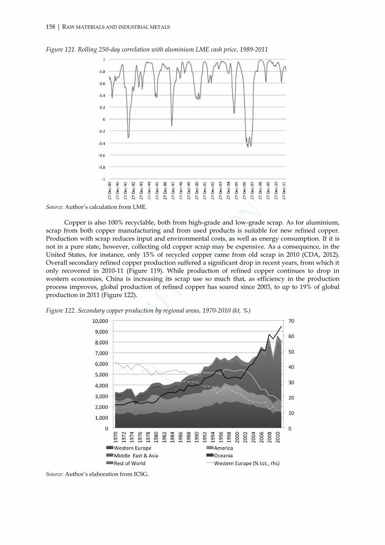
158 | RAW MATERIALS AND INDUSTRIAL METALS
Figure 121. Rolling 250-day correlation with aluminium LME cash price, 1989-2011
Source: Author’s calculation from LME.
Copper is also 100% recyclable, both from high-grade and low-grade scrap. As for aluminium, scrap from both copper manufacturing and from used products is suitable for new refined copper. Production with scrap reduces input and environmental costs, as well as energy consumption. If it is not in a pure state, however, collecting old copper scrap may be expensive. As a consequence, in the United States, for instance, only 15% of recycled copper came from old scrap in 2010 (CDA, 2012). Overall secondary refined copper production suffered a significant drop in recent years, from which it only recovered in 2010-11 (Figure 119). While production of refined copper continues to drop in western economies, China is increasing its scrap use so much that, as efficiency in the production process improves, global production of refined copper has soared since 2003, to up to 19% of global production in 2011 (Figure 122).
Figure 122. Secondary copper production by regional areas, 1970-2010 (kt, %)
Source: Author’s elaboration from ICSG.

As production of refined secondary copper continues to decline in America and Europe, Asia (led by China) has taken over its production, bringing down costs of sourcing the commodity. Roughly 65% of total secondary copper production is in Asia, which also reflects the role achieved by China as a leading actor in the global economy.
Due to its widespread industrial use in the economy, copper is also typically considered as a measure of the state of the global economy. Net production reacts to changes in industrial production with surplus/deficit, such as in 2008 and 2009 with a surplus led by the economic crisis, but levels are still small vis-à-vis total production. Consumption has been increasing in developing countries, neutralising the effects of the on-going crisis affecting more advanced economies.
Figure 123. Copper production and consumption, 1992-2012 (kt)
Source: Author’s elaboration from LME and ICSG.
Copper concentrates are also traded in the global seaborne market, where Chile is a leading exporter and China is the biggest net importer, together with Japan (Figure 124).
Figure 124. Copper concentrates major exporters (left) and importers (right), 2010 (kt)
Source: Adapted from World Metal Statistics October 2011, World Bureau of Metal Statistics in Crowson (2011).

160 | RAW MATERIALS AND INDUSTRIAL METALS
China’s high dependence on copper concentrates imported from abroad is one of the reason the country has been expanding production from copper scrap to meet sustained demand and for exports of final products with high copper content (e.g. electronic devices).
International trade
Exports and imports of refined copper in international markets also reflect the importance of China, which is importing refined copper as much as the Chilean production. Countries, like Japan, import copper concentrates for refined copper production to satisfy not only domestic consumption but also demand in international markets (see Figure 125).
Figure 125. Top 10 exporters (left) and importers (right), 2011
Source: Author’s elaboration from 2012 WBMS Yearbook.
Some other countries, like Brazil and US, are net exporter of copper concentrates but net importer of refined copper, which suggests a less developed domestic production. Overall, international trade is roughly 42% of global production (see Figure 126).
Figure 126. International trade ($bn)
Source: Author’s elaboration from ICSG, 2012 WBMS Yearbook, World Bank Commodities Database.

While exports levels have slightly increased from 2007, in relative terms, the size of international trade over production has dropped by more than 5% with the deepening of the economic crisis in advanced economies. It also reflects the underlying growth of domestic production in emerging markets, such China, Taiwan and South Korea, which have invested in supporting their domestic industry for refined copper.
Supply characteristics: towards more concentration?
As for other industrial metals, production of copper is capital-intensive and this makes supply respond slowly to demand changes. If demand is weak and the imbalance between supply and demand is moderately low, production continues. The costs of stopping production would be higher than those of producing and accumulating reserves to be sold when demand picks up. Copper can be stored for long periods with limited degradation or oxidation. From its start, a mine needs 10 to 15 years to develop, which reduces incentives to invest in exploration rather than in expanding current infrastructures. Production of refined copper products requires high initial sunk and fixed operating costs. The production of copper consists of a series of physical, chemical and electrochemical processes. A high amount of capital is required due to costs of energy, labour, and chemicals (with water) needed to produce refined copper respectively through pyrometallurgy (furnaces) and hydrometallurgy (solvent extraction and electro-winning).
With some exceptions (such as Japanese firms), most mining companies are also involved in smelting and refining copper ores into final product (Figure 127). The level of vertical and horizontal integration is high, as several companies are involved in mining and refining similar metals.
Figure 127. Copper market concentration, 2010 (kt)
Source: Raw Materials Group.
For now, strong market concentration is limited to regional areas, especially in mining copper ores. On the global scale, concentration on the supply side in international trades is growing. As markets become even more global, the need for greater economies of scale has increased concentration even further. The potential merger of Glencore and Xstrata would create the second largest player in the copper industry, with more than 1.2 megatonnes of refined copper produced each year. In 2010, the top ten copper companies had gained roughly 60% of the market share, while the top three had 30% and the largest, 11% (Ericsson, 2010). It is important to define the relevant markets, and the seaborne market may be considered developed enough to be defined as ‘global’.
Demand characteristics: overreliance on China?
Demand for copper typically derives from industrial products, which is why copper can be used as a tool to measure the pulse of the economy and its key sectors. Demand elasticity to price depends on the sector. For copper-intensive transport sectors or new technologies industries, price elasticity is considered to be very low. Higher elasticity may be found for thermal uses. During the crisis, net production has created a surplus of supply, as demand is still weak. However, surplus is lower than before the crisis and may move into negative territory again (Figure 129). As a result, there is heavy

162 | RAW MATERIALS AND INDUSTRIAL METALS
reliance in the market on growth developments in China, which will be driving demand of copper even more in the coming years (Figure 128).
Figure 128. Refined copper and GDP per capita (left) and demand forecasts (right)
Source: Rio Tinto (2012).
Supply and demand fundamentals show signs that the market is trying to find a more long-term balance and organisation. Contradictory market trends give mixed feelings about the future demand and supply patterns. On the one hand, China will not be able to drive demand through growth forever, and its greater reliance on scrap refining is a sign that the country is seeking independence. On the other hand, the lack of incentives on the supply side has delayed investments in new sites and exploration rather than in existing mines, and the widespread reduction of copper grade in ores may cause a further cut of copper concentrates supply and instability in the medium term.
Key product and market characteristics
Product and market characteristics for copper are not too different from other industrial metals, and the market can be summarised as having the following:
Limited production convertibility but high substitutability and recyclability of the final product.
Unresponsive supply to demand changes but strongly vertically and horizontally integrated industry (to reap benefits of economies of scale and scope to outweigh a capital-intensive production).
Low degradation, which increases storability.
Reasonable freight costs, as refined copper industry is located close to consumption areas.
Partial demand elasticity to price, depending on the industrial use.
High weight of emerging markets, both on the demand and supply side.
High future demand forecasts and supply forecasts, depending on the level of constraints that supply may experience in the extraction of the raw material.
Table 51. Product and market characteristics matrix
Recycling/ Production
convertibility
Substitutes/ Horizontal integration
Alternative uses/
Vertical integration
Capital intensive
production
Stora-bility
Freight costs
incidence
Elasticity to price/ demand
Concen-tration
BRICs weight
Future Consumption/
Production
Demand side
High Medium High
High High Medium
Medium
Medium
High High
Supply side
Low High High Low High Medium
Source: Author.
3.3.1.2 Exogenous factors: economic cycle and political instability
Being an indispensable metal for key sectors of the economy, copper is usually subject to some level of control from governments across the globe. As nationalism remains an unpredictable factor discouraging private sector development and incentives to invest in the long term in many countries, state control in most countries consists of tariffs to increase or reduce incentives to export (as in the case of China who is in continuous search of additional supply).

Political instability and government intervention are not the only exogenous factors. Climate change may affect extraction of copper ores in harsh locations. For instance, mining and milling close to the open pits requires the abundant availability of water.
Table 52. Key exogenous factors
Government intervention Main other external factors
Medium Economic crisis, climatic changes, political instability
Source: Author.
Finally, refined copper production is directly affected by the economic cycle and industrial production, which is still balanced overall at the global level.
Figure 129. Net production, stocks and real prices (kt, $/tonne)
Source: Author from LME and World Bank (MUVI deflator).
As Figure 129 suggests, stocks of copper react to changes in supply and demand interaction (net production). Prices reflect both stock levels and historical levels of net production, which have been smoothed by China’s entry as a global trade partner.
3.3.1.3 Empirical analysis: a solid price formation mechanism
For the empirical analysis the following set of data has been used:
Monthly data from 30/06/1992 to 31/12/2011.
Log of LME front-month price (‘spot price’) differentiated and deflated using US PPI published by the Fed.
Log of LME copper inventories.
Log of price-adjusted broad dollar index provided by the Fed.
Log of OECD Composite Leading indicator (trend restored) for China.
Log of OECD composite leading indicator (trend restored) for the OECD countries.
Due to the presence of unit root in the series of real prices and volatility clustering emerging from the differentiated price series, an ARCH(1) model appears to fit best the characteristics of the dataset.

164 | RAW MATERIALS AND INDUSTRIAL METALS
As suggested in Output #27, the empirical analysis seems to confirm fundamentals as drivers of price formation. In particular, Table 53 shows that inventories have an inverse relationship with price, as a result of the interaction between demand and supply. Demand indicators (both for OECD countries and China) have a strong positive relationship with price, confirming the strong link between market trends in copper and the global and regional economic cycle.
Table 53. Regression outputs
Independent variable Coefficient (t-test)
LME Inventories -0.12***
(-4.6)
Broad dollar index -1.02***
(-2.98)
China OECD Index 2.43**
(1.94)
OECD index 9.07***
(4.44)
Note: ***1%, **5%, *10% significance.
Source: Author’s calculation.
In addition, the model finds a negative relationship between the exchange rate and cash prices, as indicator of the impact of currency devaluation/revaluation on the price of the commodity in global markets.
With the same dataset, a Granger causality analysis assesses the relationship with financial indexes, as emerged clearly from the previous analysis run for aluminium. Also in this case, the model seeks to find a relationship among the LME front month copper contract price and the log of: monetary base (M2), S&P500, and interbank interest rate (FedFund). As illustrated by Output #28, the model finds a relationship again with M2, but none with S&P500 and FedFund. This result may point to the low degree of financialisation as the futures curve strives to move in contango, even with a low convenience yield, perhaps due to solid pressures on the demand side that keeps financial deals away. However, when splitting the two periods 1994-2001 and 2002-2011, results are in line with previous analyses on financialisation. As suggested by Output #30, no relationship emerges between spot prices and the financial index between 1994 and 2001. However, a relationship with a positive sign is found during the following period (2002-2011). The analysis, therefore, confirms what has been found already for other commodities markets (such as oil and aluminium), and in broader empirical analysis run in the first chapter.
By using a different dataset of daily data from 01/04/2003 to 31/12/2011, the Granger causality test shows a statistically insignificant relationship between inventories and convenience yield (calculated, as described in Chapter 1, by using an average annual cost of storage provided by LME and the daily 3-month Fed discount rate). Even though the test does not reveal a direct causal relationship between convenience yield (as a driver) and inventories, the convenience yield (which can be seen as the incentive to pile up inventories) seems to drive volatility, in particular with the first and second lag (Output #29). Due to the characteristics of the data, it was not possible to find another model that could establish the sign of the relationship between the convenience yield and volatility.
3.3.1.4 Market organisation: a mature market infrastructure
Like the aluminium market, the physical copper market relies on bilateral contracts and on a forward cash contract for spot pricing of the commodity. Even in this case, the high degree of storability has favoured the ‘cheapest-to-deliver’ LME model, which is the global benchmark for copper. However, despite cheap credit in this sector, no massive stock accumulation with financing operations has been pursued by market operators, since prices are not at historical lows (as with aluminium) with less prominent contango of spot-futures price curves. As explained in Section 1.2.4, convenience yield drives accumulation of stocks by pushing the futures-spot curve in contango/backwardation by increasing/decreasing the incentives to hold the commodity. As Figure 130 suggests, in recent years

copper has not been in a prolonged contango period as for aluminium. The basis has only very briefly become negative, as convenience yield was positive most of the time.
Figure 130. Basis and convenience yield (rhs)
Source: Author’s elaboration from LME and the Fed. Note: ‘Basis’ calculated as the difference between cash
forward and the maturities mentioned above.
As the convenience yield grows, the basis becomes negative so the curve is in backwardation. When the convenience yield remains around zero, the curve typically moves into contango, or close to it. The crisis has caused a drop in the convenience yield (with low interest rates and drop in global demand), but the curve has not radically switched into contango (as with aluminium), as the demand for the commodity seems to be resilient enough. Should demand of copper consistently drop and the convenience yield remains close to zero, the curve may switch in strong contango and conditions for a carry trade (as for aluminium) may ultimately emerge. If then the market does not fall in oversupply, the market may not follow the same path. However, there are signs that the market is gradually moving in oversupply and demand is slowing down, which is pushing cash forward price down and may ultimately drag the market in strong contango if demand does not pick up. LME inventories, meanwhile, have more than doubled from roughly 300,000 tonnes in December 2012 to 650,000 tonnes in June 2013 and have reached a peak on a five years time scale.
Pricing complexity is typically very low, even if the calculation of regional premia and freight costs (typically by specialised reporting agencies) may add complexity in reflecting relevant characteristics. Copper producers and users can enter into hedging strategies through an active and liquid futures market on LME or CME. LME warehouses are spread across the world, which makes delivery very cheap, reducing the impact of freight and transportation costs for those using these contracts for physical transactions.
Table 54. Copper markets organisation
Physical market setting Pricing complexity Liquidity swap/futures market Delivery points
Oligopolistic Low High High
Source: Author.
As concentration increases, the physical market setting will remain oligopolistic. This is the case for all commodities markets with capital-intensive production. However, despite market concentration, barriers to entry are high because of government interventions and other external

166 | RAW MATERIALS AND INDUSTRIAL METALS
factors that increase volatility in the short term. These factors mean that even deeper pockets are required to enter these markets and to survive in the long term.
Finally, commodities indexes, replicating the value trend of underlying commodities, have been very active for copper and other metals. However, these indexes have always been synthetic replications (except for one physical ETF run by ETF Securities in London), i.e. the financial institution offers similar returns to the underlying and hedges itself in the commodities futures markets. To reduce exposure to counterparty risk (company hedging in the underlying futures market) and improve the quality of the index, as futures markets may not be always efficient, a recent proposal for the introduction of physical exchange-traded notes may be a new, important development (SEC, 2012). This type of product structuring would require the purchase of an underlying basket of physical copper to be kept in storage and generate returns for those investing in the note or fund. On the one hand, dealing with all costs linked to keeping copper in storage, rather than using futures-based indexes, may result in lower returns if the provider of the index is unable to access storage facilities, insurance and financing at reasonable costs. On the other hand, if the index provider is also the owner of the LME-sponsored warehouse and provider of financing, incentives may emerge to pursue market practices that discriminate against, or increase barriers to supply access to their warehouses to, other metal users. Overall, however, starting up these operations requires the purchase of a quantity of physical copper that would only affect a very tiny part of global production, so the
systemic effects are negligible122.
122 In 2010, ETF securities launched a physical ETF on copper in London that has today around $47 million of assets under management. It is certainly a negligible number compared to the $161 billion of yearly copper production.

167 |
4. AGRICULTURAL COMMODITIES
4.1 Wheat market
Together with rice and corn, wheat is one of the most important and widely traded cereal grains, used mainly in the production of human food (e.g. bread). It was already being planted and harvested thousands of years ago, and it is the main input in the production of flour for bread, cakes and other types of food. Wheat is also one of the oldest futures contracts on the Chicago Board of Trade (since 1877). Its yearly global production, worth around $172 billion (USDA data), is assigned to different uses. Among others, feed for livestock has become an important use (roughly 18%), and roughly 70% of production is used for human food products (Figure 131). Waste, at roughly 4% of total production, is in line with historical averages.
Figure 131. Main wheat uses, 2009
Source: FAO Stats.
Wheat is typically harvested once per year during the summer season. However, on a global scale, harvests of different varieties and in different countries are spread across the solar year. The quality of the harvest depends on a long list of factors, which makes prices typically more volatile than metal or energy commodities (Figure 132).

168 | AGRICULTURAL COMMODITIES
Figure 132. CBOT Wheat real price, 1980-2012 ($/bushel)
Source: CBOT and World Bank (MUVI deflator $2005, rescaled to 2012).
Weather conditions, government policies (e.g. export bans or subsidies programmes), consumer preferences (e.g. meat consumption linked to growth in disposable income), fertiliser prices, and the prices of grain substitutes (e.g. rice) are some of the factors that have an impact on wheat prices, on top of supply and demand factors. Finally, there is also some level of substitutability among different classes of wheat, which may further complicate pricing on international markets. As a result of the complex interactions between factors, along with macro price trends for other commodities (not only agricultural), wheat prices exhibited significant volatility at the peak of the recent financial crisis. Over the past six years, wheat has been affected by a strong underlying economic cycle, the effects of a drop in advanced economy demand, and the prolonged and sustained growth of emerging markets (led by China).
4.1.1 Product and market characteristics: the key food commodity
Wheat is typically considered a homogeneous product that can be produced on most arable land located in most of the world’s regions. Wheat does have some homogeneous characteristics, but it can be distinguished by country of origin and end use (Laroue, 1991). The country of origin provides certain attributes such as the specific environment the wheat was grown (which ensures certain milling characteristics), an efficient grading and inspection system, and location, which helps buyers minimise freight costs. These attributes receive premia or discounts relative to the international market’s benchmark price. Moreover, wheat comes in multiple varieties or classes, which exhibit diverse milling characteristics.
Wheat can be denominated ‘winter’ wheat if planted during the autumn and harvested in the summer. This type of wheat is cultivated in warmer areas. ‘Spring’ wheat is planted in the spring and harvested in late summer in those regions that experience harsh winter conditions. The most liquid wheat futures contract is the Chicago Board of Trade Soft Red Winter Wheat futures contract, which prices low-protein winter wheat grown in the US Midwest and South. Overall, within the two broad categories of winter and spring wheat, there are at least five important classes:
Hard red spring wheat
Durum wheat
Hard red winter wheat
Soft red winter wheat
Soft white spring wheat
Soft white winter wheat
Hard and durum wheat have a high protein and gluten content, perfect for producing high-quality bread flour or semolina used to produce pasta. Most global production is hard wheat, with a global harvest occurring during summer in both the northern and southern hemispheres. Soft wheat is

usually considered lower quality and is used to prepare flour for cakes and pastries, or bread and pasta with a low gluten content. Both hard and soft wheat can have several alternative uses. For example, high-gluten hard wheat can be used for cosmetics and shampoo, while wheat starch predominant in soft wheat may be used for biodegradable plastics, alcohol (e.g. whisky) and ethanol. Wheat protein can be a meat substitute and is typically a main component of pure cereal products. When wheat is harvested, the grain is separated from the stalks and chaff. The stalks are used for various marginal applications, such as furniture. On farms, livestock are often turned loose to graze wheat fields after planting and root development in the autumn until grain production in the spring, and also after harvest to clean up leftovers. Such alternative uses are a small part of total production, however, making up not more than 3% (Figure 133).
Figure 133. Other uses of wheat and waste, 1961-2009 (% of total production)
Source: Author’s elaboration from FAO Stats.
Production
Global demand continues to grow steadily due to population growth and alternative uses, while the level of production has grown non-linearly because of the multiple (unpredictable) variables acting on production (Figure 134). A continuous short-term adjustment trend to multiple variables generates supply/demand imbalances that can reach significant amounts (as in 2008 and 2009).
Figure 134. Wheat production and consumption, 1960-2012 (kt)
Source: Author’s elaboration from USDA.

170 | AGRICULTURAL COMMODITIES
However, production is spread around the globe, which helps to minimise supply disruptions due to adverse weather in particular regions and to support resource allocation towards countries with insufficient production through the development of international trade. As Figure 135 shows, production is evenly spread among advanced and fast-growing emerging economies that want independence and food security (e.g. China and India). The European Union is the biggest producer (20%), followed closely by China, India and the United States.
Figure 135. Top producers (left) and consumers (right), 2012
Source: Author’s elaboration from USDA.
However, due to their demographics, domestic production in China and India is insufficient to cover domestic consumption. These countries are increasing investment in agriculture to secure food, but structural issues (such as availability of arable lands) may impede them to reach full independence.
Storage and freight
Once harvested, wheat is stored for long periods of time (though typically less than one year). Storage is an important component, and inventories are essentially driven by short-term supply and demand imbalances. The major harvest season is during the northern hemisphere spring and early summer. Storage and wheat futures are the components that take a crop produced once per year and assure that it is allocated efficiently throughout the year. Figure 136 confirms that wheat stocks are subject to the expectations from the summer harvest and consumption over the year, reaching their minimum during April to June, immediately before the major harvest begins.

Figure 136. Non-seasonally adjusted CBOT inventories, 2001-2012 (Toledo, Chicago, St Louis, k/bushels)123
Source: CBOT.
Like production, stocks are also exposed to underlying trends that shape incentives in the long run. Production, yields and acreage are key long-term drivers of domestic supply, which drives stocks levels together with demand trends. The 2008-09 spike in stocks reflects a surplus of over 82 million tonnes over a two-year period due to good production and the drop in global demand due to the financial crisis. Prior to that, the major drop in stocks reflected global growth driving consumption over the world’s ability to produce. In general, global ending stocks for wheat are highly volatile, by following net production (Figure 137). Production surpluses can build stocks very quickly while disappointing harvests can reduce excess stocks very quickly.
Figure 137. Net production and global ending stocks (kt)
Source: Author’s elaboration from USDA. Note: ‘net production’ is the difference between production and
consumption.
123 Due to incompleteness of the data over the covered period, data on inventories from warehouses in Ohio and Mississippi have been removed from the dataset.

172 | AGRICULTURAL COMMODITIES
Wheat can be stored safely in a cool and dry place with relatively constant temperatures and closely controlled moisture levels. Aeration systems and various grain protectants are indispensable items. Once these minimum requirements are met, storability time can be quite significant. The bulky nature of wheat and acceptable storability make it a commercially viable commodity for international shipping and for global markets. Seaborne freight costs are a key cost item in international trade and can reach unexpected levels due to capacity constraints or bottlenecks in the distribution channels (Figure 138).
Below 13% moisture, wheat can also be stored for a few years, and many governments have built strategic reserves to face sudden supply shocks or exogenous events.
Figure 138. Panamax voyage rate as percentage of Wheat CBOT front-month futures (FOB)
Source: ICAP.
International trade
The main importers of wheat are mainly low-income countries located in areas with too little rainfall to cultivate high-yields crops or in countries where arable lands are too small for their needs.
Figure 139. Top exporter (left) and importer (right) countries (kt), 2012
Source: USDA.

Western countries are the leading exporters, together with Russia and few other developing countries (e.g. Argentina, Ukraine). China is a net exporter, but supply and demand accounts are almost balanced there. Production in many developing countries (including China) is gradually falling behind demand, creating opportunity for further development of international trade. Fostered by vigorous export programmes, international wheat trade is now valued at around $42 billion (as exports value), which is roughly 20% of the total production value (Figure 140). The total turnover value of international trade (exports and imports value) is estimated at around $70 billion.
Figure 140. Wheat international trade (exports value, $bn)
Source: Author’s from USDA and World Bank.
As a result, competition among agricultural multinationals (such as the US-based Cargill and the Asia-based Wilmar) has escalated. The two key aspects in the development of international markets for grains are quality and diversification. Grain quality is crucial in global trade and often relies on the systems of inspection and infrastructure available in the exporting country, which ultimately may give a competitive advantage to domestic rather than foreign firms (Larue and Lapan, 1992). Growth of alternative uses, such as in energy, is also gradually transmitting the uncertainty present in energy and environmental policies into the grain markets, especially ethanol blend quotas (Irwin and Good, 2009) and green emission commitments.
4.1.1.1 Supply characteristics: dealing with frequent imbalances
For planting, cultivation and harvesting, wheat requires arable lands, water, machinery, labour and some products derived from crude oil and natural gas (such as fertilisers). For most final uses, wheat requires a minimum of processing to clean it and make it available mainly in the form of flour for food or feed production.
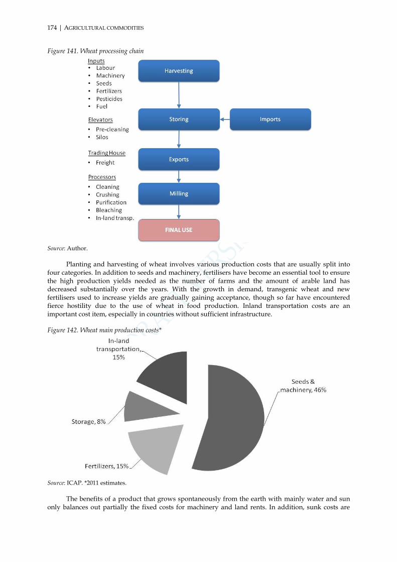
174 | AGRICULTURAL COMMODITIES
Figure 141. Wheat processing chain
Source: Author.
Planting and harvesting of wheat involves various production costs that are usually split into four categories. In addition to seeds and machinery, fertilisers have become an essential tool to ensure the high production yields needed as the number of farms and the amount of arable land has decreased substantially over the years. With the growth in demand, transgenic wheat and new fertilisers used to increase yields are gradually gaining acceptance, though so far have encountered fierce hostility due to the use of wheat in food production. Inland transportation costs are an important cost item, especially in countries without sufficient infrastructure.
Figure 142. Wheat main production costs*
Source: ICAP. *2011 estimates.
The benefits of a product that grows spontaneously from the earth with mainly water and sun only balances out partially the fixed costs for machinery and land rents. In addition, sunk costs are

limited and are often quickly outweighed by the growth in the underlying value of the land, which ultimately affects incentives to invest in efficient production systems. The possibility to convert production to alternative cultures (e.g. corn) increases opportunity costs.
Variable costs can also be significant (for fertilisers, processing and distribution costs, etc.), and are often related to external conditions that may cause a supply/demand imbalance. Cost uncertainty has led farmers to continue to rely on elevators or big trading houses, which typically buy the crop before it is harvested and hedge that crop on active futures markets. The crop may be purchased in different locations and be subject to premia and/or discounts to benchmark prices. Spot transactions involve the purchase of wheat (and grains in general) often shortly after harvest from the field or at any time of the year from the farm’s silos after some general processing. Actual access to the land can occur via direct supply contracts or through subcontracting to specialised farming companies (Oxfam, 2012).
To exploit economies of scale and scope, the major international commodity firms (the ‘ABCD’ – Archer Daniels Midland, Bunge, Cargill, and Louis Dreyfus), which account for roughly 60% of the US grain trade and roughly 75% of milling capacity (Oxfam, 2012), have gradually integrated their horizontal (across products) and vertical (from production to distribution) business models. Market concentration is low at the production level, characterised by myriad farmers and small cooperatives around the world. Greater market concentration emerges at the distribution level, with a few global commodity firms who channel production flows into the global economy. Vertical integration is accomplished through strong relationships with big farms, which receive an array of services such as access to risk management tools through global futures markets. Horizontal expansion or consolidation is often made through acquisitions of important national firms (for example, the acquisition of the state-trading enterprise Australian Wheat Board by the US multinational Cargill and the acquisition of GrainCorp, and Australian wheat company, by ADM). Consolidation will likely continue due to increased global competition and the need for international trading firms to manage and implement complex risk management procedures because their profile is exposed to several exogenous factors.
Figure 143. Wheat stock-to-use ratio, 1960-2012
Source: Author’s elaboration from USDA.
The historical importance of food security and the governance of the market consolidation process have always exerted pressure towards more concentrated markets, whether concentration was driven from the demand side (e.g. the creation of a Government monopsony through a state-trading enterprise (STE) or a subsidy programme with minimum price) or the supply side (e.g. an oligopolistic

176 | AGRICULTURAL COMMODITIES
setting). Government controls and strong global consolidation have been historical stabilisation factors for trade flows, subject to significant supply constraints. Attention focused on global concentration has helped ensure significant competition that is essential to the continued development of the international market.
On top of this underlying trend in the global market structure, the stock-to-use ratio has been trending down over the long-term (Figure 143), adding additional pressure to supply and demand balances. This trend could eventually be offset by new technological advancements in agriculture that will increase yields and minimise waste. Future production may increase due to more efficient planting (including using biogenetics) and harvesting processes, especially in developing areas like Eastern Europe and Africa. Finally, climate change could also drive changes in productivity, which could shift global production and supply chain management.
4.1.1.2 Demand characteristics: an uncertain outlook
Both foreign and domestic demand for wheat has been steadily growing over the years. Growing populations in emerging markets and economic growth have led to increased growth in consumption in recent years. Despite their populations still growing, consumption is declining both in the European Union and the United States (Figure 144).
Figure 144. Wheat consumption by region (% total and kt)
Source: Author’s elaboration from USDA.
Lower consumption has been led by the decline in feed and seed uses. Seed use, in particular, has declined from 11% of total use in 1960 to roughly 5% in 2009 (FAO stats). Alternative crops, such as maize and soybeans, have gradually expanded their share, due in part to their use in the production of energy (see 0).

Despite a strong trend for globalisation, foreign demand for wheat remains below 20% of global production (Figure 140). Food security is still an important government objective, which can affect the use of foreign supply to meet domestic needs. Changing political environments and agricultural policies may become drivers of change in foreign demand and domestic supply in the future. Several factors can affect demand in the short and long run. In the short run, consumers’ preferences relying on disposable income, reactions to market information, and alternative uses (e.g. industrial feed and seed uses linked to increased consumption of meat) drive demand patterns. In the longer term, dietary changes, new technologies and alternative uses, among others, can drive important changes in market structure.
The use of wheat for energy production (as ethanol) may remain very low in relative terms (Figure 145) as long as global weighted average yields stay around 3 tonnes per hectare (author’s estimates from USDA).
Figure 145. Future uses of wheat (forecast)
Source: OECD-FAO Stats.
Assuming that 1 tonne of wheat can produce 0.336 m3 of bioethanol, current wheat yields would produce only 1 m3 per hectare, while sugar beet can produce up to 5 m3 per hectare in the
United Kingdom (Strathclyde University).124 Technological changes in energy production from
alternative sources, driven by climate change and CO2 emissions policy actions, may change this scenario. While wheat is unlikely to play a significant part in energy production, it can still be affected by the use of other crops in energy production. In such scenarios, wheat could become even more essential in ensuring food security.
All current underlying trends assume continued world population growth and continued economic development, which would continue to put pressure on demand for food and feed for livestock (Figure 146 and Figure 145).
124 Available at http://www.esru.strath.ac.uk/EandE/Web_sites/02-03/biofuels/quant_bioethanol.htm.

178 | AGRICULTURAL COMMODITIES
Figure 146. World population by community, 1950-2050
Source: Bunge (2012) from United Nations.
While urbanisation will continue to expand in emerging markets, rural areas are undoubtedly experiencing population loss and the reduction of arable lands, also led by increasing yields and average farm size.
4.1.1.3 Key product and market characteristics
The product and market characteristics put wheat, together with similar row crops, into a group of commodities that naturally have more price volatility compared to energy and metal markets. In particular, wheat markets can rely on the following characteristics:
A renewable product with high convertibility of production to alternative cultures, as well as alternative uses.
Production not concentrated, though it is partially integrated with elevators and trading houses further along the marketing channel. There is a lack of producer control over supply since it depends on variables outside human control in many scenarios during the harvest season.
Low capital-intensive activity that depends strongly on the value of the underlying land, shaping incentives for long-term investments in rural areas, while on-going variable costs for dealing with storage and risk management are not irrelevant for the business model.
Sufficient storability for international markets.
Very low concentration at the farm level, but higher concentration at the distribution level due to economies of scale and scope requested by international markets.
Low demand elasticity as a main food ingredient, but higher demand elasticity when used in alternative ways (e.g. for feed or energy).
High supply elasticity.
Growing demand from emerging markets, which often have limited supply and strive to ensure food security.
Stable consumption in the coming years, but supply will likely be subject to further short-term constraints caused by endogenous (e.g. growth of substitutes, such as corn, for alternative uses) and exogenous (e.g. reduction in government market price support mechanisms) factors. In the long term, supply should benefit from higher yields and the market entry of new arable lands.

Table 55. Product and market characteristics matrix
Recycling/ Production
convertibility
Substitutes/ Horizontal integration
Alternative uses/
Vertical integration
Capital intensive activity
Storability Freight
costs incidence
Elasticity to price/ demand
Concen-tration
BRICs weight
Future Consumption/
Production
Demand side
Renewable Medium High
Low Medium Medium
Low
Medium
High Medium
Supply side
High High Medium High High Low
Source: Author.
4.1.2 Exogenous factors: assessing the role of government policies
As mentioned above, demand and supply of wheat are subject to several exogenous factors. In order to ensure food security (a primary need for their citizens) and for land and rural management, governments play an important exogenous role in affecting agricultural commodities. Government intervention into the wheat market has taken several forms over the years, from market price supports and incentives, to export programmes, to more neutral mechanisms such as support programmes based on arable lands and historical receipts (e.g. the new Common Agricultural Policy in the European Union). In a market that continues to become more global and open to trade flows, a single sudden decision to ban wheat exports – as Russia did after the 2010 drought – or to add a levy on imports can have significant repercussions for prices, at least in the short term. Due to their pervasive action, changes to subsidy programmes require a phased approach. Government intervention in wheat markets has been justified by the existence of imperfect competition in international markets (Corden, 1991), where monopsonistic STEs deal with an oligopolistic international trade market. In recent years, however, policies within the WTO have trended towards open global markets. Governments have responded with accommodating policies, such as the privatisation of the Australian and Canadian Wheat Boards. The European Union has been decoupling payments to producers from payments linked to the production of a specific crop after the reform of the Common Agricultural Policy (CAP) in 2003. However, the size of this programme is still significant. The CAP budget, directed to all commodity sectors, amounted to $78.2 billion (€60.8 billion) in 2012, roughly double the value of EU wheat production in the same year ($41 billion). Even though this amount accounts for less than 1% of EU GDP, it is still a significant amount in agricultural commodities
markets, where arable lands are 60% crops (Eurostat in 2007)125 and production value is typically low
in absolute terms. As a result, any additional decoupling in the European Union or reduction in US export subsidies could influence market developments. The EU decision to decouple payments from production quotas or direct price support (to be fully implemented with the new reform in 2013; see Box 8) together with the decision to increase support to the development of rural areas, may trigger interesting market developments. The OECD (2004) measured the effects of decoupling resulting in a reduction in arable land and a reduction in export subsidies, and found that consumers would benefit from greater competition. Markets are still internalising the long-term effects of this decision, resulting in a gradual reduction of export flows from Europe due to lower production subsidies. Direct government interventions on market prices have been decreasing over the years, but in the form of direct payments to producers they are still significant in many regions (see Box 8). As today, the European Union does not provide direct market support to wheat production, and the United States has reduced its support to roughly $1.1 billion. The implications of these rapid changes in subsidy programmes are still to be fully understood. Lower protection for farmers in the European Union does not only mean lower use of land (Hermans et al., 2010), but also consolidation at the local level led by greater competition among regional areas within Europe and beyond. This process may ultimately benefit final consumers, despite the potential for more volatile patterns as the market begins new developments.
The gradual reduction of harvested lands after the oversupply and quality problems in the 1980s, with subsidies based on the quantity of commodity produced (then taken over by quotas), is a
125 Available at http://epp.eurostat.ec.europa.eu/statistics_explained/index.php/Agri-environmental_statistics.

180 | AGRICULTURAL COMMODITIES
broader phenomenon affecting both the European Union and the United States as a result of technological changes and consolidation of farms (Figure 147).
Figure 147. Arable acreages (kt)
Source: Author’s from USDA.
As long as reduced acreage is offset by increases in yield and greater production, this process may be beneficial for consumers in terms of quality and cost. However, this is not a foregone conclusion; yields in Europe and the United States struggle to exceed those reached during the 1980s (5 and 3 tonnes per hectare, respectively).
Figure 148. Wheat production yields (tonne/ha)
Source: Author’s elaboration from USDA.
Subsidies and other interventions may also affect incentives to invest in agricultural infrastructure. Structurally low prices and high land values for prolonged periods can distort investment incentives. This is perhaps one of the reasons the European Union has decided to build a second pillar of investment for greater development of rural areas. The US market-oriented

programme does not explicitly tackle this issue yet. China, meanwhile, has been massively investing in agricultural infrastructure and has gained ground compared to western economies with respect to agriculture, with the ambitious intent to overcome significant obstacles (e.g. water supply and loss of agricultural lands) and become self-sufficient rather than a huge importer of agricultural products. Finally, the effects of state interventions depend in many ways on the incentives. Export subsidies, for instance, ensure high volumes but may have perverse effects on quality (Larue and Lapan, 1992). Overall, greater market-oriented supply and demand interaction improves income transfer and consumers’ welfare (OECD, 2004). However, following sudden exposure to market conditions, it can take several growing seasons for all market adjustments to occur, increasing volatility in the short term.
Box 8. The evolution of government intervention in agriculture in Europe and the United States
Government intervention into agricultural markets has played a significant role in the development of agricultural markets. In 2011, global support to agriculture reached over $252 billion (OECD, 2012), mainly concentrated in the two biggest subsidies programmes (by budget) by the European Union ($78 billion) and the United States ($74 billion).126 Including indirect support through investment in research, marketing and rural areas, the amount of resources allocated to agriculture in OECD countries soared to over $400 billion in 2011 (34% of total production value; Figure 149).127
Figure 149. Total support estimate (US$mn)
Source: Author’s elaboration from OECD Library.
Among the countries and regions most active in governmental support to agriculture, the European Union is the only one that has consistently reduced is support to agriculture, which dropped below $120 billion in 2010. Both China and the United States, the two biggest economies in the world after the European Union, have increased the size of their intervention in agricultural markets in absolute terms.
126 Including support for rural areas development, research, marketing and indirect transfers (disaster relief, etc).
127 There are three aggregates of government subsidies used in the OECD statistics. The total support estimate (TSE) is the broadest indicator of support, representing the sum of transfers to agricultural producers individually (the PSE) and collectively (the GSSE), as well as budgetary subsidies to consumers. The general services support estimate (GSSE) measures the monetary transfers associated to public financing of services such as agricultural research and development, training, inspection, marketing and promotion and public stockholding..

182 | AGRICULTURAL COMMODITIES
Figure 150. Total support estimate (TSE) by region (US$mn)
Source: Author’s elaboration from OECD Stats.
Only China appears to have increased its government contribution (direct and indirect) to the economy in 2010, both in relative (GDP) and absolute terms. The European Union, in contrast, has further reduced its direct and indirect contribution after the historical peak in 1998 (Figure 151). China has overtaken the European Union in size of total intervention, both in absolute and relative terms. Chinese intervention almost doubled in 2010, to $90 billion. Additionally, despite commitments towards a more market-oriented intervention, the United States has gradually substituted old direct support to producers (only $30 billion out of $147 billion) with indirect measures that may only partially reduce distortive effects on agricultural markets.
Figure 151. PSE (left) and TSE (right) over total local production value (%)
Source: Author’s elaboration from OECD.
The rationale used for government intervention are threefold:
Ensuring food production under fair conditions.
Promoting a sustainable use of resources.
Preserving rural areas.
The achievement of these three objectives is considered a public good (i.e. goods that are non-rival where the use by one person does not exclude another’s use) and non-excludible (people cannot be excluded from using it). Under this line of reasoning, subsidy programmes have been activated to protect domestic prices from global trade flows, to promote environmentally friendly production practices, and to

encourage investment in historical rural heritage. However, such interventions (in particular, volume-based incentives) may create significant distortions to market equilibrium and may adversely affect long-term investment incentives. As a result of significant distortions that have emerged over the years, subsidies to support output or to guarantee minimum prices are being used less and less by governments around the world
Today, such supports account for less than 30% of global subsidies. Such reductions have helped foster the development of a global and competitive market for agricultural commodities. The long-term objective is to remove obstacles and align domestic prices as much as possible with international ones. Such a result would likely benefit emerging economies, but could offer new challenges to the more advanced countries that control most of the global food supply.
The European Union Common Agricultural Policy
The Common Agricultural Policy (CAP) was first introduced in a much smaller European Union (with six countries) in 1962. Since then, the CAP has expanded (as the European Union grew) and has been progressively modified since the late 1980s to adapt its programme to important market developments. The CAP is still today the biggest item in the EU budget, but its relative weight has gradually decreased over time from over 60% to 32% of the EU budget in 2013. Total resources (including research and rural areas development) amount to $120 billion, of which $103 billion (€74 billion) are direct payments and $17 billion indirect support to agricultural markets (not to producers).
Figure 152. EU CAP expenditure (€bn)
Note: 2007 constant price.
Source: European Commission.
A multitude of interventions have been pursued over the years, but the most notable reforms started at the end of the 1980s when the distortive effects of subsidies based on volume of production or minimum market price caused oversupply and bad long-term incentives. In 1988, after the start of the 1986 WTO Uruguay Round, a ceiling on EU direct payments to farmers and a limit to quotas were introduced to help limit oversupply. This was the beginning of a more market-oriented CAP, the process of which will still take years to be completed. Exceptions still exist (e.g. fruits and some vegetables), but most of the market support subsidies have been gradually removed. From 1992 (with the MacSharry reform), the CAP introduced some adjustments to face the issues of overproduction and the problems with quotas. Measures to support prices or levels of production for specific commodities were cut and replaced by fixed payments based on land area and animals in 2002 (as the year of reference), and payments based on current planted area and animals (Figure 153).

184 | AGRICULTURAL COMMODITIES
Figure 153. EU CAP direct support expenditure ($mn)
Source: Author’s elaboration from OECD.
In 2003, the European Union decoupled subsidies from a particular production and linked payments to compliance with specific rules about the quality of product and the environment. The reform did not include sugar subsidies (of which the European Union is the biggest producer), which have been reformed in 2005 by reducing resources given for guaranteed prices.
Since the 2003 reform, the amount of decoupled payments is almost 70% of all direct support provided by the European Union to agricultural producers (Figure 153). The decline in support prices has reduced the gap with world market prices and the exportable surplus in some commodities; the European Union has become a net exporter of beef, for example (EU COM, 2009). It also caused a slight drop in production for all crops in the European Union in 2009-10, while consumption kept growing. This may have contributed to price spikes and volatile patterns.
The CAP today is therefore radically different from what it was in 1962, and the 2013 reform aims at changing its nature even further. Besides the cuts to total expenditures, the reform is going to strengthen the second pillar, i.e. investments in development of rural areas, and complete the phasing out of the direct market support programme. From 2019, the basic payment scheme will introduce a uniform payment per hectare (capped to €300,000 per year), which will be supported by additional resources for those that comply with ecological practices and organic production procedures (known as ‘greening’). Additional resources would be also set aside for areas with natural constraints, young and small farmers (to balance the strong consolidation process in act), limited coupled payments, and cross compliance (e.g. with environmental rules). Finally, the ‘new’ CAP would promote further investments in rural development, among other innovation, low emissions, and ecosystems. The standard 50% EU co-funding would be increased to 85% in less developed areas.
The US subsidies programme
The subsidies programme has been developing in the United States since 1934, through the constant reform (every five year) of the original farm bill. The 2008 Food, Conservation, and Energy Act is the current farm bill applicable to agricultural markets, which should be reformed by the end of 2013. After several reforms over the years, today the programme includes direct payments based on pre-determined rates and historical production (since 1996), guaranteed minimum prices (with support to exports), counter-cyclical payments, and yield and revenues insurance. The programme also introduces grants for production of biofuels, which can cover up to 30% of the cost of developing refineries for production of advanced biofuels, and tax breaks for producers of cellulosic biofuel. In addition, in 1985 the US Department of Agriculture (USDA) introduced the Export Enhancement Programme (EEP) to support with cash payments exports to specific countries at competitive prices. Support was limited in terms of disbursement and tonnage after the Uruguay Round and ultimately halted in 1996 (but only officially cancelled in 2008). On top of these direct interventions, there are investments in research and marketing,

investments in rural areas, and additional programmes for indirect support to the agricultural industry. Theyearly budget in 2011 was $147 billion, of which $31 billion was direct payments (Figure 154) and $116 billion indirect payments. The funding of indirect payments includes $40 billion directly from taxpayers (minus $5 billion back to consumers) and $75 billion from the government for marketing, research and infrastructure (such as direct aids, loans, insurance, disaster relief, etc.).
Figure 154. US direct support expenditures ($mn)
Source: Author’s elaboration from OECD Stats.
Direct payments are below 10% of the total production value, but when including indirect support the share rises to 39.4%. Interventions have been redistributed with general programmes (such as disaster payments) and subsidies for specific commodities production, such as corn, wheat, cotton, rice and soybeans.
Figure 155. US agricultural Subsidies, 1995-2010
Source: Environmental Working Group.
In the last decade, direct support has been focused on commodities that are indispensable for

186 | AGRICULTURAL COMMODITIES
food and energy production (roughly 55% of US agricultural subsidies; Figure 155). As a consequence, subsidies (and so prices) have a dual policy for agricultural products sold in domestic markets and abroad, with potential distortive effects in international markets.
The acknowledgement by governments of the direct and indirect impact of subsidies policies on long-term investment incentives have gradually shifted the focus of these programmes over the years from pure market support to indirect producers’ income and revenues support with fixed payments, crop insurance and disaster relief, among other interventions. More time, however, is needed to understand the full spectrum of effects that government interventions generate in these markets.
Another issue is that most of global production is priced against the US dollar in international markets, which can expose producers and merchants to exchange-rate risk. As suggested by the empirical data, the strength or weakness of the dollar is a key driver of price formation in wheat. The dollar, then, becomes an additional vehicle to channel the effects of expansionary monetary policies on commodities markets that have been generally considered anti-cyclical.
Table 56. Key exogenous factors
Government intervention Main other external factors
Medium Weather, exchange rates, oil prices, fertilisers, lands value
Source: Author.
Finally, crude oil prices have become an increasingly important factor in agricultural markets. The widespread use of petroleum-based fertilisers and the impact on incentives to produce energy from agricultural production (e.g. from ethanol) have increased the importance of oil prices in the discovery of prices for several commodities. The price of agricultural commodities may be increasingly correlated to oil prices in the short run. The more oil prices increase, the more wheat and other related crop prices could rise as this increases fertiliser costs and the incentive to produce biofuels.
4.1.3 Empirical analysis: dispelling myths and understanding the reality
Empirical analysis of the wheat market proves challenges since wheat is affected by multiple factors, with none really prevailing in the long run. This analysis uses the following dataset:
Monthly data from 1/1/2002 to 31/12/2011.
Log of front-month CBOT Wheat futures contract (deflated with US PPI published by the
Fed).128
Log of price-adjusted broad dollar index (published by the Fed).
Log of CBOT inventories in Chicago, St Louis and Toledo (seasonally adjusted, 12 months
trend).129
The Box-Jenkins methodology leads to model identification and selection through the study of the autocorrelation and partial autocorrelation paths of the time series of the logarithm real front-month price (‘spot price’). Parameter estimation using the maximum loglikelihood estimation and model checking through the anlysis of the residuals finally point at the ARIMA (1,1,0), i.e. integrated of order 1 and autoregressive of first order, to fit the characteristics of the dataset. As suggested by Output #31, the front-month wheat futures contract seems to be significantly affected by the exchange rate (negative relationship), which is a common feature in our empirical analysis across many commodities. The model suggests that inventories offer a slightly positively influence (with 10% significance level). Inventories of wheat, which are affected by several exogenous supply factors, are
128 Results of the empirical analysis are confirmed also by using the December wheat futures contract price for the reference year.
129 Due to incompleteness of data over the covered period, data on inventories from warehouses in Ohio and Mississippi have been removed from the dataset.

key drivers of price formation in the short term. Stockpiles reports can surprise markets as an endogenous response to supply and demand patterns.
Table 57. Regression output
Independent variable Coefficient (t-test)
CBOT Inventories 0.12*
(1.8)
Broad dollar index -2.01***
(-2.70)
Note: *10% **5% and ***1% significance.
Source: Author’s estimates.
ARIMA models, Granger causality tests, and GARCH models (for volatility analysis) have been used, but no other statistically significant link was found. This suggests that these factors are relevant as a whole, but it is difficult to measure singular impact. No significant link could be found, for instance, with oil prices. The use of wheat for biofuels, in addition, is still a small percentage to suggest a growing link with crude oil prices.
Furthermore, Box-Jenkins applied to a different dataset from 1/1/1990 to 31/12/2011 (monthly real price data from World Bank) suggests an ARIMA model with a 6-month seasonal component (SARIMA) to account for higher prices during the harvesting season. The seasonal difference correlation functions suggest a second-order autoregressive factor (2,1,0,6).
Table 58. SARIMA outputs
Independent variable Coefficient (t)
OECD indicator 4.25**
(2.1)
SOI index .0013**
(2.25)
Broad Dollar Index -1.02**
(-2.35)
Crude oil price 0.12**
(2.13)
Note: ***10% **5% and *1% significance. See Output #32, Output #33, Output #34, Output #35, Output #36.
Source: Author’s estimates.
As suggested by Table 58, the economic cycle (represented by OECD indicator for US demand) and the exchange rate are key drivers of price formation for wheat markets, with positive and negative relationship, respectively. The crude oil price also has a modest positive impact on wheat prices, which confirms a weak link with energy price. In this case, however, the link is most likely led by transport fuels and fertilisers, rather than biofuel markets. The weather index is very weakly linked to spot prices; it is difficult to capture weather with broad indicators. An ARCH model is used to test the relationship with Chinese demand. Output #38 shows that Chinese demand is statistically significant at 10% with a low coefficient. This relationship, however, may gain strength in the coming years, as China’s role in global agricultural markets continues to grow.
The dataset is also used to test links with financial indicators. A linear regression of differentiated levels (Output #36) suggests a positive relationship over the whole period. But the analysis also confirms what has been found in the empirical analysis in previous sections. The link between spot prices and S&P 500 does not emerge for the period before 2002 (1990-2001). However, a positive relationship emerges in the following period (2002-2011; Output #37).
Finally, a linear regression (Output #39) shows links between spot prices and both commercial (short) and index positions (long) during the period 2006-12. However, a Granger causality test between commercial and index wheat positions confirms the analysis of the first chapter about the

188 | AGRICULTURAL COMMODITIES
growth of futures markets, i.e. commercial positions appear to drive levels of index positions while the opposite is not confirmed (Output #40). This relationship is significant for three consecutive lags.
Table 59. Linear regressions outputs
(1) (2) (3) (4) (5)
D.lnspot D.lnspot D.lnspot D.lnspot D.lnspot
D.lntotindex 0.327* 0.00471 0.0473 0.0429 0.0375
(0.110) (0.114) (0.109) (0.108) (0.109)
D.lncommercial
0.421* 0.364* 0.338* 0.327*
(0.0641) (0.0621) (0.0615) (0.0615)
D.lnsp500
0.558* 0.398* 0.373*
(0.103) (0.111) (0.114)
D.lncrudeoil
0.197* 0.153**
(0.0565) (0.0599)
D.lnDollarEx
-0.608**
(0.254)
Constant 0.00229 0.00253 0.00250 0.00184 0.00164
(0.00311) (0.00290) (0.00277) (0.00275) (0.00276)
Observations 294 294 294 289 285
R-squared 0.029 0.155 0.232 0.254 0.264
Note: standard errors in parentheses; * p<0.01, ** p<0.05, *** p<0.1. Tests for the regression 5 are available in the Annex (Output #41).
Source: Author’s calculation.
Table 59 suggests that index positions lose statistical significance when additional (statistically significant) variables are added to the regression. This suggests a very limited role for index positions in front-month futures prices. More important, and always statistically significant, is the impact of commercial positions, which confirms the earlier analysis on the role of commercial positions in driving the growth of commodities futures markets.
4.1.4 Market organisation: the essential role of futures markets
Pricing of wheat contracts in the bilateral (OTC) spot market has limited complexity. Spot or forward contracts are often designed around a global benchmark price, which is referenced from a futures contract in most cases. Farmers seek price stability for their production (i.e. protection from droughts or overproduction), especially in commodities influenced by many endogenous and exogenous variables. They typically agree to a price before harvest, which is based on the price of a referencing futures contract, plus a premium or discount based on quality and local attributes. This type of contractual interaction helps both farmers that do not want exposure to unforeseen exogenous factors and the big trading houses that want to secure significant stocks for storage and trade. Grain elevators and trading houses competing for product from farmers have been quite creative in offering farmers a wide variety of products. Consider this example of a product with an embedded call option – a farmer sells wheat for $5.00 to an elevator, but has a provision that if the futures price goes to $8.00 per bushel, the elevator will allow the farmer to capture 75% of the price increase. This producer ‘pricing power’ (also for small farms) rarely exists outside the United States; a liquid and active futures market has existed in the United States for more than a century supporting such innovative products. In Europe, even with milling wheat futures contracts at LIFFE increasingly becoming a local benchmark, market practices still lack access to more sophisticated risk management tools and procedures. Often only spot transactions after harvest are available to small farmers who harvest and deliver their grain to local elevators, which may expose them to unnecessary risks.

As a consequence, futures markets are an indispensable tool for managing risk in both international markets as well as domestic markets. It is not a coincidence that the first standardised futures contract in the United States was on grain, negotiated on the Chicago Board of Trade. The development of international markets for grain is deeply linked to the development of liquid futures markets. Delivery points for both US and European futures are typically regional, though delivery is rarely taken (less than 1%) and the threat to deliver is used to ensure that contracts converge with spot prices at the futures contract’s maturity. A broader network of warehouses would make sure that deviations from convergence with spot prices are minimised. As a consequence, for instance, CME Group (running the Wheat CBOT futures contract) has expanded the network of delivery warehouses in its delivery region over the years to ensure sufficient deliverable supply and diverse liquid markets. Recently the LIFFE has decided to add an additional delivery points (the second point after Rouen, and both located in France) as the contract has gained market share and represents a bigger underlying physical market.130 As the futures contract grows in importance, its warehousing and delivery system must adapt to the underlying market. As a consequence, additional storage capacity and delivery points are most likely needed, in Europe in particular.
Table 60. Wheat market organisation
Physical market setting Pricing complexity Liquidity futures market Delivery points
Competitive (local) Oligopolistic (global)
Low High Limited (EU, US)
Source: Author.
Commodities exchanges are also working to introduce new contracts (such as the Black sea wheat contract for Russian wheat), which might take longer than expected due to difficulties in a fragmented regional environment to ratchet up liquidity to a commercial level. Some of the international trade is typically allocated through international auctions in sealed envelopes delivered to main government bodies in charge of delivering or purchasing the commodity in global markets. Transparent procedures for the allocation of significant amounts of commodities through auctions or bilateral negotiations, which does not mean transparency of details of private bilateral transactions, are crucial for efficient price formation and functioning of international markets.
To sum up, wheat market organisation relies on a complex combination of incentives influenced by several exogenous factors, which can ultimately affect market trends both in the short and long term. However, over the years, physical trading in wheat has become much more open and international and it will likely develop further in that direction, especially if major producers continue to relax market price support programmes and allow domestic prices to be realigned to global prices. Prices will likely continue to be volatile, driving the most successful market participants to continue developing innovative risk management tools.
130 In particular, LIFFE announced the expansion of storage capacity in Rouen from November 2014 and the addition of one delivery point in Dunkirk, both points located in France. See the full notice at https://globalderivatives.nyx.com/sites/globalderivatives.nyx.com/files/mo2013-09_-_milling_wheat_futures_contract_-_additional_storage_capacity.pdf.

190 | AGRICULTURAL COMMODITIES
4.2 Corn market
Corn (or maize) is a grain plant originally from Central America that has been cultivated since the early age of human kind. It is harvested once a year in several countries, mainly in Europe, the Americas, and East Asia. Corn was poorly cultivated until the 19th century, when more was discovered about the several uses that could make of corn, whether for food, feed or biofuels production. In 2012, yearly production was valued at around $254 billion and is growing due to the increase in harvested areas and new techniques to extract more from corn processing and to make the ground produce more with the use of genetically engineered seeds. There are many uses for corn, but it is mainly used for animal feedstock, processing and feed for biofuels and other products, and in the food industry (Figure 156). Corn use has steadily increased with the growth of the global economy in recent years. Corn processing and feed (more at the beginning of the century) have become primary uses for the commodity, rather than pure food uses.
Figure 156. Global corn uses, 1961-2009 (tonnes)
Source: Author’s elaboration from FAO Stats.
Corn is the most produced grain, mostly because it has the highest yield in terms of co-products that can be produced out of the primary commodity. It can be used as a feedstock, food (especially in meals with high-protein content), and in particular for the production of bioethanol (which is also included in the corn processing and partially in feed uses in the chart above). Corn is usually planted in spring and harvested from the end of the summer for sweet corn (to keep the moisture content high) to the autumn (or beginning of the winter season) for drier field corn, used for a more industrial production.
Because of the link of production with annual harvesting, corn prices may have a slight seasonal pattern. In particular, they tend to be structurally higher close to and during the harvesting period, and are accelerated to the top if forecasts for stocks and production are very low.

Figure 157. Corn real and nominal prices, 1960-2012 ($2005/tonne and $/tonne)
Source: World Bank. Note: Maize (US), no. 2, yellow, f.o.b. US Gulf ports. Real prices are annual and nominal prices are monthly data.
As for other grains, volatility is very high due to structural factors, such as limited control over supply and stocks, and the influence of several external factors (such as the weather or government interventions). After more than three decades of nominal prices floating in a stable range, in more recent years, nominal and real prices have been moving faster and with a strong upward trend. The increase also coincides with the beginning of more widespread production of corn-based alternative fuels to support more sustainable energy policies. In real terms, prices today are close to the historical peak in the 1970s (Figure 165).
4.2.1 Product and market characteristics: seeking long-term sustainability
Corn is another example of a crop (cereal) that is produced in several countries, but mainly in the United States, China, Brazil, and the European Union. There are several varieties of corn, but the properties are more or less the same for the two main varieties of corn: sweet and field corn. Sweet corn is used for human food and has high sugar content. It should be eaten fresh and can only be stored for a couple of days, without special processing. It can be found in different varieties, depending on the sugar content. Field corn is left for more time in the field to reduce the level of moisture. It is mainly used for animal feed and feedstock chemicals (and so ethanol production).
A small part of corn production (roughly 14%) is directly channelled to human food uses, while almost all of the rest is used for for livestock feed or biofuels (ethanol or biomass) and biogas through processes that allow the simultaneous production of ethanol and co-products used for livestock feed. Like other agricultural commodities, corn is not recyclable, but is renewable.
Corn is processed immediately after harvesting, before being stored or further refined. Three different processes are typically used to process corn for ethanol and feed production (Rausch and Belyea, 2006). First, wet milling is a capital-intensive process that splits the corn’s kernel into its main components, including germ, fibre and starch. This process needs high amounts of fresh water and energy (e.g. for steeping in weak sulphur acid, evaporation, hydrocyclones and centrifuge) but it has high processing yields. Several co-products can be produced, such as dried germ, corn gluten meal (for the food industry), starch for fermentation (ethanol), corn gluten feed, and crude corn oil. A bushel of corn can produce 2.5-3 gallons of ethanol. The more dried product is typically used for feed. A more diffused process, due to its high yield for ethanol production (around 3 gallons per bushel of
corn),131 is the dry-grind process, which is less capital intensive but produces a lower amount of co-
products. In fact, only one co-product can be produced because the kernel is not fractionated but crushed and mixed with amylase. This co-product is usually a feed with high protein content and high fibre (so less good for ruminants), which has high moisture content (up to 70%) and needs to be
131 See National Corn Growers Association, at http://www.cie.us/documents/HowMuchEthanol.pdf.

192 | AGRICULTURAL COMMODITIES
consumed within days. A more dried product, by contrast, could be stored for long periods. As a consequence, corn processing industries that produce ethanol are generally placed close to animal industries, since by selling feed they can recoup most of the ethanol production costs. Finally, dry milling is used to produce corn products for human consumption. It requires less water and modest kernel moisture. Co-products contain low amounts of fibres and proteins, which make them suitable for breakfast cereals, among other products.
Corn is affected by supply and demand patterns of substitute products, such as soybean. Often, substitutability depends on several factors impacting the value of co-products. In particular, costs of processing are key. Water removal in the milling process requires a lot of energy; the last 10% of water is only removed with 95% of the total energy for the entire process to get to a solid state (Rausch and Belyea, 2006).
Production and consumption
After two of years of stable production at the end of 1990s, corn production has been growing steadily since 2003, when the use of corn for biofuels became of interest for the whole industry. Driven by growing demand, net production has been gradually moving from a stable surplus (around 5% of total production) to a more balanced (or slightly negative) position. As Figure 158 shows, even with high volatility, production has met consumption with a surplus up to 5% of total production.
Figure 158. Corn production and consumption, 1960-2012 (kt)
Source: Author’s elaboration from USDA.
The United States, China, Brazil and the European Union dominate corn production, with more than three-quarters of global production between them. These four regions are also the top four global consumers of corn globally, especially where subsidies policies have been implemented to foster the development of biofuels markets (such as in the United States and Brazil). The United States produces over 40% of global production.

Figure 159. Top ten producers (left) and consumers (right) (kt), 2012
Source: USDA.
Production therefore has some degree of concentration, with ten countries/regions producing over 85% of total production (and this mainly by the top four).
International trade
Despite high internal consumption, the United States and the European Union are significant net exporters, while China and Brazil are net importers. However, the magnitude of Chinese imports, which emerges from a simple difference between production and consumption levels, is not reflected in the level of imports (around 2.5 million tonnes), perhaps due to unreported production or imports or to high domestic corn inventories. Japan would be the world’s biggest importer, with almost 16 million tonnes (Figure 160).
Figure 160. Top ten importers (left) and exporters, 2012 (right) (kt)
Source: USDA.
While exports are fairly concentrated in four countries, imports are spread across more countries.
Nevertheless, the vast majority of corn is produced for domestic use, mainly for feed and biofuels production. As a consequence, the total value of international trade is at one of its lowest

194 | AGRICULTURAL COMMODITIES
levels since 1970, just above 10% of value of total production (Figure 161). International trade for corn is around $26 billion.
The limited development of international trade is strictly linked to the high production mandates for biofuels imposed by the biggest corn producers, such as the United States and Brazil, which increases incentives for internal uses. In addition, it may be inconvenient to produce ethanol from imported corn. The need to ship abroad significant amounts of a bulk commodity and to install the ethanol plant in an area where food or animal industries are already developed and can benefit from the high-moisture co-products very much limits the development of an international market for corn. International trade is therefore limited to the use of corn in industrial food application or some feed product for livestock.
Figure 161. Value of production and international trade, 1960-2012 ($k)
Source: Author’s elaboration from USDA and World Bank.
Genetically engineered corn: opportunity or threat?
Due to its widespread use as a key component for biofuels production and the need for economies of scale to benefit from these markets and from subsidies programmes (to meet mandates), corn is increasingly produced through genetically modified solutions that ensure high production rates and lower costs. The portion of cultivated areas for genetically modified corn has been steadily increasing across the globe, reaching 29% globally but with much higher rates in the United States, Canada, and Argentina (roughly 85%).
Several biotech companies have invested billion of dollars over the years to develop intellectual property rights that can only produce results after several years, replacing state research with private investments. Today, genetically engineered seeds are essential to high-yield productions with less pesticides (Wilson and Dahl, 2010), while no evidence today points at these products being harmful for people’s health. For instance, some biotech companies have developed a type of corn that, when mixed with an enzyme (alpha amylase), can break down corn starch into sugar and make ethanol production less expensive. This would reduce the use of water, energy and chemicals in the production process. However, close attention should always be paid to the impact of new biotechnologies for direct or indirect (animal feed) human consumption.

Table 61. GMO corn cultivation in key countries
Year
Cultivation Area in Million Hectares
Total Maize GM Maize GMO Ratio
Global
1998 140 2 1.4%
2008 161 37.3 23%
2009 158 42 26%
USA
1997 29,6 2.8 9.5%
2008 35.3 28.2 80%
2009 35.2 29.9 85%
Canada 1997 1.06 0.03 2.8%
2007 1.4 1.17 84%
Argentina
1998 3.18 0.017 0.5%
2007 3.9 2.8 84%
2008 3.4 2.8 83%
2009 2.5 2.1 85%
Brazil 2008 14.7 1.3 9%
2009 14 5 36%
Source: GMO Compass.
The market for genetically modified organisms, and corn is no exception, has been developed mainly in the United States through the strict enforcement of intellectual property rights (IPRs). The United States therefore has the highest yield in corn production, followed by the European Union ( Figure 162).
Figure 162. Corn production yields (tonne/hectare)
Source: USDA.
The difference with wheat yields is particularly striking, where the United States has one of the lowest yields per hectare. The industrial use of corn and its profitability (coming from co-products) has encouraged several biotech companies to develop IPRs mainly for corn, also to meet biofuel production mandates. Today, this industry is one of the faster growing sectors in agricultural markets. Two types of IPRs have been fostering growth in the sector (Wilson and Dahl, 2010): plant patents (less detailed information is required, but IPRs can be used for free by those that have been already

196 | AGRICULTURAL COMMODITIES
using them for experimentation or production); and plant varietal protection rights (which require more detailed information but receive greater protection from unauthorised uses). This rapid growth has also attracted significant investments from big biotech companies (such as Monsanto and Syngenta), which have acquired several smaller companies in the process of licensing new traits. Competition, however, has been constantly growing and several firms are now ready to launch new traits that promise to increase yields and lower production costs not only for corn, but also for other coarse grains such as soybeans.
Storage
Corn kernels are typically subject to a drying process with heating (an aeration system) until the moisture content reaches the desired level, depending on the final use of the commodity (corn feed generally has a lower moisture level). As a result, the storability of harvested corn is related to the moisture level of corn kernels and the temperature level (as well as its humidity). Corn can be stored for long periods if stored in cooled bins in the absence of oxygen (usually in sealed bags). However, this may not stop insects degrading the quality of the commodity, especially if not sufficiently dried (below 15% moisture). As a result, storability costs may require upfront costs and the commodity may bring some additional storage risks.
For example, a moisture level higher than 18%, a cool temperature (below 5° Celsius), and
control over the presence of fines (from broken kernels) would ensure storage for up to two years.132
However, moisture is generally kept at around 15%, which prolongs the storability of the commodity. In the ethanol production process, slightly higher moisture of corn and co-products (corn-based products with high moisture) are key for the profitability of the entire process. Ethanol plants need to dispose of high-moisture co-products in a short time frame. Corn producers may also not have full control over supply and thus storage due to several exogenous factors that may impact the productivity of the soil. As a consequence, in agricultural markets, production or stockpiles reports by government authorities often have the ability to surprise markets because of the unpredictability of supply factors, which are often exposed to exogenous variables (e.g. weather events). Stocks are therefore only a short-term driver of price formation, as they are an endogenous reflection of short-term supply and demand factors that can impact the upcoming harvesting season.
As Figure 163 shows, ending stocks strictly follow surplus and deficit of production (net demand), which seems to be more or less stable after the great volatility of the 1980s.
Figure 163. Corn yearly net production and global ending stocks, 1960-2012 (kt)
Source: Author’s elaboration from USDA.
132 Please, see http://www.whetstoneag.com/MANAGING%20STORED%20GRAIN.pdf.

Stocks levels have been diminishing in recent years, both in absolute and relative terms (taking into account corn use) (Figure 164). This drop reflects an increasing negative imbalance in the net demand due to the growing demand in the last decade.
Figure 164. Corn stock-to-use ratio, 1960-2012 (%)
Source: Author’s elaboration from USDA.
A slightly downward trend in stock levels since the 1990s is also reflected in growing real prices in the last five years, close to the historical peak in the 1970s (Figure 165).
Figure 165. Ending stock levels and real prices ($2005/tonne)
Source: Author’s elaboration from World Bank and CME Group.
Finally, freight and transportation costs of available corn are similar to other grains and beans, and therefore to other bulk commodities. Storability in the medium-to-long term for medium moisture content corn allows shipping of the commodity to main global ports and thus the development of international trade in the commodity.

198 | AGRICULTURAL COMMODITIES
4.2.1.1 Supply characteristics: the role of production convertibility
The production of corn is not as capital intensive as for metal or crude oil production. However, over the years, land requires investments in production and processing of the commodity, usually right after harvesting. These investments can become an important part of the capital investments needed to run an agricultural company. For ethanol production, for instance, an additional refining process with high energy and water consumption is required. This refining process requires upfront investments and has high variable costs, but it may be outweighed by lower dependence on oil-refined products and so lower emissions of greenhouse gases (GHG). Corn production can be easily converted to other crops or alternative productions, which helps risk diversification for initial and on-going investments. Due to the high convertibility of production, elasticity of supply to demand is fairly high. Supply capacity can rapidly change, which makes it easier to steer markets with direct interventions (such as government subsidies). For production of co-products such as ethanol (a fuel from renewable sources that has been developing rapidly in some oil-intensive economies), elasticity may be lower due to initial investments required to set up a plant for the refining process of corn and the transformation into ethanol.
Production costs have a significant impact on corn production, with almost balanced contributions of operating and non-operating costs to the total cost of production (Figure 166). Costs have been increasing in recent years, and in particular in 2011.
Figure 166. Operating versus non-operating production costs ($ per planted acre)
Source: Author’s elaboration from USDA. Note: US 2011 data.
Main production costs were on the rise in 2011 due to higher fertilisers costs (as the crude oil price picked up) and also due to higher land opportunity costs (land rental rate) as the value of the land increases, ultimately affecting productivity and discouraging investments.

Figure 167. Operating and non-operating production costs (% total)
Source: Author’s elaboration from USDA. Note: US 2011 data.
Operating costs for corn are essentially seed and fertilisers (and energy costs), between them making up 79.49% of total operating costs, while non-operating costs are heavily affected by the opportunity cost of the land and the capital investment required for machinery and equipment (together, 79.62% of total non-operating costs). These costs vary across regions, but it is a reasonable to take seed, fertilisers, machinery and opportunity costs as equivalent to total production costs in most of the countries.
Increasing capital investments over the years (14.5% of total production costs in 2011) has led to an increase in the average size of farms and to gradual vertical integration. Greater market power and size also increases the benefits from subsidies programmes, which have become a key price driver in this market. As a consequence, a strong consolidation process has been led by the big grain processing companies, such as Cargill and ADM, also partly to meet biofuel mandates. Downstream has therefore become more concentrated, while upstream is still fairly fragmented, even though concentration is growing as farms need to build economies of scale to fully benefit from subsidies programmes (Elbehri et al., 2013). Due to the high amounts of corn used in biofuel production, consolidation is increasing in the farming sector to achieve higher economies of scale, which puts corn processing companies in an ideal position to integrate their business vertically as well.
4.2.1.2 Demand characteristics: the biofuel driver
On the demand side, elasticity of demand to prices is fairly high both for food uses (due to alternative products and its limited market size) and for ethanol use. For food and feed uses, demand is sustained by both advanced and emerging economies, both for the intrinsic value of co-products and for technological developments to increase yields and thus use of the land. Growing populations and urbanisation (as discussed in Section 4.1.2) will also have an important impact on future demand trends for corn. Consumption will continue to grow, though perhaps at a lower pace due to the caps introduced, or likely to be introduced, on corn production for biofuel targets (see Figure 168).

200 | AGRICULTURAL COMMODITIES
Figure 168. Future coarse grain* uses (kt)
Note: Coarse grains generally refer to cereal grains other than wheat and rice — in the OECD countries, those
used primarily for animal feed or brewing (OECD Glossary).
Source: Author’s elaboration from OECD-FAO Stats.
For ethanol use, much will depend on costs of alternative fuels. Emerging markets play an important role in driving demand as they mostly depend on fossil fuels. However, the development of alternative fuels is limited by their limited interest, in the current developing phase, in new models of growth and in environmental issues with their long-term implications for the population. Due to potential consumption (growing population, biofuels) and production (vast uncultivated areas) levels, however, emerging markets may play an important role in supporting biofuel markets in the coming years. Overall, future demand and production will still be driven by the big economies and, in particular, by the role that governments will give to the use of biofuels to reduce oil-dependence and gas emissions. In 2011, adjustments to government programmes and lower oil prices caused a slight decrease in the use of renewable sources for biofuels, which has been offset by 2012 production, and it is forecasted to increase significantly by 2021 (Figure 169).
Figure 169. Renewable fuels sources (k/tonnes)
Source: Author’s elaboration from OECD-FAO Stats.

Corn will still play a crucial role in the renewable fuels sector in the coming years, even though the gradual end of subsidy programmes or programmes to develop alternative biofuels may stabilise or reduce corn production for renewable fuels over the next decade. Conflicts around the growth of corn-ethanol and the need to use land for food production have been long-standing and may reduce the weight of corn in non-food or feed uses in the coming years. However, biofuels production will continue to grow and prices may adjust accordingly, gradually making the market self-sustained (Figure 170).
Figure 170. Ethanol and biodiesel production share (mn/litres) and prices (US$/100 litres on rhs)
Source: Author’s elaboration from OECD-FAO Stats.
In recent years, global corn production has been dependent on biofuel policies of the main producing countries, with a resultant impact on corn prices. Lower stock levels and a following period of higher prices, coupled with recent droughts, have called into question direct interventions in these markets to promote biofuel production. Much of the future demand will arguably come from how governments will finally reorient their policies towards developing biofuels markets that do not (directly or indirectly) rely on agricultural commodities.
Box 9. Current and future challenges for biofuels
Biofuels are engine or heating fuels produced from renewable sources. Biofuel production has been increasing since the beginning of the 21st century, when oil-dependent economies have started to look at energy diversification, reduction of CO2 emissions, and fostering development in rural areas through capital investments and job creation. On top of increasing energy independence, studies have also proved that biofuels may yield more energy than fossil fuels (without taking into account indirect effects on the land use; Farrell et al., 2006; Lapan and Moschin, 2009). Biofuels can be split into two main categories: ethanol and biodiesel. Both bioethanol and biodiesel can be used for low or high blending in gasoline or diesel (e.g. E85 or ED95), or as pure fuel such as 100% biodiesel fuels (B100).
Ethanol is mainly produced from corn and sugar, and currently uses, for example, around 37% of coarse grain133 production in the United States (FAO, 2012, p. 103). Ethanol is usually mixed with motor fuels to reduce the polluting impact on the environment and increase the octane rating (and so performance). In a slightly modified version, ethanol is used to produce alcoholic beverages. The ethanol
133 ‘Coarse grains’ generally refers to cereal grains other than wheat and rice — in the OECD countries, those used primarily for animal feed or brewing (OECD Glossary). It mainly consists of corn and soybeans.

202 | AGRICULTURAL COMMODITIES
production process entails different phases:
Cooking and liquefaction (first stage of saccharification).
Fermentation (second stage of saccharification of starches).
Distillation and dehydration (to remove water, CO2 and residuals used for animal food).
This process needs energy and water, but it is produced along with other co-products that cover most of the production costs (as explained above).
Figure 171. Ethanol production by regions, 2001-2012 (mn/litres)
Note: 2012 data is an estimate.
Source: Author’s elaboration from OECD-FAO Stats.
Bioethanol production is mainly produced in countries that have established programmes to subsidise production, directly or indirectly, for the indirect benefits, which are usually seen as public goods (promoting more environmentally friendly energy production or increasing energy independence). While Brazil has been subsidising ethanol production since the second oil crisis at the end of the 1970s, mainly for main transport fuel, the US has only developed a bold subsidy programme since 2003, but by 2012 had become the top producer of ethanol in the world (Figure 171).
By 2006, 75% of new cars manufactured in Brazil were flexible fuel vehicles (FFVs), using pure ethanol fuel, which causes conflicts with export uses for ethanol (Gee and McMeekin, 2010).
Biodiesel is mainly produced from vegetable oils (such as those made from rapeseed and soybean) or fat-based oils (from animals). It is used as a pure motor fuel, in particular for some old diesel engines, or for heating systems. It has very low sulphur content, so it causes very limited abrasion or damage to engines over time. Biofuel oils have been in use for decades, but oil-based diesel has been always preferred to vegetable oils due to its low cost, in particular before governments started to pay attention to the environmental costs of emissions.

Figure 172. Biodiesel production by regions, 2001-2012 (mn/litres)
Note: 2012 data is an estimate.
Source: Author’s elaboration from OECD-FAO Stats.
Over 90% of oil that comes from crushed seeds can be used as a fuel for diesel engines without further refining. Oil yields of seeds is about half that of oil to biodiesel. Biodiesel is extracted from oil through a catalyst (a strong alkaline), forming the mono-alkyl ester with the fatty acid. This process is called ‘transesterification’. There are three main products from the process: glycerine, biodiesel, and methanol (recovered from the removal of excess alcohol). Glycerine is used in the pharmaceutical industry, while methanol is re-used within the same production process.
New, alternative biofuels are emerging, thanks to new technologies, as countries strive to reduce dependence on agricultural products (with its indirect effects). As a result, there are several initiatives to develop advanced biofuels, both in Europe and the United States. Cellulosic biomass, which can be obtained from several plants (from mill residues, etc.), from wood/agri waste, and most recently from algae, may become a strategic feedstock for ethanol production. The United States, for instance, gives higher subsidies for biofuels produced from cellulosic biomass, which is likely become the main source of biofuel production. It is also a greener source of energy. While corn ethanol can reduce GHG emissions by 19%, cellulose can make this reduction up to 86% (USDA). However, a conflict may arise with forest-bioenergy and its impact on nature conservation; using forest residues complements farm landing and reduces fire risks, and so reduces the costs of fire prevention (Södeberg and Eckeberg, 2012).
The transportation fuel mandate
The widespread diffusion of biofuels has been driven by mandates to reduce oil dependence in transportation fuels, where mainly oil gasoline and oil diesel products are used. Ethanol’s share of gasoline transport fuel, for instance, will become significant both in Europe and the United States, but still rather low in comparison to the high share reached in Brazil over the years (which will be unsustainable for them).

204 | AGRICULTURAL COMMODITIES
Figure 173. Ethanol share of gasoline transport fuel, 2009-11 and 2021 (%)
Source: OECD-FAO Stats.
Biodiesel will also partially replace oil diesel fuels, but its share will not go above 10% of total diesel fuels.
Figure 174. Biodiesel share of diesel transport fuel, 2009-11 and 2021 (%)
Source: OECD-FAO Stats.

Partial replacement of oil-based transport fuels is a controversial objective, but is ‘achievable’ for governments. Overall, biofuels production will continue to increase, but will still remain low in relation to the corresponding amounts of oil consumed for energy purposes by the main countries. The scale of biofuels production is still insufficient to move prices of all underlying commodities and to transmit to their prices the instability of energy policies. However, only limited evidence has been found so far of a minimal impact of crude oil prices on corn prices (as a spillover effect of volatility from energy markets), even though this relationship could increase to cautionary levels in the coming years (see Section 4.2.3). Furthermore, new evidence suggests that shocks in corn prices may have an immediate impact on ethanol prices and so on energy diversification (Gardebroek and Hernandez, 2012).
Ethanol and biodiesel production, in tonnes of oil equivalent (7.15 barrels of oil equals approximately 1 metric tonne), have grown exponentially in the last ten years, is still very low compared to oil production (Figure 175). For instance, ethanol and biodiesel production in North America is only 2.3% of equivalent oil consumption.
Figure 175. Ethanol and biodiesel production by regions (mn oil/tonnes equivalent)
Source: BP.
However, biofuels (mainly for transport fuels) play an important role in the growth of the sector since they have significantly increased the use of land for corn production despite increasing yields (in particular, in the United States where the percentage of corn for food and feed uses have been stable in recent years; Figure 176). This situation has raised questions about corn production sustainability, in particular in periods when droughts result in substantial cuts to food supply and lead to higher prices.134
134 In the aftermath of a long drought in 2012, which pushed food prices to higher levels, the United Nations called for the immediate suspension of biofuel production mandates in the United States (Horby, 2012).

206 | AGRICULTURAL COMMODITIES
Figure 176. Corn harvested areas (k/ha)
Source: USDA.
Increasing the harvested areas for corn also reduces access to land and raises conflicts with nature conservation and risk of deforestation. In some countries, the availability of land has become a significant issue. As a result, for instance, China has purchased 1.2 million hectares in the Philippines, and South Korea has purchased 1.3 million hectares in Madagascar.
4.2.1.3 Key product and market characteristics
The product and market characteristics for corn can be summarised as follows:
Corn is a renewable commodity that has a potentially high number of substitutes.
It has high production convertibility, a high number of co-products with different uses, and limited capital use have gradually increased average farm size and shaped a vertically and horizontally integrated (with substitute products) supply structure.
For products requiring low moisture, such as feedstock, corn can be easily stored for long periods and so can be shipped worldwide in the international market as a bulky commodity.
International trade, however, has not developed at same speed of other markets, due to high internal demand for processed corn-based products and limited storability for high-moisture grains that are used for ethanol production and often processed after the harvesting.
As a result of these factors, both demand and supply elasticity tend to be very high for corn, causing their patterns to be less predictable and less stable than for other commodities.
Supply is fairly concentrated at the downstream level, while consolidation at the upstream level is still at an initial stage.
Emerging markets may be source of both high demand and potentially higher corn supply capacity, in particular through increasing yields, but currently have limited interest in biofuels and limited use for feed.
Overall, demand and production capacity may remain stable in the coming years, as corn-based biofuels and co-products suffer from structurally higher prices and policy decisions to manage lands in a more sustainable way.

Table 62. Key product and market characteristics
Recycling/ Production
convertibility
Substitutes/ Horizontal integration
Alternative uses/
Vertical integration
Capital intensive
production Storability
Freight costs
incidence
Elasticity to price/ demand
Concen-tration
BRICs weight
Future Consumption/
Production
Demand side
None High High Low/
Medium (ethanol)
Medium Medium
High
Medium
High Medium
Supply side
High High High High Mediu
m Medium
Source: Author.
4.2.2 Exogenous factors: what role for government policies?
Exogenous factors play a fundamental role in corn markets. On top of weather events such as droughts or floods, which periodically affect products of the earth and have some effects on prices (see Section 4.2.3), there are two main external factors that drive corn prices: government interventions and crude oil prices. First, government subsidies to maize producers have been growing lately, both in China and the United States (Figure 177), while the European Union has stopped its direct subsidies programme for corn.
Figure 177. US and Chinese support to maize producers, 1995-2011 ($mn)
Source: Author’s elaboration from OECD-FAO Stats and OANDA (yearly average exchange rate).
The size of recent Chinese subsidies for maize producers may suggest a change of policy towards a sustained programme of subsidies for Chinese corn production, which could signal, on the one hand, an effort to increase yields and land productivity in China and, on the other hand, the beginning of a massive plan of investments into biofuel markets.
Government interventions in recent years have reached a more significant size and had a more significant effect on the biofuel market, through which they have been driving solid growth in corn production (Sorda et al., 2010; FAO, 2011). Intervention in the biofuel market is typically pursued through:

208 | AGRICULTURAL COMMODITIES
Tax exemptions for biofuel products.
Quotas mandates (usually combined with tax exemptions or other subsidies).
Import tariffs.
Other forms of direct subsidies (e.g. loan programmes and grants).
These measures have been the catalyst for significant changes in biofuel production, in particular as a blend for transport fuel. Brazil has perhaps the oldest subsidies programme, which began after the second oil crisis at the end of the 1970s. As a result, more than 75% of vehicles in the country can now run on bioethanol mainly produced from sugar canes (Moreira, 2006). However, since 2005 Europe and, most importantly (in terms of commitments), the United States have pushed through legislative process subsidies programmes that have radically changed the landscape, and have made the latter the biggest ethanol producer in the world.
The US Energy Policy Act in 2005 set for the first time the Renewable Fuels Standards (RFS), aimed at increasing biofuels production between 2006 and 2012 to 7.5 billion gallons annually. However, in 2007 (with the Energy Independence and Security Act) this mandate was expanded (RFS 2) to at least 10.5 billion gallons annually in 2009 and to 36 billion by 2022, with minimum GHG emissions reduction thresholds (a reduction of at least 20% of life-cycle GHG for corn-based biofuels, for instance). Taking stock from the debate over food versus fuel, a cap was introduced on corn-based ethanol to 15 billion gallons. Additional ethanol production would need to come from cellulosic biomass (at least 16 billion gallons per year by 2022) and advanced biofuels (at least 4 billion gallons per year by 2022), in addition to biomass-based diesel (at least 1 billion gallons per year from 2012). The plan was implemented with an effective tax credit of 45 cents per gallon, and also discouraged ethanol imports with a tariff of 54 cents per gallon.
In Europe, on top of general CAP investments in agriculture, there are national subsidies coordinated at the European level through three key directives (CrossBorder Bioenergy Working Group, 2012):
1. Renewable Energy Directive (2009/28), which sets a new target of 10% of renewable energy135
in the transport sector by 2020 with rules on the calculation of GHG emissions and limited incentives for advanced biofuels, and lower thresholds in some countries.
2. Fuel Quality Directive (2009/30), a quality-based intervention to promote the blending of fuels and the reduction of GHG emissions by 6% per year, with 2010 as reference.
3. Energy Taxation Directive (2003/96, under review), with criteria for tax reduction in each country that does not reflect CO2 emissions (though this might change with the review) and that included a different approach for biofuels only in some countries.
Overall, the application of mandates and tax reduction is very fragmented at the European level, which reduces the effectiveness of the programme. For instance, in Germany there is no direct support to get to a 6.25% target for biofuels in the transportation sector but there are tax breaks (to end in 2013 for biodiesel and 2015 for ethanol-blended fuels), while in Italy, the target for 2020 is 10%, up from 4.5% in 2012 (below the target set by the EU Directive) with no subsidies or tax breaks, only sanctions if producers don’t comply (CrossBorder Bioenergy Working Group, 2012).
An additional exogenous factor is the growing link between prices and crude oil prices, strengthened by the production mandates and tax breaks, in particular (Irwin and Good, 2009, Hertel and Beckman, 2011). As Figure 178 suggests, the correlation between crude oil and corn prices, usually positive or negative for short periods of time, seems to be have been consistently above 70% since 2007 when the United States launched its subsidies programme.
135 The mandate of 5.75% by 2010 set by the 2003 version of the Directive was not met.

Figure 178. Three-year rolling correlation with crude oil prices
Source: Author’s calculation from World Bank. Note: crude oil is an average spot price.
However, despite the significant impact that biofuel policies have on corn production, the empirical analysis (see Section 4.2.3) cannot establish a strong causal link between the two variables, even though they seem to move in the same direction. They could both be driven by the combined effect of exchange rates and the economic cycle. Marginal effects, however, can come from the impact of crude oil on fertilisers and transport fuels.
Table 63. Key exogenous factors
Government intervention Main other external factors
High Weather, exchange rates, oil prices, fertilisers, lands value
Source: Author.
Finally, the value of land is another important exogenous factor. In fact, higher land values may lead to underinvestment in supply capacity and so to a sudden halt in, or inadequate, production levels (supply constraint) to adapt to changing demand.
4.2.3 Empirical analysis: growing link with energy commodities?
As for other grains, such as wheat, the empirical analysis is complicated by a combination of endogenous and exogenous factors that exert similar pressure on prices. The analysis used the following variables:
Log of monthly front-month CBOT corn price from 1990 to 2011 (US PPI).
Log of OECD indicator for US economy.
Log of Broad Dollar Index published by the Fed.

210 | AGRICULTURAL COMMODITIES
Log of Palmer weather index.136
The Dickey-Fuller test confirms that the corn price series is a unit root. First difference, though, does not show unit root. The test for arch effect in the series excludes a GARCH model. Analysis of correlation and autocorrelation graphs confirms a seasonal path of six months. As was done for wheat, a seasonal autoregressive integrated moving average (SARIMA) appears to be the best option. The seasonal of autocorrelation (ACF) seems to be decaying, while the partial autocorrelation (PACF) seems to cut off after two lags, leading to the choice of a seasonal ARMA (2,0). The non-seasonal component of the ACF and PACF does not show significant lags, which makes the ARIMA (0,1,0) good for this analysis. The combination of seasonal and non-seasonal components leads us to a SARIMA (2,1,0,6).
Table 64. SARIMA outputs
Independent variable Coefficient (t)
OECD demand 6.37***
(2.71)
Palmer Index .132*
(1.88)
Broad Dollar Index -.75*
(-1.79)
Note: *10% **5% and ***1% significance. See Output #42, Output #43, Output #44, and Output #46.
Source: Author’s estimates.
As Table 64 illustrates, corn prices are strongly linked to the economic cycle and so to the demand, with a solid positive relationship. The relationship with the dollar exchange-rate trend is also significant, but at 10% significance level, and inversely related to the corn price trend. The weather index has also an impact on prices, albeit small, while no meaningful relationship with crude oil was found at any level. Even though the variables have become more correlated recently, the long-term effects of this have not materialised yet and so are not sufficiently captured by log dataset.
However, a volatility analysis137 (see Output #45) shows how the volatility of crude oil prices
affects the volatility of corn prices. The dataset is shorter, from January 2002 to March 2012. Even though coefficients are very low (.23), they are statistically significant and might confirm the argument that a relationship with crude oil prices is building up, but gets diluted on a broader sample, as new technologies and biofuel policies have only begun to influence these markets in recent years.
An additional analysis was run to test links with inventories using the following dataset:
Log of monthly front-month CBOT corn real price from 2003 to 2011 (US PPI).
Log of CBOT inventories seasonally adjusted.138
The SARIMA model seems to fit well, but with some adjustments. The seasonal component of ACF seems to be decaying while the PACF seems to cut off after the first leg, which leads to choosing the seasonal ARMA (1,0). The non-seasonal component of the ACF and PACF does not show
significant lags, and so an ARIMA (0,1,0).139 As a consequence, the SARIMA (1,1,0,6) finds a very
small (.07) positive relationship between inventories and corn prices (see Output #46), which gives support to the conclusion that corn inventories are simply a function of supply and demand interaction and cannot be controlled. So data on inventories may surprise markets in the short term but they cannot be considered a crucial long-term driver of price formation. However, inventories
136 It is an indicator widely used in the US markets that shows how monthly moisture weather conditions change, whether causing drought or highly wet periods. A constant is added to account for negative values in logarithmic transformation.
137 Volatility has been calculated as the logarithm of the ratio between current price and the price of the previous observation. It is essentially a logarithm of the daily difference between prices.
138 With X12 ARIMA software.
139 (0,1,0)*(1,1,0)6 = SARIMA (1,1,0,6)

show some reaction to the shape of the futures curve. Seasonally adjusted inventories have dropped to their lowest level in decades, as the futures curve has turned backwardated (with a high convenience yield) due to constant high demand and the inability of supply capacity to keep up (Figure 179).
Figure 179. Fourth-month basis and seasonally adjusted inventories, 2003-2012 (cent/bu, kbushels)
Note: Monthly data. ‘Fourth month basis’ is the differential between front-month and fourth month futures contract.
Source: Author’s elaboration from CME Group.
Nevertheless, the relationship between corn prices and S&P 500 is assessed to verify a links with financial indexes. As Output #46 shows, the SARIMA (2,1,0,6) suggests that the corn price (as a dependent variable) is positively linked with the S&P 500 (with a coefficient of .50). However, by
modelling the inverse with GARCH model (1,1),140 S&P 500 (as dependent variable) is also positively
related to the corn price (with a coefficient of .12). To confirm the relationship, an additional analysis may be needed. As illustrated earlier in this report, the joint impact of exchange rates and interest rates (mainly driven by monetary policies), on top of the effects linked to the economic cycle, may have caused these markets to become more heavily interlinked (a pooling effect). This analysis is again confirmed by splitting the dataset into two periods (1990-2001 and 2002-2011). Linear regressions of differentiated levels show no relationship before 2002 and a statistically significant link with a positive sign after 2002 (see Output #50).
140 S&P 500 is a non-stationary variable, but becomes stationary if it is differentiated. The test for ARCH effect in the differentiated series rejects the null of no-ARCH effect.

212 | AGRICULTURAL COMMODITIES
Table 65. Linear regressions outputs
(1) (2) (3) (4) (5)
D.lnspot D.lnspot D.lnspot D.lnspot D.lnspot
D.lnindex 0.326*** 0.0144 0.0257 -0.0145 -0.00616
(0.0945) (0.105) (0.102) (0.0993) (0.0999)
D.lncommercial
0.514*** 0.463*** 0.469*** 0.471***
(0.0902) (0.0879) (0.0854) (0.0861)
D.lnsp500
0.472*** 0.275*** 0.278**
(0.0995) (0.105) (0.108)
D.lncrudeoil
0.263*** 0.260***
(0.0536) (0.0575)
D.lnDollar
-0.0534
(0.244)
Constant 0.00281 0.00270 0.00275 0.00234 0.00229
(0.00291) (0.00277) (0.00268) (0.00262) (0.00265)
Observations 312 312 312 307 303
R-squared 0.037 0.128 0.188 0.247 0.245
Note: standard errors in parentheses; *** p<0.01, ** p<0.05, * p<0.1. Tests for the linear regression 5 are available in the Annex (Output #51).
Source: Author’s calculation.
Finally, a dataset of monthly data for commodities index and commercial positions in corn futures contracts was extracted from CFTC data for the period January 2006 to March 2012. Both the commercial (short) and index (long) positions appears to be significantly and positively linked to corn prices, but the impact is small (respectively with coefficients of .52 and .31; see Output #48 and Output #49). However, Granger causality does not confirm the relationship. This may partially rule out, at least for corn markets, the idea that futures markets drive prices in underlying physical markets. If they produce an impact, as it should be the case, this impact does not alter the structure of underlying physical markets because of its negligible intensity.
Table 65 confirms this earlier analysis. Index positions for corn are only statistically significant if taken separately from other relevant variables.
By adding more variables, such as commercial positions, S&P 500 and crude oil prices, index positions constantly lose significance. Commercial positions, instead, show a constant significance, which points at the importance of commercial positions as key drivers of price formation for front-month futures contracts. The analysis thus confirms previous results in this report about the limited role of index positions in futures markets price formation mechanisms.
4.2.4 Market organisation: what future for international markets?
Pricing of physical transactions is typically not complex and relies on bilateral contracts between one or more farmers and a bigger commodity firm processing the commodity and distributing it to the market. These contracts may rely on the price of a global benchmark contract, which may often be a second or third available month futures contract (especially when the commodity is sold with a discount before harvesting). These types of contracts are not disclosed but are the result of legitimate OTC commercial bilateral transactions. The futures market, on the other hand, is highly liquid and traded on a fully transparent electronic platform in Chicago and delivered in the United States (in six

warehouse locations). Another exchange-traded futures contract is available in Europe (LIFFE) for European corn with similar characteristics to the CBOT corn futures contract, which is then delivered to sponsored warehouses located in the region. The European futures contract, however, is a newer and much less liquid contract, partly due to its commitment not to accept GMO corn for delivery. New futures contracts have also been developed in China (at the Dalian Commodity Exchange) and in Brazil (on BM&FBOVESPA), but these do not exhibit the same liquidity patterns as other globally recognised benchmarks. However, as the respective countries overcome hurdles to ensure legal certainty and financial stability, and with a more stable currency, these futures markets are most likely to become fierce competitors of European and US peers. As advanced countries remain the biggest consumption areas, however, the development of local contracts in these countries is a natural outcome that will continue to be central in the future.
As for other coarse grains, an international market has developed thanks to big trading houses using scale to promote cross-border flows by reducing handling and transportation costs. Some of the international trade is done through international auctions in sealed envelopes delivered to main government bodies in charge of delivering or purchasing the commodity in global markets (as explained in Section 4.1.4). As a consequence, while local markets have some degree of competition due to the limited concentration of the upstream part of the market, the international market – due to the scale needed to have a commercially viable business – is much more concentrated and sees few global players involved. The situation, aggravated by government subsidies to fulfil significant biofuel mandates, certainly puts pressure on the upstream to consolidate as well as to become more productive. This process may also cause a potential reduction in diversification of product varieties and a drop in general investments in rural areas across regions, as investments will be more concentrated in high-yielding arable lands mainly run by big farming companies.
Table 66. Market organisation factors
Physical market setting
Pricing complexity
Liquidity futures market
Delivery points
Competitive (local) Oligopolistic (global)
Low High Limited
(US, EU [France], China)
Source: Author.
Finally, this market organisation suggests a market that strives to soften the complex effects of a web of exogenous factors with liquid futures markets and growing consolidation. Due to the lack of control over supply, and so limited control over inventories, futures markets are essential for the upstream market, which provides some of the stability that participants in this market are always looking for.
4.3 Soybean oil
Soybean oil is extracted from soybean seeds and it is one of the most widely used edible vegetable oil with a 28% share (Figure 180), just behind the high-yield palm oil. In 2012, over 43 million tonnes were
produced with a value of more than $53 billion.141 It represents 16.3% in equivalent soybean crop
production, out of the 18% of crude soybean oil that can be theoretically extracted from a soybean, which results in over 90% of soybeans being processed to extract oil.
141 Data on production from USDA and on 2012 average nominal annual price from World Bank Commodities Database.

214 | AGRICULTURAL COMMODITIES
Figure 180. Vegetable oils,* 1997-2012 (kt)
Note: *Vegetable oil is defined as rapeseed oil (canola), soybean oil, sunflower seed oil and palm oil, except in
Japan where it excludes sunflower seed oil. Source: Author’s elaboration from FAO Stats and OECD-FAO Stats.
Soybean oil is used in multiple applications, including cooking oil, industrial food applications, oil paints, pharmaceutical products, printing inks (for its dehydrating properties), and biofuels. Non-food uses, which include biodiesel production, make up roughly one-third of total soybean oil uses (Figure 181).
Figure 181. Soybean oil uses
Note: 2009 data.
Source: Author’s elaboration from FAO Stats.
In developing economies where a combination of growing urbanisation and oil-intensive economies emerges, such as China, this commodity may become of primary importance for the development of industrial food and transport fuels, i.e. for energy and food security. More developed countries, instead, may aim at more sustainable transport fuels by promoting the use of alternative sources (biodiesel). Price patterns have in part reflected these fundamental developments. After the second oil crisis, real prices dropped drastically and reached a trough in the second half of the 1980s, as the situation stabilised. Prices then stayed within a low range until the beginning of 2000s, when they gradually rose due to soaring demand from China (first) and Brazil (afterwards), both for food and biofuel uses (Figure 182).

Figure 182. Soybean oil real prices (annual, $2005/tonne)
Source: World Bank.
The development of sophisticated production processes that allow the extraction of several co-products from crude soybean oil refining is increasing the appetite for the commodity, even though substitutes (such as palm oil) are gradually increasing their market share due to higher yields of production.
4.3.1 Product and market characteristics: the key role of by-products
Soybean oil is derived from soybeans. Soybean seeds, however, are not oil crops. The oil content is estimated at around 18%. An average of 5 kg of crude soybean oil can be extracted from one bushel (27.7 kg) of soybeans (Hammond et al., 2005), but most of it would be soybean meal with high protein content (
Table 67). The quality of the oil and the quantity of proteins can vary depending on the location of the cultivation area, the weather, and so on, which is reflected in a premium discounted or charged over a reference price.
Table 67. Soybean seed key components
1 Bushel of Soybeans (27.7kg) Weight (kg) Relative weight (%)
Soybean oil 5 18.1
Soybean meal 20.1 72.6
Soybean hulls 1.5 5.4
Source: Adapted from Hammond et al. (2005).
Seed productivity is key for the future development of the market. Assuming that each soybean contains 18% of crude oil and that no oil is wasted in the refining process, roughly 90% of soybean produced in 2012 was treated in a process involving the production of oil. Therefore, even though is not an oil crop, the oil component of soybean is key for the commercial profitability of its production.
As show in Figure 183, Soybean oil production requires two key processes: soybean processing, and soybean oil refining. Oil can be extracted from soybeans in at least in three ways (Hammond et al., 2005). Two of the three methods involve a screw-press (expeller) and are ideal for small productions, since they require low capital investments and can flexibly adapt to production levels. However, oil and co-product yields from this process are very low.

216 | AGRICULTURAL COMMODITIES
Figure 183. Soybean oil production steps
Source: Author.
The most widely used way of processing soybeans is through the use of solvents (Hammond et al., 2005; Li et al., 2006), which also allows the production of several co-products, making soybean oil production more profitable. This process is ideal for large quantities as it provides very high yields and minimal product waste. Some capital investment is required, though, in terms of energy costs, machinery, and labour force. The extraction process with solvents (typically hexane or another petroleum solvent) requires some pre-processing, such as mechanical cleaning of foreign matters (e.g. stones) and dehulling (by removing hulls, to reduce fibres content and minimise external contamination). Beans are then heated and cut into flakes, to be immerged in hexane, which is then removed through evaporation. The soy oil, free of hexane, is then further purified of soluble impurities through filtration or other methods (e.g. bleaching with activated earth). Hydrogenation may take place for oil with more saturated fats for food uses. The results of this processing are crude oil and oil cakes, which are then transformed into defatted soybean meal, ideal specifically for high-protein feed.
After extraction, crude soybean oil is then refined to remove components affecting its quality, such as free fatty acids and unsaponifiable matter. The results of this process are refined oil and lecithin (by degumming heated oil with water and centrifugation), which is used both in the pharmaceutical and food industries (Hammond et al., 2005). Neutralisation with sodium hydroxide, bleaching with acid earth, and the use of hydrogen gas and a catalyst produce a semi-solid plastic fat for food (e.g. for shortenings or confectionary fats) and cooking oil. Finally, after these steps, the injection of steam (from special water) into soybean oil produces a polished salad and cooking oil. This process requires a fair amount of energy and has an environmental impact due to the use of solvents and acid exhalations.
Both in oil extraction and refining processes, there is a list of co-products that are produced in addition to oil:
1. High-protein feed (for the animal industry). 2. Semi-solid meal (for adhesive, etc.). 3. Shortenings and other vegetable fats (for the food industry, e.g. in margarine). 4. Lubricants and oleochemicals (for resins, bioplastics, cosmetics, pharmaceuticals, paint, etc.). 5. Methylesters and glycerine (for biofuel production and pharmaceuticals, respectively).
Items 3 and 4 are direct co-products of oil refining operations, which makes soybean oil a commercially viable business, while item 5 is a derived product of further soybean oil refining. Another profitable use of soybean oil is in the production of biofuels, and in particular biodiesel. Typically, soybean oil can be transformed, through the ‘transesterification’ process (which involves methanol and a catalyst, often sodium hydroxide), into methylesters (or esters) (86%), alcohol (4%), fertilisers (1%), and glycerine (9%), which is distilled and bleached for pharmaceutical applications (Li et al., 2006). Biodiesel production has been a key driver of growth for soybean oil in recent years. Historically a cheap way to produce biofuels and other industrial food and feed products, soybean oil today faces harsh competition from multiple oil substitutes, such as canola, palm and sunflower. For industrial food and feed, strong competition comes from corn co-products, such as dried distillers grains with solubles (DDGS). Soybean biodiesel is both renewable and economically sustainable, considering the energy inputs (Pradhan et al., 2008), but lack of investment in new technologies (such as fertilisers, GMO seeds), which have been massive in corn markets, may gradually reduce its commercial viability.

Production and consumption
Global soybean oil production is one of the largest of any oilseed, with over 40 million tonnes produced per year (soybeans make up over 37% of total primary production of oil crops). Its growth has been impressive, in particular in the last decade and with the new developments in renewable fuel applications. Subject to strong supply/demand instability during the 1970s and 1980s, soybean oil production has steadily grown in the last two decades, with minimal swings in net production (rarely above 3% of total production; Figure 184).
Figure 184. Historical production, consumption and net production (kt, %)
Source: Author’s calculation from USDA.
The world’s biggest producers are China, the United States, Argentina, and Brazil, which between them produce over 79% of all soybean oil (Figure 185). While production is concentrated in a few regional areas, especially where co-products can be usefully allocated to other uses, consumption is fairly spread out across the world, with China not surprisingly at the head (with more or less balanced net demand).

218 | AGRICULTURAL COMMODITIES
Figure 185. Top ten producer (left) and consumer (right) countries, 2012 (kt)
Source: Author’s elaboration from USDA.
Technological developments are key factors for a market that faces important challenges and competition from substitute markets, such as corn. For at least a decade, a big part of the soybean production has come from genetically modified seeds largely used to increase yields. As a consequence, despite countries in the European Union banning GMO production, 77% of world soybean cultivation was based on GMO seeds in 2009, with 91% in the United States and almost 100% in Argentina.
Table 68. Soybeans GMO ratios
Year Cultivation Area in Million Hectares
Total Soybean GM Soybean GM Ratio
Worldwide
1997 67 5.1 7.6%
2008 91 65.8 72%
2009 90 69 77%
USA
1997 25.7 3.6 4%
2008 30.1 27.7 92%
2009 31 28.6 91%
Argentina
1997 6.2 1.4 22.6%
2008 16.4 16.2 99%
2009 17.5 17.4 99%
Brazil
1999 13 1.4* 10%
2007 22.5 14.5 64%
2009 23 16.2 71%
Note: * 1999-2002 illegal cultivation of GM soybeans, estimated data.
Source: GMO-Compass.org.

Since genetic engineering reduces costs and increases yields at the same time, there have been important positive developments over the years. However, in the last decade, the increase in yields has stagnated (perhaps due to lack of investments and soaring land value), leaving space for substitute markets to develop (such as palm fruit for oil production) and for new cultivation areas in Africa and Asia that are currently highly underdeveloped in terms of yields (Figure 186).
Figure 186. Soybean yields, 1961-2011 (by regions)
Source: Author’s elaboration from FAO Stats.
The lack of technological developments and the increase in land value in recent years, in particular for soybean markets, are also reflected in a slight growth in harvested areas (which may also reflect the inability of yields to keep growing) and a steady yield level. In the United States, the ethanol mandate and subsidies have caused a drop in soybean production and a switch to higher-yielding corn (Goldsmith, 2008; Figure 187).
As a consequence, the market may undergo some years of new challenges for production capacity and further development of physical market infrastructures.
Figure 187. US soybean harvested areas (acres) and yields (Bu/acre)

220 | AGRICULTURAL COMMODITIES
Source: Author’s elaboration from USDA.
International trade
As a reflection of the production structure, exports are also concentrated, with Argentina and Brazil responsible for roughly 64% of global exports. Imports, instead, are spread across several countries, with China and India the leading importers.
Figure 188. Top ten Importers (left) and exporters (right), 2012 (kt)
Source: Author’s elaboration from USDA.
Due to high domestic consumption for the many applications in which soybean crops are involved, international trade (exports) is roughly 20.9% of global yearly production, or roughly $9.2 billion. In recent years, international trade has reached peaks as high as 45% of yearly production, but after the development of significant biofuel subsidies and additional growth of domestic demand for alternative uses (e.g. in high-protein feed), volumes dropped to the level of the late 1990s (Figure 189).
As production in the United States and China is allocated mainly for internal consumption, the global market for soybean oil is led by Argentina and Brazil, since their economies can also absorb less of the commodity for alternative applications to food use, such as pharmaceuticals or advanced industrial food use.
Figure 189. Value and share of international trade
Source: Author’s calculation from USDA and World Bank.

Storage
Soybean oil can be stored in a dark, dry place and for no longer than one year (if not refrigerated). Transport, usually through trains or ships, is a relevant but not a major component of total cost in international trade. Certainly, the particular characteristics of oil storage, which requires constant control of the (low) temperature and oxygen levels, can become a disincentive for international trade if not done in high volumes.
Storage has been increasing over the long term, due to the accumulation of surpluses (especially at the beginning of 2000s), but with the development of new biofuel policies and growth of global demand driven by China, stock levels have halved since their historical peak in 2006 (Figure 190).
Figure 190. Net production and global ending stocks, 1964-2012 (kt)
Source: Author’s calculation from USDA.
These recent developments are also reflected in a falling stock-to-use ratio, a joint effect of a reduction in production capacity (driven by yields) and growing demand led by both emerging markets and government policies (Figure 191).
Figure 191.Soybean oil stock-to-use ratio, 1964-2012 (%)
Note: Global ending stocks over domestic consumption.

222 | AGRICULTURAL COMMODITIES
Source: Author’s calculation from USDA.
As stock levels represent the reaction function of supply and demand patterns, real prices seem to broadly follow the path laid down over the years. As recent stock levels have been consistently dropping to a historical low in terms of stock-to-use ratios, prices are gradually picking up and, since 2006, have moved far from the stable range in which they have been moving for two decades. As a reaction function of supply and demand, soybean oil inventories will continue to adjust to underlying factors shaping the market.
4.3.1.1 Supply characteristics: the weight of non-operating costs
Supply structure is affected by the ability to make best use of co-products generated by soybean processing and of soybean oil products afterwards. However, soybean oil has a different supply structure from raw soybean production. The production of soybean oil (with its specific refining process) cannot be easily converted to alternative products, and plants are usually designed with limited convertibility to alternatives but with high flexibility to volumes of inputs. As for other agricultural commodities, industry structure includes local producers that are typically mono-product and big commodity firms that are often horizontally and vertically integrated. Nonetheless, local farms are increasingly consolidating and investing in new technologies to benefit from the economies of scale needed to profit from domestic and international trade.
Elasticity of supply to demand changes depends on the level of fixed costs, which are very low. The dependence on variable costs due to the adaptable supply of soybeans or crude oil and low fixed costs makes supply highly responsive to new demand patterns. This structure allows flexibility to sudden changes in the production of the coarse grain.
Figure 192. Operating versus non-operating production costs in the United States ($ per planted acre)
Note: 2011 US production data.
Source: Author’s elaboration from USDA.
As soybean oil supply is closely intertwined with supply in the upstream market for soybean, costs of soybean production and processing may be important drivers of spillover effects on soybean oil markets. The main production costs may vary from country to country; in the United States, soybean production costs are chiefly affected by non-operating factors, which make up over 65% of total production costs (Figure 192). This greatly exposes the commodity to exogenous factors, such as the economic cycle and monetary policies. Total costs therefore increased when energy prices and the economic cycle largely picked up during 2011 and 2012.
The breakdown of total costs shows the dominant impact of opportunity costs for the foregone rental rate of the land (which has been substantially growing for over a decade), seed and fertilisers, and capital invested in machinery and equipment (Figure 193). Opportunity cost is the cost factor that

moves most quickly and that distinguishes production across countries. These are very high in the United States, where land can be quickly reallocated to other productive use (Goldsmith, 2008). Opportunity cost is much lower in Brazil, in contrast, as options for alternative production with the same or higher profitability are very limited. This may put Brazil and Argentina at a competitive advantage versus more developed economies. Higher land values may ultimately affect productivity by discouraging investments.
Figure 193. Operating and non-operating production costs in the United States (% of total)
Source: Author’s elaboration from USDA. Note: US 2011 data.
The role of capital investments, which account for over 20% of total US production costs in 2011, is an important sign that the industry may continue to consolidate and to seek greater economies of scale and vertical integration.
4.3.1.2 Demand characteristics: biofuel policies and emerging markets
Soybean oil demand is very diversified, depending on the use to be made of the commodity. The growing importance of soybean oil in the biodiesel industry has partially lowered elasticity of demand to price for this type of use. However, elasticity is still high as several other vegetable oils can be used for biodiesel production and the inputs for industrial food use comes into competition with several other commodities.
Among the biggest producers, emerging markets are significant consumers of soybean oil for food uses. Soy oil consumption for biofuels uses (biodiesel) is less important, at this stage of these countries’ development. Since the beginning of the 2000s, China in particular (and more recently Brazil) has been a driving factor for global demand, and its consumption today is well above that of the United States due to growing food consumption and the relative size of their populations. Despite biofuels mandates, consumption in Europe has continued to drop, also partly due to bans against GMO products and reconversion to alternative non-GMO agricultural products.

224 | AGRICULTURAL COMMODITIES
Figure 194. Soybean oil consumption levels (kt)
Source: Author’s elaboration from USDA.
As suggested by FAO statistics (Figure 195), consumption will continue to experience solid growth in the coming years, and may be driven by emerging markets that still have modest pro capita consumption of food derived from soybean oil, as well as of high-protein feed for the animal industry.
Figure 195. Future vegetable oils* consumption (kt)
Note: *Vegetable oil is defined as rapeseed oil (canola), soybean oil, sunflower seed oil and palm oil, except in
Japan where it excludes sunflower seed oil.
Source: Author’s elaboration from OECD-FAO Stats.
The many industrial food applications to meet the growing demand for protein to feed the animal industry in emerging markets and the vegetarian market in advanced countries will inevitably put pressure on demand in the coming years. However, much will depend on the conflicts arising with substitute commodities and the continuation of biofuel mandates and subsidies policies. The final use of soy oil for biodiesel has constantly increased over the years and will perhaps continue to do so (Figure 196). The fuel can be used alone (B100) or mixed with petro-diesel. As for ethanol production, biodiesel ensures lower costs of production and less gas emissions. However, it deviates production away from food uses, as well requiring the use of vast cultivable areas. The attractiveness of using soybean oil for biodiesel production is in the high yield (98%) of soybean oil that is usually transformed in biodiesel.

Figure 196. Future vegetable oils biodiesel and food uses (kt)
Source: Author’s elaboration from OECD-FAO Stats.
Soy oil has many substitute oils, such as canola, palm, corn, olive, sunflower, and rapeseed, which may limit its future developments. However, soybean oil has historically been a cheap alternative for food and other uses (biofuels), even though in recent years prices have gradually adjusted to soaring demand. Higher production yields are needed to meet future demand with the same or even less cultivation area. As a result, the market may show a fair amount of instability and, if the price of soybeans continues to grow, it may become difficult to ensure profitability since oil is only one in a long list of co-products derived from soybeans.
4.3.1.3 Key product and market characteristics
Product and market characteristics shape soybean oil markets in a way that exposes the commodity to several external factors, as with other agricultural commodities. Despite the importance of external variables, endogenous factors are key drivers in this market. In particular, soybean oil exhibits a list of important product and market characteristics:
Soybean oil is a renewable commodity and several alternative uses can be made of it.
Convertibility of production to alternative products is limited to perhaps some alternative oilseeds.
Capital investments are required, but fixed operating costs are low.
The value of underlying land is an important factor that contributes, with production costs of substitutes such as corn, to increasing the contribution needed to meet total costs.
International trade has experienced a drop in absolute values in recent years, but its development mainly depends on dealing with the on-going variable costs for storage, freight costs, and risk management (mainly currency and price risk), which may impede further growth.
Supply appears very integrated horizontally, but only partially integrated at the vertical level with strict links among farmers and trading houses.
Low concentration at the farm level is counterbalanced by the growing average size of farms, and higher concentration at the processing and refining level to reap the benefits of economies of scale and scope in international markets.
Due to the large number of co-products and their ability to substitute soybean oil in feed and food uses, demand elasticity to price changes is high.

226 | AGRICULTURAL COMMODITIES
The supply side also shows high elasticity to demand patterns, mainly due to low fixed production costs.
High demand from emerging markets will continue, both for food and feed uses, but also for biodiesel production especially if government subsidies programmes continue;
Emerging markets may be a source of high demand and potentially higher soybean oil supply capacity, in particular if increases in their yields keep up with those of other global regions.
Future demand and production capacity may grow at a stable rate in the coming years, as competitive pressure from substitutes grows and policy decisions for more sustainable land management develop further.
Table 69. Product and market characteristics
Recycling/ Production
convertibility
Substitutes/
Horizontal integration
Alternative uses/
Vertical integration
Capital intensive
production
Stora-bility
Freight costs
incidence
Elasticity to price/ demand
Concen-tration
BRICs weight
Future Consumption/
Production
Demand side
None High High
Medium Medium Medium
High
Medium
High High
Supply side
Low High High High High High
Source: Author.
4.3.2 Exogenous factors: grasping the complex interaction
As with other agricultural commodities, even though a derived product, soybean oil is affected by several exogenous factors. Among these, government intervention is again a key factor. In particular, interventions in recent years have been directed towards subsidies and direct investments for the production of biodiesel from this vegetable oil. Even with these, the question has been raised of whether agricultural commodities should in the end be diverted from food uses. The use for biofuels will increase even further to meet fuel mandates in diesel blending (as discussed in Box 9). The risk that external factors (such as oil prices) may cause additional supply constraints, and consequently impact on food prices, is becoming non-negligible (see Section 4.3.3).
Other external factors impacting on soybean oil prices are: the costs of fertilisers (which depend highly on crude oil prices and so may transfer this dependence to the price of soybean oil; EU COM, 2012); weather conditions (less predictable, more variable); and the value of the land, which may lead to structural underinvestment. Links with crude oil prices are gradually increasing. Whether this is through the common impact of the economic cycle or through biofuel policies needs further investigation, but certainly the link with crude oil prices has been strengthening in recent years (see Section 4.3.3).
As suggested in Figure 198, soybean oil prices are becoming increasingly positively correlated with crude oil prices at a pace and strength that the market has rarely experienced before, certainly not for such a prolonged period.
On top of biofuels mandates and subsidies, which are tying market up with crude oil prices, China and the United States in particular have solid programmes of subsidies for soybean oil producers based on past production (US) or for direct market price support (China). Intervention has been more consistent in the last four years (Figure 197).

Figure 197. Chinese and US support to soybean producers (US$/mn)
Note: Producer single commodity transfers.
Source: Author’s elaboration from OECD-FAO Stats.
The European Union, instead, has removed subsidies based on the nature of the commodity produced, whether based on reference production or to sustain market prices. Transfers are directly done to the producer of any commodity under the remit of the CAP. Furthermore, there are additional exogenous factors, such as costs of fertilisers, value of the land (as described in previous sections) and weather, which can impact prices with significant effects.
Table 70. Key exogenous factors
Government intervention Main other external factors
High Weather, exchange rates, oil prices, fertilisers, lands value
Source: Author.
4.3.3 Empirical analysis: what impact for biofuel policies?
The empirical analysis for soybean oil, as for other coarse grains such as corn, is a difficult exercise due to a complicated web of endogenous and exogenous factors that exert simultaneous pressures on prices. The analyses below rely on the following dataset of monthly data:
Log of monthly third-month CBOT soybean oil futures real prices from 31/01/1990 to 30/03/2012 (deflated with US PPI) as dependent variable.
Log of OECD indicator for the US and Chinese economy.
Log of Broad Dollar Index published by the Fed.
Log of Palmer weather index (to which a constant is added to account for negative values in logarithmic transformation).
The basic ARCH (autoregressive conditional heteroskedasticity) model used in this estimation helps to handle the fact that the error term is normally distributed and heteroskedastic. ARCH effects also confirm the use of an ARCH (1) model to understand the impact of key variables on soybean oil prices.142
142 See footnote 72.

228 | AGRICULTURAL COMMODITIES
Table 71. ARCH analysis outputs
Independent variable Coefficient (t)
China OECD 2.62**
(2.43)
Palmer index (lag1) -.012***
(-3.19)
Broad Dollar Index -1.09***
(-2.74)
Crude oil .078*
(1.88)
Note: *10% **5% and ***1% significance. Note: see Output #52 and Output #53. Source: Author’s estimates.
The dollar exchange rate and Chinese demand are two key drivers of price formation for soybean oil, with solid coefficients above 1, which confirms the joint impact of monetary policies (and the financial crisis) and emerging markets demand for soybean oil markets. In addition, the commodity reacts (though the link is very small) to weather conditions and crude oil prices, which shows that the combination of biofuel policies and tools based on petroleum products are gradually creating a direct link between the commodity price formation and crude oil prices. In fact, this is also confirmed by Output #54, which shows how crude oil prices Granger-cause soybean oil price volatility at 10% significance.
The relation of soybean oil prices with financial indexes confirms the analysis on the impact of the financial system on commodities markets. On the one hand, the three-year rolling correlation shows a clear path towards a structurally higher positive correlation (up to 90%!; Figure 198).
Figure 198. Three-year rolling correlation with S&P 500, January 1980 – April 2012
Note: monthly data.
Source: Author’s calculation from CME Group (CBOT) and Yahoo Finance.
On the other hand, Output #55 shows how soybean oil prices and the S&P 500 are tightly interlinked. This confirms that the two variables have been placed in a close relationship thanks to an underlying common factor putting the two variables on the same path. The empirical analysis

confirms these claims, in line with the analyses of the previous chapters. Through linear regressions of differentiated levels, Output #56 confirms that no relationship with the S&P 500 was present before 2002, while after 2002 a relationship with a positive sign is statistically significant with a coefficient equal to 0.14.
Finally, a set of linear regressions shows the lack of a statistically significant link with index positions throughout the different applications. The analysis matches earlier tests for wheat and corn, which pointed at the limited role of index positions in driving price formation for commodities front-month futures contracts. This suggests that the claim that index positions inflate commodities prices appears unfounded.
Table 72. Linear regressions outputs
(1) (2) (3) (4) (5)
D.lnspotprice D.lnspotprice D.lnspotprice D.lnspotprice D.lnspotprice
D.lnindex -0.00447 -0.0451 -0.0725 -0.0792 -0.0753
(0.0563) (0.0582) (0.0540) (0.0486) (0.0486)
D.lncommercial
0.113** 0.142*** 0.142*** 0.139***
(0.0459) (0.0427) (0.0389) (0.0387)
D.lnsp500
0.558*** 0.298*** 0.284***
(0.0768) (0.0750) (0.0765)
D.lncrudeoil
0.337*** 0.302***
(0.0382) (0.0404)
D.lnDollar
-0.487***
(0.172)
Constant 0.00258 0.00249 0.00251 0.00175 0.00162
(0.00226) (0.00224) (0.00208) (0.00187) (0.00187)
Observations 312 312 312 307 303
R-squared 0.000 0.019 0.163 0.332 0.344
Note: Standard errors in parentheses; *** p<0.01, ** p<0.05, * p<0.1. Tests for linear regression 5 are available in the Annex (Output #57).
Source: Author’s calculation.
Commercial positions, however, are strongly linked to spot prices throughout the different analyses, which also matches earlier tests suggesting a key role for these futures positions in the price formation mechanism of futures markets.
4.3.4 Market organisation
In relation to pricing in the physical market, participants rely on bilateral long-term or spot contracts, which may be linked to an active global benchmark price (as the front-month soybean oil future contract price on CBOT). Pricing is not very complex and relies on a fairly liquid futures market. However, only two active futures markets, one very liquid market based in the United States with one delivery point also in the United States, and one less liquid market based in China (DCE), point to the difficulty of introducing globally recognised benchmarks in production and consumption areas, as well as infrastructures that are not fully developed. This could increase the risk of bottlenecks in the delivery of the commodity, and at the same time it requires significant investments in infrastructure in order to develop alternative benchmarks.

230 | AGRICULTURAL COMMODITIES
Table 73. Market organisation factors
Physical market setting Pricing complexity Liquidity futures market Delivery points
Competitive (local) Oligopolistic (global)
Low High Limited
(US and China)
Source: Author.
The market structure is similar to that for other agricultural commodities. Local markets are different from international ones, with a more fragmented and competitive upstream market that is paired with a more consolidated downstream market, especially when capital investments are required (as for soybean oil refining). Consolidation is even higher in international markets, where a few trading houses with sufficient scale handle global flows of commodities.

231 |
5. SOFT COMMODITIES
5.1 Sugar market
Sugar is a carbohydrate, i.e. a combination of carbon, hydrogen and oxygen, which is produced from a plant (cane) or a root (beet) in several countries. It is mainly used in food (beverages, plus industrial and home-made food) as a sweetener or preservative (e.g. candied fruit), as well as a bulking agent in baking and other processed foods. Sugar cane and sugar beet can be also used to produce a biofuel usually blended with gasoline (ethanol). This can either be derived directly from the plant through distillation or from the main by-product, molasses. Sugarcane fibre is used to fuel boilers at sugar mills and also to generate surplus electricity. Other by-products include paper and particle board. The annual value of raw sugar production was around $82 billion in 2012, while refined sugar production
was estimated at around $52 billion in 2009.143 The product is typically extracted from a crop, then
processed (into raw sugar) and refined into granular (mostly white) sugar and ethanol. As Figure 199 shows, more than 80% of sugar is used as an ingredient for food, while roughly 20% is used also to extract ethanol.
Figure 199. Sugar uses, 2012
Note: Raw sugar equivalent.
Source: Author’s elaboration from OECD-FAO Stats.
Sugar has been extracted from cane for several centuries, and particularly after a way was found to transform sugarcane juice into crystals for longer storage. However, it was not very widely produced until the 18th century when slavery supported an increase in supply capacity, and it became even more widely produced in the 19th century, when European countries started to extract sugar from beets as an alternative to sugar cane, mainly due to the blockade of France by the British navy during the Napoleonic wars. Cane is predominantly produced in tropical and sub-tropical countries. Sugarcane and beet are harvested and processed during a period of between three and months depending on whether it is being grown in the Northern or Southern hemisphere. As a result, prices are affected by enhanced seasonal factors. As Figure 200 shows, after the two significant spikes of the
143 The value of refined sugar production is calculated with FAO Stats production data and average price of first-month white sugar futures contract traded on LIFFE.

232 | SOFT COMMODITIES
two economic crises following the oil crises during the 1970s, nominal prices have remained in a low range until recent years. Since 2006, prices have become more volatile with sharp spikes and peaks only previously seen during the oil crises.
Figure 200. Raw sugar nominal price ($cents/kg) and annualised three-year rolling volatility (rhs)
Note: International Sugar Agreement (ISA) daily price, raw, f.o.b. and stowed at greater Caribbean ports. Monthly
data.144
Source: World Bank Database from International Sugar Organisation and Thomson Reuters.
Prices and volatility have continued to grow in the aftermath of the recent financial crisis and have stabilised at a higher level for different reasons. The promotion of biofuel policies has increased demand for ethanol. The proportion of the sugar harvest used for ethanol production was 11% in 2004, but reached almost a fifth of total production in 2012. In addition, the market has reacted to the significant reduction in EU sugar exports since 2006 as a result of the WTO ruling against the EU sugar regime, which put an end to a long period of artificially low prices in some regions. In addition to automatic market price reactions, in a low price environment, the supply side has found itself with underinvestment in new infrastructures, especially where sugar is produced at the lowest cost (e.g. Brazil). This reflects in lower stock-to-use ratios and a less responsive supply capacity, which adds uncertainty to pricing and therefore creates a more volatile price pattern.
5.1.1 Product and market characteristics: the rise of sugar cane
The carbohydrate combination, which can be found in simple (monosaccharide, such as dextrose) or more complex (disaccharides, such as sucrose in raw sugar) forms, is extracted from sugar cane (a plant cultivated in tropical and sub-tropical regions, such as Brazil) or beets (a root crop cultivated in cooler climate, such as Europe). However, due to low production costs, higher crop and ethanol yields (even though lower sugar content), and compatibility with different kinds of soil around the tropical longitudinal belt, sugar cane has come to account for roughly 87% of total beet and cane production in 2012 (FAO Stats). Sugar is also preferable to corn for ethanol production, as it requires far less energy to transform molasses into alcohol.
144 The annualised volatility is calculated as σ =
, where j is any individual observation.

Table 74. Key components of sugar beet and cane (per tonne)
1 Tonne of: Sucrose Water Wet pulp Moist bagasse (dry)
Sugar cane 135kg 605kg - 260kg (130kg)
Sugar beet 160kg 302kg
(at least) 500kg 38kg
Source: Author’s elaboration from various websites and FAO (2009).
As shown in Table 74, despite a higher sugar yield from sugar beet, sugar cane produces a much more semi-liquid substance (bagasse) that is used for ethanol production, increasing the commercial viability of cane over beet. In addition, cane is more flexible in terms of the crossover between sugar and ethanol as most sugar can be produced in a first process and sucrose can be later recovered from the bagasse to produce ethanol at a lower cost.
Sugar is typically produced for two uses: as a sweetener in food or beverages (mainly in the form of a white crystallised sucrose), and ethanol production. Several natural (e.g. dextrose) and artificial substitutes (e.g. aspartame) exist today. Most notably, the natural sweetener produced from corn wheat and tapioca (high-fructose syrup, HFS) is a relatively cheap alternative that is increasingly used in corn-producing countries like the United States. This is often a result of high protection given to sugar production over cereal inputs. Other biomasses and cellulosic substances can also substitute for sugar in ethanol production. However, sugar cane has one of the highest ethanol yields of roughly 660 gallons per acres versus, for instance, 400 gallons for US corn (Coyle, 2007).
Sugar (in brown or white crystallized granules) and ethanol production from cane requires processing within 24 hours of harvest to retain the sucrose content. To increase profitability in the medium term, several refineries have been built as annexes to sugar mills to merge the processing and refining of sugar crops into one place. This potentially increases yields and the quality of molasses. However, most global trade is still in raw sugar, which then becomes an input in the refining processing carried out at strategic locations close to consumption areas. For sugar beet, even though processing is not required immediately after the root is pulled out from the soil (as for sugar cane), the last refining must usually be completed within 90 days. This requires fast processing and refining operations, with highly productive refining plants that face high sunk and fixed costs as they only work for three to four months a year. However, many sugar beet plants now go straight to a thick juice that requires a balanced pH to avoid fermentation and is then crystallised during the year, thus improving returns on fixed assets. Beet sugar is distinct from cane in the fact that the process does not have a raw sugar intermediary stage, i.e. all sugar is white crystal.
Production of refined sugar and by-products is less complex than other commodities. After initial processing, which involves cleaning and slicing, raw sugar is produced from a juice extracted both from cane (by pressing) and beet (by diffusion at high temperatures of around 70° Celsius). The pulp is then pressed to extract additional juice. The solid part left can be specifically used for animal feed, as it is rich in fibres. The bagasse produced by canes can be used as fuel for boilers if the juice boiled with lime and carbon dioxide (oxidizing agent), which makes raw sugar production from sugar cane less polluting and cheaper. After the juice is boiled in a process called ‘clarification’, evaporators remove part of the water and increase the sugar concentration to roughly 70%, so transforming the juice into syrup. By adding very fine seed crystal to the syrup boiled in a vacuum pan, sugar starts to crystallise and, through centrifugal forces, is separated from the molasses using hot water. The molasses can be mainly used for ethanol production or animal feed additives. Once crystals are separated from the molasses, they are dried until separated and can be transported, in the case of cane, as raw sugar to refining areas across the world.

234 | SOFT COMMODITIES
The refining process follows a similar process to that used to produce raw sugar.145 Raw sugar
(with around 95% sucrose content) is usually mixed with saturated syrup, centrifuged and screened to remove impurities and fibres before being dissolved in sweet water in a process known as ‘affination’. In the following ‘carbonatation’ process, inorganic ash is removed by adding milk of lime (calcium hydroxide) and bubbling gas (carbon dioxide) through the mixture. Phosphoric acid may also be used to precipitate calcium phosphate with careful control of acidity levels, ‘phosphotation’ (PH), entrapping impurities that will float on top of the tank ready to be skimmed off (filtering). The resulting coloured liquor is decolourised with bone charcoal (activated carbon) and heated in a vacuum to remove organic impurities. Finally, crystallised sugar (through the introduction of very fine sucrose crystals) is separated from the molasses through centrifugal forces. The syrup is used for other sugar products (such as sweet syrups), while the final product is the white refined sugar (over 99% sucrose) that is commonly used as a food ingredient.
Figure 201. Sugar processing and refining
Source: Author.
Storage and yields
Sugar cane ideally needs to be refined within 12 months of transformation to raw sugar. Transformation into raw sugar means that the product can be stored for a longer period, but canes and beets should be processed within few weeks (often days) of harvesting the crop. With some minimal requirements (storage in a dry and cool place), refined sugar can be stored for long periods (years) with limited deterioration. Raw sugar, due to its organic impurities, has a shorter storage life
145 For a more detailed description, see The New Zealand Institute of Chemistry website at http://nzic.org.nz/ChemProcesses/food/6E.pdf.

than refined products, but this shorter storability has not impeded the development of an active international market for raw sugar, which is then refined close to consumption areas.
The commodity is then easy to trade globally through standardised contracts. As production areas are not necessarily close to consumption, freight costs are an important part of total costs, together with costs of keeping sugar in adequate warehouses. In addition, cane-derived sugar is subject to two processes, one immediately after harvesting the raw sugar, and a second one to produce a refined product, which increase the impact of transportation costs because the product needs to travel to two locations. Refineries are generally spread across the world, so shipping costs could potentially affect those businesses that are far from crop production and refined sugar consumption areas.
During recent years, stock levels have increased as a response function to growing positive net production, but in relative terms stocks have fallen dramatically due to two factors – the significant demand boosted by biofuel policies, and the reduced supply capacity prompted by the reduction of subsidies programmes, particularly in the European Union.
Figure 202. Ending stocks (kt) and stock-to-use ratios, 1960-2013* (%)
Note: *2013 data is an estimate.
Source: Author’s elaboration from USDA.
These factors add uncertainty to the future production and consumption balance, causing volatile price patterns. In addition, supply capacity uncertainty is also reflected in anaemic yields, which have been compensated so far by increasing harvested areas for sugar cane (especially in Brazil). Growing harvested areas in some regions have then raised issues of sustainability due to concerns over deforestation. Higher sugar cane production has also compensated for decreasing harvested areas for beet production after the replacement of the EU sugar regime in 2006 (Figure 203).

236 | SOFT COMMODITIES
Figure 203. Harvested areas and yields for sugar beet and cane, 1996-2021
Source: Author’s elaboration from OECD-FAO Stats.
Sugar producers face a lack of investment to develop and improve varieties that could improve yields, which have been stable for more than a decade, such as biologically engineered crops for sugar cane. While yields are currently around 72 tonnes per hectare, the theoretical yield is as high as 280 tonnes per hectare (Duke, 1983). The development of GMO for sugar beet has helped to increase yields lately in some countries, even though harvested areas have gone down (Figure 203). However, lack of investments and the complexity of fostering new technological developments in genetically modified sugar cane is raising questions over sustainability for Brazil, one of the biggest producers in the world, as labour costs increase and the currency continues to appreciate. The increase in yields due to development in the genetics of sugar cane crops could potentially stabilise the market and improve sustainability of biofuel policies.
Production and consumption
After a drop in production during the current crisis, volumes of centrifugal sugar production146 have
recovered and reached a new historical peak. While supply seems under stress, consumption is growing steadily, reflected in an unstable net balance that has quickly gone from +10% to -5% of global production (Figure 204).
146 ‘Centrifugal sugar’ is a type of raw sugar containing 96-98% per cent sucrose, which has been isolated from sugar beet or cane by standard extraction processes (USDA). It is the unrefined sugar that is widely adopted for international trade.

Figure 204. Sugar production, consumption and net production, 1962-2013*
Note: * 2013 data are estimates.
Source: Author’s elaboration from USDA.
As production seems likely to be slow down in 2013, markets may still suffer instability in the coming months. To cope with growing demand and a stabilisation of sugar beet production, sugar cane has been massively growing in recent years, and now represents more than 80% of global sugar crop production (Figure 205).
Figure 205. Sugar cane and beet production, 1960-2013* (kt)
Note: * 2013 data is an estimate.
Source: USDA.

238 | SOFT COMMODITIES
Brazil and India are the two biggest sugar cane producers, while the European Union leads sugar beet production (Figure 207). Cane and beet production are fairly diversified in terms of production areas, even though most production is mainly used for domestic consumption or for domestic refining industries.
Figure 206. 2012 Sugar beet and cane producers (%)
Source: Author’s elaboration from USDA.
Production is fairly concentrated, with the top ten producers producing 77% of the total yearly production of sugar. The top three produce roughly half, and the top producer (Brazil) has reached a share of almost 22% (and growing) of total production. Consumption is slightly more dispersed, with the top ten consuming roughly 65% of total production. The top three, including India and the European Union, consume over 35% of total production. Concentration in consumption suggests two conclusions about the refined sugar industry – it has historically been located only in strategic points across the world, and there is potential for this market to grow even further as the populations in developing economies grow and increases their income levels and consumption of new food.
Figure 207. Top ten producers (left) and consumers (right), 2012 (kt)
Source: Author’s elaboration from USDA.

International trade
After a sustained fall in international trade in sugar until the 1990s, exports of raw sugar have gradually returned to roughly 20% of the total value of yearly production (Figure 208). International trade in raw sugar is valued around $16 billion, with big commodity trading houses managing operations that have significant cross-border implications.
Figure 208. Value of raw sugar international trade, 1960-2012 ($mn)
Source: Author’s elaboration from USDA and World Bank.
Over 55% of international trade in raw sugar is led by Brazilian exports, which account for almost 20 million out of a total of 35 million tonnes of raw sugar exports, according to USDA. If we include the broader definition of centrifugal sugar, the total for Brazilian exports soars to 25 million tonnes but becomes lower in relative terms, at roughly 45% of global exports. International trade is therefore driven by Brazilian production (and partially by Thailand), while most other countries produce raw sugar for domestic use or refining purposes. This is reflected in the widely dispersed share of global imports among the top ten global importers (Figure 209).
The European Union, following the reform of sugar policies aiming at slashing market price support and quota limits below consumption needs, has become a net importer of raw sugar for its several refining industries. The additional demand for consumption coming from Europe may become a catalyst for change in other regions into which investments in sugar production are starting to flow, such as Mexico and Australia.

240 | SOFT COMMODITIES
Figure 209. Top ten centrifugal sugar exporters (left) and importers (right), 2012
Source: USDA.
5.1.1.1 Supply characteristics: the emergence of new suppliers
Sugar is non-recyclable, renewable commodity, the production of which is limited only by the availability of land and water. Production convertibility is high, as for other cultivated products, since the land can be always assigned to alternative uses. However, machines and refining tools cannot be easily adjusted to alternative productions, even though they can be sold to reduce the impact of sunk costs.
Crop producers first process sugar crops in plants close to harvesting areas. The raw sugar then is shipped to areas where it is refined or consumed in the food industry. Due to its bulky nature and the double processing required to obtain the refined product, freight and processing are the main cost items for sugar production. Even though production costs involve a limited capital investment (sunk costs) compared to other commodities markets, operating costs – such as the workforce, machinery for refining, and the cost opportunity of land – can be substantial and determine the commercial viability of sugar production. For instance, when the European Union has cut back on quotas supporting sugar producers, they have reduced their sugar beet production since the costs for sugar processing can be too high in the region.
Operating variable and fixed production costs certainly vary across regions and also depend on the possibilities for using the land for alternative commercial activities (opportunity costs). Opportunity costs in big producing countries such as Brazil and Thailand (combined with their low labour costs, as developing economies) have historically been very low, even though their recent growth and currency appreciation is compelling these countries to improve productivity through infrastructure and research investments because of the rising labour costs and land opportunity costs. The costs of machinery, seeds/fertilisers and fuel (especially for sugar beets factories that have to burn fossil fuels to produce energy) are other key production costs that can impact on the commercial viability of the economic activity, but they suffer fewer regional influences. Both the use of oil-based products (e.g. fertilisers and fuels) and the increasing use of sugar for ethanol production have increased the link of sugar with crude oil prices and, so with the economic cycle.
Aside from the big commodity firms, refined sugar producers are typically mono-product, while sugar crop (raw sugar) producers can be vertically streamlined with big commodity houses trading other commodities, or can operate as a single producer or as part of a cooperative. As a consequence, market concentration is very low on the (sugar crop) supply side, but consolidation is increasing on the refining side since refining activities require capital commitments and supply security that are difficult to ensure in the current volatile markets without strong contractual power. Therefore, refining activities are concentrating in strategic points across the globe close to big

consumption areas. The market is becoming even more global and relies heavily on low-cost productions, which makes the consolidation process irreversible. As Figure 210 shows, exports of refined sugar have been slowing down, while raw sugar has become even more dominant in international markets. The collapse of EU white sugar exports post 2006 is the main cause of this drop, and of an increase in many importing countries of autonomous refineries.
Figure 210. Raw and refined sugar exports, 2001-2021 (kt)
Source: Author’s elaboration from OECD-FAO Stats.
However, consolidation and more vertical integration of raw sugar producers with refining activities may reduce the gap in the coming years, as raw sugar producers may look to maximise profitability by encouraging refined sugar production to be done close to harvesting areas rather than close to consumption areas.
For all these reasons, supply elasticity to demand is theoretically very high, as for other commodities that require limited sunk investments, because land and the workforce can be redirected to more profitable alternative productions. However, lack of investments in infrastructure and research (and so reduced productivity), and recent developments in government policies may impose new constraints on supply capacity and flexibility, despite the increase in harvested areas.
5.1.1.2 Demand characteristics: the key commodity for biofuels
Demand elasticity to prices of sugar for food use is very high, but much depends on market and product developments in artificial and natural alternative sweeteners. For ethanol uses, elasticity is also high as ethanol can be produced from alternative commodities, and it can be substituted by alternative sources of fuels (e.g. biomass or advanced cellulosic matter). In recent years, despite growing ending stocks, demand has been sustained by several factors that have reduced stock levels in relative terms (as discussed earlier).
In addition to biofuel policies, emerging countries play an important role in driving current and future demand patterns in terms of both production and consumption. Future demand and supply will mainly be driven by soaring populations in emerging markets and by the use of high-yield sugar cane as a source of ethanol and butanol fuels. Demand should increase by over 25% by 2021, according to OECD-FAO statistics (Figure 211).
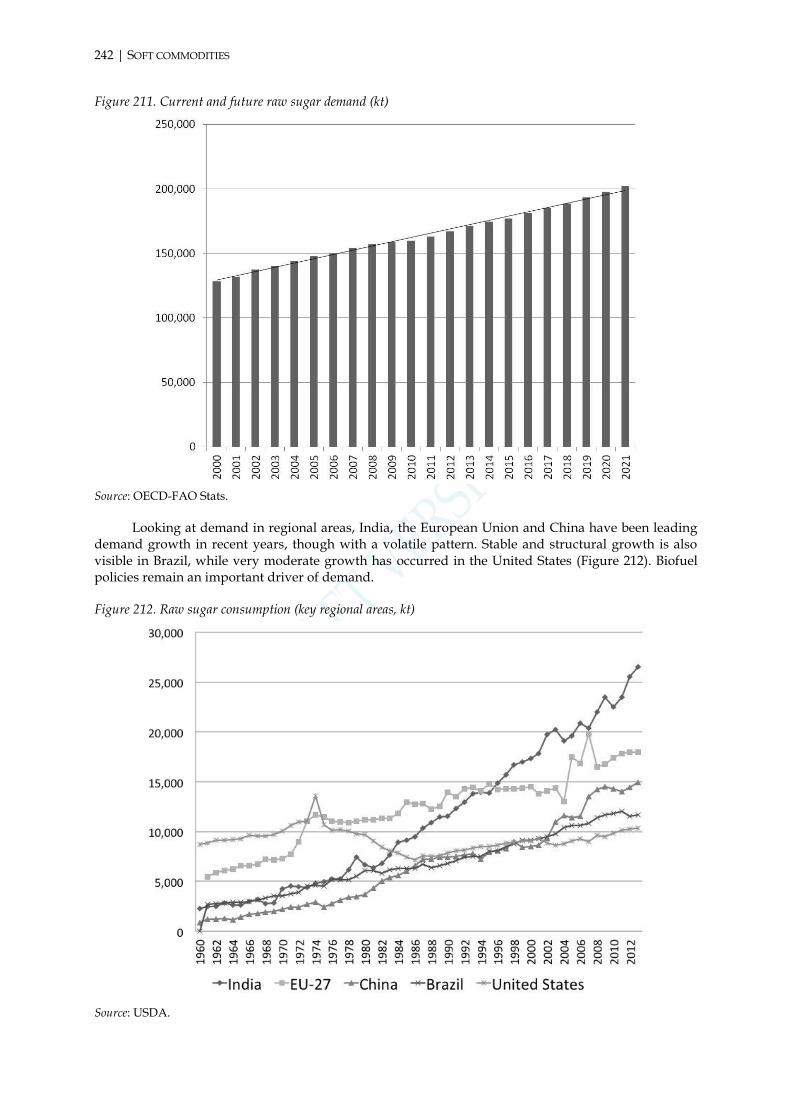
242 | SOFT COMMODITIES
Figure 211. Current and future raw sugar demand (kt)
Source: OECD-FAO Stats.
Looking at demand in regional areas, India, the European Union and China have been leading demand growth in recent years, though with a volatile pattern. Stable and structural growth is also visible in Brazil, while very moderate growth has occurred in the United States (Figure 212). Biofuel policies remain an important driver of demand.
Figure 212. Raw sugar consumption (key regional areas, kt)
Source: USDA.

Almost 75% of biofuel production will come from sugar by 2021 (Figure 213). Most of the remaining production will come from coarse grains, such as corn and sorghum for ethanol and soybean for biodiesel. Today, the contribution of sugar to biofuel production is already above 65%, as the massive biofuel production in Brazil relies almost exclusively on sugar cane processing for ethanol extraction.
Figure 213. Sources of biofuel production (kt)
Source: Author’s elaboration from OECD-FAO Stats.
While less than 25% of raw sugar is used for biofuel production today, in 2021 this may be as high as 31%, reigniting the food versus biofuel debate.
Figure 214. Food and biofuel use (kt)
Source: Author’s elaboration from OECD-FAO Stats.

244 | SOFT COMMODITIES
However, the debate is still open, with those claiming that – on top of potential increments in the productivity of the land – there is underutilised sugar capacity in the world due to distortions in trade caused by government policies, which have kept prices at artificial levels, unable to shape incentives to invest around the world (Hira, 2011). As trade distortions are gradually removed due to the WTO commitments, markets will reveal more about the economic sustainability of higher biofuel use supported by increasing sugar production.
5.1.1.3 Key product and market characteristics
The product and market characteristics of raw and refined sugar are shaped by a delicate equilibrium of endogenous and exogenous variables. Endogenous factors are important drivers of price formation. More precisely, the following endogenous characteristics can be ascertained:
Sugar is a renewable commodity with great yield potential, but limited alternative uses can be made of it (mainly in food and biofuels).
The convertibility of crop production to alternative products is unlimited, but there is much less flexibility for refining plants, which cannot be easily converted to alternative productions.
Capital investments are required, but fixed operating costs are limited.
The opportunity cost for the land may become an important factor as emerging economies become wealthier, with production costs of substitutes such as corn (which can produce both a sweetening syrup and biofuel) becoming an important driver of change.
International trade has been steadily growing in recent years and more vertical coordination between the processing and refining of raw sugar may stimulate their further concentration, thus encouraging international markets rather than production and consumption in the same region (even if subsidised by taxpayers’ money)
Supply relies on low-cost production and appears dispersed in its industrial structure but very concentrated in geographical terms. Industry consolidation is growing, however, partly due to stricter links among farmers and trading houses, as well as to more coordination among farms through cooperative instruments.
Demand elasticity to price changes is high due to the number of substitutes that can reduce the appetite for the commodity.
The supply side also shows some elasticity to demand patterns, mainly due to low fixed production costs, but growing supply constraints (such as lack of investments) may affect this elasticity in the medium term.
High demand from emerging markets will continue, both for food and biofuel uses, but the elimination of government subsidies programmes and other distortions may produce unpredictable results in the short term.
Emerging markets may be a source of both high demand and potentially higher supply capacity, in particular if they improve yields.
Future demand and production capacity may grow in the coming years, but it will very much depend on how the supply side adapts to a new, challenging environment.
Table 75. Key product and market characteristics
Recycling/ Production
convertibility
Substitutes/ Horizontal integration
Alternative uses/
Vertical integration
Capital intensive
production
Stora-bility
Freight costs
incidence
Elasticity to price/ demand
Concen-tration
BRICs weight
Future Consumption/
Production
Demand side
None High High
Low Mediu
m Medium
High Low/
medium
High High
Supply side
High High High Medium Medium High
Source: Author.

5.1.2 Exogenous factors: the effects of EU reforms
As illustrated for other crop commodities, several exogenous factors can impact the determinants of raw sugar production. Government subsidies programmes and the oil price are the main exogenous factors driving the latest market trends. For instance, the sugar reform in the European Union, aimed at keeping prices very low by subsidising local production to have a constant oversupply, has reduced quota production (indirect market price support) and replaced direct transfers based on sugar outputs with monetary transfers to producers within the general direct transfers foreseen in the CAP agreements. By the end of 2009, no direct market support was being given to sugar producers based on output, while quotas have been revised below consumption levels. The elimination of this market distortion has resulted in a drop in sugar beet production in the region, with the European Union ultimately becoming a net importer of raw sugar (mainly from Brazil). While raw sugar imports have slightly increased since 2006 (when the effects of the reform began to), refined sugar exports, the biggest item in European sugar trade, have dropped by 84% in three years, and have so far struggled to pick up again (Figure 215).
Figure 215. EU-27 (EU-15 until 2004 and EU-25 until 2006) raw imports and refined exports (kt)
Source: Author’s elaboration from USDA.
This situation may result in a shift of production towards countries with lower labour and energy costs, as well as to raw sugar producers deciding to internalise the refining process and export refined and raw products together.
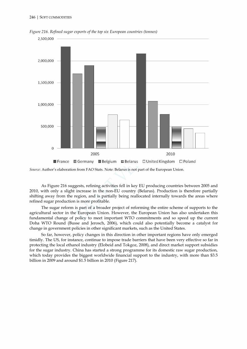
246 | SOFT COMMODITIES
Figure 216. Refined sugar exports of the top six European countries (tonnes)
Source: Author’s elaboration from FAO Stats. Note: Belarus is not part of the European Union.
As Figure 216 suggests, refining activities fell in key EU producing countries between 2005 and 2010, with only a slight increase in the non-EU country (Belarus). Production is therefore partially shifting away from the region, and is partially being reallocated internally towards the areas where refined sugar production is more profitable.
The sugar reform is part of a broader project of reforming the entire scheme of supports to the agricultural sector in the European Union. However, the European Union has also undertaken this fundamental change of policy to meet important WTO commitments and so speed up the current Doha WTO Round (Busse and Jerosch, 2006), which could also potentially become a catalyst for change in government policies in other significant markets, such as the United States.
So far, however, policy changes in this direction in other important regions have only emerged timidly. The US, for instance, continue to impose trade barriers that have been very effective so far in protecting the local ethanol industry (Elobeid and Tokgoz, 2008), and direct market support subsidies for the sugar industry. China has started a strong programme for its domestic raw sugar production, which today provides the biggest worldwide financial support to the industry, with more than $3.5 billion in 2009 and around $1.5 billion in 2010 (Figure 217).

Figure 217. Chinese and US direct support to the sugar industry ($mn)
Source: Author’s elaboration from OECD-FAO statistics.
Both interventions have been targeting direct market support for sugar prices, often coupled with tariffs to discourage imports (for instance, US import tariffs for ethanol fuel).
Table 76. Key exogenous factors
Government intervention Main other external factors
High Weather, exchange rates, oil prices, lands value
Source: Author.
Other exogenous factors can influence sugar markets. In particular, exchange rates have been the subject of strong discussion among developing and advanced countries, as the appreciation of local currencies against the dollar can cause important shifts in labour costs, final product price and opportunity costs of land. In fact, land value is another key factor influencing the dominant low-cost productions. Any policy that increases the value of the underlying land can have an indirect effect on the commercial viability of the business. Oil prices can also have important implications for sugar, both for the use of petroleum-based products, such as fertilisers and fuel for machinery, and the development of biofuel policies as a valid option to increase diversification and independence from the price of oil.
Markets have to deal with legal certainty as well, especially when it needs to ensure that trading activities are run smoothly. For instance, futures trading on sugar contracts on the Indian Exchange was halted and banned for over 17 months after claims that the local supply was undergoing large cuts due to a bad season. This was, in reality, an action by primary consumer in the world to keep control over sugar prices and make restrictions effective. Prices in local spot markets continued to grow because the flow of information into prices obviously could not be stopped by shutting down the futures markets, and the spike in price was very high and sudden. A ban on futures trading was implemented in India in 2007 for some staple food product.
Finally, weather conditions, since cultivation is in the open air, may have some impact on production (at least in the short term). Even though markets have become more equipped to give valid probabilities to weather events, this variable is still the least predictable among the exogenous factors described above.

248 | SOFT COMMODITIES
5.1.3 Market organisation: a fast developing international market
As for other commodities, physical market organisation relies on a web of bilateral and forward contracts among cooperatives of farmers and big industrial players (trading houses). Production is fairly dispersed, but international markets have a more concentrated structure. Bilateral spot and forward contracts may rely on active futures markets where benchmark contracts are continuously priced. Two liquid futures markets, in Europe for refined white sugar (on LIFFE) and in the United States for raw cane sugar (on ICE) have become reference markets for spot and future transactions. Despite being under different platforms and in different locations, ICE owns them both, which brings global reference prices for soft commodities under a single ownership. Delivery ports, however, are also available in South America, Asia (including China and India for the white sugar contract), and Oceania.
Table 77. Market organisation factors
Physical market setting Pricing complexity Liquidity futures market Delivery points
Competitive (local) Oligopolistic (global)
Low High Limited
(US and EU)
Source: Author.
Other futures markets are also active, such as the Indian exchange, but they do not have enough liquidity or are pure financial contracts trading the same contract on ICE or LIFFE, with no possibility of physical delivery.
The presence of trade barriers and other distortions to free markets has always limited the potential of sugar futures markets. However, the growth of international trade and the reduction of market distortions in the WTO Rounds, and so the limitation over artificial market prices, may increase the importance of liquid futures markets as they become a valid alternative to manage price risk in sugar trades rather than using quotas. They may increasingly become a point of reference for the pricing of international trades.

5.2 Cocoa market
Cocoa beans are a product of cocoa trees and are widely used for food and beverages production, but more recently also for pharmaceutical products (cocoa butter). Production is typically concentrated around the Equator and it was already being cultivated for human consumption (mainly as an ingredient for beverages) in Central and South America at the time of the Roman Empire. Cocoa beans were only brought to Europe in the mid-17th century. Their commercial use for chocolate production only arrived in the 19th century with the discovery of a production process that allowed the extraction of both cocoa powder and butter at a low cost. The yearly production of cocoa beans is valued at around $13 billion, and the cost of the beans is generally only a small part of total production costs of the final product, chocolate (Gilbert, 2008). Nonetheless, almost 90% of cocoa beans are used for food and beverages production (Figure 218).
Cocoa beans were also used in ancient times as money for the exchange of goods. Beans can be stored for several months in bags and traded multiple times. They hold their value well and their scarcity (due to the particular cultivation required for their production) makes them a suitable store of value during crises. As a consequence, prices patterns have followed the economic cycle, and also the growing demand of consumption coming from both emerging and developing markets. This has resulted in astonishing growth in prices, which almost tripled from 2000 to 2010, before dropping slightly recently.
Figure 218. Cocoa beans uses
Source: Author’s elaboration from FAO Stats.
In real terms, prices are still a fair way from the peak at the end of the second oil crisis, which was followed by a drop and a gradual stabilisation of prices during most of the 1980s and 1990s at between $1-2 per kilogram.

250 | SOFT COMMODITIES
Figure 219. Cocoa beans real and nominal prices
Note: International Cocoa Organization daily price, average of the first three positions on the terminal markets of
New York and London, nearest three future trading months.
Source: World Bank.
5.2.1 Product and market characteristics: new prospects for alternative uses
Cocoa beans are the seeds of a fruit (pod) produced by a tree, 10-20 metres tall, that needs specific temperatures and amounts of rainfall every year. The plant is typically grown in forests, with some shade and wind protection. Maturation of the fruits takes five to six months, and the first fruit only appears around five years after plantation. Even though the trees can even live for up to 200 hundred years, they are commercially profitable for only 25 years. A large harvest occurs from September/October to February, and a smaller one before July. Cocoa seeds are usually subject to an initial processing, which entails open pods ‘sweating’ their pulp for a few days over the seeds. This helps the fermentation process, which is followed by the process of drying the beans to reduce moisture levels (to help storage), before sending them to the market for commercialisation. The next processing stage involves roasting the beans for a couple of hours, which helps to build the chocolate aroma. This second part of the processing can also be done at the country of destination.
Cocoa seeds (or beans/nibs) are fairly homogeneous, with one variety (forastero) representing the vast majority of the global production. Other (higher quality) varieties are available but commercial production is very limited. They cannot be recycled but it is a renewable crop which is not a primary good, but can be substituted with alternative sweet food. No alternatives are available for its taste and aroma, though. Most notably, cocoa has a high vitamin E content, which makes it an important component of the human diet. Product substitutability is limited due to the unique properties of the cocoa beans, which can be at the same time a diuretic, stimulant, anti-depressant and nutritive. These qualities meant that the fruit was widely used by ancient populations around the Equator. Dark chocolate has also been proved to provide important cardiovascular health benefits (Schroeter et al. 2006; Taubert et al., 2007).

Figure 220. Historical cocoa beans uses (tonnes, %)
Source: Author’s elaboration from FAO Stats.
Cocoa beans are mainly used for chocolate production. After local early processing (involving seeds ‘sweating’ and ‘drying’), beans are exported and roasted close to consumption areas. Roasting allows reducing moisture content and adjusting the chocolate aroma to give a special flavour. Seeds are then cracked to remove shells and the internal part (the ‘nib’) is crushed with a mechanical process in order to produce storable liquor, in a process called ‘grinding’. Further processing to allow solidification or to reduce moisture content through a mechanical press produces cocoa butter and powder, respectively, which are main ingredients of chocolate production. Cocoa butter and powder are extracted in the same proportion from the processing of the beans. However, cocoa butter has more value due to its many uses in the food, beverage and non-food industries. In the industrial production of chocolate, cocoa powder or butter is only a base ingredient to which other ingredients are added (such as milk and sugar). The combination of these ingredients, moulded together at specific temperatures, is the discretionary aspect in the production process that gives value to chocolate products.
A growing share of cocoa bean production is also dedicated to pharmaceutical products because cocoa butter (typically converted into oil) has the important property of melting at body temperature. In particular, it can be used to encapsulate drugs and skin applications thanks to the Vitamin E content. As show below, non-food uses make up roughly 8% of global production and are growing with on the medium-term horizon.
Other uses also include cosmetics and soaps, as the properties of cocoa remain stable for years. There is potential for the development of by-products, which could increase the commercial attractiveness of the product. Over 60% of the pulp is typically wasted. Pulp and pods (which have a high gum component) may be products for alternative uses, such as soap or even animal feed. The processing of cocoa beans also produces oil and shells.
Production
The production of cocoa beans can be renewed but there are two important supply constraints. First, production of cocoa bean from the plant becomes commercial only five years after plantation. The tree produces beans for only 25 years in tropical and humid areas, under the shade of taller vegetation, even though the plant can live up to 200 years. Second, on top of particular needs such as shade, wind

252 | SOFT COMMODITIES
protection and roughly 10 cm of rainfall per month, cocoa is commercially produced in the open at around 15° above and below the equator line (for temperature reasons).
As shown by Figure 221, cocoa bean production has been constantly growing in the last three decades, with a significant jump after 2003 as demand from emerging markets became more sustained and when the market opened up to global competition (the liberalisation process).
Figure 221. Cocoa beans world production, 1961-2011 (tonnes)
Source: FAO Stats.
In recent years, production has slowed down and it is now stable at around 4 million tonnes, while the balance is consistently in surplus (as high as nearly 20%; Figure 222). This surplus was reflected in prices reaching a historical low around the beginning of the 2000s, and then gradually recovering to around $2 per kg.
Figure 222. Production, consumption and net production (tonnes, %)
Source: Author’s elaboration from CRB Commodity Yearbook (2011).

Production is concentrated in West Africa (66%), with a further third produced in South America and South East Asia (Figure 223). No commercial production is available in Europe. Africa’s market share has grown significantly after the end of the price controls and the opening up of markets to global competition at the end of the 1980s.
Figure 223. Cocoa beans production by region, 1961-2011 (tonnes)
Source: Author’s elaboration from FAO Stats.
Among producing countries, Ivory Coast, Indonesia and Ghana account for more than two-thirds of global production, which exposes the market to exogenous factors such as political instability in a region that has already undergone long periods of severe instability in the past decades.
Figure 224. Key global producers, 2011 (% of total)
Source: Author’s elaboration from FAO Stats.

254 | SOFT COMMODITIES
Concentration in production (the top ten producers represent 97% of cocoa bean production) is also counterbalanced by high concentration in the consumption of cocoa beans, which are mainly refined in the European Union (37%), the United States (10%), and countries where the cocoa beans are produced before being exported as a more final product.
Figure 225. Top ten producers (left) and consumers (right), 2011
Note: tonnes.
Source: Author’s elaboration from FAO Stats.
Storage
The storage life of cocoa (in bean form, but more so as a as powder or liquor) is long. Once fermented and dried, there is one year of storage life for cocoa beans before they begin to deteriorate (which goes very slowly). Another 5-6 months of storage life is gained after processing (roasting) the bean and de-shelling into nibs, while the most refined product (cocoa liquor or paste) can be stored for many years before it begins to lose its properties. Together with its limited supply, these storage characteristics allow the commodity to be more easily sold in the market, as well as imposing some anti-cyclical patterns. Due to its easy storability, freight costs have a limited impact in the long term. Cocoa beans can be directly stored after collection from the plants, which does not add more transportation steps before the final production of the refined product. However, consumption areas are typically far from production countries, so volatility in shipping costs can produce some short-term impacts on costs.
On the market side, the constant production surplus – enhanced by the recent economic crisis – has recently boosted stock variations positively, growing to 10% of total production in 2009.
Figure 226. Global stocks variations (tonnes)

Source: Author’s elaboration from FAO Stats.
This may reflect a conflict between price-elastic consumption and a rather slow adjustment of supply to changes in consumption levels. As a consequence, prices would react (with a lag) to a negative/positive supply shock reflected in variations of inventory levels rather than to a short-term variation of consumption levels (Gilbert, 2012), as argued by the storage theory. Long-term shocks to demand, however, can affect price levels with similar intensity, as they will gradually be reflected in supply levels and stock variations.
Harvested areas and yields
No important advancements have been made so far in developing genetically engineered cocoa bean production to increase yields while containing harvested areas and so the collateral effects of potentially excessive land use (e.g. deforestation and water waste). While global yields were more or less stable since the 1980s and have been declining in recent years, harvested areas have almost doubled since the beginning of 1990s, with a sharp increase at the beginning of this century being one the most significant effects of the opening up of markets in developing economies (with similar effects to those seen for other commodities covered in this report; Figure 227).
Figure 227. Global harvested areas (ha) and yield (hg/ha)
Source: Author’s elaboration from FAO Stats.
There is therefore a potential high margin for yields to exploit new technological developments in fertilisers, machinery and bio-engineering (if needed) to produce more without necessarily expanding harvested areas. Africa is no exception. Once the market was liberalised at the end of the 1980s, yields went immediately up as many inefficient producers were put out of the market and new production came in with higher and more stable yields, after a natural lag of 4-5 years (Figure 228). Since the 1990s, though, besides a higher contribution in terms of harvested areas, not much has changed.

256 | SOFT COMMODITIES
Figure 228. African harvested areas (ha) and yield (hg/ha)
Source: Author’s elaboration from FAO Stats.
Since the beginning of the 21st century, harvested areas have been growing at a speed has begun to raise questions over sustainability if it were to grow even further in the coming years.
International trade
Reflecting of the distribution of producers, international trade is organised around the same production and consumption areas, since cocoa beans are typically used in the production of chocolate around consumption areas. The top ten exporters of cocoa beans have 90% of the export market, led mainly by developing economies, while Belgium and the Netherlands are partially exporters because they are the main ports of delivery and trade in Europe. Ivory Coast accounts for almost 30% of the exports, while the European Union (in particular, big chocolate producers such as the Netherlands, Belgium and Germany) attracts almost 60% of total imports (Figure 229).
Figure 229. Top ten exporters (left) and importers (right), 2011
Note: metric tonnes.
Source: Author’s elaboration from FAO Stats.

The total value of international trade grew quickly in the last decade to reach almost $10 billion in 2010 (70% of the total yearly production value). The market is small compared to other crops, but international trade relative to total production is among the highest in international commodities markets (Figure 230).
The processing of cocoa beans, beyond the immediate cleaning and drying required after harvesting, is mainly carried out close to consumption areas by totally different market participants, which are usually much bigger and more international in market reach. Since only a few players are involved both in production/conversion and (chocolate) manufacturing, international trade is led by the big trades of those few that have the capacity to be converters and manufacturers, in addition to the market activities of single manufacturers/converters. International trade is mainly in cocoa beans as butter or liquor can be too costly to export because they require special treatment (e.g. an artificial temperature).
Figure 230. Value of international trade ($bn)
Source: Author’s elaboration from FAO Stats and World Bank.
5.2.1.1 Supply characteristics: the dominance of the refining industry
While the production process is very simple, the value chain of cocoa production has different layers and requires the involvement of several actors. In the upstream market, small-scale producers dominate production levels. Increasing coordination in cooperatives has given more contractual power to smallholders, which have to deal with big international traders. The refining industry is fairly concentrated, but with different degrees along the long processing chain, which is mainly developed abroad (Figure 231).

258 | SOFT COMMODITIES
Figure 231. Cocoa beans processing
Source: Author.
Small-scale plantations, often united through cooperatives to increase their contractual power, are the standard type of producer in tropical regions. These producers deal with local traders before the product reaches exporting companies, which are typically international firms. The exporting company is not necessarily a grinder and converter, so the product may be simply sold to an import company that will sell it or process it further once it has been imported and is close to the consumption area. While production is a competitive market, the massive economies of scale needed to run the grinding and converting process may result in high concentration, producing an oligopolistic setting (Gilbert, 2008). Therefore, to increase economies of scale and scope, the downstream part of the supply chain (converters and chocolate manufacturers) is increasingly becoming more vertically and horizontally integrated. Due to the local nature of production versus the international nature of cocoa processing, exporters, foreign grinders or chocolate manufacturers enjoy some oligopsonistic market power (UNCTAD, 2008; Kireyev, 2010). Cocoa bean processing for chocolate production also interacts with sugar and milk value chains. As a consequence, the cost of cocoa beans is only a very small part (3.5%) of total chocolate costs (Gilbert, 2008). Processing and other retail costs are the two most important production cost items.
Due to the known supply constraints, elasticity of supply to demand is fairly low. Increasing production is difficult because the plant requires time before it becomes commercially usable. Therefore, supply arrives to the market years later and may not be easy to remove, as producers are price-takers and they would not be interested in cutting their own supply once on the market. Converting land to alternative uses has both the constraint of an external environment that may not easily allow alternative cultivation, as well as the sunk costs of having spent several years bringing the area up to full production. However, the cocoa bean does not require immediate refining so it can be easily stored and shipped right after collection, which makes it easier to manage reductions in production.
5.2.1.2 Demand characteristics: the link with income growth
Since the production of cocoa is local but it is an export crop, market concentration on the demand side is high at the regional level due to the concentration among exporters. Demand concentration is much lower at global level, however, especially with the final product. Historical market fragmentation and a lack of cooperation among regional farmers have also increased the contractual

power of the demand side. This situation, however, is gradually changing as farmers coalesce to increase their contractual strength and have access to global markets and the global supply chain.
Emerging markets have a fundamental role in the production process, but a rather limited role in consumption that is dominated by European countries and the United States. However, growing populations and gradual redistribution of wealth will increase the use of cocoa and its main refined product in the dietary habits of newly developing countries. Cocoa is often seen as an expensive good that does not satisfy a primary dietary need. As a result, elasticity of demand to price is low for specific food use (e.g. chocolate) in higher-income countries, while elasticity is greater for the alternative uses of cocoa beans (e.g. pharmaceutical products). No immediately substitutable product is generally available, but products that use a very low amount of cocoa are increasingly available and that can be seen (especially by low-income consumers) as an alternative product to those costly ones with high-cocoa content. The increasing sophistication of cocoa-based products requires an increasing level of vertical integration, which would mainly leave only production, harvesting and primary processing to third parties.
5.2.1.3 Key product and market characteristics
The product and market characteristics of cocoa are those of a particular export crop that relies on a complex interaction between different value chains and income levels. These characteristics can be summarised as follows:
Cocoa beans are a renewable commodity with strong homogeneity and limited substitutes, but mainly used for one purpose (food).
New market developments are still to be seen, due to limited alternative uses of the commodity, commercial use of co-products, and very low yields due to the lack of technological developments in biological engineering.
Supply suffers important constraints due to the nature of the commodity, with a lack of production convertibility and low elasticity to short- and medium-term demand shocks.
Capital needed to produce cocoa is typically very low, and this aspect results in a production environment fragmented across several small-scale plantations, on the one hand, and in a strong processing industry enjoying an oligopsonistic power on the other. Concentration is therefore very low in the upstream market but is growing as the commodity requires more economies of scale to make processing and product refining profitable.
Cocoa beans are an export crop that relies on high storability and acceptable freight costs if exported in its raw form (beans).
Demand elasticity to price is high for higher-income consumers that have consolidated the use of chocolate in their dietary habits, but lower for low-income consumers that still perceive chocolate as a luxury good.
Emerging markets are essentially the only production area and also the consumption areas with greatest potential, as their average incomes increase due to economic development.
As future consumption depends on several aspects, including income and dietary habits, future production may need to rise to deal with recent increase in demand from emerging markets, which is driving prices out of a price range that has been consistently below $2 per kg for over 20 years.
Table 78. Product and market characteristics
Recycling/ Production
convertibility
Substitutes/ Horizontal integration
Alternative uses/Vertical integration
Capital intensive
production
Stora-bility
Freight costs
incidence
Elasticity to price/ demand
Concen-tration
BRICs weight
Future Consumption/
Production
Demand side
None Medium Low
Low High Medium
Medium
Medium
Low Medium
Supply side
Low Medium Medium Low High High
Source: Author.

260 | SOFT COMMODITIES
5.2.2 Exogenous factors: long-term effects of liberalisation
In addition to the endogenous factors described above, there are several exogenous factors that have an impact on this market. Most importantly, weather conditions in recent years and military conflicts (i.e. political instability) in past years have become drivers of changes in this market. Neither of these, however, has produced changes in this market to the same degree as the liberalisation process that shook Africa at the end of the 1980s, with the abolition of trade agreements and the pricing power of marketing boards. The process not only had heatedly debated redistribution effects, but also boosted production and productivity to unprecedented levels, driving long-term changes in the market (see Box 10). Overall, the process has reduced the pervasive government intervention that was anyway unable to increase living standards of local populations, due to great inefficiencies and consolidated corrupt systems. However, the process was implemented differently across countries and organisations controlled by governments still play an important role today in controlling resources and the share of export revenues that the domestic industry is able to extract from international traders.
Box 10. Causes and effects of market liberalisation: the case of cocoa
The post-independence (of former British and French colonies) liberalisation of marketing boards and other public (state-owned) or semi-public infrastructures, which had the power to fix prices, quality, and quantity of the commodity (Gilbert, 2009), aimed at:
Stabilising prices.
Ensuring high-quality products and more efficient production through greater competition.
Increasing transparency of marketing boards.
Reducing market power of local processing firms and exporters.
Increasing producers’ welfare and share of total value.
Since most of the liberalisation processes were completed in key producing countries in the 1990s, the effects on market operators have been significant. Liberalisation increased competition in production and intermediation/export of cocoa beans, bringing down global prices (Gilbert, 2009). It also delivered price stability and increases in production levels and productivity (as shown by Figure 227). New regions (such as Indonesia) have gradually increased their market share as lower-cost producers. The process gave opportunities to those areas showing flexibility and openness to competition, which implemented these reforms in the best possible way. For instance, Ghana and, to some extent, Ivory Coast have seen a long and incomplete implementation of the process, opening up domestic crop production but keeping control over the export industry (UNCTAD, 2008). Other countries have interpreted this process differently, or even coupled it with the liberalisation of foreign exchange regimes, leading to different results. As a result, there is still debate today over whether the transmission of world prices and disintermediation reached the farm gate in several countries, where taxation has often been used as an alternative way to control prices. In addition, a lower cocoa bean price was insufficient to influence the prices of retail products, which have increased due to the impact of other factors such as labour costs and other ingredients. It is therefore hard to quantify the beneficial effects of the process.
The liberalisation process has also generated side effects. Besides the long and troubled post-liberalisation political process of defining a new equilibrium among domestic actors, the implementation has created too much pressure too quickly on production costs in some countries, due to global competition and the legacy of local marketing boards’ pricing power. Some local producers, who were already poor, were unprepared (and lacked government support) to internalise these changes and quickly needed to coalesce into cooperatives to deal with the strong market power of global players. Some high-cost producers (especially in Central America) have greatly suffered the new competitive environment and had to modify their business to cope with a lower-cost and higher-production environment.

Figure 232. Key African producers' prices as a share of world prices (%)
Source: UNCTAD (2008), p. 35.
Whether producers’ share of the global cocoa bean price (calculated by ICCO) indeed declined after the liberalisation in Africa, this does not capture how the industry has changed (UNCTAD, 2008), in particular the change in ownership of local plantations from being mostly state-controlled. This could provide the final say on how producers’ share of the global price has actually changed the welfare and economic conditions of local populations. Questions have also been raised about the environmental sustainability of these strong competitive pressures, which initially had an impact on the quality of production (Oxfam, 2009; Gilbert, 2009).
On the one hand, opportunities emerged to expand production and business beyond local intermediaries, but on the other hand, it required consolidation that was much easier to achieve in intermediation (export) than production, with local production still fragmented in many countries today. The process also caused a general and structural reduction of production costs, and so global benchmark prices dropped to historically low levels. Quality also went down, but new market niches emerged for high-quality cocoa products. Some producers in Central America and Africa were unable to cope with this process, which worsened their standard of living and increased poverty. As a reaction to this process, a movement advocating ‘fairer’ trade emerged. This movement, represented by confederations or groups such as Oxfam, sees the liberalisation process mainly as a vertical redistribution of resources in favour of international traders that have gradually taken greater control of the cocoa (and coffee) export and processing chain. This ‘fair trade’ movement that emerged during the 1990s and early 2000s has, over time, forced even big companies to purchase cocoa and coffee at an additional premium to be redistributed for activities that would support local producers.
Another important exogenous factor is economic development. In particular, economic development supports income growth and, therefore, changes in dietary habits that typically favour higher consumption of cocoa on a regular basis. The economic cycle therefore has only a marginal impact on cocoa consumption, while more long-term economic development is able to produce important changes in the market. In the short term, cocoa even shows some anti-cyclical characteristics as the commodity can be stored for a long time without losing its properties and can be easily traded and shipped in international markets, and supply does not easily adjust to short-term economic fluctuations of demand.

262 | SOFT COMMODITIES
Table 79. Key exogenous factors
Government intervention Main other external factors
Medium Weather, political instability and military conflicts,
economic development
Source: Author.
Finally, as suggested above, the location of the top producers also raises the problem of potential political instability, which has often resulted in the past in long military conflicts. This exogenous variable is difficult to predict and thus produces a great deal of uncertainty that markets are unable to price. This factor may put cocoa prices under sudden volatile conditions that may be difficult to recover from in the short-term.
5.2.3 Empirical analysis: the role of inventories
It is hard to model directly front-month settlement prices on futures (LIFFE) for cocoa. However, as explained by Gilbert (2012), cocoa prices react to supply shocks through changes in inventory levels in the short term (as the supply does not adjust rapidly; very much in line with the storage theory illustrated in Chapter 1). Therefore, most of the empirical analysis is done on inventory levels of LIFFE (monthly data). The analysis is complicated by additional interaction of endogenous variable with exogenous factors. The following dataset of monthly data was used for this analysis:
Monthly data from March 2002 to December 2012.
Log of end of month front-month LIFFE futures contract on cocoa.
Log147 of monthly data on LIFFE stocks.
Log of OECD leading composite indicator demand indicator for OECD countries.
Log of OECD leading composite indicator demand indicator for China.
Log of price-adjusted Broad Dollar Index published by the Fed.
Log of Southern Oscillation Index (to which a constant is added to account for negative values
in logarithmic transformation).148
Log of S&P 500 (closing).
The volatility indicator is the 22-day annualised rolling standard deviation of front-month price.
Log of convenience yield at 100 days (as the difference between expected price [front-month price times 100 days annualised risk-free interest rate] and second month futures price, minus actual cost of storage).
Dividend yield (as the difference between convenience yield and basis between front and second month, over the front months).
A broad regression (see Output #58) shows white noise in its residuals but may not be sufficiently specified. However, a strong link emerges between cocoa inventories and OECD demand, convenience yield (real cost of storage), and dollar exchange. To verify these relationships and confirm their link with the theoretical background, a Granger causality test is done between cocoa stocks and dollar exchange rate index, OECD demand, convenience yield, and dividend yield (see Output #59, Output #60, Output #61, and Output #62).
147 For ‘Log’ we intend a natural logarithm (ln).
148 The Southern Oscillation Index (SOI) gives an indication of the development and intensity of El Niño or La Niña events in the Pacific Ocean. The SOI is calculated using the pressure differences between Tahiti and Darwin.

Table 80. Granger causality outputs
Independent variables Granger causality with cocoa stocks Inverse relationship
Broad Dollar Index Yes*** No
OECD demand Yes*** No
Dividend yield Yes*** No
Convenience yield Yes*** Yes**
Note: *10%, **5%, ***1% significance.
Source: Author’s calculations.
As Table 80 illustrates, the dollar exchange rate and broader demand (the general economic situation) Granger-cause cocoa stock levels. The analysis also confirms, through convenience and dividend yield, the importance of costs of storage and opportunity costs (represented by risk-free interest rates) in driving levels of stocks. In addition, a Granger causal relationship was established between spot prices and weather index, represented by SOI.
Furthermore, the empirical analysis confirms the theoretical background of the impact of monetary policies and credit easing in building a link between financial and non-financial assets. As described by Output #64, when extending the database from to March 1990, a linear regression between log front-month prices and S&P 500 closing finds that before (end) 2001 there was no relationship between cocoa prices and financial indexes. From 2002, when the decline of the dollar exchange rate started as a result of expansionary monetary policies (reflected in the expansion of the monetary base and lower interest rates), the relationship between cocoa prices and financial indexes became significant at 10% (with a negative sign). This shows once again that a common variable has affected both financial and non-financial assets and driven them in the same direction, mainly through the role of exchange rates. The small coefficient (.3), however, defines this relationship as marginal in relation to other important links established above, for instance with OECD demand. Demand and supply fundamentals are still key drivers of price formation for cocoa markets.
Finally, no Granger was able to show a clear prevalence of one of the markets in the interaction between types of market player and prices (commercial versus index positions). Output #66 suggest that, at 10%, there is a small but significant link between front-month commercial positions in the futures market (0.15) and the position of commercial players, while no significant relationship was found between prices and index positions. No definite conclusions, however, can be drawn on whether trading on physical or futures are driving price formation in cocoa markets.
5.2.4 Market organisation: an immature market infrastructure
Market organisation of physical markets for cocoa is similar to that for other commodities. It mainly relies on bilateral spot and forward contracts with price formula frequently linked to the main benchmark front-month futures contracts. However, it also depends at which stage of the long value chain we are looking at. Local intermediaries rely more on spot traders with local producers, even though small producers, due to technological developments, are also increasingly taking global benchmark futures contracts prices (front-month) as a reference price (with a discount or premium) for local trades.
Futures markets for cocoa mainly rely on two liquid contracts traded on two exchanges, one in Europe (LIFFE) and one in the United States (ICE). Delivery areas offered by the exchanges are only located in the United States and Europe. Both futures contracts accept delivery for all types of cocoa bean with a set discount. The underlying commodity is cocoa beans sealed in bags and the minimum contract size is 10 tonnes.
Table 81. Cocoa market organisation
Physical market setting Pricing complexity Liquidity futures market Delivery points
Competitive (local) Oligopolistic (global)
Low High Limited
(US and EU)
Source: Author.

264 | SOFT COMMODITIES
Due to its limited supply and high demand, cocoa is typically purchased in large quantities. Its storage life (either as a bean or in its more refined form) is long compared to other crops, and this allows the commodity to be more easily sold in the market and so purchased in bigger quantities. Its limited supply and its historically low price in recent years have made cornering attempts by big investors easier and, due to the market size, also easier to spot. For instance, in July 2010, Anthony Ward’s Armajaro hedge fund took delivery of over 241,000 tonnes of cocoa beans worth roughly $1 billion (roughly 5% of yearly global production), causing a sharp price increase leading to a historical peak on LIFFE. This trade, which corresponds to the total annual production of cocoa beans in Brazil, caused a significant shortage in the market and a widening spread between EU and US futures contracts. It is unclear whether the trade was simply aimed at speculating on future price trends, perhaps not so profitably when cocoa was offloaded later in 2010 at a lower price (over a three-month period), taking into account warehousing costs, or at cornering other market participants. As a consequence, such a trade, which is not very frequent in the market, may in the short term have prevented other market participants from finding enough positions available at specific dates due to a lack of supply. In any case, the market was deep enough to absorb the delivery in a month. The market player (as ‘non-commercial’) was then forced by price trends to sell the physical holding through a sale that lasted three months. The trade revealed itself to be very risky for the investment fund and markets have been able to hold it, though with some frictions. Management and transparency of positions for operators and regulators may help to supervise the accumulation of a position that may corner the market. In 2012, as a response to this type of event that may create disruption and loss of reputation for the exchange, LIFFE introduced a new system of delivery limits that applies to different commodities contracts on the exchange, with an important exemption for those contracts with a clear commitment to deliver the commodity to an end-user (a firm involved in
production, processing, or handling/packaging of a physical commodity)149. It therefore applies to all
positions, and exemptions must be requested by the member of the exchange.
Transparent and efficient futures markets are an opportunity to allocate resources across regions to those that value them more, in addition to being a hedging tool for big commercial counterparties. Futures markets also become an opportunity to bypass traditional intermediary channels, which can create artificial bottlenecks, so cutting transaction costs. In effect, they can limit the monopsonistic power of the processing industry. However, accessibility is an essential factor for futures markets to effectively reach the supply side. Unfortunately, cocoa futures markets do not necessarily take delivery outside Europe or the United States, which makes the expected costs for producers in Africa or other regions to sell their product prohibitively high (also due to their local fragmentation).
149 For more details, please see https://globalderivatives.nyx.com/sites/ globalderivatives.nyx.com/files/lon3635_revised_250912.pdf.

5.3 Coffee market
Coffee is a widely consumed drink extracted from coffee seeds that has an important stimulant component (caffeine). Consumption is mainly concentrated in western economies, and the value of
global production, which is mainly in developing economies, has reached over $28 billion in 2012.150
Coffee seeds are extracted from a plant cultivated in tropical regions and brewed for human consumption since medieval times. The commodity was first produced in Ethiopia, where a special Arabica variety is also produced (mocha), and only reached western countries around the 16th century. Its commercial utilisation only began only in the mid-19th century, when the drink quickly spread due to its use in coffeehouses where other activities (such as live music or dance) were also offered to coffee drinkers. The particular characteristics of caffeine became an important element of dietary habits of many people, which increased the long-term diffusion of the commodity. Over 97% of coffee beans are used today for brewed coffee production or for caffeine use in other types of drinks (Figure 233).
Figure 233. Green coffee uses
Source: Author’s elaboration from FAO Stats.
Non-food use is limited to some pharmaceutical products that require a caffeine component. Due to its production as a warm drink, coffee may be subject to seasonal demand, though this very much depends on how coffee is typically consumed.
Prices show a steady long-term downward trend as the market expanded on a global scale during 1980s and 1990s, with more efficient and productive production process. Limited alternative use of land in producing countries has supported this long-term trend. The effects of liberalisation, with the end of the international coffee agreements at the beginning of the 1990s, also helped to bring prices down to an historical low as expansion of supply has a lagged effect of 4-5 years on production levels. Since the early 2000s, however, prices have been gradually increasing again, with the spread between Arabica and Robusta varieties reaching a very high level in recent years.
150 Assuming, from USDA data, production of Arabica and Robusta was respectively 57% and 43%, it was multiplied by respective annual prices, as published by World Bank.

266 | SOFT COMMODITIES
Figure 234. Arabica and Robusta real coffee prices, 1960-2012
Source: World Bank.
The sharp increase, from the historical low at the beginning of the 2000s, is also confirmed when looking at the weighted average (by production levels) of Arabica and Robusta coffee (Figure 235). The compound annual growth rate from 2001 (the historical low) to 2012 was roughly 10%.
Figure 235. Coffee nominal weighted average price (Robusta and Arabica)
Note: Weighted average (by production levels) of Arabica and Robusta prices. Source: Author’s calculation.
In 2012, prices fell due to several factors, but overall prices appear to be in a new phase after having reached the bottom.

5.3.1 Product and market characteristics: the rise of Robusta coffee
Coffee beans are the seeds of the fruit produced by coffee plants. There are two main types of coffee seeds: Arabica and Robusta. Arabica can be found in several varieties with unique flavours due to different oil contents, so it is generally considered the high-quality coffee, both for beans and coffee blends. Robusta, on the other hand, has high caffeine content and a more standardised flavour, though it can be also found in slightly different varieties. It can be used both for low-quality coffee blends and higher-quality products. Coffee is a renewable crop with very low substitutability due to the particular substance (caffeine) and flavour that makes it a unique product. The differences among varieties have caused some authors to argue that coffee is more like wine rather than a standardised commodity (Fitter and Kaplinsky, 2001), while Ghoshray (2010) confirms that, on closer examination, the law of one price (between Arabica and Robusta) exists if we allow for non-linear adjustments from equilibrium.
Production of coffee beans can be renewed but, as for cocoa, there are significant supply constraints that slow down the reaction time to structural changes in demand. Harvesting coffee fruits from plants is commercially viable only 4-5 years after plantation. The tree can be harvested for up to three months, once a year for roughly 20 years in a belt of countries around the Equator.
Coffee requires some processing in order to extract the seed from the berry that is harvested from the coffee plant, often through labour-intensive hand picking, as not all fruits ripen at the same time. This bean (called green coffee) goes through dry and wet processing before roasting. Dry processing (the old method) involves, after removing foreign matters, placing the fruit in the sun for 2-3 weeks. Afterwards, the dried pulp is removed from the seeds, which are ready to be sold in the market. It is a natural and cheap method, but it is slow and may damage the seed. Wet processing is more widely adopted because it does not damage the seed and requires less time to wash the fruit and for the following fermentation. After processing, the green coffee bean is ready to be sold by producers to roasters and manufacturers, who will roast and grind (if sold as powder) the beans close to consumption areas. Roasted coffee will be used to prepare coffee blends sold to end-users. The roasting time shapes the flavour of coffee, and longer roasting reduces the amount of caffeine.
Roasted coffee beans or blends are typically used for coffee drink production, but coffee beans can also be processed to extract caffeine, which is a chemical compound (a stimulant) used in low quantities in other beverages (especially soft drinks) and in high concentration for pharmaceutical products, cosmetics, and even pesticides.
Robusta and Arabica varieties
Arabica and Robusta coffee are the two major categories of coffee, each with several varieties. Arabica is of higher quality, with different flavours, while Robusta is produced at low altitude with less flavour but more strength (and so higher caffeine content). Arabica coffee is heterogeneous, and so a premium based on quality is discounted in the final price. This premium is typically in a more or less stable range over time. However, from time to time (more recently, in 2011 and to some extent in 2012), the market experiences a sharp widening of the spread, which remain fairly unstable today (Figure 236).
Arabica has had fairly unstable production growth, as Robusta has come to account for almost half of the total coffee production (Figure 238). In particular, increasing global competition with the development of low-cost production of coffee by Brazil and Vietnam, supported by liberalisation processes in several countries, currency depreciation (e.g. of the Brazilian real) and technological developments to reduce the bitterness of low-quality Robusta coffee, has been gradually crowding out production of Arabica with the consequent slowing down of its production until 2005. This reduced the stocks of coffee 4-5 years down the line and resulted in a price spike in 2010 and part of 2011. In 2010-11, the situation was aggravated by bad weather conditions in Columbia and Central America before the main harvest, which enhanced this long-term structural change.

268 | SOFT COMMODITIES
Figure 236. Arabica and Robusta second-month futures prices (monthly)
Source: Author’s elaboration from ICE and LIFFE.
Even though low-cost production increased at faster rate (Figure 237), demand continued to grow strongly even after 2005 and gradually production has picked up again (again, 4-5 years later) causing the price drop of 2011-12, thanks also to supportive weather conditions. Arabica production, however, is still very volatile. As a result, coffee markets are undergoing important long-term changes that increase instability due to the inability to predict supply capacity as it is subject to very slow adjustment processes, which may push some producers out of the market in the meantime (in particular, if they do not have access to long-term credit).
Figure 237. Arabica and Robusta production (k/60 kg bags)
Source: Author’s elaboration form USDA.
Figure 238. Robusta and Arabica share of total production (%)
Source: Author’s elaboration from USDA.

Cheaper Robusta coffee may continue to play a structural role, which will result in further growth in the future. It is a very good commodity for mass production and for the stable and high margins that can be generated in international markets. Cheaper production costs and technological advancements put Robusta ahead for base coffee production. Product diversification and brand loyalty may continue to gain traction (Peluplessy, 2007) for Arabica varieties, however, as they become less widely produced and subject to more labour-intensive processing (e.g. shade grown coffee) to meet the demand of a growing part of the population that is developing more sophisticated taste for high-quality coffee.
This process of diversification is also gradually reflected in the changing correlation between Robusta and Arabica prices. The prices have historically experienced a strong positive correlation, but more recently this positive correlation is becoming weaker and periods of negative correlation are becoming more frequent and intense (Figure 239).
Figure 239. Three-year rolling correlation between Robusta and Arabica prices
Source: Author’s calculation from World Bank.
It may still take several years until this process becomes more visible, but in the meantime instability may still continue to shake the market.
Production and consumption
Production of green beans coffee has been growing since 1961, with some medium-term periods of stability during the 1970s and between mid-1980s and the end of 1990s, which saw the beginning of more diffused international trade after the liberalisation process in many countries and new WTO agreements (as discussed earlier). Production trends, however, appear to be very volatile as investment in agricultural technologies that can limit damage from the weather and plant diseases has only taken place in recent years.
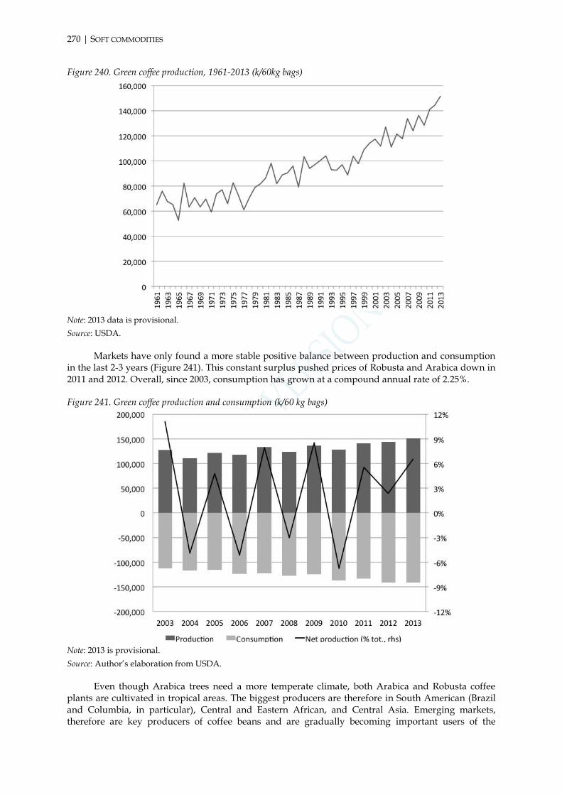
270 | SOFT COMMODITIES
Figure 240. Green coffee production, 1961-2013 (k/60kg bags)
Note: 2013 data is provisional.
Source: USDA.
Markets have only found a more stable positive balance between production and consumption in the last 2-3 years (Figure 241). This constant surplus pushed prices of Robusta and Arabica down in 2011 and 2012. Overall, since 2003, consumption has grown at a compound annual rate of 2.25%.
Figure 241. Green coffee production and consumption (k/60 kg bags)
Note: 2013 is provisional.
Source: Author’s elaboration from USDA.
Even though Arabica trees need a more temperate climate, both Arabica and Robusta coffee plants are cultivated in tropical areas. The biggest producers are therefore in South American (Brazil and Columbia, in particular), Central and Eastern African, and Central Asia. Emerging markets, therefore are key producers of coffee beans and are gradually becoming important users of the

commodity, though consumption is still mainly concentrated in western economies. Interestingly, among producing countries, those in Africa and the Americas have lost ground over the years to Asian countries (such as Vietnam and Indonesia), in particular after the liberalisation process started at the end of the 1980s and the beginning of the 1990s.
Figure 242. Production by regions (% of total)
Source: Author’s elaboration from FAO Stats.
However, single countries (more than regions) play a crucial role in coffee global production. Today, Brazil produces almost 50 million bags, which is roughly 37% of total production. Central and South America’s share of nearly 60% of global production is concentrated in a few countries (Figure 243). Therefore, any major weather events affecting production in the south of Central America (e.g. in Guatemala, Honduras) and the centre-north of South America (e.g. in Brazil or Columbia) can have important repercussions on global prices, as occurred in 2010 and 2011. Overall, the top ten producers handle over 85% of total production, which (except for Ethiopia) is mainly concentrated in Central Asia and in Mexico and Brazil in the Americas.
Figure 243. Top ten green coffee producers (left) and consumers (right), 2012
Source: Author’s elaboration from USDA.

272 | SOFT COMMODITIES
Consumption, on the other hand, is concentrated mainly in the European Union (32%) and the United States (17%). Brazil is also a big consumer of green coffee, as the main competitor of roasters located close to the key consumption areas. Below the top three (plus Japan), consumption is more or less equally split across several countries (Figure 243).
Storage and land productivity
Storability of coffee depends on the refined state of the product. The green coffee bean, the state in which coffee beans are sold at the wholesale level (in airtight bags of 60 kg), can last for more than one year. However, after around one year, the product begins to lose its original properties and is sold at a discount. Moisture in green coffee beans is an essential element. A high moisture level (above 12.5%) ensures a more intense flavour, but a shorter storage life. Moisture below 8%, instead, gives less flavour to the bean, but a longer storage life. Roasted coffee, at the end-user level, has more or less the same storage life, but it will already have started to lose its original properties after a few weeks of being packaged in airtight bags (the storage life for coffee powder is even shorter). Storage should be in a dark and dry place. Storage in bags is ideal for exchange in international markets of green coffee, which is usually roasted close to consumption areas to preserve its original flavour.
In line with the upward trend of nominal prices from the beginning of the 21st century, stocks-to-use ratios have gradually decreased to around 20%, which has partly been led by a constantly growing consumption rate across developing economies.
Figure 244. Stock-to-use ratio, 2003-2013
Note: 2013 data is provisional
Source: Author’s elaboration from USDA.
Stocks of green coffee, as for cocoa, are the response function of supply and demand changes that are then ultimately reflected into nominal prices, while structural changes to the supply side will only appear in stock levels a few years later. As suggested below, prices appear to follow a non-linear relationship with nominal prices trends that are, on average, growing.

Figure 245. Ending stocks and average nominal prices
Source: Author’s elaboration from USDA and World Bank.
The growing inability of production to keep up with higher demand growth rates is also enhanced by current productivity and harvested areas. Global harvested areas have been more or less stable in the last 20 years, while yields have stabilised around a peak reached only recently in 2008, after 20 years of growth (Figure 246).
Figure 246. Harvested areas (by regions) and global yield
Source: Author’s elaboration from FAO Stats.
The long-term increase in yield was essentially triggered by new investments in agricultural technologies after the liberalisation, in particular new sun-grown cultivations, which ensured greater production (with more space), new machinery for collection, and the development of new pesticides

274 | SOFT COMMODITIES
(frequently used for mass sun-grown production). Genetic engineering for coffee plants has not been developed successfully so far. However, the picture is different when we look at different areas. Africa and the Americas have both seen a decline in harvested areas. But while Africa appears to suffer more from land productivity and a decline in harvested areas after the liberalisation, yields in the Americas have very much compensated the slight decline in harvested areas in the last decade at least (Figure 247 and Figure 248).
Figure 247. African harvested areas and yield
Source: Author’s elaboration from FAO Stats.
Figure 248. Harvested areas and yields in the Americas
Source: Author’s elaboration from FAO Stats.
Asia is gradually overtaking Africa in terms of harvested areas, after the boost in production and supply capacity at the beginning of the 21st century. Asian countries have been the main beneficiaries of the liberalisation process. Growth in harvested areas has since stabilised at around 2.5 million hectares, while yields have continued to grow in recent years.
Figure 249. Asian harvested areas and yield
Source: Author’s elaboration from FAO Stats.

As Robusta continues to grow as the global coffee variety for mass production and emerging economies increase their consumption of coffee, Asian cultivations will become more important for global coffee production.
International trade
Due to its commercial storage life, freight costs may become more predictable and so may have a limited impact in the medium term. However, coffee fruits require a two-step refining process, which implies significant transportation costs before the commodity can be transformed into a refined product for end-users. Countries such as Brazil have high transportation costs since long-term low price production has often resulted in a lack of investments in infrastructure. As a consequence, they face more structural issues as their domestic infrastructure gradually becomes inadequate (ABN AMRO, 2012). In addition, consumption areas are far from production countries, so shipping cost volatility can produce some significant impacts on costs. However, coffee can be easily shipped by different means of transport, which noticeably reduces freight costs. Beans (green) are the form in which the commodity will continue to be traded for two reasons: grinding increases the surface area of coffee (and so costs); and roasting will become more efficient if done close to consumption areas, due to storage and quality reasons and potential synergies with grinding operations that would reduce transportation costs and build economies of scale at the port of delivery (Leibtag et al., 2007).
As a result, international trade today is around 80% of total production, with a value of more than $22 billion (the biggest soft commodities market).
Figure 250. Value of international trade ($mn)
Source: Author’s calculation from USDA and World Bank.
The leading actors in the international market for green coffee are the two low cost producers that entered the international markets on the wave of the liberalisation reforms. Vietnam and Brazil account for almost 50% of the total international trade, which points to the Robusta variety becoming the key international coffee commodity. The top ten countries have over 83% of the market share of international markets.

276 | SOFT COMMODITIES
Figure 251. Top ten green coffee exporters (left) and importers (right), 2012
Source: Author’s elaboration from USDA.
More than 40% of total exports are directed to the European Union, while the United States receives another 20% of global exports. All other countries have more or less similar shares, on the basis of their historical coffee consumption.
5.3.1.1 Supply characteristics: a simple value chain
Due to its particular characteristics, the supply of coffee has significant constraints that delay reactions to market changes. Converting land to alternative uses has both the constraint of an external environment that may not easily allow alternative cultivation, as well as the sunk costs of having spent several years bringing the area to full production. Supply, therefore, mostly faces high sunk costs but very low opportunity costs. Market developments then, such as the liberalisation process and the general reduction of production costs, may greatly impact higher-cost producers in the short term, while their ability to react is postponed to several years down the line. After the liberalisation and the entrance of new low-cost players (and also thanks to currency devaluations), African producers and processors/roasters, in particular, have been squeezed by low-cost coffee (from Asia; Oxfam 2003) and widespread practices of blending high-quality coffee for industrial production with today’s ability to reduce bitterness of cheap coffee.
On the manufacturing side, high fixed costs in manufacturing slow down the reaction of retail prices to changes in the underlying commodity price (Leibtag et al., 2007). Coffee beans are only a small part of the costs of the final product. In a cup of coffee, similarly to chocolate and cocoa beans, it is estimated that the coffee beans make up 5-7% of total costs, labour is 19-20%, rent 16-18%, diary 6-8%, and packaging and sugar 13-15% (Coffee Association of Canada, 2002).
Figure 252. Coffee’s simplified value chain
Source: Author.

The coffee supply chain is very simple, even though it is spread across many geographical levels (Figure 252). While local producers are coordinating much more through cooperatives following the growth of international trade, they are still small and fragmented in comparison to international processors and roasters that manufacture coffee or simply export beans for resale close to consumption areas. The reach of their business interest, which spans across different continents, also requires a significant size and scale. Roasters and grinders are established close to delivery ports to minimise the transportation costs.
This discrepancy of market power has often prompted claims for unfair trade conditions to be addressed by policy interventions (Talbot, 2004; Lindsey, 2004). More competition for international processors and roasters from production areas that become better equipped to sell a semi-final product may shorten the value chain and allow more value-added to be transferred to producing areas. However, this income will not necessarily reach those that are suffering the most from lower production costs, essentially the workers in coffee plantations (see Box 11). The market power of international coffee manufacturers may expose the weaker part of the value chain to aggressive competition and rent extraction. Monitoring of market practices and the use of market power by national or supranational authorities is an important element. However, changes in recent years have also gone beyond rent extraction, with new regions of the world able to produce at much lower cost, so replacing other regions where costs have not adjusted. Conditions for workers are often dependent on government policies that avoid allocating or seeking more resources to pursue social objectives. Most coffee (70%) is sold through supermarkets (Pelupessy, 2007) and many important chains have started backward vertical integration to access the margins of roasters. Coffee’s limited two-step refining process (with low production costs) and its almost direct usability in the beverage industry frequently leads to vertical integration with the green coffee bean refining industry and to some horizontal integration with the production of other beverages and soft drinks (as with big food companies, like Nestle). Access to international finance (Cardenas, 1994) has also boosted productivity and provided additional market power to vertically integrated exporters.
Box 11. The past, present and future of the ‘fair trade’ movement
The coffee crisis between 2001 and 2005, when prices fell below production costs in several countries and small producers faced high losses, set off a chain of furious reactions towards the big coffee players in particular, due to the small contribution of coffee beans to the total cost of coffee, which kept margins on coffee sales more or less the same. The action of the movement today is also directed at persuading governments and other international organisations (such as FAO) to intervene to support producers and production in compliance with a minimum set of standards. In this changing environment, a broad movement aiming to bring fairness to international markets quickly developed. The movement had some important success, with Starbucks choosing to buy only ‘fair trade’ within a broader rebranding of the company. ‘Fair trade’ associations have since then pushed for more transparency and empowerment of producers in several producing countries, and not only for coffee. In particular, cutting part of the value chain and linking cooperatives directly with retailers or consumers (Figure 253) would supposedly reduce total costs of production and increase margins for producers.
Often the organisations that set up these shortened value chains require buyers to pay an additional premium, which means that ‘fair trade’ prices are typically higher than front-month prices on international futures markets. Importers may also provide credit directly to producers in exchange of the commodity. The organisations issue a certificate to producers that requires them to be compliant with important principles on conditions of employment (e.g. with regards to child labour) and environment (e.g. no GMOs) in exchange for a small premium. The organisations also provide credit and invest in improvements to the external working environment, with schools, roads, and so on. The certification, however, does not ensure that once the money flies in, producers will indirectly redistribute it through better labour conditions for workers within the plantation. Enforcement is very difficult when production is highly fragmented, especially for small organisations working in countries with very limited rule of law.

278 | SOFT COMMODITIES
Figure 253. ‘Fair trade’ value chain
Source: Locke et al. 2010, p. 9.
As a consequence, despite the undeniable success in attracting the attention of policy-makers and international organisations towards the conditions of small producers of commodities in many parts of the world, ‘fair trade’ is still commercially limited to only 1-2% of total exports (Pelupessy, 2007). The overreliance on the ideological nature of the initiative cannot create sufficient demand for a convenient and high-quality product, limiting the potential growth of the market. In the future, the ‘fair trade’ certification could ensure that a list of quality requirements for the product is met to commercially justify the imposition of a premium. Pushing ‘fair trade’ in the niche high quality coffee market may become the way forward for promoting more socially and environmentally sustainable production in a very competitive international market, and not only for coffee.
5.3.1.2 Demand characteristics: a solid long-term growth
Demand for coffee is subject to natural constraints, as consumption by an individual cannot go over a quantity that would affect his or her health. Demand also has some cyclical patterns, since as a warm drink coffee it is consumed more during the winter. In the short term, demand elasticity to price is low as the consumption of coffee may create an addiction, making it difficult to switch to substitutes. Instead, demand for coffee may rise through increasing numbers of drinkers. In recent years, emerging markets have driven new demand, as average incomes have begun to grow for millions of people that now have new dietary requirements and a new social status. A significant market has thus been growing in the last decade and, as a result, demand forecasts are quite bullish and may continue to be so for some years ahead (Figure 254).
Elasticity of demand to prices is limited since there are almost no natural products with same characteristics and chemical components. However, among coffee varieties, Arabica and Robusta compete with each other. Over the years, demand has become more sophisticated and more receptive to different coffee flavours, leading to diversification. There might be some additional reasons to be optimistic.

Figure 254. Coffee consumption (mn bags)
Source: ICO World Coffee Market Outlook (2013).
5.3.1.3 Key product and market characteristics
The product and market characteristics of coffee are those of a commodity that relies on a complex interaction between different value chains and elasticity of demand and supply. These characteristics can be summarised as follows:
Coffee is a renewable (but not recyclable) commodity with limited short-term substitution and alternative uses (e.g. pharmaceutical products).
Production convertibility is low, even though it requires limited capital.
Supply has significant constraints that limit elasticity to demand trends.
Supply is also fragmented and lacks horizontal and vertical integration.
The processing and roasting industry is more international and so requires economies of scale that increase market power over small producers.
Green coffee has acceptable storability for international trade, with transportation costs that can be borne by those companies that benefit from sufficient economies of scale.
Supply elasticity is low, while demand elasticity to price is low in the short term.
Concentration is very low at the production level, though producers are increasingly coalescing in broader cooperatives, but concentration is growing as the value chain becomes more international (for coffee manufacturing activities).
Emerging economies manage the global production of coffee but their domestic demand is very low.
Increasing income due to greater development of emerging economies may change dietary habits and this (together with a growing population) may increase consumption of coffee, which would put bullish pressure on future consumption levels.
Table 82. Key product and market characteristics
Recycling/ Production
convertibility
Substitutes/Horizontal integration
Alternative uses/Vertical integration
Capital intensive
production
Stora-bility
Freight costs
incidence
Elasticity to price/ demand
Concen-tration
BRICs weight
Future Consumption/
Production
Demand side
None Low Low
Low Medium Medium
Medium
Medium
Low High
Supply side
Low Medium Low Low High Medium
Source: Author.

280 | SOFT COMMODITIES
5.3.2 Exogenous factors: the role of opportunity costs
Several exogenous factors can affect coffee market trends. Government intervention was historically very high before the liberalisation process and the end of the ICA agreements, which controlled prices mainly through quotas and marketing boards. With the end of such agreements and with the process of liberalisation, government interventions have become less invasive or have changed their scope. In some countries, intervention is still significant through the state ownership of main processing and roasting companies. Overall, though, government intervention has been decreasing since the beginning of the liberalisation period, but significant risks of political instability and (in some areas) military conflicts still exist for the production of coffee.
The weather is certainly an important exogenous factor that contributed to the spike and fall of Arabica prices in 2010-11. Coffee trees require heavy rain before production and low rains during harvesting. However, a major difference with cocoa production is that coffee is produced in many more countries, so the impact of weather is mitigated by some geographical diversification.
Table 83. Key exogenous factors
Government intervention Main other external factors
Medium Weather, political instability and military conflicts, economic
development, opportunity costs, economic cycle
Source: Author.
Revenues from the alternative use of the land are important opportunity cost. In some countries, a lack of infrastructures (such as domestic transportability or general logistics with different international markets) prompts the development of low-cost/margins production, which often relies on unfair working conditions, etc. Improvements to infrastructure quality and scope would certainly provide a strong foundation to increase opportunity costs and allow these economies to produce whatever maximises the interest of their own populations. However, corruption and other frictions in the governance of these countries often make this process of ‘self-sustainability’ very difficult, if not impossible.
Finally, the economic cycle, and in particular its reflection in demand trends or exchange rates through changes in prices or direct monetary policy interventions, certainly has an impact on coffee prices. The devaluation of the Brazilian real has greatly helped its coffee industry to compete more fiercely with other regions in the world. Evidence of this significant impact will be discussed in the empirical analysis of the next section.
5.3.3 Empirical analysis: the effects of lower production costs
The empirical analysis looks at the implications of global competition and how its effects on supply and demand factors affect prices. The analysis uses the following dataset:
Monthly data from January 1992 to March 2012.
Log151 of Arabica front-month nominal price (on ICE) from the World Bank.
Log of OECD Leading Composite Indicator for OECD countries (average of de-trended and smoothed and normalised component series).
Log of OECD Leading Composite Indicator for China (average of de-trended and smoothed and normalised component series).
Log of nominal Brazilian real – US dollar exchange rate.
Log of S&P 500.
Simple linear regressions of differentiated values of the Arabica price (as dependent variable) and OECD demand, Chinese demand and Brazilian real exchange rate with the US dollar show interesting results, with a statistically significant coefficient and tests on residuals that point to no spurious relations or significant misspecification (see Output #67, Output #68, and Output #69).
151 Natural logarithm.

Table 84. Regression output
Independent variable Coefficient (t-test)
OECD demand 4.15*
(1.71)
China demand 2.54**
(2.05)
BRL/USD .32***
(2.87)
Note: *10%, **5%, ***1% significance.
Source: Author’s estimates.
Both demand from OECD countries and China has had a significant effect over coffee prices in the last 20 years. Less impact was generated by changes in the value of the Brazilian real over this period. However, the relationship is statistically significant with a low coefficient spread over a 20-year period that does not necessarily exclude the potential high impact of temporary currency devaluation on the global coffee market.
Empirical tests on coffee markets also confirm that the commodity was uncorrelated with the S&P 500 before 2002. Via simple linear regression of differentiated values, the model finds that the price of Arabica became linked (with a positive sign) to the financial index from the beginning of the downward trend in the dollar exchange rate (as a reflection of expansionary monetary policies). This link became gradually stronger as the effects of such policies intensified and reached its peak with the recent financial crisis. The model proves to be robust in relation to normality, heteroskedasticity, and white noise of residuals.
Finally, the ARCH model does not support early evidence showing the different impact of commercial and index positions and their interaction with physical markets (through the front-month price). Both positions in this model appear statistically significant and their levels do affect front-month contracts. No clear evidence was found that one type of position prevails over the other in its potential impact on physical markets.
5.3.4 Market organisation: dealing with issues of market infrastructure
The organisation of coffee markets underwent important structural changes after the liberalisation process (and the replacement of marketing boards with traders/exporters) that have improved the mechanisms of transmission of global prices into local/regional prices, so linking global markets to producers’ prices (Krivonos, 2004). Between producers and international coffee manufacturers, roasters and processors have gained market power due to their local control over supply or local intermediaries.
Market microstructure is very simple. Physical market organisation relies on bilateral contracts based on global active benchmarks to which a discount or a premium is applied. The majority of coffee (especially specialty coffee) is bought and sold in an opaque but legitimate bilateral environment that may take into account global prices as a reference or simply use global markets for hedging that position. On top of the general variety difference, there are regional and product features that can modify the reference price upwards or downwards.
Futures markets are located in Europe (for Robusta futures contracts) and the United States (for Arabica futures contracts), which only deliver in their regional areas. Another futures contract (also
available in e-mini version152) is traded in Brazil with local delivery, mainly in São Paulo. Limited
delivery availability, even with the multiple trading venues where these products are traded, may create divergence between spot and future prices and increase the costs of those producers that cannot reach the market directly in this environment. Futures markets have the possibility to reduce the market power of big traders by providing access to a pool of global interests. Even though the biggest global manufacturers are American- or European-headquartered companies, the growth of
152 Cash-settled futures contracts with smaller size.

282 | SOFT COMMODITIES
consumption and current production in emerging markets will, over time, require a change of policy in the delivery points for this commodity.
Recent issues with the slow loading out of coffee from licensed warehouses have increased the need for an effective monitoring system and rules/supervision of commodity distribution systems across important consumption areas. After complaints by market participants and to meet growing demand, last year LIFFE increased the minimum loading-out rate (or movement out rate) for its warehouses to 250 tonnes per day for warehouses with 30,000 tonnes, and 500 tonnes per day for those above. As with the proposals for LME warehouses storing aluminium discussed earlier in this report, in addition to rules for regular assessment and, if needed, revisions of loading-out rates, an open cap (above 30,000 tonnes), rather than a loading-out rate based on absolute size of the warehouse or even on the average time to get the commodity out of the warehouse, would create incentives for warehouses to increase their size well beyond the threshold (if possible) and retain more of the global supply. Otherwise, if the loading-out rate above the open threshold is too high, it may push warehouses to limit their size to 30,000 tonnes, thus holding too little of the global supply (at least in the short term) to cope with market demand. The minimum loading-out rate may also be seen as a reference point for warehouses, even if it were possible to deliver more without affecting their viability. It provides the incentive for warehouses to do their job and extract an acceptable rent without colluding to constrain supply even further and increase storage time and revenues. More evidence is needed on whether the threshold is adequate for coffee futures warehousing systems before drawing any conclusions. Further analyses should look at the possibility of creating hybrid delivery systems that can allow for flexibility by involving agreements with transport and logistics companies to increase the flexibility of the warehouse system, which relies (perhaps too much) on fixed costs of labour, machineries, and so on to run its activities. A proper delivery system ensures convergence and therefore a proper price formation process and interaction between futures and physical markets.
Table 85. Coffee market organisation
Physical market setting Pricing complexity Liquidity futures market Delivery points
Competitive (regional) Oligopolistic (global)
Low High Limited
(Brazil, US and EU)
Source: Author.
Finally, the physical market setting relies on a competitive regional market, with small producers and local merchants that liaise with international coffee manufacturers and exporters. At the international level, an oligopolistic setting exists with big coffee manufacturers interacting with local farms or regional points of delivery. International investments in the upstream markets by medium-sized coffee roasters, with the direct ownership of coffee farms, have been growing, but are still limited compared to the total size of the market.

283 |
6. DRIVERS OF COMMODITIES PRICE FORMATION IN
PHYSICAL AND FUTURES MARKETS: CONCLUDING
REMARKS
his chapter summarises some of the key findings that have emerged in the previous chapters. It assigns a weight to each main driver of price formation. The first section discusses market fundamentals in driving price formation. The second section illustrates the conclusions of this
study on market organisation of commodities, highlighting the key developments in recent years led by international trade and new technologies. Finally, matrixes of weights for each key driver of price formation are presented. Illustrative tables summarise the complexity of each commodity market, pointing at the importance of bearing in mind differences when designing any policy response.
6.1 Market fundamentals
Price formation in commodities markets interacts with a complex set of endogenous and exogenous variables. Product, supply, and demand characteristics shape market structure in different ways. Market dynamics, both in physical and futures markets, can therefore vary considerably across commodities.
Product characteristics: shaping market structure
Product characteristics have an important impact on commodities price formation and the structure of underlying markets, but most of the effects are indirect. Key product characteristics are:
Quality.
Storability.
Renewability.
Recyclability.
Substitutability.
(Final) usability.
Differences among varieties are typically priced through a premium over a benchmark price, but qualities can also lead to the growth of markets in new geographical areas if technologies and margins are sufficiently high to increase substitutability in some of the uses and to attract international investments. The growth of Robusta coffee production, which is gradually becoming the most produced quality of coffee, epitomises the potential effects of qualities of commodities that can be produced at lower cost with limited differences from the most diffused variety. In general, qualities of a commodity are not radically different, which may lead to easy substitution among them.
Storability of a commodity can have different stages, which is reflected in the cost of storage and shipping. But costs of storage should be looked at under a broader definition of cost. Inventories are the response function of supply and demand patterns. Commodities that can be easily stored are more predictable and better reflect demand and supply fundamentals. When storage is difficult because of unpredictable supply or due to the nature of the product, changes in inventories can have a more significant impact in the short term, as inventories cannot predictably smooth out the effects of unpredictable supply on price formation, as is the case for agricultural and soft commodities. Where supply is more predictable, information about inventory levels is not a direct driver of price formation. Storable commodities, particularly those that are export-driven, can also expose the price formation mechanism to external factors such as freight costs (as in 2010 for iron ore). As the empirical analyses of previous sections suggest by confirming the theory of storage, inventories are a response
T

284 | CONCLUDING REMARKS
function of demand and supply by reacting to the basis (difference between futures and spot price), i.e. to the expectations about future spot prices, taking into account current demand and supply factors and the futures curve. Inventories therefore link physical to futures markets and internalise all factors that can impact on the basis, i.e. risk-free interest rates, cost of physical storage, and spot price expectations (fears of supply shortages, etc.). Therefore, policies that affect risk-free interest rates (such as monetary policies), whether designed for commodities markets or not, influence storability and, potentially, the fundamentals of commodities markets.
Renewable commodities are typically products of the earth (such as agricultural commodities). Renewability exposes supply to seasonality, which enhances the weight of exogenous factors such as the weather. Inventories become more important, as supply cannot be easily predicted. However, if the product is used for alternative productions, such as energy, the assessment becomes more complex. External factors, such as biofuel policies, are gradually linking market structure to developments in other markets (for instance, crude oil markets). The use of corn for energy production, for example, suggests a strong interest in developing greater energy independence thanks to the renewability of the commodity.
Substitutability of a product shapes market structure and moves the attention of international markets to a commodity that can generate higher returns and diversification, limiting exposure to one single use. Supply would gradually concentrate efforts on the commodity that can be produced with the highest margin (and so the lowest cost of production). However, the degree of substitutability may also depend on external factors, such as the impact of negative externalities on the environment, environmental regulation, and infrastructures. Savings generated through environmental costs favour the use of clean sources of energy over polluting ones, such as carbon.
The final usability is another crucial factor. A commodity usually needs to be processed before being used as a final or intermediate product. Processing becomes a key driver of market structure developments, and so price formation, if other products (co-products) can be produced during the same refining process. Supply will concentrate on products that can generate the highest number of co-products (also for alternative uses) while keeping costs of production more or less at the same level. The role of co-products is key in commodities markets with less capital-intensive production and high substitutability. Agricultural commodities, such as corn and soybean oil, have grown quickly in the last decade partly thanks to demand for alternative uses (such as energy, pharmaceuticals and industrial food applications). Technological developments in recent years have also widened the set of commodities whose use has been extended to new applications, in particular in the pharmaceutical and industrial food industries.
Finally, the product characteristics of a commodity also shape the business model of commodity firms. For instance, despite the increasing average size of farms, production of agricultural commodities is rarely vertically integrated in the business model of large agricultural trading houses. The trading house coordinates and supports activities of a fragmented supply, but ensures that refining and production of co-products is done through their facilities. These firms have therefore integrated much more horizontally by exploiting their size in international markets, and less vertically with local producers to which they also provide risk management services. By contrast, gas extraction and refining operations usually require a high level of vertical integration due to a capital-intensive production model and to benefit from economies of scale.
Supply factors: dealing with multiple constraints
Multiple factors affect the supply of commodities, and they reflect the significant differences among markets. Some of these factors, which impact the elasticity of supply to demand, are:
Production convertibility and capital intensity.
Horizontal and vertical integration.
Storability and transportability.
Industry concentration.
Geographical concentration (emerging markets).
Technological developments.
Supply peaks and future trends.

Convertibility of production facilities increases the elasticity of supply to demand and limits monopsonistic powers. Convertibility is typically associated with productions that have low capital intensity, i.e. low sunk costs and limited capital commitment. Agricultural commodities supply has high production convertibility, while primary aluminium factories cannot be converted to alternative productions.
Horizontal and vertical integration are important factors that can affect the elasticity of supply. Horizontal integration exploits economies of scope across different commodities markets, and commodities firms in agricultural markets frequently adopt it. Vertical integration is typical of high capital-intensive production, which exploits synergies along the value chain to maximise economies of scale and scope. However, even in capital-intensive productions, vertical integration with the final product may be only partial, as with iron ore companies and steel production. The additional refining process required for some industrial metals may discourage upstream companies from investing in vertical integration with downstream markets. Crude oil suppliers, in contrast, are very often involved in every step of the value chain until the final production of the refined product.
Storability and transportability properties are important factors that can influence the level of capital commitment that supplier will invest in the market. Limited storability and transportability can increase the rigidity of supply by requiring more capital investments to ensure that the commodity reaches the reference market. These properties may even cause suppliers to invest resources in freight markets. For instance, some crude oil companies have invested in the ownership of shipping companies running tankers to transport liquefied gas to key entry points in the main consuming regions. If capital is not available, however, this situation may weaken the contractual power of supply. Easy storability and transportability, on the other hand, can ease capital pressures on suppliers and so increase elasticity. These characteristics help to develop competitive freight markets, such as for bulk commodities like grains.
Concentration of the industry can change market structure through market power, which imposes a mark-up (monopoly or oligopoly) or ties supply to marginal costs (monopsonistic powers). Oligopolistic pressures usually emerge in commodities markets with high capital investments, such as industrial metals. Rigidity and predictability of production levels lead to a natural equilibrium that is not necessarily the outcome of collusive actions, but rather the ability (due to market characteristics) to predict competitors’ production levels and to act accordingly. Monopsonistic powers emerge where there is a lack of vertical integration and the supply side is rather small and fragmented. This is the case of some soft commodities markets, such as cocoa. Smaller growers were exposed to monopsonistic powers when markets were liberalised. Supply was not sufficiently increased or consolidated (by reducing barriers to entry) to face growing competition from other geographical areas and the rising monopsonistic power of big international exporters. Consolidation of the industry at the international level is one of the key developments of the opening-up to international competition.
Geographical concentration can expose the supply (and so price formation mechanisms) to external factors, such as political instability or weather conditions. For instance, the production of cocoa, mainly in Western Africa, was constrained by great political instability during the 1980s. Finally, proximity of supply to big consumption areas may increase elasticity and expose it less to exogenous (unforeseeable) factors.
Technological developments have been an important driver of price formation through their effects on supply. For example, new production processes for industrial metals to minimise energy consumption and increase productivity, or new hydraulic fracking technologies to extract shale gas, have been important drivers of change for the supply side and the market as a whole. In agricultural markets, new fertilisers, pesticides and genetically modified seeds, with massive investments in biotechnologies, have increased yields and average farm size while total harvested areas have remained stable or even fallen. Today, almost 100% of US corn is made out of a GMO, while the European Union has encountered some strong opposition in countries, like France, to the adoption of these technological advances based on claims of potential harm for human health.
Finally, natural constraints on the supply side, such as supply peaks in crude oil extraction in some regions (such as Northern Europe), are drivers of change in price formation for some recognised benchmarks. A general decrease in stock-to-consumption ratios across several commodities markets

286 | CONCLUDING REMARKS
confirms the difficulty for the supply side to keep up with sustained demand growth in recent years. However, not only actual production but also expectations of lower (or higher) production levels can shape current mechanisms of price formation. Expectations of shale gas (and perhaps oil) production have driven natural gas prices in the United States to historical lows. It may still to be too early to understand how the long-term geopolitical implications of the ‘unconventional revolution’ in oil and gas will again change drivers of price formation for key global consumption areas.
Demand factors: the rise of developing economies
Demand factors are crucial for commodities price formation. Empirical analyses across several markets confirm a strong and statistically significant impact of demand patterns (driven by the economic cycle) on commodities prices. A thorough understanding of these demand factors, however, is subject to several assumptions about the standard behaviour of typical commodities consumers. Different types of users with different objectives and budgets have different price elasticity, which can be assessed on average through some common factors. These factors are:
Income growth and urbanisation.
Technological developments and alternative uses.
Long-term habits and demographics.
Economic cycle.
Income level is a crucial aspect for commodities demand. Income growth changes the habits of the population and leads them to spend more on commodities that are not usually considered essential goods. The growth of emerging markets in the last decade has expanded the basket of commodities that their populations use in their daily life. The classic example is crude oil, which reflects the growth of oil-intensive emerging economies like China, but income growth has also increased emerging markets’ consumption of cocoa and coffee-based food or drinks (e.g. chocolate), which have typically been seen as products for high-income people. Both qualitative and quantitative analyses confirm that emerging markets have been a key driver of demand across all commodities markets assessed in this study. The link is strong; the growth of emerging markets is perhaps the variable with the strongest impact across diverse markets. Empirical analyses for crude oil, aluminium, copper, soybean oil and coffee show a strong link with Chinese demand growth, at least in the last 10-15 years. As a heavy industrial economy, China has imported more industrial metals and crude oil than anyone else. Demand still appears sustained, even though growth in these countries is slowing down and may continue to do so in the coming years.
Technological developments in recent years have resulted in new important applications for commodities historically used for only one purpose. Alternative uses, often supported by accommodating government interventions, have renewed production in several commodities markets. For instance, technological developments permit the production of several co-products from corn that can be used for animal feed and human food (with industrial applications). Technological developments, together with government policies, have fostered demand for renewable and clean energy production, which has pushed production for some agricultural commodities to historical peaks. Over 40% of the corn produced each year in the United States is used for energy production to meet the mandate set by law. Other developments have gradually increased volumes of cocoa or coffee used for pharmaceutical applications.
Demand factors that drive price formation can also come from changes in the long-term habits of a population. Income growth can change people’s habits, even in the short term. However, other long-term factors, such as migration, scientific research on human health, environmental factors (e.g. damage from ozone depletion) or globalised information channels, may cause significant changes in human habits that affect the consumption of commodities.
Last but not least, the economic cycle and its reflection in endogenous demand aspects (such as average personal income) and cross-border flows (international trade) have a crucial impact on demand and so on commodity price formation; empirical analyses show that the business cycle is a fundamental driver of price formation. Commodities are at the heart of the economic cycle and their price formation mechanisms immediately reflect changes to macroeconomic conditions fuelling demand. The relationship between the economic cycle and commodities prices is strongly positive across markets, in contrast to past claims about the strong anti-cyclical nature of commodities markets.

Except for precious metals (which are not covered in this study), it appears that commodities markets do not follow the cycle during a long period of growth or depression, but are very responsive to short-term drops (and rebounds) in demand.
Exogenous factors: grasping long-term implications
Factors that are exogenously imposed by commodities markets dynamics play a crucial role on the price formation mechanisms. These dynamics are:
‘Financialisation process’ and monetary policies.
Subsidies programmes.
General government interventions (e.g. export bans).
The economic cycle and other macroeconomic events.
Technological developments.
Unpredictable events (e.g. weather).
The ‘financialisation’ process can be defined as the process of alignment of commodities returns with pure financial assets (‘pooling effect’), increasing co-movements among asset classes that have historically been seen as following opposite patterns. This process is developing in an environment with much higher non-commercial investments than a decade ago, due to the joint effects of monetary policies and deregulation of the financial sector. As illustrated through qualitative and quantitative analyses in the first chapter, accommodating monetary policies, technological advances, and the growth of international markets have set this process in motion. As shown in the earlier empirical analysis, the rise of important commercial and hybrid commodities players, led by the impressive growth of global demand from emerging markets and the development of international trade, has been initially a key driver of growth for futures markets, which have attracted passive investments mainly brought by global financial institutions (see Section 1.4).
Table 86. Link between commodities prices and financial indexes before and after 2002
Before 2002 After 2002 Whole sample Model
Crude oil No Yes No ARCH
Natural Gas No No No ARIMA, Granger
Iron ore - - - -
Aluminium* No Yes Yes* ARCH, OLS
Copper No Yes No ARCH, OLS
Wheat No Yes No ARIMA, OLS
Corn No Yes No OLS
Soybean oil No Yes Yes ARCH, OLS
Sugar - - - -
Cocoa Yes** Yes** Yes** OLS
Coffee No Yes** No OLS
Note: *both ways, **Rejection at 10% level. Data up to 2011/2012.
Source: Author.
This process has increased commodities co-movements with financial assets, but no evidence so far has suggested that volatile patterns can be attributed to non-commercial investments. The empirical analysis shows, instead, that commercial positions have led the growth of non-commercial positions in an environment deeply influenced by easy access to credit and high profitability of international trade. Non-commercial positions have eventually bridged the link with financial indexes and in recent years have become by far the largest component of futures trading flows (by summing long and short open interest positions). ‘Financialisation’ is therefore an unintended development of an environment profoundly affected by the long-term effects of important policy decisions (expansionary monetary policies, opening up of international trade, and deregulation of the financial
288 | CONCLUDING REMARKS
sector). Non-commercial positions and international finance have been instrumental to the development of international commodities trade, led by the growth of emerging economies that are able to gain market share in several markets by producing at the lowest costs. The availability of cheap credit, with interests rates close to zero for a prolonged period of time and a much cheaper dollar, have thus fuelled massive investments in direct purchases of physical commodities, attracted by high profitability and the wrong assumption of a counter-cyclical nature (see Section 1.3). Liquidity has been flowing into stocks of commodities firms, which have in recent years multiplied their market capitalisation. Moreover, technological advances in the last two decades have made access to financial markets easier and cheaper from any location in the world. Real-time accessibility to global benchmark prices has strengthened the importance of key reference prices and so the functioning of their price formation mechanisms becomes of global relevance. Finally, with zero risk-free interest
rates and a falling dollar exchange rate,153 the futures curve has rapidly moved into contango for
storable and cyclical commodities, such as industrial metals. A legitimate carry trade has emerged, with financial institutions ready to finance stocks held in warehouses, even causing queues of up to one year to pull the commodity out, due to badly designed rules for warehouses. Since the early 2000s, the combined effect of all these events, with the crucial role of monetary policies (access to credit) and international trade, have created a prolonged window for carry trades across commodities markets that have increased pro-cyclicality and eventually wrapped several financial and non-financial assets up in the same basket.
Subsidies policies by governments have also been a major source of price distortion. The political objective to support national markets has prevailed for a long time. However, in recent years discussions within the WTO agreements over eliminating barriers to international trade have reversed this long-term trend. Both Europe and the United States have been leading a process of substantive reductions of subsidies to commodities markets. Aside from its still protective policy in some agricultural markets, the European Union has cut the most in relative terms, while the United States has slowed down its cuts since the inception of the financial crisis. Both Europe and the United States have virtually cancelled forms of direct intervention on prices, while favouring more indirect interventions with fixed payments (not necessarily linked to production levels or quotas). However, China has now become the biggest subsidiser of direct intervention to manipulate prices in commodities markets. In 2012, China spent more than anyone else on subsidies programmes, roughly $180 billion. As a result of the removal of past direct government interventions in the pricing of commodities markets due to lower fiscal strength and commitments to international trade, price formation mechanisms for some commodities markets are still struggling to find an eligible reference price for their regional areas. The long journey to develop a futures contract for feed wheat in Europe is a case in point. In addition, subsidised prices, coupled with higher land values, have reduced farmers’ incentives to invest in their own land, so yields in many agricultural commodities have been steady since the 1980s, while harvested areas are now going down due to the cuts to subsidies programmes. Competition over production costs compels advanced economies to invest in research and infrastructure to boost productivity. Subsidies programmes perhaps had detrimental effects on productivity, leaving advanced economies exposed to the low-cost productions of developing countries that have gradually become key global actors in international commodities markets. Finally, the need to secure commodities provision may still drive government interventions in coming years, as countries continue to behave strategically, even though international cooperation (after the Uruguay Round) and free trade agreements have become more frequent outcomes.
Several other types of government intervention have impacted commodities markets to secure commodities provision. Some political decisions, such as the Russian export ban or the Indian decision to shut down the Indian Sugar Exchange, are examples of arbitrary decisions that can distort legal certainty in cross-border trades. Well-defined non-arbitrary interventions, such as biofuel policies, can also impact commodities markets. For instance, biofuel policies in the United States have boosted corn production and growth in yields and harvested areas, which may become unsustainable once the subsidy programme ends. The liberalisation process in African countries at the end of the 1980s has
153 The reference exchange rate (in several cases a dollar index benchmarked against a basket of currencies) is strongly significant in every empirical analyses run in this study, except for natural gas.

certainly simplified the value chain at the international level, reduced costs, and promoted the growth of commodities markets such as cocoa and coffee, but with no programme to strengthen the role of a dispersed supply side operating with no infrastructures or direct access to international markets. There is a long list of other potential government interventions, such as quota production or buffer stocks, which may have a long-term impact on commodities price formation.
General macro events can also affect price formation in commodities markets, whether linked to the business cycle or not. For instance, a growing and ageing population, higher per capita income and urbanisation can affect long-term price formation mechanisms. Technological developments can change the market structure and allow more efficient production processes to take place or even new products to become commoditised (e.g. the discovery and commercialisation of shale gas). Opportunity costs linked to the use of land for alternative productions are a crucial external factor, especially in developing countries. Low-cost production in these countries relies heavily on the lack of physical and immaterial infrastructures supporting land-owners and little promotion of other productions by governments, which keeps land values, and thus opportunity costs, at a very low level. As a consequence, opportunity costs play an important role particularly for renewable commodities with high production convertibility. Finally, un predictable tail events, such as weather conditions, earthquakes or political instability, can alter the supply and demand curves, especially for those commodities that are more exposed to external factors (such as agricultural commodities).
Box 12. Key market failures in commodities markets and types of state intervention
General public (government) interventions are, in some cases, essential for the functioning of markets, including commodities. Market failures in commodities markets are essentially caused by informational gaps (information asymmetries) and market power, which may result in the inability to price positive or negative externalities (e.g. network effects), individual wrongdoing when the counterparty is unable to monitor the behaviour of other market participants, or anticompetitive equilibria due to market power.
First, markets may be unable to price (negative) externalities generated by commodities production and consumption. For example, governments have introduced a high number of environmental laws to protect the environment from the negative externalities of excessive polluting activities. Markets are unable to price these externalities because their negative impact may materialise years down the line and may not affect counterparties directly. It becomes the provision of a public good.154 The inability of the market to price environmental costs, has over the years, crowded out alternative (cleaner) commodities and so only state intervention has been able to preserve them. Second, material informational gaps may lead a counterparty to deviate from the good conduct due to his/her superior information, or due to the inability of the counterparty to monitor the other because of high costs. For example, market manipulation through cornering attempts or the diffusion of false information exploit the inability of one counterparty to monitor the quality of the information or the behaviour of the other. Third, market power may lead a firm to charge an unfair mark-up to consumers or producers by increasing barriers to entering or exiting the market. Oligopolistic or monopsonistic settings (through distribution bottlenecks) are very frequent in commodities markets, due to the scarcity of supply or to the product characteristics of the commodity. Market power can, in effect, create artificial supply or demand constraints that impede newcomers from entering the market and competing at a lower margin.
To deal with these three categories of market failures, state intervention should:
a. Provide the public good or create the conditions for the good to be delivered. b. Reduce monitoring costs by filling the informational gap. c. Ensure low market barriers to entry and exit.
To provide the public good, state intervention typically sets specific rules to preserve the provision of the good or to provide the good itself. For instance, environmental law is an important tool to preserve the environment, since it cannot be provided directly by the state. To reduce monitoring costs, in addition to rules that increase the transparency of transactions both in physical and futures markets (preserving the commercial interest of the firm in not disclosing its market strategy), state intervention can increase the effectiveness of direct surveillance of market transactions. For instance,
154 A public good is a non-excludible and non-rival product, which provision can only be provided by public entities (e.g. national defence)

290 | CONCLUDING REMARKS
transaction reporting made on a confidential basis to regulators and aggregate disclosure of positions in futures markets ensure that the supervisor can intervene in most cases when a systematic action to manipulate markets (cornering) has been put in place. This kind of intervention reduces monitoring costs by increasing the informational flow. Additional safeguards, such as business conduct rules or conflicts of interest policies, would strengthen the flow of information ex ante, rather than on occasional request from regulators. Finally, competition policies through strong enforcement measures (whether coupled with heavy administrative sanctions and/or criminal charges) are essential measures to ensure continuous supervision of both physical and futures markets and protection from market power. Minimising monopolisation attempts or monopsonistic behaviours would benefit the market as a whole, and so the entire value chain, creating more value added for the economy.
6.2 Evolving market organisation: a forward-looking perspective
Price formation mechanisms rely on the efficient functioning of physical and futures market organisation. New micro and macro developments over the years, partly due to technological advances, have entirely reshaped the physical market organisation and boosted the growth of commodities futures markets, which have become an indispensable tool to deal with complexity in international trade. This section sums up findings of the study in the following key areas for commodities markets:
Microstructural developments.
Key price formation mechanisms.
Growth of commercial market participants and international trade.
Expansion of commodities futures markets and ‘non-commercial’ investors.
Futures markets infrastructure.
Microstructural developments in commodities markets have changed the market organisation of physical commodities over the years. New international agreements to ensure legal certainty of contracts and general diffusion of the ‘rule of law’, together with technological developments and a wave of liberalisation processes that reduced state intervention in the economy, have prompted the reorganisation of commodities markets and the internationalisation of local productions. For the first time, local producers are able to compete globally and to access people eager to buy their products. The contractual power of the supply side has increased, while the buy side has faced a greater choice and benefitted from cheaper products. Accessibility to consumption areas has increased, partly through the development of competitive freight markets following massive cross-border investments by commercial and non-commercial players.
Market organisation, however, varies across commodities markets. The complexity of commodities markets mainly resides in the different types of price formation mechanisms. Benchmark-based pricing mechanisms, which apply a discount or premium to a liquid reference price, rely on the liquidity of a reference contract, which is typically a front-month futures contract. Liquidity is an essential feature that sometimes relies on a complex set of financial layers in order to align the risk profile with the underlying characteristics of the contract. For instance, in crude oil markets, reference prices are based on complex financial layers and information put together by price reporting agencies with a specific methodology that may also use editorial judgment to assess prices. Full transparency of methodologies, governance, and access to underlying data become crucial aspects for regulators to ensure the smooth functioning of the market. A regulatory framework for the provision of price assessment services and for the reliability of the information that firms voluntarily disclose (e.g. market manipulation rules in case of false or deceiving information) might ensure effective supervision by reducing monitoring costs and creating ‘public accountability’ for the well functioning of price formation mechanisms. However, the underlying liquidity of the contract is a prevailing aspect, which may even cause the market to reshape its pricing mechanism towards new benchmarks over time. Moreover, price formation can also rely on long-term contracts (LTCs), although they are a small part of the market today. For instance, reliance on LTCs occurs in particular circumstances, when the commodity cannot be easily shipped and it is difficult to build a globally recognised benchmark that would deal with specific regional issues. This price formation mechanism often does not rely on a benchmark price but on private negotiations, due to factors not linked to the actual production of the commodity. For instance, in the recent years freight costs have been a key

determinant for the conclusion of cross-border transactions in iron ore. Finally, sunk costs or high energy consumption productions may require different types of negotiations, which some firms may prefer to make through longer-term contracts. In any case, spot or forward transactions that apply a discount or a premium over a reference benchmark price have spread quickly in recent years as a key tool of price formation.
Markets have seen the astonishing growth of commercial commodities firms across all sectors, as explained in Chapter 1. There are two main reasons behind this growth: the development of international trade, and access to international finance and to cheap credit. The development of international trade, in particular after the Uruguay Round and the implementation of the WTO commitments (with the beginning of the liberalisation process in several countries), culminating with the official entry of China in the WTO between 2001 and 2004, has created the opportunity for massive cross-border investments to flow towards more competitive commodities productions. International commercial firms were well positioned to exploit their international position and increase their physical holdings. However, this growth has been only possible thanks to access to international finance, boosted by a prolonged period of accessible and cheap credit. Access to international finance, through global financial institutions or commodities trading houses with strong financial arms, has been a key factor that has boosted productivity and size, and has provided additional market power to vertically integrated international exporters. Some of these trading houses (such as Glencore), which were originally set up to offer risk management support to pure commodities firms from their significant financial arms, have been increasing investments in physical holdings, which may lead to concerns that they are now becoming ‘too-physical-to-fail’. Due to the growth of physical demand across several markets, underlying physical cross-border trades have grown, both in physical size and mostly in total value (Figure 255). The value of international trade in these commodities has soared from 2001 to 2011 by a double-digit compounded annual growth rate, which has also attracted financial participants and promoted the use of financial leverage in the physical commodities market.
Figure 255. Growth of exports value ($bn) and size, 2001-11
Value ($bn) Size
2001 2011 CAGR 2001 2011 Units
Crude oil 340.1 1,475 16% 38,262.1 38,854 kbbl/day
Natural Gas 82.4 368.5 16% 553.46 1073.32 bcum
Iron ore 14.8 180 28% 493.1 1,072.9 mn/tonnes
Wheat 19.1 47.6 10% 105.92 150.4 mn/tonnes
Aluminium* 16 38.1 9% 11.1 15.87 mn/tonnes
Corn 6.7 34.1 18% 74.67 117.03 mn/tonnes
Coffee 5.4 28.6 18% 5.45 6.81 mn/tonnes
Sugar 4 17.8 16% 21.11 31.12 mn/tonnes
Soybean oil 2.9 11.1 14% 8.25 8.52 mn/tonnes
Cocoa 2.6 8.8 13% 2.47 2.96 mn/tonnes
Copper na Na na Na na na
*Exports are estimates.
Source: Author’s calculation from World Bank, USDA, ABREE, BP, OPEC, FAO. See footnote 49 for the description of prices used for calculation.
As a result of this impressive growth, which began well before the financialisation era, commodities futures markets have been put under strong pressure to cope with the internationalisation of physical commodities markets. All major futures markets in the world have undergone a process of demutualisation, which has transformed them into for-profit companies, which have then begun to expand their volumes and range of products (see Chapter 1). A consolidation process among exchanges at the global level has increased economies of scale and competition in international markets for risk management tools, which have also become global. This

292 | CONCLUDING REMARKS
process is still on going, as suggested by the recent merger between NYSE Euronext and ICE that will create the biggest soft commodities exchange worldwide, and one of the biggest in the world for other commodities. Around the mid-2000s, at the end of the demutualisation process, liquidity pressures and the availability of passive (long) investors ready to diversify their investments prompted even further growth of commodities futures markets by providing offsetting liquidity for massive commercial investments, whether through direct short positions or positions taken by financial institutions hedging OTC contracts with commercial firms. Commercial investments boosted by the growth of international trade have driven non-commercial futures positions attracted by the high profitability of the sector, as suggested by empirical findings in this study across several markets.
The growth of international trade and commodities futures markets to support this development has ensured a long period of very low prices, reaching near-historical lows in real terms across several commodities due to global competition. However, this situation began to reverse gradually when the world entered its worst financial crisis since the Great Depression. The collapse of the financial system under the effects of imbalances caused by overly large current account deficits in western economies has revealed the advanced degree of financialisation and the link with financial assets that commodities markets have now achieved. The availability of liquidity has ensured, however, a constant flow of resources to accommodate the underlying growth of international commodities markets. Reversing this trend may plunge commodities markets into costly national ring-fencing, which would not necessarily avert the long-term effects of an underlying sustainability problem emerging from currently solid global demand across several commodities markets linked to more macro events such as an increasing population and natural constraints on global resources.
Futures market infrastructure is instrumental in the long-term process of the development of international markets and in an efficient mechanism of commodities price formation that is able to price all available information. The introduction of new technologies has also contributed to futures markets growth and brought competition among market infrastructures, beginning with the demutualisation and continuing today with a global consolidation process among big exchanges. For the smooth functioning of the market infrastructure, and so of broader price formation mechanisms, it is important to meet a set of minimum standards: a liquid cash market; a reliable infrastructure; trusted procedures to assess product quality; and effective supervision. Rules addressing these issues are typically set by the exchange itself (e.g. minimum loading-out rates). However, market findings point to two important aspects that often remain unclear. First, in cross-border transactions involving a market infrastructure located in another jurisdiction from the country of incorporation, it is often hard to understand which regulator is ultimately responsible for supervising the functioning and the rules of the exchange, and often there is no coordination among institutions on a common approach to supervise the different types of commodities markets. Closer coordination of the approaches of regulators (whether competition, commerce, or financial authorities) to commodities markets may increase legal certainty around cross-border supervision and so contribute to a well-functioning market. Second, findings show that any attempt by market infrastructures to improve delivery systems (and their governance) and increase delivery points across regions (also through agreements with existing warehouse groups) could be beneficial for price formation, as delivery points ensure a more solid and efficient interaction (convergence) between futures and physical markets. However, rules should be set to identify, disclose and manage conflicts of interest between ownership of market infrastructures and market participants. Furthermore, a minimum level of interaction among global market infrastructures when the infrastructure becomes an essential facility for the growth in volume and range of products, together with protection of intellectual property rights for new products, are important aspects for the financial market infrastructure to thrive. Accessibility to futures markets for the widest possible set of market participants should be an important factor to be borne in mind when designing policy actions. Finally, the growth of high-frequency and algorithmic trading calls for improved surveillance mechanisms and supervision over the policies of trading venues, which may permit trading practices that could ultimately become difficult to supervise in extreme market conditions, or give an unfair advantage (e.g. with the timing of disclosure). If properly supervised, high-frequency trading can provide liquidity, connectivity, and a stable and reliable flow of information through different forms of arbitrage among different markets or within the same market along the futures curve.

| 293
6.3 Matrix of weights for key drivers of price formation
1) Matrix of product, supply and demand factors
Product Supply Demand
Storability Substitutability Final
usability Freight
costs Alternative
uses Production
convertibility Capital
intensity Value chain complexity
Industry concentration
Sunk costs
Geographical concentration
Stock-to-use ratio
Income growth urbanisation
Price elasticity
Demand Forecast
Energy commodi-
ties
Crude oil
Natural gas
Industrial metals/raw material
Alumi-nium
Copper
Iron Ore
Agri-soft commodi-
ties
Wheat, Corn,
Soybean oil
Cocoa, Coffee,
White sugar
High Medium Low or none
- While product factors are important for every category of commodity, supply factors appear to be key drivers of price formation for energy commodities and industrial metals.
- Agricultural and soft commodities, however, are strongly influenced by demand factors.

2) Matrix of exogenous factors and market organisation
Exogenous factors Market organisation
Government intervention
Political instability
Weather Economic
cycle Crude oil price Financial
layers Financialisation Liquid futures
Physical price transparency
Delivery points - accessibility
Downstream concentration
Energy commodities
Crude oil -
Natural gas
Industrial metals/raw
material
Aluminium
Copper
Iron Ore
Agri-soft commodities
Wheat-Corn-Soybean oil
Cocoa-Coffee-White sugar
High Medium Low
- Exogenous factors have a significant impact on agricultural and soft commodities.
- Energy commodities and industrial metals rely on a more complex market organisation with a higher level of financialisation.

| 295
ACRONYMS
ACER Agency for the Cooperation of Energy Regulators
ACF Autocorrelation Function
API American Petroleum Institute
ARCH Autoregressive Conditional Heteroskedasticity
ARIMA Autoregressive Integrated Moving Average
ASCI Argus Sour Crude Index,
bbl barrels
bcm billion cubic metres
BDI Baltic Dry Index
BFOE Brent, Forties, Oseberg, Ekofisk
BWAVE Brent futures Weighted Average
CAGR Compound Annual Growth Rate
CAP Common Agricultural Policy
CAPEX Capital Expenditure
CBOT Chicago Board of Trade
CCP Central Counterparty
CFDs Contracts for Difference
CFTC Commodity Futures Trade Commission
CIF Cost, Insurance and Freight
CNG Compressed natural gas
COT Commitment of Traders
DDGS Dried Distillers Grains with Solubles
DFL Dated to Front Line
DWT Dead Weight Tonne
EEP Export Enhancement Programme
EIA Energy Information Administration
EFP Exchange For Physical
ERGEG European Regulators’ Group for Electricity and Gas
EROI Energy Return On Investment
ETD Exchange-Traded Derivative
ETP Exchange-Traded Product
FAO Food and Agriculture Organization of the United Nations
FOB Free-On-Board
GARCH Generalized Autoregressive Conditional Heteroskedasticity
GDP Gross Domestic Product
GHG Greenhouse Gases
GMO Genetically Modified Organism
GSCI Goldman Sachs Commodity Index
IPRs Intellectual Property Rights

296 | ACRONYMS
kb/d or kbbl/d Kilos (1,000s) of barrels per day
kt Kilos (1,000s) tonnes
LIFFE London International Financial Futures and Options Exchange
LM Lagrange Multiplier
LME London Metal Exchange
LNG Liquefied natural gas
LTC Long-Term Contract
mb/d or mmb/d millions of barrels per day
MBIO Metal Bulletin Iron Ore
mcm million cubic metres
MCY Marginal Convenience Yield
Mmbtu or MBtu Million British Thermal Units
mmt million metric tonnes
NBP National Balancing Point
NGL Natural gas liquid
NYMEX New York Mercantile Exchange
NYSE New York Stock Exchange
OI Open Interest
OPEC Organization of the Petroleum Exporting Countries
OTC Over-The-Counter
PACF Partial Autocorrelation Function
PPI Producer Price Index
ppm parts per million
PRA Price Reporting Agency
REMIT Regulation on Energy Market Integrity and Transparency
SARIMA Seasonal Autoregressive Integrated Moving Average
SGX Singapore Exchange
SX-EW Solvent Extraction and Electrowinning
TSE Total Support Estimate
TSI The Steel Index
ULCC Ultra Large Crude Carriers
USDA U.S. Department of Agriculture
VAR Vector Autoregressive Model
VEC Vector Error Correction Model
VIX Volatility Index
VLCC Very Large Crude Carriers
WFE World Federation of Exchanges
WTI West Texas Intermediate

| 297
REFERENCES
ABN AMRO (2012), “Food in a changing world”, Presentation by Rick Torcken at the ECMI-CEPS Task Force.
ABREE, (2012), “Resources and Energy Statistics 2012”, Bureau of Resources and Energy Economics of the Australian Government.
Alcoa (2011), Presentation at ECMI-CEPS Task Force on commodities price formation.
(2013), CEO Presentation of 2012 Q4 Earnings, January.
Argus Media (2012), “Chevron rivals ExxonMobil on capex”, Petroleum Argus Weekly, Vol. XLII, 48, December 7th.
(2013), “Argus Crude. Methodology and Specifications Guide”, May, available on www.argusmedia.com.
Argus Media, ICIS and Platts (2012), “The Price Reporting Code for Independent Price Reporting Organisations”, Draft IPRO code, April 30th.
Berg, A. (2011), “The rise of commodity speculation: from villainous to venerable”, chapter contribution to Prakash A. (eds), “Safeguarding food security in volatile global markets”, Food and Agriculture Organization of the United Nations.
Bertram M., K. J. Martchek and G. Rombach (2009), “Material Flow Analysis in the Aluminium Industry”, Journal of Industrial Ecology, Vol. 13, N. 5.
BHP Billiton Iron Ore Growth and Outlook (2012)
Bicchetti D. and N. Maystre, (2012), "The Synchronized And Long-Lasting Structural Change On Commodity Markets: Evidence From High Frequency Data", UNCTAD Discussion Papers 208, United Nations Conference on Trade and Development.
Blomberg J. and B. Jonsson (2007), “Calculating and Decomposing the Sources of Inefficiency within the Global Primary Aluminium Smelting Industry: A Data Envelopment Approach”, Working Paper, Lulea University of Technology.
Blomberg J. and P. Söderholm (2009), “The economics of secondary aluminium supply: An econometric analysis based on European data”, Resources, Conservation and Recycling, Vol. 53, pp. 455-463.
Boyd, Naomi E., Buyuksahin, Bahattin, Harris, Jeffrey H. and Haigh, Michael S. (2013), “The Prevalence, Sources, and Effects of Herding”, Working Paper, available at http://ssrn.com/abstract=1359251, February 27th.
Brennan, M. J. (1958), "The Supply of Storage", American Economic Review, 48, pp. 50-72.
Bruggink, P. R. and Martchek, K. J. (2004) Worldwide recycled aluminum supply and environmental impact model: Light metals 2004, Hamilton, Ontario, Canada, The Minerals, Metals & Materials Society.
Bunge (2012), “Agricultural Markets Overview”, Presentation to CEPS-ECMI Task Force, January.
Busse, M., and Jerosch, F. (2006), “Reform of the EU sugar market”, Intereconomics, Vol. 41, N. 2, pp. 104-107.
Büyüksahin, Bahattin, and Jeffrey H. Harris (2011), "Do speculators drive crude oil futures prices", Energy Journal, Vol. 32, N. 2, pp. 167-202.
Ca rdenas, M. (1994), “Stabilisation and redistribution of coffee revenues: a political economy model of commodity marketing boards”, Journal of Development Economics, n. 44, pp. 351-380.
Carter, C. (1999), "Commodity futures markets: A Survey," The Australian Journal of Agricultural and Resource Economics 43, pp. 209-247.
Carter, Colin A. & Revoredo-Giha, Cesar, (2000). "The Interaction of Working and Speculative
Commodity Stocks," 2000 Annual meeting, July 30-August 2, Tampa, FL 21820, American Agricultural Economics Association (New Name 2008: Agricultural and Applied Economics Association).

298 | REFERENCES
Cashin, Paul, John McDermott, and Alasdair Scott, “Booms and Slumps in World Commodity Prices,” Journal of Development Economics, 69, pp 277-296.
Cavalcanti, T., Mohaddes, K., and Raissi, M. (2011), “Commodity price volatility and the sources of growth”, Cambridge Working Papers in Economics 1112.
Chang H-S. (1994), “Estimating Japanese import shares of iron ore”, Resources Policy, Vol. 20, n. 2, pp. 87–93.
Chatham House (2012), “Resources Futures”, A Chatham House Report, December.
Coffee Association of Canada, The (2002), “The Current Coffee Crisis – Causes, Analysis and Solutions”, White Paper, September.
Commodity Research Bureau (2011), The CRB Commodity Yearbook, available at http://www.crbyearbook.com/.
Cooper, R., Lawrence, R. (1975), “The 1972-75 Commodity Boom”, Brookings Paper on Economic Activity, Vol. 64 1-715, pp 716-723.
Copper Development Association (CDA, 2010), “A Guide to Working with Copper and Copper Alloys”, Antimicrobial Copper, available at www.copper.org.
(2012), “The U.S. Copper-base Scrap Industry and Its By-products. An overview”, 2012 Technical Report.
Corden, W. M., “Strategic Trade Policy,” in David Greenaway, M. Bleaney and I. Stewart (eds.) (1991), Companion to Contemporary Economic Thought, Routledge, London.
Cournot A. (1838), Recherches sur les principes mathématiques de la théorie de la richesse, Hachette, Paris.
Coyle William (2007), “The Future of Biofuels. A Global Perspective”, USDA Amber Waves, Vol. 5, N. 5, November.
CrossBorder Bioenergy Working Group (2012), “EU Handbook Biofuel Markets”, CrossBorder Bioenergy Project, October.
Crowson Phillip (2011), “Price formation in the markets for industrial metals”, Paper delivered to the CEPS-ECMI Task Force, November 18th.
CRU (2013), “Aluminium ingot premiums – will they ever come down?”, CRU Insight by Ling Wong, available at http://www.crugroup.com/about-cru/cruinsight/aluminium-ingot-premiums-will-they-ever-come-down
De Long, B., A. Shleifer, L. Summers, and R. Waldmann, (1990), “Noise trader risk in financial markets”, Journal of Political Economy, Vol. 98, pp. 703-738.
De Manuel, M., and K. Lannoo (2012), Rethinking asset management, CEPS-ECMI Task Force Report, CEPS Paperback.
De Schryder S. and G. Peersman (2012), “The US Dollar Exchange Rate and the Demand for Oil”, Working Paper presented at ECB Conference, November 19th.
Downey M. (2009), Oil 101, Wooden Table Press.
Duke, J. A. (1983), “Saccharum officinarum”, Handbook of Energy Crops, Purdue University.
Elberhi A., A. Segerstedt, and P. Liu (2013), “Biofuels and the sustainability challenge: A global assessment of sustainability issues, trends and policies for biofuels and related feedstocks”, FAO Trade and Markets Division, Rome, available at http://www.fao.org/ docrep/017/i3126e/i3126e.pdf.
Elobeid, A., and Tokgoz, S. (2008), “Removing distortions in the US ethanol market: What does it imply for the United States and Brazil?”, American Journal of Agricultural Economics, Vol. 90, N. 4, pp. 918-932.
Energy Information Administration – US (2011), “2011 International Energy Outlook”, DOE/EIA-0484.
Engle, Robert F., Granger, Clive W. J. (1987) "Co-integration and error correction: Representation, estimation and testing", Econometrica, Vol. 55, N. 2, pp. 251-276.
Ericsson M. (2010), “Global Mining Towards 2030!”, Suomen mineraalistrategian avajaisseminaari, March 17th.

ETF Securities (2013), “Global Commodity ETP Quarterly”, April.
Europe Economics (2011), “Study on physical delivery out rate of LME warehouses”, Executive summary, available at http://www.lme.com/downloads/Europe_Economics_-_Summary.pdf.
European Capital Markets Institute (2012), 2012 ECMI Statistical Package, available at www.eurocapitalmarkets.org
European Commission (2009), “Why do we need a common agricultural policy?”, Directorate General for Agriculture and Rural Development, available at http://ec.europa.eu/agriculture/cap-post-
2013/reports/why_en.pdf.
(2011), “Communication on commodities and raw materials”, 25 Final, February.
(2012), “Agricultural commodity markets: current situation and prospects”, presentation to ECMI/CEPS Task Force on price formation in physical and futures commodities markets, February 10th.
Farrell J. and Shapiro C. (1990), “Horizontal mergers: an equilibrium analysis”, American Economic Review, Vol. 80, pp. 107–27.
Farrell, A. E., R. J. Plevin, B. T. Turner, A. D. Jones, M. O’Hare, and D. M. Kammen (2006), “Ethanol Can Contribute to Energy and Environmental Goals”, Science, Vol. 311, no. 5760, pp. 506-508, 27 January.
Fattouh B. (2011), “An Anatomy of Crude Oil Pricing System”, WPM 40, Oxford Institute for Energy Studies, January.
Finance Watch (2012), “Investing not betting. Making financial markets serving society.”, Position Paper on MiFID 2/MiFIR, April.
Fitter, R. and Kaplinksy, R. (2001), “Who Gains from Product Rents as the Coffee Market Becomes More Differentiated? A Value-chain Analysis”, IDS Bulletin, n. 32, pp. 69–82.
Food and Agricultural Organisation of the United Nations (2009), “Sugar Beet. White Sugar”, Agribusiness Handbook, Investment Centre Division.
(2011), “Energy-smart food for people and climate”, Issue Paper, available at http://www.fao.org/ docrep/014/i2454e/i2454e00.pdf.
(2012), “The State of Food and Agriculture”, Investing in agriculture for a better future, Rome, available at http://www.fao.org/docrep/017/i3028e/i3028e.pdf.
Foodwatch (2011), “The Hunger-Makers. How Deutsche Bank, Goldman Sachs and Other Financial Institutions are Speculating with Food at the Expense of the Poorest”, Berlin.
Frankel, J. (2006), “The Effect of Monetary Policy on Real Commodity Prices”, in “Asset Prices and
Monetary Policy “(2008), University of Chicago Press.
Gardebroek, C., Hernandez, M. (2012), “Do energy prices stimulate food price volatility? Examining volatility transmission between US oil, ethanol and corn markets”, Energy Economics, Available online 3 July 2013 http://dx.doi.org/10.1016/j.eneco.2013.06.013
Gee, S., McMeekin, A. (2010), “Eco-Innovation Systems and Problem Sequences: The Contrasting Cases of US and Brazilian Biofuels”, Industry and Innovation, 18(3), pp 301-315.
Ghoshray, A. (2010), “The extent of the world coffee market”, Bulletin of Economic Research, Vol. 62, n. 1, pp. 97-107.
Gilbert, C. L. (2008), “Value chain analysis and market power in commodity processing with application to the cocoa and coffee sectors”, Commodity market review, pp. 5-34.
(2009), “Cocoa market liberalization in retrospect”, Review of Business and Economics, Vol. 54, N. 3, pp. 294-312.
(2012), “Agricultural Prices – Key Drivers since 2006”, CEPS-ECMI Task Force Presentation, January.
(2012), "The Dynamics of the World Cocoa Price", Working Paper, available at http://mfe.be/ choconomics/gilbert2.pdf.
Gilbert, C. and Morgan W. (2010), “Food Price Volatility”, Philosophical Transactions of the Royal Society , 365(1554), pp 3023-3034.

300 | REFERENCES
Gilbert, C.L. and S. Pfuderer (2013), “The Financialization of Food Commodity Markets” Forthcoming in Jha, R., T. Gaiha and A. Deolalikar (eds.), Handbook on Food: Demand, Supply, Sustainability and Security.
Goldsmith, P. D. (2008). “Economics of soybean production, marketing and utilization”, in Johnson, LA, White, PJ and R. Galloway (eds.), Soybeans: Chemistry, Production, Processing, and Utilization, American Oil Chemists Society (AOCS) Press, Champaign, IL, pp. 117-150.
Gorton, G., and Rouwenhorst K. G. (2005), “Facts and Fantasies about Commodity Futures”, Yale ICF Working Paper No. 04-20, February.
Gorton, G., Hayashi F., and Rouwenhorst G. (2007), “The Fundamentals of Commodity Futures Returns”, Working paper, Yale University.
Granger, C. and Newbold, P. (1974) "Spurious regressions in econometrics", Journal of Econometrics, 2, pp 111–120.
Gray, Roger W. (1961), “The search for a risk premium”, Journal of Political Economy, Vol. LXIX, N.3, June, pp. 250-260.
Gray, Roger W. and David J. S. Rutledge (1971), The economics of commodity futures markets: a survey”, Review of marketing and agricultural economics.
Grossman, S. J. (1977), “The Existence of Future Markets, Noisy Rational Expectations and Informational Externalities”, The Review of Economic Studies, Vol. 44, N. 3, October, pp. 431-449.
Hammond E. G., L. A. Johnson, T. Wang, P. J. White (2005), “Soybean Oil”, in F. Shahidi (eds.), Bailey’s Industrial Oil and Fat Products, Sixth Edition, John Wiley & Sons.
Heifner, J. (1972), "Optimal Hedging Levels and Hedging Effectiveness in Cattle Feeding", Agricultural Economics Research 25, pp 25-36.
Hellmer S. (1997), “Competitive strength in iron ore production”, Luleå University of Technology, Doctoral Thesis; 1997. p. 3.
Hernandez, M., Torero, M., (2010), “Examining the dynamic relationship between spot and futures prices of agricultural commodities”, IFPRI discussion papers 988, International Food Policy Research Institute (IFPRI).
Hertel, T., Beckman, J. (2011), “Commodity Price Volatility in the Biofuel Era: An Examination of the Linkage Between Energy and Agricultural Markets”, Ch. 6 (pp 189-221) in “The Intended and Unintended Effects of U.S. Agricultural and Biotechnology Policies”, edited by J. Graff Zivin and J. Perloff, Chicago: University of Chicago Press for NBER.
Hira, A. (2011), “Sugar rush: Prospects for a global ethanol market”, Energy Policy, Vol. 39, N. 11, pp. 6925-6935.
Hull, J. C. (2006), Options, Futures, and other derivatives, Prentice Hall.
International Coffee Organization (2013), “Outlook for the World Coffee Market”, International Coffee Council, London, March 4-8.
International Energy Agency (IEA), International Energy Forum (IEF), Organization of the Petroleum Exporting Countries (OPEC), and International Organisation of Securities Commissions (IOSCO) (2011), “Oil Price Reporting Agencies”, Report to the G20 Finance Ministers, October.
International Energy Agency (IEA), Organisation for Economic Co-operation and Development (OECD), and Eurostat (2005), “Energy Statistics Manual”, available at http://www.iea.org/stats/docs/statistics_manual.pdf.
International Energy Agency (2013), “Oil Market Report”, Market Review, January 13th.
(2012), “Key World Energy Statistics”, available at http://www.iea.org/publications/ freepublications/publication/kwes.pdf.
(2012b), “2012 World Energy Outlook”, available at http://www.iea.org/W/bookshop/ add.aspx?id=433.
International Monetary Fund (2011), “People’s Republic of China. Spillover report for the 2011 article IV. Consultation and selected issues”, IMF Country Report, No. 11/193.
(2012), Global financial stability report, April.

International Organisation of Securities Commissions (IOSCO) (2009), “Task Force on Commodity Futures Markets Final Report”, Technical Committee of IOSCO, March, available at www.iosco.org.
(2012), “Principles for Oil Price Reporting Agencies”, Final Report, October 5th.
Irwin, S.H. (1954), Evolution of Futures Trading, Madison, Wisconsin.
Irwin, S.H. and D.L. Good. 2009. “Market Instability in a New Era of Corn, Soybean, and Wheat Prices”, Choices, 24(1).
JP Morgan (2011), “Oil Markets – Pipes not Punting”, Presentation by David Martin at ECMI-CEPS Task Force.
Kaldor Nicholas (1939), Speculation and Economic Stability, Review of Economic Studies 7, pp. 1-27.
Kamara, A. (1982), “Issues in Futures Markets: A Survey,” Journal of Futures Markets 2, pp 261-294.
Keynes, J. M. (1923), “Some aspects of commodity markets”, Manchester Guardian Commercial, European Reconstruction Series, Section 13, March 29, pp. 784-786.
Kireyev, A. (2010), “Export Tax and Pricing Power: Two Hypotheses on the Cocoa Market in Côte d’Ivoire”, International Monetary Fund, WP/10/269, November 1st.
KPMG (2012), “Commodity Trading Companies. Centralizing trade as a critical success factor.”, ENR Tax, KPMG International, October.
Krivonos, E. (2004), “The impact of coffee market reforms on producer prices and price transmission”, World Bank Policy Research Working Paper, n. 3358.
Lapan, H., Moschin G. (2009), “Biofuels Policies and Welfare: Is the Stick of Mandates Better than the Carrot of Subsidies?”, Iowa State University Working Paper n. 09010.
Larue, B. (1991), “Is Wheat an Homogeneous Product?”, Canadian Journal of Agricultural Economics, 39(2), pp. 103-117.
Larue, B., Lapan, H. (1992), “Market Structure, Quality and World Wheat Market”, Canadian Journal of Agricultural Economics, 40(2), pp 311-328.
Lee B., F. Preston, J. Kooroshy, R. Bailey, and G. Lahn (2012), “Resources Futures”, A Chatham House Report.
Leibtag, E., Nakamura, A., Nakamura, E., & Zerom, D. (2007), “Cost pass-through in the US coffee industry”, USDA-ERS Economic Research Report, n. 38.
Lerner, R. (2000), “The mechanics of the commodity futures markets: what they are and how they function”, Future Investment Series 2 .
Li, Y., Griffing, E., Higgins, M. and Overcash, M. (2006), “Life Cycle Assessment of Soybean Oil Production”, Journal of Food Process Engineering, n. 29, pp. 429–445.
Lindsey, B., (2004), “Grounds for Complaint? ‘Fair trade’ and the coffee crisis”, Adam Smith Institute Working Paper, London.
Locke, R. M., C. Reavis, & D. Camerone (2010), “Fair Trade Coffee: The Mainstream Debate”, MIT Sloan Working Paper.
London Metal Exchange (2011), “Warehouse Study by Europe Economics”, Board resolution, May 27th.
(2011), “LME policy and guidelines regarding the approval of good delivery points”, available at http://www.lme.com/~/media/Files/Warehousing/Locations/LME%20policy%20and%20guidelines%20for%20good%20delivery%20points.pdf, July.
Luciani Giacomo (2011), “Global Oil Markets: The Need for Reforms”, Presentation to the ECMI-CEPS Task Force on commodities price formation, September 30th.
(2013), “Security of Oil Supplies: Issues and Remedies”, forthcoming.
Luo Z. and A. Soria (2007), “Prospective Study of the World Aluminium Industry”, JRC Scientific and Technical Reports, European Commission Institute for Prospective Technological Studies.
Mayer, J. (2009), “The Growing Interdependence Between Financial and Commodity Market”, UNCTAD discussion paper n. 195.

302 | REFERENCES
Michels H.T. (2006), “”Antimicrobial characteristics of copper”, ASTM Standardization News, Vol. 11, pp-28-31.
Moss A. (2011), “Aluminium Market Outlook”, Hydro Presentation, January 13th.
Nomikos (2012), “Managing Shipping Risk in the Global Supply Chain. The Case for Freight Option”, Cass Business School Presentation, available at http://www.bbk.ac.uk/cfc/papers/ nomikos.pdf.
NYSE Euronext London International Financial Futures and Options Exchange (LIFFE) (2012), “Grading and Warehousekeeping Procedures Cocoa and Robusta Coffee”, 31 August.
O’Hara, M. (1995), Market Microstructure Theory, Basil Blackwell, Cambridge, Massachusetts.
Organisation for Economic Co-operation and Development (OECD) (2004), “Analysis of the 2003 CAP Reform”, OECD, Paris.
(2012), “Agricultural Policy Monitoring and Evaluation 2012. OECD Countries”, OECD Publishing.
Oxfam (2009), “Towards a Sustainable Cocoa Chain: Power and possibilities within the cocoa and chocolate sector”, Oxfam Research report commissioned to Jan Cappelle (IPIS), January.
(2012), “Cereal Secrets. The World’s Largest Grain Traders and Global Agriculture”, Oxfam Research Reports, August.
Peck, A. (1975),"Hedging and Income Stability: Concepts Implications and an Example." American Journal of Agricultural Economics, 57, pp 410-419.
Pelupessy, W. (2008), “The world behind the world coffee market”, Etudes rurales, n. 2, pp. 187-212.
Pindyck R. (1994), "Inventories and the Short-Run Dynamics of Commodity Prices," The America Journal of Economics, Spring 1994, 25,pp 141–59.
(2001), “The dynamics of commodity and futures markets: a primer”, Energy Journal 22, pp. 1–29.
Pirrong, S. (1993), "Contracting Practices in Bulk Shipping Markets: A Transactions Cost Explanation,"
Journal of Law and Economics, 36 (1) (1993), pp. 913-937.
(1995), “Self-Regulation of Commodity Exchanges: The Case of Market Manipulation”, Journal of Law and Economics, 38 (1) (1995), pp. 141-206.
Platts (2013), “Methodology and specification guides. Crude Oil”, May.
Pradhan A., D. S. Shrestha, J. Van Gerpen, and J. Duffield (2008), “The Energy Balance of Soybean Oil Biodiesel Production: A Review of Past Studies”, American Society of Agricultural and Biological Engineers, Vol. 51, N. 1, pp. 185-194.
Radetzki, M. (2006), “The Anatomy of Three Commodity Boom”, Resources Policy, 31 (1), pp 56-64.
Rausch, D., Belyea, L. (2006), “ The Future of Co-Products from Corn Processing”, Biotechnol, 128, 47–86.
Reinhart, Carmen, and Peter Wickham (1994), ”Commodity Price: Cyclical Weakness or Secular Decline?”, IMF Staff Papers, Vol. 41, N. 2, June.
Rogers Christopher D., Kirsty Robertson (1987), “Long-term contracts and market stability. The case of iron ore”, Resource Policy, March.
Routledge, B. R., D. J. Seppi and C. S. Spatt (2000) "Equilibrium Forward Curves for Commodities," Journal of Finance, American Finance Association, vol. 55, N. 3, pp. 1297-1338.
Rumbaugh, T., and Blancher, N. (2004), China: international trade and WTO accession, International Monetary Fund.
Schmitz J. A. (2004), “Privatization’s impact on private productivity: the case of Brazilian iron ore”, Federal Reserve Bank of Minneapolis, Research Department Staff Report 337, June.
Schroeter, Hagen, Christian Heiss, Jan Balzer, Petra Kleinbongard, Carl L. Keen, Norman K. Hollenberg, Helmut Sies, Catherine Kwik-Uribe, Harold H. Schmitz, and Malte Kelm (2006), “Epicatechin mediates beneficial effects of flavanol-rich cocoa on vascular function in humans”, PNAS, Vol. 103, N. 4, pp. 1024-1029.

Securities and Exchange Commission (2012), “Order Granting Limited Exemptions from Exchange Act Rules 101 and 102 of Regulation M to Shares of JPM XF Physical Copper Trust Pursuant to Exchange Act Rules 101(d) and 102(e)” Release No. 34-68439; File No. TP 11-10, December 14th.
Silvennoinen, A., Thorp, S., (2010), “Financialization, Crisis and Commodity Price Dynamics”, Journal of International Financial Markets, Institutions and Money, 24(1), pp 42-65.
Söderberg C., and K. Eckeberg (2012), “Rising policy conflicts in Europe over bioenergy and forestry”, Forest Policy and Economics, available at http://dx.doi.org/10.1016/j.forpol.2012.09.015.
Sorda G., M. Banse, and C. Kemfert (2010), “An Overview of Biofuel Policies Across the World”, Energy Policy, 38, pp 6977–6988.
Spencer Kyle (2012), “How Oil Really Gets Priced?”, Contribution to www.SeekingAlpha.com.
Storm P. (2011), Presentation at Global Commodity Forum, Geneva, February 1st.
Talbot, J. M. (2004), “Grounds for agreement: The political economy of the coffee commodity chain”, Rowman & Littlefield Pub Incorporated.
Tang, K., Xiong, W., (2009), "Index Investing and the Financialization of Commodities," Working paper, Princeton University.
Taubert, D., Roesen, R., & Schomig, E. (2007), “Effect of cocoa and tea intake on blood pressure: a meta-analysis”, Archives of internal medicine, Vol. 167, N. 7, p. 626.
Telser, L. G. (1958), "Futures Trading and the Storage of Cotton and Wheat", Journal of Political Economy, 66, pp. 233-255, June.
United Nation Conference on Trade and Development (UNCTAD, 2008), “Cocoa Study: Industry Structures and Competition”, Study prepared by the UNCTAD Secretariat, available at http://r0.unctad.org/infocomm/comm_docs/docs/official/ditccom20081.en.pdf.
- (2012), “Don’t blame the physical markets: Financialization is the root cause of oil and commodity price volatility”, UNCTAD Policy Brief, N. 25, September, available at http://unctad.org/en/PublicationsLibrary/presspb2012d1_en.pdf.
United States Geological Survey (2012a), “2012 Mineral Commodity Survey. Iron ore”, available at http://minerals.usgs.gov/minerals/pubs/commodity/iron_ore/mcs-2012-feore.pdf.
(2012b) “2012 Mineral Commodity Survey. Iron ore”, available at http://minerals.er.usgs.gov/ minerals/pubs/commodity/aluminum/index.htm.
US-China Business Council (2010), “Testimony of John Frisbie, President”, Trade Policy Staff Committee Hearing available at https://www.uschina.org/public/documents/2010/10/ wto_commitments_testimony.pdf.
Valiante, D. (2010), “Shaping Reforms and Business Models for the OTC Derivatives Market. Quo vadis?”, ECMI Research Report, N. 5, April.
(2011), MiFID 2.0: Casting New Light on Europe's Capital Markets, CEPS-ECMI Task Force Report, Centre for European Policy Studies Paperback.
Vansteenkiste, I., (2011), “What is driving oil futures prices? Fundamentals versus speculation”, ECB Working Paper Series, N. 1371, August.
Yellishetty, M., Ranjith, P., Tharumarajah G., (2010), “Iron ore and Steel Production Trends and Material Flows in the World: Is this Really Sustainable?” Resources, Conservation and Recycling, 54 (12), pp 1084-1094
Warell, L., Lundmark, R. (2008), “Price effects of mergers in natural resources industries”, Resources, Conservation and Recycling, 53(1–2), pp 57–69.
Wilson, W., Dahl, B. (2010), "Grain Pricing and Transportation: Dynamics and Changes in Markets," Agribusiness & Applied Economics Report.
World Trade Organisation (2001), “WTO successfully concludes negotiations on China’s entry”, Press Release, 17 September, available at http://www.wto.org/english/news_e/pres01_e/ pr243_e.htm.
Working, H. (1949), "The Theory of the Price of Storage", American Economic Review, pp. 1254-62, December.

304 | REFERENCES
(1962), “New concepts concerning futures markets and prices”, The American Economic Review, Vol. 52, N. 3, pp. 431-459.
Wright, B. D. (2011). “The Economics of Grain Price Volatility”, Applied Economic Perspectives and Policy, 33(1), pp 32–58.

| 305
ANNEX
Tables and Figures
Top commodities firms
Selection of top Industrial metals companies (copper, aluminium, iron ore)
Ownership Country Total assets Total revenues
1 ArcelorMittal Public Luxembourg 121.88 93.97
2 Bhp Billiton Public Australia-UK 102.89 71.74
3 Rio Tinto Public Australia-UK 119.55 60.54
4 Vale Private Brazil 128.70 60.40
5 Anglo American Public UK 87.28 51.12
6 Alcoa Public USA 40.12 25.00
7 Aluminumcorp of China Public China 21.87 18.72
8 Codelco State-owned Chile 20.83 17.52
9 Mitsui Chemicals Public Japan 16.27 17.48
10 Votorantim Private Brazil 38.37 16.88
11 Evraz Public Russia 16.98 16.48
12 Norsk Hydro ASA Public Norway 23.66 16.33
13 Freeport Public USA 20.30 16.10
14 China power investment State-owned China 63.39 16.08
15 Hindalco Public India 18.07 15.44
16 Norilsk Public Russia 18.91 13.31
17 United Rusal Public Russia 25.35 13.20
18 Teck Public Canada 34.22 11.51
19 Vedanta Public India 28.90 11.43
20 Newmont Mining Corporation
Public USA 24.47 10.36
21 Steel Authority of India Limited
State-owned India 8.67 10.08
22 MetalloInvest Private Russia 10.47 10.00
23 CSN Private Brazil 24.99 8.81
24 Southern Copper Corp. Subsidiary
Grupo Mexico USA 8.07 6.82
25 KGHM Polska Public Poland 9.92 6.82
26 Cliffs Natural Resources Private USA 14.54 6.55
27 Antofagasta Public Chile 11.71 6.08
28 Kazakhymys Public Kazakhstan 11.73 5.49
29 LKAB State-owned Sweden 8.29 4.80
30 Fortescue Public Australia 10.98 3.36
31 Grupo Mexico Public Mexico 1.23 2.70
32 First Quantum Public Canada 5.30 2.69
33 National Mineral Development Corporation
State-owned India 4.14 2.43
34 Noranda Private USA 1.38 1.56
35 Nalco State-owned India 2.51 1.53
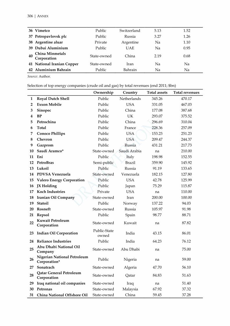
306 | ANNEX
36 Vimetco Public Switzerland 5.13 1.52
37 Petropavlovsk plc Public Russia 3.27 1.26
38 Argentine aluar Private Argentine Na 1.10
39 Dubai Aluminium Public UAE Na 0.95
40 China Minmetals Corporation
State-owned China 2.19 0.68
41 National Iranian Copper State-owned Iran Na Na
42 Aluminium Bahrain Public Bahrain Na Na
Source: Author.
Selection of top energy companies (crude oil and gas) by total revenues (end 2011; $bn)
Ownership Country Total assets Total revenues
1 Royal Dutch Shell Public Netherlands 345.26 470.17
2 Exxon Mobile Public USA 331.05 467.03
3 Sinopec Public China 177.08 387.68
4 BP Public UK 293.07 375.52
5 Petrochina Public China 296.69 310.04
6 Total Public France 228.36 257.09
7 Conoco Phillips Public USA 153.23 251.23
8 Chevron Public USA 209.47 244.37
9 Gazprom Public Russia 431.21 217.73
10 Saudi Aramco* State-owned Saudi Arabia na 210.00
11 Eni Public Italy 198.98 152.55
12 PetroBras Semi-public Brazil 359.90 145.92
13 Lukoil Public Russia 91.19 133.65
14 PDVSA Venezuela State-owned Venezuela 182.15 127.80
15 Valero Energy Corporation Public USA 42.78 125.99
16 JX Holding Public Japan 75.29 115.87
17 Koch Industries Private USA na 110.00
18 Iranian Oil Company State-owned Iran 200.00 100.00
19 Statoil Public Norway 137.22 94.03
20 Rosneft State-owned Russia 105.97 91.98
21 Repsol Public Spain 98.77 88.71
22 Kuwait Petroleum Corporation
State-owned Kuwait na 87.82
23 Indian Oil Corporation Public-State
owned India 43.15 86.01
24 Reliance Industries Public India 64.23 76.12
25 Abu Dhabi National Oil Company
State-owned Abu Dhabi na 75.00
26 Nigerian National Petroleum Corporation*
Public Nigeria na 59.00
27 Sonatrach State-owned Algeria 47.70 56.10
28 Qatar General Petroleum Corporation
State-owned Qatar 84.83 51.63
29 Iraq national oil companies State-owned Iraq na 51.40
30 Petronas State-owned Malaysia 67.92 37.32
31 China National Offshore Oil State-owned China 59.45 37.28

Corporation
32 Pemex State-owned Mexico 109.80 30.04
33 Occidental Petroleum Corporation
Public USA 60.04 24.12
34 Marathon Oil Public USA 31.30 14.60
35 Libyan national oil company State-owned Libya na Na
Source: Author.
Top global exchanges
Futures
exchange Contract
size Delivery dates Price quote
Open Interest
(at 19-Oct-2012 close)
Value of OI in USD
Cocoa
ICE Futures US
10 metric tons
H, K, N, U, Z USD per metric tons 205,758 $5,092,510,500
NYSE-LIFFE 10 metric
tons H, K, N, U, Z GBP per metric tons 197,654* $3,954,939,565
Coffee
ICE Futures US
37,500 pounds
H, K, N, U, Z USD per pounds 152,473 $9,205,557,375
NYSE-LIFFE 10 metric
tons F, H, K, N, U, X USD per metric tons 86,238* $2,177,509,500
Bolsa de Mercadorias
& Futuros
100 bags, weighing 60
net kilograms
each.
F, H, K, N, U, X Brazilian Real (BRL) per 60 net kilograms (one bag) of coffee.
8,753 $181,143,335
Tokyo Grain Exchange
50 bags (3,450
kilograms) F, H, K, N, U, X
JPY per bag (69 kilograms)
239 $2,863,899
Sugar
NYSE-LIFFE 50 tonnes H, K, Q, V, Z USD and cents per
tonne 62,927* $2,024,990,860
ICE Futures US
112,000 pounds
H, K, N, V USD Cents and hundredths of a cent per pound
707,460 $15,054,748,80
0
Tokyo Grain Exchange
10,000 kilograms
(10 metric tons)
F, H, K, N, U, X JPY per 1,000
kilograms 2,616 $7,600,289
Bolsa de Mercadorias
& Futuros
270 bags of 50 net
kilograms G, J, N, U, X
USD per 50-net kilogram bag
na na
Soybean oil
CBOT
60,000 pounds
(~ 27 metric tons)
F, H, K, N, Q, U, V, Z USD Cents per
pound 330,035
$10,099,071,000
ICE Futures US
60,000 pounds
(~ 27 metric tons)
F, H, K, N, Q, U, V, Z USD cents per
pound 150 $4,590,000
Wheat
NYSE-LIFFE 100 tonnes F, H, K, N, X GBP and pence per
tonne 14,530* $500,657,326
CBOT
5,000 bushels
(~ 136 Metric Tons)
H, K, N, U, Z USD cents per
bushel 468,562
$20,288,734,600

308 | ANNEX
Corn
CBOT
5,000 bushels
(~ 127 Metric Tons)
H, K, N, U, Z USD cents per
bushel 1,273,959
$48,091,952,250
Bolsa de Mercadorias
& Futuros
450 bags of 60-net
kilograms each
F, H, K, N, Q, U, X BRL per 60-net kilogram bag
na Na
ICE Futures US
5,000 bushels
H, K, N, U, Z USD cents per
bushel, 2,001 $1,900,950
Tokyo Grain Exchange
50,000 kilograms
(50 metric tons)
F, H, K, N, U, X JPY per 1,000
kilograms 28,515 $492,447,143
Aluminium
London Metal
Exchange 25 tonnes
Weekly prompts on every Wednesday from 3 months to 6 months. Monthly
prompts on every 3rd Wednesday from 7
months to 123 months
USD per tonne 720,846 $35,366,506,87
5
Tokyo Commodity
Exchange
5,000 kg (5 tonnes) per
contract
All even months within a year
JPY 0.1 per kg na Na
Shanghai Futures
Exchange
5 Metric Tonnes
12 months of the year Yuan (RMB) / ton na Na
Copper
London Metal
Exchange 25 tonnes
Weekly prompts on every Wednesday from 3 months to 6 months. Monthly
prompts on every 3rd Wednesday from 7
months to 123 months
USD per tonne 249,780 $49,893,555,00
0
Shanghai Futures
Exchange 5 tonnes 12 months of the year RMB / ton na Na
NYMEX 25,000
pounds
Trading is conducted for delivery during the current calendar month, the next 23
calendar months, and any March, May,
July, September, and December falling
within a 60-month period beginning with the current
month.
USD cents per pound
155,204 $13,900,458,25
0
Iron ore
Singapore Mercantile Exchange
Index data normalised to 62% Fe Iron Ore,
CFR Qingdao
n/a USD to two decimal
places n/a n/a
Crude oil
ICE Futures US
1,000 barrels n/a USD and cents per
barrel Brent Crude
1,211,530 $130,421,204,5
00

Crude WTI 510,236
$44,410,941,440
NYMEX 1,000 barrels n/a USD and cents per
barrel
Crude WTI 1,578,044
$138,431,549,440
Brent Crude 42,192
$4,541,968,800
Natural gas
ICE Futures Europe
1,000 therms of natural
gas per day (1 therm =
29.3071 kilowatt hours)
n/a GBP and pence per
therm
310,765
(UK GAS)
$33,019,191,796
NYMEX
10,000 million British
thermal units
(mmBtu)
n/a USD and cents per
mmBtu
1,213,377
(Henry Hub)
$42,213,385,830
*30 March 2012. January (F), February (G), March (H), April (J), May (K), June (M), July (N), August (Q), September (U), October (V), November (X), & December (Z). Note: Data on open interest from Chinese and Indian exchanges area not available.
Source: Author’s elaboration from exchanges’ websites.

| 310
Backwardation/contango (days per year)
1990 1991 1992 1993 1994 1995 1996 1997 1998 1999 2000 2001 2002 2003 2004 2005 2006 2007 2008 2009 2010 2011 2012*
Soybean Oil Contango 138 143 195 169 66 98 192 166 155 164 221 169 161 82 74 159 218 185 198 188 197 200 95
Backwardation 97 77 44 63 166 142 46 57 82 70 18 42 77 160 164 43 20 14 43 49 36 41 22
1990 1991 1992 1993 1994 1995 1996 1997 1998 1999 2000 2001 2002 2003 2004 2005 2006 2007 2008 2009 2010 2011 2012**
Corn Contango 164 219 225 252 212 220 105 136 251 251 232 229 249 189 239 252 252 251 252 244 252 201 41
Backwardation 89 34 28 0 41 32 150 117 0 0 20 23 3 63 13 0 0 1 0 8 0 51 98
1990 1991 1992 1993 1994 1995 1996 1997 1998 1999 2000 2001 2002 2003 2004 2005 2006 2007 2008 2009 2010 2011 2012*
Wheat Contango 160 218 102 119 187 141 79 203 251 251 252 243 203 199 251 252 251 247 188 252 253 244 134
Backwardation 93 35 151 134 66 112 174 50 2 2 1 10 50 54 2 1 2 6 8 1 0 9 5
1990 1991 1992 1993 1994 1995 1996 1997 1998 1999 2000 2001 2002 2003 2004 2005 2006 2007 2008 2009 2010 2011 2012*
Cocoa Contango 247 251 248 243 227 214 246 248 248 217 247 159 183 253 208 246 210 243 166 161 149 198 75
Backwardation 4 2 5 10 26 39 7 5 5 36 6 94 70 0 45 7 43 10 87 92 104 55 0
1990 1991 1992 1993 1994 1995 1996 1997 1998 1999 2000 2001 2002 2003 2004 2005 2006 2007 2008 2009 2010 2011 2012*
Aluminium Contango 193 252 254 253 252 243 249 230 252 254 231 200 249 141 204 129 224 198 254 254 248 246 64
Backwardation 59 2 1 1 2 11 5 24 2 0 23 54 5 113 50 125 30 56 0 0 6 8 0
1990 1991 1992 1993 1994 1995 1996 1997 1998 1999 2000 2001 2002 2003 2004 2005 2006 2007 2008 2009 2010 2011 2012*
Copper Contango 6 67 253 218 188 14 10 89 250 254 254 249 254 201 0 2 53 85 66 230 209 210 44
Backwardation 248 187 1 36 66 240 244 165 4 0 0 5 0 53 254 252 201 169 188 24 45 44 20
1990 1991 1992 1993 1994 1995 1996 1997 1998 1999 2000 2001 2002 2003 2004 2005 2006 2007 2008 2009 2010 2011 2012*
Sugar Contango 41 37 127 119 32 7 23 105 174 132 132 40 6 97 178 115 79 105 189 148 20 12 5
Backwardation 211 215 125 133 220 245 229 147 78 120 120 212 246 155 74 137 173 147 63 104 232 240 70

| 311
Liquidity curves (open interest by expiry month)
Source: Author’s calculation from CME GROUP and LIFFE.
0
5,000,000
10,000,000
15,000,000
20,000,000
25,000,000
1 2 3 4 5 6 7 8 9 10 11 12 13 14 15 16 17 18 19 20
Robusta Coffee (LIFFE)
0
100,000,000
200,000,000
300,000,000
400,000,000
500,000,000
600,000,000
700,000,000
800,000,000
900,000,000
1,000,000,000
1 3 5 7 9 11 13 15 17 19 21 23 25 27 29 31 33 35 37 39 41 43 45 47 49
Corn (CBOT)
0
5,000,000
10,000,000
15,000,000
20,000,000
25,000,000
30,000,000
35,000,000
40,000,000
45,000,000
1 2 3 4 5 6 7 8 9 10 11 12 13 14 15 16 17 18 19 20 21
White Sugar (LIFFE)
0
10,000,000
20,000,000
30,000,000
40,000,000
50,000,000
60,000,000
70,000,000
1 3 5 7 9 11 13 15 17 19 21 23 25 27 29 31 33 35 37 39
Soybean Oil (CBOT)
-10000000
10000000
30000000
50000000
70000000
90000000
110000000
130000000
150000000
1 2 3 4 5 6 7 8 9 10 11 12 13 14 15 16 17 18 19 20 21 22 23 24 25
Cocoa (LIFFE)
0
10000000
20000000
30000000
40000000
50000000
60000000
70000000
80000000
90000000
1 2 3 4 5 6 7 8 9 101112131415161718192021222324252627282930313233343536
Copper (CME)
0
100,000,000
200,000,000
300,000,000
400,000,000
500,000,000
600,000,000
700,000,000
800,000,000
900,000,000
1,000,000,000
1 2 3 4 5 6 7 8 9 101112131415161718192021222324252627282930313233343536
Crude oil (WTI, CME)
0
20,000,000
40,000,000
60,000,000
80,000,000
100,000,000
120,000,000
140,000,000
160,000,000
180,000,000
200,000,000
1 2 3 4 5 6 7 8 9 101112131415161718192021222324252627282930313233343536
Natural Gas (NYMEX, CME)

312 | ANNEX
GMO Ratio for cultivation area (%)
Year Cultivation Area in Million Hectares
Total Maize GM Maize GMO Ratio
Global
1998 140 2 1.4%
2008 161 37.3 23%
2009 158 42 26%
USA
1997 29,6 2.8 9,.5%
2008 35.3 28.2 80%
2009 35.2 29.9 85%
Canada 1997 1.06 0.03 2.8%
2007 1.4 1.17 84%
Argentina
1998 3.18 0.017 0.5%
2007 3.9 2.8 84%
2008 3.4 2.8 83%
2009 2.5 2.1 85%
South Africa
1998 2.96 0.003 0.1%
2007 2.8 1.6 57%
2009 3.0 1.9 63%
Spain 1998 0.46 0.018 3.9%
2009 0.34 0.076 20%
France 1999 3.1 0.0001 0.003%
2007 0.021
Germany* 1998 0.34 0.0004 0.1%
2008 2.08 0.003 0.15%
Portugal 1999 0.12 0.001 0.8%
2009 0.005
Czech Republic 2005 0.29 0.00015 0.05%
2009 0.27 0.006 2,4%
Honduras 2002 0.37 0.0005 0.1%
2007 0.35 0.007 2.0%
Philippines
2003 2.38 0.23 1.0%
2008 2,74 0.35 12.8%
2009 2,7 0.5 19%
Egypt 2008 0.72 0.0007 0,1%
2009 0,7 0.001 0.1%
Brazil 2008 14.7 1.3 9%
2009 14 5 36%
Source: GMO Compass.

Composition of index investing across commodities futures markets
US Futures Market1
Notional Value (Billions US$)
Futures Equivalent Contracts (Thousands)
(Notional Value > 0.5 billion US$)2 Long Short Net L (S) Long Short Net L (S)
Cocoa 1.2 (0.3) 0.9 47 (13) 35
Coffee 4.3 (1.6) 2.7 66 (25) 41
Copper 10.4 (2.9) 7.5 111 (31) 80
Corn 20.4 (6.5) 13.9 544 (172) 372
Cotton 3.8 (1.4) 2.5 108 (39) 69
Feeder Cattle 0.7 (0.2) 0.5 9 (3) 7
Gold 25.9 (5.2) 20.7 146 (29) 117
Heating Oil 10.6 (2.5) 8.1 81 (19) 62
Lean Hogs 4.3 (1.4) 2.9 140 (46) 94
Live Cattle 8.6 (2.6) 5.9 170 (53) 118
Natural Gas 18.4 (4.9) 13.5 526 (145) 381
Platinum 1.4 (0.3) 1.1 17 (4) 13
RBOB Unleaded Gas 11.2 (2.7) 8.6 93 (22) 72
Silver 7.3 (1.4) 5.8 42 (8) 34
Soybean Meal 0.9 (0.1) 0.9 20 (1) 18
Soybean Oil 4.9 (1.4) 3.5 153 (44) 109
Soybeans 20.6 (5.6) 15.0 259 (70) 190
Sugar 8.5 (2.5) 6.0 371 (110) 262
Wheat (CBOT) 15.5 (6.8) 8.7 345 (151) 194
Wheat (KCBT) 2.6 (0.7) 1.9 57 (15) 42
WTI Crude Oil 49.0 (14.0) 35.0 529 (151) 378
Subtotal (>0.5 billion US$) 230.5 (64.9) 165.5
Subtotal (<0.5 billion US$) 0.8 (0.2) 0.7
Total Notional US Mkts 231.3 (65.1) 166.2
Total Not'l Non-US Mkts 63.4 (15.1) 48.4
Total All Markets 294.7 (80.2) 214.6
Source: CFTC Index Investment data (28 September 2012).
Other graphs
Conversion factors for energy
Source: IEA Golden Rules, 2012.

314 | ANNEX
Primary vs secondary oil
Source: IEA et al. (2005, p. 70).

Unconventional gas production in the IEA’s New Policies scenario, 2035
Source: IEA WEO, 2012.
Current and planned EU-27 LNG re-gasification capacity (as of September 2011)
Source: JRC, 2012 based on “Gas Infrastructure Europe”, GIE LNG Investment Database, 2011.

316 | ANNEX
Producers, net exporters and net importers of natural gas
Source: IEA.

LNG system dynamics, 2011
Source: Rogers, 2012a.
LME Aluminium and copper stocks, 1992-2011
Year Global
Production Global
Consumption Stock
(tonnes) % Global
production Global
Production Global
Consumption Stock
(tonnes) % Global
production
Aluminium Copper
1992 19,457 18,513 1,527 7.85% 11,170 10,761 342 3.07%
1993 19,715 18,166 2,486 12.61% 11,306 10,972 600 5.30%
1994 19,112 19,762 1,675 8.76% 11,166 11,639 302 2.70%
1995 19,658 20,548 584 2.97% 11,829 12,167 296 2.51%
1996 20,846 20,650 951 4.56% 12,756 12,414 125 0.98%
1997 21,798 21,797 622 2.85% 13,599 13,080 338 2.48%
1998 22,654 21,825 636 2.81% 14,142 13,339 592 4.19%
1999 23,710 23,358 775 3.27% 14,463 14,024 790 5.46%
2000 24,464 24,871 322 1.32% 14,814 15,104 357 2.41%
2001 24,436 23,722 821 3.36% 15,675 14,686 799 5.10%
2002 26,076 25,372 1,241 4.76% 15,336 15,037 856 5.58%
2003 28,002 27,608 1,423 5.08% 15,221 15,315 431 2.83%
2004 29,940 29,957 693 2.31% 15,832 16,671 49 0.31%
2005 31,889 31,689 644 2.02% 16,651 16,680 92 0.55%
2006 33,975 33,935 698 2.06% 17,353 17,007 191 1.10%
2007 38,186 37,411 929 2.43% 18,044 18,143 199 1.10%
2008 39,669 36,900 2,338 5.89% 18,501 18,138 341 1.84%
2009 37,198 34,765 4,624 12.43% 18,613 18,178 502 2.70%
2010 41,112 39,662 4,275 10.40% 19,190 19,365 378 1.97%
2011 43,652 42,027 4,979 11.41% 19,578 19,508 372 1.90%
Note: see the Annex for full data from 1992.
Source: LME & WMBS. Thousands of metric tonnes (MT).

Econometric analysis: Stata outputs
Below, the outputs of the econometric analyses run across nine commodities markets.
First chapter
Output #1
Output #2
The Granger Theorem states that if Y and X are cointegrated, the relationship can be written as below and at least one between γ1 γ2 must be ≠ 0.
ΔYt=a1 ΔYt-1+b0 ΔXt+ b1 ΔXt-1+γ1(Yt-1- Xt-1) (eq.1)
ΔXt=a1 ΔXt-1+b0 ΔYt+ b1 ΔYt-1+γ2(Yt-1- Xt-1) (eq.2)
γ1 and γ2 are the coefficient of the cointegrating equation. At least one of them must be statistically different from zero and with negative coefficient, as it shows how a variable, when the distance between the two variables grows, is brought back to the equilibrium and the model is then stable. Those coefficients should then be between 0 and -1. It is the speed of adjustment of the dependent variable to the equilibrium. For instance, if it is equal to 0.5 it means a 50% movement back to equilibrium following a shock to the model one period later. If it is equal to 1 then there is full adjustment to the equilibrium the period after. A coefficient higher than 1 would not make much sense.
_cons -.4486328 .3264045 -1.37 0.170 -1.090881 .1936157 lnm2 1.62709 .0385993 42.15 0.000 1.55114 1.70304 commTOT Coef. Std. Err. t P>|t| [95% Conf. Interval]
Total 141.077867 311 .453626581 Root MSE = .26 Adj R-squared = 0.8510 Residual 20.9564659 310 .067601503 R-squared = 0.8515 Model 120.121401 1 120.121401 Prob > F = 0.0000 F( 1, 310) = 1776.90 Source SS df MS Number of obs = 312
. reg commTOT lnm2
Durbin-Watson d-statistic( 2, 312) = .1009832
. dwstat
_cons .0024848 .004561 0.54 0.586 -.00649 .0114596 LD. -.1069497 .055503 -1.93 0.055 -.2161641 .0022646 L1. -.0707039 .0180856 -3.91 0.000 -.1062914 -.0351165 coin1 D.coin1 Coef. Std. Err. t P>|t| [95% Conf. Interval]
MacKinnon approximate p-value for Z(t) = 0.0020 Z(t) -3.909 -3.455 -2.878 -2.570 Statistic Value Value Value Test 1% Critical 5% Critical 10% Critical Interpolated Dickey-Fuller
Augmented Dickey-Fuller test for unit root Number of obs = 310
. dfuller coin1, reg lag(1)

DRAFT LIST OF MEMBERS AND OBSERVERS - Confidential
Output #3
_cons .0205437 .006461 3.18 0.002 .0078301 .0332574 L1. -.0812382 .0178908 -4.54 0.000 -.1164428 -.0460336 coin1 D1. -2.367319 1.075996 -2.20 0.029 -4.484607 -.2500303 lnm2 LD. -.104876 .0548934 -1.91 0.057 -.2128924 .0031404 commTOT D.commTOT Coef. Std. Err. t P>|t| [95% Conf. Interval]
Total 2.06783957 309 .006692037 Root MSE = .0786 Adj R-squared = 0.0767 Residual 1.89063841 306 .006178557 R-squared = 0.0857 Model .177201164 3 .059067055 Prob > F = 0.0000 F( 3, 306) = 9.56 Source SS df MS Number of obs = 310
. reg d.commTOT dl.commTOT d.lnm2 l.coin1
_cons .0039853 .0003435 11.60 0.000 .0033093 .0046612 L1. -.0026633 .0009751 -2.73 0.007 -.004582 -.0007446 coin1 D1. -.006499 .0029625 -2.19 0.029 -.0123284 -.0006696 commTOT LD. .0947919 .0571094 1.66 0.098 -.017585 .2071687 lnm2 D.lnm2 Coef. Std. Err. t P>|t| [95% Conf. Interval]
Total .005468579 309 .000017698 Root MSE = .00413 Adj R-squared = 0.0378 Residual .005211015 306 .000017029 R-squared = 0.0471 Model .000257564 3 .000085855 Prob > F = 0.0020 F( 3, 306) = 5.04 Source SS df MS Number of obs = 310
. reg d.lnm2 dl.lnm2 dl(0).commTOT l.coin1
_cons -9.729133 .4339758 -22.42 0.000 -10.58304 -8.875222 lnm2 2.500503 .0513203 48.72 0.000 2.399523 2.601483 NONcommTOT Coef. Std. Err. t P>|t| [95% Conf. Interval]
Total 320.740798 311 1.03132089 Root MSE = .34569 Adj R-squared = 0.8841 Residual 37.0456178 310 .119501993 R-squared = 0.8845 Model 283.69518 1 283.69518 Prob > F = 0.0000 F( 1, 310) = 2373.98 Source SS df MS Number of obs = 312
. reg NONcommTOT lnm2
_cons -.0014365 .0118329 -0.12 0.903 -.0247215 .0218485 L3D. -.0945171 .0563819 -1.68 0.095 -.2054667 .0164325 L2D. -.1436072 .0591232 -2.43 0.016 -.2599513 -.0272632 LD. -.2046474 .0607481 -3.37 0.001 -.3241889 -.0851058 L1. -.1437611 .0387549 -3.71 0.000 -.220024 -.0674983 coin2 D.coin2 Coef. Std. Err. t P>|t| [95% Conf. Interval]
MacKinnon approximate p-value for Z(t) = 0.0040 Z(t) -3.709 -3.455 -2.878 -2.570 Statistic Value Value Value Test 1% Critical 5% Critical 10% Critical Interpolated Dickey-Fuller
Augmented Dickey-Fuller test for unit root Number of obs = 308
. dfuller coin2, reg lag(3)

Output #4
_cons .0255268 .0171685 1.49 0.138 -.0082566 .0593101 L1. -.1832619 .0365718 -5.01 0.000 -.255226 -.1112978 coin2 D1. -2.868 2.843853 -1.01 0.314 -8.463982 2.727982 lnm2 LD. -.1301126 .0564883 -2.30 0.022 -.2412674 -.0189579 NONcommTOT D.NONcommTOT Coef. Std. Err. t P>|t| [95% Conf. Interval]
Total 15.394331 309 .049819841 Root MSE = .20996 Adj R-squared = 0.1152 Residual 13.4892931 306 .044082657 R-squared = 0.1237 Model 1.90503788 3 .635012625 Prob > F = 0.0000 F( 3, 306) = 14.41 Source SS df MS Number of obs = 310
. reg d.NONcommTOT dl.NONcommTOT dl(0).lnm2 l.coin2
_cons .0037679 .0003417 11.03 0.000 .0030955 .0044402 L1. .0000999 .0007302 0.14 0.891 -.0013371 .0015368 coin2 D1. -.0011387 .0011296 -1.01 0.314 -.0033616 .0010841 NONcommTOT LD. .1317168 .0567432 2.32 0.021 .0200606 .243373 lnm2 D.lnm2 Coef. Std. Err. t P>|t| [95% Conf. Interval]
Total .005468579 309 .000017698 Root MSE = .00418 Adj R-squared = 0.0107 Residual .005357756 306 .000017509 R-squared = 0.0203 Model .000110823 3 .000036941 Prob > F = 0.0990 F( 3, 306) = 2.11 Source SS df MS Number of obs = 310
. reg d.lnm2 dl.lnm2 dl(0).NONcommTOT l.coin2
_cons -7.737542 .613394 -12.61 0.000 -8.944485 -6.5306 commSHORT 1.460438 .048561 30.07 0.000 1.364887 1.555989 NONcommLONG Coef. Std. Err. t P>|t| [95% Conf. Interval]
Total 434.85012 311 1.3982319 Root MSE = .59838 Adj R-squared = 0.7439 Residual 110.99847 310 .358059581 R-squared = 0.7447 Model 323.851649 1 323.851649 Prob > F = 0.0000 F( 1, 310) = 904.46 Source SS df MS Number of obs = 312
. reg NONcommLONG commSHORT
_cons -.0039797 .018784 -0.21 0.832 -.0409422 .0329828 L2D. -.1623107 .0557445 -2.91 0.004 -.2720032 -.0526182 LD. -.1722922 .057707 -2.99 0.003 -.2858464 -.058738 L1. -.137106 .0341737 -4.01 0.000 -.2043521 -.0698599 coin5 D.coin5 Coef. Std. Err. t P>|t| [95% Conf. Interval]
MacKinnon approximate p-value for Z(t) = 0.0013 Z(t) -4.012 -3.455 -2.878 -2.570 Statistic Value Value Value Test 1% Critical 5% Critical 10% Critical Interpolated Dickey-Fuller
Augmented Dickey-Fuller test for unit root Number of obs = 309
. dfuller coin5, reg lag(2)

DRAFT LIST OF MEMBERS AND OBSERVERS - Confidential
Output #5
Output #6
_cons -.0038412 .0190743 -0.20 0.841 -.0413745 .0336921 L1. -.1598455 .0332285 -4.81 0.000 -.2252308 -.0944602 coin5 D1. 1.753686 .1919461 9.14 0.000 1.375985 2.131387 commSHORT LD. -.1039714 .0501897 -2.07 0.039 -.202732 -.0052108 NONcommLONG NONcommLONG Coef. Std. Err. t P>|t| [95% Conf. Interval]D.
Total 47.5573066 309 .153907141 Root MSE = .33408 Adj R-squared = 0.2748 Residual 34.153502 306 .111612752 R-squared = 0.2818 Model 13.4038046 3 4.46793487 Prob > F = 0.0000 F( 3, 306) = 40.03 Source SS df MS Number of obs = 310
. reg d.NONcommLONG dl.NONcommLONG d.commSHORT l.coin5
_cons .0092288 .0049606 1.86 0.064 -.0005325 .0189901 L1. .018442 .0089171 2.07 0.039 .0008952 .0359888 coin5 LD. .0294207 .0146473 2.01 0.045 .0005981 .0582432 D1. .120293 .0131884 9.12 0.000 .0943413 .1462448 NONcommLONG LD. -.1805889 .0559078 -3.23 0.001 -.2906028 -.0705751 commSHORT D.commSHORT Coef. Std. Err. t P>|t| [95% Conf. Interval]
Total 3.03075463 309 .009808267 Root MSE = .08687 Adj R-squared = 0.2307 Residual 2.30139603 305 .007545561 R-squared = 0.2407 Model .729358602 4 .182339651 Prob > F = 0.0000 F( 4, 305) = 24.17 Source SS df MS Number of obs = 310
. reg d.commSHORT dl.commSHORT dl(0/1).NONcommLONG l.coin5
Prob > F = 0.0013 F( 2, 349) = 6.80
( 2) L2D.LnSp500 = 0 ( 1) LD.LnSp500 = 0
. test dl1.LnSp500 dl2.LnSp500
_cons .0010496 .0009388 1.12 0.264 -.0007967 .002896 L2D. .0584193 .0362431 1.61 0.108 -.0128632 .1297017 LD. .1234158 .035819 3.45 0.001 .0529676 .1938639 LnSp500 L2D. .1405412 .0517441 2.72 0.007 .0387716 .2423107 LD. .0747558 .0530476 1.41 0.160 -.0295773 .179089lnindexpos~n lnindexpos~n Coef. Std. Err. t P>|t| [95% Conf. Interval]D.
Total .116236705 353 .000329282 Root MSE = .01754 Adj R-squared = 0.0659 Residual .107345758 349 .000307581 R-squared = 0.0765 Model .008890947 4 .002222737 Prob > F = 0.0000 F( 4, 349) = 7.23 Source SS df MS Number of obs = 354
. reg d.lnindexposition dl(1/2).lnindexposition dl(1/2).LnSp500
D_LnSp500 ALL 1.6166 2 0.446 D_LnSp500 D.lnindexposition 1.6166 2 0.446 D_lnindexposition ALL 13.275 2 0.001 D_lnindexposition D.LnSp500 13.275 2 0.001 Equation Excluded chi2 df Prob > chi2 Granger causality Wald tests
. vargranger

Output #7
(a) 1992-2011
_cons .0003075 .0033448 0.09 0.927 -.0062483 .0068632 L5D. -.0600304 .0313864 -1.91 0.056 -.1215465 .0014858 L4D. -.0426604 .0323289 -1.32 0.187 -.1060238 .0207031 L3D. .0044932 .0323758 0.14 0.890 -.0589622 .0679487 L2D. -.0514314 .032336 -1.59 0.112 -.1148087 .0119459 LD. -.2391162 .0315153 -7.59 0.000 -.3008851 -.1773472 LnVix L5D. .1749648 .0903048 1.94 0.053 -.0020294 .351959 L4D. .1658828 .0876892 1.89 0.059 -.0059848 .3377505 L3D. .1414392 .0873137 1.62 0.105 -.0296925 .3125709 L2D. -.0719579 .0875055 -0.82 0.411 -.2434656 .0995498 LD. -.1922562 .0899523 -2.14 0.033 -.3685595 -.0159528 lncomm D_LnVix _cons .0013016 .0011713 1.11 0.266 -.0009941 .0035972 L5D. -.011337 .0109907 -1.03 0.302 -.0328784 .0102044 L4D. -.0055847 .0113208 -0.49 0.622 -.027773 .0166036 L3D. .0045817 .0113372 0.40 0.686 -.0176388 .0268022 L2D. -.0075996 .0113232 -0.67 0.502 -.0297928 .0145936 LD. -.0023716 .0110359 -0.21 0.830 -.0240016 .0192583 LnVix L5D. .0889301 .0316225 2.81 0.005 .0269512 .150909 L4D. .2622039 .0307066 8.54 0.000 .2020202 .3223876 L3D. -.1617723 .0305751 -5.29 0.000 -.2216983 -.1018462 L2D. -.1438222 .0306422 -4.69 0.000 -.2038799 -.0837645 LD. -.1129993 .0314991 -3.59 0.000 -.1747364 -.0512623 lncomm D_lncomm Coef. Std. Err. z P>|z| [95% Conf. Interval] D_LnVix 11 .105769 0.0701 75.20163 0.0000D_lncomm 11 .037038 0.1535 180.7411 0.0000 Equation Parms RMSE R-sq chi2 P>chi2
Det(Sigma_ml) = .000015 SBIC = -5.278983FPE = .0000157 HQIC = -5.346071Log likelihood = 2707.525 AIC = -5.387212Sample: 7 - 1003 No. of obs = 997
Vector autoregression
. var d.lncomm d.LnVix, lags(1/5)
D_LnVix ALL 15.761 5 0.008 D_LnVix D.lncomm 15.761 5 0.008 D_lncomm ALL 2.0707 5 0.839 D_lncomm D.LnVix 2.0707 5 0.839 Equation Excluded chi2 df Prob > chi2 Granger causality Wald tests
. vargranger

DRAFT LIST OF MEMBERS AND OBSERVERS - Confidential
(b) 1992-2001
D_LnVix ALL 5.8246 4 0.213 D_LnVix D.lncomm 5.8246 4 0.213 D_lncomm ALL 3.3238 4 0.505 D_lncomm D.LnVix 3.3238 4 0.505 Equation Excluded chi2 df Prob > chi2 Granger causality Wald tests
. vargranger
_cons .0008684 .0044837 0.19 0.846 -.0079195 .0096562 L4D. -.0829582 .0454008 -1.83 0.068 -.171942 .0060257 L3D. -.025036 .0466124 -0.54 0.591 -.1163947 .0663226 L2D. -.1299364 .0466998 -2.78 0.005 -.2214663 -.0384064 LD. -.2223783 .0455929 -4.88 0.000 -.3117388 -.1330179 LnVix L4D. .1415733 .1123532 1.26 0.208 -.078635 .3617816 L3D. -.0278712 .1110345 -0.25 0.802 -.2454948 .1897524 L2D. -.1058286 .1107003 -0.96 0.339 -.3227973 .11114 LD. -.1517995 .1119697 -1.36 0.175 -.371256 .067657 lncomm D_LnVix _cons .0010832 .001762 0.61 0.539 -.0023702 .0045366 L4D. .0082307 .0178413 0.46 0.645 -.0267377 .043199 L3D. .0314366 .0183175 1.72 0.086 -.0044649 .0673382 L2D. .0179731 .0183518 0.98 0.327 -.0179958 .053942 LD. .0087694 .0179168 0.49 0.625 -.0263469 .0438857 LnVix L4D. .2821224 .0441519 6.39 0.000 .1955863 .3686585 L3D. -.1747994 .0436336 -4.01 0.000 -.2603197 -.089279 L2D. -.1952695 .0435023 -4.49 0.000 -.2805325 -.1100065 LD. -.0884991 .0440011 -2.01 0.044 -.1747397 -.0022585 lncomm D_lncomm Coef. Std. Err. z P>|z| [95% Conf. Interval] D_LnVix 9 .098655 0.0699 35.8424 0.0000D_lncomm 9 .038769 0.1857 108.7909 0.0000 Equation Parms RMSE R-sq chi2 P>chi2
Det(Sigma_ml) = .000014 SBIC = -5.264647FPE = .0000151 HQIC = -5.360078Log likelihood = 1311.126 AIC = -5.421912Sample: 6 - 482 No. of obs = 477
Vector autoregression
. var d.lncomm d.LnVix if tin(1,482), lags(1/4)

(c) 2002-2011
D_LnVix ALL 6.8405 3 0.077 D_LnVix D.lncomm 6.8405 3 0.077 D_lncomm ALL 3.8775 3 0.275 D_lncomm D.LnVix 3.8775 3 0.275 Equation Excluded chi2 df Prob > chi2 Granger causality Wald tests
. vargranger
_cons .0000794 .0049087 0.02 0.987 -.0095415 .0097004 L3D. .0284243 .0436365 0.65 0.515 -.0571018 .1139503 L2D. .0056658 .0449432 0.13 0.900 -.0824213 .0937529 LD. -.2403403 .043649 -5.51 0.000 -.3258908 -.1547897 LnVix L3D. .2586992 .1316464 1.97 0.049 .000677 .5167214 L2D. -.0946373 .13189 -0.72 0.473 -.3531368 .1638623 LD. -.1692057 .1317911 -1.28 0.199 -.4275115 .0891002 lncomm D_LnVix _cons .0022621 .0015938 1.42 0.156 -.0008618 .0053859 L3D. -.0182942 .0141684 -1.29 0.197 -.0460638 .0094754 L2D. -.024066 .0145927 -1.65 0.099 -.0526671 .0045351 LD. .0025844 .0141725 0.18 0.855 -.0251931 .0303619 LnVix L3D. -.203528 .0427445 -4.76 0.000 -.2873056 -.1197504 L2D. -.1432191 .0428236 -3.34 0.001 -.2271517 -.0592865 LD. -.140799 .0427915 -3.29 0.001 -.2246688 -.0569293 lncomm D_lncomm Coef. Std. Err. z P>|z| [95% Conf. Interval] D_LnVix 7 .112477 0.0711 39.88595 0.0000D_lncomm 7 .03652 0.0719 40.34853 0.0000 Equation Parms RMSE R-sq chi2 P>chi2
Det(Sigma_ml) = .0000164 SBIC = -5.174484FPE = .0000173 HQIC = -5.244047Log likelihood = 1391.743 AIC = -5.288842Sample: 483 - 1003 No. of obs = 521
Vector autoregression
. var d.lncomm d.LnVix if tin(483,1003), lags(1/3)

DRAFT LIST OF MEMBERS AND OBSERVERS - Confidential
Output #8
(a) 1992-2011
D_LnVix ALL 7.4186 5 0.191 D_LnVix D.lnnoncomm 7.4186 5 0.191 D_lnnoncomm ALL 5.5129 5 0.357 D_lnnoncomm D.LnVix 5.5129 5 0.357 Equation Excluded chi2 df Prob > chi2 Granger causality Wald tests
. vargranger
_cons .0005115 .0033514 0.15 0.879 -.0060573 .0070802 L5D. -.0548423 .0315954 -1.74 0.083 -.1167681 .0070836 L4D. -.0445685 .0324387 -1.37 0.169 -.1081471 .0190101 L3D. -.0021954 .0324706 -0.07 0.946 -.0658365 .0614458 L2D. -.0532332 .0323696 -1.64 0.100 -.1166766 .0102101 LD. -.2308078 .0315803 -7.31 0.000 -.2927041 -.1689115 LnVix L5D. -.0354506 .0286149 -1.24 0.215 -.0915348 .0206336 L4D. .0610489 .0286226 2.13 0.033 .0049496 .1171482 L3D. .0137114 .0286003 0.48 0.632 -.0423441 .0697669 L2D. -.0212578 .0286929 -0.74 0.459 -.0774948 .0349792 LD. .0012344 .028681 0.04 0.966 -.0549793 .0574481 lnnoncomm D_LnVix _cons .0036861 .0036782 1.00 0.316 -.0035232 .0108953 L5D. .0075483 .0346763 0.22 0.828 -.060416 .0755126 L4D. -.0364477 .0356018 -1.02 0.306 -.1062259 .0333304 L3D. .034152 .0356368 0.96 0.338 -.0356948 .1039988 L2D. -.0477174 .035526 -1.34 0.179 -.1173471 .0219123 LD. -.0215933 .0346597 -0.62 0.533 -.089525 .0463385 LnVix L5D. -.1139606 .0314052 -3.63 0.000 -.1755135 -.0524076 L4D. -.0013663 .0314136 -0.04 0.965 -.0629359 .0602033 L3D. -.1264154 .0313891 -4.03 0.000 -.1879369 -.0648938 L2D. -.1047228 .0314907 -3.33 0.001 -.1664435 -.0430021 LD. -.0652446 .0314777 -2.07 0.038 -.1269398 -.0035495 lnnoncomm D_lnnoncomm Coef. Std. Err. z P>|z| [95% Conf. Interval] D_LnVix 11 .106207 0.0624 66.3698 0.0000D_lnnoncomm 11 .116564 0.0421 43.80507 0.0000 Equation Parms RMSE R-sq chi2 P>chi2
Det(Sigma_ml) = .0001497 SBIC = -2.978732FPE = .0001565 HQIC = -3.045821Log likelihood = 1560.85 AIC = -3.086961Sample: 7 - 1003 No. of obs = 997
Vector autoregression
. var d.lnnoncomm d.LnVix, lags(1/5)

(b) 1992-2001
.
D_LnVix ALL 5.0184 5 0.414 D_LnVix D.lnnoncomm 5.0184 5 0.414 D_lnnoncomm ALL 8.9319 5 0.112 D_lnnoncomm D.LnVix 8.9319 5 0.112 Equation Excluded chi2 df Prob > chi2 Granger causality Wald tests
. vargranger
_cons .0013162 .0044686 0.29 0.768 -.007442 .0100745 L5D. -.0503137 .0458701 -1.10 0.273 -.1402175 .0395901 L4D. -.107666 .0468536 -2.30 0.022 -.1994973 -.0158347 L3D. -.0495856 .0472605 -1.05 0.294 -.1422145 .0430433 L2D. -.1430859 .0466797 -3.07 0.002 -.2345763 -.0515954 LD. -.2172982 .0457047 -4.75 0.000 -.3068778 -.1277187 LnVix L5D. -.0375761 .0298422 -1.26 0.208 -.0960658 .0209136 L4D. .039312 .0300666 1.31 0.191 -.0196174 .0982414 L3D. -.0240012 .0300454 -0.80 0.424 -.0828891 .0348867 L2D. -.0193504 .0301539 -0.64 0.521 -.0784511 .0397502 LD. -.0143855 .0300896 -0.48 0.633 -.07336 .044589 lnnoncomm D_LnVix _cons .0032843 .0067492 0.49 0.627 -.0099439 .0165126 L5D. -.0124708 .0692811 -0.18 0.857 -.1482592 .1233176 L4D. -.0871633 .0707665 -1.23 0.218 -.225863 .0515364 L3D. .0700921 .0713811 0.98 0.326 -.0698123 .2099965 L2D. -.1249353 .0705038 -1.77 0.076 -.2631202 .0132496 LD. -.1057108 .0690312 -1.53 0.126 -.2410095 .029588 LnVix L5D. -.1531535 .045073 -3.40 0.001 -.2414949 -.0648121 L4D. -.0293285 .0454118 -0.65 0.518 -.118334 .059677 L3D. -.14651 .0453798 -3.23 0.001 -.2354528 -.0575672 L2D. -.1241801 .0455438 -2.73 0.006 -.2134442 -.034916 LD. -.1031346 .0454465 -2.27 0.023 -.1922082 -.014061 lnnoncomm D_lnnoncomm Coef. Std. Err. z P>|z| [95% Conf. Interval] D_LnVix 11 .098528 0.0715 36.66724 0.0001D_lnnoncomm 11 .148815 0.0708 36.26618 0.0001 Equation Parms RMSE R-sq chi2 P>chi2
Det(Sigma_ml) = .0002035 SBIC = -2.539016FPE = .0002232 HQIC = -2.655834Log likelihood = 672.1054 AIC = -2.731535Sample: 7 - 482 No. of obs = 476
Vector autoregression
. var d.lnnoncomm d.LnVix if tin(1,482), lags(1/5)

DRAFT LIST OF MEMBERS AND OBSERVERS - Confidential
(c) 2002-2011
D_LnVix ALL 6.0271 3 0.110 D_LnVix D.lnnoncomm 6.0271 3 0.110 D_lnnoncomm ALL 2.1708 3 0.538 D_lnnoncomm D.LnVix 2.1708 3 0.538 Equation Excluded chi2 df Prob > chi2 Granger causality Wald tests
. vargranger
_cons -.0002015 .0049101 -0.04 0.967 -.0098251 .0094221 L3D. .0339411 .0437054 0.78 0.437 -.0517198 .1196021 L2D. -.0029362 .044963 -0.07 0.948 -.091062 .0851896 LD. -.2379383 .0436259 -5.45 0.000 -.3234436 -.152433 LnVix L3D. .1359666 .0659793 2.06 0.039 .0066495 .2652838 L2D. -.0901239 .0659167 -1.37 0.172 -.2193183 .0390705 LD. .041004 .0659733 0.62 0.534 -.0883013 .1703093 lnnoncomm D_LnVix _cons .0034873 .0032461 1.07 0.283 -.002875 .0098495 L3D. .0000848 .0288939 0.00 0.998 -.0565463 .0567158 L2D. -.0152794 .0297253 -0.51 0.607 -.0735399 .0429812 LD. .0347707 .0288414 1.21 0.228 -.0217574 .0912988 LnVix L3D. -.0846017 .0436194 -1.94 0.052 -.1700941 .0008908 L2D. -.0724849 .043578 -1.66 0.096 -.1578961 .0129264 LD. .0409936 .0436154 0.94 0.347 -.044491 .1264782 lnnoncomm D_lnnoncomm Coef. Std. Err. z P>|z| [95% Conf. Interval] D_LnVix 7 .112564 0.0697 39.0216 0.0000D_lnnoncomm 7 .074417 0.0194 10.30241 0.1125 Equation Parms RMSE R-sq chi2 P>chi2
Det(Sigma_ml) = .0000682 SBIC = -3.748641FPE = .000072 HQIC = -3.818205Log likelihood = 1020.311 AIC = -3.862999Sample: 483 - 1003 No. of obs = 521
Vector autoregression
. var d.lnnoncomm d.LnVix if tin(483,1003), lags(1/3)

Output #9
(a) 1992-2011
D_LnVix ALL 9.5235 5 0.090 D_LnVix D.lnnocomlong 9.5235 5 0.090 D_lnnocomlong ALL 7.6402 5 0.177 D_lnnocomlong D.LnVix 7.6402 5 0.177 Equation Excluded chi2 df Prob > chi2 Granger causality Wald tests
. vargranger
_cons .0004232 .0033451 0.13 0.899 -.0061332 .0069795 L5D. -.0554288 .0315983 -1.75 0.079 -.1173603 .0065027 L4D. -.0440966 .0324382 -1.36 0.174 -.1076742 .0194811 L3D. -.0019844 .0324943 -0.06 0.951 -.065672 .0617032 L2D. -.0546619 .032335 -1.69 0.091 -.1180373 .0087135 LD. -.230547 .0316048 -7.29 0.000 -.2924912 -.1686028 LnVix L5D. -.0045648 .0177741 -0.26 0.797 -.0394015 .0302718 L4D. .0517498 .0178108 2.91 0.004 .0168414 .0866583 L3D. -.0010107 .0177692 -0.06 0.955 -.0358377 .0338164 L2D. -.0140857 .0184874 -0.76 0.446 -.0503202 .0221489 LD. .0184123 .0184551 1.00 0.318 -.017759 .0545836 lnnocomlong D_LnVix _cons .0037165 .0056929 0.65 0.514 -.0074414 .0148744 L5D. .021636 .0537757 0.40 0.687 -.0837625 .1270344 L4D. -.0575989 .055205 -1.04 0.297 -.1657988 .050601 L3D. .0172261 .0553005 0.31 0.755 -.0911609 .125613 L2D. -.1252399 .0550294 -2.28 0.023 -.2330955 -.0173842 LD. -.0308078 .0537867 -0.57 0.567 -.1362279 .0746123 LnVix L5D. -.0232346 .030249 -0.77 0.442 -.0825215 .0360523 L4D. -.0120244 .0303113 -0.40 0.692 -.0714336 .0473847 L3D. -.1167583 .0302406 -3.86 0.000 -.1760289 -.0574878 L2D. -.0078661 .0314628 -0.25 0.803 -.069532 .0537999 LD. .0639396 .0314079 2.04 0.042 .0023813 .1254979 lnnocomlong D_lnnocoml~g Coef. Std. Err. z P>|z| [95% Conf. Interval] D_LnVix 11 .106096 0.0644 68.59819 0.0000D_lnnocomlong 11 .18056 0.0286 29.33622 0.0011 Equation Parms RMSE R-sq chi2 P>chi2
Det(Sigma_ml) = .0003583 SBIC = -2.10616FPE = .0003744 HQIC = -2.173248Log likelihood = 1125.873 AIC = -2.214389Sample: 7 - 1003 No. of obs = 997
Vector autoregression
. var d.lnnocomlong d.LnVix, lags(1/5)

DRAFT LIST OF MEMBERS AND OBSERVERS - Confidential
(b) 1992-2001
D_LnVix ALL 8.5082 5 0.130 D_LnVix D.lnnocomlong 8.5082 5 0.130 D_lnnocomlong ALL 8.3867 5 0.136 D_lnnocomlong D.LnVix 8.3867 5 0.136 Equation Excluded chi2 df Prob > chi2 Granger causality Wald tests
. vargranger
_cons .0011988 .0044394 0.27 0.787 -.0075022 .0098998 L5D. -.0495701 .0454865 -1.09 0.276 -.1387221 .0395819 L4D. -.1089294 .0463863 -2.35 0.019 -.1998449 -.0180139 L3D. -.0459442 .0468118 -0.98 0.326 -.1376936 .0458053 L2D. -.1361711 .0462092 -2.95 0.003 -.2267393 -.0456028 LD. -.2117214 .0455857 -4.64 0.000 -.3010678 -.122375 LnVix L5D. -.0028873 .0180473 -0.16 0.873 -.0382594 .0324847 L4D. .0455337 .0180153 2.53 0.011 .0102243 .0808431 L3D. -.0215225 .0179693 -1.20 0.231 -.0567417 .0136967 L2D. -.0117164 .0188911 -0.62 0.535 -.0487424 .0253095 LD. .0146031 .0189095 0.77 0.440 -.0224589 .051665 lnnocomlong D_LnVix _cons .0007539 .0106453 0.07 0.944 -.0201105 .0216184 L5D. .0256494 .1090738 0.24 0.814 -.1881313 .2394302 L4D. -.0969172 .1112314 -0.87 0.384 -.3149267 .1210922 L3D. .1040774 .1122517 0.93 0.354 -.115932 .3240867 L2D. -.2388437 .1108066 -2.16 0.031 -.4560206 -.0216667 LD. -.1117488 .1093117 -1.02 0.307 -.3259957 .1024982 LnVix L5D. -.0403679 .0432763 -0.93 0.351 -.1251878 .044452 L4D. -.0300629 .0431996 -0.70 0.486 -.1147326 .0546069 L3D. -.1290661 .0430892 -3.00 0.003 -.2135194 -.0446128 L2D. -.017854 .0452997 -0.39 0.693 -.1066398 .0709318 LD. .0240137 .0453438 0.53 0.596 -.0648585 .1128858 lnnocomlong D_lnnocoml~g Coef. Std. Err. z P>|z| [95% Conf. Interval] D_LnVix 11 .098069 0.0782 40.48869 0.0000D_lnnocomlong 11 .235164 0.0397 19.69592 0.0323 Equation Parms RMSE R-sq chi2 P>chi2
Det(Sigma_ml) = .000506 SBIC = -1.628684FPE = .0005549 HQIC = -1.745322Log likelihood = 456.2837 AIC = -1.820896Sample: 7 - 483 No. of obs = 477
Vector autoregression
. var d.lnnocomlong d.LnVix if tin(1,483), lags(1/5)

(c) 2002-2011
D_LnVix ALL 7.8948 3 0.048 D_LnVix D.lnnocomlong 7.8948 3 0.048 D_lnnocomlong ALL 4.1631 3 0.244 D_lnnocomlong D.LnVix 4.1631 3 0.244 Equation Excluded chi2 df Prob > chi2 Granger causality Wald tests
. vargranger
_cons -.0004674 .0049074 -0.10 0.924 -.0100857 .0091508 L3D. .0405226 .0436966 0.93 0.354 -.0451211 .1261662 L2D. -.0076323 .0448613 -0.17 0.865 -.0955588 .0802941 LD. -.2366194 .0435762 -5.43 0.000 -.3220272 -.1512116 LnVix L3D. .1216999 .0459984 2.65 0.008 .0315446 .2118551 L2D. -.0678971 .0473205 -1.43 0.151 -.1606436 .0248494 LD. .0335107 .0460577 0.73 0.467 -.0567608 .1237821 lnnocomlong D_LnVix _cons .0052598 .0046603 1.13 0.259 -.0038744 .0143939 L3D. -.037147 .0414971 -0.90 0.371 -.1184799 .0441859 L2D. -.0601805 .0426032 -1.41 0.158 -.1436813 .0233202 LD. .041696 .0413828 1.01 0.314 -.0394129 .1228049 LnVix L3D. -.0746152 .0436831 -1.71 0.088 -.1602326 .0110022 L2D. -.0183554 .0449387 -0.41 0.683 -.1064336 .0697228 LD. .2348404 .0437394 5.37 0.000 .1491127 .3205681 lnnocomlong D_lnnocoml~g Coef. Std. Err. z P>|z| [95% Conf. Interval] D_LnVix 7 .112365 0.0730 41.00625 0.0000D_lnnocomlong 7 .106709 0.0650 36.19711 0.0000 Equation Parms RMSE R-sq chi2 P>chi2
Det(Sigma_ml) = .0001396 SBIC = -3.032894FPE = .0001473 HQIC = -3.102458Log likelihood = 833.8593 AIC = -3.147252Sample: 483 - 1003 No. of obs = 521
Vector autoregression
. var d.lnnocomlong d.LnVix if tin(483,1003), lags(1/3)

DRAFT LIST OF MEMBERS AND OBSERVERS - Confidential
Crude oil
Output #10
_cons -.0172424 .0078839 -2.19 0.030 -.0327837 -.0017011 D1. 12.89676 2.919459 4.42 0.000 7.141715 18.6518 lnoecd D1. -1.461619 .5042191 -2.90 0.004 -2.455571 -.4676664 lndollar D1. -.5329891 .2019181 -2.64 0.009 -.9310243 -.1349539lninventor~s lnspotprice Coef. Std. Err. t P>|t| [95% Conf. Interval]D.
Total 1.95089442 214 .009116329 Root MSE = .08728 Adj R-squared = 0.1644 Residual 1.60740152 211 .007618017 R-squared = 0.1761 Model .343492899 3 .114497633 Prob > F = 0.0000 F( 3, 211) = 15.03 Source SS df MS Number of obs = 215
. reg d.lnspotprice d.lninventories d.lndollar d.lnoecd
_cons -.036506 .0181405 -2.01 0.045 -.0722657 -.0007462 D1. 3.975196 1.612342 2.47 0.014 .7968336 7.153558 lnchina D1. -1.565516 .5324604 -2.94 0.004 -2.61514 -.5158927 lndollar D1. -.5850167 .2075468 -2.82 0.005 -.9941475 -.1758858lninventor~s lnspotprice Coef. Std. Err. t P>|t| [95% Conf. Interval]D.
Total 1.95089442 214 .009116329 Root MSE = .08994 Adj R-squared = 0.1126 Residual 1.70689007 211 .008089526 R-squared = 0.1251 Model .244004352 3 .081334784 Prob > F = 0.0000 F( 3, 211) = 10.05 Source SS df MS Number of obs = 215
. reg d.lnspotprice d.lninventories d.lndollar d.lnchina
Prob > chi2(40) = 0.2174 Portmanteau (Q) statistic = 46.6656 Portmanteau test for white noise
(note: time series has 3 gaps). wntestq res2
Residuals 1.7917 0.4083 1.7582 0.4152 (n = 212) D-H P-value asy. P-value
. omninorm res2
Prob > F = 0.0148 F(3, 208) = 3.58 Ho: model has no omitted variablesRamsey RESET test using powers of the fitted values of D.lnspotprice
. estat ovtest
Total 12.77 13 0.4657 Kurtosis 0.70 1 0.4034 Skewness 3.49 3 0.3222 Heteroskedasticity 8.58 9 0.4765 Source chi2 df p
Cameron & Trivedi's decomposition of IM-test
Prob > chi2 = 0.4765 chi2(9) = 8.58
against Ha: unrestricted heteroskedasticityWhite's test for Ho: homoskedasticity
. estat imtest,white
-.2
-.1
0.1
.2
Re
sid
ua
ls
2 2.5 3 3.5 4 4.5LnSpotPrice

Output #11
(a)
(b)
(c)
_cons .0081485 .0020093 4.06 0.000 .0042104 .0120866 L1. -.2842201 .2002123 -1.42 0.156 -.6766291 .1081888 garch L1. .239776 .0787471 3.04 0.002 .0854345 .3941174 arch ARCH _cons .0151405 .0061677 2.45 0.014 .003052 .027229 LD. -.4550465 .2145602 -2.12 0.034 -.8755767 -.0345162lnbrentsto~s lnbrentprice lnbrentprice Coef. Std. Err. z P>|z| [95% Conf. Interval]D. OPG
Log likelihood = 220.4784 Prob > chi2 = 0.0339Distribution: Gaussian Wald chi2(1) = 4.50Sample: 3 - 216 Number of obs = 214
ARCH family regression
Iteration 7: log likelihood = 220.47844 Iteration 6: log likelihood = 220.47843 Iteration 5: log likelihood = 220.47778 (switching optimization to BFGS)Iteration 4: log likelihood = 220.47393 Iteration 3: log likelihood = 220.43219 Iteration 2: log likelihood = 220.19397 Iteration 1: log likelihood = 219.30363 Iteration 0: log likelihood = 215.0574 (setting optimization to BHHH)
. arch d.lnbrentprice dl.lnbrentstocks, arch(1) garch(1)
-3-2
-10
12
se
2 2.5 3 3.5 4 4.5LnBrentPrice
Prob > chi2(40) = 0.2911 Portmanteau (Q) statistic = 44.4129 Portmanteau test for white noise
. wntestq se2
_cons .0084157 .0025403 3.31 0.001 .0034367 .0133946 L1. -.326461 .309971 -1.05 0.292 -.9339931 .2810711 garch L1. .1906678 .0695089 2.74 0.006 .0544328 .3269027 arch ARCH _cons -.0314662 .015389 -2.04 0.041 -.061628 -.0013044 D1. 4.125955 1.332705 3.10 0.002 1.513902 6.738008 lnchina LD. -.5007922 .2078281 -2.41 0.016 -.9081279 -.0934565lnbrentsto~s lnbrentprice lnbrentprice Coef. Std. Err. z P>|z| [95% Conf. Interval]D. OPG
Log likelihood = 224.4417 Prob > chi2 = 0.0006Distribution: Gaussian Wald chi2(2) = 14.77Sample: 3 - 216 Number of obs = 214
ARCH family regression
Iteration 13: log likelihood = 224.4417 Iteration 12: log likelihood = 224.4417 Iteration 11: log likelihood = 224.44166 Iteration 10: log likelihood = 224.44147 Iteration 9: log likelihood = 224.44113 Iteration 8: log likelihood = 224.44024 Iteration 7: log likelihood = 224.43629 Iteration 6: log likelihood = 224.38077 Iteration 5: log likelihood = 223.22802 (switching optimization to BFGS)Iteration 4: log likelihood = 222.21433 Iteration 3: log likelihood = 221.03819 Iteration 2: log likelihood = 219.77642 Iteration 1: log likelihood = 219.12845 Iteration 0: log likelihood = 216.65147 (setting optimization to BHHH)
. arch d.lnbrentprice dl.lnbrentstocks d.lnchina, arch(1) garch(1)
-3-2
-10
12
se
2 2.5 3 3.5 4 4.5LnBrentPrice
Prob > chi2(40) = 0.1370 Portmanteau (Q) statistic = 49.8375 Portmanteau test for white noise
. wntestq se2
_cons .0116125 .0017237 6.74 0.000 .0082341 .0149909 L1. -.8019366 .1293339 -6.20 0.000 -1.055426 -.5484469 garch L1. .1359556 .0396168 3.43 0.001 .058308 .2136032 arch ARCH _cons -.0118424 .0075442 -1.57 0.116 -.0266288 .002944 D1. -1.363367 .4803912 -2.84 0.005 -2.304917 -.4218177 lndollar D1. 11.86563 2.458424 4.83 0.000 7.04721 16.68405 lnoecd lnbrentprice lnbrentprice Coef. Std. Err. z P>|z| [95% Conf. Interval]D. OPG
Log likelihood = 232.783 Prob > chi2 = 0.0000Distribution: Gaussian Wald chi2(2) = 43.36Sample: 2 - 216 Number of obs = 215
ARCH family regression
Iteration 9: log likelihood = 232.78298 Iteration 8: log likelihood = 232.78298 Iteration 7: log likelihood = 232.78291 Iteration 6: log likelihood = 232.78266 Iteration 5: log likelihood = 232.77787 (switching optimization to BFGS)Iteration 4: log likelihood = 232.77116 Iteration 3: log likelihood = 232.74138 Iteration 2: log likelihood = 232.2745 Iteration 1: log likelihood = 228.68973 Iteration 0: log likelihood = 224.93451 (setting optimization to BHHH)
. arch d.lnbrentprice d.lnoecd d.lndollar, arch(1) garch(1)
-2-1
01
2
se
2 2.5 3 3.5 4 4.5LnBrentPrice
Prob > chi2(40) = 0.1693 Portmanteau (Q) statistic = 48.4333 Portmanteau test for white noise
(note: time series has 9 gaps). wntestq se2

DRAFT LIST OF MEMBERS AND OBSERVERS - Confidential
Output #12
D_basis12m ALL .93237 3 0.818 D_basis12m D.lninventories .93237 3 0.818 D_lninventories ALL 14.909 3 0.002 D_lninventories D.basis12m 14.909 3 0.002 Equation Excluded chi2 df Prob > chi2 Granger causality Wald tests
. vargranger
_cons .0049258 .1220454 0.04 0.968 -.2342787 .2441304 L3D. -.0039858 .0707034 -0.06 0.955 -.142562 .1345903 L2D. -.1375307 .0704133 -1.95 0.051 -.2755382 .0004768 LD. -.1030609 .0688306 -1.50 0.134 -.2379665 .0318446 basis12m L3D. -2.482749 4.128226 -0.60 0.548 -10.57392 5.608424 L2D. 1.392457 4.216714 0.33 0.741 -6.872151 9.657066 LD. -3.14403 4.23177 -0.74 0.458 -11.43815 5.150087lninventor~s D_basis12m _cons .0000921 .0019599 0.05 0.963 -.0037492 .0039335 L3D. .0017912 .0011354 1.58 0.115 -.0004342 .0040166 L2D. .0017338 .0011308 1.53 0.125 -.0004824 .0039501 LD. .0039159 .0011053 3.54 0.000 .0017494 .0060823 basis12m L3D. -.0898659 .0662949 -1.36 0.175 -.2198014 .0400697 L2D. -.0657577 .0677159 -0.97 0.332 -.1984784 .066963 LD. .0380064 .0679577 0.56 0.576 -.0951882 .171201lninventor~s D_lninvent~s Coef. Std. Err. z P>|z| [95% Conf. Interval] D_basis12m 7 1.8069 0.0335 7.339138 0.2906D_lninventories 7 .029017 0.0822 18.99269 0.0042 Equation Parms RMSE R-sq chi2 P>chi2
Det(Sigma_ml) = .0025704 SBIC = .0658039FPE = .0029335 HQIC = -.0662671Log likelihood = 30.52089 AIC = -.1558575Sample: 5 - 216 No. of obs = 212
Vector autoregression
. var d.lninventories d.basis12m, lags(1/3)

D_basis4m ALL 2.5565 3 0.465 D_basis4m D.lninventories 2.5565 3 0.465 D_lninventories ALL 9.5449 3 0.023 D_lninventories D.basis4m 9.5449 3 0.023 Equation Excluded chi2 df Prob > chi2 Granger causality Wald tests
. vargranger
_cons .0062048 .0639012 0.10 0.923 -.1190392 .1314487 L3D. -.135602 .0687216 -1.97 0.048 -.2702939 -.0009101 L2D. -.1655228 .06805 -2.43 0.015 -.2988983 -.0321472 LD. -.080839 .0679924 -1.19 0.234 -.2141017 .0524237 basis4m L3D. -1.736649 2.168673 -0.80 0.423 -5.987171 2.513872 L2D. 2.220118 2.18667 1.02 0.310 -2.065676 6.505911 LD. -2.381445 2.188641 -1.09 0.277 -6.671103 1.908214lninventor~s D_basis4m _cons .0000103 .0019833 0.01 0.996 -.0038769 .0038975 L3D. .0035267 .0021329 1.65 0.098 -.0006537 .0077072 L2D. .0030646 .0021121 1.45 0.147 -.0010749 .0072042 LD. .0053587 .0021103 2.54 0.011 .0012226 .0094948 basis4m L3D. -.0898827 .0673092 -1.34 0.182 -.2218062 .0420409 L2D. -.059588 .0678677 -0.88 0.380 -.1926063 .0734302 LD. .042102 .0679289 0.62 0.535 -.0910362 .1752403lninventor~s D_lninvent~s Coef. Std. Err. z P>|z| [95% Conf. Interval] D_basis4m 7 .946161 0.0586 13.18983 0.0401D_lninventories 7 .029366 0.0600 13.53198 0.0353 Equation Parms RMSE R-sq chi2 P>chi2
Det(Sigma_ml) = .0007218 SBIC = -1.204202FPE = .0008238 HQIC = -1.336273Log likelihood = 165.1416 AIC = -1.425864Sample: 5 - 216 No. of obs = 212
Vector autoregression
. var d.lninventories d.basis4m, lags(1/3)

DRAFT LIST OF MEMBERS AND OBSERVERS - Confidential
Output #13
D_lnsp500 ALL 4.5542 3 0.208 D_lnsp500 D.lnspotprice 4.5542 3 0.208 D_lnspotprice ALL 10.074 3 0.018 D_lnspotprice D.lnsp500 10.074 3 0.018 Equation Excluded chi2 df Prob > chi2 Granger causality Wald tests
. vargranger
_cons .0037779 .0031234 1.21 0.226 -.0023438 .0098997 L3D. .1007538 .070199 1.44 0.151 -.0368338 .2383414 L2D. -.0705911 .0691541 -1.02 0.307 -.2061307 .0649484 LD. .103706 .0697372 1.49 0.137 -.0329764 .2403885 lnsp500 L3D. .0336981 .0335076 1.01 0.315 -.0319755 .0993718 L2D. .058589 .0333396 1.76 0.079 -.0067553 .1239334 LD. -.0084503 .0335113 -0.25 0.801 -.0741312 .0572305 lnspotprice D_lnsp500 _cons .0019377 .0063883 0.30 0.762 -.0105832 .0144586 L3D. .3463921 .1435792 2.41 0.016 .064982 .6278022 L2D. .2249053 .141442 1.59 0.112 -.0523159 .5021265 LD. .1473154 .1426346 1.03 0.302 -.1322433 .4268741 lnsp500 L3D. .0948998 .0685336 1.38 0.166 -.0394236 .2292232 L2D. -.0528306 .0681899 -0.77 0.438 -.1864804 .0808192 LD. .0782124 .0685411 1.14 0.254 -.0561257 .2125505 lnspotprice D_lnspotpr~e Coef. Std. Err. z P>|z| [95% Conf. Interval] D_lnsp500 7 .045589 0.0464 10.31342 0.1121D_lnspotprice 7 .093245 0.0767 17.62315 0.0072 Equation Parms RMSE R-sq chi2 P>chi2
Det(Sigma_ml) = .0000163 SBIC = -4.99752FPE = .0000186 HQIC = -5.129591Log likelihood = 567.2332 AIC = -5.219182Sample: 5 - 216 No. of obs = 212
Vector autoregression
. var d.lnspotprice d.lnsp500, lags(1/3)

Output #14
_cons .0042667 .0064087 0.67 0.506 -.0083659 .0168994 D1. .4417079 .1392999 3.17 0.002 .167125 .7162909 lnsp500 lnspotprice Coef. Std. Err. t P>|t| [95% Conf. Interval]D.
Total 1.95089442 214 .009116329 Root MSE = .09352 Adj R-squared = 0.0406 Residual 1.86295347 213 .00874626 R-squared = 0.0451 Model .087940951 1 .087940951 Prob > F = 0.0017 F( 1, 213) = 10.05 Source SS df MS Number of obs = 215
. reg d.lnspotprice d.lnsp500
Residuals 5.3003 0.0706 6.6314 0.0363 (n = 214) D-H P-value asy. P-value
. omninorm res
Prob > chi2(40) = 0.1244 Portmanteau (Q) statistic = 50.4536 Portmanteau test for white noise
(note: time series has 2 gaps). wntestq res
-.3
-.2
-.1
0.1
.2
Re
sid
ua
ls
2 2.5 3 3.5 4 4.5LnSpotPrice
_cons .0016539 .0001728 9.57 0.000 .0013151 .0019926 L1. .1731276 .0861101 2.01 0.044 .004355 .3419002 arch ARCH _cons .0051019 .0033219 1.54 0.125 -.001409 .0116127 D1. .0725535 .031534 2.30 0.021 .0107479 .134359 lnspotprice lnsp500 D.lnsp500 Coef. Std. Err. z P>|z| [95% Conf. Interval] OPG
Log likelihood = 365.8776 Prob > chi2 = 0.0214Distribution: Gaussian Wald chi2(1) = 5.29Sample: 2 - 216 Number of obs = 215
ARCH family regression
Iteration 7: log likelihood = 365.8776 Iteration 6: log likelihood = 365.87758 Iteration 5: log likelihood = 365.87725 (switching optimization to BFGS)Iteration 4: log likelihood = 365.87654 Iteration 3: log likelihood = 365.87427 Iteration 2: log likelihood = 365.86675 Iteration 1: log likelihood = 365.83597 Iteration 0: log likelihood = 365.48875 (setting optimization to BHHH)
. arch d.lnsp500 d.lnspotprice, arch(1)
Prob > chi2(40) = 0.0716 Portmanteau (Q) statistic = 53.7666 Portmanteau test for white noise
(note: time series has 8 gaps). wntestq se2

DRAFT LIST OF MEMBERS AND OBSERVERS - Confidential
Output #15
(a) 1983-2002
(b) 2002-2011
Output #16
(a) 1994-2011
_cons .0003804 .0002303 1.65 0.099 -.000071 .0008319 L1. .6186613 .0518285 11.94 0.000 .5170792 .7202434 garch L1. .4375194 .0817145 5.35 0.000 .2773618 .5976769 arch ARCH _cons .0000212 .0037056 0.01 0.995 -.0072416 .007284 D1. -.1061058 .0893056 -1.19 0.235 -.2811414 .0689299 lnsp500 lnspotprice lnspotprice Coef. Std. Err. z P>|z| [95% Conf. Interval]D. OPG
Log likelihood = 238.9838 Prob > chi2 = 0.2348Distribution: Gaussian Wald chi2(1) = 1.41Sample: 2 - 226, but with gaps Number of obs = 219
ARCH family regression
Iteration 7: log likelihood = 238.98376 Iteration 6: log likelihood = 238.98376 Iteration 5: log likelihood = 238.98362 (switching optimization to BFGS)Iteration 4: log likelihood = 238.97622 Iteration 3: log likelihood = 238.74273 Iteration 2: log likelihood = 236.80057 Iteration 1: log likelihood = 220.12727 Iteration 0: log likelihood = 199.7378 (setting optimization to BHHH)
(note: conditioning reset at each gap)Number of gaps in sample: 3
. arch d.lnspotprice d.lnsp500, arch(1) garch(1)
-4-2
02
4
se
2 2.5 3 3.5 4LnSpotPrice
Prob > chi2(40) = 0.9346 Portmanteau (Q) statistic = 27.4271 Portmanteau test for white noise
(note: time series has 3 gaps). wntestq se2
_cons .000961 .0007915 1.21 0.225 -.0005904 .0025124 L1. .6344791 .1515962 4.19 0.000 .3373561 .9316021 garch L1. .2639878 .1461696 1.81 0.071 -.0224994 .550475 arch ARCH _cons .0101848 .0075652 1.35 0.178 -.0046427 .0250124 D1. .8139862 .1625204 5.01 0.000 .4954521 1.13252 lnsp500 lnspotprice lnspotprice Coef. Std. Err. z P>|z| [95% Conf. Interval]D. OPG
Log likelihood = 120.2889 Prob > chi2 = 0.0000Distribution: Gaussian Wald chi2(1) = 25.09Sample: 97 - 216 Number of obs = 120
ARCH family regression
Iteration 9: log likelihood = 120.28887 Iteration 8: log likelihood = 120.28886 Iteration 7: log likelihood = 120.28803 Iteration 6: log likelihood = 120.28684 Iteration 5: log likelihood = 120.24612 (switching optimization to BFGS)Iteration 4: log likelihood = 120.16366 Iteration 3: log likelihood = 119.68185 Iteration 2: log likelihood = 119.03208 Iteration 1: log likelihood = 118.97293 Iteration 0: log likelihood = 118.43568 (setting optimization to BHHH)
. arch d.lnspotprice d.lnsp500 if tin(97,216), arch(1) garch(1)
-4-2
02
4
se
2 2.5 3 3.5 4 4.5LnSpotPrice
Prob > chi2(40) = 0.1711 Portmanteau (Q) statistic = 48.3593 Portmanteau test for white noise
. wntestq se2
_cons .0061864 .000771 8.02 0.000 .0046754 .0076975 L1. .2007634 .0870412 2.31 0.021 .0301659 .371361 arch ARCH _cons .0102217 .0064399 1.59 0.112 -.0024002 .0228436 LD. .2274503 .1096355 2.07 0.038 .0125687 .442332 lnsp500 lnbrentprice lnbrentprice Coef. Std. Err. z P>|z| [95% Conf. Interval]D. OPG
Log likelihood = 219.7684 Prob > chi2 = 0.0380Distribution: Gaussian Wald chi2(1) = 4.30Sample: 3 - 216 Number of obs = 214
ARCH family regression
Iteration 8: log likelihood = 219.76844 Iteration 7: log likelihood = 219.76844 Iteration 6: log likelihood = 219.76841 Iteration 5: log likelihood = 219.76696 (switching optimization to BFGS)Iteration 4: log likelihood = 219.76458 Iteration 3: log likelihood = 219.75406 Iteration 2: log likelihood = 219.68534 Iteration 1: log likelihood = 218.75963 Iteration 0: log likelihood = 216.44421 (setting optimization to BHHH)
. arch d.lnbrentprice dl(1).lnsp500, arch(1)
-2-1
01
2
se
2 2.5 3 3.5 4 4.5LnBrentPrice
Prob > chi2(40) = 0.0569 Portmanteau (Q) statistic = 55.0560 Portmanteau test for white noise
(note: time series has 7 gaps). wntestq se2

(b) 1994-2002
(c) 2002-2011
Natural gas
Output #17
_cons .0059298 .0010507 5.64 0.000 .0038704 .0079891 L1. .3288481 .1234064 2.66 0.008 .0869759 .5707202 arch ARCH _cons -.0029828 .0080204 -0.37 0.710 -.0187025 .0127368 D1. -.2912692 .2043234 -1.43 0.154 -.6917357 .1091973 lnsp500 lnbrent D.lnbrent Coef. Std. Err. z P>|z| [95% Conf. Interval] OPG
Log likelihood = 137.1215 Prob > chi2 = 0.1540Distribution: Gaussian Wald chi2(1) = 2.03Sample: 2 - 144, but with gaps Number of obs = 137
ARCH family regression
Iteration 7: log likelihood = 137.12149 Iteration 6: log likelihood = 137.12148 Iteration 5: log likelihood = 137.12102 (switching optimization to BFGS)Iteration 4: log likelihood = 137.12014 Iteration 3: log likelihood = 137.117 Iteration 2: log likelihood = 137.10692 Iteration 1: log likelihood = 137.02013 Iteration 0: log likelihood = 136.51169 (setting optimization to BHHH)
(note: conditioning reset at each gap)Number of gaps in sample: 3
. arch d.lnbrent d.lnsp500, arch(1)
-2-1
01
2
se
2 2.5 3 3.5LnBrent
Prob > chi2(40) = 0.3304 Portmanteau (Q) statistic = 43.3522 Portmanteau test for white noise
(note: time series has 7 gaps). wntestq se2
_cons .0107565 .0082453 1.30 0.195 -.0055714 .0270844 LD. .6984865 .2455714 2.84 0.005 .2121883 1.184785 lnsp500 lnbrentprice Coef. Std. Err. t P>|t| [95% Conf. Interval]D. Robust
Root MSE = .08988 R-squared = 0.1173 Prob > F = 0.0052 F( 1, 118) = 8.09Linear regression Number of obs = 120
. reg d.lnbrentprice dl.lnsp500 if tin(97,216),r
Prob > F = 0.0701 F(3, 115) = 2.42 Ho: model has no omitted variablesRamsey RESET test using powers of the fitted values of D.lnbrentprice
. estat ovtest
Residuals 7.1661 0.0278 7.5903 0.0225 (n = 214) D-H P-value asy. P-value
. omninorm res
/sigma .1393897 .0067203 20.74 0.000 .1262182 .1525613 L3. -.1767412 .0856627 -2.06 0.039 -.344637 -.0088454 L2. -.2569548 .0665154 -3.86 0.000 -.3873226 -.126587 L1. -.1940036 .0659567 -2.94 0.003 -.3232764 -.0647308 ar ARMA _cons .002831 .0063339 0.45 0.655 -.0095832 .0152453 D1. 7.249326 2.726552 2.66 0.008 1.905383 12.59327 lnoecd D1. -5.103331 .6197163 -8.23 0.000 -6.317953 -3.88871lninventor~s lnspotprice lnspotprice Coef. Std. Err. z P>|z| [95% Conf. Interval]D. OPG
Log likelihood = 118.472 Prob > chi2 = 0.0000 Wald chi2(5) = 96.49Sample: 2 - 216 Number of obs = 215
ARIMA regression
Iteration 7: log likelihood = 118.47198 Iteration 6: log likelihood = 118.47198 Iteration 5: log likelihood = 118.47195 (switching optimization to BFGS)Iteration 4: log likelihood = 118.47195 Iteration 3: log likelihood = 118.47194 Iteration 2: log likelihood = 118.4719 Iteration 1: log likelihood = 118.47142 Iteration 0: log likelihood = 118.46263 (setting optimization to BHHH)
. arima lnspotprice lninventories lnoecd, arima(3,1,0)
-.4
-.2
0.2
.4
resid
ual,
on
e-s
tep
0 .5 1 1.5 2LnSpotPrice

DRAFT LIST OF MEMBERS AND OBSERVERS - Confidential
Output #18
Output #19
D_basis4m ALL 4.2089 3 0.240 D_basis4m D.lnspotprice 4.2089 3 0.240 D_lnspotprice ALL 7.112 3 0.068 D_lnspotprice D.basis4m 7.112 3 0.068 Equation Excluded chi2 df Prob > chi2 Granger causality Wald tests
. vargranger
_cons .0030068 .0404733 0.07 0.941 -.0763195 .0823331 L3D. -.2938412 .0843742 -3.48 0.000 -.4592116 -.1284707 L2D. -.1805484 .0833756 -2.17 0.030 -.3439615 -.0171353 LD. .0166111 .0842536 0.20 0.844 -.1485229 .1817451 basis4m L3D. -.5210432 .3157284 -1.65 0.099 -1.13986 .0977731 L2D. .1123891 .310437 0.36 0.717 -.4960562 .7208344 LD. .2572623 .3175174 0.81 0.418 -.3650604 .879585 lnspotprice D_basis4m _cons -.0004944 .0109101 -0.05 0.964 -.0218778 .020889 L3D. .0562177 .0227441 2.47 0.013 .01164 .1007954 L2D. .0083126 .0224749 0.37 0.711 -.0357375 .0523626 LD. .0263465 .0227116 1.16 0.246 -.0181675 .0708604 basis4m L3D. .1454974 .0851086 1.71 0.087 -.0213124 .3123072 L2D. -.2261905 .0836822 -2.70 0.007 -.3902047 -.0621763 LD. .029749 .0855909 0.35 0.728 -.138006 .197504 lnspotprice D_lnspotpr~e Coef. Std. Err. z P>|z| [95% Conf. Interval] D_basis4m 7 .592322 0.0999 22.98696 0.0008D_lnspotprice 7 .159668 0.0881 20.00674 0.0028 Equation Parms RMSE R-sq chi2 P>chi2
Det(Sigma_ml) = .0055065 SBIC = .8345951FPE = .0063044 HQIC = .7003442Log likelihood = -49.05157 AIC = .6091939Sample: 5 - 216, but with a gap No. of obs = 207
Vector autoregression
. var d.lnspotprice d.basis4m, lags(1/3)
D_lnm2 ALL .4983 3 0.919 D_lnm2 D.lnspotprice .4983 3 0.919 D_lnspotprice ALL 1.2171 3 0.749 D_lnspotprice D.lnm2 1.2171 3 0.749 Equation Excluded chi2 df Prob > chi2 Granger causality Wald tests
. vargranger
_cons .0030674 .0005769 5.32 0.000 .0019367 .0041981 L3D. .185915 .0675671 2.75 0.006 .0534858 .3183441 L2D. .1847375 .066534 2.78 0.005 .0543332 .3151417 LD. -.0082199 .0679279 -0.12 0.904 -.1413561 .1249163 lnm2 L3D. -.0001549 .0017746 -0.09 0.930 -.0036331 .0033232 L2D. -.0001811 .0017303 -0.10 0.917 -.0035725 .0032103 LD. -.0012386 .0017764 -0.70 0.486 -.0047202 .0022431 lnspotprice D_lnm2 _cons .0172713 .0224961 0.77 0.443 -.0268203 .0613628 L3D. -2.197661 2.63486 -0.83 0.404 -7.361892 2.96657 L2D. -1.756802 2.594572 -0.68 0.498 -6.84207 3.328466 LD. .1661343 2.648928 0.06 0.950 -5.025668 5.357937 lnm2 L3D. -.0002957 .0692022 -0.00 0.997 -.1359295 .1353381 L2D. -.2380453 .0674763 -3.53 0.000 -.3702964 -.1057943 LD. -.0348895 .0692717 -0.50 0.614 -.1706595 .1008805 lnspotprice D_lnspotpr~e Coef. Std. Err. z P>|z| [95% Conf. Interval] D_lnm2 7 .004147 0.0751 17.22161 0.0085D_lnspotprice 7 .16172 0.0601 13.55553 0.0350 Equation Parms RMSE R-sq chi2 P>chi2
Det(Sigma_ml) = 4.15e-07 SBIC = -8.666124FPE = 4.73e-07 HQIC = -8.798195Log likelihood = 956.1053 AIC = -8.887786Sample: 5 - 216 No. of obs = 212
Vector autoregression
. var d.lnspotprice d.lnm2, lags(1/3)

Aluminium
Output #20
D_lnsp500 ALL 4.4149 3 0.220 D_lnsp500 D.lnspotprice 4.4149 3 0.220 D_lnspotprice ALL 3.6556 3 0.301 D_lnspotprice D.lnsp500 3.6556 3 0.301 Equation Excluded chi2 df Prob > chi2 Granger causality Wald tests
. vargranger
_cons .0040618 .0031214 1.30 0.193 -.002056 .0101797 L3D. .1268967 .0684983 1.85 0.064 -.0073575 .2611509 L2D. -.0472398 .0680514 -0.69 0.488 -.1806181 .0861385 LD. .1029113 .0684076 1.50 0.132 -.0311652 .2369878 lnsp500 L3D. -.0112035 .0195984 -0.57 0.568 -.0496157 .0272086 L2D. .0342516 .0189727 1.81 0.071 -.0029343 .0714374 LD. .0144204 .0195444 0.74 0.461 -.0238859 .0527266 lnspotprice D_lnsp500 _cons -.002296 .0110063 -0.21 0.835 -.023868 .019276 L3D. .3301751 .2415301 1.37 0.172 -.1432151 .8035653 L2D. .232766 .2399543 0.97 0.332 -.2375357 .7030678 LD. -.1787894 .2412104 -0.74 0.459 -.651553 .2939743 lnsp500 L3D. .0048024 .0691053 0.07 0.945 -.1306416 .1402464 L2D. -.227274 .0668993 -3.40 0.001 -.3583941 -.0961539 LD. -.0327296 .0689149 -0.47 0.635 -.1678003 .1023412 lnspotprice D_lnspotpr~e Coef. Std. Err. z P>|z| [95% Conf. Interval] D_lnsp500 7 .045604 0.0458 10.17037 0.1177D_lnspotprice 7 .160803 0.0707 16.13515 0.0130 Equation Parms RMSE R-sq chi2 P>chi2
Det(Sigma_ml) = .0000499 SBIC = -3.875314FPE = .000057 HQIC = -4.007385Log likelihood = 448.2794 AIC = -4.096975Sample: 5 - 216 No. of obs = 212
Vector autoregression
. var d.lnspotprice d.lnsp500, lags(1/3)
D_lnfedfund ALL 1.9016 3 0.593 D_lnfedfund D.lnspotprice 1.9016 3 0.593 D_lnspotprice ALL 2.1412 3 0.544 D_lnspotprice D.lnfedfund 2.1412 3 0.544 Equation Excluded chi2 df Prob > chi2 Granger causality Wald tests
. vargranger
_cons -.013087 .0114313 -1.14 0.252 -.035492 .009318 L3D. .1061567 .0683125 1.55 0.120 -.0277333 .2400467 L2D. .186262 .0671007 2.78 0.006 .0547471 .3177769 LD. -.0219578 .0680614 -0.32 0.747 -.1553558 .1114401 lnfedfund L3D. .087327 .0708513 1.23 0.218 -.0515391 .226193 L2D. .0448782 .0692348 0.65 0.517 -.0908195 .1805759 LD. .0125 .0711134 0.18 0.860 -.1268796 .1518797 lnspotprice D_lnfedfund _cons .0016045 .011058 0.15 0.885 -.0200687 .0232777 L3D. .044729 .0660813 0.68 0.498 -.0847879 .1742459 L2D. .0150713 .064909 0.23 0.816 -.1121481 .1422906 LD. .0739981 .0658384 1.12 0.261 -.0550428 .203039 lnfedfund L3D. .003952 .0685372 0.06 0.954 -.1303784 .1382824 L2D. -.2375658 .0669734 -3.55 0.000 -.3688313 -.1063003 LD. -.0357746 .0687906 -0.52 0.603 -.1706018 .0990526 lnspotprice D_lnspotpr~e Coef. Std. Err. z P>|z| [95% Conf. Interval] D_lnfedfund 7 .166819 0.0556 12.49092 0.0519D_lnspotprice 7 .161371 0.0642 14.53314 0.0242 Equation Parms RMSE R-sq chi2 P>chi2
Det(Sigma_ml) = .0006775 SBIC = -1.267563FPE = .0007732 HQIC = -1.399634Log likelihood = 171.8578 AIC = -1.489224Sample: 5 - 216 No. of obs = 212
Vector autoregression
. var d.lnspotprice d.lnfedfund, lags(1/3)
_cons .0018192 .0007276 2.50 0.012 .0003931 .0032453 L1. .0057591 .2818176 0.02 0.984 -.5465932 .5581115 garch L1. .281755 .1224095 2.30 0.021 .0418368 .5216732 arch ARCH _cons -.0017147 .00322 -0.53 0.594 -.0080257 .0045963 D1. 6.630483 1.482521 4.47 0.000 3.724796 9.53617 lnoecd D1. -.7306652 .3299346 -2.21 0.027 -1.377325 -.0840053 lndollar D1. -.1325496 .0432453 -3.07 0.002 -.2173088 -.0477904lninventor~s lnspotprice lnspotprice Coef. Std. Err. z P>|z| [95% Conf. Interval]D. OPG
Log likelihood = 343.5528 Prob > chi2 = 0.0000Distribution: Gaussian Wald chi2(3) = 38.53Sample: 2 - 216 Number of obs = 215
ARCH family regression
Iteration 6: log likelihood = 343.55281 Iteration 5: log likelihood = 343.55277 (switching optimization to BFGS)Iteration 4: log likelihood = 343.55271 Iteration 3: log likelihood = 343.55245 Iteration 2: log likelihood = 343.5508 Iteration 1: log likelihood = 343.53438 Iteration 0: log likelihood = 343.14907 (setting optimization to BHHH)
. arch d.lnspotprice d.lninventories d.lndollar d.lnoecd,arch(1) garch(1)
-4-2
02
4
se
6.6 6.8 7 7.2 7.4LnSpotPrice
Prob > chi2(40) = 0.9588 Portmanteau (Q) statistic = 25.8896 Portmanteau test for white noise
. wntestq se2
(1 missing value generated). gen se2=se^2

DRAFT LIST OF MEMBERS AND OBSERVERS - Confidential
Output #21
Output #22
D_basis15m ALL 3.3525 3 0.340 D_basis15m D.lninventories 3.3525 3 0.340 D_lninventories ALL 26.52 3 0.000 D_lninventories D.basis15m 26.52 3 0.000 Equation Excluded chi2 df Prob > chi2 Granger causality Wald tests
. vargranger
_cons -.0409949 2.943182 -0.01 0.989 -5.809526 5.727536 L3D. .0211891 .0703704 0.30 0.763 -.1167344 .1591126 L2D. -.1319634 .070698 -1.87 0.062 -.270529 .0066022 LD. -.1301761 .0686082 -1.90 0.058 -.2646458 .0042936 basis15m L3D. -16.54318 50.02061 -0.33 0.741 -114.5818 81.49542 L2D. -23.54052 56.78941 -0.41 0.678 -134.8457 87.76469 LD. 87.25458 50.03453 1.74 0.081 -10.8113 185.3205lninventor~s D_basis15m _cons .0010648 .0039294 0.27 0.786 -.0066366 .0087662 L3D. .0003197 .0000939 3.40 0.001 .0001356 .0005038 L2D. .0000489 .0000944 0.52 0.604 -.0001361 .0002339 LD. -.0003063 .0000916 -3.34 0.001 -.0004859 -.0001268 basis15m L3D. .0608446 .0667811 0.91 0.362 -.0700439 .1917331 L2D. .1370704 .0758179 1.81 0.071 -.01153 .2856708 LD. .5236845 .0667997 7.84 0.000 .3927596 .6546095lninventor~s D_lninvent~s Coef. Std. Err. z P>|z| [95% Conf. Interval] D_basis15m 7 43.5396 0.0536 12.01655 0.0616D_lninventories 7 .058128 0.4590 179.8929 0.0000 Equation Parms RMSE R-sq chi2 P>chi2
Det(Sigma_ml) = 5.989265 SBIC = 7.81946FPE = 6.835244 HQIC = 7.687389Log likelihood = -791.3666 AIC = 7.597798Sample: 5 - 216 No. of obs = 212
Vector autoregression
. var d.lninventories d.basis15m, lags(1/3)
D_basis27 ALL 2.8401 3 0.417 D_basis27 D.lninventories 2.8401 3 0.417 D_lninventories ALL 23.794 3 0.000 D_lninventories D.basis27 23.794 3 0.000 Equation Excluded chi2 df Prob > chi2 Granger causality Wald tests
. vargranger
_cons .0738777 4.264199 0.02 0.986 -8.283799 8.431554 L3D. .1150182 .0695445 1.65 0.098 -.0212865 .2513228 L2D. -.0432121 .0703637 -0.61 0.539 -.1811225 .0946982 LD. -.1645968 .068206 -2.41 0.016 -.2982781 -.0309155 basis27 L3D. -51.77289 71.64125 -0.72 0.470 -192.1872 88.64138 L2D. 14.30868 81.28694 0.18 0.860 -145.0108 173.6281 LD. 98.91678 71.56767 1.38 0.167 -41.35328 239.1868lninventor~s D_basis27 _cons .0010848 .003952 0.27 0.784 -.0066609 .0088306 L3D. .0002439 .0000645 3.78 0.000 .0001175 .0003702 L2D. .0000516 .0000652 0.79 0.429 -.0000762 .0001794 LD. -.0001748 .0000632 -2.77 0.006 -.0002987 -.0000509 basis27 L3D. .0734937 .0663961 1.11 0.268 -.0566403 .2036276 L2D. .1118181 .0753356 1.48 0.138 -.0358369 .2594731 LD. .5273468 .0663279 7.95 0.000 .3973465 .6573471lninventor~s D_lninvent~s Coef. Std. Err. z P>|z| [95% Conf. Interval] D_basis27 7 63.0819 0.0523 11.69915 0.0690D_lninventories 7 .058463 0.4528 175.4152 0.0000 Equation Parms RMSE R-sq chi2 P>chi2
Det(Sigma_ml) = 12.71734 SBIC = 8.572457FPE = 14.51365 HQIC = 8.440386Log likelihood = -871.1843 AIC = 8.350796Sample: 5 - 216 No. of obs = 212
Vector autoregression
. var d.lninventories d.basis27, lags(1/3)
D_lnm2 ALL 4.6956 3 0.195 D_lnm2 D.lnspotprice 4.6956 3 0.195 D_lnspotprice ALL 9.7852 3 0.020 D_lnspotprice D.lnm2 9.7852 3 0.020 Equation Excluded chi2 df Prob > chi2 Granger causality Wald tests
. vargranger
.
_cons .003374 .0006117 5.52 0.000 .0021752 .0045729 L3D. .1615293 .0686167 2.35 0.019 .0270431 .2960154 L2D. .1515833 .0682794 2.22 0.026 .0177582 .2854085 LD. -.0154261 .0689385 -0.22 0.823 -.1505431 .1196909 lnm2 L3D. .0011257 .0052459 0.21 0.830 -.0091562 .0114075 L2D. -.0106126 .00527 -2.01 0.044 -.0209416 -.0002835 LD. -.0038584 .0052263 -0.74 0.460 -.0141018 .0063851 lnspotprice D_lnm2 _cons .0183727 .0080665 2.28 0.023 .0025627 .0341827 L3D. -1.358429 .9049203 -1.50 0.133 -3.13204 .4151823 L2D. -.3282733 .9004724 -0.36 0.715 -2.093167 1.43662 LD. -2.25508 .9091651 -2.48 0.013 -4.03701 -.4731488 lnm2 L3D. .1135307 .0691837 1.64 0.101 -.0220669 .2491284 L2D. -.0537247 .0695011 -0.77 0.440 -.1899444 .082495 LD. .024679 .0689252 0.36 0.720 -.1104119 .15977 lnspotprice D_lnspotpr~e Coef. Std. Err. z P>|z| [95% Conf. Interval] D_lnm2 7 .004107 0.0930 21.74927 0.0013D_lnspotprice 7 .05416 0.0752 17.24236 0.0084 Equation Parms RMSE R-sq chi2 P>chi2
Det(Sigma_ml) = 4.49e-08 SBIC = -10.88988FPE = 5.12e-08 HQIC = -11.02195Log likelihood = 1191.824 AIC = -11.11155Sample: 5 - 216 No. of obs = 212
Vector autoregression
. var d.lnspotprice d.lnm2, lags(1/3)
D_lnsp500 ALL 4.846 4 0.303 D_lnsp500 D.lnspotprice 4.846 4 0.303 D_lnspotprice ALL 11.063 4 0.026 D_lnspotprice D.lnsp500 11.063 4 0.026 Equation Excluded chi2 df Prob > chi2 Granger causality Wald tests
. vargranger
_cons .0041282 .0031555 1.31 0.191 -.0020564 .0103128 L4D. .0422493 .0744793 0.57 0.571 -.1037274 .188226 L3D. .0985467 .0736155 1.34 0.181 -.0457369 .2428304 L2D. -.0941826 .0733937 -1.28 0.199 -.2380315 .0496663 LD. .1125477 .0730424 1.54 0.123 -.0306127 .2557081 lnsp500 L4D. .0092126 .0609995 0.15 0.880 -.1103443 .1287694 L3D. .0343058 .0608779 0.56 0.573 -.0850127 .1536244 L2D. .1229481 .0603256 2.04 0.042 .0047121 .2411841 LD. -.0316979 .0610825 -0.52 0.604 -.1514173 .0880215 lnspotprice D_lnsp500 _cons -.0012553 .0037372 -0.34 0.737 -.0085801 .0060695 L4D. -.1632163 .08821 -1.85 0.064 -.3361047 .009672 L3D. .2449898 .0871869 2.81 0.005 .0741065 .415873 L2D. .0350832 .0869242 0.40 0.687 -.1352851 .2054516 LD. .0347904 .0865081 0.40 0.688 -.1347625 .2043432 lnsp500 L4D. .0885583 .0722451 1.23 0.220 -.0530395 .2301562 L3D. .0974282 .0721012 1.35 0.177 -.0438875 .2387439 L2D. -.0278209 .071447 -0.39 0.697 -.1678544 .1122127 LD. .057285 .0723434 0.79 0.428 -.0845054 .1990754 lnspotprice D_lnspotpr~e Coef. Std. Err. z P>|z| [95% Conf. Interval] D_lnsp500 9 .04584 0.0499 11.07766 0.1973D_lnspotprice 9 .05429 0.0825 18.96915 0.0150 Equation Parms RMSE R-sq chi2 P>chi2
Det(Sigma_ml) = 5.01e-06 SBIC = -6.07204FPE = 5.94e-06 HQIC = -6.242398Log likelihood = 688.767 AIC = -6.357981Sample: 6 - 216 No. of obs = 211
Vector autoregression

Output #23
D_lnfedfund ALL 3.7306 3 0.292 D_lnfedfund D.lnspotprice 3.7306 3 0.292 D_lnspotprice ALL 11.894 3 0.008 D_lnspotprice D.lnfedfund 11.894 3 0.008 Equation Excluded chi2 df Prob > chi2 Granger causality Wald tests
. vargranger
_cons -.0141696 .0114083 -1.24 0.214 -.0365294 .0081902 L3D. .0813969 .0698484 1.17 0.244 -.0555035 .2182973 L2D. .1613882 .0686659 2.35 0.019 .0268055 .295971 LD. -.0325107 .0688781 -0.47 0.637 -.1675092 .1024879 lnfedfund L3D. .0491297 .2091338 0.23 0.814 -.360765 .4590244 L2D. .3767963 .2099782 1.79 0.073 -.0347534 .788346 LD. .139308 .2102585 0.66 0.508 -.2727911 .551407 lnspotprice D_lnfedfund _cons .0009814 .0037021 0.27 0.791 -.0062745 .0082373 L3D. -.0286169 .0226662 -1.26 0.207 -.0730419 .0158081 L2D. .0485314 .0222825 2.18 0.029 .0048585 .0922043 LD. .0569659 .0223513 2.55 0.011 .013158 .1007737 lnfedfund L3D. .1412842 .0678651 2.08 0.037 .0082709 .2742974 L2D. -.0325564 .0681392 -0.48 0.633 -.1661067 .1009939 LD. .0304955 .0682301 0.45 0.655 -.103233 .1642241 lnspotprice D_lnspotpr~e Coef. Std. Err. z P>|z| [95% Conf. Interval] D_lnfedfund 7 .166111 0.0636 14.41054 0.0254D_lnspotprice 7 .053904 0.0839 19.42223 0.0035 Equation Parms RMSE R-sq chi2 P>chi2
Det(Sigma_ml) = .000074 SBIC = -3.482473FPE = .0000844 HQIC = -3.614544Log likelihood = 406.6382 AIC = -3.704134Sample: 5 - 216 No. of obs = 212
Vector autoregression
. var d.lnspotprice d.lnfedfund, lags(1/3)
D_lnsp500 ALL 10.361 4 0.035 D_lnsp500 D.lnm2 10.361 4 0.035 D_lnm2 ALL 8.4151 4 0.078 D_lnm2 D.lnsp500 8.4151 4 0.078 Equation Excluded chi2 df Prob > chi2 Granger causality Wald tests
. vargranger
_cons .0078648 .0073945 1.06 0.288 -.0066282 .0223579 L4D. .0332881 .0702016 0.47 0.635 -.1043044 .1708806 L3D. .1094812 .0695636 1.57 0.116 -.026861 .2458234 L2D. -.0555168 .0688961 -0.81 0.420 -.1905507 .0795171 LD. .0714856 .068723 1.04 0.298 -.0632089 .2061802 lnsp500 L4D. 1.542065 .7521136 2.05 0.040 .0679497 3.016181 L3D. .4709078 .7457328 0.63 0.528 -.9907017 1.932517 L2D. -.6972869 .7580817 -0.92 0.358 -2.1831 .7885259 LD. -2.077206 .764461 -2.72 0.007 -3.575522 -.5788903 lnm2 D_lnsp500 _cons .0038897 .0006692 5.81 0.000 .002578 .0052013 L4D. .0010433 .0063533 0.16 0.870 -.011409 .0134955 L3D. -.0128294 .0062956 -2.04 0.042 -.0251685 -.0004903 L2D. -.0094617 .0062352 -1.52 0.129 -.0216824 .002759 LD. -.0079175 .0062195 -1.27 0.203 -.0201074 .0042725 lnsp500 L4D. -.0562144 .068067 -0.83 0.409 -.1896233 .0771944 L3D. .1521915 .0674895 2.26 0.024 .0199145 .2844685 L2D. .1536575 .0686071 2.24 0.025 .01919 .2881249 LD. -.0298616 .0691844 -0.43 0.666 -.1654606 .1057373 lnm2 D_lnm2 Coef. Std. Err. z P>|z| [95% Conf. Interval] D_lnsp500 9 .045265 0.0736 16.75216 0.0328D_lnm2 9 .004097 0.1087 25.74258 0.0012 Equation Parms RMSE R-sq chi2 P>chi2
Det(Sigma_ml) = 3.11e-08 SBIC = -11.15462FPE = 3.69e-08 HQIC = -11.32498Log likelihood = 1224.98 AIC = -11.44057Sample: 6 - 216 No. of obs = 211
Vector autoregression
. var d.lnm2 d.lnsp500, lags(1/4)
lnfedfund -0.1356 1.0000 lnsp500 1.0000 lnsp500 lnfedf~d
(obs=216). correlate lnsp500 lnfedfund
lnm2 0.6125 1.0000 lnsp500 1.0000 lnsp500 lnm2
(obs=216). correlate lnsp500 lnm2
lnm2 -0.0222 1.0000 lnspotprice 1.0000 lnspot~e lnm2
(obs=216). correlate lnspotprice lnm2

DRAFT LIST OF MEMBERS AND OBSERVERS - Confidential
Output #24
Output #25
Output #26
(a) 31/1/1994 - 31/12/2001
_cons .0025083 .0007355 3.41 0.001 .0010667 .0039498 L1. -.2208841 .2241198 -0.99 0.324 -.6601508 .2183825 garch L1. .2684406 .1179057 2.28 0.023 .0373497 .4995316 arch ARCH _cons -.0025818 .0032225 -0.80 0.423 -.0088977 .0037342 D1. .4067474 .0679006 5.99 0.000 .2736647 .5398301 lnsp500 D1. .0336344 .0149869 2.24 0.025 .0042606 .0630083 lnfedfund lnspotprice lnspotprice Coef. Std. Err. z P>|z| [95% Conf. Interval]D. OPG
Log likelihood = 339.5819 Prob > chi2 = 0.0000Distribution: Gaussian Wald chi2(2) = 40.20Sample: 2 - 216 Number of obs = 215
ARCH family regression
Iteration 9: log likelihood = 339.58188 Iteration 8: log likelihood = 339.58188 Iteration 7: log likelihood = 339.58183 Iteration 6: log likelihood = 339.58069 Iteration 5: log likelihood = 339.56698 (switching optimization to BFGS)Iteration 4: log likelihood = 339.56356 Iteration 3: log likelihood = 339.55471 Iteration 2: log likelihood = 339.53897 Iteration 1: log likelihood = 338.91933 Iteration 0: log likelihood = 337.60166 (setting optimization to BHHH)
. arch d.lnspotprice d.lnfedfund d.lnsp500, arch(1) garch(1)
-4-2
02
4
se
6.6 6.8 7 7.2 7.4LnSpotPrice
Prob > chi2(40) = 0.9935 Portmanteau (Q) statistic = 21.2355 Portmanteau test for white noise
. wntestq se2
_cons .0000547 .0000524 1.04 0.297 -.0000481 .0001575 L1. .8014381 .0680704 11.77 0.000 .6680226 .9348537 garch L1. .1910367 .073663 2.59 0.010 .04666 .3354134 arch ARCH _cons .0054325 .0026988 2.01 0.044 .000143 .010722 D1. .2016718 .0461917 4.37 0.000 .1111377 .2922058 lnspotprice lnsp500 D.lnsp500 Coef. Std. Err. z P>|z| [95% Conf. Interval] OPG
Log likelihood = 382.9368 Prob > chi2 = 0.0000Distribution: Gaussian Wald chi2(1) = 19.06Sample: 2 - 216 Number of obs = 215
ARCH family regression
Iteration 9: log likelihood = 382.9368 Iteration 8: log likelihood = 382.9368 Iteration 7: log likelihood = 382.93674 Iteration 6: log likelihood = 382.936 Iteration 5: log likelihood = 382.92971 (switching optimization to BFGS)Iteration 4: log likelihood = 382.87255 Iteration 3: log likelihood = 382.80969 Iteration 2: log likelihood = 382.07073 Iteration 1: log likelihood = 380.05782 Iteration 0: log likelihood = 372.44842 (setting optimization to BHHH)
. arch d.lnsp500 d.lnspotprice, arch(1) garch(1)
_cons -.0014904 .0052413 -0.28 0.777 -.0118984 .0089177 D1. .1842347 .1156207 1.59 0.114 -.0453652 .4138345 lnsp500 lnspotprice Coef. Std. Err. t P>|t| [95% Conf. Interval]D.
Total .239184538 94 .002544516 Root MSE = .05004 Adj R-squared = 0.0161 Residual .232827957 93 .002503526 R-squared = 0.0266 Model .006356581 1 .006356581 Prob > F = 0.1145 F( 1, 93) = 2.54 Source SS df MS Number of obs = 95
. reg d.lnspotprice d.lnsp500 if tin(1,96)
-.2
-.1
0.1
.2
Re
sid
ua
ls
6.6 6.8 7 7.2 7.4LnSpotPrice
Residuals 2.1282 0.3450 1.8335 0.3998 (n = 215) D-H P-value asy. P-value
. omninorm res
Prob > F = 0.9575 F(3, 90) = 0.10 Ho: model has no omitted variablesRamsey RESET test using powers of the fitted values of D.lnspotprice
Prob > chi2 = 0.5144 chi2(2) = 1.33
against Ha: unrestricted heteroskedasticityWhite's test for Ho: homoskedasticity

(b) 31/1/2002-31/12/2011
Copper
Output #27
_cons -.0014116 .0048032 -0.29 0.769 -.0109223 .0080992 D1. .5730118 .103635 5.53 0.000 .3678042 .7782195 lnsp500 lnspotprice Coef. Std. Err. t P>|t| [95% Conf. Interval]D.
Total .417384919 120 .003478208 Root MSE = .05283 Adj R-squared = 0.1977 Residual .33207438 119 .002790541 R-squared = 0.2044 Model .085310539 1 .085310539 Prob > F = 0.0000 F( 1, 119) = 30.57 Source SS df MS Number of obs = 121
. reg d.lnspotprice d.lnsp500 if tin(96,216)
-4-2
02
4
se
6.6 6.8 7 7.2 7.4LnSpotPrice
Prob > chi2 = 0.8354 chi2(2) = 0.36
against Ha: unrestricted heteroskedasticityWhite's test for Ho: homoskedasticity
. estat imtest, white
Prob > F = 0.2792 F(3, 116) = 1.30 Ho: model has no omitted variablesRamsey RESET test using powers of the fitted values of D.lnspotprice
. estat ovtest
Residuals 2.1282 0.3450 1.8335 0.3998 (n = 215) D-H P-value asy. P-value
. omninorm res
_cons .0042343 .0004313 9.82 0.000 .0033891 .0050795 L1. .1034826 .0682329 1.52 0.129 -.0302515 .2372167 arch ARCH _cons -.0414453 .0137553 -3.01 0.003 -.0684051 -.0144854 D1. 9.074894 2.04233 4.44 0.000 5.072002 13.07779 lnoecd D1. -1.023185 .3438498 -2.98 0.003 -1.697118 -.3492516 lndollar D1. 2.438727 1.25711 1.94 0.052 -.025162 4.902617 lnchina D1. -.1215591 .0264272 -4.60 0.000 -.1733555 -.0697627lninventor~s lnspotprice lnspotprice Coef. Std. Err. z P>|z| [95% Conf. Interval]D. OPG
Log likelihood = 296.2492 Prob > chi2 = 0.0000Distribution: Gaussian Wald chi2(4) = 140.51Sample: 2 - 235 Number of obs = 234
ARCH family regression
Iteration 7: log likelihood = 296.24923 Iteration 6: log likelihood = 296.24921 Iteration 5: log likelihood = 296.24893 (switching optimization to BFGS)Iteration 4: log likelihood = 296.24845 Iteration 3: log likelihood = 296.24673 Iteration 2: log likelihood = 296.23989 Iteration 1: log likelihood = 296.21018 Iteration 0: log likelihood = 295.90287 (setting optimization to BHHH)
. arch d.lnspotprice d.lninventories d.lnchina d.lndollar d.lnoecd, arch(1)
-4-2
02
4
se
7 7.5 8 8.5LnSpotPrice
Prob > chi2(40) = 0.2678 Portmanteau (Q) statistic = 45.0817 Portmanteau test for white noise
. wntestq se2
(1 missing value generated). gen se2=se^2

DRAFT LIST OF MEMBERS AND OBSERVERS - Confidential
Output #28
D_lnm2 ALL 6.0561 3 0.109 D_lnm2 D.lnspotprice 6.0561 3 0.109 D_lnspotprice ALL 8.0006 3 0.046 D_lnspotprice D.lnm2 8.0006 3 0.046 Equation Excluded chi2 df Prob > chi2 Granger causality Wald tests
. vargranger
_cons .0028246 .0005202 5.43 0.000 .0018051 .0038441 L3D. .1816573 .0648172 2.80 0.005 .0546179 .3086968 L2D. .1851231 .0634441 2.92 0.004 .060775 .3094712 LD. .0099555 .0651955 0.15 0.879 -.1178254 .1377365 lnm2 L3D. -.0018222 .0035021 -0.52 0.603 -.0086861 .0050418 L2D. -.0077486 .0034833 -2.22 0.026 -.0145757 -.0009215 LD. -.001609 .0034753 -0.46 0.643 -.0084204 .0052025 lnspotprice D_lnm2 _cons .0145822 .0098886 1.47 0.140 -.0047992 .0339635 L3D. -1.163958 1.232176 -0.94 0.345 -3.578979 1.251062 L2D. 1.259364 1.206072 1.04 0.296 -1.104494 3.623222 LD. -2.817126 1.239368 -2.27 0.023 -5.246242 -.3880096 lnm2 L3D. -.0333465 .0665744 -0.50 0.616 -.1638299 .0971369 L2D. .0811214 .0662171 1.23 0.221 -.0486618 .2109046 LD. .1125191 .0660651 1.70 0.089 -.0169661 .2420043 lnspotprice D_lnspotpr~e Coef. Std. Err. z P>|z| [95% Conf. Interval] D_lnm2 7 .004057 0.1218 32.0268 0.0000D_lnspotprice 7 .077125 0.0573 14.03168 0.0293 Equation Parms RMSE R-sq chi2 P>chi2
Det(Sigma_ml) = 9.06e-08 SBIC = -10.21121FPE = 1.02e-07 HQIC = -10.33569Log likelihood = 1217.492 AIC = -10.41984Sample: 5 - 235 No. of obs = 231
Vector autoregression
. var d.lnspotprice d.lnm2,lag(1/3)
D_lnsp500 ALL 7.9335 3 0.047 D_lnsp500 D.lnspotprice 7.9335 3 0.047 D_lnspotprice ALL .48379 3 0.922 D_lnspotprice D.lnsp500 .48379 3 0.922 Equation Excluded chi2 df Prob > chi2 Granger causality Wald tests
. vargranger
_cons .0056233 .0030247 1.86 0.063 -.0003049 .0115516 L3D. .0945085 .0698883 1.35 0.176 -.04247 .231487 L2D. -.1256378 .0700337 -1.79 0.073 -.2629014 .0116258 LD. .0891976 .0712116 1.25 0.210 -.0503746 .2287698 lnsp500 L3D. .0526992 .0413264 1.28 0.202 -.028299 .1336974 L2D. .0832923 .0408169 2.04 0.041 .0032926 .1632919 LD. .0295868 .0403022 0.73 0.463 -.049404 .1085776 lnspotprice D_lnsp500 _cons .0018358 .005487 0.33 0.738 -.0089185 .0125901 L3D. .0636522 .1267829 0.50 0.616 -.1848376 .3121421 L2D. -.0668165 .1270467 -0.53 0.599 -.3158235 .1821905 LD. .0063284 .1291835 0.05 0.961 -.2468667 .2595234 lnsp500 L3D. .0212769 .0749693 0.28 0.777 -.1256603 .168214 L2D. .0825597 .0740451 1.11 0.265 -.0625661 .2276854 LD. .1529122 .0731114 2.09 0.036 .0096166 .2962078 lnspotprice D_lnspotpr~e Coef. Std. Err. z P>|z| [95% Conf. Interval] D_lnsp500 7 .043266 0.0710 15.74916 0.0152D_lnspotprice 7 .078488 0.0377 8.070024 0.2330 Equation Parms RMSE R-sq chi2 P>chi2
Det(Sigma_ml) = 9.76e-06 SBIC = -5.499198FPE = .0000112 HQIC = -5.633895Log likelihood = 603.7126 AIC = -5.725365Sample: 5 - 235, but with gaps No. of obs = 206
Vector autoregression
. var d.lnspotprice d.lnsp500,lag(1/3)

Output #29
Output #30
(a) 1/1/1994 - 31/12/2001
_cons -.0149996 .0102787 -1.46 0.144 -.0351454 .0051462 L3D. .1093823 .0646358 1.69 0.091 -.0173015 .2360661 L2D. .1272207 .0641943 1.98 0.048 .0014022 .2530392 LD. -.0620004 .0668535 -0.93 0.354 -.1930308 .0690301 lnfedfund L3D. -.0347372 .1394291 -0.25 0.803 -.3080133 .2385389 L2D. .5263789 .1348696 3.90 0.000 .2620394 .7907185 LD. .1590607 .1335049 1.19 0.233 -.1026042 .4207255 lnspotprice D_lnfedfund _cons .0019935 .005132 0.39 0.698 -.0080651 .0120521 L3D. -.0617407 .0322721 -1.91 0.056 -.1249928 .0015113 L2D. .0403841 .0320516 1.26 0.208 -.022436 .1032041 LD. .0042923 .0333793 0.13 0.898 -.06113 .0697146 lnfedfund L3D. .0250888 .0696157 0.36 0.719 -.1113555 .161533 L2D. .0660308 .0673392 0.98 0.327 -.0659515 .1980132 LD. .127721 .0666578 1.92 0.055 -.0029259 .2583679 lnspotprice D_lnspotpr~e Coef. Std. Err. z P>|z| [95% Conf. Interval] D_lnfedfund 7 .155332 0.1166 30.47701 0.0000D_lnspotprice 7 .077556 0.0467 11.3184 0.0790 Equation Parms RMSE R-sq chi2 P>chi2
Det(Sigma_ml) = .0001293 SBIC = -2.947655FPE = .000146 HQIC = -3.072138Log likelihood = 378.5511 AIC = -3.156287Sample: 5 - 235 No. of obs = 231
Vector autoregression
. var d.lnspotprice d.lnfedfund,lag(1/3)
D_lnfedfund ALL 17.819 3 0.000 D_lnfedfund D.lnspotprice 17.819 3 0.000 D_lnspotprice ALL 5.3541 3 0.148 D_lnspotprice D.lnfedfund 5.3541 3 0.148 Equation Excluded chi2 df Prob > chi2 Granger causality Wald tests
. vargranger
D_lninventories ALL 2.5327 3 0.469 D_lninventories D.LnConvenience 2.5327 3 0.469 D_LnConvenience ALL 7.5587 3 0.056 D_LnConvenience D.lninventories 7.5587 3 0.056 Equation Excluded chi2 df Prob > chi2 Granger causality Wald tests
. vargranger
_cons -.000579 .000607 -0.95 0.340 -.0017687 .0006106 L3D. .1235441 .0298807 4.13 0.000 .0649791 .1821091 L2D. .1535177 .0300156 5.11 0.000 .0946882 .2123472 LD. .1882658 .0297527 6.33 0.000 .1299515 .2465802lninventor~s L3D. -.000399 .0012181 -0.33 0.743 -.0027864 .0019883 L2D. .0010989 .0013063 0.84 0.400 -.0014613 .0036591 LD. .0016857 .0012339 1.37 0.172 -.0007326 .0041041LnConvenie~e D_lninvent~s _cons -.0024407 .014348 -0.17 0.865 -.0305622 .0256808 L3D. -1.321633 .706326 -1.87 0.061 -2.706007 .0627403 L2D. -1.081594 .7095159 -1.52 0.127 -2.472219 .3090321 LD. .2686374 .7033026 0.38 0.702 -1.10981 1.647085lninventor~s L3D. -.1471175 .0287931 -5.11 0.000 -.203551 -.090684 L2D. -.2587707 .0308777 -8.38 0.000 -.31929 -.1982514 LD. -.4514356 .0291666 -15.48 0.000 -.5086011 -.39427LnConvenie~e D_LnConven~e Coef. Std. Err. z P>|z| [95% Conf. Interval] D_lninventories 7 .020251 0.1097 137.313 0.0000D_LnConvenience 7 .478688 0.1831 249.6753 0.0000 Equation Parms RMSE R-sq chi2 P>chi2
Det(Sigma_ml) = .0000928 SBIC = -3.521274FPE = .0000951 HQIC = -3.560476Log likelihood = 2010.459 AIC = -3.584308Sample: 87 - 1995, but with gaps No. of obs = 1114
Vector autoregression
. var d.LnConvenience d.lninventories, lags(1/3)
D_LnConvenience ALL 3.9133 3 0.271 D_LnConvenience D.lnvol22 3.9133 3 0.271 D_lnvol22 ALL 9.6792 3 0.021 D_lnvol22 D.LnConvenience 9.6792 3 0.021 Equation Excluded chi2 df Prob > chi2 Granger causality Wald tests
. vargranger
_cons .000429 .0143279 0.03 0.976 -.0276531 .0285111 L3D. -.1460596 .0289122 -5.05 0.000 -.2027264 -.0893928 L2D. -.257025 .0309456 -8.31 0.000 -.3176773 -.1963728 LD. -.4478619 .029215 -15.33 0.000 -.5051222 -.3906016LnConvenie~e L3D. -.0424157 .2447254 -0.17 0.862 -.5220688 .4372373 L2D. -.4045816 .2468256 -1.64 0.101 -.8883508 .0791876 LD. .3109908 .2472064 1.26 0.208 -.1735248 .7955064 lnvol22 D_LnConven~e _cons .0005749 .0017386 0.33 0.741 -.0028326 .0039824 L3D. -.0023754 .0035082 -0.68 0.498 -.0092514 .0045006 L2D. .008238 .003755 2.19 0.028 .0008784 .0155976 LD. .0075258 .003545 2.12 0.034 .0005777 .0144738LnConvenie~e L3D. .053776 .0296953 1.81 0.070 -.0044257 .1119777 L2D. .0516424 .0299501 1.72 0.085 -.0070588 .1103436 LD. .1319087 .0299963 4.40 0.000 .0731169 .1907004 lnvol22 D_lnvol22 Coef. Std. Err. z P>|z| [95% Conf. Interval] D_LnConvenience 7 .479468 0.1804 245.2429 0.0000D_lnvol22 7 .058179 0.0348 40.18928 0.0000 Equation Parms RMSE R-sq chi2 P>chi2
Det(Sigma_ml) = .0007683 SBIC = -1.407446FPE = .0007878 HQIC = -1.446649Log likelihood = 833.0576 AIC = -1.47048Sample: 87 - 1995, but with gaps No. of obs = 1114
Vector autoregression
. var d.lnvol22 d.LnConvenience,lags(1/3)
_cons -.0074278 .0072414 -1.03 0.308 -.0218164 .0069608 D1. .1958418 .1806625 1.08 0.281 -.1631307 .5548143 lnsp500 lnspotprice Coef. Std. Err. t P>|t| [95% Conf. Interval]D.
Total .384020194 90 .004266891 Root MSE = .06526 Adj R-squared = 0.0019 Residual .379015907 89 .004258606 R-squared = 0.0130 Model .005004287 1 .005004287 Prob > F = 0.2813 F( 1, 89) = 1.18 Source SS df MS Number of obs = 91
. reg d.lnspotprice d.lnsp500 if tin(1,96)
Total 4.92 4 0.2954 Kurtosis 2.39 1 0.1223 Skewness 2.45 1 0.1177 Heteroskedasticity 0.09 2 0.9573 Source chi2 df p
Cameron & Trivedi's decomposition of IM-test
. estat imtest
Prob > F = 0.8411 F(3, 86) = 0.28 Ho: model has no omitted variablesRamsey RESET test using powers of the fitted values of D.lnspotprice
. estat ovtest
Prob > chi2(40) = 0.5491 Portmanteau (Q) statistic = 38.2533 Portmanteau test for white noise
(note: time series has 6 gaps). wntestq res

DRAFT LIST OF MEMBERS AND OBSERVERS - Confidential
(b) 1/1/2002 - 31/12/2011
Wheat
Output #31
Output #32
_cons .0037218 .0007265 5.12 0.000 .0022979 .0051456 L1. .4875165 .1534161 3.18 0.001 .1868265 .7882064 arch ARCH _cons .0106839 .0077767 1.37 0.169 -.0045581 .025926 D1. .5572501 .1856325 3.00 0.003 .1934171 .9210832 lnsp500 lnspotprice lnspotprice Coef. Std. Err. z P>|z| [95% Conf. Interval]D. OPG
Log likelihood = 134.927 Prob > chi2 = 0.0027Distribution: Gaussian Wald chi2(1) = 9.01Sample: 96 - 215, but with gaps Number of obs = 116
ARCH family regression
Iteration 8: log likelihood = 134.92696 Iteration 7: log likelihood = 134.92696 Iteration 6: log likelihood = 134.92657 Iteration 5: log likelihood = 134.91802 (switching optimization to BFGS)Iteration 4: log likelihood = 134.90354 Iteration 3: log likelihood = 134.86063 Iteration 2: log likelihood = 134.75282 Iteration 1: log likelihood = 134.16158 Iteration 0: log likelihood = 132.89554 (setting optimization to BHHH)
(note: conditioning reset at each gap)Number of gaps in sample: 2
. arch d.lnspotprice d.lnsp500 if tin(96,216), arch(1)
-4-2
02
4
se
7 7.5 8 8.5LnSpotPrice
Prob > chi2(40) = 0.5379 Portmanteau (Q) statistic = 38.4981 Portmanteau test for white noise
residual, one-step 5.1519 0.0761 3.1021 0.2120 (n = 119) D-H P-value asy. P-value
. omninorm res2
. graph twoway scatter res2 lnspotprice
(1 missing value generated). predict res2,res
/sigma .096607 .0053142 18.18 0.000 .0861913 .1070227 L1. -.1643384 .1015529 -1.62 0.106 -.3633786 .0347017 ar ARMA _cons -.0020008 .0085916 -0.23 0.816 -.01884 .0148385 D1. .1166612 .0649655 1.80 0.073 -.0106689 .2439912lninventor~s D1. -2.012378 .7456051 -2.70 0.007 -3.473737 -.551019 lndollar lnspotprice lnspotprice Coef. Std. Err. z P>|z| [95% Conf. Interval]D. OPG
Log likelihood = 109.2501 Prob > chi2 = 0.0247 Wald chi2(3) = 9.37Sample: 2 - 120 Number of obs = 119
ARIMA regression
Iteration 4: log likelihood = 109.25014 Iteration 3: log likelihood = 109.25013 Iteration 2: log likelihood = 109.25011 Iteration 1: log likelihood = 109.24977 Iteration 0: log likelihood = 109.23934 (setting optimization to BHHH)
. arima lnspotprice lndollar lninventories, arima(1,1,0)
-.4
-.2
0.2
.4
resi
du
al,
on
e-s
tep
.5 1 1.5 2LnSpotPrice
/sigma .1015318 .0038924 26.08 0.000 .0939027 .1091608 L2. -.3603858 .060284 -5.98 0.000 -.4785403 -.2422312 L1. -.7742695 .052494 -14.75 0.000 -.8771559 -.6713832 ar ARMA6 _cons .0004549 .003059 0.15 0.882 -.0055406 .0064504 DS6. 4.249103 2.021718 2.10 0.036 .2866076 8.211598 lnoecd lnspotprice lnspotprice Coef. Std. Err. z P>|z| [95% Conf. Interval]DS6. OPG
Log likelihood = 223.7866 Prob > chi2 = 0.0000 Wald chi2(3) = 221.45Sample: 8 - 267 Number of obs = 260
ARIMA regression
Iteration 9: log likelihood = 223.7866 Iteration 8: log likelihood = 223.7866 Iteration 7: log likelihood = 223.78656 Iteration 6: log likelihood = 223.78528 Iteration 5: log likelihood = 223.77349 (switching optimization to BFGS)Iteration 4: log likelihood = 223.73337 Iteration 3: log likelihood = 223.58475 Iteration 2: log likelihood = 222.57192 Iteration 1: log likelihood = 208.13209 Iteration 0: log likelihood = 157.13381 (setting optimization to BHHH)
. arima lnspotprice lnoecd,arima(0,1,0) sarima(2,1,0,6)
-.2
-.1
0.1
.2
resid
ual, o
ne-s
tep
.5 1 1.5 2LnSpotPrice

Output #33
Output #34
residual, one-step 4.9402 0.0846 3.9122 0.1414 (n = 252) D-H P-value asy. P-value
. omninorm res
/sigma .1011933 .0039165 25.84 0.000 .0935172 .1088694 L2. -.3752943 .0598594 -6.27 0.000 -.4926166 -.2579719 L1. -.7995302 .0516279 -15.49 0.000 -.9007191 -.6983413 ar ARMA6 _cons .0003668 .0030222 0.12 0.903 -.0055566 .0062902 DS6. .1186116 .0557126 2.13 0.033 .0094168 .2278063 lncrudeoil lnspotprice lnspotprice Coef. Std. Err. z P>|z| [95% Conf. Interval]DS6. OPG
Log likelihood = 224.52 Prob > chi2 = 0.0000 Wald chi2(3) = 244.57Sample: 8 - 267 Number of obs = 260
ARIMA regression
Iteration 8: log likelihood = 224.51995 Iteration 7: log likelihood = 224.51995 Iteration 6: log likelihood = 224.5197 Iteration 5: log likelihood = 224.51072 (switching optimization to BFGS)Iteration 4: log likelihood = 224.46905 Iteration 3: log likelihood = 224.23671 Iteration 2: log likelihood = 222.77685 Iteration 1: log likelihood = 211.60519 Iteration 0: log likelihood = 156.97337 (setting optimization to BHHH)
. arima lnspotprice lncrudeoil,arima(0,1,0) sarima(2,1,0,6)
-.3
-.2
-.1
0.1
.2
resi
du
al,
on
e-s
tep
.5 1 1.5 2LnSpotPrice
residual, one-step 6.0029 0.0497 4.4819 0.1064 (n = 251) D-H P-value asy. P-value
. omninorm res
Prob > chi2(80) = 0.1948 Portmanteau (Q) statistic = 90.6607 Portmanteau test for white noise
(note: time series has 6 gaps). wntestq res2, lags(80)
/sigma .1010806 .003842 26.31 0.000 .0935504 .1086107 L2. -.3792998 .0603076 -6.29 0.000 -.4975004 -.2610991 L1. -.7860682 .0533077 -14.75 0.000 -.8905493 -.6815871 ar ARMA6 _cons .0004352 .0029963 0.15 0.885 -.0054374 .0063078 DS6. -1.021647 .4343155 -2.35 0.019 -1.87289 -.1704043 lndollar lnspotprice lnspotprice Coef. Std. Err. z P>|z| [95% Conf. Interval]DS6. OPG
Log likelihood = 224.8438 Prob > chi2 = 0.0000 Wald chi2(3) = 222.30Sample: 8 - 267 Number of obs = 260
ARIMA regression
Iteration 8: log likelihood = 224.84383 Iteration 7: log likelihood = 224.84383 Iteration 6: log likelihood = 224.84374 Iteration 5: log likelihood = 224.84043 (switching optimization to BFGS)Iteration 4: log likelihood = 224.82312 Iteration 3: log likelihood = 224.71597 Iteration 2: log likelihood = 223.86161 Iteration 1: log likelihood = 214.2988 Iteration 0: log likelihood = 157.23534 (setting optimization to BHHH)
. arima lnspotprice lndollar,arima(0,1,0) sarima(2,1,0,6)
-.2
-.1
0.1
.2
resid
ual, o
ne-s
tep
.5 1 1.5 2LnSpotPrice
residual, one-step 3.7680 0.1520 3.2610 0.1958 (n = 252) D-H P-value asy. P-value
. omninorm res3
Prob > chi2(100) = 0.1037 Portmanteau (Q) statistic = 118.1709 Portmanteau test for white noise
(note: time series has 6 gaps). wntestq res3, lags(100)

DRAFT LIST OF MEMBERS AND OBSERVERS - Confidential
Output #35
Output #36
-
Output #37
(a) 31/1/1990 - 31/12/2001
/sigma .1012822 .0038873 26.05 0.000 .0936633 .1089011 L2. -.3490805 .0605112 -5.77 0.000 -.4676802 -.2304807 L1. -.7555815 .0528836 -14.29 0.000 -.8592314 -.6519316 ar ARMA6 _cons .0005722 .0031015 0.18 0.854 -.0055065 .006651 LDS6. .00133 .0005906 2.25 0.024 .0001723 .0024876 soi lnspotprice lnspotprice Coef. Std. Err. z P>|z| [95% Conf. Interval]DS6. OPG
Log likelihood = 223.6561 Prob > chi2 = 0.0000 Wald chi2(3) = 214.09Sample: 9 - 267 Number of obs = 259
ARIMA regression
Iteration 8: log likelihood = 223.65606 Iteration 7: log likelihood = 223.65606 Iteration 6: log likelihood = 223.65602 Iteration 5: log likelihood = 223.65377 (switching optimization to BFGS)Iteration 4: log likelihood = 223.6382 Iteration 3: log likelihood = 223.51243 Iteration 2: log likelihood = 222.55725 Iteration 1: log likelihood = 212.89977 Iteration 0: log likelihood = 160.1212 (setting optimization to BHHH)
. arima lnspotprice l.soi,arima(0,1,0) sarima(2,1,0,6)
/sigma .0990484 .0040483 24.47 0.000 .091114 .1069829 L2. -.3083535 .0652562 -4.73 0.000 -.4362534 -.1804537 L1. -.7968296 .0608154 -13.10 0.000 -.9160257 -.6776336 ar ARMA6 _cons .0001455 .003354 0.04 0.965 -.0064283 .0067193 DS6. .4694751 .1386021 3.39 0.001 .19782 .7411301 lnsp500 lnspotprice lnspotprice Coef. Std. Err. z P>|z| [95% Conf. Interval]DS6. OPG
Log likelihood = 205.0271 Prob > chi2 = 0.0000 Wald chi2(3) = 209.72Sample: 8 - 267, but with gaps Number of obs = 236
ARIMA regression
Iteration 8: log likelihood = 205.02713 Iteration 7: log likelihood = 205.02713 Iteration 6: log likelihood = 205.02709 Iteration 5: log likelihood = 205.01918 (switching optimization to BFGS)Iteration 4: log likelihood = 204.9878 Iteration 3: log likelihood = 204.83394 Iteration 2: log likelihood = 203.92691 Iteration 1: log likelihood = 194.8197 Iteration 0: log likelihood = 144.6311 (setting optimization to BHHH)
(note: filtering over missing observations)Number of gaps in sample: 12
. arima lnspotprice lnsp500,arima(0,1,0) sarima(2,1,0,6)
-.4
-.2
0.2
.4
resid
ual, o
ne-s
tep
.5 1 1.5 2LnSpotPrice
Prob > chi2(40) = 0.4032 Portmanteau (Q) statistic = 41.5452 Portmanteau test for white noise
(note: time series has 12 gaps). wntestq res4
residual, one-step 3.4180 0.1810 2.3951 0.3019 (n = 235) D-H P-value asy. P-value
. omninorm res4
_cons -.0028849 .0064762 -0.45 0.657 -.0156928 .009923 D1. .1823295 .1507972 1.21 0.229 -.115901 .4805599 lnsp500 lnspotprice Coef. Std. Err. t P>|t| [95% Conf. Interval]D.
Total .752762921 136 .005535021 Root MSE = .07427 Adj R-squared = 0.0034 Residual .744698488 135 .005516285 R-squared = 0.0107 Model .008064433 1 .008064433 Prob > F = 0.2287 F( 1, 135) = 1.46 Source SS df MS Number of obs = 137
. reg d.lnspotprice d.lnsp500 if tin(1,144)
-.2
-.1
0.1
.2
Re
sid
ua
ls
.5 1 1.5 2LnSpotPrice
Residuals 1.1661 0.5582 0.8249 0.6620 (n = 253) D-H P-value asy. P-value
. omninorm res
Prob > F = 0.6423 F(3, 132) = 0.56 Ho: model has no omitted variablesRamsey RESET test using powers of the fitted values of D.lnspotprice
. estat ovtest
Prob > chi2 = 0.2305 chi2(2) = 2.93
against Ha: unrestricted heteroskedasticityWhite's test for Ho: homoskedasticity
. estat imtest,white

(b) 31/1/2002 - 31/2/2012
Output #38
Output #39
(a)
_cons .0036139 .0092027 0.39 0.695 -.0146149 .0218427 D1. .4849231 .1999265 2.43 0.017 .0889071 .880939 lnsp500 lnspotprice Coef. Std. Err. t P>|t| [95% Conf. Interval]D.
Total 1.19294891 116 .010284042 Root MSE = .09934 Adj R-squared = 0.0404 Residual 1.13489103 115 .009868618 R-squared = 0.0487 Model .058057884 1 .058057884 Prob > F = 0.0168 F( 1, 115) = 5.88 Source SS df MS Number of obs = 117
. reg d.lnspotprice d.lnsp500 if tin(145,267)
-.2
-.1
0.1
.2
Re
sid
ua
ls
.5 1 1.5 2LnSpotPrice
Residuals 3.8458 0.1462 2.8013 0.2464 (n = 254) D-H P-value asy. P-value
. omninorm res2
Prob > F = 0.3947 F(3, 112) = 1.00 Ho: model has no omitted variablesRamsey RESET test using powers of the fitted values of D.lnspotprice
. estat ovtest
Prob > chi2 = 0.9663 chi2(2) = 0.07
against Ha: unrestricted heteroskedasticityWhite's test for Ho: homoskedasticity
. estat imtest,white
_cons .0038214 .0004067 9.40 0.000 .0030242 .0046186 L1. .2282442 .0869955 2.62 0.009 .0577363 .3987522 arch ARCH _cons -.0205877 .0105595 -1.95 0.051 -.0412839 .0001084 D1. 1.830954 .9824804 1.86 0.062 -.0946721 3.75658 lnchina lnwbprice D.lnwbprice Coef. Std. Err. z P>|z| [95% Conf. Interval] OPG
Log likelihood = 334.8536 Prob > chi2 = 0.0624Distribution: Gaussian Wald chi2(1) = 3.47Sample: 2 - 267 Number of obs = 266
ARCH family regression
Iteration 5: log likelihood = 334.85363 (switching optimization to BFGS)Iteration 4: log likelihood = 334.85362 Iteration 3: log likelihood = 334.85357 Iteration 2: log likelihood = 334.85297 Iteration 1: log likelihood = 334.84391 Iteration 0: log likelihood = 334.68875 (setting optimization to BHHH)
. arch d.lnwbprice d.lnchina, arch(1)
-4-2
02
4
se
4 4.5 5 5.5LnWBprice
Prob > chi2(40) = 0.3860 Portmanteau (Q) statistic = 41.9573 Portmanteau test for white noise
. wntestq se2
Residuals 0.1792 0.9143 0.1687 0.9191 (n = 294) D-H P-value asy. P-value
. omninorm res
(19 missing values generated). predict res, res
_cons .0022877 .0031052 0.74 0.462 -.0038238 .0083991 D1. .3272388 .1101415 2.97 0.003 .1104669 .5440107 lntotindex D.lnspot Coef. Std. Err. t P>|t| [95% Conf. Interval]
Total .85219862 293 .002908528 Root MSE = .05322 Adj R-squared = 0.0260 Residual .827192236 292 .00283285 R-squared = 0.0293 Model .025006384 1 .025006384 Prob > F = 0.0032 F( 1, 292) = 8.83 Source SS df MS Number of obs = 294
. reg d.lnspot d.lntotindex
Total 3.38 4 0.4960 Kurtosis 0.04 1 0.8498 Skewness 1.63 1 0.2020 Heteroskedasticity 1.72 2 0.4233 Source chi2 df p
Cameron & Trivedi's decomposition of IM-test
Prob > chi2 = 0.4233 chi2(2) = 1.72
against Ha: unrestricted heteroskedasticityWhite's test for Ho: homoskedasticity
. estat imtest,white
Residuals 0.1792 0.9143 0.1687 0.9191 (n = 294) D-H P-value asy. P-value
. omninorm res
(19 missing values generated). predict res, res
_cons .0022877 .0031052 0.74 0.462 -.0038238 .0083991 D1. .3272388 .1101415 2.97 0.003 .1104669 .5440107 lntotindex D.lnspot Coef. Std. Err. t P>|t| [95% Conf. Interval]
Total .85219862 293 .002908528 Root MSE = .05322 Adj R-squared = 0.0260 Residual .827192236 292 .00283285 R-squared = 0.0293 Model .025006384 1 .025006384 Prob > F = 0.0032 F( 1, 292) = 8.83 Source SS df MS Number of obs = 294
. reg d.lnspot d.lntotindex
Prob > chi2(40) = 0.7595 Portmanteau (Q) statistic = 33.4194 Portmanteau test for white noise
(note: time series has 8 gaps). wntestq res
Prob > F = 0.2836 F(3, 289) = 1.27 Ho: model has no omitted variablesRamsey RESET test using powers of the fitted values of D.lnspot
. estat ovtest

DRAFT LIST OF MEMBERS AND OBSERVERS - Confidential
(b)
Output #40
Output #41
_cons .0025306 .0028969 0.87 0.383 -.0031708 .008232 D1. .4219632 .0577369 7.31 0.000 .30833 .5355963lncommercial D.lnspot Coef. Std. Err. t P>|t| [95% Conf. Interval]
Total .85219862 293 .002908528 Root MSE = .04967 Adj R-squared = 0.1517 Residual .720419857 292 .002467191 R-squared = 0.1546 Model .131778763 1 .131778763 Prob > F = 0.0000 F( 1, 292) = 53.41 Source SS df MS Number of obs = 294
. reg d.lnspot d.lncommercial
Residuals 3.6559 0.1607 3.1249 0.2096 (n = 294) D-H P-value asy. P-value
. omninorm res2
Prob > chi2(40) = 0.6756 Portmanteau (Q) statistic = 35.4380 Portmanteau test for white noise
(note: time series has 8 gaps). wntestq res2
Total 4.71 4 0.3179 Kurtosis 0.78 1 0.3778 Skewness 1.87 1 0.1716 Heteroskedasticity 2.07 2 0.3556 Source chi2 df p
Cameron & Trivedi's decomposition of IM-test
Prob > chi2 = 0.3556 chi2(2) = 2.07
against Ha: unrestricted heteroskedasticityWhite's test for Ho: homoskedasticity
. estat imtest,white
Prob > F = 0.0033 F(3, 289) = 4.68 Ho: model has no omitted variablesRamsey RESET test using powers of the fitted values of D.lnspot
. estat ovtest
D_lncommercial ALL .19421 3 0.979 D_lncommercial D.lntotindex .19421 3 0.979 D_lntotindex ALL 11.816 3 0.008 D_lntotindex D.lncommercial 11.816 3 0.008 Equation Excluded chi2 df Prob > chi2 Granger causality Wald tests
. vargranger
_cons .0000306 .0027598 0.01 0.991 -.0053786 .0054397 L3D. -.094761 .0637973 -1.49 0.137 -.2198014 .0302795 L2D. .1037548 .0653982 1.59 0.113 -.0244233 .231933 LD. .1612675 .0636032 2.54 0.011 .0366076 .2859275lncommercial L3D. .0231628 .1096192 0.21 0.833 -.1916868 .2380124 L2D. .0444376 .1125671 0.39 0.693 -.1761899 .2650652 LD. .0061462 .1129792 0.05 0.957 -.215289 .2275814 lntotindex D_lncommer~l _cons .0008098 .001544 0.52 0.600 -.0022164 .0038361 L3D. -.0839389 .0356928 -2.35 0.019 -.1538955 -.0139824 L2D. .0750244 .0365884 2.05 0.040 .0033124 .1467363 LD. -.0777369 .0355841 -2.18 0.029 -.1474805 -.0079932lncommercial L3D. .0670288 .0613288 1.09 0.274 -.0531734 .1872309 L2D. -.0550843 .0629781 -0.87 0.382 -.178519 .0683504 LD. -.027602 .0632086 -0.44 0.662 -.1514886 .0962846 lntotindex D_lntotindex Coef. Std. Err. z P>|z| [95% Conf. Interval] D_lncommercial 7 .048985 0.0476 15.45919 0.0170D_lntotindex 7 .027406 0.0482 15.65674 0.0157 Equation Parms RMSE R-sq chi2 P>chi2
Det(Sigma_ml) = 1.38e-06 SBIC = -7.559432FPE = 1.51e-06 HQIC = -7.660954Log likelihood = 1208.066 AIC = -7.72858Sample: 5 - 313 No. of obs = 309
Vector autoregression
. var d.lntotindex d.lncommercial, lags(1/3)
Residuals 0.6626 0.7180 0.9739 0.6145 (n = 286) D-H P-value asy. P-value
. omninorm res
Prob > chi2(40) = 0.6670 Portmanteau (Q) statistic = 35.6352 Portmanteau test for white noise
(note: time series has 11 gaps). wntestq res
-.1
-.0
5
0
.05
.1
Re
sid
ua
ls
5.5 6 6.5 7LnSpot
Total 32.18 19 0.0298 Kurtosis 0.92 1 0.3368 Skewness 11.62 4 0.0204 Heteroskedasticity 19.64 14 0.1420 Source chi2 df p
Cameron & Trivedi's decomposition of IM-test
Prob > chi2 = 0.1420 chi2(14) = 19.64
against Ha: unrestricted heteroskedasticityWhite's test for Ho: homoskedasticity
. estat imtest, white
Prob > F = 0.4818 F(3, 281) = 0.82 Ho: model has no omitted variablesRamsey RESET test using powers of the fitted values of D.lnspot
. estat ovtest

Corn
Output #42
Output #43
Output #44
/sigma .0880209 .0035662 24.68 0.000 .0810312 .0950106 L2. -.3777827 .0566584 -6.67 0.000 -.488831 -.2667344 L1. -.7790741 .0567433 -13.73 0.000 -.890289 -.6678592 ar ARMA6 _cons .0007382 .0027837 0.27 0.791 -.0047177 .0061941 DS6. 6.374209 2.350164 2.71 0.007 1.767972 10.98045 lnoecd lnspot DS6.lnspot Coef. Std. Err. z P>|z| [95% Conf. Interval] OPG
Log likelihood = 250.45 Prob > chi2 = 0.0000 Wald chi2(3) = 222.19Sample: 9 - 267, but with gaps Number of obs = 251
ARIMA regression
Iteration 7: log likelihood = 250.45 Iteration 6: log likelihood = 250.45 Iteration 5: log likelihood = 250.44961 (switching optimization to BFGS)Iteration 4: log likelihood = 250.44563 Iteration 3: log likelihood = 250.38639 Iteration 2: log likelihood = 249.61697 Iteration 1: log likelihood = 237.08824 Iteration 0: log likelihood = 187.15858 (setting optimization to BHHH)
(note: filtering over missing observations)Number of gaps in sample: 4
. arima lnspot lnoecd, arima(0,1,0) sarima(2,1,0,6)
-.4
-.2
0.2
.4
resid
ual, o
ne-s
tep
4.5 5 5.5 6LnSpot
residual, one-step 4.3621 0.1129 4.0805 0.1300 (n = 251) D-H P-value asy. P-value
. omninorm res
Prob > chi2(40) = 0.1273 Portmanteau (Q) statistic = 50.3071 Portmanteau test for white noise
/sigma .0886282 .0036813 24.08 0.000 .081413 .0958433 L2. -.399321 .05824 -6.86 0.000 -.5134693 -.2851728 L1. -.7915687 .0573852 -13.79 0.000 -.9040416 -.6790958 ar ARMA6 _cons .0003165 .0027087 0.12 0.907 -.0049925 .0056255 DS6. -.7506252 .4196736 -1.79 0.074 -1.57317 .0719199 lndollar lnspot DS6.lnspot Coef. Std. Err. z P>|z| [95% Conf. Interval] OPG
Log likelihood = 248.5481 Prob > chi2 = 0.0000 Wald chi2(3) = 192.10Sample: 9 - 267, but with gaps Number of obs = 251
ARIMA regression
Iteration 7: log likelihood = 248.54809 Iteration 6: log likelihood = 248.54809 Iteration 5: log likelihood = 248.54762 (switching optimization to BFGS)Iteration 4: log likelihood = 248.54223 Iteration 3: log likelihood = 248.47426 Iteration 2: log likelihood = 247.59125 Iteration 1: log likelihood = 224.68856 Iteration 0: log likelihood = 182.78476 (setting optimization to BHHH)
(note: filtering over missing observations)Number of gaps in sample: 4
. arima lnspot lndollar, arima(0,1,0) sarima(2,1,0,6)
-.4
-.2
0.2
.4
resi
du
al,
on
e-s
tep
4.5 5 5.5 6LnSpot
Prob > chi2(40) = 0.1997 Portmanteau (Q) statistic = 47.2783 Portmanteau test for white noise
(note: time series has 4 gaps). wntestq res
residual, one-step 4.3452 0.1139 5.0662 0.0794 (n = 251) D-H P-value asy. P-value
. omninorm res
/sigma .0886495 .0036304 24.42 0.000 .081534 .095765 L2. -.3982095 .0568172 -7.01 0.000 -.5095691 -.2868499 L1. -.7748554 .0569118 -13.62 0.000 -.8864005 -.6633104 ar ARMA6 _cons .0006358 .0027517 0.23 0.817 -.0047575 .0060291 L2DS6. .1315128 .0698401 1.88 0.060 -.0053713 .2683968 lnpalmer10 lnspot DS6.lnspot Coef. Std. Err. z P>|z| [95% Conf. Interval] OPG
Log likelihood = 246.5828 Prob > chi2 = 0.0000 Wald chi2(3) = 185.95Sample: 11 - 267, but with gaps Number of obs = 249
ARIMA regression
Iteration 7: log likelihood = 246.5828 Iteration 6: log likelihood = 246.5828 Iteration 5: log likelihood = 246.58269 (switching optimization to BFGS)Iteration 4: log likelihood = 246.58108 Iteration 3: log likelihood = 246.53446 Iteration 2: log likelihood = 245.15174 Iteration 1: log likelihood = 228.61215 Iteration 0: log likelihood = 183.95633 (setting optimization to BHHH)
(note: filtering over missing observations)Number of gaps in sample: 4
. arima lnspot l(2).lnpalmer10, arima (0,1,0) sarima(2,1,0,6)
-.3
-.2
-.1
0.1
.2
resid
ual, o
ne-s
tep
4.5 5 5.5 6LnSpot
residual, one-step 5.2177 0.0736 5.9470 0.0511 (n = 249) D-H P-value asy. P-value
. omninorm res3
Prob > chi2(40) = 0.5629 Portmanteau (Q) statistic = 37.9506 Portmanteau test for white noise

DRAFT LIST OF MEMBERS AND OBSERVERS - Confidential
Output #45
Output #46
Output #47
(a)
_cons 7.752596 1.236449 6.27 0.000 5.329201 10.17599 L1. .3537349 .1470209 2.41 0.016 .0655792 .6418906 arch ARCH _cons .0095608 .2596795 0.04 0.971 -.4994018 .5185233 D1. .233293 .1011134 2.31 0.021 .0351144 .4314716 crudeoilvol cornvol D.cornvol Coef. Std. Err. z P>|z| [95% Conf. Interval] OPG
Log likelihood = -317.6569 Prob > chi2 = 0.0210Distribution: Gaussian Wald chi2(1) = 5.32Sample: 2 - 123 Number of obs = 122
ARCH family regression
Iteration 7: log likelihood = -317.65687 Iteration 6: log likelihood = -317.65688 Iteration 5: log likelihood = -317.6584 (switching optimization to BFGS)Iteration 4: log likelihood = -317.65934 Iteration 3: log likelihood = -317.66114 Iteration 2: log likelihood = -317.66599 Iteration 1: log likelihood = -317.69512 Iteration 0: log likelihood = -318.01751 (setting optimization to BHHH)
. arch d.cornvol d.crudeoilvol, arch(1)
-2-1
01
2
se
-10 -5 0 5 10CornVol
Prob > chi2(40) = 0.9578 Portmanteau (Q) statistic = 25.9689 Portmanteau test for white noise
(note: time series has 12 gaps). wntestq se2
/sigma .1150734 .0095821 12.01 0.000 .0962928 .1338539 L1. -.5719139 .0979844 -5.84 0.000 -.7639598 -.379868 ar ARMA6 _cons .0004765 .0084378 0.06 0.955 -.0160613 .0170142 DS6. .0774253 .0307579 2.52 0.012 .017141 .1377096 LnInv LnSpot DS6.LnSpot Coef. Std. Err. z P>|z| [95% Conf. Interval] OPG
Log likelihood = 61.24352 Prob > chi2 = 0.0000 Wald chi2(2) = 36.28Sample: 8 - 103, but with gaps Number of obs = 84
ARIMA regression
Iteration 7: log likelihood = 61.243523 Iteration 6: log likelihood = 61.243522 Iteration 5: log likelihood = 61.243365 (switching optimization to BFGS)Iteration 4: log likelihood = 61.241998 Iteration 3: log likelihood = 61.221421 Iteration 2: log likelihood = 60.995356 Iteration 1: log likelihood = 54.37481 Iteration 0: log likelihood = 45.843543 (setting optimization to BHHH)
(note: filtering over missing observations)Number of gaps in sample: 6
. arima LnSpot LnInv, arima(0,1,0) sarima(1,1,0,6)
-.3
-.2
-.1
0.1
.2
resid
ual, o
ne-s
tep
4.5 5 5.5 6LnSpot
Prob > chi2(40) = 0.0104 Portmanteau (Q) statistic = 63.5063 Portmanteau test for white noise
(note: time series has 6 gaps). wntestq res
residual, one-step 0.6033 0.7396 0.7363 0.6920 (n = 84) D-H P-value asy. P-value
. omninorm res
/sigma .083599 .0037434 22.33 0.000 .076262 .0909359 L2. -.4127614 .0641482 -6.43 0.000 -.5384895 -.2870333 L1. -.762438 .0674552 -11.30 0.000 -.8946477 -.6302284 ar ARMA6 _cons .0004334 .0028787 0.15 0.880 -.0052089 .0060756 DS6. .4970216 .1214415 4.09 0.000 .2590006 .7350426 lnsp500 lnspot DS6.lnspot Coef. Std. Err. z P>|z| [95% Conf. Interval] OPG
Log likelihood = 221.9034 Prob > chi2 = 0.0000 Wald chi2(3) = 149.43Sample: 9 - 267, but with gaps Number of obs = 215
ARIMA regression
Iteration 7: log likelihood = 221.90339 Iteration 6: log likelihood = 221.90339 Iteration 5: log likelihood = 221.90321 (switching optimization to BFGS)Iteration 4: log likelihood = 221.90105 Iteration 3: log likelihood = 221.86154 Iteration 2: log likelihood = 221.20152 Iteration 1: log likelihood = 208.85275 Iteration 0: log likelihood = 170.74355 (setting optimization to BHHH)
(note: filtering over missing observations)Number of gaps in sample: 22
. arima lnspot lnsp500, arima(0,1,0) sarima(2,1,0,6)
-.2
-.1
0.1
.2
resid
ual, o
ne-s
tep
4.5 5 5.5 6LnSpot

(b)
Output #48
(a)
Prob > chi2(40) = 0.5325 Portmanteau (Q) statistic = 38.6169 Portmanteau test for white noise
(note: time series has 19 gaps). wntestq res
residual, one-step 0.7873 0.6746 0.5189 0.7715 (n = 223) D-H P-value asy. P-value
. omninorm res
_cons .0000354 .0000296 1.20 0.231 -.0000226 .0000935 L1. .8087362 .0428564 18.87 0.000 .7247393 .8927331 garch L1. .1676498 .0483045 3.47 0.001 .0729747 .262325 arch ARCH _cons .0068423 .0022141 3.09 0.002 .0025028 .0111819 D1. .1192279 .0307725 3.87 0.000 .058915 .1795408 lnspot lnsp500 D.lnsp500 Coef. Std. Err. z P>|z| [95% Conf. Interval] OPG
Log likelihood = 444.8259 Prob > chi2 = 0.0001Distribution: Gaussian Wald chi2(1) = 15.01Sample: 3 - 267, but with gaps Number of obs = 243
ARCH family regression
Iteration 10: log likelihood = 444.82587 Iteration 9: log likelihood = 444.82587 Iteration 8: log likelihood = 444.82565 Iteration 7: log likelihood = 444.82399 Iteration 6: log likelihood = 444.81741 Iteration 5: log likelihood = 444.78335 (switching optimization to BFGS)Iteration 4: log likelihood = 444.39614 Iteration 3: log likelihood = 438.1037 Iteration 2: log likelihood = 428.64876 Iteration 1: log likelihood = 426.10203 Iteration 0: log likelihood = 423.82471 (setting optimization to BHHH)
(note: conditioning reset at each gap)Number of gaps in sample: 11
. arch d.lnsp500 d.lnspot, arch(1) garch(1)
Prob > chi2(40) = 0.7634 Portmanteau (Q) statistic = 33.3196 Portmanteau test for white noise
_cons .0021744 .0002231 9.75 0.000 .0017372 .0026116 L1. .1871468 .0852727 2.19 0.028 .0200155 .3542782 arch ARCH _cons .0047045 .0026536 1.77 0.076 -.0004965 .0099054 D1. .3112424 .0834118 3.73 0.000 .1477582 .4747266 lnindex lnspot D.lnspot Coef. Std. Err. z P>|z| [95% Conf. Interval] OPG
Log likelihood = 487.1791 Prob > chi2 = 0.0002Distribution: Gaussian Wald chi2(1) = 13.92Sample: 2 - 313 Number of obs = 312
ARCH family regression
Iteration 5: log likelihood = 487.17913 (switching optimization to BFGS)Iteration 4: log likelihood = 487.17911 Iteration 3: log likelihood = 487.17888 Iteration 2: log likelihood = 487.1751 Iteration 1: log likelihood = 487.09009 Iteration 0: log likelihood = 486.45931 (setting optimization to BHHH)
. arch d.lnspot d.lnindex,arch(1)
Prob > chi2(40) = 0.3405 Portmanteau (Q) statistic = 43.0906 Portmanteau test for white noise
. wntestq se2

DRAFT LIST OF MEMBERS AND OBSERVERS - Confidential
(b)
Output #49
(a)
(b)
D_lnindex ALL 4.4902 2 0.106 D_lnindex D.lnspot 4.4902 2 0.106 D_lnspot ALL 2.9255 2 0.232 D_lnspot D.lnindex 2.9255 2 0.232 Equation Excluded chi2 df Prob > chi2 Granger causality Wald tests
. vargranger
_cons .0010973 .0017375 0.63 0.528 -.0023081 .0045027 L2D. .0306905 .0572336 0.54 0.592 -.0814854 .1428664 LD. .0257725 .0576563 0.45 0.655 -.0872318 .1387768 lnindex L2D. .0430055 .0339756 1.27 0.206 -.0235854 .1095963 LD. .0618738 .0340025 1.82 0.069 -.0047699 .1285175 lnspot D_lnindex _cons .0037291 .002958 1.26 0.207 -.0020684 .0095266 L2D. .1356195 .0974372 1.39 0.164 -.0553539 .3265929 LD. -.1048346 .0981568 -1.07 0.286 -.2972184 .0875492 lnindex L2D. .0136252 .0578416 0.24 0.814 -.0997422 .1269927 LD. -.0755287 .0578875 -1.30 0.192 -.1889861 .0379287 lnspot D_lnspot Coef. Std. Err. z P>|z| [95% Conf. Interval] D_lnindex 5 .030656 0.0185 5.850102 0.2106D_lnspot 5 .05219 0.0186 5.886374 0.2078 Equation Parms RMSE R-sq chi2 P>chi2
Det(Sigma_ml) = 2.37e-06 SBIC = -7.091638FPE = 2.53e-06 HQIC = -7.163988Log likelihood = 1127.887 AIC = -7.212173Sample: 4 - 313 No. of obs = 310
Vector autoregression
_cons .0017287 .0002044 8.46 0.000 .0013282 .0021293 L1. .2978743 .1035731 2.88 0.004 .0948747 .5008738 arch ARCH _cons .0047715 .0024418 1.95 0.051 -.0000143 .0095574 D1. .5237023 .0691149 7.58 0.000 .3882396 .6591651lncommercial lnspot D.lnspot Coef. Std. Err. z P>|z| [95% Conf. Interval] OPG
Log likelihood = 506.791 Prob > chi2 = 0.0000Distribution: Gaussian Wald chi2(1) = 57.42Sample: 2 - 313 Number of obs = 312
ARCH family regression
Iteration 5: log likelihood = 506.79102 (switching optimization to BFGS)Iteration 4: log likelihood = 506.79099 Iteration 3: log likelihood = 506.79065 Iteration 2: log likelihood = 506.78551 Iteration 1: log likelihood = 506.69759 Iteration 0: log likelihood = 505.68489 (setting optimization to BHHH)
. arch d.lnspot d.lncommercial,arch(1)
Prob > chi2(40) = 0.4628 Portmanteau (Q) statistic = 40.1676 Portmanteau test for white noise
. wntestq se2
D_lncommercial ALL 10.813 2 0.004 D_lncommercial D.lnspot 10.813 2 0.004 D_lnspot ALL .85219 2 0.653 D_lnspot D.lncommercial .85219 2 0.653 Equation Excluded chi2 df Prob > chi2 Granger causality Wald tests
. vargranger
_cons .0002048 .001915 0.11 0.915 -.0035486 .0039582 L2D. .0232649 .0587898 0.40 0.692 -.0919609 .1384908 LD. .2178197 .0618738 3.52 0.000 .0965494 .3390901lncommercial L2D. .0605981 .0401766 1.51 0.131 -.0181467 .1393429 LD. .1259623 .0401583 3.14 0.002 .0472535 .204671 lnspot D_lncommer~l _cons .0037833 .0029635 1.28 0.202 -.0020252 .0095917 L2D. .0803889 .0909778 0.88 0.377 -.0979243 .2587022 LD. .0025603 .0957503 0.03 0.979 -.1851068 .1902274lncommercial L2D. .0007661 .0621738 0.01 0.990 -.1210922 .1226245 LD. -.0942447 .0621453 -1.52 0.129 -.2160473 .0275579 lnspot D_lnspot Coef. Std. Err. z P>|z| [95% Conf. Interval] D_lncommercial 5 .033838 0.1292 46.00973 0.0000D_lnspot 5 .052364 0.0121 3.793477 0.4347 Equation Parms RMSE R-sq chi2 P>chi2
Det(Sigma_ml) = 2.53e-06 SBIC = -7.025231FPE = 2.70e-06 HQIC = -7.097581Log likelihood = 1117.594 AIC = -7.145766Sample: 4 - 313 No. of obs = 310
Vector autoregression
. var d.lnspot d.lncommercial, lags(1/2)

Output #50
(a) 28/2/1990 - 31/12/2001
(b) 31/1/2002 - 31/3/2012
Output #51
_cons -.0011687 .0057619 -0.20 0.840 -.0125664 .0102289 D1. .1947901 .1333794 1.46 0.147 -.0690475 .4586277 LnSp500 D.lnspot Coef. Std. Err. t P>|t| [95% Conf. Interval]
Total .571253415 133 .004295138 Root MSE = .06526 Adj R-squared = 0.0084 Residual .562169984 132 .004258864 R-squared = 0.0159 Model .009083431 1 .009083431 Prob > F = 0.1466 F( 1, 132) = 2.13 Source SS df MS Number of obs = 134
. reg d.lnspot d.LnSp500 if tin(2,144)
Residuals 0.1789 0.9144 0.0739 0.9637 (n = 243) D-H P-value asy. P-value
. omninorm res
Prob > F = 0.1526 F(3, 129) = 1.79 Ho: model has no omitted variablesRamsey RESET test using powers of the fitted values of D.lnspot
. estat ovtest
Total 5.31 4 0.2571 Kurtosis 1.42 1 0.2328 Skewness 3.59 1 0.0581 Heteroskedasticity 0.29 2 0.8630 Source chi2 df p
Cameron & Trivedi's decomposition of IM-test
. estat imtest
-.2
-.1
0.1
.2
Re
sid
ua
ls
4.5 5 5.5 6LnSpot
_cons .0108423 .0081698 1.33 0.187 -.0053466 .0270313 D1. .6437329 .1763173 3.65 0.000 .2943484 .9931174 LnSp500 D.lnspot Coef. Std. Err. t P>|t| [95% Conf. Interval]
Total .935127295 112 .008349351 Root MSE = .08673 Adj R-squared = 0.0992 Residual .83486969 111 .007521349 R-squared = 0.1072 Model .100257605 1 .100257605 Prob > F = 0.0004 F( 1, 111) = 13.33 Source SS df MS Number of obs = 113
. reg d.lnspot d.LnSp500 if tin(145,267)
Residuals 0.0490 0.9758 0.1064 0.9482 (n = 242) D-H P-value asy. P-value
. omninorm res2
Prob > F = 0.6191 F(3, 108) = 0.60 Ho: model has no omitted variablesRamsey RESET test using powers of the fitted values of D.lnspot
. estat ovtest
Total 3.74 4 0.4423 Kurtosis 0.05 1 0.8237 Skewness 0.47 1 0.4915 Heteroskedasticity 3.22 2 0.2002 Source chi2 df p
Cameron & Trivedi's decomposition of IM-test
. estat imtest
-.2
-.1
0.1
.2
Re
sid
ua
ls
4.5 5 5.5 6LnSpot
Prob > chi2(40) = 0.6801 Portmanteau (Q) statistic = 35.3350 Portmanteau test for white noise
Residuals 0.8559 0.6519 0.9615 0.6183 (n = 297) D-H P-value asy. P-value
. omninorm res
Total 24.59 19 0.1744 Kurtosis 4.37 1 0.0365 Skewness 5.12 4 0.2748 Heteroskedasticity 15.09 14 0.3717 Source chi2 df p
Cameron & Trivedi's decomposition of IM-test
Prob > chi2 = 0.3717 chi2(14) = 15.09
against Ha: unrestricted heteroskedasticityWhite's test for Ho: homoskedasticity
. estat imtest, white
-.1
-.0
5
0
.05
.1
Re
sid
ua
ls
.5 1 1.5 2LnSpot
Prob > F = 0.4193 F(3, 299) = 0.94 Ho: model has no omitted variablesRamsey RESET test using powers of the fitted values of D.lnspot
. ovtest

DRAFT LIST OF MEMBERS AND OBSERVERS - Confidential
Soybean oil
Output #52
(a)
(b)
(c)
(d)
_cons .0042566 .0003804 11.19 0.000 .003511 .0050022 L1. .4512822 .1003649 4.50 0.000 .2545706 .6479938 arch ARCH _cons .007016 .0040471 1.73 0.083 -.0009162 .0149482 D1. -1.086871 .396006 -2.74 0.006 -1.863028 -.3107133 lndollar lnprice3mo~h lnprice3mo~h Coef. Std. Err. z P>|z| [95% Conf. Interval]D. OPG
Log likelihood = 302.4949 Prob > chi2 = 0.0061Distribution: Gaussian Wald chi2(1) = 7.53Sample: 2 - 267 Number of obs = 266
ARCH family regression
Iteration 8: log likelihood = 302.49489 Iteration 7: log likelihood = 302.49487 Iteration 6: log likelihood = 302.49284 Iteration 5: log likelihood = 302.46755 (switching optimization to BFGS)Iteration 4: log likelihood = 302.44757 Iteration 3: log likelihood = 302.41708 Iteration 2: log likelihood = 302.36249 Iteration 1: log likelihood = 302.27177 Iteration 0: log likelihood = 301.57521 (setting optimization to BHHH)
. arch d.lnprice3month d.lndollar, arch(1)
-4-2
02
4
se
4.5 5 5.5 6LnPrice3month
Prob > chi2(40) = 0.0696 Portmanteau (Q) statistic = 53.9318 Portmanteau test for white noise
_cons .0043782 .000397 11.03 0.000 .0036001 .0051563 L1. .4344254 .1020464 4.26 0.000 .2344181 .6344327 arch ARCH _cons -.0222375 .0127356 -1.75 0.081 -.0471988 .0027237 D1. 2.620072 1.077346 2.43 0.015 .5085138 4.731631 lnchina lnprice3mo~h lnprice3mo~h Coef. Std. Err. z P>|z| [95% Conf. Interval]D. OPG
Log likelihood = 300.5345 Prob > chi2 = 0.0150Distribution: Gaussian Wald chi2(1) = 5.91Sample: 2 - 267 Number of obs = 266
ARCH family regression
Iteration 8: log likelihood = 300.53445 Iteration 7: log likelihood = 300.53445 Iteration 6: log likelihood = 300.53328 Iteration 5: log likelihood = 300.51989 (switching optimization to BFGS)Iteration 4: log likelihood = 300.50984 Iteration 3: log likelihood = 300.49091 Iteration 2: log likelihood = 300.46113 Iteration 1: log likelihood = 300.40599 Iteration 0: log likelihood = 299.96558 (setting optimization to BHHH)
. arch d.lnprice3month d.lnchina, arch(1)
-4-2
02
4
se
4.5 5 5.5 6LnPrice3month
Prob > chi2(40) = 0.8108 Portmanteau (Q) statistic = 32.0406 Portmanteau test for white noise
_cons .0037245 .0004151 8.97 0.000 .0029108 .0045382 L1. .637632 .120623 5.29 0.000 .4012152 .8740488 arch ARCH _cons .0031547 .0034391 0.92 0.359 -.0035858 .0098953 L2D. .0137835 .0044735 3.08 0.002 .0050155 .0225514 LD. -.0121224 .0037985 -3.19 0.001 -.0195673 -.0046776 palmerindex lnprice3mo~h lnprice3mo~h Coef. Std. Err. z P>|z| [95% Conf. Interval]D. OPG
Log likelihood = 300.0642 Prob > chi2 = 0.0000Distribution: Gaussian Wald chi2(2) = 20.64Sample: 4 - 267 Number of obs = 264
ARCH family regression
Iteration 10: log likelihood = 300.06415 Iteration 9: log likelihood = 300.06413 Iteration 8: log likelihood = 300.0638 Iteration 7: log likelihood = 300.05885 Iteration 6: log likelihood = 299.98536 Iteration 5: log likelihood = 298.96294 (switching optimization to BFGS)Iteration 4: log likelihood = 298.56093 Iteration 3: log likelihood = 298.19989 Iteration 2: log likelihood = 297.63974 Iteration 1: log likelihood = 297.00981 Iteration 0: log likelihood = 296.11565 (setting optimization to BHHH)
. arch d.lnprice3month dl(1/2).palmerindex, arch(1)
-3-2
-10
12
se
4.5 5 5.5 6LnPrice3month
Prob > chi2(40) = 0.3130 Portmanteau (Q) statistic = 43.8108 Portmanteau test for white noise
(note: time series has 4 gaps). wntestq se2
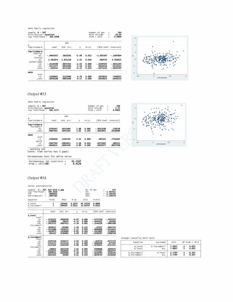
Output #53
Output #54
_cons .0038188 .0004166 9.17 0.000 .0030023 .0046353 L1. .5269845 .1122066 4.70 0.000 .3070635 .7469055 arch ARCH _cons -.024552 .0115167 -2.13 0.033 -.0471243 -.0019797 L2D. .0112477 .0052064 2.16 0.031 .0010434 .0214521 LD. -.0120399 .0045463 -2.65 0.008 -.0209505 -.0031293 palmerindex D1. 2.481874 1.031218 2.41 0.016 .460724 4.503025 lnchina D1. -.9465937 .3810291 -2.48 0.013 -1.693397 -.1997904 lndollar lnprice3mo~h lnprice3mo~h Coef. Std. Err. z P>|z| [95% Conf. Interval]D. OPG
Log likelihood = 305.6508 Prob > chi2 = 0.0000Distribution: Gaussian Wald chi2(4) = 30.05Sample: 4 - 267 Number of obs = 264
ARCH family regression
Iteration 10: log likelihood = 305.6508 Iteration 9: log likelihood = 305.6508 Iteration 8: log likelihood = 305.65065 Iteration 7: log likelihood = 305.64963 Iteration 6: log likelihood = 305.61292 Iteration 5: log likelihood = 305.11403 (switching optimization to BFGS)Iteration 4: log likelihood = 304.94717 Iteration 3: log likelihood = 304.60856 Iteration 2: log likelihood = 304.16566 Iteration 1: log likelihood = 303.5928 Iteration 0: log likelihood = 302.88927 (setting optimization to BHHH)
. arch d.lnprice3month d.lndollar d.lnchina dl(1/2).palmerindex,arch(1)
-4-2
02
46
se
4.5 5 5.5 6LnPrice3month
_cons .0026612 .0005426 4.90 0.000 .0015977 .0037246 L1. .2047762 .0905811 2.26 0.024 .0272405 .382312 garch L1. .5393028 .1193705 4.52 0.000 .305341 .7732647 arch ARCH _cons .0067463 .0041585 1.62 0.105 -.0014041 .0148968 D1. .0781047 .0415484 1.88 0.060 -.0033286 .159538 lncrudeoil lnprice3mo~h lnprice3mo~h Coef. Std. Err. z P>|z| [95% Conf. Interval]D. OPG
Log likelihood = 301.5173 Prob > chi2 = 0.0601Distribution: Gaussian Wald chi2(1) = 3.53Sample: 2 - 267 Number of obs = 266
ARCH family regression
Iteration 10: log likelihood = 301.51729 Iteration 9: log likelihood = 301.51727 Iteration 8: log likelihood = 301.51724 Iteration 7: log likelihood = 301.5171 Iteration 6: log likelihood = 301.50549 Iteration 5: log likelihood = 301.45187 (switching optimization to BFGS)Iteration 4: log likelihood = 301.4025 Iteration 3: log likelihood = 301.31019 Iteration 2: log likelihood = 301.05973 Iteration 1: log likelihood = 298.60018 Iteration 0: log likelihood = 283.68348 (setting optimization to BHHH)
. arch d.lnprice3month d.lncrudeoil, arch(1) garch(1)
-4-2
02
se
4.5 5 5.5 6LnPrice3month
Prob > chi2(40) = 0.4129 Portmanteau (Q) statistic = 41.3167 Portmanteau test for white noise
(note: time series has 5 gaps). wntestq se2
_cons .0035325 .00582 0.61 0.544 -.0078744 .0149395 L3D. .0979341 .0620489 1.58 0.114 -.0236794 .2195476 L2D. -.0318225 .0630094 -0.51 0.614 -.1553187 .0916737 LD. .180922 .0622539 2.91 0.004 .0589066 .3029373 lncrudeoil L3D. .0132102 .0195439 0.68 0.499 -.0250951 .0515155 L2D. .0353271 .0214126 1.65 0.099 -.0066408 .077295 LD. .0187256 .0196175 0.95 0.340 -.019724 .0571753 lnvol D_lncrudeoil _cons .001422 .0180885 0.08 0.937 -.0340307 .0368748 L3D. -.1643075 .1928469 -0.85 0.394 -.5422803 .2136654 L2D. -.4252666 .1958323 -2.17 0.030 -.8090908 -.0414423 LD. .3049517 .193484 1.58 0.115 -.07427 .6841734 lncrudeoil L3D. -.2053712 .0607421 -3.38 0.001 -.3244236 -.0863189 L2D. -.3139966 .06655 -4.72 0.000 -.4444322 -.183561 LD. -.5532231 .0609709 -9.07 0.000 -.6727239 -.4337223 lnvol D_lnvol Coef. Std. Err. z P>|z| [95% Conf. Interval] D_lncrudeoil 7 .094422 0.0512 13.85547 0.0313D_lnvol 7 .293462 0.2673 93.74259 0.0000 Equation Parms RMSE R-sq chi2 P>chi2
Det(Sigma_ml) = .0007265 SBIC = -1.249176FPE = .0008102 HQIC = -1.364761Log likelihood = 199.3626 AIC = -1.442511Sample: 5 - 267, but with a gap No. of obs = 257
Vector autoregression
. var d.lnvol d.lncrudeoil, lags(1/3)
D_lncrudeoil ALL 2.7797 3 0.427 D_lncrudeoil D.lnvol 2.7797 3 0.427 D_lnvol ALL 7.6657 3 0.053 D_lnvol D.lncrudeoil 7.6657 3 0.053 Equation Excluded chi2 df Prob > chi2 Granger causality Wald tests
. vargranger

DRAFT LIST OF MEMBERS AND OBSERVERS - Confidential
Output #55
(a)
(b)
Output #56
(a) 31/1/1990 - 31/12/2001
_cons .0001112 .0000893 1.25 0.213 -.0000639 .0002863 L1. .7537579 .0810172 9.30 0.000 .5949672 .9125487 garch L1. .2004418 .0647636 3.09 0.002 .0735075 .3273762 arch ARCH _cons .0074541 .0026226 2.84 0.004 .0023139 .0125943 D1. .071249 .0340167 2.09 0.036 .0045774 .1379206lnprice3mo~h lnsp500 D.lnsp500 Coef. Std. Err. z P>|z| [95% Conf. Interval] OPG
Log likelihood = 453.1115 Prob > chi2 = 0.0362Distribution: Gaussian Wald chi2(1) = 4.39Sample: 2 - 267, but with gaps Number of obs = 254
ARCH family regression
Iteration 10: log likelihood = 453.11146 Iteration 9: log likelihood = 453.11145 Iteration 8: log likelihood = 453.11134 Iteration 7: log likelihood = 453.10946 Iteration 6: log likelihood = 453.08654 Iteration 5: log likelihood = 452.86202 (switching optimization to BFGS)Iteration 4: log likelihood = 452.62465 Iteration 3: log likelihood = 451.85709 Iteration 2: log likelihood = 448.5652 Iteration 1: log likelihood = 445.32818 Iteration 0: log likelihood = 435.21784 (setting optimization to BHHH)
(note: conditioning reset at each gap)Number of gaps in sample: 6
. arch d.lnsp500 d.lnprice3month, arch(1) garch(1)
-4-2
02
4
se
5.5 6 6.5 7 7.5LnSp500
Prob > chi2(40) = 0.9981 Portmanteau (Q) statistic = 18.9113 Portmanteau test for white noise
(note: time series has 6 gaps). wntestq se2
_cons .0033653 .0003772 8.92 0.000 .002626 .0041047 L1. .7244462 .1355166 5.35 0.000 .4588385 .9900538 arch ARCH _cons .0087679 .003881 2.26 0.024 .0011613 .0163745 D1. .1425161 .0724144 1.97 0.049 .0005865 .2844458 lnsp500 lnprice3mo~h lnprice3mo~h Coef. Std. Err. z P>|z| [95% Conf. Interval]D. OPG
Log likelihood = 292.6283 Prob > chi2 = 0.0491Distribution: Gaussian Wald chi2(1) = 3.87Sample: 2 - 267, but with gaps Number of obs = 254
ARCH family regression
Iteration 10: log likelihood = 292.62832 Iteration 9: log likelihood = 292.62831 Iteration 8: log likelihood = 292.62803 Iteration 7: log likelihood = 292.62548 Iteration 6: log likelihood = 292.5422 Iteration 5: log likelihood = 292.07937 (switching optimization to BFGS)Iteration 4: log likelihood = 291.8634 Iteration 3: log likelihood = 291.63047 Iteration 2: log likelihood = 290.6925 Iteration 1: log likelihood = 289.13691 Iteration 0: log likelihood = 287.46966 (setting optimization to BHHH)
(note: conditioning reset at each gap)Number of gaps in sample: 6
. arch d.lnprice3month d.lnsp500, arch(1)
-4-2
02
se
4.5 5 5.5 6LnPrice3month
Prob > chi2(40) = 0.1605 Portmanteau (Q) statistic = 48.7928 Portmanteau test for white noise
(note: time series has 6 gaps). wntestq se2
_cons -.0033636 .0051984 -0.65 0.519 -.0136445 .0069174 D1. .1862305 .1210448 1.54 0.126 -.0531589 .4256199 lnsp500 lnprice3mo~h Coef. Std. Err. t P>|t| [95% Conf. Interval]D.
Total .488242034 136 .003590015 Root MSE = .05962 Adj R-squared = 0.0100 Residual .479828824 135 .003554288 R-squared = 0.0172 Model .008413209 1 .008413209 Prob > F = 0.1263 F( 1, 135) = 2.37 Source SS df MS Number of obs = 137
. reg d.lnprice3month d.lnsp500 if tin(1,144)
-.2
-.1
0.1
.2
Re
sid
ua
ls
4.5 5 5.5 6LnPrice3month
Prob > chi2 = 0.7058 chi2(2) = 0.70
against Ha: unrestricted heteroskedasticityWhite's test for Ho: homoskedasticity
. estat imtest,white
Prob > F = 0.9131 F(3, 132) = 0.18 Ho: model has no omitted variablesRamsey RESET test using powers of the fitted values of D.lnprice3month
. estat ovtest
Residuals 5.5116 0.0636 4.5047 0.1052 (n = 247) D-H P-value asy. P-value
. omninorm res

(b) 31/1/2002 - 31/2/2012
Output #57
_cons .0033653 .0003772 8.92 0.000 .002626 .0041047 L1. .7244462 .1355166 5.35 0.000 .4588385 .9900538 arch ARCH _cons .0087679 .003881 2.26 0.024 .0011613 .0163745 D1. .1425161 .0724144 1.97 0.049 .0005865 .2844458 lnsp500 lnprice3mo~h lnprice3mo~h Coef. Std. Err. z P>|z| [95% Conf. Interval]D. OPG
Log likelihood = 292.6283 Prob > chi2 = 0.0491Distribution: Gaussian Wald chi2(1) = 3.87Sample: 2 - 267, but with gaps Number of obs = 254
ARCH family regression
Iteration 10: log likelihood = 292.62832 Iteration 9: log likelihood = 292.62831 Iteration 8: log likelihood = 292.62803 Iteration 7: log likelihood = 292.62548 Iteration 6: log likelihood = 292.5422 Iteration 5: log likelihood = 292.07937 (switching optimization to BFGS)Iteration 4: log likelihood = 291.8634 Iteration 3: log likelihood = 291.63047 Iteration 2: log likelihood = 290.6925 Iteration 1: log likelihood = 289.13691 Iteration 0: log likelihood = 287.46966 (setting optimization to BHHH)
(note: conditioning reset at each gap)Number of gaps in sample: 6
. arch d.lnprice3month d.lnsp500, arch(1)
-4-2
02
se
4.5 5 5.5 6LnPrice3month
Prob > chi2(40) = 0.1605 Portmanteau (Q) statistic = 48.7928 Portmanteau test for white noise
Residuals 3.4578 0.1775 2.9826 0.2251 (n = 300) D-H P-value asy. P-value
. omninorm res
Prob > chi2(40) = 0.1970 Portmanteau (Q) statistic = 47.3759 Portmanteau test for white noise
Prob > F = 0.0150 F(3, 299) = 3.54 Ho: model has no omitted variablesRamsey RESET test using powers of the fitted values of D.lnspotprice
. estat ovtest
Total 27.59 19 0.0917 Kurtosis 3.57 1 0.0589 Skewness 4.53 4 0.3384 Heteroskedasticity 19.48 14 0.1473 Source chi2 df p
Cameron & Trivedi's decomposition of IM-test
Prob > chi2 = 0.1473 chi2(14) = 19.48
against Ha: unrestricted heteroskedasticityWhite's test for Ho: homoskedasticity
-.1
-.0
5
0
.05
.1
Re
sid
ua
ls
3 3.5 4 4.5LnSpotPrice

DRAFT LIST OF MEMBERS AND OBSERVERS - Confidential
Cocoa
Output #58
Output #59
_cons -.0115619 .0052151 -2.22 0.029 -.0218929 -.0012308 L2D. -.7651314 .3963509 -1.93 0.056 -1.5503 .0200367 LD. -.2687389 .3999099 -0.67 0.503 -1.060957 .5234796 lndollar L2D. .0004787 .0001613 2.97 0.004 .0001591 .0007982 LD. .0003926 .0001623 2.42 0.017 .0000712 .0007141convenienc~d L2D. -26.71155 7.007961 -3.81 0.000 -40.59427 -12.82883 LD. 25.34634 6.992639 3.62 0.000 11.49397 39.1987 lnoecd D.lnstocks Coef. Std. Err. t P>|t| [95% Conf. Interval]
Total .364525304 120 .003037711 Root MSE = .04834 Adj R-squared = 0.2308 Residual .26636632 114 .002336547 R-squared = 0.2693 Model .098158984 6 .016359831 Prob > F = 0.0000 F( 6, 114) = 7.00 Source SS df MS Number of obs = 121
. reg d.lnstocks dl(1/2).lnoecd dl(1/2).convenienceyield dl(1/2).lndollar
Total 46.13 34 0.0801 Kurtosis 1.77 1 0.1833 Skewness 12.27 6 0.0562 Heteroskedasticity 32.09 27 0.2287 Source chi2 df p
Cameron & Trivedi's decomposition of IM-test
Prob > chi2 = 0.2287 chi2(27) = 32.09
against Ha: unrestricted heteroskedasticityWhite's test for Ho: homoskedasticity
. estat imtest,white
Prob > F = 0.0938 F(3, 111) = 2.19 Ho: model has no omitted variablesRamsey RESET test using powers of the fitted values of D.lnstocks
. estat ovtest
Residuals 2.2367 0.3268 1.3632 0.5058 (n = 118) D-H P-value asy. P-value
. omninorm res
Prob > chi2(40) = 0.0337 Portmanteau (Q) statistic = 57.8422 Portmanteau test for white noise
(note: time series has 1 gap). wntestq res
Exogenous: _cons Endogenous: D.lnstocks D.lnoecd 4 1107.99 24.573* 4 0.000 3.8e-11* -18.3192* -18.1485* -17.8989* 3 1095.71 124.99 4 0.000 4.4e-11 -18.18 -18.0472 -17.853 2 1033.21 283.3 4 0.000 1.2e-10 -17.1969 -17.102 -16.9633 1 891.562 338.58 4 0.000 1.2e-09 -14.8834 -14.8265 -14.7433 0 722.274 1.9e-08 -12.1054 -12.0865 -12.0587 lag LL LR df p FPE AIC HQIC SBIC Sample: 6 - 124 Number of obs = 119 Selection-order criteria
. varsoc
D_lnoecd ALL 6.1412 4 0.189 D_lnoecd D.lnstocks 6.1412 4 0.189 D_lnstocks ALL 15.913 4 0.003 D_lnstocks D.lnoecd 15.913 4 0.003 Equation Excluded chi2 df Prob > chi2 Granger causality Wald tests
. vargranger
_cons .0000249 .0000132 1.89 0.059 -9.78e-07 .0000508 L4D. -.381368 .0863927 -4.41 0.000 -.5506945 -.2120414 L3D. 1.815831 .2302274 7.89 0.000 1.364594 2.267068 L2D. -3.419239 .2279817 -15.00 0.000 -3.866075 -2.972403 LD. 2.966666 .0836845 35.45 0.000 2.802647 3.130684 lnoecd L4D. .0003198 .0001911 1.67 0.094 -.0000546 .0006943 L3D. -.0003606 .0001972 -1.83 0.067 -.0007471 .0000258 L2D. .0000873 .0001967 0.44 0.657 -.0002981 .0004727 LD. -.0002288 .0001969 -1.16 0.245 -.0006148 .0001571 lnstocks D_lnoecd _cons -.0089326 .0061078 -1.46 0.144 -.0209036 .0030384 L4D. -13.90982 39.95672 -0.35 0.728 -92.22356 64.40392 L3D. -6.85452 106.4805 -0.06 0.949 -215.5524 201.8434 L2D. 20.62377 105.4419 0.20 0.845 -186.0385 227.286 LD. -2.207348 38.70418 -0.06 0.955 -78.06614 73.65144 lnoecd L4D. -.1423082 .0883669 -1.61 0.107 -.3155041 .0308878 L3D. .06184 .0911974 0.68 0.498 -.1169036 .2405835 L2D. -.1104736 .0909533 -1.21 0.225 -.2887389 .0677917 LD. .1463323 .0910652 1.61 0.108 -.0321521 .3248167 lnstocks D_lnstocks Coef. Std. Err. z P>|z| [95% Conf. Interval] D_lnoecd 9 .000112 0.9981 63179.78 0.0000D_lnstocks 9 .051615 0.1937 28.59675 0.0004 Equation Parms RMSE R-sq chi2 P>chi2
Det(Sigma_ml) = 2.80e-11 SBIC = -17.89886FPE = 3.80e-11 HQIC = -18.14854Log likelihood = 1107.994 AIC = -18.31924Sample: 6 - 124 No. of obs = 119
Vector autoregression
. var d.lnstocks d.lnoecd, lags(1/4)

Output #60
Output #61
D_lnconv100 ALL 13.54 5 0.019 D_lnconv100 D.lnstocks 13.54 5 0.019 D_lnstocks ALL 42.237 5 0.000 D_lnstocks D.lnconv100 42.237 5 0.000 Equation Excluded chi2 df Prob > chi2 Granger causality Wald tests
. vargranger
Exogenous: _cons Endogenous: D.lnstocks D.lnconv100 5 226.367 10.546* 4 0.032 .000107* -3.46385* -3.2541 -2.94728 4 221.094 9.2052 4 0.056 .00011 -3.44227 -3.27066 -3.01962 3 216.491 15.78 4 0.003 .000111 -3.43205 -3.29858* -3.10333 2 208.601 18.08 4 0.001 .000118 -3.36612 -3.27078 -3.13132 1 199.561 23.376 4 0.000 .000129 -3.28069 -3.22349 -3.13981* 0 187.873 .000147 -3.15039 -3.13132 -3.10343 lag LL LR df p FPE AIC HQIC SBIC Sample: 7 - 124 Number of obs = 118 Selection-order criteria
. varsoc
_cons -.0177321 .0187825 -0.94 0.345 -.0545452 .019081 L5D. -.0150828 .0960265 -0.16 0.875 -.2032912 .1731256 L4D. -.2649406 .1029035 -2.57 0.010 -.4666278 -.0632535 L3D. -.3491295 .0983568 -3.55 0.000 -.5419053 -.1563537 L2D. -.1381468 .0934045 -1.48 0.139 -.3212163 .0449227 LD. -.238503 .0891556 -2.68 0.007 -.4132448 -.0637612 lnconv100 L5D. -.9931503 .3634421 -2.73 0.006 -1.705484 -.2808169 L4D. .1701778 .3720504 0.46 0.647 -.5590276 .8993833 L3D. -.3888243 .3773409 -1.03 0.303 -1.128399 .3507502 L2D. .625776 .3827124 1.64 0.102 -.1243266 1.375879 LD. -.7343964 .3862121 -1.90 0.057 -1.491358 .0225654 lnstocks D_lnconv100 _cons -.0088269 .0044506 -1.98 0.047 -.0175499 -.000104 L5D. -.0218589 .0227538 -0.96 0.337 -.0664555 .0227376 L4D. .024404 .0243833 1.00 0.317 -.0233864 .0721944 L3D. .0467034 .0233059 2.00 0.045 .0010246 .0923822 L2D. .1058564 .0221325 4.78 0.000 .0624775 .1492353 LD. .0852532 .0211257 4.04 0.000 .0438476 .1266588 lnconv100 L5D. -.1222133 .0861187 -1.42 0.156 -.2910029 .0465762 L4D. -.0246997 .0881585 -0.28 0.779 -.1974872 .1480877 L3D. .2288172 .0894121 2.56 0.010 .0535728 .4040616 L2D. .0876845 .0906849 0.97 0.334 -.0900546 .2654236 LD. .1191221 .0915141 1.30 0.193 -.0602423 .2984865 lnstocks D_lnstocks Coef. Std. Err. z P>|z| [95% Conf. Interval] D_lnconv100 11 .200269 0.2608 41.63903 0.0000D_lnstocks 11 .047454 0.3268 57.28993 0.0000 Equation Parms RMSE R-sq chi2 P>chi2
Det(Sigma_ml) = .0000739 SBIC = -2.947279FPE = .0001074 HQIC = -3.254105Log likelihood = 226.367 AIC = -3.463847Sample: 7 - 124 No. of obs = 118
Vector autoregression
. var d.lnstocks d.lnconv100, lags(1/5)
D_dividendyield ALL 5.5033 3 0.138 D_dividendyield D.lnstocks 5.5033 3 0.138 D_lnstocks ALL 25.422 3 0.000 D_lnstocks D.dividendyield 25.422 3 0.000 Equation Excluded chi2 df Prob > chi2 Granger causality Wald tests
. vargranger
_cons -.0925152 .1686846 -0.55 0.583 -.4231309 .2381006 L3D. -.1860217 .0952118 -1.95 0.051 -.3726335 .0005901 L2D. -.1699064 .0993353 -1.71 0.087 -.3646001 .0247872 LD. -.3870866 .0897555 -4.31 0.000 -.563004 -.2111691dividendyi~d L3D. -3.417981 3.18248 -1.07 0.283 -9.655527 2.819564 L2D. -1.025197 3.254285 -0.32 0.753 -7.403479 5.353084 LD. -5.520695 3.255658 -1.70 0.090 -11.90167 .8602774 lnstocks D_dividend~d _cons -.0070619 .0046133 -1.53 0.126 -.0161039 .00198 L3D. .0056773 .0026039 2.18 0.029 .0005737 .0107809 L2D. .0117103 .0027167 4.31 0.000 .0063857 .017035 LD. .0093046 .0024547 3.79 0.000 .0044934 .0141157dividendyi~d L3D. .1693345 .0870372 1.95 0.052 -.0012553 .3399244 L2D. .0586943 .089001 0.66 0.510 -.1157445 .2331332 LD. .1630825 .0890386 1.83 0.067 -.0114299 .3375949 lnstocks D_lnstocks Coef. Std. Err. z P>|z| [95% Conf. Interval] D_dividendyield 7 1.82175 0.1802 26.37582 0.0002D_lnstocks 7 .049823 0.2306 35.96702 0.0000 Equation Parms RMSE R-sq chi2 P>chi2
Det(Sigma_ml) = .007304 SBIC = 1.314957FPE = .0092259 HQIC = 1.121817Log likelihood = -45.38496 AIC = .9897493Sample: 5 - 124 No. of obs = 120
Vector autoregression
. var d.lnstocks d.dividendyield, lags(1/3)

DRAFT LIST OF MEMBERS AND OBSERVERS - Confidential
Output #62
_cons -.0023319 .0011477 -2.03 0.042 -.0045813 -.0000826 L4D. .1113992 .0923517 1.21 0.228 -.0696068 .2924053 L3D. .0073958 .099898 0.07 0.941 -.1884007 .2031924 L2D. -.2185481 .0995293 -2.20 0.028 -.4136219 -.0234743 LD. .4009914 .0916225 4.38 0.000 .2214146 .5805681 lndollar L4D. -.0039761 .0195441 -0.20 0.839 -.0422819 .0343297 L3D. -.001333 .0204842 -0.07 0.948 -.0414812 .0388152 L2D. -.0306887 .020339 -1.51 0.131 -.0705524 .009175 LD. -.019167 .0197849 -0.97 0.333 -.0579448 .0196107 lnstocks D_lndollar _cons -.009615 .0050111 -1.92 0.055 -.0194365 .0002065 L4D. 1.390764 .4032426 3.45 0.001 .6004228 2.181105 L3D. -.1311532 .4361926 -0.30 0.764 -.986075 .7237686 L2D. -.4073755 .4345824 -0.94 0.349 -1.259141 .4443903 LD. -.7225591 .4000583 -1.81 0.071 -1.506659 .0615407 lndollar L4D. -.1909898 .085337 -2.24 0.025 -.3582474 -.0237323 L3D. .1348701 .0894416 1.51 0.132 -.0404322 .3101725 L2D. .0143291 .0888077 0.16 0.872 -.1597307 .1883889 LD. .2210972 .0863886 2.56 0.010 .0517788 .3904157 lnstocks D_lnstocks Coef. Std. Err. z P>|z| [95% Conf. Interval] D_lndollar 9 .011592 0.2034 30.38714 0.0002D_lnstocks 9 .050614 0.2247 34.4953 0.0000 Equation Parms RMSE R-sq chi2 P>chi2
Det(Sigma_ml) = 2.93e-07 SBIC = -8.643937FPE = 3.97e-07 HQIC = -8.893609Log likelihood = 557.3263 AIC = -9.064308Sample: 6 - 124 No. of obs = 119
Vector autoregression
. var d.lnstocks d.lndollar, lags(1/4)
D_lndollar ALL 4.5608 4 0.335 D_lndollar D.lnstocks 4.5608 4 0.335 D_lnstocks ALL 21.305 4 0.000 D_lnstocks D.lndollar 21.305 4 0.000 Equation Excluded chi2 df Prob > chi2 Granger causality Wald tests
. vargranger
5 553.579 1.9411 4 0.747 4.2e-07 -9.00981 -8.80006 -8.49324 4 552.608 15.616* 4 0.004 4.0e-07* -9.06115* -8.88955 -8.63851 3 544.8 1.7877 4 0.775 4.2e-07 -8.99661 -8.86313 -8.66788 2 543.906 10.752 4 0.029 4.0e-07 -9.04925 -8.95392 -8.81445 1 538.53 29.142 4 0.000 4.1e-07 -9.02593 -8.96873* -8.88505* 0 523.959 4.9e-07 -8.84676 -8.82769 -8.7998 lag LL LR df p FPE AIC HQIC SBIC Sample: 7 - 124 Number of obs = 118 Selection-order criteria
. varsoc

Output #63
(a)
(b)
D_lnvol ALL 16.259 3 0.001 D_lnvol D.lnindex 16.259 3 0.001 D_lnindex ALL .43589 3 0.933 D_lnindex D.lnvol .43589 3 0.933 Equation Excluded chi2 df Prob > chi2 Granger causality Wald tests
. vargranger
_cons .0030159 .0104727 0.29 0.773 -.0175102 .023542 L3D. .0218923 .0567351 0.39 0.700 -.0893064 .133091 L2D. -.0574218 .0553379 -1.04 0.299 -.165882 .0510385 LD. .0632297 .0553935 1.14 0.254 -.0453395 .171799 lnvol L3D. -.6408383 .1644884 -3.90 0.000 -.9632297 -.3184469 L2D. .2590291 .1647432 1.57 0.116 -.0638617 .5819199 LD. -.1814907 .1641532 -1.11 0.269 -.503225 .1402437 lnindex D_lnvol _cons .0043558 .0036238 1.20 0.229 -.0027467 .0114584 L3D. -.0102594 .0196318 -0.52 0.601 -.048737 .0282183 L2D. -.0025157 .0191483 -0.13 0.895 -.0400458 .0350144 LD. .0067352 .0191676 0.35 0.725 -.0308326 .0443029 lnvol L3D. -.088694 .0569173 -1.56 0.119 -.2002498 .0228618 L2D. -.1208887 .0570054 -2.12 0.034 -.2326173 -.0091601 LD. .1495828 .0568013 2.63 0.008 .0382544 .2609113 lnindex D_lnindex Coef. Std. Err. z P>|z| [95% Conf. Interval] D_lnvol 7 .184901 0.0549 17.89589 0.0065D_lnindex 7 .06398 0.0475 15.35966 0.0176 Equation Parms RMSE R-sq chi2 P>chi2
Det(Sigma_ml) = .0001336 SBIC = -2.984211FPE = .0001464 HQIC = -3.085967Log likelihood = 499.6791 AIC = -3.153761Sample: 5 - 312 No. of obs = 308
Vector autoregression
. var d.lnindex d.lnvol, lags(1/3)
D_lnvol ALL 13.672 3 0.003 D_lnvol D.LnCommercial 13.672 3 0.003 D_LnCommercial ALL 3.4145 3 0.332 D_LnCommercial D.lnvol 3.4145 3 0.332 Equation Excluded chi2 df Prob > chi2 Granger causality Wald tests
. vargranger
_cons .0006926 .0104582 0.07 0.947 -.0198051 .0211902 L3D. .019339 .05717 0.34 0.735 -.0927121 .1313902 L2D. -.0453552 .0564636 -0.80 0.422 -.1560219 .0653115 LD. .0385717 .0563523 0.68 0.494 -.0718768 .1490202 lnvol L3D. -.5446018 .2779408 -1.96 0.050 -1.089356 .0001521 L2D. .2970789 .2816743 1.05 0.292 -.2549925 .8491503 LD. .6854761 .2748706 2.49 0.013 .1467395 1.224213LnCommercial D_lnvol _cons 1.34e-06 .0021601 0.00 1.000 -.0042324 .0042351 L3D. -.0100222 .0118084 -0.85 0.396 -.0331663 .0131219 L2D. .0032118 .0116625 0.28 0.783 -.0196463 .02607 LD. .0180621 .0116395 1.55 0.121 -.004751 .0408751 lnvol L3D. -.0728936 .0574085 -1.27 0.204 -.1854122 .0396251 L2D. -.1555313 .0581797 -2.67 0.008 -.2695614 -.0415012 LD. .2330083 .0567744 4.10 0.000 .1217325 .3442841LnCommercial D_LnCommer~l Coef. Std. Err. z P>|z| [95% Conf. Interval] D_lnvol 7 .185642 0.0473 15.29671 0.0181D_LnCommercial 7 .038344 0.0852 28.69267 0.0001 Equation Parms RMSE R-sq chi2 P>chi2
Det(Sigma_ml) = .0000484 SBIC = -4.000301FPE = .000053 HQIC = -4.102057Log likelihood = 656.157 AIC = -4.169851Sample: 5 - 312 No. of obs = 308
Vector autoregression
. var d.LnCommercial d.lnvol, lags(1/3)

DRAFT LIST OF MEMBERS AND OBSERVERS - Confidential
Output #64
(a) 1/2/1990 - 31/12/2001
(b) 1/1/2002 - 31/3/2012
_cons .0002574 .0072319 0.04 0.972 -.0140462 .0145609 D1. .0154551 .1677976 0.09 0.927 -.3164194 .3473296 lnsp500 D.lnspot Coef. Std. Err. t P>|t| [95% Conf. Interval]
Total .91529736 135 .00677998 Root MSE = .08264 Adj R-squared = -0.0074 Residual .915239417 134 .006830145 R-squared = 0.0001 Model .000057943 1 .000057943 Prob > F = 0.9268 F( 1, 134) = 0.01 Source SS df MS Number of obs = 136
. reg d.lnspot d.lnsp500 if tin(1,143)
-.2
-.1
0.1
.2
Re
sid
ua
ls
6 6.5 7 7.5 8LnSpot
Residuals 0.8341 0.6590 0.3048 0.8586 (n = 251) D-H P-value asy. P-value
. omninorm res
Prob > F = 0.3400 F(3, 131) = 1.13 Ho: model has no omitted variablesRamsey RESET test using powers of the fitted values of D.lnspot
. estat ovtest
Prob > chi2 = 0.6573 chi2(2) = 0.84
against Ha: unrestricted heteroskedasticityWhite's test for Ho: homoskedasticity
. estat imtest,white
_cons .001204 .0080923 0.15 0.882 -.0148253 .0172333 D1. -.3073464 .1761205 -1.75 0.084 -.6562073 .0415145 lnsp500 D.lnspot Coef. Std. Err. t P>|t| [95% Conf. Interval]
Total .90123957 116 .007769307 Root MSE = .08738 Adj R-squared = 0.0173 Residual .877989327 115 .00763469 R-squared = 0.0258 Model .023250243 1 .023250243 Prob > F = 0.0836 F( 1, 115) = 3.05 Source SS df MS Number of obs = 117
. reg d.lnspot d.lnsp500 if tin(144,266)
-.2
-.1
0.1
.2
Re
sid
ua
ls
6 6.5 7 7.5 8LnSpot
Residuals 0.6897 0.7083 0.7078 0.7019 (n = 251) D-H P-value asy. P-value
. omninorm res2
Prob > F = 0.0077 F(3, 112) = 4.17 Ho: model has no omitted variablesRamsey RESET test using powers of the fitted values of D.lnspot
. estat ovtest

Output #65
Output #66
(a)
D_soi ALL .51086 2 0.775 D_soi D.lnspot .51086 2 0.775 D_lnspot ALL 6.9092 2 0.032 D_lnspot D.soi 6.9092 2 0.032 Equation Excluded chi2 df Prob > chi2 Granger causality Wald tests
. vargranger
_cons .1753696 .7223941 0.24 0.808 -1.240497 1.591236 L2D. -.3640753 .085443 -4.26 0.000 -.5315406 -.19661 LD. -.7373996 .0854538 -8.63 0.000 -.904886 -.5699131 soi L2D. -.4512998 8.18196 -0.06 0.956 -16.48765 15.58505 LD. 5.610363 8.016867 0.70 0.484 -10.10241 21.32313 lnspot D_soi _cons .0054339 .0080898 0.67 0.502 -.0104218 .0212896 L2D. .0021004 .0009568 2.20 0.028 .0002251 .0039758 LD. .0022816 .000957 2.38 0.017 .000406 .0041572 soi L2D. -.0138183 .0916264 -0.15 0.880 -.1934027 .1657661 LD. -.137119 .0897776 -1.53 0.127 -.3130798 .0388418 lnspot D_lnspot Coef. Std. Err. z P>|z| [95% Conf. Interval] D_soi 5 8.06989 0.3946 78.86541 0.0000D_lnspot 5 .090371 0.0761 9.968621 0.0410 Equation Parms RMSE R-sq chi2 P>chi2
Det(Sigma_ml) = .4864945 SBIC = 5.351571FPE = .5739883 HQIC = 5.214355Log likelihood = -299.7911 AIC = 5.120514Sample: 4 - 124 No. of obs = 121
Vector autoregression
. var d.lnspot d.soi, lags(1/2)
Exogenous: _cons Endogenous: D.lnspot D.soi 5 -285.734 4.662 4 0.324 .632022 5.21584 5.42558 5.73241 4 -288.065 1.8561 4 0.762 .614092 5.18755 5.35916 5.6102 3 -288.993 4.0885 4 0.394 .582753 5.13548 5.26895 5.46421 2 -291.038 21.962* 4 0.000 .563652* 5.10233* 5.19767* 5.33714* 1 -302.019 47.101 4 0.000 .6344 5.22066 5.27786 5.36154 0 -325.569 .88362 5.55202 5.57109 5.59899 lag LL LR df p FPE AIC HQIC SBIC Sample: 7 - 124 Number of obs = 118 Selection-order criteria
. varsoc
_cons .0047352 .0071269 0.66 0.509 -.0094826 .018953 D1. .1519512 .0812379 1.87 0.066 -.0101141 .3140165lncommerci~b D.lncocoawb Coef. Std. Err. t P>|t| [95% Conf. Interval]
Total .261450085 70 .003735001 Root MSE = .06005 Adj R-squared = 0.0345 Residual .24883327 69 .003606279 R-squared = 0.0483 Model .012616815 1 .012616815 Prob > F = 0.0657 F( 1, 69) = 3.50 Source SS df MS Number of obs = 71
. reg d.lncocoawb d.lncommercialwb
-.2
-.1
0.1
.2
Re
sid
ua
ls
5 5.2 5.4 5.6 5.8LnCocoaWB
Residuals 4.5021 0.1053 2.7918 0.2476 (n = 71) D-H P-value asy. P-value
. omninorm res
Prob > F = 0.1261 F(3, 66) = 1.98 Ho: model has no omitted variablesRamsey RESET test using powers of the fitted values of D.lncocoawb
. estat ovtest
Total 3.91 4 0.4179 Kurtosis 1.55 1 0.2125 Skewness 2.17 1 0.1407 Heteroskedasticity 0.19 2 0.9104 Source chi2 df p
Cameron & Trivedi's decomposition of IM-test
. estat imtest
Prob > chi2(33) = 0.5662 Portmanteau (Q) statistic = 31.0156 Portmanteau test for white noise
. wntestq res

DRAFT LIST OF MEMBERS AND OBSERVERS - Confidential
(b)
Coffee
Output #67
_cons .0036892 .0072702 0.51 0.613 -.0108144 .0181929 D1. .05762 .0462263 1.25 0.217 -.034599 .149839 lnindexwb D.lncocoawb Coef. Std. Err. t P>|t| [95% Conf. Interval]
Total .261450085 70 .003735001 Root MSE = .06087 Adj R-squared = 0.0078 Residual .255692544 69 .003705689 R-squared = 0.0220 Model .005757541 1 .005757541 Prob > F = 0.2168 F( 1, 69) = 1.55 Source SS df MS Number of obs = 71
. reg d.lncocoawb d.lnindexwb
_cons -.0028993 .0066279 -0.44 0.662 -.0159569 .0101583 D1. 4.15593 2.432871 1.71 0.089 -.6370939 8.948955 lnoecd lnwbarabica Coef. Std. Err. t P>|t| [95% Conf. Interval]D.
Total 1.37740551 236 .005836464 Root MSE = .07609 Adj R-squared = 0.0081 Residual 1.36051151 235 .005789411 R-squared = 0.0123 Model .016894004 1 .016894004 Prob > F = 0.0889 F( 1, 235) = 2.92 Source SS df MS Number of obs = 237
. reg d.lnwbarabica d.lnoecd
Residuals 1.1869 0.5524 1.3659 0.5051 (n = 234) D-H P-value asy. P-value
. omninorm res
-.2
-.1
0.1
.2
Re
sid
ua
ls
4.5 5 5.5 6 6.5LnWBarabica
Total 6.43 4 0.1692 Kurtosis 1.37 1 0.2413 Skewness 3.44 1 0.0637 Heteroskedasticity 1.62 2 0.4450 Source chi2 df p
Cameron & Trivedi's decomposition of IM-test
Prob > chi2 = 0.4450 chi2(2) = 1.62
against Ha: unrestricted heteroskedasticityWhite's test for Ho: homoskedasticity
. estat imtest, white
Prob > F = 0.6534 F(3, 232) = 0.54 Ho: model has no omitted variablesRamsey RESET test using powers of the fitted values of D.lnwbarabica
. estat ovtest
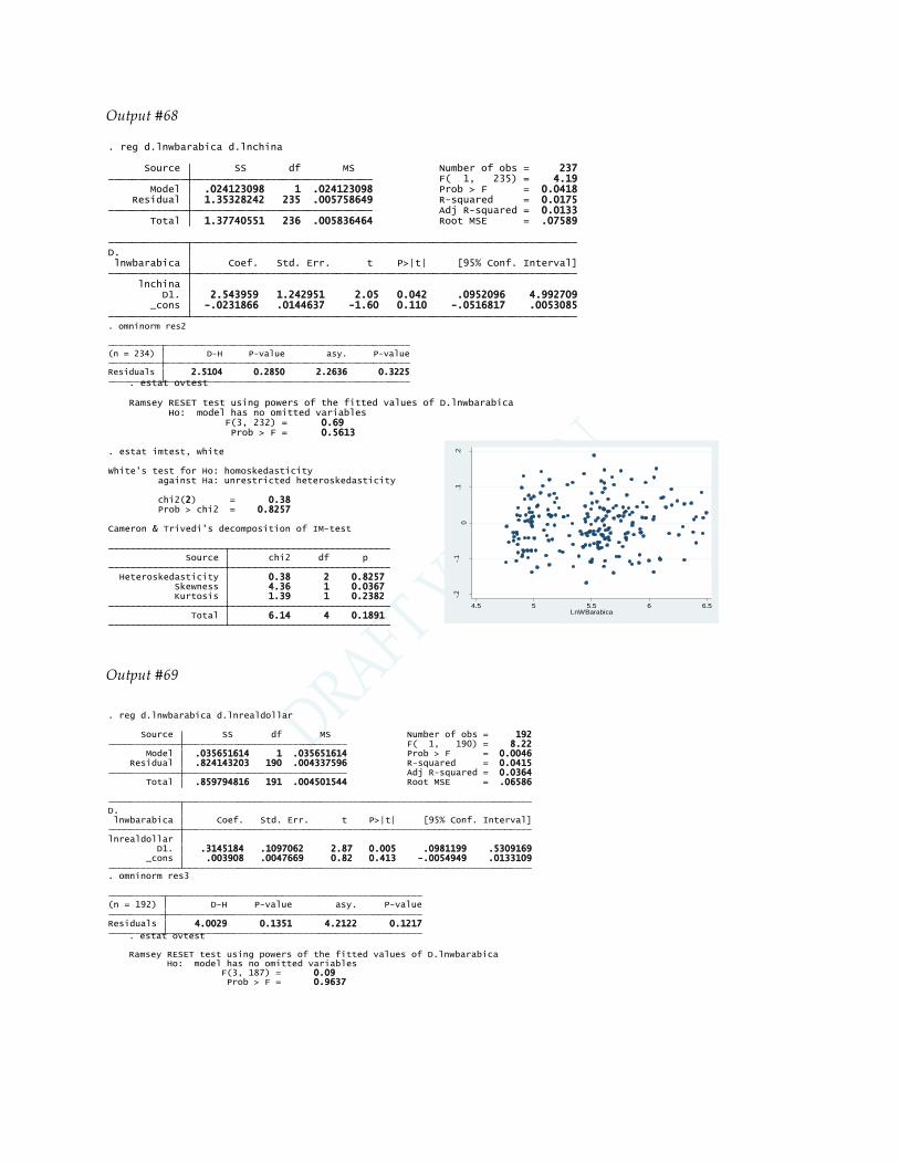
Output #68
Output #69
_cons -.0231866 .0144637 -1.60 0.110 -.0516817 .0053085 D1. 2.543959 1.242951 2.05 0.042 .0952096 4.992709 lnchina lnwbarabica Coef. Std. Err. t P>|t| [95% Conf. Interval]D.
Total 1.37740551 236 .005836464 Root MSE = .07589 Adj R-squared = 0.0133 Residual 1.35328242 235 .005758649 R-squared = 0.0175 Model .024123098 1 .024123098 Prob > F = 0.0418 F( 1, 235) = 4.19 Source SS df MS Number of obs = 237
. reg d.lnwbarabica d.lnchina
Residuals 2.5104 0.2850 2.2636 0.3225 (n = 234) D-H P-value asy. P-value
. omninorm res2
Prob > F = 0.5613 F(3, 232) = 0.69 Ho: model has no omitted variablesRamsey RESET test using powers of the fitted values of D.lnwbarabica
. estat ovtest
Total 6.14 4 0.1891 Kurtosis 1.39 1 0.2382 Skewness 4.36 1 0.0367 Heteroskedasticity 0.38 2 0.8257 Source chi2 df p
Cameron & Trivedi's decomposition of IM-test
Prob > chi2 = 0.8257 chi2(2) = 0.38
against Ha: unrestricted heteroskedasticityWhite's test for Ho: homoskedasticity
. estat imtest, white-.
2-.
10
.1.2
Re
sid
ua
ls
4.5 5 5.5 6 6.5LnWBarabica
_cons .003908 .0047669 0.82 0.413 -.0054949 .0133109 D1. .3145184 .1097062 2.87 0.005 .0981199 .5309169lnrealdollar lnwbarabica Coef. Std. Err. t P>|t| [95% Conf. Interval]D.
Total .859794816 191 .004501544 Root MSE = .06586 Adj R-squared = 0.0364 Residual .824143203 190 .004337596 R-squared = 0.0415 Model .035651614 1 .035651614 Prob > F = 0.0046 F( 1, 190) = 8.22 Source SS df MS Number of obs = 192
. reg d.lnwbarabica d.lnrealdollar
Residuals 4.0029 0.1351 4.2122 0.1217 (n = 192) D-H P-value asy. P-value
. omninorm res3
Prob > F = 0.9637 F(3, 187) = 0.09 Ho: model has no omitted variablesRamsey RESET test using powers of the fitted values of D.lnwbarabica
. estat ovtest

DRAFT LIST OF MEMBERS AND OBSERVERS - Confidential
Output #70
(a) 31/1/1992 - 31/1/2001
Total 2.94 4 0.5687 Kurtosis 0.93 1 0.3353 Skewness 1.32 1 0.2507 Heteroskedasticity 0.69 2 0.7091 Source chi2 df p
Cameron & Trivedi's decomposition of IM-test
Prob > chi2 = 0.7091 chi2(2) = 0.69
against Ha: unrestricted heteroskedasticityWhite's test for Ho: homoskedasticity
. estat imtest,white
-.2
-.1
0.1
.2
Re
sid
ua
ls
4.5 5 5.5 6 6.5LnWBarabica
_cons -.0012078 .0097962 -0.12 0.902 -.0206432 .0182276 D1. -.0402378 .2503991 -0.16 0.873 -.5370225 .4565469 lnsp500 lnwbarabica Coef. Std. Err. t P>|t| [95% Conf. Interval]D.
Total .919122679 101 .009100225 Root MSE = .09586 Adj R-squared = -0.0097 Residual .918885397 100 .009188854 R-squared = 0.0003 Model .000237282 1 .000237282 Prob > F = 0.8727 F( 1, 100) = 0.03 Source SS df MS Number of obs = 102
. reg d.lnwbarabica d.lnsp500 if tin(1,109)
Residuals 0.9607 0.6186 1.0247 0.5991 (n = 224) D-H P-value asy. P-value
. omninorm res
Total 4.74 4 0.3149 Kurtosis 1.39 1 0.2392 Skewness 3.33 1 0.0682 Heteroskedasticity 0.03 2 0.9850 Source chi2 df p
Cameron & Trivedi's decomposition of IM-test
Prob > chi2 = 0.9850 chi2(2) = 0.03
against Ha: unrestricted heteroskedasticityWhite's test for Ho: homoskedasticity
. estat imtest, white
Prob > F = 0.6692 F(3, 97) = 0.52 Ho: model has no omitted variablesRamsey RESET test using powers of the fitted values of D.lnwbarabica
. estat ovtest
-.2
-.1
0.1
.2
Re
sid
ua
ls
4.5 5 5.5 6 6.5LnWBarabica

(b) 31/1/2002 - 31/3/2012
Output #71
(a)
_cons .0084737 .0048723 1.74 0.084 -.0011699 .0181174 D1. .2549912 .102993 2.48 0.015 .0511391 .4588433 lnsp500 lnwbarabica Coef. Std. Err. t P>|t| [95% Conf. Interval]D.
Total .389156924 125 .003113255 Root MSE = .05469 Adj R-squared = 0.0394 Residual .370826047 124 .002990533 R-squared = 0.0471 Model .018330877 1 .018330877 Prob > F = 0.0146 F( 1, 124) = 6.13 Source SS df MS Number of obs = 126
. reg d.lnwbarabica d.lnsp500 if tin(109,243)
-.2
-.1
0.1
.2
Re
sid
ua
ls
4.5 5 5.5 6 6.5LnWBarabica
Total 1.85 4 0.7642 Kurtosis 0.00 1 0.9967 Skewness 1.50 1 0.2208 Heteroskedasticity 0.35 2 0.8412 Source chi2 df p
Cameron & Trivedi's decomposition of IM-test
Prob > chi2 = 0.8412 chi2(2) = 0.35
against Ha: unrestricted heteroskedasticityWhite's test for Ho: homoskedasticity
. estat imtest,white
Prob > F = 0.8002 F(3, 121) = 0.33 Ho: model has no omitted variablesRamsey RESET test using powers of the fitted values of D.lnwbarabica
. estat ovtest
Residuals 0.2879 0.8659 0.4333 0.8052 (n = 224) D-H P-value asy. P-value
. omninorm res2
_cons .0003079 .0001713 1.80 0.072 -.0000279 .0006438 L1. .7326351 .1131361 6.48 0.000 .5108924 .9543777 garch L1. .1279673 .0536113 2.39 0.017 .0228912 .2330435 arch ARCH _cons -.0003812 .0025516 -0.15 0.881 -.0053822 .0046199 D1. .2305037 .0895733 2.57 0.010 .0549432 .4060641 lnindex lnspotprice lnspotprice Coef. Std. Err. z P>|z| [95% Conf. Interval]D. OPG
Log likelihood = 527.9429 Prob > chi2 = 0.0101Distribution: Gaussian Wald chi2(1) = 6.62Sample: 2 - 313 Number of obs = 312
ARCH family regression
Iteration 13: log likelihood = 527.94291 Iteration 12: log likelihood = 527.9429 Iteration 11: log likelihood = 527.94274 Iteration 10: log likelihood = 527.935 Iteration 9: log likelihood = 527.9054 Iteration 8: log likelihood = 527.83524 Iteration 7: log likelihood = 527.75564 Iteration 6: log likelihood = 527.41263 Iteration 5: log likelihood = 522.188 (switching optimization to BFGS)Iteration 4: log likelihood = 521.59389 Iteration 3: log likelihood = 521.18405 Iteration 2: log likelihood = 520.57595 Iteration 1: log likelihood = 520.32535 Iteration 0: log likelihood = 519.59673 (setting optimization to BHHH)
. arch d.lnspotprice d.lnindex, arch(1) garch(1)
-6-4
-20
24
se
7 7.2 7.4 7.6 7.8 8LnSpotPrice

DRAFT LIST OF MEMBERS AND OBSERVERS - Confidential
(b)
_cons .0002487 .000121 2.05 0.040 .0000115 .0004859 L1. .7346519 .0866752 8.48 0.000 .5647717 .9045321 garch L1. .1624529 .0611954 2.65 0.008 .0425121 .2823936 arch ARCH _cons .0002191 .0024039 0.09 0.927 -.0044924 .0049306 D1. .1478921 .0446578 3.31 0.001 .0603644 .2354198lncommercial lnspotprice lnspotprice Coef. Std. Err. z P>|z| [95% Conf. Interval]D. OPG
Log likelihood = 528.4876 Prob > chi2 = 0.0009Distribution: Gaussian Wald chi2(1) = 10.97Sample: 2 - 313 Number of obs = 312
ARCH family regression
Iteration 15: log likelihood = 528.48759 (switching optimization to BHHH)Iteration 14: log likelihood = 528.48758 Iteration 13: log likelihood = 528.48736 Iteration 12: log likelihood = 528.48248 Iteration 11: log likelihood = 528.42999 Iteration 10: log likelihood = 528.14374 Iteration 9: log likelihood = 527.02662 Iteration 8: log likelihood = 526.53207 Iteration 7: log likelihood = 524.71949 Iteration 6: log likelihood = 523.24567 Iteration 5: log likelihood = 519.93107 (switching optimization to BFGS)Iteration 4: log likelihood = 519.22741 Iteration 3: log likelihood = 518.58064 Iteration 2: log likelihood = 518.26525 Iteration 1: log likelihood = 517.69328 Iteration 0: log likelihood = 516.8969 (setting optimization to BHHH)
. arch d.lnspotprice d.lncommercial, arch(1) garch(1)
-6-4
-20
24
se
7 7.2 7.4 7.6 7.8 8LnSpotPrice

Task Force Participants
A Member is any individual that participated in the activities of the Task Force Group in their personal capacity as experts in the topic covered by the activities of the Group. He/she may represent a commercial company, an association, a consumer group, a non-governmental organisation, or any other entity representing a commercial or non/commercial interest in the topics discussed by the Task Force. Members contributed to the Task Force meetings and provided input to the discussions through presentations and relevant material for the Final Report. Members contributed to the expenses of the Task Force through a general fee paid by their respective company or body (a discounted fee was offered to CEPS and ECMI members). The findings of the Final Report, independently drafted by ECMI and CEPS researchers, do not necessarily reflect the views expressed by the members or their respective companies. The companies and other bodies involved do not necessarily endorse the conclusions of the Final Report.
Rapporteurs are ECMI-CEPS researchers who organised the Task Force, conducted the relevant research for the meetings and coordinated the preliminary work leading to the Final Report.
The Chair is an internationally recognised expert appointed by ECMI-CEPS to steer the dialogue during the meetings and ensure that all interests around the table were sufficiently heard. The Chair also advised on the general conduct of the Task Force activities. The Chair was not involved in the drafting of the Final Report and cannot be identified in any way with the authorship of the Final Report.
Observers are academics or individuals/officials representing a governmental authority, European institution, or any other international public body. Observers have regularly followed the work of the Task Force, attended at least one of the Task Force meetings, or contributed to the discussion typically through a presentation or other material/information. The category also includes a short list of Members that have expressed an official dissenting view about the process of the Task Force and the conclusions of the Final Report, as well as individuals representing commercial entities that have provided 'external expertise' to the Task Force upon invitation.
Chair
Ann Berg
Independent Consultant to International Organisations Former Board Director, Chicago Board of Trade
Rapporteurs
Diego Valiante (author)
ECMI Head of Research - CEPS Research Fellow
CEPS
Christian Egenhofer
Associate Senior Fellow, Climate Change, Energy
CEPS

DRAFT LIST OF MEMBERS AND OBSERVERS - Confidential
Members of the Task Force
Simona Amati
Director
Kreab Gavin Anderson
Simon Andrews
Senior Manager, PwC
Former: Senior Regulatory Affairs Director at the Futures and Options Association
Chris Bird
Cargill Grain & Oilseed Supply Chain Europe
Mark Bradley
Deputy Head of Market Surveillance
London Metal Exchange
Don Casturo
Managing Director
Goldman Sachs
Roger Cogan
Senior Policy Director
International Swaps and Derivatives Association
Jennifer Cosco
Executive Director
Goldman Sachs International
Jeremy Elliott
Commodities E-Commerce
ICAP Energy Ltd
Thomas Erickson
Government & Industry Affairs
Bunge
Rodnan Garcia Ramirez
Senior Energy Analyst
REPSOL S.A.
Emile Goulmy
Sales & Product Manager Energy/Commodities
ABN AMRO Clearing Bank
Mette Hartzell
EU Public Affairs Manager
LKAB
Kevin Heffron
Chief Operating Officer
Trayport Limited
Herve Hens
Senior Consultant
Deloitte
Stephan Herbst
General Manager, Environmental Affairs
Toyota Motor Europe
Jonathan Hill
Regulation Analyst
BP
Karl-Peter Horstmann
Head of Markets Regulation, Supply & Trading
RWE
Giampiero Marcello
Upstream Oil Scenarios, Planning & Control
Eni S.p.A.
Peter McCallum
Director, Global Agribusiness
Bunge
Gary Milsted
Head of CPCC Nestle Z-Eur
Nestle Coordination Center
Arman Mohii
Product Director
NASDAQ OMX
Martin Morch Jensen
Head of Market Analysis
Dong Energy

Elizabeth Murphy
European Regulatory Lawyer & Compliance
Platts
Saad Nizari
Analyst
Goldman Sachs International
Diarmuid O'Hegarty
Chief Operating Officer
London Metal Exchange
Niels Kenneth Østergård Scheel
Consultant
Danish Agriculture & Food Council
Alessi Pelillo
Business Analyst, Risk Management
ENEL
Alessandro Profili
Director of European Affairs, Brussels Office
Alcoa
Donald Ricketts
Head of Financial Services
Fleishman-Hillard
Georgi Slavov
Head of Basic Resources & Dry Shipping Research
ICAP
Daniel Smith
Head of Corporate Development
Trayport Limited
Francesca Stevens
Head of EU Institutional Relations
Alcoa
Rick Torken
Global Head Agricultural Commodities
ABN AMRO
Geert Vanderbeke
Head of Sales Europe
ABN AMRO Clearing Bank NV
Bart Vandewaetere
Relations with European Institutions
Nestlé
Helena Walsh
Regional Director Brussels
Cicero Consulting
Elina Yrgard
Legal Counsel, EU Affairs
NASDAQ OMX
Marta Zuluaga Zilbermann
Government Relations Manager
Cargill Europe

| 375
Observers
Florence Buchholzer Deputy Head of UnitDG AGRI European Commission
Phillip Crowson Honorary ProfessorCentre for Energy, Petroleum and Mineral Law & Policy University of Dundee
Ivan Diaz-Rainey Senior Lecturer in Finance Department of Accountancy & Finance University of Otago
Bassam Fattouh Economist Oxford Instiute for Energy Studies
Christopher Gilbert Professor of Econometrics University of Trento
Dalia Grigonyte Economist DG Economic and Financial Affairs European Commission
David Higgins First Secretary Mission of Australia to the EU and Embassy
Michel Houdebine Administrator National Institute for Statistics and Economic Studies, Ministry of Finance of France
András Hujber Policy Officer DG Energy European Commission
Jasper Jorritsma Securities Markets Unit DG MARKT European Commission
Andre Kolodziejak Economist - Evaluation Manager DG AGRI European Commission
Christoph König International Cooperation Strategic Services Financial Markets Authority (FINMA) Switzerland
Karel Lannoo Chief Executive Officer CEPS
Romi Lepetska Legal Consultant at Cleary Gottlieb Steen & Hamilton LLP Previously at DG Competition, Unit D2 - Antitrust Financial Services, European Commission
Thomas Lipp Gas Transmission Network Access Federal Network Agency, Germany
Giulia Listorti Adviser Federal Office for Agriculture of the Ministry of Economic Affairs, Switzerland
Pierluigi Londero Head of Unit DG AGRI European Commission
Giacomo Luciano Scientific Director of the Master in International Energy Paris School of International Affairs - SciencePo
Craig Maclachlan Deputy Head Australian Mission to the EU
Michael Manz Head of Section International Finance & Financial Stability Unit State Secretariat for International Finance (SIF) Switzerland

Ted Morris Technical Specialist, Markets Division Financial Conduct Authority
Aude Pohardy CounsellorMinistère de l'Economie des Finances et de l'Industrie Permanent Representation of France to the EU
Alessandro Profili Director European Affairs Brussels Office Alcoa Foundation
Howard Rogers Senior Reseach Fellow Oxford Institute for Energy Studies
Raluca Rusu Market Officer DG AGRI European Commission
Wayne H. Smith Direction de la Régulation & des Affaires Internationales Autorité des marchés financiers
Adamo Uboldi Statistical Officer DG AGRI European Commission
Bas Verschoor Strategy, Policy & International Affairs Authority for the Financial Markets (AFM), The Netherlands
Rainer Wichern Deputy Head of Unit DG Economic and Financial Affairs European Commission
Peter Blogg (external contribution)
Director and Head of Product and Market Development
NYSE Liffe
Olivia Hartridge
Vice-President
Morgan Stanley
Felix Carabello
Managing Director, Energy
CME Group
Harriet Hunnable
Global Managing Director, Metals Products
CME Group
Jonathan Jachym
Executive Director
Government & Association Relations
CME Group
Jeffry Kuijpers
Agricultural Commodities & Alternative Investments
CME Group
David Martin
Executive Director, Commodities Research
JP Morgan Chase
Simon Smith
Head of Government and Regulatory Affairs
Argus Media Ltd