
The effect of liquidity on the price discovery process in credit derivatives markets in times of...
31
The effect of liquidity on the price discovery process in credit derivatives markets in times of financial distress Sergio Mayordomo a ∗ , Juan Ignacio Peña b and Juan Romo c a Department of Research and Statistics, Comisión Nacional del Mercado deValores (CNMV), C/ Miguel Ángel 11, 28010 Madrid, Spain; b Department of Business Administration, Universidad Carlos III de Madrid, C/Madrid 126, 28903 Getafe, Madrid, Spain; c Department of Statistics, Universidad Carlos III de Madrid, C/Madrid 126, 28903 Getafe, Madrid, Spain This paper analyses the role of liquidity in the price discovery process. Specifically, we focus on the credit derivatives markets in the context of the subprime crisis. We present a theoretical price discovery model for the asset swap packages (ASPs), bond and credit default swap (CDS) markets and then we test the model with data from 2005 to 2009 on Euro-denominated non-financial firms. Our empirical results show that the ASP market clearly leads the bond market in the price discovery process in all cases, while the leadership between ASPs and CDSs is very sensitive to the appearance of the subprime crisis. Before the crisis, the CDSs market leads the ASP market, but during the crisis, the ASP market leads the CDS market. The liquidity, measured as the relative number of market participants, helps to explain these results. Keywords: price discovery; vector error correction model (VECM); credit derivatives; credit spreads JEL Classification: C32; C51; G13; G14 1. Introduction The purpose of this paper is to analyse the role of liquidity in the price discovery process. Specif- ically, we focus on the credit derivatives markets in the context of the subprime crisis. Liquidity is defined in terms of the relative number of participants in a given market, i.e. the number of agents operating in one market relative to the number of participants in another market. Our results suggest that this is the main factor that determines the leadership of the price discovery process between the two markets. We present a theoretical model that helps to understand how the process of price discovery works in the asset swap, bond and credit default swap (CDS) markets. Then we present an empirical application with data from 2005 to 2009 that confirms the theoretical model’s insights. The importance of liquidity in the corporate bond market is not a new topic. Collin-Dufresne, Goldstein, and Martin (2001), Perraudin and Taylor (2003), Elton et al. (2001), Delianedis and Geske (2001) and Chen, Lesmond, and Wei (2007) among others find that liquidity is an additional factor to credit risk which is present in credit spreads. Longstaff, Mithal, and Neis (2005) and Tang andYan (2007) also support the presence of a liquidity premium in CDS spreads. Tang andYan (2007) find that both the liquidity level and the liquidity risk 1 are significant factors in determining CDS spreads. De Jong and Driessen (2006) show that not only liquidity in a given ∗ Corresponding author. Email: [email protected] 1
Transcript of The effect of liquidity on the price discovery process in credit derivatives markets in times of...
The European Journal of FinanceVol. 17, Nos. 9–10, October–November 2011, 851–881
The effect of liquidity on the price discovery process in credit derivatives marketsin times of financial distress
Sergio Mayordomoa∗, Juan Ignacio Peñab and Juan Romoc
aDepartment of Research and Statistics, Comisión Nacional del Mercado de Valores (CNMV), C/ Miguel Ángel 11,28010 Madrid, Spain; bDepartment of Business Administration, Universidad Carlos III de Madrid, C/Madrid 126,28903 Getafe, Madrid, Spain; cDepartment of Statistics, Universidad Carlos III de Madrid, C/Madrid 126, 28903Getafe, Madrid, Spain
This paper analyses the role of liquidity in the price discovery process. Specifically, we focus on the creditderivatives markets in the context of the subprime crisis. We present a theoretical price discovery modelfor the asset swap packages (ASPs), bond and credit default swap (CDS) markets and then we test themodel with data from 2005 to 2009 on Euro-denominated non-financial firms. Our empirical results showthat the ASP market clearly leads the bond market in the price discovery process in all cases, while theleadership between ASPs and CDSs is very sensitive to the appearance of the subprime crisis. Before thecrisis, the CDSs market leads the ASP market, but during the crisis, the ASP market leads the CDS market.The liquidity, measured as the relative number of market participants, helps to explain these results.
Keywords: price discovery; vector error correction model (VECM); credit derivatives; credit spreads
JEL Classification: C32; C51; G13; G14
1. Introduction
The purpose of this paper is to analyse the role of liquidity in the price discovery process. Specif-ically, we focus on the credit derivatives markets in the context of the subprime crisis. Liquidityis defined in terms of the relative number of participants in a given market, i.e. the number ofagents operating in one market relative to the number of participants in another market. Our resultssuggest that this is the main factor that determines the leadership of the price discovery processbetween the two markets. We present a theoretical model that helps to understand how the processof price discovery works in the asset swap, bond and credit default swap (CDS) markets. Thenwe present an empirical application with data from 2005 to 2009 that confirms the theoreticalmodel’s insights.
The importance of liquidity in the corporate bond market is not a new topic. Collin-Dufresne,Goldstein, and Martin (2001), Perraudin and Taylor (2003), Elton et al. (2001), Delianedis andGeske (2001) and Chen, Lesmond, and Wei (2007) among others find that liquidity is an additionalfactor to credit risk which is present in credit spreads. Longstaff, Mithal, and Neis (2005) andTang and Yan (2007) also support the presence of a liquidity premium in CDS spreads. Tangand Yan (2007) find that both the liquidity level and the liquidity risk1 are significant factors indetermining CDS spreads. De Jong and Driessen (2006) show that not only liquidity in a given
∗Corresponding author. Email: [email protected]
ISSN 1351-847X print/ISSN 1466-4364 online© 2011 Taylor & Francishttp://dx.doi.org/10.1080/1351847X.2010.538529http://www.tandfonline.com
Dow
nloa
ded
by [
Uni
vers
idad
Car
los
Iii M
adri
d] a
t 11:
41 1
2 M
arch
201
2
1
Cita bibliográfica
Published in: The European journal of finance, v. 17, n. 9-10, 2011, pp. 851-881. ISSN 1351-847X
852 S. Mayordomo et al.
market affects credit spreads, but there are also liquidity risk and liquidity spillover effects fromthe treasury bonds and equity markets.
According to Yan and Zivot (2007), an efficient price discovery process is characterized by thefast adjustment of market prices from the old equilibrium to the new equilibrium with the arrivalof new information. The new equilibrium is achieved by means of the interactions of buyers andsellers. Thus, the financial instrument price’s that contributes more and newer information to theprice discovery process should be the one with the highest number of informed market partici-pants. Assuming that in a given market, the higher the overall number of market participants, thehigher the number of informed agents and given that the overall number of market participantsis a measure of market liquidity, we state that liquidity is the common element in price discoveryanalyses that determines which market reveals information more efficiently. The price discoveryanalysis has been applied to a wide number of financial instruments such as stocks, commoditiesand credit markets among others. Working (1948), Stein (1961) and Garbade and Silver (1983)(GS henceforth) can be considered among the pioneers on this topic. GS posits a formal model toanalyse the process of price discovery and show empirically that this process is led by the marketswhere the number of participants is higher, in their case, the futures market in comparison withthe spot market. More recently, a number of analyses that study price discovery on the basis ofeither Hasbrouck’s (1995) or Gonzalo and Granger’s (1995) (GG henceforth) methodologies haveappeared. Both methodologies are supported by an empirical test based on a vector autoregression(VAR) with an Error Correction Term model. In one of these applications to the commodities mar-ket, Figuerola-Ferretti and Gonzalo (2010) (FFG henceforth) develop an econometric approachin order to match the theoretical model of GS (1983) and the econometric methodology of GGbased on the permanent-transitory (PT) decomposition. They find that the prices of futures onnon-ferrous metals are ‘information dominant’ with respect to the spot prices in the most liquidfutures markets.
The applications of the price discovery methodology to credit derivatives markets are relativelynew, if we compare them with the applications to the futures and spot markets, due to the recentdevelopment of CDS market.2 These applications analyse the efficiency of both CDS and bondmarkets in terms of price discovery. Blanco, Brennan, and Marsh (2005) and Zhu (2006) useAmerican and European corporate bonds and CDSs and obtain that the CDS market reflects theinformation more accurately and quickly than the bond market. The same results are found inBaba and Inada (2007) who repeat the same analysis for subordinated CDS and subordinatedbond spreads of Japanese mega-banks. In other analyses of price discovery based on emergingmarkets sovereign bonds and CDS, Ammer and Cai (2007) find that bond spreads lead CDS pre-miums more often than has been found for investment-grade corporate credits.3 Based on iTraxxcompanies, Dötz (2007) finds that both markets make net contributions to price discovery, withthe CDS market dominating slightly over the bond market.4 In general terms, liquidity and creditrisk factors are considered as the main determinants of the role of leadership in credit markets.
The analysis of price discovery is extended in Norden and Weber (2004), Forte and Peña (2009)and Coudert and Gex (2010) to the stock market. All of them find that the stock market leads theCDS and bond markets, while there is a leading role of the CDS market with respect to the bondmarket.5
However, a formal theoretical model that analyses the process of price discovery in creditderivatives markets is still lacking. We fill this gap presenting a theoretical model based on theparticipation of different market players and match this model with GG’s econometric methodol-ogy by means of FFG’s econometric approach. Our model is an extension of the GS model allowingfor the simultaneous participation of agents in different markets. This is our first contribution.
Dow
nloa
ded
by [
Uni
vers
idad
Car
los
Iii M
adri
d] a
t 11:
41 1
2 M
arch
201
2
2
The European Journal of Finance 853
Moreover, we find another gap in the price discovery literature in credit markets, namely, noanalysis of the price discovery process between ASPs and CDSs has been carried out up to now.6
Price discovery in credit markets has focused on bond and CDS spreads. We analyse the pricediscovery process between ASPs and CDSs in the time period from 2005 to 2009 and find that theleadership, in terms of price discovery, betweenASPs and CDSs is very sensitive to the appearanceof the subprime crisis. During the period before the crisis, the CDSs appear clearly as the moreefficient market in 87.5% of the cases. During the crisis, ASP spreads reveal more efficientlycredit risk than before up to the point that in 71.88% of the cases ASP spreads lead CDS spreadsin the price discovery process. This is our second contribution.
De Wit (2006), Felsenheimer (2004) and Francis, Kakodkar, and Martin (2003) among otherssuggest that ASP spreads should be a more accurate measure of credit risk than bond spreads.Actually, according to Schonbucher (2003), ASPs are liquid instruments and it is even easier totrade an ASP than the underlying defaultable bond alone. We give support to this idea by meansof our empirical price discovery analysis for asset swap and bond spreads up to the point thataccording to GS (1983) terms, we find that the bond market is a ‘pure satellite’ of the asset swapmarket. This finding is our third contribution.
To summarize, our analysis and results are significant contributions to an important contem-porary issue in the discipline of Financial Institutions and Markets research for the followingreasons. First, we present a simple theoretical model which helps to understand the process ofprice discovery in credit derivatives markets in the context of the recent financial crisis. Second,our empirical results may be of special interest for market regulators and investors because theyprovide a number of insights into the relative reliability of market-based credit risk measures.Given the fact of the relatively low liquidity of CDS market in comparison with bonds and ASPs,our results cast doubts on the representativeness of market prices quoted in the CDS market inperiods of financial distress as the current crisis. The key implication of this result is that inferenceson the creditworthiness of a given firm based solely in CDS spreads during periods of high marketturbulence and low liquidity are bound to be misleading. Third, given that we find that, in all cases,the ASP spread reflects credit risk more efficiently than the bond spread, our results suggest thatit is more appropriate to use the ASP spread as a credit risk indicator instead of the bond spread.
This paper is divided into four sections, in Section 2 we describe the price discovery model andthe hypotheses to test. Section 3 describes the data. Section 4 presents the price discovery results.Section 5 concludes.
2. Price discovery model
First of all, we report a brief definition of the two credit derivatives employed in this paper. A CDSis a traded insurance contract which provides protection against credit risk until the occurrenceof a credit event or the maturity date of the contract, whichever is first, in exchange for periodicpremium payments (the CDS premium or CDS spread) and/or an upfront payment. In the eventof default, CDSs are settled in one of two ways: by physical settlement or by cash settlement.A buyer of CDS protection on a single name makes regular payments of the CDS’ full runningspread to the protection seller. The CDS contract that we analyse is unfunded and so investors donot make an up-front payment (ignoring dealer margins and transaction costs). Thus, the tradedCDS premium or the market CDS spread is an at-market annuity premium rate s̄ such that themarket value of the CDS is zero at origination.
An ASP contains a defaultable coupon bond with coupon c̄ and an interest-rate swap (IRS) thatswaps the bond’s coupon (fixed leg) into Euribor plus the asset swap spread rate sA (floating leg).
Dow
nloa
ded
by [
Uni
vers
idad
Car
los
Iii M
adri
d] a
t 11:
41 1
2 M
arch
201
2
3
854 S. Mayordomo et al.
The asset swap’s fixed leg represents the buyer’s periodic fixed rate payments, while its floatingleg represents the seller’s payment. The asset swap spread is chosen so that the value of the wholepackage is the par value of the defaultable bond and for this reason it is also known as a par topar swap. The interest rate swap (IRS) included in the asset-swap package has zero cost and sothe asset swap’s cost is equal to the price of the defaultable bond included in the package. As theasset swap spread valuation is obtained using the bond’s face value (FV), an up-front paymentmust be added to the bond’s price at the investment period t to ensure that the value of the wholepackage is FV. The asset swap spread is computed by setting the present value of all cash flowsequal to zero and the up-front payment represents the net present value of the swap.
The goal of the price discovery model is to analyse the dynamics and interaction betweenCDS and ASP spreads in an equilibrium non-arbitrage model.7 The procedure is based on thebehaviour of market participants in the corresponding market place. We adapt and extend to thecredit derivatives markets, the model of price discovery developed by GS and focuses on the casewhere the arbitrageurs present a finite elasticity demand/supply of arbitrage services. We modifythe model of the price discovery developed by GS by considering five different types of marketparticipants instead of three. Each agent who participates in the market place can be classifiedinto one of the following groups:
(i) The first group is formed by arbitrageurs.Whenever there exists an adequate grade of liquidity,they try to exploit possible discrepancies among CDS and ASP prices. Thus, they investwhenever a security is trading above/below the ‘correct price’.8
(ii) Agents that only take positions in the asset swap market. They can be understood either aslong-run investors such as portfolio managers who feel attracted by asset swap characteristicsor as investors who must hold any capital requirement. Examples of these agents are insurancefirms or pension funds that invest in bonds or asset swaps as a ‘buy and hold’ strategy.
(iii) Agents that only participate in the CDS market either as protection sellers or buyers. Forinstance, the collateralized debt obligation (CDO) issuer usually enters the CDS market asa protection seller.9 These participants in the CDS market can also be understood in mostcases as speculators.10 Some examples of these agents are hedge funds that benefit fromCDS leverage effect, contrary to the ASPs or bonds, whose buyers incur an outlay at theinvestment date.
(iv) Agents that participate in both financial markets as market makers. According to Acharya,Schaefer, and Zhang (2007), most of the financial institutions that make markets in corporatebonds are also the liquidity providers in other related segments of the fixed-income markets,specifically in credit markets such as CDSs and CLOs or CDOs. This type of agents can alsobe considered as financial intermediaries who manage portfolios for different customers orsimply as investors in credit markets. We consider that these individuals take a given positionin one market or the other, attending to their reservation prices for the corresponding market.
(v) Agents that use the CDS market to hedge their positions in corporate debt. These agents buybonds or asset swaps that at the same time are hedged by means of e CDSs.11 They employCDSs to hedge their bond or ASP positions contrary to the individuals in group (iii) who donot have any underlying bond or ASP.
GS, as well as FFG, consider three types of agents and two markets in such a way that the onlyindividuals who operate in both markets are the arbitrageurs. We offer a more general model thatincludes participants who operate in both markets and hedgers. It means that both markets are notonly linked by arbitrageurs as in GS but by the two additional groups of individuals. This aspect
Dow
nloa
ded
by [
Uni
vers
idad
Car
los
Iii M
adri
d] a
t 11:
41 1
2 M
arch
201
2
4
The European Journal of Finance 855
is of special relevance for understanding price discovery in credit markets, given that price settersin the CDS market are frequently the same as in bonds or asset swap markets and the link is notonly given by the arbitrageurs.
2.1 Arbitrageur’s demand
The procedure employed by arbitrageurs to exploit potential mispricings between the CDS andthe ASP is based on a cash-and-carry strategy. The arbitrageur strategy is constructed from thefollowing portfolios depending on if asset swap spread is above (below) the CDS spread:
Portfolio I
• Long (short) position in a CDS with an annual full running premium equal to s̄t which is paid(received) quarterly.
Portfolio II
• Long (short) position in an ASP whose cost is equal to the bond’s par value. The investor paysto (receives from) the counterparty, the bond’s coupon at the coupon dates in exchange forreceiving (paying) every quarter the 3-month Euribor rate (E3m,t ) plus the asset swap spread(sA
t ). The quarterly payment dates coincide with the CDS premium payment dates.12
• Loan (deposit) with a principal equal to the bond’s FA at 3-month Euribor.13 Interest paymentdates coincide with both the CDS premium and the asset swap floating leg payment dates.
Portfolio II is equivalent to a synthetic short (long) position in a CDS and so, there should be anequivalence relationship between CDS and asset swap spreads. Otherwise, arbitrage opportunitiesmay appear.14
At origination, the cost of both portfolios is zero, and so the net payoff is also zero.A quarter afterorigination and every subsequent quarter, in case of no default, a combination of long positions onboth the CDS and ASP leads to a net payment for the investor equal to the difference between ASPand CDS spreads, sA
t − s̄t ,15 both of them converted into quarterly terms using an ‘actual/360’day count convention.16 This difference is known as the basis.
However, in case of default, the investor’s net payment differs from the basis. On the one hand,the IRS included into the ASP remains alive after default, and it should be serviced or unwoundat market value. On the other hand, the CDS accrued premium as well as loan’s accrued interestsmust be paid. Moreover, not only the underlying bond but a given number of bonds, even cheaperthan the underlying, can be delivered which gives the holder of a CDS a cheapest-to-deliver (CTD)bond option. Then, the net payment is different from the basis.
In order to find the non-arbitrage equilibrium condition, the following assumptions must beimposed:
A1. No limitations on short sales of the ASP.17
A2. No limitations on borrowing and no restrictions on participating in the ASPs and CDSsmarket (market segmentation does not affect the arbitrageur).
A3. No tax effects.A4. No additional costs except the ones required to fund an ASP position.
Dow
nloa
ded
by [
Uni
vers
idad
Car
los
Iii M
adri
d] a
t 11:
41 1
2 M
arch
201
2
5
856 S. Mayordomo et al.
Arbitrageurs can be identified as hedge fund investors whose demand takes place after identifyingsecurities that are trading above/below the correct price.Among the strategies employed to exploitarbitrage opportunities in fixed-income markets hedge funds employ merger arbitrage, fixed-income arbitrage, capital structure arbitrage, volatility arbitrage or what is known, from ourpoint of view erroneously, as statistical arbitrage that is based on the cointegration methodologyproposed by Engle and Granger (1987).18 Of the above strategies, the one employed to exploittransitory mispricings in CDS andASP spreads is the one based on the cointegration methodology.The idea is that, given two cointegrated assets, an investor can profit by buying one cointegratedasset and selling the other in case of transitory mispricings. The investor is betting that the spreadbetween the two cointegrated assets will narrow, given the cointegration’s adjustment processtowards an economic equilibrium. Thus, if the ASP spread is too high relative to the long-termequilibrium, arbitrageurs will take long positions both in CDSs and ASPs. This long-term no-arbitrage equilibrium condition is also known as the equivalence or parity relationship betweenASP and CDS spreads. Thus, we define the arbitrageurs demand on the basis of the followinglong-run equivalence relationship:
sAt = β2s̄t + β3. (1)
According to Blanco, Brennan, and Marsh’s (2005) terminology, β2 includes non-transient factorsbesides credit risk.19 The parameter β3 includes factors or imperfections that generate a constantdifference between both spreads such as institutional factors causing differences in funding ortransaction costs, or other costs in general.
The demand of arbitrageurs will depend on the grade to which the equivalence relationshipholds and on their elasticity of demand which is denoted as H :
H(β2s̄t + β3 − sAt ), H > 0. (2)
We assume that there exist an unspecified number of arbitrageurs and β2 is allowed to be differentfrom 1.20 The possibility of a default means that the cash-and-carry strategy, which is basedon long positions in the CDS and short positions in the synthetic CDS or vice versa, is notcompletely riskless. In case of default, the investor’s net payment differs from the basis and thearbitrageur could even incur losses, which means that the strategy is not exempt of risk. Anotherargument that reinforces the idea that the strategy is not riskless is that the CDS and the syntheticCDS are not exactly the same asset and thus their prices can change in a different way at agiven time period. Moreover, although we assume that there are no restrictions on corporatebond and ASP short sales, these may appear in real world.21 These restrictions make it difficult toexploit arbitrage opportunities whenever short sales are needed and this fact limits the arbitrageursdemand. Moreover, there could be constraints in the short-run availability of arbitrage capital orrestrictions to market participation. For this reason, it seems more realistic to assume that H isfinite. GS also consider as more realistic a finite value for H in the commodities markets.
2.2 Demand schedule of market participants
The behaviour of the other agents in the market place is defined according to their demandschedules. Thus, the demand schedule for the j th participant who deals only in ASP market is
Ej,t − AASP(RASPj,t − sA
t ), AASP > 0, j = 1, . . . , NASP, (3)
where according to the GS notation we define Ej,t as the ASP endowment of the j th participantimmediately prior to period t , NASP is the number of participants who deal only in the asset
Dow
nloa
ded
by [
Uni
vers
idad
Car
los
Iii M
adri
d] a
t 11:
41 1
2 M
arch
201
2
6
The European Journal of Finance 857
swap market. Let RASPj,t be the reservation price at which participant j th is willing to hold the
endowments of ASPs Ej,t while AASP represents the elasticity of demand which is assumed to bethe same for the total NASP participants. Let AASP(RASP
j,t − sAt ) be the variation in the endowments
prior to period t . An increase in the asset swap spread implies an increase in the ASP buyers’returns given that they are equal to the sum of the floating rate and the asset swap spread. Therefore,there is an increase in the ASP endowments prior to period t + 1, Ej,t+1, whenever RASP
j,t < sAt .
Notice that it is his reservation price with respect to the ASP spread what defines an investor asan ASP seller or buyer.
The demand schedule for the participants who deal only in the CDS market is as follows:
Ei,t − ACDS(s̄t − RCDSi,t ), ACDS > 0, i = 1, . . . , NCDS, (4)
where Ei,t is the CDS endowment of the ith participant immediately prior to period t , NCDS isthe number of participants who deal only in the CDS market, RCDS
i,t is the reservation price atwhich participant ith is willing to hold the endowments of CDSs Ei,t while ACDS represents theelasticity of demand which is the same for the total number of participants NCDS. The individualsoperating only in the CDS market are buyers or sellers depending on their reservation prices. Theseagents can be considered as speculators that bet on the probability of default. The individuals withs̄t > RCDS
i,t will be net suppliers of CDSs or protection sellers. They benefit from the periodicpayments that receive and are willing to provide default protection at this price.22 As s̄t > RCDS
i,t ,the CDS endowments of these individuals decrease with respect to those immediately prior toperiod t. This supply of CDSs could be absorbed by an individual ith2 with a reservation price suchthat s̄t < RCDS
i2,tor by the debt hedgers or by the other individuals that participate in both markets
at the same time. The individuals with s̄t < RCDSi2,t
are net buyers of CDSs or net default protectionbuyers.
The demand schedule of individuals who participate in both financial markets as market makersis defined from the reservation price in the corresponding market such that the endowments ofASPs are not conditioned by the endowments of CDSs. The ASPs and CDSs’ demand scheduleof these agents is as follows:
EB,ASPk,t − AB,ASP(R
B,ASPk,t − sA
t ), AB,ASP > 0, k = 1, . . . , NBOTH (5)
EB,CDSk,t − AB,CDS(s̄t − R
B,CDSk,t ), AB,CDS > 0, k = 1, . . . , NBOTH, (6)
where the notation in Equations (5) and (6) is equivalent to the one employed in Equations (3)and (4).
The demand schedule of hedgers is conditioned by their positions in ASPs. We assume that thepositions in ASPs of these agents are completely hedged. Thus, the endowments and demand ofCDSs are independent of the CDSs premium and they are equal to the endowments and demandof ASPs. The endowments of ASPs increase as the ASP spread increases:
EH,ASPh,t − AH,ASP(R
H,ASPh,t − sA
t ), AH,ASP > 0, h = 1, . . . , NH . (7)
Notation for Equation (7) is equivalent to the one in Equations (3) and (5) and it represents thedebt hedgers demand schedule for both ASPs and CDSs.
2.3 Clearing market conditions
Using all the above demand schedules for the five types of individuals, we set the clearing marketconditions for both markets.23
Dow
nloa
ded
by [
Uni
vers
idad
Car
los
Iii M
adri
d] a
t 11:
41 1
2 M
arch
201
2
7
858 S. Mayordomo et al.
The ASP market will clear at the value of sAt that solves the supply/demand equation:
NASP∑j=1
Ej,t +NBOTH∑k=1
EB,ASPk,t +
NH∑h=1
EH,ASPh,t
=NASP∑j=1
[Ej,t − AASP(RASPj,t − sA
t )] +NBOTH∑k=1
[EB,ASPk,t − AB,ASP(R
B,ASPk,t − sA
t )]
+NH∑h=1
[EH,ASPh,t − AH,ASP(R
H,ASPh,t − sA
t )] − H(β2s̄t + β3 − sAt ). (8)
The CDS market will clear at the value of s̄t that solves the supply/demand equation:
NCDS∑i=1
Ei,t +NBOTH∑k=1
EB,CDSk,t +
NH∑h=1
EH,ASPh,t
=NCDS∑i=1
[Ei,t − ACDS(s̄t − RCDSi,t )] +
NBOTH∑k=1
[EB,CDSk,t − AB,CDS(s̄t − R
B,CDSk,t )]
+NH∑h=1
[EH,ASPh,t − AH,ASP(R
H,ASPh,t − sA
t )] − H(β2s̄t + β3 − sAt ). (9)
We solve the previous equations in order to find the CDS and ASP prices that clear both mar-kets. For this purpose and as in GS, we assume that the mean reservation price for the NCDS
individuals in the CDS market is RCDSt = N−1
CDS
∑NCDSi=1 RCDS
i,t and for the NASP individuals in the
ASP market, it is given by RASPt = N−1
ASP
∑NASPj=1 RASP
j,t . For the individuals who are present in
both markets, we have that the mean reservation prices are RB,CDSt = N−1
BOTH
∑NBOTHk=1 R
B,CDSk,t and
RB,ASPt = N−1
BOTH
∑NBOTHk=1 R
B,ASPk,t , as well as for the hedgers, the reservation price is defined as
RH,ASPt = N−1
H
∑NH
h=1 RH,ASPh,t . As in GS, we assume that the elasticities are the same for all market
participants in ASP and CDS markets (AASP = AB,ASP = ACDS = AB,CDS = AH,ASP).24 SolvingEquations (8) and (9) for sA
t and s̄t as a function of the mean reservation prices, we obtain:25
sAt = C + Hβ2F + A (NCDS + NBOTH)(NHR
H,ASPt + NBOTHR
B,ASPt + NASPR
ASPt )
B, (10)
s̄t =
−D + HF + A{(NCDS(NH + NBOTH + NASP)RCDSt
+NH [NBOTH(−RH,ASPt + R
B,ASPt + R
B,CDSt ) + NASP(−R
H,ASPt + RASP
t )]+NBOTH(NBOTH + NASP)R
B,CDSt }
B(11)
where the grouped elements that appear in Equations (10) and (11) are defined as follows:
B = A(NCDS + NBOTH)(NH + NBOTH + NASP)
+ H(NCDS + NBOTH + β2NBOTH + β2NASP) (12a)
Dow
nloa
ded
by [
Uni
vers
idad
Car
los
Iii M
adri
d] a
t 11:
41 1
2 M
arch
201
2
8
The European Journal of Finance 859
C = Hβ3(NCDS + NBOTH) (12b)
D = Hβ3(NASP + NBOTH) (12c)
F = NCDSRCDSt + NBOTH(RB,ASP
t + RB,CDSt ) + NASPR
ASPt . (12d)
In order to derive the dynamic price relationship, the model in Equations (10) and (11) must becharacterized with a description of the evolution of the reservation prices. Immediately after themarket clearing in period t − 1, a given market participant in CDSs is willing to hold an amountEi,t or E
B,CDSk,t , depending on the investor’s type, at price s̄t−1. A given participant in the ASP
market is willing to hold an amount Ej,t , EB,ASPk,t or E
H,ASPh,t , depending on the investor’s type,
at price sAt−1. It implies that the corresponding reservation prices after that clearing are s̄t−1 and
sAt−1 for participants in CDS and ASP markets, respectively. Thus, the reservation prices behave
according to the following process:
RCDSi,t = s̄t−1 + vt + wCDS
i,t , i = 1, . . . , NCDS (13a)
RASPj,t = sA
t−1 + vt + wASPj,t , j = 1, . . . , NASP (13b)
RB,CDSk,t = s̄t−1 + vt + w
B,CDSk,t , k = 1, . . . , NBOTH (13c)
RB,ASPk,t = sA
t−1 + vt + wB,ASPk,t , k = 1, . . . , NBOTH (13d)
RH,ASPh,t = sA
t−1 + vt + wH,ASPh,t , h = 1, . . . , NH (13e)
such that:
cov(vt , wl,t ) = 0, ∀l (13f)
cov(we,t , wl,t ) = 0, ∀l �= e, (13g)
where vt is a white noise with finite variance that is a common component for all participants andwi,t , wj,t , wk,t and wh,t are also white noises with finite variance that represent the idiosyncraticcomponent for participants i, j , k and h, respectively.
As GS states, the price change for the above individuals, for instance RCDSi,t − s̄t−1 for the
individuals who operate only in the CDS market, reflects the arrival of new information betweenperiod t − 1 and period t which changes the price at which the ith participant is willing to holdthe quantity Ei,t of the CDS. The price changes have a component common to all participants (vt )and a component idiosyncratic to the ith participant (wi,t ). Thus, the mean reservation price canbe also expressed as follows:
RCDSt = s̄t−1 + vt + wCDS
t (14a)
RASPt = sA
t−1 + vt + wASPt (14b)
RB,CDSt = s̄t−1 + vt + wB,CDS
t (14c)
RB,ASPt = sA
t−1 + vt + wB,ASPt (14d)
RH,ASPt = sA
t−1 + vt + wH,ASPt , (14e)
Dow
nloa
ded
by [
Uni
vers
idad
Car
los
Iii M
adri
d] a
t 11:
41 1
2 M
arch
201
2
9
860 S. Mayordomo et al.
where wCDSt = N−1
CDS
∑NCDSi=1 wCDS
i,t , wASPt = N−1
ASP
∑NASPj=1 wASP
j,t , wB,CDSt = N−1
BOTH
∑NBOTHk=1 w
B,CDSk,t ,
wB,ASPt = N−1
BOTH
∑NBOTHk=1 w
B,ASPk,t and w
H,ASPt = N−1
H
∑NH
h=1 wH,ASPh,t . We substitute the expres-
sions (14) into the Equations (10) and (11) and obtain the following equation (see Appendix 1):
(�sA
t
�s̄t
)= H
B
[−(NBOTH + NCDS)
(NBOTH + NASP)
](1, −β2, −β3)
⎛⎜⎝
sAt−1
s̄t−1
1
⎞⎟⎠ +
(uASP
t
uCDSt
), (15)
where (uASPt , uCDS
t ) is a vector white noise with E(ut ) = 0 and Var(ut ) = � > 0. In ut , we includeboth the common components and the participants’ noises.26 The model in Equation (15) can bechanged into a vector error correction model (VECM) model by the subtracting vector of prices(sA
t , s̄t )′ from both sides.
Although GS provides the first step for understanding price discovery, current analyses arebased on either Hasbrouck’s (1995) or Gonzalo and Granger’s (1995) methodologies. Contraryto GS, the last two approaches are based on a VAR with an Error Correction Term model. As inFFG, we pretend to match the GS and GG methodology from the use of a VECM specification.Equation (15) can be extended, with lags of vector (�sA
t , �s̄t )′, and represented according to a
VECM specification:
�Xt = αβ ′Xt−1 +p∑
i=1
�iXt−i + ut , (16)
where Xt = (sAt , s̄t )
′ and ut is a white noise vector. According to expression (15),
α′ =(
−H
B(NBOTH + NCDS),
H
B(NBOTH + NASP)
)and β ′ = (1, −β2).
In this paper, we adopt GG’s methodology and thus, their PT component decomposition to measuremarket contribution to price discovery (see Appendix 2). We find that the percentages of pricediscovery of ASP and CDS markets can be defined from the GG price discovery metrics that wedenote as GG1 and GG2, respectively:
GG1 = α2
−α1 + α2and GG2 = −α1
−α1 + α2(17)
Or equivalently:
GG1 = NBOTH + NASP
2NBOTH + NASP + NCDSand GG2 = NBOTH + NCDS
2NBOTH + NASP + NCDS. (18)
Note that the number of hedgers are not relevant to define the price discovery metrics and asa consequence in the price discovery process.27 Note also that although the theoretical model’sliquidity variable is defined as the number of market participants in a given market relative toother market, this metric can be easily related with other commonly employed liquidity measureslike the number of contracts or the volume in a given market relative to the other.
2.4 Hypotheses
According to the price discovery metric in Equation (18), the interaction between both marketsdue to the market players that operate jointly in CDS and ASP markets is of crucial importance.
Dow
nloa
ded
by [
Uni
vers
idad
Car
los
Iii M
adri
d] a
t 11:
41 1
2 M
arch
201
2
10
The European Journal of Finance 861
0
10
20
30
40
50
60
70
1H05 2H05 1H06 2H06 1H07 2H07 1H08 2H08 1H09
0
2
4
6
8
10
12Panel A: CDS amount outstanding and bond trading (in USD trillion)
CDS
Bond
Panel B: Ratio of bond trading and CDS amount outstanding (in percentage)
0 26
0.200.17
0.120.15
0.27
0.36
0.00
0.05
0.10
0.15
0.20
0.25
0.30
0.35
0.40
1H06 2H06 1H07 2H07 1H08 2H08 1H09
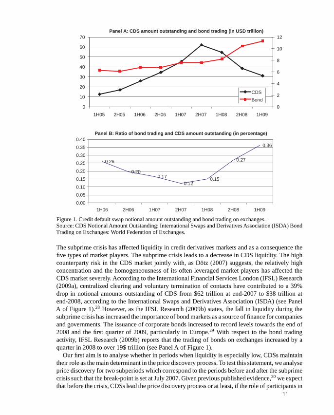
Figure 1. Credit default swap notional amount outstanding and bond trading on exchanges.Source: CDS Notional Amount Outstanding: International Swaps and Derivatives Association (ISDA) BondTrading on Exchanges: World Federation of Exchanges.
The subprime crisis has affected liquidity in credit derivatives markets and as a consequence thefive types of market players. The subprime crisis leads to a decrease in CDS liquidity. The highcounterparty risk in the CDS market jointly with, as Dötz (2007) suggests, the relatively highconcentration and the homogeneousness of its often leveraged market players has affected theCDS market severely. According to the International Financial Services London (IFSL) Research(2009a), centralized clearing and voluntary termination of contacts have contributed to a 39%drop in notional amounts outstanding of CDS from $62 trillion at end-2007 to $38 trillion atend-2008, according to the International Swaps and Derivatives Association (ISDA) (see PanelA of Figure 1).28 However, as the IFSL Research (2009b) states, the fall in liquidity during thesubprime crisis has increased the importance of bond markets as a source of finance for companiesand governments. The issuance of corporate bonds increased to record levels towards the end of2008 and the first quarter of 2009, particularly in Europe.29 With respect to the bond tradingactivity, IFSL Research (2009b) reports that the trading of bonds on exchanges increased by aquarter in 2008 to over 19$ trillion (see Panel A of Figure 1).
Our first aim is to analyse whether in periods when liquidity is especially low, CDSs maintaintheir role as the main determinant in the price discovery process. To test this statement, we analyseprice discovery for two subperiods which correspond to the periods before and after the subprimecrisis such that the break-point is set at July 2007. Given previous published evidence,30 we expectthat before the crisis, CDSs lead the price discovery process or at least, if the role of participants in
Dow
nloa
ded
by [
Uni
vers
idad
Car
los
Iii M
adri
d] a
t 11:
41 1
2 M
arch
201
2
11
862 S. Mayordomo et al.
both markets is highly influential (NBOTH is high), the price discovery measure of Equation (18)should be close to 0.5.31 According to our model, the leadership of the CDS market can beexplained by its higher liquidity (number of participants). The buy-and-hold strategy employedby the ASP or bond investors contrary to the active behaviour of CDS investors, in part due tothe leverage associated with a CDSs purchase, could lead to a higher market activity in the CDSmarket than in the bond market before the subprime crisis.Hypothesis 1: Under scenarios with high liquidity such as before the subprime crisis, the CDSmarket should lead the ASP market in the price discovery process.
The reason is that the number of participants (liquidity) in the CDS market is high relative tothe number of players in the ASP market (NCDS > NASP). In addition to the previous hypothesis,when the number of individuals who operate in both markets is high (NBOTH is high), the CDSmarket should reveal information as efficiently as the ASP market.
According toAcharya and Schaefer (2006) andAcharya, Schaefer, and Zhang (2007), in periodswith low liquidity one should expect that market makers, who at the same time are price settersin both credit markets, are financially constrained and thus their participation in both marketswill decrease. In terms of our model, notation is equivalent to say that NBOTH → 0 and the newpercentages of price discovery would change into a measure similar to the one introduced by GS:
NASP
NASP + NCDSand
NCDS
NASP + NCDS(19)
According to the IFSL Research (2009a, 2009b) reports, the attraction of bonds, and implicitlyASPs, as an investment has increased since the start of the credit crisis and large institutional, aswell as retail, investors increased their holdings due to the losses on equity markets and due to thebonds and ASPs high returns as yields during 2008.32 On the other hand, there is a drop in boththe notional amounts outstanding and the number of participants in the CDS market.33 Thus, ifthe crisis has affected activity in the CDS more severely than in the ASP market, we expect theASPs to reveal information faster and more adequately than before the crisis, up to the point thatASPs could lead the process of price discovery in some cases.34
Hypothesis 2: Under scenarios with low liquidity leading to a generalized reduction in marketparticipation in credit derivatives markets, the relative position of theASP market as an informationprovider improves with respect to the one observed under high liquid scenarios.
Finally, we analyse the process of price discovery between ASP and bond spreads.Hypothesis 3: The ASP market always (before and after the subprime crisis) leads the pricediscovery process with respect to the bond market.
3. Data
Our database contains daily data on Eurobonds and ASPs denominated in Euros and issued bynon-financial companies that are collected from Reuters and on CDSs also denominated in Eurosand issued by the same non-financial companies that are obtained from GFI.
GFI is a major inter-dealer broker, specializing in the trading of credit derivatives. GFI datacontain single-name CDSs market prices for 1, 2, 3, 4 and 5 years maturities. These pricescorrespond to actual trades, or firm bids and offers where capital is actually committed and sothey are not consensus or indications. Thus, these prices are an accurate indication of where theCDS markets have traded and closed for a given day. For some companies and for some maturities,especially 2 and 4 years, the data availability are scarce and in these cases, we employ mid-pricequotes from a credit curve also reported by GFI to fill the missing data.35 GFI data have also
Dow
nloa
ded
by [
Uni
vers
idad
Car
los
Iii M
adri
d] a
t 11:
41 1
2 M
arch
201
2
12
The European Journal of Finance 863
been used by Hull, Predescu, and White (2004), Predescu (2006), Saita (2006), Nashikkar andSubrahmanyam (2007), Fulop and Lescourret (2007) or Nashikkar, Subrahmanyam, and Mahanti(2009) among others.
For each bond there is information on both bid and ask prices, the swap spread, the assetswap spread, the sector of the entity and its geographical location, the currency, the seniority,the rating history (Fitch, S&P and Moody’s ratings), the issuance date and the amount issued,the coupon and coupon dates and the maturity. We use bonds whose maturity at the investmentdates is lower than five years. Several bonds issued by the same company may be used wheneverthey satisfy all the required criteria. The reason is that although CDS spread quotes refer to theissuer and not to an individual bond, asset swap spreads are quoted for individual bonds. Due toliquidity considerations, bonds with time to maturity equal to or less than 12 months to the datecorresponding to their last observation are excluded. Moreover, our sample contains fixed-ratesenior unsecured Euro denominated bonds whose issued quantity exceeds 300 million Euros.36
Other requirements imposed on bonds to be included in the sample are: (i) straight bonds, (ii)neither callable nor convertible, (iii) with rating history available, (iv) with constant coupons andwith a fixed frequency, (v) without a sinking fund, (vi) without options, (vii) without an oddfrequency of coupon payments, (viii) no government bonds and (ix) no inflation-indexed bonds.We cross-check the data on bonds with the equivalent data obtained from Datastream. Due toliquidity restrictions, investments are restricted to periods where there are 5-year CDS data oneither actual trades or bids and offers where capital is committed.
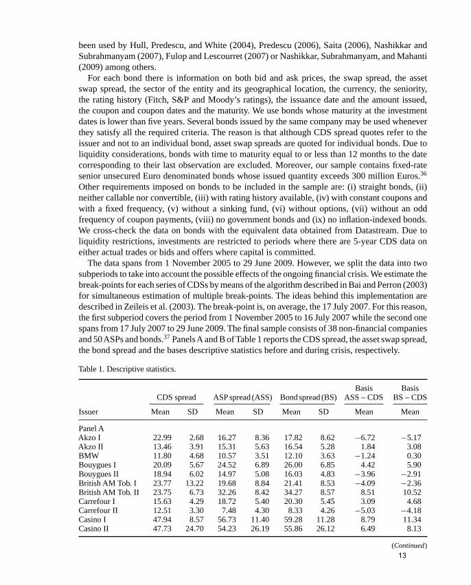
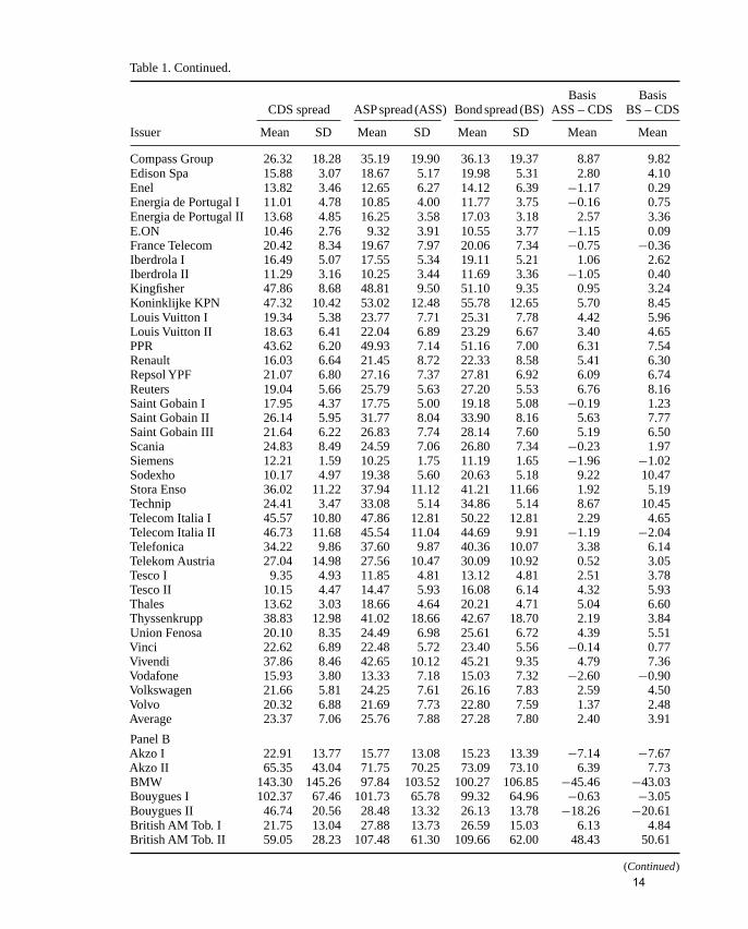
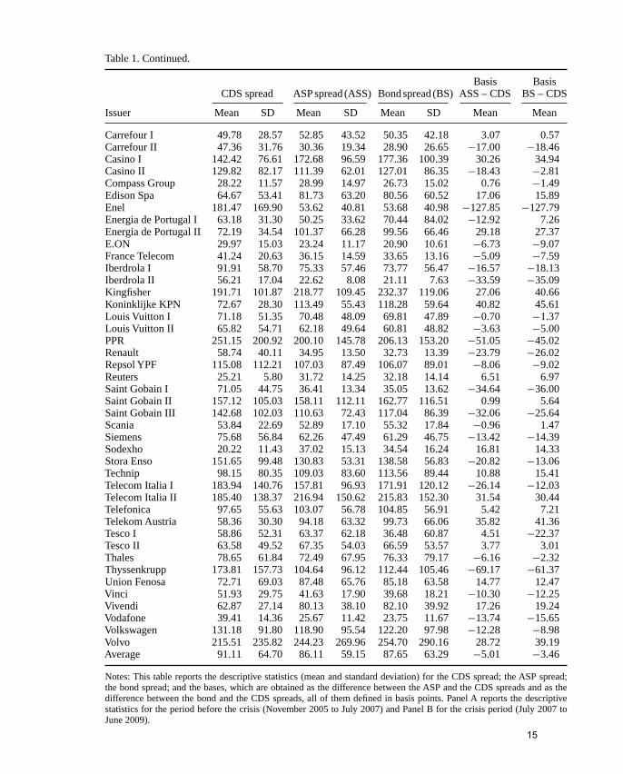
The data spans from 1 November 2005 to 29 June 2009. However, we split the data into twosubperiods to take into account the possible effects of the ongoing financial crisis. We estimate thebreak-points for each series of CDSs by means of the algorithm described in Bai and Perron (2003)for simultaneous estimation of multiple break-points. The ideas behind this implementation aredescribed in Zeileis et al. (2003). The break-point is, on average, the 17 July 2007. For this reason,the first subperiod covers the period from 1 November 2005 to 16 July 2007 while the second onespans from 17 July 2007 to 29 June 2009. The final sample consists of 38 non-financial companiesand 50ASPs and bonds.37 PanelsA and B of Table 1 reports the CDS spread, the asset swap spread,the bond spread and the bases descriptive statistics before and during crisis, respectively.
Table 1. Descriptive statistics.
Basis BasisCDS spread ASP spread (ASS) Bond spread (BS) ASS – CDS BS – CDS
Issuer Mean SD Mean SD Mean SD Mean Mean
Panel AAkzo I 22.99 2.68 16.27 8.36 17.82 8.62 −6.72 −5.17Akzo II 13.46 3.91 15.31 5.63 16.54 5.28 1.84 3.08BMW 11.80 4.68 10.57 3.51 12.10 3.63 −1.24 0.30Bouygues I 20.09 5.67 24.52 6.89 26.00 6.85 4.42 5.90Bouygues II 18.94 6.02 14.97 5.08 16.03 4.83 −3.96 −2.91British AM Tob. I 23.77 13.22 19.68 8.84 21.41 8.53 −4.09 −2.36British AM Tob. II 23.75 6.73 32.26 8.42 34.27 8.57 8.51 10.52Carrefour I 15.63 4.29 18.72 5.40 20.30 5.45 3.09 4.68Carrefour II 12.51 3.30 7.48 4.30 8.33 4.26 −5.03 −4.18Casino I 47.94 8.57 56.73 11.40 59.28 11.28 8.79 11.34Casino II 47.73 24.70 54.23 26.19 55.86 26.12 6.49 8.13
(Continued)
Dow
nloa
ded
by [
Uni
vers
idad
Car
los
Iii M
adri
d] a
t 11:
41 1
2 M
arch
201
2
13
864 S. Mayordomo et al.
Table 1. Continued.
Basis BasisCDS spread ASP spread (ASS) Bond spread (BS) ASS – CDS BS – CDS
Issuer Mean SD Mean SD Mean SD Mean Mean
Compass Group 26.32 18.28 35.19 19.90 36.13 19.37 8.87 9.82Edison Spa 15.88 3.07 18.67 5.17 19.98 5.31 2.80 4.10Enel 13.82 3.46 12.65 6.27 14.12 6.39 −1.17 0.29Energia de Portugal I 11.01 4.78 10.85 4.00 11.77 3.75 −0.16 0.75Energia de Portugal II 13.68 4.85 16.25 3.58 17.03 3.18 2.57 3.36E.ON 10.46 2.76 9.32 3.91 10.55 3.77 −1.15 0.09France Telecom 20.42 8.34 19.67 7.97 20.06 7.34 −0.75 −0.36Iberdrola I 16.49 5.07 17.55 5.34 19.11 5.21 1.06 2.62Iberdrola II 11.29 3.16 10.25 3.44 11.69 3.36 −1.05 0.40Kingfisher 47.86 8.68 48.81 9.50 51.10 9.35 0.95 3.24Koninklijke KPN 47.32 10.42 53.02 12.48 55.78 12.65 5.70 8.45Louis Vuitton I 19.34 5.38 23.77 7.71 25.31 7.78 4.42 5.96Louis Vuitton II 18.63 6.41 22.04 6.89 23.29 6.67 3.40 4.65PPR 43.62 6.20 49.93 7.14 51.16 7.00 6.31 7.54Renault 16.03 6.64 21.45 8.72 22.33 8.58 5.41 6.30Repsol YPF 21.07 6.80 27.16 7.37 27.81 6.92 6.09 6.74Reuters 19.04 5.66 25.79 5.63 27.20 5.53 6.76 8.16Saint Gobain I 17.95 4.37 17.75 5.00 19.18 5.08 −0.19 1.23Saint Gobain II 26.14 5.95 31.77 8.04 33.90 8.16 5.63 7.77Saint Gobain III 21.64 6.22 26.83 7.74 28.14 7.60 5.19 6.50Scania 24.83 8.49 24.59 7.06 26.80 7.34 −0.23 1.97Siemens 12.21 1.59 10.25 1.75 11.19 1.65 −1.96 −1.02Sodexho 10.17 4.97 19.38 5.60 20.63 5.18 9.22 10.47Stora Enso 36.02 11.22 37.94 11.12 41.21 11.66 1.92 5.19Technip 24.41 3.47 33.08 5.14 34.86 5.14 8.67 10.45Telecom Italia I 45.57 10.80 47.86 12.81 50.22 12.81 2.29 4.65Telecom Italia II 46.73 11.68 45.54 11.04 44.69 9.91 −1.19 −2.04Telefonica 34.22 9.86 37.60 9.87 40.36 10.07 3.38 6.14Telekom Austria 27.04 14.98 27.56 10.47 30.09 10.92 0.52 3.05Tesco I 9.35 4.93 11.85 4.81 13.12 4.81 2.51 3.78Tesco II 10.15 4.47 14.47 5.93 16.08 6.14 4.32 5.93Thales 13.62 3.03 18.66 4.64 20.21 4.71 5.04 6.60Thyssenkrupp 38.83 12.98 41.02 18.66 42.67 18.70 2.19 3.84Union Fenosa 20.10 8.35 24.49 6.98 25.61 6.72 4.39 5.51Vinci 22.62 6.89 22.48 5.72 23.40 5.56 −0.14 0.77Vivendi 37.86 8.46 42.65 10.12 45.21 9.35 4.79 7.36Vodafone 15.93 3.80 13.33 7.18 15.03 7.32 −2.60 −0.90Volkswagen 21.66 5.81 24.25 7.61 26.16 7.83 2.59 4.50Volvo 20.32 6.88 21.69 7.73 22.80 7.59 1.37 2.48Average 23.37 7.06 25.76 7.88 27.28 7.80 2.40 3.91
Panel BAkzo I 22.91 13.77 15.77 13.08 15.23 13.39 −7.14 −7.67Akzo II 65.35 43.04 71.75 70.25 73.09 73.10 6.39 7.73BMW 143.30 145.26 97.84 103.52 100.27 106.85 −45.46 −43.03Bouygues I 102.37 67.46 101.73 65.78 99.32 64.96 −0.63 −3.05Bouygues II 46.74 20.56 28.48 13.32 26.13 13.78 −18.26 −20.61British AM Tob. I 21.75 13.04 27.88 13.73 26.59 15.03 6.13 4.84British AM Tob. II 59.05 28.23 107.48 61.30 109.66 62.00 48.43 50.61
(Continued)
Dow
nloa
ded
by [
Uni
vers
idad
Car
los
Iii M
adri
d] a
t 11:
41 1
2 M
arch
201
2
14
The European Journal of Finance 865
Table 1. Continued.
Basis BasisCDS spread ASP spread (ASS) Bond spread (BS) ASS – CDS BS – CDS
Issuer Mean SD Mean SD Mean SD Mean Mean
Carrefour I 49.78 28.57 52.85 43.52 50.35 42.18 3.07 0.57Carrefour II 47.36 31.76 30.36 19.34 28.90 26.65 −17.00 −18.46Casino I 142.42 76.61 172.68 96.59 177.36 100.39 30.26 34.94Casino II 129.82 82.17 111.39 62.01 127.01 86.35 −18.43 −2.81Compass Group 28.22 11.57 28.99 14.97 26.73 15.02 0.76 −1.49Edison Spa 64.67 53.41 81.73 63.20 80.56 60.52 17.06 15.89Enel 181.47 169.90 53.62 40.81 53.68 40.98 −127.85 −127.79Energia de Portugal I 63.18 31.30 50.25 33.62 70.44 84.02 −12.92 7.26Energia de Portugal II 72.19 34.54 101.37 66.28 99.56 66.46 29.18 27.37E.ON 29.97 15.03 23.24 11.17 20.90 10.61 −6.73 −9.07France Telecom 41.24 20.63 36.15 14.59 33.65 13.16 −5.09 −7.59Iberdrola I 91.91 58.70 75.33 57.46 73.77 56.47 −16.57 −18.13Iberdrola II 56.21 17.04 22.62 8.08 21.11 7.63 −33.59 −35.09Kingfisher 191.71 101.87 218.77 109.45 232.37 119.06 27.06 40.66Koninklijke KPN 72.67 28.30 113.49 55.43 118.28 59.64 40.82 45.61Louis Vuitton I 71.18 51.35 70.48 48.09 69.81 47.89 −0.70 −1.37Louis Vuitton II 65.82 54.71 62.18 49.64 60.81 48.82 −3.63 −5.00PPR 251.15 200.92 200.10 145.78 206.13 153.20 −51.05 −45.02Renault 58.74 40.11 34.95 13.50 32.73 13.39 −23.79 −26.02Repsol YPF 115.08 112.21 107.03 87.49 106.07 89.01 −8.06 −9.02Reuters 25.21 5.80 31.72 14.25 32.18 14.14 6.51 6.97Saint Gobain I 71.05 44.75 36.41 13.34 35.05 13.62 −34.64 −36.00Saint Gobain II 157.12 105.03 158.11 112.11 162.77 116.51 0.99 5.64Saint Gobain III 142.68 102.03 110.63 72.43 117.04 86.39 −32.06 −25.64Scania 53.84 22.69 52.89 17.10 55.32 17.84 −0.96 1.47Siemens 75.68 56.84 62.26 47.49 61.29 46.75 −13.42 −14.39Sodexho 20.22 11.43 37.02 15.13 34.54 16.24 16.81 14.33Stora Enso 151.65 99.48 130.83 53.31 138.58 56.83 −20.82 −13.06Technip 98.15 80.35 109.03 83.60 113.56 89.44 10.88 15.41Telecom Italia I 183.94 140.76 157.81 96.93 171.91 120.12 −26.14 −12.03Telecom Italia II 185.40 138.37 216.94 150.62 215.83 152.30 31.54 30.44Telefonica 97.65 55.63 103.07 56.78 104.85 56.91 5.42 7.21Telekom Austria 58.36 30.30 94.18 63.32 99.73 66.06 35.82 41.36Tesco I 58.86 52.31 63.37 62.18 36.48 60.87 4.51 −22.37Tesco II 63.58 49.52 67.35 54.03 66.59 53.57 3.77 3.01Thales 78.65 61.84 72.49 67.95 76.33 79.17 −6.16 −2.32Thyssenkrupp 173.81 157.73 104.64 96.12 112.44 105.46 −69.17 −61.37Union Fenosa 72.71 69.03 87.48 65.76 85.18 63.58 14.77 12.47Vinci 51.93 29.75 41.63 17.90 39.68 18.21 −10.30 −12.25Vivendi 62.87 27.14 80.13 38.10 82.10 39.92 17.26 19.24Vodafone 39.41 14.36 25.67 11.42 23.75 11.67 −13.74 −15.65Volkswagen 131.18 91.80 118.90 95.54 122.20 97.98 −12.28 −8.98Volvo 215.51 235.82 244.23 269.96 254.70 290.16 28.72 39.19Average 91.11 64.70 86.11 59.15 87.65 63.29 −5.01 −3.46
Notes: This table reports the descriptive statistics (mean and standard deviation) for the CDS spread; the ASP spread;the bond spread; and the bases, which are obtained as the difference between the ASP and the CDS spreads and as thedifference between the bond and the CDS spreads, all of them defined in basis points. Panel A reports the descriptivestatistics for the period before the crisis (November 2005 to July 2007) and Panel B for the crisis period (July 2007 toJune 2009).
Dow
nloa
ded
by [
Uni
vers
idad
Car
los
Iii M
adri
d] a
t 11:
41 1
2 M
arch
201
2
15
866 S. Mayordomo et al.
4. Price discovery results
We analyse the price discovery process in two different contexts. On the one hand, before July2007 there exists a scenario of high liquidity where the number of market participants is higherthan in the second period, which represents the illiquid scenario.
The process of price discovery is analysed from an equilibrium model based on an ErrorCorrection Model and the long-run equilibrium condition is based on the existence of cointegrationbetween credit spreads. Econometric details on the model estimation of the VECM defined inEquation (16) can be found in Juselius (2006).
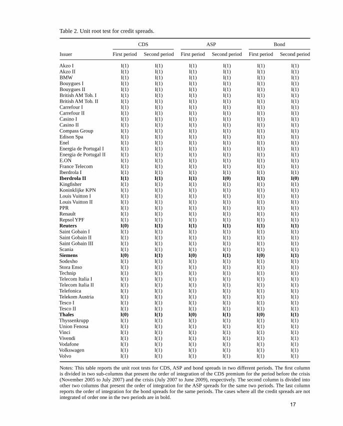
Before the price discovery analysis, we firstly verify the series stationarity by means of aNg-Perron unit root test. Table 2 shows that credit spreads are I(1) for the two periods consideredin 46 of the total 50 cases which correspond to 50 different ASPs and bonds.
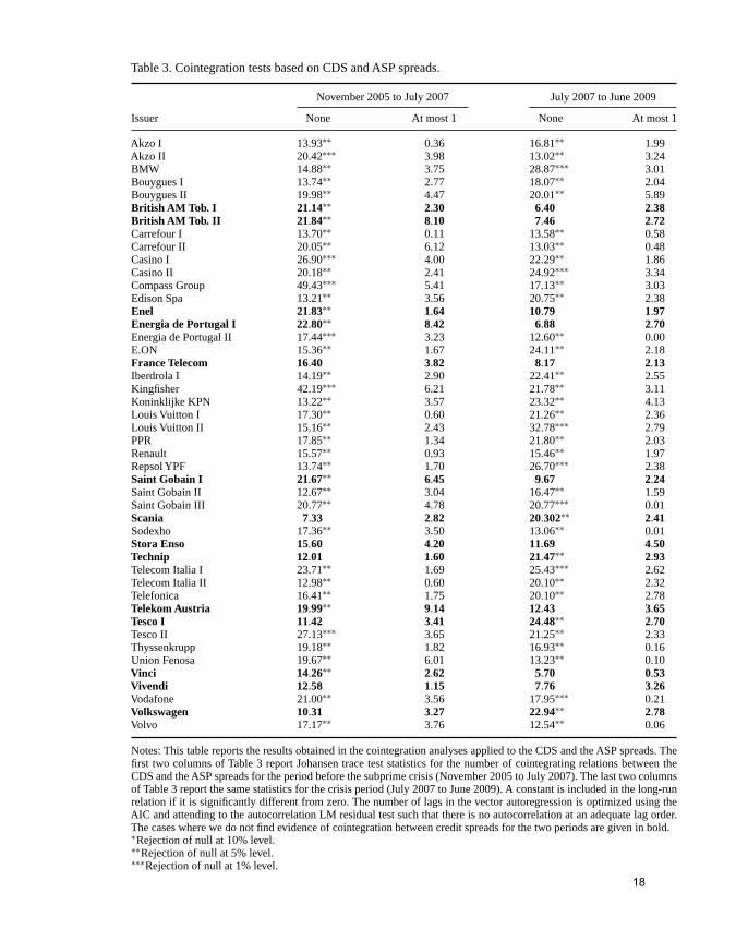
In Table 3, we report the Johansen (1991) cointegration test results for each reference entitywhenever the CDS and ASP spreads are I(1) in the two periods. In 32 of the total 46 cases, wefind cointegration between ASP and CDS spreads. We find cointegration between bond and CDSspreads in the same 32 cases.38 The number of cointegration relationships that we find is similarto one obtained in previous analyses. Norden and Weber (2004), Blanco, Brennan, and Marsh(2005) and Zhu (2006) find cointegration relationships between CDS and bond spreads in 36 of58 cases, in 26 of 33 cases and in 15 of 24 cases, respectively. De Wit (2006) finds cointegrationrelationships between CDS and ASP spreads in 88 of 144 cases. With respect to ASP and bondspreads, we find evidence of cointegration between them for all the 46 cases.39 We then test whythere is no cointegration between the ASP and CDS market. To achieve this, we run a Probitregression with heteroskedasticity robust standard errors for the total 92 cases studied in bothsubperiods, using as dependent variable a dummy variable that equals 1 if there is cointegrationand 0 otherwise. In order to control and test the effect of the crisis, we create a dummy variableequal to one if a given case corresponds to the crisis period. The cointegration seems to be morefrequent in bonds/ASPs with a high coupon rate and with a long time to maturity. The resultssuggest that the riskier the underlying bond or the longer the time to maturity, the more similarare the credit spreads in the long run. The first result is consistent with the increase in correlationacross financial markets as the risk increases. The second result suggests that the deviations amongcredit spreads are higher close to the bond maturity. We use other explanatory variables such asthe rating; the basis, which is defined as the difference between the ASP and CDS spreads; andthe crisis dummy but none of them have a significant effect on cointegration.40
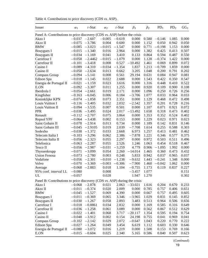
The analysis of price discovery is based on the VECM specification presented in Equations (15)and (16) and it is applied to the 32 cases, where we find a long-run equilibrium behaviour of thecredit spreads series. The vector in Equation (16) represents the coefficients that determine themarket contribution to price discovery. We conclude that a given market leads the process of pricediscovery whenever its corresponding price discovery metric (GGi for i = 1, 2) is higher than 0.5.Both markets reveal information in an equally efficient way whenever the price discovery metricsare close to 0.5 for both markets (0.45 < GGi < 0.55 for i = 1, 2). The GGi price discoverymetric is defined such that it has a lower bound of 0 and an upper bound of 1 in order to beconsistent with the definition in Equation (18) and the meaning of this metric.
4.1 The leadership of the CDS market before the crisis
Panel A of Table 4 shows that during the period before the crisis, Hypothesis 1 is confirmed andthe CDSs appear clearly as the more efficient market in 87.5% of the cases (28 cases). According
Dow
nloa
ded
by [
Uni
vers
idad
Car
los
Iii M
adri
d] a
t 11:
41 1
2 M
arch
201
2
16
The European Journal of Finance 867
Table 2. Unit root test for credit spreads.
CDS ASP Bond
Issuer First period Second period First period Second period First period Second period
Akzo I I(1) I(1) I(1) I(1) I(1) I(1)Akzo II I(1) I(1) I(1) I(1) I(1) I(1)BMW I(1) I(1) I(1) I(1) I(1) I(1)Bouygues I I(1) I(1) I(1) I(1) I(1) I(1)Bouygues II I(1) I(1) I(1) I(1) I(1) I(1)British AM Tob. I I(1) I(1) I(1) I(1) I(1) I(1)British AM Tob. II I(1) I(1) I(1) I(1) I(1) I(1)Carrefour I I(1) I(1) I(1) I(1) I(1) I(1)Carrefour II I(1) I(1) I(1) I(1) I(1) I(1)Casino I I(1) I(1) I(1) I(1) I(1) I(1)Casino II I(1) I(1) I(1) I(1) I(1) I(1)Compass Group I(1) I(1) I(1) I(1) I(1) I(1)Edison Spa I(1) I(1) I(1) I(1) I(1) I(1)Enel I(1) I(1) I(1) I(1) I(1) I(1)Energia de Portugal I I(1) I(1) I(1) I(1) I(1) I(1)Energia de Portugal II I(1) I(1) I(1) I(1) I(1) I(1)E.ON I(1) I(1) I(1) I(1) I(1) I(1)France Telecom I(1) I(1) I(1) I(1) I(1) I(1)Iberdrola I I(1) I(1) I(1) I(1) I(1) I(1)Iberdrola II I(1) I(1) I(1) I(0) I(1) I(0)Kingfisher I(1) I(1) I(1) I(1) I(1) I(1)Koninklijke KPN I(1) I(1) I(1) I(1) I(1) I(1)Louis Vuitton I I(1) I(1) I(1) I(1) I(1) I(1)Louis Vuitton II I(1) I(1) I(1) I(1) I(1) I(1)PPR I(1) I(1) I(1) I(1) I(1) I(1)Renault I(1) I(1) I(1) I(1) I(1) I(1)Repsol YPF I(1) I(1) I(1) I(1) I(1) I(1)Reuters I(0) I(1) I(1) I(1) I(1) I(1)Saint Gobain I I(1) I(1) I(1) I(1) I(1) I(1)Saint Gobain II I(1) I(1) I(1) I(1) I(1) I(1)Saint Gobain III I(1) I(1) I(1) I(1) I(1) I(1)Scania I(1) I(1) I(1) I(1) I(1) I(1)Siemens I(0) I(1) I(0) I(1) I(0) I(1)Sodexho I(1) I(1) I(1) I(1) I(1) I(1)Stora Enso I(1) I(1) I(1) I(1) I(1) I(1)Technip I(1) I(1) I(1) I(1) I(1) I(1)Telecom Italia I I(1) I(1) I(1) I(1) I(1) I(1)Telecom Italia II I(1) I(1) I(1) I(1) I(1) I(1)Telefonica I(1) I(1) I(1) I(1) I(1) I(1)Telekom Austria I(1) I(1) I(1) I(1) I(1) I(1)Tesco I I(1) I(1) I(1) I(1) I(1) I(1)Tesco II I(1) I(1) I(1) I(1) I(1) I(1)Thales I(0) I(1) I(0) I(1) I(0) I(1)Thyssenkrupp I(1) I(1) I(1) I(1) I(1) I(1)Union Fenosa I(1) I(1) I(1) I(1) I(1) I(1)Vinci I(1) I(1) I(1) I(1) I(1) I(1)Vivendi I(1) I(1) I(1) I(1) I(1) I(1)Vodafone I(1) I(1) I(1) I(1) I(1) I(1)Volkswagen I(1) I(1) I(1) I(1) I(1) I(1)Volvo I(1) I(1) I(1) I(1) I(1) I(1)
Notes: This table reports the unit root tests for CDS, ASP and bond spreads in two different periods. The first columnis divided in two sub-columns that present the order of integration of the CDS premium for the period before the crisis(November 2005 to July 2007) and the crisis (July 2007 to June 2009), respectively. The second column is divided intoother two columns that present the order of integration for the ASP spreads for the same two periods. The last columnreports the order of integration for the bond spreads for the same periods. The cases where all the credit spreads are notintegrated of order one in the two periods are in bold.
Dow
nloa
ded
by [
Uni
vers
idad
Car
los
Iii M
adri
d] a
t 11:
41 1
2 M
arch
201
2
17
868 S. Mayordomo et al.
Table 3. Cointegration tests based on CDS and ASP spreads.
November 2005 to July 2007 July 2007 to June 2009
Issuer None At most 1 None At most 1
Akzo I 13.93∗∗ 0.36 16.81∗∗ 1.99Akzo II 20.42∗∗∗ 3.98 13.02∗∗ 3.24BMW 14.88∗∗ 3.75 28.87∗∗∗ 3.01Bouygues I 13.74∗∗ 2.77 18.07∗∗ 2.04Bouygues II 19.98∗∗ 4.47 20.01∗∗ 5.89British AM Tob. I 21.14∗∗ 2.30 6.40 2.38British AM Tob. II 21.84∗∗ 8.10 7.46 2.72Carrefour I 13.70∗∗ 0.11 13.58∗∗ 0.58Carrefour II 20.05∗∗ 6.12 13.03∗∗ 0.48Casino I 26.90∗∗∗ 4.00 22.29∗∗ 1.86Casino II 20.18∗∗ 2.41 24.92∗∗∗ 3.34Compass Group 49.43∗∗∗ 5.41 17.13∗∗ 3.03Edison Spa 13.21∗∗ 3.56 20.75∗∗ 2.38Enel 21.83∗∗ 1.64 10.79 1.97Energia de Portugal I 22.80∗∗ 8.42 6.88 2.70Energia de Portugal II 17.44∗∗∗ 3.23 12.60∗∗ 0.00E.ON 15.36∗∗ 1.67 24.11∗∗ 2.18France Telecom 16.40 3.82 8.17 2.13Iberdrola I 14.19∗∗ 2.90 22.41∗∗ 2.55Kingfisher 42.19∗∗∗ 6.21 21.78∗∗ 3.11Koninklijke KPN 13.22∗∗ 3.57 23.32∗∗ 4.13Louis Vuitton I 17.30∗∗ 0.60 21.26∗∗ 2.36Louis Vuitton II 15.16∗∗ 2.43 32.78∗∗∗ 2.79PPR 17.85∗∗ 1.34 21.80∗∗ 2.03Renault 15.57∗∗ 0.93 15.46∗∗ 1.97Repsol YPF 13.74∗∗ 1.70 26.70∗∗∗ 2.38Saint Gobain I 21.67∗∗ 6.45 9.67 2.24Saint Gobain II 12.67∗∗ 3.04 16.47∗∗ 1.59Saint Gobain III 20.77∗∗ 4.78 20.77∗∗∗ 0.01Scania 7.33 2.82 20.302∗∗ 2.41Sodexho 17.36∗∗ 3.50 13.06∗∗ 0.01Stora Enso 15.60 4.20 11.69 4.50Technip 12.01 1.60 21.47∗∗ 2.93Telecom Italia I 23.71∗∗ 1.69 25.43∗∗∗ 2.62Telecom Italia II 12.98∗∗ 0.60 20.10∗∗ 2.32Telefonica 16.41∗∗ 1.75 20.10∗∗ 2.78Telekom Austria 19.99∗∗ 9.14 12.43 3.65Tesco I 11.42 3.41 24.48∗∗ 2.70Tesco II 27.13∗∗∗ 3.65 21.25∗∗ 2.33Thyssenkrupp 19.18∗∗ 1.82 16.93∗∗ 0.16Union Fenosa 19.67∗∗ 6.01 13.23∗∗ 0.10Vinci 14.26∗∗ 2.62 5.70 0.53Vivendi 12.58 1.15 7.76 3.26Vodafone 21.00∗∗ 3.56 17.95∗∗∗ 0.21Volkswagen 10.31 3.27 22.94∗∗ 2.78Volvo 17.17∗∗ 3.76 12.54∗∗ 0.06
Notes: This table reports the results obtained in the cointegration analyses applied to the CDS and the ASP spreads. Thefirst two columns of Table 3 report Johansen trace test statistics for the number of cointegrating relations between theCDS and the ASP spreads for the period before the subprime crisis (November 2005 to July 2007). The last two columnsof Table 3 report the same statistics for the crisis period (July 2007 to June 2009). A constant is included in the long-runrelation if it is significantly different from zero. The number of lags in the vector autoregression is optimized using theAIC and attending to the autocorrelation LM residual test such that there is no autocorrelation at an adequate lag order.The cases where we do not find evidence of cointegration between credit spreads for the two periods are given in bold.∗Rejection of null at 10% level.∗∗Rejection of null at 5% level.∗∗∗Rejection of null at 1% level.
Dow
nloa
ded
by [
Uni
vers
idad
Car
los
Iii M
adri
d] a
t 11:
41 1
2 M
arch
201
2
18
The European Journal of Finance 869
Table 4. Contributions to price discovery (CDS vs. ASP).
Issuer α1 t-Stat α2 t-Stat β3 β2 PD1 PD2 GG1
Panel A: Contributions to price discovery (CDS vs. ASP) before the crisisAkzo I −0.037 −2.607 −0.005 −0.619 0.000 0.580 −0.146 1.085 0.000Akzo II −0.075 −3.786 0.004 0.600 0.000 1.152 0.050 0.942 0.050BMW −0.085 −3.023 −0.015 −1.547 0.000 0.771 −0.198 1.153 0.000Bouygues I −0.015 −1.340 0.016 2.964 0.000 1.382 0.425 0.413 0.507Bouygues II −0.034 −1.169 0.041 3.410 0.133 0.864 0.594 0.487 0.550Carrefour I −0.058 −2.4462 −0.015 −1.079 0.000 1.128 −0.374 1.422 0.000Carrefour II −0.101 −3.418 0.008 0.527 −10.492 1.461 0.069 0.899 0.072Casino I −0.089 −4.310 −0.034 −1.354 1.837 1.213 −0.709 1.859 0.000Casino II −0.050 −2.634 0.013 0.662 3.205 1.048 0.200 0.791 0.202Compass Group −0.094 −5.141 0.008 0.561 29.194 0.631 0.084 0.947 0.081Edison Spa −0.018 −1.145 0.022 2.688 0.000 1.543 0.422 0.350 0.547Energia de Portugal II −0.021 −1.159 0.023 3.616 0.000 1.316 0.448 0.410 0.522E.ON −0.092 −3.307 0.011 1.255 0.000 0.920 0.109 0.900 0.108Iberdrola I −0.054 −2.661 0.019 2.171 0.000 1.096 0.250 0.726 0.256Kingfisher −0.163 −6.045 0.006 0.184 −3.706 1.077 0.033 0.964 0.033Koninklijke KPN −0.074 −1.858 0.073 2.351 0.000 1.129 0.468 0.472 0.498Louis Vuitton I −0.116 −3.405 0.032 2.032 −2.542 1.357 0.201 0.728 0.216Louis Vuitton II −0.094 −3.535 0.007 0.501 0.000 1.107 0.071 0.921 0.072PPR −0.036 −3.495 0.024 2.017 −13.492 1.658 0.318 0.473 0.402Renault −0.112 −2.707 0.075 3.864 0.000 1.353 0.352 0.524 0.402Repsol YPF −0.064 −3.438 0.002 0.153 0.000 1.229 0.023 0.971 0.023Saint Gobain II −0.078 −2.914 0.013 0.734 0.000 1.189 0.142 0.831 0.146Saint Gobain III −0.045 −2.9105 0.019 2.039 −7.708 1.614 0.255 0.588 0.303Sodexho −0.038 −1.372 0.033 2.668 6.973 1.257 0.413 0.481 0.462Telecom Italia I −0.103 −3.296 0.062 2.386 −7.878 1.221 0.346 0.577 0.375Telecom Italia II −0.056 −2.323 0.055 2.297 0.000 0.972 0.503 0.511 0.496Telefonica −0.063 −2.287 0.055 2.526 1.246 1.063 0.454 0.518 0.467Tesco II −0.056 −2.987 −0.031 −3.259 4.779 0.906 −1.095 1.992 0.000Thyssenkrupp −0.071 −3.099 0.054 2.260 −14.014 1.465 0.360 0.473 0.432Union Fenosa −0.073 −2.780 0.003 0.248 5.833 0.942 0.037 0.965 0.037Vodafone −0.056 −2.301 −0.010 −1.238 −9.632 1.443 −0.241 1.348 0.000Volvo −0.070 −3.369 −0.003 −0.306 −7.900 1.460 −0.042 1.062 0.000Average −0.068 −2.883 0.018 1.104 −0.755 1.173 0.119 0.837 0.22795% conf. interval LL −0.080 0.008 −3.457 1.077 0.151UL −0.057 0.028 1.947 1.270 0.302
Panel B: Contributions to price discovery (CDS vs. ASP) during the crisisAkzo I −0.068 −2.878 0.021 2.063 −33.021 1.616 0.204 0.670 0.233Akzo II −0.011 −0.374 0.020 2.009 0.000 0.785 0.757 0.406 0.651BMW −0.045 −1.527 0.069 4.390 0.000 0.667 0.757 0.495 0.605Bouygues I −0.011 −0.369 0.065 3.346 −3.965 1.029 0.831 0.145 0.852Bouygues II −0.030 −1.267 0.058 2.893 3.483 0.513 0.964 0.506 0.656Carrefour I −0.018 −0.8861 0.034 2.832 0.000 1.169 0.585 0.316 0.649Carrefour II −0.036 −1.258 0.061 3.089 0.000 0.562 0.867 0.512 0.629Casino I −0.022 −1.401 0.068 3.717 −20.117 1.354 0.595 0.194 0.754Casino II −0.048 −3.912 0.002 0.154 24.198 0.755 0.041 0.969 0.041Compass Group −0.102 −2.142 0.029 2.072 −0.647 1.043 0.220 0.770 0.222Edison Spa −0.027 −1.264 0.049 3.454 6.619 1.112 0.603 0.330 0.646Energia de Portugal II −0.080 −3.072 0.016 1.219 0.000 1.508 0.153 0.769 0.166E.ON −0.015 −0.604 0.025 2.340 5.165 0.586 0.840 0.507 0.623
(Continued)
Dow
nloa
ded
by [
Uni
vers
idad
Car
los
Iii M
adri
d] a
t 11:
41 1
2 M
arch
201
2
19
870 S. Mayordomo et al.
Table 4. Continued.
Issuer α1 t-Stat α2 t-Stat β3 β2 PD1 PD2 GG1
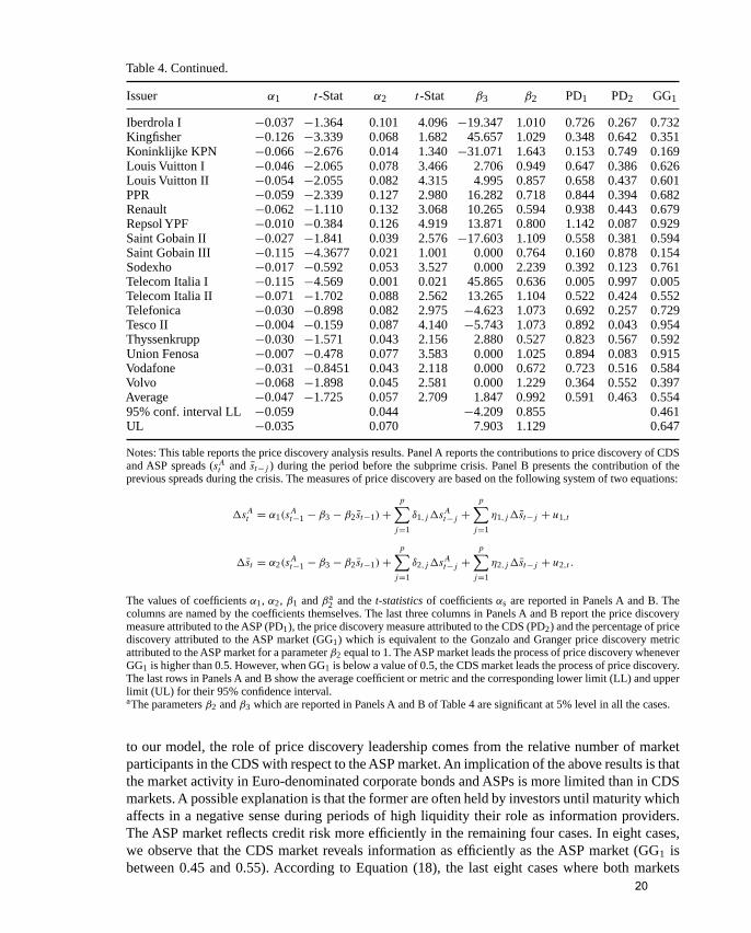
Iberdrola I −0.037 −1.364 0.101 4.096 −19.347 1.010 0.726 0.267 0.732Kingfisher −0.126 −3.339 0.068 1.682 45.657 1.029 0.348 0.642 0.351Koninklijke KPN −0.066 −2.676 0.014 1.340 −31.071 1.643 0.153 0.749 0.169Louis Vuitton I −0.046 −2.065 0.078 3.466 2.706 0.949 0.647 0.386 0.626Louis Vuitton II −0.054 −2.055 0.082 4.315 4.995 0.857 0.658 0.437 0.601PPR −0.059 −2.339 0.127 2.980 16.282 0.718 0.844 0.394 0.682Renault −0.062 −1.110 0.132 3.068 10.265 0.594 0.938 0.443 0.679Repsol YPF −0.010 −0.384 0.126 4.919 13.871 0.800 1.142 0.087 0.929Saint Gobain II −0.027 −1.841 0.039 2.576 −17.603 1.109 0.558 0.381 0.594Saint Gobain III −0.115 −4.3677 0.021 1.001 0.000 0.764 0.160 0.878 0.154Sodexho −0.017 −0.592 0.053 3.527 0.000 2.239 0.392 0.123 0.761Telecom Italia I −0.115 −4.569 0.001 0.021 45.865 0.636 0.005 0.997 0.005Telecom Italia II −0.071 −1.702 0.088 2.562 13.265 1.104 0.522 0.424 0.552Telefonica −0.030 −0.898 0.082 2.975 −4.623 1.073 0.692 0.257 0.729Tesco II −0.004 −0.159 0.087 4.140 −5.743 1.073 0.892 0.043 0.954Thyssenkrupp −0.030 −1.571 0.043 2.156 2.880 0.527 0.823 0.567 0.592Union Fenosa −0.007 −0.478 0.077 3.583 0.000 1.025 0.894 0.083 0.915Vodafone −0.031 −0.8451 0.043 2.118 0.000 0.672 0.723 0.516 0.584Volvo −0.068 −1.898 0.045 2.581 0.000 1.229 0.364 0.552 0.397Average −0.047 −1.725 0.057 2.709 1.847 0.992 0.591 0.463 0.55495% conf. interval LL −0.059 0.044 −4.209 0.855 0.461UL −0.035 0.070 7.903 1.129 0.647
Notes: This table reports the price discovery analysis results. Panel A reports the contributions to price discovery of CDSand ASP spreads (sA
t and s̄t−j ) during the period before the subprime crisis. Panel B presents the contribution of theprevious spreads during the crisis. The measures of price discovery are based on the following system of two equations:
�sAt = α1(s
At−1 − β3 − β2 s̄t−1) +
p∑j=1
δ1,j�sAt−j +
p∑j=1
η1,j�s̄t−j + u1,t
�s̄t = α2(sAt−1 − β3 − β2 s̄t−1) +
p∑j=1
δ2,j�sAt−j +
p∑j=1
η2,j�s̄t−j + u2,t .
The values of coefficients α1, α2, β1 and βa2 and the t-statistics of coefficients αs are reported in Panels A and B. The
columns are named by the coefficients themselves. The last three columns in Panels A and B report the price discoverymeasure attributed to the ASP (PD1), the price discovery measure attributed to the CDS (PD2) and the percentage of pricediscovery attributed to the ASP market (GG1) which is equivalent to the Gonzalo and Granger price discovery metricattributed to the ASP market for a parameter β2 equal to 1. The ASP market leads the process of price discovery wheneverGG1 is higher than 0.5. However, when GG1 is below a value of 0.5, the CDS market leads the process of price discovery.The last rows in Panels A and B show the average coefficient or metric and the corresponding lower limit (LL) and upperlimit (UL) for their 95% confidence interval.aThe parameters β2 and β3 which are reported in Panels A and B of Table 4 are significant at 5% level in all the cases.
to our model, the role of price discovery leadership comes from the relative number of marketparticipants in the CDS with respect to the ASP market. An implication of the above results is thatthe market activity in Euro-denominated corporate bonds and ASPs is more limited than in CDSmarkets. A possible explanation is that the former are often held by investors until maturity whichaffects in a negative sense during periods of high liquidity their role as information providers.The ASP market reflects credit risk more efficiently in the remaining four cases. In eight cases,we observe that the CDS market reveals information as efficiently as the ASP market (GG1 isbetween 0.45 and 0.55). According to Equation (18), the last eight cases where both markets
Dow
nloa
ded
by [
Uni
vers
idad
Car
los
Iii M
adri
d] a
t 11:
41 1
2 M
arch
201
2
20
The European Journal of Finance 871
reveal information in an equally efficient way could be explained by a higher market participationof the agents who operate in both markets (NBOTH is high). On average, we find that the CDSmarket leads the ASP market during the period before the crisis as the value of 0.227 for thecorresponding GG average metric in the ASP market reveals. The 95% confidence interval forthe average GG metric is 0.151–0.302, where even the upper limit implies that the CDS marketleads the ASP market. The minimum GG metric is 0, which means that the CDS market revealsall the information, while the maximum is 0.55.
4.2 The leadership of the ASP and bond markets during the crisis
Panel B of Table 4 reports the results for the subprime crisis period. Comparing Panels A and Bof Table 4, we observe that during the crisis, ASP spreads reveal more efficiently credit risk thanbefore. This result is consistent with Hypothesis 2 up to the point that in 71.88% of the cases (23cases), ASP spreads lead CDS spreads in the price discovery process. The CDS market reflectscredit risk more efficiently in the remaining nine cases. Thus, ASPs’ predominant position asinformation providers during the crisis is in line with the evidence reported in the IFSL Research(2009a, 2009b) about CDS and bond notional amounts outstanding and trading activity. Dötz(2007) states that the turbulence in the credit markets in spring 2005 was apparently handled muchbetter by the bond market than by the CDS market. The role of ASP as information providersimproves with respect to the one observed before the crisis in 84.4% of the cases (27 cases). Thisrole only worsens in five cases which could be explained by a drop in the ASPs’ liquidity thateven exceeds the drop in CDS liquidity. On average, we find that the ASP market leads the CDSmarket during the crisis as the value of 0.554 for the corresponding GG average metric reveals.The 95% confidence interval for the average GG metric is 0.461 to 0.647. The minimum GGmetric is 0.005, which means that the CDS market reveals almost all the information, while themaximum is 0.954, which means that the ASP market reveals almost all the information. Therange for this metric is wider than in the period before crisis which may be related to a decreasein the presence of the agents that operate in both markets. This idea is reinforced because inPanel B of Table 4, we do not find any GG metric close to 0.5 (0.45 < GG < 0.55). Comparingresults before and during the crisis, the ASP spreads reveal credit risk more efficiently duringthan before the crisis given that the average GG measure during the crisis (0.554 with a standarddeviation of 0.258) is almost 2.5 times the one observed before the crisis (0.227 with a standarddeviation of 0.209). We then test whether pre and during-crisis GG measures are different. Theaverage difference (0.327) is significantly greater than zero with asymptotic t-statistic equal to5.3 (p-value ≈ 0). Also, using a test of means, we obtain that the average GG measure during thecrisis is higher than the average GG measure before the crisis with asymptotic t-statistic equalto 2.7 (p-value ≈ 0.005). Panels A and B of Figure 1 help to understand these results given thatthere is one main determinant of price discovery that we are considering in this paper: liquidity.We realize that there is no generally held definition of liquidity. Many other measures have beensuggested in the literature. In fact there is a close relationship between many of the measures andactual transactions costs, and the assumption that liquidity proxies measure liquidity seems to begranted, see Goyenko, Holden and Trzcinka (2009). The analysis of price discovery is extendedto the case where the informational efficiency of CDS spreads are compared with bond spreads.Results are similar to the ones presented for CDS and ASP spreads and Hypotheses 1 and 2 alsohold.41
Other factors that may influence the price discovery process across markets are the CTD optionembedded in the CDS, a potential illiquidity premium and the existence of a high counterparty
Dow
nloa
ded
by [
Uni
vers
idad
Car
los
Iii M
adri
d] a
t 11:
41 1
2 M
arch
201
2
21
872 S. Mayordomo et al.
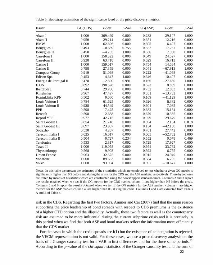
Table 5. Bootstrap estimation of the significance level of the price discovery metrics.
Issuer GG(CDS) t-Stat p-Val GG(ASP) t-Stat p-Val
Akzo I 1.000 369.499 0.000 0.233 −29.107 1.000Akzo II 0.950 29.214 0.000 0.651 12.216 0.000BMW 1.000 62.696 0.000 0.605 6.407 0.000Bouygues I 0.493 −0.689 0.755 0.852 17.237 0.000Bouygues II 0.450 −4.255 1.000 0.656 7.960 0.000Carrefour I 1.000 158.322 0.000 0.649 24.527 0.000Carrefour II 0.928 63.718 0.000 0.629 16.713 0.000Casino I 1.000 159.017 0.000 0.754 14.534 0.000Casino II 0.798 27.359 0.000 0.041 −67.913 1.000Compass Group 0.919 51.098 0.000 0.222 −41.068 1.000Edison Spa 0.453 −4.647 1.000 0.646 10.407 0.000Energia de Portugal II 0.478 −2.390 0.991 0.166 −27.630 1.000E.ON 0.892 198.328 0.000 0.623 8.809 0.000Iberdrola I 0.744 29.706 0.000 0.732 12.883 0.000Kingfisher 0.967 47.427 0.000 0.351 −13.782 1.000Koninklijke KPN 0.502 0.080 0.468 0.169 −41.129 1.000Louis Vuitton I 0.784 61.625 0.000 0.626 6.382 0.000Louis Vuitton II 0.928 44.549 0.000 0.601 7.035 0.000PPR 0.598 17.425 0.000 0.682 15.184 0.000Renault 0.598 12.688 0.000 0.679 10.335 0.000Repsol YPF 0.977 42.715 0.000 0.929 29.679 0.000Saint Gobain II 0.854 21.746 0.000 0.594 2.104 0.018Saint Gobain III 0.697 23.907 0.000 0.154 −42.130 1.000Sodexho 0.538 4.207 0.000 0.761 27.442 0.000Telecom Italia I 0.625 16.017 0.000 0.005 −52.782 1.000Telecom Italia II 0.504 0.727 0.234 0.552 0.078 0.469Telefonica 0.533 2.817 0.002 0.729 17.927 0.000Tesco II 1.000 119.058 0.000 0.954 33.782 0.000Thyssenkrupp 0.568 9.903 0.000 0.592 6.755 0.000Union Fenosa 0.963 32.525 0.000 0.915 24.949 0.000Vodafone 1.000 89.653 0.000 0.584 6.705 0.000Volvo 1.000 93.904 0.000 0.397 −10.677 1.000
Notes: In this table we present the estimates of the t-statistics which are employed to test whether a given GG metric issignificantly higher than 0.5 before and during the crisis for the CDS and the ASP markets, respectively. These hypothesesare tested by means of t-statistics which are constructed using the bootstrapped standard errors. Columns 2 and 3 reportthe results obtained when we test if the GG metrics for the CDS market, column 1, are higher than 0.5 before the crisis.Columns 5 and 6 report the results obtained when we test if the GG metrics for the ASP market, column 4, are highermetrics for the ASP market, column 4, are higher than 0.5 during the crisis. Columns 1 and 4 are extracted from PanelsA and B of Table 4.
risk in the CDS. Regarding the first two factors, Ammer and Cai (2007) find that the main reasonsupporting the price leadership of bond spreads with respect to CDS premiums is the existenceof a higher CTD option and the illiquidity. Actually, these two factors as well as the counterpartyrisk are assumed to be more influential during the current subprime crisis and it is precisely inthis period when we find that both ASP and bond markets reflect the information more efficientlythat the CDS market.
For the cases in which the credit spreads are I(1) but the existence of cointegration is rejected,the VECM representation is not valid. For these cases, we use a price discovery analysis on thebasis of a Granger causality test for a VAR in first differences and for the three same periods.42
According to the p-value of the chi-square statistics of the Granger causality test and the sum of
Dow
nloa
ded
by [
Uni
vers
idad
Car
los
Iii M
adri
d] a
t 11:
41 1
2 M
arch
201
2
22
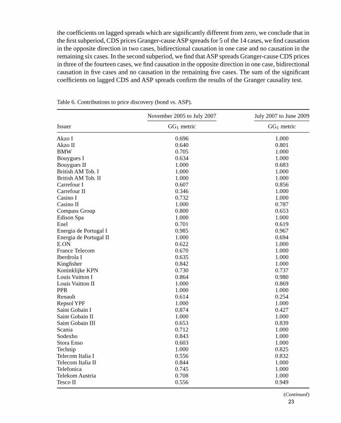
The European Journal of Finance 873
the coefficients on lagged spreads which are significantly different from zero, we conclude that inthe first subperiod, CDS prices Granger-cause ASP spreads for 5 of the 14 cases, we find causationin the opposite direction in two cases, bidirectional causation in one case and no causation in theremaining six cases. In the second subperiod, we find that ASP spreads Granger-cause CDS pricesin three of the fourteen cases, we find causation in the opposite direction in one case, bidirectionalcausation in five cases and no causation in the remaining five cases. The sum of the significantcoefficients on lagged CDS and ASP spreads confirm the results of the Granger causality test.
Table 6. Contributions to price discovery (bond vs. ASP).
November 2005 to July 2007 July 2007 to June 2009
Issuer GG1 metric GG1 metric
Akzo I 0.696 1.000Akzo II 0.640 0.801BMW 0.705 1.000Bouygues I 0.634 1.000Bouygues II 1.000 0.683British AM Tob. I 1.000 1.000British AM Tob. II 1.000 1.000Carrefour I 0.607 0.856Carrefour II 0.346 1.000Casino I 0.732 1.000Casino II 1.000 0.787Compass Group 0.800 0.653Edison Spa 1.000 1.000Enel 0.701 0.619Energia de Portugal I 0.985 0.967Energia de Portugal II 1.000 0.694E.ON 0.622 1.000France Telecom 0.670 1.000Iberdrola I 0.635 1.000Kingfisher 0.842 1.000Koninklijke KPN 0.730 0.737Louis Vuitton I 0.864 0.980Louis Vuitton II 1.000 0.869PPR 1.000 1.000Renault 0.614 0.254Repsol YPF 1.000 1.000Saint Gobain I 0.874 0.427Saint Gobain II 1.000 1.000Saint Gobain III 0.653 0.839Scania 0.712 1.000Sodexho 0.843 1.000Stora Enso 0.603 1.000Technip 1.000 0.825Telecom Italia I 0.556 0.832Telecom Italia II 0.844 1.000Telefonica 0.745 1.000Telekom Austria 0.708 1.000Tesco II 0.556 0.949
(Continued)
Dow
nloa
ded
by [
Uni
vers
idad
Car
los
Iii M
adri
d] a
t 11:
41 1
2 M
arch
201
2
23
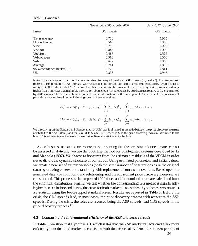
874 S. Mayordomo et al.
Table 6. Continued.
November 2005 to July 2007 July 2007 to June 2009
Issuer GG1 metric GG1 metric
Thyssenkrupp 0.723 0.915Union Fenosa 0.565 1.000Vinci 0.750 1.000Vivendi 0.883 1.000Vodafone 0.488 0.525Volkswagen 0.983 1.000Volvo 0.622 1.000Average 0.781 0.89395% confidence interval LL 0.729 0.841UL 0.833 0.945
Notes: This table reports the contributions to price discovery of bond and ASP spreads (bst and sAt ). The first column
presents the contribution of ASP spreads with respect to bond spreads during the period before the crisis. A value equal toor higher to 0.5 indicates that ASP markets lead bond markets in the process of price discovery while a value equal to orhigher than 1 indicates that negligible information about credit risk is reported by bond spreads relative to the one reportedby ASP spreads. The second column reports the same information for the crisis period. As in Table 4, the measures ofprice discovery are based on the following system of two equations:
�sAt = α1(s
At−1 − β3 − β2bst−1) +
p∑j=1
δ1,j�sAt−j +
p∑j=1
η1,j�bst−j + u1,t
�bst = α2(sAt−1 − β3 − β2bst−1) +
p∑j=1
δ2,j�sAt−j +
p∑j=1
η2,j�bst−j + u2,t .
We directly report the Gonzalo and Granger metric (GG1) that is obtained as the ratio between the price discovery measureattributed to the ASP (PD1) and the sum of PD1 and PD2, where PD2 is the price discovery measure attributed to thebond. This ratio indicates the percentage of price discovery attributed to the ASP.
As a robustness test and to overcome the shortcoming that the precision of our estimates cannotbe assessed analytically, we use the bootstrap method for cointegrated systems developed by Liand Maddala (1997). We choose to bootstrap from the estimated residuals of the VECM in ordernot to distort the dynamic structure of our model. Using estimated parameters and initial values,we create a new set of system variables (with the same number of observations as in the originaldata) by drawing observations randomly with replacement from the innovations. Based upon thegenerated data, the common trend relationship and the subsequent price discovery measures arere-estimated. This process is then repeated 1000 times and the standard errors are calculated fromthe empirical distribution. Finally, we test whether the corresponding GG metric is significantlyhigher than 0.5 before and during the crisis for both markets. To test these hypotheses, we constructa t-statistic using the bootstrapped standard errors. Results are reported in Table 5. Before thecrisis, the CDS spreads lead, in most cases, the price discovery process with respect to the ASPspreads. During the crisis, the roles are reversed being the ASP spreads lead CDS spreads in theprice discovery process.43
4.3 Comparing the informational efficiency of the ASP and bond spreads
In Table 6, we show that Hypothesis 3, which states that the ASP market reflects credit risk moreefficiently than the bond market, is consistent with the empirical evidence for the two periods of
Dow
nloa
ded
by [
Uni
vers
idad
Car
los
Iii M
adri
d] a
t 11:
41 1
2 M
arch
201
2
24
The European Journal of Finance 875
time analysed. This result confirms empirically for the first time, at least to our knowledge, thatthe ASP spread is a better measure for credit risk than bond spreads are. Only in two of a total of46 cases in the first subperiod, do bond spreads lead ASP spreads. This occurs in two cases in thesecond subperiod. The reason that explains these results may be a higher relative liquidity in theASP market, which means that the number of market participants in the ASP market (liquidity)is greater than the number of players in the bond market.
5. Conclusions
We find that liquidity does affect the price discovery process in credit derivatives markets. Wemake three contributions to the literature. Firstly, we offer a theoretical model for testing pricediscovery in credit derivatives markets that allows for simultaneous agent participation in differentmarkets. Secondly, we analyse the price discovery process between ASPs and CDSs and find thatthe leadership, in terms of price discovery, between ASPs and CDSs is very sensitive to theappearance of the subprime crisis. Before the crisis, the CDS market leads the ASP market butduring the crisis the ASP market leads the CDS market. Thirdly, to our knowledge, this is the firstprice discovery analysis based on the ASP and bond markets. We find, according to GS terms,that the bond market is a ‘pure satellite’ of the asset swap market. Thus, the ASP spread is a moreaccurate measure of credit risk than the bond spread. For this reason, it seems more appropriate touse the ASP spread as an alternative or as a complement to the CDS rather than the bond spread.
Finally, we highlight the four main policy implications that emerge from our study and whichcould be of special interest for investors and regulators alike. First, we find that during the crisis,the ASP market reveals credit risk more efficiently that the CDS market. Reasons explainingthis finding include the CTD option embedded in the CDS spread, the liquidity premium andthe counterparty risk in CDSs.44 The key implication of this result is that inferences on thecreditworthiness of a given firm based solely in CDS spreads in periods of high market turbulenceand low liquidity are bound to be misleading. Second, we find that the ASP spread leads theprice discovery process of credit risk more efficiently than the bond spread, before and duringthe crisis. For this reason, it is more appropriate to use the ASP spread as an alternative or as acomplement to the CDS spread as a measure of credit risk rather than the bond spread. However,most of the existing literature has focused primarily on the bond and CDS spreads ignoring therole of the ASP spread as a credit risk indicator. Third, our theoretical model and empirical resultshighlight the importance of the agents that operate in both markets (NBOTH) in order to providestability to the credit markets. The arbitrageurs also play a special role in these markets given thattheir demands are defined in terms of a long-run equivalence or adjustment which could reducedeviations from the equilibrium prices. Fourth, the debt hedgers do not play any apparent rolein the price discovery process if they are fully hedged. However, when they only hedge a givenproportion of the total investment in ASPs or bonds, they also contribute to the price discoveryprocess.
Acknowledgements
We are grateful to the Editors of this special issue: John Wilson, Barbara Casu, and David McMillan for their usefulcomments. We owe thanks to two anonymous referees for many astute comments that considerably improved the study. Wealso thank Isabel Figuerola-Ferretti, Javier Gil, Carlos González-Aguado, Jesús Gonzalo, Neil Kellard, María Rodríguez,Pedro Serrano, Javier Suárez and seminar participants at the XVII Foro de Finanzas and at the Emerging Scholars inBanking and Finance Conference at Cass Business School for all their comments and suggestions. Sergio Mayordomo and
Dow
nloa
ded
by [
Uni
vers
idad
Car
los
Iii M
adri
d] a
t 11:
41 1
2 M
arch
201
2
25
876 S. Mayordomo et al.
Juan Ignacio Peña acknowledge financial support from MICINN Grant Ref: ECO2009-12551. Juan Romo acknowledgesfinancial support from MICINN Grant Ref: ECO2008-05080. The usual disclaimer applies.
Notes
1. Acharya and Schaefer (2006) posit that the liquidity risk can be defined as unpredictable changes in transaction costsand in liquidity. These adverse liquidity shocks, systematic or idiosyncratic, are mainly due to high and negativechanges in financial products’ returns and reduce the amount of capital available to financial intermediaries whichlowers the ability of their trading desk to provide liquidity.
2. The value of CDSs outstanding at the end of 2004, 2005 and 2006 was $8.42, $17.1 and $34.4 trillion, respectively.The CDS market exploded over the past decade to more than $45 trillion in mid-2007 and more than $62 trillion inthe second half of the same year, according to the ISDA. The size of the CDS market in mid-2007 is roughly twice thesize of the US stock market (which is valued at about $22 trillion) and far exceeds the $7.1 trillion mortgage marketand $4.4 trillion US treasuries market. However, the notional amount outstanding decreased to $38.6 trillion at theend of 2008.
3. The main reason is the existence of a higher CTD option due to the higher risk of borrowers and also to liquidityreasons given that the higher the number of bonds issued, which they use as a liquidity measure, the more difficult isthat the CDS market leads price discovery.
4. According to Dötz (2007), the relatively large contribution of the CDS market to price discovery is not necessarilytantamount to general and lasting improvement in the processing of information; the turbulence in the credit marketsin the spring of 2005 was apparently handled much better by the bond market than by the CDS market. The weaknessesof the CDSs are likely to consist in the relatively high concentration and homogeneousness of its market players,whose herding behaviour, particularly in times of crisis, can strain liquidity, amplify market volatility and hamperprice discovery.
5. Chan-Lau and Kim (2004) relate the same three financial instruments but for emerging market sovereign issuers.In most countries, they do not find any equilibrium price relationship between equity and bond markets andin terms of price discovery, it is difficult to conclude that one particular market dominates the price discoveryprocess.
6. As far as we know, the relationship between ASP and CDS has only been treated in De Wit (2006). However, theperspective adopted in De Wit (2006) is based on the long-run equilibrium that should exist, and which the authorfinds, between ASP and CDS, ignoring the price discovery process.
7. Although we develop the case of CDS and ASP prices, the model can also be applied to study the interaction betweenCDS and bond spreads or between ASP and bond spreads.
8. A popular arbitrage strategy employed by hedge funds in credit derivatives markets defines the correct price from along-term equilibrium price based on the cointegration methodology. The arbitrageur is betting only that the spreadbetween the two cointegrated assets will narrow, which can be understood as a permanent adjustment process towardsan economic equilibrium.
9. As Dötz (2007) state, the market for synthetic CDO products, which as opposed to cash CDS products are not backedby bonds or loans but by CDSs, presents some advantages such as the better availability of CDSs relative to bonds orloans and the heavy demand among investors for unfunded supersenior tranches.
10. We may also find protection sellers who hedge their positions, again, in the CDS market or individuals that participatein the CDS market in order to hedge their exposures to other institutions that are not due to debt positions.
11. We include this type of agents in order to make the model more comprehensive, given that the nature of CDSs is toprovide insurance. In fact, CDSs are usually used to manage the credit risk.
12. As CDSs are over-the-counter (OTC) instruments, it is possible to buy a CDS contract whose maturity coincideswith the bond’s maturity and whose premium payments timing is agreed by the parties. As the bond’s maturity dateapproaches, the use of CDSs with a 5-year constant maturity would lead to overhedging, given that the maturity datesof CDSs and asset swaps do not coincide. The consequence is that the investor will pay a CDS spread above theone needed to be fully hedged. Thus, we take advantage of the range of CDSs maturities to fit a CDS curve using aPiecewise Cubic Hermite Interpolating Polynomial algorithm that allows us to match asset swap and CDS maturities.This method is also used in Levin, Perli, and Zakrajšek (2005).
13. In order to proceed in this way, we assume that the investor can borrow money at Euribor flat.14. If sA
t − s̄t > 0, then a profitable arbitrage opportunity exists. The investor should take long positions in both CDS andASP and borrow the required quantity of money in order to finance the investment at 3 months Euribor. If sA
t − s̄t < 0,the inverse strategy will lead to an arbitrage opportunity.
Dow
nloa
ded
by [
Uni
vers
idad
Car
los
Iii M
adri
d] a
t 11:
41 1
2 M
arch
201
2
26
The European Journal of Finance 877
15. A combination of short positions on both the CDS and ASP leads to a net payment for the investor equal to thedifference between CDS and ASP spreads, s̄t − sA
t .16. The net payoff is also zero at coupon payment dates while at the bond’s maturity, as in every quarterly payment, the
net payoff is equal to the basis.17. Assumption A1 is necessary to reach a two-sided bound on the CDS rate and to guarantee that the equivalence
relationship holds.18. An example of a statistical arbitrage analysis in credit derivatives markets according to the technique and concept
introduced Hogan et al. (2004) can be found in Mayordomo, Peña, and Romo (2009).19. Cossin and Lu (2005) state that the liquidity premium, the CTD option and the market segmentation explain the
pricing differences between bonds and CDS. The effect of the CTD option is more important as default risk increases.20. If the two markets price credit risk equally in the long run, then their prices should be cointegrated with cointegrating
vector [1,-1,c], suggesting a stationary basis.21. Shorting a corporate bond or an ASP with a required maturity, even years, is not an easy task. The short sale of bonds
or ASPs could be done via a repurchase agreement (repo) but as Blanco, Brennan, and Marsh (2005) explain, it isimpossible to borrow a bond via a repo. The reason is that repo market for corporate bonds is illiquid and even if itis possible to short a bond via a repo, the tenor of the agreement would be short. Schonbucher (2003) states that thislimitation could be solved by issuing credit-linked notes linked to the corresponding bond and selling them to theinvestors in the asset swap market. This alternative presents other limitations given that the issuance of credit-linkednotes takes time and implies high fixed cost. This fact implies that deviations in the equivalence relationship might notimply arbitrage opportunities whenever an asset swap short sale is needed. Thus, in some cases traders are not ableto exploit price differentials when the CDS premium is higher than the asset swap spread and as Blanco, Brennan,and Marsh (2005) suggest, this asymmetry may affect significantly the dynamic adjustment of credit spreads. Therestrictions on short-sales could be even more severe in periods of financial distress.
22. These individual interpret that RCDSi,t is the CDS price, given its probability of default. As the market price s̄t is above
the reservation price, the investor is interested in selling protection in exchange of s̄t .23. Note that the total endowments can increase exogenously from period t to period t + 1, for instance, by means of
CDS or bond issuances.24. The idea is that under the assumptions employed when defining the arbitrageurs demand, the fact that the ASP spread
is a good indicator, although not perfect, of the CDS spread and given that both spreads are prices of the credit riskof a given firm, it seems reasonable to assume that the elasticities are similar.
25. The objective of this paper is not related with the literature of credit risk pricing and so, Equations (10) and (11) arenot pricing equations of credit risk, such as the ones defined from the probability of default and recovery rates, butsimply the ASP and CDS prices that clear both markets.
26. We do not report the whole expression of ut in order to save space and also, because of the assumptions on residualsthey are not going to appear in our analysis.
27. Although hedgers are not important in the price discovery process, they must be included in the model because theseindividuals really participate in credit markets and we need them in order to make the model more comprehensive.
28. This decline in trading during the second half of 2008 reflects a combination of significantly reduced risk appetite,expectations of stable low interest rates in major markets and lower hedge fund activity. Exchange rate movementsmay also have affected to this decline. Most institutions report their positions in US dollars and the euro and thepound sterling depreciated by 30% and 12%, respectively, against the US dollar between June and December 2008.
29. During the first quarter of 2009, issuance of investment grade corporate bonds in Europe totalled a record ¤140bn,well above quarterly levels of less than ¤50bn seen in recent years. It is motivated, among other reasons, by the use ofbond markets for funding and the government guarantees to aid to the bond issuance. IFSL Research (2009b) reportsthat the amounts outstanding on the global bond market, which includes bonds, notes and money market instruments,increased 6% in 2008 to $83 trillion.
30. See for instance Norden and Weber (2004), Blanco, Brennan, and Marsh (2005), Zhu (2006), Baba and Inada (2007),Dötz (2007), Forte and Peña (2009) and Coudert and Gex (2010).
31. In a limit case, if NBOTH tends to infinity, the price discovery is equal to 0.5.32. Allocation to bonds from high-net-worth individuals increased from 27% to 29% during 2008 with equities seeing
the largest decline in their share of portfolio allocation.33. The nominal of CDSs with respect to ASP contracts serves to show how in periods of financial distress it is much
more difficult to participate in CDS than in ASP markets. The standard bond’s faced value is ¤1000 while the CDStypical notional amount is ¤10–20 million for investment grade credits and ¤2–5 million for high yield credits.
34. Ammer and Cai (2007) state that the main reason to support that bond spreads lead CDS premiums is the existenceof a higher CTD option and for liquidity reasons. In particular they employ as a liquidity measure the number of
Dow
nloa
ded
by [
Uni
vers
idad
Car
los
Iii M
adri
d] a
t 11:
41 1
2 M
arch
201
2
27
878 S. Mayordomo et al.
bonds outstanding by a given firm and find that the higher the number of bonds the less likely it is that CDSs willlead price discovery. Under illiquid scenarios, the CTD option embedded in CDS becomes more valuable and theliquidity premium to bear liquidity risk increases.
35. The GFI FENICS® Credit curve gives preference to real trades and quoted mid- points where available, and in theirabsence, it is based on the calculation of a running point level using the John Hull and Alan White methodology toensure a credit curve always exists for each reference entity. This curve is a good approximation for CDSs at anymaturity as several error analyses reveal. The median of the absolute difference in basis points between five yearsCDS premiums as defined from credit curve and the actual quotes or transaction prices for the period between April2001 and May 2002, is equal to 1.16, 2.01 and 3.82 basis points for AAA/AA, A and BBB ratings for a total of 2659,9585 and 8170 companies, respectively. Moreover, market CDS spread could be different from what we are assumingto be the true CDS spread by as much as 3.725 bps. on average.
36. This limit is set in order to avoid the selection of bonds with a small volume which could require higher transactioncosts due to their reduced liquidity.
37. Our initial sample was 285 corporate bond issuers. We found a total of 116¤ denominated bonds that mature beforeFebruary 2012 but only 67 of them include information on 5-year bid/ask CDS spreads, asset swap spreads andFenics Curve for at least 90 trading days. Of these, two bonds have been discarded because the issued amount doesnot exceed 300 millions of Euros, another four bonds were discarded because they were not investment grade bondsthroughout the whole sample period. Another four bonds were discarded because their asset swap spreads werepersistently negative and, finally, seven bonds were discarded because prices were too far from par.
38. We do not report these results because they are similar to the ones presented in Table 3. However, these results areavailable upon request.
39. Cointegration test detailed results for ASP and bond spreads are available upon request.40. The detailed results are available upon request.41. Results of this analysis are available upon request.42. These results are available upon request.43. The t-statistics presented in Table 5 are obtained using the GG metrics reported in Table 4. Moreover, we employ the
average GG metric obtained across the 1000 bootstrap repetitions and obtain similar results.44. Amato and Remolona (2003) state that when it turns out to be very costly to undertake transactions in a given
instrument, the investors must be compensated for it. This compensation is reinforced in the presence of uncertaintyabout the liquidity (or illiquidity) of an ASP, bond or CDS at a given time, and thus the investors could require apremium to bear this risk. This liquidity premium has been proved to exist both in CDS and bond markets. Longstaff,Mithal and Neis (2005) and Tang and Yan (2007) among others support the presence of a liquidity premium in CDSspreads. Collin-Dufresne, Goldstein, and Martin (2001), Perraudin and Taylor (2003), Elton et al. (2001), Delianedisand Geske (2001) and Chen, Lesmond, and Wei (2007) among others find that liquidity is an additional factor tocredit risk which is present in bond spreads.
45. We do not report the whole expression of ut in order to save space and also, because of the assumptions on residualsthey are not going to appear in our analysis.
References
Acharya, V., and S. Schaefer. 2006. Liquidity risk and correlation risk: Implications for risk management. Working Paper,London Business School.
Acharya, V., S. Schaefer, and Y. Zhang. 2007. Liquidity risk and correlation risk: A clinical study of the General Motorsand Ford Downgrade of May 2005. Working Paper, SSRN.
Amato, J., and E. Remolona. 2003. The credit spread puzzle. BIS Quarterly Review, December: 51–63.Ammer, J., and F. Cai. 2007. Sovereign CDS and bond pricing dynamics in emerging markets: Does the cheapest-to-deliver
option matter? International Finance Discussion Papers Number 912, Board of Governors of the Federal ReserveSystem.
Baba, N., and M. Inada. 2007. Price discovery of credit spreads for Japanese mega-banks: Subordinated bond and CDS.Duscussion Paper 2007-E-6, Institute for Monetary and Economic Studies, Bank of Japan.
Bai, J., and P. Perron. 2003. Computation and analysis of multiple structural change models. Journal of AppliedEconometrics 18: 1–22.
Blanco, F., S. Brennan, and I.W. Marsh. 2005. An empirical analysis of the dynamic relation between investment gradebonds and credit default swaps. Journal of Finance 60, no. 5: 2255–81.
Dow
nloa
ded
by [
Uni
vers
idad
Car
los
Iii M
adri
d] a
t 11:
41 1
2 M
arch
201
2
28
The European Journal of Finance 879
Chan-Lau, J.A., and Y.S. Kim. 2004. Equity prices, credit default swaps, and bond spreads in emerging markets. WorkingPaper, IMF.
Chen, L., D.A. Lesmond, and J. Wei. 2007. Corporate yield spreads and bond liquidity. The Journal of Finance 62, no. 1:119–49.
Collin-Dufresne, P., R. Goldstein, and S. Martin. 2001. The determinants of credit spread changes. Journal of Finance56, no. 6: 2177–207.
Cossin, D., and H. Lu. 2005. Are European corporate bonds and default swap markets segmented? Working Paper 153,FAME.
Coudert, V., and M. Gex. 2010. Contagion inside the credit default swaps market: The case of the GM and Ford crisis in2005. Journal of International Financial Markets, Institutions and Money 20, no. 2: 109–34.
De Jong, F., and J. Driessen. 2006. Liquidity risk premia in corporate bond markets. Working Paper, University ofAmsterdam.
De Wit, J. 2006. Exploring the CDS-bond basis. Working Paper, National Bank of Belgium.Delianedis, G., and R. Geske. 2001. The components of corporate credit spreads: Default, recovery, tax, jumps, liquidity,
and market factors. Working Paper, University of California.Dötz, N. 2007. Time-varying contributions by the corporate bond and CDS markets to credit risk price discovery.
Discussion Paper Series 2: Banking and Financial Studies No 08, Deutsche Bundesbank.Elton, E., D. Gruber, D. Agrawal, and C. Mann. 2001. Explaining the rate spread on corporate bonds. Journal of Finance
56, no. 1: 247–77.Engle, R., and C.W.J. Granger. 1987. Co-integration and error correction: Representation, estimation, and testing.
Econometrica 55, no. 2: 251–76.Felsenheimer, J. 2004. CDS: Mechanism, pricing and application. HVB Global Markets Research, 2 June.Figuerola-Ferretti, I., and J. Gonzalo. 2010. Modelling and measuring price discovery in commodity markets. Journal of
Econometrics 158, no. 1: 95–107.Forte, S., and J.I. Peña. 2009. Credit spreads: An empirical analysis on the informational content of stocks, bonds and
CDS. Journal of Banking and Finance 33, no. 11: 2013–25.Francis, C.,A. Kakodkar, and B. Martin. 2003. Credit derivative handbook 2003. Merrill Lynch Global Securities Research
and Economics Group.Fulop,A., and L. Lescourret. 2007.An analysis of intra-daily patterns on the CDS market. Working Paper, ESSEC Business
School.Garbade, K.D., and W.L. Silver. 1983. Price movements and price discovery in commodity markets. Review of Economics
and Statistics 65, no. 2: 289–97.Gonzalo, J., and C.W.J. Granger. 1995. Estimation of common long-memory components in cointegrated systems. Journal
of Business and Economics Statistics 13, no. 1: 27–35.Goyenko, R.Y., C.W. Holden, and C.A. Trzcinka. 2009. Do liquidity measures measure liquidity? Journal of Financial
Economics 92, no. 2: 153–81.Hasbrouck, J. 1995. One security, many markets: Determining the contributions to price discovery. Journal of Finance
50, no. 4: 1175–99.Hogan, S., R.A. Jarrow, M. Teo, and M. Warachka. 2004. Testing market efficiency using statistical arbitrage with
applications to momentum and value strategies. Journal of Financial Economics 73, no. 3: 525–65.Hull, J., M. Predescu, and A. White. 2004. The relationship between credit default swap spreads, bond yields, and credit
rating announcements. Journal of Banking and Finance 28: 2789–811.International Financial Services London (IFSL) Research. 2009a. Derivatives 2009.International Financial Services London (IFSL) Research. 2009b. Bond Markets 2009.Johansen, S. 1991. Estimation and hypothesis testing of co-integration vectors in gaussian vector autoregressive models.
Econometrica 59, no. 6: 1551–80.Juselius, K. 2006. The cointegrated VAR model: Methodology and applications. Oxford: Oxford University Press.Levin, A., R. Perli, and E. Zakrajšek. 2005. The determinants of market frictions in the corporate market. Working Paper,
Federal Reserve Board, Washington.Li, H., and G.S. Maddala. 1997. Bootstrapping cointegrating regressions. Journal of Econometrics 80, no. 2: 297–313.Longstaff, F.A., S. Mithal, and E. Neis. 2005. Corporate yield spreads: Default risk or liquidity? New evidence from the
credit default swap market. Journal of Finance 60, no. 5: 2213–53.Mayordomo, S., J.I. Peña, and J. Romo. 2009. Are there arbitrage opportunities in credit derivatives markets? A new test
and an application to the case of CDS and ASPs. Working Paper, Universidad Carlos III de Madrid.Nashikkar, A.J., and M.G. Subrahmanyam. 2007. Latent liquidity and corporate bond yield spreads. NYU Working Paper
No. FIN-07-013.
Dow
nloa
ded
by [
Uni
vers
idad
Car
los
Iii M
adri
d] a
t 11:
41 1
2 M
arch
201
2
29
880 S. Mayordomo et al.
Nashikkar, A.J., M.G. Subrahmanyam, and S. Mahanti. 2009. Limited arbitrage and liquidity in the market for credit risk.NYU Working Paper No. FIN-08-011.
Norden, L., and M. Weber. 2004. Informational efficiency of credit default swap and stock markets: The impact of creditratings announcements. Journal of Banking and Finance 28, no. 11: 2813–43.
Perraudin, W., and A. Taylor. 2003. Liquidity and bond market spreads. Working Paper, Bank of England.Predescu, M. 2006. The performance of structural models of default for firms with liquid CDS spreads. Working Paper,
Rotman School of Management, University of Toronto.Saita, L. 2006. The puzzling price of corporate default risk. Working Paper, Standford Graduate School of Business.Schonbucher, P.J. 2003. Credit derivatives pricing models: Models, pricing, implementation. Wiley Finance.Stein, J.L. 1961. The simultaneous determination of spot and future prices. The American Economic Review 51, no. 5:
1012–25.Tang, D.Y., and H. Yan. 2007. Liquidity and credit default swap spreads. Working Paper, Kennesaw State University.Working, H. 1948. Theory of the inverse carrying charge in futures markets. Journal of Farm Economics 30, no. 1: 1–28.Yan, B., and E. Zivot. 2007. The dynamics of price discovery. Working Paper Series, University of Washington.Zeileis,A., C. Kleiber,W. Krämer, and K. Hornik. 2003. Testing and dating of structural changes in practice. Computational
Statistics and Data Analysis 44, nos. 1–2: 109–23.Zhu, H. 2006. An empirical comparison of credit spreads between the bond market and the credit default swap market.
Journal of Financial Services Research 29, no. 3: 211–35.
Appendix 1
In order to obtain an expression for the credit spreads we substitute the expressions (14) into the Equations (10) and (11)and obtain the following equation:
(sAt
s̄t
)= Hβ3
B
[(NBOTH + NCDS)
−(NBOTH + NASP)
]+ Q
(sAt−1
s̄t−1
)+
(uASP
t
uCDSt
), (A1)
where (uASPt , uCDS
t ) is a vector white noise with E(ut ) = 0 and Var(ut ) = � > 0. In ut we include both the commoncomponents and the participants’noises.45 The model in Equation (15) can be changed into a VECM model by subtractingvector of prices ((sA
t , s̄t )′ from both sides:
(�sA
t
�s̄t
)= Hβ3
B
[(NBOTH + NCDS)
−(NBOTH + NASP)
]+ (Q − I )
(sAt−1
s̄t−1
)+
(uASP
t
uCDSt
)(A2)
with
Q − I = 1
B
[−H(NBOTH + NCDS) Hβ2(NBOTH + NCDS)
H(NBOTH + NASP) −Hβ2(NBOTH + NASP)
]. (A3)
The previous expression can be transformed into the following final expression (Equation (15)):
(�sA
t
�s̄t
)= H
B
[−(NBOTH + NCDS)
(NBOTH + NASP)
](1, −β2, −β3)
⎛⎜⎝sA
t−1
s̄t−1
1
⎞⎟⎠ +
(uASP
t
uCDSt
). (A4)
Appendix 2
In this paper, we adopt GG’s methodology and thus, their PT component decomposition to measure market contributionto price discovery. GG PT decomposition has the following form:
Xt = A1ft + A2zt , (A5)
Dow
nloa
ded
by [
Uni
vers
idad
Car
los
Iii M
adri
d] a
t 11:
41 1
2 M
arch
201
2
30
The European Journal of Finance 881
where ft is the permanent component, zt is the transitory component, and A1 and A2 are loading matrices. The componentsft and zt are linear combinations of Xt such that ft ∼ I (1), zt ∼ I (0), zt does not Granger cause ft in the long run and:
ft = γ ′Xt (A6a)
A1 = β⊥(α′⊥β⊥)−1 and γ = (α′⊥β⊥)−1α′⊥, (A6b)
where α⊥ and β⊥ are 2 × 1 vectors such that α′⊥α⊥ = 0 and β ′⊥β⊥ = 0 or equivalently:
α1,⊥ = H
B(NBOTH + NASP) (A7a)
α2,⊥ = H
B(NBOTH + NCDS), (A7b)
while β⊥ = (β2, 1). Taking all these things together we have that:
γ ′ =
⎡⎢⎢⎣
(NBOTH + NASP)
β2(NBOTH + NASP) + (NBOTH + NCDS),
(NBOTH + NCDS)
β2(NBOTH + NASP) + (NBOTH + NCDS)
⎤⎥⎥⎦ (A8)
and the permanent component ft is defined as:
(NBOTH + NASP)
β2(NBOTH + NASP) + (NBOTH + NCDS)sAt + (NBOTH + NCDS)
β2(NBOTH + NASP) + (NBOTH + NCDS)s̄t , (A9)
where the factor that multiplies sAt represents the price discovery measure attributed to the ASP (PD1) and the factor that
multiplies s̄t represents the price discovery measure attributed to the CDS (PD2). The ratio γ in Equation (A8) that isobtained from the orthogonal vector to α, which is denoted as α⊥ (see Equations (A7a) and (A7b)), can be understood asthe relative number of market participants in a given market with respect to the other.
The percentage of price discovery attributable to ASP and CDS markets can also be defined as:
PD1
PD1 + PD2= GG1 and
PD2
PD1 + PD2= GG2, (A10)
where GG1 and GG2 represent the GG price discovery metrics for the ASP and the CDS markets, respectively.These metrics can be defined equivalently as:
GG1 = α2
−α1 + α2and GG2 = −α1
−α1 + α2. (A11)
After substituting we obtain:
GG1 = NBOTH + NASP
2NBOTH + NASP + NCDSand GG2 = NBOTH + NCDS
2NBOTH + NASP + NCDS. (A12)
In order to be consistent with our model we investigate price discovery based on the metrics that when transformed intorelative terms are equivalent to the GG approach’s metrics of Equation (A10).A cointegrating vector between credit spreadsdifferent from (1, −1) can be theoretically supported by our price discovery model given that the standard requirementthat β2 = 1 may be very restrictive.
Dow
nloa
ded
by [
Uni
vers
idad
Car
los
Iii M
adri
d] a
t 11:
41 1
2 M
arch
201
2
31