Preliminary Comparison of Techniques for Dealing withImbalance in Software Defect Prediction

Daniel RodriguezDept of Computer Science

University of Alcala28871 Alcalá de Henares,

Madrid, Spaindaniel.rodriguezg@uah.es

Israel HerraizTechnical Univ of Madrid

(UPM)28040 Madrid, Spain(Now at AMADEUS)isra@herraiz.org

Rachel HarrisonSchool of Technology

Oxford Brookes UniversityOxford OX33 1HX, UK

rachel.harrison@brookes.ac.uk

Javier DoladoDept of Computer ScienceUniv of the Basque Country

20018 Donostia, Spainjavier.dolado@ehu.es

José C. RiquelmeDept of Computer Science

University of Seville41012 Seville, Spainriquelme@us.es

ABSTRACTImbalanced data is a common problem in data mining whendealing with classification problems, where samples of a classvastly outnumber other classes. In this situation, many datamining algorithms generate poor models as they try to opti-mize the overall accuracy and perform badly in classes withvery few samples. Software Engineering data in general anddefect prediction datasets are not an exception and in thispaper, we compare different approaches, namely sampling,cost-sensitive, ensemble and hybrid approaches to the prob-lem of defect prediction with different datasets preprocesseddifferently. We have used the well-known NASA datasetscurated by Shepperd et al. There are differences in the re-sults depending on the characteristics of the dataset and theevaluation metrics, especially if duplicates and inconsisten-cies are removed as a preprocessing step.

Further Results and replication package:http://www.cc.uah.es/drg/ease14

Categories and Subject DescriptorsD.2.8 [Software Engineering]: Metrics—complexity mea-sures, performance measures

General TermsMeasurement, Experimentation

KeywordsDefect Prediction, Imbalanced data, Data Quality

Permission to make digital or hard copies of all or part of this work for per-sonal or classroom use is granted without fee provided that copies are notmade or distributed for profit or commercial advantage and that copies bearthis notice and the full citation on the first page. Copyrights for componentsof this work owned by others than the author(s) must be honored. Abstract-ing with credit is permitted. To copy otherwise, or republish, to post onservers or to redistribute to lists, requires prior specific permission and/or afee. Request permissions from Permissions@acm.org.EASE ’14, May 13 - 14 2014, London, England, BC, United KingdomCopyright 2014 ACM 978-1-4503-2476-2/14/05 ...$15.00http://dx.doi.org/10.1145/2601248.2601294

1. INTRODUCTIONMost publicly available datasets in software defect pre-

diction are highly imbalanced, i.e., samples of non-defectivemodules vastly outnumber the defective ones. In this situ-ation, many data mining algorithms generate poor modelsbecause they try to optimize the overall accuracy but per-form badly in classes with very few samples. For example,if the number of non-defective samples outnumbers the de-fective samples by 95%, an algorithm that always predicts amodule as non-defective will obtain a very high accuracy. Asa result, many data mining algorithms obtain biased modelsthat do not take into account the minority class (defectivemodules). When the problem of imbalanced data is not con-sidered, many learning algorithms generate distorted modelsfor which (i) the impact of some factors can be hidden and(ii) the prediction accuracy can be misleading. This is dueto the fact that most data mining algorithms assume bal-anced datasets. The imbalance problem is known to affectmany machine learning algorithms such as decision tress,neural networks or support vectors machines [22]. Whendealing with imbalanced datasets, there are different alter-natives, either bootstrapping, sampling or balancing tech-niques, cost-sensitive evaluation, ensembles to wrap multi-ple classifiers making them more robust to the imbalanceproblem or hybrid techniques.

In this paper, we compare different types of algorithms todeal with imbalanced data in the domain of defect predictionusing well-known NASA datasets considering (i) differentevaluation metrics including the Matthew’s Correlation Co-efficient which has not been used in the domain of softwaredefect prediction and (ii) with different cleaning processes(in particular considering the removal of duplicates and in-consistencies).

The rest of the paper is organised as follows. Section 2describes the related work. Next, Section 3 briefly describesthe approaches to deal with imbalanced data, followed by theexperimental work in Section 4. Finally, Section 5 concludesthe paper and outlines future work.

2. RELATED WORKDefect prediction has been an important research topic

for more than a decade with an increasing number of papersincluding two recent systematic literature reviews [5, 19].Many classification techniques for defect prediction have

been proposed, including techniques which originated fromthe field of statistics (regression [2], and Support Vector Ma-chines [12], etc.), machine learning techniques (such as clas-sification trees [23]), neural networks [24], probabilistic tech-niques (such as Naıve Bayes [34] and Bayesian networks), en-sembles of different techniques and metaheuristic techniquessuch as ant colonies [45], etc. However, there are discrepan-cies among the outcomes as: (i) no classifier is consistentlybetter than the others; (ii) there is no optimum metric toevaluate and compare classifiers as highlighted in the follow-ing papers [31, 48, 34]; (iii) there are quality issues regardingthe data such as imbalanced class overlaps, outliers, trans-formation issues, etc.Seiffert et al. [41] analysed 15 software-quality data sets

of different sizes and levels of imbalance (including CM1,KC1, KC2, KC3, MW1 and PC1 from NASA datasets).For the NASA datasets, the authors used Halstead and Mc-Cabe base metrics together with some lines of code met-rics, i.e., attributes were manually selected. The authorsconcluded that boosting almost always outperforms sam-pling techniques using the area-under-the-curve (AUC) andKolmogorov-Smirnov (K-S) statistic as performance mea-sure.Khoshgoftaar et al. [25] also highlighted the problem of

imbalanced datasets when dealing with defect prediction andused Case-Based Reasoning to deal with this problem.In relation to the performance and evaluation of the clas-

sifiers, there is no technique that has consistently performedbetter than others. Several papers have compared multipletechniques with multiple evaluation measures. For exam-ple, Peng [37] proposes a performance metric to evaluatethe merit of classification algorithms using a broad selectionof classification algorithms and performance measures. Theexperimental results, using 13 classification algorithms with11 measures over 11 software defect datasets, indicate thatthe classifier which obtains the best result for a given datasetaccording to a given measure may perform poorly with a dif-ferent measure. The results of the experiment indicate thatSupport Vector Machines, the k-nearest neighbor algorithmand the C4.5 algorithm were ranked as the top three classi-fiers. Also Peng et al. [38] used ten NASA datasets to rankclassification algorithms, showing that a CART boosting al-gorithm and the C4.5 decision-tree algorithm with boostingare ranked as the optimum algorithms for defect prediction.Lessman et al. [26] also compared 22 classifiers grouped intostatistical, nearest neighbour, neural networks, support vec-tor machine, decision trees and ensemble methods over tendatasets from the NASA repository. The authors discussseveral performance metrics such as TPr and FPr but ad-vocate the use of Area Under the ROC (AUC) as the best in-dicator for comparing the different classifiers. This is knownnot to be optimal in the case of highly imbalanced datasets.Arisholm et al. [1] compared a classification tree algorithm

(C4.5), a coverage rule algorithm (PART), logistic regres-sion, back–propagation neural networks and Support VectorMachines over 13 releases of a Telecom middleware systemdeveloped in Java using three types of metrics: (i) object-oriented metrics, (ii) churn (delta) metrics between succes-sive releases, and (iii) process management metrics from aconfiguration management system. The authors concluded

that although there are no significe differences regarding thetechniques used, large differences can be observed dependingon the criteria used to compare them. The authors also pro-pose a new cost-effectiveness metric based on AUC and num-ber of statements so that larger modules are more expensiveto test. The same approach of considering module size inconjunction with the AUC as evaluation metrics has beenexplored by Mende and Koschke [32] using NASA datasetsand three versions of Eclipse with random forests [4] as theclassification technique.

3. APPROACHES TO DEAL WITH IMBAL-ANCED DATA

We can classify the different approaches to deal with im-balanced data as sampling, cost-sensitive, ensemble approachesor hybrid approaches. We next briefly describe the tech-niques used in this work.

3.1 Sampling TechniquesSampling techniques are classified as oversampling or un-

dersampling and are based on adding or removing instancesof the training dataset as a preprocessing step. The simpleprocedure of replicating instances from the minority class to-wards a more balanced distribution is called Random Over-Sampling (ROS), whereas Random Under-Sampling (RUS)removes instances from the majority class.

There are more sophisticated or intelligent approaches tothe generation of new artificial instances rather than thereplication of instances. The most popular technique iscalled SMOTE (Synthetic Minority Over-sampling Technique) [8]which generates new instances based on a number of nearestneighbours. Other techniques that remove instances intel-ligently include the Edited Nearest Neighbour (ENN) andWilson’s Editing that remove instances in which close neigh-bours belong to a different class [46].

3.2 Cost-Sensitive ClassifiersCost-Sensitive Classifiers (CSC) adapt classifiers to han-

dle imbalanced datasets by either (i) adding weights to in-stances (if the base classifier algorithm allows this) or re-sampling the training data according to the costs assignedto each class in a predefined cost matrix, or (ii) generatinga model that minimises the expected cost (multiplying thepredicted probability distribution with the misclassificationcosts). The idea is to penalise differently the different typesof error (in binary classification, the false positives and falsenegatives).

The problem with CSC is defining the cost matrix as thereis no systematic approach to do so. However, it is commonpractice to set the cost to equalize the class distribution.

3.3 EnsemblesEnsembles or meta-learners combine multiple models to

obtain better predictions. They are typically classified asBagging, Boosting and Stacking (Stacked generalization).We have used Bagging and Boosting algorithms in this work.

Bagging [3] (also known as Bootstrap aggregating) is anensemble technique in which a base learner is applied to mul-tiple equal size datasets created from the original data usingbootstraping. Predictions are based on voting of the indi-vidual predictions. An advantage of bagging is that it doesnot require any modification to the learning algorithm and

takes advantage of the instability of the base classifier to cre-ate diversity among individual ensembles so that individualmembers of the ensemble perform well in different regionsof the data. Bagging does not perform well with classifiersif their output is robust to perturbation of the data such asnearest-neighbour (NN) classifiers.Boosting techniques generate multiple models that com-

plement each other inducing models that improve regions ofthe data where previous induced models preformed poorly.This is achieved by increasing the weights of instances wronglyclassified, so new learners focus on those instances. Finally,classification is based on a weighted voted among all mem-bers of the ensemble. In particular, AdaBoost.M1 [15] isa popular boosting algorithm for classification. The set oftraining examples is assigned an equal weight at the be-ginning and the weight of instances is either increased ordecreased depending on whether the learner classified thatinstance incorrectly or not. The following iterations focuson those instances with higher weights. AdaBoost.M1 canbe applied to any base learner.Rotation Forests [40] combine randomly chosen subsets of

attributes (random subspaces) and bagging approaches withprincipal components feature generation to construct an en-semble of decision trees. Principal Component Analysis isused as a feature selection technique combining subsets ofattributes which are used with a bootstrapped subset of thetraining data by the base classifier.A problem with ensembles is that their models are difficult

to interpret (they behave as blackboxes) in comparison todecision trees or rules which provide an explanation of theirdecision making process.

3.4 Hybrid ApproachesThe SMOTEBoost goal is to reduce the bias inherent in

the learning procedure due to the class imbalance, and in-crease the sampling weight for the minority class. Intro-ducing SMOTE [6] in each round of boosting will enableeach learner to be able to sample more of the minority classcases, and also learn better and broader decision regionsfor the minority class. Using SMOTE in each round ofboosting enhances the probability of selection for the diffi-cult minority class cases that are dominated by the majorityclass points [7]. SMOTEBoost is a combination of SMOTEand a boosting procedure, in this case, a variant of the Ad-aBoost.M2 procedure [14].RUSBoost [42] is based on the AdaBoost.M2 and so SMOTE-

Boost and RUSBoost are similar. In SMOTEBoost, SMOTEis applied to the training data during each round of boost-ing. The difference is that RUSBoost applies Random UnderSampling instead of SMOTE. The application of SMOTE atthis point has two drawbacks that RUSBoost is designed toovercome. First, it increases the complexity of the algo-rithm, SMOTE must find the k nearest neighbours of theminority class examples, and extrapolate between them tomake new synthetic examples. RUS, on the other hand,simply deletes the majority class examples at random. Sec-ond, since SMOTE is an oversampling technique, it resultsin longer model training times. On the other hand, RUSproduces smaller training data sets and, therefore, shortermodel training times [42]. Like SMOTEBoost, RUSBoostcombines Boosting and filtering, but it uses RUS instead ofthe SMOTE as filter.MetaCost [11] combines bagging with cost-sensitive clas-

sification. Bagging is used to relabel training data so thateach training instance is assigned the prediction that min-imizes the expected cost. Based on the modified trainingdata, MetaCost induces a single new classifier based on thenew relabeled data which provides information about how adecision was reached.

4. EXPERIMENTAL WORK

4.1 DatasetsIn this paper, we have used available software defect pre-

diction datasets generated from projects carried out at NASA.These datasets are available in two different versions fromthe PROMISE repository1[33] and by Shepperd et al.2 [43]who analysed different problems and differences with thesedatasets and curated the repository.

Table 1 shows some basic statistics for both versions ofthe datasets, the original one (referred to as MDP) and thePROMISE version. Both versions have been preprocessedby Shepperd et al. generating two new datasets for eachversion in which instances presenting problems such as im-plausible values have been removed. The difference betweenD’ and D” is that duplicates and inconsistencies have beenremoved in D”. Table 1 shows number of instances for eachdataset, their imbalance ratio (IR), percentage of duplicates,inconsistencies (equal values for all attributes of an instancebut the class) and other problems (for a complete descrip-tion of problems we refer to [43]). It can be observed thatmost datasets are highly imbalanced, varying from less than1% to 30% and there are large numbers of duplicates andinconsistencies in some of the datasets which seems to bethe biggest problem.

All datasets contain attributes mainly composed of differ-ent McCabe [30], Halstead [20] and count metrics. The lastattribute represent the class (defective) which has 2 possi-ble values (whether a module has reported defects or not).The McCabe metrics are based on the count of the numberof paths contained in a program based on its graph. Hal-stead’s Software Science metrics are based on simple countsof tokens grouped into (i) operators such as keywords fromprogramming languages, arithmetic operators, relational op-erators and logical operators and (ii) operands that includevariables and constants.

These sets of metrics (both McCabe and Halstead) havebeen used for QA during development, testing and mainte-nance. Generally, the developers or maintainers use thresh-old values. For example, if the cyclomatic complexity (v(g))of a module is between 1 and 10, it is considered to have avery low risk of being defective; however, any value greaterthan 50 is considered to have an unmanageable complexityand risk. Although these metrics have been used for longtime, there are no generally agreed thresholds.

Table 1 shows that there are large differences in the level ofimbalance or Imbalance Ratio (IR). After the cleaning pro-cess data is more balanced. In the original datasets thereare two datasets (PC2, MC1) with less than 1% of the pos-itive cases (defective modules). But most of the problemsseem to come from the fact that some datasets have manyduplicates and inconsistencies. If problematic cases are re-moved, the percentage of imbalance is affected as is the case

1https://code.google.com/p/promisedata/2http://nasa-softwaredefectdatasets.wikispaces.com/

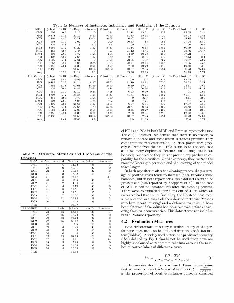
Table 1: Number of Instances, Imbalance and Problems of the DatasetsMDP # Inst % IR % Dupl %Incons # Inst D’ % Probl Inst %IR D’ # Inst D” % Probl Inst D” %IR D”CM1 505 9.5 5.15 0 344 31.88 12.21 327 35.25 12.84JM1 10878 19.32 24.16 8.17 9593 11.83 18.34 7720 29.03 20.88KC1 2107 15.42 50.78 12.01 2095 0.57 15.51 1162 44.85 25.3KC3 458 9.39 2.62 0 200 56.33 18 194 57.64 18.56KC4 125 48.8 8 7.2 n.a 100 n.a n.a 100 n.aMC1 9466 0.72 84.22 1.12 8737 51.14 0.78 1952 80.49 1.84MC2 161 32.3 2.48 0 127 21.12 34.65 124 22.36 35.48MW1 403 7.69 3.72 1.24 264 34.49 10.23 250 37.72 10PC1 1107 6.87 7.68 1.17 759 32.07 8.04 679 37.13 8.1PC2 5589 0.41 17.61 0 1493 72.55 1.07 722 86.87 2.22PC3 1563 10.24 5.05 0.38 1125 28.41 12.44 1053 31.35 12.35PC4 1458 12.21 11.39 0.21 1399 7.68 12.72 1270 12.48 13.86PC5 17186 3 91.53 10.04 16962 10.37 2.96 1694 90.23 27.04Avg 13.53 24.18 3.2 35.26 12.25 51.18 15.71

PROMISE # Inst % IR % Dupl %Incons # Inst D’ % Probl Inst %IR D’ # Inst D” % Probl Inst D” %IR D”CM1 498 9.84 18.88 0.4 495 0.6 9.7 437 12.25 10.53JM1 10885 19.35 24.14 8.17 9591 11.89 18.34 7720 29.08 0.28KC1 1783 18.28 60.01 14.19 2095 0.79 15.51 1162 53.11 25.3KC2 522 20.5 34.87 22.61 484 7.28 20.66 325 37.74 28.31KC3 458 9.39 37.12 0.44 458 6.33 9.39 324 31 12.96MC1 9398 0.72 84.83 1.13 8737 51.51 0.78 1952 81.07 1.84MC2 161 32.3 3.73 1.24 159 0 32.7 155 3.11 32.9MW1 403 7.69 8.93 1.74 402 0 7.71 375 6.7 7.47PC1 1109 6.94 21.64 1.17 1083 6.67 6.65 919 17.67 6.53PC2 5589 0.41 82.68 1.79 5356 20.81 0.43 1362 76.88 1.54PC3 1563 10.24 12.09 0.58 1535 3.45 10.29 1409 8.83 10.5PC4 1458 12.21 11.39 0.21 1379 7.68 12.91 1270 12.48 13.86PC5 17186 3 91.53 10.04 16962 10.37 2.96 1694 90.23 27.04Avg 11.61 37.83 4.9 9.8 11.39 35.4 13.77

Table 2: Attribute Statistics and Problems of theDatasets

MDP # Att # Probl % Prob # Att D’ Removed

CM1 41 6 14.63 38 3JM1 22 9 40.91 22 0KC1 22 4 18.18 22 0KC3 41 3 7.32 40 1KC4 41 30 73.17 0 41MC1 40 5 12.5 39 1MC2 41 2 4.88 40 1MW1 41 4 9.76 38 3PC1 41 8 19.51 38 3PC2 41 8 19.51 37 4PC3 41 7 17.07 38 3PC4 41 11 26.83 38 3PC5 40 5 12.5 39 1Avg 21.29

PROMISE Att Prob %Prob Att D’ RemovedCM1 22 15 68.18 21 1JM1 22 16 72.73 22 0KC1 22 16 72.73 22 0KC2 22 15 68.18 22 0KC3 40 1 2.5 40 0MC1 39 4 10.26 39 0MC2 40 0 0 40 0MW1 38 0 0 38 0PC1 22 15 68.18 22 0PC2 37 3 8.11 23 14PC3 38 3 7.89 38 0PC4 38 8 21.05 38 0PC5 39 4 10.26 39 0Avg 31.54

of KC1 and PC5 in both MDP and Promise repositories (seeTable 1). However, we believe that there is no reason toremove duplicate and inconsistent instances provided theycome from the real distribution, i.e., data points were prop-erly collected from the data. PC5 seems to be a special caseas it has many duplicates. Features with a single value canbe safely removed as they do not provide any predictive ca-pability for the classifiers. On the contrary, they confuse themachine learning algorithms and the learning of the modeltakes longer.

In both repositories after the cleaning process the percent-age of positive cases tends to increase (data becomes morebalanced) but in both repositories, some datasets seem to beproblematic (also reported by Shepperd et al). In the caseof KC4, it had no instances left after the cleaning process.There were 26 numerical attributes out of 41 in which allinstances had 0 as values (including the Halstead base mea-sures and and as a result all their derived metrics). Perhapszero here meant ’missing’ and a different result could havebeen obtained if the values had been removed before consid-ering them as inconsistencies. This dataset was not includedin the Promise repository.

4.2 Evaluation MeasuresWith dichotomous or binary classifiers, many of the per-

formance measures can be obtained from the confusion ma-trix (Table 3). A widely used metric, the predictive accuracy(Acc) defined by Eq. 1 should not be used when data arehighly imbalanced as it does not take into account the num-ber of correct labels of different classes.

Acc =TP + TN

TP + TN + FP + FN(1)

Other metrics should be considered. From the confusionmatrix, we can obtain the true positive rate (TPr = TP

TP+FN)

is the proportion of positive instances correctly classified

Table 3: Confusion Matrix for Two ClassesAct

Pos Neg

Pred

Pos True Pos(TP )

False Pos(FP )Type I error(False alarm)

PPV=Conf =Prec =

TPTP+FP

Neg False Neg(FN)Type II error

True Neg(TN)

NPV =TN

FN+TN

Recall =Sens =TPr =

TPTP+FN

Spec =TNr =

TNFP+TN

(also called recall or sensitivity); the False negative rate(FNr = FN

TP+FN) is the proportion of positive instances mis-

classified as belonging to the negative class; the True nega-tive rate (TNr = TN

FP+TN) is the proportion of negative in-

stances correctly classified (specificity); and finally, the falsepositive rate (FPr = FP

FP+TN) is the proportion of negative

cases misclassified (also called false alarm rate). The Posi-tive Prediction Value, also known as Confidence or Precision( TPTP+FP

) or the Negative Predicted Value ( TNFN+TN

) do noteither consider the TN or the TP respectively.There is a trade-off between the true positive rate and

true negative rate as the objective is to maximise both met-rics. Another widely used metric when measuring the per-formance of classifiers applied to highly imbalance data isthe f-measure (f1) [47] which is the harmonic median ofprecision and recall (Eq. 2). However, there are also somecriticisims to the f-measure metric as it does not take intothe TN (negative cases).

f −measure =2 · precision · recallprecision+ recall

=2 · TP

2 · TP + FP + FN(2)

where precision ( TPTP+FP

) is the proportion of positive pre-dictions that are correct and recall is the TPr previouslydefined.A more suitable and interesting performance metric for bi-

nary classification when data are imbalanced is Matthew’sCorrelation Coefficient (MCC) [29]. MCC can also be cal-culated from the confusion matrix as shown in Eq. (3) andis simple to understand. Its range goes from -1 to +1; thecloser to one the better as it indicates perfect predictionwhereas a value of 0 means that classification is not bet-ter than random prediction and negative values mean thatpredictions are worst than random.

MCC =TP × TN − FP × FN√

(TP + FP )(TP + FN)(TN + FP )(TN + FN)(3)

Another evaluation technique to consider when data is im-balanced is the Receiver Operating Characteristic (ROC) [13]curve which provides a graphical visualisation of the resultsThe Area Under the ROC Curve (AUC) also provides a

quality measure between positive and negative rates with asingle value. It can be calculated as Eq.(4).

AUC =1 + TPr − FPr

2(4)

Similarly to ROC, another widely used evaluation tech-nique is the Precision-Recall Curve (PRC), which depicts a

trade off between precision and recall and can also be sum-marised into a single value as the Area Under the Precision-Recall Curve (AUPRC) [9].

4.3 Base ClassifiersIn this work, we have used the following base learners

implemented in Weka:

• C4.5 [39] (known as J48 in Weka) is a decision tree.Decision trees are constructed in a top-down approach.The leaves of the tree correspond to classes, nodes cor-respond to features, and branches to their associatedvalues. To classify a new instance, one simply exam-ines the features tested at the nodes of the tree andfollows the branches corresponding to their observedvalues in the instance.

• The Naıve Bayes (NB) [36] uses the Bayes theorem topredict the class for each case, assuming that the pre-dictive attributes are independent given a category. ABayesian classifier assigns a set of attributesA1, . . . , An

to a class C such that P (C|A1, . . . , An) is maximum,that is the probability of the class description valuegiven the attribute instances, is maximal.

4.4 Empirical ResultsWe have generated multiple results for all the techniques

and metrics previously mentioned usingWeka’s Experimenterusing 5 times 5 Cross Validation (5x5CV) over all algorithmsand datasets. We next present the most relevant results to-gether with a discussion leaving other material on the com-panion Web site. With respect to the algorithms, RUS andROS were used to balance the data so that the majority andminority class represented the 75% and 25% respectively (inour case, exact balancing, 50:50 distribution, in both ROSand RUS did not perform as well as a more moderated bal-ance). It is not trivial to set the optimal balance level. TheSMOTE filter increases the minority class by 200%. It worthnoting that we used Weka’s filtered classifier, so that thesesampling filters are applied only to the training folds of thestratified CV folds, not the whole dataset in advance (thelatter approach will provide over optimistic results). For thecost-sensitive classifiers (including the MetaCost classifier),we used cost matrix that penalises false positives (defectivemodules classified as non-defective) by ten times the costof false negatives (non-defective modules classified as defec-tive). We choose this value as the average Imbalance Ratio(IR) is close to 10%. We also used the default parametersfor the metalearners algorithms as in general they seem towork well.

Tables 4 and 5 show the results of using as base learner theC4.5 algorithm (called J48 in Weka) with the default param-eters (using pruning, with the minimum number of instancesper leaf as two and no Laplace smoothing). The first numer-ical column shows the results for the base classifier and therest of the columns show the results of the different algo-rithms and whether they are statistically significant usingthe t-test at 0.10 significance level. These results were ob-tained with Weka’s experimenter tool and we must performfurther statistical analyses in our future work. There arebig differences in some datasets. For example, when usingJ48, MC1 and PC5. In some cases such as PC2, after re-moving all problematic instances, the cost algorithms failed(we believe that after the cross validation some folds had no

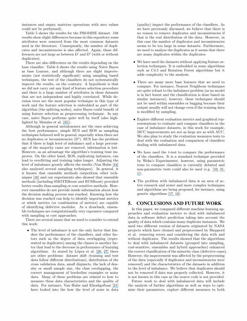
instances and empty matrices operations with zero valuescould not be performed).Table 5 shows the results for the PROMISE dataset. J48

results show slight differences because in this repository someattributes were removed from the most common datasetsused in the literature. Consequently, the number of dupli-cates and inconsistencies is also affected. Again, these dif-ferences are not large as between D’ and D”(with or withoutduplicates).There are also differences on the results depending on the

base classifier. Table 6 shows the results using Naıve Bayesas base Learner, and although there are slight improve-ments (not statistically significant) using sampling basedtechniques, the rest of the classifiers do not systematicallyimprove the results, on the contrary. A hypothesis is thatwe did not carry out any kind of feature selection procedureand there is a large number of attributes in these datasetsthat are not independent and highly correlated. While de-cision trees are the most popular technique in this type ofwork and the feature selection is embedded as part of thealgorithm (the splitting nodes), naıve Bayes could benefit ofusing feature selection as preprocessing technique. In anycase, naıve Bayes performs quite well by itself (also high-lighted by Menzies et al. [35]).Although in general metalearners are the ones achieving

the best performance, simple RUS and ROS as samplingtechniques behaved well in general, especially when there areno duplicates or inconsistencies (D”). RUS has the problemthat if there is high level of imbalance and a large percent-age of the majority cases are removed, information is lost.However, as an advantage the algorithm’s training time im-proves. On the other hand, ROS, replicating instances, canlead to overfitting and training takes longer. Adjusting thelevel of imbalance greatly affects the results (Van Hulse [44]also analysed several sampling techniques). In general, itis known that ensemble methods outperform other tech-niques [16] and our experiments also showed that ensemblemethods (including SMOTEBoost and RUSBoost) providedbetter results than sampling or cost sensitive methods. How-ever ensembles do not provide inside information about howthe decision making process was reached. Knowing how thedecision was reached can help to identify important metricsor which metrics (or combination of metrics) are capableof identifying defective modules. As a drawback, ensem-ble techniques are computationally very expensive comparedwith sampling or cost approaches.There are several issues that we need to consider to extend

this work:

• The level of imbalance is not the only factor that hin-ders the performance of the classifiers, and other fac-tors such as the degree of data overlapping (repre-sented as duplicates) among the classes is another fac-tor that lead to the decrease in performance of learningalgorithms. As stated by Lopez et al. [28, 27] thereare other problems: dataset shift (training and testdata follow different distributions), distribution of thecross validation data, small disjuncts, the lack of den-sity or small sample size, the class overlapping, thecorrect management of borderline examples or noisydata. Many of these problems are related to how tomeasure these data characteristics and the quality ofdata. For instance, Van Hulse and Khoshgoftaar [21]have looked into the how the level of noise in data

(quality) impact the performance of the classifiers. Aswe have previously discussed, we believe that there isno reason to remove duplicates and inconsistencies ifthat is the real distribution of the data. However, inthis case the number of duplicates and inconsistenciesseems to be too large in some datasets. Furthermore,we need to analyse the duplicates as it seems that thereare many duplicates within the duplicates.

• We have used the datasets without applying feature se-lection techniques. It is embedded in some algorithmssuch as C4.5 and Rotation Forest algorithms but itadds complexity to the analysis.

• There are many more base learners that we need tocompare. For instance, Nearest Neighbour techniquesare quite robust to the imbalance problem (as no modelis in fact learnt and the classification is done based onsimilar instances); however, these techniques shouldnot be used within ensembles or bagging because theiroutput usually will not change even if the training datais modified by sampling.

• Explore different evaluation metrics and graphical rep-resentations to evaluate and compare classifiers in thecase of imbalance datasets, in this work for example,MCC improvements are not as large are as with AUC.We also plan to study the evaluation measures tests todeal with the evaluation and comparison of classifiersdealing with imbalanced data.

• We have used the t-test to compare the performanceof the classifiers. It is a standard technique providedby Weka’s Experimenter, however, using parametrictests to compare classifiers is currently debated andnon-parametric tests could also be used (e.g. [10, 31,1]).

• The problem with imbalanced data is an area of ac-tive research and newer and more complex techniquesand algorithms are being proposed, for instance, usinggenetic algorithms [17, 18].

5. CONCLUSIONS AND FUTURE WORKIn this paper, we compared different machine learning ap-

proaches and evaluation metrics to deal with imbalanceddata in software defect prediction taking into account thequality of data which contains many duplicate instances. Weused two different version of datasets originated by NASAprojects which have cleaned and preprocessed by Shepperdet al. removing errors and considering the data with andwithout duplicates. The results showed that the algorithmsto deal with imbalanced datasets (grouped into sampling,cost-sensitive, ensembles and hybrid approaches) enhancedthe correct classification of the minority class (defective cases).However, the improvement was affected by the preprocessingof the data (especially if duplicates and inconsistencies wereremoved) and the characteristics of the datasets in additionto the level of imbalance. We believe that duplicates shouldnot be removed if data was properly collected. However, itis not known in this case as the source code is not provided.

Future work to deal with imbalanced data will includethe analysis of further algorithms as well as ways to opti-mise their parameters, explore different measures to both

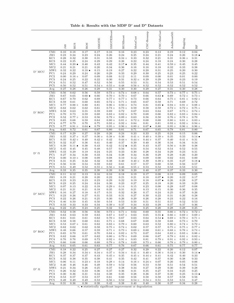
Table 4: Results with the MDP D’ and D” Datasets

J48

RUS

ROS

SM

OTE

SM

OTEBoost

RUSBoost

Meta

Cost

CSC-R

esa

mp

CSC-M

inCost

AdaBoostM

1

Bagging

RF

D’ MCC

CM1 0.10 0.18 0.17 0.17 0.16 0.16 0.23 0.23 0.13 0.19 0.12 0.04JM1 0.23 0.24 0.23 0.24 0.26 0.24 0.25 0.24 0.21 0.24 0.26 0.18 •KC1 0.28 0.32 0.30 0.31 0.33 0.34 ◦ 0.33 0.32 0.21 0.31 0.36 ◦ 0.31KC3 0.22 0.25 0.24 0.29 0.29 0.26 0.22 0.24 0.18 0.24 0.30 0.28MC1 0.44 0.20 • 0.40 0.43 0.42 0.17 • 0.35 0.44 0.41 0.59 ◦ 0.45 0.45MC2 0.21 0.21 0.21 0.20 0.34 0.36 0.16 0.16 0.18 0.32 0.33 0.38MW1 0.32 0.22 0.10 • 0.15 0.19 0.27 0.22 0.20 0.31 0.25 0.20 0.30PC1 0.24 0.29 0.24 0.26 0.29 0.33 0.29 0.30 0.25 0.23 0.25 0.22PC2 0.00 0.16 ◦ 0.07 0.09 0.08 0.12 0.11 0.09 0.00 0.01 0.01 0.00PC3 0.24 0.25 0.22 0.22 0.30 0.31 0.32 ◦ 0.29 0.29 0.29 0.23 0.19PC4 0.51 0.52 0.47 0.52 0.56 0.55 0.53 0.51 0.54 0.53 0.51 0.54PC5 0.50 0.52 0.51 0.54 ◦ 0.55 ◦ 0.48 0.56 ◦ 0.52 0.52 0.52 0.52 0.52Avg 0.27 0.28 0.26 0.29 0.31 0.30 0.30 0.29 0.27 0.31 0.30 0.28

D’ ROC

CM1 0.56 0.62 0.56 0.59 0.73 ◦ 0.74 ◦ 0.68 ◦ 0.64 0.57 0.73 ◦ 0.77 ◦ 0.75 ◦JM1 0.67 0.65 0.60 • 0.66 0.70 ◦ 0.70 ◦ 0.67 0.66 0.63 • 0.69 0.72 ◦ 0.73 ◦KC1 0.67 0.70 0.62 0.69 0.77 ◦ 0.77 ◦ 0.73 0.66 0.64 0.75 ◦ 0.81 ◦ 0.82 ◦KC3 0.59 0.61 0.60 0.65 0.72 ◦ 0.71 ◦ 0.65 0.67 0.59 0.71 0.69 0.72MC1 0.77 0.88 ◦ 0.80 0.81 0.96 ◦ 0.93 ◦ 0.74 0.81 0.65 • 0.94 ◦ 0.91 ◦ 0.88 ◦MC2 0.62 0.62 0.62 0.61 0.73 ◦ 0.73 ◦ 0.59 0.58 0.59 0.72 ◦ 0.72 ◦ 0.75 ◦MW1 0.58 0.63 0.55 0.59 0.69 0.72 0.67 0.63 0.64 0.67 0.73 ◦ 0.74 ◦PC1 0.70 0.73 0.59 0.68 0.83 ◦ 0.82 ◦ 0.70 0.68 0.66 0.82 ◦ 0.83 ◦ 0.84 ◦PC2 0.52 0.77 ◦ 0.53 0.56 0.79 ◦ 0.89 ◦ 0.63 0.56 0.50 0.76 ◦ 0.78 ◦ 0.70PC3 0.65 0.68 0.59 0.64 0.80 ◦ 0.81 ◦ 0.72 ◦ 0.68 0.68 0.80 ◦ 0.81 ◦ 0.83 ◦PC4 0.77 0.79 0.70 0.75 0.93 ◦ 0.92 ◦ 0.84 0.81 0.81 0.92 ◦ 0.92 ◦ 0.94 ◦PC5 0.77 0.91 ◦ 0.64 • 0.79 0.95 ◦ 0.96 ◦ 0.89 ◦ 0.67 • 0.80 0.95 ◦ 0.96 ◦ 0.96 ◦Avg 0.65 0.72 0.61 0.67 0.80 0.81 0.71 0.67 0.65 0.79 0.81 0.80

D’ f1

CM1 0.17 0.29 0.27 0.28 0.26 0.24 0.33 0.33 0.25 0.24 0.15 0.06JM1 0.32 0.37 ◦ 0.37 0.36 ◦ 0.38 ◦ 0.36 0.41 ◦ 0.40 ◦ 0.39 ◦ 0.35 0.33 0.14 •KC1 0.35 0.42 ◦ 0.40 0.42 ◦ 0.42 0.44 ◦ 0.44 ◦ 0.44 ◦ 0.37 0.40 0.41 ◦ 0.31KC3 0.32 0.37 0.36 0.41 0.40 0.37 0.39 0.40 0.36 0.34 0.34 0.34MC1 0.39 0.11 • 0.38 0.43 0.42 0.12 • 0.35 0.43 0.37 0.56 ◦ 0.39 0.38MC2 0.45 0.45 0.45 0.48 0.57 0.56 0.54 0.54 0.52 0.54 0.52 0.55MW1 0.33 0.29 0.19 0.24 0.25 0.33 0.30 0.28 0.34 0.29 0.23 0.31PC1 0.27 0.34 0.30 0.33 0.34 0.38 0.34 0.36 0.29 0.28 0.26 0.20PC2 0.00 0.10 ◦ 0.08 0.09 0.08 0.10 0.12 0.09 0.00 0.02 0.01 0.00PC3 0.31 0.35 0.32 0.32 0.38 0.40 0.40 ◦ 0.39 0.39 ◦ 0.35 0.27 0.18 •PC4 0.56 0.58 0.54 0.59 0.62 0.61 0.57 0.57 0.60 0.58 0.56 0.57PC5 0.51 0.49 0.52 0.55 ◦ 0.56 ◦ 0.46 0.55 ◦ 0.53 0.52 0.53 0.53 0.51Avg 0.33 0.35 0.35 0.38 0.39 0.36 0.39 0.40 0.37 0.37 0.33 0.30

D” MCC

CM1 0.11 0.12 0.13 0.16 0.16 0.18 0.19 0.17 0.08 0.13 0.09 0.05JM1 0.19 0.21 0.20 0.20 0.22 0.21 0.21 0.18 0.07 • 0.20 0.22 0.17KC1 0.23 0.23 0.23 0.23 0.29 0.22 0.19 0.18 0.07 • 0.26 0.28 0.27KC3 0.23 0.25 0.24 0.24 0.30 0.23 0.27 0.25 0.18 0.20 0.33 0.29MC1 0.07 0.13 0.22 0.18 0.29 ◦ 0.14 0.15 0.23 0.08 0.28 0.07 0.08MC2 0.21 0.21 0.21 0.18 0.35 0.31 0.21 0.13 0.15 0.30 0.36 0.35MW1 0.16 0.27 0.18 0.17 0.31 0.32 0.26 0.17 0.24 0.25 0.37 0.26PC1 0.23 0.26 0.27 0.31 0.33 0.31 0.27 0.30 0.22 0.31 0.26 0.28PC3 0.22 0.26 0.21 0.25 0.30 0.26 0.29 0.26 0.28 0.23 0.22 0.16PC4 0.46 0.50 0.45 0.50 0.54 0.53 0.50 0.51 0.51 0.51 0.52 0.53PC5 0.33 0.33 0.33 0.34 0.39 ◦ 0.37 0.34 0.33 0.29 0.37 0.37 0.36Avg 0.22 0.25 0.24 0.25 0.32 0.28 0.26 0.25 0.20 0.28 0.28 0.25

D” ROC

CM1 0.52 0.58 0.56 0.56 0.73 ◦ 0.71 ◦ 0.64 0.60 0.55 0.66 ◦ 0.72 ◦ 0.72 ◦JM1 0.63 0.63 0.59 0.63 0.67 ◦ 0.67 ◦ 0.63 0.65 0.55 • 0.66 ◦ 0.69 ◦ 0.69 ◦KC1 0.61 0.61 0.61 0.62 0.70 ◦ 0.67 0.63 0.64 0.54 • 0.69 ◦ 0.70 ◦ 0.71 ◦KC3 0.58 0.58 0.60 0.61 0.71 ◦ 0.68 0.67 0.68 0.59 0.68 0.73 ◦ 0.70MC1 0.53 0.67 ◦ 0.61 0.62 0.83 ◦ 0.79 ◦ 0.60 0.63 0.52 0.80 ◦ 0.74 ◦ 0.72 ◦MC2 0.62 0.62 0.62 0.58 0.75 ◦ 0.74 ◦ 0.62 0.57 0.57 0.75 ◦ 0.75 ◦ 0.77 ◦MW1 0.48 0.66 0.57 0.59 0.71 ◦ 0.73 ◦ 0.69 ◦ 0.60 0.61 ◦ 0.68 ◦ 0.76 ◦ 0.74 ◦PC1 0.65 0.70 0.61 0.70 0.84 ◦ 0.82 ◦ 0.73 0.67 0.64 0.82 ◦ 0.83 ◦ 0.86 ◦PC3 0.62 0.66 0.57 0.62 0.80 ◦ 0.79 ◦ 0.69 0.66 0.67 0.78 ◦ 0.81 ◦ 0.82 ◦PC4 0.76 0.76 0.69 0.73 0.92 ◦ 0.91 ◦ 0.83 0.81 0.79 ◦ 0.91 ◦ 0.92 ◦ 0.93 ◦PC5 0.66 0.66 0.66 0.68 0.79 ◦ 0.78 ◦ 0.69 0.73 ◦ 0.66 0.78 ◦ 0.79 ◦ 0.80 ◦Avg 0.61 0.65 0.61 0.63 0.77 0.76 0.67 0.66 0.61 0.75 0.77 0.77

D” f1

CM1 0.18 0.22 0.25 0.27 0.27 0.27 0.32 0.29 0.22 0.20 0.12 0.07JM1 0.28 0.34 0.34 ◦ 0.34 ◦ 0.37 ◦ 0.34 ◦ 0.41 ◦ 0.40 ◦ 0.36 ◦ 0.34 ◦ 0.30 0.14 •KC1 0.37 0.37 0.37 0.43 0.45 ◦ 0.35 0.45 ◦ 0.44 ◦ 0.41 0.42 0.40 0.33KC3 0.32 0.38 0.35 0.38 0.41 0.35 0.42 0.41 0.37 0.30 0.38 0.33MC1 0.06 0.11 0.23 ◦ 0.18 0.28 ◦ 0.14 0.16 ◦ 0.24 ◦ 0.07 0.26 0.05 0.06MC2 0.46 0.46 0.46 0.49 0.59 ◦ 0.52 0.56 0.53 0.50 0.51 0.54 0.51MW1 0.21 0.34 0.26 0.25 0.37 0.38 0.34 0.27 0.29 0.30 0.39 0.28PC1 0.26 0.32 0.33 0.36 0.37 0.36 0.31 0.35 0.27 0.34 0.25 0.25PC3 0.30 0.36 0.31 0.34 0.38 0.35 0.38 0.36 0.37 0.30 0.25 0.13 •PC4 0.53 0.57 0.53 0.57 0.61 0.60 0.56 0.58 0.58 0.57 0.58 0.56PC5 0.49 0.49 0.49 0.53 0.56 ◦ 0.52 0.54 ◦ 0.54 ◦ 0.51 0.53 0.51 0.47Avg 0.31 0.36 0.36 0.38 0.42 0.38 0.40 0.40 0.36 0.37 0.34 0.28

◦, • statistically significant improvement or degradation

Table 5: Results using Promise D’ using J48

J48

RUS

ROS

SM

OTE

SM

OTEBoost

RUSBoost

Meta

Cost

AdaBoostM

1

Bagging

RF

MCC

CM1 0.10 0.13 0.13 0.13 0.09 0.15 0.17 0.11 0.06 0.00JM1 0.21 0.24 0.23 0.23 0.26 0.25 0.24 0.25 0.26 0.16 •KC1 0.28 0.32 0.30 0.33 0.34 0.35 ◦ 0.35 ◦ 0.32 0.34 ◦ 0.33 ◦KC2 0.41 0.40 0.42 0.44 0.32 0.30 0.44 0.45 0.45 0.44KC3 0.26 0.28 0.24 0.26 0.30 0.20 0.30 0.24 0.22 0.21MC1 0.43 0.20 • 0.39 0.45 0.39 0.13 • 0.04 • 0.58 ◦ 0.45 0.44MC2 0.18 0.18 0.18 0.25 0.36 ◦ 0.30 0.17 0.29 0.23 0.27MW1 0.27 0.25 0.19 0.18 0.26 0.26 0.23 0.24 0.20 0.25PC1 0.34 0.31 0.33 0.32 0.35 0.29 0.32 0.36 0.38 0.33PC2 0.00 0.11 ◦ 0.06 0.11 0.09 0.08 0.05 0.05 0.00 0.00PC3 0.18 0.26 0.24 0.22 0.31 ◦ 0.32 ◦ 0.31 ◦ 0.23 0.20 0.18PC4 0.46 0.51 0.45 0.51 0.55 0.53 0.52 0.52 0.52 0.53PC5 0.50 0.53 0.52 0.54 0.56 ◦ 0.46 0.55 ◦ 0.52 0.52 0.53Avg 0.28 0.29 0.28 0.31 0.32 0.28 0.29 0.32 0.29 0.28

ROC

CM1 0.55 0.60 0.57 0.57 0.69 ◦ 0.74 ◦ 0.66 0.68 ◦ 0.71 ◦ 0.75 ◦JM1 0.66 0.66 0.60 • 0.66 0.70 ◦ 0.69 ◦ 0.66 0.69 ◦ 0.72 ◦ 0.73 ◦KC1 0.68 0.70 0.63 0.68 0.77 ◦ 0.77 ◦ 0.73 0.75 ◦ 0.80 ◦ 0.81 ◦KC2 0.73 0.71 0.70 0.72 0.75 0.77 0.77 0.76 0.83 ◦ 0.83 ◦KC3 0.60 0.67 0.53 0.64 0.79 ◦ 0.77 ◦ 0.74 ◦ 0.71 0.78 ◦ 0.79 ◦MC1 0.75 0.86 ◦ 0.78 0.81 0.93 ◦ 0.91 ◦ 0.51 • 0.93 ◦ 0.91 ◦ 0.90 ◦MC2 0.60 0.60 0.60 0.64 0.76 ◦ 0.72 ◦ 0.62 0.71 ◦ 0.69 ◦ 0.71 ◦MW1 0.54 0.66 0.62 0.61 0.75 ◦ 0.75 ◦ 0.65 0.76 ◦ 0.75 ◦ 0.72 ◦PC1 0.65 0.75 ◦ 0.67 0.70 0.85 ◦ 0.82 ◦ 0.76 ◦ 0.85 ◦ 0.86 ◦ 0.84 ◦PC2 0.50 0.74 ◦ 0.38 0.59 0.74 ◦ 0.83 ◦ 0.55 0.75 ◦ 0.75 ◦ 0.60PC3 0.62 0.66 0.57 0.65 0.81 ◦ 0.80 ◦ 0.73 ◦ 0.79 ◦ 0.81 ◦ 0.82 ◦PC4 0.78 0.79 0.70 0.74 0.92 ◦ 0.92 ◦ 0.85 0.92 ◦ 0.92 ◦ 0.94 ◦PC5 0.77 0.91 ◦ 0.65 • 0.81 0.95 ◦ 0.96 ◦ 0.88 ◦ 0.94 ◦ 0.96 ◦ 0.96 ◦Avg 0.65 0.72 0.62 0.68 0.80 0.80 0.70 0.79 0.81 0.80

◦, • statistically significant improvement or degradation

Table 6: Results with the Naıve Bayes as Base Learner

NB

RUS

ROS

SM

OTE

SM

OTEBoost

RUSBoost

Meta

Cost

CSC-R

esa

mp

CSC-M

inCost

AdaBoostM

1

Bagging

RF

MCC

CM1 0.21 0.21 0.21 0.21 0.17 0.18 0.20 0.21 0.21 0.21 0.22 0.20JM1 0.22 0.23 0.22 0.23 ◦ 0.18 • 0.23 0.24 ◦ 0.23 0.23 0.22 0.22 0.21KC1 0.29 0.30 0.30 0.31 ◦ 0.26 0.27 0.33 0.31 ◦ 0.31 ◦ 0.29 0.30 0.31KC3 0.26 0.26 0.28 0.28 0.27 0.26 0.21 0.29 0.29 0.24 0.29 0.29MC1 0.20 0.18 0.19 • 0.18 • 0.15 • 0.14 0.17 0.19 • 0.19 • 0.20 0.19 0.18MC2 0.31 0.31 0.31 0.33 0.31 0.24 0.32 0.32 0.32 0.38 0.33 0.33MW1 0.32 0.31 0.31 0.31 0.30 0.24 • 0.23 • 0.31 0.31 0.33 0.32 0.33PC1 0.28 0.26 0.27 0.27 0.16 • 0.16 • 0.16 • 0.27 0.27 0.26 0.28 0.27PC2 0.08 0.13 0.09 0.09 0.03 0.13 0.15 0.08 0.08 0.06 0.08 0.09PC3 0.15 0.23 0.14 0.13 0.05 0.08 0.02 • 0.11 • 0.11 • 0.16 0.18 0.14PC4 0.32 0.31 0.34 0.38 ◦ 0.28 0.05 • 0.25 • 0.35 0.35 0.37 0.34 0.28PC5 0.42 0.44 0.42 0.42 0.27 • 0.21 • 0.41 0.42 0.42 0.42 0.42 0.41Avg 0.25 0.26 0.26 0.26 0.20 0.18 0.22 0.26 0.26 0.26 0.26 0.25

ROC

CM1 0.70 0.71 0.71 0.71 0.57 • 0.61 • 0.70 0.70 0.61 • 0.66 0.73 0.71JM1 0.69 0.69 0.69 0.69 0.58 • 0.60 • 0.69 0.69 0.58 • 0.59 • 0.69 ◦ 0.66 •KC1 0.79 0.79 0.79 0.79 0.73 • 0.63 • 0.78 • 0.79 0.65 • 0.79 0.79 0.79KC3 0.68 0.68 0.67 0.68 0.66 0.65 0.67 0.68 0.65 0.64 0.68 0.70MC1 0.91 0.91 0.91 0.91 0.86 • 0.75 • 0.90 • 0.91 0.78 • 0.88 0.91 0.91MC2 0.73 0.73 0.73 0.73 0.72 0.65 • 0.69 • 0.73 0.64 • 0.70 0.73 0.73MW1 0.75 0.75 0.75 0.76 0.75 0.71 0.72 0.75 0.71 0.74 0.75 0.76PC1 0.78 0.78 0.79 0.78 0.67 • 0.58 • 0.73 • 0.78 0.64 • 0.77 0.80 ◦ 0.78PC2 0.83 0.86 0.83 0.81 0.59 0.79 0.87 0.83 0.60 • 0.71 0.86 0.83PC3 0.77 0.77 0.76 0.76 0.51 • 0.63 • 0.61 • 0.77 0.57 • 0.77 0.77 0.74PC4 0.83 0.82 0.83 0.84 ◦ 0.73 0.56 • 0.74 • 0.83 0.67 • 0.84 0.82 0.82PC5 0.94 0.94 0.94 0.94 0.90 • 0.75 • 0.94 • 0.94 0.73 • 0.94 0.94 0.94Avg 0.78 0.79 0.78 0.78 0.69 0.66 0.75 0.78 0.65 0.75 0.79 0.78

◦, • statistically significant improvement or degradation

deal with the quality and characteristics of the data and tocompare algorithms and statistical analyses. It is also neces-sary to study other repositories (e.g., open source systems)in order to study the quality of such repositories, validategeneric claims found in the literature and provide guidelinesfor the problem of imbalance in defect prediction.

AcknowledgmentsThe authors thank S. Garcia for helping with the imple-mentation of some algorithms and the anonymous reviewersfor their comments and suggestions. This research has beenpartially supported by European Commission funding underthe 7th Framework Programme IAPP Marie Curie programfor project ICEBERG no. 324356, and projects TIN2011-68084-C02-00 and TIN2013-46928-C3-2-R.

6. REFERENCES[1] E. Arisholm, L. C. Briand, and E. B. Johannessen. A

systematic and comprehensive investigation ofmethods to build and evaluate fault prediction models.Journal of Systems and Software, 83(1):2–17, 2010.

[2] S. Bibi, G. Tsoumakas, I. Stamelos, and I. Vlahvas.Software defect prediction using regression viaclassification. In IEEE International Conference onComputer Systems and Applications (AICCSA 2006),pages 330–336, 8 2006.

[3] L. Breiman. Bagging predictors. Machine Learning,24:123–140, 1996.

[4] L. Breiman. Random forests. Machine Learning,45(1):5–32, 2001.

[5] C. Catal and B. Diri. A systematic review of softwarefault prediction studies. Expert Systems withApplications, 36(4):7346 – 7354, 2009.

[6] N. Chawla, K. Bowyer, L. Hall, and W. Kegelmeyer.Smote: Synthetic minority over-sampling technique.Journal of Artificial Intelligence Research, 16:321–357,2002.

[7] N. Chawla, A. Lazarevic, L. Hall, and K. Bowyer.Smoteboost: Improving prediction of the minorityclass in boosting. In 7th European Conference onPrinciples and Practice of Knowledge Discovery inDatabases(PKDD 2003), pages 107–119, 2003.

[8] N. V. Chawla, K. W. Bowyer, L. O. Hall, and W. P.Kegelmeyer. Smote: Synthetic minority over-samplingtechnique. J. Artif. Intell. Res. (JAIR), 16:321–357,2002.

[9] J. Davis and M. Goadrich. The relationship betweenprecision-recall and roc curves. In Proceedings of the23rd international conference on Machine learning(ICLM’06, ICML’06, pages 233–240, New York, NY,USA, 2006. ACM.

[10] J. Demsar. Statistical comparisons of classifiers overmultiple data sets. Journal of Machine LearningResearch, 7:1–30, Dec. 2006.

[11] P. Domingos. Metacost: a general method for makingclassifiers cost-sensitive. In Proceedings of the fifthACM SIGKDD international conference on Knowledgediscovery and data mining, KDD ’99, pages 155–164,New York, NY, USA, 1999. ACM.

[12] K. O. Elish and M. O. Elish. Predicting defect-pronesoftware modules using support vector machines.Journal of Systems and Software, 81(5):649–660, 2008.

[13] T. Fawcett. An introduction to roc analysis. PatternRecogn. Lett., 27(8):861–874, June 2006.

[14] Y. Freund and R. Schapire. A decision-theoreticgeneralization of on-line learning and an application toboosting. Journal of Computer and System Sciences,55(1):119–139, 1997.

[15] Y. Freund and R. E. Schapire. Experiments with anew boosting algorithm. In Thirteenth InternationalConference on Machine Learning, pages 148–156, SanFrancisco, 1996. Morgan Kaufmann.

[16] M. Galar, A. Fernandez, E. Barrenechea, H. Bustince,and F. Herrera. A review on ensembles for the classimbalance problem: Bagging-, boosting-, andhybrid-based approaches. IEEE Transactions onSystems, Man, and Cybernetics, Part C: Applicationsand Reviews, 42(4):463–484, 2012.

[17] M. Galar, A. Fernandez, E. Barrenechea, andF. Herrera. EUSboost: Enhancing ensembles for highlyimbalanced data-sets by evolutionary undersampling.Pattern Recognition, null(null), May 2013.

[18] S. Garcıa, R. Aler, and I. M. Galvan. Usingevolutionary multiobjective techniques for imbalancedclassification data. In K. Diamantaras, W. Duch, andL. S. Iliadis, editors, Artificial Neural Networks -ICANN 2010, volume 6352 of Lecture Notes inComputer Science, pages 422–427. Springer BerlinHeidelberg, 2010.

[19] T. Hall, S. Beecham, D. Bowes, D. Gray, andS. Counsell. A systematic literature review on faultprediction performance in software engineering.Transactions on Software Engineering, In Press –2011.

[20] M. Halstead. Elements of software science. ElsevierComputer Science Library. Operating AndProgramming Systems Series; 2. Elsevier, New York ;Oxford, 1977.

[21] J. V. Hulse and T. Khoshgoftaar. Knowledgediscovery from imbalanced and noisy data. Data &Knowledge Engineering, 68(12):1513–1542, 2009.

[22] N. Japkowicz and S. Stephen. The class imbalanceproblem: A systematic study. Intelligent DataAnalysis, 6(5):429–449, Oct. 2002.

[23] T. M. Khoshgoftaar, E. Allen, and J. Deng. Usingregression trees to classify fault-prone softwaremodules. IEEE Transactions on Reliability,51(4):455–462, 2002.

[24] T. M. Khoshgoftaar, E. Allen, J. Hudepohl, andS. Aud. Application of neural networks to softwarequality modeling of a very large telecommunicationssystem. IEEE Transactions on Neural Networks,8(4):902–909, 1997.

[25] T. M. Khoshgoftaar and N. Seliya. Analogy-basedpractical classification rules for software qualityestimation. Empirical Software Engineering,8(4):325–350, 2003.

[26] S. Lessmann, B. Baesens, C. Mues, and S. Pietsch.Benchmarking classification models for software defectprediction: A proposed framework and novel findings.IEEE Transactions on Software Engineering,34(4):485–496, July-Aug. 2008.

[27] V. Lopez, A. Fernandez, and F. Herrera. On theimportance of the validation technique for

classification with imbalanced datasets: Addressingcovariate shift when data is skewed. InformationSciences, 257:1–13, 2014.

[28] V. Lopez, A. Fernandez, J. G. Moreno-Torres, andF. Herrera. Analysis of preprocessing vs. cost-sensitivelearning for imbalanced classification. open problemson intrinsic data characteristics. Expert Systems withApplications, 39(7):6585–6608, June 2012.

[29] B. W. Matthews. Comparison of the predicted andobserved secondary structure of t4 phage lysozyme.Biochimica et biophysica acta, 405(2):442–451, Oct.1975.

[30] T. McCabe. A complexity measure. IEEETransactions on Software Engineering, 2(4):308–320,December 1976.

[31] T. Mende and R. Koschke. Revisiting the evaluationof defect prediction models. In Proceedings of the 5thInternational Conference on Predictor Models inSoftware Engineering (PROMISE’09), pages 1–10,New York, NY, USA, 2009. ACM.

[32] T. Mende and R. Koschke. Effort-aware defectprediction models. In Proceedings of the 2010 14thEuropean Conference on Software Maintenance andReengineering (CSMR’10), CSMR’10, pages 107–116,Washington, DC, USA, 2010. IEEE Computer Society.

[33] T. Menzies, B. Caglayan, E. Kocaguneli, J. Krall,F. Peters, and B. Turhan. The promise repository ofempirical software engineering data, June 2012.

[34] T. Menzies, A. Dekhtyar, J. Distefano, andJ. Greenwald. Problems with precision: A response tocomments on data mining static code attributes tolearn defect predictors. IEEE Transactions onSoftware Engineering, 33(9):637–640, 2007.

[35] T. Menzies, J. Greenwald, and A. Frank. Data miningstatic code attributes to learn defect predictors. IEEETransactions on Software Engineering, 2007.

[36] T. Mitchell. Machine Learning. McGraw Hill, 1997.

[37] Y. Peng, G. Kou, G. Wang, H. Wang, and F. Ko.Empirical evaluation of classifiers for software riskmanagement. International Journal of InformationTechnology & Decision Making (IJITDM),08(04):749–767, 2009.

[38] Y. Peng, G. Wang, and H. Wang. User preferencesbased software defect detection algorithms selectionusing MCDM. Information Sciences, In Press.:–, 2010.

[39] J. Quinlan. C4.5: Programs for machine learning.Morgan Kaufmann, San Mateo, California, 1993.

[40] J. Rodriguez, L. Kuncheva, and C. Alonso. Rotationforest: A new classifier ensemble method. IEEETransactions on Pattern Analysis and MachineIntelligence, 28(10):1619–1630, oct 2006.

[41] C. Seiffert, T. Khoshgoftaar, and J. Van Hulse.Improving software-quality predictions with datasampling and boosting. Systems, Man andCybernetics, Part A: Systems and Humans, IEEETransactions on, 39(6):1283–1294, 2009.

[42] C. Seiffert, T. Khoshgoftaar, J. Van Hulse, andA. Napolitano. RUSBoost: A hybrid approach toalleviating class imbalance. IEEE Transactions onSystems, Man and Cybernetics, Part A: Systems andHumans, 40(1):185–197, 2010.

[43] M. Shepperd, Q. Song, Z. Sun, and C. Mair. Dataquality: Some comments on the nasa software defectdatasets. IEEE Transactions on Software Engineering,39(9):1208–1215, 2013.

[44] J. Van Hulse, T. M. Khoshgoftaar, and A. Napolitano.Experimental perspectives on learning fromimbalanced data. In Proceedings of the 24thinternational conference on Machine learning (ICLM),ICML ’07, pages 935–942, New York, NY, USA, 2007.ACM.

[45] O. Vandecruys, D. Martens, B. Baesens, C. Mues,M. De Backer, and R. Haesen. Mining softwarerepositories for comprehensible software faultprediction models. Journal of Systems and Software,81(5):823–839, 2008.

[46] D. Wilson. Asymptotic properties of nearest neighborrules using edited data. IEEE Transactions onSystems, Man and Cybernetics, (3):408–421, 1972.

[47] I. H. Witten, E. Frank, and M. A. Hall. Data Mining:Practical Machine Learning Tools and Techniques(Third Edition). Morgan Kaufmann, 2011.

[48] H. Zhang and X. Zhang. Comments on ”data miningstatic code attributes to learn defect predictors”. IEEETransactions on Software Engineering, 33(9):635–637,2007.