Predicting Software Defects in Varying Develop-ment Lifecycles using Bayesian Nets

ISSN 1470-5559

RR-05-11 December 2005 Department of Computer Science

Norman Fenton, Martin Neil, William Marsh, Paul Krause and Rajat Mishra

Predicting Software Defects in Varying DevelopmentLifecycles using Bayesian Nets

Norman Fenton‡, Martin Neil‡,W illiam Marsh

Department of Computer ScienceQueen Mary, University of London

Mile End Road, Londonand ‡Agena Ltd, Londonnorman,martin,william

@dcs.qmul.ac.uk

Paul KrauseDepartment of Computing

University of SurreyGuildford, SURREY, UKp.krause@surrey.ac.uk

Rajat MishraPhilips Software Centre,

Bangalore, Indiarajat.mishra@philips.com

ABSTRACTAn important decision problem in many software projects i swhen to stop testing and release software for use. For manysoftware products, time to market is critical and thereforeunnecessary testing time must be avoided. However,unreliable software is commercially damaging. Effectivedecision support tools for this problem have been built usingcausal models represented by Bayesian Networks (BNs), whichincorporate both empirical data and expert judgement.Previously, this has required a custom-built BN for eachsoftware development lifecycle. We describe a more generalBN, which, together with the AgenaRisk toolset, allows causalmodels to be applied to any development lifecycle without theneed to build a BN from scratch. The model and toolset haveevolved in a number of collaborative projects and hencecapture significant commercial input. Extensive validationtrials have taken place among partners on the EC fundedproject MODIST (this includes Philips, Israel AircraftIndustries and QinetiQ) and the feedback so far has been verygood. For example, for projects within the range of the modelspredictions of defects are very accurate. Moreover, the causalmodelling approach enables decision-makers to reason in away that is not possible with other regression-based models ofsoftware defects.

Categories and Subject DescriptorsD.2.8 [Software Engineering] Metrics – Product metrics.K.6.3 [Management of Computing and Information Systems]Software Management – Software development.

General TermsManagement, Measurement, Reliability.

KeywordsCausal Models, Dynamic Bayesian Networks, Software Defects,Decision Support.

1. INTRODUCTIONA number of authors, for example [3, 6, 21], have recently usedBayesian Networks (BNs) in software engineeringmanagement. In our own earlier work [8] we have shown howBNs can be used to predict the number of software defectsremaining undetected after testing. This work lead to the AIDtool [20] developed in partnership with Philips, and used topredict software defects in consumer electronic products.Project managers use a BN-based tool such as AID to helpdecide when to stop testing and release software, trading-offthe time for additional testing against the likely benefit.

Rather than relying only on data from previous projects, thiswork uses causal models of the Project Manager’sunderstanding, covering mechanisms such as:

• poor quality development increases the number ofdefects likely to be present

• high quality testing increases the proportion of defectsfound.

Causal models are important because they allow all theevidence to be taken into account, even when differentevidence conflicts. Suppose that few defects are found duringtesting – does this mean that testing is poor or thatdevelopment was outstanding and the software has few defectsto find? Regression-based models of software defects are littlehelp to a Project Manager who must decide between thesealternatives [10]. Data from previous projects is used to buildthe BN, with expert judgements on the strength of each causalmechanism.

In this paper, we extend the earlier work by describing a muchmore flexible and general method of using BNs for defectprediction. We also describe how the AgenaRisk [1] toolset i sused to create an effective decision support system from theBN. An important limitation of the earlier work was the needto build a different BN for each software development lifecycle– to reflect both the differing number of testing stages in thelifecycle and the differing metrics data available. Given thework required to build a BN, this severely limits thepractically of the approach. To overcome this limitation, wedescribe a BN that models the creation and detection ofsoftware defects without commitment to a particulardevelopment lifecycle. We then show how a softwaredevelopment organisation can adapt this BN to theirdevelopment lifecycle and metrics data with much less effortthan is needed to build a tailored BN from scratch.

The contents of the remainder of the paper are as follows: inSection 2 we introduce BNs and show how they are used forcausal modelling in software engineering. Section 3introduces the idea of a ‘phase’ as a sub-part of a software

Permission to make digital or hard copies of all or part of this work forpersonal or classroom use is granted without fee provided that copiesare not made or distributed for profit or commercial advantage and thatcopies bear this notice and the full citation on the first page. To copyotherwise, or republish, to post on servers or to redistribute to lists,requires prior specific permission and/or a fee.Conference’04, Month 1–2, 2004, City, State, Country.Copyright 2004 ACM 1-58113-000-0/00/0004…$5.00.

lifecycle and shows how several phase models can becombined to model different lifecycles. The phase model i sdescribed in detail in Section 4; Section 5 shows how it i sadapted to different development lifecycles. An experimentalvalidation of defect predictions is described in Section 6.

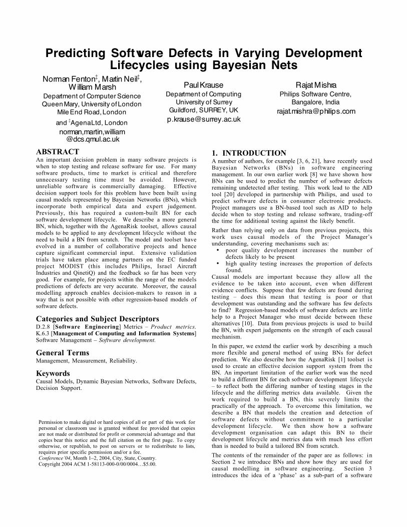
2. DEFECT PREDICTION WITH BNs2.1 Bayesian NetsA Bayesian net [13] (BN) is a graph (such as that shown inFigure 1) together with an associated set of probability tables.The nodes represent uncertain variables and the arcs representthe causal/relevance relationships between the variables.

Figure 1 BN for Defect Prediction

The BN of Figure 1 forms a causal model of the process ofinserting, finding and fixing software defects. The variable‘effective KLOC implemented’ represents the complexity-adjusted size of the functionality implemented; as the amountof functionality increases the number of potential defectsrises.

The ‘probability of avoiding defect in development’determines ‘defects in’ given total potential defects. Thisnumber represents the number of defects (before testing) thatare in the new code that has been implemented.

However, inserted defects may be found and fixed: the residualdefects are those remaining after testing. Variablesrepresenting a number of defects take a value in a numericrange, discretised into numeric interval.

There is a probability table for each node, specifying how theprobability of each state of the variable depends on the statesof its parents. Some of these are deterministic: for example the‘Residual defects’ is simply the numerical difference betweenthe ‘Defects in’ and the ‘Defects fixed’. In other cases, we canuse standard statistical functions: for example the process of

finding defects is modelled as a sequence of independentexperiments, one for each defect present, using the‘Probability of finding a defect’ as a characteristic of thetesting process:

Defects found = B(Defects inserted, Prob finding a defect)

where B(n,p) is the Binomial distribution for n trials withprobability p . For variables without parents the table justcontains the prior probabilities of each state.

The BN represents the complete joint probability distribution– assigning a probability to each combination of states of allthe variables – but in a factored form, greatly reducing thespace needed. When the states of some variables are known, thejoint probability distribution can be recalculated conditionedon this ‘evidence’ and the updated marginal probabilitydistribution over the states of each variable can be observed.

The quality of the development and testing processes i srepresented in the BN of Figure 1 by four variables discretisedover the 0 to 1 interval:

• probability of avoiding specification defects• probability of avoiding defects in development• probability of finding defects• probability of fixing defects.

The BN in Figure 1 is a simplified version the BN at the heartof the decision support system for software defects. None ofthese probability variables (or the ‘Effective KLOCimplemented’ variable) are entered directly by the user:instead, these variables have further parents modelling thecauses of process quality as we describe in Section 4.

2.2 Decision Support with BNsAlthough the underlying theory (Bayesian probability) hasbeen around for a long time, executing realistic BN models wasonly first made possible in the late 1980s as a result ofbreakthrough algorithms and software tools that implementthem [13]. Methods for building large-scale BNs are even morerecent ([11, 19]) but it is only such work that has made i tpossible to apply BNs to the problems of softwareengineering.

Drawing on this work in various commercial projects withAgena, Fenton and Neil have built BN-based applications thathave proved the technology is both viable and effective.Several of these applications have been related to systems orsoftware assessment. Especially significant was the TRACStool [18] to assess vehicle reliability for QinetiQ (on behalf ofthe MOD) and the AID tool [20] to predict software defects inconsumer electronic products for Philips. Much of themodelling work described here has been done as part of theMODIST project [9], which extends the ideas in AID. Thetoolset implementation has been based on Agena’s AgenaRisktechnology that was extended to incorporate recentdevelopments in building large-scale BNs that was undertakenin the SCULLY, SIMP and SCORE projects [11].

Two features of AgenaRisk are especially critical for buildingthis model:

• Large tables can be handled efficiently. For example, inthe default model here the number of defects may rangefrom 0 to 3000, in intervals of varying size.

• Probability tables are generated from numerical andstatistical expressions by simulation. The expressiongiven above using the binomial distribution is not only

the conceptual model but also how the model i sspecified.

2.3 Building the BN ModelLike all BNs, the defect model was built using a mixture ofdata and expert judgements. Understanding cause and effect i sa basic form of human knowledge, underlying our decisions.For example, a project manager knows that more rigoroustesting increases the number – and proportion of – defectsfound during testing and therefore reduces the numberremaining in the delivered software.

It is obvious that the relationship is not the other way round.However, it is equally obvious that we need to take intoaccount whatever evidence we have about: the likely numberof defects in the software following development; thecapabilities of the team; and the adequacy of the time allowed.The expert’s understanding of cause and effect is used toconnect the variables of the net with arcs drawn from cause toeffect.

To ensure that our model is consistent with these empiricalfindings, the probability tables in the net are constructedusing data, whenever it is available. However, when there i smissing data, or the data does not take account of all the causalinfluences, expert judgement must be used as well.

3. VARYING THE LIFECYCLEWhen we describe defects being inserted in ‘implementation’and removed in ‘testing’ we are referring to the activities thatmake up the software development lifecycle. We need to fit adecision support system to the lifecycle being used butpractical lifecycles vary greatly. In this section, we describehow this can be achieved without having to build a bespokeBN for every different lifecycle. The solution has two steps:the idea of a lifecycle ‘phase’ modelled by a BN and a methodof linking separate phase models into a model for an entirelifecycle.

3.1 A Lifecycle PhaseWe model a development lifecycle as made up from ‘phases’,but a phase is not a fixed development process as in thetraditional waterfall lifecycle. Instead, a phase can consist ofany number and combination of such development processes.For example, in the ‘incremental delivery’ approach the phasescould correspond to the code increments; each phase thenincludes all the development processes: specification, design,coding and testing. Even in a traditional waterfall lifecycle itis likely that a phase includes more than one process with, forexample, the testing phases involving some new design andcoding work.

The incremental and waterfall models are just two ends of acontinuum. To cover all parts of this continuum, we considerall phases to include one or more of the followingdevelopment activities:

• Specification/documentation: This covers any activitywhose objective is to understand or describe someexisting or proposed functionality. It includes:requirements gathering writing, reviewing, or changingany documentation (other than comments in code).

• Development (or more simply coding): This covers anyactivity that starts with some predefined requirements(however vague) and ends with executable code.

• Testing and rework: This covers any activity thatinvolves executing code in such a way that defects arefound and noted; it also includes fixing known defects.

The phase BN includes all these activities, allowing the extentof each activity in any actual phase to be adjusted. In the mostgeneral case, a software project will consist of a combinationof these phases. In Section 4 we describe the BN model for onephase in more detail. First, in the next section, we describehow multiple instances of the BN are linked to model anarbitrary lifecycle.

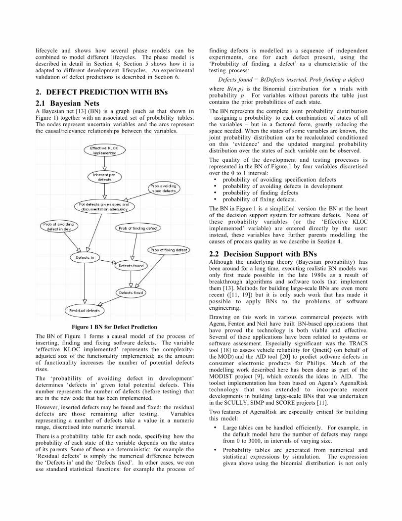
3.2 Linking Phases: Dynamic BNsWhatever the development lifecycle, the main objective is:given information about current and past phases we would liketo be able to predict attributes of quality for future phases. Wetherefore think of the set of phases as a time series that definesthe project overall. This is readily expressed as a DynamicBayesian Network (DBN) [2]. A DBN allows time-indexedvariables: in each time frame one of the parents of a time-indexed variable is the variable from the previous time frame.Figure 2 show how this is applied when the quality attribute i sthe number of residual defects.

Figure 2 A Dynamic BN Modelling a Software Lifecycle

The dynamic variable is shown with a bold boundary. Weconstruct the DBN with two nodes for each time-indexedvariable: the value in the previous time frame is the ‘input’node (here ‘Residual defects pre’) and it has no parents in thenet. The node representing the value in this time frame i scalled the ‘output node’ (here ‘Residual defects post’). Notethat the variable for the current time frame ‘Residual defectspost’ depends on the one for the previous time frame, but as anancestor rather than as a parent since it is clearer to representthe model with the intermediate variable ‘Total defects in’.

As well as defects, we also model the documentation quality asa time-varying quality attribute. Recall that documentationincludes specification, which even in iterative developmentsis often prepared in one phase and implemented in a laterphase. We consider specification errors as defects so a phasein which documentation is the main activity may lead to animportant incremental change in documentation quality that i spassed on to the next phase.

4. MODELLING A SINGLE PHASEWe describe the ‘phase-level BN’, which models a singlesoftware development phase, first giving an overview and thendescribing two part of the BN in more detail.

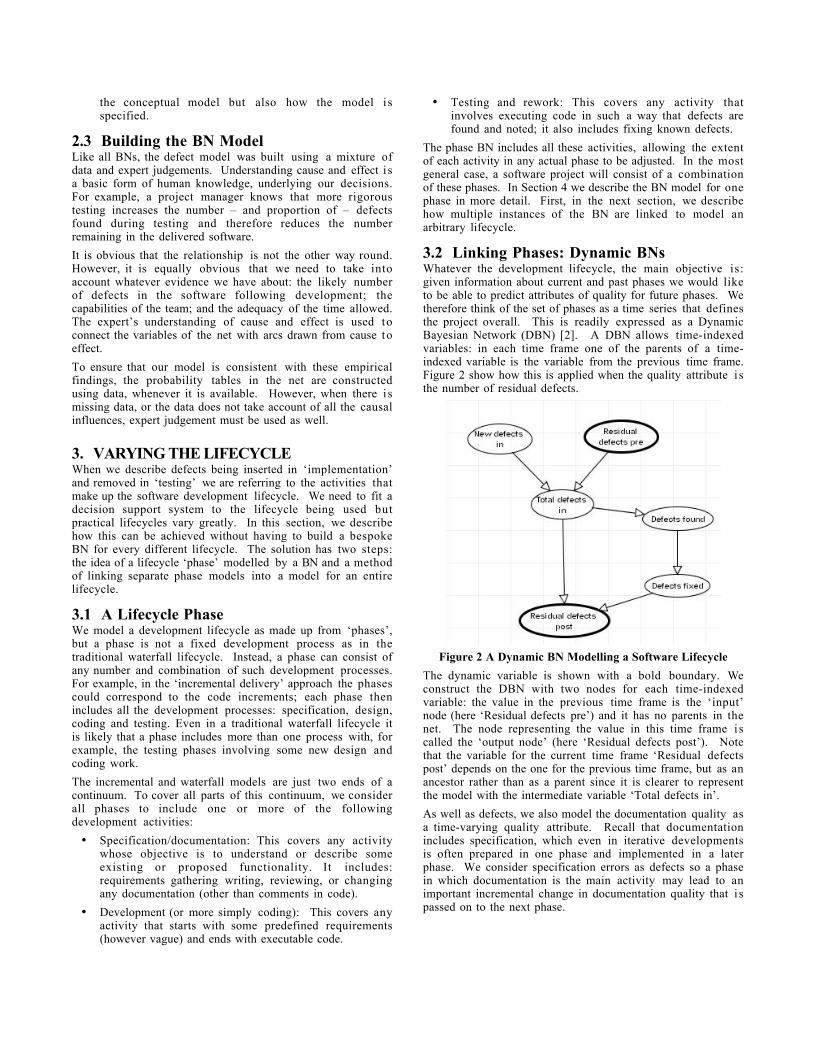
4.1 OverviewThe phase BN is best presented as six ‘subnets’, eachconsisting of BN variables, as shown in Figure 3, with greyarrows marking where there is at least one variable in onesubnet which is a parent of a variables in different subnets.The subnet plays no part in inference but is a useful for guidefor the user of the BN.

Specification and Documentation

Scale of New Functionality Implemented

Defect Insertion

and Discovery

Design and Development

Testing and Rework

Figure 3 Subnets of the Phase BN

The subnets are:

• Scale of New Functionality Implemented. Since we are tobuild and test some software we may be implementingsome new functionality in this phase. This subnet

provides a measure of the size of this functionality.

• Specification and Documentation. This subnet isconcerned with measuring the amount of specificationand documentation work in the phase, the quality of thespecification process and determining the change in thequality of the documentation as a result of the work donein the phase (modelled as a time-indexed variable).

• Design and Development. This subnet models thequality of the design and development process, whichinfluences the probability of inserting each of thepotential defects into the software.

• Testing and Rework. This subnet models the quality ofthe testing process and the rework process, influencingthe probabilities of finding and fixing defects.

• Defect and Insertion and Discovery. This subnet followsthe pattern already described in Section 2.1, adapted tohandle changes to the number of defects using a time-indexed variable. The amount of ‘new functionalityimplemented’ will influence the inherent number ofdefects in the new code. We distinguish betweenpotential defects from poor specification and ‘inherentpotential defects’, which are independent of thespecification. The number of these is a function of thenumber of function points delivered (based on empiricaldata by Jones [14, 15]).

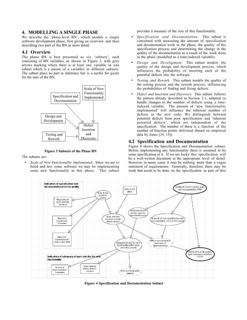
4.2 Specification and DocumentationFigure 4 shows the Specification and Documentation subnet.Before implementing any functionality there is assumed to besome specification of it. If we are lucky this specification willbe a well-written document at the appropriate level of detail.However, in many cases it may be nothing more than a vaguestatement of requirements. Generally, therefore, there may bework that needs to be done on the specification as part of this

Figure 4 Specification and Documentation Subnet

lifecycle phase.

The ‘scale of all new specification and documentation work inthis phase’ and ‘spec & doc process quality’ will determine the‘adequacy of documentation for new functionality (after specwork this phase)’ that is being implemented in this phase. If,for example, there is very little new functionality (and so the‘scale of new specification and documentation work’ is low)then, even if the ‘spec & doc process quality’ is poor, it i slikely that adequacy of documentation will be sufficient. Onthe other hand, if there is a lot of new functionality the scale ofnew specification and documentation work is likely to behigh, which means that the process quality will need to begood in order for the documentation to be adequate.

This subnet shows the use of ‘indicator’ nodes: for examplethe experience of the staff is an indicator of the processquality. Indicators can easily be tailored to match theinformation available in the software developmentenvironment – see Section 5.

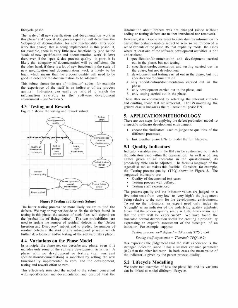
4.3 Testing and ReworkFigure 5 shows the testing and rework subnet.

Figure 5 Testing and Rework Subnet

The better testing process the more likely we are to find thedefects. We may or may not decide to fix the defects found intesting in this phase; the success of such fixes will depend onthe ‘probability of fixing defect’. The two probabilities areused to update the number of residual defects in the ‘DefectInsertion and Discovery’ subnet and to predict the number ofresidual defects at the start of any subsequent phase in whichfurther development and/or testing of the software takes place.

4.4 Variations on the Phase ModelIn principle, the phase net can describe any phase, even if i tincludes only some of the software development activities. Aphase with no development or testing (i.e. was justspecification/documentation) is modelled by setting the newfunctionality implemented to zero, and the development,testing and rework effort to zero.

This effectively restricted the model to the subnet concernedwith specification and documentation and ensured that the

information about defects was not changed (since withoutcoding or testing defects are neither introduced nor removed).

However, it is irksome for users to enter dummy information toensure that certain variables are set to zero, so we introduced aset of variants of the phase BN that explicitly model the caseswhere at least one of the software development activities is notundertaken:

1. specification/documentation and development carriedout in the phase, but not testing

2 . specification/documentation and testing carried out inthe phase, but not development

3. development and testing carried out in the phase, but notspecification/documentation

4. only specification/documentation carried out in thephase

5. only development carried out in the phase, and6. only testing carried out in the phase.

These BNs are constructed by selecting the relevant subnetsand omitting those that are irrelevant. The BN modelling thegeneral case is known as the ‘all activities’ phase BN.

5. APPLICATION METHODOLOGYThere are two steps for applying the defect prediction model toa specific software development environment:

1. choose the ‘indicators’ used to judge the qualities of thedifferent processes

2. link together phase BNs to model the full lifecycle.

5.1 Quality IndicatorsIndicator variables used in the BN can be customised to matchthe indicators used within the organisation. As well as editingnames given to an indicator in the questionnaire, itsprobability table can be adjusted. The formula language of theAgenaRisk toolset makes this feasible. Consider, for example,the ‘Testing process quality’ (TPQ) shown in Figure 5. Thesuggested indicators are:

• Quality of documented test cases• Testing process well defined• Testing staff experienced

The process quality and the indicator values are judged on afive-point scale from ‘very low’ to ‘very high’: the judgementbeing relative to the norm for the development environment.To set up the indicators, an expert need only judge its‘strength’ as an indicator of the underlying quality attribute.Given that the process quality really is high, how certain is i tthat the staff will be experienced? We have found thetruncated normal distribution useful for creating a probabilityexpressing an expert’s assessment of the ‘strength’ of anindicator. For example, suppose:

Testing process well defined = TNormal(‘TPQ’, 0.6)

Testing staff experience = TNormal(‘TPQ’, 0.2)

this expresses the judgement that the staff experience is thestronger indicator, since it has a smaller variance parameter(0.2) than the other indicator. In both cases the mean value ofthe indicator is given by the parent process quality.

5.2 Lifecycle ModellingWe show two examples of how the phase BN and its variantscan be linked to model different lifecycles.

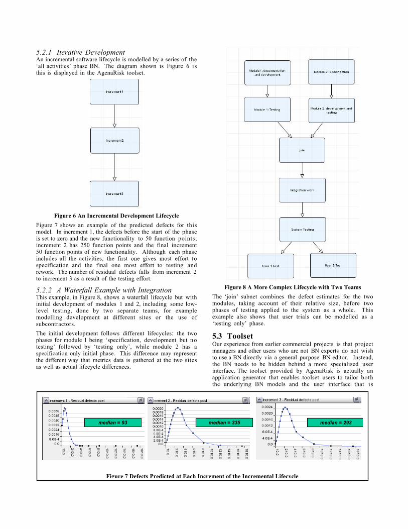
5.2.1 Iterative DevelopmentAn incremental software lifecycle is modelled by a series of the‘all activities’ phase BN. The diagram shown is Figure 6 i sthis is displayed in the AgenaRisk toolset.

Figure 6 An Incremental Development Lifecycle

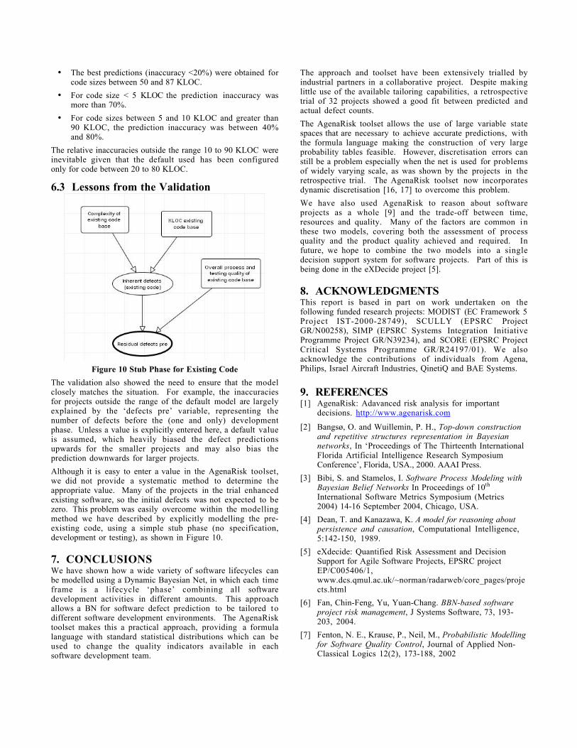
Figure 7 shows an example of the predicted defects for thismodel. In increment 1, the defects before the start of the phaseis set to zero and the new functionality to 50 function points;increment 2 has 250 function points and the final increment50 function points of new functionality. Although each phaseincludes all the activities, the first one gives most effort tospecification and the final one most effort to testing andrework. The number of residual defects falls from increment 2to increment 3 as a result of the testing effort.

5.2.2 A Waterfall Example with IntegrationThis example, in Figure 8, shows a waterfall lifecycle but withinitial development of modules 1 and 2, including some low-level testing, done by two separate teams, for examplemodelling development at different sites or the use ofsubcontractors.

The initial development follows different lifecycles: the twophases for module 1 being ‘specification, development but notesting’ followed by ‘testing only’, while module 2 has aspecification only initial phase. This difference may representthe different way that metrics data is gathered at the two sitesas well as actual lifecycle differences.

Figure 8 A More Complex Lifecycle with Two Teams

The ‘join’ subnet combines the defect estimates for the twomodules, taking account of their relative size, before twophases of testing applied to the system as a whole. Thisexample also shows that user trials can be modelled as a‘testing only’ phase.

5.3 ToolsetOur experience from earlier commercial projects is that projectmanagers and other users who are not BN experts do not wishto use a BN directly via a general purpose BN editor. Instead,the BN needs to be hidden behind a more specialised userinterface. The toolset provided by AgenaRisk is actually anapplication generator that enables toolset users to tailor boththe underlying BN models and the user interface that i s

median = 93 median = 335 median = 293

Figure 7 Defects Predicted at Each Increment of the Incremental Lifecycle

provided to the end-users when the application is generated.

The main functions provided to the end-user are:

1. Observations can be entered using a questionnaireinterface, where questions correspond to BN variables.Each question includes an explanation and the user canselect a state (if the number of states is small) or enter anumber (if the states of the variable are intervals in anumeric range). Answers given are collected into‘scenarios’ that can be named and saved. At least onescenario is created for each software development projectbut it is possible to create and compare multiplescenarios for a project.

2 . Predictions are displayed as probability distributionsand as summary statistics (mean, median, variance).Distributions are displayed either as bar charts or as linegraphs (see Figure 7) depending on the type of variableand the number of states. The predictions for severalscenarios can be superimposed for ease of comparison.Summary statistics can be exported to a spreadsheet.

The questionnaires shown to the end user can be configuredwidely. For example, questions can be grouped and orderedarbitrarily and the question text is fully editable. Not allvariables need have a question, allowing any BN variable to behidden from the end user.

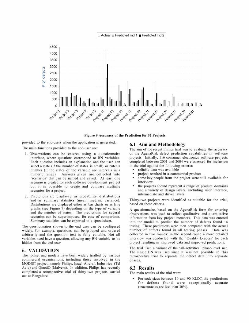
6. VALIDATIONThe toolset and models have been widely trialled by variouscommercial organisations, including those involved in theMODIST project, namely Philips, Israel Aircraft Industries (TelAviv) and QinetiQ (Malvern). In addition, Philips has recentlycompleted a retrospective trial of thirty-two projects carriedout at Bangalore.

6.1 Aim and MethodologyThe aim of the recent Philips trial was to evaluate the accuracyof the AgenaRisk defect prediction capabilities in softwareprojects. Initially, 116 consumer electronics software projectscompleted between 2001 and 2004 were assessed for inclusionin the trial against the following criteria:

• reliable data was available• project resulted in a commercial product• some key people from the project were still available for

interview• the projects should represent a range of product domains

and a variety of design layers, including user interface,intermediate and driver layers.

Thirty-two projects were identified as suitable for the trial,based on these criteria.

A questionnaire, based on the AgenaRisk form for enteringobservations, was used to collect qualitative and quantitativeinformation from key project members. This data was enteredinto the model to predict the number of defects found intesting. These predictions were then compared with the actualnumber of defects found in all testing phases. Data wascollected in two rounds: in the second round a more detailedinterview was conducted with the ‘Quality Leaders’ for eachproject resulting in improved data and improved predictions.

The trial used a variant of the ‘all-activities’ phase-level net.The single BN was used since it was not possible in thisretrospective trial to separate the defect data into separatephases.

6.2 ResultsThe main results of the trial were:

• For code sizes between 10 and 90 KLOC, the predictionsfor defects found were exceptionally accurate(inaccuracies are less than 30%).

0

500

1000

1500

2000

2500

3000

3500

4000

4500

Projec

t 1

Projec

t 3

Projec

t 5

Projec

t 7

Projec

t 9

Projec

t 11

Projec

t 13

Projec

t 15

Projec

t 17

Projec

t 19

Projec

t 21

Projec

t 23

Projec

t 25

Projec

t 27

Projec

t 29

Projec

t 31

# o

f def

ects

Actual Predicted rnd 1 Predicted rnd 2

Figure 9 Accuracy of the Prediction for 32 Projects

• The best predictions (inaccuracy <20%) were obtained forcode sizes between 50 and 87 KLOC.

• For code size < 5 KLOC the prediction inaccuracy wasmore than 70%.

• For code sizes between 5 and 10 KLOC and greater than90 KLOC, the prediction inaccuracy was between 40%and 80%.

The relative inaccuracies outside the range 10 to 90 KLOC wereinevitable given that the default used has been configuredonly for code between 20 to 80 KLOC.

6.3 Lessons from the Validation

Figure 10 Stub Phase for Existing Code

The validation also showed the need to ensure that the modelclosely matches the situation. For example, the inaccuraciesfor projects outside the range of the default model are largelyexplained by the ‘defects pre’ variable, representing thenumber of defects before the (one and only) developmentphase. Unless a value is explicitly entered here, a default valueis assumed, which heavily biased the defect predictionsupwards for the smaller projects and may also bias theprediction downwards for larger projects.

Although it is easy to enter a value in the AgenaRisk toolset,we did not provide a systematic method to determine theappropriate value. Many of the projects in the trial enhancedexisting software, so the initial defects was not expected to bezero. This problem was easily overcome within the modellingmethod we have described by explicitly modelling the pre-existing code, using a simple stub phase (no specification,development or testing), as shown in Figure 10.

7. CONCLUSIONSWe have shown how a wide variety of software lifecycles canbe modelled using a Dynamic Bayesian Net, in which each timeframe is a lifecycle ‘phase’ combining all softwaredevelopment activities in different amounts. This approachallows a BN for software defect prediction to be tailored todifferent software development environments. The AgenaRisktoolset makes this a practical approach, providing a formulalanguage with standard statistical distributions which can beused to change the quality indicators available in eachsoftware development team.

The approach and toolset have been extensively trialled byindustrial partners in a collaborative project. Despite makinglittle use of the available tailoring capabilities, a retrospectivetrial of 32 projects showed a good fit between predicted andactual defect counts.

The AgenaRisk toolset allows the use of large variable statespaces that are necessary to achieve accurate predictions, withthe formula language making the construction of very largeprobability tables feasible. However, discretisation errors canstill be a problem especially when the net is used for problemsof widely varying scale, as was shown by the projects in theretrospective trial. The AgenaRisk toolset now incorporatesdynamic discretisation [16, 17] to overcome this problem.

We have also used AgenaRisk to reason about softwareprojects as a whole [9] and the trade-off between time,resources and quality. Many of the factors are common inthese two models, covering both the assessment of processquality and the product quality achieved and required. Infuture, we hope to combine the two models into a singledecision support system for software projects. Part of this isbeing done in the eXDecide project [5].

8. ACKNOWLEDGMENTSThis report is based in part on work undertaken on thefollowing funded research projects: MODIST (EC Framework 5Project IST-2000-28749), SCULLY (EPSRC ProjectGR/N00258), SIMP (EPSRC Systems Integration InitiativeProgramme Project GR/N39234), and SCORE (EPSRC ProjectCritical Systems Programme GR/R24197/01). We alsoacknowledge the contributions of individuals from Agena,Philips, Israel Aircraft Industries, QinetiQ and BAE Systems.

9. REFERENCES[1] AgenaRisk: Adavanced risk analysis for important

decisions. http://www.agenarisk.com

[2] Bangsø, O. and Wuillemin, P. H., Top-down constructionand repetitive structures representation in Bayesiannetworks, In ‘Proceedings of The Thirteenth InternationalFlorida Artificial Intelligence Research SymposiumConference’, Florida, USA., 2000. AAAI Press.

[3] Bibi, S. and Stamelos, I. Software Process Modeling withBayesian Belief Networks In Proceedings of 10th

International Software Metrics Symposium (Metrics2004) 14-16 September 2004, Chicago, USA.

[4] Dean, T. and Kanazawa, K. A model for reasoning aboutpersistence and causation, Computational Intelligence,5:142-150, 1989.

[5] eXdecide: Quantified Risk Assessment and DecisionSupport for Agile Software Projects, EPSRC projectEP/C005406/1,www.dcs.qmul.ac.uk/~norman/radarweb/core_pages/projects.html

[6] Fan, Chin-Feng, Yu, Yuan-Chang. BBN-based softwareproject risk management, J Systems Software, 73, 193-203, 2004.

[7] Fenton, N. E., Krause, P., Neil, M., Probabilistic Modellingfor Software Quality Control, Journal of Applied Non-Classical Logics 12(2), 173-188, 2002

[8] Fenton, N. E., Krause, P., Neil, M., Software Measurement:Uncertainty and Causal Modelling, IEEE Software 10(4),116-122, 2002.

[9] Fenton, N. E., Marsh, W., Neil, M., Cates, P., Forey, S. andTailor, T. Making Resource Decisions for SoftwareProjects. In Proceedings of 26th InternationalConference on Software Engineering (ICSE 2004),(Edinburgh, United Kingdom, May 2004) IEEE ComputerSociety 2004, ISBN 0-7695-2163-0, 397-406

[10] Fenton, N. E. and Neil, M. A Critique of Software DefectPrediction Models, IEEE Transactions on SoftwareEngineering, 25(5), 675-689, 1999.

[11] Fenton, N. E. and Neil, M. SCULLY: Scaling up BayesianNets for Software Risk Assessment, Queen MaryUniversity of London,www.dcs.qmul.ac.uk/research/radar/Projects, 2001.

[12] Fenton, N. E. and Pfleeger, S.L. Software Metrics: ARigorous and Practical Approach (2nd Edition), PWS,ISBN: 0534-95429-1, 1998.

[13] Jensen, F.V. An Introduction to Bayesian Networks, UCLPress, 1996.

[14] Jones, C. Programmer Productivity, McGraw Hill, 1986.

[15] Jones, C. Software sizing, IEE Review 45(4), 165-167,1999.

[16] Koller, D., Lerner, U. and Angelov, D. A General Algorithmfor Approximate Inference and its Application to HybridBayes Nets, In Proceedings of the 15th Annual Conferenceon Uncertainty in AI (UAI), Stockholm, Sweden, August1999, pages 324—333

[17] Kozlov, A.V. and Koller, D. Nonuniform dynamicdiscretization in hybrid networks, Proceedings of the13th Annual Conference on Uncertainty in AI (UAI),Providence, Rhode Island, August 1997, pages 314--325.

[18] Neil, M., Fenton, N. E., Forey, S. and Harris, R. UsingBayesian Belief Networks to Predict the Reliability ofMilitary Vehicles, IEE Computing and ControlEngineering, 12(1), 2001, pp. 11-20.

[19] Neil, M., Fenton, N. E., Nielsen, L. Building large-scaleBayesian Networks, The Knowledge Engineering Review,15(3), 2000, pp. 257-284.

[20] Neil, M., Krause, P., Fenton, N. E., Software QualityPrediction Using Bayesian Networks in SoftwareEngineering with Computational Intelligence, (EdKhoshgoftaar TM), Kluwer, ISBN 1-4020-7427-1, Chapter6, 2003

[21] Stamelosa, I., Angelisa, L., Dimoua, P., Sakellaris, P. On theuse of Bayesian belief networks for the prediction ofsoftware productivity Information and Software Tech, 45(1), 51-60, 2003.