Eur Biophys J (1993) 22:41-51 European Biophysics Journal @ Springer-Verlag 1993

Predicting secondary structures of membrane proteins with neural networks Hero Fariselli, Mario Compiani*, Rita Casadio

Laboratory of Biophysics. Department of Baology, University of Bologna, 1-40126 Bologna, Italy

Received: 13 October 1992 / Accepted: 3 February 1993

Abstract. Back-propagation, feed-forward neural net- works are used to predict the secondary structures of membrane proteins whose structures are known to atom- ic resolution. These networks are trained on globular proteins and can predict globular protein structures hav- ing no homology to those of the training set with correla- tion coefficients (C,) of 0.45, 0.32 and 0.43 for e-helix, /?-strand and random coil structures, respectively. When tested on membrane proteins, neural networks trained on globular proteins do, on average, correctly predict (Q~) 62%, 38% and 69% of the residues in the e-helix, fl- strand and random coil structures. These scores rank higher than those obtained with the currently used statis- tical methods and are comparable to those obtained with the joint approaches tested so far on membrane proteins. The lower success score for/?-strand as compared to the other structures suggests that the sample offl-strand pat- terns contained in the training set is less representative than those of e-helix and random coil. Our analysis, which includes the effects of the network parameters and of the structural composition of the training set on the prediction, shows that regular patterns of secondary structures can be successfully extrapolated from globular to membrane proteins.

Key words: Membrane protein prediction - Protein struc- ture prediction - Neural networks - Protein folding

Introduction

Accurate prediction of protein folding from the sequence of amino acid residues remains a major unsolved problem in spite of considerable progress in developing methods based on different approaches, including energy mini- mization procedures (Li and Scheraga 1987; Friedrichs

* Present address." Department of Chemistry, University of Cameri- no, Camerino, Italy

Correspondence to: R. Casadio

and Wolynes 1989; Hinds and Levitt 1992) and molecular dynamics (Karplus and Petsko 1990). A step towards its solution is the prediction of secondary structure motifs based on the knowledge of the residue sequence, since it is generally accepted that the primary structure plays a central role in defining the protein's folding (Anfinsen 1973). This is an important starting point for modeling super-secondary and tertiary aspects of protein structure and for devising experiments in order to obtain further information with site-specific mutagenesis and chemical or immunological techniques (Blundell et al. 1987).

The number of proteins whose amino acid sequences have been deduced from cloned DNA sequences is rapid- ly increasing and is much larger than the number of three- dimensional structures which have been determined by X-ray crystallography (Bowie et al. 1991 ; Chothia 1992). This is especially true for several membrane proteins whose primary sequence and function have been exten- sively described and whose crystallographic structure is still unknown (Von Heijne 1988; Jennings 1989). The complete three-dimensional structure has been deter- mined at high resolution for only four membrane proteins: the photosynthetic reaction centers from Rhodopseudomonas viridis (Deisenhofer et al. 1985) and from the related species Rhodobacter sphaeroides (Feher et al. 1989), the pore-forming protein porin from the outer membrane of Rhodobacter capsulatus (Schiltz et al. 1991; Weiss etal. 1991) and melittin from bee venom (Terwilliger et al. 1982). In addition, a structural model for the transmembrane e-helices of bacteriorhodopsin is known at 3.5/~ resolution, based on high-resolution elec- tron cryo-microscopy (Henderson et al. 1990).

All of the current methods for predicting the sec- ondary structure of proteins are classified according to basic principles as: i) mathematical/statistical, ii) based on homology (sequence similarity) with known struc- tures, iii) empirical (usually based on hydropathy scales indicating the non-polar versus polar nature of the amino acid residues), iv) joint approaches which combine differ- ent methods (for review, see: Schulz 1988; Fasman 1989; Garnier and Levin 1991; Hirst and Sternberg 1992).

42

A significant recent addition to pattern recognition algorithms has resulted from the advent of automated computational devices, such as neural networks, which embody rules learned by means of a training procedure (Mfiller and Reinhardt 1990). This method was used to predict conformational states of globular proteins (Qian and Sejnowski 1988; Holley and Karplus 1989; McGre- gor et al. 1989; Pascarella and Bossa 1989; Kneller et al. 1990; Stolorz et al. 1992; Muskal and Kim 1992) and the e-helix traits of bacteriorhodopsin (Bohr et al. 1988). When the three conformational states e-helix, fi-strand and random coil are discriminated, the prediction accura- cy is similar to, or even better than, that obtained with other statistical methods (Qian and Sejnowski 1988; Holley and Karplus 1989). The success score ranks around 6 3 - 6 5 % of total predictions, an accuracy value which presently seems to be the upper limit of all mathe- matical/statistical predictive algorithms (Garnier and Levin 1991; Hirst and Sternberg 1992). On the other hand, the more successful predictive methods based on the existence of structure/sequence or function/sequence correlations (Garnier and Levin 1991), including joint predictive methods (Garnier and Robson 1989; Vis- wanadhan et al. 1991), are not feasible when the ho- mologous counterpart is not present in the data base. This is the case for most membrane proteins of known amino acid sequence which have no structural or func- tional homology with the membrane and globular proteins of the data base currently available.

When membrane proteins are predicted with statisti- cal methods based on rules obtained from globular proteins, an additional problem arises, since the predic- tion accuracy is usually lower than that obtained for globular proteins (Wallace et al. 1986). A possible reason is that the most hydrophobic residues, which are asso- ciated with //-strand conformations in water-soluble proteins, are also found in e-helix structures of mem- brane proteins (Jfihnig 1989). Better results are usually obtained when empirical methods, tailored to the mem- brane proteins of known crystallographic structure, are used (for review, see Fasman and Gilbert 1990).

Apparently, a trade-off exists between accuracy and scope of the predictive method in the sense that the more precise the prediction the more specific the class of proteins to which it can be applied. Both the accuracy and the specificity are critically dependent on the a priori knowledge which is used for properly tuning the ad- justable parameters of the predictive method. In this re- spect one of the most appealing features of neural net- works is that this approach requires a minimum of a priori knowledge and provides an automatic tool for ex- tracting general predictive rules from data bases of large dimension. In principle this predictive method can be applied to any kind of protein and this is relevant since the vast majority of structural details in the presently available data base relate to globular proteins.

In this paper we address the question of whether neu- ral networks, trained on a data base containing globular proteins, can be used to predict the structure of mem- brane proteins. Our results indicate that structural motifs of secondary structure can be successfully extrapolated

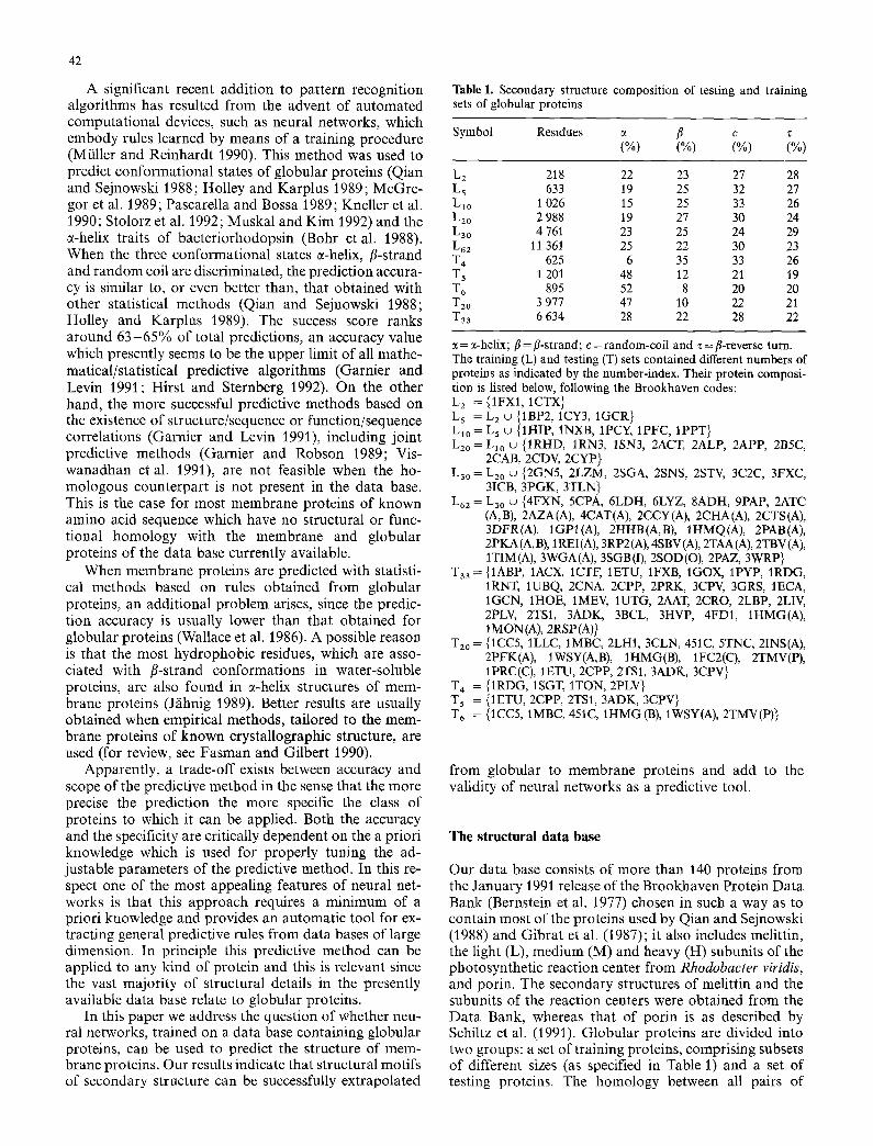
Table 1. Secondary structure composition of testing and training sets of globular proteins

Symbol Resldues c~ fl c (%) (%) (%) (%)

L 2 218 22 23 27 28 L s 633 19 25 32 27 Llo 1 026 15 25 33 26 Lzo 2 988 19 27 30 24 L3o 4 761 23 25 24 29 L62 l] 361 25 22 30 23 T 4 625 6 35 33 26 T 5 1 201 48 12 21 19 T 6 895 52 8 20 20 T2o 3 977 47 10 22 21 T33 6 634 28 22 28 22

c~ = a-helix; fl = fl-strand; c = random-coil and z = fl-reverse turn. The training (L) and testing (T) sets contained different numbers of proteins as indicated by the number-index. Their protein composi- tion is listed below, following the Brookhaven codes: L 2 = {1FX1, 1CTX} L 5 = L z u {1BP2, 1CY3, 1GCR} Llo = L 5 u {1HIP, 1NXB, 1PCY, 1PFC, 1PPT} L2o = Lao w {1RHD, IRN3, 1SN3, 2ACT, 2ALP, 2APP, 2B5C,

2CAB, 2CDV, 2GYP} L3o = L2o u {2GN5, 2LZM, 2SGA, 2SNS, 2STV, 3C2C, 3FXC,

3ICB, 3PGK, 3TLN} L62 = L3o tj {4FXN, 5CPA, 6LDH, 6LYZ, 8ADH, 9PAP, 2ATC

(A,B), 2AZA(A), 4CAT(A), 2CCY(A), 2CHA(A), 2CTS(A), 3DFR(A), 1GPI(A), 2HHB(A,B), 1HMQ(A), 2PAB(A), 2PKA (A, B), 1REI (A), 3RP2 (A), 4SBV (A), 2TAA (A), 2TBV (A), 1TIM(A), 3WGA(A), 3SGB(I), 2SOD(O), 2PAZ, 3WRP}

T33 = {1ABP, 1ACX, ICTF, 1ETU, 1FXB, 1GOX, 1PYP, 1RDG, IRNT, IUBQ, 2CNA, 2CPP, 2PRK, 3CPV, 3GRS, 1ECA, 1GCN, 1HOE, 1MEV, 1UTG, 2AAT, 2CRO, 2LBP, 2LIV, 2PLV, 2TS1, 3ADK, 3BCL, 3HVP, 4FDt, 1HMG(A), 1MON(A), 2RSP(A)} {1CC5, 1LLC, 1MBC, 2LH1, 3CLN, 451C, 5TNC, 2INS(A), 2PFK(A), IWSY(A,B), 1HMG(B), 1FC2(C), 2TMV(P), lPRC(C), 1ETU, 2CPP, 2TS1, 3ADK, 3CPV} {1RDG, 1SGT, 1TON, 2PLV} {1ETU, 2CPP, 2TS1, 3ADK, 3CPV} {1CC5, 1MBC, 451C, 1HMG (B), 1WSY(A), 2TMV(P)}

T 2 0 =

T 4

T 5 = T 6 =

from globular to membrane proteins and add to the validity of neural networks as a predictive tool.

The structural data base

Our data base consists of more than 140 proteins from the January 1991 release of the Brookhaven Protein Data Bank (Bernstein et al. 1977) chosen in such a way as to contain most of the proteins used by Qian and Sejnowski (1988) and Gibrat et al. (1987); it also includes melittin, the light (L), medium (M) and heavy (H) subunits of the photosynthetic reaction center from Rhodobacter viridis, and porin. The secondary structures of melittin and the subunits of the reaction centers were obtained from the Data Bank, whereas that of porin is as described by Schiltz et al. (1991). Globular proteins are divided into two groups: a set of training proteins, comprising subsets of different sizes (as specified in Table 1) and a set of testing proteins. The homology between all pairs of

43

Table 2. Secondary structure composition of the set of membrane proteins

Symbol Residues a fl c z (%) (%) (%) (%)

L 273 57 4 23 16 H 258 20 22 28 30 M 323 53 4 27 16 ML 26 85 0 7 8 BR 249 66 n.d. n.d. n.d. P 301 6 57 29 9 TMp 1 880 46 9 25 20 TMp 2 1181 36 21 26 17

L, H and M are the subunits of the photosynthetic reaction center of Rhodopseudomonas viridis; ML, BR and P stand for melittin, bacteriorhodopsin and porin respectively; T~p 2 and Turn are the sets of membrane proteins, excluding bacteriorhodopsin, with or without porin

proteins of the training and testing sets is very low, as determined by applying the FASTP program for a com- parison of sequences (Lipman and Pearson 1985). The only exception is the significant homology existing be- tween the L and M subunits of the reaction center com- plex.

Assignment of the secondary structure of each protein residue is done using the program DSSP, described by Kabsch and Sander (1983 a). Although the program clas- sifies secondary structures into 8 types, we grouped these into 3 or 4 types, depending on the experiments. Three types are routinely considered: e-helix, fl-strand and coil. 31o-helix is included in coil, except when we follow the partition described by Gibrat et al. (1987) (henceforth denoted as the GOR partition), in which this type is con- sidered as coil or e-helix, depending on the way it occurs in the sequence (coil, when 3 residues of the 31o-helix type occur as an isolated run; otherwise, e-helix). When net- works with four-output neurons are used, fl-turns are treated as a separate structural type.

The structural composition of the different training and testing sets consisting of globular proteins is shown in Table 1. For three-output networks, the percentage of random coil structure results from the total sum of the two rightmost columns. In Table 2 the structural compo- sition of the set of membrane proteins is reported.

Architecture and adjustable parameters of the networks

The feed-forward neural networks usually applied to sec- ondary structure prediction perform as pattern classifiers (Qian and Sejnowski 1988; Bohr et al. 1988; Holley and Karplus 1989; McGregor et al. 1989; Kneller et al. 1990; Viswanadhan et al. 1991), learning the optimal mapping between the input pattern (the primary sequence) and the output pattern (the corresponding secondary structure, as assigned with DSSP). The network design comprises two or more layers of non-linear processing units (the neurons) with adjustable connection strengths, or weights, between them. The extra units (hidden neurons), in be- tween the input and the output layers, allow the network

to perform more powerful computations and accelerate the learning rate; however, when predicting secondary structure of proteins, it was found that using complex networks can even result in worse performance (Qian and Sejnowski 1988; Holley and Karplus 1989; our results in Sect. e).

Learning is automatically performed by the network by means of the back-propagation algorithm (Rumelhart et al. 1986).

According to the network approach the adjustable parameters are: the number of hidden layers, the number of units in the hidden layers, the size of the input window, the learning rate and the initial values of the connections.

If not specified, the networks used in this study rou- tinely contain no hidden units. In some experiments with one hidden layer, the number of hidden units is three or five. The binary encoding scheme described in Bohr et al. (1988) is used for the input patterns. Our networks per- form with an input window size of 17 groups, each group with 20 units representing one of the amino acid residues, for a total of 17 x 20 = 340 input units. The output layer consists of 3 and 4 units, depending on the number of structures discriminated.

The learning rate is typically 0.01 and the weights are initially assigned random values in the range [ - 1 0 -2 10-2]. Changing the rate and the absolute values of the initial weights in the interval [0.001, 1], affects the rate of the training process but leads only to negligible changes in the overall performance of the prediction. The learning algorithm is stopped when the fractional change of the error function per cycle is less than 5 x 10 -4.

Investigating the role of the composition of the train- ing set on the efficiency of the prediction, different sets of weights are generated by training the network on differ- ent training sets, or by training it on the same training set in which structure assignment is based on the partition described by Gibrat et al. (1987). Alternatively, a set of weights (L*2) is generated by randomly reducing the numbers of back propagation cycles relative to the coil structure, so as to counterbalance the preponderance of this structure type within the data base. The performance of the network is compared to that of a random predic- tor, namely an algorithm which assigns residues to the different structures, with a probability inversely propor- tional to the number of structural types discriminated. The network was simulated on a personal computer using a program written in C.

In the following, accuracy indices (see Appendix) are evaluated both on an overall and on a protein-by-protein basis. In the former case, the index refers to the overall performance of the network evaluated by considering success and/or failure for each single residue in the testing set. In the latter case, the value of accuracy is computed as the mean of the values of the success rate obtained by applying the predictive method to each protein of the testing set. In this way, one may estimate the scattering of the pre&ctive performance of the method on each indi- vidual protein.

For each testing set, we routinely evaluate the perfor- mance rating on the basis of the values of Q3, Q,, PC~ and C,. In particular, a comparison of Qi and PC~, according

44

E O

.2 "O

13_

L o (D

1.00

0.95

0 .90

0 .85

0 .80

0.75

0 .70

0 65

0 .60

0 .55

0.50 A

0 .45

0 .40

0 .35

0 .30

0

D-© ©

o o L

• . . . . . • Tz3

A & T 20

-© zx 6

. . . - "

& A

I I I J 4 6 8 10 12

Residues T ra ined (~ 10 s )

I 14

Fig. 1. Dependence of the learning and testing capabihties of the network on the size of the train- ing set. The traimng sets of progressively increasing size and similar structural composition (L2, Ls, L10, L2o, L3o and L62 ) are also tested, as indicated by L. The testing sets consist of globular proteins (T33, T2o ). The structure composition of the train- ing and testing sets is shown in Tables 1 and 2

v

c

O C) r- O

O

x..

3

1.000

0.B00

0,600

0.400

0,200

0.000

0 - - 0 Alpha-hel ix • .... • Beta-strand z~ - Zx Random-coi l

. ~ f g . . . . T3 3

Q @

I I I I I I I 2 4 6 8 10 12 14

Residues T ra ined ( x 103 )

Fig. 2. Dependence of correct assignment of the network to different structural types on the size of the training set. Correlation coefficients for the three structural types discriminated are shown for the learning (L) and testing sets. Training sets (which are also tested) are the same as in Fig. 1. The structural composition of the testing set (T3~) is specified in Table 1

to (2 A) and (6 A) shown in the Appendix, allows an esti- mate of the number of correct, under- and over-predic- tions performed by the network in the testing phase for each discriminated structural type. As discussed in the Appendix, the accuracy is ranked according to the C, values.

Results

a) Training and testing the network

The learning and testing capabilities of the neural net- work depend on the size of the training set, that is the number of associations between the input and output patterns on which the network has been trained. The network trained on a small training set memorizes pat- terns which are too specific to reliably generalize on the never-seen-before proteins of the testing sets: this is indi- cated by the large values of the accuracy indices obtained by testing the training sets. The performance on the test- ing sets is however low, irrespective of the structural com- positions of the training and testing sets.

As the training set increases, the most general (i.e., most frequently found) patterns are more and more effec- tively classified and eventually play the role of distin- guishing markers for the pattern inclusion in the appro- priate structural class. Under these conditions, the Q3, Q,, PC i and C~ values, computed by testing the learning set, approach those obtained when the testing sets are predicted. These limiting values seem not to be affected by a further increase of the size of the training set and represent the maximal performance of the network (Qian and Sejnowski J988).

In Fig. I correct predictions of a three-output network trained on sets of globular proteins of different sizes and nearly constant structural composition are shown as a function of the number of residues trained. It is evident that when the network is trained with a large number of res idues , Q3 ranges from 0.63 to 0.66, irrespective of the size and structural composition of the testing set. This result compares well with others obtained with similar network models (Qian and Sejnowski 1988; Stolorz et al. 1992) and indicates that the network is performing in a "saturation" regime.

45

Table 3. Three-state predictxon of different sets of globular proteins

Accu- Learning L62 L~z racy

Testing L62 T33 Tzo L62 T33 T2o

Q3 0.66 0.63 0.64 0.64 0 . 6 0 0.65

Q~ 0.50 0.49 0.54 0.67 0.64 0.70 Qa 0.35 0.33 0.35 0.52 0.47 0.51 Q~ 0.86 0.83 0.82 0.67 0.63 0.62

PC, 0.63 0.62 0.78 0.53 0.52 0.71 PCa 0.60 0.58 0.37 0.51 0.50 0.32 PC~ 0.68 0.64 0.61 0.76 0.70 0.71

C, 0.43 0.40 0.44 0.44 0.39 0.45 C a 0.36 0.33 0.29 0.38 0.35 0.32 C~ 0.42 0.38 0.42 0.43 0.36 0.43

Table 4. Four-state prediction of different sets of globular proteins

Accuracy Learning L62

Testing L62 T33 T2o

Q3 0.53 0.48 0.55

Q, 0.64 0.61 0.69 Q¢ 0.47 0.42 0.46 Q, 0.41 0.31 0.32 Q~ 0.57 0.51 0.53

PC~ 0.55 0.54 0.74 PCp 0.54 0.51 0.34 PC~ 0.53 0.43 0.47 PCc 0.50 0.42 0.42

c~ 0.44 0.40 0.48 Ca 0.38 0.33 0.31 C~ 0.33 0.22 0.26 c~ 0.32 0.22 0.30

In Fig. 2, the dependence of the correlation coeffi- cients on the number of residues trained is presented. When training is carried out on sets of small size, the C, values of the learning sets maximally diverge from those of the testing set and the prediction is barely better than for a random predictor (for which Ci = 0). On increasing the size of the training set, the discriminating capability of the network between different structural types increas- es on the testing set and concomitantly it decreases on the learning set. Asymptotically, when the network maximal- ly differs from a random predictor, C, values are peaked around 0.4, except for the/~-strand structure.

Although performing under conditions of maximal generalization, the discriminating capability of the net- work between different structural types may depend on the composition of the testing relative to the traimng set.

In order to test this possibility, the predictive scores obtained on two sets of globular proteins, T33 and T2o are compared in Table 3. As shown in Table I, T33 is characterized by a structural composition similar to that of the learning set, which contains a large preponderance of the coil structure (50%). T2o, in turn, comprises glob- ular proteins whose structural composition is similar to that of membrane proteins, with an e-helix content com-

parable to that of random coil, and twice as much of that ofT33.

The values of all the accuracy indices computed in the testing and learning phases under conditions of maximal performance are listed in Table 3 (see the results when learning is performed on L62 ).

Noticeably, patterns of/?-strand structure are discrim- inated worse than those of c~-helix and random-coil, both in the learning and testing sets. This is indicated by the comparatively low values of Qp and Cp for this structural type, when testing on L62 and T33. According to (2A), since Np < N~, the low Q~ value implies that Pp is signifi- cantly lower than P~. However, PC~ is comparable with PCi for the other structural types. When Tzo is predicted, PCp markedly decreases, indicating in this c a s e n o t only that Pp < P, and Pc, but also that the number of over-pre- dictions for the B-structure increases significantly a s

compared to T33. Concomitantly also C a decreases. Con- sidering that, on passing from T33 to T2o, the accuracy for c~-helix and random coil structures is barely affected, if not improved, the results on /~-strands further confirm the observation that this structural type is scarcely recog- nized and indicate that when this is so, the structural composition of the testing relative to the training set is also relevant in determining the score.

The predictive performance of our network on the /~-strand structures contained in T33 is, however, consis- tent with what has been observed by other authors, when using three-output networks with different topologies trained on a data base of composition in secondary struc- tures similar to ours (compare with Qian and Sejnowski 1988; Holley and Karplus 1989; Kneller etal. 1990; Stolorz et al. 1992).

b) Prediction efficiency atzd structural composition of the tra#Tbtg set

It is therefore worth assessing the role of the relative frequency of each structural type in the training set in determining the performance of the network under condi- tions of maximal capability of generalization. For this purpose, we used a three-output network with a modified learning cycle and a four-output network trained on the same data base. In the first case the information con- tained in the training set is encoded in the weights with a 50% random reduction of the number of back-propaga- tion cycles relative to the random coil structure. This is equivalent to using an effective training set (L*2) with an approximately equal number of residues for each struc- tural type. When the four-output network is used, a sim- ilar balancing of the training set is obtaind since/3-reverse turns are discriminated from random coils (see Table 1). The results are listed in Tables 3 and 4, where the predic- tive performance on the different sets of globular proteins is compared using three-output networks trained on L6z and L* 2 and a four-output network trained on I262. In Table 3, the PC, and Q, values display opposite trends when, on passing from L62 to L* 2, the training set is equilibrated with respect to its structural content. From this and from (2A) and (6A), it can be inferred that the

46

number of over-predictions decreases for the coil struc- ture and increases for the c~-helix and/7-strand types. Con- comitantly, considering (2 A) and the fact that N,- is con- stant on passing from L6z to L'62, the number of under- predictions, compared to over-predictions, behaves in the opposite way. Accordingly, the Ci values, which are sym- metrical functions of under- and over-predictions (3 A) exhibit only slight variations. The increase of Cn indicates that the prediction of fl-strands is improved by decreasing the preponderance of the coil structure in the training set. Similar conclusions for the e-helix and /7-strand struc- tures can be drawn from the results obtained with the four-output network (Table 4).

These results indicate that counterbalancing the coil structure in the training set is, however, not sufficient to equalize the accuracy of the prediction of/7-strands with that of s-helix and coil types.

c) Predictions of globular and membrane proteins

Although the network performs on sets of globular proteins of large size and different structure composition (T33 and Tz0 ) at the best of its capability, it should be expected that testing on single proteins or on sets of small size may or may not reflect the overall efficiency of the method. This is evident when the accuracy indices are calculated for each protein of the training and testing sets. As an example, in Fig. 3 the numbers of occurrences of C, values relative to the three structures discriminated by the network in L62 and T33 are presented. Apparently, values of C i ranging around 0.4 occur more frequently than others when the 62 and 33 proteins of the training and testing sets are tested. The Ci values are, however, scattered widely around the mean value, as also indicated by the standard deviation (Table 5). Depending on the protein tested, the performance of the network ranges from optimal values to scores which are typical of a random predictor. This is also confirmed by the other accuracy indices, calculated as the mean of the values obtained for each protein of the testing set. The results are shown in Table 5, where the performance of a random predictor tested on the same proteins is also reported for comparison.

Consistent with these observations, when sets of small size, comprising only few globular proteins, are tested with the three- and four-output networks, the overall per- formance of the prediction can be higher or lower than that obtained with T33 or T2o. As presented in Table 6, the T 5 set, which comprises only five proteins with a high percentage of c~-helix structure, and whose structural composition is similar to that of membrane proteins (Table 1), is very efficiently predicted. In contrast T 4 (which consists of proteins characterized by a high per- centage of fl-strand structure) and T 6 (of structural com- position similar to Ts) are poorly predicted with respect to the e-helix and/7-strand structures, respectively.

Also for testing sets of small size, the success rate of /7-strand prediction improves by counterbalancing the preponderance of the random coil structure in the data base. This is evident when the accuracy indices for the

50

k

o

25

20

15

10

5

L62 Alpha-helix Beta-strand

~ Randorn-cod

0 , , - 1 . 0 0 - 0 . 7 5 - 0 . 5 0 - 0 . 2 5 0.00 0.25 0.50 0.75

Correlotion Coefficients (C~)

50

1.00

25

20

15

T53

Alpha-helix Beta-strand

EZ~] Ra ndom-coil

5-

o , , , , , - .00 - 0 . 7 5 - 0 . 5 0 - 0 . 2 5 0.00 0.25 0,50 0.75 1.00

b Correlahon Coefficients (C~)

Fig. 3 a, b. Distributions of the values of the correlation coefficients obtained for each protein when the training (a) and testing (b) sets are predicted with a three-output network trained on L62. The C i values for a random predictor would peak around 0 (see Table 5). As specified in Table 1, L62 and T33 comprise 62 and 33 proteins, respectively

fl-strand structure obtained for the sets of small size with L* 2 are compared to those calculated with a three-output network trained on L62 (Table 6). The same conclusions hold when the same sets are tested with the four-output network trained on L6z (data not shown).

Membrane proteins of known crystallographic struc- ture are grouped in a testing set of small size and are predicted using the network trained on globular proteins. The set TMp 2 including porin (an unusually fl-strand-rich membrane protein), whose secondary structure assign- ment is not from DSSP, is treated separately from TMm, which includes all the other membrane proteins. As is reported in Table 6, the network trained on L62 performs efficiently in predicting the e-helix and random-coil re- gions of membrane proteins. However, in keeping with what was noticed before for T6, fl-strand structure is poorly predicted.

The prediction of this structural type improves either when porin is included in the set (TMP2) or when L* 2 is used as a training set. In the first case, the content of fl-strands of the set of the membrane proteins in enhanced in the testing as compared to the training set; is the latter case the structural content of the training set is balanced. As discussed above, with both strategies the predictive score on the fl-strand structures increases.

Table 5. Average accuracy of the prediction on the testing and training sets

Accuracy Learning L62 L62 Random L~2 L~2

Testing L62 T33 L62 + T33 L62 T33

47

(Q 3) 0,64 +- 0.08 0.59 _ 0.08 0.31 +- 0.04 0.62 +- 0.09 0.57 + 0.09

(Q~) 0.45 -I- 0.24 0.37 + 0.21 0.31 _ 0.09 0.62 ___ 0.25 0.54 +- 0.20 (Q~) 0.29+_0.14 0.31 +_0.13 0.313-0.10 0.45+_0.17 0.47___0.16 (Qc) 0.84+_0.07 0.793-0.09 0.30+_0.06 0.65+_0.13 0.61 +_0.14

(PC~> 0,52 3- 0.32 0.47 3- 0.33 0.22 +_ 0.22 0.45 + 0.30 0.40 _ 0.20 (PC~) 0.54 + 0.32 0.50 3- 0.28 0.19 _ 0.16 0.46 ___ 0.28 0.40 ___ 0.24 (PCc) 0.65+_0.12 0.62+_0.14 0.503-0.17 0.743-0.11 0.68+_0.14

(Ca) 0.38+0.20 0.29_+0.15 -0.01 +-0.06 0.39+-0.20 0.29+-0.16 (C¢) 0.33+-0.16 0.34+_0.14 0.01 +_0.09 0.36+_0.16 0.35+_0.14 (Co) 0.44+_0.13 0.35+_0.10 0.00+_0.10 0.44+_0.12 0 35+_0.10

The mean value ((x)) of each accuracy index is (x) = 2~ s Pj xs, where Ps is the frequency of the x s value of the index 33 proteins, in the training and testing sets, respectively). The variance is calculated as' var (x)=2;j Ps (xs-(x)) 2

Table 6. Three-state prediction of small sets of globular and membrane proteins

in the set (with 62 and

Accuracy Learning L62 L~2

Testing T 5 T4 T6 TMP1 TMp2 T5 T4 T 6 Turn TMP2

Q3 0.64 0.63 0.63 0.60 0.56 0.64 0.60 0.65 0.59 0.55

Q~ 0.53 0.36 0.57 0.47 0.47 0.67 0.61 0.73 0.60 0.61 Qp 0.37 0.28 0,14 0.18 0.16 0.59 0.45 0.30 0.38 0.30 Qc 0.84 0.86 0,81 0.83 0.83 0.63 0.69 0.62 0.62 0.62

PC~ 0.81 0.16 0,81 0.79 0.66 0,74 0.15 0.73 0.69 0.55 PCp 0.47 0.75 0.12 0.13 0.30 0,40 0.66 0.17 0.16 0.32 PC c 0.57 0.70 0.59 0.62 0.57 0,64 0.77 0.71 0.72 0.66

c, 0.45 0.17 0.44 0.41 0.37 0.45 0.22 0.43 0.39 0.33 c a 0.35 0.33 0.05 0.05 0.08 0.41 0.36 0.15 0.13 0.13 cc 0.41 0.35 0.42 0.42 0.37 0.39 0.38 0.46 0.43 0.38

d) Prediction of membrane proteins with neural networks trained on membrane and globular proteins

As is shown in Table 7, the secondary structure of mem- brane proteins is predicted by using a network trained on TMp2, with a jackknife procedure so as to exclude alterna- tively from the learning set the protein to be tested.

The accuracy of the prediction is calculated for each membrane protein, including bacteriorhodopsin which was not included in the training set and whose e-helix secondary structure was assigned on the basis of cryo- electron microscopy (Henderson et al. 1990). These values are compared to those obtained when the network trained on L* 2 is used. As discussed in the previous section (and shown in Table 6)° with this set of weights the/?-strand structural type is better predicted, although the score for ~-helix structure is somewhat lower than with L62.

The overall performance of membrane proteins in pre- dicting membrane proteins is poor, as it should be, con- sidering the low success rates of the network trained on sets of small size (see Fig. 1). The exceptions of the L and M subunits can be traced back to the sequence homology of these proteins. However, this is not sufficient to over- come the success score obtained by the network trained with the set of globular proteins. In conclusion, four out

of six membrane proteins, are better discriminated in their structure content by using the network trained on globular proteins.

e) Dependence of the predictive accuracy on the size of the input window and of the hidden layer

Secondary structures of membrane proteins are also pre- dicted with networks characterized by input windows of different sizes (Table 8). In the same way as with globular proteins (Qian and Sejnowski 1988; Holley and Karplus 1989), accuracy increases at increasing window size, when the nearest-neighbour interactions are included. In the absence of hidden layers, the best accuracy is obtained at a window size of 13-17 input units. This is shown in Table 8, both for testing sets of large and small dimen- sions, comprising globular and membrane proteins, re- spectively. When predicting globular proteins, similar re- sults were also obtained by using networks with a hidden layer consisting of two units (Holley and Karplus 1989) and forty units (Qian and Sejnowski 1988).

The effect of varying the size of the hidden layer at a constant input window of 17 units is shown in Table 9. As previously reported, the presence of hidden units im-

48

Table 7. Prediction of membrane proteins with neural networks trained on membrane and globular proteins

Accu- Learning L~2 (X) racy

Testing H L M ML P BR

Q3 0.57 0.56 0.63 0.58 0.42 - 0.57

Q, 0.72 0.55 0.63 0.50 0.72 0.63 0.62 QB 0.34 0.40 0.50 * 0.27 - 0.38 Q, 0.61 0.58 0.65 1.00 0.60 - 0.69

PC~, 0.38 0.79 0.83 1.00 0.11 0.86 0.66 PCp 0.47 0.06 0.08 0.00 0.87 - 0.30 PC~ 0.78 0.64 0.76 0.40 0.50 - 0.62

C~ 0.34 0.36 0.49 0.37 0.18 0.41 0.36 C o 0.26 0.07 0.13 * 0.28 - 0.19 C~ 0.39 0.37 0.50 0.54 0.24 - 0.41

Learning TMp 2

Q3 0.51 0.66 0.67 0.46 0.35 - 0.53

Q, 0.42 0.77 0.69 0.41 0,28 0.68 0.53 Qa 0.17 0.10 0.17 * 0,09 - 0.13 Qc 0.68 0.55 0.70 0.75 0.76 - 0.69

PC, 0.29 0.73 0.78 1.00 0.06 0.87 0.62 PC o 0.34 0.04 0.05 0.00 0.67 - 0.22 PC c 0.65 0.71 0.73 0.21 0.45 - 0.55

C~ 0.13 0.40 0.46 0.31 -0 .01 0.45 0.29 Cp 0.10 0.00 0.03 * 0.06 - 0.05 C~ 0.20 0.43 0.51 0.18 0.21 - 0.31

* Structure not present in the protein. - Structures different from a-helix are not assigned in bacteriorhodopsin, which is not included in the training set of membrane proteins. ( x ) is the mean value of each accuracy index

TaMe 8. Effect of input window size on predtctive accuracy

Window Accu- Training Testing size racy L62

T33 TMp1 TMP2

3 Q3 0.58 0.57 0.51 0.48 c , 0.21 0.22 0.18 0.16 c a 0.24 0.22 0.05 - 0.02 c~ 0.28 0.29 0.28 0.24

7 Q3 0.62 0.62 0.54 0.50 c , 0.34 0.36 0.27 0.23 C o 0.29 0.30 - 0 . 0 2 -0 .01 Cc 0.37 0.37 0.39 0.34

13 Q3 0.64 0.63 0.60 0.56 C~ 0,40 0.41 0.39 0.33 C o 0.34 0.34 0.07 0.09 C~ 0.40 0.39 0.46 0.40

17 Q3 0.66 0.63 0.60 0.56 C, 0.43 0.40 0.41 0.37 C o 0.36 0.33 0.05 0.08 c c 0 42 0.42 0.42 0.37

21 Q3 0.67 0.62 0.60 0.55 C~ 0 45 0.40 0.39 0.35 C o 0.38 0.32 0.07 0.09 Cc 0.44 0.37 0.39 0.34

Table 9. Effect of hidden layer size on predictive accuracy

Hidden Accu- Training Testing units racy L62

T33 TMp1 TMP2

0 Q3 0.66 0.63 0.60 0.56 C~ 0.43 0.40 0.41 0.37 C o 0.36 0.33 0.05 0.08 C c 0.42 0.38 0.42 0.37

2 Q3 0.66 0.60 0.56 0.54 c~ 0.47 0.36 0.34 0.30 c o 0.37 0.30 0.06 0.14 c c 0.44 0.35 0.40 0.37

5 Q3 0.71 0.61 0.56 0.53 C~ 0.52 0 37 0.29 0.27 C o 0.45 0.31 0.08 0.11 C c 0.51 0.35 0.35 0.31

Table 10. Performance of different networks on membrane and globular proteins

Testing TMp 2 T33

Q3 C~ C o Cc Q3 C, c o C~

Network N* 0.55 033 0.13 0.38 0.60 0.39 0.35 0.36 N 3 0.56 0.37 0.08 0.37 0.63 0.40 0.33 0.38 N a t 0.54 0.32 0.11 0.34 0.60 0.37 0.33 0.35 N~o g 0,51 0.23 0.19 0.30 0.55 0.33 0.31 0.29

N* and N 3 are three-output networks trained on L* 2 and on L6z respectively; N 3~ is trained on L62 in which residues are grouped in structural classes according to the G O R partit ion (see Structural Data Base); the weights and the thresholds implemented in Naog are the informational parameters and thresholds of Gibrat et al. (1987)

Table 11. I n values of different predictive methods tested on mem- brane proteins

Protein CF BUR G O R III COMB* N 3

H 0.273 0.424 0,367 0.355 0.460 M 0.336 0.055 0.373 0.448 0.445 L 0.280 0.108 0.170 0.352 0.325

I n values for predictions with the CF (Chou and Fasman 1974) and BUR (Burgess et al. 1974) methods are derived from Wallace et al. (1986). I n for predictions with GOR III and the joint method C O M B I N E (COMB*) are evaluated from the Q3 indices shown in Gamier et al. (1990). N 3 is as in Table 10

p r o v e s t h e p e r f o r m a n c e o n t h e l e a r n i n g sets , w h e r e a s i t d e c r e a s e s t h e p r e d i c t i v e a c c u r a c y o n t h e t e s t i n g sets. I n o u r case , t h i s is so b o t h for g l o b u l a r a n d m e m b r a n e p r o t e i n s ( T a b l e 9), w h i c h a r e b e s t p r e d i c t e d w i t h t h e n e t - w o r k w i t h n o h i d d e n un i t s . T h e r e su l t s c o n f i r m t h a t for t h e spec i f ic t a s k o f s e c o n d a r y s t r u c t u r e p r e d i c t i o n t h e s i m p l e s t n e t w o r k m o d e l is c a p a b l e of e x t r a c t i n g t h e fea- t u r e s c o m m o n to t h e t r a i n i n g a n d t e s t i n g sets a n d o f

a c h i e v i n g t h e b e s t p r e d i c t i v e a c c u r a c y .

49

f) Comparison with other predictive methods

The directional information parameters calculated by Gibrat et al. (1987) on the basis of the information theory with a data base of similar structural composition as ours, although with a different residue assignment, are used as weights of a three-output network (N~oR) (Compiani et al. 1991). For comparison, a neural network (N~) is trained o n L62 , in which assignment is done according to the GOR partition.

From the data shown in Table 10, it is evident that the highest success rate for both globular and membrane proteins is obtained with the networks trained o n L62

and L~2, although the//-strand structure of membrane proteins is better discriminated by the N~OR.

Wallace et al. (1986), discussing the performance of the most frequently used statistical methods on membrane proteins, evaluated their accuracy on the subunits of the reaction center in terms of the I B index (5 A). In Table 11 it is shown that when I B is computed from the data ob- tained for the three subunits with the neural approach (N~), the score is significantly higher than with the other methods and similar to that obtained with COMBINE (COMB*). This is however a joint method based on the information theory, on homology search of short similar sequences and on the recognition of patterns of hydro- phobic/hydrophilic residues (Garnier and Robson 1989).

Discussion

A major difficulty in devising predictive methods for membrane proteins is the paucity of examples presently available in the data base. It is therefore difficult to treat this protein class as a separate class when using mathe- matical/statistical methods. The strategy we adopt in this work is not to rely on any general property of the class (structural, functional or chemico-physical) which would per se discriminate between membrane and globu- lar proteins and to focus on neural networks as predictive tools which automatically extract information about the sequence-to-structure mapping by learning from exam- ples. The neural approach works at the best of its capabil- ity only when the number of examples used in the training phase is much larger than the number of residues from membrane proteins known at atomic resolution.

To circumvent this problem, we are forced to train the network on globular proteins and to compare the accura- cy of the prediction on similar grounds, namely on sets of similar size and similar structural compositions.

To sharpen our predictive tool, we investigated its per- formance under different conditions. We show that our networks, when trained on large sets of globular proteins, reach a "saturation" regime, which corresponds to condi- tions of maximal generalization, as shown in Fig. 1 and Fig. 2. However, as clearly indicated by the value of Cp being lower than C~ and C c,/?-strand structures are less well discriminated than e-helix and random coil types.

The accuracy for/?-strands, which compares with that obtained by other authors using neural networks (Qian and Sejnowski 1988; Holley and Karplus 1989; Kneller et al. 1990; Stolorz et al. 1992) can be improved by equili-

brating the content of the data base with respect to the structural types discriminated, but remains lower than for e-helices and random coils, as shown in Tables 3 and 4.

These results suggest that/~-strand patterns are not as exhaustively represented as e-helix and coil patterns in the testing and training sets. This might reflect the great variety of//-strand arrangements in globular proteins (Garratt et al. 1985; Fasman 1989) and/or the great ambi- guity of the corresponding patterns (Compiani et al. 1992). In this respect, it should be considered that the sliding input window of 17 residues is large enough to include the relevant sequence context which specifies the conformation of a given residue in a protein (Kabsch and Sander 1984). Windows of this size have also been used in other statistical methods (Gibrat et al. 1987) and corre- spond to maximal performance of neural networks (Qian and Sejnowski 1988; Holley and Karplus 1989; Stolorz et al. 1992; our results).

A further problem arises on discussing the evaluation of the network performance on sets of small size.

The prediction of small protein sets, and of a single protein as a limiting case, might deviate enormously from the overall performance of the network, as indicated by the sensible scattering of the accuracy indices in Table 5. It is evident that when the size of the testing set is small, the accuracy of the prediction may be particularly affect- ed by the relative content in each type of secondary struc- ture in the testing and in the training set. In this case, when the content of any structural type is below 10%, the accuracy for that structure markedly decreases, as is ap- parent from the C, values shown in Table 6 for T 4 and T 6 , two sets comprising four and six proteins, with low con- tents of e-helix and//-strand structures, respectively (see Table 1). This effect is partially alleviated when using bal- anced training sets.

These observations have prompted us to evaluate the accuracy indices on sets of globular proteins of size and structural composition similar to those of the set of mem- brane proteins. When the three structural types e-helix, /?-strand and random coil are discriminated, the data in Table 6 show that secondary structures of membrane proteins are predicted as well as those of a set of globular proteins of similar size and composition (T6). e-helix and random coil types are recognized with the maximal accu- racy attained by the networks in predicting large sets of globular proteins. The /?-strand structure of membrane proteins and ofT 6 is, however, poorly discriminated. This finding, as discussed above, can be explained by consider- ing the low content of this structure in both sets, as com- pared to the learning set, and can be also traced back to the minor overall performance of the network in recog- nizing//-strand patterns.

Our data show that with neural networks trained on globular proteins it is possible to predict correctly from 50% to 72% of e-helix structures, from 27% to 50% of the/?-strand structures and from 58% to 100% of random coil types of membrane proteins. These scores are signifi- cantly higher than those obtained with the statistical or empirical methods discussed by Wallace et al. (1986). These authors, considering the performance of the most used statistical methods on membrane proteins, conclud-

50

ed that structural rules based on globular proteins are inappropriate for the predictions of the folding of mem- brane proteins. On the contrary, our results obtained with the neural approach, at the present available accura- cy, indicate that regular patterns of secondary structures are common to globular and membrane proteins. Evi- dently feed-forward neural networks without hidden lay- ers are capable of extracting the information pertinent to short-range interactions in the primary residue sequence as well as or even better than the directional information parameters evaluated by Gibrat et al. (1987) (see Table 10). This confirms the fact that the mapping performed by the single layer of modifiable weights is stronger than first-or- der statistics (Qian and Sejnowski 1988). The efficiency of the network on globular proteins can be equalled by statistical methods based on second-order statistics (i.e. including residue pair interactions (Gibrat et al. 1987)). The latter method, however, attains scores similar to ours on membrane proteins (Table 11) only when used jointly with other algorithms (Gamier et al. 1990). The accuracy of the prediction does not seem to increase on increasing the number of units in the hidden layer (Table 9), suggest- ing that the simplest network topology is sufficient to learn all the relevant features common to the training and testing sets.

A major drawback of this approach is, however, the limit of its accuracy (comparable to that of presently available statistical tools), which suggests it should be used with caution and possibly along with experimental tests of the predicted structure. Apparently, the influence of the local amino acid sequence seems to carry only about 65% of the information necessary to fully specify the protein folding (Gibrat et al. 1991) and this is general- ly considered a possible explanation of the present limit of all mathematical/statistical methods. What remains to be assessed is whether long-range interactions, specific for each protein fold (Allewell 1991), or chaperonin-assisted folding (Rapaport 1991) are to be considered in order to significantly improve the capability of any predictive method, including neural networks.

Appendix

Measures ofaccuracy

As already discussed by other authors (Schulz and Schirmer 1979), a number of quality indices have been proposed for a comparison of different predictive meth- ods, each index emphasizing different aspects. We focus on the ones listed below in order to evaluate the efficiency of our networks as compared to that of other predictive algorithms.

The simplest measure of predictive performance is given by the fraction of total correct predictions (com- monly expressed on a percentage basis):

Qa = z , P~/N (1 A)

where N is the total number of observed residues and P~ is the total number of residues correctly assigned to struc- ture i.

Index Q~ indicates the fraction of correct predictions for each structure type:

Q~ = P~/N~ = P,/(P~ + U~) (2A)

where N, is the number of observed residues in the struc- ture type i, P, is the total number of residues of structure i correctly predicted and U~ is the number of under-pre- dicted cases.

Although very commonly used, Q3 and Q~ do not take over-predictions into account and may be affected by the relative abundance of a secondary structure type in the data base. In this respect, a more meaningful mea- sure of accuracy is the Matthews' correlation coefficient (Matthews 1975), which for a particular secondary struc- ture type (i) makes allowance for its possible preponder- ance by punishing over- and under-prediction. It is given

by: (3 A)

C~ = (P, R , - U, O,)/[(R, + U~) (R, + 0,) (P~ + U~) (P~ + 0~)] t/2

where P~ is the number of residues correctly predicted in structure i, R~ that of residues which do not have structure i and are correctly rejected, O, and U, the number of over-predicted and under-predicted cases. The coefficient ranges between - 1 and 1, the latter being the value of the ideal perfect correlation and 0 indicating a prediction no better than random.

The prediction index defined by Burgess et al. (1974) includes the Q3 value and the number (S) of possible structural types discriminated for each residue:

I , = Q3 S--1 ON Q3 N 1/S (4A)

I~ = (Q3 S - 1)/(S - 1) 1/S _< Q a -< 1 (5 A)

I B varies from - 1 to 1. We calculate it in order to com- pare our results for membrane proteins with those listed by Wallace et al. (1986).

A direct measure of the probability of correctly assign- ing a residue to a secondary structure type is obtained from the fraction of correct prediction for each structure, defined by Kabsch and Sander (1983 b) as:

PC~ = P~/(P~ + Oz) (6 A)

with P~ and Oi are the number of residues correctly and over-predicted, respectively.

Acknowledgements. We thank Drs. P. Arrigo (CNR, Genova, Italy) and A. Pastore (EMBL, Heidelberg, Germany) for collaborations. We are also indebted to Drs. M. Crimi and M. Degli Esposti (Uni- versity of Bologna, Italy), to Profs. G. Venturoli, B.A. Melandri (University of Bologna, Italy), and A. Colosimo (University of Ro- ma, Italy) for comments and discussions. This work was partially supported by the Consiglio Nazionale delle Ricerche of Italy (CNR, grant no. 894687).

References

Allewell N (1991) Long-range interactions in proteins. TIBS 16:239 240

Anfinsen CB (1973) Principles that govern the folding of protein chains. Science 181:223-230

Bernstein FC, Koetzle TF, Williams GJB, Meyer EF, Brlce MD, Rodgers JR, Kennard O, Shimanouchi T, Tasumi M (1977) The

5l

protein data bank: a computer-based archival file for macro- molecular structures. J Mol Biol 112:535-542

Blundell TL, Sibanda BL, Sternberg MJE, Thornton JM (1987) Knowledge-based prediction of protein structures and the de- sign of novel molecules. Nature 326:347-352

Bohr H, Bohr J, Brunak S, Cotterill RMJ, Lautrup B, Norskov L, Olsen OH, Petersen SB (1988) Protein secondary structure and homology by neural networks. The e-helices in rhodop- sin. FEBS Lett 241:223-228

Bowie JU, Ltithy R, Easenberg D (1991) A method to identify protein sequences that fold into a known three-dimensional structure. Science 235:164-170

Burgess AW, Ponnuswamy PK, Scheraga HA (1974) Analysis of conformations of amino acid residues and prediction of back- bone topography in proteins. Isr J Chem 12:239-286

Chothia C (1992) One thousand families for the molecular biologist. Nature 357:543-544

Chou PY, Fasman GD (1974) Prediction of protein conformation. Biochemistry 13:222-244

Compiani M, Fariselli P, Casadio R (1991) Neural networks extract- ang general features of protein secondary structures. In: Caianiel- lo ER (ed) Parallel architectures and neural networks. World Scientific, Singapore, pp 227-237

Compiani M, Fariselli P, Casadio R (1992) The statistical be- haviour of perceptrons. In: Caianiello ER (ed) Parallel archi- tectures and neural networks. World Scientific, Singapore, pp 111-117

Deisenhofer J, Epp O, Miki K, Huber R, Michel H (1985) Structure of the protein subunits in the photosynthetic reaction centre of Rhodopseudomonas viridis at 3/~ resolution. Nature 318:618 624

Fasman GD (1989) The development of the prediction of protein structure. In: Fasman GD (ed) Prediction of protein structure and the principles of protean conformation. Plenum Press, New York, pp 193-316

Fasman GD, Gilbert WA (1990) The prediction of transmembrane protein sequences and their conformation: an evaluation. TIBS 15:89-92

Feher G, Allen JP, Okamura MY, Rees DC (1989) Structure and function of bacterial photosynthetic reaction centres. Nature 339:111-116

Friedrichs MS, Wolynes PG (1989) Towards protein tertiary struc- ture recognition by means of associative memory hamiltonians. Science 246:371-373

Gamier J, Levin JM (1991) The protein code: what is the present status? CABIOS 7:133-142

Garnier J, Robson B (1989) The GOR method for predicting sec- ondary structures in proteins. In: Fasman GD (ed) Prediction of protein structure and the principles of protein conformation. Plenum Press, New York, pp 417 465

Gamier J, Levin JM, Gibrat JF, Biou V (1990) Secondary structure prediction and protein design. Biochem Soc Symp 57:11 24

Garratt RC, Taylor WR, Thornton JM (1985) The influence of tertiary structure on secondary structure prediction. Accessibility versus predictability for fl-structure. FEBS Lett 188:59 62

Gibrat JF, Garnier J, Robson B (1987) Further developments of protein secondary structure prediction using information theo- ry. J Mol Biol 198:425-443

Gibrat JF, Robson B, Gamier J (1991) Influence of the local amino acid sequence upon the zones of the torsional angles ~b and ~/, adopted by residues in proteins. Biochemistry 30:1578-1586

Henderson R, Baldwin JM, Ceska TA, Zemlin F, Beckmann E, Downing KH (1990) Model for the structure of bacterio- rhodopsin based on high-resolution electron cryo-mieroseopy. J Mol Biol 213.899-929

Hinds DA, Levitt M (1992) A lattice model for protein structure prediction at low resolution. Proc Natl Acad Sci USA 89:2536- 2540

Hirst JD, Sternberg JE (1992) Prediction of structural and function- al features of protein and nucleic acid sequences by artificial neural network. Biochemistry 31:7211-7218

Holley HL, Karplus M (1989) Protein secondary structure predic- tion with a neural network. Proc Natl Acad Sci USA 86:152- 156

J/ihnig F (1989) Structure prediction for membrane proteans. In: Fas- man GD (ed) Prediction of protein structure and the principle of protein conformation. Plenum Press, New York, pp 707-717

Jennangs ML (1989) Topography of membrane proteins. Annu Rev Biochem 58 999-1027

Kabsch W, Sander C (1983 a) Dictionary of protein secondary struc- ture:pattern of hydrogen-bonded and geometrical features. Bio- polymers 22:2577-2637

Kabsch W, Sander C (1983 b) How good are predictions of protein secondary structure? FEBS Lett 155' 179-182

Kabsch W, Sander C (1984) On the use of sequence homologies to predict protein structure: adentical pentapeptides can have com- pletely different conformation. Proc Natl Acad Sci USA 81:1075 1078

Karplus M, Petsko GA (1990) Molecular dynamics simulations in biology. Nature 347:631 639

Kneller DG, Cohen FE, Langridge R (1990) Improvements an protein secondary structure prediction by an enhanced neural network. J Mol Biol 214:171-182

Li Z, Scheraga HA (1987) Monte Carlo-minimization approach to the multiple-minima problem an protein folding. Proc Natl Acad Sci USA 84:6611-6615

Lipman DJ, Pearson WR (1985) Rapid and sensitive similarity searches. Science 227:1435-1441

Matthews BW (1975) Comparison of the predicted and observed secondary structure of T4 phage lysozyme. Biochim Biophys Acta 405:442 451

McGregor M, Flores TP, Sternberg MJE (1989) Prediction of fl- turns in proteins using neural networks. Protein Eng 2:521 526

M/iller D, Reanhardt J (1990) Neural networks. Springer, Berlin Headelberg New York

Muskal SM, Kim SH (1992) Predicting protein secondary structure content. A tandem neural network approach. J Mol Biol 225:713 727

Pascarella S, Bossa F (1989) PRONET: a microcomputer program for predicting the secondary structure of proteins with a neural network. CABIOS 5:319-320

Qian N, Sejnowski TG (1988) Predicting the secondary structure of globular proteins using neural network models. J Mol Biol 202:865-884

Rapaport TA (1991) A bacterium catches up. Nature 369:107 108 Rumelhart DE, Hinton GE, Williams RJ (1986) Learning represen-

tation by back-propagating errors. Nature 323:533 536 Schiltz E, Kreusch A, Nestel U, Schultz E (1991) Primary structure

of porin from Rhodobacter capsulatus. Eur J Biochem 199:587- 594

Schulz GE (1988) A critical evaluation of methods for prediction of protein secondary structures. Ann Rev Biophys Chem 17:1-21

Schulz GE, Schirmer RH (1979) Principles of protein structure. Springer, Berlin Heidelberg New York

Stolorz P, Lapedes A, Xia Y (1992) Predicting protein secondary structure using neural net and statistical methods. J Mol Biol 225:363 377

Terwillager TC, Weissman L, Eisenberg D (1982) The structure of melittin in the form I crystals and its implication for melittin's lytic and surface activities. Biophys J 27:353-361

Viswanadhan VN, Denckla B, Weinsteln JN (1991) New joint pre- diction algorithm (QT-JASEP) improves the prediction of protein secondary structure. Biochemistry 30:11164-11172

Von Heajne G (1988) Transcending the impenetrable: how proteins come to terms with membranes. Biochim Biophys Aeta 947:307-333

Wallace BA, Cascio M, Mielke DL (1986) Evaluation of methods for the prediction of membrane protein secondary structures. Proc Natl Acad Sci USA 83:9423-9427

Weiss MS, Kreusch A, Schiltz E, Nestel U, Welte W, Weckesser J, Schulz GE (1991) The structure of porin from Rhodobacter cap- sulatus at 1.8 ~ resolution. FEBS Lett 280:379 382