arX

iv:h

ep-t

h/04

0401

8v2

15

Jan

2010

Preprint typeset in JHEP style - HYPER VERSION hep-th/0404018v2

LPTHE/04-07

The Automorphic Membrane

Boris Pioline

LPTHE, Universites Paris 6 et 7

Boıte 126, Tour 16, 1er etage, 4 place Jussieu,

F-75252 Paris CEDEX 05, FRANCE

E-mail: pioline@lpthe.jussieu.fr

Andrew Waldron

Department of Mathematics,

One Shields Avenue,

University of California,

Davis, CA 95616, USA

Email: wally@math.ucdavis.edu

Abstract: We present a 1-loop toroidal membrane winding sum reproducing the conjec-

tured M -theory, four-graviton, eight derivative, R4 amplitude. The U -duality and toroidal

membrane world-volume modular groups appear as a Howe dual pair in a larger, excep-

tional, group. A detailed analysis is carried out for M -theory compactified on a 3-torus,

where the target-space SL(3,Z)×SL(2,Z) U -duality and SL(3,Z) world-volume modular

groups are embedded in E6(6)(Z). Unlike previous semi-classical expansions, U -duality is

built in manifestly and realized at the quantum level thanks to Fourier invariance of cu-

bic characters. In addition to winding modes, a pair of new discrete, flux-like, quantum

numbers are necessary to ensure invariance under the larger group. The action for these

modes is of Born-Infeld type, interpolating between standard Polyakov and Nambu-Goto

membrane actions. After integration over the membrane moduli, we recover the known

R4 amplitude, including membrane instantons. Divergences are disposed of by trading the

non-compact volume integration for a compact integral over the two variables conjugate

to the fluxes – a constant term computation in mathematical parlance. As byproducts, we

suggest that, in line with membrane/fivebrane duality, the E6 theta series also describes

five-branes wrapped on T 6 in a manifestly U-duality invariant way. In addition we uncover

a new action of E6 on ten dimensional pure spinors, which may have implications for ten

dimensional super Yang–Mills theory. An extensive review of SL(3) automorphic forms is

included in an Appendix.

Contents

1. Introduction 2

2. R4 couplings, membranes and theta series: a review 3

2.1 R4 couplings and theta correspondences 3

2.2 Exact R4 amplitude in 8 dimensions 5

3. E6 minimal representation and theta series 7

3.1 From modular and U -duality invariance to E6 8

3.2 Theta series, representations and spherical vectors 8

3.3 Minimal representation of E6 9

3.4 E6 spherical vector 11

3.5 Identification of physical parameters 12

3.6 E6 Casimirs 15

4. Integrating over membrane world-volume moduli 16

4.1 Integration over SL(3) shape moduli 16

4.2 Integration over membrane volume – degenerate orbits 20

4.3 Membrane wrapping sum 21

4.4 Integration over membrane volume – non-degenerate orbit 24

5. Membranes on higher dimensional torii, membrane/5-brane duality 25

5.1 BPS membranes on T 4 25

5.2 Membrane/five-brane duality and pure spinors 27

6. Discussion 28

A. Summation measure and degenerate contributions 29

B. SL(3,Z) automorphic forms 31

B.1 Continuous representations by unitary induction 31

B.2 Fundamental domain of SL(3,Z) 34

B.3 SL(3) Eisenstein Series 36

B.4 Constant term computations 37

C. Membrane world-volume integrals 41

– 1 –

1. Introduction

Despite much evidence for its existence as a quantum theory, a tractable microscopic defini-

tion of M-theory is still missing years after the original conjecture [1, 2]. Various proposed

definitions suffer either from a lack of computability or ties to specific backgrounds and

energetics. Supermembranes remain one of the most promising candidates, because they

(i) imply the equations of motion of eleven-dimensional supergravity as a consistency re-

quirement (even at the classical level) [3], (ii) reduce to the ordinary type II string by

double reduction [4], and (iii) are equivalent to a continuous version of M(atrix) theory

in light-cone gauge [5, 6, 7]. However, the nonlinearities of the membrane world-volume

theory and the lack of an obvious genus expansion have so far stymied any attempt at

direct quantization.

In a recent series of works, we have proposed to test the supermembrane M -theory

hypothesis in a simple setting avoiding the usual quantization difficulties [8, 9]. Our pro-

posal is that four graviton, eight derivative couplings in toroidally compactified M-theory

follow from a one-loop BPS membrane amplitude. Here, “one-loop” refers to the membrane

world-volume topology, namely a torus T 3, while “BPS” to the fact that only bosonic and

fermionic zero-modes of the embedding coordinate and the world-volume metric contribute,

fluctuations canceling by virtue of supersymmetry.

The basis for this proposal can be summarized as follows: Supersymmetry requires

that the R4 amplitude receives corrections from BPS states only, as exemplified by the

one-loop computation of the R4 amplitude in string theory, which indeed reduces to a sum

of zero-mode worldsheet instanton configurations. In addition, the exact R4 amplitude,

determined on the basis of supersymmetry and U -duality [10, 11, 12, 13, 14], exhibits

membrane instantons with only toroidal topology, wrapped on T 3 subtorii of the target

space T d 1. Therefore, we expect that only toroidal membrane topologies T 3 contribute to

this amplitude. Since U -duality relates membrane instantons to perturbative contributions,

a treatment of membrane instantons that maintains manifest U -duality symmetry, will nec-

essarily reproduce the complete R4 amplitude, including its compactification-independent

part.

In this Article, we demonstrate that our proposal [8], does yield the correct R4 am-

plitude, in the simplest non-trivial case of M-theory compactified on a 3-torus. Instead

of quantizing the classical membrane action,, we assume that the result of this quanti-

zation will reduce to a sum over discrete zero-mode configurations, invariant under all

quantum symmetries. Invariance under the U-duality group SL(3,Z) × SL(2,Z) and the

world-volume modular group SL(3,Z) is then shown to require a larger symmetry group,

E6(6)(Z), under which the partition function is automorphic. In the process, we discover

new discrete, flux-like, degrees of freedom on the membrane worldvolume, necessary to

ensure U-duality invariance. We are also lead to a new prescription for dealing with the

divergence associated to the membrane volume, which makes a crucial use of these new

degrees of freedom. Our calculations are mathematically rigorous only in the degener-

ate sectors, corresponding to Kaluza-Klein contributions, the proof in the non-degenerate,

1Membrane instanton corrections in less supersymmetric settings have been discussed in [15].

– 2 –

membrane instanton sector falls short at a technical difficulty, for which we can only suggest

a resolution.

This Article is organized as follows: In Section 2, we outline the general strategy

proposed in [8], and review the exact R4 amplitude for M-theory compactified on a 3-torus,

obtained in [12] on the basis of supersymmetry and U -duality. In Section 3, we recall the

construction of the E6 theta series from our earlier work [9] and identify physical parameters

(γAB ; gMN , CMNP ) with those entering the exceptional theta series. In Section 4, we

carry out the integration over the shape moduli of the world-volume T 3 and show how to

produce the U -duality R4 amplitude from a constant term integration which regulates the

membrane world-volume integration. In Section 5, we indicate how these results generalize

to higher torii. We also point out the possible relevance of the E6 theta series for five-branes

compactified on T 6, which indicates that membrane/five-brane duality may be contained in

our framework. Not unrelatedly, we also uncover a new action of E6 on pure spinors in ten

dimensions (first announced in [16]). It would be interesting to understand the implications

for ten dimensional super Yang–Mills theory. Our conclusions, including various caveats

and speculations are presented in Section . Finally, Appendix A gives more details on the

E−6 theta series, Appendix B describes relevant aspects of SL(3) automorphic forms which

may usefully supplement our recent review [16], and Appendix C is a sample membrane

volume integral computation, illustrating the typical divergence of such integrals.

2. R4 couplings, membranes and theta series: a review

In this section, we outline the general approach, first proposed in [8]. We then review the

existing knowledge about R4 couplings in 8 dimensions, which we shall attempt to derive

from the membrane prospective.

2.1 R4 couplings and theta correspondences

To summarize the salient steps of our construction, recall first that the analogous one-loop

computation in type II string theory compactified on T d yields a partition function for

string winding modes invariant under the world-volume modular group SL(2,Z) times the

T -duality group SO(d, d,Z). The R4 amplitude is then obtained by integrating over the

fundamental domain of the toroidal lattice moduli space SL(2,R)/SO(2)

f1−loopR4 =

∫

SO(2)\SL(2,R)/SL(2,Z)

dγ Zstr(γαβ ; gµν , Bµν) . (2.1)

Here γαβ is the unit volume constant metric on the world-volume 2-torus while gµν and

Bµν are the constant target space d-torus metric and 2-form gauge field. Correspondingly,

the one-loop BPS membrane amplitude for M-theory compactified on T d is a partition

function for membrane winding modes, invariant under the modular group of the 3-torus

SL(3,Z) times the U -duality group Ed(Z). The M -theory four graviton, eight-derivative

amplitude ought emerge after integrating over the fundamental domain of the moduli space

– 3 –

of constant metrics on the toroidal world-volume:

f exactR4

?=

∫

SO(3)\Gl(3,R)/SL(3,Z)

dγ Zmem(γAB ; gMN , CMNP ) . (2.2)

Here γAB is the constant metric on the world-volume 3-torus and gMN and CMNR the

constant toroidal target-space metric and 3-form gauge field. In contrast to string ampli-

tude (2.1), we expect to integrate over volume of the metric γAB because the membrane

world-volume theory is not conformally invariant. We return to this important point later.

As a preliminary study, a semi-classical Polyakov quantization of the BPS membrane,

based on a constant instanton summation measure, was performed in [8]. We found the

correct instantonic saddle points: Euclidean membranes wrapping all subtorii T 3 of the

target space T d, but with an incorrect summation measure, incompatible with U-duality.

Similarly, the Hamiltonian interpretation of the same result gave a consistent spectrum

of BPS states running inside the loop, but with the wrong multiplicities. This result is

hardly surprising, since the membrane world-volume theory exhibits U -duality symmetry

at the classical level [17, 18], but quantum membrane self-interactions are expected to

depend non-trivially on the instanton number. This was confirmed in a U(N) matrix model

computation in [19], who found the correct instanton summation measure, in agreement

with expectations from U-duality.

This failure of semi-classical quantization suggests a different approach: U -duality

invariance should be manifestly built in from the beginning. To that end, observe that

the string theory partition function is simply a standard Gaussian theta series, invariant

under the symplectic group Sp(2d,Z), which contains SL(2,Z)×SO(d, d,Z) as commuting

subgroups. The string theory moduli gµν , Bµν live on a slice of the symplectic period matrix

moduli space according to the decomposition(SL(2,R)/SO(2)

)×(SO(d, d,R)/[SO(d) × SO(d)]

)⊂ Sp(2d)/U(d) , (2.3)

which is clearly preserved under the discrete SL(2,Z) × SO(d, d,Z) T -duality subgroup2.

More generally, the string winding mode partition function gives a correspondence between

automorphic forms of the modular group SL(2,Z) and the T -duality group SO(d, d,Z),

by integrating with respect to the fundamental domain of either of the two factors. By

analogy, we propose that the partition function of the membrane winding modes should

be a theta series for a larger group including SL(3,Z) × Ed(Z) as commuting subgroups.

Specifically, we consider the following candidates

d = 3 Gl(3)× [SL(2) × SL(3)] ⊂ E6

d = 4 Gl(3) × [SL(5)] ⊂ E7

d = 5 Gl(3) × [SO(5, 5)] ⊂ E8 .

(2.4)

Here the Gl(3) factor is to be interpreted as the world-volume modular group of a toroidal

membrane (including the R+ volume factor) while the bracketed factor is the U -duality

2For d = 2, the group Sp(4) contain extra discrete generators which preserve this slice, which in particular

can exchange the world-sheet and target space complex structures [20].

– 4 –

group Ed of d-toroidally compactified M -theory. The choice of the overarching group E6,7,8

is the most economic guess, and will be justified a posteriori below. A prime reason to

consider these groups is the fact that their minimal representation naturally involves cubic

characters, which are expected when dealing with membrane Chern–Simons couplings.

According to our proposal, BPS supermembrane quantization therefore amounts to the

construction of theta series for the exceptional groups E6,7,8. The existence of exceptional

theta series is known to mathematicians, but explicit expressions were unavailable until

recently. In an earlier Article we have explicitly computed the generic summand in the

theta series for any simply laced group G using techniques of representation theory [9].

The explicit summation measure and non-generic degenerate contributions have in turn

been computed in [21]. An important feature of exceptional theta series is that invariance

under the arithmetic subgroup G(Z) does not reduce to the usual Poisson resummation of

Gaussian sums, but instead involves Fourier invariant cubic characters. This meshes nicely

with the inherently cubic membrane couplings to the background 3-form CMNR. Another

important result from [9], is the requirement of extra flux-like quantum numbers over and

above membrane winding numbers to realize the larger exceptional symmetries.

In this work, we concentrate on the d = 3 case, which has all the features of interest

including membrane instantons, and carry out the integration in (2.2) using for Zmem the

theta series of E6.

2.2 Exact R4 amplitude in 8 dimensions

The four-graviton, eight-derivative amplitude in M-theory has received much attention in

recent years, since it is determined completely non-perturbatively on the basis of super-

symmetry and U -duality. The original conjecture by Green and Gutperle for type IIB

string theory in ten dimensions [10] was later generalized to compactification on higher-

dimensional tori T d in [12, 11, 13, 14]. For the case d = 3 of main interest in this Article,

the result proposed in [12] reads

fR4 = ESL(3)3,3/2 (G) + E

SL(2)2,1 (τ) (2.5)

where the two terms are Eisenstein series for the two factors of the U -duality group

SL(3,Z) × SL(2,Z), namely

ESL(3)3,s =

∑

mM∈Z3\{0}

[V 2/3

mMGMNmN

]s, E

SL(2)2,s =

∑

(m,n)∈Z2\{0}

[τ2

|m+ nτ |2]s

, (2.6)

whereGMN is the constant metric on the target space torus T 3 with volume V = det1/2 GMN ,

and τ is the volume modulus τ = C + i Vl3M

complexified by the constant 3-form gauge field

C = C123 on T 3. The moduli take values in the product of symmetric spaces

(GMN , τ) ∈ [SO(3)\SL(3,R)/SL(3,Z)] × [SO(2)\SL(2,R)/SL(2,Z)] , (2.7)

and transform under the left action of the U -duality group. The hat appearing on E

denotes the fact that the automorphic forms appearing in (2.5) are really the finite terms

– 5 –

following the pole at s = 3/2 (respectively s = 1),

ESL(3)3,s =

2π

s− 3/2+ E

SL(3)3,3/2 + O(s−3/2) , E

SL(2)2,s =

π

s− 1+ E

SL(2)2,1 + O(s−1) . (2.8)

The conjecture (2.5) has been checked in many different ways:

1. The original motivation came from a perturbative analysis in type IIA string theory

compactified on T 2. From this viewpoint, the 3 × 3 matrix GMN encodes the string

coupling constant gs and the complex structure U of the 2-torus, whereas the complex

modulus τ corresponds to the complexified Kahler class T of the 2-torus. Upon

expansion around the cusp at gs = 0, the result (2.5) reproduces the tree-level and

one-loop contributions in type IIA compactified on T 2, together with an infinite set

of non-perturbative effects attributed to Euclidean D0-branes winding around the

torus T 2:

fR4 =

[2ζ(3)V

g2s− 2π logU4

2 |η(U)|2 + fD0R4

]+[−2π log T 4

2 |η(T )|2]

(2.9)

Here the two terms in brackets correspond to the contribution of the first and second

term in (2.5), respectively. The summation measure for D0-instantons can be easily

extracted from this result, and was successfully rederived from a matrix model com-

putation in [22]. The second term arises purely at one-loop, and includes the effect

of perturbative worldsheet instantons. Actually, the two terms above contribute to

different kinematical structures (t8t8 ± ǫ8ǫ8)R4, which we will not distinguish (they

are identical in dimension D ≤ 7). The vanishing of the R4 amplitude at two loops

implied by (2.5) has been recently confirmed [24] (see also [25] for a review of recent

advances on two-loop technology).

2. The first term in (2.5) was derived up to an infinite additive constant from a one-

loop computation in eleven-dimensional supergravity compactified on a two torus

for which the integer summation variables mM are Kaluza-Klein momenta of the

graviton, or rather their canonical conjugates [26]. (This computation missed the

second term, which can be attributed to membrane instantons wrapping T 3.) Indeed,

expanding (2.5) around the cusp at V → ∞, one obtains

fR4 =2π2V

3l3M+

∑

mM∈Z3\{0}

V[m[1]m[1]

]3/2 − 2π log(V/l3M )

+ πV∑

m[3]∈Z\{0}

µ(m[3])√∣∣m[3]m[3]

∣∣exp

(− 2π

l3M

√∣∣m[3]m[3]

∣∣ + 2πim[3]C[3]

).

(2.10)

The single summation integer m[3] can be viewed as a target space three-form3 mMNP

which counts target 3-torus wrappings of an M2-brane with tension 1/l3M . This is the

3So m[3] = m123 and m[3]m[3] = V 2(m123)2 where the volume factors come from three contractions with

the target space metric GMN .

– 6 –

main reason to expect that a one-loop supermembrane computation should reproduce

membrane instantons and hence the full R4 couplings if U -duality can be maintained.

In this Article, we search for a derivation of this result in terms of fundamental super

membrane excitations so that wrappings are expressed in terms of winding numbers

mMNP =1

3!ǫABC ZM

A ZNB ZP

C . (2.11)

The integer-valued matrix ZMA counts windings of the Ath world-volume cycle about

the Mth target space one. The summation measure µ(m[3]) for membrane instantons

on T d is easily extracted from the SL(2) weight 1 Eisenstein series, and reads

µ(m[3]) =∑

n|m[3]

n . (2.12)

A semi-classical supermembrane computation [8] already yields the correct U -duality

invariant exponent in (2.10) but does not correctly predict the counting of states

given by µ(m[3]). It is an important challenge to rederive the result (2.10) including

the correct measure factor from the membrane theory.

3. It was shown at the linearized level for M-theory on d = 3 [27] or at the non-linear level

for type IIB [28] that supersymmetry requires the R4 amplitude to be an eigenmode

of the Laplacian on the moduli space with a specific eigenvalue:

∆(2)SO(3)\SL(3)fR4 = ∆

(2)SO(2)\SL(2)fR4 = 0 (2.13)

in the d = 3 case. It is also possible to check that the SL(3) part is annihilated

by the cubic Casimir ∆(3)SO(3)\SL(3), defined below in (3.23). In fact, the analysis

in [27, 28] was not sensitive to possible holomorphic anomalies, and indeed, due to

the subtraction of the pole in (2.8), the right-hand side of (2.13) picks up a non-

vanishing constant value, 2π. This can be viewed as the result from logarithmic

infrared divergences, as expected for R4 couplings in 8 dimensions, in close analogy

with gauge couplings in 4 dimensions [29]4. Under mild assumptions on the behavior

at small coupling, equation (2.13)together with U-duality invariance in fact imply

the correctness of (2.5).

The result (2.5) is therefore on a very firm footing, and is one of the few exact non-

perturbative M-theoretic results available. Its derivation from first principles is therefore

a central problem of this field, to which we now turn.

3. E6 minimal representation and theta series

As discussed in the Introduction, our contention is that the exact R4 amplitude (2.5) follows

from a one-loop computation in the BPS membrane theory, whose partition function is

provided by the E6 theta series. In this Section we recall the motivation for this claim,

review the construction of the E6 theta series, and identify the physical parameters inside

the moduli space of the E6 theta series.4Recall that in the terminology of [29], the holomorphic anomaly originates from the degenerate orbit,

i.e., the contribution of Kaluza-Klein gravitons.

– 7 –

3.1 From modular and U-duality invariance to E6

We posit that the correlator of four graviton vertex operators on a supermembrane of

topology T 3, at leading order in momenta, reduces to the partition function for the mem-

brane winding modes, except for a summation measure which incorporates the effects of

non-Abelian interactions for multiply wrapped membranes. The partition function of these

winding modes should furthermore be invariant under SL(3,Z) × SL(2,Z) U -duality, to-

gether with SL(3,Z) modular transformations. Invariance under the two SL(3,Z) factors

is automatic as soon as the membrane theory is invariant under world-volume and target

space diffeomorphisms. Invariance under the SL(2,Z) factor is a highly non-trivial state-

ment from the point of view of the membrane, although under double reduction it amounts

to the T -duality symmetry of the type II string. A natural way to realize this symmetry

is to require invariance under the larger group E6, through the two-stage decomposition

SL(3) ×(SL(2)× R+

)× SL(3) ⊂ SL(3)3 ⊂ E6 (3.1)

Other possibilities exist, but only this one seems to lead to a natural membrane interpre-

tation. One should therefore construct an automorphic theta series for E6. This has been

undertaken in [9, 21], which we review here for completeness:

3.2 Theta series, representations and spherical vectors

Given a group G, a theta series is constructed as follows (see e.g. [16] for a more complete

discussion): Let ρ be a representation of G acting on functions of some space X. Let f be

a function invariant under the action of the maximal compact subgroup K ⊂ G,

ρ(k)f = f , ∀k ∈ K . (3.2)

For so called spherical representations, this function is unique and known as the spherical

vector. Let δ be a distribution in the dual space of X, invariant under an arithmetic

subgroup G(Z) ⊂ G. Then the series

θ(g) = 〈δ, ρ(g)f〉 , (3.3)

is a function on G/K, invariant under right action by G(Z), hence an automorphic form5

for G(Z). The term “theta series” is usually reserved for the case when ρ is the minimal

representation, i.e. the one of smallest functional dimension. In particular, the minimal

representation carries no free parameter (excepting An, which admits a one-parameter

family of minimal representations, associated to the homogeneity degree s in Eisenstein

series such as (2.6)). This is a desirable feature for applications to supermembrane physics.

The minimal representation was constructed explicitly for all simply laced groups in [30],

based on the quantization of maximally nilpotent coadjoint orbits. The spherical vector was

computed in our earlier work [9], and the invariant distribution δ was obtained recently by

5To be precise, automorphic forms are usually required to be eigenfunctions of the Laplacian and higher

order invariant differential operators associated with the Casimirs of G. This may be achieved by requiring

irreducibility of the representation ρ.

– 8 –

adelic methods [21]. For example, when G = Sp(2,Z), one recovers the standard Gaussian

theta series, as follows: The minimal representation is the metaplectic representation acting

on X = L2(R) with generators ∂2x, x

2 and x∂x + ∂xx; the (quasi)spherical vector f is the

Gaussian f = e−x2, and δ is the comb distribution δZ, invariant under integer shifts and

Fourier transform. The latter can be viewed adelically as the product over all primes p of

the spherical vector fp over the p-adic field Qp, which is simply the unit function on the

p-adic integers, invariant under integer shifts and Fourier transform.

3.3 Minimal representation of E6

We now turn to details of the E6 theta series. Representations of non-compact groups

are generally obtained by quantizing the coadjoint orbit of an element e in G∗. The rep-

resentation of smallest dimension arises upon choosing a non-diagonalizable element e of

maximal nilpotency, which can always be conjugated into the lowest root E−ω. The gener-

ators E−ω, Eω and Hω = [Eω, E−ω] form an SL(2) subalgebra, with maximal commuting

algebra SL(6) in E6,

E6 ⊃ SL(2) × SL(6)

78 = (3, 1) ⊕ (2, 20) ⊕ (1, 35) . (3.4)

The Cartan generator Hω of this SL(2) subalgebra grades G into 5 subspaces which form

representations of the commutant SL(6):

Hω charge 2 1 0 −1 −2

SL(6) irreps 1 20 1 + 35 20 1

generators Eω {Eβ , Eγ} {Hω,Hβ,Hγ ,Hα, E±α} {E−β, E−γ} E−ω

(3.5)

The stabilizer S of E−ω is given by the grade -2 and grade -1 subspace, together with

the non-singlet part of the grade 0 subspace. Therefore, the coadjoint orbit O = S\G of

E−ω can be parameterized by the orthogonal complement to the stabilizer S, namely the

grade 1 and grade 2 spaces, together with the singlet in the grade 0 space. It carries the

canonical Kirillov-Kostant symplectic structure and admits a right action of the group G.

The action of G can thus be represented in terms of canonical generators acting by Poisson

brackets. For E6, we then have a representation on functions of a 22 dimensional, classical,

phase space O.

The minimal representation of E6 acts on functions of half as many variables and is

obtained by quantization of the classical system. The first step is to choose a polarization

or Lagrangian subspace of O, i.e.: split the 22 coordinates into 11 positions and momenta.

This is easily done by noting that the grade 1 subspace commutes to Eω and hence forms a

Heisenberg subalgebra. A particular choice of polarization is to break the symmetry SL(6)

to a subgroup H0 = SL(3) × SL(3) realized linearly on positions, which decomposes the

grade 1 subspace as 20 = 1+(3, 3)+(3, 3)+1. We choose as positions one of the two copies

of 1 + (3, 3) and call (Eγ0 , EγMA) position operators with (Eβ0 , EβA

M) being their conjugate

– 9 –

momenta. An extra position variable y corresponding to Eω plays the role of ~. These

generators are represented in the usual way

Eω = iy ,

Eβ0 = y ∂x0 , Eγ0 = ix0 ,

EβAM

= y ∂ZMA

, EγMA

= iZMA .

(3.6)

The remaining generators may be obtained using Weyl reflections as explained in [30, 9],

and are displayed in Figure 1. Pertinently, the generator for the negative root −β0 involves

the cubic H0 invariant I3 ≡ detZ,

E−β0 = −x0∂y −idetZ

y2. (3.7)

Functions invariant under the maximal compact subgroup Usp(4) of E6 must be annihilated

by the compact generator

Kβ0 = Eβ0 + E−β0 = y ∂x0 − x0∂y −idetZ

y2. (3.8)

Recognizing the first two terms as an SO(2) rotation generator, this restricts the Usp(4)

invariant functional space to

f(y, x0, ZMA ) = exp

(ix0 detZ

y(y2 + x20)

)f(y2 + x20, Z

MA ) . (3.9)

Automorphic E6 invariance in this polarization of the minimal representation relies on

(Fourier) invariance of the cubic character exp(idet(Z)/x0) (these are discussed further

in [31]). Furthermore, in this scheme, the shifts of the target space three-form C can be

identified with the action of the generator E−β0 = y∂x0 , whose effect is to shift x0 →x0 + Cy. The spherical functions thus couple to the C field by a cubic phase

exp(i

C detZ

y2 + [x0 + Cy]2

). (3.10)

reminiscent of the Chern–Simons coupling exp(iC detZ) expected for a membrane. This

cubic coupling is one of the main reasons to believe that E6 can appear as an overarching

group for the membrane on T 3. The appearance of additional variables (y, x0) in the

denominator is a new feature predicted by this E6 symmetry.

To summarize, E6 is represented on functions of 11 variables (y, x0, ZMA ) with a = 1, 2, 3

and A = 1, 2, 3. The generators of the SL(3) × SL(3) subgroup act linearly by matrix

multiplication on Z = (ZMA ) from the left and right leaving y and x0 invariant, while all

remaining generators act non-linearly. The physical interpretation of these 11 variables

will be discussed below.

– 10 –

Eω = iy

Eβ0= y ∂x0

EβA

M

= y ∂ZM

A

Eγ0= ix0

EγM

A

= iZMA

LBA = −ZM

A ∂ZM

B

= −E−αA

B

SL(3)L

RMN = −ZM

A ∂ZN

A

= −E−αN

M

SL(3)R

EαA

M

= −x0∂ZM

A

+ i2y εABCεMNRZ

NB ZR

C

E−αM

A

= ZMA ∂x0

− iy2 εABCε

MNR∂ZN

B

∂ZR

C

HαM

A

= −x0∂x0+ ZM

A ∂ZM

A

+ (1− δAB)(1 − δMN )ZNB ∂ZN

B

+ 2 (no sum on A, M)

Hβ0= −y∂y + x0∂x0

Hω = −2y∂y − x0∂x0− Z · ∂Z − 6

E−β0

= −x0∂y − i detZy2

E−βA

M

= ZMA ∂y +

i2 x0 εABCε

MNR ∂ZN

B

∂ZR

C

+ 1y(ZM

A [Z · ∂Z + 2]− ZNA ZM

B ∂ZN

B

)

E−γ0

= −y det[∂Z ]− i(y∂y + x0∂x0+ Z · ∂Z + 6)∂x0

E−γM

A

= i(y∂y + x0∂x0+ 4)∂ZM

A

+ iZNA ∂ZN

A

∂ZM

B

+ 12y εABCεMNRZ

NB ZR

C

E−ω = −i(y∂y + x0∂x0

+ Z · ∂Z + 6)∂y + x0 det[∂Z ]

− iy

(2Z · ∂Z + 1

2 (Z · ∂Z)2 − 12Z

MA ZN

B ∂ZN

B

∂ZN

A

+ 6)+ det(Z)

y2 ∂x0

(3.11)

Figure 1: Infinitesimal generators for the E6 minimal representation.

3.4 E6 spherical vector

The spherical vector fE6 is invariant under the maximal compact subgroup Usp(4) of

E6 generated by Kδ = Eδ + E−δ for any positive root δ. So determining the spherical

vector amounts to solving a complicated system partial differential equations KδfE6 = 0.

Invariance under the maximal compact subgroup of the linearly acting SL(3) × SL(3)

implies that fE6 is a function of the quadratic, cubic and quartic invariants trZtZ, det(Z),

and tr(ZtZ)2. Invariance under the remaining compact generators fixes this function to

be [9]

fE6 =exp(−S1 − iS2)

(y2 + x20) S1, (3.12)

where

S1 =

√det[ZZt + (y2 + x20)I ]

y2 + x20, S2 = − x0 det(Z)

y(y2 + x20). (3.13)

– 11 –

The exponential weight S1 + iS2 should be thought of as the classical action of a mem-

brane with quantum numbers y, x0, ZMA , at the origin of the moduli space E6/Usp(4) ⊃

[SL(3,R)/SO(3)]3 . In the next Section we explain how to couple the theory to world-

volume and target-space moduli. At this point, we note that the integers ZMA are naturally

interpreted as windings arising from the zero-modes of transverse membrane coordinates:

XM (σA) = ZMA σA + · · · , ZM

A = ∂AXM . (3.14)

The action S1 is a Born-Infeld type-generalization of the Polyakov membrane action.

The additional quantum numbers y, x0 are necessary for manifest U -duality but can-

not correspond to propagating membrane world-volume degrees of freedom which have

already been accounted for by the windings ZMA . We propose, therefore, that they in-

stead correspond to field strengths of a pair of two-form gauge fields BAB and BAB,MNR

(transforming as target space scalar and three-form densities), which have no propagating

degrees of freedom in 3 dimensions, but whose field strengths take only quantized values.

Clearly if correct, our proposal, based on maintaining U -duality, provides a detailed

microscope for examining fundamental membrane M -theory excitations. In particular, it

would be interesting to extend U -duality invariance of the classical zero-mode action to

quantum fluctuations. A remarkable feature of the E6 spherical vector (3.12) is the simple

exponential (corresponding to the Bessel function of index 1/2) which receives no quan-

tum corrections about the classical action. In contrast, higher En cases involve genuine,

“quantum corrected”, Bessel functions of S1.

3.5 Identification of physical parameters

We now present the decomposition of the extended duality group E6 into world-volume

modular and target space U -duality groups. Examining the E6 Dynkin diagram in Figure 2,

we identify three commuting SL(3) subgroups with positive roots

∆+SL(3)L

= {α12, α23, α13} , ∆+SL(3)R

= {α12, α23, α13} , ∆+SL(3)NL

= {β0,−ω,−γ0} .(3.15)

The first two factors SL(3)L and SL(3)R act linearly on ZMA by left and right multiplication,

respectively. In line with our identification of ZMA as the winding numbers ∂AX

M of the

membrane, one may thus associate SL(3)L and SL(3)R with the modular groups of the

world-volume and target space 3-torii. The remaining SL(2) U -duality group, acting by

fractional linear transformations on the complex modulus τ = C + i Vl3M

(with C ≡ C123)

must reside in the remaining non-linearly acting SL(3)NL. A further decomposition

SL(3)NL ⊃ SL(2)τ × R+ν (3.16)

allows the remaining R+ν factor to be identified with the volume of the world-volume 3-

torus. In the classical membrane theory, the membrane volume does not decouple because,

in contrast to strings, the world-volume theory is not Weyl invariant.

One may wonder if this choice of parameterization is ambiguous. In particular, one may

have considered identifying the world volume modular group with the non-linearly realized

– 12 –

g g g g g

1

α32

3

α21

4

α11

5

α12

6

α23

g

×

β02

−ω...

α21 = (0, 0, 1, 0, 0, 0)

α32 = (1, 0, 0, 0, 0, 0)

α31 = (1, 0, 1, 0, 0, 0)

α12= (0, 0, 0, 0, 1, 0)

α23= (0, 0, 0, 0, 0, 1)

α13= (0, 0, 0, 0, 1, 1)

α11= (0, 0, 0, 1, 0, 0)

α21= (0, 0, 0, 1, 1, 0)

α31= (0, 0, 0, 1, 1, 1)

α12= (0, 0, 1, 1, 0, 0)

α22= (0, 0, 1, 1, 1, 0)

α32= (0, 0, 1, 1, 1, 1)

α13= (1, 0, 1, 1, 0, 0)

α23= (1, 0, 1, 1, 1, 0)

α33= (1, 0, 1, 1, 1, 1)

β0 = (0, 1, 0, 0, 0, 0) γ0 = (1, 1, 2, 3, 2, 1)

β11= (0, 1, 0, 1, 0, 0) γ1

1 = (1, 1, 2, 2, 2, 1)

β21= (0, 1, 0, 1, 1, 0) γ2

1 = (1, 1, 2, 2, 1, 1)

β31= (0, 1, 0, 1, 1, 1) γ3

1 = (1, 1, 2, 2, 1, 0)

β12= (0, 1, 1, 1, 0, 0) γ1

2 = (1, 1, 1, 2, 2, 1)

β22= (0, 1, 1, 1, 1, 0) γ2

2 = (1, 1, 1, 2, 1, 1)

β32= (0, 1, 1, 1, 1, 1) γ3

2 = (1, 1, 1, 2, 1, 0)

β13= (1, 1, 1, 1, 0, 0) γ1

3 = (0, 1, 1, 2, 2, 1)

β23= (1, 1, 1, 1, 1, 0) γ2

3 = (0, 1, 1, 2, 1, 1)

β33= (1, 1, 1, 1, 1, 1) γ3

3 = (0, 1, 1, 2, 1, 0)

ω = (1, 2, 2, 3, 2, 1)

Figure 2: Dynkin diagram and positive roots for E6

factor SL(3)NL. However, thanks to the triality symmetry of the extended E6 Dynkin

diagram in Figure 2, one can show by using an appropriate intertwiner that any two of the

SL(3)L,R,NL groups can be made to act linearly. Identifying the world-volume modular

group with the linearly realized SL(3)L is convenient for our purposes, since we wish to

integrate over the moduli space of world-volume metrics SO(3)\SL(3). Moreover, the

combination of linearly acting world-volume and target-space modular groups is necessary

for our membrane interpretation of the exceptional theta series.

– 13 –

To determine the decomposition of SL(3)NL into world-volume and U -duality parts, we

recall (as observed in Section 3.3) that the target three-form couples through the exponen-

tial of the generator e−β0 . Therefore we associate the non-linear SL(2) U -duality group with

that generated by {Eβ0 ,Hβ0 , E−β0}. The maximal commutant to the SL(2) ⊂ SL(3)NL is

the R+ group generated by

Hν = 2Hω −Hβ0 = −3y∂y − 3x0∂x0 − 2Z · ∂Z − 12 . (3.17)

From the expressions for the E6 generators in Figure 1 we read off the scaling weights of

the various quantum numbers with respect to target and world volumes:

quantum numbers y x0 ZMA

target-space −1 1 0

world-volume −3 −3 −2

(3.18)

Therefore we choose the following couplings

y → νV 1/3y , x0 → νV −1/3x0 , Z → ν2/3e−1ZE , (3.19)

where the 3× 3 matrices

γ ≡ ν2/3 eet , G ≡ V 2/3 EEt , (3.20)

are the world-volume and target-space metrics, respectively. Note that although relative

scalings of the two volumes amongst the variables (y, x0, ZMA ) are fixed, we will justify the

overall ones by the results. We may now state our U -duality and world-volume modular

invariant membrane winding formula

θE6(γ;G,C) = V ν2∑

(y,x0,Z)

∈Z11\{0}

µ(y,x0,Z)e− 2π

l3M

√det(ZGZt+γ|x0+τy|2)

|x0+τy|2 −2πi detZ(

x0+Cy

y|x0+τy|2

)

√det(ZGZt+γ|x0+τy|2)

+ degen.

(3.21)

Salient features of this result include

• Although the variables ZMA of the minimal representation in Figure 1 are real-valued,

once integrated against the distribution δ in (3.3), they are restricted to integers.

(This is also the origin of the overall factors 2π in the exponent.) Hence their natural

interpretation as winding numbers.

• The real exponent is a Born-Infeld membrane action. It interpolates between Nambu-

Goto (large membrane volume V ≫ ν) and Polyakov-like (V ≪ ν) actions.

• The membrane tension appears correctly as 1/l3M while the overall factor of the target

space volume V matches correctly that of the bulk term in (2.10).

• The subleading degenerate terms and summation measure µ(y, x0, Z) are known [21]

and described in Appendix A. The latter is derived from a p-adic analog of the spher-

ical vector. It is a complicated number theoretic function representing the quantum

degeneracies of winding states and was inaccessible to previous semi-classical ap-

proaches [8].

– 14 –

• The SL(2) modulus τ = C + i Vl3M

coupling to the fluxes (y, x0) may be written

covariantly as |HMNR + CMNRH|2 + |H|2 where x0 ↔ HMNR = dBMNR and y ↔H ≡ dB. The interpretation of x0 as a target space 3-form is justified both by its

coupling to the Chern-Simons 3-form and generalizations to higher torii discussed in

Section 5.

The simplest check of our proposal is whether it is a zero mode of the Laplacian on the

U -duality moduli space, as required by supersymmetry. This is the topic of the next

Section.

3.6 E6 Casimirs

The desired R4 amplitude (2.5) is a zero mode of the Laplacian and invariant cubic opera-

tor of the SL(3)×SL(2) U -duality group. This is in fact separately true for the geometric

target space SL(3) subgroup (and also the Laplacian of the non-linear SL(2) factor with

which we deal later). We can easily verify this property of our E6 based R4 amplitude as a

simple consistency check: By virtue of the formula (3.3), relations valid for the enveloping

algebra of the representation ρ apply also to the corresponding (differential) operators act-

ing on moduli g. We therefore examine the quadratic and cubic Casimirs of the subgroups

SL(3)L,R,NL,

C2 =1

3!

∑

α∈∆+

[H 2

α − 6EαE−α

]Weyl

, (3.22)

C3 =1

2

∏

α∈∆+

Hα +9

2

[ ∑

α∈∆+

HαEαE−α − 3∑

α,β,γ∈∆+

α+β=γ

(EαEβE−γ + E−αE−βEγ

)]Weyl

.

(3.23)

Here α1,2 are simple roots and ∆+ = {α1,2, α1+α2} is the positive root lattice (see (3.15)).

These compact expressions are “classical”, the square brackets denote Weyl ordering av-

eraging each term over all distinct orderings. Also, Hα1 ≡ Hα1 +Hα1+α2 , Hα2 ≡ −Hα2 −Hα1+α2 and Hα1+α2 ≡ Hα1 −Hα2 . Inserting the explicit expressions for the minimal rep-

resentation E6 generators (see Figure 1) yields invariant differential operators ∆(2,3)SL(3)R,L,NL

subject to particular relations

∆(2)SL(3)L

= ∆(2)SL(3)R

= ∆(2)SL(3)NL

, ∆(3)SL(3)L

= ∆(3)SL(3)R

= ∆(3)SL(3)NL

. (3.24)

As explained above in (2.13), supersymmetry requires that the invariant target space op-

erators ∆(2)SL(3)R

= 0 = ∆(3)SL(3)R

. However, upon integrating over the SL(3)L fundamental

domain of the world-volume torus shape moduli, the operators ∆(2,3)SL(3)L

no longer act and

must therefore return zero. Hence (3.24), in turn, implies vanishing of the target space

invariants. As in the 1-loop string computation [29], infrared divergences may lead to holo-

morphic anomalies, and a constant non-vanishing right-hand side for (2.13). The explicit

world-volume moduli integration is the subject of the following Section.

– 15 –

4. Integrating over membrane world-volume moduli

An important difference between supermembranes and superstrings is the absence of a

classical Weyl symmetry. An integral over all membrane volumes is, in general, divergent

and must be appropriately regulated. On the other hand, integrations over SL(3) shape

moduli of a world-volume 3-torus are better defined. This part of our calculation is com-

pletely analogous to its stringy counterpart: The summation over windings is decomposed

into SL(3,Z) orbits and the integration over shape moduli can be performed by unfolding

their fundamental domain.

An additional puzzle, at this stage, is the role of the flux-like quantum numbers (y, x0).

Our solution is to relate this difficulty to regulating the volume integral: Replacing the

volume integral by one over additional compact moduli corresponding to shifts of the fluxes

at the same time integrates out these additional quantum numbers while projecting out the

dependence on the volume modulus. This procedure is a general technique in the theory

of automorphic forms known as a constant term computation6. We begin the computation

by integrating over shape moduli.

4.1 Integration over SL(3) shape moduli

The next step of our investigation of the conjecture that

Zmem(γAB ;GMN , CMNP ) = θE6(γAB ;GMN , CMNP ) , (4.1)

is to evaluate the modular integral over the SO(3)\SL(3) shape moduli of the world-volume

3-torus. Let us begin with a general description of the SL(3)L modular integral:

4.1.1 Modular integral and orbit decomposition

The theta series summand at an arbitrary point of the moduli space SO(3)\SL(3), withIwasawa gauge coset representative

e−1 =

1/L √

L/T2 √LT2

·

1 A1 A2

1 T1

1

, (4.2)

is given in (3.21) depending on moduli e through (3.20). This summand was obtained by

acting on the spherical vector with the linear SL(3)L representation ρL(e) acting by left

multiplication on the windings ZMA . One is therefore left to compute

θSl3×Sl3 =

∫

Fde θE6(y, x0, e

−1Z) . (4.3)

The integration is over the fundamental domain F = SO(3)\SL(3)L/SL(3,Z) of the mod-

uli space of unit-volume constant metrics on T 3, with invariant measure

de =d2T

T 22

d2AdL

L4. (4.4)

6An excellent review and useful results for SL(3) can be found in [32].

– 16 –

We lose no generality evaluating all other (target space) moduli at the origin. We stress

again, that by construction θSl3×Sl3 is an automorphic form of the U -duality group SL(3,Z)×SL(2,Z) ⊂ SL(3,Z)× SL(3,Z).

Modular integrals of this type can be computed by the general method of orbits: one

restricts the summation on integers in θE6 to one representative in each orbit of the lin-

ear SL(3,Z)L action, and at the same time enlarges the integration domain to the image

of the fundamental domain under the SL(3,Z) orbit generators. Since Z transforms by

SL(3,Z) left-multiplication, orbits are labeled by the rank of the 3×3 matrix Z. The non-

degenerate orbits have rank(Z) = 3 and the fundamental domain can be enlarged to the

full SO(3)\SL(3) moduli space. At the other end of the rank spectrum, the rank(Z) = 0

orbit contains the single element Z = 0. The shape integral then yields only a factor of

the volume of the fundamental domain F . After integration over the volume factor R+ν ,

these two orbits will correspond to the Eisenstein series ESL(2)2,1 in (2.5), hence to membrane

instantons. The rank(Z) = 1, 2 orbits require a detailed understanding of the fundamental

domain F . They correspond to toroidal, supergravity Kaluza–Klein excitations with am-

plitude ESL(3)3,3/2 . We deal with these terms first for which we are able to present a rigorous

computation:

4.1.2 Rank 1 and 2 winding modes

To performing the integral over shape moduli it is convenient to rewrite the E6 spherical

vector in the integral representation

fE6 =1√π

∫ ∞

0

dt

t1/2exp

(− 1

4t(y2 + x20)2− t det[ZZt + (y2 + x20)I] − i

x0 det(Z)

y(y2 + x20)

). (4.5)

Since SL(3)L acts on the matrix Z by left multiplication, Z → e−1Z, it leaves the phase

invariant. We may further set x0 = 0 as it can be reinstated by an SO(2) rotation in the

(y, x0) plane.

We must now compute∫Frk=1,2

de fE6 with respect to unfolded fundamental domains

Frk=1,2. The SL(3) fundamental domain F is known [33, 34], a complete description is

given in Appendix B.2, see in particular equations (B.17) and (B.19). Its construction is

in terms of a height function given by the maximal abelian torus coordinate L3 in (4.2)

along with the actions of an (overcomplete) set of SL(3,Z) generators S1,...,5, T1,2 and U1,2

given in (B.16,B.18).

Rank 1 (twice degenerate) orbit: In this case the winding matrix Z may be rotated

by an SL(3,Z) transformation from the right into a single row

Z =

p1 p2 p3 . (4.6)

The range of the linear mapping Z is generated by a single SL(3)L left-invariant vector

transforming as a projective vector under the right SL(3)R action. The matrix (4.6) is left

– 17 –

invariant with respect to SL(3,Z) elements of the form

1 ∗ ∗∗ ∗∗ ∗

, (4.7)

spanned by generators S2, T1,2,3 and U2. The conditions from the remaining generators

may be unfolded yielding the integration range

Frk=1 ={0 ≤ T1 ≤

1

2, T 2

1 + T 22 ≥ 1 , −1

2≤ A1,2 ≤

1

2, 0 ≤ L < ∞

}. (4.8)

We find

∫

Frk=1

de fE6 =1√π

∫

Frk=1

de

∫dt

t1/2exp

(− 1

4y4t− ty4

[y2 +

p21 + p22 + p23L2

])

=1

(p21 + p22 + p23)3/2

π

3|y| K1(|y|) . (4.9)

The first factor is easily recognized as an Eisenstein series of SL(3)R in the minimal repre-

sentation, with index 3/2. On the other hand, reinstating the x0 dependence dependence

in the second term, |y| →√y2 + x20, yields the spherical vector (B.12) of the Eisenstein

series of SL(3)NL in the minimal representation, with index 0. Both of these can be

identified with the general Eisenstein series (B.28) with (λ32, λ21) equal to (−2, 1)R and

(1, 1)NL, respectively. Hence, up to an overall normalization7 we obtain, in the notation of

Appendix B.3, ∫

Fde θrk=1

E6= E(gR;−2, 1) E(gNL; 1, 1) . (4.10)

The SL(3)R moduli are gR = EEt, the unit, target space metric. We postpone dealing

with the SL(3)NL moduli gNL to our discussion of the membrane world-volume integration

in Section 4.2.

Rank 2 (singly degenerate) orbit: The winding matrix Z may be rotated by an

SL(3,Z) transformation into two rows,

Z =

a1 p1 p2

a2 p3

≡

~v

~w

. (4.11)

This configuration is invariant under the left SL(3,Z) action of elements of the form

1 ∗1 ∗

∗

. (4.12)

7The rank 1 and 2 normalizations are computable, but unimportant since we have no such control over

the rank 3 computation. Note also, there is in principle a six-fold ambiguity in the above identification,

which is irrelevant due to the Selberg functional relations discussed in Appendix B.1.

– 18 –

These are spanned by generators T2,3. All other generators may be unfolded yielding the

integration range

Frk=2 ={− 1

2≤ T1 , A2 ≤

1

2, −∞ < A1 < ∞ , 0 ≤ T2, L < ∞

}. (4.13)

We find

∫

Frk=2

de fE6 =1√π

∫

Frk=2

de

∫dt

t1/2e− 1

4y4t−ty2

[y4+y2

(L~v2

T2+

(~w+A1~v2)

L2

)+

|~v×~w|2LT2

]

=1

|~v × ~w|31

y2

∫ ∞

0

dt dT2 dL

t T 22 L3

e− 1

4ty4−ty2

(

y2+ 1L2

)(

y2+ LT2

)

.

(4.14)

Here the integrals over compact circles T1 and A2 are trivial and we performed the Gaussian

integral over A1 explicitly. We now change variables

r1 = 1/L2 , r2 = L/T2 , (4.15)

and rescale ri → riy2, t → t/y5, obtaining

∫

Frk=2

de fE6 =y3

2|~v × ~w|3∫ ∞

0

dt

t

√r1dr1dr2 e−

y4t−ty(1+r1)(1+r2) .

(4.16)

The integral over r2 is of Gamma function type. Carrying out the Bessel-type integration

with respect to t and changing variable to r1 = u2 − 1, we find

∫

Frk=2

de fE6 =4y2

|~v × ~w|3∫ ∞

1K1(uy)

√u2 − 1 du (4.17)

=2πe−y

|~v × ~w|3

Comparing again to (B.28) and (B.12), we recognize the product of SL(3)NL and SL(3)Rcontinuous representations with parameters (λ32, λ21) = (1, 1), (1,−2), respectively. Hence

the rank 2 result is a product of corresponding SL(3) Eisenstein series. However, as ex-

plained in Appendix B.4, minimal parabolic Eisenstein series obey Selberg relations, which

amount to invariance8 under (Weyl group) permutations of the labels λ1, λ2, λ3. These are

generated by reflections about radial lines λ21 = λ32, 2λ21 = −λ32 and λ21 = −2λ32 in

the (λ32, λ21)-plane depicted in Figure 3. In particular, this implies, up to normalization,

equality of the rank 2 and rank 1 winding sums. Hence∫

Fde(θrk=1E6

+ θrk=2E6

)= E(gNL;−2, 1) E(gR;−2, 1) . (4.18)

Observe from Figure 3 that the point (−2, 1) corresponds to vanishing quadratic and cubic

Casimirs as predicted in Section 3.6.

8The classical example is the SL(2) relation ESL(2)s ∝ E

SL(2)1−s . Equality holds for appropriate normal-

ization by a function of s, see (B.43).

– 19 –

4.2 Integration over membrane volume – degenerate orbits

Before dealing with rank 3 and 0 winding sums, we study the rank 2 and 1 results and

learn how to handle the membrane world volume integral. The lack of conformal (Weyl)

invariance of the classical supermembrane theory has been a key stumbling block, intimately

related to its gapless, continuous spectrum. This is precisely the sector where we expect

to find new physics.

We start with an Iwasawa decomposition of SL(3)NL moduli refined to exhibit the

SL(2) U -duality subgroup:

gNL =

1ν2/3

ν1/3

ν1/3

1

1√τ2 √

τ2

1

1 τ11

1 n1 n2

1

1

. (4.19)

The membrane world volume modulus ν and target space moduli (τ1, τ2) were already

introduced in Section 3.5. There are, however, two additional possible moduli (n1, n2).

Automorphy implies that these are compact unit interval valued variables. In contrast, the

world volume modulus is non-compact taking any real positive value. In a (semi)classical

supermembrane setting, the moduli (n1, n2) have no particular meaning and should be set

to zero; one would further have to integrate over all world volumes ν ∈ R+, which is an

ill-defined non-compact integral. In particular this integral can be performed explicitly for

the rank 1 and 2 winding sums (4.18) and seen to be divergent (see Appendix C for a

sample computation).

Instead we propose exchanging the world-volume modulus ν for the compact moduli

(n1, n2). An integral over these moduli is well defined, and known as a constant term

computation in the mathematical literature. Physically, we could then view (y, x0) as aux-

iliary quantum numbers, necessary for U -duality based on a hidden exceptional symmetry

group. They are “integrated out” by performing the (n1, n2) integrals. Indeed, (y, x0) and

(n1, n2) are world volume canonical conjugates. Essentially we are adding auxiliary world

volume fields to make the exceptional symmetry manifest, and in turn integrating them

out. The constant term result is then invariant under a subgroup SL(2), the Levi part of

the parabolic group P2 with unipotent radical spanned by (n1, n2).

Placing faith in our proposal we must now compute∫ 10 dn1dn2E(gNL;−2, 1). Physicists

can easily perform this computation by using the sum representation of the Eisenstein

series and Poisson resumming, i.e. a small radius expansion in one direction [14]. A

general mathematical machinery involving p-adic integrations has been developed for these

computations by Langlands [35] (again a useful account is given in [32] and for completeness

these results are reproduced in Appendix B.4). Using (B.48), the part of the result required

here is ∫ 1

0dn1dn2E(gNL; 1− 2s, 1) =

π

ζ(3)

1

s− 3/2+ analytic . (4.20)

In this normalization the leading behavior at s = 3/2 is a simple pole. Importantly it is

ν-independent! The subleading analytic terms9 depend both on the volume modulus ν and

9In fact, since we have not studied the overall normalization, one might argue that the leading contribu-

– 20 –

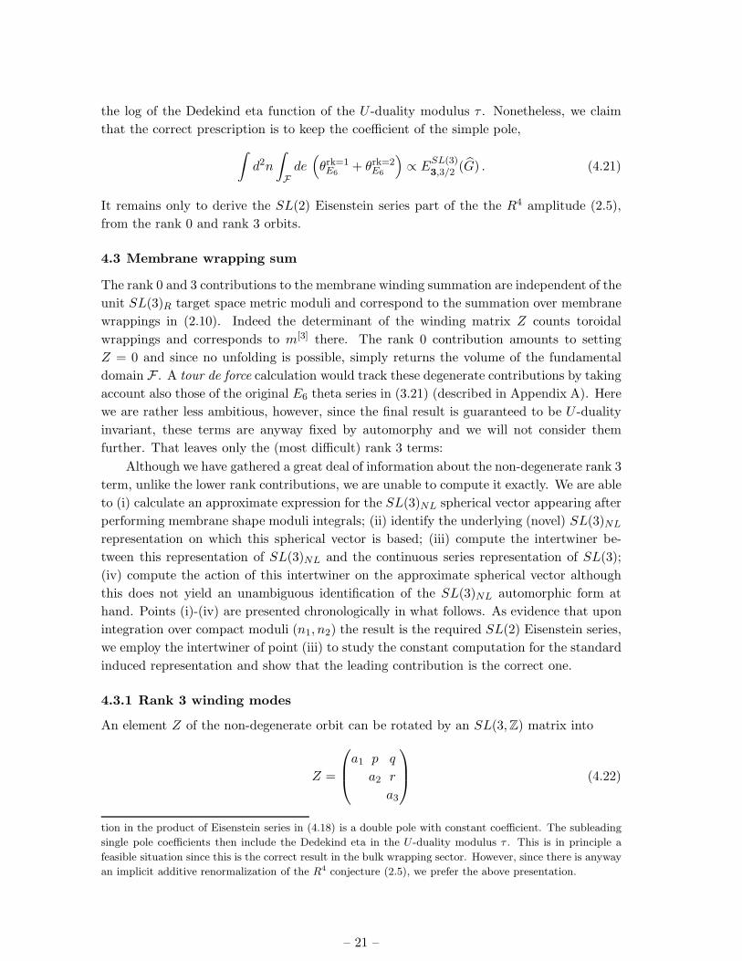
the log of the Dedekind eta function of the U -duality modulus τ . Nonetheless, we claim

that the correct prescription is to keep the coefficient of the simple pole,

∫d2n

∫

Fde(θrk=1E6

+ θrk=2E6

)∝ E

SL(3)3,3/2 (G) . (4.21)

It remains only to derive the SL(2) Eisenstein series part of the the R4 amplitude (2.5),

from the rank 0 and rank 3 orbits.

4.3 Membrane wrapping sum

The rank 0 and 3 contributions to the membrane winding summation are independent of the

unit SL(3)R target space metric moduli and correspond to the summation over membrane

wrappings in (2.10). Indeed the determinant of the winding matrix Z counts toroidal

wrappings and corresponds to m[3] there. The rank 0 contribution amounts to setting

Z = 0 and since no unfolding is possible, simply returns the volume of the fundamental

domain F . A tour de force calculation would track these degenerate contributions by taking

account also those of the original E6 theta series in (3.21) (described in Appendix A). Here

we are rather less ambitious, however, since the final result is guaranteed to be U -duality

invariant, these terms are anyway fixed by automorphy and we will not consider them

further. That leaves only the (most difficult) rank 3 terms:

Although we have gathered a great deal of information about the non-degenerate rank 3

term, unlike the lower rank contributions, we are unable to compute it exactly. We are able

to (i) calculate an approximate expression for the SL(3)NL spherical vector appearing after

performing membrane shape moduli integrals; (ii) identify the underlying (novel) SL(3)NL

representation on which this spherical vector is based; (iii) compute the intertwiner be-

tween this representation of SL(3)NL and the continuous series representation of SL(3);

(iv) compute the action of this intertwiner on the approximate spherical vector although

this does not yield an unambiguous identification of the SL(3)NL automorphic form at

hand. Points (i)-(iv) are presented chronologically in what follows. As evidence that upon

integration over compact moduli (n1, n2) the result is the required SL(2) Eisenstein series,

we employ the intertwiner of point (iii) to study the constant computation for the standard

induced representation and show that the leading contribution is the correct one.

4.3.1 Rank 3 winding modes

An element Z of the non-degenerate orbit can be rotated by an SL(3,Z) matrix into

Z =

a1 p q

a2 r

a3

(4.22)

tion in the product of Eisenstein series in (4.18) is a double pole with constant coefficient. The subleading

single pole coefficients then include the Dedekind eta in the U -duality modulus τ . This is in principle a

feasible situation since this is the correct result in the bulk wrapping sector. However, since there is anyway

an implicit additive renormalization of the R4 conjecture (2.5), we prefer the above presentation.

– 21 –

No SL(3,Z) generators leave this orbit representative invariant, so the fundamental domain

can be completely unfolded to

Frk=3 ={−∞ < T1, A1, A2 < ∞ , 0 ≤ T2, L < ∞

}. (4.23)

We again employ the integral representation of the spherical vector (4.5) and the change of

world volume shape variables (4.15). The integral with respect to A2 and T1 is Gaussian.

The subsequent integral over A1 leads to

∫dtdr1dr2

t3/2a2a23r1/22 y3

exp

[− 1

4ty4− t

(r1a21 + y2)(r2a

22 + y2)(a23 + r1r2y

2)

2r1r2

]

×K0

(t(r1a

21 + y2)(r2a

22 + y2)(a23 + r1r2y

2)

2r1r2

).

(4.24)

In the limit where the argument of K0 is very large, this reduces to

∫r1dr1dr2dt

t2

exp(− 1

4ty4− t

(a21r1+y2)(a22r2+y2)(a23+y2r1r2)r1r2

)

r1/21 a2a23y

3√

(a21r1 + y2)(a22r2 + y2)(a23 + y2r1r2). (4.25)

The integral over r1, r2, t can be performed in the saddle point approximation, and finally

gives

fSL(3) =

∫

Frk=3

defE6 ∼exp

[− (y2+x2

0+x21)

3/2

y2+x20

− ix0x3

1

y(y2+x20)

]

x51(y2 + x20 + x21)

1/4(4.26)

where x31 ≡ a1a2a3 = detZ is the wrapping number. This saddle point result for the

spherical vector becomes exact in the limit where (y, x0, x1) are scaled to infinity at the same

rate. The fact that the result depends on the determinant of the matrix Z is guaranteed

by SL(3)L-invariance, and implies that the result is an SL(3)R singlet, as it should if

it is to reproduce the SL(2) part in (2.5) after integration over the volume factor. The

representation under SL(3)NL is however more tricky to identify.

4.3.2 Representation of the non-degenerate orbit under SL(3)NL

Beginning with the E6 minimal representation in Figure 1, we can obtain the representation

of SL(3)NL by studying the action of the generators (E±ω, E±β0 , E±γ0 ,Hβ0 ,Hγ0) restricted

to functions ϕ(y, x0, z ≡ x31 = det(Z)). We find

Eβ0 = y∂x0 , E−β0 = −x0∂y − izy2

,

Eγ0 = ix0 , E−γ0 = −i(6 + x0∂x0 + y∂y + 3z∂z)∂x0

−y(6 + z2∂2z + 6z∂z)∂z ,

Eω = iy , E−ω = −i(6 + x0∂x0 + y∂y + 3z∂z)∂y+x(6 + z2∂2

z + 6z∂z)∂z−3i

y (2 + z2∂2z + 4z∂z) +

1y2

z∂y ,

Hβ0 = x0∂x0 − y∂y , Hγ0 = −2x0∂x0 − y∂y − 3z∂z − 6 .

(4.27)

– 22 –

In Section 3.6 we argued that upon integrating out SL(3)L moduli, the remaining SL(3)R,NL

Casimir invariants should vanish. Indeed a straightforward computation yields

∆(2)SL(3)NL

= 0 = ∆(3)SL(3)NL

. (4.28)

The spherical vector for the representation (4.27) may in principle be computed by solving

the partial differential equations associated to the maximal compact subgroup SO(3). We

are not able to integrate these equations exactly, however the leading result in the limit

where y, x0, x1 are scaled to infinity simultaneously agrees with (4.26).

4.3.3 Intertwiner from cubic to induced representations

We now identify the novel “cubic” SL(3)NL representation found in (4.27). As we recall

in Appendix B.1, all continuous irreducible representations of SL(3) can be obtained by

induction from the minimal parabolic subgroup P of lower triangular matrices, with a

character (B.2). These are natural candidates so long as the parameters (λ32, λ21) lie at

the intersection of vanishing quadratic and cubic Casimir loci depicted in Figure 3:

(λ32, λ21) ∈ {(−1, 2), (1, 1), (2,−1), (1,−2), (−1,−1), (−2, 1)} . (4.29)

Note that these six solutions are related by action of the Weyl group, hence the cor-

responding Eisenstein series by Selberg’s relations (B.47). We begin therefore with the

representation (B.6) and search for an intertwiner bringing it to the form (4.27). Let us

now perform a few changes of variables: We first Fourier transform over v,w, and write

∂w = ix0, ∂v = iy. The generator −Eγ becomes y∂0 + ∂x ≡ Eβ0 . Similarly we identify Eβ

with Eγ0 . In order to get rid of the ∂x term, we redefine

x → x1 + x0/y, ∂x → ∂1, ∂0 → ∂0 − ∂1/y, ∂ → ∂ + x0∂1/y2 . (4.30)

The generator Hβ0 now becomes −y∂+x0∂0+2x1∂1. We eliminate the last term by further

redefining

x1 = x2/y2 , ∂1 → y2∂2 , ∂0 → ∂0, ∂ → ∂ + 2x2∂2/y (4.31)

The generator E−γ0 now reads −x0∂ + x22∂2/y2. We put x2 = 1/x3 so that

E−β0 = −x0∂ − ∂3y2

+ (1− λ32)

(−x0

y− 1

x3y2

)(4.32)

Only when λ32 = 1, the singular term 1/(x3y2) disappears, so we may Fourier transform

one last time over x3 and write ∂3 = −iz. This yields a one-parameter family of SL(3)

representations [16] depending on λ32. Setting also λ21 = 1, we obtain precisely the repre-

sentation (4.27). We have thus identified the SL(3)NL representation arising by integrating

the E6 theta series over the action of SL(3)L at a generic (rank 3) point, with the Eisenstein

series of SL(3)NL with parameters (λ32, λ21) = (1, 1),∫

Fde θrk=3

E6∼ E(gNL; 1, 1) . (4.33)

Because the point (1, 1) lies at the intersection of two lines of single poles, it is not clear

however whether the right-hand side should be understood as the residue, or whether some

finite term should be kept – we will return to this point shortly.

– 23 –

4.3.4 Intertwining the spherical vector

We begin with the known spherical vector (B.9) of the continuous representation computed

in Appendix B.1. Because λ32 = λ21 = 1 in the intertwined SL(3)NL representation, we

must study the limit s = t = 0. We may however regard non-zero s and t as a regulator.

In particular, representing the exact continuous representation spherical vector as

fSL(3) =πs+t

Γ(s)Γ(t)

∫ ∞

0

dt1dt2

t1+s1 t1+t

2

exp

(−π(1 + x2 + (v + xw)2)

t1− π(1 + v2 + w2)

t2

),

(4.34)

and intertwining to the representation (4.27) (i.e. performing the string of Fourier trans-

forms and variable changes of the preceding Section), in the saddle approximation we

recover the action appearing in the exponent of (4.26). The final t2 integration yields an

overall infinite factor, however. This situation is reminiscent of the spherical vector for the

maximal parabolic Eisenstein series which can be obtained by a single Fourier transform

over the variable w. The rationale being that the continuous representation induced from

the minimal parabolic with abelian character (B.2), is equivalent to that induced from

the maximal parabolic with a non-trivial representation in the SL(2) Levi subgroup. The

possibility of attaching cusp forms correspondint to discrete representations to the Levi

factor, does lead to independent Eisenstein series, however [36]. Due to this type of sub-

tlety, we cannot unambiguously identify the rank 3 winding sum with a minimal parabolic

Eisenstein series at λ32 = λ21 = 1.

4.4 Integration over membrane volume – non-degenerate orbit

We now return to the issue of integrating over the membrane volume ν ∈ R+. As we

argued above, the correct prescription is to compute the constant term corresponding to the

maximal parabolic group P2 generated by (n1, n2). Physically, this amounts to computing

the Fourier coefficients associated to (n1, n2) at zero momentum, or equivalently, averaging

over the action of Eγ0 and Eω. Since (y, x0) are the conjugate variables (from (4.27)), one

should evaluate the spherical vector at the origin y = x0 = 0. Unfortunately, this is the

limit where the saddle point approximation used to derive (4.26) breaks down. This is also

the limit in which the degenerate contributions are obtained, on which we have no control.

A better strategy is therefore to intertwine back to the standard induced representa-

tion (B.6), for which constant terms are completely known. Having just established that

the SL(3)NL representation (4.27) is equivalent to the induced representation (−1,−1), it

remains to establish how the double pole at (−1,−1) should be regularized. Unfortunately,

we have not been able to settle this point, however it is easy to find an ad hoc prescription

which gives the correct result: expanding the constant term computation (B.45) around

λ21 = −1 + ǫ1, λ32 = −1 + ǫ2, we have

EP2 = 2t3−ǫ1− 1

2ǫ2

1 ζ(2− ǫ2)ESL(2)

2,1− 12ǫ2+ 2t

32+ 1

2ǫ1− 1

2ǫ2

1 ζ(3− ǫ1 − ǫ2)ξ(1− ǫ1)

ξ(ǫ1 − 1)E

SL(2)

2,3/2− 12ǫ2− 1

2ǫ2

+ 2t12ǫ1+ǫ2

1 ζ(2− ǫ1)ξ(1− ǫ2)ξ(2− ǫ1 − ǫ2)

ξ(ǫ2 − 1)ξ(ǫ1 + ǫ2 − 2)E

SL(2)

2,3/2− 12ǫ2− 1

2ǫ2. (4.35)

– 24 –

In this formula, the R+ν modulus is related to the membrane volume by t1 = ν1/6. Picking

the residue of the 1/ǫ2 pole, extracting from it the finite term following the 1/ǫ1 pole, and

using the relation ζ ′(2) = −ζ(3)/(4π2), we find

limǫ1,ǫ2→0

ǫ2∂ǫ1ǫ1EP2 =2π3

3ζ(3E

SL(2)

2,1− 12ǫ1+

2π4

3ζ(3)log t1 +

π2

3t31 + cste (4.36)

The volume independent term does indeed reproduce the SL(2) Eisenstein series from

(2.5)! The meaning of the other terms is however far from clear. It would be interesting

to obtain a detailed understanding of the singularity at (λ32, λ21) = (1, 1) from the point

of view of the membrane computation.

5. Membranes on higher dimensional torii, membrane/5-brane duality

Having extolled our present understanding of the consequences of the E6 theta series con-

jecture for M-theory on T 3, we now briefly discuss the the higher dimensional generalization

of our construction, and present a provocative hint that our framework may incorporate

membrane/fivebrane duality.

5.1 BPS membranes on T 4

Let us first discuss the generalization of our construction to the case of M-theory compact-

ified on T 4–similar considerations can be applied to E8 and T5 compactifications. Here,

we expect a symmetry under the U-duality group SL(5), which contains the obvious geo-

metrical symmetry SL(4) of the target 4-torus, together with U-duality reflections which

invert the volume of a sub 3-torus,

RM → l3MRNRP

, l3M → l6MRMRNRP

(5.1)

for any choice of 3 directions (M,N,P ) out of 4. The R4 couplings have been argued in [12]

to be given by an SL(5) Eisenstein series of weight 3/2.

Just as for T 3, we expect this amplitude to be derivable from a one-loop amplitude

in membrane theory, i.e., an integral over the partition function describing minimal maps

T 3 → T 4. In order to that the symmetry under SL(3)×SL(5) be non-linearly realized, we

assume an overarching symmetry under E7(7)(Z) in the minimal representation, which now

has dimension 17. The canonical presentation of the minimal representation has a linearly

realized SL(6) subgroup, under which the 17 variables are arranged as a 6×6 antisymmetric

matrix X, and two singlets (y, x0,X). The spherical vector has been worked out in [9],

and, for large quantum numbers, becomes an exponential of minus the action

S =

√det(X + |z|I6)

|z|2 − ix0Pf(X)

y|z|2 , (5.2)

where z ≡ y + ix0.

This action however does not have a direct intepretation in terms of T4 winding modes,

which would make a 3 × 4 matrix of integers. It is however possible to make a judicious

– 25 –

choice of polarization for the Heisenberg subalgebra where SL(3)×SL(4) is linearly realized,

as follows. Let us examine the E6 and E7 extended Dynkin diagrams

g g g g

−ω β0

×

g

g

. . .× g g g g g g

g

×−ω β0

. . .× (5.3)

The longest root−ω is denoted by a ×. The node labeled β0 determines the Levi subalgebra

acting linearly on the Heisenberg subalgebra (positions and momenta). It is obtained by

deleting nodes −ω and β0 which yields SL(6) and SO(6, 6) groups, respectively. The

choice of a set of momenta and coordinates, i.e., a polarization, breaks these groups to a

subgroup. The node marked with a cross determines a choice of polarization appropriate for

membrane winding sums. The remaining nodes are subgroups linearly acting on positions,

namely SL(3)× SL(3) and SL(3)× SL(4)–precisely the linear actions from left and right

on 3 and 4-torus winding matrices. Note that only for E6 does the canonical polarization

determined by the node attached to β0 coincide with the membrane inspired one. For E8,

5-torus winding sums, more general choices of β0 are even necessary.

Deleting the node marked with a cross from the extended Dynkin diagrams, leaves

the U -duality and world-volume groups. We have discussed the E6 case in detail. For E7,

the two rightmost nodes correspond to the SL(3) membrane world-volume shape moduli.

The nodes remaining on the left form SL(6) ⊃ SL(5)×R+, a product of the T4 U -duality

group and the world-volume. (For T4, the integration over world-volumes is also regulated

by quantum fluxes.) Also, just as E6 has a triality, duality of the E7 Dynkin diagram

implies that there is no ambiguity in the choice of linearly acting, SL(3), world-volume

modular group.

By looking at the root lattice, we may now determine the transformation properties

of the seventeen variables of the minimal representation with respect to the linearly acting

SL(3)×SL(4) subgroup: the singlet y remains unaffected, while x0 and the elements of the

6× 6 antisymmetric matrix X reassemble themselves into a 4× 3 matrix Z and a 4-vector

X,

X =

X12

X31

X23

x0

, Z =

X14 X15 X16

X24 X25 X26

X34 X35 X36

y∂X56 y∂X64 y∂X45

. (5.4)

The derivatives in the last row indicate that a Fourier transform should be performed in

these variables before the symmetry becomes linearly realized. The spherical vector in this

new polarization now reads

S =

√det(ZtZ + I3×3(y2 +Xt

0X0)) +R/y2

y2 +Xt0X0

+ i

√det(ZZt +X0Xt

0)

y(y2 +Xt0X0)

(5.5)

– 26 –

where R stands for

R = (y2 +Xt0X0)[(y

2 +Xt0X0 + trZZt)Xt

0ZZtX0 −Xt0ZZtZZtX0]

+ Xt0X0 detZtZ − det(ZZt +X0X

t0) . (5.6)

This action generalizes its E6 counterpart (3.13). Again it is an Born–Infeld-like inter-

polation between Nambu-Goto and Polyakov formulations. Over and above the winding

quantum numbers Z, additional fluxes (y,X0) are necessary for manifest U -duality invari-

ance. Their interpretation as a target space scalar and three-form also carries through to

the 4-torus case: the vector X may be interpreted as a 3-form flux on the world-volume,

carrying also a 3-form index in target space. It would be most interesting if the integration

over the world-volume SL(3) shape moduli could be carried out for this theory also.

5.2 Membrane/five-brane duality and pure spinors

Going back to the T 3, E6 case, and in line with the idea of membrane/five-brane duality,

it is now interesting to ask if a change of polarization might bring the minimal E6 theta

series to a form which could be interpreted as a five-brane partition function10.

Indeed, as noticed in [9], it is possible to choose a polarization where SL(5) becomes

linearly realized, instead of SL(3) × SL(3). By Fourier transforming the one-row of the

3× 3 matrix, the 11 variables (y, x0, ZMA ) rearrange themselves into a 5× 5 antisymmetric

matrix X,

X =

0 −∂Z33

∂Z23

Z11 Z1

2

0 −∂Z13Z21 Z2

2

0 Z31 Z3

2

a/s 0 x00

(5.7)

and a singlet y. In fact, these 11 variables can be supplemented by a 5-vector vi, ex-

pressed in terms of the others as yvi = 14ǫ

ijklmXijXkl, in such a way that the 16 variables

(y,Xij , ǫijklmvm) transform as a Majorana–Weyl spinor λ of SO(5, 5) ⊂ E6, subject to the

“pure spinor” constraint λΓµλ = 0, for all µ = 1 . . . 10. This is the direct analog for E6

of the “string inspired” representation of D4 on 6 variables mij, subject to the quadratic

constraint ǫijklmijmkl = 0. A completely analogous construction for the E7 minimal rep-

resentation holds also, see [16] for details.

In this polarization, the E6 spherical vector now takes the very simple form11,

fE6 = K1

(√λλ), Kt(x) ≡ x−tKt(x) . (5.8)

We now claim that this can be interpreted as the partition function for the five-brane.

Indeed, we can view the 5 × 5 antisymmetric matrix X as the electric flux on the five-

brane, Xij = H0ij, equal by the self-duality condition to the magnetic components, Xij =

(1/6)ǫijklmHklm. An SL(6)-invariant partition function for fluxes on a single five-brane

10We are grateful to L. Motl for forcing us to address this question.11Minimal representations and their spherical vectors have been studied before in this presentation in [37].

– 27 –

has been constructed long ago by Dolan and Nappi in [38], where the SL(6) invariance was

non-linearly realized thanks to Gaussian Poisson resummation – in other words, the SL(6)

symmetry was embedded in an overarching symplectic group Sp(10) acting linearly on the

10 variables Xij . Here, we find that by adding an extra variable y, best thought of as the

number of five-branes, the geometric symmetry SL(6) is enlarged to a complete E6(6) group.

This is the symmetry group expected for a five-brane wrapped on a T 6 with metric gij ,

3-form Cijk and dual 6-form Eijklmn parameterized by the symmetric space E6(6)/Usp(4).

It would be very interesting to use this information to compute the partition function for

y overlapping five-branes.

Independently of these mem- and five-brane considerations, let us note that pure

spinors of D5 (albeit with a different real form, SO(1, 9)) arise naturally in the description

of 10-dimensional Yang-Mills theory: as observed by Berkovits [39], theN = 1 superalgebra

in ten dimensions

{Qα, Qβ} = ΓµαβPµ , (5.9)

becomes cohomological when auxiliary, pure spinor variables λα obeying

λΓµλ = 0 , (5.10)

are introduced, because one can then form the nilpotent operator

Q ≡ λαQα . (5.11)

Superfields are then also functions of pure spinors λα. Here, we have shown that the space

of functions of λα is precisely the minimal representation of E6. A tantalizing possibility,

therefore, is a hidden E6 symmetry of d = 10 super Yang-Mills theory.

6. Discussion

In this Article, we have attempted to compute the R4 coupling in M-theory compactified

on T 3, from a one-loop computation in the microscopic membrane theory. Our basic

assumption has been that, at least at the zero-mode level, the membrane theory enjoys an

“overarching” symmetry under the minimal representation E6(6)(Z), which mixes world-

volume and target space. This provides the most economical way to realize both the

modular symmetry SL(3,Z) on the world-volume, and U-duality SL(3,Z) × SL(2,Z) in

target space. An important consequence is that there should be two discrete degrees of

freedom, y and x0, over and above the nine evident winding numbers ZMA = ∂AX

M . After

integrating over the worldvolume moduli, only the U-duality symmetry remains.

Using explicit computations and representation theoretic arguments, we have found

that the rank(Z) = 1 and rank(Z) = 2 contributions were equal, and reproduced the SL(3)

part of the R4 coupling in (2.5), while the rank 0 and 3 contributions ought reproduce the

SL(2) part, i.e., the membrane instanton sum. A fully satisfying proof would require an

understanding of the regularization of the poles of the Eisenstein series at (λ21, λ32) = (1, 1),

which we have not been able to obtain thus far. A possible avenue to this end would be to

derive the exact expression for the integrated spherical vector beyond the steepest descent

– 28 –

approximation (4.26), and study the limit (y, x0) → (0, 0). This would shed much desired

light on the interpretation of the new quantum numbers (y, x0), which has remained rather

elusive.

On this subject, we may offer the following observations: the E6 and E7 cases suggest

that the singlet x0 (resp. the 4-vector X) should correspond to a flux carrying 3-form

index both on the membrane world volume. On the other hand, rescaling the winding

variables Z → yZ and also x0 → yx0, we observe that the variable y appears linearly as an

overall factor in the action (3.13). Therefore, it is natural to identify it with the number

of membranes. It would be interesting to understand how to introduce these degrees of

freedom in an off-shell membrane action, which would realize the overarching symmetry

non-linearly. Equation (3.13) does at least predict the shape of the action of such a theory,

restricted to zero-modes. The putative appearance of a membrane number, even calls for

a second quantized membrane field theory.

Another interesting question is how does the double dimensional reduction of a mem-

brane winding sum to the T -duality invariant string amplitude work? At the level of the

final amplitude (2.5), this is no mystery since this is essentially how it was conjectured in

the first place [12]. However, the string amplitude is based on a T -duality/world-volume

modular group, dual pair construction for the symplectic groups. An appealing, but not

necessary, scheme would be to embed these in the exceptional groups proposed here. Un-

fortunately this seems not to work, since a quick perusal of the branching rules for the E6

does not yield the requisite Sp(8) subgroup.

Finally, we have presented two observations that reach beyond the subject of superme-

mbranes: first, that the minimal representation of E6 can also be used to describe stacks

of N five-branes wrapped on T 6, in a manifestly U-duality invariant way: it would be very

interesting to use this result to compute five-brane partition functions at finite N . Second,

pure spinors in ten dimensions carry an action of E6: the implications for 10-dimensional

Yang-Mills theory remain to be uncovered.

Acknowledgments

It is a pleasure to thank David Kazhdan and Stephen Miller, our mathematical muses,

for extensive consultations. We would also like to acknowledge Colette Moeglin, Lubos

Motl, Misha Movshev, Hermann Nicolai, Jan Plefka and Alexander Polishchuk for useful

discussions. We thank the Albert Einstein Institut fur Gravitationsphysik and the Jef-

ferson Physical Laboratory at Harvard University for kind hospitality. A.W. thanks also

Max Planck Institut fur Mathematik and LPTHE Universite Paris 6 et 7 for hospital-

ity. Research supported in part by NSF grant PHY01-40365 and the European Network

HPRN-CT-2000-00131.

A. Summation measure and degenerate contributions

It is well known that the summation measure of a theta series may be expressed adelically,

i.e., as a product over primes of the spherical vector over the p-adic base field (see e.g. [16]

– 29 –

for a physicist’s review)

µ(y, x0, Z) =∏

p prime

fQp(y, x0, Z) . (A.1)

The function fp is determined by requiring invariance under the maximal compact subgroup

Usp(4,Qp). Its explicit form can be obtained by noting that the exponent or “action” S

in (3.21) has a simple rewriting in terms of the Euclidean norm on a certain Lagrangian

submanifold. Some details: Consider the space of coordinates X = (x0, y, Z) along with

canonical momenta P . Introduce a “Hamiltonian”

H =detZ

||(y, x0)||. (A.2)

For now ||v|| ≡ √v.v denotes the Euclidean norm of a vector v. The Lagrangian subman-

ifold is described by the subspace (X,P = ∇XH). The action then has a very simple

rewriting

S = ||(X,∇XH)||+ ix0H

y ||(y, x0)||. (A.3)

Recalling that the exponential form of the E6 spherical vector arose because of the identity

K1/2(x) =√

π2x exp(−x) we may write

fE6R =

K1/2(Re(S))e−iIm(S)

||(y, x0)||2, (A.4)

where Kt(x) ≡ x−tKt(x).

The p-adic spherical vector was obtained recently in [21], and takes a very similar form.

In the E6 case, it reads, for ||y||p ≤ ||x0||p,

fE6Qp

= ||x0||−2p

p ||(x0, Z,∇ZdetZx0

,∇x0detZx0

)||−1p − 1

p− 1exp

(−i

detZ

yx0

)(A.5)

if ||(x0, Z,∇ZdetZx0

,∇x0detZx0

)||p ≤ 1, and 0 otherwise. The opposite case ||y||p > ||x0||pis simply obtained by a Weyl reflection, the effect of which is to eliminate the phase and

exchange y and x0. Notice that the p-adic spherical vector can be simply obtained from the

real one by replacing the orthogonal norm ||.||2 by the p-adic norm and the function K1/2

by its simple (algebraic) p-adic analog. The summation measure is the product of p-adic

spherical vectors over all prime p, therefore has support on rational numbers X such that,

for all prime p, either ||y||p ≤ ||x0||p and ||(x0, Z,∇ZdetZx0

,∇x0detZx0

)||p ≤ 1, or ||y||p > ||x0||pand ||(y, Z,∇Z

detZy ,∇y

detZy )||p ≤ 1. Thus, the summation measure has support on integers

(y, x0, Z) such that gcd(y, x0) divides ∇Z(detZ) and (gcd(y, x0))2 divides detZ.

The degenerate terms for exceptional theta series have also been determined in [21].

These terms are familiar to physicists in the context of the large volume expansion of the

well known non-holomorphic SL(2) Eisenstein series, see for example equation (2.10). The

explicit expression for the E6 minimal theta series given in (3.21) is the analog of the bulk

membrane instanton term in (2.10). In [21], the degenerate terms for the E6 theta series

– 30 –

are found to be

θE6 =∑

y∈Z\{0}(x0,Z)∈Z

10

∏

p prime

fE6Qp

(y, x0, Z)

fE6

R (y, x0, Z) +∑

(x0,Z)

µ(x0, Z)f(x0, Z) + α1 + α2 .

(A.6)

The leading term is the one above in (3.21). As exploited in a cosmological context in [40],

the minimal representation has a natural conformal symmetry, the underlying geometry

of the eleven dimensional space with variables (y, x0,X) being conical. The second term

in (A.6) corresponds to the limit y → 0 at the tip of the cone: the regulated spherical vector

f is obtained by dropping the phase factor in (A.4), and setting y = 0 in the remaining

part. The final two terms α1 and α2 are automorphic forms built from singlet and minimal

representations of the Levi subgroup SL(6) ⊂ E6. Again, for details we refer the reader

to [21].

B. SL(3,Z) automorphic forms

A most useful account of SL(3,Z) automorphic forms may be found in [32]. In particular,

the constant term computations presented in Section B.4 are derived in detail there. It was

realized long ago, especially by Langlands, that representation theory plays a central role in

the theory of automorphic forms. Therefore in Section B.1 we construct the continuous se-

ries irreducible representations of SL(3) upon which SL(3,Z) invariant automorphic forms

are based. We review the fundamental domain construction for SL(3,Z) in Section B.2

(a computation first tackled many years ago by Minkowski!). The remaining sections deal

with SL(3) Eisenstein series and their constant terms.

B.1 Continuous representations by unitary induction

All continuous unitary irreducible representations of SL(3) have been constructed long

ago in [36], by unitary induction techniques. According to the general philosophy of Kir-

illov [41], they are in one-to-one correspondence with coadjoint orbits. We recall these

results here for convenience.

SL(3) admits a parabolic subgroup P of upper triangular matrices

P ≡

p =

t3 ∗ ∗0 t2 ∗0 0 t1

: t1t2t3 = 1

⊂ SL(3) , (B.1)

A one-dimensional representation of P is given by the character

χ(p, λ) =3∏

i=1

sgnǫi(ti) |ti|ρi . (B.2)

Here ǫi = ±1 and the three complex variables ρi are conveniently parameterized as

ρ1 = λ1 + 1 , ρ2 = λ2 , ρ3 = λ3 − 1 , (B.3)

– 31 –

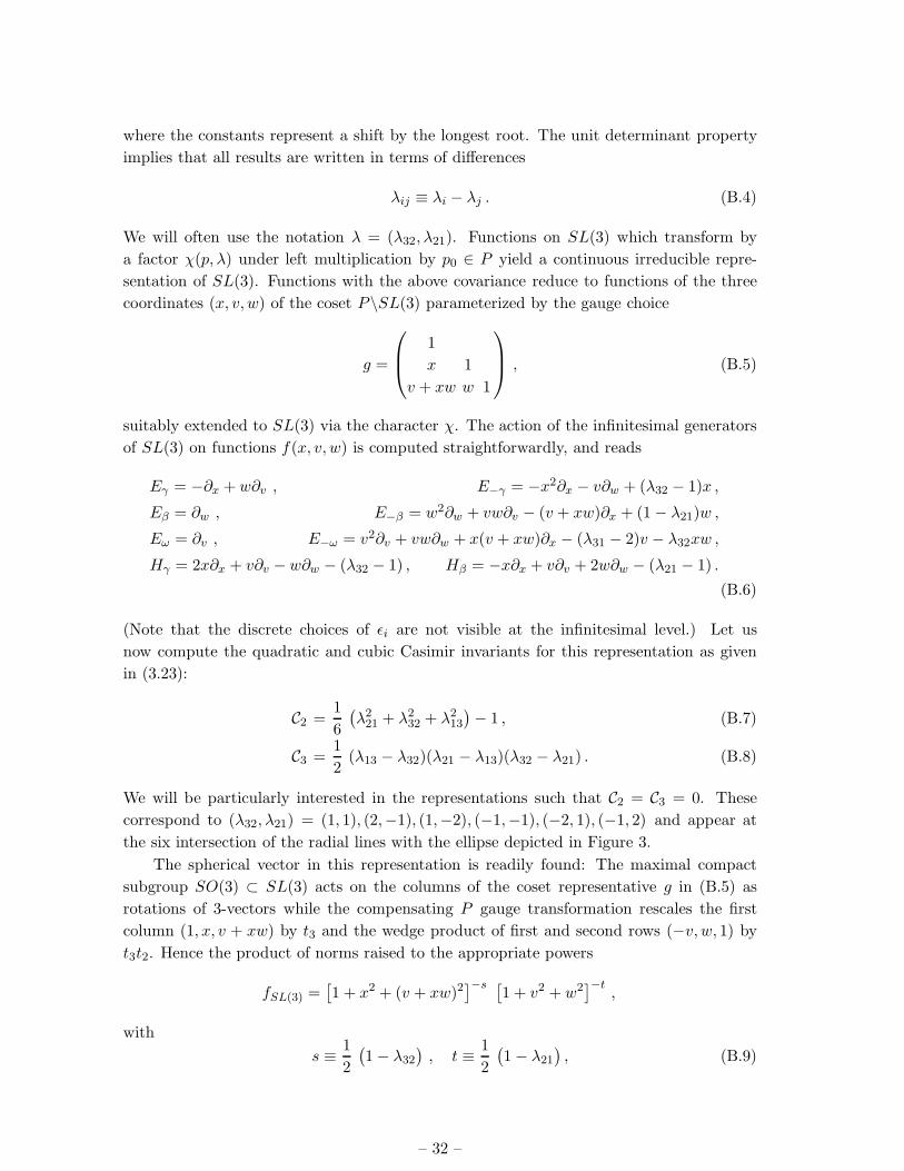
where the constants represent a shift by the longest root. The unit determinant property

implies that all results are written in terms of differences

λij ≡ λi − λj . (B.4)

We will often use the notation λ = (λ32, λ21). Functions on SL(3) which transform by

a factor χ(p, λ) under left multiplication by p0 ∈ P yield a continuous irreducible repre-

sentation of SL(3). Functions with the above covariance reduce to functions of the three

coordinates (x, v, w) of the coset P\SL(3) parameterized by the gauge choice

g =

1

x 1

v + xw w 1

, (B.5)

suitably extended to SL(3) via the character χ. The action of the infinitesimal generators

of SL(3) on functions f(x, v, w) is computed straightforwardly, and reads

Eγ = −∂x +w∂v , E−γ = −x2∂x − v∂w + (λ32 − 1)x ,

Eβ = ∂w , E−β = w2∂w + vw∂v − (v + xw)∂x + (1− λ21)w ,

Eω = ∂v , E−ω = v2∂v + vw∂w + x(v + xw)∂x − (λ31 − 2)v − λ32xw ,

Hγ = 2x∂x + v∂v − w∂w − (λ32 − 1) , Hβ = −x∂x + v∂v + 2w∂w − (λ21 − 1) .

(B.6)

(Note that the discrete choices of ǫi are not visible at the infinitesimal level.) Let us

now compute the quadratic and cubic Casimir invariants for this representation as given

in (3.23):

C2 =1

6

(λ221 + λ2

32 + λ213

)− 1 , (B.7)

C3 =1

2(λ13 − λ32)(λ21 − λ13)(λ32 − λ21) . (B.8)

We will be particularly interested in the representations such that C2 = C3 = 0. These

correspond to (λ32, λ21) = (1, 1), (2,−1), (1,−2), (−1,−1), (−2, 1), (−1, 2) and appear at

the six intersection of the radial lines with the ellipse depicted in Figure 3.

The spherical vector in this representation is readily found: The maximal compact

subgroup SO(3) ⊂ SL(3) acts on the columns of the coset representative g in (B.5) as

rotations of 3-vectors while the compensating P gauge transformation rescales the first

column (1, x, v + xw) by t3 and the wedge product of first and second rows (−v,w, 1) by

t3t2. Hence the product of norms raised to the appropriate powers

fSL(3) =[1 + x2 + (v + xw)2

]−s [1 + v2 + w2

]−t,

with

s ≡ 1

2

(1− λ32

), t ≡ 1

2

(1− λ21

), (B.9)

– 32 –

λ

λ

21

32

(−1,2)

(−2,1)

(−1,−1)

(1,−2)

(2,−1)

(1,1)

Figure 3: Vanishing loci of C2, C3 in the (λ32, λ21) plane. The quadratic Casimir vanishes on the

ellipse, the cubic on the dotted radial lines, while the dashed lines correspond to simple poles of

Eisenstein series.

is simultaneously invariant under the right action of P and left action of SO(3) and is

therefore the desired spherical vector.

It is also interesting to obtain the minimal representation from the limit in which the

induced representation (B.6) approaches any one of the simple pole dashed lines in Figure 3.

For example, setting λ32 = 1 and λ21 = 1 − 2t, the induced representation acts faithfully

on functions φ(v,w), by setting ∂x = 0. We then find

Eγ = w∂v , E−γ = −v∂w ,

Eβ = ∂w , E−β = w2∂w + vw∂v + 2tw ,

Eω = ∂v , E−ω = v2∂v + vw∂w − 2tv ,

Hγ = v∂v −w∂w , Hβ = v∂v + 2w∂w + 2t .

(B.10)

The spherical vector of this representation is simply fSL(3),min = [1 + v2 + w2]−t corre-

sponding to an Eisenstein series ESL(3)3,t in the fundamental representation. Another useful

presentation of the minimal representation, used in the Text, is obtained by Fourier trans-

form over (v,w) → 1i (∂v, ∂w). In this case we find

Eγ = −v∂w , E−γ = w∂v ,

Eβ = −iw , E−β = iw∂2w + 3i∂w + iv∂w∂v − 2it∂w ,

Eω = −iv , E−ω = iv∂2v + 3i∂v + iw∂v∂w − 2it∂v ,

Hγ = −v∂v + w∂w , Hβ = −v∂v − 2w∂w + 2t− 3 .

(B.11)

– 33 –

The spherical vector is then

fSL(3),min = K1−t

(√v2 + w2

), Kt(x) ≡ x−tKt(x) . (B.12)

This form corresponds to the non-degenerate terms in a large volume expansion of the

Eisenstein series in the fundamental representation [9].

B.2 Fundamental domain of SL(3,Z)

The fundamental domain of SL(3,Z) in SO(3)\SL(3,R) was first computed by Minkowski [33],

here we follow the modern treatment of [34]. We parameterize the coset SO(3)\SL(3,R)in the Iwasawa gauge as,

e =

1L √

LT2 √

LT2

·

1 A1 A2

1 T1

1

≡ 1

L

(~e1 ~e2 ~e3

)(B.13)

where we defined the three vectors

~e1 =

1

0

0

, ~e2 =

A1√L3

T2

0

, ~e3 =

A2√L3

T2T1

√L3T2

. (B.14)

The fundamental domain is constructed by maximizing a height function

h(e) ≡ (~e1)1 (~e2)2 (~e3)3 = L3 . (B.15)

The function h is invariant under the right action of the following SL(3,Z) elements12

S2 =

1

1

−1

, T1 =

1 1

1

1

, T2 =

1 1

1

1

, T3 =

1

1 1

1

,

U1 =

−1

−1

1

, U2 =

1

−1

−1

, (B.16)

Therefore, we can always move to a fundamental domain of the Gl(2,Z) in the bottom

right hand 2× 2 block along with strip conditions on the A1,2,

T 21 + T 2

2 ≥ 1 , 0 ≤ A1, T1 ≤1

2, −1

2≤ A2 ≤

1

2. (B.17)

12Note that the set of elements {S1,2,3,4,5 , T1,2,3, U1,2} is convenient for determining the fundamental

domain, yet overcomplete–PSL(2,Z) is generated by the shift and clock matrices

1 1

1

1

and

1

1

1

.

– 34 –

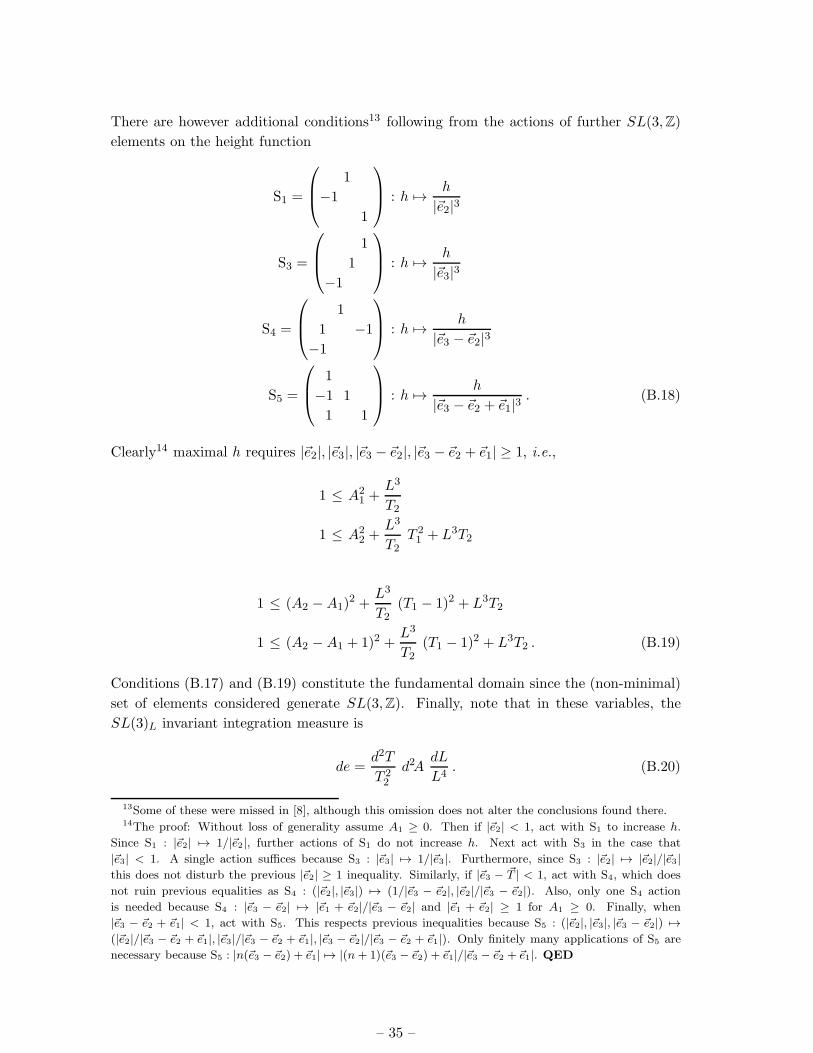
There are however additional conditions13 following from the actions of further SL(3,Z)

elements on the height function

S1 =

1

−1

1

: h 7→ h

|~e2|3

S3 =

1

1

−1

: h 7→ h

|~e3|3

S4 =

1

1 −1

−1

: h 7→ h

|~e3 − ~e2|3

S5 =

1

−1 1

1 1

: h 7→ h

|~e3 − ~e2 + ~e1|3. (B.18)

Clearly14 maximal h requires |~e2|, |~e3|, |~e3 − ~e2|, |~e3 − ~e2 + ~e1| ≥ 1, i.e.,

1 ≤ A21 +

L3

T2

1 ≤ A22 +

L3

T2T 21 + L3T2

1 ≤ (A2 −A1)2 +

L3

T2(T1 − 1)2 + L3T2

1 ≤ (A2 −A1 + 1)2 +L3

T2(T1 − 1)2 + L3T2 . (B.19)

Conditions (B.17) and (B.19) constitute the fundamental domain since the (non-minimal)

set of elements considered generate SL(3,Z). Finally, note that in these variables, the

SL(3)L invariant integration measure is

de =d2T

T 22

d2AdL

L4. (B.20)

13Some of these were missed in [8], although this omission does not alter the conclusions found there.14The proof: Without loss of generality assume A1 ≥ 0. Then if |~e2| < 1, act with S1 to increase h.

Since S1 : |~e2| 7→ 1/|~e2|, further actions of S1 do not increase h. Next act with S3 in the case that

|~e3| < 1. A single action suffices because S3 : |~e3| 7→ 1/|~e3|. Furthermore, since S3 : |~e2| 7→ |~e2|/|~e3|this does not disturb the previous |~e2| ≥ 1 inequality. Similarly, if |~e3 − ~T | < 1, act with S4, which does

not ruin previous equalities as S4 : (|~e2|, |~e3|) 7→ (1/|~e3 − ~e2|, |~e2|/|~e3 − ~e2|). Also, only one S4 action

is needed because S4 : |~e3 − ~e2| 7→ |~e1 + ~e2|/|~e3 − ~e2| and |~e1 + ~e2| ≥ 1 for A1 ≥ 0. Finally, when

|~e3 − ~e2 + ~e1| < 1, act with S5. This respects previous inequalities because S5 : (|~e2|, |~e3|, |~e3 − ~e2|) 7→(|~e2|/|~e3 − ~e2 + ~e1|, |~e3|/|~e3 − ~e2 + ~e1|, |~e3 − ~e2|/|~e3 − ~e2 + ~e1|). Only finitely many applications of S5 are

necessary because S5 : |n(~e3 − ~e2) + ~e1| 7→ |(n+ 1)(~e3 − ~e2) + ~e1|/|~e3 − ~e2 + ~e1|. QED

– 35 –

B.3 SL(3) Eisenstein Series

In this Appendix we review prescient aspects of the theory of Eisenstein series and gather

formulae needed in the main text for SL(3). For our purposes it suffices to consider

Eisenstein series based on the minimal parabolic subgroup

P =

∗ ∗ ∗∗ ∗∗

⊂ SL(3,R) , (B.21)

which we decompose into its nilpotent radical and Levi components

P = MN , M =

∗∗∗

, N =

1 ∗ ∗1 ∗1

. (B.22)

A general element g ∈ SL(3,R) has the Iwasawa decomposition

g = k

t3

t2t1

1 a3 a2

1 a11

(B.23)

where t1t2t3 = 1 and k ∈ SO(3) the maximal compact subgroup of SL(3,R). We can then

introduce the function on SL(3)

F (g;λ) ≡ tλ1+11 tλ2

2 tλ3−13 = tλ21−1

2 tλ31−23 , λij ≡ λi − λj, (B.24)

which is manifestly invariant under left action of the compact SO(3) and right action of

the nilpotent N . It is also an eigenfunction of the SL(3,R)-invariant differential operators

∆(2,3)SL(3) introduced in Section 3.6.

To produce an automorphic form, we average (automorphize) F (g;λ) over the right

action of SL(3,Z). Indeed since F (g;λ) = F (gn;λ) for n ∈ N it suffices to sum over

N(Z)\SL(3,Z) (where N(Z) ≡ SL(3,Z) ∩ P ). Therefore, the SL(3) Eisenstein series for

the minimal parabolic is defined as

E(g;λ) =∑

γ∈N(Z)\SL(3,Z)F (gγ;λ) . (B.25)

This is now manifestly invariant under left action of SO(3) and right action of SL(3,Z),

therefore an automorphic function on SO(3)\SL(3). As usual, this automorphic form

can be decomposed as in (3.3), where the representation ρ is precisely the representation

induced from the minimal parabolic P with character (B.2)15.

15Indeed, the right action on g can be converted into a left action on γ, which takes value in P\SL(3).Eisenstein series for the minimal parabolics are defined in a similar way. For example, for P1 defined

in (B.32), elements of SL(3,R) are decomposed as

g = k

t31√t3

1√t3

11√τ2 √

τ2

1

1 τ11

1 a3 a2

1

1

, k ∈ SO(3) .

Then instead of automorphizing F (g;λ), one averages over φ(τ1+ iτ2) tλ3−13 where φ is an SL(2) cusp form.

– 36 –

Let us spell out this formula explicitly in a form perhaps more familiar to physicists:

Firstly observe that the greatest common divisor of any row (or column) of an element of

SL(3,Z) is unity. Let mt ≡ (m1,m2,m3), nt ≡ (n1, n2, n3) where gcd(mi) = gcd(ni) = 1.

The summation matrix γ is subject to the equivalence relation

γ =(m n p

)∼ γn =

(m n+n3m p+n1n+n2m

),

n ≡

1 n3 n2

1 n1

1

∈ N(Z) . (B.26)

Note that the column vector p is completely determined modulo integer shifts by m and n

once these two row vectors are specified. Therefore the summation over γ ∈ N(Z)\SL(3,Z)amounts to summing over mi and ni subject to gcd(mi) = gcd(ni) = 1 and n ∼ n+ n3m,

n3 ∈ Z.

To display the summand of (B.25) we compute the Iwasawa decomposition of gγ

gγ = k′

√mtGm ∗ ∗√

mtGm ntGn− (mtGn)2

mtGm∗1

√

mtGm ntGn− (mtGn)2

, (B.27)

where k′ ∈ SO(3) and the matrix G ≡ gtg. Orchestrating, we find

E(g;λ) =∑

{(m,n)∈Z3⊗Z3 :

gcd(m)=gcd(n)=1,

m6=0, n∼n+zm6=0}

(mtGm

)−s (mtGm ntGn− (mtGn)2

)−t

=1

4ζ(2s+ 2t)ζ(2t)

∑

{(m,n)∈Z3⊗Z3 :

m6=0, n∼n+zm6=0}

(mtGm

)−s (mtGm ntGn− (mtGn)2

)−t,

(B.28)

where

2s ≡ 1− λ32 , 2t ≡ 1− λ21 . (B.29)

In particular, observe that, in accordance with (B.5), if we set mt = (1, x, v + xw) and

nt = (0, 1, w) (which makes sense adelically) the summand in (B.28) matches the spherical

vector (B.9).

B.4 Constant term computations

By construction, the Eisenstein series E(g;λ) is invariant under right action of SL(3,Z)

and therefore of its Borel subgroup N(Z), which acts on (a1, a2, a3) as

E(a1, a2, a3) = E(a1 + n1, a2 + n2 + n1a3, a3 + n3) , ni ∈ Z . (B.30)

– 37 –

(we drop the dependence on ti and λi). This Heisenberg group includes two distinct Z×Z

subgroups,

N1 ≡

1 ∗ ∗1

1

, N2 ≡

1 ∗1 ∗1

, (B.31)

which can be viewed as the unipotent radicals of two associate maximal parabolic subgroups

of SL(3,Z),

P1 ≡

∗ ∗ ∗∗ ∗∗ ∗

⊂ SL(3,R) ⊃

∗ ∗ ∗∗ ∗ ∗

∗

≡ P2 . (B.32)

One may therefore construct the two Fourier series expansions

E(a1, a2, a3) =∑

m2,m3

e2πi(m2a2+m3a3)Em2,m3

P1(a1) (B.33)

=∑

m1,m2

e2πi(m1a1+m2[a2−a1a3])Em1,m2

P2(a3) . (B.34)

The Fourier zero-modes E0,0P1

(a1) ≡ EP1(g, λ) and E0,0P2

(a3) ≡ EP3(g, λ), are called the con-

stant terms of the Eisenstein series E(g;λ) with respect to parabolics P1, P2, respectively.

Evidently they may also be obtained by performing compact integrations

EPi(g, λ) =

∫

Ni/[SL(3,Z)∩Ni]dn E(gn;λ) . (B.35)

This is a general definition for constant terms. A third constant term computation, relative

to the minimal parabolic, is also possible

EP (g, λ) =

∫

N/[SL(3,Z)∩N ]dn E(gn;λ) . (B.36)

The N/[SL(3,Z) ∩N ] is simply the set of upper triangular matrices

N/[SL(3,Z) ∩N ] =

1 n1 n2

1 n3

1

: 0 ≤ n1, n2, n3 < 1

. (B.37)

Hence, from the Fourier expansions (B.33) and (B.34) we find

EP (g;λ) =

∫ 1

0dn1E

0,0P1

(a1 + n1) =

∫ 1

0dn3E

0,0P2

(a3 + n3) . (B.38)

These relations provide a useful check on the constant term computations.

Although constant term computations amount to the usual large volume expansion in

String Theory–amenable to explicit computations via Schwinger’s integral representation

and Poisson resummation, for general parabolics and higher groups this method becomes

unwieldy. Fortunately the task of computing SL(3) constant terms has already been tackled

by mathematicians. Here we rely heavily on the analysis of [32].

– 38 –

First, recall the SL(2) case

∑

(m,n)6=0,gcd(m,n)=1

(τ2

|m+ nτ |2)s

=1

2ζ(s)

∑

(m,n)6=0

(τ2

|m+ nτ |2)s

= τ s2 +ξ(2s − 1)

ξ(2s)τ1−s2 +

∑

n 6=0

an(τ2) e2πinτ1 .

≡ E1−2s(τ) . (B.39)

Here

ξ(s) ≡ π−s/2Γ(s/2)ζ(s) , (B.40)

is the completed Riemann Zeta function and

an(τ2) =

√τ2

ξ(2s)µs(n)n

s−1/2Ks−1/2(2πτ2|n|) , µs(n) ≡∑

m|nm−2s+1 . (B.41)

Note that, in particular,

∫ 1

0dτ1Es(τ) = τ

12− 1

s2 +

ξ(−s)

ξ(s)τ

12+ 1

s2 . (B.42)

Here ξ(s) = π−s/2Γ(s/2)ζ(s) is the completed Riemann Zeta function. Selberg’s functional

relation

ξ(s)Es(τ) = ξ(−s)E−s(τ) , (B.43)

may be obtained from the constant terms. Indeed, multiplying (B.39) by ζ(2s) and using

ξ(s) = ξ(1 − s) we see that these are indeed invariant under s → 1 − s. Note that the

symmetric form of the SL(2) Eisenstein series in (B.43) is related to the usual one based

on the fundamental representation of SL(2) by E1−2s(τ) = ESL(2)2,s /(2ζ(2s)).

For SL(3) the following formulae hold:

EP1(g, λ) = tλ31− 1

2λ21− 3

23 Eλ21(τ) +

ξ(λ23)

ξ(λ32)tλ21− 1

2λ31− 3

23 Eλ31(τ)

+ξ(λ12)ξ(λ13)

ξ(λ21)ξ(λ31)tλ12− 1

2λ32− 3

23 Eλ32(τ) , (B.44)

where τ = a1 + i t1t2 in this formula;

EP2(g, λ) = tλ12− 1

2λ32+

32

1 Eλ32(τ) +ξ(λ12)

ξ(λ21)tλ21− 1

2λ31+

32

1 Eλ31(τ)

+ξ(λ23)ξ(λ13)

ξ(λ32)ξ(λ31)tλ31− 1

2λ21+

32

1 Eλ21(τ) , (B.45)

here τ = a3 + i t2t3 .

– 39 –

By virtue of (B.38), inserting the constant term result for the SL(2) Eisenstein se-

ries (B.42) in either (B.33) or (B.34), yields

EP (g, λ) = tλ1+11 tλ2

2 tλ3−13 + tλ2+1

1 tλ12 tλ3−1

3ξ(λ12)ξ(λ21)

tλ1+11 tλ3

2 tλ2−13

ξ(λ23)ξ(λ32)

+ tλ3+11 tλ1

2 tλ2−13

ξ(λ13)ξ(λ31)

ξ(λ23)ξ(λ32)

tλ2+11 tλ3

2 tλ1−13

ξ(λ12)ξ(λ21)

ξ(λ13)ξ(λ31)

+ tλ3+11 tλ2

2 tλ1−13

ξ(λ12)ξ(λ21)

ξ(λ13)ξ(λ31)

ξ(λ23)ξ(λ32)

=∑

s∈S(3)tλs(1)+1

1 tλs(2)

2 tλs(3)−1

3

∏1≤i<j≤3

s−1(i)>s−1(j)

ξ(λij)ξ(λji)

.

(B.46)

In particular observe that

ξ(λ21)ξ(λ31)ξ(λ32) EP (g, λ) =

∑

s∈S(3)tλs(1)+1

1 tλs(2)

2 tλs(3)−1

3 ξ(λs(2)s(1))ξ(λs(3)s(1))ξ(λs(3)s(2)) , (B.47)

is manifestly symmetric under the action of the Weyl group S(3) on λ. This relation in fact

extends to the Eisenstein series E(g, λ) and is the generalization of the Selberg functional

relation (B.43) to SL(3).

Another interesting calculation is to compute the constant terms in the case 2t =

1 − λ21 = 0, i.e. when only the quadratic summand is present in (B.28) which ought

correspond to the fundamental representation Eisenstein series ESL(3)3,s (g). Setting t = 0

in (B.28) leads to a divergent sum over n but the analytic continuation to t = 0 is regular

and can be obtained by studying the constant term formulae:

EP1(g; 1 − 2s, 1) = t−2s3 + t

s−3/23

ξ(2s − 1)

ξ(2s)E2−2s(τ)

EP2(g; 1 − 2s, 1) = t−2s+31

ξ(2s − 2)

ξ(2s)+ ts1 E1−2s(τ) . (B.48)

Here we used E1(τ) = 1 and the fact that ξ(s) has a pole at s = 1. Indeed these results

agree with those for the SL(d + 1) Eisenstein series in the fundamental representation

defined by

ESL(d+1)d+1,s (g) ≡

∑

m∈Zd+1\{0}gcd(m)=1

(1

mGmt

)s

≡ 1

2ζ(2s)E

SL(d+1)d+1,s (g) , (B.49)

for which a simple large volume computation yields

∫ 1

0ddn E

SL(d+1)d+1,s (gn) =

t−2sd+1 +

ξ(2s−1)ξ(2s) t

2s−1d

−1

d+1 ESL(d)d,s−1/2(γ) , n =

1 n1 · · · nd

1. . .

1

,

t1+d−2s1

ξ(2s−d)ξ(2s) + t

2s/d1 E

SL(d)d,s (γ) , n =

1 n1

1 n2

. . ....

1

.

– 40 –

(B.50)

Note that γ ∈ SL(d) is obtained by respectively decomposing g = aγn with n ∈ N1,d and

a ∈ M1,d. In the case d = 2, ESL(2)2,s (γ) = E1−2s(τ) with τ as in footnote 15.

C. Membrane world-volume integrals

An alternative proposal to obtain an SL(2) automorphic form from an SL(3) one, is to inte-

grate over a volume modulus by decomposing SL(3)NL ⊃ SL(2)U ×R+. Here we perform

this computation for a simple toy model–an SL(3) Eisenstein series in the fundamental

representation ESL(3)3,s (gNL). Firstly, we decompose the SL(3) moduli as

gNL =

(νgU 0

0 1ν2

). (C.1)

Holding the 2×2 metric gU = gU (τ) constant, we can compute the metric on the membrane

world-volume modulus dσ2 = −16tr dgdg

−1 = dν2

ν2 to determine the measure of integration.

Therefore we study

∫ ∞

0

dν

νE

SL(3)3,s (g) =

∫ ∞

0

dν

ν

∑

{(µ,m):µ∈Z2 , m∈Z

(µ,m) 6=(0,0,0)}

(1

νµtγµ+ m2

ν2

)s

(C.2)

= 2 G(s) ζ(2s3

)E

SL(2)

2, 2s3

(gU ) +A , (C.3)

where

G(s) ≡∫ ∞

0

dν

ν1−2s(1 + ν3)s=

Γ( s3)Γ(2s3 )

3Γ(s). (C.4)

The complete integral is however divergent, because of the degenerate contributions at

m = 0 or µ = (0, 0), which are given by the formal expression

A =

∫ ∞

0

dν

ν1+s

(12+ E

SL(2)2,s (gU )

). (C.5)

This supports the conclusion in the Text that the membrane volume integration is diver-

gent. We have not been able to find a consistent regularization scheme.

References

[1] P. K. Townsend, “The eleven-dimensional supermembrane revisited,” Phys. Lett. B 350, 184

(1995) [arXiv:hep-th/9501068].

[2] E. Witten, “String theory dynamics in various dimensions,” Nucl. Phys. B 443 (1995) 85

[arXiv:hep-th/9503124].

[3] E. Bergshoeff, E. Sezgin and P. K. Townsend, “Supermembranes And Eleven-Dimensional

Supergravity,” Phys. Lett. B 189, 75 (1987).

[4] M. J. Duff, P. S. Howe, T. Inami and K. S. Stelle, “Superstrings In D = 10 From

Supermembranes In D = 11,” Phys. Lett. B 191, 70 (1987).

– 41 –

[5] B. de Wit, J. Hoppe and H. Nicolai, “On The Quantum Mechanics Of Supermembranes,”

Nucl. Phys. B 305, 545 (1988).

[6] B. de Wit, M. Luscher and H. Nicolai, “The Supermembrane Is Unstable,” Nucl. Phys. B 320,

135 (1989).

[7] T. Banks, W. Fischler, S. H. Shenker and L. Susskind, “M theory as a matrix model: A

conjecture,” Phys. Rev. D 55, 5112 (1997) [arXiv:hep-th/9610043].

[8] B. Pioline, H. Nicolai, J. Plefka and A. Waldron, “R4 couplings, the fundamental membrane

and exceptional theta correspondences,” JHEP 0103, 036 (2001), hep-th/0102123.

[9] D. Kazhdan, B. Pioline and A. Waldron, “Minimal representations, spherical vectors, and

exceptional theta series. I,” Commun. Math. Phys. 226, 1 (2002) [arXiv:hep-th/0107222].

[10] M. B. Green and M. Gutperle, “Effects of D-instantons,” Nucl. Phys. B 498, 195 (1997)

[arXiv:hep-th/9701093].

[11] M. B. Green and P. Vanhove, “D-instantons, strings and M-theory,” Phys. Lett. B 408, 122

(1997) [arXiv:hep-th/9704145].

[12] E. Kiritsis and B. Pioline, “On R4 threshold corrections in type IIB string theory and (p, q)

string instantons,” Nucl. Phys. B 508, 509 (1997) [arXiv:hep-th/9707018].

[13] B. Pioline and E. Kiritsis, “U -duality and D-brane combinatorics,” Phys. Lett. B 418, 61

(1998) [arXiv:hep-th/9710078].

[14] N. A. Obers and B. Pioline, “Eisenstein series and string thresholds,” Commun. Math. Phys.

209, 275 (2000) [arXiv:hep-th/9903113].

[15] J. A. Harvey and G. W. Moore, “Superpotentials and membrane instantons,”

arXiv:hep-th/9907026.

[16] B. Pioline and A. Waldron, “Automorphic forms: a physicist’s survey”, Frontiers in Number

Theory, Physics and Geometry, Les Houches, France, 2003 [arXiv:hep-th/0312068].

[17] M. J. Duff and J. X. Lu, “Duality Rotations In Membrane Theory,” Nucl. Phys. B 347, 394

(1990).

[18] A. Lukas and B. A. Ovrut, “U-duality symmetries from the membrane world-volume,” Nucl.

Phys. B 502, 191 (1997) [arXiv:hep-th/9704178].

[19] F. Sugino and P. Vanhove, “U -duality from matrix membrane partition function,”

hep-th/0107145.

[20] R. Dijkgraaf, E. Verlinde and H. Verlinde, “C = 1 Conformal Field Theories On Riemann

Surfaces,” Commun. Math. Phys. 115 (1988) 649.

[21] D. Kazhdan and A. Polishchuk, “Minimal representations: spherical vectors and automorphic

functionals” arXiv:math.RT/0209315.

[22] G. W. Moore, N. Nekrasov and S. Shatashvili, “D-particle bound states and generalized

instantons,” Commun. Math. Phys. 209 (2000) 77 [arXiv:hep-th/9803265]; M. B. Green and

M. Gutperle, “D-instanton partition functions,” Phys. Rev. D 58 (1998) 046007

[arXiv:hep-th/9804123];

[23] I. K. Kostov and P. Vanhove, “Matrix string partition functions,” Phys. Lett. B 444 (1998)

196 [arXiv:hep-th/9809130].

– 42 –

[24] R. Iengo and C. J. Zhu, “Explicit modular invariant two-loop superstring amplitude relevant

for R4,” JHEP 9906 (1999) 011 [arXiv:hep-th/9905050]; R. Iengo, “Computing the R4 term

at two super-string loops,” JHEP 0202 (2002) 035 [arXiv:hep-th/0202058].

[25] E. D’Hoker and D. H. Phong, “Lectures on two-loop superstrings,” arXiv:hep-th/0211111.

[26] M. B. Green, M. Gutperle and P. Vanhove, “One loop in eleven dimensions,” Phys. Lett. B

409 (1997) 177 [arXiv:hep-th/9706175].

[27] N. Berkovits, “Construction of R4 terms in N = 2 D = 8 superspace,” Nucl. Phys. B 514

(1998) 191 [arXiv:hep-th/9709116]; B. Pioline, “A note on non-perturbative R4 couplings,”

Phys. Lett. B 431 (1998) 73 [arXiv:hep-th/9804023].

[28] M. B. Green and S. Sethi, “Supersymmetry constraints on type IIB supergravity,” Phys.

Rev. D 59 (1999) 046006 [arXiv:hep-th/9808061].

[29] L. J. Dixon, V. Kaplunovsky and J. Louis, “Moduli Dependence Of String Loop Corrections

To Gauge Coupling Constants,” Nucl. Phys. B 355 (1991) 649.

[30] D. Kazhdan and G. Savin, Isr. Math. Conf. Proceedings 3 (1990) 209.

[31] B. Pioline, “Cubic free field theory,” arXiv:hep-th/0302043.

[32] S. Miller, “Cusp forms on SL3(Z)\SL3(R)/SO3(R)”, Ph. D. Thesis, Princeton 1997.

Available at http://www.math.rutgers.edu/∼sdmiller/thesis.html.

[33] H. Minkowski, “Gesammelte Abhandlungen”, Chelsea, New York, 1911 (reprinted 1967).

[34] D. Grenier, “Fundamental Domains for Pn/GL(n,Z)”, Ph.D. Thesis, Univ. of California at

San Diego, June 1986; “On the shape of fundamental domains in Gl(n,R)/O(n)”, Pac. J.

Math. 160, 53 (1993); D. Gordon, D. Grenier and A. Terras, “Hecke Operators and the

Fundamental Domain for SL(3,Z)”, Math. Comp. 48, 159 (1987).

[35] R. Langlands, “Euler products”, Yale Mathematical Monographs 1, Yale University Press,

1971. Available at

http://www.sunsite.ubc.ca/DigitalMathArchive/Langlands/automorphic.html

[36] I. Vahutinskii, Dokl. Akad. Nauk SSSR 170 (1966) 21; Mat. Sb (N.S.) 75(117) (1968) 303.

[37] A. Dvorsky and S. Sahi, “Explicit Hilbert spaces for certain unipotent representations II.”,

Invent. Math. 138, 203 (1999) [arXiv:math.RT/9904051].

[38] L. Dolan and C. R. Nappi, “A modular invariant partition function for the fivebrane,” Nucl.

Phys. B 530 (1998) 683 [arXiv:hep-th/9806016].

[39] N. Berkovits, “Super-Poincare covariant quantization of the superstring,” JHEP 0004, 018

(2000) [arXiv:hep-th/0001035].

[40] B. Pioline and A. Waldron, “Quantum cosmology and conformal invariance,” Phys. Rev.

Lett. 90 (2003), arXiv:hep-th/0209044.

[41] A.A. Kirillov, “Merits and demerits of the orbit method”, Bull. Amer. Math. Soc. (N.S.) 36,

433 (1999).

– 43 –