Predicting process performance in the manufacturing and ...
128
Predicting process performance in the manufacturing and agricultural sectors using machine learning techniques by Sibusiso Comfort Khoza Thesis presented in fulfilment of the requirements for the degree of Master of Engineering (Industrial Engineering) in the Faculty of Engineering at Stellenbosch University Supervisor: Prof. Jacomine Grobler March 2021
-
Upload
khangminh22 -
Category
Documents
-
view
0 -
download
0
Transcript of Predicting process performance in the manufacturing and ...

Predicting process performance in themanufacturing and agricultural sectors
using machine learning techniques
by
Sibusiso Comfort Khoza
Thesis presented in fulfilment of the requirements for the degree ofMaster of Engineering (Industrial Engineering)in the Faculty of Engineering at Stellenbosch University
Supervisor: Prof. Jacomine Grobler
March 2021

Stellenbosch University https://scholar.sun.ac.za

Declaration
By submitting this thesis electronically, I declare that the entirety of the work contained thereinis my own, original work, that I am the sole author thereof (save to the extent explicitly otherwisestated), that reproduction and publication thereof by Stellenbosch University will not infringeany third party rights and that I have not previously in its entirety or in part submitted it forobtaining any qualification.
March 2021
Copyright © 2021 Stellenbosch University
All rights reserved
i
Stellenbosch University https://scholar.sun.ac.za

ii
Stellenbosch University https://scholar.sun.ac.za

Abstract
The business-to-business (B2B) expenditure in the African manufacturing industry is projectedto rise to almost two-thirds of $1 trillion by 2030, whilst the global agriculture and agriprocessingsector is projected to remain the largest economic sector with a B2B expenditure just $84.7 billionshy of $1 trillion by 2030. Amongst researchers and policymakers, there is a general consensusthat a robust manufacturing sector is the fundamental route towards economic development andgrowth. In the manufacturing sector, product quality has become one of the most importantfactors in the success of companies. Improving agricultural productivity will be key in combatingthe poverty that has befallen the African continent. The increasing demand for quality land(60% of which is claimed to be in the African continent) and yields are seen as key drivers for theexpected growth of the global agricultural sector. The technological innovations seen by bothsectors produce data that can be mined to derive insights that will help improve quality andproductivity, thus improving the bottom line for businesses. In this thesis, cognisance is given tothe fact that some answers to business questions can either be numerical or categorical in nature;hence, two case studies are carried out to demonstrate the application of machine learning inproviding categorical and numerical answers to business questions. In the first case study, theuse of machine learning algorithms in quality control is compared to the use of statistical processmonitoring, a classical quality management technique. The test dataset has a large number offeatures which require the use of principal component analysis and clustering to isolate the datainto potential process groups. In the second case study, several machine learning algorithmswere applied to predict daily milk yield in a dairy farm.
Random forest, support vector machine and naive Bayes algorithms were used to predict whenthe manufacturing process is out of control or will produce a poor quality product. The randomforest algorithm performed significantly better than both the naive Bayes and SVM algorithmson all three clusters of the dataset. The results were benchmarked against Hotelling’s T 2 controlcharts which were trained using 80% of each cluster dataset and tested on the remaining 20%. Incomparison with Hotelling’s T 2 multivariate statistical process monitoring charts, the randomforest algorithm emerges as the better quality control method. The significance of this study isthat it is arguably the first study comparing the application of machine learning algorithms tostatistical process control.
Random forest, support vector machine, and multilinear regression algorithms were used topredict daily milk yield in a dairy farm. The algorithms were applied on two subsets from adairy farm dataset; in addition to daily milk yield, the first subset entails only the featuresthat describe environmental conditions at the dairy farm, whilst the second subset entails the“environmental” features as well as other features that may be regarded as “health” features.Using the mean absolute percentage error as a primary metric, no algorithm is seen as superiorto other algorithms on the first subset (at a significance level of 0.1). The stepwise multilinearregression algorithm performed significantly better than all non-linear-model-based algorithms.
iii
Stellenbosch University https://scholar.sun.ac.za

iv Abstract
The significance of this second case study is that it compares the commonly applied multilinearregression algorithms to predict daily milk yield to the less commonly applied random forestalgorithm, whilst also assessing the impact of data normalisation.
Stellenbosch University https://scholar.sun.ac.za

Opsomming
Na verwagting sal die besigheid tot besigheid (B2B) uitgawes van die Afrika-vervaardigingsbedryfteen 2030 tot byna twee derdes van $ 1 triljoen styg, terwyl die wereldwye landbou- en landbou-verwerkingsektor na verwagting die grootste ekonomiese sektor sal bly met B2B-uitgawes net $84,7 miljard minder as $ 1 triljoen teen 2030. Onder navorsers en beleidmakers is daar algemenekonsensus dat ’n robuuste vervaardigingsektor die fundamentele weg na ekonomiese ontwikkelingen groei is. In die vervaardigingsektor het die kwaliteit van die produk een van die belangrikstefaktore in die sukses van ondernemings geword. Die verbetering van landbouproduktiwiteit saldie sleutel wees tot die bestryding van die armoede wat die Afrika-kontinent getref het. Toene-mende vraag, en die kwaliteit van grond (waarvan 60% beweer word op die vasteland van Afrikais) en opbrengste word gesien as die belangrikste dryfvere vir die verwagte groei in die land-bousektor. Die tegnologiese innovasies wat deur beide sektore gesien word, lewer data op watontgin kan word om insigte te verkry wat sal help om kwaliteit en produktiwiteit te verbeter, ensodoende die wins van ondernemings te verbeter. In hierdie tesis word kennis gegee aan die feitdat sommige antwoorde op sakevrae numeries of kategories van aard kan wees; dus word tweegevallestudies uitgevoer om die toepassing van masjienleer te demonstreer vir die verskaffingvan kategoriese en numeriese antwoorde op besigheidsvrae. In die eerste gevallestudie word diegebruik van masjienleeralgoritmes in kwaliteitsbeheer vergelyk met die gebruik van statistieseprosesmonitering, ’n klassieke kwaliteitsbestuurstegniek. Die toetsdatastel het ’n groot aantalveranderlikes, wat die gebruik van hoofkomponentontleding en groepering vereis om die data inpotensiele prosesgroepe te isoleer. In die tweede gevallestudie is daar verskeie masjienleeralgo-ritmes toegepas om die daaglikse melkopbrengs in ’n melkboerdery te voorspel.
’n random forest, support vector machine- en naive Bayes-algoritme is gebruik om te voorspelwanneer die vervaardigingsproses buite beheer is of ’n produk van swak gehalte sal lewer. Dierandom forest-algoritme het aansienlik beter gevaar as die naive Bayes en SVM-algoritmes opal drie groepe van die datastel. Die resultate is getoets teen die T 2 -kontrolekaart van Hotelling,wat geleer is met behulp van 80% van elke groep-datastel en op die oorblywende 20 % getoets is.In vergelyking met Hotelling se T 2 meerveranderlike statistiese prosesmoniteringskaarte, komdie random forest-algoritme steeds na vore as die beter gehaltebeheer metode. Die hoofbydraevan hierdie studie is dat dit waarskynlik die eerste studie is wat die toepassing van masjienleer-algoritmes vergelyk met statistiese prosesbeheer.
Random forest, support vector machine en multilineere regressie algoritmes is gebruik om melkop-brengs vir ’n melkboerdery te voorspel. Die algoritmes is toegepas op twee dele van ‘n melkboerdery-datastel; benewens die daaglikse melkopbrengs, bevat die eerste datastel slegs die veranderlikeswat die omgewingstoestande op die melkplaas beskryf, terwyl die tweede datastel die omgew-ingsveranderlikes sowel as ander veranderlikes bevat wat as gesondheidskenmerke beskou kanword. As die gemiddelde absolute persentasiefout as primere maatstaf gebruik word, word geenalgoritme as beter beskou in vergelyking met die ander algoritmes op die eerste datastel nie(op ’n betekenisvlak van 0.1). Die stapsgewyse multilineere regressie algoritme het aansienlik
v
Stellenbosch University https://scholar.sun.ac.za

vi Opsomming
beter gevaar as alle nie-lineere-model-gebaseerde algoritmes. Die hoofbydrae van hierdie studieis dat dit die algemeen toegepaste multilineere regressie algoritmes om daaglikse melkopbrengstete voorspel vergelyk met die minder algemeen toegepaste random forest algoritme, terwyl dieimpak van data-normalisering ook beoordeel word.
Stellenbosch University https://scholar.sun.ac.za

Acknowledgements
The author wishes to acknowledge the following people and institutions for their variouscontributions towards the completion of this work:
• My supervisor, Prof. Jacomine Grobler, for the immeasurable support provided through-out the completion of this thesis.
• Stefano Benni and coleauges from the University of Bologna’s department of Agriculturaland Food Sciences for providing the datasets and insight used in the precision agriculturecase study in this thesis.
• My friend Sbusiso Skosana for assisting with the editing and structuring of the document.
• My friend Seromo Podile for assisting with the editing of syntax in LaTeX.
• My friend Fritz Shongwe for editing grammatical errors that were made in some earlydrafts of this thesis.
• My friend Codesa Ndlovu for editing grammatical errors that were made in some earlydrafts of this thesis.
• My friend Given Nkalanga for editing grammatical errors that were made in some earlydrafts of this thesis.
vii
Stellenbosch University https://scholar.sun.ac.za

viii
Stellenbosch University https://scholar.sun.ac.za

Table of Contents
Abstract iii
Opsomming v
Acknowledgements vii
List of Figures xiii
List of Tables xv
1 Introduction 1
1.1 Background . . . . . . . . . . . . . . . . . . . . . . . . . . . . . . . . . . . . . . . 1
1.1.1 Quality control overview . . . . . . . . . . . . . . . . . . . . . . . . . . . . 2
1.1.2 Precision agriculture overview . . . . . . . . . . . . . . . . . . . . . . . . . 4
1.2 Problem description . . . . . . . . . . . . . . . . . . . . . . . . . . . . . . . . . . 5
1.3 Research objectives and scope . . . . . . . . . . . . . . . . . . . . . . . . . . . . . 5
1.4 Thesis organisation . . . . . . . . . . . . . . . . . . . . . . . . . . . . . . . . . . . 6
2 Machine Learning: Revolutionary Data Science Techniques for Big Data 9
2.1 An overview of data science, big data and machine learning . . . . . . . . . . . . 9
2.1.1 Paradigms of machine learning techniques . . . . . . . . . . . . . . . . . . 10
2.1.2 Supervised learning techniques . . . . . . . . . . . . . . . . . . . . . . . . 11
2.1.3 Classification algorithms . . . . . . . . . . . . . . . . . . . . . . . . . . . . 11
2.1.4 Common unspervised learning techniques . . . . . . . . . . . . . . . . . . 11
2.2 Data Mining: The CRISP-DM Methodology . . . . . . . . . . . . . . . . . . . . . 12
2.2.1 Overview of the CRISP-DM methodology . . . . . . . . . . . . . . . . . . 12
2.2.2 The Generic CRISP-DM Reference Model . . . . . . . . . . . . . . . . . . 14
2.3 Naive Bayes algorithm or classifier . . . . . . . . . . . . . . . . . . . . . . . . . . 16
2.4 Support vector machines . . . . . . . . . . . . . . . . . . . . . . . . . . . . . . . . 17
ix
Stellenbosch University https://scholar.sun.ac.za

x Table of Contents
2.4.1 Linear separability in a feature space . . . . . . . . . . . . . . . . . . . . . 18
2.4.2 The learning problem . . . . . . . . . . . . . . . . . . . . . . . . . . . . . 18
2.4.3 Hard margin SVM . . . . . . . . . . . . . . . . . . . . . . . . . . . . . . . 20
2.4.4 Soft margin SVM . . . . . . . . . . . . . . . . . . . . . . . . . . . . . . . . 23
2.4.5 Kernel mapping . . . . . . . . . . . . . . . . . . . . . . . . . . . . . . . . 25
2.5 Decision tree learning . . . . . . . . . . . . . . . . . . . . . . . . . . . . . . . . . 26
2.5.1 Classification and Regression Trees (CART) . . . . . . . . . . . . . . . . . 27
2.5.2 Random forests . . . . . . . . . . . . . . . . . . . . . . . . . . . . . . . . 28
2.6 Chapter summary . . . . . . . . . . . . . . . . . . . . . . . . . . . . . . . . . . . 28
3 Process Quality Control 29
3.1 Quality management overview . . . . . . . . . . . . . . . . . . . . . . . . . . . . . 29
3.2 Quality control . . . . . . . . . . . . . . . . . . . . . . . . . . . . . . . . . . . . . 30
3.2.1 Statistical process control and application in manufacturing . . . . . . . . 30
3.2.2 Construction and utilisation of control charts . . . . . . . . . . . . . . . . 30
3.2.3 Application of statistical process control in the manufacturing industry . 32
3.3 Univariate X and R control charts . . . . . . . . . . . . . . . . . . . . . . . . . . 32
3.3.1 Statistical basis of the control charts . . . . . . . . . . . . . . . . . . . . . 32
3.3.2 Constructing and using X and R control charts . . . . . . . . . . . . . . . 33
3.4 Univariate XmR control charts . . . . . . . . . . . . . . . . . . . . . . . . . . . . 35
3.5 Multivariate Hotelling’s T 2 control charts . . . . . . . . . . . . . . . . . . . . . . 36
3.5.1 Statistical basis of Hotelling’s T 2 control charts . . . . . . . . . . . . . . . 37
3.5.2 Constructing and using charts for subgroups . . . . . . . . . . . . . . . . 38
3.5.3 Constructing and using charts for individuals . . . . . . . . . . . . . . . . 39
3.6 Machine learning applications in manufacturing . . . . . . . . . . . . . . . . . . . 41
3.7 Chapter summary . . . . . . . . . . . . . . . . . . . . . . . . . . . . . . . . . . . 42
4 Precision Agriculture 45
4.1 Overview of Precision Agriculture and Machine Learning Application Opportunities 45
4.2 Application of Machine Learning in Agriculture . . . . . . . . . . . . . . . . . . . 46
4.2.1 Crop Management . . . . . . . . . . . . . . . . . . . . . . . . . . . . . . . 46
4.2.2 Livestock Management . . . . . . . . . . . . . . . . . . . . . . . . . . . . . 47
4.2.3 Water Management . . . . . . . . . . . . . . . . . . . . . . . . . . . . . . 47
4.2.4 Soil Management . . . . . . . . . . . . . . . . . . . . . . . . . . . . . . . . 48
4.3 Chapter Summary . . . . . . . . . . . . . . . . . . . . . . . . . . . . . . . . . . . 48
Stellenbosch University https://scholar.sun.ac.za

Table of Contents xi
5 Manufacturing Case Study 49
5.1 Methodology and experimental setup . . . . . . . . . . . . . . . . . . . . . . . . . 49
5.1.1 Manufacturing dataset characterisation . . . . . . . . . . . . . . . . . . . 49
5.1.2 Methodology and tools . . . . . . . . . . . . . . . . . . . . . . . . . . . . . 50
5.1.3 Feature selection and dimensionality reduction . . . . . . . . . . . . . . . 51
5.1.4 Clustering . . . . . . . . . . . . . . . . . . . . . . . . . . . . . . . . . . . . 52
5.1.5 Class balancing . . . . . . . . . . . . . . . . . . . . . . . . . . . . . . . . . 53
5.1.6 Performance metrics for model evaluation . . . . . . . . . . . . . . . . . . 53
5.2 Algorithmic hyper-parameter tuning and selection . . . . . . . . . . . . . . . . . 54
5.3 Classification: Algorithmic comparative study . . . . . . . . . . . . . . . . . . . . 56
5.3.1 ML Classifier performance assessments . . . . . . . . . . . . . . . . . . . . 56
5.3.2 Random forest algorithm and SPC chart comparison . . . . . . . . . . . . 61
5.4 Chapter summary . . . . . . . . . . . . . . . . . . . . . . . . . . . . . . . . . . . 62
6 Precision Agriculture Case Study 63
6.1 Background . . . . . . . . . . . . . . . . . . . . . . . . . . . . . . . . . . . . . . . 63
6.2 Methodology and experimental setup . . . . . . . . . . . . . . . . . . . . . . . . . 64
6.2.1 Dataset characterisation . . . . . . . . . . . . . . . . . . . . . . . . . . . . 64
6.2.2 Dataset Normalisation . . . . . . . . . . . . . . . . . . . . . . . . . . . . . 67
6.2.3 Data subsetting through explanatory variable selection . . . . . . . . . . . 68
6.2.4 Methodology, tools and algorithms . . . . . . . . . . . . . . . . . . . . . . 74
6.3 Algorithmic hyper-parameter tuning . . . . . . . . . . . . . . . . . . . . . . . . . 74
6.3.1 Algorithmic performance metrics . . . . . . . . . . . . . . . . . . . . . . . 74
6.3.2 Hyper-parameter tuning and selection for the “environmental subset” . . 75
6.3.3 Hyper-parameter tuning and selection for the “full set” . . . . . . . . . . 80
6.4 Algorithmic comparative study . . . . . . . . . . . . . . . . . . . . . . . . . . . . 85
6.4.1 Evaluation on “environmental subset” . . . . . . . . . . . . . . . . . . . . 85
6.4.2 Evaluation on “full set” . . . . . . . . . . . . . . . . . . . . . . . . . . . . 90
6.5 Chapter summary . . . . . . . . . . . . . . . . . . . . . . . . . . . . . . . . . . . 95
7 Summary and Conclusion 97
7.1 Thesis summary . . . . . . . . . . . . . . . . . . . . . . . . . . . . . . . . . . . . 97
7.2 Appraisal of thesis contributions . . . . . . . . . . . . . . . . . . . . . . . . . . . 98
8 Future Work 101
8.1 Improvements of the Classifier-SPC comparative study . . . . . . . . . . . . . . . 101
Stellenbosch University https://scholar.sun.ac.za

xii Table of Contents
8.2 Improvements to regressor comparative study . . . . . . . . . . . . . . . . . . . . 102
References 103
Stellenbosch University https://scholar.sun.ac.za

List of Figures
1.1 Walter Shewhart’s first control chart [48] . . . . . . . . . . . . . . . . . . . . . . . 3
2.1 The relationship between artificial intelligence, machine learning, and data science. 10
2.2 Machine learning techniques. . . . . . . . . . . . . . . . . . . . . . . . . . . . . . 12
2.3 Four-level dissection of the CRISP-DM Methodology [91] . . . . . . . . . . . . . 13
2.4 Phases of the CRISP-DM Reference Model [91] . . . . . . . . . . . . . . . . . . . 14
2.5 Overview of the CRISP-DM reference model generic tasks and outputs [91] . . . 16
2.6 Linear separation of a feature space in 2D . . . . . . . . . . . . . . . . . . . . . . 18
2.7 Support vector machines: hard margin hyperplanes derived from negative andpositive support vectors . . . . . . . . . . . . . . . . . . . . . . . . . . . . . . . . 21
3.1 Imperative for controlling both process mean and process variability. (a) µ andσ at nominal levels. (b) Process mean µ1 > µ0. (c) Process standard deviationσ1 > σ0 . . . . . . . . . . . . . . . . . . . . . . . . . . . . . . . . . . . . . . . . . 31
3.2 Example X and R control charts . . . . . . . . . . . . . . . . . . . . . . . . . . . 34
3.3 Example XmR control charts . . . . . . . . . . . . . . . . . . . . . . . . . . . . . 36
5.1 Variance explanation of principal components. . . . . . . . . . . . . . . . . . . . . 52
5.2 Biplot of component 1 and 2 . . . . . . . . . . . . . . . . . . . . . . . . . . . . . 53
5.3 Classification Model performance in first cluster . . . . . . . . . . . . . . . . . . . 57
5.4 Classification Model performance in second cluster . . . . . . . . . . . . . . . . . 58
5.5 Classification Model performance in third cluster . . . . . . . . . . . . . . . . . . 58
5.6 Classification Model performance in first cluster . . . . . . . . . . . . . . . . . . . 59
5.7 Classification Model performance in second cluster . . . . . . . . . . . . . . . . . 60
5.8 Classification Model performance in third cluster . . . . . . . . . . . . . . . . . . 61
6.1 Dataset Correlogram . . . . . . . . . . . . . . . . . . . . . . . . . . . . . . . . . . 69
6.2 Dataset Summary Boxplots . . . . . . . . . . . . . . . . . . . . . . . . . . . . . . 70
6.3 Dataset Summary Boxplots . . . . . . . . . . . . . . . . . . . . . . . . . . . . . . 70
xiii
Stellenbosch University https://scholar.sun.ac.za
xiv List of Figures
6.4 Dataset Summary Boxplots . . . . . . . . . . . . . . . . . . . . . . . . . . . . . . 71
6.5 Dataset Summary Histograms . . . . . . . . . . . . . . . . . . . . . . . . . . . . . 71
6.6 Dataset Summary Histograms . . . . . . . . . . . . . . . . . . . . . . . . . . . . . 72
6.7 Dataset Summary Histograms . . . . . . . . . . . . . . . . . . . . . . . . . . . . . 72
6.8 Standardised Dataset Summary Boxplots . . . . . . . . . . . . . . . . . . . . . . 73
6.9 Normalised Dataset Summary Boxplots . . . . . . . . . . . . . . . . . . . . . . . 73
6.10 5-fold cross validation . . . . . . . . . . . . . . . . . . . . . . . . . . . . . . . . . 85
6.11 Regression Model Mean Absolute Error performance . . . . . . . . . . . . . . . . 87
6.12 Regression Model RMSPE performance . . . . . . . . . . . . . . . . . . . . . . . 88
6.13 Regression Model R2 performance . . . . . . . . . . . . . . . . . . . . . . . . . . 89
6.14 Regression Model Mean Absolute Error performance (“on full set”) . . . . . . . . 91
6.15 Regression Model R2 performance . . . . . . . . . . . . . . . . . . . . . . . . . . 93
6.16 Regression Model R2 performance . . . . . . . . . . . . . . . . . . . . . . . . . . 94
Stellenbosch University https://scholar.sun.ac.za

List of Tables
1.1 Selected Historical Milestones in Pursuit of Quality [36] . . . . . . . . . . . . . . 4
5.1 Naive Bayes classifier hyper-parameter tuning in cluster 1 . . . . . . . . . . . . . 54
5.2 Naive Bayes classifier hyper-parameter tuning in cluster 2 . . . . . . . . . . . . . 55
5.3 Naive Bayes classifier hyper-parameter tuning in cluster 3 . . . . . . . . . . . . . 55
5.4 Radial kernel SVM classifier hyper-parameter tuning in cluster 1 . . . . . . . . . 55
5.5 Radial kernel SVM classifier hyper-parameter tuning in cluster 2 . . . . . . . . . 55
5.6 Radial kernel SVM classifier hyper-parameter tuning in cluster 3 . . . . . . . . . 55
5.7 Random forest classifier hyper-parameter tuning in cluster 1 . . . . . . . . . . . . 55
5.8 Random forest classifier hyper-parameter tuning in cluster 2 . . . . . . . . . . . . 56
5.9 Random forest classifier hyper-parameter tuning in cluster 3 . . . . . . . . . . . . 56
5.10 Classification Accuracy Mann Whitney Test p-Values on Cluster 1 . . . . . . . . 56
5.11 Classification Accuracy Mann Whitney Test p-Values on Cluster 2 . . . . . . . . 57
5.12 Classification Accuracy Mann Whitney Test p-Values on Cluster 3 . . . . . . . . 59
5.13 Kappa Mann Whitney Test p-Values on Cluster 1 . . . . . . . . . . . . . . . . . . 59
5.14 Kappa Mann Whitney Test p-Values on Cluster 2 . . . . . . . . . . . . . . . . . . 60
5.15 Kappa Mann Whitney Test p-Values on Cluster 3 . . . . . . . . . . . . . . . . . . 60
5.16 Summary of classification model test results: number of statistically significantresults in the form of wins− draws− losses per algorithm by cluster. . . . . . . 61
5.17 Hotelling’s T 2 vs random forest evaluation summary: number of statistically sig-nificant results in the form of wins− draws− losses per technique by cluster. . 62
6.1 Aggregated Dairy Dataset . . . . . . . . . . . . . . . . . . . . . . . . . . . . . . . 65
6.2 Summary Statistics of Aggregated Dairy Dataset . . . . . . . . . . . . . . . . . . 66
6.3 Generic Cow Dairy Dataset . . . . . . . . . . . . . . . . . . . . . . . . . . . . . . 67
6.4 Radial kernel SVM regressor hyper-parameter tuning . . . . . . . . . . . . . . . . 75
6.5 Standardised-Feature-Based Radial kernel SVM regressor hyper-parameter tuning 75
6.6 Normalised-Feature-Based Radial kernel SVM regressor hyper-parameter tuning 75
xv
Stellenbosch University https://scholar.sun.ac.za

xvi List of Tables
6.7 Polynomial kernel SVM regressor hyper-parameter tuning . . . . . . . . . . . . . 76
6.8 Standardised-Feature-Based Polynomial kernel SVM regressor hyper-parametertuning . . . . . . . . . . . . . . . . . . . . . . . . . . . . . . . . . . . . . . . . . . 77
6.9 Normalised-Feature-Based Polynomial kernel SVM regressor hyper-parameter tun-ing . . . . . . . . . . . . . . . . . . . . . . . . . . . . . . . . . . . . . . . . . . . . 78
6.10 Random forest regressor hyper-parameter tuning . . . . . . . . . . . . . . . . . . 78
6.11 Standardised-Feature-Based random forest regressor hyper-parameter tuning . . 78
6.12 Normalised-Feature-Based random forest regressor hyper-parameter tuning . . . 78
6.13 General linear model hyper-parameter tuning . . . . . . . . . . . . . . . . . . . . 79
6.14 Standardised-Feature-Based General linear model hyper-parameter tuning . . . . 79
6.15 Normalised-Feature-Based General linear model hyper-parameter tuning . . . . . 79
6.16 Step-wise Multilinear regressor hyper-parameter tuning . . . . . . . . . . . . . . 79
6.17 Standardised-Feature-Based Step-wise Multilinear regressor hyper-parameter tun-ing . . . . . . . . . . . . . . . . . . . . . . . . . . . . . . . . . . . . . . . . . . . . 79
6.18 Normalised-Feature-Based Step-wise Multilinear regressor hyper-parameter tuning 79
6.19 Radial kernel SVR hyper-parameter tuning (on “full set”) . . . . . . . . . . . . . 80
6.20 Standardised-Feature-Based Radial kernel SVR hyper-parameter tuning (on “fullset”) . . . . . . . . . . . . . . . . . . . . . . . . . . . . . . . . . . . . . . . . . . . 80
6.21 Normalised-Feature-Based Radial kernel SVR hyper-parameter tuning (on “fullset”) . . . . . . . . . . . . . . . . . . . . . . . . . . . . . . . . . . . . . . . . . . . 80
6.22 Polynomial kernel SVR hyper-parameter tuning (on “full set”) . . . . . . . . . . 81
6.23 Standardised-Feature-Based Polynomial kernel SVR hyper-parameter tuning (on“full set”) . . . . . . . . . . . . . . . . . . . . . . . . . . . . . . . . . . . . . . . . 82
6.24 Normalised-Feature-Based Polynomial kernel SVR hyper-parameter tuning (on“full set”) . . . . . . . . . . . . . . . . . . . . . . . . . . . . . . . . . . . . . . . . 83
6.25 Random forest regressor hyper-parameter tuning (on “full set”) . . . . . . . . . . 83
6.26 Standardised-Feature-Based random forest regressor hyper-parameter tuning (on“full set”) . . . . . . . . . . . . . . . . . . . . . . . . . . . . . . . . . . . . . . . . 83
6.27 Normalised-Feature-Based random forest regressor hyper-parameter tuning (on“full set”) . . . . . . . . . . . . . . . . . . . . . . . . . . . . . . . . . . . . . . . . 83
6.28 General linear model hyper-parameter tuning (on “full set”) . . . . . . . . . . . . 84
6.29 Standardised-Feature-Based General linear model hyper-parameter tuning (on“full set”) . . . . . . . . . . . . . . . . . . . . . . . . . . . . . . . . . . . . . . . . 84
6.30 Normalised-Feature-Based General linear model hyper-parameter tuning (on “fullset”) . . . . . . . . . . . . . . . . . . . . . . . . . . . . . . . . . . . . . . . . . . . 84
6.31 Step-wise Multilinear model hyper-parameter tuning (on “full set”) . . . . . . . . 84
6.32 Standardised-Feature-Based Step-wise Multilinear model hyper-parameter tuning(on “full set”) . . . . . . . . . . . . . . . . . . . . . . . . . . . . . . . . . . . . . . 84
Stellenbosch University https://scholar.sun.ac.za

List of Tables xvii
6.33 Normalised-Feature-Based Step-wise Multilinear model hyper-parameter tuning(on “full set”) . . . . . . . . . . . . . . . . . . . . . . . . . . . . . . . . . . . . . . 84
6.34 Mean Absolute Percentage Error Mann-Whitney Test results (p-values) of regres-sion models. . . . . . . . . . . . . . . . . . . . . . . . . . . . . . . . . . . . . . . . 86
6.35 Root Mean Square Percentage Error Mann-Whitney Test results (p-values) ofregression models. . . . . . . . . . . . . . . . . . . . . . . . . . . . . . . . . . . . 88
6.36 Coefficient of Determination (R2) Mann-Whitney Test results (p-values) of re-gression models. . . . . . . . . . . . . . . . . . . . . . . . . . . . . . . . . . . . . 89
6.37 Mean Absolute Percentage Error Mann-Whitney Test results (p-values) of regres-sion models on “full set”. . . . . . . . . . . . . . . . . . . . . . . . . . . . . . . . 90
6.38 Root Mean Square Percentage Error Mann-Whitney Test results (p-values) ofregression models on “full set”. . . . . . . . . . . . . . . . . . . . . . . . . . . . . 92
6.39 Coefficient of Determination (R2) Mann-Whitney Test results (p-values) of re-gression models (on “full set”). . . . . . . . . . . . . . . . . . . . . . . . . . . . . 93
Stellenbosch University https://scholar.sun.ac.za

xviii
Stellenbosch University https://scholar.sun.ac.za

CHAPTER 1
Introduction
1.1 Background
The manufacturing and agricultural sectors are arguably the most important drivers of economicvalue for developing countries and conventional industrialisation of the African continent is yet tobe witnessed. Such is the view presented by Carmignani and Mandeville [16]. The percentage-wise contributions of the African agricultural sector towards total gross domestic product (GDP)have declined substantially since the beginning of the post-colonial period. Economic researchershave associated the relative decline in the contribution of the agricultural sector to GDP withthe increase in non-manufacturing industry (e.g. mining) and services [16]. The manufacturingsector has shown only marginal change, with its GDP contribution stagnant around 10% [16].The lack of economic growth in the African agricultural and manufacturing sectors needs to beaddressed for Africa to realise overall economic growth due to the following reasons:
• High profitability of raw material exports (agricultural products included) is among themain economic value drivers for developing countries relying on primary sector produc-tion [50][51].
• In the case of manufacturing, there is a general consensus that conventional industrialisa-tion plays a pivotal role in the economic development of nations [34].
Despite the manufacturing and agricultural sectors being known drivers of economic growth, aplethora of challenges exists that renders sustainable adoption of these sectors easier said thandone [23][72]. The ratio of output to input captures some of the challenges surrounding thesectors, from the business and environmental points of view [23][72]. In an ideal scenario wherethe ratio of outputs to inputs is constant, businesses in both sectors would maximise profits byincreasing inputs; however, an increase in physical input resources would work to the detrimentof the environment. In reality, however, resources are often finite; hence, the cost of doingbusiness increases with the mismanagement of finite resources whilst the environment remainsnegatively impacted. Developing countries do not necessarily have to “reinvent the wheel” whenit comes to these resource efficiency challenges that Western countries have faced in the near anddistant past. Manufacturing quality control and improvement can be argued to be one of the keyfactors that promote the efficient use of available resources for businesses and the environment,
1
Stellenbosch University https://scholar.sun.ac.za

2 Chapter 1. Introduction
by minimising operating costs and facilitating customer retention [23]. Furthermore, precisionagriculture is recognised as one of the best approaches towards managing agricultural productioninputs in a manner that is productive and environmentally sustainable [12].
1.1.1 Quality control overview
Quality control has been a pivotal aspect of the manufacturing industry for several decades. Theincreasingly competitive nature of modern manufacturing environments and customer qualityexpectations drives the need for organisations to strive for superior product quality. The in-creasing integration of revolutionary sensor technology, radio-frequency identification, and the“internet of things” into the manufacturing industry, facilitates the collection of data at multiplepoints of the manufacturing process. However, with this enormous amount of data, there arechallenges presented by its complexity, velocity and volume [96].
Despite the origin of product quality being timeless, the concept of product quality control isone that dates back to the Middle Ages. According to Feigenbaum in [36], the chronologicalevolution of quality control (QC) can be divided into five phases; namely, operator QC, foremanQC, inspection QC, statistical QC, and total QC. It was during his employment with BellTelephone Laboratories in 1924 that Walter Andrew Shewhart laid the foundation for statisticalquality control (SQC) that would have his name recognised as the father of statistical qualitycontrol. Since the inception of SQC, the area has received enrichment from the work of severalquality control philosophers, statisticians and researchers. Amongst others, the most prominentcontributors include H.F. Dodge, W. Edwards Deming and Joseph M. Juran. Doubtlessly, SQCis popular in quality literature; however, claims have been made that despite the apparent lackof literary evidence, there is chronology in SQC developments [36].
Hossain et al [36] state that the origin of SQC is detailed in Juran’s documentation of hismemoirs of the mid-1920s. Juran is quoted in [36] stating:
“... as a young engineer at Western Electric’s Hawthorne Works, I was drawn into a BellTelephone Laboratories initiative to make use of the science of statistics for solving variousproblems facing Hawthorne’s Inspection Branch. The end results of that initiative came to beknown as statistical quality control or SQC.”
The above statement is presented by Hossain et al [36] as evidence that SQC is a concept that wasintroduced in Bell Telephone Laboratories during the mid-1920s. With the rapid expansion ofBell Telephone Laboratories during this period, they were confronted with different quality issuesstemming from their mass production of telephone hardware [88]. Due to the quality issues, BellTelephone Laboratories assembled a team with the objective of resolving the production qualityissues through statistical sciences. The initiative gave birth to what is now referred to as SQC.Walter A. Shewhart is recognised as the first person to apply statistically inclined strategiestowards the control of product and process quality [36]. Despite having depicted what resemblesmodern-day control charts on May 16, 1924 (see Figure 1.1) in a memorandum that he issuedduring his employment with Bell Telephone Laboratories, Shewhart only concocted the termstatistical quality control after 1931 in his book Economic Control of Quality of ManufacturedProducts [32].
SQC has seen revolutionary changes since its inception in the 1920s [36]. Table 1.1 provides anoutline of the selected breakthroughs in the history of SQC. SQC has been utilised in a multitudeof applications [36]. To highlight a few examples, Chimka and Oden [18] utilised Hotelling’s T 2
control charts to analyse gene expression in DNA microarray data. Matthes et al. [61] contended
Stellenbosch University https://scholar.sun.ac.za

1.1. Background 3
that the healthcare industry has embraced SQC to monitor and analyse causes of healthcareprocess variations. These examples show that SQC has seen its application past the boundariesof the manufacturing industry.
Figure 1.1: Walter Shewhart’s first control chart [48]
Trends in literature allude to the rising popularity in the use of machine learning techniquesfor quality control in modern manufacturing environments. The prevalent trends lean towardsthe application of machine learning algorithms to predict the occurrence of defective productsin manufacturing processes. The manufacturing industry has long relied on statistical processcontrol (SPC) as an industry-wide quality control methodology [56]. The use of SPC techniqueshas evolved over the years to suit modern manufacturing environments that track and monitormany continuous and batch process variables. These techniques are referred to as multivariatestatistical process control (MSPC) techniques [10]. Both MSPC and machine learning canbe used for monitoring a manufacturing process and indicating when an intervention may berequired to ensure quality products are produced. With the rise of machine learning, a question
Stellenbosch University https://scholar.sun.ac.za

4 Chapter 1. Introduction
Table 1.1: Selected Historical Milestones in Pursuit of Quality [36]
Year Milestone1924 Development of the “control chart” by W.A. Shewhart1931 Introduction of SQC by W.A. Shewhart in his book titled
Economic Control of Quality of Manufactured Products1940 Application of statistical sampling techniques for U.S. Bureau of the Census
by W. Edwards Deming1941 U.S. War Department quality-control techniques education by W. Edwards Deming1950 Addressing of Japanese scientists, engineers and corporate executives by W. Edwards Deming1951 Publishment of the Quality Control Handbook by J.M. Juran1954 Japanese Union of Scientists and Engineers’ (JUSE) address by J.M. Juran1968 Total Quality Control (TQC) elements outline by Kaouri Ishikawa1970 Introduction of zero-defects concept by Philip Crosby1979 Publishment of Quality is Free by Philip Crosby1980 Integration of TQC into Total Quality Management (TQM) by Western Manufacturing Industry1980s Pioneering the concept of Six Sigma by Motorola1982 Publishment of Quality, Productivity and Competitive Position by W. Edwards Deming1984 Publishment of Quality Without Tears: The Art of Hassle-Free Management by Philip Crosby1986 Publishment of Out of Crisis by W. Edwards Deming1987 Creation of the Malcom Baldrige National Quality Award by the U.S. Congress1988 Adoption of total quality (TQ) into the U.S. Department of Defense by
Defense Secretary Frank Carlucci1993 Wide Integration of TQ approach into curriculum of U.S. higher learning institutions
that may be raised by a manufacturer may be: Can my business have better control of productquality through machine learning?
1.1.2 Precision agriculture overview
The historical backdrop of precision agriculture has demonstrated that it is more emphaticallyaffected by technology-based advancements as opposed to developments in data-driven decisionsupport [70]. For instance, when originally presented, yield and global positioning system (GPS)monitors were seen as technology-based advances that could be integrated into pre-existing farmhardware to add value [70]. Mulla and Khosla [70] state that agribusiness started installing bothyield and GPS monitors into farm combine harvesters as a major aspect of the standard dealspackage. Presently, this amalgamation of technological innovations is generally received by anyfarmer, so it is possessed by both experts of precision farming and practitioners of conventionalfarming [70]. Integration of GPS technology to farming machinery empowered numerous othertechnology-based forward leaps in precision farming, for example, autosteering, and moreover,equipment GPS coordinates were of paramount importance for variable fertiliser rate applicationinnovation (i.e. variable rate fertiliser spreading technology) [70].
Interestingly, data analysis and decision support systems (DSS) for inferring the management(or control) zones or recommending variable fertiliser rates have not been ingrained in routineagricultural operations to a great extent [70]. Sound data analysis usually gives birth to tai-lored, useful decision support systems. By and large these capacities are performed by cropretailers, specialists, and agribusiness specialist organisations as an operational expense. Thereis by all accounts a pattern towards more of a spotlight being played on data analysis and DSSin precision agriculture [62][80]. Specifically, researchers and large companies are starting toconcentrate on “big data” issues, including blends of spatially and time differing yield, cropstress, climatic (atmospheric), and ground fertility data [62]. This information is an overlayof many separate farming operations with a view towards recognising and demonstrating as-sociations with landscape or soil attributes that could be utilised to construct knowledge thatadvises precision agriculture decisions [70]. All in all, the value, volume, and variety of “big”
Stellenbosch University https://scholar.sun.ac.za

1.2. Problem description 5
databases are expanding, whilst the extent to which the management decisions are being vi-sualised and executed is becoming more concise [70]. Progressively, there may be an emergingpattern towards more grounded dependence on predicting precision farming operations’ perfor-mance, dependent on expert-system-based simulation models and short-term weather forecastsand conveying suggestions to farmers through smart mobile phones and the internet [70][80].
Inside the innovation domain, an intensifying amalgamation of proximal sensing and roboticsis being observed [70]. Sensors mounted on aeronautical and ground robots are progressivelybeing utilised to scout for crop stress and relieve related damages [70]. Noteworthy researchendeavors are being coordinated towards improved programming calculations that are committedto improved coordination and routing between multitudes of aeronautical and ground robots sentin enormous agrarian fields [70]. Be that as it may, the amalgamation of proximal sensing androbotics is unlikely to be fruitful without intensified accentuation on data analysis and DSSthat allow the “big data” gathered with these advances to be rapidly and precisely transformedinto valuable suggestions and strategies for farm operations management [70]. Many analyticstools are progressively being utilised for this reason, including neural network analysis, computervision, and partial least squares analysis [70].
The resolution (spatial and temporal) of remote sensing data has improved significantly sincethe origin of precision farming [70]. In the early years of the adoption of precision agriculture,satellite data spatial resolutions were around 30 m radii, whilst temporal resolutions had lagsof weeks to months [70][11]. Nowadays, spatial resolutions are within a few centimetres’ radii,whilst temporal resolutions only lag by a couple of days [70][71]. With recent degrees of spatialand temporal resolution, all things considered, precision farmers will probably soon be capableof reaching “tailored” management strategies on a week-after-week basis for each plant in theirfarm [70].
1.2 Problem description
The main aim of this research is to investigate and demonstrate the applicability of machinelearning algorithms in the prediction of process performance in a manufacturing and agricul-tural environment. A case study from each environment is investigated. Specifically, in themanufacturing case study, the primary aim is to train classification algorithms and statisticalprocess control charts, and thereafter statistically compare the performances across multiple test“experiments”. For manufacturers, this case study demonstrates how they can reach an answerto the question: “Which techniques are best suited for quality control on our processes?”. Inthe dairy farming case study, the aim is to train regression algorithms, and statistically comparetheir performance across multiple test “experiments”. For farmers willing to or already prac-tising precision farming, this case study demonstrates the ability of various machine learningalgorithms to accurately predict process performance and supporting decisions such as: “Howmany cows do I need to satisfy milk demand under varying operating conditions?”
1.3 Research objectives and scope
The following objectives are pursued in this thesis:
Stellenbosch University https://scholar.sun.ac.za

6 Chapter 1. Introduction
I To conduct a review of the literature relevant to this study. In particular:
(a) To review the legacy approach of SQC (or SPC), as well as highlights of ML pertainingto process quality control in context of the manufacturing industry,
(b) To review big data science and machine learning techniques, with more focus on thesupervised learning algorithms that are often used to draw knowledge from data, and
(c) To understand the current developments in precision agriculture and the opportunityfor its application in the context of a developing country, as well as the relevance ofML in this respect.
II To perform exploratory data analyses on the datasets relevant to the case studies in thisthesis.
III To apply relevant data preparation (i.e. pre-processing) techniques based on the outcomesof Objective II.
IV To formulate accurate classification models suitable as a basis for decision support in re-spect of quality control in the Bosch manufacturing case study through identifying prod-ucts that may fail on the downstream side of the supply chain before they leave the shopfloor. The models should be trained using subsets of the Bosch dataset (after achievingthe outcomes of Objective III) and optimised hyper-parameters.
V To formulate appropriate control charts for statistically monitoring the quality of the Boschmanufacturing processes through identifying products that may fail on the downstreamside of their supply chain before they leave the shop floor. The control charts should be“trained” using subsets of the Bosch dataset after achieving the outcomes of Objective III.
VI To formulate accurate regression models suitable as a basis for decision support for capacityplanning through forecasting milk yield of a generic cow in a dairy farm located in Bologna,Italy. The models should be trained using subsets of a dairy farm dataset (after achievingthe outcomes of Objective III) and optimised hyper-parameters.
VII To establish sufficient validation subsets in pursuit of validating the performance of themodels built for Objectives IV-VI.
VIII To implement the models built per Objectives IV-VI in context of the validation subsetsestablished per Objective VII in a statistically sound approach. In particular to:
(a) compare the performances of classification algorithms in predicting product failure inthe case of the Bosch manufacturing case study,
(b) compare the best performing classifiers to the performance of the control chart, and
(c) compare the performance of regression algorithms in predicting milk yield in the caseof the dairy farm case study.
IX To finally recommend appropriate future work relevant to the contributions of this thesis.
1.4 Thesis organisation
Following this introductory chapter, the remainder of this thesis is composed of seven morechapters and a bibliography. The next chapter (i.e. Chapter 2) of the thesis provides a review
Stellenbosch University https://scholar.sun.ac.za

1.4. Thesis organisation 7
of the relevant literature in data science and machine learning algorithms. More specifically,Chapter 2 entails a review of literature pertaining to the concepts of data science, big data andmachine learning. Chapter 2 explores the differences between the main paradigms of ML, anddocuments the mathematical bases of the naive bayes, support vector machines, decision treesand random forest algorithms. Chapter 2 serves the purpose of fulfillment of Objective I(a).
The third chapter i.e. Chapter 3, provides a review of the relevant literature in process qualitycontrol. More specifically, to fulfill Objective I(b), Chapter 3 provides overviews of the conceptsof quality management and quality control as relevant in the manufacturing industry. Chapter 3further reviews the prominent approach generally referred to as statistical process control (withmore focus on the use of control charts) in the manufacturing industry, and finally the chapteralso highlights some applications of ML in the manufacturing industry.
In fulfilling Objective I(c), the fourth chapter i.e. Chapter 4, provides a review of the perti-nent literature related to precision agriculture. More specifically, this chapter provides a furtheroverview of the precision agriculture background in Subsection 1.1.2, and utilises a specific caseof a cassava farming study in Mozambique as a detailed illustration of the current opportunitiesfor the application of precision agriculture, and consequently machine learning in developingcountries. Chapter 4 also highlights the application of ML in various aspects of precision agri-culture.
Chapter 5 serves the purpose of fulfilling Objectives II-V, VII, VIII(a) and VIII(b) using a man-ufacturing dataset from Bosch as a case study. Chapter 5 ultimately focuses on the applicationof classification algorithms in quality control on the Bosch dataset, and conducting a statisticallysound comparative study of their performance within identified manufacturing processes. Chap-ter 5 further compares the performance of the best performing algorithm to the performance ofa prominent multivariate control chart.
Chapter 6 serves the purpose of fulfilling Objectives II-III, VI and VIII(c) using a precisionlivestock farming dataset from a farm located near Bologna in Italy as a case study. Chapter 6ultimately focuses on the application of regression algorithms in predicting milk yield of a generic(average) cow on the dairy farm dataset, and conducting a statistically sound comparative studyof their performance on the variants of the dairy farm data.
Finally, Chapters 7 and 8 conclude the thesis. More specifically, Chapter 7 provides a summaryand an appraisal of the contributions of the thesis, and Chapter 8, in fulfillment of Objective IX,recommends the relevant future work, following the findings of this thesis.
Stellenbosch University https://scholar.sun.ac.za

8 Chapter 1. Introduction
Stellenbosch University https://scholar.sun.ac.za

CHAPTER 2
Machine Learning: Revolutionary DataScience Techniques for Big Data
The purpose of this chapter is to introduce the reader to the concept of ML and some of thealgorithms that exist in that realm for data science applications. Section 2.1 opens with anoverview of ML and supervised learning. Section 2.2 follows with a review of the data miningprocess, particularly focusing on a fairly recently proposed generic framework for the successfulcompletion of data mining projects, the CRoss Industry Standard for Data Mining (CRISP-DM)methodology. The reader is then introduced to the naive Bayes algorithm in Section 2.3, whichis an algorithm with a simple statistical basis. In 2.4, the focus then shifts towards a review ofvarious configurations of the support vector machine (SVM) algorithm, which arguably presentsa bit more “mathematical complexity”. Section 2.5 follows with a description of decision treelearning algorithms; more specifically, the Classification And Regression Trees (CART), andrandom forest algorithms are described. The chapter then closes in Section 2.6 with a briefsummary of the contents presented.
2.1 An overview of data science, big data and machine learning
Saltz and Stanton [81] define data science as an emerging field concerned with the extraction,processing, analysis, visualisation, and management of big data. Saltz and Stanton [81] furtherstate that data science is multidisciplinary. They define data science as a collection of funda-mental principles that provide support and guidance for principle-based knowledge and insightextraction from data. The actual extraction process is referred to as data mining. Provost andFawcett [76] further argue that data mining is the essence of data science.
It can be argued that the importance of the data mining industry (and consequently, the datascience discipline) stems from the emergence of big data. Provost and Fawcett [76] also refer to“Big Data” as the datasets that cannot be processed using traditional approaches due to theirlarge sizes or volumes and complexity.
Machine learning refers to an application of artificial intelligence (AI) that enables machines tolearn and improve without human aid or reprogramming [38]. Izzary-Nones et al. [38] defineartificial intelligence as the development of computer systems capable of performing tasks thatneed human intelligence.
9
Stellenbosch University https://scholar.sun.ac.za

10Chapter 2. Machine Learning: Revolutionary Data Science Techniques for Big
Data
Ben-David and Shalev-Shwartz [84] define machine learning as the automated discernment ofuseful patterns in data. Mohammed et al. [66] define machine learning as a branch of artificialintelligence (AI) geared towards giving machines the ability to perform their jobs with skill,through the use of intelligent software. Ben-David and Shalev-Shwartz [84] state that machinelearning teaches computers to learn from experience, like humans and animals. Ben-Davidand Shalev-Shwartz [84] further state that machine learning algorithms utilise computationalmethods to learn directly from information without depending on a predefined mathematicalequation as a model; these algorithms adapt and perform better with the increase in the numberof learning observations. Figure 2.1 summarises the relationships between ML, AI and datascience.
AI Data ScienceML
Figure 2.1: The relationship between artificial intelligence, machine learning, and data science.
2.1.1 Paradigms of machine learning techniques
The techniques used by machine learning are mainly categorised or classified as either supervisedlearning or unsupervised learning. Supervised learning techniques train models on known inputand output data so they can predict future outputs, whereas unsupervised learning techniquesfind intrinsic patterns in input data [84].
Supervised learning techniques are geared at building evidence-based prediction models in thepresence of uncertainty [84]. According to Ben-David and Shalev-Shwartz, supervised learningalgorithms take datasets of known features (input data) and known responses (output data) andtrain the models to make decent predictions for the responses to new data with similar features.Kotsiantis [43] refers to supervised learning as the process of learning a set of rules from externalinstances to construct generalised hypotheses that will enable the making of predictions aboutfuture instances. Because supervised learning techniques make generalisations based on specificinstances, they are also referred to as inductive learning techniques [43].
Ben-David and Shalev-Shwartz [84] state that unsupervised learning techniques are geared to-wards finding intrinsic patterns in data. These techniques are used for drawing inferences fromdatasets consisting of features and not labelled responses [84].
Stellenbosch University https://scholar.sun.ac.za

2.1. An overview of data science, big data and machine learning 11
2.1.2 Supervised learning techniques
Supervised learning techniques are techniques that attempt to discover the relationships thatmay exist between independent variables and the dependent variable(s)/output(s) [59]. Thediscovered relationships are represented in structures referred to as models [59].
Supervised learning techniques are categorised as either classification techniques or regressiontechniques; the difference between classification techniques and regression techniques lies in thetype of output predicted by the built models [84]. Classification techniques train models topredict predefined discrete outputs or classes; the models that result can be collectively referredto as classifiers [59]. Regression techniques train models to predict continuous outputs, whichare not necessarily predefined; regression-based models are referred to as regressors [59].
2.1.3 Classification algorithms
Various classification algorithms that are available for class prediction include the following:
• Support vector machines (SVMs): these algorithms perceive observations as points in p-dimensional space (where p is the number of features in the dataset excluding the responsevariables). The points are positioned in the p-dimensional space, and the best hyperplaneis then employed to separate points of different classes. The coordinates of the points thatlie closest to the best hyperplane are referred to as support vectors [21].
• Naive Bayes (NB): this algorithm uses Bayes’ theorem to classify observations, with anaive/strong assumption that the features in the data are independent [33].
• Decision Trees: an algorithm that follows a tree-like structure. A decision tree iterativelybreaks down a dataset into smaller subsets while incrementally developing a (decision)tree. The built tree is made up of decision nodes and leaf nodes; the decision nodesrepresent features and its branches are the possible entries to this feature while the leafnodes represent the classes or decisions [14].
• Random forest: this algorithm employs multiple decision trees and predicts the mostprobable class based on the “majority vote” of the decision trees [15].
2.1.4 Common unspervised learning techniques
According to Ben-David and Shalev-Shwartz [84], clustering techniques and principal componentanalysis (PCA) are the most common type of unsupervised learning techniques.
Clustering techniques are mostly used in exploratory data analysis to discern groupings orpatterns in data[84]. The most popular clustering algorithm is the K-means algorithm; thisalgorithm assigns observations to a specified number of groups or clusters using their feature-respective similarities.
Principal component analysis (PCA) is a dimensionality reduction technique for large datasets [40];it is a technique geared towards the goal of increasing interpretability of large datasets whileminimising loss of of information. It achieves its goals so by deriving uncorrelated factors thatprogressively maximise variance. Finding such uncorrelated factors, the principal components,
Stellenbosch University https://scholar.sun.ac.za

12Chapter 2. Machine Learning: Revolutionary Data Science Techniques for Big
Data
decreases to tackling an eigenvalue/eigenvector issue, and the uncorrelated factors are charac-terised by the dataset at hand. In Figure 2.2, which summarises the ML techniques describedin this section, PCA would be a prime example of the class “dimension reduction”.
MachineLearning
UnsupervisedLearning
DimensionReduction
Clustering
SupervisedLearning
RegressionClassification
Figure 2.2: Machine learning techniques.
2.2 Data Mining: The CRISP-DM Methodology
The CRoss Industry Standard for Data Mining (CRISP-DM) methodology is a structured pro-cess model proposed for executing data mining projects [91]. As the reader may speculate fromwhat is arguably implied by its name, the process model is not dependent on either the industrysector or the technology utilised [91]. In [91], it is argued that a standard process model for datamining is beneficial for the data mining industry. Moreover, it is argued that the commercialsuccess of the data mining industry is still without assurance; this lack of assurance may be ad-dressed by the inability of early adopters to successfully execute their data mining projects [91].The inability to successfully execute these projects will not be attributed to the ineptitude ofearly adopters to use data mining properly, but rather towards assertions that data mining is a“fool’s errand”.
2.2.1 Overview of the CRISP-DM methodology
The CRISP-DM methodology is outlined in the form of a hierarchical process model, composedof four levels of abstraction. From general to specific, the four levels are: phases, generic tasks,specialised tasks, and process instances as represented in Figure 2.3.
At the highest level, the proposed data mining process model is organised into a few phases [91].Within each of the phases, there are second-level generic tasks. The second level is referredto as “generic”, because the intention is to keep it general enough to account for all conceivedpossibilities of data mining situations. The generic tasks are configured to conceivably ingrainas much completeness and stability as possible. Completeness is meant in the sense that theoverall process of data mining is covered, for any application. Stability is meant in the sensethat the validity of the model is highly unlikely to be nullified by unforeseen developments indata mining, such as new techniques for modelling.
Stellenbosch University https://scholar.sun.ac.za

2.2. Data Mining: The CRISP-DM Methodology 13
Figure 2.3: Four-level dissection of the CRISP-DM Methodology [91]
The third level is referred to as the specialised task level [91]. The specialised task level is whereit is described how activities within the generic tasks ought to be executed in specific datamining situations. For instance, within the build model generic task, the third level specialisedtask may be called build response model, which entails tasks particular to the problem and datamining tools at hand [91].
The portrayal of phases and tasks as separate steps performed in a particular sequence depictsan ideal series of events [91]. In practice, most of the steps can be executed in a differentsequence and it is frequently essential to backtrack to antecedent tasks and repeat some of theactivities. The CRISP-DM framework does not endeavour to account for all of the conceivablepaths through the data mining process since that would likely drastically increase the complexityof the process, whilst incremental benefits remain considerably low [91].
The final level is referred to as the process instance level, which entails records of actions,decisions and results of actual engagements of a data mining process [91]. The organisation ofa process instance follows the tasks as defined at the higher levels; however, it represents whatreally transpired in a specific data mining engagement, instead of what generally happens insimilar engagements [91].
The CRISP-DM methodology highlights the differences between the Reference Model and theUser Guide (see Figure 2.3) [91]. The Reference Model outlines a brief overview of phases, tasksand their end-results, and gives a description of what to do in data mining projects, while onthe other hand, the User Guide provides intricate tips and hints during each task within eachphase, and delineates how to do data mining projects [91].
Stellenbosch University https://scholar.sun.ac.za

14Chapter 2. Machine Learning: Revolutionary Data Science Techniques for Big
Data
2.2.2 The Generic CRISP-DM Reference Model
The data mining project life cycle is made up of six phases as shown in Figure 2.4. The sequenceof the phases is flexible [91]. The arrows are focused on outlining only the most important andmost frequent dependencies between phases; however, in a specific data mining project, the nextphase or task of a phase to be performed is determined by the outcome of a preceding phase ortask of a phase.
The outer circle shown in Figure 2.4 symbolises the cyclic nature of the data mining processitself [91]. The deployment of a solution does not mean the data mining process has reached itsfinal conclusion. Lessons from a data mining process and a deployed solution often trigger newbusiness questions.
Figure 2.4: Phases of the CRISP-DM Reference Model [91]
In [91], each phase is outlined as follows:
• Business Understanding
The first phase focuses on understanding the project objectives and requirements from abusiness point of view, and then translating that understanding into a data mining problemdefinition, and a project plan draft aimed at achieving the objectives.
• Data Understanding
Stellenbosch University https://scholar.sun.ac.za

2.2. Data Mining: The CRISP-DM Methodology 15
The data understanding phase commences with initial data collection and proceeds withactivities aimed at familiarising the project team with the data, identifying potential dataquality challenges, discovering initial insights into the data, or detecting subsets withinteresting properties to form hypotheses about the “concealed” information. There is aclose association between the Data Understanding phase and the Business Understandingphase. To some extent, understanding the available data is crucial for the formulation ofthe data mining problem and the project plan.
• Data Preparation
The data preparation phase encompasses all activities involved in the construction ofthe final dataset (data that will serve as an input into the modelling tool(s)) from theinitial unprocessed data. There is always a likelihood that data preparation tasks will beperformed multiple times, without following any particular order. Tasks entail tabling,recording and selecting attributes, cleaning the data, constructing new attributes, andtransforming the data for modeling tools.
• Modelling
In the modelling phase, the focus shifts towards selection and application of various mod-elling techniques, and calibrating their respective parameters to optimal values. Moreoften than not, there is a plethora of modelling techniques for the same type of datamining problem. Some techniques work best for specific formats of data. Hence, thereis a close association between modelling and data preparation. Data problems are oftenrealised while modelling, which usually triggers ideas for the construction of new data.
• Evaluation
At this stage in a data mining project, at least one model deemed to have acceptablequality (from a data analysis perspective) has been built. Before a project proceeds to themodel deployment phase, it is imperative that a thorough evaluation of the model and areview of the steps executed to produce the model be carried out, to provide certainty thatit properly delivers the business objectives. A key objective is to ensure that all imperativebusiness issues have been sufficiently taken into consideration. The end of this phase ismarked by a decision on the utilisation of the data mining results.
• Deployment
Creation of a model generally does not imply that a project has come to an end. Usually,the acquired knowledge needs to be packaged and presented in a manner that is user-friendly for the customer. The complexity of the deployment phase is dependent on theproject-specific requirements; it can be as simple as producing a report or as complexas implementing a reproducible process for data mining. More often than not, it is thecustomer, instead of the data analyst, who executes the deployment steps. Nonetheless,an upfront understanding of the actions that need to be executed in order to apply createdmodels in practice, is imperative.
The phases of the CRISP-DM, as well as their respective generic tasks and outputs thereof, aresummarised in Figure 2.5.
Stellenbosch University https://scholar.sun.ac.za

16Chapter 2. Machine Learning: Revolutionary Data Science Techniques for Big
Data
Figure 2.5: Overview of the CRISP-DM reference model generic tasks and outputs [91]
2.3 Naive Bayes algorithm or classifier
This section presents the naive Bayes (NB) classification algorithm, as well as the relevantnotation to facilitate the basic understanding of its learning process.
The naive Bayes algorithm has proven effective in various practical applications, including med-ical diagnosis, computer systems performance management and text classification [25, 35, 63].The naive Bayes classifier is usually not expected to perform better than most classifiers, anexpectation based on the understanding of how the naive Bayes classifier works.
Let TTT be a training dataset containing observations, each with their categorical response variablesor class labels. TTT contains k classes, C1, C2, . . . , Ck. Each observation is presented as ann-dimensional vector, x = {x1, x2, ..., xn}, representing n measured values of the n features, F1,F2, . . . , Fn, respectively.
According to Leung [47] and Rish [78], when presented with an observation x, the NB classifierwill predict that x belongs to the class having the highest a posteriori probability, conditionedon x. That is, x is predicted to belong to the class Ci if and only if
P (Ci|x) > P(Cj|x) for 1 ≤ j ≤ k, j 6= i.
Thus the class that maximises P (Ci|x) can be found. The class Ci for which P (Ci|x) is maxi-mized is called the maximum posteriori hypothesis. In simple terms, the classifier finds the most
Stellenbosch University https://scholar.sun.ac.za

2.4. Support vector machines 17
likely class for an observation/object based on the most frequent class of similar observations inits training set, without any regard for possible relationships between the individual features ofthe observations/objects. By Bayes’ theorem
P (Ci|x) = P(x|Ci)P(Ci)P(x) .
As P (x) is the same for all Ci, only P (x|Ci)P(Ci) must be maximised. If the class a prioriprobabilities, P (Ci), are not known, then it is commonly assumed that the classes are equallylikely, i.e., P (C1) = P (C2) = ... = P (Ck), and therefore only P (x|Ci) need be maximised.Otherwise P (x|Ci)P(Ci) is to be maximised. It is important to note that class priori probabilityestimates may be computed using P (Ci) = freq(Ci, T )/|T |.
Datasets with many features make it computationally expensive to compute P (x|Ci). To re-duce the computational complexity in evaluating P (x|Ci)P(Ci), the naive assumption of classlabel conditional independence is made. This “naive assumption” presumes that the values ofthe features are conditionally independent, given the class label of the observation. Mathe-matically, this assumption can be expressed as P (x|Ci) ≈
∏nk=1 P (xk|Ci). The probabilities
P (x1|Ci), P (x2|Ci), ..., P (xn|Ci) can easily be estimated from T .
If feature Fk is categorical, then P (xk|Ci) is the number of observations of class Ci in TTT havingthe value xk for feature Fk, divided by freq(Ci,TTT ), the number of observation of class Ci in TTT .
If Fk is continuous-valued, then it is assumed that the values have a Gaussian distribution witha mean µ and standard deviation σ defined by
g(x, µCi , σ) = 1σ√
2πe−(xk−µCi)
2/
2σ2
,
so that,
P (xk|Ci) = g(xk, µCi , σCi),
where µCi and σCi (i.e. the mean and standard deviation of observation values of feature Fk)for training observations of class Ci need to be computed [47].
To predict the class label of x, P (x|Ci)P(Ci) is evaluated for each class Ci. The NB classifierpredicts that the class label of x is Ci if and only if it is the class that maximises P (x|Ci)P(Ci)[47].
2.4 Support vector machines
This section presents the support vector machine algorithm, as well as the relevant notationto facilitate the basic understanding of its learning process. The algorithm is presented in thecontext of a classification application, but it is applicable in regression modeling as well.
Support vector machine (SVM) classifiers have been seen to have practical applications in thefield of medicine, specifically for diagnosis and treatment recommendations [29]. This section andits subsections are focused on elucidating how the SVM algorithm is able to produce classificationmodels for datasets of binary (two-class) target variables.
Stellenbosch University https://scholar.sun.ac.za

18Chapter 2. Machine Learning: Revolutionary Data Science Techniques for Big
Data
2.4.1 Linear separability in a feature space
A hyperplane in an n-dimensional feature space can be mathematically represented as follows:
f(x) = xTw + b =
n∑i=1
xiwi + b = 0.
Division by ||w||, givesxTw
||w||= Pw(x) = − b
||w||,
implying that a projection of any point x on the plane (or position vector with its tail at theorigin, and its head on the plane onto the vector w is always −b/||w||, meaning, w is the normalvector of the plane, and |b|/||w|| is the shortest or minimum distance from the origin to theplane [[6] [90]]. It must be noted that the equation of the hyperplane is not unique. c f(x) = 0represents the same plane for any value of c.
The n-dimensional space (Rn) is separated/partitioned into two regions by the hyperplane.Specifically, a mapping function is defined as y = sign(f(x)) ∈ {−1, 1},
f(x) = xTw + b =
{> 0, y = sign(f(x)) = 1, x ∈ P< 0, y = sign(f(x)) = −1, x ∈ N.
Any point x ∈ P on the positive side of the plane is mapped to 1, while any point x ∈ N on thenegative side is mapped to -1. A point x of unknown class will be classified to P if f(x) > 0, orN if f(x) < 0. An example of linear separation of 2D space is shown in Figure 2.6, where twopoints, X1 and X2 lie on opposite sides of the hyperplane of normal vector W=(1, 2), and arethus classified differently with respect to the hyperplane.
Figure 2.6: Linear separation of a feature space in 2D
2.4.2 The learning problem
Given a training set with K observations of two linearly separable classes positive (P) andnegative (N):
{(xi, yi), i = 1, · · · ,K},
Stellenbosch University https://scholar.sun.ac.za

2.4. Support vector machines 19
where yi ∈ {−1, 1} labels xi belong to either of the two classes. The desired outcome is ahyperplane in terms of w and b, that linearly separates the two classes.
Before completion of the training, the initial predicted output y′ = sign(f(x)), may not be thesame as the desired output y. The four possible cases can be mathematically represented asfollows:
Case Input (x, y) Output y′ = sign(f(x)) result
1 (x, y = 1) y′ = 1 = y correct
2 (x, y = −1) y′ = 1 6= y incorrect
3 (x, y = 1) y′ = −1 6= y incorrect
4 (x, y = −1) y′ = −1 = y correct
The classifier learns by updating the weight vector w whenever the result is incorrect (i.e.y′ 6= y), meaning that the learning process is a “mistake driven” one:
• If (x, y = −1) but y′ = 1 6= y (case 2 above), then
wnew = wold + ηyx = wold − ηx.
The same x is presented again, as
f(x) = xTwnew + b = xTwold − ηxTx + b < xTwold + b.
The output y′ = sign(f(x)) is more likely to be y = −1 as desired. Here η ∈ (0, 1) isreferred to as the learning rate.
• If (x, y = 1) but y′ = −1 6= y (case 3 above), then
wnew = wold + ηyx = wold + ηx.
The same x is presented again, as
f(x) = xTwnew + b = xTwold + ηxTx + b > xTwold + b.
The output y′ = sign(f(x)) is more likely to be y = 1 as desired.
To summarise the two “incorrect” cases, the learning law can be given as:
if yf(x) = y(xTwold + b) < 0, then wnew = wold + ηyx.
The two “correct” cases (case 1 and case 4) can also be summarised as
yf(x) = y(xTw + b) ≥ 0,
which is the condition that should be satisfied by a successful classifier.
It is initially assumed that w = 0, and the K training observations are presented repeatedly,the learning law during training will eventually yield:
w =
K∑i=1
λiyixi,
Stellenbosch University https://scholar.sun.ac.za

20Chapter 2. Machine Learning: Revolutionary Data Science Techniques for Big
Data
where λi > 0. Note that w is expressed as a linear combination of the training observations.After receiving a new observation (xi, yi), vector w is updated by:
if yif(xi) = yi(xTi wold + b) = yi
K∑j=1
λjyj(xTi xj) + b
< 0,
then wnew = wold + ηyixi =K∑j=1
λjyjxj + ηyixi, i.e. λnewi = λoldi + η.
Now both the decision function:
f(x) = xTw + b =K∑j=1
λjyj(xTxj) + b,
and the learning law:
if yi
K∑j=1
λjyj(xTi xj) + b
< 0, then λnewi = λoldi + η,
are expressed in terms of the inner production of input vectors.
2.4.3 Hard margin SVM
For a decision hyperplane xTw + b = 0 to separate the two classes P = {(xi, 1)} and N ={(xi,−1)}, it has to satisfy
yi(xTi w + b) ≥ 0,
for both xi ∈ P and xi ∈ N . Among all the hyperplanes that satisfy this condition, the desiredone is the optimal H0 that separates the two classes with the maximal margin (the distancebetween the decision plane and the closest observation points).
The optimal hyperplane should be in the middle of the two classes, such that the distance fromthe plane to the closest point on either side is the same. Two additional planes H+ and H−that are parallel to H0 and go through the point(s) closest to the hyperplane on either side, asshown in Figure 2.7 are defined:
xTw + b = 1, and xTw + b = −1.
All points xi ∈ P belonging to the positive class/side should satisfy
xTi w + b ≥ 1, yi = 1,
and all points xi ∈ N belonging to the negative class/side should satisfy
xTi w + b ≤ −1, yi = −1.
The combination of these into a single inequality can be expressed as:
yi(xTi w + b) ≥ 1, (i = 1, · · · ,K)
The equality holds for those points that lie on the hyperplanes H+ or H−; these points arereferred to as support vectors. For the so-called support vectors,
xTi w + b = yi,
Stellenbosch University https://scholar.sun.ac.za

2.4. Support vector machines 21
meaning, the following holds for all support vectors:
b = yi − xTi w = yi −K∑j=1
λjyj(xTi xj).
Moreover, the distances from the origin to the three parallel hyperplanes H−, H0 and H+ are,respectively, |b − 1|/||w||, |b|/||w||, and |b + 1|/||w||, and the distance between planes H− andH+ is 2/||w||.
Figure 2.7: Support vector machines: hard margin hyperplanes derived from negative and positivesupport vectors
The objective is to maximise this distance, or, equivalently, to minimise the norm ||w||. Nowthe problem of finding the optimal decision hyperplane in terms of w and b can be formulatedas:
minimise1
2wTw =
1
2||w||2 (objective function),
subject to yi(xTi w + b) ≥ 1, or 1− yi(xTi w + b) ≤ 0, (i = 1, · · · ,m).
This constrained optimisation problem is referred to as a quadratic program (QP) problemdue to the objective function being a quadratic type [90]. If the objective function was linearinstead, the problem would be referred to as a linear program (LP) problem). This QP primalproblem can be solved using the method of positive Lagrange multipliers to combine the objectivefunction and constraint. To minimise the resulting primal Lagrangian function
Lp(w, b) =1
2||w||2 +
K∑i=1
λi(1− yi(xTi w + b)),
Stellenbosch University https://scholar.sun.ac.za
22Chapter 2. Machine Learning: Revolutionary Data Science Techniques for Big
Data
w.r.t. the primal variables w, b and the Lagrange coefficients λi ≥ 0 (i = 1, · · · , λK), let
∂
∂WLp(w, b) = 0,
∂
∂bLp(w, b) = 0.
These lead, respectively, to
w =K∑j=1
λjyjxj , andK∑i=1
λiyi = 0.
Substituting these two equations back into the expression of L(w, b), the dual problem (withrespect to λi) of the above primal problem can be obtained as:
maximise Ld(λ) =
K∑i=1
λi −1
2
K∑i=1
K∑j=1
λiλjyiyjxTi ,xj ,
subject to λi ≥ 0,K∑i=1
λiyi = 0.
The dual problem is related to the primal problem by:
Ld(λ) = inf(w,b)Lp(w, b, λ),
i.e., Ld is the largest/highest lower bound (infimum) of Lp for all w and b.
Solving this dual problem (an easier problem than the primal one), λi is obtained, from whichw of the optimal plane can be found.
Those points xi on either of the two hyperplanes H+ and H− (for which the equality yi(wTxi +
b) = 1 holds) are called support vectors and they correspond to non-negative Lagrange multipliersλi > 0 [90]. The training depends only on the support vectors, while all other points/observationsaway from the hyperplanes H+ and H− are of no importance.
For a support vector xi (on the H− or H+ plane), the constraining condition is
yi(xTi w + b
)= 1 (i ∈ sv),
here sv is a set of all indices of support vectors xi (corresponding to λi > 0). Substituting
w =K∑j=1
λjyjxj =∑j∈sv
λjyjxj ,
the following is obtained:
yi(∑j∈sv
λjyjxTi xj + b) = 1.
Note that the summation only contains terms corresponding to those support vectors xj withλj > 0, i.e.
yi∑j∈sv
λjyjxTi xj = 1− yib
For the optimal weight vector w and optimal b:
||w||2 = wTw =∑i∈sv
λiyixTi
∑j∈sv
λjyjxj =∑i∈sv
λiyi∑j∈sv
λjyjxTi xj
=∑i∈sv
λi(1− yib) =∑i∈sv
λi − b∑i∈sv
λiyi
=∑i∈sv
.λi
Stellenbosch University https://scholar.sun.ac.za

2.4. Support vector machines 23
The last equality is due to∑K
i=1 λiyi = 0 shown above. Since the distance between the twomargin planes H+ and H− is 2/||w||, the margin, i.e. the distance between H+ (or H−) and theoptimal decision plane H0, is then
1
||w||=
(∑i∈sv
λi
)−1/2
.
2.4.4 Soft margin SVM
When the linear separability condition for the two classes cannot be satisfied (e.g., due to noise),the condition for the optimal hyperplane can be relaxed by including an extra term:
yi(xTi w + b) ≥ 1− ξi, (i = 1, · · · ,K).
For minimum error, ξi ≥ 0 should be minimised as well as ||w||, and the objective functionbecomes:
minimise wTw + C
K∑i=1
ξki ,
subject to yi(xTi w + b) ≥ 1− ξi, and ξi ≥ 0; (i = 1, · · · ,m).
Here C is a regularisation parameter that controls the trade-off between maximising the marginand minimising the training error. Small C values tend to emphasise the margin while ignoringthe outliers in the training data, while large C values are likely to overfit the training data.
When k = 2, it is called 2-norm soft margin problem:
minimise wTw + CK∑i=1
ξ2i ,
subject to yi(xTi w + b) ≥ 1− ξi, (i = 1, · · · ,K).
(2.1)
It must be noted that the condition ξi ≥ 0 is dropped, as if ξi < 0, xii can be set to zero andthe objective function is further reduced. Alternatively, by letting k = 1, the problem can beformulated as:
minimise wTw + C
K∑i=1
ξi,
subject to yi(xTi w + b) ≥ 1− ξi and ξi ≥ 0; (i = 1, · · · ,K).
(2.2)
This is called a 1-norm soft margin problem. The algorithm based on 1-norm setup, whencompared to 2-norm algorithm, is less sensitive to outliers in training data. When the data isnoisy, the 1-norm method should be used to ignore the outliers.
2-Norm soft margin
The primal Lagrangian for 2-norm problem above is:
Lp(w, b, ξ, λ) =1
2wTw +
C
2
K∑i=1
ξ2i −
K∑i=1
λi[yi(wTx + b)− 1 + ξi].
Stellenbosch University https://scholar.sun.ac.za

24Chapter 2. Machine Learning: Revolutionary Data Science Techniques for Big
Data
Substituting
∂L
∂w= w −
K∑i=1
yiλixi = 0;∂L
∂ξ= Cξ − λ = 0;
∂L
∂b=
K∑i=1
yiλi = 0
into the primal Lagrangian, the dual problem can be obtained as:
maximise Ld(λ) =K∑i=1
λi −1
2
K∑i=1
K∑j=1
yiyjλiλjxTj xi −
1
2C
K∑i=1
λ2i
=K∑i=1
λi −1
2
K∑i=1
K∑j=1
yiyjλiλj(xTj xi +
1
Cδij)
subject to λi ≥ 0,K∑i=1
λiyi = 0.
This QP program can be solved for λi. All support vectors xi corresponding to λi > 0 satisfy:
yi(xTi w + b) = 1− ξi.
Substituting w =∑
j∈sv yjλjxj into this equation, the following is obtained:
yi(∑j∈sv
yjλj(xTi xj) + b) = 1− ξi, i.e., yi
∑j∈sv
yjλj(xTi xj) = 1− ξi − yib.
The optimal weight w, can be given by:
||w||2 = wTw =∑i∈sv
λiyixTi
∑j∈sv
λjyjxj =∑i∈sv
λiyi∑j∈sv
λjyjxTi xj
=∑i∈sv
λi(1− ξi − yib) =∑i∈sv
λi −∑i∈sv
λiξi − b∑i∈sv
yiλi
=∑i∈sv
λi −∑i∈sv
λiξi =∑i∈sv
λi −1
C
∑i∈sv
λ2i .
The last equation is due to ξi = λi/C. The optimal margin is
1/||w|| = (∑i∈sv
λi −1
C
∑i∈sv
λ2i )−1/2.
1-Norm soft margin
The primal Lagrangian for 1-norm problem above is:
Lp(w, b, ξ, λ, γ) =1
2wTw + C
K∑i=1
ξi −K∑i=1
λi[yi(wTx + b)− 1 + ξi]−
K∑i=1
γiξi,
with λi ≥ 0 and γi ≥ 0. Substituting
∂L
∂w= w −
K∑i=1
yiλixi = 0;∂L
∂ξ= C − λi − γi = 0;
∂L
∂b=
K∑i=1
yiλi = 0
Stellenbosch University https://scholar.sun.ac.za

2.4. Support vector machines 25
into the primal Lagrangian, the dual problem is obtained as:
maximise Ld(λ, γ) =
K∑i=1
λi −1
2
K∑i=1
K∑j=1
yiyjλiλjxTj xi −
K∑i=1
λiξi −K∑i=1
γiξi + C
K∑i=1
ξi
=K∑i=1
λi −1
2
K∑i=1
K∑j=1
yiyjλiλjxTj xi,
subject to 0 ≤ λi ≤ C,K∑i=1
λiyi = 0.
Note that interestingly, the objective function of the dual problem is identical to that of thelinearly separable problem discussed previously, due to the nice cancellation based on C = λi+γi.Also, since λi ≥ 0 and γi ≥ 0, it can be deduced that 0 ≤ λi ≤ C. Solving this QP problem forλi, the optimal decision plane is obtained w and b with the margin
(∑i∈sv
∑j∈sv
λiλjyiyjxTi xj)
−1/2.
2.4.5 Kernel mapping
The algorithm as described above converges only for linearly separable data. If the datasetis not linearly separable, the observations can be mapped in a higher feature space of higherdimensions: x
x −→ φ(x),
in which their classes can be linearly separated. The decision function in the new space becomes:
f(x) = φ(x)Tw + b =
K∑j=1
λjyj(φ(x)Tφ(xj)) + b,
where
w =K∑j=1
λjyjφ(xj),
and b are the parameters of the decision plane in the new space. As the vectors xi appear onlyin inner products in both the decision function and the learning law, the mapping function φ(x)does not need to be explicitly specified. Instead, all that is needed is the inner product of thevectors in the new space. The function φ(x) is a kernel-induced implicit mapping.
A kernel is a function that takes two vectors xi and xj as arguments and returns the value ofthe inner product of their images φ(xi) and φ(xj):
K(xi,xj) = φ(xi)Tφ(xj).
As only the inner product of the two vectors in the new space is returned, the dimensionality ofthe new space is not important.
The learning algorithm in the kernel space can be obtained by replacing all inner products inthe learning algorithm in the original space with the kernels:
f(x) = φ(x)Tw + b =K∑j=1
λjyjK(x,xj) + b.
Stellenbosch University https://scholar.sun.ac.za

26Chapter 2. Machine Learning: Revolutionary Data Science Techniques for Big
Data
The parameter b can be found from any support vectors xi:
b = yi − φ(xi)Tw = yi −
K∑j=1
λjyj(φ(xi)Tφ(xj)) = yi −
K∑j=1
λjyjK(xi,xj).
As an example, for the linear kernel:
If x = [x1, · · · , xn]T , z = [z1, · · · , zn]T , then
K(x, z) = xT z =n∑i=1
xizi.
Another example would be polynomial kernels, which can be defined as follows:
If x = [x1, x2]T , z = [z1, z2]T , then
K(x, z) = (xT z)2 = (x1z1 + x2z2)2 = x21z
21 + x2
2z22 + 2x1z1x2z2
= < (x21, x
22,√
2x1x2), (z21 , z
22 ,√
2z1z2) >= φ(x)Tφ(z).
This is a mapping from a 2-D space to a 3-D space. The order can be changed from 2 to generald.
In a similar fashion, the radial kernel can be expressed as
K(x, z) = e−||x−z||2/2σ2
.
There are many different types of kernels that can be defined. Other kernels may be as complexas
K(x, z) = K(x, z)K(x,x)−1/2K(z, z)−1/2.
2.5 Decision tree learning
This section presents the decision-tree-based ML algorithms, CART and random forest, as wellas the relevant notation to facilitate the basic understanding of their learning process.
Decision tree algorithms are amongst the most popular approaches for representation of clas-sification models [79]. A decision tree model is characterised by the presence of three entities,namely root nodes, internal nodes and leaf nodes. Nodes without any incoming edges (from adigraph perspective) are referred to as “root” nodes, nodes with exactly one incoming edge andat least two outgoing edges are referred to as “internal nodes”, and finally nodes without anyoutgoing edges and only one incoming edge are referred to as “leaf” nodes (sometimes referredto as terminal nodes, they denote the final decision) [79]. There is a multitude of tree-based MLalgorithms in literature, with two of the most commonly used being classification and regressiontrees (CART), and random forests. In the same class as the CART algorithm, there are twoother popular algorithms, namely the ID3 and the C4.5 algorithm. The ID3 and C4.5 algo-rithms will not be reviewed for the purpose of this dissertation, because the CART algorithmholds several key advantages over them [85]. Sharma and Kumar [85] conducted a thoroughreview on tree-based algorithms. In the review, it is stated that, among the CART, ID3, andC4.5 algorithms, for the best combination of speed, ability to handle missing values and abilityto deal with different types of data, the CART algorithm has the advantage over the others.
Stellenbosch University https://scholar.sun.ac.za

2.5. Decision tree learning 27
2.5.1 Classification and Regression Trees (CART)
The CART algorithm is a popular non-parametric ML algorithm developed by Leo Breiman[14] for the production of tree-based classification and/or regression models, depending on theoutput variable [55]. The CART algorithm can utilise both numerical and categorical features[89]. CART-based models are produced in two stages, with the first one aimed at tree growthand the second stage focused on choosing the “right” tree size [89]. During the first stage,the CART algorithm generates a classification tree by recursively doing binary partitions/splitson the data; the dataset size is successively reduced by each split/partition and within eachsplit/partition, the dataset becomes more homogeneous. During the second stage, the optimaltree size is computed and applied to stop the tree growth.
For classification purposes, the production/growth of the tree commences at the root node, whichcontains the entirety of the training dataset with features matrix F of n number of features xjand K number of observations, and a corresponding class vector Y of k number of classesconsisting of K instances/observations. The splitting of “parent” nodes tp into left-hand andright-hand “child” nodes tl and tr is achieved through the use of if − then statements onthe attribute/feature values xj (i.e. for each observation). The value in the jth feature is usedto determine whether that observation should be sent to tl or tr, depending on whether thevalue of xj is at most xRj or not; the splitting value xRj is chosen for the splitting, such that thehomogeneity within the resulting left and right partitions Pl and Pr is maximised.
Lewis [49] claims that the main objective of splitting a parent node into two child nodes is toachieve maximum improvement in classification accuracy by maximising the purity/homogeneitywithin each resultant child node. The maximisation of the purity within the resulting child nodesis equivalent to the maximisation of the change in impurity from the parent node to the childnodes. The impurity of a node is given in terms of the impurity function i(t), and the changethereof is then given as:
∆i(t) = i(tp)− E[i(tc)]
where i(tp) denotes the impurity of the parent node and E[i(tc)] denotes the expected combinedimpurity of the child nodes. For each split, i(tp) is constant, and E[i(tc)] can be expressedin terms of the probability of being partitioned into the left-hand child node P (tl)i(tl) and theprobability of being partitioned into the right-hand child node P (tr)i(tr). Thus, with each node,the CART classifier searches through all possible values at each attribute that will form the bestsplitting test/question which can be mathematically expressed as the following optimisationproblem:
argmax [i(tp)− P (tl)i(tl)− P (tr)i(tr)]
xj ≤ xRj , j = 1 · · · , k
Having formulated the problem mathematically, selecting/defining the best “impurity” function(sometimes referred to as the “splitting” function/criterion) i(t) [49]. The CART classifier canuse many different impurity functions [49, 67, 87]; however, the two most popular choices inpractice are the Gini criterion and the Twoing criterion [49].
Although the ultimate goal is to grow a tree that perfectly classifies all unseen (testing) instances,growing a large tree that perfectly fits the training observations often results in overfitted com-plex models that perform poorly on unseen instances. On the other hand, growing a tree thatis “too small”, results in underfitted models that are not able to discern/discover important
Stellenbosch University https://scholar.sun.ac.za

28Chapter 2. Machine Learning: Revolutionary Data Science Techniques for Big
Data
patterns/relationships in the training observations. Thus, the optimal tree size is one that findsthe best trade-off/position between over-fitting and under-fitting on the training observations.There are two pruning approaches that can be used by the CART algorithm to achieve theoptimal tree, namely the pre-pruning method and the post-pruning method [75].
The pre-pruning method is sometimes referred to as the stopping criterion, and as implied bythe alternative term “stopping criterion”, this approach forces the recursive growth procedureto stop when the criterion is met [75]. Examples of pre-pruning are maximum tree depth (treedepth is defined as the number of branching/splitting levels) both minimum node size (node sizeis defined as the number of instances in a node), both of which terminate the growth procedurewhen their respective specified values are reached [89].
The post-pruning method can also be referred to as the backward pruning method. The post-pruning approach allows the tree to grow to the maximum size before pruning it back to theoptimal tree size that can classify unseen observations with better accuracy [75]. Examples ofpost-pruning are minimum error pruning, reduced error pruning and error complexity pruning[75].
The original form of the CART algorithm produces formidable classification models; however,there are several methods with which the performance of these models can be enhanced. Theenhancement methods for CART are commonly referred to as ensemble methods; examples ofthese methods include bagging, boosting and random forests [67]. Ensemble methods methodsmake predictions based on the majority vote of a committee of trees. The most popular of theensemble methods is random forests, which is elucidated in the next subsection.
2.5.2 Random forests
Random forests is an ensemble method that was first introduced by Leo Breiman [15]. In randomforests, a number of bootstrap samples (sampling with replacement) are taken from the trainingdataset. Within each bootstrap sample, a small random sample of attributes is chosen, and thebest node splitting rules are made using only the selected attributes [53]. CART models areproduced for each bootstrap sample, and in the case of classification, the predicted class is theone that obtains the majority of the “votes” from the CART models [67].
2.6 Chapter summary
The purpose of this chapter was to introduce the reader to the concept of ML and some of thealgorithms that exist in that realm for data science applications. Section 2.1 opened with anoverview of ML in the context of data science and the basic paradigms in this realm, togetherwith more focus towards a discussion of supervised learning. Section 2.2 followed with a reviewof the data mining process, particularly focusing on a recently proposed generic framework forthe process for the successful completion of data mining projects, the CRISP-DM methodology.The reader was then introduced to the notion of the naive Bayes algorithm in Section 2.3, whichis an algorithm with simple statistical basis. In 2.4, the focus then shifted towards a review ofvarious configurations of the SVM algorithm, which arguably presents a bit more “mathematicalcomplexity” compared to the naive Bayes. Finally, Section 2.5 followed with a description ofdecision tree learning algorithms; more specifically, the CART and random forest algorithmswere described.
Stellenbosch University https://scholar.sun.ac.za

CHAPTER 3
Process Quality Control
This chapter, through a review of literature, aims to present the reader with the context withinwhich machine learning algorithms can be applied for QC in the manufacturing industry, as wellas the legacy tools predominantly applied in that context. Apart from the chapter summarywhich concludes it, this chapter consists of five sections. In Section 3.1, a brief overview of qualitymanagement in the context of the manufacturing industry is given. In Section 3.2, the focus isdirected towards quality control in the manufacturing industry, specifically highlighting the useof legacy tools in quality control. Sections 3.3 and 3.4 provide the necessary understanding ofthe logic behind the X chart and XmR chart, respectively as legacy tools in quality monitoringpractices for univariate processes. Section 3.5 focuses on presenting the mathematical andstatistical logic behind Hotelling’s T 2 control chart as legacy tool for multivariate process qualitycontrol. Section 3.6 highlights some views and experiences on the application of machine learningin the manufacturing industry. Finally, Section 3.7 summarises the chapter.
3.1 Quality management overview
ISO 9000 [86] defines QM as “management with regard to quality”; where management refersto “the coordinated activities to direct and control an organisation”, and quality refers to “thedegree to which, a set of inherent attributes of an object fulfils requirements”. ISO furtherstates that QM can entail the establishment of quality policies and quality objectives, as wellas processes aimed at achieving the quality objectives thereof, through quality planning, qualityassurance, quality control, and quality improvement.
ISO [86] also introduces seven quality management principles (QMPs) upon which the ISO 9000series and related quality management standards are based; these principles are derived fromthe philosophies and principles set in motion by “quality gurus” such as Deming and Juran inthe aftermath of the Second World War. These principles do not necessarily have a preset orderof priority, hence, organisations can prioritise each QMP differently. The process approachprinciple is one such principle, and its statement is as follows: “Consistent and predictableresults are achieved more effectively and efficiently when activities are understood and managedas interrelated processes that function as a coherent system”. The rationale behind this principleis that, by understanding how a system (consisting of interrelated processes) produces results,an organisation can better optimise this system and its performance [86]. Practices of quality
29
Stellenbosch University https://scholar.sun.ac.za

30 Chapter 3. Process Quality Control
monitoring and prediction have paramount importance when it comes to adhering to the “processapproach” principle (ISO 9000, 2015).
3.2 Quality control
ISO 9000 [86] defines quality control as a “part of quality management focused on fulfillingquality requirements”. Evans and Lindsay [28] provide a definition of QC from Juran’s trilogy,which states that QC is an operational process of meeting quality goals.
3.2.1 Statistical process control and application in manufacturing
This subsection provides a definition of SPC and a brief overview of how it is applied to aidquality control in practice.
Evans and Lindsay [28] define statistical process control (SPC) as a process monitoring method-ology aimed at the identification of assignable (special) causes of process variation and cueingthe need for corrective action when necessary. They further state that the presence of specialcauses means that a process is out of control, whereas the presence of variation due to commoncauses means the process is in statistical control. A process is in statistical control when itsvariances and averages remain constant over time [28].
SPC mostly depends on the use of control charts; these are basic tools that are used for qualityimprovement [28]. Evans and Lindsay (2008) also state that SPC is a technique that has beenproven to improve productivity and quality. They further state that SPC gives firms a meansof quality capability demonstration. Evans and Lindsay [28] also claim that SPC is not effectivefor levels of quality approaching six sigma (i.e. when the tolerance for defective products isless than 3.4 defective products in a sample of 1 million products); however, it is considerablyeffective for firms in their initial stages of quality endeavours.
3.2.2 Construction and utilisation of control charts
The famous control chart was invented by Walter Andrew Shewhart of Bell Telephone Laborato-ries on the 24 May 1924 [41]. The purpose of control charts is to monitor stability and variabilityof a process [39][88]. Maintaining control over both the process mean µ and process variabilityσ is paramount in minimising the probability of performing outside specification limits. Fig-ure 3.1 illustrates the quality characteristic of a process. In Figure 3.1(a) both the process meanµ and process standard deviation σ are in (statistical) control at their nominal values (i.e., µ0
and σ0); as a result, the quality characteristic is mostly achieved within the specification limits.However, in Figure 3.1(b) µ has shifted to a value µ1 > µ0, leading to a higher proportion ofnonconforming output, despite σ = σ0. In Figure 3.1(c) σ has increased to a value σ1 > σ0,leading to a higher proportion of nonconforming output, despite µ = µ0.
Monitoring stability and variability is achieved through graphically representing the controlchart by plotting of a process parameter against time. A typical control chart is represented bya graph entailing a central line, a lower control limit, and an upper control limit; these elementsare present in what is recognised as Shewhart’s first control chart as depicted in Figure 1.1.Control charts are recognised amongst the most important SQC techniques in quality control
Stellenbosch University https://scholar.sun.ac.za

3.2. Quality control 31
and improvement. They are viewed as proactive statistical tools for monitoring processes andsignaling when processes become out of control [36].
Figure 3.1: Imperative for controlling both process mean and process variability. (a) µ and σ at nominallevels. (b) Process mean µ1 > µ0. (c) Process standard deviation σ1 > σ0
Control charts are based on certain “statistics” that are related to the distributions of the mea-sured process variables [68]. To achieve the dual objective of monitoring both stability (mean)and variability, control charts are normally used in pairs. Examples of paired basic univariatecontrol charts are XXX and R (sample mean and range) charts and XmR (individual observationand moving range, also known as “individuals”) charts. The R chart is the most common toolfor monitoring process variability, with the s chart (sample standard deviation chart) beingits alternative [68]. With the multivariate nature of modern manufacturing environments, themost relevant types of control charts are referred to as multivariate control charts. Examples ofmultivariate charts are Hotelling’s T 2, cumulative sum (CUSUM) and exponentially weightedmoving average (EWMA) control charts [60]. The general guidelines of constructing controlcharts can be summarised in six steps (steps 1 to 4 constitute the first phase and steps 5 and 6are referred to as the second phase) as follows:
1. Process data preparation
(a) Select measurement to be monitored and controlled.
(b) Determine sample size and sampling interval (i.e. number of observations per sampleand how often sampling will be done).
(c) Set up the control chart platform, this could be on a physical paper sheet or acomputer.
2. Process data collection
(a) Record data points.
(b) Compute relevant “statistics”: averages, standard deviations, ranges etc dependingon chart type.
(c) Graphically plot the statistics on the chart platform.
3. Determination of “trial” control limits
(a) Plot the central line (process average) of the relevant statistic on the chart platform.
(b) Compute and plot the control limits on the chart platform.
4. Analyses and interpretation
(a) Scrutinise chart for lack of statistical control
(b) Omit out-of-control data points (samples)
(c) Recalculate control limits (if needed)
Stellenbosch University https://scholar.sun.ac.za

32 Chapter 3. Process Quality Control
5. Utilisation as a problem solving (quality monitoring) tool
(a) Proceed with second phase of data collection and plotting.
(b) Identify out-of-control data points, and take remedial action.
6. Determination of process capability utilising control chart data points
Basic types of control charts plot the averages of measurements of quality variables or attributesin samples taken from the process against time (or chronological order identifier of samples).Charts typically have a central line (CL) and lower and upper control limits (LCL and UCL).The central line represents where the measurement of the process attribute in question shouldfall, provided there are no unusual sources of variability present [68]. The control limits aredetermined from some simple statistical considerations that can be reviewed in [68].
3.2.3 Application of statistical process control in the manufacturing industry
This subsection highlights some views and experiences that were published regarding the appli-cation of SPC in the manufacturing industry.
Madanhire and Mbohwa [57] conducted a study and found that between 50% and 75% of themanufacturing businesses that were interviewed in developing countries were certain that SPChad greater benefits when it came to quality control as opposed to finished product inspection.Most of the benefits were shown to be attributed to the use of control charts.
Woodall and Ncube [92] claim that the univariate cumulative sum (CUSUM) method is oftenpreferred over Hotelling’s T 2 method for multivariate manufacturing processes with attributesthat are of bivariate normal random nature.
The lack of suggestions for implementing control chart types for datasets in the absence ofdomain knowledge is one important observation. In this thesis, only the Hotelling’s T 2 chartwill be used to track and monitor processes as it is the predominant method in the reviewsconducted.
3.3 Univariate X and R control charts
This section presents the X and R control charts as examples of univariate control charts, aswell as their relevant notations and symbols.
3.3.1 Statistical basis of the control charts
Suppose a process variable or quality characteristic x is normally distributed with known meanµ and known standard deviation σ. If {x1, x2, ..., xn} is a sample of size n, then its average is
x =x1 + x2 + ...+ xn
n(3.1)
, and it is known that x is normally distributed (i.e. the central limit theorem) with mean µand standard deviation σx = σ/n. Moreover, there is a 100(1−α)% confidence that any sample
Stellenbosch University https://scholar.sun.ac.za

3.3. Univariate X and R control charts 33
mean will fall between
µ− Zα/2σx = µ− Zα/2σ√n
and µ+ Zα/2σx = µ+ Zα/2σ√n
(3.2)
Hence, if µ and σ of a process variable are known, equation 3.2 could be used to establish thelower and upper control limits for its sample means (x). It is common practice to substituteZα/2 with a value of 3, i.e. to employ three-sigma limits [68]. A sample mean plotting outsideof the control limits serves as indication that the process mean is most probably no longer equalto µ [68].
3.3.2 Constructing and using X and R control charts
In practice, µ and σ of a process are usually not known [68]. Thus, they ought to be estimatedfrom preliminary samples taken when the process is thought to be in control; these estimationsare done during the first phase of constructing the charts. The first phase in the construction ofthe X -and R-charts begins with the collection of data. This phase usually requires a minimumof 25 to 30 samples, with each sample sized between 3 and 10 (5 is the most commonly usedsample size) [19]. The small sample sizes are often the best choice due to the generally high costsof sampling and inspecting continuous measurements [68]. The preliminary number of samplesis indicated by m, and n denotes the number of observations in a sample (i.e. sample size). Forthe ith sample, the mean (Xi) and the range (Ri) are calculated. Xi and Ri values are plottedon their respective control charts. Once Xi and Ri are calculated, the overall mean (¯x) andaverage range (Ri) are computed next. These values serve the purposes of specifying the centrallines for the X and R-charts, respectively. It is important to note that ¯x is regarded as the bestestimate for the process average µ, and R aids is one of the two common ways to estimate σfrom samples of a normally distributed process. The overall mean across all m sample(s) canbe given as:
¯x =
m∑i=1
xi . (3.3)
The average range across all m sample(s) can be mathematically expressed as:
R =m∑i=1
Ri . (3.4)
The control limits of the x and R charts are computed using estimators of µ and σ based on ¯x,and R as follows:
UCLx = ¯x+A2R UCLR = RD4
CLx = ¯x CLR = R
LCLx = ¯x−A2R LCLR = RD3
where A2, D3 and D4 are sample-size-dependent constants for a normally distributed process.
Stellenbosch University https://scholar.sun.ac.za

34 Chapter 3. Process Quality Control
Figure 3.2: Example X and R control charts
All points are expected to plot within the bounds represented by the control limits if the processis in statistical control as seen in the example shown in Figure 3.2. If any points are plottedoutside the control limits or if any “non-random” patterns are observed, then there may be aspecial cause affecting the process. The process should be subjected to scrutiny to discern thecause. If special causes are found, then the associated points are eliminated from the samples,and the trial control limits are recomputed. It should be noted that eliminating points maylower the overall variation such that the newly calculated limits become “tighter”, and morepoints plot outside the limits as a consequence [68]. It is not always possible to find specialcauses, in which case there are two commonly undertaken courses of action. The first of theseentails eliminating the points regardless of having failed to identify the special causes; this actionis considered to be without any analytical justification, other than that those points could berepresentative of an out-of-control state [68]. The alternative course of action is retaining all thepoints regardless and proceeding with the trial control limits as representative of the currentcontrolled states of the process. It should be noted that such an action may result in controllimits that are too wide, if the points were indicating truly out-of-control states. However, ifthe number of points plotting outside the control limits is few in relation to the rest (e.g. 2 outof 30), then the control limits will not undergo significant distortion [68].
Once the control limits and central lines are established, the second phase entails using thecontrol charts to monitor the future of the process. Collier and Evans [19] state that some ofthe most common traits used to identify an out-of-control process are:
• A point plotting outside control limits,
• a progressive trend,
• an average value shift, and
• a cyclical pattern.
Stellenbosch University https://scholar.sun.ac.za

3.4. Univariate XmR control charts 35
3.4 Univariate XmR control charts
A multitude of situations exist in which the monitoring sample size is n = 1 (i.e. at eachsampling point there is exactly one individual observation). As an example, processes that haveintegrated inspection and measurement technology such that measurement data is generated aseach unit is being manufactured and there is no sound justification for sub-grouping, can besubject to individual monitoring.
In these situations, the XmR control charts can be utilised. The mean (µ) of the process isestimated in a similar way to that of the x chart. The variability of the process is estimatedusing the moving range between consecutive observations as a basis [68]. The moving range ismathematically defined as:
MRi = |xi − xi−1| . (3.5)
The relevant control limits and central lines for the XmR control charts can then be computedas follows:
UCLx = x+ 3MR
d2UCLMR = MRD4
CLx = ¯x CLMR = MR
LCLx = x− 3MR
d2LCLMR = MRD3
where d2, D3 and D4 are sample-size-dependent constants (at n = 2) for a normally distributedprocess.
The procedures for monitoring using these charts, once the first phase limits are established,are similar to the second phase monitoring described for the X and R control charts in subsec-tion 3.3.2. An example of the XmR control charts is illustrated in Figure 3.3.
Stellenbosch University https://scholar.sun.ac.za

36 Chapter 3. Process Quality Control
Figure 3.3: Example XmR control charts
3.5 Multivariate Hotelling’s T 2 control charts
A multitude of situations exist in which simultaneous monitoring of at least two related qualityattributes is necessary. Let us take as an example, a washer, which has both an inner diameter(x1) and an outer diameter (x2) that together determine its fitness for purpose. Suppose diame-ters x1 and x2 have independent normal distributions. Since both features are continuous mea-surements, each attribute could be monitored by applying the usual x chart. The process maybe considered to be in control only if the sample means of both measurements fall within theirrespective control limits; however, the independent monitoring of two such measurements can bequite misleading [68]. When using the usual 3σ limits, the probability of either one of the featuresplotting outside those limits is 0.27%. However, the probability of both variables simultaneouslyexceeding their 3σ control limits whilst they are both in control is (0.27%)(0.27%) = 0.000729%(type I error probability, i.e. the probability that an out-of-control or “bad” signal will be ob-served while the processes are in control or “good”, as opposed to the type II error probability,which is the probability that an in-control or “good” signal will be observed while the processesare out of control or “bad”), which is substantially smaller than 0.27%. Moreover, the prob-ability of both measurements simultaneously plotting within their respective 3σ control limits
Stellenbosch University https://scholar.sun.ac.za
3.5. Multivariate Hotelling’s T 2 control charts 37
whilst the process is truly in control is (99.73%)(99.73%) = 99.460729%. Therefore, it can beargued that using two independent x charts tends to distort simultaneous monitoring of x1 andx2, in that the probability of a type I error and the probability of a point correctly plotting incontrol are not equal to their individual control chart counterpart levels. It should be noted thatthe control limits of the univariate x charts can be adjusted to account for such a distortion.The degree of distortion in the monitoring procedure increases with an increase in the numberof different quality variables to be monitored. Generally, if given p statistically independentquality variables for a process or product, each of which has an x chart with a type I errorprobability of α, then the joint type I error probability of the all-variable-inclusive monitoringprocedure is
α′ = 1− (1− α)p, (3.6)
and the joint probability of all p variables simultaneously plotting within control limits whilethe process is truly in control is
P (all p means plotting in control when truly in control) = (1− α)p = 1− α′. (3.7)
Through examining equations 3.6 and 3.7, it becomes evident that even a moderate number ofindependent variables can severely distort the joint monitoring procedure. Moreover, in caseswhere the variables are not statistically independent, Equations 3.6 and 3.7 are not applicableand quantifying the distortion would be a challenging task [68]. Such problems that involvesimultaneous monitoring of more than one quality variable were pioneered by Harold Hotellingin 1947 [37], and are referred to as multivariate quality-control problems.
3.5.1 Statistical basis of Hotelling’s T 2 control charts
Univariate statistical quality control charts as explored in Sections 3.3 and 3.4 (Subsection 3.3.1)are generally based on the normal distribution. The univariate probability density function(PDF) of the normal distribution with mean µ and variance σ2 is defined as
P (x) =1
σ√
2πe−
12
(x−µ)2/σ2 −∞ < x <∞ . (3.8)
The exponential term (excluding the −12) can be rewritten as
(x− µ)(σ2)−1(x− µ) . (3.9)
The quantity defined by Equation 3.9 is the square of the standardised distance between x andµ in standard deviation units. A similar approach can be applied in the case of the multivariatenormal distribution. As a demonstration, a case where p variables given by x1, x2, . . . , xpwith means µ1, µ2, . . . , µp may be considered. These variables and means can be arrangedin p-component vectors XTXTXT = [[[x1, x2, ..., xp]]] and µµµ = [[[µ1, µ2, ..., µp]]] respectively. Moreover, thevariances and covariances of the random variables in XXX are contained in the p × p covariancematrix ΣΣΣ. Essentially, ΣΣΣ has its main diagonal elements as the variances σ2
1, σ22, . . . , σ2
p,and its off-diagonal elements are the covariances. The generalised square of the standardiseddistance from XXX to µµµ can be given by
(X − µX − µX − µ)T (ΣΣΣ)−1(X − µX − µX − µ) . (3.10)
Stellenbosch University https://scholar.sun.ac.za

38 Chapter 3. Process Quality Control
The PDF of the multivariate normal distribution is obtained through merely substituting theexponential term represented by Equation 3.9 by the generalised version expressed by Equa-tion 3.10 in the well-known univariate PDF expression given by Equation 3.8, and modifyingthe constant term 1/
√2πσ2 into a more generalised form that gives the total “area under”
the normal probability density function one for a p-dimensional multivariable function. Themultivariate normal PDF is thus given as
P (XXX|µµµ,ΣΣΣ) =1
(2π)n/2|ΣΣΣ|1/2e−
12
(XXX−µµµ)TΣΣΣ−1(XXX−µµµ), (3.11)
where −∞ < xj <∞ , j = 1, 2, ..., p.
3.5.2 Constructing and using charts for subgroups
In practice, µµµ and ΣΣΣ of a process are usually not known [68], consistent with the situation of theunivariate charts. The first phase of constructing the Hotelling charts aims to estimate µµµ andΣΣΣ from an in-control state of m preliminary p-variate vector samples of size n. If each of thesesamples has observations X1, X2, ..., XnX1, X2, ..., XnX1, X2, ..., Xn, then each sample has a sample mean vector given by
XXX =
n∑k=1
XiXiXi , (3.12)
and a sample covariance matrix given by
S =1
n− 1
n∑i=1
(Xi − X)(Xi − X)T . (3.13)
The preliminary number of samples (m) usually ranges from 20 to 25 [68]. The unbiased esti-mator of µµµ can be given as
¯XXX =
m∑k=1
XkXkXk , (3.14)
where XkXkXk is the kth sample mean vector from n p-variate observations (XiXiXi). The unbiasedestimator of ΣΣΣ is
SSS =m∑k=1
SkSkSk . (3.15)
The T 2 test statistic, which is a multivariate counterpart of the square of the student’s t statistic,plotted on the Hotelling control charts is computed as follows:
T 2 = n(XXX − ¯XXX)T SSS−1(XXX − ¯XXX) . (3.16)
Stellenbosch University https://scholar.sun.ac.za

3.5. Multivariate Hotelling’s T 2 control charts 39
One noteworthy difference between the univariate x chart and the multivariate T 2 chart iscomputation of control limits in phase I (preparing in control parameters) and phase II (processmonitoring). The phase I Hotelling chart in-control limits differ from those used in phase II,whereas this is not the case with their x-chart counterparts. In phase I, the control limits arecomputed as
UCL =p(m− 1)(n− 1)
mn−m− p+ 1Fα,p,mn−m−p+1
LCL = 0 , (3.17)
where Fα,p,mn−m−p+1 represents the F distribution at α significance level, with p degrees offreedom for the numerator mn−m− p+ 1.
During the monitoring application in phase II, the control limits are obtained by multiplyingequation 3.17 by (m+ 1)/(m− 1). Thus, the control limits in the second phase are computed as
UCL =p(m+ 1)(n− 1)
mn−m− p+ 1Fα,p,mn−m−p+1
LCL = 0 . (3.18)
The identification of out-of-control conditions using the Hotelling chart is a simple process; pointsplotting above the UCL are out-of-control points. This simplicity is due to the fact that thechart is directionally invariant i.e. the direction towards which the sample mean vector deviatesfrom the average sample mean vector is not important, only the magnitude of deviation. Thecloser a sample mean vector is to the phase I average sample mean vector, the closer the T 2 is tothe LCL. Conversely, the farther a sample mean vector is from the phase I average sample meanvector, the farther the T 2 is from the LCL (the UCL of the Hotelling chart serves the purpose ofboth the LCLs and UCLs of the appropriate individual x-charts that could have been plotted forall p variables). Despite the simplicity of identifying out-of-control signals, it is rather difficultto identify which of the p variables is the cause [68].
3.5.3 Constructing and using charts for individuals
As mentioned in Section 3.4, in some practices, the sample size is reasonably n = 1. Due to arequirement to monitor multiple quality variables simultaneously, there would naturally be aninclination towards multivariate control charts with n = 1.
To estimate µµµ and ΣΣΣ from an in-control state of m preliminary p-variate vector samples of sizen = 1, a similar approach is used to the one used in Subsection 3.5.2. The unbiased estimatorof µµµ can be given as
XXX =m∑i=1
XiXiXi , (3.19)
where XiXiXi is the ith individual observation (or sample) vector of length p× 1.
In the case of individual observations, the estimator of ΣΣΣ is regarded as a significant issue whenusing the Hotelling chart [68]. There are two estimators that have predominantly been compared
Stellenbosch University https://scholar.sun.ac.za

40 Chapter 3. Process Quality Control
in literature [68]. The first of these is similar to the one covered in Subsection 3.5.2, which canbe expressed for individual observations as
S1 =1
m− 1
m∑i=1
(Xi − X)(Xi − X)T . (3.20)
The challenge with using S1S1S1 as an estimator for ΣΣΣ is the sensitivity that it tends to havetowards individual outliers [68]. The second estimator uses the difference between consecutiveobservations given as:
vivivi = Xi+1Xi+1Xi+1 −XiXiXi , (3.21)
where i = 1, 2, ...,m − 1. It can be argued that vivivi represents a directionally variant movingrange. These successive vector differences can be arranged into a matrix VVV as follows:
VVV =
v1v1v1
v2v2v2
.
.
.vm−1vm−1vm−1
.
The second estimator for ΣΣΣ is then computed as
S2S2S2 =1
2
VVV TVVV
(m− 1). (3.22)
The T 2 statistic, in the case of individuals is thus computed as
T 2 = (XXX − XXX)TSSS−1(XXX − XXX) , (3.23)
where SSS = S1S1S1 or SSS = S2S2S2. Thus, leading to two distinct sets of T 2 statistic values.
As covered in the discussion on the computation of control limits for sub-grouped data (i.e.n > 1) in Subsection 3.5.2, the phase I Hotelling chart limits differ from those used in phase II,whilst this is not the case with their univariate counterparts. The same discussion is valid inthe case of individual multivariate observations. In phase I, the control limits are computed as
UCL =(m− 1)2
mβα,p/2,(m−p−1)/2
LCL = 0 , (3.24)
where βα,p/2,(m−p−1)/2 represents the upper statistic of the β distribution at α significance level,with parameters p/2 and m− p− 1.
During the monitoring application in phase II, the control limits in the second phase are com-puted as
Stellenbosch University https://scholar.sun.ac.za

3.6. Machine learning applications in manufacturing 41
UCL =p(m+ 1)(m− 1)
m2 −mpFα,p,m−p
LCL = 0 , (3.25)
where Fα,p,m−p represents the F distribution statistic at α significance level, with p degrees offreedom for the numerator m− p.
3.6 Machine learning applications in manufacturing
This section highlights some views and experiences that were published with regards to theapplication of machine learning algorithms to either predict product quality or predict faultsthat could affect product quality in the manufacturing industry. Some of the highlights involvethe application of machine learning algorithms in conjunction with statistical process control.
Wuest et al. [93] suggested using cluster analysis and supervised machine learning when dealingwith complex (multivariate or highly dimensional) manufacturing environments, as opposed tousing conventional methods such as cause-effect relationships, because these traditional methodsare less suitable due to the growing complexity of modern manufacturing environments.
Chiang et al. [17] conducted a study to compare the classifying capabilities of the fault discrimi-nant algorithm (FDA) and support vector machine (SVM). The dataset used in this comparisonwas generated using the Tennessee Eastman (manufacturing) process simulator. The simulatorused to generate the dataset had the capability of simulating normal plant operating conditions,including 21 types of faults (mostly mechanical) that could occur in these simulated conditions.The high dimensionality of the dataset was solved using principal component analysis (PCA).The results of this study showed that SVM had a much lower fault misclassification rate thanFDA (6% vs 18%, respectively).
Gao and Hou [30] also used the same Tennessee Eastman Process simulator used by Chiang et al.(2004) and conducted a study to compare the use of SVM in conjunction with grid search (GS),genetic algorithm (GA), and particle swarm optimisation (PSO) in fault prediction. The resultsof this study showed that all three combinations produced comparable accuracies; however, theGS-SVM approach, was more time-efficient. The study also showed that introducing PCA intothe GS-SVM approach is a more efficient approach with comparable accuracy.
Escobar and Morales-Menendez [27] applied an “intelligent supervisory control system” based onthe logistic regression ML algorithm in detecting rare poor quality events in a high conformance(lean) manufacturing environment. The results of the experimental stage of this applicationshowed a 100% sensitivity on the detection of defects.
Lieber et al. [54] proposed a framework based on unsupervised and supervised machine learn-ing for optimising pattern identification and predicting the quality of intermediate products ininterlinked manufacturing processes based on a hot rolling mill process case study. The resultsof this study showed that better energy efficiency and sustainability of the interlinked processescould be achieved through the use of this data mining based framework.
Ahsan et al. [2] found that the use of PCA in conjunction with Hotelling’s T 2 based controlcharts for a network intrusion detection system, performed similarly to regular T 2 control charts,with less computation time.
Stellenbosch University https://scholar.sun.ac.za
42 Chapter 3. Process Quality Control
Yu et al. [94] investigated the performance of a multivariate statistical process monitoring(MSPM) approach using artificial neural networks for identifying sources of out-of-control signalsin a manufacturing process. The results of this investigation showed that the neural network-based system had a higher accuracy in comparison to the system with no incorporation of neuralnetworks.
Sanchez-Fernandez et al. [83] carried out a study in two plants; namely, the Tennessee Eastman(manufacturing) plant and a wastewater treatment plant. The study found that incorporatingPCA into Hotelling’s T 2 has a higher fault detection rate as compared with using the univariateexponentially weighted moving average (EWMA) method in both MSPC environments.
Kourti and Macgregor [56] claim that conventional MSPC chart methods such as Hotelling’sT 2 and χ2are seen to be effective only when the multivariate space does not have extensivedimensionality. Methods that allow visibility of the contribution to the out-of-control condi-tion is suggested in conjunction with these traditional approaches; one such approach involvesincorporating PCA, in conjunction with the use of these traditional MSPC charts.
Yu et al. [95] state that the use of conventional T 2 in multivariate statistical process con-trol (MSPC) is effective, but that it has shortcomings when it comes to locating the origin ofassignable causes. Yu et al. [95] found that the incorporation of a stacked denoising auto-encoder(SDAE) into the T 2 MSPC control charts for multivariate process pattern recognition (MPPR)helps detect process-intrinsic patterns better.
Bakshi [7] summarises the application of PCA in MSPC via Shewhart-type CUSUM and EWMAcontrol charts by simply constructing the charts based on the principal component scores cor-responding to the observations in the multivariate manufacturing process.
Finally, Zhang et al. [96] used a two-stage approach of clustering and supervised learning topredict product failures on a manufacturing dataset from a competition that was hosted byBosch on Kaggle. Zhang et al. overcame the high dimensionality of the dataset through the useof PCA. Zhang et al. [96] found that the random forest classification algorithm achieved thehighest score, outperforming the logistic regression, naive Bayes, gradient boosting and decisiontree classification algorithms.
Most of the reviewed papers employ the application of ML classifiers in manufacturing envi-ronments with domain knowledge of features and processes. Domain knowledge is critical forsuccessful data science projects. One of the two case studies analysed in this thesis is negativelyaffected by a lack of domain knowledge.
3.7 Chapter summary
The purpose of this chapter was to present the reader with the context within which machinelearning algorithms can be applied for QC in the manufacturing industry, as well as the legacytools predominantly applied in that context. Apart from this chapter summary which concludesit, this chapter consisted of five sections. In Section 3.1, a brief overview of quality managementin the context of the manufacturing industry was presented. In Section 3.2, the focus wasdirected towards quality control in the manufacturing industry, specifically highlighting the useof legacy tools in quality control. Sections 3.3 and 3.4 provided the necessary understanding ofthe logic behind the X chart and XmR chart respectively, as legacy tools in quality monitoringpractices for univariate processes. Finally, to ultimately facilitate understanding of the contentscovered later in the thesis, Section 3.5 focused on presenting the mathematical and statistical
Stellenbosch University https://scholar.sun.ac.za

3.7. Chapter summary 43
logic behind Hotelling’s T 2 control chart as a legacy tool for multivariate process quality control.Section 3.6 highlighted some views and experiences on the application of machine learning inthe manufacturing industry.
Stellenbosch University https://scholar.sun.ac.za

44 Chapter 3. Process Quality Control
Stellenbosch University https://scholar.sun.ac.za

CHAPTER 4
Precision Agriculture
This chapter aims to provide a brief description of the literature related to the gaps in traditionalagricultural approaches that are still predominantly followed in developing countries and theML application opportunities presented by modern precision agriculture. The chapter opensin Section 4.1 with a brief description of the components of “precision agriculture” and howit creates the opportunity for ML applications in the agricultural industry. Section 4.2, thenreviews the application of ML in various aspects of agriculture, as facilitated by the advancesin agricultural technology, to bring “precision” into the relevant processes. Finally, Section 4.3closes with a brief summary of the chapter’s contents.
4.1 Overview of Precision Agriculture and Machine Learning Ap-plication Opportunities
With an objective of contributing to research on improving food safety and nutrition in vulner-able rural populations, Salvador, Steenkamp and McCrindle [82] consolidated available knowl-edge on the production, consumption and nutritional value of cassava in Mozambique. Theiroverview of the distribution, consumption patterns and nutritional value of cassava emphasisedthe need for the publication of existing data on the subsistence crop. Commercialisation ofcassava farming could benefit a great deal from precision agricultural practices.
Modern precision driven agricultural operations deploy various sensors to capture the data gen-erated by machinery and the dynamic crop, soil, and weather conditions. This data lends itself tomachine learning and other data-intense approaches to drive agricultural productivity, minimis-ing environmental impact, and to support accurate and faster decision-making. Liakos et al [52]argued that by applying machine learning to sensor data, farm management systems are evolv-ing into real-time artificial intelligence-enabled programs that provide rich recommendations andinsights for farmer decision support and action. An exhaustive study into the production andconsumption of cassava in Mozambique could provide data that would aid in demonstrating thepotential impact of precision agriculture in developing economies.
45
Stellenbosch University https://scholar.sun.ac.za

46 Chapter 4. Precision Agriculture
4.2 Application of Machine Learning in Agriculture
Liakos et al [52] reviewed various studies investigating the application of machine learningin agricultural production systems. The studies covered applications spanning across essentialaspects of agriculture: crop management, including applications in yield prediction, diseasedetection, and crop quality; livestock management, including applications in animal welfare andlivestock production; water management; and soil management.
4.2.1 Crop Management
The prediction, estimation, and mapping of crop yields can be enhanced by the use of ma-chine learning to foster precision in matching the demand and supply of crops while increasingproductivity. An exemplary application is provided by Ramos et al. [77], who proposed anon-destructive method to count the number of fruits on a coffee branch by using informationfrom digital images of a single side of the branch and its growing fruits. Ramos et al. con-structed a machine vision system (MVS) capable of counting and identifying harvestable andnon-harvestable fruits in a set of images which correspond to a specific coffee branch. Theirwork illustrates the potential of providing information to coffee growers to optimise economicbenefits and plan their agricultural operations. In another study on yield prediction, Ali etal. [4] developed multiple linear regression (MLR), artificial neural network (ANN) and adap-tive neuro-fuzzy inference system (ANFIS) models to estimate the grassland biomass (kg drymatter/ha/day) of two intensively managed grassland farms in Ireland.
Optimal crop yields can be viewed as a function of the efficacy of pest and disease control inopen-air (arable farming) and greenhouse conditions. Liakos et al [52] acknowledge that whilethe practice of the spraying of pesticides is widely adopted and effective, it has a significant fi-nancial and environmental cost which can be reduced through applying ML capabilities providedby precision agriculture management. Pantazi et al. [74] utilised three supervised hierarchicalself-organising models, including a supervised Kohonen network (SKN), counter propagationartificial neural network (CP-ANN) and XY-fusion network (XY-F) for the detection and dis-crimination between healthy Silybum marianum plants and those that are infected by smutfungus Microbotyum silybum. This study demonstrated the potential for a method to accu-rately identify systemically infected S. marianum plants during vegetative growth by observingfeatures such as images with leaf spectra using a handheld visible and NIR spectrometer. Astudy by Moshou et al. [69] presented a method to detect either yellow rust infected or healthywheat, based on ANN models and spectral reflectance features. The accurate detection of eitherinfected or healthy plants enables the precise targeting of pesticides to precise locations in thefield where it’s needed.
The accurate detection of crop quality is an aspect of crop management with the potential toincrease agricultural product price and reduce waste. Zhang et al. [97] studied the detection andclassification of common types of botanical and non-botanical foreign matter that are embeddedinside cotton lint. They applied learning models such linear discriminant analysis (LDA) anda support vector machine (SVM) using short wave infrared hyperspectral transmittance imagesdepicting cotton along with botanical and non-botanical types of foreign matter. The studyachieved the objective of quality improvement while minimising fiber damages.
Stellenbosch University https://scholar.sun.ac.za

4.2. Application of Machine Learning in Agriculture 47
4.2.2 Livestock Management
A number of forecasts have shown that the worldwide demand for meat and animal productsis expected to increase by at least 40% in the next 15 years [9], thus prompting more emphasison the production and welfare of livestock. To highlight the significance of animal welfare,the European Union has made a significant investment in the Welfare Quality project, whichaims to develop a methodology to score animal welfare on farms. Berckmans [9] argues thatpositive product yields will be possible through applying continuous, fully automatic monitoringand improvement of animal health and welfare, enabled by precision livestock farming (PLF)systems.
Machine learning techniques can be applied to problems pertaining to the health and wellbeingof animals through monitoring animal behaviour for the early detection of diseases. Livestockmanagement deals with issues in the production system. These production problems lend them-selves to the use of ML for the accurate estimation of economic balances for the producers basedon production line monitoring. Dutta et al. [26] presented a method for the classification of cattlebehaviour based on ML models using data collected by collar sensors with magnetometers andthree-axis accelerometers. They applied various supervised machine learning techniques such asensemble learning (EL)/bagging with a tree learner to process observed features like grazing,ruminating, resting, and walking, which were recorded using collar systems with a three-axisaccelerometer and magnetometer. The study demonstrated the potential capability to predictevents such as oestrus and the recognition of dietary changes on cattle.
Liakos et al [52] also reviewed studies dedicated to livestock production. These studies weredeveloped for the prediction and estimation of farming parameters for optimising the economicefficiency of the production system. In one such study, Caninx et al. [22] presented a methodfor the prediction of the rumen fermentation pattern from milk fatty acids using artificial neuralnetworks (ANN) combined with feature selection. They concluded that milk fatty acids havegreat potential for predicting molar proportions of individual volatile fatty acids in the rumen.The study demonstrated the ability to accurately predict rumen fermentations, which play asignificant role for the evaluation of diets for milk production.
Bonora et al. [13] developed a mathematical (regression) model based on the step-wise multi-linear regression algorithm to predict the milk yield (in litres) from external climatic data insummertime. The model was validated in a different year, and tested at a different farm. Thetest results showed a mean absolute error smaller than 2%. This study by Bonora et al. [13] isby far the most relevant for the purposes of the case study used in this thesis. Other studieshighlight the different algorithms that have been applied in different case studies.
4.2.3 Water Management
In addition to water’s role as an essential resource in agriculture, its management plays a sig-nificant role in hydrological, climatological, and agronomical balance [52]. The complex processof evapotranspiration is of high importance in water resource management in agriculture pro-duction. Various studies focus on the accurate estimation of evapotranspiration highlightingits importance in the design and operation management of irrigation systems. Mehdizadeh etal. [64] developed a computational method for the estimation of monthly mean evapotranspi-ration for arid and semi-arid regions. It used monthly mean climatic data such as maximum,minimum, and mean temperature; relative humidity; solar radiation; and wind speed whichwas collected from 44 meteorological stations in Iran for the period 1951 to 2010. Their studyconcluded that multivariate adaptive regression splines (MARS) and SVM-radial basis func-
Stellenbosch University https://scholar.sun.ac.za

48 Chapter 4. Precision Agriculture
tion (SVM-RBF) models performed better than empirical equations used in the estimation ofmonthly mean evapotranspiration.
Dew point temperature is an important factor in the estimation of evapotranspiration. Theprediction of daily dew point temperature provides scope for the use of ML techniques asdemonstrated by Mohammadi et al. [65]. They proposed an extreme-learning-machine-based(ELM-based) model for prediction of daily dew point temperature using weather data such asaverage air temperature, relative humidity, atmospheric pressure, vapour pressure, and horizon-tal global solar radiation. Mohammadi et al. [65] argue that in addition to being an efficientmethod, deploying ELM provides significantly higher precision than the SVM and ANN tech-niques for predicting daily dew point temperature.
4.2.4 Soil Management
The application of ML in the prediction and estimation of agricultural soil properties such assoil drying, condition, temperature, and moisture content, allows researchers to understand thedynamics of ecosystems and complex soil processes. The use of reliable analysis methods thatare based on ML to estimate soil properties provides an alternative to soil measurement methodsthat are generally time-consuming and expensive. In order to develop an approach to remotelyenable agricultural management decisions, Coopersmith et al. [20] presented a method thataccurately evaluates the soil drying, with evapotranspiration and precipitation data, in a regionlocated in Urbana, IL of the United States. In another study on soil management, Navhi etal. [73] developed a new method based on a self-adaptive evolutionary-extreme learning machine(SaE-ELM) model and observed features such as daily weather data for the estimation of dailysoil temperature at six different depths of 5, 10, 20, 30, 50, and 100 cm in two different climateconditions and regions of Iran, Bandar Abbas, and Kerman.
4.3 Chapter Summary
This chapter aimed to provide a brief description of the literature related to the gaps in tra-ditional agricultural approaches that are still predominantly followed in developing countriesand the ML application opportunities presented by modern precision agriculture. The chapteropened in Section 4.1 with a brief description of the components of “precision agriculture” andhow it creates the opportunity for ML applications in the agricultural industry. Section 4.2, thenreviewed the application of ML in various aspects of agriculture, as facilitated by the advancesin agricultural technology, to bring “precision” into the relevant processes.
Stellenbosch University https://scholar.sun.ac.za

CHAPTER 5
Manufacturing Case Study
The purpose of the study described in this chapter is to compare machine learning and SPC formanufacturing quality control. To achieve this aim, a subset of the publicly available (throughthe kaggle website) Bosch manufacturing process dataset [1] is used, and a similar unsupervised-supervised approach to that of Zhang et al. [96] is followed. This chapter, however, extends thework of Zhang et al. [96] by testing additional supervised learning algorithms and evaluatingthe machine learning approach against a traditional SPC approach. Section 5.1 describes themethodology and experimental setup of the study; Section 5.2 presents the algorithmic hyper-parameter tuning done ahead of the final algorithmic comparative study; Section 5.3 presentsthe results of the algorithmic comparative study obtained after following the methodology pre-sented in Section 5.1 with the hyper-parameters highlighted in Section 5.2 fixed, and Section 5.4summarises the chapter.
5.1 Methodology and experimental setup
5.1.1 Manufacturing dataset characterisation
Observations in the dataset represent products as they move through the production lines. Thefeatures in the dataset are anonymised; they are given names relating to their line, stationnumber, and feature number which follow the convention of “L# S## F###”. The end resultof whether a product is a success or a failure is given as a binary class named “Responses”, with 0representing a success and 1 representing a failure. The dataset used in this thesis contains onlythe numerical product line features. The dataset consists of 968 features, 20 001 observations,and 0.56% of failed products.
The use of the Bosch dataset resulted in a number of unique challenges:
• Poor domain knowledge: the anonymised features present a problem since the domainknowledge of the manufacturing process is not available. The different processes need tobe discovered before the responses can be predicted. This added step presents furthercomputational complexity and potential reliability issues with the results.
49
Stellenbosch University https://scholar.sun.ac.za

50 Chapter 5. Manufacturing Case Study
• High sparsity; since several manufacturing stations serve a similar purpose to a product(i.e. these stations work in “parallel” to reduce overall shop floor time), this leaves a largeproportion of features within an observation having no data or having inputs as zeros.
• High imbalance; since there is a high imbalance in the distribution of the responses onlya very small proportion of the products failed.
5.1.2 Methodology and tools
Principal component analysis (PCA) and a K-means algorithm are used for the unsupervisedlearning phase, and random forest, support vector machine and naive Bayes algorithms are usedfor the classification phase. These algorithms were selected because they cover a wide range ofapplications, and have been used in multiple cases for classification and regression problems. Thebest machine learning based classification model is then compared to a Hotelling’s T 2 chart. Theplatform that will be used for the purpose of this study is RStudio. The complete methodologyis described in more detail below:
Dimensionality Reduc-tion: Use PCA to reducedimensionality and iden-tify important features
Clustering: Iso-late production pro-cesses/station groups
using K-means algorithm
Classification: Trainand validate differentclassifiers on each pro-
cess group (cluster)
Evaluate the classifiers:statistically assess val-idation metric scores
“Train and validate” con-trol charts: Establish
in-control chart param-eters with “training
set” then plot “valida-tion set” against limits
Compare best ML al-gorithm to control chart
• Step 1: Principal component analysis - PCA is used to reduce dimensionality in the datasetby combining correlated features such that the end result is a dataset consisting of featuresthat are uncorrelated. This technique helps combine all features representing similar pro-duction processes since they are correlated. The resulting number of principal componentsbecomes the new number of features. These principal component features are then further
Stellenbosch University https://scholar.sun.ac.za

5.1. Methodology and experimental setup 51
reduced according to the variances they account for in the dataset; the first and secondprincipal component features normally remain in the dataset since principal componentfeatures are named in increasing order of the variance accounted for. A reduced dataset isthen produced by removing principal component features that account for very low vari-ance. A scatter plot of the first and second principal components is then visualised toestimate the number of clusters in the dataset, which represents the number of processgroups that use similar stations.
• Step 2: Clustering - With the aid of visual data (a scatter plot) the observations of thedataset are grouped into different production processes using the K-means algorithm. Kis chosen as the number of clusters seen from the scatter plot. The K-means algorithm isthen used to divide the clusters in the dataset (this is the reduced dataset with originalinputs based on a selected number of principal components).
• Step 3: Classification - After clustering and subsetting of the dataset according to itsclusters, the resulting datasets are then over- and undersampled to overcome the classimbalance. Models are then trained and tested 30 times each, using N-fold cross valida-tion with the value of N chosen as 30. A model applied on each cluster can undergo the30-fold cross validation multiple times, depending on the number of different combina-tions of hyper-parameters randomly chosen within the functions provided by the CARET(Classification And REgression Training) package in RStudio.
• Step 4: Compare ML algorithms based on chosen performance metrics and choose the bestalgorithm in each cluster to compare to MSPC Hotelling’s T 2 control chart.
• Step 5: Train and Test Hotelling’s T 2 based control charts. Each cluster is then arrangedin increasing order of the numerical product ID (SPC chart control limits are establishedover time, and product ID values increase over time) and split into a training and test set(80%:20%). The training set is used to establish and fix control limits. The test set datais then plotted on the control charts to provide indications of whether the process is seenas in-control or not.
• Step 6: Compare the best algorithms in each cluster with the MSPC control chart’sperformance. The same metrics used to compare ML algorithms are used here with aslight modification of the meaning of the confusion matrix outputs. In the case of thecontrol charts, TP refers to instances where the charts indicate that a process is not incontrol and the actual responses are positive (failures), TN refers to instances where thecharts indicate that a process is in control and the actual responses are negative (success or“0”), FP refers to instances where the charts indicate that a process is not in control andthe actual responses are negative (success or “0”), and FN refers to instances where thecharts indicate that a process is in control and the actual responses are positive (failures).
5.1.3 Feature selection and dimensionality reduction
In this subsection, the highly dimensional dataset is reduced to its important variables usingprincipal component analysis (PCA); consequentially, a normalised dataset is obtained as aresult of using PCA.
The results of principal component analysis show that more than 50% of the variance is accountedfor by features grouped as component 1 features (Comp.1), and just above 10% of the varianceis accounted for by component 2 features, while the remaining component features lack variance,i.e. less than 10% (these are features with constant values, which are regarded as noise that
Stellenbosch University https://scholar.sun.ac.za

52 Chapter 5. Manufacturing Case Study
models cannot learn from) as shown in Figure 5.1. The selected component features to reducedimensionality and feed useful information into the models are, therefore, chosen as component1 and component 2 features with their respective principal component scores.
Figure 5.1: Variance explanation of principal components.
5.1.4 Clustering
Using the first two principal components, a biplot is produced to decide on the number of clustersof “homogeneous” products or similar groups of stations to divide the dataset into, as shownin Figure 5.2. The black points within the figure are product IDs, and the red/grey pointsare features/process variables; the Comp.1 and Comp.2 axes are the principal scores of eachproduct ID on the first and second principal components, and the top and right axes are thecontributions of the features on the first two principal components. Visually, it can be seen thatdespite some variation within clusters, there are most probably 3 product clusters (product IDgroups) and/or 3 different feature groups (3 types of processes/stations); hence, a decision ismade to split the dataset into 3 clusters, thus concluding the unsupervised learning phase.
The K-means clustering algorithm is thus used with k = 3 to split the dataset into threeproduction process groups, based on the Comp.1 and Comp.2 scores. The results obtained fromthe K-means algorithm are 3 clusters of data which can be summarised as: Cluster 1: 9757observations, Cluster 2: 1074 observations, and Cluster 3: 9169 observations.
Stellenbosch University https://scholar.sun.ac.za

5.1. Methodology and experimental setup 53
Figure 5.2: Biplot of component 1 and 2
5.1.5 Class balancing
After clustering, it is assumed that each cluster represents data from a single manufacturingprocess. Each cluster dataset is then over- and undersampled to balance the distribution of theclasses. The balancing of the responses in the dataset is of prime importance if classificationaccuracy is to be used as a performance metric.
5.1.6 Performance metrics for model evaluation
The CARET package in RStudio is used to execute 30-fold cross-validated training, hyper-parameter tuning and testing of the ML algorithms in each cluster. For hyper-parameter tuningpurposes, a performance metric to be optimised needs to be specified within the CARET modeltraining function.
Most classification problems use classification accuracy (default metric optimised in CARETclassification modelling) as the primary measure of performance; however, according to Bekkaret al. [8], imbalanced class proportions lead to misreading of common classifier evaluation metricssuch as accuracy. Accuracy is simply a measure of the overall effectiveness of a classificationmodel, since it represents the proportion of instances correctly predicted by a model. Anothercommon metric is sensitivity, which is the conditional probability of a model predicting trueminority/positive class given the minority/positive class. Specificity is similar to sensitivity, butwith regard to the negative or majority class. Therefore, sensitivity and specificity measure theeffectiveness of a classifier on a single class, i.e. positive and negative classes, respectively. Inthe case of evaluating models in imbalanced class problems, metrics that combine specificity andsensitivity are preferred [8], because they are less influenced by imbalance. In a paper precedingthis study, Khoza and Grobler [42] used three of these combined metrics, namely Mathew’sCorrelation Coefficient (MCC), G-mean and balanced accuracy, to evaluate the performance ofmodels built from the dataset used in this chapter. In this study, the algorithms are compared
Stellenbosch University https://scholar.sun.ac.za

54 Chapter 5. Manufacturing Case Study
based on their performance in the test sets using the accuracy and Kappa metrics. Classificationaccuracy and Kappa are not suitable for evaluation of models trained using imbalanced datasets[24]; however, the problem of having an imbalanced-class dataset was overcome by having thedataset randomly over- and undersampled [46]. Once the imbalance in a dataset is addressed,the MCC and Kappa metrics of the models trained using the balanced data will most likely becorrelated [24]. The accuracy metric is then also used when comparing the “best” algorithmsto the control chart. Accuracy values range from 0 (imperfect classifier making no correctpredictions at all, i.e. 0% of its predictions are correct) to 1 (perfect classifier making onlycorrect predictions, i.e. 100% of its predictions are correct).
In the confusion matrix, true positives (TP) are positive predictions that are actually positive,true negatives (TN) are negative predictions that are actually negative, false positives (FP) arepositive predictions that are actually negative and false negative (FN) are negative predictionsthat are actually positive. The relevant equations for computing these metrics are given asfollows:
ActualAccuracy =TP + TN
TP + TN + FP + FN(5.1)
Kappa =ActualAccuracy − ExpectedAccuracy
1− ExpectedAccuracy(5.2)
Where,
ExpectedAccuracy =(TN + FP )(TN + FN) + (FN + TP )(FP + TP )
(TP + TN + FP + FN)2(5.3)
5.2 Algorithmic hyper-parameter tuning and selection
This section presents, where relevant, the combinations of tuning hyper-parameters that wereevaluated to enhance the accuracy of the classification models. The combinations of hyper-parameters that are evaluated are chosen within the trainControl function in CARET.
The naive Bayes classifier has 3 hyper-parameters that can be tuned using the CARET package;the naive Bayes tuning hyper-parameters are: usekernel, fL and adjust. For the purpose of thisstudy, on all 3 clusters, fL and adjust are kept constant at 0 and 1, respectively. The usekernelhyper-parameter is used to achieve the best naive Bayes model for each cluster as shown inTables 5.1, 5.2 and 5.3.
Table 5.1: Naive Bayes classifier hyper-parameter tuning in cluster 1
Usekernel FL Adjust Accuracy Kappa AccuracySD KappaSD
1 FALSE 0.00 1.00 0.60 0.20 0.03 0.052 TRUE 0.00 1.00 0.68 0.36 0.03 0.07
Stellenbosch University https://scholar.sun.ac.za

5.2. Algorithmic hyper-parameter tuning and selection 55
Table 5.2: Naive Bayes classifier hyper-parameter tuning in cluster 2
Usekernel FL Adjust Accuracy Kappa AccuracySD KappaSD
1 FALSE 0.00 1.00 0.58 0.16 0.09 0.192 TRUE 0.00 1.00 0.78 0.56 0.08 0.15
Table 5.3: Naive Bayes classifier hyper-parameter tuning in cluster 3
Usekernel FL Adjust Accuracy Kappa AccuracySD KappaSD
1 FALSE 0.00 1.00 0.58 0.18 0.03 0.062 TRUE 0.00 1.00 0.66 0.32 0.03 0.06
The radial-kernel-based SVM classifier has 2 hyper-parameters that can be tuned using CARET;the radial SVM tuning hyper-parameters are sigma and C. For the purpose of this study, sigmavalues are kept constant at 1.33, 0.73 and 3.40, for clusters 1, 2 and 3, respectively. The C hyper-parameter is used to achieve the best radial SVM model in each cluster as shown in Tables 5.4,5.5 and 5.6.
Table 5.4: Radial kernel SVM classifier hyper-parameter tuning in cluster 1
Sigma C Accuracy Kappa AccuracySD KappaSD
1 1.33 0.25 0.69 0.38 0.03 0.062 1.33 0.50 0.72 0.44 0.03 0.063 1.33 1.00 0.75 0.50 0.03 0.05
Table 5.5: Radial kernel SVM classifier hyper-parameter tuning in cluster 2
Sigma C Accuracy Kappa AccuracySD KappaSD
1 0.73 0.25 0.83 0.66 0.08 0.152 0.73 0.50 0.84 0.68 0.08 0.153 0.73 1.00 0.85 0.71 0.07 0.13
Table 5.6: Radial kernel SVM classifier hyper-parameter tuning in cluster 3
Sigma C Accuracy Kappa AccuracySD KappaSD
1 3.40 0.25 0.74 0.47 0.03 0.062 3.40 0.50 0.74 0.47 0.03 0.053 3.40 1.00 0.76 0.52 0.03 0.06
The random forest (RF) algorithm has only 1 hyper-parameter that can be tuned in the platformprovided by the CARET package; the tuning hyper-parameter mtry is constant at a value of2. Due to the datasets having been condensed to only 2 predictor variables, the RF classifierscan only be built using mtry = 2 on all 3 clusters as shown in Tables 5.7, 5.8 and 5.9; mtry isessentially the number of randomly selected predictor variables that can be used to build the“trees” that make up the “forest”.
Table 5.7: Random forest classifier hyper-parameter tuning in cluster 1
mtry Accuracy Kappa AccuracySD KappaSD
1 2.00 1.00 1.00 0.00 0.01
Stellenbosch University https://scholar.sun.ac.za

56 Chapter 5. Manufacturing Case Study
Table 5.8: Random forest classifier hyper-parameter tuning in cluster 2
mtry Accuracy Kappa AccuracySD KappaSD
1 2.00 1.00 1.00 0.01 0.02
Table 5.9: Random forest classifier hyper-parameter tuning in cluster 3
mtry Accuracy Kappa AccuracySD KappaSD
1 2.00 1.00 0.99 0.00 0.01
5.3 Classification: Algorithmic comparative study
5.3.1 ML Classifier performance assessments
In each cluster, the performances of three ML classification algorithms i.e. random forest,naive Bayes and SVM are compared using the Classification Accuracy and Kappa metrics. Thesamples of the model metrics are obtained using 30-fold cross-validation; hence, there are 30samples of each metric for each algorithm per cluster. The models compared are those whichare obtained with the hyper-parameter combinations highlighted in Section 5.2. The statisticaltest performed on each cluster is the two-tailed non-parametric Mann-Whitney U test at a 0.05significance level and the results are summarised in Table 5.16.
The Mann-Whitney test results shown in Table 5.10 suggest that the all 3 models tested on thefirst cluster are statistically distinguishable from one another in terms of their accuracy at a0.05 level of significance; hence, they can be ranked in terms of their performance. Boxplots canbe employed to visually examine how each model performs relative to other models. Throughdetailed visual examination of the boxplots in Figure 5.3, it can be confidently argued that therandom forest classifier far outclasses both the naive Bayes classifier and radial SVM classifierin terms of the central tendency and spread of classification accuracy in terms of the cluster 1subset; furthermore, it can also be argued that the radial SVM classifier outperforms the naiveBayes classifier. Not only does Figure 5.3 essentially show that the classifiers are not equallyeffective, but also that they are not equally reliable or consistent (most consistent classifiersshowing the lowest interquartile range).
Table 5.10: Classification Accuracy Mann Whitney Test p-Values on Cluster 1
Naive Bayes Radial SVM Random forestNaive Bayes 1 0 0Radial SVM 0 1 0Random forest 0 0 1
Stellenbosch University https://scholar.sun.ac.za

5.3. Classification: Algorithmic comparative study 57
Figure 5.3: Classification Model performance in first cluster
On the second cluster, the Mann-Whitney test p-Values matrix presented in Table 5.11 showsthat the models are statistically distinguishable from one another in terms of their accuracy ata 0.05 level of significance. The arguments made regarding the ranking of the classifiers on theirclassification accuracy in the first cluster, can also be made in the case of the second cluster.Figure 5.4, presents boxplots that serve the purpose of visually scrutinising the statistical testresults. Despite the naive Bayes and Radial SVM algorithms producing better models relativeto those seen on the first cluster subset, the model produced by the random forest algorithm stillappears to the best of the 3. In spite of the accuracy range intersections, the Radial SVM modelappears to effectively outperform the naive Bayes model, regardless of the former appearing tohave a relatively larger spread.
Table 5.11: Classification Accuracy Mann Whitney Test p-Values on Cluster 2
Naive.Bayes Radial.SVM Random.Forest.Classifier
Naive Bayes 1 0 0
Radial SVM 0 1 0
Random forest Classifier 0 0 1
The Mann-Whitney tests executed to compare the 3 algorithms in respect of the third clustershow that the accuracy differences among the models are also statistically significant at a 0.05significance level. Table 5.12 emphasises where the models are statistically distinguishable fromone another in terms of their accuracy at a 0.05 level of significance level. Figure 5.5, presentsboxplots that serve the purpose of visually scrutinising the statistical test results. From ex-amining Figure 5.5, it can be argued that the apparent lack of intersections of the accuracyranges among the 3 models suggests that there is no contest among the 3 models on the thirdcluster; the random forest model outperforms the Radial SVM model; in turn, the Radial SVMoutperforms the naive Bayes model.
Stellenbosch University https://scholar.sun.ac.za

58 Chapter 5. Manufacturing Case Study
Figure 5.4: Classification Model performance in second cluster
Figure 5.5: Classification Model performance in third cluster
To highlight consistency with, and further validate the results of the comparative study con-ducted by Khoza and Grobler [42], leading to this thesis, the algorithms are also assessed interms of the Kappa metric (which should correlate to Mathew’s correlation co-efficient on class-
Stellenbosch University https://scholar.sun.ac.za

5.3. Classification: Algorithmic comparative study 59
balanced datasets [24]).
Table 5.12: Classification Accuracy Mann Whitney Test p-Values on Cluster 3
Naive.Bayes Radial.SVM Random.Forest.Classifier
Naive Bayes 1 0 0
Radial SVM 0 1 0
Random forest classifier 0 0 1
In respect of the first cluster, the Mann-Whitney test p-value matrix represented in Table 5.13suggests that the performances of the 3 algorithms in terms of the Kappa (κ) metric are statis-tically distinguishable at a 0.05 significance level. Through visually examining the boxplots inFigure 5.6, a confident argument can be made that the random forest model far outclasses theRadial SVM model; in turn, the Radial SVM outperforms the naive Bayes model.
Table 5.13: Kappa Mann Whitney Test p-Values on Cluster 1
Naive.Bayes Radial.SVM Random.Forest.Classifier
Naive Bayes 1 0 0
Radial SVM 0 1 0
Random forest classifier 0 0 1
Figure 5.6: Classification Model performance in first cluster
Apropos to the second cluster subset, the Mann-Whitney test p-value matrix represented inTable 5.14 suggests that the performances of the 3 algorithms in terms of the Kappa metricare statistically distinguishable at a 0.05 significance level. Eyeballing the boxplots presented inFigure 5.7, it can be argued that the random forest model outclasses the Radial SVM model; inturn, the Radial SVM outperforms the naive Bayes model, despite the intersecting Kappa valueranges. The medians and means of the Kappa values of 3 models appear to have considerably
Stellenbosch University https://scholar.sun.ac.za

60 Chapter 5. Manufacturing Case Study
Table 5.14: Kappa Mann Whitney Test p-Values on Cluster 2
Naive.Bayes Radial.SVM Random.Forest.ClassifierNaive Bayes 1 0 0Radial SVM 0 1 0Random forest classifier 0 0 1
large deviations from one model to another. Despite producing slightly improved models in thesecond cluster compared with the first cluster, the Radial SVM and naive Bayes algorithms arestill outclassed by the random forest algorithm.
Figure 5.7: Classification Model performance in second cluster
Vis-a-vis the third cluster, the Mann-Whitney test p-value matrix in Table 5.15 suggests thatthe differences in the performances of the 3 algorithms in terms of the Kappa metric are statis-tically conspicuous at a 0.05 significance level. By optically scrutinising the boxplots presentedFigure 5.8, it can be argued that the Random Forest model far outclasses the Radial SVMmodel; sequentially, the Radial SVM outclasses the naive Bayes model, without any noticeableintersection of Kappa value ranges.
Table 5.15: Kappa Mann Whitney Test p-Values on Cluster 3
Naive.Bayes Radial.SVM Random.Forest.ClassifierNaive Bayes 1 0 0Radial SVM 0 1 0Random forest classifier 0 0 1
The results of the statistical test are then summarised for each algorithm in each cluster, andpresented in the form: W −D − L, where W is the number of “wins”, D is the number of“draws”, and L is the number of “losses” a model has against the other model(s) in the same
Stellenbosch University https://scholar.sun.ac.za

5.3. Classification: Algorithmic comparative study 61
Figure 5.8: Classification Model performance in third cluster
cluster, based on the Mann-Whitney U test. The best performing model’s “results” are shownin bold in Table 5.16. It is apparent that the random forest algorithm is the best performingalgorithm in all three clusters, as has been statistically shown in terms of both performancemetrics. The results observed between the random forest and the naive Bayes classifiers areconsistent with the results obtained by Zhang et al., despite having used different performancemetrics. The SVM algorithm was not included in the Zhang et al. study.
Table 5.16: Summary of classification model test results: number of statistically significant results inthe form of wins− draws− losses per algorithm by cluster.
Test dataset ML Algorithm Classification Cohen’s(Cluster) Accuracy Kappa
1 Random forest 2− 0− 02− 0− 02− 0− 0 2− 0− 02− 0− 02− 0− 0Naive Bayes 0− 0− 2 0− 0− 2Support vector machine 1− 0− 1 1− 0− 1
2 Random forest 2− 0− 02− 0− 02− 0− 0 2− 0− 02− 0− 02− 0− 0Naive Bayes 0− 0− 2 0− 0− 2Support vector machine 1− 0− 1 1− 0− 1
3 Random forest 2− 0− 02− 0− 02− 0− 0 2− 0− 02− 0− 02− 0− 0Naive Bayes 0− 0− 2 0− 0− 2Support vector machine 1− 0− 1 1− 0− 1
5.3.2 Random forest algorithm and SPC chart comparison
Finally, the performance of the random forest algorithm is compared to the “monitoring ability”of MSPC Hotelling’s T 2 control chart. The “training” and “testing” of the control charts are donefor each cluster as described in step 6 of the methodology subsection 5.1.2. The “test” results arebased on the plotting of future observations in the fixed control chart limits established during
Stellenbosch University https://scholar.sun.ac.za
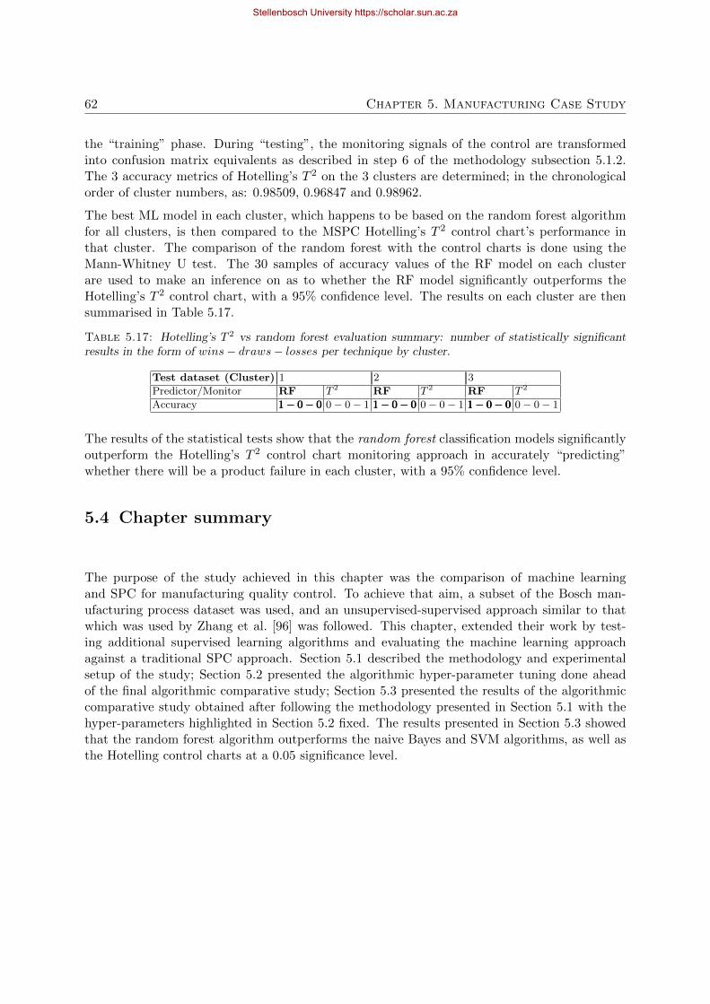
62 Chapter 5. Manufacturing Case Study
the “training” phase. During “testing”, the monitoring signals of the control are transformedinto confusion matrix equivalents as described in step 6 of the methodology subsection 5.1.2.The 3 accuracy metrics of Hotelling’s T 2 on the 3 clusters are determined; in the chronologicalorder of cluster numbers, as: 0.98509, 0.96847 and 0.98962.
The best ML model in each cluster, which happens to be based on the random forest algorithmfor all clusters, is then compared to the MSPC Hotelling’s T 2 control chart’s performance inthat cluster. The comparison of the random forest with the control charts is done using theMann-Whitney U test. The 30 samples of accuracy values of the RF model on each clusterare used to make an inference on as to whether the RF model significantly outperforms theHotelling’s T 2 control chart, with a 95% confidence level. The results on each cluster are thensummarised in Table 5.17.
Table 5.17: Hotelling’s T 2 vs random forest evaluation summary: number of statistically significantresults in the form of wins− draws− losses per technique by cluster.
Test dataset (Cluster) 1 2 3
Predictor/Monitor RF T 2 RF T 2 RF T 2
Accuracy 1− 0− 01− 0− 01− 0− 0 0− 0− 1 1− 0− 01− 0− 01− 0− 0 0− 0− 1 1− 0− 01− 0− 01− 0− 0 0− 0− 1
The results of the statistical tests show that the random forest classification models significantlyoutperform the Hotelling’s T 2 control chart monitoring approach in accurately “predicting”whether there will be a product failure in each cluster, with a 95% confidence level.
5.4 Chapter summary
The purpose of the study achieved in this chapter was the comparison of machine learningand SPC for manufacturing quality control. To achieve that aim, a subset of the Bosch man-ufacturing process dataset was used, and an unsupervised-supervised approach similar to thatwhich was used by Zhang et al. [96] was followed. This chapter, extended their work by test-ing additional supervised learning algorithms and evaluating the machine learning approachagainst a traditional SPC approach. Section 5.1 described the methodology and experimentalsetup of the study; Section 5.2 presented the algorithmic hyper-parameter tuning done aheadof the final algorithmic comparative study; Section 5.3 presented the results of the algorithmiccomparative study obtained after following the methodology presented in Section 5.1 with thehyper-parameters highlighted in Section 5.2 fixed. The results presented in Section 5.3 showedthat the random forest algorithm outperforms the naive Bayes and SVM algorithms, as well asthe Hotelling control charts at a 0.05 significance level.
Stellenbosch University https://scholar.sun.ac.za

CHAPTER 6
Precision Agriculture Case Study
The purpose of the study described in this chapter is to compare several regression ML algo-rithms for predicting milk yield for precision livestock farming. To achieve this aim, a datasetfrom a dairy farm equipped with various sensor devices is used. The chapter opens with a briefbackground of the case study in Section 6.1. The chapter then proceeds to describe the exper-imental setup and highlight the methodology to be used in executing the comparative studyin Section 6.2. Section 6.3 then presents the algorithmic hyper-parameter tuning of each algo-rithm ahead of the final algorithmic comparative study, and Section 6.4 presents the results ofthe algorithmic comparative study obtained based on the methodology and experimental setuppresented in Section 6.2 with the hyper-parameters highlighted in Section 6.3 fixed. Finally,Section 6.5 summarises the contents of the chapter.
6.1 Background
Precision Livestock farming (PLF) has greatly improved from earlier days, mostly in dairy cowfarming. PLF is mainly focused on real-time monitoring of animal health, increasing milk yieldin animals, improving farming conditions, reducing production costs and it is also useful in earlydisease detection [9]. A typical example of a recent PLF innovation is the Automatic MilkingSystem (AMS), which was introduced in the early 1990s.
The main significance of the AMS is in providing the farmer with real-time milk production dataand data on cow behavior. All data records are kept in the AMS database. The data recordscan be useful in management optimisation and herd characterisation which are under-researchedfields.
The case study is based on a farm in Italy, located near Bologna. The barn is a rectangular-shaped building 51 metres in length and 21 metres in width. The building consists of a haystorage site, a feed delivery path and feeding site, and a wrestling site in the centre of thebuilding.
Automated milking is performed by a robotic milking system. After every milking, data relatingto milk quality and quantity is recorded on the AMS. The AMS is also useful in managing sup-plemental feeding. The “refusal” (i.e., no permission to be milked) and “access” (i.e., permissionto be milked) of the cows are determined by the anticipated milk yield, lactation period and theaverage milk production. The milking robot is encoded to ensure regular visits to each cow as
63
Stellenbosch University https://scholar.sun.ac.za

64 Chapter 6. Precision Agriculture Case Study
per the cow’s productivity and its anticipated maximum milk yield per visit.
Livestock behaviour data is obtained through a collar mounted on the cow’s neck. This collarserves to identify the cow and sense its activity. The monitor detects the activity level of eachcow by measuring the intensity and the duration of movement. This instrument is also widelyused for heat detection in livestock.
PCE-HT71 stand-alone data loggers are used to measure internal temperature, dew point andhumidity in a cycle of 30 minutes on the farm. The PCE-HT71 stand-alone equipment is 0.5 oCaccurate with a resolution of 0.1 oC. Two instruments are placed in the central cubicle rows,at an elevation of 1 metre from the floor. Exterior climate data is captured by a PCE-FWS20weather station installed a few metres from the barn.
6.2 Methodology and experimental setup
6.2.1 Dataset characterisation
The dataset used in this case study is an aggregate of the AMS, cow activity and temperature-humidity datasets of the farm over the period from 19 June 2015 to 31 August 2015. Bonora etal. [13] used a 2014 dataset from the same farm to develop a mathematical (regression) modelthat can be used to predict the daily milk yield (in litres) of a generic (average) cow usingenvironment-related independent variables; the dataset used in this thesis was used as a singlevalidation set by Bonora et al. [13]. According to them, in addition to total milk yield at anyobservation, the aggregated dataset consists of 12 other features that may be used to predictmilk yield, namely:
• Time (i.e. date-&-time).
• Time as Number (i.e. date-&-time formatted as numeric).
• Average of “milkings” (i.e. daily average number of milking events per cow).
• Lactations (i.e. a mathematical product of the sum of days into the milk production phaseand “average of milkings”).
• Conductivity sum (i.e. sum of all cow thermal conductivity values during all milkingevents).
• 24-hour feed (i.e. total feed consumed over a 24-hour period).
• “No of cows” (i.e. number of cows available for milk production within the barn).
• Dew-point indoor (i.e. the indoor dew-point temperature in oC).
• Milk temperature sum (i.e. Avg − temperature of milk × No of cows × average ofmilkings).
• Total 24h activity (i.e. sum of activity levels of all cows in the barn determined using thecollars for “measuring intensity and the duration of movements” over a 24-hour period).
• Indoors THI (i.e. temperature-humidity index, a measure of heat stress).
Stellenbosch University https://scholar.sun.ac.za
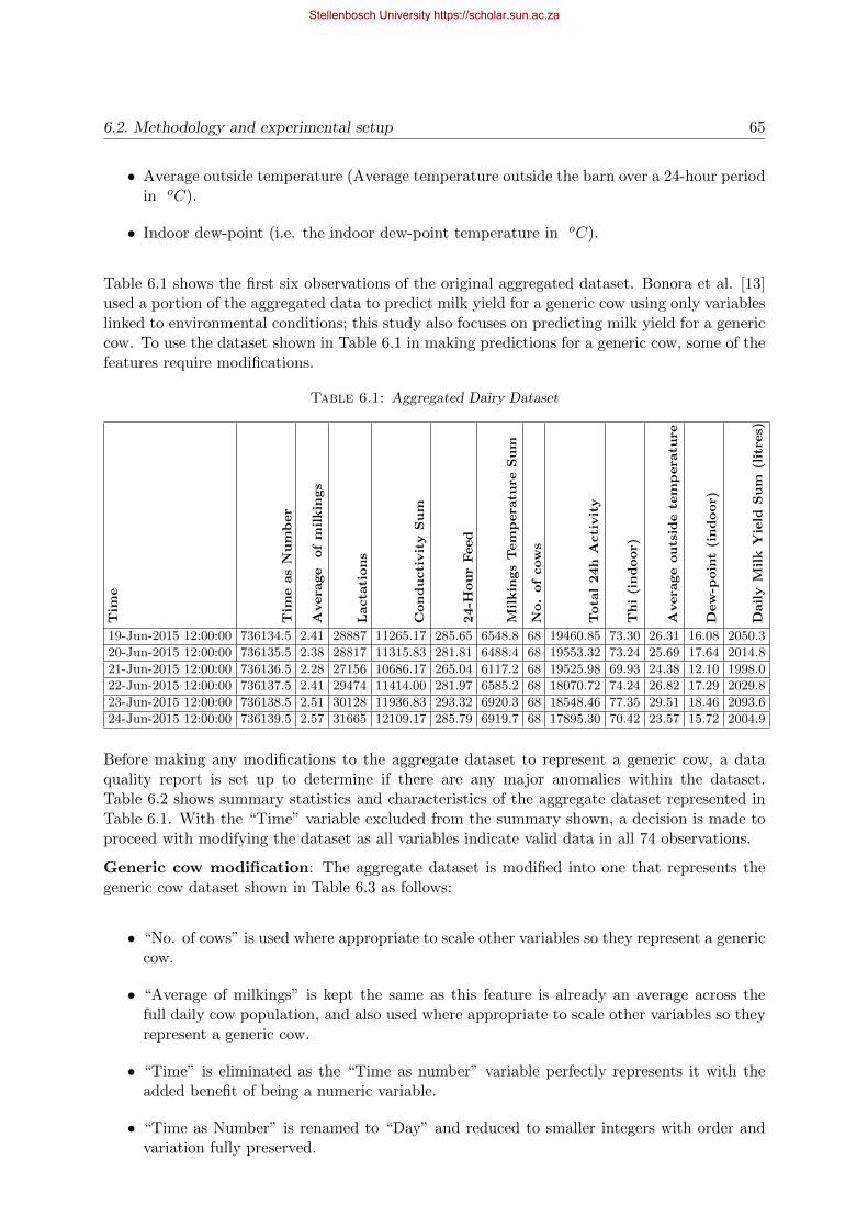
6.2. Methodology and experimental setup 65
• Average outside temperature (Average temperature outside the barn over a 24-hour periodin oC).
• Indoor dew-point (i.e. the indoor dew-point temperature in oC).
Table 6.1 shows the first six observations of the original aggregated dataset. Bonora et al. [13]used a portion of the aggregated data to predict milk yield for a generic cow using only variableslinked to environmental conditions; this study also focuses on predicting milk yield for a genericcow. To use the dataset shown in Table 6.1 in making predictions for a generic cow, some of thefeatures require modifications.
Table 6.1: Aggregated Dairy Dataset
Tim
e
Tim
eas
Nu
mb
er
Avera
ge
of
mil
kin
gs
Lacta
tion
s
Con
du
cti
vit
yS
um
24-H
ou
rFeed
Mil
kin
gs
Tem
pera
ture
Su
m
No.
of
cow
s
Tota
l24h
Acti
vit
y
Th
i(i
nd
oor)
Avera
ge
ou
tsid
ete
mp
era
ture
Dew
-poin
t(i
nd
oor)
Dail
yM
ilk
Yie
ldS
um
(lit
res)
19-Jun-2015 12:00:00 736134.5 2.41 28887 11265.17 285.65 6548.8 68 19460.85 73.30 26.31 16.08 2050.3
20-Jun-2015 12:00:00 736135.5 2.38 28817 11315.83 281.81 6488.4 68 19553.32 73.24 25.69 17.64 2014.8
21-Jun-2015 12:00:00 736136.5 2.28 27156 10686.17 265.04 6117.2 68 19525.98 69.93 24.38 12.10 1998.0
22-Jun-2015 12:00:00 736137.5 2.41 29474 11414.00 281.97 6585.2 68 18070.72 74.24 26.82 17.29 2029.8
23-Jun-2015 12:00:00 736138.5 2.51 30128 11936.83 293.32 6920.3 68 18548.46 77.35 29.51 18.46 2093.6
24-Jun-2015 12:00:00 736139.5 2.57 31665 12109.17 285.79 6919.7 68 17895.30 70.42 23.57 15.72 2004.9
Before making any modifications to the aggregate dataset to represent a generic cow, a dataquality report is set up to determine if there are any major anomalies within the dataset.Table 6.2 shows summary statistics and characteristics of the aggregate dataset represented inTable 6.1. With the “Time” variable excluded from the summary shown, a decision is made toproceed with modifying the dataset as all variables indicate valid data in all 74 observations.
Generic cow modification: The aggregate dataset is modified into one that represents thegeneric cow dataset shown in Table 6.3 as follows:
• “No. of cows” is used where appropriate to scale other variables so they represent a genericcow.
• “Average of milkings” is kept the same as this feature is already an average across thefull daily cow population, and also used where appropriate to scale other variables so theyrepresent a generic cow.
• “Time” is eliminated as the “Time as number” variable perfectly represents it with theadded benefit of being a numeric variable.
• “Time as Number” is renamed to “Day” and reduced to smaller integers with order andvariation fully preserved.
Stellenbosch University https://scholar.sun.ac.za

66 Chapter 6. Precision Agriculture Case Study
Table 6.2: Summary Statistics of Aggregated Dairy Dataset
24-H
ou
rFeed
Avera
ge
of
mil
kin
gs
Avera
ge
ou
tsid
ete
mp
era
ture
Con
du
cti
vit
yS
um
Dail
yM
ilk
Yie
ldS
um
(lit
res)
Dew
-poin
t(i
nd
oor)
Lacta
tion
s
Mil
kin
gs
Tem
pera
ture
Su
m
No
of
cow
s
Th
i(i
nd
oor)
Tim
eas
Nu
mb
er
Tota
l24h
Acti
vit
y
Mean 247.45 2.39 30.29 10983.05 1776.52 18.99 29773.65 6261.86 66.20 78.32 736171.00 18807.30
Std.Dev 18.81 0.13 3.20 805.38 140.05 2.49 2137.91 456.10 2.23 3.79 21.51 1360.11
Min 216.80 2.04 22.48 9145.50 1502.60 12.10 24507.00 5268.00 62.00 69.93 736134.50 14794.73
Q1 234.24 2.31 27.79 10481.17 1678.20 17.44 28817.00 5973.20 64.00 74.75 736152.50 18070.72
Median 241.57 2.41 30.87 10980.33 1725.35 19.42 29896.50 6250.15 66.00 78.90 736171.00 18937.80
Q3 265.04 2.48 33.16 11490.00 1905.60 20.76 31183.00 6535.70 68.00 81.53 736189.50 19499.31
Max 293.32 2.65 36.47 12784.50 2093.60 24.17 34146.00 7327.50 69.00 85.16 736207.50 22647.63
MAD 12.37 0.12 3.71 745.38 91.62 2.51 1696.09 412.61 2.97 4.40 27.43 974.46
IQR 29.27 0.17 5.32 979.00 224.75 3.29 2312.00 537.78 4.00 6.63 36.50 1397.19
CV 0.08 0.05 0.11 0.07 0.08 0.13 0.07 0.07 0.03 0.05 0.00 0.07
Skewness 0.77 -0.49 -0.48 -0.04 0.69 -0.46 -0.28 0.14 -0.31 -0.37 0.00 -0.10
SE.Skewness 0.28 0.28 0.28 0.28 0.28 0.28 0.28 0.28 0.28 0.28 0.28 0.28
Kurtosis -0.54 -0.12 -0.71 -0.40 -0.70 -0.05 -0.22 -0.23 -1.29 -0.84 -1.25 1.02
N.Valid 74.00 74.00 74.00 74.00 74.00 74.00 74.00 74.00 74.00 74.00 74.00 74.00
Pct.Valid 100.00 100.00 100.00 100.00 100.00 100.00 100.00 100.00 100.00 100.00 100.00 100.00
• “Lactations” variable is averaged across all cows and milkings; however, it will be left outas its variation and order should perfectly correlate to “Day” for any unique individualgeneric cow, and this condition isn’t perfectly satisfied by the modification as observed inTable 6.3 (poor correlation).
• “Conductivity sum” is averaged across all cows and milking events and renamed to “Av-erage Conductivity”.
• “24-hour feed” is averaged over daily number of cows and renamed to “Average daily feed”.
• “Milk temperature sum” is averaged across all cows and milking events and renamed to“Milk temperature”.
• “Total 24h activity” is averaged across the daily number of cows.
• Indoor “THI” is kept unchanged; it is only renamed to “ITHI”.
• “Average outside temperature” is renamed to “Outdoor Temperature” without value al-terations
• Indoor “Dew-point” is renamed to “Dew point Temperature” without value alterations.
• “Relative Humidity” is an additional variable that represents outdoor relative humidity,and is estimated using the August-Roche-Magnus approximation [3, 5, 58] on the assump-tion that there are no humidification or dehumidification devices in the barn, i.e. the
Stellenbosch University https://scholar.sun.ac.za

6.2. Methodology and experimental setup 67
indoor dew point temperature is equal to the outdoor dew point temperature
RH =e
17.625Tdp243.04+Tdp
e17.625T243.04+T
where, RH is the relative humidity (a fraction between 0 and 1, can also be expressed asa percentage), T is the temperature in oC and Tdp is the dew point temperature in oC.
Table 6.3: Generic Cow Dairy Dataset
Day
Avera
ge
Dail
yM
ilkin
gs
Lacta
tion
s
Avera
ge
Con
du
cti
vit
y
Avera
ge
Dail
yFeed
(Kg)
Mil
kT
em
pera
ture
(oC
)
Nu
mb
er
of
Cow
s
Acti
vit
y
ITH
I
Ou
tdoor
Tem
pera
ture
(oC
)
Dew
poin
tT
em
pera
ture
(oC
)
Rela
tive
Hu
mid
ity
Mil
kyie
ld(L
)
34 2.41 176.14 68.69 4.20 39.93 68 286.19 73.30 26.31 16.08 0.53 30.15
35 2.38 177.88 69.85 4.14 40.05 68 287.55 73.24 25.69 17.64 0.61 29.63
36 2.28 175.20 68.94 3.90 39.47 68 287.15 69.93 24.38 12.10 0.46 29.38
34 2.41 179.72 69.60 4.15 40.15 68 265.75 74.24 26.82 17.29 0.56 29.85
37 2.51 176.19 69.81 4.31 40.47 68 272.77 77.35 29.51 18.46 0.51 30.79
38 2.57 180.94 69.20 4.20 39.54 68 263.17 70.42 23.57 15.72 0.61 29.48
Before proceeding to build predictive models using the generic cow dataset, it is vital that thedata is visualised using boxplots and histograms to identify any concerning anomalies. Fig-ures 6.2, 6.3 and 6.4 show the boxplots of the features of the generic cow dataset represented inTable 6.3; despite some outliers in some of the feature values observed, a decision is made thatall observations should remain in the dataset as the variation is not large enough to assume thatvalues may be due to input error. Figures 6.5, 6.6 and 6.7 show the histograms of the features ofthe generic cow dataset; the shown histograms also display variation that is deemed acceptablefor the dataset.
6.2.2 Dataset Normalisation
One of the most important decisions to be made prior to the training of predictive modelsis whether data should be normalised or not. Much as there may be general normalisationguidelines for each type of predictive algorithm; one must heed the “no-free-lunch theorem”which essentially states that for any predictive algorithm there exists a dataset on which itdoes not succeed in outperforming other algorithms(i.e. there is a dataset on which a differentlearner would perform better) [84]. Hence, in this study, it is decided that each algorithm willbe trained on 3 versions of a dataset, and performance will be compared across all 3 versions ofeach algorithm. Each algorithm will be trained and tested on 3 versions of a dataset, namely:
• non-normalised dataset
• standardised dataset (gaussian normalisation of features using µ and σ)
Stellenbosch University https://scholar.sun.ac.za

68 Chapter 6. Precision Agriculture Case Study
• normalised dataset (min-max normalisation, similar to standardisation, except minimumand range are used instead of µ and σ, respectively)
The non-normalised features are displayed by means of boxplots in Figures 6.2, 6.3 and 6.4.The standardised and normalised features are also displayed by means of boxplots in Figure 6.8and Figure 6.9, respectively. It should be noted that the dependent or target variable is notnormalised during training and testing of models.
6.2.3 Data subsetting through explanatory variable selection
This part of the study explains how the features of the generic cow dataset are used to producesubsets for building models that predict milk yield.
The first part of the dairy farm case study focuses on the impact of environmental conditions onthe milk yield of a generic cow. It should be noted that the potential multicollinearity problemthat can be anticipated when looking at the correlogram in Figure 6.1 is immaterial in this study.The focus on the ability of the algorithms to make good predictions of the dependent variable(milk yield) rather than finding “true” model internal parameters such as the β coefficients of amultilinear regression; multicollinearity generally does not affect the predictions of the responsevariable [45]. The explanatory variables used in this part are as follows (in addition to milkyield, the features implicated in this part of the study produce a dataset that will be referredto as the “environmental subset” from this point forth):
• Day,
• ITHI,
• Outdoor temperature,
• Dew point temperature, and
• Relative humidity.
Finally, the last part of the dairy farm study focuses on how in addition to environmentalconditions, cow health and behaviour predict milk yield (in addition to milk yield, the featuresimplicated in this part of the study produce a dataset that will be referred to as the “full set” fromthis point forward). In addition to the already listed variables that account for environmentalconditions, the explanatory variables used in this part are as follows:
• Average Daily milkings,
• Average conductivity,
• Average daily feed,
• Activity, and
• Milk temperature.
Stellenbosch University https://scholar.sun.ac.za

6.2. Methodology and experimental setup 69
Figure 6.1: Dataset Correlogram
Stellenbosch University https://scholar.sun.ac.za

70 Chapter 6. Precision Agriculture Case Study
Figure 6.2: Dataset Summary Boxplots
Figure 6.3: Dataset Summary Boxplots
Stellenbosch University https://scholar.sun.ac.za

6.2. Methodology and experimental setup 71
Figure 6.4: Dataset Summary Boxplots
Figure 6.5: Dataset Summary Histograms
Stellenbosch University https://scholar.sun.ac.za

72 Chapter 6. Precision Agriculture Case Study
Figure 6.6: Dataset Summary Histograms
Figure 6.7: Dataset Summary Histograms
Stellenbosch University https://scholar.sun.ac.za

6.2. Methodology and experimental setup 73
Figure 6.8: Standardised Dataset Summary Boxplots
Figure 6.9: Normalised Dataset Summary Boxplots
Stellenbosch University https://scholar.sun.ac.za

74 Chapter 6. Precision Agriculture Case Study
6.2.4 Methodology, tools and algorithms
After pre-processing each dataset, a similar approach to the supervised learning phase describedin subsection 5.1.2 of the manufacturing case study is used for the different regression algorithms.The CARET package in RStudio facilitates the training, tuning and testing of the regressionalgorithms using 30-fold cross validation. The algorithms compared in this case study are:
• Radial-kernel support vector machine (RSVM)
• Polynomial-kernel support vector machine (eliminates the need to consider linear SVM)
• Random forest (RF),
• General (multi)linear model (GLM),
• Step-wise multilinear regression algorithm (SML).
6.3 Algorithmic hyper-parameter tuning
6.3.1 Algorithmic performance metrics
Using various metrics, the different regression algorithms are evaluated against each other andagainst the step-wise multilinear regression algorithm used by Borona et al. [13] on the datasetused in this thesis. The metrics computed for each of models are:
• Mean absolute error proportion (MAEP), commonly referred to as Mean absolute percent-age error (MAPE)
• Root mean square percentage error (RMSPE)
• Coefficient of determination (R-squared i.e. R2)
MAEP is the primary metric to be used in determining the best model, because it is the metricthat was used by Borona et al. [13] in their algorithmic performance assessment. The RMSPEmetric is often correlated to the MAEP metric, and the R2 is used solely to monitor the ability ofthe model to generalise. The metrics can be computed for a dataset comprising of n observationsusing the predicted dependent variable values yi and the average of the dependent variable valuesyi as follows:
MAEP = (1
n)
n∑i=1
∣∣∣∣yi − yiyi
∣∣∣∣ (6.1)
RMSPE =
√1
nΣni=1
(yi − yiyi
)2(6.2)
R2 = 1−( 1n)∑n
i=1 (yi − yi)( 1n)∑n
i=1 (yi − y). (6.3)
Stellenbosch University https://scholar.sun.ac.za
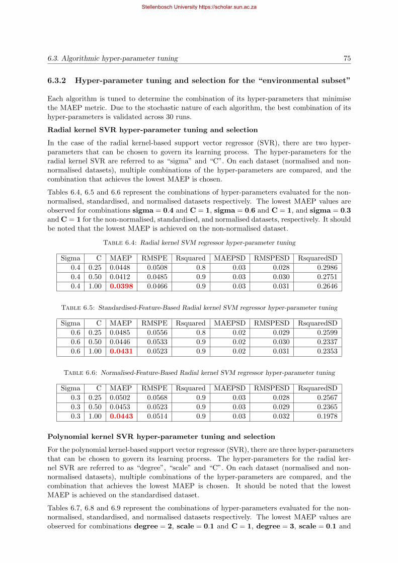
6.3. Algorithmic hyper-parameter tuning 75
6.3.2 Hyper-parameter tuning and selection for the “environmental subset”
Each algorithm is tuned to determine the combination of its hyper-parameters that minimisethe MAEP metric. Due to the stochastic nature of each algorithm, the best combination of itshyper-parameters is validated across 30 runs.
Radial kernel SVR hyper-parameter tuning and selection
In the case of the radial kernel-based support vector regressor (SVR), there are two hyper-parameters that can be chosen to govern its learning process. The hyper-parameters for theradial kernel SVR are referred to as “sigma” and “C”. On each dataset (normalised and non-normalised datasets), multiple combinations of the hyper-parameters are compared, and thecombination that achieves the lowest MAEP is chosen.
Tables 6.4, 6.5 and 6.6 represent the combinations of hyper-parameters evaluated for the non-normalised, standardised, and normalised datasets respectively. The lowest MAEP values areobserved for combinations sigma = 0.4 and C = 1, sigma = 0.6 and C = 1, and sigma = 0.3and C = 1 for the non-normalised, standardised, and normalised datasets, respectively. It shouldbe noted that the lowest MAEP is achieved on the non-normalised dataset.
Table 6.4: Radial kernel SVM regressor hyper-parameter tuning
Sigma C MAEP RMSPE Rsquared MAEPSD RMSPESD RsquaredSD
0.4 0.25 0.0448 0.0508 0.8 0.03 0.028 0.2986
0.4 0.50 0.0412 0.0485 0.9 0.03 0.030 0.2751
0.4 1.00 0.0398 0.0466 0.9 0.03 0.031 0.2646
Table 6.5: Standardised-Feature-Based Radial kernel SVM regressor hyper-parameter tuning
Sigma C MAEP RMSPE Rsquared MAEPSD RMSPESD RsquaredSD
0.6 0.25 0.0485 0.0556 0.8 0.02 0.029 0.2599
0.6 0.50 0.0446 0.0533 0.9 0.02 0.030 0.2337
0.6 1.00 0.0431 0.0523 0.9 0.02 0.031 0.2353
Table 6.6: Normalised-Feature-Based Radial kernel SVM regressor hyper-parameter tuning
Sigma C MAEP RMSPE Rsquared MAEPSD RMSPESD RsquaredSD
0.3 0.25 0.0502 0.0568 0.9 0.03 0.028 0.2567
0.3 0.50 0.0453 0.0523 0.9 0.03 0.029 0.2365
0.3 1.00 0.0443 0.0514 0.9 0.03 0.032 0.1978
Polynomial kernel SVR hyper-parameter tuning and selection
For the polynomial kernel-based support vector regressor (SVR), there are three hyper-parametersthat can be chosen to govern its learning process. The hyper-parameters for the radial ker-nel SVR are referred to as “degree”, “scale” and “C”. On each dataset (normalised and non-normalised datasets), multiple combinations of the hyper-parameters are compared, and thecombination that achieves the lowest MAEP is chosen. It should be noted that the lowestMAEP is achieved on the standardised dataset.
Tables 6.7, 6.8 and 6.9 represent the combinations of hyper-parameters evaluated for the non-normalised, standardised, and normalised datasets respectively. The lowest MAEP values areobserved for combinations degree = 2, scale = 0.1 and C = 1, degree = 3, scale = 0.1 and
Stellenbosch University https://scholar.sun.ac.za

76 Chapter 6. Precision Agriculture Case Study
C = 0.25, and degree = 1, scale = 0.1 and C = 1 for the non-normalised, standardised, andnormalised datasets respectively.
Table 6.7: Polynomial kernel SVM regressor hyper-parameter tuning
Degree Scale C MAEP RMSPE Rsquared MAEPSD RMSPESD RsquaredSD
1 0.00 0.25 0.0564 0.1 0.75 0.024 0.0262 0.4
1 0.00 0.50 0.0561 0.1 0.75 0.024 0.0261 0.4
1 0.00 1.00 0.0553 0.1 0.75 0.024 0.0259 0.4
1 0.01 0.25 0.053 0.1 0.75 0.024 0.0258 0.4
1 0.01 0.50 0.0524 0.1 0.74 0.023 0.0251 0.4
1 0.01 1.00 0.0518 0.1 0.74 0.022 0.0238 0.4
1 0.10 0.25 0.0508 0.1 0.77 0.020 0.0224 0.4
1 0.10 0.50 0.0486 0.1 0.79 0.020 0.0248 0.3
1 0.10 1.00 0.0469 0.1 0.78 0.021 0.0270 0.4
2 0.00 0.25 0.0561 0.1 0.75 0.024 0.0261 0.4
2 0.00 0.50 0.0552 0.1 0.75 0.024 0.0259 0.4
2 0.00 1.00 0.0538 0.1 0.75 0.024 0.0257 0.4
2 0.01 0.25 0.0523 0.1 0.74 0.023 0.0251 0.4
2 0.01 0.50 0.0516 0.1 0.74 0.022 0.0238 0.4
2 0.01 1.00 0.0497 0.1 0.79 0.020 0.0223 0.3
2 0.10 0.25 0.046 0.1 0.79 0.020 0.0242 0.3
2 0.10 0.50 0.0463 0.1 0.80 0.021 0.0254 0.3
2 0.10 1.00 0.0459 0.1 0.80 0.020 0.0250 0.3
3 0.00 0.25 0.0557 0.1 0.75 0.024 0.0260 0.4
3 0.00 0.50 0.0542 0.1 0.75 0.024 0.0257 0.4
3 0.00 1.00 0.0526 0.1 0.75 0.024 0.0256 0.4
3 0.01 0.25 0.0518 0.1 0.74 0.023 0.0244 0.4
3 0.01 0.50 0.0495 0.1 0.79 0.021 0.0227 0.3
3 0.01 1.00 0.0512 0.1 0.79 0.020 0.0229 0.3
3 0.10 0.25 0.0474 0.1 0.77 0.019 0.0236 0.3
3 0.10 0.50 0.0477 0.1 0.77 0.019 0.0241 0.3
3 0.10 1.00 0.0503 0.1 0.76 0.019 0.0233 0.3
Random forest regressor hyper-parameter tuning and selection
In the case of the random forest, there is one hyper-parameter that can be chosen to governits learning process. The hyper-parameter for random forest is the number of random samplesof attributes to use at splitting nodes referred to as “mtry”. On each dataset (normalised andnon-normalised datasets), different values of the hyper-parameter are compared, and the valueachieving the lowest MAEP is chosen.
Tables 6.10, 6.11 and 6.12 represent the combinations of hyper-parameters evaluated for thenon-normalised, standardised, and normalised datasets, respectively. The lowest MAEP valuesare observed on mtry = 5, mtry = 5, and mtry = 3 for the non-normalised, standardised, andnormalised datasets, respectively. It should be noted that the lowest MAEP is achieved on thestandardised dataset.
General (multi)linear model and step-wise multilinear regression
In the case of the general (multi)linear “model” and step-wise multilinear regression, apart fromindicating whether the general (multi)linear regression model should have an intercept or not,
Stellenbosch University https://scholar.sun.ac.za

6.3. Algorithmic hyper-parameter tuning 77
Table 6.8: Standardised-Feature-Based Polynomial kernel SVM regressor hyper-parameter tuning
Degree Scale C MAEP RMSPE Rsquared MAEPSD RMSPESD RsquaredSD
1 0.00 0.25 0.05744 0.06417 0.7 0.03 0.025 0.3821
1 0.00 0.50 0.057 0.06369 0.7 0.03 0.025 0.3823
1 0.00 1.00 0.0561 0.06261 0.7 0.03 0.026 0.3840
1 0.01 0.25 0.0535 0.05982 0.7 0.03 0.026 0.3859
1 0.01 0.50 0.05259 0.05861 0.7 0.03 0.027 0.3967
1 0.01 1.00 0.05203 0.05759 0.7 0.03 0.027 0.3872
1 0.10 0.25 0.05039 0.05617 0.7 0.03 0.028 0.3517
1 0.10 0.50 0.04842 0.05510 0.8 0.03 0.030 0.3204
1 0.10 1.00 0.04626 0.05410 0.8 0.03 0.031 0.3145
2 0.00 0.25 0.057 0.06369 0.7 0.03 0.025 0.3822
2 0.00 0.50 0.05609 0.06261 0.7 0.03 0.026 0.3839
2 0.00 1.00 0.05436 0.06070 0.7 0.03 0.026 0.3844
2 0.01 0.25 0.05246 0.05845 0.7 0.03 0.027 0.3936
2 0.01 0.50 0.0517 0.05721 0.7 0.03 0.027 0.3779
2 0.01 1.00 0.04987 0.05539 0.8 0.03 0.027 0.3521
2 0.10 0.25 0.04583 0.05259 0.8 0.02 0.027 0.3003
2 0.10 0.50 0.04605 0.05369 0.8 0.02 0.028 0.2986
2 0.10 1.00 0.04601 0.05368 0.8 0.02 0.027 0.2908
3 0.00 0.25 0.0566 0.06321 0.7 0.03 0.025 0.3841
3 0.00 0.50 0.05484 0.06119 0.7 0.03 0.026 0.3817
3 0.00 1.00 0.053 0.05921 0.7 0.03 0.027 0.3897
3 0.01 0.25 0.05184 0.05747 0.7 0.03 0.028 0.3851
3 0.01 0.50 0.04975 0.05510 0.8 0.03 0.027 0.3587
3 0.01 1.00 0.05042 0.05618 0.8 0.03 0.028 0.3200
3 0.10 0.25 0.04576 0.05323 0.8 0.02 0.026 0.3092
3 0.10 0.50 0.0463 0.05342 0.8 0.02 0.027 0.3136
3 0.10 1.00 0.04953 0.05635 0.8 0.02 0.027 0.3217
there are no other hyper-parameters that can be chosen to govern the learning process. A decisionis made to allow the general linear regression algorithm to have an intercept; the premise of thisdecision is that the algorithm will reach an intercept of “zero” if having no intercept produces thebest model. These algorithms do not have multiple combinations of hyper-parameters that canbe specified to control the learning process; however, Tables 6.13, 6.14 and 6.15, and Tables 6.16,6.17 and 6.18 summarise the performance of the algorithms on the non-normalised, standardised,and normalised datasets respectively. It should be noted that the general (multi)linear regressionalgorithm achieves the lowest MAEP in the standardised dataset whilst the step-wise multilinearregression algorithm performs best on the non-normalised dataset.
Stellenbosch University https://scholar.sun.ac.za

78 Chapter 6. Precision Agriculture Case Study
Table 6.9: Normalised-Feature-Based Polynomial kernel SVM regressor hyper-parameter tuning
Degree Scale C MAEP RMSPE Rsquared MAEPSD RMSPESD RsquaredSD
1 0.00 0.25 0.0565 0.1 0.86 0.022 0.0248 0.3
1 0.00 0.50 0.0561 0.1 0.86 0.022 0.0247 0.3
1 0.00 1.00 0.0552 0.1 0.86 0.022 0.0245 0.3
1 0.01 0.25 0.0529 0.1 0.86 0.022 0.0240 0.3
1 0.01 0.50 0.0522 0.1 0.85 0.022 0.0235 0.3
1 0.01 1.00 0.0516 0.1 0.83 0.022 0.0236 0.3
1 0.10 0.25 0.0512 0.1 0.79 0.023 0.0251 0.4
1 0.10 0.50 0.0488 0.1 0.80 0.028 0.0307 0.3
1 0.10 1.00 0.0471 0.1 0.80 0.030 0.0332 0.3
2 0.00 0.25 0.0561 0.1 0.86 0.022 0.0247 0.3
2 0.00 0.50 0.0552 0.1 0.86 0.022 0.0245 0.3
2 0.00 1.00 0.0536 0.1 0.86 0.022 0.0242 0.3
2 0.01 0.25 0.0521 0.1 0.85 0.022 0.0235 0.3
2 0.01 0.50 0.0514 0.1 0.83 0.022 0.0235 0.3
2 0.01 1.00 0.0504 0.1 0.80 0.022 0.0242 0.3
2 0.10 0.25 0.0472 0.1 0.82 0.026 0.0289 0.3
2 0.10 0.50 0.0477 0.1 0.80 0.028 0.0310 0.4
2 0.10 1.00 0.0477 0.1 0.80 0.028 0.0314 0.3
3 0.00 0.25 0.0556 0.1 0.86 0.022 0.0246 0.3
3 0.00 0.50 0.0541 0.1 0.85 0.022 0.0243 0.3
3 0.00 1.00 0.0524 0.1 0.86 0.022 0.0238 0.3
3 0.01 0.25 0.0515 0.1 0.84 0.021 0.0233 0.3
3 0.01 0.50 0.05 0.1 0.81 0.022 0.0238 0.3
3 0.01 1.00 0.051 0.1 0.80 0.024 0.0271 0.3
3 0.10 0.25 0.048 0.1 0.78 0.026 0.0295 0.3
3 0.10 0.50 0.0484 0.1 0.77 0.026 0.0293 0.3
3 0.10 1.00 0.0501 0.1 0.75 0.027 0.0294 0.4
Table 6.10: Random forest regressor hyper-parameter tuning
mtry MAEP RMSPE Rsquared MAEPSD RMSPESD RsquaredSD
2 0.0439 0.051 0.8712 0 0.03 0.255
3 0.0429 0.050 0.8443 0 0.03 0.281
5 0.0428 0.050 0.8516 0 0.03 0.271
Table 6.11: Standardised-Feature-Based random forest regressor hyper-parameter tuning
mtry MAEP RMSPE Rsquared MAEPSD RMSPESD RsquaredSD
2 0.0418 0.048 0.8940 0 0.03 0.185
3 0.0417 0.048 0.8790 0 0.03 0.224
5 0.0414 0.048 0.9032 0 0.03 0.159
Table 6.12: Normalised-Feature-Based random forest regressor hyper-parameter tuning
mtry MAEP RMSPE Rsquared MAEPSD RMSPESD RsquaredSD
2 0.0425 0.050 0.8027 0 0.03 0.339
3 0.0415 0.048 0.8016 0 0.03 0.341
5 0.0419 0.049 0.8016 0 0.03 0.342
Stellenbosch University https://scholar.sun.ac.za

6.3. Algorithmic hyper-parameter tuning 79
Table 6.13: General linear model hyper-parameter tuning
Intercept MAEP RMSPE Rsquared MAEPSD RMSPESD RsquaredSD
TRUE 0.0489 0.055 0.8344 0 0.03 0.302
Table 6.14: Standardised-Feature-Based General linear model hyper-parameter tuning
Intercept MAEP RMSPE Rsquared MAEPSD RMSPESD RsquaredSD
TRUE 0.0482 0.054 0.7145 0 0.03 0.408
Table 6.15: Normalised-Feature-Based General linear model hyper-parameter tuning
Intercept MAEP RMSPE Rsquared MAEPSD RMSPESD RsquaredSD
TRUE 0.0483 0.056 0.815 0 0.02 0.351
Table 6.16: Step-wise Multilinear regressor hyper-parameter tuning
Parameter MAEP RMSPE Rsquared MAEPSD RMSPESD RsquaredSD
none 0.0482 0.053 0.8228 0 0.03 0.296
Table 6.17: Standardised-Feature-Based Step-wise Multilinear regressor hyper-parameter tuning
Parameter MAEP RMSPE Rsquared MAEPSD RMSPESD RsquaredSD
none 0.0492 0.056 0.8065 0 0.03 0.306
Table 6.18: Normalised-Feature-Based Step-wise Multilinear regressor hyper-parameter tuning
Parameter MAEP RMSPE Rsquared MAEPSD RMSPESD RsquaredSD
none 0.0533 0.06 0.8668 0 0.03 0.239
Stellenbosch University https://scholar.sun.ac.za

80 Chapter 6. Precision Agriculture Case Study
6.3.3 Hyper-parameter tuning and selection for the “full set”
Radial kernel SVR hyper-parameter tuning and selection
Tables 6.19, 6.20 and 6.21 represent the combinations of hyper-parameters evaluated for thenon-normalised, standardised, and normalised datasets respectively. The lowest MAEP val-ues are observed for combinations sigma = 0.1 and C = 1 for the non-normalised “full set”,sigma = 0.1 and C = 1 for the standardised “full set”, and sigma = 0.1 and C = 1 for thenormalised “full set”. It should be noted that the lowest MAEP is achieved on the normaliseddataset.
Table 6.19: Radial kernel SVR hyper-parameter tuning (on “full set”)
Sigma C MAEP RMSPE Rsquared MAEPSD RMSPESD RsquaredSD
0.1 0.25 0.0315 0.0367 0.9 0.02 0.023 0.1994
0.1 0.50 0.0264 0.0309 0.9 0.02 0.023 0.1946
0.1 1.00 0.0255 0.0296 0.9 0.02 0.022 0.2043
Table 6.20: Standardised-Feature-Based Radial kernel SVR hyper-parameter tuning (on “full set”)
Sigma C MAEP RMSPE Rsquared MAEPSD RMSPESD RsquaredSD
0.1 0.25 0.0196 0.0232 0.9 0.02 0.022 0.1202
0.1 0.50 0.0167 0.0202 1.0 0.02 0.021 0.0930
0.1 1.00 0.0147 0.0179 1.0 0.01 0.018 0.0675
Table 6.21: Normalised-Feature-Based Radial kernel SVR hyper-parameter tuning (on “full set”)
Sigma C MAEP RMSPE Rsquared MAEPSD RMSPESD RsquaredSD
0.1 0.25 0.0202 0.0243 0.9 0.02 0.021 0.1525
0.1 0.50 0.0168 0.0205 1.0 0.02 0.020 0.1154
0.1 1.00 0.0146 0.0176 1.0 0.01 0.017 0.0816
Polynomial kernel SVR hyper-parameter tuning and selection on “full set”
Tables 6.22, 6.23 and 6.24 represent the combinations of hyper-parameters evaluated for thenon-normalised, standardised, and normalised datasets respectively. The lowest MAEP valuesare observed for combinations degree = 1, scale = 0.1 and C = 1 for the non-normalised “fullset”, degree = 1, scale = 0.1 for the standardised “full set’ ’and C = 1, and degree = 1,scale = 0.1 and C = 1 for the normalised “full set”. The normalised-feature-based modelachieved the lowest MAEP (MAPE).
Random forest regressor hyper-parameter tuning and selection on “full set”
Tables 6.25, 6.26 and 6.27 represent the combinations of hyper-parameters evaluated for thenon-normalised, standardised, and normalised datasets respectively. The lowest MAEP valuesare observed on mtry = 10 for the non-normalised “full set”, mtry = 10 for the standardised“full set”, and mtry = 10 for the normalised “full set” as well. It should be noted the lowestMAEP is achieved on the normalised “full set”.
General (multi)linear model and step-wise multilinear regression hyper-parametertuning on “full set”
Tables 6.28, 6.29 and 6.30, and Tables 6.31, 6.32 and 6.33 summarise the performance of thealgorithms on the non-normalised, standardised, and normalised datasets, respectively. It should
Stellenbosch University https://scholar.sun.ac.za

6.3. Algorithmic hyper-parameter tuning 81
Table 6.22: Polynomial kernel SVR hyper-parameter tuning (on “full set”)
Degree scale C MAEP RMSPE Rsquared MAEPSD RMSPESD RsquaredSD
1 0.00 0.25 0.0561 0.1 0.88 0.024 0.0248 0.2
1 0.00 0.50 0.0547 0.1 0.88 0.024 0.0245 0.2
1 0.00 1.00 0.0509 0.1 0.88 0.024 0.0243 0.2
1 0.01 0.25 0.0444 0.1 0.88 0.022 0.0226 0.2
1 0.01 0.50 0.0374 0.0 0.88 0.019 0.0200 0.2
1 0.01 1.00 0.0309 0.0 0.89 0.016 0.0171 0.3
1 0.10 0.25 0.0227 0.0 0.91 0.013 0.0146 0.2
1 0.10 0.50 0.0213 0.0 0.92 0.012 0.0136 0.2
1 0.10 1.00 0.0199 0.0 0.93 0.011 0.0129 0.2
2 0.00 0.25 0.0547 0.1 0.88 0.024 0.0245 0.2
2 0.00 0.50 0.0509 0.1 0.88 0.024 0.0243 0.2
2 0.00 1.00 0.0464 0.1 0.88 0.023 0.0233 0.2
2 0.01 0.25 0.0373 0.0 0.89 0.019 0.0202 0.2
2 0.01 0.50 0.0307 0.0 0.89 0.016 0.0173 0.3
2 0.01 1.00 0.0234 0.0 0.91 0.013 0.0151 0.2
2 0.10 0.25 0.0209 0.0 0.93 0.014 0.0153 0.2
2 0.10 0.50 0.0208 0.0 0.93 0.014 0.0152 0.2
2 0.10 1.00 0.0226 0.0 0.92 0.014 0.0153 0.2
3 0.00 0.25 0.0527 0.1 0.87 0.024 0.0245 0.2
3 0.00 0.50 0.0492 0.1 0.88 0.023 0.0235 0.2
3 0.00 1.00 0.043 0.0 0.88 0.021 0.0219 0.2
3 0.01 0.25 0.0328 0.0 0.89 0.018 0.0187 0.3
3 0.01 0.50 0.0253 0.0 0.90 0.015 0.0165 0.3
3 0.01 1.00 0.0219 0.0 0.92 0.013 0.0152 0.2
3 0.10 0.25 0.0227 0.0 0.93 0.016 0.0181 0.2
3 0.10 0.50 0.0229 0.0 0.93 0.015 0.0177 0.2
3 0.10 1.00 0.0251 0.0 0.93 0.017 0.0213 0.2
be noted that the general (multi)linear regression algorithm achieves the lowest MAEP on thestandardised dataset whilst the step-wise multilinear regression algorithm performs best on thenon-normalised dataset.
Stellenbosch University https://scholar.sun.ac.za

82 Chapter 6. Precision Agriculture Case Study
Table 6.23: Standardised-Feature-Based Polynomial kernel SVR hyper-parameter tuning (on “full set”)
Degree scale C MAEP RMSPE Rsquared MAEPSD RMSPESD RsquaredSD
1 0.00 0.25 0.05559 0.06127 0.9 0.03 0.029 0.1304
1 0.00 0.50 0.05368 0.05920 0.9 0.03 0.028 0.1270
1 0.00 1.00 0.04886 0.05404 0.9 0.03 0.026 0.1218
1 0.01 0.25 0.03797 0.04226 0.9 0.02 0.022 0.1113
1 0.01 0.50 0.02535 0.02860 0.9 0.01 0.015 0.1139
1 0.01 1.00 0.01506 0.01726 1.0 0.01 0.010 0.1277
1 0.10 0.25 0.00893 0.01039 1.0 0.01 0.007 0.0180
1 0.10 0.50 0.00555 0.00640 1.0 0.00 0.004 0.0073
1 0.10 1.00 0.00448 0.00506 1.0 0.00 0.003 0.0064
2 0.00 0.25 0.05368 0.05920 0.9 0.03 0.028 0.1260
2 0.00 0.50 0.04885 0.05403 0.9 0.03 0.026 0.1207
2 0.00 1.00 0.04097 0.04550 0.9 0.02 0.023 0.1117
2 0.01 0.25 0.02505 0.02827 0.9 0.01 0.015 0.1259
2 0.01 0.50 0.0148 0.01694 0.9 0.01 0.010 0.1514
2 0.01 1.00 0.01016 0.01178 1.0 0.01 0.008 0.0342
2 0.10 0.25 0.00755 0.00859 1.0 0.00 0.005 0.0243
2 0.10 0.50 0.00613 0.00696 1.0 0.00 0.004 0.0289
2 0.10 1.00 0.00609 0.00687 1.0 0.00 0.004 0.0180
3 0.00 0.25 0.05134 0.05669 0.9 0.03 0.027 0.1249
3 0.00 0.50 0.04466 0.04954 0.9 0.02 0.025 0.1057
3 0.00 1.00 0.0348 0.03880 0.9 0.02 0.020 0.1064
3 0.01 0.25 0.01815 0.02043 0.9 0.01 0.012 0.1703
3 0.01 0.50 0.01188 0.01387 1.0 0.01 0.009 0.0875
3 0.01 1.00 0.00836 0.00961 1.0 0.01 0.006 0.0245
3 0.10 0.25 0.00831 0.00947 1.0 0.00 0.005 0.0298
3 0.10 0.50 0.00779 0.00873 1.0 0.00 0.005 0.0232
3 0.10 1.00 0.00775 0.00867 1.0 0.00 0.005 0.0210
Stellenbosch University https://scholar.sun.ac.za

6.3. Algorithmic hyper-parameter tuning 83
Table 6.24: Normalised-Feature-Based Polynomial kernel SVR hyper-parameter tuning (on “full set”)
Degree scale C MAEP RMSPE Rsquared MAEPSD RMSPESD RsquaredSD
1 0.00 0.25 0.0554 0.1 0.96 0.023 0.0238 0.1
1 0.00 0.50 0.0536 0.1 0.96 0.023 0.0233 0.1
1 0.00 1.00 0.0489 0.1 0.96 0.021 0.0224 0.1
1 0.01 0.25 0.0379 0.0 0.97 0.018 0.0194 0.1
1 0.01 0.50 0.0253 0.0 0.98 0.014 0.0149 0.0
1 0.01 1.00 0.0151 0.0 0.98 0.009 0.0097 0.0
1 0.10 0.25 0.0086 0.0 0.99 0.006 0.0066 0.0
1 0.10 0.50 0.0055 0.0 1.00 0.004 0.0041 0.0
1 0.10 1.00 0.0044 0.0 1.00 0.003 0.0029 0.0
2 0.00 0.25 0.0536 0.1 0.96 0.023 0.0232 0.1
2 0.00 0.50 0.0489 0.1 0.96 0.021 0.0224 0.1
2 0.00 1.00 0.0408 0.0 0.97 0.019 0.0202 0.1
2 0.01 0.25 0.0249 0.0 0.97 0.013 0.0147 0.1
2 0.01 0.50 0.0146 0.0 0.98 0.009 0.0098 0.0
2 0.01 1.00 0.0097 0.0 0.99 0.007 0.0075 0.0
2 0.10 0.25 0.0073 0.0 1.00 0.004 0.0046 0.0
2 0.10 0.50 0.006 0.0 1.00 0.004 0.0042 0.0
2 0.10 1.00 0.0057 0.0 1.00 0.004 0.0040 0.0
3 0.00 0.25 0.0514 0.1 0.96 0.022 0.0229 0.1
3 0.00 0.50 0.0445 0.0 0.97 0.020 0.0214 0.1
3 0.00 1.00 0.0345 0.0 0.97 0.017 0.0185 0.1
3 0.01 0.25 0.0178 0.0 0.98 0.010 0.0113 0.0
3 0.01 0.50 0.0116 0.0 0.99 0.008 0.0087 0.0
3 0.01 1.00 0.0079 0.0 0.99 0.005 0.0056 0.0
3 0.10 0.25 0.0079 0.0 0.99 0.005 0.0051 0.0
3 0.10 0.50 0.0073 0.0 0.99 0.004 0.0042 0.0
3 0.10 1.00 0.0073 0.0 0.99 0.004 0.0041 0.0
Table 6.25: Random forest regressor hyper-parameter tuning (on “full set”)
mtry MAEP RMSPE Rsquared MAEPSD RMSPESD RsquaredSD
2 0.0275 0.032 0.9193 0 0.02 0.185
6 0.0241 0.028 0.9459 0 0.02 0.122
10 0.0239 0.028 0.9519 0 0.02 0.102
Table 6.26: Standardised-Feature-Based random forest regressor hyper-parameter tuning (on “full set”)
mtry MAEP RMSPE Rsquared MAEPSD RMSPESD RsquaredSD
2 0.0179 0.021 0.9472 0 0.02 0.184
6 0.0081 0.010 0.9701 0 0.01 0.142
10 0.0046 0.006 0.9958 0 0.01 0.018
Table 6.27: Normalised-Feature-Based random forest regressor hyper-parameter tuning (on “full set”)
mtry MAEP RMSPE Rsquared MAEPSD RMSPESD RsquaredSD
2 0.0176 0.021 0.9779 0 0.02 0.059
6 0.0078 0.010 0.9916 0 0.01 0.029
10 0.0045 0.006 0.9973 0 0.01 0.013
Stellenbosch University https://scholar.sun.ac.za

84 Chapter 6. Precision Agriculture Case Study
Table 6.28: General linear model hyper-parameter tuning (on “full set”)
Intercept MAEP RMSPE Rsquared MAEPSD RMSPESD RsquaredSD
TRUE 0.0211 0.024 0.9292 0 0.01 0.158
Table 6.29: Standardised-Feature-Based General linear model hyper-parameter tuning (on “full set”)
Intercept MAEP RMSPE Rsquared MAEPSD RMSPESD RsquaredSD
TRUE 1e-04 0 1 0 0 0
Table 6.30: Normalised-Feature-Based General linear model hyper-parameter tuning (on “full set”)
Intercept MAEP RMSPE Rsquared MAEPSD RMSPESD RsquaredSD
TRUE 1e-04 0 1 0 0 0
Table 6.31: Step-wise Multilinear model hyper-parameter tuning (on “full set”)
Parameter MAEP RMSPE Rsquared MAEPSD RMSPESD RsquaredSD
none 0.0216 0.024 0.9357 0 0.01 0.156
Table 6.32: Standardised-Feature-Based Step-wise Multilinear model hyper-parameter tuning (on “fullset”)
Parameter MAEP RMSPE Rsquared MAEPSD RMSPESD RsquaredSD
none 1e-04 0 1 0 0 0
Table 6.33: Normalised-Feature-Based Step-wise Multilinear model hyper-parameter tuning (on “fullset”)
Parameter MAEP RMSPE Rsquared MAEPSD RMSPESD RsquaredSD
none 1e-04 0 1 0 0 0
Stellenbosch University https://scholar.sun.ac.za

6.4. Algorithmic comparative study 85
6.4 Algorithmic comparative study
Finally, the performance of the best tuned algorithm from each of the 3 forms on each datasetis assessed against the best tuned of all other algorithms from each of the 3 forms on thesame dataset. Through visualisation tools such as boxplots, it can be generally shown thatthe performance of each tuned algorithm is of a stochastic nature. One of the contributingfactors to this stochasticity is the random resampling of the training and test dataset acrossthe 30 different experiments. The different training sets result in varied initialisation and/orfinalisation of the internal algorithm parameters (not hyper-parameters), such as the normalvector (or weight vector) of support vector machines and the β coefficients of linear regressionalgorithms. An illustration of how different experiments have different training and test setsis shown in Figure 6.10. Due to the stochastic nature of the algorithms, statistical tests areperformed to determine if the observed performance differences exist in all 3 metrics for eachdataset. The statistical test performed on the model metrics is the non-parametric Mann-Whitney U test with a 10% significance level.
←−All Dataset Observations−→Experiment 1
Experiment 2
Experiment 3
Experiment 4
Experiment 5
Training
Test
Figure 6.10: 5-fold cross validation
6.4.1 Evaluation on “environmental subset”
Tables 6.34, 6.35 and 6.36 show the p-values from the Mann-Whitney tests conducted on eachmodel against each of the other models on the “environmental subset”. Statistical test results canbe visually scrutinised by means of boxplots. Krzywinski and Altman [44] recommend boxplotsas a means of supplementing analyses and conveying more information than merely looking atthe average and standard deviation. In addition to the sample minimum, sample maximum,inter-quartile range and median, the mean (red diamond) is also shown in the visual boxplotillustrations to provide a more thorough representation of the spread and central tendency of thedata samples. Figures 6.11, 6.12 and 6.13 show the boxplots of each model on the “environmentalsubset” in terms of MAEP, RMSPE and coefficient of determination (R2), respectively.
Table 6.34 shows that there is a lack of statistical significance in the difference in MAEP (MAPE)performances between most models. It can be observed from Table 6.34 that normalisation ofthe dataset does not yield statistically significant differences in the performance of the mod-els of the same algorithm; however, when compared to models from different algorithms, thereare some observed statistically significant differences. The most prominent statistically signifi-cant differences can be seen when comparing the normalised-feature-based step-wise multilinearregression model (stepwise multilinear regression 3) against all random forest and radial ker-nel SVR models. Other statistically significant differences can be seen when comparing thenon-normalised-feature-based and normalised-feature-based general multilinear regression mod-els (linear regression and linear regression 3 in Table 6.34) against the non-normalised-feature-
Stellenbosch University https://scholar.sun.ac.za

86 Chapter 6. Precision Agriculture Case Study
Table 6.34: Mean Absolute Percentage Error Mann-Whitney Test results (p-values) of regression mod-els.
Ran
dom
.Fore
st.R
egre
ssor
Ran
dom
.Fore
st.R
egre
ssor.
2
Ran
dom
.Fore
st.R
egre
ssor.
3
Rad
ial.
Kern
el.
SV
R
Rad
ial.
Kern
el.
SV
R.2
Rad
ial.
Kern
el.
SV
R.3
Poly
nom
ial.
Kern
el.
SV
R
Poly
nom
ial.
Kern
el.
SV
R.2
Poly
nom
ial.
Kern
el.
SV
R.3
Lin
ear.
Regre
ssio
n
Lin
ear.
Regre
ssio
n.2
Lin
ear.
Regre
ssio
n.3
Ste
pw
ise.M
ult
ilin
ear.
Regre
ssio
n
Ste
pw
ise.M
ult
ilin
ear.
Regre
ssio
n.2
Ste
pw
ise.M
ult
ilin
ear.
Regre
ssio
n.3
Random forest regressor 1 0.84 0.62 0.74 0.69 0.87 0.31 0.54 0.43 0.16 0.29 0.18 0.41 0.29 0.06
Random forest regressor 2 0.84 1 0.85 0.79 0.58 0.74 0.2 0.35 0.33 0.15 0.2 0.09 0.45 0.14 0.03
Random forest regressor 3 0.62 0.85 1 0.8 0.56 0.6 0.25 0.46 0.45 0.15 0.23 0.11 0.29 0.13 0.04
Radial Kernel SVR 0.74 0.79 0.8 1 0.57 0.62 0.21 0.29 0.3 0.1 0.15 0.12 0.27 0.15 0.03
Radial Kernel SVR 2 0.69 0.58 0.56 0.57 1 0.81 0.54 0.79 0.62 0.25 0.47 0.28 0.68 0.43 0.09
Radial Kernel SVR 3 0.87 0.74 0.6 0.62 0.81 1 0.39 0.63 0.57 0.24 0.39 0.17 0.57 0.31 0.06
Polynomial Kernel SVR 0.31 0.2 0.25 0.21 0.54 0.39 1 0.79 0.95 0.63 0.87 0.57 0.9 0.71 0.19
Polynomial Kernel SVR 2 0.54 0.35 0.46 0.29 0.79 0.63 0.79 1 0.94 0.53 0.71 0.46 0.88 0.53 0.18
Polynomial Kernel SVR 3 0.43 0.33 0.45 0.3 0.62 0.57 0.95 0.94 1 0.6 0.83 0.6 1 0.66 0.23
Linear Regression 0.16 0.15 0.15 0.1 0.25 0.24 0.63 0.53 0.6 1 0.85 0.99 0.49 0.99 0.47
Linear Regression 2 0.29 0.2 0.23 0.15 0.47 0.39 0.87 0.71 0.83 0.85 1 0.69 0.75 0.83 0.31
Linear Regression 3 0.18 0.09 0.11 0.12 0.28 0.17 0.57 0.46 0.6 0.99 0.69 1 0.56 0.9 0.46
Stepwise Multilinear Regression 0.41 0.45 0.29 0.27 0.68 0.57 0.9 0.88 1 0.49 0.75 0.56 1 0.76 0.27
Stepwise Multilinear Regression 2 0.29 0.14 0.13 0.15 0.43 0.31 0.71 0.53 0.66 0.99 0.83 0.9 0.76 1 0.46
Stepwise Multilinear Regression 3 0.06 0.03 0.04 0.03 0.09 0.06 0.19 0.18 0.23 0.47 0.31 0.46 0.27 0.46 1
based radial kernel SVR and standardised-feature-based random forest models. These statisti-cally significant differences in MAEP sample values can be visually scrutinised using the boxplotsin Figure 6.11. For the statistically significant differences against the normalised-feature-basedstep-wise multilinear regression model, it can be deduced that the model “loses” in all casesas the visual deviations show its mean MAEP exceeding 5% (0.05) whilst the other modelshave mean MAEP values well below 5%; the other models also seem to have almost 75% ofMAEP values below 5%, whereas the normalised-feature-based step-wise multilinear regressionmodel seems to have more than 50% of MAEP values above 5%. For the statistically significantdifference between the normalised-feature-based general multilinear regression model and thestandardised-feature-based random forest model, the mean and median of the latter are clearlylocated below that of the former; furthermore, it can be seen that more than 25% of the randomforest model MAEP values are below 2.5% with an interquartile range that renders the thirdquartile below 5%, whereas almost 50% of the “linear regression 3” MAEP values are above 5%.
In addition to the analyses on the primary MAEP metric, the models are further assessed interms of the RMSPE metric. Table 6.35 shows that there is a lack of statistical significancein the difference in RMSPE performances between most models. From Table 6.35, it is alsoapparent that normalisation of the dataset does not yield statistically significant differences inthe performance of the models of the same algorithm; however, when compared to models fromdifferent algorithms, there are some observed statistically significant differences. Some of theobserved statistically significant RMSPE differences coincide with those observed for the MAEPmetric. Similar to the MAEP metric performance differences, the most prominent statistically
Stellenbosch University https://scholar.sun.ac.za

6.4. Algorithmic comparative study 87
Figure 6.11: Regression Model Mean Absolute Error performance
significant differences can be seen when comparing the normalised-feature-based step-wise mul-tilinear regression model (stepwise multilinear regression 3) against all random forest and radialkernel SVR models, with the exception of the standardised-feature-based radial kernel SVRmodel (standardised-feature-based radial kernel SVR 3). These results can be interpreted bysaying “stepwise multilinear regression 3” loses to given random forest and radial kernel SVRmodels through visually scrutinising the RMSPE boxplots in Figure 6.12. Other statisticallysignificant RMSPE differences can be seen when comparing the standarised-feature-based ran-dom forest model to the non-normalised-feature-based polynomial kernel SVR model, and thenormalised-feature-based general multilinear regression model with the verdict being that therandom forest model wins against both, as can be deduced from visual scrutiny of the respectiveboxplots in Figure 6.12.
The third and final performance metric which the models are evaluated against is the coefficientof determination (R2). Unlike the MAEP and RMSPE metric, which assess the ability of themodel to produce milk yield predictions that are as close as possible to the actual milk yieldvalues, the R2 metric assesses how much of the variation in the actual (observed) milk yieldis accounted for by the milk yield predictions achieved by the models. Table 6.13 shows thatthere are no statistically significant differences in R2. By examining the boxplots (including theoutliers) in Figure 6.13 it can be seen that the R2 values are ranging across almost the samevalues; hence, the statistical test results have “visual justification”.
Stellenbosch University https://scholar.sun.ac.za

88 Chapter 6. Precision Agriculture Case Study
Table 6.35: Root Mean Square Percentage Error Mann-Whitney Test results (p-values) of regressionmodels.
Ran
dom
.Fore
st.R
egre
ssor
Ran
dom
.Fore
st.R
egre
ssor.
2
Ran
dom
.Fore
st.R
egre
ssor.
3
Rad
ial.
Kern
el.
SV
R
Rad
ial.
Kern
el.
SV
R.2
Rad
ial.
Kern
el.
SV
R.3
Poly
nom
ial.
Kern
el.
SV
R
Poly
nom
ial.
Kern
el.
SV
R.2
Poly
nom
ial.
Kern
el.
SV
R.3
Lin
ear.
Regre
ssio
n
Lin
ear.
Regre
ssio
n.2
Lin
ear.
Regre
ssio
n.3
Ste
pw
ise.M
ult
ilin
ear.
Regre
ssio
n
Ste
pw
ise.M
ult
ilin
ear.
Regre
ssio
n.2
Ste
pw
ise.M
ult
ilin
ear.
Regre
ssio
n.3
Random forest regressor 1 0.82 0.77 0.91 0.47 0.63 0.31 0.41 0.42 0.2 0.27 0.21 0.54 0.3 0.06Random forest regressor 2 0.82 1 0.8 0.94 0.32 0.5 0.1 0.23 0.27 0.14 0.18 0.09 0.35 0.16 0.03Random forest regressor 3 0.77 0.8 1 0.87 0.42 0.62 0.15 0.35 0.34 0.22 0.33 0.11 0.48 0.14 0.07Radial Kernel SVR 0.91 0.94 0.87 1 0.48 0.48 0.16 0.26 0.28 0.13 0.26 0.14 0.44 0.18 0.03Radial Kernel SVR 2 0.47 0.32 0.42 0.48 1 0.88 0.63 0.92 0.64 0.44 0.68 0.39 0.92 0.66 0.18Radial Kernel SVR 3 0.63 0.5 0.62 0.48 0.88 1 0.39 0.55 0.58 0.31 0.58 0.3 0.79 0.38 0.09Polynomial Kernel SVR 0.31 0.1 0.15 0.16 0.63 0.39 1 0.75 0.87 0.92 0.82 0.64 0.66 0.89 0.41Polynomial Kernel SVR 2 0.41 0.23 0.35 0.26 0.92 0.55 0.75 1 0.91 0.75 0.96 0.56 0.84 0.65 0.31Polynomial Kernel SVR 3 0.42 0.27 0.34 0.28 0.64 0.58 0.87 0.91 1 0.91 0.9 0.72 0.75 0.82 0.44Linear Regression 0.2 0.14 0.22 0.13 0.44 0.31 0.92 0.75 0.91 1 0.75 0.95 0.52 0.9 0.4Linear Regression 2 0.27 0.18 0.33 0.26 0.68 0.58 0.82 0.96 0.9 0.75 1 0.64 0.9 0.72 0.27Linear Regression 3 0.21 0.09 0.11 0.14 0.39 0.3 0.64 0.56 0.72 0.95 0.64 1 0.46 0.94 0.56Stepwise Multilinear Regression 0.54 0.35 0.48 0.44 0.92 0.79 0.66 0.84 0.75 0.52 0.9 0.46 1 0.54 0.22Stepwise Multilinear Regression 2 0.3 0.16 0.14 0.18 0.66 0.38 0.89 0.65 0.82 0.9 0.72 0.94 0.54 1 0.6Stepwise Multilinear Regression 3 0.06 0.03 0.07 0.03 0.18 0.09 0.41 0.31 0.44 0.4 0.27 0.56 0.22 0.6 1
Figure 6.12: Regression Model RMSPE performance
Stellenbosch University https://scholar.sun.ac.za

6.4. Algorithmic comparative study 89
Table 6.36: Coefficient of Determination (R2) Mann-Whitney Test results (p-values) of regressionmodels.
Ran
dom
.Fore
st.R
egre
ssor
Ran
dom
.Fore
st.R
egre
ssor.
2
Ran
dom
.Fore
st.R
egre
ssor.
3
Rad
ial.
Kern
el.
SV
R
Rad
ial.
Kern
el.
SV
R.2
Rad
ial.
Kern
el.
SV
R.3
Poly
nom
ial.
Kern
el.
SV
R
Poly
nom
ial.
Kern
el.
SV
R.2
Poly
nom
ial.
Kern
el.
SV
R.3
Lin
ear.
Regre
ssio
n
Lin
ear.
Regre
ssio
n.2
Lin
ear.
Regre
ssio
n.3
Ste
pw
ise.M
ult
ilin
ear.
Regre
ssio
n
Ste
pw
ise.M
ult
ilin
ear.
Regre
ssio
n.2
Ste
pw
ise.M
ult
ilin
ear.
Regre
ssio
n.3
Random forest regressor 1 0.87 0.89 0.8 0.92 0.98 0.67 0.8 0.87 0.93 0.49 1 0.83 0.74 0.97Random forest regressor 2 0.87 1 0.65 0.92 0.9 0.94 0.52 0.59 0.71 0.8 0.37 0.88 0.67 0.58 0.85Random forest regressor 3 0.89 0.65 1 0.56 0.71 0.74 0.94 0.99 0.93 0.83 0.72 0.8 0.93 0.94 0.88Radial Kernel SVR 0.8 0.92 0.56 1 0.79 0.87 0.56 0.6 0.72 0.77 0.41 0.85 0.6 0.58 0.74Radial Kernel SVR 2 0.92 0.9 0.71 0.79 1 0.97 0.66 0.68 0.77 0.84 0.41 0.94 0.75 0.67 0.9Radial Kernel SVR 3 0.98 0.94 0.74 0.87 0.97 1 0.61 0.68 0.79 0.9 0.39 0.88 0.77 0.68 0.99Polynomial Kernel SVR 0.67 0.52 0.94 0.56 0.66 0.61 1 0.96 0.92 0.79 0.67 0.85 0.92 0.92 0.61Polynomial Kernel SVR 2 0.8 0.59 0.99 0.6 0.68 0.68 0.96 1 0.99 0.89 0.62 0.85 0.9 0.94 0.79Polynomial Kernel SVR 3 0.87 0.71 0.93 0.72 0.77 0.79 0.92 0.99 1 0.93 0.58 0.92 1 0.92 0.93Linear Regression 0.93 0.8 0.83 0.77 0.84 0.9 0.79 0.89 0.93 1 0.51 0.98 0.94 0.77 0.97Linear Regression 2 0.49 0.37 0.72 0.41 0.41 0.39 0.67 0.62 0.58 0.51 1 0.65 0.56 0.62 0.46Linear Regression 3 1 0.88 0.8 0.85 0.94 0.88 0.85 0.85 0.92 0.98 0.65 1 0.92 0.85 0.98Stepwise Multilinear Regression 0.83 0.67 0.93 0.6 0.75 0.77 0.92 0.9 1 0.94 0.56 0.92 1 0.96 0.85Stepwise Multilinear Regression 2 0.74 0.58 0.94 0.58 0.67 0.68 0.92 0.94 0.92 0.77 0.62 0.85 0.96 1 0.68Stepwise Multilinear Regression 3 0.97 0.85 0.88 0.74 0.9 0.99 0.61 0.79 0.93 0.97 0.46 0.98 0.85 0.68 1
Figure 6.13: Regression Model R2 performance
Stellenbosch University https://scholar.sun.ac.za

90 Chapter 6. Precision Agriculture Case Study
6.4.2 Evaluation on “full set”
Table 6.37: Mean Absolute Percentage Error Mann-Whitney Test results (p-values) of regression modelson “full set”.
Lin
ear.
Regre
ssio
n
Lin
ear.
Regre
ssio
n.2
Lin
ear.
Regre
ssio
n.3
Poly
nom
ial.
Kern
el.
SV
R
Poly
nom
ial.
Kern
el.
SV
R.2
Poly
nom
ial.
Kern
el.
SV
R.3
Rad
ial.
Kern
el.
SV
R
Rad
ial.
Kern
el.
SV
R.2
Rad
ial.
Kern
el.
SV
R.3
Ran
dom
.Fore
st.R
egre
ssor
Ran
dom
.Fore
st.R
egre
ssor.
2
Ran
dom
.Fore
st.R
egre
ssor.
3
Ste
pw
ise.M
ult
ilin
ear.
Regre
ssio
nS
tepw
ise.M
ult
ilin
ear.
Regre
ssio
n.2
Ste
pw
ise.M
ult
ilin
ear.
Regre
ssio
n.3
Linear Regression 1 0 0 0.71 0 0 0.23 0 0 0.81 0 0 0 0 0Linear Regression 2 0 1 0.97 0 0 0 0 0 0 0 0 0 0 0.91 0.73Linear Regression 3 0 0.97 1 0 0 0 0 0 0 0 0 0 0 0.75 0.66Polynomial Kernel SVR 0.71 0 0 1 0 0 0.16 0.01 0.01 0.58 0 0 0 0 0Polynomial Kernel SVR 2 0 0 0 0 1 0.74 0 0 0 0 0.19 0.06 0 0 0Polynomial Kernel SVR 3 0 0 0 0 0.74 1 0 0 0 0 0.21 0.09 0 0 0Radial Kernel SVR 0.23 0 0 0.16 0 0 1 0 0 0.36 0 0 0 0 0Radial Kernel SVR 2 0 0 0 0.01 0 0 0 1 0.77 0 0 0 0 0 0Radial Kernel SVR 3 0 0 0 0.01 0 0 0 0.77 1 0 0 0 0 0 0Random forest regressor 0.81 0 0 0.58 0 0 0.36 0 0 1 0 0 0 0 0Random forest regressor 2 0 0 0 0 0.19 0.21 0 0 0 0 1 0.6 0 0 0Random forest regressor 3 0 0 0 0 0.06 0.09 0 0 0 0 0.6 1 0 0 0Stepwise Multilinear Regression 0 0 0 0 0 0 0 0 0 0 0 0 1 0 0Stepwise Multilinear Regression 2 0 0.91 0.75 0 0 0 0 0 0 0 0 0 0 1 0.95Stepwise Multilinear Regression 3 0 0.73 0.66 0 0 0 0 0 0 0 0 0 0 0.95 1
Table 6.37 shows that there are statistical significant differences in MAEP performances betweenmost models when the ”full” dataset is used. It can be observed from Table 6.37 that normali-sation of the dataset yields statistically significant differences in the performance of the modelsof the same algorithm (i.e. for each algorithm, statistical significance is observed between theunnormalised-feature-based model and the other 2 models that are based on standardised ornormalised features). In fact, looking at Table 6.37 and Figure 6.14, it can be argued that theonly statistical test results that require some degree of visual scrutiny are those that allude tothe statistically insignificant differences between the relevant models. An observation can bemade that standardisation and normalisation of dataset predictor variables yield models thatperform such that the observed difference between them is statistically insignificant (at 10%level of significance) for the same algorithm (e.g. “random forest regressor 2” vs “random for-est regressor 3”); this observation can be further supplemented by scrutinising the boxplots inFigure 6.14, which shows that these models have almost identical boxplots. Another observa-tion that can be made from Table 6.37 is that, on the non-normalised feature version of thedataset, there are no statistically significant differences between the algorithms, except againstthe stepwise multilinear regression. Through visual scrutiny of the boxplots, it can be arguedthat the stepwise multilinear regression algorithm“loses” to the other algorithms in this caseon unnormalised features. The standardised-feature-based and normalised-feature-based step-wise multilinear regression and general multilinear regression models differences in performanceagainst each other can also be observed as statistically insignificant; the relevant boxplots inFigure 6.14 show almost similar values with no noticeable deviations from each other. The lackof statistical significance in the difference between the standardised-feature-based random for-
Stellenbosch University https://scholar.sun.ac.za

6.4. Algorithmic comparative study 91
est model and standardised-feature-based and normalised-feature-based polynomial kernel SVRmodels, can be justified by the almost “intersecting” interquartile ranges observed from the rel-evant boxplots in Figure 6.14. What is perhaps much clearer is that the linear models performmuch better when given more variables and normalised, as seen from the almost “zero” errors.
Figure 6.14: Regression Model Mean Absolute Error performance (“on full set”)
In terms of the RMSPE metric, the arguments that were made in the case of the MAEP metricare applicable. Through visually comparing the p-values in Table 6.38 and those in Table 6.37,it can be seen that statistically significant differences (at a two-tailed 5% significance level) areobserved on the same pairs of models, despite the p-values not necessarily being equal. Thetrends in the spread and central tendency values seen on the RMSPE boxplots in Figure 6.15can be argued to be identical to the trends already seen in Figure 6.14. It can also be arguedthat the RMSPE metric is correlated to the MAEP metric in the case of the models comparedin respect of the “full set”.
In terms of the R2 metric, it can be seen from Table 6.39 that there are no statistically significantdifferences between most of the models (i.e. the generalising abilities of most models are notstatistically significantly different). This lack of statistical significance in the difference betweenmost of the model R2 values may be justified by the fact that most of the models have medianR2 values that are almost the same (i.e. there are no noticeable deviations in the median values;hence, this is in agreement with the null hypotheses of the Mann-Whitney tests), as seen inFigure 6.16. Visual scrutiny can also be applied on the boxplots in Figure 6.16 in the casesof the model pairs that are significantly different (statistically). The statistically significantdifferences that are seen in Table 6.39 imply that the standardised-feature-based polynomialand radial kernel SVR models are each “outperformed” by both the standardised-feature-basedand normalised-feature-based general multilinear models and step-wise multilinear models; thisobservation may also be visually supplemented by the relative locations of the median R2 valuesof the models. In respect of the “full set”, any form of feature normalisation appears to have
Stellenbosch University https://scholar.sun.ac.za

92 Chapter 6. Precision Agriculture Case Study
Table 6.38: Root Mean Square Percentage Error Mann-Whitney Test results (p-values) of regressionmodels on “full set”.
Lin
ear.
Regre
ssio
n
Lin
ear.
Regre
ssio
n.2
Lin
ear.
Regre
ssio
n.3
Poly
nom
ial.
Kern
el.
SV
R
Poly
nom
ial.
Kern
el.
SV
R.2
Poly
nom
ial.
Kern
el.
SV
R.3
Rad
ial.
Kern
el.
SV
R
Rad
ial.
Kern
el.
SV
R.2
Rad
ial.
Kern
el.
SV
R.3
Ran
dom
.Fore
st.R
egre
ssor
Ran
dom
.Fore
st.R
egre
ssor.
2
Ran
dom
.Fore
st.R
egre
ssor.
3
Ste
pw
ise.M
ult
ilin
ear.
Regre
ssio
nS
tepw
ise.M
ult
ilin
ear.
Regre
ssio
n.2
Ste
pw
ise.M
ult
ilin
ear.
Regre
ssio
n.3
Linear Regression 1 0 0 0.75 0 0 0.22 0 0 0.6 0 0 0 0 0Linear Regression 2 0 1 0.99 0 0 0 0 0 0 0 0 0 0 0.77 0.59Linear Regression 3 0 0.99 1 0 0 0 0 0 0 0 0 0 0 0.9 0.5Polynomial Kernel SVR 0.75 0 0 1 0 0 0.16 0.02 0.02 0.49 0 0 0 0 0Polynomial Kernel SVR 2 0 0 0 0 1 0.75 0 0 0 0 0.2 0.09 0 0 0Polynomial Kernel SVR 3 0 0 0 0 0.75 1 0 0 0 0 0.22 0.12 0 0 0Radial Kernel SVR 0.22 0 0 0.16 0 0 1 0 0 0.52 0 0 0 0 0Radial Kernel SVR 2 0 0 0 0.02 0 0 0 1 0.76 0 0 0 0 0 0Radial Kernel SVR 3 0 0 0 0.02 0 0 0 0.76 1 0 0 0 0 0 0Random forest regressor 0.6 0 0 0.49 0 0 0.52 0 0 1 0 0 0 0 0Random forest regressor 2 0 0 0 0 0.2 0.22 0 0 0 0 1 0.73 0 0 0Random forest regressor 3 0 0 0 0 0.09 0.12 0 0 0 0 0.73 1 0 0 0Stepwise Multilinear Regression 0 0 0 0 0 0 0 0 0 0 0 0 1 0 0Stepwise Multilinear Regression 2 0 0.77 0.9 0 0 0 0 0 0 0 0 0 0 1 0.76Stepwise Multilinear Regression 3 0 0.59 0.5 0 0 0 0 0 0 0 0 0 0 0.76 1
improved all models in terms of the spread of the R2 values; however, relative to the SVMalgorithms, the general multilinear algorithm and step-wise multilinear algorithm have producedmore improved models. It should be noted that the R2 of almost 1 are likely a result of havingat most 3 validation samples per fold/experiment since 30-fold cross validation is carried out on74 observations.
Stellenbosch University https://scholar.sun.ac.za

6.4. Algorithmic comparative study 93
Figure 6.15: Regression Model R2 performance
Table 6.39: Coefficient of Determination (R2) Mann-Whitney Test results (p-values) of regressionmodels (on “full set”).
Lin
ear.
Regre
ssio
n
Lin
ear.
Regre
ssio
n.2
Lin
ear.
Regre
ssio
n.3
Poly
nom
ial.
Kern
el.
SV
R
Poly
nom
ial.
Kern
el.
SV
R.2
Poly
nom
ial.
Kern
el.
SV
R.3
Rad
ial.
Kern
el.
SV
R
Rad
ial.
Kern
el.
SV
R.2
Rad
ial.
Kern
el.
SV
R.3
Ran
dom
.Fore
st.R
egre
ssor
Ran
dom
.Fore
st.R
egre
ssor.
2
Ran
dom
.Fore
st.R
egre
ssor.
3
Ste
pw
ise.M
ult
ilin
ear.
Regre
ssio
n
Ste
pw
ise.M
ult
ilin
ear.
Regre
ssio
n.2
Ste
pw
ise.M
ult
ilin
ear.
Regre
ssio
n.3
Linear Regression 1 0.12 0.12 0.78 0.29 0.17 0.77 0.85 0.65 0.84 0.17 0.15 0.42 0.12 0.12Linear Regression 2 0.12 1 0.98 0.12 0.09 0.12 0.13 0.09 0.12 0.12 0.17 0.13 0.12 0.79 0.92Linear Regression 3 0.12 0.98 1 0.12 0.1 0.13 0.13 0.09 0.12 0.12 0.19 0.15 0.12 0.77 0.9Polynomial Kernel SVR 0.78 0.12 0.12 1 0.35 0.21 0.61 0.93 0.79 0.96 0.26 0.18 0.36 0.12 0.12Polynomial Kernel SVR 2 0.29 0.09 0.1 0.35 1 0.72 0.28 0.3 0.54 0.36 0.63 0.51 0.15 0.09 0.09Polynomial Kernel SVR 3 0.17 0.12 0.13 0.21 0.72 1 0.24 0.21 0.34 0.19 0.99 0.6 0.12 0.12 0.12Radial Kernel SVR 0.77 0.13 0.13 0.61 0.28 0.24 1 0.61 0.49 0.61 0.26 0.23 0.67 0.13 0.12Radial Kernel SVR 2 0.85 0.09 0.09 0.93 0.3 0.21 0.61 1 0.75 1 0.22 0.16 0.35 0.09 0.09Radial Kernel SVR 3 0.65 0.12 0.12 0.79 0.54 0.34 0.49 0.75 1 0.78 0.41 0.22 0.29 0.12 0.12Random forest regressor 0.84 0.12 0.12 0.96 0.36 0.19 0.61 1 0.78 1 0.2 0.17 0.34 0.12 0.12Random forest regressor 2 0.17 0.17 0.19 0.26 0.63 0.99 0.26 0.22 0.41 0.2 1 0.51 0.14 0.17 0.16Random forest regressor 3 0.15 0.13 0.15 0.18 0.51 0.6 0.23 0.16 0.22 0.17 0.51 1 0.13 0.13 0.13Stepwise Multilinear Regression 0.42 0.12 0.12 0.36 0.15 0.12 0.67 0.35 0.29 0.34 0.14 0.13 1 0.12 0.12Stepwise Multilinear Regression 2 0.12 0.79 0.77 0.12 0.09 0.12 0.13 0.09 0.12 0.12 0.17 0.13 0.12 1 0.83Stepwise Multilinear Regression 3 0.12 0.92 0.9 0.12 0.09 0.12 0.12 0.09 0.12 0.12 0.16 0.13 0.12 0.83 1
Stellenbosch University https://scholar.sun.ac.za

94 Chapter 6. Precision Agriculture Case Study
Figure 6.16: Regression Model R2 performance
Stellenbosch University https://scholar.sun.ac.za

6.5. Chapter summary 95
6.5 Chapter summary
The purpose of the study described in this chapter was to compare several regression ML algo-rithms for predicting milk yield for precision livestock farming. To achieve that aim, a datasetfrom a dairy farm equipped with various sensor devices was used. The chapter opened in Sec-tion 6.1 with a brief background to the case study. The chapter then proceeded to describe inSection 6.2 the experimental setup and highlight the methodology used in executing the com-parative study. Section 6.3 then presented the algorithmic hyper-parameter selection of eachalgorithm used ahead of the final algorithmic comparative study, and Section 6.4 presented theresults of the algorithmic comparative study obtained based on the methodology and experimen-tal setup presented in Section 6.2 with the hyper-parameters highlighted in Section 6.3 fixed.The results presented in Section 6.4 showed that no algorithm significantly outperformed otheralgorithms in the “environmental” subset, whilst the stepwise multilinear regression algorithmsignificantly outperforms the other algorithms (including the random forest algorithm) in the“full” set.
Stellenbosch University https://scholar.sun.ac.za

96 Chapter 6. Precision Agriculture Case Study
Stellenbosch University https://scholar.sun.ac.za
CHAPTER 7
Summary and Conclusion
This final chapter is comprised of two sections. Section 7.1 provides a chapter-by-chapter sum-mary of the research work documented in this thesis. Section 7.2 then follows with an appraisalof the contributions made by this thesis.
7.1 Thesis summary
The introductory chapter of this thesis, Chapter 1, opened with Section 1.1 which gives a generalbackground to the state of the manufacturing and agricultural sectors on the African continent.More specifically, 1.1.1 focused on the manufacturing sector problem which is being consideredin the thesis. Section 1.1.2 followed with a background focusing on the agricultural sectorproblem being considered for the purpose of this thesis. The problems considered in the thesisare then described in Section 1.2. Section 1.3 followed with the delimitation of the thesis scopeand objectives. The introductory chapter was then closed in Section 1.4 with an outline of howthe remainder of the thesis was organised.
Excluding the introductory and concluding chapters, the remainder of this thesis was composedof five more chapters and a bibliography. Chapter 2 of the thesis provided a review of therelevant literature in data science and machine learning. More specifically, Chapter 2 entaileda review of literature pertaining to the concepts of data science, big data and machine learning.Chapter 2 served the purpose of fulfilling Objective I(a). Section 2.1 opened with an overviewof ML in the context of data science and the basic paradigms in this realm, together with adeeper focus on a discussion of supervised learning. Section 2.2 followed with a review of thedata mining process, particularly focusing on the CRISP-DM methodology, a recently proposedgeneric framework for the successful completion of data mining projects. The reader was thenintroduced to the notion of the naive bayes algorithm in Section 2.3, which is an algorithm with asimple statistical basis. In 2.4, the focus then shifted towards a review of various configurationsof the SVM algorithm. Finally, Section 2.5 followed with a description of decision tree learningalgorithms; more specifically, the CART and random forest algorithms. Section 2.6 concludedthe chapter.
The third chapter i.e. Chapter 3, provided a review of the relevant literature in process qualitycontrol. More specifically, to fulfill Objective I(b), Chapter 3 provided overviews of the conceptsof quality management and quality control as relevant in the manufacturing industry. Chapter 3further reviewed the prominent approach generally referred to as statistical process control (with
97
Stellenbosch University https://scholar.sun.ac.za

98 Chapter 7. Summary and Conclusion
more focus on the use of control charts) in the manufacturing industry, and finally the chapteralso highlighted some applications of ML in the manufacturing industry. Apart from the chap-ter summary which concluded it, this chapter consisted of 5 Sections. In Section 3.1, a briefoverview of quality management in the context of the manufacturing industry was presented.In Section 3.2, the focus was directed towards quality control in the manufacturing industry,specifically towards highlighting the use of legacy tools and machine learning in quality con-trol. Sections 3.3 and 3.4 provided the necessary understanding of the logic behind the X chartand XmR chart, respectively, as legacy tools in quality monitoring practices for univariate pro-cesses. Finally, to ultimately facilitate understanding of the contents covered later in the thesis,Section 3.5 focused on presenting the mathematical and statistical logic behind Hotelling’s T 2
control chart as a legacy tool for multivariate process quality control.
In fulfilling Objective I(c), Chapter 4, provided a review of the pertinent literature related toprecision agriculture. More specifically, this chapter provided a further overview of the precisionagriculture background to that given earlier in subsection 1.1.2. Chapter 4 also highlightedthe application of ML in various aspects of precision agriculture. More specifically, the chapteropened in Section 4.1 with a brief description of the components of “precision agriculture”.Section 4.2, then reviewed the application of ML in various aspects of agriculture, as facilitatedby the advances in agricultural technology, to bring “precision” into the relevant processes.Section 4.3 summarised and concluded the chapter.
Chapter 5 fulfilled Objectives II-V, VII, VIII(a) and VIII(b) using a manufacturing datasetfrom Bosch as a case study. Chapter 5 ultimately focused on the application of classificationalgorithms in quality control on the Bosch dataset, and on conducting a statistically soundcomparative study of their performance within identified manufacturing processes. Chapter 5further compared the performance of the best performing algorithm to the performance of aprominent multivariate control chart. More specifically, Section 5.1 described the methodologyand experimental setup of the study; Section 5.2 presented the algorithmic hyper-parametertuning done ahead of the final algorithmic comparative study. Section 5.3 presented the resultsof the algorithmic comparative study obtained after following the methodology presented inSection 5.1 with the hyper-parameters highlighted in Section 5.2 fixed. Section 5.4 concludedthe chapter.
Chapter 6 served the purpose of fulfilling Objectives II-III, VI and VIII(c) using a precisionlivestock farming dataset from a farm located near Bologna in Italy as a case study. Chapter 6ultimately focused on the application of regression algorithms in predicting milk yield of a generic(average) cow on the dairy farm dataset, and on conducting a statistically sound comparativestudy of their performances on the variants of the dairy farm data. More specifically, the chapteropened with a brief background of the case study in Section 6.1. The chapter then proceededto describe the experimental setup and highlight the methodology to be used in executing thecomparative study in Section 6.2. Section 6.3 then presented the algorithmic hyper-parameterselection of each algorithm used ahead of the final algorithmic comparative study. Section 6.4presented the results of that study which were obtained based on the methodology and experi-mental setup presented in Section 6.2 with the hyper-parameters highlighted in Section 6.3 fixed.Section 6.5 concluded the chapter.
7.2 Appraisal of thesis contributions
The contributions of this thesis are fourfold. This section gives an overview and appraisal of
Stellenbosch University https://scholar.sun.ac.za

7.2. Appraisal of thesis contributions 99
these contributions.
Contribution 1 The development of an experimental setup to compare ML classification algo-rithms and multivariate control charts.
Pertaining to the manufacturing case study, the overall aim of this thesis was to conduct acomparative study between ML classification algorithms and the legacy Hotelling control chartfor MSPC in product failure monitoring. This study was made possible by incorporating variousideas from the fields of ML and MSPC, to reach common performance metrics that can be usedto assess classification algorithms against control charts. Chapter 5 describes how control chartrules applicable for the Hotelling chart as addressed in Chapter 3 are translated into classificationalgorithm metrics derived from the confusion matrix.
Contribution 2 An investigation into anonymised attributes of a dataset for a supervised learn-ing case study.
The Bosch manufacturing dataset used in Chapter 5 is composed of anonymised features. Suffi-cient knowledge of dataset features is one of the general requirements of the supervised learningML paradigm. Several reasons can be given for why feeding datasets from more than one processas the same dataset into a model is probably not good practice. As an example, data normal-isation, which depends on column values, can misrepresent the process where values are zeros,because that feature is not necessarily measured for all the products that go through the shopfloor (i.e. some products do not go through some of the stations). There is no way of knowingwhether the zero is an actual measurement or the absence of data. The use of principal com-ponent analysis and visual-insight-aided clustering based on the most important componentsin Chapter 5 allows for the construction of more homogeneous “individual” subsets from theoriginal raw data. This is an approach that can be used for other similar cases.
Contribution 3 Establishment of an approach for the investigation and evaluation of the in-fluence of dataset normalisation on model performance.
Pertaining to the agricultural sector (dairy farm) case study, the overall aim of this thesis wasto conduct a comparative study between the performances of several ML regression algorithmsfor predicting milk yield. One of the common practices in data mining projects is the use ofalgorithm-specific guidelines for normalisation (pre-processing) of data; due to differences thatare inherent in datasets, this practice is not deterministic. Through normalisation, Chapter 6 ofthis thesis describes the different regression models that can be achieved by each algorithm on thesame dataset. It can be argued that exploring different normalisation options can enable noviceML practitioners to produce many different models using only the few ML algorithms they arefamiliar with. In 6.4, it was shown that, at times, statistically indistinguishable performancesbetween models of the same algorithm A produced through different normalisation options doesnot imply that any of the models can be selected for deployment; looking at models from anotheralgorithm B which are also statistically indistinguishable from one another can highlight whichof the models from algorithm A and algorithm B are statistically distinguishable (i.e. thebiggest difference). Examining statistically distinguishable models aids in the selection of thebest model for deployment.
Contribution 4 Application of a more rapid statistically sound algorithmic comparative studyon the precision agriculture case study.
The precision agriculture case study utilised in this thesis is mostly dependent on the datasetprovided by Bonara et al. [13]. It can be argued that other less commonly applied regressionalgorithms may perform better than the stepwise multilinear regression algorithm in predictingmilk yield; in addition to SVM-based algorithms, this thesis also applies the random forest
Stellenbosch University https://scholar.sun.ac.za

100 Chapter 7. Summary and Conclusion
algorithm, a less common algorithm in the prediction of milk yield (probably the first time sucha comparison is being done in the context of predicting milk yield). Furthermore, the validationof the model in Bonara et al. [13], provides a single value for each metric. In Chapter 6,this study utilises 30-fold cross-validation in a 2015 summertime dataset. The benefits of thisapproach are twofold. The first benefit of using the 30-fold cross validation is that it allows fortraining models and validating them in a shorter period, which may shorten the overall durationof such data mining projects. The second benefit is that this approach allows for conductingstatistically sound comparisons between different algorithms from 30 values of each metric fromthe same dataset. More specifically, in 6.4, the step-wise multilinear regression algorithm iscompared to other algorithms using non-parametric statistical tests based on 30 values of eachmetric.
Stellenbosch University https://scholar.sun.ac.za
CHAPTER 8
Future Work
This last chapter documents suggestions for six avenues of further study as future work basedon the contributions of this thesis. Each suggestion is stated, elaborated upon and brieflymotivated.
8.1 Improvements of the Classifier-SPC comparative study
Suggestion 1 Expand and diversify multivariate control chart types tested on the Bosch man-ufacturing case study so as to give a good representation of the legacy SPC methodology.
In Chapter 5, the comparative study between ML classification algorithms starts off by com-paring three ML algorithms used in the prediction of failed products. In each case, the bestalgorithm is then compared to the performance of Hotelling’s T 2 control chart. The best MLmodel outperforms the Hotelling charts in each case. This approach may be viewed as inconsis-tent, because only one type of multivariate control chart was investigated, and it can be arguedthat it was not necessarily the best control chart type for each of these cases. Furthermore, itcan be argued that, out of familiarity, organisations may prefer trying other control chart typesbefore buying into the idea of using ML models for quality control purposes. It can also beargued that, for any business to accept and adopt seemingly different quality control practices,it must be convinced that a complete paradigm shift is absolutely necessary. In essence, if othermultivariate control charts can provide a monitoring solution of higher quality in comparisonto Hotelling’s T 2 chart, then it wouldn’t be necessary to consider using ML algorithms such asrandom forest to build models that predict product failure.
Suggestion 2 Improving the statistical validation against Hotelling’s T 2 chart through balancingof samples.
In Chapter 5, the comparative study between the best ML classification model of each clusteragainst Hotelling’s T 2 chart, the samples are not balanced. In each statistical test, there are 30samples of the accuracy metric for the ML algorithm, and 1 sample based on a large validationset for Hotelling’s chart. Regular non-parametric Statistical tests based on small unbalancedsamples are often perceived as less powerful [31]. The new approach intends to exploit thelarge nature of each cluster of the dataset and employ a methodology that produces 30 differentvalidation suites that are ordered and of a large size. This approach is expected to yield balancedsamples for statistical testing and visualisation purposes.
Suggestion 3 Perform a more in-depth hyper-parameter optimisation and evaluation in respect
101
Stellenbosch University https://scholar.sun.ac.za

102 Chapter 8. Future Work
of the naive Bayes and SVM classification algorithms.
The results of the hyper-parameter “optimisation” and selection in Chapter 5 showed that thenaive Bayes and SVM classifiers were far outclassed by the random forest classifier. The selectedcombinations of hyper-parameters of these algorithms can benefit from further affirmation byoptimisation and validation in the form of non-parametric statistical tests.
Suggestion 4 Assessment of the temporal dynamics of the classification models.
In any business, much as it is understood that the data mining process is not a “push button”exercise, the importance of ability to generate solutions quickly must not be underestimated.The longer it takes to generate and deploy solutions, the more money is lost in the form ofopportunity cost for all stakeholders. Modern manufacturing environments are inherently fast-paced in their nature; hence, it is especially important to study the temporal dynamics of thealgorithms.
8.2 Improvements to regressor comparative study
Suggestion 5 Perform a more in-depth hyper-parameter optimisation and evaluation in respectof the random forest and SVM regression algorithms.
This is similar to Suggestion 3, but it is applicable in context of Chapter 6. However, themotivation for this suggestion is that the solutions generated by these algorithms produce “in-consistent” performance as demonstrated by the relevant visualisations in Chapter 6.
Suggestion 6 Assessment of the temporal dynamics of the regression models.
This is very similar to Suggestion 4. Agricultural businesses, like any other type of business,have business routines that they have to execute in available business time. In general, thelonger it takes to generate solutions, the higher the chances of clients losing interest in thatsolution.
Stellenbosch University https://scholar.sun.ac.za

References
[1] [Online]. url: https://www.kaggle.com/c/bosch-production-line-performance.
[2] Muhammad Ahsan et al. “Intrusion Detection System Using Multivariate Control ChartHotelling’s T2 Based on PCA”. In: International Journal on Advanced Science, Engineer-ing and Information Technology 8 (Oct. 2018), p. 1905. doi: 10.18517/ijaseit.8.5.3421.
[3] Oleg A. Alduchov and Robert E. Eskridge. “Improved Magnus Form Approximation ofSaturation Vapor Pressure”. In: Journal of Applied Meteorology 35.4 (Apr. 1996), pp. 601–609.
[4] Iftikhar Ali et al. “Modeling managed grassland biomass estimation by using multitem-poral remote sensing data—A machine learning approach”. In: IEEE Journal of SelectedTopics in Applied Earth Observations and Remote Sensing 10.7 (2016), pp. 3254–3264.
[5] E. F. August. “Ueber die Berechnung der Expansivkraft des Wasserdunstes”. In: Annalender Physik 89.5 (1828), pp. 122–137. doi: 10.1002/andp.18280890511.
[6] Mariette Awad and Rahul Khanna. “Support Vector Machines for Classification”. In: Effi-cient Learning Machines: Theories, Concepts, and Applications for Engineers and SystemDesigners. Berkeley, CA: Apress, 2015, pp. 39–66.
[7] Bhavik R Bakshi. “Multiscale PCA with application to multivariate statistical processmonitoring”. In: AIChE journal 44.7 (1998), pp. 1596–1610.
[8] Mohamed Bekkar, Hassiba Djema, and T.A. Alitouche. “Evaluation measures for mod-els assessment over imbalanced data sets”. In: Journal of Information Engineering andApplications 3 (Jan. 2013), pp. 27–38.
[9] Daniel Berckmans. “Precision livestock farming technologies for welfare management inintensive livestock systems”. In: Scientific and Technical Review of the Office Internationaldes Epizooties 33.1 (2014), pp. 189–196.
[10] Sotiris Bersimis, John Panaretos, and Stelios Psarakis. “Multivariate statistical processcontrol charts and the problem of interpretation: a short overview and some applicationsin industry”. In: Proceedings of the 7th Hellenic European Conference on Computer Math-ematics and its Applications, Athens Greece. 2005.
[11] AU Bhatti, DJ Mulla, and BE Frazier. “Estimation of soil properties and wheat yields oncomplex eroded hills using geostatistics and thematic mapper images”. In: Remote Sensingof Environment 37.3 (1991), pp. 181–191.
[12] Rodolfo Bongiovanni and Jess Lowenberg-DeBoer. “Precision agriculture and sustainabil-ity”. In: Precision agriculture 5.4 (2004), pp. 359–387.
103
Stellenbosch University https://scholar.sun.ac.za

104 REFERENCES
[13] Filippo Bonora et al. “ICT monitoring and mathematical modelling of dairy cows per-formances in hot climate conditions: a study case in Po valley (Italy)”. In: AgriculturalEngineering International : The CIGR e-journal 2018 (Sept. 2018).
[14] L. Breiman et al. Classification and Regression Trees. Monterey, CA: Wadsworth andBrooks, 1984.
[15] Leo Breiman. “Random Forests”. In: Machine Learning 45.1 (Oct. 2001), pp. 5–32.
[16] Fabrizio Carmignani and Thomas Mandeville. “Never been industrialized: A tale of Africanstructural change”. In: Structural change and economic dynamics 31 (2014), pp. 124–137.
[17] Leo H. Chiang, Mark E. Kotanchek, and Arthur K. Kordon. “Fault diagnosis based onFisher discriminant analysis and support vector machines”. In: Computers Chemical En-gineering 28 (2004), pp. 1389–1401.
[18] Justin R Chimka and Kevin J Oden. “Statistical quality control for DNA microarray data:A model of Type I error”. In: Quality Engineering 20.4 (2008), pp. 426–434.
[19] David A Collier and James Robert Evans. OM6: Operations and Supply Chain Manage-ment. Cengage Learning, 2017.
[20] Evan J Coopersmith et al. “Machine learning assessments of soil drying for agriculturalplanning”. In: Computers and electronics in agriculture 104 (2014), pp. 93–104.
[21] Corinna Cortes and Vladimir Vapnik. “Support-vector networks”. In: Machine learning20.3 (1995), pp. 273–297.
[22] M Craninx et al. “Artificial neural network models of the rumen fermentation pattern indairy cattle”. In: Computers and Electronics in Agriculture 60.2 (2008), pp. 226–238.
[23] Ahmed M Deif. “A system model for green manufacturing”. In: Journal of Cleaner Pro-duction 19.14 (2011), pp. 1553–1559.
[24] Rosario Delgado and Xavier-Andoni Tibau Alberdi. “Why Cohen’s Kappa should beavoided as performance measure in classification”. In: PLoS ONE 14 (Sept. 2019), pp. 1–26. doi: 10.1371/journal.pone.0222916.
[25] Pedro Domingos and Michael Pazzani. “On the Optimality of the Simple Bayesian Clas-sifier under Zero-One Loss”. In: Machine Learning 29.2 (Nov. 1997), pp. 103–130. doi:10.1023/A:1007413511361. url: https://doi.org/10.1023/A:1007413511361.
[26] Ritaban Dutta et al. “Dynamic cattle behavioural classification using supervised ensembleclassifiers”. In: Computers and Electronics in Agriculture 111 (2015), pp. 18–28.
[27] Carlos A Escobar and Ruben Morales-Menendez. “Machine learning techniques for qualitycontrol in high conformance manufacturing environment”. In: Advances in MechanicalEngineering 10.2 (2018), p. 1687814018755519.
[28] James R Evans and William M Lindsay. The management and control of quality. Tech.rep. South Western, 2002.
[29] Dmitriy Fradkin and Ilya Muchnik. “Support vector machines for classification”. In: DI-MACS Series in Discrete Mathematics and Theoretical Computer Science (Jan. 2006).
[30] Xin Gao and Jian Hou. “An improved SVM integrated GS-PCA fault diagnosis approachof Tennessee Eastman process”. In: Neurocomputing 174 (2016), pp. 906–911.
[31] Joseph I. Gastwirth and Jane-Ling Wang. “Nonparametric tests in small unbalanced sam-ples: Application in employment-discrimination cases”. In: Canadian Journal of Statistics15.4 (1987), pp. 339–348. doi: 10.2307/3315253.
Stellenbosch University https://scholar.sun.ac.za

REFERENCES 105
[32] David L Goetsch and Stanley B Davis. “Introduction to total quality”. In: Quality FunctionDeployment (1997), pp. 245–279.
[33] David J. Hand and Keming Yu. “Idiot’s Bayes—Not So Stupid After All?” In: InternationalStatistical Review 69.3 (2001), pp. 385–398.
[34] Nobuya Haraguchi, Bruno Martorano, and Marco Sanfilippo. “What factors drive success-ful industrialization? Evidence and implications for developing countries”. In: StructuralChange and Economic Dynamics 49 (2019), pp. 266–276.
[35] Joseph Hellerstein, T.s Jayram, and Irina Rish. “Recognizing End-User Transactions inPerformance Management.” In: July 2000, pp. 596–602.
[36] Muhammad Hossain et al. “The development and research tradition of statistical qualitycontrol”. In: International Journal of Productivity and Quality Management - Int J ProdQual Manag 5 (Jan. 2010). doi: 10.1504/IJPQM.2010.029505.
[37] Harold Hotelling. “Multivariate quality control. Techniques of statistical analysis”. In:McGraw-Hill, New York (1947).
[38] Amina Irizarry-Nones, Anjali Palepu, and Merrick Wallace. Artificial Intelligence (AI).Boston University, 2017.
[39] AD Jennings and PR Drake. “Machine tool condition monitoring using statistical qualitycontrol charts”. In: International Journal of Machine Tools and Manufacture 37.9 (1997),pp. 1243–1249.
[40] Ian T Jolliffe and Jorge Cadima. “Principal component analysis: a review and recent devel-opments”. In: Philosophical Transactions of the Royal Society A: Mathematical, Physicaland Engineering Sciences 374.2065 (2016), p. 20150202.
[41] Joseph M Juran. “Early SQC: A historical supplement”. In: Quality Progress 30.9 (1997),pp. 73–82.
[42] Sibusiso C Khoza and Jacomine Grobler. “Comparing Machine Learning and StatisticalProcess Control for Predicting Manufacturing Performance”. In: EPIA Conference onArtificial Intelligence. Springer. 2019, pp. 108–119.
[43] Sotiris B Kotsiantis, I Zaharakis, and P Pintelas. “Supervised machine learning: A reviewof classification techniques”. In: Emerging artificial intelligence applications in computerengineering 160 (2007), pp. 3–24.
[44] Martin Krzywinski and Naomi Altman. “Points of Significance: Visualizing samples withbox plots”. In: Nature Methods 11 (Jan. 2014), pp. 119–120. doi: 10.1038/nmeth.2813.
[45] Michael H Kutner et al. Applied linear statistical models. Vol. 5. McGraw-Hill Irwin NewYork, 2005.
[46] Guillaume Lemaıtre, Fernando Nogueira, and Christos K Aridas. “Imbalanced-learn: Apython toolbox to tackle the curse of imbalanced datasets in machine learning”. In: TheJournal of Machine Learning Research 18.1 (2017), pp. 559–563.
[47] K Ming Leung. “Naive Bayesian classifier”. In: Polytechnic University Department of Com-puter Science/Finance and Risk Engineering (2007).
[48] Miriam R Levin. Cultures of control. Vol. 9. Psychology Press, 2000.
[49] Roger J Lewis. “An introduction to classification and regression tree (CART) analysis”.In: Annual meeting of the society for academic emergency medicine in San Francisco,California. Vol. 14. 2000.
Stellenbosch University https://scholar.sun.ac.za

106 REFERENCES
[50] W Arthur Lewis. Growth and Fluctuations 1870-1913 (Routledge Revivals). Routledge,2009.
[51] W Arthur Lewis. “The evolution of the international economic order”. In: InternationalEconomics Policies and their Theoretical Foundations. Elsevier, 1982, pp. 15–37.
[52] Konstantinos G Liakos et al. “Machine learning in agriculture: A review”. In: Sensors 18.8(2018), p. 2674.
[53] Andy Liaw, Matthew Wiener, et al. “Classification and regression by randomForest”. In:R news 2.3 (2002), pp. 18–22.
[54] Daniel Lieber et al. “Quality Prediction in Interlinked Manufacturing Processes based onSupervised Unsupervised Machine Learning”. In: Procedia CIRP 7 (2013). Forty SixthCIRP Conference on Manufacturing Systems 2013, pp. 193–198. issn: 2212-8271.
[55] Wei-Yin Loh. “Classification and Regression Trees”. In: Wiley Interdisciplinary Reviews:Data Mining and Knowledge Discovery 1 (Jan. 2011), pp. 14–23. doi: 10.1002/widm.8.
[56] J.F. MacGregor and T. Kourti. “Statistical process control of multivariate processes”. In:Control Engineering Practice 3.3 (1995), pp. 403–414. issn: 0967-0661.
[57] Ignatio Madanhire and Charles Mbohwa. “Application of Statistical Process Control (SPC)in Manufacturing Industry in a Developing Country”. In: Procedia CIRP 40 (Dec. 2016),pp. 580–583. doi: 10.1016/j.procir.2016.01.137.
[58] Gustav Magnus. “Versuche uber die Spannkrafte des Wasserdampfs”. In: Annalen derPhysik 137.2 (1844), pp. 225–247. doi: 10.1002/andp.18441370202. url: https://
onlinelibrary.wiley.com/doi/abs/10.1002/andp.18441370202.
[59] Oded Maimon and Lior Rokach. “Introduction to Supervised Methods”. In: Jan. 2005,pp. 149–164. doi: 10.1007/0-387-25465-X_8.
[60] Robert L Mason and John C Young. Multivariate statistical process control with industrialapplications. Vol. 9. Siam, 2002.
[61] Nikolas Matthes et al. “Statistical process control for hospitals: methodology, user educa-tion, and challenges”. In: Quality Management in Healthcare 16.3 (2007), pp. 205–214.
[62] Alex McBratney et al. “Future directions of precision agriculture”. In: Precision agriculture6.1 (2005), pp. 7–23.
[63] Andrew McCallum, Kamal Nigam, et al. “A comparison of event models for naive Bayestext classification”. In: AAAI-98 workshop on learning for text categorization. Vol. 752. 1.Citeseer. 1998, pp. 41–48.
[64] Saeid Mehdizadeh, Javad Behmanesh, and Keivan Khalili. “Using MARS, SVM, GEPand empirical equations for estimation of monthly mean reference evapotranspiration”.In: Computers and Electronics in Agriculture 139 (2017), pp. 103–114.
[65] Kasra Mohammadi et al. “Extreme learning machine based prediction of daily dew pointtemperature”. In: Computers and Electronics in Agriculture 117 (2015), pp. 214–225.
[66] Mohssen Mohammed, Muhammad Badruddin Khan, and Eihab Bashier. Machine Learn-ing: Algorithms and Applications. July 2016. isbn: 9781498705387. doi: 10.1201/9781315371658.
[67] GG Moisen. “Classification and regression trees”. In: In: Jørgensen, Sven Erik; Fath, BrianD.(Editor-in-Chief). Encyclopedia of Ecology, volume 1. Oxford, UK: Elsevier. p. 582-588.(2008), pp. 582–588.
[68] Douglas C Montgomery. Introduction to statistical quality control /. 7th ed. Previous ed.:2005. Hoboken, N.J. : John Wiley Sons, Inc., c2013.
Stellenbosch University https://scholar.sun.ac.za

REFERENCES 107
[69] Dimitrios Moshou et al. “Automatic detection of ‘yellow rust’in wheat using reflectancemeasurements and neural networks”. In: Computers and electronics in agriculture 44.3(2004), pp. 173–188.
[70] David Mulla and Raj Khosla. “Historical evolution and recent advances in precision farm-ing”. In: Soil-Specific Farming Precision Agriculture (2016), pp. 1–35.
[71] David J Mulla. “Twenty five years of remote sensing in precision agriculture: Key advancesand remaining knowledge gaps”. In: Biosystems engineering 114.4 (2013), pp. 358–371.
[72] Constansia Musvoto et al. “Imperatives for an agricultural green economy in South Africa”.In: South African Journal of Science 111.1-2 (2015), pp. 01–08.
[73] Behnaz Nahvi et al. “Using self-adaptive evolutionary algorithm to improve the perfor-mance of an extreme learning machine for estimating soil temperature”. In: Computersand Electronics in Agriculture 124 (2016), pp. 150–160.
[74] Xanthoula Eirini Pantazi et al. “Detection of Silybum marianum infection with Microbotryumsilybum using VNIR field spectroscopy”. In: Computers and Electronics in Agriculture 137(2017), pp. 130–137.
[75] Nikita Patel and Saurabh Upadhyay. “Study of various decision tree pruning methods withtheir empirical comparison in WEKA”. In: International journal of computer applications60.12 (2012).
[76] Foster Provost and Tom Fawcett. “Data Science and its Relationship to Big Data andData-Driven Decision Making”. In: Big Data 1.1 (2013), pp. 51–59.
[77] PJ Ramos et al. “Automatic fruit count on coffee branches using computer vision”. In:Computers and Electronics in Agriculture 137 (2017), pp. 9–22.
[78] Irina Rish et al. “An empirical study of the naive Bayes classifier”. In: IJCAI 2001 workshopon empirical methods in artificial intelligence. Vol. 3. 22. 2001, pp. 41–46.
[79] Lior Rokach and Oded Maimon. “Decision Trees”. In: vol. 6. Jan. 2005, pp. 165–192. doi:10.1007/0-387-25465-X_9.
[80] Veronica Saiz-Rubio and Francisco Rovira-Mas. “From smart farming towards agriculture5.0: a review on crop data management”. In: Agronomy 10.2 (2020), p. 207.
[81] Jeffrey S. Saltz and Jeffrey M. Stanton. An Introduction to Data Science. 1st. ThousandOaks, CA, USA: Sage Publications, Inc., 2017. isbn: 150637753X, 9781506377537.
[82] EM Salvador, Vanessa Steenkamp, and Cheryl Myra Ethelwyn McCrindle. “Production,consumption and nutritional value of cassava (Manihot esculenta, Crantz) in Mozambique:An overview”. In: (2014).
[83] A Sanchez-Fernandez et al. “Fault detection based on time series modeling and multivari-ate statistical process control”. In: Chemometrics and Intelligent Laboratory Systems 182(2018), pp. 57–69.
[84] Shai Shalev-Shwartz and Shai Ben-David. Understanding machine learning: From theoryto algorithms. Cambridge university press, 2014.
[85] Himani Sharma and Sunil Kumar. “A survey on decision tree algorithms of classificationin data mining”. In: International Journal of Science and Research (IJSR) 5.4 (2016),pp. 2094–2097.
[86] International Organization for Standardization. ISO 9000. Tech. rep. International Orga-nization for Standardization, 1995.
Stellenbosch University https://scholar.sun.ac.za

108 REFERENCES
[87] Dan Steinberg and Phillip Colla. “CART: classification and regression trees”. In: The topten algorithms in data mining 9 (2009), p. 179.
[88] Michael Stuart, Eamonn Mullins, and Eileen Drew. “Statistical quality control and im-provement”. In: European journal of operational research 88.2 (1996), pp. 203–214.
[89] Roman Timofeev. “Classification and regression trees (CART) theory and applications”.In: Humboldt University, Berlin (2004).
[90] Vladimir Vapnik. The nature of statistical learning theory. Springer science & businessmedia, 2013.
[91] Rudiger Wirth and Jochen Hipp. “CRISP-DM: Towards a standard process model for datamining”. In: Proceedings of the 4th international conference on the practical applicationsof knowledge discovery and data mining. Springer-Verlag London, UK. 2000, pp. 29–39.
[92] William H Woodall and Matoteng M Ncube. “Multivariate CUSUM quality-control pro-cedures”. In: Technometrics 27.3 (1985), pp. 285–292.
[93] Thorsten Wuest, Chris Irgens, and Klaus-Dieter Thoben. “An approach to quality mon-itoring in manufacturing using supervised machine learning on product state data”. In:Journal of Intelligent Manufacturing 25 (Sept. 2014), pp. 1167–1180.
[94] Jianbo Yu, Lifeng Xi, and Xiaojun Zhou. “Identifying source(s) of out-of-control signalsin multivariate manufacturing processes using selective neural network ensemble”. In: En-gineering Applications of Artificial Intelligence 22.1 (2009), pp. 141–152. issn: 0952-1976.
[95] Jianbo Yu, Xiaoyun Zheng, and Shijin Wang. “Stacked denoising autoencoder-based fea-ture learning for out-of-control source recognition in multivariate manufacturing process”.In: Quality and Reliability Engineering International 35.1 (2019), pp. 204–223. doi: 10.1002/qre.2392.
[96] Darui Zhang, Bin Xu, and Jasmine Wood. “Predict failures in production lines: A two-stage approach with clustering and supervised learning”. In: 2016 IEEE InternationalConference on Big Data (Big Data). IEEE. 2016, pp. 2070–2074.
[97] Mengyun Zhang, Changying Li, and Fuzeng Yang. “Classification of foreign matter em-bedded inside cotton lint using short wave infrared (SWIR) hyperspectral transmittanceimaging”. In: Computers and Electronics in Agriculture 139 (2017), pp. 75–90.
Stellenbosch University https://scholar.sun.ac.za