The continued advance of genome assess-ment technologies has brought the promise of genomic medicine1–3. Genome-wide asso-ciation (GWA) studies have uncovered many loci related to genetic predisposition to human diseases and traits. However, in most cases, these loci explain such a small fraction of phenotypic variability that their use for predicting diseases is limited3,4.

Several explanations3,4 have been pro-posed for our scant progress in predicting health outcomes from genetic markers. First, the currently identified SNPs might not fully describe genetic diversity. For instance, these SNPs may not capture some forms of genetic variability that are due to copy number variation.

Second, genetic mechanisms might involve complex interactions among genes and between genes and environmental con-ditions, or epigenetic mechanisms which are not fully captured by additive models. However, opportunities may exist for improving predictions by exploiting additive genetic variation5.

A third explanation — the one we focus on here — lies in the limitations posed by the genetic models and statistical methods that are commonly used to study genetic predisposition in humans. Indeed, single-marker regression (SMR), the most commonly used approach to study the

association between diseases and genotypes in humans, makes sense under the assump-tion that only a few genes affect genetic predisposition. This approach is unsatis-factory for many important human traits which may be affected by a large number of small-effect, possibly interacting, genes6,7. Quantitative genetic theory8,9 addresses this latter problem. The foundations of this theory were established early in the twenti-eth century by Fisher10 and Wright11, who proposed methods for describing the resem-blance between relatives and for estimating trait heritability. Building on those princi-ples, quantitative geneticists12,13 developed pedigree-based methods to predict genetic values (BOX 1).

Over many decades, these predictions were used for selective breeding in animals and plants. More recently, methods for whole-genome marker-enabled prediction (WGP) of genetic values were developed14. Unlike GWA studies, these methods use all available genetic information jointly. Crucially, essential to these methods is the prediction of genetic values and phenotypes, instead of the identification of specific genes, which has been the central focus of human GWA studies. Positive results from simula-tion studies14,15 and empirical evidence16–21

have prompted the relatively quick adoption of these methods for commercial breeding.

Here we outline the potential use of these quantitative genetic methods for predicting human health-related outcomes. We first describe the methodology and then discuss the challenges and opportunities associated with the application of WGP to disease-related traits in humans. We propose that, even within the limits imposed by currently identified SNPs, alternative statistical meth-ods may offer opportunities to advance our ability to predict disease. These methods can be readily applied to human traits, as the type of data required for implementing them is the same as that used in standard GWA studies.

Whole-genome marker-enabled predictionBuilding predictive models of complex phe-notypes can be extremely challenging, as such traits can be affected by many loci that interact in cryptic ways. Ideally, one would select a model (that is, a subset of markers and interaction terms) in the set of all pos-sible models that can be built from p marker genotypes. Models can be compared based on a model comparison criterion or by tra-ditional hypothesis testing. However, when p is large, exploring all possible models is not feasible. The search among different models can be simplified by, for example, ruling out epistasis. Nevertheless, with a large p, it is also not feasible to test all possible addi-tive and dominance models. In practice, most human GWA studies choose models by selecting markers based on some form of SMR. Unfortunately, when markers are in linkage disequilibrium (LD) with many quantitative trait loci (QTLs), a situation that is highly likely for complex traits, SMR yields inconsistent estimates of marker effects. For these and other reasons, selecting a model when the number of candidate predictors is large is a daunting task, and the initial SMR approach has not been very successful for complex traits.

WGP methods. An alternative is to infer a predictive function using all available markers jointly. Such WGP methods were pioneered by Meuwissen et al.14, who pro-posed regressing phenotypes on all marker covariates jointly using a linear model. With p>>n (in which n is the number of

S t u dy d e S i g n S — o p i n i o n

Predicting genetic predisposition in humans: the promise of whole-genome markersGustavo de los Campos, Daniel Gianola and David B. Allison

Abstract | Although genome-wide association studies have identified markers that are associated with various human traits and diseases, our ability to predict such phenotypes remains limited. A perhaps overlooked explanation lies in the limitations of the genetic models and statistical techniques commonly used in association studies. We propose that alternative approaches, which are largely borrowed from animal breeding, provide potential for advances. We review selected methods and discuss the challenges and opportunities ahead.

PersPectives

880 | DeCeMBeR 2010 | VOLUMe 11 www.nature.com/reviews/genetics

© 20 Macmillan Publishers Limited. All rights reserved10

individuals in the data set), one can usu-ally infer genetic values accurately even when large uncertainty about marker effects persists. That is, predictions can be made even when the information about the effect of each genetic marker is limited. The problem of uncovering signal from noisy data in large-p with small-n prob-lems is not unique to genomic applications. Alternatives to the linear model14 exist in the statistical and machine-learning litera-ture. The remainder of this section pro-vides an overview of WGP methods. We begin by describing a general formulation of the problem and then introduce several ways in which markers can be incorporated into models.

Standard quantitative genetic models. In a quantitative genetic model8, a continu-ous phenotype yi (i = 1,…,n) is described as the sum of a genetic signal (termed ‘genetic value’) gi and of a model residual ei, which includes all sources of variation omitted in gi; that is, yi = gi + ei. The model may include additional effects (for example, effects of experimental conditions), which are ignored here for simplicity. This model is used to derive concepts such as heritability and also to derive predictions of genetic values given phenotypes (BOX 1).

Marker-based quantitative genetic models. In WGP models, genetic values are viewed as a function of all available markers. Consequently, the genetic model becomes yi = g(xi,θ) + ei in which g(xi,θ) is a func-tion mapping from the marker genotypes xi = (xi1,…,xip)′ onto genetic values and θ denotes the collection of model unknowns — parameters to be estimated from the data. Several methods are available; they differ in how marker genotypes are incorporated into g(xi,θ) and in how parameters are estimated.

Predicting phenotypes. Predictions of yet-to-be observed phenotypes (for example, assessment of genetic risk of new patients) are commonly derived in two steps. First, the model is fitted to a reference sample (or training sample); this yields estimates of model unknowns θ. Once an estimate of the unknowns is available, prediction of genetic predisposition of individuals with yet-to-be observed phenotypes is per-formed by evaluating the genetic function with parameters replaced by estimates, that is, gi = g(xi,θ).

These methods have been commonly applied to continuous traits (for exam-ple, body weight). BOX 2 shows how this

methodology could be applied to a human disease trait and BOX 3 gives an example drawn from the animal-breeding literature21, in which WGP methods are compared with family-based predictions. As mentioned above, WGP can be implemented using dif-ferent statistical models and estimation tech-niques. An overview of the most commonly used is provided next.

Linear models. Meuwissen, Hayes and Goddard14 pioneered the use of WGP. They suggested incorporating dense markers into statistical models using a very simple idea:

regress phenotypes on marker genotypes using a linear regression model, that is,

g(xi,β) = ∑xij j

pβ

j =1

The genetic model becomes:

yi = ∑xij j + i [model 1]p

j=1β ε

In an additive model, xij represents the

number of copies of a diallelic marker (for example, a SNP), that is, xij ∈ {0,1,2} and bj is the additive effect of the allele coded as one at the jth marker. The predicted genetic

Box 1 | Quantitative genetic concepts: from heritability to prediction

In a standard quantitative genetic model8, a continuous phenotype (yi; i = 1,…,n) is expressed as

yi = g

i + e

i in which g

i is a genetic value and e

i is a non-genetic component.

Variance componentsWhen genetic values and model residuals are uncorrelated the phenotypic variance Var(y

i) = σ

can be decomposed as σ = σ + σ ε in which σ is the genetic variance and σ ε is the variance due to non-genetic factors. Genetic values can be further decomposed into additive a

i,

dominance di and epistatic ζ

i components as g

i = a

i + d

i + ζ

i . Under the conditions described

elsewhere55,56, these components are uncorrelated; therefore, σ = σ + σ + σ ζ in whichσ = Var(a

i)

, σ = Var(d

i)

and σ ζ = Var(ζ

i) are genetic variance components due to additive,

dominance and epistatic effects, respectively.Broad-sense heritability is the proportion of the phenotypic variance that can be attributed to

genetic factors, that is,σ

σ εσ

Narrow-sense heritability is the proportion of phenotypic variance that can be attributed to additive genetic effects, that is,

σσ εσ

Resemblance between relativesThis can be quantified through the expected correlation between genetic values of related individuals Cor(g

i,g

i′). For example, Sewall Wright’s method of path coefficients can be used to evaluate the expected degree of resemblance due to additive effects over complex pedigrees, and Cockerham55 and Kempthorne56 developed a complementary theory for describing the resemblance between relatives due to dominance and diverse forms of epistasis.

Pedigree-based predictionsThe resemblance between relatives can be used to predict genetic values using phenotypic and pedigree information. Building upon ideas from Fisher10 and Wright11, Henderson12,13 developed statistical methods for predicting genetic values for infinitesimal traits. In matrix notation, the genetic model is y = g + e in which y = {y

i}, g = {g

i} and e = {e

i} are vectors of

phenotypes, genetic values and model residuals, respectively. The (co)variance matrices of genetic values and model residuals are denoted Cov{g

i,g

i′} = G and Cov{ei,e

i′} = R , respectively. In pedigree-based models, G = G

0σ 2

g in which G

0 contains pedigree-derived (co)variances

describing the resemblance between relatives and σ 2g is a variance parameter to be

estimated from data. Under multivariate normality, the Best Linear Unbiased Predictor (BLUP)12 of g given y is E[g|y] = G[G + R]–1y = Hy, in which H = G[G + R]-1 is a matrix generalization of heritability.

Whole-genome marker-enabled predictionMarker-based prediction models can be obtained by simply replacing G

0 in the BLUP equations

with a marker-based relationship matrix, examples of this are found in REFS 52,57–60. Another approach consists of describing genetic values as functions of marker genotypes; these methods are further discussed in the main text and in BOX 2. Hence, the modern availability of genome-wide SNP data connects the long-standing and well-developed domain of the study of the resemblance between relatives as a function of pedigree relations with the study of associations of genetic markers with phenotypes into a single unified field.

P e r s P e c t i v e s

NATURe ReVIeWS | Genetics VOLUMe 11 | DeCeMBeR 2010 | 881

© 20 Macmillan Publishers Limited. All rights reserved10

value of an individual whose genotype is xi = {xij} is obtained by multiplying marker genotype codes by estimated marker effects {b̂ j} and summing across markers; that is,

ĝi = ∑xij p

j=1β̂j

The example provided in BOX 3 shows an application of a linear model for prediction of genetic values of Holstein sires.

Penalized estimation methods. Using current genotyping technologies, the number of

markers (p) typically exceeds the number of individuals in the data set (n), and the estimation of marker effects through ordinary least squares (OLS) is not feasible. Instead, penalized estimation and Bayesian estimation methods are commonly used — these over-come infeasibility, reduce the mean-squared error of estimates and may prevent over-fitting. Penalized etimates are obtained as the solu-tion to an optimization problem, the objec-tive function of which embeds a compromise between a measure of goodness of fit — for example, a residual sum of squares — and

a measure of model complexity or penalty component. In linear models (for example, model 1), the penalty component is usually a function of marker effects, for example, the sum of squares of regression coefficients. Relative to estimates that are obtained by opti-mization of a goodness-of-fit measure alone (for example, OLS or maximum likelihood), penalized estimates are shrunk towards zero; this introduces bias but reduces the variance of estimates, yielding a smaller mean-squared error. For a given number of markers, bias and variance of estimates decreases with increasing sample size, and therefore, so does the mean-squared error of estimates.

Several penalized estimation methods (for example, RR22, Least Absolute Shrinkage and Selection Operator (LASSO)23 and elastic Net24) are available; they differ according to the penalty function used and consequently on the type of shrinkage of estimates. Penalized estimation methodology is an active area of statistical research and new methods are rap-idly emerging (for an overview, see REF. 27).

Bayesian estimation methods. These approaches offer an alternative way of obtain-ing shrinkage estimates of marker effects. Indeed, for most penalized estimates (for example, RR22, LASSO23 and elastic Net24), there is an equivalent Bayesian estimate. In Bayesian models, shrinkage of estimates of effects is controlled by the prior distribu-tion that was assigned to marker effects. Different types of priors induce different types of shrinkage of estimates of effects. The Gaussian prior yields estimates equivalent to those obtained with RR, with an extent of shrinkage that is homogeneous across markers. This type of shrinkage may not be appropriate if some markers are linked to QTLs whereas others are located in regions of the genome that are not associated with genetic variances. However, using a scaled-t or a double exponential prior, as in the Bayes A model14 and the Bayesian LASSO of Park and Casella19,25, respectively, yields marker-specific shrinkage of effect estimates.

The Bayesian connection is useful in many respects: first, non-continuous and censored phenotypes can be dealt with easily as missing data problems; second, unlike penalized-estimation methods, Bayesian models provide measures of uncertainty about estimates and predictions; and third, regularization parameters can be dealt with by assigning an appropriate prior to these unknowns.

Semi-parametric models. The linear model 1 accounts for additive effects, but genetic predisposition may involve non-additive

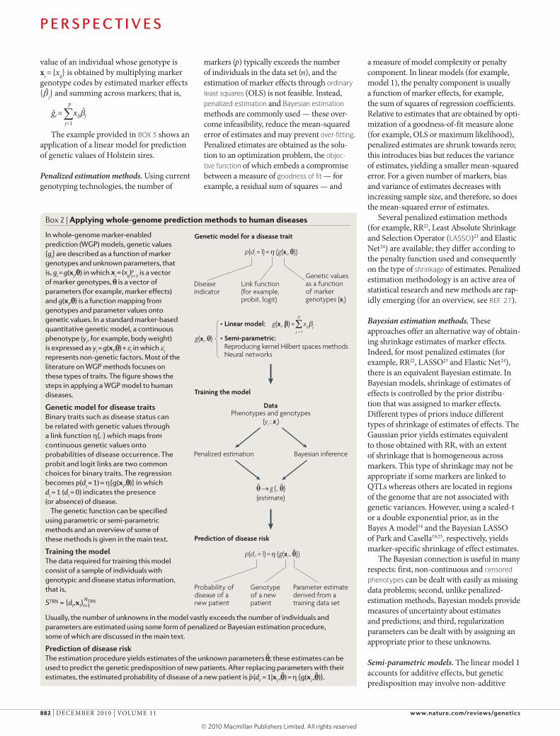
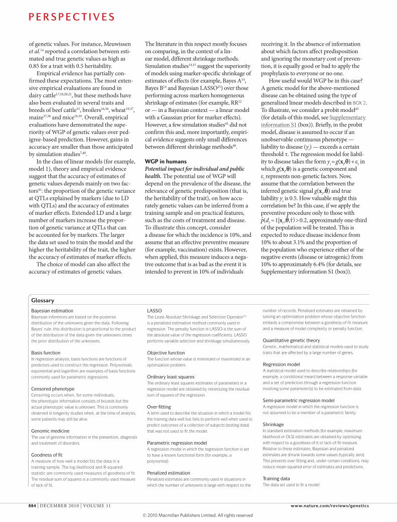
Box 2 | Applying whole-genome prediction methods to human diseases

In whole-genome marker-enabled prediction (WGP) models, genetic values {g

i} are described as a function of marker

genotypes and unknown parameters, that is, g

i = g(x

i,θ) in which is a vector

of marker genotypes, θ is a vector of parameters (for example, marker effects) and g(x

i,θ) is a function mapping from

genotypes and parameter values onto genetic values. In a standard marker-based quantitative genetic model, a continuous phenotype (y

i, for example, body weight)

is expressed as yi = g(x

i,θ) + e

i in which e

i

represents non-genetic factors. Most of the literature on WGP methods focuses on these types of traits. The figure shows the steps in applying a WGP model to human diseases.

Genetic model for disease traitsBinary traits such as disease status can be related with genetic values through a link function η{. } which maps from continuous genetic values onto probabilities of disease occurrence. The probit and logit links are two common choices for binary traits. The regression becomes p(d

i = 1) = η{g(x

i,θ)} in which

di = 1 (d

i = 0) indicates the presence

(or absence) of disease.The genetic function can be specified

using parametric or semi-parametric methods and an overview of some of these methods is given in the main text.

training the modelThe data required for training this model consist of a sample of individuals with genotypic and disease status information, that is,

Usually, the number of unknowns in the model vastly exceeds the number of individuals and parameters are estimated using some form of penalized or Bayesian estimation procedure, some of which are discussed in the main text.

Prediction of disease riskThe estimation procedure yields estimates of the unknown parameters θ; these estimates can be used to predict the genetic predisposition of new patients. After replacing parameters with their estimates, the estimated probability of disease of a new patient is p̂ (di′ = 1|x

i′,θ) = η {g(xi′,θ)}.

Nature Reviews | Genetics

Genetic model for a disease trait

Training the model

Prediction of disease risk

Σp

j = 1

Disease indicator

Link function(for example,probit, logit)

Genetic values as a function of markergenotypes (xi)

p(di = 1) = {g(xi, θ)}

g(xi, θ)

(yi ; xi)

θ → g (., θ)ˆ

ˆ

ˆ

η

g(xi, β) = xij j• Linear model:

• Semi-parametric:Reproducing kernel Hilbert spaces methodsNeural networks

p(di′ = 1) = {g(xi′, θ)}η

DataPhenotypes and genotypes

Penalized estimation Bayesian inference

(estimate)

Probability ofdisease of a new patient

Parameter estimatederived from atraining data set

Genotype of a newpatient

β

P e r s P e c t i v e s

882 | DeCeMBeR 2010 | VOLUMe 11 www.nature.com/reviews/genetics

© 20 Macmillan Publishers Limited. All rights reserved10

gene actions such as dominance or epistasis. In principle, the linear model can be extended to accommodate these effects. However, with large p, including all possible interactions is computationally feasible only to a limited extent. An alternative is to use semi-parametric methods, such as reproducing kernel Hilbert spaces (RKHS) regressions26 or neural networks27.

Gianola et al.28,29 suggested using RKHS methods for WGP. Unlike parametric regression models — in which the genetic function is explicitly defined — in RKHS regressions, a collection of real-valued func-tions is implicitly defined by choosing a ‘reproducing kernel’, K(xi,xi′) (REF 26). This function maps from pairs of genotypes (xi,xi′) into a real number and must be positive semi-definite26. From a Bayesian perspective30–32, the reproducing kernel defines the a priori correlations between evaluations of the function (that is, genetic values) at pairs of genotypes Cor[g(xi),g(xi′)]. The choice of kernel is the central element of model specification. Some parametric models (for example, ridge regression) can be represented as RKHS regressions32–34. Alternatively, kernels can be chosen to maximize the performance of the model (for example, predictive ability). To this end, one can develop algorithms that evaluate a wide variety of kernels and pick one that that is optimal according to some model selection criterion (for example, a measure of predic-tive ability). Overviews of how this can be implemented are given in REFS 32–34.

In linear models and in RKHS, the basis functions used to regress phenotypes on markers are defined a priori and this imposes some constraints on the types of patterns that these methods can capture. In neural networks, the basis functions used to regress phenotypes are inferred from the data and this gives neural networks a great flexibility. This generality comes with a price: the interpretation of parameter estimates is not straightforward and over-fitting may occur27. Pre-selection of markers and use of penalized or Bayesian estimation methods are ways of confronting over-fitting.

evidence for the usefulness of WgpFactors that affect the accuracy of WGP. The usefulness of WGP methods in the context of preventive and personalized medicine will depend on how prevalent a disease is, the heritability of the trait and the accuracy with which genetic predisposition (that is, genetic values) can be inferred. Several simulation studies14,15 in animal breeding indicate that these methods can yield accurate predictions

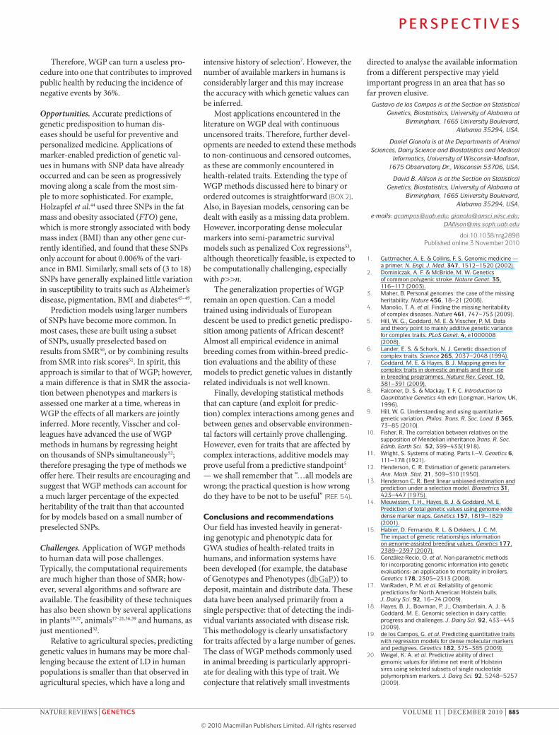
Box 3 | Whole-genome marker-enabled prediction: an example application

Accurate estimates of the breeding values of dairy sires can be obtained by evaluating the performance of a large number of daughters of each sire (progeny testing). However, progeny testing is expensive and many years are required to collect such information. This delays breeding decisions and reduces the rate of genetic gain. The best pedigree-based predictor of the genetic value of newborn sires is the average estimated genetic value of the parents (PA). This is the conceptual equivalent of using family history in human applications61.

Whole-genome marker-enabled prediction (WGP) offers an alternative method for predicting the genetic values of young sires. Unlike PA, WGP can account for genetic differences between individuals with equivalent pedigrees (that is, those due to sampling of genes at meiosis).

Vazquez et al.21 compared the performance of WGP with that of PA.

DataThe data consisted of 4,608 Holstein sires genotyped using the Illumina BovineSNP50 Bead Chip. Sires born before 1999 (n = 2,821) were used to train the models and those born between 1999 and 2003 (n = 893) were used for validation. The target of prediction was sires’ predicted transmitted ability for US-Holstein Net Merit Index (Net Merit PTA), a highly accurate estimate of the sire’s ability to produce valuable offspring.

ModelsPredictions were obtained using a linear regression

Σ β βµ ε

in which yi is the Net Merit PTA of the ith sire, m is an effect common to all sires, PA

i is the average

Net Merit PTA of the parents of sire i, bPA

is a regression coefficient, xij∈ {0,1,2} are counts of the

number of copies of one of the alleles of the jth SNP, bj is the additive effect of the same SNP and

ei is a model residual. Models differed on how many SNPs (from zero to 32,518 SNPs) were included,

how the SNPs were selected (here we present results for evenly spaced SNPs only) and on whether the regression on PA was included. Regression coefficients were estimated using the sires in the training set and the predictive ability was evaluated by the correlation between the Net Merit PTA and WGP in the validation sample.

ResultsThe figure above, produced with data from REF. 21, gives the correlation between the WGP of Net Merit PTA and progeny test Net Merit PTA versus the number of SNPs in models with (blue dots) and without (red dots) the PA. The horizontal lines give the predictive correlation of PA (no SNPs) and of a model including 32,518 SNPs. The PA alone (p = 0) yielded a predictive correlation of 0.41, WGP including all available markers (with or without PA) reached a predictive correlation of 0.65. The predictive ability increased monotonically with the number of markers, and the difference between the correlations obtained with and without PA decreased as the number of markers in the model increased. This occurs because, in infinitesimal traits, as the number of markers increases so does the proportion of genetic variance at quantitative trait loci that can be explained by markers41.

Nature Reviews | Genetics

Number of SNPs

Pred

ictiv

e co

rrel

atio

n

10,0008,0006,0004,0002,00000

0.1

0.2

0.3

0.4

0.5

0.6

0.7

Full model (32,518 SNPs)

PA (no SNP)

P e r s P e c t i v e s

NATURe ReVIeWS | Genetics VOLUMe 11 | DeCeMBeR 2010 | 883

© 20 Macmillan Publishers Limited. All rights reserved10

of genetic values. For instance, Meuwissen et al.14 reported a correlation between esti-mated and true genetic values as high as 0.85 for a trait with 0.5 heritability.

empirical evidence has partially con-firmed these expectations. The most exten-sive empirical evaluations are found in dairy cattle17,18,20,21, but these methods have also been evaluated in several traits and breeds of beef cattle35, broilers16,36, wheat19,37, maize37,38 and mice19,39. Overall, empirical evaluations have demonstrated the supe-riority of WGP of genetic values over ped-igree-based prediction. However, gains in accuracy are smaller than those anticipated by simulation studies7,40.

In the class of linear models (for example, model 1), theory and empirical evidence suggest that the accuracy of estimates of genetic values depends mainly on two fac-tors41: the proportion of the genetic variance at QTLs explained by markers (due to LD with QTLs) and the accuracy of estimates of marker effects. extended LD and a large number of markers increase the propor-tion of genetic variance at QTLs that can be accounted for by markers. The larger the data set used to train the model and the higher the heritability of the trait, the higher the accuracy of estimates of marker effects.

The choice of model can also affect the accuracy of estimates of genetic values.

The literature in this respect mostly focuses on comparing, in the context of a lin-ear model, different shrinkage methods. Simulation studies14,15 suggest the superiority of models using marker-specific shrinkage of estimates of effects (for example, Bayes A14, Bayes B14 and Bayesian LASSO25) over those performing across-markers homogeneous shrinkage of estimates (for example, RR22 or — in a Bayesian context — a linear model with a Gaussian prior for marker effects). However, a few simulation studies42 did not confirm this and, more importantly, empiri-cal evidence suggests only small differences between different shrinkage methods40.

Wgp in humansPotential impact for individual and public health. The potential use of WGP will depend on the prevalence of the disease, the relevance of genetic predisposition (that is, the heritability of the trait), on how accu-rately genetic values can be inferred from a training sample and on practical features, such as the costs of treatment and disease. To illustrate this concept, consider a disease for which the incidence is 10%, and assume that an effective preventive measure (for example, vaccination) exists. However, when applied, this measure induces a nega-tive outcome that is as bad as the event it is intended to prevent in 10% of individuals

receiving it. In the absence of information about which factors affect predisposition and ignoring the monetary cost of preven-tion, it is equally good or bad to apply the prophylaxis to everyone or no one.

How useful would WGP be in this case? A genetic model for the above-mentioned disease can be obtained using the type of generalized linear models described in BOX 2. To illustrate, we consider a probit model43 (for details of this model, see Supplementary information S1 (box)). Briefly, in the probit model, disease is assumed to occur if an unobservable continuous phenotype — liability to disease (yi) — exceeds a certain threshold τ. The regression model for liabil-ity to disease takes the form yi = g(xi,θ) + ei in which g(xi,θ) is a genetic component and ei represents non-genetic factors. Now, assume that the correlation between the inferred genetic signal g(xi′,θ) and true liability yi is 0.5. How valuable might this correlation be? In this case, if we apply the preventive procedure only to those with p̂(di′ = 1|xi′,θ, ) > 0.2, approximately one-third of the population will be treated. This is expected to reduce disease incidence from 10% to about 3.1% and the proportion of the population who experience either of the negative events (disease or iatrogenic) from 10% to approximately 6.4% (for details, see Supplementary information S1 (box)).

Glossary

Bayesian estimationBayesian inferences are based on the posterior distribution of the unknowns given the data. Following Bayes’ rule, this distribution is proportional to the product of the distribution of the data given the unknowns times the prior distribution of the unknowns.

Basis function In regression analysis, basis functions are functions of predictors used to construct the regression. Polynomials, exponential and logarithm are examples of basis functions commonly used for parametric regressions.

Censored phenotypeCensoring occurs when, for some individuals, the phenotypic information consists of bounds but the actual phenotypic value is unknown. This is commonly observed in longevity studies when, at the time of analysis, some patients may still be alive.

Genomic medicineThe use of genome information in the prevention, diagnosis and treatment of disorders.

Goodness of fitA measure of how well a model fits the data in a training sample. The log likelihood and R-squared statistic are commonly used measures of goodness of fit. The residual sum of squares is a commonly used measure of lack of fit.

LASSOThe Least Absolute Shrinkage and Selection Operator23 is a penalized estimation method commonly used in regression. The penalty function in LASSO is the sum of the absolute value of the regression coefficients. LASSO performs variable selection and shrinkage simultaneously.

Objective functionThe function whose value is minimized or maximized in an optimization problem.

Ordinary least squares The ordinary least squares estimates of parameters in a regression model are obtained by minimizing the residual sum of squares of the regression.

Over-fittingA term used to describe the situation in which a model fits the training data well but fails to perform well when used to predict outcomes of a collection of subjects (testing data) that was not used to fit the model.

Parametric regression modelA regression model in which the regression function is set to have a known functional form (for example, a polynomial).

Penalized estimationPenalized estimates are commonly used in situations in which the number of unknowns is large with respect to the

number of records. Penalized estimates are obtained by solving an optimization problem whose objective function embeds a compromise between a goodness-of-fit measure and a measure of model complexity or penalty function.

Quantitative genetic theoryGenetic, mathematical and statistical models used to study traits that are affected by a large number of genes.

Regression modelA statistical model used to describe relationships (for example, a conditional mean) between a response variable and a set of predictors through a regression function involving some parameter(s) to be estimated from data.

Semi-parametric regression modelA regression model in which the regression function is not assumed to be a member of a parametric family.

ShrinkageIn standard estimation methods (for example, maximum likelihood or OLS) estimates are obtained by optimizing with respect to a goodness-of-it or lack-of-fit measure. Relative to these estimates, Bayesian and penalized estimates are shrunk towards some values (typically zero). This prevents over-fitting and, under certain conditions, may reduce mean-squared error of estimates and predictions.

Training dataThe data set used to fit a model.

P e r s P e c t i v e s

884 | DeCeMBeR 2010 | VOLUMe 11 www.nature.com/reviews/genetics

© 20 Macmillan Publishers Limited. All rights reserved10

Therefore, WGP can turn a useless pro-cedure into one that contributes to improved public health by reducing the incidence of negative events by 36%.

Opportunities. Accurate predictions of genetic predisposition to human dis-eases should be useful for preventive and personalized medicine. Applications of marker-enabled prediction of genetic val-ues in humans with SNP data have already occurred and can be seen as progressively moving along a scale from the most sim-ple to more sophisticated. For example, Holzapfel et al.44 used three SNPs in the fat mass and obesity associated (FTO) gene, which is more strongly associated with body mass index (BMI) than any other gene cur-rently identified, and found that these SNPs only account for about 0.006% of the vari-ance in BMI. Similarly, small sets of (3 to 18) SNPs have generally explained little variation in susceptibility to traits such as Alzheimer’s disease, pigmentation, BMI and diabetes45–49.

Prediction models using larger numbers of SNPs have become more common. In most cases, these are built using a subset of SNPs, usually preselected based on results from SMR50, or by combining results from SMR into risk scores51. In spirit, this approach is similar to that of WGP; however, a main difference is that in SMR the associa-tion between phenotypes and markers is assessed one marker at a time, whereas in WGP the effects of all markers are jointly inferred. More recently, Visscher and col-leagues have advanced the use of WGP methods in humans by regressing height on thousands of SNPs simultaneously52; therefore presaging the type of methods we offer here. Their results are encouraging and suggest that WGP methods can account for a much larger percentage of the expected heritability of the trait than that accounted for by models based on a small number of preselected SNPs.

Challenges. Application of WGP methods to human data will pose challenges. Typically, the computational requirements are much higher than those of SMR; how-ever, several algorithms and software are available. The feasibility of these techniques has also been shown by several applications in plants19,37, animals17–21,36,39 and humans, as just mentioned52.

Relative to agricultural species, predicting genetic values in humans may be more chal-lenging because the extent of LD in human populations is smaller than that observed in agricultural species, which have a long and

intensive history of selection7. However, the number of available markers in humans is considerably larger and this may increase the accuracy with which genetic values can be inferred.

Most applications encountered in the literature on WGP deal with continuous uncensored traits. Therefore, further devel-opments are needed to extend these methods to non-continuous and censored outcomes, as these are commonly encountered in health-related traits. extending the type of WGP methods discussed here to binary or ordered outcomes is straightforward (BOX 2). Also, in Bayesian models, censoring can be dealt with easily as a missing data problem. However, incorporating dense molecular markers into semi-parametric survival models such as penalized Cox regressions53, although theoretically feasible, is expected to be computationally challenging, especially with p>>n.

The generalization properties of WGP remain an open question. Can a model trained using individuals of european descent be used to predict genetic predispo-sition among patients of African descent? Almost all empirical evidence in animal breeding comes from within-breed predic-tion evaluations and the ability of these models to predict genetic values in distantly related individuals is not well known.

Finally, developing statistical methods that can capture (and exploit for predic-tion) complex interactions among genes and between genes and observable environmen-tal factors will certainly prove challenging. However, even for traits that are affected by complex interactions, additive models may prove useful from a predictive standpoint5 — we shall remember that “…all models are wrong; the practical question is how wrong do they have to be not to be useful” (REF. 54).

Conclusions and recommendationsOur field has invested heavily in generat-ing genotypic and phenotypic data for GWA studies of health-related traits in humans, and information systems have been developed (for example, the database of Genotypes and Phenotypes (dbGaP)) to deposit, maintain and distribute data. These data have been analysed primarily from a single perspective: that of detecting the indi-vidual variants associated with disease risk. This methodology is clearly unsatisfactory for traits affected by a large number of genes. The class of WGP methods commonly used in animal breeding is particularly appropri-ate for dealing with this type of trait. We conjecture that relatively small investments

directed to analyse the available information from a different perspective may yield important progress in an area that has so far proven elusive.

Gustavo de los Campos is at the Section on Statistical Genetics, Biostatistics, University of Alabama at

Birmingham, 1665 University Boulevard, Alabama 35294, USA.

Daniel Gianola is at the Departments of Animal Sciences, Dairy Science and Biostatistics and Medical

Informatics, University of Wisconsin-Madison, 1675 Observatory Dr., Wisconsin 53706, USA.

David B. Allison is at the Section on Statistical Genetics, Biostatistics, University of Alabama at

Birmingham, 1665 University Boulevard, Alabama 35294, USA.

e-mails: gcampos@uab.edu; gianola@ansci.wisc.edu; DAllison@ms.soph.uab.edu

doi:10.1038/nrg2898Published online 3 November 2010

1. Guttmacher, A. E. & Collins, F. S. Genomic medicine — a primer. N. Engl. J. Med. 347, 1512–1520 (2002).

2. Dominiczak, A. F. & McBride, M. W. Genetics of common polygenic stroke. Nature Genet. 35, 116–117 (2003).

3. Maher, B. Personal genomes: the case of the missing heritability. Nature 456, 18–21 (2008).

4. Manolio, T. A. et al. Finding the missing heritability of complex diseases. Nature 461, 747–753 (2009).

5. Hill, W. G., Goddard, M. E. & Visscher, P. M. Data and theory point to mainly additive genetic variance for complex traits. PLoS Genet. 4, e1000008 (2008).

6. Lander, E. S. & Schork, N. J. Genetic dissection of complex traits. Science 265, 2037–2048 (1994).

7. Goddard, M. E. & Hayes, B. J. Mapping genes for complex traits in domestic animals and their use in breeding programmes. Nature Rev. Genet. 10, 381–391 (2009).

8. Falconer, D. S. & Mackay, T. F. C. Introduction to Quantitative Genetics 4th edn (Longman, Harlow, UK, 1996).

9. Hill, W. G. Understanding and using quantitative genetic variation. Philos. Trans. R. Soc. Lond. B 365, 73–85 (2010).

10. Fisher, R. The correlation between relatives on the supposition of Mendelian inheritance.Trans. R. Soc. Edinb. Earth Sci. 52, 399–433(1918).

11. Wright, S. Systems of mating. Parts I.–V. Genetics 6, 111–178 (1921).

12. Henderson, C. R. Estimation of genetic parameters. Ann. Math. Stat. 21, 309–310 (1950).

13. Henderson C. R. Best linear unbiased estimation and prediction under a selection model. Biometrics 31, 423–447 (1975).

14. Meuwissen, T. H., Hayes, B. J. & Goddard, M. E. Prediction of total genetic values using genome-wide dense marker maps. Genetics 157, 1819–1829 (2001).

15. Habier, D. Fernando, R. L. & Dekkers, J. C. M. The impact of genetic relationships information on genome-assisted breeding values. Genetics 177, 2389–2397 (2007).

16. González-Recio, O. et al. Non-parametric methods for incorporating genomic information into genetic evaluations: an application to mortality in broilers. Genetics 178, 2305–2313 (2008).

17. VanRaden, P. M. et al. Reliability of genomic predictions for North American Holstein bulls. J. Dairy Sci. 92, 16–24 (2009).

18. Hayes, B. J., Bowman, P. J., Chamberlain, A. J. & Goddard, M. E. Genomic selection in dairy cattle: progress and challenges. J. Dairy Sci. 92, 433–443 (2009).

19. de los Campos, G. et al. Predicting quantitative traits with regression models for dense molecular markers and pedigrees. Genetics 182, 375–385 (2009).

20. Weigel, K. A. et al. Predictive ability of direct genomic values for lifetime net merit of Holstein sires using selected subsets of single nucleotide polymorphism markers. J. Dairy Sci. 92, 5248–5257 (2009).

P e r s P e c t i v e s

NATURe ReVIeWS | Genetics VOLUMe 11 | DeCeMBeR 2010 | 885

© 20 Macmillan Publishers Limited. All rights reserved10

21. Vazquez, A. et al. Predictive ability of subsets of SNP with and without parent average in US Holsteins. J. Dairy Sci. 2010 (doi:10.3168/jds.2010–3335).

22. Hoerl, A. E. & Kennard, R. W. Ridge regression: biased estimation for non-orthogonal problems. Technometrics 12, 55–67 (1970).

23. Tibshirani, R. Regression shrinkage and selection via the LASSO. J. R. Stat. Soc. Series B 58, 267–288 (1996).

24. Zou, H. & Hastie, T. Regularization and variable selection via the elastic net. J.R. Stat. Soc. Series B 67, 301–320 (2005).

25. Park, T. & Casella, G. The Bayesian LASSO. J. Am. Stat. Assoc. 103, 681–686 (2008).

26. Wahba, G. Spline Models for Observational Data (Society for Industrial and Applied Mathematics, Philadelphia, 1990).

27. Hastie, T., Tibshirani, R. & Friedman, J. The Elements of Statistical Learning: Data Mining, Inference, and Prediction 2nd edn (Springer-Verlag, New York, 2009).

28. Gianola, D., Fernando, R. L. & Stella, A. Genomic-assisted prediction of genetic value with semiparametric procedures. Genetics 173, 1761–1776 (2006).

29. Gianola, D. & van Kaam, J. B. Reproducing kernel Hilbert spaces regression methods for genomic assisted prediction of quantitative traits. Genetics 178, 2289–2303 (2008).

30. Kimeldorf, G. S. & Wahba, G. A correspondence between Bayesian estimation on stochastic process and smoothing by splines. Ann. Math. Stat. 41, 495–502 (1970).

31. de los Campos, G., Gianola, D. & Rosa, G. J. M. Reproducing kernel Hilbert spaces regression: a general framework for genetic evaluation. J. Anim. Sci. 87, 1883–1887 (2009).

32. de los Campos, G., Gianola, D., Rosa, G. J. M., Weigel, K. & Crossa, J. Semi-parametric genomic-enabled prediction of genetic values using reproducing kernel Hilbert spaces regressions. Genetics Res. 92, 295–308 (2010).

33. Shawe-Taylor, J. & Cristianini, N. Kernel Methods for Pattern Analysis (Cambridge Univ. Press, UK, 2004).

34. Schaid, D. J. Genomic similarity and kernel methods I: advancements by building on mathematical and statistical foundations. Hum. Hered. 70, 109–131 (2010).

35. Garrick, D. J. The nature, scope and impact of some whole-genome analyses in beef cattle in 9th World Congress on Genetics Applied to Livestock (Leipzig, Germany, 2010).

36. Long, N. et al. Radial basis function regression methods for predicting quantitative traits using SNP markers. Genetics Res. 92, 209–225 (2010).

37. Crossa, J. et al. Prediction of genetic values of quantitative traits in plant breeding using pedigree and molecular markers. Genetics 2 Sep 2010 (doi:10.1534/genetics.110.118521).

38. Piepho, H. P. Ridge regression and extensions for genomewide selection in maize. Crop Sci. 49, 1165–1176 (2009).

39. Legarra, A., Robert-Granié, C., Manfredi, E. & Elsen, J. M. Performance of genomic selection in mice. Genetics 180, 611–618 (2008).

40. Jannink, J. L., Lorenz, A. J. & Hiroyoshi, I. Genomic selection in plant breeding: from theory to practice. Brief. Funct. Genomics 9, 166–177 (2010).

41. Goddard, M. E. Genomic selection: prediction of accuracy and maximization of long term response. Genetica 136, 245–257 (2009).

42. Zhong, S., Dekkers, J. C., Fernando R. L. & Jannink, J. L. Factors affecting accuracy from genomic selection in populations derived from multiple inbred lines: a barley case study. Genetics 182, 355–364 (2009).

43. Gianola, D. Theory and analysis of threshold characters. J. Anim. Sci. 54, 1079–1096 (1982).

44. Holzapfel C. et al. Genes and lifestyle factors in obesity: results from 12462 subjects from MONICA/KORA. Int. J. Obes. 1–8 (2010).

45. Seshadri, S. et al. Genome-wide analysis of genetic loci associated with Alzheimer disease. JAMA 303, 1832–1840 (2010).

46. Valenzuela, R. K. et al. Predicting phenotype from genotype: normal pigmentation. J. Forensic Sci. Soc. 55, 315–322 (2010).

47. Willer, C. J. et al. Six new loci associated with body mass index highlight a neuronal influence on body weight regulation. Nature Genet. 41, 25–34 (2008).

48. Zhao, J. et al. The role of obesity-associated loci identified in genome-wide association studies in the determination of pediatric BMI. Obesity 17, 2254–2257 (2009).

49. van Hoek, M. et al. Predicting type 2 diabetes based on polymorphisms from genome-wide association studies: a population-based study. Diabetes 57, 3122–3128 (2008).

50. Wary, N. R., Goddard, M. E. & Visscher, P. M. Prediction of indivual genetic risk to diseases from genome-wide association studies. Genome Res. 17, 1520–1528 (2007).

51. Purcell, S. M. et al. Common polygenic variation contributes to risk of schizophrenia and bipolar disorder. Nature 460, 748–752 (2009).

52. Yang, J. et al. Common SNPs explain a large proportion of the heritability for human height. Nature Genet. 42, 565–569 (2010).

53. Witten, D. M. & Tibshirani, R. Survival analysis with high-dimensional covariates. Stat. Methods Med. Res. 19, 29–51 (2010).

54. Box, G. E. P. & Draper, N. R. Empirical Model-Building and Response Surfaces (Wiley, New York, 1987).

55. Cockerham, C. C. An extension of the concept of partitioning hereditary variance for analysis of covariance among relatives when epistasis is present. Genetics 39, 859–882 (1954).

56. Kempthorne, O. The correlation between relatives in a random mating population. Proc. R. Soc. Lond. B 143, 103–113 (1954).

57. Lynch, M. & Ritland, K. Estimation of pairwise relatedness with molecular markers. Genetics 152, 1753–1766 (1999).

58. Eding, J. H. & Meuwissen, T. H. Marker based estimates of between and within population kinships for the conservation of genetic diversity. J. Anim. Breed. Genet. 118, 141–159 (2001).

59. Visscher, P. M. et al. Assumption-free estimation of heritability from genome-wide identity-by-descent sharing between full siblings. PLoS Genet. 2, e41 (2006).

60. Hayes, B. J. & Goddard, M. E. Prediction of breeding values using marker-derived relationship matrices. J. Anim. Sci. 86, 2089–2092 (2008).

61. Feng, R., McClure, L. A., Tiwari, H. K. & Howard, G. A new estimate of family disease history providing improved prediction of disease risks. Stat. Med. 28, 1269–1283 (2009).

AcknowledgementsWe are grateful to K. Grimes, A. Vazquez, Y. Klimentidis and S. Cofield for their helpful comments on this paper.

Competing interests statementThe authors declare competing financial interests: see Web version for details.

FuRtHeR inFoRMAtionGustav de los campo’s homepage: http://www.soph.uab.edu/ssg/people/camposdbGap: http://www.ncbi.nlm.nih.gov/gapNature Reviews Genetics series on study designs: http://www.nature.com/nrg/series/studydesigns/index.htmlNature Reviews Genetics series on Modelling: http://www.nature.com/nrg/series/modelling/index.htmlNature Reviews Genetics series on Genome-wide association studies: http://www.nature.com/nrg/series/gwas/index.html

SuppLeMentARy inFoRMAtionsee online article: s1 (box)

All links ARe ActiVe in tHe online PDf

P e r s P e c t i v e s

886 | DeCeMBeR 2010 | VOLUMe 11 www.nature.com/reviews/genetics

© 20 Macmillan Publishers Limited. All rights reserved10